Welcome message from author
This document is posted to help you gain knowledge. Please leave a comment to let me know what you think about it! Share it to your friends and learn new things together.
Transcript


I N T R O D U C T I O N T O Q U A N T U M M E C H A N I C S
Third edition
Changes and additions to the new edition of this classic textbook include:
David J. Griffiths received his BA (1964) and PhD (1970) from Harvard University. He taught at HampshireCollege, Mount Holyoke College, and Trinity College before joining the faculty at Reed College in 1978. In2001–2002 he was visiting Professor of Physics at the Five Colleges (UMass, Amherst, Mount Holyoke,Smith, and Hampshire), and in the spring of 2007 he taught Electrodynamics at Stanford. Although his PhDwas in elementary particle theory, most of his research is in electrodynamics and quantum mechanics. He isthe author of over fifty articles and four books: Introduction to Electrodynamics (4th edition, CambridgeUniversity Press, 2013), Introduction to Elementary Particles (2nd edition, Wiley-VCH, 2008), Introduction toQuantum Mechanics (2nd edition, Cambridge, 2005), and Revolutions in Twentieth-Century Physics(Cambridge, 2013).
Darrell F. Schroeter is a condensed matter theorist. He received his BA (1995) from Reed College and hisPhD (2002) from Stanford University where he was a National Science Foundation Graduate ResearchFellow. Before joining the Reed College faculty in 2007, Schroeter taught at both Swarthmore College andOccidental College. His record of successful theoretical research with undergraduate students was recognizedin 2011 when he was named as a KITP-Anacapa scholar.
A new chapter on Symmetries and Conservation Laws
New problems and examples
Improved explanations
More numerical problems to be worked on a computer
New applications to solid state physics
Consolidated treatment of time-dependent potentials
2

INT ROD UCT ION TO Q UANT UMMECHANICS
Third editionDAVID J. GRIFFITHS and DARRELL F. SCHROETER
Reed College, Oregon
3

University Printing House, Cambridge CB2 8BS, United Kingdom
One Liberty Plaza, 20th Floor, New York, NY 10006, USA
477 Williamstown Road, Port Melbourne, VIC 3207, Australia
314–321, 3rd Floor, Plot 3, Splendor Forum, Jasola District Centre, New Delhi – 110025, India
79 Anson Road, #06–04/06, Singapore 079906
Cambridge University Press is part of the University of Cambridge.
It furthers the University’s mission by disseminating knowledge in the pursuit of education, learning, and research at the highestinternational levels of excellence.
www.cambridge.org
Information on this title: www.cambridge.org/9781107189638
DOI: 10.1017/9781316995433
Second edition © David Griffiths 2017
Third edition © Cambridge University Press 2018
This publication is in copyright. Subject to statutory exception and to the provisions of relevant collective licensing agreements, noreproduction of any part may take place without the written permission of Cambridge University Press.
This book was previously published by Pearson Education, Inc. 2004
Second edition reissued by Cambridge University Press 2017
Third edition 2018
Printed in the United Kingdom by TJ International Ltd. Padstow Cornwall, 2018
A catalogue record for this publication is available from the British Library.
Library of Congress Cataloging-in-Publication Data
Names: Griffiths, David J. | Schroeter, Darrell F.
Title: Introduction to quantum mechanics / David J. Griffiths (Reed College, Oregon), Darrell F. Schroeter (Reed College, Oregon).
Description: Third edition. | blah : Cambridge University Press, 2018.
Identifiers: LCCN 2018009864 | ISBN 9781107189638
Subjects: LCSH: Quantum theory.
Classification: LCC QC174.12 .G75 2018 | DDC 530.12–dc23
LC record available at https://lccn.loc.gov/2018009864
ISBN 978-1-107-18963-8 Hardback
Additional resources for this publication at www.cambridge.org/IQM3ed
Cambridge University Press has no responsibility for the persistence or accuracy of URLs for external or third-party internet websitesreferred to in this publication and does not guarantee that any content on such websites is, or will remain, accurate or appropriate.
4

5

Contents
Preface
I Theory
1 The Wave Function1.1 The Schrödinger Equation1.2 The Statistical Interpretation1.3 Probability
1.3.1 Discrete Variables1.3.2 Continuous Variables
1.4 Normalization1.5 Momentum1.6 The Uncertainty PrincipleFurther Problems on Chapter 1
2 Time-Independent Schrödinger Equation2.1 Stationary States2.2 The Infinite Square Well2.3 The Harmonic Oscillator
2.3.1 Algebraic Method2.3.2 Analytic Method
2.4 The Free Particle2.5 The Delta-Function Potential
2.5.1 Bound States and Scattering States2.5.2 The Delta-Function Well
2.6 The Finite Square WellFurther Problems on Chapter 2
3 Formalism3.1 Hilbert Space3.2 Observables
3.2.1 Hermitian Operators3.2.2 Determinate States
3.3 Eigenfunctions of a Hermitian Operator3.3.1 Discrete Spectra3.3.2 Continuous Spectra
6
3.4 Generalized Statistical Interpretation3.5 The Uncertainty Principle
3.5.1 Proof of the Generalized Uncertainty Principle3.5.2 The Minimum-Uncertainty Wave Packet3.5.3 The Energy-Time Uncertainty Principle
3.6 Vectors and Operators3.6.1 Bases in Hilbert Space3.6.2 Dirac Notation3.6.3 Changing Bases in Dirac Notation
Further Problems on Chapter 3
4 Quantum Mechanics in Three Dimensions4.1 The Schröger Equation
4.1.1 Spherical Coordinates4.1.2 The Angular Equation4.1.3 The Radial Equation
4.2 The Hydrogen Atom4.2.1 The Radial Wave Function4.2.2 The Spectrum of Hydrogen
4.3 Angular Momentum4.3.1 Eigenvalues4.3.2 Eigenfunctions
4.4 Spin4.4.1 Spin 1/24.4.2 Electron in a Magnetic Field4.4.3 Addition of Angular Momenta
4.5 Electromagnetic Interactions4.5.1 Minimal Coupling4.5.2 The Aharonov–Bohm Effect
Further Problems on Chapter 4
5 Identical Particles5.1 Two-Particle Systems
5.1.1 Bosons and Fermions5.1.2 Exchange Forces5.1.3 Spin5.1.4 Generalized Symmetrization Principle
5.2 Atoms5.2.1 Helium5.2.2 The Periodic Table
5.3 Solids5.3.1 The Free Electron Gas5.3.2 Band Structure
Further Problems on Chapter 5
7
6 Symmetries & Conservation Laws6.1 Introduction
6.1.1 Transformations in Space6.2 The Translation Operator
6.2.1 How Operators Transform6.2.2 Translational Symmetry
6.3 Conservation Laws6.4 Parity
6.4.1 Parity in One Dimension6.4.2 Parity in Three Dimensions6.4.3 Parity Selection Rules
6.5 Rotational Symmetry6.5.1 Rotations About the z Axis6.5.2 Rotations in Three Dimensions
6.6 Degeneracy6.7 Rotational Selection Rules
6.7.1 Selection Rules for Scalar Operators6.7.2 Selection Rules for Vector Operators
6.8 Translations in Time6.8.1 The Heisenberg Picture6.8.2 Time-Translation Invariance
Further Problems on Chapter 6
II Applications
7 Time-Independent Perturbation Theory7.1 Nondegenerate Perturbation Theory
7.1.1 General Formulation7.1.2 First-Order Theory7.1.3 Second-Order Energies
7.2 Degenerate Perturbation Theory7.2.1 Two-Fold Degeneracy7.2.2 “Good” States7.2.3 Higher-Order Degeneracy
7.3 The Fine Structure of Hydrogen7.3.1 The Relativistic Correction7.3.2 Spin-Orbit Coupling
7.4 The Zeeman Effect7.4.1 Weak-Field Zeeman Effect7.4.2 Strong-Field Zeeman Effect7.4.3 Intermediate-Field Zeeman Effect
7.5 Hyperfine Splitting in Hydrogen
8

Further Problems on Chapter 7
8 The Varitional Principle8.1 Theory8.2 The Ground State of Helium8.3 The Hydrogen Molecule Ion8.4 The Hydrogen MoleculeFurther Problems on Chapter 8
9 The WKB Approximation9.1 The “Classical” Region9.2 Tunneling9.3 The Connection FormulasFurther Problems on Chapter 9
10 Scattering10.1 Introduction
10.1.1 Classical Scattering Theory10.1.2 Quantum Scattering Theory
10.2 Partial Wave Analysis10.2.1 Formalism10.2.2 Strategy
10.3 Phase Shifts10.4 The Born Approximation
10.4.1 Integral Form of the Schrödinger Equation10.4.2 The First Born Approximation10.4.3 The Born Series
Further Problems on Chapter 10
11 Quantum Dynamics11.1 Two-Level Systems
11.1.1 The Perturbed System11.1.2 Time-Dependent Perturbation Theory11.1.3 Sinusoidal Perturbations
11.2 Emission and Absorption of Radiation11.2.1 Electromagnetic Waves11.2.2 Absorption, Stimulated Emission, and Spontaneous Emission11.2.3 Incoherent Perturbations
11.3 Spontaneous Emission11.3.1 Einstein’s A and B Coefficients11.3.2 The Lifetime of an Excited State11.3.3 Selection Rules
11.4 Fermi’s Golden Rule11.5 The Adiabatic Approximation
11.5.1 Adiabatic Processes
9

11.5.2 The Adiabatic TheoremFurther Problems on Chapter 11
12 Afterword12.1 The EPR Paradox12.2 Bell’s Theorem12.3 Mixed States and the Density Matrix
12.3.1 Pure States12.3.2 Mixed States12.3.3 Subsystems
12.4 The No-Clone Theorem12.5 Schrödinger’s Cat
Appendix Linear AlgebraA.1 VectorsA.2 Inner ProductsA.3 MatricesA.4 Changing BasesA.5 Eigenvectors and EigenvaluesA.6 Hermitian Transformations
Index
10
Preface
Unlike Newton’s mechanics, or Maxwell’s electrodynamics, or Einstein’s relativity, quantum theory was notcreated—or even definitively packaged—by one individual, and it retains to this day some of the scars of itsexhilarating but traumatic youth. There is no general consensus as to what its fundamental principles are, howit should be taught, or what it really “means.” Every competent physicist can “do” quantum mechanics, but thestories we tell ourselves about what we are doing are as various as the tales of Scheherazade, and almost asimplausible. Niels Bohr said, “If you are not confused by quantum physics then you haven’t really understoodit”; Richard Feynman remarked, “I think I can safely say that nobody understands quantum mechanics.”
The purpose of this book is to teach you how to do quantum mechanics. Apart from some essentialbackground in Chapter 1, the deeper quasi-philosophical questions are saved for the end. We do not believeone can intelligently discuss what quantum mechanics means until one has a firm sense of what quantummechanics does. But if you absolutely cannot wait, by all means read the Afterword immediately after finishingChapter 1.
Not only is quantum theory conceptually rich, it is also technically difficult, and exact solutions to all butthe most artificial textbook examples are few and far between. It is therefore essential to develop specialtechniques for attacking more realistic problems. Accordingly, this book is divided into two parts;1 Part Icovers the basic theory, and Part II assembles an arsenal of approximation schemes, with illustrativeapplications. Although it is important to keep the two parts logically separate, it is not necessary to study thematerial in the order presented here. Some instructors, for example, may wish to treat time-independentperturbation theory right after Chapter 2.
This book is intended for a one-semester or one-year course at the junior or senior level. A one-semestercourse will have to concentrate mainly on Part I; a full-year course should have room for supplementarymaterial beyond Part II. The reader must be familiar with the rudiments of linear algebra (as summarized inthe Appendix), complex numbers, and calculus up through partial derivatives; some acquaintance with Fourieranalysis and the Dirac delta function would help. Elementary classical mechanics is essential, of course, and alittle electrodynamics would be useful in places. As always, the more physics and math you know the easier itwill be, and the more you will get out of your study. But quantum mechanics is not something that flowssmoothly and naturally from earlier theories. On the contrary, it represents an abrupt and revolutionarydeparture from classical ideas, calling forth a wholly new and radically counterintuitive way of thinking aboutthe world. That, indeed, is what makes it such a fascinating subject.
At first glance, this book may strike you as forbiddingly mathematical. We encounter Legendre,Hermite, and Laguerre polynomials, spherical harmonics, Bessel, Neumann, and Hankel functions, Airyfunctions, and even the Riemann zeta function—not to mention Fourier transforms, Hilbert spaces, hermitianoperators, and Clebsch–Gordan coefficients. Is all this baggage really necessary? Perhaps not, but physics islike carpentry: Using the right tool makes the job easier, not more difficult, and teaching quantum mechanicswithout the appropriate mathematical equipment is like having a tooth extracted with a pair of pliers—it’spossible, but painful. (On the other hand, it can be tedious and diverting if the instructor feels obliged to giveelaborate lessons on the proper use of each tool. Our instinct is to hand the students shovels and tell them to
11

start digging. They may develop blisters at first, but we still think this is the most efficient and exciting way tolearn.) At any rate, we can assure you that there is no deep mathematics in this book, and if you run intosomething unfamiliar, and you don’t find our explanation adequate, by all means ask someone about it, or lookit up. There are many good books on mathematical methods—we particularly recommend Mary Boas,Mathematical Methods in the Physical Sciences, 3rd edn, Wiley, New York (2006), or George Arfken and Hans-Jurgen Weber, Mathematical Methods for Physicists, 7th edn, Academic Press, Orlando (2013). But whateveryou do, don’t let the mathematics—which, for us, is only a tool—obscure the physics.
Several readers have noted that there are fewer worked examples in this book than is customary, and thatsome important material is relegated to the problems. This is no accident. We don’t believe you can learnquantum mechanics without doing many exercises for yourself. Instructors should of course go over as manyproblems in class as time allows, but students should be warned that this is not a subject about which anyonehas natural intuitions—you’re developing a whole new set of muscles here, and there is simply no substitutefor calisthenics. Mark Semon suggested that we offer a “Michelin Guide” to the problems, with varyingnumbers of stars to indicate the level of difficulty and importance. This seemed like a good idea (though, likethe quality of a restaurant, the significance of a problem is partly a matter of taste); we have adopted thefollowing rating scheme:
an essential problem that every reader should study;
a somewhat more difficult or peripheral problem;
an unusually challenging problem, that may take over an hour.
(No stars at all means fast food: OK if you’re hungry, but not very nourishing.) Most of the one-star problemsappear at the end of the relevant section; most of the three-star problems are at the end of the chapter. If acomputer is required, we put a mouse in the margin. A solution manual is available (to instructors only) fromthe publisher.
In preparing this third edition we have tried to retain as much as possible the spirit of the first andsecond. Although there are now two authors, we still use the singular (“I”) in addressing the reader—it feelsmore intimate, and after all only one of us can speak at a time (“we” in the text means you, the reader, and I,the author, working together). Schroeter brings the fresh perspective of a solid state theorist, and he is largelyresponsible for the new chapter on symmetries. We have added a number of problems, clarified manyexplanations, and revised the Afterword. But we were determined not to allow the book to grow fat, and forthat reason we have eliminated the chapter on the adiabatic approximation (significant insights from thatchapter have been incorporated into Chapter 11), and removed material from Chapter 5 on statisticalmechanics (which properly belongs in a book on thermal physics). It goes without saying that instructors arewelcome to cover such other topics as they see fit, but we want the textbook itself to represent the essentialcore of the subject.
We have benefitted from the comments and advice of many colleagues, who read the originalmanuscript, pointed out weaknesses (or errors) in the first two editions, suggested improvements in thepresentation, and supplied interesting problems. We especially thank P. K. Aravind (Worcester Polytech),Greg Benesh (Baylor), James Bernhard (Puget Sound), Burt Brody (Bard), Ash Carter (Drew), EdwardChang (Massachusetts), Peter Collings (Swarthmore), Richard Crandall (Reed), Jeff Dunham (Middlebury),Greg Elliott (Puget Sound), John Essick (Reed), Gregg Franklin (Carnegie Mellon), Joel Franklin (Reed),
12

Henry Greenside (Duke), Paul Haines (Dartmouth), J. R. Huddle (Navy), Larry Hunter (Amherst), DavidKaplan (Washington), Don Koks (Adelaide), Peter Leung (Portland State), Tony Liss (Illinois), JeffryMallow (Chicago Loyola), James McTavish (Liverpool), James Nearing (Miami), Dick Palas, Johnny Powell(Reed), Krishna Rajagopal (MIT), Brian Raue (Florida International), Robert Reynolds (Reed), Keith Riles(Michigan), Klaus Schmidt-Rohr (Brandeis), Kenny Scott (London), Dan Schroeder (Weber State), MarkSemon (Bates), Herschel Snodgrass (Lewis and Clark), John Taylor (Colorado), Stavros Theodorakis(Cyprus), A. S. Tremsin (Berkeley), Dan Velleman (Amherst), Nicholas Wheeler (Reed), Scott Willenbrock(Illinois), William Wootters (Williams), and Jens Zorn (Michigan).
1 This structure was inspired by David Park’s classic text Introduction to the Quantum Theory, 3rd edn, McGraw-Hill, New York (1992).
13

Part ITheory
◈
14
1The Wave Function
◈
15

(1.1)
(1.2)
1.1 The Schrödinger EquationImagine a particle of mass m, constrained to move along the x axis, subject to some specified force (Figure 1.1). The program of classical mechanics is to determine the position of the particle at any given time:
. Once we know that, we can figure out the velocity , the momentum , thekinetic energy , or any other dynamical variable of interest. And how do we go aboutdetermining ? We apply Newton’s second law: . (For conservative systems—the only kind weshall consider, and, fortunately, the only kind that occur at the microscopic level—the force can be expressed asthe derivative of a potential energy function,1 , and Newton’s law reads
.) This, together with appropriate initial conditions (typically the position andvelocity at ), determines .
Figure 1.1: A “particle” constrained to move in one dimension under the influence of a specified force.
Quantum mechanics approaches this same problem quite differently. In this case what we’re looking foris the particle’s wave function, , and we get it by solving the Schrödinger equation:
Here i is the square root of , and is Planck’s constant—or rather, his original constant (h) divided by :
The Schrödinger equation plays a role logically analogous to Newton’s second law: Given suitable initialconditions (typically, ), the Schrödinger equation determines for all future time, just as, inclassical mechanics, Newton’s law determines for all future time.2
16

(1.3)
1.2 The Statistical InterpretationBut what exactly is this “wave function,” and what does it do for you once you’ve got it? After all, a particle, byits nature, is localized at a point, whereas the wave function (as its name suggests) is spread out in space (it’s afunction of x, for any given t). How can such an object represent the state of a particle? The answer is providedby Born’s statistical interpretation, which says that gives the probability of finding the particle atpoint x, at time t—or, more precisely,3
Probability is the area under the graph of . For the wave function in Figure 1.2, you would be quite likelyto find the particle in the vicinity of point A, where is large, and relatively unlikely to find it near point B.
Figure 1.2: A typical wave function. The shaded area represents the probability of finding the particle betweena and b. The particle would be relatively likely to be found near A, and unlikely to be found near B.
The statistical interpretation introduces a kind of indeterminacy into quantum mechanics, for even if youknow everything the theory has to tell you about the particle (to wit: its wave function), still you cannotpredict with certainty the outcome of a simple experiment to measure its position—all quantum mechanicshas to offer is statistical information about the possible results. This indeterminacy has been profoundlydisturbing to physicists and philosophers alike, and it is natural to wonder whether it is a fact of nature, or adefect in the theory.
Suppose I do measure the position of the particle, and I find it to be at point C.4 Question: Where was theparticle just before I made the measurement? There are three plausible answers to this question, and they serveto characterize the main schools of thought regarding quantum indeterminacy:
1. The realist position: The particle was at C. This certainly seems reasonable, and it is the response Einstein advocated. Note, however,that if this is true then quantum mechanics is an incomplete theory, since the particle really was at C, and yet quantum mechanics was unableto tell us so. To the realist, indeterminacy is not a fact of nature, but a reflection of our ignorance. As d’Espagnat put it, “the position of theparticle was never indeterminate, but was merely unknown to the experimenter.”5 Evidently is not the whole story—some additionalinformation (known as a hidden variable) is needed to provide a complete description of the particle.
2. The orthodox position: The particle wasn’t really anywhere. It was the act of measurement that forced it to “take a stand” (though howand why it decided on the point C we dare not ask). Jordan said it most starkly: “Observations not only disturb what is to be measured, theyproduce it …We compel [the particle] to assume a definite position.”6 This view (the so-called Copenhagen interpretation), is associatedwith Bohr and his followers. Among physicists it has always been the most widely accepted position. Note, however, that if it is correctthere is something very peculiar about the act of measurement—something that almost a century of debate has done precious little toilluminate.
17

3. The agnostic position: Refuse to answer. This is not quite as silly as it sounds—after all, what sense can there be in making assertionsabout the status of a particle before a measurement, when the only way of knowing whether you were right is precisely to make ameasurement, in which case what you get is no longer “before the measurement”? It is metaphysics (in the pejorative sense of the word) toworry about something that cannot, by its nature, be tested. Pauli said: “One should no more rack one’s brain about the problem ofwhether something one cannot know anything about exists all the same, than about the ancient question of how many angels are able to siton the point of a needle.”7 For decades this was the “fall-back” position of most physicists: they’d try to sell you the orthodox answer, but ifyou were persistent they’d retreat to the agnostic response, and terminate the conversation.
Until fairly recently, all three positions (realist, orthodox, and agnostic) had their partisans. But in 1964John Bell astonished the physics community by showing that it makes an observable difference whether theparticle had a precise (though unknown) position prior to the measurement, or not. Bell’s discovery effectivelyeliminated agnosticism as a viable option, and made it an experimental question whether 1 or 2 is the correctchoice. I’ll return to this story at the end of the book, when you will be in a better position to appreciate Bell’sargument; for now, suffice it to say that the experiments have decisively confirmed the orthodoxinterpretation:8 a particle simply does not have a precise position prior to measurement, any more than theripples on a pond do; it is the measurement process that insists on one particular number, and thereby in asense creates the specific result, limited only by the statistical weighting imposed by the wave function.
What if I made a second measurement, immediately after the first? Would I get C again, or does the actof measurement cough up some completely new number each time? On this question everyone is inagreement: A repeated measurement (on the same particle) must return the same value. Indeed, it would betough to prove that the particle was really found at C in the first instance, if this could not be confirmed byimmediate repetition of the measurement. How does the orthodox interpretation account for the fact that thesecond measurement is bound to yield the value C? It must be that the first measurement radically alters thewave function, so that it is now sharply peaked about C (Figure 1.3). We say that the wave function collapses,upon measurement, to a spike at the point C (it soon spreads out again, in accordance with the Schrödingerequation, so the second measurement must be made quickly). There are, then, two entirely distinct kinds ofphysical processes: “ordinary” ones, in which the wave function evolves in a leisurely fashion under theSchrödinger equation, and “measurements,” in which suddenly and discontinuously collapses.9
Figure 1.3: Collapse of the wave function: graph of immediately after a measurement has found theparticle at point C.
Example 1.1Electron Interference. I have asserted that particles (electrons, for example) have a wave nature,encoded in . How might we check this, in the laboratory?
The classic signature of a wave phenomenon is interference: two waves in phase interfereconstructively, and out of phase they interfere destructively. The wave nature of light was confirmed in
18

1801 by Young’s famous double-slit experiment, showing interference “fringes” on a distant screenwhen a monochromatic beam passes through two slits. If essentially the same experiment is done withelectrons, the same pattern develops,10 confirming the wave nature of electrons.
Now suppose we decrease the intensity of the electron beam, until only one electron is present inthe apparatus at any particular time. According to the statistical interpretation each electron willproduce a spot on the screen. Quantum mechanics cannot predict the precise location of that spot—allit can tell us is the probability of a given electron landing at a particular place. But if we are patient,and wait for a hundred thousand electrons—one at a time—to make the trip, the accumulating spotsreveal the classic two-slit interference pattern (Figure 1.4). 11
Figure 1.4: Build-up of the electron interference pattern. (a) Eight electrons, (b) 270 electrons, (c)2000 electrons, (d) 160,000 electrons. Reprinted courtesy of the Central Research Laboratory,Hitachi, Ltd., Japan.
Of course, if you close off one slit, or somehow contrive to detect which slit each electron passesthrough, the interference pattern disappears; the wave function of the emerging particle is now entirelydifferent (in the first case because the boundary conditions for the Schrödinger equation have beenchanged, and in the second because of the collapse of the wave function upon measurement). But withboth slits open, and no interruption of the electron in flight, each electron interferes with itself; itdidn’t pass through one slit or the other, but through both at once, just as a water wave, impinging ona jetty with two openings, interferes with itself. There is nothing mysterious about this, once you haveaccepted the notion that particles obey a wave equation. The truly astonishing thing is the blip-by-blipassembly of the pattern. In any classical wave theory the pattern would develop smoothly andcontinuously, simply getting more intense as time goes on. The quantum process is more like thepointillist painting of Seurat: The picture emerges from the cumulative contributions of all theindividual dots.12
19

20

1.3 Probability
21

(1.4)
1.3.1 Discrete Variables
Because of the statistical interpretation, probability plays a central role in quantum mechanics, so I digressnow for a brief discussion of probability theory. It is mainly a question of introducing some notation andterminology, and I shall do it in the context of a simple example.
Imagine a room containing fourteen people, whose ages are as follows:
one person aged 14,one person aged 15,three people aged 16,two people aged 22,two people aged 24,five people aged 25.
If we let represent the number of people of age j, then
while , for instance, is zero. The total number of people in the room is
(In the example, of course, .) Figure 1.5 is a histogram of the data. The following are some questionsone might ask about this distribution.
Figure 1.5: Histogram showing the number of people, , with age j, for the example in Section 1.3.1.
Question 1 If you selected one individual at random from this group, what is the probability that thisperson’s age would be 15?Answer One chance in 14, since there are 14 possible choices, all equally likely, of whom only one has thatparticular age. If is the probability of getting age j, then
, and so on. In general,
22

(1.5)
(1.6)
(1.7)
(1.8)
(1.9)
Notice that the probability of getting either 14 or 15 is the sum of the individual probabilities (in this case,1/7). In particular, the sum of all the probabilities is 1—the person you select must have some age:
Question 2 What is the most probable age?Answer 25, obviously; five people share this age, whereas at most three have any other age. The mostprobable j is the j for which is a maximum.Question 3 What is the median age?Answer 23, for 7 people are younger than 23, and 7 are older. (The median is that value of j such that theprobability of getting a larger result is the same as the probability of getting a smaller result.)Question 4 What is the average (or mean) age?Answer
In general, the average value of j (which we shall write thus: ) is
Notice that there need not be anyone with the average age or the median age—in this example nobodyhappens to be 21 or 23. In quantum mechanics the average is usually the quantity of interest; in that context ithas come to be called the expectation value. It’s a misleading term, since it suggests that this is the outcomeyou would be most likely to get if you made a single measurement (that would be the most probable value, notthe average value)—but I’m afraid we’re stuck with it.
Question 5 What is the average of the squares of the ages?Answer You could get , with probability 1/14, or , with probability 1/14, or
, with probability 3/14, and so on. The average, then, is
In general, the average value of some function of j is given by
(Equations 1.6, 1.7, and 1.8 are, if you like, special cases of this formula.) Beware: The average of the squares, , is not equal, in general, to the square of the average, . For instance, if the room contains just two
babies, aged 1 and 3, then , but .
23

(1.11)
(1.10)
Now, there is a conspicuous difference between the two histograms in Figure 1.6, even though they havethe same median, the same average, the same most probable value, and the same number of elements: Thefirst is sharply peaked about the average value, whereas the second is broad and flat. (The first might representthe age profile for students in a big-city classroom, the second, perhaps, a rural one-room schoolhouse.) Weneed a numerical measure of the amount of “spread” in a distribution, with respect to the average. The mostobvious way to do this would be to find out how far each individual is from the average,
and compute the average of . Trouble is, of course, that you get zero:
(Note that is constant—it does not change as you go from one member of the sample to another—so it canbe taken outside the summation.) To avoid this irritating problem you might decide to average the absolutevalue of . But absolute values are nasty to work with; instead, we get around the sign problem by squaringbefore averaging:
This quantity is known as the variance of the distribution; σ itself (the square root of the average of the squareof the deviation from the average—gulp!) is called the standard deviation. The latter is the customary measureof the spread about .
Figure 1.6: Two histograms with the same median, same average, and same most probable value, but differentstandard deviations.
There is a useful little theorem on variances:
Taking the square root, the standard deviation itself can be written as
24
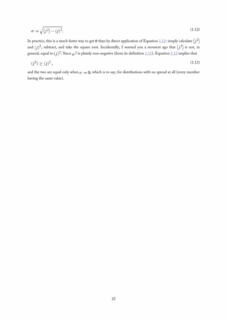
(1.12)
(1.13)
In practice, this is a much faster way to get σ than by direct application of Equation 1.11: simply calculate and , subtract, and take the square root. Incidentally, I warned you a moment ago that is not, ingeneral, equal to . Since is plainly non-negative (from its definition 1.11), Equation 1.12 implies that
and the two are equal only when , which is to say, for distributions with no spread at all (every memberhaving the same value).
25

(1.14)
(1.15)
(1.16)
(1.17)
(1.18)
(1.19)
1.3.2 Continuous Variables
So far, I have assumed that we are dealing with a discrete variable—that is, one that can take on only certainisolated values (in the example, j had to be an integer, since I gave ages only in years). But it is simple enoughto generalize to continuous distributions. If I select a random person off the street, the probability that her ageis precisely 16 years, 4 hours, 27 minutes, and 3.333… seconds is zero. The only sensible thing to speak aboutis the probability that her age lies in some interval—say, between 16 and 17. If the interval is sufficientlyshort, this probability is proportional to the length of the interval. For example, the chance that her age isbetween 16 and 16 plus two days is presumably twice the probability that it is between 16 and 16 plus one day.(Unless, I suppose, there was some extraordinary baby boom 16 years ago, on exactly that day—in which casewe have simply chosen an interval too long for the rule to apply. If the baby boom lasted six hours, we’ll takeintervals of a second or less, to be on the safe side. Technically, we’re talking about infinitesimal intervals.)Thus
The proportionality factor, , is often loosely called “the probability of getting x,” but this is sloppylanguage; a better term is probability density. The probability that x lies between a and b (a finite interval) isgiven by the integral of :
and the rules we deduced for discrete distributions translate in the obvious way:
Example 1.2Suppose someone drops a rock off a cliff of height h. As it falls, I snap a million photographs, atrandom intervals. On each picture I measure the distance the rock has fallen. Question: What is theaverage of all these distances? That is to say, what is the time average of the distance traveled?13
Solution: The rock starts out at rest, and picks up speed as it falls; it spends more time near the top, sothe average distance will surely be less than . Ignoring air resistance, the distance x at time t is
The velocity is , and the total flight time is . The probability that a26

∗
The velocity is , and the total flight time is . The probability that aparticular photograph was taken between t and is , so the probability that it shows adistance in the corresponding range x to is
Thus the probability density (Equation 1.14) is
(outside this range, of course, the probability density is zero).We can check this result, using Equation 1.16:
The average distance (Equation 1.17) is
which is somewhat less than , as anticipated.Figure 1.7 shows the graph of . Notice that a probability density can be infinite, though
probability itself (the integral of ρ) must of course be finite (indeed, less than or equal to 1).
Figure 1.7: The probability density in Example 1.2: .
Problem 1.1 For the distribution of ages in the example in Section 1.3.1:(a) Compute and .(b) Determine for each j, and use Equation 1.11 to compute the standard
deviation.(c) Use your results in (a) and (b) to check Equation 1.12.
27
∗
Problem 1.2(a) Find the standard deviation of the distribution in Example 1.2.(b) What is the probability that a photograph, selected at random, would
show a distance x more than one standard deviation away from theaverage?
Problem 1.3 Consider the gaussian distribution
where A, a, and are positive real constants. (The necessary integrals areinside the back cover.)(a) Use Equation 1.16 to determine A.(b) Find , , and σ.(c) Sketch the graph of .
28
(1.20)
(1.21)
(1.22)
(1.23)
(1.24)
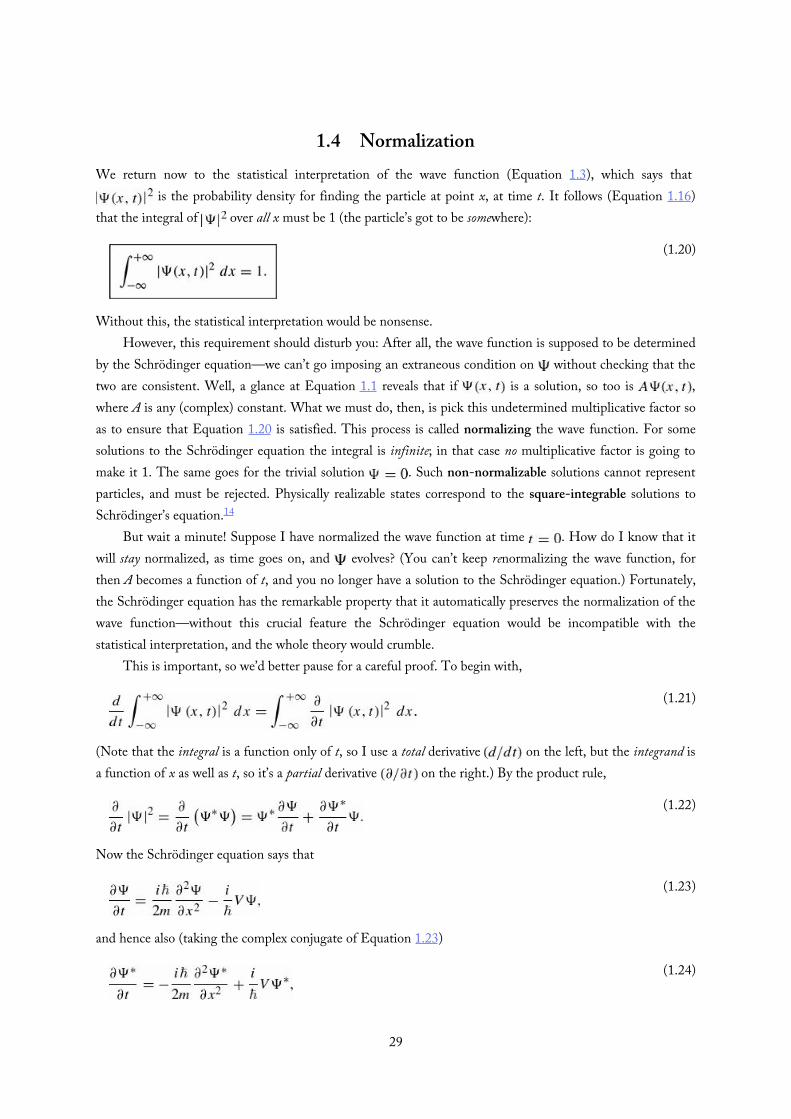
1.4 NormalizationWe return now to the statistical interpretation of the wave function (Equation 1.3), which says that
is the probability density for finding the particle at point x, at time t. It follows (Equation 1.16)that the integral of over all x must be 1 (the particle’s got to be somewhere):
Without this, the statistical interpretation would be nonsense.However, this requirement should disturb you: After all, the wave function is supposed to be determined
by the Schrödinger equation—we can’t go imposing an extraneous condition on without checking that thetwo are consistent. Well, a glance at Equation 1.1 reveals that if is a solution, so too is ,where A is any (complex) constant. What we must do, then, is pick this undetermined multiplicative factor soas to ensure that Equation 1.20 is satisfied. This process is called normalizing the wave function. For somesolutions to the Schrödinger equation the integral is infinite; in that case no multiplicative factor is going tomake it 1. The same goes for the trivial solution . Such non-normalizable solutions cannot representparticles, and must be rejected. Physically realizable states correspond to the square-integrable solutions toSchrödinger’s equation.14
But wait a minute! Suppose I have normalized the wave function at time . How do I know that itwill stay normalized, as time goes on, and evolves? (You can’t keep renormalizing the wave function, forthen A becomes a function of t, and you no longer have a solution to the Schrödinger equation.) Fortunately,the Schrödinger equation has the remarkable property that it automatically preserves the normalization of thewave function—without this crucial feature the Schrödinger equation would be incompatible with thestatistical interpretation, and the whole theory would crumble.
This is important, so we’d better pause for a careful proof. To begin with,
(Note that the integral is a function only of t, so I use a total derivative on the left, but the integrand isa function of x as well as t, so it’s a partial derivative on the right.) By the product rule,
Now the Schrödinger equation says that
and hence also (taking the complex conjugate of Equation 1.23)
29

(1.25)
(1.26)
(1.27)
∗
so
The integral in Equation 1.21 can now be evaluated explicitly:
But must go to zero as x goes to infinity—otherwise the wave function would not benormalizable.15 It follows that
and hence that the integral is constant (independent of time); if is normalized at , it stays normalizedfor all future time. QED
Problem 1.4 At time a particle is represented by the wave function
where A, a, and b are (positive) constants.(a) Normalize (that is, find A, in terms of a and b).(b) Sketch , as a function of x.(c) Where is the particle most likely to be found, at ?(d) What is the probability of finding the particle to the left of a? Check your
result in the limiting cases and .(e) What is the expectation value of x?
Problem 1.5 Consider the wave function
where A, , and ω are positive real constants. (We’ll see in Chapter 2 for whatpotential (V) this wave function satisfies the Schrödinger equation.)(a) Normalize .(b) Determine the expectation values of x and .(c) Find the standard deviation of x. Sketch the graph of , as a function
of x, and mark the points and , to illustrate the sensein which σ represents the “spread” in x. What is the probability that theparticle would be found outside this range?
30

31

(1.28)
(1.29)
(1.30)
(1.31)
1.5 MomentumFor a particle in state , the expectation value of x is
What exactly does this mean? It emphatically does not mean that if you measure the position of one particleover and over again, is the average of the results you’ll get. On the contrary: The firstmeasurement (whose outcome is indeterminate) will collapse the wave function to a spike at the value actuallyobtained, and the subsequent measurements (if they’re performed quickly) will simply repeat that same result.Rather, is the average of measurements performed on particles all in the state , which means that eitheryou must find some way of returning the particle to its original state after each measurement, or else you haveto prepare a whole ensemble of particles, each in the same state , and measure the positions of all of them:
is the average of these results. I like to picture a row of bottles on a shelf, each containing a particle in thestate (relative to the center of the bottle). A graduate student with a ruler is assigned to each bottle, and at asignal they all measure the positions of their respective particles. We then construct a histogram of the results,which should match , and compute the average, which should agree with . (Of course, since we’re onlyusing a finite sample, we can’t expect perfect agreement, but the more bottles we use, the closer we ought tocome.) In short, the expectation value is the average of measurements on an ensemble of identically-prepared systems,not the average of repeated measurements on one and the same system.
Now, as time goes on, will change (because of the time dependence of ), and we might beinterested in knowing how fast it moves. Referring to Equations 1.25 and 1.28, we see that16
This expression can be simplified using integration-by-parts:17
(I used the fact that , and threw away the boundary term, on the ground that goes to zero at infinity.) Performing another integration-by-parts, on the second term, we conclude:
What are we to make of this result? Note that we’re talking about the “velocity” of the expectation value ofx, which is not the same thing as the velocity of the particle. Nothing we have seen so far would enable us tocalculate the velocity of a particle. It’s not even clear what velocity means in quantum mechanics: If the particledoesn’t have a determinate position (prior to measurement), neither does it have a well-defined velocity. Allwe could reasonably ask for is the probability of getting a particular value. We’ll see in Chapter 3 how toconstruct the probability density for velocity, given ; for the moment it will suffice to postulate that theexpectation value of the velocity is equal to the time derivative of the expectation value of position:
32

(1.32)
(1.33)
(1.34)
(1.35)
(1.36)
(1.37)
Equation 1.31 tells us, then, how to calculate directly from .Actually, it is customary to work with momentum , rather than velocity:
Let me write the expressions for and in a more suggestive way:
We say that the operator18 x “represents” position, and the operator “represents” momentum; tocalculate expectation values we “sandwich” the appropriate operator between and , and integrate.
That’s cute, but what about other quantities? The fact is, all classical dynamical variables can be expressedin terms of position and momentum. Kinetic energy, for example, is
and angular momentum is
(the latter, of course, does not occur for motion in one dimension). To calculate the expectation value of anysuch quantity, , we simply replace every p by , insert the resulting operator between and , and integrate:
For example, the expectation value of the kinetic energy is
Equation 1.36 is a recipe for computing the expectation value of any dynamical quantity, for a particle instate ; it subsumes Equations 1.34 and 1.35 as special cases. I have tried to make Equation 1.36 seemplausible, given Born’s statistical interpretation, but in truth this represents such a radically new way of doingbusiness (as compared with classical mechanics) that it’s a good idea to get some practice using it before wecome back (in Chapter 3) and put it on a firmer theoretical foundation. In the mean time, if you prefer tothink of it as an axiom, that’s fine with me.
33

∗
(1.38)
Problem 1.6 Why can’t you do integration-by-parts directly on the middleexpression in Equation 1.29—pull the time derivative over onto x, note that
, and conclude that ?
Problem 1.7 Calculate . Answer:
This is an instance of Ehrenfest’s theorem, which asserts that expectation valuesobey the classical laws.19
Problem 1.8 Suppose you add a constant to the potential energy (by “constant”I mean independent of x as well as t). In classical mechanics this doesn’t changeanything, but what about quantum mechanics? Show that the wave function picksup a time-dependent phase factor: . What effect does this have onthe expectation value of a dynamical variable?
34

(1.39)
(1.40)
1.6 The Uncertainty PrincipleImagine that you’re holding one end of a very long rope, and you generate a wave by shaking it up and downrhythmically (Figure 1.8). If someone asked you “Precisely where is that wave?” you’d probably think he was alittle bit nutty: The wave isn’t precisely anywhere—it’s spread out over 50 feet or so. On the other hand, if heasked you what its wavelength is, you could give him a reasonable answer: it looks like about 6 feet. Bycontrast, if you gave the rope a sudden jerk (Figure 1.9), you’d get a relatively narrow bump traveling downthe line. This time the first question (Where precisely is the wave?) is a sensible one, and the second (What isits wavelength?) seems nutty—it isn’t even vaguely periodic, so how can you assign a wavelength to it? Ofcourse, you can draw intermediate cases, in which the wave is fairly well localized and the wavelength is fairlywell defined, but there is an inescapable trade-off here: the more precise a wave’s position is, the less precise isits wavelength, and vice versa.20 A theorem in Fourier analysis makes all this rigorous, but for the moment Iam only concerned with the qualitative argument.
Figure 1.8: A wave with a (fairly) well-defined wavelength, but an ill-defined position.
Figure 1.9: A wave with a (fairly) well-defined position, but an ill-defined wavelength.
This applies, of course, to any wave phenomenon, and hence in particular to the quantum mechanicalwave function. But the wavelength of is related to the momentum of the particle by the de Broglieformula:21
Thus a spread in wavelength corresponds to a spread in momentum, and our general observation now says thatthe more precisely determined a particle’s position is, the less precisely is its momentum. Quantitatively,
where is the standard deviation in x, and is the standard deviation in p. This is Heisenberg’s famousuncertainty principle. (We’ll prove it in Chapter 3, but I wanted to mention it right away, so you can test itout on the examples in Chapter 2.)
Please understand what the uncertainty principle means: Like position measurements, momentummeasurements yield precise answers—the “spread” here refers to the fact that measurements made onidentically prepared systems do not yield identical results. You can, if you want, construct a state such that
35

∗
position measurements will be very close together (by making a localized “spike”), but you will pay a price:Momentum measurements on this state will be widely scattered. Or you can prepare a state with a definitemomentum (by making a long sinusoidal wave), but in that case position measurements will be widelyscattered. And, of course, if you’re in a really bad mood you can create a state for which neither position normomentum is well defined: Equation 1.40 is an inequality, and there’s no limit on how big and can be—just make some long wiggly line with lots of bumps and potholes and no periodic structure.
Problem 1.9 A particle of mass m has the wave function
where A and a are positive real constants.(a) Find A.(b) For what potential energy function, , is this a solution to the
Schrödinger equation?(c) Calculate the expectation values of , and .(d) Find and . Is their product consistent with the uncertainty
principle?
36
(1.41)
(1.42)
(1.43)
Further Problems on Chapter 1
Problem 1.10 Consider the first 25 digits in the decimal expansion of π (3, 1,4, 1, 5, 9, … ).(a) If you selected one number at random, from this set, what are the
probabilities of getting each of the 10 digits?(b) What is the most probable digit? What is the median digit? What is the
average value?(c) Find the standard deviation for this distribution.
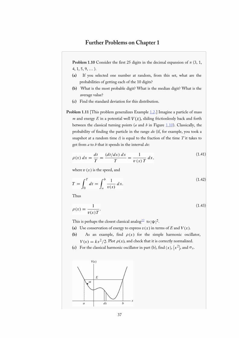
Problem 1.11 [This problem generalizes Example 1.2.] Imagine a particle of massm and energy E in a potential well , sliding frictionlessly back and forthbetween the classical turning points (a and b in Figure 1.10). Classically, theprobability of finding the particle in the range dx (if, for example, you took asnapshot at a random time t) is equal to the fraction of the time T it takes toget from a to b that it spends in the interval dx:
where is the speed, and
Thus
This is perhaps the closest classical analog22 to .(a) Use conservation of energy to express in terms of E and .(b) As an example, find for the simple harmonic oscillator,
. Plot , and check that it is correctly normalized.(c) For the classical harmonic oscillator in part (b), find , , and .
37

∗∗
(1.44)
Figure 1.10: Classical particle in a potential well.
Problem 1.12 What if we were interested in the distribution of momenta , for the classical harmonic oscillator (Problem 1.11(b)).
(a) Find the classical probability distribution (note that p ranges from to ).
(b) Calculate , , and .(c) What’s the classical uncertainty product, , for this system? Notice
that this product can be as small as you like, classically, simply by sending . But in quantum mechanics, as we shall see in Chapter 2, the
energy of a simple harmonic oscillator cannot be less than , where is the classical frequency. In that case what can you say about
the product ?
Problem 1.13 Check your results in Problem 1.11(b) with the following“numerical experiment.” The position of the oscillator at time t is
You might as well take (that sets the scale for time) and (thatsets the scale for length). Make a plot of x at 10,000 random times, andcompare it with .Hint: In Mathematica, first define
then construct a table of positions:
and finally, make a histogram of the data:
Meanwhile, make a plot of the density function, , and, using Show,superimpose the two.
Problem 1.14 Let be the probability of finding the particle in the range , at time t.
(a) Show that
where
What are the units of ? Comment: J is called the probability38

∗∗
What are the units of ? Comment: J is called the probabilitycurrent, because it tells you the rate at which probability is “flowing” pastthe point x. If is increasing, then more probability is flowing intothe region at one end than flows out at the other.
(b) Find the probability current for the wave function in Problem 1.9. (Thisis not a very pithy example, I’m afraid; we’ll encounter more substantialones in due course.)
Problem 1.15 Show that
for any two (normalizable) solutions to the Schrödinger equation (with thesame ), and .
Problem 1.16 A particle is represented (at time ) by the wave function
(a) Determine the normalization constant A.(b) What is the expectation value of x?(c) What is the expectation value of p? (Note that you cannot get it from
. Why not?)(d) Find the expectation value of .(e) Find the expectation value of .(f) Find the uncertainty in .(g) Find the uncertainty in .(h) Check that your results are consistent with the uncertainty principle.
Problem 1.17 Suppose you wanted to describe an unstable particle, thatspontaneously disintegrates with a “lifetime” τ. In that case the totalprobability of finding the particle somewhere should not be constant, butshould decrease at (say) an exponential rate:
A crude way of achieving this result is as follows. In Equation 1.24 we tacitlyassumed that V (the potential energy) is real. That is certainly reasonable, butit leads to the “conservation of probability” enshrined in Equation 1.27. Whatif we assign to V an imaginary part:
where is the true potential energy and Γ is a positive real constant?(a) Show that (in place of Equation 1.27) we now get
39
(1.45)
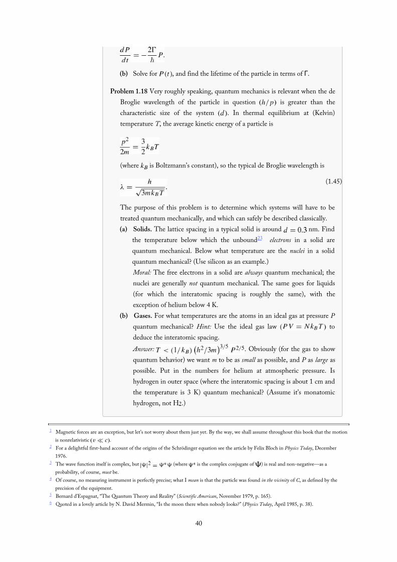
(b) Solve for , and find the lifetime of the particle in terms of Γ.
Problem 1.18 Very roughly speaking, quantum mechanics is relevant when the deBroglie wavelength of the particle in question is greater than thecharacteristic size of the system . In thermal equilibrium at (Kelvin)temperature T, the average kinetic energy of a particle is
(where is Boltzmann’s constant), so the typical de Broglie wavelength is
The purpose of this problem is to determine which systems will have to betreated quantum mechanically, and which can safely be described classically.(a) Solids. The lattice spacing in a typical solid is around nm. Find
the temperature below which the unbound23 electrons in a solid arequantum mechanical. Below what temperature are the nuclei in a solidquantum mechanical? (Use silicon as an example.)Moral: The free electrons in a solid are always quantum mechanical; thenuclei are generally not quantum mechanical. The same goes for liquids(for which the interatomic spacing is roughly the same), with theexception of helium below 4 K.
(b) Gases. For what temperatures are the atoms in an ideal gas at pressure Pquantum mechanical? Hint: Use the ideal gas law todeduce the interatomic spacing.Answer: . Obviously (for the gas to showquantum behavior) we want m to be as small as possible, and P as large aspossible. Put in the numbers for helium at atmospheric pressure. Ishydrogen in outer space (where the interatomic spacing is about 1 cm andthe temperature is 3 K) quantum mechanical? (Assume it’s monatomichydrogen, not H .)
1 Magnetic forces are an exception, but let’s not worry about them just yet. By the way, we shall assume throughout this book that the motionis nonrelativistic .
2 For a delightful first-hand account of the origins of the Schrödinger equation see the article by Felix Bloch in Physics Today, December1976.
3 The wave function itself is complex, but (where is the complex conjugate of ) is real and non-negative—as aprobability, of course, must be.
4 Of course, no measuring instrument is perfectly precise; what I mean is that the particle was found in the vicinity of C, as defined by theprecision of the equipment.
5 Bernard d’Espagnat, “The Quantum Theory and Reality” (Scientific American, November 1979, p. 165).6 Quoted in a lovely article by N. David Mermin, “Is the moon there when nobody looks?” (Physics Today, April 1985, p. 38).
40

7 Ibid., p. 40.8 This statement is a little too strong: there exist viable nonlocal hidden variable theories (notably David Bohm’s), and other formulations
(such as the many worlds interpretation) that do not fit cleanly into any of my three categories. But I think it is wise, at least from apedagogical point of view, to adopt a clear and coherent platform at this stage, and worry about the alternatives later.
9 The role of measurement in quantum mechanics is so critical and so bizarre that you may well be wondering what precisely constitutes ameasurement. I’ll return to this thorny issue in the Afterword; for the moment let’s take the naive view: a measurement is the kind of thingthat a scientist in a white coat does in the laboratory, with rulers, stopwatches, Geiger counters, and so on.
10 Because the wavelength of electrons is typically very small, the slits have to be extremely close together. Historically, this was first achievedby Davisson and Germer, in 1925, using the atomic layers in a crystal as “slits.” For an interesting account, see R. K. Gehrenbeck, PhysicsToday, January 1978, page 34.
11 See Tonomura et al., American Journal of Physics, Volume 57, Issue 2, pp. 117–120 (1989), and the amazing associated video atwww.hitachi.com/rd/portal/highlight/quantum/doubleslit/. This experiment can now be done with much more massive particles, including“Bucky-balls”; see M. Arndt, et al., Nature 40, 680 (1999). Incidentally, the same thing can be done with light: turn the intensity so low thatonly one “photon” is present at a time and you get an identical point-by-point assembly of the interference pattern. See R. S. Aspden,M. J. Padgett, and G. C. Spalding, Am. J. Phys. 84, 671 (2016).
12 I think it is important to distinguish things like interference and diffraction that would hold for any wave theory from the uniquely quantummechanical features of the measurement process, which derive from the statistical interpretation.
13 A statistician will complain that I am confusing the average of a finite sample (a million, in this case) with the “true” average (over the wholecontinuum). This can be an awkward problem for the experimentalist, especially when the sample size is small, but here I am only concernedwith the true average, to which the sample average is presumably a good approximation.
14 Evidently must go to zero faster than , as . Incidentally, normalization only fixes the modulus of A; the phaseremains undetermined. However, as we shall see, the latter carries no physical significance anyway.
15 A competent mathematician can supply you with pathological counterexamples, but they do not arise in physics; for us the wave functionand all its derivatives go to zero at infinity.
16 To keep things from getting too cluttered, I’ll suppress the limits of integration .17 The product rule says that
from which it follows that
Under the integral sign, then, you can peel a derivative off one factor in a product, and slap it onto the other one—it’ll cost you a minus sign,and you’ll pick up a boundary term.
18 An “operator” is an instruction to do something to the function that follows; it takes in one function, and spits out some other function. Theposition operator tells you to multiply by x; the momentum operator tells you to differentiate with respect to x (and multiply the result by
).19 Some authors limit the term to the pair of equations and 20 That’s why a piccolo player must be right on pitch, whereas a double-bass player can afford to wear garden gloves. For the piccolo, a sixty-
fourth note contains many full cycles, and the frequency (we’re working in the time domain now, instead of space) is well defined, whereasfor the bass, at a much lower register, the sixty-fourth note contains only a few cycles, and all you hear is a general sort of “oomph,” with novery clear pitch.
21 I’ll explain this in due course. Many authors take the de Broglie formula as an axiom, from which they then deduce the association ofmomentum with the operator . Although this is a conceptually cleaner approach, it involves diverting mathematicalcomplications that I would rather save for later.
22 If you like, instead of photos of one system at random times, picture an ensemble of such systems, all with the same energy but with randomstarting positions, and photograph them all at the same time. The analysis is identical, but this interpretation is closer to the quantum notionof indeterminacy.
23 In a solid the inner electrons are attached to a particular nucleus, and for them the relevant size would be the radius of the atom. But theouter-most electrons are not attached, and for them the relevant distance is the lattice spacing. This problem pertains to the outer electrons.
41

2Time-Independent Schrödinger Equation
◈
42
(2.1)
(2.3)
(2.4)
(2.2)
2.1 Stationary StatesIn Chapter 1 we talked a lot about the wave function, and how you use it to calculate various quantities ofinterest. The time has come to stop procrastinating, and confront what is, logically, the prior question: Howdo you get in the first place? We need to solve the Schrödinger equation,
for a specified potential1 . In this chapter (and most of this book) I shall assume that V is independentof t. In that case the Schrödinger equation can be solved by the method of separation of variables (thephysicist’s first line of attack on any partial differential equation): We look for solutions that are products,
where (lower-case) is a function of x alone, and is a function of t alone. On its face, this is an absurdrestriction, and we cannot hope to obtain more than a tiny subset of all solutions in this way. But hang on,because the solutions we do get turn out to be of great interest. Moreover (as is typically the case withseparation of variables) we will be able at the end to patch together the separable solutions in such a way as toconstruct the most general solution.
For separable solutions we have
(ordinary derivatives, now), and the Schrödinger equation reads
Or, dividing through by :
Now, the left side is a function of t alone, and the right side is a function of x alone.2 The only way this canpossibly be true is if both sides are in fact constant—otherwise, by varying t, I could change the left sidewithout touching the right side, and the two would no longer be equal. (That’s a subtle but crucial argument,so if it’s new to you, be sure to pause and think it through.) For reasons that will appear in a moment, we shallcall the separation constant E. Then
or
43

(2.5)
(2.6)
(2.7)
(2.8)
(2.9)
(2.10)
and
or
Separation of variables has turned a partial differential equation into two ordinary differential equations(Equations 2.4 and 2.5). The first of these is easy to solve (just multiply through by dt and integrate); thegeneral solution is , but we might as well absorb the constant C into (since the quantity ofinterest is the product . Then3
The second (Equation 2.5) is called the time-independent Schrödinger equation; we can go no further with ituntil the potential is specified.
The rest of this chapter will be devoted to solving the time-independent Schrödinger equation, for avariety of simple potentials. But before I get to that you have every right to ask: What’s so great about separablesolutions? After all, most solutions to the (time dependent) Schrödinger equation do not take the form
. I offer three answers—two of them physical, and one mathematical:1. They are stationary states. Although the wave function itself,
does(obviously) depend on t, the probability density,
does not—the time-dependence cancels out.4 The same thing happens in calculating the expectationvalue of any dynamical variable; Equation 1.36 reduces to
Every expectation value is constant in time; we might as well drop the factor altogether, and simplyuse in place of . (Indeed, it is common to refer to as “the wave function,” but this is sloppylanguage that can be dangerous, and it is important to remember that the true wave function alwayscarries that time-dependent wiggle factor.) In particular, is constant, and hence (Equation 1.33)
. Nothing ever happens in a stationary state.
2. They are states of definite total energy. In classical mechanics, the total energy (kinetic plus potential) iscalled the Hamiltonian:
The corresponding Hamiltonian operator, obtained by the canonical substitution , is44

(2.11)
(2.12)
(2.13)
(2.14)
(2.15)
The corresponding Hamiltonian operator, obtained by the canonical substitution , istherefore5
Thus the time-independent Schrödinger equation (Equation 2.5) can be written
and the expectation value of the total energy is
(Notice that the normalization of entails the normalization of .) Moreover,
and hence
So the variance of H is
But remember, if , then every member of the sample must share the same value (the distributionhas zero spread). Conclusion: A separable solution has the property that every measurement of the totalenergy is certain to return the value E. (That’s why I chose that letter for the separation constant.)
3. The general solution is a linear combination of separable solutions. As we’re about to discover, thetime-independent Schrödinger equation (Equation 2.5) yields an infinite collection of solutions
, , which we write as , each with its associated separation constant; thus there is a different wave function for each allowed energy:
Now (as you can easily check for yourself) the (time-dependent) Schrödinger equation (Equation 2.1)has the property that any linear combination6 of solutions is itself a solution. Once we have found theseparable solutions, then, we can immediately construct a much more general solution, of the form
It so happens that every solution to the (time-dependent) Schrödinger equation can be written in thisform—it is simply a matter of finding the right constants so as to fit the initialconditions for the problem at hand. You’ll see in the following sections how all this works out inpractice, and in Chapter 3 we’ll put it into more elegant language, but the main point is this: Onceyou’ve solved the time-independent Schrödinger equation, you’re essentially done; getting from there
45

(2.16)
(2.17)
(2.18)
to the general solution of the time-dependent Schrödinger equation is, in principle, simple andstraightforward.
A lot has happened in the past four pages, so let me recapitulate, from a somewhat different perspective.Here’s the generic problem: You’re given a (time-independent) potential , and the starting wave function
; your job is to find the wave function, , for any subsequent time t. To do this you must solvethe (time-dependent) Schrödinger equation (Equation 2.1). The strategy is first to solve the time-independent Schrödinger equation (Equation 2.5); this yields, in general, an infinite set of solutions, ,each with its own associated energy, . To fit you write down the general linear combination ofthese solutions:
the miracle is that you can always match the specified initial state7 by appropriate choice of the constants .To construct you simply tack onto each term its characteristic time dependence (its “wiggle factor”),
:8
The separable solutions themselves,
are stationary states, in the sense that all probabilities and expectation values are independent of time, but thisproperty is emphatically not shared by the general solution (Equation 2.17): the energies are different, fordifferent stationary states, and the exponentials do not cancel, when you construct .
Example 2.1Suppose a particle starts out in a linear combination of just two stationary states:
(To keep things simple I’ll assume that the constants and the states are real.) What is thewave function at subsequent times? Find the probability density, and describe its motion.Solution: The first part is easy:
where and are the energies associated with and . It follows that
The probability density oscillates sinusoidally, at an angular frequency ; this iscertainly not a stationary state. But notice that it took a linear combination of stationary states (with
46

(2.19)
(2.20)
(2.21)
∗
different energies) to produce motion.9
You may be wondering what the coefficients represent physically. I’ll tell you the answer, though theexplanation will have to await Chapter 3:
A competent measurement will always yield one of the “allowed” values (hence the name), and is theprobability of getting the particular value .10 Of course, the sum of these probabilities should be 1:
and the expectation value of the energy must be
We’ll soon see how this works out in some concrete examples. Notice, finally, that becausethe constants are independent of time, so too is the probability of getting a particular energy, and, a fortiori, the expectationvalue of H. These are manifestations of energy conservation in quantum mechanics.
Problem 2.1 Prove the following three theorems:(a) For normalizable solutions, the separation constant E must be real. Hint:
Write E (in Equation 2.7) as (with and Γ real), and showthat if Equation 1.20 is to hold for all t, Γ must be zero.
(b) The time-independent wave function can always be taken to be real(unlike , which is necessarily complex). This doesn’t mean thatevery solution to the time-independent Schrödinger equation is real; whatit says is that if you’ve got one that is not, it can always be expressed as alinear combination of solutions (with the same energy) that are. So youmight as well stick to s that are real. Hint: If satisfies Equation2.5, for a given E, so too does its complex conjugate, and hence also thereal linear combinations and .
(c) If is an even function (that is, then canalways be taken to be either even or odd. Hint: If satisfies Equation2.5, for a given E, so too does , and hence also the even and oddlinear combinations .
47

∗ Problem 2.2 Show that E must exceed the minimum value of , for everynormalizable solution to the time-independent Schrödinger equation. What is theclassical analog to this statement? Hint: Rewrite Equation 2.5 in the form
if , then and its second derivative always have the same sign—arguethat such a function cannot be normalized.
48

(2.22)
(2.23)
(2.24)
(2.25)
(2.26)
2.2 The Infinite Square WellSuppose
(Figure 2.1). A particle in this potential is completely free, except at the two ends and , wherean infinite force prevents it from escaping. A classical model would be a cart on a frictionless horizontal airtrack, with perfectly elastic bumpers—it just keeps bouncing back and forth forever. (This potential isartificial, of course, but I urge you to treat it with respect. Despite its simplicity—or rather, precisely because ofits simplicity—it serves as a wonderfully accessible test case for all the fancy machinery that comes later. We’llrefer back to it frequently.)
Figure 2.1: The infinite square well potential (Equation 2.22).
Outside the well, (the probability of finding the particle there is zero). Inside the well, where , the time-independent Schrödinger equation (Equation 2.5) reads
or
(By writing it in this way, I have tacitly assumed that ; we know from Problem 2.2 that won’twork.) Equation 2.24 is the classical simple harmonic oscillator equation; the general solution is
where A and B are arbitrary constants. Typically, these constants are fixed by the boundary conditions of theproblem. What are the appropriate boundary conditions for ? Ordinarily, both and arecontinuous,11 but where the potential goes to infinity only the first of these applies. (I’ll justify these boundaryconditions, and account for the exception when , in Section 2.5; for now I hope you will trust me.)
Continuity of requires that
49

(2.29)
(2.30)
(2.31)
(2.32)
(2.27)
(2.28)
so as to join onto the solution outside the well. What does this tell us about A and B? Well,
so , and hence
Then , so either (in which case we’re left with the trivial—non-normalizable—solution , or else , which means that
But is no good (again, that would imply , and the negative solutions give nothing new,since and we can absorb the minus sign into A. So the distinct solutions are
Curiously, the boundary condition at does not determine the constant A, but rather the constantk, and hence the possible values of E:
In radical contrast to the classical case, a quantum particle in the infinite square well cannot have just any oldenergy—it has to be one of these special (“allowed”) values.12 To find A, we normalize :13
This only determines the magnitude of A, but it is simplest to pick the positive real root: (thephase of A carries no physical significance anyway). Inside the well, then, the solutions are
As promised, the time-independent Schrödinger equation has delivered an infinite set of solutions (onefor each positive integer . The first few of these are plotted in Figure 2.2. They look just like the standingwaves on a string of length a; , which carries the lowest energy, is called the ground state, the others, whoseenergies increase in proportion to , are called excited states. As a collection, the functions have someinteresting and important properties:
1. They are alternately even and odd, with respect to the center of the well: is even, is odd, iseven, and so on.14
2. As you go up in energy, each successive state has one more node (zero-crossing): has none (the endpoints don’t count), has one, has two, and so on.
3. They are mutually orthogonal, in the sense that15
50
(2.33)
(2.34)
(2.35)
(2.36)
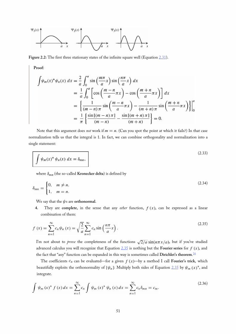
Figure 2.2: The first three stationary states of the infinite square well (Equation 2.31).
Proof:
Note that this argument does not work if . (Can you spot the point at which it fails?) In that casenormalization tells us that the integral is 1. In fact, we can combine orthogonality and normalization into asingle statement:
where (the so-called Kronecker delta) is defined by
We say that the s are orthonormal.4. They are complete, in the sense that any other function, , can be expressed as a linear
combination of them:
I’m not about to prove the completeness of the functions , but if you’ve studiedadvanced calculus you will recognize that Equation 2.35 is nothing but the Fourier series for , andthe fact that “any” function can be expanded in this way is sometimes called Dirichlet’s theorem.16
The coefficients can be evaluated—for a given —by a method I call Fourier’s trick, whichbeautifully exploits the orthonormality of : Multiply both sides of Equation 2.35 by , andintegrate.
(Notice how the Kronecker delta kills every term in the sum except the one for which .) Thus the51

(2.37)
(2.38)
(2.39)
(2.40)
(Notice how the Kronecker delta kills every term in the sum except the one for which .) Thus thenth coefficient in the expansion of is17
These four properties are extremely powerful, and they are not peculiar to the infinite square well. Thefirst is true whenever the potential itself is a symmetric function; the second is universal, regardless of theshape of the potential.18 Orthogonality is also quite general—I’ll show you the proof in Chapter 3.Completeness holds for all the potentials you are likely to encounter, but the proofs tend to be nasty andlaborious; I’m afraid most physicists simply assume completeness, and hope for the best.
The stationary states (Equation 2.18) of the infinite square well are
I claimed (Equation 2.17) that the most general solution to the (time-dependent) Schrödinger equation is alinear combination of stationary states:
(If you doubt that this is a solution, by all means check it!) It remains only for me to demonstrate that I can fitany prescribed initial wave function, by appropriate choice of the coefficients :
The completeness of the s (confirmed in this case by Dirichlet’s theorem) guarantees that I can alwaysexpress in this way, and their orthonormality licenses the use of Fourier’s trick to determine theactual coefficients:
That does it: Given the initial wave function, , we first compute the expansion coefficients ,using Equation 2.40, and then plug these into Equation 2.39 to obtain . Armed with the wavefunction, we are in a position to compute any dynamical quantities of interest, using the procedures inChapter 1. And this same ritual applies to any potential—the only things that change are the functional formof the s and the equation for the allowed energies.
Example 2.2A particle in the infinite square well has the initial wave function
for some constant A (see Figure 2.3). Outside the well, of course, . Find .
52

Figure 2.3: The starting wave function in Example 2.2.
Solution: First we need to determine A, by normalizing :
so
The nth coefficient is (Equation 2.40)
Thus (Equation 2.39):
Example 2.3
Check that Equation 2.20 is satisfied, for the wave function in Example 2.2. If you measured the53

(2.41)
Check that Equation 2.20 is satisfied, for the wave function in Example 2.2. If you measured theenergy of a particle in this state, what is the most probable result? What is the expectation value of theenergy?Solution: The starting wave function (Figure 2.3) closely resembles the ground state (Figure 2.2).This suggests that should dominate,19 and in fact
The rest of the coefficients make up the difference:20
The most likely outcome of an energy measurement is —more than 99.8% of allmeasurements will yield this value. The expectation value of the energy (Equation 2.21) is
As one would expect, it is very close to (5 in place of —slightly larger, because ofthe admixture of excited states.
Of course, it’s no accident that Equation 2.20 came out right in Example 2.3. Indeed, this follows fromthe normalization of (the s are independent of time, so I’m going to do the proof for ; if thisbothers you, you can easily generalize the argument to arbitrary .
(Again, the Kronecker delta picks out the term in the summation over m.) Similarly, the expectationvalue of the energy (Equation 2.21) can be checked explicitly: The time-independent Schrödinger equation(Equation 2.12) says
so
54

∗
∗
Problem 2.3 Show that there is no acceptable solution to the (time-independent)Schrödinger equation for the infinite square well with or . (This is aspecial case of the general theorem in Problem 2.2, but this time do it by explicitlysolving the Schrödinger equation, and showing that you cannot satisfy theboundary conditions.)
Problem 2.4 Calculate , and , for the nth stationarystate of the infinite square well. Check that the uncertainty principle is satisfied.Which state comes closest to the uncertainty limit?
Problem 2.5 A particle in the infinite square well has as its initial wave function aneven mixture of the first two stationary states:
(a) Normalize . (That is, find A. This is very easy, if you exploit theorthonormality of and . Recall that, having normalized at ,you can rest assured that it stays normalized—if you doubt this, check itexplicitly after doing part (b).)
(b) Find and . Express the latter as a sinusoidal functionof time, as in Example 2.1. To simplify the result, let .
(c) Compute . Notice that it oscillates in time. What is the angularfrequency of the oscillation? What is the amplitude of the oscillation? (Ifyour amplitude is greater than , go directly to jail.)
(d) Compute . (As Peter Lorre would say, “Do it ze kveek vay, Johnny!”)(e) If you measured the energy of this particle, what values might you get,
and what is the probability of getting each of them? Find the expectationvalue of H. How does it compare with and ?
Problem 2.6 Although the overall phase constant of the wave function is of nophysical significance (it cancels out whenever you calculate a measurable quantity),the relative phase of the coefficients in Equation 2.17 does matter. For example,suppose we change the relative phase of and in Problem 2.5:
where ϕ is some constant. Find , and , and compare your55

∗
where ϕ is some constant. Find , and , and compare yourresults with what you got before. Study the special cases and .(For a graphical exploration of this problem see the applet in footnote 9 of thischapter.)
Problem 2.7 A particle in the infinite square well has the initial wave function
(a) Sketch , and determine the constant A.(b) Find .(c) What is the probability that a measurement of the energy would yield the
value ?(d) Find the expectation value of the energy, using Equation 2.21.21
Problem 2.8 A particle of mass m in the infinite square well (of width starts outin the state
for some constant A, so it is (at equally likely to be found at any point inthe left half of the well. What is the probability that a measurement of the energy(at some later time would yield the value ?
Problem 2.9 For the wave function in Example 2.2, find the expectation value ofH, at time , the “old fashioned” way:
Compare the result we got in Example 2.3. Note: Because is independent oftime, there is no loss of generality in using .
56

(2.42)
(2.43)
2.3 The Harmonic OscillatorThe paradigm for a classical harmonic oscillator is a mass m attached to a spring of force constant k. Themotion is governed by Hooke’s law,
(ignoring friction), and the solution is
where
is the (angular) frequency of oscillation. The potential energy is
its graph is a parabola.Of course, there’s no such thing as a perfect harmonic oscillator—if you stretch it too far the spring is
going to break, and typically Hooke’s law fails long before that point is reached. But practically any potentialis approximately parabolic, in the neighborhood of a local minimum (Figure 2.4). Formally, if we expand
in a Taylor series about the minimum:
subtract (you can add a constant to with impunity, since that doesn’t change the force),recognize that (since is a minimum), and drop the higher-order terms (which are negligible aslong as stays small), we get
which describes simple harmonic oscillation (about the point , with an effective spring constant . That’s why the simple harmonic oscillator is so important: Virtually any oscillatory motion is
approximately simple harmonic, as long as the amplitude is small.22
57

(2.44)
(2.45)
Figure 2.4: Parabolic approximation (dashed curve) to an arbitrary potential, in the neighborhood of a localminimum.
The quantum problem is to solve the Schrödinger equation for the potential
(it is customary to eliminate the spring constant in favor of the classical frequency, using Equation 2.42). Aswe have seen, it suffices to solve the time-independent Schrödinger equation:
In the literature you will find two entirely different approaches to this problem. The first is a straightforward“brute force” solution to the differential equation, using the power series method; it has the virtue that thesame strategy can be applied to many other potentials (in fact, we’ll use it in Chapter 4 to treat the hydrogenatom). The second is a diabolically clever algebraic technique, using so-called ladder operators. I’ll show youthe algebraic method first, because it is quicker and simpler (and a lot more fun);23 if you want to skip thepower series method for now, that’s fine, but you should certainly plan to study it at some stage.
58
(2.46)
(2.47)
(2.48)
(2.49)
(2.50)
(2.51)
2.3.1 Algebraic Method
To begin with, let’s rewrite Equation 2.45 in a more suggestive form:
where is the momentum operator.24 The basic idea is to factor the Hamiltonian,
If these were numbers, it would be easy:
Here, however, it’s not quite so simple, because and x are operators, and operators do not, in general,commute is not the same as , as we’ll see in a moment—though you might want to stop right now andthink it through for yourself). Still, this does motivate us to examine the quantities
(the factor in front is just there to make the final results look nicer).Well, what is the product ?
As anticipated, there’s an extra term, involving . We call this the commutator of x and ; it is ameasure of how badly they fail to commute. In general, the commutator of operators and (written withsquare brackets) is
In this notation,
We need to figure out the commutator of x and . Warning: Operators are notoriously slippery to workwith in the abstract, and you are bound to make mistakes unless you give them a “test function,” , to acton. At the end you can throw away the test function, and you’ll be left with an equation involving theoperators alone. In the present case we have:
59

(2.52)
(2.53)
(2.54)
(2.55)
(2.56)
(2.57)
(2.58)
Dropping the test function, which has served its purpose,
This lovely and ubiquitous formula is known as the canonical commutation relation.25
With this, Equation 2.50 becomes
or
Evidently the Hamiltonian does not factor perfectly—there’s that extra on the right. Notice that theordering of and is important here; the same argument, with on the left, yields
In particular,
Meanwhile, the Hamiltonian can equally well be written
In terms of , then, the Schrödinger equation26 for the harmonic oscillator takes the form
(in equations like this you read the upper signs all the way across, or else the lower signs).Now, here comes the crucial step: I claim that:
If satisfies the Schrödinger equation with energy E (that is: , then satisfies theSchrödinger equation with energy : .
Proof:
(I used Equation 2.56 to replace by in the second line. Notice that whereas the60

(I used Equation 2.56 to replace by in the second line. Notice that whereas theordering of and does matter, the ordering of and any constants—such as , and E—does not;an operator commutes with any constant.)
By the same token, is a solution with energy :
Here, then, is a wonderful machine for generating new solutions, with higher and lower energies—if wecould just find one solution, to get started! We call ladder operators, because they allow us to climb up anddown in energy; is the raising operator, and the lowering operator. The “ladder” of states is illustratedin Figure 2.5.
Figure 2.5: The “ladder” of states for the harmonic oscillator.
But wait! What if I apply the lowering operator repeatedly? Eventually I’m going to reach a state withenergy less than zero, which (according to the general theorem in Problem 2.3) does not exist! At some pointthe machine must fail. How can that happen? We know that is a new solution to the Schrödinger
61

(2.60)
(2.61)
(2.62)
(2.59)
equation, but there is no guarantee that it will be normalizable—it might be zero, or its square-integral might beinfinite. In practice it is the former: There occurs a “lowest rung” (call it such that
We can use this to determine :
or
This differential equation is easy to solve:
so
We might as well normalize it right away:
so , and hence
To determine the energy of this state we plug it into the Schrödinger equation (in the form of Equation 2.58),, and exploit the fact that :
With our foot now securely planted on the bottom rung (the ground state of the quantum oscillator), wesimply apply the raising operator (repeatedly) to generate the excited states,27 increasing the energy by with each step:
where is the normalization constant. By applying the raising operator (repeatedly) to , then, we can (inprinciple) construct all28 the stationary states of the harmonic oscillator. Meanwhile, without ever doing thatexplicitly, we have determined the allowed energies!
62

(2.63)
(2.65)
(2.64)
Example 2.4Find the first excited state of the harmonic oscillator.Solution: Using Equation 2.62,
We can normalize it “by hand”:
so, as it happens, .I wouldn’t want to calculate this way (applying the raising operator fifty times!), but never
mind: In principle Equation 2.62 does the job—except for the normalization.
You can even get the normalization algebraically, but it takes some fancy footwork, so watch closely. Weknow that is proportional to ,
but what are the proportionality factors, and ? First note that for “any”29 functions and ,
In the language of linear algebra, is the hermitian conjugate (or adjoint) of .
Proof:
and integration by parts takes to (the boundary terms vanish, forthe reason indicated in footnote 29), so
In particular,
But (invoking Equations 2.58 and 2.62)
63

(2.67)
(2.68)
(2.69)
(2.66)
so
But since and are normalized, it follows that and , and hence30
Thus
and so on. Clearly
which is to say that the normalization factor in Equation 2.62 is (in particular, ,confirming our result in Example 2.4).
As in the case of the infinite square well, the stationary states of the harmonic oscillator are orthogonal:
This can be proved using Equation 2.66, and Equation 2.65 twice—first moving and then moving :
Unless , then, must be zero. Orthonormality means that we can again use Fourier’s trick(Equation 2.37) to evaluate the coefficients , when we expand as a linear combination of stationarystates (Equation 2.16). As always, is the probability that a measurement of the energy would yield thevalue .
64

(2.70)
∗
∗
Example 2.5Find the expectation value of the potential energy in the nth stationary state of the harmonicoscillator.Solution:
There’s a beautiful device for evaluating integrals of this kind (involving powers of x or : Use thedefinition (Equation 2.48) to express x and in terms of the raising and lowering operators:
In this example we are interested in :
So
But is (apart from normalization) , which is orthogonal to , and the same goes for , which is proportional to . So those terms drop out, and we can use Equation 2.66 to
evaluate the remaining two:
As it happens, the expectation value of the potential energy is exactly half the total (the other half, ofcourse, is kinetic). This is a peculiarity of the harmonic oscillator, as we’ll see later on (Problem 3.37).
Problem 2.10(a) Construct .(b) Sketch , and .(c) Check the orthogonality of , and , by explicit integration. Hint:
If you exploit the even-ness and odd-ness of the functions, there is reallyonly one integral left to do.
Problem 2.11(a) Compute , and , for the states (Equation 2.60) and
(Equation 2.63), by explicit integration. Comment: In this and otherproblems involving the harmonic oscillator it simplifies matters if you
65
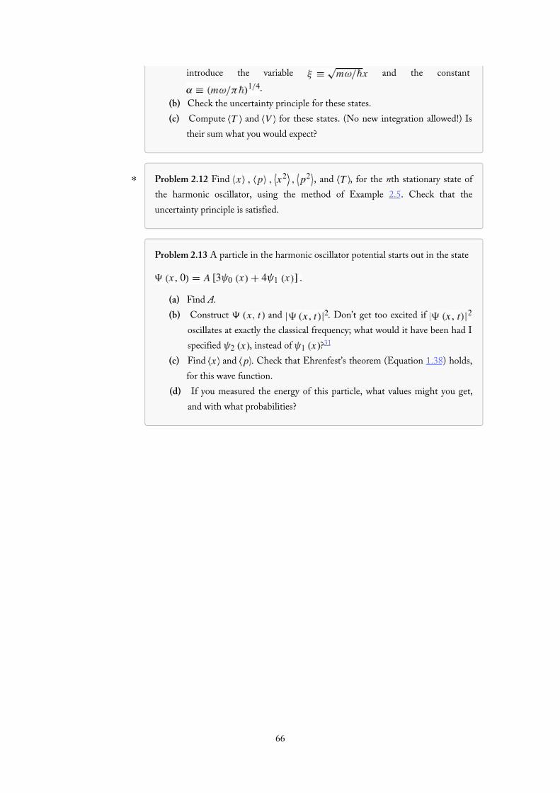
∗
introduce the variable and the constant .
(b) Check the uncertainty principle for these states.(c) Compute and for these states. (No new integration allowed!) Is
their sum what you would expect?
Problem 2.12 Find , and , for the nth stationary state ofthe harmonic oscillator, using the method of Example 2.5. Check that theuncertainty principle is satisfied.
Problem 2.13 A particle in the harmonic oscillator potential starts out in the state
(a) Find A.(b) Construct and . Don’t get too excited if
oscillates at exactly the classical frequency; what would it have been had Ispecified , instead of ?31
(c) Find and . Check that Ehrenfest’s theorem (Equation 1.38) holds,for this wave function.
(d) If you measured the energy of this particle, what values might you get,and with what probabilities?
66

(2.71)
(2.72)
(2.73)
(2.74)
(2.75)
(2.76)
(2.77)
(2.78)
2.3.2 Analytic Method
We return now to the Schrödinger equation for the harmonic oscillator,
and solve it directly, by the power series method. Things look a little cleaner if we introduce the dimensionlessvariable
in terms of ξ the Schrödinger equation reads
where K is the energy, in units of :
Our problem is to solve Equation 2.73, and in the process obtain the “allowed” values of K (and hence of .To begin with, note that at very large ξ (which is to say, at very large completely dominates over
the constant K, so in this regime
which has the approximate solution (check it!)
The B term is clearly not normalizable (it blows up as ; the physically acceptable solutions, then,have the asymptotic form
This suggests that we “peel off” the exponential part,
in hopes that what remains, , has a simpler functional form than itself.32 Differentiating Equation2.78,
and
67

(2.79)
(2.80)
(2.81)
(2.82)
(2.83)
so the Schrödinger equation (Equation 2.73) becomes
I propose to look for solutions to Equation 2.79 in the form of power series in ξ:33
Differentiating the series term by term,
and
Putting these into Equation 2.80, we find
It follows (from the uniqueness of power series expansions34 ) that the coefficient of each power of ξ mustvanish,
and hence that
This recursion formula is entirely equivalent to the Schrödinger equation. Starting with , it generatesall the even-numbered coefficients:
and starting with , it generates the odd coefficients:
We write the complete solution as
68

(2.84)
where
is an even function of ξ, built on , and
is an odd function, built on . Thus Equation 2.82 determines in terms of two arbitrary constants and —which is just what we would expect, for a second-order differential equation.
However, not all the solutions so obtained are normalizable. For at very large j, the recursion formulabecomes (approximately)
with the (approximate) solution
for some constant C, and this yields (at large ξ, where the higher powers dominate)
Now, if h goes like , then (remember ?—that’s what we’re trying to calculate) goes like (Equation 2.78), which is precisely the asymptotic behavior we didn’t want.35 There is only one
way to wiggle out of this: For normalizable solutions the power series must terminate. There must occur some“highest” j (call it , such that the recursion formula spits out (this will truncate either the series
or the series ; the other one must be zero from the start: if n is even, and if n is odd).For physically acceptable solutions, then, Equation 2.82 requires that
for some positive integer n, which is to say (referring to Equation 2.74) that the energy must be
Thus we recover, by a completely different method, the fundamental quantization condition we foundalgebraically in Equation 2.62.
It seems at first rather surprising that the quantization of energy should emerge from a technical detail inthe power series solution to the Schrödinger equation, but let’s look at it from a different perspective.Equation 2.71 has solutions, of course, for any value of E (in fact, it has two linearly independent solutions forevery . But almost all of these solutions blow up exponentially at large x, and hence are not normalizable.Imagine, for example, using an E that is slightly less than one of the allowed values (say, , andplotting the solution: Figure 2.6(a). Now try an E slightly larger (say, ; the “tail” now blows up in theother direction (Figure 2.6(b)). As you tweak the parameter in tiny increments from 0.49 to 0.51, the graph
69

(2.85)
“flips over” at precisely the value 0.5—only here does the solution escape the exponential asymptotic growththat renders it physically unacceptable.36
Figure 2.6: Solutions to the Schrödinger equation for (a) , and (b) .
For the allowed values of K, the recursion formula reads
If , there is only one term in the series (we must pick to kill , and in Equation 2.85yields :
and hence
(which, apart from the normalization, reproduces Equation 2.60). For we take ,37 and Equation2.85 with yields , so
and hence
70
(2.86)
(confirming Equation 2.63). For yields , and gives , so
and
and so on. (Compare Problem 2.10, where this last result was obtained by algebraic means).In general, will be a polynomial of degree n in ξ, involving even powers only, if n is an even
integer, and odd powers only, if n is an odd integer. Apart from the overall factor or they are the so-called Hermite polynomials, .38 The first few of them are listed in Table 2.1. By tradition, the arbitrarymultiplicative factor is chosen so that the coefficient of the highest power of ξ is . With this convention, thenormalized39 stationary states for the harmonic oscillator are
They are identical (of course) to the ones we obtained algebraically in Equation 2.68.
Table 2.1: The first few Hermite polynomials, .
In Figure 2.7(a) I have plotted for the first few ns. The quantum oscillator is strikingly differentfrom its classical counterpart—not only are the energies quantized, but the position distributions have somebizarre features. For instance, the probability of finding the particle outside the classically allowed range (thatis, with x greater than the classical amplitude for the energy in question) is not zero (see Problem 2.14), and inall odd states the probability of finding the particle at the center is zero. Only at large n do we begin to seesome resemblance to the classical case. In Figure 2.7(b) I have superimposed the classical position distribution(Problem 1.11) on the quantum one (for ; if you smoothed out the bumps, the two would fit prettywell.
71

Figure 2.7: (a) The first four stationary states of the harmonic oscillator. (b) Graph of , with theclassical distribution (dashed curve) superimposed.
Problem 2.14 In the ground state of the harmonic oscillator, what is theprobability (correct to three significant digits) of finding the particle outside theclassically allowed region? Hint: Classically, the energy of an oscillator is
, where a is the amplitude. So the “classicallyallowed region” for an oscillator of energy E extends from to
. Look in a math table under “Normal Distribution” or “ErrorFunction” for the numerical value of the integral, or evaluate it by computer.
72
∗∗
(2.87)
(2.89)
(2.90)
(2.88)
Problem 2.15 Use the recursion formula (Equation 2.85) to work out and . Invoke the convention that the coefficient of the highest power of ξ is
to fix the overall constant.
Problem 2.16 In this problem we explore some of the more useful theorems(stated without proof) involving Hermite polynomials.
(a) The Rodrigues formula says that
Use it to derive and .(b) The following recursion relation gives you in terms of the two
preceding Hermite polynomials:
Use it, together with your answer in (a), to obtain and .(c) If you differentiate an nth-order polynomial, you get a polynomial of
order . For the Hermite polynomials, in fact,
Check this, by differentiating and .(d) is the nth z-derivative, at , of the generating function
; or, to put it another way, it is the coefficient of in the Taylor series expansion for this function:
Use this to obtain , and .
73

(2.91)
(2.92)
(2.93)
(2.94)
(2.95)
(2.96)
2.4 The Free ParticleWe turn next to what should have been the simplest case of all: the free particle everywhere).Classically this would just be motion at constant velocity, but in quantum mechanics the problem issurprisingly subtle. The time-independent Schrödinger equation reads
or
So far, it’s the same as inside the infinite square well (Equation 2.24), where the potential is also zero; thistime, however, I prefer to write the general solution in exponential form (instead of sines and cosines), forreasons that will appear in due course:
Unlike the infinite square well, there are no boundary conditions to restrict the possible values of k (and henceof ; the free particle can carry any (positive) energy. Tacking on the standard time dependence,
,
Now, any function of x and t that depends on these variables in the special combination (forsome constant represents a wave of unchanging shape, traveling in the -direction at speed v: A fixedpoint on the waveform (for example, a maximum or a minimum) corresponds to a fixed value of the argument,and hence to x and t such that
Since every point on the waveform moves with the same velocity, its shape doesn’t change as it propagates.Thus the first term in Equation 2.94 represents a wave traveling to the right, and the second represents a wave(of the same energy) going to the left. By the way, since they only differ by the sign in front of k, we might aswell write
and let k run negative to cover the case of waves traveling to the left:
Evidently the “stationary states” of the free particle are propagating waves; their wavelength is ,and, according to the de Broglie formula (Equation 1.39), they carry momentum
74

(2.98)
(2.99)
(2.100)
(2.101)
(2.102)
(2.103)
(2.97)
The speed of these waves (the coefficient of t over the coefficient of is
On the other hand, the classical speed of a free particle with energy E is given by (purekinetic, since , so
Apparently the quantum mechanical wave function travels at half the speed of the particle it is supposed torepresent! We’ll return to this paradox in a moment—there is an even more serious problem we need toconfront first: This wave function is not normalizable:
In the case of the free particle, then, the separable solutions do not represent physically realizable states. A freeparticle cannot exist in a stationary state; or, to put it another way, there is no such thing as a free particle with adefinite energy.
But that doesn’t mean the separable solutions are of no use to us. For they play a mathematical role that isentirely independent of their physical interpretation: The general solution to the time-dependent Schrödingerequation is still a linear combination of separable solutions (only this time it’s an integral over the continuousvariable k, instead of a sum over the discrete index :
(The quantity is factored out for convenience; what plays the role of the coefficient in Equation
2.17 is the combination .) Now this wave function can be normalized (for appropriate . But it necessarily carries a range of ks, and hence a range of energies and speeds. We call it a wave
packet.40
In the generic quantum problem, we are given , and we are asked to find . For a freeparticle the solution takes the form of Equation 2.101; the only question is how to determine so as tomatch the initial wave function:
This is a classic problem in Fourier analysis; the answer is provided by Plancherel’s theorem (see Problem2.19):
75

(2.104)
(2.105)
is called the Fourier transform of ; is the inverse Fourier transform of (the onlydifference is the sign in the exponent).41 There is, of course, some restriction on the allowable functions: Theintegrals have to exist.42 For our purposes this is guaranteed by the physical requirement that itself benormalized. So the solution to the generic quantum problem, for the free particle, is Equation 2.101, with
Example 2.6A free particle, which is initially localized in the range , is released at time :
where A and a are positive real constants. Find .Solution: First we need to normalize :
Next we calculate , using Equation 2.104:
Finally, we plug this back into Equation 2.101:
Unfortunately, this integral cannot be solved in terms of elementary functions, though it can of coursebe evaluated numerically (Figure 2.8). (There are, in fact, precious few cases in which the integral for
(Equation 2.101) can be carried out explicitly; see Problem 2.21 for a particularly beautifulexample.)
76

Figure 2.8: Graph of (Equation 2.105) at (the rectangle) and at (thecurve).
In Figure 2.9 I have plotted and . Note that for small a, is narrow (in , while is broad (in , and vice versa for large a. But k is related to momentum, by Equation 2.97, so
this is a manifestation of the uncertainty principle: the position can be well defined (small , or themomentum (large , but not both.
Figure 2.9: (a) Graph of . (b) Graph of .
I return now to the paradox noted earlier: the fact that the separable solution travels at the“wrong” speed for the particle it ostensibly represents. Strictly speaking, the problem evaporated when wediscovered that is not a physically realizable state. Nevertheless, it is of interest to figure out howinformation about the particle velocity is contained in the wave function (Equation 2.101). The essential ideais this: A wave packet is a superposition of sinusoidal functions whose amplitude is modulated by ϕ(Figure 2.10); it consists of “ripples” contained within an “envelope.” What corresponds to the particle velocityis not the speed of the individual ripples (the so-called phase velocity), but rather the speed of the envelope(the group velocity)—which, depending on the nature of the waves, can be greater than, less than, or equal to,the velocity of the ripples that go to make it up. For waves on a string, the group velocity is the same as thephase velocity. For water waves it is one-half the phase velocity, as you may have noticed when you toss a rockinto a pond (if you concentrate on a particular ripple, you will see it build up from the rear, move forwardthrough the group, and fade away at the front, while the group as a whole propagates out at half that speed).What I need to show is that for the wave function of a free particle in quantum mechanics the group velocityis twice the phase velocity—just right to match the classical particle speed.
77

(2.106)
(2.107)
(2.108)
(2.109)
∗
(2.110)
Figure 2.10: A wave packet. The “envelope” travels at the group velocity; the “ripples” travel at the phasevelocity.
The problem, then, is to determine the group velocity of a wave packet with the generic form
In our case , but what I have to say now applies to any kind of wave packet, regardless of itsdispersion relation (the formula for ω as a function of . Let us assume that is narrowly peaked aboutsome particular value . (There is nothing illegal about a broad spread in k, but such wave packets changeshape rapidly—different components travel at different speeds, so the whole notion of a “group,” with a well-defined velocity, loses its meaning.) Since the integrand is negligible except in the vicinity of , we may aswell Taylor-expand the function about that point, and keep only the leading terms:
where is the derivative of ω with respect to k, at the point .Changing variables from k to (to center the integral at , we have
The term in front is a sinusoidal wave (the “ripples”), traveling at speed . It is modulated by the integral(the “envelope”), which is a function of , and therefore propagates at the speed . Thus the phasevelocity is
while the group velocity is
(both of them evaluated at .In our case, , so , whereas , which is twice as great.
This confirms that the group velocity of the wave packet matches the classical particle velocity:
Problem 2.17 Show that and areequivalent ways of writing the same function of x, and determine the constants Cand D in terms of A and B, and vice versa. Comment: In quantum mechanics,when , the exponentials represent traveling waves, and are most convenientin discussing the free particle, whereas sines and cosines correspond to standingwaves, which arise naturally in the case of the infinite square well.
78

∗∗
Problem 2.18 Find the probability current, J (Problem 1.14) for the free particlewave function Equation 2.95. Which direction does the probability flow?
Problem 2.19 This problem is designed to guide you through a “proof” ofPlancherel’s theorem, by starting with the theory of ordinary Fourier series on afinite interval, and allowing that interval to expand to infinity.
(a) Dirichlet’s theorem says that “any” function on the interval can be expanded as a Fourier series:
Show that this can be written equivalently as
What is , in terms of and ?(b) Show (by appropriate modification of Fourier’s trick) that
(c) Eliminate n and in favor of the new variables and . Show that (a) and (b) now become
where is the increment in k from one n to the next.(d) Take the limit to obtain Plancherel’s theorem. Comment: In view
of their quite different origins, it is surprising (and delightful) that thetwo formulas—one for in terms of , the other for interms of —have such a similar structure in the limit .
Problem 2.20 A free particle has the initial wave function
where A and a are positive real constants.(a) Normalize .(b) Find .(c) Construct , in the form of an integral.(d) Discuss the limiting cases very large, and a very small).
79

∗
(2.111)
Problem 2.21 The gaussian wave packet. A free particle has the initial wavefunction
where A and a are (real and positive) constants.(a) Normalize .(b) Find . Hint: Integrals of the form
can be handled by “completing the square”: Let ,and note that . Answer:
(c) Find . Express your answer in terms of the quantity
Sketch (as a function of at , and again for some very large t.Qualitatively, what happens to , as time goes on?
(d) Find , and . Partial answer: , butit may take some algebra to reduce it to this simple form.
(e) Does the uncertainty principle hold? At what time t does the system comeclosest to the uncertainty limit?
80

2.5 The Delta-Function Potential
81

2.5.1 Bound States and Scattering States
We have encountered two very different kinds of solutions to the time-independent Schrödinger equation:For the infinite square well and the harmonic oscillator they are normalizable, and labeled by a discrete index n;for the free particle they are non-normalizable, and labeled by a continuous variable k. The former representphysically realizable states in their own right, the latter do not; but in both cases the general solution to thetime-dependent Schrödinger equation is a linear combination of stationary states—for the first type thiscombination takes the form of a sum (over , whereas for the second it is an integral (over . What is thephysical significance of this distinction?
In classical mechanics a one-dimensional time-independent potential can give rise to two rather differentkinds of motion. If rises higher than the particle’s total energy on either side (Figure 2.11(a)), thenthe particle is “stuck” in the potential well—it rocks back and forth between the turning points, but it cannotescape (unless, of course, you provide it with a source of extra energy, such as a motor, but we’re not talkingabout that). We call this a bound state. If, on the other hand, E exceeds on one side (or both), then theparticle comes in from “infinity,” slows down or speeds up under the influence of the potential, and returns toinfinity (Figure 2.11(b)). (It can’t get trapped in the potential unless there is some mechanism, such asfriction, to dissipate energy, but again, we’re not talking about that.) We call this a scattering state. Somepotentials admit only bound states (for instance, the harmonic oscillator); some allow only scattering states (apotential hill with no dips in it, for example); some permit both kinds, depending on the energy of theparticle.
82

(2.112)
(2.113)
Figure 2.11: (a) A bound state. (b) Scattering states. (c) A classical bound state, but a quantum scattering state.
The two kinds of solutions to the Schrödinger equation correspond precisely to bound and scatteringstates. The distinction is even cleaner in the quantum domain, because the phenomenon of tunneling (whichwe’ll come to shortly) allows the particle to “leak” through any finite potential barrier, so the only thing thatmatters is the potential at infinity (Figure 2.11(c)):
In real life most potentials go to zero at infinity, in which case the criterion simplifies even further:
Because the infinite square well and harmonic oscillator potentials go to infinity as , they admitbound states only; because the free particle potential is zero everywhere, it only allows scattering states.43 In
83

this section (and the following one) we shall explore potentials that support both kinds of states.
84

(2.114)
(2.116)
(2.118)
(2.115)
(2.117)
2.5.2 The Delta-Function Well
The Dirac delta function is an infinitely high, infinitesimally narrow spike at the origin, whose area is 1(Figure 2.12):
Technically, it isn’t a function at all, since it is not finite at (mathematicians call it a generalizedfunction, or distribution).44 Nevertheless, it is an extremely useful construct in theoretical physics. (Forexample, in electrodynamics the charge density of a point charge is a delta function.) Notice that would be a spike of area 1 at the point a. If you multiply by an ordinary function , it’s the sameas multiplying by ,
because the product is zero anyway except at the point a. In particular,
That’s the most important property of the delta function: Under the integral sign it serves to “pick out” thevalue of at the point a. (Of course, the integral need not go from to ; all that matters is thatthe domain of integration include the point a, so to would do, for any .)
Figure 2.12: The Dirac delta function (Equation 2.114).
Let’s consider a potential of the form
where α is some positive constant.45 This is an artificial potential, to be sure (so was the infinite square well),but it’s delightfully simple to work with, and illuminates the basic theory with a minimum of analytical clutter.The Schrödinger equation for the delta-function well reads
it yields both bound states and scattering states .We’ll look first at the bound states. In the region , so
85

(2.119)
(2.120)
(2.124)
(2.125)
(2.121)
(2.122)
(2.123)
where
is negative, by assumption, so κ is real and positive.) The general solution to Equation 2.119 is
but the first term blows up as , so we must choose :
In the region is again zero, and the general solution is of the form ; this time it’s the second term that blows up (as , so
It remains only to stitch these two functions together, using the appropriate boundary conditions at . I quoted earlier the standard boundary conditions for :
In this case the first boundary condition tells us that , so
is plotted in Figure 2.13. The second boundary condition tells us nothing; this is (like the walls of theinfinite square well) the exceptional case where V is infinite at the join, and it’s clear from the graph that thisfunction has a kink at . Moreover, up to this point the delta function has not come into the story at all.It turns out that the delta function determines the discontinuity in the derivative of , at . I’ll show younow how this works, and as a byproduct we’ll see why is ordinarily continuous.
Figure 2.13: Bound state wave function for the delta-function potential (Equation 2.125).
The idea is to integrate the Schrödinger equation, from to , and then take the limit as :
86

(2.126)
(2.127)
(2.128)
(2.129)
(2.130)
(2.131)
(2.132)
The first integral is nothing but , evaluated at the two end points; the last integral is zero, in the limit , since it’s the area of a sliver with vanishing width and finite height. Thus
Ordinarily, the limit on the right is again zero, and that’s why is ordinarily continuous. But when is infinite at the boundary, this argument fails. In particular, if , Equation 2.116 yields
For the case at hand (Equation 2.125),
and hence . And . So Equation 2.128 says
and the allowed energy (Equation 2.120) is
Finally, we normalize :
so (choosing the positive real root):
Evidently the delta function well, regardless of its “strength” α, has exactly one bound state:
What about scattering states, with ? For the Schrödinger equation reads
where
87

(2.133)
(2.134)
(2.135)
(2.137)
(2.138)
(2.140)
(2.136)
(2.139)
is real and positive. The general solution is
and this time we cannot rule out either term, since neither of them blows up. Similarly, for ,
The continuity of at requires that
The derivatives are
and hence . Meanwhile, , so the second boundarycondition (Equation 2.128) says
or, more compactly,
Having imposed both boundary conditions, we are left with two equations (Equations 2.136 and 2.138)in four unknowns , B, F, and —five, if you count k. Normalization won’t help—this isn’t a normalizablestate. Perhaps we’d better pause, then, and examine the physical significance of these various constants. Recallthat gives rise (when coupled with the wiggle factor to a wave functionpropagating to the right, and leads to a wave propagating to the left. It follows that A (inEquation 2.134) is the amplitude of a wave coming in from the left, B is the amplitude of a wave returning tothe left; F (Equation 2.135) is the amplitude of a wave traveling off to the right, and G is the amplitude of awave coming in from the right (see Figure 2.14). In a typical scattering experiment particles are fired in fromone direction—let’s say, from the left. In that case the amplitude of the wave coming in from the right will bezero:
A is the amplitude of the incident wave, B is the amplitude of the reflected wave, and F is the amplitude ofthe transmitted wave. Solving Equations 2.136 and 2.138 for B and F, we find
(If you want to study scattering from the right, set ; then G is the incident amplitude, F is the reflectedamplitude, and B is the transmitted amplitude.)
88

(2.141)
(2.142)
(2.144)
(2.143)
Figure 2.14: Scattering from a delta function well.
Now, the probability of finding the particle at a specified location is given by , so the relative46
probability that an incident particle will be reflected back is
R is called the reflection coefficient. (If you have a beam of particles, it tells you the fraction of the incomingnumber that will bounce back.) Meanwhile, the probability that a particle will continue right on through is thetransmission coefficient47
Of course, the sum of these probabilities should be 1—and it is:
Notice that R and T are functions of β, and hence (Equations 2.133 and 2.138) of E:
The higher the energy, the greater the probability of transmission (which makes sense).This is all very tidy, but there is a sticky matter of principle that we cannot altogether ignore: These
scattering wave functions are not normalizable, so they don’t actually represent possible particle states. Weknow the resolution to this problem: form normalizable linear combinations of the stationary states, just as wedid for the free particle—true physical particles are represented by the resulting wave packets. Thoughstraightforward in principle, this is a messy business in practice, and at this point it is best to turn the problemover to a computer.48 Meanwhile, since it is impossible to create a normalizable free-particle wave functionwithout involving a range of energies, R and T should be interpreted as the approximate reflection andtransmission probabilities for particles with energies in the vicinity of E.
Incidentally, it might strike you as peculiar that we were able to analyze a quintessentially time-dependent problem (particle comes in, scatters off a potential, and flies off to infinity) using stationary states.After all, (in Equations 2.134 and 2.135) is simply a complex, time-independent, sinusoidal function,extending (with constant amplitude) to infinity in both directions. And yet, by imposing appropriate boundaryconditions on this function we were able to determine the probability that a particle (represented by a localized
89

∗
∗
(2.145)
wave packet) would bounce off, or pass through, the potential. The mathematical miracle behind this is, Isuppose, the fact that by taking linear combinations of states spread over all space, and with essentially trivialtime dependence, we can construct wave functions that are concentrated about a (moving) point, with quiteelaborate behavior in time (see Problem 2.42).
As long as we’ve got the relevant equations on the table, let’s look briefly at the case of a delta-functionbarrier (Figure 2.15). Formally, all we have to do is change the sign of α. This kills the bound state, of course(Problem 2.2). On the other hand, the reflection and transmission coefficients, which depend only on , areunchanged. Strange to say, the particle is just as likely to pass through the barrier as to cross over the well!Classically, of course, a particle cannot make it over an infinitely high barrier, regardless of its energy. In fact,classical scattering problems are pretty dull: If , then and —the particle certainlymakes it over; if then and —it rides up the hill until it runs out of steam, and thenreturns the same way it came. Quantum scattering problems are much richer: The particle has some nonzeroprobability of passing through the potential even if . We call this phenomenon tunneling; it is themechanism that makes possible much of modern electronics—not to mention spectacular advances inmicroscopy. Conversely, even if there is a possibility that the particle will bounce back—though Iwouldn’t advise driving off a cliff in the hope that quantum mechanics will save you (see Problem 2.35).
Figure 2.15: The delta-function barrier.
Problem 2.22 Evaluate the following integrals:(a) .(b) .(c) .
Problem 2.23 Delta functions live under integral signs, and two expressions and involving delta functions are said to be equal if
for every (ordinary) function .(a) Show that
where c is a real constant. (Be sure to check the case where c is negative.)(b) Let be the step function:
90
(2.146)
∗∗
∗
(2.147)
∗∗
(In the rare case where it actually matters, we define to be 1/2.)Show that .
Problem 2.24 Check the uncertainty principle for the wave function in Equation2.132. Hint: Calculating can be tricky, because the derivative of has a stepdiscontinuity at . You may want to use the result in Problem 2.23(b). Partialanswer: .
Problem 2.25 Check that the bound state of the delta-function well (Equation2.132) is orthogonal to the scattering states (Equations 2.134 and 2.135).
Problem 2.26 What is the Fourier transform of ? Using Plancherel’stheorem, show that
Comment: This formula gives any respectable mathematician apoplexy. Althoughthe integral is clearly infinite when , it doesn’t converge (to zero or anythingelse) when , since the integrand oscillates forever. There are ways to patch itup (for instance, you can integrate from to , and interpret Equation2.147 to mean the average value of the finite integral, as . The source ofthe problem is that the delta function doesn’t meet the requirement (square-integrability) for Plancherel’s theorem (see footnote 42). In spite of this, Equation2.147 can be extremely useful, if handled with care.
Problem 2.27 Consider the double delta-function potential
where α and a are positive constants.(a) Sketch this potential.(b) How many bound states does it possess? Find the allowed energies, for
and for , and sketch the wave functions.(c) What are the bound state energies in the limiting cases (i) and (ii)
(holding α fixed)? Explain why your answers are reasonable, bycomparison with the single delta-function well.
91

∗∗ Problem 2.28 Find the transmission coefficient, for the potential in Problem 2.27.
92
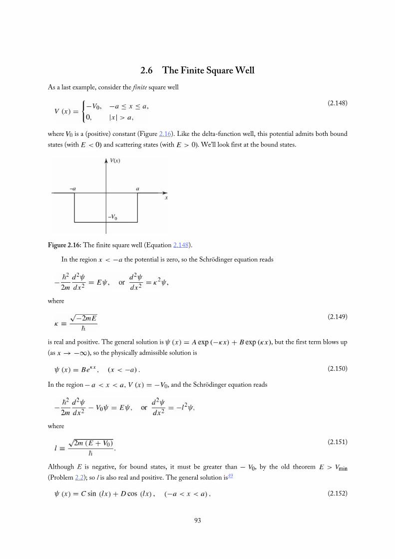
(2.148)
(2.149)
(2.151)
(2.150)
(2.152)
2.6 The Finite Square WellAs a last example, consider the finite square well
where is a (positive) constant (Figure 2.16). Like the delta-function well, this potential admits both boundstates (with and scattering states (with . We’ll look first at the bound states.
Figure 2.16: The finite square well (Equation 2.148).
In the region the potential is zero, so the Schrödinger equation reads
where
is real and positive. The general solution is , but the first term blows up(as , so the physically admissible solution is
In the region , and the Schrödinger equation reads
where
Although E is negative, for bound states, it must be greater than , by the old theorem (Problem 2.2); so l is also real and positive. The general solution is49
93
(2.154)
(2.158)
(2.159)
(2.153)
(2.155)
(2.156)
(2.157)
where C and D are arbitrary constants. Finally, in the region the potential is again zero; the generalsolution is , but the second term blows up (as , so we are leftwith
The next step is to impose boundary conditions: and continuous at and . But we cansave a little time by noting that this potential is an even function, so we can assume with no loss of generalitythat the solutions are either even or odd (Problem 2.1(c)). The advantage of this is that we need only imposethe boundary conditions on one side (say, at ; the other side is then automatic, since .I’ll work out the even solutions; you get to do the odd ones in Problem 2.29. The cosine is even (and the sineis odd), so I’m looking for solutions of the form
The continuity of , at , says
and the continuity of says
Dividing Equation 2.156 by Equation 2.155, we find that
This is a formula for the allowed energies, since κ and l are both functions of E. To solve for E, we firstadopt some nicer notation: Let
According to Equations 2.149 and 2.151, , so , and Equation 2.157reads
This is a transcendental equation for z (and hence for as a function of (which is a measure of the“size” of the well). It can be solved numerically, using a computer, or graphically, by plotting and
on the same grid, and looking for points of intersection (see Figure 2.17). Two limiting casesare of special interest:
1. Wide, deep well. If is very large (pushing the curve upward on the graph, andsliding the zero crossing, , to the right) the intersections occur just slightly below , withn odd; it follows (Equations 2.158 and 2.151) that
94

(2.160)
(2.161)
(2.162)
(2.164)
(2.165)
(2.166)
(2.163)
But is the energy above the bottom of the well, and on the right side we have precisely theinfinite square well energies, for a well of width (see Equation 2.30)—or rather, half of them, sincethis n is odd. (The other ones, of course, come from the odd wave functions, as you’ll discover inProblem 2.29.) So the finite square well goes over to the infinite square well, as ; however,for any finite there are only a finite number of bound states.
2. Shallow, narrow well. As decreases, there are fewer and fewer bound states, until finally, for , only one remains. It is interesting to note, however, that there is always one bound state, no
matter how “weak” the well becomes.
Figure 2.17: Graphical solution to Equation 2.159, for (even states).
You’re welcome to normalize (Equation 2.154), if you’re interested (Problem 2.30), but I’m going tomove on now to the scattering states . To the left, where , we have
where (as usual)
Inside the well, where ,
where, as before,
To the right, assuming there is no incoming wave in this region, we have
Here A is the incident amplitude, B is the reflected amplitude, and F is the transmitted amplitude.50
There are four boundary conditions: Continuity of at says
95

(2.167)
(2.168)
(2.169)
(2.170)
(2.171)
(2.172)
(2.173)
(2.174)
∗
continuity of at gives
continuity of at yields
and continuity of at requires
We can use two of these to eliminate C and D, and solve the remaining two for B and F (see Problem 2.32):
The transmission coefficient , expressed in terms of the original variables, is given by
Notice that (the well becomes “transparent”) whenever the sine is zero, which is to say, when
where n is any integer. The energies for perfect transmission, then, are given by
which happen to be precisely the allowed energies for the infinite square well. T is plotted in Figure 2.18, as afunction of energy.51
Figure 2.18: Transmission coefficient as a function of energy (Equation 2.172).
Problem 2.29 Analyze the odd bound state wave functions for the finite squarewell. Derive the transcendental equation for the allowed energies, and solve it
96

∗∗
∗
graphically. Examine the two limiting cases. Is there always an odd bound state?
Problem 2.30 Normalize in Equation 2.154, to determine the constants Dand F.
Problem 2.31 The Dirac delta function can be thought of as the limiting case of arectangle of area 1, as the height goes to infinity and the width goes to zero. Showthat the delta-function well (Equation 2.117) is a “weak” potential (even though itis infinitely deep), in the sense that . Determine the bound state energyfor the delta-function potential, by treating it as the limit of a finite square well.Check that your answer is consistent with Equation 2.132. Also show thatEquation 2.172 reduces to Equation 2.144 in the appropriate limit.
Problem 2.32 Derive Equations 2.170 and 2.171. Hint: Use Equations 2.168 and2.169 to solve for C and D in terms of F:
Plug these back into Equations 2.166 and 2.167. Obtain the transmissioncoefficient, and confirm Equation 2.172.
Problem 2.33 Determine the transmission coefficient for a rectangular barrier(same as Equation 2.148, only with in the region
. Treat separately the three cases , and (note that the wave function inside the barrier is different in the three cases).Partial answer: for ,52
Problem 2.34 Consider the “step” potential:53
(a) Calculate the reflection coefficient, for the case , and comment onthe answer.
(b) Calculate the reflection coefficient for the case .
(c) For a potential (such as this one) that does not go back to zero to the97

(2.175)
(c) For a potential (such as this one) that does not go back to zero to theright of the barrier, the transmission coefficient is not simply (with A the incident amplitude and F the transmitted amplitude), becausethe transmitted wave travels at a different speed. Show that
for . Hint: You can figure it out using Equation 2.99, or—moreelegantly, but less informatively—from the probability current (Problem2.18). What is T, for ?
(d) For , calculate the transmission coefficient for the step potential,and check that .
Problem 2.35 A particle of mass m and kinetic energy approaches anabrupt potential drop (Figure 2.19).54
Figure 2.19: Scattering from a “cliff” (Problem 2.35).
(a) What is the probability that it will “reflect” back, if ? Hint:This is just like Problem 2.34, except that the step now goes down,instead of up.
(b) I drew the figure so as to make you think of a car approaching a cliff, butobviously the probability of “bouncing back” from the edge of a cliff is farsmaller than what you got in (a)—unless you’re Bugs Bunny. Explain whythis potential does not correctly represent a cliff. Hint: In Figure 2.20 thepotential energy of the car drops discontinuously to , as it passes
; would this be true for a falling car?(c) When a free neutron enters a nucleus, it experiences a sudden drop in
potential energy, from outside to around MeV (millionelectron volts) inside. Suppose a neutron, emitted with kinetic energy 4MeV by a fission event,strikes such a nucleus. What is the probability it will be absorbed, therebyinitiating another fission? Hint: You calculated the probability of reflection
98

in part (a); use to get the probability of transmission throughthe surface.
Figure 2.20: The double square well (Problem 2.47).
99

Further Problems on Chapter 2
Problem 2.36 Solve the time-independent Schrödinger equation with appropriateboundary conditions for the “centered” infinite square well: (for
(otherwise). Check that your allowed energiesare consistent with mine (Equation 2.30), and confirm that your s can beobtained from mine (Equation 2.31) by the substitution (and appropriate renormalization). Sketch your first three solutions, andcompare Figure 2.2. Note that the width of the well is now .
Problem 2.37 A particle in the infinite square well (Equation 2.22) has the initialwave function
Determine A, find , and calculate , as a function of time. What isthe expectation value of the energy? Hint: and can be reduced,by repeated application of the trigonometric sum formulas, to linearcombinations of and , with .
Problem 2.38(a) Show that the wave function of a particle in the infinite square well
returns to its original form after a quantum revival time .That is: for any state (not just a stationary state).
(b) What is the classical revival time, for a particle of energy E bouncing backand forth between the walls?
(c) For what energy are the two revival times equal?55
Problem 2.39 In Problem 2.7(d) you got the expectation value of the energy bysumming the series in Equation 2.21, but I warned you (in footnote 21) not totry it the “old fashioned way,” , because thediscontinuous first derivative of renders the second derivativeproblematic. Actually, you could have done it using integration by parts, butthe Dirac delta function affords a much cleaner way to handle such anomalies.(a) Calculate the first derivative of (in Problem 2.7), and express the
answer in terms of the step function, , defined in Equation2.146.
(b) Exploit the result of Problem 2.23(b) to write the second derivative of in terms of the delta function.
(c) Evaluate the integral , and check that you getthe same answer as before.
Problem 2.40 A particle of mass m in the harmonic oscillator potential (Equation100

∗∗ Problem 2.40 A particle of mass m in the harmonic oscillator potential (Equation2.44) starts out in the state
for some constant A.
101

∗∗∗
∗∗
(a) Determine A and the coefficients in the expansion of this state in termsof the stationary states of the harmonic oscillator.
(b) In a measurement of the particle’s energy, what results could you get, andwhat are their probabilities? What is the expectation value of the energy?
(c) At a later time T the wave function is
for some constant B. What is the smallest possible value of T?
Problem 2.41 Find the allowed energies of the half harmonic oscillator
(This represents, for example, a spring that can be stretched, but notcompressed.) Hint: This requires some careful thought, but very little actualcalculation.
Problem 2.42 In Problem 2.21 you analyzed the stationary gaussian free particlewave packet. Now solve the same problem for the traveling gaussian wavepacket, starting with the initial wave function
where l is a (real) constant. [Suggestion: In going from to ,change variables to before doing the integral.] Partial answer:
where , as before. Notice that has the structureof a gaussian “envelope” modulating a traveling sinusoidal wave. What is thespeed of the envelope? What is the speed of the traveling wave?
Problem 2.43 Solve the time-independent Schrödinger equation for a centeredinfinite square well with a delta-function barrier in the middle:
Treat the even and odd wave functions separately. Don’t bother to normalizethem. Find the allowed energies (graphically, if necessary). How do theycompare with the corresponding energies in the absence of the delta function?
102

Explain why the odd solutions are not affected by the delta function.Comment on the limiting cases and .
Problem 2.44 If two (or more) distinct56 solutions to the (time-independent)Schrödinger equation have the same energy E, these states are said to bedegenerate. For example, the free particle states are doubly degenerate—onesolution representing motion to the right, and the other motion to the left.But we have never encountered normalizable degenerate solutions, and this isno accident. Prove the following theorem: In one dimension57
there are no degenerate bound states. [Hint: Suppose there aretwo solutions, and , with the same energy E. Multiply the Schrödingerequation for by , and the Schrödinger equation for by , andsubtract, to show that is a constant. Use the factthat for normalizable solutions at to demonstrate that thisconstant is in fact zero. Conclude that is a multiple of , and hence thatthe two solutions are not distinct.]
Problem 2.45 In this problem you will show that the number of nodes of thestationary states of a one-dimensional potential always increases with energy.58
Consider two (real, normalized) solutions and to the time-independent Schrödinger equation (for a given potential , with energies
.(a) Show that
(b) Let and be two adjacent nodes of the function . Show that
(c) If has no nodes between and , then it must have the samesign everywhere in the interval. Show that (b) then leads to acontradiction. Therefore, between every pair of nodes of must have at least one node, and in particular the number of nodesincreases with energy.
Problem 2.46 Imagine a bead of mass m that slides frictionlessly around a circularwire ring of circumference L. (This is just like a free particle, except that
.) Find the stationary states (with appropriatenormalization) and the corresponding allowed energies. Note that there are(with one exception) two independent solutions for each energy —corresponding to clockwise and counter-clockwise circulation; call them
and . How do you account for this degeneracy, in view of thetheorem in Problem 2.44 (why does the theorem fail, in this case)?
103

∗∗
∗∗∗
∗∗
Problem 2.47 Attention: This is a strictly qualitative problem—no calculationsallowed! Consider the “double square well” potential (Figure 2.20). Supposethe depth and the width a are fixed, and large enough so that several boundstates occur.(a) Sketch the ground state wave function and the first excited state , (i)
for the case , (ii) for , and (iii) for .(b) Qualitatively, how do the corresponding energies and vary, as b
goes from 0 to ? Sketch and on the same graph.(c) The double well is a very primitive one-dimensional model for the
potential experienced by an electron in a diatomic molecule (the two wellsrepresent the attractive force of the nuclei). If the nuclei are free to move,they will adopt the configuration of minimum energy. In view of yourconclusions in (b), does the electron tend to draw the nuclei together, orpush them apart? (Of course, there is also the internuclear repulsion toconsider, but that’s a separate problem.)
Problem 2.48 Consider a particle of mass m in the potential
(a) How many bound states are there?(b) In the highest-energy bound state, what is the probability that the particle
would be found outside the well ? Answer: 0.542, so even thoughit is “bound” by the well, it is more likely to be found outside than inside!
Problem 2.49(a) Show that
satisfies the time-dependent Schrödinger equation for the harmonicoscillator potential (Equation 2.44). Here is any real constant with thedimensions of length.59
(b) Find , and describe the motion of the wave packet.(c) Compute and , and check that Ehrenfest’s theorem (Equation
1.38) is satisfied.
Problem 2.50 Consider the moving delta-function well:
where v is the (constant) velocity of the well.
(a) Show that the time-dependent Schrödinger equation admits the exact104

∗∗
(2.176)
∗∗∗
(2.177)
(a) Show that the time-dependent Schrödinger equation admits the exactsolution60
where is the bound-state energy of the stationary deltafunction. Hint: Plug it in and check it! Use the result of Problem 2.23(b).
(b) Find the expectation value of the Hamiltonian in this state, and commenton the result.
Problem 2.51 Free fall. Show that
satisfies the time-dependent Schrödinger equation for a particle in a uniformgravitational field,
where is the free gaussian wave packet (Equation 2.111). Find as afunction of time, and comment on the result.61
Problem 2.52 Consider the potential
where a is a positive constant, and “sech” stands for the hyperbolic secant.(a) Graph this potential.(b) Check that this potential has the ground state
and find its energy. Normalize , and sketch its graph.(c) Show that the function
(where , as usual) solves the Schrödinger equation for any(positive) energy E. Since as ,
This represents, then, a wave coming in from the left with no accompanyingreflected wave (i.e. no term . What is the asymptotic form of
at large positive x? What are R and T, for this potential? Comment:This is a famous example of a reflectionless potential—every incident particle,regardless its energy, passes right through.62
105
(2.178)
(2.179)
(2.180)
(2.181)
(2.182)
Problem 2.53 The Scattering Matrix. The theory of scattering generalizes in apretty obvious way to arbitrary localized potentials (Figure 2.21). To the left(Region I), , so
To the right (Region III), is again zero, so
In between (Region II), of course, I can’t tell you what is until you specifythe potential, but because the Schrödinger equation is a linear, second-orderdifferential equation, the general solution has got to be of the form
where and are two linearly independent particular solutions.63
There will be four boundary conditions (two joining Regions I and II, and twojoining Regions II and III). Two of these can be used to eliminate C and D,and the other two can be “solved” for B and F in terms of A and G:
The four coefficients , which depend on k (and hence on E), constitute a matrix S, called the scattering matrix (or S-matrix, for short). The S-
matrix tells you the outgoing amplitudes (B and F) in terms of the incomingamplitudes (A and G):
In the typical case of scattering from the left, , so the reflection andtransmission coefficients are
For scattering from the right, , and
(a) Construct the S-matrix for scattering from a delta-function well(Equation 2.117).
(b) Construct the S-matrix for the finite square well (Equation 2.148). Hint:This requires no new work, if you carefully exploit the symmetry of theproblem.
106

∗∗∗
(2.183)
(2.184)
Figure 2.21: Scattering from an arbitrary localized potential except in Region II); Problem 2.53.
Problem 2.54 The transfer matrix.64 The S-matrix (Problem 2.53) tells you theoutgoing amplitudes and in terms of the incoming amplitudes and —Equation 2.180. For some purposes it is more convenient to work with thetransfer matrix, , which gives you the amplitudes to the right of the potential
and in terms of those to the left and :
(a) Find the four elements of the M-matrix, in terms of the elements of theS-matrix, and vice versa. Express , and (Equations 2.181 and2.182) in terms of elements of the M-matrix.
(b) Suppose you have a potential consisting of two isolated pieces(Figure 2.22). Show that the M-matrix for the combination is the productof the two M-matrices for each section separately:
(This obviously generalizes to any number of pieces, and accounts for theusefulness of the M-matrix.)
(c) Construct the M-matrix for scattering from a single delta-functionpotential at point a:
(d) By the method of part (b), find the M-matrix for scattering from thedouble delta-function
What is the transmission coefficient for this potential?
Figure 2.22: A potential consisting of two isolated pieces (Problem 2.54).
Problem 2.55 Find the ground state energy of the harmonic oscillator, to five107

∗∗
Problem 2.55 Find the ground state energy of the harmonic oscillator, to fivesignificant digits, by the “wag-the-dog” method. That is, solve Equation 2.73numerically, varying K until you get a wave function that goes to zero at largeξ. In Mathematica, appropriate input code would be
Plot[Evaluate[
u[x] /.NDSolve[
{u [x] -(x2 - K)*u[x] == 0, u[0] == 1, u [0] == 0},u[x], {x, 0, b}
]],
{x, a, b}, PlotRange - {c, d} ]
(Here is the horizontal range of the graph, and is the verticalrange—start with .) We know that thecorrect solution is , so you might start with a “guess” of .Notice what the “tail” of the wave function does. Now try , and notethat the tail flips over. Somewhere in between those values lies the correctsolution. Zero in on it by bracketing K tighter and tighter. As you do so, youmay want to adjust a, b, c, and d, to zero in on the cross-over point.
Problem 2.56 Find the first three excited state energies (to five significant digits)for the harmonic oscillator, by wagging the dog (Problem 2.55). For the first(and third) excited state you will need to set .)
Problem 2.57 Find the first four allowed energies (to five significant digits) for theinfinite square well, by wagging the dog. Hint: Refer to Problem 2.55, makingappropriate changes to the differential equation. This time the condition youare looking for is .
Problem 2.58 In a monovalent metal, one electron per atom is free to roamthroughout the object. What holds such a material together—why doesn’t itsimply fall apart into a pile of individual atoms? Evidently the energy of thecomposite structure must be less than the energy of the isolated atoms. Thisproblem offers a crude but illuminating explanation for the cohesiveness ofmetals.(a) Estimate the energy of N isolated atoms, by treating each one as an
electron in the ground state of an infinite square well of width a(Figure 2.23(a)).
(b) When these atoms come together to form a metal, we get N electrons in amuch larger infinite square well of width Na (Figure 2.23(b)). Because ofthe Pauli exclusion principle (which we will discuss in Chapter 5) therecan only be one electron (two, if you include spin, but let’s ignore that) in
108

(2.185)
(2.186)
∗∗∗
each allowed state. What is the lowest energy for this system(Figure 2.23(b))?
(c) The difference of these two energies is the cohesive energy of the metal—the energy it would take to tear it apart into isolated atoms. Find thecohesive energy per atom, in the limit of large N.
(d) Atypical atomic separation in a metal is a few Ångström (say, Å).What is the numerical value of the cohesive energy per atom, in thismodel? (Measured values are in the range of 2–4 eV.)
Figure 2.23 (a) N electrons in individual wells of width a. (b) N electrons in asingle well of width Na.
Problem 2.59 The “bouncing ball.”65 Suppose
(a) Solve the (time-independent) Schrödinger equation for this potential.Hint: First convert it to dimensionless form:
by letting and (the is just so isnormalized with respect to z when is normalized with respect to . What are the constants a and ε? Actually, we might as well set —this amounts to a convenient choice for the unit of length. Find thegeneral solution to this equation (in Mathematica DSolve will do thejob). The result is (of course) a linear combination of two (probablyunfamiliar) functions. Plot each of them, for . One ofthem clearly does not go to zero at large z (more precisely, it’s notnormalizable), so discard it. The allowed values of ε (and hence of aredetermined by the condition . Find the ground state numerically (in Mathematica FindRoot will do it), and also the 10th, .Obtain the corresponding normalization factors. Plot and ,
109
(2.187)
(2.188)
(2.189)
(2.190)
(2.191)
∗∗∗
for . Just as a check, confirm that and areorthogonal.
(b) Find (numerically) the uncertainties and for these two states, andcheck that the uncertainty principle is obeyed.
(c) The probability of finding the ball in the neighborhood dx of height x is(of course) . The nearest classical analog wouldbe the fraction of time an elastically bouncing ball (with the same energy,
spends in the neighborhood dx of height x (see Problem 1.11). Showthat this is
or, in our units (with ,
Plot and for the state , on the range ; superimpose the graphs (Show, in Mathematica), and
comment on the result.
Problem 2.60 The potential. Suppose
where α is some positive constant with the appropriate dimensions. We’d liketo find the bound states—solutions to the time-independent Schrödingerequation
with negative energy .(a) Let’s first go for the ground state energy, . Prove, on dimensional
grounds, that there is no possible formula for —no way to construct(from the available constants m, , and a quantity with the units ofenergy. That’s weird, but it gets worse ….
(b) For convenience, rewrite Equation 2.190 as
Show that if satisfies this equation with energy E, then so too does , with energy , for any positive number . [This is a
catastrophe: if there exists any solution at all, then there’s a solution forevery (negative) energy! Unlike the square well, the harmonic oscillator,
110

(2.192)
(2.193)
(2.194)
∗∗∗
(2.195)
and every other potential well we have encountered, there are no discreteallowed states—and no ground state. A system with no ground state—nolowest allowed energy—would be wildly unstable, cascading down tolower and lower levels, giving off an unlimited amount of energy as itfalls. It might solve our energy problem, but we’d all be fried in theprocess.] Well, perhaps there simply are no solutions at all ….
(c) (Use a computer for the remainder of this problem.) Show that
satisfies Equation 2.191 (here is the modified Bessel function oforder ig, and . Plot this function, for (you mightas well let for the graph; this just sets the scale of length). Noticethat it goes to 0 as and as . And it’s normalizable:determine A.66 How about the old rule that the number of nodes countsthe number of lower-energy states? This function has an infinite numberof nodes, regardless of the energy (i.e. of . I guess that’s consistent,since for any E there are always an infinite number of states with evenlower energy.
(d) This potential confounds practically everything we have come to expect.The problem is that it blows up too violently as . If you move the“brick wall” over a hair,
it’s suddenly perfectly normal. Plot the ground state wave function, for and (you’ll first need to determine the appropriate value of
, from to . Notice that we have introduced a newparameter , with the dimensions of length, so the argument in (a) isout the window. Show that the ground state energy takes the form
for some function f of the dimensionless quantity β.
Problem 2.61 One way to obtain the allowed energies of a potential wellnumerically is to turn the Schrödinger equation into a matrix equation, bydiscretizing the variable x. Slice the relevant interval at evenly spaced points
, with , and let (likewise .Then
(The approximation presumably improves as decreases.) The discretized111
(2.196)
(2.200)
(2.201)
(2.197)
(2.198)
(2.199)
(The approximation presumably improves as decreases.) The discretizedSchrödinger equation reads
or
In matrix form,
where (letting
and
(what goes in the upper left and lower right corners of depends on theboundary conditions, as we shall see). Evidently the allowed energies are theeigenvalues of the matrix (or would be, in the limit .67
Apply this method to the infinite square well. Chop the interval into equal segments (so that , letting
and . The boundary conditions fix ,leaving
(a) Construct the matrix , for , and . (Makesure you are correctly representing Equation 2.197 for the special cases
and .)(b) Find the eigenvalues of for these three cases “by hand,” and compare
them with the exact allowed energies (Equation 2.30).
112
∗∗
(2.202)
(2.203)
(2.204)
(2.205)
(c) Using a computer (Mathematica’s Eigenvalues package will do it) findthe five lowest eigenvalues numerically for and , andcompare the exact energies.
(d) Plot (by hand) the eigenvectors for , 2, and 3, and (by computer,Eigenvectors) the first three eigenvectors for and .
Problem 2.62 Suppose the bottom of the infinite square well is not flat , but rather
Use the method of Problem 2.61 to find the three lowest allowed energiesnumerically, and plot the associated wave functions (use .
Problem 2.63 The Boltzmann equation68
gives the probability of finding a system in the state n (with energy , attemperature T is Boltzmann’s constant). Note: The probability here refersto the random thermal distribution, and has nothing to do with quantumindeterminacy. Quantum mechanics will only enter this problem throughquantization of the energies .(a) Show that the thermal average of the system’s energy can be written as
(b) For a quantum simple harmonic oscillator the index n is the familiarquantum number, and . Show that in this case thepartition function Z is
You will need to sum a geometric series. Incidentally, for a classical simpleharmonic oscillator it can be shown that .
(c) Use your results from parts (a) and (b) to show that for the quantumoscillator
For a classical oscillator the same reasoning would give .
(d) Acrystal consisting of N atoms can be thought of as a collection of oscillators (each atom is attached by springs to its 6 nearest neighbors,
113
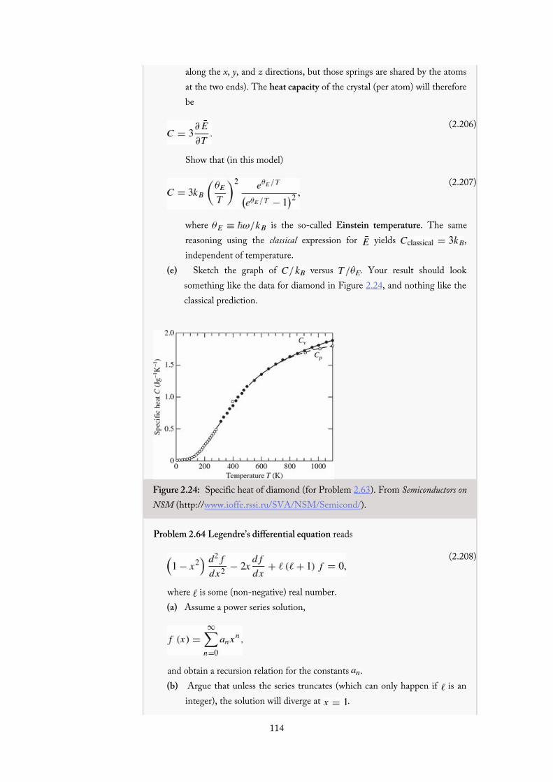
(2.206)
(2.207)
(2.208)
along the x, y, and z directions, but those springs are shared by the atomsat the two ends). The heat capacity of the crystal (per atom) will thereforebe
Show that (in this model)
where is the so-called Einstein temperature. The samereasoning using the classical expression for yields ,independent of temperature.
(e) Sketch the graph of versus . Your result should looksomething like the data for diamond in Figure 2.24, and nothing like theclassical prediction.
Figure 2.24: Specific heat of diamond (for Problem 2.63). From Semiconductors onNSM (http://www.ioffe.rssi.ru/SVA/NSM/Semicond/).
Problem 2.64 Legendre’s differential equation reads
where is some (non-negative) real number.(a) Assume a power series solution,
and obtain a recursion relation for the constants .(b) Argue that unless the series truncates (which can only happen if is an
integer), the solution will diverge at .
114

(c) When is an integer, the series for one of the two linearly independentsolutions (either or depending on whether is even or odd) willtruncate, and those solutions are called Legendre polynomials .Find , and from the recursion relation.Leave your answer in terms of either or .69
1 It is tiresome to keep saying “potential energy function,” so most people just call V the “potential,” even though this invites occasionalconfusion with electric potential, which is actually potential energy per unit charge.
2 Note that this would not be true if V were a function of t as well as x.3 Using Euler’s formula,
you could equivalently write
the real and imaginary parts oscillate sinusoidally. Mike Casper (of Carleton College) dubbed the “wiggle factor”—it’s the characteristictime dependence in quantum mechanics.
4 For normalizable solutions, E must be real (see Problem 2.1(a)).5 Whenever confusion might arise, I’ll put a “hat” (^) on the operator, to distinguish it from the dynamical variable it represents.6 A linear combination of the functions is an expression of the form
where are (possibly complex) constants.7 In principle, any normalized function is fair game—it need not even be continuous. How you might actually get a particle into that
state is a different question, and one (curiously) we seldom have occasion to ask.8 If this is your first encounter with the method of separation of variables, you may be disappointed that the solution takes the form of an
infinite series. Occasionally it is possible to sum the series, or to solve the time-dependent Schrödinger equation without recourse toseparation of variables—see, for instance, Problems 2.49, 2.50, and 2.51. But such cases are extremely rare.
9 This is nicely illustrated in an applet by Paul Falstad, at www.falstad.com/qm1d/.10 Some people will tell you that is “the probability that the particle is in the nth stationary state,” but this is bad language: the particle is
in the state , not , and anyhow, in the laboratory you don’t “find the particle to be in a particular state,” you measure some observable,and what you get is a number, not a wave function.
11 That’s right: is a continuous function of x, even though need not be.12 Notice that the quantization of energy emerges as a rather technical consequence of the boundary conditions on solutions to the time-
independent Schrödinger equation.13 Actually, it’s that must be normalized, but in view of Equation 2.7 this entails the normalization of .14 To make this symmetry more apparent, some authors center the well at the origin (running it now from to . The even functions
are then cosines, and the odd ones are sines. See Problem 2.36.15 In this case the s are real, so the complex conjugation (*) of is unnecessary, but for future purposes it’s a good idea to get in the habit of
putting it there.16 See, for example, Mary Boas, Mathematical Methods in the Physical Sciences, 3rd edn (New York: John Wiley, 2006), p. 356; can even
have a finite number of finite discontinuities.17 It doesn’t matter whether you use m or n as the “dummy index” here (as long as you are consistent on the two sides of the equation, of
course); whatever letter you use, it just stands for “any positive integer.”18 Problem 2.45 explores this property. For further discussion, see John L. Powell and Bernd Crasemann, Quantum Mechanics (Addison-
Wesley, Reading, MA, 1961), Section 5–7.19 Loosely speaking, tells you the “amount of that is contained in .”20 You can look up the series
and
115

in math tables, under “Sums of Reciprocal Powers” or “Riemann Zeta Function.”21 Remember, there is no restriction in principle on the shape of the starting wave function, as long as it is normalizable. In particular,
need not have a continuous derivative. However, if you try to calculate using in such a case, you mayencounter technical difficulties, because the second derivative of is ill defined. It works in Problem 2.9 because the discontinuitiesoccur at the end points, where the wave function is zero anyway. In Problem 2.39 you’ll see how to manage cases like Problem 2.7.
22 Note that , since by assumption is a minimum. Only in the rare case is the oscillation not even approximatelysimple harmonic.
23 We’ll encounter some of the same strategies in the theory of angular momentum (Chapter 4), and the technique generalizes to a broad classof potentials in supersymmetric quantum mechanics (Problem 3.47; see also Richard W. Robinett, Quantum Mechanics (Oxford UniversityPress, New York, 1997), Section 14.4).
24 Put a hat on x, too, if you like, but since we usually leave it off.25 In a deep sense all of the mysteries of quantum mechanics can be traced to the fact that position and momentum do not commute. Indeed,
some authors take the canonical commutation relation as an axiom of the theory, and use it to derive .26 I’m getting tired of writing “time-independent Schrödinger equation,” so when it’s clear from the context which one I mean, I’ll just call it
the “Schrödinger equation.”27 In the case of the harmonic oscillator it is customary, for some reason, to depart from the usual practice, and number the states starting with
, instead of . Of course, the lower limit on the sum in a formula such as Equation 2.17 should be altered accordingly.28 Note that we obtain all the (normalizable) solutions by this procedure. For if there were some other solution, we could generate from it a
second ladder, by repeated application of the raising and lowering operators. But the bottom rung of this new ladder would have to satisfyEquation 2.59, and since that leads inexorably to Equation 2.60, the bottom rungs would be the same, and hence the two ladders would infact be identical.
29 Of course, the integrals must exist, and this means that and must go to zero at .30 Of course, we could multiply and by phase factors, amounting to a different definition of the ; but this choice keeps the wave
functions real.31 However, does oscillate at the classical frequency—see Problem 3.40.32 Note that although we invoked some approximations to motivate Equation 2.78, what follows is exact. The device of stripping off the
asymptotic behavior is the standard first step in the power series method for solving differential equations—see, for example, Boas (footnote16), Chapter 12.
33 According to Taylor’s theorem, any reasonably well-behaved function can be expressed as a power series, so Equation 2.80 ordinarilyinvolves no loss of generality. For conditions on the applicability of the method, see Boas (footnote 16) or George B. Arfken and Hans-Jurgen Weber, Mathematical Methods for Physicists, 7th edn, Academic Press, Orlando (2013), Section 7.5.
34 See, for example, Arfken and Weber (footnote 33), Section 1.2.35 It’s no surprise that the ill-behaved solutions are still contained in Equation 2.82; this recursion relation is equivalent to the Schrödinger
equation, so it’s got to include both the asymptotic forms we found in Equation 2.76.36 It is possible to set this up on a computer, and discover the allowed energies “experimentally.” You might call it the wag the dog method:
When the tail wags, you know you’ve just passed over an allowed value. Computer scientists call it the shooting method (Nicholas Giordano,Computational Physics, Prentice Hall, Upper Saddle River, NJ (1997), Section 10.2). See Problems 2.55–2.57.
37 Note that there is a completely different set of coefficients for each value of n.38 The Hermite polynomials have been studied extensively in the mathematical literature, and there are many tools and tricks for working with
them. A few of these are explored in Problem 2.16.39 I shall not work out the normalization constant here; if you are interested in knowing how it is done, see for example Leonard Schiff,
Quantum Mechanics, 3rd edn, McGraw-Hill, New York (1968), Section 13.40 Sinusoidal waves extend out to infinity, and they are not normalizable. But superpositions of such waves lead to interference, which allows for
localization and normalizability.41 Some people define the Fourier transform without the factor of . Then the inverse transform becomes
, spoiling the symmetry of the two formulas.42 The necessary and sufficient condition on is that be finite. (In that case is also finite, and in
fact the two integrals are equal. Some people call this Plancherel’s theorem, leaving Equation 2.102 without a name.) See Arfken and Weber(footnote 33), Section 20.4.
43 If you are irritatingly observant, you may have noticed that the general theorem requiring (Problem 2.2) does not really apply toscattering states, since they are not normalizable. If this bothers you, try solving the Schrödinger equation with , for the free particle,and note that even linear combinations of these solutions cannot be normalized. The positive energy solutions by themselves constitute acomplete set.
44 The delta function can be thought of as the limit of a sequence of functions, such as rectangles (or triangles) of ever-increasing height andever-decreasing width.
116
45 The delta function itself carries units of 1 length (see Equation 2.114), so α has the dimensions energy length.46 This is not a normalizable wave function, so the absolute probability of finding the particle at a particular location is not well defined;
nevertheless, the ratio of probabilities for the incident and reflected waves is meaningful. More on this in the next paragraph.47 Note that the particle’s velocity is the same on both sides of the well. Problem 2.34 treats the general case.48 There exist some powerful programs for analyzing the scattering of a wave packet from a one-dimensional potential; see, for instance,
“Quantum Tunneling and Wave Packets,” at PhET Interactive Simulations, University of Colorado Boulder, https://phet.colorado.edu.49 You can, if you like, write the general solution in exponential form . This leads to the same final result, but since the
potential is symmetric, we know the solutions will be either even or odd, and the sine/cosine notation allows us to exploit this right from thestart.
50 We could look for even and odd functions, as we did in the case of bound states, but the scattering problem is inherently asymmetric, sincethe waves come in from one side only, and the exponential notation (representing traveling waves) is more natural in this context.
51 This remarkable phenomenon was observed in the laboratory before the advent of quantum mechanics, in the form of the Ramsauer–Townsend effect. For an illuminating discussion see Richard W. Robinett, Quantum Mechanics, Oxford University Press, 1997, Section12.4.1.
52 This is a good example of tunneling—classically the particle would bounce back.53 For interesting commentary see C. O. Dib and O. Orellana, Eur. J. Phys. 38, 045403 (2017).54 For further discussion see P. L. Garrido, et al., Am. J. Phys. 79, 1218 (2011).55 The fact that the classical and quantum revival times bear no obvious relation to one another (and the quantum one doesn’t even depend on
the energy) is a curious paradox; see D. F. Styer, Am. J. Phys. 69, 56 (2001).56 If two solutions differ only by a multiplicative constant (so that, once normalized, they differ only by a phase factor , they represent the
same physical state, and in this sense they are not distinct solutions. Technically, by “distinct” I mean “linearly independent.”57 In higher dimensions such degeneracy is very common, as we shall see in Chapters 4 and 6. Assume that the potential does not consist of
isolated pieces separated by regions where —two isolated infinite square wells, for instance, would give rise to degenerate boundstates, for which the particle is either in one well or in the other.
58 M. Moriconi, Am. J. Phys. 75, 284 (2007).59 This rare example of an exact closed-form solution to the time-dependent Schrödinger equation was discovered by Schrödinger himself, in
1926. One way to obtain it is explored in Problem 6.30. For a discussion of this and related problems see W. van Dijk, et al., Am. J. Phys. 82,955 (2014).
60 See Problem 6.35 for a derivation.61 For illuminating discussion see M. Nauenberg, Am. J. Phys. 84, 879 (2016).62 R. E. Crandall and B. R. Litt, Annals of Physics, 146, 458 (1983).63 See any book on differential equations—for example, John L. Van Iwaarden, Ordinary Differential Equations with Numerical Techniques,
Harcourt Brace Jovanovich, San Diego, 1985, Chapter 3.64 For applications of this method see, for instance, D. J. Griffiths and C. A. Steinke, Am. J. Phys. 69, 137 (2001) or S. Das, Am. J. Phys. 83,
590 (2015).65 This problem was suggested by Nicholas Wheeler.66 is normalizable as long as g is real—which is to say, provided . For more on this strange problem see A. M. Essin and
D. J. Griffiths, Am. J. Phys. 74, 109 (2006), and references therein.67 For further discussion see Joel Franklin, Computational Methods for Physics (Cambridge University Press, Cambridge, UK, 2013), Section
10.4.2.68 See, for instance, Daniel V. Schroeder, An Introduction to Thermal Physics, Pearson, Boston (2000), Section 6.1.69 By convention Legendre polynomials are normalized such that . Note that the nonvanishing coefficients will take different
values for different .
117

3Formalism
◈
118
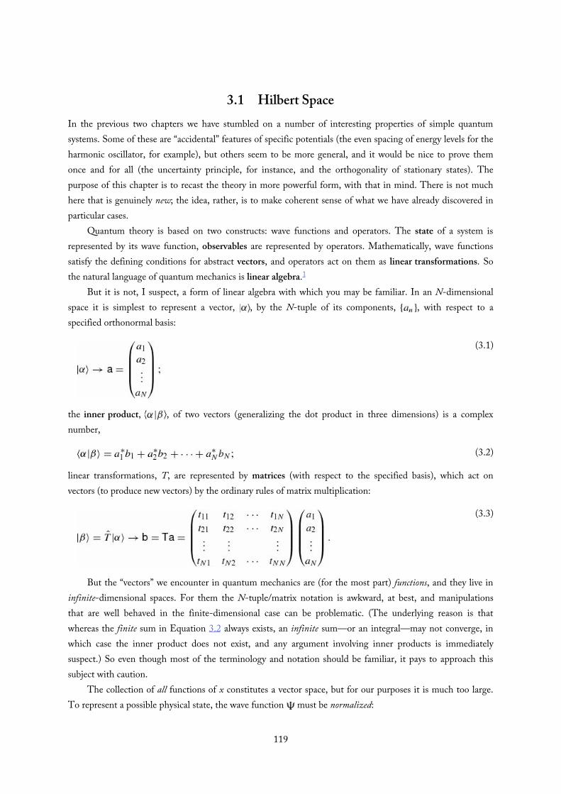
(3.1)
(3.2)
(3.3)
3.1 Hilbert SpaceIn the previous two chapters we have stumbled on a number of interesting properties of simple quantumsystems. Some of these are “accidental” features of specific potentials (the even spacing of energy levels for theharmonic oscillator, for example), but others seem to be more general, and it would be nice to prove themonce and for all (the uncertainty principle, for instance, and the orthogonality of stationary states). Thepurpose of this chapter is to recast the theory in more powerful form, with that in mind. There is not muchhere that is genuinely new; the idea, rather, is to make coherent sense of what we have already discovered inparticular cases.
Quantum theory is based on two constructs: wave functions and operators. The state of a system isrepresented by its wave function, observables are represented by operators. Mathematically, wave functionssatisfy the defining conditions for abstract vectors, and operators act on them as linear transformations. Sothe natural language of quantum mechanics is linear algebra.1
But it is not, I suspect, a form of linear algebra with which you may be familiar. In an N-dimensionalspace it is simplest to represent a vector, , by the N-tuple of its components, , with respect to aspecified orthonormal basis:
the inner product, , of two vectors (generalizing the dot product in three dimensions) is a complexnumber,
linear transformations, T, are represented by matrices (with respect to the specified basis), which act onvectors (to produce new vectors) by the ordinary rules of matrix multiplication:
But the “vectors” we encounter in quantum mechanics are (for the most part) functions, and they live ininfinite-dimensional spaces. For them the N-tuple/matrix notation is awkward, at best, and manipulationsthat are well behaved in the finite-dimensional case can be problematic. (The underlying reason is thatwhereas the finite sum in Equation 3.2 always exists, an infinite sum—or an integral—may not converge, inwhich case the inner product does not exist, and any argument involving inner products is immediatelysuspect.) So even though most of the terminology and notation should be familiar, it pays to approach thissubject with caution.
The collection of all functions of x constitutes a vector space, but for our purposes it is much too large.To represent a possible physical state, the wave function must be normalized:
119

(3.4)
(3.5)
(3.6)
(3.7)
(3.9)
(3.11)
(3.8)
(3.10)
The set of all square-integrable functions, on a specified interval,2
constitutes a (much smaller) vector space (see Problem 3.1(a)). Mathematicians call it ; physicists callit Hilbert space.3 In quantum mechanics, then:
We define the inner product of two functions, and , as follows:
If f and g are both square-integrable (that is, if they are both in Hilbert space), their inner product isguaranteed to exist (the integral in Equation 3.6 converges to a finite number).4 This follows from the integralSchwarz inequality:5
You can check for yourself that definition (Equation 3.6) satisfies all the conditions for an inner product(Problem 3.1(b)). Notice in particular that
Moreover, the inner product of with itself ,
is real and non-negative; it’s zero only when .6
A function is said to be normalized if its inner product with itself is 1; two functions are orthogonal iftheir inner product is 0; and a set of functions, , is orthonormal if they are normalized and mutuallyorthogonal:
Finally, a set of functions is complete if any other function (in Hilbert space) can be expressed as a linearcombination of them:
If the functions are orthonormal, the coefficients are given by Fourier’s trick:
120

∗
(3.12)as you can check for yourself. I anticipated this terminology, of course, back in Chapter 2. (Thestationary states of the infinite square well (Equation 2.31) constitute a complete orthonormal set on theinterval ; the stationary states for the harmonic oscillator (Equation 2.68 or 2.86) are a completeorthonormal set on the interval .)
Problem 3.1(a) Show that the set of all square-integrable functions is a vector space (refer
to Section A.1 for the definition). Hint: The main point is to show thatthe sum of two square-integrable functions is itself square-integrable. UseEquation 3.7. Is the set of all normalized functions a vector space?
(b) Show that the integral in Equation 3.6 satisfies the conditions for aninner product (Section A.2).
Problem 3.2 (a) For what range of ν is the function in Hilbert space, on the
interval ? Assume ν is real, but not necessarily positive.(b) For the specific case , is in this Hilbert space? What about
? How about ?
121

3.2 Observables
122
(3.13)
(3.15)
(3.16)
(3.17)
(3.18)
(3.19)
(3.20)
(3.14)
3.2.1 Hermitian Operators
The expectation value of an observable can be expressed very neatly in inner-product notation:7
Now, the outcome of a measurement has got to be real, and so, a fortiori, is the average of manymeasurements:
But the complex conjugate of an inner product reverses the order (Equation 3.8), so
and this must hold true for any wave function . Thus operators representing observables have the very specialproperty that
We call such operators hermitian.8
Actually, most books require an ostensibly stronger condition:
But it turns out, in spite of appearances, that this is perfectly equivalent to my definition (Equation 3.16), asyou will prove in Problem 3.3. So use whichever you like. The essential point is that a hermitian operator canbe applied either to the first member of an inner product or to the second, with the same result, and hermitianoperators naturally arise in quantum mechanics because their expectation values are real:
Well, let’s check this. Is the momentum operator, for example, hermitian?
I used integration by parts, of course, and threw away the boundary term for the usual reason: If and are square integrable, they must go to zero at .9 Notice how the complex conjugation of i
compensates for the minus sign picked up from integration by parts—the operator (without the i) is nothermitian, and it does not represent a possible observable.
The hermitian conjugate (or adjoint) of an operator is the operator such that
A hermitian operator, then, is equal to its hermitian conjugate: .
123

∗
∗
Problem 3.3 Show that if for all h (in Hilbert space), then for all f and g (i.e. the two definitions of “hermitian” —
Equations 3.16 and 3.17—are equivalent). Hint: First let , and then let.
Problem 3.4(a) Show that the sum of two hermitian operators is hermitian.(b) Suppose is hermitian, and α is a complex number. Under what
condition (on α) is hermitian?(c) When is the product of two hermitian operators hermitian?(d) Show that the position operator and the Hamiltonian operator
are hermitian.
Problem 3.5(a) Find the hermitian conjugates of x, i, and .(b) Show that (note the reversed order),
and for a complex number c.(c) Construct the hermitian conjugate of (Equation 2.48).
124

(3.21)
(3.22)
(3.23)
(3.24)
(3.25)
3.2.2 Determinate States
Ordinarily, when you measure an observable Q on an ensemble of identically prepared systems, all in the samestate , you do not get the same result each time—this is the indeterminacy of quantum mechanics. Question:Would it be possible to prepare a state such that every measurement of Q is certain to return the same value(call it q)? This would be, if you like, a determinate state, for the observable Q. (Actually, we already knowone example: Stationary states are determinate states of the Hamiltonian; a measurement of the energy, on aparticle in the stationary state , is certain to yield the corresponding “allowed” energy .)
Well, the standard deviation of Q, in a determinate state, would be zero, which is to say,
(Of course, if every measurement gives q, their average is also q: . I used the fact that (and hencealso ) is a hermitian operator, to move one factor over to the first term in the inner product.) But theonly vector whose inner product with itself vanishes is 0, so
This is the eigenvalue equation for the operator ; is an eigenfunction of , and q is the correspondingeigenvalue:
Measurement of Q on such a state is certain to yield the eigenvalue, q.10
Note that the eigenvalue is a number (not an operator or a function). You can multiply any eigenfunctionby a constant, and it is still an eigenfunction, with the same eigenvalue. Zero does not count as aneigenfunction (we exclude it by definition—otherwise every number would be an eigenvalue, since
for any linear operator and all q). But there’s nothing wrong with zero as an eigenvalue. Thecollection of all the eigenvalues of an operator is called its spectrum. Sometimes two (or more) linearlyindependent eigenfunctions share the same eigenvalue; in that case the spectrum is said to be degenerate.(You encountered this term already, for the case of energy eigenstates, if you worked Problems 2.44 or 2.46.)
For example, determinate states of the total energy are eigenfunctions of the Hamiltonian:
which is precisely the time-independent Schrödinger equation. In this context we use the letter E for theeigenvalue, and the lower case for the eigenfunction (tack on the wiggle factor to make it
, if you like; it’s still an eigenfunction of .
Example 3.1Consider the operator
where ϕ is the usual polar coordinate in two dimensions. (This operator might arise in a physical125

(3.27)
(3.28)
(3.29)
(3.26)
where ϕ is the usual polar coordinate in two dimensions. (This operator might arise in a physicalcontext if we were studying the bead-on-a-ring; see Problem 2.46.) Is hermitian? Find itseigenfunctions and eigenvalues.
Solution: Here we are working with functions on the finite interval , with theproperty that
since ϕ and describe the same physical point. Using integration by parts,
so is hermitian (this time the boundary term disappears by virtue of Equation 3.26).The eigenvalue equation,
has the general solution
Equation 3.26 restricts the possible values of the q:
The spectrum of this operator is the set of all integers, and it is nondegenerate.
Problem 3.6 Consider the operator , where (as in Example 3.1) ϕ isthe azimuthal angle in polar coordinates, and the functions are subject to Equation3.26. Is hermitian? Find its eigenfunctions and eigenvalues. What is thespectrum of ? Is the spectrum degenerate?
126

3.3 Eigenfunctions of a Hermitian OperatorOur attention is thus directed to the eigenfunctions of hermitian operators (physically: determinate states ofobservables). These fall into two categories: If the spectrum is discrete (i.e. the eigenvalues are separated fromone another) then the eigenfunctions lie in Hilbert space and they constitute physically realizable states. If thespectrum is continuous (i.e. the eigenvalues fill out an entire range) then the eigenfunctions are notnormalizable, and they do not represent possible wave functions (though linear combinations of them—involving necessarily a spread in eigenvalues—may be normalizable). Some operators have a discrete spectrumonly (for example, the Hamiltonian for the harmonic oscillator), some have only a continuous spectrum (forexample, the free particle Hamiltonian), and some have both a discrete part and a continuous part (forexample, the Hamiltonian for a finite square well). The discrete case is easier to handle, because the relevantinner products are guaranteed to exist—in fact, it is very similar to the finite-dimensional theory (theeigenvectors of a hermitian matrix). I’ll treat the discrete case first, and then the continuous one.
127

3.3.1 Discrete Spectra
Mathematically, the normalizable eigenfunctions of a hermitian operator have two important properties:
Theorem 1 Their eigenvalues are real.Proof: Suppose
(i.e. is an eigenfunction of , with eigenvalue q), and11
. Then
(q is a number, so it comes outside the integral, and because the first function in the inner product iscomplex conjugated (Equation 3.6), so too is the q on the right). But cannot be zero ( isnot a legal eigenfunction), so , and hence q is real. QED
This is comforting: If you measure an observable on a particle in a determinate state, you will at least get a realnumber.
Theorem 2 Eigenfunctions belonging to distinct eigenvalues are orthogonal.Proof: Suppose
and is hermitian. Then , so
(again, the inner products exist because the eigenfunctions are in Hilbert space). But q is real (fromTheorem 1), so if it must be that . QED
That’s why the stationary states of the infinite square well, for example, or the harmonic oscillator, areorthogonal—they are eigenfunctions of the Hamiltonian with distinct eigenvalues. But this property is notpeculiar to them, or even to the Hamiltonian—the same holds for determinate states of any observable.
Unfortunately, Theorem 2 tells us nothing about degenerate states . However, if two (or more)eigenfunctions share the same eigenvalue, any linear combination of them is itself an eigenfunction, with thesame eigenvalue (Problem 3.7), and we can use the Gram–Schmidt orthogonalization procedure (ProblemA.4) to construct orthogonal eigenfunctions within each degenerate subspace. It is almost never necessary to dothis explicitly (thank God!), but it can always be done in principle. So even in the presence of degeneracy theeigenfunctions can be chosen to be orthonormal, and we shall always assume that this has been done. Thatlicenses the use of Fourier’s trick, which depends on the orthonormality of the basis functions.
In a finite-dimensional vector space the eigenvectors of a hermitian matrix have a third fundamentalproperty: They span the space (every vector can be expressed as a linear combination of them). Unfortunately,
128

the proof does not generalize to infinite-dimensional spaces. But the property itself is essential to the internalconsistency of quantum mechanics, so (following Dirac12 ) we will take it as an axiom (or, more precisely, as arestriction on the class of hermitian operators that can represent observables):
Axiom: The eigenfunctions of an observable operator are complete: Any function (in Hilbert space)can be expressed as a linear combination of them.13
Problem 3.7(a) Suppose that and are two eigenfunctions of an operator ,
with the same eigenvalue q. Show that any linear combination of f and g isitself an eigenfunction of , with eigenvalue q.
(b) Check that and are eigenfunctions ofthe operator , with the same eigenvalue. Construct two linearcombinations of f and g that are orthogonal eigenfunctions on the interval
.
Problem 3.8(a) Check that the eigenvalues of the hermitian operator in Example 3.1 are
real. Show that the eigenfunctions (for distinct eigenvalues) areorthogonal.
(b) Do the same for the operator in Problem 3.6.
129
(3.30)
(3.31)
(3.32)
(3.33)
(3.34)
3.3.2 Continuous Spectra
If the spectrum of a hermitian operator is continuous, the eigenfunctions are not normalizable, and the proofsof Theorems 1 and 2 fail, because the inner products may not exist. Nevertheless, there is a sense in which thethree essential properties (reality, orthogonality, and completeness) still hold. I think it’s best to approach thiscase through specific examples.
Example 3.2Find the eigenfunctions and eigenvalues of the momentum operator (on the interval ).
Solution: Let be the eigenfunction and p the eigenvalue:
The general solution is
This is not square-integrable for any (complex) value of p—the momentum operator has noeigenfunctions in Hilbert space.
And yet, if we restrict ourselves to real eigenvalues, we do recover a kind of ersatz“orthonormality.” Referring to Problems 2.23(a) and 2.26,
If we pick , so that
then
which is reminiscent of true orthonormality (Equation 3.10)—the indices are now continuousvariables, and the Kronecker delta has become a Dirac delta, but otherwise it looks just the same. I’llcall Equation 3.33 Dirac orthonormality.
Most important, the eigenfunctions (with real eigenvalues) are complete, with the sum (in Equation3.11) replaced by an integral: Any (square-integrable) function can be written in the form
The “coefficients” (now a function, ) are obtained, as always, by Fourier’s trick:
130

(3.35)
(3.36)
(3.38)
(3.40)
(3.37)
(3.39)
Alternatively, you can get them from Plancherel’s theorem (Equation 2.103); indeed, the expansion(Equation 3.34) is nothing but a Fourier transform.
The eigenfunctions of momentum (Equation 3.32) are sinusoidal, with wavelength
This is the old de Broglie formula (Equation 1.39), which I promised to justify at the appropriate time. Itturns out to be a little more subtle than de Broglie imagined, because we now know that there is actually nosuch thing as a particle with determinate momentum. But we could make a normalizable wave packet with anarrow range of momenta, and it is to such an object that the de Broglie relation applies.
What are we to make of Example 3.2? Although none of the eigenfunctions of lives in Hilbert space, acertain family of them (those with real eigenvalues) resides in the nearby “suburbs,” with a kind of quasi-normalizability. They do not represent possible physical states, but they are still very useful (as we have alreadyseen, in our study of one-dimensional scattering).14
Example 3.3Find the eigenfunctions and eigenvalues of the position operator.
Solution: Let be the eigenfunction and y the eigenvalue:
Here y is a fixed number (for any given eigenfunction), but x is a continuous variable. What functionof x has the property that multiplying it by x is the same as multiplying it by the constant y? Obviouslyit’s got to be zero, except at the one point ; in fact, it is nothing but the Dirac delta function:
This time the eigenvalue has to be real; the eigenfunctions are not square integrable, but again theyadmit Dirac orthonormality:
If we pick , so
then
These eigenfunctions are also complete:
131

(3.41)
(3.42)
with
(trivial, in this case, but you can get it from Fourier’s trick if you insist).
If the spectrum of a hermitian operator is continuous (so the eigenvalues are labeled by a continuousvariable—p or y, in the examples; z, generically, in what follows), the eigenfunctions are not normalizable,they are not in Hilbert space and they do not represent possible physical states; nevertheless, theeigenfunctions with real eigenvalues are Dirac orthonormalizable and complete (with the sum now anintegral). Luckily, this is all we really require.
Problem 3.9(a) Cite a Hamiltonian from Chapter 2 (other than the harmonic oscillator)
that has only a discrete spectrum.(b) Cite a Hamiltonian from Chapter 2 (other than the free particle) that has
only a continuous spectrum.(c) Cite a Hamiltonian from Chapter 2 (other than the finite square well) that
has both a discrete and a continuous part to its spectrum.
Problem 3.10 Is the ground state of the infinite square well an eigenfunction ofmomentum? If so, what is its momentum? If not, why not? [For furtherdiscussion, see Problem 3.34.]
132
(3.43)
(3.44)
(3.45)
(3.46)
(3.47)
3.4 Generalized Statistical InterpretationIn Chapter 1 I showed you how to calculate the probability that a particle would be found in a particularlocation, and how to determine the expectation value of any observable quantity. In Chapter 2 you learnedhow to find the possible outcomes of an energy measurement, and their probabilities. I am now in a positionto state the generalized statistical interpretation, which subsumes all of this, and enables you to figure out thepossible results of any measurement, and their probabilities. Together with the Schrödinger equation (whichtells you how the wave function evolves in time) it is the foundation of quantum mechanics.
Generalized statistical interpretation: If you measure an observable on a particle in the state , you are certain to getone of the eigenvalues of the hermitian operator .15 If the spectrum of is discrete, the probability of getting theparticular eigenvalue associated with the (orthonormalized) eigenfunction is
If the spectrum is continuous, with real eigenvalues and associated (Dirac-orthonormalized) eigenfunctions , the probabilityof getting a result in the range dz is
Upon measurement, the wave function “collapses” to the corresponding eigenstate.16
The statistical interpretation is radically different from anything we encounter in classical physics. Asomewhat different perspective helps to make it plausible: The eigenfunctions of an observable operator arecomplete, so the wave function can be written as a linear combination of them:
(For simplicity, I’ll assume that the spectrum is discrete; it’s easy to generalize this discussion to thecontinuous case.) Because the eigenfunctions are orthonormal, the coefficients are given by Fourier’s trick:17
Qualitatively, tells you “how much is contained in ,” and given that a measurement has to return oneof the eigenvalues of , it seems reasonable that the probability of getting the particular eigenvalue wouldbe determined by the “amount of ” in . But because probabilities are determined by the absolute square ofthe wave function, the precise measure is actually . That’s the essential message of the generalizedstatistical interpretation.18
Of course, the total probability (summed over all possible outcomes) has got to be one:
and sure enough, this follows from the normalization of the wave function:
133

(3.48)
(3.49)
(3.50)
(3.51)
(3.52)
(3.53)
(3.54)
(3.55)
Similarly, the expectation value of Q should be the sum over all possible outcomes of the eigenvalue times theprobability of getting that eigenvalue:
Indeed,
but , so
So far, at least, everything looks consistent.Can we reproduce, in this language, the original statistical interpretation for position measurements?
Sure—it’s overkill, but worth checking. A measurement of x on a particle in state must return one of theeigenvalues of the position operator. Well, in Example 3.3 we found that every (real) number y is aneigenvalue of x, and the corresponding (Dirac-orthonormalized) eigenfunction is .Evidently
so the probability of getting a result in the range dy is , which is precisely the original statisticalinterpretation.
What about momentum? In Example 3.2 we found the (Dirac-orthonormalized) eigenfunctions of themomentum operator, , so
This is such an important quantity that we give it a special name and symbol: the momentum space wavefunction, . It is essentially the Fourier transform of the (position space) wave function —which, by Plancherel’s theorem, is its inverse Fourier transform:
According to the generalized statistical interpretation, the probability that a measurement of momentum134

(3.56)
∗
(3.57)
According to the generalized statistical interpretation, the probability that a measurement of momentumwould yield a result in the range dp is
Example 3.4A particle of mass m is bound in the delta function well . What is the probabilitythat a measurement of its momentum would yield a value greater than ?
Solution: The (position space) wave function is (Equation 2.132)
(where ). The momentum space wave function is therefore
(I looked up the integral). The probability, then, is
(again, I looked up the integral).
Problem 3.11 Find the momentum-space wave function, , for a particle inthe ground state of the harmonic oscillator. What is the probability (to twosignificant digits) that a measurement of p on a particle in this state would yield avalue outside the classical range (for the same energy)? Hint: Look in a math tableunder “Normal Distribution” or “Error Function” for the numerical part—or useMathematica.
Problem 3.12 Find for the free particle in terms of the function introduced in Equation 2.101. Show that for the free particle isindependent of time. Comment: the time independence of for the freeparticle is a manifestation of momentum conservation in this system.
Problem 3.13 Show that
Hint: Notice that , and use135

(3.58)
Hint: Notice that , and useEquation 2.147. In momentum space, then, the position operator is .More generally,
In principle you can do all calculations in momentum space just as well(though not always as easily) as in position space.
136

3.5 The Uncertainty PrincipleI stated the uncertainty principle (in the form ), back in Section 1.6, and you have checked itseveral times, in the problems. But we have never actually proved it. In this section I will prove a more generalversion of the uncertainty principle, and explore some of its ramifications. The argument is beautiful, butrather abstract, so watch closely.
137

(3.59)
(3.60)
(3.61)
3.5.1 Proof of the Generalized Uncertainty Principle
For any observable A, we have (Equation 3.21):
where . Likewise, for any other observable, B,
Therefore (invoking the Schwarz inequality, Equation 3.7),
Now, for any complex number z,
Therefore, letting ,
But (exploiting the hermiticity of in the first line)
(Remember, and are numbers, not operators, so you can write them in either order.) Similarly,
so
where
is the commutator of the two operators (Equation 2.49). Conclusion:
138

(3.62)
(3.63)
∗
This is the (generalized) uncertainty principle. (You might think the i makes it trivial—isn’t the right sidenegative? No, for the commutator of two hermitian operators carries its own factor of i, and the two cancelout;19 the quantity in parentheses is real, and its square is positive.)
As an example, suppose the first observable is position , and the second is momentum
. We worked out their commutator back in Chapter 2 (Equation 2.52):
So
or, since standard deviations are by their nature positive,
That’s the original Heisenberg uncertainty principle, but we now see that it is just one application of a muchmore general theorem.
There is, in fact, an “uncertainty principle” for every pair of observables whose operators do not commute—wecall them incompatible observables. Incompatible observables do not have shared eigenfunctions—at least,they cannot have a complete set of common eigenfunctions (see Problem 3.16). By contrast, compatible(commuting) observables do admit complete sets of simultaneous eigenfunctions (that is: states that aredeterminate for both observables).20 For example, in the hydrogen atom (as we shall see in Chapter 4) theHamiltonian, the magnitude of the angular momentum, and the z component of angular momentum aremutually compatible observables, and we will construct simultaneous eigenfunctions of all three, labeled bytheir respective eigenvalues. But there is no eigenfunction of position that is also an eigenfunction ofmomentum; these operators are incompatible.
Note that the uncertainty principle is not an extra assumption in quantum theory, but rather a consequenceof the statistical interpretation. You might wonder how it is enforced in the laboratory—why can’t youdetermine (say) both the position and the momentum of a particle? You can certainly measure the position ofthe particle, but the act of measurement collapses the wave function to a narrow spike, which necessarilycarries a broad range of wavelengths (hence momenta) in its Fourier decomposition. If you now measure themomentum, the state will collapse to a long sinusoidal wave, with (now) a well-defined wavelength—but theparticle no longer has the position you got in the first measurement.21 The problem, then, is that the secondmeasurement renders the outcome of the first measurement obsolete. Only if the wave function weresimultaneously an eigenstate of both observables would it be possible to make the second measurementwithout disturbing the state of the particle (the second collapse wouldn’t change anything, in that case). Butthis is only possible, in general, if the two observables are compatible.
Problem 3.14
139

(3.64)
(3.65)
(3.66)
(3.67)
∗
(a) Prove the following commutator identities:
(b) Show that
(c) Show more generally that
for any function that admits a Taylor series expansion.(d) Show that for the simple harmonic oscillator
Hint: Use Equation 2.54.
Problem 3.15 Prove the famous “(your name) uncertainty principle,” relating theuncertainty in position to the uncertainty in energy :
For stationary states this doesn’t tell you much—why not?
Problem 3.16 Show that two noncommuting operators cannot have a complete setof common eigenfunctions. Hint: Show that if and have a complete set of
common eigenfunctions, then for any function in Hilbert space.
140

(3.69)
(3.70)
(3.68)
3.5.2 The Minimum-Uncertainty Wave Packet
We have twice encountered wave functions that hit the position-momentum uncertainty limit :the ground state of the harmonic oscillator (Problem 2.11) and the Gaussian wave packet for the free particle(Problem 2.21). This raises an interesting question: What is the most general minimum-uncertainty wavepacket? Looking back at the proof of the uncertainty principle, we note that there were two points at whichinequalities came into the argument: Equation 3.59 and Equation 3.60. Suppose we require that each of thesebe an equality, and see what this tells us about .
The Schwarz inequality becomes an equality when one function is a multiple of the other: , for some complex number c (see Problem A.5). Meanwhile, in Equation 3.60 I threw away the real part of z;equality results if Re , which is to say, if Re . Now, is certainly real,so this means the constant c must be pure imaginary—let’s call it ia. The necessary and sufficient condition forminimum uncertainty, then, is
For the position-momentum uncertainty principle this criterion becomes:
which is a differential equation for as a function of x. Its general solution (see Problem 3.17) is
Evidently the minimum-uncertainty wave packet is a gaussian—and, sure enough, the two examples weencountered earlier were gaussians.22
Problem 3.17 Solve Equation 3.69 for . Note that and are constants(independent of x).
141

(3.71)
(3.72)
3.5.3 The Energy-Time Uncertainty Principle
The position-momentum uncertainty principle is often written in the form
(the “uncertainty” in x) is loose notation (and sloppy language) for the standard deviation of the results ofrepeated measurements on identically prepared systems.23 Equation 3.71 is often paired with the energy-timeuncertainty principle,
Indeed, in the context of special relativity the energy-time form might be thought of as a consequence of theposition-momentum version, because x and t (or rather, ct) go together in the position-time four-vector, whilep and E (or rather, ) go together in the energy-momentum four-vector. So in a relativistic theoryEquation 3.72 would be a necessary concomitant to Equation 3.71. But we’re not doing relativistic quantummechanics. The Schrödinger equation is explicitly nonrelativistic: It treats t and x on a very unequal footing(as a differential equation it is first-order in t, but second-order in x), and Equation 3.72 is emphatically notimplied by Equation 3.71. My purpose now is to derive the energy-time uncertainty principle, and in thecourse of that derivation to persuade you that it is really an altogether different beast, whose superficialresemblance to the position-momentum uncertainty principle is actually quite misleading.
After all, position, momentum, and energy are all dynamical variables—measurable characteristics of thesystem, at any given time. But time itself is not a dynamical variable (not, at any rate, in a nonrelativistictheory): You don’t go out and measure the “time” of a particle, as you might its position or its energy. Time isthe independent variable, of which the dynamical quantities are functions. In particular, the in the energy-time uncertainty principle is not the standard deviation of a collection of time measurements; roughlyspeaking (I’ll make this more precise in a moment) it is the time it takes the system to change substantially.
As a measure of how fast the system is changing, let us compute the time derivative of the expectationvalue of some observable, :
Now, the Schrödinger equation says
(where is the Hamiltonian). So
But is hermitian, so , and hence
142

(3.73)
(3.74)
(3.75)
(3.76)
This is an interesting and useful result in its own right (see Problems 3.18 and 3.37). It has no name, thoughit surely deserves one; I’ll call it the generalized Ehrenfest theorem. In the typical case where the operatordoes not depend explicitly on time,24 it tells us that the rate of change of the expectation value is determinedby the commutator of the operator with the Hamiltonian. In particular, if commutes with , then isconstant, and in this sense Q is a conserved quantity.
Now, suppose we pick and , in the generalized uncertainty principle (Equation 3.62),and assume that Q does not depend explicitly on t:
Or, more simply,
Let’s define , and
Then
and that’s the energy-time uncertainty principle. But notice what is meant by , here: Since
represents the amount of time it takes the expectation value of Q to change by one standard deviation.25 Inparticular, depends entirely on what observable you care to look at—the change might be rapid forone observable and slow for another. But if is small, then the rate of change of all observables must bevery gradual; or, to put it the other way around, if any observable changes rapidly, the “uncertainty” in theenergy must be large.
Example 3.5In the extreme case of a stationary state, for which the energy is uniquely determined, all expectationvalues are constant in time —as in fact we noticed some time ago (seeEquation 2.9). To make something happen you must take a linear combination of at least twostationary states—say:
If a, b, , and are real,
143

The period of oscillation is . Roughly speaking, and (for the exact calculation see Problem 3.20), so
which is indeed .
Example 3.6Let be the time it takes a free-particle wave packet to pass a particular point (Figure 3.1).Qualitatively (an exact version is explored in Problem 3.21), . But
, so , and therefore,
which is by the position-momentum uncertainty principle.
Figure 3.1: A free particle wave packet approaches the point A (Example 3.6).
Example 3.7The Δ particle lasts about s, before spontaneously disintegrating. If you make a histogram of allmeasurements of its mass, you get a kind of bell-shaped curve centered at 1232 MeV/ , with a widthof about 120 MeV/ (Figure 3.2). Why does the rest energy sometimes come out higher than1232, and sometimes lower? Is this experimental error? No, for if we take to be the lifetime of theparticle (certainly one measure of “how long it takes the system to change appreciably”),
whereas MeV s. So the spread in m is about as small as the uncertainty principleallows—a particle with so short a lifetime just doesn’t have a very well-defined mass.26
144

∗
Figure 3.2: Measurements of the Δ mass (Example 3.7).
Notice the variety of specific meanings attaching to the term in these examples: In Example 3.5 it’s aperiod of oscillation; in Example 3.6 it’s the time it takes a particle to pass a point; in Example 3.7 it’s thelifetime of an unstable particle. In every case, however, is the time it takes for the system to undergo“substantial” change.
It is often said that the uncertainty principle means energy is not strictly conserved in quantummechanics—that you’re allowed to “borrow” energy , as long as you “pay it back” in a time
; the greater the violation, the briefer the period over which it can occur. Now, there aremany legitimate readings of the energy-time uncertainty principle, but this is not one of them. Nowhere doesquantum mechanics license violation of energy conservation, and certainly no such authorization entered intothe derivation of Equation 3.76. But the uncertainty principle is extraordinarily robust: It can be misusedwithout leading to seriously incorrect results, and as a consequence physicists are in the habit of applying itrather carelessly.
Problem 3.18 Apply Equation 3.73 to the following special cases: (a) ; (b) ; (c) ; (d) . In each case, comment on the result, with
particular reference to Equations 1.27, 1.33, 1.38, and conservation of energy (seeremarks following Equation 2.21).
Problem 3.19 Use Equation 3.73 (or Problem 3.18 (c) and (d)) to show that:(a) For any (normalized) wave packet representing a free particle
, moves at constant velocity (this is the quantum analog to Newton’sfirst law). Note: You showed this for a gaussian wave packet in Problem2.42, but it is completely general.
(b) For any (normalized) wave packet representing a particle in the harmonic
oscillator potential , oscillates at the classicalfrequency. Note: You showed this for a particular gaussian wave packet inProblem 2.49, but it is completely general.
Problem 3.20 Test the energy-time uncertainty principle for the wave function inProblem 2.5 and the observable x, by calculating , , and exactly.
145

Problem 3.21 Test the energy-time uncertainty principle for the free particle wavepacket in Problem 2.42 and the observable x, by calculating , , and exactly.
Problem 3.22 Show that the energy-time uncertainty principle reduces to the“your name” uncertainty principle (Problem 3.15), when the observable inquestion is x.
146

3.6 Vectors and Operators
147

(3.77)
(3.80)
(3.78)
(3.79)
3.6.1 Bases in Hilbert Space
Imagine an ordinary vector A in two dimensions (Fig. 3.3(a)). How would you describe this vector tosomeone? You might tell them “It’s about an inch long, and it points 20 clockwise from straight up, withrespect to the page.” But that’s pretty awkward. A better way would be to introduce cartesian axes, x and y,and specify the components of A: (Fig. 3.3(b)). Of course, your sister might draw adifferent set of axes, and , and she would report different components: (Fig. 3.3(c)) …but it’s all the same vector—we’re simply expressing it with respect to two different bases
and . The vector itself lives “out there in space,” independent of anybody’s (arbitrary) choiceof coordinates.
Figure 3.3: (a) Vector A. (b) Components of A with respect to xy axes. (c) Components of A with respect to axes.
The same is true for the state of a system in quantum mechanics. It is represented by a vector, , thatlives “out there in Hilbert space,” but we can express it with respect to any number of different bases. The wavefunction is actually the x “component” in the expansion of in the basis of positioneigenfunctions:
(the analog to ) with standing for the eigenfunction of with eigenvalue x.27 The momentum spacewave function is the p component in the expansion of in the basis of momentumeigenfunctions:
(with standing for the eigenfunction of with eigenvalue p).28 Or we could expand in the basis ofenergy eigenfunctions (supposing for simplicity that the spectrum is discrete):
(with standing for the nth eigenfunction of —Equation 3.46). But it’s all the same state; the functions and Φ, and the collection of coefficients , contain exactly the same information—they are simply threedifferent ways of identifying the same vector:
148
(3.81)
(3.82)
(3.83)
(3.84)
(3.85)
(3.86)
Operators (representing observables) are linear transformations on Hilbert space—they “transform” onevector into another:
Just as vectors are represented, with respect to an orthonormal basis ,29 by their components,
operators are represented (with respect to a particular basis) by their matrix elements30
In this notation Equation 3.81 says
or, taking the inner product with ,
and hence (since )
Thus the matrix elements of tell you how the components transform.31
Later on we will encounter systems that admit only a finite number N of linearly independent states. Inthat case lives in an N-dimensional vector space; it can be represented as a column of components(with respect to a given basis), and operators take the form of ordinary matrices. These are thesimplest quantum systems—none of the subtleties associated with infinite-dimensional vector spaces arise.Easiest of all is the two-state system, which we explore in the following example.
Example 3.8Imagine a system in which there are just two linearly independent states:32
The most general state is a normalized linear combination:
The Hamiltonian can be expressed as a (hermitian) matrix (Equation 3.83); suppose it has the specificform
149
(3.87)
(3.88)
where g and h are real constants. If the system starts out (at ) in state , what is its state at timet?
Solution: The (time-dependent) Schrödinger equation33 says
As always, we begin by solving the time-independent Schrödinger equation:
that is, we look for the eigenvectors and eigenvalues of . The characteristic equation determines theeigenvalues:
Evidently the allowed energies are and . To determine the eigenvectors, we write
so the normalized eigenvectors are
Next we expand the initial state as a linear combination of eigenvectors of the Hamiltonian:
Finally, we tack on the standard time-dependence (the wiggle factor) :
If you doubt this result, by all means check it: Does it satisfy the time-dependent Schrödinger equation(Equation 3.87)? Does it match the initial state when ?34
Just as vectors look different when expressed in different bases, so too do operators (or, in the discretecase, the matrices that represent them). We have already encountered a particularly nice example:
150

(“Position space” is nothing but the position basis; “momentum space” is the momentum basis.) If someoneasked you, “What is the operator, , representing position, in quantum mechanics?” you would probablyanswer “Just x itself.” But an equally correct reply would be “ ,” and the best response would be “Withrespect to what basis?”
I have often said “the state of a system is represented by its wave function, ,” and this is true, inthe same sense that an ordinary vector in three dimensions is “represented by” the triplet of its components;but really, I should always add “in the position basis.” After all, the state of the system is a vector in Hilbertspace, ; it makes no reference to any particular basis. Its connection to is given by Equation3.77: . Having said that, for the most part we do in fact work in position space, and noserious harm comes from referring to the wave function as “the state of the system.”
151
(3.89)
(3.90)
(3.91)
(3.93)
(3.94)
(3.92)
3.6.2 Dirac Notation
Dirac proposed to chop the bracket notation for the inner product, , into two pieces, which he calledbra, , and ket, (I don’t know what happened to the c). The latter is a vector, but what exactly is theformer? It’s a linear function of vectors, in the sense that when it hits a vector (to its right) it yields a (complex)number—the inner product. (When an operator hits a vector, it delivers another vector; when a bra hits avector, it delivers a number.) In a function space, the bra can be thought of as an instruction to integrate:
with the ellipsis waiting to be filled by whatever function the bra encounters in the ket to its right. In afinite-dimensional vector space, with the kets expressed as columns (of components with respect to somebasis),
the bras are rows:
and is the matrix product. The collection of all bras constitutes anothervector space—the so-called dual space.
The license to treat bras as separate entities in their own right allows for some powerful and prettynotation. For example, if is a normalized vector, the operator
picks out the portion of any other vector that “lies along” :
we call it the projection operator onto the one-dimensional subspace spanned by . If is a discreteorthonormal basis,
then
(the identity operator). For if we let this operator act on any vector , we recover the expansion of in the basis:
152

(3.95)
(3.96)
(3.97)
(3.98)
(3.99)
Similarly, if is a Dirac orthonormalized continuous basis,
then
Equations 3.93 and 3.96 are the tidiest ways to express completeness.Technically, the guts of a ket or a bra (the ellipsis in or ) is a name—the name of the vector in
question: “α,” or “n,” or for that matter “Alice,” or “Bob.” It is endowed with no intrinsic mathematicalattributes. Of course, it may be helpful to choose an evocative name—for instance, if you’re working in thespace of square-integrable functions, it is natural to name each vector after the function it represents: .Then, for example, we can write the definition of a hermitian operator as we did in Equation 3.17:
Strictly speaking, in Dirac notation this is a nonsense expression: f here is a name, and operators act on vectors,not on names. The left side should properly be written as
but what are we to make of the right side? really means “the bra dual to ,” but what is its name? Isuppose we could say
but that’s a mouthful. However, since we have chosen to name each vector after the function it represents, andsince we do know how acts on the function (as opposed to the name) f , this in fact becomes35
and we are OK after all.36
An operator takes one vector in Hilbert space and delivers another:
The sum of two operators is defined in the obvious way,
and the product of two operators is
(first apply to , and then apply to what you got—being careful, of course, to respect their ordering).Occasionally we shall encounter functions of operators. They are typically defined by the power series
153

(3.100)
(3.101)
(3.102)
∗
expansion:
and so on. On the right-hand side we have only sums and products, and we know how to handle them.
Problem 3.23 Show that projection operators are idempotent: .Determine the eigenvalues of , and characterize its eigenvectors.
Problem 3.24 Show that if an operator is hermitian, then its matrix elements inany orthonormal basis satisfy . That is, the corresponding matrix isequal to its transpose conjugate.
Problem 3.25 The Hamiltonian for a certain two-level system is
where is an orthonormal basis and ϵ is a number with the dimensions ofenergy. Find its eigenvalues and eigenvectors (as linear combinations of and ). What is the matrix representing with respect to this basis?
Problem 3.26 Consider a three-dimensional vector space spanned by anorthonormal basis , , . Kets and are given by
(a) Construct and (in terms of the dual basis , , ).(b) Find and , and confirm that .(c) Find all nine matrix elements of the operator , in this basis,
and construct the matrix . Is it hermitian?
Problem 3.27 Let be an operator with a complete set of orthonormaleigenvectors:
(a) Show that can be written in terms of its spectral decomposition:
154

(3.103)
(3.104)
∗∗
Hint: An operator is characterized by its action on all possible vectors, sowhat you must show is that
for any vector .(b) Another way to define a function of is via the spectral decomposition:
Show that this is equivalent to Equation 3.100 in the case of .
Problem 3.28 Let (the derivative operator). Find
(a) .
(b) .
Problem 3.29 Consider operators and that do not commute with each other
but do commute with their commutator: (for instance, and ).
(a) Show that
Hint: You can prove this by induction on n, using Equation 3.65.(b) Show that
where is any complex number. Hint: Express as a power series.(c) Derive the Baker–Campbell–Hausdorff formula:37
Hint: Define the functions
Note that these functions are equal at , and show that they satisfy
the same differential equation: and
155

. Therefore, the functions are themselves equal forall .38
156
(3.106)
(3.107)
(3.108)
3.6.3 Changing Bases in Dirac Notation
The advantage of Dirac notation is that it frees us from working in any particular basis, and makestransforming between bases seamless. Recall that the identity operator can be written as a projection onto acomplete set of states (Equations 3.93 and 3.96); of particular interest are the position eigenstates , themomentum eigenstates , and the energy eigenstates (we will assume those are discrete) :
Acting on the state vector with each of these resolutions of the identity gives
Here we recognize the position-space, momentum-space, and “energy-space” wave functions (Equations3.77–3.79) as the components of the vector in the respective bases.
Example 3.9Derive the transformation from the position-space wave function to the momentum-space wavefunction. (We already know the answer, of course, but I want to show you how this works out inDirac notation.)
Solution: We want to find given . We can relate the twoby inserting a resolution of the identity:
Now, is the momentum eigenstate (with eigenvalue p) in the position basis—what we called , in Equation 3.32. So
157
(3.109)
(3.110)
Plugging this into Equation 3.108 gives
which is precisely Equation 3.54.
Just as the wave function takes different forms in different bases, so do operators. The position operatoris given by
in the position basis, or
in the momentum basis. However, Dirac notation allows us to do away with the arrows and stick to equalities.Operators act on kets (for instance, ); the outcome of this operation can be expressed in any basis bytaking the inner product with an appropriate basis vector. That is,
or
In this notation it is straightforward to transform operators between bases, as the following exampleillustrates.
Example 3.10Obtain the position operator in the momentum basis (Equation 3.110) by inserting a resolution of theidentity on the left-hand side.
Solution:
where I’ve used the fact that is an eigenstate of ; x can then be pulled out of theinner product (it’s just a number) and
158

Finally we recognize the integral as (Equation 3.54).
Problem 3.30 Derive the transformation from the position-space wave function tothe “energy-space” wave function using the technique of Example 3.9.Assume that the energy spectrum is discrete, and the potential is time-independent.
159

∗
(3.111)
∗∗∗
Further Problems on Chapter 3
Problem 3.31 Legendre polynomials. Use the Gram–Schmidt procedure(Problem A.4) to orthonormalize the functions , and , on theinterval . You may recognize the results—they are (apart fromnormalization)39 Legendre polynomials (Problem 2.64 and Table 4.1).
Problem 3.32 An anti-hermitian (or skew-hermitian) operator is equal to minusits hermitian conjugate:
(a) Show that the expectation value of an anti-hermitian operator isimaginary.
(b) Show that the eigenvalues of an anti-hermitian operator are imaginary.(c) Show that the eigenvectors of an anti-hermitian operator belonging to
distinct eigenvalues are orthogonal.(d) Show that the commutator of two hermitian operators is anti-hermitian.
How about the commutator of two anti-hermitian operators?(e) Show that any operator can be written as a sum of a hermitian operator
and an anti-hermitian operator , and give expressions for and interms of and its adjoint .
Problem 3.33 Sequential measurements. An operator , representing observableA, has two (normalized) eigenstates and , with eigenvalues and ,respectively. Operator , representing observable B, has two (normalized)eigenstates and , with eigenvalues and . The eigenstates are relatedby
(a) Observable A is measured, and the value is obtained. What is the stateof the system (immediately) after this measurement?
(b) If B is now measured, what are the possible results, and what are theirprobabilities?
(c) Right after the measurement of B, A is measured again. What is theprobability of getting ? (Note that the answer would be quite different ifI had told you the outcome of the B measurement.)
Problem 3.34(a) Find the momentum-space wave function for the nth stationary
state of the infinite square well.
(b) Find the probability density . Graph this function, for , 160

∗
(3.112)
(3.113)
(b) Find the probability density . Graph this function, for , , , and . What are the most probable values of p, for
large n? Is this what you would have expected?40 Compare your answer toProblem 3.10.
(c) Use to calculate the expectation value of , in the nth state.Compare your answer to Problem 2.4.
Problem 3.35 Consider the wave function
where n is some positive integer. This function is purely sinusoidal (withwavelength ) on the interval , but it still carries a range ofmomenta, because the oscillations do not continue out to infinity. Find themomentum space wave function . Sketch the graphs of and , and determine their widths, and (the distance betweenzeros on either side of the main peak). Note what happens to each width as
. Using and as estimates of and , check that theuncertainty principle is satisfied. Warning: If you try calculating , you’re infor a rude surprise. Can you diagnose the problem?
Problem 3.36 Suppose
for constants A and a.(a) Determine A, by normalizing .(b) Find , , and (at time ).(c) Find the momentum space wave function , and check that it is
normalized.(d) Use to calculate , , and (at time ).(e) Check the Heisenberg uncertainty principle for this state.
Problem 3.37 Virial theorem. Use Equation 3.73 to show that
where T is the kinetic energy . In a stationary state the left sideis zero (why?) so
This is called the virial theorem. Use it to prove that for stationarystates of the harmonic oscillator, and check that this is consistent with the
161

∗∗
(3.114)
∗∗
∗∗∗
results you got in Problems 2.11 and 2.12.
Problem 3.38 In an interesting version of the energy-time uncertainty principle41 , where τ is the time it takes to evolve into a state
orthogonal to . Test this out, using a wave function that is a linearcombination of two (orthonormal) stationary states of some (arbitrary)
potential: .
Problem 3.39 Find the matrix elements and in the(orthonormal) basis of stationary states for the harmonic oscillator (Equation2.68). You already calculated the “diagonal” elements in Problem2.12; use the same technique for the general case. Construct the corresponding(infinite) matrices, X and P. Show that isdiagonal, in this basis. Are its diagonal elements what you would expect?Partial answer:
Problem 3.40 The most general wave function of a particle in the simple harmonicoscillator potential is
Show that the expectation value of position is
where the real constants C and ϕ are given by
Thus the expectation value of position for a particle in the harmonic oscillatoroscillates at the classical frequency ω (as you would expect from Ehrenfest’stheorem; see problem 3.19(b)). Hint: Use Equation 3.114. As an example, findC and ϕ for the wave function in Problem 2.40.
Problem 3.41 A harmonic oscillator is in a state such that a measurement of theenergy would yield either or , with equal probability. Whatis the largest possible value of in such a state? If it assumes this maximalvalue at time , what is ?
Problem 3.42 Coherent states of the harmonic oscillator. Among the stationarystates of the harmonic oscillator (Equation 2.68) only hits theuncertainty limit ; in general, , as youfound in Problem 2.12. But certain linear combinations (known as coherent
162

states) also minimize the uncertainty product. They are (as it turns out)eigenfunctions of the lowering operator:42
(the eigenvalue α can be any complex number).(a) Calculate , , , in the state . Hint: Use the technique in
Example 2.5, and remember that is the hermitian conjugate of . Donot assume α is real.
(b) Find and ; show that .(c) Like any other wave function, a coherent state can be expanded in terms
of energy eigenstates:
Show that the expansion coefficients are
(d) Determine by normalizing . Answer: .(e) Now put in the time dependence:
and show that remains an eigenstate of , but the eigenvalueevolves in time:
So a coherent state stays coherent, and continues to minimize theuncertainty product.
(f) Based on your answers to (a), (b), and (e), find and as functions oftime. It helps if you write the complex number α as
for real numbers C and ϕ. Comment: In a sense, coherent states behavequasi-classically.
(g) Is the ground state itself a coherent state? If so, what is theeigenvalue?
Problem 3.43 Extended uncertainty principle.43 The generalized uncertaintyprinciple (Equation 3.62) states that
163

(3.115)
where .(a) Show that it can be strengthened to read
where . Hint: Keep the Re term inEquation 3.60.
(b) Check Equation 3.115 for the case (the standard uncertaintyprinciple is trivial, in this case, since ; unfortunately, the extendeduncertainty principle doesn’t help much either).
Problem 3.44 The Hamiltonian for a certain three-level system is represented bythe matrix
where a, b, and c are real numbers.(a) If the system starts out in the state
what is ?(b) If the system starts out in the state
what is ?
Problem 3.45 Find the position operator in the basis of simple harmonic oscillatorenergy states. That is, express
in terms of . Hint: Use Equation 3.114.
Problem 3.46 The Hamiltonian for a certain three-level system is represented bythe matrix
Two other observables, A and B, are represented by the matrices
164

∗∗
(3.116)
(3.118)
(3.117)
where ω, , and μ are positive real numbers.(a) Find the eigenvalues and (normalized) eigenvectors of , , and .(b) Suppose the system starts out in the generic state
with . Find the expectation values (at ) ofH, A, and B.
(c) What is ? If you measured the energy of this state (at time t), whatvalues might you get, and what is the probability of each? Answer thesame questions for observables A and for B.
Problem 3.47 Supersymmetry. Consider the two operators
for some function . These may be multiplied in either order to constructtwo Hamiltonians:
and are called supersymmetric partner potentials. Theenergies and eigenstates of and are related in interesting ways.44
(a) Find the potentials and , in terms of the superpotential, .
(b) Show that if is an eigenstate of with eigenvalue , then is an eigenstate of with the same eigenvalue. Similarly, show that if
is an eigenstate of with eigenvalue , then is aneigenstate of with the same eigenvalue. The two Hamiltonianstherefore have essentially identical spectra.
(c) One ordinarily chooses such that the ground state of satisfies
and hence . Use this to find the superpotential , in termsof the ground state wave function, . (The fact that annihilates
means that actually has one less eigenstate than , and ismissing the eigenvalue .)
(d) Consider the Dirac delta function well,
165

(3.119)
(3.120)
∗∗
∗∗
(the constant term, , is included so that ). It has asingle bound state (Equation 2.132)
Use the results of parts (a) and (c), and Problem 2.23(b), to determine thesuperpotential and the partner potential . This partnerpotential is one that you will likely recognize, and while it has no boundstates, the supersymmetry between these two systems explains the factthat their reflection and transmission coefficients are identical (see the lastparagraph of Section 2.5.2).
Problem 3.48 An operator is defined not just by its action (what it does to thevector it is applied to) but its domain (the set of vectors on which it acts). In afinite-dimensional vector space the domain is the entire space, and we don’tneed to worry about it. But for most operators in Hilbert space the domain isrestricted. In particular, only functions such that remains in Hilbertspace are allowed in the domain of . (As you found in Problem 3.2, thederivative operator can knock a function out of .)A hermitian operator is one whose action is the same as that of itsadjoint45 (Problem 3.5). But what is required to represent observables isactually something more: the domains of and must also be identical. Suchoperators are called self-adjoint.46
(a) Consider the momentum operator, , on the finite interval . With the infinite square well in mind, we might define its
domain as the set of functions such that (it goeswithout saying that and are in ). Show that ishermitian: , with . But is it self-adjoint?Hint: as long as , there is no restriction on or
—the domain of is much larger than the domain of .47
(b) Suppose we extend the domain of to include all functions of the form , for some fixed complex number . What condition must
we then impose on the domain of in order that be hermitian? Whatvalue(s) of will render self-adjoint? Comment: Technically, then, thereis no momentum operator on the finite interval—or rather, there areinfinitely many, and no way to decide which of them is “correct.” (InProblem 3.34 we avoided the issue by working on the infinite interval.)
(c) What about the semi-infinite interval, ? Is there a self-adjoint momentum operator in this case?48
Problem 3.49
166

(a) Write down the time-dependent “Schrödinger equation” in momentumspace, for a free particle, and solve it. Answer:
.(b) Find for the traveling gaussian wave packet (Problem 2.42), and
construct for this case. Also construct , and note thatit is independent of time.
(c) Calculate and by evaluating the appropriate integrals involving Φ,and compare your answers to Problem 2.42.
(d) Show that (where the subscript 0 denotes thestationary gaussian), and comment on this result.
1 If you have never studied linear algebra, you should read the Appendix before continuing.2 For us, the limits (a and b) will almost always be , but we might as well keep things more general for the moment.3 Technically, a Hilbert space is a complete inner product space, and the collection of square-integrable functions is only one example of a
Hilbert space—indeed, every finite-dimensional vector space is trivially a Hilbert space. But since is the arena of quantum mechanics, it’swhat physicists generally mean when they say “Hilbert space.” By the way, the word complete here means that any Cauchy sequence offunctions in Hilbert space converges to a function that is also in the space: it has no “holes” in it, just as the set of all real numbers has noholes (by contrast, the space of all polynomials, for example, like the set of all rational numbers, certainly does have holes in it). Thecompleteness of a space has nothing to do with the completeness (same word, unfortunately) of a set of functions, which is the property thatany other function can be expressed as a linear combination of them. For an accessible introduction to Hilbert space see Daniel T. Gillespie,A Quantum Mechanics Primer (International Textbook Company, London, 1970), Sections 2.3 and 2.4.
4 In Chapter 2 we were obliged on occasion to work with functions that were not normalizable. Such functions lie outside Hilbert space, andwe are going to have to handle them with special care. For the moment, I shall assume that all the functions we encounter are in Hilbertspace.
5 For a proof, see Frigyes Riesz and Bela Sz.-Nagy, Functional Analysis (Dover, Mineola, NY, 1990), Section 21. In a finite-dimensionalvector space the Schwarz inequality, , is easy to prove (see Problem A.5). But that proof assumes the existence ofthe inner products, which is precisely what we are trying to establish here.
6 What about a function that is zero everywhere except at a few isolated points? The integral (Equation 3.9) would still vanish, even thoughthe function itself does not. If this bothers you, you should have been a math major. In physics such pathological functions do not occur, butin any case, in Hilbert space two functions are considered equivalent if the integral of the absolute square of their difference vanishes.Technically, vectors in Hilbert space represent equivalence classes of functions.
7 Remember that is the operator constructed from Q by the replacement . These operators are linear, in the sense that
for any functions f and g and any complex numbers a and b. They constitute linear transformations (Section A.3) on the space of all functions.However, they sometimes carry a function inside Hilbert space into a function outside it (see Problem 3.2(b)), and in that case the domain ofthe operator (the set of functions on which it acts) may have to be restricted (see Problem 3.48).
8 In a finite-dimensional vector space hermitian operators are represented by hermitian matrices; a hermitian matrix is equal to its transposeconjugate: . If this is unfamiiar to you please see the Appendix.
9 As I mentioned in Chapter 1, there exist pathological functions that are square-integrable but do not go to zero at infinity. However, suchfunctions do not arise in physics, and if you are worried about it we will simply restrict the domain of our operators to exclude them. Onfinite intervals, though, you really do have to be more careful with the boundary terms, and an operator that is hermitian on maynot be hermitian on or . (If you’re wondering about the infinite square well, it’s safest to think of those wave functions asresiding on the infinite line—they just happen to be zero outside .) See Problem 3.48.
10 I’m talking about a competent measurement, of course—it’s always possible to make a mistake, and simply get the wrong answer, but that’snot the fault of quantum mechanics.
11 It is here that we assume the eigenfunctions are in Hilbert space—otherwise the inner product might not exist at all.12 P. A. M. Dirac, The Principles of Quantum Mechanics, Oxford University Press, New York (1958).13 In some specific cases completeness is provable (we know that the stationary states of the infinite square well, for example, are complete,
because of Dirichlet’s theorem). It is a little awkward to call something an “axiom” that is provable in some cases, but I don’t know a betterway to do it.
14 What about the eigenfunctions with nonreal eigenvalues? These are not merely non-normalizable—they actually blow up at .167
14 What about the eigenfunctions with nonreal eigenvalues? These are not merely non-normalizable—they actually blow up at .Functions in what I called the “suburbs” of Hilbert space (the entire metropolitan area is sometimes called a “rigged Hilbert space”; see, forexample, Leslie Ballentine’s Quantum Mechanics: A Modern Development, World Scientific, 1998) have the property that although they haveno (finite) inner product with themselves, they do admit inner products with all members of Hilbert space. This is not true for eigenfunctionsof with nonreal eigenvalues. In particular, I showed that the momentum operator is hermitian for functions in Hilbert space, but theargument depended on dropping the boundary term (in Equation 3.19). That term is still zero if g is an eigenfunction of with a realeigenvalue (as long as f is in Hilbert space), but not if the eigenvalue has an imaginary part. In this sense any complex number is aneigenvalue of the operator , but only real numbers are eigenvalues of the hermitian operator —the others lie outside the space over which
is hermitian.15 You may have noticed that there is an ambiguity in this prescription, if involves the product xp. Because and do not commute
(Equation 2.52)—whereas the classical variables x and p, of course, do—it is not clear whether we should write or (or perhaps somelinear combination of the two). Luckily, such observables are very rare, but when they do occur some other consideration must be invoked toresolve the ambiguity.
16 In the case of continuous spectra the collapse is to a narrow range about the measured value, depending on the precision of the measuringdevice.
17 Notice that the time dependence—which is not at issue here—is carried by the coefficients; to make this explicit I write . In the specialcase of the Hamiltonian , when the potential energy is time independent, the coefficients are in fact constant, as we saw inSection 2.1.
18 Again, I am scrupulously avoiding the all-too-common claim “ is the probability that the particle is in the state .” This is nonsense:The particle is in the state , period. Rather, is the probability that a measurement of Q would yield the value . It is true that such ameasurement will collapse the state to the eigenfunction , so one might correctly say “ is the probability that a particle which is nowin the state will be in the state subsequent to a measurement of Q” …but that’s a quite different assertion.
19 More precisely, the commutator of two hermitian operators is itself anti-hermitian , and its expectation value is imaginary
(Problem 3.32).20 This corresponds to the fact that noncommuting matrices cannot be simultaneously diagonalized (that is, they cannot both be brought to
diagonal form by the same similarity transformation), whereas commuting hermitian matrices can be simultaneously diagonalized. SeeSection A.5.
21 Bohr and Heisenberg were at pains to track down the mechanism by which the measurement of x (for instance) destroys the previouslyexisting value of p. The crux of the matter is that in order to determine the position of a particle you have to poke it with something—shinelight on it, say. But these photons impart to the particle a momentum you cannot control. You now know the position, but you no longerknow the momentum. Bohr’s famous debates with Einstein include many delightful examples, showing in detail how experimentalconstraints enforce the uncertainty principle. For an inspired account see Bohr’s article in Albert Einstein: Philosopher-Scientist, edited by PaulA. Schilpp, Open Court Publishing Co., Peru, IL (1970). In recent years the Bohr/Heisenberg explanation has been called into question; fora nice discussion see G. Brumfiel, Nature News https://doi.org/10.1038/nature.2012.11394.
22 Note that it is only the dependence of on x that is at issue here—the “constants” A, a, , and may all be functions of time, and forthat matter may evolve away from the minimal form. All I’m asserting is that if, at some instant, the wave function is gaussian in x, then(at that instant) the uncertainty product is minimal.
23 Many casual applications of the uncertainty principle are actually based (often inadvertently) on a completely different—and sometimesquite unjustified—measure of “uncertainty.” See J. Hilgevoord, Am. J. Phys. 70, 983 (2002).
24 Operators that depend explicitly on t are quite rare, so almost always . As an example of explicit time dependence, consider thepotential energy of a harmonic oscillator whose spring constant is changing (perhaps the temperature is rising, so the spring becomes moreflexible): .
25 This is sometimes called the “Mandelstam–Tamm” formulation of the energy-time uncertainty principle. For a review of alternativeapproaches see P. Busch, Found. Phys. 20, 1 (1990).
26 In truth, Example 3.7 is a bit of a fraud. You can’t measure s on a stop-watch, and in practice the lifetime of such a short-livedparticle is inferred from the width of the mass plot, using the uncertainty principle as input. However, the point is valid, even if the logic is
backwards. Moreover, if you assume the Δ is about the same size as a proton , then sec is roughly the time it takes
light to cross the particle, and it’s hard to imagine that the lifetime could be much less than that.27 I hesitate to call it (Equation 3.39), because that is its form in the position basis, and the whole point here is to free ourselves from any
particular basis. Indeed, when I first defined Hilbert space as the set of square-integrable functions—over x—that was already too restrictive,committing us to a specific representation (the position basis). I want now to think of it as an abstract vector space, whose members can beexpressed with respect to any basis you like.
28 In position space it would be (Equation 3.32).29 I’ll assume the basis is discrete; otherwise n becomes a continuous index and the sums are replaced by integrals.30 This terminology is inspired, obviously, by the finite-dimensional case, but the “matrix” will now typically have an infinite (maybe even
uncountable) number of elements.
31 In matrix notation Equation 3.86 becomes (with the vectors expressed as columns), by the ordinary rules of matrix multiplication168

(3.105)
31 In matrix notation Equation 3.86 becomes (with the vectors expressed as columns), by the ordinary rules of matrix multiplication—see Equation A.42.
32 Technically, the “equals” signs here mean “is represented by,” but I don’t think any confusion will arise if we adopt the customary informalnotation.
33 We began, back in Chapter 1, with the Schrödinger equation for the wave function in position space; here we generalize it to the statevector in Hilbert space.
34 This is a crude model for (among other things) neutrino oscillations. In that context represents (say) the electron neutrino, and themuon neutrino; if the Hamiltonian has a nonvanishing off-diagonal term then in the course of time the electron neutrino will turn into amuon neutrino (and back again).
35 Note that , by virtue of Equation 3.20.36 Like his delta function, Dirac’s notation is beautiful, powerful, and obedient. You can abuse it (everyone does), and it won’t bite. But once in
a while you should pause to ask yourself what the symbols really mean.37 This is a special case of a more general formula that applies when and do not commute with . See, for example, Eugen Merzbacher,
Quantum Mechanics, 3rd edn, Wiley, New York (1998), page 40.38 The product rule holds for differentiating operators as long as you respect their order:
39 Legendre didn’t know what the best convention would be; he picked the overall factor so that all his functions would go to 1 at , andwe’re stuck with his unfortunate choice.
40 See F. L. Markley, Am. J. Phys. 40, 1545 (1972).41 See L. Vaidman, Am. J. Phys. 60, 182 (1992) for a proof.42 There are no normalizable eigenfunctions of the raising operator.43 For interesting commentary and references, see R. R. Puri, Phys. Rev. A 49, 2178 (1994).44 Fred Cooper, Avinash Khare, and Uday Sukhatme, Supersymmetry in Quantum Mechanics, World Scientific, Singapore, 2001.45 Mathematicians call them “symmetric” operators.46 Because the distinction rarely intrudes, physicists tend to use the word “hermitian” indiscriminately; technically, we should always say “self-
adjoint,” meaning both in action and in domain.47 The domain of is something we stipulate; that determines the domain of .48 J. von Neumann introduced machinery for generating self-adjoint extensions of hermitian operators—or in some cases proving that they
cannot exist. For an accessible introduction see G. Bonneau, J. Faraut, and B. Valent, Am. J. Phys. 69, 322 (2001); for an interestingapplication see M. T. Ahari, G. Ortiz, and B. Seradjeh, Am. J. Phys. 84, 858 (2016).
169

4Quantum Mechanics in Three Dimensions
◈
170

(4.1)
(4.2)
(4.3)
(4.4)
(4.5)
(4.6)
(4.7)
(4.8)
4.1 The Schrödinger EquationThe generalization to three dimensions is straightforward. Schrödinger’s equation says
the Hamiltonian operator is obtained from the classical energy
by the standard prescription (applied now to y and z, as well as x):
or
for short. Thus
where
is the Laplacian, in cartesian coordinates.The potential energy V and the wave function are now functions of and t. The
probability of finding the particle in the infinitesimal volume is , and thenormalization condition reads
with the integral taken over all space. If V is independent of time, there will be a complete set of stationarystates,
where the spatial wave function satisfies the time-independent Schrödinger equation:
The general solution to the (time-dependent) Schrödinger equation is
171

(4.9)
∗
(4.10)
(4.11)
(4.12)
∗
with the constants determined by the initial wave function, , in the usual way. (If the potentialadmits continuum states, then the sum in Equation 4.9 becomes an integral.)
Problem 4.1(a) Work out all of the canonical commutation relations for components of
the operators r and p: , , , , and so on.Answer:
where the indices stand for x, y, or z, and , , and .(b) Confirm the three-dimensional version of Ehrenfest’s theorem,
(Each of these, of course, stands for three equations—one for eachcomponent.) Hint: First check that the “generalized” Ehrenfest theorem,Equation 3.73, is valid in three dimensions.
(c) Formulate Heisenberg’s uncertainty principle in three dimensions.Answer:
but there is no restriction on, say, .
Problem 4.2 Use separation of variables in cartesian coordinates to solve theinfinite cubical well (or “particle in a box”):
(a) Find the stationary states, and the corresponding energies.(b) Call the distinct energies , in order of increasing energy.
Find , and . Determine their degeneracies (that is,the number of different states that share the same energy). Comment: Inone dimension degenerate bound states do not occur (see Problem 2.44),but in three dimensions they are very common.
(c) What is the degeneracy of , and why is this case interesting?
172

173

(4.13)
(4.16)
(4.14)
(4.15)
4.1.1 Spherical Coordinates
Most of the applications we will encounter involve central potentials, for which V is a function only of thedistance from the origin, . In that case it is natural to adopt spherical coordinates, (Figure 4.1). In spherical coordinates the Laplacian takes the form1
In spherical coordinates, then, the time-independent Schrödinger equation reads
Figure 4.1: Spherical coordinates: radius r, polar angle θ, and azimuthal angle ϕ.
We begin by looking for solutions that are separable into products (a function of r times a function of θand ϕ):
Putting this into Equation 4.14, we have
Dividing by YR and multiplying by :
The term in the first curly bracket depends only on r, whereas the remainder depends only on θ and ϕ;accordingly, each must be a constant. For reasons that will appear in due course,2 I will write this “separationconstant” in the form :
174
(4.17)
Problem 4.3(a) Suppose , for some constants A and a. Find E and
, assuming as .(b) Do the same for , assuming
175

(4.18)
(4.20)
(4.21)
(4.22)
(4.25)
(4.19)
(4.23)
(4.24)
4.1.2 The Angular Equation
Equation 4.17 determines the dependence of on θ and ϕ; multiplying by , it becomes:
You might recognize this equation—it occurs in the solution to Laplace’s equation in classicalelectrodynamics. As always, we solve it by separation of variables:
Plugging this in, and dividing by ,
The first term is a function only of θ, and the second is a function only of ϕ, so each must be a constant. Thistime3 I’ll call the separation constant :
The ϕ equation is easy:
Actually, there are two solutions: and , but we’ll cover the latter by allowing m to runnegative. There could also be a constant factor in front, but we might as well absorb that into Θ. Incidentally,in electrodynamics we would write the azimuthal function in terms of sines and cosines, instead ofexponentials, because electric fields are real. But there is no such constraint on the wave function, andexponentials are a lot easier to work with. Now, when ϕ advances by , we return to the same point in space(see Figure 4.1), so it is natural to require that4
In other words, , or . From this it follows that m must bean integer:
The θ equation,
may not be so familiar. The solution is
176

(4.27)
(4.28)
(4.26)
where is the associated Legendre function, defined by5
and is the th Legendre polynomial, defined by the Rodrigues formula:
For example,
and so on. The first few Legendre polynomials are listed in Table 4.1. As the name suggests, is apolynomial (of degree ) in x, and is even or odd according to the parity of . But is not, in general, apolynomial6 —if m is odd it carries a factor of :
etc. (On the other hand, what we need is , and , so is always apolynomial in , multiplied—if m is odd—by . Some associated Legendre functions of arelisted in Table 4.2.)
Table 4.1: The first few Legendre polynomials, : (a) functional form, (b) graph.
Table 4.2: Some associated Legendre functions, : (a) functional form, (b) graphs of (inthese plots r tells you the magnitude of the function in the direction θ; each figure should be rotated about the z axis).
177

(4.30)
(4.31)
(4.32)
(4.33)
(4.29)
Notice that must be a non-negative integer, for the Rodrigues formula to make any sense; moreover, if , then Equation 4.27 says . For any given , then, there are possible values of m:
But wait! Equation 4.25 is a second-order differential equation: It should have two linearly independentsolutions, for any old values of and m. Where are all the other solutions? Answer: They exist, of course, asmathematical solutions to the equation, but they are physically unacceptable, because they blow up at and/or (see Problem 4.5).
Now, the volume element in spherical coordinates7 is
so the normalization condition (Equation 4.6) becomes
It is convenient to normalize R and Y separately:
The normalized angular wave functions8 are called spherical harmonics:
As we shall prove later on, they are automatically orthogonal:
In Table 4.3 I have listed the first few spherical harmonics.
Table 4.3: The first few spherical harmonics, .
178
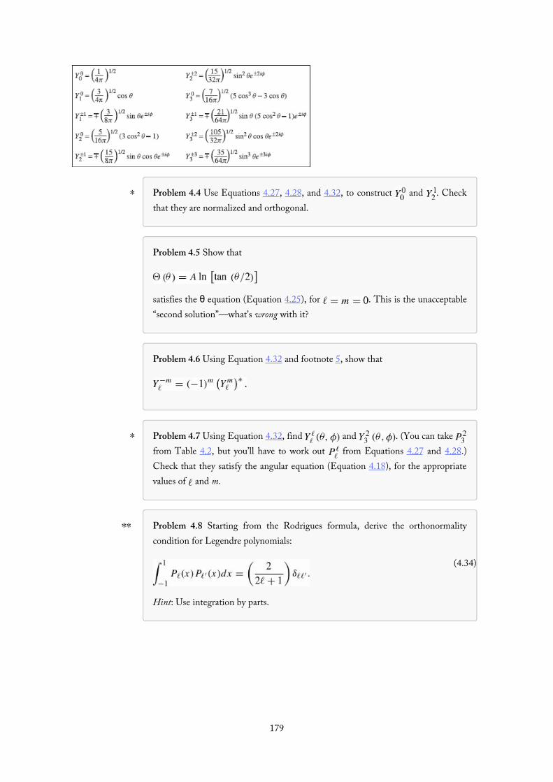
∗
∗
∗∗
(4.34)
Problem 4.4 Use Equations 4.27, 4.28, and 4.32, to construct and . Checkthat they are normalized and orthogonal.
Problem 4.5 Show that
satisfies the θ equation (Equation 4.25), for . This is the unacceptable“second solution”—what’s wrong with it?
Problem 4.6 Using Equation 4.32 and footnote 5, show that
Problem 4.7 Using Equation 4.32, find and . (You can take from Table 4.2, but you’ll have to work out from Equations 4.27 and 4.28.)Check that they satisfy the angular equation (Equation 4.18), for the appropriatevalues of and m.
Problem 4.8 Starting from the Rodrigues formula, derive the orthonormalitycondition for Legendre polynomials:
Hint: Use integration by parts.
179
(4.35)
(4.37)
(4.38)
(4.39)
(4.40)
(4.41)
(4.36)
4.1.3 The Radial Equation
Notice that the angular part of the wave function, , is the same for all spherically symmetricpotentials; the actual shape of the potential, , affects only the radial part of the wave function, ,which is determined by Equation 4.16:
This simplifies if we change variables: Let
so that , , , and hence
This is called the radial equation;9 it is identical in form to the one-dimensional Schrödinger equation(Equation 2.5), except that the effective potential,
contains an extra piece, the so-called centrifugal term, . It tends to throw theparticle outward (away from the origin), just like the centrifugal (pseudo-)force in classical mechanics.Meanwhile, the normalization condition (Equation 4.31) becomes
That’s as far as we can go until a specific potential is provided.
Example 4.1Consider the infinite spherical well,
Find the wave functions and the allowed energies.
Solution: Outside the well the wave function is zero; inside the well, the radial equation says
where
180
(4.42)
(4.43)
(4.44)
(4.46)
(4.45)
Our problem is to solve Equation 4.41, subject to the boundary condition . The case is easy:
But remember, the actual radial wave function is , and blows up as . So10 . The boundary condition then requires , and hence , for
some integer N. The allowed energies are
(same as for the one-dimensional infinite square well, Equation 2.30). Normalizing yields :
Notice that the radial wave function has nodes (or, if you prefer, N “lobes”).The general solution to Equation 4.41 (for an arbitrary integer ) is not so familiar:
where is the spherical Bessel function of order , and is the spherical Neumann functionof order . They are defined as follows:
For example,
and so on. The first few spherical Bessel and Neumann functions are listed in Table 4.4. For small x(where and ),
etc. Notice that Bessel functions are finite at the origin, but Neumann functions blow up at the origin.181

(4.49)
(4.50)
(4.51)
(4.47)
(4.48)
etc. Notice that Bessel functions are finite at the origin, but Neumann functions blow up at the origin.Accordingly, , and hence
There remains the boundary condition, . Evidently k must be chosen such that
that is, is a zero of the th-order spherical Bessel function. Now, the Bessel functions areoscillatory (see Figure 4.2); each one has an infinite number of zeros. But (unfortunately for us) theyare not located at nice sensible points (such as multiples of π); they have to be computednumerically.11 At any rate, the boundary condition requires that
where is the Nth zero of the th spherical Bessel function. The allowed energies, then, are givenby
It is customary to introduce the principal quantum number, n, which simply orders the allowedenergies, starting with 1 for the ground state (see Figure 4.3). The wave functions are
with the constant to be determined by normalization. As before, the wave function has radial nodes.12
Table 4.4 The first few spherical Bessel and Neumann functions, and ; asymptotic forms forsmall x.
182

Figure 4.2: Graphs of the first four spherical Bessel functions.
Figure 4.3: Energy levels of the infinite spherical well (Equation 4.50). States with the same value ofN are connected by dashed lines.
Notice that the energy levels are -fold degenerate, since there are different values ofm for each value of (see Equation 4.29). This is the degeneracy to be expected for a sphericallysymmetric potential, since m does not appear in the radial equation (which determines the energy).But in some cases (most famously the hydrogen atom) there is extra degeneracy, due to coincidencesin the energy levels not attributable to spherical symmetry alone. The deeper reason for such“accidental” degeneracy is intriguing, as we shall see in Chapter 6.
183

∗∗
Problem 4.9(a) From the definition (Equation 4.46), construct and .(b) Expand the sines and cosines to obtain approximate formulas for
and , valid when . Confirm that they blow up at the origin.
Problem 4.10(a) Check that satisfies the radial equation with and
.(b) Determine graphically the allowed energies for the infinite spherical well,
when . Show that for large N, .Hint: First show that . Plot x and on thesame graph, and locate the points of intersection.
Problem 4.11 A particle of mass m is placed in a finite spherical well:
Find the ground state, by solving the radial equation with . Show that thereis no bound state if .
184

(4.52)
(4.53)
4.2 The Hydrogen AtomThe hydrogen atom consists of a heavy, essentially motionless proton (we may as well put it at the origin), ofcharge e, together with a much lighter electron (mass , charge ) that orbits around it, bound by themutual attraction of opposite charges (see Figure 4.4). From Coulomb’s law, the potential energy of theelectron13 (in SI units) is
and the radial equation (Equation 4.37) says
(The effective potential—the term in square brackets—is shown in Figure 4.5.) Our problem is to solve thisequation for , and determine the allowed energies. The hydrogen atom is such an important case that I’mnot going to hand you the solutions this time—we’ll work them out in detail, by the method we used in theanalytical solution to the harmonic oscillator. (If any step in this process is unclear, you may want to refer backto Section 2.3.2 for a more complete explanation.) Incidentally, the Coulomb potential (Equation 4.52)admits continuum states (with ), describing electron-proton scattering, as well as discrete bound states,representing the hydrogen atom, but we shall confine our attention to the latter.14
Figure 4.4: The hydrogen atom.
Figure 4.5: The effective potential for hydrogen (Equation 4.53), if .
185

186

(4.54)
(4.55)
(4.56)
(4.59)
(4.60)
(4.57)
(4.58)
4.2.1 The Radial Wave Function
Our first task is to tidy up the notation. Let
(For bound states, E is negative, so κ is real.) Dividing Equation 4.53 by E, we have
This suggests that we introduce
so that
Next we examine the asymptotic form of the solutions. As , the constant term in the bracketsdominates, so (approximately)
The general solution is
but blows up (as ), so . Evidently,
for large ρ. On the other hand, as the centrifugal term dominates;15 approximately, then:
The general solution (check it!) is
but blows up (as ), so . Thus
for small ρ.The next step is to peel off the asymptotic behavior, introducing the new function :
187

(4.61)
(4.62)
(4.63)
in the hope that will turn out to be simpler than . The first indications are not auspicious:
and
In terms of , then, the radial equation (Equation 4.56) reads
Finally, we assume the solution, , can be expressed as a power series in ρ:
Our problem is to determine the coefficients . Differentiating term by term:
(In the second summation I have renamed the “dummy index”: . If this troubles you, write out thefirst few terms explicitly, and check it. You may object that the sum should now begin at , but thefactor kills that term anyway, so we might as well start at zero.) Differentiating again,
Inserting these into Equation 4.61,
Equating the coefficients of like powers yields
or:
This recursion formula determines the coefficients, and hence the function : We start with (thisbecomes an overall constant, to be fixed eventually by normalization), and Equation 4.63 gives us ; putting
188

(4.64)
(4.65)
(4.69)
(4.70)
(4.66)
(4.67)
(4.68)
this back in, we obtain , and so on.16
Now let’s see what the coefficients look like for large j (this corresponds to large ρ, where the higherpowers dominate). In this regime the recursion formula says17
so
Suppose for a moment that this were the exact result. Then
and hence
which blows up at large ρ. The positive exponential is precisely the asymptotic behavior we didn’t want, inEquation 4.57. (It’s no accident that it reappears here; after all, it does represent the asymptotic form of somesolutions to the radial equation—they just don’t happen to be the ones we’re interested in, because they aren’tnormalizable.)
There is only one escape from this dilemma: The series must terminate. There must occur some integer Nsuch that
(beyond this all coefficients vanish automatically).18 In that case Equation 4.63 says
Defining
we have
But determines E (Equations 4.54 and 4.55):
so the allowed energies are
189
(4.71)
(4.72)
(4.73)
(4.75)
(4.76)
(4.77)
(4.78)
(4.79)
(4.74)
This is the famous Bohr formula—by any measure the most important result in all of quantum mechanics.Bohr obtained it in 1913 by a serendipitous mixture of inapplicable classical physics and premature quantumtheory (the Schrödinger equation did not come until 1926).
Combining Equations 4.55 and 4.68, we find that
where
is the so-called Bohr radius.19 It follows (again, from Equation 4.55) that
The spatial wave functions are labeled by three quantum numbers (n, , and m):20
where (referring back to Equations 4.36 and 4.60)
and is a polynomial of degree in ρ, whose coefficients are determined (up to an overallnormalization factor) by the recursion formula
The ground state (that is, the state of lowest energy) is the case ; putting in the accepted values forthe physical constants, we get:21
In other words, the binding energy of hydrogen (the amount of energy you would have to impart to theelectron in its ground state in order to ionize the atom) is 13.6 eV. Equation 4.67 forces , whence also
(see Equation 4.29), so
The recursion formula truncates after the first term (Equation 4.76 with yields ), so is aconstant , and
190

(4.80)
(4.81)
(4.82)
(4.83)
(4.85)
(4.84)
Normalizing it, in accordance with Equation 4.31:
so . Meanwhile, , and hence the ground state of hydrogen is
If the energy is
this is the first excited state—or rather, states, since we can have either (in which case ) or (with , 0, or +1); evidently four different states share this same energy. If , the recursionrelation (Equation 4.76) gives
so , and therefore
(Notice that the expansion coefficients are completely different for different quantum numbers n and .)If the recursion formula terminates the series after a single term; is a constant, and we find
(In each case the constant is to be determined by normalization—see Problem 4.13.)For arbitrary n, the possible values of (consistent with Equation 4.67) are
and for each there are possible values of m (Equation 4.29), so the total degeneracy of the energylevel is
In Figure 4.6 I plot the energy levels for hydrogen. Notice that different values of carry the same energy (fora given n)—contrast the infinite spherical well, Figure 4.3. (With Equation 4.67, dropped out of sight, inthe derivation of the allowed energies, though it does still affect the wave functions.) This is what gives rise tothe “extra” degeneracy of the Coulomb potential, as compared to what you would expect from sphericalsymmetry alone ( , as opposed to ).
191

(4.86)
(4.87)
(4.88)
(4.89)
Figure 4.6: Energy levels for hydrogen (Equation 4.70); is the ground state, with eV; aninfinite number of states are squeezed in between and ; separates the bound statesfrom the scattering states. Compare Figure 4.3, and note the extra (“accidental”) degeneracy of the hydrogenenergies.
The polynomial (defined by the recursion formula, Equation 4.76) is a function well known toapplied mathematicians; apart from normalization, it can be written as
where
is an associated Laguerre polynomial, and
is the qth Laguerre polynomial.22 The first few Laguerre polynomials are listed in Table 4.5; some associatedLaguerre polynomials are given in Table 4.6. The first few radial wave functions are listed in Table 4.7, andplotted in Figure 4.7.) The normalized hydrogen wave functions are23
They are not pretty, but don’t complain—this is one of the very few realistic systems that can be solved at all,in exact closed form. The wave functions are mutually orthogonal:
192

(4.90)
This follows from the orthogonality of the spherical harmonics (Equation 4.33) and (for ) from thefact that they are eigenfunctions of with distinct eigenvalues.
Table 4.5: The first few Laguerre polynomials.
Table 4.6: Some associated Laguerre polynomials.
Table 4.7: The first few radial wave functions for hydrogen, .
193

Figure 4.7: Graphs of the first few hydrogen radial wave functions, .
194

Visualizing the hydrogen wave functions is not easy. Chemists like to draw density plots, in which thebrightness of the cloud is proportional to (Figure 4.8). More quantitative (but perhaps harder todecipher) are surfaces of constant probability density (Figure 4.9). The quantum numbers n, , and m can beidentified from the nodes of the wave function. The number of radial nodes is, as always, given by (forhydrogen this is ). For each radial node the wave function vanishes on a sphere, as can be seen inFigure 4.8. The quantum number m counts the number of nodes of the real (or imaginary) part of the wavefunction in the ϕ direction. These nodes are planes containing the z axis on which the real or imaginary partof vanishes.24 Finally, gives the number of nodes in the θ direction. These are cones about the z axison which vanishes (note that a cone with opening angle is the plane itself).
Figure 4.8: Density plots for the first few hydrogen wave functions, labeled by . Printed bypermission using “Atom in a Box” by Dauger Research. You can make your own plots by going to:http://dauger.com.
195
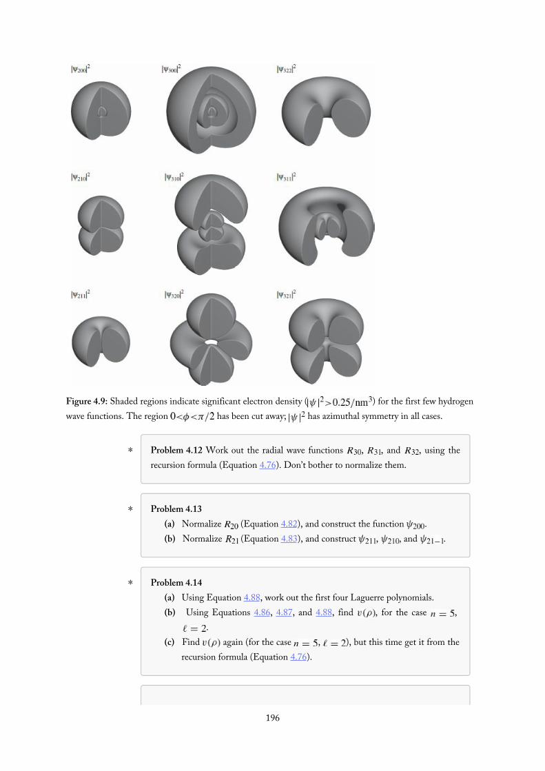
∗
∗
∗
Figure 4.9: Shaded regions indicate significant electron density ( ) for the first few hydrogenwave functions. The region has been cut away; has azimuthal symmetry in all cases.
Problem 4.12 Work out the radial wave functions , , and , using therecursion formula (Equation 4.76). Don’t bother to normalize them.
Problem 4.13(a) Normalize (Equation 4.82), and construct the function .(b) Normalize (Equation 4.83), and construct , , and .
Problem 4.14(a) Using Equation 4.88, work out the first four Laguerre polynomials.(b) Using Equations 4.86, 4.87, and 4.88, find , for the case ,
.(c) Find again (for the case , ), but this time get it from the
recursion formula (Equation 4.76).
196

∗ Problem 4.15(a) Find and for an electron in the ground state of hydrogen. Express
your answers in terms of the Bohr radius.(b) Find and for an electron in the ground state of hydrogen. Hint:
This requires no new integration—note that , andexploit the symmetry of the ground state.
(c) Find in the state , , . Hint: this state is notsymmetrical in x, y, z. Use .
Problem 4.16 What is the most probable value of r, in the ground state ofhydrogen? (The answer is not zero!) Hint: First you must figure out the probabilitythat the electron would be found between r and .
Problem 4.17 Calculate , in the ground state of hydrogen. Hint: This takestwo pages and six integrals, or four lines and no integrals, depending on how youset it up. To do it the quick way, start by noting that
.25
Problem 4.18 A hydrogen atom starts out in the following linear combination ofthe stationary states , , and , , :
(a) Construct . Simplify it as much as you can.(b) Find the expectation value of the potential energy, . (Does it depend
on t?) Give both the formula and the actual number, in electron volts.
197

(4.91)
(4.93)
(4.94)
(4.92)
4.2.2 The Spectrum of Hydrogen
In principle, if you put a hydrogen atom into some stationary state , it should stay there forever.However, if you tickle it slightly (by collision with another atom, say, or by shining light on it), the atom mayundergo a transition to some other stationary state—either by absorbing energy, and moving up to a higher-energy state, or by giving off energy (typically in the form of electromagnetic radiation), and moving down.26
In practice such perturbations are always present; transitions (or, as they are sometimes called, quantumjumps) are constantly occurring, and the result is that a container of hydrogen gives off light (photons), whoseenergy corresponds to the difference in energy between the initial and final states:
Now, according to the Planck formula,27 the energy of a photon is proportional to its frequency:
Meanwhile, the wavelength is given by , so
where
is known as the Rydberg constant. Equation 4.93 is the Rydberg formula for the spectrum of hydrogen; itwas discovered empirically in the nineteenth century, and the greatest triumph of Bohr’s theory was its abilityto account for this result—and to calculate in terms of the fundamental constants of nature. Transitions tothe ground state lie in the ultraviolet; they are known to spectroscopists as the Lyman series.Transitions to the first excited state fall in the visible region; they constitute the Balmer series.Transitions to (the Paschen series) are in the infrared; and so on (see Figure 4.10). (At roomtemperature, most hydrogen atoms are in the ground state; to obtain the emission spectrum you must firstpopulate the various excited states; typically this is done by passing an electric spark through the gas.)
198

∗
Figure 4.10: Energy levels and transitions in the spectrum of hydrogen.
Problem 4.19 A hydrogenic atom consists of a single electron orbiting a nucleuswith Z protons. ( would be hydrogen itself, is ionized helium,
is doubly ionized lithium, and so on.) Determine the Bohr energies , the binding energy , the Bohr radius , and the Rydberg constant
for a hydrogenic atom. (Express your answers as appropriate multiples ofthe hydrogen values.) Where in the electromagnetic spectrum would the Lymanseries fall, for and ? Hint: There’s nothing much to calculate here—in the potential (Equation 4.52) , so all you have to do is make thesame substitution in all the final results.
Problem 4.20 Consider the earth–sun system as a gravitational analog to thehydrogen atom.
(a) What is the potential energy function (replacing Equation 4.52)? (Let be the mass of the earth, and M the mass of the sun.)
(b) What is the “Bohr radius,” , for this system? Work out the actualnumber.
(c) Write down the gravitational “Bohr formula,” and, by equating to theclassical energy of a planet in a circular orbit of radius , show that
. From this, estimate the quantum number n of the earth.(d) Suppose the earth made a transition to the next lower level . How
much energy (in Joules) would be released? What would the wavelengthof the emitted photon (or, more likely, graviton) be? (Express your answerin light years—is the remarkable answer28 a coincidence?)
199

200

(4.95)
(4.96)
4.3 Angular MomentumAs we have seen, the stationary states of the hydrogen atom are labeled by three quantum numbers: n, , andm. The principal quantum number determines the energy of the state (Equation 4.70); and m are relatedto the orbital angular momentum. In the classical theory of central forces, energy and angular momentum arethe fundamental conserved quantities, and it is not surprising that angular momentum plays an important)role in the quantum theory.
Classically, the angular momentum of a particle (with respect to the origin) is given by the formula
which is to say,29
The corresponding quantum operators30 are obtained by the standard prescription , , . In this section we’ll obtain the eigenvalues of the the angular momentum
operators by a purely algebraic technique reminiscent of the one we used in Chapter 2 to get the allowedenergies of the harmonic oscillator; it is all based on the clever exploitation of commutation relations. Afterthat we will turn to the more difficult problem of determining the eigenfunctions.
201
(4.97)
(4.98)
(4.99)
(4.100)
(4.101)
(4.102)
(4.103)
4.3.1 Eigenvalues
The operators and do not commute; in fact
From the canonical commutation relations (Equation 4.10) we know that the only operators here that fail tocommute are x with , y with , and z with . So the two middle terms drop out, leaving
Of course, we could have started out with or , but there is no need to calculate theseseparately—we can get them immediately by cyclic permutation of the indices , , :
These are the fundamental commutation relations for angular momentum; everything follows from them.Notice that , , and are incompatible observables. According to the generalized uncertainty
principle (Equation 3.62),
or
It would therefore be futile to look for states that are simultaneously eigenfunctions of and . On theother hand, the square of the total angular momentum,
does commute with :
(I used Equation 3.65 to reduce the commutators; of course, any operator commutes with itself .) It followsthat also commutes with and :
or, more compactly,
202

(4.104)
(4.106)
(4.107)
(4.108)
(4.109)
(4.111)
(4.105)
(4.110)
So is compatible with each component of L, and we can hope to find simultaneous eigenstates of and(say) :
We’ll use a ladder operator technique, very similar to the one we applied to the harmonic oscillator backin Section 2.3.1. Let
Its commutator with is
so
Also (from Equation 4.102)
I claim that if f is an eigenfunction of and , so also is : Equation 4.107 says
so is an eigenfunction of , with the same eigenvalue , and Equation 4.106 says
so is an eigenfunction of with the new eigenvalue . We call the raising operator, becauseit increases the eigenvalue of by , and the lowering operator, because it lowers the eigenvalue by .
For a given value of , then, we obtain a “ladder” of states, with each “rung” separated from its neighborsby one unit of in the eigenvalue of (see Figure 4.11). To ascend the ladder we apply the raising operator,and to descend, the lowering operator. But this process cannot go on forever: Eventually we’re going to reacha state for which the z-component exceeds the total, and that cannot be.31 There must exist a “top rung”, ,such that32
Let be the eigenvalue of at the top rung (the appropriateness of the letter “ ” will appear in a moment):
Now,
or, putting it the other way around,
203

(4.113)
(4.115)
(4.112)
(4.114)
It follows that
and hence
This tells us the eigenvalue of in terms of the maximum eigenvalue of .
Figure 4.11: The “ladder” of angular momentum states.
Meanwhile, there is also (for the same reason) a bottom rung, , such that
Let be the eigenvalue of at this bottom rung:
Using Equation 4.112, we have
204
(4.116)
(4.118)
(4.117)
(4.119)
and therefore
Comparing Equations 4.113 and 4.116, we see that , so either (which isabsurd—the bottom rung would be higher than the top rung!) or else
So the eigenvalues of are , where m (the appropriateness of this letter will also be clear in amoment) goes from to , in N integer steps. In particular, it follows that , and hence
, so must be an integer or a half-integer. The eigenfunctions are characterized by the numbers andm:
where
For a given value of , there are different values of m (i.e. “rungs” on the “ladder”).Some people like to illustrate this with the diagram in Figure 4.12 (drawn for the case ). The
arrows are supposed to represent possible angular momenta (in units of )—they all have the same length (in this case ), and their z components are the allowed values of m ( ).
Notice that the magnitude of the vectors (the radius of the sphere) is greater than the maximum z component!(In general, , except for the “trivial” case .) Evidently you can’t get the angularmomentum to point perfectly along the z direction. At first, this sounds absurd. “Why can’t I just pick my axesso that z points along the direction of the angular momentum vector?” Well, to do that you would have toknow all three components simultaneously, and the uncertainty principle (Equation 4.100) says that’simpossible. “Well, all right, but surely once in a while, by good fortune, I will just happen to aim my z axisalong the direction of L.” No, no! You have missed the point. It’s not merely that you don’t know all threecomponents of L; there just aren’t three components—a particle simply cannot have a determinate angularmomentum vector, any more than it can simultaneously have a determinate position and momentum. If has a well-defined value, then and do not. It is misleading even to draw the vectors in Figure 4.12—atbest they should be smeared out around the latitude lines, to indicate that and are indeterminate.
205
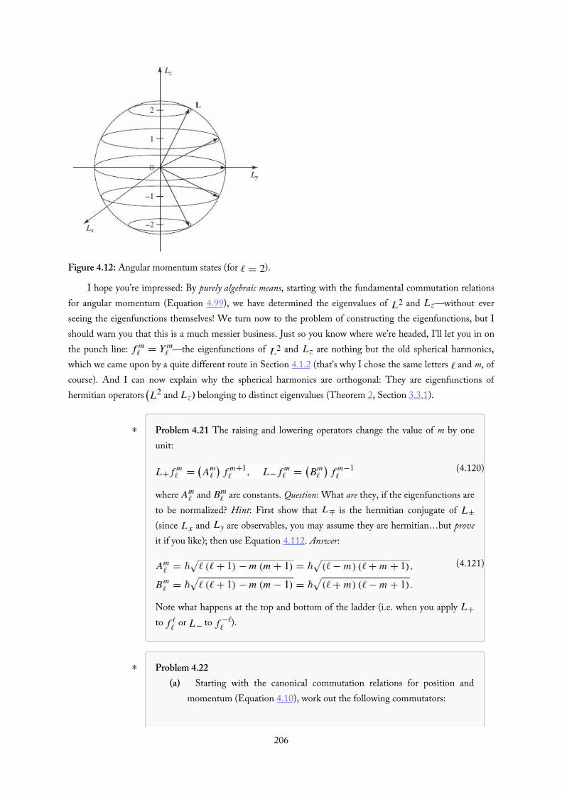
∗
(4.120)
(4.121)
∗
Figure 4.12: Angular momentum states (for ).
I hope you’re impressed: By purely algebraic means, starting with the fundamental commutation relationsfor angular momentum (Equation 4.99), we have determined the eigenvalues of and —without everseeing the eigenfunctions themselves! We turn now to the problem of constructing the eigenfunctions, but Ishould warn you that this is a much messier business. Just so you know where we’re headed, I’ll let you in onthe punch line: —the eigenfunctions of and are nothing but the old spherical harmonics,which we came upon by a quite different route in Section 4.1.2 (that’s why I chose the same letters and m, ofcourse). And I can now explain why the spherical harmonics are orthogonal: They are eigenfunctions ofhermitian operators and belonging to distinct eigenvalues (Theorem 2, Section 3.3.1).
Problem 4.21 The raising and lowering operators change the value of m by oneunit:
where and are constants. Question: What are they, if the eigenfunctions areto be normalized? Hint: First show that is the hermitian conjugate of (since and are observables, you may assume they are hermitian…but proveit if you like); then use Equation 4.112. Answer:
Note what happens at the top and bottom of the ladder (i.e. when you apply to or to ).
Problem 4.22(a) Starting with the canonical commutation relations for position and
momentum (Equation 4.10), work out the following commutators:
206
(4.122)
∗∗
(b) Use these results to obtain directly from Equation4.96.
(c) Find the commutators and (where, of course, and ).
(d) Show that the Hamiltonian commutes with allthree components of L, provided that V depends only on r. (Thus H, ,and are mutually compatible observables.)
Problem 4.23(a) Prove that for a particle in a potential the rate of change of the
expectation value of the orbital angular momentum L is equal to theexpectation value of the torque:
where
(Thisis the rotational analog to Ehrenfest’s theorem.)(b) Show that for any spherically symmetric potential. (This is
one form of the quantum statement of conservation of angularmomentum.)
207
(4.123)
(4.124)
(4.125)
(4.126)
(4.127)
(4.128)
(4.129)
4.3.2 Eigenfunctions
First of all we need to rewrite , , and in spherical coordinates. Now, , and thegradient, in spherical coordinates, is:33
meanwhile, , so
But , , and (see Figure 4.1), and hence
The unit vectors and can be resolved into their cartesian components:
Thus
So
and
We shall also need the raising and lowering operators:
But , so
208

(4.130)
(4.131)
(4.132)
(4.133)
∗
In particular (Problem 4.24(a)):
and hence (Problem 4.24(b)):
We are now in a position to determine . It’s an eigenfunction of , with eigenvalue :
But this is precisely the “angular equation” (Equation 4.18). And it’s also an eigenfunction of , with theeigenvalue :
but this is equivalent to the azimuthal equation (Equation 4.21). We have already solved this system ofequations! The result (appropriately normalized) is the spherical harmonic, . Conclusion: Sphericalharmonics are the eigenfunctions of and . When we solved the Schrödinger equation by separation ofvariables, in Section 4.1, we were inadvertently constructing simultaneous eigenfunctions of the threecommuting operators H, , and :
Incidentally, we can use Equation 4.132 to rewrite the Schrödinger equation (Equation 4.14) more compactly:
There is a curious final twist to this story: the algebraic theory of angular momentum permits (andhence also m) to take on half -integer values (Equation 4.119), whereas separation of variables yieldedeigenfunctions only for integer values (Equation 4.29).34 You might suppose that the half-integer solutions arespurious, but it turns out that they are of profound importance, as we shall see in the following sections.
Problem 4.24(a) Derive Equation 4.131 from Equation 4.130. Hint: Use a test function;
otherwise you’re likely to drop some terms.(b) Derive Equation 4.132 from Equations 4.129 and 4.131. Hint: Use
Equation 4.112.
209

∗
∗∗
Problem 4.25(a) What is ? (No calculation allowed!)(b) Use the result of (a), together with Equation 4.130 and the fact that
, to determine , up to a normalization constant.(c) Determine the normalization constant by direct integration. Compare
your final answer to what you got in Problem 4.7.
Problem 4.26 In Problem 4.4 you showed that
Apply the raising operator to find . Use Equation 4.121 to get thenormalization.
Problem 4.27 Two particles (masses and ) are attached to the ends of amassless rigid rod of length a. The system is free to rotate in three dimensionsabout the (fixed) center of mass.
(a) Show that the allowed energies of this rigid rotor are
is the moment of inertia of the system. Hint: First express the (classical)energy in terms of the angular momentum.
(b) What are the normalized eigenfunctions for this system? (Let θ and ϕdefine the orientation of the rotor axis.) What is the degeneracy of thenth energy level?
(c) What spectrum would you expect for this system? (Give a formula for thefrequencies of the spectral lines.) Answer:
.(d) Figure 4.13 shows a portion of the rotational spectrum of carbon
monoxide (CO). What is the frequency separation betweenadjacent lines? Look up the masses of 12C and 16O, and from , ,and determine the distance between the atoms.
210
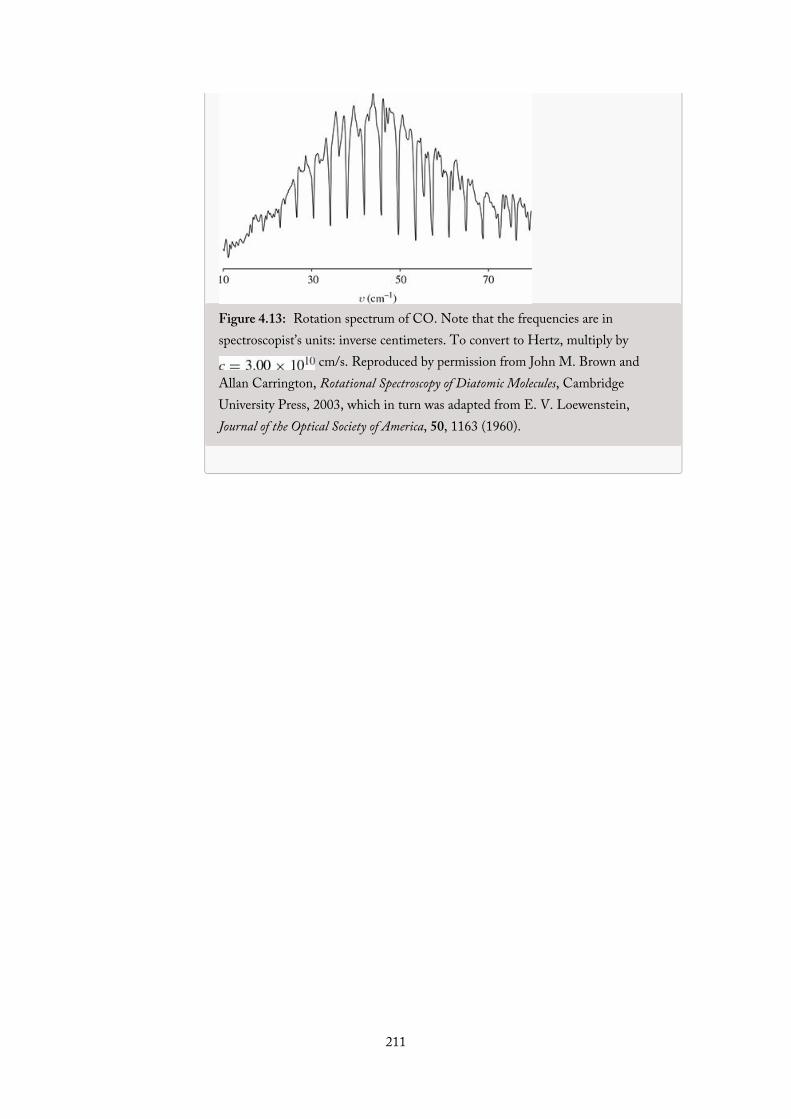
Figure 4.13: Rotation spectrum of CO. Note that the frequencies are inspectroscopist’s units: inverse centimeters. To convert to Hertz, multiply by
cm/s. Reproduced by permission from John M. Brown andAllan Carrington, Rotational Spectroscopy of Diatomic Molecules, CambridgeUniversity Press, 2003, which in turn was adapted from E. V. Loewenstein,Journal of the Optical Society of America, 50, 1163 (1960).
211
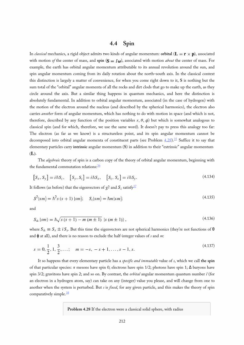
(4.134)
(4.135)
(4.136)
(4.137)
4.4 SpinIn classical mechanics, a rigid object admits two kinds of angular momentum: orbital ( ), associatedwith motion of the center of mass, and spin ( ), associated with motion about the center of mass. Forexample, the earth has orbital angular momentum attributable to its annual revolution around the sun, andspin angular momentum coming from its daily rotation about the north–south axis. In the classical contextthis distinction is largely a matter of convenience, for when you come right down to it, S is nothing but thesum total of the “orbital” angular momenta of all the rocks and dirt clods that go to make up the earth, as theycircle around the axis. But a similar thing happens in quantum mechanics, and here the distinction isabsolutely fundamental. In addition to orbital angular momentum, associated (in the case of hydrogen) withthe motion of the electron around the nucleus (and described by the spherical harmonics), the electron alsocarries another form of angular momentum, which has nothing to do with motion in space (and which is not,therefore, described by any function of the position variables ) but which is somewhat analogous toclassical spin (and for which, therefore, we use the same word). It doesn’t pay to press this analogy too far:The electron (as far as we know) is a structureless point, and its spin angular momentum cannot bedecomposed into orbital angular momenta of constituent parts (see Problem 4.28).35 Suffice it to say thatelementary particles carry intrinsic angular momentum (S) in addition to their “extrinsic” angular momentum
.The algebraic theory of spin is a carbon copy of the theory of orbital angular momentum, beginning with
the fundamental commutation relations:36
It follows (as before) that the eigenvectors of and satisfy37
and
where . But this time the eigenvectors are not spherical harmonics (they’re not functions of θand ϕ at all), and there is no reason to exclude the half-integer values of s and m:
It so happens that every elementary particle has a specific and immutable value of s, which we call the spinof that particular species: π mesons have spin 0; electrons have spin 1/2; photons have spin 1; Δ baryons havespin 3/2; gravitons have spin 2; and so on. By contrast, the orbital angular momentum quantum number l (foran electron in a hydrogen atom, say) can take on any (integer) value you please, and will change from one toanother when the system is perturbed. But s is fixed, for any given particle, and this makes the theory of spincomparatively simple.38
Problem 4.28 If the electron were a classical solid sphere, with radius
212

(4.138)
(the so-called classical electron radius, obtained by assuming the electron’s mass isattributable to energy stored in its electric field, via the Einstein formula
), and its angular momentum is , then how fast (in m/s) would apoint on the “equator” be moving? Does this model make sense? (Actually, theradius of the electron is known experimentally to be much less than , but thisonly makes matters worse.)39
213

(4.139)
(4.140)
(4.141)
(4.142)
(4.143)
4.4.1 Spin 1/2
By far the most important case is , for this is the spin of the particles that make up ordinary matter(protons, neutrons, and electrons), as well as all quarks and all leptons. Moreover, once you understand spin
1/2, it is a simple matter to work out the formalism for any higher spin. There are just two eigenstates: ,
which we call spin up (informally, ), and , spin down . Using these as basis vectors, the general
state40 of a spin-1/2 particle can be represented by a two-element column matrix (or spinor):
with
representing spin up, and
for spin down.With respect to this basis the spin operators become matrices,41 which we can work out by noting
their effect on and . Equation 4.135 says
If we write as a matrix with (as yet) undetermined elements,
then the first equation says
so and . The second equation says
so and . Conclusion:
Similarly,
214

(4.144)
(4.145)
(4.146)
(4.147)
(4.148)
(4.149)
(4.150)
from which it follows that
Meanwhile, Equation 4.136 says
so
Now , so and , and hence
Since , , and all carry a factor of , it is tidier to write S , where
These are the famous Pauli spin matrices. Notice that , , , and are all hermitian matrices (as theyshould be, since they represent observables). On the other hand, and are not hermitian—evidently theyare not observable.
The eigenspinors of are (or course):
If you measure on a particle in the general state χ (Equation 4.139), you could get , with probability , or , with probability . Since these are the only possibilities,
(i.e. the spinor must be normalized: ).42
But what if, instead, you chose to measure ? What are the possible results, and what are theirrespective probabilities? According to the generalized statistical interpretation, we need to know theeigenvalues and eigenspinors of . The characteristic equation is
Not surprisingly (but it gratifying to see how it works out), the possible values for are the same as those for . The eigenspinors are obtained in the usual way:
215

(4.151)
(4.152)
so . Evidently the (normalized) eigenspinors of are
As the eigenvectors of a hermitian matrix, they span the space; the generic spinor χ (Equation 4.139) can beexpressed as a linear combination of them:
If you measure , the probability of getting is , and the probability of getting is . (Check for yourself that these probabilities add up to 1.)
Example 4.2Suppose a spin-1/2 particle is in the state
What are the probabilities of getting and , if you measure and ?
Solution: Here and , so for the probability of getting is , and the probability of getting is . For the
probability of getting is , and the probability of getting is . Incidentally, the expectation value of is
which we could also have obtained more directly:
I’d like now to walk you through an imaginary measurement scenario involving spin 1/2, because it servesto illustrate in very concrete terms some of the abstract ideas we discussed back in Chapter 1. Let’s say westart out with a particle in the state . If someone asks, “What is the z-component of that particle’s spinangular momentum?”, we can answer unambiguously: . For a measurement of is certain to returnthat value. But if our interrogator asks instead, “What is the x-component of that particle’s spin angularmomentum?” we are obliged to equivocate: If you measure , the chances are fifty-fifty of getting either or . If the questioner is a classical physicist, or a “realist” (in the sense of Section 1.2), he will regard thisas an inadequate—not to say impertinent—response: “Are you telling me that you don’t know the true state ofthat particle?” On the contrary; I know precisely what the state of the particle is: . “Well, then, how come
216

(4.153)
∗
you can’t tell me what the x-component of its spin is?” Because it simply does not have a particular x-component of spin. Indeed, it cannot, for if both and were well-defined, the uncertainty principle wouldbe violated.
At this point our challenger grabs the test-tube and measures the x-component of the particle’s spin; let’ssay he gets the value . “Aha!” (he shouts in triumph), “You lied! This particle has a perfectly well-defined value of : .” Well, sure—it does now, but that doesn’t prove it had that value, prior to yourmeasurement. “You have obviously been reduced to splitting hairs. And anyway, what happened to youruncertainty principle? I now know both and .” I’m sorry, but you do not: In the course of yourmeasurement, you altered the particle’s state; it is now in the state , and whereas you know the value of , you no longer know the value of . “But I was extremely careful not to disturb the particle when I measured
.” Very well, if you don’t believe me, check it out: Measure , and see what you get. (Of course, he may get , which will be embarrassing to my case—but if we repeat this whole scenario over and over, half the
time he will get .)To the layman, the philosopher, or the classical physicist, a statement of the form “this particle doesn’t
have a well-defined position” (or momentum, or x-component of spin angular momentum, or whatever)sounds vague, incompetent, or (worst of all) profound. It is none of these. But its precise meaning is, I think,almost impossible to convey to anyone who has not studied quantum mechanics in some depth. If you findyour own comprehension slipping, from time to time (if you don’t, you probably haven’t understood theproblem), come back to the spin-1/2 system: It is the simplest and cleanest context for thinking through theconceptual paradoxes of quantum mechanics.
Problem 4.29(a) Check that the spin matrices (Equations 4.145 and 4.147) obey the
fundamental commutation relations for angular momentum, Equation4.134.
(b) Show that the Pauli spin matrices (Equation 4.148) satisfy the productrule
where the indices stand for x, y, or z, and is the Levi-Civita symbol:+1 if , 231, or 312; if , 213, or 321; 0otherwise.
Problem 4.30 An electron is in the spin state
(a) Determine the normalization constant A.(b) Find the expectation values of , , and .(c) Find the “uncertainties” , , and . Note: These sigmas are
standard deviations, not Pauli matrices!
217
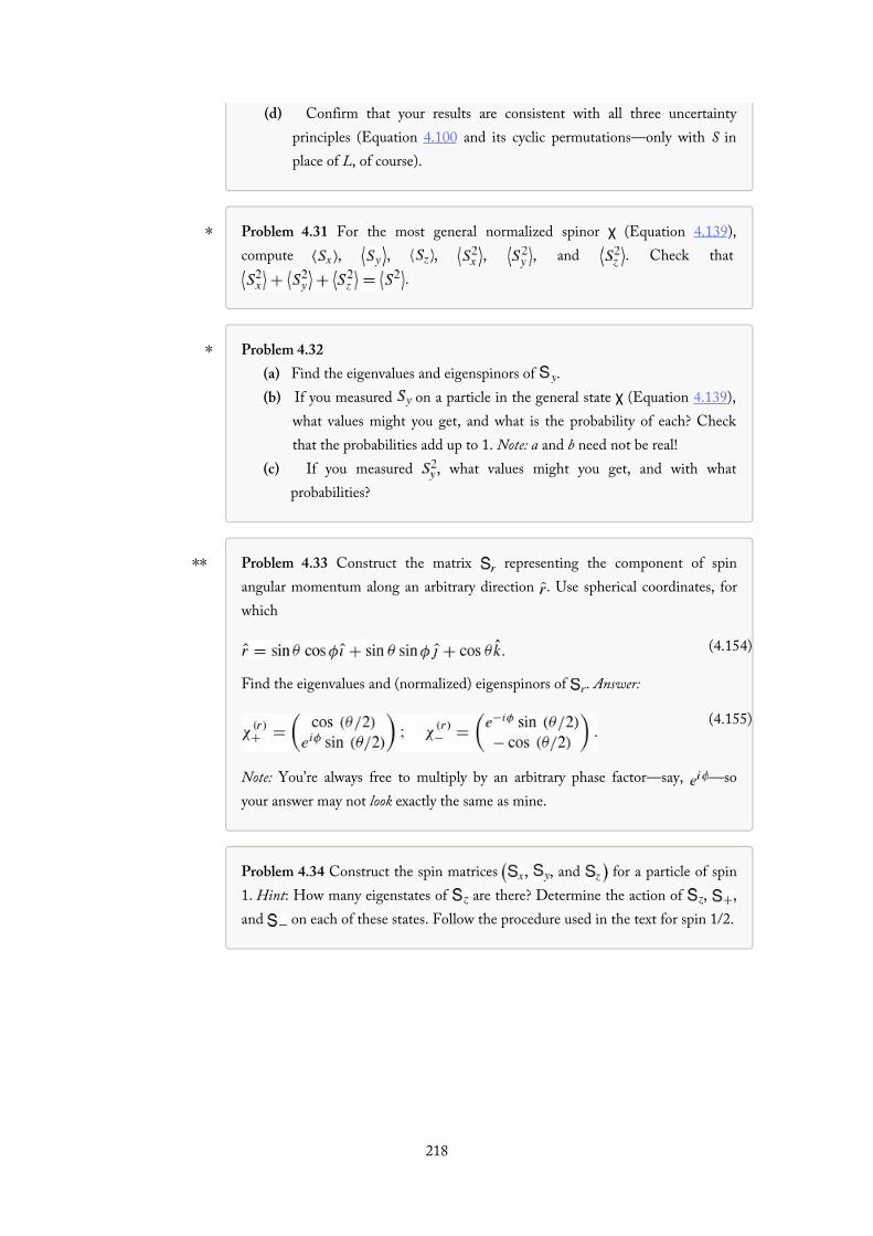
∗
∗
∗∗
(4.154)
(4.155)
(d) Confirm that your results are consistent with all three uncertaintyprinciples (Equation 4.100 and its cyclic permutations—only with S inplace of L, of course).
Problem 4.31 For the most general normalized spinor χ (Equation 4.139),compute , , , , , and . Check that
.
Problem 4.32(a) Find the eigenvalues and eigenspinors of .(b) If you measured on a particle in the general state χ (Equation 4.139),
what values might you get, and what is the probability of each? Checkthat the probabilities add up to 1. Note: a and b need not be real!
(c) If you measured , what values might you get, and with whatprobabilities?
Problem 4.33 Construct the matrix representing the component of spinangular momentum along an arbitrary direction . Use spherical coordinates, forwhich
Find the eigenvalues and (normalized) eigenspinors of . Answer:
Note: You’re always free to multiply by an arbitrary phase factor—say, —soyour answer may not look exactly the same as mine.
Problem 4.34 Construct the spin matrices , , and for a particle of spin1. Hint: How many eigenstates of are there? Determine the action of , ,and on each of these states. Follow the procedure used in the text for spin 1/2.
218

(4.159)
(4.160)
(4.161)
(4.162)
(4.156)
(4.157)
(4.158)
4.4.2 Electron in a Magnetic Field
A spinning charged particle constitutes a magnetic dipole. Its magnetic dipole moment, , is proportional toits spin angular momentum, S:
the proportionality constant, γ, is called the gyromagnetic ratio.43 When a magnetic dipole is placed in amagnetic field B, it experiences a torque, , which tends to line it up parallel to the field (just like acompass needle). The energy associated with this torque is44
so the Hamiltonian matrix for a spinning charged particle, at rest45 in a magnetic field B, is
where is the appropriate spin matrix (Equations 4.145 and 4.147, in the case of spin 1/2).
Example 4.3Larmor precession: Imagine a particle of spin 1/2 at rest in a uniform magnetic field, which points inthe z-direction:
The Hamiltonian (Equation 4.158) is
The eigenstates of are the same as those of :
The energy is lowest when the dipole moment is parallel to the field—just as it would be classically.Since the Hamiltonian is time independent, the general solution to the time-dependent
Schrödinger equation,
can be expressed in terms of the stationary states:
The constants a and b are determined by the initial conditions:
219

(4.163)
(4.164)
(4.165)
(4.166)
(4.167)
(of course, ). With no essential loss of generality46 I’ll write and , where α is a fixed angle whose physical significance will appear in a moment. Thus
To get a feel for what is happening here, let’s calculate the expectation value of S, as a function oftime:
Similarly,
and
Thus is tilted at a constant angle α to the z axis, and precesses about the field at the Larmorfrequency
just as it would classically47 (see Figure 4.14). No surprise here—Ehrenfest’s theorem (in the formderived in Problem 4.23) guarantees that evolves according to the classical laws. But it’s nice to seehow this works out in a specific context.
Figure 4.14: Precession of in a uniform magnetic field.
220

(4.169)
(4.168)
(4.170)
Example 4.4The Stern–Gerlach experiment: In an inhomogeneous magnetic field, there is not only a torque, but alsoa force, on a magnetic dipole:48
This force can be used to separate out particles with a particular spin orientation. Imagine a beam ofheavy neutral atoms,49 traveling in the y direction, which passes through a region of static butinhomogeneous magnetic field (Figure 4.15)—say
where is a strong uniform field and the constant α describes a small deviation from homogeneity.(Actually, what we’d prefer is just the z component of this field, but unfortunately that’s impossible—itwould violate the electromagnetic law ; like it or not, the x component comes along for theride.) The force on these atoms is50
Figure 4.15: The Stern–Gerlach apparatus.
But because of the Larmor precession about , oscillates rapidly, and averages to zero; the netforce is in the z direction:
and the beam is deflected up or down, in proportion to the z component of the spin angularmomentum. Classically we’d expect a smear (because would not be quantized), but in fact the beamsplits into separate streams, beautifully demonstrating the quantization of angular momentum.(If you use silver atoms, all the inner electrons are paired, in such a way that their angular momentacancel. The net spin is simply that of the outermost—unpaired—electron, so in this case ,and the beam splits in two.)
The Stern–Gerlach experiment has played an important role in the philosophy of quantummechanics, where it serves both as the prototype for the preparation of a quantum state and as anilluminating model for a certain kind of quantum measurement. We tend casually to assume that theinitial state of a system is known (the Schrödinger equation tells us how it subsequently evolves)—butit is natural to wonder how you get a system into a particular state in the first place. Well, if you wantto prepare a beam of atoms in a given spin configuration, you pass an unpolarized beam through aStern–Gerlach magnet, and select the outgoing stream you are interested in (closing off the others
221

∗∗
with suitable baffles and shutters). Conversely, if you want to measure the z component of an atom’sspin, you send it through a Stern–Gerlach apparatus, and record which bin it lands in. I do not claimthat this is always the most practical way to do the job, but it is conceptually very clean, and hence auseful context in which to explore the problems of state preparation and measurement.
Problem 4.35 In Example 4.3:(a) If you measured the component of spin angular momentum along the x
direction, at time t, what is the probability that you would get ?(b) Same question, but for the y component.(c) Same, for the z component.
Problem 4.36 An electron is at rest in an oscillating magnetic field
where and ω are constants.(a) Construct the Hamiltonian matrix for this system.(b) The electron starts out (at in the spin-up state with respect to the
x axis (that is: ). Determine at any subsequent time.Beware: This is a time-dependent Hamiltonian, so you cannot get inthe usual way from stationary states. Fortunately, in this case you cansolve the time-dependent Schrödinger equation (Equation 4.162)directly.
(c) Find the probability of getting , if you measure . Answer:
(d) What is the minimum field required to force a complete flip in ?
222

(4.171)
(4.172)
(4.173)
(4.174)
4.4.3 Addition of Angular Momenta
Suppose now that we have two particles, with spins and . Say, the first is in the state and thesecond in the state . We denote the composite state by :
Question: What is the total angular momentum,
of this system? That is to say: what is the net spin, s, of the combination, and what is the z component, m?The z component is easy:
so
it’s just the sum. But s is much more subtle, so let’s begin with the simplest nontrivial example.
Example 4.5Consider the case of two spin- particles—say, the electron and the proton in the ground state ofhydrogen. Each can have spin up or spin down, so there are four possibilities in all:51
This doesn’t look right: m is supposed to advance in integer steps, from to , so it appears that —but there is an “extra” state with .
One way to untangle this problem is to apply the lowering operator, to the state, using Equation 4.146:
Evidently the three states with are (in the notation ):
223

(4.175)
(4.176)
(4.177)
(4.178)
(4.179)
(4.180)
(As a check, try applying the lowering operator to ; what should you get? See Problem 4.37(a).)This is called the triplet combination, for the obvious reason. Meanwhile, the orthogonal state with
carries :
(If you apply the raising or lowering operator to this state, you’ll get zero. See Problem 4.37(b).)I claim, then, that the combination of two spin-1/2 particles can carry a total spin of 1 or 0,
depending on whether they occupy the triplet or the singlet configuration. To confirm this, I need toprove that the triplet states are eigenvectors of with eigenvalue , and the singlet is aneigenvector of with eigenvalue 0. Now,
Using Equations 4.145 and 4.147, we have
Similarly,
It follows that
and
Returning to Equation 4.177 (and using Equation 4.142), we conclude that
224
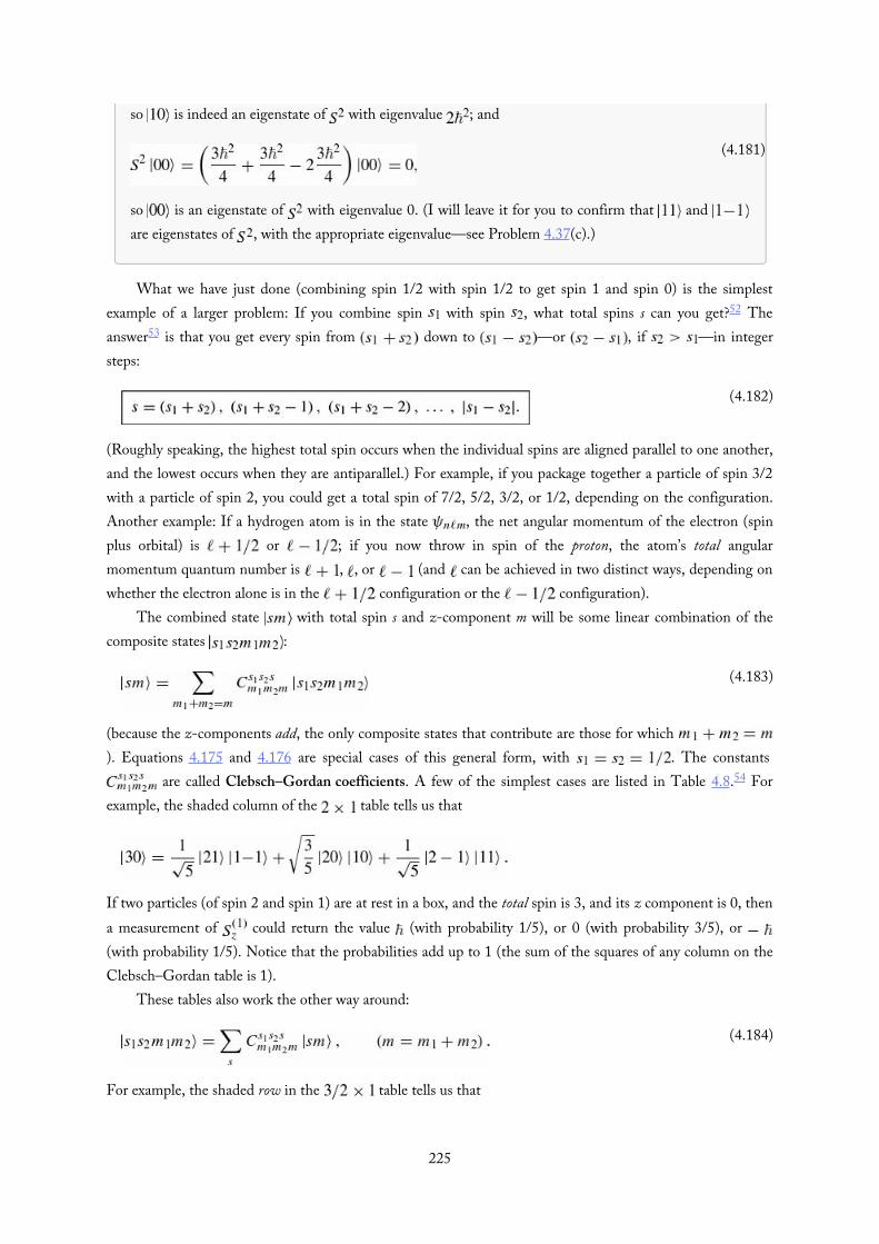
(4.181)
(4.182)
(4.183)
(4.184)
so is indeed an eigenstate of with eigenvalue ; and
so is an eigenstate of with eigenvalue 0. (I will leave it for you to confirm that and are eigenstates of , with the appropriate eigenvalue—see Problem 4.37(c).)
What we have just done (combining spin 1/2 with spin 1/2 to get spin 1 and spin 0) is the simplestexample of a larger problem: If you combine spin with spin , what total spins s can you get?52 Theanswer53 is that you get every spin from down to —or , if —in integersteps:
(Roughly speaking, the highest total spin occurs when the individual spins are aligned parallel to one another,and the lowest occurs when they are antiparallel.) For example, if you package together a particle of spin 3/2with a particle of spin 2, you could get a total spin of 7/2, 5/2, 3/2, or 1/2, depending on the configuration.Another example: If a hydrogen atom is in the state , the net angular momentum of the electron (spinplus orbital) is or ; if you now throw in spin of the proton, the atom’s total angularmomentum quantum number is , , or (and can be achieved in two distinct ways, depending onwhether the electron alone is in the configuration or the configuration).
The combined state with total spin s and z-component m will be some linear combination of thecomposite states :
(because the z-components add, the only composite states that contribute are those for which ). Equations 4.175 and 4.176 are special cases of this general form, with . The constants
are called Clebsch–Gordan coefficients. A few of the simplest cases are listed in Table 4.8.54 Forexample, the shaded column of the table tells us that
If two particles (of spin 2 and spin 1) are at rest in a box, and the total spin is 3, and its z component is 0, thena measurement of could return the value (with probability 1/5), or 0 (with probability 3/5), or (with probability 1/5). Notice that the probabilities add up to 1 (the sum of the squares of any column on theClebsch–Gordan table is 1).
These tables also work the other way around:
For example, the shaded row in the table tells us that
225

∗
If you put particles of spin 3/2 and spin 1 in the box, and you know that the first has and thesecond has (so m is necessarily 1/2), and you measured the total spin, s, you could get 5/2 (withprobability 3/5), or 3/2 (with probability 1/15), or 1/2 (with probability 1/3). Again, the sum of theprobabilities is 1 (the sum of the squares of each row on the Clebsch–Gordan table is 1).
Table 4.8: Clebsch–Gordan coefficients. (A square root sign is understood for every entry; the minus sign, if present,goes outside the radical.)
If you think this is starting to sound like mystical numerology, I don’t blame you. We will not be usingthe Clebsch–Gordan tables much in the rest of the book, but I wanted you to know where they fit into thescheme of things, in case you encounter them later on. In a mathematical sense this is all applied group theory—what we are talking about is the decomposition of the direct product of two irreducible representations ofthe rotation group into a direct sum of irreducible representations (you can quote that, to impress yourfriends).
Problem 4.37(a) Apply to (Equation 4.175), and confirm that you get .(b) Apply to (Equation 4.176), and confirm that you get zero.(c) Show that and (Equation 4.175) are eigenstates of , with the
appropriate eigenvalue.
Problem 4.38 Quarks carry spin 1/2. Three quarks bind together to make abaryon (such as the proton or neutron); two quarks (or more precisely a quark andan antiquark) bind together to make a meson (such as the pion or the kaon).Assume the quarks are in the ground state (so the orbital angular momentum iszero).
226
∗
(4.185)
(a) What spins are possible for baryons?(b) What spins are possible for mesons?
Problem 4.39 Verify Equations 4.175 and 4.176 using the Clebsch–Gordan table.
Problem 4.40(a) Aparticle of spin 1 and a particle of spin 2 are at rest in a configuration
such that the total spin is 3, and its z component is . If you measured thez-component of the angular momentum of the spin-2 particle, whatvalues might you get, and what is the probability of each one? Comment:Using Clebsch–Gordan tables is like driving a stick-shift—scary andfrustrating when you start out, but easy once you get the hang of it.
(b) An electron with spin down is in the state of the hydrogen atom. Ifyou could measure the total angular momentum squared of the electronalone (not including the proton spin), what values might you get, andwhat is the probability of each?
Problem 4.41 Determine the commutator of with (where ). Generalize your result to show that
Comment: Because does not commute with , we cannot hope to find statesthat are simultaneous eigenvectors of both. In order to form eigenstates of weneed linear combinations of eigenstates of . This is precisely what the Clebsch–Gordan coefficients (in Equation 4.183) do for us. On the other hand, it followsby obvious inference from Equation 4.185 that the sum does commutewith , which only confirms what we already knew (see Equation 4.103).]
227

4.5 Electromagnetic Interactions
228
(4.187)
(4.188)
(4.190)
(4.191)
∗∗∗
(4.192)
(4.193)
(4.186)
(4.189)
4.5.1 Minimal Coupling
In classical electrodynamics55 the force on a particle of charge q moving with velocity v through electric andmagnetic fields E and B is given by the Lorentz force law:
This force cannot be expressed as the gradient of a scalar potential energy function, and therefore theSchrödinger equation in its original form (Equation 1.1) cannot accommodate it. But in the moresophisticated form
there is no problem. The classical Hamiltonian for a particle of charge q and momentum p, in the presence ofelectromagnetic fields is56
where A is the vector potential and is the scalar potential:
Making the standard substitution , we obtain the Hamiltonian operator57
and the Schrödinger equation becomes
This is the quantum implementation of the Lorentz force law; it is sometimes called the minimal couplingrule.58
Problem 4.42(a) Using Equation 4.190 and the generalized Ehrenfest theorem (3.73),
show that
Hint: This stands for three equations—one for each component. Work itout for, say, the x component, and then generalize your result.
(b) As always (see Equation 1.32) we identify with . Show that59
229

(4.194)
∗∗∗
(4.195)
(c) In particular, if the fields E and B are uniform over the volume of thewave packet, show that
so the expectation value of v moves according to the Lorentz force law, aswe would expect from Ehrenfest’s theorem.
Problem 4.43 Suppose
where and K are constants.(a) Find the fields E and B.(b) Find the allowed energies, for a particle of mass m and charge q, in these
fields. Answer:
where and . Comment: In twodimensions and y, with this is the quantum analog tocyclotron motion; is the classical cyclotron frequency, and is zero.
The allowed energies, , are called Landau Levels.60
230

(4.196)
(4.198)
(4.199)
(4.200)
(4.197)
4.5.2 The Aharonov–Bohm Effect
In classical electrodynamics the potentials A and are not uniquely determined; the physical quantities are thefields, E and B.61 Specifically, the potentials
(where Λ is an arbitrary real function of position and time) yield the same fields as and A. (Check that foryourself, using Equation 4.189.) Equation 4.196 is called a gauge transformation, and the theory is said to begauge invariant.
In quantum mechanics the potentials play a more direct role (it is they, not the fields, that appear in theEquation 4.191), and it is of interest to ask whether the theory remains gauge invariant. It is easy to show(Problem 4.44) that
satisfies Equation 4.191 with the gauge-transformed potentials and (Equation 4.196). Since differsfrom only by a phase factor, it represents the same physical state,62 and in this sense the theory is gaugeinvariant. For a long time it was taken for granted that there could be no electromagnetic influences in regionswhere E and B are zero—any more than there can be in the classical theory. But in 1959 Aharonov andBohm63 showed that the vector potential can affect the quantum behavior of a charged particle, even when theparticle is confined to a region where the field itself is zero.
Example 4.6Imagine a particle constrained to move in a circle of radius b (a bead on a wire ring, if you like). Alongthe axis runs a solenoid of radius , carrying a steady electric current I (see Figure 4.16). If thesolenoid is extremely long, the magnetic field inside it is uniform, and the field outside is zero. But thevector potential outside the solenoid is not zero; in fact (adopting the convenient gauge condition
),64
where is the magnetic flux through the solenoid. Meanwhile, the solenoid itself isuncharged, so the scalar potential is zero. In this case the Hamiltonian (Equation 4.190) becomes
(Problem 4.45(a)). But the wave function depends only on the azimuthal angle ϕ and
, so , and the Schrödinger equation reads
231

(4.201)
(4.202)
(4.203)
(4.204)
(4.205)
(4.206)
Figure 4.16: Charged bead on a circular ring through which a long solenoid passes.
This is a linear differential equation with constant coefficients:
where
Solutions are of the form
with
Continuity of , at , requires that be an integer:
and it follows that
The solenoid lifts the two-fold degeneracy of the bead-on-a-ring (Problem 2.46): positive n,representing a particle traveling in the same direction as the current in the solenoid, has a somewhatlower energy (assuming q is positive) than negative n, describing a particle traveling in the oppositedirection. More important, the allowed energies clearly depend on the field inside the solenoid, eventhough the field at the location of the particle is zero!65
232
More generally, suppose a particle is moving through a region where B is zero (so ), but Aitself is not. (I’ll assume that A is static, although the method can be generalized to time-dependentpotentials.) The Schrödinger equation,
233

(4.207)
(4.208)
(4.209)
(4.210)
(4.211)
(4.212)
(4.213)
(4.214)
can be simplified by writing
where
and is some (arbitrarily chosen) reference point. (Note that this definition makes sense only when throughout the region in question66 —otherwise the line integral would depend on the path
taken from to r, and hence would not define a function of r.) In terms of , the gradient of is
but , so
and it follows that
(Problem 4.45(b)). Putting this into Equation 4.207, and cancelling the common factor of , we are leftwith
Evidently satisfies the Schrödinger equation without A. If we can solve Equation 4.212, correcting for thepresence of a (curl-free) vector potential will be trivial: just tack on the phase factor .
Aharonov and Bohm proposed an experiment in which a beam of electrons is split in two, and they passeither side of a long solenoid before recombining (Figure 4.17). The beams are kept well away from thesolenoid itself, so they encounter only regions where . But A, which is given by Equation 4.198, is notzero, and the two beams arrive with different phases:67
The plus sign applies to the electrons traveling in the same direction as A—which is to say, in the samedirection as the current in the solenoid. The beams arrive out of phase by an amount proportional to themagnetic flux their paths encircle:
This phase shift leads to measurable interference, which has been confirmed experimentally by Chambers andothers.68
234

∗∗
Figure 4.17: The Aharonov–Bohm effect: The electron beam splits, with half passing either side of a longsolenoid.
What are we to make of the Aharonov–Bohm effect? It seems our classical preconceptions are simplymistaken: There can be electromagnetic effects in regions where the fields are zero. Note, however, that thisdoes not make A itself measurable—only the enclosed flux comes into the final answer, and the theoryremains gauge invariant.69
Problem 4.44 Show that (Equation 4.197) satisfies the Schrödinger equation(Equation 4.191 with the potentials and (Equation 4.196).
Problem 4.45(a) Derive Equation 4.199 from Equation 4.190.(b) Derive Equation 4.211, starting with Equation 4.210.
235

∗
(4.215)
(4.216)
∗∗∗
∗∗
(4.217)
(4.218)
∗∗∗
(4.220)
(4.219)
Further Problems on Chapter 4
Problem 4.46 Consider the three-dimensional harmonic oscillator, for which thepotential is
(a) Show that separation of variables in cartesian coordinates turns this intothree one-dimensional oscillators, and exploit your knowledge of the latterto determine the allowed energies. Answer:
(b) Determine the degeneracy of .
Problem 4.47 Because the three-dimensional harmonic oscillator potential (seeEquation 4.215) is spherically symmetrical, the Schrödinger equation can alsobe handled by separation of variables in spherical coordinates. Use the powerseries method (as in Sections 2.3.2 and 4.2.1) to solve the radial equation. Findthe recursion formula for the coefficients, and determine the allowed energies.(Check that your answer is consistent with Equation 4.216.) How is N relatedto n in this case? Draw the diagram analogous to Figures 4.3 and 4.6, anddetermine the degeneracy of nth energy level.70
Problem 4.48(a) Prove the three-dimensional virial theorem:
(for stationary states). Hint: refer to Problem 3.37.(b) Apply the virial theorem to the case of hydrogen, and show that
(c) Apply the virial theorem to the three-dimensional harmonic oscillator(Problem 4.46), and show that in this case
Problem 4.49 Warning: Attempt this problem only if you are familiar with vectorcalculus. Define the (three-dimensional) probability current by generalizationof Problem 1.14:
236

(4.221)
(4.222)
∗∗∗
(4.223)
(4.224)
∗∗∗
(a) Show that J satisfies the continuity equation
which expresses local conservation of probability. It follows (from thedivergence theorem) that
where is a (fixed) volume and is its boundary surface. In words: Theflow of probability out through the surface is equal to the decrease inprobability of finding the particle in the volume.
(b) Find J for hydrogen in the state , , . Answer:
(c) If we interpret as the flow of mass, the angular momentum is
Use this to calculate for the state , and comment on the result.71
Problem 4.50 The (time-independent) momentum space wave function in threedimensions is defined by the natural generalization of Equation 3.54:
(a) Find the momentum space wave function for the ground state ofhydrogen (Equation 4.80). Hint: Use spherical coordinates, setting thepolar axis along the direction of p. Do the θ integral first. Answer:
(b) Check that is normalized.(c) Use to calculate , in the ground state of hydrogen.(d) What is the expectation value of the kinetic energy in this state? Express
your answer as a multiple of , and check that it is consistent with thevirial theorem (Equation 4.218).
Problem 4.51 In Section 2.6 we noted that the finite square well (in onedimension) has at least one bound state, no matter how shallow or narrow itmay be. In Problem 4.11 you showed that the finite spherical well (threedimensions) has no bound state, if the potential is sufficiently weak. Question:What about the finite circular well (two dimensions)? Show that (like the one-
237

dimensional case) there is always at least one bound state. Hint: Look up anyinformation you need about Bessel functions, and use a computer to draw thegraphs.
Problem 4.52(a) Construct the spatial wave function for hydrogen in the state ,
, . Express your answer as a function of r, θ, ϕ, and a (theBohr radius) only—no other variables (ρ, z, etc.) or functions (Y, v, etc.),or constants (A, , etc.), or derivatives, allowed (π is okay, and e, and 2,etc.).
(b) Check that this wave function is properly normalized, by carrying out theappropriate integrals over r, θ, and ϕ.
(c) Find the expectation value of in this state. For what range of s (positiveand negative) is the result finite?
Problem 4.53(a) Construct the wave function for hydrogen in the state , ,
. Express your answer as a function of the spherical coordinates r,θ, and ϕ.
(b) Find the expectation value of r in this state. (As always, look up anynontrivial integrals.)
(c) If you could somehow measure the observable on an atom inthis state, what value (or values) could you get, and what is the probabilityof each?
Problem 4.54 What is the probability that an electron in the ground state ofhydrogen will be found inside the nucleus?(a) First calculate the exact answer, assuming the wave function (Equation
4.80) is correct all the way down to . Let b be the radius of thenucleus.
(b) Expand your result as a power series in the small number , andshow that the lowest-order term is the cubic: . Thisshould be a suitable approximation, provided that (which it is).
(c) Alternatively, we might assume that is essentially constant over the(tiny) volume of the nucleus, so that . Check thatyou get the same answer this way.
(d) Use and to get a numerical estimatefor P. Roughly speaking, this represents the “fraction of its time that theelectron spends inside the nucleus.”
Problem 4.55(a) Use the recursion formula (Equation 4.76) to confirm that when
the radial wave function takes the form
238
∗∗∗
(4.225)
∗∗∗
and determine the normalization constant by direct integration.(b) Calculate and for states of the form .(c) Show that the “uncertainty” in r is for such states.
Note that the fractional spread in r decreases, with increasing n (in thissense the system “begins to look classical,” with identifiable circular“orbits,” for large n). Sketch the radial wave functions for several values ofn, to illustrate this point.
Problem 4.56 Coincident spectral lines.72 According to the Rydberg formula(Equation 4.93) the wavelength of a line in the hydrogen spectrum isdetermined by the principal quantum numbers of the initial and final states.Find two distinct pairs that yield the same . For example,
and will do it, but you’re not allowed to usethose!
Problem 4.57 Consider the observables and .(a) Construct the uncertainty principle for .(b) Evaluate in the hydrogen state .(c) What can you conclude about in this state?
Problem 4.58 An electron is in the spin state
(a) Determine the constant A by normalizing χ.(b) If you measured on this electron, what values could you get, and what
is the probability of each? What is the expectation value of ?(c) If you measured on this electron, what values could you get, and what
is the probability of each? What is the expectation value of ?(d) If you measured on this electron, what values could you get, and what
is the probability of each? What is the expectation value of ?
Problem 4.59 Suppose two spin-1/2 particles are known to be in the singletconfiguration (Equation 4.176). Let be the component of the spin angularmomentum of particle number 1 in the direction defined by the vector a.Similarly, let be the component of 2’s angular momentum in the directionb. Show that
where θ is the angle between a and b.
Problem 4.60(a) Work out the Clebsch–Gordan coefficients for the case ,
anything. Hint: You’re looking for the coefficients A and B in
239

∗∗∗
∗∗∗
such that is an eigenstate of . Use the method of Equations 4.177through 4.180. If you can’t figure out what (for instance) does to
, refer back to Equation 4.136 and the line before Equation 4.147.Answer:
where the signs are determined by .(b) Check this general result against three or four entries in Table 4.8.
Problem 4.61 Find the matrix representing for a particle of spin 3/2 (using asyour basis the eigenstates of ). Solve the characteristic equation to determinethe eigenvalues of .
Problem 4.62 Work out the spin matrices for arbitrary spin s, generalizing spin1/2 (Equations 4.145 and 4.147), spin 1 (Problem 4.34), and spin 3/2(Problem 4.61). Answer:
where
Problem 4.63 Work out the normalization factor for the spherical harmonics, asfollows. From Section 4.1.2 we know that
240

(4.226)
∗∗
the problem is to determine the factor (which I quoted, but did not derive,in Equation 4.32). Use Equations 4.120, 4.121, and 4.130 to obtain arecursion relation giving in terms of . Solve it by induction on m toget up to an overall constant, . Finally, use the result ofProblem 4.25 to fix the constant. You may find the following formula for thederivative of an associated Legendre function useful:
Problem 4.64 The electron in a hydrogen atom occupies the combined spin andposition state
(a) If you measured the orbital angular momentum squared , what valuesmight you get, and what is the probability of each?
(b) Same for the z component of orbital angular momentum .(c) Same for the spin angular momentum squared .(d) Same for the z component of spin angular momentum .
Let be the total angular momentum.(e) If you measured , what values might you get, and what is the
probability of each?(f) Same for .(g) If you measured the position of the particle, what is the probability density
for finding it at ?(h) If you measured both the z component of the spin and the distance from
the origin (note that these are compatible observables), what is theprobability per unit r for finding the particle with spin up and at radius r?
Problem 4.65 If you combine three spin- particles, you can get a total spin of3/2 or 1/2 (and the latter can be achieved in two distinct ways). Construct thequadruplet and the two doublets, using the notation of Equations 4.175 and4.176:
241
∗∗
(4.227)
(4.229)
(4.228)
Hint: The first one is easy: ; apply the lowering operator to gettheother states in the quadruplet. For the doublets you might start with thefirst two in thesinglet state, and tack on the third:
Take it from there make sure is orthogonal to and to . Note:the two doublets are not uniquely determined—any linear combination ofthem would still carry spin 1/2. The point is to construct two independentdoublets.
Problem 4.66 Deduce the condition for minimum uncertainty in and (thatis, equality in the expression ), for a particle of spin 1/2in the generic state (Equation 4.139). Answer: With no loss of generality wecan pick a to be real; then the condition for minimum uncertainty is that b iseither pure real or else pure imaginary.
Problem 4.67 Magnetic frustration. Consider three spin-1/2 particles arranged onthe corners of a triangle and interacting via the Hamiltonian
where J is a positive constant. This interaction favors opposite alignment ofneighboring spins (antiferromagnetism, if they are magnetic dipoles), but thetriangular arrangement means that this condition cannot be satisfiedsimultaneously for all three pairs (Figure 4.18). This is known as geometrical“frustration.”(a) Show that the Hamiltonian can be written in terms of the square of the
total spin, , where .(b) Determine the ground state energy, and its degeneracy.(c) Now consider four spin-1/2 particles arranged on the corners of a square,
and interacting with their nearest neighbors:
In this case there is a unique ground state. Show that the Hamiltonian inthis case can be written
What is the ground state energy?
242

∗∗
∗∗
Figure 4.18: The figure shows three spins arranged around a triangle, wherethere is no way for each spin to be anti-aligned with all of its neighbors. Incontrast, there is no such frustration with four spins arranged around a square.
Problem 4.68 Imagine a hydrogen atom at the center of an infinite spherical wellof radius b. We will take b to be much greater than the Bohr radius , so thelow-n states are not much affected by the distant “wall” at . But since
we can use the method of Problem 2.61 to solve the radial equation(4.53) numerically.(a) Show that (in Problem 2.61) takes the form
(b) We want (so as to sample a reasonable number of points withinthe potential) and (so the wall doesn’t distort the atom too much).Thus
Let’s use and . Find the three lowest eigenvalues of , for , , and , and plot the corresponding
eigenfunctions. Compare the known (Bohr) energies (Equation 4.70).Note: Unless the wave function drops to zero well before , theenergies of this system cannot be expected to match those of freehydrogen, but they are of interest in their own right as allowed energies of“compressed” hydrogen.73
Problem 4.69 Find a few of the Bohr energies for hydrogen by “wagging the dog”(Problem 2.55), starting with Equation 4.53—or, better yet, Equation 4.56; infact, why not use Equation 4.68 to set , and tweak n? We know thatthe correct solutions occur when n is a positive integer, so you might start with
, 1.9, 2.9, etc., and increase it in small increments—the tail shouldwag when you pass 1, 2, 3, …. Find the lowest three ns, to four significantdigits, first for , and then for and . Warning: Mathematicadoesn’t like to divide by zero, so you might change ρ to inthe denominator. Note: in all cases, but only for (Equation 4.59). So for you can use , . For you might be tempted to use and , but Mathematica is
243
lazy, and will go for the trivial solution ; better, therefore, to use(say) and .
Problem 4.70 Sequential Spin Measurements.(a) At time a large ensemble of spin-1/2 particles is prepared, all of
them in the spin-up state (with respect to the z axis).74 They are notsubject to any forces or torques. At time each spin is measured—some along the z direction and others along the x direction (but we aren’ttold the results). At time their spin is measured again, this timealong the x direction, and those with spin up (along x) are saved as asubensemble (those with spin down are discarded). Question: Of thoseremaining (the subensemble), what fraction had spin up (along z or x,depending on which was measured) in the first measurement?
(b) Part (a) was easy—trivial, really, once you see it. Here’s a more pithygeneralization: At time an ensemble of spin-1/2 particles isprepared, all in the spin-up state along direction a. At time theirspins are measured along direction b (but we are not told the results), andat time their spins are measured along direction c. Those withspin up (along c) are saved as a subensemble. Of the particles in thissubensemble, what fraction had spin up (along b) in the firstmeasurement? Hint: Use Equation 4.155 to show that the probability ofgetting spin up (along b) in the first measurement is ,and (by extension) the probability of getting spin up in bothmeasurements is . Find the otherthree probabilities , , and . Beware: If the outcome of thefirst measurement was spin down, the relevant angle is now the supplementof . Answer: .
Problem 4.71 In molecular and solid-state applications, one often uses a basis oforbitals aligned with the cartesian axes rather than the basis usedthroughout this chapter. For example, the orbitals
are a basis for the hydrogen states with and .(a) Show that each of these orbitals can be written as a linear combination of
the orbitals with , , and .(b) Show that the states are eigenstates of the corresponding component
of angular momentum: . What is the eigenvalue in each case.
(c) Make contour plots (as in Figure 4.9) for the three orbitals. In244

(4.230)
(c) Make contour plots (as in Figure 4.9) for the three orbitals. InMathematica use ContourPlot3D.
Problem 4.72 Consider a particle with charge q, mass m, and spin s, in a uniformmagnetic field . The vector potential can be chosen as
(a) Verify that this vector potential produces a uniform magnetic field .(b) Show that the Hamiltonian can be written
where is the gyromagnetic ratio for orbital motion.Note: The term linear in makes it energetically favorable for the magneticmoments (orbital and spin) to align with the magnetic field; this is the originof paramagnetism in materials. The term quadratic in leads to theopposite effect: diamagnetism.75
Problem 4.73 Example 4.4, couched in terms of forces, was a quasi-classicalexplanation for the Stern–Gerlach effect. Starting from the Hamiltonian for aneutral, spin- particle traveling through the magnetic field given byEquation 4.169,
use the generalized Ehrenfest theorem (Equation 3.73) to show that
Comment: Equation 4.170 is therefore a correct quantum-mechanicalstatement, with the understanding that the quantities refer to expectationvalues.
Problem 4.74 Neither Example 4.4 nor Problem 4.73 actually solved theSchrödinger equation for the Stern–Gerlach experiment. In this problem wewill see how to set up that calculation. The Hamiltonian for a neutral, spin-
particle traveling through a Stern–Gerlach device is
where B is given by Equation 4.169. The most general wave function for aspin- particle—including both spatial and spin degrees of freedom—is76
245

(a) Put into the Schrödinger equation
to obtain a pair of coupled equations for . Partial answer:
(b) We know from Example 4.3 that the spin will precess in a uniform field . We can factor this behavior out of our solution—with no loss of
generality—by writing
Find the coupled equations for . Partial answer:
(c) If one ignores the oscillatory term in the solution to (b)—on the groundsthat it averages to zero (see discussion in Example 4.4)—one obtainsuncoupled equations of the form
Based upon the motion you would expect for a particle in the “potential” , explain the Stern–Gerlach experiment.
Problem 4.75 Consider the system of Example 4.6, now with a time-dependentflux through the solenoid. Show that
with
is a solution to the time-dependent Schrödinger equation.
Problem 4.76 The shift in the energy levels in Example 4.6 can be understoodfrom classical electrodynamics. Consider the case where initially no currentflows in the solenoid. Now imagine slowly increasing the current.(a) Calculate (from classical electrodynamics) the emf produced by the
changing flux and show that the rate at which work is done on the chargeconfined to the ring can be written
246

(4.231)
where ω is the angular velocity of the particle.(b) Calculate the z component of the mechanical angular momentum,77
for a particle in the state in Example 4.6. Note that the mechanicalangular momentum is not quantized in integer multiples of !78
(c) Show that your result from part (a) is precisely equal to the rate at whichthe stationary state energies change as the flux is increased: .
1 In principle, this can be obtained by change of variables from the cartesian expression 4.5. However, there are much more efficient ways ofgetting it; see, for instance, M. Boas, Mathematical Methods in the Physical Sciences 3rd edn, Wiley, New York (2006), Chapter 10, Section 9.
2 Note that there is no loss of generality here—at this stage could be any complex number. Later on we’ll discover that must in fact be aninteger, and it is in anticipation of that result that I express the separation constant in a way that looks peculiar now.
3 Again, there is no loss of generality here, since at this stage m could be any complex number; in a moment, though, we will discover that mmust in fact be an integer. Beware: The letter m is now doing double duty, as mass and as a separation constant. There is no graceful way toavoid this confusion, since both uses are standard. Some authors now switch to M or μ for mass, but I hate to change notation in mid-stream, and I don’t think confusion will arise, a long as you are aware of the problem.
4 This is more slippery than it looks. After all, the probability density ( ) is single valued regardless of m. In Section 4.3 we’ll obtain thecondition on m by an entirely different—and more compelling—argument.
5 Some books (including earlier editions of this one) do not include the factor in the definition of . Equation 4.27 assumes that ; for negative values we define
A few books (including earlier versions of this one) define . I am adopting now the more standard convention used byMathematica.
6 Nevertheless, some authors call them (confusingly) “associated Legendre polynomials.”7 See, for instance, Boas (footnote 1), Chapter 5, Section 4.8 The normalization factor is derived in Problem 4.63.9 Those ms are masses, of course—the separation constant m does not appear in the radial equation.
10 Actually, all we require is that the wave function be normalizable, not that it be finite: at the origin is normalizable (because ofthe in Equation 4.31). For a compelling general argument that , see Ramamurti Shankar, Principles of Quantum Mechanics, 2ndedn (Plenum, New York, 1994), p. 342. For further discussion see F. A. B. Coutinho and M. Amaku, Eur. J. Phys. 30, 1015 (2009).
11 Milton Abramowitz and Irene A. Stegun, eds., Handbook of Mathematical Functions, Dover, New York (1965), Chapter 10, provides anextensive listing.
12 We shall use this notation ( as a count of the number of radial nodes, n for the order of the energy) with all central potentials. Both nand N are by their nature integers (1, 2, 3, …); n is determined by N and (conversely, N is determined by n and ), but the actual relationcan (as here) be complicated. In the special case of the Coulomb potential, as we shall see, there is a delightfully simple formula relating thetwo.
13 This is what goes into the Schrödinger equation—not the electric potential .14 Note, however, that the bound states by themselves are not complete.15 This argument does not apply when (although the conclusion, Equation 4.59, is in fact valid for that case too). But never mind: All I
am trying to do is provide some motivation for a change of variables (Equation 4.60).16 You might wonder why I didn’t use the series method directly on —why factor out the asymptotic behavior before applying this
procedure? Well, the reason for peeling off is largely aesthetic: Without this, the sequence would begin with a long string of zeros (thefirst nonzero coefficient being ); by factoring out we obtain a series that starts out with . The factor is more critical—ifyou don’t pull that out, you get a three-term recursion formula, involving , and (try it!), and that is enormously more difficultto work with.
17 Why not drop the 1 in ? After all, I’m ignoring in the numerator, and in the denominator. In thisapproximation it would be fine to drop the 1 as well, but keeping it makes the argument a little cleaner. Try doing it without the 1, and
247

you’ll see what I mean.18 This makes a polynomial of order , with (therefore) roots, and hence the radial wave function has nodes.19 It is customary to write the Bohr radius with a subscript: . But this is cumbersome and unnecessary, so I prefer to leave the subscript off.20 Again, n is the principal quantum number; it tells you the energy of the electron (Equation 4.70). For unfortunate historical reasons is
called the azimuthal quantum number and m the magnetic quantum number; as we’ll see in Section 4.3, they are related to the angularmomentum of the electron.
21 An electron volt is the energy acquired by an electron when accelerated through an electric potential of 1 volt: 1 eV = J.22 As usual, there are rival normalization conventions in the literature. Older physics books (including earlier editions of this one) leave off the
factor . But I think it is best to adopt the Mathematica standard (which sets ). As the names suggest, and are polynomials (of degree q) in x. Incidentally, the associated Laguerre polynomials can also be written in the form
23 If you want to see how the normalization factor is calculated, study (for example), Leonard I. Schiff, Quantum Mechanics, 2nd edn,McGraw-Hill, New York, 1968, page 93. In books using the older normalization convention for the Laguerre polynomials (see footnote 22)the factor under the square root will be cubed.
24 These planes aren’t visible in Figure 4.8 or 4.9, since these figures show the absolute value of , and the real and imaginary parts of the wavefunction vanish on different sets of planes. However, since both sets contain the z axis, the wave function itself must vanish on the z axis for
(see Figure 4.9).25 The idea is to reorder the operators in such a way that appears either to the left or to the right, because we know (of course) what
is.26 By its nature, this involves a time-dependent potential, and the details will have to await Chapter 11; for our present purposes the actual
mechanism involved is immaterial.27 The photon is a quantum of electromagnetic radiation; it’s a relativistic object if there ever was one, and therefore outside the scope of
nonrelativistic quantum mechanics. It will be useful in a few places to speak of photons, and to invoke the Planck formula for their energy,but please bear in mind that this is external to the theory we are developing.
28 Thanks to John Meyer for pointing this out.29 Because angular momentum involves the product of position and momentum, you might worry that the ambiguity addressed in Chapter 3
(footnote 15, page 102) would arise. Fortunately, only different components of r and p are multiplied, and they commute (Equation 4.10).30 To reduce clutter (and avoid confusion with the unit vectors ) I’m going to take the hats off operators for the rest of the
chapter.31 Formally, , but (and likewise for ), so
.32 Actually, all we can conclude is that is not normalizable—its norm could be infinite, instead of zero. Problem 4.21 explores this
alternative.33 George Arfken and Hans-Jurgen Weber, Mathematical Methods for Physicists, 7th edn, Academic Press, Orlando (2013), Section 3.10.34 For an interesting discussion, see I. R. Gatland, Am. J. Phys. 74, 191 (2006).35 For a contrary interpretation, see Hans C. Ohanian, “What is Spin?”, Am. J. Phys. 54, 500 (1986).36 We shall take these as postulates for the theory of spin; the analogous formulas for orbital angular momentum (Equation 4.99) were derived
from the known form of the operators (Equation 4.96). Actually, they both follow from rotational invariance in three dimensions, as we shallsee in Chapter 6. Indeed, these fundamental commutation relations apply to all forms of angular momentum, whether spin, orbital, or thecombined angular momentum of a composite system, which could be partly spin and partly orbital.
37 Because the eigenstates of spin are not functions, I will switch now to Dirac notation. By the way, I’m running out of letters, so I’ll use m forthe eigenvalue of , just as I did for (some authors write and at this stage, just to be absolutely clear).
38 Indeed, in a mathematical sense, spin 1/2 is the simplest possible nontrivial quantum system, for it admits just two basis states (recallExample 3.8). In place of an infinite-dimensional Hilbert space, with all its subtleties and complications, we find ourselves working in anordinary two-dimensional vector space; instead of unfamiliar differential equations and fancy functions, we are confronted with matrices and two-component vectors. For this reason, some authors begin quantum mechanics with the study of spin. (An outstandingexample is John S. Townsend, A Modern Approach to Quantum Mechanics, 2nd edn, University Books, Sausalito, CA, 2012.) But the price ofmathematical simplicity is conceptual abstraction, and I prefer not to do it that way.
39 If it comforts you to picture the electron as a tiny spinning sphere, go ahead; I do, and I don’t think it hurts, as long as you don’t take itliterally.
40 I’m only talking about the spin state, for the moment. If the particle is moving around, we will also need to deal with its position state ,but for the moment let’s put that aside.
41 I hate to be fussy about notation, but perhaps I should reiterate that a ket (such as ) is a vector in Hilbert space (in this case a -
dimensional vector space), whereas a spinor χ is a set of components of a vector, with respect to a particular basis and , in the
248

case of spin , displayed as a column. Physicists sometimes write, for instance, , but technically this confuses a vector (which
lives “out there” in Hilbert space) with its components (a string of numbers). Similarly, (for example) is an operator that acts on kets; it isrepresented (with respect to the chosen basis) by a matrix (sans serif), which multiplies spinors—but again, , though perfectlyintelligible, is sloppy language.
42 People often say that is the “probability that the particle is in the spin-up state,” but this is bad language; what they mean is that if youmeasured , is the probability you’d get . See footnote 18, page 103.
43 See, for example, David J. Griffiths, Introduction to Electrodynamics, 4th edn (Pearson, Boston, 2013), Problem 5.58. Classically, thegyromagnetic ratio of an object whose charge and mass are identically distributed is , where q is the charge and m is the mass. Forreasons that are fully explained only in relativistic quantum theory, the gyromagnetic ratio of the electron is (almost) exactly twice theclassical value: .
44 Griffiths (footnote 43), Problem 6.21.45 If the particle is allowed to move, there will also be kinetic energy to consider; moreover, it will be subject to the Lorentz force ,
which is not derivable from a potential energy function, and hence does not fit the Schrödinger equation as we have formulated it so far. I’llshow you later on how to handle this (Problem 4.42), but for the moment let’s just assume that the particle is free to rotate, but otherwisestationary.
46 This does assume that a and b are real; you can work out the general case if you like, but all it does is add a constant to t.47 See, for instance, Richard P. Feynman and Robert B. Leighton, The Feynman Lectures on Physics (Addison-Wesley, Reading, 1964), Volume
II, Section 34-3. Of course, in the classical case it is the angular momentum vector itself, not just its expectation value, that precesses aroundthe magnetic field.
48 Griffiths (footnote 43), Section 6.1.2. Note that F is the negative gradient of the energy (Equation 4.157).49 We make them neutral so as to avoid the large-scale deflection that would otherwise result from the Lorentz force, and heavy so we can
construct localized wave packets and treat the motion in terms of classical particle trajectories. In practice, the Stern–Gerlach experimentdoesn’t work, for example, with a beam of free electrons. Stern and Gerlach themselves used silver atoms; for the story of their discovery seeB. Friedrich and D. Herschbach, Physics Today 56, 53 (2003).
50 For a quantum mechanical justification of this equation see Problem 4.73.51 More precisely, the composite system is in a linear combination of the four states listed. For spin I find the arrows more evocative than
the four-index kets, but you can always revert to the formal notation if you’re worried about it.52 I say spins, for simplicity, but either one (or both) could just as well be orbital angular momentum (for which, however, we would use the
letter ).53 For a proof you must look in a more advanced text; see, for instance, Claude Cohen-Tannoudji, Bernard Diu, and Franck Laloë, Quantum
Mechanics, Wiley, New York (1977), Vol. 2, Chapter X.54 The general formula is derived in Arno Bohm, Quantum Mechanics: Foundations and Applications, 2nd edn, Springer, 1986, p. 172.55 Readers who have not studied electrodynamics may want to skip Section 4.5.56 See, for example, Herbert Goldstein, Charles P. Poole, and John Safko, Classical Mechanics, 3rd edn, Prentice Hall, Upper Saddle River, NJ,
2002, page 342.57 In the case of electrostatics we can choose A = 0, and is the potential energy V.58 Note that the potentials are given, just like the potential energy V in the regular Schrödinger equation. In quantum electrodynamics (QED)
the fields themselves are quantized, but that’s an entirely different theory.59 Note that p does not commute with B, so , but A does commute with B, so .60 For further discussion see Leslie E. Ballentine, Quantum Mechanics: A Modern Development, World Scientific, Singapore (1998),
Section 11.3.61 See, for example, Griffiths (footnote 43), Section 10.1.2.62 That is to say, , , etc. are unchanged. Because Λ depends on position, (with p represented by the operator ) does
change, but as you found in Equation 4.192, p does not represent the mechanical momentum in this context (in Lagrangian mechanics is the so-called canonical momentum).
63 Y. Aharonov and D. Bohm, Phys. Rev. 115, 485 (1959). For a significant precursor, see W. Ehrenberg and R. E. Siday, Proc. Phys. Soc.London B62, 8 (1949).
64 See, for instance, Griffiths (footnote 43), Equation 5.71.65 It is a peculiar property of superconducting rings that the enclosed flux is quantized: , where is an integer. In that case
the effect is undetectable, since , and is just another integer. (Incidentally, the charge q here turns
out to be twice the charge of an electron; the superconducting electrons are locked together in pairs.) However, flux quantization is enforcedby the superconductor (which induces circulating currents to make up the difference), not by the solenoid or the electromagnetic field, and itdoes not occur in the (nonsuperconducting) example considered here.
66 The region in question must also be simply connected (no holes). This might seem like a technicality, but in the present example we need toexcise the solenoid itself, and that leaves a hole in the space. To get around this we treat each side of the solenoid as a separate simply-connected region. If that bothers you, you’re not alone; it seems to have bothered Aharanov and Bohm as well, since—in addition to thisargument—they provided an alternative solution to confirm their result (Y. Aharonov and D. Bohm, Phys. Rev. 115, 485 (1959)). The
249
Aharonov–Bohm effect can also be cast as an example of Berry’s phase (see Chapter 11), where this issue does not arise (M. Berry,Proc. Roy. Soc. Lond. A 392, 45 (1984)).
67 Use cylindrical coordinates centered on the axis of the solenoid; put on the incoming beam, and let ϕ run on one side and on the other, with always.
68 R. G. Chambers, Phys. Rev. Lett. 5, 3 (1960).69 Aharonov and Bohm themselves concluded that the vector potential has a physical significance in quantum mechanics that it lacks in
classical theory, and most physicists today would agree. For the early history of the Aharonov–Bohm effect see H. Ehrlickson, Am. J. Phys.38, 162 (1970).
70 For some damn reason energy levels are traditionally counted starting with , for the harmonic oscillator. That conflicts with goodsense and with our explicit convention (footnote 12), but please stick with it for this problem.
71 Schrödinger (Annalen der Physik 81, 109 (1926), Section 7) interpreted as the electric current density (this was before Born published hisstatistical interpretation of the wave function), and noted that it is time-independent (in a stationary state): “we may in a certain sense speakof a return to electrostatic and magnetostatic atomic models. In this way the lack of radiation in [a stationary] state would, indeed, find astartlingly simple explanation.” (I thank Kirk McDonald for calling this reference to my attention.)
72 Nicholas Wheeler, “Coincident Spectral Lines” (unpublished Reed College report, 2001).73 For a variety of reasons this system has been much studied in the literature. See, for example, J. M. Ferreyra and C. R. Proetto, Am. J. Phys.
81, 860 (2013).74 N. D. Mermin, Physics Today, October 2011, page 8.75 That’s not obvious but we’ll prove it in Chapter 7.76 In this notation, gives the probability of finding the particle in the vicinity of r with spin up, and similarly measuring its
spin along the z axis to be up, and similarly for with spin down.77 See footnote 62 for a discussion of the difference between the canonical and mechanical momentum.78 However, the electromagnetic fields also carry angular momentum, and the total (mechanical plus electromagnetic) is quantized in integer
multiples of . For a discussion see M. Peshkin, Physics Reports 80, 375 (1981) or Chapter 1 of Frank Wilczek, Fractional Statistics andAnyon Superconductivity, World Scientific, New Jersey (1990).
250

5Identical Particles
◈
251

(5.2)
(5.3)
(5.4)
(5.5)
(5.6)
(5.7)
(5.1)
(5.8)
(5.9)
5.1 Two-Particle SystemsFor a single particle, is a function of the spatial coordinates, r, and the time, t (I’ll ignore spin, for themoment). The state of a two-particle system is a function of the coordinates of particle one , thecoordinates of particle two , and the time:
Its time evolution is determined by the Schrödinger equation:
where H is the Hamiltonian for the whole works:
(the subscript on indicates differentiation with respect to the coordinates of particle 1 or particle 2, as thecase may be). The statistical interpretation carries over in the obvious way:
is the probability of finding particle 1 in the volume and particle 2 in the volume ; as always, must be normalized:
For time-independent potentials, we obtain a complete set of solutions by separation of variables:
where the spatial wave function satisfies the time-independent Schrödinger equation:
and E is the total energy of the system. In general, solving Equation 5.7 is difficult, but two special cases canbe reduced to one-particle problems:
1. Noninteracting particles. Suppose the particles do not interact with one another, but each is subject tosome external force. For example, they might be attached to two different springs. In that case thetotal potential energy is the sum of the two:
and Equation 5.7 can be solved by separation of variables:
Plugging Equation 5.9 into Equation 5.7, dividing by , and collecting the terms in alone252

(5.10)
(5.11)
(5.12)
(5.14)
(5.13)
Plugging Equation 5.9 into Equation 5.7, dividing by , and collecting the terms in aloneand in alone, we find that and each satisfy the one-particle Schrödinger equation:
and . In this case the two-particle wave function is a simple product of one-particle wavefunctions,
and it makes sense to say that particle 1 is in state a, and particle 2 is in state b. But any linearcombination of such solutions will still satisfy the (time-dependent) Schrödinger equation—forinstance
In this case the state of particle 1 depends on the state of particle 2, and vice versa. If you measured theenergy of particle 1, you might get (with probability 9/25), in which case the energy of particle 2 isdefinitely , or you might get (probability 16/25), in which case the energy of particle 2 is .We say that the two particles are entangled (Schrödinger’s lovely term). An entangled state is one thatcannot be written as a product of single-particle states.1
2. Central potentials. Suppose the particles interact only with one another, via a potential that dependson their separation:
The hydrogen atom would be an example, if you include the motion of the proton. In this case thetwo-body problem reduces to an equivalent one-body problem, just as it does in classical mechanics(see Problem 5.1).
In general, though, the two particles will be subject both to external forces and to mutual interactions, and thismakes the analysis more complicated. For example, think of the two electrons in a helium atom: each feels theCoulomb attraction of the nucleus (charge ), and at the same time they repel one another:
We’ll take up this problem in later sections.
253

(5.15)
and (the center of mass).(a) Show that , , and
, , where
is the reduced mass of the system.(b) Show that the (time-independent) Schrödinger equation (5.7) becomes
(c) Separate the variables, letting . Note that satisfies the one-particle Schrödinger equation, with the total mass
in place of m, potential zero, and energy , while satisfies the one-particle Schrödinger equation with the reduced mass inplace of m, potential , and energy . The total energy is the sum:
. What this tells us is that the center of mass moves like afree particle, and the relative motion (that is, the motion of particle 2 withrespect to particle 1) is the same as if we had a single particle with thereduced mass, subject to the potential V. Exactly the same decompositionoccurs in classical mechanics;2 it reduces the two-body problem to anequivalent one-body problem.
Problem 5.2 In view of Problem 5.1, we can correct for the motion of the nucleusin hydrogen by simply replacing the electron mass with the reduced mass.
(a) Find (to two significant digits) the percent error in the binding energy ofhydrogen (Equation 4.77) introduced by our use of m instead of μ.
(b) Find the separation in wavelength between the red Balmer lines for hydrogen and deuterium (whose nucleus contains
a neutron as well as the proton).(c) Find the binding energy of positronium (in which the proton is replaced
by a positron—positrons have the same mass as electrons, but oppositecharge).
(d) Suppose you wanted to confirm the existence of muonic hydrogen, inwhich the electron is replaced by a muon (same charge, but 206.77 timesheavier). Where (i.e. at what wavelength) would you look for the“Lyman-α” line ?
Problem 5.3 Chlorine has two naturally occurring isotopes, Cl35 and Cl37. Showthat the vibrational spectrum of HCl should consist of closely spaced doublets,with a splitting given by , where ν is the frequency of the
254

Problem 5.3 Chlorine has two naturally occurring isotopes, Cl35 and Cl37. Showthat the vibrational spectrum of HCl should consist of closely spaced doublets,with a splitting given by , where ν is the frequency of theemitted photon. Hint: Think of it as a harmonic oscillator, with ,where μ is the reduced mass (Equation 5.15) and k is presumably the same forboth isotopes.
255

(5.18)
(5.16)
(5.17)
5.1.1 Bosons and Fermions
Suppose we have two noninteracting particles, number 1 in the (one-particle) state , and number 2 inthe state . In that case is the product (Equation 5.9):
Of course, this assumes that we can tell the particles apart—otherwise it wouldn’t make any sense to claimthat number 1 is in state and number 2 is in state ; all we could say is that one of them is in the state and the other is in state , but we wouldn’t know which is which. If we were talking classical mechanics thiswould be a silly objection: You can always tell the particles apart, in principle—just paint one of them red andthe other one blue, or stamp identification numbers on them, or hire private detectives to follow them around.But in quantum mechanics the situation is fundamentally different: You can’t paint an electron red, or pin alabel on it, and a detective’s observations will inevitably and unpredictably alter its state, raising the possibilitythat the two particles might have secretly switched places. The fact is, all electrons are utterly identical, in away that no two classical objects can ever be. It’s not just that we don’t know which electron is which; Goddoesn’t know which is which, because there is really no such thing as “this” electron, or “that” electron; all wecan legitimately speak about is “an” electron.
Quantum mechanics neatly accommodates the existence of particles that are indistinguishable in principle:We simply construct a wave function that is noncommittal as to which particle is in which state. There areactually two ways to do it:
the theory admits two kinds of identical particles: bosons (the plus sign), and fermions (the minus sign).Boson states are symmetric under interchange, ; fermion states are antisymmetricunder interchange, . It so happens that
This connection between spin and statistics (bosons and fermions have quite different statistical properties)can be proved in relativistic quantum mechanics; in the nonrelativistic theory it is simply taken as an axiom.3
It follows, in particular, that two identical fermions (for example, two electrons) cannot occupy the samestate. For if , then
and we are left with no wave function at all.4 This is the famous Pauli exclusion principle. It is not (as youmay have been led to believe) a weird ad hoc assumption applying only to electrons, but rather a consequenceof the rules for constructing two-particle wave functions, applying to all identical fermions.
Example 5.1Suppose we have two noninteracting (they pass right through one another…never mind how youwould set this up in practice!) particles, both of mass m, in the infinite square well (Section 2.2). Theone-particle states are
256

∗
(where ). If the particles are distinguishable, with number 1 in state and number2 in state , the composite wave function is a simple product:
For example, the ground state is
the first excited state is doubly degenerate:
and so on. If the two particles are identical bosons, the ground state is unchanged, but the first excitedstate is nondegenerate:
(still with energy ). And if the particles are identical fermions, there is no state with energy ; theground state is
and its energy is .
Problem 5.4(a) If and are orthogonal, and both are normalized, what is the
constant A in Equation 5.17?(b) If (and it is normalized), what is A? (This case, of course,
occurs only for bosons.)
Problem 5.5(a) Write down the Hamiltonian for two noninteracting identical particles in
the infinite square well. Verify that the fermion ground state given inExample 5.1 is an eigenfunction of , with the appropriate eigenvalue.
(b) Find the next two excited states (beyond the ones given in the example)—wave functions, energies, and degeneracies—for each of the three cases
257

(distinguishable, identical bosons, identical fermions).
258
(5.20)
(5.21)
(5.22)
(5.23)
(5.19)
5.1.2 Exchange Forces
To give you some sense of what the symmetrization requirement (Equation 5.17) actually does, I’m going towork out a simple one-dimensional example. Suppose one particle is in state , and the other is in state
, and these two states are orthogonal and normalized. If the two particles are distinguishable, andnumber 1 is the one in state , then the combined wave function is
if they are identical bosons, the composite wave function is (see Problem 5.4 for the normalization)
and if they are identical fermions, it is
Let’s calculate the expectation value of the square of the separation distance between the two particles,
Case 1: Distinguishable particles. For the wave function in Equation 5.19,
(the expectation value of in the one-particle state ),
and
In this case, then,
(Incidentally, the answer would—of course—be the same if particle 1 had been in state , and particle 2 instate .)
Case 2: Identical particles. For the wave functions in Equations 5.20 and 5.21,
259

(5.24)
(5.25)
(5.26)
Similarly,
(Naturally, , since you can’t tell them apart.) But
where
Thus
Comparing Equations 5.23 and 5.25, we see that the difference resides in the final term:
identical bosons (the upper signs) tend to be somewhat closer together, and identical fermions (the lowersigns) somewhat farther apart, than distinguishable particles in the same two states. Notice that vanishesunless the two wave functions actually overlap: if is zero wherever is nonzero, the integral inEquation 5.24 is zero. So if represents an electron in an atom in Chicago, and represents an electron inan atom in Seattle, it’s not going to make any difference whether you antisymmetrize the wave function ornot. As a practical matter, therefore, it’s okay to pretend that electrons with non-overlapping wave functions
260

∗
∗∗
are distinguishable. (Indeed, this is the only thing that allows chemists to proceed at all, for in principle everyelectron in the universe is linked to every other one, via the antisymmetrization of their wave functions, and ifthis really mattered, you wouldn’t be able to talk about any one unless you were prepared to deal with them all!)
The interesting case is when the overlap integral (Equation 5.24) is not zero. The system behaves asthough there were a “force of attraction” between identical bosons, pulling them closer together, and a “forceof repulsion” between identical fermions, pushing them apart (remember that we are for the moment ignoringspin). We call it an exchange force, although it’s not really a force at all5 —no physical agency is pushing onthe particles; rather, it is a purely geometrical consequence of the symmetrization requirement. It is also astrictly quantum mechanical phenomenon, with no classical counterpart.
Problem 5.6 Imagine two noninteracting particles, each of mass m, in the infinitesquare well. If one is in the state (Equation 2.28), and the other in state
, calculate , assuming (a) they are distinguishable particles, (b)they are identical bosons, and (c) they are identical fermions.
Problem 5.7 Two noninteracting particles (of equal mass) share the sameharmonic oscillator potential, one in the ground state and one in the first excitedstate.
(a) Construct the wave function, , assuming (i) they aredistinguishable, (ii) they are identical bosons, (iii) they are identicalfermions. Plot in each case (use, for instance, Mathematica’sPlot3D).
(b) Use Equations 5.23 and 5.25 to determine for each case.(c) Express each in terms of the relative and center-of-mass
coordinates and , and integrate over R toget the probability of finding the particles a distance apart:
(the 2 accounts for the fact that r could be positive or negative). Graph for the three cases.
(d) Define the density operator by
is the expected number of particles in the interval dx. Compute for each of the three cases and plot your results. (The result may
surprise you.)
261
Problem 5.8 Suppose you had three particles, one in state , one in state , and one in state . Assuming , , and are orthonormal,
construct the three-particle states (analogous to Equations 5.19, 5.20, and 5.21)representing (a) distinguishable particles, (b) identical bosons, and (c) identicalfermions. Keep in mind that (b) must be completely symmetric, under interchangeof any pair of particles, and (c) must be completely anti-symmetric, in the samesense. Comment: There’s a cute trick for constructing completely antisymmetricwave functions: Form the Slater determinant, whose first row is , ,
, etc., whose second row is , , , etc., and so on (thisdevice works for any number of particles).6
262

∗∗
(5.27)
(5.28)
(5.29)
5.1.3 Spin
It is time to bring spin into the story. The complete state of an electron (say) includes not only its position wavefunction, but also a spinor, describing the orientation of its spin:7
When we put together the two-particle state,8
it is the whole works, not just the spatial part, that has to be antisymmetric with respect to exchange:
Now, a glance back at the composite spin states (Equations 4.175 and 4.176) reveals that the singletcombination is antisymmetric (and hence would have to be joined with a symmetric spatial function), whereasthe three triplet states are all symmetric (and would require an antisymmetric spatial function). Thus the Pauliprinciple actually allows two electrons in a given position state, as long as their spins are in the singletconfiguration (but they could not be in the same position state and in the same spin state—say, both spin up).
Problem 5.9 In Example 5.1 and Problem 5.5(b) we ignored spin (or, if youprefer, we assumed the particles are in the same spin state).
(a) Do it now for particles of spin 1/2. Construct the four lowest-energyconfigurations, and specify their energies and degeneracies. Suggestion:Use the notation , where is defined in Example 5.1 and
in Section 4.4.3.9
(b) Do the same for spin 1. Hint: First work out the spin-1 analogs to thespin-1/2 singlet and triplet configurations, using the Clebsch–Gordancoefficients; note which of them are symmetric and whichantisymmetric.10
263
(5.30)
(5.31)
(5.32)
(5.34)
∗∗
(5.33)
5.1.4 Generalized Symmetrization Principle
I have assumed, for the sake of simplicity, that the particles are noninteracting, the spin and position aredecoupled (with the combined state a product of position and spin factors), and the potential is time-independent. But the fundamental symmetrization/antisymmetrization requirement for identicalbosons/fermions is much more general. Let us define the exchange operator, , which interchanges the twoparticles:11
Clearly, , and it follows (prove it for yourself) that the eigenvalues of are . Now, if the twoparticles are identical, the Hamiltonian must treat them the same: and . It follows that and are compatible observables,
and hence (Equation 3.73)
If the system starts out in an eigenstate of —symmetric , or antisymmetric —then itwill stay that way forever. The symmetrization axiom says that for identical particles the state is not merelyallowed, but required to satisfy
with the plus sign for bosons, and the minus sign for fermions.12 If you have n identical particles, of course,the state must be symmetric or antisymmetric under the interchange of any two:
This is the general statement, of which Equation 5.17 is a special case.
Problem 5.10 For two spin-1/2 particles you can construct symmetric andantisymmetric states (the triplet and singlet combinations, respectively). For threespin-1/2 particles you can construct symmetric combinations (the quadruplet, inProblem 4.65), but no completely anti-symmetric configuration is possible.
(a) Prove it. Hint: The “bulldozer” method is to write down the most generallinear combination:
What does antisymmetry under tell you about the coefficients?(Note that the eight terms are mutually orthogonal.) Now invokeantisymmetry under .
(b) Suppose you put three identical noninteracting spin-1/2 particles in the264

(5.35)
∗∗
(b) Suppose you put three identical noninteracting spin-1/2 particles in theinfinite square well. What is the ground state for this system, what is itsenergy, and what is its degeneracy? Note: You can’t put all three in theposition state (why not?); you’ll need two in and the other in .But the symmetric configuration
is no good (because there’s no antisymmetric spin combination to go withit), and you can’t make a completely antisymmetric combination of thosethree terms. …In this case you simply cannot construct an antisymmetricproduct of a spatial state and a spin state. But you can do it with anappropriate linear combination of such products. Hint: Form the Slaterdeterminant (Problem 5.8) whose top row is , ,
.(c) Show that your answer to part (b), properly normalized, can be written in
the form
where is the wave function of two particles in the stateand the singlet spin configuration,
and is the wave function of the ith particle in the spin upstate: . Noting that is antisymmetric in
, check that is antisymmetric in all three exchanges , , and .
Problem 5.11 In Section 5.1 we found that for noninteracting particles the wavefunction can be expressed as a product of single-particle states (Equation 5.9)—or,for identical particles, as a symmetrized/antisymmetrized linear combination ofsuch states (Equations 5.20 and 5.21). For interacting particles this is no longerthe case. A famous example is the Laughlin wave function,13 which is anapproximation to the ground state of N electrons confined to two dimensions in aperpendicular magnetic field of strength B (the setting for the fractional quantumHall effect). The Laughlin wave function is
where q is a positive odd integer and
265

(Spin is not at issue here; in the ground state all the electrons have spin down withrespect to the direction of B, and that is a trivially symmetric configuration.)
(a) Show that has the proper antisymmetry for fermions.(b) For , describes noninteracting particles (by which I mean that it
can be written as a single Slater determinant—see Problem 5.8). This istrue for any N, but check it explicitly for . What single particlestates are occupied in this case?
(c) For values of q greater than 1, cannot be written as a single Slaterdeterminant, and describes interacting particles (in practice, Coulombrepulsion of the electrons). It can, however, be written as a sum of Slaterdeterminants. Show that, for and , can be written as asum of two Slater determinants.
Comment: In the noninteracting case (b) we can describe the wavefunction as “three particles occupying the three single-particle states ,
and ,” but in the interacting case (c), no corresponding statementcan be made; in that case, the different Slater determinants that make up
correspond to occupation of different sets of single-particle states.
266

(5.36)
(5.37)
5.2 AtomsA neutral atom, of atomic number Z, consists of a heavy nucleus, with electric charge Ze, surrounded by Zelectrons (mass m and charge ). The Hamiltonian for this system is14
The term in curly brackets represents the kinetic plus potential energy of the jth electron, in the electric fieldof the nucleus; the second sum (which runs over all values of j and k except ) is the potential energyassociated with the mutual repulsion of the electrons (the factor of 1/2 in front corrects for the fact that thesummation counts each pair twice). The problem is to solve Schrödinger’s equation,
for the wave function .15
Unfortunately, the Schrödinger equation with Hamiltonian in Equation 5.36 cannot be solved exactly (atany rate, it hasn’t been), except for the very simplest case, (hydrogen). In practice, one must resort toelaborate approximation methods. Some of these we shall explore in Part II; for now I plan only to sketchsome qualitative features of the solutions, obtained by neglecting the electron repulsion term altogether. InSection 5.2.1 we’ll study the ground state and excited states of helium, and in Section 5.2.2 we’ll examine theground states of higher atoms.
Problem 5.12(a) Suppose you could find a solution to the Schrödinger
equation (Equation 5.37), for the Hamiltonian in Equation 5.36.Describe how you would construct from it a completely symmetricfunction, and a completely antisymmetric function, which also satisfy theSchrödinger equation, with the same energy. What happens to thecompletely antisymmetric function if is symmetric in(say) its first two arguments ?
(b) By the same logic, show that a completely antisymmetric spin state for Zelectrons is impossible, if (this generalizes Problem 5.10(a)).
267

(5.38)
(5.41)
(5.39)
(5.40)
(5.42)
(5.43)
5.2.1 Helium
After hydrogen, the simplest atom is helium . The Hamiltonian,
consists of two hydrogenic Hamiltonians (with nuclear charge ), one for electron 1 and one for electron 2,together with a final term describing the repulsion of the two electrons. It is this last term that causes all thetrouble. If we simply ignore it, the Schrödinger equation separates, and the solutions can be written asproducts of hydrogen wave functions:
only with half the Bohr radius (Equation 4.72), and four times the Bohr energies (Equation 4.70)—if youdon’t see why, refer back to Problem 4.19. The total energy would be
where eV. In particular, the ground state would be
(Equation 4.80), and its energy would be
Because is a symmetric function, the spin state has to be antisymmetric, so the ground state of heliumshould be a singlet configuration, with the spins “oppositely aligned.” The actual ground state of helium isindeed a singlet, but the experimentally determined energy is eV, so the agreement is not very good.But this is hardly surprising: We ignored electron–electron repulsion, which is certainly not a smallcontribution. It is clearly positive (see Equation 5.38), which is comforting—evidently it brings the totalenergy up from to eV (see Problem 5.15).
The excited states of helium consist of one electron in the hydrogenic ground state, and the other in anexcited state:
(If you try to put both electrons in excited states, one immediately drops to the ground state, releasing enoughenergy to knock the other one into the continuum , leaving you with a helium ion (He+) and a freeelectron. This is an interesting system in its own right—see Problem 5.13—but it is not our present concern.)We can construct both symmetric and antisymmetric combinations, in the usual way (Equation 5.17); theformer go with the antisymmetric spin configuration (the singlet)—they are called parahelium—while thelatter require a symmetric spin configuration (the triplet)—they are known as orthohelium. The ground state isnecessarily parahelium; the excited states come in both forms. Because the symmetric spatial state brings theelectrons closer together (as we discovered in Section 5.1.2), we expect a higher interaction energy inparahelium, and indeed, it is experimentally confirmed that the parahelium states have somewhat higherenergy than their orthohelium counterparts (see Figure 5.1).
268

∗∗
Figure 5.1: Energy level diagram for helium (the notation is explained in Section 5.2.2). Note that paraheliumenergies are uniformly higher than their orthohelium counterparts. The numerical values on the vertical scaleare relative to the ground state of ionized helium (He+): eV eV; to get the total energyof the state, subtract 54.4 eV.
Problem 5.13(a) Suppose you put both electrons in a helium atom into the state;
what would the energy of the emitted electron be? (Assume no photonsare emitted in the process.)
(b) Describe (quantitatively) the spectrum of the helium ion, He+. That is,state the “Rydberg-like” formula for the emitted wavelengths.
Problem 5.14 Discuss (qualitatively) the energy level scheme for helium if (a)electrons were identical bosons, and (b) if electrons were distinguishable particles(but with the same mass and charge). Pretend these “electrons” still have spin 1/2,so the spin configurations are the singlet and the triplet.
Problem 5.15(a) Calculate for the state (Equation 5.41). Hint: Do the
integral first, using spherical coordinates, and setting the polar axis
269

along , so that
The integral is easy, but be careful to take the positive root. You’ll haveto break the integral into two pieces, one ranging from 0 to , theother from to . Answer: .
(b) Use your result in (a) to estimate the electron interaction energy in theground state of helium. Express your answer in electron volts, and add itto (Equation 5.42) to get a corrected estimate of the ground stateenergy. Compare the experimental value. (Of course, we’re still workingwith an approximate wave function, so don’t expect perfect agreement.)
Problem 5.16 The ground state of lithium. Ignoring electron–electron repulsion,construct the ground state of lithium . Start with a spatial wave function,analogous to Equation 5.41, but remember that only two electrons can occupy thehydrogenic ground state; the third goes to .16 What is the energy of thisstate? Now tack on the spin, and antisymmetrize (if you get stuck, refer back toProblem 5.10). What’s the degeneracy of the ground state?
270

5.2.2 The Periodic Table
The ground state electron configurations for heavier atoms can be pieced together in much the same way. Tofirst approximation (ignoring their mutual repulsion altogether) the individual electrons occupy one-particlehydrogenic states , called orbitals, in the Coulomb potential of a nucleus with charge Ze. If electronswere bosons (or distinguishable particles) they would all shake down to the ground state , andchemistry would be very dull indeed. But electrons are in fact identical fermions, subject to the Pauli exclusionprinciple, so only two can occupy any given orbital (one with spin up, and one with spin down—or, moreprecisely, in the singlet configuration). There are hydrogenic wave functions (all with the same energy )for a given value of n, so the shell has room for two electrons, the shell holds eight, takes18, and in general the nth shell can accommodate electrons. Qualitatively, the horizonal rows on thePeriodic Table correspond to filling out each shell (if this were the whole story, they would have lengths 2, 8,18, 32, 50, etc., instead of 2, 8, 8, 18, 18, etc.; we’ll see in a moment how the electron–electron repulsionthrows the counting off).
With helium, the shell is filled, so the next atom, lithium , has to put one electron intothe shell. Now, for we can have or ; which of these will the third electron choose?In the absence of electron–electron interactions, they have the same energy (the Bohr energies depend on n,remember, but not on ). But the effect of electron repulsion is to favor the lowest value of , for the followingreason. Angular momentum tends to throw the electron outward, and the farther out it gets, the moreeffectively the inner electrons screen the nucleus (roughly speaking, the innermost electron “sees” the fullnuclear charge Ze, but the outermost electron sees an effective charge hardly greater than e). Within a givenshell, therefore, the state with lowest energy (which is to say, the most tightly bound electron) is , andthe energy increases with increasing . Thus the third electron in lithium occupies the orbital (2,0,0).17 Thenext atom (beryllium, with ) also fits into this state (only with “opposite spin”), but boron hasto make use of .
Continuing in this way, we reach neon , at which point the shell is filled, and weadvance to the next row of the periodic table and begin to populate the shell. First there are two atoms(sodium and magnesium) with , and then there are six with (aluminum through argon).Following argon there “should” be 10 atoms with and ; however, by this time the screening effectis so strong that it overlaps the next shell; potassium and calcium choose , ,in preference to , . After that we drop back to pick up the , stragglers (scandiumthrough zinc), followed by , (gallium through krypton), at which point we again make apremature jump to the next row , and wait until later to slip in the and orbitals from the
shell. For details of this intricate counterpoint I refer you to any book on atomic physics.18
I would be delinquent if I failed to mention the archaic nomenclature for atomic states, because allchemists and most physicists use it (and the people who make up the Graduate Record Exam love this sort ofthing). For reasons known best to nineteenth-century spectroscopists, is called s (for “sharp”), isp (for “principal”), is d (“diffuse”), and is f (“fundamental”); after that I guess they ran out ofimagination, because it now continues alphabetically (g, h, i, skip j, just to be utterly perverse, k, l, etc.).19 Thestate of a particular electron is represented by the pair , with n (the number) giving the shell, and (theletter) specifying the orbital angular momentum; the magnetic quantum number m is not listed, but anexponent is used to indicate the number of electrons that occupy the state in question. Thus the configuration
271

(5.45)
(5.44)
tells us that there are two electrons in the orbital (1,0,0), two in the orbital (2,0,0), and two in somecombination of the orbitals (2,1,1), (2,1,0), and (2,1,−1). This happens to be the ground state of carbon.
In that example there are two electrons with orbital angular momentum quantum number 1, so the totalorbital angular momentum quantum number, L (capital L—not to be confused with the L denoting —instead of , to indicate that this pertains to the total, not to any one particle) could be 2, 1, or 0. Meanwhile,the two electrons are locked together in the singlet state, with total spin zero, and so are the two electrons, but the two electrons could be in the singlet configuration or the triplet configuration. So thetotal spin quantum number S (capital, again, because it’s the total) could be 1 or 0. Evidently the grand total(orbital plus spin), J, could be 3, 2, 1, or 0 (Equation 4.182). There exist rituals, known as Hund’s Rules (seeProblem 5.18) for figuring out what these totals will be, for a particular atom. The result is recorded as thefollowing hieroglyphic:
(where S and J are the numbers, and L the letter—capitalized, because we’re talking about the totals). Theground state of carbon happens to be 3 P0: the total spin is 1 (hence the 3), the total orbital angularmomentum is 1 (hence the P), and the grand total angular momentum is zero (hence the 0). In Table 5.1 theindividual configurations and the total angular momenta (in the notation of Equation 5.45) are listed, for thefirst four rows of the Periodic Table.20
Table 5.1: Ground-state electron configurations for the first four rows of the Periodic Table.
272
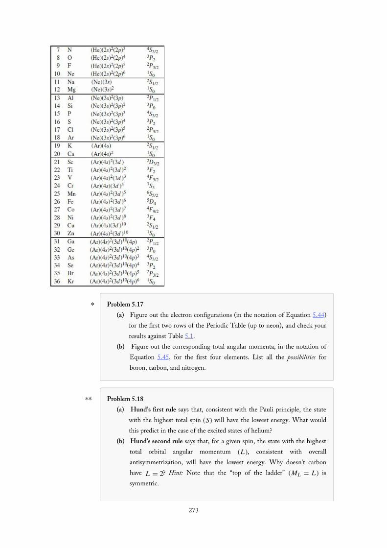
∗
∗∗
Problem 5.17(a) Figure out the electron configurations (in the notation of Equation 5.44)
for the first two rows of the Periodic Table (up to neon), and check yourresults against Table 5.1.
(b) Figure out the corresponding total angular momenta, in the notation ofEquation 5.45, for the first four elements. List all the possibilities forboron, carbon, and nitrogen.
Problem 5.18(a) Hund’s first rule says that, consistent with the Pauli principle, the state
with the highest total spin will have the lowest energy. What wouldthis predict in the case of the excited states of helium?
(b) Hund’s second rule says that, for a given spin, the state with the highesttotal orbital angular momentum , consistent with overallantisymmetrization, will have the lowest energy. Why doesn’t carbonhave ? Hint: Note that the “top of the ladder” issymmetric.
(c) Hund’s third rule says that if a subshell is no more than half filled,273

(c) Hund’s third rule says that if a subshell is no more than half filled,then the lowest energy level has ; if it is more than halffilled, then has the lowest energy. Use this to resolve theboron ambiguity in Problem 5.17(b).
(d) Use Hund’s rules, together with the fact that a symmetric spin state mustgo with an antisymmetric position state (and vice versa) to resolve thecarbon and nitrogen ambiguities in Problem 5.17(b). Hint: Always go tothe “top of the ladder” to figure out the symmetry of a state.
Problem 5.19 The ground state of dysprosium (element 66, in the 6th row of thePeriodic Table) is listed as 5 I8. What are the total spin, total orbital, and grandtotal angular momentum quantum numbers? Suggest a likely electronconfiguration for dysprosium.
274

5.3 SolidsIn the solid state, a few of the loosely-bound outermost valence electrons in each atom become detached, androam around throughout the material, no longer subject only to the Coulomb field of a specific “parent”nucleus, but rather to the combined potential of the entire crystal lattice. In this section we will examine twoextremely primitive models: first, the “electron gas” theory of Sommerfeld, which ignores all forces (except theconfining boundaries), treating the wandering electrons as free particles in a box (the three-dimensionalanalog to an infinite square well); and second, Bloch’s theory, which introduces a periodic potentialrepresenting the electrical attraction of the regularly spaced, positively charged, nuclei (but still ignoreselectron–electron repulsion). These models are no more than the first halting steps toward a quantum theoryof solids, but already they reveal the critical role of the Pauli exclusion principle in accounting for “solidity,”and provide illuminating insight into the remarkable electrical properties of conductors, semi-conductors, andinsulators.
275
(5.46)
(5.48)
(5.49)
(5.50)
(5.47)
5.3.1 The Free Electron Gas
Suppose the object in question is a rectangular solid, with dimensions , , , and imagine that an electroninside experiences no forces at all, except at the impenetrable walls:
The Schrödinger equation,
separates, in Cartesian coordinates: , with
and . Letting
we obtain the general solutions
The boundary conditions require that , so , and , so
where each n is a positive integer:
The (normalized) wave functions are
and the allowed energies are
where k is the magnitude of the wave vector, .If you imagine a three-dimensional space, with axes , , , and planes drawn in at ,
, , … , at , , , … , and at , , , … ,
276

(5.51)
(5.52)
(5.53)
each intersection point represents a distinct (one-particle) stationary state (Figure 5.2). Each block in thisgrid, and hence also each state, occupies a volume
of “k-space,” where is the volume of the object itself. Suppose our sample contains N atoms, andeach atom contributes d free electrons. (In practice, N will be enormous—on the order of Avogadro’s number,for an object of macroscopic size—whereas d is a small number—1, 2, or 3, typically.) If electrons were bosons(or distinguishable particles), they would all settle down to the ground state, .21 But electrons are in factidentical fermions, subject to the Pauli exclusion principle, so only two of them can occupy any given state.They will fill up one octant of a sphere in k-space,22 whose radius, , is determined by the fact that each pairof electrons requires a volume (Equation 5.51):
Thus
where
is the free electron density (the number of free electrons per unit volume).
277
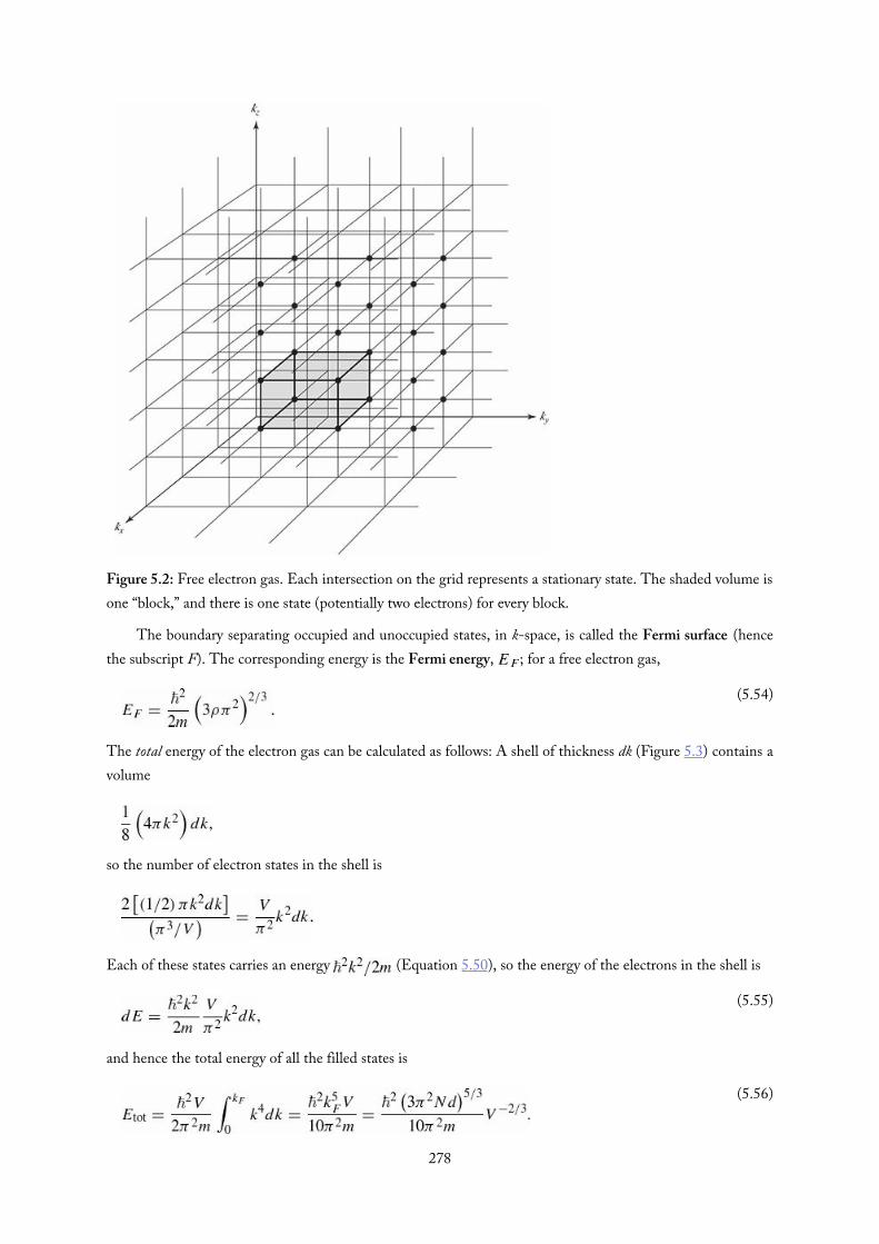
(5.54)
(5.55)
(5.56)
Figure 5.2: Free electron gas. Each intersection on the grid represents a stationary state. The shaded volume isone “block,” and there is one state (potentially two electrons) for every block.
The boundary separating occupied and unoccupied states, in k-space, is called the Fermi surface (hencethe subscript F). The corresponding energy is the Fermi energy, ; for a free electron gas,
The total energy of the electron gas can be calculated as follows: A shell of thickness dk (Figure 5.3) contains avolume
so the number of electron states in the shell is
Each of these states carries an energy (Equation 5.50), so the energy of the electrons in the shell is
and hence the total energy of all the filled states is
278

(5.57)
Figure 5.3: One octant of a spherical shell in k-space.
This quantum mechanical energy plays a role rather analogous to the internal thermal energy of anordinary gas. In particular, it exerts a pressure on the walls, for if the box expands by an amount dV, the totalenergy decreases:
and this shows up as work done on the outside by the quantum pressure P. Evidently
Here, then, is a partial answer to the question of why a cold solid object doesn’t simply collapse: There is astabilizing internal pressure, having nothing to do with electron–electron repulsion (which we have ignored)or thermal motion (which we have excluded), but is strictly quantum mechanical, and derives ultimately fromthe antisymmetrization requirement for the wave functions of identical fermions. It is sometimes calleddegeneracy pressure, though “exclusion pressure” might be a better term.23
Problem 5.20 Find the average energy per free electron , as a fractionof the Fermi energy. Answer: .
Problem 5.21 The density of copper is 8.96 g/cm3, and its atomic weight is 63.5g/mole.
(a) Calculate the Fermi energy for copper (Equation 5.54). Assume ,and give your answer in electron volts.
(b) What is the corresponding electron velocity? Hint: Set .Is it safe to assume the electrons in copper are nonrelativistic?
(c) At what temperature would the characteristic thermal energy ( ,where is the Boltzmann constant and T is the Kelvin temperature)equal the Fermi energy, for copper? Comment: This is called the Fermi
279

temperature, . As long as the actual temperature is substantially belowthe Fermi temperature, the material can be regarded as “cold,” with mostof the electrons in the lowest accessible state. Since the melting point ofcopper is 1356 K, solid copper is always cold.
(d) Calculate the degeneracy pressure (Equation 5.57) of copper, in theelectron gas model.
Problem 5.22 Helium-3 is fermion with spin (unlike the more commonisotope helium-4 which is a boson). At low temperatures , helium-3can be treated as a Fermi gas (Section 5.3.1). Given a density of 82 kg/m3,calculate (Problem 5.21(c)) for helium-3.
Problem 5.23 The bulk modulus of a substance is the ratio of a small decrease inpressure to the resulting fractional increase in volume:
Show that , in the free electron gas model, and use your result inProblem 5.21(d) to estimate the bulk modulus of copper. Comment: The observedvalue is N/m2, but don’t expect perfect agreement—after all, we’reneglecting all electron–nucleus and electron–electron forces! Actually, it is rathersurprising that this calculation comes as close as it does.
280

(5.59)
(5.60)
(5.61)
(5.58)
(5.62)
5.3.2 Band Structure
We’re now going to improve on the free electron model, by including the forces exerted on the electrons bythe regularly spaced, positively charged, essentially stationary nuclei. The qualitative behavior of solids isdictated to a remarkable degree by the mere fact that this potential is periodic—its actual shape is relevant onlyto the finer details. To show you how it goes, I’m going to develop the simplest possible model: a one-dimensional Dirac comb, consisting of evenly spaced delta-function spikes (Figure 5.4).24 But first I need tointroduce a powerful theorem that vastly simplifies the analysis of periodic potentials.
Figure 5.4: The Dirac comb, Equation 5.64.
A periodic potential is one that repeats itself after some fixed distance a:
Bloch’s theorem tells us that for such a potential the solutions to the Schrödinger equation,
can be taken to satisfy the condition
for some constant q (by “constant” I mean that it is independent of x; it may well depend on E).25 In amoment we will discover that q is in fact real, so although itself is not periodic, is:
as one would certainly expect.26
Of course, no real solid goes on forever, and the edges are going to spoil the periodicity of , andrender Bloch’s theorem inapplicable. However, for any macroscopic crystal, containing something on theorder of Avogadro’s number of atoms, it is hardly imaginable that edge effects can significantly influence thebehavior of electrons deep inside. This suggests the following device to salvage Bloch’s theorem: We wrap thex axis around in a circle, and connect it onto its tail, after a large number of periods; formally, weimpose the boundary condition
It follows (from Equation 5.60) that
so , or , and hence
281
(5.63)
(5.64)
(5.65)
(5.67)
(5.68)
(5.69)
(5.70)
(5.66)
In particular, q is necessarily real. The virtue of Bloch’s theorem is that we need only solve the Schrödingerequation within a single cell (say, on the interval ); recursive application of Equation 5.60 generatesthe solution everywhere else.
Now, suppose the potential consists of a long string of delta-function spikes (the Dirac comb):
(In Figure 5.4 you must imagine that the x axis has been “wrapped around”, so the Nth spike actually appearsat .) No one would pretend that this is a realistic model, but remember, it is only the effect ofperiodicity that concerns us here; the classic Kronig–Penney model27 used a repeating rectangular pattern, andmany authors still prefer that one.28 In the region the potential is zero, so
or
where
as usual.The general solution is
According to Bloch’s theorem, the wave function in the cell immediately to the left of the origin is
At , must be continuous, so
its derivative suffers a discontinuity proportional to the strength of the delta function (Equation 2.128, withthe sign of α switched, since these are spikes instead of wells):
Solving Equation 5.68 for yields
282
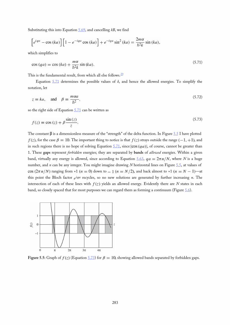
(5.71)
(5.72)
(5.73)
Substituting this into Equation 5.69, and cancelling kB, we find
which simplifies to
This is the fundamental result, from which all else follows.29
Equation 5.71 determines the possible values of k, and hence the allowed energies. To simplify thenotation, let
so the right side of Equation 5.71 can be written as
The constant β is a dimensionless measure of the “strength” of the delta function. In Figure 5.5 I have plotted , for the case . The important thing to notice is that strays outside the range , and
in such regions there is no hope of solving Equation 5.71, since , of course, cannot be greater than1. These gaps represent forbidden energies; they are separated by bands of allowed energies. Within a givenband, virtually any energy is allowed, since according to Equation 5.63, , where N is a hugenumber, and n can be any integer. You might imagine drawing N horizontal lines on Figure 5.5, at values of
ranging from +1 down to , and back almost to +1 —atthis point the Bloch factor recycles, so no new solutions are generated by further increasing n. Theintersection of each of these lines with yields an allowed energy. Evidently there are N states in eachband, so closely spaced that for most purposes we can regard them as forming a continuum (Figure 5.6).
Figure 5.5: Graph of (Equation 5.73) for , showing allowed bands separated by forbidden gaps.
283

Figure 5.6: The allowed energies for a periodic potential form essentially continuous bands.
So far, we’ve only put one electron in our potential. In practice there will be Nd of them, where d is againthe number of “free” electrons per atom. Because of the Pauli exclusion principle, only two electrons canoccupy a given spatial state, so if , they will half fill the first band, if they will completely fill thefirst band, if they half fill the second band, and so on. (In three dimensions, and with more realisticpotentials, the band structure may be more complicated, but the existence of allowed bands, separated byforbidden gaps, persists—band structure is the signature of a periodic potential.30 )
Now, if the topmost band is only partly filled, it takes very little energy to excite an electron to the nextallowed level, and such a material will be a conductor (a metal). On the other hand, if the top band iscompletely filled, it takes a relatively large energy to excite an electron, since it has to jump across the forbiddenzone. Such materials are typically insulators, though if the gap is rather narrow, and the temperaturesufficiently high, then random thermal energy can knock an electron over the hump, and the material is asemiconductor (silicon and germanium are examples).31 In the free electron model all solids should be metals,since there are no large gaps in the spectrum of allowed energies. It takes the band theory to account for theextraordinary range of electrical conductivities exhibited by the solids in nature.
Problem 5.24(a) Using Equations 5.66 and 5.70, show that the wave function for a particle
in the periodic delta function potential can be written in the form
(Don’t bother to determine the normalization constant C.)
(b) At the top of a band, where , (a) yields 284

∗∗
(b) At the top of a band, where , (a) yields (indeterminate). Find the correct wave function for this case. Note whathappens to at each delta function.
Problem 5.25 Find the energy at the bottom of the first allowed band, for the case, correct to three significant digits. For the sake of argument, assume
eV.
Problem 5.26 Suppose we use delta function wells, instead of spikes (i.e. switch thesign of α in Equation 5.64). Analyze this case, constructing the analog to Figure5.5. This requires no new calculation, for the positive energy solutions (except thatβ is now negative; use for the graph), but you do need to work out thenegative energy solutions (let and , for ); yourgraph will now extend to negative z). How many states are there in the firstallowed band?
Problem 5.27 Show that most of the energies determined by Equation 5.71 aredoubly degenerate. What are the exceptional cases? Hint: Try it for
, to see how it goes. What are the possible values of in each case?
Problem 5.28 Make a plot of E vs. q for the band structure in Section 5.3.2. Use (in units where ). Hint: In Mathematica, ContourPlot
will graph as defined implicitly by Equation 5.71. On other platforms theplot can be obtained as follows:
You will then have a list of pairs which you canplot.
Choose a large number (say 30,000) of equally-spaced values for the energy inthe range and .
For each value of E, compute the right-hand side of Equation 5.71. If theresult is between and 1, solve for q from Equation 5.71 and record the pairof values and (there are two solutions for each energy).
285

(5.74)
Further Problems on Chapter 5
Problem 5.29 Suppose you have three particles, and three distinct one-particlestates , , and ) are available. How many different three-particle states can be constructed (a) if they are distinguishable particles, (b) ifthey are identical bosons, (c) if they are identical fermions? (The particles neednot be in different states— would be one possibility, ifthe particles are distinguishable.)
Problem 5.30 Calculate the Fermi energy for electrons in a two-dimensionalinfinite square well. Let σ be the number of free electrons per unit area.
Problem 5.31 Repeat the analysis of Problem 2.58 to estimate the cohesive energyfor a three-dimensional metal, including the effects of spin.
Problem 5.32 Consider a free electron gas (Section 5.3.1) with unequal numbersof spin-up and spin-down particles and respectively). Such a gaswould have a net magnetization (magnetic dipole moment per unit volume)
where is the Bohr magneton. (The minus sign is there, ofcourse, because the charge of the electron is negative.)(a) Assuming that the electrons occupy the lowest energy levels consistent
with the number of particles in each spin orientation, find . Checkthat your answer reduces to Equation 5.56 when .
(b) Show that for (which is to say, ), the energy density is
The energy is a minimum for , so the ground state will have zeromagnetization. However, if the gas is placed in a magnetic field (or in thepresence of interactions between the particles) it may be energeticallyfavorable for the gas to magnetize. This is explored in Problems 5.33 and5.34.
Problem 5.33 Pauli paramagnetism. If the free electron gas (Section 5.3.1) isplaced in a uniform magnetic field , the energies of the spin-up andspin-down states will be different:32
286

∗∗∗
There will be more spin-down states occupied than spin-up states (since theyare lower in energy), and consequently the system will acquire a magnetization(see Problem 5.32).(a) In the approximation that , find the magnetization that
minimizes the total energy. Hint: Use the result of Problem 5.32(b).(b) The magnetic susceptibility is33
Calculate the magnetic susceptibility for aluminum and compare the experimental value34 of
.
Problem 5.34 The Stoner criterion. The free-electron gas model (Section 5.3.1)ignores the Coulomb repulsion between electrons. Because of the exchangeforce (Section 5.1.2), Coulomb repulsion has a stronger effect on two electronswith antiparallel spins (which behave in a way like distinguishable particles)than two electrons with parallel spins (whose position wave function must beantisymmetric). As a crude way to take account of Coulomb repulsion, pretendthat every pair of electrons with opposite spin carries extra energy U, whileelectrons with the same spin do not interact at all; this adds to the total energy of the electron gas. As you will show, above a critical valueof U, it becomes energetically favorable for the gas to spontaneously magnetize
; the material becomes ferromagnetic.(a) Rewrite in terms of the density ρ and the magnetization M
(Equation 5.74).(b) Assuming that , for what minimum value of U is a non-zero
magnetization energetically favored? Hint: Use the result ofProblem 5.32(b).
Problem 5.35 Certain cold stars (called white dwarfs) are stabilized againstgravitational collapse by the degeneracy pressure of their electrons (Equation5.57). Assuming constant density, the radius R of such an object can becalculated as follows:(a) Write the total electron energy (Equation 5.56) in terms of the radius, the
number of nucleons (protons and neutrons) N, the number of electronsper nucleon d, and the mass of the electron m. Beware: In this problem weare recycling the letters N and d for a slightly different purpose than in thetext.
(b) Look up, or calculate, the gravitational energy of a uniformly densesphere. Express your answer in terms of G (the constant of universal
287
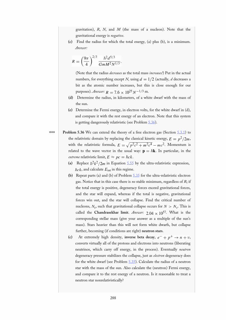
∗∗∗
gravitation), R, N, and M (the mass of a nucleon). Note that thegravitational energy is negative.
(c) Find the radius for which the total energy, (a) plus (b), is a minimum.Answer:
(Note that the radius decreases as the total mass increases!) Put in the actualnumbers, for everything except N, using (actually, d decreases abit as the atomic number increases, but this is close enough for ourpurposes). Answer: m.
(d) Determine the radius, in kilometers, of a white dwarf with the mass ofthe sun.
(e) Determine the Fermi energy, in electron volts, for the white dwarf in (d),and compare it with the rest energy of an electron. Note that this systemis getting dangerously relativistic (see Problem 5.36).
Problem 5.36 We can extend the theory of a free electron gas (Section 5.3.1) tothe relativistic domain by replacing the classical kinetic energy, ,with the relativistic formula, . Momentum isrelated to the wave vector in the usual way: . In particular, in theextreme relativistic limit, .(a) Replace in Equation 5.55 by the ultra-relativistic expression,
, and calculate in this regime.(b) Repeat parts (a) and (b) of Problem 5.35 for the ultra-relativistic electron
gas. Notice that in this case there is no stable minimum, regardless of R; ifthe total energy is positive, degeneracy forces exceed gravitational forces,and the star will expand, whereas if the total is negative, gravitationalforces win out, and the star will collapse. Find the critical number ofnucleons, , such that gravitational collapse occurs for . This iscalled the Chandrasekhar limit. Answer: . What is thecorresponding stellar mass (give your answer as a multiple of the sun’smass). Stars heavier than this will not form white dwarfs, but collapsefurther, becoming (if conditions are right) neutron stars.
(c) At extremely high density, inverse beta decay, ,converts virtually all of the protons and electrons into neutrons (liberatingneutrinos, which carry off energy, in the process). Eventually neutrondegeneracy pressure stabilizes the collapse, just as electron degeneracy doesfor the white dwarf (see Problem 5.35). Calculate the radius of a neutronstar with the mass of the sun. Also calculate the (neutron) Fermi energy,and compare it to the rest energy of a neutron. Is it reasonable to treat aneutron star nonrelativistically?
288

∗∗∗
(5.75)
Problem 5.37 An important quantity in many calculations is the density of states :
For a one-dimensional band structure,
where counts the number of states in the range dq (seeEquation 5.63), and the factor of 2 accounts for the fact that states with q and
have the same energy. Therefore
(a) Show that for (a free particle) the density of states is given by
(b) Find the density of states for by differentiating Equation 5.71 withrespect to q to determine . Note: Your answer should be written asa function of E only (well, and α, m, , a, and N) and must not contain q(use k as a shorthand for , if you like).
(c) Make a single plot showing for both and (inunits where ). Comment: The divergences at the bandedges are examples of van Hove singularities.35
Problem 5.38 The harmonic chain consists of N equal masses arranged along aline and connected to their neighbors by identical springs:
where is the displacement of the jth mass from its equilibrium position.This system (and its extension to two or three dimensions—the harmoniccrystal) can be used to model the vibrations of a solid. For simplicity we willuse periodic boundary conditions: , and introduce the ladderoperators36
where and the frequencies are given by
289
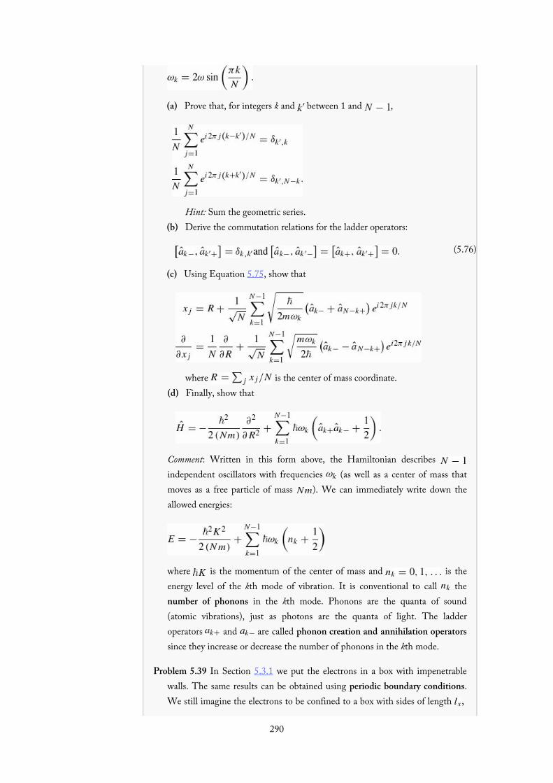
(5.76)
(a) Prove that, for integers k and between 1 and ,
Hint: Sum the geometric series.(b) Derive the commutation relations for the ladder operators:
(c) Using Equation 5.75, show that
where is the center of mass coordinate.(d) Finally, show that
Comment: Written in this form above, the Hamiltonian describes independent oscillators with frequencies (as well as a center of mass thatmoves as a free particle of mass ). We can immediately write down theallowed energies:
where is the momentum of the center of mass and is theenergy level of the kth mode of vibration. It is conventional to call thenumber of phonons in the kth mode. Phonons are the quanta of sound(atomic vibrations), just as photons are the quanta of light. The ladderoperators and are called phonon creation and annihilation operatorssince they increase or decrease the number of phonons in the kth mode.
Problem 5.39 In Section 5.3.1 we put the electrons in a box with impenetrablewalls. The same results can be obtained using periodic boundary conditions.We still imagine the electrons to be confined to a box with sides of length ,
290
, and but instead of requiring the wave function to vanish on each wall, werequire it to take the same value on opposite walls:
In this case we can represent the wave functions as traveling waves,
rather than as standing waves (Equation 5.49). Periodic boundary conditions—while certainly not physical—are often easier to work with (to describesomething like electrical current a basis of traveling waves is more natural thana basis of standing waves) and if you are computing bulk properties of amaterial it shouldn’t matter which you use.(a) Show that with periodic boundary conditions the wave vector satisfies
where each n is an integer (not necessarily positive). What is the k-spacevolume occupied by each block on the grid (corresponding to Equation5.51)?
(b) Compute , , and for the free electron gas with periodicboundary conditions. What compensates for the larger volume occupiedby each k-space block (part (a)) to make these all come out the same as inSection 5.3.1?
1 The classic example of an entangled state is two spin-1/2 particles in the singlet configuration (Equation 4.176).2 See, for example, Jerry B. Marion and Stephen T. Thornton, Classical Dynamics of Particles and Systems, 4th edn, Saunders, Fort Worth, TX
(1995), Section 8.2.3 It seems strange that relativity should have anything to do with it, and there has been a lot of discussion as to whether it might be possible to
prove the spin-statistics connection in other ways. See, for example, Robert C. Hilborn, Am. J. Phys. 63, 298 (1995); Ian Duck andE. C. G. Sudarshan, Pauli and the Spin-Statistics Theorem, World Scientific, Singapore (1997). For a comprehensive bibliography on spinand statistics see C. Curceanu, J. D. Gillaspy, and R. C. Hilborn, Am. J. Phys. 80, 561 (2010).
4 I’m still leaving out the spin, don’t forget—if this bothers you (after all, a spinless fermion is an oxymoron), assume they’re in the same spinstate. I’ll show you how spin affects the story in Section 5.1.3
5 For an incisive critique of this terminology see W. J. Mullin and G. Blaylock, Am. J. Phys. 71, 1223 (2003).6 To construct a completely symmetric configuration, use the permanent (same as determinant, but without the minus signs).7 In the absence of coupling between spin and position, we are free to assume that the state is separable in its spin and spatial coordinates. This
just says that the probability of getting spin up is independent of the location of the particle. In the presence of coupling, the general statewould take the form of a linear combination: as in Problem 4.64.
8 I’ll let stand for the combined spin state; in Dirac notation it is some linear combination of the states . I assume thatthe state is again a simple product of a position state and a spin state; as you’ll see in Problem 5.10, this is not always true when three ormore electrons are involved—even in the absence of coupling.
9 Of course, spin requires three dimensions, whereas we ordinarily think of the infinite square well as existing in one dimension. But it couldrepresent a particle in three dimensions that is confined to a one-dimensional wire.
10 This problem was suggested by Greg Elliott.11 switches the particles ; this means exchanging their positions, their spins, and any other properties they might possess. If you
like, it switches the labels, 1 and 2. I claimed (in Chapter 1) that all our operators would involve multiplication or differentiation; that was alie. The exchange operator is an exception—and for that matter so is the projection operator (Section 3.6.2).
12 It is sometimes alleged that the symmetrization requirement (Equation 5.33) is forced by the fact that and commute. This is false: It is291

12 It is sometimes alleged that the symmetrization requirement (Equation 5.33) is forced by the fact that and commute. This is false: It isperfectly possible to imagine a system of two distinguishable particles (say, an electron and a positron) for which the Hamiltonian issymmetric, and yet there is no requirement that the state be symmetric (or antisymmetric). But identical particles have to occupy symmetricor antisymmetric states, and this is a new fundamental law—on a par, logically, with Schrödinger’s equation and the statistical interpretation.Of course, there didn’t have to be any such things as identical particles; it could have been that every single particle in the universe wasdistinguishable from every other one. Quantum mechanics allows for the possibility of identical particles, and nature (being lazy) seized theopportunity. (But don’t complain—this makes matters enormously simpler!)
13 “Robert B. Laughlin—Nobel Lecture: Fractional Quantization.” Nobelprize.org. Nobel Media AB 2014. http://www.nobelprize.org/nobel_prizes/physics/laureates/1998/laughlin-lecture.html .
14 I’m assuming the nucleus is stationary. The trick of accounting for nuclear motion by using the reduced mass (Problem 5.1) works only forthe two-body problem; fortunately, the nucleus is so much heavier than the electrons that the correction is extremely small even in the caseof hydrogen (see Problem 5.2(a)), and it is smaller still for other atoms. There are more interesting effects, due to magnetic interactionsassociated with electron spin, relativistic corrections, and the finite size of the nucleus. We’ll look into these in later chapters, but all of themare minute corrections to the “purely coulombic” atom described by Equation 5.36.
15 Because the Hamiltonian (5.36) makes no reference to spin, the product still satisfies theSchrödinger equation. However, for such product states cannot in general meet the (anti-)symmetrization requirement, and it isnecessary to construct linear combinations, with permuted indices (see Problem 5.16). But that comes at the end of the story; for themoment we are only concerned with the spatial wave function.
16 Actually, would do just as well, but electron–electron repulsion favors , as we shall see.17 This standard argument has been called into question by W. Stacey and F. Marsiglio, EPL, 100, 43002 (2012).18 See, for example, Ugo Fano and L. Fano, Basic Physics of Atoms and Molecules, Wiley, New York (1959), Chapter 18, or the classic by
Gerhard Herzberg, Atomic Spectra and Atomic Structure, Dover, New York (1944).19 The shells themselves are assigned equally arbitrary nicknames, starting (don’t ask me why) with K: The K shell is , the L shell is
, M is , and so on (at least they’re in alphabetical order).20 After krypton—element 36—the situation gets more complicated (fine structure starts to play a significant role in the ordering of the states)
so it is not for want of space that the table terminates there.21 I’m assuming there is no appreciable thermal excitation, or other disturbance, to lift the solid out of its collective ground state. If you like,
I’m talking about a “cold” solid, though (as you will see in Problem 5.21(c)), typical solids are still “cold,” in this sense, far above roomtemperature.
22 Because N is such a huge number, we need not worry about the distinction between the actual jagged edge of the grid and the smoothspherical surface that approximates it.
23 We derived Equations 5.52, 5.54, 5.56, and 5.57 for the special case of an infinite rectangular well, but they hold for containers of any shape,as long as the number of particles is extremely large.
24 It would be more natural to let the delta functions go down, so as to represent the attractive force of the nuclei. But then there would benegative energy solutions as well as positive energy solutions, and that makes the calculations more cumbersome (see Problem 5.26). Since allwe’re trying to do here is explore the consequences of periodicity, it is simpler to adopt this less plausible shape; if it comforts you, think ofthe nuclei as residing at , , , ….
25 The proof of Bloch’s theorem will come in Chapter 6 (see Section 6.2.2).26 Indeed, you might be tempted to reverse the argument, starting with Equation 5.61, as a way of proving Bloch’s theorem. It doesn’t work,
for Equation 5.61 alone would allow the phase factor in Equation 5.60 to be a function of x.27 R. de L. Kronig and W. G. Penney, Proc. R. Soc. Lond., ser. A, 130, 499 (1930).28 See, for instance, David Park, Introduction to the Quantum Theory, 3nd edn, McGraw-Hill, New York (1992).29 For the Kronig–Penney potential (footnote 27, page 221), the formula is more complicated, but it shares the qualitative features we are
about to explore.30 Regardless of dimension, if d is an odd integer you are guaranteed to have partially-filled bands and you would expect metallic behavior. If d
is an even integer, it depends on the specific band structure whether there will be partially-filled bands or not. Interestingly, some materials,called Mott insulators, are nonconductors even though d is odd. In that case it is the interactions between electrons that leads to theinsulating behavior, not the presence of gaps in the single-particle energy spectrum.
31 Semiconductors typically have band gaps of 4 eV or less, small enough that thermal excitation at room temperature ( eV)produces perceptible conductivity. The conductivity of a semiconductor can be controlled by doping: including a few atoms of larger orsmaller d; this puts some “extra” electrons into the next higher band, or creates some holes in the previously filled one, allowing in either casefor weak electric currents to flow.
32 Here we are considering only the coupling of the spin to the magnetic field, and ignoring any coupling of the orbital motion.33 Strictly speaking, the susceptibility is , but the difference is negligible when, as here, .34 For some metals, such as copper, the agreement is not so good—even the sign is wrong: copper is diamagnetic . The explanation
for this discrepancy lies in what has been left out of our model. In addition to the paramagnetic coupling of the spin magnetic moment to anapplied field there is a coupling of the orbital magnetic moment to an applied field and this has both paramagnetic and diamagnetic
292

contributions (see Problem 4.72). In addition, the free electron gas model ignores the tightly-bound core electrons and these also couple tothe magnetic field. In the case of copper, it is the diamagnetic coupling of the core electrons that dominates.
35 These one-dimensional Van Hove singularities have been observed in the spectroscopy of carbon nanotubes; see J. W. G. Wildöer et al.,Nature, 391, 59 (1998).
36 If you are familiar with the classical problem of coupled oscillators, these ladder operators are straightforward to construct. Start with thenormal mode coordinates you would use to decouple the classical problem, namely
The frequencies are the classical normal mode frequencies, and you simply create a pair of ladder operators for each normal mode, byanalogy with the single-particle case (Equation 2.48).
293

6Symmetries & Conservation Laws
◈
294
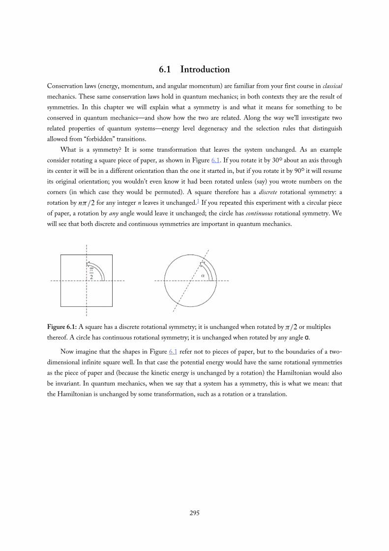
6.1 IntroductionConservation laws (energy, momentum, and angular momentum) are familiar from your first course in classicalmechanics. These same conservation laws hold in quantum mechanics; in both contexts they are the result ofsymmetries. In this chapter we will explain what a symmetry is and what it means for something to beconserved in quantum mechanics—and show how the two are related. Along the way we’ll investigate tworelated properties of quantum systems—energy level degeneracy and the selection rules that distinguishallowed from “forbidden” transitions.
What is a symmetry? It is some transformation that leaves the system unchanged. As an exampleconsider rotating a square piece of paper, as shown in Figure 6.1. If you rotate it by 30 about an axis throughits center it will be in a different orientation than the one it started in, but if you rotate it by 90 it will resumeits original orientation; you wouldn’t even know it had been rotated unless (say) you wrote numbers on thecorners (in which case they would be permuted). A square therefore has a discrete rotational symmetry: arotation by for any integer n leaves it unchanged.1 If you repeated this experiment with a circular pieceof paper, a rotation by any angle would leave it unchanged; the circle has continuous rotational symmetry. Wewill see that both discrete and continuous symmetries are important in quantum mechanics.
Figure 6.1: A square has a discrete rotational symmetry; it is unchanged when rotated by or multiplesthereof. A circle has continuous rotational symmetry; it is unchanged when rotated by any angle α.
Now imagine that the shapes in Figure 6.1 refer not to pieces of paper, but to the boundaries of a two-dimensional infinite square well. In that case the potential energy would have the same rotational symmetriesas the piece of paper and (because the kinetic energy is unchanged by a rotation) the Hamiltonian would alsobe invariant. In quantum mechanics, when we say that a system has a symmetry, this is what we mean: thatthe Hamiltonian is unchanged by some transformation, such as a rotation or a translation.
295

(6.1)
6.1.1 Transformations in Space
In this section, we introduce the quantum mechanical operators that implement translations, inversions, androtations. We define each of these operators by how it acts on an arbitrary function. The translation operatortakes a function and shifts it a distance a. The operator that accomplishes this is defined by the relation
The sign can be confusing at first; this equation says that the translated function at x is equal to theuntranslated function at (Figure 6.2)—the function itself has been shifted to the right by an amounta.
Figure 6.2: A wave function and the translated wave function . Note that thevalue of at x is equal to the value of at .
The operator that reflects a function about the origin, the parity operator in one dimension, is defined by
The effect of parity is shown graphically in Figure 6.3. In three dimensions parity changes the sign of all threecoordinates: .2
296

(6.2)
∗
Figure 6.3: A function and the function after a spatial inversion. Thevalue of at x is equal to the value of at .
Finally, the operator that rotates a function about the z axis through an angle is most naturallyexpressed in polar coordinates as
When we take up the study of rotations in Section 6.5, we will introduce expressions for rotations aboutarbitrary axes. The action of the rotation operator on a function is illustrated in Figure 6.4.
Figure 6.4: A function and the rotated function after a counter-clockwiserotation about the vertical axis by an angle .
Problem 6.1 Consider the parity operator in three dimensions.(a) Show that is equivalent to a mirror
reflection followed by a rotation.(b) Show that, for expressed in polar coordinates, the action of the parity
operator is
(c) Show that for the hydrogenic orbitals,
That is, is an eigenstate of the parity operator, with eigenvalue . Note: This result actually applies to the stationary states of any
central potential . For a central potential, the eigenstatesmay be written in the separable form where only theradial function —which plays no role in determining the parity of thestate—depends on the specific functional form of .
297

(6.3)
(6.4)
∗
6.2 The Translation OperatorEquation 6.1 defines the translation operator. We can express in terms of the momentum operator, towhich it is intimately related. To that end, we replace by its Taylor series3
The right-hand side of this equation is the exponential function,4 so
We say that momentum is the “generator” of translations.5
Note that is a unitary operator:6
The first equality is obvious physically (the inverse operation of shifting something to the right is shifting it byan equal amount to the left), and the second equality then follows from taking the adjoint of Equation 6.3 (seeProblem 6.2).
Problem 6.2 Show that, for a Hermitian operator , the operator is unitary. Hint: First you need to prove that the adjoint is given by
; then prove that . Problem 3.5 may help.
298

(6.5)
(6.6)
(6.7)
6.2.1 How Operators Transform
So far I have shown how to translate a function; this has an obvious graphical interpretation via Figure 6.2. Wecan also consider what it means to translate an operator. The transformed operator is defined to be theoperator that gives the same expectation value in the untranslated state as does the operator in thetranslated state :
There are two ways to calculate the effect of a translation on an expectation value. One could actually shift thewave function over some distance (this is called an active transformation) or one could leave the wave functionwhere it was and shift the origin of our coordinate system by the same amount in the opposite direction (apassive transformation). The operator is the operator in this shifted coordinate system.
Using Equation 6.1,
Here I am using the fact that the adjoint of an operator is defined such that, if , then (see Problem 3.5). Because Equation 6.5 is to hold for all , it follows that
The transformed operator for the case is worked out in Example 6.1. Figure 6.5 illustrates theequivalence of the two ways of carrying out the transformation.
Example 6.1Find the operator obtained by applying a translation through a distance a to the operator . That is,what is the action of , as defined by Equation 6.6, on an arbitrary ?Solution: Using the definition of (Equation 6.6) and a test function we have
and since (Equation 6.4),
From Equation 6.1
and from Equation 6.1 again, , so
Finally we may read off the operator
299
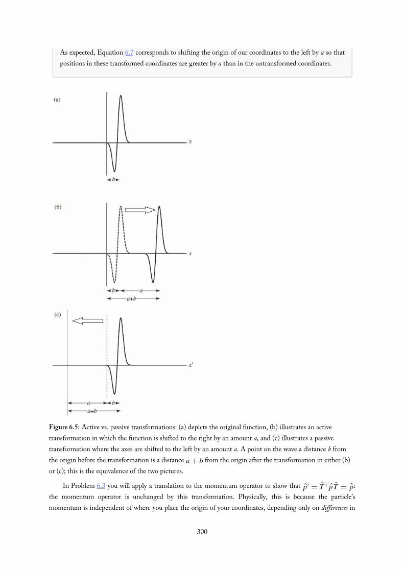
As expected, Equation 6.7 corresponds to shifting the origin of our coordinates to the left by a so thatpositions in these transformed coordinates are greater by a than in the untransformed coordinates.
Figure 6.5: Active vs. passive transformations: (a) depicts the original function, (b) illustrates an activetransformation in which the function is shifted to the right by an amount a, and (c) illustrates a passivetransformation where the axes are shifted to the left by an amount a. A point on the wave a distance b fromthe origin before the transformation is a distance from the origin after the transformation in either (b)or (c); this is the equivalence of the two pictures.
In Problem 6.3 you will apply a translation to the momentum operator to show that :the momentum operator is unchanged by this transformation. Physically, this is because the particle’smomentum is independent of where you place the origin of your coordinates, depending only on differences in
300
(6.8)
position: . Once you know how the position and momentum operators behave under atranslation, you know how any operator does, since
Problem 6.4 will walk you through the proof.
Problem 6.3 Show that the operator obtained by applying a translation to theoperator is .
Problem 6.4 Prove Equation 6.8. You may assume that can be written ina power series
for some constants .
301

(6.9)
(6.10)
6.2.2 Translational Symmetry
So far we have seen how a function behaves under a translation and how an operator behaves under atranslation. I am now in a position to make precise the notion of a symmetry that I mentioned in theintroduction. A system is translationally invariant (equivalent to saying it has translational symmetry) if theHamiltonian is unchanged by the transformation:
Because is unitary (Equation 6.4) we can multiply both sides of this equation by to get
Therefore, a system has translational symmetry if the Hamiltonian commutes with the translation operator:
For a particle of mass m moving in a one-dimensional potential, the Hamiltonian is
According to Equation 6.8, the transformed Hamiltonian is
so translational symmetry implies that
Now, there are two very different physical settings where Equation 6.10 might arise. The first is a constantpotential, where Equation 6.10 holds for every value of a; such a system is said to have continuoustranslational symmetry. The second is a periodic potential, such as an electron might encounter in a crystal,where Equation 6.10 holds only for a discrete set of as; such a system is said to have discrete translationalsymmetry. The two cases are illustrated in Figure 6.6.
302
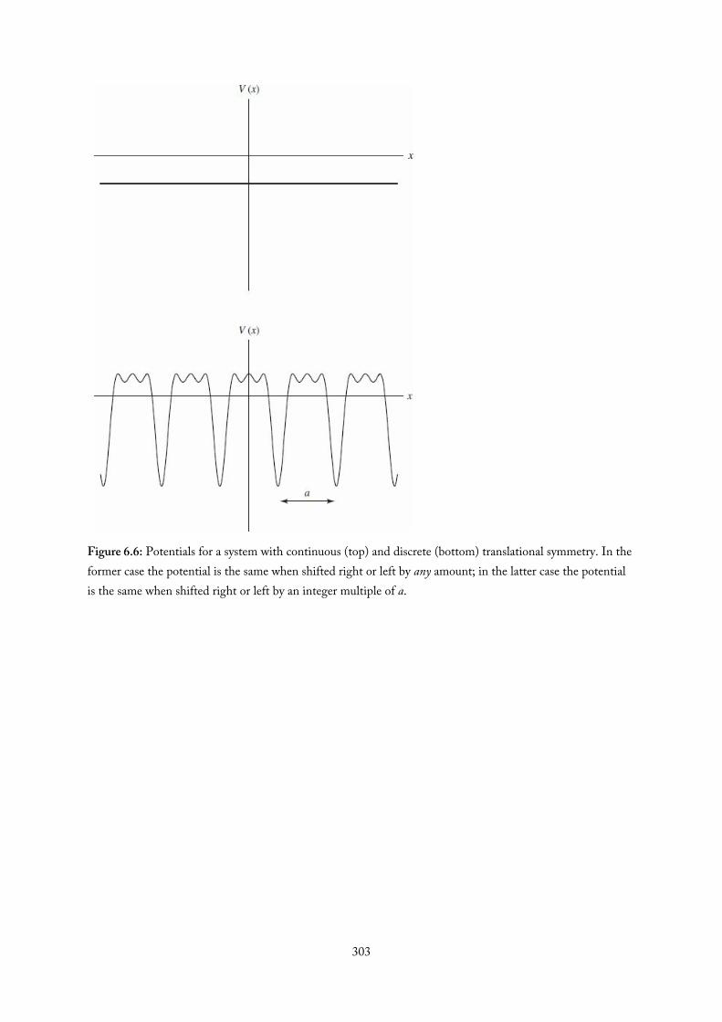
Figure 6.6: Potentials for a system with continuous (top) and discrete (bottom) translational symmetry. In theformer case the potential is the same when shifted right or left by any amount; in the latter case the potentialis the same when shifted right or left by an integer multiple of a.
303

(6.11)
(6.12)
Discrete Translational Symmetry and Bloch’s Theorem
What are the implications of translational symmetry? For a system with a discrete translational symmetry, themost important consequence is Bloch’s theorem; the theorem specifies the form taken by the stationary states.We used this theorem in Section 5.3.2; I will now prove it.
In Section A.5 it is shown that if two operators commute, then they have a complete set of simultaneouseigenstates. This means that if the Hamiltonian is translationally invariant (which is to say, if it commuteswith the translation operator), then the eigenstates of the Hamiltonian can be chosen to besimultaneously eigenstates of :
where is the eigenvalue associated with . Since is unitary, its eigenvalues have magnitude 1 (seeProblem A.30), which means that can be written as for some real number ϕ. By convention wewrite where is called the crystal momentum. Therefore, the stationary states of a particle ofmass m moving in a periodic potential have the property
There is a more illuminating way to write Equation 6.11:7
where is a periodic function of x: and is a traveling wave (recall that a travelingwave by itself describes a free particle—Section 2.4) with wavelength . Equation 6.12 is Bloch’s theoremand it says that the stationary states of a particle in a periodic potential are periodic functions multiplyingtraveling waves. Note that just because the Hamiltonian is translationally invariant, that doesn’t mean thestationary states themselves are translationally invariant, it simply means that they can be chosen to beeigenstates of the translation operator.
Bloch’s theorem is truly remarkable. It tells us that the stationary states of a particle in a periodicpotential (such as an electron in a crystal) are, apart from a periodic modulation, traveling waves. As such, theyhave a nonzero velocity.8 This means that an electron could travel through a perfect crystal without scattering!That has dramatic implications for electronic conduction in solids.
304

(6.13)
∗∗∗
Continuous Translational Symmetry and Momentum Conservation
If a system has continuous translation symmetry then the Hamiltonian commutes with for any choice ofa. In this case it is useful to consider an infinitesimal translation
where δ is an infinitesimal length.9
If the Hamiltonian has continuous translational symmetry, then it must be unchanged under anytranslation, including an infinitesimal one; equivalently it commutes with the translation operator, and hence
So if the Hamiltonian has continuous translational symmetry, it must commute with the momentumoperator. And if the Hamiltonian commutes with momentum, then according to the “generalized Ehrenfest’stheorem” (Equation 3.73)
This is a statement of momentum conservation and we have now shown that continuous translationalsymmetry implies that momentum is conserved. This is our first example of a powerful general principle:symmetries imply conservation laws.10
Of course, if we’re talking about a single particle of mass m moving in a potential , the onlypotential that has continuous translational symmetry is the constant potential, which is equivalent to the freeparticle. And it is pretty obvious that momentum is conserved in that case. But the analysis here readilyextends to a system of interacting particles (see Problem 6.7). The fact that momentum is conserved in thatcase as well (so long as the Hamiltonian is translationally invariant) is a highly nontrivial result. In any event,the point to remember is that conservation of momentum is a consequence of translational symmetry.
Problem 6.5 Show that Equation 6.12 follows from Equation 6.11. Hint: Firstwrite , which is certainly true for some , and then showthat is necessarily a periodic function of x.
Problem 6.6 Consider a particle of mass m moving in a potential withperiod a. We know from Bloch’s theorem that the wave function can be written inthe form of Equation 6.12. Note: It is conventional to label the states withquantum numbers n and q as where is the nthenergy for a given value of q.
(a) Show that u satisfies the equation
305

(6.14)(b) Use the technique from Problem 2.61 to solve the differentialequation for . You need to use a two-sided difference for the firstderivative so that you have a Hermitian matrix to diagonalize:
. For the potential in the interval 0 to a let
with . (You will need to modify the technique slightlyto account for the fact that the function is periodic.) Find the lowesttwo energies for the following values of the crystal momentum: = ,
, 0, , π. Note that q and describe the same wavefunction (Equation 6.12), so there is no reason to consider values of outside of the interval from to π. In solid state physics, the values ofq inside this range constitute the first Brillouin zone.
(c) Make a plot of the energies and for values of q between and . If you’ve automated the code that you used in part (b), youshould be able to show a large number of q values in this range. If not,simply plot the values that you computed in (b).
Problem 6.7 Consider two particles of mass and (in one dimension) thatinteract via a potential that depends only on the distance between the particles
, so that the Hamiltonian is
Acting on a two-particle wave function the translation operator would be
(a) Show that the translation operator can be written
where is the total momentum.(b) Show that the total momentum is conserved for this system.
306

(6.15)
6.3 Conservation LawsIn classical mechanics the meaning of a conservation law is straightforward: the quantity in question is thesame before and after some event. Drop a rock, and potential energy is converted into kinetic energy, but thetotal is the same just before it hits the ground as when it was released; collide two billiard balls andmomentum is transferred from one to the other, but the total remains unchanged. But in quantum mechanicsa system does not in general have a definite energy (or momentum) before the process begins (or afterward).What does it mean, in that case, to say that the observable Q is (or is not) conserved? Here are twopossibilities:
Under what conditions does each of these conservation laws hold?Let us stipulate that the observable in question does not depend explicitly on time: . In that
case the generalized Ehrenfest theorem (Equation 3.73) tells us that the expectation value of Q is independentof time if The operator commutes with the Hamiltonian. It so happens that the same criterion guaranateesconservation by the second definition.
I will now prove this result. Recall that the probability of getting the result in a measurement of Q attime t is (Equation 3.43)
where is the corresponding eigenvector: .11 We know that the time evolution of the wavefunction is (Equation 2.17)
where the are the eigenstates of , and therefore
Now the key point: since and commute we can find a complete set of simultaneous eigenstates for them(see Section A.5); without loss of generality then . Using the orthonormality of the ,
which is clearly independent of time.
First definition: The expectation value is independent of time.
Second definition: The probability of getting any particular value is independent of time.
307

6.4 Parity
308

(6.17)
(6.18)
(6.19)
(6.20)
(6.16)
6.4.1 Parity in One Dimension
A spatial inversion is implemented by the parity operator ; in one dimension,
Evidently, the parity operator is its own inverse: ; in Problem 6.8 you will show that it isHermitian: . Putting this together, the parity operator is unitary as well:
Operators transform under a spatial inversion as
I won’t repeat the argument leading up to Equation 6.17, since it is identical to the one by which we arrived atEquation 6.6 in the case of translations. The position and momentum operators are “odd under parity”(Problem 6.10):
and this tells us how any operator transforms (see Problem 6.4):
A system has inversion symmetry if the Hamiltonian is unchanged by a parity transformation:
or, using the unitarity of the parity operator,
If our Hamiltonian describes a particle of mass m in a one-dimensional potential , then inversionsymmetry simply means that the potential is an even function of position:
The implications of inversion symmetry are two: First, we can find a complete set of simultaneouseigenstates of and . Let such an eigenstate be written ; it satisfies
since the eigenvalues of the parity operator are restricted to (Problem 6.8). So the stationary states of apotential that is an even function of position are themselves even or odd functions (or can be chosen as such,in the case of degeneracy).12 This property is familiar from the simple harmonic oscillator, the infinite squarewell (if the origin is placed at the center of the well), and the Dirac delta function potential, and you proved itin general in Problem 2.1.
Second, according to Ehrenfest’s theorem, if the Hamiltonian has an inversion symmetry then
309

so parity is conserved for a particle moving in a symmetric potential. And not just the expectation value, but theprobability of any particular outcome in a measurement, in accord with the theorem of Section 6.3. Parityconservation means, for example, that if the wave function of a particle in a harmonic oscillator potential iseven at then it will be even at any later time t; see Figure 6.7.
Figure 6.7: This filmstrip shows the time evolution of a particular wave function fora particle in the harmonic oscillator potential. The solid and dashed curves are the real and imaginary parts ofthe wave function respectively, and time increases from top to bottom. Since parity is conserved, a wavefunction which is initially an even function of position (as this one is) remains an even function at all latertimes.
310
∗ Problem 6.8(a) Show that the parity operator is Hermitian.(b) Show that the eigenvalues of the parity operator are .
311
(6.21)
(6.22)
(6.23)
(6.24)
∗
6.4.2 Parity in Three Dimensions
The spatial inversion generated by the parity operator in three dimensions is
The operators and transform as
Any other operator transforms as
Example 6.2Find the parity-transformed angular momentum operator , in terms of .Solution: Since , Equation 6.23 tells us that
We have a special name for vectors like , that are even under parity. We call them pseudovectors,since they don’t change sign under parity the way “true” vectors, such as or , do. Similarly, scalarsthat are odd under parity are called pseudoscalars, since they do not behave under parity the way that“true” scalars (such as which is even under parity) do. See Problem 6.9. Note: The labels scalarand vector describe how the operators behave under rotations; we will define these terms carefully inthe next section. “True” vectors and pseudovectors behave the same way under a rotation—they areboth vectors.
In three dimensions, the Hamiltonian for a particle of mass m moving in a potential will haveinversion symmetry if . Importantly, any central potential satisfies this condition. As in theone-dimensional case, parity is conserved for such systems, and the eigenstates of the Hamiltonian may bechosen to be simultaneously eigenstates of parity. In Problem 6.1 you proved that the eigenstates of a particlein a central potential, written , are eigenstates of parity:13
Problem 6.9(a) Under parity, a “true” scalar operator does not change:
whereas a pseudoscalar changes sign. Show therefore that
for a “true” scalar, whereas for a pseudoscalar. Note: the
312

anti-commutator of two operators and is defined as
.(b) Similarly, a “true” vector changes sign
whereas a pseudovector is unchanged. Show therefore that
for a “true” vector and for a pseudovector.
313
(6.25)
(6.26)
∗
6.4.3 Parity Selection Rules
Selection rules tell you when a matrix element is zero based on the symmetry of the situation. Recall that amatrix element is any object of the form ; an expectation value is a special case of a matrix elementwith . One operator whose selection rules are physically important is the electric dipole momentoperator
The selection rules for this operator—the operator itself is nothing more than the charge of the particle timesits position—determine which atomic transitions are allowed and which are forbidden (see Chapter 11). It isodd under parity since the position vector is odd:
Now consider the matrix elements of the electric dipole operator between two states and (we label the corresponding kets and . Using Equation 6.25 we have
From this we see immediately that
This is called Laporte’s rule; it says that matrix elements of the dipole moment operator vanish between stateswith the same parity. The reasoning by which we obtained Equation 6.26 can be generalized to deriveselection rules for any operator, as long as you know how that operator transforms under parity. In particular,Laporte’s rule applies to any operator that is odd under parity. The selection rule for an operator that is even underparity, such as , is derived in Problem 6.11.
Problem 6.10 Show that the position and momentum operators are odd underparity. That is, prove Equations 6.18, 6.19, and, by extension, 6.21 and 6.22.
Problem 6.11 Consider the matrix elements of between two definite-paritystates: . Under what conditions is this matrix element guaranteedto vanish? Note that the same selection rule would apply to any pseudovectoroperator, or any “true” scalar operator.
Problem 6.12 Spin angular momentum, , is even under parity, just like orbitalangular momentum :
314

(6.27)
∗
Acting on a spinor written in the standard basis (Equation 4.139), the parityoperator becomes a matrix. Show that, due to Equation 6.27, this matrixmust be a constant times the identity matrix. As such, the parity of a spinor isn’tvery interesting since both spin states are parity eigenstates with the sameeigenvalue. We can arbitrarily choose that parity to be , so the parity operatorhas no effect on the spin portion of the wave function.14
Problem 6.13 Consider an electron in a hydrogen atom.(a) Show that if the electron is in the ground state, then necessarily .
No calculation allowed.(b) Show that if the electron is in an state, then need not vanish.
Give an example of a wave function for the energy level that has anon-vanishing and compute for this state.
315
6.5 Rotational Symmetry
316
(6.28)
(6.29)
(6.30)
(6.31)
∗∗
6.5.1 Rotations About the z Axis
The operator that rotates a function about the z axis by an angle (Equation 6.2)
is closely related to the z component of angular momentum (Equation 4.129). By the same reasoning that ledto Equation 6.3,
and we say that is the generator of rotations about the z axis (compare Equation 6.3).How do the operators and transform under rotations? To answer this question we use the
infinitesimal form of the operator:
Then the operator transforms as
(I used Equation 4.122 for the commutator). Similar calculations show that and . We cancombine these results into a matrix equation
That doesn’t look quite right for a rotation. Shouldn’t it be
Yes, but don’t forget, we are assuming is infinitesimal, so (dropping terms of order and higher) and .15
Problem 6.14 In this problem you will establish the correspondence betweenEquations 6.30 and 6.31.
(a) Diagonalize the matrix16
to obtain the matrix
317

where is the unitary matrix whose columns are the (normalized)eigenvectors of .
(b) Use the binomial expansion to show that is a diagonalmatrix with entries and on the diagonal.
(c) Transform back to the original basis to show that
agrees with the matrix in Equation 6.31.
318

(6.32)
(6.33)
(6.34)
6.5.2 Rotations in Three Dimensions
Equation 6.29 can be generalized in the obvious way to a rotation about an axis along the unit vector n:
Just as linear momentum is the generator of translations, angular momentum is the generator of rotations.Any operator (with three components) that transforms the same way as the position operator under
rotations is called a vector operator. By “transforms the same way” we mean that where is thesame matrix as appears in . In particular for a rotation about the z axis, we would have(Equation 6.31)
This transformation rule follows from the commutation relations17
(see Problem 6.16), and we may take Equation 6.33 as the definition of a vector operator. So far we haveencountered three such operators, , and :
(see Equations 4.99 and 4.122).A scalar operator is a single quantity that is unchanged by rotations; this is equivalent to saying that the
operator commutes with :
We can now classify operators as either scalars or vectors, based on their commutation relations with (howthey transform under a rotation), and as “true” or pseudo-quantities, based on their commutators with (howthey transform under parity). These results are summarized in Table 6.1.18
Table 6.1: Operators are classified as vectors or scalars based on their commutation relations with , which encodehow they transform under a rotation, and as pseudo- or “true” quantities based on their commutation relations with , which encode how they transform under a spatial inversion. The curly brackets in the first column denote the anti-commutator, defined in Problem 6.9. To include the spin in this table, one simply replaces everywhere it appearsin the third column with (Problems 6.12 and 6.32, respectively, discuss the effect of parity androtations on spinors). , like , is then a pseudovector and is a pseudoscalar.
319

320

(6.35)
(6.36)
(6.37)
(6.38)
continuous rotational symmetry
For a particle of mass m moving in a potential , the Hamiltonian
is rotationally invariant if (the central potentials studied in Section 4.1.1). In this case theHamiltonian commutes with a rotation by any angle about an arbitrary axis
In particular, Equation 6.35 must hold for an infinitesimal rotation
which means that the Hamiltonian commutes with the three components of L:
What, then, are the consequences of rotational invariance?From Equation 6.36 and Ehrenfest’s theorem
for a central potential. Thus, angular momentum conservation is a consequence of rotational invariance. Andbeyond the statement 6.37, angular momentum conservation means that the probability distributions (for eachcomponent of the angular momentum) are independent of time as well—see Section 6.3.
Since the Hamiltonian for a central potential commutes with all three components of angularmomentum, it also commutes with . The operators , , and form a complete set of compatibleobservables for the bound states of a central potential. Compatible means that they commute pairwise
so that the eigenstates of can be chosen to be simultaneous eigenstates of and .
Saying they are complete means that the quantum numbers n, , and m uniquely specify a bound state of theHamiltonian. This is familiar from our solution to the hydrogen atom, the infinite spherical well, and thethree-dimensional harmonic oscillator, but it is true for any central potential.19
321

∗
∗
Problem 6.15 Show how Equation 6.34 guarantees that a scalar is unchanged by arotation: .
Problem 6.16 Working from Equation 6.33, find how the vector operator transforms for an infinitesimal rotation by an angle δ about the y axis. That is,find the matrix in
Problem 6.17 Consider the action of an infinitesimal rotation about the n axis ofan angular momentum eigenstate . Show that
and find the complex numbers (they will depend on δ, n, and as well as mand . This result makes sense: a rotation doesn’t change the magnitude of theangular momentum (specified by but does change its projection along the z axis(specified by .
322

(6.39)
6.6 DegeneracySymmetry is the source of most20 degeneracy in quantum mechanics. We have seen that a symmetry impliesthe existence of an operator that commutes with the Hamiltonian
So why does symmetry lead to degeneracy in the energy spectrum? The basic idea is this: if we have astationary state , then is a stationary state with the same energy. The proof isstraightforward:
For example, if you have an eigenstate of a spherically-symmetric Hamiltonian and you rotate that state aboutsome axis, you must get back another state of the same energy.
You might think that symmetry would always lead to degeneracy, and that continuous symmetries wouldlead to infinite degeneracy, but that is not the case. The reason is that the two states and might bethe same.21 As an example, consider the Hamiltonian for the harmonic oscillator in one dimension; itcommutes with parity. All of its stationary states are either even or odd, so when you act on one with theparity operator you get back the same state you started with (perhaps multiplied by , but that, physically, isthe same state). There is therefore no degeneracy associated with inversion symmetry in this case.
In fact, if there is only a single symmetry operator (or if there are multiple symmetry operators that allcommute), you do not get degeneracy in the spectrum. The reason is the same theorem we’ve now quotedmany times: since and commute, we can find simultaneous eigenstates of and and these statestransform into themselves under the symmetry operation: .
But what if there are two operators that commute with the Hamiltonian call them and , but do notcommute with each other? In this case, degeneracy in the energy spectrum is inevitable. Why?
First, consider a state that is an eigenstate of both and with eigenvalues and respectively.Since and commute we know that the state is also an eigenstate of with eigenvalue .Since and do not commute we know (Section A.5) that there cannot exist a complete set of simultaneouseigenstates of all three operators , and . Therefore, there must be some such that is distinctfrom specifically, it is not an eigenstate of meaning that the energy level is at least doublydegenerate. The presence of multiple non-commuting symmetry operators guarantees degeneracy of the energyspectrum.
This is precisely the situation we have encountered in the case of central potentials. Here theHamiltonian commutes with rotations about any axis or equivalently with the generators , , and but those rotations don’t commute with each other. So we know that there will be degeneracy in the spectrumof a particle in a central potential. The following example shows exactly how much degeneracy is explained byrotational invariance.
Example 6.3Consider an eigenstate of a central potential with energy . Use the fact that the Hamiltonian
323
for a central potential commutes with any component of , and therefore also with and , toshow that are necessarily also eigenstates with the same energy as .22
Solution: Since the Hamiltonian commutes with we have
so
or
(I canceled the constant from both sides in the last expression). Thisargument could obviously be repeated to show that has the same energy as , and so onuntil you’ve exhausted the ladder of states. Therefore, rotational invariance explains why states whichdiffer only in the quantum number m have the same energy, and since there are different values ofm, is the “normal” degeneracy for energies in a central potential.
Of course, the degeneracy of hydrogen (neglecting spin) is (Equation 4.85) which isgreater than .23 Evidently hydrogen has more degeneracy than is explained byrotational invariance alone. The source of the extra degeneracy is an additional symmetry that is unique to the
potential; this is explored in Problem 6.34.24
In this section we have focused on continuous rotational symmetry, but discrete rotational symmetry, asexperienced (for instance) by an electron in a crystal, can also be of interest. Problem 6.33 explores one suchsystem.
Problem 6.18 Consider the free particle in one dimension: . ThisHamiltonian has both translational symmetry and inversion symmetry.
(a) Show that translations and inversion don’t commute.(b) Because of the translational symmetry we know that the eigenstates of
can be chosen to be simultaneous eigenstates of momentum, namely (Equation 3.32). Show that the parity operator turns into
; these two states must therefore have the same energy.(c) Alternatively, because of the inversion symmetry we know that the
eigenstates of can be chosen to be simultaneous eigenstates of parity,namely
Show that the translation operator mixes these two states together; theytherefore must be degenerate.
Note: Both parity and translational invariance are required to explain the324
Note: Both parity and translational invariance are required to explain thedegeneracy in the free-particle spectrum. Without parity, there is no reason for
and to have the same energy (I mean no reason based onsymmetries discussed thus far …obviously you can plug them in to the time-independent Schrödinger equation and show it’s true).
Problem 6.19 For any vector operator one can define raising and loweringoperators as
(a) Using Equation 6.33, show that
(b) Show that, if is an eigenstate of and with eigenvalues and respectively, then either is zero or is also
an eigenstate of and with eigenvalues and respectively. This means that, acting on a state with maximal
, the operator either “raises” both the and m values by 1 ordestroys the state.
325
6.7 Rotational Selection RulesThe most general statement of the rotational selection rules is the Wigner–Eckart Theorem; as a practicalmatter, it is arguably the most important theorem in all of quantum mechanics. Rather than prove thetheorem in full generality I will work out the selection rules for the two classes of operators one encountersmost often: scalar operators (in Section 6.7.1) and vector operators (in Section 6.7.2). In deriving theseselection rules we consider only how the operators behave under a rotation; therefore, the results of thissection apply equally well to “true” scalars and pseudoscalars, and those of the next section apply equally wellto “true” vectors and pseudeovectors. These selection rules can be combined with the parity selection rules ofSection 6.4.3 to obtain a larger set of selection rules for the operator.
326
(6.40)
(6.41)
(6.42)
(6.43)
(6.44)
(6.45)
6.7.1 Selection Rules for Scalar Operators
The commutation relations for a scalar operator with the three components of angular momentum(Equation 6.34) can be rewritten in terms of the raising and lowering operators as
We derive selection rules for by sandwiching these commutators between two states of definite angularmomentum, which we will write as and . These might be hydrogenic orbitals, but they neednot be (in fact they need not even be eigenstates of any Hamiltonian but I’ll leave the quantum number nthere so they look familiar); we require only that is an eigenstate of and with quantum numbers and m respectively.25
Sandwiching Equation 6.40 between two such states gives
or
and therefore
using the hermiticity of . Equation 6.43 says that the matrix elements of a scalar operator vanish unless . Repeating this procedure with Equation 6.42 we get
This tells us that the matrix elements of a scalar operator vanish unless .26 These, then, arethe selection rules for a scalar operator: and .
However, we can get even more information about the matrix elements from the remainingcommutators: (I’ll just do the case and leave the – case for Problem 6.20)
327
(6.46)
(6.47)
where (from Problem 4.21)
(I also used the fact that is the Hermitian conjugate of : .)27 Both terms inEquation 6.45 are zero unless and , as we proved in Equations 6.43 and 6.44. When these
conditions are satisfied, the two coefficients are equal and Equation 6.45 reduces to
Evidently the matrix elements of a scalar operator are independent of m.The results of this section can be summarized as follows:
The funny-looking matrix element on the right, with two bars, is called a reduced matrix element and is justshorthand for “a constant that depends on n, , and , but not m.”
Example 6.4(a) Find for all four of the degenerate states of a hydrogen atom.
Solution: From Equation 6.47 we have, for the states with , the following equality:
To calculate the reduced matrix element we simply pick any one of these expectation values:
The spherical harmonics are normalized (Equation 4.31), so the angular integral is 1, and the radialfunctions are listed in Table 4.7, giving
That determines three of the expectation values. The final expectation value is
328

(6.48)
(6.49)
∗
Summarizing:
(b) Find the expectation value of for an electron in the superposition state
Solution: We can expand the expectation value as
From Equation 6.47 we see that two of these matrix elements vanish, and
Problem 6.20 Show that the commutator leads to the same rule,
Equation 6.46, as does the commutator .
Problem 6.21 For an electron in the hydrogen state
find after first expressing it in terms of a single reduced matrix element.
329

330
(6.50)
(6.51)
(6.52)
(6.53)
(6.54)
(6.55)
(6.56)
(6.57)
(6.58)
6.7.2 Selection Rules for Vector Operators
We now move on to the selection rules for a vector operator . This is significantly more work than the scalarcase, but the result is central to understanding atomic transitions (Chapter 11). We begin by defining, byanalogy with the angular momentum raising and lowering operators, the operators28
Written in terms of these operators, Equation 6.33 becomes
as you will show in Problem 6.22(a).29 Just as for the scalar operator in Section 6.7.1, we sandwich each ofthese commutators between two states of definite angular momentum to derive (a) conditions under whichthe matrix elements are guaranteed to vanish and (b) relations between matrix elements with differing valuesof m or different components of .
From Equation 6.51,
and since our states are eigenstates of , this simplifies to
Equation 6.55 says that either , or else the matrix element of must vanish. Equation 6.50works out similarly (see Problem 6.22) and this first set of commutators gives us the selection rules for m:
Note that, if desired, these expressions can be turned back into selection rules for the x- and y-components ofour operator, since
331

(6.59)
(6.60)
(6.61)
(6.62)
(6.63)
The remaining commutators, Equations 6.52–6.54, yield a selection rule on and relations among thenonzero matrix elements. As shown in Problem 6.24, the results may be summarized as30
The constants in these expressions are precisely the Clebsch–Gordan coefficients that appeared inthe addition of angular momenta (Section 4.4.3). The Clebsch–Gordan coefficient vanishes unless
(since the z-components of angular momentum add) and unless (Equation 4.182). In particular, the matrix elements of any
component of a vector operator, , are nonzero only if
Example 6.5Find all of the matrix elements of between the states with and :
where , , and .Solution: With the vector operator , our components are , , and
. We start by calculating one of the matrix elements,
From Equation 6.61 we can then determine the reduced matrix element
Therefore
332

We can now find all of the remaining matrix elements from Equations 6.59–6.60 with the help of theClebsch–Gordan table. The relevant coefficients are shown in Figure 6.8. The nonzero matrixelements are
with the reduced matrix element given by Equation 6.63. The other thirty-six matrix elements vanishdue to the selection rules (Equations 6.56–6.58 and 6.62). We have determined all forty-five matrixelements and have only needed to evaluate a single integral. I’ve left the matrix elements in terms of and but it’s straightforward to write them in terms of x and y using the expressions on page 259.
Figure 6.8: The Clebsch–Gordan coefficients for .
It is no coincidence that the Clebsch–Gordan coefficients appear in Equations 6.59–6.61. States haveangular momentum, but operators also carry angular momentum. A scalar operator (Equation 6.34) has —it is unchanged by a rotation—just as a state of angular momentum 0 is unchanged. A vector operator(Equation 6.33) has ; its three components transform into each other under a rotation in the same way
333

∗
(6.64)
(6.65)
(6.66)
∗∗
∗
the triplet of states with angular momentum transform into each other.31 When we act on a state withan operator, we add together the angular momentum of the state and the operator to obtain the angularmomentum of the resultant state; this addition of angular momenta is the source of the Clebsch–Gordancoefficients in Equations 6.59–6.61.32
Problem 6.22(a) Show that the commutation relations, Equations 6.50–6.54, follow from
the definition of a vector operator, Equation 6.33. If you didProblem 6.19 you already derived one of these.
(b) Derive Equation 6.57.
Problem 6.23 The Clebsch–Gordan coefficients are defined by Equation 4.183.Adding together two states with angular momentum and produces a statewith total angular momentum J according to
(a) From Equation 6.64, show that the Clebsch–Gordan coefficients satisfy
(b) Apply to Equation 6.64 to derive the recursionrelations for Clebsch–Gordan coefficients:
Problem 6.24(a) Sandwich each of the six commutation relations in Equations 6.52–6.54
between and to obtain relations between matrix elementsof . As an example, Equation 6.52 with the upper signs gives
(b) Using the results in Problem 6.23, show that the six expressions youwrote down in part (a) are satisfied by Equations 6.59–6.61.
Problem 6.25 Express the expectation value of the dipole moment for anelectron in the hydrogen state
334

in terms of a single reduced matrix element, and evaluate the expectation value.Note: this is the expectation value of a vector so you need to compute all threecomponents. Don’t forget Laporte’s rule!
335
(6.67)
(6.68)
(6.69)
(6.71)
6.8 Translations in TimeIn this section we study time-translation invariance. Consider a solution to the time-dependentSchrödinger equation
We can define the operator that propagates the wave function forward in time, by
can be expressed in terms of the Hamiltonian, and doing so is straightforward if the Hamiltonian is notitself a function of time. In that case, expanding the right-hand side of Equation 6.67 in a Taylor seriesgives33
Therefore, in the case of a time-independent Hamiltonian, the time-evolution operator is34
We say that the Hamiltonian is the generator of translations in time. Note that is a unitary operator(see Problem 6.2).
The time-evolution operator offers a compact way to state the procedure for solving the time-dependentSchrödinger equation. To see the correspondence, write out the wave function at time as a
superposition of stationary states :
Then
In this sense Equation 6.71 is shorthand for the process of expanding the initial wave function in terms ofstationary states and then tacking on the “wiggle factors” to obtain the wave function at a later time(Section 2.1).
336

337

(6.72)
6.8.1 The Heisenberg Picture
Just as for the other transformations studied in this chapter, we can examine the effect of applying timetranslation to operators, as well as to wave functions. The transformed operators are called Heisenberg-pictureoperators and we follow the convention of giving them a subscript H rather than a prime:
Example 6.6A particle of mass m moves in one dimension in a potential :
Find the position operator in the Heisenberg picture for an infinitesimal time translation δ.Solution: From Equation 6.71,
Applying Equation 6.72, we have
so
(making use of the fact that the Heisenberg-picture operators at time 0 are just the untransformedoperators). This looks exactly like classical mechanics: . The Heisenbergpicture illuminates the connection between classical and quantum mechanics: the quantum operatorsobey the classical equations of motion (see Problem 6.29).
Example 6.7A particle of mass m moves in one dimension in a harmonic-oscillator potential:
Find the position operator in the Heisenberg picture at time t.Solution: Consider the action of on a stationary state . (Introducing allows us to replace theoperator with the number , since .) Writing in terms ofraising and lowering operators we have (using Equations 2.62, 2.67, and 2.70)
338

(6.73)
(6.74)
Thus35
Or, using Equation 2.48 to express in terms of and ,
As in Example 6.6 we see that the Heisenberg-picture operator satisfies the classical equation ofmotion for a mass on a spring.
In this book we have been working in the Schrödinger picture, so-named by Dirac because it was thepicture that Schrödinger himself had in mind. In the Schrödinger picture, the wave function evolves in timeaccording to the Schrödinger equation
The operators and have no time dependence of their own, and the time dependence ofexpectation values (or, more generally, matrix elements) comes from the time dependence of the wavefunction:36
In the Heisenberg picture, the wave function is constant in time, , and the operatorsevolve in time according to Equation 6.72. In the Heisenberg picture, the time dependence of expectationvalues (or matrix elements) is carried by the operators.
Of course, the two pictures are entirely equivalent since
339

∗
∗∗
A nice analogy for the two pictures runs as follows. On an ordinary clock, the hands move in a clockwisedirection while the numbers stay fixed. But one could equally well design a clock where the hands arestationary and the numbers move in the counter-clockwise direction. The correspondence between these twoclocks is roughly the correspondence between the Schrödinger and Heisenberg pictures, the handsrepresenting the wave function and the numbers representing the operator. Other pictures could beintroduced as well, in which both the hands of the clock and the numbers on the dial move at intermediaterates such that the clock still tells the correct time.37
Problem 6.26 Work out for the system in Example 6.7 and comment onthe correspondence with the classical equation of motion.
Problem 6.27 Consider a free particle of mass m. Show that the position andmomentum operators in the Heisenberg picture are given by
Comment on the relationship between these equations and the classical equations
of motion. Hint: you will first need to evaluate the commutator ; this will
allow you to evaluate the commutator .
340

(6.75)
(6.76)
(6.77)
∗
6.8.2 Time-Translation Invariance
If the Hamiltonian is time-dependent one can still write the formal solution to the Schrödinger equation interms of the time-translation operator, :
but no longer takes the simple form 6.71.38 (See Problem 11.23 for the general case.) For an infinitesimaltime interval δ (see Problem 6.28)
Time-translation invariance means that the time evolution is independent of which time interval we areconsidering. In other words
for any choice of and . This ensures that if the system starts in state at time and evolves for a time δthen it will end up in the same state as if the system started in the same state at time and evolved forthe same amount of time δ; i.e. the experiment proceeds the same on Thursday as it did on Tuesday,assuming identical conditions. Plugging Equation 6.76 into Equation 6.77 we see that the requirement forthis to be true is , and since this must hold true for all and , it must be that theHamiltonian is in fact time-independent after all (for time-translation invariance to hold):
In that case the generalized Ehrenfest theorem says
Therefore, energy conservation is a consequence of time-translation invariance.We have now recovered all the classical conservation laws: conservation of momentum, energy, and
angular momentum, and seen that they are each related to a continuous symmetry of the Hamiltonian (spatialtranslation, time translation, and rotation, respectively). And in quantum mechanics, discrete symmetries(such as parity) can also lead to conservation laws.
Problem 6.28 Show that Equations 6.75 and 6.76 are the solution to theSchrödinger equation for an infinitesimal time δ. Hint: expand in aTaylor series.
Problem 6.29 Differentiate Equation 6.72 to obtain the Heisenberg equations ofmotion
341
(6.78)
∗∗∗
(6.79)
(for and independent of time).39 Plug in and to obtain thedifferential equations for and in the Heisenberg picture for a singleparticle of mass m moving in a potential .
Problem 6.30 Consider a time-independent Hamiltonian for a particle moving inone dimension that has stationary states with energies .
(a) Show that the solution to the time-dependent Schrödinger equation canbe written
where , known as the propagator, is
Here is the probability for a quantum mechanical particleto travel from position to position x in time t.
(b) Find K for a particle of mass m in a simple harmonic oscillator potentialof frequency ω. You will need the identity
(c) Find if the particle from part (a) is initially in the state40
Compare your answer with Problem 2.49. Note: Problem 2.49 is a specialcase with
(d) Find K for a free particle of mass m. In this case the stationary states arecontinuous, not discrete, and one must make the replacement
in Equation 6.79.(e) Find for a free particle that starts out in the state
Compare your answer with Problem 2.21.
342

343

(6.80)
(6.81)
∗∗
Further Problems on Chapter 6
Problem 6.31 In deriving Equation 6.3 we assumed that our function had a Taylorseries. The result holds more generally if we define the exponential of anoperator by its spectral decomposition,
rather than its power series. Here I’ve given the operator in Dirac notation;acting on a position-space function (see the discussion on page 123) thismeans
where is the momentum space wave function corresponding to and is defined in Equation 3.32. Show that the operator , as givenby Equation 6.81, applied to the function
(whose first derivative is undefined at gives the correct result.
Problem 6.32 Rotations on spin states are given by an expression identical toEquation 6.32, with the spin angular momentum replacing the orbital angularmomentum:
In this problem we will consider rotations of a spin- state.(a) Show that
where the are the Pauli spin matrices and and are ordinary vectors.Use the result of Problem 4.29.
(b) Use your result from part (a) to show that
Recall that .(c) Show that your result from part (b) becomes, in the standard basis of spin
up and spin down along the z axis, the matrix
344

where θ and ϕ are the polar coordinates of the unit vector that describesthe axis of rotation.
(d) Verify that the matrix in part (c) is unitary.(e) Compute explicitly the matrix where is a rotation by an
angle about the z axis and verify that it returns the expected result.Hint: rewrite your result for in terms of and .
(f) Construct the matrix for a π rotation about the x axis and verify that itturns an up spin into a down spin.
(g) Find the matrix describing a rotation about the z axis. Why is thisanswer surprising?41
Problem 6.33 Consider a particle of mass m in a two-dimensional infinite squarewell with sides of length L. With the origin placed at the center of the well,the stationary states can be written as
with energies
for positive integers and .(a) The two states and for are clearly degenerate. Show that a
rotation by 90 counterclockwise about the center of the square carries oneinto the other,
and determine the constant of proportionality. Hint: write in polarcoordinates.
(b) Suppose that instead of and we choose the basis and forour two degenerate states:
Show that if a and b are both even or both odd, then and areeigenstates of the rotation operator.
(c) Make a contour plot of the state for and and verify(visually) that it is an eigenstate of every symmetry operation of the square(rotation by an integer multiple of , reflection across a diagonal, orreflection along a line bisecting two sides). The fact that and arenot connected to each other by any symmetry of the square means thatthere must be additional symmetry explaining the degeneracy of these twostates.42
345

∗∗∗ Problem 6.34 The Coulomb potential has more symmetry than simply rotationalinvariance. This additional symmetry is manifest in an additional conservedquantity, the Laplace–Runge–Lenz vector
where is the potential energy, .43 The complete setof commutators for the conserved quantities in the hydrogen atom is
The physical content of these equations is that (i) is a conserved quantity,(ii) is a conserved quantity, (iii) is a vector, and (iv) is a vector ((v) hasno obvious interpretation). There are two additional relations between thequantities , , and . They are
(a) From the result of Problem 6.19, and the fact that is a conservedquantity, we know that for some constants
. Apply (vii) to the state to show that
(b) Use (vi) to show that
(c) From your results to parts (a) and (b), obtain the constants . Youshould find that is nonzero unless . Hint: Consider
and use the fact that are Hermitian conjugates.Figure 6.9 shows how the degenerate states of hydrogen are related by thegenerators and .
346
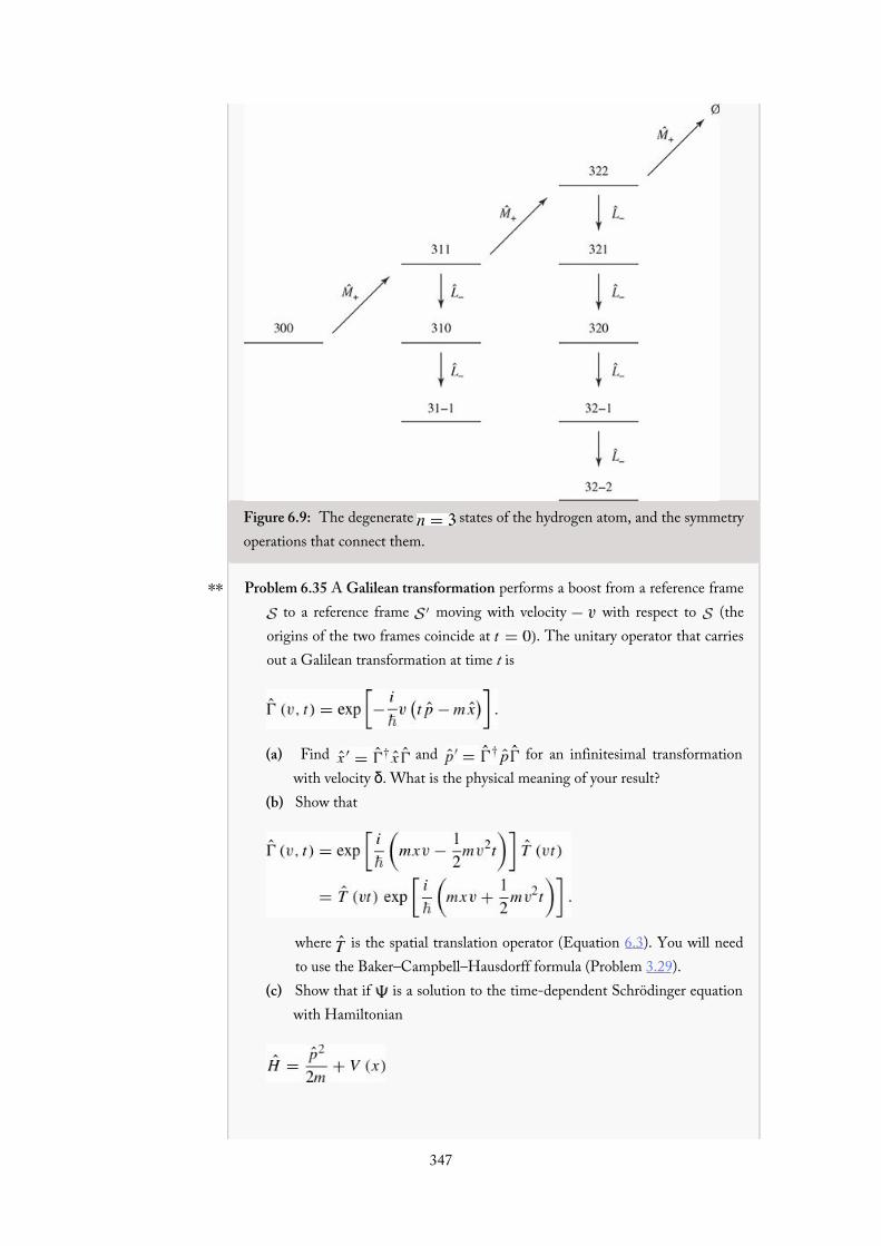
∗∗
Figure 6.9: The degenerate states of the hydrogen atom, and the symmetryoperations that connect them.
Problem 6.35 A Galilean transformation performs a boost from a reference frame to a reference frame moving with velocity with respect to (the
origins of the two frames coincide at . The unitary operator that carriesout a Galilean transformation at time t is
(a) Find and for an infinitesimal transformationwith velocity δ. What is the physical meaning of your result?
(b) Show that
where is the spatial translation operator (Equation 6.3). You will needto use the Baker–Campbell–Hausdorff formula (Problem 3.29).
(c) Show that if is a solution to the time-dependent Schrödinger equationwith Hamiltonian
then the boosted wave function is a solution to the347
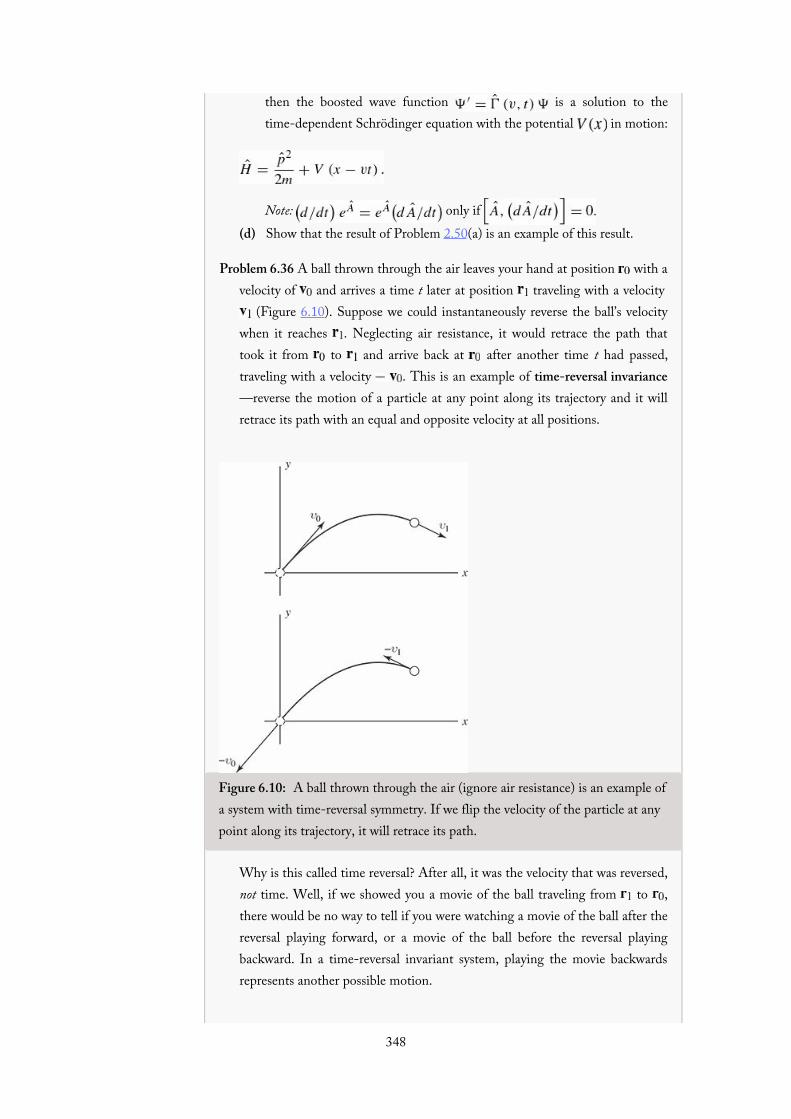
then the boosted wave function is a solution to thetime-dependent Schrödinger equation with the potential in motion:
Note: only if (d) Show that the result of Problem 2.50(a) is an example of this result.
Problem 6.36 A ball thrown through the air leaves your hand at position with avelocity of and arrives a time t later at position traveling with a velocity
(Figure 6.10). Suppose we could instantaneously reverse the ball’s velocitywhen it reaches . Neglecting air resistance, it would retrace the path thattook it from to and arrive back at after another time t had passed,traveling with a velocity . This is an example of time-reversal invariance—reverse the motion of a particle at any point along its trajectory and it willretrace its path with an equal and opposite velocity at all positions.
Figure 6.10: A ball thrown through the air (ignore air resistance) is an example ofa system with time-reversal symmetry. If we flip the velocity of the particle at anypoint along its trajectory, it will retrace its path.
Why is this called time reversal? After all, it was the velocity that was reversed,not time. Well, if we showed you a movie of the ball traveling from to ,there would be no way to tell if you were watching a movie of the ball after thereversal playing forward, or a movie of the ball before the reversal playingbackward. In a time-reversal invariant system, playing the movie backwardsrepresents another possible motion.
A familiar example of a system that does not exhibit time-reversal348

(6.82)
A familiar example of a system that does not exhibit time-reversalsymmetry is a charged particle moving in an external magnetic field.44 In thatcase, when you reverse the velocity of the particle, the Lorentz force will alsochange sign and the particle will not retrace its path; this is illustrated inFigure 6.11.
Figure 6.11: An external magnetic field breaks time-reversal symmetry. Shown isthe trajectory of a particle of charge traveling in a uniform magnetic fieldpointing into the page. If we flip the particle’s velocity from to at thepoint shown, the particle does not retrace its path, but instead moves onto a newcircular orbit.
The time-reversal operator is the operator that reverses the momentum ofthe particle , leaving its position unchanged. A better name wouldreally be the “reversal of the direction of motion” operator.45 For a spinlessparticle, the time-reversal operator simply complex conjugates the position-space wave function46
(a) Show that the operators and transform under time reversal as
Hint: Do this by calculating the action of and on an arbitrary testfunction .
(b) We can write down a mathematical statement of time-reversal invariancefrom our discussion above. We take a system, evolve it for a time t,reverse its momentum, and evolve it for time t again. If the system istime-reversal invariant it will be back where it started, albeit with itsmomentum reversed (Figure 6.10). As an operator statement this says
349
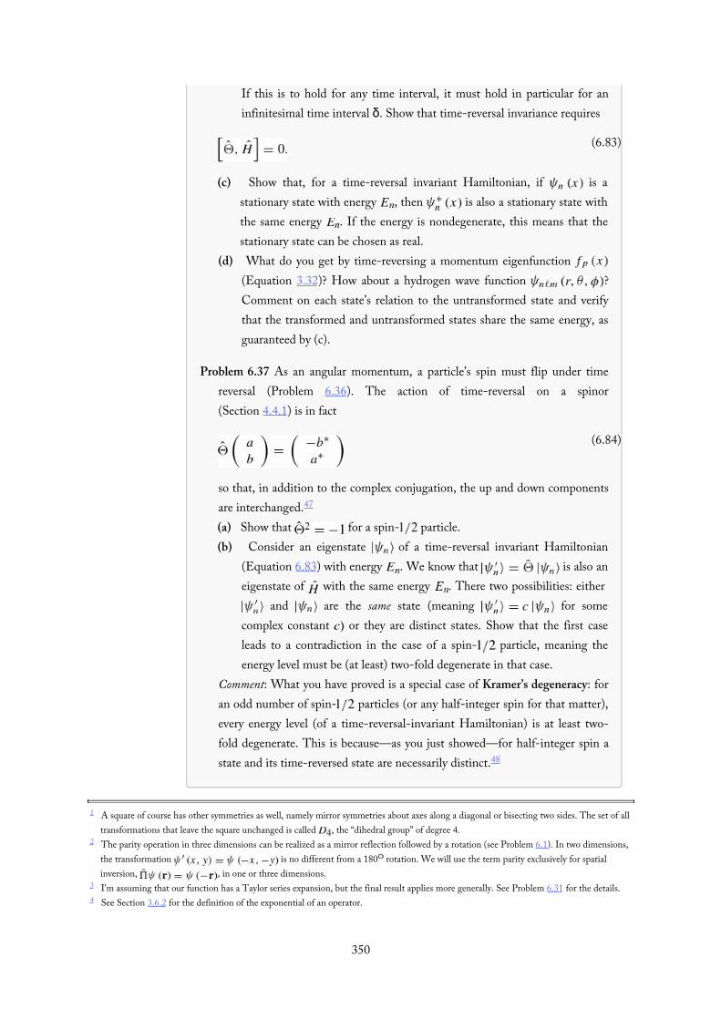
(6.83)
(6.84)
If this is to hold for any time interval, it must hold in particular for aninfinitesimal time interval δ. Show that time-reversal invariance requires
(c) Show that, for a time-reversal invariant Hamiltonian, if is astationary state with energy , then is also a stationary state withthe same energy . If the energy is nondegenerate, this means that thestationary state can be chosen as real.
(d) What do you get by time-reversing a momentum eigenfunction (Equation 3.32)? How about a hydrogen wave function ?Comment on each state’s relation to the untransformed state and verifythat the transformed and untransformed states share the same energy, asguaranteed by (c).
Problem 6.37 As an angular momentum, a particle’s spin must flip under timereversal (Problem 6.36). The action of time-reversal on a spinor(Section 4.4.1) is in fact
so that, in addition to the complex conjugation, the up and down componentsare interchanged.47
(a) Show that for a spin- particle.(b) Consider an eigenstate of a time-reversal invariant Hamiltonian
(Equation 6.83) with energy . We know that is also aneigenstate of with the same energy . There two possibilities: either
and are the same state (meaning for somecomplex constant or they are distinct states. Show that the first caseleads to a contradiction in the case of a spin- particle, meaning theenergy level must be (at least) two-fold degenerate in that case.
Comment: What you have proved is a special case of Kramer’s degeneracy: foran odd number of spin- particles (or any half-integer spin for that matter),every energy level (of a time-reversal-invariant Hamiltonian) is at least two-fold degenerate. This is because—as you just showed—for half-integer spin astate and its time-reversed state are necessarily distinct.48
1 A square of course has other symmetries as well, namely mirror symmetries about axes along a diagonal or bisecting two sides. The set of alltransformations that leave the square unchanged is called , the “dihedral group” of degree 4.
2 The parity operation in three dimensions can be realized as a mirror reflection followed by a rotation (see Problem 6.1). In two dimensions,the transformation is no different from a 180 rotation. We will use the term parity exclusively for spatialinversion, , in one or three dimensions.
3 I’m assuming that our function has a Taylor series expansion, but the final result applies more generally. See Problem 6.31 for the details.4 See Section 3.6.2 for the definition of the exponential of an operator.
5 The term comes from the study of Lie groups (the group of translations is an example). If you’re interested, an introduction to Lie groups350

5 The term comes from the study of Lie groups (the group of translations is an example). If you’re interested, an introduction to Lie groups(written for physicists) can be found in George B. Arfken, Hans J. Weber, and Frank E. Harris, Mathematical Methods for Physicists, 7th edn,Academic Press, New York (2013), Section 17.7.
6 Unitary operators are discussed in Problem A.30. A unitary operator is one whose adjoint is also its inverse: .7 It is clear that Equation 6.12 satisfies Equation 6.11. In Problem 6.5 you’ll prove that they are in fact equivalent statements.8 For a delightful proof using perturbation theory, see Neil Ashcroft and N. David Mermin, Solid State Physics, Cengage, Belmont, 1976 (p.
765), after you have completed Problem 6.6 and studied Chapter 7.9 For the case of continuous symmetries, it is often much easier to work with the infinitesimal form of the transformation; any finite
transformation can then be built up as a product of infinitesimal transformations. In particular, the finite translation by a is a sequence of Ninfinitesimal translations with in the limit that :
For a proof see R. Shankar, Basic Training in Mathematics: A Fitness Program for Science Students, Plenum Press, New York, 1995 (p.11).10 In the case of a discrete translational symmetry, momentum is not conserved, but there is a conserved quantity closely related to the discrete
translational symmetry, which is the crystal momentum. For a discussion of crystal momentum see Steven H. Simon, The Oxford Solid StateBasics, Oxford, 2013, p.84.
11 If the spectrum of is degenerate there are distinct eigenvectors with the same eigenvalue : for ,then we need to sum over those states:
Except for the sum over i the proof proceeds unchanged.12 For bound (normalizable) states in one dimension, there is no degeneracy and every bound state of a symmetric potential is automatically an
eigenstate of parity. (However, see Problem 2.46.) For scattering states, degeneracy does occur.13 Note that Equation 6.24 could equivalently be written as . The fact that parity commutes with every component of the angular
momentum and therefore also is the reason you can find simultaneous eigenstates of , , and .14 However, it turns out that antiparticles of spin have opposite parity. Thus the electron is conventionally assigned parity , but the
positron then has parity .15 To go the other way, from infinitesimal to finite, see Problem 6.14.16 See Section A.5.17 The Levi-Civita symbol is defined in Problem 4.29.18 Of course, not every operator will fit into one of these categories. Scalar and vector operators are simply the first two instances in a hierarchy
of tensor operators. Next come second-rank tensors (the inertia tensor from classical mechanics or the quadrupole tensor fromelectrodynamics are examples), third-rank tensors, and so forth.
19 This follows from the fact that the radial Schrödinger equation (Equation 4.35) has at most a single normalizable solution so that, once youhave specified and m, the energy uniquely specifies the state. The principal quantum number n indexes those energy values that lead tonormalizable solutions.
20 When we can’t identify the symmetry responsible for a particular degeneracy, we call it an accidental degeneracy. In most such cases, thedegeneracy turns out to be no accident at all, but instead due to symmetry that is more difficult to identify than, say, rotational invariance.The canonical example is the larger symmetry group of the hydrogen atom (Problem 6.34).
21 This is highly non-classical. In classical mechanics, if you take a Keplerian orbit there will always be some axis about which you can rotate itto get a different Keplerian orbit (of the same energy) and in fact there will be an infinite number of such orbits with different orientations.In quantum mechanics, if you rotate the ground state of hydrogen you get back exactly the same state regardless of which axis you choose,and if you rotate one of the states with and , you get back a linear combination of the three orthogonal states with thesequantum numbers.
22 Of course, we already know the energies are equal since the radial equation, Equation 4.35, does not depend on m. This exampledemonstrates that rotational invariance is behind the degeneracy.
23 I don’t mean that they necessarily occur in this order. Look back at the infinite spherical well (Figure 4.3): starting with the ground state thedegeneracies are . These are precisely the degrees of degeneracy we expect for rotational invariance forinteger but the symmetry considerations don’t tell us where in the spectrum each degeneracy will occur.
24 For the three-dimensional harmonic oscillator the degeneracy is (Problem 4.46) which again is greaterthan . For a discussion of the additional symmetry in the oscillator problem see D. M. Fradkin, Am. J. Phys. 33, 207 (1965).
25 Importantly, they satisfy Equations 4.118 and 4.120.26 The other root of the quadratic is ; since and are non-negative integers this isn’t
possible.
351

(6.70)
27 Since and are Hermitian,
28 The operators are, up to constants, components of what are known as spherical tensor operators of rank 1, written where k is therank and q the component of the operator:
Similarly, the scalar operator f treated in Section 6.7.1 is a rank-0 spherical tensor operator:
29 Equations 6.51–6.54 each stand for two equations: read the upper signs all the way across, or the lower signs.30 A warning about notation: In the selection rules for the scalar operator r,
and for a component (say z) of the vector operator r,
the two reduced matrix elements are not the same. One is the reduced matrix element for r and one is the reduced matrix element for r, andthese are different operators that share the same name. You could tack on a subscript and to distinguishbetween the two if that helps keep them straight.
31 In the case of the position operator , this correspondence is particularly evident when we rewrite the operator with the help of Table 4.3:
32 Since , one could rewrite the selection rules for a scalar operator (Equation 6.47) as
33 Why is this analysis limited to the case where is independent of time? Whether or not depends on time, Schrödinger’s equation says . However, if is time dependent then the second derivative of is given by
and higher derivatives will be even more complicated. Therefore, Equation 6.69 only follows from Equation 6.68 when has no timedependence. See also Problem 11.23.
34 This derivation assumes that the actual solution to Schrodinger’s equation, , can be expanded as a Taylor series in t, and nothingguarantees that. B. R. Holstein and A. R. Swift, A. J. Phys. 40, 829 (1989) give an innocent-seeming example where such an expansion doesnot exist. Nonetheless, Equation 6.71 still holds in such cases as long as we define the exponential function through its spectraldecomposition (Equation 3.103):
See also M. Amaku et al., Am. J. Phys. 85, 692 (2017).35 Since Equation 6.73 holds for any stationary state and since the constitute a complete set of states, the operators must in fact be
identical.36 I am assuming that , like or , has no explicit time dependence.37 Of these other possible pictures the most important is the interaction picture (or Dirac picture) which is often employed in time-dependent
perturbation theory.
352

(6.85)
38 And is a function of both the initial time and the final time t, not simply the amount of time for which the wave function has evolved.39 For time-dependent and the generalization is
40 The integrals in (c)–(e) can all be done with the following identity:
which was derived in Problem 2.21.41 For a discussion of how this sign change is actually measured, see S. A. Werner et al., Phys. Rev. Lett. 35, 1053 (1975).42 See F. Leyvraz, et al., Am. J. Phys. 65, 1087 (1997) for a discussion of this “accidental” degeneracy.43 The full symmetry of the Coulomb Hamiltonian is not just the obvious three-dimensional rotation group (known to mathematicians as
SO(3)), but the four-dimensional rotation group (SO(4)), which has six generators and . (If the four axes are w, x, y, and z, thegenerators correspond to rotations in each of the six orthogonal planes, wx, wy, wz (that’s and yz, zx, xy (that’s .
44 By external magnetic field, I mean that we we only reverse the velocity of our charge q, and not the velocities of the charges producing themagnetic field. If we reversed those velocities as well, the magnetic field would also switch directions, the Lorentz force on the charge qwould be unchanged by the reversal, and the system would in fact be time-reversal invariant.
45 See Eugene P. Wigner, Group Theory and its Applications to Quantum Mechanics and Atomic Spectra (Academic Press, New York, 1959), p.325.
46 Time reversal is an anti-unitary operator. An anti-unitary operator satisfies
whereas a unitary operator satisfies the same two equations without the complex conjugates. I won’t define the adjoint of an anti-unitaryoperator; instead I use for an anti-unitary operator where we might have used or interchangeably for a unitary operator.
47 For arbitrary spin,
where the first term is a rotation by π about the y axis and is the operator that performs the complex conjugation.48 What about in the case of a spin-0 particle—does time-reversal symmetry tell us anything interesting? Actually it does. For one thing, the
stationary states can be chosen as real; you proved this back in Problem 2.2 but we now see that it is a consequence of time-reversalsymmetry. Another example is the degeneracy of the energy levels in a periodical potential (Section 5.3.2 and Problem 6.6) for states withcrystal momentum q and . This can be ascribed to inversion symmetry if the potential is symmetric, but the degeneracy persists evenwhen inversion symmetry is absent (try it out!); that is a result of time-reversal symmetry.
353

Part IIApplications
◈
354

7Time-Independent Perturbation Theory
◈
355

7.1 Nondegenerate Perturbation Theory
356

(7.1)
(7.2)
(7.4)
(7.5)
(7.6)
(7.3)
7.1.1 General Formulation
Suppose we have solved the (time-independent) Schrödinger equation for some potential (say, the one-dimensional infinite square well):
obtaining a complete set of orthonormal eigenfunctions, ,
and the corresponding eigenvalues . Now we perturb the potential slightly (say, by putting a little bump inthe bottom of the well—Figure 7.1). We’d like to find the new eigenfunctions and eigenvalues:
but unless we are very lucky, we’re not going to be able to solve the Schrödinger equation exactly, for thismore complicated potential. Perturbation theory is a systematic procedure for obtaining approximate solutionsto the perturbed problem, by building on the known exact solutions to the unperturbed case.
Figure 7.1: Infinite square well with small perturbation.
To begin with we write the new Hamiltonian as the sum of two terms:
where is the perturbation (the superscript 0 always identifies the unperturbed quantity). For the momentwe’ll take to be a small number; later we’ll crank it up to 1, and H will be the true Hamiltonian. Next wewrite and as power series in :
Here is the first-order correction to the nth eigenvalue, and is the first-order correction to the ntheigenfunction; and are the second-order corrections, and so on. Plugging Equations 7.5 and 7.6 into
357

(7.7)
(7.8)
Equation 7.3, we have:
or (collecting like powers of :
To lowest order1 this yields , which is nothing new (Equation 7.1). To first order ,
To second order ,
and so on. (I’m done with , now—it was just a device to keep track of the different orders—so crank it up to1.)
358

(7.9)
7.1.2 First-Order Theory
Taking the inner product of Equation 7.7 with (that is, multiplying by and integrating),
But is hermitian, so
and this cancels the first term on the right. Moreover, , so2
This is the fundamental result of first-order perturbation theory; as a practical matter, it may well be the mostfrequently used equation in quantum mechanics. It says that the first-order correction to the energy is theexpectation value of the perturbation, in the unperturbed state.
Example 7.1The unperturbed wave functions for the infinite square well are (Equation 2.31)
Suppose we perturb the system by simply raising the “floor” of the well a constant amount (Figure 7.2). Find the first-order correction to the energies.
Figure 7.2: Constant perturbation over the whole well.
Solution: In this case , and the first-order correction to the energy of the nth state is
359
(7.10)
(7.11)
The corrected energy levels, then, are ; they are simply lifted by the amount . Ofcourse! The only surprising thing is that in this case the first-order theory yields the exact answer.Evidently for a constant perturbation all the higher corrections vanish.3 On the other hand, if theperturbation extends only half-way across the well (Figure 7.3), then
In this case every energy level is lifted by . That’s not the exact result, presumably, but it doesseem reasonable, as a first-order approximation.
Figure 7.3: Constant perturbation over half the well.
Equation 7.9 is the first-order correction to the energy; to find the first-order correction to the wavefunction we rewrite Equation 7.7:
The right side is a known function, so this amounts to an inhomogeneous differential equation for . Now,the unperturbed wave functions constitute a complete set, so (like any other function) can be expressed as alinear combination of them:
(There is no need to include in the sum, for if satisfies Equation 7.10, so too does ,for any constant α, and we can use this freedom to subtract off the term.4 ) If we could determine thecoefficients , we’d be done.
Well, putting Equation 7.11 into Equation 7.10, and using the fact that satisfies the unperturbedSchrödinger equation (Equation 7.1), we have
360

(7.12)
(7.13)
∗
∗
Taking the inner product with ,
If , the left side is zero, and we recover Equation 7.9; if , we get
or
so
Notice that the denominator is safe (since there is no coefficient with as long as the unperturbed energyspectrum is nondegenerate. But if two different unperturbed states share the same energy, we’re in serioustrouble (we divided by zero to get Equation 7.12); in that case we need degenerate perturbation theory, whichI’ll come to in Section 7.2.
That completes first-order perturbation theory: The first-order correction to the energy, , is given byEquation 7.9, and the first-order correction to the wave function, , is given by Equation 7.13.
Problem 7.1 Suppose we put a delta-function bump in the center of the infinitesquare well:
where α is a constant.(a) Find the first-order correction to the allowed energies. Explain why the
energies are not perturbed for even n.(b) Find the first three nonzero terms in the expansion (Equation 7.13) of
the correction to the ground state, .
Problem 7.2 For the harmonic oscillator , the allowedenergies are
where is the classical frequency. Now suppose the spring constantincreases slightly: . (Perhaps we cool the spring, so it becomes less
361

flexible.)(a) Find the exact new energies (trivial, in this case). Expand your formula as
a power series in ϵ, up to second order.(b) Now calculate the first-order perturbation in the energy, using Equation
7.9. What is here? Compare your result with part (a). Hint: It is notnecessary—in fact, it is not permitted—to calculate a single integral indoing this problem.
Problem 7.3 Two identical spin-zero bosons are placed in an infinite square well(Equation 2.22). They interact weakly with one another, via the potential
(where is a constant with the dimensions of energy, and a is the width of thewell).
(a) First, ignoring the interaction between the particles, find the ground stateand the first excited state—both the wave functions and the associatedenergies.
(b) Use first-order perturbation theory to estimate the effect of the particle–particle interaction on the energies of the ground state and the firstexcited state.
362
(7.14)
(7.15)
∗∗
7.1.3 Second-Order Energies
Proceeding as before, we take the inner product of the second-order equation (Equation 7.8) with :
Again, we exploit the hermiticity of :
so the first term on the left cancels the first term on the right. Meanwhile, , and we are left witha formula for :
But
(because the sum excludes , and all the others are orthogonal), so
or, finally,
This is the fundamental result of second-order perturbation theory.We could go on to calculate the second-order correction to the wave function , the third-order
correction to the energy, and so on, but in practice Equation 7.15 is ordinarily as far as it is useful to pursuethis method.5
Problem 7.4 Apply perturbation theory to the most general two-level system. Theunperturbed Hamiltonian is
and the perturbation is
with , and real, so that is hermitian. As in Section 7.1.1, is363
∗
∗∗
∗∗
with , and real, so that is hermitian. As in Section 7.1.1, isa constant that will later be set to 1.
(a) Find the exact energies for this two-level system.(b) Expand your result from (a) to second order in (and then set to 1).
Verify that the terms in the series agree with the results from perturbationtheory in Sections 7.1.2 and 7.1.3. Assume that .
(c) Setting , show that the series in (b) only converges if
Comment: In general, perturbation theory is only valid if the matrixelements of the perturbation are small compared to the energy levelspacings. Otherwise, the first few terms (which are all we ever calculate)will give a poor approximation to the quantity of interest and, as shownhere, the series may fail to converge at all, in which case the first fewterms tell us nothing.
Problem 7.5(a) Find the second-order correction to the energies for the potential in
Problem 7.1. Comment: You can sum the series explicitly, obtaining for odd n.
(b) Calculate the second-order correction to the ground state energy forthe potential in Problem 7.2. Check that your result is consistent with theexact solution.
Problem 7.6 Consider a charged particle in the one-dimensional harmonicoscillator potential. Suppose we turn on a weak electric field , so that thepotential energy is shifted by an amount .
(a) Show that there is no first-order change in the energy levels, and calculatethe second-order correction. Hint: See Problem 3.39.
(b) The Schrödinger equation can be solved directly in this case, by a changeof variables: . Find the exact energies, and showthat they are consistent with the perturbation theory approximation.
Problem 7.7 Consider a particle in the potential shown in Figure 7.3.(a) Find the first-order correction to the ground-state wave function. The
first three nonzero terms in the sum will suffice.(b) Using the method of Problem 2.61 find (numerically) the ground-state
wave function and energy. Use and . Compare
364

the energy obtained numerically to the result from first-orderperturbation theory (see Example 7.1).
(c) Make a single plot showing (i) the unperturbed ground-state wavefunction, (ii) the numerical ground-state wave function, and (ii) the first-order approximation to the ground-state wave function. Note: Make sureyou’ve properly normalized your numerical result,
365

7.2 Degenerate Perturbation TheoryIf the unperturbed states are degenerate—that is, if two (or more) distinct states and share the sameenergy—then ordinary perturbation theory fails: (Equation 7.12) and (Equation 7.15) blow up(unless, perhaps, the numerator vanishes, —a loophole that will be important to us lateron). In the degenerate case, therefore, there is no reason to trust even the first-order correction to the energy(Equation 7.9), and we must look for some other way to handle the problem. Note this is not a minorproblem; almost all applications of perturbation theory involve degeneracy.
366

(7.16)
(7.17)
(7.18)
7.2.1 Two-Fold Degeneracy
Suppose that
with and both normalized. Note that any linear combination of these states,
is still an eigenstate of , with the same eigenvalue :
Typically, the perturbation will “break” (or “lift”) the degeneracy: As we increase (from 0 to 1), thecommon unperturbed energy splits into two (Figure 7.4). Going the other direction, when we turn off theperturbation, the “upper” state reduces down to one linear combination of and , and the “lower” statereduces to some (orthogonal) linear combination, but we don’t know a priori what these “good” linearcombinations will be. For this reason we can’t even calculate the first-order energy (Equation 7.9)—we don’tknow what unperturbed states to use.
Figure 7.4: “Lifting” of a degeneracy by a perturbation.
The “good” states are defined as the limit of the true eigenstates as the perturbation is switched off but that isn’t how you find them in realistic situations (if you knew the exact eigenstates you
wouldn’t need perturbation theory). Before I show you the practical techniques for calculating them, we’ll lookat an example where we can take the limit of the exact eigenstates.
Example 7.2Consider a particle of mass m in a two-dimensional oscillator potential
to which is added a perturbation
367
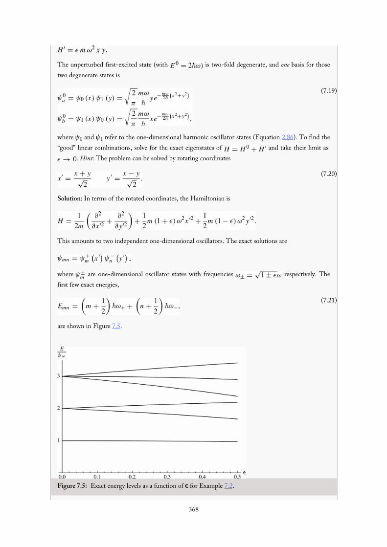
(7.19)
(7.20)
(7.21)
The unperturbed first-excited state (with is two-fold degenerate, and one basis for thosetwo degenerate states is
where and refer to the one-dimensional harmonic oscillator states (Equation 2.86). To find the“good” linear combinations, solve for the exact eigenstates of and take their limit as
. Hint: The problem can be solved by rotating coordinates
Solution: In terms of the rotated coordinates, the Hamiltonian is
This amounts to two independent one-dimensional oscillators. The exact solutions are
where are one-dimensional oscillator states with frequencies respectively. Thefirst few exact energies,
are shown in Figure 7.5.
Figure 7.5: Exact energy levels as a function of ϵ for Example 7.2.
368
(7.22)
(7.23)
(7.25)
(7.26)
(7.24)
The two states which grow out of the degenerate first-excited states as ϵ is increased have , (lower state) and , (upper state). If we track these states back to (in that
limit we get
Therefore the “good” states for this problem are
In this example we were able to find the exact eigenstates of H and then turn off the perturbation tosee what states they evolve from. But how do we find the “good” states when we can’t solve the systemexactly?
For the moment let’s just write the “good” unperturbed states in generic form (Equation 7.17), keeping αand β adjustable. We want to solve the Schrödinger equation,
with and
Plugging these into Equation 7.24, and collecting like powers of (as before) we find
But (Equation 7.18), so the first terms cancel; at order we have
Taking the inner product with :
Because is hermitian, the first term on the left cancels the first term on the right. Putting in Equation7.17, and exploiting the orthonormality condition (Equation 7.16), we obtain
or, more compactly,
369
(7.28)
(7.29)
(7.30)
(7.31)
(7.32)
(7.33)
(7.27)
where
Similarly, the inner product with yields
Notice that the Ws are (in principle) known—they are just the “matrix elements” of , with respect tothe unperturbed wave functions and . Written in matrix form, Equations 7.27 and 7.29 are
The eigenvalues of the matrix give the first-order corrections to the energy and the correspondingeigenvectors tell us the coefficients α and β that determine the “good” states.6
The Appendix (Section A.5) shows how to obtain the eigenvalues of a matrix; I’ll reproduce those stepshere to find a general solution for . First, move all the terms in Equation 7.30 to the left-hand side.
This equation only has non-trivial solutions if the matrix on the left is non-invertible—that is to say, if itsdeterminant vanishes:
where we used the fact that . Solving the quadratic,
This is the fundamental result of degenerate perturbation theory; the two roots correspond to the twoperturbed energies.
Example 7.3Returning to Example 7.2, show that diagonalizing the matrix gives the same “good” states wefound by solving the problem exactly.
Solution: We need to calculate the matrix elements of . First,
370

(7.34)
(7.35)
(the integrands are both odd functions). Similarly, , and we need only compute
These two integrals are equal, and recalling (Equation 2.70)
we have
Therefore, the matrix is
The (normalized) eigenvectors of this matrix are
These eigenvectors tell us which linear combination of and are the good states:
just as in Equation 7.23. The eigenvalues of the matrix ,
give the first-order corrections to the energy (compare 7.33).
If it happens that in Equation 7.30 then the two eigenvectors are
and the energies,
are precisely what we would have obtained using nondegenerate perturbation theory (Equation 7.9). We have371

are precisely what we would have obtained using nondegenerate perturbation theory (Equation 7.9). We havesimply been lucky: The states and were already the “good” linear combinations. Obviously, it would begreatly to our advantage if we could somehow guess the “good” states right from the start—then we could goahead and use nondegenerate perturbation theory. As it turns out, we can very often do this by exploiting thetheorem in the following section.
372
(7.37)
(7.38)
(7.36)
7.2.2 “Good” States
Theorem: Let A be a hermitian operator that commutes with and . If and (thedegenerate eigenfunctions of are also eigenfunctions of A, with distinct eigenvalues,
then and are the “good” states to use in perturbation theory.
Proof: Since and A commute, there exist simultaneous eigenstates where
The fact that A is hermitian means
(making use of the fact that μ is real). This holds true for any value of and taking the limit as we have
and similarly
Now the good states are linear combinations of and : . From above itfollows that either , in which case and the good state is simply , or
and the good state is . QED
Once we identify the “good” states, either by solving Equation 7.30 or by applying this theorem, we canuse these “good” states as our unperturbed states and apply ordinary non-degenerate perturbation theory.7 Inmost cases, the operator will be suggested by symmetry; as you saw in Chapter 6, symmetries are associatedwith operators that commute with —precisely what are required to identify the good states.
Example 7.4Find an operator that satisfies the requirements of the preceding theorem to construct the “good”states in Examples 7.2 and 7.3.
Solution: The perturbation has less symmetry than . had continuous rotational symmetry,but is only invariant under rotations by integer multiples of π. For , take theoperator that rotates a function counterclockwise by an angle π. Acting on our stats and
373

(7.39)
operator that rotates a function counterclockwise by an angle π. Acting on our stats and we have
That’s no good; we need an operator with distinct eigenvalues. How about the operator thatinterchanges x and y? This is a reflection about a 45 diagonal of the well. Call this operator . commutes with both and , since they are unchanged when you switch x and y. Now,
So our degenerate eigenstates are not eigenstates of . But we can construct linear combinations thatare:
Then
These are “good” states, since they are eigenstates of an operator with distinct eigenvalues ,and commutes with both and .
Moral: If you’re faced with degenerate states, look around for some hermitian operator A that commuteswith and ; pick as your unperturbed states ones that are simultaneously eigenfunctions of and A(with distinct eigenvalues). Then use ordinary first-order perturbation theory. If you can’t find such anoperator, you’ll have to resort to Equation 7.33, but in practice this is seldom necessary.
Problem 7.8 Let the two “good” unperturbed states be
where and are determined (up to normalization) by Equation 7.27 (orEquation 7.29). Show explicitly that
(a) are orthogonal ;(b) ;(c) , with given by Equation 7.33.
Problem 7.9 Consider a particle of mass m that is free to move in a one-dimensional region of length L that closes on itself (for instance, a bead that slidesfrictionlessly on a circular wire of circumference L, as in Problem 2.46).
(a) Show that the stationary states can be written in the form
374

where , , , … , and the allowed energies are
Notice that—with the exception of the ground state —these areall doubly degenerate.
(b) Now suppose we introduce the perturbation
where . (This puts a little “dimple” in the potential at , asthough we bent the wire slightly to make a “trap”.) Find the first-ordercorrection to , using Equation 7.33. Hint: To evaluate the integrals,exploit the fact that to extend the limits from to ;after all, is essentially zero outside .
(c) What are the “good” linear combinations of and , for thisproblem? (Hint: use Eq. 7.27.) Show that with these states you get thefirst-order correction using Equation 7.9.
(d) Find a hermitian operator A that fits the requirements of the theorem,and show that the simultaneous eigenstates of and A are precisely theones you used in (c).
375

(7.40)
(7.41)
(7.42)
∗
7.2.3 Higher-Order Degeneracy
In the previous section I assumed the degeneracy was two-fold, but it is easy to see how the methodgeneralizes. In the case of n-fold degeneracy, we look for the eigenvalues of the matrix
For three-fold degeneracy (with degenerate states , , and the first-order corrections to the energies are the eigenvalues of , determined by solving
and the “good” states are the corresponding eigenvectors:8
Once again, if you can think of an operator A that commutes with and , and use the simultaneouseigenfunctions of A and , then the W matrix will automatically be diagonal, and you won’t have to fuss withcalculating the off-diagonal elements of or solving the characteristic equation.9 (If you’re nervous about mygeneralization from two-fold degeneracy to n-fold degeneracy, work Problem 7.13.)
Problem 7.10 Show that the first-order energy corrections computed inExample 7.3 (Equation 7.34) agree with an expansion of the exact solution(Equation 7.21) to first order in ϵ.
Problem 7.11 Suppose we perturb the infinite cubical well (Problem 4.2) byputting a delta function “bump” at the point :
Find the first-order corrections to the energy of the ground state and the (triplydegenerate) first excited states.
Problem 7.12 Consider a quantum system with just three linearly independentstates. Suppose the Hamiltonian, in matrix form, is
where is a constant, and ϵ is some small number .(a) Write down the eigenvectors and eigenvalues of the unperturbed
Hamiltonian .
376
(b) Solve for the exact eigenvalues of . Expand each of them as a powerseries in ϵ, up to second order.
(c) Use first- and second-order non-degenerate perturbation theory to findthe approximate eigenvalue for the state that grows out of thenondegenerate eigenvector of . Compare the exact result, from (b).
(d) Use degenerate perturbation theory to find the first-order correction to thetwo initially degenerate eigenvalues. Compare the exact results.
Problem 7.13 In the text I asserted that the first-order corrections to an n-folddegenerate energy are the eigenvalues of the W matrix, and I justified this claim asthe “natural” generalization of the case . Prove it, by reproducing the stepsin Section 7.2.1, starting with
(generalizing Equation 7.17), and ending by showing that the analog to Equation7.27 can be interpreted as the eigenvalue equation for the matrix .
377

(7.43)
(7.44)
7.3 The Fine Structure of HydrogenIn our study of the hydrogen atom (Section 4.2) we took the Hamiltonian—called the Bohr Hamiltonian—tobe
(electron kinetic energy plus Coulombic potential energy). But this is not quite the whole story. We havealready learned how to correct for the motion of the nucleus: Just replace m by the reduced mass (Problem5.1). More significant is the so-called fine structure, which is actually due to two distinct mechanisms: arelativistic correction, and spin-orbit coupling. Compared to the Bohr energies (Equation 4.70), finestructure is a tiny perturbation—smaller by a factor of , where
is the famous fine structure constant. Smaller still (by another factor of is the Lamb shift, associated withthe quantization of the electric field, and smaller by yet another order of magnitude is the hyperfine structure,which is due to the interaction between the magnetic dipole moments of the electron and the proton. Thishierarchy is summarized in Table 7.1. In the present section we will analyze the fine structure of hydrogen, asan application of time-independent perturbation theory.
Table 7.1: Hierarchy of corrections to the Bohr energies of hydrogen.
Problem 7.14(a) Express the Bohr energies in terms of the fine structure constant and the
rest energy of the electron.(b) Calculate the fine structure constant from first principles (i.e., without
recourse to the empirical values of , e, , and . Comment: The finestructure constant is undoubtedly the most fundamental pure(dimensionless) number in all of physics. It relates the basic constants ofelectromagnetism (the charge of the electron), relativity (the speed oflight), and quantum mechanics (Planck’s constant). If you can solve part(b), you have the most certain Nobel Prize in history waiting for you. ButI wouldn’t recommend spending a lot of time on it right now; many smartpeople have tried, and all (so far) have failed.
378

379

(7.45)
(7.46)
(7.47)
(7.48)
(7.49)
(7.50)
(7.51)
7.3.1 The Relativistic Correction
The first term in the Hamiltonian is supposed to represent kinetic energy:
and the canonical substitution yields the operator
But Equation 7.45 is the classical expression for kinetic energy; the relativistic formula is
The first term is the total relativistic energy (not counting potential energy, which we aren’t concerned with atthe moment), and the second term is the rest energy—the difference is the energy attributable to motion.
We need to express T in terms of the (relativistic) momentum,
instead of velocity. Notice that
so
This relativistic equation for kinetic energy reduces (of course) to the classical result (Equation 7.45), in thenonrelativistic limit ; expanding in powers of the small number , we have
The lowest-order10 relativistic correction to the Hamiltonian is therefore
In first-order perturbation theory, the correction to is given by the expectation value of in theunperturbed state (Equation 7.9):
380
(7.52)
(7.53)
(7.54)
(7.55)
(7.56)
(7.57)
(7.58)
Now, the Schrödinger equation (for the unperturbed states) says
and hence11
So far this is entirely general; but we’re interested in hydrogen, for which :
where is the Bohr energy of the state in question.To complete the job, we need the expectation values of and , in the (unperturbed) state
(Equation 4.89). The first is easy (see Problem 7.15):
where a is the Bohr radius (Equation 4.72). The second is not so simple to derive (see Problem 7.42), but theanswer is12
It follows that
or, eliminating a (using Equation 4.72) and expressing everything in terms of (using Equation 4.70):
Evidently the relativistic correction is smaller than , by a factor of about .You might have noticed that I used non-degenerate perturbation theory in this calculation (Equation
7.52), in spite of the fact that the hydrogen atom is highly degenerate. But the perturbation is sphericallysymmetric, so it commutes with and . Moreover, the eigenfunctions of these operators (taken together)have distinct eigenvalues for the states with a given . Luckily, then, the wave functions are the“good” states for this problem (or, as we say, n, , and m are the good quantum numbers), so as it happens theuse of nondegenerate perturbation theory was legitimate (see the “Moral” to Section 7.2.1).
From Equation 7.58 we see that some of the degeneracy of the nth energy level has lifted. The -fold degeneracy in m remains; as we saw in Example 6.3 it is due to rotational symmetry, a symmetry thatremains intact with this perturbation. On the other hand, the “accidental” degeneracy in has disappeared;
381

∗
∗∗
∗∗∗
since its source is an additional symmetry unique to the potential (see Problem 6.34), we expect thatdegeneracy to be broken by practically any perturbation.
Problem 7.15 Use the virial theorem (Problem 4.48) to prove Equation 7.56.
Problem 7.16 In Problem 4.52 you calculated the expectation value of in thestate . Check your answer for the special cases (trivial), (Equation 7.56), (Equation 7.57), and (Equation 7.66).Comment on the case .
Problem 7.17 Find the (lowest-order) relativistic correction to the energy levels ofthe one-dimensional harmonic oscillator. Hint: Use the technique of Problem2.12.
Problem 7.18 Show that is hermitian, for hydrogen states with . Hint:For such states is independent of θ and ϕ, so
(Equation 4.13). Using integration by parts, show that
Check that the boundary term vanishes for , which goes like
near the origin.The case of is more subtle. The Laplacian of picks up a delta function
(see, for example, D. J. Griffiths, Introduction to Electrodynamics, 4th edn,Eq. 1.102). Show that
and confirm that is hermitian.13
382

383
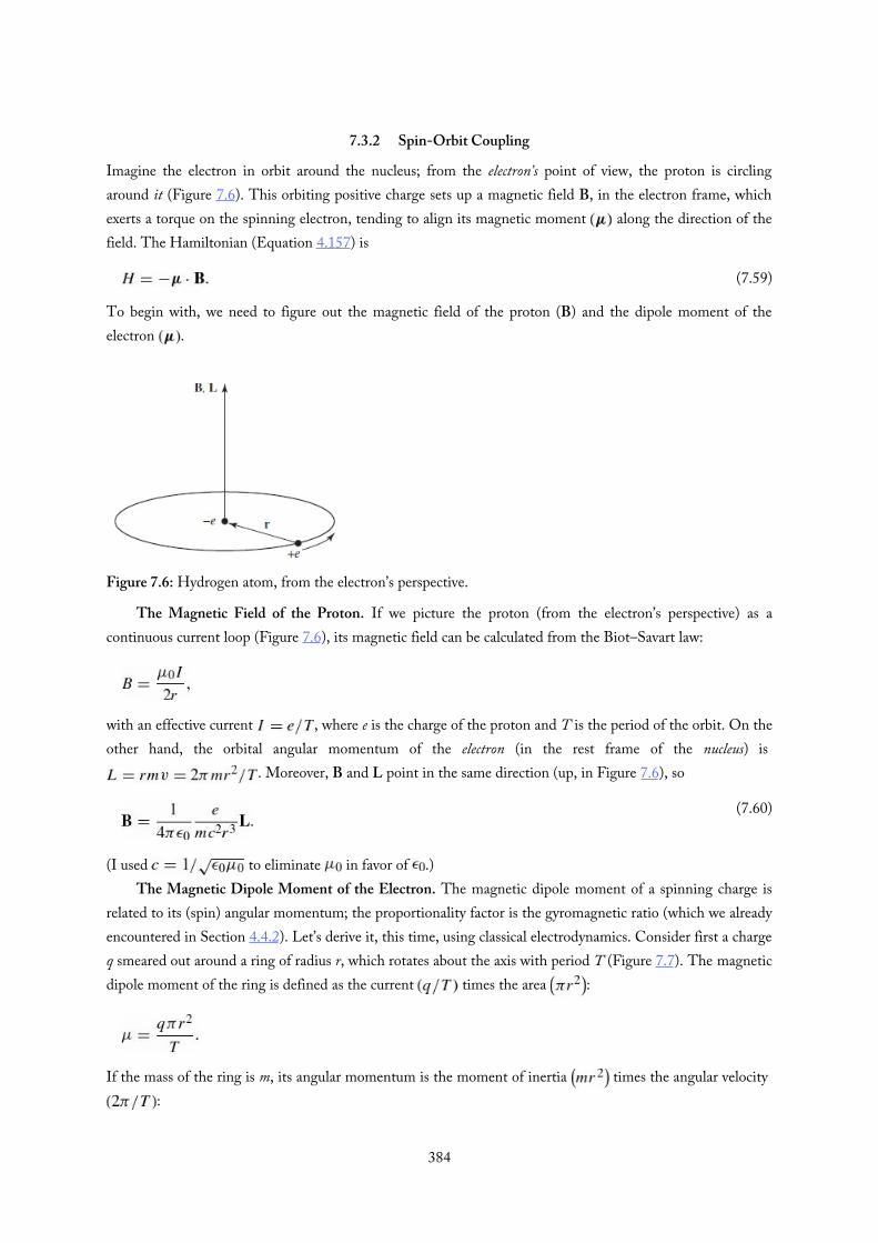
(7.60)
(7.59)
7.3.2 Spin-Orbit Coupling
Imagine the electron in orbit around the nucleus; from the electron’s point of view, the proton is circlingaround it (Figure 7.6). This orbiting positive charge sets up a magnetic field B, in the electron frame, whichexerts a torque on the spinning electron, tending to align its magnetic moment along the direction of thefield. The Hamiltonian (Equation 4.157) is
To begin with, we need to figure out the magnetic field of the proton (B) and the dipole moment of theelectron .
Figure 7.6: Hydrogen atom, from the electron’s perspective.
The Magnetic Field of the Proton. If we picture the proton (from the electron’s perspective) as acontinuous current loop (Figure 7.6), its magnetic field can be calculated from the Biot–Savart law:
with an effective current , where e is the charge of the proton and T is the period of the orbit. On theother hand, the orbital angular momentum of the electron (in the rest frame of the nucleus) is
. Moreover, B and L point in the same direction (up, in Figure 7.6), so
(I used to eliminate in favor of .)The Magnetic Dipole Moment of the Electron. The magnetic dipole moment of a spinning charge is
related to its (spin) angular momentum; the proportionality factor is the gyromagnetic ratio (which we alreadyencountered in Section 4.4.2). Let’s derive it, this time, using classical electrodynamics. Consider first a chargeq smeared out around a ring of radius r, which rotates about the axis with period T (Figure 7.7). The magneticdipole moment of the ring is defined as the current times the area :
If the mass of the ring is m, its angular momentum is the moment of inertia times the angular velocity :
384

(7.61)
(7.62)
(7.63)
The gyromagnetic ratio for this configuration is evidently . Notice that it is independent of r(and . If I had some more complicated object, such as a sphere (all I require is that it be a figure ofrevolution, rotating about its axis), I could calculate and S by chopping it into little rings, and adding uptheir contributions. As long as the mass and the charge are distributed in the same manner (so that thecharge-to-mass ratio is uniform), the gyromagnetic ratio will be the same for each ring, and hence also for theobject as a whole. Moreover, the directions of and S are the same (or opposite, if the charge is negative), so
Figure 7.7: A ring of charge, rotating about its axis.
That was a purely classical calculation, however; as it turns out the electron’s magnetic moment is twicethe classical value:
The “extra” factor of 2 was explained by Dirac, in his relativistic theory of the electron.14
Putting all this together, we have
But there is a serious fraud in this calculation: I did the analysis in the rest frame of the electron, but that’s notan inertial system—it accelerates, as the electron orbits around the nucleus. You can get away with this if youmake an appropriate kinematic correction, known as the Thomas precession.15 In this context it throws in afactor of 1/2:16
This is the spin-orbit interaction; apart from two corrections (the modified gyromagnetic ratio for theelectron and the Thomas precession factor—which, coincidentally, exactly cancel one another) it is just whatyou would expect on the basis of a naive classical model. Physically, it is due to the torque exerted on the
385

(7.65)
(7.66)
(7.67)
(7.68)
(7.69)
(7.64)
magnetic dipole moment of the spinning electron, by the magnetic field of the proton, in the electron’sinstantaneous rest frame.
Now the quantum mechanics. In the presence of spin-orbit coupling, the Hamiltonian no longercommutes with L and S, so the spin and orbital angular momenta are not separately conserved (see Problem7.19). However, does commute with , and the total angular momentum
and hence these quantities are conserved (Equation 3.73). To put it another way, the eigenstates of and are not “good” states to use in perturbation theory, but the eigenstates of , , , and are. Now
so
and therefore the eigenvalues of are
In this case, of course, . Meanwhile, the expectation value of (see Problem 7.43)17 is
and we conclude that
or, expressing it all in terms of :18
It is remarkable, considering the totally different physical mechanisms involved, that the relativisticcorrection and the spin-orbit coupling are of the same order . Adding them together, we get thecomplete fine-structure formula (see Problem 7.20):
Combining this with the Bohr formula, we obtain the grand result for the energy levels of hydrogen, includingfine structure:
386

∗
∗∗
Fine structure breaks the degeneracy in (that is, for a given n, the different allowed values of do notall carry the same energy), but it still preserves degeneracy in j (see Figure 7.8). The z-component eigenvaluesfor orbital and spin angular momentum and are no longer “good” quantum numbers—the stationarystates are linear combinations of states with different values of these quantities; the “good” quantum numbersare n, , s, j, and .19
Figure 7.8: Energy levels of hydrogen, including fine structure (not to scale).
Problem 7.19 Evaluate the following commutators: (a) , (b) ,(c) , (d) , (e) , (f) . Hint: L and S satisfythe fundamental commutation relations for angular momentum (Equations 4.99and 4.134), but they commute with each other.
Problem 7.20 Derive the fine structure formula (Equation 7.68) from therelativistic correction (Equation 7.58) and the spin-orbit coupling (Equation7.67). Hint: Note that (except for , where only the plus signoccurs); treat the plus sign and the minus sign separately, and you’ll find that youget the same final answer either way.
Problem 7.21 The most prominent feature of the hydrogen spectrum in the visibleregion is the red Balmer line, coming from the transition to . First ofall, determine the wavelength and frequency of this line according to the Bohrtheory. Fine structure splits this line into several closely-spaced lines; the question
387

is: How many, and what is their spacing? Hint: First determine how many sublevelsthe level splits into, and find for each of these, in eV. Then do the samefor . Draw an energy level diagram showing all possible transitions from
to . The energy released (in the form of a photon) is , the first part being common to all of them, and (due to
fine structure) varying from one transition to the next. Find (in eV) for eachtransition. Finally, convert to photon frequency, and determine the spacingbetween adjacent spectral lines (in Hz)—not the frequency interval between eachline and the unperturbed line (which is, of course, unobservable), but the frequencyinterval between each line and the next one. Your final answer should take theform: “The red Balmer line splits into (???) lines. In order of increasing frequency,they come from the transitions (1) to , (2) to
, …. The frequency spacing between line (1) and line (2) is (???) Hz,the spacing between line (2) and line (3) is (???) Hz, ….”
Problem 7.22 The exact fine-structure formula for hydrogen (obtained from theDirac equation without recourse to perturbation theory) is20
Expand to order (noting that , and show that you recover Equation7.69.
388

(7.70)
(7.71)
(7.72)
(7.73)
7.4 The Zeeman EffectWhen an atom is placed in a uniform external magnetic field , the energy levels are shifted. Thisphenomenon is known as the Zeeman effect. For a single electron, the perturbation is21
where
(Equation 7.62) is the magnetic dipole moment associated with electron spin, and
(Equation 7.61) is the dipole moment associated with orbital motion.22 Thus
The nature of the Zeeman splitting depends critically on the strength of the external field in comparisonwith the internal field (Equation 7.60) that gives rise to spin-orbit coupling. If , then finestructure dominates, and can be treated as a small perturbation, whereas if , then the Zeemaneffect dominates, and fine structure becomes the perturbation. In the intermediate zone, where the two fieldsare comparable, we need the full machinery of degenerate perturbation theory, and it is necessary todiagonalize the relevant portion of the Hamiltonian “by hand.” In the following sections we shall explore eachof these regimes briefly, for the case of hydrogen.
Problem 7.23 Use Equation 7.60 to estimate the internal field in hydrogen, andcharacterize quantitatively a “strong” and “weak” Zeeman field.
389

(7.74)
(7.75)
(7.76)
(7.78)
7.4.1 Weak-Field Zeeman Effect
If , fine structure dominates; we treat as the “unperturbed” Hamiltonian and as the perturbation. Our “unperturbed” eigenstates are then those appropriate to fine structure: andthe “unperturbed” energies are (Equation 7.69). Even though fine structure has lifted some of thedegeneracy in the Bohr model, these states are still degenerate, since the energy does not depend on or .Luckily the states are the “good” states for treating the perturbation (meaning we don’t have towrite down the matrix for —it’s already diagonal) since commutes with (so long as we align with the z axis) and , and each of the degenerate states is uniquely labeled by the two quantum numbers and .
In first-order perturbation theory, the Zeeman correction to the energy is
where, as mentioned above, we align with the z axis to eliminate the off-diagonal elements of . Now . Unfortunately, we do not immediately know the expectation value of S. But we can figure
it out, as follows: The total angular momentum is constant (Figure 7.9); L and S precess rapidlyabout this fixed vector. In particular, the (time) average value of S is just its projection along J:
But , so , and hence
from which it follows that23
The term in square brackets is known as the Landé g-factor, .24
Figure 7.9: In the presence of spin-orbit coupling, L and S are not separately conserved; they precess aboutthe fixed total angular momentum, J.
390

(7.79)
(7.80)
(7.81)
∗
The energy corrections are then
where
is the so-called Bohr magneton. Recall (Example 6.3) that degeneracy in the quantum number m is aconsequence of rotational invariance.25 The perturbation picks out a specific direction in space (thedirection of which breaks the rotational symmetry and lifts the degeneracy in m.
The total energy is the sum of the fine-structure part (Equation 7.69) and the Zeeman contribution(Equation 7.79). For example, the ground state , , , and therefore splits intotwo levels:
with the plus sign for , and minus for . These energies are plotted (as functions of in Figure 7.10.
Figure 7.10: Weak-field Zeeman splitting of the ground state of hydrogen; the upper line hasslope 1, the lower line has slope .
Problem 7.24 Consider the (eight) states, . Find the energy ofeach state, under weak-field Zeeman splitting, and construct a diagram likeFigure 7.10 to show how the energies evolve as increases. Label each lineclearly, and indicate its slope.
Problem 7.25 Use the Wigner–Eckart theorem (Equations 6.59–6.61) to provethat the matrix elements of any two vector operators, V and W, are proportionalin a basis of angular-momentum eigenstates:
391
(7.82)
Comment: With replaced by j (the theorem holds regardless of whether the statesare eigenstates of orbital, spin, or total angular momentum), and
, this proves Equation 7.77.
392

(7.83)
(7.84)
(7.85)
(7.86)
∗∗
7.4.2 Strong-Field Zeeman Effect
If , the Zeeman effect dominates26 and we take the “unperturbed” Hamiltonian to be and the perturbation to be . The Zeeman Hamiltonian is
and it is straightforward to compute the “unperturbed” energies:
The states we are using here: are degenerate, since the energy does not depend on , and there is anadditional degeneracy due to the fact that, for example, and or and have the same energy. Again we are lucky; are the “good” states for treating the perturbation. Thefine structure Hamiltonian commutes with both and with (these two operators serve as A in thetheorem of Section 7.2.2); the first operator resolves the degeneracy in and the second resolves thedegeneracy from coincidences in .
In first-order perturbation theory the fine structure correction to these levels is
The relativistic contribution is the same as before (Equation 7.58); for the spin-orbit term (Equation 7.63) weneed
(note that for eigenstates of and . Putting all this together (Problem7.26), we conclude that
(The term in square brackets is indeterminate for ; its correct value in this case is 1—see Problem 7.28.)The total energy is the sum of the Zeeman part (Equation 7.83) and the fine structure contribution (Equation7.86).
Problem 7.26 Starting with Equation 7.84, and using Equations 7.58, 7.63, 7.66,and 7.85, derive Equation 7.86.
Problem 7.27 Consider the (eight) states, . Find the energy ofeach state, under strong-field Zeeman splitting. Express each answer as the sum ofthree terms: the Bohr energy, the fine-structure (proportional to , and theZeeman contribution (proportional to . If you ignore fine structurealtogether, how many distinct levels are there, and what are their degeneracies?
393

Problem 7.28 If , then , , and the “good” states are the same for weak and strong fields. Determine (from Equation 7.74) and the
fine structure energies (Equation 7.69), and write down the general result for the Zeeman effect—regardless of the strength of the field. Show that the
strong-field formula (Equation 7.86) reproduces this result, provided that weinterpret the indeterminate term in square brackets as 1.
394

(7.87)
7.4.3 Intermediate-Field Zeeman Effect
In the intermediate regime neither nor dominates, and we must treat the two on an equal footing, asperturbations to the Bohr Hamiltonian (Equation 7.43):
I’ll confine my attention here to the case (you get to do in Problem 7.30). It’s not obvious whatthe “good” states are, so we’ll have to resort to the full machinery of degenerate perturbation theory. I’ll choosebasis states characterized by , j, and .27 Using the Clebsch–Gordan coefficients (Problem 4.60 or Table4.8) to express as linear combinations of ,28 we have:
In this basis the nonzero matrix elements of are all on the diagonal, and given by Equation 7.68; has four off-diagonal elements, and the complete matrix is (see Problem 7.29):
where
The first four eigenvalues are already displayed along the diagonal; it remains only to find the eigenvalues ofthe two blocks. The characteristic equation for the first of these is
395

(7.88)
and the quadratic formula gives the eigenvalues:
The eigenvalues of the second block are the same, but with the sign of β reversed. The eight energies arelisted in Table 7.2, and plotted against in Figure 7.11. In the zero-field limit they reduce to thefine structure values; for weak fields they reproduce what you got in Problem 7.24; for strong fields
we recover the results of Problem 7.27 (note the convergence to five distinct energy levels, at veryhigh fields, as predicted in Problem 7.27).
Table 7.2: Energy levels for the states of hydrogen, with fine structure and Zeeman splitting.
Figure 7.11: Zeeman splitting of the states of hydrogen, in the weak, intermediate, and strong fieldregimes.
Problem 7.29 Work out the matrix elements of and , and construct the Wmatrix given in the text, for .
396

∗∗∗ Problem 7.30 Analyze the Zeeman effect for the states of hydrogen, in theweak, strong, and intermediate field regimes. Construct a table of energies(analogous to Table 7.2), plot them as functions of the external field (as inFigure 7.11), and check that the intermediate-field results reduce properly in thetwo limiting cases. Hint: The Wigner–Eckart theorem comes in handy here. InChapter 6 we wrote the theorem in terms of the orbital angular momentum butit also holds for states of total angular momentum j. In particular,
for any vector operator V (and is a vector operator).
397
(7.89)
(7.90)
(7.91)
(7.92)
(7.93)
(7.95)
(7.94)
7.5 Hyperfine Splitting in HydrogenThe proton itself constitutes a magnetic dipole, though its dipole moment is much smaller than the electron’sbecause of the mass in the denominator (Equation 7.62):
(The proton is a composite structure, made up of three quarks, and its gyromagnetic ratio is not as simple asthe electron’s—hence the explicit g-factor , whose measured value is 5.59 as opposed to 2.00 for theelectron.) According to classical electrodynamics, a dipole sets up a magnetic field29
So the Hamiltonian of the electron, in the magnetic field due to the proton’s magnetic dipole moment, is(Equation 7.59)
According to perturbation theory, the first-order correction to the energy (Equation 7.9) is theexpectation value of the perturbing Hamiltonian:
In the ground state (or any other state for which the wave function is spherically symmetric, and thefirst expectation value vanishes (see Problem 7.31). Meanwhile, from Equation 4.80 we find that
, so
in the ground state. This is called spin-spin coupling, because it involves the dot product of two spins(contrast spin-orbit coupling, which involves .
In the presence of spin-spin coupling, the individual spin angular momenta are no longer conserved; the“good” states are eigenvectors of the total spin,
As before, we square this out to get
But the electron and proton both have spin 1/2, so . In the triplet state (spins “parallel”)398

(7.96)
(7.97)
(7.98)
(7.99)
But the electron and proton both have spin 1/2, so . In the triplet state (spins “parallel”)the total spin is 1, and hence ; in the singlet state the total spin is 0, and . Thus
Spin-spin coupling breaks the spin degeneracy of the ground state, lifting the triplet configuration anddepressing the singlet (see Figure 7.12). The energy gap is
The frequency of the photon emitted in a transition from the triplet to the singlet state is
and the corresponding wavelength is cm, which falls in the microwave region. This famous 21-centimeter line is among the most pervasive forms of radiation in the universe.
Figure 7.12: Hyperfine splitting in the ground state of hydrogen.
Problem 7.31 Let a and b be two constant vectors. Show that
(the integration is over the usual range: , . Use thisresult to demonstrate that
for states with . Hint: Do theangular integrals first.
Problem 7.32 By appropriate modification of the hydrogen formula, determinethe hyperfine splitting in the ground state of (a) muonic hydrogen (in which a
399
muon—same charge and g-factor as the electron, but 207 times the mass—substitutes for the electron), (b) positronium (in which a positron—same massand g-factor as the electron, but opposite charge—substitutes for the proton), and(c) muonium (in which an anti-muon—same mass and g-factor as a muon, butopposite charge—substitutes for the proton). Hint: Don’t forget to use thereduced mass (Problem 5.1) in calculating the “Bohr radius” of these exotic“atoms,” but use the actual masses in the gyromagnetic ratios. Incidentally, theanswer you get for positronium eV) is quite far from theexperimental value eV); the large discrepancy is due to pairannihilation , which contributes an extra , anddoes not occur (of course) in ordinary hydrogen, muonic hydrogen, ormuonium.30
400
(7.100)
(7.101)
(7.102)
Further Problems on Chapter 7
Problem 7.33 Estimate the correction to the ground state energy of hydrogen dueto the finite size of the nucleus. Treat the proton as a uniformly chargedspherical shell of radius b, so the potential energy of an electron inside theshell is constant: ; this isn’t very realistic, but it is the simplestmodel, and it will give us the right order of magnitude. Expand your result inpowers of the small parameter , where a is the Bohr radius, and keeponly the leading term, so your final answer takes the form
Your business is to determine the constant A and the power n. Finally, put in m (roughly the radius of the proton) and work out the actual
number. How does it compare with fine structure and hyperfine structure?
Problem 7.34 In this problem you will develop an alternative approach todegenerate perturbation theory. Consider an unperturbed Hamiltonian with two degenerate states and (energy ), and a perturbation .Define the operator that projects31 onto the degenerate subspace:
The Hamiltonian can be written
where
The idea is to treat as the “unperturbed” Hamiltonian and as theperturbation; as you’ll soon discover, is nondegenerate, so we can useordinary nondegenerate perturbation theory.(a) First we need to find the eigenstates of .
i. Show that any eigenstate (other than or of is alsoan eigenstate of with the same eigenvalue.
ii. Show that the “good” states (with α and βdetermined by solving Equation 7.30) are eigenstates of withenergies .
(b) Assuming that and are distinct, you now have a nondegenerateunperturbed Hamiltonian and you can do nondegenerate
401

∗∗∗
perturbation theory using the perturbation . Find an expression for theenergy to second order for the states in (ii).Comment: One advantage of this approach is that it also handles the casewhere the unperturbed energies are not exactly equal, but very close:32
. In this case one must still use degenerate perturbation theory;an important example of this occurs in the nearly-free electronapproximation for calculating band structure.33
Problem 7.35 Here is an application of the technique developed in Problem 7.34.Consider the Hamiltonian
(a) Find the projection operator (it’s a matrix) that projects ontothe subspace spanned by
Then construct the matrices and .(b) Solve for the eigenstates of and verify…
i. that its spectrum is nondegenerate,ii. that the nondegenerate eigenstate of
is also an eigenstate of with the same eigenvalue.(c) What are the “good” states, and what are their energies, to first order in
the perturbation?
Problem 7.36 Consider the isotropic three-dimensional harmonic oscillator(Problem 4.46). Discuss the effect (in first order) of the perturbation
(for some constant on(a) the ground state;(b) the (triply degenerate) first excited state. Hint: Use the answers to
Problems 2.12 and 3.39.
Problem 7.37 Van der Waals interaction. Consider two atoms a distance R apart.Because they are electrically neutral you might suppose there would be noforce between them, but if they are polarizable there is in fact a weak
402

(7.103)
(7.104)
(7.105)
(7.107)
(7.108)
(7.109)
(7.106)
attraction. To model this system, picture each atom as an electron (mass m,charge attached by a spring (spring constant to the nucleus (charge
, as in Figure 7.13. We’ll assume the nuclei are heavy, and essentiallymotionless. The Hamiltonian for the unperturbed system is
The Coulomb interaction between the atoms is
(a) Explain Equation 7.104. Assuming that and are both much lessthan R, show that
(b) Show that the total Hamiltonian plus Equation 7.105) separates intotwo harmonic oscillator Hamiltonians:
under the change variables
(c) The ground state energy for this Hamiltonian is evidently
Without the Coulomb interaction it would have been , where . Assuming that , show that
Conclusion: There is an attractive potential between the atoms,proportional to the inverse sixth power of their separation. This is the vander Waals interaction between two neutral atoms.
(d) Now do the same calculation using second-order perturbation theory.Hint: The unperturbed states are of the form , where
is a one-particle oscillator wave function with mass m and springconstant k; is the second-order correction to the ground state energy,
403

∗∗
(7.110)
(7.111)
(7.112)
for the perturbation in Equation 7.105 (notice that the first-ordercorrection is zero).34
Figure 7.13: Two nearby polarizable atoms (Problem 7.37).
Problem 7.38 Suppose the Hamiltonian H, for a particular quantum system, is afunction of some parameter ; let and be the eigenvalues andeigenfunctions of . The Feynman–Hellmann theorem35 states that
(assuming either that is nondegenerate, or—if degenerate—that the sare the “good” linear combinations of the degenerate eigenfunctions).(a) Prove the Feynman–Hellmann theorem. Hint: Use Equation 7.9.(b) Apply it to the one-dimensional harmonic oscillator, (i) using
(this yields a formula for the expectation value of , (ii) using (this yields , and (iii) using (this yields a relation between and . Compare your answers to Problem 2.12, and the virial theorempredictions (Problem 3.37).
Problem 7.39 Consider a three-level system with the unperturbed Hamiltonian
and the perturbation
Since the matrix is diagonal (and in fact identically in the basisof states and , you might assume they are the good states, butthey’re not. To see this:(a) Obtain the exact eigenvalues for the perturbed Hamiltonian
.(b) Expand your results from part (a) as a power series in up to second
order.(c) What do you obtain by applying nondegenerate perturbation theory to
find the energies of all three states (up to second order)? This would workif the assumption about the good states above were correct.
Moral: If any of the eigenvalues of are equal, the states that diagonalize 404

∗∗
Moral: If any of the eigenvalues of are equal, the states that diagonalize are not unique, and diagonalizing does not determine the “good” states.When this happens (and it’s not uncommon), you need to use second-orderdegenerate perturbation theory (see Problem 7.40).
Problem 7.40 If it happens that the square root in Equation 7.33 vanishes, then ; the degeneracy is not lifted at first order. In this case,
diagonalizing the matrix puts no restriction on α and β and you still don’tknow what the “good” states are. If you need to determine the “good” states—for example to calculate higher-order corrections—you need to use second-order degenerate perturbation theory.(a) Show that, for the two-fold degeneracy studied in Section 7.2.1, the first-
order correction to the wave function in degenerate perturbation theory is
(b) Consider the terms of order (corresponding to Equation 7.8 in thenondegenerate case) to show that α and β are determined by finding theeigenvectors of the matrix (the superscript denotes second order, not
squared) where
and that the eigenvalues of this matrix correspond to the second-orderenergies .
(c) Show that second-order degenerate perturbation theory, developed in ,gives the correct energies to second order for the three-state Hamiltonianin Problem 7.39.
Problem 7.41 A free particle of mass m is confined to a ring of circumference Lsuch that . The unperturbed Hamiltonian is
to which we add a perturbation
(a) Show that the unperturbed states may be written
for and that, apart from , all of these states are405
∗∗
∗∗∗
(7.113)
for and that, apart from , all of these states aretwo-fold degenerate.
(b) Find a general expression for the matrix elements of the perturbation:
(c) Consider the degenerate pair of states with . Construct the matrix and calculate the first-order energy corrections, . Note that the
degeneracy does not lift at first order. Therefore, diagonalizing does nottell us what the “good” states are.
(d) Construct the matrix (Problem 7.40) for the states , andshow that the degeneracy lifts at second order. What are the good linearcombinations of the states with ?
(e) What are the energies, accurate to second order, for these states?36
Problem 7.42 The Feynman–Hellmann theorem (Problem 7.38) can be used todetermine the expectation values of and for hydrogen.37 The effectiveHamiltonian for the radial wave functions is (Equation 4.53)
and the eigenvalues (expressed in terms of 38 are (Equation 4.70)
(a) Use in the Feynman–Hellmann theorem to obtain . Checkyour result against Equation 7.56.
(b) Use to obtain . Check your answer with Equation 7.57.
Problem 7.43 Prove Kramers’ relation:39
which relates the expectation values of r to three different powers , , and , for an electron in the state of hydrogen. Hint:
Rewrite the radial equation (Equation 4.53) in the form
and use it to express in terms of , , and . Thenuse integration by parts to reduce the second derivative. Show that
, and . Take it from there.
406

∗∗∗
∗∗∗
Problem 7.44(a) Plug , , , and into Kramers’ relation (Equation
7.113) to obtain formulas for , , , and . Note that youcould continue indefinitely, to find any positive power.
(b) In the other direction, however, you hit a snag. Put in , and showthat all you get is a relation between and .
(c) But if you can get by some other means, you can apply the Kramersrelation to obtain the rest of the negative powers. Use Equation 7.57(which is derived in Problem 7.42) to determine , and check youranswer against Equation 7.66.
Problem 7.45 When an atom is placed in a uniform external electric field , theenergy levels are shifted—a phenomenon known as the Stark effect (it is theelectrical analog to the Zeeman effect). In this problem we analyze the Starkeffect for the and states of hydrogen. Let the field point in the zdirection, so the potential energy of the electron is
Treat this as a perturbation on the Bohr Hamiltonian (Equation 7.43). (Spinis irrelevant to this problem, so ignore it, and neglect the fine structure.)(a) Show that the ground state energy is not affected by this perturbation, in
first order.(b) The first excited state is four-fold degenerate: , , , .
Using degenerate perturbation theory, determine the first-ordercorrections to the energy. Into how many levels does split?
(c) What are the “good” wave functions for part (b)? Find the expectationvalue of the electric dipole moment , in each of these “good”states. Notice that the results are independent of the applied field—evidently hydrogen in its first excited state can carry a permanent electricdipole moment.
Hint: There are lots of integrals in this problem, but almost all of them arezero. So study each one carefully, before you do any calculations: If the ϕintegral vanishes, there’s not much point in doing the r and θ integrals! Youcan avoid those integrals altogether if you use the selection rules ofSections 6.4.3 and 6.7.2. Partial answer: ; all otherelements are zero.
Problem 7.46 Consider the Stark effect (Problem 7.45) for the states ofhydrogen. There are initially nine degenerate states, (neglecting spin, asbefore), and we turn on an electric field in the z direction.(a) Construct the matrix representing the perturbing Hamiltonian.
Partial answer: , , .
407

∗∗∗
(b) Find the eigenvalues, and their degeneracies.
Problem 7.47 Calculate the wavelength, in centimeters, of the photon emittedunder a hyperfine transition in the ground state of deuterium.Deuterium is “heavy” hydrogen, with an extra neutron in the nucleus; theproton and neutron bind together to form a deuteron, with spin 1 andmagnetic moment
the deuteron g-factor is 1.71.
Problem 7.48 In a crystal, the electric field of neighboring ions perturbs theenergy levels of an atom. As a crude model, imagine that a hydrogen atom issurrounded by three pairs of point charges, as shown in Figure 7.14. (Spin isirrelevant to this problem, so ignore it.)(a) Assuming that , , and , show that
where
(b) Find the lowest-order correction to the ground state energy.(c) Calculate the first-order corrections to the energy of the first excited
states . Into how many levels does this four-fold degeneratesystem split, (i) in the case of cubic symmetry, ; (ii) in thecase of tetragonal symmetry, ; (iii) in the general case oforthorhombic symmetry (all three different)? Note: you might recognizethe “good” states from Problem 4.71.
Figure 7.14: Hydrogen atom surrounded by six point charges (crude model
408

(7.114)
(7.115)
for a crystal lattice); Problem 7.48.
Problem 7.49 A hydrogen atom is placed in a uniform magnetic field (the Hamiltonian can be written as in Equation 4.230). Use the Feynman–Hellman theorem (Problem 7.38) to show that
where the electron’s magnetic dipole moment40 (orbital plus spin) is
The mechanical angular momentum is defined in Equation 4.231.Note: From Equation 7.114 it follows that the magnetic susceptibility of
N atoms in a volume V and at 0 K (when they’re all in the ground state) is41
where is the ground-state energy. Although we derived Equation 7.114 fora hydrogen atom, the expression applies to multi-electron atoms as well—evenwhen electron–electron interactions are included.
Problem 7.50 For an atom in a uniform magnetic field ,Equation 4.230 gives
where and refer to the total orbital and spin angular momentum of allthe electrons.(a) Treating the terms involving as a perturbation, compute the shift of
the ground state energy of a helium atom to second order in . Assumethat the helium ground state is given by
where refers to the hydrogenic ground state (with .(b) Use the results of Problem 7.49 to calculate the magnetic susceptibility of
helium. Given a density of , obtain a numerical value for thesusceptibility. Note: The experimental result is (thenegative sign means that helium is a diamagnet). The results can bebrought closer by taking account of screening, which increases the orbitalradius (see Section 8.2).
Problem 7.51 Sometimes it is possible to solve Equation 7.10 directly, without409

∗∗∗ Problem 7.51 Sometimes it is possible to solve Equation 7.10 directly, withouthaving to expand in terms of the unperturbed wave functions (Equation7.11). Here are two particularly nice examples.(a) Stark effect in the ground state of hydrogen.
(i) Find the first-order correction to the ground state of hydrogen inthe presence of a uniform external electric field (see Problem7.45). Hint: Try a solution of the form
your problem is to find the constants A, B, and C that solveEquation 7.10.
(ii) Use Equation 7.14 to determine the second-order correction tothe ground state energy (the first-order correction is zero, as youfound in Problem 7.45(a)). Answer: .
(b) If the proton had an electric dipole moment p, the potential energy of theelectron in hydrogen would be perturbed in the amount
(i) Solve Equation 7.10 for the first-order correction to the groundstate wave function.
(ii) Show that the total electric dipole moment of the atom is(surprisingly) zero, to this order.
(iii) Use Equation 7.14 to determine the second-order correction tothe ground state energy. What is the first-order correction?
Problem 7.52 Consider a spinless particle of charge q and mass m constrained tomove in the xy plane under the influence of the two-dimensional harmonicoscillator potential
(a) Construct the ground state wave function, , and write down itsenergy. Do the same for the (degenerate) first excited states.
(b) Now imagine that we turn on a weak magnetic field of magnitude pointing in the z-direction, so that (to first order in ) the Hamiltonianacquires an extra term
Treating this as a perturbation, find the first-order corrections to the energiesof the ground state and first excited states.
410
∗∗∗
(7.117)
(7.116)
∗∗∗
Problem 7.53 Imagine an infinite square well (Equation 2.22) into which weintroduce a delta-function perturbation,
where is a positive constant, and (to simplify matters, let , where .42
(a) Find the first-order correction to the nth allowed energy (Equation 2.30),assuming is small. (What does “small” mean, in this context?)
(b) Find the second-order correction to the allowed energies. (Leave youranswer as a sum.)
(c) Now solve the Schrödinger equation exactly, treating separately theregions and , and imposing the boundaryconditions at . Derive the transcendental equation for the energies:
Here , , and .Check that Equation 7.116 reproduces your result from part (a), in theappropriate limit.
(d) Everything so far holds just as well if is negative, but in that case theremay be an additional solution with negative energy. Derive thetranscendental equation for a negative-energy state:
where and . Specialize to the symmetrical case , and show that you recover the energy of the delta-function well
(Equation 2.132), in the appropriate regime.(e) There is in fact exactly one negative-energy solution, provided that
. First, prove this (graphically), for the case . (Below that critical value there is no negative-energy solution.)
Next, by computer, plot the solution v, as a function of p, for , and . Verify that the solution only exists within the
predicted range of p.(f) For plot the ground state wave function, , for
, , and , to show how thesinusoidal shape (Figure 2.2) evolves into the exponential shape(Figure 2.13), as the delta function well “deepens.”43
Problem 7.54 Suppose you want to calculate the expectation value of someobservable Ω, in the nth energy eigenstate of a system that is perturbed by :
411
(7.118)
(7.119)
(7.120)
Replacing by its perturbation expansion, Equation 7.5,44
The first-order correction to is therefore
or, using Equation 7.13,
(assuming the unperturbed energies are nondegenerate, or that we are usingthe “good” basis states).(a) Suppose (the perturbation itself). What does Equation 7.118 tell
us in this case? Explain (carefully) why this is consistent with Equation7.15.
(b) Consider a particle of charge q (maybe an electron in a hydrogen atom, ora pith ball connected to a spring), that is placed in a weak electric field
pointing in the x direction, so that
The field will induce an electric dipole moment, , in the “atom.”The expectation value of is proportional to the applied field, and theproportionality factor is called the polarizability, α. Show that
Find the polarizability of the ground state of a one-dimensional harmonicoscillator. Compare the classical answer.
(c) Now imagine a particle of mass m in a one-dimensional harmonicoscillator with a small anharmonic perturbation45
Find (to first order), in the nth energy eigenstate. Answer:
. Comment: As the temperature increases, higher-energy states are populated, and the particles move farther (on average)from their equilibrium positions; that’s why most solids expand withrising temperature.
Problem 7.55 Crandall’s Puzzle.46 Stationary states of the one-dimensionalSchrödinger equation ordinarily respect three “rules of thumb”: (1) the
412
∗∗∗
energies are nondegenerate, (2) the ground state has no nodes, the firstexcited state has one node, the second has two, and so on, and (3) if thepotential is an even function of x, the ground state is even, the first excitedstate is odd, the second is even, and so on. We have already seen that the“bead-on-a-ring” (Problem 2.46) violates the first of these; now suppose weintroduce a “nick” in at the origin:
(If you don’t like the delta function, make it a gaussian, as in Problem 7.9.)This lifts the degeneracy, but what is the sequence of even and odd wavefunctions, and what is the sequence of node numbers? Hint: You don’t reallyneed to do any calculations, here, and you’re welcome to assume that α issmall, but by all means solve the Schrödinger equation exactly if you prefer.
Problem 7.56 In this problem we treat the electron–electron repulsion term in thehelium Hamiltonian (Equation 5.38) as a perturbation,
(This will not be very accurate, because the perturbation is not small, incomparison to the Coulomb attraction of the nucleus …but it’s a start.)(a) Find the first-order correction to the ground state,
(You have already done this calculation, if you worked Problem 5.15—only we didn’t call it perturbation theory back then.)
(b) Now treat the first excited state, in which one electron is in thehydrogenic ground state, , and the other is in the state .Actually, there are two such states, depending on whether the electronspins occupy the singlet configuration (parahelium) or the triplet(orthohelium):47
Show that
where
413
Evaluate these two integrals, put in the actual numbers, and compare yourresults with Figure 5.2 (the measured energies are eV and eV).48
Problem 7.57 The Hamiltonian for the Bloch functions (Equation 6.12) can beanalyzed with perturbation theory by defining and such that
In this problem, don’t assume anything about the form of .(a) Determine the operators and (express them in terms of ).(b) Find to second order in q. That is, find expressions for , , and
(in terms of the and matrix elements of in the “unperturbed”states
(c) Show that the constants are all zero. Hint: See Problem 2.1(b) to getstarted. Remember that is periodic.
Comment: It is conventional to write where is the effectivemass of particles in the band since then, as you’ve just shown,
just like the free particle (Equation 2.92) with .
1 As always (footnote 34, page 49) the uniqueness of power series expansions guarantees that the coefficients of like powers are equal.2 In this context it doesn’t matter whether we write or (with the extra vertical bar), because we are using the wave
function itself to label the state. But the latter notation is preferable, because it frees us from this convention. For instance, if we used todenote the nth state of the harmonic oscillator (Equation 2.86), makes sense, but is unintelligible (operators act onvectors/functions, not on numbers).
3 Incidentally, nothing here depends on the specific nature of the infinite square well—the same holds for any potential, when theperturbation is a constant.
4 Alternatively, a glance at Equation 7.5 reveals that any component in might as well be pulled out and combined with the first term.In fact, the choice ensures that —with 1 as the coefficient of in Equation 7.5—is normalized (to first order in :
but the orthonormality of the unperturbed states means thatthe first term is 1 and , as long as has no component.
5 In the short-hand notation , , the first three corrections to the energy are
The third-order correction is given in Landau and Lifschitz, Quantum Mechanics: Non-Relativistic Theory, 3rd edn, Pergamon, Oxford(1977), page 136; the fourth and fifth orders (together with a powerful general technique for obtaining the higher orders) are developed byNicholas Wheeler, Higher-Order Spectral Perturbation (unpublished Reed College report, 2000). Illuminating alternative formulations oftime-independent perturbation theory include the Dalgarno–Lewis method and the closely related “logarithmic” perturbation theory (see, forexample, T. Imbo and U. Sukhatme, Am. J. Phys. 52, 140 (1984), for LPT, and H. Mavromatis, Am. J. Phys. 59, 738 (1991), for Delgarno–Lewis).
6 This assumes that the eigenvalues of are distinct so that the degeneracy lifts at first order. If not, any choice of α and β satisfies414
(7.77)
6 This assumes that the eigenvalues of are distinct so that the degeneracy lifts at first order. If not, any choice of α and β satisfiesEquation 7.30; you still don’t know what the good states are. The first-order energies are correctly given by Equation 7.33 when thishappens, and in many cases that’s all you require. But if you need to know the “good” states—for example to calculate higher-ordercorrections—you will have to use second-order degenerate perturbation theory (see Problems 7.39, 7.40, and 7.41) or employ the theorem ofSection 7.2.2.
7 Note that the theorem is more general than Equation 7.30. In order to identify the good states from Equation 7.30, the energies needto be different. In some cases they are the same and the energies of the degenerate states split at second, third, or higher order inperturbation theory. But the theorem allows you to identify the good states in every case.
8 If the eigenvalues are degenerate, see footnote 6.9 Degenerate perturbation theory amounts to diagonalization of the degenerate part of the Hamiltonian; see Problems 7.34 and 7.35.10 The kinetic energy of the electron in hydrogen is on the order of 10 eV, which is minuscule compared to its rest energy (511,000 eV), so
the hydrogen atom is basically nonrelativistic, and we can afford to keep only the lowest-order correction. In Equation 7.50, p is therelativistic momentum (Equation 7.48), not the classical momentum mv. It is the former that we now associate with the quantum operator
, in Equation 7.51.11 An earlier edition of this book claimed that is not hermitian for states with (calling into question the maneuver leading to
Equation 7.54). That was incorrect— is hermitian, for all (see Problem 7.18).12 The general formula for the expectation value of any power of r is given in Hans A. Bethe and Edwin E. Salpeter, Quantum Mechanics of
One- and Two-Electron Atoms, Plenum, New York (1977), p. 17.13 Thanks to Edward Ross and Li Yi-ding for fixing this problem.14 We have already noted that it can be dangerous to picture the electron as a spinning sphere (see Problem 4.28), and it is not too surprising
that the naive classical model gets the gyromagnetic ratio wrong. The deviation from the classical expectation is known as the g-factor: . Thus the g-factor of the electron, in Dirac’s theory, is exactly 2. But quantum electrodynamics reveals tiny corrections
to this: is actually . The calculation and measurement (which agree to exquisite precision) of the so-called anomalous magnetic moment of the electron were among the greatest achievements of twentieth-century physics.
15 One way of thinking of it is that the electron is continually stepping from one inertial system to another; Thomas precession amounts tothe cumulative effect of all these Lorentz transformations. We could avoid the whole problem, of course, by staying in the lab frame, inwhich the nucleus is at rest. In that case the field of the proton is purely electric, and you might wonder why it exerts any torque on theelectron. Well, the fact is that a moving magnetic dipole acquires an electric dipole moment, and in the lab frame the spin-orbit coupling isdue to the interaction of the electric field of the nucleus with the electric dipole moment of the electron. Because this analysis requires moresophisticated electrodynamics, it seems best to adopt the electron’s perspective, where the physical mechanism is more transparent.
16 More precisely, Thomas precession subtracts 1 from the gyromagnetic ratio (see R. R. Haar and L. J. Curtis, Am. J. Phys., 55, 1044 (1987)).17 In Problem 7.43 the expectation values are calculated using the hydrogen wave functions —that is, eigenstates of —whereas we
now want eigenstates of —which are linear combinations of and . But since is independent of m, itdoesn’t matter.
18 The case looks problematic, since we are ostensibly dividing by zero. On the other hand, the numerator is also zero, since in this case; so Equation 7.67 is indeterminate. On physical grounds there shouldn’t be any spin-orbit coupling when . In any event, the
problem disappears when the spin-orbit coupling is added to the relativistic correction, and their sum (Equation 7.68) is correct for all . Ifyou’re feeling uneasy about this whole calculation, I don’t blame you; take comfort in the fact that the exact solution can be obtained by usingthe (relativistic) Dirac equation in place of the (nonrelativistic) Schrödinger equation, and it confirms the results we obtain here by lessrigorous means (see Problem 7.22.)
19 To write (for given and as a linear combination of we would use the appropriate Clebsch–Gordan coefficients(Equation 4.183).
20 Bethe and Salpeter (footnote 12, page 298), page 238.21 This is correct to first order in B. We are ignoring a term of order in the Hamiltonian (the exact result was calculated in Problem 4.72).
In addition, the orbital magnetic moment (Equation 7.72) is proportional to the mechanical angular momentum, not the canonical angularmomentum (see Problem 7.49). These neglected terms give corrections of order , comparable to the second-order corrections from .Since we’re working to first order, they are safe to ignore in this context.
22 The gyromagnetic ratio for orbital motion is just the classical value —it is only for spin that there is an “extra” factor of 2.23 While Equation 7.78 was derived by replacing S by its average value, the result is not an approximation; and J are both vector
operators and the states are angular-momentum eigenstates. Therefore, the matrix elements can be evaluated by use of the Wigner–Eckarttheorem (Equations 6.59–6.61). It follows (Problem 7.25) that the matrix elements are proportional:
and the constant of proportionality is the ratio of reduced matrix elements. All that remains is to evaluate : see Claude Cohen-Tannoudji, Bernard Diu, and Franck Laloë, Quantum Mechanics, Wiley, New York (1977), Vol. 2, Chapter X.
24 In the case of a single electron, where , .
415

25 That example specifically treated orbital angular momentum, but the same argument holds for the total angular momentum.26 In this regime the Zeeman effect is also known as the Paschen–Back effect.27 You can use , , states if you prefer—this makes the matrix elements of easier, but those of more difficult; the W matrix will
be more complicated, but its eigenvalues (which are independent of basis) are the same either way.28 Don’t confuse the notation in the Clebsch–Gordan tables with (in Section 7.4.1) or (in Section 7.4.2);
here n is always 2, and s (of course) is always .29 If you are unfamiliar with the delta function term in Equation 7.90, you can derive it by treating the dipole as a spinning charged spherical
shell, in the limit as the radius goes to zero and the charge goes to infinity (with held constant). See D. J. Griffiths, Am. J. Phys., 50, 698(1982).
30 For details see Griffiths, footnote 29, page 311.31 See page 118 for a discussion of projection operators.32 See Problem 7.4 for a discussion of what close means in this context.33 See, for example, Steven H. Simon, The Oxford Solid State Basics (Oxford University Press, 2013), Section 15.1.34 There is an interesting fraud in this well-known problem. If you expand to order , the extra term has a nonzero expectation value
in the ground state of , so there is a nonzero first-order perturbation, and the dominant contribution goes like , not . Themodel gets the power “right” in three dimensions (where the expectation value is zero), but not in one. See A. C. Ipsen and K. Splittorff,Am. J. Phys. 83, 150 (2015).
35 Feynman obtained Equation 7.110 while working on his undergraduate thesis at MIT (R. P. Feynman, Phys. Rev. 56, 340, 1939);Hellmann’s work was published four years earlier in an obscure Russian journal.
36 See D. Kiang, Am. J. Phys. 46 (11), 1978 and L.-K. Chen, Am. J. Phys. 72 (7), 2004 for further discussion of this problem. It is shown thateach degenerate energy level, , splits at order 2n in perturbation theory. The exact solution to the problem can also be obtained as thetime-independent Schrödinger equation for reduces to the Mathieu equation.
37 C. Sánchez del Rio, Am. J. Phys., 50, 556 (1982); H. S. Valk, Am. J. Phys., 54, 921 (1986).38 In part (b) we treat as a continuous variable; n becomes a function of , according to Equation 4.67, because N, which must be an integer,
is fixed. To avoid confusion, I have eliminated n, to reveal the dependence on explicitly.39 This is also known as the (second) Pasternack relation. See H. Beker, Am. J. Phys. 65, 1118 (1997). For a proof based on the Feynman–
Hellmann theorem (Problem 7.38) see S. Balasubramanian, Am. J. Phys. 68, 959 (2000).40 For most purposes we can take this to be the magnetic moment of the atom as well. The proton’s larger mass means that its contribution to
the dipole moment is orders of magnitude smaller than the electron’s contribution.41 See Problem 5.33 for the definition of magnetic susceptibility. This formula does not apply when the ground state is degenerate (see Neil
W. Ashcroft and N. David Mermin, Solid State Physics (Belmont: Cengage, 1976), p. 655); atoms with non-degenerate ground states have (see Table 5.1).
42 We adopt the notation of Y. N. Joglekar, Am. J. Phys. 77, 734 (2009), from which this problem is drawn.43 For the corresponding analysis of the delta function barrier (positive see Problem 11.34.44 In general, Equation 7.5 does not deliver a normalized wave function, but the choice in Equation 7.11 guarantees normalization
to first order in , which is all we require here (see footnote 4, page 282).45 This is just a generic tweak to the simple harmonic oscillator potential, ; κ is some constant, and the factor of –1/6 is for convenience.46 Richard Crandall introduced me to this problem.47 It seems strange, at first glance, that spin has anything to do with it, since the perturbation itself doesn’t involve spin (and I’m not even
bothering to include the spin state explicitly). The point, of course, is that an antisymmetric spin state forces a symmetric (position) wavefunction, and vice versa, and this does affect the result.
48 If you want to pursue this problem further, see R. C. Massé and T. G. Walker, Am. J. Phys. 83, 730 (2015).
416

8The Variational Principle
◈
417

(8.1)
8.1 TheorySuppose you want to calculate the ground state energy, , for a system described by the Hamiltonian H, butyou are unable to solve the (time-independent) Schrödinger equation. The variational principle will get youan upper bound for , which is sometimes all you need, and often, if you’re clever about it, very close to theexact value. Here’s how it works: Pick any normalized function whatsoever; I claim that
That is, the expectation value of H, in the (presumably incorrect) state is certain to overestimate the groundstate energy. Of course, if just happens to be one of the excited states, then obviously exceeds ; thepoint is that the same holds for any whatsoever.
Proof: Since the (unknown) eigenfunctions of H form a complete set, we can express as a linearcombination of them:1
Since is normalized,
(assuming the eigenfunctions themselves have been orthonormalized: ). Meanwhile,
But the ground state energy is, by definition, the smallest eigenvalue, , and hence
which is what we were trying to prove.
This is hardly surprising. After all, might be the actual wave function (at, say, ). If you measuredthe particle’s energy you’d be certain to get one of the eigenvalues of H, the smallest of which is , so theaverage of multiple measurements cannot be lower than .
Example 8.1Suppose we want to find the ground state energy for the one-dimensional harmonic oscillator:
Of course, we already know the exact answer in this case (Equation 2.62): ; but this418
(8.2)
(8.3)
(8.5)
(8.6)
(8.7)
(8.4)
Of course, we already know the exact answer in this case (Equation 2.62): ; but thismakes it a good test of the method. We might pick as our “trial” wave function the gaussian,
where b is a constant, and A is determined by normalization:
Now
where, in this case,
and
so
According to Equation 8.1, this exceeds for any b; to get the tightest bound, let’s minimize :
Putting this back into , we find
In this case we hit the ground state energy right on the nose—because (obviously) I “just happened” topick a trial function with precisely the form of the actual ground state (Equation 2.60). But thegaussian is very easy to work with, so it’s a popular trial function, even when it bears little resemblanceto the true ground state.
Example 8.2Suppose we’re looking for the ground state energy of the delta function potential:
Again, we already know the exact answer (Equation 2.132): . As before, we’ll use a419

(8.8)
(8.9)
(8.10)
(8.11)
Again, we already know the exact answer (Equation 2.132): . As before, we’ll use agaussian trial function (Equation 8.2). We’ve already determined the normalization, and calculated
; all we need is
Evidently
and we know that this exceeds for all b. Minimizing it,
So
which is indeed somewhat higher than , since .
I said you can use any (normalized) trial function whatsoever, and this is true in a sense. However, fordiscontinuous functions it takes some fancy footwork to assign a sensible meaning to the second derivative(which you need, in order to calculate ). Continuous functions with kinks in them are fair game, however,as long as you are careful; the next example shows how to handle them.2
Example 8.3Find an upper bound on the ground state energy of the one-dimensional infinite square well(Equation 2.22), using the “triangular” trial wave function (Figure 8.1):3
where A is determined by normalization:
In this case
420

(8.12)
(8.13)
(8.14)
as indicated in Figure 8.2. Now, the derivative of a step function is a delta function (see Problem2.23(b)):
and hence
The exact ground state energy is (Equation 2.30), so the theorem works .
Alternatively, you can exploit the hermiticity of :
Figure 8.1: Triangular trial wave function for the infinite square well (Equation 8.10).
Figure 8.2: Derivative of the wave function in Figure 8.1.
421
∗
∗∗
The variational principle is extraordinarily powerful, and embarrassingly easy to use. What a physicalchemist does, to find the ground state energy of some complicated molecule, is write down a trial wavefunction with a large number of adjustable parameters, calculate , and tweak the parameters to get thelowest possible value. Even if has little resemblance to the true wave function, you often get miraculouslyaccurate values for . Naturally, if you have some way of guessing a realistic , so much the better. The onlytrouble with the method is that you never know for sure how close you are to the target—all you can be certainof is that you’ve got an upper bound.4 Moreover, as it stands the technique applies only to the ground state(see, however, Problem 8.4).5
Problem 8.1 Use a gaussian trial function (Equation 8.2) to obtain the lowestupper bound you can on the ground state energy of (a) the linear potential:
; (b) the quartic potential: .
Problem 8.2 Find the best bound on for the one-dimensional harmonicoscillator using a trial wave function of the form
where A is determined by normalization and b is an adjustable parameter.
Problem 8.3 Find the best bound on for the delta function potential , using a triangular trial function (Equation 8.10, only centered
at the origin). This time a is an adjustable parameter.
Problem 8.4(a) Prove the following corollary to the variational principle: If ,
then , where is the energy of the first excited state.Comment: If we can find a trial function that is orthogonal to the exactground state, we can get an upper bound on the first excited state. Ingeneral, it’s difficult to be sure that is orthogonal to , since(presumably) we don’t know the latter. However, if the potential isan even function of x, then the ground state is likewise even, and henceany odd trial function will automatically meet the condition for thecorollary.6
(b) Find the best bound on the first excited state of the one-dimensionalharmonic oscillator using the trial function
422

Problem 8.5 Using a trial function of your own devising, obtain an upper boundon the ground state energy for the “bouncing ball” potential (Equation 2.185), andcompare it with the exact answer (Problem 2.59):
Problem 8.6(a) Use the variational principle to prove that first-order non-degenerate
perturbation theory always overestimates (or at any rate neverunderestimates) the ground state energy.
(b) In view of (a), you would expect that the second-order correction to theground state is always negative. Confirm that this is indeed the case, byexamining Equation 7.15.
423

(8.15)
(8.16)
(8.17)
(8.18)
(8.19)
(8.20)
8.2 The Ground State of HeliumThe helium atom (Figure 8.3) consists of two electrons in orbit around a nucleus containing two protons (alsosome neutrons, which are irrelevant to our purpose). The Hamiltonian for this system (ignoring fine structureand smaller corrections) is:
Our problem is to calculate the ground state energy, . Physically, this represents the amount of energy itwould take to strip off both electrons. (Given it is easy to figure out the “ionization energy” required toremove a single electron—see Problem 8.7.) The ground state energy of helium has been measured to greatprecision in the laboratory:
This is the number we would like to reproduce theoretically.
Figure 8.3: The helium atom.
It is curious that such a simple and important problem has no known exact solution.7 The trouble comesfrom the electron–electron repulsion,
If we ignore this term altogether, H splits into two independent hydrogen Hamiltonians (only with a nuclearcharge of , instead of e); the exact solution is just the product of hydrogenic wave functions:
and the energy is eV (Equation 5.42).8 This is a long way from eV, but it’s a start.To get a better approximation for we’ll apply the variational principle, using as the trial wave
function. This is a particularly convenient choice because it’s an eigenfunction of most of the Hamiltonian:
Thus
424
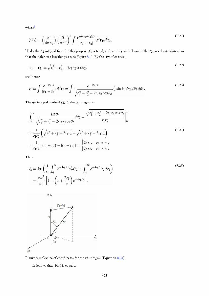
(8.21)
(8.22)
(8.23)
(8.24)
(8.25)
where9
I’ll do the integral first; for this purpose is fixed, and we may as well orient the coordinate system sothat the polar axis lies along (see Figure 8.4). By the law of cosines,
and hence
The integral is trivial ; the integral is
Thus
Figure 8.4: Choice of coordinates for the -integral (Equation 8.21).
It follows that is equal to
425
(8.26)
(8.28)
(8.29)
(8.30)
(8.31)
(8.27)
The angular integrals are easy , and the integral becomes
Finally, then,
and therefore
Not bad (remember, the experimental value is eV). But we can do better.We need to think up a more realistic trial function than (which treats the two electrons as though
they did not interact at all). Rather than completely ignoring the influence of the other electron, let us say that,on the average, each electron represents a cloud of negative charge which partially shields the nucleus, so thatthe other electron actually sees an effective nuclear charge that is somewhat less than 2. This suggests thatwe use a trial function of the form
We’ll treat Z as a variational parameter, picking the value that minimizes . (Please note that in thevariational method we never touch the Hamiltonian itself —the Hamiltonian for helium is, and remains,Equation 8.15. But it’s fine to think about approximating the Hamiltonian as a way of motivating the choice ofthe trial wave function.)
This wave function is an eigenstate of the “unperturbed” Hamiltonian (neglecting electron repulsion),only with Z, instead of 2, in the Coulomb terms. With this in mind, we rewrite H (Equation 8.15) as follows:
The expectation value of H is evidently
Here is the expectation value of in the (one-particle) hydrogenic ground state (with nuclearcharge Z); according to Equation 7.56,
426

(8.32)
(8.33)
(8.34)
(8.35)
∗
The expectation value of is the same as before (Equation 8.26), except that instead of we now wantarbitrary Z—so we multiply a by :
Putting all this together, we find
According to the variational principle, this quantity exceeds for any value of Z. The lowest upperbound occurs when is minimized:
from which it follows that
This seems reasonable; it tells us that the other electron partially screens the nucleus, reducing its effectivecharge from 2 down to about 1.69. Putting in this value for Z, we find
The ground state of helium has been calculated with great precision in this way, using increasinglycomplicated trial wave functions, with more and more adjustable parameters.10 But we’re within 2% of thecorrect answer, and, frankly, at this point my own interest in the problem begins to wane.11
Problem 8.7 Using eV for the ground state energy of helium,calculate the ionization energy (the energy required to remove just one electron).Hint: First calculate the ground state energy of the helium ion, He+, with a singleelectron orbiting the nucleus; then subtract the two energies.
Problem 8.8 Apply the techniques of this Section to the H − and Li+ ions (eachhas two electrons, like helium, but nuclear charges and ,respectively). Find the effective (partially shielded) nuclear charge, and determinethe best upper bound on , for each case. Comment: In the case of H − youshould find that eV, which would appear to indicate that there isno bound state at all, since it would be energetically favorable for one electron tofly off, leaving behind a neutral hydrogen atom. This is not entirely surprising,since the electrons are less strongly attracted to the nucleus than they are inhelium, and the electron repulsion tends to break the atom apart. However, itturns out to be incorrect. With a more sophisticated trial wave function (see
427

Problem 8.25) it can be shown that eV, and hence that a boundstate does exist. It’s only barely bound, however, and there are no excited boundstates,12 so H − has no discrete spectrum (all transitions are to and from thecontinuum). As a result, it is difficult to study in the laboratory, although it existsin great abundance on the surface of the sun.13
428

(8.36)
(8.37)
(8.38)
(8.39)
8.3 The Hydrogen Molecule IonAnother classic application of the variational principle is to the hydrogen molecule ion, H , consisting of asingle electron in the Coulomb field of two protons (Figure 8.5). I shall assume for the moment that theprotons are fixed in position, a specified distance R apart, although one of the most interesting byproducts ofthe calculation is going to be the actual value of R. The Hamiltonian is
where r and are the distances to the electron from the respective protons. As always, our strategy will be toguess a reasonable trial wave function, and invoke the variational principle to get a bound on the ground stateenergy. (Actually, our main interest is in finding out whether this system bonds at all—that is, whether itsenergy is less than that of a neutral hydrogen atom plus a free proton. If our trial wave function indicates thatthere is a bound state, a better trial function can only make the bonding even stronger.)
Figure 8.5: The hydrogen molecule ion, .
To construct the trial wave function, imagine that the ion is formed by taking a hydrogen atom in itsground state (Equation 4.80),
bringing the second proton in from “infinity,” and nailing it down a distance R away. If R is substantiallygreater than the Bohr radius, the electron’s wave function probably isn’t changed very much. But we wouldlike to treat the two protons on an equal footing, so that the electron has the same probability of beingassociated with either one. This suggests that we consider a trial function of the form
(Quantum chemists call this the LCAO technique, because we are expressing the molecular wave function as alinear combination of atomic orbitals.)
Our first task is to normalize the trial function:
429
(8.40)
(8.41)
(8.42)
(8.43)
(8.44)
The first two integrals are 1 (since itself is normalized); the third is more tricky. Let
Picking coordinates so that proton 1 is at the origin and proton 2 is on the z axis at the point R (Figure 8.6),we have
and therefore
The ϕ integral is trivial . To do the θ integral, let , so that Then
The r integral is now straightforward:
Evaluating the integrals, we find (after some algebraic simplification),
I is called an overlap integral; it measures the amount by which overlaps (notice that it goes to 1as , and to 0 as ). In terms of I, the normalization factor (Equation 8.39) is
430

(8.45)
(8.46)
(8.47)
(8.48)
(8.49)
Figure 8.6: Coordinates for the calculation of I (Equation 8.40).
Next we must calculate the expectation value of H in the trial state . Noting that
(where eV is the ground state energy of atomic hydrogen)—and the same with in place of r—we have
It follows that
I’ll let you calculate the two remaining quantities, the so-called direct integral,
and the exchange integral,
The results (see Problem 8.9) are
and
431

(8.50)
(8.51)
(8.52)
∗
Putting all this together, and recalling (Equations 4.70 and 4.72) that , weconclude:
According to the variational principle, the ground state energy is less than . Of course, this is only theelectron’s energy—there is also potential energy associated with the proton–proton repulsion:
Thus the total energy of the system, in units of , and expressed as a function of , is less than
This function is plotted in Figure 8.7. Evidently bonding does occur, for there exists a region in which thegraph goes below , indicating that the energy is less than that of a neutral atom plus a free proton eV). It’s a covalent bond, with the electron shared equally by the two protons. The equilibrium separation ofthe protons is about 2.4 Bohr radii, or 1.3 Å (the experimental value is 1.06 Å). The calculated binding energyis 1.8 eV, whereas the experimental value is 2.8 eV (the variational principle, as always, over estimates theground state energy—and hence under estimates the strength of the bond—but never mind: The essentialpoint was to see whether binding occurs at all; a better variational function can only make the potential welleven deeper.
Figure 8.7: Plot of the function , Equation 8.52, showing existence of a bound state.
Problem 8.9 Evaluate D and X (Equations 8.46 and 8.47). Check your answersagainst Equations 8.48 and 8.49.
432
∗∗
(8.53)
∗∗∗
Problem 8.10 Suppose we used a minus sign in our trial wave function (Equation8.38):
Without doing any new integrals, find (the analog to Equation 8.52) for thiscase, and construct the graph. Show that there is no evidence of bonding.14 (Sincethe variational principle only gives an upper bound, this doesn’t prove that bondingcannot occur for such a state, but it certainly doesn’t look promising.)
Problem 8.11 The second derivative of , at the equilibrium point, can beused to estimate the natural frequency of vibration of the two protons in thehydrogen molecule ion (see Section 2.3). If the ground state energy of thisoscillator exceeds the binding energy of the system, it will fly apart. Show that infact the oscillator energy is small enough that this will not happen, and estimatehow many bound vibrational levels there are. Note: You’re not going to be able toobtain the position of the minimum—still less the second derivative at that point—analytically. Do it numerically, on a computer.
433

(8.54)
(8.55)
(8.56)
(8.58)
8.4 The Hydrogen MoleculeNow consider the hydrogen molecule itself, adding a second electron to the hydrogen molecule ion we studiedin Section 8.3. Taking the two protons to be at rest, the Hamiltonian is
where and are the distances of electron 1 from each proton and and are the distances of electron 2from each proton; as shown in Figure 8.8. The six potential energy terms describe the repulsion between thetwo electrons, the repulsion between the two protons, and the attraction of each electron to each proton.
Figure 8.8: Diagram of H showing the distances on which the potential energy depends.
For the variational wave function, associate one electron with each proton, and symmetrize:
We’ll calculate the normalization in a moment. Since this spatial wave function is symmetric underinterchange, the electrons must occupy the antisymmetric (singlet) spin state. Of course, we could also choosethe trial wave function
in which case the electrons would be in a symmetric (triplet) spin state. These two variational wave functionsconstitute the Heitler–London approximation.15 It is not obvious which of Equations 8.55 or 8.56 would beenergetically favored, so let’s calculate the energy of each one, and find out.16
First we need to normalize the wave functions. Note that
Normalization requires
434
(8.59)
(8.60)
(8.61)
(8.62)
(8.63)
The individual orbitals are normalized and the overlap integral was given the symbol I and calculated inEquation 8.43. Thus
To calculate the expectation value of the energy, we will start with the kinetic energy of particle 1. Since is the ground state of the hydrogen Hamiltonian, the same trick that brought us to Equation 8.45 gives
Taking the inner product with then gives
These inner products were calculated in Section 8.3 and the kinetic energy of particle 1 is
The kinetic energy of particle 2 is of course the same, so the total kinetic energy is simply twiceEquation 8.62. The calculation of the electron–proton potential energy is similar; you will show inProblem 8.13 that
435
(8.64)
(8.65)
(8.66)
(8.67)
(8.68)
and the total electron–proton potential energy is four times this amount.The electron–electron potential energy is given by
The first two integrals in Equation 8.64 are equal, as you can see by interchanging the labels 1 and 2. We willgive the two remaining integrals the names
so that
The evaluation of these integrals is discussed in Problem 8.14. Note that the integral is just theelectrostatic potential energy of two charge distributions and . The exchangeterm has no such classical counterpart.
When we add all of the contributions to the energy—the kinetic energy, the electron–proton potentialenergy, the electron–electron potential energy, and the proton–proton potential energy (which is a constant,
)—we get
A plot of and is shown in Figure 8.9. Recall that the state requires placing the two electronsin the singlet spin configuration, whereas means putting them in a triplet spin configuration. According tothe figure, bonding only occurs if the two electrons are in a singlet configuration—something that isconfirmed experimentally. Again, it’s a covalent bond.
436

(8.69)
Figure 8.9: The total energy of the singlet (solid curve) and triplet (dashed curve) states for H , as a functionof the separation R between the protons. The singlet state has a minimum at around 1.6 Bohr radii,representing a stable bond. The triplet state is unstable and will dissociate, as the energy is minimized for
.
Locating the minimum on the plot, our calculation predicts a bond length of 1.64 Bohr radii (theexperimental value is 1.40 Bohr radii), and suggests a binding energy of 3.15 eV (whereas the experimentalvalue is 4.75 eV). The trends here follow those of the Hydrogen molecule ion: the calculation overestimatesthe bond length and underestimates the binding energy, but the agreement is surprisingly good for avariational calculation with no adjustable parameters.
The difference between the singlet and triplet energies is called the exchange splitting J. In the Heitler–London approximation it is
which is roughly (negative because the singlet is lower in energy) at the equilibrium separation. Thismeans a strong preference for having the electron spins anti-aligned. But in this treatment of H2 we’ve left outcompletely the (magnetic) spin–spin interaction between the electrons—remember that the spin–spininteraction between the proton and the electron is what leads to hyperfine splitting (Section 7.5). Were weright to ignore it here? Absolutely: applying Equation 7.92 to two electrons a distance R apart, the energy ofthe spin–spin interaction is something like in this system, five orders of magnitude smaller than theexchange splitting.
This calculation shows us that different spin configurations can have very different energies, even whenthe interaction between the spins is negligible. And that helps us understand ferromagnetism (where the spinsin a material align) and anti-ferromagnetism (where the spins alternate). As we’ve just seen, the spin–spininteraction is way too weak to account for this—but the exchange splitting isn’t. Counterintuitively, it’s not amagnetic interaction that accounts for ferromagnetism, but an electrostatic one! H2 is a sort of inchoate anti-ferromagnet where the Hamiltonian, which is independent of the spin, selects a certain spatial ground stateand the spin state comes along for the ride, to satisfy the Fermi statistics.
437

∗∗∗
(8.70)
Problem 8.12 Show that the antisymmetric state (Equation 8.56) can be expressedin terms of the molecular orbitals of Section 8.3—specifically, by placing oneelectron in the bonding orbital (Equation 8.38) and one in the anti-bondingorbital (Equation 8.53).
Problem 8.13 Verify Equation 8.63 for the electron–proton potential energy.
Problem 8.14 The two-body integrals and are defined in Equations 8.65and 8.66. To evaluate we write
where is the angle between and (Figure 8.8), and
(a) Consider first the integral over . Align the z axis with (which is aconstant vector for the purposes of this first integral) so that
Do the angular integration first and show that
(b) Plug your result from part (a) back into the relation for , and show that
Again, do the angular integration first.Comment: The integral can also be evaluated in closed form, but the procedureis rather involved.17 We will simply quote the result,
438

(8.72)
(8.71)
∗
where is Euler’s constant, is the exponentialintegral
and is obtained from I by switching the sign of R:
Problem 8.15 Make a plot of the kinetic energy for both the singlet and tripletstates of H2, as a function of . Do the same for the electron-proton potentialenergy and for the electron–electron potential energy. You should find that thetriplet state has lower potential energy than the singlet state for all values of R.However, the singlet state’s kinetic energy is so much smaller that its total energycomes out lower. Comment: In situations where there is not a large kinetic energycost to aligning the spins, such as two electrons in a partially filled orbital in anatom, the triplet state can come out lower in energy. This is the physics behindHund’s first rule.
439

∗∗
Further Problems on Chapter 8
Problem 8.16(a) Use the function (for , otherwise 0) to
get an upper bound on the ground state of the infinite square well.(b) Generalize to a function of the form , for some
real number p. What is the optimal value of p, and what is the best boundon the ground state energy? Compare the exact value. Answer:
.
Problem 8.17(a) Use a trial wave function of the form
to obtain a bound on the ground state energy of the one-dimensionalharmonic oscillator. What is the “best” value of a? Compare withthe exact energy. Note: This trial function has a “kink” in it (adiscontinuous derivative) at ; do you need to take account of this,as I did in Example 8.3?
(b) Use on the interval to obtain a bound onthe first excited state. Compare the exact answer.
Problem 8.18(a) Generalize Problem 8.2, using the trial wave function18
for arbitrary n. Partial answer: The best value of b is given by
(b) Find the least upper bound on the first excited state of the harmonicoscillator using a trial function of the form
Partial answer: The best value of b is given by
440
∗∗
(8.73)
(8.74)
(8.75)
(c) Notice that the bounds approach the exact energies as . Why isthat? Hint: Plot the trial wave functions for , , and ,and compare them with the true wave functions (Equations 2.60 and2.63). To do it analytically, start with the identity
Problem 8.19 Find the lowest bound on the ground state of hydrogen you can getusing a gaussian trial wave function
where A is determined by normalization and b is an adjustable parameter.Answer: eV.
Problem 8.20 Find an upper bound on the energy of the first excited state of thehydrogen atom. A trial function with will automatically be orthogonalto the ground state (see footnote 6); for the radial part of you can use thesame function as in Problem 8.19.
Problem 8.21 If the photon had a nonzero mass , the Coulombpotential would be replaced by the Yukawa potential,
where . With a trial wave function of your own devising, estimatethe binding energy of a “hydrogen” atom with this potential. Assume ,and give your answer correct to order .
Problem 8.22 Suppose you’re given a two-level quantum system whose (time-independent) Hamiltonian admits just two eigenstates, (with energy
), and (with energy ). They are orthogonal, normalized, andnondegenerate (assume is the smaller of the two energies). Now we turn ona perturbation , with the following matrix elements:
where h is some specified constant.(a) Find the exact eigenvalues of the perturbed Hamiltonian.(b) Estimate the energies of the perturbed system using second-order
perturbation theory.(c) Estimate the ground state energy of the perturbed system using the
variational principle, with a trial function of the form
where ϕ is an adjustable parameter. Note: Writing the linear combination441
(8.76)
(8.77)
∗∗∗
(8.79)
(8.80)
(8.78)
where ϕ is an adjustable parameter. Note: Writing the linear combinationin this way is just a neat way to guarantee that is normalized.
(d) Compare your answers to (a), (b), and (c). Why is the variationalprinciple so accurate, in this case?
Problem 8.23 As an explicit example of the method developed in Problem 8.22,consider an electron at rest in a uniform magnetic field , for whichthe Hamiltonian is (Equation 4.158):
The eigenspinors, and , and the corresponding energies, and , aregiven in Equation 4.161. Now we turn on a perturbation, in the form of auniform field in the x direction:
(a) Find the matrix elements of , and confirm that they have the structureof Equation 8.74. What is h?
(b) Using your result in Problem 8.22(b), find the new ground state energy,in second-order perturbation theory.
(c) Using your result in Problem 8.22(c), find the variational principle boundon the ground state energy.
Problem 8.24 Although the Schrödinger equation for helium itself cannot besolved exactly, there exist “helium-like” systems that do admit exact solutions.A simple example19 is “rubber-band helium,” in which the Coulomb forces arereplaced by Hooke’s law forces:
(a) Show that the change of variables from , , to
turns the Hamiltonian into two independent three-dimensional harmonicoscillators:
(b) What is the exact ground state energy for this system?(c) If we didn’t know the exact solution, we might be inclined to apply the
method of Section 8.2 to the Hamiltonian in its original form (Equation
442
∗∗∗
(8.82)
(8.81)
∗∗∗
8.78). Do so (but don’t bother with shielding). How does your resultcompare with the exact answer? Answer: .
Problem 8.25 In Problem 8.8 we found that the trial wave function with shielding(Equation 8.28), which worked well for helium, is inadequate to confirm theexistence of a bound state for the negative hydrogen ion.Chandrasekhar20 used a trial wave function of the form
where
In effect, he allowed two different shielding factors, suggesting that oneelectron is relatively close to the nucleus, and the other is farther out. (Becauseelectrons are identical particles, the spatial wave function must be symmetrizedwith respect to interchange. The spin state—which is irrelevant to thecalculation—is evidently antisymmetric.) Show that by astute choice of theadjustable parameters and you can get less than eV.Answer:
where and . Chandrasekhar used (since this is larger than 1, the motivating interpretation as an effective nuclearcharge cannot be sustained, but never mind—it’s still an acceptable trial wavefunction) and .
Problem 8.26 The fundamental problem in harnessing nuclear fusion is gettingthe two particles (say, two deuterons) close enough together for the attractive(but short-range) nuclear force to overcome the Coulomb repulsion. The“bulldozer” method is to heat the particles up to fantastic temperatures, andallow the random collisions to bring them together. A more exotic proposal ismuon catalysis, in which we construct a “hydrogen molecule ion,” only withdeuterons in place of protons, and a muon in place of the electron. Predict theequilibrium separation distance between the deuterons in such a structure, andexplain why muons are superior to electrons for this purpose.21
Problem 8.27 Quantum dots. Consider a particle constrained to move in twodimensions in the cross-shaped region shown in Figure 8.10. The “arms” ofthe cross continue out to infinity. The potential is zero within the cross, andinfinite in the shaded areas outside. Surprisingly, this configuration admits apositive-energy bound state.22
443

Figure 8.10: The cross-shaped region for Problem 8.27.
(a) Show that the lowest energy that can propagate off to infinity is
any solution with energy less than that has to be a bound state. Hint: Goway out one arm (say, ), and solve the Schrödinger equation byseparation of variables; if the wave function propagates out to infinity, thedependence on x must take the form with .
(b) Now use the variational principle to show that the ground state hasenergy less than . Use the following trial wave function(suggested by Jim McTavish):
Normalize it to determine A, and calculate the expectation value of H.Answer:
Now minimize with respect to α, and show that the result is less than . Hint: Take full advantage of the symmetry of the problem—
you only need to integrate over 1/8 of the open region, since the otherseven integrals will be the same. Note however that whereas the trial wavefunction is continuous, its derivatives are not—there are “roof-lines” at thejoins, and you will need to exploit the technique of Example 8.3.23
444

(8.83)
(8.84)
(8.85)
(8.86)
(8.87)
Problem 8.28 In Yukawa’s original theory (1934), which remains a usefulapproximation in nuclear physics, the “strong” force between protons andneutrons is mediated by the exchange of π-mesons. The potential energy is
where r is the distance between the nucleons, and the range is related to themass of the meson: . Question: Does this theory account for theexistence of the deuteron (a bound state of the proton and the neutron)?
The Schrödinger equation for the proton/neutron system is (see Problem5.1):
where μ is the reduced mass (the proton and neutron have almost identicalmasses, so call them both m), and r is the position of the neutron (say) relativeto the proton: . Your task is to show that there exists a solutionwith negative energy (a bound state), using a variational trial wave function ofthe form
(a) Determine A, by normalizing .
(b) Find the expectation value of the Hamiltonian inthe state . Answer:
(c) Optimize your trial wave function, by setting . This tellsyou β as a function of γ (and hence—everything else being constant—of
), but let’s use it instead to eliminate γ in favor of β:
(d) Setting , plot as a function of β, for .What does this tell you about the binding of the deuteron? What is theminimum value of for which you can be confident there is a boundstate (look up the necessary masses)? The experimental value is 52 MeV.
Problem 8.29 Existence of Bound States. A potential “well” (in one dimension) isa function that is never positive for all , and goes to zeroat infinity as .24
(a) Prove the following Theorem: If a potential well supports at least445

∗∗
(8.88)
(8.89)
(8.90)
(8.91)
(a) Prove the following Theorem: If a potential well supports at leastone bound state, then any deeper/wider well for all will also support at least one bound state. Hint: Use the ground state of , , as a variational test function.
(b) Prove the following Corollary: Every potential well in one dimension hasa bound state.25 Hint: Use a finite square well (Section 2.6) for .
(c) Does the Theorem generalize to two and three dimensions? How aboutthe Corollary? Hint: You might want to review Problems 4.11 and 4.51.
Problem 8.30 Performing a variational calculation requires finding the minimumof the energy, as a function of the variational parameters. This is, in general, avery hard problem. However, if we choose the form of our trial wave functionjudiciously, we can develop an efficient algorithm. In particular, suppose weuse a linear combination of functions :
where the are the variational parameters. If the are an orthonormal set , but is not necessarily normalized, then is
where . Taking the derivative with respect to (andsetting the result equal to 0) gives26
recognizable as the jth row in an eigenvalue problem:
The smallest eigenvalue of this matrix gives a bound on the ground stateenergy and the corresponding eigenvector determines the best variational wavefunction of the form 8.88.(a) Verify Equation 8.90.(b) Now take the derivative of Equation 8.89 with respect to and show
that you get a result redundant with Equation 8.90.(c) Consider a particle in an infinite square well of width a, with a sloping
floor:
446

(8.57)
Using a linear combination of the first ten stationary states of the infinitesquare well as the basis functions,
determine a bound for the ground state energy in the case . Make a plot of the optimized variational wave
function. [Note: The exact result is .]
1 If the Hamiltonian admits scattering states, as well as bound states, then we’ll need an integral as well as a sum, but the argument isunchanged.
2 For a collection of interesting examples see W. N. Mei, Int. J. Math. Educ. Sci. Tech. 30, 513 (1999).3 There is no point in trying a function (such as the gaussian) that extends outside the well, because you’ll get , and Equation 8.1
tells you nothing.4 In practice this isn’t much of a limitation, and there are sometimes ways of estimating the accuracy. The binding energy of helium has been
calculated to many significant digits in this way (see for example G. W. Drake et al., Phys. Rev. A 65, 054501 (2002), or VladimirI. Korobov, Phys. Rev. A 66, 024501 (2002).
5 For a systematic extension of the variational principle to the calculation of excited state energies see, for example, Linus Pauling andE. Bright Wilson, Introduction to Quantum Mechanics, With Applications to Chemistry, McGraw-Hill, New York (1935, paperback edition1985), Section 26.
6 You can extend this trick to other symmetries. Suppose there is a Hermitian operator A such that . The ground state (assumingit is nondegenerate) must be an eigenstate of A; call the eigenvalue : . If you choose a variational function that is aneigenstate of A with a different eigenvalue: with , you can be certain that and are orthogonal (see Section 3.3). Foran application see Problem 8.20.
7 There do exist exactly soluble three-body problems with many of the qualitative features of helium, but using non-Coulombic potentials (seeProblem 8.24).
8 Here a is the ordinary Bohr radius and eV is the nth Bohr energy; recall that for a nucleus with atomic number Z, and (Problem 4.19). The spin configuration associated with Equation 8.18 will be antisymmetric (the singlet).
9 You can, if you like, interpret Equation 8.21 as first-order perturbation theory, with (Problem 7.56(a)). However, I regard this asa misuse of the method, since the perturbation is comparable in size to the unperturbed potential. I prefer, therefore, to think of it as avariational calculation, in which we are looking for a rigorous upper bound on .
10 The classic studies are E. A. Hylleraas, Z. Phys. 65, 209 (1930); C. L. Pekeris, Phys. Rev. 115, 1216 (1959). For more recent work, seefootnote 4.
11 The first excited state of helium can be calculated in much the same way, using a trial wave function orthogonal to the ground state. SeePhillip J. E. Peebles, Quantum Mechanics, Princeton U.P., Princeton, NJ (1992), Section 40.
12 Robert N. Hill, J. Math. Phys. 18, 2316 (1977).13 For further discussion see Hans A. Bethe and Edwin E. Salpeter, Quantum Mechanics of One- and Two-Electron Atoms, Plenum, New York
(1977), Section 34.14 The wave function with the plus sign (Equation 8.38) is called the bonding orbital. Bonding is associated with a buildup of electron
probability in between the two nuclei. The odd linear combination (Equation 8.53) has a node at the center, so it’s not surprising that thisconfiguration doesn’t lead to bonding; it is called the anti-bonding orbital.
15 W. Heitler and F. London, Z. Phys. 44, 455 (1928). For an English translation see Hinne Hettema, Quantum Chemistry: Classic ScientificPapers, World Scientific, New Jersey, PA, 2000.
16 Another natural variational wave function consists of placing both electrons in the bonding orbital studied in Section 8.3:
also paired with a singlet spin state. If you expand this function you’ll see that half the terms—such as —involve attaching447
also paired with a singlet spin state. If you expand this function you’ll see that half the terms—such as —involve attachingtwo electrons to the same proton, which is energetically costly because of the electron–electron repulsion in Equation 8.54. The Heitler–London approximation, Equation 8.55, amounts to dropping the offending terms from Equation 8.57.
17 The calculation was done by Y. Sugiura, Z. Phys. 44, 455 (1927).18 W. N. Mei, Int. J. Educ. Sci. Tech. 27, 285 (1996).19 For a more sophisticated model, see R. Crandall, R. Whitnell, and R. Bettega, Am. J. Phys 52, 438 (1984).20 S. Chandrasekhar, Astrophys. J. 100, 176 (1944).21 The classic paper on muon-catalyzed fusion is J. D. Jackson, Phys. Rev. 106, 330 (1957); for a more recent popular review, see J. Rafelski
and S. Jones, Scientific American, November 1987, page 84.22 This model is taken from R. L. Schult et al., Phys. Rev. B 39, 5476 (1989). For further discussion see J. T. Londergan and D. P. Murdock,
Am. J. Phys. 80, 1085 (2012). In the presence of quantum tunneling a classically bound state can become unbound; this is the reverse: Aclassically unbound state is quantum mechanically bound.
23 W.-N. Mei gets a somewhat better bound (and avoids the roof-lines) using
but the integrals have to be done numerically.24 To exclude trivial cases, we also assume it has nonzero area . Notice that for the purposes of this problem neither the
infinite square well nor the harmonic oscillator is a “potential well,” though both of them, of course, have bound states.25 K. R. Brownstein, Am. J. Phys. 68, 160 (2000) proves that any one-dimensional potential satisfying admits a bound
state (as long as is not identically zero)—even if it runs positive in some places.26 Each , being complex, stands for two independent parameters (its real and imaginary parts). One could take derivatives with respect to the
real and imaginary parts,
but it is also legitimate (and simpler) to treat and as the independent parameters:
You get the same result either way.
448

9The WKB Approximation
◈
The WKB (Wentzel, Kramers, Brillouin)1 method is a technique for obtaining approximate solutions to thetime-independent Schrödinger equation in one dimension (the same basic idea can be applied to many otherdifferential equations, and to the radial part of the Schrödinger equation in three dimensions). It is particularlyuseful in calculating bound state energies and tunneling rates through potential barriers.
The essential idea is as follows: Imagine a particle of energy E moving through a region where thepotential is constant. If , the wave function is of the form
The plus sign indicates that the particle is traveling to the right, and the minus sign means it is going to theleft (the general solution, of course, is a linear combination of the two). The wave function is oscillatory, withfixed wavelength and unchanging amplitude . Now suppose that is not constant, butvaries rather slowly in comparison to , so that over a region containing many full wavelengths the potential isessentially constant. Then it is reasonable to suppose that remains practically sinusoidal, except that thewavelength and the amplitude change slowly with x. This is the inspiration behind the WKB approximation.In effect, it identifies two different levels of x-dependence: rapid oscillations, modulated by gradual variation inamplitude and wavelength.
By the same token, if (and V is constant), then is exponential:
And if is not constant, but varies slowly in comparison with , the solution remains practicallyexponential, except that A and κ are now slowly-varying functions of x.
Now, there is one place where this whole program is bound to fail, and that is in the immediate vicinityof a classical turning point, where . For here (or goes to infinity, and can hardly be saidto vary “slowly” in comparison. As we shall see, a proper handling of the turning points is the most difficultaspect of the WKB approximation, though the final results are simple to state and easy to implement.
449

(9.1)
(9.2)
(9.3)
(9.4)
(9.5)
(9.6)
(9.7)
9.1 The “Classical” RegionThe Schrödinger equation,
can be rewritten in the following way:
where
is the classical formula for the (magnitude of the) momentum of a particle with total energy E and potentialenergy . For the moment, I’ll assume that , so that is real; we call this the “classical”region, for obvious reasons—classically the particle is confined to this range of x (see Figure 9.1). In general, is some complex function; we can express it in terms of its amplitude, , and its phase, —both ofwhich are real:
Using a prime to denote the derivative with respect to x,
and
Putting this into Equation 9.1:
This is equivalent to two real equations, one for the real part and one for the imaginary part:
and
450

(9.8)
(9.9)
(9.10)
(9.11)
Figure 9.1: Classically, the particle is confined to the region where .
Equations 9.6 and 9.7 are entirely equivalent to the original Schrödinger equation. The second one iseasily solved:
where C is a (real) constant. The first one (Equation 9.6) cannot be solved in general—so here comes theapproximation: We assume that the amplitude A varies slowly, so the term is negligible. (More precisely, weassume that is much less than both and .) In that case we can drop the left side ofEquation 9.6, and we are left with
and therefore
(I’ll write this as an indefinite integral, for now—any constant of integration can be absorbed into C, whichthereby becomes complex. I’ll also absorb a factor of .) Then
Notice that
which says that the probability of finding the particle at point x is inversely proportional to its (classical)momentum (and hence its velocity) at that point. This is exactly what you would expect—the particle doesn’tspend long in the places where it is moving rapidly, so the probability of getting caught there is small. In fact,the WKB approximation is sometimes derived by starting with this “semi-classical” observation, instead of bydropping the term in the differential equation. The latter approach is cleaner mathematically, but theformer offers a more illuminating physical rationale. The general (approximate) solution, of course, will be alinear combination the two solutions in Equation 9.10, one with each sign.
451
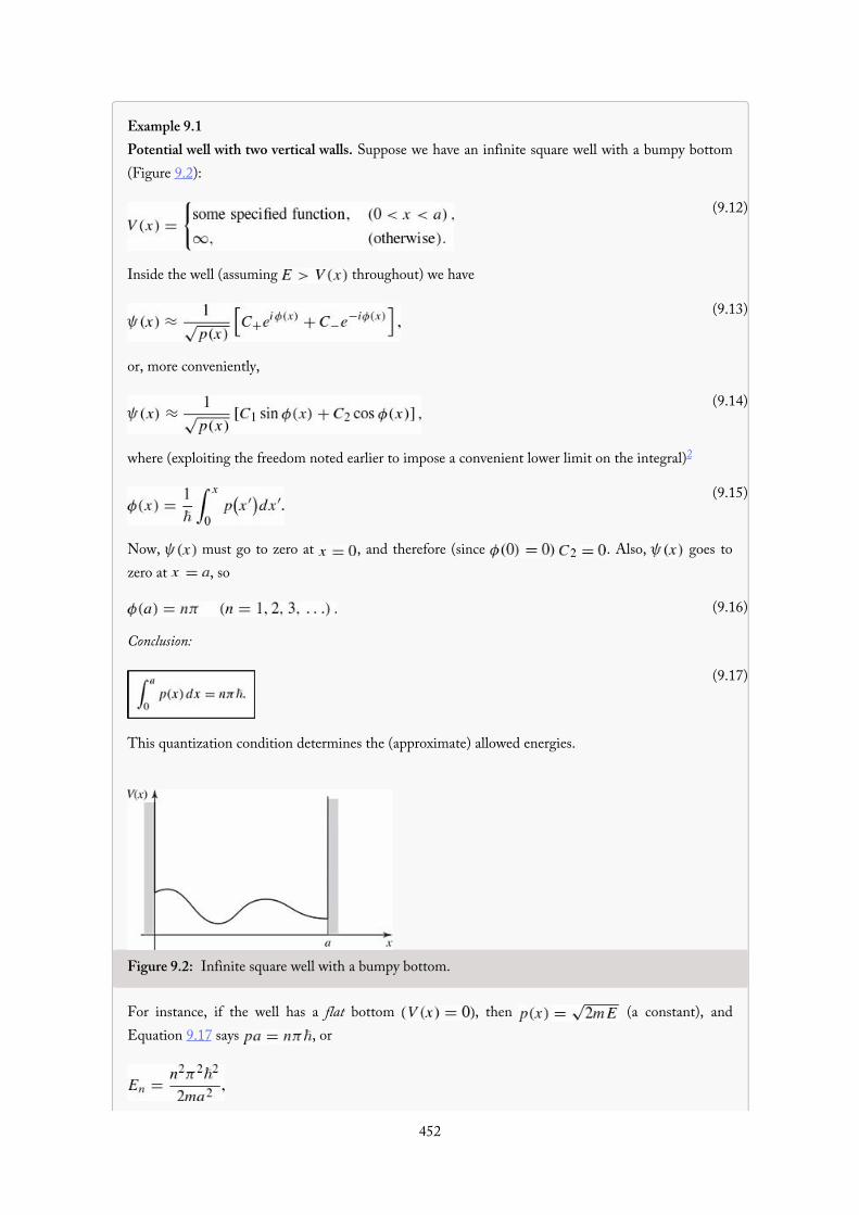
(9.12)
(9.13)
(9.14)
(9.15)
(9.17)
(9.16)
Example 9.1Potential well with two vertical walls. Suppose we have an infinite square well with a bumpy bottom(Figure 9.2):
Inside the well (assuming throughout) we have
or, more conveniently,
where (exploiting the freedom noted earlier to impose a convenient lower limit on the integral)2
Now, must go to zero at , and therefore (since . Also, goes tozero at , so
Conclusion:
This quantization condition determines the (approximate) allowed energies.
Figure 9.2: Infinite square well with a bumpy bottom.
For instance, if the well has a flat bottom , then (a constant), andEquation 9.17 says , or
452

∗
∗∗
which is the old formula for the energy levels of the infinite square well (Equation 2.30). In this casethe WKB approximation yields the exact answer (the amplitude of the true wave function is constant,so dropping cost us nothing).
Problem 9.1 Use the WKB approximation to find the allowed energies of aninfinite square well with a “shelf,” of height , extending half-way across(Figure 7.3):
Express your answer in terms of and (the nth allowedenergy for the infinite square well with no shelf). Assume that , but donot assume that . Compare your result with what we got inSection 7.1.2, using first-order perturbation theory. Note that they are inagreement if either is very small (the perturbation theory regime) or n is verylarge (the WKB—semi-classical—regime).
Problem 9.2 An alternative derivation of the WKB formula (Equation 9.10) isbased on an expansion in powers of . Motivated by the free-particle wavefunction, , we write
where is some complex function. (Note that there is no loss of generalityhere—any nonzero function can be written in this way.)
(a) Put this into Schrödinger’s equation (in the form of Equation 9.1), andshow that
(b) Write as a power series in :
and, collecting like powers of , show that
(c) Solve for and , and show that—to first order in —yourecover Equation 9.10.
Note: The logarithm of a negative number is defined by ,where n is an odd integer. If this formula is new to you, try exponentiating bothsides, and you’ll see where it comes from.
453

454

(9.18)
(9.19)
(9.20)
(9.21)
(9.22)
9.2 TunnelingSo far, I have assumed that , so is real. But we can easily write down the corresponding result inthe non-classical region —it’s the same as before (Equation 9.10), only now is imaginary:3
Consider, for example, the problem of scattering from a rectangular barrier with a bumpy top(Figure 9.3). To the left of the barrier ,
where A is the incident amplitude, B is the reflected amplitude, and (see Section 2.5). To theright of the barrier ,
where F is the transmitted amplitude. The transmission probability is
In the tunneling region , the WKB approximation gives
Figure 9.3: Scattering from a rectangular barrier with a bumpy top.
If the barrier is very high and/or very wide (which is to say, if the probability of tunneling is small), thenthe coefficient of the exponentially increasing term must be small (in fact, it would be zero if the barrierwere infinitely broad), and the wave function looks something like4 Figure 9.4. The relative amplitudes of theincident and transmitted waves are determined essentially by the total decrease of the exponential over thenonclassical region:
455
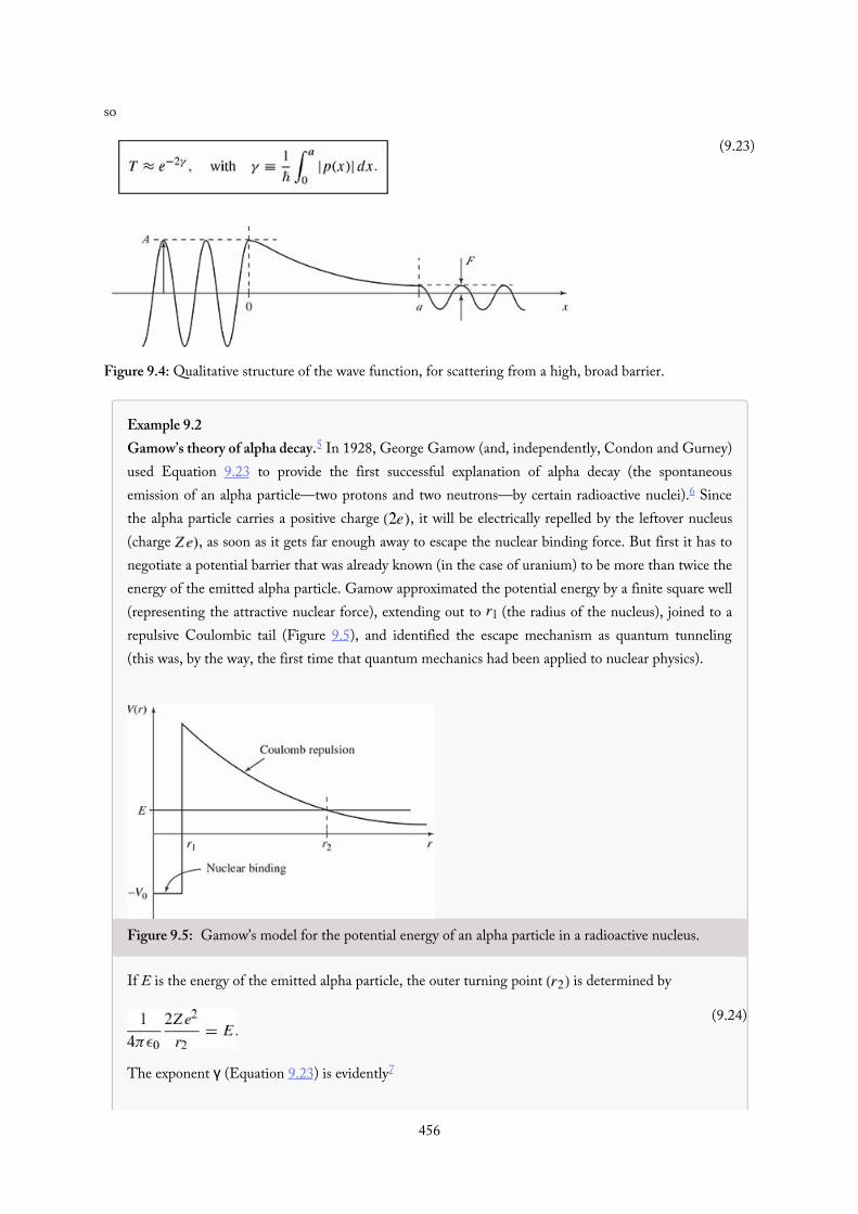
(9.23)
(9.24)
so
Figure 9.4: Qualitative structure of the wave function, for scattering from a high, broad barrier.
Example 9.2Gamow’s theory of alpha decay.5 In 1928, George Gamow (and, independently, Condon and Gurney)used Equation 9.23 to provide the first successful explanation of alpha decay (the spontaneousemission of an alpha particle—two protons and two neutrons—by certain radioactive nuclei).6 Sincethe alpha particle carries a positive charge , it will be electrically repelled by the leftover nucleus(charge , as soon as it gets far enough away to escape the nuclear binding force. But first it has tonegotiate a potential barrier that was already known (in the case of uranium) to be more than twice theenergy of the emitted alpha particle. Gamow approximated the potential energy by a finite square well(representing the attractive nuclear force), extending out to (the radius of the nucleus), joined to arepulsive Coulombic tail (Figure 9.5), and identified the escape mechanism as quantum tunneling(this was, by the way, the first time that quantum mechanics had been applied to nuclear physics).
Figure 9.5: Gamow’s model for the potential energy of an alpha particle in a radioactive nucleus.
If E is the energy of the emitted alpha particle, the outer turning point is determined by
The exponent γ (Equation 9.23) is evidently7
456

(9.25)
(9.26)
(9.27)
(9.28)
(9.29)
The integral can be done by substitution , and the result is
Typically, , and we can simplify this result using the small angle approximation :
where
and
(One fermi (fm) is m, which is about the size of a typical nucleus.)If we imagine the alpha particle rattling around inside the nucleus, with an average velocity v, the
time between “collisions” with the “wall” is about , and hence the frequency of collisions is .The probability of escape at each collision is , so the probability of emission, per unit time, is
, and hence the lifetime of the parent nucleus is about
Unfortunately, we don’t know v—but it hardly matters, for the exponential factor varies over afantastic range (twenty-five orders of magnitude), as we go from one radioactive nucleus to another;relative to this the variation in v is pretty insignificant. In particular, if you plot the logarithm of theexperimentally measured lifetime against , the result is a beautiful straight line(Figure 9.6),8 just as you would expect from Equations 9.26 and 9.29.
457
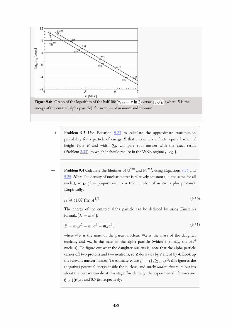
∗
∗∗
(9.30)
(9.31)
Figure 9.6: Graph of the logarithm of the half-life versus (where E is theenergy of the emitted alpha particle), for isotopes of uranium and thorium.
Problem 9.3 Use Equation 9.23 to calculate the approximate transmissionprobability for a particle of energy E that encounters a finite square barrier ofheight and width . Compare your answer with the exact result(Problem 2.33), to which it should reduce in the WKB regime .
Problem 9.4 Calculate the lifetimes of U238 and Po212, using Equations 9.26 and9.29. Hint: The density of nuclear matter is relatively constant (i.e. the same for allnuclei), so is proportional to A (the number of neutrons plus protons).Empirically,
The energy of the emitted alpha particle can be deduced by using Einstein’sformula :
where is the mass of the parent nucleus, is the mass of the daughternucleus, and is the mass of the alpha particle (which is to say, the He4
nucleus). To figure out what the daughter nucleus is, note that the alpha particlecarries off two protons and two neutrons, so Z decreases by 2 and A by 4. Look upthe relevant nuclear masses. To estimate v, use ; this ignores the(negative) potential energy inside the nucleus, and surely underestimates v, but it’sabout the best we can do at this stage. Incidentally, the experimental lifetimes are
yrs and 0.5 μs, respectively.
458

Problem 9.5 Zener Tunneling. In a semiconductor, an electric field (if it’s largeenough) can produce transitions between energy bands—a phenomenon known asZener tunneling. A uniform electric field , for which
makes the energy bands position dependent, as shown in Figure 9.7. It is thenpossible for an electron to tunnel from the valence (lower) band to the conduction(upper) band; this phenomenon is the basis for the Zener diode. Treating the gapas a potential barrier through which the electron may tunnel, find the tunnelingprobability in terms of and (as well as m, , .
Figure 9.7: (a) The energy bands in the absence of an electric field. (b) In thepresence of an electric field an electron can tunnel between the energy bands.
459

(9.32)
(9.33)
9.3 The Connection FormulasIn the discussion so far I have assumed that the “walls” of the potential well (or the barrier) are vertical, so thatthe “exterior” solution is simple, and the boundary conditions trivial. As it turns out, our main results(Equations 9.17 and 9.23) are reasonably accurate even when the edges are not so abrupt (indeed, in Gamow’stheory they were applied to just such a case). Nevertheless, it is of some interest to study more closely whathappens to the wave function at a turning point , where the “classical” region joins the “nonclassical”region, and the WKB approximation itself breaks down. In this section I’ll treat the bound state problem(Figure 9.1); you get to do the scattering problem for yourself (Problem 9.11).9
For simplicity, let’s shift the axes over so that the right hand turning point occurs at (Figure 9.8).In the WKB approximation, we have
(Assuming remains greater than E for all , we can exclude the positive exponent in this region,because it blows up as .) Our task is to join the two solutions at the boundary. But there is a seriousdifficulty here: In the WKB approximation, goes to infinity at the turning point (where . Thetrue wave function, of course, has no such wild behavior—as anticipated, the WKB method simply fails in thevicinity of a turning point. And yet, it is precisely the boundary conditions at the turning points thatdetermine the allowed energies. What we need to do, then, is splice the two WKB solutions together, using a“patching” wave function that straddles the turning point.
Figure 9.8: Enlarged view of the right-hand turning point.
Since we only need the patching wave function in the neighborhood of the origin, we’ll approximatethe potential by a straight line:
and solve the Schrödinger equation for this linearized V:
460

(9.34)
(9.35)
(9.37)
(9.36)
(9.38)
or
where
The αs can be absorbed into the independent variable by defining
so that
This is Airy’s equation, and the solutions are called Airy functions.10 Since the Airy equation is a second-order differential equation, there are two linearly independent Airy functions, Ai and Bi . They arerelated to Bessel functions of order 1/3; some of their properties are listed in Table 9.1 and they are plotted inFigure 9.9. Evidently the patching wave function is a linear combination of Ai and Bi :
for appropriate constants a and b.
Table 9.1: Some properties of the Airy functions.
461

(9.39)
(9.40)
Figure 9.9: Graph of the Airy functions.
Now, is the (approximate) wave function in the neighborhood of the origin; our job is to match it tothe WKB solutions in the overlap regions on either side (see Figure 9.10). These overlap zones are closeenough to the turning point that the linearized potential is reasonably accurate (so that is a goodapproximation to the true wave function), and yet far enough away from the turning point that the WKBapproximation is reliable.11 In the overlap regions Equation 9.33 holds, and therefore (in the notation ofEquation 9.35)
Figure 9.10: Patching region and the two overlap zones.
In particular, in overlap region 2,
and therefore the WKB wave function (Equation 9.32) can be written as
Meanwhile, using the large-z asymptotic forms12 of the Airy functions (from Table 9.1), the patching wave462

(9.41)
(9.42)
(9.43)
(9.44)
(9.45)
(9.46)
(9.47)
Meanwhile, using the large-z asymptotic forms12 of the Airy functions (from Table 9.1), the patching wavefunction (Equation 9.38) in overlap region 2 becomes
Comparing the two solutions, we see that
Now we go back and repeat the procedure for overlap region 1. Once again, is given by Equation9.39, but this time x is negative, so
and the WKB wave function (Equation 9.32) is
Meanwhile, using the asymptotic form of the Airy function for large negative z (Table 9.1), the patchingfunction (Equation 9.38, with reads
Comparing the WKB and patching wave functions in overlap region 1, we find
or, putting in Equation 9.42 for a:
These are the so-called connection formulas, joining the WKB solutions at either side of the turning point.We’re done with the patching wave function now—its only purpose was to bridge the gap. Expressingeverything in terms of the one normalization constant D, and shifting the turning point back from the originto an arbitrary point , the WKB wave function (Equation 9.32) becomes
Example 9.3Potential well with one vertical wall. Imagine a potential well that has one vertical side (at and
463

(9.48)
(9.49)
(9.50)
one sloping side (Figure 9.11). In this case , so Equation 9.47 says
or
For instance, consider the “half-harmonic oscillator”,
In this case
where
is the turning point. So
and the quantization condition (Equation 9.48) yields
In this particular case the WKB approximation actually delivers the exact allowed energies (which areprecisely the odd energies of the full harmonic oscillator—see Problem 2.41).
464

(9.51)
(9.52)
Figure 9.11: Potential well with one vertical wall.
Example 9.4Potential well with no vertical walls. Equation 9.47 connects the WKB wave functions at a turningpoint where the potential slopes upward (Figure 9.12(a)); the same reasoning, applied to a downward-sloping turning point (Figure 9.12(b)), yields (Problem 9.10)
In particular, if we’re talking about a potential well (Figure 9.12(c)), the wave function in the “interior”region can be written either as
(Equation 9.47), or as
(Equation 9.51). Evidently the arguments of the sine functions must be equal, modulo π:13 , from which it follows that
This quantization condition determines the allowed energies for the “typical” case of a potential wellwith two sloping sides. Notice that it differs from the formulas for two vertical walls (Equation 9.17)or one vertical wall (Equation 9.48) only in the number that is subtracted from n (0, 1/4, or 1/2).
465

∗∗
∗
Since the WKB approximation works best in the semi-classical (large regime, the distinction ismore in appearance than in substance. In any event, the result is extraordinarily powerful, for itenables us to calculate (approximate) allowed energies without ever solving the Schrödinger equation, bysimply evaluating one integral. The wave function itself has dropped out of sight.
Figure 9.12: Upward-sloping and downward-sloping turning points.
Problem 9.6 The “bouncing ball” revisited. Consider the quantum mechanicalanalog to the classical problem of a ball (mass bouncing elastically on thefloor.14
(a) What is the potential energy, as a function of height x above the floor?(For negative x, the potential is infinite—the ball can’t get there at all.)
(b) Solve the Schrödinger equation for this potential, expressing your answerin terms of the appropriate Airy function (note that Bi blows up forlarge z, and must therefore be rejected). Don’t bother to normalize .
(c) Using m/s2 and kg, find the first four allowedenergies, in joules, correct to three significant digits. Hint: See MiltonAbramowitz and Irene A. Stegun, Handbook of Mathematical Functions,Dover, New York (1970), page 478; the notation is defined on page 450.
(d) What is the ground state energy, in eV, of an electron in this gravitationalfield? How high off the ground is this electron, on the average? Hint: Usethe virial theorem to determine .
Problem 9.7 Analyze the bouncing ball (Problem 9.6) using the WKBapproximation.
(a) Find the allowed energies, , in terms of m, g, and .(b) Now put in the particular values given in Problem 9.6(c), and compare
the WKB approximation to the first four energies with the “exact” results.(c) About how large would the quantum number n have to be to give the ball
an average height of, say, 1 meter above the ground?
466
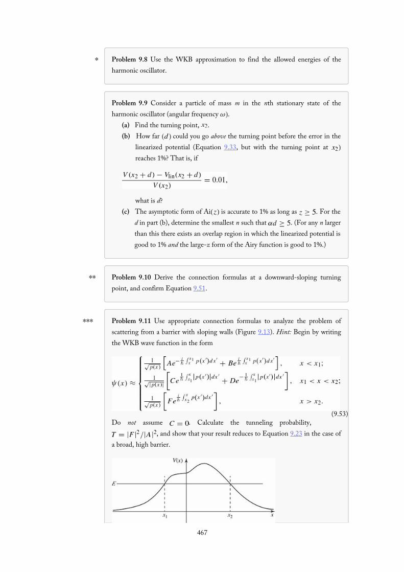
∗
∗∗
∗∗∗
(9.53)
Problem 9.8 Use the WKB approximation to find the allowed energies of theharmonic oscillator.
Problem 9.9 Consider a particle of mass m in the nth stationary state of theharmonic oscillator (angular frequency .
(a) Find the turning point, .(b) How far could you go above the turning point before the error in the
linearized potential (Equation 9.33, but with the turning point at reaches 1%? That is, if
what is d?(c) The asymptotic form of Ai is accurate to 1% as long as . For the
d in part (b), determine the smallest n such that . (For any n largerthan this there exists an overlap region in which the linearized potential isgood to 1% and the large-z form of the Airy function is good to 1%.)
Problem 9.10 Derive the connection formulas at a downward-sloping turningpoint, and confirm Equation 9.51.
Problem 9.11 Use appropriate connection formulas to analyze the problem ofscattering from a barrier with sloping walls (Figure 9.13). Hint: Begin by writingthe WKB wave function in the form
Do not assume . Calculate the tunneling probability, , and show that your result reduces to Equation 9.23 in the case of
a broad, high barrier.
467
∗∗
Figure 9.13: Barrier with sloping walls.
Problem 9.12 For the “half-harmonic oscillator” (Example 9.3), make a plotcomparing the normalized WKB wave function for to the exact solution.You’ll have to experiment to determine how wide to make the patching region.Note: You can do the integrals of by hand, but feel free to do themnumerically. You’ll need to do the integral of numerically to normalizethe wave function.
468

∗∗
(9.54)
∗∗
(9.55)
∗∗
(9.56)
(9.57)
Further Problems on Chapter 9
Problem 9.13 Use the WKB approximation to find the allowed energies of thegeneral power-law potential:
where ν is a positive number. Check your result for the case . Answer:15
Problem 9.14 Use the WKB approximation to find the bound state energy for thepotential in Problem 2.52. Compare the exact answer:
Problem 9.15 For spherically symmetrical potentials we can apply the WKBapproximation to the radial part (Equation 4.37). In the case it isreasonable16 to use Equation 9.48 in the form
where is the turning point (in effect, we treat as an infinite wall).Exploit this formula to estimate the allowed energies of a particle in thelogarithmic potential
(for constants and . Treat only the case . Show that the spacingbetween the levels is independent of mass. Partial answer:
Problem 9.16 Use the WKB approximation in the form of Equation 9.52,
to estimate the bound state energies for hydrogen. Don’t forget the centrifugalterm in the effective potential (Equation 4.38). The following integral mayhelp:
469
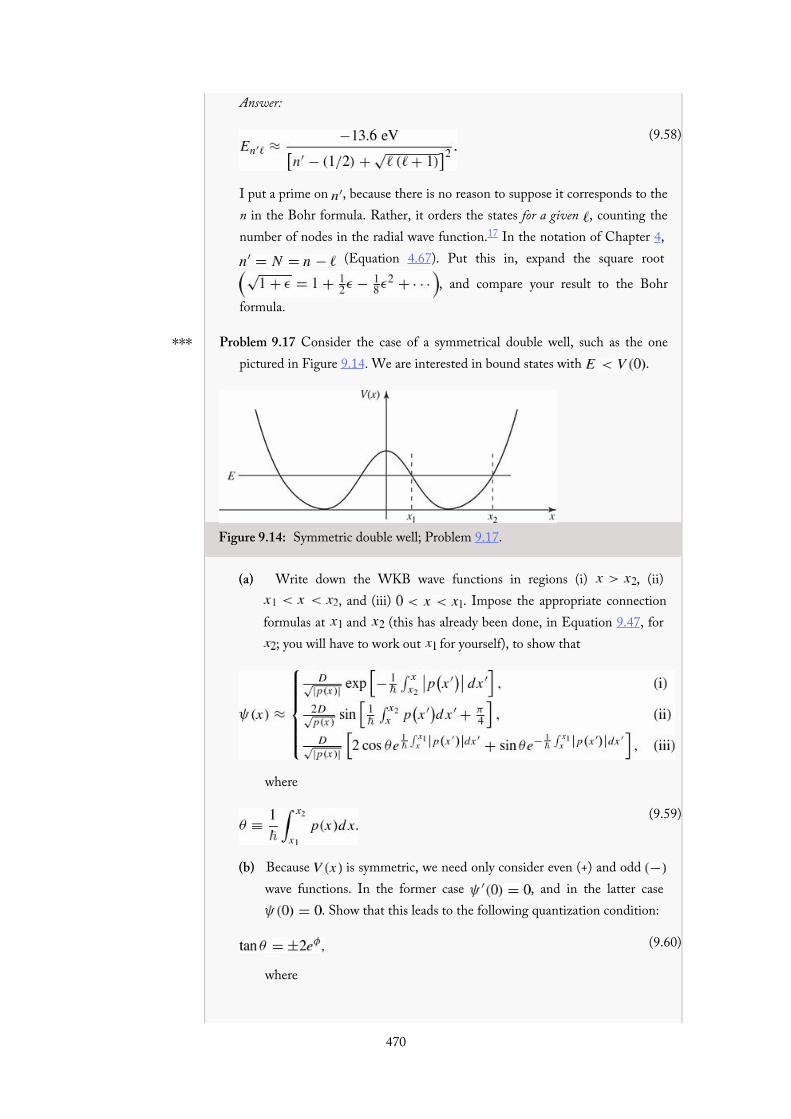
(9.58)
∗∗∗
(9.59)
(9.60)
Answer:
I put a prime on , because there is no reason to suppose it corresponds to then in the Bohr formula. Rather, it orders the states for a given , counting thenumber of nodes in the radial wave function.17 In the notation of Chapter 4,
(Equation 4.67). Put this in, expand the square root
, and compare your result to the Bohrformula.
Problem 9.17 Consider the case of a symmetrical double well, such as the onepictured in Figure 9.14. We are interested in bound states with .
Figure 9.14: Symmetric double well; Problem 9.17.
(a) Write down the WKB wave functions in regions (i) , (ii) , and (iii) . Impose the appropriate connection
formulas at and (this has already been done, in Equation 9.47, for ; you will have to work out for yourself), to show that
where
(b) Because is symmetric, we need only consider even (+) and odd wave functions. In the former case , and in the latter case
. Show that this leads to the following quantization condition:
where
470
(9.61)
(9.62)
(9.63)
(9.64)
(9.65)
Equation 9.60 determines the (approximate) allowed energies (note thatE comes into and , so θ and ϕ are both functions of .
(c) We are particularly interested in a high and/or broad central barrier, inwhich case ϕ is large, and is huge. Equation 9.60 then tells us that θmust be very close to a half-integer multiple of π. With this in mind,write , where , and show that thequantization condition becomes
(d) Suppose each well is a parabola:18
Sketch this potential, find θ (Equation 9.59), and show that
Comment: If the central barrier were impenetrable , we wouldsimply have two detached harmonic oscillators, and the energies,
, would be doubly degenerate, since the particlecould be in the left well or in the right one. When the barrier becomesfinite (putting the two wells into “communication”), the degeneracy islifted. The even states have slightly lower energy, and the odd ones
have slightly higher energy.(e) Suppose the particle starts out in the right well—or, more precisely, in a
state of the form
which, assuming the phases are picked in the “natural” way, will beconcentrated in the right well. Show that it oscillates back and forthbetween the wells, with a period
(f) Calculate ϕ, for the specific potential in part (d), and show that for , .
Problem 9.18 Tunneling in the Stark Effect. When you turn on an externalelectric field, the electron in an atom can, in principle, tunnel out, ionizing the
471
(9.66)
atom. Question: Is this likely to happen in a typical Stark effect experiment?We can estimate the probability using a crude one-dimensional model, asfollows. Imagine a particle in a very deep finite square well (Section 2.6).(a) What is the energy of the ground state, measured up from the bottom of
the well? Assume . Hint: This is just the ground stateenergy of the infinite square well (of width .
(b) Now introduce a perturbation (for an electron in an electricfield we would have . Assume it is relativelyweak . Sketch the total potential, and note that theparticle can now tunnel out, in the direction of positive x.
(c) Calculate the tunneling factor γ (Equation 9.23), and estimate the time itwould take for the particle to escape (Equation 9.29). Answer:
, .(d) Put in some reasonable numbers: eV (typical binding energy for
an outer electron), m (typical atomic radius), V/m (strong laboratory field), e and m the charge and mass of theelectron. Calculate τ, and compare it to the age of the universe.
Problem 9.19 About how long would it take for a (full) can of beer at roomtemperature to topple over spontaneously, as a result of quantum tunneling?Hint: Treat it as a uniform cylinder of mass m, radius R, and height h. As thecan tips, let x be the height of the center above its equilibrium position .The potential energy is mgx, and it topples when x reaches the critical value
. Calculate the tunneling probability (Equation9.23), for . Use Equation 9.29, with the thermal energy
to estimate the velocity. Put in reasonablenumbers, and give your final answer in years.19
Problem 9.20 Equation 9.23 tells us the (approximate) transmission probabilityfor tunneling through a barrier, when —a classically forbiddenprocess. In this problem we explore the complementary phenomenon:reflection from a barrier when (again, a classically forbiddenprocess). We’ll assume that is an even analytic function, that goes to zeroas (Figure 9.15). Question: What is the analog to Equation 9.23?(a) Try the obvious approach: assume the potential vanishes for , and
use the WKB approximation (Equation 9.13) in the scattering region:
Impose the usual boundary conditions at , and solve for the reflectionprobability, .
472

(9.67)
Figure 9.15: Reflection from a barrier (Problem 9.20).
Unfortunately, the result is uninformative. It’s true that the Ris exponentially small (just as the transmission coefficient is, for
, but we’ve thrown the baby out with the bath water—thisapproximation is simply too drastic. The correct formula is
and is defined by . Notice that (like γ in Equation 9.23)goes like ; it is in fact the leading term in an expansion in powers of :
. In the classical limit , and γ go to infinity, so R and T go to zero, as expected. It is not easy toderive Equation 9.67,20 but let’s look at some examples.
(b) Suppose , for some positive constants and a.Plot , plot for , and show that
. Plot R as a function of E, for fixed .
(c) Suppose . Plot , and express in termsof an elliptic integral. Plot R as a function of E.
1 In Holland it’s KWB, in France it’s BWK, and in England it’s JWKB (for Jeffreys).2 We might as well take the positive sign, since both are covered by Equation 9.13.3 In this case the wave function is real, and the analogs to Equations 9.6 and 9.7 do not follow necessarily from Equation 9.5, although they are
still sufficient. If this bothers you, study the alternative derivation in Problem 9.2.4 This heuristic argument can be made more rigorous—see Problem 9.11.5 For a more complete discussion, and alternative formulations, see B. R. Holstein, Am. J. Phys. 64, 1061 (1996).6 For an interesting brief history see E. Merzbacher, “The Early History of Quantum Tunneling,” Physics Today, August 2002, p. 44.7 In this case the potential does not drop to zero on the left side of the barrier (moreover, this is really a three-dimensional problem), but the
essential idea, contained in Equation 9.23, is all we really need.8 This figure is reprinted by permission from David Park, Introduction to the Quantum Theory, 3rd edn, Dover Publications, New York (2005);
it was adapted from I. Perlman and J. O. Rasmussen, “Alpha Radioactivity,” Encyclopedia of Physics, Vol. 42, Springer (1957).9 Warning: The following argument is quite technical, and you may wish to skip it on a first reading.
10 Classically, a linear potential means a constant force, and hence a constant acceleration—the simplest nontrivial motion possible, and thestarting point for elementary mechanics. It is ironic that the same potential in quantum mechanics yields stationary states that are unfamiliartranscendental functions, and plays only a peripheral role in the theory. Still, wave packets can be reasonably simple—see Problem 2.51 andespecially footnote 61, page 81.
11 This is a delicate double constraint, and it is possible to concoct potentials so pathological that no such overlap region exists. However, in473
11 This is a delicate double constraint, and it is possible to concoct potentials so pathological that no such overlap region exists. However, inpractical applications this seldom occurs. See Problem 9.9.
12 At first glance it seems absurd to use a large-z approximation in this region, which after all is supposed to be reasonably close to the turningpoint at (so that the linear approximation to the potential is valid). But notice that the argument here is , and if you study thematter carefully (see Problem 9.9) you will find that there is (typically) a region in which is large, but at the same time it is reasonable toapproximate by a straight line. Indeed, the asymptotic forms of the Airy functions are precisely the WKB solutions to Airy’s equation,and since we are already using in the overlap region (Figure 9.10) it is not really a new approximation to do the same for .
13 Not —an overall minus sign can be absorbed into the normalization factors D and .14 For more on the quantum bouncing ball see Problem 2.59, J. Gea-Banacloche, Am. J. Phys. 67, 776 (1999), and N. Wheeler,
“Classical/quantum dynamics in a uniform gravitational field”, unpublished Reed College report (2002). This may sound like an awfullyartificial problem, but the experiment has actually been done, using neutrons (V. V. Nesvizhevsky et al., Nature 415, 297 (2002)).
15 As always, the WKB result is most accurate in the semi-classical (large regime. In particular, Equation 9.54 is not very good for theground state . See W. N. Mei, Am. J. Phys. 66, 541 (1998).
16 Application of the WKB approximation to the radial equation raises some delicate and subtle problems, which I will not go into here. Theclassic paper on the subject is R. Langer, Phys. Rev. 51, 669 (1937).
17 I thank Ian Gatland and Owen Vajk for pointing this out.18 Even if is not strictly parabolic in each well, this calculation of θ, and hence the result (Equation 9.64) will be approximately correct, in
the sense discussed in Section 2.3, with , where is the position of the minimum.19 R. E. Crandall, Scientific American, February, 1997, p. 74.20 L. D. Landau and E. M. Lifshitz, Quantum Mechanics: Non-Relativistic Theory, Pergamon Press, Oxford (1958), pages 190–191. R. L. Jaffe,
Am. J. Phys. 78, 620 (2010) shows that reflection (for can be regarded as tunneling in momentum space, and obtains Equation9.67 by a clever analog to the argument yielding Equation 9.23.
474

10Scattering
◈
475

10.1 Introduction
476

(10.1)
(10.2)
10.1.1 Classical Scattering Theory
Imagine a particle incident on some scattering center (say, a marble bouncing off a bowling ball, or a protonfired at a heavy nucleus). It comes in with energy E and impact parameter b, and it emerges at somescattering angle θ—see Figure 10.1. (I’ll assume for simplicity that the target is symmetrical about the z axis,so the trajectory remains in one plane, and that the target is very heavy, so its recoil is negligible.) Theessential problem of classical scattering theory is this: Given the impact parameter, calculate the scattering angle.Ordinarily, of course, the smaller the impact parameter, the greater the scattering angle.
Figure 10.1: The classical scattering problem, showing the impact parameter b and the scattering angle θ.
Example 10.1Hard-sphere scattering. Suppose the target is a billiard ball, of radius R, and the incident particle is aBB, which bounces off elastically (Figure 10.2). In terms of the angle α, the impact parameter is
, and the scattering angle is , so
Evidently
477

(10.3)
(10.4)
Figure 10.2: Elastic hard-sphere scattering.
More generally, particles incident within an infinitesimal patch of cross-sectional area will scatterinto a corresponding infinitesimal solid angle (Figure 10.3). The larger is, the bigger will be; theproportionality factor, , is called the differential (scattering) cross-section:1
In terms of the impact parameter and the azimuthal angle ϕ, and , so
(Since θ is typically a decreasing function of b, the derivative is actually negative—hence the absolute valuesign.)
Figure 10.3: Particles incident in the area scatter into the solid angle .
478

(10.5)
(10.6)
(10.7)
(10.8)
(10.10)
∗∗∗
(10.9)
Example 10.2Hard-sphere scattering (continued). In the case of hard-sphere scattering (Example 10.1)
so
This example is unusual, in that the differential cross-section is independent of θ.
The total cross-section is the integral of , over all solid angles:
roughly speaking, it is the total area of incident beam that is scattered by the target. For example, in the caseof hard-sphere scattering,
which is just what we would expect: It’s the cross-sectional area of the sphere; BB’s incident within this areawill hit the target, and those farther out will miss it completely. But the virtue of the formalism developedhere is that it applies just as well to “soft” targets (such as the Coulomb field of a nucleus) that are not simply“hit-or-miss”.
Finally, suppose we have a beam of incident particles, with uniform intensity (or luminosity, as particlephysicists call it)
The number of particles entering area (and hence scattering into solid angle ), per unit time, is , so
This is sometimes taken as the definition of the differential cross-section, because it makes reference only toquantities easily measured in the laboratory: If the detector subtends a solid angle , we simply count thenumber recorded per unit time (the event rate, dN), divide by , and normalize to the luminosity of theincident beam.
Problem 10.1 Rutherford scattering. An incident particle of charge and kineticenergy E scatters off a heavy stationary particle of charge .
(a) Derive the formula relating the impact parameter to the scattering479

(10.11)
(a) Derive the formula relating the impact parameter to the scatteringangle.2 Answer: .
(b) Determine the differential scattering cross-section. Answer:
(c) Show that the total cross-section for Rutherford scattering is infinite.
480
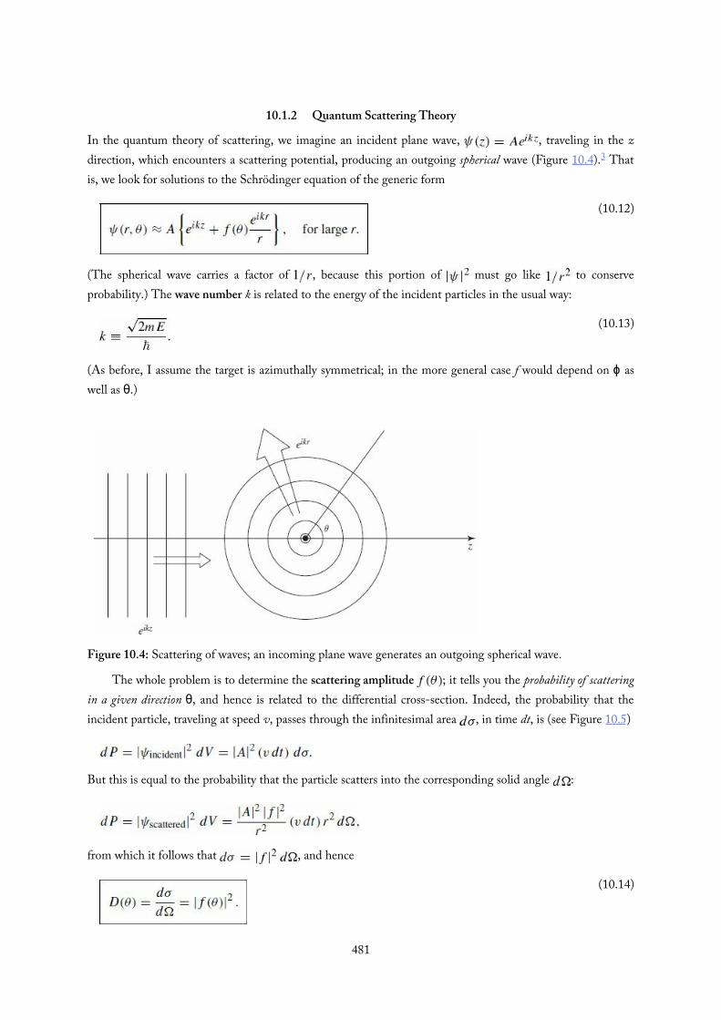
(10.12)
(10.13)
(10.14)
10.1.2 Quantum Scattering Theory
In the quantum theory of scattering, we imagine an incident plane wave, , traveling in the zdirection, which encounters a scattering potential, producing an outgoing spherical wave (Figure 10.4).3 Thatis, we look for solutions to the Schrödinger equation of the generic form
(The spherical wave carries a factor of , because this portion of must go like to conserveprobability.) The wave number k is related to the energy of the incident particles in the usual way:
(As before, I assume the target is azimuthally symmetrical; in the more general case f would depend on ϕ aswell as θ.)
Figure 10.4: Scattering of waves; an incoming plane wave generates an outgoing spherical wave.
The whole problem is to determine the scattering amplitude ; it tells you the probability of scatteringin a given direction θ, and hence is related to the differential cross-section. Indeed, the probability that theincident particle, traveling at speed v, passes through the infinitesimal area , in time dt, is (see Figure 10.5)
But this is equal to the probability that the particle scatters into the corresponding solid angle :
from which it follows that , and hence
481

Evidently the differential cross-section (which is the quantity of interest to the experimentalist) is equal to theabsolute square of the scattering amplitude (which is obtained by solving the Schrödinger equation). In thefollowing sections we will study two techniques for calculating the scattering amplitude: partial wave analysisand the Born approximation.
Figure 10.5: The volume dV of incident beam that passes through area in time dt.
Problem 10.2 Construct the analogs to Equation 10.12 for one-dimensional andtwo-dimensional scattering.
482

10.2 Partial Wave Analysis
483

(10.16)
(10.17)
(10.19)
(10.15)
(10.18)
10.2.1 Formalism
As we found in Chapter 4, the Schrödinger equation for a spherically symmetrical potential admits theseparable solutions
where is a spherical harmonic (Equation 4.32), and satisfies the radial equation (Equation4.37):
At very large r the potential goes to zero, and the centrifugal contribution is negligible, so
The general solution is
the first term represents an outgoing spherical wave, and the second an incoming one—for the scattered wavewe want . At very large r, then,
as we already deduced (on physical grounds) in the previous section (Equation 10.12).That’s for very large r (more precisely, for ; in optics it would be called the radiation zone). As in
one-dimensional scattering theory, we assume that the potential is “localized,” in the sense that exterior tosome finite scattering region it is essentially zero (Figure 10.6). In the intermediate region (where V can beignored but the centrifugal term cannot),4 the radial equation becomes
and the general solution (Equation 4.45) is a linear combination of spherical Bessel functions:
However, neither (which is somewhat like a sine function) nor (which is a sort of generalized cosinefunction) represents an outgoing (or an incoming) wave. What we need are the linear combinations analogousto and ; these are known as spherical Hankel functions:
The first few spherical Hankel functions are listed in Table 10.1. At large r, (the Hankel function ofthe first kind) goes like , whereas (the Hankel function of the second kind) goes like ;for outgoing waves, then, we need spherical Hankel functions of the first kind:
484

(10.20)
(10.21)
(10.22)
(10.23)
Figure 10.6: Scattering from a localized potential: the scattering region (dark), the intermediate region, where (shaded), and the radiation zone (where ).
Table 10.1: Spherical Hankel functions, and .
The exact wave function, in the exterior region (where ), is
The first term is the incident plane wave, and the sum (with expansion coefficients ) is the scatteredwave. But since we are assuming the potential is spherically symmetric, the wave function cannot depend onϕ.5 So only terms with survive (remember, ). Now (from Equations 4.27 and 4.32)
where is the th Legendre polynomial. It is customary to redefine the expansion coefficients :
You’ll see in a moment why this peculiar notation is convenient; is called the th partial wave amplitude.For very large r, the Hankel function goes like (Table 10.1), so
485

(10.24)
(10.25)
(10.26)
(10.27)
where
This confirms more rigorously the general structure postulated in Equation 10.12, and tells us how tocompute the scattering amplitude, , in terms of the partial wave amplitudes . The differential cross-section is
and the total cross-section is
(I used the orthogonality of the Legendre polynomials, Equation 4.34, to do the angular integration.)
486
(10.28)
(10.29)
(10.30)
(10.32)
(10.33)
(10.31)
10.2.2 Strategy
All that remains is to determine the partial wave amplitudes, , for the potential in question. This isaccomplished by solving the Schrödinger equation in the interior region (where is not zero), andmatching it to the exterior solution (Equation 10.23), using the appropriate boundary conditions. The onlyproblem is that as it stands my notation is hybrid: I used spherical coordinates for the scattered wave, butcartesian coordinates for the incident wave. We need to rewrite the wave function in a more consistentnotation.
Of course, satisfies the Schrödinger equation with . On the other hand, I just argued that thegeneral solution to the Schrödinger equation with can be written in the form
In particular, then, it must be possible to express in this way. But is finite at the origin, so noNeumann functions are allowed in the sum blows up at ), and since has no ϕdependence, only terms occur. The resulting expansion of a plane wave in terms of spherical waves isknown as Rayleigh’s formula:6
Using this, the wave function in the exterior region (Equation 10.23) can be expressed entirely in terms of rand θ:
Example 10.3Quantum hard-sphere scattering. Suppose
The boundary condition, then, is
so
for all θ, from which it follows (Problem 10.3) that
487
(10.34)
(10.35)
(10.36)
∗∗
In particular, the total cross-section (Equation 10.27) is
That’s the exact answer, but it’s not terribly illuminating, so let’s consider the limiting case of low-energy scattering: . (Since , this amounts to saying that the wavelength is muchgreater than the radius of the sphere.) Referring to Table 4.4, we note that is much larger than
, for small z, so
and hence
But we’re assuming , so the higher powers are negligible—in the low-energy approximationthe scattering is dominated by the term. (This means that the differential cross-section isindependent of θ, just as it was in the classical case.) Evidently
for low energy hard-sphere scattering. Surprisingly, the scattering cross-section is four times thegeometrical cross-section—in fact, σ is the total surface area of the sphere. This “larger effective size” ischaracteristic of long-wavelength scattering (it would be true in optics, as well); in a sense, these waves“feel” their way around the whole sphere, whereas classical particles only see the head-on cross-section(Equation 10.8).
Problem 10.3 Prove Equation 10.33, starting with Equation 10.32. Hint: Exploitthe orthogonality of the Legendre polynomials to show that the coefficients withdifferent values of must separately vanish.
Problem 10.4 Consider the case of low-energy scattering from a spherical delta-function shell:
where α and a are constants. Calculate the scattering amplitude, , thedifferential cross-section, , and the total cross-section, σ. Assume ,so that only the term contributes significantly. (To simplify matters, throwout all terms right from the start.) The main problem, of course, is to
488

determine . Express your answer in terms of the dimensionless quantity . Answer: .
489

(10.37)
(10.38)
(10.39)
(10.40)
10.3 Phase ShiftsConsider first the problem of one-dimensional scattering from a localized potential on the half-line
(Figure 10.7). I’ll put a “brick wall” at , so a wave incident from the left,
is entirely reflected
Whatever happens in the interaction region , the amplitude of the reflected wave has got to bethe same as that of the incident wave , by conservation of probability. But it need not have thesame phase. If there were no potential at all (just the wall at ), then , since the total wavefunction (incident plus reflected) must vanish at the origin:
If the potential is not zero, the wave function (for ) takes the form
Figure 10.7: One-dimensional scattering from a localized potential bounded on the right by an infinite wall.
The whole theory of scattering reduces to the problem of calculating the phase shift7 δ (as a function ofk, and hence of the energy ), for a specified potential. We do this, of course, by solving theSchrödinger equation in the scattering region , and imposing appropriate boundary conditions(see Problem 10.5). The advantage of working with the phase shift (as opposed to the complex number B) isthat it exploits the physics to simplify the mathematics (trading a complex quantity—two real numbers—for asingle real quantity).
Now let’s return to the three-dimensional case. The incident plane wave carries no angularmomentum in the z direction (Rayleigh’s formula contains no terms with ), but it includes all values ofthe total angular momentum . Because angular momentum is conserved (by a sphericallysymmetric potential), each partial wave (labelled by a particular ) scatters independently, with (again) nochange in amplitude8 —only in phase.
If there is no potential at all, then , and the th partial wave is (Equation 10.28)
490

(10.42)
(10.43)
(10.44)
(10.45)
(10.46)
(10.47)
(10.48)
(10.41)
But (from Equation 10.19 and Table 10.1)
So for large r
The second term inside the square brackets represents an incoming spherical wave; it comes from the incidentplane wave, and is unchanged when we now introduce a potential. The first term is the outgoing wave; it picksup a phase shift (due to the scattering potential):
Think of it as a converging spherical wave (the term, due exclusively to the component in ),which is phase shifted an amount on the way in, and again on the way out (hence the 2), emerging as anoutgoing spherical wave (the term, due to the part of plus the scattered wave).
In Section 10.2.1 the whole theory was expressed in terms of the partial wave amplitudes ; now wehave formulated it in terms of the phase shifts . There must be a connection between the two. Indeed,comparing the asymptotic (large r) form of Equation 10.23
with the generic expression in terms of (Equation 10.44), we find9
It follows in particular (Equation 10.25) that
and (Equation 10.27)
Again, the advantage of working with phase shifts (as opposed to partial wave amplitudes) is that they areeasier to interpret physically, and simpler mathematically—the phase shift formalism exploits conservation ofangular momentum to reduce a complex quantity (two real numbers) to a single real one .
Problem 10.5 A particle of mass m and energy E is incident from the left on thepotential
491

(a) If the incoming wave is (where ), find the reflectedwave. Answer:
(b) Confirm that the reflected wave has the same amplitude as the incidentwave.
(c) Find the phase shift δ (Equation 10.40) for a very deep well .Answer: .
Problem 10.6 What are the partial wave phase shifts for hard-spherescattering (Example 10.3)?
Problem 10.7 Find the S-wave partial wave phase shift forscattering from a delta-function shell (Problem 10.4). Assume that the radial wavefunction goes to 0 as . Answer:
492

10.4 The Born Approximation
493
(10.49)
(10.50)
(10.51)
(10.52)
(10.53)
(10.54)
(10.55)
10.4.1 Integral Form of the Schrödinger Equation
The time-independent Schrödinger equation,
can be written more succinctly as
where
This has the superficial appearance of the Helmholtz equation; note, however, that the “inhomogeneous”term itself depends on . Suppose we could find a function that solves the Helmholtz equationwith a delta function “source”:
Then we could express as an integral:
For it is easy to show that this satisfies Schrödinger’s equation, in the form of Equation 10.50:
is called the Green’s function for the Helmholtz equation. (In general, the Green’s function for a lineardifferential equation represents the “response” to a delta-function source.)
Our first task10 is to solve Equation 10.52 for . This is most easily accomplished by taking theFourier transform, which turns the differential equation into an algebraic equation. Let
Then
But
and (see Equation 2.147)
494

(10.56)
(10.57)
(10.58)
(10.59)
(10.60)
(10.61)
so Equation 10.52 says
It follows11 that
Putting this back into Equation 10.54, we find:
Now, r is fixed, as far as the s integration is concerned, so we may as well choose spherical coordinates with the polar axis along r (Figure 10.8). Then , the ϕ integral is trivial , and
the θ integral is
Thus
Figure 10.8: Convenient coordinates for the integral in Equation 10.58.
The remaining integral is not so simple. It pays to revert to exponential notation, and factor thedenominator:
These two integrals can be evaluated using Cauchy’s integral formula:
495
(10.62)
(10.63)
(10.64)
(10.65)
if lies within the contour (otherwise the integral is zero). In the present case the integration is along thereal axis, and it passes right over the pole singularities at . We have to decide how to skirt the poles—I’ll goover the one at and under the one at (Figure 10.9). (You’re welcome to choose some other conventionif you like—even winding seven times around each pole—you’ll get a different Green’s function, but, as I’llshow you in a minute, they’re all equally acceptable.)12
Figure 10.9: Skirting the poles in the contour integral (Equation 10.61).
For each integral in Equation 10.61 I must “close the contour” in such a way that the semicircle atinfinity contributes nothing. In the case of , the factor goes to zero when s has a large positive imaginarypart; for this one I close above (Figure 10.10(a)). The contour encloses only the singularity at , so
In the case of , the factor goes to zero when s has a large negative imaginary part, so we close below(Figure 10.10(b)); this time the contour encloses the singularity at (and it goes around in the clockwisedirection, so we pick up a minus sign):
Conclusion:
Figure 10.10: Closing the contour in Equations 10.63 and 10.64.
This, finally, is the Green’s function for the Helmholtz equation—the solution to Equation 10.52. (Ifyou got lost in all that analysis, you might want to check the result by direct differentiation—see Problem
496
(10.66)
(10.67)
(10.68)
∗∗
10.8.) Or rather, it is a Green’s function for the Helmholtz equation, for we can add to any function that satisfies the homogeneous Helmholtz equation:
clearly, the result still satisfies Equation 10.52. This ambiguity corresponds precisely to theambiguity in how to skirt the poles—a different choice amounts to picking a different function .
Returning to Equation 10.53, the general solution to the Schrödinger equation takes the form
where satisfies the free-particle Schrödinger equation,
Equation 10.67 is the integral form of the Schrödinger equation; it is entirely equivalent to the more familiardifferential form. At first glance it looks like an explicit solution to the Schrödinger equation (for any potential)—which is too good to be true. Don’t be deceived: There’s a under the integral sign on the right hand side,so you can’t do the integral unless you already know the solution! Nevertheless, the integral form can be verypowerful, and it is particularly well suited to scattering problems, as we’ll see in the following section.
Problem 10.8 Check that Equation 10.65 satisfies Equation 10.52, by directsubstitution. Hint: .13
Problem 10.9 Show that the ground state of hydrogen (Equation 4.80) satisfiesthe integral form of the Schrödinger equation, for the appropriate V and E (notethat E is negative, so , where ).
497

(10.69)
(10.72)
(10.73)
(10.74)
(10.75)
(10.76)
(10.77)
(10.70)
(10.71)
(10.78)
10.4.2 The First Born Approximation
Suppose is localized about —that is, the potential drops to zero outside some finite region (as istypical for a scattering problem), and we want to calculate at points far away from the scattering center.Then for all points that contribute to the integral in Equation 10.67, so
and hence
Let
then
and therefore
(In the denominator we can afford to make the more radical approximation ; in the exponent weneed to keep the next term. If this puzzles you, try including the next term in the expansion of thedenominator. What we are doing is expanding in powers of the small quantity , and dropping all butthe lowest order.)
In the case of scattering, we want
representing an incident plane wave. For large r, then,
This is in the standard form (Equation 10.12), and we can read off the scattering amplitude:
This is exact.14 Now we invoke the Born approximation: Suppose the incoming plane wave is not substantiallyaltered by the potential; then it makes sense to use
where
498

(10.79)
(10.80)
(10.81)
(10.82)
(10.83)
(10.84)
inside the integral. (This would be the exact wave function, if V were zero; it is essentially a weak potentialapproximation.15 ) In the Born approximation, then,
(In case you have lost track of the definitions of and k, they both have magnitude k, but the former pointsin the direction of the incident beam, while the latter points toward the detector—see Figure 10.11;
is the momentum transfer in the process.)
Figure 10.11: Two wave vectors in the Born approximation: points in the incident direction, k in thescattered direction.
In particular, for low energy (long wavelength) scattering, the exponential factor is essentially constantover the scattering region, and the Born approximation simplifies to
(I dropped the subscript on r, since there is no likelihood of confusion at this point.)
Example 10.4Low-energy soft-sphere scattering. 16 Suppose
In this case the low-energy scattering amplitude is
(independent of θ and ϕ), the differential cross-section is
and the total cross-section is
499

(10.86)
(10.87)
(10.88)
(10.90)
(10.91)
(10.92)
(10.85)
(10.89)
For a spherically symmetrical potential, —but not necessarily at low energy—the Bornapproximation again reduces to a simpler form. Define
and let the polar axis for the integral lie along , so that
Then
The integral is trivial , and the integral is one we have encountered before (see Equation 10.59).Dropping the subscript on r, we are left with
The angular dependence of f is carried by κ; in Figure 10.11 we see that
Example 10.5Yukawa scattering. The Yukawa potential (which is a crude model for the binding force in an atomicnucleus) has the form
where β and μ are constants. The Born approximation gives
(You get to work out the integral for yourself, in Problem 10.11.)
Example 10.6Rutherford scattering. If we put in , , the Yukawa potential reduces to theCoulomb potential, describing the electrical interaction of two point charges. Evidently the scatteringamplitude is
or (using Equations 10.89 and 10.51):
500

(10.93)
(10.94)
∗
∗∗
∗
The differential cross-section is the square of this:
which is precisely the Rutherford formula (Equation 10.11). It happens that for the Coulombpotential classical mechanics, the Born approximation, and quantum field theory all yield the sameresult. As they say in the computer business, the Rutherford formula is amazingly “robust.”
Problem 10.10 Find the scattering amplitude, in the Born approximation, forsoft-sphere scattering at arbitrary energy. Show that your formula reduces toEquation 10.82 in the low-energy limit.
Problem 10.11 Evaluate the integral in Equation 10.91, to confirm the expressionon the right.
Problem 10.12 Calculate the total cross-section for scattering from a Yukawapotential, in the Born approximation. Express your answer as a function of E.
Problem 10.13 For the potential in Problem 10.4,(a) calculate , , and σ, in the low-energy Born approximation;(b) calculate for arbitrary energies, in the Born approximation;(c) show that your results are consistent with the answer to Problem 10.4, in
the appropriate regime.
501
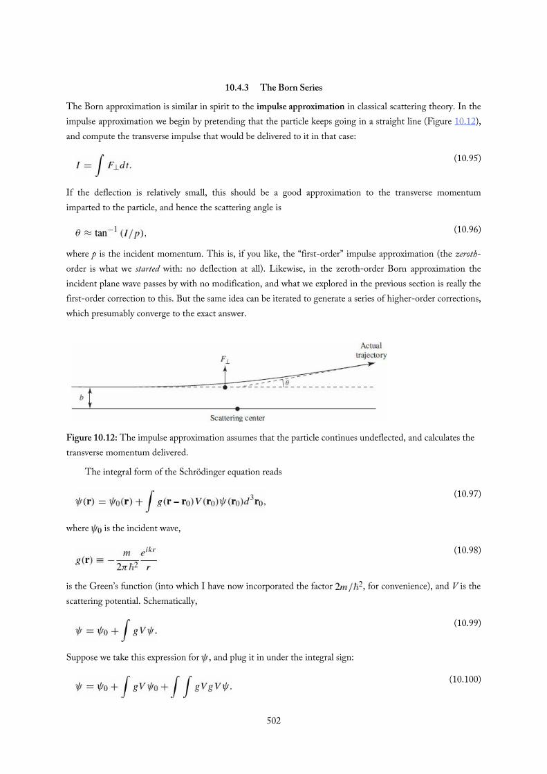
(10.95)
(10.96)
(10.97)
(10.98)
(10.99)
(10.100)
10.4.3 The Born Series
The Born approximation is similar in spirit to the impulse approximation in classical scattering theory. In theimpulse approximation we begin by pretending that the particle keeps going in a straight line (Figure 10.12),and compute the transverse impulse that would be delivered to it in that case:
If the deflection is relatively small, this should be a good approximation to the transverse momentumimparted to the particle, and hence the scattering angle is
where p is the incident momentum. This is, if you like, the “first-order” impulse approximation (the zeroth-order is what we started with: no deflection at all). Likewise, in the zeroth-order Born approximation theincident plane wave passes by with no modification, and what we explored in the previous section is really thefirst-order correction to this. But the same idea can be iterated to generate a series of higher-order corrections,which presumably converge to the exact answer.
Figure 10.12: The impulse approximation assumes that the particle continues undeflected, and calculates thetransverse momentum delivered.
The integral form of the Schrödinger equation reads
where is the incident wave,
is the Green’s function (into which I have now incorporated the factor , for convenience), and V is thescattering potential. Schematically,
Suppose we take this expression for , and plug it in under the integral sign:
502

(10.101)
∗∗∗
Iterating this procedure, we obtain a formal series for :
In each integrand only the incident wave function appears, together with more and more powers of gV.The first Born approximation truncates the series after the second term, but it is pretty clear how onegenerates the higher-order corrections.
The Born series can be represented diagrammatically as shown in Figure 10.13. In zeroth order isuntouched by the potential; in first order it is “kicked” once, and then “propagates” out in some new direction;in second order it is kicked, propagates to a new location, is kicked again, and then propagates out; and so on.In this context the Green’s function is sometimes called the propagator—it tells you how the disturbancepropagates between one interaction and the next. The Born series was the inspiration for Feynman’sformulation of relativistic quantum mechanics, which is expressed entirely in terms of vertex factors andpropagators , connected together in Feynman diagrams.
Figure 10.13: Diagrammatic interpretation of the Born series (Equation 10.101).
Problem 10.14 Calculate θ (as a function of the impact parameter) for Rutherfordscattering, in the impulse approximation. Show that your result is consistent withthe exact expression (Problem 10.1(a)), in the appropriate limit.
Problem 10.15 Find the scattering amplitude for low-energy soft-spherescattering in the second Born approximation. Answer:
503

∗∗∗
(10.102)
∗∗
(10.103)
(10.104)
Further Problems on Chapter 10
Problem 10.16 Find the Green’s function for the one-dimensional Schrödingerequation, and use it to construct the integral form (analogous to Equation10.66). Answer:
Problem 10.17 Use your result in Problem 10.16 to develop the Bornapproximation for one-dimensional scattering (on the interval
, with no “brick wall” at the origin). That is, choose , and assume to evaluate the integral. Show
that the reflection coefficient takes the form:
Problem 10.18 Use the one-dimensional Born approximation (Problem 10.17) tocompute the transmission coefficient for scattering from a deltafunction (Equation 2.117) and from a finite square well (Equation 2.148).Compare your results with the exact answers (Equations 2.144 and 2.172).
Problem 10.19 Prove the optical theorem, which relates the total cross-section tothe imaginary part of the forward scattering amplitude:
Hint: Use Equations 10.47 and 10.48.
Problem 10.20 Use the Born approximation to determine the total cross-sectionfor scattering from a gaussian potential
Express your answer in terms of the constants , a, and m (the mass of theincident particle), and , where E is the incident energy.
Problem 10.21 Neutron diffraction. Consider a beam of neutrons scattering froma crystal (Figure 10.14). The interaction between neutrons and the nuclei inthe crystal is short ranged, and can be approximated as
where the are the locations of the nuclei and the strength of the potential is504
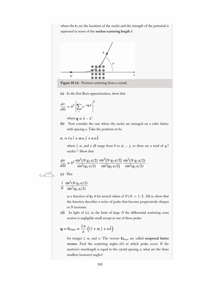
where the are the locations of the nuclei and the strength of the potential isexpressed in terms of the nuclear scattering length b.
Figure 10.14: Neutron scattering from a crystal.
(a) In the first Born approximation, show that
where .(b) Now consider the case where the nuclei are arranged on a cubic lattice
with spacing a. Take the positions to be
where l, m, and n all range from 0 to , so there are a total of nuclei.17 Show that
(c) Plot
as a function of for several values of N to show thatthe function describes a series of peaks that become progressively sharperas N increases.
(d) In light of (c), in the limit of large N the differential scattering crosssection is negligibly small except at one of these peaks:
for integer l, m, and n. The vectors are called reciprocal latticevectors. Find the scattering angles at which peaks occur. If theneutron’s wavelength is equal to the crystal spacing a, what are the threesmallest (nonzero) angles?
505
∗∗∗
(10.105)
(10.106)
(10.107)
(10.108)
(10.109)
(10.110)
Comment: Neutron diffraction is one method used, to determine crystalstructures (electrons and x-rays can also be used and the same expression forthe locations of the peaks holds). In this problem we looked at a cubicarrangement of atoms, but a different arrangement (hexagonal for example)would produce peaks at a different set of angles. Thus from the scattering dataone can infer the underlying crystal structure.
Problem 10.22 Two-dimensional scattering theory. By analogy with Section 10.2,develop partial wave analysis for two dimensions.(a) In polar coordinates the Laplacian is
Find the separable solutions to the (time-independent) Schrödingerequation, for a potential with azimuthal symmetry .Answer:
where j is an integer, and satisfies the radial equation
(b) By solving the radial equation for very large r (where both and thecentrifugal term go to zero), show that an outgoing radial wave has theasymptotic form
where . Check that an incident wave of the form satisfies the Schrödinger equation, for (this is trivial, if you usecartesian coordinates). Write down the two-dimensional analog toEquation 10.12, and compare your result to Problem 10.2. Answer:
(c) Construct the analog to Equation 10.21 (the wave function in the regionwhere but the centrifugal term cannot be ignored). Answer:
where is the Hankel function (not the spherical Hankel function!) of order j.18
506

(10.111)
(10.112)
(10.113)
(10.114)
(10.115)
(10.116)
(10.117)
(d) For large z,
Use this to show that
(e) Adapt the argument of Section 10.1.2 to this two-dimensional geometry.Instead of the area , we have a length, db, and in place of the solid angle
we have the increment of scattering angle ; the role of thedifferential cross-section is played by
and the effective “width” of the target (analogous to the total cross-section) is
Show that
(f) Consider the case of scattering from a hard disk (or, in three dimensions,an infinite cylinder19) of radius a:
By imposing appropriate boundary conditions at , determine B.You’ll need the analog to Rayleigh’s formula:
(where is the Bessel function of order J). Plot B as a function of ka, for .
Problem 10.23 Scattering of identical particles. The results for scattering of aparticle from a fixed target also apply to the scattering of two particles in thecenter of mass frame. With , satisfies
507

(10.118)
(see Problem 5.1) where is the interaction between the particles(assumed here to depend only on their separation distance). This is the one-particle Schrödinger equation (with the reduced mass μ in place of m).(a) Show that if the two particles are identical (spinless) bosons, then
must be an even function of (Figure 10.15).(b) By symmetrizing Equation 10.12 (why is this allowed?), show that the
scattering amplitude in this case is
where is the scattering amplitude of a single particle of mass μ froma fixed target .
(c) Show that the partial wave amplitudes of vanish for all odd powers of .
(d) How are the results of (a)–(c) different if the particles are identicalfermions (in a triplet spin state).
(e) Show that the scattering amplitude for identical fermions vanishes at .
(f) Plot the logarithm of the differential scattering cross section for fermionsand for bosons in Rutherford scattering (Equation 10.93).20
Figure 10.15: Scattering of identical particles.
1 This is terrible language: D isn’t a differential, and it isn’t a cross-section. To my ear, the words “differential cross-section” would attachmore naturally to . But I’m afraid we’re stuck with this terminology. I should also warn you that the notation is nonstandard—mostpeople just call it (which makes Equation 10.3 look like a tautology). I think it will be less confusing if we give the differentialcross-section its own symbol.
2 This isn’t easy, and you might want to refer to a book on classical mechanics, such as Jerry B. Marion and Stephen T. Thornton, ClassicalDynamics of Particles and Systems, 4th edn, Saunders, Fort Worth, TX (1995), Section 9.10.
3 For the moment, there’s not much quantum mechanics in this; what we’re really talking about is the scattering of waves, as opposed toparticles, and you could even think of Figure 10.4 as a picture of water waves encountering a rock, or (better, since we’re interested in three-dimensional scattering) sound waves bouncing off a basketball.
4 What follows does not apply to the Coulomb potential, since goes to zero more slowly than , as , and the centrifugal termdoes not dominate in this region. In this sense the Coulomb potential is not localized, and partial wave analysis is inapplicable.
5 There’s nothing wrong with θ dependence, of course, because the incoming plane wave defines a z direction, breaking the spherical508
5 There’s nothing wrong with θ dependence, of course, because the incoming plane wave defines a z direction, breaking the sphericalsymmetry. But the azimuthal symmetry remains; the incident plane wave has no ϕ dependence, and there is nothing in the scattering processthat could introduce any ϕ dependence in the outgoing wave.
6 For a guide to the proof, see George Arfken and Hans-Jurgen Weber, Mathematical Methods for Physicists, 7th edn, Academic Press,Orlando (2013), Exercises 15.2.24 and 15.2.25.
7 The 2 in front of δ is conventional. We think of the incident wave as being phase shifted once on the way in, and again on the way out; δ isthe “one way” phase shift, and the total is .
8 One reason this subject can be so confusing is that practically everything is called an “amplitude”: is the “scattering amplitude”, isthe “partial wave amplitude”, but the first is a function of θ, and both are complex numbers. I’m now talking about “amplitude” in theoriginal sense: the (real, of course) height of a sinusoidal wave.
9 Although I used the asymptotic form of the wave function to draw the connection between and , there is nothing approximate aboutthe result (Equation 10.46). Both of them are constants (independent of r), and means the phase shift in the asymptotic region (where theHankel functions have settled down to ).
10 Warning: You are approaching two pages of heavy analysis, including contour integration; if you wish, skip straight to the answer, Equation10.65.
11 This is clearly sufficient, but it is also necessary, as you can easily show by combining the two terms into a single integral, and usingPlancherel’s theorem, Equation 2.103.
12 If you are unfamiliar with this technique you have every right to be suspicious. In truth, the integral in Equation 10.60 is simply ill-defined—it does not converge, and it’s something of a miracle that we can make sense of it at all. The root of the problem is that doesn’t reallyhave a legitimate Fourier transform; we’re exceeding the speed limit, here, and just hoping we won’t get caught.
13 See, for example, D. Griffiths, Introduction to Electrodynamics, 4th edn (Cambridge University Press, Cambridge, UK, 2017), Section 1.5.3.14 Remember, is by definition the coefficient of at large r.15 Typically, partial wave analysis is useful when the incident particle has low energy, for then only the first few terms in the series contribute
significantly; the Born approximation is more useful at high energy, when the deflection is relatively small.16 You can’t apply the Born approximation to hard-sphere scattering —the integral blows up. The point is that we assumed the
potential is weak, and doesn’t change the wave function much in the scattering region. But a hard sphere changes it radically—from tozero.
17 It makes no difference that this crystal isn’t “centered” at the origin: shifting the crystal by R amounts to adding R to each of the , and thatdoesn’t affect After all, we’re assuming an incident plane wave, which extends to in the x and y directions.
18 See Mary Boas, Mathematical Methods in the Physical Sciences, 3rd edn (Wiley, New York, 2006), Section 12.17.19 S. McAlinden and J. Shertzer, Am. J. Phys. 84, 764 (2016).20 Equation 10.93 was derived by taking the limit of Yukawa scattering (Example 10.5) and the result for is missing a phase factor (see
Albert Messiah, Quantum Mechanics, Dover, New York, NY (1999), Section XI.7). That factor drops out of the cross-section for scatteringfrom a fixed potential—giving the correct answer in Example 10.6—but would show up in the cross-section for scattering of identicalparticles.
509
(11.1)
(11.2)
(11.3)
(11.4)
11Quantum Dynamics
◈
So far, practically everything we have done belongs to the subject that might properly be called quantumstatics, in which the potential energy function is independent of time: . In that case the (time-dependent) Schrödinger equation,
can be solved by separation of variables:
where satisfies the time-independent Schrödinger equation,
Because the time dependence of separable solutions is carried by the exponential factor , whichcancels out when we construct the physically relevant quantity , all probabilities and expectation values(for such states) are constant in time. By forming linear combinations of these stationary states we obtain wavefunctions with more interesting time dependence,
but even then the possible values of the energy , and their respective probabilities , are constant.If we want to allow for transitions (quantum jumps, as they are sometimes called) between one energy
level and another, we must introduce a time-dependent potential (quantum dynamics). There are precious fewexactly solvable problems in quantum dynamics. However, if the time-dependent part of the Hamiltonian issmall (compared to the time-independent part), it can be treated as a perturbation. The main purpose of thischapter is to develop time-dependent perturbation theory, and study its most important application: theemission or absorption of radiation by an atom.
Problem 11.1 Why isn’t it trivial to solve the time-dependent Schrödingerequation (11.1), in its dependence on t ? After all, it’s a first-order differentialequation.
(a) How would you solve the equation
(for , if k were a constant?(b) What if k is itself a function of t? (Here and might also depend
on other variables, such as r—it doesn’t matter.)(c) Why not do the same thing for the Schrödinger equation (with a time-
dependent Hamiltonian)? To see that this doesn’t work, consider the
510

simple case
where and are themselves time-independent. If the solution in part(b) held for the Schrödinger equation, the wave function at time would be
but of course we could also write
Why are these generally not the same? [This is a subtle matter; if youwant to pursue it further, see Problem 11.23.]
511

(11.5)
(11.6)
(11.8)
(11.9)
(11.7)
11.1 Two-Level SystemsTo begin with, let us suppose that there are just two states of the (unperturbed) system, and . They areeigenstates of the unperturbed Hamiltonian, :
and they are orthonormal:
Any state can be expressed as a linear combination of them; in particular,
The states and might be position-space wave functions, or spinors, or something more exotic—itdoesn’t matter. It is the time dependence that concerns us here, so when I write , I simply mean the stateof the system at time t. In the absence of any perturbation, each component evolves with its characteristicwiggle factor:
Informally, we say that is the “probability that the particle is in state ”—by which we really mean theprobability that a measurement of the energy would yield the value . Normalization of requires, ofcourse, that
512
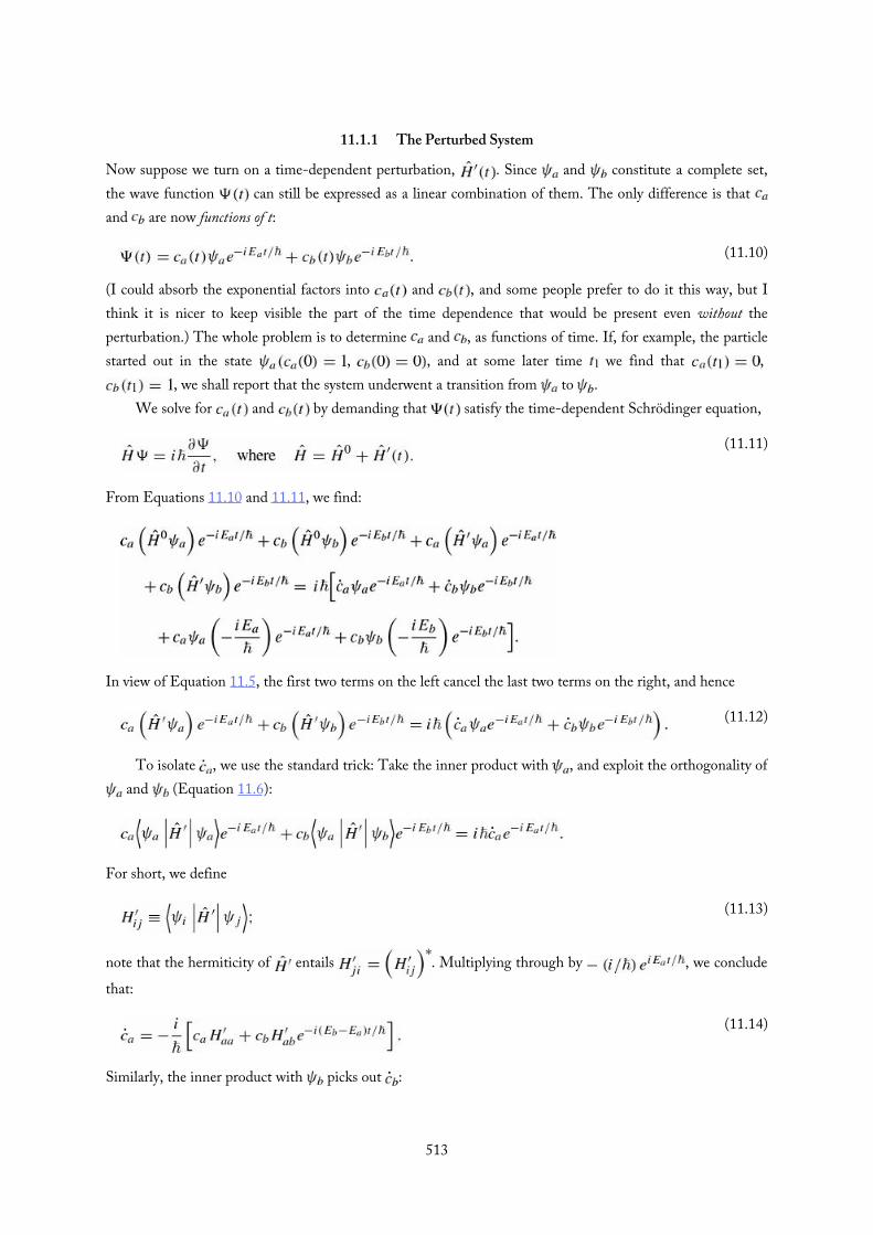
(11.10)
(11.11)
(11.12)
(11.13)
(11.14)
11.1.1 The Perturbed System
Now suppose we turn on a time-dependent perturbation, . Since and constitute a complete set,the wave function can still be expressed as a linear combination of them. The only difference is that and are now functions of t:
(I could absorb the exponential factors into and , and some people prefer to do it this way, but Ithink it is nicer to keep visible the part of the time dependence that would be present even without theperturbation.) The whole problem is to determine and , as functions of time. If, for example, the particlestarted out in the state , , and at some later time we find that ,
, we shall report that the system underwent a transition from to .We solve for and by demanding that satisfy the time-dependent Schrödinger equation,
From Equations 11.10 and 11.11, we find:
In view of Equation 11.5, the first two terms on the left cancel the last two terms on the right, and hence
To isolate , we use the standard trick: Take the inner product with , and exploit the orthogonality of and (Equation 11.6):
For short, we define
note that the hermiticity of entails . Multiplying through by , we conclude
that:
Similarly, the inner product with picks out :
513

(11.15)
(11.16)
(11.17)
(11.18)
∗
∗
and hence
Equations 11.14 and 11.15 determine and ; taken together, they are completely equivalent tothe (time-dependent) Schrödinger equation, for a two-level system. Typically, the diagonal matrix elements of
vanish (see Problem 11.5 for the general case):
If so, the equations simplify:
where
(I’ll assume that , so .)
Problem 11.2 A hydrogen atom is placed in a (time-dependent) electric field . Calculate all four matrix elements of the perturbation
between the ground state and the (quadruply degenerate) first excitedstates . Also show that for all five states. Note: There is only oneintegral to be done here, if you exploit oddness with respect to z; only one of the
states is “accessible” from the ground state by a perturbation of this form,and therefore the system functions as a two-state configuration—assumingtransitions to higher excited states can be ignored.
Problem 11.3 Solve Equation 11.17 for the case of a time-independentperturbation, assuming that and . Check that
. Comment: Ostensibly, this system oscillates between“pure ” and “some .” Doesn’t this contradict my general assertion that notransitions occur for time-independent perturbations? No, but the reason is rathersubtle: In this case and are not, and never were, eigenstates of theHamiltonian—a measurement of the energy never yields or . In time-dependent perturbation theory we typically contemplate turning on theperturbation for a while, and then turning it off again, in order to examine thesystem. At the beginning, and at the end, and are eigenstates of the exactHamiltonian, and only in this context does it make sense to say that the systemunderwent a transition from one to the other. For the present problem, then,
514
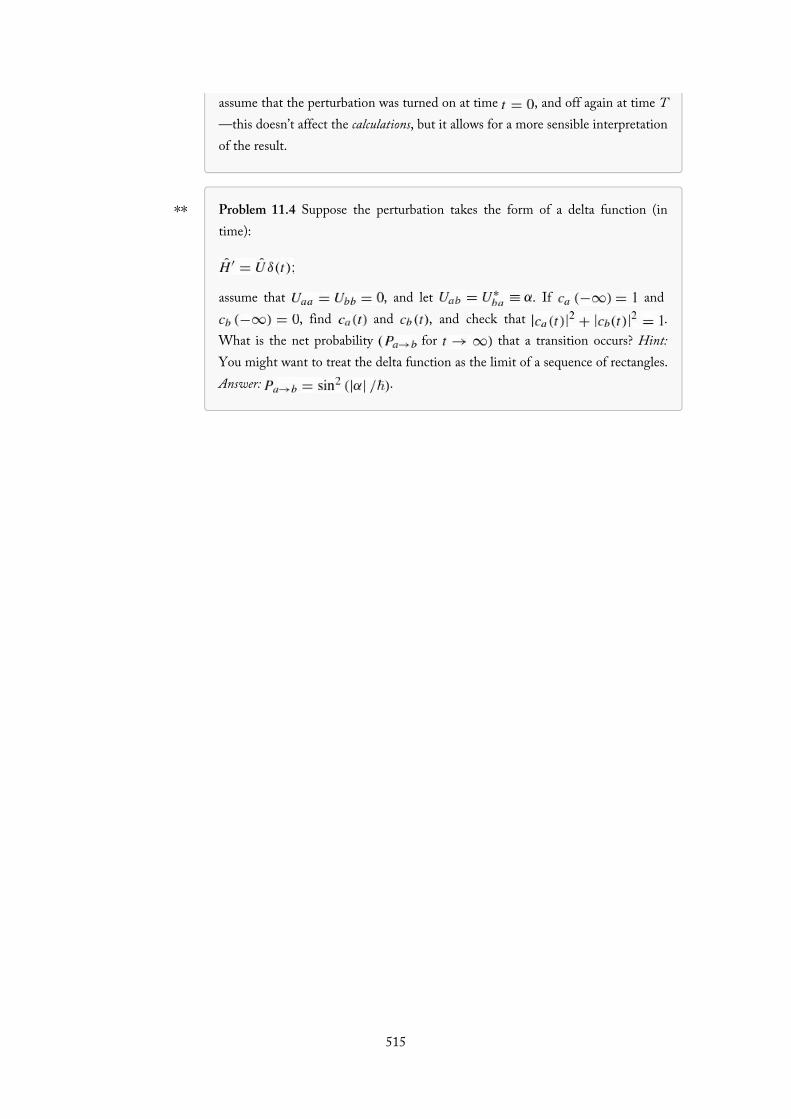
∗∗
assume that the perturbation was turned on at time , and off again at time T—this doesn’t affect the calculations, but it allows for a more sensible interpretationof the result.
Problem 11.4 Suppose the perturbation takes the form of a delta function (intime):
assume that , and let . If and , find and , and check that .
What is the net probability for that a transition occurs? Hint:You might want to treat the delta function as the limit of a sequence of rectangles.Answer: .
515

(11.20)
(11.21)
(11.22)
(11.23)
(11.19)
11.1.2 Time-Dependent Perturbation Theory
So far, everything is exact: We have made no assumption about the size of the perturbation. But if is“small,” we can solve Equation 11.17 by a process of successive approximations, as follows. Suppose theparticle starts out in the lower state:
If there were no perturbation at all, they would stay this way forever:Zeroth Order:
(I’ll use a superscript in parentheses to indicate the order of the approximation.)To calculate the first-order approximation, we insert the zeroth-order values on the right side of
Equation 11.17:First Order:
Now we insert these expressions on the right side of Equation 11.17 to obtain the second-order approximation:Second Order:
while is unchanged . (Notice that includes the zeroth-order term; the second-order correction would be the integral part alone.)
In principle, we could continue this ritual indefinitely, always inserting the nth-order approximation intothe right side of Equation 11.17, and solving for the th order. The zeroth order contains no factors of
, the first-order correction contains one factor of , the second-order correction has two factors of , and
so on.1 The error in the first-order approximation is evident in the fact that (the
exact coefficients must, of course, obey Equation 11.9). However, is equal to 1 to first
order in , which is all we can expect from a first-order approximation. And the same goes for the higherorders.
Equation 11.21 can be written in the form
(where I’ve restored the exponential we factored out in Equation 11.10). This suggests a nice pictorial516

(11.24)
(11.25)
(where I’ve restored the exponential we factored out in Equation 11.10). This suggests a nice pictorialinterpretation: reading from right to left, the system remains in state a from time 0 to time (picking up the“wiggle factor” , makes a transition from state a to state b at time , and then remains in state buntil time t (picking up the “wiggle factor” . This process is represented in Figure 11.1. (Don’ttake the picture too literally: there is no sharp transition between these states; in fact, you integrate over all thetimes at which this transition can occur.)
Figure 11.1: Pictorial representation of Equation 11.23.
This interpretation of the perturbation series is especially illuminating at higher orders and for multi-level systems, where the expressions become complicated. Consider Equation 11.22, which can be written
The two terms here describe a process where the system remains in state a for the entire time, and a secondprocess where the system transitions from a to b at time and then back to a at time . Graphically, this isshown in Figure 11.2.
Figure 11.2: Pictorial representation of Equation 11.24.
With the insight provided by these pictures, it is easy to write down the general result for a multi-levelsystem:2
For , this is represented by the diagram in Figure 11.3. The first-order term describes a direct transitionfrom i to n, and the second-order term describes a process where the transition occurs via an intermediate (or“virtual”) state m.
517

∗∗
(11.26)
(11.27)
(11.28)
∗
∗∗
∗
Figure 11.3: Pictorial representation of Equation 11.25 for .
Problem 11.5 Suppose you don’t assume .(a) Find and in first-order perturbation theory, for the case
. Show that , to first
order in .(b) There is a nicer way to handle this problem. Let
Show that
where
So the equations for and are identical in structure to Equation 11.17(with an extra factor tacked onto .
(c) Use the method in part (b) to obtain and in first-orderperturbation theory, and compare your answer to (a). Comment on anydiscrepancies.
Problem 11.6 Solve Equation 11.17 to second order in perturbation theory, forthe general case .
Problem 11.7 Calculate and , to second order, for the perturbation inProblem 11.3. Compare your answer with the exact result.
Problem 11.8 Consider a perturbation to a two-level system with matrix elements
where τ and α are positive constants with the appropriate units.
(a) According to first-order perturbation theory, if the system starts off in the518

(a) According to first-order perturbation theory, if the system starts off in thestate , at , what is the probability that it will befound in the state b at ?
(b) In the limit that , . Compute the limit ofyour expression from part (a) and compare the result of Problem 11.4.
(c) Now consider the opposite extreme: . What is the limit of yourexpression from part (a)? Comment: This is an example of the adiabatictheorem (Section 11.5.2).
519

(11.29)
(11.30)
(11.32)
(11.34)
(11.35)
(11.31)
(11.33)
11.1.3 Sinusoidal Perturbations
Suppose the perturbation has sinusoidal time dependence:
so that
where
(As before, I’ll assume the diagonal matrix elements vanish, since this is almost always the case in practice.)To first order (from now on we’ll work exclusively in first order, and I’ll dispense with the superscripts) wehave (Equation 11.21):
That’s the answer, but it’s a little cumbersome to work with. Things simplify substantially if we restrictour attention to driving frequencies that are very close to the transition frequency , so that the secondterm in the square brackets dominates; specifically, we assume:
This is not much of a limitation, since perturbations at other frequencies have a negligible probability ofcausing a transition anyway. Dropping the first term, we have
The transition probability—the probability that a particle which started out in the state will be found, attime t, in the state —is
The most remarkable feature of this result is that, as a function of time, the transition probability oscillatessinusoidally (Figure 11.4). After rising to a maximum of —necessarily much less than 1,else the assumption that the perturbation is “small” would be invalid—it drops back down to zero! At times
, where , the particle is certain to be back in the lower state. If you wantto maximize your chances of provoking a transition, you should not keep the perturbation on for a long period;you do better to turn it off after a time , and hope to “catch” the system in the upper state. In
520

∗∗
(11.36)
Problem 11.9 it is shown that this “flopping” is not an artifact of perturbation theory—it occurs also in theexact solution, though the flopping frequency is modified somewhat.
Figure 11.4: Transition probability as a function of time, for a sinusoidal perturbation (Equation 11.35).
As I noted earlier, the probability of a transition is greatest when the driving frequency is close to the“natural” frequency, .3 This is illustrated in Figure 11.5, where is plotted as a function of ω. Thepeak has a height of and a width ; evidently it gets higher and narrower as time goes on.(Ostensibly, the maximum increases without limit. However, the perturbation assumption breaks down beforeit gets close to 1, so we can believe the result only for relatively small t. In Problem 11.9 you will see that theexact result never exceeds 1.)
Figure 11.5: Transition probability as a function of driving frequency (Equation 11.35).
Problem 11.9 The first term in Equation 11.32 comes from the part of , and the second from . Thus dropping the first term is formally
equivalent to writing , which is to say,
(The latter is required to make the Hamiltonian matrix hermitian—or, if youprefer, to pick out the dominant term in the formula analogous to Equation 11.32for .) Rabi noticed that if you make this so-called rotating waveapproximation at the beginning of the calculation, Equation 11.17 can be solvedexactly, with no need for perturbation theory, and no assumption about thestrength of the field.
(a) Solve Equation 11.17 in the rotating wave approximation (Equation521
(11.37)
(a) Solve Equation 11.17 in the rotating wave approximation (Equation11.36), for the usual initial conditions: . Expressyour results and in terms of the Rabi flopping frequency,
(b) Determine the transition probability, , and show that it neverexceeds 1. Confirm that .
(c) Check that reduces to the perturbation theory result (Equation11.35) when the perturbation is “small,” and state precisely what smallmeans in this context, as a constraint on V.
(d) At what time does the system first return to its initial state?
522

11.2 Emission and Absorption of Radiation
523

(11.38)
(11.39)
(11.40)
(11.41)
11.2.1 Electromagnetic Waves
An electromagnetic wave (I’ll refer to it as “light”, though it could be infrared, ultraviolet, microwave, x-ray,etc.; these differ only in their frequencies) consists of transverse (and mutually perpendicular) oscillatingelectric and magnetic fields (Figure 11.6). An atom, in the presence of a passing light wave, respondsprimarily to the electric component. If the wavelength is long (compared to the size of the atom), we canignore the spatial variation in the field;4 the atom, then, is exposed to a sinusoidally oscillating electric field
(for the moment I’ll assume the light is monochromatic, and polarized along the z direction). The perturbingHamiltonian is5
where q is the charge of the electron.6 Evidently7
Typically, is an even or odd function of z; in either case is odd, and integrates to zero (this isLaporte’s rule, Section 6.4.3; for some examples see Problem 11.2). This licenses our usual assumption thatthe diagonal matrix elements of vanish. Thus the interaction of light with matter is governed by preciselythe kind of oscillatory perturbation we studied in Section 11.1.3, with
Figure 11.6: An electromagnetic wave.
524
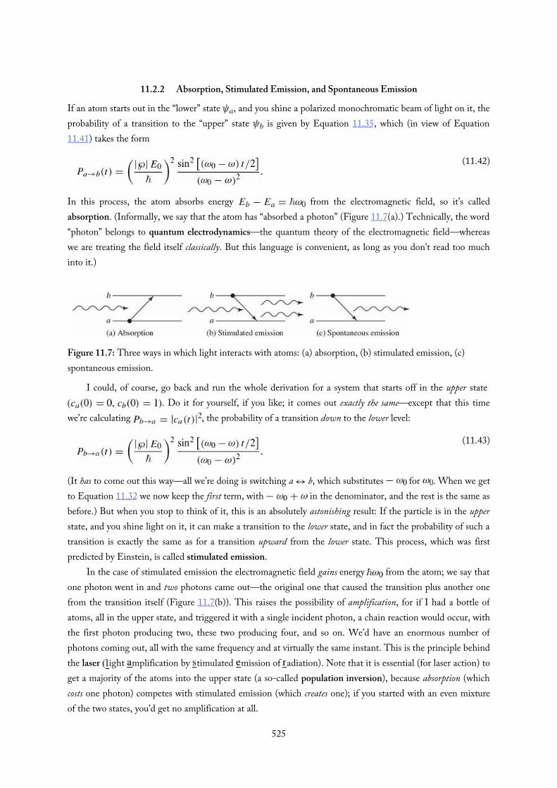
(11.42)
(11.43)
11.2.2 Absorption, Stimulated Emission, and Spontaneous Emission
If an atom starts out in the “lower” state , and you shine a polarized monochromatic beam of light on it, theprobability of a transition to the “upper” state is given by Equation 11.35, which (in view of Equation11.41) takes the form
In this process, the atom absorbs energy from the electromagnetic field, so it’s calledabsorption. (Informally, we say that the atom has “absorbed a photon” (Figure 11.7(a).) Technically, the word“photon” belongs to quantum electrodynamics—the quantum theory of the electromagnetic field—whereaswe are treating the field itself classically. But this language is convenient, as long as you don’t read too muchinto it.)
Figure 11.7: Three ways in which light interacts with atoms: (a) absorption, (b) stimulated emission, (c)spontaneous emission.
I could, of course, go back and run the whole derivation for a system that starts off in the upper state . Do it for yourself, if you like; it comes out exactly the same—except that this time
we’re calculating , the probability of a transition down to the lower level:
(It has to come out this way—all we’re doing is switching a b, which substitutes for . When we getto Equation 11.32 we now keep the first term, with in the denominator, and the rest is the same asbefore.) But when you stop to think of it, this is an absolutely astonishing result: If the particle is in the upperstate, and you shine light on it, it can make a transition to the lower state, and in fact the probability of such atransition is exactly the same as for a transition upward from the lower state. This process, which was firstpredicted by Einstein, is called stimulated emission.
In the case of stimulated emission the electromagnetic field gains energy from the atom; we say thatone photon went in and two photons came out—the original one that caused the transition plus another onefrom the transition itself (Figure 11.7(b)). This raises the possibility of amplification, for if I had a bottle ofatoms, all in the upper state, and triggered it with a single incident photon, a chain reaction would occur, withthe first photon producing two, these two producing four, and so on. We’d have an enormous number ofphotons coming out, all with the same frequency and at virtually the same instant. This is the principle behindthe laser ight mplification by timulated mission of adiation). Note that it is essential (for laser action) toget a majority of the atoms into the upper state (a so-called population inversion), because absorption (whichcosts one photon) competes with stimulated emission (which creates one); if you started with an even mixtureof the two states, you’d get no amplification at all.
525

There is a third mechanism (in addition to absorption and stimulated emission) by which radiationinteracts with matter; it is called spontaneous emission. Here an atom in the excited state makes a transitiondownward, with the release of a photon, but without any applied electromagnetic field to initiate the process(Figure 11.7(c)). This is the mechanism that accounts for the normal decay of an atomic excited state. At firstsight it is far from clear why spontaneous emission should occur at all. If the atom is in a stationary state(albeit an excited one), and there is no external perturbation, it should just sit there forever. And so it would, ifit were really free of all external perturbations. However, in quantum electrodynamics the fields are nonzeroeven in the ground state—just as the harmonic oscillator (for example) has nonzero energy (to wit: in itsground state. You can turn out all the lights, and cool the room down to absolute zero, but there is still someelectromagnetic radiation present, and it is this “zero point” radiation that serves to catalyze spontaneousemission. When you come right down to it, there is really no such thing as truly spontaneous emission; it’s allstimulated emission. The only distinction to be made is whether the field that does the stimulating is one thatyou put there, or one that God put there. In this sense it is exactly the reverse of the classical radiative process,in which it’s all spontaneous, and there is no such thing as stimulated emission.
Quantum electrodynamics is beyond the scope of this book,8 but there is a lovely argument, due toEinstein,9 which interrelates the three processes (absorption, stimulated emission, and spontaneous emission).Einstein did not identify the mechanism responsible for spontaneous emission (perturbation by the ground-state electromagnetic field), but his results nevertheless enable us to calculate the spontaneous emission rate,and from that the natural lifetime of an excited atomic state.10 Before we turn to that, however, we need toconsider the response of an atom to non-monochromatic, unpolarized, incoherent electromagnetic wavescoming in from all directions—such as it would encounter, for instance, if it were immersed in thermalradiation.
526
(11.44)
(11.45)
(11.46)
(11.47)
(11.48)
(11.49)
(11.50)
(11.51)
11.2.3 Incoherent Perturbations
The energy density in an electromagnetic wave is11
where is (as before) the amplitude of the electric field. So the transition probability (Equation 11.43) is(not surprisingly) proportional to the energy density of the fields:
But this is for a monochromatic wave, at a single frequency ω. In many applications the system is exposed toelectromagnetic waves at a whole range of frequencies; in that case , where is theenergy density in the frequency range , and the net transition probability takes the form of an integral:12
The term in curly brackets is sharply peaked about (Figure 11.5), whereas is ordinarily quitebroad, so we may as well replace by , and take it outside the integral:
Changing variables to , extending the limits of integration to (since theintegrand is essentially zero out there anyway), and looking up the definite integral
we find
This time the transition probability is proportional to t. The bizarre “flopping” phenomenon characteristic ofa monochromatic perturbation gets “washed out” when we hit the system with an incoherent spread offrequencies. In particular, the transition rate is now a constant:
Up to now, we have assumed that the perturbing wave is coming in along the y direction (Figure 11.6),and polarized in the z direction. But we are interested in the case of an atom bathed in radiation coming fromall directions, and with all possible polarizations; the energy in the fields is shared equally among thesedifferent modes. What we need, in place of , is the average of , where
527

(11.53)
(11.54)
(11.52)
(generalizing Equation 11.40), and the average is over all polarizations and all incident directions.The averaging can be carried out as follows: Choose spherical coordinates such that the direction of
propagation is along x, the polarization is along z, and the vector defines the spherical angles θ andϕ (Figure 11.8).13 (Actually, is fixed, here, and we’re averaging over all and consistent with —which is to say, over all θ and ϕ. But we might as well integrate over all directions of , keeping and fixed—it amounts to the same thing.) Then
and
Figure 11.8: Axes for the averaging of .
Conclusion: The transition rate for stimulated emission from state b to state a, under the influence ofincoherent, unpolarized light incident from all directions, is
where is the matrix element of the electric dipole moment between the two states (Equation 11.51), and is the energy density in the fields, per unit frequency, evaluated at .
528

11.3 Spontaneous Emission
529

(11.55)
(11.56)
(11.57)
(11.58)
(11.59)
(11.61)
(11.62)
(11.60)
11.3.1 Einstein’s A and B Coefficients
Picture a container of atoms, of them in the lower state , and of them in the upper state . LetA be the spontaneous emission rate,14 so that the number of particles leaving the upper state by this process,per unit time, is .15 The transition rate for stimulated emission, as we have seen (Equation 11.54), isproportional to the energy density of the electromagnetic field: , where ; thenumber of particles leaving the upper state by this mechanism, per unit time, is . The absorptionrate is likewise proportional to —call it ; the number of particles per unit time joining theupper level is therefore . All told, then,
Suppose these atoms are in thermal equilibrium with the ambient field, so that the number of particles ineach level is constant. In that case , and it follows that
On the other hand, we know from statistical mechanics16 that the number of particles with energy E, inthermal equilibrium at temperature T, is proportional to the Boltzmann factor, , so
and hence
But Planck’s blackbody formula17 tells us the energy density of thermal radiation:
comparing the two expressions, we conclude that
and
Equation 11.60 confirms what we already knew: the transition rate for stimulated emission is the same as forabsorption. But it was an astonishing result in 1917—indeed, Einstein was forced to “invent” stimulatedemission in order to reproduce Planck’s formula. Our present attention, however, focuses on Equation 11.61,for this tells us the spontaneous emission rate —which is what we are looking for—in terms of thestimulated emission rate —which we already know. From Equation 11.54 we read off
530

(11.63)
and it follows that the spontaneous emission rate is
Problem 11.10 As a mechanism for downward transitions, spontaneous emissioncompetes with thermally stimulated emission (stimulated emission for whichblackbody radiation is the source). Show that at room temperature ( K)thermal stimulation dominates for frequencies well below Hz, whereasspontaneous emission dominates for frequencies well above Hz. Whichmechanism dominates for visible light?
Problem 11.11 You could derive the spontaneous emission rate (Equation 11.63)without the detour through Einstein’s A and B coefficients if you knew the groundstate energy density of the electromagnetic field, , for then it would simplybe a case of stimulated emission (Equation 11.54). To do this honestly wouldrequire quantum electrodynamics, but if you are prepared to believe that theground state consists of one photon in each classical mode, then the derivation isfairly simple:
(a) To obtain the classical modes, consider an empty cubical box, of side l,with one corner at the origin. Electromagnetic fields (in vacuum) satisfythe classical wave equation18
where f stands for any component of E or of B. Show that separation ofvariables, and the imposition of the boundary condition on all sixsurfaces yields the standing wave patterns
with
There are two modes for each triplet of positive integers , corresponding to the two polarization states.
(b) The energy of a photon is (Equation 4.92), so the energyin the mode is
What, then, is the total energy per unit volume in the frequency range 531
What, then, is the total energy per unit volume in the frequency range , if each mode gets one photon? Express your answer in the form
and read off . Hint: refer to Figure 5.3.(c) Use your result, together with Equation 11.54, to obtain the spontaneous
emission rate. Compare Equation 11.63.
532

(11.65)
(11.66)
(11.67)
(11.68)
(11.64)
11.3.2 The Lifetime of an Excited State
Equation 11.63 is our fundamental result; it gives the transition rate for spontaneous emission. Suppose, now,that you have somehow pumped a large number of atoms into the excited state. As a result of spontaneousemission, this number will decrease as time goes on; specifically, in a time interval dt you will lose a fraction Adt of them:
(assuming there is no mechanism to replenish the supply).19 Solving for , we find:
evidently the number remaining in the excited state decreases exponentially, with a time constant
We call this the lifetime of the state—technically, it is the time it takes for to reach of itsinitial value.
I have assumed all along that there are only two states for the system, but this was just for notationalsimplicity—the spontaneous emission formula (Equation 11.63) gives the transition rate for regardless of what other states may be accessible (see Problem 11.24). Typically, an excited atom has manydifferent decay modes (that is: can decay to a large number of different lower-energy states, , , ,…). In that case the transition rates add, and the net lifetime is
Example 11.1Suppose a charge q is attached to a spring and constrained to oscillate along the x axis. Say it starts outin the state (Equation 2.68), and decays by spontaneous emission to state . From Equation11.51 we have
You calculated the matrix elements of x back in Problem 3.39:
where ω is the natural frequency of the oscillator (I no longer need this letter for the frequency of thestimulating radiation). But we’re talking about emission, so must be lower than n; for our purposes,then,
Evidently transitions occur only to states one step lower on the “ladder”, and the frequency of the
533

(11.69)
(11.70)
(11.71)
(11.72)
(11.73)
(11.74)
Evidently transitions occur only to states one step lower on the “ladder”, and the frequency of thephoton emitted is
Not surprisingly, the system radiates at the classical oscillator frequency. The transition rate(Equation 11.63) is
and the lifetime of the nth stationary state is
Meanwhile, each radiated photon carries an energy , so the power radiated is :
or, since the energy of an oscillator in the nth state is ,
This is the average power radiated by a quantum oscillator with (initial) energy E.For comparison, let’s determine the average power radiated by a classical oscillator with the same
energy. According to classical electrodynamics, the power radiated by an accelerating charge q is givenby the Larmor formula:20
For a harmonic oscillator with amplitude , , and the acceleration is . Averaging over a full cycle, then,
But the energy of the oscillator is , so , and hence
This is the average power radiated by a classical oscillator with energy E. In the classical limit the classical and quantum formulas agree;21 however, the quantum formula (Equation 11.72) protectsthe ground state: If the oscillator does not radiate.
534
∗
Problem 11.12 The half-life of an excited state is the time it would take forhalf the atoms in a large sample to make a transition. Find the relation between
and τ (the “lifetime” of the state).
Problem 11.13 Calculate the lifetime (in seconds) for each of the four states of hydrogen. Hint: You’ll need to evaluate matrix elements of the form
, , and so on. Remember that , , and . Most of these integrals are zero, so inspect
them closely before you start calculating. Answer: seconds for allexcept , which is infinite.
535

(11.75)
(11.76)
11.3.3 Selection Rules
The calculation of spontaneous emission rates has been reduced to a matter of evaluating matrix elements ofthe form
As you will have discovered if you worked Problem 11.13, (if you didn’t, go back right now and do so!) thesequantities are very often zero, and it would be helpful to know in advance when this is going to happen, so wedon’t waste a lot of time evaluating unnecessary integrals. Suppose we are interested in systems like hydrogen,for which the Hamiltonian is spherically symmetrical. In that case we can specify the states with the usualquantum numbers n, , and m, and the matrix elements are
Now, r is a vector operator, and we can invoke the results of Chapter 6 to obtain the selection rules22
These conditions follow from symmetry alone. If they are not met, then the matrix element is zero, and thetransition is said to be forbidden. Moreover, it follows from Equations 6.56–6.58 that
So it is never necessary to compute the matrix elements of both x and y; you can always get one from theother.
Evidently not all transitions to lower-energy states can proceed by electric dipole radiation; most areforbidden by the selection rules. The scheme of allowed transitions for the first four Bohr levels in hydrogen isshown in Figure 11.9. Notice that the state is “stuck”: it cannot decay, because there is no lower-energy state with . It is called a metastable state, and its lifetime is indeed much longer than that of, forexample, the states , , and . Metastable states do eventually decay, by collisions, or by“forbidden” transitions (Problem 11.31), or by multiphoton emission.
Figure 11.9: Allowed decays for the first four Bohr levels in hydrogen.
536
(11.77)
∗∗
(11.78)
∗∗
Problem 11.14 From the commutators of with x, y, and z (Equation 4.122):
obtain the selection rule for and Equation 11.76. Hint: Sandwich eachcommutator between and .
Problem 11.15 Obtain the selection rule for as follows:(a) Derive the commutation relation
Hint: First show that
Use this, and (in the final step) the fact that , todemonstrate that
The generalization from z to r is trivial.(b) Sandwich this commutator between and , and work out
the implications.
Problem 11.16 An electron in the , , state of hydrogen decaysby a sequence of (electric dipole) transitions to the ground state.
(a) What decay routes are open to it? Specify them in the following way:
(b) If you had a bottle full of atoms in this state, what fraction of them woulddecay via each route?
(c) What is the lifetime of this state? Hint: Once it’s made the first transition,it’s no longer in the state , so only the first step in each sequence isrelevant in computing the lifetime.
537
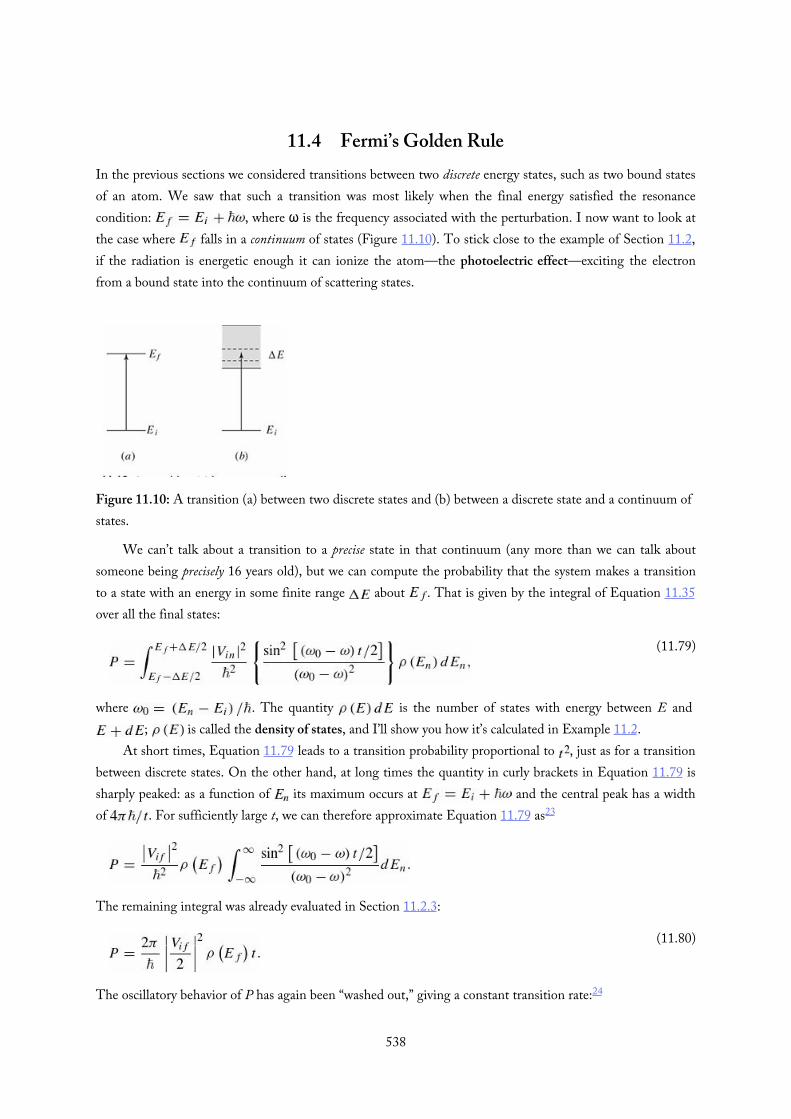
(11.79)
(11.80)
11.4 Fermi’s Golden RuleIn the previous sections we considered transitions between two discrete energy states, such as two bound statesof an atom. We saw that such a transition was most likely when the final energy satisfied the resonancecondition: , where ω is the frequency associated with the perturbation. I now want to look atthe case where falls in a continuum of states (Figure 11.10). To stick close to the example of Section 11.2,if the radiation is energetic enough it can ionize the atom—the photoelectric effect—exciting the electronfrom a bound state into the continuum of scattering states.
Figure 11.10: A transition (a) between two discrete states and (b) between a discrete state and a continuum ofstates.
We can’t talk about a transition to a precise state in that continuum (any more than we can talk aboutsomeone being precisely 16 years old), but we can compute the probability that the system makes a transitionto a state with an energy in some finite range about . That is given by the integral of Equation 11.35over all the final states:
where . The quantity is the number of states with energy between E and ; is called the density of states, and I’ll show you how it’s calculated in Example 11.2.
At short times, Equation 11.79 leads to a transition probability proportional to , just as for a transitionbetween discrete states. On the other hand, at long times the quantity in curly brackets in Equation 11.79 issharply peaked: as a function of its maximum occurs at and the central peak has a widthof . For sufficiently large t, we can therefore approximate Equation 11.79 as23
The remaining integral was already evaluated in Section 11.2.3:
The oscillatory behavior of P has again been “washed out,” giving a constant transition rate:24
538

(11.81)
(11.82)
(11.83)
(11.84)
Equation 11.81 is known as Fermi’s Golden Rule.25 Apart from the factor of , it says that the transitionrate is the square of the matrix element (this encapsulates all the relevant information about the dynamics ofthe process) times the density of states (how many final states are accessible, given the energy supplied by theperturbation—the more roads are open, the faster the traffic will flow). It makes sense.
Example 11.2Use Fermi’s Golden Rule to obtain the differential scattering cross-section for a particle of mass m andincident wave vector scattering from a potential (Figure 11.11).
Figure 11.11: A particle with incident wave vector is scattered into a state with wave vector k.
Solution:We take our initial and final states to be plane waves:
Here I’ve used a technique called box normalization; I place the whole setup inside a box of length lon a side. This makes the free-particle states normalizable and countable. Formally, we want the limit
; in practice l will drop out of our final expression. Using periodic boundary conditions,26 theallowed values of are
for integers , , and . Our perturbation is the scattering potential, , and the relevantmatrix element is
We need to determine the density of states. In a scattering experiment we measure the number ofparticles scatterred into a solid angle . We want to count the number of states with energiesbetween E and , with wave vectors lying inside . In k space these states occupy a sectionof a spherical shell of radius k and thickness dk that subtends a solid angle ; it has a volume
539
(11.85)
(11.86)
(11.87)
(11.88)
∗∗∗
and contains a number of states27
Since this gives
From Fermi’s Golden Rule, the rate at which particles are scattered into the solid angle is28
This is closely related to the differential scattering cross section:
where is the flux (or probability current) of incident particles. For an incident wave of the form , the probability current is (Equation 4.220).
and
This is exactly what we got from the first Born approximation (Equation 10.79).
Problem 11.17 In the photoelectric effect, light can ionize an atom if its energy exceeds the binding energy of the electron. Consider the photoelectric effect
for the ground state of hydrogen, where the electron is kicked out withmomentum . The initial state of the electron is (Equation 4.80) and itsfinal state is29
as in Example 11.2.(a) For light polarized along the z direction, use Fermi’s Golden Rule to
compute the rate at which electrons are ejected into the solid angle inthe dipole approximation.30
540

Hint:To evaluate the matrix element, use the following trick. Write
pull outside the integral, and what remains is straightforward tocompute.
(b) The photoelectric cross section is defined as
where the quantity in the numerator is the rate at which energy isabsorbed per photoelectron) and the quantity in thedenominator is the intensity of the incident light. Integrate your resultfrom (a) over all angles to obtain , and compute the photoelectriccross section.
(c) Obtain a numerical value for the photoelectric cross section for ultravioletlight of wavelength (n.b. this is the wavelength of the incidentlight, not the scattered electron). Express your answer in mega-barns
.
541

11.5 The Adiabatic Approximation
542

11.5.1 Adiabatic Processes
Imagine a perfect pendulum, with no friction or air resistance, oscillating back and forth in a vertical plane. Ifyou grab the support and shake it in a jerky manner the bob will swing around chaotically. But if you verygently move the support (Figure 11.12), the pendulum will continue to swing in a nice smooth way, in thesame plane (or one parallel to it), with the same amplitude. This gradual change of the external conditionsdefines an adiabatic process. Notice that there are two characteristic times involved: , the “internal” time,representing the motion of the system itself (in this case the period of the pendulum’s oscillations), and , the“external” time, over which the parameters of the system change appreciably (if the pendulum were mountedon a rotating platform, for example, would be the period of the platform’s motion). An adiabatic process isone for which (the pendulum executes many oscillations before the platform has movedappreciably).31
Figure 11.12: Adiabatic motion: If the case is transported very gradually, the pendulum inside keeps swingingwith the same amplitude, in a plane parallel to the original one.
What if I took this pendulum up to the North Pole, and set it swinging—say, in the direction ofPortland (Figure 11.13). For the moment, pretend the earth is not rotating. Very gently (that is, adiabatically),I carry it down the longitude line passing through Portland, to the equator. At this point it is swinging north-south. Now I carry it (still swinging north–south) part way around the equator. And finally, I take it back upto the North Pole, along the new longitude line. The pendulum will no longer be swinging in the same planeas it was when I set out—indeed, the new plane makes an angle Θ with the old one, where Θ is the anglebetween the southbound and the northbound longitude lines. More generally, if you transport the pendulumaround a closed loop on the surface of the earth, the angular deviation (between the initial plane of the swingand the final plane) is equal to the solid angle subtended by the path with respect to the center of the sphere,as you can prove for yourself if you are interested.
543
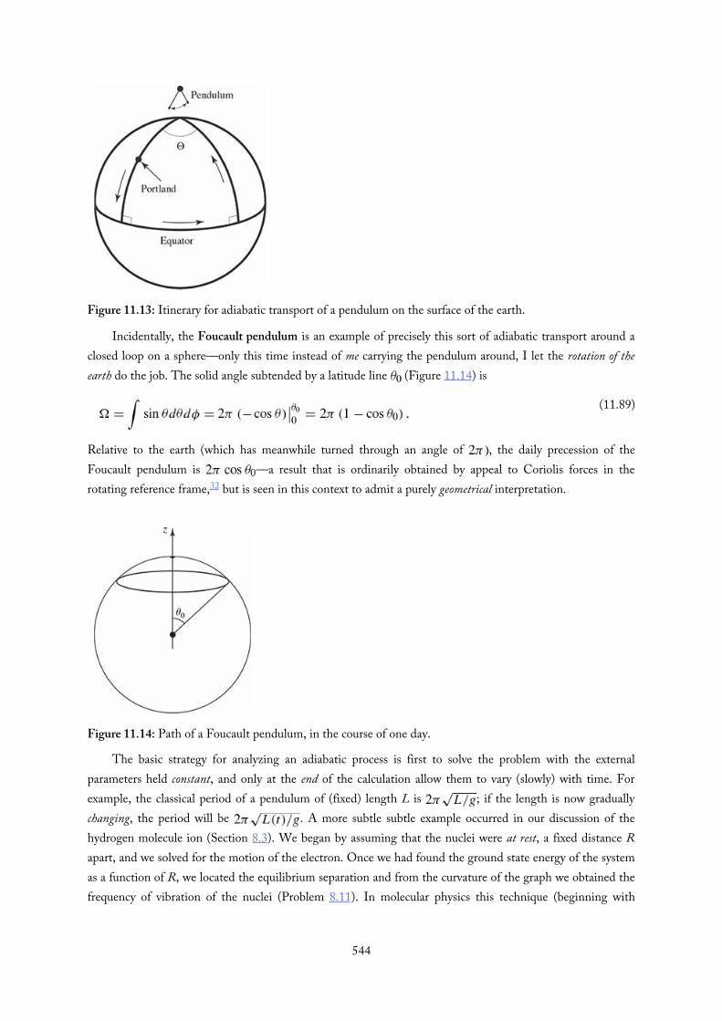
(11.89)
Figure 11.13: Itinerary for adiabatic transport of a pendulum on the surface of the earth.
Incidentally, the Foucault pendulum is an example of precisely this sort of adiabatic transport around aclosed loop on a sphere—only this time instead of me carrying the pendulum around, I let the rotation of theearth do the job. The solid angle subtended by a latitude line (Figure 11.14) is
Relative to the earth (which has meanwhile turned through an angle of , the daily precession of theFoucault pendulum is —a result that is ordinarily obtained by appeal to Coriolis forces in therotating reference frame,32 but is seen in this context to admit a purely geometrical interpretation.
Figure 11.14: Path of a Foucault pendulum, in the course of one day.
The basic strategy for analyzing an adiabatic process is first to solve the problem with the externalparameters held constant, and only at the end of the calculation allow them to vary (slowly) with time. Forexample, the classical period of a pendulum of (fixed) length L is ; if the length is now graduallychanging, the period will be . A more subtle subtle example occurred in our discussion of thehydrogen molecule ion (Section 8.3). We began by assuming that the nuclei were at rest, a fixed distance Rapart, and we solved for the motion of the electron. Once we had found the ground state energy of the systemas a function of R, we located the equilibrium separation and from the curvature of the graph we obtained thefrequency of vibration of the nuclei (Problem 8.11). In molecular physics this technique (beginning with
544

nuclei at rest, calculating electronic wave functions, and using these to obtain information about the positionsand—relatively sluggish—motion of the nuclei) is known as the Born–Oppenheimer approximation.
545

(11.90)
(11.91)
11.5.2 The Adiabatic Theorem
In quantum mechanics, the essential content of the adiabatic approximation can be cast in the form of atheorem. Suppose the Hamiltonian changes gradually from some initial form to some final form .The adiabatic theorem33 states that if the particle was initially in the nth eigenstate of , it will be carried(under the Schrödinger equation) into the nth eigenstate of . (I assume that the spectrum is discrete andnondegenerate throughout the transition, so there is no ambiguity about the ordering of the states; theseconditions can be relaxed, given a suitable procedure for “tracking” the eigenfunctions, but I’m not going topursue that here.)
Example 11.3Suppose we prepare a particle in the ground state of the infinite square well (Figure 11.15(a)):
Figure 11.15: (a) Particle starts out in the ground state of the infinite square well. (b) If the wallmoves slowly, the particle remains in the ground state. (c) If the wall moves rapidly, the particle is left(momentarily) in its initial state.
If we now gradually move the right wall out to , the adiabatic theorem says that the particle willend up in the ground state of the expanded well (Figure 11.15(b)):
(apart from a phase factor, which we’ll discuss in a moment). Notice that we’re not talking about asmall change in the Hamiltonian (as in perturbation theory)—this one is huge. All we require is that ithappen slowly.
Energy is not conserved here—of course not: Whoever is moving the wall is extracting energy fromthe system, just like the piston on a slowly expanding cylinder of gas. By contrast, if the well expandssuddenly, the resulting state is still (Figure 11.15c), which is a complicated linear combinationof eigenstates of the new Hamiltonian (Problem 11.18). In this case energy is conserved (at least, itsexpectation value is); as in the free expansion of a gas (into a vacuum) when the barrier is suddenlyremoved; no work is done.
According to the adiabatic theorem, a system that starts out in the nth eigenstate of the initialHamiltonian will evolve as the nth eigenstate of the instantaneous Hamiltonian , as the
546

(11.92)
(11.93)
(11.94)
(11.96)
(11.97)
(11.98)
(11.95)
Hamiltonian gradually changes. However, this doesn’t tell us what happens to the phase of the wave function.For a constant Hamiltonian it would pick up the standard “wiggle factor”
but the eigenvalue may now itself be a function of time, so the wiggle factor naturally generalizes to
This is called the dynamic phase. But it may not be the end of the story; for all we know there may be anadditional phase factor, , the so-called geometric phase. In the adiabatic limit, then, the wave function attime t takes the form34
where is the nth eigenstate of the instantaneous Hamiltonian,
Equation 11.93 is the formal statement of the adiabatic theorem.Of course, the phase of is itself arbitrary (it’s still an eigenfunction, with the same eigenvalue,
whatever phase you choose), so the geometric phase itself carries no physical significance. But what if we carrythe system around a closed cycle (like the pendulum we hauled down to the equator, around, and back to thenorth pole), so that the Hamiltonian at the end is identical to the Hamiltonian at the beginning? Then the netphase change is a measurable quantity. The dynamic phase depends on the elapsed time, but the geometricphase, around an adiabatic closed cycle, depends only on the path taken.35 It is called Berry’s phase:36
Example 11.4Imagine an electron (charge , mass at rest at the origin, in the presence of a magnetic fieldwhose magnitude is constant, but whose direction sweeps out a cone, of opening angle α, atconstant angular velocity ω (Figure 11.16):
The Hamiltonian (Equation 4.158) is
where
The normalized eigenspinors of are
547

(11.99)
(11.100)
(11.101)
(11.102)
(11.103)
(11.104)
(11.105)
and
they represent spin up and spin down, respectively, along the instantaneous direction of (seeProblem 4.33). The corresponding eigenvalues are
Figure 11.16: The magnetic field sweeps around in a cone, at angular velocity ω (Equation 11.96).
Suppose the electron starts out with spin up, along B(0):
The exact solution to the time-dependent Schrödinger equation is (Problem 11.20):
where
or, expressing it as a linear combination of and :
Evidently the (exact) probability of a transition to spin down (along the current direction of B) is
548

(11.106)
(11.107)
∗
The adiabatic theorem says that this transition probability should vanish in the limit ,where is the characteristic time for changes in the Hamiltonian (in this case, and is thecharacteristic time for changes in the wave function (in this case, . Thus theadiabatic approximation means : the field rotates slowly, in comparison with the phase of the(unperturbed) wave functions. In the adiabatic regime (Equation 11.104), and therefore
as advertised. The magnetic field leads the electron around by its nose, with the spin always pointingin the direction of B. By contrast, if then , and the system bounces back and forthbetween spin up and spin down (Figure 11.17).
Figure 11.17: Plot of the transition probability, Equation 11.106, in the non-adiabatic regime .
Problem 11.18 A particle of mass m is in the ground state of the infinite squarewell (Equation 2.22). Suddenly the well expands to twice its original size—theright wall moving from a to —leaving the wave function (momentarily)undisturbed. The energy of the particle is now measured.
(a) What is the most probable result? What is the probability of getting thatresult?
(b) What is the next most probable result, and what is its probability?Suppose your measurement returned this value; what would you concludeabout conservation of energy?
(c) What is the expectation value of the energy? Hint: If you find yourselfconfronted with an infinite series, try another method.
549

∗∗
∗
Problem 11.19 A particle is in the ground state of the harmonic oscillator withclassical frequency ω, when suddenly the spring constant quadruples, so ,without initially changing the wave function (of course, will now evolvedifferently, because the Hamiltonian has changed). What is the probability that ameasurement of the energy would still return the value ? What is theprobability of getting ? Answer: 0.943.
Problem 11.20 Check that Equation 11.103 satisfies the time-dependentSchrödinger equation for the Hamiltonian in Equation 11.97. Also confirmEquation 11.105, and show that the sum of the squares of the coefficients is 1, asrequired for normalization.
Problem 11.21 Find Berry’s phase for one cycle of the process in Example 11.4.Hint: Use Equation 11.105 to determine the total phase change, and subtract offthe dynamical part. You’ll need to expand (Equation 11.104) to first order in
.
Problem 11.22 The delta function well (Equation 2.117) supports a single boundstate (Equation 2.132). Calculate the geometric phase change when α graduallyincreases from to . If the increase occurs at a constant rate ,what is the dynamic phase change for this process?37
550

∗∗∗
(11.108)
(11.110)
(11.111)
(11.109)
Further Problems on Chapter 11
Problem 11.23 In Problem 11.1 you showed that the solution to
(where is a function of is
This suggests that the solution to the Schrödinger equation (11.1) might be
It doesn’t work, because is an operator, not a function, and doesnot (in general) commute with .(a) Try calculating , using Equation 11.108. Note: as always, the
exponentiated operator is to be interpreted as a power series:
Show that if , then satisfies the Schrödinger equation.
(b) Check that the correct solution in the general case is
UGLY! Notice that the operators in each term are “time-ordered,” in the sense that the latest appears at the far left, followed bythe next latest, and so on . Dyson introduced thetime-ordered product of two operators:
or, more generally,
where .
551

(11.112)
∗∗
(11.113)
(11.114)
(11.115)
(11.116)
(11.117)
(11.118)
(11.119)
(c) Show that
and generalize to higher powers of . In place of , in equation 11.108,
we really want :
This is Dyson’s formula; it’s a compact way of writing Equation 11.109,the formal solution to Schrödinger’s equation. Dyson’s formula plays afundamental role in quantum field theory.38
Problem 11.24 In this problem we develop time-dependent perturbation theoryfor a multi-level system, starting with the generalization of Equations 11.5 and11.6:
At time we turn on a perturbation , so that the total Hamiltonianis
(a) Generalize Equation 11.10 to read
and show that
where
(b) If the system starts out in the state , show that (in first-orderperturbation theory)
and
(c) For example, suppose is constant (except that it was turned on at 552

(11.120)
(11.121)
(11.122)
∗
(c) For example, suppose is constant (except that it was turned on at , and switched off again at some later time . Find the probability oftransition from state N to state M , as a function of T. Answer:
(d) Now suppose is a sinusoidal function of time: .Making the usual assumptions, show that transitions occur only to stateswith energy , and the transition probability is
(e) Suppose a multi-level system is immersed in incoherent electromagneticradiation. Using Section 11.2.3 as a guide, show that the transition ratefor stimulated emission is given by the same formula (Equation 11.54) asfor a two-level system.
Problem 11.25 For the examples in Problem 11.24 (c) and (d), calculate , tofirst order. Check the normalization condition:
and comment on any discrepancy. Suppose you wanted to calculate theprobability of remaining in the original state ; would you do better to use
, or ?
Problem 11.26 A particle starts out (at time in the Nth state of the infinitesquare well. Now the “floor” of the well rises temporarily (maybe water leaksin, and then drains out again), so that the potential inside is uniform but timedependent: , with .(a) Solve for the exact , using Equation 11.116, and show that the wave
function changes phase, but no transitions occur. Find the phase change, , in terms of the function .
(b) Analyze the same problem in first-order perturbation theory, andcompare your answers.
Comment: The same result holds whenever the perturbation simplyadds a constant (constant in x, that is, not in to the potential; it hasnothing to do with the infinite square well, as such. Compare Problem1.8.
Problem 11.27 A particle of mass m is initially in the ground state of the (one-dimensional) infinite square well. At time a “brick” is dropped into thewell, so that the potential becomes
553

∗∗∗
(11.123)
(11.124)
(11.125)
(11.126)
where . After a time T, the brick is removed, and the energy of theparticle is measured. Find the probability (in first-order perturbation theory)that the result is now .
Problem 11.28 We have encountered stimulated emission, (stimulated)absorption, and spontaneous emission. How come there is no such thing asspontaneous absorption?
Problem 11.29 Magnetic resonance. A spin-1/2 particle with gyromagnetic ratioγ, at rest in a static magnetic field , precesses at the Larmor frequency
(Example 4.3). Now we turn on a small transverse radiofrequency(rf) field, , so that the total field is
(a) Construct the Hamiltonian matrix (Equation 4.158) for thissystem.
(b) If is the spin state at time t, show that
where is related to the strength of the rf field.(c) Check that the general solution for and , in terms of their initial
values and , is
where
(d) If the particle starts out with spin up (i.e. , , find theprobability of a transition to spin down, as a function of time. Answer:
(e) Sketch the resonance curve,
as a function of the driving frequency ω (for fixed and . Note that554
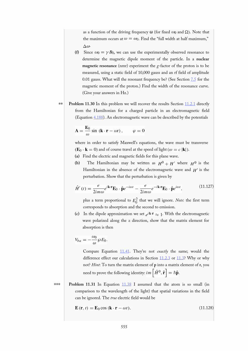
∗∗
(11.127)
∗∗∗
(11.128)
as a function of the driving frequency ω (for fixed and . Note thatthe maximum occurs at . Find the “full width at half maximum,”
.(f) Since , we can use the experimentally observed resonance to
determine the magnetic dipole moment of the particle. In a nuclearmagnetic resonance (nmr) experiment the g-factor of the proton is to bemeasured, using a static field of 10,000 gauss and an rf field of amplitude0.01 gauss. What will the resonant frequency be? (See Section 7.5 for themagnetic moment of the proton.) Find the width of the resonance curve.(Give your answers in Hz.)
Problem 11.30 In this problem we will recover the results Section 11.2.1 directlyfrom the Hamiltonian for a charged particle in an electromagnetic field(Equation 4.188). An electromagnetic wave can be described by the potentials
where in order to satisfy Maxwell’s equations, the wave must be transverse and of course travel at the speed of light .
(a) Find the electric and magnetic fields for this plane wave.(b) The Hamiltonian may be written as where is the
Hamiltonian in the absence of the electromagnetic wave and is theperturbation. Show that the perturbation is given by
plus a term proportional to that we will ignore. Note: the first termcorresponds to absorption and the second to emission.
(c) In the dipole approximation we set . With the electromagneticwave polarized along the z direction, show that the matrix element forabsorption is then
Compare Equation 11.41. They’re not exactly the same; would thedifference effect our calculations in Section 11.2.3 or 11.3? Why or whynot? Hint: To turn the matrix element of p into a matrix element of r, you
need to prove the following identity: .
Problem 11.31 In Equation 11.38 I assumed that the atom is so small (incomparison to the wavelength of the light) that spatial variations in the fieldcan be ignored. The true electric field would be
555

(11.129)
(11.130)
(11.131)
∗∗∗
(11.132)
(11.133)
If the atom is centered at the origin, then over the relevant volume , so , and that’s why we could afford to drop
this term. Suppose we keep the first-order correction:
The first term gives rise to the allowed (electric dipole) transitions weconsidered in the text; the second leads to so-called forbidden (magneticdipole and electric quadrupole) transitions (higher powers of lead to evenmore “forbidden” transitions, associated with higher multipole moments).39
(a) Obtain the spontaneous emission rate for forbidden transitions (don’tbother to average over polarization and propagation directions, thoughthis should really be done to complete the calculation). Answer:
(b) Show that for a one-dimensional oscillator the forbidden transitions gofrom level n to level , and the transition rate (suitably averaged over
and is
(Note: Here ω is the frequency of the photon, not the oscillator.) Find theratio of the “forbidden” rate to the “allowed” rate, and comment on theterminology.
(c) Show that the transition in hydrogen is not possible even by a“forbidden” transition. (As it turns out, this is true for all the highermultipoles as well; the dominant decay is in fact by two-photon emission,and the lifetime is about a tenth of a second.40 )
Problem 11.32 Show that the spontaneous emission rate (Equation 11.63) for atransition from to in hydrogen is
where
(The atom starts out with a specific value of m, and it goes to any of the states consistent with the selection rules: . Notice that
the answer is independent of m.) Hint: First calculate all the nonzero matrix
556

(11.134)
(11.135)
∗∗∗
elements of x, y, and z between and for the case .From these, determine the quantity
Then do the same for . You may find useful the following recursionformulas (which hold for :41
and the orthogonality relation Equation 4.33.
Problem 11.33 The spontaneous emission rate for the 21-cm hyperfine line inhydrogen (Section 7.5) can be obtained from Equation 11.63, except that thisis a magnetic dipole transition, not an electric one:42
where
are the magnetic moments of the electron and proton (Equation 7.89), and , are the singlet and triplet configurations (Equations 4.175 and 4.176).
Because , the proton contribution is negligible, so
Work out (use whichever triplet state you like). Put in the actualnumbers, to determine the transition rate and the lifetime of the triplet state.Answer: years.
Problem 11.34 A particle starts out in the ground state of the infinite square well(on the interval . Now a wall is slowly erected, slightly off-center:43
where rises gradually from 0 to . According to the adiabatic theorem,the particle will remain in the ground state of the evolving Hamiltonian.(a) Find (and sketch) the ground state at . Hint: This should be the
ground state of the infinite square well with an impenetrable barrier at . Note that the particle is confined to the (slightly) larger left
“half” of the well.
557

∗∗∗
(11.136)
(11.137)
(11.138)
(b) Find the (transcendental) equation for the ground state energy at time t.Answer:
where , , , and .(c) Setting , solve graphically for z, and show that the smallest z goes
from π to as T goes from 0 to . Explain this result.(d) Now set and solve numerically for z, using , 1, 5, 20,
100, and 1000.(e) Find the probability that the particle is in the right “half” of the well, as
a function of z and δ. Answer: , where . Evaluate this
expression numerically for the T’s and δ in part (d). Comment on yourresults.
(e) Plot the ground state wave function for those same values of T and δ.Note how it gets squeezed into the left half of the well, as the barriergrows.44
Problem 11.35 The case of an infinite square well whose right wall expands at aconstant velocity can be solved exactly.45 A complete set of solutions is
where is the width of the well and isthe nth allowed energy of the original well (width . The general solution is alinear combination of the Φ’s:
whose coefficients are independent of t.(a) Check that Equation 11.136 satisfies the time-dependent Schrödinger
equation, with the appropriate boundary conditions.(b) Suppose a particle starts out in the ground state of the initial
well:
Show that the expansion coefficients can be written in the form
where is a dimensionless measure of the speed withwhich the well expands. (Unfortunately, this integral cannot be evaluated
558

(11.139)
∗∗∗
(11.140)
(11.141)
(11.143)
(11.142)
in terms of elementary functions.)(c) Suppose we allow the well to expand to twice its original width, so the
“external” time is given by . The “internal” time is the periodof the time-dependent exponential factor in the (initial) ground state.Determine and , and show that the adiabatic regime corresponds to
, so that over the domain of integration. Usethis to determine the expansion coefficients, . Construct , andconfirm that it is consistent with the adiabatic theorem.
(d) Show that the phase factor in can be written in the form
where is the nth instantaneous eigenvalue, attime t. Comment on this result. What is the geometric phase? If the wellnow contracts back to its original size, what is Berry’s phase for the cycle?
Problem 11.36 The driven harmonic oscillator. Suppose the one-dimensionalharmonic oscillator (mass m, frequency is subjected to a driving force of theform , where is some specified function. (I havefactored out for notational convenience; has the dimensions oflength.) The Hamiltonian is
Assume that the force was first turned on at time : for .This system can be solved exactly, both in classical mechanics and in quantummechanics.46
(a) Determine the classical position of the oscillator, assuming it started fromrest at the origin . Answer:
(b) Show that the solution to the (time-dependent) Schrödinger equation forthis oscillator, assuming it started out in the nth state of the undrivenoscillator ( where is given by Equation 2.62),can be written as
(c) Show that the eigenfunctions and eigenvalues of are
(d) Show that in the adiabatic approximation the classical position (Equation559

(11.144)
(11.145)
(11.146)
(11.147)
(11.148)
(d) Show that in the adiabatic approximation the classical position (Equation11.141) reduces to . State the precise criterion foradiabaticity, in this context, as a constraint on the time derivative of f.Hint: Write as and useintegration by parts.
(e) Confirm the adiabatic theorem for this example, by using the results in (c)and (d) to show that
Check that the dynamic phase has the correct form (Equation 11.92). Isthe geometric phase what you would expect?
Problem 11.37 Quantum Zeno Paradox.47 Suppose a system starts out in anexcited state , which has a natural lifetime τ for transition to the groundstate . Ordinarily, for times substantially less than τ, the probability of atransition is proportional to t (Equation 11.49):
If we make a measurement after a time t, then, the probability that the systemis still in the upper state is
Suppose we do find it to be in the upper state. In that case the wave functioncollapses back to , and the process starts all over again. If we make a secondmeasurement, at , the probability that the system is still in the upper state is
which is the same as it would have been had we never made the firstmeasurement at t (as one would naively expect).However, for extremely short times, the probability of a transition is notproportional to t, but rather to (Equation 11.46):48
(a) In this case what is the probability that the system is still in the upperstate after the two measurements? What would it have been (after thesame elapsed time) if we had never made the first measurement?
(b) Suppose we examine the system at n regular (extremely short) intervals,from out to (that is, we make measurements at , ,
, …, . What is the probability that the system is still in the upperstate at time T? What is its limit as ? Moral of the story: Because
560

∗∗∗
(11.149)
(11.151)
(11.152)
(11.153)
(11.154)
(11.150)
of the collapse of the wave function at every measurement, a continuouslyobserved system never decays at all!49
Problem 11.38 The numerical solution to the time-independent Schrödingerequation in Problem 2.61 can be extended to solve the time-dependentSchrödinger equation. When we discretize the variable x, we obtain the matrixequation
The solution to this equation can be written
If is time independent, the exact expression for the time-evolution operatoris50
and for small enough, the time-evolution operator can be approximated as
While Equation 11.152 is the most obvious way to approximate , anumerical scheme based on it is unstable, and it is preferable to use Cayley’sform for the approximation:51
Combining Equations 11.153 and 11.150 we have
This has the form of a matrix equation which can be solved for theunknown . Because the matrix is tri-diagonal,52 efficient algorithms exist for doing so.53
(a) Show that the approximation in Equation 11.153 is accurate to secondorder. That is, show that Equations 11.151 and 11.153, expanded aspower series in , agree up through terms of order . Verify that thematrix in Equation 11.153 is unitary.
As an example, consider a particle of mass m moving in one dimensionin a simple harmonic oscillator potential. For the numerical part set
, , and (this just defines the units of mass, time, andlength).
(b) Construct the Hamiltonian matrix for spatial grid561
∗∗∗
(11.155)
(11.156)
(b) Construct the Hamiltonian matrix for spatial gridpoints. Set the spatial boundaries where the dimensionless length is
(far enough out that we can assume that the wave functionvanishes there for low-energy states). By computer, find the lowest twoeigenvalues of , and compare the exact values. Plot the correspondingeigenfunctions. Are they normalized? If not, normalize them before doingpart (c).
(c) Take (from part (b)) and use Equation 11.154to evolve the wave function from time to . Create amovie (Animate, in Mathematica) showing Re , Im , and
, together with the exact result. Hint: You need to decide what touse for . In terms of the number of time steps , . Inorder for the approximation of the exponential to hold, we need to have
. The energy of our state is of order , and therefore . So you will need at least (say) 100 time steps.
Problem 11.39 We can use the technique of Problem 11.38 to investigate timeevolution when the Hamiltonian does depend on time, as long as we choose small enough. Evaluating at the midpoint of each time step we simplyreplace Equation 11.154 with54
Consider the driven harmonic oscillator of Problem 11.36 with
where A is a constant with the units of length and Ω is the driving frequency.In the following we will set and look at the effect ofvarying Ω. Use the same parameters for the spatial discretization as inProblem 11.38, but set . For a particle that starts off in the groundstate at , create a movie showing the numerical and exact solutions aswell as the instantaneous ground state from to for(a) . In line with the adiabatic theorem, you should see that the
numerical solution is close (up to a phase) to the instantaneous groundstate.
(b) . In line with what you’ve learned about sudden perturbations,you should see that the numerical solution is barely affected by the drivingforce.
(c) .
1 Notice that is modified in every even order, and in every odd order; this would not be true if the perturbation included diagonal terms,or if the system started out in a linear combination of the two states.
2 Perturbation theory for multi-level systems is treated in Problem 11.24.
562

3 For very small t, is independent of ω; it takes a couple of cycles for the system to “realize” that the perturbation is periodic.4 For visible light Å, while the diameter of an atom is around 1 Å, so this approximation is reasonable; but it would not be for x-
rays. Problem 11.31 explores the effect of spatial variation of the field.5 The energy of a charge q in a static field E is . You may well object to the use of an electrostatic formula for a manifestly time-
dependent field. I am implicitly assuming that the period of oscillation is long compared to the time it takes the charge to move around(within the atom).
6 As usual, we assume the nucleus is heavy and stationary; it is the wave function of the electron that concerns us.7 The letter is supposed to remind you of electric dipole moment (for which, in electrodynamics, the letter p is customarily used—in this
context it is rendered as a squiggly to avoid confusion with momentum). Actually, is the off-diagonal matrix element of the zcomponent of the dipole moment operator, . Because of its association with electric dipole moments, radiation governed by Equation11.40 is called electric dipole radiation; it is overwhelmingly the dominant kind, at least in the visible region. See Problem 11.31 forgeneralizations and terminology.
8 For an accessible treatment see Rodney Loudon, The Quantum Theory of Light, 2nd edn (Clarendon Press, Oxford, 1983).9 Einstein’s paper was published in 1917, well before the Schrödinger equation. Quantum electrodynamics comes into the argument via the
Planck blackbody formula, which dates from 1900.10 For an alternative derivation using “seat-of-the-pants” quantum electrodynamics, see Problem 11.11.11 David J. Griffiths, Introduction to Electrodynamics, 4th edn, (Cambridge University Press, Cambridge, UK, 2017), Section 9.2.3. In general,
the energy per unit volume in electromagnetic fields is
For electromagnetic waves, the electric and magnetic contributions are equal, so
and the average over a full cycle is , since the average of cos2 (or sin2) is 1/2.12 Equation 11.46 assumes that the perturbations at different frequencies are independent, so that the total transition probability is a sum of the
individual probabilities. If the different components are coherent (phase-correlated), then we should add amplitudes , not probabilities, and there will be cross-terms. For the applications we will consider the perturbations are always incoherent.
13 I’ll treat as though it were real, even though in general it will be complex. Since
we can do the whole calculation for the real and imaginary parts separately, and simply add the results. In Equation 11.54 the absolute valuesigns denote both the vector magnitude and the complex amplitude:
14 Normally I’d use R for a transition rate, but out of deference to der Alte everyone follows Einstein’s notation in this context.15 Assume that and are very large, so we can treat them as continuous functions of time and ignore statistical fluctuations.16 See, for example, Daniel Schroeder, An Introduction to Thermal Physics (Pearson, Upper Saddle River, NJ, 2000), Section 6.1.17 Schroeder, footnote 16, Section 7.4.18 Griffiths, footnote 11, Section 9.2.1.19 This situation is not to be confused with the case of thermal equilibrium, which we considered in the previous section. We assume here that
the atoms have been lifted out of equilibrium, and are in the process of cascading back down to their equilibrium levels.20 See, for example, Griffiths, footnote 11, Section 11.2.1.21 This is an example of Bohr’s Correspondence Principle. In fact, if we express P in terms of the energy above the ground state, the two
formulas are identical.22 See Equation 6.62 (Equation 6.26 eliminates , or derive them from scratch using Problems 11.14 and 11.15.23 This is the same set of approximations we made in Equations 11.46–11.48.24 In deriving Equation 11.35, our perturbation was
since we dropped the other (off-resonance) exponential. That is the source of the two inside the absolute value in Equation 11.81. Fermi’sGolden rule can also be applied to a constant perturbation, , if we set drop the 2:
563

25 It is actually due to Dirac, but Fermi is the one who gave it the memorable name. See T. Visser, Am. J. Phys. 77, 487 (2009) for the history.Fermi’s Golden Rule doesn’t just apply to transitions to a continuum of states. For instance, Equation 11.54 can be considered an example.In that case, we integrated over a continuous range of perturbation frequencies—not a continuum of final states—but the end result is thesame.
26 Periodic boundary conditions are discussed in Problem 5.39. In the present context we use periodic boundary conditions—as opposed toimpenetrable walls—because they admit traveling-wave solutions.
27 Each state in k-space “occupies” a volume of , as shown in Problem 5.39.28 See footnote 24.29 This is an approximation; we really should be using a scattering state of hydrogen. For an extended discussion of the photoelectric effect,
including comparison to experiment and the validity of this approximation, see W. Heitler, The Quantum Theory of Radiation, 3rd edn,Oxford University Press, London (1954), Section 21.
30 The result here is too large by a factor of four; correcting this requires a more careful derivation of the matrix element for radiativetransitions (see Problem 11.30). Only the overall factor is affected though; the more interesting features (the dependence on k and arecorrect.
31 For an interesting discussion of classical adiabatic processes, see Frank S. Crawford, Am. J. Phys. 58, 337 (1990).32 See, for example, Jerry B. Marion and Stephen T. Thornton, Classical Dynamics of Particles and Systems, 4th edn, Saunders, Fort Worth, TX
(1995), Example 10.5. Geographers measure latitude up from the equator, rather than down from the pole, so .33 The adiabatic theorem, which is usually attributed to Ehrenfest, is simple to state, and it sounds plausible, but it is not easy to prove. The
argument will be found in earlier editions of this book, Section 10.1.2.34 I’m suppressing the dependence on other variables; only the time dependence is at issue here.35 As Michael Berry puts it, the dynamic phase answers the question “How long did your trip take?” and the geometric phase, “Where have
you been?”36 For more on this subject see Alfred Shapere and Frank Wilczek, eds., Geometric Phases in Physics, World Scientific, Singapore (1989);
Andrei Bernevig and Taylor Hughes, Topological Insulators and Topological Superconductors, Princeton University Press, Princeton, NJ (2013),Chapter 2.
37 If is real, the geometric phase vanishes. You might try to beat the rap by tacking an unnecessary (but perfectly legal) phase factor ontothe eigenfunctions: , where is an arbitrary (real) function. Try it. You’ll get a nonzero geometric phase, all right, butnote what happens when you put it back into Equation 11.93. And for a closed loop it gives zero.
38 The interaction picture is intermediate between the Heisenberg and Schrödinger pictures (see Section 6.8.1). In the interaction picture, thewave function satisfies the “Schrödinger equation”
where the interaction- and Schrödinger-picture operators are related by
and the wave functions satisfy
If you apply the Dyson series to the Schrödinger equation in the interaction picture, you end up with precisely the perturbation series derivedin Section 11.1.2. For more details see Ramamurti Shankar, Principles of Quantum Mechanics, 2nd edn, Springer, New York (1994), Section18.3.
39 For a systematic treatment (including the role of the magnetic field) see David Park, Introduction to the Quantum Theory, 3rd edn (McGraw-Hill, New York, 1992), Chapter 11.
40 See Masataka Mizushima, Quantum Mechanics of Atomic Spectra and Atomic Structure, Benjamin, New York (1970), Section 5.6.41 George B. Arfken and Hans J. Weber, Mathematical Methods for Physicists, 7th edn, Academic Press, San Diego (2013), p. 744.42 Electric and magnetic dipole moments have different units—hence the factor of (which you can check by dimensional analysis).43 Julio Gea-Banacloche, Am. J. Phys. 70, 307 (2002) uses a rectangular barrier; the delta-function version was suggested by M. Lakner and
J. Peternelj, Am. J. Phys. 71, 519 (2003).44 Gea-Banacloche (footnote 43) discusses the evolution of the wave function without using the adiabatic theorem.45 S. W. Doescher and M. H. Rice, Am. J. Phys. 37, 1246 (1969).46 See Y. Nogami, Am. J. Phys. 59, 64 (1991), and references therein.
564

47 This phenomenon doesn’t have much to do with Zeno, but it is reminiscent of the old adage, “a watched pot never boils,” so it is sometimescalled the watched pot effect.
48 In the argument leading to linear time dependence, we assumed that the function in Equation 11.46 was a sharp spike.However, the width of the “spike” is of order , and for extremely short t this assumption fails, and the integral becomes
.49 This argument was introduced by B. Misra and E. C. G. Sudarshan, J. Math. Phys. 18, 756 (1977). The essential result has been confirmed
in the laboratory: W. M. Itano, D. J. Heinzen, J. J. Bollinger, and D. J. Wineland, Phys. Rev. A 41, 2295 (1990). Unfortunately, theexperiment is not as compelling a test of the collapse of the wave function as its designers hoped, for the observed effect can perhaps beaccounted for in other ways—see L. E. Ballentine, Found. Phys. 20, 1329 (1990); T. Petrosky, S. Tasaki, and I. Prigogine, Phys. Lett. A 151,109 (1990).
50 If you choose small enough, you can actually use this exact form. Routines such as Mathematica’s MatrixExp can be used to find(numerically) the exponential of a matrix.
51 See A. Goldberg et al., Am. J. Phys. 35, 177 (1967) for further discussion of these approximations.52 A tri-diagonal matrix has nonzero entries only along the diagonal and one space to the right or left of the diagonal.53 Use your computing enviroment’s built-in linear equation solver; in Mathematica that would be x = LinearSolve[M, b]. To learn how it
actually works, see A. Goldberg et al., footnote 51.54 C. Lubich, in Quantum Simulations of Complex Many-Body Systems: From Theory to Algorithms, edited by J. Grotendorst, D. Marx, and
A. Muramatsu (John von Neumann Institute for Computing, Jülich, 2002), Vol. 10, p. 459. Available for download from the NeumannInstitute for Computing (NIC) website.
565

12Afterword
◈
Now that you have a sound understanding of what quantum mechanics says, I would like to return to thequestion of what it means—continuing the story begun in Section 1.2. The source of the problem is theindeterminacy associated with the statistical interpretation of the wave function. For (or, more generally,the quantum state—it could be a spinor, for example) does not uniquely determine the outcome of ameasurement; all it tells us is the statistical distribution of possible results. This raises a profound question:Did the physical system “actually have” the attribute in question prior to the measurement (the so-calledrealist viewpoint), or did the act of measurement itself “create” the property, limited only by the statisticalconstraint imposed by the wave function (the orthodox position)—or can we duck the issue entirely, on thegrounds that it is “metaphysical” (the agnostic response)?
According to the realist, quantum mechanics is an incomplete theory, for even if you know everythingquantum mechanics has to tell you about the system (to wit: its wave function), still you cannot determine all ofits features. Evidently there is some other information, unknown to quantum mechanics, which (together with
) is required for a complete description of physical reality.The orthodox position raises even more disturbing problems, for if the act of measurement forces the
system to “take a stand,” helping to create an attribute that was not there previously,1 then there is somethingvery peculiar about the measurement process. Moreover, in order to account for the fact that an immediatelyrepeated measurement yields the same result, we are forced to assume that the act of measurement collapsesthe wave function, in a manner that is difficult, at best, to reconcile with the normal evolution prescribed bythe Schrödinger equation.
In light of this, it is no wonder that generations of physicists retreated to the agnostic position, andadvised their students not to waste time worrying about the conceptual foundations of the theory.
566

(12.1)
12.1 The EPR ParadoxIn 1935, Einstein, Podolsky, and Rosen2 published the famous EPR paradox, which was designed to prove(on purely theoretical grounds) that the realist position is the only tenable one. I’ll describe a simplifiedversion of the EPR paradox, due to David Bohm (call it EPRB). Consider the decay of the neutral pi mesoninto an electron and a positron:
Assuming the pion was at rest, the electron and positron fly off in opposite directions (Figure 12.1). Now, thepion has spin zero, so conservation of angular momentum requires that the electron and positron occupy thesinglet spin configuration:
If the electron is found to have spin up, the positron must have spin down, and vice versa. Quantummechanics can’t tell you which combination you’ll get, in any particular pion decay, but it does say that themeasurements will be correlated, and you’ll get each combination half the time (on average). Now suppose welet the electron and positron fly far off—10 meters, in a practical experiment, or, in principle, 10 light years—and then you measure the spin of the electron. Say you get spin up. Immediately you know that someone 20meters (or 20 light years) away will get spin down, if that person examines the positron.
Figure 12.1: Bohm’s version of the EPR experiment: A at rest decays into an electron–positron pair.
To the realist, there’s nothing surprising about this—the electron really had spin up (and the positronspin down) from the moment they were created …it’s just that quantum mechanics didn’t know about it. Butthe “orthodox” view holds that neither particle had either spin up or spin down until the act of measurementintervened: Your measurement of the electron collapsed the wave function, and instantaneously “produced”the spin of the positron 20 meters (or 20 light years) away. Einstein, Podolsky, and Rosen considered such“spooky action-at-a-distance” (Einstein’s delightful term) preposterous. They concluded that the orthodoxposition is untenable; the electron and positron must have had well-defined spins all along, whether quantummechanics knows it or not.
The fundamental assumption on which the EPR argument rests is that no influence can propagate fasterthan the speed of light. We call this the principle of locality. You might be tempted to propose that thecollapse of the wave function is not instantaneous, but “travels” at some finite velocity. However, this wouldlead to violations of angular momentum conservation, for if we measured the spin of the positron before thenews of the collapse had reached it, there would be a fifty–fifty probability of finding both particles with spinup. Whatever you might think of such a theory in the abstract, the experiments are unequivocal: No suchviolation occurs—the (anti-)correlation of the spins is perfect. Evidently the collapse of the wave function—whatever its ontological status—is instantaneous.3
567
Problem 12.1 Entangled states. The singlet spin configuration (Equation 12.1) isthe classic example of an entangled state—a two-particle state that cannot beexpressed as the product of two one-particle states, and for which, therefore, onecannot really speak of “the state” of either particle separately.4 You might wonderwhether this is somehow an artifact of bad notation—maybe some linearcombination of the one-particle states would disentangle the system. Prove thefollowing theorem:
Consider a two-level system, and , with . (For example, mightrepresent spin up and spin down.) The two-particle state
(with and ) cannot be expressed as a product
for any one-particle states and .
Hint: Write and as linear combinations of and .
Problem 12.2 Einstein’s Boxes. In an interesting precursor to the EPR paradox,Einstein proposed the following gedanken experiment:5 Imagine a particleconfined to a box (make it a one-dimensional infinite square well, if you like). It’sin the ground state, when an impenetrable partition is introduced, dividing thebox into separate halves, and , in such a way that the particle is equally likelyto be found in either one.6 Now the two boxes are moved very far apart, and ameasurement is made on to see if the particle is in that box. Suppose theanswer is yes. Immediately we know that the particle will not be found in the(distant) box .
(a) What would Einstein say about this?(b) How does the Copenhagen interpretation account for it? What is the
wave function in , right after the measurement on ?
568
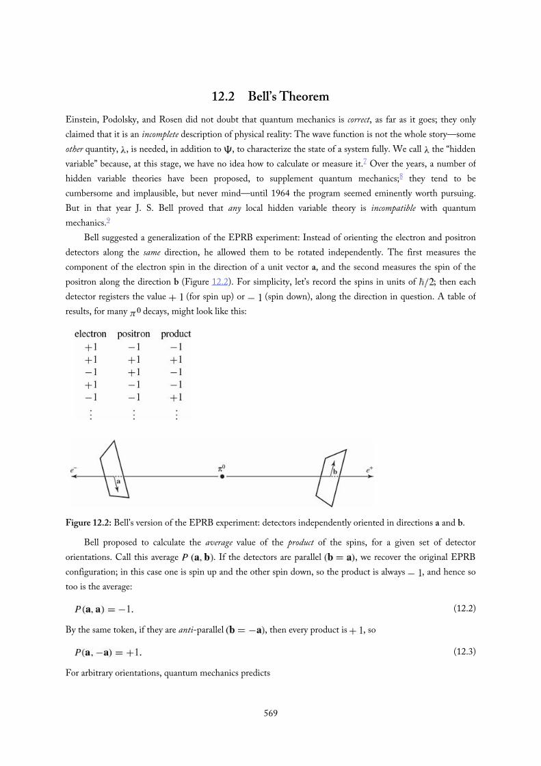
(12.2)
(12.3)
12.2 Bell’s TheoremEinstein, Podolsky, and Rosen did not doubt that quantum mechanics is correct, as far as it goes; they onlyclaimed that it is an incomplete description of physical reality: The wave function is not the whole story—someother quantity, , is needed, in addition to , to characterize the state of a system fully. We call the “hiddenvariable” because, at this stage, we have no idea how to calculate or measure it.7 Over the years, a number ofhidden variable theories have been proposed, to supplement quantum mechanics;8 they tend to becumbersome and implausible, but never mind—until 1964 the program seemed eminently worth pursuing.But in that year J. S. Bell proved that any local hidden variable theory is incompatible with quantummechanics.9
Bell suggested a generalization of the EPRB experiment: Instead of orienting the electron and positrondetectors along the same direction, he allowed them to be rotated independently. The first measures thecomponent of the electron spin in the direction of a unit vector a, and the second measures the spin of thepositron along the direction b (Figure 12.2). For simplicity, let’s record the spins in units of ; then eachdetector registers the value (for spin up) or (spin down), along the direction in question. A table ofresults, for many decays, might look like this:
Figure 12.2: Bell’s version of the EPRB experiment: detectors independently oriented in directions a and b.
Bell proposed to calculate the average value of the product of the spins, for a given set of detectororientations. Call this average . If the detectors are parallel , we recover the original EPRBconfiguration; in this case one is spin up and the other spin down, so the product is always , and hence sotoo is the average:
By the same token, if they are anti-parallel , then every product is , so
For arbitrary orientations, quantum mechanics predicts
569
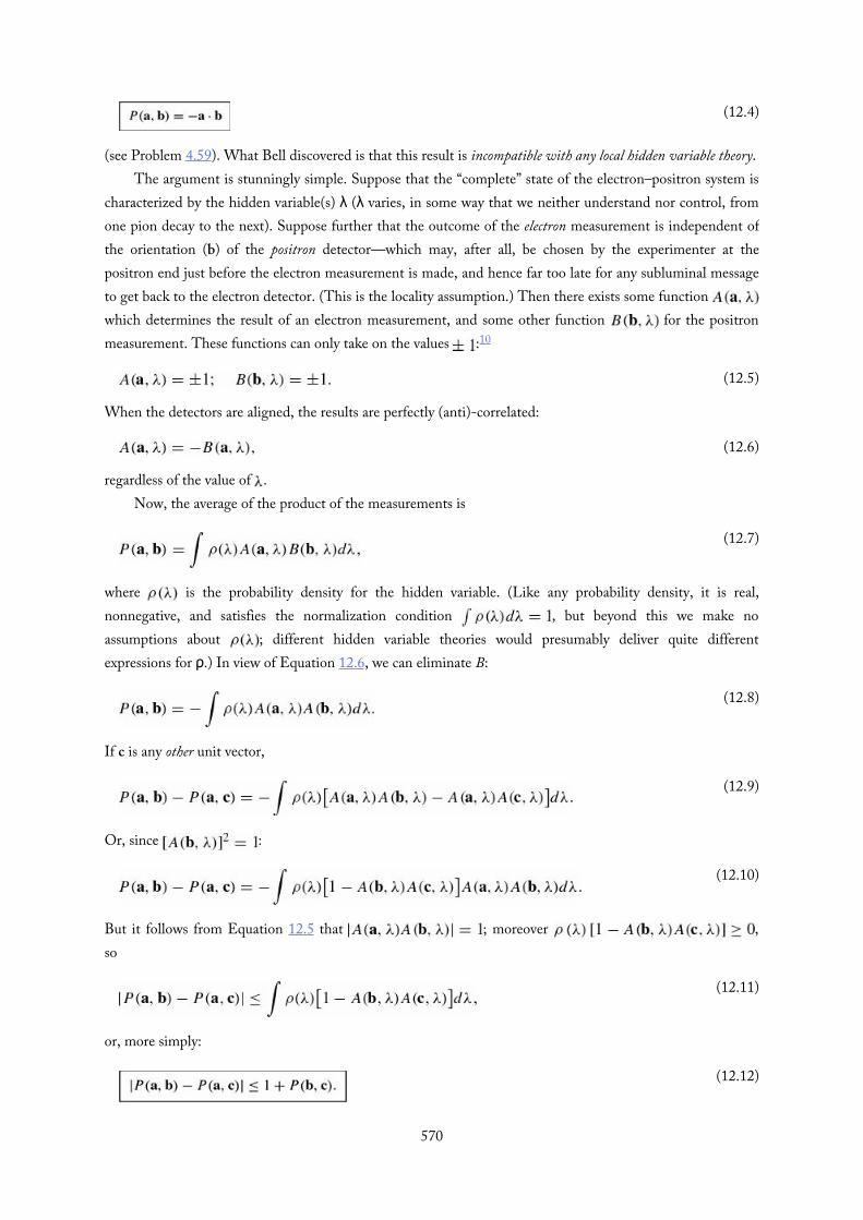
(12.4)
(12.7)
(12.8)
(12.9)
(12.10)
(12.11)
(12.12)
(12.5)
(12.6)
(see Problem 4.59). What Bell discovered is that this result is incompatible with any local hidden variable theory.The argument is stunningly simple. Suppose that the “complete” state of the electron–positron system is
characterized by the hidden variable(s) λ (λ varies, in some way that we neither understand nor control, fromone pion decay to the next). Suppose further that the outcome of the electron measurement is independent ofthe orientation (b) of the positron detector—which may, after all, be chosen by the experimenter at thepositron end just before the electron measurement is made, and hence far too late for any subluminal messageto get back to the electron detector. (This is the locality assumption.) Then there exists some function which determines the result of an electron measurement, and some other function for the positronmeasurement. These functions can only take on the values :10
When the detectors are aligned, the results are perfectly (anti)-correlated:
regardless of the value of .Now, the average of the product of the measurements is
where is the probability density for the hidden variable. (Like any probability density, it is real,nonnegative, and satisfies the normalization condition , but beyond this we make noassumptions about ; different hidden variable theories would presumably deliver quite differentexpressions for ρ.) In view of Equation 12.6, we can eliminate B:
If c is any other unit vector,
Or, since :
But it follows from Equation 12.5 that ; moreover ,so
or, more simply:
570
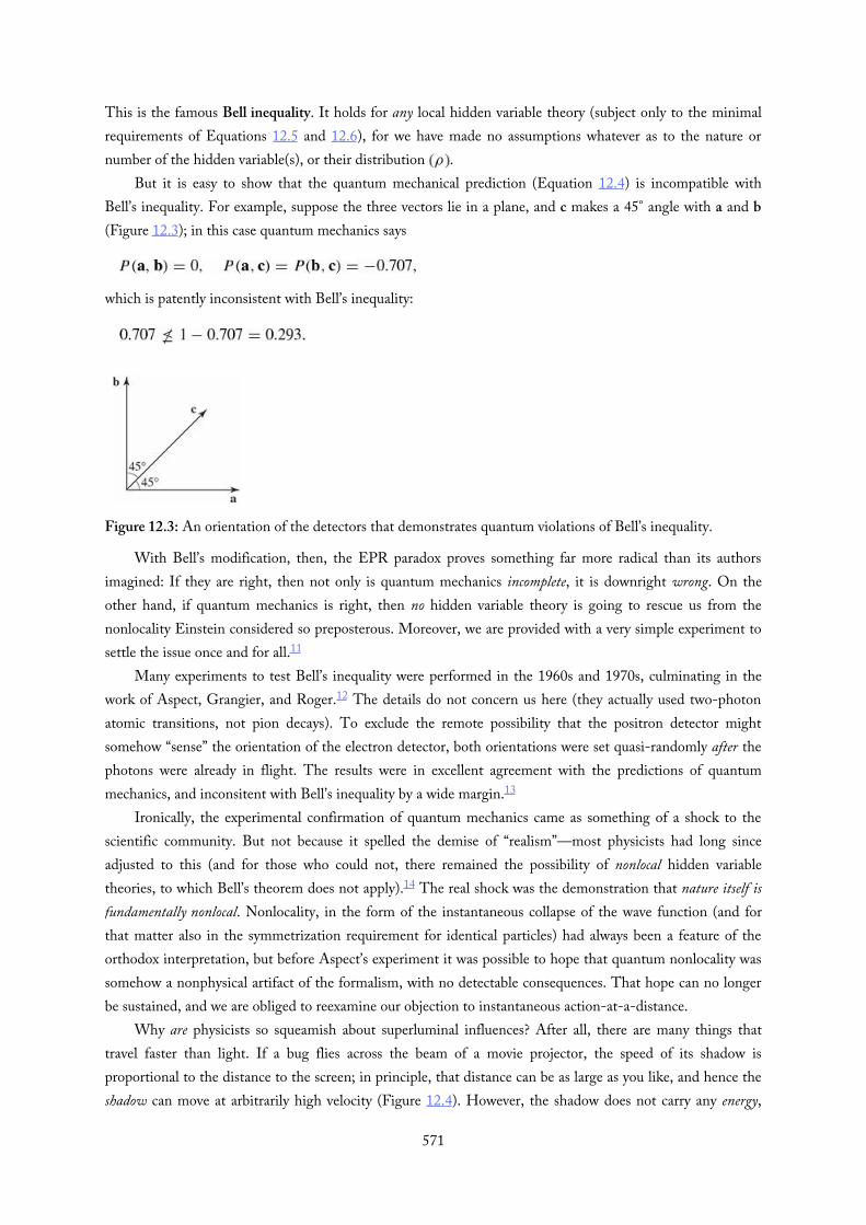
This is the famous Bell inequality. It holds for any local hidden variable theory (subject only to the minimalrequirements of Equations 12.5 and 12.6), for we have made no assumptions whatever as to the nature ornumber of the hidden variable(s), or their distribution .
But it is easy to show that the quantum mechanical prediction (Equation 12.4) is incompatible withBell’s inequality. For example, suppose the three vectors lie in a plane, and c makes a 45° angle with a and b(Figure 12.3); in this case quantum mechanics says
which is patently inconsistent with Bell’s inequality:
Figure 12.3: An orientation of the detectors that demonstrates quantum violations of Bell’s inequality.
With Bell’s modification, then, the EPR paradox proves something far more radical than its authorsimagined: If they are right, then not only is quantum mechanics incomplete, it is downright wrong. On theother hand, if quantum mechanics is right, then no hidden variable theory is going to rescue us from thenonlocality Einstein considered so preposterous. Moreover, we are provided with a very simple experiment tosettle the issue once and for all.11
Many experiments to test Bell’s inequality were performed in the 1960s and 1970s, culminating in thework of Aspect, Grangier, and Roger.12 The details do not concern us here (they actually used two-photonatomic transitions, not pion decays). To exclude the remote possibility that the positron detector mightsomehow “sense” the orientation of the electron detector, both orientations were set quasi-randomly after thephotons were already in flight. The results were in excellent agreement with the predictions of quantummechanics, and inconsitent with Bell’s inequality by a wide margin.13
Ironically, the experimental confirmation of quantum mechanics came as something of a shock to thescientific community. But not because it spelled the demise of “realism”—most physicists had long sinceadjusted to this (and for those who could not, there remained the possibility of nonlocal hidden variabletheories, to which Bell’s theorem does not apply).14 The real shock was the demonstration that nature itself isfundamentally nonlocal. Nonlocality, in the form of the instantaneous collapse of the wave function (and forthat matter also in the symmetrization requirement for identical particles) had always been a feature of theorthodox interpretation, but before Aspect’s experiment it was possible to hope that quantum nonlocality wassomehow a nonphysical artifact of the formalism, with no detectable consequences. That hope can no longerbe sustained, and we are obliged to reexamine our objection to instantaneous action-at-a-distance.
Why are physicists so squeamish about superluminal influences? After all, there are many things thattravel faster than light. If a bug flies across the beam of a movie projector, the speed of its shadow isproportional to the distance to the screen; in principle, that distance can be as large as you like, and hence theshadow can move at arbitrarily high velocity (Figure 12.4). However, the shadow does not carry any energy,
571

nor can it transmit any information from one point on the screen to another. A person at point X cannot causeanything to happen at point Y by manipulating the passing shadow.
Figure 12.4: The shadow of the bug moves across the screen at a velocity greater than c, provided the screenis far enough away.
On the other hand, a causal influence that propagated faster than light would carry unacceptableimplications. For according to special relativity there exist inertial frames in which such a signal propagatesbackward in time—the effect preceding the cause—and this leads to inescapable logical anomalies. (You could,for example, arrange to kill your infant grandfather. Think about it …not a good idea.) The question is, arethe superluminal influences predicted by quantum mechanics and detected by Aspect causal, in this sense, orare they somehow ethereal enough (like the bug’s shadow) to escape the philosophical objection?
Well, let’s consider Bell’s experiment. Does the measurement of the electron influence the outcome of thepositron measurement? Assuredly it does—otherwise we cannot account for the correlations in the data. Butdoes the measurement of the electron cause a particular outcome for the positron? Not in any ordinary sense ofthe word. There is no way the person manning the electron detector could use his measurement to send asignal to the person at the positron detector, since he does not control the outcome of his own measurement(he cannot make a given electron come out spin up, any more than the person at X can affect the passingshadow of the bug). It is true that he can decide whether to make a measurement at all, but the positronmonitor, having immediate access only to data at his end of the line, cannot tell whether the electron has beenmeasured or not. The lists of data compiled at the two ends, considered separately, are completely random. Itis only later, when we compare the two lists, that we discover the remarkable correlations. In another referenceframe the positron measurements occur before the electron measurements, and yet this leads to no logicalparadox—the observed correlation is entirely symmetrical in its treatment, and it is a matter of indifferencewhether we say the observation of the electron influenced the measurement of the positron, or the other wayaround. This is a wonderfully delicate kind of influence, whose only manifestation is a subtle correlationbetween two lists of otherwise random data.
We are led, then, to distinguish two types of influence: the “causal” variety, which produce actual changesin some physical property of the receiver, detectable by measurements on that subsystem alone, and an“ethereal” kind, which do not transmit energy or information, and for which the only evidence is a correlationin the data taken on the two separate subsystems—a correlation which by its nature cannot be detected byexamining either list alone. Causal influences cannot propagate faster than light, but there is no compellingreason why ethereal ones should not. The influences associated with the collapse of the wave function are ofthe latter type, and the fact that they “travel” faster than light may be surprising, but it is not, after all,catastrophic.15
572

∗∗ Problem 12.3 One example16 of a (local) deterministic (“hidden variable”) theoryis …classical mechanics! Suppose we carried out the Bell experiment with classicalobjects (baseballs, say) in place of the electron and proton. They are launched (by akind of double pitching machine) in opposite directions, with equal and oppositespins (angular momenta), and . Now, these are classical objects—their angular momenta can point in any direction, and this direction is set (let’s sayrandomly) at the moment of launch. Detectors placed 10 meters or so on eitherside of the launch point measure the spin vectors of their respective baseballs.However, in order to match the conditions for Bell’s theorem, they only record thesign of the component of S along the directions a and b:
Thus each detector records either or , in any given trial.In this example the “hidden variable” is the actual orientation of , specified
(say) by the polar and azimuthal angles θ and ϕ: :(a) Choosing axes as in the figure, with a and b in the x–y plane and a along
the x axis, verify that
where η is the angle between a and b (take it to run from to ).(b) Assuming the baseballs are launched in such a way that is equally
likely to point in any direction, compute . Answer: .(c) Sketch the graph of , from to , and (on the same
graph) the quantum formula (Equation 12.4, with ). For whatvalues of η does this hidden variable theory agree with the quantum-mechanical result?
(d) Verify that your result satisfies Bell’s inequality, Equation 12.12. Hint:The vectors a, b, and c define three points on the surface of a unit sphere;the inequality can be expressed in terms of the distances between thosepoints.
Figure 12.5: Axes for Problem 12.3.
573

574

12.3 Mixed States and the Density Matrix
575

(12.13)
(12.15)
(12.16)
(12.17)
(12.18)
(12.19)
(12.21)
(12.14)
(12.20)
12.3.1 Pure States
In this book we have dealt with particles in pure states, —a harmonic oscillator in its nth stationary state,for instance, or in a specific linear combination of stationary states, or a free particle in a gaussian wave packet.The expectation value of some observable A is then
it’s the average of measurements on an ensemble of identically-prepared systems, all of them in the same state . We developed the whole theory in terms of (a vector in Hilbert space, or, in the position basis, the
wave function).But there are other ways to formulate the theory, and a particularly useful one starts by defining the
density operator,17
With respect to an orthonormal basis an operator is represented by a matrix; the ij element of thematrix representing the operator is
In particular, the ij element of the density matrix ρ is
The density matrix (for pure states) has several interesting properties:
The expectation value of an observable A is
We could do everything using the density matrix, instead of the wave function, to represent the state of aparticle.
Example 12.1In the standard basis
representing spin up and spin down along the z direction (Equation 4.149), construct the densitymatrix for an electron with spin up along the x direction.
576

(12.22)
(12.23)
(12.24)
(12.25)
(12.26)
Solution: In this case
(Equation 4.151). So
and hence
Or, more efficiently,
Note that ρ is hermitian, its trace is 1, and
Problem 12.4(a) Prove properties 12.17, 12.18, 12.19, and 12.20.(b) Show that the time evolution of the density operator is governed by the
equation
(This is the Schrödinger equation, expressed in terms of .)
Problem 12.5 Repeat Example 12.1 for an electron with spin down along the ydirection.
577

578

(12.27)
(12.28)
(12.29)
(12.30)
(12.31)
(12.34)
(12.35)
(12.32)
(12.33)
12.3.2 Mixed States
In practice it is often the case that we simply don’t know the state of the particle. Suppose, for example, we areinterested in an electron emerging from the Stanford Linear Accelerator. It might have spin up (along somechosen direction), or it might have spin down, or it might be in some linear combination of the two—we justdon’t know.18 We say that the particle is in a mixed state.19
How should we describe such a particle? I could simply list the probability, , that it’s in each possiblestate . The expectation value of an observable would now be the average of measurements taken over anensemble of systems that are not identically prepared (they are not all in the same state); rather, a fraction of them is in each (pure) state :
There’s a slick way to package this information, by generalizing the density operator:
Again, it becomes a matrix when referred to a particular basis:
The density matrix encodes all the information available to us about the system.Like any probabilities,
The density matrix for mixed states retains most of the properties we identified for pure states:
but ρ is idempotent only if it represents a pure state:
(indeed, this is a quick way to test whether the state is pure).
Example 12.2Construct the density matrix for an electron that is either in the spin-up state or the spin-down state(along z), with equal probability.
579

(12.36)
(12.37)
(12.38)
Solution: In this case , so
Note that ρ is hermitian, and its trace is 1, but
this is not a pure state.
Problem 12.6(a) Prove properties 12.31, 12.32, 12.33, and 12.34.(b) Show that Tr , and equal to 1 only if ρ represents a pure state.(c) Show that if and only if ρ represents a pure state.
Problem 12.7(a) Construct the density matrix for an electron that is either in the state spin
up along x (with probability 1/3) or in the state spin down along y (withprobability 2/3).
(b) Find for the electron in (a).
Problem 12.8(a) Show that the most general density matrix for a spin-1/2 particle can be
written in terms of three real numbers :
where are the three Pauli matrices. Hint: It has to behermitian, and its trace must be 1.
(b) In the literature, a is known as the Bloch vector. Show that ρ represents apure state if and only if , and for a mixed state . Hint: UseProblem 12.6(c). Thus every density matrix for a spin-1/2 particlecorresponds to a point in the Bloch sphere, of radius 1. Points on thesurface are pure states, and points inside are mixed states.
(c) What is the probability that a measurement of would return the value , if the tip of the Bloch vector is at (i) the north pole
, (ii) the center of the sphere , (iii) thesouth pole ?
580

(d) Find the spinor χ representing the (pure) state of the system, if the Blochvector lies on the equator, at azimuthal angle ϕ.
581
(12.39)
(12.40)
12.3.3 Subsystems
There is another context in which one might invoke the density matrix formalism: an entangled state, such asthe singlet spin configuration of an electron/positron pair,
Suppose we are interested only in the positron: what is it’s state? I cannot say …a measurement could returnspin up (fifty–fifty probability) or spin down. This has nothing to do with ignorance; I know the state of thesystem precisely. But the subsystem (the positron) by itself does not occupy a pure state. If I insist on talkingabout the positron alone, the best I can do is to tell you its density matrix:
representing the 50/50 mixture.Of course, this is the same as the density matrix representing a positron in a specific (but unknown) spin
state (Example 12.2). I’ll call it a subsystem density matrix, to distinguish it from an ignorance density matrix.The EPRB paradox illustrates the difference. Before the electron spin was measured, the positron (alone) wasrepresented by the “subsystem” density matrix (Equation 12.40); when the electron is measured the positron isknocked into a definite state …but we (at the distant positron detector) don’t know which. The positron isnow represented by the “ignorance” density matrix (Equation 12.36). But the two density matrices areidentical! Our description of the state of the positron has not been altered by the measurement of the electron—all that has changed is our reason for using the density matrix formalism.
582

(12.45)
(12.41)
(12.42)
(12.43)
(12.44)
12.4 The No-Clone TheoremQuantum measurements are typically destructive, in the sense that they alter the state of the system measured.This is how the uncertainty principle is enforced in the laboratory. You might wonder why we don’t just makea bunch of identical copies (clones) of the original state, and measure them, leaving the system itselfunscathed. It can’t be done. Indeed, if you could build a cloning device (a “quantum Xerox machine”),quantum mechanics would be out the window.
For example, it would then be possible to send superluminal messages using the EPRB apparatus.20 Saythe message to be transmitted, from the operator of the electron detector (conventionally “Alice”) to theoperator of the positron detector (“Bob”), is either “yes” (“drop the bomb”) or “no.” If the message is to be“yes,” Alice measures (of the electron). Never mind what result she gets—all that matters is that she makesthe measurement, for this means that the positron is now in the pure state or (never mind which). If shewants to say “no,” she measures , and that means the positron is now in the definite state or (nevermind which). In any case, Bob makes a million clones of the positron, and measures on half of them, and
on the other half. If the first group are all in the same state (all or all ), then Alice must have measured , and the message is “yes” (the group should be a 50/50 mixture). If all the measurements yield the
same answer (all or all ), then Alice must have measured , and the message is “no” (in that case the measurements should be a 50/50 mixture).
It doesn’t work, because you can’t make a quantum Xerox machine, as Wootters, Zurek, and Dieksproved in 1982.21 Schematically, we want the machine to take as input a particle in state (the one to becopied), plus a second particle in state (the “blank sheet of paper”), and spit out two particles in the state
(original plus copy):
Suppose we have made a device that successfully clones the state :
and also works for state :
( and might be spin up and spin down, for example, if the particle is an electron). So far, so good.But what happens when we feed in a linear combination ? Evidently we get22
which is not at all what we wanted—what we wanted was
You can make a machine to clone spin-up electrons and spin-down electrons, but it will fail for any nontriviallinear combinations (such as eigenstates of ). It’s as though you bought a Xerox machine that copies verticallines perfectly, and also horizontal lines, but completely distorts diagonals.
The no-clone theorem turned out to have an importance well beyond “merely” protecting quantum583

The no-clone theorem turned out to have an importance well beyond “merely” protecting quantummechanics from superluminal communication (and hence an inescapable conflict with special relativity).23 Inparticular, it opened up the field of quantum cryptography, which exploits the theorem to detecteavesdropping.24 This time Alice and Bob want to agree on a key for decoding messages, without thecumbersome necessity of actually meeting face-to-face. Alice is to send the key (a string of numbers) to Bobvia a stream of carefully prepared photons.25 But they are worried that their nemesis, Eve, might try tointercept this communication, and thereby crack the code, without their knowledge. Alice prepares a string ofphotons in four different states: linearly polarized (horizontal and vertical ), and circularly polarized(left and right ), which she sends to Bob. Eve hopes to capture and clone the photons en route, sendingthe originals along to Bob, who will be none the wiser. (Later on, she knows, Alice and Bob will comparenotes on a sample of the photons, to make sure there has been no tampering—that’s why she has to clonethem perfectly, to go undetected.) But the no-clone theorem guarantees that Eve’s Xerox machine will fail;26
Alice and Bob will catch the eavesdropping when they compare the samples. (They will then, presumably,discard that key.)
584

(12.46)
12.5 Schrödinger’s CatThe measurement process plays a mischievous role in quantum mechanics: It is here that indeterminacy,nonlocality, the collapse of the wave function, and all the attendant conceptual difficulties arise. Absentmeasurement, the wave function evolves in a leisurely and deterministic way, according to the Schrödingerequation, and quantum mechanics looks like a rather ordinary field theory (much simpler than classicalelectrodynamics, for example, since there is only one field , instead of two (E and B), and it’s a scalar). It isthe bizarre role of the measurement process that gives quantum mechanics its extraordinary richness andsubtlety. But what, exactly, is a measurement? What makes it so different from other physical processes?27
And how can we tell when a measurement has occurred?Schrödinger posed the essential question most starkly, in his famous cat paradox:28
A cat is placed in a steel chamber, together with the following hellish contraption…. In a Geiger counter there is a tiny amount ofradioactive substance, so tiny that maybe within an hour one of the atoms decays, but equally probably none of them decays. If one decaysthen the counter triggers and via a relay activates a little hammer which breaks a container of cyanide. If one has left this entire system foran hour, then one would say the cat is living if no atom has decayed. The first decay would have poisoned it. The wave function of theentire system would express this by containing equal parts of the living and dead cat.
At the end of the hour, then, the wave function of the cat has the schematic form
The cat is neither alive nor dead, but rather a linear combination of the two, until a measurement occurs—until, say, you peek in the window to check. At that moment your observation forces the cat to “take a stand”:dead or alive. And if you find him to be dead, then it’s really you who killed him, by looking in the window.
Schrödinger regarded this as patent nonsense, and I think most people would agree with him. There issomething absurd about the very idea of a macroscopic object being in a linear combination of two palpablydifferent states. An electron can be in a linear combination of spin up and spin down, but a cat simply cannotbe in a linear combination of alive and dead. But how are we to reconcile this with quantum mechanics?
The Schrödinger cat paradox forces us to confront the question “What constitutes a ‘measurement,’ inquantum mechanics”? Does the “measurement” really occur when we peek in the keyhole? Or did it happenmuch earlier, when the atom did (or did not) decay? Or was it when the Geiger counter registered (or did not)the decay, or when the hammer did (or did not) hit the vial of cyanide? Historically, there have been manyanswers to this question. Wigner held that measurement requires the intervention of human consciousness;Bohr thought it meant the interaction between a microscopic system (subject to the laws of quantummechanics) and a macroscopic measuring apparatus (described by classical laws); Heisenberg maintained thata measurement occurs when a permanent record is left; others have pointed to the irreversible nature of ameasurement. The embarrassing fact is that none of these characterizations is entirely satisfactory. Mostphysicists would say that the measurement occurred (and the cat became either alive or dead) well before welooked in the window, but there is no real consensus as to when or why.
And this still leaves the deeper question of why a macroscopic system cannot occupy a linear combinationof two clearly distinct states—a baseball, say, in a linear combination of Seattle and Toronto. Suppose youcould get a baseball into such a state, what would happen to it? In some ultimate sense the macroscopic systemmust itself be described by the laws of quantum mechanics. But wave functions, in the first instance, represent
585
individual elementary particles; the wave function of a macroscopic object would be a monstrouslycomplicated composite structure, built out of the wave functions of its constituent particles. And it issubject to constant bombardment from the environment29 —subject, that is, to continuous “measurement”and the attendant collapse. In this process, presumably, “classical” states are statistically favored, and inpractice the linear combination devolves almost instantaneously into one of the ordinary configurations weencounter in everyday life. This phenomenon is called decoherence, and although it is still not entirelyunderstood it appears to be the fundamental mechanism by which quantum mechanics reduces to classicalmechanics in the macroscopic realm.30
In this book I have tried to tell a consistent and coherent story: The wave function represents the state ofa particle (or system); particles do not in general possess specific dynamical properties (position, momentum,energy, angular momentum, etc.) until an act of measurement intervenes; the probability of getting aparticular value in any given experiment is determined by the statistical interpretation of ; uponmeasurement the wave function collapses, so that an immediately repeated measurement is certain to yield thesame result. There are other possible interpretations—nonlocal hidden variable theories, the “many worlds”picture, “consistent histories,” ensemble models, and others—but I believe this one is conceptually the simplest,and certainly it is the one shared by most physicists today.31 It has stood the test of time, and emergedunscathed from every experimental challenge. But I cannot believe this is the end of the story; at the very least,we have much to learn about the nature of measurement and the mechanism of collapse. And it is entirelypossible that future generations will look back, from the vantage point of a more sophisticated theory, andwonder how we could have been so gullible.
1 This may be strange, but it is not mystical, as some popularizers would like to suggest. The so-called wave–particle duality, which Niels Bohrelevated to the status of a cosmic principle (complementarity), makes electrons sound like unpredictable adolescents, who sometimes behavelike adults, and sometimes, for no particular reason, like children. I prefer to avoid such language. When I say that a particle does not have a
particular attribute before its measurement, I have in mind, for example, an electron in the spin state ; a measurement of the x-
component of its angular momentum could return the value , or (with equal probability) the value , but until the measurement ismade it simply does not have a well-defined value of .
2 A. Einstein, B. Podolsky, and N. Rosen, Phys. Rev. 47, 777 (1935).3 Bohr wrote a famous rebuttal to the EPR paradox (Phys. Rev. 48, 696 (1935)). I doubt many people read it, and certainly very few
understood it (Bohr himself later admitted that he had trouble making sense of his own argument), but it was a relief that the great man hadsolved the problem, and everybody else could go back to business. It was not until the mid-1960s that most physicists began to worryseriously about the EPR paradox.
4 Although the term “entanglement” is usually applied to systems of two (or more) particles, the same basic notion can be extended to singleparticle states (Problem 12.2 is an example). For an interesting discussion see D. V. Schroeder, Am. J. Phys. 85, 812 (2017).
5 See T. Norsen, Am. J. Phys. 73, 164 (2005).6 The partition is inserted rapidly; if it is done adiabatically the particle may be forced into the (however slightly) larger of the two, as you
found in Problem 11.34.7 The hidden variable could be a single number, or it could be a whole collection of numbers; perhaps is to be calculated in some future
theory, or maybe it is for some reason of principle incalculable. It hardly matters. All I am asserting is that there must be something—if only alist of the outcomes of every possible experiment—associated with the system prior to a measurement.
8 D. Bohm, Phys. Rev. 85, 166, 180 (1952).9 Bell’s original paper (Physics 1, 195 (1964), reprinted as Chapter 2 in John S. Bell, Speakable and Unspeakable in Quantum Mechanics,
Cambridge University Press, UK (1987)) is a gem: brief, accessible, and beautifully written.10 This already concedes far more than a classical determinist would be prepared to allow, for it abandons any notion that the particles could
have well-defined angular momentum vectors with simultaneously determinate components. The point of Bell’s argument is to demonstratethat quantum mechanics is incompatible with any local deterministic theory—even one that bends over backwards to be accommodating. Ofcourse, if you reject Equation 12.5, then the theory is manifestly incompatible with quantum mechanics.
11 It is an embarrassing historical fact that Bell’s theorem, which is now universally recognized as one of the most profound discoveries of the586

11 It is an embarrassing historical fact that Bell’s theorem, which is now universally recognized as one of the most profound discoveries of thetwentieth century, was barely noticed at the time, with the exception of an inspired fringe element. For a fascinating account, see DavidKaiser, How the Hippies Saved Physics, W. W. Norton, New York, 2011.
12 A. Aspect, P. Grangier, and G. Roger, Phys. Rev. Lett. 49, 91 (1982). There were logically possible (if implausible) loopholes in the Aspectexperiment, which were gradually closed over the ensuing years; see J. Handsteiner et al., Phys. Rev. Lett. 118, 060401 (2017). It is nowpossible to test Bell’s inequality in the undergraduate laboratory: D. Dehlinger and M. W. Mitchell, Am. J. Phys. 70, 903 (2002).
13 Bell’s theorem involves averages and it is conceivable that an apparatus such as Aspect’s contains some secret bias which selects out anonrepresentative sample, thus distorting the average. In 1989, an improved version of Bell’s theorem was proposed, in which the contrastbetween the quantum prediction and that of any local hidden variable theory is even more dramatic. See D. Greenberger, M. Horne, A.Shimony, and A. Zeilinger, Am. J. Phys. 58, 1131 (1990) and N. D. Mermin, Am. J. Phys. 58, 731, (1990). An experiment of this kindsuitable for an undergraduate laboratory has been carried out by Mark Beck and his students: Am. J. Phys. 74, 180 (2006).
14 It is a curious twist of fate that the EPR paradox, which assumed locality in order to prove realism, led finally to the demise of locality andleft the issue of realism undecided—the outcome (as Bell put it) Einstein would have liked least. Most physicists today consider that if theycan’t have local realism, there’s not much point in realism at all, and for this reason nonlocal hidden variable theories occupy a ratherperipheral niche. Still, some authors—notably Bell himself, in Speakable and Unspeakable in Quantum Mechanics (footnote 9 in this chapter)—argue that such theories offer the best hope of bridging the conceptual gap between the measured system and the measuring apparatus,and for supplying an intelligible mechanism for the collapse of the wave function.
15 An enormous amount has been written about Bell’s theorem. My favorite is an inspired essay by David Mermin in Physics Today (April1985, page 38). An extensive bibliography will be found in L. E. Ballentine, Am. J. Phys. 55, 785 (1987).
16 This problem is based on George Greenstein and Arthur G. Zajonc, The Quantum Challenge, 2nd edn., Jones and Bartlett, Sudbury, MA(2006), Section 5.3.
17 It’s actually the “projection operator” onto the state —see Equation 3.91.18 I’m not talking about any fancy quantum phenomenon (Heisenberg uncertainty or Born indeterminacy, which would apply even if we knew
the precise state); I’m talking here about good old-fashioned ignorance.19 Do not confuse a linear combination of two pure states, which itself is still a pure state (the sum of two vectors in Hilbert space is another
vector in Hilbert space) with a mixed state, which is not represented by any (single) vector in the Hilbert space.20 Starting around 1975, members of the so-called “Fundamental Fysiks Group” proposed a series of increasingly ingenious schemes for faster-
than-light communication—inspiring in turn a succession of increasingly sophisticated rebuttals, culminating in the no-clone theorem,which finally put a stop to the whole misguided enterprise. For a fascinating account, see Chapter 11 of Kaiser’s How the Hippies SavedPhysics (footnote 11, page 451).
21 W. K. Wootters and W. H. Zurek, Nature 299, 802 (1982); D. Dieks, Phys. Lett. A 92, 271 (1982).22 This assumes that the device acts linearly on the state , as it must, since the time-dependent Schrödinger equation (which presumably
governs the process) is linear.23 The no-clone theorem is one of the foundations for quantum information theory, “teleportation,” and quantum computation. For a brief
history and a comprehensive bibliography, see F. W. Strauch, Am. J. Phys. 84, 495 (2016).24 For a brief summary, see W. K. Wootters and W. H. Zurek, Physics Today, February 2009, page 76.25 Electrons would do, but traditionally the story is told using photons. By the way, there is no entanglement involved, and they’re not in a
hurry—this has nothing to do with EPR or superluminal signals.26 If Alice and Bob were foolish enough to use just two orthogonal photon states (say, and ), then Eve might get lucky, and use a
quantum Xerox machine that does faithfully clone those two states. But as long as they include nontrivial linear combinations (such as and ), the cloning is certain to fail, and the eavesdropping will be detected.
27 There is a school of thought that rejects this distinction, holding that the system and the measuring apparatus should be described by onegreat big wave function which itself evolves according to the Schrödinger equation. In such theories there is no collapse of the wave function,but one must typically abandon any hope of describing individual events—quantum mechanics (in this view) applies only to ensembles ofidentically prepared systems. See, for example, Philip Pearle, Am. J. Phys. 35, 742 (1967), or Leslie E. Ballentine, Quantum Mechanics: AModern Development, 2nd edn, World Scientific, Singapore (1998).
28 E. Schrödinger, Naturwiss. 48, 52 (1935); translation by Josef M. Jauch, Foundations of Quantum Mechanics, Addison-Wesley, Reading, MA(1968), page 185.
29 This is true even if you put it in an almost complete vacuum, cool it down practically to absolute zero, and somehow shield out the cosmicbackground radiation. It is possible to imagine a single electron avoiding all contact for a significant time, but not a macroscopic object.
30 See, for example, M. Schlosshauer, Decoherence and the Quantum-to-Classical Transition, Springer, (2007), or W. H. Zurek, Physics Today,October, 2014, page 44.
31 See Daniel Styer et al., Am. J. Phys. 70, 288 (2002).
587

588

AppendixLinear Algebra
◈
Linear algebra abstracts and generalizes the arithmetic of ordinary vectors, as we encounter them in first-yearphysics. The generalization is in two directions: (1) we allow the scalars to be complex numbers, and (2) we donot restrict ourselves to three dimensions.
589

(A.1)
(A.2)
(A.3)
(A.4)
(A.6)
(A.7)
(A.8)
(A.9)
(A.10)
(A.5)
A.1 VectorsA vector space consists of a set of vectors ( , , , … ), together with a set of scalars (a, b, c, … ),1 whichis closed2 under two operations: vector addition and scalar multiplication.
The “sum” of any two vectors is another vector:
Vector addition is commutative:
and associative:
There exists a zero (or null) vector,3 , with the property that
for every vector . And for every vector there is an associated inverse vector ,4 such that
The “product” of any scalar with any vector is another vector:
Scalar multiplication is distributive with respect to vector addition:
and with respect to scalar addition:
It is also associative with respect to the ordinary multiplication of scalars:
Multiplication by the scalars 0 and 1 has the effect you would expect:
Evidently (which we write more simply as .There’s a lot less here than meets the eye—all I have done is to write down in abstract language the
familiar rules for manipulating vectors. The virtue of such abstraction is that we will be able to apply ourknowledge and intuition about the behavior of ordinary vectors to other systems that happen to share thesame formal properties.
Vector Addition
Scalar Multiplication
590

(A.11)
(A.12)
(A.13)
(A.14)
(A.15)
(A.16)
(A.17)
(A.18)
A linear combination of the vectors , , , … , is an expression of the form
A vector is said to be linearly independent of the set , , , … , if it cannot be written as a linearcombination of them. (For example, in three dimensions the unit vector is linearly independent of and ,but any vector in the xy plane is linearly dependent on and .) By extension, a set of vectors is “linearlyindependent” if each one is linearly independent of all the rest. A collection of vectors is said to span the spaceif every vector can be written as a linear combination of the members of this set.5 A set of linearly independentvectors that spans the space is called a basis. The number of vectors in any basis is called the dimension of thespace. For the moment we shall assume that the dimension is finite.
With respect to a prescribed basis
any given vector
is uniquely represented by the (ordered) n-tuple of its components:
It is often easier to work with the components than with the abstract vectors themselves. To add vectors, youadd their corresponding components:
to multiply by a scalar you multiply each component:
the null vector is represented by a string of zeroes:
and the components of the inverse vector have their signs reversed:
The only disadvantage of working with components is that you have to commit yourself to a particular basis,and the same manipulations will look very different to someone using a different basis.
Problem A.1 Consider the ordinary vectors in three dimensions
, with complex components.(a) Does the subset of all vectors with constitute a vector space? If so,
what is its dimension; if not, why not?(b) What about the subset of all vectors whose z component is 1? Hint:
Would the sum of two such vectors be in the subset? How about the nullvector?
(c) What about the subset of vectors whose components are all equal?
591
∗ Problem A.2 Consider the collection of all polynomials (with complexcoefficients) of degree in x.
(a) Does this set constitute a vector space (with the polynomials as “vectors”)?If so, suggest a convenient basis, and give the dimension of the space. Ifnot, which of the defining properties does it lack?
(b) What if we require that the polynomials be even functions?(c) What if we require that the leading coefficient (i.e. the number
multiplying ) be 1?(d) What if we require that the polynomials have the value 0 at ?(e) What if we require that the polynomials have the value 1 at ?
Problem A.3 Prove that the components of a vector with respect to a given basisare unique.
592

(A.22)
(A.23)
(A.24)
(A.25)
(A.19)
(A.20)
(A.21)
(A.26)
A.2 Inner ProductsIn three dimensions we encounter two kinds of vector products: the dot product and the cross product. Thelatter does not generalize in any natural way to n-dimensional vector spaces, but the former does—in thiscontext it is usually called the inner product. The inner product of vectors and is a complex number(which we write as ), with the following properties:
Apart from the generalization to complex numbers, these axioms simply codify the familiar behavior of dotproducts. A vector space with an inner product is called an inner product space.
Because the inner product of any vector with itself is a non-negative number (Equation A.20), its squareroot is real—we call this the norm of the vector:
it generalizes the notion of “length.” A unit vector (one whose norm is 1) is said to be normalized (the wordshould really be “normal,” but I guess that sounds too judgmental). Two vectors whose inner product is zeroare called orthogonal (generalizing the notion of “perpendicular”). A collection of mutually orthogonalnormalized vectors,
is called an orthonormal set. It is always possible (see Problem A.4), and almost always convenient, to choosean orthonormal basis; in that case the inner product of two vectors can be written very neatly in terms of theircomponents:
the norm (squared) becomes
and the components themselves are
(These results generalize the familiar formulas , , and , , , for the three-dimensional orthonormal basis , , .) From now on we
shall always work in orthonormal bases, unless it is explicitly indicated otherwise.Another geometrical quantity one might wish to generalize is the angle between two vectors. In ordinary
vector analysis , but because the inner product is in general a complex number, theanalogous formula (in an arbitrary inner product space) does not define a (real) angle θ. Nevertheless, it is stilltrue that the absolute value of this quantity is a number no greater than 1,
593
(A.28)
∗
(A.27)
This important result is known as the Schwarz inequality; the proof is given in Problem A.5. So you can, ifyou like, define the angle between and by the formula
Problem A.4 Suppose you start out with a basis that is notorthonormal. The Gram–Schmidt procedure is a systematic ritual for generatingfrom it an orthonormal basis . It goes like this:
(i) Normalize the first basis vector (divide by its norm):
(ii) Find the projection of the second vector along the first, and subtract itoff:
This vector is orthogonal to ; normalize it to get .(iii) Subtract from its projections along and :
This is orthogonal to and ; normalize it to get . And so on.Use the Gram–Schmidt procedure to orthonormalize the 3-space basis
.
Problem A.5 Prove the Schwarz inequality (Equation A.27). Hint: Let , and use .
Problem A.6 Find the angle (in the sense of Equation A.28) between the vectors and .
Problem A.7 Prove the triangle inequality: .
594

595

(A.29)
(A.30)
(A.31)
(A.32)
(A.33)
(A.34)
(A.35)
A.3 MatricesSuppose you take every vector (in 3-space) and multiply it by 17, or you rotate every vector by 39° about the zaxis, or you reflect every vector in the xy plane—these are all examples of linear transformations. A lineartransformation6 takes each vector in a vector space and “transforms” it into some other vector
, subject to the condition that the operation be linear:
for any vectors and any scalars a, b.If you know what a particular linear transformation does to a set of basis vectors, you can easily figure out
what it does to any vector. For suppose that
or, more compactly,
If is an arbitrary vector,
then
Evidently takes a vector with components into a vector with components7
Thus the elements uniquely characterize the linear transformation (with respect to a given basis), justas the n components uniquely characterize the vector (with respect to that basis):
If the basis is orthonormal, it follows from Equation A.30 that
596
(A.36)
(A.37)
(A.38)
(A.39)
(A.40)
(A.41)
(A.42)
It is convenient to display these complex numbers in the form of a matrix:8
The study of linear transformations reduces, then, to the theory of matrices. The sum of two linear
transformations is defined in the natural way:
this matches the usual rule for adding matrices (you add the corresponding elements):
The product of two linear transformations is the net effect of performing them in succession—first ,then :
What matrix represents the combined transformation ? It’s not hard to work it out:
Evidently
—this is the standard rule for matrix multiplication: to find the ikth element of the product, you look at theith row of S, and the kth column of T, multiply corresponding entries, and add. The same prescription allowsyou to multiply rectangular matrices, as long as the number of columns in the first matches the number ofrows in the second. In particular, if we write the n-tuple of components of as an column matrix (or“column vector”):9
the transformation rule (Equation A.33) can be expressed as a matrix product:
Now some matrix terminology:
The transpose of a matrix (which we shall write with a tilde: ) is the same set of elements, but with
597

(A.43)
(A.44)
(A.45)
(A.46)
(A.48)
(A.49)
(A.50)
(A.47)
For a square matrix taking the transpose amounts to reflecting in the main diagonal (upper left to lowerright):
A (square) matrix is symmetric if it is equal to its transpose; it is antisymmetric if this operation reversesthe sign:
A matrix is real if all its elements are real, and imaginary if they are all imaginary:
A square matrix is hermitian (or self-adjoint) if it is equal to its hermitian conjugate; if hermitianconjugation introduces a minus sign, the matrix is skew hermitian (or anti-hermitian):
In this notation the inner product of two vectors (with respect to an orthonormal basis—Equation A.24),can be written very neatly as a matrix product:
Notice that each of the three operations defined in this paragraph, if applied twice, returns you to the originalmatrix.
Matrix multiplication is not, in general, commutative ; the difference between the two
rows and columns interchanged. In particular, the transpose of a column matrix is a row matrix:
The (complex) conjugate of a matrix (which we denote, as usual, with an asterisk, ), consists of thecomplex conjugate of every element:
The hermitian conjugate (or adjoint) of a matrix (indicated by a dagger, ) is the transposeconjugate:
598

(A.51)
(A.52)
(A.53)
(A.54)
(A.55)
(A.57)
(A.58)
(A.59)
(A.60)
∗
(A.56)
Matrix multiplication is not, in general, commutative ; the difference between the twoorderings is called the commutator:10
The transpose of a product is the product of the transposes in reverse order:
(see Problem A.11), and the same goes for hermitian conjugates:
The identity matrix (representing a linear transformation that carries every vector into itself) consists ofones on the main diagonal, and zeroes everywhere else:
In other words,
The inverse of a (square) matrix (written ) is defined in the obvious way:11
A matrix has an inverse if and only if its determinant12 is nonzero; in fact,
where is the matrix of cofactors (the cofactor of element is times the determinant of thesubmatrix obtained from by erasing the ith row and the jth column). A matrix that has no inverse is said tobe singular. The inverse of a product (assuming it exists) is the product of the inverses in reverse order:
A matrix is unitary if its inverse is equal to its hermitian conjugate:13
Assuming the basis is orthonormal, the columns of a unitary matrix constitute an orthonormal set, and so toodo its rows (see Problem A.12). Linear transformations represented by unitary matrices preserve innerproducts, since (Equation A.50)
Problem A.8 Given the following two matrices:
599

∗
∗
compute: (a) , (b) , (c) , (d) , (e) , (f) , (g) , and (h) . Check that . Does have an inverse?
Problem A.9 Using the square matrices in Problem A.8, and the column matrices
find: (a) , (b) , (c) , (d) .
Problem A.10 By explicit construction of the matrices in question, show that anymatrix T can be written
(a) as the sum of a symmetric matrix S and an antisymmetric matrix A;(b) as the sum of a real matrix R and an imaginary matrix M;(c) as the sum of a hermitian matrix H and a skew-hermitian matrix K.
Problem A.11 Prove Equations A.52, A.53, and A.58. Show that the product oftwo unitary matrices is unitary. Under what conditions is the product of twohermitian matrices hermitian? Is the sum of two unitary matrices necessarilyunitary? Is the sum of two hermitian matrices always hermitian?
Problem A.12 Show that the rows and columns of a unitary matrix constituteorthonormal sets.
Problem A.13 Noting that , show that the determinant of ahermitian matrix is real, the determinant of a unitary matrix has modulus 1 (hencethe name), and the determinant of an orthogonal matrix (footnote 13) is either
or .
600

(A.61)
(A.62)
(A.63)
(A.64)
A.4 Changing BasesThe components of a vector depend, of course, on your (arbitrary) choice of basis, and so do the elements ofthe matrix representing a linear transformation. We might inquire how these numbers change when we switchto a different basis. The old basis vectors, are—like all vectors—linear combinations of the new ones, :
(for some set of complex numbers ), or, more compactly,
This is itself a linear transformation (compare Equation A.30),14 and we know immediately how thecomponents transform:
(where the superscript indicates the basis). In matrix form
What about the matrix representing a linear transformation —how is it modified by a change of basis?Well, in the old basis we had (Equation A.42)
and Equation A.63—multiplying both sides by —entails15 , so
Evidently
In general, two matrices ( and ) are said to be similar if for some (nonsingular) matrix .What we have just found is that matrices representing the same linear transformation, with respect to differentbases, are similar. Incidentally, if the first basis is orthonormal, the second will also be orthonormal if and onlyif the matrix is unitary (see Problem A.16). Since we always work in orthonormal bases, we are interestedmainly in unitary similarity transformations.
While the elements of the matrix representing a given linear transformation may look very different in thenew basis, two numbers associated with the matrix are unchanged: the determinant and the trace. For thedeterminant of a product is the product of the determinants, and hence
601
(A.65)
(A.66)
(A.68)
∗
(A.67)
And the trace, which is the sum of the diagonal elements,
has the property (see Problem A.17) that
(for any two matrices and ), so
Problem A.14 Using the standard basis for vectors in three dimensions:(a) Construct the matrix representing a rotation through angle θ
(counterclockwise, looking down the axis toward the origin) about the zaxis.
(b) Construct the matrix representing a rotation by 120 (counterclockwise,looking down the axis) about an axis through the point (1,1,1).
(c) Construct the matrix representing reflection through the xy plane.(d) Check that all these matrices are orthogonal, and calculate their
determinants.
Problem A.15 In the usual basis , construct the matrix representing arotation through angle θ about the x axis, and the matrix representing arotation through angle θ about the y axis. Suppose now we change bases, to
. Construct the matrix S that effects this change ofbasis, and check that and are what you would expect.
Problem A.16 Show that similarity preserves matrix multiplication (that is, if , then ). Similarity does not, in general, preserve
symmetry, reality, or hermiticity; show, however, that if is unitary, and ishermitian, then is hermitian. Show that carries an orthonormal basis intoanother orthonormal basis if and only if it is unitary.
Problem A.17 Prove that Tr = Tr . It follows immediately that Tr = Tr , but is it the case that Tr = Tr , in
general? Prove it, or disprove it. Hint: The best disproof is always acounterexample—the simpler the better!
602

603
(A.69)
(A.72)
(A.73)
(A.70)
(A.71)
A.5 Eigenvectors and EigenvaluesConsider the linear transformation in 3-space consisting of a rotation, about some specified axis, by an angleθ. Most vectors (with tails at the origin) will change in a rather complicated way (they ride around on a coneabout the axis), but vectors that happen to lie along the axis have very simple behavior: They don’t change atall . If θ is 180°, then vectors which lie in the the “equatorial” plane reverse signs
. In a complex vector space16 every linear transformation has “special” vectors like these,which are transformed into scalar multiples of themselves:
they are called eigenvectors of the transformation, and the (complex) number is their eigenvalue. (The nullvector doesn’t count, even though in a trivial sense it obeys Equation A.69 for any and any ; technically, aneigenvector is any nonzero vector satisfying Equation A.69.) Notice that any (nonzero) multiple of aneigenvector is still an eigenvector, with the same eigenvalue.
With respect to a particular basis, the eigenvector equation assumes the matrix form
or
(Here 0 is the (column) matrix whose elements are all zero.) Now, if the matrix had an inverse, wecould multiply both sides of Equation A.71 by , and conclude that . But by assumption isnot zero, so the matrix must in fact be singular, which means that its determinant is zero:
Expansion of the determinant yields an algebraic equation for :
where the coefficients depend on the elements of (see Problem A.20). This is called the characteristicequation for the matrix; its solutions determine the eigenvalues. Notice that it’s an nth-order equation, so (bythe fundamental theorem of algebra) it has n (complex) roots.17 However, some of these may be multipleroots, so all we can say for certain is that an matrix has at least one and at most n distinct eigenvalues.The collection of all the eigenvalues of a matrix is called its spectrum; if two (or more) linearly independenteigenvectors share the same eigenvalue, the spectrum is said to be degenerate.
To construct the eigenvectors it is generally easiest simply to plug each back into Equation A.70 andsolve “by hand” for the components of . I’ll show you how it goes by working out an example.
Example 1.1
604
(A.74)
(A.75)
(A.76)
(A.77)
Find the eigenvalues and eigenvectors of the following matrix:
Solution: The characteristic equation is
and its roots are 0, 1, and i. Call the components of the first eigenvector ; then
which yields three equations:
The first determines (in terms of ): ; the second determines : ; and the third isredundant. We may as well pick (since any multiple of an eigenvector is still an eigenvector):
For the second eigenvector (recycling the same notation for the components) we have
which leads to the equations
with the solution , ; this time I’ll pick , so
Finally, for the third eigenvector,
605

(A.78)
(A.79)
(A.80)
(A.81)
which gives the equations
whose solution is , with undetermined. Choosing , we conclude
If the eigenvectors span the space (as they do in the preceding example), we are free to use them as abasis:
In this basis the matrix representing takes on a very simple form, with the eigenvalues strung out along themain diagonal, and all other elements zero:
and the (normalized) eigenvectors are
A matrix that can be brought to diagonal form (Equation A.79) by a change of basis is said to bediagonalizable (evidently a matrix is diagonalizable if and only if its eigenvectors span the space). Thesimilarity matrix that effects the diagonalization can be constructed by using the eigenvectors (in the old basis)as the columns of :
606

(A.82)
Example 1.2In Example A.1,
so (using Equation A.57)
you can check for yourself that
and
There’s an obvious advantage in bringing a matrix to diagonal form: it’s much easier to work with.Unfortunately, not every matrix can be diagonalized—the eigenvectors have to span the space. If thecharacteristic equation has n distinct roots, then the matrix is certainly diagonalizable, but it may bediagonalizble even if there are multiple roots. (For an example of a matrix that cannot be diagonalized, seeProblem A.19.) It would be handy to know in advance (before working out all the eigenvectors) whether agiven matrix is diagonalizable. A useful sufficient (though not necessary) condition is the following: A matrixis said to be normal if it commutes with its hermitian conjugate:
Every normal matrix is diagonalizable (its eigenvectors span the space). In particular, every hermitian matrix isdiagonalizable, and so is every unitary matrix.
Suppose we have two diagonalizable matrices; in quantum applications the question often arises: Canthey be simultaneously diagonalized (by the same similarity matrix )? That is to say, does there exist a basisall of whose members are eigenvectors of both matrices? In this basis, both matrices would be diagonal. Theanswer is yes if and only if the two matrices commute, as we shall now prove. (By the way, if two matricescommute with respect to one basis, they commute with respect to any basis—see Problem A.23.)
We first show that if a basis of simultaneous eigenvectors exists then the matrices commute. Actually, it’strivial in the (simultaneously) diagonal form:
607

(A.83)
(A.84)
(A.85)
(A.86)
(A.87)
The converse is trickier. We start with the special case where the spectrum of is nondegenerate. Letthe basis of eigenvectors of be labeled
We assume and we want to prove that is also an eigenvector of .
and from Equation A.84
Equation A.86 says that the vector is an eigenvector of with eigenvalue . But by assumption,the spectrum of is nondegenerate and that means that must be (up to a constant) itself. If we callthe constant ,
so is an eigenvector of .All that remains is to relax the assumption of nondegeneracy. Assume now that has at least one
degenerate eigenvalue such that both and are eigenvectors of with the same eigenvalue :
We again assume that the matrices and commute, so
which leads to the conclusion (as in the nondegenerate case) that both and areeigenvectors of with eigenvalue . But this time we can’t say that is a constant times since anylinear combination of and is an eigenvector of with eigenvalue . All we know is that
for some constants . So and are not eigenvectors of (unless the constants and just happento vanish). But suppose we choose a different basis of eigenvectors ,
608

(A.88)
(A.89)
(A.90)
∗
(A.91)
(A.92)
for some constants , such that and are eigenvectors of :
The s are still eigenvectors of , with the same eigenvalue , since any linear combinations of and are. But can we construct linear combinations (A.88) that are eigenvectors of V—how do we get theappropriate coefficients ? Answer: We solve the eigenvalue problem18
I’ll let you show (Problem A.24) that the eigenvectors constructed in this way satisfy Equation A.88,completing the proof.19 What we have seen is that, when the spectrum contains degeneracy, the eigenvectorsof one matrix aren’t automatically eigenvectors of a second commuting matrix, but we can always choose a linearcombination of them to form a simultaneous basis of eigenvectors.
Problem A.18 The matrix representing a rotation of the xy plane is
Show that (except for certain special angles—what are they?) this matrix has noreal eigenvalues. (This reflects the geometrical fact that no vector in the plane iscarried into itself under such a rotation; contrast rotations in three dimensions.)This matrix does, however, have complex eigenvalues and eigenvectors. Find them.Construct a matrix S that diagonalizes T. Perform the similarity transformation
explicitly, and show that it reduces T to diagonal form.
Problem A.19 Find the eigenvalues and eigenvectors of the following matrix:
Can this matrix be diagonalized?
Problem A.20 Show that the first, second, and last coefficients in thecharacteristic equation (Equation A.73) are:
For a matrix with elements , what is ?
609
(A.93)
(A.94)
∗
Problem A.21 It’s obvious that the trace of a diagonal matrix is the sum of itseigenvalues, and its determinant is their product (just look at Equation A.79). Itfollows (from Equations A.65 and A.68) that the same holds for anydiagonalizable matrix. Prove that in fact
for any matrix. (The ’s are the n solutions to the characteristic equation—in thecase of multiple roots, there may be fewer linearly-independent eigenvectors thanthere are solutions, but we still count each as many times as it occurs.) Hint:Write the characteristic equation in the form
and use the result of Problem A.20.
Problem A.22 Consider the matrix
(a) Is it normal?(b) Is it diagonalizable?
Problem A.23 Show that if two matrices commute in one basis, then theycommute in any basis. That is:
Hint: Use Equation A.64.
Problem A.24 Show that the computed from Equations A.88 and A.90 areeigenvectors of .
Problem A.25 Consider the matrices
(a) Verify that they are diagonalizable and that they commute.(b) Find the eigenvalues and eigenvectors of and verify that its spectrum is
nondegenerate.
610
(c) Show that the eigenvectors of are eigenvectors of as well.
Problem A.26 Consider the matrices
(a) Verify that they are diagonalizable and that they commute.(b) Find the eigenvalues and eigenvectors of and verify that its spectrum is
degenerate.(c) Are the eigenvectors that you found in part (b) also eigenvectors of ? If
not, find the vectors that are simultaneous eigenvectors of both matrices.
611

(A.95)
(A.98)
(A.96)
(A.97)
A.6 Hermitian TransformationsIn Equation A.48 I defined the hermitian conjugate (or “adjoint”) of a matrix as its transpose-conjugate:
. Now I want to give you a more fundamental definition for the hermitian conjugate of a lineartransformation: It is that transformation which, when applied to the first member of an inner product, givesthe same result as if itself had been applied to the second vector:
(for all vectors and ).20 I have to warn you that although everybody uses it, this is lousy notation. For αand β are not vectors (the vectors are and ), they are names. In particular, they are endowed with nomathematical properties at all, and the expression “ ” is literally nonsense: Linear transformations act onvectors, not labels. But it’s pretty clear what the notation means: is the name of the vector , and
is the inner product of the vector with the vector . Notice in particular that
whereas
for any scalar c.If you’re working in an orthonormal basis (as we always do), the hermitian conjugate of a linear
transformation is represented by the hermitian conjugate of the corresponding matrix; for (using EquationsA.50 and A.53),
So the terminology is consistent, and we can speak interchangeably in the language of transformations or ofmatrices.
In quantum mechanics, a fundamental role is played by hermitian transformations . Theeigenvectors and eigenvalues of a hermitian transformation have three crucial properties:
1. The eigenvalues of a hermitian transformation are real.
Proof: Let be an eigenvalue of : , with . Then
Meanwhile, if is hermitian, then
But (Equation A.20), so , and hence is real. QED
2. The eigenvectors of a hermitian transformation belonging to distinct eigenvalues are
612
∗
∗∗
Proof: Suppose and , with . Then
and if is hermitian,
But (from (1)), and , by assumption, so . QED
3. The eigenvectors of a hermitian transformation span the space.As we have seen, this is equivalent to the statement that any hermitian matrix can be diagonalized.This rather technical fact is, in a sense, the mathematical support on which much of quantummechanics leans. It turns out to be a thinner reed than one might have hoped, because the proof doesnot carry over to infinite-dimensional vector spaces.
Problem A.27 A hermitian linear transformation must satisfy for all vectors and . Prove that it is (surprisingly) sufficient that
for all vectors . Hint: First let , and thenlet .
Problem A.28 Let
(a) Verify that T is hermitian.(b) Find its eigenvalues (note that they are real).(c) Find and normalize the eigenvectors (note that they are orthogonal).(d) Construct the unitary diagonalizing matrix S, and check explicitly that it
diagonalizes T.(e) Check that and Tr(T) are the same for T as they are for its
diagonalized form.
Problem A.29 Consider the following hermitian matrix:
(a) Calculate and Tr .(b) Find the eigenvalues of T. Check that their sum and product are
consistent with (a), in the sense of Equation A.93. Write down thediagonalized version of T.
613

∗∗∗
(A.99)
(A.100)
(A.101)
(c) Find the eigenvectors of T. Within the degenerate sector, construct twolinearly independent eigenvectors (it is this step that is always possible fora hermitian matrix, but not for an arbitrary matrix—contrast ProblemA.19). Orthogonalize them, and check that both are orthogonal to thethird. Normalize all three eigenvectors.
(d) Construct the unitary matrix S that diagonalizes T, and show explicitlythat the similarity transformation using S reduces T to the appropriatediagonal form.
Problem A.30 A unitary transformation is one for which .(a) Show that unitary transformations preserve inner products, in the sense
that , for all vectors , .(b) Show that the eigenvalues of a unitary transformation have modulus 1.(c) Show that the eigenvectors of a unitary transformation belonging to
distinct eigenvalues are orthogonal.
Problem A.31 Functions of matrices are typically defined by their Taylor seriesexpansions. For example,
(a) Find , if
(b) Show that if M is diagonalizable, then
Comment: This is actually true even if M is not diagonalizable, but it’sharder to prove in the general case.
(c) Show that if the matrices M and N commute, then
Prove (with the simplest counterexample you can think up) that EquationA.101 is not true, in general, for non-commuting matrices.21
(d) If H is hermitian, show that is unitary.
1 For our purposes, the scalars will be ordinary complex numbers. Mathematicians can tell you about vector spaces over more exotic fields, butsuch objects play no role in quantum mechanics. Note that α, β, γ …are not (ordinarily) numbers; they are names (labels)—“Charlie,” forinstance, or “F43A-9GL,” or whatever you care to use to identify the vector in question.
614

2 That is to say, these operations are always well-defined, and will never carry you outside the vector space.3 It is customary, where no confusion can arise, to write the null vector without the adorning bracket: .4 This is funny notation, since α is not a number. I’m simply adopting the name “–Charlie” for the inverse of the vector whose name is
“Charlie.” More natural terminology will suggest itself in a moment.5 A set of vectors that spans the space is also called complete, though I personally reserve that word for the infinite-dimensional case, where
subtle questions of convergence may arise.6 In this chapter I’ll use a hat (^) to denote linear transformations; this is not inconsistent with my convention in the text (putting hats on
operators), for (as we shall see) quantum operators are linear transformations.7 Notice the reversal of indices between Equations A.30 and A.33. This is not a typographical error. Another way of putting it (switching
in Equation A.30) is that if the components transform with , the basis vectors transform with .8 I’ll use boldface capital letters, sans serif, to denote square matrices.9 I’ll use a boldface lower-case letters, sans serif, for row and column matrices.
10 The commutator only makes sense for square matrices, of course; for rectangular matrices the two orderings wouldn’t even be the same size.11 Note that the left inverse is equal to the right inverse, for if and , then (multiplying the second on the left by and
invoking the first) we get .12 I assume you know how to evaluate determinants. If not, see Mary L. Boas, Mathematical Methods in the Physical Sciences, 3rd edn (John
Wiley, New York, 2006), Section 3.3.13 In a real vector space (that is, one in which the scalars are real) the hermitian conjugate is the same as the transpose, and a unitary matrix is
orthogonal: . For example, rotations in ordinary 3-space are represented by orthogonal matrices.14 Notice, however, the radically different perspective: In this case we’re talking about one and the same vector, referred to two completely
different bases, whereas before we were thinking of a completely different vector, referred to the same basis.15 Note that certainly exists—if were singular, the s would not span the space, so they wouldn’t constitute a basis.16 This is not always true in a real vector space (where the scalars are restricted to real values). See Problem A.18.17 It is here that the case of real vector spaces becomes more awkward, because the characteristic equation need not have any (real) solutions at
all. See Problem A.18.18 You might worry that the matrix is not diagonalizable, but you need not. The matrix is a 2 2 block of the transformation written in
the basis ; it is diagonalizable by virtue of the fact that itself is diagonalizable.19 I’ve only proved it for a two-fold degeneracy, but the argument extends in the obvious way to a higher-order degeneracy; you simply need to
diagonalize a bigger matrix .20 If you’re wondering whether such a transformation necessarily exists, that’s a good question, and the answer is “yes.” See, for instance, Paul
R. Halmos, Finite Dimensional Vector Spaces, 2nd edn, van Nostrand, Princeton (1958), Section 44.21 See Problem 3.29 for the more general “Baker–Campbell–Hausdorff” formula.
615

Index
21-centimeter line 313
Aabsorption 411–422, 436active transformation 236–237addition of angular momenta 176–180adiabatic approximation 426–433adiabatic process 426–428adiabatic theorem 408, 428–433adjoint 45, 95, 471agnostic 5, 446Aharonov–Bohm effect 182–186Airy function 364–365Airy’s equation 364allowed energy 28
bands 220–224bouncing ball 369delta-function well 66finite square well 72–73harmonic oscillator 44, 51, 187, 370helium atom 210–212hydrogen atom 147, 303–304, 372infinite cubical well 132, 216–217infinite spherical well 139–142infinite square well 32periodic potential 220–224potential well 356–357, 367–369power-law potential 371
allowed transitions 246, 421, 438alpha decay 360–361alpha particle 360angular equation 134–138, 164angular momentum 157–165
addition 176–180canonical 197commutation relations 157, 162, 166, 303, 421conservation 162, 250–251eigenfunctions 162–164eigenvalues 157–162generator of translations 248–249
616

intrinsic 166mechanical 197operator 157, 163orbital 165spin 165
anharmonic oscillator 324anomalous magnetic moment 301antibonding 340anticommutator 246antiferromagnetism 193, 345anti-hermitian matrix 471anti-hermitian operator 124antisymmetric matrix 471antisymmetric state 201, 206anti-unitary operator 274Aspect, A. 451associated Laguerre polynomial 150associated Legendre function 135, 137, 192, 439atomic nomenclature 213–215atoms 209–216average 9–10azimuthal angle 133, 135azimuthal quantum number 147
BBaker–Campbell–Hausdorff formula 121, 272Balmer series 155–156, 304band structure 220–225baryon 180basis 113–115, 465, 473bead on a ring 79, 97, 183–184, 293–294, 317–318, 325Bell, J. 5–6, 449Bell’s inequality 451Bell’s theorem 449–454Berry, M. 430Berry’s phase 185, 430–433Bessel function 140–141, 381–382
spherical 140–141binding energy 148Biot–Savart law 300blackbody spectrum 416Bloch, F. 3, 216
function 240, 326sphere 458theorem 220–221, 238–240vector 458
617

Bohm, D. 6, 447Bohr, N. 5, 107, 462
energies 147, 194, 295–296formula 147Hamiltonian 143, 295magneton 226, 306radius 147, 298
Boltzmann constant 23, 88Boltzmann factor 88, 416bonding 340, 344Born, M. 4
approximation 380, 388–397–Oppenheimer approximation 428series 395–397statistical interpretation 3–8
boson 201, 202bouncing ball 332, 369boundary conditions 32, 64–65
delta-function 64–65finite square well 71–72impenetrable wall 216, 230periodic 230–231, 424
bound states 61–63, 143, 352degenerate 78delta-function 64–66finite cylindrical well 70–72, 188–189finite spherical well 143finite square well 72variational principle 352
box normalization 424bra 117–118Brillouin zone 241bulk modulus 220
Ccanonical commutation relation 41, 132canonical momentum 183cat paradox 461–462Cauchy’s integral formula 389causal influence 452–453Cayley’s approximation 443central potential 132, 199centrifugal term 139Chandrasekhar, S. 349Chandrasechar limit 228change of basis 121–123
618

characteristic equation 476, 481classical electron radius 167classical region 354–358, 362–363classical scattering theory 376–379, 395classical velocity 55–56, 58–59classical wave equation 417Clebsch–Gordan coefficients 178–180, 190, 259–262coefficient
A and B 416–417Clebsch–Gordan 178–180, 190, 259–262reflection 67, 75, 375transmission 67, 359, 370
cofactor 472coherent radiation 414coherent state 126–127cohesive energy 84–85, 225coincident spectral lines 190“cold” solid 218, 220collapse 6, 102, 170, 443, 446–447, 453column matrix 470commutator 41, 108
angular momentum 157, 162, 303, 421canonical 41, 132matrix 471uncertainty principle and 106–107
commuting operators 40–41compatible observables 107–108, 251complementarity principle 446complete inner product space 92completeness
eigenfunctions 34–36, 99set of functions 34–36, 93Hilbert space 92quantum mechanics 5, 446, 449
complete set of vectors 465component 465conductor 223conjugate
complex 471hermitian 471
connection formulas 362–371conservation laws 242–243
angular momentum 162, 250–251energy 37, 112–113, 266–267momentum 240–241parity 244–246
619

probability 22, 187–188conservative system 3continuity equation 187continuous spectrum 99–102continuous symmetry 232continuous variable 11–14continuum state 143contour integral 390Copenhagen interpretation 5correspondence principle 420Coulomb barrier 360, 349–350Coulomb potential 143, 209, 213, 381, 394Coulomb repulsion 360covalent bond 340, 344Crandall’s puzzle 324–325cross product 466cross-section 377–378, 426crystal 229–230, 320–321, 398
momentum 239–240, 275cubic symmetry 321cyclotron motion 182
Dd (diffuse) 213D4 232de Broglie formula 19, 55de Broglie wavelength 19, 23decay modes 418decoherence 462degeneracy 252–253, 269–271
free particle 254higher-order 294–295hydrogen 149, 253, 270–272infinite spherical well 253Kramers’ 275lifting 287–288pressure 219, 227–228rotational 253three-dimensional oscillator 253two-fold 286–294
degenerate perturbation theory 283, 286–295, 314–315first-order 290second-order 317–318
degenerate spectra 96, 476degenerate states 78delta-function potential 61–70
620

barrier 68–69, 440bound state 64–66, 329, 331bump 283, 285, 294, 323, 325, 440Dirac comb 221interaction 284moving 80scattering states 66–69shell 385, 387source 388time-dependent 433well 64–70, 329, 331
densitymatrix 455–459of states 228–229, 423operator 455plot 151–152
d’Espagnat, B. 5destructive measurement 459determinant 206, 472determinate state 96–97deuterium 320deuteron 320, 351diagonal form 478diagonalization 294, 478–480diamagnetism 196, 322Dieks, D. 459differential scattering cross-section 377, 424–425dihedral group 232dimension 465dipole moment
electric 246–248, 302, 319magnetic 172, 299–301, 305
Dirac, P. 301comb 220–223delta function 61–70, 74, 78, 80, 82–83, 99–102, 330equation 304notation 117–123orthonormality 99–102
direct integral 339Dirichlet’s theorem 34, 60discrete spectrum 98–99discrete symmetry 232discrete variable 8–11dispersion relation 59distinguishable particles 203distribution 63
621

domain 130doping 223–224dot product 466double-slit experiment 7–8double well 70, 79, 372–374dual space 118dynamic phase 429–430Dyson’s formula 434
Eeffective nuclear charge 335–336effictive mass 326effective potential 138Ehrenfest’s theorem 18, 48, 80, 132, 162, 174eigenfunction 96
angular momentum 162–164continuous spectra 99–102determinate states 96Dirac notation 117–123discrete spectra 98–99hermitian operators 97–102incompatible observables 107momentum 99–100position 101
eigenspinor 169eigenvalue 96, 475–482
angular momentum 157–160determinate states 96generalized statistical interpretation 102–105hermitian transformations 483
eigenvector 475–484Einstein, A. 5
A and B coefficients 416–417boxes 448EPR paradox 447–448, 452mass-energy formula 362temperature 89
electric dipole moment 246–248, 302, 319, 411electric dipole radiation 411electric dipole transition 438electric quadrupole transition 438electromagnetic
field 181–182, 411Hamiltonian 181interaction 181–186wave 411
622

electronconfiguration 213–215gas 216–220g-factor 301, 311in magnetic field 172–176, 430–432interference 7–8magnetic dipole moment 300–301volt 148
electron–electron repulsion 209–211, 325, 333–335, 343elements 213–216energy
binding 148cohesive 84–85conservation 37, 112–113, 266–267ionization 148, 333, 336photon 155relativistic 296second-order 284–286
energy-time uncertainty principle 109–113ensemble 16entangled state 199, 448EPR paradox 447–448, 451ethereal influence 453Euler’s formula 26even function 30, 33, 71–72event rate 378exchange force 203–205exchange integral 339exchange operator 207exchange splitting 344excited state 33
helium 211–212infinite square well 33lifetime 418
exclusion principle 202, 213, 218, 223exotic atom 313expectation value 10, 16–18
effect of perturbation 323–324generalized Ehrenfest theorem 110generalized statistical interpretation 103–104Hamiltonian 30harmonic oscillator 47–48stationary state 27time derivative 110
extended uncertainty principle 127–128
623

Ff (fundamental) 213Fermi, E. 423
energy 218, 225Golden Rule 422–426surface 218temperature 219
fermion 201–208, 218ferromagnetism 345Feynman diagram 396Feynman–Hellmann theorem 316, 318–319, 321fine structure 295–304
constant 295exact 304hydrogen 295–304relativistic correction 295–299spin-orbit coupling 295–296, 299–304
finite spherical well 143finite square well 70–76
shallow, narrow 72deep, wide 72
first Born approximation 391–395flux quantization 184forbidden energies 223–224forbidden transition 246, 421, 438Foucault pendulum 426–428Fourier series 34Fourier transform 56, 69–70, 104
inverse 56Fourier’s trick 34, 100–102fractional quantum Hall effect 209free electron density 221free electron gas 216–220free particle 55–61, 111–112, 267–268frustration 193fundamental theorem of algebra 476fusion 349–350
GGalilean transformation 272Gamow, G. 360
theory of alpha decay 360–361gap 223–224gauge invariance 182gauge transformation 182–183gaussian 108–109
624

function 14, 328–329, 331–332, 347integral 61wave packet 61, 77, 108–109, 130
generalized Ehrenfest theorem 110generalized function 63generalized statistical interpretation 102–105generalized symmetrization principle 207generalized uncertainty principle 105–108generating function 54generator
rotations 248–249translations in space 235translations in time 263
geometric phase 429–430g-factor 301
deuteron 320electron 301, 311Landé 306muon 313positron 313proton 311
Golden Rule 422–426“good” quantum number 298, 305–308“good” state 287–295Gram–Schmidt orthogonalization 98, 468graphical solution 72Green’s function 388–391, 397ground state 33, 327
delta function well 329elements 214–215harmonic oscillator 328helium 332–336hydrogen atom 148hydrogen ion (H−) 336, 349hydrogen molecule 341–346hydrogen molecule ion 337–341infinite spherical well 139infinite square well 33, 329–331, 346lithium atom 212upper bound 327, 332variational principle 327–332
group theory 180group velocity 58–59gyromagnetic ratio 172, 300, 305
H
625

half harmonic oscillator 77, 368, 371half-integer angular momentum 160, 164, 201half-life 361, 420Hamiltonian 27–28
atom 209discrete and continuous spectra 102electromagnetic 181helium 210, 333hydrogen atom 143hydrogen molecule 341hydrogen molecule ion 337magnetic dipole in magnetic field 172–176, 195–196, 299relativistic correction 296–297
Hankel function 381–382hard-sphere scattering 376–378, 384harmonic chain 229–230harmonic crystal 229–230harmonic oscillator 39–54, 267–268, 315
algebraic solution 48–54allowed energies 44analytic solution 39–48changing spring constant 432coherent states 44, 126–127driven 441–442, 444ground state 328, 332, 346–347half 368, 371perturbed 283–284, 286–289, 324relativistic correction 298radiation from 419–420stationary states 46, 52three-dimensional 187, 315two-dimensional 287–288, 322–323WKB approximation 370
heat capacity 89Heisenberg, W. 462
picture 264–267, 434uncertainty principle 19–20, 107, 132
Heitler–London approximation 341–342, 344helium 210–212
electron-electron repulsion 210, 325excited states 211, 325, 336ground state 325, 332–336ion 211, 336ionization energy 336ortho- 211–212para- 211–212
626

“rubber band” model 348–349helium-3 220Helmholtz equation 388, 391Hermite polynomial 52–54hermitian conjugate 45, 95, 161, 471hermitian matrix 471hermitian operator 94–95, 297, 299
continuous spectra 99–102discrete spectra 98–99eigenfunctions 97–102eigenvalues 97–102, 483
hermitian transformation 482–485hidden variable 5–6, 449, 454Hilbert space 91–94, 100–101, 113–114hole 223–224Hooke’s law 39Hund’s rules 214–215, 346hydrogen atom 143–156
allowed energies 147, 149. 194binding energy 148degeneracy 149, 253, 270–272fine structure 295–304ground state 148, 312, 347hyperfine structure 295–296, 311–313in infinite spherical well 194muonic 200, 313potential 143radial wave function 144, 152–154radius 147spectrum 155–156Stark effect 319–320, 322, 374variational principle 347wave functions 151Zeeman effect 304–310
hydrogenic atom 155–156hydrogen ion (H−) 336, 349hydrogen molecule 341–346hydrogen molecule ion 337–341hyperfine splitting 295–296, 311–313, 320, 439
Iidempotent operator 119identical particles 198–231
bosons 201, 205fermions 201, 205two-particle systems 198–207
627

identity matrix 472identity operator 118, 121–122impact parameter 376impenetrable walls 216, 230impulse approximation 395incident wave 66–68, 379incoherent perturbation 413–415incompatible observables 107–108, 158incompleteness 5, 446, 449indeterminacy 4, 452indistinguishable particles 201infinite cubical well 132, 216–217, 294infinite spherical well 139–142, 194infinite square well 31–39
moving wall 428–429, 432, 440perturbed 279–286, 323rising barrier 440rising floor 436two particles 202–203, 205variational principle 329–331, 346WKB approximation 356–357
infinitesimal transformation 240inner product 92–93, 466–468inner product space 467interaction picture 434intrinsic angular momentum 166insulator 223integration by parts 17interference 7–8inverse beta decay 228inverse Fourier transform 56inverse matrix 472inversion symmetry 243–244ionization 148, 336, 422, 425
JJordan, P. 5
Kket 117–118kinetic energy 18, 296–297Kramers’ degeneracy, 275Kramers’ relation 319Kronecker delta 33–34Kronig–Penney model 221–222
L
628

ladder operators 41–47, 158–159, 163, 229–230Laguerre polynomial 150Lamb shift 295–296Landau levels 182Landé g-factor 306Laplacian 131, 133Larmor formula 419Larmor frequency 173Larmor precession 172laser 412–413Laughlin wave function 208LCAO representation 337Legendre function 135, 137Legendre polynomial 90, 135–136, 138Levi-Civita symbol 171Lie group 235lifetime 23, 112, 361–362, 418
excited state 418–420lifting degeneracy 287linear algebra 464–485
changing bases 473–475eigenvectors and eigenvalues 475–484inner product 466–468matrices 468–473vectors 464–466
linear combination 28, 465linear independence 465linear operator 94linear transformation 91, 94, 468lithium atom 212lithium ion 336locality 447Lorentz force law 181lowering operator 41–47, 159, 161–162luminosity 378Lyman series 155–156
Mmagnetic dipole 172
anomalous moment 301electron 301, 311energy 172, 299, 304force on 174moment 172, 299, 300–301, 305proton 311transition 438
629
magneticfield 172–176, 300, 430flux 183–184frustration 193quantum number 149resonance 436–437susceptibility 226
magnetization 226Mandelstam–Tamm uncertainty principle 111many worlds interpretation 6, 462matrix 91, 468–473
adjoint 471antisymmetric 471characteristic equation 476column 476complex conjugate 471density 455–459determinant 472diagonal 478eigenvectors and eigenvalues 475–482element 115, 120, 126, 469function of 485hermitian 471, 483–484hermitian conjugate 471identity 472imaginary 471inverse 472normal 479orthogonal 472Pauli 168, 171real 471row 470similar 474simultaneous diagonalization 479singular 472skew hermitian 471spectrum 476spin 168, 171–172, 191symmetric 471transpose 470–471tri-diagonal 444unitary 472, 474zero 476
mean 9–11measurement 3–8, 30, 170, 462
cat paradox 461–462
630
destructive 459generalized statistical interpretation 102–105indeterminacy 96, 452repeated 6, 170sequential 124, 194–195simultaneousuncertainty principle 107–108
median 9–10Mermin, N. 5, 453meson 180, 447metal 84, 223metastable state 421minimal coupling 181–182minimum-uncertainty 108–109, 193mixed state 456–458momentum 16–18
angular 157–165canonical 183conservation 240–241de Broglie formula 19, 23eigenfunctions/eigenvalues 99–100generator of translations 235mechanical 197operator 17, 41, 95, 99–100, 131relativistic 296–297transfer 392
momentum space 104–105, 121–123, 188most probable configuration 9Mott insulator 223muon 313, 349muon catalysis 349–350muonic hydrogen 200, 313muonium 313
Nnearly-free electron approximation 314Neumann function 140–141neutrino oscillation 117neutron diffraction 397–398neutron star 228no-clone theorem 459–460node 33, 140–142, 146nomenclature (atomic) 213–215nondegenerate perturbation theory 279–286noninteracting particles 198–199nonlocality 447, 451–452
631

non-normalizable function 14, 56, 66norm 467normal matrix 479normalization 14–16, 30, 93
box 424free particle 56, 424harmonic oscillator 45–46hydrogen 150spherical coordinates 136spherical harmonics 191–192spinor 169three dimensions 131two-particle systems 198, 203variational principle 327vector 467wave function 14–16
nuclear fusion 349–350nuclear lifetime 360–362nuclear magnetic resonance 437nuclear motion 200–201, 209nuclear scattering length 398null vector 96, 464
Oobservable 94–97, 99
determinate state 96–97hermitian operator 94–95incompatible 107–108
observer 461–462odd function 33operator 17
anti-unitary 274angular mometum 157, 163anti-hermitian 124commuting 40–41differentiating 121Dirac notation 120exchange 207Hamiltonian 27–28hermitian 94–95identity 118, 121–122incompatible 252–253ladder 41–47, 158–159, 161–163linear 94lowering 41–47, 159, 161–163momentum 17, 41
632
noncommuting 252–253parity 233–234, 243–248position 17, 101product rule 121projection 118, 121–122, 314raising 41–47, 159, 161–163rotation 233–234, 248–251scalar 250vector 249–250
optical theorem 397orbital 213, 337orbital angular momentum 165orthodox position 5, 446orthogonality 33
eigenfunctions 98–99functions 93Gram–Schmidt procedure 98, 468hydrogen wave functions 151spherical harmonics 137vectors 467
orthogonal matrix 472orthohelium 211–212orthonormality 33, 46, 467
Dirac 99–102, 118eigenfunctions 100functions 93vectors 467
orthorhombic symmetry 321overlap integral 339
Pp (principal) 213parahelium 211–212paramagnetism 196, 226parity 233–234, 243–248
hydrogen states 234polar coordinates 234spherical harmonics 234
partial wave 380–387Paschen-Back effect 307Paschen series 155–156passive transformation 236–237Pasternack relation 319Pauli, W. 5
exclusion principle 202, 213, 218, 223paramagnetism 226
633

spin matrices 168, 171periodic boundary conditionsPeriodic Table 213–216permanent 206perturbation theory 279–326
constant 281–282degenerate 283, 286–295, 314–315, 317expectation value 323–324first order 279–284, 332higher order 285, 317nondegenerate 279–286second order 279, 284–286time-independent 279–326time-dependent 402, 405–411
phaseBerry’s 185, 430–433dynamic 429–430gauge transformation 183, 185geometric 429–430wave function 18, 32, 38, 185
phase shift 385–387phase velocity 58–59phonon 230photoelectric effect 422, 425–426photon 7, 155, 412, 417Plancherel’s theorem 56, 60, 69–70Planck formula 155, 312Planck’s blackbody spectrum 416–417Planck’s constant 3polar angle 133polarization 411, 414polarizability 324population inversion 413position
eigenfunctions/eigenvalues 101generalized statistical interpretation 104–105operator 17, 265–265space
position-momentum uncertainty principle 19–20, 107position space wave function 104, 121–123positronium 200, 313potential 25
Coulomb 143delta-function 61–70Dirac comb 221effective 138
634
finite square well 70–76hydrogen 143infinite square well 31–39Kronig–Penney 221–222power law 371reflectionless 81scalar 181sech-squared 81, 371, 375spherically symmetrical 132, 371, 393–394step 75–76super- 129vector 181Yukawa 347, 351–352
potential well 352, 355–358, 367–369power law potential 371power series method 40, 49–50, 145principal quantum number 140, 147probability 8–14
Born statistical interpretation 3–8conservation 22, 188continuous variables 11–14current 22, 60, 187–188density quad 12–13discrete variables 8–11generalized statistical interpretation 102–105reflection 67, 375transition 409transmission 67, 359
projection operator 118, 121–122, 314propagator 267–268, 396proton
g-factor 311magnetic moment 311magnetic field 300
pseudovector 245–247, 250pure state 455–456
Qquantum
computation 460cryptography 460dot 350–351dynamics 402–445electrodynamics 181, 301, 412, 417Hall effect 209information 460
635

jump 155, 402Xerox machine 459–460Zeno effect 442–443
quantum numberangular momentum 160, 166azimuthal 147“good” 298, 305–308magnetic 147principal 140, 147
quark 180
RRabi flopping 410, 414radial equation 138–143radial wave function 138, 144, 152radiation 411–418radiation zone 381radius
Bohr 147, 298classical electron 167
raising operator 41–47, 159, 161–162Ramsauer-Townsend effect 74Rayleigh’s formula 383realist position 5, 170, 446reciprocal lattice 399recursion formula 50–52, 148reduced mass 200reduced matrix element 256reflected wave 66–68reflection coefficient 67, 375reflectionless potential 81relativistic correction 296–299
harmonic oscillator 298hydrogen 295–299
relativistic energy 296relativistic momentum 296resonance curve 437revival time 76Riemann zeta function 36–37rigged Hilbert space 100–101rigid rotor 165Rodrigues formula 54, 135“roof lines” 351rotating wave approximation 410rotations 233–234, 248–262
generator 248–249
636

infinitesimal 248–251spinor 269
row matrix 470Runge–Lenz vector 270–272Rutherford scattering 379, 394Rydberg constant 155Rydberg formula 155
Ss (sharp) 213scalar 464
pseudo- 246, 250“true” 246, 250
scalar multiplication 465scalar operator 250scalar potential 181scattering 376–401, 424–425
amplitude 380angle 376Born approximation 380, 388–397classical 376–379cross-section 377–378hard-sphere 376–378, 384, 387identical particles 400–401length 398low energy 393matrix 81–82one dimensionalpartial wave analysis 380–387phase shift 385–387Rutherford 379, 394soft-sphere 393, 395, 397two dimensional 399–400Yukawa 394–395
scattering states 61–63, 66–70, 81–82delta function 66–70finite square well 73–76tunneling 68–69, 358–362, 370, 375
Schrödinger, E. 188Schrödinger equation 3, 131–132
electromagnetic 181helium 348hydrogen 143integral form 388–391momentum space 130normalization 14–16
637
radial 138spherical coordinates 133three-dimensional 131–132time dependent 3, 15, 24–31, 131, 402–403time independent 25–26, 132two-particle systems 198–200WKB approximation 354–375
Schrödinger picture 265, 434Schrödinger’s cat 461–462Schwarz inequality 92, 106, 467–468screening 213, 335–336sech-squared potential 81, 371, 375selection rules 246, 420–422
parity 246–248scalar operator 255–258vector operator 258–262
self-adjoint matrix 471self-adjoint operator 130semiclassical regime 358semiconductor 223separable solution 25–31separation of variables 25–26, 133–134sequential measurements 194–195shell 213shielding 335–336shooting method 194similar matrices 474simple harmonic oscillator equation 31simultaneous diagonalization 479singlet configuration 177, 206, 312singular matrix 472sinusoidal perturbation 408–411sinusoidal wave 56skew-hermitian matrix 124, 471skew-hermitian operator 124Slater determinant 206S-matrix 81–82solenoid 183–184solids 23–24, 84, 216–225
band structure 220–224free electron model 216–220Kronig–Penney model 221–222
Sommerfeld, A. 216span 465spectral decomposition 120spectrum 96, 476
638
blackbody 416–417coincident lines 190degenerate 96, 476hydrogen 155–156matrix 476
spherical Bessel function 140–141, 381–382spherical coordinates 132–134
angular equation 134–138radial equation 138–154separation of variables 133
spherical Hankel function 381–382spherical harmonic 137–138, 191–192, 234spherical Neumann function 140–141spherically symmetric potential 132–134, 371, 393–394spherical tensor 258spin 165–180, 191
commutation relations 166down 167entangled states 177, 199, 447matrix 168, 191one 172one-half 167–171singlet 177statistics 201three-halves 191triplet 177up 167
spinor 167, 247spin-orbit coupling 295, 299–304spin-spin coupling 312, 344spontaneous emission 412–413, 416–422
hydrogen 439lifetime of excited state 418–420selection rules 420–422
square-integrable function 14, 92–93square well
double 79finite 70–76infinite 31–39
standard deviation 11Stark effect 286, 319–320, 322, 374state
mixed 456–458pure 455–456
stationary states 25–31, 324–325delta-function well 66
639

free particle 55–56harmonic oscillator 44infinite square well 31–32virial theorem 125
statistical interpretation 3–8, 102–105statistics (spin and) 201step function 69, 330Stern–Gerlach experiment 174–175, 196stimulated emission 412–413Stoner criterion 227subsystem 459superconductor 184superluminal influence 452superpotential 129supersymmetry 40, 129symmetric matrix 471symmetric state 201, 206symmetrization principle 201, 207symmetry 232–275
continuous 232cubic 321discrete 232inversion 243orthorhombic 321rotational 250–251, 269–270spherical 132–134. 371, 393tetragonal 321translational 238–242
TTaylor series 39Taylor’s theorem 49tensor operator 250tetragonal symmetry 321thermal energy 219theta function 330Thomas precession 302three-particle state 225time-dependent perturbation theory 402, 405–411, 434–435
Golden Rule 422–426two-level systems 403–411
time-dependent Schrödinger equation 3, 15, 24–31, 131, 197–198, 402–403, 433–434numerical solution 443–445
time evolution operator 262–268time-independent perturbation theory 279–326
degenerate 283, 286–295, 314–315, 317
640

nondegenerate 279–286time-independent Schrödinger equation 25–26
bouncing ball 332, 369delta-function barrier 440delta-function well 63–70finite square well 70–74free particle 55–61harmonic oscillator 39–54helium atom 210hydrogen atom 143hydrogen molecule 341hydrogen molecule ion 337infinite square well 31–39stationary states 25–31three dimensions 132two-particle 198–200
time-ordered product 434time reversal 272–275time translation 266–267total cross-section 378, 383–384trace 474transfer matrix 82–83transformation
active 236–237hermitian 482–484infinitesimal 240linear 91, 468of operators 235–237unitary 484
transition 155, 402allowed 438electric dipole 438electric quadrupole 438forbidden 421, 438magnetic dipole 438passive 236–237
transition probability 409transition rate 414–415translation 232–233
generator 235infinitesimal 240–241operator 232–233, 235–242, 268symmetry 238–242time 262–268
transmission coefficient 67, 75, 359, 370transmitted wave 66–68
641
transpose 470–471triangle inequality 468tri-diagonal matrix 444triplet configuration 177, 312“true” vector 245–247, 250tunneling 63, 68–69, 358–362, 370
in Stark effect 374turning point 61–62, 354–355, 363–364, 366two-fold degeneracy 286–294two-level system 403–411two-particle systems 198–200
Uuncertainty principle 19–20, 105–113
angular momentum 132, 158energy-time 109–113extended 127–128generalized 105–108Heisenberg 132position-momentum 19–20, 132minimum-uncertainty wave packet 108–109
unitary matrix 472, 474, 484unitary transformation 484unit vector 467unstable particle 23
Vvalence electron 216van der Waals interaction 315–316van Hove singularity 229variables
continuous 11–14discrete 8–11hidden 5–6, 449, 454separation of 25–26, 133
variance 11variational principle 327–353
bouncing ball 332delta function well 331excited states 331–332harmonic oscillator 328, 331–332helium 332–336hydrogen 347hydrogen ion (H−) 336hydrogen molecule 341–346hydrogen molecule ion 337–341infinite square well 327–332
642

quantum dot 350–351Yukawa potential 347
vector 91, 464–466addition 464changing bases 473–475column 470Dirac notationinverse 464null 464operator 249–250pseudo- 245–247, 250row 470“true” 245–247, 250unit 467zero 464–465
vector potential 181vector space 464velocity 17
classical 56, 58–59group 58–59phase 58–59
vertex factor 396virial theorem 125, 187, 298
Wwag the dog method 51, 83–84, 194watched pot phenomenon 442–443wave function 3–8, 14–16
collapse 6, 102, 170, 443, 446–447, 453free particle 55–61hydrogen 151infinite square well 32Laughlin 208–209momentum space 104–105, 121–123, 188normalization 14–16position space 104, 121–123radial 138, 144, 152statistical interpretation 3–8three dimensions 131–132two-particle 198–200unstable particle 23
wavelength 19, 155de Broglie 19, 23
wave number 379wave packet 56–61
gaussian 61, 77, 108–109, 130
643

minimum-uncertainty 108–109wave-particle duality 446wave vector 217white dwarf 227wiggle factor 26, 29Wigner, E. 462Wigner–Eckart theoren 255–262, 307WKB approximation 354–375
“classical” region 355, 363connection formulas 362–371double well 372–374hydrogen 372non-vertical walls 368–369one vertical wall 367–368radial wave function 371tunneling 358–362, 374–375two vertical walls 356–357
Wootters, W. 459
YYoung’s double-slit experiment 7–8Yukawa potential 347, 351–352, 394Yukawa scattering 394
ZZeeman effect 304–310
intermediate-field 309–310strong-field 307–308weak-field 305–307
Zener diode 362Zener tunneling 362–363Zeno effect 442–443zero matrix 476zero vector 464–465Zurek, W. 459
644
Related Documents