Introduction to Quantum Gravity Ibon39708/lectures/2018_ws/… · Geometry is determined by matter, which is quantised Einstein equations G = 8ˇG c4 T Quantum eld theory tells us

Introduction to Quantum Gravity I

Lecture notes, winter term 2018 / 19

N. Bodendorfer∗

Institute for Theoretical Physics, University of Regensburg,93040 Regensburg, Germany

Last compiled: September 26, 2018

Disclaimer:

This is a set of lecture notes for the lecture “Introduction to Quantum Gravity I”. As such,they have not undergone the same level of scrutiny in error checking as published articles andshould not be treated as a reference. They are neither necessary nor sufficient substitutes forconsulting textbooks or attending the lectures.

Expected course span: 2 semesters.

Duration: 2 hour lecture + 3 hour exercise / week.

First semester: winter term 18/19. 15 lectures.

∗[email protected]

1

Necessary Prerequisites:

• Classical mechanics

• Special relativity

Useful knowledge (basic introductions are provided for what is necessary for this course):

• Classical field theory

• Gauge theory

• Quantum mechanics

• General relativity

• Quantum field theory

• Differential geometry

• Lie groups

About this script:

• Italic comments are to be presented only orally, whereas standard font is to be writtenon the black board. Exceptions are theorems / definitions.

Conventions:

• Einstein summation convention: Repeated indices are summed over their whole range

• Conventions for indices are sometimes changed to facilitate comparison with the mosteasily available literature

2

Contents

0 Aim and Literature 50.1 Aim of the lecture . . . . . . . . . . . . . . . . . . . . . . . . . . . . . . . . . 50.2 Suggested literature and sources used to assemble these notes . . . . . . . . . 6

1 Introduction 81.1 Motivations for studying quantum gravity . . . . . . . . . . . . . . . . . . . . 81.2 Possible scenarios for observations . . . . . . . . . . . . . . . . . . . . . . . . 81.3 Approaches to quantum gravity . . . . . . . . . . . . . . . . . . . . . . . . . . 9

2 Constrained Hamiltonian systems 122.1 Hamiltonian systems without gauge symmetry . . . . . . . . . . . . . . . . . 12

2.1.1 Legendre transform and equations of motion . . . . . . . . . . . . . . 122.1.2 Phase space and Poisson brackets . . . . . . . . . . . . . . . . . . . . . 13

2.2 Constrained Hamiltonian systems . . . . . . . . . . . . . . . . . . . . . . . . . 152.2.1 Legendre transform . . . . . . . . . . . . . . . . . . . . . . . . . . . . 152.2.2 Stability algorithm . . . . . . . . . . . . . . . . . . . . . . . . . . . . . 162.2.3 Gauge transformations . . . . . . . . . . . . . . . . . . . . . . . . . . . 172.2.4 Field theory . . . . . . . . . . . . . . . . . . . . . . . . . . . . . . . . . 192.2.5 Example: Maxwell theory = U(1) gauge theory . . . . . . . . . . . . . 20

2.3 The geometry of the constraint surface . . . . . . . . . . . . . . . . . . . . . . 232.3.1 Regularity conditions . . . . . . . . . . . . . . . . . . . . . . . . . . . 232.3.2 First and second class split . . . . . . . . . . . . . . . . . . . . . . . . 232.3.3 Small excursion: quantisation . . . . . . . . . . . . . . . . . . . . . . . 242.3.4 The Dirac bracket . . . . . . . . . . . . . . . . . . . . . . . . . . . . . 252.3.5 Gauge fixing . . . . . . . . . . . . . . . . . . . . . . . . . . . . . . . . 262.3.6 Degrees of freedom . . . . . . . . . . . . . . . . . . . . . . . . . . . . . 282.3.7 Gauge invariant functions . . . . . . . . . . . . . . . . . . . . . . . . . 292.3.8 Gauge unfixing . . . . . . . . . . . . . . . . . . . . . . . . . . . . . . . 30

3 Time Reparametrisation Invariant Systems 353.1 Parametrised systems . . . . . . . . . . . . . . . . . . . . . . . . . . . . . . . 353.2 General examples . . . . . . . . . . . . . . . . . . . . . . . . . . . . . . . . . . 38

4 Crash course in General Relativity 404.1 Manifolds . . . . . . . . . . . . . . . . . . . . . . . . . . . . . . . . . . . . . . 404.2 Vectors and covectors . . . . . . . . . . . . . . . . . . . . . . . . . . . . . . . 42

4.2.1 Vectors . . . . . . . . . . . . . . . . . . . . . . . . . . . . . . . . . . . 424.2.2 Covectors . . . . . . . . . . . . . . . . . . . . . . . . . . . . . . . . . . 44

4.3 Metrics and tensors . . . . . . . . . . . . . . . . . . . . . . . . . . . . . . . . . 454.4 Geodesics . . . . . . . . . . . . . . . . . . . . . . . . . . . . . . . . . . . . . . 484.5 Integration . . . . . . . . . . . . . . . . . . . . . . . . . . . . . . . . . . . . . 494.6 Covariant derivatives . . . . . . . . . . . . . . . . . . . . . . . . . . . . . . . . 504.7 Lie derivatives . . . . . . . . . . . . . . . . . . . . . . . . . . . . . . . . . . . 514.8 Riemann tensor . . . . . . . . . . . . . . . . . . . . . . . . . . . . . . . . . . . 534.9 Action and field equations . . . . . . . . . . . . . . . . . . . . . . . . . . . . . 544.10 Physical effects . . . . . . . . . . . . . . . . . . . . . . . . . . . . . . . . . . . 554.11 Cosmology . . . . . . . . . . . . . . . . . . . . . . . . . . . . . . . . . . . . . 56

3

5 Canonical General Relativity 605.1 Hypersurface deformations . . . . . . . . . . . . . . . . . . . . . . . . . . . . . 615.2 The ADM formulation . . . . . . . . . . . . . . . . . . . . . . . . . . . . . . . 63

5.2.1 Strategy . . . . . . . . . . . . . . . . . . . . . . . . . . . . . . . . . . . 635.2.2 Fundamental forms . . . . . . . . . . . . . . . . . . . . . . . . . . . . . 645.2.3 Legendre transform . . . . . . . . . . . . . . . . . . . . . . . . . . . . 67

5.3 Phase space extension . . . . . . . . . . . . . . . . . . . . . . . . . . . . . . . 695.4 Connection variables . . . . . . . . . . . . . . . . . . . . . . . . . . . . . . . . 71

6 Quantisation of constrained Hamiltonian systems 756.1 Quantisation without constraints . . . . . . . . . . . . . . . . . . . . . . . . . 75

6.1.1 Abstract physical systems . . . . . . . . . . . . . . . . . . . . . . . . 756.1.2 Algebraic structure of Hamiltonian mechanics . . . . . . . . . . . . . . 766.1.3 Algebraic structure of quantum mechanics . . . . . . . . . . . . . . . . 776.1.4 Quantisation map . . . . . . . . . . . . . . . . . . . . . . . . . . . . . 786.1.5 GNS construction . . . . . . . . . . . . . . . . . . . . . . . . . . . . . 796.1.6 Subtleties . . . . . . . . . . . . . . . . . . . . . . . . . . . . . . . . . . 80

6.2 Quantisation with constraints . . . . . . . . . . . . . . . . . . . . . . . . . . . 846.2.1 Reduced quantisation . . . . . . . . . . . . . . . . . . . . . . . . . . . 846.2.2 Dirac quantisation . . . . . . . . . . . . . . . . . . . . . . . . . . . . . 846.2.3 Quantisation of second class systems . . . . . . . . . . . . . . . . . . . 86

7 Representation theory of SO(3) 877.1 Lie groups . . . . . . . . . . . . . . . . . . . . . . . . . . . . . . . . . . . . . . 87

7.1.1 Group structure . . . . . . . . . . . . . . . . . . . . . . . . . . . . . . 877.1.2 Manifold structure . . . . . . . . . . . . . . . . . . . . . . . . . . . . . 89

7.2 Lie Algebras . . . . . . . . . . . . . . . . . . . . . . . . . . . . . . . . . . . . . 907.2.1 Infinitesimal Rotations . . . . . . . . . . . . . . . . . . . . . . . . . . . 907.2.2 Lie Algebras . . . . . . . . . . . . . . . . . . . . . . . . . . . . . . . . 917.2.3 Casimir operators . . . . . . . . . . . . . . . . . . . . . . . . . . . . . 92

7.3 Unitary irreducible representations of SO(3) . . . . . . . . . . . . . . . . . . . 937.3.1 Simplifying facts . . . . . . . . . . . . . . . . . . . . . . . . . . . . . . 937.3.2 Classification of so(3) representations . . . . . . . . . . . . . . . . . . 93

7.4 Group representations and SU(2) . . . . . . . . . . . . . . . . . . . . . . . . . 977.5 Recoupling theory . . . . . . . . . . . . . . . . . . . . . . . . . . . . . . . . . 98

7.5.1 Dual representations . . . . . . . . . . . . . . . . . . . . . . . . . . . . 997.5.2 Intertwiners . . . . . . . . . . . . . . . . . . . . . . . . . . . . . . . . . 99

7.6 Harmonic analysis on SU(2) . . . . . . . . . . . . . . . . . . . . . . . . . . . . 1027.6.1 Haar measure . . . . . . . . . . . . . . . . . . . . . . . . . . . . . . . . 1027.6.2 Peter-Weyl Theorem . . . . . . . . . . . . . . . . . . . . . . . . . . . . 103

4

0 Aim and Literature

0.1 Aim of the lecture

Aim: Basic introduction into canonical quantum gravity, following the canonical loop quan-tum gravity programme

Content:

• Introduction

• Constrained Hamiltonian systems:

Develop a universal classical formalism to describe physical theories with gaugesymmetry

Understand the geometry of the phase space of gauge systems and learn to ma-nipulate it

• Quantisation of constrained Hamiltonian systems

Consistently combine gauge symmetry and quantisation

• Generally covariant systems

Understand theories that are invariant under general coordinate transformations

Applications to cosmology

• Canonical general relativity

Understand the ADM formulation, known as geometrodynamics

Formulate general relativity on a Yang-Mills phase space

• Quantum cosmology

Test quantisation methods on a simpler system

Obtain an understanding of possible quantum gravity effects

• Quantum kinematics

Understand how to quantise a basic set of observables

Solve the “non-dynamical” quantum constraints

• Geometric operators

Quantise the classical expressions for area and volume

Understand the physics of spin networks

• Quantum Dynamics

Sketch the implementation of the Hamiltonian constraint

Overview of existing alternative proposals for the dynamics

5

0.2 Suggested literature and sources used to assemble these notes

Constrained systems

• Dirac: “Lectures on Quantum Mechanics” (1964, basics, concise and easily accessible)

• Henneaux & Teitelboim: “Quantization of Gauge Systems” (1992, exhaustive, wellwritten)

General relativity

• Carroll: “Spacetime and Geometry”, lecture notes available as gr-qc/9712019

• Wald: “General Relativity” (more advanced)

Differential geometry

• Fecko: “Differential Geometry and Lie Groups for Physicists” (very elementary)

• Nakahara: “Geometry, Topology and Physics”

• Frankel: “The Geometry of Physics”

Representation theory of SO(3)

• Sexl, Urbantke: “Relativity, Groups, Particles”

Quantum gravity (general)

• Kiefer “Quantum gravity” (textbook)

• Oriti “Approaches to Quantum Gravity” (broad collection of review articles)

Canonical loop quantum gravity

• Gambini / Pullin: “A First Course in Loop Quantum Gravity” (elementary introduc-tion)

• Rovelli: “Quantum Gravity” (intermediate level)

• Thiemann: “Modern Canonical Quantum General Relativity” (advanced and mathe-matical presentation)

Covariant path integral formulation

• Rovelli, Vidotto: “Covariant loop quantum gravity” (available at http://www.cpt.

univ-mrs.fr/~rovelli/IntroductionLQG.pdf)

Online sources

• wikipedia.org (for brief introductions to the necessary mathematics)

• Research articles at arxiv.org

6

Other lecture notes on / introductions to the subject:

• Thiemann: “Introduction to Modern Canonical Quantum General Relativity” https:

//arxiv.org/abs/gr-qc/0110034

• Thiemann: “Lectures on loop quantum gravity” https://arxiv.org/abs/gr-qc/0210094

• Dona, Speziale: “Introductory lectures to loop quantum gravity” https://arxiv.org/

abs/1007.0402

• Giesel, Sahlmann: “From Classical To Quantum Gravity: Introduction to Loop Quan-tum Gravity” https://arxiv.org/abs/1203.2733

• Bilson-Thompson, Vaid: “LQG for the Bewildered” https://arxiv.org/abs/1402.

3586

• Bodendorfer: “An elementary introduction to loop quantum gravity” https://arxiv.

org/abs/1607.05129

7

1 Introduction

Shortened version of the introduction of arXiv:1607.05129 (including references).

1.1 Motivations for studying quantum gravity

Gather some motivations for conducting research in quantum gravity. Choice here representsthe personal preferences.

• Geometry is determined by matter, which is quantised

Einstein equations Gµν = 8πGc4Tµν

Quantum field theory tells us that matter is quantisedTwo possibilities to reconcile:

1. Also geometry quantised (considered more likely)

2. Geometry classical, energy-momentum tensor is an expectation value

While the second approach seems to be a logical possibility, most researchers considerthe first case to be more probable and the second as an approximation to it. Secondpossibility tricky, e.g. superpositions of particles...

• Singularities in classical general relativity“big bang”, black hole singularity, . . .→ signals breakdown of theoretical description

• Black hole thermodynamicsClassical black holes exhibit thermodynamic behaviour.3 Laws of thermodynamics map to black holes. Thermal Hawking radiation.→ What are the microstates to be counted?

• Cutoff for quantum field theory (QFT)Divergences in QFT, need cutoff or regularisation.→ Provided by quantum gravity?

1.2 Possible scenarios for observations

• Modified dispersion relations / deformed symmetriesStrong bounds from experiments which are sensitive to such effects piling up over a longtime or distance, such as observations of particle emission in a supernova.

• Quantum gravity effects at black hole horizonsWhile quantum gravity is believed to resolve the singularities inside a black hole, an ob-servation of this fact is a priori impossible due to the horizons shielding the singularity.However, modifications at horizon scale possible in some models / scenarios. On theother hand, it might be possible to observe signatures of evaporating black holes whichwere formed at colliders, which however generally requires a lowering of the Planck scalein the TeV range, possibly due to extra dimensions.

• CosmologyE.g. quantum gravity signature in cosmic microwave background.Follows e.g. from singularity resolution of the “big bang”

• Particle spectrum from unificationMainly in string theory, often include supersymmetry.

8

• Gauge / GravityAn indirect way of observing quantum gravity effects is via the gauge / gravity corre-spondence, which relates quantum field theories and quantum gravity.

1.3 Approaches to quantum gravity

List of the largest existing research programmes.

• Semiclassical gravity

Energy-momentum-tensor is expectation value.

Need self-consistent solution

First step towards quantum gravity, matter fields are treated using full QFT, geometryclassical. Beyond QFT on CS: the energy-momentum tensor is QFT expectation value.The state in which this expectation value is evaluated in turn depends on the geometry,need self-consistent solution.

• Ordinary quantum field theory

Perturbative QFT around given background metric

Suffers from non-renormalisability

Effective field theory treatment possible

Quantise the deviation of the metric from a given background. General relativity isnon-renormalisable in the standard picture, but possible to use effective field theory upto some energy scale lower than the Planck scale. Does not aim to understand quantumgravity in extreme situations, such as cosmological or black hole singularities.

• Supergravity

Locally supersymmetric gravity theory

Aimed at unification

Better UV behaviour, but still non-renormalisable (maybe up to d = 4,N = 8)

Invented to provide a unified theory of matter and geometry with better UV behaviour.Local supersymmetry relating matter and gravitational degrees of freedom.Improved the UV behaviour of the theories, but still non-renormalisable (maybe up tod = 4,N = 8). Nowadays, mostly considered within string theory, where 10-dimensionalsupergravity appears as a low energy limit.

• Asymptotic safety

Find non-Gaussian fix point in renormalisation group flow

Renormalisation group flow assumed to possess a non-trivial fixed point with finite cou-plings. Solve renormalisation group equations in suitably truncated theory space. Up tonow, much evidence in certain truncations.

• Canonical quantisation: Wheeler-de Witt

No split in background / perturbation

Hilbert space hard to define

9

Canonical quantisation of the Arnowitt-Deser-Misner formulation. Uses spatial metricand its conjugate momentum as canonical variables.Hamiltonian constraint operator is extremely difficult to define due to its non-linearity,scalar product not known.

• Euclidean quantum gravity

Wick rotation to Euclidean space

Evaluate path integral over all metrics

Allows to extract thermodynamic properties of black holes. Path integral is often approx-imated by the exponential of the classical on-shell action. Wick rotation to Euclideanspace is well defined only for a certain limited class of spacetimes, dynamical phenomenahard to track.

• Causal dynamical triangulations

Specific incarnation of asymptotic safety

Uses discretisation of action

Uses certain discretisation, makes it easier to handle on computer. Path integral eval-uated using Monte Carlo techniques.

• String theory

Replace point particle concept by 1-dimensional string

Particles as vibration modes of quantum strings

Initially conceived as a theory of the strong interactions, particle concept replaced byone-dimensional strings. Particle spectrum of string theory includes a massless spin 2excitation. Consistency demands (in lowest order) the Einstein equations (for super-gravity) to be satisfied. Quantisation of gravity is achieved via unification.Main problem is wrong spacetime dimension: 26 for bosonic strings, 10 for supersym-metric strings, and 11 in the case of M-theory. Compactify some of the extra dimen-sions, but large amount of arbitrariness. Limited understanding of non-perturbativestring theory.

• Gauge / gravity

Gravity theory defined via conformal field theory on spacetime boundary

Requires dictionary between two descriptions

Grown out of string theory, but was later recognised to be applicable more widely. Oncea complete dictionary known, use the gauge / gravity to define quantum gravity on thatclass of spacetimes.Main problem is the lack of a complete dictionary. Usually very hard to find gauge theoryduals of realistic gravity theories, many known examples are very special supersymmetrictheories.

• Loop quantum gravity

Canonical quantisation of GR in connection formulation

No unification / particle content added by hand

10

Spirit of the Wheeler-de Witt approach, but based on connection variables. Main ad-vantage: rigorously define a Hilbert space and techniques to quantise the Hamiltonianconstraint. Application to symmetry reduced models: loop quantum cosmology. Mainproblem: obtain general relativity by coarse graining / renormalisation group flow. Sit-uation roughly the opposite of that in string theory. Regularisation ambiguities present.Path integral approach: spin foams + group field theory approach.

11

2 Constrained Hamiltonian systems

Hamiltonian formalism is basis for canonical quantisation. We need to incorporate gaugesymmetry in this formalism.

2.1 Hamiltonian systems without gauge symmetry

Before moving to constrained systems, we have to recall what happens in the unconstrainedcase.

2.1.1 Legendre transform and equations of motion

Obtain Hamiltonian system:

1. Define Hamiltonian system from scratch

2. Start with Lagrangian and Legendre transform

The second option usually better:

• Most theories are given in Lagrangian form

• The Lagrangian formalism is simpler to set upno Poisson brackets, no interpretation of momenta, ...

• Lagrangians exhibit manifest invariances, such as Lorentz invariance

• No need to guess gauge generators (later)

Consider a time-independent Lagrangian

L(q1, . . . , qn, q1, . . . , qn

)≡ L

(qi, qi

)(2.1)

and the action

S =

∫dtL. (2.2)

Time dependent Lagrangians normally don’t occur in fundamental physics. The generalisa-tion to field theories is straight forward.

Equations of motion from least action principle δS = 0:

d

dt

∂L

∂qi=∂L

∂qi⇔ ∂2L

∂qi∂qjqj =

∂L

∂qi− ∂2L

∂qi∂qjqj . (2.3)

⇒ accelerations qj are uniquely determined ⇔ det ∂2L∂qi∂qj

6= 0. We assume this for now.

Canonical momenta:

pi =∂L

∂qi(2.4)

Idea of Hamiltonian formalism:

• Use the qi and pi as independent variables

• Set up first order evolution equations for them

12

In order to set up equations for qi and pi, we could use a function whose variation is the sumof variations in qi and pi only:

δ(piq

i − L)

= qiδpi + piδqi − ∂L

∂qiδqi − ∂L

∂qiδqi = qiδpi −

∂L

∂qiδqi (2.5)

so thatH := piq

i(qj , pj)− L = H(qi, pi) (2.6)

H defined uniquely ⇔ we can express all the qi uniquely as functions of qj , pj .

Necessary condition: det ∂2L∂qi∂qj

= det ∂pi∂qj6= 0.

Least action principle:

0 = δ

∫dtL = δ

∫dt(piq

i −H)

=

∫dt

(piδq

i + qiδpi −∂H

∂qiδqi − ∂H

∂piδpi

)(2.7)

=

∫dt

(−piδqi +

d

dt

(piδq

i)

+ qiδpi −∂H

∂qiδqi − ∂H

∂piδpi

)

=

∫dt

((−pi −

∂H

∂qi

)δqi +

(qi − ∂H

∂pi

)δpi

)

⇒ Canonical equation of motion:

pi = −∂H∂qi

, qi =∂H

∂pi. (2.8)

2.1.2 Phase space and Poisson brackets

The following concepts turn out to be highly useful later.

We will be rather imprecise with the underlying mathematics in this section.

Definition 1. The space coordinatised by q1, . . . , qn is called configuration space.

The concept of a manifold etc. will be introduced only later.

Example: The location of a point particle in Rn.

Restrict for simplicity to qi ∈ R. ( pi ∈ R always).

Definition 2. R2n, coordinatised by all qi and pi, is called phase space Γ.

Example: The location and momentum of a point particle in R3.

General case: co-tangential bundle over configuration space.

Definition 3. A phase space function f is a “sufficiently smooth” function on phasespace, i.e. f = f(qi, pi).

13

All physical observables are phase space functions and vice versa (without gauge symmetry).

The set of phase space function forms an algebra over R (roughly: addition + multiplication).

The algebraic structure of classical mechanics will be discussed in more detail later in section6.1.2. For now, we do not specify what an algebra is. The mention here is meant for studentsalready familiar with the mathematical concept of an algebra.

Definition 4. The Poisson bracket between two phase space functions f and g is defined as

f, g =∂f

∂qi∂g

∂pi− ∂g

∂qi∂f

∂pi(2.9)

It satisfies

• Antisymmetry: f, g = −g, f• Linearity: for c1, c2 ∈ R: c1f2 + c2f2, g = c1 f1, g+ c2 f2, g• Leibniz property: f1f2, g = f1 f2, g+ f1, g f2

• Jacobi identity: f, g, h+ g, h, f+ h, f, g = 0

The Poisson bracket adds the structure of a Poisson algebra.

Canonical equation of motion:

qi =qi, H

, pi = pi, H . (2.10)

In generalf = f,H (2.11)

for any phase space function.

⇒ H is the generator of time translations. Evolution is a flow on phase space.

q

p qp

Figure 2.1: An integral curve (black) in phase space with tangents agreeing with the Hamil-tonian vector field (blue).

14

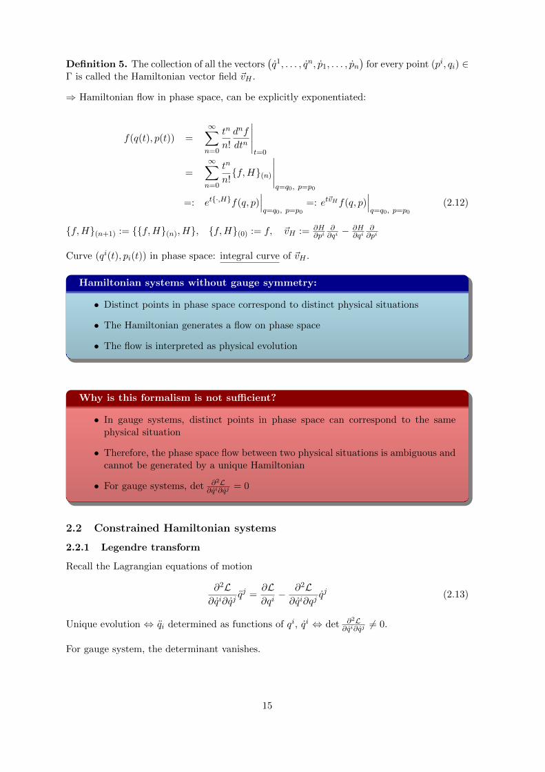
Definition 5. The collection of all the vectors(q1, . . . , qn, p1, . . . , pn

)for every point (pi, qi) ∈

Γ is called the Hamiltonian vector field ~vH .

⇒ Hamiltonian flow in phase space, can be explicitly exponentiated:

f(q(t), p(t)) =

∞∑

n=0

tn

n!

dnf

dtn

∣∣∣∣∣t=0

=∞∑

n=0

tn

n!f,H(n)

∣∣∣∣∣q=q0, p=p0

=: et·,Hf(q, p)∣∣∣q=q0, p=p0

=: et~vHf(q, p)∣∣∣q=q0, p=p0

(2.12)

f,H(n+1) := f,H(n), H, f,H(0) := f, ~vH := ∂H∂pi

∂∂qi− ∂H

∂qi∂∂pi

Curve (qi(t), pi(t)) in phase space: integral curve of ~vH .

Hamiltonian systems without gauge symmetry:

• Distinct points in phase space correspond to distinct physical situations

• The Hamiltonian generates a flow on phase space

• The flow is interpreted as physical evolution

Why is this formalism is not sufficient?

• In gauge systems, distinct points in phase space can correspond to the samephysical situation

• Therefore, the phase space flow between two physical situations is ambiguous andcannot be generated by a unique Hamiltonian

• For gauge systems, det ∂2L∂qi∂qj

= 0

2.2 Constrained Hamiltonian systems

2.2.1 Legendre transform

Recall the Lagrangian equations of motion

∂2L∂qi∂qj

qj =∂L∂qi− ∂2L∂qi∂qj

qj (2.13)

Unique evolution ⇔ qi determined as functions of qi, qi ⇔ det ∂2L∂qi∂qj

6= 0.

For gauge system, the determinant vanishes.

15

⇒ Canonical momenta pi = ∂L∂qi

cannot be uniquely expressed as functions of qi, qi, because

det∂pi

∂qj= 0 (2.14)

i.e. we can vary the qi without affecting the pi.

There exists a vj with ∂pi

∂qjvj = 0 by assumption. Therefore, pi invariant under qi 7→ qi + εvi.

We express as many qi through qi, pi as possible by using pi = ∂L∂qi

.

Additionally, we obtain relations φm(qi, pi) = 0, m = 1, . . . ,M .

If there were any qi left in the φm, we could use those equations to express the qi as functionsof qi, pi.

Definition 6. The φm(qi, pi), m = 1, . . . ,M are called primary constraints.

The Legendre transform still has the property that

δ(piq

i − L)

= qiδpi + piδqi − ∂L

∂qiδqi − ∂L

∂qiδqi = qiδpi −

∂L∂qi

δqi (2.15)

i.e. qi, pi are the dynamical variables of the Hamiltonian formulation.

Hamiltonian H is not unique due to the φm(qi, pi) = 0.

Any “total” Hamiltonian HT = H + umφm is on the same footing. um: arbitrary functions.

2.2.2 Stability algorithm

Strategy: Use HT as a Hamiltonian and work out consequences.

The um are arbitrary functions, sometimes they are velocities which cannot be expressed usingonly qi, pi

Extend Poisson brackets to the um (not necessarily phase space functions) in some wayconsistent with the symmetries of the bracket.

f = f,H + umφm = f,H+ um f, φm+ f, umφm = f,H+ um f, φm (2.16)

⇒ Extension is irrelevant, but necessary for the formalism.

Important: Use φm = 0 only after evaluating the Poisson brackets.

Definition 7. A weak equality is denoted by ≈ and means “equality modulo constraints”.It may be used only after all Poisson brackets have been evaluated.

Example: φm ≈ 0, but φm, f(q, p) 6≈ 0 in general.

Consistency of φm ≈ 0 with the Hamiltonian evolution implies

φm = φm, HT = φm, H + unφn ≈ φm, H+ un φm, φn!≈ 0 (2.17)

⇒ Consistency conditions, 4 possibilities:

16

1. Trivially satisfied, e.g. 0 = 0

2. Inconsistent theory, e.g. 1 = 0 (exercise)

3. Condition on the un

4. New constraint χk(q, p) = 0, independent of the un

Definition 8. The set of all χk(q, p) = 0 are called secondary constraints.

For secondary constraints, one uses the equations of motion, as opposed to primary con-straints. Distinction of minor importance.

Secondary constraints⇒ reiterate the consistency algorithm⇒ possibly tertiary constraints,. . . .

At some point, this algorithm will stop, i.e. give no new conditions, or the theory is incon-sistent.

We obtained K new constraints.

Set of all constraints: φ1, . . . , φM+K := φ1, . . . , φM , χ1, . . . , χK

Denote as φj , j = 1, . . . , J = M +K.

View solving for um as solving inhomogeneous linear equation system:

φj ≈ φj , H+ um φj , φm ≈ 0 (2.18)

J equations for M ≤ J unknowns. Assume that solution exists, otherwise theory inconsistent.

Special solution: Um.

Several homogeneous solutions: V ma φj , φm ≈ 0, a = 1, . . . , A.

These are vectors V m in the kernel of φj , φm

General solution: um = Um + vaV ma .

Consistent total Hamiltonian: HT = H + Umφm + vaφa =: H ′ + vaφa, with φa = V ma φm.

⇒ We are so far left with A arbitrary functions va in the Hamiltonian.

2.2.3 Gauge transformations

The following terminology turns out to be very useful and crucial when studying the geometryof the constraint surface later on.

Definition 9. A phase space function f is called first class if it has vanishing Poissonbracket with all constraints, i.e. f, φj ≈ 0. Otherwise, it is called second class.

17

Linear combination of first class functions are again first class.

Examples:

• All φa are primary first class constraints by their definition.

• HT is first class by the consistency algorithm.Because all constraints are preserved in time

• ⇒ H ′ is first class by linearity.

Theorem 1. The Poisson bracket of two first class functions is again first class.

Proof: Exercises.

Influence of the va on infinitesimal dynamics: (neglect O(δt2))

f(δt) = f0 + f δt = f0 + f,HT δt = f0 +f,H ′

δt︸ ︷︷ ︸

unique

+ va f, φa δt︸ ︷︷ ︸arbitrary

(2.19)

Difference in evolution:

∆f(δt) = δt (va1 − va2)︸ ︷︷ ︸εa

f, φa = εa f, φa (2.20)

⇒ Ambiguity is generated by εaφa, where εa arbitrary.

⇒ The φa generate infinitesimal gauge transformations:

• Change the canonical variables q, p

• Do not change the physical state of the system

The consequences of this last statement will be worked out below. It is true for now by theassumption that we have a consistent and predictive theory.

Do the primary first class constraints exhaust the generators of gauge transformations?

Commutator of two infinitesimal gauge transformations: Exercise

∆f = εa1εb2 f, φa, φb (2.21)

⇒ Also Poisson brackets of primary first class constraints generate gauge transformations.

These may be secondary constraints.

Similar argument for transformations generated by H ′ and φa.

While these arguments extend the list of gauge generators, we cannot proof that they give allgenerators.

Dirac’s conjecture: All first class constraints generate gauge transformations.

Status of this conjecture is disputed.

18

• Nontrivial to formulate precisely (what transformations are gauge on the Lagrangianlevel?)

• Counterexamples exist, but are pathological

• Proof exists under simplifying regularity conditions that are generically satisfied(see Henneaux & Teitelboim)

• True for the main practical examples

Here (and in most literature): Assume the conjecture to be satisfied.

• No natural distinction between primary and secondary constraints at the Hamiltonianlevel

• Quantisation algorithms treat primary and secondary constraints on the same footing

There is a canonical distinction between first class and second class constraints due to thePoisson bracket, see next section.

Definition 10. The extended Hamiltonian HE is given by H ′ plus an arbitrary combinationof first class constraints.

We will take HE as the generator of our dynamics.

2.2.4 Field theory

Generalisations to an infinite number of degrees of freedom:.

• qn, n = 1, 2, . . . becomes q(x), x ∈ R3

• ∑n becomes∫d3x

• ∂L∂qn = pn becomes δL

δq(x) = p(x)

where L =∫d3xL(x) and p(x) is defined as δqL =

∫d3x p(x)δq(x)

Usually, the variational derivative can be used like a standard derivative of L(x) w.r.t.q(x). This stops working as soon as additional, e.g. spatial, derivatives act inside L(x).

Example: L(x) = 12 q(x)2 − 1

2q(x)2

• p(x) = δLδq(x) = q(x), because δqL =

∫d3x q(x)δq(x)

• H =∫d3x (p(x)q(x)− L) =

∫d3x

(12p(x)2 + 1

2q(x)2)

19

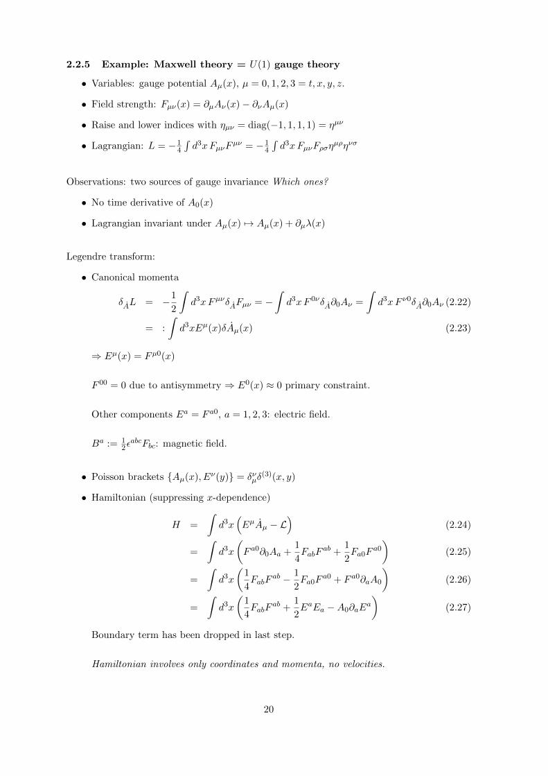
2.2.5 Example: Maxwell theory = U(1) gauge theory

• Variables: gauge potential Aµ(x), µ = 0, 1, 2, 3 = t, x, y, z.

• Field strength: Fµν(x) = ∂µAν(x)− ∂νAµ(x)

• Raise and lower indices with ηµν = diag(−1, 1, 1, 1) = ηµν

• Lagrangian: L = −14

∫d3xFµνF

µν = −14

∫d3xFµνFρση

µρηνσ

Observations: two sources of gauge invariance Which ones?

• No time derivative of A0(x)

• Lagrangian invariant under Aµ(x) 7→ Aµ(x) + ∂µλ(x)

Legendre transform:

• Canonical momenta

δAL = −1

2

∫d3xFµνδAFµν = −

∫d3xF 0νδA∂0Aν =

∫d3xF ν0δA∂0Aν (2.22)

= :

∫d3xEµ(x)δAµ(x) (2.23)

⇒ Eµ(x) = Fµ0(x)

F 00 = 0 due to antisymmetry ⇒ E0(x) ≈ 0 primary constraint.

Other components Ea = F a0, a = 1, 2, 3: electric field.

Ba := 12εabcFbc: magnetic field.

• Poisson brackets Aµ(x), Eν(y) = δνµδ(3)(x, y)

• Hamiltonian (suppressing x-dependence)

H =

∫d3x

(EµAµ − L

)(2.24)

=

∫d3x

(F a0∂0Aa +

1

4FabF

ab +1

2Fa0F

a0

)(2.25)

=

∫d3x

(1

4FabF

ab − 1

2Fa0F

a0 + F a0∂aA0

)(2.26)

=

∫d3x

(1

4FabF

ab +1

2EaEa −A0∂aE

a

)(2.27)

Boundary term has been dropped in last step.

Hamiltonian involves only coordinates and momenta, no velocities.

20

• Stability algorithm: HT = H +∫d3xu(x)E0(x)

E0(x) =E0(x), HT

= ∂aE

a(x)

Does not involve u(x) ⇒ new secondary constraint G(x) := ∂aEa(x) ≈ 0 (“Gauß law”)

G(x) = G(x), HT =G(x),

∫d3x 1

4FabFab

→ Spatial derivatives, need smearing function (but neglect boundary terms):∫

d3xλ(x)G(x),1

4

∫d3y Fab(y)F ab(y)

(2.28)

=

∫d3x d3y (∂aλ(x))Ea(x), Ac(y) ∂bF bc(y) (2.29)

= −∫d3x d3y (∂aλ(x)) δac δ

(3)(x, y)∂bFbc(y) (2.30)

= −∫d3x (∂cλ(x)) ∂bF

bc(x) (2.31)

=

∫d3xλ(x)∂c∂bF

bc(x) = 0 (2.32)

⇒ Constraint stable, algorithm terminates.

• Extended Hamiltonian HE =∫d3x

(14FabF

ab + 12E

aEa + λG+ µE0), λ, µ arbitrary

• Infinitesimal gauge transformations:

Ea(x),

∫d3y λ(y)G(y)

= 0

E0(x),

∫d3y λ(y)G(y)

= 0

Aa(x),

∫d3y λ(y)G(y)

= −∂aλ(x)

A0(x),

∫d3y λ(y)G(y)

= 0

⇒ A0, E0, Ea invariant, Aa 7→ Aa − ∂aλ

A0(x),

∫d3y µ(y)E0(y)

= µ(x)

others are zero

⇒ Aa, E0, Ea invariant, A0 7→ A0 + µ

Invariant functions (observables): Ea, Fab = εabcBc ⇔ electric + magnetic field

Fab contains (locally) all gauge invariant information of Aa.Counterexamples can be constructed e.g. when the spacetime is not simply connected.Then, consider closed non-contractable field lines.

E0 also gauge invariant, but vanishes on constraint surface.

A0 takes arbitrary values under gauge transformations.

21

• Physical degrees of freedom (DOF):

Ea has to satisfy ∂aEa = 0. ⇒ 2 phase space DOF.

Aa can be arbitrarily shifted by ∂aλ. ⇒ 2 phase space DOF.

In total: 2+2 phase space DOF = 2 configuration space DOF (position + velocity).

• Gauge degrees of freedom:

A0 and E0 do not fulfil any physical purpose.A0 is arbitrary and E0 is zero.

Demand that also A0 = 0 throughout the evolution, i.e. impose constraint A0 ≈ 0.

Stability algorithm: ⇒ µ = 0.

Discard A0 and E0 from theory, as they don’t appear in HE and are consistently zero.

More complicated for Gauß law, but similarly possible in principle.

This process is known as gauge fixing.

We note that

1.A0(x), E0(y)

= δ(x, y)

→ Gauge generator and gauge fixing condition are second class pairs.the generator sets one variable to zero, while it generates arbitrary changes in theother one.

2. Original theory with gauge freedom and gauge fixed theory are equivalent.Given a gauge fixed theory, it has to be possible to construct a “gauge-unfixed”theory with additional gauge invariance.Reverse process must be possible: gauge unfixing

These concepts will now be formalised by studying the geometry of the constraint sur-face.

Legendre transform for Constrained systems

• Not all velocities can be solved for the momenta, leading to constraints

• Stability of constraints under evolution may lead to further constraints

• First class constraints generate gauge transformations

22

2.3 The geometry of the constraint surface

2.3.1 Regularity conditions

Many equivalent ways to define a constraint, e.g. p1 = 0⇔ p21 = 0⇔

√|p1| = 0.

Why are two of the above constraints ill-suited for the Hamiltonian formalism?

Some regularity assumptions needed:

• For simplicity: assume constraints to be linearly independentOtherwise, one can usually pick locally an independent subset

• The constraints can be taken as the first J coordinates in a regular coordinate systemin the vicinity of the constraint surface

• The variations δφj =∂φj∂qiδqi+

∂φj∂pi

δpi are non-vanishing, well defined, and locally linearly

independent on the constraint surface (excludes p21 = 0 and

√|p1| = 0)

(here, locally = everywhere, e.g. with arbitrary smearing functions)

• We assume these conditions to be valid globally

With these restrictions in mind, we continue our investigation.

2.3.2 First and second class split

Recall:

• first class constraints ↔ gauge transformations

• second class pairs ↔ transformation generator + gauge fixing

→ Need to separate the constraints in first and second class.

Is this always possible? Is this unique in some sense?

Define the matrix Cij = φi, φj.

Assume rank(Cij) constant on the constraint surface as another regularity condition.

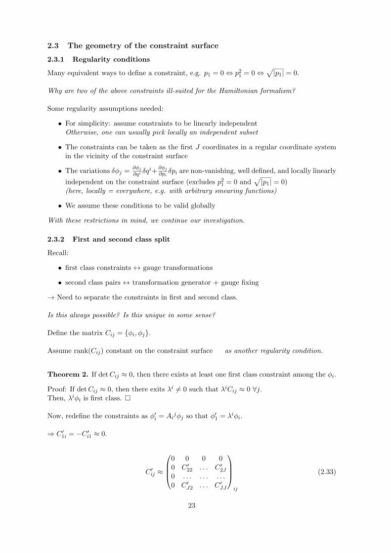
Theorem 2. If detCij ≈ 0, then there exists at least one first class constraint among the φi.

Proof: If detCij ≈ 0, then there exits λi 6= 0 such that λiCij ≈ 0 ∀j.Then, λiφi is first class.

Now, redefine the constraints as φ′i = Aijφj so that φ′1 = λiφi.

⇒ C ′1i = −C ′i1 ≈ 0.

C ′ij ≈

0 0 0 00 C ′22 . . . C ′2J0 . . . . . . . . .0 C ′J2 . . . C ′JJ

ij

(2.33)

23

Rename C ′ by C and reiterate this procedure until detCij 6≈ 0.

⇒ Split into first class constraints γa and second class constraints χα.

Cij =

(0 00 Cαβ

)(2.34)

Cαβ antisymmetric ⇒ Number of second class constraints is even.

Determinant of antisymmetric matrix of odd dimension vanishes.

Because: detC = detCT = det−C = (−1)n detC

Note that this is not true any more for fermions due to Graßmann numbers.

The above split is not unique. Invariant under

γa 7→ Aabγb, χα 7→ Aα

βχβ +Aαaγa (2.35)

for detAab 6= 0 and detAα

β 6= 0

Also, one can add squares of second class constraints to first class constraints.

In the following, we assume detCαβ 6= 0 everywhere on χα = 0 (without necessarily havingγa = 0) as a technical condition.

2.3.3 Small excursion: quantisation

The following will be made more precise later in section 6.

Quantisation: maps phase space functions to linear operators on a Hilbert space, so that

• [f , g] := f g − gf = i~f, g

Works only for a limited set up phase space functions. (Groenewold-van Hove theorem)

In general: ordering ambiguities.

Elements of the Hilbert space are “kets”: |ψ〉

Constraints: φi ≈ 0 7→ φi |ψ〉 != 0

Physical states: φi |ψ〉phys = 0 ⇔ eiλj φj |ψ〉phys = |ψ〉phys

Is this consistent?

• Assume φi |ψ〉phys = 0

• ⇒ φiφj |ψ〉phys = 0

• ⇒(φiφj − φjφi

)|ψ〉phys = 0

24

• ⇒ φi, φj |ψ〉phys = 0 (up to ordering problems)

Two cases:

• Only first class constraints: φi, φj = cijkφk, ⇒ cijkφk |ψ〉phys = 0

Consistent (up to ordering)

• Second class constraints present: ∃ i, j : φi, φj 6= cijkφk ⇒ ”1” |ψ〉phys = 0

Inconsistent

Two options to proceed:

• Change quantisation prescription for second class constraints (later)

• Get rid of second class constraints classically (now)

There is no general rule of path is best to follow. Solving constraints classically can be veryhard in practise. Quantising constraints is ambiguous. Therefore, both options should beexplored.

2.3.4 The Dirac bracket

The action of second class constraints doesn’t preserve the constraint surface.

Simply because they don’t Poisson-commute with some of the constraints. E.g. choose theconstraints as local coordinates off the constraint surface.

⇒ they cannot be treated as gauge generators.

⇒ develop a strategy for solving them classically.

Consider the following example: from Dirac’s book, similar to the Maxwell example

• Configuration space is Rn, coordinates q1, . . . qn.

• Canonical momenta p1, . . . , pn.

• Second class constraints χ1 = q1 ≈ 0, χ2 = p1 ≈ 0

q1 and p1 are not of importance, we would like to simply set them to zero and thus solve theconstraints.

However, q1, p1 = 1 6= 0, → inconsistent with Poisson bracket.

Need to modify the Poisson bracket after solving constraints:

f, g∗ =n∑

i=2

(∂f

∂qi∂g

∂pi− ∂g

∂qi∂f

∂pi

)(2.36)

New bracket ·, ·∗ is consistent with strongly setting χ1 = χ2 = 0 and still satisfies all prop-erties of ·, ·.

→ Need to generalise this idea!

Guiding principles:

25

• χα, ·∗ = 0 strongly.

• Preserve all properties of the Poisson bracket (bi-linearity, . . . )This is particularly important, because those properties are reflected by commutatorsupon quantisation

• Modification should depend only on the bracket arguments and the second class con-straints

Solution: Dirac bracket

f, g∗ = f, g − f, χαCαβ χβ, g (2.37)

where CαβCβγ = δαγ .

Properties of the Dirac bracket:

• Antisymmetry: f, g∗ = −g, f∗• Linearity: for c1, c2 ∈ R: c1f2 + c2f2, g∗ = c1 f1, g∗ + c2 f2, g∗• Leibniz property: f1f2, g∗ = f1 f2, g∗ + f1, g∗ f2

• Jacobi identity: f, g, h∗∗ + g, h, f∗∗ + h, f, g∗∗ = 0

• Second class compatibility: χα, ·∗ = 0 strongly

• First class compatibility: f, ·∗ ≈ f, · for any first class f

Proof: Exercises.

No changes in formalism:

• HE still generates the dynamics, as it is first class

• First class constraints still generate gauge transformations

• Solving second class constraints is consistent with the Dirac bracketE.g. solving constraints by using reduced set of phase space coordinates so that χα = 0.

• First class constraints cannot be set to zero even with Dirac bracket

The Dirac bracket is weakly unaffected by choosing a different (but equivalent) set of secondclass constraints. (Exercises)

2.3.5 Gauge fixing

We may want to get rid of the gauge degrees of freedom and work only with second classconstraints / Dirac bracket.

Given gauge generators γa:

→ introduce gauge conditions Cb(q, p) ≈ 0

Cb(q, p) ≈ 0 restricts the allowed part of phase space

26

0

~v

C 0

~vC

Figure 2.2: The two constraint surfaces γ ≈ 0 and C ≈ 0 intersect non-tangentially. Thevector fields ~vγ and ~vC prescribe a flow along their respective constraint surfaces. ~vγ ∦ ~vCat the intersection, which is equivalent to γ,C 6≈ 0. Gauge fixing C ≈ 0 thus selects arepresentative of the equivalence class of points on γ ≈ 0 under the flow generated by ~vγ .

Necessary properties:

• Accessibility:For any given (q, p), there must exist a gauge transformation q 7→ q′, p 7→ p′, such thatCb(q

′, p′) ≈ 0.

• Completeness:The gauge is fixed completely, i.e. no more gauge transformations are possible.

Infinitesimally, δua Cb, γa ≈ 0 ⇒ δua = 0, or det Cb, γa 6≈ 0.

After a complete gauge fixing, no first class constraints are left.

Geometric interpretation: figure 2.2

Completeness is globally non-trivial in general: Gribov copies, figure 2.3.

27

0

1 0

2 0

3 0

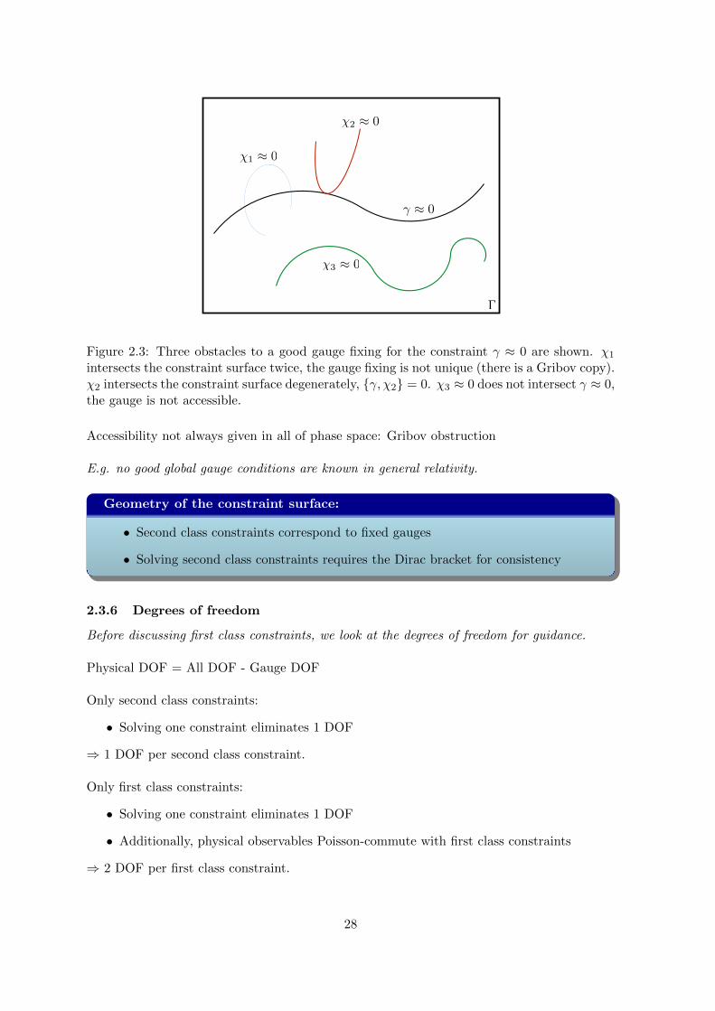
Figure 2.3: Three obstacles to a good gauge fixing for the constraint γ ≈ 0 are shown. χ1

intersects the constraint surface twice, the gauge fixing is not unique (there is a Gribov copy).χ2 intersects the constraint surface degenerately, γ, χ2 = 0. χ3 ≈ 0 does not intersect γ ≈ 0,the gauge is not accessible.

Accessibility not always given in all of phase space: Gribov obstruction

E.g. no good global gauge conditions are known in general relativity.

Geometry of the constraint surface:

• Second class constraints correspond to fixed gauges

• Solving second class constraints requires the Dirac bracket for consistency

2.3.6 Degrees of freedom

Before discussing first class constraints, we look at the degrees of freedom for guidance.

Physical DOF = All DOF - Gauge DOF

Only second class constraints:

• Solving one constraint eliminates 1 DOF

⇒ 1 DOF per second class constraint.

Only first class constraints:

• Solving one constraint eliminates 1 DOF

• Additionally, physical observables Poisson-commute with first class constraints

⇒ 2 DOF per first class constraint.

28

Consistent with gauge fixing: 1 first class constraint = 2 second class constraints (gaugegenerator and fixing)

DOF counting so simple only for finite dimensional systems.

For field theories, need to discuss the functional spaces of the Lagrange multipliers. Case bycase study with physical input.

2.3.7 Gauge invariant functions

Recall phase space functions C∞(Γ):

• Algebra A with addition “+ : A×A → A” and multiplication “· : A×A → A”

• Lie Algebra with Lie bracket (= Poisson bracket) ·, · : A×A → A

• Operations related via fg, h∗ = f, h∗ g + f g, h∗

System constrained to be on constraint surface Σ.

⇒ phase space functions that agree on Σ cannot be distinguished.

This means that the relevant functions are only those on Σ and we should develop a formalismthat refers only to such functions.

We want to study C∞(Σ).

N = functions vanishing on Σ.

• N is an ideal in C∞(Γ): f · g ∈ N ∀ f ∈ N , g ∈ C∞(Γ)

• N = λaγa + λαχα

Define quotient algebra C∞(Γ)/N= equivalence class of phase space functions differing by an element of N

C∞(Γ)/N = C∞(Σ) with addition “+” and multiplication “·”

Any function on Σ defines an equivalence class. Conversely, every equivalence class definesa function on Σ.

Ideal property of N is needed:

(f1 + λa1γa + λα1χα)·(f2 + λa2γa + λα2χα) =

f1f2 + (λa1γa + λα1χα) f2 + f1 (λa2γa + λα2χα) + . . .︸ ︷︷ ︸

!=λa3γa+λα3 χα

(2.38)Otherwise, the product would depend on the choice of representative of the equivalence class.

Note that we didn’t show so far that the Lie bracket extends to C∞(Σ)!

29

Definition 11. An observable F is a function on the constraint surface C∞(Σ) that Poisson-commutes weakly with all the first class constraints:

F, γa∗ ≈ 0. (2.39)

F does not depend on the representative, as γa + χα, γb∗ ≈ 0.

Two steps:

1. Restrict to constraint surface Σ

2. Gauge invariance condition w.r.t. Dirac bracket

We do not explain how the measurement process is supposed to take place. While this isclassically often clear, it becomes a problem at the quantum level. Determining observablesof the theory in our formalism was possible purely starting from the action principle.

Alternative characterisation: Well defined bracket structure in C∞(Σ)

• Addition and multiplication well defined

• Bracket well defined if only second class constraints (Dirac Bracket)

• With first class constraints:

f + λaγa, g∗ = f, g∗ + λaγa, g∗!≈ f, g∗ (2.40)

⇒ g has to Poisson commute weakly with the first class constraints. Similar for f

⇒ Bracket on C∞(Σ) well defined only for observables!

⇒ Necessary to consider all first class constraints (primary and secondary) as gauge genera-tors!

The well defined bracket structure is mandatory for quantisation.

2.3.8 Gauge unfixing

Gauge fixing suggests that second class systems can also be viewed as first class systems.

How to construct a first class system from a second class one?

Example:

• Phase space coordinates: (q1, q2, p1, p2) ∈ R4

•qi, pj

= δij

• Second class constraints χ1 = q2 ≈ 0, χ2 = p2 ≈ 0

• First class Hamiltonian H = H(q1, q2, p1, p2) =∑∞

i,j,k,l=0 cijkl(q1)i(q2)j(p1)k(p2)l

Taylor expansion in all four variables.Note that ci1k0 = 0 and ci0k1 = 0 due to first class property.

30

Physical content: Only q1, p1 interesting.

Solve with Dirac bracket:

• Dirac bracket:q1, p1

∗ = 1

• Solve constraints explicitly: q2 = 0 = p2

• Hamiltonian: H =∑∞

i,k=0 ci0k0(q1)i(p1)k

Transform to first class system now.

• Drop one constraint

• Call the other one the gauge generator

• Use original Poisson bracket

Observation: Not unique. Keep e.g. q2 ≈ 0, p2 ≈ 0, q2 + p2 ≈ 0, . . .

As an example, keep p2 and drop q2.

⇒ H not gauge invariant in general

H, p2 =

∞∑

i,j,k,l=0

cijkl (q1)ij (q2)j−1(p1)k(p2)l (2.41)

Need first class Hamiltonian H that agrees with H upon setting q2 = 0

⇒ H =∑∞

i,k,l=0 ci0kl(q1)i(p1)k(p2)l

We can also add arbitrary powers of p2 ≈ 0.

We removed all powers of q2 from H. This was trivial here, because we could simply Taylorexpand H in the constraints. For more complicated constraints, this is more involved.

Physical observables: q1, p1 both Poisson-commute with p2.

Evolution:f(q1, p1), H

=

f(q1, p1),

∞∑

i,k=0

ci0k0(q1)i(p1)k

+

∞∑

i,k=0

∞∑

l=1

ci0kl(q1)i(p1)k

f(q1, p1), (p2)l

︸ ︷︷ ︸0

+O(p2)

≈f(q1, p1), H

∗ (2.42)

Physical evolution of observables invariant.

We can redefine the Hamiltonian by adding arbitrary powers of p2, in particular remove allpowers of p2 from it. Gives H on surface q2 = 0 = p2.

Conclusion from example:

31

• Dropping gauge fixing conditions generally leads to second class Hamiltonians

• Second class property comes from powers of the gauge fixing condition inside H

• Need to remove these powers by adding powers of the gauge fixing conditions

• By going back to the gauge q2 = 0, we recover the original Hamiltonian theoryWe do not necessarily recover the exact first class Hamiltonian that we started from,since we are free to add arbitrary powers of first class constraints to it, which in thiscase means we can add powers of at least 2 of second class constraints. But we recoverthe same physics.

• This is simple if we have a Taylor expansion of H in terms of the gauge fixing condition,but this is usually not the case.

→ Formalise this idea by only using the available structure (Poisson bracket)

Simplify notation, q2 7→ q, p2 7→ p.

Heuristic idea:

• The remaining first class constraint p generates changes in the gauge fixing q, herebecause q, p = 1

• We do not want H to depend on q

• Flow evaluation point along the gauge orbit of p to q = 0

p 0

q 0 q q

~vp

Figure 2.4: The gauge unfixing projector will evaluate a function at q = 0 by moving theevaluation point along ~vp until it satisfies q = 0. The reason why Pf Poisson-commutes withp is then simply that changes in q don’t matter for the evaluation of the phase space function,as we always flow to q = 0.

PH = e−·,pqH =∞∑

n=0

(−q)nn!H, p(n) (2.43)

32

For any phase space function: gauge unfixing projector

P = e−·,pq =∞∑

n=0

(−q)nn!·, p(n) (2.44)

·, γ(n+1) :=·, γ(n), γ

, ·, γ(0) := ·.

Applying P takes us to q = 0 along the gauge orbit of p.

Therefore, Pf has to Poisson-commute with p. If we would have flown not along the Hamil-tonian vector field of p, this would not have been true.

P computes a gauge invariant extension. Two constraints needed to define P.

Example: if one thinks of p being the Hamiltonian and q the time (here then also a phasespace variable, see later in parametrised systems), then we always evaluate a given phasespace function at a given time t = 0. In this case, P would map any phase space function toits initial values at t = 0.

Check that P deletes powers of the gauge condition:

• Gauge condition q, gauge generator p, cn phase space functions independent of q.

• q, p(1) = 1

• qk, p(1) = kqk−1

• qk, p(n) = k(k − 1) . . . (k − n+ 1)qk−n = k!(k−n)!q

k−n

P∞∑

k=0

ckqk =

∞∑

k=0

ckqk −

∞∑

k=0

1

1!kckq

k−1q +∞∑

k=0

1

2!k(k − 1)ckq

k−2q2 ± . . . (2.45)

=∞∑

k=0

ckqk

k∑

n=0

(−1)nk!

(k − n)!n!(2.46)

=∞∑

k=0

ckqk

k∑

n=0

(−1)n(k

n

)=∞∑

k=0

ckqkδk,0 (2.47)

= c0 q0 = c0 (2.48)

For general second class constraints: Cαβ = χα, χβ

Pick first class subset γa (half number) + other half χb

P = e−·,Cabγbχa =

∞∑

n=0

(−1)n

n!

. . .·, Ca1b1γb1

, . . . , Canbnγbn

χa1 . . . χan (2.49)

γa≈∞∑

n=0

(−1)n

n!. . . ·, γb1 , . . . , γbnCa1b1χa1 . . . Canbnχan (2.50)

In practise, gauge unfixing is useful only if the series terminates or can be summed.

33

This happens e.g. in the connection formulation of general relativity, useful for quantumgravity.

Question: when does this not happen? How do the gauge constraints have to look like?

E.g. when the gauge generator includes several powers of the canonical variables.

Some properties of P (locally):

• (Pf) + (Pg) = P(f + g)

• Pf,Pg γa≈ f, g∗(γa,χb) Formalism equivalent to Dirac bracket

• (Pf) · (Pg)γa≈ P(f · g)

One can see that P is consistent with multiplication only up to constraints only whentaking the projector w.r.t. to several first class constraints. Then, the order in whichgauge transformations are applied is important, but one can show that the Hamiltonianvector fields of the constraints Cabγb weakly commute. See theorem 2.2.1 in Thiemann’sbook.

• P(λaγa + µbχb)γa≈ 0

• P generates all γa-observables (Take a γa-observable Oγ, then POγ = Oγ)

These properties are important for reduced phase space quantisations. In particular, the firstidentity allows one to compute the Poisson bracket of observables, which one needs to findrepresentations of classical observables.

One may choose the clarifying notation Pχγ .

Remark: Batalin-Fradkin-Tyutin-formalism is an alternative to gauge unfixing, but intro-duces new DOF.

Gauge fixing / unfixing:

• One can rewrite first class systems (partially) as second class systems, and theother way around

• Physically, this corresponds to fixing gauge conditions, or lifting them

• While these descriptions are equivalent classically, they may have different valuesas starting points for a quantisation

34

3 Time Reparametrisation Invariant Systems

Generally covariant systems are a fundamental technical tool to account for the fact thatchoices of coordinates, which are merely a tool for convenient descriptions of a phenomenon,should be of no physical relevance.

Goal of this section: Study time-reparametrisation invariant systems.

Next two sections: Generally covariant systems (e.g. general relativity)

Gedankenexperiment: Measure position of a harmonic oscillator.

q

Question: How is this done? Which input is needed? Is the above question well defined byitself?

• Question not well defined. We need to specify a measurement time

• What is time?

• Some physical significance of time coordinate, e.g. clock.

• Any clock is a physical objectAlready Newton was unhappy with his definition of absolute time and aware that onewould need some relational notion to supersede it.

Main idea:

• Clock should be modelled in our theoretical description: t(τ)

• τ arbitrary temporal parameter

• Describe “correlations” clock t(τ) - position q(τ)

• Physics invariant under (monotonic) relabelings τ 7→ f(τ)

3.1 Parametrised systems

Consider example system:

• canonical variables qi, pi

• Hamiltonian H0

35

Action:

S[qi(t), pi(t)] =

∫ t2

t1

dt

(pidqi

dt−H0

)(3.1)

Introduce time variable q0 := t, conjugate momentum p0.

Search for equivalent action where time is a variable:

S[q0(τ), p0(τ), qi(τ), pi(τ)] =

∫ τ2

τ1

dτ

(p0dq0

dτ+ pi

dqi

dτ− u0 (p0 +H0)

)(3.2)

Equations of motion for new variables:Variations of p and q independently:

δS

δp0=

dq0

dτ− u0 =0 (3.3)

δS

δq0= − d

dτp0 =0 (3.4)

δS

δu0=− (p0 +H0) =0 (3.5)

(2): p0 constant of motion(3): p0 = −H0 The only constant of motion (without solving the EOM) in general time-independent systems(1): u0 measures change of clock q0 w.r.t. τ

Insert into action: Possible due to exercise, consider p0, u0 as auxiliary fields, but not q0

S =

∫ τ2

τ1

dτ

(p0dq0

dτ+ pi

dqi

dτ− u0

(p0 +H0

))(3.6)

=

∫ τ2

τ1

dτ

(pidqi

dτ− dq0

dτH0

)(3.7)

=

∫ t2

t1

dt

(pidqi

dt−H0

)(3.8)

The new action is therefore equivalent to the original one.

u0 (p0 +H0) in action leads to constraint: γ = p0 +H0 ≈ 0:

• No du0

dτ in action ⇒ pu ≈ 0 primary constraint

• Hamiltonian: u0 (p0 +H0) =: u0γ

• Stability: dpudτ = − (p0 +H0)

!≈ 0 ⇒ γ ≈ 0

⇒ The Hamiltonian vanishes on the constraint surface

• H is sum of constraints Here only 1

• H is not strongly zero! ·, H 6≈ 0 in general

Interpretation:

36

• Time evolution = gauge transformation

• Flow generated by p0 +H0(qi, pi):

H0 evolves qi, pi in the usual way

p0 evolves the time q0

p0 = −H0 stays constant

⇒ qi, pi and q0 evolve (advance in coordinate time τ) simultaneously!

This means that the clock “ticks” when the other canonical variable evolve.

• Changing u0 changes evolution speed of qi(τ), pi(τ), q0(τ) similarly.⇒ Correlations qi(q0), pi(q

0) independent of u0

This means that it does not matter how fast we proceed in the evolution: Changing speed(u0) just changes how fast we sample all correlations, but eventually we will sample allof them.

How to recover the usual observables, e.g. q(t0)?

Simple model: free particle, H0 = p2

2m , γ = p0 +H0 ≈ 0

• Need constant of motion equal to q(t0) How could this be done?

• qt0(τ) := q(τ)− p(τ)m

(q0(τ)− t0

)

•qt0 , p0 + p2

2m

= −p(τ)

m + p(τ)m = 0

⇒ qt0 constant of motion that agrees with q(t0)

Remarks on constructing observables:

• Construction principle:Evolve q0, qi, pi in “time” τ until q0(τ) = t0

• Requires solving the equations of motion (EOM)This succeeded here because we chose a very simple system

• Solutions to EOM ⇔ initial data at some time t0 ⇔ Constants of motion in the(q0, p0, q

i, pi)-systemNote that “constants of motion” here are not only those that one considers in classicalmechanics, e.g. the energy or angular momentum, which can be found by looking at thesymmetries of the system. Here, we need to explicitly solve the EOM to obtain theseconstants of motion.

It is always possible to parametrise a given Hamiltonian system:

1. Add canonical pair q0, p0 and Lagrange multiplier u0

37

2. Replace extended Hamiltonian: HE 7→ u0 (p0 +HE)

3. Add constraint p0 +HE ≈ 0

4. Keep all other constraintsThe first class constraints appearing in HE are still first class constraints here, theirmultipliers are just multiplied by u0, which doesn’t change anything.

This can bring explicitly time dependent systems in time-independent form.

However, “deparametrising” is not straight forward and may even be impossible to achieveglobally (e.g. general relativity).

⇒ Important to develop a formalism with gauge invariance

Once one restricts to a part of phase space where a certain gauge condition used for de-parametrisation is accessible, it is possible to compute the Poisson brackets of physical ob-servables (the constants of motion) by using properties of the gauge unfixing projector, withoutsolving the equations of motion. This allows one to construct reduced phase space quantisa-tions of these subsectors of the theory.

3.2 General examples

Example: Free relativistic particle:

• Action: S[Xµ(τ)] = −m∫w ds = −m

∫ τ2τ1dτ√−dXµ

dτdXν

dτ ηµν

• w world line of particle, Embedding map Xµ(τ) = (t(τ), x(τ), y(τ), z(τ))µ,η = diag(−1, 1, 1, 1), τ arbitrary temporal parameterThe action is the proper length of the world line.Lower and raise indices with η

• Canonical momenta: pµ := dLd( dX

µ

dτ )= m√

...dXµdτ

• Proper time s: ds =√. . .dτ ⇒ d

ds = 1√...

ddτ ⇒ pµ = m

dXµds = muµ (uµ = four

velocity)

• Constraint: pµpµ = −m2 ⇒ γ := pµp

µ +m2 ≈ 0 (mass shell condition)Movement of the particle is in the temporal direction, follows from sign choice in theaction.

• Hamiltonian: H = pµdXµ

dτ − L =√...

m

(pµp

µ +m2)

• Extended Hamiltonian: HE = λγ ≈ 0, λ Lagrange multiplier

• Canonical equations of motion:

ddτ pµ = 0 (four velocity is constant)

38

ddτX

µ = 2λ pµ (for λ = 12m :

dXµds = 1

mpµ)

• Independent Dirac observables:

pi (p0 from γ ≈ 0)

Xi − pi X0−t0p0

(X0 gauge DOF, shifted by γ)

Note: Other parametrisation, e.g. w.r.t. X1 instead of X0 possible.

⇒ Many physically equivalent choices in formulating Dirac observables.

This example (worldline) can be generalised to higher dimensions:

• World-surface: classical strings (exercises)

• World-volumes: branes

• Vary metric: general relativity (with different action)

Example: Homogeneous Lagrangian: L(qi, c qi) = cL(qi, qi) (exercises)

Reparametrisation invariant systems:

• Any Hamiltonian system can be written as a reparametrisation invariant system

• The Hamiltonian is a sum of constraints(if no time-dependent canonical transformations)

• Time evolution = gauge transformation

• Physical statements are correlations between evolving objects

39

4 Crash course in General Relativity

How do we measure distance?

• Experiment: Compare to a given ruler (metre des archives, Urmeter)

• Theoretical description: assign length to coordinate unitsE.g. distance = (x2 − x1) implicitly refers to regular units of x

Generalisation: units of x may be irregular and subject to change over time.

Physical picture: the spacetime on which physics takes place is dynamical

To describe this, we need a few concepts:

• Manifold (arena where physics takes place)

• Metric (assignment of distance between points)

• Geodesics (what are straight lines, c.f. Newton’s axions)

• Curvature (tensors derived from metric)

• Integration theory (for well-defined actions, i.e. coordinate independent)

In the following: Crash course on those subjects, only relevant details, no mathematicalrigour.

4.1 Manifolds

The main point of defining manifolds for us is to allow for more general spaces than that ofRn, possibly with globally non-trivial topologies.

We do not discuss issues like local topology here, in the sense of defining continuity. Usually,one would start from a topological manifold and work ones way up.

Properties of an n-dimensional (differentiable) manifold Mn

• A space that locally looks like Rn

• There exists a collection of invertible maps (charts), from subsets of Mn to subsets ofRn. A collection of maps covering all of Mn is called atlas.All points in the manifold need to be included in the charts.→ provides local coordinates

• Maps are consistent with each other on overlaps and sufficiently smooth→ change of coordinates well-defined→ transfers differential calculus from Rn to Mn

Example: 2-Sphere

• We need at least 2 charts ( e.g. northern / southern hemisphere)

40

Further examples: 2-Torus, handle-body, . . .

Mn

Rn Rn

Definition 12. A diffeomorphism is a bijective map from one manifold to another (or itself),where both the map and its inverse are sufficiently often differentiable.

• A diffeomorphism induces a change of coordinatesMoves coordinates from one point to another along its inverse

• Later: diffeomorphism invariance = invariance under general coordinate transforma-tions

Mn

1

P

(P )

Figure 4.1: A diffeomorphism induces a change of coordinates: we can assign to P thecoordinates of Φ(P ) or equivalently move the coordinates in a neighbourhood of Φ(P ) to aneighbourhood of P using Φ−1. In local coordinates: Φα(xi) = yα(xi).

Bottom line:

41

• We can consistently use coordinates in spaces with general topologiesThese will usually be simple spaces like Rn or spheres.

• We can transfer differential calculus from Rn to those spaces

4.2 Vectors and covectors

4.2.1 Vectors

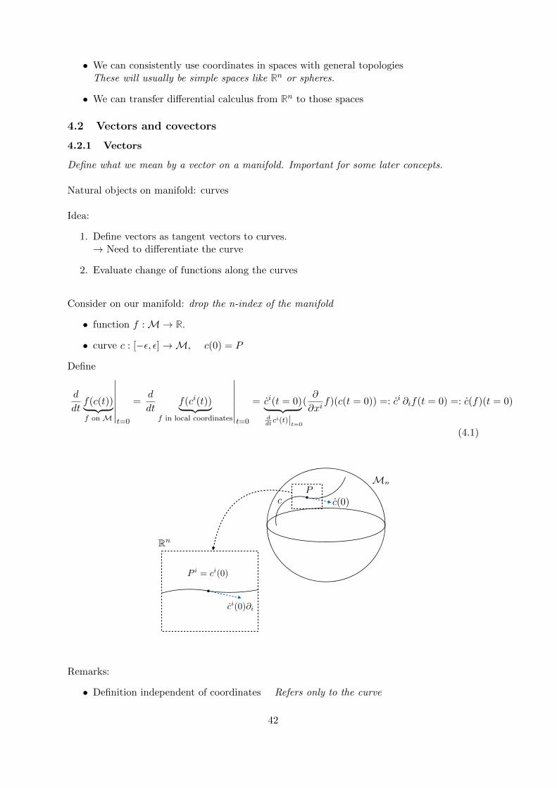
Define what we mean by a vector on a manifold. Important for some later concepts.

Natural objects on manifold: curves

Idea:

1. Define vectors as tangent vectors to curves.→ Need to differentiate the curve

2. Evaluate change of functions along the curves

Consider on our manifold: drop the n-index of the manifold

• function f :M→ R.

• curve c : [−ε, ε]→M, c(0) = P

Define

d

dtf(c(t))︸ ︷︷ ︸f on M

∣∣∣∣∣∣∣t=0

=d

dtf(ci(t))︸ ︷︷ ︸

f in local coordinates

∣∣∣∣∣∣∣t=0

= ci(t = 0)︸ ︷︷ ︸ddtci(t)|

t=0

(∂

∂xif)(c(t = 0)) =: ci ∂if(t = 0) =: c(f)(t = 0)

(4.1)

Pc

Rn

Mn

c(0)

P i = ci(0)

ci(0)@i

Remarks:

• Definition independent of coordinates Refers only to the curve

42

• Change of coordinates yα = yα(xi)

∂∂xi

= ∂yα

∂xi∂∂yα ⇔ ∂

∂yα = ∂xi

∂yα∂∂xi

⇒ cα = ∂yα

∂xici ⇔ ci = ∂xi

∂yα cα

Transformation behaviour of a vector (upper index)

• ci: components of a vector, ∂i: basis vectors

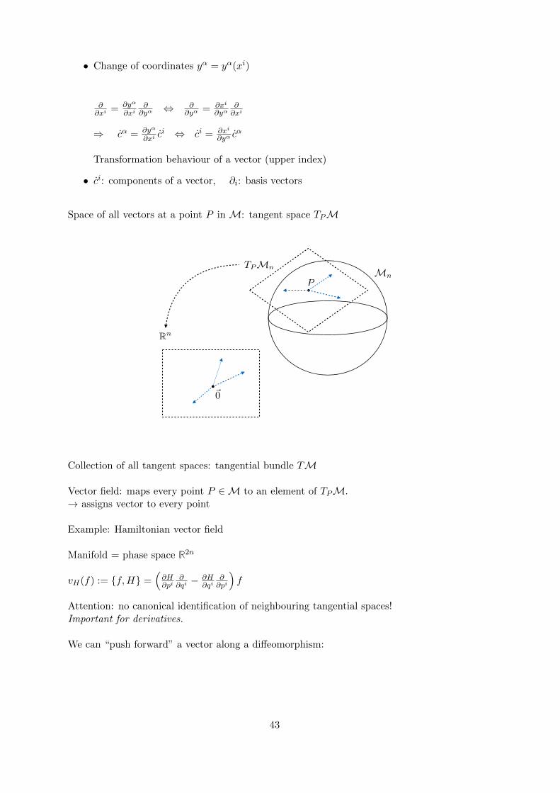
Space of all vectors at a point P in M: tangent space TPM

P

Rn

Mn

TP Mn

~0

Collection of all tangent spaces: tangential bundle TM

Vector field: maps every point P ∈M to an element of TPM.→ assigns vector to every point

Example: Hamiltonian vector field

Manifold = phase space R2n

vH(f) := f,H =(∂H∂pi

∂∂qi− ∂H

∂qi∂∂pi

)f

Attention: no canonical identification of neighbouring tangential spaces!Important for derivatives.

We can “push forward” a vector along a diffeomorphism:

43

Mn

c

c

We move the curve c with Φ to a new curve Φ(c) and use this curve to define a vector atΦ(c(0)).

(Φ∗c) (f)(Φ(P )) := ddtf(Φ(c(t)))

∣∣t=0

=∂Φ(x)α

∂xi(P )ci(t = 0)

︸ ︷︷ ︸(Φ∗c)

α(Φ(P ))

( ∂∂yα f)(Φ(P ))

We can push forward along general maps, not only diffeomorphisms.

4.2.2 Covectors

Idea: Covector = linear map from vectors to R.

Cotangent space at P : T ∗PM• Dual basis: dxi

• dxi(∂j) := ∂jxi = δij

• Expansion in basis: w = widxi

• w(v) = widxi(vj∂j) = vjwiδ

ij = viwi

• Coordinate change: wα = wi∂xi

∂yα (exercise)

Collection of all cotangent spaces: cotangent bundle T ∗M

Covectorfield analogous.

Evaluation w(v) independent of the choice of coordinates. (Exercise)

Attention: No canonical identification of vectors and covectors! Needs additional structure.

We can “pull back” a covector along a diffeomorphism: Also along general maps

44

We simply push the vector it takes as an argument forward. This means that the co-vector isdefined at Φ(P ) and the vector at P , thus we pull back the co-vector from Φ(P ) to P .

(Φ∗w)(v)(P ) := w(Φ∗v)(Φ(P ))

(Φ∗w)(v)(P ) = (Φ∗w)i(P )dxi(vi(P )∂i) = wα(Φ(P ))dyα(

(Φ∗v)β (Φ(P ))∂β

)= wα(Φ(P ))vi(P )∂Φα

∂xi(P )

⇒ wi(P ) = wα(Φ(P ))∂Φα

∂xi(P )

Diffeomorphisms are bijective:

• Push forward covectors along Φ = Pull back covectors along Φ−1

e.g. (Φ∗w)α(Φ(P )) = wi(P )∂(Φ−1)i

∂yα (Φ(P )) (exercise)

• Pull back vectors along Φ = Push forward vectors along Φ−1 (exercise)

In general: involved maps not bijective Then no such thing as pushing forward a form if themap used is not invertible.

Pullbacks and pushforwards are compatible with index contraction (exercise).

4.3 Metrics and tensors

We need an assignment of distance to a curve in a manifold.

Infinitesimal line element:

• Euclidean space = R3 with standard metric:

ds2 = (dx1)2 + (dx2)2 + (dx3)2 =

3∑

i,j=1

δijdxidxj (4.2)

• Generalisation: xi are local coordinates on Mn

ds2 =n∑

i,j=1

gij(x)dxidxj , gij(x) = metric tensor (symmetric) (4.3)

Tensor: something that transforms like a tensor (see the following).

The indices of a tensor transform like the indices of vectors / co-vectors.

The infinitesimal distance ds2 should be coordinate independent:

• Consider change of coordinates xi = xi(yα)

• dxi = dxi(y) = dxi

dyαdyα

• ⇒ gij(x)dxidxj = gij(x(y))dxi

dyαdxj

dyβ︸ ︷︷ ︸gαβ(y)

dyαdyβ =: gαβ(y)dyαdyβ

45

Rules for tensors:

• Tensorial objects with a lower (covariant) index transform as Tα(y) = dxi

dyαTi(x(y))

• Tensorial objects with an upper (contravariant) index transform as Tα(y) = dyα

dxiT i(x(y))

Note:

• Same index structure on both sides of the equalityThe index structure automatically fixes how a tensor index transforms.

• Summed always over upper / lower indices

• ∂i = ∂∂xi

behaves as with a lower indexNote however that an object with the components 1/T i is not a tensor, in particular nota covariant one.

• Transformations from coordinate changes cancel in summations:Tαα(y(x)) = dyα

dxidxj

dyαTij(x) = δjiT

ij(x) = T ii(x)

• Multiple indices transform as Tα1...αmβ1...βn = dyα1

dxi1. . . dy

αm

dximdxj1

dyβ1. . . dx

jn

dyβnT i1...imj1...jn

• Important: coordinates xi, yα, . . . are not tensors. Here, i, α, . . . label the differentcoordinates.

• But the differentials dxi, dyα transform as tensors with upper index

Notation:

• The metric tensor transforms as a rank 2 covariant tensor.

• Upper indices: contravariant

• T i1...imj1...jn is a tensor of rank (m,n)

• A scalar, e.g. T ii, does not change under coordinate transformations

Inverse metric: gij such that gijgjk = δki rank 2 contravariant tensor

Raise and lower indices with the metric:

• T igij =: Tj transforms with a lower index

• Uigij =: U j transforms with an upper index

How to obtain metrics?

1. Prescribe them from scratch

2. Induce a metric by embedding Mn into Rn+m with Euclidean metric

Embedding example: 2-sphere.

• Define subset S2 as the subset of R3 satisfying (x1)2 + (x2)2 + (x3)2 = R2

46

• Examples of local coordinates:

Cartesian coordinates (x1, x2, x3) on subset S2 ⊂ R3: metric known

Spherical coordinates θ, φ: metric via change of coordinatesx1 = R sin θ cosφx2 = R sin θ sinφx3 = R cos θCompute metric: gθθ = dxi

dyθdxi

dyθδij = R2, gφφ = R2 sin2 θ, gθφ = 0

Define distance d(c) along a curve c : [a, b]→Mn:

d(c) =

∫

cds :=

∫

c

√gijdxidxj :=

∫ b

adλ

√gij(c(λ))

dxi

dλ

dxj

dλ(4.4)

λ parametrises the curve.

d(c) is called the “proper distance”. As opposed to coordinate distance

Two invariances:

• Reparametrisation of λ

• Changes of coordinates xi → yα

Example: Length of great circle on a sphere with radius R.

• Great circle: φ ∈ [0, 2π), θ = π/2. Take φ = λ to parametrise the great circle.

∫ 2π

0dλ

√gij(c(λ))

dxi

dλ

dxj

dλ=

∫ 2π

0dφ√gφφ =

∫ 2π

0dφR sin(π/2) = 2πR (4.5)

• Other parameterisations possible, e.g. take twice φ = const, θ ∈ [0, π) as exercise

Pull backs and push forwards along diffeomorphisms can be generalised to tensors:

(Φ∗T )α1...αm(Φ(P )) =∂Φ(x)α1

∂xi1(P ) . . .

∂Φ(x)αm

∂xim(P )T i1...im(P ) (4.6)

Similar for covariant indices.

So far: Riemannian metric, positive definite.

For general relativity: Pseudo-Riemannian metric: only non-degenerate.

E.g. Minkowski metric η = diag(−1, 1, 1, 1)

Use greek indices µ, ν, . . . instead of i, j, . . . to remember this.

47

4.4 Geodesics

How do test particles move on a Riemannian manifold without exterior forces?

In flat space: straight line, constant distance per time

• Straight w.r.t. cartesian coordinates

• Not “straight” w.r.t. general coordinates

Invariant generalisation: shortest path = “geodesic”→ Need equations to compute shortest path

Extremise length functional d(c) w.r.t. c for given endpoints of the curve c.

Assume that the curve parameter λ is “affine”, i.e. measures proper distance.

•√gij

dxi

dλdxj

dλ = const

• Curved space analogue of constant velocity magnitude = speed

• Call curve parameter now s to remember this!

δd(c) = 0, after a long calculation: (see wikipedia: “Geodesics in general relativity”)

d2xi

ds2+ Γijk

dxj

ds

dxk

ds= 0, Γijk =

1

2gil (∂jglk + ∂kglj − ∂lgjk) (4.7)

Γijk: Christoffel symbols. They are not tensors! See next section

In flat space and cartesian coordinates, this reduces to vanishing acceleration.

Newtonian mechanics without external forces on curved manifolds:

• Particles move along geodesics in space

• Constant speed dsdt w.r.t. absolute time t ∼ λ

General relativity without external forces (later)

• Particles more along geodesics in spacetimeThere then is no question of how fast one traverses the geodesic. If one traverses itfaster, one is at a later time, i.e. also the observer is.

NB: The geodesic equation is more complicated in a non-affine parametrisation.For example w.r.t. a coordinate, e.g. the time.

48

4.5 Integration

We need to define integration over Riemannian manifolds in order to define an action prin-ciple for the metric and in order to construct invariant quantities.

Substitution rule for multidimensional integration over region R in the x-coordinate space:

∫

Rdnx =

∫

y(R)

∣∣∣∣det

(∂xi

∂yα

)∣∣∣∣ dny (4.8)

∣∣∣det(∂xi

∂yα

)∣∣∣ is called the (absolute value of the) Jacobian (determinant).

Multi-dimensional generalisation of dx = ∂x∂ydy.

Infinitesimal shifts in the new variables yα define a parallelepiped in the xi-coordinate spacewhose volume is accounted for by the Jacobi determinant. In other words, it follows fromdnx ∝ εi1...indxi1 . . . dxin.

We want a coordinate-invariant integral:

∫

R. . . (x)dnx

!=

∫

y(R). . . (y)dny (4.9)

Otherwise, one would always have to specify the coordinate system in which the integral is tobe performed.

This integral should somehow also include the metric, as we would like an integral over thewhole space to give its proper volume.

Requirements:

• Should only depend on a region in M

• Should reproduce the proper volume of M if the unit function is integrated

An object built from the metric with no indices is its determinant.

Transformation of the metric determinant:

det (gij)→ det

(∂xi

∂yα∂xj

∂yβgij

)= det

(∂xi

∂yα

)2

det (gij) (4.10)

Invariant integral for some scalar function f : change of coordinates with positive determinant

∫f(x)

√det (gij) (x)dnx (4.11)

=

∫f(x(y))

√det (gij) (x(y))

∣∣∣∣det

(∂xi

∂yα

)∣∣∣∣ dny (4.12)

=

∫f(y)

√det (gαβ)(y)dny (4.13)

Integration is over the same regions in the manifold.

49

The integral does not depend on the choice of coordinates.

Note that the absolute value here is necessary, since we don’t specify the orientation of theregion over which we integrate. In 1 dimension, one can keep track of this orientation e.g. byflipping the integration boundaries in the substitution x 7→ y = −x, in which case we shouldnot use the absolute value, i.e. dx = dx

dydy.

4.6 Covariant derivatives

For action principle, need derivatives ∂µ := ∂∂xµ of the metric and other tensors.

Coordinate change:

∂µTν → dxµ

′

dyµ∂µ′

dyν

dxν′T ν′ 6= dxµ

′

dyµdyν

dxν′∂µ′T

ν′ (4.14)

Need to compensate the ∂µ′dyν

dxν′term.

Usual way in physics: Covariant derivative DµTν := ∂µT

ν +AνµρTρ

Example: Electromagnetism with charged scalar particles

• Scalar particle wave functions Ψ(x) transform as Ψ(x)→ eiφ(x)Ψ(x) under U(1) gaugetransformation

• ∂µΨ(x)→ eiφ(x)∂µΨ(x) + eiφ(x)Ψ(x)i∂µφ(x)

• Introduce gauge potential Aµ, so that Aµ(x)→ Aµ(x)− ∂µφ(x)Those are the gauge transformations generated by the Gauß law in the previous chapter.

• DµΨ(x) := (∂µ + iAµ)Ψ(x)→ eiφ(x)DµΨ(x)

Now back to connections on tangential bundle:

Connection Aνµρ transforms as Aνµρ →dxµ

′

dyµdxρ

′

dyρdyν

dxν′Aν′µ′ρ′

︸ ︷︷ ︸tensorial piece

− dxµ′

dyµdxν

′

dyρ∂µ′

dyν

dxν′︸ ︷︷ ︸non-tensorial piece

Neither ∂µTν nor AνµρT

ν transform as a tensor, but DµTν does.

Generalise: Require that Dµ reduces to ∂µ scalars and Leibniz property:that is the usual rules for derivatives

• DµTν = ∂µTν −AρµνTρ• DµT = ∂µT (T is a scalar, no indices)

• DµTρν = ∂µT

ρν +AρµσT σν −AσµνT ρσ

• Dµ (S......T......) = S......Dµ (T ......) + (DµS

......)T

...... Leibniz property

General rules for Dµ:

• Act once with partial derivative

50

• Act on each index separately with connection as above

• Sum all pieces

A vector is parallel transported along a curve c(λ) ⇔ cµ(λ)Dµ(c(λ))vν(λ) = 0

• Connects neighbouring tangent spaces

• Provides a notion of constancy of a vector field

A priori, we can define any connection on our manifold.

For GR: Aνµρ = Γνµρ.

∇µ := Dµ with Aνµρ = Γνµρ.

Properties:

• ∇µgνσ = 0 (metric compatibility)Length of parallely transported vectors remains constant.

• Γνµρ = Γνρµ (torsion freeness)Assumption in the standard formulation of GR.Equivalent alternative: Teleparallel gravity has torsion, but no curvature. Connectionis still metric compatible.Einstein-Cartan-Theory encodes torsion as additional DOFs. Connection is still metriccompatible.

• An affinely parametrised geodesic curve c with cµ = dcµ

ds satisfies

cµ∇µcν = 0 (4.15)

• A non-affinely parametrised geodesic with cµ = dcµ

dλ satisfies

cµ∇µcν = α(λ)cν (4.16)

4.7 Lie derivatives

Is there another natural derivative for tensors which does not require any new structure?

Covariant derivative:

• Requires connection, may be metric compatible

• Derivative w.r.t. vector at the evaluation point

Lie derivative:

• Does not require any additional structure on top of the differentiable manifold

• Derivative w.r.t. vector field in a neighbourhood of the evaluation point

51

→ computes the change of a tensor w.r.t. the flow along a vector field

→ infinitesimal diffeomorphism

Mn

Pt(P )

N

Figure 4.2: An 1-parameter family Φt of diffeomorphisms satisfies ∂∂tf(Φt(P ))

∣∣t=t0

=

N(Φt0(P ))f , where N = N i∂i is a vector field and f a function, in a neighbourhood ofP . Φ0 = id. In other words, we take Φt(P ) to be the curve c(t) in defining vectors.

Lie derivative of a tensor field T along a vector field N :

(LNT ) (P ) =d

dt

((Φ−t)∗T (Φt(P ))

)∣∣∣∣t=0

=d

dt

(((Φt)

∗T ) (P ))∣∣∣∣t=0

(4.17)

Indices of T are suppressed, i.e. contracted with basis vectors.

Note the brackets in the definition. The push-forward is of a tensor at Φt(P ), whereas thepullback is evaluated at P .

The pullback of a tensor T is the push-forward along the inverse diffeomorphism, which im-plies equality of the two definitions follows.

The push forward / pull back allows us to identify the tangent spaces at different points, butdepends on chosen diffeomorphism!

Infinitesimally around P : (Φt(x))i = xi + tN i

⇒ ∂(Φt)i

∂xj= δij + t∂N

i

∂xj

Here we see that knowledge of the vector field is needed in a neighbourhood of P .

52

Example:

(LNv) =d

dt

((Φ−t)∗v(Φt(P ))

)∣∣∣∣t=0

(4.18)

= limt→0

∂(Φ−t)i

∂xj(Φt(P ))vj(P + tN)∂i − vi(P )∂i

t(4.19)

= limt→0

vi(P + tN)− vi(P )− tvj ∂N i

∂xj(Φt(P ))

t∂i (4.20)

=(N j∂jv

i − vj∂jN i)

(P )∂i (4.21)

Other properties:

• Reduces to partial derivative on scalar functions f : LNf = N i∂if

• On covectors: (LNw)i = N j∂jwi + wj∂iNj , LNw =

(N j∂jwi + wj∂iN

j)dxi

• Compatible with index contraction

• Leibniz rule: LN (T1T2) = T1LNT2 + (LNT1)T2

• General tensors: (LNT )i j = Nk∂kTij − T kj∂kN i + T ik∂jN

k

One partial derivative

For each index: add one transformation as above

• Lie bracket: [v1, v2](f) := v1(v2(f))− v2(v1(f)) = (Lv1v2) (f)

4.8 Riemann tensor

What is curvature? Examine R2 vs S2.

Move vector around closed curve:

N

S

A B

α

Figure 4.3: Parallel transport of a vector around a closed loop on a sphere reveals a deficitangle α. Picture by Fred the Oyster, CC-BY-SA 4.0, https: // commons. wikimedia. org/w/ index. php? curid= 35124171 .

In case of parallel transport along geodesics, the scalar product (angle) of the transportedvector and the curve tangent is constant.

53

Idea: Transport of vectors around closed curves reveals curvature.

How to compute curvature infinitesimally?

Infinitesimal generator of translation:

• Euclidean space: ∂i = ∂∂xi

. eti∂if(x1, . . . , xn) = f(x1 + t1, . . . , xn + tn)

• Curved space: Dµ, ∇µWe cannot use the Lie derivative because the concept of curvature has to require more struc-ture than merely a differential manifold. The part on S2 which we parallel transport aroundlooks like R2 from the point of view of the manifold.

We compute: (∇µ∇ν −∇ν∇µ)T ρ = RµνρσT

σ

Rµνρσ = ∂µΓρνσ − ∂νΓρµσ + ΓγσνΓρµγ − ΓγσµΓρνγ (4.22)

is called Riemann curvature tensor.By construction, it transforms as a tensor.

The matrix Mρσ := δρσ + δvµδwνRµν

ρσ computes the parallel transport around an infinites-

imal parallelogram spanned by δvµ, δwν .

Rµνρσ depends only on the metric. More generally, on a connection Aρµν .

Further definitions:

• Ricci curvature tensor: Rµν = Rµσνσ = Rµρ

ν′σ gνν′ g

ρσ

• Ricci scalar: R = Rµµ = Rµνgµν Gauß curvature in 2 dimensions

4.9 Action and field equations

Aim: field equations form-invariant under arbitrary changes of coordinates→ tensor equations→ action principle invariant under the choice of coordinatesWe then just vary the action principle w.r.t. tensors to obtain tensor equations

Simplicity assumptions:

• Metric is the only field (No torsion and non-metricity)

• At most second time derivatives of the metric Otherwise phase space enlarged, moreinitial data

In 3+1 dimensions ⇒ Einstein-Hilbert action

SEH =1

16πG

∫d4x√−det g (R+ 2Λ) (4.23)

Plus boundary terms depending on boundary conditions.Free parameters:

54

• Newton constant G. Often: 8πG = κ or similar conventions.

• Cosmological constant Λ

NB: In higher dimensions: additional non-trivial Lovelock terms allowed.Powers of the Riemann tensor, contracted such that only second derivatives appear.

In four dimensions: Variation yields Einstein equations: (exercises)

Gµν + Λgµν = Rµν −1

2Rgµν + Λgµν = 0 (4.24)

All involved quantities are tensors:

• Equations transform as tensors

• Equations are form-invariant under coordinate changesThis means that in any coordinate system, they are given by the above tensors

• No coordinates are preferred or have physical meaning

Addition of matter:S = SEH + Smatter (4.25)

Example: Scalar field with potential:

Sscalar = −1

2

∫d4x√−det g ((∇µφ)(∇µφ) + V (φ)) (4.26)

Note that the covariant derivative reduces to a partial derivative when action on a scalar suchas φ.

→ Need proper definition of matter action on curved spacetime.

Field equations with matter:

Gµν = Rµν −1

2Rgµν + Λgµν =

8πG

c4Tµν (4.27)

Tµν =−2√−det g

δSmatter

δgµνEnergy-Momentum-Tensor (4.28)

Note that δgSmatter =∫d4x (. . .)µν︸ ︷︷ ︸

δSmatterδgµν

δgµν

4.10 Physical effects

Very short qualitative sketch about effects appearing in General Relativity. Field equationsnon-linear and hard to analyse.

Solve field equations and analyse:

• Gravitational attraction can overwhelm all other repulsive forces→ Collapse to a black hole

55

• Event horizons prohibit information from exiting certain regionsAttention: Very non-trivial to define “region”, because one should not refer to coordi-nates. In the case of black holes, the geometry is distorted in such a way that sayingthat no particle can escape the black hole just means that particles cannot escape theirown light-cone.

• Generic occurrence of singularities, but typically shielded by horizonsCosmic censorship hypothesis (Penrose)Note that the cosmic censorship hypothesis excludes the big bang explicitly.

• Cosmological solutions determine the evolution of the universe

• Gravitational waves in the weak field limit

Generic difficulties:

• Non-linearity of the equations, hard to solve

• Avoid coordinate related artefacts

coordinate singularities

Gauge invariant notions of energy, . . .

4.11 Cosmology

In this section, we study what general relativity tells us about the evolution of the universe asa whole. Symmetry assumptions lead to solvable equations.

Observation: universe looks homogeneous and isotropic on large scales.

Idea: attempt to solve Einstein equations under symmetry assumptions.

Choose metric

g =

−N2(t) 0 0 00 a2(t) 0 00 0 a2(t) 00 0 0 a2(t)

(4.29)

Spatially homogeneous, isotropic, and flat, but non-trivial time evolution.

We choose the coordinate volume∫d3x of σ to be 1. Either:

• σ is compact, e.g. Torus.

• Work in fiducial cell for non-compact σ.

Action, Λ = 0, up to boundary terms: (remember that κ = 8πG)

SEH =1

2κ

∫d4x√−det gR = −3

κ

∫dt

1

Na2a (4.30)

Equations of motion w.r.t. N :δSEH

δN=

3

κN2a2a = 0 (4.31)

56

For non-degenerate metric ( a,N 6= 0,∞ ): a = 0

⇒ Trivial evolution without matter

Add matter content: massless scalar field.

S = SEH + Sm=0 =1

2κ

∫d4x√−det gR− 1

2

∫d4x√−det g ((∇µφ)(∇µφ))

= −3

κ

∫dt

1

Na2a+

∫dt

a3

2Nφ2 (4.32)

Variation w.r.t. N :δS

δN=

1

N2

(3

κa2a− 1

2φ2a3

)= 0 (4.33)

Relates change in geometry and change in matter.

EOM for a:

δS

δa= −3a2

κN+

3a2φ2

2N(4.34)

=d

dt

δS

δa=

d

dt

(−6aa

κN

)=

d

dtpa (4.35)

EOM for φ:

δS

δφ= 0 =

d

dt

δS

δφ=

d

dt

(a3φ

N

):=

d

dtpφ (4.36)

Hamiltonian formulation:

• φ = Npφ/a3

• a = −Nκpa6a

• S independent of N ⇒ primary constraint pN ≈ 0

• Hamiltonian:

HT = paa+ pφφ+ pN N − L+ λpN (4.37)

= −Nκp2a

6a+Np2

φ

a3+Nκp2

a

12a−Np2

φ

2a3+ λpN (4.38)

= N

(−κp

2a

12a+

p2φ

2a3

)+ λpN (4.39)

• Stability of pN : H := −κp2a12a +

p2φ2a3≈ 0

• N functions as Lagrange multiplier, drop pN

• Poisson brackets: a, pa = 1, φ, pφ = 1

For quantum theory (later): change variables

• v = a3

57

• b = − 3aaN = κ pa

2a2

• Set 12πG = 1 ⇒ κ = 8πG = 2/3

• v, b = a3, κ pa2a2 = 2

332 = 1

Then, H = N

(p2φ2v − b2v

2

)= NH ≈ 0

Time evolution = gauge transformation

Coordinate time t has no physical significance

Hamiltonian equations of motion:

v = v,H = −Nbv b = b,H = Np2φ

2v2+

1

2Nb2 (4.40)

φ = φ,H = Npφv

pφ = pφ, H = 0. (4.41)

Furthermore: H = 0 ⇔ p2φ = b2v2

Options:

• Set N = 1, then t measures proper time

• Use scalar field as a clock

Here, take second route, but also set N = 1The correlations between φ and the geometry are the same, no matter how fast we traversethe spacetime in the temporal direction by choosing N

pφ: constant of motion.

Insert p2φ = b2v2 into b: b = b2, ⇒ b = −1

t−t0 .

Insert into v: v = vt−t0 ⇒ v = ±|pφ|(t− t0)

Choose v > 0 Corresponds to an arbitrary choice of orientation of the manifold.

We reach v = 0, b =∞ within finite proper time

v = 0: “Big Bang” / “Big Crunch” singularity

R ∝ a2

a2∝ v2

v2∝ b2 →∞: curvature singularity

R ∝ P 2φ

v2∝ matter energy density

Scalar field. Inserting v(t) into φ

φ = ±Sign(pφ)1

t− t0⇔ φ− φ0 = ±Sign(pφ) Log (t− t0) . (4.42)

58

v as a function of φ, pφ

v(φ) = |pφ| exp (±Sign(pφ)(φ− φ0)) . (4.43)

Dirac observable: v at a given “time” φ

v|φ=φ := v exp(∓Sign(pφ)(φ− φ)

). (4.44)

v|φ=φ: volume v of the universe at scalar field time φ.

Show as exercise that v|φ=φ Poisson-commutes with the Hamiltonian constraint.

Other independent Dirac observable: pφ

Physics:

• at some point φ in scalar field time: fix v and pφ

• b determined via H = 0

Deparametrisation:

Consider φ as time.

Pφ generates shifts in φ.

H = 0 ⇔ pφ = ±√b2v2

True Hamiltonian: Htrue = ±bv = Generator of φ-time translations

ddφv(φ) = v,Htrue = ±v(φ)

⇒ v ∝ exp(±φ)

ddφb(φ) = b,Htrue = ∓b(φ)

⇒ b ∝ exp(∓φ)

⇒ bv ∝ Pφ = const

Spatially flat, homogeneous, isotropic cosmology:

• Hamiltonian is constrained to vanish

• Time parameter has no physical meaning

• Dirac observables are correlations between physical fields

59

5 Canonical General Relativity

Spacetime-covariant formulation of GR:

• Compute spacetime metric for the spacetime as a whole from manifestly spacetime-covariant equations“Manifestly” here means “obviously”

• Extract fields on a three-dimensional “equal time” spatial sliceby pulling back the relevant quantities to the slice

Canonical formulation of GR:

• Set up a Hamiltonian system on the spatial slice

• Spatial metric + its conjugate momentum as variables

• Evolve to a neighbouring spatial slice using the Hamiltonian

x0

x1, x2, x3

SS

M4

Figure 5.1: An everywhere spacelike surface S within the four-dimensional spacetime isshown. We may make small deformations δS of the surface, resulting in four independentfunctions in the solutions to the Hamiltonian equations of motion. An example light-cone isshown, indicating the spacelike nature of S.

Causal structure:

• Providing the values of all canonical variables on a spatial slice should determine thefuture evolution (up to gauge)

• We restrict ourselves to spacetimes which can be foliated by spatial surfaces ( “globalhyperbolicity”)Important for initial value problem, no closed timelike curves, . . . .

Expectations:

60

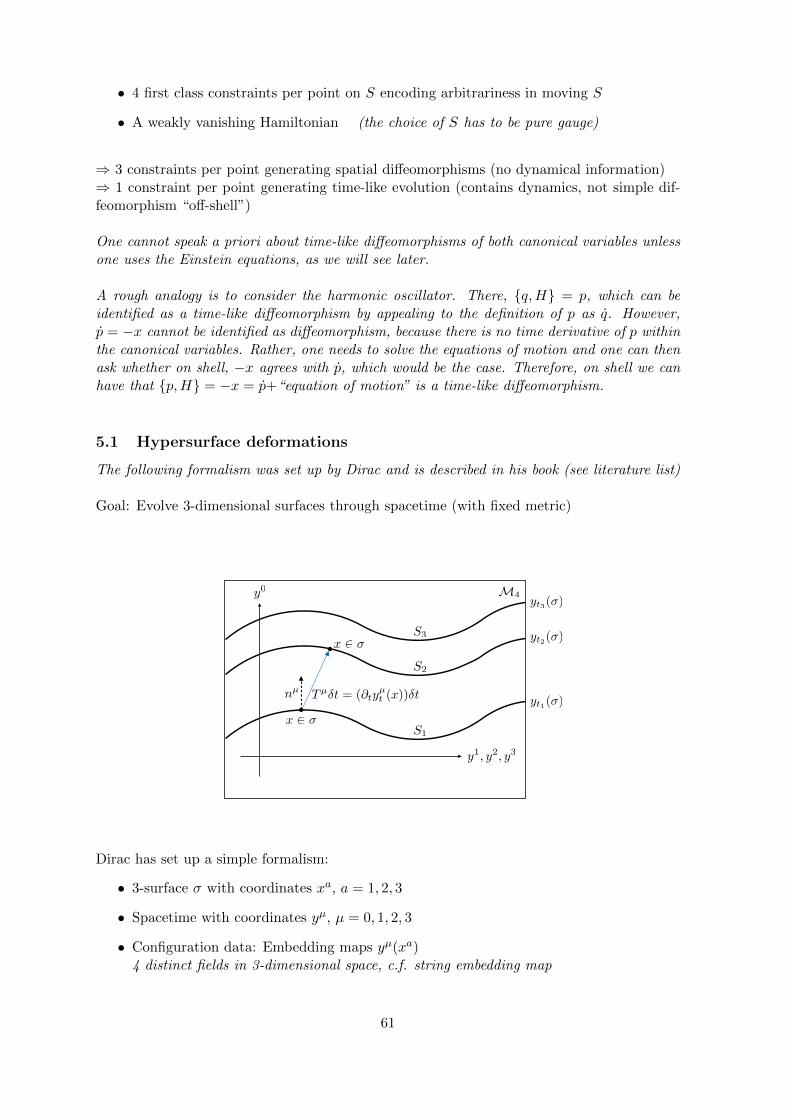
• 4 first class constraints per point on S encoding arbitrariness in moving S

• A weakly vanishing Hamiltonian (the choice of S has to be pure gauge)

⇒ 3 constraints per point generating spatial diffeomorphisms (no dynamical information)⇒ 1 constraint per point generating time-like evolution (contains dynamics, not simple dif-feomorphism “off-shell”)

One cannot speak a priori about time-like diffeomorphisms of both canonical variables unlessone uses the Einstein equations, as we will see later.

A rough analogy is to consider the harmonic oscillator. There, q,H = p, which can beidentified as a time-like diffeomorphism by appealing to the definition of p as q. However,p = −x cannot be identified as diffeomorphism, because there is no time derivative of p withinthe canonical variables. Rather, one needs to solve the equations of motion and one can thenask whether on shell, −x agrees with p, which would be the case. Therefore, on shell we canhave that p,H = −x = p+“equation of motion” is a time-like diffeomorphism.

5.1 Hypersurface deformations

The following formalism was set up by Dirac and is described in his book (see literature list)

Goal: Evolve 3-dimensional surfaces through spacetime (with fixed metric)

M4

S3

S2

S1

x 2

x 2

y1, y2, y3

y0

nµ

yt1()

yt2()

yt3()

Tµt = (@tyµt (x))t

Dirac has set up a simple formalism:

• 3-surface σ with coordinates xa, a = 1, 2, 3

• Spacetime with coordinates yµ, µ = 0, 1, 2, 3

• Configuration data: Embedding maps yµ(xa)4 distinct fields in 3-dimensional space, c.f. string embedding map

61

yµt (xa): 1-parameter family of configurations = embeddings of σt should not be confused with the “time” y0 in the target space

• Canonical momenta wµ(x) generate shifts in embedding coordinates yµ.

• Poisson bracket yµ(x), wν(x′) = δµν δ(3)(x, x′)

The histories above are generated by the Hamiltonian H =∫σ d

3xωµTµ, where Tµ are arbi-

trary (t-dependent) parameters.

Infinitesimally, yµ 7→ yµ + Tµδt

We want a formalism purely on σ.

Decompose Tµ = Nnµ +Nµ, with Nµ = ∂yµ

∂xaNa Push-forward of a vector on σ to S.

Pull back covectors to σ: va := vµ∂yµ

∂xa

Need also perpendicular part to S:→ non-unit time-like conormal nµ = εµνρσε

abc ∂yν

∂xa∂yρ

∂xb∂yσ

∂xc .

→ Unit time-like conormal nµ := nµ/√−nµnµ.

Define generators relative to S:

• H = w⊥ := wµnµ moves surface normal to S

• Ha = wµ∂yµ

∂xa changes coordinates on S, but leaves S invariant.

yµ(x),∫σ d

3xNaHa = Na∂ayµ(x)

→ one constraint per point for dynamics→ three constraints per point for spatial diffeomorphisms, no dynamical information

Compute algebra: (exercises)

H[M ],H[N ] = Ha[qab (M∂bN −N∂bM)

](5.1)

H[M ],Ha[Na] = −H [LNM ] (5.2)

Ha[Ma],Ha[Na] = −Ha [LNMa] . (5.3)

Dirac algebra / hypersurface deformation algebra

62

M4

N1

N1

N2

N2

~N

y1, y2, y3

y0

Figure 5.2: Executing two normal deformations in reverse order leads to a tangential shiftwith Na = qab (N1∂bN2 −N2∂bN1).

Hypersurface deformations:

• A simple model ⇒ algebra of surface deformations

• Any generally covariant canonical theory needs to satisfy this algebraNext section: derive it from GR by brute force

• Represent this algebra in quantum theoryThis provides a notion of quantum general covariance

5.2 The ADM formulation

Start with the EH action and perform the Dirac analysis by brute force.

5.2.1 Strategy

Goal: Hamiltonian formulation of Einstein-Hilbert action (κ = 8πG)Note that there are different conventions for κ in the literature!

SEH =1

2κ

∫

Md4x√−gR (5.4)

Strategy:

• Formalism includes split into spacetime-slices

• But slicing arbitrary

⇒ Hamiltonian evolution along some time-like vector field Tµ

63

M4Xt3()

Xt2()

Xt1()

S3

S2

S1

Nµt

TµtNnµt

x 2

x 2

X1, X2, X3

X0

Figure 5.3: The class of spacetimes we consider is topologically equivalent to R×σ, where σ isa three-dimensional manifold. M4 is foliated by three-dimensional spatial slices Xt(σ), t ∈ R.We distinguish between the slices S, subsets of M4, and σ, which is mapped to St via theembedding map Xt. Time evolution is along the vector field Tµ = ∂tX

µt . The decomposition

into normal and tangential components is Tµ = Nnµ +Nµ.

We slightly change notation here from yt 7→ Xt to conform with literature.

• Tµ is arbitrarily chosen, i.e. gauge parameter

• Decomposition Tµ = Nnµ +Nµ

N = Lapse function, Nµ = Shift vector. (Nµnµ = 0)

• Tµ determines a slicing t 7→ Xt(σ) given a slice S0 at t0

• all slicings are equivalent (gauge related)

• space-like foliation: TµTµ = −N2 +NµNµ < 0 ⇒ N 6= 0, choose N > 0.

Idea:∫d4x =

∫dt∫d3x, write integrands in coordinates t, xa adapted to the slicing.

• Metric not specified yet, can be still chosen arbitrarily in those coordiantes!

• The physical location of a neighbouring slice (i.e. how the slices are embedded in agiven spacetime) is determined by N and Nµ

5.2.2 Fundamental forms

Needs some geometrical concepts to be introduced first: “time”-derivative of the metric formomenta

Goal: metric and its time derivative as tensors on σ.

1. Define suitable tensors on S as a subset of M

64

2. Pull back to σ along embedding map.The second step is trivial if all tensors are purely spatial

Definition 13. The first fundamental form is defined as qµν := gµν + nµnν .

• qµν is the spatial projection of gµν

• qµνnν = 0

• qµν invertible only in spatial directions

→ spatial metric qab = (∂aXµt )(∂bX

νt )qµν after pull back to σ.

Definition 14. The second fundamental form is defined as Kµν := qµρqν

σ∇ρnσ.

• Kµν = 12Lnqµν (exercise)

Kµν is 1/2 the Lie derivative of the spatial metric along the hypersurface normal

• Kµν = K(µν) := 12 (Kµν +Kνµ) symmetric

• Kµνnν = 0

With Tµ = Nnµ +Nµ:

• 2Kµν = 1N

(LT qµν − L ~Nqµν

)

We choose to write ~N in the second Lie derivative to point out the difference between N andNa.

Need to understand geometry of the 3-surface σ.

Covariant derivative associated to qµν : Dµ, defined by

• Dµqνρ = 0

• D[µDν]f := 12 (DµDν −DνDµ) f = 0 on scalars f

• Preserves spatial tensors

Unique by theorem in differential geometry.

Can be constructed as

• Dµf = qµν∇ν f for scalars f

• Dµvν = qµρqν

σ∇ρvσ• Obeys Leibniz rule

f , vν : arbitrary smooth extensions of f, vν in a neighbourhood of S.

Dµ is independent of the extensions.

65

Pull back to σ: Davb = ∂avb − Γcabvc, Γcab = 12qcd (∂bqda + ∂aqdb − ∂dqab)

Construct Riemann tensor from Dµ: (DµDν −DνDµ) vρ =: R(3)µνρ

σvσ with vρnρ = 0

Fundamental identities: (exercises)

• Gauß equation: R(3)µνρσ = −2Kρ[µKσ]ν + qµ

µ′qνν′qρ

ρ′qσσ′R

(4)µ′ν′ρ′σ′

• Codacci equation: R(4) = R(3) +(KµνK

µν −K2)

+ 2∇µ (nν∇νnµ − nµ∇νnν)with K := Kµ

µ

Need metric in coordinates t, xa

The idea is now to obtain the form of the metric by expressing the infinitesimal line elementvia the changes that varying t and x produces via the embedding map X

dXµ = (∂tXµ)dt+ (∂aX

µ)dxa

Suppress t-subscript: X(t, xa) := Xt(xa)

Tµ = ∂tXµ = Nnµ +Nµ

ds2 = gµνdXµdXν (5.5)

= gµν ((∂tXµ)dt+ (∂aX

µ)dxa)(

(∂tXν)dt+ (∂bX

ν)dxb)

(5.6)

= (−N2 +NµNµ)dt2 + 2Nµgµν(∂aXν)dtdxa + (∂aX

µ)(∂bXν)gµν (5.7)

ADM (Arnowitt-Deser-Misner)-form of the metric.

gµν =

(−N2 +NaNa Na

Na qab

)gµν =

(−1/N2 Na/N2

Na/N2 qab −NaN b/N2

)(5.8)

Coordinate expressions:

nµ ∝ εµνρσεabc(∂aXν)(∂bXρ)(∂cX

σ) ∝ (1,~0)µ

Spatial vectors have a vanishing t-component

⇒ nµ = (−N,~0) and nµ = (1/N,−Na/N)

Tµ = Nnµ +Nµ = (1, (Na −Na)) = (1,~0)µ not in conflict with arbitrary lapse and shift!

⇒ Tµ∂µ has only a ∂t component

Coordinates are adapted to the slicing, not the metric!

In these coordinates,√−g = |N |√q (exercise).

For Einstein-Hilbert action:

66

• By Codacci equation:√−gR(4) expressed in terms of qµν , Kµν , N , + total derivative

→ pull everything back to σ.

ADM-form of the action:

SADM =1

2κ

∫

Rdt

∫

σd3x

√det q N

(R+KabK

ab −K2)

(5.9)

From now on: R := R(3).

5.2.3 Legendre transform

Perform Legendre transform & canonical analysis of

SADM =1

2κ

∫

Rdt

∫

σd3x

√det q N

(R+KabK

ab −K2)

(5.10)

Neglect boundary terms throughout.

Note that while we chose adapted coordinates to a specific slicing, we are still completely gen-eral in that we can assign any metric to those coordinates. Only by specifying lapse, shift,etc. we actually specify how this foliation lies inside a given spacetime equipped with a metric.Changing these assignments is what constraints are doing, so the gauge transformations ofour theory will take care of this freedom.

Time derivative qab = LT qab hidden in Kab indices pulled back to σ. (due to T = ∂t)

More precisely, qab = (∂aXµt )(∂bX

νt ) LT qµν

Due to Tµ = (1,~0), LT qµν = ∂tqµν .

Kab = 12N

(LT qab − L ~Nqab

)

Canonical momenta:

• P ab := δSδqab

= 12κ

√q(Kab − qabK

), qab(x), P cd(y) = δc(aδ

db)δ

(3)(x, y)

• PN := δSδN

= 0

• PNa := δSδNa

= 0

qab = 2NKab + L ~Nqab

3+1 primary constraints per point

C := PN ≈ 0, Ca := PNa ≈ 0. (5.11)

Useful identities:

• P = −√qκ K

• Kab = κ√q (2Pab − qabP )

• KabKab = κ2

q

(4PabP

ab − P 2)

67

Total Hamiltonian:

HT =

∫d3x

(P abqab + PN N + PNaNa − LEH + λC + λaCa

)(5.12)

=

∫d3x

(N

(2κ√q

(P abPab −

1

2P 2

)−√q

2κR

)+ P abL ~Nqab + λC + λaCa

)(5.13)

Stability of constraints:

• C = 2κ√q

(P abPab − 1

2P2)−√q

2κR =: H

• Ca = −2qac∇bP bc = −2∇bP ba =: HaWe used −2

∫d3xNa∇bP ba =

∫d3xP abL ~Nqab up to boundary terms (exercises).

The form∫d3xP abL ~Nqab is convenient in that it manifestly generates Lie derivatives. How-

ever, the expression does not vanish in general depending on the boundary conditions chosen,as it differs from −2

∫d3xNa∇bP ba by a boundary term. For the distinction to be relevant,

Na has to be non-vanishing on the boundary.

Two new constraints:

• H: scalar constraint, Hamiltonian constraint also super-Hamiltonian constraint

• Ha vector constraint, (spatial) diffeomorphism constraint

Compute algebra: (exercise)

H[M ],H[N ] = Ha[qab (M∂bN −N∂bM)

](5.14)

H[M ],Ha[Na] = −H [LNM ] (5.15)

Ha[Ma],Ha[Na] = −Ha [LNMa] . (5.16)

⇒ All constraints are stable and first class.

Interpretation of Ha: (again dropping boundary terms)

• qab(x),Ha[Na] = qab(x),∫d3y P abLNqab = LNqab(x)

• P ab(x),Ha[Na] = P ab(x),−∫d3y qabLNP ab = LNP ab(x)

Ha generates spatial diffeomorphisms

By Leibniz property of the Lie derivative:

• f(P ab, qab),Ha[Na] = LNf(P ab, qab)

This also explains 2 of the above algebra relations.

No direct physical information in Ha, changes only coordinates on initial value slice.

Interpretation of H:

• qab(x),H[N ] = 2NκKab = LNnqab

68

• P ab(x),H[N ] = qabNH2 −N√q

(qaρqbσ − qabqρσ

)R

(4)ρσ + LNnP ab

Remarks:

• H generates diffeomorphism normal to hypersurface S on qab

• Second computation very hard

• Normal diffeomorphism only if subset of vacuum Einstein equations (R(4)µν = 0) and

H = 0 are satisfied

• Einstein equations needed to turn second time derivative of qab into canonical dataWe need an equivalent formulation, the covariant EOM, where we have a manifest iden-tification of LNnP

ab with the canonical data.

• Einstein equations logically needed here to specify theoryOtherwise, it could have been any theory / Lagrangian that we are dealing with here.

• Other vacuum Einstein equations from

H ∝ Gµνnµnν Ha ∝ Gµνnµqνa

• Group generated by H,Ha: Bergmann-Komar group BK(M)

• BK(M) agrees with Diff(M) only on-shellWe also say that BK(M) is the dynamical symmetry group, while Diff(M) is a kine-matical one

5.3 Phase space extension

It is possible to start canonical quantisation at this point, leading to the Wheeler-de Witttheory, or Geometrodynamics. However, mathematical problems occur along the way, inparticular it is not known how to construct a spatially diffeomorphism-invariant integrationmeasure on the space of all metrics. It is therefore helpful to change the canonical variables tosome “more compact” objects, e.g. a connection taking values in the Lie algebra of a compactLie group, and then to use holonomies of that connection.

Idea from coupling fermions.

Minkowski space: γ-matrices γIγJ + γJγI = 2ηIJ14, I = 0, 1, 2, 3

Curved spacetime: ηIJ → gµν .

If we have eµI so that gµν = eµI eµJη

IJ , we can use γµ = eµI γI

eµI is called a vier-bein, or an orthonormal frame

At each point in σ, three linearly independent tangent vectors.

Construct orthonormal frame:

69

• eai , i = 1, 2, 3, so that eai qabebj = δij

• ea1, ea2, ea3: three orthonormal vectors

• Encodes metric: qab = eiaejbδij , where eiae

bi = δba

• Also, qab = eai ebjδij

• Unique up to rotation and orientation change: eai → ±Rijeaj• We choose positive orientation: det eai =

√q−1

⇒ Using eai instead of qab introduces local gauge invarianceThis is just the rotation of local frames.

i, j are indices in an internal space.

eai is called a triad (dreibein).

Strategy:

1. Extend the phase space and prescribe new Poisson bracketSomething like eai and a conjugate, encoding both qab and P ab

2. Introduce new constraint which kills new degrees of freedom

3. Relate gauge invariant part of new phase space to old phase space

4. Write old constraints in terms of new phase space variables

⇒ Leaves dynamics generated for qab and P ab invariant

New variables:

• Eai :=√qeai ⇒ qqab = Eai E

bjδij

• Kia, with Kab := Ki

(aejb)δij

•Kia(x), Ebj (y)

= κδ(3)(x, y)δbaδ

ij

Relation to old phase space via P ab ↔ Kab

Need rotation generator:

• Should map Eai 7→ ΛijEaj , Ki

a 7→ ΛijKja with Λij antisymmetric

⇒ Needs to contain 1 power of Eai and Kia

• Should then enforce Ki[ae

jb]δij = 0 qab is already symmetric due to ei[ae

jb]δij = 0

⇒ Gauß constraint Gij [Λij ] := 1

κ

∫d3xEa[iKa|j]Λ

ij ≈ 0

Check:0 ≈ Ea[iKa|j]e

ibejc = EaiKaje

i[be

jc] =√qKi

[bec]i (5.17)

Gauge transformations:

70

• Eai , Gkl[Λkl] = ΛijEaj

• Kia, Gkl[Λ

kl] = ΛijKja

Algebra: Gij [Λij ], Gkl[Ωkl] = Gij [(ΛΩ− ΩΛ)ij ]

Objects with contracted internal indices are invariant:

Eai Ebi, Gkl[Λkl] = ΛijEajE

bi + Eai ΛijEbj = (Λji + Λij)E

aiEbj = 0 (5.18)

Similar for Kia.

9+9 DOF per point - 3 rotations - 3 constraints = 6+6 DOF per point as before (withoutimposing H, Ha)

Express ADM variables in terms of new variables:

• detEai =√q(3−1) = q

• qab = 1detEE

ai E

bi

• P ab = 12κ

√q(Kab − qabK

), with

√qKa

b = KiaE

bi

Non-vanishing Poisson bracket: (exercise)

qab[E,K](x), P cd[E,K](y)

K,E

= κδc(aδdb)δ

(3)(x, y) (5.19)

⇒ Dynamics generated by H, Ha is invariant for qab and P ab

Evolution of Eai , Kia depends on new arbitrary gauge parameters Λij

Both Eai and Kia transform as internal vectors. In order to compute holonomies, i.e. expo-

nentiate a Lie algebra to a group, we need one of the canonical variables to transform as aconnection.

5.4 Connection variables

Need to construct connection out of canonical variables

Connection should transform as

ωaij , Gkl[Λkl] = −DaΛij := −∂aΛij − [ωa,Λ]ij = −∂aΛij − ωaikΛkj + ωakjΛik (5.20)

Connection extends the covariant derivative to internal indices:

• Davi = ∂av

i + ωaijvj

• Davib = ∂av

i + ωaijvj − Γcabv

ic

71

We can construct a connection by compatibility with eia:

Daeib = ∂ae

ib + ωa

ijejb − Γcabe

ic

!= 0 (5.21)

Can be solved for ωaij = Γa

ij := −ebj

(∂ae

ib − Γcabe

ic

)= −ebj∇aeib

Γaij = −Γaji, because −ebj∇aebi = (∇aebj)ebi −∇aδij = ebi∇aebj

Γaij : Spin connection

Γaij , Gkl[Λkl] = −Λjkebk∇aebi − ebj∇a

(Λikebk

)= −∂aΛij − ΓaikΛ

kj + ΓakjΛi

k (5.22)

⇒ correct transformation behaviour.

Different index structure of Γaij and Eai , but same number of DOF!

Isomorphism: Antisymmetric pair [ij]↔ k single internal index.

• Let aij = −aji• Define ak = −1

2εijkaij

• aij = −εijkak, because −εijk(−)12εmnkamn = 1

2(δmi δnj − δmj δni )amn = aij

Define ωia = −12εijkωajk.

⇒ Davib = ∂av

ib + εijkωajvbk − Γcabv

ic

⇒ 0 = ∂aeib + εijkΓajebk − Γcabe

ic

⇒ Γia = 12εijkebk

(∂beaj − ∂aebj + ecje

la∂becl

)

Define Aia := Γia(E) +Kia

From now on: Da acts with Aia

connection + vector = connection

The added vector transforms “homogeneously”, i.e. with the commutator part of the connec-tion transformation, while the affine part, producing the derivative in the transformation law,stays as it is.

Poisson brackets:

•Aia(x), Ebj (y)

= κδ(3)(x, y)δbaδ

ij

•Eai (x), Ebj (y)

= 0

•Aia(x), Ajb(y)

=

Γia(x),Kjb (y)

+Kia(x),Γjb(y)

= 0 (exercise)

→ Aia and Ebj are canonically conjugate.

Compute new Gauß law:

72

• Gij [Λij ] := 1κ

∫d3xEa[iKa|j]Λ

ij ≈ 0

• Gk[Λk] := Gij [−εijkΛk] = − 1κ

∫d3xΛkε

ijkEa[iKa|j] = 1κ

∫d3xΛkDaE

ak (exercise)

Action of Gauß law:

•Aia(x), Gk[Λ

k]

=Aia(x),−

∫d3y(DbΛ

k)Ebk

= −DaΛi(x)

•Eai (x), Gk[Λ

k]

=Eai (x),

∫d3yΛkε

kmnAbmEbn

= εiknΛkE

an(x)

For the quantum theory, it is interesting to perform a rescaling of the canonical variables.This changes spectra of the geometric operators.

Rescale the canonical variables: (interesting in quantum theory)

• (β)Eai := 1βE

ai

• (β)Aia := Γia + βKia

We still have:

(β)Aia(x), (β)Ebj (y)

= κδ(3)(x, y)δbaδij

“Ashtekar-Barbero variables” (1986 (β = i), 1994 (β ∈ R))

Drop (β) notation from now on.

Write all constraints in the new variables (κ = 1): (exercises) (all (β) implied!)

Gk[Λk] =

∫d3xΛkDaE

ak (5.23)

Ha[Na] =

∫d3xEaiL ~NAai =

∫d3xNaF iabE

bi +Gij [...] + boundary (5.24)

H[N ] =

∫

Σd3xN

(β2E

aiEbj

2√qεijkF kab −

(1 + β2

)√q

Ki[aK

jb]E

aiEbj

)(5.25)

Field strength F iab = 2∂[aAib] + εijkAjaAkb

Kia = (Aia − Γia)/β Again, the (β) subscript is implied on Aia and Eai .

Remarks:

• Gk and Ha have a clear interpretation

• H looks complicated, hard to quantise

• β = ±i special: simplifies H

• β 6∈ R has complicated reality conditions, hard to quantise

• Most quantisation progress so far for β ∈ R

73

Canonical general relativity:

• The phase space of general relativity can be parametrised by a spatial metric andits momentum, related to the extrinsic curvature of the spatial slice

• The Hamiltonian and spatial diffeomorphism constraint encode the dynamics ofthe theory as well as the gauge structure

• The ADM phase space can be enlarged to contain an additional local SO(3) gaugeredundancy and equipped with connection variables

74

6 Quantisation of constrained Hamiltonian systems

6.1 Quantisation without constraints

6.1.1 Abstract physical systems

Before discussing the algebraic properties of classical and quantum mechanics, let us considerwhat structure we need to do physics

Physical quantities q1, q2, . . . ∈ Q.

Operations on physical quantities:

• Add and scale physical quantities (e.g. addition of mass, velocity, . . . )→ Vector space

• Multiply physical quantities, ( e.g. torque = force x distance)→ Algebra Not necessarily commutative

Definition 15. An algebra A over C is a C-vector space equipped with a bilinear productA×A → A.

One may in principle forbid addition of structurally different quantities, e.g. with differentdimensions, or the multiplication of all elements with all other elements.

“Less obvious” properties: Those are used in our current physical theories

• Adjoint element q∗: real vs. complex objects

(q∗)∗ = q,

(q1q2)∗ = q∗2q∗1

(cq)∗ = cq∗, c ∈ C

E.g. complex conjugation.

up to here: ∗-algebra

• Norm: ‖ · ‖ : A → [0,∞) How large can a quantity be at most?

‖q1q2‖ ≤ ‖q1‖‖q2‖ ‖q1 + q2‖ ≤ ‖q1‖+ ‖q2‖ ‖cq‖ = |c|‖q‖

Existence of a norm requires us to work with bounded quantities, e.g. eiq

• Completeness: all Cauchy series in Q converge in Q.

Normed and complete algebra: Banach algebra

• ∗-compatibility of the norm: ‖q∗q‖ = ‖q‖2, ‖q∗‖ = ‖q‖

up to here: C∗-algebra

75

Structure of C∗-algebra!

All of these can in principle be dropped.

State of the system: map ω from Q to C.

• Linearity: ω(c1q1 + c2q2) = c1ω(q1) + c2ω(q2), c1, c2 ∈ CMotivated by classical evaluation of phase space functions at a phase space point, oth-erwise inconsistent with addition of phase space functions.

• Positivity: ω(q∗q) ≥ 0

Assigns values to physical quantities.

6.1.2 Algebraic structure of Hamiltonian mechanics

Canonical quantisation is a representation of the algebraic structure of classical mechanicson Hilbert spaces. It is therefore necessary to study this structure beforehand.

Functions on phase space form an algebra

• Vector space: addition f1 + f2 and multiplication cf , c ∈ C

• Bilinear product: multiplication f1 · f2 = f2 · f1, commutative!

Mathematical properties

• Norm: ‖f‖ = supq,p f(q, p) limit to bounded smooth functions.

• Adjoint element: complex conjugation, e.g. (q + ip)∗ = (q − ip)

• Cauchy series converge: limn→∞ fn → f

The set of bounded continuous functions is complete under the sup norm.

Additional structure:

• Poisson bracket A×A → A, → Poisson algebra

• Generator of dynamics: Hamiltonian H

States:

• ωq0,p0(f) = f(q0, p0) Evaluation on phase space point

• Can be generalised to probability distributions

76

6.1.3 Algebraic structure of quantum mechanics

We need a suitable algebraic structure to represent / modify that of Hamiltonian mechanics.

Experiment:

• Quantities which are canonically conjugate at the classical level cannot be measuredsimultaneously with arbitrary precision

→ modify algebra to take canonical conjugacy into account

→ ordering important qp 6= pq

because measurements in different orders → different results

• Superposition of classical states / solutions

→ linear structure Photon takes all paths simultaneously, superposition of solutions

Construction of quantum mechanics:

• Non-commutativity: physical quantities are operators

• Superposition: linear operators on vector space, for linear Schrodinger equation

• Adjoint element: scalar product in the vector space

• Scalar product + completeness + norm (derived from scalar product): Hilbert space

Definition 16. A Hilbert space H is a vector space with a scalar product that is also acomplete metric space with a norm induced by the inner product.

Notation:

• Elements of H: “kets” |x〉

• Scalar product: 〈x, y〉 = 〈x | y〉

• Norm for Hilbert space elements: ‖ |x〉 ‖2 := 〈x, x〉 ≥ 0, equality only if |x〉 = 0.

• Adjointness:⟨x, Ay

⟩=⟨A∗x, y

⟩

• Operator norm: sup|x〉∈H, ‖|x〉‖6=0‖A|x〉‖‖|x〉‖ = c ⇔ A has norm c

Boundedness:

• A bounded: c ∈ [0,∞)

• A unbounded: otherwise, “c =∞”

77

A self-adjoint (modulo domain issues): A∗ = A

A self-adjoint ⇒ A has real spectrum (eigenvalues in the finite dimensional case)

Inequalities for operator norm:

• ‖AB‖ ≤ ‖A‖‖B‖ ∀A, B ∈ B(H) bounded linear operators

• ‖A+ B‖ ≤ ‖A‖+ ‖B‖, ∀A, B ∈ B(H)

6.1.4 Quantisation map

After having discussed what mathematical structure we want to use for quantum mechanics,we need to figure out how to construct a quantum system given a classical system.

Algebraic properties of Poisson bracket are mimicked by commutator [A, B] = AB − BA

• Bi-linearity: [λA+ µB, C] = λ[A, C] + µ[B, C] and [C, λA+ µB] = λ[C, A] + µ[C, B]

• Antisymmetry: [A, B] = −[B, A]

• Leibniz property: [AB, C] = A[B, C] + [A, C]B ordering matters!

• Jacobi identity: [A, [B, C]] + [B, [C, A]] + [C, [A, B]] = 0

∀A, B, C ∈ GL(H), λ, µ ∈ C

Quantisation map (ideal version, see however subtleties):

Given a classical Hamiltonian system, we look for linear operators on a Hilbert space so that

[f , g] = i~ f, g (6.1)

where ~ = h2π is the Planck constant and f, g are phase space functions.

Dynamics:

Heisenberg picture:

f(t) = eiH(t−t0)/~f(t0)e−iH(t−t0)/~ = f(t0) + (t− t0)−i~

[f , H]︸ ︷︷ ︸f,H

+O((t− t0)2

)(6.2)

Possible outcome of individual measurements: spectrum of f . roughly: eigenvalues

Expectation value over many measurements:⟨

Ψ∣∣∣ f∣∣∣ Ψ⟩

:=⟨

Ψ, fΨ⟩

for 〈Ψ | Ψ〉 = 1

The concrete outcome of the measurement is not determined, but we can additionally ask forthe probability of a specific outcome by looking at the components of |Ψ〉 in an eigenbasis of f .

Decompose |Ψ〉 =∑

n cn |fn〉 with f |fn〉 = fn |fn〉.

78

Then, |cn|2 is the probability of the measure outcome fn.

⟨Ψ∣∣∣ f∣∣∣ Ψ⟩

=∑

n |cn|2fn

Schrodinger picture:

|Ψ(t)〉 = e−iH(t−t0)/~ |Ψ(t0)〉 (6.3)

Equivalence of dynamical pictures:⟨

Ψ(t0)∣∣∣ f(t)

∣∣∣ Ψ(t0)⟩

=⟨

Ψ(t)∣∣∣ f(t0)

∣∣∣ Ψ(t)⟩

The dynamics is either in the states or in the operators

6.1.5 GNS construction

Are there other structures than Hilbert spaces satisfying all needed properties for QM?

We now abstractly formulate what we want to achieve:

Consider the “free algebra” F of all phase space functions with no commutativity assumption:

• Example element: µf1f2 + γf3 6= µf2f1 + γf3, fi phase space function, µ, γ ∈ C

Identify f1f2 − f2f1 = i~f1, f2

⇒ abstract “quantum” (unital) *-algebra B

This is an ~-deformation of the classical commutative algebra (deformation quantisation).

unital algebra: ∃1 ∈ A : 1f = f1 = f ∀ f ∈ A

Not necessary here: C∗-property: Banach (= normed and complete) ∗-algebra with ‖f∗f‖ =‖f‖2

Our task in quantum mechanics is to find representations of this algebra.

Theorem 3. (Gelfand-Naimark-Segal) Let ω be a positive, normed, and linear functionalon a unital ∗-algebra A. ω determines the GNS data (Hω, ρω, 0ω) consisting of a Hilbert spaceHω, a representation of A on Hω, and a normed cyclic vector |0ω〉 ∈ Hω, so that

ω(f) = 〈0ω | ρω(f) | 0ω〉Hω , ∀f ∈ A. (6.4)

The GNS data is unique up to unitary equivalence.

|0〉 cyclic ⇔ B(H) |0〉 is dense in H, B(H) = bounded linear operators on H.

This deep theorem tells us that we do not need to look beyond Hilbert spaces for finding a goodarena for quantum physics. We recall however that the ∗-property is needed for this.

79

⇒ Hilbert space representations are all we need to consider!

Remarks:

• The ∗-property is needed to define 〈a | b〉 := ω(a∗b) with |b〉 = b |0ω〉 and 〈a| = 〈0ω| a∗

• If the representation is by bounded operators, then the operator norm induces a C∗-norm on the quantum ∗-algebra B

• Related to Gelfand-Naimark theorem: Every C∗-algebra A is isometrically *-isomorphicto a C∗-algebra of bounded operators on a HS.

Example: ω(A∗BC) = 〈A |B | C〉, where |C〉 = C |0〉, |A〉 = A |0〉

States are produced by operators acting on the cyclic vector |0〉, which may or may not havethe interpretation of a vacuum = lowest energy eigenstate of the Hamiltonian.

6.1.6 Subtleties

Quantisation is not unique:

• Classical theory = limit of quantum theory where the involved actions are ~

→ We try to infer a general theory from a certain limit

Main issue: factor ordering

Example system:

• Classical phase space x, p = 1

• Hilbert space: L2(R, dx)

• Hilbert space element: |ψ〉 ⇔ square integrable function Ψ(x),∫∞−∞ dxΨ(x)Ψ(x) <∞

• Operators: xΨ(x) = xΨ(x), pΨ(x) = −i~ ddxΨ(x)

Question: What is xp? Different options:

• xp or px

• Symmetric ordering 12 (xp+ px)

• . . .

→ No good answer, needs additional input

Is it possible in principle to find operators for all phase space functions so that [f , g] =

i~ f, g?

Theorem 4. (Groenewold-van Hove) It is not possible to find a consistent quantisationif we extend the allowed degree of polynomials in q, p beyond 2 in both variables.

80

This theorem tells us that we should in principle never expect to be able to represent all phasespace functions as operators. Therefore, additional input is needed in constructing a canoni-cal quantisation.

Main lesson:

• Need to choose point-separating subset of phase space functions to quantise consistently

Point-separating set of functions: We can tell points in phase space apart by knowing thevalue of all functions in the set.e.g. q, p for one-dimensional system

For all phase space functions, can formalise with the Moyal product

f ∗ g = f · g +∞∑

n=1

1

n!

(i~2

)nΠn(f, g)︸ ︷︷ ︸

constructed from Poisson bracket

(6.5)

• Deformation quantisation: the star product is an ~-deformation of the usual multipli-cation.f ∗ g − g ∗ f = i~f, g+O(~3)

• Same as Hilbert space representation

Given a point-separating subset that we can quantise, is the quantisation unique?

To proof a theorem, simplify to bounded operators:

• Classical phase space functions: eiλx, eiµp, λ, µ ∈ R

• Operators: eiλx, eiµp

Baker-Campbell-Hausdorff formula for [A, [A, B]] = [B, [A, B]] = 0:

eAeB = eBeAe[A,B], eA+B = eAeBe−12

[A,B] (6.6)

Algebra: eiλxeiµp = e−i~λµeiµpeiλx Weyl-form of the canonical commutation relations (CCR)

Adjointness: eiλx∗

= e−iλx, eiµp∗

= e−iµp

Note that the hat is over the complete exponential, not only over x and p. The derivation ofthe Weyl-from of the CCR is thus only formal here, but the result is what one would expectfor well-behaved operators. We take this algebra here as a classical starting point and lookfor representations.

U(λ) := eiλx and W (µ) := eiµp are two one-parameter unitary groups:

• U(λ)−1 = U(λ)∗ = U(−λ)

• W (µ)−1 = W (µ)∗ = W (−µ)

81

Theorem 5. (Stone-von Neumann) All jointly irreducible and weakly continuous one pa-rameter unitary groups U(λ) and W (µ) acting on a separable Hilbert space H and satisfyingthe Weyl-form of the canonical commutation relations are unitarily equivalent.

Separable Hilbert space: H admits a countable orthonormal basis.

U(λ) and W (µ) jointly irreducible: The set U(λ) : λ ∈ R ∪ W (µ) : µ ∈ R is irreducible

irreducible: There are no invariant subspaces, more later in group theory

Weak continuity: limλ→0

⟨Ψ∣∣∣ U(λ)

∣∣∣ Ψ′⟩

= 〈Ψ | Ψ′〉

Weak continuity ⇒ x := −i ddλ∣∣λ=0

U(λ) exists (Stone’s theorem)

This theorem tells us that under the given technical assumptions, all representations of theWeyl-form CCR are unitarily equivalent, i.e. the same up to a choice of basis.

The original theorems assumed strong continuity, however this can be relaxed to weak conti-nuity

How can we avoid this theorem?

Drop weak continuity and separability!

Consider the Hilbert space of almost-periodic functions

• Spanned by fλ(x) = eiλx : λ ∈ R

• Scalar product: 〈fλ, fλ′〉 := δλ,λ′ (Kronecker delta!)

Note that in the Stone-von Neumann representation, 〈fλ, fλ′〉SvN = 2πδ(λ, λ′) (Dirac delta!)

This is only formal because plane waves are not square integrable, as the Dirac delta shows.

Action of operators:

• eiλx |fλ′〉 = |fλ+λ′〉

• eiµp |fλ〉 = ei~µλ |fλ〉

No weak continuity:

〈fλ, fλ〉 = 1 6= 0 = limλ′→0

⟨fλ, eiλ

′xfλ

⟩(6.7)

⇒ x := ddλ

∣∣λ=0

eiλx = limλ→0U(λ)−U(0)

λ does not exist

The differential quotient diverges when taking the expectation value w.r.t. |fλ〉.

However, p exists, as W (µ) is weakly continuous.

What is the Hilbert space?

82

Complete w.r.t. norm induced by scalar product:

⇒ Bohr compactification of the real line, RBohr.

This is a compact Abelian group that contains R, but is much larger than it. In particular, anormalised Haar measure exists.

Important for loop quantum cosmology (later).

Main lessons:

• We can avoid uniqueness by dropping weak continuity

• Physics may be different in different representations.

Here, need to regularise x, e.g. via x ≈ 1λ sin(λx) = 1

2iλ

(U(λ)− U(−λ)

)

→ finite regularisation scale λ

• Separability can be regained by the dynamics / constraints via superselection

The above examples illustrate the finite-dimensional case. What about infinite dimensions?

What about field theories, i.e. infinite dimensional phase space?

→ Uncountably many unitarily inequivalent representations in quantum field theory (byHaag’s theorem)

The details are somewhat technical and won’t be covered here.

Additional subtlety: Not possible to determine the representation using finite number ofmeasurements (Fell’s theorem)

Roughly, states written as expectation values w.r.t. density matrices in a representation ob-tained from a faithful state on a C∗-algebra are weakly dense in the set of all states on thatalgebra.

Quantisation of unconstrained systems:

• Algebraic structure of classical mechanics is mapped to quantum mechanics

• Factor ordering problems prohibit us from quantising all phase space functionsconsistently

• Representations of a certain sub-algebra of phase space functions are in generalnot unique, but may be under additional assumptions

• Dynamical input and physical intuition is likely needed to find the “correct”representation

83

6.2 Quantisation with constraints

6.2.1 Reduced quantisation

Solve all constraints classically

• Find enough Dirac observables and their Poisson brackets or, equivalently:

• Impose gauge conditions and compute Dirac bracket

⇒ standard quantisation

Pracitcal problem: Observable algebras / Dirac bracket are often too complicated to findrepresentations

Conceptual problems for generally covariant systems:

• Fixes a classical notion of time (gauge condition)

• Quantum constraints define a notion of quantum general covariance

• Choice of gauge / observables not unique, may lead to inequivalent quantum theories

The question of which quantum theory is the correct one then arises. This question isvery subtle, since in all quantisations, one picks a preferred sub-algebra of observables.Mapping these observables to other ones is highly ambiguous at the level of operators.

• No good global gauge conditions in GR

This means that no single gauge fixed classical quantisation is applicable in all situations

→ Explore different methods of quantisation with constraints

6.2.2 Dirac quantisation

Idea: quantise first class constraints and impose on states

Set of constraints φα(qj , pj) ≈ 0

Quantise unconstrained phase space:

• |Ψ〉 ∈ H, kinematical Hilbert space

• Operators, qi, pi

Constraint operators: φα := φα(qj , pj) in a specific ordering

Physical states: φα |ψ〉phys = 0

(Weak) Quantum Dirac observables: [O, φα] ≈ 0, ≈ w.r.t. φα

Is this consistent?

• Assume φα |ψ〉phys = 0

• ⇒ φαφβ |ψ〉phys = 0

84

• ⇒(φαφβ − φβφα

)|ψ〉phys = 0

• ⇒ φα, φβ |ψ〉phys = 0 (up to ordering problems)

Two cases:

• Only first class constraints: φα, φβ = cαβγφγ , ⇒ cαβγφγ |ψ〉phys = 0

Consistent (up to ordering)

• Second class constraints present: ∃α, β : φα, φβ 6= cαβγφγ ⇒ ”1” |ψ〉phys = 0

Inconsistent

⇒ Only first class constraints can be treated using Dirac quantisation

Recall: Second class systems can be transformed to first class systems via gauge unfixing.

Subtleties for Dirac quantisation:

• Ordering problems may spoil the constraint algebra:

cαβγφγ 6= cαβγφγ in general, cαβγφγ |ψ〉phys?= 0

• On Hphys, only quantum Dirac observables are well defined operators:

f |ψ〉phys 7→ |ψ′〉phys ⇒ (f φα − φαf) |ψ〉phys = 0 ⇒ [f , φα] ∝ φβ

This may lead to problems when imposing the constraints iteratively. We will encounterthis when quantising the constraints of GR.

• [φα, φβ] = cαβγφγ inconsistent with φα being self-adjoint and cαβγ anti-self-adjoint:

[φα, φβ]∗ = −[φα, φβ],(cαβγφγ

)∗= −φγ cαβγ (6.8)

Unless cαβγ commutes with φα, but this is e.g. not true for general relativity.

• On Hphys, the kinematical scalar product may not be well defined.→ Need new scalar product, systematically e.g. via refined algebraic quantisation

Possible weakening of required structure:

• No scalar product on the kinematical representation space i.e. no Hilbert space→ Scalar product only on Hphys

• Quantum constraints not self-adjoint→ Complex spectrum allowed as long as zero is included

• Solving constraints on the dual Hilbert space

The dual Hilbert space H∗ is much larger than H (for infinite-dimensional systems) andcan contain a broader class of states which don’t need to be normalisable w.r.t. to thenaive transfer of the scalar product of H

An example is the solution to the spatial diffeomorphism constraint, where one (roughly)needs to average w.r.t. spatial diffeomorphisms. The dual Hilbert space can support theresulting state.

85

Variation: Master constraint: M =∑

α φ2α

• Different detection of Dirac observables: [O, [O,M ]] ≈ 0

• Technical advantages, e.g. existence of physical Hilbert space

6.2.3 Quantisation of second class systems

To quantise second class constraints, we need to weaken the condition on their imposition notto produce the above inconsistency

“Weak” imposition of constraints:⟨ψw

∣∣∣ φα∣∣∣ ψ′w

⟩= 0

|ψw〉 span the weak solution space Hw

In general:⟨ψw

∣∣∣ φαφβ∣∣∣ ψ′w

⟩6= 0 ⇒ No inconsistency, even for second class constraints

Weak imposition is therefore weaker than the above strong imposition a la Dirac

Examples:

• Gupta-Bleuler formalism for electrodynamics

• Virasoro constraints for quantum string

Quantisation of systems with constraints:

• The same problems as for quantisation without constraints also occur

• Additionally, there are several methods to impose the constraints

• Different schemes may lead to different quantum theories

86

7 Representation theory of SO(3)

The representation theory of SO(3) is key for loop quantum gravity. Much of the kinematicalLQG structure rests on it.

Ashtekar-Barbero variables: local gauge invariance under SO(3)

Quantum theory: represent classical Poisson-algebraic structures⇒ Need representation theory of SO(3)

Goal of section:

• Concept of Lie group / Lie algebra

• Representations of SO(3) / so(3)

• Invariant tensors and recoupling

Methodology:

• Introduce concepts using SO(3) as example

• Generalise to arbitrary Lie groups

7.1 Lie groups

7.1.1 Group structure

vi, wi: vectors in 3-dim. Euclidean space

Rotation: vi 7→ Rijvj .

Defining property: leaves scalar product (angles and lengths) invariant:

viwjδij 7→ RikRjlδijv

kwl!

= vkwlδkl (7.1)

⇒ RikRjlδij = δkl ⇔ RTR = 1

Products of rotations are rotations: (R1R2)T (R1R2) = RT2 RT1 R1R2 = 1

Inverse rotation R−1 = RT .

Abstraction:

Definition 17. A group G is a non-empty set together with a multiplication operationsatisfying the following properties:

1. Closure: gh ∈ G, ∀g, h ∈ G

2. Associativity: g(hk) = (gh)k, ∀g, h, k ∈ G

3. Identity element: ∃e ∈ G : eg = ge = g, ∀g ∈ G

4. Inverse element: ∀g ∈ G : ∃g−1 ∈ G : gg−1 = g−1g = e

87

Remarks:

• e is unique

• gh 6= hg in general.

• Abelian group: gh = hg

Above: explicit realisation of rotations acting on vectors in R3

Group concept more general:

• Abstract concept: group

• Explicit realisation: representation on a vector space

Definition 18. A representation (ρ, V ) of a group G on a vector space V is a map ρ : G→GL(V ) (from G to the linear invertible maps on V ), so that

ρ(g)ρ(h) = ρ(gh) ∀g, h ∈ G (7.2)

Remarks:

• V is called “representation space”

• For dimV = n <∞, GL(V ) = GL(n) = invertible n× n matrices

• dimV is called the dimension of the representation

• Action of g on components of a vector v = vαeα, where eα is a basis of V :ρ(g)v = (ρ(g)αβv

β)eα

• We restrict to vector spaces over R or C, but general fields are possible

• A representation is called faithful if ρ is injective trivial rep. ρ(g) = 1 not faithful

• (ρ, V ) irreducible ⇔ 6 ∃ ρ-invariant subspace of V

Example for reducible representation:

ρ(g) =

(R(g) 03

03 R(g)

)(7.3)

Question: are there more representations of the rotation group SO(3)?

Such questions are of crucial importance for physics!

Theoretical approach to elementary particle physics:

1. Find the underlying symmetry group

2. Study the representation theory of this group

3. Particles (= things that exist) transform under representations

4. Particle properties = representation properties

88

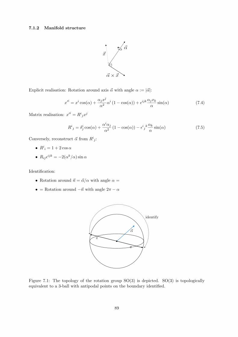
7.1.2 Manifold structure

~↵~x

~↵ ~x

Explicit realisation: Rotation around axis ~α with angle α := |~α|:

x′i

= xi cos(α) +αjx

j

α2αi (1− cos(α)) + εijk

αjxkα

sin(α) (7.4)

Matrix realisation: x′i = Rijxj

Rij = δij cos(α) +αiαjα2

(1− cos(α))− εijkαkα

sin(α) (7.5)

Conversely, reconstruct ~α from Rij :

• Rii = 1 + 2 cosα

• Rijεijk = −2(αk/α) sinα

Identification:

• Rotation around ~n = ~α/α with angle α =

• = Rotation around −~n with angle 2π − α

~↵

identify

Figure 7.1: The topology of the rotation group SO(3) is depicted. SO(3) is topologicallyequivalent to a 3-ball with antipodal points on the boundary identified.

89

Topology:SO(3) ∼ 3-Ball with antipodal identification ∼ RP3

∼ means diffeomorphic

SO(3) is connected, but not simply connected

• ∃ path from every point to every other point

• ∃ non-contractible loops = ∃ distinct paths between two points which are not continu-ously deformable into each other

⇒ SO(3) is a manifold

The group of permutations, or discrete symmetry groups, are not manifolds

Definition 19. A Lie group is a group G with the additional structure of a differentiablemanifold, so that the group multiplication and inversion are smooth maps.

7.2 Lie Algebras

7.2.1 Infinitesimal Rotations

Infinitesimal transformations are a key technique in the study of Lie groups. The structureof infinitesimal transformations determines the group to a large extend.

Infinitesimal rotation: R = 1 + Λ

RTR = 1 ⇒ ΛT = −Λ

Λ =

0 −α3 α2

α3 0 −α1

−α2 α1 0

=: αiΛi (7.6)

Λ1 :=

0 0 00 0 −10 1 0

, Λ2 :=

0 0 10 0 0−1 0 0

, Λ3 :=

0 −1 01 0 00 0 0

(7.7)

(Λi)jk = −εijk

We note the conceptual difference between the index i and jk.

Λi generates rotations around the i-axis.

Relation to finite transformation:

90

R(~α) = R(~α/2)R(~α/2) = . . . = R(~α/N)N

For N →∞: R(~α/N) ≈ 1 + αiΛi/N

⇒ R(~α) = limN→∞(1 + αiΛi/N

)N= exp

(αiΛi

)

Linear combinations of the Λi also generate rotations

What about products?

(Λ1Λ2)T = Λ2Λ1 =

0 1 00 0 00 0 0

6= αiΛi

Need antisymmetry:

(ΛiΛj − ΛjΛi)mo= εimnεjno − εjmnεino= δioδjm − δijδom − δojδmi + δijδom

= −εijkεkmo = εijk (Λk)mo (7.8)

The commutator [Λi,Λj ] = ΛiΛj − ΛjΛi of two generators is again a generator

Abstraction:

7.2.2 Lie Algebras

Consider Λi as a specific realisation of the generators of an abstract algebra:

Definition 20. A Lie algebra is a vector space g together with a map [·, ·] : g × g → g,(x, y) 7→ [x, y], called Lie bracket, that satisfies

1. Bi-linearity: [ax + by, z] = a[x, z] + b[y, z] and [z, ax + by] = a[z, x] + b[z, y] ∀x, y, z ∈g, a, b ∈ C

2. [x, x] = 0 ∀x ∈ g.

3. Jacobi identity: [x, [y, z]] + [y, [z, x]] + [z, [x, y]] = 0 ∀x, y, z ∈ g

1. + 2. ⇒ [x, y] = −[y, x]

Remarks:

• Lie bracket not associative: [[x, y], z] 6= [x, [y, z]] in general

• Flexibility law: [x, [y, x]] = [[x, y], x]

We consider only finite-dimensional Lie algebras.

Choose basis XA of Lie algebra, A = 1, . . . , n = dim g

91

Lie bracket: [XA, XB] = fCAB XC

fCAB are called structure constants of g.

Properties:

• Antisymmetry: fCAB = −fCBA• Jacobi identity: fDAEf

EBC + fDBEf

ECA + fDCEf

EAB = 0

As before: Explicit realisation on vector space = representation.

Definition 21. A representation of a Lie algebra g on a vector space V is a map ρ : g→ gl(V ),so that

ρ(x)ρ(y)− ρ(y)ρ(x) = ρ([x, y]) ∀x, y ∈ g (7.9)

gl(V ) = endomorphisms of V = linear maps from V to V

These do not need to be invertible. This notation makes sense since the invertible generallinear group GL(V ) is obtained by exponentiating gl(V ), which makes the maps invertible.

Idea: study representations of the Lie algebra (find the generators) and exponentiate to ob-tain the Lie group.

Notation: Lie group: SO(3), Lie algebra so(3), often so(3).

7.2.3 Casimir operators

Physical interest: g-invariant objects

E.g. invariant under some symmetries encoded in g.

For so(3): ΛiΛjδij = −2 1

1 commutes with all elements of g.

For general Lie algebras: Need analogue of δij

How can this be done?

The available structure so far are only the structure constants. We can define:

Killing-Cartan tensor: gAB := fCDAfDCB

Restrict to gAB non-degenerate (semi-simple Lie algebras)

92

Inverse: gAB

Definition 22. The quadratic Casimir operator C of a Lie algebra is defined as XAXBgAB.

Remarks:

• [C, x] = 0 ∀x ∈ g (exercises)

• fABC := gADfDBC is totally antisymmetric (exercises)

• Higher order (in XA) Casimir operators exist in general

• Irreducible representation: C ∝ 1Otherwise, a non-trivial invariant subspace exists where C acts differently, e.g. C =diag(2, 1).

Proportionality constant used to classify the representation.Example: mass and spin of a particle (Poincare group).one quadratic and one quartic Casimir operator

7.3 Unitary irreducible representations of SO(3)

7.3.1 Simplifying facts

For quantum mechanics: representation on Hilbert space H.

Additional structure: scalar product 〈·, ·〉 As opposed to vector space

Physically plausible: action of symmetry leaves physics invariant

Unitary representation: 〈ρ(g)v, ρ(g)w〉 = 〈v, w〉 ∀v, w ∈ H.

Simplifying facts from theory of Lie groups:

• Every continuous representation of a compact Lie group in a Hilbert space is equivalentto a unitary representation→ enough to consider unitary representations

• Every continuous unitary representation of a compact Lie group is a direct orthogonalsum of irreducible sub-representations→ enough to consider irreducible representations, take orthogonal sums afterwards

• Every continuous irreducible representation of a compact Lie group in a Hilbert spaceis finite-dimensional→ enough to consider finite-dimensional representations

7.3.2 Classification of so(3) representations

Strategy:

1. Derive some necessary conditions on representations of algebra while assuming theirexistence

93

2. Verify existence by explicitly constructing the representation using the necessary con-ditions

3. Exponentiate to obtain the group representations

Unitary representation:〈v, w〉 = 〈ρ(g)v, ρ(g)w〉 = 〈ρ(g)∗ρ(g)v, w〉 ⇒ ρ(g)∗ρ(g) = 1

Infinitesimal rotation: (generic representation)

ρ(g) = 1 + αiΛi ⇒ Λ∗i = −Λi

Alternative definition: ρ(g) = 1− iαiJi ⇒ J∗i = Ji

Generators are hermitian (Ji) or anti-hermitian (Λi).

Choose generators Ji hermitian: J∗i = Ji

[Ji, Jj ] = iεijkJk

Casimir operator: J2 := JiJjδij = λ1, λ > 0.

Analyse spectrum of another operator, J3, that can be diagonal simultaneously.

Ladder operators: J± := J1 ± iJ2 = J∗∓

[J+, J−] = 2J3, [J3, J±] = ±J±, J2 = J±J∓ ∓ J3 + J23

Let xm be an eigenvector for J3 with

J3 |xm〉 = m |xm〉 , 〈xm | xm〉 = 1 (7.10)

As a hermitian matrix, J3 has to have n = dimH eigenvalues

Properties of vectors J± |xm〉

• J3J± |xm〉 = (J±J3 + [J3, J±]) |xm〉 = (m± 1)J± |xm〉

• 〈J±xm | J±xm〉 = λ∓m−m2

Either J± |xm〉 = 0, or (m± 1) is also an eigenvalue of J3

Representation finite-dimensional: ∃ largest eigenvalue j.

J+ |xj〉 = 0, λ = j + j2

Use J− to construct further eigenvectors: J− |xj〉 , (J−)2 |xj〉 , . . .

Finite number of eigenvalues:

∃N ≥ 1 : (J−)N−1 |xj〉 6= 0, (J−)N |xj〉 = 0

94

J3(J−)N−1 |xj〉 = j′(J−)N−1 |xj〉

⇒ λ = (j′)2 − j′, j − (N − 1) = j′

⇒ N = 2j + 1, j = −j′

⇒ j = 0, 12 , 1,

32 , . . . j is called the “highest weight” of the representation

Eigenvalues: m = −j,−j + 1, . . . , j − 1, j

Eigenvectors: |xj〉 , J− |xj〉 , . . . , (J−)2j |xj〉Span subspace invariant under J3, J−.

J+ invariance: J+(J−)p |xj〉 = J+J−(J−)p−1 |xj〉 = (J2 + J3− J23 )(J−)p−1 |xj〉 ∝ (J−)p−1 |xj〉

⇒ subspace invariant under all generators

Representation irreducible ⇒ H = span(|xj〉 , J− |xj〉 , . . . , (J−)2j |xj〉)

There cannot be any other eigenvectors and eigenvectors cannot be degenerate. Otherwise,we could build a new ladder from those, and thus an invariant subspace.

Up to here: assumed existence of representation.

Now: Compute matrix elements of J1, J2, J3 ⇔ J+, J−, J3

J3 |xm〉 = m |xm〉

J± |xm〉 =√j(j + 1)∓m−m2 |xm±1〉, 〈xm, x′m〉 = δm,m′

The matrices (Ji)mm′ = 〈xm | Ji | xm′〉 provide representations of the Lie algebra so(3).

We don’t check this explicitly here, but it can be done.

Examples:

• j = 0:

J1 = J2 = J3 = 0, trivial representation, 1-dimensional, Casimir eigenvalue j(j+1) = 0

• j = 1:

J3 :=

1 0 00 0 00 0 −1

, J1 :=

1√2

0 1 01 0 10 1 0

, J2 :=

1√2

0 −i 0i 0 −i0 i 0

(7.11)

Defining or adjoint representation, dimension 3, Casimir eigenvalue j(j + 1) = 2

95

Adjoint rep.: G acts on its algebra as hXh−1, X ∈ g, h ∈ G. The dimension of thisrepresentation is the same as the number of generators, here 2j + 1 = 3.

Equivalent to defining representation Λ1,Λ2,Λ3.

Equivalent representation: ∃ vector space isomorphism S : SJiS−1 = Λi

• j = 1/2:

Ji = σi/2, σi: Pauli matrices

σ3 :=

(1 00 −1

), σ1 :=

(0 11 0

), σ2 :=

(0 −ii 0

), (7.12)

Anti-commutator relation: [σi, σj ]+ := σiσj + σjσi = 2δij1

• j = 2:

5-dim. representation on traceless symmetric tensors T ij , T ijδij = 0

Infinitesimally:

(1 + ταiΛi

)⊗(1 + ταjΛj

)≈ 1⊗ 1 + ταi (1⊗ Λi + Λi ⊗ 1) =: 1⊗ 1 + ταiti

titi = Λ2 ⊗ 1 + 1⊗ Λ2 + 2Λi ⊗ Λi

Need action of Λi ⊗ Λi, rest known:

We are now somewhat sloppy with the upper / lower indices:

(Λi ⊗ Λi

)jkmn = εijmεikn = δjkδ

mn − δjnδmk

(Λi ⊗ Λi

)jkmnT

mn = δjkTmm − T kj = −T jk

(titi)jk

mnTmn = −2T jk − 2T jk − 2T jk = −6T jk

j(j + 1) = 6, Casimir C = −61. The normalisation of C is a choice of convention.

• j = n ∈ N:

Traceless symmetric rank n tensors (exercises)

96

7.4 Group representations and SU(2)

Up to now: Lie algebra representations

Strategy for Lie group representation: exponentiate

R(~α) = exp(αiti), αiti = ddτ

∣∣τ=0

exp(ταiti)

Already known:

• j = 0: 1-dim. rep., ti = 0, R(α) = 1

• j = 1: 3-dim. rep., ti = Λi, Rij = δij cos(α) +

αiαjα2 (1− cos(α))− εijk αkα sin(α)

• j ∈ N: derives from j = 1 (exercise)

New: j = 1/2

Hermitian generators: Jj := itj , [Jj , Jk] = iεjklJl

αiJi = 12α

iσi

We again compute powers of the generators to find a recurring pattern which allows us toevaluate the exponential explicitly:

(αiσi)2 = αiαjσiσj = α21

With αi = αni, nini = 1:(−iαjJj)2 = −

(α2

)21, (−iαjJj)3 = i

(α2

)3niσi

U(~α) := exp(−iαjJj) = 1 cos(α/2)− injσj sin(α/2) (7.13)

=

(cos(α/2)− in3 sin(α/2) −i(n1 − in2) sin(α/2)−i(n1 + in2) sin(α/2) cos(α/2) + in3 sin(α/2)

)(7.14)

Unitary, U †U = 1, and unimodular, detU = 1, matrix

The adjoint on the representation space is simply transpose + conjugate, denoted by †

New feature: U(2π~n) = −1, U(α~n) = −U(−(2π − α)~n)

• U(α~n) representation of SO(3) only for α sufficiently small

• 0 ≤ α ≤ 2πSU(2) is a double cover of (“twice as large as”) SO(3)

There exists a group homomorphism from SU(2) to SO(3) which hits every point inSO(3) twice.

For each element in SO(3), there are two SU(2) elements

97

The j = 1/2-rep. is called a two-valued representation of SO(3)

These reps. are needed for physics (fermions)!

Topological structure of U(α)

• U =

(a bc d

), a, b, c, d ∈ C

• Unitarity: |a|2 + |b|2 = 1 = |c|2 + |d|2, a = λd, c = −λb

• Unimodularity: ad− bc = 1, ⇒ λ = 1

• Independent relation |a|2 + |b|2 = 1 ⇒ 3-sphere S3

3-Ball with radius 2π with boundary identified as one point corresponding to −1 in thegroup

Comparison with SO(3):

Rij(π~n) = −δij + 2ninj depends on ni up to a sign, → RP3.Opposite points of the 3-ball boundary at Radius π are identified.

U(2π~n) = −12 does not have this dependence, thus a different topology.

a, b map to ~α

• |Re(a)| ≤ 1 ⇒ ∃!α ∈ [0, 2π] : cos(α/2) = Re(a)

• Im(a) = −n3 sin(α/2) determines n3 (except for sin(α/2) = 0, where U is independentof ~n. )

• b determines n1, n2

From now on: talk about representations of SU(2)

• SU(2) = universal covering group of SO(3)

• The Lie algebras su(2) and so(3) coincide

• SU(2) is simply connected (no non-contractible loops)The antipodal identification we had in SO(3) is dropped for SU(2)

• j = 1/2 is the defining representation

• Representations with j ∈ N are not faithful, i.e. ρ(g) is not injective

7.5 Recoupling theory

Generalisation of addition of angular momentum in quantum mechanics. What is the product(as opposed to direct sum) of two representations?

98

7.5.1 Dual representations

Element in representation space V : vector v = vαeα for some basis eα

Construct dual vector space V ∗ = space of linear functionals on V

w = wαeα ∈ V ∗, with dual basis eα, eα(eβ) = δαβ

w(v) = wαvα

Idea: Construct representation on V ∗ that leaves w(v) invariant

vα 7→ ρ(g)αβvβ

⇒ wα 7→ ρ(g−1)βαwβ

Then, wαvα 7→ wγρ(g−1)γαρ(g)αβv

β = wγρ(g−1g)γβvβ = wαv

α

Definition 23. Given a representation (ρ, V ) of a group G, the dual representation (ρ∗, V ∗)is defined as ρ∗(g) = ρ(g−1)T .

Check representation property:

ρ∗(g1)ρ∗(g2) = ρ(g−11 )Tρ(g−1

2 )T =(ρ(g−1

2 )ρ(g−11 ))T

=(ρ(g−1

2 g−11 ))T

= ρ((g1g2)−1

)T=

ρ∗(g1g2)

7.5.2 Intertwiners

Recall: representation irreducible = no invariant subspaces

Example for reducible representation: symmetric tensors T ij

Trace part T ijδij is invariant under rotations, trivial j = 0 rep. .

Trace free part is an irreducible representation with j = 2.

⇒ the rep. on symmetric tensors decomposes into the direct sum of the j = 0 and j = 2reps.

Dimensions: 6 = 5 + 1

For general 2-tensors, we additionally have the 3-dimensional anti-symmetric part. Then,3⊗ 3 = 5⊕ 3⊕ 1.

→ Generalise this concept to arbitrary representations.

General (completely reducible) representation: ρ(g) =⊕

k ρjk(g)

Representation space decomposes: V =⊕

k Vjk

99

Needed: decomposition of vectors in sub-vectors ~vk:

vα =∑

k (ck)αβ v

βk

Simplest case: ρ(g) = ρj1(g)⊗ ρj2(g)

c.f. angular momentum in quantum mechanics.

Solution: Clebsh-Gordan coefficients:

|j1,m1〉 |j2,m2〉 =

|j1+j2|∑

j=|j1−j2|

j∑

m=−j|j,m〉 〈j,m | j1,m1; j2,m2〉︸ ︷︷ ︸

Cj,mj1,m1;j2,m2

(7.15)

Remember that m here is the label we call α above, i.e. m belongs to a specific basis, while αis more general

|j,m〉 is a basis vector and thus corresponds to a lower index m, and vice versa for 〈j,m|

Remarks:

• Each j only once in decomposition of tensor product of two jsThis is true for SU(2), but not for general groups!

• Cj,mj1,m1;j2,m2can be computed or looked up

• Invariance under the group action:

From 〈j,m | j1,m1; j2,m2〉 =⟨j,m

∣∣ ρ(g−1)ρ(g)∣∣ j1,m1; j2,m2

⟩

Action on basis elements: considered as vectors with one non-zero component

ρ(g)v = (ρ(g)αβvβ)eα = vβ (ρ(g)αβeα)

ρ(g)w = (ρ(g−1)βαwβ)eα = wβ(ρ(g−1)βαe

α)

(Cjj1,j2

)αα1α2 7→ ρ(g−1)αβ

(Cjj1,j2

)ββ1β2ρ(g)β1α1ρ(g)β2α2 =

(Cjj1,j2

)αα1α2

With g 7→ g−1, usual invariance condition on vector / co-vector indices

Cjj1,j2 ∈ Inv(Vj1 ⊗ Vj2 ⊗ V ∗j ), Inv(. . .) = space of g-invariant maps from (. . .) to C

• Cjj1,j2 is called an intertwiner (invariant map)It connects different representations in a g-invariant way

How to construct more intertwiners?It would be good to have two-valent intertwiners and use those along with the Clebsh-Gordancoefficients to build up higher ones by contraction.

Two-valent intertwiners: (exercises)

100

• εm,m′j := (−1)j−mδm,−m′ ∈ Inv(V ∗j ⊗ V ∗j ) Note that m ∈ −j,−j + 1, . . . , j

• εj;m,m′ := (−1)j−mδm,−m′ ∈ Inv(Vj ⊗ Vj)• Trivial intertwiner: δmm′ ∈ Inv(Vj ⊗ V ∗j )

• These are the only two-valent intertwiners up to equivalence

3J-symbol:

(j1 j2 jm1 m2 m

)= Cj,m

′

j1,m1;j2,m2εj;m′,m Many symmetries

Fact for SU(2) (without proof):

ρj1(g)⊗ ρj2(g) =

|j1+j2|⊕

j=|j1−j2|

ρj(g) (7.16)

In words: Every irreducible representation appears only once when decomposing the tensorproduct of two representations.

⇒ The Clebsh-Gordan coefficients constitute all three-valent intertwiners (up to equivalenceand lower / upper index position)

Higher intertwiners can all be built from contracting three-valent intertwiners:

j1

j2

j3

j4

=X

j

cj

j1

j2

j3

j4

j

=X

j

c0j

j1

j2

j3

j4

j

Figure 7.2: A 4-valent intertwiner can be written as a sum over an intermediate recoupling.

Similar for n-valent intertwiners:

j1

j2

j3 j4

jn

jn1

j12 j123. . .

101

We get all higher-valent intertwiners this way.

Many relations and asymptotics (j →∞) known among these intertwiners, including graph-ical calculus. Details not important for this lecture.

7.6 Harmonic analysis on SU(2)

The Hilbert space in loop quantum gravity will be build out of SU(2) representations. Forthis, we need an orthogonality relation among different representations and a generalisationof the Fourier transform to functions on SU(2).

7.6.1 Haar measure

So far no integration on groups. For scalar product, we would like to integrate functions ofgroup elements (parallel transports of the connection).

Integration of a function f : G→ C over a Lie group G.

Need to define∫G dµ(g)f(g)

• Can use topology of the Lie group for σ-algebras to develop measure theory

• Need to select a certain measure µ

Invariance criterion:∫G dµ(g)f(g) =

∫G dµ(g)f(hg) =

∫G dµ(h−1g)f(g)

Theorem 6. Let G be a compact Lie group and f : G → C. There exists a measure, theHaar measure µH , so that

•∫G dµH(g) = 1 (Normalisation)

•∫G dµH(g)f(g) =

∫G dµ(g)f(hg) =

∫G dµ(g)f(gh) (Left- and right-invariance)

µ(g) can be explicitly computed, but its precise form is irrelevant for this lecture.

What is important for the quantum theory are only some orthogonality relations which wewill state now.

Wigner matrices (Dj)mn(g) := (ρ(g)j)mn

Just the matrix elements in the (j,m) basis

dj := 2j + 1 = dim. of representation space with label j

Important relation for later:∫

SU(2)dµH(g)(Dj)mn(g)(Dj′)m

′n′(g) =

1

djδj,j

′δm,m

′δn,n′ (7.17)

In words: 2 representations with j 6= j′ are orthogonal in the above sense

The scalar product in the Hilbert space will later be constructed using the Haar measure µH ,so that this relation will translate into an orthogonality relation for different quantum states,

102

which will be labelled by irreducible representations j.

→ Orthogonality relations for the Hilbert space

→ Similar orthonormal basis for intertwiner space

7.6.2 Peter-Weyl Theorem

The Wigner matrices provide us with an orthonormal set of functions on SU(2). Do theyform a complete basis?

Theorem 7. (Peter and Weyl) The matrices√dj(D

j)mn(g) form a complete orthonormalbasis of of L2(SU(2), dµH). The theorem generalises to arbitrary compact Lie groups.

⇒ Analogue of Fourier transform

f ∈ L2(SU(2), dµH) ⇒ f(g) =

∞∑

j=0, 12,...

j∑

m,n=−j(fj)m

n

︸ ︷︷ ︸Fourier components

√dj(D

j)mn(g)︸ ︷︷ ︸waves

(7.18)

103