Introduction to Problem

Introduction to Problem ●  Glaucoma: 2nd leading cause of blindness in the world ●  Risk factor for developing glaucoma:

o  high intraocular pressure (IOP) - regulated by aqueous humor flow in anterior chamber

●  Strong correlation between those with diabetes and developing glaucoma

Open-angle Glaucoma ●  Open-angle glaucoma is the more common form of

glaucoma (90% of glaucoma patients) ●  Results when resistance to outflow increases due to

obstructions in the trabecular meshwork and Schlemm’s canal

●  Normal IOP is considered to be within the range of 1500 Pa to 2900 Pa (glaucoma.org)

Previous Models ●  2-D Model:

o  Developed by J.A. Ferreira et. al (2014) o  Models pressure in relation to increased resistance in Trabecular

Meshwork/Schlemm’s Canal o  Does not account for buoyancy-driven flow

J.A. Ferreira et. al. ●  Equations:

o  System 1 applies to anterior chamber (Navier-Stokes) o  System 2 applies to Trabecular Meshwork/Schlemm’s

canal (Darcy’s Law)

Results

Previous Models ●  3-D Model:

o  Developed by Fitt and Gonzalez (2006) o  Buoyancy-driven flow o  Excludes Trabecular Meshwork/Schlemm’s Canal

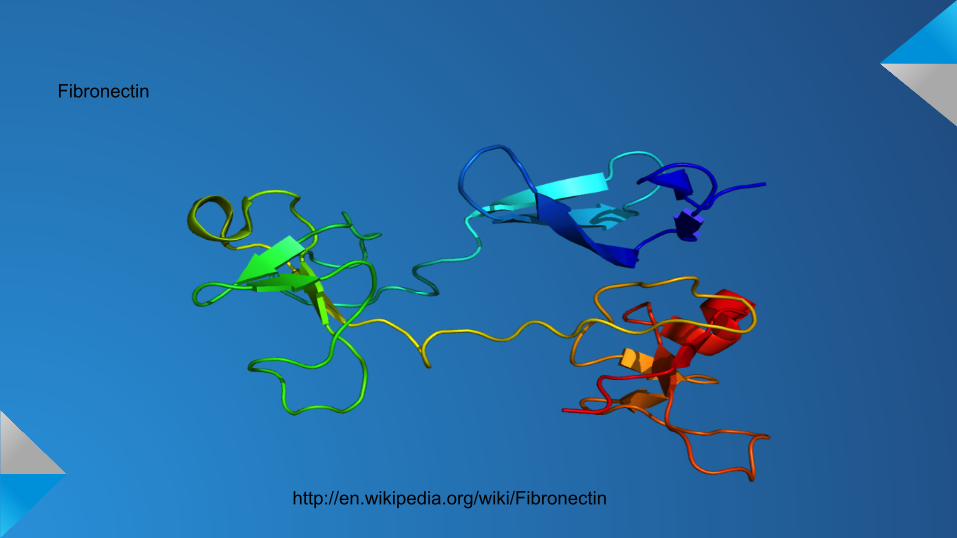
Fibronectin

http://en.wikipedia.org/wiki/Fibronectin

Fibronectin ●  Serves as linker in Extracellular Matrices

o  ...like the one found in the Trabecular Meshwork ●  Studies have found increased glucose concentration

results in a higher rate of fibronectin production (Roy, Sayon and Tsuyoshi Sato, 2002)

●  “These findings indicate that a high glucose level in aqueous humor of patients with diabetes may increase fibronectin synthesis and accumulation in trabecular meshwork and accelerate the depletion of trabecular meshwork cells…”

Objectives ●  Model IOP under different glucose concentrations in

aqueous humor ●  Compare results of commercial and academic software ●  Develop parallel code to solve equations in model

Method & Equations ●  Flow of AH in anterior chamber simulated using

modified Navier-Stokes equations: ●  Flow in Trabecular Meshwork/Schlemm’s canal:

Finite Element Method ●  No guarantee for solution to 3D Navier-Stokes ●  Solve using numerical methods ●  Split geometry up into discrete set of cells

o  creates a mesh ●  Galerkin method

o  converts PDEs to system of linear equations

Parameters Parameter Value

Initial Velocity 1.2 mm/s

Outlet Pressure 1200 Pa

Reference Temperature 22 C

Aqueous Humor Density 1000 kg/m3

Aqueous Humor Viscosity 0.001 kg/(ms)

Aqueous Humor Specific Heat 4182 J/(kgK) [water property]

Aqueous Humor Thermal Conductivity 0.6 W/ (mK)

Glucose Concentration 99.1001 mg/dL (healthy eye); 144.1456 mg/dL (type 2 diabetic eye)

Hardware and Software ●  Hardware:

o  Star1 o  Darter

●  Software: o  Deal.II - FEM software library o  Cubit - mesh generator o  COMSOL Multiphysics Tool

COMSOL

●  multi-physics simulation tool: o  2D

§  gives a basic understanding of fluid flow in eye o  2D - axis-symmetry

§  perform simulation in 2D but create 3D result based on that

o  3D §  slow, but most accurate simulation of fluid flow

Deal.II ●  C++ FEM software library ●  Step-35:

o  Standard Navier-Stokes flow o  Modified to incorporate 2D mesh generated in Cubit

●  3D simulations: o  Simulations are too slow o  Modify to make parallel

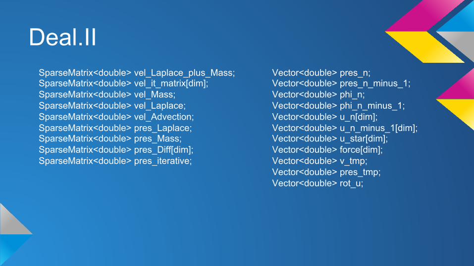
Deal.II SparseMatrix<double> vel_Laplace_plus_Mass; SparseMatrix<double> vel_it_matrix[dim]; SparseMatrix<double> vel_Mass; SparseMatrix<double> vel_Laplace; SparseMatrix<double> vel_Advection; SparseMatrix<double> pres_Laplace; SparseMatrix<double> pres_Mass; SparseMatrix<double> pres_Diff[dim]; SparseMatrix<double> pres_iterative;

Vector<double> pres_n; Vector<double> pres_n_minus_1; Vector<double> phi_n; Vector<double> phi_n_minus_1; Vector<double> u_n[dim]; Vector<double> u_n_minus_1[dim]; Vector<double> u_star[dim]; Vector<double> force[dim]; Vector<double> v_tmp; Vector<double> pres_tmp; Vector<double> rot_u;

Deal.II for (typename Triangulation<dim>::active_cell_iterator cell = triangulation. begin_active(); cell != triangulation.end(); ++cell) { for (unsigned int f=0; f<GeometryInfo<dim>::faces_per_cell; ++f) {

if (cell->face(f)->at_boundary()) { double x=cell->face(f)->center()[0]; double y=cell->face(f)->center()[1]; //double z=cell->face(f)->center()[2]; if (x==4.0)

{ cell->face(f)->set_boundary_indicator (1);

} else if (x==5.0 && ((y>=5.7 && y<=6.245) || (y<=-5.7 && y>=-6.245))) {

cell->face(f)->set_boundary_indicator (2); } }

} }

Mesh Refinement

Velocity - 2D

COMSOL Simulation Deal.II Simulation

Pressure - 2D

COMSOL Simulation Deal.II Simulations

Velocity - 3D (Deal.II)

Velocity - 3D (COMSOL)

Pressure - 3D (Deal.II)

Relative Data (COMSOL)

Relative Data (COMSOL)

Parallel Code ●  Code has been developed to solve 1D Laplace problem

in parallel ●  Makes use of MPI and Trilinos packages ●  Galerkin Method

Example int tmp2=0; for (int i=0;i<NumMyElements;++i) { off=offset[MyGlobalElements[i]]; double aij_tmp[off]; int col_loc_tmp[off]; for (int j=tmp2;j<off+tmp2;++j)

{ aij_tmp[j-tmp2]=aij[j]; col_loc_tmp[j-tmp2]=col_loc[j]; }

A.InsertGlobalValues(MyGlobalElements[i],off,aij_tmp,col_loc_tmp); tmp2=off; }

Output for N=5 with 3 processors Processor Row Index Col Index Value 0 0 0 1 0 0 1 0 0 1 0 -1 0 1 1 2 0 1 2 -1 1 2 2 2 1 2 3 -1 1 2 1 -1 1 3 2 -1 1 3 3 2 1 3 4 -1 2 4 4 1 2 4 3 0

Solution time: 0.000562 (sec.) total iterations: 4 Solved x: Epetra::Vector MyPID GID Value 0 0 0 0 1 25 Solved x: Epetra::Vector 1 2 50 1 3 75 Solved x: Epetra::Vector 2 4 100

Problems ●  Deal.II code documentation makes many assumptions about its users

o  assumes a strong background in mathematics, particularly numerical and finite element methods

o  users not familiar with these concepts may be better suited using a different piece of software

●  COMSOL o  modifying equations is not straightforward

●  These issues drastically slowed down our progress

Conclusions and Future Goals ●  Velocity patterns seem consistent

o  why not pressure? ●  3D simulations need continued refinement

o  Deal.II 3D simulations will need to be run in parallel

●  Begin modifying equations for 2D simulations ●  Begin expanding Laplace 1D code to work for 2D/

3D.

Acknowledgments

●  NSF and CSURE ●  University of Tennessee and ORNL ●  Kwai Wong and Christian Halloy ●  Ben Ramsey and Jacob Pollack

References 1. Canning, C. R. (2002, 12). Fluid flow in the anterior chamber of a human eye. Mathematical Medicine and Biology, 19(1), 31-60. doi: 10.1093/imammb19.1.31 2. Crowder, T.r., and V.j. Ervin. "Numerical Simulations of Fluid Pressure in the Human Eye." Applied Mathematics and Computation 219.24 (2013): 11119-1133. Print. 3. Ferreira, J.a., P. De Oliveira, P.m. Da Silva, and J.n. Murta. "Numerical Simulation of Aqueous Humor Flow: From Healthy to Pathologic Situations." Applied Mathematics and Computation 226 (2014): 777-92. Print. 4. Heys, J. J., Barocas, V. H., & Taravella, M. J. (2001, 12). Modeling Passive Mechanical Interaction Between Aqueous Humor and Iris. Journal of Biomechanical Engineering, 123(6), 540. doi: 10.1115/1.1411972

References 5. Fitt, A. D., and G. Gonzalez. "Fluid Mechanics of the Human Eye: Aqueous Humour Flow in The Anterior Chamber." Bulletin of Mathematical Biology 68.1 (2006): 53-71. Print. 6. Roy, Sayon and Tsuyoshi Sato. "Effect of High Glucose on Fibronectin Expressions and Cell Proliferation in Trabecular Meshwork Cells." Investigative Ophthalmology and Visual Science 43.1 (2002): 170-175. Print. 7. Villamarin, Adan, Sylvain Roy, Reda Hasballa, Orestis Vardoulis, Philippe Reymond, and Nikolaos Stergiopulos. "3D Simulation of the Aqueous Flow in the Human Eye." Medical Engineering & Physics 34.10 (2012): 1462-470. Print.