Introduction to Optimization Lecture 2: Dynamic Programming and Branch&Bound Dimo Brockhoff INRIA Lille – Nord Europe September 25, 2015 TC2 - Optimisation Université Paris-Saclay, Orsay, France Anne Auger INRIA Saclay – Ile-de-France

Welcome message from author
This document is posted to help you gain knowledge. Please leave a comment to let me know what you think about it! Share it to your friends and learn new things together.
Transcript

Introduction to Optimization
Lecture 2: Dynamic Programming and Branch&Bound
Dimo Brockhoff
INRIA Lille – Nord Europe
September 25, 2015
TC2 - Optimisation
Université Paris-Saclay, Orsay, France
Anne Auger
INRIA Saclay – Ile-de-France
2 TC2: Introduction to Optimization, U. Paris-Saclay, Sep. 25, 2015 © Anne Auger and Dimo Brockhoff, INRIA 2
Mastertitelformat bearbeiten
supplementary material to last week’s lecture
3 TC2: Introduction to Optimization, U. Paris-Saclay, Sep. 25, 2015 © Anne Auger and Dimo Brockhoff, INRIA 3
Mastertitelformat bearbeiten
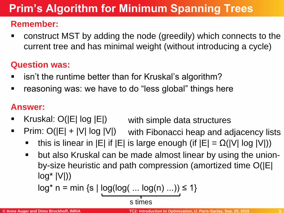
Remember:
construct MST by adding the node (greedily) which connects to the
current tree and has minimal weight (without introducing a cycle)
Question was:
isn’t the runtime better than for Kruskal’s algorithm?
reasoning was: we have to do “less global” things here
Answer:
Kruskal: O(|E| log |E|)
Prim: O(|E| + |V| log |V|)
this is linear in |E| if |E| is large enough (if |E| = Ω(|V| log |V|))
but also Kruskal can be made almost linear by using the union-
by-size heuristic and path compression (amortized time O(|E|
log* |V|))
log* n = min {s | log(log( ... log(n) ...)) ≤ 1}
Prim’s Algorithm for Minimum Spanning Trees
with simple data structures
with Fibonacci heap and adjacency lists
s times

4 TC2: Introduction to Optimization, U. Paris-Saclay, Sep. 25, 2015 © Anne Auger and Dimo Brockhoff, INRIA 4
Mastertitelformat bearbeiten
Announcements
5 TC2: Introduction to Optimization, U. Paris-Saclay, Sep. 25, 2015 © Anne Auger and Dimo Brockhoff, INRIA 5
Mastertitelformat bearbeiten
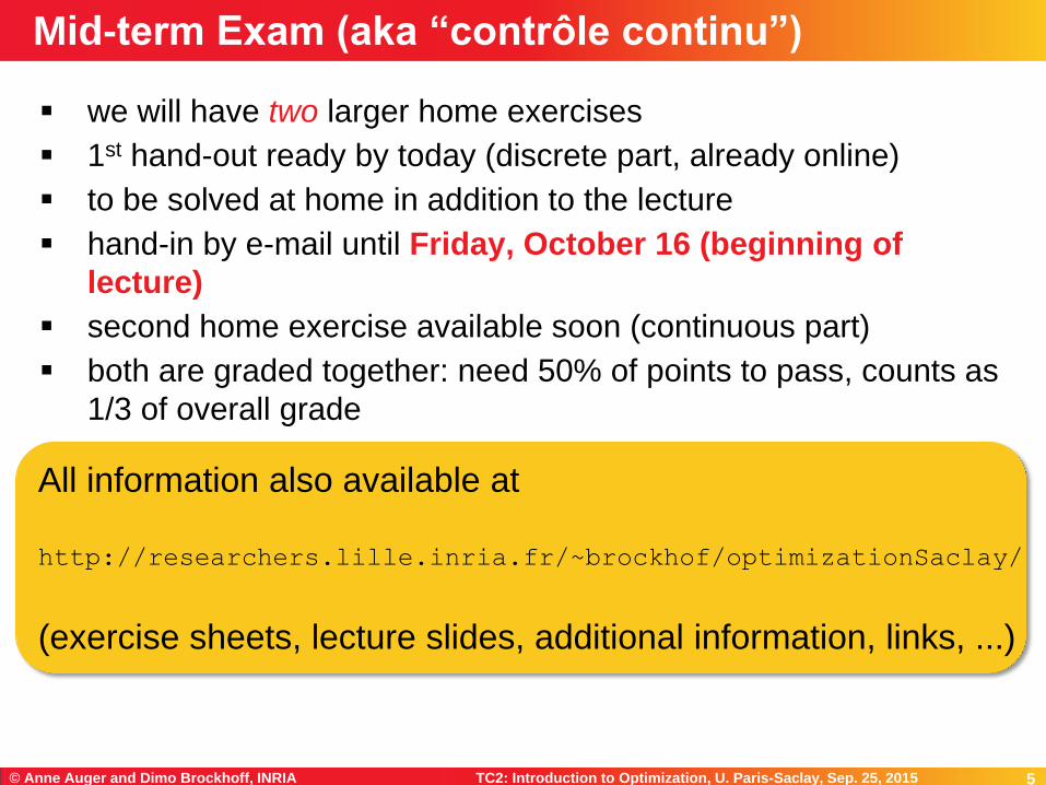
we will have two larger home exercises
1st hand-out ready by today (discrete part, already online)
to be solved at home in addition to the lecture
hand-in by e-mail until Friday, October 16 (beginning of
lecture)
second home exercise available soon (continuous part)
both are graded together: need 50% of points to pass, counts as
1/3 of overall grade
Mid-term Exam (aka “contrôle continu”)
All information also available at
http://researchers.lille.inria.fr/~brockhof/optimizationSaclay/
(exercise sheets, lecture slides, additional information, links, ...)

6 TC2: Introduction to Optimization, U. Paris-Saclay, Sep. 25, 2015 © Anne Auger and Dimo Brockhoff, INRIA 6
Mastertitelformat bearbeiten
Presentation Blackbox Optimization Lecture
7 TC2: Introduction to Optimization, U. Paris-Saclay, Sep. 25, 2015 © Anne Auger and Dimo Brockhoff, INRIA 7
Mastertitelformat bearbeiten
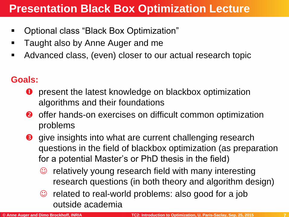
Optional class “Black Box Optimization”
Taught also by Anne Auger and me
Advanced class, (even) closer to our actual research topic
Goals:
present the latest knowledge on blackbox optimization
algorithms and their foundations
offer hands-on exercises on difficult common optimization
problems
give insights into what are current challenging research
questions in the field of blackbox optimization (as preparation
for a potential Master’s or PhD thesis in the field)
relatively young research field with many interesting
research questions (in both theory and algorithm design)
related to real-world problems: also good for a job
outside academia
Presentation Black Box Optimization Lecture

8 TC2: Introduction to Optimization, U. Paris-Saclay, Sep. 25, 2015 © Anne Auger and Dimo Brockhoff, INRIA 8
Mastertitelformat bearbeiten
Why are we interested in a black box scenario?
objective function F often noisy, non-differentiable, or
sometimes not even understood or available
objective function F contains lecagy or binary code, is based
on numerical simulations or real-life experiments
most likely, you will see such problems in practice...
Objective: find x with small F(x) with as few function evaluations as
possible
assumption: internal calculations of algo irrelevant
Black Box Scenario
black box

9 TC2: Introduction to Optimization, U. Paris-Saclay, Sep. 25, 2015 © Anne Auger and Dimo Brockhoff, INRIA 9
Mastertitelformat bearbeiten
Search space too large
exhaustive search impossible
Non conventional objective function or search space
mixed space, function that cannot be computed
Complex objective function
non-smooth, non differentiable, noisy, ...
What Makes an Optimization Problem Difficult?
stochastic search algorithms
well suited because they:
• don’t make many assumptions on f
• are invariant wrt. translation/rotation
of the search space, scaling of f, ...
• are robust to noise
10 TC2: Introduction to Optimization, U. Paris-Saclay, Sep. 25, 2015 © Anne Auger and Dimo Brockhoff, INRIA 10
Mastertitelformat bearbeiten
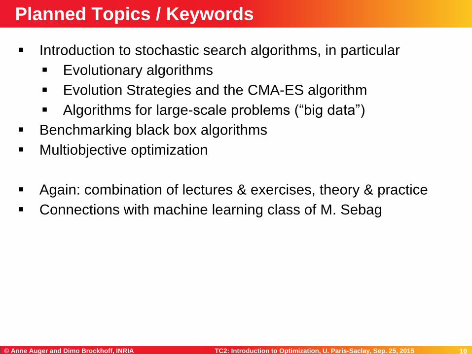
Introduction to stochastic search algorithms, in particular
Evolutionary algorithms
Evolution Strategies and the CMA-ES algorithm
Algorithms for large-scale problems (“big data”)
Benchmarking black box algorithms
Multiobjective optimization
Again: combination of lectures & exercises, theory & practice
Connections with machine learning class of M. Sebag
Planned Topics / Keywords

11 TC2: Introduction to Optimization, U. Paris-Saclay, Sep. 25, 2015 © Anne Auger and Dimo Brockhoff, INRIA 11
Mastertitelformat bearbeiten
Date Topic
Fri, 18.9.2015 DB Introduction and Greedy Algorithms
Fri, 25.9.2015 DB Dynamic programming and Branch and Bound
Fri, 2.10.2015 DB Approximation Algorithms and Heuristics
Fri, 9.10.2015 AA Introduction to Continuous Optimization
Fri, 16.10.2015 AA End of Intro to Cont. Opt. + Gradient-Based Algorithms I
Fri, 30.10.2015 AA Gradient-Based Algorithms II
Fri, 6.11.2015 AA Stochastic Algorithms and Derivative-free Optimization
16 - 20.11.2015 Exam (exact date to be confirmed)
Course Overview
all classes + exam are from 14h till 17h15 (incl. a 15min break)
here in PUIO-D101/D103

12 TC2: Introduction to Optimization, U. Paris-Saclay, Sep. 25, 2015 © Anne Auger and Dimo Brockhoff, INRIA 12
Mastertitelformat bearbeiten
Dynamic Programming
shortest path problem
Dijkstra's algorithm
Floyd’s algorithm
exercise: a dynamic programming algorithm for the
knapsack problem (KP)
Branch and Bound
applied to Integer Linear Programs
Overview of Today’s Lecture
13 TC2: Introduction to Optimization, U. Paris-Saclay, Sep. 25, 2015 © Anne Auger and Dimo Brockhoff, INRIA 13
Mastertitelformat bearbeiten
Dynamic Programming
14 TC2: Introduction to Optimization, U. Paris-Saclay, Sep. 25, 2015 © Anne Auger and Dimo Brockhoff, INRIA 14
Mastertitelformat bearbeiten
Wikipedia:
“[...] dynamic programming is a method for solving a complex
problem by breaking it down into a collection of simpler
subproblems.”
But that’s not all:
dynamic programming also makes sure that the subproblems
are not solved too often but only once by keeping the solutions
of simpler subproblems in memory (“trading space vs. time”)
it is an exact method, i.e. in comparison to the greedy approach,
it always solves a problem to optimality
Dynamic Programming

15 TC2: Introduction to Optimization, U. Paris-Saclay, Sep. 25, 2015 © Anne Auger and Dimo Brockhoff, INRIA 15
Mastertitelformat bearbeiten
Optimal Substructure
A solution can be constructed efficiently from optimal solutions
of sub-problems
Overlapping Subproblems
Wikipedia: “[...] a problem is said to have overlapping
subproblems if the problem can be broken down into
subproblems which are reused several times or a recursive
algorithm for the problem solves the same subproblem over and
over rather than always generating new subproblems.”
Note: in case of optimal substructure but independent subproblems,
often greedy algorithms are a good choice; in this case, dynamic
programming is often called “divide and conquer” instead
Two Properties Needed
16 TC2: Introduction to Optimization, U. Paris-Saclay, Sep. 25, 2015 © Anne Auger and Dimo Brockhoff, INRIA 16
Mastertitelformat bearbeiten
Main idea: solve larger subproblems by breaking them down to
smaller, easier subproblems in a recursive manner
Typical Algorithm Design:
decompose the problem into subproblems and think about how
to solve a larger problem with the solutions of its subproblems
specify how you compute the value of a larger problem
recursively with the help of the optimal values of its subproblems
(“Bellman equation”)
bottom-up solving of the subproblems (i.e. computing their
optimal value), starting from the smallest by using a table
structure to store the optimal values and the Bellman equality
(top-down approach also possible, but less common)
eventually construct the final solution (can be omitted if only the
value of an optimal solution is sought)
Main Idea Behind Dynamic Programming
17 TC2: Introduction to Optimization, U. Paris-Saclay, Sep. 25, 2015 © Anne Auger and Dimo Brockhoff, INRIA 17
Mastertitelformat bearbeiten
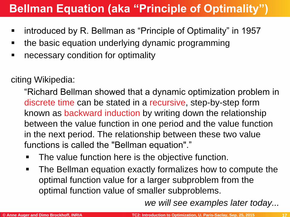
introduced by R. Bellman as “Principle of Optimality” in 1957
the basic equation underlying dynamic programming
necessary condition for optimality
citing Wikipedia:
“Richard Bellman showed that a dynamic optimization problem in
discrete time can be stated in a recursive, step-by-step form
known as backward induction by writing down the relationship
between the value function in one period and the value function
in the next period. The relationship between these two value
functions is called the "Bellman equation".”
The value function here is the objective function.
The Bellman equation exactly formalizes how to compute the
optimal function value for a larger subproblem from the
optimal function value of smaller subproblems.
we will see examples later today...
Bellman Equation (aka “Principle of Optimality”)
18 TC2: Introduction to Optimization, U. Paris-Saclay, Sep. 25, 2015 © Anne Auger and Dimo Brockhoff, INRIA 18
Mastertitelformat bearbeiten
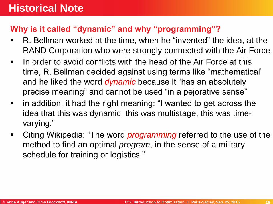
Why is it called “dynamic” and why “programming”?
R. Bellman worked at the time, when he “invented” the idea, at the
RAND Corporation who were strongly connected with the Air Force
In order to avoid conflicts with the head of the Air Force at this
time, R. Bellman decided against using terms like “mathematical”
and he liked the word dynamic because it “has an absolutely
precise meaning” and cannot be used “in a pejorative sense”
in addition, it had the right meaning: “I wanted to get across the
idea that this was dynamic, this was multistage, this was time-
varying.”
Citing Wikipedia: “The word programming referred to the use of the
method to find an optimal program, in the sense of a military
schedule for training or logistics.”
Historical Note
19 TC2: Introduction to Optimization, U. Paris-Saclay, Sep. 25, 2015 © Anne Auger and Dimo Brockhoff, INRIA 19
Mastertitelformat bearbeiten
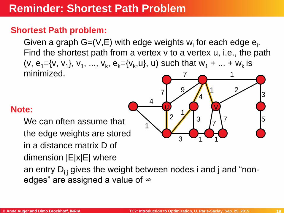
Shortest Path problem:
Given a graph G=(V,E) with edge weights wi for each edge ei.
Find the shortest path from a vertex v to a vertex u, i.e., the path
(v, e1={v, v1}, v1, ..., vk, ek={vk,u}, u) such that w1 + ... + wk is
minimized.
Note:
We can often assume that
the edge weights are stored
in a distance matrix D of
dimension |E|x|E| where
an entry Di,j gives the weight between nodes i and j and “non-
edges” are assigned a value of ∞
Reminder: Shortest Path Problem
u v
7
7
4
1
2
9 4
1
1
2
3 1
7 7
3
5
3 1 1

20 TC2: Introduction to Optimization, U. Paris-Saclay, Sep. 25, 2015 © Anne Auger and Dimo Brockhoff, INRIA 20
Mastertitelformat bearbeiten
Optimal Substructure
The optimal path from u to v, if it contains another vertex p can
be constructed by simply joining the optimal path from u to p with
the optimal path from p to v.
Overlapping Subproblems
Optimal shortest
sub-paths can be reused
when computing longer paths:
e.g. the optimal path from u to p
is contained in the optimal path from
u to q and in the optimal path from u to v.
Opt. Substructure and Overlapping Subproblems
u v q
7
7
4
1
2
9 4
1
1
2
3 1
7 7
3
5
3 1 1 p
21 TC2: Introduction to Optimization, U. Paris-Saclay, Sep. 25, 2015 © Anne Auger and Dimo Brockhoff, INRIA 21
Mastertitelformat bearbeiten
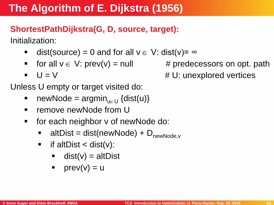
ShortestPathDijkstra(G, D, source, target):
Initialization:
dist(source) = 0 and for all v V: dist(v)= ∞
for all v V: prev(v) = null # predecessors on opt. path
U = V # U: unexplored vertices
Unless U empty or target visited do:
newNode = argminuU {dist(u)}
remove newNode from U
for each neighbor v of newNode do:
altDist = dist(newNode) + DnewNode,v
if altDist < dist(v):
dist(v) = altDist
prev(v) = u
The Algorithm of E. Dijkstra (1956)
22 TC2: Introduction to Optimization, U. Paris-Saclay, Sep. 25, 2015 © Anne Auger and Dimo Brockhoff, INRIA 22
Mastertitelformat bearbeiten
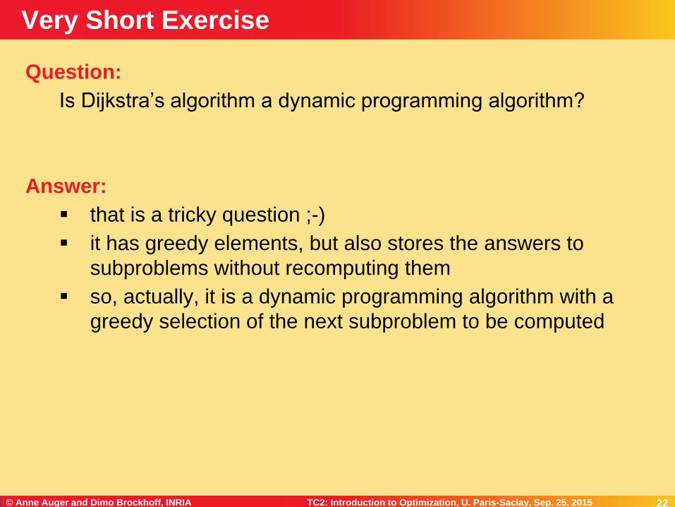
Question:
Is Dijkstra’s algorithm a dynamic programming algorithm?
Answer:
that is a tricky question ;-)
it has greedy elements, but also stores the answers to
subproblems without recomputing them
so, actually, it is a dynamic programming algorithm with a
greedy selection of the next subproblem to be computed
Very Short Exercise
23 TC2: Introduction to Optimization, U. Paris-Saclay, Sep. 25, 2015 © Anne Auger and Dimo Brockhoff, INRIA 23
Mastertitelformat bearbeiten
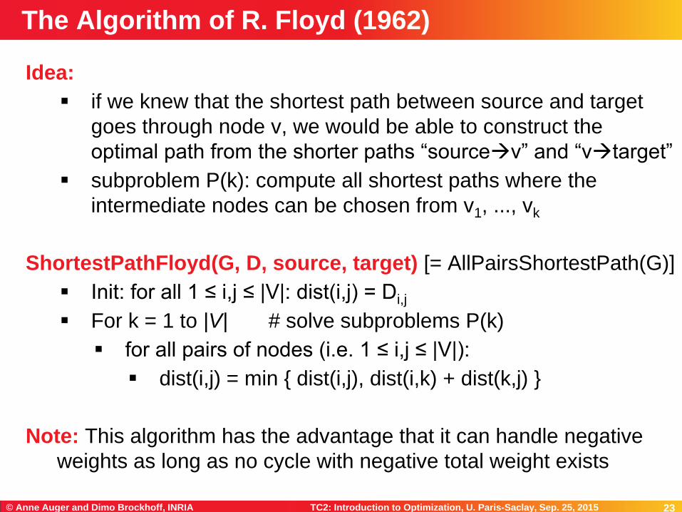
Idea:
if we knew that the shortest path between source and target
goes through node v, we would be able to construct the
optimal path from the shorter paths “sourcev” and “vtarget”
subproblem P(k): compute all shortest paths where the
intermediate nodes can be chosen from v1, ..., vk
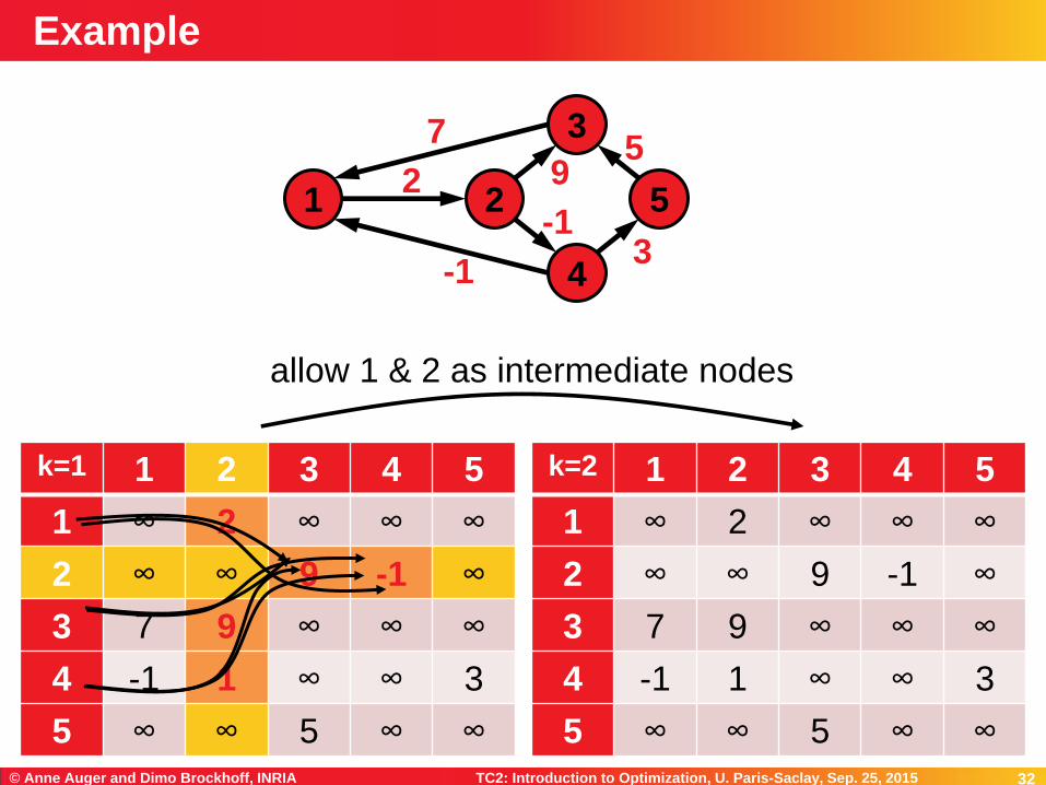
ShortestPathFloyd(G, D, source, target) [= AllPairsShortestPath(G)]
Init: for all 1 ≤ i,j ≤ |V|: dist(i,j) = Di,j
For k = 1 to |V| # solve subproblems P(k)
for all pairs of nodes (i.e. 1 ≤ i,j ≤ |V|):
dist(i,j) = min { dist(i,j), dist(i,k) + dist(k,j) }
Note: This algorithm has the advantage that it can handle negative
weights as long as no cycle with negative total weight exists
The Algorithm of R. Floyd (1962)

24 TC2: Introduction to Optimization, U. Paris-Saclay, Sep. 25, 2015 © Anne Auger and Dimo Brockhoff, INRIA 24
Mastertitelformat bearbeiten Example
k=0 1 2 3 4 5
1
2
3
4
5
1
3
5
4
2
7
2
-1
-1 3
5 9

25 TC2: Introduction to Optimization, U. Paris-Saclay, Sep. 25, 2015 © Anne Auger and Dimo Brockhoff, INRIA 25
Mastertitelformat bearbeiten Example
k=0 1 2 3 4 5
1 ∞ 2 ∞ ∞ ∞
2 ∞ ∞ 9 -1 ∞
3 7 ∞ ∞ ∞ ∞
4 -1 ∞ ∞ ∞ 3
5 ∞ ∞ 5 ∞ ∞
1
3
5
4
2
7
2
-1
-1 3
5 9

26 TC2: Introduction to Optimization, U. Paris-Saclay, Sep. 25, 2015 © Anne Auger and Dimo Brockhoff, INRIA 26
Mastertitelformat bearbeiten Example
k=0 1 2 3 4 5
1 ∞ 2 ∞ ∞ ∞
2 ∞ ∞ 9 -1 ∞
3 7 ∞ ∞ ∞ ∞
4 -1 ∞ ∞ ∞ 3
5 ∞ ∞ 5 ∞ ∞
1
3
5
4
2
7
2
-1
-1 3
5 9
k=1 1 2 3 4 5
1
2
3
4
5
allow 1 as intermediate node

27 TC2: Introduction to Optimization, U. Paris-Saclay, Sep. 25, 2015 © Anne Auger and Dimo Brockhoff, INRIA 27
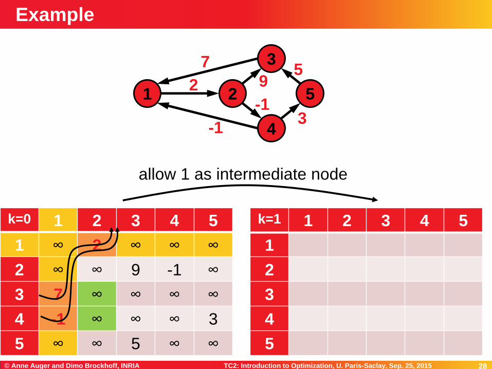
Mastertitelformat bearbeiten Example
k=0 1 2 3 4 5
1 ∞ 2 ∞ ∞ ∞
2 ∞ ∞ 9 -1 ∞
3 7 ∞ ∞ ∞ ∞
4 -1 ∞ ∞ ∞ 3
5 ∞ ∞ 5 ∞ ∞
1
3
5
4
2
7
2
-1
-1 3
5 9
k=1 1 2 3 4 5
1
2
3
4
5
allow 1 as intermediate node
28 TC2: Introduction to Optimization, U. Paris-Saclay, Sep. 25, 2015 © Anne Auger and Dimo Brockhoff, INRIA 28
Mastertitelformat bearbeiten Example
k=0 1 2 3 4 5
1 ∞ 2 ∞ ∞ ∞
2 ∞ ∞ 9 -1 ∞
3 7 ∞ ∞ ∞ ∞
4 -1 ∞ ∞ ∞ 3
5 ∞ ∞ 5 ∞ ∞
1
3
5
4
2
7
2
-1
-1 3
5 9
k=1 1 2 3 4 5
1
2
3
4
5
allow 1 as intermediate node

29 TC2: Introduction to Optimization, U. Paris-Saclay, Sep. 25, 2015 © Anne Auger and Dimo Brockhoff, INRIA 29
Mastertitelformat bearbeiten Example
k=0 1 2 3 4 5
1 ∞ 2 ∞ ∞ ∞
2 ∞ ∞ 9 -1 ∞
3 7 ∞ ∞ ∞ ∞
4 -1 ∞ ∞ ∞ 3
5 ∞ ∞ 5 ∞ ∞
1
3
5
4
2
7
2
-1
-1 3
5 9
k=1 1 2 3 4 5
1
2
3 9
4 1
5
allow 1 as intermediate node
30 TC2: Introduction to Optimization, U. Paris-Saclay, Sep. 25, 2015 © Anne Auger and Dimo Brockhoff, INRIA 30
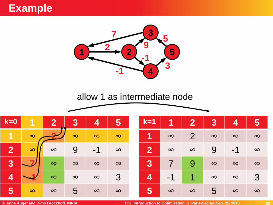
Mastertitelformat bearbeiten Example
k=0 1 2 3 4 5
1 ∞ 2 ∞ ∞ ∞
2 ∞ ∞ 9 -1 ∞
3 7 ∞ ∞ ∞ ∞
4 -1 ∞ ∞ ∞ 3
5 ∞ ∞ 5 ∞ ∞
1
3
5
4
2
7
2
-1
-1 3
5 9
k=1 1 2 3 4 5
1 ∞ 2 ∞ ∞ ∞
2 ∞ ∞ 9 -1 ∞
3 7 9 ∞ ∞ ∞
4 -1 1 ∞ ∞ 3
5 ∞ ∞ 5 ∞ ∞
allow 1 as intermediate node

31 TC2: Introduction to Optimization, U. Paris-Saclay, Sep. 25, 2015 © Anne Auger and Dimo Brockhoff, INRIA 31
Mastertitelformat bearbeiten Example
1
3
5
4
2
7
2
-1
-1 3
5 9
allow 1 & 2 as intermediate nodes
k=2 1 2 3 4 5
1 ∞ 2 ∞ ∞ ∞
2 ∞ ∞ 9 -1 ∞
3 7 9 ∞ ∞ ∞
4 -1 1 ∞ ∞ 3
5 ∞ ∞ 5 ∞ ∞
k=1 1 2 3 4 5
1 ∞ 2 ∞ ∞ ∞
2 ∞ ∞ 9 -1 ∞
3 7 9 ∞ ∞ ∞
4 -1 1 ∞ ∞ 3
5 ∞ ∞ 5 ∞ ∞
32 TC2: Introduction to Optimization, U. Paris-Saclay, Sep. 25, 2015 © Anne Auger and Dimo Brockhoff, INRIA 32
Mastertitelformat bearbeiten Example
1
3
5
4
2
7
2
-1
-1 3
5 9
allow 1 & 2 as intermediate nodes
k=2 1 2 3 4 5
1 ∞ 2 ∞ ∞ ∞
2 ∞ ∞ 9 -1 ∞
3 7 9 ∞ ∞ ∞
4 -1 1 ∞ ∞ 3
5 ∞ ∞ 5 ∞ ∞
k=1 1 2 3 4 5
1 ∞ 2 ∞ ∞ ∞
2 ∞ ∞ 9 -1 ∞
3 7 9 ∞ ∞ ∞
4 -1 1 ∞ ∞ 3
5 ∞ ∞ 5 ∞ ∞
33 TC2: Introduction to Optimization, U. Paris-Saclay, Sep. 25, 2015 © Anne Auger and Dimo Brockhoff, INRIA 33
Mastertitelformat bearbeiten Example
1
3
5
4
2
7
2
-1
-1 3
5 9
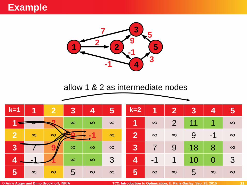
allow 1 & 2 as intermediate nodes
k=2 1 2 3 4 5
1 ∞ 2 11 1 ∞
2 ∞ ∞ 9 -1 ∞
3 7 9 18 8 ∞
4 -1 1 10 0 3
5 ∞ ∞ 5 ∞ ∞
k=1 1 2 3 4 5
1 ∞ 2 ∞ ∞ ∞
2 ∞ ∞ 9 -1 ∞
3 7 9 ∞ ∞ ∞
4 -1 1 ∞ ∞ 3
5 ∞ ∞ 5 ∞ ∞

34 TC2: Introduction to Optimization, U. Paris-Saclay, Sep. 25, 2015 © Anne Auger and Dimo Brockhoff, INRIA 34
Mastertitelformat bearbeiten Example
1
3
5
4
2
7
2
-1
-1 3
5 9
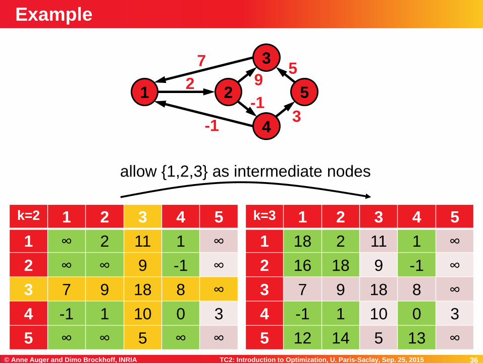
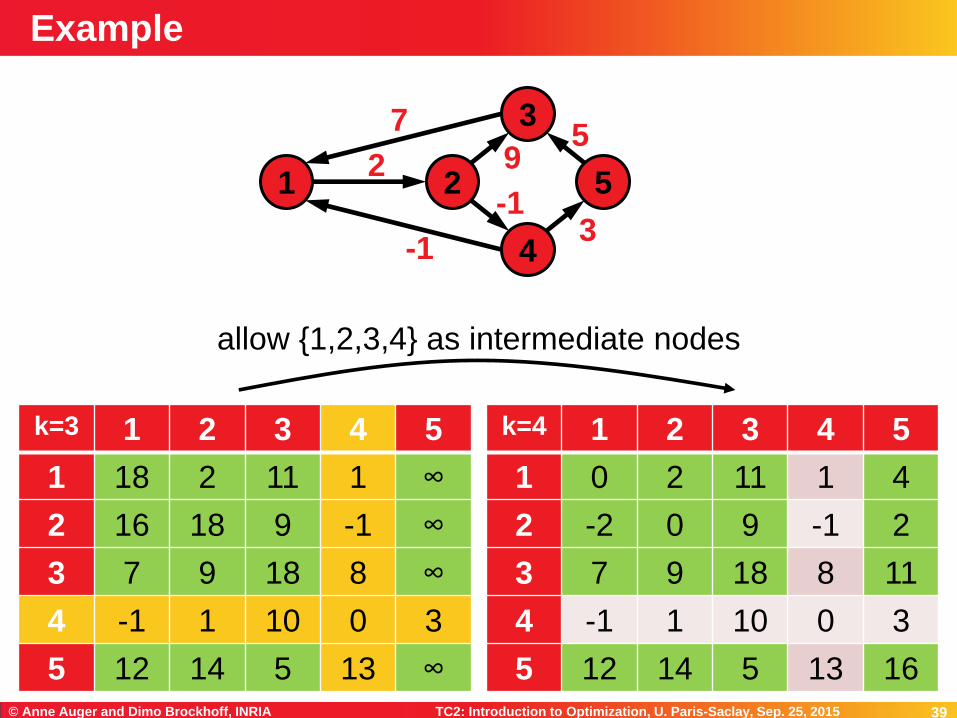
allow {1,2,3} as intermediate nodes
k=3 1 2 3 4 5
1 ∞ 2 11 1 ∞
2 ∞ ∞ 9 -1 ∞
3 7 9 18 8 ∞
4 -1 1 10 0 3
5 ∞ ∞ 5 ∞ ∞
k=2 1 2 3 4 5
1 ∞ 2 11 1 ∞
2 ∞ ∞ 9 -1 ∞
3 7 9 18 8 ∞
4 -1 1 10 0 3
5 ∞ ∞ 5 ∞ ∞

35 TC2: Introduction to Optimization, U. Paris-Saclay, Sep. 25, 2015 © Anne Auger and Dimo Brockhoff, INRIA 35
Mastertitelformat bearbeiten Example
1
3
5
4
2
7
2
-1
-1 3
5 9
allow {1,2,3} as intermediate nodes
k=3 1 2 3 4 5
1 11 ∞
2 9 ∞
3 7 9 18 8 ∞
4 10 3
5 5 ∞
k=2 1 2 3 4 5
1 ∞ 2 11 1 ∞
2 ∞ ∞ 9 -1 ∞
3 7 9 18 8 ∞
4 -1 1 10 0 3
5 ∞ ∞ 5 ∞ ∞
36 TC2: Introduction to Optimization, U. Paris-Saclay, Sep. 25, 2015 © Anne Auger and Dimo Brockhoff, INRIA 36
Mastertitelformat bearbeiten Example
1
3
5
4
2
7
2
-1
-1 3
5 9
allow {1,2,3} as intermediate nodes
k=3 1 2 3 4 5
1 18 2 11 1 ∞
2 16 18 9 -1 ∞
3 7 9 18 8 ∞
4 -1 1 10 0 3
5 12 14 5 13 ∞
k=2 1 2 3 4 5
1 ∞ 2 11 1 ∞
2 ∞ ∞ 9 -1 ∞
3 7 9 18 8 ∞
4 -1 1 10 0 3
5 ∞ ∞ 5 ∞ ∞
37 TC2: Introduction to Optimization, U. Paris-Saclay, Sep. 25, 2015 © Anne Auger and Dimo Brockhoff, INRIA 37
Mastertitelformat bearbeiten Example
1
3
5
4
2
7
2
-1
-1 3
5 9
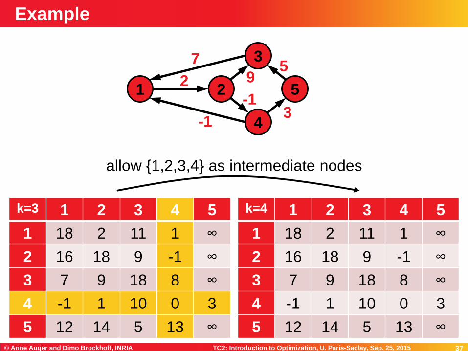
k=4 1 2 3 4 5
1 18 2 11 1 ∞
2 16 18 9 -1 ∞
3 7 9 18 8 ∞
4 -1 1 10 0 3
5 12 14 5 13 ∞
k=3 1 2 3 4 5
1 18 2 11 1 ∞
2 16 18 9 -1 ∞
3 7 9 18 8 ∞
4 -1 1 10 0 3
5 12 14 5 13 ∞
allow {1,2,3,4} as intermediate nodes

38 TC2: Introduction to Optimization, U. Paris-Saclay, Sep. 25, 2015 © Anne Auger and Dimo Brockhoff, INRIA 38
Mastertitelformat bearbeiten Example
1
3
5
4
2
7
2
-1
-1 3
5 9
k=4 1 2 3 4 5
1 1
2 -1
3 8
4 -1 1 10 0 3
5 13
k=3 1 2 3 4 5
1 18 2 11 1 ∞
2 16 18 9 -1 ∞
3 7 9 18 8 ∞
4 -1 1 10 0 3
5 12 14 5 13 ∞
allow {1,2,3,4} as intermediate nodes
39 TC2: Introduction to Optimization, U. Paris-Saclay, Sep. 25, 2015 © Anne Auger and Dimo Brockhoff, INRIA 39
Mastertitelformat bearbeiten Example
1
3
5
4
2
7
2
-1
-1 3
5 9
k=4 1 2 3 4 5
1 0 2 11 1 4
2 -2 0 9 -1 2
3 7 9 18 8 11
4 -1 1 10 0 3
5 12 14 5 13 16
k=3 1 2 3 4 5
1 18 2 11 1 ∞
2 16 18 9 -1 ∞
3 7 9 18 8 ∞
4 -1 1 10 0 3
5 12 14 5 13 ∞
allow {1,2,3,4} as intermediate nodes
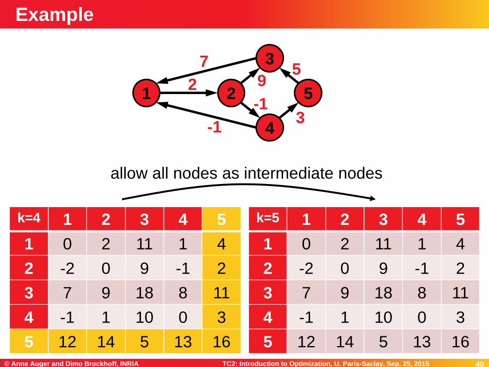
40 TC2: Introduction to Optimization, U. Paris-Saclay, Sep. 25, 2015 © Anne Auger and Dimo Brockhoff, INRIA 40
Mastertitelformat bearbeiten Example
1
3
5
4
2
7
2
-1
-1 3
5 9
allow all nodes as intermediate nodes
k=5 1 2 3 4 5
1 0 2 11 1 4
2 -2 0 9 -1 2
3 7 9 18 8 11
4 -1 1 10 0 3
5 12 14 5 13 16
k=4 1 2 3 4 5
1 0 2 11 1 4
2 -2 0 9 -1 2
3 7 9 18 8 11
4 -1 1 10 0 3
5 12 14 5 13 16

41 TC2: Introduction to Optimization, U. Paris-Saclay, Sep. 25, 2015 © Anne Auger and Dimo Brockhoff, INRIA 41
Mastertitelformat bearbeiten Example
1
3
5
4
2
7
2
-1
-1 3
5 9
allow all nodes as intermediate nodes
k=5 1 2 3 4 5
1 0 2 9 1 4
2 -2 0 7 -1 2
3 7 9 16 8 11
4 -1 1 8 0 3
5 12 14 5 13 16
k=4 1 2 3 4 5
1 0 2 11 1 4
2 -2 0 9 -1 2
3 7 9 18 8 11
4 -1 1 10 0 3
5 12 14 5 13 16
42 TC2: Introduction to Optimization, U. Paris-Saclay, Sep. 25, 2015 © Anne Auger and Dimo Brockhoff, INRIA 42
Mastertitelformat bearbeiten
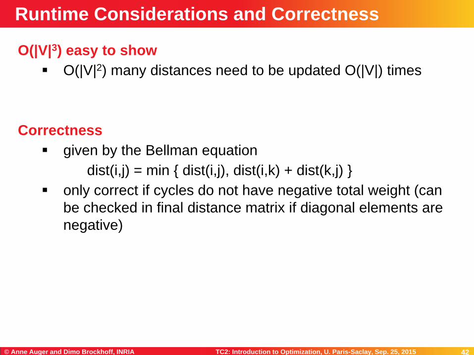
O(|V|3) easy to show
O(|V|2) many distances need to be updated O(|V|) times
Correctness
given by the Bellman equation
dist(i,j) = min { dist(i,j), dist(i,k) + dist(k,j) }
only correct if cycles do not have negative total weight (can
be checked in final distance matrix if diagonal elements are
negative)
Runtime Considerations and Correctness

43 TC2: Introduction to Optimization, U. Paris-Saclay, Sep. 25, 2015 © Anne Auger and Dimo Brockhoff, INRIA 43
Mastertitelformat bearbeiten
Construct matrix of predecessors P alongside distance matrix
Pi,j = predecessor of node j on path from i to j
no extra costs (asymptotically)
But How Can We Actually Construct the Paths?
44 TC2: Introduction to Optimization, U. Paris-Saclay, Sep. 25, 2015 © Anne Auger and Dimo Brockhoff, INRIA 44
Mastertitelformat bearbeiten
Exercise:
The Knapsack Problem and Dynamic Programming
http://researchers.lille.inria.fr/
~brockhof/optimizationSaclay/

46 TC2: Introduction to Optimization, U. Paris-Saclay, Sep. 25, 2015 © Anne Auger and Dimo Brockhoff, INRIA 46
Mastertitelformat bearbeiten
Branch and Bound
47 TC2: Introduction to Optimization, U. Paris-Saclay, Sep. 25, 2015 © Anne Auger and Dimo Brockhoff, INRIA 47
Mastertitelformat bearbeiten
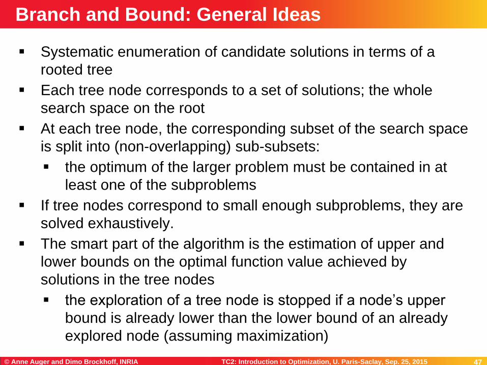
Systematic enumeration of candidate solutions in terms of a
rooted tree
Each tree node corresponds to a set of solutions; the whole
search space on the root
At each tree node, the corresponding subset of the search space
is split into (non-overlapping) sub-subsets:
the optimum of the larger problem must be contained in at
least one of the subproblems
If tree nodes correspond to small enough subproblems, they are
solved exhaustively.
The smart part of the algorithm is the estimation of upper and
lower bounds on the optimal function value achieved by
solutions in the tree nodes
the exploration of a tree node is stopped if a node’s upper
bound is already lower than the lower bound of an already
explored node (assuming maximization)
Branch and Bound: General Ideas
48 TC2: Introduction to Optimization, U. Paris-Saclay, Sep. 25, 2015 © Anne Auger and Dimo Brockhoff, INRIA 48
Mastertitelformat bearbeiten
Needed for successful application of branch and bound:
optimization problem
finite set of solutions
clear idea of how to split problem into smaller subproblems
efficient calculation of the following modules:
upper bound calculation
lower bound calculation
Applying Branch and Bound
49 TC2: Introduction to Optimization, U. Paris-Saclay, Sep. 25, 2015 © Anne Auger and Dimo Brockhoff, INRIA 49
Mastertitelformat bearbeiten
Assume w.l.o.g. maximization of f(x) here
Lower Bounds
any actual feasible solution will give a lower bound (which will be
exact if the solution is the optimal one for the subproblem)
hence, sampling a (feasible) solution can be one strategy
using a heuristic to solve the subproblem another one
Upper Bounds
upper bounds can be achieved by solving a relaxed version of
the problem formulations (i.e. by either loosening or removing
constraints)
Note: the better/tighter the bounds, the quicker the branch and
bound tree can be pruned
Computing Bounds (Maximization Problems)

50 TC2: Introduction to Optimization, U. Paris-Saclay, Sep. 25, 2015 © Anne Auger and Dimo Brockhoff, INRIA 50
Mastertitelformat bearbeiten
Exact, global solver
Can be slow; only exponential worst-case runtime
due to the exhaustive search behavior if no pruning of the
search tree is possible
but might work well in some cases
Advantages:
can be stopped if lower and upper bound are “close enough” in
practice (not necessarily exact anymore then)
can be combined with other techniques, e.g. “branch and cut”
(not covered here)
Properties of Branch and Bound Algorithms
51 TC2: Introduction to Optimization, U. Paris-Saclay, Sep. 25, 2015 © Anne Auger and Dimo Brockhoff, INRIA 51
Mastertitelformat bearbeiten
0-1 problems:
choose unfixed variable xi
one subproblem defined by setting xi to 0
one subproblem defined by setting xi to 1
General integer problem:
choose unfixed variable xi
choose a value c that xi can take
one subproblem defined by restricting xi ≤ c
one subproblem defined by restricting xi > c
Combinatorial Problems:
branching on certain discrete choices, e.g. an edge/vertex is
chosen or not chosen
The branching decisions are then induced as additional constraints
when defining the subproblems.
Example Branching Decisions

52 TC2: Introduction to Optimization, U. Paris-Saclay, Sep. 25, 2015 © Anne Auger and Dimo Brockhoff, INRIA 52
Mastertitelformat bearbeiten
Several strategies (again assuming maximization):
choose the subproblem with highest upper bound
gain the most in reducing overall upper bound
if upper bound not the optimal value, this problem needs to
be branched upon anyway sooner or later
choose the subproblem with lowest lower bound
simple DFS or BFS
problem-specific approach most likely to be a good choice
Which Tree Node to Branch on?
53 TC2: Introduction to Optimization, U. Paris-Saclay, Sep. 25, 2015 © Anne Auger and Dimo Brockhoff, INRIA 53
Mastertitelformat bearbeiten
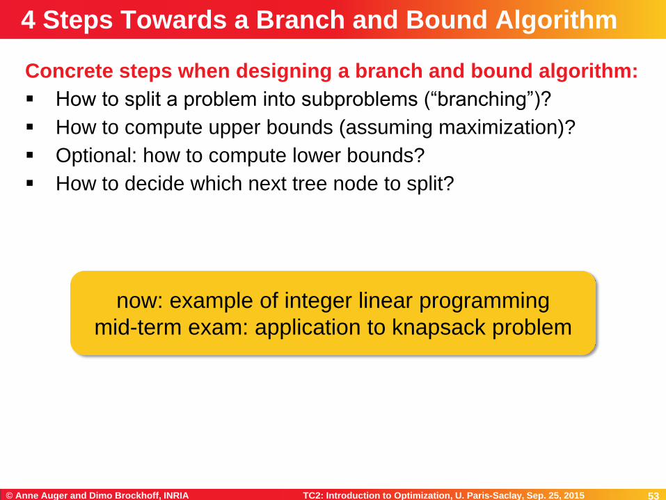
Concrete steps when designing a branch and bound algorithm:
How to split a problem into subproblems (“branching”)?
How to compute upper bounds (assuming maximization)?
Optional: how to compute lower bounds?
How to decide which next tree node to split?
4 Steps Towards a Branch and Bound Algorithm
now: example of integer linear programming
mid-term exam: application to knapsack problem
54 TC2: Introduction to Optimization, U. Paris-Saclay, Sep. 25, 2015 © Anne Auger and Dimo Brockhoff, INRIA 54
Mastertitelformat bearbeiten
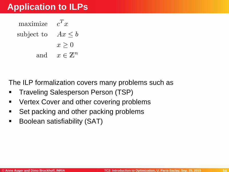
The ILP formalization covers many problems such as
Traveling Salesperson Person (TSP)
Vertex Cover and other covering problems
Set packing and other packing problems
Boolean satisfiability (SAT)
Application to ILPs

55 TC2: Introduction to Optimization, U. Paris-Saclay, Sep. 25, 2015 © Anne Auger and Dimo Brockhoff, INRIA 55
Mastertitelformat bearbeiten
Do not restrict the solutions to integers and round the solution
found of the relaxed problem (=remove the integer constraints)
by a continuous solver (i.e. solving the so-called LP relaxation)
no guarantee to be exact
Exploiting the instance property of A being total unimodular:
feasible solutions are guaranteed to be integer in this case
algorithms for continuous relaxation can be used (e.g. the
simplex algorithm)
Using heuristic methods (typically without any quality guarantee)
we’ll see these type of algorithms in next week’s lecture
Using exact algorithms such as branch and bound
Ways of Solving an ILP

56 TC2: Introduction to Optimization, U. Paris-Saclay, Sep. 25, 2015 © Anne Auger and Dimo Brockhoff, INRIA 56
Mastertitelformat bearbeiten
Here, we just give an idea instead of a concrete algorithm...
How to split a problem into subproblems (“branching”)?
How to compute upper bounds (assuming maximization)?
Optional: how to compute lower bounds?
How to decide which next tree node to split?
Branch and Bound for ILPs
57 TC2: Introduction to Optimization, U. Paris-Saclay, Sep. 25, 2015 © Anne Auger and Dimo Brockhoff, INRIA 57
Mastertitelformat bearbeiten
Here, we just give an idea instead of a concrete algorithm...
How to compute upper bounds (assuming maximization)?
How to split a problem into subproblems (“branching”)?
Optional: how to compute lower bounds?
How to decide which next tree node to split?
Branch and Bound for ILPs
58 TC2: Introduction to Optimization, U. Paris-Saclay, Sep. 25, 2015 © Anne Auger and Dimo Brockhoff, INRIA 58
Mastertitelformat bearbeiten
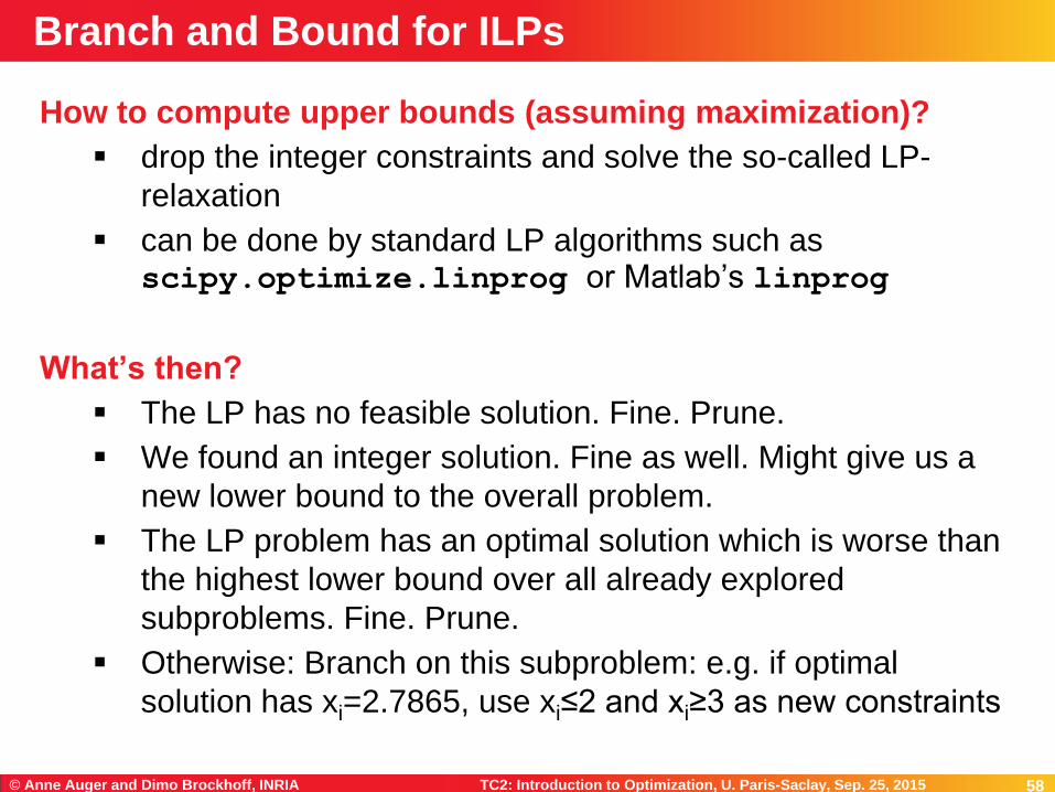
How to compute upper bounds (assuming maximization)?
drop the integer constraints and solve the so-called LP-
relaxation
can be done by standard LP algorithms such as scipy.optimize.linprog or Matlab’s linprog
What’s then?
The LP has no feasible solution. Fine. Prune.
We found an integer solution. Fine as well. Might give us a
new lower bound to the overall problem.
The LP problem has an optimal solution which is worse than
the highest lower bound over all already explored
subproblems. Fine. Prune.
Otherwise: Branch on this subproblem: e.g. if optimal
solution has xi=2.7865, use xi≤2 and xi≥3 as new constraints
Branch and Bound for ILPs
59 TC2: Introduction to Optimization, U. Paris-Saclay, Sep. 25, 2015 © Anne Auger and Dimo Brockhoff, INRIA 59
Mastertitelformat bearbeiten
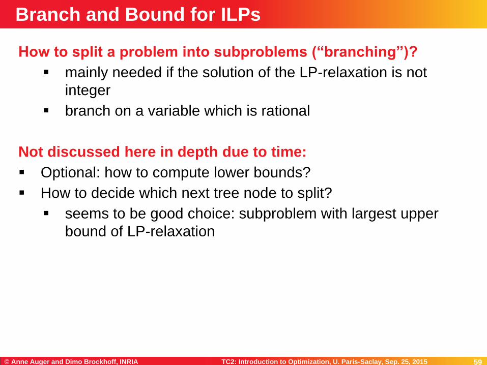
How to split a problem into subproblems (“branching”)?
mainly needed if the solution of the LP-relaxation is not
integer
branch on a variable which is rational
Not discussed here in depth due to time:
Optional: how to compute lower bounds?
How to decide which next tree node to split?
seems to be good choice: subproblem with largest upper
bound of LP-relaxation
Branch and Bound for ILPs
60 TC2: Introduction to Optimization, U. Paris-Saclay, Sep. 25, 2015 © Anne Auger and Dimo Brockhoff, INRIA 60
Mastertitelformat bearbeiten
I hope it became clear...
...what the algorithm design ideas of dynamic programming and
branch and bound are
...for which problem types they are supposed to be suitable
...and how to apply the dynamic programming idea to the
knapsack problem
Conclusions
Related Documents


![Introduction to Optimization: Benchmarkingresearchers.lille.inria.fr/.../optimizationSaclay/... · Pattern search [Hooke and Jeeves 1961] Trust-region methods (NEWUOA, BOBYQA) [Powell](https://static.cupdf.com/doc/110x72/5ec5384fc69ea076bd4df4c8/introduction-to-optimization-ben-pattern-search-hooke-and-jeeves-1961-trust-region.jpg)

