Introduction to Multivariate Public Key Cryptography · Slide 1 Introduction to Multivariate Public Key Cryptography Geovandro Carlos C. F. Pereira PhD advisor: Prof. Dr. Paulo S.

Slide 1

Introduction to Multivariate Public

Key Cryptography

Geovandro Carlos C. F. Pereira PhD advisor: Prof. Dr. Paulo S. L. M. Barreto

LARC - Computer Architecture and Networking Lab

Department of Computer Engineering and Digital Systems

Escola Politécnica

University of Sao Paulo

Slide 2

Agenda

• Motivation to Post-Quantum Crypto

• Introduction to MPKC

• Matsumoto-Imai Encryption

• UOV Signature

• Technique for Key Size Reduction

• Security Analysis

Slide 3

Motivation

Internet of Things (IoT)

Any object connected to the internet

Slide 4

Motivation

• Typical Platforms

Smartcard (Java Card)

Sensor node Arduino

Slide 5

Motivation

• Typical Platforms

• Resources

• Instruction set of 8, 16 or 32 bits

• Small amount of RAM(2-8 KiB) and ROM (32-128 KiB)

• Low clock: 5-40 MHz

• Energy is expensive

Smartcard (Java Card) Sensor node Arduino

Slide 6

Motivation

• Symmetric Crypto: ok

Slide 7

Motivation


• Conventional Asymmetric Criptography: bottleneck

Security relies on a few computational problems.

Slide 8

Motivation




“Complex” operations (e.g. multiple-precision arithmetic).

Slide 9

Motivation





Threats in medium and long-terms:

• Shor [1997]

Quantum algorithm for DLP e IFP

Slide 10

Motivation






• Shor [1997]


• Barbulescu, Joux,...[2013]

Conventional algorithms for DLP over binary fields in quase-polynomial time

End of pairings over binary fields (it was the most suitable for WSNs)

Slide 11

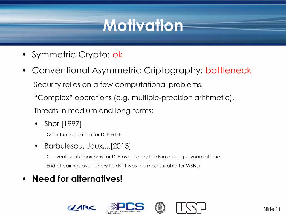
Motivation






• Shor [1997]


• Barbulescu, Joux,...[2013]

Conventional algorithms for DLP over binary fields in quase-polynomial time

End of pairings over binary fields (it was the most suitable for WSNs)

• Need for alternatives!

Slide 12

Motivation

• Post-Quantum Cryptography

Cryptosystems that resist to quantum algorithms.

Slide 13

Motivation



Main lines of research:

• Hash-based

• Very efficient, large signatures.

Slide 14

Motivation




• Hash-based


• Code-based

• Public Key Encryption schemes

• Singatures (one-time, large keys)

Slide 15

Motivation




• Hash-based


• Code-based



• Lattice-based

• Encryption, Digital signatures, FHE

Slide 16

Motivation




• Hash-based


• Code-based



• Lattice-based

• Encryption, Digital signatures, FHE

• Multivariate Quadratic (MQ)

• Some digital signature schemes are robust (original UOV, 14 years)

• Most of the encryption constructions were broken (Jintai has a new perspective about it)

Slide 17

Motivation

• Conventional Public Key Cryptography

• Need coprocessors in smartcards.

• Low flexibility for use or optimizations.

Slide 18

Motivation




• Advantages of MPKC

• Simplicity of Operations (matrices and vectors).

• Small fields avoid multiple-precision arithmetic.

• Long term security. (prevention against spying)

• Efficiency

Signature generation in 804 cycles by Ding [ASAP 2008].

Slide 19

Motivation




• Advantages of MPKC

• Simplicity of Operations (matrices and vectors).

• Small fields avoid multiple-precision arithmetic.

• Long term security. (prevention against spying)

• Efficiency

Signature generation in 804 cycles by Ding [ASAP 2008].

• Main Challenge

• Relatively large key sizes.

Slide 20

•MPKC Constructions

Slide 21

Multivariate Public Key Cryptography

• Basic Property:

• Cryptosystems whose public keys are a set of multivariate polynomials.

Slide 22

Multivariate Public Key Cryptography

• Basic Property:

• Cryptosystems whose public keys are a set of multivariate polynomials.

• Notation: the public key is given as:

𝑃 𝑥1, ⋯ , 𝑥𝑛 = (𝑝1 𝑥1, ⋯ , 𝑥𝑛 , 𝑝2 𝑥1, ⋯ , 𝑥𝑛 , ⋯ , 𝑝𝑚(𝑥1, ⋯ , 𝑥𝑛))

Slide 23

MPKC Encryption

• Given a plaintext 𝑀 = 𝑥1, ⋯ , 𝑥𝑛 .

Slide 24

MPKC Encryption


• Ciphertext is simply a polynomial evaluation:

𝑃 𝑀 = 𝑝1 𝑥1, ⋯ , 𝑥𝑛 , ⋯ , 𝑝𝑚 𝑥1, ⋯ , 𝑥𝑛 = (𝑐1, ⋯ , 𝑐𝑚)

Slide 25

MPKC Encryption


• Ciphertext is simply a polynomial evaluation:

𝑃 𝑀 = 𝑝1 𝑥1, ⋯ , 𝑥𝑛 , ⋯ , 𝑝𝑚 𝑥1, ⋯ , 𝑥𝑛 = (𝑐1, ⋯ , 𝑐𝑚)

• To decrypt one needs to know a trapdoor so that it is

feasible to invert the quadratic map to find the plaintext:

𝑥1, ⋯ , 𝑥𝑛 = 𝑃

−1 𝑐1, ⋯ , 𝑐𝑚

Slide 26

MPKC Signature

• Public Key:

𝑃 𝑥1, ⋯ , 𝑥𝑛 = 𝑝1 𝑥1, ⋯ , 𝑥𝑛 , ⋯ , 𝑝𝑚 𝑥1, ⋯ , 𝑥𝑛

Slide 27

MPKC Signature

• Public Key:

𝑃 𝑥1, ⋯ , 𝑥𝑛 = 𝑝1 𝑥1, ⋯ , 𝑥𝑛 , ⋯ , 𝑝𝑚 𝑥1, ⋯ , 𝑥𝑛

• Private Key: a trapdoor for computing 𝑃−1.

Slide 28

MPKC Signature

• Public Key:

𝑃 𝑥1, ⋯ , 𝑥𝑛 = 𝑝1 𝑥1, ⋯ , 𝑥𝑛 , ⋯ , 𝑝𝑚 𝑥1, ⋯ , 𝑥𝑛


• Sign: given a hash (ℎ1, ⋯ , ℎ𝑚), compute

𝑥1, ⋯ , 𝑥𝑛 = 𝑃

−1 ℎ1, ⋯ , ℎ𝑚

Slide 29

MPKC Signature

• Public Key:

𝑃 𝑥1, ⋯ , 𝑥𝑛 = 𝑝1 𝑥1, ⋯ , 𝑥𝑛 , ⋯ , 𝑝𝑚 𝑥1, ⋯ , 𝑥𝑛



𝑥1, ⋯ , 𝑥𝑛 = 𝑃

−1 ℎ1, ⋯ , ℎ𝑚

• Verify: ℎ1, ⋯ , ℎ𝑛 = 𝑃 𝑥1, ⋯ , 𝑥𝑚

Slide 30

MPKC Signature

• Public Key:

𝑃 𝑥1, ⋯ , 𝑥𝑛 = 𝑝1 𝑥1, ⋯ , 𝑥𝑛 , ⋯ , 𝑝𝑚 𝑥1, ⋯ , 𝑥𝑛



𝑥1, ⋯ , 𝑥𝑛 = 𝑃

−1 ℎ1, ⋯ , ℎ𝑚

• Verify: ℎ1, ⋯ , ℎ𝑛 = 𝑃 𝑥1, ⋯ , 𝑥𝑚

• All vars. and coeffs. are in the small field 𝑘.

Slide 31

Security

• Direct attack is to solve the set of equations:

𝑃 𝑀 = 𝑃 𝑝1 𝑥1, ⋯ , 𝑥𝑛 , ⋯ , 𝑝𝑚 𝑥1, ⋯ , 𝑥𝑛 = (𝑐1, ⋯ , 𝑐𝑚)

Slide 32

Security



• Solving a set of 𝑚 randomly chosen (nonlinear) equations with 𝑛 variables is NP-complete.

Slide 33

Security



• Solving a set of 𝑚 randomly chosen (nonlinear) equations with 𝑛 variables is NP-complete.

• But this does not necessarily ensure the security of the systems.

Slide 34

Security

• Most of the schemes do not use exactly random maps.

Slide 35

Security


• Many systems have the structure

𝑃(𝑥1, ⋯ , 𝑥𝑛) = 𝐿1 ∘ 𝐹 ∘ 𝐿2(𝑥1, ⋯ , 𝑥𝑛)

Slide 36

Security



𝑃(𝑥1, ⋯ , 𝑥𝑛) = 𝐿1 ∘ 𝐹 ∘ 𝐿2(𝑥1, ⋯ , 𝑥𝑛)

• 𝐹 is a quadratic map with certain structure. (central map)

Slide 37

Security



𝑃(𝑥1, ⋯ , 𝑥𝑛) = 𝐿1 ∘ 𝐹 ∘ 𝐿2(𝑥1, ⋯ , 𝑥𝑛)


• This structure enables computing 𝐹−1 easily.

Slide 38

Security



𝑃(𝑥1, ⋯ , 𝑥𝑛) = 𝐿1 ∘ 𝐹 ∘ 𝐿2(𝑥1, ⋯ , 𝑥𝑛)


• This structure enables computing 𝐹−1 easily.

• 𝐿1 and 𝐿2 are full-rank linear maps used to hide 𝐹.

Slide 39

Security

• MQ-Problem: Given a set of 𝑚 quadratic polynomials in 𝑛

variables x = (𝑥1, ⋯ , 𝑥𝑛), solve the system:

𝑝1 𝑥 = ⋯ = 𝑝𝑚 𝑥 = 0

Slide 40

Security

• MQ-Problem: Given a set of 𝑚 quadratic polynomials in 𝑛

variables x = (𝑥1, ⋯ , 𝑥𝑛), solve the system:

𝑝1 𝑥 = ⋯ = 𝑝𝑚 𝑥 = 0

• IP-Problem: Given two polynomial maps 𝐹1, 𝐹2: 𝐾𝑛⟶𝐾𝑚.

The problem is to look for two linear transformations 𝐿1 and

𝐿2 (if they exist) s.t.:

𝐹1(𝑥1, ⋯ , 𝑥𝑛) = 𝐿1 ∘ 𝐹 ∘ 𝐿2(𝑥1, ⋯ , 𝑥𝑛)

Slide 41

Multivariate Quadratic

Construction

• MQ system with 𝑚 equations in 𝑛 vars, all coefs. in 𝔽𝑞:

Polynomial notation:

Vector notation:

𝑝𝑘 𝑥1, … , 𝑥𝑛 = 𝑥𝑃𝑘 𝑥𝑇 + 𝐿(𝑘)𝑥 + 𝑐(𝑘)

𝑝𝑘 𝑥1, … , 𝑥𝑛 ≔ 𝑃𝑖𝑗𝑘𝑥𝑖𝑥𝑗

𝑖,𝑗+ 𝐿𝑖

𝑘𝑥𝑖

𝑖+ 𝑐(𝑘)

Slide 42

(Pure) Quadratic Map

𝑃(𝑘) 𝑥

𝑥𝑇

= ℎ𝑘

𝒫 𝑥 = ℎ ⇔ 𝑥 𝑃(𝑘) 𝑥𝑇 = ℎ𝑘 (𝑘 = 1,… ,𝑚)

Slide 43

Matsumoto-Imai Cryptosystem

• Previously, many unsuccesfull attempts to construct an

encryption scheme.

• Small number of variables.

• Huge key sizes.

• In 1988, Matsumoto and Imai adopted a “Big” Field in their

C* construction.

Slide 44


• 𝑘 is a small finite field with 𝑘 = 𝑞.

Slide 45



• 𝐾 = 𝑘 𝑥 /(𝑔(𝑥)) a degree 𝑛 extension of 𝑘.

Slide 46




• The linear map 𝜙:𝐾 → 𝑘𝑛 and 𝜙−1: 𝑘𝑛 → 𝐾 .

𝜙 𝑎0 + 𝑎1𝑥 +⋯+ 𝑎𝑛−1𝑥𝑛−1 = (𝑎0, 𝑎1, ⋯ , 𝑎𝑛−1)

Slide 47





𝜙 𝑎0 + 𝑎1𝑥 +⋯+ 𝑎𝑛−1𝑥𝑛−1 = (𝑎0, 𝑎1, ⋯ , 𝑎𝑛−1)

• Build a map 𝐹 over 𝐾 :

𝐹 = 𝐿1 ∘ 𝜙 ∘ 𝐹 ∘ 𝜙−1 ∘ 𝐿2

where the 𝐿𝑖 are randomly chosen invertible maps over 𝑘𝑛

Slide 48





𝜙 𝑎0 + 𝑎1𝑥 +⋯+ 𝑎𝑛−1𝑥𝑛−1 = (𝑎0, 𝑎1, ⋯ , 𝑎𝑛−1)

• Build a map 𝐹 over 𝐾 :

𝐹 = 𝐿1 ∘ 𝜙 ∘ 𝐹 ∘ 𝜙−1 ∘ 𝐿2

where the 𝐿𝑖 are randomly chosen invertible maps over 𝑘𝑛

• Inversion of 𝐹 is related to the IP Problem

Slide 49


• The map 𝐹 adopted was:

𝐹 ∶ 𝐾 ⟶ 𝐾

𝑋 ⟼ 𝑋𝑞𝜃+1

Slide 50



𝐹 ∶ 𝐾 ⟶ 𝐾


• Let

𝐹 𝑥1, ⋯ , 𝑥𝑛 = 𝜙 ∘ 𝐹 ∘ 𝜙−1 𝑥1, ⋯ , 𝑥𝑛 = (𝐹1 𝑥1, ⋯ , 𝑥𝑛 , ⋯ , 𝐹 𝑚(𝑥1, ⋯ , 𝑥𝑛))

Slide 51



𝐹 ∶ 𝐾 ⟶ 𝐾


• Let

𝐹 𝑥1, ⋯ , 𝑥𝑛 = 𝜙 ∘ 𝐹 ∘ 𝜙−1 𝑥1, ⋯ , 𝑥𝑛 = (𝐹1 𝑥1, ⋯ , 𝑥𝑛 , ⋯ , 𝐹 𝑚(𝑥1, ⋯ , 𝑥𝑛))

• 𝐹𝑖 are quadratic polynomials because the map

𝑋 ⟼ 𝑋𝑞𝜃 is linear (it is the Frobenius automorphism of

order 𝜃).

Slide 52


• Encryption is done by the quadratic map over 𝑘𝑛

𝐹 = 𝐿1 ∘ 𝜙 ∘ 𝐹 ∘ 𝜙−1 ∘ 𝐿2

where 𝐿𝑖 are affine maps over 𝑘𝑛.

Slide 53


• Encryption is done by the quadratic map over 𝑘𝑛

𝐹 = 𝐿1 ∘ 𝜙 ∘ 𝐹 ∘ 𝜙−1 ∘ 𝐿2

where 𝐿𝑖 are affine maps over 𝑘𝑛.

• Decryption is the inverse process

𝐹 −1 = 𝐿2−1 ∘ 𝜙 ∘ 𝐹−1 ∘ 𝜙−1 ∘ 𝐿1

−1

Slide 54


• Requirement: G.C.D. 𝑞𝜃 + 1, 𝑞𝑛 − 1 = 1

to ensure the invertibility of the decryption map 𝐹 −1

Slide 55


• Requirement: G.C.D. 𝑞𝜃 + 1, 𝑞𝑛 − 1 = 1

to ensure the invertibility of the decryption map 𝐹 −1

• 𝐹−1 𝑋 = 𝑋𝑡 , 𝑋 ∈ 𝐾 where 𝑡 × 𝑞𝜃 + 1 ≡ 1 𝑚𝑜𝑑(𝑞𝑛 − 1).

• The public key includes 𝑘 and 𝐹 = (𝐹1 ,⋯ , 𝐹𝑛 )

• The private key includes 𝐿1, 𝐿2 and 𝐾 .

• Trapdoor to invert 𝐹 [Patarin]

Slide 56

UOV Signature


• ℎ = 𝐻𝑎𝑠ℎ(𝑀)

Slide 57

UOV Signature



• Split vars. into 2 sets: oil variables: O ≔ (𝑥1, ⋯ , 𝑥𝑜)

vinegar variables: 𝑉 ≔ (𝑥1′ , … , 𝑥𝑣

′ )

Slide 58

UOV Signature



• Split vars. into 2 sets: oil variables: O ≔ (𝑥1, ⋯ , 𝑥𝑜)

vinegar variables: 𝑉 ≔ (𝑥1′ , … , 𝑥𝑣

′ )

Slide 59

UOV Signature

𝑓𝑘 𝑥1, ⋯ , x𝑜, 𝑥1′ , … , 𝑥𝑣

′ = ℎ𝑘 =

= 𝐹𝑖𝑗𝑘𝑥𝑖𝑥′𝑗

𝑂×𝑉

+ 𝐹𝑖𝑗𝑘𝑥′𝑖𝑥′𝑗

𝑉×𝑉

+ 𝐿𝑖𝑘𝑥𝑖

𝑂

+ 𝐿𝑖𝑘𝑥′𝑖

𝑉

+ 𝑐(𝑘)



• Choose uniformly at random vinegars: 𝑉 ≔ (𝑥1′ , … , 𝑥𝑣

′ )

Slide 60

UOV Signature

𝑓𝑘 𝑥1, ⋯ , x𝑜, 𝑥1′ , … , 𝑥𝑣

′ = ℎ𝑘 =


𝑂×𝑉


𝑉×𝑉


𝑂


𝑉

+ 𝑐(𝑘)



• Fix vinegars: 𝑉 ≔ 𝑥1′ , … , 𝑥𝑣

′

• This becomes an 𝑜𝑥𝑜 system of linear equations.

Slide 61

UOV Signature

𝑓𝑘 𝑥1, ⋯ , x𝑜, 𝑥1′ , … , 𝑥𝑣

′ = ℎ𝑘


𝑂×𝑉


𝑉×𝑉


𝑂


𝑉

+ 𝑐(𝑘)



• Fix vinegars: 𝑉 ≔ 𝑥1′ , … , 𝑥𝑣

′

• This becomes an 𝑜𝑥𝑜 system of linear equations.

• It has a solution with high probability (≈ 1 − 1/𝑞).

Slide 62

UOV Signature

𝑓𝑘 𝑥1, ⋯ , x𝑜, 𝑥1′ , … , 𝑥𝑣

′ =


𝑂×𝑉


𝑉×𝑉


𝑂


𝑉

+ 𝑐(𝑘)


• Oil variables not mixed.

Slide 63

UOV Signature

𝐹(𝑘) =

0

Vinegar

variables

Oil

variables

𝒙𝟏 … 𝒙𝒗 … 𝒙𝒏 𝒙𝟏

⋮

𝒙𝒗

𝒙𝒏

⋮

Vinegar variables

Oil variables

Slide 64

Rainbow Signature

• Rainbow Quadratic Map

• UOV key sizes.

Slide 65

MQ Signatures

Scheme Public Key

(KiB)

113.4

99.4

77.7

66.7

14.5

11.0

10.2

Slide 66

•Technique for Key Size

Reduction

• Technique for reduction of UOV public keys.

Slide 67

MQ Signatures - Cyclic UOV


• Part of the public key with short representation.

Slide 68



• Part of the public key with short representation.

• Achieves a 6x reduction factor for 80-bit security.

Slide 69


Public matrix of coefficients 𝑀𝑃

Slide 70


𝑃(1)

𝑃(2) 𝑀𝑃 = ⋮

⋮ 𝑚𝑥l ′

l ′ =𝑛 𝑛 + 1

2

𝑃(𝑚)

Public matrix of coefficients 𝑀𝑃

Slide 71


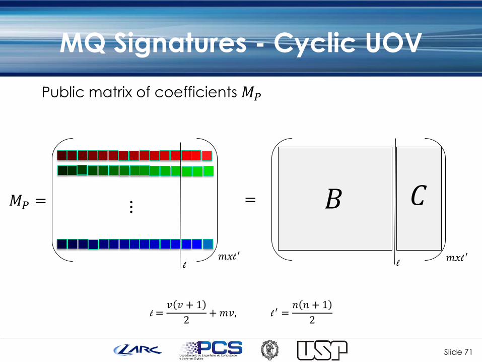
𝑀𝑃 = ⋮

𝑚𝑥l ′

𝐵 𝐶

l

=

𝑚𝑥l ′ l

l =𝑣 𝑣 + 1

2+𝑚𝑣, l ′ =

𝑛 𝑛 + 1

2

Private matrix of coefficients 𝑀𝐹

Slide 72


𝐹 1

𝐹 2

𝐹 𝑚

𝑀𝐹 = ⋮

⋮ 𝑚𝑥l ′

l ′ =𝑛 𝑛 + 1

2

0

l

l =𝑣 𝑣 + 1

2+𝑚𝑣,

0

0

0

0

Private matrix of coefficients 𝑀𝐹

Slide 73


𝑀𝐹 = 𝐹

l =𝑣 𝑣 + 1

2+𝑚𝑣,

=

𝑚𝑥l ′ l

l ′ =𝑛 𝑛 + 1

2

⋮

𝑚𝑥l ′ l

0

0

0

• There is a linear relation between 𝐵 and 𝐹 which only depends on 𝐵,𝐹 and 𝑆 [Petzoldt et. al, 2010]

Slide 74


𝑀𝐹 = 𝐹

𝑚𝑥l ′

𝑀𝑃 = 𝐵 𝐶

𝑚𝑥l ′

𝐵 = 𝐹 ∙ 𝐴𝑈𝑂𝑉(S)

𝑎𝑖𝑗𝑟𝑠 =

𝑠𝑟𝑖 . 𝑠𝑠𝑖 , 𝑖 = 𝑗 𝑠𝑟𝑖 . 𝑠𝑠𝑗 + 𝑠𝑟𝑗 . 𝑠𝑠𝑖 , 𝑖 ≠ 𝑗

1 ≤ 𝑖 ≤ 𝑣, 𝑖 ≤ 𝑗 ≤ 𝑛

1 ≤ 𝑟 ≤ 𝑣, 𝑟 ≤ 𝑠 ≤ 𝑛

l

l

0

By choosing 𝐴𝑈𝑂𝑉(𝑆) invertible:

• 𝐹 can be computed from 𝐵 and 𝐴𝑈𝑂𝑉−1

Slide 75


𝐹 = 𝐵 ∙ 𝐴𝑈𝑂𝑉−1



• Thus, the choice of 𝐵 becomes flexible.

Slide 76






• In particular:

𝐵 = 0 does not result in a valid F,

𝐵 = Identity blocks, reveals too much info of 𝐴𝑈𝑂𝑉−1 ,

𝐵 circulant was adopted by [Petzoldt et. al, 2010]

Slide 77






• In particular:

𝐵 = 0 does not result in a valid F,

𝐵 = Identity blocks, reveals too much info of 𝐴𝑈𝑂𝑉−1 ,

𝐵 circulant was adopted by [Petzoldt et. al, 2010]

Slide 78



Petzoldt et. al. showed by theorem that the choice of a

circulant 𝐵 provides consistent UOV signatures.

Adopting 𝐵 circulant:

Slide 79


𝑀𝑃 = 𝐵 𝐶

𝑚𝑥l ′

|𝑴𝑷| = l+𝑚(l ′ − l)

𝒃 = (𝑏1, ⋯ , 𝑏l)

⋮

𝑚𝑥l ′

l

⋯

l

Public matrices 𝑃 𝑘

Slide 80


𝑃 1


Slide 81


𝑃 2


Slide 82


𝑃 3


Slide 83


𝑃 4


Slide 84


⋯

• Idea: Find equivalent private keys that enables solving any

given public key system.

Slide 85

Equivalent Keys in UOV



• A class of equivalent private keys with a simpler structure.

Slide 86




• A class of equivalent private keys with a simpler structure.

• Thus, private keys can be built using this short structure.

Slide 87


• UOV public key:

𝑃(𝑖) = 𝑆𝐹(𝑖)𝑆𝑇 , 1 ≤ 𝑖 ≤ 𝑚

Slide 88


• UOV public key:

𝑃(𝑖) = 𝑆𝐹(𝑖)𝑆𝑇 , 1 ≤ 𝑖 ≤ 𝑚

• Question: Are there classes of keys 𝑆′and 𝐹′ s.t.

𝑃(𝑖) = 𝑆𝐹(𝑖)𝑆𝑇 = 𝑆′𝐹′

(𝑖)𝑆′𝑇, 1 ≤ 𝑖 ≤ 𝑚

where matrices 𝐹′(𝑖)

share with 𝐹(𝑖) the same trapdoor structure?

Slide 89


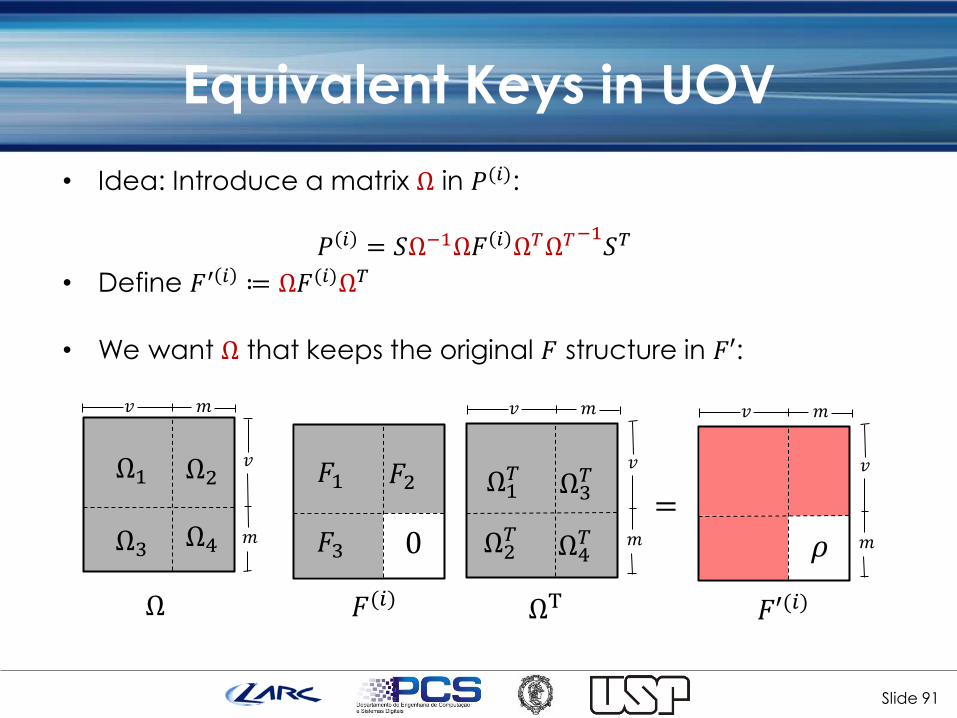
• Idea: Introduce a matrix Ω in 𝑃(𝑖):

𝑃 𝑖 = 𝑆Ω−1Ω𝐹 𝑖 Ω𝑇Ω𝑇

−1𝑆𝑇

• Define 𝐹′ 𝑖 ≔ Ω𝐹(𝑖)Ω𝑇

Slide 90


• Idea: Introduce a matrix Ω in 𝑃(𝑖):

𝑃 𝑖 = 𝑆Ω−1Ω𝐹 𝑖 Ω𝑇Ω𝑇

−1𝑆𝑇

• Define 𝐹′ 𝑖 ≔ Ω𝐹(𝑖)Ω𝑇

• We want Ω that keeps the original 𝐹 structure in 𝐹′:

Slide 91


Ω1 Ω2

Ω3 Ω4

𝐹1 𝐹2

𝐹3 =

𝐹′(𝑖) 𝐹(𝑖)

𝜌

Ω1𝑇 Ω3

𝑇

Ω2𝑇 Ω4

𝑇

𝑣 𝑚

𝑣

𝑚

𝑣 𝑚

𝑣

𝑚

𝑣 𝑚

𝑣

𝑚 0

Ω ΩT

• From the previous equality we obtain:

𝜌 = Ω3𝐹1 + Ω4𝐹3 Ω3

𝑇 + Ω3𝐹2Ω4𝑇 = 0

and Ω3 = 0 is a solution.

Slide 92


Ω1 Ω2

0 Ω4

Ω =

𝑣 𝑚

𝑣

𝑚

• Thus, 𝐹′(𝑖) = Ω𝐹(𝑖)Ω𝑇 has the same structure of 𝐹 𝑖 .

• Going back to definition

𝑃 𝑖 = 𝑆Ω−1(Ω𝐹 𝑖 Ω𝑇)Ω𝑇−1𝑆𝑇

Slide 93




𝑃 𝑖 = 𝑆Ω−1(𝐹′(𝑖))Ω𝑇−1𝑆𝑇

Slide 94




𝑃 𝑖 = 𝑆Ω−1(𝐹′(𝑖))Ω𝑇−1𝑆𝑇

• So, defining 𝑆′ ≔ 𝑆Ω−1 one finally gets:

𝑃 𝑖 = 𝑆′𝐹′(𝑖)𝑆′𝑇

Slide 95


• Note that Ω−1 has the same structure of Ω.

Slide 96


Ω1−1

0

𝑆′ = 𝑆Ω−1 = 𝑆1 𝑆2

𝑆3 𝑆4

Ω2−1

Ω4−1

𝑣 𝑚

𝑣

𝑚

Ω−1 𝑆

Ω1−1 Ω2

−1

Ω4−1

• By choosing suitable values of Ω𝑖−1, it is possible to get:

𝑆1′ = 𝐼𝑣𝑥𝑣

𝑆2′ = 0𝑣𝑥𝑚

𝑆4′ = 𝐼𝑚𝑥𝑚

what implies

𝑆3′ = 𝑆3𝑆1

−1𝑆2𝑆1−1 + 𝑆4(𝑆4 − 𝑆3𝑆1

−1𝑆2)−1

Slide 97


• Structure of 𝑆′:

Slide 98


𝑆′ =

𝑆3′

𝑚 𝑣

𝑚

𝑣

• Structure of 𝑆′:

• So, the answer is yes, there exist equivalent 𝑆′, 𝐹′(𝑖)

s.t.

𝑆′𝐹′

(𝑖)(𝑆′)𝑇 = (𝑆Ω−1) Ω𝐹 𝑖 Ω𝑇 𝑆Ω−1 𝑇 = 𝑃 𝑖

and 𝐹′(𝑖)

have the desired trapdoor structure.

Slide 99


𝑆′ =

𝑆3′

𝑚 𝑣

𝑚

𝑣

Slide 100

Recap. MQ Schemes

Slide 101

Thanks!

Questions?

Introduction to Multivariate Public Key Cryptography · Slide 1 Introduction to Multivariate Public Key Cryptography Geovandro Carlos C. F. Pereira PhD advisor: Prof. Dr. Paulo S.

Documents