Introduction to Molecular Phylogeny Starting point: a set of homologous, aligned DNA or protein sequences Result of the process: a tree describing evolutionary.

Introduction to Molecular Phylogeny Introduction to Molecular Phylogeny

Starting point: a set of homologous, aligned DNA or protein sequences

Result of the process: a tree describing evolutionary relationships between studied sequences = a genealogy of sequences = a phylogenetic tree

CLUSTAL W (1.74) multiple sequence alignment

Xenopus ATGCATGGGCCAACATGACCAGGAGTTGGTGTCGGTCCAAACAGCGTT---GGCTCTCTAGallus ATGCATGGGCCAGCATGACCAGCAGGAGGTAGC---CAAAATAACACCAACATGCAAATGBos ATGCATCCGCCACCATGACCAGCAGGAGGTAGCACCCAAAACAGCACCAACGTGCAAATGHomo ATGCATCCGCCACCATGACCAGCAGGAGGTAGCACTCAAAACAGCACCAACGTGCAAATGMus ATGCATCCGCCACCATGACCAGCAGGAGGTAGCACTCAAAACAGCACCAACGTGCAAATGRattus ATGCATCCGCCACCATGACCAGCGGGAGGTAGCTCTCAAAACAGCACCAACGTGCAAATG ****** **** ********* * *** * * *** * * *

Alignment and GapsAlignment and Gaps The quality of the alignment is essential : each column of

the alignment (site) is supposed to contain homologous residues (nucleotides, amino acids) that derive from a common ancestor.

==> Unreliable parts of the alignment must be omitted from further phylogenetic analysis.

Most methods take into account only substitutions ; gaps (insertion/deletion events) are not used.

==> gaps-containing sites are ignored.Xenopus ATGCATGGGCCAACATGACCAGGAGTTGGTGTCggtCCAAACAGCGTT---GGCTCTCTAGallus ATGCATGGGCCAGCATGACCAGCAGGAGGTAGC---CAAAATAACACCaacATGCAAATGBos ATGCATCCGCCACCATGACCAGCAGGAGGTAGCagtCAAAACAGCACCaacGTGCAAATGHomo ATGCATCCGCCACCATGACCAGCAGGAGGTAGCagtCAAAACAGCACCaacGTGCAAATGMus ATGCATCCGCCACCATGACCAGCAGGAGGTAGCactCAAAACAGCACCaacGTGCAAATGRattus ATGCATCCGCCACCATGACCAGCGGGAGGTAGCtctCAAAACAGCACCaacGTGCAAATG

Phylogenetic TreePhylogenetic Tree Internal branch : between 2 nodes. External branch : between a node and a leaf Horizontal branch length is proportional to evolutionary distances between

sequences and their ancestors (unit = substitution / site). Tree Topology = shape of tree = branching order between nodes

HomoBosMusRattus0.0110.0250.0120.011Gallus0.0380.0660.01RootNodeLeafBranch

Rooted and Unrooted TreesRooted and Unrooted Trees

Most phylogenetic methods produce unrooted trees. This is because they detect differences between sequences, but have no means to orient residue changes relatively to time.

Two means to root an unrooted tree : The outgroup method : include in the analysis a group of sequences

known a priori to be external to the group under study; the root is by necessity on the branch joining the outgroup to other sequences.

Make the molecular clock hypothesis : all lineages are supposed to have evolved with the same speed since divergence from their common ancestor. The root is at the equidistant point from all tree leaves.

Unrooted TreeUnrooted Tree

0.02

RattusMusBosHomoGallus

Rooted TreeRooted Tree

XenopusHomoBosMusRattusGallus0.02

Universal phylogenyUniversal phylogeny

deduced from comparison deduced from comparison of SSU and LSU rRNA of SSU and LSU rRNA sequences (2508 sequences (2508 homologous sites) using homologous sites) using Kimura’s 2-parameter Kimura’s 2-parameter distance and the NJ distance and the NJ method. method.

The absence of root in this The absence of root in this tree is expressed using a tree is expressed using a circular design.circular design.

BacteriaBacteriaArchaeaArchaea

EucaryaEucarya

Number of possible tree topologies Number of possible tree topologies for n taxafor n taxa

n Ntrees

4 3

5 15

6 105

7 945

... ...

10 2,027,025

... ...

20 ~ 2 x1020

Ntrees=3.5.7...(2n−5)= (2n−5)!2n−3(n−3)!

Methods for Phylogenetic Methods for Phylogenetic reconstructionreconstruction

Four main families of methods : Parsimony Distance methods Maximum likelihood methods Bayesian methods

Parsimony (1)Parsimony (1) Step 1: for a given tree topology (shape), and for a given

alignment site, determine what ancestral residues (at tree nodes) require the smallest total number of changes in the whole tree. Let d be this total number of changes.

Example: At this site and for this tree shape, at least 3 substitution events are needed to explain the nucleotide pattern at tree leaves. Several distinct scenarios with 3 changes are possible.

X: ancestral nucleotide : substitution event

Parsimony (2)Parsimony (2) Step 2:

Compute d (step 1) for each alignment site. Add d values for all alignment sites. This gives the length L of tree.

Step 3: Compute L value (step 2) for each possible tree shape. Retain the shortest tree(s)

= the tree(s) that require the smallest number of changes = the most parsimonious tree(s).

Some properties of ParsimonySome properties of Parsimony

Several trees can be equally parsimonious (same length, the shortest of all possible lengths).

The position of changes on each branch is not uniquely defined => parsimony does not allow to define tree branch lengths in a unique way.

The number of trees to evaluate grows extremely fast with the number of compared sequences :The search for the shortest tree must often be restricted to a fraction

of the set of all possible tree shapes (heuristic search) => there is no mathematical certainty of finding the shortest (most parsimonious) tree.

Evolutionary DistancesEvolutionary Distances

They measure the total number of substitutions that occurred on both lineages since divergence from last common ancestor.

Divided by sequence length. Expressed in substitutions / site

ancestor

sequence 1 sequence 2

Quantification of evolutionary distances (1):Quantification of evolutionary distances (1):

The problem of hidden or multiple changesThe problem of hidden or multiple changes D (true evolutionary distance) fraction of

observed differences (p)

D = p + hidden changes Through hypotheses about the nature of the

residue substitution process, it becomes possible to estimate D from observed differences between sequences.

AAGCAGGAAAAGC

Hypotheses of the model :(a) All sites evolve independently and following the same process.

(b) Substitutions occur according to two probabilities :

One for transitions, one for transversions.

Transitions : G <—>A or C <—>T Transversions : other changes

(c) The base substitution process is constant in time.

Quantification of evolutionary distance (d) as a function of the fraction of observed differences (p: transitions, q: transversions):

Quantification of evolutionary distances (2):Quantification of evolutionary distances (2): Kimura’s two parameter distance (DNA)Kimura’s two parameter distance (DNA)

Kimura (1980) J. Mol. Evol. 16:111Kimura (1980) J. Mol. Evol. 16:111

d=−12

ln[(1−2p−q) 1−2q]

Quantification of evolutionary distances (3):Quantification of evolutionary distances (3): PAM and Kimura’s distances (proteins)PAM and Kimura’s distances (proteins)

Hypotheses of the model (Dayhoff, 1979) :(a) All sites evolve independently and following the same process.

(b) Each type of amino acid replacement has a given, empirical probability :Large numbers of highly similar protein sequences have been collected; probabilities of replacement of any a.a. by any other have been tabulated.

(c) The amino acid substitution process is constant in time. Quantification of evolutionary distance (d) :

the number of replacements most compatible with the observed pattern of amino acid changes and individual replacement probabilities.

Kimura’s empirical approximation : d = - ln( 1 - p - 0.2 p2 ) (Kimura, 1983) where p = fraction of observed differences

Quantification of evolutionary distances (4):Quantification of evolutionary distances (4): Synonymous and non-synonymous distances Synonymous and non-synonymous distances

(coding DNA): Ka, Ks(coding DNA): Ka, Ks Hypothesis of previous models :

(a) All sites evolve independently and following the same process. Problem: in protein-coding genes, there are two classes of

sites with very different evolutionary rates. non-synonymous substitutions (change the a.a.): slow synonymous substitutions (do not change the a.a.): fast

Solution: compute two evolutionary distances Ka = non-synonymous distance = nbr. non-synonymous substitutions / nbr. non-synonymous sites

Ks = synonymous distance = nbr. synonymous substitutions / nbr. synonymous sites

The genetic codeThe genetic code

TTT Phe TCT Ser TAT Tyr TGT CysTTC Phe TCC Ser TAC Tyr TGC CysTTA Leu TCA Ser TAA stop TGA stopTTG Leu TCG Ser TAG stop TGG Trp

CTT Leu CCT Pro CAT His CGT ArgCTC Leu CCC Pro CAC His CGC ArgCTA Leu CCA Pro CAA Gln CGA ArgCTG Leu CCG Pro CAG Gln CGG Arg

ATT Ile ACT Thr AAT Asn AGT SerATC Ile ACC Thr AAC Asn AGC SerATA Ile ACA Thr AAA Lys AGA ArgATG Met ACG Thr AAG Lys AGG Arg

GTT Val GCT Ala GAT Asp GGT GlyGTC Val GCC Ala GAC Asp GGC GlyGTA Val GCA Ala GAA Glu GGA GlyGTG Val GCG Ala GAG Glu GGG Gly

Quantification of evolutionary distances (6):Quantification of evolutionary distances (6): Calculation of Ka and KsCalculation of Ka and Ks

The details of the method are quite complex. Roughly : Split all sites of the 2 compared genes in 3 categories :

I: non degenerate, II: partially degenerate, III: totally degenerate Compute the number of non-synonymous sites = I + 2/3 II Compute the number of synonymous sites = III + 1/3 II Compute the numbers of synonymous and non-synonymous changes Compute, with Kimura’s 2-parameter method, Ka and Ks

Frequently, one of these two situations occur : Evolutionarily close sequences : Ks is informative, Ka is not. Evolutionarily distant sequences : Ks is saturated , Ka is informative.

Li, Wu & Luo (1985) Mol.Biol.Evol. 2:150Li, Wu & Luo (1985) Mol.Biol.Evol. 2:150

Ka and Ks : exampleKa and Ks : example

# sites observed diffs. J & C K2P KA KS

10254 0.077 0.082 0.082 0.035 0.228

Urotrophin gene of rat (AJ002967) and mouse (Y12229) Urotrophin gene of rat (AJ002967) and mouse (Y12229)

Saturation: loss of phylogenetic signal Saturation: loss of phylogenetic signal When compared homologous sequences have experienced too many

residue substitutions since divergence, it is impossible to determine the phylogenetic tree, whatever the tree-building method used.

NB: with distance methods, the saturation phenomenon may express itself through mathematical impossibility to compute d. Example: Jukes-Cantor: p 0.75 => d

NB: often saturation may not be detectable

ancestorseq. 1seq. 2seq. 3

Quantification of evolutionary distances (7):Quantification of evolutionary distances (7):

Other distance measures Other distance measures

Several other, more realistic models of the evolutionary process at the molecular level have been used : Accounting for biased base compositions

(Tajima & Nei). Accounting for variation of the evolutionary

rate across sequence sites. etc ...

A B C

tree

A B CA 0B 3 0C 4 3 0

distance matrix

Correspondence between trees and Correspondence between trees and distance matricesdistance matrices

• Any phylogenetic tree induces a matrix of Any phylogenetic tree induces a matrix of distances between sequence pairsdistances between sequence pairs• “ “Perfect” distance matrices correspond to a Perfect” distance matrices correspond to a single phylogenetic treesingle phylogenetic tree

Building phylogenetic trees by Building phylogenetic trees by distance methodsdistance methods

General principle :

Sequence alignment (1)

Matrix of evolutionary distances between sequence pairs (2)

(unrooted) tree

(1) Measuring evolutionary distances. (2) Tree computation from a matrix of distance values.

i

j

kli

ljlc

lk

ll

mm

Any unrooted tree induces a distance Any unrooted tree induces a distance between sequences : between sequences :

(i,m) = l(i,m) = lii + l + lcc + l + lrr + l + lmm

lm

lr

It is possible to compute the values of branch lengths that create the It is possible to compute the values of branch lengths that create the best match between best match between and the evolutionary distance d : and the evolutionary distance d :

Distance matrix -> tree (1):

€

Δ = (dx,y −1≤x<y≤n

∑ δx,y )2minimizeminimize

It is then possible to compute the total tree length : S = sum of all branch lengths

tree topology ==> «best» branch lengths ==> total tree lengthtree topology ==> «best» branch lengths ==> total tree length

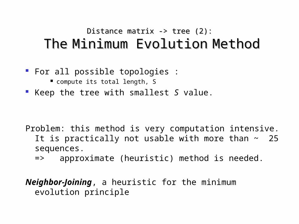
Distance matrix -> tree (2):Distance matrix -> tree (2):

TheThe Minimum EvolutionMinimum Evolution MethodMethod

For all possible topologies : compute its total length, S

Keep the tree with smallest S value.

Problem: this method is very computation intensive. It is practically not usable with more than ~ 25 sequences.=> approximate (heuristic) method is needed.

Neighbor-Joining, a heuristic for the minimum evolution principle

Distance matrix -> tree (3):Distance matrix -> tree (3):

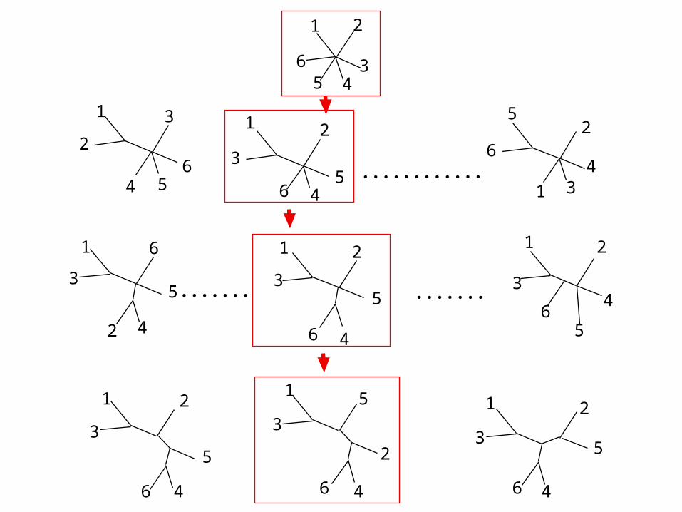
TheThe Neighbor-Joining Method: algorithmNeighbor-Joining Method: algorithmStep 1: Use d distances measured between the N sequences

Step 2: For all pairs i et j: consider the following bush-like topology, and compute Si,j , the sum of all “best” branch lengths.

Step 3: Retain the pair (i,j) with smallest Si,j value . Group i and j in the tree.Step 4: Compute new distances d between N-1 objects:

pair (i,j) and the N-2 remaining sequences: d(i,j),k = (di,k + dj,k) / 2Step 5: Return to step 1 as long as N ≥ 4.

Saitou & Nei (1987) Mol.Biol.Evol. 4:406

k1k3k4k5k2

1 2

345

6

6

2

3

23

54

............

5

6

31

2

4

5

6

..............

5

2

1

4 56

1 2

6

2

4

1

3

1

3

6

2

4

5

1

3

4

5

1

3

6 4

5

2

1

3

6 4

1

3

6 4

2

5

Distance matrix -> tree (5):Distance matrix -> tree (5):

TheThe Neighbor-Joining Method (NJ): propertiesNeighbor-Joining Method (NJ): properties

NJ is a fast method, even for hundreds of sequences. The NJ tree is an approximation of the minimum evolution

tree (that whose total branch length is minimum). In that sense, the NJ method is very similar to parsimony

because branch lengths represent substitutions. NJ produces always unrooted trees, that need to be rooted

by the outgroup method. NJ always finds the correct tree if distances are tree-like. NJ performs well when substitution rates vary among

lineages. Thus NJ should find the correct tree if distances are well estimated.

Maximum likelihood methods (1)Maximum likelihood methods (1)(programs fastDNAml, PAUP*, PROML, PROTML)(programs fastDNAml, PAUP*, PROML, PROTML)

Hypotheses The substitution process follows a probabilistic model

whose mathematical expression, but not parameter values, is known a priori.

Sites evolve independently from each other. All sites follow the same substitution process (some

methods use a discrete gamma distribution of site rates). Substitution probabilities do not change with time on

any tree branch. They may vary between branches.

Maximum likelihood methods (2)Maximum likelihood methods (2)

Probabilistic model of theProbabilistic model of theevolution of homologousevolution of homologoussequencessequences

llii, branch lengths = expected, branch lengths = expected

number of subst. per site along branchnumber of subst. per site along branch

, relative rates of base substitutions, relative rates of base substitutions(e.g., transition/transversion, G+C-bias)(e.g., transition/transversion, G+C-bias)

Thus, one can compute Thus, one can compute

ProbaProbabranch ibranch i(x (x y) y)

for any bases x & y, any branch i, any set of for any bases x & y, any branch i, any set of values values

l7l8l3l4l1l2l5l6l10l9se 3se 6se 1se 2se 5se 4

Maximum likelihood algorithm (1) Maximum likelihood algorithm (1)

Step 1: Let us consider a given rooted tree, a given site, and a given set of branch lengths. Let us compute the probability that the observed pattern of nucleotides at that site has evolved along this tree.

S1, S2, S3, S4: observed bases at site in seq. 1, 2, 3, 4 : unknown and variable ancestral basesl1, l2, …, l6: given branch lengths

P(S1, S2, S3, S4) =

P() Pl5() Pl6() Pl1(,S1) Pl2(,S2) Pl3(,S3) Pl4(,S4)

where P(S7) is estimated by the average base frequencies in studied sequences.

S1S2S3S4l1l2l3l4l5l6

Maximum likelihood algorithm (2) Maximum likelihood algorithm (2)

Step 2: compute the probability that entire sequences have evolved :

P(Sq1, Sq2, Sq3, Sq4) = all sites P(S1, S2, S3, S4)

Step 2: compute branch lengths l1, l2, …, l6 and value of parameter that give the highest P(Sq1, Sq2, Sq3, Sq4) value. This is the likelihood of the tree.

Step 3: compute the likelihood of all possible trees. The tree predicted by the method is that having the highest likelihood.

Maximum likelihood : properties Maximum likelihood : properties

This is the best justified method from a theoretical viewpoint.

Sequence simulation experiments have shown that this method works better than all others in most cases.

But it is a very computer-intensive method.

It is nearly always impossible to evaluate all possible trees because there are too many. A partial exploration of the space of possible trees is done.

Reliability of phylogenetic trees: the Reliability of phylogenetic trees: the bootstrap bootstrap

The phylogenetic information expressed by an unrooted tree resides entirely in its internal branches.

The tree shape can be deduced from the list of its internal branches.

Testing the reliability of a tree = testing the reliability of each internal branch.

124356 internal branch separating group 1+4 from group 6+2+5+3

Bootstrap procedureBootstrap procedure

The support of each internal branch is expressed as percent of replicates.

1 Nacgtacatagtatagcgtctagtggtaccgtatgaggtacatagtatgg-gtatactggtaccgtatgacgtaaat-gtatagagtctaatggtac-gtatgacgtacatggtatagcgactactggtaccgtatg

real alignment random sampling, with replacement, of N sites

1 Ngatcagtcatgtataggtctagtggtacgtatattgagagtcatgtatggtgtatactggtacgtaattgac-gtaatgtataggtctaatggtactgtaattgacggtcatgtataggactactggtacgtatat

“artificial” alignments} 1000 timestree-building methodsame tree-building method

tree = series of internal branches “artificial” treesfor each internal

branch, compute fraction of “artificial” trees containing this

internal branch

"bootstrapped” tree"bootstrapped” tree

Xenopus

Homo

Bos

Mus

Rattus

Gallus0.02979146

Bootstrap procedure : propertiesBootstrap procedure : properties

Internal branches supported by ≥ 90% of replicates are considered as statistically significant.

The bootstrap procedure only detects if sequence length is enough to support a particular node.

The bootstrap procedure does not help determining if the tree-building method is good. A wrong tree can have 100 % bootstrap support for all its branches!

€

Pr(τ | X)∝ Pr(X | τ ,v,θv,θ

∫∫ ) . Prprior(v,θ)dvdθ

Bayesian inference of phylogenetic treesBayesian inference of phylogenetic trees

Aim : compute the Aim : compute the posterior probabilityposterior probability of all tree topologies, of all tree topologies,given the sequence alignment.given the sequence alignment.

likelihood oflikelihood oftree + parameterstree + parameters

prior probability ofprior probability ofparameter valuesparameter values

: tree topology: tree topology

XX: aligned sequences: aligned sequences

vv: set of tree branch lengths: set of tree branch lengths

: parameters of substitution model (e.g., transit/transv ratio): parameters of substitution model (e.g., transit/transv ratio)

Analytical computation of Pr(Analytical computation of Pr(|X) is impossible in general.|X) is impossible in general.

A computational technique calledA computational technique calledMetropolis-coupled Markov chain Monte CarloMetropolis-coupled Markov chain Monte Carlo [ MC [ MC33 ] ]

is used to generate a statistical sample from the posterior is used to generate a statistical sample from the posterior distribution of trees.distribution of trees.

(example: generate a random sample of 10,000 trees)(example: generate a random sample of 10,000 trees)

Result:Result:- Retain the tree having highest probability (that found most Retain the tree having highest probability (that found most often among the sample).often among the sample).

- Compute the Compute the posterior probabilitiesposterior probabilities of all clades of that of all clades of that tree: fraction of sampled trees containing given clade.tree: fraction of sampled trees containing given clade.

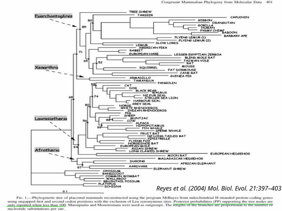
Reyes et al. (2004) Mol. Biol. Evol. 21:397–403

Overcredibility of Bayesian estimation of clade support ?Overcredibility of Bayesian estimation of clade support ?

Bayesian clade support is much stronger than bootstrap support :Bayesian clade support is much stronger than bootstrap support :

Douady et al. (2003) Mol. Biol. Evol. 20:248–254

Bayesian Posterior Bayesian Posterior probabilityprobability

Bootstrapped Bootstrapped Posterior probabilityPosterior probability

Boostrap support in ML analysisBoostrap support in ML analysis

So,So,

Bayesian clade support is highBayesian clade support is highBootstrap clade support is lowBootstrap clade support is low

which one is closer to true support ?which one is closer to true support ?

Conclusion from simulation experiments :Conclusion from simulation experiments :

o when sequence evolution fits exactly the probability when sequence evolution fits exactly the probability model used, Bayesian support is correct, bootstrap is model used, Bayesian support is correct, bootstrap is pessimistic.pessimistic.

o Bayesian inference is sensitive to small model Bayesian inference is sensitive to small model misspecifications and becomes too optimistic.misspecifications and becomes too optimistic.

PHYML :PHYML : a Fast, and Accurate Algorithm to Estimate Large Phylogenies by Maximum Likelihood

ML requires to find what quantitative (e.g., branch lengths) and ML requires to find what quantitative (e.g., branch lengths) and qualitative (tree topology) parameter values correspond to the qualitative (tree topology) parameter values correspond to the highest probability for sequences to have evolved.highest probability for sequences to have evolved.

PHYML adjusts topology and branch lengths simultaneously.PHYML adjusts topology and branch lengths simultaneously.

Because only a few iterations are sufficient to reach an optimum, PHYML is a fast, but accurate, ML algorithm.

Guindon & Gascuel (2003) Syst. Biol. 52(5):696–704

Tree and sequence simulation experimentTree and sequence simulation experiment

P, PHYMLP, PHYMLF, fastDNAmlF, fastDNAmlL, NJMLL, NJMLD, DNAPARSD, DNAPARSN, NJN, NJ

5000 random trees5000 random trees40 taxa, 500 bases40 taxa, 500 basesno molecular clockno molecular clockvarying tree lengthvarying tree lengthK2P, K2P, = 2 = 2

distance < parsimony ~ PHYML << Bayesian < classical MLdistance < parsimony ~ PHYML << Bayesian < classical ML NJ DNAPARS PHYML MrBayes fastDNAml,PAUPNJ DNAPARS PHYML MrBayes fastDNAml,PAUP

Comparison of running time for various tree-building algorithmsComparison of running time for various tree-building algorithms

WWW resources for molecular phylogeny (1)

Compilations A list of sites and resources:

http://www.ucmp.berkeley.edu/subway/phylogen.html An extensive list of phylogeny programs

http://evolution.genetics.washington.edu/phylip/software.html

Databases of rRNA sequences and associated software

The rRNA WWW Server - Antwerp, Belgium.http://rrna.uia.ac.be

The Ribosomal Database Project - Michigan State University

http://rdp.cme.msu.edu/html/

WWW resources for molecular phylogeny (2)

Database similarity searches (Blast) :http://www.ncbi.nlm.nih.gov/BLAST/http://www.infobiogen.fr/services/menuserv.htmlhttp://bioweb.pasteur.fr/seqanal/blast/intro-fr.htmlhttp://pbil.univ-lyon1.fr/BLAST/blast.html

Multiple sequence alignmentClustalX : multiple sequence alignment with a graphical interface(for all types of computers).http://www.ebi.ac.uk/FTP/index.html and go to ‘software’

Web interface to ClustalW algorithm for proteins:http://pbil.univ-lyon1.fr/ and press “clustal”

WWW resources for molecular phylogeny (3) Sequence alignment editor SEAVIEW : for windows and unix

http://pbil.univ-lyon1.fr/software/seaview.html

Programs for molecular phylogeny PHYLIP : an extensive package of programs for all platforms

http://evolution.genetics.washington.edu/phylip.html CLUSTALX : beyond alignment, it also performs NJ PAUP* : a very performing commercial package

http://paup.csit.fsu.edu/index.html PHYLO_WIN : a graphical interface, for unix only

http://pbil.univ-lyon1.fr/software/phylowin.html MrBayes : Bayesian phylogenetic analysis

http://morphbank.ebc.uu.se/mrbayes/ PHYML : fast maximum likelihood tree building

http://www.lirmm.fr/~guindon/phyml.html WWW-interface at Institut Pasteur, Paris

http://bioweb.pasteur.fr/seqanal/phylogeny

WWW resources for molecular phylogeny (4)

Tree drawingNJPLOT (for all platforms)http://pbil.univ-lyon1.fr/software/njplot.html

Lecture notes of molecular systematicshttp://www.bioinf.org/molsys/lectures.html

WWW resources for molecular phylogeny (5)

Books Laboratory techniques

Molecular Systematics (2nd edition), Hillis, Moritz & Mable eds.; Sinauer, 1996.

Molecular evolutionFundamentals of molecular evolution (2nd edition); Graur & Li; Sinauer, 2000.

Evolution in generalEvolution (2nd edition); M. Ridley; Blackwell, 1996.

Gene tree Gene tree vs. vs. Species tree Species tree

The evolutionary history of genes reflects that of species that carry them, except if : horizontal transfer = gene transfer between

species (e.g. bacteria, mitochondria) Gene duplication : orthology/ paralogy

Orthology / ParalogyOrthology / Paralogy

Homology : two genes are homologous iff they have a common ancestor.

Orthology : two genes are orthologous iff they diverged following a speciation event.

Paralogy : two genes are paralogous iff they diverged following a duplication event.

Orthology ≠ functional equivalence

PrimatesRodentsHuman ancestral GNS geneGNSGNS1GNS1GNS1GNS2GNS2GNS2! speciation duplicationRatMouseRatMouse

Reconstruction of species phylogeny: Reconstruction of species phylogeny: artefacts due to paralogy artefacts due to paralogy

!! Gene loss can occur during evolution : even with complete genome sequences it may be !! Gene loss can occur during evolution : even with complete genome sequences it may be difficult to detect paralogy !!difficult to detect paralogy !!

RatMouseRatMouseGNS1GNS1GNS1GNS2GNS2GNS2GNS1GNS2HamsterHamster speciation duplicationMouseRatGNSGNSGNSHamstertrue treetree obtained with a partial sampling of homologous genes