Welcome message from author
This document is posted to help you gain knowledge. Please leave a comment to let me know what you think about it! Share it to your friends and learn new things together.
Transcript


Michael T. Vaughn Introduction to Mathematical Physics

Each generation has its unique needs and aspirations. When Charles Wiley firstopened his small printing shop in lower Manhattan in 1807, it was a generationof boundless potential searching for an identity. And we were there, helping todefine a new American literary tradition. Over half a century later, in the midstof the Second Industrial Revolution, it was a generation focused on buildingthe future. Once again, we were there, supplying the critical scientific, technical,and engineering knowledge that helped frame the world. Throughout the 20thCentury, and into the new millennium, nations began to reach out beyond theirown borders and a new international community was born. Wiley was there, ex-panding its operations around the world to enable a global exchange of ideas,opinions, and know-how.
For 200 years, Wiley has been an integral part of each generation’s journey,enabling the flow of information and understanding necessary to meet theirneeds and fulfill their aspirations. Today, bold new technologies are changingthe way we live and learn. Wiley will be there, providing you the must-haveknowledge you need to imagine new worlds, new possibilities, and new oppor-tunities.
Generations come and go, but you can always count on Wiley to provide youthe knowledge you need, when and where you need it!
William J. Pesce Peter Booth WileyPresident and Chief Executive Officer Chairman of the Board
1807–2007 Knowledge for Generations
Michael T. Vaughn
Introduction to Mathematical Physics
WILEY-VCH Verlag GmbH & Co. KGaA

The Author Michael T. Vaughn Physics Department - 111DA Northeastern University Boston Boston MA-02115 USA
All books published by Wiley-VCH are carefully produced. Nevertheless, authors, editors, and publisher do not warrant the information contained in these books, including this book, to be free of errors. Readers are advised to keep in mind that statements, data, illustrations, procedural details or other items may inadvertently be inaccurate.
Library of Congress Card No.: applied for
British Library Cataloguing-in-Publication Data A catalogue record for this book is available from the British Library.
Bibliographic information published by the Deutsche Nationalbibliothek Die Deutsche Nationalbibliothek lists this publication in the Deutsche Nationalbibliografie; detailed bibliographic data are available in the Internet at <http://dnb.d-nb.de>.
2007 WILEY-VCH Verlag GmbH & Co. KGaA, Weinheim
All rights reserved (including those of translation into other languages). No part of this book may be reproduced in any form – by photoprinting, microfilm, or any other means – nor transmitted or translated into a machine language without written permission from the publishers. Registered names, trademarks, etc. used in this book, even when not specifically marked as such, are not to be considered unprotected by law.
Typesetting Uwe Krieg, Berlin Printing betz-druck GmbH, Darmstadt Binding Litges & Dopf GmbH, Heppenheim Wiley Bicentennial Logo Richard J. Pacifico
Printed in the Federal Republic of Germany Printed on acid-free paper
ISBN 978-3-527-40627-2
Contents
1 Infinite Sequences and Series 11.1 Real and Complex Numbers . . . . . . . . . . . . . . . . . . . . . . . . . . 3
1.1.1 Arithmetic . . . . . . . . . . . . . . . . . . . . . . . . . . . . . . . 31.1.2 Algebraic Equations . . . . . . . . . . . . . . . . . . . . . . . . . . 41.1.3 Infinite Sequences; Irrational Numbers . . . . . . . . . . . . . . . . 51.1.4 Sets of Real and Complex Numbers . . . . . . . . . . . . . . . . . . 7
1.2 Convergence of Infinite Series and Products . . . . . . . . . . . . . . . . . . 81.2.1 Convergence and Divergence; Absolute Convergence . . . . . . . . . 81.2.2 Tests for Convergence of an Infinite Series of Positive Terms . . . . . 101.2.3 Alternating Series and Rearrangements . . . . . . . . . . . . . . . . 111.2.4 Infinite Products . . . . . . . . . . . . . . . . . . . . . . . . . . . . 13
1.3 Sequences and Series of Functions . . . . . . . . . . . . . . . . . . . . . . . 141.3.1 Pointwise Convergence and Uniform Convergence of Sequences of
Functions . . . . . . . . . . . . . . . . . . . . . . . . . . . . . . . . 141.3.2 Weak Convergence; Generalized Functions . . . . . . . . . . . . . . 151.3.3 Infinite Series of Functions; Power Series . . . . . . . . . . . . . . . 16
1.4 Asymptotic Series . . . . . . . . . . . . . . . . . . . . . . . . . . . . . . . . 191.4.1 The Exponential Integral . . . . . . . . . . . . . . . . . . . . . . . . 191.4.2 Asymptotic Expansions; Asymptotic Series . . . . . . . . . . . . . . 201.4.3 Laplace Integral; Watson’s Lemma . . . . . . . . . . . . . . . . . . . 22
A Iterated Maps, Period Doubling, and Chaos . . . . . . . . . . . . . . . . . . 26Bibliography and Notes . . . . . . . . . . . . . . . . . . . . . . . . . . . . . . . . 30Problems . . . . . . . . . . . . . . . . . . . . . . . . . . . . . . . . . . . . . . . 31
2 Finite-Dimensional Vector Spaces 372.1 Linear Vector Spaces . . . . . . . . . . . . . . . . . . . . . . . . . . . . . . 41
2.1.1 Linear Vector Space Axioms . . . . . . . . . . . . . . . . . . . . . . 412.1.2 Vector Norm; Scalar Product . . . . . . . . . . . . . . . . . . . . . . 432.1.3 Sum and Product Spaces . . . . . . . . . . . . . . . . . . . . . . . . 472.1.4 Sequences of Vectors . . . . . . . . . . . . . . . . . . . . . . . . . . 492.1.5 Linear Functionals and Dual Spaces . . . . . . . . . . . . . . . . . . 49
2.2 Linear Operators . . . . . . . . . . . . . . . . . . . . . . . . . . . . . . . . 512.2.1 Linear Operators; Domain and Image; Bounded Operators . . . . . . 512.2.2 Matrix Representation; Multiplication of Linear Operators . . . . . . 54
Introduction to Mathematical Physics. Michael T. VaughnCopyright c© 2007 WILEY-VCH Verlag GmbH & Co. KGaA, WeinheimISBN: 978-3-527-40627-2
VI Contents
2.2.3 The Adjoint Operator . . . . . . . . . . . . . . . . . . . . . . . . . . 562.2.4 Change of Basis; Rotations; Unitary Operators . . . . . . . . . . . . 572.2.5 Invariant Manifolds . . . . . . . . . . . . . . . . . . . . . . . . . . . 612.2.6 Projection Operators . . . . . . . . . . . . . . . . . . . . . . . . . . 63
2.3 Eigenvectors and Eigenvalues . . . . . . . . . . . . . . . . . . . . . . . . . . 642.3.1 Eigenvalue Equation . . . . . . . . . . . . . . . . . . . . . . . . . . 642.3.2 Diagonalization of a Linear Operator . . . . . . . . . . . . . . . . . 652.3.3 Spectral Representation of Normal Operators . . . . . . . . . . . . . 672.3.4 Minimax Properties of Eigenvalues of Self-Adjoint Operators . . . . 71
2.4 Functions of Operators . . . . . . . . . . . . . . . . . . . . . . . . . . . . . 752.5 Linear Dynamical Systems . . . . . . . . . . . . . . . . . . . . . . . . . . . 77A Small Oscillations . . . . . . . . . . . . . . . . . . . . . . . . . . . . . . . . 80Bibliography and Notes . . . . . . . . . . . . . . . . . . . . . . . . . . . . . . . . 83Problems . . . . . . . . . . . . . . . . . . . . . . . . . . . . . . . . . . . . . . . 84
3 Geometry in Physics 933.1 Manifolds and Coordinates . . . . . . . . . . . . . . . . . . . . . . . . . . . 97
3.1.1 Coordinates on Manifolds . . . . . . . . . . . . . . . . . . . . . . . 973.1.2 Some Elementary Manifolds . . . . . . . . . . . . . . . . . . . . . . 983.1.3 Elementary Properties of Manifolds . . . . . . . . . . . . . . . . . . 101
3.2 Vectors, Differential Forms, and Tensors . . . . . . . . . . . . . . . . . . . . 1043.2.1 Smooth Curves and Tangent Vectors . . . . . . . . . . . . . . . . . . 1043.2.2 Tangent Spaces and the Tangent Bundle T (M) . . . . . . . . . . . . 1053.2.3 Differential Forms . . . . . . . . . . . . . . . . . . . . . . . . . . . 1063.2.4 Tensors . . . . . . . . . . . . . . . . . . . . . . . . . . . . . . . . . 1093.2.5 Vector and Tensor Fields . . . . . . . . . . . . . . . . . . . . . . . . 1103.2.6 The Lie Derivative . . . . . . . . . . . . . . . . . . . . . . . . . . . 114
3.3 Calculus on Manifolds . . . . . . . . . . . . . . . . . . . . . . . . . . . . . 1163.3.1 Wedge Product: p-Forms and p-Vectors . . . . . . . . . . . . . . . . 1163.3.2 Exterior Derivative . . . . . . . . . . . . . . . . . . . . . . . . . . . 1203.3.3 Stokes’ Theorem and its Generalizations . . . . . . . . . . . . . . . 1233.3.4 Closed and Exact Forms . . . . . . . . . . . . . . . . . . . . . . . . 128
3.4 Metric Tensor and Distance . . . . . . . . . . . . . . . . . . . . . . . . . . . 1303.4.1 Metric Tensor of a Linear Vector Space . . . . . . . . . . . . . . . . 1303.4.2 Raising and Lowering Indices . . . . . . . . . . . . . . . . . . . . . 1313.4.3 Metric Tensor of a Manifold . . . . . . . . . . . . . . . . . . . . . . 1323.4.4 Metric Tensor and Volume . . . . . . . . . . . . . . . . . . . . . . . 1333.4.5 The Laplacian Operator . . . . . . . . . . . . . . . . . . . . . . . . 1343.4.6 Geodesic Curves on a Manifold . . . . . . . . . . . . . . . . . . . . 135
3.5 Dynamical Systems and Vector Fields . . . . . . . . . . . . . . . . . . . . . 1393.5.1 What is a Dynamical System? . . . . . . . . . . . . . . . . . . . . . 1393.5.2 A Model from Ecology . . . . . . . . . . . . . . . . . . . . . . . . . 1403.5.3 Lagrangian and Hamiltonian Systems . . . . . . . . . . . . . . . . . 142
3.6 Fluid Mechanics . . . . . . . . . . . . . . . . . . . . . . . . . . . . . . . . . 148

Contents VII
A Calculus of Variations . . . . . . . . . . . . . . . . . . . . . . . . . . . . . . 152B Thermodynamics . . . . . . . . . . . . . . . . . . . . . . . . . . . . . . . . 153Bibliography and Notes . . . . . . . . . . . . . . . . . . . . . . . . . . . . . . . . 158Problems . . . . . . . . . . . . . . . . . . . . . . . . . . . . . . . . . . . . . . . 159
4 Functions of a Complex Variable 1674.1 Elementary Properties of Analytic Functions . . . . . . . . . . . . . . . . . . 169
4.1.1 Cauchy–Riemann Conditions . . . . . . . . . . . . . . . . . . . . . 1694.1.2 Conformal Mappings . . . . . . . . . . . . . . . . . . . . . . . . . . 171
4.2 Integration in the Complex Plane . . . . . . . . . . . . . . . . . . . . . . . . 1764.2.1 Integration Along a Contour . . . . . . . . . . . . . . . . . . . . . . 1764.2.2 Cauchy’s Theorem . . . . . . . . . . . . . . . . . . . . . . . . . . . 1774.2.3 Cauchy’s Integral Formula . . . . . . . . . . . . . . . . . . . . . . . 178
4.3 Analytic Functions . . . . . . . . . . . . . . . . . . . . . . . . . . . . . . . 1794.3.1 Analytic Continuation . . . . . . . . . . . . . . . . . . . . . . . . . 1794.3.2 Singularities of an Analytic Function . . . . . . . . . . . . . . . . . 1824.3.3 Global Properties of Analytic Functions . . . . . . . . . . . . . . . . 1844.3.4 Laurent Series . . . . . . . . . . . . . . . . . . . . . . . . . . . . . 1864.3.5 Infinite Product Representations . . . . . . . . . . . . . . . . . . . . 188
4.4 Calculus of Residues: Applications . . . . . . . . . . . . . . . . . . . . . . . 1904.4.1 Cauchy Residue Theorem . . . . . . . . . . . . . . . . . . . . . . . 1904.4.2 Evaluation of Real Integrals . . . . . . . . . . . . . . . . . . . . . . 191
4.5 Periodic Functions; Fourier Series . . . . . . . . . . . . . . . . . . . . . . . 1954.5.1 Periodic Functions . . . . . . . . . . . . . . . . . . . . . . . . . . . 1954.5.2 Doubly Periodic Functions . . . . . . . . . . . . . . . . . . . . . . . 197
A Gamma Function; Beta Function . . . . . . . . . . . . . . . . . . . . . . . . 199A.1 Gamma Function . . . . . . . . . . . . . . . . . . . . . . . . . . . . 199A.2 Beta Function . . . . . . . . . . . . . . . . . . . . . . . . . . . . . . 203
Bibliography and Notes . . . . . . . . . . . . . . . . . . . . . . . . . . . . . . . . 204Problems . . . . . . . . . . . . . . . . . . . . . . . . . . . . . . . . . . . . . . . 205
5 Differential Equations: Analytical Methods 2115.1 Systems of Differential Equations . . . . . . . . . . . . . . . . . . . . . . . 213
5.1.1 General Systems of First-Order Equations . . . . . . . . . . . . . . . 2135.1.2 Special Systems of Equations . . . . . . . . . . . . . . . . . . . . . 215
5.2 First-Order Differential Equations . . . . . . . . . . . . . . . . . . . . . . . 2165.2.1 Linear First-Order Equations . . . . . . . . . . . . . . . . . . . . . . 2165.2.2 Ricatti Equation . . . . . . . . . . . . . . . . . . . . . . . . . . . . 2185.2.3 Exact Differentials . . . . . . . . . . . . . . . . . . . . . . . . . . . 220
5.3 Linear Differential Equations . . . . . . . . . . . . . . . . . . . . . . . . . . 2215.3.1 nth Order Linear Equations . . . . . . . . . . . . . . . . . . . . . . 2215.3.2 Power Series Solutions . . . . . . . . . . . . . . . . . . . . . . . . . 2225.3.3 Linear Independence; General Solution . . . . . . . . . . . . . . . . 2235.3.4 Linear Equation with Constant Coefficients . . . . . . . . . . . . . . 225
VIII Contents
5.4 Linear Second-Order Equations . . . . . . . . . . . . . . . . . . . . . . . . 2265.4.1 Classification of Singular Points . . . . . . . . . . . . . . . . . . . . 2265.4.2 Exponents at a Regular Singular Point . . . . . . . . . . . . . . . . . 2265.4.3 One Regular Singular Point . . . . . . . . . . . . . . . . . . . . . . 2295.4.4 Two Regular Singular Points . . . . . . . . . . . . . . . . . . . . . . 229
5.5 Legendre’s Equation . . . . . . . . . . . . . . . . . . . . . . . . . . . . . . 2315.5.1 Legendre Polynomials . . . . . . . . . . . . . . . . . . . . . . . . . 2315.5.2 Legendre Functions of the Second Kind . . . . . . . . . . . . . . . . 235
5.6 Bessel’s Equation . . . . . . . . . . . . . . . . . . . . . . . . . . . . . . . . 2375.6.1 Bessel Functions . . . . . . . . . . . . . . . . . . . . . . . . . . . . 2375.6.2 Hankel Functions . . . . . . . . . . . . . . . . . . . . . . . . . . . . 2395.6.3 Spherical Bessel Functions . . . . . . . . . . . . . . . . . . . . . . . 240
A Hypergeometric Equation . . . . . . . . . . . . . . . . . . . . . . . . . . . . 241A.1 Reduction to Standard Form . . . . . . . . . . . . . . . . . . . . . . 241A.2 Power Series Solutions . . . . . . . . . . . . . . . . . . . . . . . . . 242A.3 Integral Representations . . . . . . . . . . . . . . . . . . . . . . . . 244
B Confluent Hypergeometric Equation . . . . . . . . . . . . . . . . . . . . . . 246B.1 Reduction to Standard Form . . . . . . . . . . . . . . . . . . . . . . 246B.2 Integral Representations . . . . . . . . . . . . . . . . . . . . . . . . 247
C Elliptic Integrals and Elliptic Functions . . . . . . . . . . . . . . . . . . . . 249Bibliography and Notes . . . . . . . . . . . . . . . . . . . . . . . . . . . . . . . . 254Problems . . . . . . . . . . . . . . . . . . . . . . . . . . . . . . . . . . . . . . . 255
6 Hilbert Spaces 2616.1 Infinite-Dimensional Vector Spaces . . . . . . . . . . . . . . . . . . . . . . 264
6.1.1 Hilbert Space Axioms . . . . . . . . . . . . . . . . . . . . . . . . . 2646.1.2 Convergence in Hilbert space . . . . . . . . . . . . . . . . . . . . . 267
6.2 Function Spaces; Measure Theory . . . . . . . . . . . . . . . . . . . . . . . 2686.2.1 Polynomial Approximation; Weierstrass Approximation Theorem . . 2686.2.2 Convergence in the Mean . . . . . . . . . . . . . . . . . . . . . . . . 2706.2.3 Measure Theory . . . . . . . . . . . . . . . . . . . . . . . . . . . . 271
6.3 Fourier Series . . . . . . . . . . . . . . . . . . . . . . . . . . . . . . . . . . 2736.3.1 Periodic Functions and Trigonometric Polynomials . . . . . . . . . . 2736.3.2 Classical Fourier Series . . . . . . . . . . . . . . . . . . . . . . . . . 2746.3.3 Convergence of Fourier Series . . . . . . . . . . . . . . . . . . . . . 2756.3.4 Fourier Cosine Series; Fourier Sine Series . . . . . . . . . . . . . . . 279
6.4 Fourier Integral; Integral Transforms . . . . . . . . . . . . . . . . . . . . . . 2816.4.1 Fourier Transform . . . . . . . . . . . . . . . . . . . . . . . . . . . 2816.4.2 Convolution Theorem; Correlation Functions . . . . . . . . . . . . . 2846.4.3 Laplace Transform . . . . . . . . . . . . . . . . . . . . . . . . . . . 2866.4.4 Multidimensional Fourier Transform . . . . . . . . . . . . . . . . . . 2876.4.5 Fourier Transform in Quantum Mechanics . . . . . . . . . . . . . . . 288
6.5 Orthogonal Polynomials . . . . . . . . . . . . . . . . . . . . . . . . . . . . 2896.5.1 Weight Functions and Orthogonal Polynomials . . . . . . . . . . . . 2896.5.2 Legendre Polynomials and Associated Legendre Functions . . . . . . 2906.5.3 Spherical Harmonics . . . . . . . . . . . . . . . . . . . . . . . . . . 292

Contents IX
6.6 Haar Functions; Wavelets . . . . . . . . . . . . . . . . . . . . . . . . . . . . 294A Standard Families of Orthogonal Polynomials . . . . . . . . . . . . . . . . . 305Bibliography and Notes . . . . . . . . . . . . . . . . . . . . . . . . . . . . . . . . 310Problems . . . . . . . . . . . . . . . . . . . . . . . . . . . . . . . . . . . . . . . 311
7 Linear Operators on Hilbert Space 3197.1 Some Hilbert Space Subtleties . . . . . . . . . . . . . . . . . . . . . . . . . 3217.2 General Properties of Linear Operators on Hilbert Space . . . . . . . . . . . 324
7.2.1 Bounded, Continuous, and Closed Operators . . . . . . . . . . . . . 3247.2.2 Inverse Operator . . . . . . . . . . . . . . . . . . . . . . . . . . . . 3257.2.3 Compact Operators; Hilbert–Schmidt Operators . . . . . . . . . . . . 3267.2.4 Adjoint Operator . . . . . . . . . . . . . . . . . . . . . . . . . . . . 3277.2.5 Unitary Operators; Isometric Operators . . . . . . . . . . . . . . . . 3297.2.6 Convergence of Sequences of Operators in H . . . . . . . . . . . . . 329
7.3 Spectrum of Linear Operators on Hilbert Space . . . . . . . . . . . . . . . . 3307.3.1 Spectrum of a Compact Self-Adjoint Operator . . . . . . . . . . . . 3307.3.2 Spectrum of Noncompact Normal Operators . . . . . . . . . . . . . 3317.3.3 Resolution of the Identity . . . . . . . . . . . . . . . . . . . . . . . 3327.3.4 Functions of a Self-Adjoint Operator . . . . . . . . . . . . . . . . . 335
7.4 Linear Differential Operators . . . . . . . . . . . . . . . . . . . . . . . . . . 3367.4.1 Differential Operators and Boundary Conditions . . . . . . . . . . . 3367.4.2 Second-Order Linear Differential Operators . . . . . . . . . . . . . . 338
7.5 Linear Integral Operators; Green Functions . . . . . . . . . . . . . . . . . . 3397.5.1 Compact Integral Operators . . . . . . . . . . . . . . . . . . . . . . 3397.5.2 Differential Operators and Green Functions . . . . . . . . . . . . . . 341
Bibliography and Notes . . . . . . . . . . . . . . . . . . . . . . . . . . . . . . . . 344Problems . . . . . . . . . . . . . . . . . . . . . . . . . . . . . . . . . . . . . . . 345
8 Partial Differential Equations 3538.1 Linear First-Order Equations . . . . . . . . . . . . . . . . . . . . . . . . . . 3568.2 The Laplacian and Linear Second-Order Equations . . . . . . . . . . . . . . 359
8.2.1 Laplacian and Boundary Conditions . . . . . . . . . . . . . . . . . . 3598.2.2 Green Functions for Laplace’s Equation . . . . . . . . . . . . . . . . 3608.2.3 Spectrum of the Laplacian . . . . . . . . . . . . . . . . . . . . . . . 363
8.3 Time-Dependent Partial Differential Equations . . . . . . . . . . . . . . . . 3668.3.1 The Diffusion Equation . . . . . . . . . . . . . . . . . . . . . . . . . 3678.3.2 Inhomogeneous Wave Equation: Advanced and Retarded Green
Functions . . . . . . . . . . . . . . . . . . . . . . . . . . . . . . . . 3698.3.3 The Schrödinger Equation . . . . . . . . . . . . . . . . . . . . . . . 373
8.4 Nonlinear Partial Differential Equations . . . . . . . . . . . . . . . . . . . . 3768.4.1 Quasilinear First-Order Equations . . . . . . . . . . . . . . . . . . . 3768.4.2 KdV Equation . . . . . . . . . . . . . . . . . . . . . . . . . . . . . 3788.4.3 Scalar Field in 1 + 1 Dimensions . . . . . . . . . . . . . . . . . . . 3808.4.4 Sine-Gordon Equation . . . . . . . . . . . . . . . . . . . . . . . . . 383
A Lagrangian Field Theory . . . . . . . . . . . . . . . . . . . . . . . . . . . . 384

X Contents
Bibliography and Notes . . . . . . . . . . . . . . . . . . . . . . . . . . . . . . . . 386Problems . . . . . . . . . . . . . . . . . . . . . . . . . . . . . . . . . . . . . . . 387
9 Finite Groups 3919.1 General Properties of Groups . . . . . . . . . . . . . . . . . . . . . . . . . . 393
9.1.1 Group Axioms . . . . . . . . . . . . . . . . . . . . . . . . . . . . . 3939.1.2 Cosets and Classes . . . . . . . . . . . . . . . . . . . . . . . . . . . 3959.1.3 Algebras; Group Algebra . . . . . . . . . . . . . . . . . . . . . . . . 397
9.2 Some Finite Groups . . . . . . . . . . . . . . . . . . . . . . . . . . . . . . . 3999.2.1 Cyclic Groups . . . . . . . . . . . . . . . . . . . . . . . . . . . . . 3999.2.2 Dihedral Groups . . . . . . . . . . . . . . . . . . . . . . . . . . . . 3999.2.3 Tetrahedral Group . . . . . . . . . . . . . . . . . . . . . . . . . . . 400
9.3 The Symmetric Group SN . . . . . . . . . . . . . . . . . . . . . . . . . . . 4019.3.1 Permutations and the Symmetric Group SN . . . . . . . . . . . . . . 4019.3.2 Permutations and Partitions . . . . . . . . . . . . . . . . . . . . . . 404
9.4 Group Representations . . . . . . . . . . . . . . . . . . . . . . . . . . . . . 4069.4.1 Group Representations by Linear Operators . . . . . . . . . . . . . . 4069.4.2 Schur’s Lemmas and Orthogonality Relations . . . . . . . . . . . . . 4109.4.3 Kronecker Product of Representations . . . . . . . . . . . . . . . . . 4179.4.4 Permutation Representations . . . . . . . . . . . . . . . . . . . . . . 4189.4.5 Representations of Groups and Subgroups . . . . . . . . . . . . . . . 422
9.5 Representations of the Symmetric Group SN . . . . . . . . . . . . . . . . . 4249.5.1 Irreducible Representations of SN . . . . . . . . . . . . . . . . . . . 4249.5.2 Outer Products of Representations of Sm ⊗ Sn . . . . . . . . . . . . 4269.5.3 Kronecker Products of Irreducible Representations of SN . . . . . . 428
9.6 Discrete Infinite Groups . . . . . . . . . . . . . . . . . . . . . . . . . . . . . 431A Frobenius Reciprocity Theorem . . . . . . . . . . . . . . . . . . . . . . . . 435B S-Functions and Irreducible Representations of SN . . . . . . . . . . . . . . 437
B.1 Frobenius Generating Function for the Simple Characters of SN . . . 437B.2 Graphical Calculation of the Characters χ (λ)
(m) . . . . . . . . . . . . . 442B.3 Outer Products of Representations of Sm ⊗ Sn . . . . . . . . . . . . 446
Bibliography and Notes . . . . . . . . . . . . . . . . . . . . . . . . . . . . . . . . 451Problems . . . . . . . . . . . . . . . . . . . . . . . . . . . . . . . . . . . . . . . 451
10 Lie Groups and Lie Algebras 45710.1 Lie Groups . . . . . . . . . . . . . . . . . . . . . . . . . . . . . . . . . . . 46010.2 Lie Algebras . . . . . . . . . . . . . . . . . . . . . . . . . . . . . . . . . . . 461
10.2.1 The Generators of a Lie Group . . . . . . . . . . . . . . . . . . . . . 46110.2.2 The Lie Algebra of a Lie Group . . . . . . . . . . . . . . . . . . . . 46210.2.3 Classification of Lie Algebras . . . . . . . . . . . . . . . . . . . . . 465
10.3 Representations of Lie Algebras . . . . . . . . . . . . . . . . . . . . . . . . 46910.3.1 Irreducible Representations of SU(2) . . . . . . . . . . . . . . . . . 46910.3.2 Addition of Angular Momenta . . . . . . . . . . . . . . . . . . . . . 47110.3.3 SN and the Irreducible Representations of SU(2) . . . . . . . . . . . 47410.3.4 Irreducible Representations of SU(3) . . . . . . . . . . . . . . . . . 476
Contents XI
A Tensor Representations of the Classical Lie Groups . . . . . . . . . . . . . . 482A.1 The Classical Lie Groups . . . . . . . . . . . . . . . . . . . . . . . . 482A.2 Tensor Representations of U(n) and SU(n) . . . . . . . . . . . . . . 483A.3 Irreducible Representations of SO(n) . . . . . . . . . . . . . . . . . 487
B Lorentz Group; Poincaré Group . . . . . . . . . . . . . . . . . . . . . . . . 489B.1 Lorentz Transformations . . . . . . . . . . . . . . . . . . . . . . . . 489B.2 SL(2, C) and the Homogeneous Lorentz Group . . . . . . . . . . . . 493B.3 Inhomogeneous Lorentz Transformations; Poincaré Group . . . . . . 496
Bibliography and Notes . . . . . . . . . . . . . . . . . . . . . . . . . . . . . . . . 498Problems . . . . . . . . . . . . . . . . . . . . . . . . . . . . . . . . . . . . . . . 499
Index 507
Preface
Mathematics is an essential ingredient in the education of a professional physicist, indeedin the education of any professional scientist or engineer in the 21st century. Yet when itcomes to the specifics of what is needed, and when and how it should be taught, there isno broad consensus among educators. The crowded curricula of undergraduates, especiallyin North America where broad general education requirements are the rule, leave little roomfor formal mathematics beyond the standard introductory courses in calculus, linear algebra,and differential equations, with perhaps one advanced specialized course in a mathematicsdepartment, or a one-semester survey course in a physics department.
The situation in (post)-graduate education is perhaps more encouraging—there are manyinstitutes of theoretical physics, in some cases joined with applied mathematics, where moderncourses in mathematical physics are taught. Even in large university physics departments thereis room to teach advanced mathematical physics courses, even if only as electives for studentsspecializing in theoretical physics. But in small and medium physics departments, the teachingof mathematical physics often is restricted to a one-semester survey course that can do littlemore than cover the gaps in the mathematical preparation of its graduate students, leavingmany important topics to be discussed, if at all, in the standard physics courses in classicaland quantum mechanics, and electromagnetic theory, to the detriment of the physics contentof those courses.
The purpose of the present book is to provide a comprehensive survey of the mathematicsunderlying theoretical physics at the level of graduate students entering research, with enoughdepth to allow a student to read introductions to the higher level mathematics relevant tospecialized fields such as the statistical physics of lattice models, complex dynamical systems,or string theory. It is also intended to serve the research scientist or engineer who needs a quickrefresher course in the subject of one or more chapters in the book.
We review the standard theories of ordinary differential equations, linear vector spaces,functions of a complex variable, partial differential equations and Green functions, and thespecial functions that arise from the solutions of the standard partial differential equations ofphysics. Beyond that, we introduce at an early stage modern topics in differential geometryarising from the study of differentiable manifolds, spaces whose points are characterized bysmoothly varying coordinates, emphasizing the properties of these manifolds that are inde-pendent of a particular choice of coordinates. The geometrical concepts that follow lead tohelpful insights into topics ranging from thermodynamics to classical dynamical systems toEinstein’s classical theory of gravity (general relativity). The usefulness of these ideas is, inmy opinion, as significant as the clarity added to Maxwell’s equations by the use of vectornotation in place of the original expressions in terms of individual components, for example.
Introduction to Mathematical Physics. Michael T. VaughnCopyright c© 2007 WILEY-VCH Verlag GmbH & Co. KGaA, WeinheimISBN: 978-3-527-40627-2

XIV Preface
Thus I believe that it is important to introduce students of science to geometrical methods asearly as possible in their education.
The material in Chapters 1–8 can form the basis of a one-semester graduate course onmathematical methods, omitting some of the mathematical details in the discussion of Hilbertspaces in Chapters 6 and 7 if necessary. There are many examples interspersed with the maindiscussion, and exercises that the student should work out as part of the reading. There areadditional problems at the end of each chapter; these are generally more challenging, but pro-vide possible homework assignments for a course. The remaining two chapters introduce thetheory of finite groups and Lie groups—topics that are important for the understanding ofsystems with symmetry, especially in the realm of condensed matter, atoms, nuclei, and sub-nuclear physics. But these topics can often be developed as needed in the study of particularsystems, and are thus less essential in a first course. Nevertheless, they have been included inpart because of my own research interests, and in part because group theory can be fun!
Each chapter begins with an overviewthat summarizes the topics discussed in thechapter—the student should read this throughin order to get an idea of what is coming in thechapter, without being too concerned with thedetails that will be developed later. The exam-ples and exercises are intended to be studiedtogether with the material as it is presented.The problems at the end of the chapter are ei-ther more difficult, or require integration ofmore than one local idea. The diagram at theright provides a flow chart for the chapters ofthe book.
1 3
24 9
8 7
6
10
5
Flow chart for chapters of the book.
I would like to thank many people for their encouragement and advice during the longcourse of this work. Ron Aaron, George Alverson, Tom Kephart, and Henry Smith have readsignificant parts of the manuscript and contributed many helpful suggestions. Tony Devaneyand Tom Taylor have used parts of the book in their courses and provided useful feedback. Pe-ter Kahn reviewed an early version of the manuscript and made several important comments.Of course none of these people are responsible for any shortcomings of the book.
I have benefited from many interesting discussions over the years with colleagues andfriends on mathematical topics. In addition to the people previously mentioned, I recall es-pecially Ken Barnes, Haim Goldberg, Marie Machacek, Jeff Mandula, Bob Markiewicz, PranNath, Richard Slansky, K C Wali, P K Williams, Ian Jack, Tim Jones, Brian Wybourne, andmy thesis adviser, David C Peaslee.
Michael T Vaughn
Boston, MassachusettsOctober 2006

1 Infinite Sequences and Series
In experimental science and engineering, as well as in everyday life, we deal with integers,or at most rational numbers. Yet in theoretical analysis, we use real and complex numbers,as well as far more abstract mathematical constructs, fully expecting that this analysis willeventually provide useful models of natural phenomena. Hence we proceed through the con-struction of the real and complex numbers starting from the positive integers1. Understandingthis construction will help the reader appreciate many basic ideas of analysis.
We start with the positive integers and zero, and introduce negative integers to allow sub-traction of integers. Then we introduce rational numbers to permit division by integers. Fromarithmetic we proceed to analysis, which begins with the concept of convergence of infinitesequences of (rational) numbers, as defined here by the Cauchy criterion. Then we defineirrational numbers as limits of convergent (Cauchy) sequences of rational numbers.
In order to solve algebraic equations in general, we must introduce complex numbers andthe representation of complex numbers as points in the complex plane. The fundamentaltheorem of algebra states that every polynomial has at least one root in the complex plane,from which it follows that every polynomial of degree n has exactly n roots in the complexplane when these roots are suitably counted. We leave the proof of this theorem until we studyfunctions of a complex variable at length in Chapter 4.
Once we understand convergence of infinite sequences, we can deal with infinite series ofthe form
∞∑
n=1
xn
and the closely related infinite products of the form
∞∏
n=1
xn
Infinite series are central to the study of solutions, both exact and approximate, to the differ-ential equations that arise in every branch of physics. Many functions that arise in physicsare defined only through infinite series, and it is important to understand the convergenceproperties of these series, both for theoretical analysis and for approximate evaluation of thefunctions.
1To paraphrase a remark attributed to Leopold Kronecker: “God created the positive integers; all the rest is humaninvention.”
Introduction to Mathematical Physics. Michael T. VaughnCopyright c© 2007 WILEY-VCH Verlag GmbH & Co. KGaA, WeinheimISBN: 978-3-527-40627-2
Introduction to Mathematical Physics
Michael T. Vaughn 2007 WILEY-VCH Verlag GmbH & Co.
2 1 Infinite Sequences and Series
We review some of the standard tests (comparison test, ratio test, root test, integral test)for convergence of infinite series, and give some illustrative examples. We note that absoluteconvergence of an infinite series is necessary and sufficient to allow the terms of a series to berearranged arbitrarily without changing the sum of the series.
Infinite sequences of functions have more subtle convergence properties. In addition topointwise convergence of the sequence of values of the functions taken at a single point,there is a concept of uniform convergence on an interval of the real axis, or in a region ofthe complex plane. Uniform convergence guarantees that properties such as continuity anddifferentiability of the functions in the sequence are shared by the limit function. There is alsoa concept of weak convergence, defined in terms of the sequences of numbers generated byintegrating each function of the sequence over a region with functions from a class of smoothfunctions (test functions). For example, the Dirac δ-function and its derivatives are defined interms of weakly convergent sequences of well-behaved functions.
It is a short step from sequences of functions to consider infinite series of functions, espe-cially power series of the form
∞∑
n=0
anzn
in which the an are real or complex numbers and z is a complex variable. These series arecentral to the theory of functions of a complex variable. We show that a power series convergesabsolutely and uniformly inside a circle in the complex plane (the circle of convergence), withconvergence on the circle of convergence an issue that must be decided separately for eachparticular series.
Even divergent series can be useful. We show some examples that illustrate the idea ofa semiconvergent, or asymptotic, series. These can be used to determine the asymptotic be-havior and approximate asymptotic values of a function, even though the series is actually di-vergent. We give a general description of the properties of such series, and explain Laplace’smethod for finding an asymptotic expansion of a function defined by an integral representation(Laplace integral) of the form
I(z) =∫ a
0
f(t)ezh(t) dt
Beyond the sequences and series generated by the mathematical functions that occur insolutions to differential equations of physics, there are sequences generated by dynamicalsystems themselves through the equations of motion of the system. These sequences canbe viewed as iterated maps of the coordinate space of the system into itself; they arise inclassical mechanics, for example, as successive intersections of a particle orbit with a fixedplane. They also arise naturally in population dynamics as a sequence of population counts atperiodic intervals.
The asymptotic behavior of these sequences exhibits new phenomena beyond the simpleconvergence or divergence familiar from previous studies. In particular, there are sequencesthat converge, not to a single limit, but to a periodic limit cycle, or that diverge in such a waythat the points in the sequence are dense in some region in a coordinate space.
1.1 Real and Complex Numbers 3
An elementary prototype of such a sequence is the logistic map defined by
Tλ : x→ xλ = λx(1 − x)
This map generates a sequence of points xn with
xn+1 = λxn(1 − xn)
(0 < λ < 4) starting from a generic point x0 in the interval 0 < x0 < 1. The behavior ofthis sequence as a function of the parameter λ as λ increases from 0 to 4 provides a simpleillustration of the phenomena of period doubling and transition to chaos that have been animportant focus of research in the past 30 years or so.
1.1 Real and Complex Numbers
1.1.1 Arithmetic
The construction of the real and complex number systems starting from the positive integersillustrates several of the structures studied extensively by mathematicians. The positive inte-gers have the property that we can add, or we can multiply, two of them together and get athird. Each of these operations is commutative:
x y = y x (1.1)
and associative:
x (y z) = (x y) z (1.2)
(here denotes either addition or multiplication), but only for multiplication is there an identityelement e, with the property that
e x = x = x e (1.3)
Of course the identity element for addition is the number zero, but zero is not a positive integer.Properties (1.2) and (1.3) are enough to characterize the positive integers as a semigroup undermultiplication, denoted by Z∗ or, with the inclusion of zero, a semigroup under addition,denoted by Z+.
Neither addition nor multiplication has an inverse defined within the positive integers. Inorder to define an inverse for addition, it is necessary to include zero and the negative integers.Zero is defined as the identity for addition, so that
x+ 0 = x = 0 + x (1.4)
and the negative integer −x is defined as the inverse of x under addition,
x+ (−x) = 0 = (−x) + x (1.5)
4 1 Infinite Sequences and Series
With the inclusion of the negative integers, the equation
p+ x = q (1.6)
has a unique integer solution x (≡ q− p) for every pair of integers p, q. Properties (1.2)–(1.5)characterize the integers as a group Z under addition, with 0 as an identity element. The factthat addition is commutative makes Z a commutative, or Abelian, group. The combinedoperations of addition with zero as identity, and multiplication satisfying Eqs. (1.2) and (1.3)with 1 as identity, characterize Z as a ring, a commutative ring since multiplication is alsocommutative. To proceed further, we need an inverse for multiplication, which leads to theintroduction of fractions of the form p/q (with integers p, q). One important property of frac-tions is that they can always be reduced to a form in which the integers p, q have no commonfactors2. Numbers of this form are rational. With both addition and multiplication havingwell-defined inverses (except for division by zero, which is undefined), and the distributivelaw
a ∗ (x+ y) = a ∗ x+ a ∗ c = y (1.7)
satisfied, the rational numbers form a field, denoted by Q.
Exercise 1.1. Let p be a prime number. Then√p is not rational.
Note. Here and throughout the book we use the convention that when a proposition is simplystated, the problem is to prove it, or to give a counterexample that shows it is false.
1.1.2 Algebraic Equations
The rational numbers are adequate for the usual operations of arithmetic, but to solve algebraic(polynomial) equations, or to carry out the limiting operations of calculus, we need more. Forexample, the quadratic equation
x2 − 2 = 0 (1.8)
has no rational solution, yet it makes sense to enlarge the rational number system to includethe roots of this equation. The real algebraic numbers are introduced as the real roots ofpolynomials of any degree with integer coefficients. The algebraic numbers also form a field.
Exercise 1.2. Show that the roots of a polynomial with rational coefficients can be ex-pressed as roots of a polynomial with integer coefficients.
Complex numbers are introduced in order to solve algebraic equations that would other-wise have no real roots. For example, the equation
x2 + 1 = 0 (1.9)
has no real solutions; it is “solved” by introducing the imaginary unit i ≡√−1 so that the
roots are given by x = ±i. Complex numbers are then introduced as ordered pairs (x, y) ∼2The study of properties of the positive integers, and their factorization into products of prime numbers, belongs
to a fascinating branch of pure mathematics known as number theory, in which the reducibility of fractions is one ofthe elementary results.
1.1 Real and Complex Numbers 5
x+ iy, of real numbers; x, y can be restricted to be rational (algebraic) to define the complexrational (algebraic) numbers.
Complex numbers can be represented as points (x, y) in a plane (the complex plane) in anatural way, and the magnitude of the complex number x+ iy is defined by
|x+ iy| ≡√x2 + y2 (1.10)
In view of the identity
eiθ = cos θ + i sin θ (1.11)
we can also write
x+ iy = reiθ (1.12)
with r = |x + iy| and tan θ = y/x. These relations have an obvious interpretation in termsof the polar coordinates of the point (x, y). We also define
arg z ≡ θ (1.13)
for z = 0. The angle arg z is the phase of z. Evidently it can only be defined as mod 2π;adding any integer multiple of 2π to arg z does not change the complex number z, since
e2πi = 1 (1.14)
Equation (1.14) is one of the most remarkable equations of mathematics.
1.1.3 Infinite Sequences; Irrational Numbers
To complete the construction of the real and complex numbers, we need to look at someelementary properties of sequences, starting with the formal definitions:
Definition 1.1. A sequence of numbers (real or complex) is an ordered set of numbers inone-to-one correspondence with the positive integers; write zn ≡ z1, z2, . . ..
Definition 1.2. The sequence zn is bounded if there is some positive number M such that|zn| < M for all positive integers n.
Definition 1.3. The sequence xn of real numbers is increasing (decreasing) if xn+1 > xn(xn+1 < xn) for every n. The sequence is nondecreasing (nonincreasing) if xn+1 ≥ xn(xn+1 ≤ xn) for every n. A sequence belonging to one of these classes is monotone (ormonotonic).
Remark. The preceding definition is restricted to real numbers because it is only for realnumbers that we can define a “natural” ordering that is compatible with the standard measureof the distance between the numbers.
Definition 1.4. The sequence zn is a Cauchy sequence if for every ε > 0 there is a positiveinteger N such that |zp − zq| < ε whenever p, q > N .
6 1 Infinite Sequences and Series
Definition 1.5. The sequence zn is convergent to the limit z (write zn → z) if for everyε > 0 there is a positive integer N such that |zn − z| < ε whenever n > N .
There is no guarantee that a Cauchy sequence of rational numbers converges to a rational,or even algebraic, limit. For example, the sequence xn defined by
xn ≡(
1 +1n
)n(1.15)
converges to the limit e = 2.71828 . . ., the base of natural logarithms. It is true, thoughnontrivial to prove, that e is not an algebraic number. A real number that is not algebraic istranscendental. Another famous transcendental number is π, which is related to e throughEq. (1.14).
If we want to insure that every Cauchy sequence of rational numbers converges to a limit,we must include the irrational numbers, which can be defined as limits of Cauchy sequencesof rational numbers. As examples of such sequences, imagine the infinite, nonterminating,nonperiodic decimal expansions of transcendental numbers such as e or π, or algebraic num-bers such as
√2. Countless computer cycles have been used in calculating the digits in these
expansions.The set of real numbers, denoted by R, can now be defined as the set containing rational
numbers together with the limits of Cauchy sequences of rational numbers. The set of complexnumbers, denoted by C, is then introduced as the set of all ordered pairs (x, y) ∼ x+iy of realnumbers. Once we know that every Cauchy sequence of real (or rational) numbers convergesto a real number, it is a simple exercise to show that every Cauchy sequence of complexnumbers converges to a complex number.
Monotonic sequences are especially important, since they appear as partial sums of infiniteseries of positive terms. The key property is contained in the
Theorem 1.1. A monotonic sequence xn is convergent if and only if it is bounded.
Proof. If the sequence is unbounded, it will diverge to ±∞, which simply means that forany positive number M , no matter how large, there is an integer N such that xn > M (orxn < −M if the sequence is monotonic nonincreasing) for any n ≥ N . This is true, sincefor any positive number M , there is at least one member xN of the sequence with xN > M(or xN < −M )—otherwise M would be a bound for the sequence—and hence xn > M (orxn < −M ) for any n ≥ N in view of the monotonic nature of the sequence.
If the monotonic nondecreasing sequence xn is bounded from above, then in order tohave a limit, there must be a bound that is smaller than any other bound (such a bound is theleast upper bound of the sequence). If the sequence has a limit X , thenX is certainly the leastupper bound of the sequence, while if a least upper bound X exists, then it must be the limitof the sequence. For if there is some ε > 0 such that X − xn > ε for all n, then X − ε willbe an upper bound to the sequence smaller than X .
The existence of a least upper bound is intuitively plausible, but its existence cannot beproven from the concepts we have introduced so far. There are alternative axiomatic formu-lations of the real number system that guarantee the existence of the least upper bound; theconvergence of any bounded monotonic nondecreasing sequence is then a consequence as justexplained. The same argument applies to bounded monotonic nonincreasing sequences, whichmust then have a greatest lower bound to which the sequence converges.
1.1 Real and Complex Numbers 7
1.1.4 Sets of Real and Complex Numbers
We also need some elementary definitions and results about sets of real and complex numbersthat are generalized later to other structures.
Definition 1.6. For real numbers, we can define an open interval:
(a, b) ≡ x| a < x < b
or a closed interval:
[a, b] ≡ x| a ≤ x ≤ b
as well as semiopen (or semiclosed) intervals:
(a, b] ≡ x| a < x ≤ b and [a, b) ≡ x| a ≤ x < b
A neighborhood of the real number x0 is any open interval containing x0. An ε-neighborhoodof x0 is the set of all points x such that
|x− x0| < ε (1.16)
This concept has an obvious extension to complex numbers: An (ε)-neighborhood of thecomplex number z0, denoted by Nε(z0), is the set of all points z such that
0 < |z − z0| < ε (1.17)
Note that for complex numbers, we exclude the point z0 from the neighborhood Nε(z0).
Definition 1.7. The set S of real or complex numbers is open if for every x in S, there is aneighborhood of x lying entirely in S. S is closed if its complement is open. S is bounded ifthere is some positive M such that x < M for every x in S (M is then a bound of S).
Definition 1.8. x is a limit point of the set S if every neighborhood of x contains at least onepoint of S.
While x itself need not be a member of the set S, this definition implies that every neigh-borhood of x in fact contains an infinite number of points of S. An alternative definition of aclosed set can be given in terms of limit points, and one of the important results of analysis isthat every bounded infinite set contains at least one limit point.
Exercise 1.3. Show that the set S of real or complex numbers is closed if and only if everylimit point of S is an element of S.
Exercise 1.4. (Bolzano–Weierstrass theorem) Every bounded infinite set of real or com-plex numbers contains at least one limit point.
Definition 1.9. The set S is everywhere dense, or simply dense, in a region R if there is atleast one point of S in any neighborhood of every point in R.
Example 1.1. The set of rational numbers is everywhere dense on the real axis.
8 1 Infinite Sequences and Series
1.2 Convergence of Infinite Series and Products
1.2.1 Convergence and Divergence; Absolute Convergence
If zk is a sequence of numbers (real or complex), the formal sum
S ≡∞∑
k=1
zk (1.18)
is an infinite series, whose partial sums are defined by
sn ≡n∑
k=1
zk (1.19)
The series∑
zk is convergent (to the value s) if the sequence sn of partial sums convergesto s, otherwise divergent. The series is absolutely convergent if the series
∑|zk| is con-
vergent; a series that is convergent but not absolutely convergent is conditionally convergent.Absolute convergence is an important property of a series, since it allows us to rearrange termsof the series without altering its value, while the sum of a conditionally convergent series canbe changed by reordering it (this is proved later on).
Exercise 1.5. If the series∑
zk is convergent, then the sequence zk → 0.
Exercise 1.6. If the series∑
zk is absolutely convergent, then it is convergent.
To study absolute convergence, we need only consider a series∑
xk of positive real num-bers (
∑|zk| is such a series). The sequence of partial sums of a series of positive real num-
bers is obviously nondecreasing. From the theorem on monotonic sequences in the previoussection then follows
Theorem 1.2. The series∑
xk of positive real numbers is convergent if and only if thesequence of its partial sums is bounded.
Example 1.2. Consider the geometric series
S(x) ≡∞∑
k=0
xk (1.20)
for which the partial sums are given by
sn =n∑
k=0
xk =1 − x
1 − xn+1(1.21)
These partial sums are bounded if 0 ≤ x < 1, in which case
sn → 11 − x
(1.22)
1.2 Infinite Series and Products 9
The series diverges for x ≥ 1. The corresponding series
S(z) ≡∞∑
k=0
zk (1.23)
for complex z is then absolutely convergent for |z| < 1, divergent for |z| > 1. Thebehavior on the unit circle |z| = 1 in the complex plane must be determined separately(the series actually diverges everywhere on the circle since the sequence zk → 0; seeExercise 1.5).
Remark. We will see that the function S(z) defined by the series (1.23) for |z| < 1 canbe defined to be 1/(1 − z) for complex z = 1, even outside the region of convergence of theseries, using the properties of S(z) as a function of the complex variable z. This is an exampleof a procedure known as analytic continuation, to be explained in Chapter 4.
Example 1.3. The Riemann ζ-function is defined by
ζ(s) ≡∞∑
n=1
1ns
(1.24)
The series for ζ(s) with s = σ + iτ is absolutely convergent if and only if the series forζ(σ) is convergent. Denote the partial sums of the latter series by
sN (σ) =N∑
n=1
1nσ
(1.25)
Then for σ ≤ 1 and N ≥ 2m (m integer), we have
sN (σ) ≥ sN (1) ≥ s2m(1) > s2m−1 (1) +12> · · · > m
2(1.26)
Hence the sequence sN (σ) is unbounded and the series diverges. Note that for s = 1,Eq. (1.24) is the harmonic series, which is shown to diverge in elementary calculuscourses. On the other hand, for σ > 1 and N ≤ 2m with m integer, we have
sN (σ) < s2m(σ) < s2m−1 (σ) +(
12
)(m−1) (σ−1)
< · · ·(1.27)
<m−1∑
k=0
(12
)k(σ−1)
<1
1 − 2(1−σ)
Thus the sequence sN (σ) is bounded and hence converges, so that the series (1.24) forζ(s) is absolutely convergent for σ = Re s > 1. Again, we will see in Chapter 4 thatζ(s) can be defined for complex s beyond the range of convergence of the series (1.24) byanalytic continuation.
10 1 Infinite Sequences and Series
1.2.2 Tests for Convergence of an Infinite Series of Positive Terms
There are several standard tests for convergence of a series of positive terms:Comparison test. Let
∑xk and
∑yk be two series of positive numbers, and suppose that
for some integer N > 0 we have yk ≤ xk for all k > N . Then(i) if
∑xk is convergent,
∑yk is also convergent, and
(ii) if∑yk is divergent,
∑xk is also divergent.
This is fairly obvious, but to give a formal proof, let sn and tn denote the sequences ofpartial sums of
∑xk and
∑yk, respectively. If yk ≤ xk for all k > N , then
tn − tN ≤ sn − sN
for all n > N . Thus if sn is bounded, then tn is bounded, and if tn is unbounded, thensn is unbounded.
Remark. The comparison test has been used implicitly in the discussion of the ζ-function toshow the absolute convergence of the series 1.24 for σ = Re s > 1.
Ratio test. Let∑xk be a series of positive numbers, and let rk ≡ xk+1/xk be the ratios
of successive terms. Then(i) if only a finite number of rk > a for some a with 0 < a < 1, then the series converges,
and(ii) if only a finite number of rk < 1, then the series diverges.
In case (i), only a finite number of the rk are larger than a, so there is some positive M suchthat xk < Mak for all k, and the series converges by comparison with the geometric series.In case (ii), the series diverges since the individual terms of the series do not tend to zero.
Remark. The ratio test works if the largest limit point of the sequence rk is either greaterthan 1 or smaller than 1. If the largest limit point is exactly equal to 1, then the ratio testdoes not answer the question of convergence, as seen by the example of the ζ-function series(1.24).
Root test. Let∑xk be a series of positive numbers, and let k ≡ k
√xk. Then
(i) if only a finite number of k > a for some positive a < 1, then the series converges,and
(ii) if infinitely many k > 1, the series diverges.As with the ratio test, we can construct a comparison with the geometric series. In case (i),only a finite number of roots k are bigger than a, so there is some positive M such thatxk < Mak for all k, and the series converges by comparison with the geometric series. Incase (ii), the series diverges since the individual terms of the series do not tend to zero.
Remark. The root test, like the ratio test, works if the largest limit point of the sequencek is either greater than 1 or smaller than 1, but fails to decide convergence if the largestlimit point is exactly equal to 1.
Integral test. Let f(t) be a continuous, positive, and nonincreasing function for t ≥ 1, andlet xk ≡ f(k) (k = 1, 2, . . .). Then
∑xk converges if and only if the integral
I ≡∫ ∞
1
f(t) dt <∞ (1.28)
1.2 Infinite Series and Products 11
also converges. To show this, note that
∫ k+1
k
f(t) dt ≤ xk ≤∫ k
k−1
f(t) dt (1.29)
which is easy to see by drawing a graph. The partial sums sn of the series then satisfy
∫ n+1
1
f(t) dt ≤ sn =n∑
k=1
xk ≤ x1 +∫ n
1
f(t) dt (1.30)
and are bounded if and only if the integral (1.28) converges.
Remark. If the integral (1.28) converges, it provides a (very) rough estimate of the value ofthe infinite series, since
∫ ∞
N+1
f(t) dt ≤ s− sN =∞∑
k=N+1
xk ≤∫ ∞
N
f(t) dt (1.31)
1.2.3 Alternating Series and Rearrangements
In addition to a series of positive terms, we consider an alternating series of the form
S ≡∞∑
k=0
(−1)kxk (1.32)
with xk > 0 for all k. Here there is a simple criterion (due to Leibnitz) for convergence: ifthe sequence xk is nonincreasing, then the series S converges if and only if xk → 0, andif S converges, its value lies between any two successive partial sums. This follows from theobservation that for any n the partial sums sn of the series (1.32) satisfy
s2n+1 < s2n+3 < · · · < s2n+2 < s2n (1.33)
Example 1.4. The alternating harmonic series
A ≡ 1 − 12
+13− 1
4+ · · · =
∞∑
k=0
(−1)k
k + 1(1.34)
is convergent according to this criterion, even though it is not absolutely convergent (theseries of absolute values is the harmonic series we have just seen to be divergent). In fact,evaluating the logarithmic series (Eq. (1.69) below) for z = 1 shows that A = ln 2.
Is there any significance of the ordering of terms in an infinite series? The short answeris that terms can be rearranged at will in an absolutely convergent series without changing thevalue of the sum, while changing the order of terms in a conditionally convergent series canchange its value, or even make it diverge.

12 1 Infinite Sequences and Series
Definition 1.10. If n1, n2, . . . is a permutation of 1, 2, . . ., then the sequence ζk is arearrangement of zk if
ζk = znk(1.35)
for every k. Then also the series∑ζk is a rearrangement of
∑zk.
Example 1.5. The alternating harmonic series (1.34) can be rearranged in the form
A′ =(
1 +13− 1
2
)+(
15
+17− 1
4
)+ · · · (1.36)
which is still a convergent series, but its value is not the same as that of A (see below).
Theorem 1.3. If the series∑zk is absolutely convergent, and
∑ζk is a rearrangement of∑
zk, then∑ζk is absolutely convergent.
Proof. Let sn and σn denote the sequences of partial sums of∑
zk and∑
ζk, re-spectively. If ε > 0, choose N such that |sn − sm| < ε for all n,m > N , and letQ ≡ maxn1, . . . , nN. Then |σn − σm| < ε for all n,m > Q.
On the other hand, if a series in not absolutely convergent, then its value can be changed(almost at will) by rearrangement of its terms. For example, the alternating series in its originalform (1.34) can be expressed as
A =∞∑
n=0
(1
2n+ 1− 1
2n+ 2
)=
∞∑
n=0
1(2n+ 1)(2n+ 2)
(1.37)
This is an absolutely convergent series of positive terms whose value is ln 2 = 0.693 . . ., asalready noted. On the other hand, the rearranged series (1.36) can be expressed as
A′ =∞∑
n=0
(1
4n+ 1+
14n+ 3
− 12n+ 2
)=
∞∑
n=0
8n+ 52(n+ 1)(4n+ 1)(4n+ 3)
(1.38)
which is another absolutely convergent series of positive terms. Including just the first term ofthis series shows that
A′ >56> ln 2 = A (1.39)
In fact, any series that is not absolutely convergent can be rearranged into a divergent series.
Theorem 1.4. If the series∑xk of real terms is conditionally convergent, then there is a
divergent rearrangement of∑xk.
Proof. Let ξ1, ξ2, . . . be the sequence of positive terms in xk, and −η1,−η2, . . . be thesequence of negative terms. Then at least one of the series
∑ξk ,
∑ηk is divergent (otherwise
the series would be absolutely convergent). Suppose∑ξk is divergent. Then we can choose
a sequence n1, n2, . . . such that
nm+1−1∑
k=nm
ξk > 1 + ηm (1.40)
1.2 Infinite Series and Products 13
(m = 1, 2, . . .), and the rearranged series
S′ ≡n2−1∑
k=n1
ξk − η1 +n3−1∑
k=n2
ξk − η2 + · · · (1.41)
is divergent.
Remark. It follows as well that a conditionally convergent series∑zk of complex terms
must have a divergent rearrangement. For if zk = xk + iyk, then either∑xk or
∑yk is
conditionally convergent, and hence has a divergent rearrangement.
1.2.4 Infinite Products
Closely related to infinite series are infinite products of the form∞∏
m=1
(1 + zm) (1.42)
(zm is a sequence of complex numbers), with partial products
pn ≡n∏
m=1
(1 + zk) (1.43)
The product∏
(1+zm) is convergent (to the value p) if the sequence pn of partial productsconverges to p = 0, convergent to zero if a finite number of factors are 0, divergent to zero ifpn → 0 with no vanishing pn, and divergent if pn is divergent. The product is absolutelyconvergent if
∏(1 + |zm|) is convergent; a product that is convergent but not absolutely
convergent is conditionally convergent.The absolute convergence of a product is simply related to the absolute convergence of a
related series: if xm is a sequence of positive real numbers, then the product∏
(1 + xm)is convergent if and only if the series
∑xm is convergent. This follows directly from the
observationn∑
m=1
xm <
n∏
m=1
(1 + xm) < exp
(n∑
m=1
xm
)(1.44)
Also, the product∏
(1−xm) is convergent if and only if the series∑xm is convergent (show
this).
Example 1.6. Consider the infinite product
P ≡∞∏
m=2
(m3 − 1m3 + 1
)<
∞∏
m=2
(1 − 1
m3
)(1.45)
The product is (absolutely) convergent, since the series∞∑
m=1
1m3
= ζ(3)
is convergent. Evaluation of the product is left as a problem.
14 1 Infinite Sequences and Series
1.3 Sequences and Series of Functions
1.3.1 Pointwise Convergence and Uniform Convergence of Sequences ofFunctions
Questions of convergence of sequences and series of functions in some domain of variablescan be answered at each point by the methods of the preceding section. However, the issues ofcontinuity and differentiability of the limit function require more care, since the limiting pro-cedures involved approaching a point in the domain need not be interchangeable with passingto the limit of the sequence or series (convergence of an infinite series of functions is definedin the usual way in terms of the convergence of the sequence of partial sums of the series).Thus we introduce
Definition 1.11. The sequence fn(z) of functions of the variable z (real or complex) is(pointwise) convergent to the function f(z) in the region R:
fn(z) → f(z) in S
if the sequence fn(z0) → f(z0) at every point z0 in R.
Definition 1.12. fn(z) is uniformly convergent to f(z) in the closed, bounded R:
fn(z) ⇒ f(z) in S
if for every ε > 0 there is a positive integer N such that |fn(z) − f(z)| < ε for every n > Nand every point z in R.
Remark. Note the use of different arrow symbols (→ and ⇒) to denote strong and uniformconvergence, as well as the symbol () introduced below to denote weak convergence.
Example 1.7. Consider the sequence xn. Evidently xn → 0 for 0 ≤ x < 1. Also,the sequence xn ⇒ 0 on any closed interval 0 ≤ x ≤ 1 − δ (0 < δ < 1), since for anysuch x, we have |xn| < ε for all n > N if N is chosen so that |1 − δ|N < ε. However,we cannot say that the sequence is uniformly convergent on the open interval 0 < x < 1,since if 0 < ε < 1 and n is any positive integer, we can find some x in (0, 1) such thatxn > ε. The point here is that to discuss uniform convergence, we need to consider aregion that is closed and bounded, with no limit point at which the series is divergent.
It is one of the standard theorems of advanced calculus that properties of continuity of theelements of a uniformly convergent sequence are shared by the limit of the sequence. Thus iffn(z) ⇒ f(z) in the region R, and if each of the fn(z) is continuous in the closed boundedregion R, then the limit function f(z) is also continuous in R. Differentiability requires aseparate check that the sequence of derivative functions f ′n(z) is convergent, since it maynot be. If the sequence of derivatives actually is uniformly convergent, then it converges to thederivative of the limit function f(z).
Example 1.8. Consider the function f(z) defined by the series
f(z) ≡∞∑
n=1
1n2
sinn2πz (1.46)
1.3 Sequences and Series of Functions 15
This series is absolutely and uniformly convergent on the entire real axis, since it isbounded by the convergent series
ζ(2) =∞∑
n=1
1n2
(1.47)
However, the formal series
f ′(z) ≡ π
∞∑
n=1
cosn2πz (1.48)
converges nowhere, since the terms in the series do not tend to zero for large n. A similarexample is the series
g(z) ≡∞∑
n=1
an sin 2nπz (1.49)
for which the convergence properties of the derivative can be worked out as an exercise.Functions of this type were introduced as illustrative examples by Weierstrass.
1.3.2 Weak Convergence; Generalized Functions
There is another type of convergent sequence, whose limit is not a function in the classicalsense, but which defines a kind of generalized function widely used in physics. Suppose C isa class of well-behaved functions (test functions) on a region R–typically functions that arecontinuous with continuous derivatives of suitably high order. Then the sequence of functionsfn(z) (that need not themselves be in C) is weakly convergent (relative to C) if the sequence
∫
Rfn(z) g(z) dτ
(1.50)
is convergent for every function g(z) in the class C. The limit of a weakly convergent sequenceis a generalized function, or distribution. It need not have a value at every point of R. If
∫
Rfn(z) g(z) dτ
→∫
Rf(z) g(z) dτ (1.51)
for every g(z) in C, then fn(z) f(z) (the symbol denotes weak convergence), but theweak convergence need not define the value of the limit f(z) at discrete points.
Example 1.9. Consider the sequence fn(x) defined by
fn(x) =
n
2− 1n≤ x ≤ 1
n
0 , otherwise(1.52)

16 1 Infinite Sequences and Series
Then fn(x) → 0 for every x = 0, but∫ ∞
−∞fn(x) dx = 1 (1.53)
for n = 1, 2, . . ., and, if g(x) is continuous at x = 0,∫ ∞
−∞fn(x) g(x) dx
→ g(0) (1.54)
The weak limit of the sequence fn(x) thus has the properties attributed to the Dirac δ-function δ(x), defined here as a distribution on the class of functions continuous at x = 0.The derivative of the δ-function can be defined as a generalized function on the class offunctions with continuous derivative at x = 0 using integration by parts to write∫ ∞
−∞δ′(x) g(x) dx = −
∫ ∞
−∞δ(x) g′(x) dx = −g′(0) (1.55)
Similarly, the nth derivative of the δ-function is defined as a generalized function on theclass of functions with the continuous nth derivative at x = 0 by∫ ∞
−∞δ(n)(x) g(x) dx = −
∫ ∞
−∞δ(n−1)(x) g′(x) dx
(1.56)= · · · = (−1)n g(n)(0)
using repeated integration by parts.
1.3.3 Infinite Series of Functions; Power Series
Convergence properties of infinite series
∞∑
k=0
fk(z)
of functions are identified with those of the corresponding sequence
sn(z) ≡n∑
k=0
fk(z) (1.57)
of partial sums. The series∑k fk(z) is (pointwise, uniformly, weakly) convergent on R
if the sequence sn(z) is (pointwise, uniformly, weakly) convergent on R, and absolutelyconvergent if the sum of absolute values,
∑
k
|fk(z)|
is convergent.
1.3 Sequences and Series of Functions 17
An important class of infinite series of functions is the power series
S(z) ≡∞∑
n=0
anzn (1.58)
in which an is a sequence of complex numbers and z a complex variable. The basic con-vergence properties of power series are contained in
Theorem 1.5. Let S(z) ≡∑∞n=0 anz
n be a power series, αn ≡ n√|an|, and let α be the
largest limit point of the sequence αn. Then
(i) If α = 0, then the series S(z) is absolutely convergent for all z, and uniformly on anybounded region of the complex plane,
(ii) If α does not exist (α = ∞), then S(z) is divergent for any z = 0,
(iii) If 0 < α < ∞, then S(z) is absolutely convergent for |z| < r ≡ 1/α, uniformly withinany circle |z| ≤ ρ < r, and S(z) is divergent for |z| > r.
Proof. Since n√|anzn| = αn|z|, results (i)–(iii) follow directly from the root test.
Thus the region of convergence of a power series is at least the interior of a circle in thecomplex plane, the circle of convergence, and r is the radius of convergence. Note that con-vergence tests other than the root test can be used to determine the radius of convergence of agiven power series. The behavior of the series on the circle of convergence must be determinedseparately for each series; various possibilities are illustrated in the examples and problems.
Now suppose we have a function f(z) defined by a power series
f(z) =∞∑
n=0
anzn (1.59)
with the radius of convergence r > 0. Then f(z) is differentiable for |z| < r, and its derivativeis given by the series
f ′(z) =∞∑
n=0
(n+ 1)an+1 zn (1.60)
which is absolutely convergent for |z| < r (show this). Thus a power series can be differenti-ated term by term inside its circle of convergence. Furthermore, f(z) is differentiable to anyorder for |z| < r, and the kth derivative is given by the series
f (k)(z) =∞∑
n=0
(n+ k)!n!
an+k zn (1.61)
since this series is also absolutely convergent for |z| < r. It follows that
ak = f (k) (0)/k! (1.62)
18 1 Infinite Sequences and Series
Thus every power series with positive radius of convergence is a Taylor series defining afunction with derivatives of any order. Such functions are analytic functions, which we studymore deeply in Chapter 4.
Example 1.10. Following are some standard power series; it is a useful exercise to verifythe radius of convergence for each of these power series using the tests given here.
(i) The binomial series is
(1 + z)α ≡∞∑
n=0
(α
n
)zn (1.63)
where(α
n
)≡ α(α− 1) · · · (α− n+ 1)
n!=
Γ(α+ 1)n! Γ(α− n+ 1)
(1.64)
is the generalized binomial coefficient. Here Γ(z) is the Γ-function that generalizes the ele-mentary factorial function; it is discussed at length in Appendix A. For α = m = 0, 1, 2, . . .,the series terminates after m+ 1 terms and thus converges for all z; otherwise, note that
(α
n+ 1
)/(α
n
)=α− n
n+ 1−→ −1 (1.65)
whence the series (1.63) has the radius of convergence r = 1.(ii) The exponential series
ez ≡∞∑
n=0
zn
n!(1.66)
has infinite radius of convergence.(iii) The trigonometric functions are given by the power series
sin z ≡∞∑
n=0
(−1)nz2n+1
(2n+ 1)!(1.67)
cos z ≡∞∑
n=0
(−1)nz2n
(2n)!(1.68)
with infinite radius of convergence.(iv) The logarithmic series
ln(1 + z) ≡∞∑
n=0
(−1)nzn+1
n+ 1(1.69)
has the radius of convergence r = 1.(v) The arctangent series
tan−1 z ≡∞∑
n=0
(−1)nz2n+1
2n+ 1(1.70)
has the radius of convergence r = 1.
1.4 Asymptotic Series 19
1.4 Asymptotic Series
1.4.1 The Exponential Integral
Consider the function E1(z) defined by
E1(z) ≡∫ ∞
z
e−t
tdt = e−z
∫ ∞
0
e−u
u+ zdu ≡ e−z I(z) (1.71)
E1(z) is the exponential integral, a tabulated function. An expansion of E1(z) about z = 0 isgiven by
E1(z) =∫ ∞
1
e−t
tdt−
∫ z
1
e−t
tdt = − ln z +
∫ z
1
1 − e−t
tdt+
∫ ∞
1
e−t
tdt
(1.72)
= − ln z −[∫ 1
0
1 − e−t
tdt−
∫ ∞
1
e−t
tdt
]−
∞∑
n=1
(−1)n
n
zn
n!
Here the term in the square brackets is the Euler–Mascheroni constant γ = 0.5772 . . ., andthe power series has infinite radius of convergence.
Suppose now |z| is large. Then the series (1.72) converges slowly, and a better estimate ofthe integral I(z) can be obtained by introducing the expansion
1u+ z
=1z
∞∑
n=0
(−1)n(uz
)n(1.73)
into the integral (1.71). Then term-by-term integration leads to the series expansion
I(z) =∞∑
n=0
(−1)nn!zn+1
(1.74)
Unfortunately, the formal power series (1.74) diverges for all finite z. This is due to thefact that the series expansion (1.73) of 1/(u + z) is not convergent over the entire range ofintegration 0 ≤ u <∞. However, the main contribution to the integral comes from the regionof small u, where the expansion does converge, and, in fact, the successive terms of the seriesfor I(z) decrease in magnitude for n+ 1 ≤ |z|; only for n+ 1 > |z| do they begin to diverge.This suggests that the series (1.74) might provide a useful approximation to the integral I(z)if appropriately truncated.
To obtain an estimate of the error in truncating the series, note that repeated integration byparts in Eq. (1.71) gives
I(z) =N∑
n=0
(−1)nn!zn+1
+ (−1)N+1(N + 1) !∫ ∞
0
e−u
(u+ z)N+2du
(1.75)≡ SN (z) +RN (z)
20 1 Infinite Sequences and Series
If Re z > 0, then we can bound the remainder term RN (z) by
|RN (z)| ≤ (N + 1)!|z|N+2
(1.76)
since |u + z| ≥ |z| for all u ≥ 0 when Re z ≥ 0. Hence the remainder term RN (z) → 0 asz → ∞ in the right half of the complex plane, so that I(z) can be approximated by SN (z)with a relative error that vanishes as z → ∞ in the right half-plane. In fact, when Re z < 0we have
|RN (z)| ≤ (N + 1)!
|Im z|N+2(1.77)
so that the series (1.74) is valid in any sector −δ ≤ arg z ≤ δ with 0 < δ < π.Note also thatfor fixed z, |RN (z)| has a minimum for N + 1 ∼= |z|, so that we can obtain a “best” estimateof I(z) by truncating the expansion after about N + 1 terms.
The series (1.74) is an asymptotic (or semiconvergent) series for the function I(z) de-fined by Eq. (1.71). Asymptotic series are useful, often more useful than convergent series,in exhibiting the behavior of functions such as solutions to differential equations, for limitingvalues of their arguments. An asymptotic series can also provide a practical method for eval-uating a function, even though it can never give the “exact” value of the function because it isdivergent. The device of integration by parts, for which the illegal power series expansion ofthe integrand is a shortcut, is one method of generating an asymptotic series. Watson’s lemma,introduced below, provides another.
1.4.2 Asymptotic Expansions; Asymptotic Series
Before looking at more examples, we introduce some standard terminology associated withasymptotic expansions.
Definition 1.13. f(z) is of order g(z) as z → z0, or f(z) = O[g(z)] as z → z0, if thereis some positive M such that |f(z)| ≤ M |g(z)| in some neighborhood of z0. Also, f(z) =o[g(z)] (read “f(z) is little o g(z)”) as z → z0 if
limz→z0
f(z)/g(z) = 0 (1.78)
Example 1.11. We have
(i) zn+1 = o(zn) as z → 0 for any n.
(ii) e−z = o(zn) for any n as z → ∞ in the right half of the complex plane.
(iii) E1(z) = O(e−z/z), or E1(z) = o(e−z), as z → ∞ in any sector −δ ≤ arg z ≤ δwith 0 < δ < π. Also, E1(z) = O(ln z) as z → 0.
Definition 1.14. The sequence fn(z) is an asymptotic sequence for z → z0, if for eachn = 1, 2, . . ., we have fn+1(z) = o[fn(z)] as z → z0.
1.4 Asymptotic Series 21
Example 1.12. We have
(i) (z − z0)n is an asymptotic sequence for z → z0.
(ii) If λn is a sequence of complex numbers such that Re λn+1 < Re λn for all n, thenzλn is an asymptotic sequence for z → ∞.
(iii) If λn is any sequence of complex numbers, then zλn e−nz is an asymptotic se-quence for z → ∞ in any sector −δ ≤ arg z ≤ δ with 0 < δ < π
2 .
Definition 1.15. If fn(z) is an asymptotic sequence for z → z0, then
f(z) ∼N∑
n=1
anfn(z) (1.79)
is an asymptotic expansion (to N terms) of f(z) as z → z0 if
f(z) −N∑
n=1
anfn(z) = o[fN (z)] (1.80)
as z → z0. The formal series
f(z) ∼∞∑
n=1
anfn(z) (1.81)
is an asymptotic series for f(z) as z → z0 if
f(z) −N∑
n=1
anfn(z) = O[fN+1(z)] (1.82)
as z → z0 (N = 1, 2, . . .). The series (1.82) may converge or diverge, but even if it converges,it need not actually converge to the function, since we say f(z) is asymptotically equal tog(z), or f(z) ∼ g(z), as z → z0 with respect to the asymptotic sequence fn(z) if
f(z) − g(z) = o[fn(z)] (1.83)
as z → z0 for n = 1, 2, . . .. For example, we have
f(z) ∼ f(z) + e−z (1.84)
with respect to the sequence z−n as z → ∞ in any sector with Re z > 0. Thus a functionneed not be uniquely determined by its asymptotic series.
Of special interest are asymptotic power series
f(z) ∼∞∑
n=0
anzn
(1.85)
22 1 Infinite Sequences and Series
for z → ∞ (generally restricted to some sector in the complex plane). Such a series can beintegrated term by term, so that if F ′(z) = f(z), then
F (z) ∼ a0z + a1 ln z + c−∞∑
n=1
an+1
nzn(1.86)
for z → ∞. On the other hand, the derivative
f ′(z) ∼ −∞∑
n=1
nanzn+1
(1.87)
only if it is known that f ′(z) has an asymptotic power series expansion.
1.4.3 Laplace Integral; Watson’s Lemma
Now consider the problem of finding an asymptotic expansion of the integral
J(x) =∫ a
0
F (t)e−xt dt (1.88)
for x large and positive (the variable is called x here to emphasize that it is real, although theseries derived can often be extended into a sector of the complex plane). It should be clearthat such an asymptotic expansion will depend on the behavior of F (t) near t = 0, since thatis where the exponential factor is the largest, especially in the limit of large positive x. Theimportant result is contained in
Theorem 1.6. (Watson’s lemma). Suppose that the function F (t) in Eq. (1.88) is integrableon 0 ≤ x ≤ a, with an asymptotic expansion for t→ 0+ of the form
F (t) ∼ tb∞∑
n=0
cntn (1.89)
with b > −1. Then an asymptotic expansion for J(x) as x→ ∞ is
J(x) ∼∞∑
n=0
cnΓ(n+ b+ 1)xn+b+1
(1.90)
Here
Γ(ξ + 1) ≡∫ ∞
0
tξe−t dt (1.91)
is the Γ-function, which will be discussed at length in Chapter 4. Note that for integer valuesof the argument, we have Γ(n+ 1) = n!.Proof. To derive the series (1.90), let 0 < ε < a, and consider the integral
Jε(x) ≡∫ ε
0
F (t)e−xt dt ∼∞∑
n=0
cn
∫ ε
0
tn+b e−xt dt (1.92)

1.4 Asymptotic Series 23
Note that
J(x) − Jε(x) =∫ a
ε
F (t)e−xt dt = e−ε x∫ a−ε
0
F (τ + ε)e−xτ dτ (1.93)
is exponentially small compared to J(x) for x → ∞, since F (t) is assumed to be integrableon 0 ≤ t ≤ a. Hence J(x) and Jε(x) are approximated by the same asymptotic power series.
The asymptotic character of the series (1.89) implies that for any N , we can choose εsmall enough that the error term
∆Nε (x) ≡
∣∣∣∣Jε(x) −N−1∑
n=0
cn
∫ ε
0
tn+be−xt dt∣∣∣∣ < C
∫ ε
0
tN+be−xt dt (1.94)
for some constant C. But we also know that
Γ(N + b+ 1)xN+b+1
−∫ ε
0
tn+be−xt dt =∫ ∞
ε
tn+be−xt dt(1.95)
= e−εx∫ ∞
0
(τ + ε)n+be−xτ dτ
The right-hand side is exponentially small for x→ ∞; hence the error term is bounded by
∣∣∆Nε (x)
∣∣ < CΓ(N + b+ 1)xN+b+1
(1.96)
Thus the series on the right-hand side of Eq. (1.90) is an asymptotic power series for Jε(x)and thus also for J(x).
We can use Watson’s lemma to derive an asymptotic expansion for z → ∞ of a functionI(z) defined by the integral representation (Laplace integral)
I(z) =∫ a
0
f(t)ezh(t) dt (1.97)
with f(t) and h(t) continuous real functions3 on the interval 0 ≤ t ≤ a. For z large andpositive, we can expect that the most important contribution to the integral will be from theregion in t near the maximum of h(t), with contributions from outside this region being expo-nentially small in the limit Re z → +∞. There is actually no loss of generality in assumingthat the maximum of h(t) occurs at t = 0.4
The integral (1.97) can be converted to the form (1.88) by introducing a new variableu ≡ h(0) − h(t), and approximating I(z) by
I(z) ∼ Iε(z) ≡ −ezh(0)
∫ ε
0
f(t)h′(t)
e−zu du (1.98)
3It is enough that f(t) is integrable, but we will rarely be concerned about making the most general technicalassumptions.
4Suppose h(t) has a maximum at an interior point (t = b, say) of the interval of integration. Then we can splitthe integral (1.97) into two parts, the first an integral from 0 to b, the second an integral from b to a, and apply thepresent method to each part.

24 1 Infinite Sequences and Series
The asymptotic expansion of Iε(z) is then obtained from the expansion of f(t)/h′(t) fort → 0+, as just illustrated, provided that such an expansion in the form (1.89) exists. Notethat the upper limit ε (> 0) in this integral can be chosen at will. This method of generatingasymptotic series is due to Laplace.
Example 1.13. Consider the integral
I(z) =∫ ∞
0
e−z sinh t dt (1.99)
Changing the variable of integration to u = sinh t gives
I(z) =∫ ∞
0
(1 + u2)−1/2 e−zu du (1.100)
Expanding
(1 + u2)−1/2 =∞∑
n=0
(−1)nΓ(n+ 1
2 )n! Γ( 1
2 )u2n (1.101)
then gives the asymptotic series
I(z) ∼ e−z∞∑
n=0
(−1)nΓ(n+ 1
2 )Γ( 1
2 )(2n)!n!
1z2n+1
(1.102)
for z → ∞ with |arg z| ≤ π2 − δ and fixed 0 ≤ δ < π
2 .
Now suppose the function h(t) in Eq. (1.97) has a maximum at t = 0, with the expansion
h(t) ∼ h(0) −Atp + · · · (1.103)
for t ∼= 0, with A > 0 and p > 0. Then we can introduce a new variable u = tp intoEq. (1.97), which gives
I(z) ∼ 1pezh(0) f(0)
∫ ∞
0
u1p e−Auz
du
u= ezh(0) f(0)
Γ( 1p )
p (Az)1p
(1.104)
Note that Γ( 1p ) = Γ( 1
2 ) =√π in the important case p = 2 that corresponds to the usual
quadratic behavior of a function near a maximum. In any case, the leading behavior of I(z)for z → ∞ (with Re z > 0) follows directly from the leading behavior of h(t) near t = 0.
Example 1.14. Consider the integral
K0(z) =∫ ∞
0
e−z cosh t dt (1.105)

1.4 Asymptotic Series 25
which is a known representation for the modified Bessel function K0(z). Since cosh t ∼=1 + t2/2 near t = 0, the leading term in the asymptotic expansion of K0(z) for z → ∞ isgiven by
K0(z) ∼ e−z√
π
2z(1.106)
Here the complete asymptotic expansion ofK0(z) can be derived by changing the variableof integration to u ≡ cosh t. This gives
K0(z) =∫ ∞
1
(u2 − 1)−1/2e−zu du
=√
12 e
−z∫ ∞
0
v−1/2(1 + 12v)
−1/2e−zv dv (1.107)
(v = u− 1). Expanding (1 + 12v)
−1/2 then provides the asymptotic series
K0(z) ∼ e−z∞∑
n=0
(−1)n[Γ(n+ 1
2 )]2
n! Γ( 12 )
(12z
)n+12
(1.108)
again for z → ∞ with |arg z| ≤ π2 − δ and fixed 0 ≤ δ < π
2 .
The method introduced here must be further modified if either of the functions f(t) or h(t)in Eq. (1.97) does not have an asymptotic power series expansion for t → 0. Consider, forexample, the Γ-function introduced above in Eq. (1.91), which we can write in the form
Γ(ξ + 1) =∫ ∞
0
eξ ln t e−t dt (1.109)
The standard method to find an asymptotic expansion for ξ → +∞ does not work here, sinceln t has no power series expansion for t → 0. However, we can note that the argument(−t+ξ ln t) of the exponential has a maximum for t = ξ. Since the location of the maximumdepends on ξ (it is a moving maximum), we change variables and let t ≡ ξu, so that Eq. (1.109)becomes
Γ(ξ + 1) = ξξ+1
∫ ∞
0
eξ lnu e−ξu du (1.110)
Now the argument in the exponent can be expanded about the maximum at u = 1 to give
Γ(ξ + 1) ∼= ξξ+1e−ξ∫ ∞
0
e−12 ξ(u−1)2 du ∼=
√2πξ
(ξ
e
)ξ(1.111)
This is the first term in Stirling’s expansion of the Γ-function; the remaining terms will bederived in Chapter 4.
26 1 Infinite Sequences and Series
A Iterated Maps, Period Doubling, and Chaos
We have been concerned in this chapter with the properties of infinite sequences and seriesfrom the point of view of classical mathematics, in which the important question is whetheror not the sequence or series converges, with asymptotic series recognized as useful for char-acterizing the limiting behavior of functions, and for approximate evaluation of the functions.
Sequences generated by dynamical systems can have a richer structure. For example, thesuccessive intersections of a particle trajectory with a fixed plane through which the trajectorypasses more or less periodically, or the population counts of various species in an ecosystemat definite time intervals, can be treated as sequences generated by a map T that takes each ofthe possible initial states of the system into its successor. The qualitative properties of suchmaps are interesting and varied.
As a simple prototype of such a map, consider the logistic map
Tλ : x → fλ(x) ≡ λx(1 − x) (1.A1)
that maps the unit interval 0 < x < 1 into itself for 0 < λ < 4 (the maximum value ofx(1 − x) in the unit interval is 1/4). Starting from a generic point x0 in the unit interval, Tλgenerates a sequence xn defined by
xn+1 = λxn (1 − xn) (1.A2)
If λ < 1, we have
xn+1 < λxn < · · · < λn+1x0 < λn+1 (1.A3)
and the sequence converges to 0. But the sequence does not converge to 0 if λ > 1, and thebehavior of the sequence as λ increases is quite interesting.
Remark. A generic map of the type (1.A1) that maps a coordinate space (or manifold, tobe introduced in Chapter 3) into itself, defines a discrete-time dynamical system generated byiterations of the map. The bibliography at the end of the chapter has some suggestions forfurther reading.
To analyze the behavior of the sequence in general, note that the map (1.A1) has fixedpoints x∗ (points for which x∗ = fλ (x∗)) at
x∗ = 0, 1 − 1λ (1.A4)
If the sequence (1.A2) starts at one of these points, it will remain there, but it is important toknow how the sequence develops from an initial value of x near one of the fixed points. If aninitial point close to the fixed point is driven toward the fixed point by successive iterations ofthe map, then the fixed point is stable; if it is driven away from the fixed point, then the fixedpoint is unstable. The sequence can only converge, if it converges at all, to one of its fixedpoints, and indeed only to a stable fixed point.
To determine the stability of the fixed points in Eq. (1.A4), note that
xn+1 = fλ (xn) ∼= x∗ + f ′λ (x∗) (xn − x∗) (1.A5)
A Iterated Maps, Period Doubling, and Chaos 27
for xn ∼= x∗, so that
n ≡ xn+1 − x∗xn − x∗
∼= f ′λ (x∗) (1.A6)
Stability of the fixed point x∗ requires xn → x∗ from a starting point sufficiently closeto x∗. Hence it is necessary that |n| < 1 for large n, which requires
−1 < f ′λ (x∗) < 1 (1.A7)
This criterion for the stability of the fixed point is quite general. Note that if
f ′λ (x∗) = 0 (1.A8)
the convergence of the sequence will be especially rapid. With εn = xn − x∗, we have
εn+1∼= 1
2f′′(x∗)ε2n (1.A9)
and the convergence to the fixed point is exponential; the fixed point is superstable.
Exercise 1.A1. Find the values of λ for which each of the fixed points in (1.A4) issuperstable.
Remark. The case |f ′λ (x∗)| = 1 requires special attention, since the ratio test fails. Thefixed point may be stable in this case as well.
For the map defined by Eq. (1.A2), we have
f ′λ (x∗) = λ (1 − 2x∗) (1.A10)
so the fixed point x∗ = 0 is stable only for λ ≤ 1, while the fixed point x∗ = 1−1/λ is stablefor 1 ≤ λ ≤ 3. Hence for 1 ≤ λ ≤ 3, the sequence xn converges,
xn → 1 − 1λ ≡ xλ (1.A11)
It requires proof that this is true for any initial value x0 in the interval (0, 1), but a numericalexperiment starting from a few randomly chosen points may be convincing.
What happens for λ > 3? For λ slightly above 3 (λ = 3.1, say), a numerical study showsthat the sequence begins to oscillate between two fixed numbers that vary continuously fromx∗ = 2
3 as λ is increased above 3, and bracket the now unstable fixed point x∗ = xλ. To studythis behavior analytically, consider the iterated sequence
xn+2 = λ2 xn(1 − xn) [1 − λxn(1 − xn)] = f(f(xn)) ≡ f [2] (xn) (1.A12)
This sequence still has the fixed points given by Eq. (1.A4), but two new fixed points
x±∗ ≡ 12λ
λ+ 1 ±√
(λ+ 1)(λ− 3) (1.A13)
appear. These new fixed points are real for λ > 3, and the original sequence (1.A2) eventuallyappears to oscillate between them (with period 2) for λ > 3.
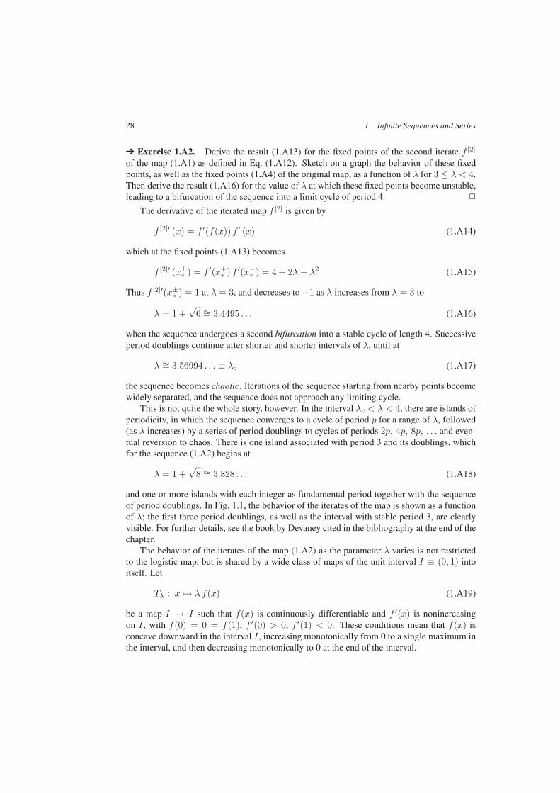
28 1 Infinite Sequences and Series
Exercise 1.A2. Derive the result (1.A13) for the fixed points of the second iterate f [2]
of the map (1.A1) as defined in Eq. (1.A12). Sketch on a graph the behavior of these fixedpoints, as well as the fixed points (1.A4) of the original map, as a function of λ for 3 ≤ λ < 4.Then derive the result (1.A16) for the value of λ at which these fixed points become unstable,leading to a bifurcation of the sequence into a limit cycle of period 4.
The derivative of the iterated map f [2] is given by
f [2]′ (x) = f ′(f(x)) f ′ (x) (1.A14)
which at the fixed points (1.A13) becomes
f [2]′ (x±∗ ) = f ′(x+∗ ) f ′(x−∗ ) = 4 + 2λ− λ2 (1.A15)
Thus f [2]′(x±∗ ) = 1 at λ = 3, and decreases to −1 as λ increases from λ = 3 to
λ = 1 +√
6 ∼= 3.4495 . . . (1.A16)
when the sequence undergoes a second bifurcation into a stable cycle of length 4. Successiveperiod doublings continue after shorter and shorter intervals of λ, until at
λ ∼= 3.56994 . . . ≡ λc (1.A17)
the sequence becomes chaotic. Iterations of the sequence starting from nearby points becomewidely separated, and the sequence does not approach any limiting cycle.
This is not quite the whole story, however. In the interval λc < λ < 4, there are islands ofperiodicity, in which the sequence converges to a cycle of period p for a range of λ, followed(as λ increases) by a series of period doublings to cycles of periods 2p, 4p, 8p, . . . and even-tual reversion to chaos. There is one island associated with period 3 and its doublings, whichfor the sequence (1.A2) begins at
λ = 1 +√
8 ∼= 3.828 . . . (1.A18)
and one or more islands with each integer as fundamental period together with the sequenceof period doublings. In Fig. 1.1, the behavior of the iterates of the map is shown as a functionof λ; the first three period doublings, as well as the interval with stable period 3, are clearlyvisible. For further details, see the book by Devaney cited in the bibliography at the end of thechapter.
The behavior of the iterates of the map (1.A2) as the parameter λ varies is not restrictedto the logistic map, but is shared by a wide class of maps of the unit interval I ≡ (0, 1) intoitself. Let
Tλ : x → λ f(x) (1.A19)
be a map I → I such that f(x) is continuously differentiable and f ′(x) is nonincreasingon I , with f(0) = 0 = f(1), f ′(0) > 0, f ′(1) < 0. These conditions mean that f(x) isconcave downward in the interval I , increasing monotonically from 0 to a single maximum inthe interval, and then decreasing monotonically to 0 at the end of the interval.
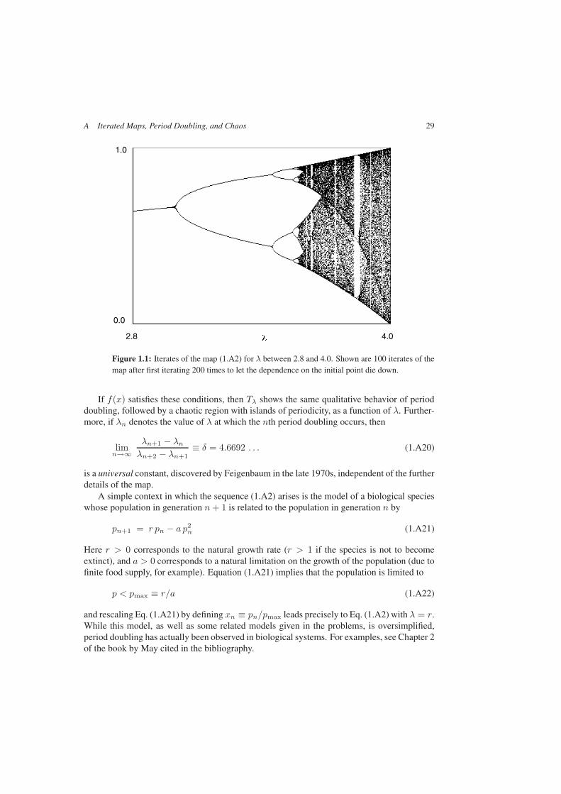
A Iterated Maps, Period Doubling, and Chaos 29
1.0
0.0
2.8 4.0
Figure 1.1: Iterates of the map (1.A2) for λ between 2.8 and 4.0. Shown are 100 iterates of themap after first iterating 200 times to let the dependence on the initial point die down.
If f(x) satisfies these conditions, then Tλ shows the same qualitative behavior of perioddoubling, followed by a chaotic region with islands of periodicity, as a function of λ. Further-more, if λn denotes the value of λ at which the nth period doubling occurs, then
limn→∞
λn+1 − λnλn+2 − λn+1
≡ δ = 4.6692 . . . (1.A20)
is a universal constant, discovered by Feigenbaum in the late 1970s, independent of the furtherdetails of the map.
A simple context in which the sequence (1.A2) arises is the model of a biological specieswhose population in generation n+ 1 is related to the population in generation n by
pn+1 = r pn − a p2n (1.A21)
Here r > 0 corresponds to the natural growth rate (r > 1 if the species is not to becomeextinct), and a > 0 corresponds to a natural limitation on the growth of the population (due tofinite food supply, for example). Equation (1.A21) implies that the population is limited to
p < pmax ≡ r/a (1.A22)
and rescaling Eq. (1.A21) by defining xn ≡ pn/pmax leads precisely to Eq. (1.A2) with λ = r.While this model, as well as some related models given in the problems, is oversimplified,period doubling has actually been observed in biological systems. For examples, see Chapter 2of the book by May cited in the bibliography.
30 1 Infinite Sequences and Series
Bibliography and Notes
The first three sections of this chapter are intended mainly as a review of topics that willbe familiar to students who have taken a standard advanced calculus course, and no specialreferences are given to textbooks at that level. A classic reference dealing with advancedmethods of analysis is
E. T. Whittaker and G. N. Watson, A Course of Modern Analysis (4th edition), Cam-bridge University Press (1958).
The first edition of this work was published in 1902 but it is valuable even today. In additionto its excellent and thorough treatment of the classical aspects of complex analysis and thetheory of special functions, it contains many of the notorious Cambridge Tripos problems,which the modern reader may find even more challenging than the students of the time!
A basic reference on theory of convergence of sequences and series is
Konrad Knopp, Infinite Sequences and Series, Dover (1956).
This compact monograph summarizes the useful tests for convergence of series, and gives acollection of elementary examples.
Two books that specialize in the study of asymptotic expansions are
A. Erdélyi, Asymptotic Expansions, Dover (1955), andN. Bleistein and R. A. Handelsman, Asymptotic Expansions of Integrals, Dover(1986).
The first of these is a concise survey of methods of generating asymptotic expansions, bothfrom integral representations and from differential equations. The second is a more compre-hensive survey of the various methods used to generate asymptotic expansions of functionsdefined by integral representations. It also has many examples of the physical and mathemat-ical contexts in which such integrals may occur. The book by Whittaker and Watson notedabove, the book on functions of a complex variable by Carrier, Krook, and Pierson in Chap-ter 4 and the book on advanced differential equations by Bender and Orszag cited in Chapter 5also deal with asymptotic expansions.
A readable introduction to the theory of bifurcation and chaos is
R. L. Devaney, An Introduction to Chaotic Dynamical Systems (2nd edition), West-view Press (2003).
Starting at the level of a student who has studied ordinary differential equations, this bookclearly explains the mathematical foundations of the phenomena that occur in the study ofiterated maps. A comprehensive introduction to chaos in discrete and continuous dynamicalsystems is
Kathleen T. Alligood, Tim D. Sauer, and James A. Yorke, Chaos: An Introductionto Dynamical Systems, Springer (1997).
Each chapter has a serious computer project at the end, as well as simpler exercises. A moreadvanced book is
Edward Ott, Chaos in Dynamical Systems, Cambridge University Press (1993).
Problems 31
Two early collections of reprints and review articles on the relevance of these phenomenato physical and biological systems are
R. M. May (ed.), Theoretical Ecology (2nd edition), Blackwell Scientific Publishers,Oxford (1981), andP. Cvitanoviç (ed.), Universality in Chaos (2nd edition), Adam Hilger Ltd., Bristol(1989).
The first of these is a collection of specially written articles by May and others on variousaspects of theoretical ecology. Of special interest here is the observation of the phenomenonof period doubling in ecosystems. The second book contains a collection of reprints of classicarticles by Lorenz, May, Hénon, Feigenbaum, and others, leading to the modern studies ofchaos and related behavior of dynamical systems, with some useful introductory notes byCvitanoviç.
The reader should be aware that the behavior of complex dynamical systems is an impor-tant area of ongoing research, so that it is important to look at the current literature to get anup-to-date view of the subject. Nevertheless, the concepts presented here and in later chaptersare fundamental to the field. Further readings with greater emphasis on differential equationsand partial differential equations are found at the end of Chapters 2 and 8.
Problems5
1. Show that
limn→∞
(1 +
z
n
)n=
∞∑
k=0
zk
k!(= ez)
2. Show that
ζ(s) =∏
p
(1 − 1
ps
)−1
where∏p denotes a product over all primes p.
3. Investigate the convergence of the following series:
(i)∞∑
n=1
1n− ln
(1 +
1n
)
(ii)∞∑
n=1
1 − n ln
(2n+ 12n− 1
)
(iii)∞∑
n=2
1na (lnn)b
Explain how convergence depends on the complex numbers a, b in (iii).
5When a proposition is simply stated, the problem is to prove it, or to give a counterexample that shows it is false.
32 1 Infinite Sequences and Series
4. Investigate the convergence of the following series:
(i)∞∑
n=0
(n+ 1)a zn
(ii)∞∑
n=0
(n+ n1)! (n+ n2)!n! (n+ n3)!
zn
(iii)∞∑
n=0
e−na cos(bn2z)
where a, b are real numbers, n1, n2, n3 are positive integers, and z is a (variable) complexnumber. How do the convergence properties depend on a, b, z ?
5. Find the sums of the following series:
(i) S = 1 +14− 1
16− 1
64+
1256
+ · · ·
(ii) S =1
1 · 3 +1
2 · 4 +1
3 · 5 +1
4 · 6 + · · ·
(iii) S =10!
+21!
+32!
+43!
+ · · ·
(iv) f(z) =∞∑
n=0
(−1)n(n+ 1)2
(2n+ 1)!z2n+1
6. Find a closed form expression for the sums of the series
Sp ≡∞∑
n=1
1n(n+ 1) · · · (n+ p)
(p = 0, 1, 2, . . .).
Remark. The result obtained here can be used to improve the rate of convergence ofa series whose terms tend to zero like 1/np+1 for large n; subtracting a suitably chosenmultiple of Sp from the series will leave a series whose terms tend to zero at least asfast as 1/np+2 for large n. As a further exercise, apply this method to accelerate theconvergence of the series for the ζ-function ζ(p) with p integer.
7. The quantum states of a simple harmonic oscillator with frequency ν are the states |n〉with energies
En = (n+ 12 )hν

Problems 33
(n = 0, 1, 2, . . .) where h is Planck’s constant. For an ensemble of such oscillators inthermal equilibrium at temperature T , the probability of finding an oscillator in the state|n〉 is given by
Pn = A exp(− EnkT
)
where A is a constant to be determined, and the exponential factor is the standard Boltz-mann factor.
(i) Evaluate the constant A by requiring
∞∑
0
Pn = 1
(ii) Find the average energy 〈E(T )〉 of a single oscillator of the ensemble.
Remark. These results are used in the study of blackbody radiation in Problem 4.9.
8. Investigate the convergence of the following products:
(i)∞∏
m=1
m(m+ a+ b)(m+ a)(m+ b)
(ii)∞∏
m=1
(1 − z2
m2
)
where a, b are the real numbers and z is a (variable) complex number.
9. Evaluate the infinite product
∞∏
m=1
1 + exp(iω/2m)
2
Hint. Note that 1 + e12 iω = (1 − eiω)/(1 − e
12 iω).
10. Evaluate the infinite products
(i)∞∏
n=1
1 − 1
(n+ 1)2
(ii)∞∏
n=2
(n3 − 1n3 + 1
)
11. Show that∞∏
m=0
(1 + z2m
)=
11 − z
34 1 Infinite Sequences and Series
12. The Euler–Mascheroni constant γ is defined by
γ ≡ limN→∞
N∑
n=1
1n− ln(N + 1)
(i) Show that γ is finite (i.e., the limit exists). Hint. Show that
γ = limN→∞
N∑
n=1
1n− ln
(1 +
1n
)
(ii) Show that
N∑
n=1
1n
=∫ 1
0
1 − (1 − t)N
tdt
(iii) Show that∫ 1
0
(1 − e−t
t
)dt−
∫ ∞
1
e−t
tdt = γ
13. The error function erf(z) is defined by
erf(z) ≡ 2√π
∫ z
0
e−t2dt
(i) Find the power series expansion of erf(z) about z = 0.
(ii) Find an asymptotic expansion of erf(z) valid for z large and positive. For what rangeof arg z is this asymptotic series valid?
(iii) Find an asymptotic expansion of erf(z) valid for z large and negative. For whatrange of arg z is this asymptotic series valid?
14. Find an asymptotic power series expansion of
f(z) ≡∫ ∞
0
e−zt
1 + t2dt
valid for z large and positive. For what range of arg z is this expansion valid? Give anestimate of the error in truncating the series after N terms.
15. Find an asymptotic power series expansion of
f(z) ≡∫ ∞
0
(1 +
t
z
)αe−zt dt
valid for z large and positive (here α is a complex constant). For what range of arg z isthis expansion valid? Give an estimate of the error in truncating the series after N terms.
Problems 35
16. The modified Bessel function Kλ(z) of order λ is defined by the integral representation
Kλ(z) =∫ ∞
0
e−z cosh t cosh λt dt
(i) Find an asymptotic expansion of Kλ(z) valid for z → ∞ in the right half-plane withλ fixed.
(ii) Find an asymptotic expansion of Kλ(z) for λ → ∞ with z fixed in the right half ofthe complex plane (Re z > 0).
17. Find an asymptotic expansion of
f(z) ≡∫ ∞
0
e−zt−1/t dt
valid for z large and positive.
18. The reaction rate for the fusion of nuclei A and B in a hot gas (in the center of a star, forexample) at temperature T can be expressed as
R(T ) =C
(kT )32
∫ ∞
0
S(E) exp(− b√
E− E
kT
)dE (*)
where S(E) is often a smoothly varying function of the relative energy E. The ex-ponential factor exp(−E/kT ) in (∗) is the usual Boltzmann factor, while the factorexp(−b/
√E) is the probability of tunneling through the energy barrier created by the
Coulomb repulsion between the two nuclei. The constant b is given by
b =ZAZBe
2
√2mAmB
mA +mB
wheremA,mB are the masses, ZAe, ZBe the charges of the two nuclei, and is Planck’sconstant.
(i) Find the energy E∗ = E∗(T ) at which the integrand in (∗) is a maximum, neglectingthe energy dependence of S(E).
(ii) Find the width ∆ = ∆(T ) of the peak of the integrand near E∗, again neglecting theenergy dependence of S(E).
(iii) Find an approximate value for R(T ), assuming ∆ E∗.
Remark. A detailed discussion of nuclear reaction rates in stars can be found in
C. E. Rolfs and W. S. Rodney, Cauldrons in the Cosmos: Nuclear Astrophysics,University of Chicago Press (1988).
among many other books on the physics of stars.
19. Find the value(s) of λ for which the fixed points of the iterated logistic map (Eq. (1.A12))are superstable.
36 1 Infinite Sequences and Series
20. Consider the sequence xn defined by
xn+1 = αxn(1 − x2n)
Find the fixed points of this sequence, and the ranges of α for which each fixed point isstable. Also find the values of α for which there is a superstable fixed point.
21. Consider the sequence xn defined by
xn+1 = xn eλ(1−xn)
with λ > 0 real, and x0 > 0.
(i) For what range of λ is xn bounded?
(ii) For what range of λ is xn convergent? Find the limit of the sequence, as a functionof λ.
(iii) What can you say about the behavior of the sequence for λ > λ0, where λ0 is thelargest value of λ for which the sequence converges?
(iv) Does the map
Tλ : x → x eλ(1−x)
have any fixed point(s)? What can you say about the stability of the fixed point(s) forvarious values of λ?
22. Consider the sequence xn defined by
xn+1 =r xn
(1 + xn)b
with b, r > 0 real, and x0 > 0.
(i) For what range of b, r is xn bounded for all x > 0?
(ii) For what range of b, r is xn convergent? Find the limit of the sequence (as afunction of b, r).
(iii) What can you say about the behavior of the sequence outside the region in the b–rplane for which the sequence converges?
(iv) Does the map
Tr,b : x → r x
(1 + x)b
have any fixed point(s)? What can you say about the stability of the fixed point(s) forvarious values of b, r?
2 Finite-Dimensional Vector Spaces
Many physical systems are described by linear equations. The simple harmonic oscillator isthe first example encountered by most students of physics. Electrical circuits with resistance,capacitance, and inductance are linear systems with many independent variables. Maxwell’sequations for the electromagnetic fields, the heat equation and general wave equations arelinear (partial) differential equations. A universal characteristic of systems described by linearequations is the superposition principle, which states that any linear superposition of solutionsto the equations is also a solutions of the equations. The theory of linear vector spaces andlinear operators provides a natural and elegant framework for the description of such systems.
In this chapter, we introduce the mathematical foundations of the theory of linear vectorspaces, starting with a set of axioms that characterize such spaces. These axioms describeaddition of vectors, and multiplication of vectors by scalars. Here scalars may be real orcomplex numbers; the distinction between real and complex vector spaces is important whensolutions to algebraic equations are needed. A basis is a set of linearly independent vectorssuch that any vector can be expressed as a linear combination of the basis vectors; the co-efficients are the components, or coordinates, of the vector in the basis. If the basis vectorsform a finite set with n elements, then the vector space is finite dimensional (dimension n);otherwise, it is infinite dimensional. With coordinates introduced, every n-dimensional vectorspace can be identified with the space of ordered n-tuples of scalars. In this chapter, we con-sider mainly finite-dimensional vector spaces, though we also treat function spaces as vectorspaces in examples where dimensionality is not critical. The complications associated withinfinite-dimensional spaces, especially Hilbert spaces, will appear in Chapters 6 and 7.
Here we consider only vector spaces in which nonzero vectors have a positive definitelength (or norm); the distance between two vectors x and y is the length of the vector x − y.If a scalar product satisfying natural axioms can also be defined, the vector space is unitary.Any basis of a unitary vector space can be transformed into a set of mutually orthogonal unitvectors; vector components are then the projections of the vector onto the unit vectors.
A scalar-valued function defined on a vector space or function space is called a functional.Many functionals can be defined on function spaces, for example, the action integral of clas-sical mechanics to be considered in Chapter 3. Linear functionals defined on a linear vectorspace V are of special interest; they form another linear vector space, the dual space V∗ of V .An important result is that a bounded linear functional Λ on a unitary vector space has theform of a scalar product, Λ[x] = (u, x) with u a vector in the space, so that V and V∗ areequivalent. Linear functionals defined on function spaces are also known as distributions;a notable example is the Dirac δ-function introduced in Chapter 1, defined here as a linearfunctional on the space of continuous functions.
Introduction to Mathematical Physics. Michael T. VaughnCopyright c© 2007 WILEY-VCH Verlag GmbH & Co. KGaA, WeinheimISBN: 978-3-527-40627-2
Introduction to Mathematical Physics
Michael T. Vaughn 2007 WILEY-VCH Verlag GmbH & Co.
38 2 Finite-Dimensional Vector Spaces
Linear operators on a linear vector space arise in many contexts. A system of n linearalgebraic equations
a11x1 + a12x2 + · · · + a1nxn = c1a21x1 + a22x2 + · · · + a2nxn = c2
...an1x1 + an2x2 + · · · + annxn = cn
can be written in the short form
Ax = c
in which x denotes a vector in an n-dimensional space (real or complex), c is a known vector,and A is an n × n matrix. If the determinant of the matrix A is not equal to zero, theseequations have a unique solution for every c.
In general, a linear operator A on a linear vector space is defined by the property that ifx1 and x2 are vectors and c1 and c2 are scalars, then
A(c1x1 + c2x2) = c1Ax1 + c2Ax2
Then if we know how A acts on a set of basis vectors, we can define the action of A on anylinear combination of the basis. A linear operator is also known as a linear transformation.
Important characteristics of a linear operator are its domain (the space on which it is de-fined) and its image, or range (the space into which it maps its domain). The domain of alinear operator A on a finite-dimensional vector space Vn can always be extended to includethe entire space, and A can then be represented by an n × n matrix. The theory of linearoperators on Vn is thus equivalent to the theory of finite-dimensional matrices. Questions ofdomain and image are more subtle in infinite-dimensional spaces (see Chapter 7).
For a linear operator A on a finite-dimensional space we have the alternatives(i) A is nonsingular: A defines a one-to-one map of Vn onto itself, and the equation
Ax = y has a unique solution x = A−1y, or(ii) A is singular: the homogeneous equation Ax = 0 has a nontrivial solution, and Vn
is mapped into a smaller subspace of itself by A.The first alternative requires that the determinant of the matrix representing A be nonzero; thesecond, that the determinant vanishes.
The homogeneous equation
Ax = λx
has solutions only for discrete values of λ, the eigenvalues (characteristic values) of A; thecorresponding solutions are the eigenvectors of A. The eigenvalues of a linear operator Adefine the spectrum of A; in many applications, determining the spectrum of an operator iscritical, as we shall see. In a finite-dimensional space Vn, the eigenvalues are obtained bysolving the characteristic equation
det ‖A − λ1‖ ≡ pA(λ) = 0
in which pA(λ) is a polynomial of degree n in λ, the characteristic polynomial of A.
2 Finite-Dimensional Vector Spaces 39
The adjoint A† of a linear operator A on V can be defined as a linear operator on the dualspace V∗. If V is a unitary vector space, then A† is a linear operator on V itself; then A isself-adjoint, or Hermitian, if A† = A. A projection operator projects vectors onto a linearsubspace. Unitary operators transform an orthonormal basis into another orthonormal basis;the length of a vector and the scalar product between two vectors are unchanged by a unitarytransformation. A unitary operator on a real vector space is simply a rotation, or orthogonaltransformation. Explicit matrix representations are constructed for rotations in two and threedimensions.
Self-adjoint operators play a special role in quantum mechanics. States of a quantummechanical system are represented as vectors in a unitary vector space V , and the physicalobservables of the system by self-adjoint operators on V . The eigenvalues of an operator cor-respond to the allowed values of the observables in states of the system, and the eigenvectorsof the operator to states in which the observable has the corresponding eigenvalue. Espe-cially important is the operator corresponding to the Hamiltonian of a system; its eigenvaluescorrespond to the allowed energy levels of the system.
A question of general interest is whether an operator has eigenvalues and eigenvectors. Itturns out that a general linear operator A on the finite-dimensional space Vn has the form
A = D + N
where D is a diagonalizable operator (one with a diagonal matrix representation in some basis)whose eigenvalues are the eigenvalues of A, and N is a nilpotent operator (Np = 0 for someinteger p) and DN = ND. The spectral properties of operators on an infinite-dimensionalspace are more complicated in general, and are discussed in Chapter 7.
An important class of linear operators on a unitary vector space V is normal operators; Ais a normal operator if
A†A = AA†
In a finite-dimensional space, it is true that every normal operator has a complete orthonormalsystem of eigenvectors, which leads to the spectral representation
A =∑
k
λkPk
where the λk are the eigenvalues of A and the Pk are the projection operators ontoorthogonal subspaces such that
∑
k
Pk = 1
A is diagonal in the basis defined by the eigenvectors; hence N = 0 for normal operators.If A is normal, and λ is an eigenvalue of A, then λ∗ is an eigenvalue of A†. Self-adjointoperators are normal, with real eigenvalues; unitary operators are normal, with eigenvalueslying on the unit circle in the complex λ-plane.
40 2 Finite-Dimensional Vector Spaces
The eigenvalues of a self-adjoint operator have minimax properties that lead to usefulapproximation methods for determining the spectra. These methods are based on the funda-mental result: if A is a self-adjoint operator on the n-dimensional space Vn, with eigenvaluesordered so that λ1 ≤ λ2 ≤ · · · ≤ λn, and if A′ is the restriction of A to a subspace ofdimension m < n, with eigenvalues λ′1 ≤ λ′2 ≤ · · · ≤ λ′m similarly ordered, then
λh ≤ λ′h ≤ λh+n−m
(h = 1, . . . ,m). Thus the eigenvalues of the restricted operator provide bounds on the eigen-values of the full operator. The inequalities λh ≤ λ′h remain true in an infinite-dimensionalspace for self-adjoint operators with a discrete spectrum.
Many quantum mechanics textbooks use thus result to derive a variational method forestimating the ground state energy of a system, which is lower than the lowest eigenvalue ofany restriction of the Hamiltonian operator of the system to a subspace of the state space ofthe system. Beyond that, however, the nth lowest eigenvalue of the restricted Hamiltonian isan upper bound to the nth lowest eigenvalue of the full Hamiltonian, so the method providesan upper bound for the energies of excited states as well.
Functions of operators can be defined in terms of power series expansions, and by othermethods when the spectrum of the operator is known. One example is the exponential func-tion, which is used to provide a formal solution
x(t) = etAx(0)
to the linear differential equation
dx
dt= Ax
with constant coefficients, starting from x(0) at t = 0.This solution is applied in Section 2.5 to the study of linear dynamical systems, which
are described exactly by this equation, with time as the independent variable. The qualita-tive behavior of the system is determined by the spectrum of A. Components of x(0) alongeigenvectors belonging to eigenvalues with negative real part decrease exponentially with in-creasing t, and are irrelevant to the behavior of the system at large time. Eigenvalues of Athat are purely imaginary correspond to oscillatory modes of the system, with closed orbitsand definite frequencies. If any eigenvalue of A has a positive real part, any component of theinitial state x(0) along the associated eigenvector grows exponentially in time, and the systemis unstable.
Real physical systems are rarely exactly linear, but the behavior near an equilibrium pointof the system is often well approximated by a linear model. For an energy-conserving system,this gives small oscillations with well-defined characteristic frequencies that are analyzed inAppendix A. Instabilities can be present in systems that do not conserve energy, but exponen-tial growth is a signal that the linear theory is no longer valid. There is some discussion ofnonlinear systems in Chapter 8 as well as in books cited in the bibliography.
2.1 Linear Vector Spaces 41
2.1 Linear Vector Spaces
2.1.1 Linear Vector Space Axioms
A linear vector space V is a collection of vectors such that if x and y are vectors in V , then sois any linear combination of the form
u = ax+ by (2.1)
where a and b are numbers (scalars). V is real or complex, depending on whether scalars aretaken from the real numbers R or the complex numbers C (in mathematics, scalars can betaken from any field, but here we are only concerned with real and complex vector spaces).
Addition of vectors, and multiplication by scalars must satisfy a natural set of axioms.Addition of vectors must be commutative:
x+ y = y + x (2.2)
for all x and y. Multiplication by scalars must satisfy the associative law:
a(bx) = (ab)x (2.3)
and the distributive laws:
a(x+ y) = ax+ ay (a+ b)x = ax+ bx (2.4)
for all a, b, x, and y. There must also be a zero vector (denoted by θ when it is necessary todistinguish it from the scalar 0) such that
x+ θ = x (2.5)
for all x, and for every vector x there must be a vector −x (negative x) such that
x+ (−x) = θ (2.6)
Exercise 2.1. Show that the axioms (2.2)–(2.6) imply that
1 · x = x 0 · x = θ
for all x. Hint. Use the distributive laws.
Definition 2.1. A vector of the form a1x1 + . . .+akxk is a linear combination of the vectorsx1, . . . , xk (here the coefficients a1, . . . , ak are scalars). The vectors x1, . . . , xk are linearlydependent if there is a nontrivial linear combination of the vectors that vanishes, that is, ifthere are coefficients a1, . . . , ak, not all zero, such that
a1x1 + . . .+ akxk = θ (2.7)
If no such coefficients exist, then the vectors x1, . . . , xk are linearly independent.
42 2 Finite-Dimensional Vector Spaces
If the vectors x1, . . . , xk are linearly dependent, then we can express at least one of themas a linear combination of the others. For suppose we have a linear combination of the vectorsthat vanishes, as in Eq. (2.7), with at least one nonvanishing coefficient. Then we can takea1 = 0 (renumbering the vectors if necessary) and solve for x1 to get
x1 = −a2
a1x2 − · · · − an
a1xn (2.8)
Definition 2.2. A linear manifold M in the linear vector space V is a set of elements of Vsuch that if x, y are in M, then so is the linear combination ax+ by for any scalars a and b.
Thus M is itself a linear vector space, a subspace of V . If we have a set x1, . . . , xk ofelements of V , then we can define the linear manifold M ≡ M(x1, . . . , xk), the manifoldspanned by x1, . . . , xk, as the set of all linear combinations of x1, . . . , xk.
Definition 2.3. The vectors x1, . . . , xk form a basis of the linear manifold M if (i) the vec-tors x1, . . . , xk are linearly independent and (ii) the manifold M is spanned by the x1, . . . , xk.If M has a basis with k elements, then k is the dimension of M. If M has no basis with afinite number of elements, then M is infinite dimensional.
Example 2.1. The set of continuous functions on an interval a ≤ x ≤ b forms a linearvector space C(a, b), with addition and multiplication by scalars defined in the naturalway. The monomials 1, x, x2, x3, . . . are linearly independent; hence C(a, b) is infinitedimensional.
The concept of dimension is important, the more so because it uniquely characterizes alinear vector space: if x1, . . . , xk and y1, . . . , ym are two bases of M, then k = m. To showthis, suppose that m > k. Then each of the vectors y1, . . . , ym can be expressed in terms ofthe basis x1, . . . , xk as
yp = ap1x1 + · · · + apkxk (2.9)
(p = 1, . . . ,m). But the first k of these equations can be solved to express the x1, . . . , xk interms of y1, . . . , yk (if the determinant of the coefficients were zero, then a linear combinationof y1, . . . , yk would be zero), and the remaining yk+1, . . . , ym can be expressed in terms ofthe x1, . . . , xk. Since this is inconsistent with the assumption that the y1, . . . , ym are linearlyindependent, we must have m = k.
It follows that if we have an n-dimensional vector space Vn, then any set of n linearlyindependent vectors x1, . . . , xn forms a basis of Vn, and any vector x in Vn can be expressedas a (unique) linear combination
x = a1x1 + . . .+ anxn (2.10)
The coefficients a1, . . . , an in this expansion are the components of the vector x (with respectto the basis x1, . . . , xn); we have a one-to-one correspondence between vectors and orderedn-tuples (a1, . . . , an) of scalars. Evidently this correspondence depends on the basis chosen;the components of a vector depend on the coordinate system.
2.1 Linear Vector Spaces 43
2.1.2 Vector Norm; Scalar Product
We introduce the length, or norm of a vector x, to be denoted by ‖x‖. The norm shouldbe positive definite, that is, ‖x‖ ≥ 0 for any vector x, and ‖x‖ = 0 if and only if x = θ.Once length is defined, the distance between two vectors x and y is defined by ‖x− y‖. Thisdistance should satisfy as an axiom the triangle inequality:
∣∣∣∣‖x‖ − ‖y‖∣∣∣∣ ≤ ‖x− y‖ ≤ ‖x‖ + ‖y‖ (2.11)
with equality if and only if y = ax for some real a; these inequalities are satisfied by thesides of any triangle in the Euclidean plane. With this norm, definitions of open, closed, andbounded sets, and limit points of sets and sequences in a vector space can be made by analogywith the definitions in Chapter 1 for real and complex numbers.
A scalar product of two vectors x, y must satisfy axioms of Hermitian symmetry:
(y, x) = (x, y)∗ (2.12)
and bilinearity:
(y, a1x1 + a2x2) = a1(y, x1) + a2(y, x2) (2.13)
(b1y1 + b2y2, x) = b∗1(y1, x) + b∗2(y2, x) (2.14)
If such a scalar product exists, then a standard norm is defined by
‖x‖2 ≡ (x, x) (2.15)
A vector space with scalar product satisfying axioms (2.12)–(2.14) is unitary. These axiomscorrespond to standard properties of three-dimensional vectors, apart from the presence of thecomplex conjugate. The complex conjugate is needed to make the norm positive definite ina complex vector space, since if z is a complex number, then |z|2 = z∗z is positive definite,while z2 is not.
Remark. We are concerned here mainly with unitary spaces, but there are spaces withpositive definite norm that satisfy the triangle inequality with no scalar product. For example,the length of a vector x = ξ1, . . . , ξn can be defined for any p ≥ 1 by
‖x‖ ≡(
n∑
k=1
|ξk|p) 1
p
(2.16)
(Check that this satisfies the triangle inequality.) This space is denoted by p; only for p = 2can a scalar product satisfying the axioms be defined on p.
Remark. A physically interesting space with a length defined that is not positive definiteis the four-dimensional spacetime in which we live, with its standard (Minkowski) metric.Spacelike and timelike vectors have norm-squared of opposite sign, and there are nonzerovectors with zero norm (lightlike vectors). Spaces with such indefinite metrics will be dis-cussed later.
44 2 Finite-Dimensional Vector Spaces
Definition 2.4. The vectors x and y in a unitary vector space are orthogonal if and only if
(x, y) = 0 (2.17)
The vectors x1, . . . , xm form an orthogonal system if
(xk, xl) = 0 (2.18)
for all k = l. The vector φ is a unit vector if ‖φ‖ = 1. The vectors φ1, . . . , φm form anorthonormal system if
(φk, φl) = δkl =
1, k = l
0, k = l(2.19)
The vectors in an orthonormal system are mutually orthogonal unit vectors; they are espe-cially convenient to use as a basis for a coordinate system. If the vectors φ1, . . . , φm form anorthonormal system, then the components a1, . . . , am of a vector
x = a1φ1 + . . .+ amφm (2.20)
are given simply by ak = (φk, x), and we can write
x = (φ1, x)φ1 + · · · + (φm, x)φm (2.21)
It is clear from this that the vectors in an orthonormal system are linearly independent, sincethe only linear combination of φ1, . . . , φm that vanishes necessarily has vanishing coefficients.Even if x cannot be expressed as a linear combination of φ1, . . . , φm , it is still true that
m∑
k=1
|(φk, x)|2 ≤ ‖x‖2 (2.22)
(Bessel’s inequality), since it follows from the positivity condition that
‖x−m∑
k=1
(φk, x)φk ‖2 = ‖x‖2 −m∑
k=1
|(φk, x)|2 ≥ 0 (2.23)
Note that the equality holds if and only if
x =m∑
k=1
(φk, x)φk (2.24)
Bessel’s inequality leads directly to the Schwarz inequality: if x, y are any two vectors, then
|(x, y)| ≤ ‖x‖ ‖y‖ (2.25)
with equality if and only if y is a scalar multiple of x. To show this, simply consider the unitvector φ ≡ y/‖y‖ and apply Bessel’s inequality.
2.1 Linear Vector Spaces 45
Remark. The Schwarz inequality corresponds to the bound | cosϑ| ≤ 1 for real angles ϑ,since for real vectors it is generally true that
(x, y) = ‖x‖ ‖y‖ cosϑ (2.26)
where ϑ is the angle between x and y.
An orthonormal system φ1, . . . , φm can be constructed from linearly independent vectorsx1, . . . , xm by a standard method known as the Gram–Schmidt orthogonalization process: let
φ1 =x1
‖x1‖(2.27)
and then let
ψk ≡ xk −k−1∑
p=1
(φp, xk)φp φk ≡ ψk‖ψk‖
(2.28)
(k = 2, . . . ,m). It is easy to see that the φ1, . . . , φm form an orthonormal system, since noneof the ψk can vanish due to the assumed linear independence of the xk. Furthermore, thelinear manifolds defined are the same at each stage of the process, that is,
M(φ1) = M(x1)M(φ1, φ2) = M(x1, x2)
...M(φ1, φ2, . . . , φm) = M(x1, x2, . . . , xm)
(2.29)
We can now introduce the concept of a complete orthonormal system.
Definition 2.5. The orthonormal system φ1, φ2, . . . is complete if and only if the only vectororthogonal to every φk is the zero vector; i.e., (φk, x) = 0 for all k if and only if x = θ.
This definition has been carefully stated to remain valid in an infinite-dimensional space,though the existence of a basis in the infinite-dimensional case requires an additional axiom.If a basis exists, as it must in a finite-dimensional space, then it can be made into a completeorthonormal system by the Gram–Schmidt process. Properties of a vector can be expressed interms of its components with respect to this complete orthonormal system in a standard way.
Theorem 2.1. The orthonormal system φ1, . . . , φm in the n-dimensional linear vector spaceVn is complete if and only if
(i) m = n,(ii) φ1, . . . , φm is a basis of Vn,(iii) for every vector x in Vn, we have
‖x‖2 =m∑
k=1
|(φk, x)|2 (2.30)
(iv) for every pair of vectors x and y in Vn, we have
(x, y) =m∑
k=1
(x, φk)(φk, y) (2.31)
46 2 Finite-Dimensional Vector Spaces
Any one of these conditions is necessary and sufficient for all of them. The conditions notalready been dealt with explicitly can be verified from expansion (2.21).
Example 2.2. The space Rn of ordered n-tuples of real numbers of the form (x1, . . . , xn)is a real n-dimensional vector space. Addition and multiplication by scalars are defined inthe obvious way: if x = (x1, . . . , xn) and y = (y1, . . . , yn), then
ax+ by = (ax1 + by1, . . . , axn + byn) (2.32)
The scalar product can be defined by
(x, y) =n∑
k=1
xkyk (2.33)
(this definition is not unique—see Exercise 2.2). The vectors
φ1 = (1, 0, . . . , 0)φ2 = (0, 1, . . . , 0) (2.34)
...
φn = (0, 0, . . . , 1)
define a complete orthonormal system, and the xk and yk are just the components of x andy with respect to this complete orthonormal system.
Example 2.3. The space Cn of ordered n-tuples of complex numbers of the form(ξ1, . . . , ξn) is an n-dimensional complex vector space. Addition and multiplication byscalars are defined in the obvious way: if x = (ξ1, . . . , ξn) and y = (η1, . . . , ηn), then
ax+ by = (aξ1 + bη1, . . . , aξn + bηn) (2.35)
The scalar product can be defined by
(x, y) =n∑
k=1
ξ∗kηk (2.36)
Note the presence of the complex conjugate of the components of the vector on the leftside of the scalar product; this is necessary to ensure positive definiteness of the norm,which is here given by
‖x‖2 =n∑
k=1
|ξk|2 (2.37)
The complete orthonormal system φ1, φ2, . . . , φn defined in the previous example is alsoa complete orthonormal system in Cn. In Cn, however, the scalars (and hence the com-ponents) are complex.
2.1 Linear Vector Spaces 47
In a sense, the preceding two examples are the only possibilities for real or complex n-dimensional vector spaces. If there is a one-to-one map between two linear vector spaces Uand V such that if u1 ↔ v1 and u2 ↔ v2 under the map, then
au1 + bu2 ↔ av1 + bv2 (2.38)
for any scalars a and b (U and V must have the same scalars), then U and V are isomorphic,and the corresponding map is an isomorphism. If in addition, the vector spaces are unitary and
(u1, u2) = (v1, v2) (2.39)
whenever u1 ↔ v1 and u2 ↔ v2 under the map, then the map is an isometry, and the spacesare isometric. It is clear that any n-dimensional real vector space is isomorphic to Rn, andany n-dimensional complex vector space is isomorphic to Cn. If we identify a vector in then-dimensional vector space Vn with the n-tuple defined by its components with respect tosome fixed basis, then we have an isomorphism between Vn and Rn (or between Vn and Cn
if Vn is complex). If Vn is unitary, then the isomorphism can be extended to an isometry.
Exercise 2.2. Consider the linear vector space Cn with the scalar product of x =(ξ1, . . . , ξn) and y = (η1, . . . , ηn), defined by
(x, y) =n∑
k=1
ξ∗kwkηk
What restrictions must be put on the wk in order that Cn, with this scalar product, be a unitaryvector space? If these restrictions are satisfied, denote the corresponding unitary vector spaceby Cn(w1, . . . , wn). Construct an explicit map between Cn(w1, . . . , wn) and the standardCn that is both an isomorphism and an isometry.
2.1.3 Sum and Product Spaces
We can join two linear vector spaces U and V together to make a new vector space W ≡ U⊕V ,the direct sum of U and V . Take ordered pairs 〈u, v〉 of vectors with u from U and v from V ,and define
a 〈u1, v1〉 + b 〈u2, v2〉 ≡ 〈au1 + bu2, av1 + bv2〉 (2.40)
This defines U ⊕ V as a linear vector space. If U and V are unitary, define the scalar productin U ⊕ V by
(〈u1, v1〉, 〈u2, v2〉) ≡ (u1, u2) + (v1, v2) (2.41)
where the first scalar product on the right-hand side is taken in U and the second is taken in V .This defines U ⊕ V as a unitary vector space.
Exercise 2.3. Let U and V be a linear vector spaces of dimensions m and n, respectively.Show that the dimension of the direct sum U ⊕ V is given by dim(U ⊕ V) = m+ n.

48 2 Finite-Dimensional Vector Spaces
Exercise 2.4. If U and V are linear vector spaces with the same scalars, then the tensorproduct W ≡ U ⊗V is defined as follows: start with ordered pairs 〈u, v〉 ≡ u⊗v of vectors ufrom U and v from V , and include all linear combinations of the form
∑
k,l
akl uk ⊗ vl (*)
with the uk from U and the vl from V . If U , V are unitary, define a scalar product onU ⊗ V by
(u1 ⊗ v1, u2 ⊗ v2) ≡ (u1, u2)(v1, v2)
and by bilinearity for linear combinations of the type (∗).(i) Show that if φ1, φ2, . . . is an orthonormal system in U and ψ1, ψ2, . . . is an orthonormal
system in V , then the vectors
Φkl ≡ φk ⊗ ψl
form an orthonormal system in U ⊗ V . The Φkl form a complete orthonormal system inU ⊗ V if and only if the φk are complete in U and the ψl are complete in V .
(ii) Show that if dim U = m and dim V = n, then dim(U ⊗ V) = mn.(iii) Does every vector in U ⊗ V have the form u⊗ v with u from U and v from V?
If M is a linear manifold in the unitary vector space V , the orthogonal complement of M,denoted by M⊥, is the set of all vectors x in V such that (y, x) = 0 for all y in M. Thus M⊥
contains the vectors that are orthogonal to every vector in M. If M is finite dimensional, thenevery vector x in V can be decomposed according to
x = x′ + x′′ (2.42)
where x′ is in M (x′ is the projection of x onto M), and x′′ is in M⊥. This result is knownas the projection theorem; it is equivalent to expressing V as the direct sum
V = M⊕M⊥ (2.43)
To prove the theorem, let φ1, . . . , φm be an orthonormal basis of M (such a basis exists sinceM is finite dimensional). Then define
x′ ≡m∑
k=1
(φk, x)φk x′′ ≡ x− x′ (2.44)
This provides the required decomposition.
Exercise 2.5. Let M be a finite-dimensional linear manifold in the unitary vector space(M need not be finite dimensional here). Then (M⊥)⊥ = M.

2.1 Linear Vector Spaces 49
2.1.4 Sequences of Vectors
We are also interested in sequences of vectors and their convergence properties. In a finite-dimensional vector space Vn with a norm, these properties are directly related to those ofsequences in the field of scalars. We define a Cauchy sequence to be a sequence x1, x2, . . .of vectors such that for every ε > 0 there is an integer N such that ‖xp − xq‖ < ε wheneverp, q > N . The sequence x1, x2, . . . converges if there is a vector x such that for every ε > 0there is an integer N such that ‖xp − x‖ < ε whenever p > N . These definitions parallel thedefinitions for sequences of real and complex numbers given in Chapter 1.
If we represent a vector in Vn by its components ξ1, . . . , ξn with respect to some basis,then the sequence x1, x2, . . . of vectors is a Cauchy sequence if and only if each of the se-quences ξ1k, ξ2k, . . . , ξnk is a Cauchy sequence. Here ξpk denotes the pth componentof the vector xk. To see this in a unitary space with a complete orthonormal system given byφ1, . . . , φn, suppose
xk =n∑
p=1
ξkpφp (2.45)
Then, since
‖xk − xm‖2 =n∑
p=1
|ξkp − ξmp|2 (2.46)
it follows that the sequence of vectors is a Cauchy sequence if and only if each of the se-quences of components is a Cauchy sequence. In Vn, every Cauchy sequence of vectorsconverges to a limit vector because the corresponding Cauchy sequences of the componentsmust converge (recall that this is how the real and complex number systems were constructedfrom the rationals).
It is not so simple in an infinite-dimensional space; a sequence φ1, φ2, . . . of orthonor-mal vectors is not a Cauchy sequence, yet each sequence of components of these vectorsconverges to zero, which leads to the concept of weak convergence in an infinite-dimensionalspace. This and other subtleties will be discussed in Chapter 6.
2.1.5 Linear Functionals and Dual Spaces
Definition 2.6. A function defined on a linear vector space V that takes on scalar values iscalled a functional, or distribution, on V . The functional Λ is a linear functional if
Λ[ax+ by] = aΛ[x] + bΛ[y] (2.47)
for all vectors x, y and scalars a, b. The functional Λ is bounded if there is some positiveconstant C such that
|Λ[x]| ≤ C‖x‖ (2.48)
for every vector x in V . The smallest C for which this is true is the bound |Λ| of Λ.
50 2 Finite-Dimensional Vector Spaces
Theorem 2.2. If Λ is a linear functional on the finite-dimensional unitary vector space Vn,then there is a vector u in Vn such that Λ has the form of a scalar product
Λ[x] = (u, x) ≡ Λu[x] (2.49)
Proof. If φ1, . . . , φn is a complete orthonormal system in Vnand Λ[φk] = ak, then
Λφ = Λ∑
k
ξkφk =∑
k
akξk = (u, φ) (2.50)
with (note the complex conjugation here)
u =∑
k
a∗kφk (2.51)
It follows that every linear functional on Vn is bounded, with |Λu| = ‖u‖, since
|(u, x)| ≤ ‖u‖‖x‖ (2.52)
for all x by the Schwarz inequality (2.25). This need not be true in an infinite-dimensionalspace. For example, the Dirac δ-function δ(x) introduced in Section 1.3 is a linear functionaldefined on the space C1 of functions f(x) that are continuous at x = 0; we have
δ[f ] = f(0) (2.53)
This is not of the form (u, f) with u in C1. However, it is not required to have that form, asa function with unit norm can have an arbitrarily large value at a single point. To see this,consider the sequence of functions φn defined by
φn(x) =
√n
2− 1n≤ x ≤ 1
n
0 otherwise(2.54)
Then ‖φn‖ = 1 and δ[φn] =√n/2. Hence the Dirac δ-function is not bounded.
The linear functionals on V form a linear vector space V∗, the dual space of V . Ifx1, x2, . . . is a basis of V , then the dual basis u1, u2, . . . of V∗ is defined by the relations
uk[x] = δk (2.55)
Equation (2.55) resembles the relations that define an orthonormal system, except that here theu1, u2, . . . need not belong to the same vector space as the x1, x2, . . .. In a unitary space V ,relations (2.55) define a dual basis even if the original basis x1, x2, . . . is not orthogonal.A simple two-dimensional illustration of this is given in Fig. 2.1, in which we start from anonorthogonal pair of X and Y axes, and construct the X-axis orthogonal to the Y-axis andthe Y-axis orthogonal to the X-axis. Nevertheless, the general theorem provides a naturalone-to-one correspondence between bounded linear functionals in V∗ and vectors in V . Thisrelation is not quite linear in a complex vector space, since Eq. (2.51) shows that
Λau+bv = a∗Λu + b∗Λv, (2.56)
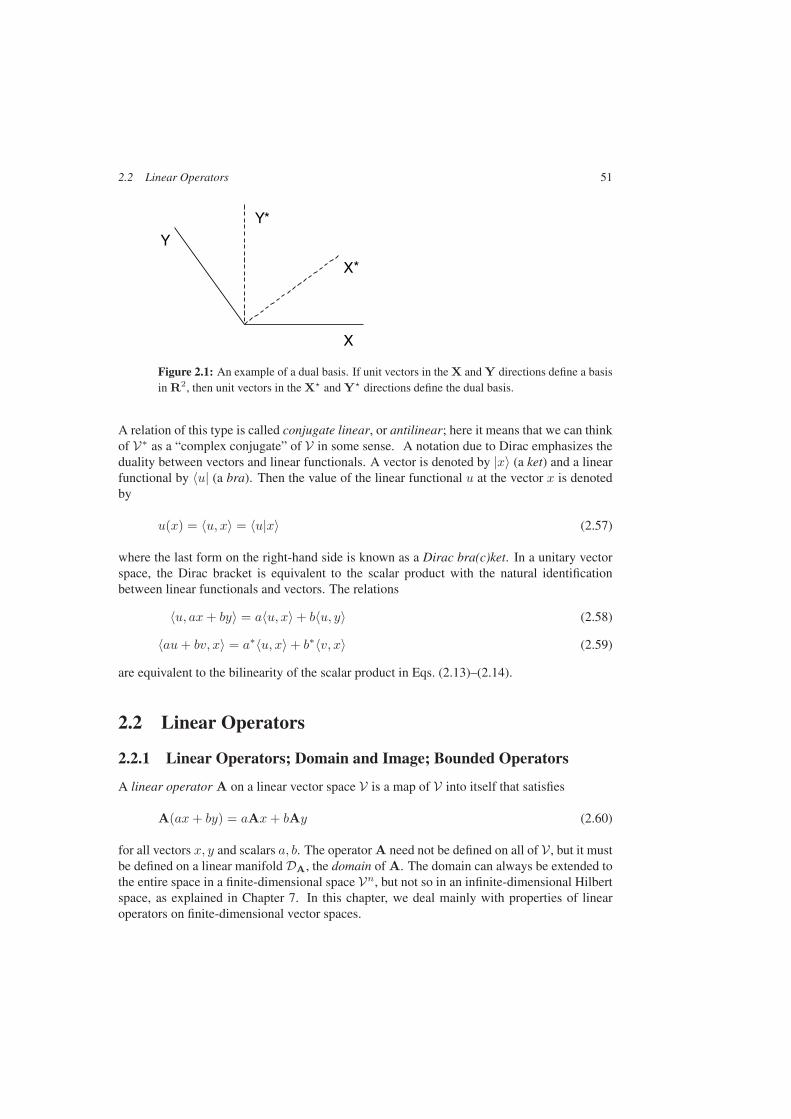
2.2 Linear Operators 51
X
Y
X*
Y*
Figure 2.1: An example of a dual basis. If unit vectors in the X and Y directions define a basisin R2, then unit vectors in the X and Y directions define the dual basis.
A relation of this type is called conjugate linear, or antilinear; here it means that we can thinkof V∗ as a “complex conjugate” of V in some sense. A notation due to Dirac emphasizes theduality between vectors and linear functionals. A vector is denoted by |x〉 (a ket) and a linearfunctional by 〈u| (a bra). Then the value of the linear functional u at the vector x is denotedby
u(x) = 〈u, x〉 = 〈u|x〉 (2.57)
where the last form on the right-hand side is known as a Dirac bra(c)ket. In a unitary vectorspace, the Dirac bracket is equivalent to the scalar product with the natural identificationbetween linear functionals and vectors. The relations
〈u, ax+ by〉 = a〈u, x〉 + b〈u, y〉 (2.58)
〈au+ bv, x〉 = a∗〈u, x〉 + b∗〈v, x〉 (2.59)
are equivalent to the bilinearity of the scalar product in Eqs. (2.13)–(2.14).
2.2 Linear Operators
2.2.1 Linear Operators; Domain and Image; Bounded Operators
A linear operator A on a linear vector space V is a map of V into itself that satisfies
A(ax+ by) = aAx+ bAy (2.60)
for all vectors x, y and scalars a, b. The operator A need not be defined on all of V , but it mustbe defined on a linear manifold DA, the domain of A. The domain can always be extended tothe entire space in a finite-dimensional space Vn, but not so in an infinite-dimensional Hilbertspace, as explained in Chapter 7. In this chapter, we deal mainly with properties of linearoperators on finite-dimensional vector spaces.

52 2 Finite-Dimensional Vector Spaces
The set of all vectors y such that y = Axfor some x in the domain of A is the image ofA (imA)1or the range of A (RA), as indicatedschematically in Fig. 2.2. It is easy to see thatimA is a linear manifold; its dimension is therank ρ(A) of A. The set of vectors x such that
Ax = θ (2.61)
defines a linear manifold kerA, the kernel (ornull space) of A. Figure 2.2 is a schematic illus-tration of kerA and imA. If the only solutionto Eq. (2.61) is the zero vector (kerA = θ),then the operator A is nonsingular. If there arenonzero solutions, then A is singular. In a vec-tor space of finite dimension n, we have
ρ(A) + dim(kerA) = n (2.62)
ker A
im A
Figure 2.2: Schematic illustrationof the kernel and image of an opera-tor A. The kernel (kerA) is the mani-fold mapped into the zero vector by A,while the image (imA) is the map ofthe entire space V under A.
Equation (2.62) says that the dimension of imA is the original dimension of the space reducedby the dimension of the subspace which A annihilates (transforms into the zero vector).
To prove this intuitively plausible relation, let m = dim(imA) and let y1, . . . , ym be abasis of imA, with
yk = Axk (2.63)
(k = 1, . . . ,m). The vectors x1, . . . , xm are linearly independent; if∑ckxk = θ then∑
ckyk = θ by linearity, but y1, . . . , ym are linearly independent so all the ck must vanish.We can then choose xm+1, . . . , xn to complete a basis of Vn. Since the y1, . . . , ym form abasis of imA, the action of A on the xm+1, . . . , xn can be expressed as
Axk =m∑
=1
c(k) y (2.64)
(k = m+ 1, . . . , n). Now define vectors zm+1, . . . , zn by
zk ≡ xk −m∑
=1
c(k) x (2.65)
The zm+1, . . . , zn are linearly independent (show this) and Azk = θ (k = m + 1, . . . , n).Hence they define a basis of kerA (kerA = M(zm+1, . . . , zn)) and Vn can be expressed as
Vn = M(x1, . . . , xm) ⊕ kerA (2.66)
from which Eq. (2.62) follows.
1More precisely, the image of DA under A, but the shorter terminology has become standard.
2.2 Linear Operators 53
The inhomogeneous equation
Ax = y (2.67)
can have a solution only if y is in imA. If A is nonsingular, then imA is the entire vectorspace V , and Eq. (2.67) has a unique solution for every y in V . If A is singular, then Eq. (2.67)has a solution only if y is in imA, and the solution is not unique, since any solution ofthe homogeneous equation (2.61) (i.e., any vector in kerA) can be added to a solution ofEq. (2.67) to obtain a new solution. If Eq. (2.67) has a unique solution for every x in V , thendefine the operator A−1, the inverse of A, by
A−1y = x (2.68)
Exercise 2.6. A and B are linear operators on the finite-dimensional vector space Vn.(i) The product AB is nonsingular if and only if both A and B are nonsingular.(ii) If A and B are nonsingular, then
(AB)−1 = B−1A−1
(iii) If A is nonsingular and BA = 1, then AB = 1.
Remark. Statement (iii) means that if B is a left inverse of A, then B is also a right inverse.This is true only in a finite-dimensional space; a counterexample in infinite dimensions can befound in Chapter 7.
Definition 2.7. The linear operator A is bounded if there is a constant C > 0 such that‖Ax‖ ≤ C‖x‖ for every vector x. The smallest C for which this inequality is true is thebound of A, denoted by |A|.Theorem 2.3. Every linear operator on a finite-dimensional unitary vector space Vn isbounded.
Proof. To show this, suppose φ1, . . . , φn is a complete orthonormal system and let
φ =n∑
k=1
ξkφk (2.69)
be a unit vector. Then
Aφ =n∑
k=1
ξkAφk (2.70)
and
‖Aφ‖2 ≤(
n∑
k=1
|ξk| ‖Aφk‖)2
≤n∑
k=1
|ξk|2n∑
k=1
‖Aφk‖2 ≤ C2‖φ‖2 (2.71)
where
C2 ≡n∑
k=1
‖Aφk‖2 (2.72)
Remark. The theorem is even if the space Vn is not unitary, but the proof is slightly moresubtle, and we do not give it here.
54 2 Finite-Dimensional Vector Spaces
2.2.2 Matrix Representation; Multiplication of Linear Operators
Linear operators can be given an explicit realization in terms of matrices. If the linear operatorA is defined on a basis x1, x2, . . . of V , then we have
Axk =∑
j
Ajkxj (2.73)
and the action of A on a vector x =∑k ξkxk is given by
Ax =∑
j
(∑
k
Ajkξk
)xj ≡
∑
j
ηjxj (2.74)
This corresponds to the standard matrix multiplication rule
η1η2...
=
A11 A12 · · ·A21 A22 · · ·
......
. . .
ξ1ξ2...
(2.75)
if we identify x with the column vector (ξk) formed by its components and A with the matrix(Ajk). The Ajk are the matrix elements of A in the basis x1, x2, . . .. The kth column of thematrix contains the components of the vector Axk.
Exercise 2.7. Show that if V is a unitary vector space with complex scalars, then theoperator A = 0 if and only if (x,Ax) = 0 for every vector x in V . Show that the condition(x,Ax) = 0 for every vector x in V is not sufficient to have A = 0 in a real vector space Vby constructing a nonsingular linear operator A on R2 such that
(x,Ax) = 0
for every x in R2.
Remark. The theme of this exercise will reappear in several contexts, as certain algebraicproperties are relevant only in complex vector spaces.
The product of two linear operators A and B is defined in a natural way as
(AB)x = A(Bx) (2.76)
Acting on a basis x1, x2, . . . this gives
(AB)xk = A∑
j
Bjkxj =∑
j,
AjBjkxj (2.77)
so that
(AB)k =∑
j
AjBjk (2.78)
This explains the standard rule for matrix multiplication.
2.2 Linear Operators 55
The order of the operators in the product is important; multiplication of operators (or theircorresponding matrices) is not commutative in general.
Definition 2.8. The commutator [A,B] of two operators A and B is defined by
[A,B] ≡ AB − BA = −[B,A] (2.79)
and the anticommutator A,B by
A,B ≡ AB + BA = B,A (2.80)
The operators A, B commute if [A,B] = 0 (⇒ AB = BA) and anticommute ifA,B = 0 (⇒ AB = −BA).
Example 2.4. The 2 × 2 Pauli matrices σx, σy, σz (sometimes called σ1, σ2, σ3) aredefined by
σx ≡(
0 11 0
)σy ≡
(0 −ii 0
)σz ≡
(1 00 −1
)(2.81)
Some quick arithmetic shows that
σ2x = σ2
y = σ2z = 1 (2.82)
and
σxσy = iσz = −σyσx σyσz = iσx = −σzσy σzσx = iσy = −σxσz (2.83)
so that two different Pauli matrices do not commute under multiplication, but the minussigns show that they anticommute. Note that
trσa = 0 trσaσb = 2δab (2.84)
(here tr denotes the trace defined in Eq. (2.103)) so that any 2 × 2 matrix A can beexpressed in the form
A = a01 + a · σ (2.85)
with a0 and a = (ax, ay, az) determined by
a0 = 12 trA a = 1
2 tr σA (2.86)
These results are useful in dealing with general 2 × 2 matrices.
Exercise 2.8. (i) Show that if a = (ax, ay, az) and b = (bx, by, bz), then
σ · a σ · b = a · b+ i σ · a× b
(ii) Show that if n is a three-dimensional unit vector, then
eiσ·nξ = cos ξ + i σ · n sin ξ
for any complex number ξ.
56 2 Finite-Dimensional Vector Spaces
2.2.3 The Adjoint Operator
To every linear operator A on V corresponds a linear operator A† (the adjoint of A) on thedual space V∗ of linear functionals on V (see Section 2.1.5) defined by
〈A†u, x〉 = 〈u,Ax〉 (2.87)
for every vector x in V and every linear functional u in V∗. If V is a unitary vector space, thisis equivalent to
(A†y, x) = (y,Ax) (2.88)
for every pair of vectors x, y in V .
Exercise 2.9. Show that
(A†)† = A (aA)† = a∗A† (AB)† = B†A†
where a is a scalar, and A, B are linear operators on the linear vector space V .
Exercise 2.10. If A is a linear operator on a unitary vector space V , then
kerA = (imA†)⊥ kerA† = (imA)⊥
If V is finite dimensional, then
dim(imA) = ρ(A) = ρ(A†) = dim(imA†)
Remark. Thus, in a finite-dimensional vector space, A is nonsingular if and only if A† is
nonsingular. An infinite-dimensional counterexample will be seen in Chapter 7.
In a unitary vector space a matrix element of an operator with respect to a complete or-thonormal system can be expressed as a scalar product. If φ1, φ2, . . . is a complete orthonor-mal system and
Aφk =∑
j
Ajkφj (2.89)
then the orthonormality conditions give
Ajk = (φj ,Aφk) (2.90)
The matrix elements of the adjoint operator are given by
(A†)jk = (φj ,A†φk) = (Aφj , φk) = A∗kj (2.91)
so the matrix representing A† is obtained from the matrix representing A by complex conjuga-tion and transposition (interchanging rows and columns, or reflecting about the main diagonalof the matrix).
2.2 Linear Operators 57
Definition 2.9. The operator A is self-adjoint, or Hermitian, if
A† = A (2.92)
In terms of the operator matrix elements, this requires
(y,Ax) = (x,Ay)∗ (2.93)
for every pair of vectors x, y.
Remark. It follows that the diagonal matrix elements (x,Ax) of a Hermitian operator A arereal for every vector x. In a complex vector space, it is also sufficient for A to be Hermitianthat (x,Ax) be real for every vector x, but not so in a real vector space, where (x,Ax) is realfor all x for any linear operator A (see Exercise 2.7).
Remark. Self-adjoint is defined by Eq. (2.92) and Hermitian by Eq. (2.93). In a finite-dimensional space, these two conditions are equivalent and the terms self-adjoint and Hermit-ian are often used interchangeably. In an infinite-dimensional space, some care is required,since the operators A and A† may not be defined on the same domain. Such subtle points willbe discussed further in Chapter 7.
2.2.4 Change of Basis; Rotations; Unitary Operators
The coordinates of a vector x, and elements of the matrix representing a linear operator A,depend on the basis chosen in the vector space V . Suppose x1, x2, . . . and y1, y2, . . . are twosets of basis vectors in V . Then define a linear operator S by
Sxk = yk =∑
j
Sjkxj (2.94)
(k = 1, 2, . . .). S is nonsingular (show this), and
xk = S−1yk ≡∑
j
Sjkyj (2.95)
where the Sjk = (S−1)jk are the elements of the matrix inverse of the matrix (Sjk). Thecoordinates of a vector
x =∑
k
ξkxk =∑
ηy (2.96)
in the two bases are related by
ξk =∑
Skη η =∑
k
Skξk (2.97)
The operator S can also be viewed as a transformation of vectors:
x′ ≡ Sx (2.98)
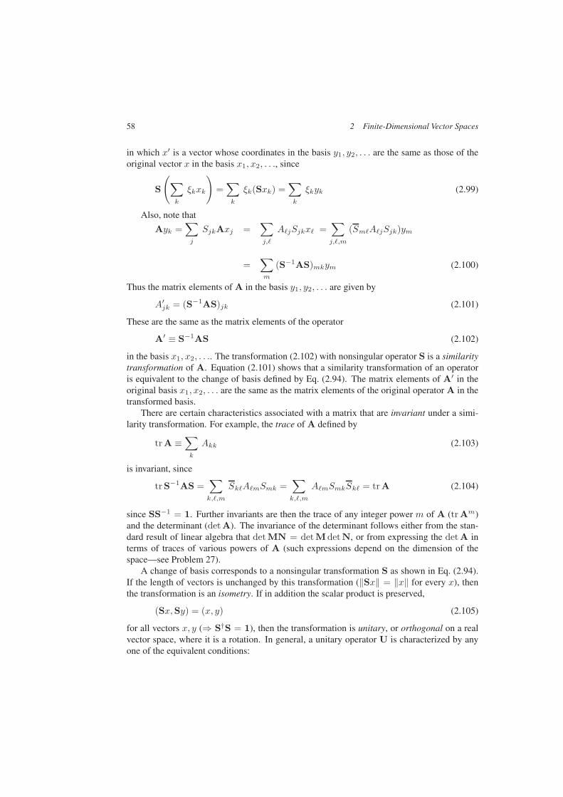
58 2 Finite-Dimensional Vector Spaces
in which x′ is a vector whose coordinates in the basis y1, y2, . . . are the same as those of theoriginal vector x in the basis x1, x2, . . ., since
S
(∑
k
ξkxk
)=∑
k
ξk(Sxk) =∑
k
ξkyk (2.99)
Also, note that
Ayk =∑
j
SjkAxj =∑
j,
AjSjkx =∑
j,,m
(SmAjSjk)ym
=∑
m
(S−1AS)mkym (2.100)
Thus the matrix elements of A in the basis y1, y2, . . . are given by
A′jk = (S−1AS)jk (2.101)
These are the same as the matrix elements of the operator
A′ ≡ S−1AS (2.102)
in the basis x1, x2, . . .. The transformation (2.102) with nonsingular operator S is a similaritytransformation of A. Equation (2.101) shows that a similarity transformation of an operatoris equivalent to the change of basis defined by Eq. (2.94). The matrix elements of A′ in theoriginal basis x1, x2, . . . are the same as the matrix elements of the original operator A in thetransformed basis.
There are certain characteristics associated with a matrix that are invariant under a simi-larity transformation. For example, the trace of A defined by
trA ≡∑
k
Akk (2.103)
is invariant, since
trS−1AS =∑
k,,m
SkAmSmk =∑
k,,m
AmSmkSk = trA (2.104)
since SS−1 = 1. Further invariants are then the trace of any integer power m of A (trAm)and the determinant (detA). The invariance of the determinant follows either from the stan-dard result of linear algebra that detMN = detMdetN, or from expressing the detA interms of traces of various powers of A (such expressions depend on the dimension of thespace—see Problem 27).
A change of basis corresponds to a nonsingular transformation S as shown in Eq. (2.94).If the length of vectors is unchanged by this transformation (‖Sx‖ = ‖x‖ for every x), thenthe transformation is an isometry. If in addition the scalar product is preserved,
(Sx,Sy) = (x, y) (2.105)
for all vectors x, y (⇒ S†S = 1), then the transformation is unitary, or orthogonal on a realvector space, where it is a rotation. In general, a unitary operator U is characterized by anyone of the equivalent conditions:

2.2 Linear Operators 59
(i) U†U = 1 = UU†, or simply U† = U−1,
(ii) (Ux,Uy) = (x, y) = (U†x,U†y) for every pair of vectors x, y.
(iii) ‖Ux‖ = ‖x‖ = ‖U†x‖ for every vector x.
(iv) if φ1, φ2, . . . is a complete orthonormal system, then Uφ1,Uφ2, . . . is also a com-plete orthonormal system.
Example 2.5. Consider a rotation in twodimensions in which the coordinate axes are ro-tated by an angle θ (see Fig. 2.3). The unit vec-tors ux′ , uy′ along the X ′, Y ′ axes are related tothe unit vectors ux, uy along the X,Y axes by
ux′ = ux cos θ + uy sin θuy′ = −ux sin θ + uy cos θ (2.106)
Thus the matrix corresponding to the rotation is
R(θ) =(
cos θ − sin θsin θ cos θ
)(2.107)
Note that R−1(θ) = R(−θ).
X
X'Y'
Y
Figure 2.3: Rotation of coordinate axesin two dimensions.
Remark. The rotation R(θ) presented here is a rotation of coordinate axes that changes thecomponents of vectors, which are viewed as intrinsic objects independent of the coordinatesystem. This viewpoint (the passive point of view) is emphasized further in Chapter 3. Thealternative active point of view considers rotations as operations on the vectors themselves,so that a rotation R(θ) rotates vectors through an angle θ while keeping the coordinate axesfixed. Evidently the two views of rotations are inverse to each other:
R(θ) = R(−θ) (2.108)
since rotating the a vector through angle θ induces the same change in the components of avector as rotating the coordinate axes through angle −θ.
Example 2.6. Consider a rotation in three dimensions as illustrated in Fig. 2.4. Therotation is characterized by three angles (the Euler angles) φ, θ, ψ, which are defined asfollows:
φ is the angle from the Y -axis to the line of nodes (0 ≤ φ < 2π),
θ is the angle from the Z-axis to the Z ′-axis (0 ≤ θ ≤ π) and
ψ is the angle from the line of nodes to the Y ′-axis (0 ≤ ψ < 2π)
where the angles are uniquely defined in the ranges given.2
2In some classical mechanics books, notably the book by Goldstein cited in the bibliography, the angle φ is definedfrom the X-axis to the line of nodes, and the angle ψ from the line of nodes to the X′-axis. It is technically moreconvenient in quantum mechanics to use the definition given here.
60 2 Finite-Dimensional Vector Spaces
ZZ'
Y
X
X'
Y'
line of nodes
Figure 2.4: Euler angles for rotations in three dimensions. The line of nodes is the intersectionof the X–Y plane and the X ′–Y ′ plane, in the direction of the vector uz × u′
z .
Denote the associated rotation matrix by R(φ, θ, ψ). If Rn(θ) denotes a rotation byangle θ about an axis along the unit vector n, then
R(φ, θ, ψ) = Rz′(ψ)Ru(θ)Rz(φ) (2.109)
where u is a unit vector along the line of nodes, since the full rotation is a product of
(i) rotation by angle φ about the Z-axis,
(ii) rotation by angle θ about the line of nodes, and
(iii) rotation by angle ψ about the Z ′-axis.
To compute the matrix R(φ, θ, ψ), it is better to express the rotation as a product of ro-tations about fixed axes (the X , Y , Z axes, say). It turns out that this can be done, witha strikingly simple result. Note first that the rotation about the line of nodes can be ex-pressed as a rotation about the Y -axis if we first undo the rotation through φ about theZ-axis, rotate by angle θ, and then redo the rotation about the Z-axis, i.e.,
Ru(θ) = Rz(φ)Ry(θ)R−1z (φ) (2.110)
The rotation about the Z ′-axis can be expressed as a rotation about the Z-axis if we undothe rotation about the line of nodes, rotate through ψ about theZ-axis, and redo the rotationabout the line of nodes, so that
Rz′(ψ) = Ru(θ)Rz(ψ)R−1u (θ) (2.111)
Then
R(φ, θ, ψ) = Rz(φ)Ry(θ)Rz(ψ) (2.112)
and the rotation R(φ, θ, ψ) is obtained as the product of

2.2 Linear Operators 61
(i) rotation by angle ψ about the Z-axis,
(ii) rotation by angle θ about the Y -axis, and
(iii) rotation by angle φ about the Z-axis.
Thus the rotations about the fixed axes have the same angles as the rotations about the mov-ing axes, but they are done in reverse order! The final result for the matrix correspondingto a general rotation in three dimensions is then
R(φ, θ, ψ) (2.113)
=
cosψ cos θ cosφ− sinψ sinφ − sinψ cos θ cosφ− cosψ sinφ sin θ cosφcosψ cos θ sinφ+ sinψ cosφ − sinψ cos θ sinφ+ cosψ cosφ sin θ sinφ
− cosψ sin θ sinψ sin θ cos θ
Note that Eq. (2.112) is easier to remember than this result!
2.2.5 Invariant Manifolds
A linear manifold M in Vn is an invariant manifold of the linear operator A if Ax is in Mfor every vector x in M. If M has dimension m and a basis x1, . . . , xm, there are linearlyindependent vectors xm+1, . . . , xn that complete a basis of Vn. Let M∗ denote the (n−m)-dimensional manifold spanned by xm+1, . . . , xn; then
Vn = M⊕M∗ (2.114)
This is similar to the split of a unitary space V into M⊕M⊥, but M⊥ is unique, while themanifold M∗ is not, since to each of the basis vectors xm+1, . . . , xn can be added an arbitraryvector in M. The matrix representation of A has the form
A =(AM B0 AM∗
)(2.115)
in this basis. AM is the restriction of A to M, and AM∗ the restriction of A to M∗, Notethat M∗ is also an invariant manifold of A if and only if B = 0. The properties of A thatdecide whether or not it is possible to find a basis in which B = 0 are examined below.
Two invariant manifolds of the operator A are kerA and imA. In fact, all the manifoldsker(Ak) and im(Ak) (k = 0, 1, 2, . . .) are invariant manifolds of A; we have
ker(A0) = θ ⊆ ker(A) ⊆ ker(A2) ⊆ · · · (2.116)
and
im(A0) = Vn ⊇ im(A) ⊇ im(A2) ⊇ · · · (2.117)
At each stage, there is a linear manifold Mk such that
Vn = Mk ⊕ ker(Ak) (2.118)
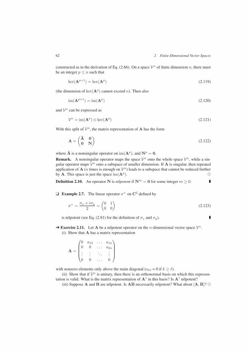
62 2 Finite-Dimensional Vector Spaces
constructed as in the derivation of Eq. (2.66). On a space Vn of finite dimension n, there mustbe an integer p ≤ n such that
ker(Ap+1) = ker(Ap) (2.119)
(the dimension of ker(Ap) cannot exceed n). Then also
im(Ap+1) = im(Ap) (2.120)
and Vn can be expressed as
Vn = im(Ap) ⊕ ker(Ap) (2.121)
With this split of Vn, the matrix representation of A has the form
A =(A 00 N
)(2.122)
where A is a nonsingular operator on im(Ap), and Np = 0.
Remark. A nonsingular operator maps the space Vn onto the whole space Vn, while a sin-gular operator maps Vn onto a subspace of smaller dimension. If A is singular, then repeatedapplication of A (n times is enough on Vn) leads to a subspace that cannot be reduced furtherby A. This space is just the space im(Ap).
Definition 2.10. An operator N is nilpotent if Nm = 0 for some integer m ≥ 0.
Example 2.7. The linear operator σ+ on C2 defined by
σ+ =σx + iσy
2=(
0 10 0
)(2.123)
is nilpotent (see Eq. (2.81) for the definition of σx and σy).
Exercise 2.11. Let A be a nilpotent operator on the n-dimensional vector space Vn.(i) Show that A has a matrix representation
A =
0 a12 . . . a1n
0 0 . . . a2n
......
. . ....
0 0 . . . 0
with nonzero elements only above the main diagonal (ak = 0 if k ≥ ).(ii) Show that if Vn is unitary, then there is an orthonormal basis on which this represen-
tation is valid. What is the matrix representation of A† in this basis? Is A† nilpotent?(iii) Suppose A and B are nilpotent. Is AB necessarily nilpotent? What about [A,B]?

2.2 Linear Operators 63
2.2.6 Projection Operators
We have seen that if M is a linear manifold in a unitary vector space V , then any vector x in Vcan be uniquely expressed as
x = x′ + x′′ (2.124)
with x′ in M and x′′ in M⊥ (see Eq. (2.42)). The (or-thogonal) projection operator (or projector) PM onto Mis defined by
PMx ≡ x′ (2.125)
for every vector x. If M is a one-dimensional manifoldwith a unit vector φ, then
Pφx = (φ, x)φ (2.126)
selects the component of x in the direction of φ and elimi-nates the orthogonal components, as shown in Fig. 2.5.
x
P x
Figure 2.5: Projection Pφ ontothe unit vector φ.
More generally, if M is a manifold with an orthonormal basis φ1, φ2, . . ., then
PMx =∑
k
(φk, x)φk (2.127)
Every projection operator P is Hermitian and idempotent
P2 = P (2.128)
(repeated application of a projection operator gives the same result as the first projection). Theconverse is also true: any Hermitian operator that is idempotent is a projection operator (seethe exercise below). If P projects onto M, then 1 − P projects onto M⊥, since for every xexpressed as in Eq. (2.124), we have
(1− PM)x = x′′ = (PM⊥)x (2.129)
Exercise 2.12. Show that if P is a Hermitian operator with P2 = P, then P is a projectionoperator. What is the manifold onto which it projects?
Exercise 2.13. Let M, N be linear manifolds, and P, Q the projection operators ontoM, N . Under what conditions on M and N is it true that
(i) P + Q is a projection operator,
(ii) P− Q is a projection operator,
(iii) PQ is a projection operator, and
(iv) PQ = QP?
Give a geometrical description of these conditions.
64 2 Finite-Dimensional Vector Spaces
2.3 Eigenvectors and Eigenvalues
2.3.1 Eigenvalue Equation
Definition 2.11. If the linear operator A transforms a nonzero vector x into a scalar multipleof itself,
Ax = λx (2.130)
then x is an eigenvector of A, and λ is the corresponding eigenvalue. The eigenvectors ofA belonging to eigenvalue λ, together with the zero vector, form a linear manifold Mλ, theeigenmanifold of A belonging to eigenvalue λ. The dimension mλ of Mλ is the geometricmultiplicity of the eigenvalue λ. The set of distinct eigenvalues of A is the spectrum of A.
Eigenvectors belonging to distinct eigenvalues are linearly independent. To see this, sup-pose Axk = λkxk (k = 0, 1, . . . , p) and
x0 = c1x1 + · · · + cpxp (2.131)
with x1, . . . , xp linearly independent, and c1, . . . , cp nonvanishing. Then
Ax0 = λ0x0 = c1λ1x1 + · · · + cpλpxp (2.132)
is consistent with linear independence of x1, . . . , xp only if
λ0 = λ1 = · · · = λp (2.133)
Equation (2.130) has a nonzero solution if and only if λ satisfies the characteristic equa-tion
pA(λ) ≡ det ‖A − λ1‖ = 0 (2.134)
On a space Vn of finite dimension n, det ‖A − λ1‖ is a polynomial of degree n, the charac-teristic polynomial of A, and the eigenvalues of A are the roots of this polynomial. From thefundamental theorem of algebra derived in Chapter 4, it follows that pA(λ) can be expressedin the factorized form
pA(λ) = (−1)n(λ− λ1)p1 · · · (λ− λm)pm (2.135)
with λ1, . . . , λm the distinct roots of pA(λ), and p1, . . . , pm the corresponding multiplicities(p1 + · · · + pm = n). pk is the algebraic multiplicity of the eigenvalue λk. It is importantto note that the characteristic polynomial is independent of the coordinate system used toevaluate the determinant, since if S is a nonsingular matrix, then
det ‖S−1(A − λ1)S‖ = det(S−1) det ‖A − λ1‖ det(S) = det ‖A − λ1‖ (2.136)
(it is a standard result of linear algebra that detMN = detMdetN).
2.3 Eigenvectors and Eigenvalues 65
2.3.2 Diagonalization of a Linear Operator
Definition 2.12. The operator A is diagonalizable if it has a basis of eigenvectors.
To understand this definition, suppose x1, . . . , xn is a basis with
Axk = λkxk (2.137)
(k = 1, . . . , n). In this basis, A has the matrix representation
A =
λ1 0 . . . 00 λ2 . . . 0...
.... . .
...0 0 . . . λn
≡ diag(λ1, λ2, . . . , λn) (2.138)
with nonvanishing matrix elements only on the diagonal. In a general basis y1, . . . , yn, thereis then a nonsingular matrix S such that S−1AS is diagonal in that basis.
The operator A is certainly diagonalizable if each root of the characteristic polynomialpA(λ) is simple (multiplicity = 1), since we can then choose one eigenvector for each eigen-value to create a set of n linearly independent eigenvectors of A; these must form a basisof Vn. On the other hand, suppose λ0 is a multiple root of pA(λ) (an eigenvalue of multi-plicity > 1 is sometimes called degenerate). Then there may be fewer linearly independenteigenvectors belonging to λ0 than the algebraic multiplicity allows, as shown by the followingexample.
Example 2.8. Consider the 2 × 2 matrix
A =(µ 10 µ
)(2.139)
that has λ = µ as a double root of its characteristic polynomial pA(λ) = (λ − µ)2. Theonly eigenvectors belonging to the eigenvalue µ are multiples of the unit vector
φ =(
10
)(2.140)
and there is no second linearly independent eigenvector.
Remark. Note that
(A − µ1)2 = 0 (2.141)
so that A satisfies its own characteristic equation pA(A) = 0. This is true in general.
The geometric multiplicity of an eigenvalue is always less than or equal to the algebraicmultiplicity of the eigenvalue. To see this, suppose µ is an eigenvalue of A, and M the corre-sponding eigenmanifold (of dimension m). If x1, . . . , xm is a basis of M, and xm+1, . . . , xn

66 2 Finite-Dimensional Vector Spaces
a set of linearly independent vectors that complete a basis of Vn, then A has the matrix repre-sentation
A =
µ 0 . . . 0 a1m+1 . . . a1n
0 µ . . . 0 a2m+1 . . . a2n
......
. . ....
......
0 0 . . . µ amm+1 . . . amn0 0 . . . 0...
...... A
0 0 . . . 0
(2.142)
with A an operator on the linear manifold M∗ ≡ M(xm+1, . . . , xn) of dimension n − m.The characteristic polynomial of A can then be written as
pA(λ) = (µ− λ)m det ‖A − λ1‖ (2.143)
so the algebraic multiplicity of µ is at least m.If the algebraic multiplicity p of µ is actually greater than m, then the operator A defined
on M∗ must have an eigenvector belonging to eigenvalue µ. We can choose this eigenvectorto be the basis vector xm+1; then
Axm+1 = µxm+1 + ym+1 (2.144)
where
ym+1 =m∑
k=1
akm+1xk (2.145)
is a vector in M. Thus the manifold M1 ≡ M(x1, . . . , xm+1) of dimension m + 1 isan invariant manifold of A. This procedure can be repeated until we have a manifold Mµ
whose dimension is equal to the algebraic multiplicity p of the eigenvalue µ. The matrixrepresentation of A on Mµ then has the form
Aµ =
µ . . . 0 a1m+1 . . . a1p
.... . .
......
...0 . . . µ amm+1 . . . amp0 . . . 0 µ . . . am+1 p
......
.... . .
...0 . . . 0 0 . . . µ
≡ µ1 + Nµ (2.146)
Nµ = Aµ − µ1 has nonzero elements only above the main diagonal, hence is nilpotent; infact
Np−m+1µ = 0 (2.147)
2.3 Eigenvectors and Eigenvalues 67
Thus if the characteristic polynomial pA(λ) of A has roots λ1, . . . , λm with algebraicmultiplicities p1, . . . , pm as in the factorized form (2.135), then there are invariant manifoldsM1, . . . ,Mm of dimensions p1, . . . , pm, respectively, such that the restriction Ak of A toMk has the form
Ak = λk1 + Nk (2.148)
with Nk nilpotent,
Npk−mk+1k = 0 (2.149)
(mk is the geometric multiplicity of the eigenvalue λk). The eigenmanifold Mk is a subsetof Mk; the two manifolds are the same if and only if pk = mk. The vector space Vn can beexpressed as
Vn = M1 ⊕ · · · ⊕Mm (2.150)
and A can be expressed in the form (the Jordan canonical form)
A = D + N (2.151)
where D is a diagonalizable matrix, N is nilpotent (N = 0 if and only if A is diagonal-izable), and N commutes with D (since D is just a multiple of 1 on each of the invariantmanifolds Mk). Equation (2.151) is the unique split of a linear operator A into the sum of adiagonalizable operator D and a nilpotent operator N that commutes with D.
Now suppose B is an operator that commutes with A. Then B also commutes with anypower of A, ApB = BAp. If x is a vector in Mk, then
ApkBx = BApkx = λpk
k x (2.152)
so that Bx is also in Mk. Thus each of the manifolds Mk is an invariant manifold of B, onwhich B can be expressed as the sum of a diagonalizable matrix and a nilpotent operator as inEq. (2.151). Thus B can be expressed in the form
B = D′ + N′ (2.153)
with D′ diagonalizable, N′ nilpotent and D′N′ = N′D′. Furthermore, there is a basis inwhich both D and D′ are diagonal, N and N′ have nonzero elements only above the maindiagonal, and N commutes with N′. In particular, if A and B are each diagonalizable andAB = BA, then there is a basis of vectors that are simultaneous eigenvectors of A and B.
2.3.3 Spectral Representation of Normal Operators
The study of the eigenvectors and eigenvalues of linear operators on Vn in the precedingsection leads to the general structure expressed in Eq. (2.151). On a unitary vector space,however, there is a broad class of operators for which it is possible to go further and constructa complete orthonormal system of eigenvectors. This is the class of normal operators, forwhich we have the formal
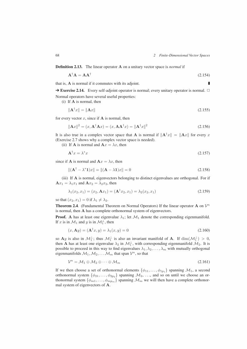
68 2 Finite-Dimensional Vector Spaces
Definition 2.13. The linear operator A on a unitary vector space is normal if
A†A = AA† (2.154)
that is, A is normal if it commutes with its adjoint.
Exercise 2.14. Every self-adjoint operator is normal; every unitary operator is normal.
Normal operators have several useful properties:(i) If A is normal, then
‖A†x‖ = ‖Ax‖ (2.155)
for every vector x, since if A is normal, then
‖Ax‖2 = (x,A†Ax) = (x,AA†x) = ‖A†x‖2 (2.156)
It is also true in a complex vector space that A is normal if ‖A†x‖ = ‖Ax‖ for every x(Exercise 2.7 shows why a complex vector space is needed).
(ii) If A is normal and Ax = λx, then
A†x = λ∗x (2.157)
since if A is normal and Ax = λx, then
‖(A† − λ∗1)x‖ = ‖(A − λ1)x‖ = 0 (2.158)
(iii) If A is normal, eigenvectors belonging to distinct eigenvalues are orthogonal. For ifAx1 = λ1x1 and Ax2 = λ2x2, then
λ1(x2, x1) = (x2,Ax1) = (A†x2, x1) = λ2(x2, x1) (2.159)
so that (x2, x1) = 0 if λ1 = λ2.
Theorem 2.4. (Fundamental Theorem on Normal Operators) If the linear operator A on Vnis normal, then A has a complete orthonormal system of eigenvectors.
Proof. A has at least one eigenvalue λ1; let M1 denote the corresponding eigenmanifold.If x is in M1 and y is in M⊥
1 , then
(x,Ay) = (A†x, y) = λ1(x, y) = 0 (2.160)
so Ay is also in M⊥1 ; thus M⊥
1 is also an invariant manifold of A. If dim(M⊥1 ) > 0,
then A has at least one eigenvalue λ2 in M⊥1 , with corresponding eigenmanifold M2. It is
possible to proceed in this way to find eigenvalues λ1, λ2, . . . , λm with mutually orthogonaleigenmanifolds M1,M2, . . .Mm that span Vn, so that
Vn = M1 ⊕M2 ⊕ · · · ⊕Mm (2.161)
If we then choose a set of orthonormal elements φ11, . . . , φ1p1 spanning M1, a secondorthonormal system φ21, . . . , φ2p2 spanning M2, . . ., and so on until we choose an or-thonormal system φm1, . . . , φmpm
spanning Mm we will then have a complete orthonor-mal system of eigenvectors of A.

2.3 Eigenvectors and Eigenvalues 69
The converse is also true; if A has a complete orthonormal system of eigenvectors, thenA is normal. For if φ1, . . . , φn is a complete orthonormal system of eigenvectors of A witheigenvalues λ1, . . . , λn (not necessarily distinct), then A and A† are represented by diagonalmatrices,
A = diag(λ1, . . . , λn) A† = diag(λ∗1, . . . , λ∗n) (2.162)
Then A is normal, since
A†A = diag(λ∗1λ1, . . . , λ∗nλn) = AA† (2.163)
If A is a normal operator with distinct eigenvalues λ1, . . . , λm and corresponding eigen-manifolds M1, . . .Mm, introduce the projection operators
P1 ≡ PM1 , . . . ,Pm ≡ PMm(2.164)
The operators P1, . . . ,Pm are the eigenprojectors of A. They have the properties
PkP = PPk = 0 k = (2.165)
P1 + · · · + Pm = 1 (2.166)
and
A =m∑
k=1
λkPk = λ1P1 + · · · + λmPm (2.167)
Equation (2.167) is the spectral representation of the normal operator A.
Example 2.9. A simple example is provided by the 2 × 2 matrix
σz =(
1 00 −1
)(2.168)
introduced in Eq. (2.81). This matrix is already diagonal; its eigenvalues are 1 and −1.The corresponding eigenprojectors are given by
P+ =(
1 00 0
)P− =
(0 00 1
)(2.169)
in terms of which the spectral representation of σz is
σz = P+ − P− (2.170)
Note also that P± = 12 (1 ± σz) since 1 ± σz gives zero when it acts on the eigenvector
of σz with eigenvalue ∓1, but this formula works only because σz has just two distincteigenvalues.
Exercise 2.15. Find the eigenvalues and eigenprojectors for the σx and σy in Eq. (2.81).
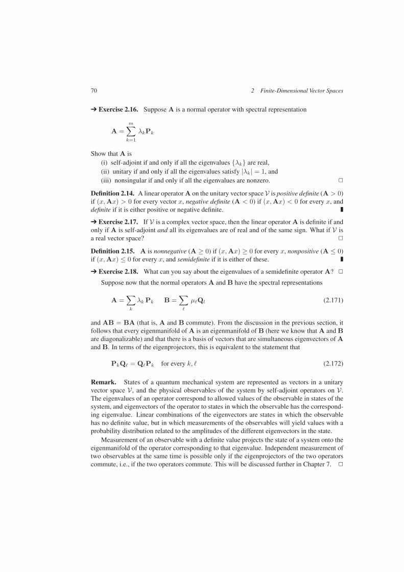
70 2 Finite-Dimensional Vector Spaces
Exercise 2.16. Suppose A is a normal operator with spectral representation
A =m∑
k=1
λkPk
Show that A is(i) self-adjoint if and only if all the eigenvalues λk are real,(ii) unitary if and only if all the eigenvalues satisfy |λk| = 1, and(iii) nonsingular if and only if all the eigenvalues are nonzero.
Definition 2.14. A linear operator A on the unitary vector space V is positive definite (A > 0)if (x,Ax) > 0 for every vector x, negative definite (A < 0) if (x,Ax) < 0 for every x, anddefinite if it is either positive or negative definite.
Exercise 2.17. If V is a complex vector space, then the linear operator A is definite if andonly if A is self-adjoint and all its eigenvalues are of real and of the same sign. What if V isa real vector space?
Definition 2.15. A is nonnegative (A ≥ 0) if (x,Ax) ≥ 0 for every x, nonpositive (A ≤ 0)if (x,Ax) ≤ 0 for every x, and semidefinite if it is either of these.
Exercise 2.18. What can you say about the eigenvalues of a semidefinite operator A?
Suppose now that the normal operators A and B have the spectral representations
A =∑
k
λk Pk B =∑
µQl (2.171)
and AB = BA (that is, A and B commute). From the discussion in the previous section, itfollows that every eigenmanifold of A is an eigenmanifold of B (here we know that A and Bare diagonalizable) and that there is a basis of vectors that are simultaneous eigenvectors of Aand B. In terms of the eigenprojectors, this is equivalent to the statement that
PkQ = QPk for every k, (2.172)
Remark. States of a quantum mechanical system are represented as vectors in a unitaryvector space V , and the physical observables of the system by self-adjoint operators on V .The eigenvalues of an operator correspond to allowed values of the observable in states of thesystem, and eigenvectors of the operator to states in which the observable has the correspond-ing eigenvalue. Linear combinations of the eigenvectors are states in which the observablehas no definite value, but in which measurements of the observables will yield values with aprobability distribution related to the amplitudes of the different eigenvectors in the state.
Measurement of an observable with a definite value projects the state of a system onto theeigenmanifold of the operator corresponding to that eigenvalue. Independent measurement oftwo observables at the same time is possible only if the eigenprojectors of the two operatorscommute, i.e., if the two operators commute. This will be discussed further in Chapter 7.

2.3 Eigenvectors and Eigenvalues 71
2.3.4 Minimax Properties of Eigenvalues of Self-Adjoint Operators
The natural frequencies of a vibrating system (a string, or a drum head) are the eigenvalues of alinear differential operator. Energy levels of a quantum mechanical system are eigenvalues ofthe Hamiltonian operator of the system. Theoretical understanding of such systems requiresa knowledge of the spectra of these operators. In actual physical systems, there are oftentoo many degrees of freedom to allow an exact computation of the eigenvalues, even withthe power of modern computers. Hence we need to find relatively simple ways to estimateeigenvalues.
Powerful methods for estimating eigenvalues are based on extremum principles. If a realfunction f(x) of a real variable x is known to have a relative minimum at some point x∗, thena very accurate estimate of the minimum value f∗ ≡ f(x∗) can be obtained with a moderatelyaccurate knowledge of x∗. Since the behavior of f(x) is parabolic near the minimum, weknow that f − f∗ will be quadratic in x− x∗.
Here the (real) eigenvalues of a self-adjoint operator A on the linear vector space V arebounded by the eigenvalues of the restriction of the operator to any subspace V0. If the sub-space V0 contains vectors close to the actual eigenvectors of A, then estimates of the eigen-values can be quite accurate, since the errors in the eigenvalues are of second order in the(presumed small) errors of the eigenvector.
Suppose A is a self-adjoint operator in Vn. Let the eigenvalues of A be arranged in non-decreasing order so that λ1 ≤ λ2 ≤ · · · ≤ λn, with corresponding orthonormal eigenvectorsφ1, φ2, . . . , φn. Then for any vector x,
(x,Ax) =n∑
k=1
λk |(φk, x)|2 ≥ λ1
n∑
k=1
|(φk, x)|2 = λ1‖x‖2 (2.173)
(and equality if x = cφ1 for some scalar c). Similarly,
(x,Ax) ≤ λn
n∑
k=1
|(φk, x)|2 = λn‖x‖2 (2.174)
for any vector x (and equality if x = cφn for some scalar c). Thus
λ1 = inf‖φ‖=1
(φ,Aφ) λn = sup‖φ‖=1
(φ,Aφ) (2.175)
Here “inf” (Latin: infimum) denotes the greatest lower bound (or simply minimum) and “sup”(Latin: supremum) the least upper bound (or maximum) (over the unit sphere ‖φ‖ = 1).
Remark. Equation (2.175) is the basis of the standard variational method used in quan-tum mechanics to estimate the lowest (ground state) energy of a system with Hamiltonian H.Choose a unit vector (trial wave function) φ = φα, dependent on a set of (variational) param-eters α, and minimize the energy
E(α) = (φα,Hφα) (2.176)
with respect to the parameters α. This leads to an upper bound for the ground state energythat is often an excellent approximation to its actual value. As explained below, this methodcan also be extended to generate upper bounds for excited state energies.
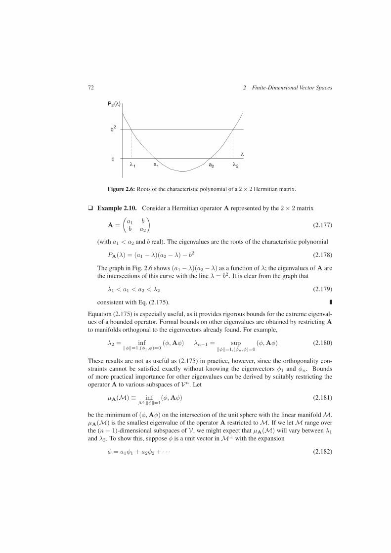
72 2 Finite-Dimensional Vector Spaces
a1 a2
b2
λ1 λ2
0
P2(λ)
λ
Figure 2.6: Roots of the characteristic polynomial of a 2 × 2 Hermitian matrix.
Example 2.10. Consider a Hermitian operator A represented by the 2 × 2 matrix
A =(a1 bb a2
)(2.177)
(with a1 < a2 and b real). The eigenvalues are the roots of the characteristic polynomial
PA(λ) = (a1 − λ)(a2 − λ) − b2 (2.178)
The graph in Fig. 2.6 shows (a1 − λ)(a2 − λ) as a function of λ; the eigenvalues of A arethe intersections of this curve with the line λ = b2. It is clear from the graph that
λ1 < a1 < a2 < λ2 (2.179)
consistent with Eq. (2.175).
Equation (2.175) is especially useful, as it provides rigorous bounds for the extreme eigenval-ues of a bounded operator. Formal bounds on other eigenvalues are obtained by restricting Ato manifolds orthogonal to the eigenvectors already found. For example,
λ2 = inf‖φ‖=1,(φ1,φ)=0
(φ,Aφ) λn−1 = sup‖φ‖=1,(φn,φ)=0
(φ,Aφ) (2.180)
These results are not as useful as (2.175) in practice, however, since the orthogonality con-straints cannot be satisfied exactly without knowing the eigenvectors φ1 and φn. Boundsof more practical importance for other eigenvalues can be derived by suitably restricting theoperator A to various subspaces of Vn. Let
µA(M) ≡ infM,‖φ‖=1
(φ,Aφ) (2.181)
be the minimum of (φ,Aφ) on the intersection of the unit sphere with the linear manifold M.µA(M) is the smallest eigenvalue of the operator A restricted to M. If we let M range overthe (n − 1)-dimensional subspaces of V , we might expect that µA(M) will vary between λ1
and λ2. To show this, suppose φ is a unit vector in M⊥ with the expansion
φ = a1φ1 + a2φ2 + · · · (2.182)

2.3 Eigenvectors and Eigenvalues 73
If a1 = 0, then φ1 is in M, and µA(M) = λ1. If a1 = 0, let
a =√z21 + c22 a1 = a sinα a2 = a cosα (2.183)
Then the unit vector
ψ ≡ cosα φ1 − sinα φ2 (2.184)
is in M, since it is orthogonal to the vector φ that spans M⊥, and we have
µA(M) = cos2 αλ1 + sin2 αλ2 (2.185)
Thus we have
λ1 ≤ µA(M) ≤ λ2 (2.186)
for any subspace M of dimension n − 1, with equality for M = [M(φ1)]⊥. This argumentcan be extended show that if M is a subspace of dimension n− h, then
µA(M) ≤ λh+1 (2.187)
with equality for M = [M(φ1, . . . , φh)]⊥. Thus the eigenvalue λh+1 is larger than thesmallest eigenvalue of any restriction of A to a manifold of dimension n−h (h = 0, . . . , n−1).
To work from the other end, let
νA(M) ≡ supM,‖φ‖=1
(φ,Aφ) (2.188)
νA(M) is the largest eigenvalue of the operator A restricted to the manifold M. Then
λh ≤ νA(M) (2.189)
for any manifold of dimension h, with equality for M = M(φ1, . . . , φh); the eigenvalue λhis smaller than the largest eigenvalue of any restriction of A to a manifold of dimension h.
Inequalities (2.187) and (2.189) provide rigorous bounds for the eigenvalue λh. One fur-ther refinement is to let M be a linear manifold of dimension m with PM the projectionoperator onto M, and let
A′ = AM ≡ PMAPM (2.190)
be the restriction of A to M. A′ is a self-adjoint operator on M; its eigenvalues λ′k can beordered so that
λ′1 ≤ λ′2 ≤ · · · ≤ λ′m (2.191)
The preceding inequalities imply here that
λh ≤ λ′h ≤ λh+n−m (2.192)
so that the eigenvalues of A′ give direct bounds on the eigenvalues of A.

74 2 Finite-Dimensional Vector Spaces
a1a2
a31
2 3
P3( )
Figure 2.7: Roots of the characteristic polynomial of a 3 × 3 Hermitian matrix.
Remark. Thus if a linear operator A on V is restricted to an m-dimensional subspace of V ,the eigenvalues of the restricted operator are upper bounds on the corresponding eigenvaluesof the full operator; the inequalities λh ≤ λ′h give bounds for the lowest m eigenvalues, andnot just the lowest. In quantum mechanical systems, this provides estimates of excited stateenergies as well as ground state energies.
Example 2.11. Let A be a self-adjoint operator with a 3 × 3 matrix representation
A =
a1 0 b10 a2 b2b∗1 b∗2 a3
(2.193)
(with a1 < a2 < a3 real). The characteristic polynomial of A is
P (λ) = (a1 − λ)(a2 − λ)(a2 − λ) − (a1 − λ) |b2|2 − (a2 − λ) |b1|2 (2.194)
The roots of the P (λ) correspond to the solutions of
(λ− a1)(λ− a2)(λ− a3) = (λ− a1) |b2|2 + (λ− a2) |b1|2 (2.195)
Here the left-hand side is a cubic and the right-hand side a straight line as a function of λas shown in Fig. 2.7. The eigenvalues are the values of λ at the intersections of the cubicand the straight line. These eigenvalues evidently satisfy the inequalities
λ1 < a1 < λ2 < a2 < λ3 (2.196)
consistent with the general inequalities (2.192). Note that it is essential to diagonalize the2× 2 matrix in the upper-left corner in order to conclude that a1 < λ2 < a2, although theinequalities λ1 < a1 and a3 < λ3 are true in general (that is, even if the two zero elementsin the matrix are replaced by a real parameter c).
2.4 Functions of Operators 75
2.4 Functions of Operators
If A is a linear operator, it is straightforward to define powers of A, and then polynomials ofA as linear combinations of powers of A. If A is nonsingular, then negative integer powersof A are defined as powers of A−1. If a function f(z) is an analytic function of a complexvariable z in some neighborhood of z = 0, then a natural way to define f(A) is through thepower series expansion of f(z). Thus, for example, we have the formal definitions
(1− αA)−1 =∞∑
n=0
αnAn (2.197)
and
etA =∞∑
n=0
tn
n!An (2.198)
To give meaning to such series, we need to define convergence of sequences of operators.
Definition 2.16. Let Ak be a sequence of linear operators on the linear vector space V .Then the sequence converges uniformly to A (Ak ⇒ A) if |Ak − A| → 0. The sequenceconverges strongly to A (Ak → A) if Akx → Ax for every vector x, and weakly to A(Ak A) if (y,Akx) → (y,Ax) for every pair of vectors x, y.
As with sequences of vectors, strong and weak convergence of sequences of operators areequivalent in a finite-dimensional space Vn. The equivalence of uniform convergence followsfrom the observation that if φ1, φ2, . . . , φn is a complete orthonormal system, and if thesequences Akφ1, Akφ2, . . . , Akφn all converge, then also |Ak − A| → 0, since
|Ak − A|2 ≤n∑
m=1
‖(Ak − A)φm‖2 (2.199)
It is clear that an infinite series of operators on Vn converges if and only if the corre-sponding series of complex numbers obtained by replacing A by |A| is convergent. Thus, theinfinite series (2.197) converges if |α| |A| < 1. It does not converge as an operator series if|α| |A| ≥ 1, although the series (
∑αnAn)x may converge as a series of vectors for some x.
The infinite series (2.198) converges for all t (even uniformly) if A is bounded.Suppose A is a normal operator with eigenvalues λ1, . . . , λm, corresponding eigenprojec-
tors P1, . . . ,Pm, and thus spectral representation given by Eq. (2.167). If f(z) is any functiondefined on the spectrum of A, then define
f(A) ≡m∑
k=1
f(λk)Pk (2.200)
This definition is as general as possible, and coincides with other natural definitions. Further-more, it provides the equivalent of analytic continuation beyond the circle of convergence ofa power series. In the following examples, it is understood that A is a normal operator withspectral representation (2.167).
76 2 Finite-Dimensional Vector Spaces
Example 2.12. Suppose f(z) = 1/z. Then if A is nonsingular, we have
f(A) =m∑
k=1
1λk
Pk = A−1 (2.201)
as expected (no eigenvalue vanishes if A is nonsingular).
Example 2.13. Suppose f(z) = z∗. Then we have
f(A) =m∑
k=1
λ∗k Pk = A† (2.202)
so the adjoint operator is the equivalent of the complex conjugate of a complex number (atleast for a normal operator).
Example 2.14. Suppose f(z) = 1/(1 − αz). Then if 1/α is not in the spectrum of A,we have
f(A) =m∑
k=1
11 − αλk
Pk = (1− αA)−1 (2.203)
which gives the analytic continuation of the series (2.197) outside its circle of convergencein the complex α-plane.
Example 2.15. Suppose
w = f(z) =z − i
z + i(2.204)
which maps the real z-axis into the unit circle except the point w = 1 (show this). If A isself-adjoint (the λk are all real), then the operator
U ≡ f(A) =m∑
k=1
λk − i
λk + iPk =
A − i1A + i1
(2.205)
is unitary. U is the Cayley transform of A. Also, if U is unitary with no eigenvalue = 1,then
A = f−1(U) = i1 + U1− U
(2.206)
is self-adjoint. A is the inverse Cayley transform of U.
Example 2.16. Suppose f(z) =√z, and suppose A ≥ 0. Then
f(A) =m∑
k=1
√λk Pk =
√A ≥ 0 (2.207)
and (√
A)2 = A.
2.5 Linear Dynamical Systems 77
2.5 Linear Dynamical Systems
A system whose coordinates x1, . . . , xn evolve in time according to the equations of motion
dxkdt
=∑
Akx (2.208)
is a linear dynamical system. The coordinates x1, . . . , xn characterize a vector in a linearvector space Vn, which allows Eq. (2.208) to be written in the compact form
dx
dt= Ax (2.209)
in which A is a linear operator on Vn with matrix elements Ak.The solution to Eq. (2.209) that starts from the vector x(0) at time t = 0 is
x(t) = etAx(0) (2.210)
This defines a solution for all t, according to the discussion in Section 2.4. To describe thetime dependence of the solution in more detail, recall the general decomposition
A = D + N (2.211)
with D diagonalizable and N nilpotent (Eq. (2.151)). Choose a basis x1, . . . , xn in which Dis diagonal, with eigenvalues λ1, . . . , λn, and suppose that x(0) is expressed as
x(0) =n∑
k=1
ξk0xk (2.212)
Then the solution (2.210) has the form
x(t) =n∑
k=1
ξk(t)xk (2.213)
with ξk(0) = ξk0. If N = 0, this solution has the simple form
ξk(t) = eλktξk0 (2.214)
Example 2.17. Consider a damped harmonic oscillator, with the equation of motion
d2x
dt2+ 2γ
dx
dt+ ω2
0x = 0 (2.215)
where γ > 0 to insure damping, and ω0 is real. With the new variable
u ≡ dx
dt(2.216)
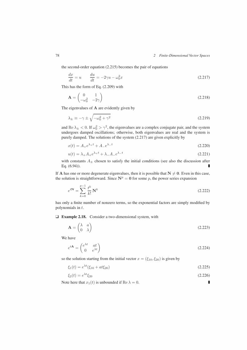
78 2 Finite-Dimensional Vector Spaces
the second-order equation (2.215) becomes the pair of equations
dx
dt= u
du
dt= −2γu− ω2
0x (2.217)
This has the form of Eq. (2.209) with
A =(
0 1−ω2
0 −2γ
)(2.218)
The eigenvalues of A are evidently given by
λ± ≡ −γ ±√−ω2
0 + γ2 (2.219)
and Reλ± < 0. If ω20 > γ2, the eigenvalues are a complex conjugate pair, and the system
undergoes damped oscillations; otherwise, both eigenvalues are real and the system ispurely damped. The solutions of the system (2.217) are given explicitly by
x(t) = A+eλ+t +A−eλ−t (2.220)
u(t) = λ+A+eλ+t + λ−A−eλ−t (2.221)
with constants A± chosen to satisfy the initial conditions (see also the discussion afterEq. (6.94)).
If A has one or more degenerate eigenvalues, then it is possible that N = 0. Even in this case,the solution is straightforward. Since Np = 0 for some p, the power series expansion
etN =p−1∑
k=0
tk
k!Nk (2.222)
has only a finite number of nonzero terms, so the exponential factors are simply modified bypolynomials in t.
Example 2.18. Consider a two-dimensional system, with
A =(λ a0 λ
)(2.223)
We have
etA =(eλt at0 eλt
)(2.224)
so the solution starting from the initial vector x = (ξ10, ξ20) is given by
ξ1(t) = eλt(ξ10 + atξ20) (2.225)
ξ2(t) = eλtξ20 (2.226)
Note here that x1(t) is unbounded if Reλ = 0.
2.5 Linear Dynamical Systems 79
In general, the behavior of the solution ξk(t) for t→ ∞ depends on the corresponding eigen-value λk of A:
(i) if Reλk < 0, then ξk(t) → 0 for t→ ∞,
(ii) if Reλk > 0, then ξk(t) → ∞ for t→ ∞, and
(iii) if Reλk = 0, then ξk(t) moves around a circle of fixed radius |ξk0| in the complexξ-plane if N = 0, unless λk = 0, in which case ξk(t) is constant.
The behavior of ξk(t) for t → ∞ if Reλk = 0 is qualitatively independent of whether or notN = 0, as the exponential factor dominates the asymptotic behavior. If N = 0, the ξk(t)corresponding to Reλk = 0 grows in magnitude like a power of t for t→ ∞ (the power maybe zero if the corresponding vector xk is actually an eigenvector of A).
The vector x = θ is a fixed point, or equilibrium solution, of Eq. (2.209), since if x(0) = θ,then x(t) = θ for all t. A fixed point x∗ is stable if there is a neighborhood N (x∗) of x∗such that any solution starting in N (x∗) remains in N (x∗) for all t. x∗ is asymptoticallystable if there is a neighborhood of the x∗ such that any solution starting in the neighborhoodapproaches x∗ asymptotically for t→ ∞. Such a fixed point is a sink, or an attractor.
It is clear here that x(0) = θ is asymptotically stable if and only if Reλk < 0 for everyeigenvalue of A, while stability requires only Reλk ≤ 0 and N = 0 on the invariant man-ifolds belonging to the eigenvalues with Reλk = 0. Physically, asymptotic stability meansthat small displacements from the equilibrium will eventually be exponentially damped, whilesimple stability allows bounded oscillations without damping, at least in some directions. Afixed point for which Reλk > 0 for every eigenvalue of A is a source, or repellor. Thesolution curves move outward in all directions from a source.
A fixed point for which no eigenvalue hasReλk = 0 is hyperbolic. In general, a hy-perbolic fixed point will have a stable mani-fold Ms spanned by the invariant manifoldsMk for those eigenvalues with Reλk < 0,and an unstable manifold Mu spanned bythe invariant manifolds Mk for those eigen-values with Reλk > 0. As t → ∞, the so-lution curves will be drawn very close to theunstable manifold as the components in thestable manifold are exponentially damped.The simple case of a two-dimensional sys-tem for which the operator A has one pos-itive and one negative eigenvalue is illus-trated in Fig. 2.8. Imaginary parts of theeigenvalues will give oscillatory behaviornot shown in the figure.
X1
X2
Figure 2.8: Schematic form of solutions toEq. (2.208) in the hyperbolic case with onepositive and one negative eigenvalue.
The types of behavior described here occur in nonlinear systems as well. As already noted,a nonlinear system can often be approximated by a linear system near a fixed point, and thelinear properties qualitatively describe the system near the fixed point.
80 2 Finite-Dimensional Vector Spaces
A Small Oscillations
Energy conservation is a fundamental principle for many systems in classical mechanics (suchsystems are called conservative). For example, a harmonic oscillator of mass m and naturalfrequency ω0 has a total energy
E = 12mu
2 + 12mω
20x
2 (2.A1)
(u = dx/dt). This corresponds to the equation of motion (2.215) with γ = 0 (no damp-ing). For a conservative system with coordinates x1, . . . , xn and corresponding velocitiesu1, . . . , un (uk = dxk/dt), the energy often has the form
E = 12
n∑
k,=1
ukTk(x)u + V (x1, . . . , xn) (2.A2)
Here the first term is the kinetic energy T of the system (hence the matrix T(x), which maydepend on the coordinates, must be positive definite), and V (x1, . . . , xn) is the potential en-ergy of the system.
An equilibrium of the system corresponds to a stationary point of the potential energy.If the system has an equilibrium at a point x0 with coordinates x10, . . . , xn0, then the firstderivatives of the potential vanish at x0, and we can assume that the expansion
V (x) V (x0) + 12
n∑
k,=1
(xk − xk0)Vk(x − x0) + · · · (2.A3)
exists, with
Vk =∂2V
∂xk∂x
∣∣∣∣x=x0
(2.A4)
The matrix V = (Vk) is positive definite at a stable equilibrium, which corresponds to a(local) minimum of the potential energy. Thus the eigenvalues of V determine whether or notthe equilibrium is stable. The kinetic energy can also be approximated near the equilibriumpoint x0 by the quadratic function
T 12
n∑
k,=1
ukKku (2.A5)
with Kk = Tk(x0). Thus the total energy has the approximate quadratic form
E V (x0) + 12
n∑
k,=1
ukKku + 12
n∑
k,=1
(xk − xk0)Vk(x − x0) (2.A6)
near the equilibrium point (the constant is not important for the motion near x0 and will bedropped).
A Small Oscillations 81
Since the matrix K is positive definite, we can choose a coordinate system in which it isdiagonal, with positive eigenvalues, so that the kinetic energy has the form
K = 12
n∑
k=1
µk
(dξkdt
)2
(2.A7)
where the ξk = xk − xk0 are the coordinates of the displacement from equilibrium, and µkis the “mass” associated with the coordinate ξk. Introduce rescaled coordinates yk ≡ √
µkξk;the quadratic energy (2.A6) then has the form
E = 12
n∑
k=1
(dykdt
)2
+ 12
n∑
k,=1
yk V k y (2.A8)
where the V k = Vk/√µkµ are the matrix elements of the potential energy matrix in terms
of the rescaled coordinates. In the operator form,
V = K−12 VK−1
2 (2.A9)
The operator V is self-adjoint (check this), so that we can diagonalize it by a unitarytransformation, which does not affect the form of the kinetic energy in Eq. (2.A8). Denotethe eigenvalues of V by a1, . . . , an, and coordinates of a vector in the basis in which V isdiagonal by η1, . . . , ηn. Then the quadratic energy has the form
E = 12
n∑
k=1
(dηkdt
)2
+ akη2k
(2.A10)
and the equations of motion for the ηk are
d2ηkdt2
= −akηk (2.A11)
Thus each of the ηk evolves independently of the others; the ηk define the normal modes ofthe system near the equilibrium x0.
If ak > 0, which will be the case for all the eigenvalues of V at a stable equilibrium, letak ≡ ω2
k, and the coordinate ηk oscillates with (angular) frequency ωk, which is a naturalfrequency of the system. If ak < 0, then let ak ≡ −α2
k, and the coordinate ηk is proportionalto exp(±αkt), so it will in general have a component that grows exponentially for large t. Inpractice, this means that the coordinate ηk moves away from the equilibrium point, so that theapproximation of a small displacement from equilibrium becomes invalid, and the equilibriumis unstable in the direction defined by the coordinate ηk. Finally, if ak = 0, then the coordinateηk evolves in time with constant velocity. Such a mode is called a zero mode; the approximateenergy (2.A10) is independent of the corresponding coordinate. This zero mode indicates asymmetry of the approximate system, which may or may not be a symmetry of the originalsystem as well.
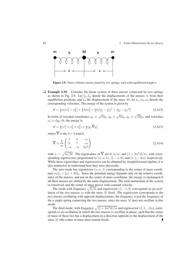
82 2 Finite-Dimensional Vector Spaces
a
m mMk k
a
Figure 2.9: Three collinear masses joined by two springs, each with equilibrium length a.
Example 2.19. Consider the linear system of three masses connected by two springsas shown in Fig. 2.9. Let ξ1, ξ2 denote the displacements of the masses m from theirequilibrium positions, and ξ3 the displacement of the mass M ; let u1, u2, u3 denote thecorresponding velocities. The energy of the system is given by
E = 12m(u2
1 + u22) + 1
2Mu23 + 1
2k[(ξ1 − ξ3)2 + (ξ2 − ξ3)2] (2.A12)
In terms of rescaled coordinates y1 ≡√mξ1, y2 ≡
√mξ2, y3 ≡
√Mξ3, and velocities
vk ≡ dyk/dt, the energy is
E = 12 (v2
1 + v22 + v2
3) + 12 (y,Vy) (2.A13)
where V is the 3 × 3 matrix
V ≡ k
m
1 0 −α0 1 −α−α −α 2α2
(2.A14)
with α =√m/M . The eigenvalues of V are 0, k/m, and (1 + 2α2)k/m, with corre-
sponding eigenvectors proportional to (α, α, 1), (1,−1, 0), and (1, 1,−2α), respectively.While these eigenvalues and eigenvectors can be obtained by straightforward algebra, it isalso instructive to understand how they arise physically.
The zero mode has eigenvector (α, α, 1) corresponding to the center of mass coordi-nate m(ξ1 + ξ2) +Mξ3. Since the potential energy depends only on the relative coordi-nates of the masses, and not on the center of mass coordinate, the energy is unchanged ifall three masses are shifted by the same displacement. The total momentum of the systemis conserved, and the center of mass moves with constant velocity.
The mode with frequency√k/m and eigenvector (1,−1, 0) corresponds to an oscil-
lation of the two masses m with the mass M fixed. The eigenvector corresponds to thetwo masses oscillating with opposite displacements; the frequency is just the frequency ofthe a single spring connecting the two masses, since the mass M does not oscillate in thismode.
The third mode, with frequency√
(1 + 2α2)k/m and eigenvector (1, 1,−2α), corre-sponds to an oscillation in which the two masses m oscillate in phase, such that the centerof mass of these two has a displacement in a direction opposite to the displacement of themass M (the center of mass must remain fixed).
Bibliography and Notes 83
Bibliography and Notes
There are many modern textbooks on the subject of linear algebra and finite-dimensionalvector spaces, to which no special references are given. A classic book on finite-dimensionalvector spaces is
Paul R. Halmos, Finite Dimensional Vector Spaces (2nd edition), van Nostrand(1958).
It is quite readable, though mathematically formal and rigorous, and contains many usefulexercises.
A standard earlier textbook is
Frederick W. Byron, Jr. and Robert W. Fuller, Mathematics of Classical and Quan-tum Physics, Dover (1992).
It is a reprint of a two-volume work first published in 1969–70. It has a thorough treatment oflinear vector spaces and operators, with many physics examples.
An excellent introduction to linear vector spaces and linear operators that leads to theapplications to dynamical systems is in
Morris W. Hirsch and Stephen Smale, Differential Equations, Dynamical Systemsand Linear Algebra, Academic Press (1974).
Starting from the analysis of linear systems, the book describes dynamical systems in termsof vector fields, and proceeds to a general description of the qualitative behavior of systemsnear critical points of the vector field. A major revision of this book that has more emphasison nonlinear systems is
Morris W. Hirsch, Stephen Smale and Robert Devaney, Differential Equations,Dynamical Systems and an Introduction to Chaos (2nd edition), Academic Press(2004).
In this new edition, the discussion of vector spaces has been drastically reduced, and moreemphasis has been given to nonlinear systems; there are many new applications and examples,especially of systems with chaotic behavior. There are also many computer-generated picturesto illustrate qualitative behavior of systems.
A standard graduate textbook on classical mechanics is
Herbert Goldstein, Classical Mechanics (2nd edition), Addison-Wesley (1980).
This book describes the theory of rotations in three dimensions and its application to themotion of a rigid body with one point held fixed. It also has a useful chapter on the theoryof small oscillations. However, it does not make use of the geometrical ideas introduced inChapter 3, in contrast to several books cited there.
An excellent alternative that also has a good discussion of small oscillations is
L. D. Landau and E. M. Lifshitz, Mechanics (3rd edition), Butterworth (1976).
This was the first of the famous series by Landau and Lifshitz that covered the foundations ofphysics at a graduate level as viewed in the 1960s. It is still useful today.
84 2 Finite-Dimensional Vector Spaces
Problems
1. Consider a real two-dimensional vector space with vectors x1, x2, and x3 that satisfy
‖x1‖2 = ‖x3‖2 = 1 ‖x2‖2 = 54 (∗)
andx3 = x2 − (x1, x2)x1 (∗∗)
(i) Show that x1, x3 form a basis.
(ii) How many linearly independent vectors x2 satisfy (∗) and (∗∗)?
(iii) For a vector x2 satisfying (∗) and (∗∗), find a unit vector orthogonal to x2. Expressthis vector as a linear combination of x1 and x3.
2. Let φ1, φ2 be an orthonormal system in C2 and consider the unit vectors u1, u2, u3
defined by
u1 = φ1 u2 = −12φ1 +
√3
2 φ2 u3 = −12φ1 −
√3
2 φ2
(i) Draw a picture of the three unit vectors in the plane.
(ii) Show that for any vector x in C2,
‖x‖2 = 23
3∑
k=1
|(uk, x)|2 (∗)
(iii) Show that any vector x in C2 can be written as
x = 23
3∑
k=1
(uk, x)uk (∗∗)
Remark. Here (∗∗) looks like the expansion of a vector along a complete orthonormalsystem, except for the factor 2
3 . In fact the vectors u1, u2, u3 form a (tight) frame, whichis characterized by a relation of the form (∗), although the constant may be different. Thevectors u1, u2, u3 do not form a basis, since they are not linearly independent; they are“redundant,” or “overcomplete.” Such sets are nevertheless useful in various contexts;see the book by Daubechies cited in Chapter 6, where this example is given.
3. Show that the polynomials p(t) of degree ≤ N form a linear vector space if we defineaddition and multiplication by scalars (which may be real or complex) in the natural way.What is the dimension of this space? Write down a basis for this space. If we define thescalar product of two polynomials p(t) and q(t) by
(p, q) ≡∫ 1
0
p∗(t)q(t) dt
then this space is unitary (verify this). Compute explicitly the first four elements of thecomplete orthonormal system obtained by the Gram–Schmidt process from the basis youhave just given.
Problems 85
4. (i) Show that
N∑
n=1
e2πikn
N e−2πiqn
N = Nδkq
(k, q = 1, . . . , N ).
(ii) Show that a set of numbers f1, . . . , fN can be expressed in the form
fn =N∑
k=1
cke2πikn
N (∗)
with coefficients ck given by
ck =1N
N∑
m=1
fm e− 2πikm
N
(iii) Show that if the f1, . . . , fN are real, then cN−k = c∗k (k = 1, . . . , N ).
Remark. Expansion (∗) is the finite Fourier transform.
5. Show that
N−1∑
n=1
sinnπk
Nsin
nπq
N=N
2δkq
(k, q = 1, . . . , N − 1) and thus that the set of numbers f1, . . . , fN−1 can be expressedas
fn =N−1∑
k=1
bk sinkπn
N
with coefficients bk given by
bk =2N
N−1∑
m=1
fm sinmπk
N
Remark. This expansion is the finite Fourier sine transform.
6. A lattice is a set of vectors such that if x1 and x2 are lattice vectors, then any linearcombination
x = n1x1 + n2x2
86 2 Finite-Dimensional Vector Spaces
of x1 and x2 with integer coefficients n1 and n2 is also a lattice vector. The linearlyindependent vectors e1, . . . , eN are generators of an N -dimensional lattice if the latticeconsists of all linear combinations
x =N∑
k=1
nkek
with integer coefficients n1, . . . , nN . The reciprocal lattice, or dual lattice, is the set ofvectors k for which k · x is an integer for any lattice vector x.
(i) Show that the reciprocal lattice is actually a lattice, that is, if k1 and k2 are in thereciprocal lattice, then so is any linear combination n1k1+n2k2 with integer coefficients.
(ii) The reciprocal lattice is generated by the basis dual to e1, . . . , eN in RN .
7. (i) If A, B and C are three linear operators, then
[[A,B],C] + [[B,C],A] + [[C,A],B] = 0
Remark. This result is the Jacobi identity.
(ii) A, B and C satisfy the further identities
A,B,C − A, B,C = [B, [A,C]]
[A,B],C − A, [B,C] = [A,C,B]
[A,B,C] − [A, B,C] = [B, A,C]
8. Let A be a linear operator on a unitary vector space V . If M is an invariant manifold ofA, then M⊥ is an invariant manifold of A†.
9. Show that with addition and multiplication by scalars defined in the natural way, thelinear operators on an n-dimensional vector space Vn themselves form a linear vectorspace. What is the dimension of the vector space? Give a basis for linear operators onC2 that includes the three Pauli matrices defined by Eq. (2.81).
10. Let U and V be unitary operators. Then
(i) UV is unitary,
(ii) U + V is unitary if and only if
UV† = ωP + ω2(1− P)
with P a projection operator and ω3 = 1.
11. What are the Euler angles (φ, θ, ψ) of the rotation inverse to the rotation R(φ, θ, ψ), giventhe constraints 0 ≤ φ < 2π, 0 ≤ θ ≤ π, and 0 ≤ ψ < 2π?
Problems 87
12. Show that the rotation R(φ, θ, ψ) in three dimensions can be expressed as a product of
(i) rotation through angle ψ about the Z ′-axis,
(ii) rotation through angle θ about the Y ′-axis, and
(iii) rotation through angle φ about the Z ′-axis.
13. Let n = n(θ, φ) be a unit vector in the direction defined by the usual spherical anglesθ, φ. Show that the matrix corresponding to rotation through angle Φ about n can beexpressed as
Rn(Φ) = R(φ, θ, ξ)Rz(Φ)R−1(φ, θ, ξ)
with an arbitrary angle ξ.
14. Show that the eigenvalues of the proper rotation matrix Rn(Φ) in Problem 13 are
λ = 1, e±iΦ
Remark. The eigenvector n belonging to eigenvalue 1 is evidently along the axis ofrotation.
(ii) Explain the relation of the (complex) eigenvectors belonging to eigenvaluesexp(±iΦ) to real coordinate axes in the plane normal to n. What is the form of therotation matrix in a real basis?
15. Show that if R is a proper rotation matrix that is symmetric, then either R is the identity,or R corresponds to a rotation through angle π about some axis.
16. (i) Let Rx(Φ),Ry(Φ), and Rz(Φ) be the 3 × 3 matrices corresponding to rotationsthrough angle Φ about theX , Y , and Z axes, respectively. Write down explicit forms forthese matrices.
(ii) Define the matrices Lx,Ly , and Lz by
Lα ≡ iR′α(Φ = 0)
(α = x, y, z) where the prime denotes differentiation with respect to Φ. Show that thecommutator
[Lα,Lβ] ≡ LαLβ − LβLα = i∑
γ
εαβγLγ
where εαβγ is the usual antisymmetric symbol on three indices.
Remark. These commutation relations can be written informally as−→L×−→
L = i−→L . That
the commutators of Lx,Ly , and Lz are expressed as linear combinations of themselvesmeans that the Lx,Ly, and Lz span a Lie algebra. This and more general Lie algebrasare studied in Chapter 10.
(iii) Show that
Rα(Φ) = exp(−iLαΦ)
88 2 Finite-Dimensional Vector Spaces
17. (i) Show that any 2 × 2 matrix M can be expressed as
M = expi(ξ01 +
−→σ · −→ξ
)
where −→σ denotes the usual three Pauli matrices, and 1 is the 2 × 2 unit matrix.
(ii) Show that M is unitary if and only if ξ0 and−→ξ are real.
(iii) Show that
trM = 2 exp(iξ0) cos |−→ξ | detM = exp(2iξ0)
18. Let Sα ≡ 12σα where σα are the 2 × 2 Pauli matrices (Eq. (2.81)) (α = x, y, z).
(i) Show that the Sα satisfy the same commutation relations as the Lα in Problem 16.
Remark. The 2 × 2 matrices Uα(Φ) defined by
Uα(Φ) ≡ exp(−iSαΦ)
then satisfy the same multiplication rules as the corresponding 3 × 3 matrices Rα(Φ)defined in Problem 16, and can thus be used to study geometrical properties of rotations.This is useful, since 2 × 2 matrices are easier to multiply than 3 × 3 matrices.
(ii) Find explicit 2×2 matrices Ux(θ),Uy(θ),Uz(θ) corresponding to rotations throughangle θ about each of the coordinate axes.
(iii) Construct a 2 × 2 matrix U(φ, θ, ψ) corresponding to a rotation characterized byEuler angles φ, θ, ψ.
19. Suppose A is a 2 × 2 matrix with detA = 1. Show that
12 trAA† ≥ 1
and the equality is true if and only if A is unitary.
20. A rotation in a real vector space is described by a real unitary matrix R, also known asan orthogonal matrix. The matrix R can be diagonalized in a complex vector space, butnot in a real vector space, since its eigenvalues are complex (see Example 2.5, where theeigenvalues of the two-dimensional rotation matrix are exp(±iθ)). Show that
(i) in 2n dimensions, the eigenvalues of a proper rotation matrix R (detR = 1) occurin complex conjugate pairs of the form
λ = e±iθ1 , e±iθ2 , . . . , e±iθn
(ii) in 2n+ 1 dimensions, the eigenvalues have the same form with an additional eigen-value λ2n+1 = 1. (Note. You may use the fact that the complex roots of a polynomialwith real coefficients occur in complex conjugate pairs.)
Problems 89
(iii) a proper rotation R in 2n dimensions can be brought to the standard form
R =
cos θ1 − sin θ1 0 0 . . . 0 0sin θ1 cos θ1 0 0 . . . 0 0
0 0 cos θ2 − sin θ2 . . . 0 00 0 sin θ2 cos θ2 . . . 0 0...
......
.... . .
......
0 0 0 0 . . . cos θn − sin θn0 0 0 0 . . . sin θn cos θn
What is the corresponding form in 2n+ 1 dimensions? How do these results change fora rotation-reflection matrix (a real unitary matrix R with detR = −1)?
21. Consider the matrix
A =12
(3 −1
−1 3
)
Find the eigenvalues of A, and find one eigenvector for each distinct eigenvalue.
22. Consider the matrices
A1 ≡ 12
(1
√3√
3 −1
)A2 ≡ 1
2
(1 −
√3
−√
3 −1
)A3 ≡
(−1 00 1
)
(i) Show that
AkAlAk = Am
where (k, l,m) denotes a cyclic permutation of (1, 2, 3).
(ii) Show that the operators P±k ≡ 1
2 (1 ± Ak) are projectors (k = 1, 2, 3), and find theprojection manifolds.
(iii) Find a complete orthonormal set of eigenvectors of each Ak, together with the cor-responding eigenvalues.
23. The linear operator A on C2 has the matrix representation
A =(
1 −ii −1
)
(i) Find the eigenvalues of A, and express the corresponding eigenvectors in terms ofthe unit vectors
u+ ≡(
10
)u− ≡
(01
)
(ii) Find matrices representing the eigenprojectors of A in the u+, u− basis.
(iii) Find matrices representing the operators√
A and(1 + A2
)−12 in the same basis.
90 2 Finite-Dimensional Vector Spaces
24. A linear operator A on C2 has the matrix representation
A =(
1 10 1 + ε
)
(i) Find the eigenvalues of A, and express the corresponding (normalized) eigenvectorsin terms of the unit vectors u± defined above in Problem 23.
(ii) What is the angle between the eigenvectors belonging to the two eigenvalues?
(iii) What happens in the limit ε→ 0?
(iv) Repeat the analysis of parts (i)–(iii) for the operator A†.
25. Let φ1, . . . φn be a complete orthonormal system in Vn. Define the linear operator U by
Uφk = φk+1 (k = 1,. . . , n-1) Uφn = φ1
(i) Show that U is unitary.
(ii) Find the eigenvalues of U and a corresponding orthonormal system of eigenvectors.
26. Consider a linear operator A on Vn whose matrix representation in one orthonormalbasis has the form
A = (ξkη∗ + ηkξ∗ )
where ξ ≡ (ξk) and η ≡ (ηk) are two linearly independent vectors in Vn. Find theeigenvalues and eigenvectors of A.
27. (i) Show that any 2 × 2 matrix A satisfies
detA = 12
(trA)2 − trA2
(ii) Show that any 3 × 3 matrix A satisfies
detA = 16
(trA)3 − 3(trA)(trA2) + 2 trA3
(iii) For extra credit, derive the corresponding relation between detA and the traces ofpowers of A for a 4 × 4 matrix.
28. Show that
detA = etr(lnA)
for any linear operator A on Vn.
29. Suppose A is a positive definite linear operator on the real vector space Vn. Show that
G(A) ≡∫ ∞
∞· · ·∫ ∞
∞e−(x,Ax) dx1 · · · dxn =
√πn
detA

Problems 91
where (x,Ax) is the usual scalar product
(x,Ax) =n∑
j,k=1
xjAjkxk
30. A linear operator A is represented by the 4 × 4 matrix
A =
a1 0 0 b10 a2 0 b20 0 a3 b3b∗1 b∗2 b∗3 a4
with a1 < a2 < a3 < a4 real, and bk = 0 (k = 1, 2, 3). By sketching the characteristicpolynomial pA(λ), show that the eigenvalues of A (suitably ordered) satisfy
λ1 < a1 < λ2 < a2 < λ3 < a3 < λ4
31. The linear operator A can be expressed as
A = X + iY
where X and Y are Hermitian operators defined by
X =A + A†
2Y =
A − A†
2i
(this is the Cartesian decomposition of A).
(i) Show that A is normal if and only if
[X,Y] = 0
(ii) Show that the nonsingular linear operator A has a unique left polar decompositionof the form
A = RU
with R > 0 and U unitary, and express R and U in terms of A. Also find the right polardecomposition
A = U′R′
with R′ > 0 and U′ unitary.
(iii) Under what conditions on the polar decompositions in part (ii) is A normal? Stateand prove both necessary and sufficient conditions.
92 2 Finite-Dimensional Vector Spaces
32. The linear operator A on C2 has the matrix representation
A =(
1 ξ0 1
)
with ξ a complex number. What are the eigenvalues of A? Is A positive definite? Find amatrix representation for each of the operators
S ≡√
A and H(t) ≡ etA
33. Linear operators A and B on C2 are represented by the matrices
A =(
0 10 0
)and B =
(0 01 0
)
Find the matrices representing the operators
C = etAetB D = etBetA and F = et(A+B)
34. Let A be a 3 × 3 matrix given by
A ≡
a b 00 a b0 0 a
Evaluate the matrix
B ≡ e−atetA
35. Linear operators A and B on C3 are represented by the matrices
A =
0 1 00 0 10 0 0
and B =
0 0 01 0 00 1 0
Find the matrices representing the operators
C = etAetB , D = etBetA and F = et(A+B)
36. Consider the linear nth-order differential equation
u(n)(t) + α1u(n−1)(t) + · · · + αn−1u
′(t) + αnu(t) = 0
with constant coefficients α1, . . . , αn. Express this equation in the matrix form
dx
dt= Ax
by introducing the vector
x = (u, u′, . . . , u(n−1))T
(where xT denotes the transpose of x). Find an explicit representation of the matrix A.Show that the eigenvalues of A are the roots of the polynomial
p(λ) = λn + α1λn−1 + · · · + αn−1λ+ αn
3 Geometry in Physics
Analytic and algebraic methods are essential both for deriving exact results and for obtain-ing useful approximations to the behavior of complex systems. However, it is important toaugment these traditional methods with geometrical ideas, which are often easy to visualize,and which can provide useful insights into the qualitative behavior of a system. Such qual-itative understanding is especially relevant when analyzing lengthy numerical computations,both for evaluating the accuracy and validity of the computations, and for extracting generalconclusions from numerical results.
Moreover, there is a deep connection between geometry and gravitation at the classicallevel, first formalized in Einstein’s theory of gravity (general relativity), which has led to theprediction of exotic phenomena such as black holes and gravitational radiation that have onlybeen confirmed in the last 30 years or so. Beyond that, one of the fundamental problems ofcontemporary physics is to find a theory of gravity that incorporates quantum physics. Thishas stimulated the development and application of even deeper geometrical ideas to variousstring theories.
Thus we introduce here some basic elements of differential geometry. We begin with theconcept of a manifold, which is simply a collection of points labeled by coordinates. Thenumber of coordinates required to identify a point is the dimension of the manifold. An atlason a manifold is defined by a set of overlapping regions (coordinate patches) in each of whichpoints are characterized by smoothly varying n-tuples x1, . . . , xn of numbers such that inthe regions of overlap, the different sets of coordinates are smooth functions of each other.Mathematical properties such as continuity and differentiability of functions on the manifoldare defined in terms of the corresponding properties of functions of the coordinates. Assumedsmoothness properties of the relations between coordinates ensure that these properties donot depend on which particular set of equivalent coordinate systems is used to describe themanifold; there is no preferred coordinate system on the manifold.
For example, the space and time in which we live appears to be a four-dimensional mani-fold, spacetime, though string theorists suggest that there may be extra dimensions that havenot yet been observed. The spatial coordinates of a classical system of N particles definea 3N -dimensional manifold, the configuration space of the system; the coordinates togetherwith the particle momenta define a 6N -dimensional manifold, the phase space of the system.These variables are drastically reduced in number when a system is considered in thermo-dynamics, where the states of a system are described by a small number of thermodynamicvariables such as temperature, pressure, volume, etc. These variables also define a manifold,the (thermodynamic) state space of the system.
Introduction to Mathematical Physics. Michael T. VaughnCopyright c© 2007 WILEY-VCH Verlag GmbH & Co. KGaA, WeinheimISBN: 978-3-527-40627-2
Introduction to Mathematical Physics
Michael T. Vaughn 2007 WILEY-VCH Verlag GmbH & Co.
94 3 Geometry in Physics
With each point P in a manifold M is associated a linear vector space TP , the tangentspace atP , whose dimension is the same as the dimension of M. A vectorv in TP correspondsto an equivalence class of curves with the same tangent vector at P , and is represented by thedifferential operator v · ∇, the directional derivative. The collection of the tangent spaces atall the points of M, together with M itself, defines the tangent bundle T (M) of M.
A differential form, or simply form, at a point P is an element of vector space T ∗P dual
to the tangent space at P . A form α is represented naturally by an expression α · dx, whichcorresponds to a line element normal to a surface of dimension n − 1. The collection ofthe cotangent spaces at all the points of a manifold M, together with the manifold itself,defines the cotangent bundle T ∗(M) of M. If M is the configuration space of a classicalmechanical system, for example, then T (M) is a manifold characterized by the coordinatesand the velocities, while T ∗(M) is the phase space manifold defined by the coordinates ofthe system and their conjugate momenta.
Tensors of rank greater than 1 are defined in the usual way as products of vectors anddifferential forms. A special type of tensor, a p-form, is obtained from the antisymmetricproduct (also known as wedge product, or exterior product) of p elementary differential forms.This is a generalization of the cross-product of three-dimensional vectors. A p-form definesan element of an oriented p-dimensional surface in the manifold, and provides the integrandof a surface integral. The volume element in an n-dimensional manifold is an n-form. The setof all p-forms (p = 1, . . . , n) on a manifold M defines the exterior algebra E(M) of M.
A vector field is introduced as a collection of vectors, one for each point of a manifold,such that the components of the vectors are smooth functions of the coordinates. A vectorfield is defined by a set of first-order differential equations
dxk
dt= vk(x)
that have a unique solution passing through a given point if the vk(x) are smooth. The solu-tions to these equations define the integral curves, or lines of flow, of the field; they fill themanifold without intersecting each other. Familiar examples are the lines of flow of electricand magnetic fields, and of the velocity flow of a fluid. Associated with a vector field v is adifferential operator Lv, the Lie derivative, that drags the functions on which it acts along thelines of flow of the field.
A generalization of the−→∇ operator of three-dimensional vector calculus is the exterior
derivative d, which transforms a p-form into a (p + 1)-form. This operator appears in thegeneralized Stokes’ theorem, which relates the integral of a p-form σ over the boundary ∂Rof a closed region R to the integral of the exterior derivative dσ over the entire region R,
∫
R
dσ =∫
∂R
σ
When R is a closed region in the manifold, this formula is equivalent to the divergence theo-rem of elementary calculus; here it can be used to define the divergence of a vector field.
A metric tensor g = (gjk) on a manifold defines a distance ds between nearby pointsaccording to the standard rule
ds2 = gjk(x)dxjdxk
3 Geometry in Physics 95
Also associated with the metric tensor is a natural n-form volume element
Ω =√|detg| dx1 ∧ dx2 ∧ · · · ∧ dxn ≡ ρ(x) dx1 ∧ dx2 ∧ · · · ∧ dxn
The line element ds2 is supposed to be independent of the coordinates on the manifold.This leads to a transformation law for the components of the metric tensor under a changeof coordinates that also leads to an easy calculation of the transformation of the volume ele-ment. These transformation laws are useful even in mundane problems involving curvilinearcoordinates in three dimensions.
There is also a natural definition of the length of a curve joining two points a and b:
ab(C) =∫ b
a
√gjk(x)xjxk dλ ≡
∫ b
a
√σ dλ
where λ is a parameter that varies smoothly along the curve and x = dx/dλ. A geodesic is acurve for which the path length between two points is an extremum relative to nearby curves.Finding the extrema of integrals such as ab(C) is a fundamental problem of the calculus ofvariations, which is briefly reviewed in Appendix A. There it is shown that an extremal curvemust satisfy a set of differential equations, the Euler–Lagrange equations. These lead to thestandard geodesic equations if we make a natural choice of parameter along the curve, as seenin Section 3.4.6.
Apart from defining a measure of distance, the metric tensor provides a natural dualitybetween vectors and forms, in which the metric tensor is used for raising and lowering indiceson tensor components, transforming components of a vector into components of a form, andvice versa. One important use of this duality is to give a general definition of the Laplacian ∆,a differential operator that acts on scalar functions in an n-dimensional manifold according to
∆f = div (grad f)
Since the gradient df of a scalar function is a 1-form, the metric tensor needs to be applied toconvert the gradient into a vector field before taking the divergence. This leads to
∆f =1
ρ(x)
n∑
k,=1
∂
∂xk
gk(x)ρ(x)
∂f
∂x
where the gk(x) are elements of the matrix g−1. Further refinements are needed to define aLaplacian operator on vector fields or forms, but those are beyond the scope of this book.
There has been a massive body of research in the last 40 years or so analyzing the behaviorof dynamical systems, which can be represented as vector fields on a manifold. Here weintroduce a simple two-dimensional model from ecology that illustrates some of the methodsavailable to analyze complex systems. The differential equations of the model have fixedpoints that fix the qualitative behavior of the solutions in the plane, and allow a sketch of thelines of flow of the associated vector field even without detailed calculations.
The Lagrangian and Hamiltonian formulations of the dynamics of classical mechanicalsystems can also be described in geometric terms. The configuration space of a system is amanifold M with (generalized) coordinates q = qk; the tangent bundle T (M) of M is
96 3 Geometry in Physics
characterized by the qk and the corresponding velocities q = qk. The Lagrangian of thesystem is a function defined on the tangent bundle that serves to define the action integral
S[q(t)] =∫ b
a
L(q, q, t) dt
associated with a path q(t) of the system joining points a and b in M. Hamilton’s principlerequires that the action integral for the actual trajectory of the system be an extremum rela-tive to nearby paths. This leads to Lagrange’s equations of motion using the methods of thecalculus of variations.
In the Hamiltonian formulation, the conjugate momenta p = pk of the system are intro-duced as components of a 1-form field on the configuration space; the phase space defined bythe coordinates qk and the conjugate momenta pk is identified with the cotangent bundleT ∗(M) of M. The Hamiltonian of the system is defined by
H(q, p, t) =∑
k
pkqk − L(q, q, t)
Hamilton’s equations of motion, which can also be derived from Hamilton’s principle, are
dqk
dt=∂H
∂pk
dpkdt
=∂H
∂qk
These equations define the trajectories of the system in phase space, which are also the integralcurves of a vector field on T ∗(M) that is closely related to the Hamiltonian.
There is a canonical 2-form
ω ≡∑
k
dpk ∧ dqk
defined on the phase space (the dpk form a basis of 1-forms in momentum space). This formis used to associate vectors and 1-forms on the phase space. Canonical transformations (alsoknown as symplectic transformations) are introduced as transformations of the phase spacecoordinates that leave the canonical form invariant. For a Hamiltonian independent of time,transformations that translate the system by a time τ are canonical, and define a one-parametergroup of canonical transformations of the system. Other canonical transformations can makeexplicit other constants of motion that a system may, or may not, have.
An ideal fluid can be described in terms of a few smooth functions such as density, velocity,pressure, and temperature defined on the space occupied by the fluid. The integral curves ofthe velocity field provide a nice picture of the fluid behavior, and conservation laws of the fluidare also naturally expressed in the geometric language of this chapter. A brief description ofthe basic equations governing fluids is found in Section 3.6.
The description of many-particle systems by a few thermodynamic variables is one of theconceptual highlights of theoretical physics. Visualizing the space of states as a manifoldwhose coordinates are the thermodynamic variables, and the first law (energy conservation)as a relation between forms on this manifold, clarifies many relations between thermodynamicvariables and their derivatives, as we explain in Appendix B.

3.1 Manifolds and Coordinates 97
U1 U2U1 U2
Figure 3.1: Two coordinate patches U1 and U2 in a manifold M. The two sets of coordinatesin the overlap region U1 ∩ U2 are required to be smooth one-to-one functions of each other.
3.1 Manifolds and Coordinates
3.1.1 Coordinates on Manifolds
A manifold is characterized as a set of points that can be identified by n-tuples (x1, . . . , xn) ofreal numbers (coordinates), such that the coordinates vary smoothly in some neighborhood ofeach point in the manifold. In general, these coordinates are defined only over some boundedregion of the manifold (a coordinate patch); more than one coordinate patch will be neededto cover the whole manifold. There will be regions in which two or more coordinate patchesoverlap as shown schematically in Fig. 3.1. In these regions, points will have more than oneset of coordinates, and the coordinates of one set will be functions of the other set as we movethrough the overlap region. If these functions are one to one and smooth (here smooth meansdifferentiable to whatever order is needed), then the manifold is a differentiable manifold.Here all manifolds are assumed to be differentiable unless otherwise stated.1
Definition 3.1. A set M of points is a manifold if for every point p in M there is an(open) neighborhood Np of p on which there is a continuous one-to-one mapping onto abounded open subset of Rn for some n. The smallest n for which such a mapping exists is thedimension of M. We thus have a collection of open sets U1, . . . ,UN that taken together coverthe manifold, and a set of functions (maps) φ1, . . . , φN such that for every point p in Uk, thereis an element (φ1
k(p), . . . , φnk (p)) of Rn, the coordinates of p under the map φk (here we use
1Mathematicians often start from the concept of a topological space on which open and closed sets are definedin some abstract way; continuity of functions (or mappings) is defined in terms of the images of open sets. Here wealways deal with manifolds defined concretely in terms of coordinates, so that we can use the standard notions of openand closed sets and of continuity in Rn introduced in elementary calculus. In particular, for discussions of limits,continuity, closure, etc., we can define an ε-neighborhood of a point P with coordinates x0 = (x10, . . . , xn0) insome coordinate system to be the set of points x such that
‖x − x0‖ < ε
where ‖x − x0‖ is the Euclidean norm on Rn. This use of the norm is independent of the possible existence of ametric on the manifold as described below, but serves simply to give a concrete definition of neighborhood. Sincecoordinate transformations are required to be smooth, it does not matter which particular coordinates are used todefine neighborhoods.

98 3 Geometry in Physics
superscripts to label the coordinates). The pair (Uk, φk) is a chart; a collection of charts thatcovers the manifold is an atlas.
If the open sets Uk and Ul overlap, then the map φkl ≡ φk φ−1l defines a function (the
transition function) that maps the image of Ul in Rn onto the image of Uk in Rn; that is, itdefines the coordinates φk as functions of the coordinates φl. More simply stated, the func-tion φk φ−1
l defines a coordinate transformation in the overlap region. If all the transitionfunctions in an atlas are differentiable, then M is a differentiable manifold. If the transitionfunctions are all analytic (differentiable to all orders), then M is an analytic manifold. A man-ifold on which the coordinates are complex, and the mappings between coordinate systems areanalytic as functions of the complex coordinates, is a complex manifold.
Example 3.1. Rn is a manifold of dimension n. The space Cn of n-tuples of complexnumbers is a manifold of dimension 2n, which can also be viewed as a complex manifoldof dimension n. The linear manifolds introduced in Chapter 2 are manifolds in the senseused here, with the additional restriction that only linear transformations of the coordinatesare allowed.
3.1.2 Some Elementary Manifolds
Example 3.2. The circle S1 defined in R2 by
x21 + x2
2 = 1 (3.1)
is a one-dimensional manifold. However, there is no single coordinate that covers theentire circle, since the angle θ shown on the left-hand circle in Fig. 3.2 is not continuousaround the entire circle, whether we choose the range of θ to be −π ≤ θ < π or 0 ≤ θ <2π. One solution is to introduce two overlapping arcs A1 and A2 as shown on the right ofthe figure. On A1 use the angle θ1 measured counterclockwise from the horizontal axis,on A2 the angle θ2 measured clockwise from the axis. A suitable range for θ1 and θ2 is
−π2 − δ1 ≤ θ1 ≤ π
2 + δ1 − π2 − δ2 ≤ θ2 ≤ π
2 + δ2 (3.2)
where δ1, δ2 are small positive angles (so that the two arcs overlap). Evidently
θ2 = π − θ1 (θ1, θ2 > 0) θ2 = −π − θ1 (θ1, θ2 < 0) (3.3)
The first relation covers the upper interval of overlap; the second, the lower. Note thatthere is no requirement that the relation between the two coordinates has the same form onthe disjoint intervals of overlap.
There are mappings of the circle S1 into the real line R1 that illustrate the topologicaldistinction between the two. Consider, for example, the mapping
θ → x ≡ θ
π2 − θ2(3.4)
that maps the interval −π < θ < π (an open arc on the circle) onto the entire real line. Inorder to map the point on the circle corresponding to θ = ±π, we must add to the real linea single “point” at infinity (∞).

3.1 Manifolds and Coordinates 99
A2θ θ2 θ1
A1
Figure 3.2: The manifold S1 (the circle). The usual polar angle θ is shown on the left. To havecoordinates that are everywhere smooth, it is necessary to split the circle into two overlappingarcs A1 and A2, with angles θ1 (measured counterclockwise from the horizontal axis) and θ2(measured clockwise from the axis).
Example 3.3. The unit sphere S2 defined in R3 by
x21 + x2
2 + x23 = 1 (3.5)
is a two-dimensional manifold. The usual spherical coordinates θ, φ do not cover thewhole manifold, since φ is undefined at the poles (θ = 0, π), and the range 0 ≤ φ < 2πleaves a line of discontinuity of φ that joins the two poles (think of the International DateLine on the surface of the Earth, for example). A coordinate system that covers all but onepoint of the sphere is the stereographic projection illustrated in Fig. 3.3, which maps thesphere minus the North pole into the entire plane R2 (details of the projection are left toProblem 1). Note that the complex plane, which includes a point at ∞ (see Chapter 4), ismapped into the entire sphere, as the North pole is the image of the point ∞.
Example 3.4. The unit ball Bn is defined in Rn as the set of points that satisfy
x21 + · · · + x2
n < 1 (3.6)
Bn is a submanifold of Rn, and yet it can be mapped into all of Rn by the map
r → r′ ≡ r
1 − r(3.7)
which transforms the open interval 0 < r < 1 into the positive real axis, thus stretchingthe ball to an infinite radius.
Example 3.5. The (unit) sphere Sn is defined in Rn+1 as the set of points that satisfy
x21 + · · · + x2
n+1 = 1 (3.8)
It is also the boundary of the unit ball Bn+1; note that the sphere is not included in thedefinition of the ball. Again, there is no single coordinate system that covers the wholesphere smoothly. A generalization of the stereographic projection described above for S2
maps the entire sphere Sn except for one point onto Rn. To include an image for the last
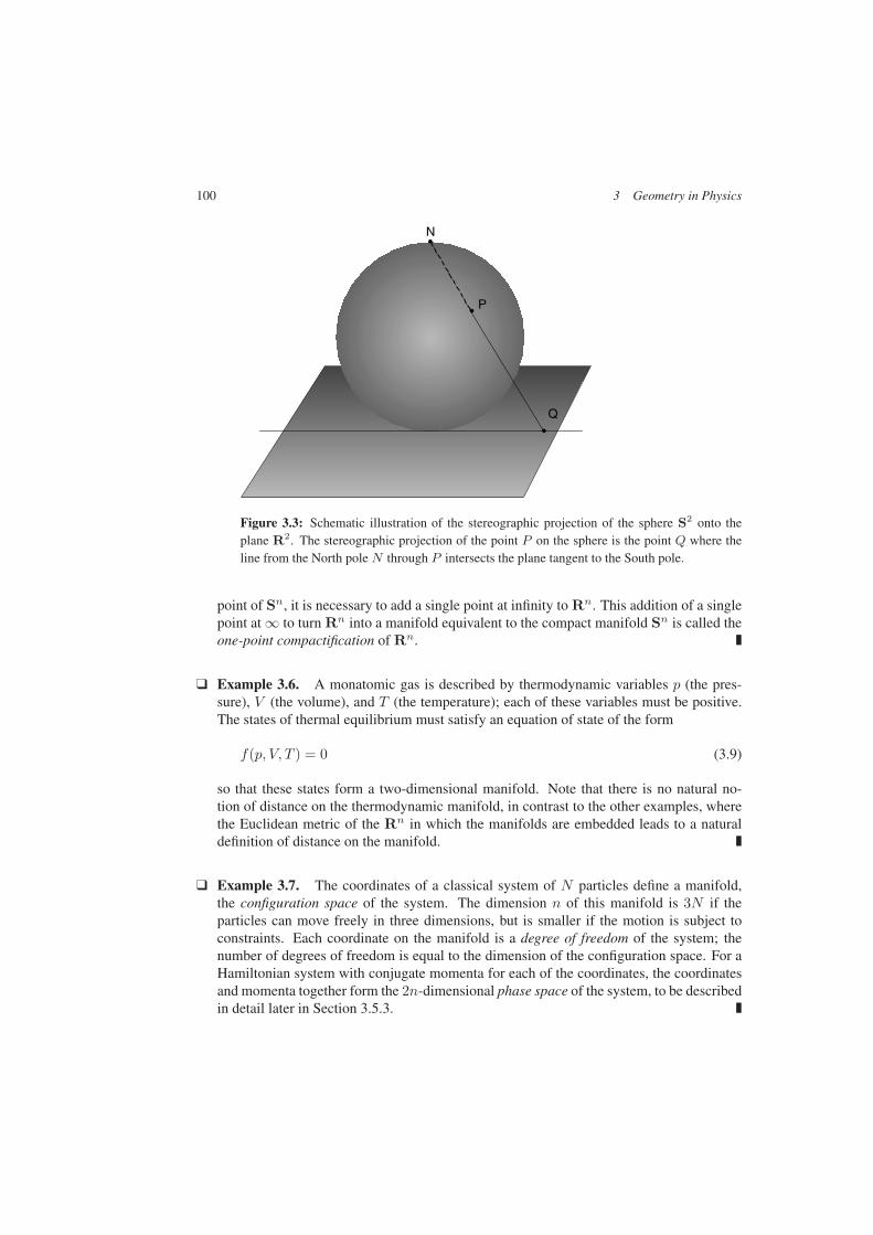
100 3 Geometry in Physics
N
P
Q•
•
•
Figure 3.3: Schematic illustration of the stereographic projection of the sphere S2 onto theplane R2. The stereographic projection of the point P on the sphere is the point Q where theline from the North pole N through P intersects the plane tangent to the South pole.
point of Sn, it is necessary to add a single point at infinity to Rn. This addition of a singlepoint at ∞ to turn Rn into a manifold equivalent to the compact manifold Sn is called theone-point compactification of Rn.
Example 3.6. A monatomic gas is described by thermodynamic variables p (the pres-sure), V (the volume), and T (the temperature); each of these variables must be positive.The states of thermal equilibrium must satisfy an equation of state of the form
f(p, V, T ) = 0 (3.9)
so that these states form a two-dimensional manifold. Note that there is no natural no-tion of distance on the thermodynamic manifold, in contrast to the other examples, wherethe Euclidean metric of the Rn in which the manifolds are embedded leads to a naturaldefinition of distance on the manifold.
Example 3.7. The coordinates of a classical system of N particles define a manifold,the configuration space of the system. The dimension n of this manifold is 3N if theparticles can move freely in three dimensions, but is smaller if the motion is subject toconstraints. Each coordinate on the manifold is a degree of freedom of the system; thenumber of degrees of freedom is equal to the dimension of the configuration space. For aHamiltonian system with conjugate momenta for each of the coordinates, the coordinatesand momenta together form the 2n-dimensional phase space of the system, to be describedin detail later in Section 3.5.3.

3.1 Manifolds and Coordinates 101
A
A
B B
Figure 3.4: Representation of the torus on the plane. The two sides marked A are to be identi-fied, as are the two sides marked B. Imagine the rectangle to be rolled up. Then glue the twosides marked A together (in the direction of the arrows) to form a hollow cylinder. Finally, gluethe two sides marked B together (in the direction of the arrows).
3.1.3 Elementary Properties of Manifolds
If M and N are manifolds, the product manifold M×N is defined as the set of ordered pairs(x, y) where x is a point from M and y is a point from N . If x has coordinates (x1, . . . , xm)and y has coordinates (y1, . . . , yn), then (x, y) has coordinates (x1, . . . , xm, y1, . . . , yn). Ev-idently the dimension of M×N is the sum of the dimensions of M and N . Note that if Mand N are linear vector spaces, the product manifold is actually the direct sum M⊕N of thetwo vector spaces, not the tensor product.
Example 3.8. It is easy to see that Rm × Rn = Rm+n.
Example 3.9. The torus T is the product S1 × S1 of two circles. It can be representedin the plane as a rectangle in which opposite sides are identified; that is, a point on theupper side A is the same as the point opposite on the lower side A in Fig. 3.4, and a pointon the left side B is the same as the opposite point on the right side B. The torus is alsoequivalent to the unit cell in the complex plane shown in Fig. 4.5.
Example 3.10. The n-torus T n is the product S1 × · · · × S1 (n factors) of n circles.
Coordinates are introduced to give a concrete description of a manifold. However, manyproperties of a manifold are independent of the specific coordinates assigned to points ofthe manifold. Indeed, it is a principle of physics that all observable properties of a physicalsystem should be independent of the coordinates used to describe the system, at least withina restricted class of coordinate systems.2 For example, the distance between two points ina manifold is defined in terms of coordinates in a region containing the two points. Oncedefined, however, it must be the same for any equivalent set of coordinates on the region.
2This is the essence of principles of relativity from Galileo to Einstein. Einstein’s principle of general relativityis the broadest, since it insists that the equations of physics be unchanged by diffeomorphisms of the spacetimemanifold, which are defined shortly.
102 3 Geometry in Physics
Equivalence of two differentiable manifolds M1 and M2 means that there is a one-to-onemap between the manifolds for which the coordinates in any region in M2 are smooth func-tions of the coordinates in the corresponding region of M1. Such a map is a diffeomorphism.If such a map exists, then the two manifolds are diffeomorphic, or simply equivalent. If onlycontinuity of the map is required, then the map is a homeomorphism, and the manifolds arehomeomorphic.
Example 3.11. The unit ball Bn is diffeomorphic to all of Rn, since the radial rescalingin Eq. (3.7) is differentiable for 0 ≤ r < 1.
Example 3.12. Consider the group SU(2) of unitary 2 × 2 matrices with determinant+1. Every matrix in this group has the form
U = exp (πiσ · a) (3.10)
where σ = (σ1, σ2, σ3) denote the three Pauli matrices, and a is a vector with |a| ≤ 1 (if|a| = 1, then U = −1 independent of the direction of a). The map
a→ r =a
1 − |a| (3.11)
takes the group manifold into R3 augmented by a single point at ∞ that corresponds toU = −1. As seen above, this is the one-point compactification of R3 to the sphere S3.Thus the group SU(2) is diffeomorphic to S3.
Convergence properties of sequences of points in a manifold are defined in terms of thecorresponding properties of the sequences in Rn of the coordinates of the points. Becausewe require all coordinate transformations to be smooth, these convergence properties will notdepend on which particular coordinate system we use to test the convergence. Thus, for exam-ple, the sequence x1, x2, . . . of points in an n-dimensional manifold is a Cauchy sequenceif the sequence of coordinates is a Cauchy sequence in Rn, using any positive definite normon Rn.
A function f(x) defined on a manifold M maps the points of the manifold to real (orcomplex) numbers; there may be exceptional points, or singular points at which the functionis not defined. The function does not depend on the coordinate system introduced on themanifold; hence is also called a scalar field. The field is continuous (differentiable, smooth,. . .) if f(x) is a continuous (differentiable, smooth, . . .) function of the coordinates. Again,these properties of the field are coordinate independent because of our restriction to smoothcoordinate transformations.
A manifold is closed if every Cauchy sequence of points in the manifold converges to alimit in the manifold. If a manifold is M is not closed, then new points can be defined as limitpoints of Cauchy sequences in the manifold. The manifold obtained from M by adjoining thelimits of all Cauchy sequences in M is the closure of M, denoted by CM, or by M. Recallthat a region in Rn is compact if it is closed (contains all its limit points) and bounded (it canbe contained inside a sufficiently large sphere). A manifold M is compact if it is equivalentto the union of a finite number of compact regions in some Rn.

3.1 Manifolds and Coordinates 103
C
C2
C1
Figure 3.5: Illustrations of the sphere S2 and torus T 2. Any closed curve C on S2 can besmoothly contracted to a single point. On the other hand, the curves labeled C1 and C2 on T 2
cannot be smoothly contracted to a point, nor deformed into each other.
Example 3.13. The sphere Sn is compact; by its definition it is a closed bounded regionin Rn+1. The unit ball Bn is not compact even though it is bounded, since it is not closed.There are sequences of points in Bn that converge to a point on the boundary sphere Sn−1,which is not part of Bn.
Example 3.14. Rn is not compact but, as just noted, addition of a single point at ∞ turnsit into a compact manifold, the one-point compactification of Rn, equivalent to Sn.
Two manifolds of the same dimension are always equivalent locally, (i.e., in some neigh-borhood of any point) since they are represented by coordinates in Rn. However, even withthe limited structure we have introduced so far, there are manifolds of the same dimension thatare not globally equivalent, i.e., there is no global diffeomorphism that takes one manifold intothe other. A compact manifold cannot be equivalent to a noncompact manifold (Bn and Sn
are not globally equivalent, for example). Manifolds can be classified according to the kindsof distinct closed curves and surfaces that can be constructed in them. This classification isone of the main problems of algebraic topology.
Example 3.15. The sphere S2 has no nontrivial closed loops; every closed loop on thesphere can be contracted smoothly to a single point. However, on the two-dimensionaltorus T 2 ∼ S1×S1, closed curves corresponding to one circuit around either of the circlescannot be contracted to a point (see Fig. 3.5). Closed curves in T 2 are characterized bya pair of integers (n1, n2) (the winding numbers), depending on how many times theywrap around each of the two circles. Curves with different winding numbers cannot becontinuously deformed into each other. Since the winding numbers are independent of thecoordinates, they are topological invariants of the manifold. Equivalence classes of closedcurves in a manifold define a group, the homotopy group of the manifold.
Example 3.16. The group SO(3) of rotations in three dimensions looks like a ball B3 ofradius π, since every rotation can be characterized by an axis n and an angle θ (0 ≤ θ ≤ π).But, unlike in SU(2), a rotation about n through angle π is the same as a rotation about−n through angle π. Thus the opposite ends of a diameter of the ball correspond to thesame rotation, and any diameter is a closed path that cannot be shrunk to a point.

104 3 Geometry in Physics
3.2 Vectors, Differential Forms, and Tensors
3.2.1 Smooth Curves and Tangent Vectors
The concept of a curve in a manifold is intuitive. A formal statement of this intuitive conceptis that a curve on the manifold M is a map from an open interval on the real axis into M.A curve is defined parametrically by the coordinates x1(λ), . . . , xk(λ) of the points onthe curve3 as functions of a real parameter λ over some range λ1 < λ < λ2. The curveis differentiable (smooth, analytic) if these coordinates are differentiable (smooth, analytic)functions of the parameter λ.
If f(x) is a differentiable function defined on M, and C is a smooth curve in M, then thefunction
g(λ) ≡ f [x(λ)] (3.12)
defined on the curve C is a differentiable function of λ, and
dg
dλ=
n∑
k=1
dxk
dλ
∂f
∂xk=
n∑
k=1
ξk(λ)∂f
∂xk(3.13)
by the chain rule. The ξk(λ) = dxk/dλ define the components of a vector tangent to thecurve at the point, and the derivative operator
d
dλ≡
n∑
k=1
ξk(λ)∂
∂xk= ξk(λ)
∂
∂xk=
−→ξ · −→∇ (3.14)
itself is identified with the tangent vector.This is more abstract than the traditional physicist’s view of a vector. However, if we recall
the geometrical interpretation of the derivative dy/dx as the tangent to a curve y = y(x) intwo dimensions, then we can recognize Eq. (3.14) as a generalization of this interpretation tocurves in higher dimensional spaces. The derivative operator in Eq. (3.14) is the directionalderivative in the direction of the tangent. It is also known as the Lie derivative when it isapplied to vectors and tensors. The form
−→ξ · −→∇ emphasizes the view of this derivative as
an intrinsic (i.e., coordinate-independent) entity, although the components of ξ depend on thecoordinate system.
Remark. With the notation (ξk ∂/∂xk) we introduce the (Einstein) summation convention,which instructs us to sum over a pair of repeated indices, unless explicitly instructed not to. Inthis chapter, we use the summation convention without further comment. However, we insistthat the pair of indices must consist of one subscript and one superscript, understanding that asubscript (superscript) in the denominator of a partial derivative is equivalent to a superscript(subscript) in the numerator.
3We use here superscripts to identify the coordinates x1, . . . , xk in keeping with historical usage. The readeris alerted to be aware of the distinction between these superscripts and exponents.

3.2 Vectors, Forms and Tensors 105
3.2.2 Tangent Spaces and the Tangent Bundle T (M)
The tangent vectors at a point P in the manifold M define a linear vector space TP , the tangentspace to M at P . A vector V in TP corresponds to the class of smooth curves through P withtangent vector V .4.
If x1, . . . , xn provides a coordinate system in a neighborhood of P , a natural set of basisvectors in the tangent space TP is given by the partial derivatives
ek ≡ ∂
∂xk(3.15)
This is the coordinate basis associated with the x1, . . . , xn.If y1, . . . , yn is another set of coordinates, smooth functions of the old coordinates
x1, . . . , xn, then we have the corresponding coordinate basis
fk ≡ ∂
∂yk=∂xm
∂yk∂
∂xm=∂xm
∂ykem (3.16)
(by the chain rule again), so long as the Jacobian determinant5
J ≡ ∂(x1, . . . , xn)∂(y1, . . . , yn)
≡ det
∥∥∥∥∥∂xm
∂yk
∥∥∥∥∥ = 0 (3.17)
This leads to the transformation law for the components of vectors. If
V = ξk∂
∂xk= ηk
∂
∂yk(3.18)
then we have
ξk = ηm∂xk
∂ymand ηm = ξk
∂ym
∂xk(3.19)
to relate the components of the vector in the two coordinate systems. This follows yet againfrom the application of the chain rule, here to the components of the tangent vector:
dxk
dλ=∂xk
∂ymdym
dλ(3.20)
The following exercise illustrates how the relations in Eq. (3.19) are generalizations of therelations for changing basis in a linear vector space.
Exercise 3.1. Suppose φ1, . . . , φn and ψ1, . . . , ψn are two bases on the linear vectorspace Vn, related by
ψk =n∑
j=1
Sjkφj
4Note that there is an arbitrary positive scale factor in the definition of the tangent vector5A geometrical interpretation of the Jacobian will be given later.

106 3 Geometry in Physics
with constants Sjk. Find relations between the components of a vector in the two bases. Thatis, if
x =n∑
j=1
ξjφj =n∑
k=1
ηkψk
express the ξj in terms of the ηk and vice versa. Show that these relations are specialcases of Eq. (3.19) for a linear coordinate transformation.
The manifold M together with the collection of tangent spaces at each point of the mani-fold forms a structure known as the tangent bundle T (M).
Example 3.17. If M is the n-dimensional configuration space of a mechanical system,then the tangent space at a point of M is defined by the velocities associated with trajec-tories that pass through the point. The tangent bundle T (M) is the 2n-dimensional spacedefined by the coordinates and velocities of the system.
Remark. The concept of a bundle, or fiber bundle, over a manifold is important in differentialgeometry and its applications to physics. In general, a fiber bundle consists of a manifold M,the base space, and another space F , such as a linear vector space or a Lie group, the fiberspace. A copy of F is attached to each point of the manifold. A function on the manifold thathas values in F is a (cross)-section of the bundle. If the space F is a linear vector space, suchas the tangent space T (M) introduced here, then the bundle is a vector bundle. To completethe definition of a fiber bundle, it is necessary to also specify a group G (the structure group)of diffeomorphisms of the fiber space. If F is a real n-dimensional linear vector space, thestructure group might be the group SO(n) of rotations of Rn, or even the group GL(n,R) ofnonsingular linear operators on Rn. In this book, we consider only the tangent bundle and theclosely related cotangent bundle introduced below. For more general bundles, see the book byFrankel cited in the bibliography.
The slice of the tangent bundle corresponding to the points from M in some neighborhoodU of a point P is locally equivalent to a product U × Vn. However, the complete tangentbundle T (M) may, or may not, be globally equivalent to the product M×Vn. This dependshow vectors at different points in the manifold are related. Can we define parallel curves, orparallel vectors at different points, for example? These important questions are important forunderstanding general relativity, but we must refer the reader to the bibliography for answers.
3.2.3 Differential Forms
The tangent space TP to the manifold M at a point P is a linear vector space. As in Sec-tion 2.1.5, we can introduce the dual space T ∗
P of linear functionals on TP . An element ω ofT ∗P maps TP into the real (or perhaps complex) numbers,
ω : v → ω(v)
such that
ω(a1v1 + a2v2) = a1ω(v1) + a2ω(v2) (3.21)

3.2 Vectors, Forms and Tensors 107
for any pair of vectors v1, v2 and any pair of numbers a1, a2. Such a linear functional ωis a (differential) 1-form, or simply form. The dual relation between forms and vectors isemphasized in the various notations
ω(v) = (ω, v) = 〈ω, v〉 = 〈ω|v〉 = v(ω) (3.22)
for the number (scalar) associated with the pair ω, v. The space T ∗P is the cotangent space of
M at P , and a 1-form is sometimes called a cotangent vector.A basis ek on TP induces a preferred basis µk on T ∗
P , the dual basis, with
〈µk, em〉 = δkm (3.23)
so that if v = vk ek, then µk(v) = vk, and if ω = ωkµk, then
(ω, v) = ωk vk (3.24)
A coordinate system xk on a region U in M provides a natural (coordinate) basis ∂/∂xkof vectors and a corresponding coordinate basis dxk of 1-forms; we have
⟨dxk,
∂
∂xm
⟩= δkm (3.25)
In a coordinate basis, a form ω is expressed as
ω = αkdxk =
−→α · −→dx (3.26)
The expression−→α ·−→dx again emphasizes the intrinsic, coordinate-independent nature of a form.
Under a smooth coordinate transformation from x1, . . . , xn to y1, . . . , yn, we have
dxk =∂xk
∂ymdym (3.27)
which leads to the transformation law for the components of a 1-form
ω = αk dxk = βm dy
m (3.28)
We have
βm = αk∂xk
∂ymand αk = βm
∂ym
∂xk(3.29)
Note that the role of the partial derivatives is reversed here, compared to the transformationlaw (3.19) for the components of a vector. That is, if
ηm ≡ Smk ξk and βm ≡ Skm αk (3.30)
then the matrices S and S, with elements
Smk =∂ym
∂xkand Skm =
∂xk
∂ym(3.31)
are inverse to each other.
108 3 Geometry in Physics
The manifold M together with the collection of cotangent spaces at each point of the man-ifold forms a structure known as the cotangent bundle T ∗(M), just as the manifold togetherwith the collection of tangent spaces at each point forms the tangent bundle.
Example 3.18. If M is the n-dimensional configuration space of a Hamiltonian systemof classical mechanics, then the cotangent bundle T ∗(M) is the 2n-dimensional phasespace defined by the coordinates and conjugate momenta of the system, as discussed inmore detail in Section 3.5.3.
Remark. We introduced the tangent space TP of vectors at a point P and then defined1-forms as linear functionals on TP . Alternatively, we could have introduced the cotangentspace T ∗
P of forms as a linear vector space spanned by the coordinate differentials and thendefined vectors as linear functionals on T ∗
P . This duality is emphasized by Eq. (3.22), as wellas by the discussion of dual spaces in Section 2.1.5.
Remark. A change of basis on the tangent space TP or cotangent space T ∗P need not be a
coordinate transformation, since there is no necessary relation between the transformationsat neighboring points. However, the transformation laws for the components of vectors andforms are still related if we insist that the transformations on TP and T ∗
P change a pair of dualbases into another pair of dual bases. See Problem 3 for details.
Remark. In an older terminology, the components of a 1-form were known as the covariantcomponents of a vector. They transform in the same way as the components of the gradient,which was treated as the prototype of a vector, perhaps since so many fields are expressed asthe gradient of some scalar potential. The components of a (tangent) vector were known as thecontravariant components of a vector, since they transform according to the inverse (contra)transformation law. This emphasis on transformation laws led to a proliferation of indices,and tended to obscure the point that vectors and forms are geometrical and physical objectsthat do not depend on the particular coordinate system used to describe the manifold in whichthey live. The modern view emphasizes the intrinsic properties of forms and vectors, and theduality relation between them.
Remark. In a manifold with a metric, there is a natural mapping between vectors and formsinduced by a metric tensor, as will appear soon in Section 3.4. Here we note that in a linearvector space Rn with the (Euclidean) scalar product as defined in Chapter 2, the distinctionbetween vectors and forms is purely formal, and we can identify the vector
V = V k∂
∂xk(3.32)
and the form
V = Vk dxk (3.33)
with the same numerical components Vk = V k in any Cartesian coordinate basis.
Exercise 3.2. Show that if these numerical components are the same in one coordinatebasis, they are the same in any basis obtained by a rotation from the original basis, i.e., showthat these components have the same transformation law under rotations.
3.2 Vectors, Forms and Tensors 109
3.2.4 Tensors
Tensors arise when we consider the products of vectors and forms. The tensor product oflinear vector spaces has been introduced in Section 2.1.3. Here we introduce the tensor spaces
T (M,N)P ≡ TP ⊗ · · · ⊗ TP︸ ︷︷ ︸
M times
⊗ T ∗P ⊗ · · · ⊗ T ∗
P︸ ︷︷ ︸N times
(3.34)
at a point P in a manifold. Elements of T (M,N)P are formed from linear combinations of
products of M vectors from TP and N 1-forms from T ∗P . Elements of this space are
(MN
)
tensors. If N = 0, we have a tensor of rank M . If M = 0, we have a dual tensor of rank N .Otherwise, we have a mixed tensor of rank M +N .
Example 3.19. A linear operator on a linear vector space is a(11
)tensor, since the equa-
tion y = Ax becomes
yj = A kj xk (3.35)
in terms of components.
Example 3.20. The inertia tensor of a rigid body about some point is a (symmetric)tensor of rank 2. Since a rigid body is defined only in a Euclidean space, we need notdistinguish between vector and form indices, at least for Cartesian components.
Tensor components are defined with respect to some basis. Corresponding to coordinatesx1, . . . , xn in some neighborhood of P is the coordinate basis
e j1...jNi1...iM
≡ ∂
∂xi1⊗ · · · ⊗ ∂
∂xiM⊗ dxj1 ⊗ · · · ⊗ dxjN (3.36)
on the tensor space T (M,N)P . A tensor T is expressed in terms of this basis as
T = T i1...iMj1...jN
e j1...jNi1...iM
(3.37)
(summation convention in effect). The T i1...iMj1...jN
are the components of T.
A tensor can also be introduced as a functional: an(MN
)tensor is a linear functional on the
linear vector space T (N,M)P ,
T = T ( . , . . . , .︸ ︷︷ ︸N arguments
| . , . . . , .︸ ︷︷ ︸M arguments
) (3.38)
in which the first N arguments require vectors, and the last M arguments need forms, in orderto reduce the functional to a scalar. This is equivalent to the statement
T (M,N)∗P = T (N,M)
P (3.39)
that generalizes the duality of vectors and 1-forms. Again, note that in a manifold with ametric, there is a natural mapping between a tensor and its dual induced by the metric tensor.
110 3 Geometry in Physics
Inserting arguments in the empty slots in the functional (3.38) reduces the rank of thetensor. Thus if v is a vector, then
T ( . , . . . , v | . , . . . , . ) (3.40)
is an(MN−1
)tensor with components
T i1,...,iMj1,...,jN−1j
vj (3.41)
Similarly, if ω is a (1-)form, then
T ( . , . . . , . | . , . . . , ω) (3.42)
is an(M−1N
)tensor with components
T i1,...,iM−1ij1...jN
ωi (3.43)
The reduction of rank by inserting arguments in the functional is called contraction.A mixed
(MN
)tensor can also be contracted with itself to give an
(M−1N−1
)tensor T with
components
T i1,...,iM−1j1,...,jN−1
≡ T i1,...,iM−1mj1,...,jN−1m
(3.44)
Example 3.21. For a linear operator A on TP , with components A kj in some basis, the
contraction
A ≡ A kk (3.45)
is a scalar already identified as the trace of A. It is indeed a scalar, as its value is indepen-dent of the coordinate system.
3.2.5 Vector and Tensor Fields
A vector field v on a manifold M is a map from the manifold into the tangent bundle T (M)such that at each point x in M, there is attached a vector v(x) in the tangent space Tx, whosecomponents are smooth functions of the coordinates. Simple fluid flow is described by avelocity field u(x), the velocity of the fluid element at x. The electric field E(x) and themagnetic field B(x) due to a system of charges and currents are vector fields. As alreadynoted, a vector field v(x) can be identified with the directional derivative
v = vk(x)∂
∂xk=
−→v · −→∇ (3.46)
More intuitive is the visualization of a vector field by drawing some of its integral curves,which are also known as streamlines (fluid flow), lines of force (electric fields), or flux lines(magnetic fields). Two examples are shown in Fig. 3.6. The integral curve of the vectorfield v(x) passing through a point P is generated by starting at P , moving in the direction of

3.2 Vectors, Forms and Tensors 111
(b)(a)
Figure 3.6: Examples of the integral curves of a vector field: (a) the streamlines of a fluidflowing through a pipe with a nonconstant cross-section, and (b) schematic representation of thelines of force of the electric field due to equal and opposite charges (an extended dipole).
the field at that point and continuing in the direction of the field at each point. This can beaccomplished by solving the system of first-order differential equations
dxk
dλ= vk(x) (3.47)
with initial condition x = x(P ) at λ = 0. This system has a unique solution provided thevk(x) are well-behaved functions, not all zero, at the point P.6 Two integral curves cannotintersect, except perhaps at points where v(x) = 0 or where v(x) is undefined. Such pointsare singular points of the vector field.
Remark. The electric field is undefined at the location of a point charge, for example. Also,a point where v(x) = 0 is a fixed point of Eq. (3.47). The solution to Eq. (3.47) starting atsuch a point P does not generate a curve but remains fixed at P . However, integral curves nearthe point P may approach P asymptotically, diverge from P , or exhibit hyperbolic behavioras illustrated in Fig. 2.8. Understanding the generic behavior of solutions near a fixed point isthe object of the stability analysis in Section 2.5.
The vector field v in Eq. (3.46) defines a tangent vector at each point on an integral curveof the field. To generate a finite displacement along the curve, say from λ0 to λ0 + α, we canformally exponentiate the differential operator to give
xk(λ0 + α) = exp(αd
dλ
)xk(λ0) = xk(λ0) +
∞∑
n=1
[dn
dλnxk(λ)
]
λ=λ0
αn
n!(3.48)
This formal Taylor series expansion actually converges only if the coordinates xk(λ) are ana-lytic functions of the parameter λ along the curve. This may, or may not, be the case.
6It is sufficient that there is some constant M > 0 such that
|vk(x) − vk(x′)| < M‖x − x′‖for all k and all x, x′ in some neighborhood of P (Lipschitz condition). For proofs, consult a textbook on differentialequations. Note that the Lipschitz condition includes the case in which the vk(x) are differentiable at P , but is morerestrictive than continuity of the vk(x) at P .
112 3 Geometry in Physics
The partial derivatives ∂/∂xk with respect to the coordinates xk define a basis for the tan-gent space Tx at each point x. But at each x, we can choose any set of n linearly independentvectors as a basis for Tx , and in some open region U around x, we can choose any n linearlyindependent vector fields as a basis.
Can we use these fields to define a coordinate system? To answer this question, supposewe have two vector fields
v =d
dλ= vk
∂
∂xkand w =
d
dµ= wk
∂
∂xk(3.49)
Let us carry out displacements from a point O, as shown in Fig. 3.7. First move a distance dλalong the integral curve of v through O to the pointA. The coordinates then change accordingto
xk(A) − xk(O) vk(O)dλ (3.50)
Then move a distance dµ along the integral curve of w through A, arriving at the point Pwhose coordinates are given by
xk(P ) − xk(A) wk(A)dµ (3.51)
Alternatively, move first dµ along the integral curve of w through O to Q, with
xk(B) − xk(O) wk(O)dµ (3.52)
and then dλ along the integral curve of v through Q, arriving at the point P ′, with
xk(P ′) − xk(B) vk(B)dλ (3.53)
If v and w are to generate a coordinate system, either order of carrying out the two dis-placements should lead to the same final coordinates, and hence the same final point, as inFig. 3.7(b). But we can compute
wk(A) wk(O) +[vm
∂wk
∂xm
]
Odλ (3.54)
and
vk(B) vk(O) +[wm
∂vk
∂wm
]
Odµ (3.55)
Then
xk(P ) − xk(P ′) [vm
∂wk
∂xm− wm
∂vk
∂xm
]
Odλ dµ (3.56)
The term in brackets must vanish if P and P ′ are the same points. Now the commutator ofthe two operators v and w is defined by
[v, w] =[d
dλ,d
dµ
]=[vm
∂wk
∂xm− wm
∂vk
∂xm
]∂
∂xk(3.57)

3.2 Vectors, Forms and Tensors 113
O
P'
B
PA
O
A
B
P
(a) (b)
Figure 3.7: (a) A general displacement from point O along the integral curves of two vectorfields v and w. A displacement dλ along the integral curve of v carries us from O to A, and afurther displacement dµ along the integral curve ofw throughA carries us to P . A displacementdµ along the integral curve of w through O to B, followed by a displacement dλ along theintegral curve of v through B takes us to P ′. In general, the points P and P ′ are not thesame, but if the vector fields v and w commute (have vanishing Lie bracket), as in (b), then thetwo paths lead to the same endpoint, and the vector fields v and w can be used as a part of acoordinate basis.
This commutator is also called the Lie bracket of the two vector fields. In order for λ and µ tobe coordinates, this commutator must vanish. More generally, a necessary condition for a setof vector fields to form the basis of a coordinate system is that the Lie bracket, or commutator,of any pair of the fields must vanish.
Remark. This condition should not be a surprise—we expect mixed partial derivatives withrespect to a pair of coordinates to be independent of the ordering of the derivatives.
The vanishing of the commutator (3.57) is also sufficient. A formal way to see this is tonote the formal expression
xk(λ0 + α, µ0 + β) = exp(αd
dλ+ β
d
dµ
)xk(λ0, µ0) (3.58)
based on Eq. (3.48). The exponential factorizes into a displacement α of the coordinate λ anda displacement β of the coordinate µ if (and only if) the derivative operators commute.
Exercise 3.3. Suppose r, θ are the standard polar coordinates in the plane defined by
x = r cos θ y = r sin θ
Consider the radial and tangential unit vectors
er ≡ cos θ ex + sin θ ey eτ ≡ − sin θ ex + cos θ ey
Corresponding to these are the vector fields
∂
∂r≡ cos θ
∂
∂x+ sin θ
∂
∂y
∂
∂τ≡ − sin θ
∂
∂x+ cos θ
∂
∂y
114 3 Geometry in Physics
Do these vector fields form a coordinate basis? If not, find a suitable coordinate basis for polarcoordinates, and express this basis in terms of ∂/∂x and ∂/∂y.
A 1-form field ω on a manifold M is a map that takes each point x in M to a 1-form ω(x)in the cotangent space T ∗
x . If f(x) is a differentiable function (scalar field) on M the gradientdf of f is the 1-form field defined by
⟨df,
d
dλ
⟩=df
dλ(3.59)
In a coordinate basis, the gradient can be expressed as
df =∂f
∂x1dx1 + · · · + ∂f
∂xndxn =
∂f
∂xkdxk =
−→∇f · −→dx (3.60)
Thus the components of df in this basis are just the partial derivatives of f , as introduced inelementary calculus. We can also note that df is the element of T ∗
P whose value on v in TPis the directional derivative of f along v. Since this derivative vanishes in any direction on asurface f = constant, df is in some sense normal to such a surface. If a metric is defined onM, this statement can be made more precise, as will be seen soon.
The tensor space T (M,N)P is introduced at each point P of a manifold. A tensor field of
type(MN
)is a collection of
(MN
)tensors defined at each point on the manifold (or in some
region of the manifold). The field is continuous (differentiable, smooth,. . .) if its componentsin some coordinate basis are continuous (differentiable, smooth,. . .).
Example 3.22. Stress and strain in an elastic medium are (symmetric) tensor fields ofrank 2.
Example 3.23. The electromagnetic field F = (Fµν) is an antisymmetric tensor field ofrank 2. The electromagnetic stress–energy tensor T = (Tµν) is a symmetric tensor fieldof rank 2.
Remark. The examples given here all have rank 2. Tensors of higher rank are less commonin macroscopic physics, appearing mainly in the theories of elasticity in deformable solids,and also in Einstein’s theory of gravity (general relativity). However, they are relevant inquantum theories with higher symmetries, as in the examples discussed in Chapter 10. It isuseful to realize that conceptually, at least, higher rank tensors are no more complicated thanthose of rank 2.
3.2.6 The Lie Derivative
The Lie derivative Lv associated with a vector field v is an operator that measures the rate ofchange along integral curves of the vector field. The Lie derivative of a scalar function f(x)is the directional derivative
Lvf(x) =−→v · −→∇f(x) (3.61)
The Lie derivative Lv of a vector field w has been introduced in Eq. (3.57) as the commutator
Lvw = [v, w] (3.62)
3.2 Vectors, Forms and Tensors 115
It measures the change in the coordinate distance along integral curves of w between inter-sections with two nearby integral curves of v, as we move along the integral curves of v. IfLvw = 0, then this coordinate distance does not change as we move along the integral curves,and the fields v and w can be a part of a coordinate basis.
Expressions for the Lie derivative of other types of tensor fields can be generated usingthe Leibniz rule
Lv (ab) = (Lva) b+ a (Lvb) (3.63)
Example 3.24. To obtain a rule for the Lie derivative of a 1-form ω, note that the Leibnizrule gives
(Lv ω, u) = Lv (ω, u) − (ω,Lv u) (3.64)
for any vector u. Now
Lv (ω, u) = vk∂
∂xk(ωu) = vk
(∂ω∂xk
u +∂u
∂xkω
)(3.65)
and
(ω,Lv u) = ω
(vk
∂u
∂xk− uk
∂v
∂xk
)(3.66)
so that
(Lv ω) = vk∂ω∂xk
+ ωk∂vk
∂x(3.67)
Note the positive sign here, in contrast to the negative sign in Eq. (3.57).
Remark. Note that the Lie derivative does not change the rank of a tensor.
Example 3.25. The Lie derivative appears naturally in the description of the flow of afluid with velocity field U . The co-moving derivative, which measures the rate of changeof a property of a fixed drop of the fluid moving with the flow, rather than at a fixed pointin space, is expressed as
d
dt=
∂
∂t+ LU (3.68)
Fluids are discussed at greater length in Section 3.6.
Another important use of the Lie derivative is to identify invariants. If T is a tensor such that
LvT = 0 (3.69)
then T is constant along any integral curve of v; T is an invariant of the vector field v.
116 3 Geometry in Physics
3.3 Calculus on Manifolds
3.3.1 Wedge Product: p-Forms and p-Vectors
A general tensor of type(
0N
)has components αi1,...,iN with no particular symmetry under
permutations of the indices. However, such a tensor can be split into sets of componentsthat have definite symmetry, i.e., they transform according to irreducible representationsof thegroup SN that permutes the indices of the tensor; such sets are invariant under change of basis.General irreducible representations are studied in Chapter 10; for now we are interested onlyin completely symmetric or completely antisymmetric tensors.
If σ and τ are 1-forms, and
ω = σ ⊗ τ (3.70)
then introduce the symmetric and antisymmetric forms
ωS ≡ 12 (σ ⊗ τ + τ ⊗ σ) ωA ≡ 1
2 (σ ⊗ τ − τ ⊗ σ) (3.71)
If µk is a basis of 1-forms and
σ = αkµk τ = βkµ
k (3.72)
then
ωS = 12 (αkβ + αβk)µk ⊗ µ ≡ 1
2 ωSk µ
k ⊗ µ (3.73)
ωA = 12 (αkβ − αβk)µk ⊗ µ ≡ 1
2 ωAk µ
k ⊗ µ (3.74)
where the factor 12 is to compensate for double counting in the sum over k and .
Exercise 3.4. Show that ωSk (ωAk) remain symmetric (antisymmetric) under any change
of basis on the tensor space T (0,2)P on which the forms are defined.
The antisymmetric part of the product of two 1-forms σ and τ is important enough thatit has a special name, the wedge product (also exterior product or Grassmann product in themathematical literature). It is denoted by
σ ∧ τ ≡ 12 (σ ⊗ τ − τ ⊗ σ) = −τ ∧ σ (3.75)
In terms of components of σ and τ with respect to a basis µk, we have
σ ∧ τ = 12 (αkβ − αβk) µk ∧ µ (3.76)
Exercise 3.5. Show that if σ and τ are 1-forms, and v is a vector, then
〈σ ∧ τ, v〉 = 〈σ, v〉τ − σ〈τ, v〉
The wedge product generalizes the three-dimensional cross product A×B of vectors. Indeed,this cross product is often denoted by A ∧ B in the European literature.

3.3 Calculus on Manifolds 117
The wedge product of two 1-forms is a 2-form. The antisymmetric product of p 1-formsis a p-form. If σ1, . . . , σp are 1-forms, we have
σ1 ∧ · · · ∧ σp ≡1p!
∑
i1,...,ip
εi1,...,ip σ1 ⊗ · · · ⊗ σp (3.77)
where εi1,...,ip is the usual antisymmetric (Levi-Civita) symbol with p indices defined as by
εi1,...,ip = εi1,...,ip =
+1, if i1, . . . , ip is an even permutation of 1 . . . p−1, if i1, . . . , ip is an odd permutation of 1 . . . p0, if any two indices are equal
(3.78)
and the division by p! is needed to compensate for multiple counting in the sum over i1, . . . , ip.A p-form σ can be expressed in terms of components as
σ =1p!σi1,...,ip µ
i1 ∧ · · · ∧ µip (3.79)
Exercise 3.6. Show that the wedge product of a p-form σp and a q-form τq is a (p + q)-form, with
σp ∧ τq = (−1)pq τq ∧ σp
Evidently this generalizes the antisymmetry of the wedge product of two 1-forms.
The appearance of coordinate differentials as a basis for forms suggests that forms can beintegrated. For example, a 1-form σ = σk dx
k appears naturally as the integrand of a lineintegral
∫
C
σ =∫
C
σk dxk (3.80)
along a curveC, and the dxk in the integral are the usual coordinate differentials of elementarycalculus. Note that it may be necessary to use more than one coordinate patch to integratealong the entire curve C.
Similarly, a 2-form σ = 12σk dx
k ∧ dx appears naturally as the integrand of a surfaceintegral
∫
S
σ = 12
∫
S
σk dxk ∧ dx (3.81)
over a surface S. In this context, the product dxk ∧dx represents an oriented surface elementdefined by the line elements dxk and dx; the orientation arises from the antisymmetry of thewedge product.
Remark. Expressing a surface element as a 2-form dx ∧ dy leads directly to understandingthe appearance of the Jacobian determinant when integration variables are changed. If
u = u(x, y) v = v(x, y) (3.82)
118 3 Geometry in Physics
then
du =∂u
∂xdx+
∂u
∂ydy dv =
∂v
∂xdx+
∂v
∂ydy (3.83)
whence
du ∧ dv =(∂u
∂x
∂v
∂y− ∂u
∂y
∂v
∂x
)dx ∧ dy (3.84)
The minus sign and the absence of dx ∧ dx and dy ∧ dy terms follow from the antisymmetryof the wedge product that is associated with the orientation of the surface element.
In general, a p-form appears as an integrand in a p-dimensional integral. If σ is a smoothp-form defined on a manifold M, and R is a p-dimensional submanifold of M, then wedenote such an integral simply by
I ≡∫
R
σ (3.85)
where I represents a number, the value of the integral. To relate this integral to the usualintegral of elementary calculus, and to apply the usual methods to evaluate the integral, weneed to introduce a coordinate system (or a covering set of coordinate patches) on R. Ifx1, . . . , xp is such a coordinate system, then the form σ can be expressed as
σ = fσ(x1, . . . , xp) dx1 ∧ · · · ∧ dxp (3.86)
(locally on each coordinate patch in R, if necessary). The integral I is then given by
I =∫
R
fσ(x1, . . . , xp) dx1, . . . , dxp (3.87)
where now the dx1, . . . , dxp are the usual coordinate differentials of elementary calculus,rather than a set of abstract basis elements for forms.
Remark. Note that the antisymmetry of the underlying p-form leads to the relation
dy1 ∧ · · · ∧ dyp = det∥∥∥∥∂yk
∂x
∥∥∥∥ dx1 ∧ · · · ∧ dxp (3.88)
for changing variables from x1, . . . , xp to y1, . . . , yp in a p-dimensional integral, where thedeterminant is the usual Jacobian. This result leads to a natural definition of volume elementon a manifold with a metric tensor, as will be seen in the next section.
In an n-dimensional manifold, there are no p-forms at all with p > n, and there is exactlyone independent n-form, which in a coordinate basis is proportional to
Ω ≡ dx1 ∧ · · · ∧ dxn =1n!εi1,...,indx
i1 ∧ · · · ∧ dxin (3.89)
where εi1,...,in is the Levi-Civita symbol defined in Eq. (3.78).

3.3 Calculus on Manifolds 119
Exercise 3.7. Show that the dimension of the linear vector space Ep(P ) of p-forms at apoint P is given by
dp =(n
p
)
Note that this implies dn−p = dp.
Definition 3.2. The collection of all p-forms (p = 1, . . . , n) at a point P of an n-dimensionalmanifold M defined the exterior algebra E(P ) at P , with product of forms defined as thewedge product.
Exercise 3.8. Show that the dimension of E(P ) is 2n.
The p-forms have been introduced as antisymmetric tensor products of 1-forms at apoint P . These can be extended to p-form fields defined on a region of a manifold—evenon the entire manifold. One important field on a manifold is the fundamental volume form
Ω(x) ≡ ρ(x) dx1 ∧ · · · ∧ dxn (3.90)
where ρ(x) is a somewhat arbitrary density function that is modified by a Jacobian determinantunder a change of coordinates. However, in a manifold with a metric tensor, there is a naturaldefinition of the fundamental volume form (see Section 3.4). If it is possible to define acontinuous n-form on the n-dimensional manifold M with ρ(x) nowhere vanishing, then Mis (internally) orientable, and we can take ρ(x) to be positive everywhere on M.
The volume form serves to define another duality between vectors and forms. If σ is ap-form, then the (Hodge)*-dual of σ is the antisymmetric
(n−p
0
)tensor V defined by
V i1,...,in−p = (∗σ)i1,...,in−p ≡ 1p!
1ρ(x)
εi1,...,inσin−p+1,...,in (3.91)
Conversely, if V is an antisymmetric(n−p
0
)tensor, then the (Hodge)*-dual of V is the p-form
σ defined by
σi1,...,ip = (∗V )i1,...,ip ≡ 1(n− p)!
ρ(x)εi1,...,inVip+1,...,in (3.92)
Example 3.26. Consider the real linear vector space R3 with the usual volume form
Ω = dx1 ∧ dx2 ∧ dx3 (3.93)
A 2-form
σ = 12 σjkdx
j ∧ dxk (3.94)
is dual to the vector
∗σ = 12εjkσjk
∂
∂x≡ ∗σ
∂
∂x(3.95)
120 3 Geometry in Physics
Conversely, a vector
V = V ∂
∂x(3.96)
corresponds to the dual 2-form
∗V = 12 εjkl V
dxj ∧ dxk ≡ 12
∗Vjk dxj ∧ dxk (3.97)
Thus in three dimensions (only), the wedge product, or vector product, of two vectors canbe identified with another vector as in the usual expression C = A × B.
Exercise 3.9. Show that if σ is a p-form, then ∗(∗σ) = (−1)p(n−p)σ.
Exercise 3.10. Show that the dual of the volume form is a constant scalar function (a0-vector), and, in fact, ∗Ω = 1.
3.3.2 Exterior Derivative
The derivative operator−→∇ of elementary vector calculus can be generalized to a linear oper-
ator d, the exterior derivative, which transforms a p-form field into a (p + 1)-form field. Theoperator d is defined by the following rules:
1. For a scalar field f , df is simply the gradient of f , defined in a coordinate basis by theusual rule, Eq. (3.59),
df =∂f
∂xkdxk (3.98)
so that if
v = vk∂
∂xk(3.99)
is a vector field, then
(df, v) = vk∂f
∂xk=
−→v · −→∇f(x) (3.100)
which is the directional derivative of f in the direction of v.2. The operator d is linear, so that if σ and τ are p-forms, then
d(σ + τ ) = dσ + dτ (3.101)
3. If σ is a p-form and τ is a q-form, then
d(σ ∧ τ ) = dσ ∧ τ + (−1)pσ ∧ dτ (3.102)
4. Poincaré’s lemma. For any form σ,
d(dσ) = 0 (3.103)

3.3 Calculus on Manifolds 121
Remark. It is actually enough to assume that this is true for 0-forms (scalars) only, but wedo not want to go into details of the proof of the generalized formula, Eq. (3.103).
The combination of rules 1–4 allows us to construct explicit representations for the doperator in terms of components. If
σ = σk dxk (3.104)
is a 1-form, then dσ is given by
dσ = dσk ∧ dxk =∂σk∂xj
dxj ∧ dxk =12
(∂σk∂xj
− ∂σj∂xk
)dxj ∧ dxk (3.105)
where Poincaré’s lemma has been used to set d(dxk) = 0. Thus dσ is a generalization of
curl σ =−→∇ ×−→
σ of elementary calculus. Note that if σ = df , with f being a scalar function,then
dσ =∂2f
∂xj∂xkdxj ∧ dxk = 0 (3.106)
since the second derivative is symmetric in j and k, while the wedge product is antisymmetric.This is consistent with Poincaré’s lemma d(df) = 0, and corresponds to the elementary result
curl grad f =−→∇ ×−→∇f = 0 (3.107)
Similarly, if
σ = 12 σk dx
k ∧ dx (3.108)
is a 2-form, then
dσ =12∂σk∂xm
dxk ∧ dx ∧ dxm (3.109)
=16
(∂σk∂xm
+∂σmk∂x
+∂σm∂xk
)dxk ∧ dx ∧ dxm (3.110)
with obvious generalization to higher forms.
Example 3.27. In three dimensions, we have the standard volume element
Ω = 16 εjkl dx
j ∧ dxk ∧ dx (3.111)
so that
dxj ∧ dxk ∧ dx = εjkl Ω (3.112)
The 2-form σ is the dual of a vector V , σ = ∗V , with
σjk = εjkmVm (3.113)
122 3 Geometry in Physics
Thus
dσ =(∂V m
∂xm
)Ω = (div V ) Ω (3.114)
and the divergence of a vector field V can be expressed as
(div V ) Ω = d ∗V (3.115)
In view of Exercise 3.10, we also have
div V = ∗d(∗V ) (3.116)
This definition serves to define the divergence of a vector field in any dimension.
Exercise 3.11. Show that in a space with a general volume form defined by Eq. (3.90),the divergence of the vector field V is given by
div V =1
ρ(x)∂
∂xk[ρ(x)V k
]
Show also that
LVΩ = (div V )Ω
This is yet another geometrical property of the Lie derivative.
Exercise 3.12. Show that Poincaré’s lemma also gives the identity
div curl−→V = 0
of elementary calculus.
Definition 3.3. If σ is a p-form and V is a vector field, the contraction of σ with V defines a(p− 1)-form that we denote by
iV σ ≡ σ(V, . ) (3.117)
or, in terms of components,
(iV σ)i1,...,ip−1 = σk i1,...,ip−1Vk (3.118)
as in Eq. (3.44).
Remark. iV σ is sometimes called an interior derivative, or interior product.
Exercise 3.13. Show that if σ is a p-form and τ is a q-form, then
iV (σ ∧ τ ) = σ ∧ (iV τ ) + (−1)q(iV σ) ∧ τ
Note that we define iV σ by contracting the first index of σ with the vector index of V . Thealternative of contraction with the pth index leads to more awkward minus signs.
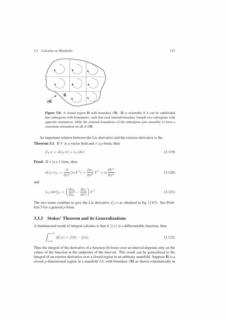
3.3 Calculus on Manifolds 123
R
∂R
Figure 3.8: A closed region R with boundary ∂R. R is orientable if it can be subdividedinto subregions with boundaries, such that each internal boundary bounds two subregions withopposite orientation, while the external boundaries of the subregions join smoothly to form aconsistent orientation on all of ∂R.
An important relation between the Lie derivative and the exterior derivative is the
Theorem 3.1. If V is a vector field and σ a p-form, then
LV σ = d(iV σ) + iV (dσ) (3.119)
Proof. If σ is a 1-form, then
d(iV σ)k =∂
∂xk(σV ) =
∂σ∂xk
V + σ∂V
∂xk(3.120)
and
[iV (dσ)]k =(∂σk∂x
− ∂σ∂xk
)V (3.121)
The two terms combine to give the Lie derivative LV σ as obtained in Eq. (3.67). See Prob-lem 5 for a general p-form.
3.3.3 Stokes’ Theorem and its Generalizations
A fundamental result of integral calculus is that if f(x) is a differentiable function, then
∫ x=b
x=a
df(x) = f(b) − f(a) (3.122)
Thus the integral of the derivative of a function (0-form) over an interval depends only on thevalues of the function at the endpoints of the interval. This result can be generalized to theintegral of an exterior derivative over a closed region in an arbitrary manifold. Suppose R is aclosed p-dimensional region in a manifold M, with boundary ∂R as shown schematically in
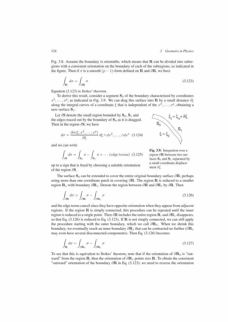
124 3 Geometry in Physics
Fig. 3.8. Assume the boundary is orientable, which means that R can be divided into subre-gions with a consistent orientation on the boundary of each of the subregions, as indicated inthe figure. Then if σ is a smooth (p− 1)-form defined on R and ∂R, we have
∫
R
dσ =∫
∂R
σ (3.123)
Equation (3.123) is Stokes’ theorem.To derive this result, consider a segment S0 of the boundary characterized by coordinates
x2, . . . , xp, as indicated in Fig. 3.9. We can drag this surface into R by a small distance δξalong the integral curves of a coordinate ξ that is independent of the x2, . . . , xp, obtaining anew surface S1.
Let δS denote the small region bounded by S0, S1 andthe edges traced out by the boundary of S0 as it is dragged.Then in the region δS, we have
dσ =∂σ(ξ, x2, . . . , xp)
∂ξdξ ∧dx2, . . . ,∧dxn (3.124)
and we can write∫
δS
dσ =∫
S0
σ−∫
S1
σ+ · · · (edge terms) (3.125)
up to a sign that is fixed by choosing a suitable orientationof the region δS.
ξ = ξ 0
ξ = ξ0
+ δξ
SS0
1
1
Fig. 3.9: Integration over aregion δR between two sur-faces S0 and S1 separated bya small coordinate displace-ment δξ.
The surface S0 can be extended to cover the entire original boundary surface ∂R, perhapsusing more than one coordinate patch in covering ∂R. The region R is reduced to a smallerregion R1 with boundary ∂R1. Denote the region between ∂R and ∂R1 by δR. Then
∫
δR
dσ =∫
∂R
σ −∫
∂R1
σ (3.126)
and the edge terms cancel since they have opposite orientation when they appear from adjacentregions. If the region R is simply connected, this procedure can be repeated until the innerregion is reduced to a single point. Then δR includes the entire region R, and ∂R1 disappears,so that Eq. (3.126) is reduced to Eq. (3.123). If R is not simply connected, we can still applythe procedure starting with the outer boundary, which we call ∂R0. When we shrink thisboundary, we eventually reach an inner boundary ∂R1 that can be contracted no further (∂R1
may even have several disconnected components). Then Eq. (3.126) becomes∫
R
dσ =∫
∂R0
σ −∫
∂R1
σ (3.127)
To see that this is equivalent to Stokes’ theorem, note that if the orientation of ∂R0 is “out-ward” from the region R, then the orientation of ∂R1 points into R. To obtain the consistent“outward” orientation of the boundary ∂R in Eq. (3.123), we need to reverse the orientation
3.3 Calculus on Manifolds 125
of ∂R1. The integral on the right-hand side of Eq. (3.127) is then an integral over the entireboundary of R.
The general Stokes’ theorem (Eq. (3.123)) includes the elementary version∮
C
−→V · −→dl =
∫
S
curl−→V · −→dS (3.128)
that relates the integral of a vector−→V around a closed curve C to the integral of curl
−→V over
a surface S bounded by C.
Remark. Equation (3.128) shows that any surface bounded by C can be chosen, since theintegral on the right-hand side depends only on the boundary curve C.
Example 3.28. A magnetic field−→B can be expressed in terms of a vector potential
−→A as
−→B = curl
−→A (3.129)
The magnetic flux Φ through a surface S bounded by the closed curve C can then beexpressed as
Φ =∫
S
−→B · −→dS =
∮
C
−→A · −→dl (3.130)
Note that this is invariant under a gauge transformation−→A → −→
A +−→∇χ for any single-
valued gauge function χ.
Exercise 3.14. The vector potential at the point −→r due to a point magnetic dipole −→m atthe origin is given by
−→A (
−→r ) = k
−→m ×−→rr3
(3.131)
where k is a constant. Find the magnetic flux through a circular loop of radius R with centerat a distance d from the dipole, oriented perpendicular to the line from the dipole to the center(i) by using the result of the previous example, and (ii) by integrating the magnetic field overa spherical cap with center at the dipole, and bounded by the circular loop.
Stokes’ theorem also includes the divergence theorem in three dimensions,∮
S
−→V · −→dS =
∫
R
(div−→V ) Ω (3.132)
that relates the flow of a vector−→V across a closed surface S to the integral of the divergence
of−→V over the volume R bounded by S. The divergence theorem leads to relations between
global conservation laws and local equations of continuity. For example, the total electriccharge QR in a region R is given in terms of the charge density ρ by
QR =∫
R
ρ Ω (3.133)

126 3 Geometry in Physics
The current I across a surface S is expressed in terms of the current density j as
I =∫
S
j · −→dS (3.134)
Conservation of charge means that the total charge in a closed region changes only if chargeflows across the boundary of the region. This is expressed formally as
dQR
dt=
d
dt
∫
R
ρ Ω =∫
R
∂ρ
∂tΩ = −
∫
∂R
j · −→dS (3.135)
where as above, ∂R denotes the boundary of R. Hence, using Eq. (3.132), we have∫
∂R
j · −→dS =∫
R
(divj
)Ω (3.136)
for any region R, and then∫
R
(∂ρ
∂t+ divj
)Ω (3.137)
Since this is true for any R, the integrand must vanish everywhere, so that
∂ρ
∂t+ divj = 0 (3.138)
Remark. Equation (3.138) is the equation of continuity. It is also true for matter flow in afluid, where ρ is the mass density and j = ρu is the mass flow density, and the total mass ofthe fluid is conserved. See Section 3.6 for further discussion of fluids.
Stokes’ theorem also serves to show the equivalence between differential and integralforms of Maxwell’s equations for electric and magnetic fields. Gauss’ Law
∫
S
−→E · −→dS = 4πkQ = 4πk
∫
R
ρ Ω (3.139)
relates the flux of the electric field E through a closed surface S to the total charge Q in the Rbounded by S (k is a constant that relates the unit of charge and the unit of electric field). Thedivergence theorem allows us to write this in the form
∫
R
(div
−→E − 4πkρ
)Ω (3.140)
(ρ is again the charge density) for any region R, and hence
div−→E = 4πkρ (3.141)
In the absence of magnetic charge, the total magnetic flux through any closed surface vanishes,and thus the magnetic field satisfies
div−→B = 0 (3.142)
3.3 Calculus on Manifolds 127
Faraday’s Law
∮
C
−→E · −→dl = − d
dt
∫
S
−→B · −→dS (3.143)
relates the integral of the electric field around a closed curve C to the rate of change of themagnetic flux through a surface S bounded by C (in view of Eq. (3.130), any surface Sbounded by C will do here). Stokes’ theorem allows us to write this equation as
∫
S
(curl
−→E +
∂−→B
∂t
)· −→dS = 0 (3.144)
for any surface S, and then
curl−→E = − ∂
−→B
∂t(3.145)
Finally, the original version of Ampère’s Law
∫
C
−→B · −→dl = 4παI = 4πα
∫
S
j · −→dS (3.146)
relates the integral of the magnetic field around a closed curve C to the current I flowingthrough a surface S bounded by the curve (α is a constant that relates the unit of current to theunit of magnetic field). Ampère’s Law corresponds to the differential law
curl−→B = 4παj (3.147)
But this equation as it stands is inconsistent with the equation of continuity, Eq (3.138), whichis derived from conservation of electric charge, since div curl B = 0 always, while div j = 0only if the charge density is time independent.
Maxwell’s great step forward was to recognize that adding a term proportional to the rateof change of the electric field to the right-hand side of Eq. (3.147) would restore consistencywith charge conservation, and he proposed the modified form
curl−→B = 4πα
(j +
14πk
∂−→E
dt
)(3.148)
The term proportional to ∂ E/∂t on the right-hand side of Eq. (3.148) is sometimes called the(Maxwell) displacement current density. It is analogous to the time derivative of the magneticfield in Faraday’s Law (apart from a significant minus sign), and leads to a consistent classicaltheory of electromagnetic radiation.
Remark. Equations (3.141), (3.142), (3.145), and (3.148) are Maxwell’s equations. Notethat in SI units, the constants k and α are given by k = 1/4πε0 and α = µ0/4π.
128 3 Geometry in Physics
3.3.4 Closed and Exact Forms
Poincaré’s lemma 3.103 states that d(dσ) = 0 for any form σ, and we have noted the specialcases
curl grad f = 0 and div curl−→V = 0
from elementary vector calculus. Is the converse true? That is, if ω is a form such that dω = 0,is there always a form σ such that ω = dσ? To answer this question, we introduce the
Definition 3.4. The form ω is closed if
dω = 0 (3.149)
The form ω is exact if there is a form σ such that
ω = dσ (3.150)
Poincaré’s lemma tells us that every exact form is closed. Here we ask: is every closed formexact? If ω is a closed form, then there is always a form σ such that ω = dσ locally, butit may not be possible to extend this relation to the entire manifold. In fact the existence ofclosed forms that are not exact is an important topological characteristic of a manifold. Herewe simply illustrate this with some examples.
Example 3.29. On the circle, with coordinate angle θ, the form dθ is closed. But it is notexact, since there is no single-valued function on the circle whose gradient is dθ.
Example 3.30. If−→V is a vector in a two-dimensional manifold M, such that curl
−→V = 0,
then we can define a function f(x) by
f(x) =∫ x
x0
−→V · −→dl (3.151)
If the manifold M is simply connected (this means that any closed curve in the manifoldcan be smoothly deformed to a circle of arbitrarily small radius), the integral defining f(x)is independent of the path of integration from x0 to x. For if C1 and C2 are two smoothcurves joining x0 and x, then Stokes’ theorem insures that
∫
C1
−→V · −→dl −
∫
C2
−→V · −→dl =
∫
Rcurl
−→V · d−→S = 0 (3.152)
where R is a region (any region) bounded by the curves C1 and C2, such that R liesentirely in the manifold M. Then also
grad f = grad∫ x
x0
−→V · −→dl =
−→V (3.153)
It should be clear that the crucial point is that the manifold be simply connected. Other-wise, there could be two paths joining x0 and xwith no region between them lying entirelyinside the manifold, and then we could not apply Stokes’ theorem in Eq. (3.152).
3.3 Calculus on Manifolds 129
Example 3.31. Consider the magnetic field−→B due to a hypothetical magnetic charge
(monopole) of strength g located at the origin,
−→B = κg
r
r3(3.154)
where κ is a constant to set the physical units of g.−→B satisfies div
−→B = 0 everywhere
except at the location of the charge, yet there is no single vector potential−→A such that
−→B = curl
−→A
everywhere except at the origin. As Dirac discovered in the early 1930s, any such vectorpotential
−→A will be singular on some curve extending from the origin to ∞. He called this
singularity a “string” (this Dirac string has no direct connection to modern string theory).For example, consider two vector potentials
−→AN =
κg
r(z + r)(xey − yex)
−→AS =
κg
r(z − r)(xey − yex)
(3.155)
−→AN is singular along the negative Z-axis (the “string” for
−→AN ), while
−→AS is singular
along the positive Z-axis. Nonetheless, we have
−→B = curl
−→AN = curl
−→AS (3.156)
except along the Z-axis (show this). Thus, just as we often need more than a single coor-dinate patch to cover a manifold (as here in the case of R3 with the origin removed), wemay need more than a single function to describe the vector potential of a magnetic field,as explained by T. T. Wu and C. N. Yang [Phys. Rev. D12, 3843 (1975)].
Exercise 3.15. Find a function Λ such that
−→AN −−→
AS =−→∇Λ
except along the Z-axis.
Remark. Thus−→AN and
−→AS are gauge equivalent, as we already know from Eq. (3.156).
This gauge equivalence, together with the gauge transformation properties of quantum me-chanical wave functions for charged particles, leads to the Dirac quantization condition thatthe product of the fundamental unit e of electric charge and the corresponding unit g of mag-netic charge must be an integer multiple of a fundamental constant. Though many searcheshave been made, a magnetic monopole has never been observed.

130 3 Geometry in Physics
3.4 Metric Tensor and Distance
3.4.1 Metric Tensor of a Linear Vector Space
Many general properties of a manifold do not require the concept of a metric, or measure ofdistance, on the manifold. However, metric is especially important in our physical spacetime,so we want to consider the added structure a metric brings to a manifold.
Definition 3.5. A metric tensor g on a (real) linear vector space is a symmetric(02
)tensor that
maps each pair (u, v) of vectors into a real number
g(u, v) = g(v, u) = u · v (3.157)
(the scalar product of u and v). The components of the metric tensor
gjk ≡ g(ej , ek) = ej · ek (3.158)
in a basis em define a real symmetric matrix g. We require g to be nonsingular (or non-degenerate), i.e., if g(u, v) = 0 for every v, then u = 0, which is equivalent to the matrixcondition detg = 0. In terms of the components of u and v, the scalar product (3.157) hasthe form
u · v = gjkujvk (3.159)
The matrix g can be diagonalized, and the basis vectors rescaled so that
g = diag ( 1, . . . , 1︸ ︷︷ ︸p times
, −1, . . . ,−1︸ ︷︷ ︸q times
) (3.160)
(there are no zero eigenvalues since g is nonsingular). The pair (p, q) is the signature of themetric. The pair (q, p) is equivalent to the pair (p, q), since the overall sign of the metric is ingeneral arbitrary. If the rescaled metric in Eq. (3.160) has diagonal elements all of the samesign (that is, the signature is either (p, 0) or (0, q)), then the metric is definite; otherwise, it isindefinite. An indefinite metric is sometimes called a pseudometric.
Remark. In the discussion of linear vector spaces in Chapter 2, we insisted that the metricbe positive definite. This is often appropriate, but not in describing relativistic physics of thespacetime manifold in which we live. The spacetime manifold of special relativity is describedby coordinates x0 = ct, x1, x2, x3 in R4 (t is the usual time coordinate, x1, x2, x3 are theusual Cartesian space coordinates, and c is the speed of light) with a metric tensor
g = diag (1,−1,−1,−1) (3.161)
the Minkowski metric, with signature (1, 3). This metric is not definite, but is evidently non-singular. In some contexts, it is more convenient to use a metric g = diag (−1, 1, 1, 1) withsignature (3, 1). The reader should recognize either version.
3.4 Metric Tensor and Distance 131
3.4.2 Raising and Lowering Indices
The metric tensor can be used to define a direct correspondence between vectors and 1-forms.If v is a vector, then
v ≡ g( . , v) (3.162)
is a 1-form associated with v. Conversely, if the matrix g is nonsingular, as required, thenthe inverse matrix g defines a symmetric
(20
)tensor that maps pairs (σ, τ ) of forms into real
numbers:
g(σ, τ ) = g(τ, σ) = σ · τ (3.163)
Then g maps the 1-form ω into the associated vector ω, with
ω = g( . , ω) (3.164)
Since g is the matrix inverse of g, we have
g( . ,g( . , v)) = v (3.165)
The correspondence between vectors and 1-forms using the metric tensor can be described interms of components. If
g = (gjk) and g = (gjk) (3.166)
in some coordinate system, then we have the relations
vj = gjkvk and ωk = gkjωj (3.167)
between components of associated vectors and 1-forms. Thus the metric tensor is used forraising and lowering of indices between components of associated vectors and 1-forms. Thusthe metric tensor is used for raising and lowering of indices.
Raising and lowering of indices with the metric tensor can also be applied to tensors ofhigher rank. Thus a tensor of rank N can be expressed as a
(pq
)tensor with any p, q so long as
p+ q = N . Starting from a pure(N0
)tensor T of rank N with components T k1,...,kN , we can
form an(N−qq
)tensor with components T kq+1,...,kN
j1,...,jqby lowering indices using the metric
tensor,
T kq+1,...,kN
j1,...,jq= gj1k1 , . . . , gjqkq
T k1,...,kN (3.168)
Remark. Here we lowered the first q indices of the original tensor T. This is simple, but notnecessary, and in general we get different mixed tensor components by lowering a differentset of q indices. If the original tensor T is either symmetric or completely antisymmetric,however, then the alternatives will differ by at most an overall sign.

132 3 Geometry in Physics
3.4.3 Metric Tensor of a Manifold
A metric tensor g(x) on a manifold M is a metric defined on the tangent space TP at eachpoint P of M in such a way that the components of g in some coordinate basis are continuous(even differentiable) to some order. Continuity guarantees that the signature of the metric is aglobal property of the manifold, since the signature can change along a curve only if det(g)vanishes at some point on the curve, contrary to the assumption that g is nonsingular. g(x)will often be described simply as the metric of M. A manifold with a metric is Riemannian,and its geometry is Riemannian geometry.
The metric tensor provides a measure of distance along smooth curves in the manifold, inparticular along lines of flow of a vector field. Suppose v = d/dλ is a vector field with coor-dinates xk = xk(λ) along an integral curve of the field. Then the distance ds correspondingto an infinitesimal parameter change dλ along the curve is given by
ds2 = g(d
dλ,d
dλ
)dλ2 = gjk
dxj
dλ
dxk
dλdλ2 = gjkx
j xkdλ2 (3.169)
where we introduce the notation
xm ≡ dxm
dλ(3.170)
for the components of the tangent vector along the curve.
Remark. A metric tensor g(x) is Euclidean if g(x) = 1 for all x; the corresponding co-ordinate system is Cartesian. A metric tensor is pseudo-Euclidean if it is constant over theentire manifold, (e.g., the Minkowski metric of relativistic spacetime). A manifold is flat ifit has a metric tensor that is (pseudo)-Euclidean in some coordinate system. It is importantto determine whether a manifold with a given metric tensor g(x) is flat, especially in Ein-stein’s theory of gravity (general relativity) where gravity appears as a deviation of the metricof spacetime from the flat Minkowski metric. To provide a definitive answer, we need theconcept of curvature, which is described in the books on general relativity cited at the end ofthe chapter, but the study of geodesics (see Section 3.4.6) can provide some hints.
Example 3.32. For the standard polar coordinates r, θ in the plane (see Exercise 3.3), theEuclidean distance corresponding to an infinitesimal coordinate displacement is
ds2 = dx2 + dy2 = dr2 + r2dθ2 (3.171)
corresponding to nonvanishing elements
grr = g(∂
∂r,∂
∂r
)= 1 gθθ = g
(∂
∂θ,∂
∂θ
)= r2 (3.172)
of the metric tensor.
Example 3.33. Consider the standard spherical coordinates r, θ, φ on R3 defined interms of Cartesian coordinates x, y, z by
x = r sin θ cosφ y = r sin θ sinφ z = r cos θ (3.173)

3.4 Metric Tensor and Distance 133
The Euclidean distance ds corresponding to a displacement (dr, dθ, dφ) is again obtainedby transformation from Cartesian coordinates, and is given by
ds2 = dr2 + r2dθ2 + r2 sin2 θdφ2 (3.174)
The metric tensor then has nonvanishing elements
grr = 1 gθθ = r2 gφφ = r2 sin2 θ (3.175)
The spherical volume element is derived from this metric tensor in Section 3.4.4.
Example 3.34. From the metric tensor of R3 expressed in spherical coordinates, wealso obtain a metric tensor on the 2-sphere S2, the metric induced on S2 by the Euclideanmetric of the R3 in which the sphere is embedded. With coordinates θ, φ on S2, the metrictensor is given by
gθθ = a2 gφφ = a2 sin2 θ gθφ = 0 (3.176)
with a being an arbitrary scale factor.
These examples show that the metric tensor need not be constant, even if the underlyingmanifold is flat, as is any Rn with its standard Euclidean metric—the form of the metricis coordinate dependent. In the examples of polar and spherical coordinates, the Euclideanmetric is recovered by transforming back to Cartesian coordinates. However, the inducedmetric (Eq. (3.176)) on S2 cannot be transformed into a flat metric. One indication of thisis the fact that geodesics through a point can intersect away from that point, as explained inSection 3.4.6.
3.4.4 Metric Tensor and Volume
In a manifold with a metric tensor, there is a natural volume element. As already noted,changing coordinates from x1, . . . , xn to y1, . . . , yn leads to the transformation
dy1 ∧ · · · ∧ dyn = |detJ| dx1 ∧ · · · ∧ xn (3.177)
where J is the Jacobian matrix
J = (Jk) =(∂yk
∂x
)(3.178)
and the determinant is the usual Jacobian.If g denotes the metric tensor in the x coordinate system, h the metric tensor in the y
coordinate system, then the components of the two tensors are related by
gjk =∂ym
∂xj∂yn
∂xkhmn (3.179)
which we can write in the matrix form as
g = J†hJ (3.180)
134 3 Geometry in Physics
Evidently
detg = (detJ)∗ deth (detJ) (3.181)
and then√|detg| dx1 ∧ · · · ∧ xn =
√|deth| dy1 ∧ · · · ∧ dyn (3.182)
in view of Eq. (3.177). Thus we have a natural volume form on the manifold,
Ω =√|detg| dx1 ∧ · · · ∧ dxn (3.183)
Ω is invariant under (smooth) coordinate transformations.
Example 3.35. For the standard spherical coordinates (Eq. (3.173)), we have
detg = r4 sin2 θ (3.184)
which gives the standard volume form
Ω = r2 sin θ dr ∧ dθ ∧ dφ (3.185)
Further examples are given in the problems.
3.4.5 The Laplacian Operator
A important differential operator in many branches of physics is the Laplacian operator ∆,defined in Cartesian coordinates by
∆ = ∇2 =∂2
∂x2+
∂2
∂y2+
∂2
∂z2= div(grad) (3.186)
To define the Laplacian on a general manifold M, we note that the divergence of a vector fieldis defined by Eq. (3.116) in Example 3.27, with an explicit form given in Exercise 3.11 for amanifold with volume form given by
Ω(x) ≡ ρ(x) dx1 ∧ · · · ∧ dxn (3.187)
(Eq. (3.90)), with
ρ(x) =√|detg| (3.188)
However, the gradient df of a scalar function f is a 1-form, that we need to convert to avector field before using Eq. (3.116) to define the divergence. If M has a metric tensor g withinverse g, then we can convert the gradient df into a vector field
δf = g(·, df) (3.189)

3.4 Metric Tensor and Distance 135
The Laplacian of the scalar f can then be defined by
∆f =∗d ∗δf (3.190)
or, in terms of components,
∆f =1√
|detg|∂
∂xj
(√|detg| gjk ∂f
∂xk
)(3.191)
Example 3.36. For the standard spherical coordinates (Eq. (3.173)), we have
grr = 1 gθθ =1r2
gφφ =1
r2 sin2 θ(3.192)
and then
∆ =1r2
∂
∂r
(r2∂
∂r
)+
1r2 sin θ
∂
∂θ
(sin θ
∂
∂θ
)+
1r2 sin2 θ
∂2
∂φ2(3.193)
This result will no doubt be familiar to many readers.
Exercise 3.16. Standard cylindrical coordinates ρ, φ, z are defined in terms of Cartesiancoordinates x, y, z by
x = ρ cosφ y = ρ sinφ z = z (3.194)
(i) Find an expression for the infinitesimal line element ds in terms of dρ, dz, and dφ, andthus the components of the metric tensor.(ii) Find an expression for the volume element Ω in terms of dρ, dz, and dφ.(iii) Find the Laplacian ∆ in terms of partial derivatives with respect to ρ, z, and φ.
3.4.6 Geodesic Curves on a Manifold
In a manifold with a positive definite metric, the path length along a curve C : x = x(λ)joining two points a and b can be expressed as
ab(C) =∫ b
a
√gjk(x)xjxk dλ ≡
∫ b
a
√σ dλ (3.195)
where we define
σ ≡ gjk(x)xjxk (3.196)
The distance between the two points a and b is the minimum value of ab(C) for any curve Cjoining the two points. A curve on which this minimum is achieved is a geodesic connectinga and b, the analog of a straight line in a Euclidean space.
136 3 Geometry in Physics
Finding the extrema (maxima or minima) of an integral such as ab(C), a functional of thecurve C, is a standard problem in the calculus of variations, which we review in Appendix A.From this, it follows that a geodesic curve must satisfy the Euler–Lagrange equations (3.A10)
d
dλ
∂√σ
∂xj− ∂
√σ
∂xj= 0 (3.197)
To express these in a standard form, note first that
∂√σ
∂xj=
1√σgjkx
k ∂√σ
∂xj=
12√σ
∂gk∂xj
xkx (3.198)
Then also
d
dλ
∂√σ
∂xj=
1√σ
gjkx
k +∂gjk∂x
xkx − 12σ
gjkxk dσ
dλ
(3.199)
and
dσ
dλ= x
∂σ
∂x+ x
∂σ
∂x=∂gmn∂x
xxmxn + 2gmxxm
= 2x (gmxm + Γ,mnxmxn)
(3.200)
where we have introduced the Christoffel symbols (of the first kind)
Γj,k ≡12
(∂gjk∂x
+∂gj∂xk
− ∂gk∂xj
)= Γj,k (3.201)
After some algebra, we can write the Euler–Lagrange equations as
d
dλ
∂√σ
∂xj− ∂
√σ
∂xj=
1√σ
(δ j − 1
σgjkx
kx)(
gmxm + Γ,mnxmxn
)
≡ M kj (x)gkD = 0
(3.202)
where
M kj (x) =
(σδ kj − gjx
kx)/σ3/2 (3.203)
and
D ≡ x + Γmnxmxn (3.204)
Here we have used the metric tensor to raise the free index, and
Γmn = gjΓ,mn =12gj
(∂gjm∂xn
+∂gjn∂xm
− ∂gmn∂xj
)(3.205)
The Γmn are also Christoffel symbols (of the second kind).
3.4 Metric Tensor and Distance 137
The matrix factor M(x) = (M kj (x)) is singular, since
M(x) kj xk = 0 (3.206)
Thus the component ofD along the tangent vector x is not constrained by the Euler–Lagrangeequations. However, the transverse components of D must satisfy the geodesic equation
D = x + Γmnxmxn = 0 (3.207)
To deal with the tangential component of D, note that Eq. (3.200) tells us that
2xkgkD = 2xkgk(x + Γmnxmxn) =
dσ
dλ(3.208)
The parameter λ along the curve is arbitrary, so long as it increases continuously as we moveforward along the curve. It is natural to choose λ to be proportional to the length s along thegeodesic. Then, since ds =
√σ dλ,
√σ is constant along the curve, the right-hand side of
Eq. (3.208) vanishes, and the tangential component of D also satisfies the geodesic equation.
Exercise 3.17. Derive transformation laws for Γj,k (Eq. (3.201)) and Γmn (Eq. (3.205))under coordinate transformations. Are the Christoffel symbols components of a tensor? Ex-plain.
Remark. The Christoffel symbols are important in the geometry of the manifold, as they pro-vide a connection between the tangent spaces at different points of a manifold that is essentialto the discussion of curvature, parallel transport of vectors, and covariant differentiation in thebooks noted at the end of the chapter.
Example 3.37. For the sphere S2 with metric (3.176), we have nonzero Christoffel sym-bols
Γθ,φφ = −a2 sin θ cos θ Γφ,θφ = Γφ,φθ = a2 sin θ cos θ (3.209)
and
Γθφφ = − sin θ cos θ Γφθφ = Γφφ,φθ = cot θ (3.210)
The geodesic equations then read
θ − sin θ cos θ φ2 = 0 φ+ 2 cot θ φ θ = 0 (3.211)
The second equation can be written as
d
dλln φ =
φ
φ= −2 cot θ θ = −2
d
dλln(sin θ) (3.212)
from which we have
φ =C
sin2 θ(3.213)
138 3 Geometry in Physics
where C = sin2 θ0 φ0 is given by the initial conditions (θ0, φ0). Then the first equation is
θ = C2 cos θsin3 θ
(3.214)
which gives
θ2 = A− C2
sin2 θ(3.215)
where A = θ 20 + sin2 θ0 φ
20 is another constant of integration. Note that
θ2 + sin2 θ φ2 = A (3.216)
so that σ is constant along the geodesic, consistent with the parameter λ being proportionalto the arc length along the curve. The remaining integrations can also be done in closedform; we leave that to the reader. Problems 11 and 12 deal with two questions of interest.
It is instructive to use the symmetry of the sphere to obtain the geodesics more simply.To find the geodesic between two points on the sphere, choose a coordinate system withone point on the equator at longitude φ = φ0, and the other is at a latitude θ and the samelongitude. Then a solution of the geodesic equations is φ = 0 and θ = θ0, a constantω, and the geodesics are arcs along the line of constant longitude joining the two points.It can be expressed in any coordinate system on the sphere using the rotation matrices ofEq. (2.113). Viewed in three dimensions, the line of constant longitude is a circle about thecenter of the sphere. Such a circle is called a great circle—it is a circle of maximum radiusthat can be drawn on the sphere. Knowledge of the great circle geodesics is of practicalimportance to seafarers and airplane pilots, although these are fixed, while wind and oceancurrents are more variable and less predictable currents
Note that both the short and long arcs of a great circle joining two points satisfy the ge-odesic equations; one has minimum, the other maximum, length relative to nearby curves.Joining two diametrically opposed points, which we can take to be the poles of the sphere,there are infinitely many geodesics, since any line of constant longitude joining two polesis a great circle, and hence a geodesic. These facts are an indication, though not yet acomplete proof, that a sphere is not flat.
The derivation of the geodesic equation above assumed that the metric was definite. Ina manifold with an indefinite metric, the direction of a tangent vector can be classified aspositive (σ > 0), negative (σ < 0), or null (σ = 0). In any case, the geodesic equationleads to curves that can be called geodesics, but for negative directions, we must define a realdistance by
ds =√−σ dλ (3.217)
For null geodesics, we need to provide a suitable parametrization along the curve, since σ = 0by definition. The geodesics may also correspond to relative maxima rather than relativeminima of the “distance.”

3.5 Dynamical Systems and Vector Fields 139
Example 3.38. In Minkowski spacetime, coordinates are denoted by
x = xµ = (x0 = ct, x1, x2, x3) = (x0, x) (3.218)
using the standard range µ = 0, 1, 2, 3 for Greek indices. The metric tensor is given byg = diag(1,−1,−1,−1) everywhere, as already noted (see Eq. (3.161)); hence
σ = (x0)2 − x · x (3.219)
Tangent vectors with σ > 0 are timelike, those with σ < 0 are spacelike, and those withσ = 0 are null, or lightlike. The geodesic equations are xµ = 0, with the straight lines
xµ = aµ + bµλ ⇒ x = a+ bλ (3.220)
as solutions (notation as defined in Eq. (3.218)). Evidently σ = (b0)2 −b ·b, and we havethe cases:
1. σ > 0: The geodesic corresponds to the trajectory of a massive particle movingwith velocity v = (b/b0)c = βc. If we choose σ = 1, then we must have
b0 = 1/√
1 − β2 ≡ γ b = b0β = β/√
1 − β2 (3.221)
and the parameter λ is the proper time along the trajectory, often denoted by τ . It corre-sponds physically to the time measured by an observer moving along the trajectory.
2. σ < 0: The geodesic corresponds to a rod moving with velocity v = βcn in thedirection of the unit vector n = b/|b|, where β = b0/|b|. If we choose σ = −1, then
b = γn b0 = βγ (3.222)
where again γ = 1/√
1 − β2. Here the parameter λ is the proper length along the rod. Itcorresponds physically to the length measured by an observer moving along with the rod.
3. σ = 0: The geodesic corresponds to a light ray moving in the direction of the unitvector n = b/|b|. The scale of the parameter λ is arbitrary.
Minkowski space and the Lorentz transformations that leave the metric g invariant arediscussed at length in Appendix B of Chapter 10.
3.5 Dynamical Systems and Vector Fields
3.5.1 What is a Dynamical System?
We have discussed several examples of dynamical systems without explaining exactly what isa dynamical system. The broadest concept of a dynamical systems is a set of variables, usuallybut not always defining a manifold, the state space of the system, together with a set of rulesfor generating the evolution in time of a system, the equations of motion of the system.
The equations of motion may be expressed as maps that generate the states of the systemat discrete time intervals, as in Appendix A of Chapter 1. They may be a finite set of ordinaryfirst-order differential equations, generating a vector field as described in this chapter. Or
140 3 Geometry in Physics
they may be a set of partial differential equations for a set of dynamical variables that arethemselves defined as functions (fields) on some manifold—for example, the electromagneticfields in space for which the equations of motion are Maxwell’s equations, or the velocity fieldof a fluid, for which the equations of motion are derived in Section 3.6.
In this section, we give two examples. The first is a simple model from ecology in whichthe two variables are the populations of a predator species and a prey species. These variablessatisfy relatively simple nonlinear differential equations that allow a straightforward analysisof the qualitative behavior of the solutions. The second is a study of the geometrical propertiesof Hamiltonian systems, which include energy-conserving systems of classical mechanics.
3.5.2 A Model from Ecology
A simple model that illustrates a two-dimensional vector field as a dynamical system is theLotka–Volterra model of predator–prey relations. The populations of the predator (x1) andprey (x2) are supposed to satisfy the differential equations
x1 =dx1
dt= −λx1 + ax1x2
x2 =dx2
dt= µx2 − bx1x2
(3.223)
where λ, µ, a, and b are positive constants.
Remark. The signs of these constants are based on a set of simple but realistic assumptionsabout the nature of the system. It is supposed that the predator population will decline inthe absence of prey, so that λ > 0. However, the predators can survive if sufficient prey isavailable (a > 0). It is also supposed that the prey population will grow exponentially (µ > 0)in the absence of predators, who serve to limit the prey population (b > 0).
There are two fixed points where the vector field vanishes:
O : x1 = x2 = 0 and P : x1 =µ
bx2 =
λ
a(3.224)
The character of each fixed point is established by linearizing the equations near the fixedpoint. The linear equations can then be analyzed as in Section 2.5.
To analyze the equations further, introduce the scaled variables y1 and y2 by
x1 =µ
by1 x2 =
λ
ay2 (3.225)
Then the Lotka–Volterra equations (3.223) become
y1 = −λy1(1 − y2) y2 = µy2(1 − y1) (3.226)
Near the origin O, we have
y1 −λy1 y2 µy2 (3.227)
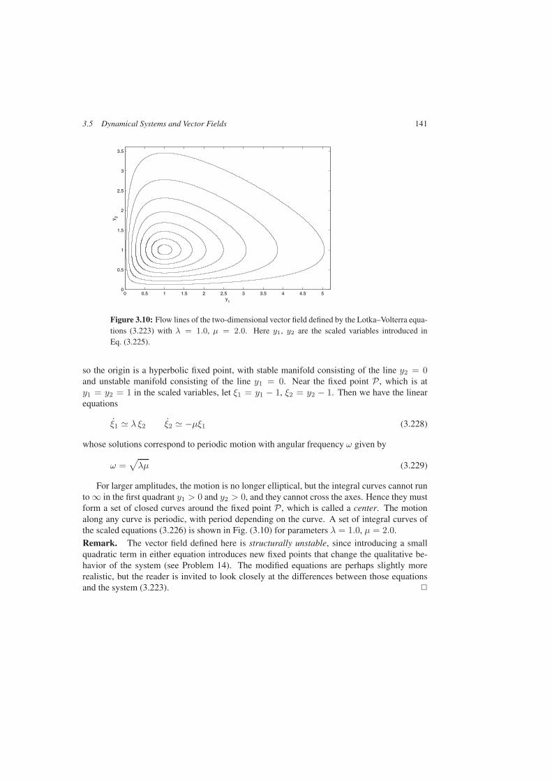
3.5 Dynamical Systems and Vector Fields 141
0 0.5 1 1.5 2 2.5 3 3.5 4 4.5 50
0.5
1
1.5
2
2.5
3
3.5
y1
y 2
Figure 3.10: Flow lines of the two-dimensional vector field defined by the Lotka–Volterra equa-tions (3.223) with λ = 1.0, µ = 2.0. Here y1, y2 are the scaled variables introduced inEq. (3.225).
so the origin is a hyperbolic fixed point, with stable manifold consisting of the line y2 = 0and unstable manifold consisting of the line y1 = 0. Near the fixed point P , which is aty1 = y2 = 1 in the scaled variables, let ξ1 = y1 − 1, ξ2 = y2 − 1. Then we have the linearequations
ξ1 λ ξ2 ξ2 −µξ1 (3.228)
whose solutions correspond to periodic motion with angular frequency ω given by
ω =√λµ (3.229)
For larger amplitudes, the motion is no longer elliptical, but the integral curves cannot runto ∞ in the first quadrant y1 > 0 and y2 > 0, and they cannot cross the axes. Hence they mustform a set of closed curves around the fixed point P , which is called a center. The motionalong any curve is periodic, with period depending on the curve. A set of integral curves ofthe scaled equations (3.226) is shown in Fig. (3.10) for parameters λ = 1.0, µ = 2.0.
Remark. The vector field defined here is structurally unstable, since introducing a smallquadratic term in either equation introduces new fixed points that change the qualitative be-havior of the system (see Problem 14). The modified equations are perhaps slightly morerealistic, but the reader is invited to look closely at the differences between those equationsand the system (3.223).

142 3 Geometry in Physics
3.5.3 Lagrangian and Hamiltonian Systems
A classical dynamical system is defined on an n-dimensional configuration space C with co-ordinates q = q1, . . . , qn on each coordinate patch in the atlas of C. These are the gen-eralized coordinates of the system, and we follow tradition in denoting them by qk ratherthan xk in this context. At each point of C, we have the tangent space with coordinatesq = q1, . . . , qn, the velocities of the system. The Lagrangian dynamics of the system isbased on the introduction of a Lagrangian L(q, q, t), which depends on the coordinates andvelocities, and perhaps explicitly on the time t. The dynamical trajectories of the system aredetermined from Hamilton’s principle, which requires that the action integral
S[q(t)] =∫ b
a
L(q, q, t) dt (3.230)
from point a to point b in C be an extremum along the actual trajectory, compared to nearbytrajectories. As explained in Appendix A, this leads to the Euler–Lagrange equations of mo-tion
d
dt
∂L
∂qk− ∂L
∂qk= 0 (3.231)
(k = 1, . . . , n).
Example 3.39. For a particle of mass m moving in a one-dimensional potential V (x),the Lagrangian is
L = 12mx
2 − V (x) (3.232)
leading to the Euler–Lagrange equation
mx+dV
dx= 0 (3.233)
This is the same as Newton’s second law with force F = −dV/dx.
Example 3.40. For a simple harmonic oscillator in one dimension (V = 12mω
2x2), wehave the equation of motion
x(t) + ω2x(t) = 0 (3.234)
The solution corresponding to initial position x0 and initial velocity x0 is
x(t) = x0 cosωt− (x0/ω) sinωt = A cos(ωt+ φ) (3.235)
The amplitude A and phase φ are expressed as
A =√x2
0 + (x0/ω)2 φ = tan−1(x0/ωx0) (3.236)
in terms of the initial position and velocity.
3.5 Dynamical Systems and Vector Fields 143
Hamiltonian dynamics is expressed in terms of the coordinates q = q1, . . . , qn and theconjugate momenta p = p1, . . . , pn introduced by
pk =∂L
∂qk(3.237)
(k = 1, . . . , n). The Hamiltonian is defined by
H(q, p, t) ≡ pkqk − L(q, q, t) (3.238)
The equations of motion for the coordinates and momenta are
qk =dqk
dt=∂H
∂pkpk =
dpkdt
= − ∂H
∂qk(3.239)
(k = 1, . . . , n). These are Hamilton’s equations of motion.
Remark. Hamilton’s equations (3.239) are equivalent to the Lagrange equations (3.231).However, a careful derivation of this equivalence needs to note that in taking partial deriva-tives, the Lagrangian is expressed as a function of the coordinates and the velocities, while theHamiltonian is expressed as a function of the coordinates and momenta. See Problem 17.
Example 3.41. For a particle of mass m in a central potential V (r), the Lagrangian is
L = 12m
(x2 + y2 + z2
)− V (r) = 1
2m(r2 + r2θ2 + r2 sin2 θ φ2
)− V (r) (3.240)
where the second expression is in terms of the usual spherical coordinates defined inEq. (3.173). The Lagrange equations of motion in spherical coordinates are
d
dt
∂L
∂r= mr =
∂L
∂r= mr
(θ2 + sin2 θ φ2
)− dV
dr(3.241)
d
dt
∂L
∂θ= mr2θ + 2mrrθ =
∂L
∂θ= mr2 sin θ cos θ φ2 (3.242)
d
dt
∂L
∂φ= mr2 sin2 θ φ+ 2mr sin2 θ rφ+ 2mr2 sin θ cos θ θφ =
∂L
∂φ= 0 (3.243)
Note that for a particle constrained to move on the surface of a sphere (r = 0), the equa-tions of motion for θ and φ are the same as the geodesic equations (3.211).
The conjugate momenta in spherical coordinates are
pr = mr pθ = mr2 θ pφ = mr2 sin2 θ φ (3.244)
and the Hamiltonian is expressed as
H =1
2m
(p2r +
p2θ
r2+
p2φ
r2 sin2 θ
)+ V (r) (3.245)
in terms of these coordinates and momenta.
144 3 Geometry in Physics
Exercise 3.18. Write down explicitly Hamilton’s equations of motion for the Hamilton-ian (3.245). Show that these equations of motion are equivalent to Eqs. (3.241)–(3.243).
If the Hamiltonian is independent of the coordinate qa, then qa is a cyclic coordinate, oran ignorable coordinate. The corresponding momentum pa then satisfies
pa = −∂H∂qa
= 0 (3.246)
so that pa is conserved on any trajectory of the system—pa is a constant of the motion.
Example 3.42. The Hamiltonian equation (3.245) is independent of the spherical coor-dinate φ. Hence the conjugate momentum pφ = mr2 sin2 θ φ is a constant of the motion.Note that pφ is the Z-component of the angular momentum of the particle.
We have implicitly assumed that the momenta pk defined by Eq. (3.237) are indepen-dent. For this to be the case, it is necessary that the matrix M defined by
M = (Mjk) =(
∂2L
∂qj∂qk
)(3.247)
is nonsingular everywhere in C. For a Lagrangian with the standard form of a kinetic energyquadratic in the velocities minus a potential energy V (q), we have
L = 12 qj Mjk(q) qk − V (q) (3.248)
and the momenta will be independent if the matrix M(q) is nonsingular everywhere in C.Then also M(q) can serve as a metric tensor on the tangent space at each point, and we have
pj =∂L
∂qj= Mjk(q) qk (3.249)
Thus the momentum space and the velocity space at each point are dual to each other.The Hamiltonian is related to a vector field X defined on the phase space of the dynamical
system by
X =d
dt= qk
∂
∂qk+ pk
∂
∂pk≡ XH (3.250)
From Hamilton’s equations of motion, we have
X =∂H
∂pk
∂
∂qk− ∂H
∂qk
∂
∂pk(3.251)
The integral curves of X are the phase space trajectories of the system if H is time indepen-dent. The Lie derivative LX transports vectors and forms along the trajectories; in particular,
XH = LXH =∂H
∂pk
∂H
∂qk− ∂H
∂qk∂H
∂pk= 0 (3.252)

3.5 Dynamical Systems and Vector Fields 145
Thus the Hamiltonian is constant along the integral curves of X. When H is identified withthe total energy of the system, Eq. (3.252) is a statement of conservation of energy.
Remark. For a general scalar function f , we have
Xf = LXf =∂H
∂pk
∂f
∂qk− ∂H
∂qk∂f
∂pk(3.253)
The right-hand side of this equation is the Poisson bracket of H and f , denoted by H, f.See Problem 19 for a general definition of the Poisson bracket.
The velocities q = q1, . . . , qn transform as components of a vector on C, since under acoordinate transformation q = q1, . . . , qn → Q = Q1, . . . , Qn, we have
qk → Qk =(∂Qk
∂q
)q (3.254)
On the other hand, the momenta p = p1, . . . , pn transform according to p→ P , with
Pk =∂L
∂Qk=
∂q
∂Qk∂L
∂q=(∂q
∂Qk
)p (3.255)
Hence the momenta are the components of a 1-form σ,
σ ≡ pk dqk (3.256)
at each point of C; σ is known as the Poincaré 1-form. Note that σ is not a 1-form field on Csince the pk are not functions of the coordinates. However, it is a 1-form field on the phasespace T ∗(C), and its exterior derivative is the canonical 2-form
ω = dσ = dpk ∧ dqk (3.257)
The canonical 2-form is nonsingular on the phase space T ∗(C), and it provides a uniquecorrespondence between vectors and forms on the phase space; if V is a vector field in thephase space, then (recall the notation iV introduced in Eq. (3.117))
iVω = ω(V, . ) (3.258)
is the 1-form field associated with V.
Remark. The canonical 2-form ω is often denoted by Ω in classical mechanics textbooks;here we use ω to avoid confusion with the volume form Ω.
Exercise 3.19. (i) Show that the 2-form ω is antisymmetric,
ω(U,V) = −ω(V,U) (3.259)
for every pair of vector fields U, V defined on T ∗(C). Then also show that
(iVω,V) = ω(V,V) = 0 (3.260)
for every vector field V on T ∗(C).
146 3 Geometry in Physics
(ii) Show that for every vector V, there is a vector U such that
(iVω,U) = ω(V,U) > 0 (3.261)
so that ω is nonsingular. In particular, suppose
V = ak∂
∂qk+ bk
∂
∂pk
is defined on the tangent space of some point in the phase space. Find an explicit representa-tion for the form iVω, and find a vector U such that ω(U,V) > 0.
Remark. In Exercise 2.7, it was stated that if A is a linear operator on a complex vectorspace such that (x,Ax) = 0 for every vector x, then A = 0. The form ω shows why thestatement is not true in a real vector space.
Definition 3.6. A form ω satisfying Eq. (3.260) is symplectic. A manifold on which such a2-form field exists on the entire manifold is a symplectic manifold; the 2-form field defines asymplectic structure on the manifold.
Exercise 3.20. If ω is a 2-form such that ω(V,V) = 0 for every vector V, then
ω(U,V) = −ω(V,U)
for every pair of vectors U, V.
Exercise 3.21. If σ is a 1-form on the phase space, then there is a unique vector Vσ suchthat
σ = ω(Vσ, . ) = iVσω (3.262)
These exercises show that ω can serve as a (pseudo-)metric to relate vectors and forms onphase space, as stated. By contrast, the kinetic energy matrix introduced in Eq. (3.247) servesas a metric on the original configuration space C (see Eq. (3.249)).
The vector field X (Eq. (3.250)) that defines the trajectories of the system is related to theHamiltonian by
iXω ≡ ω(X, . ) = −∂H∂qk
dqk − ∂H
∂pkdpk (3.263)
In general, we have
dH =∂H
∂qkdqk +
∂H
∂pkdpk +
∂H
∂t(3.264)
Hence if H does not depend explicitly on time, we have
iXω = − dH (3.265)
From Theorem 3.3.1, it then follows that
LXω = iX(dω) + d(iXω) = 0 (3.266)

3.5 Dynamical Systems and Vector Fields 147
since
dω = d(dσ) = 0 d(iXω) = −d(dH) = 0 (3.267)
by Poincaré’s lemma. Thus the canonical 2-form ω is invariant along the trajectories of thesystem in phase space, as are the successive powers of ω,
ω2 = ω ∧ ω , . . . , ωn = ω ∧ · · · ∧ ω︸ ︷︷ ︸n factors
(3.268)
The forms ω, ω2, . . . ωn are the Poincaré invariants of the system. The form ωn is the volumeelement in phase space. Invariance of ωn along the trajectories of the system means that ifwe start with a small region in phase space and let it develop in time according to Hamilton’sequations of motion, the volume of the region will remain constant as the region evolves intime. This result is known as Liouville’s theorem; it is an important and useful property of thephase space flow of a dynamical system.
The canonical 2-form ω is invariant under coordinate transformations q → Q, with thecorresponding transformation p→ P of the momenta given by Eq. (3.255), in the sense that
ω = dpk ∧ dqk = dPk ∧ dQk (3.269)
However there are more general transformations (q, p) → (Q,P ) of the phase space that leaveω invariant as in Eq. (3.269). Such transformations are called canonical transformations, orsymplectic transformations.
One use of canonical transformations is to attempt to reduce a Hamiltonian to a form thatdepends on as few coordinates as possible, so that the momenta corresponding to the remain-ing coordinates are constants of the motion. For example, the use of spherical coordinatesfor a spherically symmetric system shows explicitly the conservation of angular momentum,which is not so obvious in Cartesian coordinates, for example.
Relatively few systems can be completely solved in this way; a system for which theHamiltonian can be completely expressed in terms of conserved momenta is called integrable.However, many systems are “nearly” integrable, in the sense that an integrable system can beused as a starting point for a systematic approximation scheme. One such scheme is classicalperturbation theory, a simple example of which appears in Problem 20.
Example 3.43. The Hamiltonian of the one-dimensional harmonic oscillator is
H =p2
2m+
12mω2x2 (3.270)
Rescaling the variables from (x, p) to (X,P ) defined by
X ≡√mω x P ≡ p√
mω(3.271)
is a canonical transformation. In terms of (X,P ), the Hamiltonian is
H = 12 ω(P 2 +X2) (3.272)
148 3 Geometry in Physics
We can further introduce variables J, α by
X ≡√
2J sinα P ≡√
2J cosα (3.273)
corresponding to
J = 12 (P 2 +X2) tanα =
P
X(3.274)
In terms of these variables, the Hamiltonian is given simply by
H = ωJ (3.275)
The variables J, α are action-angle variables. Since the Hamiltonian (3.275) is indepen-dent of the angle variable α, the conjugate momentum J (the action variable) is a constantof the motion, and
α =∂H
∂J= ω (3.276)
Thus the motion in the phase space defined by the variables (X,P ) is a circle of radius√2J , with angular velocity given by α = ω. Note that for the special case of simple
harmonic oscillator, the angular velocity α is independent of the action variable. This isnot true in general (see Problem 20).
Exercise 3.22. Show that the transformation to action-angle variables is canonical, i.e.,show that
dJ ∧ dα = dP ∧ dX
Then explain the choice of√
2J , rather than some arbitrary function of J , as the “radius”variable in Eq. (3.273).
3.6 Fluid Mechanics
A real fluid consists of a large number of atoms or molecules whose interactions are suffi-ciently strong that the motion of the fluid on a macroscopic scale appears to be smooth flowsuperimposed on the thermal motion of the individual atoms or molecules, the thermal motionbeing generally unobservable except through the Brownian motion of particles introduced intothe fluid.
An ideal fluid is characterized by a mass density ρ = ρ(x, t) and a velocity field u =u(x, t), as well as thermodynamic variables such as pressure p = p(x, t) and temperatureT = T (x, t). If the fluid is a gas, then it is often important to consider the equation of staterelating ρ, p, and T . For a liquid, on the other hand, it is usually a good approximation to treatthe density as constant (incompressible flow).
Remark. It is implicitly assumed that the time scales associated with the fluid flow are longenough for local thermodynamic equilibrium to be established, though the temperature mayvary within the fluid.
3.6 Fluid Mechanics 149
Conservation of matter means that the total mass in a region R can only change if matterflows across the boundary of the region. Thus we have
d
dt
∫
R
ρΩ = −∫
∂R
ρu · −→dS (3.277)
where Ω is the volume form on R, and−→dS is an outward normal to the boundary surface ∂R.
The integral on the left is the rate of change of the total mass within R, while the integralon the right is the rate at which matter flows out across the boundary surface. Using Stokes’theorem, we then have
∫
R
∂ρ
∂t+ ∇ · (ρu)
Ω = 0 (3.278)
Since this is true for any region R, the integrand must vanish7, and we then have the equationof continuity
∂ρ
∂t+ div (ρu) = 0 (3.279)
Associated with the velocity field u are a vector field U , and a 1-form field U ,
U = uk∂
∂xkU = ukdx
k (3.280)
where the components uk and uk are related by the metric tensor g in the usual way. Ina Cartesian coordinate system in a flat space, these components are equal (uk = uk), butwe want to be able to consider both curvilinear coordinate systems and the nonflat metricsassociated with very massive stars, for example. The integral curves of the vector field U arethe lines of flow, or streamlines of the fluid flow.
Exercise 3.23. Show that
LU U = (u · ∇)u+ 12∇u2 (3.281)
where u2 = u · u = 〈U , U〉. Then show also that
〈LU U , U〉 = (u · ∇)u2 (3.282)
(recall Eq. (3.67)).
The equation of continuity (3.279) can be expressed as(∂
∂t+ LU
)ρΩ = 0 (3.283)
using Exercise 3.11, where LU is the Lie derivative associated with the velocity field U .
7Technically, the integrand in Eq. (3.278) must be continuous. For a mass of water flowing through a pipe, thereis a discontinuity at the leading edge of the water, which produces δ-function singularities in the partial derivatives inthe integrand. However, the δ-function singularities must and do cancel in the end.
150 3 Geometry in Physics
Newton’s second law for a moving element of fluid is
ρdu
dt= ρ
∂u
∂t+ (u · ∇)u
= f (3.284)
where f is the force per unit volume on the fluid element. If p is the pressure in the fluid, andΦ is the gravitational potential, then
f = −∇p− ρ∇Φ (3.285)
and Eq. (3.284) becomes Euler’s equation
∂u
∂t+ (u · ∇)u = − 1
ρ∇p− ∇Φ (3.286)
In the language of forms, Euler’s equation takes the form(∂
∂t+ LU
)U = − 1
ρdp+ d
(12u
2 − Φ)
(3.287)
using the results of Exercise 3.23. Then also
12
(∂
∂t+ LU
)u2 +
1ρLU p+ LU Φ = 0 (3.288)
For steady (time-independent) flow of an incompressible fluid, this becomes
LU ( 12ρu
2 + p+ ρΦ) = 0 (3.289)
so that the quantity 12ρu
2 + p + ρΦ is constant along each streamline of the fluid flow. Thisis Bernoulli’s principle, which is equivalent to conservation of energy of a drop of fluid as itmoves along a streamline.
The momentum density Π of the fluid is the vector field
Π = ρU (3.290)
From the equation of continuity and Euler’s equation, we have
∂Πk
∂t= −uk ∂
∂x(ρU ) − ∂
∂xk(p+ ρΦ) ≡ −∂T
k
∂x(3.291)
where the stress tensor T is a symmetric(20
)tensor defined by
T = (p+ ρΦ)g + ρU ⊗ U (3.292)
and g = g−1 is the dual of the metric tensor.
Remark. The concept of a stress tensor is more general; it appears in electromagnetic theory,as well as in the general theory of elastic media. It is always related to a rate of change ofmomentum density by the local form, Eq. (3.291), of Newton’s second law.
3.6 Fluid Mechanics 151
The force f exerted by the fluid across a surface σ is then expressed in terms of componentsof the stress tensor by
fk = Tkgm(∗σ)m (3.293)
where ∗σm = εjkmσjk is a vector that can be identified with the usual normal to the surface.This local interpretation of the stress tensor is valid in any coordinate system, and can also begeneralized to nonflat spaces.
In a Euclidean space with a Cartesian coordinate system (and only in such a space), themomentum density can be integrated to define a total momentum. If R is a region fixed inspace (not co-moving with the fluid), then the total fluid momentum P in R has components
P k =∫
R
ΠkΩ (3.294)
Then also
dP k
dt=∫
R
∂Πk
∂tΩ = −
∫
R
∂Tk
∂xΩ = −
∫
∂R
Tkgm∗σm (3.295)
where the last equality follows from Stokes’ theorem. Here ∂R is the boundary of R and ∗σis the (outward) normal to ∂R introduced above.
The vorticity α of the flow is a 2-form defined by
α = dU (3.296)
(α = curl u in ordinary vector notation). If S is a two-dimensional surface bounded by theclosed curve C, then
∫
S
α =∫
C
U =∫
C
u · d (3.297)
by Stokes’ theorem. Thus α is a measure of the average tangential component of the velocityfield around a closed curve. If α = 0 throughout a simply connected region, then this integralvanishes for any closed curve in the region, and the flow is called irrotational. In this case,there is a scalar function φ (the velocity potential) such that
U = dφ (3.298)
in the region. For steady state flow of a incompressible fluid, the velocity potential must satisfyLaplace’s equation
∇2 φ = 0 (3.299)
Methods of finding solutions to Laplace’s equation will be discussed in Chapter 8.
152 3 Geometry in Physics
A Calculus of Variations
Consider an integral of the form
S[x(τ )] ≡∫ b
a
F (x, x, τ) dτ (3.A1)
from point a to point b along a set of smooth curves C : x = x(τ ) in a one-dimensionalmanifold, where here, as in Section 3.4,
x =dx
dτ(3.A2)
Higher derivatives may also be present, but they are absent from the examples we considerhere, so we do not discuss them further (see, however, Problem 22). An integral of the type,Eq. (3.A1), is a functional of the curve x(τ ). We have encountered linear functionals inSection 2.1.5, and quadratic functionals in Section 2.3.4, but here we are concerned with moregeneral functionals, such as the one encountered in the study of geodesics on a manifold inSection 3.4.6.
The problem of interest is to find a curve x = x∗(τ ) for which the integral S[x(τ )] is anextremum. By analogy with the extremum conditions for functions of n variables, we expectthe condition for an extremum to have the form
δS
δx(τ )= 0 (3.A3)
but we need a definition of δS/δx(τ ). To provide such a definition, consider a curve
x(τ ) = x∗(τ ) + εη(τ ) (3.A4)
near the curve x = x∗(τ ). The variation of S[x(τ )] is given by
δS[x(τ )] = ε
∫ b
a
(∂F
∂xη(τ ) +
∂F
∂xη(τ )
)dτ (3.A5)
The second term can be integrated by parts to give
δS[x(τ )] = ε
∫ b
a
(∂F
∂x− d
dτ
∂F
∂x
)η(τ )dτ + εη(τ )F (x, x, τ)
∣∣∣∣τ=b
τ=a
(3.A6)
The endpoint term in the integration by parts vanishes, since S[x(τ )] is defined by an integralbetween fixed endpoints, so that we must have
η(a) = η(b) = 0 (3.A7)
and
δS[x(τ )] = ε
∫ b
a
(∂F
∂x− d
dτ
∂F
∂x
)η(τ )dτ (3.A8)
B Thermodynamics 153
From Eq. (3.A4), we have the identification δx(τ ) = εη(τ ), and thus
δS
δx(τ )=
1ε
δS
δη(τ )=∂F
∂x− d
dτ
∂F
∂x(3.A9)
The extremum condition, Eq. (3.A3), then becomes
d
dτ
∂F
∂x− ∂F
∂x= 0 (3.A10)
This differential equation is the Euler–Lagrange equation for the functional S[x(τ )]. Inthe present context, the Euler–Lagrange equation is typically a second-order differential equa-tion whose solution is required to pass through two particular points. The question of existenceand uniqueness of the solutions satisfying endpoint conditions is not so simple as for a sys-tem of first-order equations with fixed initial conditions, and there may be no solutions, onesolution, or more than one solution satisfying the endpoint conditions.
Remark. Beyond geodesics, functionals of the type, Eq. (3.A1), form the basis of the La-grangian formulation of classical mechanics, in which the function F (x, x, τ) is the Lagrang-ian of a system, and the Euler–Lagrange equations are the classical Lagrange equations ofmotion for the system, as discussed at length in Section 3.5.3.
If the integral (3.A1) is over a curve in an n-dimensional manifold with coordinates givenby x1, . . . , xn, then minimizing with respect to each of the coordinates leads to an Euler–Lagrange equation in each variable, so that we have the n conditions
d
dτ
∂F
∂xk− ∂F
∂xk= 0 (3.A11)
(k = 1, . . . , n).
B Thermodynamics
Consider a simple thermodynamic system, such as a one-component gas, described by thevariables T (temperature), p (pressure), V (volume), U (internal energy), and S (entropy).The system satisfies the first law in the form
dU = T dS − p dV (3.B12)
where the T dS term represents the heat absorbed by the system, and the term p dV the workdone by the system on its environment. The system is supposed to satisfy an equation of stateof the form
f(p, V, T ) = 0 (3.B13)
that allows any of the variables to be expressed in terms of two independent variables. Theprecise form of the equation of state is not important here; the essential point is that theequation of state defines a two-dimensional manifold in the space of the three variables p, V ,T , the thermodynamic state space of the system.
154 3 Geometry in Physics
The properties of forms allow us to derive some completely general relations between thederivatives of the thermodynamic variables in a relatively simple way. For example, the firstlaw (Eq. (3.B12)) implies
T =(∂U
∂S
)
V
p = −(∂U
∂V
)
S
(3.B14)
Here we use the standard thermodynamic notation(∂u
∂x
)
y
to denote the partial derivative of u with respect to x, holding y fixed. In other words, we aretreating u as a function of the variables x and y, so that u = u(x, y) and
du =(∂u
∂x
)
y
dx+(∂u
∂y
)
x
dy (3.B15)
If instead we want to treat u as a function of the variables x and y, with y = y(x, z), then
dy =(∂y
∂x
)
z
dx+(∂y
∂z
)
x
dz (3.B16)
so that(∂u
∂z
)
x
=(∂u
∂y
)
x
(∂y
∂z
)
x
(3.B17)
and(∂u
∂x
)
z
=(∂u
∂x
)
y
+(∂u
∂y
)
x
(∂y
∂x
)
z
(3.B18)
Equality of mixed second partial derivatives then gives the relation(∂T
∂V
)
S
= −(∂p
∂S
)
V
(3.B19)
Since d(dU) = 0, we have
dT ∧ dS = dp ∧ dV (3.B20)
With
dS =(∂S
∂T
)
V
dT +(∂S
∂V
)
T
dV dp =(∂p
∂T
)
V
dT +(∂p
∂V
)
T
dV (3.B21)
we have(∂S
∂V
)
T
dT ∧ dV =(∂p
∂T
)
V
dT ∧ dV (3.B22)

B Thermodynamics 155
so that(∂S
∂V
)
T
=(∂p
∂T
)
V
(3.B23)
Taking other combinations of independent variables leads to the further relations(∂T
∂p
)
S
=(∂V
∂S
)
p
(∂V
∂T
)
p
= −(∂S
∂p
)
T
(3.B24)
Equations (3.B19), (3.B23), and (3.B24) are the (thermodynamic) Maxwell relations. Theyare completely general, and do not depend on the specific form of the equation of state.
Changing independent variables for U from S and V to T and V in Eq. (3.B12) gives
dU = T
(∂S
∂T
)
V
dT +[T
(∂S
∂V
)
T
− p
]dV (3.B25)
so that(∂U
∂V
)
T
= T
(∂S
∂V
)
T
− p = T
(∂p
∂T
)
V
− p (3.B26)
This relates the dependence of the energy on volume at constant temperature, which is a mea-sure of the interaction between the particles in the gas, to the dependence of the pressure ontemperature at constant volume. Note that for an ideal gas, in which the interactions betweenthe particles are negligible, the equation of state
pV = nRT (3.B27)
(R is the gas constant, n is the number of moles of the gas) implies that both sides ofEq. (3.B26) vanish, and the internal energy of the ideal gas depends only on temperature.
Exercise 3.B1. The (Helmholtz) free energy F of a thermodynamic system is related tothe internal energy by
F ≡ U − TS
(i) Show that
dF = −p dV − S dT
(ii) Use this to derive directly the Maxwell relation (3.B23),(∂p
∂T
)
V
=(∂S
∂V
)
T
(iii) Show that(∂F
∂T
)
p
= −S + p
(∂S
∂p
)
T
156 3 Geometry in Physics
Exercise 3.B2. The enthalpy H of a thermodynamic system is defined by
H ≡ U + pV
(i) Show that
dH = T dS + V dp
(ii) Use this to derive the Maxwell relation(∂T
∂p
)
S
=(∂V
∂S
)
p
stated above.
Other general identities can be derived using the general properties of forms. For example,if we view y as a function of x and u in Eq. (3.B15), so that
dy =(∂y
∂x
)
u
dx+(∂y
∂u
)
x
dz (3.B28)
then we have[1 −
(∂u
∂y
)
x
(∂y
∂u
)
x
]du =
[(∂y
∂x
)
u
+(∂y
∂u
)
x
(∂u
∂x
)
y
]dx (3.B29)
Since(∂u
∂y
)
x
(∂y
∂u
)
x
= 1 (3.B30)
the left-hand side of Eq. (3.B29) vanishes, and thus(∂y
∂x
)
u
= −(∂y
∂u
)
x
(∂u
∂x
)
y
(3.B31)
or(∂x
∂y
)
u
(∂y
∂u
)
x
(∂u
∂x
)
y
= −1 (3.B32)
Note the minus sign on the right-hand side of Eqs. (3.B31) and (3.B32). Naive cancelation ofpartial derivatives here would be an error.
To illustrate the use of these results, consider the heat capacity C of a thermodynamicsystem, the rate at which heat must be added to raise the temperature of the system. If thermalenergy δQ is added to the system, then we have
δQ = T dS ≡ C dT (3.B33)
The heat capacity depends on the conditions under which heat is added to the system. Forexample, the volume of the system may be held fixed (imagine a gas in a rigid container),
B Thermodynamics 157
in which case the heat capacity CV at constant volume is relevant. On the other hand, theheat capacity Cp at constant pressure is appropriate if the system is held at constant pressure(imagine a gas in a balloon at atmospheric pressure). The difference between Cp and CV isdue to the fact that the system at constant pressure will expand as heat is added, doing workon its environment, so less energy will be converted to internal energy of the system.
We have
CV =(∂U
∂T
)
V
= T
(∂S
∂T
)
V
(3.B34)
Cp =(∂U
∂T
)
p
+ p
(∂V
∂T
)
p
= T
(∂S
∂T
)
p
(3.B35)
Exercise 3.B3. Show that the heat capacity at constant pressure of a system is
Cp =(∂H
∂T
)
p
where H is the enthalpy introduced above.
Now(∂S
∂T
)
p
=(∂S
∂T
)
V
+(∂S
∂V
)
T
(∂V
∂T
)
p
(3.B36)
so that
Cp − CV = T
(∂S
∂V
)
T
(∂V
∂T
)
p
= T
(∂p
∂T
)
V
(∂V
∂T
)
p
(3.B37)
where the second equality follows from the Maxwell relation (3.B23).The thermal expansion coefficient β and the isothermal compressibility k are defined by
β ≡ 1V
(∂V
∂T
)
p
kT ≡ − 1V
(∂V
∂p
)
T
(3.B38)
and from Eq. (3.B32), we have(∂p
∂T
)
V
= −(∂p
∂V
)
T
(∂V
∂T
)
p
=β
kT(3.B39)
It follows that
Cp − CV =β2V T
kT(3.B40)
which can be tested experimentally. Note that this relation implies Cp ≥ CV , since kT isalways positive—an increase in pressure at fixed temperature must always lead to a decreasein volume for a stable system.
158 3 Geometry in Physics
Bibliography and Notes
An excellent elementary introduction to the concepts of this chapter from a physics point ofview is
Bernard F. Schutz, Geometrical Methods of Mathematical Physics, Cambridge Uni-versity Press (1980).
It is well written, with many useful diagrams and examples. A modern comprehensive intro-duction aimed at theoretical physicists is
Theodore Frankel, The Geometry of Physics (2nd edition), Cambridge UniversityPress (2004).
A modern advanced undergraduate textbook on classical mechanics that introduces geo-metrical concepts at various stages is
Tom W. B. Kibble and Frank H. Berkshire, Classical Mechanics (5th edition), Im-perial College Press (2004).
The final two chapters are a nice elementary introduction to the general area of dynamicalsystems and chaos.
Dynamical systems and vector fields are closely related. An early text that emphasizesgeometry in classical mechanics is
V. I. Arnold, Mathematical Methods of Classical Mechanics, Springer (1974).
The book by Hirsch, Smale and Devaney cited in Chapter 2 is also oriented to a geometricalanalysis of dynamical systems.
Two recent classical mechanics textbooks in a similar spirit are
Jorge V. José and Eugene J. Saletan, Classical Dynamics: A Contemporary Ap-proach, Cambridge University Press (1998), andJoseph L. McCauley, Classical Mechanics, Cambridge University Press (1997),
These books emphasize the view of trajectories of Hamiltonian systems as flows in phasespace along which the canonical 2-form is invariant, in addition to treating standard topics.
Two classic elementary introductions to thermodynamics are
Enrico Fermi, Thermodynamics, Dover (1956), andA. B. Pippard, The Elements of Classical Thermodynamics, Cambridge UniversityPress (1957).
Enrico Fermi was arguably the greatest experimental physicist of the 20th century, as well as amajor theorist. He was also a magnificent teacher and writer, and his book on thermodynamicsis relevant even now. Pippard’s book is another clear introduction by a distinguished physicist.
Many books on general relativity give an introduction to the geometrical ideas discussedhere as a prelude to general relativity. Two relatively elementary books are
Bernard F. Schutz, A First Course in General Relativity, Cambridge University Press(1985). andSean M. Carroll, Spacetime Geometry: An Introduction to General Relativity,Addison-Wesley (2004)

Problems 159
Problems
1. The stereographic projection of the unit sphere S2 from the North pole onto the planetangent to the South pole is obtained from the figure at the right by rotating the entirefigure about the vertical line through the poles (compare with Fig. 3.3).(i) Show that the coordinates (xN , yN ) ofthe image Q in the plane of the point P withusual spherical angles (θ, φ) is given by (notethat 2α = π − θ)
xN = 2 cotθ
2cosφ yN = 2 cot
θ
2sinφ
N
P
QS
(ii) Find the corresponding image (xS , yS) of the stereographic projection of P from theSouth pole onto a plane tangent to the North pole.
(iii) Express (xS, yS) in terms of (xN , yN ).
Remark. These functions are differentiable to all orders in the region of the spheredefined by δ ≤ θ ≤ π − δ (0 < δ < π
2 ). Thus the two stereographic projections form anatlas that covers the entire sphere.
2. (i) Find a diffeomorphism mapping the open square (−1 < x < 1,−1 < y < 1) ontothe entire plane R2.
(ii) Find a diffeomorphism mapping the open disk D (x2 + y2 < 1) (also defined as theunit ball B2) onto the entire plane R2.
(iii) Combine these two results to find a diffeomorphism that maps the open square ontothe open disk D. Comment on the fact that the sharp corners of the square have beensmoothed out in the disk.
3. Let ek be a basis of the tangent space TP and S = (Skm) a nonsingular matrix. Showthat
(i) the vectors em defined by
em = Skm ek
also form a basis.
(ii) the basis ωk of T ∗P dual to ek and the basis ωm dual to em are related by
ωm = Smk ωk
where S = (Smk) is the matrix inverse of S.
(iii) if S = S(x) defines a change of basis on the tangent spaces Tx for x in someneighborhood of P , then S defines a coordinate transformation only if
∂
∂xSmk(x) =
∂
∂xkSm(x)
where S = S−1 as in part (ii).
160 3 Geometry in Physics
4. Show that the exterior derivative commutes with the Lie derivative. First, show that if Vis a vector field and σ is a 1-form field, then
LV (dσ) = d(LV σ)
Then show that this relation is true for a general p-form σ. (Hint: use induction togetherwith the Leibniz rule for differentiation of a product.)
5. Show that if V is a vector field and σ a p-form, then
LV σ = iV (dσ) + d(iV σ)
6. Prolate spheroidal coordinates ξ, η, φ on R3 are defined in terms of Cartesian coordinatesx, y, z by
x = c sinh ξ sin η cosφ y = c sinh ξ sin η sinφ z = c cosh ξ cos η
where c is a constant with dimensions of length.
(i) Describe the surfaces of constant ξ, η, φ. What are the ranges of ξ, η, φ? Whatsubsets of R3 correspond to coordinate singularities with this range of coordinates?
(ii) An alternative version of the coordinate set is u, v, φ with u ≡ c cosh ξ and v ≡cos η. What are the ranges of u, v, φ? What subsets of R3 correspond to coordinatesingularities with this range of coordinates?
(iii) Find the metric tensor and the preferred volume form in these coordinates. Considerboth the set ξ, η, φ and the set u, v, φ.
(iv) Express the Laplacian in terms of partial derivatives with respect to these coordi-nates.
Remark. These coordinates are useful for both the classical and quantum mechanicalproblem of a single charge q moving in the Coulomb field of two fixed point chargesQ1 and Q2 (the fixed charges are placed at the foci of the spheroids of constant u), aswell as scattering problems with spheroidal scatterers. They also simplify the problem ofcomputing the electrostatic potential of a charged conducting prolate spheroid, and thelimiting case of a long thin needle with a rounded edge.
7. Consider a system with two fixed charges q1 and q2, separated by a distance R, and acharge q of mass M that is free to move in the Coulomb field of these charges. Expressthe Coulomb potential energy of the system in terms of the position of the moving chargein prolate spheroidal coordinates with the fixed charges at the foci of the spheroid.
8. Oblate spheroidal coordinates ξ, η, φ on R3 are defined in terms of Cartesian coordinatesx, y, z by
x = c cosh ξ sin η cosφ y = c cosh ξ sin η sinφ z = c sinh ξ cos η
(again c is a constant with dimensions of length).

Problems 161
(i) Describe the surfaces of constant ξ, η, φ. What are the ranges of ξ, η, φ? Whatsubsets of R3 correspond to coordinate singularities with this range of coordinates?
(ii) An alternative version of the coordinate set is u, v, φ with u ≡ c sinh ξ and v ≡cos η. What are the ranges of u, v, φ? What subsets of R3 correspond to coordinatesingularities with this range of coordinates?
(iii) Compute the metric tensor and the preferred volume form in these coordinates. Con-sider both the set ξ, η, φ and the set u, v, φ.
(iv) Express the Laplacian in terms of partial derivatives with respect to these coordi-nates.
Remark. These coordinates are useful for scattering problems with oblate spheroidalscatterers. They also simplify the computation of the electrostatic potential of a chargedconducting oblate spheroid and its limiting case of a circular disk.
9. Parabolic coordinates ξ, η, φ on R3 are defined in terms of Cartesian coordinates x, y, zby
x = ξη cosφ y = ξη sinφ z = 12
(ξ2 − η2
)
(i) Describe the surfaces of constant ξ, η, φ. What are the ranges of ξ, η, φ? Whatsubsets of R3 correspond to coordinate singularities with this range of coordinates?
(ii) Compute the metric tensor and preferred volume form in these coordinates.
(iii) Express the Laplacian in terms of partial derivatives with respect to these coordi-nates.
Remark. These coordinates are useful for scattering problems with parabolic scatter-ers. They are also useful in the quantum mechanical problem of the Coulomb scatteringof a charge (an electron, for example) by a fixed point charge (an atomic nucleus, forexample).
10. Four-dimensional spherical coordinates r, α, θ, φ are defined in terms of Cartesian coor-dinates w, x, y, z by
x = r sinα sin θ cosφ y = r sinα sin θ sinφ
w = r cosα z = r sinα cos θ
(i) Express the four-dimensional Euclidean metric in terms of the coordinates r, α, θ, φ.
(ii) Express the four-dimensional volume element in terms of r, α, θ, φ.
(iii) Use this volume element to compute the four-volume of a ball of radius R.
(iv) Compute the surface “area” of the sphere S3 bounding the ball of radius R.
(v) Express the four-dimensional Laplacian in terms of partial derivatives with respectto these coordinates.

162 3 Geometry in Physics
11. The geographic latitude α on a spherical surface is related to the spherical angle θ byα = π/2 − θ (and is usually given in degrees, minutes and seconds, rather than inradians). Find an expression for the maximum latitude reached by the great circle startingfrom initial conditions θ0, θ0, φ0.
12. (i) What is the shortest distance between points (θ1, φ1) and (θ2, φ2) on the sphere S2?Hint. Let R be the radius of the sphere, and use the result that the geodesic is an arc of agreat circle.
(ii) Find the tangent vector to this geodesic at the initial point (θ1, φ1).
(iii) Find the geodesic curve joining the points (θ1, φ1) and (θ2, φ2) on the sphere S2
using the arc length along the curve as parameter.
13. How does Stokes’ theorem∫
R
dσ =∫
∂R
σ
work if R is a region in a one-dimensional manifold? Explain this in the language ofelementary calculus.
14. Consider the extension of the two-dimensional dynamical system introduced in Sec-tion 3.5.2 defined by
x1 =dx1
dt= (−λ+ ax2 + px1)x1
x2 =dx2
dt= (µ− bx1 + qx2)x2
where the parameters λ, µ, a, b are all positive, as in Eq. (3.223). The signs of p, q arenot specified, though one might expect them to be negative in the context of the Lotka–Volterra model.
(i) Find the fixed points of this dynamical system.
(ii) Investigate the stability of each of these fixed points. Note especially under whatconditions, if any, on the parameters p, q each of these fixed points will be stable.
(iii) Under what conditions on the parameters p, q do all the fixed points lie in the quad-rant x1 ≥ 0 , x2 ≥ 0?
(iv) Explain why one might expect p, q to be negative. Under what conditions might oneor the other of them be positive?
15. An alternative action for a relativistic free particle of mass m is
S =12
∫ xµgµν(x)xν
ξ(λ)+m2ξ(λ)
dλ
where ξ(λ) is a positive and monotonic increasing function of λ; it plays the role of aone-dimensional “metric” along the particle trajectory. Changing the parameter from λto µ = µ(λ) leaves the action invariant if ξ(λ) is replaced by η(µ) such that
η(µ)dµ = ξ(λ)dλ

Problems 163
(i) Show that if we choose ξ(λ) = 1, then the equations of motion for the xµ(λ) areexactly the geodesic equations (3.207).
(ii) Show that if we fix ξ(λ) by requiring δS/δξ(λ) = 0, the action reduces to thestandard geodesic action.
16. The classical trajectory of a relativistic free particle is an extremum of the relativisticaction, but it is in fact a maximum. To see why, consider first the geodesic from the point(0,0) to the point (2T,0), which is simply the trajectory x = (ct,0) of a particle at restat the origin. Next consider the trajectory of a particle starting at the origin at t = 0. Itis with constant velocity v until time t = (1 − ε) ∗ T (0 < ε < 1). It is then acceleratedwith constant acceleration −v/εT until time t = (1 + ε) ∗ T , after which it moves withconstant velocity −v until it returns to the origin at time t = 2T .
(i) Write an explicit formula for this trajectory, using the time of the observer at rest asthe parameter along the curve.
(ii) Integrate the standard Lagrangian to show that the action S for this trajectory com-pared to the action S0 for the observer at rest satisfies
√1 − v2
c2<
S
S0< (1 − ε)
√1 − v2
c2+ ε
Remark. This suggests that the action for the particle at rest is a maximum, thoughthis calculation actually shows only that it is not a minimum. This result also resolvesto the so-called twin paradox, which is the nonintuitive statement that a twin who movesalong the trajectory described above appears younger than the other twin who remainsat rest at the origin. Since the action is proportional to the proper time along the parti-cle trajectory, more proper time has elapsed for the twin who remains at rest, assumingthat physical clocks run at a rate proportional to the proper time, even in an acceler-ated system. This last assumption is Einstein’s equivalence principle, which has beenexperimentally tested.
17. The partial derivatives of the Lagrangian in Eq. (3.231) are taken with L as a function ofthe xk and xk, while the partial derivatives of the Hamiltonian in Eq. (3.239) are takenwith H as a function of the xk and pk. Use the relations in Appendix B between partialderivatives with different variables held fixed to show that the two sets of equations areequivalent.
18. (i) Express the kinetic energy for a free particle of mass m in terms of the prolate spher-oidal coordinates ξ, η, φ and the alternate set u, v, φ introduced in Problem 6.
(ii) Find the momenta conjugate to each of these coordinates, and express the Hamilton-ian in terms of the momenta and coordinates.
(iii) Find the Lagrangian and Hamiltonian equations of motion in each of these coordi-nate systems.
164 3 Geometry in Physics
19. If f is a function on the phase space of a Hamiltonian system, let Xf be a vector fieldsuch that
iXfω = −df
where ω is the canonical 2-form (Eq. (3.257)) on the phase space.
(i) Show that Xf is given uniquely by
Xf =∂f
∂pk
∂
∂qk− ∂f
∂qk∂
∂pk
(ii) The Poisson bracket of two scalar functions f , g is defined by
f, g ≡ ω(Xf ,Xg)
Show that
f, g =∂f
∂pk
∂g
∂qk− ∂f
∂qk∂g
∂pk
and that
[Xf ,Xg] = Xf,g
(iii) If H is the Hamiltonian of the system, and f is a scalar function of the coordinates,momenta, and possibly time, then
df
dt= H, f +
∂f
∂t
where the derivative on the left-hand side is the time derivative of f along a trajectory ofthe system.
Remark. The Poisson bracket is a classical analog of the quantum mechanical commu-tator, as discussed in many quantum mechanics textbooks.
20. Consider a nonlinear oscillator, with Hamiltonian
H = 12 ω(P 2 +X2) + 1
4λX4
in terms of the variables introduced in the example at the end of Section 3.5.3.
(i) Express this Hamiltonian in terms of the action-angle variables J , α introduced inEq. (3.273).
(ii) Write down Hamilton’s equations of motion for J , α.
(iii) From the equation for α, find an approximate expression for the period as a functionof J by averaging the right-hand side of the equation over a complete period, assumingthat α is constant (which it actually is not, but nearly so for small λ).
Remark. This problem is a prototype for classical perturbation theory.
Problems 165
21. Use Euler’s equation (3.287) to show that the vorticity α defined by Eq. (3.296) satisfies(∂
∂t+ LU
)α = d
(∂
∂t+ LU
)U =
1ρ2
dρ ∧ dp
Remark. If the fluid is incompressible, or if it satisfies an equation of state p = f(ρ),then the right-hand side vanishes, and vorticity is carried along with the fluid flow.
22. Consider an integral of the form
S[x(τ )] ≡∫ b
a
F (x, x, x, τ) dτ
from point a to point b along a set of smooth curves C : x = x(τ ) in a one-dimensionalmanifold, where here
x =dx
dτx =
d2x
dτ2
Derive the conditions that must be satisfied by a curve x = x∗(τ ) for which S[x(τ )] is anextremum relative to nearby curves? Find differential equation(s) of the Euler–Lagrangetype, and boundary conditions that must be satisfied at the endpoints of the interval [a, b].
23. The Gibbs function G of a thermodynamic system is related to the internal energy by
G ≡ U − TS + pV
(i) Show that for the thermodynamic system in Appendix B,
dG = V dp− S dT
(ii) Show that(∂G
∂T
)
V
= V
(∂S
∂V
)
T
− S
24. Show that for an ideal gas,
(i) the entropy is given by
S = S0(T ) + nR ln(V
V0
)
where S0(T ) is the entropy at volume V0 and temperature T ,
(ii) if the internal energy of the gas is given by U = αnRT , with α constant, then
S0(T ) = σ0 + αnR ln(T
T0
)
where σ0 is the entropy at temperature T0, volume V0, and
(iii) the heat capacities of the gas are related by
Cp − CV = nR
4 Functions of a Complex Variable
There are many functions f(x) of a real variable x whose definition contains a natural exten-sion of the function to complex values of its argument. For example, functions defined by aconvergent power series, or by an integral representation such as the Laplace integral intro-duced in Chapter 1, are already defined in some regions of the complex plane. Extending thedefinition of functions into the complex plane leads to new analytical tools that can be used tostudy these functions. In this chapter we survey some of these tools and present a collectionof detailed examples.
Analytic functions of a complex variable are functions that are differentiable in a regionof the complex plane. This definition is not quite so straightforward as for functions definedonly for real argument; when the derivative is defined as a limit
f ′(z) = limz→z0
f(z) − f(z0)z − z0
in the complex plane, the limit must exist independent of the direction from which z → z0 inthe complex plane. This requires special relations (the Cauchy–Riemann conditions) betweenthe partial derivatives of the real and imaginary parts of an analytic function; these relationsfurther imply that the real and imaginary parts of an analytic function satisfy Laplace’s equa-tion in two dimensions. Analytic functions define mappings of one complex region into an-other that are conformal (angle-preserving) except at singular points where the function or itsinverse is not differentiable. These conformal mappings are described and some elementarymappings worked out in detail.
If a function f(z) is not single valued in a neighborhood of some point z0 (for example,√z near z = 0), then f(z) has a branch point at z0. Branch points generally come in pairs,
and can be connected by a branch cut such that the function is single valued in the complexplane excluding the cut. The domain of a function with branch points is a multisheeted surface(a Riemann surface) in which crossing a branch cut leads from one sheet of the surface to thenext. Some important Riemann surfaces are described.
Integrals of analytic functions in the complex plane have many useful properties that fol-low from Cauchy’s theorem: the integral of an analytic function around a closed curve Cvanishes if there are no singularities of the function inside the curve. This leads to the Cauchyintegral formula
∮
C
f(ξ)ξ − z
dξ = 2πif(z)
which expresses the values of a function f(z) analytic within the region bounded by the closedcurve C in terms of its values on the boundary. It also leads to the Cauchy residue theorem,
Introduction to Mathematical Physics. Michael T. VaughnCopyright c© 2007 WILEY-VCH Verlag GmbH & Co. KGaA, WeinheimISBN: 978-3-527-40627-2
Introduction to Mathematical Physics
Michael T. Vaughn 2007 WILEY-VCH Verlag GmbH & Co.
168 4 Functions of a Complex Variable
which expresses the integral of an analytic function with isolated singularities inside a contourin terms of the behavior of the function near these singularities. Several examples are given toshow how this can be used to evaluate some definite integrals that are important in physics.
The Cauchy integral formula is also used to obtain power series expansions of an analyticfunction about a regular point and about an isolated singular point. The formal process ofanalytic continuation that leads to the global concept of an analytic function is explained withthe use of the power series expansions.
The singular points of an analytic function are characterized as poles, essential singu-larities or branch points, depending on the behavior of the function near the singularity. Iff(z) A/(z − z0)n for z → z0, with A a constant and n a positive integer, then f(z) has apole of order n at z0. If f(z) has a power series expansion around z0 that includes an infinitenumber of negative integer powers of (z − z0), then f(z) has an essential singularity at z0.Functions with branch points are not single valued and require the introduction of branch cutsand a Riemann surface to provide a maximal analytic continuation.
We show that every nonconstant analytic function has at least one singular point (possiblyat ∞). This leads to a simple proof of the fundamental theorem of algebra that every noncon-stant polynomial has at least one root. It follows that every polynomial of degree n has exactlyn roots (counted according to multiplicity), and then can be expressed as a constant multipleof a product of factors (z − zk), where the zk are the zeros of the polynomial.
The factorization of polynomials has several important consequences: (i) a function whoseonly singularities are poles can be expressed as a ratio of two polynomials, (ii) an entirefunction (a function whose only singularity is at ∞) can be expressed as an entire functionwith no zeros times a product of factors determined by its zeros (Weierstrass factorizationtheorem), and (iii) a function whose only singularities in the finite plane are poles can beexpressed as a sum over terms determined by the singular parts of the function at the polesplus an entire function (Mittag–Leffler theorem).
Periodic functions of a real variable are familiar from the study of oscillatory systems.A general expansion of periodic functions in terms of trigonometric functions is the Fourierseries expansion. Here we derive this expansion for periodic analytic functions by relating itto a Laurent expansion in the complex variable w ≡ e2πiz/α, where α is the period. Furtherproperties of Fourier series will appear in the context of linear vector space theory in Chapter 6.
In addition to simply periodic functions, there are also analytic functions that have twoindependent periods in the complex plane. If f(z + α) = f(z) and f(z + β) = f(z) withβ/α a complex number, not real, then f(z) is a doubly periodic function, known for historicalreasons as an elliptic function if its only singularities are poles. Some general properties ofthese functions are described here. A standard set of elliptic functions will be studied furtherin Appendix A of Chapter 5.
The Γ-function is an extension to the complex plane of the factorial function n! defined forinteger n. Many properties of the Γ-function and the related beta function, including Stirling’sformula for the asymptotic behavior of Γ(x) for large positive x, are derived in Appendix Aas an important illustration of the methods that can be used to study functions in the complexplane.
4.1 Elementary Properties 169
4.1 Elementary Properties of Analytic Functions
4.1.1 Cauchy–Riemann Conditions
Consider a function f(z) of the complex variable z = x+ iy; write
f(z) = w = u+ iv = u(x, y) + iv(x, y) (4.1)
with u(x, y) and v(x, y) real. f(z) is continuous at z0 if
limz→z0
f(z) = f(z0) (4.2)
This looks like the definition of continuity for a function of a real variable, except that thelimit must exist as z → z0 from any direction in the complex z-plane.
Similarly, f(z) is differentiable at z0 if the limit
limz→z0
f(z) − f(z0)z − z0
exists from any direction in the complex plane. If the limit does exist, then the derivative off(z) at z0 is equal to the limit; we have
df
dz
∣∣∣∣z0
≡ limz→z0
f(z) − f(z0)z − z0
≡ f ′(z0) (4.3)
If f(z) = u(x, y) + iv(x, y) is differentiable at z0 = x0 + iy0, then
f ′(z0) =[∂u
∂x+ i
∂v
∂x
]
(x0,y0)
=[∂v
∂y− i
∂u
∂y
]
(x0,y0)
(4.4)
where the two expressions on the right-hand side are obtained by taking the limit z → z0 firstparallel to the real axis, then parallel to the imaginary axis. Hence the partial derivatives ofu(x, y) and v(x, y) must exist at (x0, y0). Moreover, the two limits must be equal, so that thepartial derivatives must satisfy the Cauchy–Riemann conditions
∂u
∂x=∂v
∂y,
∂v
∂x= −∂u
∂y(4.5)
The converse is also true: If u(x, y) and v(x, y) are real functions with continuous firstpartial derivatives in some neighborhood of (x0, y0), and if the conditions (4.5) are satisfied at(x0, y0), then f(z) = u(x, y)+iv(x, y) is differentiable at z0 = x0+iy0, with derivative givenby Eq. (4.4). Thus the Cauchy–Riemann conditions, together with the continuity conditions,are both necessary and sufficient for differentiability of f(z).Definition 4.1. The function f(z) of the complex variable z is analytic (regular, holomorphic)at the point z0 if f(z) is differentiable at z0 and in some neighborhood of z0.
Remark. To understand why analyticity requires f(z) to be differentiable in a neighborhoodof z0, and not just at z0 itself, consider the function
f(z) ≡ (12|z|2 − 1) z∗ (4.6)

170 4 Functions of a Complex Variable
f(z) is continuous everywhere in the complex plane, and is actually differentiable on the unitcircle |z| = 1. But it is not differentiable anywhere off the unit circle, and hence not in theneighborhood of any point on the circle, so it is nowhere analytic. Note that the condition(4.13) is satisfied by f(z) only on the unit circle. Similarly, it is important that the Cauchy–Riemann conditions are satisfied in some neighborhood of a point. The functions
u(x, y) = x2 v(x, y) = y2 (4.7)
satisfy the Cauchy–Riemann conditions at the origin (x = y = 0), but nowhere else. Hencethe function f(z) = x2 + iy2 is nowhere analytic.
If f(z) is analytic in a region R, then the Cauchy–Riemann conditions imply that
∂2u
∂x2+∂2u
∂y2= 0 =
∂2v
∂x2+∂2v
∂y2(4.8)
(Laplace’s equation) in R. Thus both the real and imaginary parts of an analytic functionsatisfy the two-dimensional Laplace’s equation. The Cauchy–Riemann conditions also give
∂u
∂x
∂v
∂x+∂u
∂y
∂v
∂y= ∇u · ∇v = 0 (4.9)
Now ∇u (∇v) is orthogonal to the curve u(x, y) = constant (v(x, y) = constant) at everypoint, and Eq. (4.9) shows that ∇u and ∇v are orthogonal. Hence any curve of constant uis orthogonal to any curve of constant v at any point where the two curves intersect. Thusan analytic function generates two families of mutually orthogonal curves. More generally,the analytic function generates a conformal map from the complex z-plane to the complexw-plane, as explained in the next section.
Another view of the Cauchy–Riemann conditions is obtained by treating z ≡ x + iy andz∗ ≡ x− iy as the independent variables. Then
∂
∂z=
12
(∂
∂x− i
∂
∂y
)and
∂
∂z∗=
12
(∂
∂x+ i
∂
∂y
)(4.10)
whence, with f(z, z∗) = u(z, z∗) + iv(z, z∗),
∂f
∂z=
12
(∂u
∂x+∂v
∂y
)+
12i
(∂v
∂x− ∂u
∂y
)(4.11)
∂f
∂z∗=
12
(∂u
∂x− ∂v
∂y
)+
12i
(∂v
∂x+∂u
∂y
)(4.12)
The Cauchy–Riemann conditions are then equivalent to the condition
∂f
∂z∗= 0 (4.13)
so that f(z, z∗) is an analytic function of z if and only if it is both differentiable with respectto z and independent of z∗.
4.1 Elementary Properties 171
4.1.2 Conformal Mappings
The function w = u+ iv defines a mapping of the complex z-plane into the complex w-plane.The mapping is conformal if angle and sense of rotation are preserved by the mapping; thatis, if C1, C2 are curves in the z-plane that intersect at an angle α, then the correspondingimage curves C ′
1, C′2 in the w-plane intersect at the same angle α, with the sense of rotation
preserved.If w = f(z) is analytic in a region R of the z-plane, then the mapping of R onto its image
in the w-plane is conformal, except at points where f ′(z) = 0. To show this, let z0 be a pointin R, and C be a curve through z0 that makes an angle ξ with respect to the real z axis. Thenthe image curve C ′ in the w-plane passes through w0 = f(z0) at an angle ξ′ with respect tothe real w axis, where
ξ′ − ξ = limw→w0on C′
arg(w − w0) − limz→z0on C
arg(z − z0)
= limz→z0on C
arg[f(z) − f(z0)
z − z0
]= arg f ′(z0) (4.14)
independent of the curve C if f(z) is analytic at z0 and f ′(z0) = 0.
Examples. (i) Linear transformations
• w = z + b is a (rigid) translation by b of the whole z-plane.
• w = z ( real) is a scale transformation by scale factor .
• w = eiϕz (ϕ real) is a (rigid) rotation through angle ϕ of the whole z-plane.
The general linear transformation
w = az + b (4.15)
(a = eiϕ) consists of a scale transformation by scale factor , rotation through angle ϕ,followed by translation by b. The transformation has a fixed point at ∞ and, if a = 1, asecond fixed point at
z =b
1 − a(4.16)
(ii) Reciprocal transformation
The reciprocal transformation, or inversion is defined by
w = 1/z (4.17)
If z = x+ iy = reiϕ, then w = u+ iv = e−iϕ with = 1/r; in terms of real variables,
u =x
r2, v = − y
r2and x =
u
2, y = − v
2(4.18)
The point z = ∞ is defined to be the image of 0 under the reciprocal transformation. Thefixed points of the transformation are at z = ±1.

172 4 Functions of a Complex Variable
(iii) Linear fractional transformation
The general linear fractional (or bilinear) transformation is defined by
w =az + b
cz + d(4.19)
with ∆ ≡ ad − bc = 0 (if ∆ = 0, the mapping becomes w = a/c, a constant). The inversetransformation
z =−dw + b
cw − a(4.20)
is also a linear fractional transformation (hence the term bilinear). The transformation isthus a one-to-one mapping of the complex plane (including the point at ∞) into itself; thetransformation has at most two fixed points, at
z =a− d±
√(a− d)2 + 4bc2c
(4.21)
The point z = ∞ is mapped into w = a/c, while the point z = −d/c is mapped into the pointw = ∞.
The linear fractional transformation is the most general one-to-one mapping of the com-plex plane including the point at ∞ onto itself—as will be seen shortly, any more complicatedmapping will not be one to one. With the mapping of the points z1, z2, z3 into the pointsw1, w2, w3 is associated the unique linear fractional transformation
(w − w1)(w2 − w3)(w − w3)(w2 − w1)
=(z − z1)(z2 − z3)(z − z3)(z2 − z1)
(4.22)
Remark. There is a one-to-one correspondence between linear fractional transformationsand 2 × 2 matrices A with detA = 1—see Problem 2.
(iv) Powers and roots
Consider the transformation
w = z2 (4.23)
This transformation is conformal except at z = 0,∞ (note that w′(0) = 0). However itis not one to one; as z ranges over the entire z-plane, the w-plane is covered twice, sincez = r eiθ → w = r2 e2iθ and a single circle around z = 0, corresponding to θ ranging from 0to 2π, covers the corresponding circle in the w-plane twice. Hence each point in the w-planeis the image of two points in the z-plane.
The inverse transformation
z =√w (4.24)
is analytic and conformal except for the points w = 0,∞, which correspond to the points inthe z-plane where the map (4.23) is not conformal. However, the map (4.24) is double valued:to each point in the w-plane, there are two corresponding points in the z-plane.

4.1 Elementary Properties 173
Figure 4.1: Mapping of the z-plane into the two-sheeted Riemann surface corresponding toa double covering of the w-plane. The unshaded upper half z-plane is mapped into the top(unshaded) copy of the w-plane, while the shaded lower half z-plane is mapped into the bottom(shaded) copy of the w-plane The straight line is the branch cut separating the two sheets of theRiemann surface.
The map can be made single valued if we view the image of the z-plane under the transfor-mation (4.23) not as a single complex plane, but as a two-sheeted surface (the Riemann surfacefor the map (4.24)) whose sheets are connected by a line drawn from w = 0 to w = ∞, asshown in Fig. 4.1. Passage from one sheet to the other is by circling the point w = 0 once,corresponding to a path from a point z0 in the z-plane to the point −z0. A second circuitaround w = 0 leads back to the original sheet, as it corresponds to a return from −z0 to z0 inthe z-plane.
The line in the w-plane from 0 to ∞ separating the two sheets is a branch cut. It can bedrawn along any path from 0 to ∞, although it is usually convenient to draw it along eitherthe positive real axis or the negative real axis—in Fig. 4.1 it is drawn along the positive realaxis. The points w = 0 and w = ∞ are branch points (in w) of the function z =
√w.
Remark. In general, a branch point z0 of an analytic function f(z) is a point z0 near whichthe function is analytic but not single valued, in the sense that if a circle of arbitrarily smallradius is drawn around z0, and the values of the function followed continuously around thecircle, the value of the function does not return to its original value after one complete circle.This definition will be made more formal in Section 4.3.
More generally, if n is any integer ≥ 2, the transformation
w = zn (4.25)
is conformal except at z = 0,∞ [again w′(0) = 0]. However, there are n distinct pointsin the z-plane that map into a single point in the w-plane: if w0 = zn0 , then the pointszk ≡ z0 exp(2πik/n) also map into w0 (k = 1, . . . , n − 1). In order to make the inverse

174 4 Functions of a Complex Variable
transformation
z = n√w (4.26)
unique, the image of the z-plane under the transformation (4.25) must be constructed as ann-sheeted Riemann surface, on which passage from one sheet to the next is made traversing aclosed path around the point w = 0. Encircling the point w = 0 a total of n times in the samedirection returns to the original sheet. The sheets are again separated by a branch cut in thew-plane from 0 to ∞; as above, the actual location of the cut can be chosen at will.
It is also possible to consider fractional powers: if p and q are integers with no commonfactors, then the transformation
w = zp/q (4.27)
is still conformal except at z = 0,∞. The transformation can be viewed as a one-to-onemapping from a q-sheeted Riemann surface with a branch cut from z = 0 to z = ∞ to ap-sheeted Riemann surface with a branch cut from w = 0 to w = ∞.
(v) Exponential and logarithm
The transformation
w = ez (4.28)
is conformal except at ∞. However, since e2πi = 1, the points z and z ± 2nπi with n =1, 2, . . . map to the same value of w. Thus to make the inverse transformation
z = lnw (4.29)
unique, the image of the z-plane under (4.28) must be represented as a Riemann surface withan infinite number of sheets, separated by a branch cut in the w-plane from 0 to ∞. Onthis Riemann surface, w = eiϕ, with −∞ < ϕ < ∞, and to each point on this surfacecorresponds a unique
z = ln + iϕ (4.30)
If we take the branch cut in the w-plane along the negative real axis (this is a generally usefulchoice), then each strip
(2n− 1)π ≤ Im z < (2n+ 1)π (4.31)
(n = 0,±1,±2, . . .) in the z-plane is mapped onto one sheet of the w-plane. Circling theorigin w = 0 once in a counterclockwise (clockwise) sense corresponds to increasing (de-creasing) the value of φ by 2π.
The exponential function and the trigonometric functions are closely related in view ofdeMoivre’s formula
eiz = cos z + i sin z (4.32)

4.1 Elementary Properties 175
This formula is valid throughout the complex plane, since both sides of the equation have thesame power series expansion, with an infinite radius of convergence.
Many useful identities can be derived from Eq. (4.32). For example,
cos z =eiz + e−iz
2= cosh iz (4.33)
and
sin z =eiz − e−iz
2i= i sinh iz (4.34)
These equations serve to define the trigonometric functions throughout the complex plane.Also,
e2iz =1 + i tan z1 − i tan z
(4.35)
from which it follows that
tan−1 z =12i
ln(
1 + iz
1 − iz
)(4.36)
Derivation of these and further identities is left to the reader.
Example 4.1. As a final example, note that the map
w = sin z (4.37)
is conformal except at z = ±(2n+1)π/2 (n = 0, 1, 2, . . .) and z = ∞, but not one to onesince z, z′ ≡ π− z, z± 2nπ, and z′ ± 2nπ (n = 1, 2, . . .) all map to the same value of w.To make the inverse transformation
z = sin−1 w (4.38)
one to one, it is necessary to represent the image of the z-plane under the mapping (4.37)as a Riemann surface with an infinite number of sheets connected by branch cuts joiningthe branch points w = ±1. If we take the branch cut to be
−∞ < w ≤ −1 and 1 ≤ w <∞
then each strip
(2n− 1)π
2≤ Re e z < (2n+ 1)
π
2(4.39)
(n = 0,±1,±2, . . .) is mapped onto one sheet of the w-surface. Note that it is allowed(and useful in this case) to take the branch cut from −1 to 1 through the point ∞ in w.
176 4 Functions of a Complex Variable
4.2 Integration in the Complex Plane
4.2.1 Integration Along a Contour
Consider the integral
I ≡∫
C
f(z) dz ≡ P + iQ (4.40)
of the function f(z) ≡ u(x, y) + iv(x, y) over the curve C joining points z1 and z2 in thecomplex z-plane. If C can be represented parametrically as
C : x = x(t) , y = y(t) (t1 ≤ t ≤ t2) (4.41)
with x(t) and y(t) having piecewise continuous derivatives on (t1 ≤ t ≤ t2), then C is acontour. The integral (4.40) is a contour integral, which can be expressed in terms of realsingle-variable integrals as
P =∫ t2
t1
u[x(t), y(t)]x′(t) − v[x(t), y(t)]y′(t) dt (4.42)
Q =∫ t2
t1
v[x(t), y(t)]x′(t) + u[x(t), y(t)]y′(t) dt (4.43)
using dz = dx+ idy, and expressing the integrand in terms of x, y.A natural question to ask whether the integral (4.40) is independent of the actual contour
joining the endpoints z1 and z2 of the contour.1
If we write the integrals P and Q in the form
P =∫
(u dx− v dy), Q =∫
(v dx+ u dy) (4.44)
then this question is equivalent to the question of whether the integrands are exact differentials.Are there functions φ(x, y) and ψ(x, y) such that
u(x, y)dx− v(x, y)dy = dφ(x, y) (4.45)
v(x, y)dx+ u(x, y)dy = dψ(x, y) (4.46)
If such functions exist, then the integrals
P = φ(x2, y2) − φ(x1, y1), Q = ψ(x2, y2) − ψ(x1, y1) (4.47)
are independent of contour.2
1This question is also encountered in the discussion of conservative forces in mechanics: is the work done by aforce independent of the path joining two endpoints? If so, the force can be derived from a potential energy function.
2The functions φ and ψ here are analogous to the potential energy in mechanics.
4.2 Integration in the Complex Plane 177
Equations (4.45) and (4.46) imply that u and v can be expressed as partial derivatives of φand ψ according to
u(x, y) =∂φ
∂x=∂ψ
∂y(4.48)
v(x, y) =∂ψ
∂x= −∂φ
∂y(4.49)
If further u(x, y) and v(x, y) have continuous first partial derivatives in a simply connectedregion R containing the contour C, then the mixed second partial derivatives of φ and ψ canbe taken in either order, so that
∂2φ
∂y∂x=∂u
∂y= −∂v
∂x=
∂2φ
∂x∂y(4.50)
∂2ψ
∂y∂x=∂v
∂y=∂u
∂x=
∂2ψ
∂x∂y(4.51)
in R. Equations (4.50) and (4.51) are precisely the Cauchy–Riemann conditions (4.5) for theanalyticity of f(z) in R.
4.2.2 Cauchy’s Theorem
The connection between independence of path of the contour integral and analyticity of f(z)is stated formally as
Cauchy’s Theorem. Let f(z) be analytic in the simply connected region R, and let f ′(z)be continuous in R. Then if z1 and z2 are any two points in R, the contour integral
∫ z2
z1
f(z) dz
is independent of the actual contour in R joining z1 and z2. Then also for any closed contourin R, the contour integral
∮
C
f(z) dz = 0 (4.52)
The assumption of continuity of f ′(z) is actually not needed, and its elimination is centralto the theory of functions of a complex variable. However, this requires a lengthy technicalproof, and we refer the interested reader to the standard mathematics texts for details.
The result (4.52) has important implications for the evaluation of integrals in the complexplane. It means that we can deform the contour of an integral whose integrand is analyticin any way we wish, so long as we keep the endpoints of the integral fixed and do not crossany singularities of the integrand. Furthermore, since an integral around the total boundaryof a multiply connected region can be expressed as a sum of integrals around boundariesof simply connected regions, Eq. (4.52) holds as well when C is the total boundary of amultiply connected region in which the integrand is analytic. Thus when we deform a contourof integration to cross an isolated singularity of the integrand, we can express the resultingintegral as the sum of the original integral and an integral around a tiny circle enclosing thesingularity of the integrand.
178 4 Functions of a Complex Variable
4.2.3 Cauchy’s Integral Formula
Cauchy’s theorem (4.52) states that the integral of an analytic function around a closed contourvanishes if the function is analytic everywhere inside the contour. If the function has oneisolated singularity inside the contour, it turns out that we can also evaluate the integral interms of the behavior of the function near the singular point.
First note that if K is a circle of radius about z = 0, then
∮
K
zn dz = in+1
∫ 2π
0
ei(n+1)ϕ dϕ =
2πi n = −10 otherwise
(4.53)
where it is to be understood that the circle K is followed a counterclockwise sense. Hence ifC is any closed contour that encloses z0 in a counterclockwise sense, then
∮
C
(z − z0)n dz =
2πi n = −10 otherwise
(4.54)
These results lead to theCauchy integral formula. Let f(z) be analytic in the simply connected region R en-
closed by the closed contour C. Then for z in the interior of R, we have∮
C
f(ξ)ξ − z
dξ = 2πif(z) (4.55)
Proof. Let K be a circle of radius about z lying entirely in R. Then∮
C
f(ξ)ξ − z
dξ = f(z)∮
K
1ξ − z
dξ +∮
K
f(ξ) − f(z)ξ − z
dξ (4.56)
and note that the second integral on the right-hand side vanishes, since the integrand is analyticon and within K.
The integral formula (4.55) can also be differentiated under the integral sign to give
f ′(z) =1
2πi
∮
C
f(ξ)(ξ − z)2
dξ (4.57)
and further to give the nth derivative,
f (n)(z) =n !2πi
∮
C
f(ξ)(ξ − z)n+1
dξ (4.58)
Exercise 4.1. Let f(z) be analytic within the circle Kρ : |z − z0| = ρ, and suppose|f(z)| < M on Kρ. Then
|f (n)(z0)| ≤n!Mρn
(n = 0, 1, 2, . . .).

4.3 Analytic Functions 179
It is also true that integration is the inverse of differentiation. If f(z) is analytic in thesimply connected region R, then the integral
F (z) ≡∫ z
z0
f(ξ) dξ (4.59)
is analytic in R, and F ′(z) = f(z), just as in ordinary calculus. A further consequence isthat if f(z) is continuous in a simply connected region R, and if
∮Cf(ξ) dξ = 0 for every
closed contour C in R, then f(z) is analytic in R. In this case the integral in Eq. (4.59) isindependent of path in R, and thus defines an analytic function F (z) whose derivative is f(z).
Remark. An important consequence of the Cauchy integral theorem is that the values ofan analytic function in a region of analyticity are completely determined by the values on theboundary of the region. Indeed, if f(ξ) is continuous on the closed contour C, then
f(z) ≡ 12πi
∮
C
f(ξ)ξ − z
dξ (4.60)
defines a function analytic within the region bounded by C. Moreover, if a function is analyticin a region R, then it has derivatives of all orders in R, and the derivatives are analytic in R.These are all obtained by differentiating Eq. (4.60) with respect to z.
4.3 Analytic Functions
4.3.1 Analytic Continuation
We have introduced analytic functions as functions differentiable in a region of the complexplane, and as functions that define a conformal mapping from one complex plane (or Riemannsurface) to another. However, the properties of contour integrals of analytic functions, and thepower series representations derived from them, can be used to extend the domain of definitionof an analytic function by a process known as analytic continuation. This leads to a globalconcept of an analytic function.
To begin, note that if u1(z), u2(z), . . . are analytic in a region R, and if the series
f(z) ≡∞∑
n=1
un(z) (4.61)
is uniformly convergent in R, then f(z) is analytic in R. To show this, simply let C be anyclosed contour in R. Then
∮
C
f(z) dz =∞∑
n=1
∮
C
un(z) dz = 0 (4.62)

180 4 Functions of a Complex Variable
since the uniform convergence of the series permits the interchange of summation and inte-gration.3
In particular, the power series
f(z) ≡∞∑
n=0
an(z − z0)n (4.63)
which is uniformly convergent within its circle of convergence is analytic within its circle ofconvergence and, as already shown in Chapter 1, has derivative given by
f ′(z) ≡∞∑
n=0
(n+ 1) an+1(z − z0)n (4.64)
On the other hand, suppose f(z) is analytic in the simply connected region R. Let z0 bean interior point of R, and suppose the circle K : |z − z0| = and its interior lie entirelyin R. Then for z inside K, we can expand the denominator in the Cauchy formula to give
f(z) ≡ 12πi
∮
K
f(ξ)ξ − z
dξ =1
2πi
∞∑
n=0
[∮
K
f(ξ)(ξ − z0)n+1
dξ
](z − z0)n
=∞∑
n=0
f (n)(z0)n!
(z − z0)n (4.65)
Thus any function analytic in a region can be expanded in a Taylor series about any interiorpoint z0 of the region. The series converges inside any circle in which the function is analytic;hence the radius of convergence of a power series about z0 is the distance to the nearestsingular point of analytic function defined by the power series.
Example 4.2. f(z) = 1/(1 + z2) is not analytic at z = ±i. Thus the Taylor series ex-pansion of f(z) about z = 0 has radius of convergence = 1. (Verify this by constructingthe series.)
Example 4.3. f(z) = ln(1 + z) is not analytic at z = −1; it has a branch point there.Hence we know that the Taylor series expansion of f(z) about z = 0 has radius of conver-gence = 1, even without computing explicitly the coefficients in the series.
An analytic function is uniquely defined by its values in any finite region; even by its valueson a bounded sequence of points within its domain of analyticity. This follows from the
3Uniform convergence means that given ε > 0, there is some integer N such that˛˛f(z) −
NXn=1
un(z)
˛˛ < ε
everywhere on the contour C. Hence, if L is the total length of the contour, then˛˛I
C
»f(z) −
NXn=1
un(z)
–˛˛ < εL

4.3 Analytic Functions 181
Theorem 4.1. Suppose f(z) is analytic in the region R, and zk is a sequence of points in Rwith limit point z0 in R, and suppose f(zk) = 0 (k = 1, 2, . . .). Then f(z) = 0 everywhere.
Proof. Since f(z) is analytic, the Taylor series (4.63) for f(z) about z0 has radius of conver-gence r > 0. Now suppose a0 = 0, a1 = 0, . . . , aN = 0 but aN+1 = 0. Then if 0 < < r,the sequence ann is bounded, and a short calculation shows that there is some positiveconstant M such that
|f(z) − aN+1(z − z0)N+1| > M |z − z0|N+2 (4.66)
for |z − z0| < . Then also
|f(z)| > |aN+1 −M(z − z0)||(z − z0)|N+1 (4.67)
(think of f(z), aN+1(z−z0)N+1 andM(z−z0)N+2 as three sides of a triangle in the complexplane). But the right-hand side of Eq. (4.67) is positive for |z − z0| small enough, so thatf(z) = 0 in some neighborhood of z0, contrary to assumption that f(zk) = 0 (k = 1, 2, . . .).Hence every coefficient in the Taylor series must vanish, and f(z) = 0 everywhere.
Now suppose R1 and R2 are overlapping regions, with f1(z) analytic in R1 and f2(z)analytic in R2, and suppose
f1(z) = f2(z) (4.68)
in some neighborhood of a point z0 in R1 ∩ R2. Then the preceding argument shows thatf1(z) − f2(z) = 0 everywhere in R1 ∩R2. Thus the function f(z) defined by
f(z) ≡ f1(z) (4.69)
for z in R1, and by
f(z) ≡ f2(z) (4.70)
for z in R2, is analytic in R1 ∪ R2. f(z) defines the (unique) analytic continuation of f1(z)from R1 to R1 ∪R2.
Example 4.4. The function
f(z) ≡ 11 + z
(4.71)
is the analytic continuation of the geometric series∑∞
n=0 (−1)nzn from |z| < 1 to theentire z-plane except for z = −1.
Remark. The uniqueness is based on the result that an analytic function that vanishes in aninterval (even on a bounded infinite set of points) vanishes everywhere. The correspondingstatement for functions of a real variable is not true, as can be seen from the example
f(x) =
exp(−1/x2) x > 00 x ≤ 0
(4.72)

182 4 Functions of a Complex Variable
which, as a function of the real variable x, has continuous derivatives of any order (even atx = 0), vanishes on an interval, and yet does not vanish everywhere.
A formal method of defining analytic continuation uses power series. Suppose
f(z) =∞∑
n=0
an(z − z0)n (4.73)
with radius of convergence r > 0. If |z1 − z0| < r, then f(z) is analytic at z1, the powerseries
f(z) =∞∑
n=0
bn(z − z1)n (4.74)
has radius of convergence r1 > 0, and the new coefficients bn can be computed from the an. Ifthe circle |z−z1| < r1 extends beyond the circle |z−z0| < r, then f(z) has been analyticallycontinued beyond the circle of convergence of the series in Eq. (4.73). Proceeding in thisway, we can analytically continue f(z) into a maximal region, the domain of holomorphyof f(z), whose boundary, if any, is the natural boundary of f(z). Each power series is afunctional element of f(z), and the complete collection of functional elements defines theanalytic function f(z). The values of f(z) obtained by the power series method are the sameas those obtained by any other method; the analytic continuation is unique.
4.3.2 Singularities of an Analytic Function
The analytic continuation process leads to a domain of holomorphy for an analytic functionthat may be a region in the z-plane, the entire z-plane, or a multisheeted Riemann surface,introduced in the discussion of conformal maps, with sheets separated by branch cuts joiningpairs of branch points of the function. Within this domain of holomorphy there may be isolatedsingular points where the function is not analytic. The task now is to classify these singularpoints and characterize the behavior of an analytic function near such points.
Definition 4.2. The analytic function f(z) is singular at the point z0 if it is not analyticthere. The point z0 is an isolated singularity of f(z) if f(z) is analytic at every point in someneighborhood of z0 except at z0 itself.
The isolated singularities of an analytic function fall into three classes: (i) poles, (ii) (iso-lated) essential singularities4, and (iii) branch points. As we have seen, branch points come inpairs, and are associated with nontrivial Riemann surfaces, but each branch point is isolated inthe examples we have seen. However, the general series expansions of functions about polesand essential singularities are not valid near a branch point; expansions about a branch pointneed special attention.
Definition 4.3. The analytic function f(z) has a pole at the isolated singularity z0 if thereis a positive integer n such that (z − z0)n f(z) is analytic at z0. The order of the pole is thesmallest n for which this is the case. If f(z) is analytic and single valued in a neighborhoodof the singular point z0, but there is no positive integer for which (z − z0)n f(z) is analytic atz0, then z0 is an essential singularity of f(z).
4If a f(z) has a sequence of singular points with a limit point z0, then z0 is also described as an essentialsingularity of f(z), but it is not isolated. In the present context, only isolated essential singularities are considered.
4.3 Analytic Functions 183
Definition 4.4. The singular point z0 is a branch point of the analytic function f(z) if ineach sufficiently small neighborhood of z0 there is a circle K : |z − z0| = such that
(i) f(z) is analytic on and within K, except at z0 itself, and(ii) the functional element of f(z) obtained by analytic continuation once aroundK from
any point z1 on K is distinct from the initial functional element.
Remark. Condition (ii) essentially requires that∮K
f ′(z) dz = 0 for all less than some
ρ0 > 0, since f(z) does not return to the same value after one trip around the circle.
The complex plane can be extended to include the point ∞ as the image of z = 0 under thereciprocal transformation. Thus f(z) is analytic at ∞ if g(ξ) ≡ f(1/ξ) is analytic at ξ = 0,and f(z) has a pole of order n (or an essential singularity) at ∞ if g(ξ) has a pole of order n(or an essential singularity) at ξ = 0.
Example 4.5. f(z) = (z− z0)−n has a pole of order n at z0, Thus f(z) = zn has a poleof order n at ∞.
Example 4.6. f(z) = ez has an essential singularity at ∞, and f(z) = exp[1/(z − z0)]has an essential singularity at z0.
Example 4.7. The functions f(z) = ln(z− z0) and gα(z) = (z− z0)α, with α not beingan integer, have a branch point at z0. Each of these functions has a second branch pointat ∞, and the functions can be made single valued in the complex plane with an arbitrarybranch cut from z0 to ∞.
If f(z) has a pole of order n at z0, then the function φ(z) ≡ (z − z0)n f(z) is analytic atz0 and the power series
φ(z) =∞∑
k=0
ak(z − z0)k (4.75)
has radius of convergence r > 0. Then also
f(z) =a0
(z − z0)n+
a1
(z − z0)n−1+ · · · + an−1
z − z0+
∞∑
k=0
ak+n(z − z0)k (4.76)
and the series is absolutely convergent for 0 < |z − z0| < r. There is a similar expansionnear an essential singularity, to be derived below, that includes an infinite number of negativepowers of z − z0.
The behavior of an analytic function near a singularity depends on the type of singularity.If f(z) is (single valued), bounded and analytic in the region 0 < |z − z0| < , then f(z) isanalytic at z0, so that if z0 is an isolated singularity of f(z), then f(z) must be unboundedin any neighborhood of z0. If z0 is a pole of order n as in Eq. (4.76), then we can let bn ≡1/a0 = 0, and expand
1f(z)
=∞∑
k=n
bk(z − z0)k (4.77)
184 4 Functions of a Complex Variable
with positive radius of convergence, so that 1/f(z) is analytic and bounded in some neighbor-hood of z0. On the other hand, if f(z) has an essential singularity at z0, then |f(z)| assumesarbitrarily small values in any neighborhood of z0, for otherwise 1/f(z) would be boundedin the neighborhood, and hence analytic at z0. Since an essential singularity of f(z) is alsoan essential singularity of f(z) − α for any complex α, this means that f(z) assumes val-ues arbitrarily close to any complex number α in any neighborhood of an isolated essentialsingularity.5
A branch point is a singularity that limits the circle of convergence of a power seriesexpansion of an analytic function. However the function need not be unbounded in any neigh-borhood of a branch point (consider, for example,
√z near z = 0). Branch points of an
analytic function occur in pairs. If the analytic function f(z) has one branch point (at z1, say),it necessarily has a second branch point z2 (perhaps at ∞). To see this, let Kn be the circle|z − z1| = n (n = 1, 2, . . .). If f(z) has no branch point other than z1 within Kn for all n,then then the point z = ∞, which is the image of w = 0 under the reciprocal transformationw = 1/z introduced earlier, can be classified as a branch point of f(z).
A branch cut for the analytic function f(z) is a line joining a pair of branch points off(z), such that (i) there is a region R surrounding the cut in which f(z) is analytic, exceptpossibly on the cut itself, and (ii) if z1 and z2 are two points in R, the functional element off(z) obtained by analytic continuation from z1 to z2 is the same for any path in R that doesnot cross the cut. While the branch points of a function are well defined, the location of thecut joining a pair of branch points is not unique; it may be chosen for convenience.
4.3.3 Global Properties of Analytic Functions
From the classification of isolated singularities, we can proceed to study the global propertiesof analytic functions.
Definition 4.5. f(z) is an entire function if it is analytic for all finite z.
Example 4.8. Any polynomial p(z) is an entire function.
Example 4.9. The function ez is an entire function.
The power series expansion of an entire function about any point in the finite z-plane hasinfinite radius of convergence. Hence an entire function is either a polynomial of some degreen, in which case it has a pole of order n at ∞, or it is defined by an infinite power serieswith coefficients an that rapidly tend to zero for large n, in which case it has an essentialsingularity at ∞. Thus a nonconstant analytic function must be unbounded somewhere. Thiscan be expressed as a formal theorem:
Theorem 4.2. If the entire function f(z) is bounded for all finite z, then f(z) is a constant.
Proof. If f(z) is bounded for all finite z, it is bounded in a neighborhood of ∞, and henceanalytic there, so its power series expansion about z = 0 can have only a constant term.
5The precise statement is that in any neighborhood of an essential singularity, an analytic function f(z) assumesall complex values with at most one exception (Picard’s theorem). A careful discussion is given in the book byCopson.
4.3 Analytic Functions 185
Not only the singular points, but the points where an analytic function vanishes are ofinterest. We have the formal definition:
Definition 4.6. f(z) has a zero of order n at z0 if 1/f(z) has a pole of order n at z0. If f(z)is a polynomial, then z0 is a root (of multiplicity n) of the polynomial.
The properties of analytic functions lead to the most elegant proof of the algebraic fact thata polynomial of degree n has n roots, when multiple roots are counted with their multiplicity.This results follows from the
Fundamental theorem of algebra. Every nonconstant polynomial has at least one root.
Proof. If p(z) is a nonconstant polynomial, then p(z) → ∞ as z → ∞, whence 1/p(z) → 0.If 1/p(z) is also bounded in every finite region, it must be a constant. Since we assumed thatp(z) is a nonconstant polynomial, 1/p(z) must be unbounded in the neighborhood of somefinite point z0, which is then a root of p(z).
It follows that if p(z) is a polynomial of degree n, there exist unique points z1, . . . , zn, notnecessarily distinct, and a unique constant α such that
p(z) = α(z − z1) · · · (z − zn) (4.78)
For if z1 is a root of p(z), then p1(z) ≡ p(z)/(z − z1) is a polynomial of degree n − 1,which, if n > 1, has at least one root z2. Then further p2(z) ≡ p(z)/(z − z1)(z − z2)is a polynomial of degree n − 2. Proceeding in this way, we reach a constant polynomialp(z)/(z − z1) · · · (z − zn) (whose value we denote by α).
Remark. Thus every polynomial of degree n has exactly n roots, counted according tomultiplicity, and we can formally carry out the factorization in Eq. (4.78), even if we cannotcompute the roots explicitly.
Definition 4.7. f(z) is a rational function if f(z) = p(z)/q(z) where p(z) and q(z) arepolynomials with no common root (hence no common factor).The rational function r(z) = p(z)/q(z) is analytic in the finite z-plane except for poles at theroots of q(z). If q(z) has a root of multiplicity n at z0, then r(z) has a pole of order n at z0. Ifp(z) has degree p, and q(z) has degree q, then
(i) if q > p, then r(z) has a zero of order q − p at ∞,(ii) if q = p, then r(z) is analytic at ∞, with r(∞) = 0,(iii) if q < p, then r(z) has a pole of order p− q at ∞.
These properties are more or less evident by inspection. Less obvious, but nonetheless true,is that a function analytic everywhere including ∞, except for a finite number of poles, is arational function. For if f(z) is analytic in the finite plane except for poles at z1, . . . , zm oforder n1, . . . , nm, then (z − z1)n1 · · · (z − zm)nmf(z) is an entire function. If this functionhas at most a pole at ∞, then it is a polynomial, so that f(z) is a rational function.
Definition 4.8. A function f(z) analytic in a region R except for a finite number of poles ismeromorphic in R.
The preceding discussion shows that a function meromorphic in the entire complex planeincluding the point at ∞ is a rational function.
186 4 Functions of a Complex Variable
4.3.4 Laurent Series
The discussion following Eq. (4.76) suggests that there might be a power series expansion ofan analytic function valid even in the neighborhood of an isolated singularity z0, if negativepowers of z − z0 are included. Such an expansion can be derived for a function f(z) analyticin an annular region
R : 1 ≤ |z − z0| ≤ 2
Let K1 be the circle |z − z0| = 1, and let K2 be the circle |z − z0| = 2. Then for z in R,the Cauchy integral formula (4.55) gives
f(z) =1
2πi
∮
K2
f(ξ)ξ − z
dξ −∮
K1
f(ξ)ξ − z
dξ
(4.79)
(both integrals are to be taken counterclockwise). Expanding the denominators in these inte-grals leads to the expansion
f(z) =∞∑
n=0
[an(z − z0)n + bn(z − z0)−n−1
](4.80)
where
an =1
2πi
∮
K2
f(ξ)(ξ − z0)n+1
dξ (4.81)
and
bn =1
2πi
∮
K1
f(ξ)(ξ − z0)n dξ (4.82)
Now the series
∞∑
n=0
an(z − z0)n
is absolutely convergent for |z−z0| < 2, uniformly within any circle |z−z0| = r2 < 2, andthe circle of convergence of the series can be extended up to the singularity of f(z) outsideK2 closest to z0. Also, the series
∞∑
n=0
bn(z − z0)−n−1
is absolutely convergent for |z−z0| > 1, uniformly within any circle |z−z0| = r1 > 1, andthe circle of convergence of the series can be extended up to the singularity of f(z) inside K1
closest to z0. The complete series (4.80) is thus absolutely convergent for 1 < |z− z0| < 2,uniformly within any ring r1 ≤ |z − z0| ≤ r2 (with 1 < r1 < r2 < 2).
4.3 Analytic Functions 187
The series (4.80) is a Laurent series for f(z) about z0. It is unique for fixed 1, 2. Iff(z) is analytic within the circle K : |z − z0| = , except possibly at z0 itself, then theinner radius 1 in the expansion (4.80) can be shrunk to zero, and the function has the uniqueLaurent series expansion
f(z) =∞∑
n=−∞an(z − z0)n (4.83)
about z0, where
an =1
2πi
∮
K
f(ξ)(ξ − z)n+1
dξ (4.84)
The series (4.83) is absolutely convergent for 0 < |z − z0| < and the circle of convergencecan be extended to the singularity of f(z) closest to z0. Here
R(z) ≡∞∑
n=0
an(z − z0)n (4.85)
is the regular part of f(z) at z0, and
S(z) ≡∞∑
n=1
a−n(z − z0)n
(4.86)
is the singular part of f(z) at z0. S(z) = 0 if (and only if) f(z) is analytic at z0. If f(z) hasa pole at z0, then S(z) is a nonzero finite sum, while if f(z) has an essential singularity at z0,then S(z) is an infinite series convergent for all |z − z0| > 0.
Definition 4.9. The coefficient a−1 in Eq. (4.83) is the residue of f(z) at z0.This coefficient has a special role in evaluating integrals of the function f(z), as will be seenin the next section.
Example 4.10. The logarithmic derivative of the analytic function f(z) is defined by
d
dz[ln f(z) ] =
f ′(z)f(z)
(4.87)
If f(z) has a zero of order n, then near z0 we have
f(z) a(z − z0)n and f ′(z) na(z − z0)n−1 (4.88)
so that the logarithmic derivative has a simple pole with residue n at z0. Also, if f(z) hasa pole of order n at z0, the logarithmic derivative has a simple pole with residue −n. Thisresult will be used to derive the useful formula, Eq. (4.105).

188 4 Functions of a Complex Variable
4.3.5 Infinite Product Representations
There are useful representations of analytic functions in the form of series and products thatare not simply power series expansions of the forms (4.63) and (4.83). In particular, thereare representations that explicitly display the zeros and poles of a function by expressing thefunction as a product of its zeros times entire functions chosen to make the product converge,or as a sum over the singular parts of a function at its poles, modified by suitable polynomialsto insure convergence of the sum.
Example 4.11. The function (sinπz)/π is a function with simple zeros at each of theintegers. If we are careful to combine the zeros at z = ±n, we can write
sinπz = πz h(z)∞∏
n=1
(1 − z2
n2
)(4.89)
The infinite product is absolutely convergent for all finite z, according to the criteria devel-oped in Section 1.2, so the function h(z) on the right-hand side must be an entire functionwith no zeros. It takes a further calculation to show that in fact h(z) = 1.
Example 4.12. A closely related function is π cotπz, which is meromorphic in the z-plane with an essential singularity at ∞. This function has simple poles at each of theintegers, with residue = 1, suggesting the expansion
π cotπz =1z
+∞∑
n=1
(1
z − n+
1z + n
)=
1z
+∞∑
n=1
2zz2 − n2
(4.90)
This series is absolutely convergent in the finite z-plane except on the real axis at theintegers, although here, too, a further calculation is needed to show that a possible entirefunction that might have been added to the right-hand side is not present.
First letH(z) be an entire function with no zeros in the finite plane. Then there is an entirefunction h(z) such that
H(z) = eh(z) (4.91)
since if we define h(z) ≡ lnH(z) by taking the principal branch of the logarithm, there canbe no singularities of h(z) in the finite plane. An entire function F (z) with a finite number ofzeros at z1, . . . , zm with multiplicities q1, . . . , qm can evidently be written in the form
F (z) = H(z)m∏
k=1
(z − zk)qk (4.92)
whereH(z) is an entire function with no zeros in the finite plane. If F (z) is an entire functionwith an infinite number of zeros at z1, z2, . . .with corresponding multiplicities q1, q2, . . ., thenthis representation must be modified, since the infinite product in Eq. (4.92) does not convergeas written.

4.3 Analytic Functions 189
The Weierstrass factorization theorem asserts that a general representation of an entirefunction with zeros at z1, z2, . . . with corresponding multiplicities q1, q2, . . . is given by
F (z) = H(z)∞∏
k=1
[(1 − z
zk
)eγk(z)
]qk
(4.93)
where the functions γk(z) are polynomials that can be chosen to make the product convergeif it is actually an infinite product, and H(z) is an entire function with no zeros in the finiteplane that has the representation (4.91).
To derive Eq. (4.93), we construct polynomials γk(z) that insure the convergence of theinfinite product. First, note that the product
∞∏
k=1
(1 − z
zk
)qk
(4.94)
is absolutely convergent if and only if the series
∞∑
k=1
qk
∣∣∣∣z
zk
∣∣∣∣ (4.95)
is convergent, as explained in Section 1.2. There is no guarantee that this will be the case,even though the sequence zk → ∞ for an entire function (it is left as an exercise to showthis). However, it is always possible to find a sequence of integers s1, s2, . . . such that theseries
S ≡∞∑
k=1
qk
∣∣∣∣z
zk
∣∣∣∣sk
(4.96)
is absolutely convergent for every finite z. This is true because for any finite z, there is aninteger N such that |z/zk| < 1/2 for every k > N , and if we choose sk = k + qk, forexample, we will have
qk
∣∣∣∣z
zk
∣∣∣∣sk
<qk2qk
(12
)k<
(12
)k(4.97)
and the series S will converge by comparison with the geometric series. Once a suitablesequence s1, s2, . . . has been found, it is sufficient to choose the polynomial γk(z) to be
γk(z) =sk−1∑
m=1
1m
(z
zk
)m(4.98)
The reader is invited to construct a careful proof of this statement.There is also a standard representation for a function that is meromorphic in the finite
plane. Suppose f(z) has poles of order p1, . . . , pm at the points z1, . . . , zm, and suppose thesingular part (4.86) of f(z) at zk is given by
Sk(z) =pk∑
n−1
ak,n(z − zk)n
(4.99)
190 4 Functions of a Complex Variable
Then f(z) can be expressed as
f(z) =m∑
k=1
Sk(z) +Q(z) (4.100)
where Q(z) is an entire function. If f(z) has a pole at ∞, then Q(z) is a polynomial, and theexpansion corresponds to the partial fraction expansion of the polynomial in the denominatorof f(z) when it is expressed as a ratio of two polynomials.
If f(z) has an infinite number of poles, at a sequence z1, z2, . . . of points that convergesto ∞, then the question of convergence of the sum over the singular parts of the function atthe poles must be addressed. The result is the Mittag–Leffler theorem, which states that everyfunction f(z) meromorphic in the finite plane, with poles at z1, z2, . . . of order p1, p2, . . ., canbe expanded in the form
f(z) =∞∑
k=1
[Sk(z) − σk(z)] +E(z) (4.101)
where E(z) is an entire function, and the functions σk(z) are polynomials that can be chosento make the sum converge if it is actually an infinite series. The proof of this theorem is similarto the proof of the Weierstrass factorization theorem, in that polynomials can be constructedto approximate the singular parts Sk(z) as closely as required when |z/zk| 1.
Important examples of expansions of the types (4.93) and (4.101) appear in the discussionof the Γ-function in Appendix A.
4.4 Calculus of Residues: Applications
4.4.1 Cauchy Residue Theorem
Suppose R is a simply connected region bounded by the closed contour C, and that f(z) is ananalytic function. From Cauchy’s theorem (Eq. (4.52)), we know that if f(z) has no singularpoints in R, then
∮
C
f(z) dz = 0
If f(z) is analytic in R except for an isolated singularity at z0, then we can insert the Laurentseries expansion (4.83) into the contour integral to obtain
∮
C
f(z) dz = 2πia−1 (4.102)
where a−1 is the coefficient of (z−z0)−1 in the series (4.83). As noted earlier, this coefficientis the residue of f(z) at z0,
a−1 ≡ Resz=z0 f(z) (4.103)
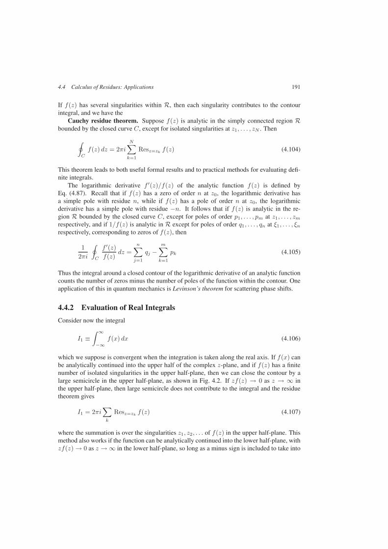
4.4 Calculus of Residues: Applications 191
If f(z) has several singularities within R, then each singularity contributes to the contourintegral, and we have the
Cauchy residue theorem. Suppose f(z) is analytic in the simply connected region Rbounded by the closed curve C, except for isolated singularities at z1, . . . , zN . Then
∮
C
f(z) dz = 2πiN∑
k=1
Resz=zkf(z) (4.104)
This theorem leads to both useful formal results and to practical methods for evaluating defi-nite integrals.
The logarithmic derivative f ′(z)/f(z) of the analytic function f(z) is defined byEq. (4.87). Recall that if f(z) has a zero of order n at z0, the logarithmic derivative hasa simple pole with residue n, while if f(z) has a pole of order n at z0, the logarithmicderivative has a simple pole with residue −n. It follows that if f(z) is analytic in the re-gion R bounded by the closed curve C, except for poles of order p1, . . . , pm at z1, . . . , zmrespectively, and if 1/f(z) is analytic in R except for poles of order q1, . . . , qn at ξ1, . . . , ξnrespectively, corresponding to zeros of f(z), then
12πi
∮
C
f ′(z)f(z)
dz =n∑
j=1
qj −m∑
k=1
pk (4.105)
Thus the integral around a closed contour of the logarithmic derivative of an analytic functioncounts the number of zeros minus the number of poles of the function within the contour. Oneapplication of this in quantum mechanics is Levinson’s theorem for scattering phase shifts.
4.4.2 Evaluation of Real Integrals
Consider now the integral
I1 ≡∫ ∞
−∞f(x) dx (4.106)
which we suppose is convergent when the integration is taken along the real axis. If f(x) canbe analytically continued into the upper half of the complex z-plane, and if f(z) has a finitenumber of isolated singularities in the upper half-plane, then we can close the contour by alarge semicircle in the upper half-plane, as shown in Fig. 4.2. If zf(z) → 0 as z → ∞ inthe upper half-plane, then large semicircle does not contribute to the integral and the residuetheorem gives
I1 = 2πi∑
k
Resz=zkf(z) (4.107)
where the summation is over the singularities z1, z2, . . . of f(z) in the upper half-plane. Thismethod also works if the function can be analytically continued into the lower half-plane, withzf(z) → 0 as z → ∞ in the lower half-plane, so long as a minus sign is included to take into
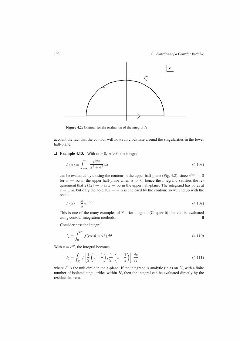
192 4 Functions of a Complex Variable
C
z
Figure 4.2: Contour for the evaluation of the integral I1.
account the fact that the contour will now run clockwise around the singularities in the lowerhalf-plane.
Example 4.13. With α > 0, a > 0, the integral
F (α) ≡∫ ∞
−∞
eiαx
x2 + a2dx (4.108)
can be evaluated by closing the contour in the upper half-plane (Fig. 4.2), since eiαz → 0for z → ∞ in the upper half-plane when α > 0; hence the integrand satisfies the re-quirement that zf(z) → 0 as z → ∞ in the upper half-plane. The integrand has poles atz = ±ia, but only the pole at z = +ia is enclosed by the contour, so we end up with theresult
F (α) =π
ae−αa (4.109)
This is one of the many examples of Fourier integrals (Chapter 6) that can be evaluatedusing contour integration methods.
Consider next the integral
I2 ≡∫ 2π
0
f(cos θ, sin θ) dθ (4.110)
With z = eiθ , the integral becomes
I2 =∮
K
f
[12
(z +
1z
),
12i
(z − 1
z
)]dz
iz(4.111)
where K is the unit circle in the z-plane. If the integrand is analytic (in z) on K, with a finitenumber of isolated singularities within K, then the integral can be evaluated directly by theresidue theorem.
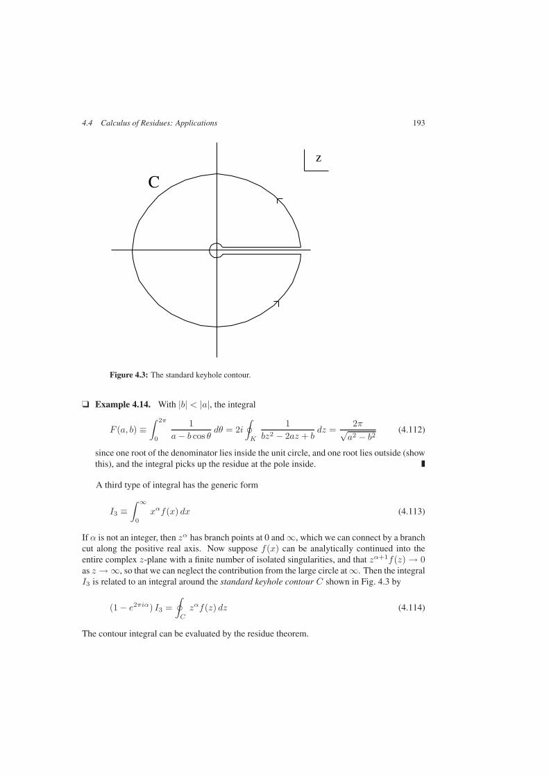
4.4 Calculus of Residues: Applications 193
C
z
Figure 4.3: The standard keyhole contour.
Example 4.14. With |b| < |a|, the integral
F (a, b) ≡∫ 2π
0
1a− b cos θ
dθ = 2i∮
K
1bz2 − 2az + b
dz =2π√a2 − b2
(4.112)
since one root of the denominator lies inside the unit circle, and one root lies outside (showthis), and the integral picks up the residue at the pole inside.
A third type of integral has the generic form
I3 ≡∫ ∞
0
xαf(x) dx (4.113)
If α is not an integer, then zα has branch points at 0 and ∞, which we can connect by a branchcut along the positive real axis. Now suppose f(x) can be analytically continued into theentire complex z-plane with a finite number of isolated singularities, and that zα+1f(z) → 0as z → ∞, so that we can neglect the contribution from the large circle at ∞. Then the integralI3 is related to an integral around the standard keyhole contour C shown in Fig. 4.3 by
(1 − e2πiα) I3 =∮
C
zαf(z) dz (4.114)
The contour integral can be evaluated by the residue theorem.
194 4 Functions of a Complex Variable
Example 4.15. With 0 < |a| < 1, we have the integral
Ia(z) ≡∫ ∞
0
1xa(x− z)
dx =(
11 − e−2πia
) ∮
C
1ξa(ξ − z)
dξ
(4.115)
=(
11 − e−2πia
)2πiza
=π
sinπa(−z)−a
Here we can use the fact that Ia(z) must be positive when z is real and negative to becertain we are on the proper sheet of the Riemann surface of the function (−z)−a. Start-ing (−z)−a real and positive on the negative real z-axis, we can move anywhere in thez-plane with an implicit branch cut along the positive real z-axis, since Ia(z) will have adifferent value there depending on how we approach the axis. This integral is a prototypefor integrating a function along a path joining two branch points.
A closely related integral is
I4 ≡∫ ∞
0
f(x) dx (4.116)
If f(x) can be analytically continued into the entire complex z-plane, with a finite number ofisolated singularities, then we can convert this integral into an integral
I4 =i
2π
∮
C
(ln z)f(z) dz (4.117)
around the standard keyhole contour. For if we choose the branch cut of ln z along the positivereal axis from 0 to ∞, then
lnxe2πi = lnx+ 2πi (4.118)
and if z(ln z)f(z) → 0 as z → 0 and as z → ∞, we can again neglect the contribution fromthe large circle at ∞.
Example 4.16. The integral∫ ∞
0
11 + x3
dx =i
2π
∮
C
ln z1 + z3
dz (4.119)
=iπ
3
5
(ω − ω∗)(ω∗ + 1)− 3
(ω + 1)(ω∗ + 1)− 1
(ω − ω∗)(ω + 1)
=
π
3√
3
where
ω =12(1 + i
√3) = e
iπ3 and ω∗ =
12(1 − i
√3) = e−
iπ3 (4.120)
are the complex cube roots of −1. The contour integral has picked up the contributionsfrom all three of the cube roots.
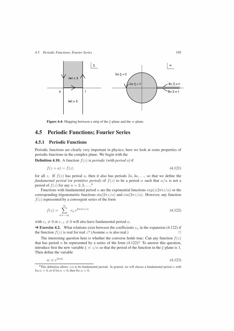
4.5 Periodic Functions; Fourier Series 195
0 1
w
|w| > 1
Im
Re
|w| < 1
Im
Re
Figure 4.4: Mapping between a strip of the ξ-plane and the w-plane.
4.5 Periodic Functions; Fourier Series
4.5.1 Periodic Functions
Periodic functions are clearly very important in physics; here we look at some properties ofperiodic functions in the complex plane. We begin with the
Definition 4.10. A function f(z) is periodic (with period a) if
f(z + a) = f(z) (4.121)
for all z. If f(z) has period a, then it also has periods 2a, 3a, . . ., so that we define thefundamental period (or primitive period) of f(z) to be a period α such that α/n is not aperiod of f(z) for any n = 2, 3, . . ..6
Functions with fundamental period α are the exponential functions exp(±2πiz/α) or thecorresponding trigonometric functions sin(2πz/α) and cos(2πz/α). However, any functionf(z) represented by a convergent series of the form
f(z) =∞∑
n=−∞cn e
2nπiz/α (4.122)
with c1 = 0 or c−1 = 0 will also have fundamental period α.
Exercise 4.2. What relations exist between the coefficients cn in the expansion (4.122) ifthe function f(z) is real for real z? (Assume α is also real.)
The interesting question here is whether the converse holds true: Can any function f(z)that has period α be represented by a series of the form (4.122)? To answer this question,introduce first the new variable ξ ≡ z/α so that the period of the function in the ξ-plane is 1.Then define the variable
w ≡ e2πiξ (4.123)
6This definition allows ±α to be fundamental periods. In general, we will choose a fundamental period α withIm α > 0, or if Im α = 0, then Re α > 0.
196 4 Functions of a Complex Variable
The function f(z) is completely specified by its values in the strip 0 ≤ Re ξ ≤ 1 in the ξ-plane,which is mapped into the entire w-plane by (4.123) as shown in Fig. 4.4. Thus periodicity off(z) in z or ξ is equivalent to a requirement that f(z) be a single-valued function of w. If fis analytic in the w-plane in some annular region R : w1 < |w| < w2, then we can expand fin a Laurent series
f =∞∑
n=−∞cn w
n (4.124)
convergent within the annular region R. When we return to the variable z, this series isprecisely of the form (4.122), and the region of convergence is a strip of the form
S : − ln w2 < 2π Im( zα
)< − ln w1
The coefficients cn in the Laurent expansion (4.124) can be expressed as contour integrals
cn =1
2πi
∮
C
f(w)wn+1
dw (4.125)
where C is a circle of radius w0 inside R. This circle corresponds to the line
L : ξ = x+ iη | 0 ≤ x ≤ 1, w0 = e−2πη
in the ξ-plane, and the integral formula (4.125) can also be written as
cn =1
2πwn0
∫ 1
0
f(x) e−2πinx dx (4.126)
When f(z) is an analytic function of z in a strip of the form S, then the expansion (4.122)is convergent inside the strip, uniformly in any closed region lying entirely within the strip.The expansion (4.122) is known as a (complex) Fourier series. The series has the alternativeexpression in terms of trigonometric functions as
f(z) =∞∑
n=0
an cos(
2nπzα
)+
∞∑
n=1
bn sin(
2nπzα
)(4.127)
in which the coefficients an and bn are real if f(z) is real for real z. The coefficients cn, or anand bn, are the Fourier coefficients of f(z).
Exercise 4.3. Express the function tanπξ as a single-valued function of the variablew = e2πiξ . Then find Fourier series expansions of tanπξ and cotπξ valid for Im ξ > 0.
Periodic functions on the real z-axis that cannot be analytically continued into the complexplane also have Fourier series expansions of the forms (4.122) and (4.127), with coefficientsgiven by Eq. (4.126) with w0 = 1. However, the convergence properties are not the same,since the series cannot converge away from the real axis (the strip of convergence has zerowidth). These expansions will be examined further in Chapter 6 where Fourier series arerevisited in the context of linear vector space theory.
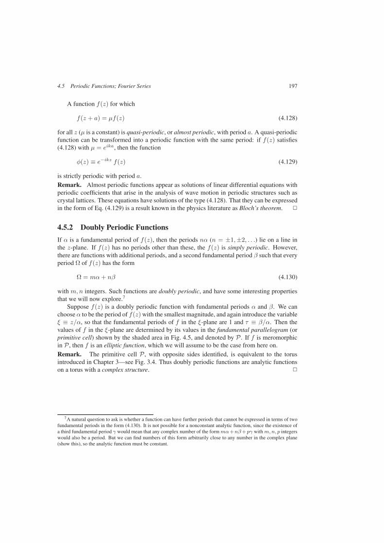
4.5 Periodic Functions; Fourier Series 197
A function f(z) for which
f(z + a) = µf(z) (4.128)
for all z (µ is a constant) is quasi-periodic, or almost periodic, with period a. A quasi-periodicfunction can be transformed into a periodic function with the same period: if f(z) satisfies(4.128) with µ = eika, then the function
φ(z) ≡ e−ikz f(z) (4.129)
is strictly periodic with period a.
Remark. Almost periodic functions appear as solutions of linear differential equations withperiodic coefficients that arise in the analysis of wave motion in periodic structures such ascrystal lattices. These equations have solutions of the type (4.128). That they can be expressedin the form of Eq. (4.129) is a result known in the physics literature as Bloch’s theorem.
4.5.2 Doubly Periodic Functions
If α is a fundamental period of f(z), then the periods nα (n = ±1,±2, . . .) lie on a line inthe z-plane. If f(z) has no periods other than these, the f(z) is simply periodic. However,there are functions with additional periods, and a second fundamental period β such that everyperiod Ω of f(z) has the form
Ω = mα+ nβ (4.130)
with m,n integers. Such functions are doubly periodic, and have some interesting propertiesthat we will now explore.7
Suppose f(z) is a doubly periodic function with fundamental periods α and β. We canchoose α to be the period of f(z) with the smallest magnitude, and again introduce the variableξ ≡ z/α, so that the fundamental periods of f in the ξ-plane are 1 and τ ≡ β/α. Then thevalues of f in the ξ-plane are determined by its values in the fundamental parallelogram (orprimitive cell) shown by the shaded area in Fig. 4.5, and denoted by P . If f is meromorphicin P , then f is an elliptic function, which we will assume to be the case from here on.
Remark. The primitive cell P , with opposite sides identified, is equivalent to the torusintroduced in Chapter 3—see Fig. 3.4. Thus doubly periodic functions are analytic functionson a torus with a complex structure.
7A natural question to ask is whether a function can have further periods that cannot be expressed in terms of twofundamental periods in the form (4.130). It is not possible for a nonconstant analytic function, since the existence ofa third fundamental period γ would mean that any complex number of the form mα+nβ +pγ with m, n, p integerswould also be a period. But we can find numbers of this form arbitrarily close to any number in the complex plane(show this), so the analytic function must be constant.
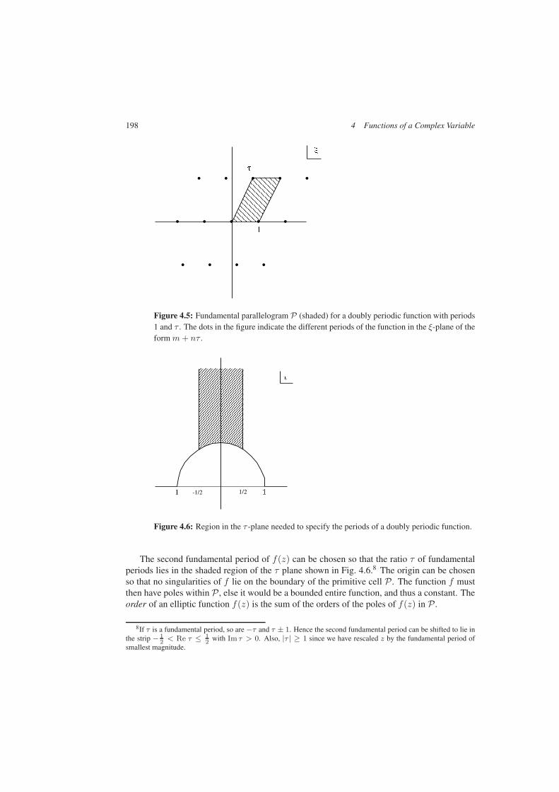
198 4 Functions of a Complex Variable
•
•
•
• ••
•
• • • •
• •
•
Figure 4.5: Fundamental parallelogram P (shaded) for a doubly periodic function with periods1 and τ . The dots in the figure indicate the different periods of the function in the ξ-plane of theform m+ nτ .
1/2-1/2
Figure 4.6: Region in the τ -plane needed to specify the periods of a doubly periodic function.
The second fundamental period of f(z) can be chosen so that the ratio τ of fundamentalperiods lies in the shaded region of the τ plane shown in Fig. 4.6.8 The origin can be chosenso that no singularities of f lie on the boundary of the primitive cell P . The function f mustthen have poles within P , else it would be a bounded entire function, and thus a constant. Theorder of an elliptic function f(z) is the sum of the orders of the poles of f(z) in P .
8If τ is a fundamental period, so are −τ and τ ± 1. Hence the second fundamental period can be shifted to lie inthe strip − 1
2< Re τ ≤ 1
2with Im τ > 0. Also, |τ | ≥ 1 since we have rescaled z by the fundamental period of
smallest magnitude.

A Gamma Function; Beta Function 199
If K is the boundary of P , then the periodicity of f(z) implies∮
K
f(ξ) dξ = 0 (4.131)
since the contributions to the integral from opposite sides of P cancel. Thus the sum of theresidues of f at the poles in P must be zero. Hence f cannot have just one simple poleinside P; the minimum order of an elliptic function is 2, corresponding to a function thathas either a double pole with zero residue, or a pair of simple poles with equal and oppositeresidues.
The order n of an elliptic function f is also equal to the number of zeros of f inside P(counted with appropriate multiplicity), since double periodicity also implies
12πi
∮
K
f ′(ξ)f(ξ)
dξ = 0 (4.132)
as in Eq. (4.131). We know from Eq. (4.105) that this integral is equal to the number of zerosminus the number of poles of f inside P . Then f assumes any complex value c exactly ntimes inside P9, since if f is an elliptic function of order n, so is f − c.
Some elliptic functions that occur in physics are introduced in Appendix A of Chapter 5.
A Gamma Function; Beta Function
A.1 Gamma Function
An important special function that has already made a brief appearance in Chapter 1 is theΓ-function, defined for Re z > 0 by the integral
Γ(z) ≡∫ ∞
0
tz−1 e−t dt (4.A1)
When z is a positive integer n+1, the integral can be evaluated using integration by parts, forexample, to give
Γ(n+ 1) =∫ ∞
0
tn e−t dt = n! (4.A2)
(n = 0, 1, 2, . . .). Also, when z is a half-integer, we can let t = u2 to obtain
Γ(n+ 12 ) =
∫ ∞
0
tn−12 e−t dt = 2
∫ ∞
0
u2n e−u2du =
(2n) !22n n !
√π (4.A3)
(n = 0, 1, 2, . . .).The Γ-function defined by Eq. (4.A1) is the analytic continuation of the factorial function
defined for integers into the half-plane Re z > 0. Note that it is analytic, since the derivative
Γ′(z) =∫ ∞
0
(ln t)tz−1 e−t dt (4.A4)
9The reader is invited to provide a modification of this statement for a value c that occurs on the boundary of P .

200 4 Functions of a Complex Variable
is well defined for Re z > 0. Integration by parts in Eq. (4.A1) gives the recursion formula
zΓ(z) = Γ(z + 1) (4.A5)
and then
z(z + 1) · · · (z + n) Γ(z) = Γ(z + n+ 1) (4.A6)
(n = 1, 2, . . .) for Re z > 0. But the right-hand side is analytic for Re z > −n − 1, sothis equation provides the analytic continuation of Γ(z) to the half-plane Re z > −n − 1.It follows that Γ(z) is analytic everywhere in the finite z-plane except for simple poles atz = 0,−1,−2, . . ., with residue at the pole at z = −n given by (−1)n/n !. These analyticityproperties also follow from the expansion
Γ(z) =∫ 1
0
tz−1 e−t dt+∫ ∞
1
tz−1 e−t dt
=∞∑
n=0
(−1)n
n!1
z + n+
∫ ∞
1
tz−1 e−t dt (4.A7)
where we note that the sum is absolutely convergent everywhere except at the poles, and theintegral is an entire function with an essential singularity at ∞.
Consider now the product Γ(z)Γ(1− z), which has poles at each integer, with the residueof the pole at z = n given simply by (−1)n. It is thus plausible that
Γ(z)Γ(1 − z) =π
sinπz. (4.A8)
To show that this is actually the case, suppose 0 < Re z < 1. Then
Γ(z)Γ(1 − z) =∫ ∞
0
tz−1 e−t dt∫ ∞
0
u−z e−u du
= 4∫ ∞
0
x2z−1 e−x2dx
∫ ∞
0
y1−2z e−y2dy
= 4∫ ∞
0
r e−r2dr
∫ π2
0
(cot θ)2z−1 dθ
= 2∫ ∞
0
s2z−1
1 + s2ds =
π
sinπz(4.A9)
where the last integral is evaluated using the standard keyhole contour introduced in the pre-ceding section. The result (4.A8), derived for 0 < Re z < 1, is then true everywhere byanalytic continuation.
An infinite product representation of the Γ-function is derived from the expression
Γ(z) = limn→∞
∫ n
0
(1 − t
n
)ntz−1 dt = lim
n→∞
nz
∫ 1
0
(1 − u)n uz−1 du
= limn→∞
nz
n !z(z + 1) · · · (z + n)
(4.A10)
A Gamma Function; Beta Function 201
valid for Re z > 0. It follows that
1Γ(z)
= z limn→∞
n−z
n∏
m=1
(1 +
z
m
)
= z limn→∞
exp
[(n∑
m=1
1m
− lnn
)z
]n∏
m=1
[(1 +
z
m
)e−
zm
]
= z eγz∞∏
m=1
[(1 +
z
m
)e−
zm
](4.A11)
where γ is the Euler–Mascheroni constant defined by
γ ≡ limn→∞
(n∑
m=1
1m
− lnn
)(4.A12)
(see Eq. (1.72) and Problem 1.12 for further details). The infinite product is convergent forall finite z due to the inclusion of the factor exp(−z/m). This is an example of the factorexp[γm(z)] introduced in Eq. (4.93).
Exercise 4.A1. Using the infinite product representation (4.A11) or otherwise, derive theduplication formula
Γ(z)Γ(z + 12 ) =
√π Γ(2z)22z−1
(4.A13)
This result and Eq. (4.A8) are quite useful.
The infinite product representation (4.A11) can be used to derive an integral representa-tion for the logarithmic derivative of the Γ-function, which appears in some physics contexts.Taking the logarithm of both sides of Eq. (4.A11) gives
ln Γ(z) = −γz − ln z +∞∑
m=1
[ zm
− ln(1 +
z
m
)](4.A14)
and then, by differentiation,
Γ′(z)Γ(z)
=d
dz[ ln Γ(z) ] = −γ − 1
z+ z
∞∑
m=1
1m(z +m)
(4.A15)
Now recall the result
γ =∫ 1
0
(1 − e−t
t
)dt−
∫ ∞
1
e−t
tdt (4.A16)
from Problem (1.12), and note that
1z +m
=∫ ∞
0
e−(z+m) t dt (4.A17)
202 4 Functions of a Complex Variable
We then get the integral representation
d
dz[ ln Γ(z)] =
∫ ∞
0
(e−t
t− e−zt
1 − e−t
)dt (4.A18)
valid for Re z > 0. Since∫ ∞
0
e−t − e−zt
tdt = ln z (4.A19)
we have the alternative representation (still for Re z > 0)
d
dz[ ln Γ(z) ] = ln z +
∫ ∞
0
(1t− 1
1 − e−t
)e−zt dt (4.A20)
The Bernoulli numbers B2n are defined by the expansions
t
1 − e−t= 1 + 1
2 t+∞∑
n=1
B2n
(2n) !t2n (4.A21)
t
et − 1= 1 − 1
2 t+∞∑
n=1
B2n
(2n) !t2n (4.A22)
The term in parentheses in the integrand in Eq. (4.A20) can be expanded to obtain the asymp-totic expansion
d
dz[ ln Γ(z) ] ∼ ln z − 1
2z−
∞∑
n=1
B2n
2n1z2n
(4.A23)
for z → ∞ in any sector |arg z| ≤ 12φ − δ (0 < δ < π
2 ). This expansion can be integratedterm-by-term to give
ln Γ(z) ∼ (z − 12 ) ln z − z + C +
∞∑
n=0
B2n+2
(2n+ 1)(2n+ 2)1
z2n+1(4.A24)
where the constant C must be determined separately. The calculation in Section 1.4 gives (seeEq. (1.111))
C = 12 ln(2π) (4.A25)
The corresponding asymptotic expansion of the Γ-function itself is then given by
Γ(z) ∼√
2πz
(ze
)zexp
∞∑
n=0
B2n+2
(2n+ 1)(2n+ 2)
=
√2πz
(ze
)z 1 +
112z
+1
288z2+O
(1z3
)(4.A26)
(Stirling’s series). The expansion of n! for large n obtained from this using Eq. (4.A2) isimportant in statistical physics.

A Gamma Function; Beta Function 203
A.2 Beta Function
Now consider the product
Γ(α)Γ(β) =∫ ∞
0
xα−1 e−x dx∫ ∞
0
yβ−1 e−y dy
=∫ ∞
0
∫ u
0
xα−1(u− x)β−1 e−u dx du
=∫ ∞
0
uα+β−1 e−u du∫ 1
0
tα−1(1 − t)β−1 dt
= Γ(α+ β)∫ 1
0
tα−1(1 − t)β−1 dt (4.A27)
where u = x+ y and x = ut.The beta function B(α, β) is defined by
B(α, β) ≡∫ 1
0
tα−1(1 − t)β−1 dt =Γ(α)Γ(β)Γ(α+ β)
(4.A28)
where the integral is defined for Re α > 0, Re β > 0. The ratio of the Γ-functions thenprovides the analytic continuation of B(α, β) to all α, β. A second integral representation ofthe beta function is
B(α, β) =∫ ∞
0
(1 − e−w)β−1 e−αw dw (4.A29)
which follows from the substitution t = e−w in Eq. (4.A28).For fixed β, B(α, β) is an analytic function of α with simple poles at α = 0,−1,−2, . . .
corresponding to the poles of Γ(α). The residue at the pole at α = −n is given by
Resα=−nB(α, β) =(−1)n
n !Γ(β)
Γ(−n+ β)(4.A30)
=(n− β)(n− β − 1) · · · (1 − β)
n !
(n = 0, 1, 2, . . .). Note that if β = m is a positive integer, the apparent poles at α =−m,−m− 1, . . . are not actually present.
The B-function can be expanded as a sum over its poles according to
Γ(α)Γ(β)Γ(α+ β)
=∞∑
n=0
(n− β)(n− β − 1) · · · (1 − β)n !
1α+ n
(4.A31)
If Re β > 0, the series is absolutely convergent for all α except at the poles.
Exercise 4.A2. Prove the convergence of the series (4.A31).
204 4 Functions of a Complex Variable
Bibliography and Notes
An introduction to the classical theory of functions of a complex variable is given in the bookof Whittaker and Watson cited in Chapter 1. Another brief introduction is contained in thetwo paperback volumes
Konrad Knopp, Theory of Functions (Parts I and II), Dover (1945, 1947).
These two volumes cover the basics of analytic functions, power series, contour integration,and Cauchy’s theorems. The proofs of the Weierstrass factorization theorem and the Mittag-Leffler theorem sketched here are given in detail in the second volume, which also has anintroduction to the theory of doubly periodic functions (elliptic functions).
A classic work that is still quite readable today is
E. T. Copson, Theory of Functions of a Complex Variable, Clarendon Press, Oxford(1935).
After a general discussion of the properties of analytic functions, there is extensive treatmentof many important special functions, including the Gamma function, hypergeometric, Le-gendre and Bessel functions, and the various elliptic functions. There is also a nice derivationof Picard’s theorem.
Good modern textbooks at an introductory level are
J. W. Brown and R, V. Churchill, Complex Variables and Applications (7th edition),McGraw-Hill (2004).
This standard is still a favorite after more than 50 years. It covers the basics and includes someuseful discussion of applications of conformal mappings.
E. B. Saff and A. D. Snider, Fundamentals of Complex Analysis (3rd edition),Prentice-Hall (2003).
This book also has a good treatment of conformal mappings, and also has several sections onnumerical methods in various contexts.
J. E. Marsden and M. E. Hoffman, Basic Complex Analysis (3rd edition),W. H. Freeman (1998).
In addition to a well-written introduction to the basics, this book has nice treatments of con-formal mappings and of asymptotic methods, and a chapter on the Laplace transform.
A more advanced textbook is
G. F. Carrier, M. Krook, and C. E. Pierson, Functions of a Complex Variable: The-ory and Technique, Hod Books, Ithaca (1983).
This excellent book has a thorough introduction to the theory of functions of a complex vari-able and its applications to other problems. While there are few formal proofs, the mathemat-ics is explained clearly and illustrated with well-chosen examples and exercises. There arelengthy chapters on conformal mappings, special functions, asymptotic methods, and integraltransform methods, all of which get to the meat of the applications of these methods. There isalso a useful chapter on the Wiener–Hopf method and singular integral equations.

Problems 205
Problems
1. For each of the mappings
(i ) w =z2 + 1z2 − 1
(ii) w = tan z
explain: For what values of z does the mapping fail to be conformal? What are thebranch points of the map in the w-plane? What is the structure of the Riemann surfacecorresponding to the w-plane? Find appropriate branch cuts in the w-plane, and indicatewhat region of the z-plane is mapped onto each sheet of the w-plane. Sketch some detailsof the mapping.
2. Consider the linear fractional transformation
z → w =az + b
cz + d
with ∆ ≡ ad− bc = 1. With this transformation we can associate the 2 × 2 matrix
A ≡(a bc d
)
(note that detA = ∆ = 1).
(i) Show that the result of the linear fractional transformation with associated matrix A1
followed by the linear fractional transformation with associated matrix A2 is a linearfractional transformation whose associated matrix is the matrix product A2A1.
Remark. Thus the transformation group SL(2) defined by 2 × 2 matrices A withdetA = 1 has a nonlinear realization by linear fractional transformations of the complexplane.
(ii) Show that if the matrix A is real, then the associated linear fractional transformationmaps the upper half z-plane into the upper half w-plane.
3. Discuss the analytic properties of each of the functions below. In particular, locate andclassify the singularities of each function, calculate the residue at each pole, join eachpair of branch points with a suitable cut and calculate the discontinuity across the cut,and describe the Riemann surface on which each function is defined.
(i)z
(z2 − a2)2
(ii)sin zz
(iii)1√z
ln(
1 +√z
1 −√z
)
(iv)∫ ∞
0
e−t
t+ zdt

206 4 Functions of a Complex Variable
4. Is it always true that
ln z1z2 = ln z1 + ln z2
when z1 and z2 are complex? Explain your answer with words and pictures.
5. Consider the function
f(z) =1
a+ bz + i√z
where a, b are real constants. f(z) is defined on the two-sheeted Riemann surface as-sociated with
√z. Choose the branch cut in the z-plane to run from 0 to ∞ along the
positive real axis, and define the principal sheet to be where√z is positive as the real
axis is approached from the upper half z-plane (note that Im√z > 0 on this sheet). Find
the pole(s) of f(z) on the Riemann surface, noting carefully on which sheet each pole islocated. Consider all possible sign combinations for a, b.
6. Derive the power series
tan−1 z =∞∑
n=0
(−1)nz2n+1
2n+ 1
7. Use the arctangent series from the preceding problem to show that
π
8=
∞∑
n=0
1(4n+ 1)(4n+ 3)
8. Show that
1sin2 z
=∞∑
n=−∞
1(z + nπ)2
From this result, show that
ζ(2) =∞∑
n=1
1n2
=π2
6
Then evaluate the series
Σ4(z) ≡∞∑
n=−∞
1(z + nπ)4
and the sum
ζ(4) =∞∑
n=1
1n4

Problems 207
9. Planck’s radiation law. In an ideal blackbody at (absolute) temperature T , the electro-magnetic energy density between frequencies ν and ν + dν is given by
uνdν =(
8πhν3
c3
)1
exp(hνkT
)− 1
dν
where h is Planck’s original constant (h = 2π), k is the Boltzmann constant, and c isthe speed of light.
(i) Show that the total energy density is proportional to the fourth power of temperature,
U(T ) ≡∫ ∞
0
uν dν = aT 4
Remark. This is the Stefan–Boltzmann law for blackbody radiation; the power radiatedfrom a blackbody is proportional to its energy density, and hence also to the fourth powerof the temperature.
(ii) Evaluate the Stefan–Boltzmann constant a in terms of h, k, and c.
10. Consider the expansion
1√1 − 2hz + h2
=∞∑
n=0
cn(z)hn
For fixed h > 0, find the region in the z-plane for which this series is convergent.
11. Find the conditions under which the series
S(z) ≡∞∑
n=1
zn
(1 − zn)(1 − zn+1)
is convergent and evaluate the sum.
12. If F (z) is an entire function with zeros at z1, z2, . . ., then the sequence zk → ∞.
13. Evaluate the integrals
(i)∫ ∞
0
11 + x6
dx
(ii)∫ ∞
−∞
1(1 + x2)(1 − 2αx+ x2)
dx
with α being a fixed complex number.
14. Suppose m and n are positive integers with m < n. Evaluate the integral
Im,n ≡∫ ∞
0
x2m
1 + x2ndx

208 4 Functions of a Complex Variable
15. Evaluate the integrals
(i)∫ π
0
11 + sin2 θ
dθ
(ii)∫ 2π
0
sin2 θ
a+ b cos θdθ
(iii)∫ ∞
−∞
cos ax− cos bxx2
dx
(iv)∫ ∞
0
cos ax1 + x4
dx
with a, b real and positive.
16. Evaluate the integral
In(a) ≡∫ ∞
0
xa−1
1 + x2ndx
with n being a positive integer, and 0 < a < 2n.
17. Evaluate the integral
∫ ∞
0
ln x1 + x2
dx
18. Evaluate the integral
I(a) ≡∫ ∞
0
dx
cosh ax
19. Consider the function h(z) defined by
h(z) ≡ 2√π
∫ ∞
0
x2e−x2
1 − ze−x2 dx
(i) Evaluate h(0).
(ii) Find the power series expansion of h(z) about z = 0. For what region in the z-planeis the series convergent?
(iii) For what region in the z-plane is h(z) defined by the integral? Locate the singular-ities of h(z). Find suitable branch cuts connecting branch points of h(z), and describethe Riemann surface of the function.
Problems 209
20. (i) Compute the volume V(Sn) of the sphere Sn. First, consider the n-dimensionalintegral
In ≡∫ ∞
−∞· · ·
∫ ∞
−∞e−r
2dx1, . . . , dxn
with r2 = x21 + · · · + x2
n (r is the radial coordinate in n-dimensional spherical coordi-nates). In Cartesian coordinates, the integral can be expressed as a product of n identicalone-dimensional integrals. In spherical coordinates, it is given by
In = V(Sn−1)∫ ∞
0
rn−1e−r2dr
which can be evaluated in terms of a Γ-function. Then evaluate V(Sn−1).
(ii) Evaluate the volume V(Bn) of an n-dimensional ball Bn of radius R.
(iii) Compare your results with the standard results for n = 1, 2, 3.
Remark. Once these results are expressed in terms of Γ-functions, there is no need forthe dimension n to be an integer. Extending these results to noninteger n is useful inrenormalization group analyses both in quantum field theory and in statistical mechanicsof many-body systems.
21. Show that 1/Γ(z) can be written as a contour integral according to
1Γ(z)
=1
2πi
∫
C
(−t)−z e−t dt
where C is the standard keyhole contour shown in Fig. 4.3.
22. Show that∫ 1
0
xa−1 (1 − x)b−1
(x+ p)a+bdx =
Γ(a) Γ(b)Γ(a+ b)
1(1 + p)a pb
for Re a > 0,Re b > 0, p > 0.
23. Show that
In ≡∫ π
2
0
sin2n θ dθ = 22n−1 [Γ(n+ 12 )]2
Γ(2n+ 1)
for n = 0, 1, 2, . . .. Evaluate this for n = 0 to show that
Γ(
12
)=
√π
Finally, show that
In =π
22n+1
(2n)!(n!)2
210 4 Functions of a Complex Variable
24. Recall the Riemann ζ-function defined in Chapter 1 for Re s > 1 by
ζ(s) ≡∞∑
n=1
1ns
(i) Show that
ζ(s) =1
Γ(s)
∫ ∞
0
xs−1
ex − 1dx
for Re s > 1.
(ii) Show that
ζ(s) =Γ(1 − s)
2πi
∫
C
(−t)s−1
et − 1dt
where C is the standard keyhole contour shown in Fig. 4.3. Then show that ζ(s) isanalytic in the finite s-plane except for a simple pole at s = 1 with residue 1.
(iii) Evaluate ζ(−p) (p = 0, 1, 2, . . .) in terms of Bernoulli numbers (Eqs. (4.A21) and(4.A22)).
25. Find the sum of the series
∞∑
n=0
e−nb cos 2πnz
(b > 0). For what values of z does the series converge?
26. Suppose the elliptic function f(z) of order n has zeros at a1, . . . , an and poles atb1, . . . , bn in a primitive cell P . Show that
n∑
k=1
ak −n∑
k=1
bk = pα+ qβ
where α, β are the fundamental periods of f(z), and p, q are integers.Hint. Evaluate the integral
12πi
∮
K
zf ′(z)f(z)
dz
around the boundary K of P .
5 Differential Equations: Analytical Methods
In Chapter 3, we introduced the concept of vector fields and their lines of flow (integral curves)as solutions of a system of first-order differential equations. It is relatively straightforward togenerate a solution to such a system, numerically if necessary, starting from an initial point inthe n-dimensional manifold on which the equations are defined. This solution will be unique,provided of course that the initial point is not a singular point of the vector field defined by theequations. However, there are also questions of long-term stability of solutions—do solutionsthat start from nearby points remain close to each other? and if so, for how long?—that areespecially important both in principle and in practice, and many of these questions are stillopen to active research. They are only mentioned briefly here to remind the reader that thereis more to using mathematics than providing input to a computer.
Moreover, not all systems of differential equations in physics are posed as initial valueproblems. A vibrating string, for example, is described by a linear second-order differentialequation with boundary conditions at the endpoints of the string. Thus we need to considermethods to find general solutions to a differential equation, and then deal with the questionsof existence and uniqueness of solutions satisfying various possible constraints. For linearsystems, the theory of linear vector spaces and linear operators in Chapters 2, 6, and 7 isuseful, but analytic techniques are still needed to construct explicit solutions.
We begin with the standard form of a system of n first-order differential equations
d
dzuk(z) = hk(u1, . . . , un; z)
(k = 1, . . . , n), where u1, . . . , un are the functions to be determined, and z is the indepen-dent variable; here u1, . . . , un and z may complex. Extending the range of the variables tothe complex plane allows us to make use of the theory of functions of a complex variableelaborated in Chapter 4. We note that a general nth-order differential equation for a singlefunction u can be reduced to a system of n first-order equations by introducing as independentvariables the function u and its first n− 1 derivatives u′, . . . , u(n−1).
The simplest differential equation is the linear first-order equation
d
dzu(z) + p(z)u(z) = f(z)
We construct the general solution to the homogeneous equation [f(z) = 0] with initial con-dition u(z0) = u0, and show how the analytic properties of the solution are related to theanalytic properties of the coefficient p(z). We then show how to find the solution to the inho-mogeneous equation.
Introduction to Mathematical Physics. Michael T. VaughnCopyright c© 2007 WILEY-VCH Verlag GmbH & Co. KGaA, WeinheimISBN: 978-3-527-40627-2
Introduction to Mathematical Physics
Michael T. Vaughn 2007 WILEY-VCH Verlag GmbH & Co.
212 5 Differential Equations
We also look at some special nonlinear first-order equations. The Bernoulli equation isreduced to a linear equation by a change of variables. The first-order Ricatti equation isrelated to a linear second-order equation. We show how to solve a first-order equation that isan exact differential. Of course there is no universal method to reduce the general first-orderequation to an exact differential!
We present the nth-order linear differential equation as a linear operator equation
L[u] ≡ u(n)(z) + p1(z)u(n−1)(z) + · · · + pn−1(z)u′(z) + pn(z)u(z) = f(z)
on the linear vector space Cn of n-times differentiable functions of the variable z. The linearequation L[u] = 0 with constant coefficients is related to the equation of a linear dynamicalsystem introduced in Section 2.5; its solution is a linear combination of exponential functionsof the form exp(αz) with constants α expressed as the roots of a polynomial of degree n. Wealso find solutions when the roots of polynomial are degenerate.
The general solution of the homogeneous equation L[u] = 0 is obtained formally as alinear combination of n fundamental solutions that define an n-dimensional vector space. Ifthe coefficients p1(z), . . . , pn(z) are analytic functions of the complex variable z, then thesolutions to L[u] = 0 are analytic except perhaps where one or more of the coefficients issingular. The behavior of solutions near a singular point is of special interest, for the singularpoints often correspond to the boundary of a physical region in the variable z. A regularsingular point is one at which the singularity of the general solution is at most a pole or abranch point; the general solution has an essential singularity at an irregular singular point.We note that the general solution of the inhomogeneous equation L[u] = f is given as aparticular solution of L[u] = f plus any solution of the homogeneous equation.
Second-order linear equations are especially important in mathematical physics, since theyarise in the analysis of partial differential equations involving the Laplacian operator whenthese equations are reduced to ordinary differential equations by separating variables, as willappear in Chapter 8. Here we show how to extract the leading behavior of solutions nearsingular points. For equations with one or two regular singular points, we can obtain a generalsolution in terms of elementary functions.
The second-order linear equation with three regular singular points is the hypergeometricequation, and its solutions are hypergeometric functions. We describe the Legendre equationand some of its solutions as a model of this equation, and devote Appendix A to a detailedanalysis of the general hypergeometric equation and the hypergeometric functions.
When two of the regular singular points are merged in a special way to create an irregularsingular point, the hypergeometric equation becomes the confluent hypergeometric equation.Bessel’s equation is the version of this equation most often met, and we describe the importantproperties of several types of Bessel functions. We also provide an extensive analysis of thegeneral confluent hypergeometric equation and the confluent hypergeometric equations thatsatisfy it in Appendix B.
In Appendix C, we analyze a nonlinear differential equation that arises in the classical de-scription of the motion of a pendulum, or of an anharmonic (nonlinear) oscillator The solutionto this equation is expressed in terms of elliptic functions, which are examples of the doublyperiodic functions introduced in Chapter 4.
5.1 Systems of Differential Equations 213
5.1 Systems of Differential Equations
5.1.1 General Systems of First-Order Equations
Differential equations with one independent variable are ordinary differential equations; thosewith more than one independent variable are partial differential equations. Chapter 8 is aboutpartial differential equations; in this chapter we deal with ordinary differential equations, inparticular, with systems of first-order differential equations of the form
d
dzuk(z) = hk(u1, . . . , un; z) (5.1)
(k = 1, . . . , n), in which z is the independent variable, and u1, . . . , un are the functions to bedetermined. The number n of independent equations is the order n of the system.
Remark. The general nth order ordinary differential equation has the form
F (v, v′, . . . , v(n); z) = 0 (5.2)
where v = v(z) is the function to be determined, and v′, . . . , v(n) denote the derivatives of vwith respect to z. We assume that ∂F/∂v(n) not identically zero, so that F actually dependson v(n), and that Eq. (5.2) can be solved, perhaps not uniquely, for v(n) so that we have
v(n) = f(v, v′, . . . , v(n−1); z) (5.3)
This nth order equation can be expressed as a system of n first-order equations, so that thereis no loss of generality in starting with a system (5.1) of first-order equations. To see this,simply define u1 = v, u2 = v′, . . . , un = v(n−1). Then Eq. (5.3) is equivalent to the system
u′n = f(u1, . . . , un; z)u′n−1 = un
... (5.4)
u′1 = u2
of n first-order equations of the form (5.1) for the u1, . . . , un.
In Chapter 3, the system (5.1) defined a vector field, and its solutions were the integralcurves of the vector field when the independent variable z was a real parameter and the func-tions hk(u1, . . . , un; z) were independent of z. In many systems, the independent variablehas the physical meaning of time, and Eqs. (5.1) are equations of motion. However, if thefunctions h1, . . . , hn are defined and well behaved for complex z, it is natural look for waysto make use of the theory of functions of a complex variable introduced in Chapter 4, whetheror not complex values of z have any obvious physical meaning.
The system (5.1) does not by itself determine a set of functions u1, . . . , un. In order toobtain a definite solution, it is necessary to specify a set of conditions, such as the values ofthe u1, . . . , un at some fixed value z0 of the variable z. If we are given the initial conditions
u1(z0) = u10, . . . , un(z0) = un0 (5.5)
214 5 Differential Equations
then we can imagine generating a solution to Eq. (5.1) by an iterative procedure. Start fromthe initial conditions and take a small step δz. Then advance from z0 to z0 + δz using thedifferential equations, so that
uk(z0 + δz) = uk0 + hk(u10, . . . , un0, z0) δz (5.6)
(k = 1, . . . , n). A sequence of steps from z0 to z1 ≡ z0 + δz to z2 ≡ z1 + δz and so on,generates an approximate solution along an interval of the real axis, or even a curve in thecomplex plane. We can imagine that the accuracy of the approximation could be improvedby taking successively smaller steps. This procedure, which can be implemented numericallywith varying degrees of sophistication, has an internal consistency check: if we advance fromz0 to z1 and then return from z1 to z0, perhaps using different steps, then we should reproducethe initial conditions. Similarly, if we move around a closed path in the complex plane andreturn to z0, then we should return to the initial conditions, unless by chance we have encircleda branch point of the solution.
A more formal method of generating a solution to the system of equations (5.1) is toevaluate higher derivatives at z0 according to
u′′k =du′kdz
=n∑
m=1
∂hk∂um
dumdz
+∂hk∂z
=n∑
m=1
hm∂hk∂um
+∂hk∂z
(5.7)
(k = 1, . . . , n), and so forth, assuming the relevant partial derivatives exist. If they exist, thehigher derivatives can all be evaluated at z0 in terms of the initial conditions (5.5), leadingto a formal power series expansion of the solutions u1, . . . , un about z0. If these series havea positive radius of convergence, then a complete solution can be constructed in principle byanalytic continuation.
These ideas lead to many important questions in the theory of differential equations.Among these are:
(i) Do the solutions obtained by the iterative method converge to a solution in the limitδz → 0? Do the formal power series solutions actually converge? If they do, what is theirradius of convergence?
(i) What about the existence and uniqueness of solutions that satisfy other types of condi-tions. For example, does a second-order equation have a solution with specified values at twodistinct points? If so, is this solution unique?
(ii) What is the behavior of solutions near singular points of the equations, where oneof the functions hk(u1, u2, . . . , un; z) in Eq. (5.1), or the function f(v, v′, . . . , v(n−1); z) inEq. (5.3), becomes singular? Are there other singularities in the solutions that cannot be iden-tified as singularities of the equations? The only singularities of solutions to linear equationsare singularities of the coefficients, but the solutions of nonlinear equations often have singularpoints that depend on the initial conditions, or boundary conditions, imposed on the solutions.
(iii) Can we understand qualitative properties of solutions without necessarily construct-ing them explicitly. This involves the use of various schemes for constructing approximatesolutions in a local region, as well as tools for characterizing global properties of solutions.
(iv) What approximate schemes are known for computing numerical solutions? Sincefew differential equations allow complete analytic solutions, it is important to have reliablemethods for determining solutions numerically.
5.1 Systems of Differential Equations 215
Various aspects of these issues are discussed in this and subsequent chapters, with the no-table exception of numerical methods, which are mentioned only briefly. With the widespreadavailability of powerful computers, numerical methods are certainly important, but computa-tional physics is a subject that is complementary to the mathematics discussed in this book.
5.1.2 Special Systems of Equations
Certain special classes of differential equations have been studied extensively. A system de-scribed by Eq. (5.1) is linear if each of the functions hk(u1, . . . , un; z) is linear in the vari-ables u1, . . . , un, though not necessarily in z. Similarly, Eq. (5.3) is linear if the functionf(v, v′, . . . , v(n−1); z) is linear in the variables v, v′, . . . , v(n−1). Linear equations are es-pecially important in physics; many fundamental equations of physics are linear (Maxwell’sequations, the wave equation, the diffusion equation and the Schrödinger equation, for exam-ple). They also describe small oscillations of a system about an equilibrium configuration,and the analysis of the stability of equilibria depends heavily on the properties of these linearequations.
An autonomous system of equations is one in which the functions hk(u1, . . . , un; z) inEq. (5.1) are independent of z. Such a system is unchanged by a translation of the variable z;the solutions can be characterized by curves in the space of the variables u1, . . . , un on whichthe location of the point z = 0 is arbitrary. Equations (3.47) that define a vector field areautonomous, and we have seen how the solutions define a family of integral curves of thevector field.
Remark. An autonomous system of order n can generally be reduced to a system of ordern− 1 by choosing one variable un ≡ τ , say, and rewriting the remaining equations in (5.1) inthe form
hn(u1, u2, . . . ; τ )dukdτ
= hk(u1, u2, . . . ; τ ) (5.8)
for k = 1, . . . , n − 1. Conversely, a nonautonomous system of order n can always be trans-formed into an autonomous system of order n + 1 by introducing a new dependent variableun+1 ≡ z. These transformations may, or may not, be useful.
A system of differential equations of the form (5.1) is scale invariant if it is invariant underthe scale transformation z → az (a is a constant). To be precise, this means that
du
dz= h(u; z) = h(u; az) (5.9)
If we define g(u; z) = zh(u; z), then we have g(u; z) = g(u; az), so that g(u; z) is actuallyindependent of z. If we then introduce the variable τ = ln z, we have
zdu
dz=du
dτ= g(u) (5.10)
which is an autonomous equation in the variable τ . This argument evidently applies as wellto a system of the form (5.1).

216 5 Differential Equations
Exercise 5.1. A differential equation is scale covariant, or isobaric, if it is invariant underthe scale transformation z → az together with u→ ap u for some p. Show that if we let
u(z) ≡ zp w(z)
then the resulting equation for w will be scale invariant.
While the properties of autonomy and scale invariance allow the reduction of a differentialequation to one of lower order, there is no guarantee that this is a simplification. For example,an nth order linear equation is reduced to a nonlinear equation of order n−1, which is seldomhelpful. But there is such a variety of differential equations to deal with that there are nouniversal methods; all potentially useful tools are of interest.
5.2 First-Order Differential Equations
5.2.1 Linear First-Order Equations
The simplest differential equation is the linear homogeneous first-order equation. This has thestandard form
u′(z) + p(z)u(z) = 0 (5.11)
If we write this as
du
u= −p(z) dz (5.12)
then we find the standard general solution
u(z) = u(z0) exp−∫ z
z0
p(ξ) dξ
(5.13)
if p(z) is analytic at z0. The solution thus obtained is uniquely determined by the value u(z0),and is analytic wherever p(z) is analytic.
We can also see that if p(z) has a simple pole at z1 with residue α, then
u(z) ∼ (z − z1)−α (5.14)
as z → z1. This follows from the observation that∫ z
z0
p(ξ) dξ =∫ z
z0
α
ξ − z1dξ + C = α ln
(z − z1z0 − z1
)+ C (5.15)
where C is a constant of integration. Thus for z z1, we have
u(z) Au(z0) exp[−α ln
(z − z1z0 − z1
)]= Au(z0)
(z0 − z1z − z1
)α(5.16)
for z → z1, with A = exp(−C) another constant. Note that if α is a negative integer, then thesolution u(z) will be analytic at z1 even though the equation is singular; a singularity of the

5.2 First-Order Differential Equations 217
equation does not always give rise to a singularity of the solution. If p(z) has a pole of higherorder or an essential singularity at z1, then the integral of p(ξ) will have a pole or essentialsingularity, and hence the solution will have an essential singularity there. Thus the behaviorof the solution near a singularity of p(z) is governed by the properties of the singularity.
To solve the corresponding inhomogeneous equation
u′(z) + p(z)u(z) = f(z) (5.17)
we can make the standard substitution
u(z) = w(z)h(z) (5.18)
where
h(z) = exp−∫ z
z0
p(ξ) dξ
(5.19)
is a solution of the homogeneous equation if p(z) is analytic at z0. If f(z) = 0, then w(z) isconstant, but in general w(z) satisfies the simple equation
h(z)w′(z) = f(z) (5.20)
that has the general solution
w(z) = u(z0) +∫ z
z0
f(ξ)h(ξ)
dξ (5.21)
if f(z) is analytic at z0. The solution is uniquely determined by u(z0).Exercise 5.2. Find the solution u(z) of the differential equation
du(z)dz
+ αu(z) = A cosωz
satisfying the initial condition u(0) = 1. Here A, α, and ω are real constants.
A nonlinear equation closely related to the linear equation is the Bernoulli equation
u′(z) + ρ(z)u(z) = f(z)[u(z)]α (5.22)
with α = 1 a constant. If we let
w(z) = [u(z)]1−α (5.23)
then w(z) satisfies the linear inhomogeneous first-order equation
w′(z) + (1 − α)ρ(z)w(z) = (1 − α)f(z) (5.24)
We can solve this equation using the standard methods just described.
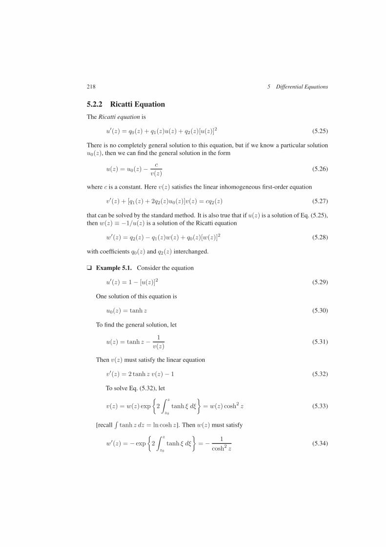
218 5 Differential Equations
5.2.2 Ricatti Equation
The Ricatti equation is
u′(z) = q0(z) + q1(z)u(z) + q2(z)[u(z)]2 (5.25)
There is no completely general solution to this equation, but if we know a particular solutionu0(z), then we can find the general solution in the form
u(z) = u0(z) −c
v(z)(5.26)
where c is a constant. Here v(z) satisfies the linear inhomogeneous first-order equation
v′(z) + [q1(z) + 2q2(z)u0(z)]v(z) = cq2(z) (5.27)
that can be solved by the standard method. It is also true that if u(z) is a solution of Eq. (5.25),then w(z) ≡ −1/u(z) is a solution of the Ricatti equation
w′(z) = q2(z) − q1(z)w(z) + q0(z)[w(z)]2 (5.28)
with coefficients q0(z) and q2(z) interchanged.
Example 5.1. Consider the equation
u′(z) = 1 − [u(z)]2 (5.29)
One solution of this equation is
u0(z) = tanh z (5.30)
To find the general solution, let
u(z) = tanh z − 1v(z)
(5.31)
Then v(z) must satisfy the linear equation
v′(z) = 2 tanh z v(z) − 1 (5.32)
To solve Eq. (5.32), let
v(z) = w(z) exp
2∫ z
z0
tanh ξ dξ
= w(z) cosh2 z (5.33)
[recall∫
tanh z dz = ln cosh z]. Then w(z) must satisfy
w′(z) = − exp
2∫ z
z0
tanh ξ dξ
= − 1cosh2 z
(5.34)
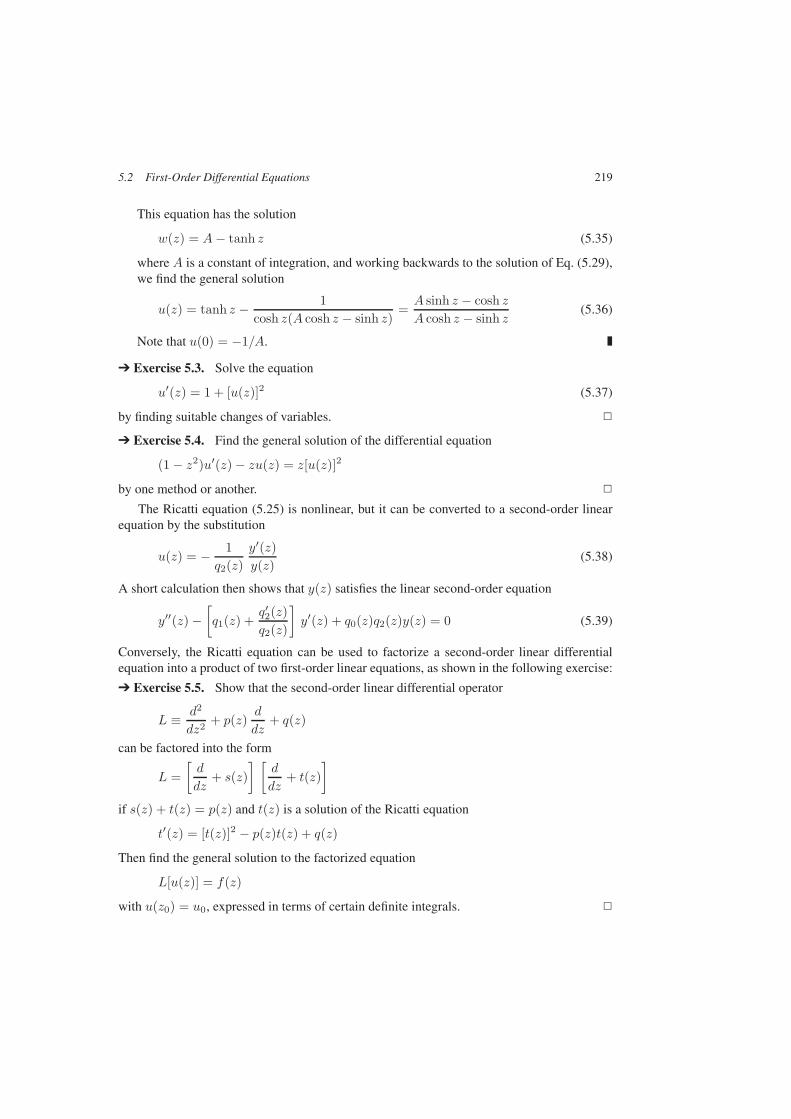
5.2 First-Order Differential Equations 219
This equation has the solution
w(z) = A− tanh z (5.35)
where A is a constant of integration, and working backwards to the solution of Eq. (5.29),we find the general solution
u(z) = tanh z − 1cosh z(A cosh z − sinh z)
=A sinh z − cosh zA cosh z − sinh z
(5.36)
Note that u(0) = −1/A.
Exercise 5.3. Solve the equation
u′(z) = 1 + [u(z)]2 (5.37)
by finding suitable changes of variables.
Exercise 5.4. Find the general solution of the differential equation
(1 − z2)u′(z) − zu(z) = z[u(z)]2
by one method or another.
The Ricatti equation (5.25) is nonlinear, but it can be converted to a second-order linearequation by the substitution
u(z) = − 1q2(z)
y′(z)y(z)
(5.38)
A short calculation then shows that y(z) satisfies the linear second-order equation
y′′(z) −[q1(z) +
q′2(z)q2(z)
]y′(z) + q0(z)q2(z)y(z) = 0 (5.39)
Conversely, the Ricatti equation can be used to factorize a second-order linear differentialequation into a product of two first-order linear equations, as shown in the following exercise:
Exercise 5.5. Show that the second-order linear differential operator
L ≡ d2
dz2+ p(z)
d
dz+ q(z)
can be factored into the form
L =[d
dz+ s(z)
] [d
dz+ t(z)
]
if s(z) + t(z) = p(z) and t(z) is a solution of the Ricatti equation
t′(z) = [t(z)]2 − p(z)t(z) + q(z)
Then find the general solution to the factorized equation
L[u(z)] = f(z)
with u(z0) = u0, expressed in terms of certain definite integrals.
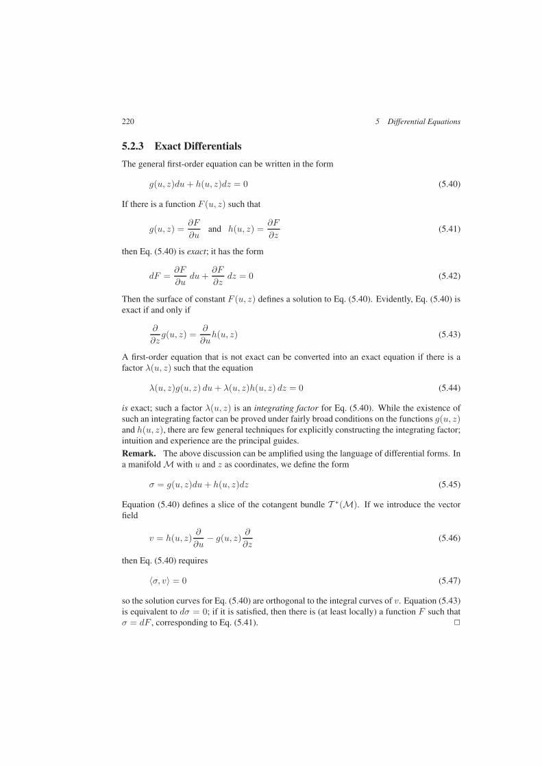
220 5 Differential Equations
5.2.3 Exact Differentials
The general first-order equation can be written in the form
g(u, z)du+ h(u, z)dz = 0 (5.40)
If there is a function F (u, z) such that
g(u, z) =∂F
∂uand h(u, z) =
∂F
∂z(5.41)
then Eq. (5.40) is exact; it has the form
dF =∂F
∂udu+
∂F
∂zdz = 0 (5.42)
Then the surface of constant F (u, z) defines a solution to Eq. (5.40). Evidently, Eq. (5.40) isexact if and only if
∂
∂zg(u, z) =
∂
∂uh(u, z) (5.43)
A first-order equation that is not exact can be converted into an exact equation if there is afactor λ(u, z) such that the equation
λ(u, z)g(u, z) du+ λ(u, z)h(u, z) dz = 0 (5.44)
is exact; such a factor λ(u, z) is an integrating factor for Eq. (5.40). While the existence ofsuch an integrating factor can be proved under fairly broad conditions on the functions g(u, z)and h(u, z), there are few general techniques for explicitly constructing the integrating factor;intuition and experience are the principal guides.
Remark. The above discussion can be amplified using the language of differential forms. Ina manifold M with u and z as coordinates, we define the form
σ = g(u, z)du+ h(u, z)dz (5.45)
Equation (5.40) defines a slice of the cotangent bundle T ∗(M). If we introduce the vectorfield
v = h(u, z)∂
∂u− g(u, z)
∂
∂z(5.46)
then Eq. (5.40) requires
〈σ, v〉 = 0 (5.47)
so the solution curves for Eq. (5.40) are orthogonal to the integral curves of v. Equation (5.43)is equivalent to dσ = 0; if it is satisfied, then there is (at least locally) a function F such thatσ = dF , corresponding to Eq. (5.41).
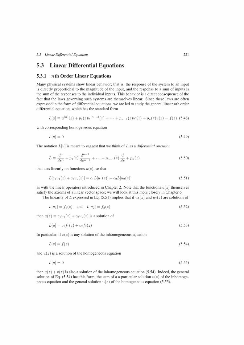
5.3 Linear Differential Equations 221
5.3 Linear Differential Equations
5.3.1 nth Order Linear Equations
Many physical systems show linear behavior; that is, the response of the system to an inputis directly proportional to the magnitude of the input, and the response to a sum of inputs isthe sum of the responses to the individual inputs. This behavior is a direct consequence of thefact that the laws governing such systems are themselves linear. Since these laws are oftenexpressed in the form of differential equations, we are led to study the general linear nth orderdifferential equation, which has the standard form
L[u] ≡ u(n)(z) + p1(z)u(n−1)(z) + · · · + pn−1(z)u′(z) + pn(z)u(z) = f(z) (5.48)
with corresponding homogeneous equation
L[u] = 0 (5.49)
The notation L[u] is meant to suggest that we think of L as a differential operator
L ≡ dn
dzn+ p1(z)
dn−1
dzn−1+ · · · + pn−1(z)
d
dz+ pn(z) (5.50)
that acts linearly on functions u(z), so that
L[c1u1(z) + c2u2(z)] = c1L[u1(z)] + c2L[u2(z)] (5.51)
as with the linear operators introduced in Chapter 2. Note that the functions u(z) themselvessatisfy the axioms of a linear vector space; we will look at this more closely in Chapter 6.
The linearity of L expressed in Eq. (5.51) implies that if u1(z) and u2(z) are solutions of
L[u1] = f1(z) and L[u2] = f2(z) (5.52)
then u(z) ≡ c1u1(z) + c2u2(z) is a solution of
L[u] = c1f1(z) + c2f2(z) (5.53)
In particular, if v(z) is any solution of the inhomogeneous equation
L[v] = f(z) (5.54)
and u(z) is a solution of the homogeneous equation
L[u] = 0 (5.55)
then u(z) + v(z) is also a solution of the inhomogeneous equation (5.54). Indeed, the generalsolution of Eq. (5.54) has this form, the sum of a a particular solution v(z) of the inhomoge-neous equation and the general solution u(z) of the homogeneous equation (5.55).

222 5 Differential Equations
5.3.2 Power Series Solutions
If the variable z in Eq. (5.50) is meaningful as a complex variable, and if the coefficientsp1(z), . . . , pn(z) are analytic functions of z, then we can make extensive use of the theoryof analytic functions developed in Chapter 4. In this case, a point z0 is a regular point ofEq. (5.49) if p1(z), . . . , pn(z) are all analytic at z0, otherwise a singular point. Solutions to thehomogeneous equation (5.49) can be constructed as Taylor series about any regular point z0,with coefficients depending on the n arbitrary constants u(z0), u′(z0), . . . , u(n−1)(z0), andthe Taylor series has a positive radius of convergence. It is plausible (and true) that the solutionwill be analytic in any region where p1(z), . . . , pn(z) are all analytic.
Example 5.2. Consider the second-order equation
u′′(z) + zu(z) = 0 (5.56)
whose coefficients are analytic everywhere in the finite z-plane. If we try to construct aseries solution
u(z) = 1 +∞∑
n=1
anzn (5.57)
then we find that a1 is arbitrary, since the first derivative u′(0) is arbitrary, a2 = 0, and thehigher coefficients are determined from the recursion relation
an+3 = − an(n+ 2)(n+ 3)
(5.58)
Thus the solution to Eq. (5.56) satisfying
u(0) = 1 and u′(0) = a (5.59)
has the expansion
u(z) = 1 +∞∑
n=1
(−1)n(3n− 2)(3n− 5) . . . 1
(3n)!z3n
(5.60)
+ az
[1 +
∞∑
n=1
(−1)n(3n− 1)(3n− 4) . . . 2
(3n+ 1)!z3n
]
Note that the series in Eq. (5.60) each have infinite radius of convergence. Hence thegeneral solution to Eq. (5.56) is an entire function, which is not surprising since the coef-ficients in the equation are entire functions.
Exercise 5.6. Find the basic solutions of the differential equation
u′′(z) + z2u(z) = 0
at z = 0. Express these solutions as power series in z. What are the singularities of thesesolutions?

5.3 Linear Differential Equations 223
5.3.3 Linear Independence; General Solution
To further explore the consequences of the linearity of equations (5.48) and (5.49), as ex-pressed in Eqs. (5.51)–(5.53), we first introduce the concept of linear independence for func-tions, which is the same as the standard vector space definition in Chapter 2.
Definition 5.1. The functions u1(z), u2(z), . . . , un(z) are linearly dependent if there existconstants c1, c2, . . . , cn (not all zero) such that
c1u1(z) + c2u2(z) + · · · + cnun(z) = 0 (5.61)
Otherwise the functions are linearly independent. The left-hand side of Eq. (5.61) is a linearcombination of the functions u1(z), u2(z), . . . , un(z) regarded as vectors.
One test for linear independence of the functions u1(z), u2(z), . . . , un(z) is to considerthe Wronskian determinant defined by
W (u1, u2, . . . , un; z) =
∣∣∣∣∣∣∣∣∣∣∣∣∣∣∣
u1(z) u2(z) . . . un(z)
u′1(z) u′2(z) . . . u′n(z)
......
...
u(n−1)1 (z) u
(n−1)2 (z) . . . u
(n−1)n (z)
∣∣∣∣∣∣∣∣∣∣∣∣∣∣∣
(5.62)
If u1(z), u2(z), . . . , un(z) are linearly dependent, then W (u1, u2, . . . , un; z) vanishes every-where. If the Wronskian does not vanish everywhere, then u1(z), u2(z), . . . , un(z) are lin-early independent.
Remark. Note, however, that the vanishing of the Wronskian at a single point z0 does notby itself imply that the functions are linearly dependent, for W (u; z0) = 0 simply means thatthere are constants a1, a2, . . . , an, not all zero, such that
a1u(k)1 (z0) + a2u
(k)2 (z0) + · · · + anu
(k)n (z0) = 0 (5.63)
(k = 0, 1, . . . , n− 1). Then the linear combination
h(z) ≡ a1u1(z) + a2u2(z) + · · · + anun(z) (5.64)
is a function that vanishes together with its first n − 1 derivatives at z0. This alone does notguarantee that h(z) = 0 everywhere, but if h(z) also satisfies an nth order linear differentialequation such as Eq. (5.48), then the nth and higher derivatives of h(z) also vanish, and h(z)does vanish everywhere, and u1(z), u2(z), . . . , un(z) are linearly dependent.
If the functions u1(z), u2(z), . . . , un(z) are solutions to the linear equations (5.48)or (5.49) of order n, then the Wronskian satisfies the linear equation
d
dzW (u1, u2, . . . , un; z) + p1(z)W (u1, u2, . . . , un; z) = 0 (5.65)
Exercise 5.7. Derive Eq. (5.65) from the definition (5.62).
224 5 Differential Equations
Equation (5.65) has the standard solution
W (u1, u2, . . . , un; z) = W (u1, u2, . . . , un; z0) exp−∫ z
z0
p1(z) dz
(5.66)
Hence if the Wronskian of a set of n solutions to Eqs. (5.48) vanishes at a single point, itvanishes everywhere, and the solutions are linearly dependent. Conversely, if the Wronskianis nonzero at a point where p1(z) is analytic, then it can vanish only at a singularity of p1(z)or at ∞. The solution u(z) of Eq. (5.49) that satisfies
u(z0) = ξ1 u′(z0) = ξ2 , . . . , u(n−1)(z0) = ξn (5.67)
at a regular point z0 can be uniquely expressed as
u(z) =n∑
k=1
ckuk(z) (5.68)
with coefficients c1, c2, . . . , cn are determined from the equations
c1u1(z0) + · · · + cnun(z0) = ξ1
c1u′1(z0) + · · · + cnu
′n(z0) = ξ2
... (5.69)
c1u(n−1)1 (z0) + · · · + cnu
(n−1)n (z0) = ξn
These equations have a unique solution since the determinant of the coefficients on the left-hand side is just the Wronskian W (u1, u2, . . . , un; z0), which is nonzero since the solutionsu1(z), u2(z), . . . , un(z) are linearly independent.
Thus the general solution of Eq. (5.49) defines an n-dimensional linear vector space. Theinitial conditions (5.67) choose a particular vector from this solution space. We can introducea fundamental set of solutions u1(z; z0), . . . , un(z; z0) at a regular point z0 of Eq. (5.49) bythe conditions
u(m−1)k (z0; z0) = δkm (5.70)
(k,m = 1, . . . , n). These n solutions are linearly independent, since the Wronskian
W (u1, u2, . . . , un; z0) = 1 (5.71)
The general solution of Eq. (5.49) can be expressed as a linear combination of the fundamentalsolutions according to
u(z) =n∑
k=1
u(k−1)(z0)uk(z; z0) (5.72)
so that the functions defined by Eq. (5.70) form a basis of the n-dimensional solution space.

5.3 Linear Differential Equations 225
5.3.4 Linear Equation with Constant Coefficients
Of special importance is the linear nth order equation
L[u] ≡ u(n)(z) + α1u(n−1)(z) + · · · + αnu(z) = 0 (5.73)
with constant coefficients α1, . . . , αn. This equation can be solved algebraically, since
L[eλz] = p(λ)eλz (5.74)
where p(λ) is the nth degree polynomial
p(λ) = λn + α1λn−1 + · · · + αn (5.75)
Hence u(z) = eλz is a solution of Eq. (5.73) if and only if λ is a root of p(λ).If the roots λ1, . . . , λn of p(λ) are distinct, then the general solution of Eq. (5.73) is
u(z) = c1eλ1z + · · · + cne
λnz (5.76)
with coefficients c1, . . . , cn determined by the values of u(z) and its first n − 1 derivativesat some point z0. If the roots are not distinct, however, then further linearly independentsolutions must be found. These appear immediately if we note that
L[zmeλz] =∂k
∂λk[p(λ)eλz
]=
m∑
k=0
(m
k
)p(k)(λ)zm−keλz (5.77)
Hence u(z) = zmeλz is a solution of Eq. (5.73) if and only if
p(λ) = 0 p′(λ) = 0 , . . . , p(m)(λ) = 0 (5.78)
that is, if λ is a root of p(λ) of multiplicity ≥ m+ 1. If this is the case, then u(z) = ρ(z) eλz
is also a solution for any polynomial ρ(z) of degree ≤ m+ 1.The final result is that if the polynomial p(λ) has the distinct roots λ1, . . . , λq with multi-
plicities m1, . . . ,mq, respectively, then the general solution of Eq. (5.73) is
u(z) = ρ1(z)eλ1z + · · · + ρq(z)eλnz (5.79)
where ρ1(z), . . . , ρq(z) are arbitrary polynomials of degrees d1 ≤ m1 − 1, . . . , dq ≤ mq − 1,respectively.
A more general system of linear first-order equations with constant coefficients is
u′k(z) =∑
Aku(z) (5.80)
(k = 1, . . . , n), with A = (Ak) a matrix of constants. As explained in Section 2.5, thissystem can also be reduced to a set of algebraic equations. Comparison of this system toEq. (5.73) is left to Problem 6.
226 5 Differential Equations
5.4 Linear Second-Order Equations
5.4.1 Classification of Singular Points
Linear second-order differential equations often appear in physics, both in systems of cou-pled oscillators and as a result of separation of variables in partial differential equations (seeChapter 8) such as Laplace’s equation or the wave equation. Thus we go into great detail inexamining these equations and some of their solutions. The linear homogeneous second-orderdifferential equation has the standard form
L[u] ≡ u′′(z) + p(z)u′(z) + q(z)u(z) = 0 (5.81)
also known as the Sturm–Liouville equation. Just as for the general linear equation, z0 is aregular (or ordinary) point of L[u] = 0 if p(z) and q(z) are analytic at z0, otherwise a singularpoint. The singular point z0 is a regular singular point if (z − z0) p(z) and (z − z0)2q(z) areanalytic at z0, otherwise an irregular singular point. As we shall see, the solutions neara regular singular point z0 behave no worse than a power of (z − z0), perhaps multiplied byln(z−z0). At an irregular singular point, the general solution will have an essential singularity.
Remark. To characterize the nature of the point at ∞, let ξ ≡ 1/z. Then Eq. (5.81) becomes
ξ4d2
dξ2
[u
(1ξ
)]+
2ξ3 − ξ2p
(1ξ
)d
dξ
[u
(1ξ
)]+ q
(1ξ
)u
(1ξ
)= 0 (5.82)
Thus ∞ is a regular point if [z2p(z) − 2z] and z4q(z) are analytic at ∞, a regular singularpoint if z p(z) and z2q(z) are analytic at ∞, and an irregular singular point otherwise.
The standard method for solving linear equations with analytic functions as coefficientsis to look for power series solutions.1 If z0 is a regular point of Eq. (5.81), then the generalsolution is analytic at z0. It can be expanded in a power series about z0, and the series willconverge inside the largest circle about z0 containing no singular points of the equation. Thesolution and its first derivative at z0 must be determined from initial conditions. Singularpoints require more discussion, which we now provide.
5.4.2 Exponents at a Regular Singular Point
If z0 is a regular singular point, then let
P (z) ≡ (z − z0)p(z) =∞∑
n=0
pn(z − z0)n (5.83)
Q(z) ≡ (z − z0)2q(z) =∞∑
n=0
qn(z − z0)n (5.84)
Because z0 is a regular singular point, both P (z) andQ(z) are analytic at z0; hence both serieshave positive radius of convergence.
1The following analysis is often called the method of Frobenius.
5.4 Linear Second-Order Equations 227
Now try a solution of the form
u(z) = (z − z0)α[
1 +∞∑
n=1
an(z − z0)n]
(5.85)
Equations (5.83)–(5.85) can be inserted into Eq. (5.81) and coefficients of each power of(z − z0) set equal. For the lowest power, this gives the indicial equation
α (α− 1) + αp0 + q0 = 0 (5.86)
that has roots
α = 12
[1 − p0 ±
√(1 − p0)2 − 4q0
]≡ α± (5.87)
The roots α± are the exponents of the singularity at z0; note also that
p0 = 1 − α+ − α− q0 = α+α− (5.88)
The coefficients in the power series can then be determined from the equations
[α(α+ 1) + (α+ 1)p0 + q0] a1 + αp1 + q1 = 0... (5.89)
[(α+ n)(α+ n− 1) + (α+ n) p0 + q0] an + [(α+ n− 1) p1 + q1] an−1
+ · · · + [(α+ 1) pn−1 + qn−1] a1 + αpn + qn = 0
If α+ − α− = 0, 1, 2, . . ., we have two linearly independent solutions to Eq. (5.81),
u±(z) = (z − z0)α±
[1 +
∞∑
n=1
a(±)n (z − z0)n
](5.90)
The general solution is an arbitrary linear combination of u+(z) and u−(z).If α+ = α−, there is only one power series solution. If
α+ = α− + n (5.91)
(n = 1, 2, . . .), then the solution u−(z) is not uniquely determined, since the coefficient of
a(−)n in Eq. (5.89) is
(α− + n)(α− + n− 1) + (α− + n)(1 − α+ − α−) + α+α− = 0 (5.92)
In either case, one solution of Eq. (5.81) is given by
u+(z) = (z − z0)α+ f+(z) (5.93)
with f+(z) analytic at z0 and f+(z0) = 1 by convention.

228 5 Differential Equations
To find a second solution, let
u(z) ≡ w(z)u+(z) (5.94)
This substitution is generally useful when one solution to a differential equation is known, butit is especially needed here since the power series method fails. w(z) must satisfy the equation
u+(z)w′′(z) +[2u′+(z) + p(z)u+(z)
]w′(z) = 0 (5.95)
This can be solved in the usual way to give
w′(z) =C
[u+(z)]2exp
−∫ z
p(ξ) dξ
(5.96)
with C a constant. Since
p(z) =1 − α+ − α−
z − z0+ r(z) =
n+ 1 − 2α+
z − z0+ r(z) (5.97)
with r(z) analytic at z0, we can use Eq. (5.93) to write
w′(z) =K
(z − z0)n+1
1[f+(z)]2
exp−∫ z
z0
r(ξ) dξ
≡ Kg(z)
(z − z0)n+1(5.98)
where K is another constant, and
g(z) =1
[f+(z)]2exp
−∫ z
z0
r(ξ) dξ
(5.99)
is analytic at z0 with g(z0) = 1. The function w(z) is then given by
w(z) = K1 +K
∫ z g(ξ)(ξ − z0)n+1
dξ (5.100)
where K1 is yet another constant, which corresponds to a multiple of the first solution u+(z)in the solution u(z) and can be ignored here. Expanding g(ξ) about z0 and integrating term-by-term leads to
w(z) =K
(z − z0)n
∞∑
m=0m =n
g(n)(z0)n!
ln(z − z0) +g(m)(z0)m− n
(z − z0)m
m!
(5.101)
Then a second linearly independent solution to Eq. (5.81) is given by
u−(z) ≡ (z − z0)α−f−(z) +g(n)(z0)n!
u+(z) ln(z − z0) (5.102)
where
f−(z) = f+(z)∞∑
m=0m =n
g(m)(z0)m− n
(z − z0)m
m!(5.103)
is analytic at z0. Thus when α+−α− = n = 0, 1, 2, . . ., the general solution has a logarithmicbranch point at z0 unless g(n)(z0) = 0. Hence, an integer exponent difference at a regularsingular point signals the possible presence of a logarithmic singularity in addition to theusual power law behavior.

5.4 Linear Second-Order Equations 229
5.4.3 One Regular Singular Point
Linear second-order equations with one, two or three singular points have been thoroughlystudied. The second-order equation whose only singular point is a regular singular point at z0is uniquely given by
u′′(z) +2
z − z0u′(z) = 0 (5.104)
The exponents of the singularity are α = 0,−1 and the general solution of the equation is
u(z) = a+b
z − z0(5.105)
with a and b arbitrary constants.
Remark. Note that if α = −1, the equation
u′′(z) +1 − α
z − z0u′(z) = 0 (5.106)
has a regular singular point at ∞ in addition to the regular singular point at z0. However, thegeneral solution
u(z) = a+b
(z − z0)α(5.107)
is analytic at ∞ if α = 2, 3, . . . . Thus in exceptional cases, a regular singular point of anequation may not be reflected as a singularity of the general solution.
Exercise 5.8. Find the general solution to Eq. (5.106) if α = 0.
5.4.4 Two Regular Singular Points
The general equation with two regular singular points at z1 and z2 is given by
u′′(z) +[1 − α− β
z − z1+
1 + α+ β
z − z2
]u′(z)
[αβ(z1 − z2)2
(z − z1)2(z − z2)2
]u(z) = 0 (5.108)
with exponents (α, β) at z1 and (−α,−β) at z2. The exponents at z1 and z2 must be equaland opposite in order to have ∞ as a regular point. A standard form of the equation, with thesingular points at 0 and ∞, is reached by the transformation
ξ =z − z1z − z2
(5.109)
that maps z1 to 0, z2 to ∞, and transforms Eq. (5.108) into
u′′(ξ) +(
1 − α− β
ξ
)u′(ξ) +
αβ
ξ2u(ξ) = 0 (5.110)
230 5 Differential Equations
The general solution of this equation is
u(ξ) = aξα + bξβ (5.111)
if α = β; if α = β, the general solution is
u(ξ) = aξα(1 + c ln ξ) (5.112)
The two regular singular points in Eq. (5.108) can be merged into one irregular singularpoint. Let
z2 = z1 + η α =k
η= −β (5.113)
and take the limit η → 0 (this is a confluence of the singular points). Then Eq. (5.108)becomes
u′′(z) +2
z − z1u′(z) − k2
(z − z1)4u(z) = 0 (5.114)
which has an irregular singular point at z1 and no other singular points.The singular point can be moved to ∞ by the transformation
ξ =1
z − z1(5.115)
whence the equation becomes
u′′(ξ) − k2 u(ξ) = 0 (5.116)
with general solution
u(ξ) = c+ ekξ + c− e−kξ (5.117)
where c± are arbitrary constants.
Remark. The general solution to the original equation is evidently given by
u(z) = c+ ek/(z−z1) + c− e−k/(z−z1) (5.118)
but this is less obvious than the solution to the transformed equation.
Exercise 5.9. Derive Eq. (5.116) from Eq. (5.114).
The equation with three regular singular points can be transformed to the hypergeometricequation; a confluence of two of the singular points leads to the confluent hypergeometricequation. The general equations are studied in Appendices A and B. In the next two sections,we look at Legendre’s equation as an example of the hypergeometric equation, and Bessel’sequation as an example of the confluent hypergeometric equation.
5.5 Legendre’s Equation 231
5.5 Legendre’s Equation
5.5.1 Legendre Polynomials
An important differential equation in physics is Legendre’s equation
(z2 − 1)u′′(z) + 2zu′(z) − λ(λ+ 1)u(z) = 0 (5.119)
which has the standard form of Eq. (5.81), with
p(z) =2z
z2 − 1and q(z) = − λ(λ+ 1)
z2 − 1(5.120)
where λ is a parameter that can be complex in general, although we will find that it is requiredto be an integer in many physical contexts. The singular points of this equation are at z = ±1and z = ∞; each of the singular points is regular. The indicial equations at z = ±1 havedouble roots at α = 0, so we can expect to find solutions u±(z) that are analytic at z = ±1,and second solutions v±(z) with logarithmic singularities at z = ±1.
Exercise 5.10. Find the exponents of the singular point of Eq. (5.119) at ∞.
We look for solutions as power series around z = 0. Since z = 0 is a regular point ofEq. (5.119). we expect to find a general solution of the form
u(z) =∞∑
k=0
akzk (5.121)
with a0, a1 arbitrary and the remaining coefficients determined by the differential equation.Inserting this series into Eq. (5.119) and setting the coefficient of each term in the power seriesto zero, we have the recursion relation
(k + 1)(k + 2)ak+2 = [k(k + 1) − λ(λ+ 1)]ak (5.122)
If we express this recursion relation as a ratio
ak+2
ak=k(k + 1) − λ(λ+ 1)
(k + 1)(k + 2)=
(k − λ)(k + λ+ 1)(k + 1)(k + 2)
(5.123)
then we can see that the ratio |ak+2/ak| tends to 1 for large k. This means that the radius ofconvergence of the power series is equal to 1 in general, as expected from a solution that isanalytic except for possible singularities at z = ±1,∞.
However, these singularities will not be present if the infinite series actually terminates,which will be the case if λ is an integer.2 If λ = n ≥ 0, the recursion relation gives an+2 = 0,and there is a polynomial solution Pn(z) of degree n. If we choose the initial conditionPn(1) = 1, then Pn(z) is the Legendre polynomial of degree n. Note also that only even orodd powers of z will appear in Pn(z), depending on whether n is even or odd; thus we have
Pn(−z) = (−1)nPn(z) (5.124)
2Note that if λ = n, we can take n ≥ 0, since λ and −λ − 1 give rise to the same set of solutions to Eq. (5.119).
232 5 Differential Equations
The first few Legendre polynomials can be found explicitly; we have
P0(z) = 1 P1(z) = 1 P2(z) = 12 (3z2 − 1) (5.125)
Exercise 5.11. Find explicit forms for P3(z) and P4(z).
Another way to write Legendre’s equation is
L[u] =d
dz(z2 − 1)
d
dz
u(z) = λ(λ+ 1)u(z) (5.126)
This looks like an eigenvalue equation, and in Chapter 7, we will see that it is when we look ateigenvalue problems for linear differential operators from a vector space viewpoint. Here wederive some properties of the Pn(z) that follow from a representation of the solution knownas Rodrigues’ formula,
Pn(z) = Cndn
dzn(z2 − 1)n (5.127)
First we note that Pn(z) defined by Eq. (5.127) is a polynomial of degree n. Then let
un(z) =(z2 − 1
)n(5.128)
and note that
(z2 − 1)u′n(z) = 2nzun(z) (5.129)
If we differentiate this equation n+ 1 times, we have
(z2 − 1)u(n+2)n (z) + 2(n+ 1)zu(n+1)
n (z) + n(n+ 1)u(n)n (z) =
(5.130)
= 2nzu(n+1)n (z) + 2n(n+ 1)u(n)
n (z)
which leads to Legendre’s equation (5.119), since Eq. (5.130) is equivalent to
d
dz
[(z2 − 1)u(n+1)
n (z)]
= (z2−1)u(n+2)n (z)+2zu(n+1)
n (z) = n(n+1)u(n)n (z) (5.131)
which shows that u(n)n (z) satisfies Legendre’s equation.
Exercise 5.12. The constant Cn in Eq. (5.127) is determined by the condition Pn(1) = 1.Note that
(z2 − 1)n = (z − 1)n(z + 1)n
and evaluate the derivative
dn
dzn(z2 − 1)n
for z = 1. Then find the constant Cn.
5.5 Legendre’s Equation 233
Many other useful properties of Legendre polynomials can be derived from Rodrigues’formula. For example, Cauchy’s theorem allows us to write
Pn(z) =1
2πi
∮
C
Pn(ξ)ξ − z
dξ (5.132)
where C is any closed contour encircling the point t once counterclockwise. Then insertingthe Rodrigues formula and integrating by parts n times gives Schläfli’s integral representation
Pn(z) =1
2n+1πi
∮
C
(ξ2 − 1)n
(ξ − z)n+1dξ (5.133)
for the Legendre polynomials.
Exercise 5.13. In the Schläfli representation (5.133) for the Pn(z), suppose that z is realwith −1 ≤ z ≤ 1, and let the contour C be a circle of radius
√1 − z2 about z. Show that
Eq. (5.133) then leads to
Pn(z) =12π
∫ 2π
0
(z + i
√1 − z2 sin θ
)ndθ (5.134)
Equation (5.134) is Laplace’s integral formula for the Legendre polynomials.
Consider next the series
S(t, z) ≡∞∑
n=0
tnPn(z) (5.135)
If we use the Schläfli integral for the Pn(z) and sum the geometric series, we obtain
∞∑
n=0
tnPn(z) =1
2πi
∮
C
∞∑
n=0
(t
2
)n (ξ2 − 1)n
(ξ − z)n+1dξ
(5.136)
=1πi
∮
C
12ξ − 2z + t(1 − ξ2)
dξ
The contourC must be chosen so that the geometric series inside the integral is absolutely anduniformly convergent on C, and such that only one of the two poles of the integrand of thelast integral inside the contour. This can be done for −1 ≤ z ≤ 1 and t in a region inside theunit circle but off the real axis (the reader is invited to work out the details). The contour forthe second integral can then be deformed in any way so long as that one pole of the integrandremains inside the contour. Evaluating the residue at the pole then gives the result
S(t, z) =∞∑
n=0
tnPn(z) =1√
1 − 2zt+ t2(5.137)
The function S(z, t) is a generating function for the Legendre polynomials. Note that if−1 ≤ t ≤ 1, the series converges for |z| < 1, but there is a larger region of convergence in

234 5 Differential Equations
the complex z-plane (see Problem 8). The series (5.137) is used in Chapter 6 to derive orthog-onality relations for the Legendre polynomials. It also appears in the multipole expansion inelectrostatics (see Chapter 8) and elsewhere.
Exercise 5.14. Use either the Rodrigues formula (5.127) or the generating function (5.137)to derive the recursion formulas
(2n+ 1)zPn(z) = (n+ 1)Pn+1(z) + nPn(z)
and
(z2 − 1)P ′n(z) = nzPn(z) − nPn−1(z)
for the Legendre polynomials.
Legendre’s equation (5.119) has a polynomial solution if the parameter λ is an integer. Butin any event, it has a solution Pλ(z) that is analytic at z = 1, and scaled so that Pλ(1) = 1.Pλ(z) is the Legendre function of the first kind. In order to study this solution, we change thevariable to
t = 12 (1 − z)
Then the interval −1 ≤ z ≤ 1 is mapped to the interval 0 ≤ t ≤ 1, and z = 1 in mapped tot = 0. In terms of the variable t, Legendre’s equation is
t(t− 1)u′′(t) + (2t− 1)u′(t) − λ(λ+ 1)u(t) = 0 (5.138)
with regular singular points at t = 0, 1,∞. The solution that is analytic at t = 0 with u(0) = 1has the power series expansion
u(t) = 1 +∞∑
k=1
cktk (5.139)
The differential equation then requires
(k1)2ck+1 = [k(k + 1) − λ(λ+ 1)]ck = (k − λ)(k + λ+ 1)ck (5.140)
and thus
ck =Γ(k + λ+ 1)Γ(k − λ)
Γ(λ+ 1)Γ(−λ)· 1(k!)2
(5.141)
This is a hypergeometric series, as introduced in Appendix A, with parameters a = −λ,b = λ + 1 and c = 1, and thus the Legendre function of the first kind can be expressed as ahypergeometric function,
Pλ(z) = F (−λ, λ+ 1| 12 (1 − z)) (5.142)
Exercise 5.15. Show that the recursion formulas of Exercise 5.14 are also valid for theLegendre functions Pn(z) even if n (= λ) is not an integer.

5.5 Legendre’s Equation 235
5.5.2 Legendre Functions of the Second Kind
We have seen that if the parameter λ in Legendre’s equation is an integer, there is a polynomialsolution. Any independent solution must have a logarithmic singularity at z = ±1, since theindicial equations at z = ±1 have double roots at α = 0, as already noted. If we are interestedin solutions for |z| > 1, which are occasionally relevant, we can let ξ = 1/z. In terms of thevariable ξ, Legendre’s equation is
ξ2d
dξ
(ξ2 − 1)
d
dξ
u(ξ) + λ(λ+ 1)u(ξ) = 0 (5.143)
or, in a form from which the singularities can be seen directly,
ξ2(ξ2 − 1)u′′(ξ) + 2ξ3u′(ξ) + λ(λ+ 1)u(ξ) = 0 (5.144)
This equation has regular singular points at ξ = 0,±1. The exponents at ξ = 0 are given by
α = λ+ 1,−λ (5.145)
A solution with exponent λ + 1 at ξ = 0 is proportional to the Legendre function of secondkind, denoted by Qλ(z).
There are several ways to look at the properties of the Qλ(z). The most straightforward isto start from Eq. (5.144) and define
u(ξ) = ξλ+1v(ξ) (5.146)
Then v(ξ) satisfies the differential equation
ξ(ξ2 − 1)v′′(ξ) + 2[(λ+ 1)(ξ2 − 1) + ξ2]v′(ξ) + (λ+ 1)(λ+ 2)ξv(ξ) = 0 (5.147)
This equation has a solution v(ξ) with v(0) = 1 and a power series expansion
v(ξ) = 1 +∞∑
k=1
bkξk (5.148)
with coefficients bk determined by the differential equation. Inserting this power series intoEq. (5.147) and equating coefficients of ξk+1 gives the recursion formula
(k + 2)(2λ+ k + 3)bk+2 = (λ+ k + 1)(λ+ k + 2)bk (5.149)
after noting that
(λ+ 1)(λ+ 2) + 2k(λ+ 2) + k(k − 1) = (λ+ k + 1)(λ+ k + 2) (5.150)
From the recursion formula, we can see that b1 = 0, since b−1 = 0, Hence b2k+1 = 0(k = 1, 2, . . .), and the solution v(ξ) is a power series in ξ2.
Exercise 5.16. Use the recursion formula to express the coefficients b2k (k = 1, 2, . . .) interms of Γ-functions and thus find an explicit series representation of v(ξ). What is the radiusof convergence of this series?
236 5 Differential Equations
Exercise 5.17. Change the variable in Eq. (5.147) to η = ξ2 and determine the resultingdifferential equation for w(η) = v(ξ). Compare this with the hypergeometric equation inAppendix A and then express w(η) as a hypergeometric function.
Another approach is to start with the Schläfli representation (5.133), and consider a con-tour integral of the form
Iλ(z) = Kλ
∫
C
(1 − ξ2)λ
(z − ξ)λ+1dξ (5.151)
over a contour C in the complex ξ-plane. If λ is not an integer, then the integrand has branchpoints at ξ = ±1 that were not present for λ = n, but that is not a problem so long as we payattention to the branch cuts. The integral Iλ(z) can lead to a solution of Legendre’s equationwith an appropriate choice of contour C, since we have, after some algebra,
d
dz(z2 − 1)
d
dz− λ(λ+ 1)
(1 − ξ2)λ
(z − ξ)λ+1= − d
dξ
(1 − ξ2)λ+1
(z − ξ)λ+2
(5.152)
We can then choose the contour C to simply be the line −1 ≤ ξ ≤ 1; then we have
Qλ(z) =1
2λ+1
∫ 1
−1
(1 − ξ2)λ
(z − ξ)λ+1dξ (5.153)
Here the choice of branch cuts of the integrand is such that (1 − ξ2)λ is real and positive onthe interval −1 ≤ ξ ≤ 1, as is (z − ξ)λ+1 when z is real and z > 1. The choice of constantfactor is standard.
Exercise 5.18. Use Eq. (5.153) to show that
Qλ(z) →[Γ(λ+ 1)]2
2Γ(2λ+ 2)
(2z
)λ+1
for z → ∞.
When λ = n is a positive integer, then Eq. (5.153) can be used to show that
Qn(z) =12
∫ 1
−1
Pn(t)z − t
dt (5.154)
(see Problem 10). It then follows that
Qn(z) =12Pn(z) ln
z + 1z − 1
− qn−1(z) (5.155)
where qn−1(z) is a polynomial of degree n− 1 given by
qn(z) =12
∫ 1
−1
Pn(z) − Pn(t)z − t
dt (5.156)
[Show that qn(z) actually is a polynomial of degree n− 1]. We have the explicit forms
Q0(z) =12
lnz + 1z − 1
Q1(z) =z
2lnz + 1z − 1
− 1 (5.157)
Exercise 5.19. Find explicit forms for Q2(z) and Q3(z).
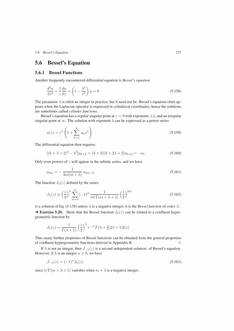
5.6 Bessel’s Equation 237
5.6 Bessel’s Equation
5.6.1 Bessel Functions
Another frequently encountered differential equation is Bessel’s equation
d2u
dz2+
1z
du
dz+(
1 − λ2
z2
)u = 0 (5.158)
The parameter λ is often an integer in practice, but it need not be. Bessel’s equation often ap-pears when the Laplacian operator is expressed in cylindrical coordinates; hence the solutionsare sometimes called cylinder functions.
Bessel’s equation has a regular singular point at z = 0 with exponents ±λ, and an irregularsingular point at ∞. The solution with exponent λ can be expressed as a power series
u(z) = zλ
(1 +
∞∑
k=1
akzk
)(5.159)
The differential equation then requires
[(k + λ+ 2)2 − λ2]ak+2 = (k + 2)(k + 2λ+ 2)ak+2 = −ak (5.160)
Only even powers of z will appear in the infinite series, and we have
a2m = − 14m(m+ λ)
a2m−2 (5.161)
The function Jλ(z) defined by the series
Jλ(z) ≡(z
2
)λ ∞∑
m=0
(−1)m1
m! Γ(m+ λ+ 1)
(z2
)2m
(5.162)
is a solution of Eq. (5.158) unless λ is a negative integer; it is the Bessel function of order λ.
Exercise 5.20. Show that the Bessel function Jλ(z) can be related to a confluent hyper-geometric function by
Jλ(z) =1
Γ(λ+ 1)
(z2
)λe−izF (λ+ 1
2 |2λ+ 1|2iz)
Thus many further properties of Bessel functions can be obtained from the general propertiesof confluent hypergeometric functions derived in Appendix B.
If λ is not an integer, then J−λ(z) is a second independent solution. of Bessel’s equation.However, if λ is an integer n ≥ 0, we have
J−n(z) = (−1)nJn(z) (5.163)
since 1/Γ(m+ λ+ 1) vanishes when m+ λ is a negative integer.

238 5 Differential Equations
A second independent solution of Bessel’s equation for all λ is defined by
Nλ(z) =Jλ(z) cosπλ− J−λ(z)
sin πλ(5.164)
Nλ(z) is a Bessel function of second kind, or Neumann function.
Exercise 5.21. Show that the Wronskian
W (Nλ, Jλ) =A
z
and evaluate the constant A. One way to do this is to consider the behavior for z → 0. Thisshows that Jλ(z) and Nλ(z) are independent solutions for all λ.
The Bessel functions satisfy the recursion relations
Jλ−1 + Jλ+1 =2λzJλ(z)
(5.165)
Jλ−1 − Jλ+1 = 2J ′λ(z)
that follow from direct manipulation of the power series (5.162). The Neumann functionssatisfy the same recursion relations, as do the Hankel functions to be introduced soon.
A generating function for the Bessel functions of integer order is
F (t, z) = ez(t−1t ) =
∞∑
n=−∞tnJn(z) (5.166)
From the generating function, it follows that Jn(z) can be expressed as a contour integral
Jn(z) =1
2πi
∮
C
exp[z
2
(t− 1
t
)]dt
tn+1(5.167)
where the contour C in the t-plane encircles t = 0 once in a counterclockwise direction. If wechoose the contour to be the unit circle in the t-plane and let t = exp(iθ), then this integralbecomes
Jn(z) =12π
∫ 2π
0
eiz sin θe−inθ dθ (5.168)
and then, since J0(z) is real,
Jn(z) =1π
∫ π
0
cos(nθ − z sin θ) dθ (5.169)
Exercise 5.22. Show that the coefficient of t0 in Eq. (5.166) is J0(z) by computingthis coefficient as a power series in z. Then show that the other terms satisfy the recursionrelations (5.165) by looking at the partial derivatives of F (t, z).
Remark. The choice of contour in Eq. (5.167) leads to an integral representation for theBessel function Jn(z). Other choices of contour can lead to different solutions and differentintegral representations. See Problem 13 for one example.
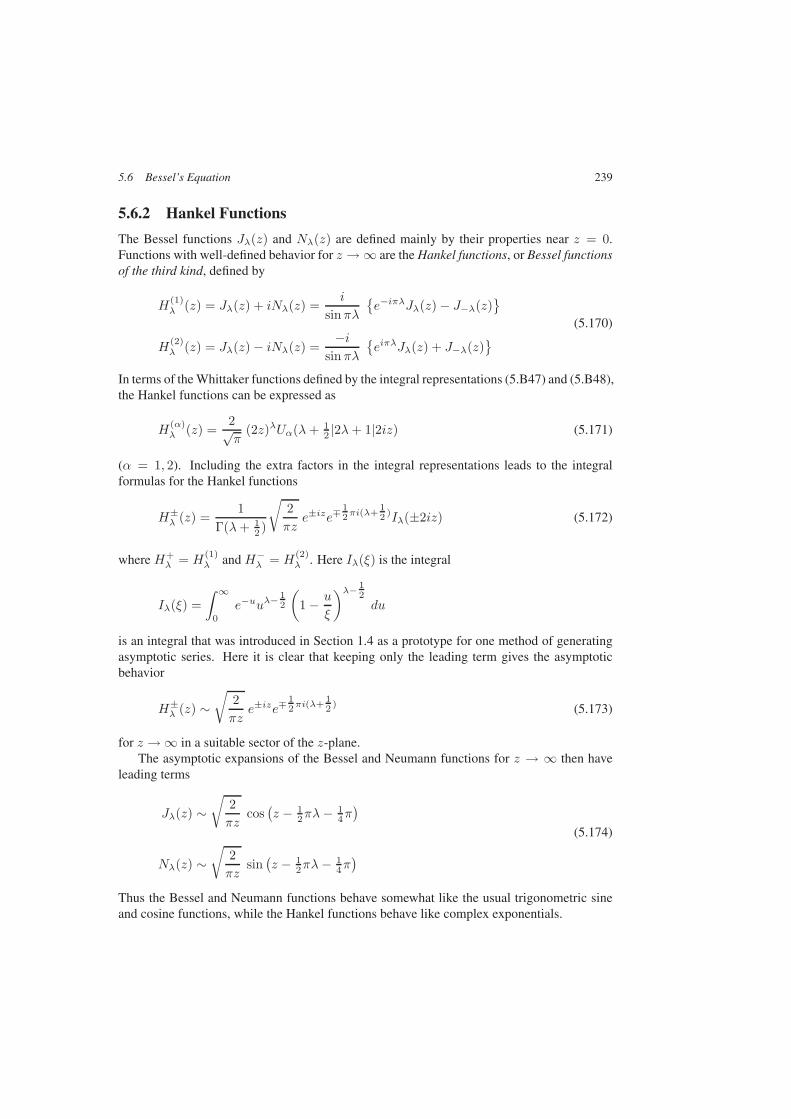
5.6 Bessel’s Equation 239
5.6.2 Hankel Functions
The Bessel functions Jλ(z) and Nλ(z) are defined mainly by their properties near z = 0.Functions with well-defined behavior for z → ∞ are the Hankel functions, or Bessel functionsof the third kind, defined by
H(1)λ (z) = Jλ(z) + iNλ(z) =
i
sinπλe−iπλJλ(z) − J−λ(z)
(5.170)
H(2)λ (z) = Jλ(z) − iNλ(z) =
−isinπλ
eiπλJλ(z) + J−λ(z)
In terms of the Whittaker functions defined by the integral representations (5.B47) and (5.B48),the Hankel functions can be expressed as
H(α)λ (z) =
2√π
(2z)λUα(λ+ 12 |2λ+ 1|2iz) (5.171)
(α = 1, 2). Including the extra factors in the integral representations leads to the integralformulas for the Hankel functions
H±λ (z) =
1Γ(λ+ 1
2 )
√2πz
e±ize∓12πi(λ+
12 )Iλ(±2iz) (5.172)
where H+λ = H
(1)λ and H−
λ = H(2)λ . Here Iλ(ξ) is the integral
Iλ(ξ) =∫ ∞
0
e−uuλ−12
(1 − u
ξ
)λ− 12du
is an integral that was introduced in Section 1.4 as a prototype for one method of generatingasymptotic series. Here it is clear that keeping only the leading term gives the asymptoticbehavior
H±λ (z) ∼
√2πz
e±ize∓12πi(λ+
12 ) (5.173)
for z → ∞ in a suitable sector of the z-plane.The asymptotic expansions of the Bessel and Neumann functions for z → ∞ then have
leading terms
Jλ(z) ∼√
2πz
cos(z − 1
2πλ− 14π)
(5.174)
Nλ(z) ∼√
2πz
sin(z − 1
2πλ− 14π)
Thus the Bessel and Neumann functions behave somewhat like the usual trigonometric sineand cosine functions, while the Hankel functions behave like complex exponentials.
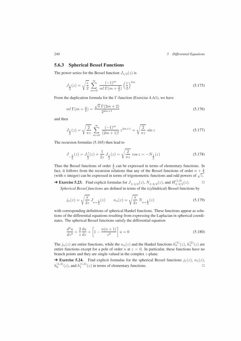
240 5 Differential Equations
5.6.3 Spherical Bessel Functions
The power series for the Bessel function J1/2(z) is
J12(z) =
√z
2
∞∑
m=0
(−1)m
m! Γ(m+ 32 )
(z2
)2m
(5.175)
From the duplication formula for the Γ-function (Exercise 4.A1), we have
m! Γ(m+ 32 ) =
√π Γ(2m+ 2)
22m+1(5.176)
and then
J12(z) =
√2πz
∞∑
m=0
(−1)m
(2m+ 1)!z2m+1 =
√2πz
sin z (5.177)
The recursion formulas (5.165) then lead to
J−12
(z) = J ′12
(z) +12z
J12
(z) =
√2πz
cos z = −N12
(z) (5.178)
Thus the Bessel functions of order 12 can be expressed in terms of elementary functions. In
fact, it follows from the recursion relations that any of the Bessel functions of order n + 12
(with n integer) can be expressed in terms of trigonometric functions and odd powers of√z.
Exercise 5.23. Find explicit formulas for J± 3/2(z), N± 3/2(z), and H(1,2)± 3/2(z).
Spherical Bessel functions are defined in terms of the (cylindrical) Bessel functions by
jn(z) =√
π
2zJn+
12(z) nn(z) =
√π
2zNn+
12(z) (5.179)
with corresponding definitions of spherical Hankel functions. These functions appear as solu-tions of the differential equations resulting from expressing the Laplacian in spherical coordi-nates. The spherical Bessel functions satisfy the differential equation
d2u
dz2+
2z
du
dz+[1 − n(n+ 1)
z2
]u = 0 (5.180)
The jn(z) are entire functions, while the nn(z) and the Hankel functions h(1)n (z), h(2)
n (z) areentire functions except for a pole of order n at z = 0. In particular, these functions have nobranch points and they are single-valued in the complex z-plane.
Exercise 5.24. Find explicit formulas for the spherical Bessel functions j1(z), n1(z),h
(1,2)0 (z), and h(1,2)
1 (z) in terms of elementary functions.
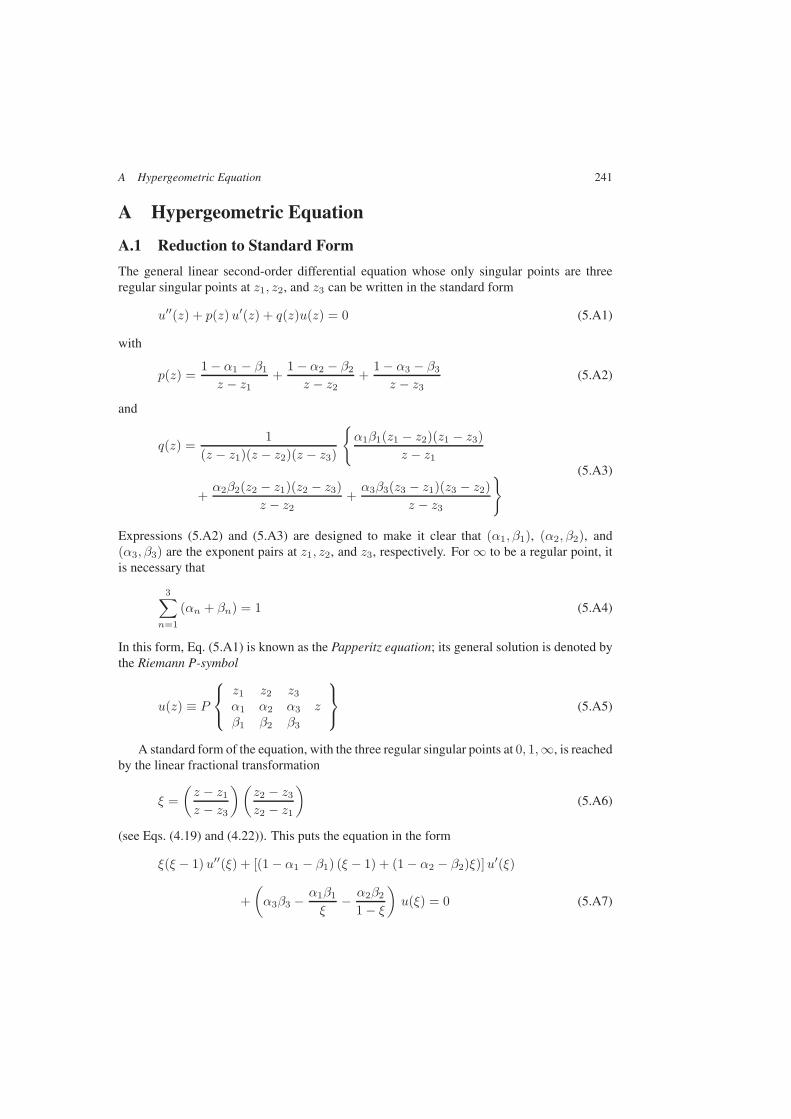
A Hypergeometric Equation 241
A Hypergeometric Equation
A.1 Reduction to Standard Form
The general linear second-order differential equation whose only singular points are threeregular singular points at z1, z2, and z3 can be written in the standard form
u′′(z) + p(z)u′(z) + q(z)u(z) = 0 (5.A1)
with
p(z) =1 − α1 − β1
z − z1+
1 − α2 − β2
z − z2+
1 − α3 − β3
z − z3(5.A2)
and
q(z) =1
(z − z1)(z − z2)(z − z3)
α1β1(z1 − z2)(z1 − z3)
z − z1(5.A3)
+α2β2(z2 − z1)(z2 − z3)
z − z2+α3β3(z3 − z1)(z3 − z2)
z − z3
Expressions (5.A2) and (5.A3) are designed to make it clear that (α1, β1), (α2, β2), and(α3, β3) are the exponent pairs at z1, z2, and z3, respectively. For ∞ to be a regular point, itis necessary that
3∑
n=1
(αn + βn) = 1 (5.A4)
In this form, Eq. (5.A1) is known as the Papperitz equation; its general solution is denoted bythe Riemann P-symbol
u(z) ≡ P
z1 z2 z3α1 α2 α3 zβ1 β2 β3
(5.A5)
A standard form of the equation, with the three regular singular points at 0, 1,∞, is reachedby the linear fractional transformation
ξ =(z − z1z − z3
)(z2 − z3z2 − z1
)(5.A6)
(see Eqs. (4.19) and (4.22)). This puts the equation in the form
ξ(ξ − 1)u′′(ξ) + [(1 − α1 − β1) (ξ − 1) + (1 − α2 − β2)ξ)]u′(ξ)
+(α3β3 −
α1β1
ξ− α2β2
1 − ξ
)u(ξ) = 0 (5.A7)
242 5 Differential Equations
The general solution of Eq. (5.A7) can be expressed as
u(ξ) = P
0 1 ∞α1 α2 α3 ξβ1 β2 β3
(5.A8)
In this form, (α1, β1), (α2, β2), and (α3, β3) are the exponents of the regular singularpoints at 0, 1,∞, respectively. Now two of these exponents can be made to vanish by asuitable factorization of the unknown function. If we let
u(ξ) = ξα1(ξ − 1)α2w(ξ) (5.A9)
then w(ξ) must satisfy
ξ(ξ − 1)w′′(ξ) + [(1 + α1 − β1)(ξ − 1) + (1 + α2 − β2)ξ)]w′(ξ)
+ (α1 + α2 + α3)(α1 + α2 + β3)w(ξ) = 0 (5.A10)
There are only three independent parameters in this equation, since two of the exponents havebeen forced to vanish by Eq. (5.A9), and there is still one relation imposed by Eq. (5.A4). Astandard choice of parameters is given by
a = α1 + α2 + α3 b = α1 + α2 + β3 c = 1 + α1 − β1 (5.A11)
Then Eq. (5.A4) requires
1 + α2 − β2 = a+ b− c+ 1 (5.A12)
and Eq. (5.A10) can be written as
ξ(ξ − 1)w′′(ξ) + [(a+ b+ 1)ξ − c]w′(ξ) + abw(ξ) = 0 (5.A13)
This is the standard form of the hypergeometric equation.
Exercise 5.A1. Show that a formal general solution to Eq. (5.A13) is given by the P-symbol
w(ξ) = P
0 1 ∞0 0 a ξ
1 − c c− a− b b
from which it follows that the exponents of the singularity at ξ = 0 are 0 and 1 − c, so thatone solution of Eq. (5.A13) is analytic at ξ = 0.
A.2 Power Series Solutions
The particular solution of Eq. (5.A13) that is analytic at ξ = 0 and has w(0) = 1 is defined bythe power series
F (a, b|c|ξ) = 1 +ab
cξ +
a(a+ 1)b(b+ 1)c(c+ 1)
ξ2 + · · ·
=Γ(c)
Γ(a)Γ(b)
∞∑
n=0
Γ(a+ n)Γ(b+ n)Γ(c+ n)n!
ξn (5.A14)
A Hypergeometric Equation 243
unless 1 − c is a positive integer, a case to be dealt with later. The series on the right-handside of Eq. (5.A14) is the hypergeometric series, and its analytic continuation is the hyperge-ometric function F (a, b|c|ξ). The series has radius of convergence r = 1 in general, and thehypergeometric function has singularities, which turn out to be branch points in general, at 1and ∞, unless a or b is a negative integer, in which case the series (5.A14) has only a finitenumber of terms, and the hypergeometric function is simply a polynomial.
Remark. The polynomial solutions are especially important in physics, since they haveno singularities in the finite ξ-plane, and the physical context in which the hypergeometricequation appears often demands solutions that are nonsingular. The Legendre polynomialsdescribed in Section 5.5, as well as other polynomials to be considered in Chapter 6, aresolutions to special forms of the hypergeometric equation.
To find a second solution of the hypergeometric equation (5.A13) near ξ = 0, let
w(ξ) = ξ1−cv(ξ) (5.A15)
Then v(ξ) satisfies another hypergeometric equation
ξ(ξ−1) v′′(ξ)+[(a+b−2c+3)ξ+c−2] v′(ξ)+(a−c+1)(b−c+1) v(ξ) = 0 (5.A16)
that has a solution analytic and nonzero at ξ = 0 given by the hypergeometric function F (a−c+ 1, b− c+ 1|2 − c|ξ), unless c− 1 is a positive integer.
Thus, if c is not an integer, the general solution to the hypergeometric equation (5.A13) is
w(ξ) = AF (a, b|c|ξ) +Bξ1−cF (a− c+ 1, b− c+ 1|2 − c|ξ) (5.A17)
where A and B are arbitrary constants. If c is an integer, a second solution must be found bythe method described in the previous section, or by analytic continuation in c in one or anotherof the representations derived below.
To study the behavior of the solution (5.A17) near ξ = 1, let η ≡ 1 − ξ and let
v(η) ≡ w(1 − η) (5.A18)
Then v(η) satisfies the hypergeometric equation
η(η − 1) v′′(η) + [(a+ b+ 1)η − (a+ b− c+ 1)] v′(η) + ab v(η) = 0 (5.A19)
with the general solution
v(η) = C F (a, b|a+ b− c+ 1|η) +Dηc−a−bF (c− a, c− b|c− a− b+ 1|η) (5.A20)
(unless c − a − b is an integer), where C and D are arbitrary constants. Thus the generalsolution of the hypergeometric equation (5.A13) can also be written as
w(ξ) = C F (a, b|a+ b− c+ 1|1 − ξ)
+D(1 − ξ)c−a−bF (c− a, c− b|c− a− b+ 1|1 − ξ) (5.A21)

244 5 Differential Equations
A.3 Integral Representations
Now recall the binomial expansion
(1 − uξ)−a =∞∑
m=0
Γ(a+m)Γ(a)
(uξ)m
m!(5.A22)
and the integral (Eq. (4.A28))∫ 1
0
ub+m−1(1 − u)c−b−1 du =Γ(b+m)Γ(c− b)
Γ(c+m)(5.A23)
(m = 0, 1, 2, . . .). These two can be combined to give the integral representation
F (a, b|c|ξ) =Γ(c)
Γ(b)Γ(c− b)
∫ 1
0
(1 − uξ)−aub−1(1 − u)c−b−1 du (5.A24)
(Re c > Re b > 0). Equation (5.A24) provides the analytic continuation of F (a, b|c|ξ) tothe complex ξ-plane with a branch cut along the positive real axis from 1 to ∞. With a newintegration variable t = 1/u, this has the alternate form
F (a, b|c|ξ) =Γ(c)
Γ(b)Γ(c− b)
∫ ∞
1
(t− ξ)−ata−c(t− 1)c−b−1 dt (5.A25)
Now suppose 0 < Re b < Re c < Re a+ 1, and 0 < Re a < 1, and consider the integral
I ≡ 12i
∫
C
(ξ − t)−ata−c(1 − t)c−b−1 dt (5.A26)
where 0 < ξ < 1 and C is the contour shown in Fig. 5.1. If we choose
(i) the branch cut of ta−c along the negative real axis from −∞ to 0,
(ii) the branch cut of (ξ − t)−a along the positive real axis from ξ to ∞, and
(iii) the branch cut of (1 − t)c−b−1 along the positive real axis from 1 to ∞,then the integral I can be written as
I = sin π(a− c)∫ 0
−∞(ξ − t)−a(−t)a−c (1 − t)c−b−1 dt
+ sinπa∫ 1
ξ
(t− ξ)−ata−c (1 − t)c−b−1 dt (5.A27)
+ sinπ(a+ b− c+ 1)∫ ∞
1
(t− ξ)−ata−c (t− 1)c−b−1 dt = 0
With t = 1 − u, the first term in I can be expressed as a hypergeometric function,∫ 0
−∞(ξ − t)−a(−t)a−c(1 − t)c−b−1 dt =
=∫ ∞
1
(u− 1 + ξ)−auc−b−1(u− 1)a−c du (5.A28)
=Γ(b)Γ(a− c+ 1)Γ(a+ b− c+ 1)
F (a, b|a+ b− c+ 1|1 − ξ)
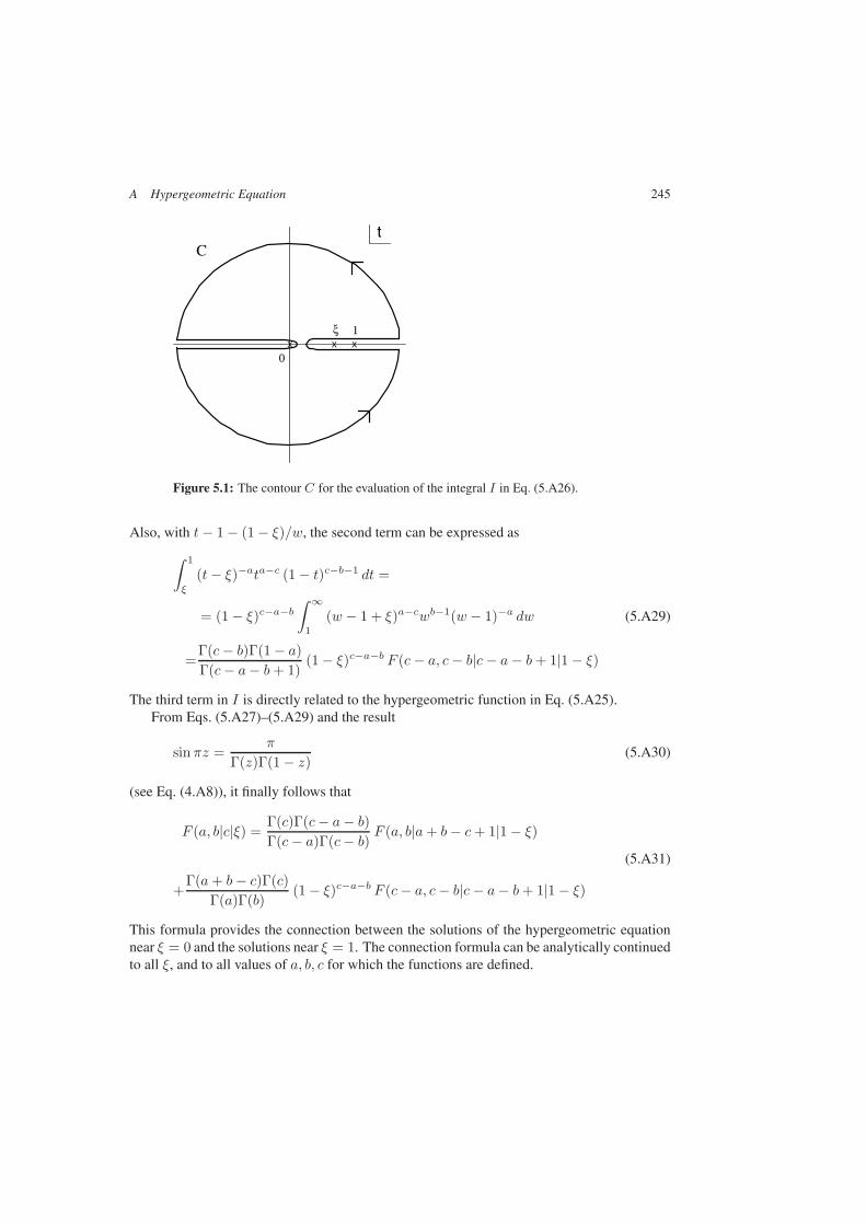
A Hypergeometric Equation 245
XXX
Ct
0
1ξ
Figure 5.1: The contour C for the evaluation of the integral I in Eq. (5.A26).
Also, with t− 1 − (1 − ξ)/w, the second term can be expressed as
∫ 1
ξ
(t− ξ)−ata−c (1 − t)c−b−1 dt =
= (1 − ξ)c−a−b∫ ∞
1
(w − 1 + ξ)a−cwb−1(w − 1)−a dw (5.A29)
=Γ(c− b)Γ(1 − a)Γ(c− a− b+ 1)
(1 − ξ)c−a−b F (c− a, c− b|c− a− b+ 1|1 − ξ)
The third term in I is directly related to the hypergeometric function in Eq. (5.A25).From Eqs. (5.A27)–(5.A29) and the result
sin πz =π
Γ(z)Γ(1 − z)(5.A30)
(see Eq. (4.A8)), it finally follows that
F (a, b|c|ξ) =Γ(c)Γ(c− a− b)Γ(c− a)Γ(c− b)
F (a, b|a+ b− c+ 1|1 − ξ)
(5.A31)
+Γ(a+ b− c)Γ(c)
Γ(a)Γ(b)(1 − ξ)c−a−b F (c− a, c− b|c− a− b+ 1|1 − ξ)
This formula provides the connection between the solutions of the hypergeometric equationnear ξ = 0 and the solutions near ξ = 1. The connection formula can be analytically continuedto all ξ, and to all values of a, b, c for which the functions are defined.
246 5 Differential Equations
B Confluent Hypergeometric Equation
B.1 Reduction to Standard Form
Another common linear second-order equation has the general form
u′′(z) +(
1 − α− β
z
)u′(z) +
(αβ
z2+
2κz
− γ2
)u(z) = 0 (5.B32)
where the choice of constants is motivated by the form of the solutions obtained below. Thisequation has a regular singular point at z = 0, with exponents α and β, and an irregularsingular point at ∞. We can make one of the exponents at z = 0 vanish by the substitution
u(z) = zαv(z) (5.B33)
that leads to the equation
v′′(z) +(
1 + α− β
z
)v′(z) +
(2κz
− γ2
)v(z) = 0 (5.B34)
whose exponents at z = 0 are 0 and β − α.The asymptotic form of this equation for z → ∞ is
v′′(z) − γ2v(z) = 0 (5.B35)
This equation has solutions exp(±γz), which suggests the substitution
v(z) = e−γzw(z) (5.B36)
Then w(z) satisfies the equation
w′′(z) +[1 + α− β
z− 2γ
]w′(z) +
[2κ− γ(1 + α− β)
z
]w(z) = 0 (5.B37)
Now let ξ = 2γz, 2γa = γ(1 + α− β) − 2κ and c = 1 + α− β. Then Eq. (5.B37) becomes
ξw′′(ξ) + (c− ξ)w′(ξ) − aw(ξ) = 0 (5.B38)
This is the standard form of the confluent hypergeometric equation. It has a regular singularpoint at ξ = 0 with exponents 0 and 1 − c, and an irregular singular point at ∞.
The solution F (a|c|ξ) of Eq. (5.B38) that is analytic at ξ = 0 with F (0) = 1 is defined bythe power series
F (a|c|ξ) = 1 +a
cξ +
a(a+ 1)c(c+ 1)
ξ2 + · · · =Γ(c)Γ(a)
∞∑
n=0
Γ(a+ n)Γ(c+ n)
ξn
n!(5.B39)
(again unless 1 − c is a positive integer, which will be considered later). F (a|c|ξ) is theconfluent hypergeometric series; it defines an entire function. It is a polynomial if a is zero ora negative integer; otherwise, it has an essential singularity at ∞.

B Confluent Hypergeometric Equation 247
Remark. Here again the polynomial solutions are very important in physics. The Laguerrepolynomials and Hermite polynomials that appear in the quantum mechanics of the hydrogenatom and the simple harmonic oscillator can be expressed in terms of confluent hypergeomet-ric functions. (see Section 6.5). Bessel functions (see Section 5.6) are not polynomials, butthey also appear in solutions of the wave equation and other equations in physics. The variousforms of Bessel functions are closely related to confluent hypergeometric functions (see alsoExercise 5.20, for example).
To obtain a second solution of Eq. (5.B38) near ξ = 0, let
w(ξ) = ξ1−cv(ξ) (5.B40)
Then v(ξ) satisfies a confluent hypergeometric equation
ξv′′(ξ) + (2 − c− ξ)v′(ξ) − (a− c+ 1)v(ξ) = 0 (5.B41)
This has a solution that is analytic and nonzero at ξ = 0 given by the confluent hypergeometricfunction F (a− c+ 1|2 − c|ξ), unless c− 1 is a positive integer.
Thus the general solution to the confluent hypergeometric equation (5.B38) is given by
w(ξ) = AF (a|c|ξ) +Bξ1−cF (a− c+ 1|2 − c|ξ) (5.B42)
if c is not an integer, whereA andB are arbitrary constants. If c is an integer, a second solutionmust be found by other methods, such as those discussed above.
Remark. Equation (5.B38) can be obtained from the hypergeometric equation
z(z − 1)w′′(z) + [(a+ b+ 1)z) − c]w′(z) + abw(z) = 0 (5.A13)
by letting ξ ≡ bz and passing to the limit b → ∞. Then the regular singular points at ξ = b(z = 1) and ∞ in the hypergeometric equation merge to become the irregular singular pointat ∞ in the confluent hypergeometric equation. Then also
F (a|c|ξ) = limb→∞
F (a, b|c|ξ/b) (5.B43)
so the solution (5.B42) is a limit of the solution (5.A17) to the hypergeometric equa-tion (5.A13) by the same confluence.
B.2 Integral Representations
F (a|c|ξ) also has the integral representation
F (a|c|ξ) =Γ(c)
Γ(a)Γ(c− a)
∫ 1
0
eξtta−1(1 − t)c−a−1 dt (5.B44)
if Re c > Re a > 0. This can be verified by expanding the exponential eξt inside the integraland integrating term-by-term.
248 5 Differential Equations
From this integral representation we have
F (a|c|ξ) Γ(c)Γ(a)Γ(c− a)
∫ 1
−∞eξtta−1(1 − t)c−a−1 dt
(5.B45)
+∫ −∞
0
eξtta−1(1 − t)c−a−1 dt
Now let u = ξ(1 − t) in the first integral, and u = −ξt in the second. Then we have
F (a|c|ξ) =Γ(c)
Γ(a)Γ(c− a)
ξa−ceξ
∫ ∞
0
e−uuc−a−1
(1 − u
ξ
)a−1
du
(5.B46)
+(−ξ)−a∫ ∞
0
e−uua−1
(1 +
u
ξ
)c−a−1
du
The representation (5.B46) can be used to derive an asymptotic series for F (a|c|ξ) by ex-panding the integrand in a power series in u/ξ, as explained in Section 1.4. In the resultingexpansion, the first integral dominates for Re ξ > 0, the second for Re ξ < 0.
Another pair of linearly independent solutions of the confluent hypergeometric equationare the functions U1(a|c|ξ) and U2(a|c|ξ) defined by
U1(a|c|ξ) ≡1
Γ(c− a)ξa−ceξ
∫ ∞
0
e−uuc−a−1
(1 − u
ξ
)a−1
du (5.B47)
for Re c > Re a > 0, 0 < arg ξ < 2π, and
U2(a|c|ξ) ≡1
Γ(a)(−ξ)−a
∫ ∞
0
e−uua−1
(1 +
u
ξ
)c−a−1
du (5.B48)
for Re a > 0, −π < arg ξ < π. These functions are confluent hypergeometric functions ofthe third kind, or Whittaker functions. They are distinguished because they capture the twodistinct forms of asymptotic behavior of solutions of the confluent hypergeometric equationas z → ∞. It follows from Eq. (5.B46) that
F (a|c|ξ) =Γ(c)Γ(a)
U1(a|c|ξ) +Γ(c)
Γ(c− a)U2(a|c|ξ) (5.B49)
for 0 < arg ξ < π.Comparison of the asymptotic behavior of the integral representations also leads
U1(a|c|ξ) =Γ(1 − c)Γ(1 − a)
eiπ(a−c)F (a|c|ξ)− Γ(c− 1)Γ(c− a)
eiπaξ1−cF (a−c+1|2−c|ξ) (5.B50)
for 0 < arg ξ < 2π, and
U2(a|c|ξ) =Γ(1 − c)
Γ(a− c+ 1)eiπaF (a|c|ξ)+ Γ(c− 1)
Γ(a)eiπaξ1−cF (a−c+1|2−c|ξ) (5.B51)
for −π < arg ξ < π, which express the Whittaker functions in terms of the solutions definednear ξ = 0.
C Elliptic Integrals and Elliptic Functions 249
C Elliptic Integrals and Elliptic Functions
A nonlinear differential equation that arises in mechanics is
(du
dz
)2
= (1 − u2)(1 − k2u2) (5.C52)
where k2 is a parameter that for now we will assume to satisfy 0 ≤ k2 < 1. Note that ifk2 > 1, we can introduce rescaled variables w ≡ ku , ξ ≡ kz. Then w satisfies
(dw
dξ
)2
= (1 − w2)(1 − α2w2) (5.C53)
with α2 ≡ 1/k2 < 1. It is left to the problems to show how this equation arises in the problemof a simple pendulum, and the problem of a nonlinear oscillator.
A solution u(z) of this equation with u(0) = 0 is obtained from the integral
z =∫ u
0
1√(1 − t2)(1 − k2t2)
dt (5.C54)
with t− sinφ, this solution can also be written as
z =∫ θ
0
1√1 − k2 sin2 φ
dφ (5.C55)
with u = sin θ. As u increases from 0 to 1 (or θ increases from 0 to π/2), z increases from 0to K(k), where
K(k) ≡∫ 1
0
1√(1 − t2)(1 − k2t2)
dt =∫ π
2
0
1√1 − k2 sin2 φ
dφ (5.C56)
is the complete elliptic integral of the first kind, of modulus k.
Exercise 5.C2. Show that the complete elliptic integral K(k) defined by Eq. (5.C56) canbe expressed as a hypergeometric function according to
K(k) = 12πF ( 1
2 ,12 |1|k
2) (5.C57)
Hint. A brute force method is to expand the integrand in a power series and integrate term byterm. It is more elegant to show that K(k) satisfies a hypergeometric equation.
The function inverse to the function z(u) defined by Eq. (5.C54) is
u(z) ≡ sn(z, k) = sin θ (5.C58)
This defines the (Jacobi) elliptic function sn(z, k) as a function that increases from 0 to 1 for0 ≤ z ≤ K(k). The modulus k is not always written explicitly when it is fixed, so it is alsocommon to write simply u = sn z.
250 5 Differential Equations
Now Eq. (5.C54) is derived from Eq. (5.C52) by choosing
du
dz= +
√(1 − u2)(1 − k2u2) (5.C59)
but as z increases beyond K(k), the sign of the derivative must change, since it follows froma direct calculation that
d2u
dz2= −4u
[1 − 1
2 (1 + k2)u2]
(5.C60)
Thus u′′(z) < 0 when u = 1 (we have assumed 0 ≤ k2 < 1). In the dynamical systemsdescribed by this equation, the points u = ±1 correspond to the turning points of the system.Thus when we continue the integral in Eq. (5.C54) in the complex t-plane, we wrap aroundthe lower side of the branch cut of
√1 − t2, which we can take to run from −1 to 1 as shown
in Fig. 5.2. A complete clockwise circuit of the contour C around the branch cut from −1 to 1corresponds to an increase of z by 4K(k), while u = u(z) has returned to its original locationon the Riemann surface of the integrand. Thus
sn(z + 4K, k) = sn(z, k) (5.C61)
so that sn(z, k) is periodic with period 4K(k).From Fig. 5.2, it is clear that there are other closed contours on the Riemann surface of
the integrand in Eq. (5.C54) that cannot be deformed into C without crossing one or morebranch points of the integrand3 (these branch points are at t = ±1 and at t = ±α ≡ ±1/k;the integrand is analytic at ∞). Note that these branch points are of the square root type, sothe integrand changes sign on encircling one of the branch points. Hence if we make a circuitaround a closed contour L that encircles any two of the branch points, the integral will returnto its original value. If we let
P ≡∮
L
1√(1 − t2)(1 − k2t2)
dt = 0 (5.C62)
then P will be a period for the function u = u(z).A closed contour that cannot be deformed into the contour C is the contour C ′ shown in
Fig. 5.2, which encircles the branch points of the integrand at t = +1 and t = +α. Thecorresponding period is given by
P = 2i∫ α
1
1√(t2 − 1)(1 − k2t2)
dt = 2i∫ 1
0
1√(1 − ξ2)(1 − k′ 2ξ2)
dξ
(5.C63)
= 2iK(k′) ≡ 2iK ′(k)
Here k′ 2 ≡ 1 − k2 (k′ is the complementary modulus of the elliptic integral, and the secondintegral is obtained by the change of variable
ξ2 ≡ 1 − k2t2
1 − k2(5.C64)
3When we speak of deformations of contours here and below, we understand that the deformations are forbiddento cross singularities of the integrand unless explicitly stated otherwise.
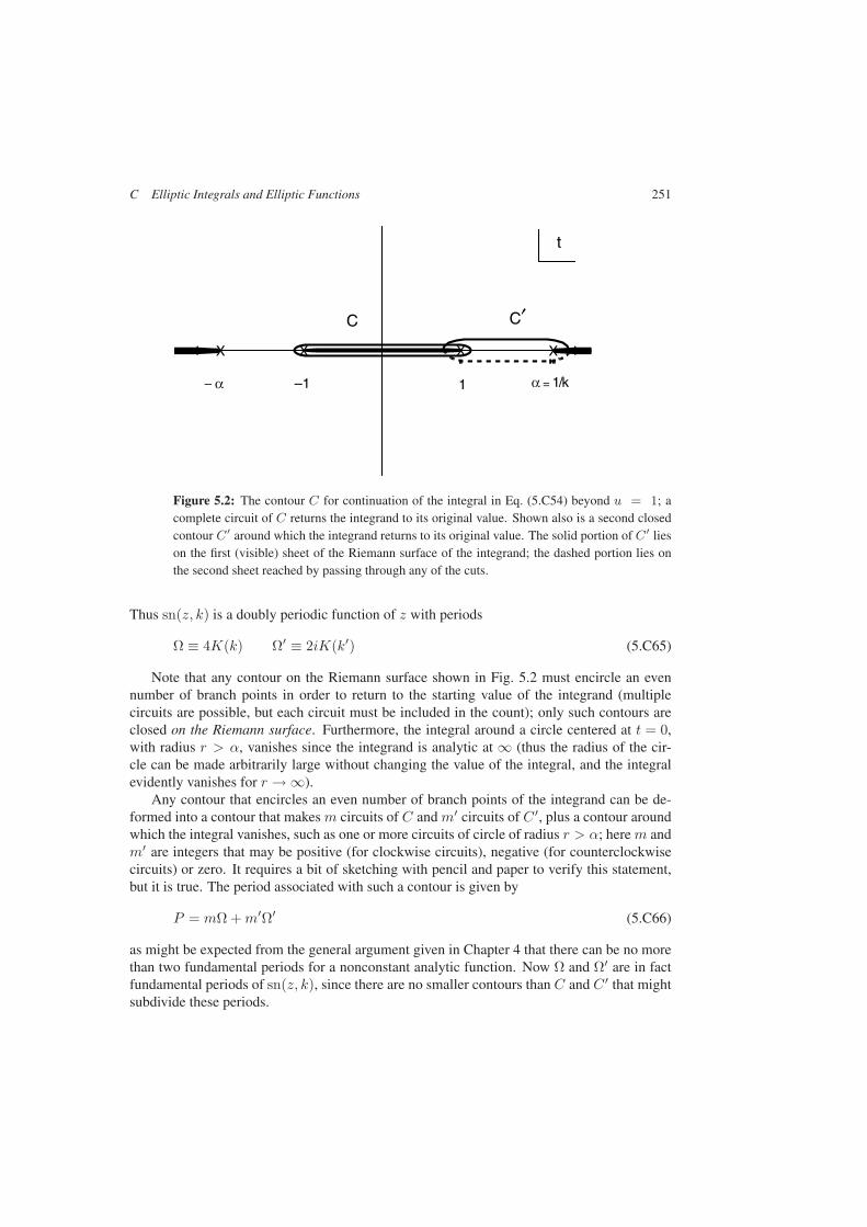
C Elliptic Integrals and Elliptic Functions 251
XXX
C
1 α = 1/k–1
t
X
− α
C′
Figure 5.2: The contour C for continuation of the integral in Eq. (5.C54) beyond u = 1; acomplete circuit of C returns the integrand to its original value. Shown also is a second closedcontour C ′ around which the integrand returns to its original value. The solid portion of C ′ lieson the first (visible) sheet of the Riemann surface of the integrand; the dashed portion lies onthe second sheet reached by passing through any of the cuts.
Thus sn(z, k) is a doubly periodic function of z with periods
Ω ≡ 4K(k) Ω′ ≡ 2iK(k′) (5.C65)
Note that any contour on the Riemann surface shown in Fig. 5.2 must encircle an evennumber of branch points in order to return to the starting value of the integrand (multiplecircuits are possible, but each circuit must be included in the count); only such contours areclosed on the Riemann surface. Furthermore, the integral around a circle centered at t = 0,with radius r > α, vanishes since the integrand is analytic at ∞ (thus the radius of the cir-cle can be made arbitrarily large without changing the value of the integral, and the integralevidently vanishes for r → ∞).
Any contour that encircles an even number of branch points of the integrand can be de-formed into a contour that makes m circuits of C and m′ circuits of C ′, plus a contour aroundwhich the integral vanishes, such as one or more circuits of circle of radius r > α; herem andm′ are integers that may be positive (for clockwise circuits), negative (for counterclockwisecircuits) or zero. It requires a bit of sketching with pencil and paper to verify this statement,but it is true. The period associated with such a contour is given by
P = mΩ +m′Ω′ (5.C66)
as might be expected from the general argument given in Chapter 4 that there can be no morethan two fundamental periods for a nonconstant analytic function. Now Ω and Ω′ are in factfundamental periods of sn(z, k), since there are no smaller contours than C and C ′ that mightsubdivide these periods.

252 5 Differential Equations
Remark. The two-sheeted Riemann surface illustrated in Fig. 4.1 is isomorphic to atorus T 2, since the elliptic integral provides a diffeomorphism from the Riemann surfaceonto the unit cell of the lattice shown in Fig. 4.5 (the elliptic function sn z provides the inversemapping). This unit cell is evidently equivalent to the rectangle in Fig. 3.4, which we haveseen in Chapter 3 to be equivalent to a torus.
There are other Jacobi elliptic functions related to the integrals (5.C54) and (5.C55). Withz and θ related by Eq. (5.C55), define
cn(z, k) ≡ cos θ dn(z, k) ≡√
1 − k2 sin2 θ (5.C67)
where again the dependence on k is not always written explicitly. Jacobi also defined θ ≡am z, the amplitude of z. Note that for real θ, dn z is bounded between k′ =
√1 − k2 and 1,
so that it can never become negative.These functions satisfy many relations similar to those for the trigonometric functions to
which they reduce for k → 0. For example, it is clear that
sn2 z + cn2 z = 1 (5.C68)
k2 sn2 z + dn2 z = 1 (5.C69)
The derivatives of the functions are easily evaluated, since Eq. (5.C55) implies
dz
dθ=
1√1 − k2 sin2 θ
=1
dn z(5.C70)
Then we have
d
dzsn z = cos θ
dθ
dz= cn z dn z (5.C71)
and similarly,
d
dzcn z = − sn z dn z
d
dzdn z = −k2 sn z cn z (5.C72)
It follows directly from the definitions that
sn(−z) = − sn z cn(−z) = cn z dn(−z) = dn z (5.C73)
Also, since z → z + 2K corresponds to θ → θ + π, we have
sn(z + 2K) = − sn z cn(z + 2K) = − cn z dn(z + 2K) = dn z (5.C74)
Thus cn z has a real period 4K, while dn z has a real period 2K.To see what happens when z increases by 2iK ′, recall that this corresponds to one circuit
of the contour C ′ in Fig. 5.2. As we go around this circuit, cn z =√
1 − t2 and dn z =√1 − k2t2 change sign, while sn z returns to its initial value; thus we have
sn(z + 2iK ′) = sn z cn(z + 2iK ′) = − cn z dn(z + 2iK ′) = − dn z (5.C75)
C Elliptic Integrals and Elliptic Functions 253
Equations (5.C74) and (5.C75) show that cn z has a complex fundamental period 2K + 2iK ′,while Eq. (5.C75) shows that dn z has a second fundamental period 4iK ′.
To locate the poles of sn z, we return to the integral (5.C54) and let u→ ∞. Then
z =∫ 1
0
1√(1 − t2)(1 − k2t2)
dt+ i
∫ 1/k
1
1√(t2 − 1)(1 − k2t2)
dt
±∫ ∞
1/k
1√(t2 − 1)(k2t2 − 1)
dt (5.C76)
The sign ambiguity in z reflects the fact that there are two distinct routes from 1 to ∞, onepassing above the cut in Fig. 5.2, the other passing below. The first integral is equal to K(k),the second integral is equal to K ′(k), while the third integral is also equal to K(k), whichis most easily shown by changing variables to ξ ≡ 1/kt. Thus the values of z for whichu = sn z → ∞ are given by
z = iK ′ 2K + iK ′ (5.C77)
together with the points obtained by translation along the lattice generated by the fundamentalperiods 4K and 2iK ′. These points correspond to contours in the t-plane that make extracircuits of the branch points shown in Fig. 5.2.
To show that these points are simple poles of u = sn z, note that
z − iK ′ = +∫ ∞
u
1√(t2 − 1)(k2t2 − 1)
dt (5.C78)
z − 2K − iK ′ = −∫ ∞
u
1√(t2 − 1)(k2t2 − 1)
dt (5.C79)
Since the integral on the right-hand side is approximated by 1/ku for u→ ∞, we have
limz→iK′
(z − iK ′) sn z =1k
(5.C80)
limz→2K+iK′
(z − 2K − iK ′) sn z = −1k
(5.C81)
Thus the singularities of sn z in its fundamental parallelogram are two simple poles, withequal and opposite residues. From the relations (5.C68) and (5.C69), it follows that cn z anddn z have poles at the same points.
Exercise 5.C3. Compute the residues of cn z and dn z at their poles at z = iK ′ and atz = 2K − iK ′.
Exercise 5.C4. Show that
E(e) = 12πF ( 1
2 ,−12 |1|e
2)
by one means or another.
254 5 Differential Equations
Bibliography and Notes
There are many introductory books on differential equations. One highly recommended bookis
Martin Braun, Differential Equations and Their Applications (4th edition), Springer(1993).
This is a substantial book that covers many interesting examples and applications at a reason-ably introductory level. Another excellent introduction is
George F. Simmons, Differential Equations with Applications and Historical Notes(2nd edition), McGraw-Hill (1991).
In addition to covering standard topics, this book has digressions into various interesting ap-plications, as well as many biographical and historical notes that enrich the book beyond thelevel of an ordinary textbook.
An advanced book that covers the analytical treatment of differential equations in greatdepth is
Carl M. Bender and Steven A. Orszag, Advanced Mathematical Methods for Scien-tists and Engineers, McGraw-Hill (1978).
This book treats a wide range of analytic approximation methods, and has an excellent discus-sion of asymptotic methods.
The treatment of linear equations and the special functions associated with the linearsecond-order equation is classical; more detail can be found in the work of Whittaker andWatson cited in Chapter 1. Detailed discussions of the second-order differential equationsarising from the partial differential equations of physics, and for understanding the propertiesof these solutions, can be found in the classic work of Morse and Feshbach cited in Chapter 8.
Elliptic functions and elliptic integrals are treated in the book by Copson cited in Chap-ter 4, as well as in the book by Whittaker and Watson. There is also a book
Harry E. Rauch and Aaron Lebowitz, Elliptic Functions, Theta Functions and Rie-mann Surfaces, Williams and Wilkins (1973).
that describes the Riemann surfaces associated with the elliptic functions in great detail. Amodern treatment of elliptic functions can be found in
K. Chandrasekharan, Elliptic Functions, Springe (1985).
This book gives a through survey of the varieties of elliptic functions and the related theta-functions and modular functions from a contemporary point of view.
A nice treatment of elliptic functions in the context of soluble two-dimensional models instatistical mechanics is given by
Rodney J. Baxter, Exactly Solved Models in Statistical Mechanics, Academic Press(1982).
It should not be surprising that doubly periodic functions are exceptionally useful in describingphysics on a two-dimensional lattice.

Problems 255
Problems
1. Find the general solution of the differential equation
u(z)u′′(z) − [u′(z) ]2 = 6z [u(z) ]2
2. Consider the differential equation
(1 − z)u′′(z) + z u′(z) − u(z) = (1 − z)2
Evidently u(z) = z is a solution of the related homogeneous equation. Find the generalsolution of the inhomogeneous equation.
3. An nth order linear differential operator of the form (5.50) is factorizable if it can bewritten in the form
L =[d
dz+ s1(z)
]· · ·
[d
dz+ sn(z)
]
=n∏
k=1
[d
dz+ sk(z)
]
with known functions s1(z), . . . , sn(z).
Show that if L is factorizable, then the general solution of the equation L[u] = f can beconstructed by solving the sequence of linear inhomogeneous first-order equations
[d
dz+ sk(z)
]uk(z) = uk−1(z)
(k = 1, . . . , n) with u0(z) = f(z).
4. The time evolution of a radioactive decay chain (or sequence of irreversible chemicalreactions) 1 → 2 → . . .→ n is described by the set of coupled differential equations
u′1(t) = −λ1 u1(t)
u′2(t) = −λ2 u2(t) + λ1 u1(t)
u′3(t) = −λ3 u3(t) + λ2 u2(t)
...
u′n(t) = λn−1 un−1(t)
is the population of species k at time t, and λk is the rate per unit time for the processk → k + 1.
(i) Find explicit solutions for u1(t), u2(t) and u3(t) in terms of the initial values u1(0),u2(0), and u3(0).
256 5 Differential Equations
(ii) At what time will u2(t) reach its maximum value?
(iii) Find a set of basic solutions u(m)k (t) that satisfy
u(m)k (0) = δkm
(k,m = 1, . . . , n), and interpret these solutions physically.
(iv) Express the solution uk(t) that satisfies
uk(0) = ck
(k = 1, . . . , n) in terms of these basic solutions.
5. In the preceding problem, suppose we start with a pure sample of species 1, so that
u1(0) = N u2(0) = 0 u3(0) = 0
(i) How long will it take for u1(t) to fall to half its initial value?
(ii) At what time will u2(t) reach its maximum value? What is this maximum value?
(iii) If species 3 is the endpoint of the reaction (this is equivalent to setting λ3 = 0), howlong will it take for u3(t) to reach half its final value?
6. Consider the nth order linear differential equation with constant coefficients
L[u] ≡ u(n)(z) + α1u(n−1)(z) + · · · + αnu(z) = 0
with constant coefficients (Eq. (5.73)).
(i) Express this equation as a matrix equation
v′ = Av
with vector v = (u, u′, . . . , u(n−1).
(ii) Show that the eigenvalues of A are exactly the roots of the polynomial p(λ) inEq. (5.75).
(iii) Express the matrix A = D + N, as defined in Eq. (2.151).
7. Consider the differential equation
d2u
dz2+(λ− c
e−αz
z
)u(z) = 0
(i) Locate and classify the singular points of this equation.
(ii) Find a solution that is analytic at z = 0, neglecting terms that are o(z3).
(iii) Find a linearly independent solution near z = 0, neglecting terms that are o(z2).
Problems 257
8. (i) Find the radius of convergence of the series
S(t, z) =∞∑
n=0
tnPn(z) =1√
1 − 2zt+ t2
as a function of t, if z is real and −1 ≤ z ≤ 1.
(ii) Find the region of convergence in the complex z-plane if t is real with |t| < 1.
9. Find the coefficients cn(z) in the expansion
1 − t2
(1 − 2zt+ t2)3/2=
∞∑
n=0
cn(t)Pn(z)
where |t| < 1 and the Pn(z) are the Legendre polynomials. For what values of z doesthis series converge?
10. Consider the representation (5.153)
Qλ(z) =1
2λ+1
∫ 1
−1
(1 − ξ2)λ
(z − ξ)λ+1dξ
of the Legendre function of the second kind. Use this representation together with theRodrigues formula to show that for λ = n a positive integer,
Qn(z) =12
∫ 1
−1
Pn(t)z − t
dt
where Pn(t) is the corresponding Legendre polynomial.
11. (i) Show that the Wronskian determinant (Eq. (5.62)) of Pλ(z) and Qλ(z) defined by
W (Pλ, Qλ) = PλQ′λ − P ′
λQλ
satisfies the differential equation
1W
dW
dz= − ln(z2 − 1)
and thus
Pλ(z)Q′λ(z) − P ′
λ(z)Qλ(z) =A
z2 − 1
(ii) Evaluate the constant A. Note. One way to do this is to consider the asymptoticbehavior of the equation for z → ∞.
(iii) Show that if we define Qλ(z) = qλ(z)Pλ(z), then qλ(z) satisfies
q′λ(z)[Pλ(z)]2 =
A
z2 − 1

258 5 Differential Equations
(iv) Finally, show that
Qλ(z) = APλ(z)∫ ∞
z
1(t2 − 1)[Pλ(t)]2
dt
12. Show that the Legendre functions of the second kind satisfy the same recursion relations
(2λ+ 1)zQλ(z) = (λ+ 1)Qλ+1(z) + λQλ(z)
and
(z2 − 1)Q′λ(z) = λzQλ(z) − λQλ−1(z)
as the Legendre polynomials and functions of the first kind (see Exercise 5.14).
13. Show that the Bessel function Jλ(z) has the integral representation
Jλ(z) = Cλ
(z2
)λ ∫ 1
−1
eizu(1 − u2)λ−12 du
= Cλ
(z2
)λ ∫ π
0
eiz cos θ(sin θ)2λ dθ
and evaluate the constant Cλ.
14. Use the result of the previous problem to show that the spherical Bessel function
jλ(z) =√
π
2zJλ+
12(s)
has the integral representation
jλ(z) =√πCλ
(z2
)λ+12∫ π
0
eiz cos θ(sin θ)2λ+1 dθ
Then show that for integer n,
jn(z) = An
∫ 1
−1
e−iz cos θPn(cos θ) d(cos θ)
and evaluate the constant An.
15. Show that the hypergeometric function satisfies the recursion formulas
(i) aF (a+ 1, b|c|ξ) − bF (a, b+ 1|c|ξ) = (a− b)F (a, b|c|ξ)
(ii) F (a+ 1, b|c|ξ) − F (a, b+ 1|c|ξ) =(b− a
c
)ξ F (a+ 1, b+ 1|c+ 1|ξ)
(iii)d
dξF (a, b|c|ξ) =
ab
cF (a+ 1, b+ 1|c+ 1|ξ)
Problems 259
16. Show that the general solution of the hypergeometric equation can be expressed as
w(ξ) = A1ξ−aF (a, a− c+ 1|a− b+ 1|1/ξ)
+A2 ξ−bF (b− c+ 1, b|b− a+ 1|1/ξ)
and find the coefficients A1 and A2 when w(ξ) = F (a, b|c|ξ).
17. Show that the confluent hypergeometric function satisfies the recursion formulas
(i) aF (a+ 1|c+ 1|ξ) − cF (a|c|ξ) = (a− c)F (a|c+ 1|ξ)
(ii) c[F (a+ 1|c|ξ) − F (a|c|ξ)] = ξF (a+ 1|c+ 1|ξ)
(iii)d
dξF (a|c|ξ) =
a
cF (a+ 1|c+ 1|ξ)
18. Show that the confluent hypergeometric function satisfies
F (c− a|c|ξ) = eξF (a|c| − ξ)
using the integral representations given in Appendix B.
19. Conservation of energy for a simple pendulum (mass m, length L, angular displacementθ) has the form
12mL2
(dθ
dt
)2
+mgL(1 − cos θ) = E
(i) Introduce the variable u ≡ sin 12θ and rescale the time variable in order to reduce the
conservation of energy equation to an equation of the form (5.C52).
(ii) Derive an expression for the period of the pendulum in terms of a complete ellipticintegral.
20. Consider an anharmonic one-dimensional oscillator with potential energy
V (x) = 12mω
2x2 + 12mσx
4
Sketch the potential energy function for each of the cases:
(i) σ > 0 , ω2 > 0 (ii) σ > 0 , ω2 < 0 (iii) σ < 0 , ω2 > 0
In each case, introduce new variables so that the conservation of energy equation
m
2
(dx
dt
)2
+ V (x) = E
takes the form of Eq. (5.C52). Under what conditions can the variables in the resultingequation be chosen so that the parameter k2 satisfies 0 < k2 < 1?

260 5 Differential Equations
21. Show that the change of variable x = u2 transforms Eq. (5.C52) into
(dx
dz
)2
= 4x(1 − x)(1 − k2x)
Remark. Thus the quartic polynomial on the right-hand side of Eq. (5.C52) can betransformed into a cubic. This does not reduce the number of branch points of dx/dz,but simply relocates one of them to ∞.
22. Show that the circumference of the ellipse
x2
a2+y2
b2= 1
is given by 4aE(e), where e =√a2 − b2/a is the eccentricity of the ellipse and
E(e) ≡∫ 1
0
√1 − e2t2
1 − t2dt
is the complete elliptic integral of the second kind (of modulus e).
6 Hilbert Spaces
Linear vector spaces are often useful in the description of states of physical systems and theirtime evolution, as already noted in Chapter 2. However, there are many systems whose statespace is infinite dimensional, i.e., there are infinitely many degrees of freedom of the system.For example, a vibrating string allows harmonics with any integer multiple of the fundamentalfrequency of the string. More generally, any system described by a linear wave equationwill have an infinite set of normal modes and corresponding frequencies. Thus we need tounderstand how the theory of infinite-dimensional linear vector spaces differs from the finite-dimensional theory described in Chapter 2.
The theory of linear operators and their spectra is also more complicated in infinite dimen-sions. Especially important is the existence of operators with spectra that are continuous, orunbounded, or even nonexistent. In Chapter 7, we will examine the theory of linear operators,especially differential and integral operators, in infinite-dimensional spaces.
In this chapter, we deal first with the subtle issues of convergence that arise in infinitedimensional spaces. We then proceed to discuss the expansion of functions in terms of variousstandard sets of basis functions—the Fourier series in terms of trigonometric functions, andexpansions of functions in terms of certain sets of orthogonal polynomials that arise in thesolution of second-order differential equations. The reader who is more interested in practicalapplications can proceed directly to Section 6.3 where Fourier series are introduced.
As a prototype for an infinite-dimensional vector space, we consider first the space 2(C)of sequences x ≡ (ξ1, ξ2, . . .) of complex numbers with
∞∑
k=1
|ξk|2 <∞
A scalar product of x = (ξ1, ξ2, . . .) and y = (η1, η2, . . .) given by
(x, y) ≡∞∑
k=1
ξk∗ηk
satisfies the axioms appropriate to a unitary vector space, and we show that the series con-verges if x and y are in 2(C). The space 2(C) satisfies two new axioms that characterize aHilbert space: the axiom of separability, which requires the existence of a countable basis, andthe axiom of completeness, which requires that the limit of a Cauchy sequence to belong tothe space. Thus the space 2(C) provides a model Hilbert space in the same way that n-tuplesof real or complex numbers provided model finite-dimensional vector spaces.
Introduction to Mathematical Physics. Michael T. VaughnCopyright c© 2007 WILEY-VCH Verlag GmbH & Co. KGaA, WeinheimISBN: 978-3-527-40627-2
Introduction to Mathematical Physics
Michael T. Vaughn 2007 WILEY-VCH Verlag GmbH & Co.

262 6 Hilbert Spaces
Functions defined on a domain Ω in Rn or Cn also have a natural vector space structure,and a scalar product
(f, g) =∫
Ω
f∗(x)g(x)w(x)dx
can be introduced that satisfies the standard axioms. Here w(x) is a nonnegative weight func-tion that can be introduced into the scalar product; often w(x) = 1 everywhere on Ω, but thereare many problems for which other weight functions are useful. To construct a Hilbert space,the space of continuous functions must be enlarged to include the limits of Cauchy sequencesof continuous functions, just as the set of rational numbers needed to be enlarged to includethe limits of Cauchy sequences of rationals. This expanded space, denoted by L2(Ω), includes“functions” for which
‖f‖2 ≡∫
Ω
|f(x)|2w(x) dΩ
is finite. Here the integral understood as a Lebesgue integral, which is a generalization ofthe Riemann integral of elementary calculus. We discuss briefly the Lebesgue integral aftera short introduction to the concept of measure, on which Lebesgue integration is based. Wealso note that the elements of L2(Ω) need not be functions in the classical sense, since theyneed not be continuous, or even well defined at every point of Ω.
Convergence of sequences of vectors in Hilbert space is subtle: there are no less than fourtypes of convergence: uniform convergence and pointwise convergence as defined in classicalanalysis, weak convergence as defined in Chapter 1 and again here in a vector space context,and strong convergence in Hilbert space, also known as convergence in the mean (weak andstrong convergence are equivalent in a finite-dimensional space).
Every continuous function can be expressed as the limit of a uniformly convergent se-quence of polynomials (Weierstrass approximation theorem). On the other hand, a Cauchysequence of polynomials need not have a pointwise limit. While these subtleties are not oftencrucial in practice, it is important to be aware of their existence in order to avoid drawing falseconclusions on the basis of experience with finite-dimensional vector spaces.
There are various sets of basis functions in a function space that are relevant to physicalapplications. The classical example is Fourier series expansion of a periodic function in termsof complex exponential functions (or in terms of the related trigonometric functions). If f(t)is a well-behaved function with period T , then it can be expressed as a Fourier series in termsof complex exponential functions as
f(t) =
√1T
∞∑
n=−∞cn exp
(2πintT
)
with complex Fourier coefficients cn given by
cn =
√1T
∫ T
0
exp(−2πint
T
)f(t) dt
Note that c−n = c∗n if f(t) is real. Each Fourier series represents a function with period T as asuperposition of functions corresponding to pure oscillators with frequencies fn = nf0, where
6 Hilbert Spaces 263
f0 = 1/T is the fundamental frequency corresponding to period T ; the Fourier coefficients cnand c−n are amplitudes of the frequency component fn in the function f(t). One peculiaritywe note is the Gibbs phenomenon in the Fourier series expansion of a step function; this is aphenomenon that generally occurs in the approximation of discontinuous functions by seriesof continuous functions.
Other important sets of bases are certain families of orthogonal polynomials that appear assolutions to second-order linear differential equations. In particular, there are several familiesof orthogonal polynomials related to the hypergeometric equation and the confluent hyperge-ometric equation discussed in Chapter 5. Some important properties of the Legendre polyno-mials are derived in detail, and the corresponding properties of Gegenbauer, Jacobi, Laguerre,and Hermite polynomials are summarized in Appendix A.
A nonperiodic function f(t) that vanishes for t→ ±∞ can be expressed as a superpositionof functions with definite (angular) frequency ω by the Fourier integral
f(t) =12π
∫ ∞
−∞c(ω)e−iωt dω
which is obtained from the Fourier series by carefully passing to the limit T → ∞. Thefunction c(ω) is obtained from f(t) by a similar integral
c(ω) =∫ ∞
−∞eiωtf(t) dt
The functions f(t) and c(ω) are Fourier transforms of each other. If f(t) describes the evolu-tion of a system as a function of time t, then c(ω) describes the frequency spectrum (ω = 2πf )associated with the system. If t is actually a spatial coordinate x, then the correspondingFourier transform variable is often denoted by k (the wave number, or propagation vector).
Another integral transform, useful for functions f(t) defined for 0 ≤ t < ∞, is theLaplace transform
Lf(p) ≡∫ ∞
0
f(t)e−pt dt
which is obtained from the Fourier transform by rotation of the integration contour in thecomplex t-plane. These transforms, as well as the related Mellin transform introduced as aproblem, have various applications. Here the transforms are used to evaluate integrals, and tofind solutions to certain second-order linear differential equations.
There are many physical problems in which it is important to analyze the behavior of asystem on various scales. For example, renormalization group and block spin methods inquantum field theory and statistical mechanics explicitly consider the behavior of physicalquantities on a wide range of scales. This leads to the concept of multiresolution analysisusing a set of basis functions designed to explore the properties of a function at successivelyhigher levels of resolution. This concept is illustrated here with the Haar functions. The newbasis functions introduced in passing from one resolution to a finer resolution are wavelets.Some methods of constructing wavelet bases are described in Section 6.6.
264 6 Hilbert Spaces
6.1 Infinite-Dimensional Vector Spaces
6.1.1 Hilbert Space Axioms
The basic linear vector space axioms admit infinite-dimensional vector spaces, and fur-ther axioms are needed to define more clearly the possibilities. For example, consider thelinear vector space C∞ whose elements are sequences of complex numbers of the formx = (ξ1, ξ2, . . .), y = (η1, η2, . . .), . . ., with addition and multiplication by scalars definedin the obvious way. This vector space satisfies the basic axioms, and it has a basis
φ1 = (1, 0, 0, . . .)
φ2 = (0, 1, 0, . . .) (6.1)
φ3 = (0, 0, 1, . . .)...
that is countable, i.e., in one-to-one correspondence with the positive integers. This space istoo large for most purposes; if we introduce a scalar product by
(x, y) ≡∞∑
k=1
ξ∗k ηk (6.2)
then the infinite sum on the right-hand side does not converge in general. However, we canrestrict the space to include only those vectors x = (ξ1, ξ2, . . .) for which
‖x‖2 ≡∞∑
k=1
|ξk|2 <∞ (6.3)
that is, vectors of finite length ‖x‖ as defined by Eq. (6.3). This defines a space 2(C), whichis evidently a vector space; the addition of two vectors of finite length leads to a vector offinite length since
|ξk + ηk|2 ≤ 2(|ξk|2 + |ηk|2) (6.4)
It is also a unitary vector space; if ‖x‖ and ‖y‖ are finite, then the scalar product defined byEq. (6.2) is an absolutely convergent series since
|ξkηk| ≤ 12 (|ξk|2 + |ηk|2) (6.5)
The two important properties of 2(C) that require axioms beyond those for a finite-dimensional unitary vector space are:
1. 2(C) is separable. This means that 2(C) has a countable basis.1 One such basis in2(C) has been defined by Eq. (6.1).
1Mathematicians generally define separability in terms of the existence of a countable set of elements that iseverywhere dense (see Definition (1.9)). In the present context, that is equivalent to the existence of a countablebasis.
6.1 Infinite-Dimensional Vector Spaces 265
2. 2(C) is complete, or closed. This means that every Cauchy sequence defined in 2(C)has a limit in 2(C).
The proof of the latter statement is similar to the corresponding proof in the finite-di-mensional case. If x1 = (ξ11, ξ12, . . .), x2 = (ξ21, ξ12, . . .), . . . is a sequence of vectors in2(C), then x1, x2, . . . is a Cauchy sequence if and only if ξ1k, ξ2k, . . . is a Cauchy sequencefor every k = 1, 2, . . ., since
|ξmk − ξnk|2 ≤ ‖xm − xn‖2 ≤∞∑
k=1
|ξmk − ξnk|2 (6.6)
Thus the sequence x1, x2, . . . converges to a limit x if and only if the sequence ξ1k, ξ2k, . . .converges to a limit, call it ξk, for every k = 1, 2, . . .; in the case of convergence, we have
x = (ξ1, ξ2, . . .) (6.7)
Remark. The crucial point here is that 2(C) has been constructed so that the limit (6.7) is inthe space. The space π2(C) of vectors x = (ξ1, ξ2, . . .) with only a finite number of nonzerocomponents satisfies all the axioms except completeness, since the limit vector in (6.7) neednot have a finite number of nonzero components (this shows the independence of the axiomof completeness). In fact, the space 2(C) is obtained from π2(C) precisely by includingthe limit points of all Cauchy sequences in π2(C), in much the same way as the real numberswere obtained from the rational numbers by including the limit points of all Cauchy sequencesof rationals. Thus we can say that 2(C) is the completion, or closure, of π2(C).
An infinite-dimensional unitary vector space that is separable and complete is a Hilbertspace.2 The example 2(C) provides a model Hilbert space. Any complex Hilbert space isisomorphic and isometric to 2(C) in the same way that any n-dimensional complex unitaryvector space is isomorphic and isometric to Cn. Similarly, any real Hilbert space is isomorphicand isometric to the space 2(R) of sequences of real numbers with finite length as definedby (6.3).
A finite-dimensional linear manifold in a Hilbert space is always closed, but an infinite-dimensional linear manifold may or may not be. If φ1, φ2, . . . is an orthonormal system inthe Hilbert space H, then M(φ1, φ2, . . .) denotes the linear manifold consisting of linearcombinations of φ1, φ2, . . . with a finite number of vanishing terms. Including the limit pointsof all Cauchy sequences of vectors in M(φ1, φ2, . . .) gives a subspace M[φ1, φ2, . . .], theclosure of M(φ1, φ2, . . .).
As in the finite-dimensional case, the orthonormal system φ1, φ2, . . . is complete if andonly if the only vector orthogonal to all the φk is the zero vector θ. Equivalent conditions arecontained in the
Theorem 6.1. The orthonormal system φ1, φ2, . . . in the Hilbert space H is complete if andonly if
2A finite-dimensional unitary space is sometimes called a Hilbert space as well, since the axioms of separabilityand completeness are satisfied automatically (i.e., as a consequence of the other axioms) for such spaces. Here wereserve the term Hilbert space for infinite-dimensional spaces.

266 6 Hilbert Spaces
(i) for every vector x in H, we have
x =∞∑
k=1
(φk, x)φk (6.8)
(ii) for every vector x in H, we have
‖x‖2 =∞∑
k=1
|(φk, x)|2 (6.9)
(iii) for every pair of vectors x and y in H, we have
(x, y) =∞∑
k=1
(x, φk)(φk, y) (6.10)
(iv) H = M [φ1, φ2, . . .], that is, H is a closed linear manifold spanned by the orthonormalsystem φ1, φ2, . . ..Any one of these conditions is necessary and sufficient for all of them. It is left as an exercisefor the reader to show this.
Note, however, that while the expansion (6.8) in terms of a complete orthonormal systemis always possible, there are nonorthogonal bases for which the only vector orthogonal toevery element of the basis is the zero vector, but for which there are vectors that do not admitan expansion as a linear combination of the basis vectors.
Example 6.1. Let φ1, φ2, . . . be a complete orthonormal system in the Hilbert space H,and define vectors ψ1, ψ2, . . . by
ψn =√
12 (φn − φn+1) (6.11)
Then the ψ1, ψ2, . . . are linearly independent, and (ψn, x) = 0 for all n if and only if x =θ. However, the ψ1, ψ2, . . . are not orthogonal, and not every vector in H has a convergentexpansion in terms of the ψ1, ψ2, . . .. For example, we have the formal expansion
φ1 ∼√
2 (ψ1 + ψ2 + ψ3 + · · · ) ∼√
2∞∑
k=1
ψk (6.12)
But
‖φ1 −√
2N∑
k=1
ψk‖ = ‖φN+1‖ = 1 (6.13)
Hence the expansion (6.12) does not converge strongly to φ1, although it does convergeweakly. This example shows that it is necessary to use extra caution with nonorthogonalbases in Hilbert space.
6.1 Infinite-Dimensional Vector Spaces 267
6.1.2 Convergence in Hilbert space
The concept of weak convergence, introduced in the discussion of sequences of functions inChapter 1, is also relevant to sequences in Hilbert space. Here we have the
Definition 6.1. If the sequence xk in a unitary vector space V is such that the sequenceof numbers (xk, y) converges to (x, y) for every y in V , then the sequence xk is weaklyconvergent to x, denoted by
xk x (6.14)
(look closely at the half arrow here).
In a finite-dimensional space, weak convergence is equivalent to ordinary (strong) conver-gence, since if φ1, . . . , φn is a complete orthonormal system, and if
(xk, φp) → ξp (6.15)
for p = 1, . . . , n, then for any ε > 0, there is an N such that
|(xk, φp) − ξp| < ε (6.16)
for all p = 1, . . . , n whenever k > N . Then also
‖xk −n∑
p=1
ξpφp‖2 < nε2 (6.17)
so that xk →∑np=1 ξpφp in the usual (strong) sense. In an infinite-dimensional space, we
can no longer be sure that an N exists for which the inequality (6.16) is satisfied for all p, andthere are sequences that converge weakly, but not strongly.
Example 6.2. Let φ1, φ2, . . . be an infinite orthonormal system in a Hilbert space H.Then (φn, x) → 0 for any x in H, since
‖x‖2 ≤∞∑
n=1
|(φn, x)|2 (6.18)
is finite (the sequence of terms of a convergent series must converge to zero). Thus thesequence φn converges weakly to the zero vector θ. On the other hand, ‖φn‖ = 1 forall n, so the φn cannot converge strongly to zero.
Exercise 6.1. Let M be an infinite-dimensional linear manifold in the Hilbert space H.Then
(i) M⊥ is closed,(ii) M = (M⊥)⊥ if and only if M is closed, and(iii) H = M⊕M⊥.

268 6 Hilbert Spaces
Exercise 6.2. Show that if xn x and yn → y, then (xn, yn) → (x, y). Is it truethat if xn x and yn y, then (xn, yn) → (x, y)?
An important result is that a weakly convergent sequence must be bounded.3
Theorem 6.2. If the sequence xn of vectors in the Hilbert space H is weakly convergentto x, then it is bounded (there is an M > 0 such that ‖xn − x‖ ≤M for all n = 1, 2, . . .).
The proof is long and somewhat technical, and we will not present it here. The previousexample might make it plausible. The converse of this theorem is an analog of the Bolzano–Weierstrass theorem for real or complex numbers (see Exercise 1.4).
Theorem 6.3. Any infinite bounded set in the Hilbert space H contains a weakly convergentsubsequence.
Proof. Let φ1, φ2, . . . be a complete orthonormal system in H, and let xn be a boundedinfinite set in H. Then there is a subsequence x1n such that the sequence ξ1n ≡ (φ1, x1n)of numbers is convergent to a limit, call it ξ1. This follows from the plain version ofthe Bolzano–Weierstrass theorem in Exercise 1.1.4. The subsequence x1n is bounded;hence we can choose from it a subsequence x2n such that the sequence of numbersξ2n ≡ (φ2, x2n) is convergent to a limit, call it ξ2. Proceeding in this way, we obtain anested set of subsequences xkn such that the sequences of numbers ξkn ≡ (φk, xkn)converge to limits ξk, for each k = 1, 2, . . .. Let
x∗ =∞∑
k=1
ξkφk (6.19)
Then the sequence yn, with yn ≡ xnn, converges (weakly) to x∗.
6.2 Function Spaces; Measure Theory
6.2.1 Polynomial Approximation; Weierstrass Approximation Theorem
Consider spaces of (complex-valued) functions defined on some domain Ω, which may be aninterval of the real axis, a region in the complex plane, or some higher dimensional domain.There is a natural vector space structure for such functions, and properties such as continu-ity, differentiability, and integrability are preserved by vector addition and multiplication byscalars. A scalar product can be introduced on the function space by
(f, g) =∫
Ω
f∗(x)w(x)g(x)dΩ (6.20)
where dΩ is a suitably defined volume element on Ω, and w(x) is a weight function satisfyingw(x) > 0 on Ω except possibly at the boundary of Ω (often w(x) = 1 everywhere, but otherweight functions are sometimes convenient). This scalar product allows us to introduce normand distance between functions in the usual way.4
3This is the analog of the uniform boundedness principle, or Banach–Steinhaus theorem, in real analysis.4As noted above, norm and length can be defined with no associated scalar product. Function spaces with such
norms are Banach spaces. These are also important in mathematics; further discussion may be found in books citedat the end of the chapter.
6.2 Function Spaces; Measure Theory 269
Complications arise with sequences of functions in a function space; the limiting processesinvolved in the definitions of continuity and differentiability need not be interchangeable withtaking the limit of a sequence (see Section 1.3). Furthermore, there are several distinct con-cepts of convergence of sequences of functions. In addition to the classical pointwise anduniform convergence, and the weak convergence introduced in Section 1.3, there are the con-cepts of strong and weak convergence in Hilbert space as defined above. Thus we examinethe conditions under which sequences of functions converge in the various senses, and theproperties of the limit functions.
One important result is that a continuous function can be approximated on a finite intervalby a uniformly convergent sequence of polynomials. This is stated formally as the
Theorem 6.4. (Weierstrass Approximation theorem). If the function f(t) is continuous onthe closed interval a ≤ t ≤ b, then there is a sequence pn(t) of polynomials that convergesuniformly to f(t) for a ≤ t ≤ b.
Remark. If the function f(t) is k times continuously differentiable on the interval, then thesequence of polynomials can be constructed so that the sequence of derivatives p(k)
n (t) alsoconverges uniformly to the derivative f (k)(t) on the interval.
We will not give a complete proof, but we can construct a sequence of polynomials that isuniformly convergent. Let
Jn =∫ 1
−1
(1 − t2)n dt = 2∫ 1
0
(1 − t2)n dt >2
n+ 1(6.21)
where the last inequality follows from noting that 1 − t2 > 1 − t of 0 ≤ t < 1, and define
Πn(t|f) ≡ 1Jn
∫ 1
0
f(u)[1 − (u− t)2
]ndu (6.22)
Then the sequence Πn(t|f) convergent uniformly to f(t) for a ≤ t ≤ b.
Remark. It is important to realize that the existence of a uniformly convergent sequence ofpolynomials is not equivalent to a power series expansion. For example, the function f(t) =√t is continuous on 0 ≤ t ≤ 1, and hence can be approximated uniformly by a sequence of
polynomials in t. Yet we know that it has no convergent power series expansion around t = 0,since it has a branch point singularity at t = 0 in the complex t-plane. The point is that thecoefficient of a fixed power of t in the approximating polynomial can depend on n.
Remark. This theorem underlies approximate methods for computing transcendental (non-polynomial) functions. Since computers are only able to compute polynomials directly, anycomputation of a transcendental function is some kind of polynomial approximation. Thetheorem assures us that we can choose fixed coefficients to approximate the function over adefinite interval to a specified degree of accuracy. It remains, of course, to determine the mostefficient polynomial for any particular function.

270 6 Hilbert Spaces
6.2.2 Convergence in the Mean
A sequence fn of functions converges to a limit f in the (strong) Hilbert space sense if‖fn − f‖ → 0. With Hilbert space norm from the scalar product (6.20),
∫
Ω
|fn(x) − f(x)|2 w(x) dΩ → 0 (6.23)
for n → ∞. In this case, we also say that fn converges in the mean to f , since the meansquare deviation of fn from the limit function tends to zero. Convergence in the mean doesnot imply uniform convergence, or even pointwise convergence, although it does imply weakconvergence in the sense that
∫
Ω
g∗(x)w(x) [fn(x) − f(x)] dΩ
→ 0 (6.24)
for every integrable function g(x). Uniform convergence implies convergence in the mean,but there are sequences of functions that converge to a limit at every point of an interval, butdo not converge in the mean, or even weakly in the Hilbert space sense.
Example 6.3. Consider the sequence of functions fn(t) defined on [−1, 1] by
fn+1(t) ≡ 2(n+ 1)Jn+1
t2(1 − t2)n (6.25)
with Jn defined in Eq. (6.21). Now fn(t) → 0 for every t, but if g(t) is continuous on[−1, 1], then
∫ 1
−1
g(t)fn+1(t) dt =1
Jn+1
∫ 1
−1
d
dt[tg(t)] (1 − t2)n+1 dt (6.26)
The sequence of integrals on the right-hand side converges to g(0) for every continuousfunction g(t), so the sequence fn(t) 0. The sequence converges weakly as a se-quence of linear functionals; we have
fn(t) tδ′(t) (6.27)
where δ′(t) is the derivative of the Dirac δ-function introduced in Chapter 1, but this limitis not in the Hilbert space of functions on [−1, 1]. Note that each of the fn(t) definedby Eq. (6.25) has continuous derivatives of all orders on [−1, 1], but the lack of uniformconvergence allows the weak limit to be nonzero.
A variety of function spaces on a domain Ω are of interest:C: C(Ω) contains functions continuous on Ω.Ck: Ck(Ω) contains functions continuous together with their first k derivatives on Ω.D: D(Ω) contains functions piecewise continuous on Ω.Dk: Dk(Ω) contains functions whose kth derivative is piecewise continuous on Ω.5
5Note that any function in Dk(Ω) is also in Ck−1(Ω), since the integral of the piecewise continuous kth deriva-tive is continuous in Ω.

6.2 Function Spaces; Measure Theory 271
Each of these function spaces is a linear vector space that can be made unitary with a scalarproduct of the form (6.20). It then satisfies all the Hilbert space axioms except completeness.The limit of a Cauchy sequence of functions in one of these spaces need not be a function inthe space, and not every function f(x) for which
‖f‖2 ≡∫
Ω
|f(x)|2 w(x) dΩ (6.28)
is defined belongs to one of these classes on Ω. To satisfy the axiom of completeness, we needto introduce a new kind of integral, the Lebesgue integral, which is a generalization, based onthe concept of measure, of the usual (Riemann) integral. In the next section, we give a briefdescription of measure, and then explain how the Lebesgue integral is defined. To obtain acomplete function space, we need to understand the integral (6.28) as a Lebesgue integral, andinclude all functions f on the domain Ω for which the integral is finite.
6.2.3 Measure Theory
The measure of a set S of real numbers, complex numbers, or, for that matter, a set of vectorsin Rn or Cn, is a non-negative number associated with the set that corresponds roughly to thelength, or area, or volume of the set. The measure µ(S) must have the property that if S1 andS2 are disjoint (nonoverlapping) sets, then
µ(S1 ∪ S2) = µ(S1) + µ(S2) (6.29)
Thus the measure is additive. A set is of measure zero if it can be contained within a set ofarbitrarily small measure.
Measure can be defined on the real axis in a natural way by defining the measure of aninterval (open or closed) to be the length of the interval. Additivity then requires that themeasure of a collection of disjoint intervals is the sum of the length of the intervals.
A countable set of real numbers has measure zero. If the elements of the set are x1, x2, . . .,then enclose x1 inside an interval of measure ε/2, x2 inside an interval of measure ε/4, andso on, with xn enclosed inside an interval of length ε/2n. The total length of the enclosingintervals is then ε, which can be made arbitrarily small. Hence the set has measure zero. Anexample of an uncountable set of measure zero is the Cantor set in the following exercise:
Exercise 6.3. Consider the closed interval 0 ≤ t ≤ 1. Remove the open interval
13 < t < 2
3
(the “middle open third”) from this interval. From each of the remaining intervals, remove theopen middle third (thus excluding 1
9 < t < 29 and 7
9 < t < 89 ). Proceed in this manner ad
infinitum, and let S denotes the set of numbers that remain.(i) Show that S is a set of measure zero. (Hint. What is the total measure of the pieces
that have been removed from [0,1]?)(ii) Show that S is uncountable (note that S does not consist solely of rational numbers
of the form m/3n with m,n integer).
Remark. The set S is the Cantor set. It is an uncountable set of measure zero. The Cantorset and its generalizations underlie much modern work on fractal geometry.
272 6 Hilbert Spaces
A step function σ(x) is a function that assumes a finite set of values σ1, . . . , σn on setsS1, . . . ,Sn covering a domain Ω. Integration is defined for a step function by
∫
Ω
σ(x) dx =n∑
k=1
σk µ(Sk) (6.30)
Note that if the sets S1, . . . ,Sn consist of discrete subintervals of an interval of the real axis,then this definition coincides with the usual (Riemann) integral.
Remark. With this definition of the integral, the value of a function on a set of measurezero is irrelevant, so long as it is finite. Two functions are be identified if they differ only ona set of measure zero, since they have the same integral over any finite interval. In general,any property such as equality, or continuity, etc., that holds everywhere except on a set ofmeasure zero is said to hold almost everywhere. This identification of functions that are equalalmost everywhere is an extension of the classical notion of a function needed to define thecompletion of function spaces.
A function F (x) is measurable on a domain Ω if there is a sequence σ1, σ2, . . . of stepfunctions that converges to F (x) almost everywhere on Ω. If F (x) is measurable on Ω, andif σ1, σ2, . . . is a sequence of step functions that converges to F (x) almost everywhere on Ω,then form the sequence I1, I2, . . . defined by
In ≡∫
Ω
σn(x) dx (6.31)
If this sequence converges to a finite limit I , then F (x) is (Lebesgue) integrable, or summable,on Ω, and we define the Lebesgue integral of F (x) over Ω by
∫
Ω
F (x) dx ≡ I = limn→∞ In (6.32)
If the ordinary (Riemann) integral of F (x) over Ω exists, then so does Lebesgue integral,and it is equal to the Riemann integral. However, the Lebesgue integral may exist when theRiemann integral does not.
The function space L2(Ω) is the space of complex-valued functions f(x) on the domainΩ for which f(x) is measurable on Ω, and the integral (6.28) exists as a Lebesgue integral. Itfollows from the basic properties of Lebesgue integrals that L2(Ω) is a normed linear vectorspace, and it is unitary with scalar product defined by Eq. (6.20). The crucial property ofL2(Ω) is that it is a Hilbert space; every Cauchy sequence in L2(Ω) converges to a limit inL2(Ω). This is a consequence of the
Theorem 6.5. (Riesz–Fischer theorem). If f1, f2, . . . is a Cauchy sequence of functions inL2(Ω), then there is a function f in L2(Ω) such that
limn→∞ ‖f − fn‖ = 0 (6.33)
The proof is too complicated to give here; details can be found in books on real analysis.The main point of the theorem is that there actually exists a function space that satisfies thecompleteness axiom, unlike the more familiar function spaces of the type Ck or Dk,
6.3 Fourier Series 273
6.3 Fourier Series
6.3.1 Periodic Functions and Trigonometric Polynomials
The classical expansion of functions along an orthogonal basis is the Fourier series expansionin terms of either trigonometric functions or the corresponding complex exponential func-tions. Fourier series were introduced here in Chapter 4 as an expansion of periodic analyticfunctions. Now we look at expansions in terms of various Hilbert space complete orthonormalsystems formed from the trigonometric functions.
If f(t) is a periodic function of the real variable t (often time) with fundamental period T ,the fundamental frequency ν and angular frequency ω are defined by6
ν ≡ ω
2π≡ 1T
(6.34)
Such periodic functions have a natural linear vector space structure, since a linear combinationof functions with period T has the same period T . A natural closure of this vector space is theHilbert space L2(0, T ) with scalar product defined by
(f, g) =∫ T
0
f∗(t)g(t)dt (6.35)
The trigonometric functions sinωt, cosωt, or the corresponding complex exponentialfunctions exp(±iωt), have a special place among functions with period T : the trigonomet-ric functions describe simple harmonic motion with frequency ν = ω/2π, and the complexexponential functions describe motion with constant angular velocity ω around a circle in thecomplex plane (the sign defines the sense of rotation). To include all periodic functions withthe same period, it is necessary to include also functions whose frequency is an integer multi-ple of the fundamental frequency (these frequencies νn ≡ nν, n = 2, 3, . . . are harmonics ofthe fundamental frequency). Thus we have a set of complex exponential functions
φn(t) ≡√
1Teinωt (6.36)
(n = 0,±, 1 ± 2, . . .), and a set of trigonometric functions
C0(t) ≡√
1T
Cn(t) ≡√
2T
cosnωt Sn(t) ≡√
2T
sinnωt (6.37)
(n = 1, 2, . . .). That each of the sets φn and C0, Cn, Sn is an orthonormal systemfollows from some elementary integration. The Weierstrass approximation theorem can beadapted to show that any continuous periodic function can be uniformly approximated by asequence of finite linear combinations of these functions (“trigonometric polynomials”), sothat each of the sets is actually a complete orthonormal system.
6Note that ω is sometimes called the frequency, although it isn’t. Just remember that ω = 2π/T .
274 6 Hilbert Spaces
6.3.2 Classical Fourier Series
A standard Fourier series expansion is obtained by introducing the variable
x ≡ 2πtT
= ωt (6.38)
so that the period of the function in the variable x is 2π, and choosing the primary domainof the function to be the interval −π ≤ x ≤ π. Then any function f(x) in L2(−π, π) withperiod 2π has the Fourier series expansion
f(x) =∞∑
n=−∞cnφn(x) =
1√2π
∞∑
n=−∞cne
inx (6.39)
with Fourier coefficients cn given by
cn = (φn, f) =1√2π
∫ π
−πe−inxf(x) dx (6.40)
Note that c−n = c∗n if f(x) is real.The corresponding real form of the Fourier series is
f(x) =a0√2π
+1√π
∞∑
n=1
[an cosnx+ bn sinnx] (6.41)
with Fourier coefficients an and bn given by
a0 = c0 =1√2π
∫ π
−πf(x) dx (6.42)
an = (Cn, f) =1√π
∫ π
−πcosnx f(x) dx (6.43)
bn = (Sn, f) =1√π
∫ π
−πsinnx f(x) dx (6.44)
(n = 1, 2, . . .). These expansions correspond to the series (4.122) and (4.127), although herethey are defined not just for analytic functions, but for all functions in L2(−π, π). Note thatthe factors of 1/
√2π were absorbed in the Fourier coefficients in Chapter 4; here they are
placed symmetrically between the series (6.39) (or (6.41)) and the coefficients in Eq. (6.40)(or Eqs. (6.43)–(6.44)). There is no universal convention for defining these factors; whateveris most convenient for the problem at hand will do. In the vector space context, we want towork with orthonormal vectors as defined by Eqs. (6.36) or (6.37); in the context of analyticfunction expansions, there is no reason to insert factors of 1/
√2π.
The vector space norm of the function f(x) is given by
‖f‖2 =∫ π
−π|f(x)|2 dx =
∞∑
n=−∞|cn|2 = |a0|2 +
∞∑
n=1
(|an|2 + |bn|2
)(6.45)

6.3 Fourier Series 275
This result is known as Parseval’s theorem. It requires the Fourier coefficients an, bn, and cnto vanish for large n, and fast enough that the series converge.
Exercise 6.4. Show that if
f(x) =1√2π
∞∑
n=−∞cne
inx and g(x) =1√2π
∞∑
n=−∞dne
inx
are any two functions in L2(−π, π), then
(f, g) ≡∫ π
−πf∗(x)g(x) dx =
∞∑
n=−∞c∗ndn
This is the standard form for the scalar product in terms of vector components.
Exercise 6.5. Find the Fourier series expansions of each of the following functions definedby the formulas for −π < x < π, and elsewhere by f(x+ 2π) = f(x).
(i) f(x) = x (ii) f(x) = x2 (iii) f(x) = sin |x|
6.3.3 Convergence of Fourier Series
The Fourier series converges in the Hilbert space sense for functions in L2(−π, π), whileit converges absolutely and uniformly if the function f(x) is analytic in some strip −a <Imx < a about the real axis in the complex x-plane. To see what happens in the intermediatecases, consider the partial sums of the series (6.39) given by
fN (x) ≡N∑
n=−Ncnφn(x) =
12π
N∑
n=−N
∫ π
−πein(x−y)f(y) dy (6.46)
Now
N∑
n=−Neinu =
sin(N + 12 )u
sin 12u
≡ DN (u) (6.47)
(the series is a a geometric series). The function DN (u) is the Dirichlet kernel. It is an evenfunction of u and
∫ π
−πDN (u) du = 2π (6.48)
which follows from integrating the defining series (6.47) term by term. Thus we have
fN (x) =12π
∫ π
−πDN (x− y)f(y) dy =
12π
∫ π−x
−π−xDN (u)f(x+ u) du (6.49)
Now suppose the function f is piecewise continuous, so that the one-sided limits
f±(x0) ≡ limε→0+
f(x0 ± ε) (6.50)

276 6 Hilbert Spaces
exist at every point x0. Then we can write
fn(x0) − 12 [f+(x0) + f−(x0)] =
12π
∫ 0
−πDN (u)[f(x0 + u) − f−(x0)] du
(6.51)
+12π
∫ π
0
DN (u)[f(x0 + u) − f+(x0)] du
If the right side vanishes for largeN , then the Fourier series will converge to the average of theleft- and right-hand limits of f(x) at x0, and to the value f(x0) if the function is continuous.
The two integrals on the right-hand side of Eq. (6.51) can be written as
∆N± = ± 1
π
∫ ± 12π
0
f(x0 ± 2v) − f±(x0)
sin v
sin(2N + 1)v dv (6.52)
(here v = 12u). These integrals are Fourier coefficients for the functions in braces, and hence
vanish for large N if the functions are in a Hilbert space such as L2(0,±12π). This will
certainly be the case if f(x) has one-sided derivative at x0 and may be the case even if itdoes not. Thus there are reasonably broad conditions that are sufficient for the pointwiseconvergence of the Fourier series. The convergence properties can be illustrated further witha pair of examples.
Example 6.4. Consider the function f(x) defined for −π ≤ x ≤ π by
f(x) = |x| (6.53)
Then the Fourier coefficients of f(x) are given by
√2π c0 = 2
∫ π
0
xdx = π2 (6.54)
and
√2π cn =
∫ π
0
e−inxxdx−∫ 0
−πe−inxxdx = 2
∫ π
0
x cosnx dx
(6.55)
=
−4/n2 n odd
0 n even
which leads to the Fourier series
f(x) =π
2− 4π
∞∑
n=0
cos(2n+ 1)x(2n+ 1)2
(6.56)
The series is absolutely and uniformly convergent on the entire real axis. However, itdiverges if Imx = 0, since the series then contains an exponentially increasing part. Thisshould not be surprising, since the function f(x) is not analytic.

6.3 Fourier Series 277
-2 0 2
0
0.2
0.4
0.6
0.8
1H(x)
x-2 0 2
0
0.2
0.4
0.6
0.8
1
H(x)
x
-2 0 2
0
0.2
0.4
0.6
0.8
1H(x)
x-2 0 2
0
0.2
0.4
0.6
0.8
1H(x)
x
Figure 6.1: Approximations HN (x) to the function H(x) by the truncated Fourier series (6.61) forN = 4 (upper left), N = 10 (upper right), N = 20 (lower left), and N = 40 (lower right).
Example 6.5. Consider the (Heaviside) step function H(x) defined for −π ≤ x ≤ π by
H(x) =
1 0 < x < π
0 −π < x < 0(6.57)
and elsewhere by f(x+ 2π) = f(x). The Fourier coefficients of H(x) are given by
√2π c0 =
∫ π
0
dx = π (6.58)
and for n > 0 by
√2π cn =
∫ π
0
e−inxdx =1in
(1 − einπ
)=
2/in n odd
0 n even(6.59)
which leads to the Fourier series
H(x) =12
+2π
∞∑
n=0
sin(2n+ 1)x(2n+ 1)
(6.60)
278 6 Hilbert Spaces
The Fourier series (6.60) is convergent except at the points 0,±π,±2π, . . . of discon-tinuity of H(x); at these points, the series has the value 1
2 . The partial sums HN (x) of theseries, defined by
HN (x) =12
+2π
N∑
n=0
sin(2n+ 1)x(2n+ 1)
(6.61)
are shown in Fig. 6.1 for N = 4, 10, 20, 40.One interesting feature that can be seen in these graphs is that the partial sums over-
shoot the function near the discontinuity at x = 0. This overshoot does not disappear inthe limit as N → ∞; it simply moves closer to the discontinuity. To see this, note thatEq. (6.49) gives here
HN (x) =12π
∫ π
0
D2N+1(x− y) dy =12π
∫ π−x
−x
sin(2N + 32 )u
sin 12u
du (6.62)
and the discontinuity function
∆N (x) = HN (x) −HN (−x) =(6.63)
=12π
∫ x
−x
sin(2N + 32 )u
sin 12u
du+12π
∫ π+x
π−x
sin(2N + 32 )u
sin 12u
du
A short calculation shows that the first maximum of ∆N (x) for x > 0 occurs for
x =π
2(N + 1)≡ xN (6.64)
The value of ∆N (x) at this maximum is given by
∆N (xN ) =1π
∫ xN
0
sin(2N + 32 )u
sin 12u
du+12π
∫ π+xN
π−xN
sin(2N + 32 )u
sin 12u
du
(6.65)
2π
∫ π
0
sin ξξ
dξ + · · ·
where the neglected terms are O(1/N) for N → ∞. This last result follows from sub-stituting ξ = (2N + 3
2 )u and approximating sin 12u 1
2u in the first integral on theright-hand side of Eq. (6.63). The final integral has the numerical value 1.179 . . .. Thusthe maximum of the partial sum of the series overshoots the function by about 18% of themagnitude of the discontinuity on each side.
This effect is known as the Gibbs phenomenon; it is a consequence of the attempt toapproximate a discontinuous function by a sequence of smooth functions. It is a generalproperty of Fourier series, and other series as well, though the magnitude of the overshootmay depend on the particular set of smooth functions used.

6.3 Fourier Series 279
These examples illustrate the characteristic convergence properties of the Fourier seriesexpansion of a function in L2. While the series is guaranteed to converge in the Hilbert spacesense, the expansion of a discontinuous function converges slowly, especially near points ofdiscontinuity. The smoother the function, the more rapidly the Fourier coefficients an, bn(or cn) vanish for large n. The analytic properties of the series are best seen in the complexexponential form (6.39) of the series. Write
f(x) = f0 +∞∑
n=1
f−n e−inx +∞∑
n=1
fn einx ≡ f0 + f−(x) + f+(x) (6.66)
(fn = cn/√
2π). Then it is clear that if the series converges in the Hilbert space for realx, the function f+(x) [f−(x)] is analytic in the half-plane Imx > 0 [Imx < 0], since theimaginary part of x provides an exponentially decreasing factor that enhances the convergenceof the series. If the function f(x) is actually analytic in a strip including the real axis, then thecoefficients c±n must vanish faster than any power of n for large n. However, we have seenthat Fourier series converge on the real axis alone for a much broader class of functions, andthere is no guarantee even of pointwise convergence on the real axis.
6.3.4 Fourier Cosine Series; Fourier Sine Series
There are other important trigonometric series. Consider, for example, the set of functionsψn(x) defined by
ψ0 ≡√
1π
ψn(x) ≡√
2π
cosnx (6.67)
(n = 1, 2, . . .). This set is a complete orthonormal system on the interval 0 ≤ x ≤ π, and anyfunction f(x) in L2(0, π) can be expanded as
f(x) =∞∑
n=0
anψn(x) (6.68)
with
a0 = (ψ0, f) =
√1π
∫ π
0
f(x) dx (6.69)
an = (ψn, f) =
√2π
∫ π
0
cosnxf(x) dx (6.70)
The series (6.68) is a Fourier cosine series; it can be obtained from the classical Fourierseries (6.41) by defining f(−x) ≡ f(x) (0 ≤ x ≤ π), extending f(x) to be an even functionof x on the interval −π ≤ x ≤ π. Then the only nonvanishing Fourier coefficients in theclassical series (6.41) are those of the cosnx terms (n = 0, 1, 2, . . .).
Another complete orthonormal system on the interval 0 ≤ x ≤ π is the set φn(x)defined by
φn(x) ≡√
2π
sinnx (6.71)
280 6 Hilbert Spaces
(n = 1, 2, . . .). Any function f(x) in L2(0, π) can be extended to an odd function of x on theinterval −π ≤ x ≤ π by defining f(−x) ≡ −f(x) (0 ≤ x ≤ π). Then the only nonvanishingFourier coefficients in the classical series (6.41) are those of the sinnx terms (n = 1, 2, . . .),and f(x) can be expanded as a Fourier sine series
f(x) =∞∑
n=1
bnφn(x) (6.72)
with
bn = (φn, f) =
√2π
∫ π
0
sinnxf(x) dx (6.73)
(n = 1, 2, . . .).A function f(x) in L2(0, π) has both a Fourier sine series and a Fourier cosine series.
These series are unrelated in general, since one is the classical Fourier series of the odd exten-sion of f(x) to the interval −π ≤ x ≤ π, while the other is the classical Fourier series of theeven extension.
Example 6.6. Consider the function f(x) = 1 on 0 ≤ x ≤ π. The function has a oneterm Fourier cosine series f(x) = 1, while the Fourier sine series is given by
f(x) =4π
∞∑
n=0
sin(2n+ 1)x(2n+ 1)
(6.74)
since the odd extension of f(x) is simply given by
fodd(x) = H(x) −H(−x) (6.75)
where H(x) is the step function introduced above in Eq. (6.199).
Exercise 6.6. Find the Fourier sine series and cosine series expansions of the functionsdefined by
(i) f(x) = x
(ii) f(x) = x(π − x)
(iii) f(x) = e−αx
(iv) f(x) =
1 0 ≤ x < π
2
−1 π2 ≤ x < π
(6.76)
for 0 < x < π.
6.4 Fourier Integral; Integral Transforms 281
6.4 Fourier Integral; Integral Transforms
6.4.1 Fourier Transform
The Fourier series expansion of a function with period T expresses the function in termsof oscillators with frequencies νn that are integer multiples of the fundamental frequencyν = 1/T . The longer the period, the smaller the interval between the frequencies, and it isplausible that in the limit T → ∞, the spectrum of frequencies becomes continuous. To seehow this happens, write the Fourier series expansion of f(t) in the form
f(t) =1T
∞∑
n=−∞cn exp
(−2πint
T
)(6.77)
(here the minus sign in the exponential is a convention), with
cn =∫ 1
2T
− 12T
exp(
2πintT
)f(t) dt (6.78)
If we let ωn ≡ 2πn/T and ∆ω ≡ 2π/T , then the series (6.77) becomes
f(t) =12π
∞∑
n=−∞c(ωn) exp (−iωnt)∆ω (6.79)
In the limit T → ∞, the series becomes the integral
f(t) =12π
∫ ∞
−∞c(ω)e−iωt dω (6.80)
with
c(ω) =∫ ∞
−∞eiωtf(t) dt (6.81)
Equation (6.80) defines f(t) as a Fourier integral, the continuous version of the Fourierseries (6.77). The function c(ω) is the Fourier transform of f(t), and f(t) is the (inverse)Fourier transform of c(ω).7 Note that if f(t) is real, then
c∗(ω) = c(−ω) (6.82)
The Fourier integrals (6.80) and (6.81) exist under various conditions. If
‖f‖2 =∫ ∞
−∞|f(t)|2 dt <∞ (6.83)
7There is no universal notation here: the Fourier transform c(ω) of f(t) defined by the integral (6.81) is denotedvariously by f(ω), f(ω), F (ω), and F [f ]. Moreover, there are various arrangements of the factor of 2π betweenthe Fourier transform and its inverse. Finally, the signs in the exponentials can be reversed, which is equivalent to thesubstitution c(ω) → c(−ω).

282 6 Hilbert Spaces
so that f(t) is in L2(−∞,∞), then the integrals (6.80) and (6.81) exist as vector space limits.Then also
‖c‖2 =∫ ∞
−∞|c(ω)|2 dω = 2π‖f‖2 (6.84)
a result known as Plancherel’s formula, the integral version of Parseval’s formula (6.45). Onthe other hand, if the integral (6.81) is absolutely convergent, so that
∫ ∞
−∞|f(t)| dt <∞ (6.85)
then the integral (6.81) defines c(ω) as a continuous function of ω.
Remark. The condition (6.85) is distinct from (6.83). For example, the function
f(t) ≡ |t|1 + t2
(6.86)
is in L2(−∞,∞), but the Fourier integral is not absolutely convergent. On the other hand, thefunction
f(t) ≡ e−α|t|√|t|
(6.87)
has an absolutely convergent Fourier integral if Reα > 0. However, f(t) is not inL2(−∞,∞) due to the singularity of |f(t)|2 at t = 0, and neither is its Fourier transformc(ω), whose evaluation is left as a problem.
The Fourier transform is defined by (6.81) for real ω. However, the definition provides anatural analytic continuation to complex ω, since we can write
f(t) = f+(t) + f−(t) (6.88)
with
f+(t) =
f(t) t > 00 t < 0
and f−(t) =
0 t > 0f(t) t < 0
(6.89)
and corresponding Fourier transforms
c+(ω) =∫ ∞
0
eiωtf(t) dt and c−(ω) =∫ 0
−∞eiωtf(t) dt (6.90)
If the Fourier transform of f(t) exists for real ω, then c+(ω) is analytic in the upper half ω-plane Imω > 0, since exp(iωt) is then exponentially damped for t→ +∞. Similarly, c−(ω)is analytic in the lower half ω-plane Imω < 0. This analytic continuation to the complexω-plane corresponds to the continuation to the complex x-plane in Eq. (6.66). The analyticproperties of the Fourier transform can often be used to evaluate the Fourier integral (6.80) bythe contour integration methods of Chapter 4.
6.4 Fourier Integral; Integral Transforms 283
Example 6.7. Consider the function f(t) defined by
f(t) =
e−αt t > 00 t < 0
(6.91)
(Reα > 0). The Fourier transform of f(t) is given by
c(ω) =∫ ∞
0
eiωte−αt dt =1
α− iω(6.92)
which has a pole at ω = −iα. The corresponding Fourier integral∫ ∞
−∞c(ω) exp(−iωt) dω (6.93)
can be evaluated as a contour integral; see Eq. (4.108) for a similar integral.
One especially useful property of the Fourier transform is that differentiation with respectto t becomes multiplication by −iω in the Fourier transform: if f(t) has Fourier transformc(ω) defined by (6.81), and if the derivative f ′(t) has a Fourier transform, the Fourier trans-form of f ′(t) is given by −iωc(ω). This result can be used to transform differential equationsin which derivatives appear with constant coefficients.
Example 6.8. Consider a forced, damped harmonic oscillator for which the equation ofmotion is
d2x
dt2+ 2γ
dx
dt+ ω2
0x = f(t) (6.94)
with γ > 0 to ensure damping (and ω0 real), and suppose that the forcing term f(t) can beexpressed as a Fourier integral according to Eq. (6.80). If we also write
x(t) =12π
∫ ∞
−∞a(ω)e−iωt dω (6.95)
then the equation of motion is reduced to the algebraic equation(−ω2 − 2iγω + ω2
0
)a(ω) = c(ω) (6.96)
Then we have the solution
a(ω) =c(ω)
ω20 − ω2 − 2iγω
(6.97)
from which x(t) is obtained by evaluating the Fourier integral. Note that the zeroes of thedenominator at
ω = −iγ ±√ω2
0 − γ2 ≡ ω± (6.98)
284 6 Hilbert Spaces
are both in the lower half ω-plane when γ > 0. Thus if the forcing term vanishes for t < 0,so that c(ω) is analytic in the upper half ω-plane, then a(ω) is also analytic in the upperhalf-plane, and the solution x(t) also vanishes for t < 0, as expected from causality. Thusit satisfies the initial conditions x(0) = 0 and x′(0) = 0 if f(t) = 0 for t < 0, although ithas no apparent dependence on the initial conditions.
To find a solution for t > 0 that satisfies the general initial conditions
x(0) = x0 x′(0) = v0 (6.99)
it is necessary to add to x(t) a solution
A+e−iω+t +A−e−iω−t (6.100)
of the homogeneous equation, with
A+ +A− = x0 (6.101)
and
ω+A+ − ω−A− = iv0 (6.102)
in order to satisfy the initial conditions.
6.4.2 Convolution Theorem; Correlation Functions
The convolution of the functions f(t) and g(t), denoted by f ∗ g, is defined by
(f ∗ g)(t) ≡∫ ∞
−∞f(t− u)g(u) du (6.103)
If f(t) and g(t) are expressed as Fourier integrals according to
f(t) =12π
∫ ∞
−∞c(ω)e−iωt dω g(t) =
12π
∫ ∞
−∞d(ω)e−iωt dω (6.104)
then we can write
(f ∗ g)(t) =12π
∫ ∞
−∞
∫ ∞
−∞c(ω)e−iω(t−u)g(u) dudω (6.105)
But the Fourier inversion formula (6.81) gives∫ ∞
−∞eiωug(u) du = d(ω) (6.106)
so that the convolution integral is given by
(f ∗ g)(t) =12π
∫ ∞
−∞c(ω) d(ω)e−iωt dω (6.107)
6.4 Fourier Integral; Integral Transforms 285
Thus the Fourier transform of the convolution f ∗ g is given by the ordinary product of theFourier transforms of f and g and conversely, the Fourier transform of the ordinary product off and g is the convolution f ∗ g.
Example 6.9. The solution (6.97) to Eq. (6.94) in the preceding example has the form
a(ω) = k(ω)c(ω) (6.108)
where c(ω) is the Fourier transform of the forcing term, and
k(ω) =1
ω20 − ω2 − 2iγω
= − 1(ω − ω+)(ω − ω−)
(6.109)
where ω± are defined by Eq. (6.98). Thus the solution x(t) can be written as a convolution
x(t) =∫ ∞
−∞K(t− u) f(u) du (6.110)
with
K(τ ) =12π
∫ ∞
−∞k(ω)e−iωτ dτ =
i(e−iω+τ − e−iω−τ )/∆ (τ > 0)
0 (τ < 0)(6.111)
(here ∆ = ω+ − ω− = 2√ω2
0 − γ2). The result (6.111) is derived by closing the contourin the upper half ω-plane for τ < 0 and in the lower half ω-plane for τ > 0 (note that thetwo poles of k(ω) lie in the lower half-plane). The functionK(τ ) is the Green function (orresponse function) for the forced oscillator. Green functions will be discussed in greaterdetail in Chapters 7 and 8.
Closely related to the convolution f ∗ g is the correlation function8
Cf,g(T ) ≡∫ ∞
−∞f∗(t) g(t+ T ) dt (6.112)
The correlation function can also be expressed as a Fourier integral according to
Cf,g(T ) =12π
∫ ∞
−∞c∗(ω) d(ω)e−iωT dω (6.113)
following the analysis given above. A special case of interest is the correlation function of fwith itself (the autocorrelation function of f ), defined by
Af (T ) ≡∫ ∞
−∞f∗(t) f(t+ T ) dt =
12π
∫ ∞
−∞|c(ω)|2 e−iωT dω (6.114)
Thus |c(ω)|2 is the Fourier transform of the autocorrelation function; if |c(ω)|2 has a peak atω = ω0, say, then the autocorrelation function will have an important component with period2π/ω0. |c(ω)|2 is also known as the spectral density of f(t).
8In some contexts, the correlation function is normalized by dividing by ‖f‖‖g‖.

286 6 Hilbert Spaces
6.4.3 Laplace Transform
Suppose now that f(t) is a function that vanishes for t < 0, and consider the integral
c(ω) =∫ ∞
0
f(t)eiωt dt (6.115)
If the standard Fourier integral (6.81) converges for real ω, then the integral (6.115) convergesfor Imω > 0 as already noted, but the class of functions for which this integral converges forsome complex ω is larger, since it includes functions f(t) that grow no faster than exponen-tially as t → ∞. In particular, if there are (real) constants M and a such that |f(t)| ≤ Meat
for all t ≥ 0, then the integral (6.115) converges and defines an analytic function of ω in thehalf-plane Imω > a. If we define ω ≡ ip, then we can define
Lf(p) ≡ c(ip) =∫ ∞
0
f(t)e−pt dt (6.116)
Lf(p) is the Laplace transform of f(t); it is analytic in the half-plane Re p > a. TheLaplace transform be inverted using the standard Fourier integral formula (6.80) and changingthe integration variable from ω to p; this gives
f(t) =1
2πi
∫ b+i∞
b−i∞Lf(p)ept dp (6.117)
where the integral is taken along a line Re p = b(< a) parallel to the imaginary p-axis.The Laplace transform can be useful for solving differential equations since the derivative
of a function has a fairly simple Laplace transform; we have
d
dp(Lf)(p) = −
∫ ∞
0
tf(t)e−pt dt (6.118)
and∫ ∞
0
df(t)dt
e−pt dt = p(Lf)(p)− f(0) (6.119)
Example 6.10. Recall the confluent hypergeometric equation (5.B38)
ξf ′′(ξ) + (c− ξ)f ′(ξ) − af(ξ) = 0 (6.120)
If
f(ξ) =∫ ∞
0
h(t)e−ξt dt (6.121)
then h(t) must satisfy the first-order equation
t(1 + t)h′(t) + [1 − a+ (2 − c)t]h(t) = 0 (6.122)
6.4 Fourier Integral; Integral Transforms 287
This equation has the solution
h(t) = Ata−1(1 + t)c−a−1 (6.123)
(A is an arbitrary constant), which leads to
f(ξ) = A
∫ ∞
0
ta−1(1 + t)c−a−1e−ξt dt(6.124)
=A
ξa
∫ ∞
0
ua−1(1 +u
ξ)c−a−1e−u du
Note that this solution depends only on one arbitrary constant A. This is due to the as-sumption (6.121) that f(ξ) is actually a Laplace transform of some function h(t), whichimplies that f(ξ) → 0 for ξ → ∞. Hence the solutions of Eq. (6.120) that do not vanishfor ξ → ∞ are lost. Note also that it is necessary that Re a > 0 for the integral (6.121)to exist; if this is not the case, then there are no solutions of Eq. (6.120) that vanish forξ → ∞. Finally, note that the solution (6.124) is just the Whittaker function of the secondkind defined by Eq. (5.B51).
In this example, a solution to a second-order differential equation was found as the Laplacetransform of a function that satisfies a first-order equation. Problem 14 is an example of howthe Laplace transform can be used to reduce directly a second-order equation to a first-orderequation.
Fourier and Laplace transform methods are quite similar, since the two transforms arerelated in the complex plane (only the contours of integration are different). The classes offunctions on which the two transforms are defined overlap, but are not identical. There arerelated transforms that deal with other classes of functions; one such transform is the Mellintransform introduced in Problem 15.
6.4.4 Multidimensional Fourier Transform
Multidimensional Fourier transforms are obtained directly by repeating the one-dimensionalFourier transform. A function f of the n-dimensional vector x = (x1, . . . , xn) can be ex-pressed as an n-dimensional Fourier integral
f(x) =1
(2π)12n
∫eik·xφ(k) dnk (6.125)
with the Fourier transform φ(k) given by
φ(k) =1
(2π)12n
∫e−ik·xf(x) dnx (6.126)
Here k = (k1, . . . , kn), dnk = dk1 . . . dkn, and k · x = k1x1 + · · · + knxn is the usualscalar product. The convergence properties are again varied: f(x) is in L2(Rn) if and only ifφ(k) is in L2(Rn), but the Fourier integral (6.125) is also well defined for other φ(k). As inone dimension, there are variations in allocating the factors of 2π and the choice of ±i in theexponential.
288 6 Hilbert Spaces
6.4.5 Fourier Transform in Quantum Mechanics
The Fourier transform plays a special role in quantum mechanics, in which a particle is de-scribed by a probability amplitude (wave function) ψ(x, t) that depends on position x andtime t. The corresponding variable in the spatial Fourier transform φ(k, t) is the wave vec-tor k; the momentum p of the particle is related to k by
p = k (6.127)
where is Planck’s constant. Thus the probability amplitudes ψ(x, t) for position and φ(k, t)for momentum are Fourier transforms of each other. Furthermore, wave functions with definitefrequency,
ψ(x, t) = ψ0(x)e−iωt (6.128)
correspond to particle states of definite energy E = ω.For a nonrelativistic particle of mass m, the free-particle wave function ψ(x, t) satisfies
the Schrödinger equation
i∂ψ
∂t= −
2
2m∇2ψ (6.129)
This equation has plane wave solutions
ψk(x, t) = Aeik·x−iωkt (6.130)
[although these are not in L2(R3)] where the Schrödinger equation requires the relation
E = ωk =
2k2
2m=
p2
2m(6.131)
which is exactly the energy–momentum relation for a free particle.A complete solution to the Schrödinger equation (6.129) starting from an initial wave
function ψ(x, 0) at t = 0 [assumed to be in L2(R3)], can be obtained using the Fouriertransform. If the initial wave function is expressed as
ψ(x, 0) =∫A(k)eik·x d3k (6.132)
then the wave function
ψ(x, t) =∫A(k)eik·x−iωkt d3k (6.133)
is a solution of (6.129) that satisfies the initial conditions; it is unique, since the Fourier inte-gral (6.132) uniquely defines A(k) through the inverse Fourier transform. Further propertiesof the Schrödinger equation will be discussed in Chapter 8.

6.5 Orthogonal Polynomials 289
6.5 Orthogonal Polynomials
6.5.1 Weight Functions and Orthogonal Polynomials
Consider an interval [a, b] on the real axis and weight function w(t) in the scalar product
(f, g) =∫ b
a
f∗(t)w(t)g(t) dt (6.134)
as introduced in Eq. (6.20). it is straightforward in principle to construct a sequence p0(t),p1(t), p2(t), . . . of polynomials of degree n that form an orthonormal system.9 The functions1, t, t2, . . . are linearly independent, and orthogonal (even orthonormal) polynomials can beconstructed by the Gram–Schmidt process; note that these polynomials have real coefficients.
The orthonormal system π0(t), π1(t), π2(t), . . . formed by normalizing these polynomialsis complete in L2(a, b). Any function f(t) in L2(a, b) can be expanded as
f(t) =∞∑
n=0
cnπn(t) (6.135)
where the series converges in the Hilbert space sense; the expansion coefficients are given by
cn = (πn, f) =∫ b
a
π∗n(t)w(t)f(t) dt (6.136)
One general property of the orthogonal polynomials constructed in this way is that thepolynomial πn(t) has n simple zeroes, all within the interval [a, b], To see this, suppose thatπn(t) changes sign at the points ξ1, . . . , ξm within [a, b] (note that m ≤ n, since πn(t) is ofdegree n). Then the function
πn(t)(t− ξ1) · · · (t− ξm)
does not change sign in [a, b], so that the integral∫ b
a
πn(t)w(t)(t− ξ1) · · · (t− ξm) dt = 0 (6.137)
But πn(t) is orthogonal to all polynomials of degree ≤ n − 1 by construction; hence m = nand πn(t) has the form
πn(t) = Cn(t− ξ1) · · · (t− ξm) (6.138)
The families of polynomials introduced here all appear as solutions to the linear second-order differential equation (5.81) with special coefficients. It is plausible that in order tohave a polynomial solutions, the differential equation can have at most two singular pointsin the finite t-plane/ This requires the second-order equation to have the form of either thehypergeometric equation (5.A13) or the confluent hypergeometric equation (5.B38), perhapswith singular points shifted by a linear change of variable. The polynomial solutions of theseequations are obtained from the general forms F (a, b|c|ξ) or F (a|c|ξ) by setting the parametera = −n (n = 0, 1, 2, . . .).
9This is true even for an infinite interval if the weight function w(t) decreases rapidly enough.
290 6 Hilbert Spaces
6.5.2 Legendre Polynomials and Associated Legendre Functions
We look first for orthogonal polynomials on the interval [−1, 1]. It turns out that the Le-gendre polynomials introduced in Section 5.5 are orthogonal on [−1, 1], with weight functionw(t) = 1. To show this, we can use Rodrigues’ formula from Section 5.5,
Pn(t) =1
2nn!dn
dtn(t2 − 1
)n= Cnu
(n)n (t) (5.127)
We have now evaluated the constant Cn, and here again un(t) =(t2 − 1
)n. If m < n, we
can integrate by parts m times to evaluate the scalar product
(Pm, Pn) =∫ 1
−1
Pm(t)Pn(t) dt = CmCn
∫ 1
−1
u(m)m (t)u(n)
n (t) dt = · · ·
= (−1)mCmCn(2m)!∫ 1
−1
u(n−m)n (t) dt (6.139)
= (−1)mCmCn(2m)!u(n−m−1)n
∣∣1−1
= 0
Thus the Pn(t) are orthogonal on [−1, 1]. If m = n, the same procedure gives
(Pn, Pn) =∫ 1
−1
[Pn(t)]2 dt = C2n (2n)!
∫ 1
−1
(1 − t2
)ndt
(6.140)
= C2n (2n)! 22n+1 [Γ(n+ 1)]2
Γ(2n+ 2)=
22n+ 1
Thus a set πn(t) of orthonormal polynomials on [−1, 1] is given in terms of the Pn(t) by
πn(t) =
√2n+ 1
2Pn(t) (6.141)
These results can also be obtained using the generating function (5.137) (see Problem 16).
Exercise 6.7. Show that applying the Gram–Schmidt process to the linearly independentmonomials 1, t, t2, t3 leads to the first four polynomials π0(t), . . . , π3(t).
We note here the recursion formulas for the Legendre polynomials
(n+ 1)Pn+1(t) = (2n+ 1)tPn(t) − nPn(z) (6.142)
(t2 − 1)P ′n(t) = ntPn(t) − nPn−1(t) (6.143)
from Exercise 5.14. These relations can be derived by differentiating the generating function
S(ξ, t) =1√
1 − 2ξt+ ξ2=
∞∑
n=0
ξnPn(t) (5.137)
with respect to ξ and t, respectively. Equation (6.142) is useful for evaluating Pn(t) numeri-cally if n is not too large.
6.5 Orthogonal Polynomials 291
Also important are the associated Legendre functions P an (t) defined for −1 ≤ t ≤ 1 by
P an (t) = (−1)a (1 − t2)12ada
dtaPn(t) = (−1)aCn (1 − t2)
12au(n+a)
n (t) (6.144)
with a = 0, 1, 2, . . . integer and n = a, a + 1, a + 2, . . .. For fixed integer a, the P an (t) areorthogonal on [−1, 1]. To show this, suppose that n < m. We then have the scalar product
(P am, Pan ) =
∫ 1
−1
P am(t)P an (t) dt =
= CmCn
∫ 1
−1
u(m+a)m (t)(1 − t2)au(n+a)
n (t) dt = · · · (6.145)
= CmCnA(n,a)
∫ 1
−1
u(n−m)n (t) dt = CmCnA(n,a) u
(n−m−1)n
∣∣1−1
= 0
after integrating by parts n+ a times; the constant A(n,a) is given by
A(n,a) = (−1)n+a dn+a
dtn+a
(1 − t2)a u(n+a)
n (t)
= (−1)n (2n)!(n+ a)!(n− a)!
(6.146)
Thus the P an (t) are orthogonal on [−1, 1]. To find the normalization, we can evaluate theintegral for m = n. We have
(P an , Pan ) =
∫ 1
−1
[P an (t)]2 dt = C2n(−1)nA(n,a)
∫ 1
−1
(1 − t2
)ndt
(6.147)
= C2n (2n)!
(n+ a)!(n− a)!
22n+1 [Γ(n+ 1)]2
Γ(2n+ 2)=
22n+ 1
(n+ a)!(n− a)!
Then for fixed a = 0, 1, 2, . . . , the functions πan(t) defined by
πan(t) =
√2n+ 1
2
√(n− a)!(n+ a)!
P an (t) (6.148)
(n = a, a+ 1, a+ 2, . . .) form a complete orthonormal system on [−1, 1].Exercise 6.8. Show that the associated Legendre function P an (t) is a solution of the
differential equation
(1 − t2)u′′(t) − 2tu′(t) +n(n+ 1) − a2
1 − t2
u(t) = 0
Note the conventional sign change from the original Legendre equation.
Remark. From the preceding discussion, it follows that the polynomials F an (t) defined by
F an (t) = (−1)ada
dtaPn+a(t) = (−1)aCnu
(n+2a)n+a (t) (6.149)
form a set of orthogonal polynomials on [−1, 1] with weight function w(t) = (1 − t2)a. Itis left to the reader to express these polynomials in terms of the Gegenbauer polynomialsdescribed in Appendix A.
292 6 Hilbert Spaces
6.5.3 Spherical Harmonics
Legendre polynomials and the associated Legendre functions appear in a number of contexts,but they first appear to most physicists in the study of partial differential equations involvingthe Laplacian, such as Poisson’s equation or the Schrödinger equation. These equations willbe analyzed at great length in Chapter 8. Here we simply note that for many systems, it is con-venient to use the spherical coordinates r, θ, φ introduced in Eq. (3.173). In these coordinates,the Laplacian has the form
∆ =1r2
∂
∂r
(r2
∂
∂r
)+
1sin θ
∂
∂θ
(sin θ
∂
∂θ
)+
1sin2 θ
∂2
∂φ2
(6.150)
as derived in Chapter 3 (see Eq. (3.193). We look for solutions of the relevant partial differen-tial equation that have the form
f(r, θ, φ) = R(r)Y (θ, φ) (6.151)
In most such cases, the angular function Y (θ, φ) must be a solution of the partial differentialequation
1
sin θ∂
∂θ
(sin θ
∂
∂θ
)+
1sin2 θ
∂2
∂φ2
Y (θ, φ) = λY (θ, φ) (6.152)
with λ such that the Y (θ, φ) is
(i) single valued as a function of φ, and
(ii) nonsingular as a function of θ over the range 0 ≤ θ ≤ π including the endpoints.
To satisfy the first requirement, we can expand Y (θ, φ) as a Fourier series
Y (θ, φ) =∞∑
m=0
[Am(cos θ) cos(mφ) +Bm(cos θ) sin(mφ)]
=∞∑
m=−∞Cm(cos θ) eimφ (6.153)
Then the coefficients Am(cos θ), Bm(cos θ), Cm(cos θ) must satisfy the differential equation
1
sin θd
dθ
(sin θ
d
dθ
)− m2
1 − coss θ
Xm(cos θ) = λXm(cos θ) (6.154)
(here Xm = Am, Bm, Cm). Now introduce the variable t = cos θ, and express Eq. (6.154) interms of t as
d
dt(1 − t2)
d
dt− m2
1 − t2
Xm(t) = λXm(t) (6.155)
From Exercise 6.8, we see that this is the differential equation for the associated Legendrefunction Pmn (t), with λ = −n(n+ 1) (n = m,m+ 1, . . . ).
6.5 Orthogonal Polynomials 293
Thus we have solutions to Eq. (6.152) of the form
Cnm(θ, φ) = P |m|n (cosθ) eimφ (6.156)
for n = 0, 1, 2, . . . ; m = 0,±1, . . . ,±n. Using the normalization integral (6.147), we findfunctions
Ynm(θ, φ) =
√2n+ 1
4π(n− |m|)!(n+ |m|)!P
|m|n (cos θ) eimφ (6.157)
that form a complete orthonormal system on the surface of the sphere S2. The Ynm(θ, φ) arespherical harmonics.
One important result is the spherical harmonic addition theorem. Suppose we have twounit vectors
n = n(θ, φ) and n′ = n′(θ′, φ′)
and let Θ be the angle between n and n′. Then we have
n · n′ = cosΘ = cos θ cos θ′ + sin θ sin θ′ cos(φ− φ′) (6.158)
The spherical harmonic addition theorem states that
Pn(cosΘ) =4π
2n+ 1
n∑
m=−nY ∗nm(θ′, φ′)Ynm(θ, φ) (6.159)
To show this, note that n · n′ is a scalar; hence Pn(cosΘ) is as well. Since the Laplacian ∆ isa scalar, so is the differential operator in Eq. (6.152). Hence
1
sin θ∂
∂θ
(sin θ
∂
∂θ
)+
1sin2 θ
∂2
∂φ2
Pn(cosΘ) = −n(n+ 1)Pn(cosΘ) (6.160)
since this differential equation is certainly true in a coordinate system with the Z-axis chosenalong n′, as cosΘ = cos θ in such a coordinate system. But any solution of Eq. (6.160) mustbe a linear combination of spherical harmonics Ynm(θ, φ) (m = n, n− 1, . . . ,−n+ 1,−n).Hence we can write
Pn(cosΘ) =n∑
m=−ncnm(θ′, φ′) Ynm(θ, φ) (6.161)
Since cosΘ depends on φ and φ′ only in the combination (φ−φ′), the coefficient cnm(θ′, φ′)must be proportional to Y ∗
nm(θ′, φ′) (note that cnm must satisfy Eq. (6.160) in the primedvariables). The overall scale on the right-hand side of Eq. (6.159) is fixed by considering thecase when both n and n′ are in the Z-direction.
294 6 Hilbert Spaces
6.6 Haar Functions; Wavelets
Fourier series and Fourier integral methods permit the extraction of frequency informationfrom a function of time. However, these methods have two important limitations when ap-plied to real signals. First, they require a knowledge of the signal over the entire domain ofdefinition, so that analysis of the signal must wait until the entire signal has been received(although some analysis can often begin while the signal is being recorded). Furthermore,the standard Fourier analysis converts a function of time into a function of frequency, anddoes not deal directly with the important problem of a signal at a standard frequency (the car-rier frequency) upon which is superimposed an information bearing signal either in the formof amplitude modulation (as in the case of AM radio), or frequency modulation (FM radio,television). Decoding such a signal involves analysis both in time and in frequency.
There are many problems that involve the structure of a function at various scales, both inthe use of renormalization group methods in quantum field theory and the statistical mechanicsof phase transitions, and in macroscopic applications to signal processing and analysis. WhileFourier series can be used to analyze the behavior of functions with a fixed period, they arenot well suited for the rescaling of the time interval or spatial distances (“zooming in” and“zooming out”) needed in these problems. Thus it is important to have sets of functions thathave the flexibility to resolve multiple scales.
A simple set of such functions consists of the Haar functions h0(t), hn,k(t),
h0(t) =
1 0 < t ≤ 10 otherwise
(6.162)
(the characteristic function of the interval [0, 1], also known as the “box” function), and
hn,k(t) =
1 2k − 2 < 2nt ≤ 2k − 1−1 2k − 1 < 2nt ≤ 2k0 otherwise
(6.163)
(n = 1, 2, . . . ; k = 1, . . . , n). The first four Haar functions are shown in Fig. 6.2.The Haar functions are orthogonal, since
∫ 1
0
h0(t)hn,k(t) dt =∫ 1
0
hn,k(t) dt = 0 (6.164)
and∫ 1
0
hm,q(t)hn,k(t) dt =(
12
)n−1δmnδkq (6.165)
Thus the functions χn,k(t) defined by
χn,k(t) ≡√
2n−1hn,k(t) (6.166)
form an orthonormal system on the interval 0 ≤ t ≤ 1, and the orthonormal system formedby h0(t) and the χn,k(t) is complete since any integrable function can be approximated by
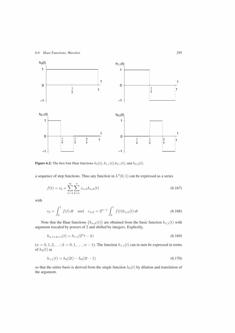
6.6 Haar Functions; Wavelets 295
1
1
h0(t)
t0
–1
1–2
1
1
h1,1(t)
0
–1
1–2
t
1
1
h2,1(t)
0
–1
1–2
3–4
1–4
t
1
h2,2(t)
0
–1
11–2
3–4
1–4
t
Figure 6.2: The first four Haar functions h0(t), h1,1(t),h2,1(t), and h2,2(t).
a sequence of step functions. Thus any function in L2(0, 1) can be expressed as a series
f(t) = c0 +∞∑
n=1
n∑
k=1
cn,khn,k(t) (6.167)
with
c0 =∫ 1
0
f(t) dt and cn,k = 2n−1
∫ 1
0
f(t)hn,k(t) dt (6.168)
Note that the Haar functions hn,k(t) are obtained from the basic function h1,1(t) withargument rescaled by powers of 2 and shifted by integers. Explicitly,
hn+1,k+1(t) = h1,1(2nt− k) (6.169)
(n = 0, 1, 2, . . . ; k = 0, 1, . . . , n− 1). The function h1,1(t) can in turn be expressed in termsof h0(t) as
h1,1(t) = h0(2t) − h0(2t− 1) (6.170)
so that the entire basis is derived from the single function h0(t) by dilation and translation ofthe argument.

296 6 Hilbert Spaces
Expansion (6.167) resolves a function in L2(0, 1) into components cn,k with respect to theHaar basis. The index n defines a scale (2−n in time or 2n in frequency) on which the detailsof the function are resolved, and the index k defines the evolution of these details over the nsteps from t = 0 to t = 1 at this scale. Thus the expansion can describe the time evolution ofthe function on a range of frequency scales, in contrast to the standard Fourier analysis, whichdescribes either the time dependence of the function, or the frequency composition of thefunction, but not the time dependence of frequency components. The price of this expansionis that the frequency scales are multiples of the fundamental frequency times 2n, rather thanany integer multiple, and the time steps are submultiples of the fundamental period (hencedependent on the fundamental frequency chosen) by a power of 2, rather than continuous.
The preceding analysis can be extended to functions defined on the entire real axis, at leastto those in L2(−∞,∞), with the added feature that the time scale can be expanded as wellas contracted by powers of two. The Haar functions are used as an explicit example, but theanalysis can be generalized to other families of functions. First let
φ(t) ≡ h0(t) (6.171)
and consider the shifted functions
φ0,k(t) ≡ φ(t− k) (6.172)
(k = 0,±1,±2, . . . ). The φ0,k form an orthonormal system that defines a subspace V0 ofL2(−∞,∞) consisting of elements of the form
a(t) =∞∑
k=−∞αkφ0,k(t) (6.173)
with
‖a‖2 =∫ ∞
−∞|a(t)|2 dt =
∞∑
k=−∞|αk|2 <∞ (6.174)
V0 is the (infinite-dimensional) space of functions that are piecewise constant on intervals ofthe form k < t ≤ k + 1. It is equivalent to the sequence space 2(R) or 2(C), depending onwhether the αk are real or complex.
For any function f(t) in L2(−∞,∞), the component f0 of f in V0 is
f0(t) =∞∑
k=−∞f0,kφ0,k(t) (6.175)
with coefficients
f0,k =∫ ∞
−∞φ0,k(t)f(t) dt =
∫ k+1
k
f(t) dt (6.176)
(k = 0,±1,±2, . . . ).
6.6 Haar Functions; Wavelets 297
f0 is an approximation to f by step functions of unit length, and indeed the best approximationin the mean square sense with origin fixed (for a particular function, shifting the origin mightimprove the approximation, but that is beside the point here).
This approximation can be refined by reducing the scale of the interval. Thus consider thenew basis functions
φ1,k(t) ≡√
2φ(2t− k) =√
2φ0,k(2t) (6.177)
(k = 0,±1,±2, . . . ), where the factor of√
2 normalizes the φ1,k . The φ1,k form an or-thonormal system that defines a subspace V1 of L2(∞,∞) whose elements are functions thatare piecewise constant on intervals of the form k < 2t ≤ k+1. The space V1 includes V0 as aproper subspace (a function that is piecewise constant on intervals of length 1 is also piecewiseconstant on intervals of length 1
2 ). Note that
φ0,k(t) =√
12 (φ1,2k(t) + φ1,2k+1(t)) (6.178)
gives an explicit expression for the basis vectors of V0 in terms of those of V1. The componentf1 of a function f in V1 is
f1(t) =∞∑
k=−∞f1,kφ1,k(t) (6.179)
with
f1,k =∫ ∞
−∞φ1,k(t)f(t) dt =
√2∫ (k+1)/2
k/2
f(t) dt
(6.180)
=
√12
∫ k+1
k
f(u
2
)du
(k = 0,±1,±2, . . . ). The last integral shows how the detail of f on a finer scale is blown upin the construction of f1.
Continuing this process leads to a sequence of nested subspaces
· · · ⊂ V−2 ⊂ V−1 ⊂ V0 ⊂ V1 ⊂ V2 ⊂ · · · (6.181)
(it is possible to go backwards from V0 to coarser scales by doubling the interval over whichthe functions are piecewise continuous), such that a complete orthonormal system on Vn isgiven by the set φn,k with
φn,k(t) ≡ 2n2 φ(2nt− k) (6.182)
(k = 0,±1,±2, . . . ) for each n = 0,±1,±2, . . .. A distinctive feature of this set is that allthe functions are obtained from the single scaling function φ(t) by rescaling and shifting theargument. A nested sequence (6.181) of subspaces, with a complete orthonormal system oneach subspace obtained from a single scaling function by a relation like Eq. (6.182), is calleda multiresolution analysis.
298 6 Hilbert Spaces
The component fn of a function f in Vn has the explicit representation
fn(t) =∞∑
k=−∞fn,kφn,k(t) (6.183)
with
fn,k =∫ ∞
−∞φn,k(t)f(t) dt = 2
n2
∫ (k+1)/2n
k/2n
f(t) dt
(6.184)
=(
12
)n2∫ k+1
k
f( u
2n)du
(k = 0,±1,±2, . . . ), again showing the resolution of the fine scale details of f . For anyfunction f in L2(−∞,∞), the sequence of approximations . . . , f−2, f−1, f0, f1, f2, . . .converges to f as a vector space limit since, as already noted, every square integrable functioncan be approximated by a sequence of step functions.
At each stage in the sequence (6.181), a new space is added. If Wn is the orthogonalcomplement of Vn in Vn+1, then
Vn+1 = Vn ⊕Wn (6.185)
(n = 0,±1,±2, . . .), and the convergence of the sequence fn is equivalent to
L2(−∞,∞) = ⊕∞−∞Wn (6.186)
The space Wn is the wavelet space at level n; it is where new structure in a function is resolvedthat was not present in the component fn. Equation (6.185) can be seen as an illustration ofthe split of a function in Vn+1 into a low frequency part (in Vn) and a high frequency part(in Wn).
From the fundamental relation
φ(t) = φ(2t) + φ(2t− 1) (6.187)
(this can be seen by inspection) and Eq. (6.182) it follows that
φn,k(t) =√
12 (φn+1,2k(t) + φn+1,2k+1(t)) (6.188)
[see Eqs. (6.177) and (6.178)]. Then the set of vectors ψn,k defined by
ψn,k(t) ≡√
12 (φn+1,2k(t) − φn+1,2k+1(t)) (6.189)
are orthogonal to the φn,k in Vn+1. Hence the ψn,k must be in Wn. The ψn,k areorthonormal by construction, and together with the φn,k are equivalent to the set φn+1,kwhich is a complete orthonormal system in Vn+1 = Vn ⊕ Wn. Hence the ψn,k form acomplete orthonormal system in Wn. The ψn,k are wavelets at scale 2n in frequency (orscale 2−n in t); they are orthogonal to all functions in Vn.
6.6 Haar Functions; Wavelets 299
The ψn,k(t) can be obtained from a single function ψ(t), the fundamental wavelet (ormother wavelet), which is given here by
ψ(t) = φ(2t) − φ(2t− 1) (6.190)
which is equivalent to Eq. (6.170) since ψ(t) = h1,1(t) [compare this with the correspondingrelation (6.187) for φ(t)]. Corresponding to Eq. (6.182) for the φn,k, we have
ψn,k(t) ≡ 2n2 ψ(2nt− k) (6.191)
The ψn,k are related to the Haar functions hn,k by
ψn,k(t) ≡ 2n2 hn+1,k+1(t) (6.192)
except that here n and k can range over all integers without restriction.An important advance of the 1980s was the discovery that the multiresolution analysis
described here with the Haar functions could also be carried out with other, smoother choicesfor the scaling function φ(t). The essential features of the multiresolution analysis are
(i) The space L2(−∞,∞) is decomposed into a nested sequence of subspaces Vn asin (6.181), such that if f is in L2, then the sequence fn (fn is the component of f in Vn)converges to f . Also, if f(t) is in Vn then f(2t) is in Vn+1 so that the space Vn+1 is anexact rescaling of the space Vn .
(ii) There is a scaling function φ(t) such that the translations of φ(t) by integers,
φ0,k(t) ≡ φ(t− k) (6.193)
(k = 0,±1,±2, . . . ), form a complete orthonormal system on V0, and the dilations of φ(t) by2n, together with integer translations,
φn,k(t) ≡ 2n2 φ(2nt− k) (6.194)
(k = 0,±1,±2, . . . ), form a complete orthonormal system on Vn for each integer n.The nesting condition (6.181) implies that φ(t) is in V1. Hence there must be an expansion
φ(t) =∞∑
k=−∞ckφ(2t− k) (6.195)
of φ(t) in terms of its rescaled and shifted versions. Equation (6.187) is a relation of this typefor the “box” function h0(t). If we introduce the Fourier transform
Φ(ω) ≡∫ ∞
−∞eiωtφ(t) dt (6.196)
then the relation (6.195) leads to
Φ(ω) =∞∑
k=−∞ck
∫ ∞
−∞eiωtφ(2t− k) dt
(6.197)
= 12
∞∑
k=−∞cke
12 ikω
∫ ∞
−∞e
12 iωτφ(τ ) dτ
300 6 Hilbert Spaces
Thus the Fourier transform is scaled according to
Φ(ω) = H( 12ω)Φ( 1
2ω) (6.198)
where
H(ω) = 12
∞∑
k=−∞cke
ikω (6.199)
Iterating this equation gives
Φ(ω) =
∞∏
k=1
H( ω
2k)
Φ(0) (6.200)
and it will be seen shortly that Φ(0) = 1. Thus the Fourier transform of the scaling functioncan be expressed formally as an infinite product. Proving convergence of the infinite productrequires some heavy analysis in general, but it does converge for the examples described here.
Example 6.11. With c0 = c1 = 1 (and all other cn = 0), we have the function
H(ω) = 12 (1 + eiω) =
1 − e2iω
2(1 − eiω)= e
12 iω cos 1
2ω (6.201)
and
Φ(ω) = limm→∞
1 − eiω
2m(1 − eiω/2m)=
1 − eiω
−iω = e12 iω
sin 12ω
12ω
(6.202)
which is precisely the Fourier transform of h0(t).
Exercise 6.9. Show that the Fourier transform of the Haar function h0(t) defined byEq. (6.162) is given by
h0(ω) =1 − eiω
−iω = e12 iω
sin 12ω
12ω
as claimed in the preceding example.
If the functions φ0,k(t) defined by Eq. (6.193) form an orthonormal system, then
Ik ≡∫ ∞
−∞φ∗(t)φ(t− k) dt =
12π
∫ ∞
−∞|Φ(ω)|2 eikω dω = δk0 (6.203)
Now we can write
Ik =12π
∞∑
m=−∞
∫ 2π
0
|Φ(ω + 2mπ)|2 eikω dω (6.204)
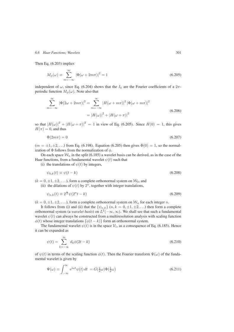
6.6 Haar Functions; Wavelets 301
Then Eq. (6.203) implies
Mφ(ω) ≡∞∑
m=−∞|Φ(ω + 2mπ)|2 = 1 (6.205)
independent of ω, since Eq. (6.204) shows that the Ik are the Fourier coefficients of a 2π-periodic function Mφ(ω). Note also that
∞∑
m=−∞|Φ(2ω + 2mπ)|2 =
∞∑
m=−∞|H(ω +mπ)|2 |Φ(ω +mπ)|2
(6.206)= |H(ω)|2 + |H(ω + π)|2
so that |H(ω)|2 + |H(ω + π)|2 = 1 in view of Eq. (6.205). Since H(0) = 1, this givesH(π) = 0, and thus
Φ(2mπ) = 0 (6.207)
(m = ±1,±2, . . .) from Eq. (6.198). Equation (6.205) then gives Φ(0) = 1, so the normal-ization of Φ follows from the normalization of φ.
On each space Wn in the split (6.185) a wavelet basis can be derived, as in the case of theHaar functions, from a fundamental wavelet ψ(t) such that
(i) the translations of ψ(t) by integers,
ψ0,k(t) ≡ ψ(t− k) (6.208)
(k = 0,±1,±2, . . . ), form a complete orthonormal system on W0, and(ii) the dilations of ψ(t) by 2n, together with integer translations,
ψn,k(t) ≡ 2n2 ψ(2nt− k) (6.209)
(k = 0,±1,±2, . . . ), form a complete orthonormal system on Wn for each integer n.It follows from (i) and (ii) that the ψn,k (n, k = 0,±1,±2, . . .) then form a complete
orthonormal system (a wavelet basis) on L2(−∞,∞). We shall see that such a fundamentalwavelet ψ(t) can always be constructed from a multiresolution analysis with scaling functionφ(t) whose integer translations φ(t− k) form an orthonormal system.
The fundamental wavelet ψ(t) is in the space V1, as a consequence of Eq. (6.185). Henceit can be expanded as
ψ(t) =∞∑
k=−∞dkφ(2t− k) (6.210)
of ψ(t) in terms of the scaling function φ(t). Then the Fourier transform Ψ(ω) of the funda-mental wavelet is given by
Ψ(ω) ≡∫ ∞
−∞eiωtψ(t) dt = G( 1
2ω)Φ( 12ω) (6.211)

302 6 Hilbert Spaces
where
G(ω) ≡ 12
∞∑
k=−∞dke
ikω (6.212)
is a 2π-periodic function that corresponds to the function H(ω) introduced in the scalingrelation for φ(t). If the functions ψ0,k(t) defined by Eq. (6.208) form an orthonormalsystem, then the function G(ω) must satisfy
|G(ω)|2 + |G(ω + π)|2 = 1 (6.213)
Equation (6.213) is derived following the steps in Eqs. (6.203)–(6.206) above, with ψ in placeof φ.
Orthogonality of the functions ψ0,k(t) and φ0,(t) leads to the condition
G∗(ω)H(ω) +G∗(ω + π)H(ω + π) = 0 (6.214)
by a similar analysis. A “natural” choice of G(ω) that satisfies Eqs. (6.213) and (6.214) is
G(ω) = e±iωH∗(ω + π) (6.215)
This G(ω) can be multiplied by a phase factor exp(2imω) for any integerm; this correspondssimply to an integer translation of the wavelet basis. In terms of the coefficients cn and dn,the solution (6.215) gives
dn = (−1)n+1c−n±1 (6.216)
The fundamental wavelet ψ(t) can then be derived from the scaling function φ(t) usingEq. (6.210), or Ψ(ω) can be determined from Φ(ω) using Eq. (6.211).
Example 6.12. For the Haar functions, with H(ω) = 12 (1 + eiω), we can choose
G(ω) = 12 (1 − eiω) = −eiωH∗(ω + π) (6.217)
This gives the scaling function
ψ(t) = φ(2t) − φ(2t− 1) (6.218)
which is just the Haar function h1,1(t). Note also that
Ψ(ω) = i(1 − e
12 iω)2
ω= e
12 iω
sin2 14ω
14 iω
(6.219)
as expected from Eq. (6.211).
Two types of scaling function have been studied extensively:(i) Spline functions. A spline function of order n is a function that consists of polynomials
of degree n on each of a finite number of intervals, joined together at points (“knots”) withcontinuous derivatives up to order n− 1.

6.6 Haar Functions; Wavelets 303
Wavelets starting from a scaling function ψ(t) with Fourier transform
Ψ(ω) = eiN2 ω
(sin 1
2ω12ω
)N(6.220)
have been constructed by Battle and Lemarié. The function ψ(t) obtained from Ψ(ω) is anN th order spline function on the interval 0 < t < N (check this). The function
Mψ(ω) ≡∞∑
m=−∞|Ψ(ω + 2mπ)|2 (6.221)
is not equal to one for N > 1, so the functions ψ(t− k) are not orthonormal. An orthonor-mal system can be constructed from the function φ(t) whose Fourier transform is
Φ(ω) =Ψ(ω)√Mψ(ω)
(6.222)
φ(t) is no longer confined to the interval 0 < t < N , although it decays exponentially fort→ ±∞. The linear spline function is studied further in the problems.
(ii) Compactly supported wavelets.10 In 1988, Daubechies discovered new orthonor-mal bases of wavelets derived from a scaling function φ(t) that has compact support. Suchwavelets can be useful for analyzing functions defined only on a finite interval, or on a circle.For these bases, the function H(ω) must be a trigonometric polynomial of the form
H(ω) = 12
N∑
k=0
ckeikω (6.223)
(with this definition, φ(t) vanishes outside the interval 0 ≤ t ≤ N ), with H(0) = 1 and suchthat Eq. (6.206) is satisfied. Since this implies H(π) = 0, we can write
H(ω) =(
1 + eiω
2
)nK(ω) (6.224)
with 0 < n ≤ N and K(ω) a trigonometric polynomial of degree N − n. Then also
|H(ω)|2 =(cos2 1
2ω)n |K(ω)|2 =
(1 + cosω
2
)n|K(ω)|2 (6.225)
and, since the ck are real, we have
|K(ω)|2 =N−n∑
k=0
ak cos kω ≡ P(sin2 1
2ω)
(6.226)
10The support of a function is the smallest collection of closed intervals outside of which the function vanisheseverywhere. Here compact means that the support is bounded. For example, the support of the Haar function h0(t)is the interval 0 ≤ t ≤ 1, which is compact; the Haar function has compact support.

304 6 Hilbert Spaces
3.02.01.00.0-0.5
0.0
0.5
1.0
1.5
t
φ(t)
3.02.01.00.0-2.0
-1.5
-1.0
-0.5
0.0
0.5
1.0
1.5
t
ψ(t)
Figure 6.3: The scaling function φ(t) (left) and the fundamental wavelet ψ(t) corresponding to theminimal polynomial with n = 2 (right).
with P (y) a polynomial of degree N − n in the variable y ≡ sin2 12ω = 1
2 (1 − cosω).Now
|H(ω + π)|2 =(
1 − cosω2
)n|K(ω + π)|2 =
(sin2 1
2ω)nP(cos2 1
2ω)
(6.227)
so that Eq. (6.206) implies
(1 − y)nP (y) + ynP (1 − y) = 1 (6.228)
There is a (unique) polynomial Pn(y) of degree n− 1
Pn(y) =n−1∑
k=0
(n+ k − 1n− 1
)yk (6.229)
that satisfies Eq. (6.228). To this can be added a polynomial of the form ynR(y − 12 ), with
R(z) an odd polynomial in its argument, since such a polynomial adds nothing to the right-hand side of Eq. (6.228). Thus the most general solution to Eq. (6.228) has the form
P (y) = Pn(y) + ynR(y − 12 ) (6.230)
with R(z) an odd polynomial in z (with real coefficients).The polynomial P (sin2 1
2ω) gives |K(ω)|2 from Eq. (6.226). To extract K(ω), it is nec-essary to carry out some further algebra. A complete discussion may be found in the lecturesof Daubechies cited at the end of the chapter. Here we just give two examples.
Example 6.13. With n = 1, the minimal polynomial P1(y) = 1 and the correspondingscale function is the Haar function h0(t), which has already been discussed at length.
Example 6.14. With n = 2, the minimal polynomial is
P2(y) = 1 + 2y = 2 − cosω = 2 − 12
(eiω + e−iω
)(6.231)

A Standard Families of Orthogonal Polynomials 305
To have
P2(sin2 12ω) =
∣∣a+ beiω∣∣2 ≡ |K(ω)|2 (6.232)
we need a2 + b2 = 2 and ab = −12 [note also that a+ b = 1 since P (0) = 1], which leads
to the solutions
a = 12 (1 ±
√3) b = 1
2 (1 ∓√
3) (6.233)
Then
K(ω) = 12 (1 ±
√3) + 1
2 (1 ∓√
3)eiω (6.234)
and
H(ω) = 18
1 ±
√3 + (3 ±
√3)eiω + (3 ∓
√3)e2iω + (1 ∓
√3)e3iω
(6.235)
The corresponding recursion coefficients are given by
c0 = 14 (1 ±
√3) c1 = 1
4 (3 ±√
3) c2 = 14 (3 ∓
√3) c3 = 1
4 (1 ∓√
3) (6.236)
The scaling function φ(t) and the fundamental wavelet ψ(t) associated with these co-efficients are shown in Fig. 6.3. These functions are continuous, but not differentiable;smoother functions are obtained for larger intervals of support (see the Daubechies lec-tures for more details). Note that the two choices of sign in the roots do not correspond totruly distinct wavelet forms. Changing the sign of the roots is equivalent to the transfor-mation
H(ω) → e3iωH∗(ω) (6.237)
that has the effect of sending φ(t) into its reflection about t = 32 .
A Standard Families of Orthogonal Polynomials
The methods described here can be used to analyze other families of orthogonal polynomials.In the following pages, we summarize the properties of the families that satisfy either thehypergeometric equation or the confluent hypergeometric equation. These are the
• Gegenbauer polynomials Gan(t): weight function w(t) = (1 − t2)a, and
• Jacobi polynomials P (a,b)n (t): weight function w(t) = (1 − t)a(1 + t)b
on the interval −1 ≤ t ≤ 1, the
• (associated) Laguerre polynomials Lan(t): weight function w(t) = tae−t
on the interval 0 ≤ t <∞, and the
• Hermite polynomials Hn(t): weight function: w(t) = e−t2
on the interval −∞ ≤ t < ∞. Derivation of the properties of these polynomials is left to theproblems.
Remark. The reader should be aware that, except for Legendre polynomials, there are vari-ous normalization and sign conventions for the polynomial families.
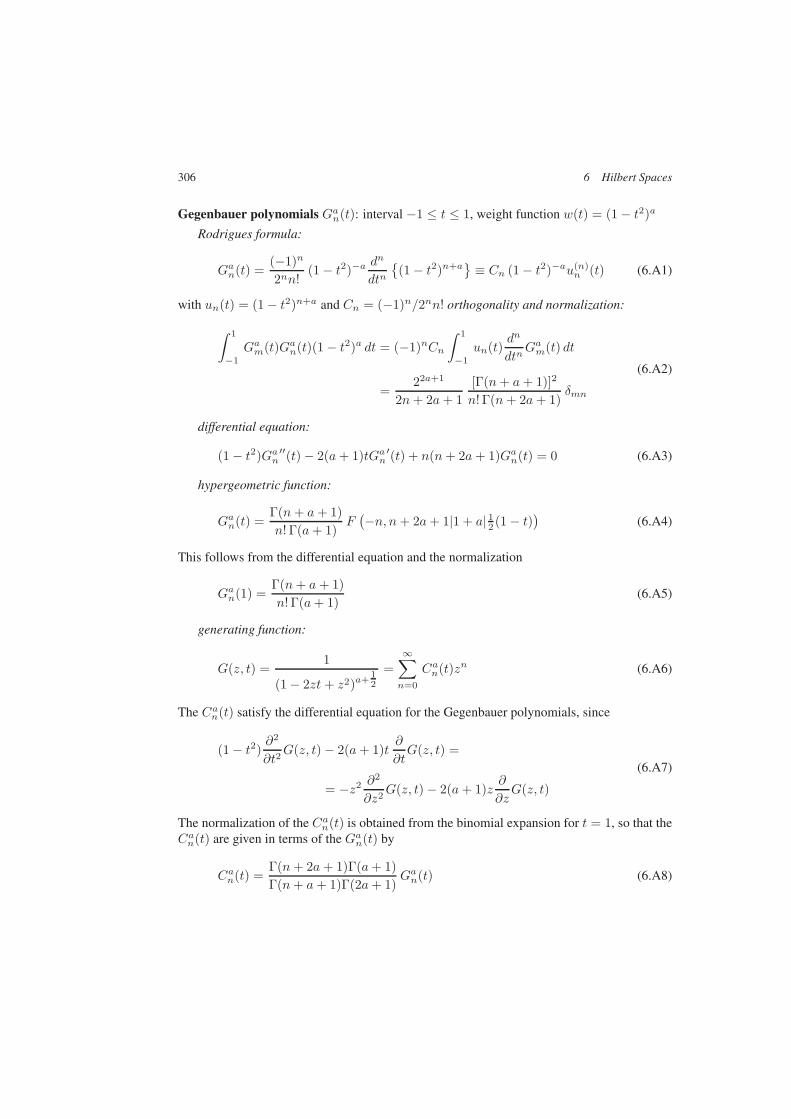
306 6 Hilbert Spaces
Gegenbauer polynomials Gan(t): interval −1 ≤ t ≤ 1, weight function w(t) = (1 − t2)a
Rodrigues formula:
Gan(t) =(−1)n
2nn!(1 − t2)−a
dn
dtn(1 − t2)n+a
≡ Cn (1 − t2)−au(n)
n (t) (6.A1)
with un(t) = (1 − t2)n+a and Cn = (−1)n/2nn! orthogonality and normalization:
∫ 1
−1
Gam(t)Gan(t)(1 − t2)a dt = (−1)nCn∫ 1
−1
un(t)dn
dtnGam(t) dt
(6.A2)
=22a+1
2n+ 2a+ 1[Γ(n+ a+ 1)]2
n! Γ(n+ 2a+ 1)δmn
differential equation:
(1 − t2)Gan′′(t) − 2(a+ 1)tGan
′(t) + n(n+ 2a+ 1)Gan(t) = 0 (6.A3)
hypergeometric function:
Gan(t) =Γ(n+ a+ 1)n! Γ(a+ 1)
F(−n, n+ 2a+ 1|1 + a| 12 (1 − t)
)(6.A4)
This follows from the differential equation and the normalization
Gan(1) =Γ(n+ a+ 1)n! Γ(a+ 1)
(6.A5)
generating function:
G(z, t) =1
(1 − 2zt+ z2)a+12
=∞∑
n=0
Can(t)zn (6.A6)
The Can(t) satisfy the differential equation for the Gegenbauer polynomials, since
(1 − t2)∂2
∂t2G(z, t) − 2(a+ 1)t
∂
∂tG(z, t) =
(6.A7)
= −z2 ∂2
∂z2G(z, t) − 2(a+ 1)z
∂
∂zG(z, t)
The normalization of the Can(t) is obtained from the binomial expansion for t = 1, so that theCan(t) are given in terms of the Gan(t) by
Can(t) =Γ(n+ 2a+ 1)Γ(a+ 1)Γ(n+ a+ 1)Γ(2a+ 1)
Gan(t) (6.A8)
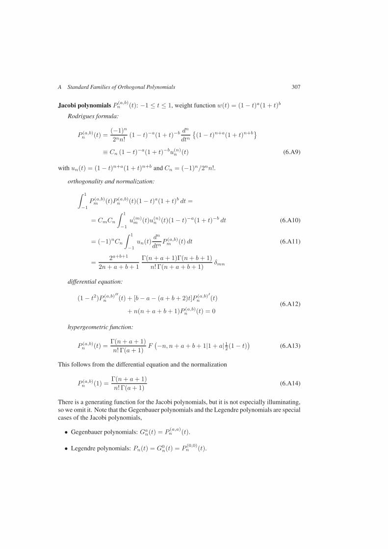
A Standard Families of Orthogonal Polynomials 307
Jacobi polynomials P (a,b)n (t): −1 ≤ t ≤ 1, weight function w(t) = (1 − t)a(1 + t)b
Rodrigues formula:
P (a,b)n (t) =
(−1)n
2nn!(1 − t)−a(1 + t)−b
dn
dtn(1 − t)n+a(1 + t)n+b
≡ Cn (1 − t)−a(1 + t)−bu(n)n (t) (6.A9)
with un(t) = (1 − t)n+a(1 + t)n+b and Cn = (−1)n/2nn!.
orthogonality and normalization:
∫ 1
−1
P (a,b)m (t)P (a,b)
n (t)(1 − t)a(1 + t)b dt =
= CmCn
∫ 1
−1
u(m)m (t)u(n)
n (t)(1 − t)−a(1 + t)−b dt (6.A10)
= (−1)nCn∫ 1
−1
un(t)dn
dtnP (a,b)m (t) dt (6.A11)
=2a+b+1
2n+ a+ b+ 1Γ(n+ a+ 1)Γ(n+ b+ 1)
n! Γ(n+ a+ b+ 1)δmn
differential equation:
(1 − t2)P (a,b)n
′′(t) + [b− a− (a+ b+ 2)t]P (a,b)
n
′(t)
(6.A12)+ n(n+ a+ b+ 1)P (a,b)
n (t) = 0
hypergeometric function:
P (a,b)n (t) =
Γ(n+ a+ 1)n! Γ(a+ 1)
F(−n, n+ a+ b+ 1|1 + a| 12 (1 − t)
)(6.A13)
This follows from the differential equation and the normalization
P (a,b)n (1) =
Γ(n+ a+ 1)n! Γ(a+ 1)
(6.A14)
There is a generating function for the Jacobi polynomials, but it is not especially illuminating,so we omit it. Note that the Gegenbauer polynomials and the Legendre polynomials are specialcases of the Jacobi polynomials,
• Gegenbauer polynomials: Gan(t) = P(a,a)n (t).
• Legendre polynomials: Pn(t) = G0n(t) = P
(0,0)n (t).
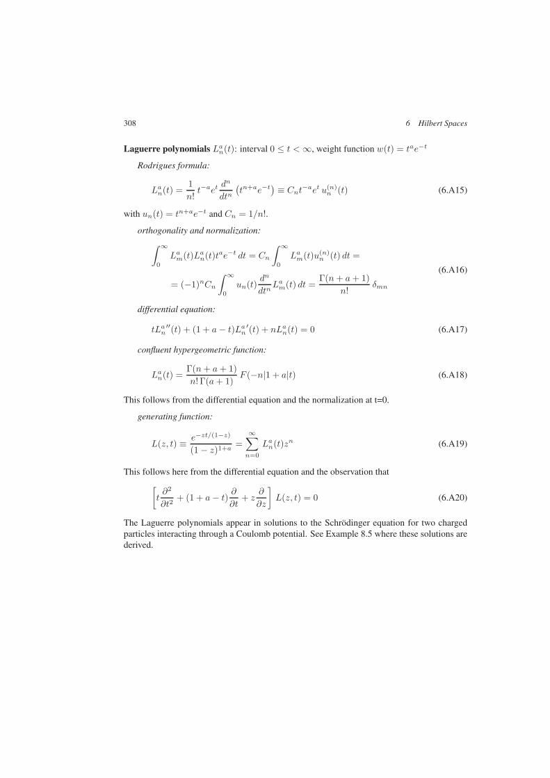
308 6 Hilbert Spaces
Laguerre polynomials Lan(t): interval 0 ≤ t <∞, weight function w(t) = tae−t
Rodrigues formula:
Lan(t) =1n!t−aet
dn
dtn(tn+ae−t
)≡ Cnt
−aet u(n)n (t) (6.A15)
with un(t) = tn+ae−t and Cn = 1/n!.
orthogonality and normalization:∫ ∞
0
Lam(t)Lan(t)tae−t dt = Cn
∫ ∞
0
Lam(t)u(n)n (t) dt =
(6.A16)
= (−1)nCn∫ ∞
0
un(t)dn
dtnLam(t) dt =
Γ(n+ a+ 1)n!
δmn
differential equation:
tLan′′(t) + (1 + a− t)Lan
′(t) + nLan(t) = 0 (6.A17)
confluent hypergeometric function:
Lan(t) =Γ(n+ a+ 1)n! Γ(a+ 1)
F (−n|1 + a|t) (6.A18)
This follows from the differential equation and the normalization at t=0.
generating function:
L(z, t) ≡ e−zt/(1−z)
(1 − z)1+a=
∞∑
n=0
Lan(t)zn (6.A19)
This follows here from the differential equation and the observation that
[t∂2
∂t2+ (1 + a− t)
∂
∂t+ z
∂
∂z
]L(z, t) = 0 (6.A20)
The Laguerre polynomials appear in solutions to the Schrödinger equation for two chargedparticles interacting through a Coulomb potential. See Example 8.5 where these solutions arederived.
A Standard Families of Orthogonal Polynomials 309
Hermite polynomials Hn(t): interval: −∞ ≤ t <∞, weight function: w(t) = e−t2
Rodrigues formula:
Hn(t) = (−1)net2 dn
dtn
(e−t
2)≡ et
2u(n)(t) (6.A21)
with u(t) = (−1)ne−t2.
orthogonality and normalization:∫ ∞
−∞Hm(t)Hn(t)e−t
2dt = (−1)n
∫ ∞
−∞e−t
2 dn
dtnHn(t) dt
(6.A22)
= 2nn!∫ ∞
−∞e−t
2dt = 2nn!
√π δmn
differential equation:
H ′′n(t) − 2tH ′
n(t) + 2nHn(t) = 0 (6.A23)
confluent hypergeometric function:
H2n(t) = (−1)n(2n)!n!
F (−n| − 12 |t
2) (6.A24)
H2n+1(t) = (−1)n(2n+ 1)!
n!tF (−n| 12 |t
2) (6.A25)
generating function:
H(z, t) ≡ e−z2+2zt =
∞∑
n=0
Hn(t)zn
n!(6.A26)
One derivation of this formula is to consider the sum
e−(z−t)2 =∞∑
n=0
[dn
dzne−(z−t)2
]
z=0
zn
n!=
(6.A27)
=∞∑
n=0
(−1)n[dn
dtne−t
2]zn
n!= e−t
2∞∑
n=0
Hn(t)zn
n!
The Hermite polynomials and the related Hermite functions hn(t) = Hn(t) exp(−12 t
2) in-troduced in Problems 6.20 and 7.16 appear in wave functions for the quantum mechanicalharmonic oscillator.
310 6 Hilbert Spaces
Bibliography and Notes
A sequel to the book by Halmos on finite-dimensional vector spaces cited in Chapter 2 is
Paul R. Halmos, Introduction to Hilbert Space (2nd edition), Chelsea (1957).
This is a brief and terse monograph, but it covers important material. To delve more deeplyinto Hilbert space, the dedicated student can also work through the excellent companion book
Paul R. Halmos, A Hilbert Space Problem Book (2nd edition), Springer (1982),
that has a rich collection of mathematical exercises and problems, with discussion, hints,solutions and references. A classic work on function spaces is
R. Courant and D. Hilbert, Methods of Mathematical Physics (vol. 1), Interscience(1953),
It contains a detailed treatment of the function spaces and orthonormal systems introducedhere, as well as a more general discussion of Hilbert spaces and linear operators.
A more modern book that provides a good introduction to function spaces, and especiallyFourier analysis, at a fairly elementary level is
Gerald B. Folland, Fourier Analysis and Its Applications, Wadsworth & Brooks/Cole (1992).
The handbook by Abramowitz and Irene Stegun cited in Chapter 8 has a comprehensive listof formulas and graphs of special functions that arise in mathematical physics and elsewhere.It is an extremely useful reference.
Wavelet analysis has been an important topic of recent research in applied mathematics.An early survey of the uses of wavelet transforms by one of the prime movers is
Ingrid Daubechies, Ten Lectures on Wavelets, SIAM (1992).
A more recent survey, with history and applications, of wavelet analysis is
Stéphane Jaffard, Yves Meyer and Robert D. Ryan, Wavelets: Tools for Science andTechnology, SIAM (2001),
Especially interesting is the broad range of applications discussed by the authors, althoughmain emphasis of the book is on signal processing. A recent elementary introduction is
David F. Walnut, Introduction to Wavelet Analysis, Birkhäuser (2002).
Problems 311
Problems
1. Let φ1, φ2, . . . be a complete orthonormal system in a Hilbert space H. Define vectorsψ1, ψ2, . . . by
ψn = Cn
(n∑
k=1
φk − nφn+1
)
(n = 1, 2, . . .).
(i) Show that ψ1, ψ2, . . . form an orthogonal system in H.
(ii) Find constants Cn that make ψ1, ψ2, . . . into an orthonormal system in H.
(iii) Show that if (ψn, x) = 0 for all n = 1, 2, . . ., then x = θ.
(iv) Verify that
‖φk‖2 = 1 =∞∑
n=1
|(ψn, φk)|2
(k = 1, 2, . . . ).
2. If xn x, then xn → x if and only if ‖xn‖ → ‖x‖.
3. Use Fourier series to evaluate the sums
ζ(2) =∞∑
n=1
1n2
and ζ(4) =∞∑
n=1
1n4
4. Find the Fourier series expansions of each of the following functions defined by theformulas for −π < x < π, and elsewhere by f(x+ 2π) = f(x).
(i) f(x) =
1/2a 0 < |x| < a (< π)0 otherwise
(ii) f(x) =
cos ax 0 < |x| < π/2a (< π)
0 otherwise
(iii) f(x) = coshαx
(iv) f(x) = sinhαx
5. Show that the functions φn(x) defined by
φn(x) ≡√
2π
cos(n+ 12 )x

312 6 Hilbert Spaces
(n = 0, 1, 2, . . .) form a complete orthonormal system in L2(0, π). Show also that thefunctions ψn(x) defined by
ψn(x) ≡√
2π
sin(n+ 12 )x
(n = 0, 1, 2, . . .) form a complete orthonormal system in L2(0, π).
6. Show that the Fourier transform and its inverse are equivalent to the formal relation∫ ∞
−∞eik(x−y) dk = 2πδ(x− y)
Give a corresponding formal expression for the discrete sum
limN→∞
DN (x− y) =∞∑
k=−∞eik(x−y)
whereDN (x−y) is the Dirichlet kernel defined by Eq. (6.47). Finally, derive the Poissonsummation formula (here c(ω) is the Fourier transform of f(t) defined by Eq. (6.81)).
∞∑
n=−∞f(n) = 2π
∞∑
k=−∞c(2πk)
7. Find the Fourier transform c(ω) of the function f(t) defined by
f(t) ≡ e−α|t|√|t|
(Reα > 0). Is c(ω) in L2(−∞,∞)? Explain your answer.
8. Find the Fourier transform of the function f(t) defined by
f(t) ≡ sinαtt
with α real. Then use Plancherel’s formula to evaluate the integral
∫ ∞
−∞
(sinαtt
)2
dt
9. Consider the Gaussian pulse
f(t) = Ae−iω0te−12α(t−t0)2
which corresponds to a signal of frequency ω0 restricted to a time interval ∆t of order1/√α about t0 by the Gaussian modulating factor exp− 1
2α(t − t0)2, which is some-times called a window function.
Problems 313
(i) Find the Fourier transform of this pulse.
(ii) Show that the intensity |Ff(ω)|2 of the pulse as a function of frequency is peakedat ω = ω0 with a finite width ∆ω due to the Gaussian modulating factor. Give a precisedefinition to this width (there are several reasonable definitions), and compute it.
(iii) Use the same definition as in part (ii) to give a precise evaluation of the time duration∆t of the pulse, and show that
∆ω · ∆t = constant
with constant of order 1 independent of the parameter α. (The precise constant willdepend on the definitions of ∆ω and ∆t).
10. (i) Show that
N∑
n=1
e2πikn
N e−2πiqn
N = Nδkq
(ii) Show that a set of numbers f1, . . . , fN can be expressed in the form
fn =N∑
k=1
cke2πikn
N (*)
with coefficients ck given by
ck =1N
N∑
m=1
fm e− 2πikm
N
(iii) Suppose the f1, . . . , fN are related to a signal
f(t) =∞∑
k=−∞ξke
2πiktT
by fn = f(nT/N). Express the coefficients ck of the finite Fourier transform in termsof the coefficients ξk in the complete Fourier series.
(iv) Show that if the f1, . . . , fN are real, then cN−k = c∗k (k = 1, . . . , N ).
Remark. The expansion (∗) is known as the finite Fourier transform. If the sequencef1, . . . , fN results from the measurement of a signal of duration T at discrete intervals∆t = T/N , then (∗) is an approximation to the Fourier integral transform, and ck cor-responds to the amplitude for frequency νk = k/T (k = 1, . . . , N ). The appearance ofhigh frequency components of the complete signal in the ck found in part (iii) is knownas aliasing; it is one of the problems that must be addressed in reconstructing a signalfrom a discrete set of observations. The result in (iv) means that the frequencies actuallysampled lie in the range 1/T ≤ ν ≤ N/2T (explain this).
314 6 Hilbert Spaces
11. Show that
N−1∑
n=1
sinnπk
Nsin
nπq
N=N
2δkq
and thus that the set of numbers f1, . . . , fN−1 can be expressed as
fn =N−1∑
k=1
bk sinkπn
N
with coefficients bk given by
bk =2N
N−1∑
m=1
fm sinmπk
N
Remark. This expansion is known as the finite Fourier sine transform.
12. Find the Laplace transforms of the functions
(i) f(t) = cosαt
(ii) f(t) = taLan(t)
where Lan(t) is the associated Laguerre polynomial defined by Eq. (6.A15).
13. Show that if f(t) is periodic with period τ , then the Laplace transform of f(t) is givenby
Lf(p) =F (p)
1 − e−pτ
where
F (p) =∫ τ
0
f(t)e−pt dt
14. Consider the differential equation
tf ′′(t) + f ′(t) + tf(t) = 0
(Bessel’s equation of order zero), and let
u(p) ≡∫ ∞
0
f(t)e−pt dt
be the Laplace transform of f(t).

Problems 315
(i) Show that u(p) satisfies the first-order differential equation
(p2 + 1)u′(p) + pu(p) = 0
(ii) Find the solution of this equation that is the Laplace transform of the Bessel functionJ0(t). Recall that the Bessel function has the integral representation (see problem 5.13).
J0(t) =1π
∫ π
0
eit cos θ dθ
15. The Mellin transform of f(t) is defined by
Mf(s) ≡∫ ∞
0
ts−1f(t) dt
(i) Show that the Mellin transform of f(t) exists for s = iξ (ξ real) if∫ ∞
0
|f(t)|2 dtt<∞
Remark. This condition is sufficient but not necessary, as in the case of the Fouriertransform.
(ii) Show that if the preceding inequality is satisfied, then the inverse Mellin transformis
f(t) =1
2πi
∫ i∞
−i∞
Mf(s)ts
ds
Also,∫ i∞
−i∞|Mf(s)|2 ds =
∫ ∞
0
|f(t)|2 dtt
(iii) Use the preceding result to show that if σ > 0,∫ ∞
0
|Γ(σ + iτ)|2 dτ =πΓ(2σ)
22σ
16. Show that the generating function
S(t, z) =1√
1 − 2zt+ t2=
∞∑
n=0
tnPn(z)
for the Legendre polynomials satisfies∫ 1
−1
S(u, z)S(v, z) dz =1√uv
ln(
1 +√uv
1 −√uv
)
Use this result to derive the orthogonality (Eq. (6.139)) and normalization (Eq. (6.140))of the Pn(t).

316 6 Hilbert Spaces
17. Show that the Gegenbauer polynomials Can(t) defined by Eq. (6.A6) satisfy
(n+ 1)Can+1(t) − (2n+ 2a+ 1)tCan(t) + (n+ 2a)Can−1(t) = 0
and
d
dtCan(t) = (2a+ 1)Ca+1
n−1(t)
18. Show that the Laguerre polynomials satisfy
tLan(t) = (n+ 1)Lan+1(t) − (2n+ a+ 1)Lan(t) + (n+ a)Lan−1(t)
and
d
dtLan(t) = −La+1
n−1(t) = Lan(t) − La+1n (t)
19. Show that the Hermite polynomials satisfy
Hn(−t) = (−1)nHn(t)
Then evaluate Hn(0) and H ′n(0) (n = 0, 1, . . .). Show further that
Hn+1(t) − 2tHn(t) + 2nHn−1(t) = 0
and
d
dtHn(t) = 2nHn−1(t)
20. Define Hermite functions hn(t) in terms of the Hermite polynomials Hn(t) by
hn(t) ≡ e−12 t
2Hn(t)
Show that∫ ∞
−∞hn(t)eiωt dt = in
√2π hn(ω)
Remark. Thus hn(t) is its own Fourier transform apart from a constant factor.
21. The Chebysheff polynomials Tn(t) are defined by
T0(t) = 1 Tn(t) =1
2n−1cos(n cos−1 t)
(n = 1, 2, . . .).
(i) Show that Tn(t) is indeed a polynomial of degree n.
(ii) Show that the Tn(t) are orthogonal polynomials on the interval −1 ≤ t ≤ 1 forsuitably chosen weight function w(t) [which you should find].
Find normalization constants Cn that make the Tn(t) into a complete orthonormalsystem.
Problems 317
22. Consider the Bessel function Jλ(x) defined by Eq. (5.162) as a solution of Bessel’s equa-tion (5.158)
d2u
dx2+
1x
du
dx+(
1 − λ2
x2
)u = 0
(i) Show that
d
dx
x
[Jλ(αx)
d
dxJλ(βx) − Jλ(βx)
d
dxJλ(αx)
]= (α2−β2)xJλ(αx)Jλ(βx)
(ii) Then show that
∫ b
a
xJλ(αx)Jλ(βx) dx = (α2 − β2)xJλ(αx)Jλ(βx)∣∣∣∣b
a
Remark. This shows that if α and β are chosen so that the endpoint terms vanish, thenJλ(αx) and Jλ(βx) are orthogonal functions on the interval [a, b] with weight functionw(x) = x (we assume 0 ≤ a < b here).
23. Consider the spherical Bessel function jn(x) defined in Section 5.6.3 as a solution of thedifferential equation (5.180)
d2u
dx2+
2x
du
dx+[1 − n(n+ 1)
x2
]u = 0
(i) Show that
d
dx
x2
[jn(αx)
d
dxjn(βx) − jn(βx)
d
dxjn(αx)
]= (α2−β2)x2jnαx)jn(βx)
(ii) Then show that
∫ b
a
x2jn(αx)jn(βx) dx = (α2 − β2)x2jn(αx)jn(βx)∣∣∣∣b
a
Remark. Again, if α and β are chosen so that the endpoint terms vanish, thenjn(αx) and jn(βx) are orthogonal functions on the interval [a, b] with weight functionw(x) = x2 (again we assume 0 ≤ a < b).
24. Consider the “hat” function g(t) defined by
g(t) =
t 0 < t ≤ 12 − t 1 < t < 20 otherwise
318 6 Hilbert Spaces
(i) Show that g(t) satisfies the relation
g(t) = 12g(2t) + g(2t− 1) + 1
2g(2t− 2)
(ii) Show that g(t) is obtained from the Haar function h0(t) by convolution,
g(t) =∫ ∞
−∞h0(τ )h0(t− τ ) dτ
(iii) Show that the Fourier transform of g(t) is given by
g(ω) ≡∫ ∞
−∞eiωtg(t) dt = eiω
(sin 1
2ω12ω
)2
(iv) Evaluate the function H(ω) defined by Eq. (6.199), and verify Eq. (6.198).
(v) Evaluate the sum
Mg(ω) ≡∞∑
m=−∞|g(ω + 2mπ)|2
and then use Eq. (6.222) to construct the Fourier transform Φ(ω) of a scaling functionφ(t) for which the φ(t− k) form an orthonormal system.
(vi) From the analytic properties of the Φ(ω) just constructed, estimate the rate of expo-nential decay of φ(t) for t→ ±∞.
25. For n = 1, the simplest nonminimal solution to Eq. (6.228) can be written as
P (y) = 1 + 2ν(ν + 2)y(y − 12 )
(the parametrization in terms of ν is chosen for convenience in the solution). In terms ofthe Fourier transform variable ω, we have
P (sin2 12ω) = 1 − 1
2ν(ν + 2) cosω(1 − cosω)
Now find constants a, b, c such that
P (sin2 12ω) =
∣∣a+ beiω + ce2iω∣∣2 ≡ |K(ω)|2
where K(ω) has been introduced in Eq. (6.224) [note that K(0) = 1]. For what rangeof values of ν are these constants real? For what value(s) of ν does the function H(ω)reduce to the case of n = 2 with minimal polynomial? For what values of ν does thescaling function reduce to the “box” function?
7 Linear Operators on Hilbert Space
The theory of linear operators on a Hilbert space H requires deeper analysis than the studyof finite-dimensional operators given in Chapter 2. The infinite dimensionality of H allowsmany new varieties of operator behavior, as illustrated by three examples.
First is a linear operator A with a complete orthonormal system of eigenvectors, whoseeigenvalues are real but form an unbounded set. A cannot be defined on all of H, but only onan open linear manifold which is, however, dense in H. Thus care must be taken to character-ize the domain of an operator on H.
Second is the linear operator X that transforms a function f(x) in L2(−1, 1) to the func-tion xf(x), which is also in L2(−1, 1). X is bounded, self-adjoint, and everywhere defined onL2(−1, 1), but it has no proper eigenvectors. We need to introduce the concept of a continuousspectrum to describe the spectrum of X.
The third example is an operator U that shifts the elements of a complete orthonormalsystem so that the image of U is a proper (but still infinite-dimensional) subspace of H. Upreserves the length of vectors (U is isometric) but is not unitary, since U† is singular. U hasno eigenvectors at all, while U† has an eigenvector for each complex number λ with |λ| < 1.
The general properties of linear operators introduced in Section 2.2 are reviewed withspecial attention to new features allowed by the infinite dimensionality of H. Linear operatorsneed not be bounded. Unbounded operators cannot be defined on the entire Hilbert space H,but at best on a dense subset D of H, the domain of the operator, which must be carefullyspecified. Bounded operators are continuous, which allows them to be defined on all of H.Convergence of sequences of operators has three forms—uniform, strong, and weak—thelatter two being related to strong and weak convergence of sequences of vectors.
Some linear operators on H behave more like their finite-dimensional counterparts. Com-pact operators transform every weakly convergent sequence of vectors into a strongly conver-gent sequence. Hilbert–Schmidt operators have a finite norm, and themselves form a Hilbertspace. Many of the integral operators introduced later are of this type. Finally, there areoperators of finite rank, whose range is finite dimensional.
The adjoint operator is defined by analogy with the finite-dimensional case, but questionsof domain are important for unbounded operators, since there are operators that are formallyHermitian, but which have no self-adjoint extension. There are operators that are isometricbut not unitary, for example, the shift operator U cited above. Further illustrations of potentialpitfalls in infinite dimensions are given both in the text and in the problems.
The theory of the spectra of normal operators is outlined. Compact normal operatorshave a complete orthonormal system of eigenvectors belonging to discrete eigenvalues, andthe eigenvalues form a sequence that converges to 0. A noncompact self-adjoint operator
Introduction to Mathematical Physics. Michael T. VaughnCopyright c© 2007 WILEY-VCH Verlag GmbH & Co. KGaA, WeinheimISBN: 978-3-527-40627-2
Introduction to Mathematical Physics
Michael T. Vaughn 2007 WILEY-VCH Verlag GmbH & Co.
320 7 Linear Operators on Hilbert Space
A may have a continuous spectrum as well as a discrete spectrum. A formal constructionadmitting this possibility is obtained by introducing the concept of a resolution of the identity,a nondecreasing family Eλ of projection operators that interpolates between 0 for λ → −∞and 1 for λ → ∞. For every self-adjoint operator A there is a resolution of the identity interms of which A can be expressed as
A =∫
λ dEλ
This generalizes the representation of a self-adjoint operator in terms of a complete orthonor-mal system of eigenvectors to include the continuous spectrum.
The definition of a linear differential operator as a Hilbert space operator must includeassociated boundary conditions. The formal adjoint of a differential operator is defined by in-tegration by parts, which introduces boundary terms. In order to make an operator self-adjoint,a set of boundary conditions must be imposed that insure that these boundary terms vanish forany function satisfying the boundary conditions. There are various possible boundary condi-tions, each leading to a distinct self-adjoint extension of the formal differential operator.
These ideas are illustrated with the operator
P =1i
d
dx
which is a momentum operator in quantum mechanics, and the second-order operator
L =d
dx
[p(x)
d
dx
]+ s(x)
(the Sturm–Liouville operator), which often appears in physics after the reduction of second-order partial differential equations involving the Laplacian (see Chapter 8) to ordinary differ-ential equations.
If Ω is a region in Rn, an integral operator K on L2(Ω) has the form
(Kf)(x) =∫
Ω
K(x, y)f(y)dy
If∫
Ω
∫
Ω
|K(x, y)|2 dxdy <∞
then K is compact, and if K is self-adjoint, or even normal, it then must have a completeorthonormal system of eigenvectors belonging to discrete eigenvalues. Such an integral op-erator often appears as the inverse of a differential operator, in which context it is a Greenfunction. If the Green function of a differential operator L has a discrete spectrum, so doesthe differential operator itself, although it is unbounded. This is most important in view ofthe other possibilities for the spectrum of a noncompact operator. If the Green function of Lcan be constructed explicitly, then it also provides the solution to inhomogeneous differentialequation
Lu = f
7.1 Some Hilbert Space Subtleties 321
7.1 Some Hilbert Space Subtleties
Many of the concepts that were introduced in the study of linear operators on finite-dimensional vector spaces are also relevant to linear operators on a Hilbert spaceH.1 However,there are new features in H, as illustrated by the following three examples.
Example 7.1. Let φ1, φ2, . . . be a complete orthonormal system on the Hilbert space H,and define the linear operator A by
Aφn = nφn (7.1)
(n = 1, 2, . . .). A has a complete orthonormal system of eigenvectors, and A is definedon any finite linear combination of the φ1, φ2, . . ., a set that is everywhere dense in H.However, A is not defined everywhere in H. The limit as N → ∞ of the vector
φN ≡N∑
n=1
1nφn (7.2)
is an element φ∞ of H, but the limit of the vector
AφN =N∑
n=1
φn (7.3)
is not. Hence Aφ∞ is not defined.Moreover, if we try to define an inverse A of A by
Aφn =1nφn (7.4)
then we have AA = 1 (there is no problem here since the range of A is a subset of thedomain of A), but it is not exactly true that AA = 1 since A is not defined on the entireHilbert space. Thus it is necessary to pay careful attention to the domain of an operator.
In general, a linear operator A is defined on H by specifying a linear manifold DA ⊂ H(the domain of A) and the vectors Ax at least for some basis of DA. The vector Ax isthen defined for any finite linear combination of the basis vectors, but it may, or may notbe possible to extend the domain of A to include the entire space H, or even all the limitpoints of sequences in DA. As we have just seen, the sequence φN) is bounded (in fact,convergent), but for the linear operator A defined by Eq. (7.1), the sequence AφN isunbounded, and hence has no limit in H.
If a linear operator A′ can be defined on a larger manifold DA′ ⊃ DA , with A′x = Axon DA, then A′ is an extension of A (A′ ⊃ A or A ⊂ A′). Thus, to be precise, we shouldwrite AA ⊂ 1 for the operator A in the present example, but often we will just writeAA = 1 anyway.
1We remind the reader that by our convention, a Hilbert space is infinite dimensional unless otherwise stated.

322 7 Linear Operators on Hilbert Space
Remark. The domain of the operator A defined by Eq. (7.1) can be characterized precisely.The vector
φ =∞∑
n=1
cnφn (7.5)
is in DA if and only if
∞∑
n=1
n2 |cn|2 <∞ (7.6)
DA is dense in H, but does not include the vector φ∞, for example.
Example 7.2. In the preceding example, the unboundedness of the operator A definedby Eq. (7.1) led to the lack of an extension of A to all of H. In this example, we will seethat even for a bounded operator, there can be something new in Hilbert space.
Consider the Hilbert space L2(−1, 1) of functions f(x) that are square integrable onthe interval −1 ≤ x ≤ 1, and define the linear operator X by
Xf(x) = xf(x) (7.7)
X is self-adjoint, and it is bounded, since
‖Xf‖2 =∫ 1
−1
|xf(x)|2 dx <∫ 1
−1
|f(x)|2 dx = ‖f‖2 (7.8)
Moreover, it is defined everywhere on L2(−1, 1).However, the eigenvalue equation
Xf(x) = λf(x) (7.9)
has no solution in L2(−1, 1), since the eigenvalue equation implies f(x) = 0 for x = λ,and this in turn means∫ 1
−1
|f(x)|2 dx = 0 (7.10)
as a Lebesgue integral. There is a formal solution
fλ(x) = δ(x− λ) (7.11)
for any value of λ between −1 and 1, but the Dirac δ-function is not in L2(−1, 1). Thus Xis a bounded self-adjoint linear operator that does not have a complete orthonormal systemof eigenvectors. The concept of discrete eigenvalues must be generalized to include acontinuous spectrum associated with solutions to the eigenvalue equation that are almost,but not quite in the Hilbert space. This will be explained in detail in Section 7.3.

7.1 Some Hilbert Space Subtleties 323
Example 7.3. Let φ1, φ2, . . . be a complete orthonormal system on the Hilbert space H,and define the linear operator U (the shift operator) by
Uφn = φn+1 (7.12)
Then
U
( ∞∑
n=1
cnφn
)=
∞∑
n=1
cnφn+1 (7.13)
is defined for every vector x =∑
cnφn in H, and ‖Ux‖ = ‖x‖, so that U†U = 1.Nevertheless, U is not unitary. We have
U†φn+1 = φn (7.14)
(n = 1, 2, . . .), but
U†φ1 = θ (7.15)
since (φ1,Ux) = 0 for every vector x. Thus
UU† = 1− P1 (7.16)
where P1 is the projection operator onto the linear manifold spanned by φ1.The spectrum of the operators U and U† is also interesting. U has no spectrum at all
since there are no solutions to the eigenvalue equation
Ux = λx (7.17)
On the other hand, the eigenvalue equation
U†x = λx (7.18)
requires the coefficients cn in the expansion of x to satisfy the simple recursion relation
cn+1 = λcn (7.19)
Thus U† has eigenvectors of the form
φλ = Nλ
(φ1 +
∞∑
n=1
λnφn+1
)(7.20)
that belong to H for any λ with |λ| < 1. Note that φλ is a unit vector if we chose thenormalization constant Nλ so that
|Nλ|2 = 1 − |λ|2 (7.21)
Eigenvectors belonging to different eigenvalues are not orthogonal, since
(φλ, φµ) =N∗λNµ
1 − λ∗µ(7.22)
and there is no completeness relation for these eigenvectors.

324 7 Linear Operators on Hilbert Space
7.2 General Properties of Linear Operators on HilbertSpace
7.2.1 Bounded, Continuous, and Closed Operators
A linear operator A on a Hilbert space H is defined on a domain DA ⊂ H. It is generallyassumed that DA contains a basis of H (if there is a nonzero vector x in D⊥
A , then Ax canbe defined arbitrarily). Then A is also defined on any finite linear combination of the basisvectors, and, in particular, on the complete orthonormal system formed from the basis bythe Gram–Schmidt process. Hence we can assume that DA contains a complete orthonormalsystem of H, and thus is dense in H.
Definition 7.1. The linear operator A is bounded if there is a constant C > 0 such that‖Ax‖ ≤ C‖x‖ for all x in DA. The smallest C for which the inequality is true is the boundof A (|A|).2
Definition 7.2. A is continuous at the point x0 in DA if for every sequence xn of vectorsin DA that converges to x0, the sequence Axn converges to Ax0.
Since A is linear, it is actually true that A is continuous at every point in DA if it iscontinuous at x = θ. For if Ayn converges to θ whenever yn converges to θ, then alsoA(xn − x0) converges to θ whenever xn − x0 converges to θ.
An important result is that if A is bounded, then A is continuous. For if A is bounded andxn converges to θ, then ‖Axn‖ converges to 0, since ‖Axn‖ ≤ |A| ‖xn‖ and ‖xn‖converges to 0. Conversely, if A is continuous (even at θ), then A is bounded. For supposeA is continuous at x = θ, but unbounded. Then there is a sequence yn of unit vectors suchthat ‖Ayn‖ > n for all n. But if we let xn ≡ yn/n, then xn converges to θ, but ‖Axn‖ > 1for all n, so Axn cannot converge to θ, contradicting the assumption of continuity.
Definition 7.3. A is closed if for every sequence xn of vectors in DA that converges to x0
for which the sequence Axn is also convergent, the limit x0 is in DA, and the sequenceAxn converges to Ax0.
If A is bounded, then A has a closed extension (denoted by [A]) whose domain is H. Forif x is a vector, then there is a Cauchy sequence xn of vectors in DA that converges to x. Butif A is bounded, then the sequence Axn is also convergent, and we can define the limit tobe Ax. An unbounded operator A may, or may not, have a closed extension. The operator Aintroduced in Example 7.1 is closed when its domain is extended to include all vectors
φ =∞∑
n=1
anφn (7.23)
for which∑∞n=1 n
2 |an|2 <∞.
2The bound |A| defined here is sometimes called the norm (or operator norm) of A. The norm introduced belowis then called the Hilbert–Schmidt norm to distinguish it from the operator norm.

7.2 General Properties of Linear Operators on H 325
However, consider the linear operator B defined by Bφn = φ1 (n = 1, 2, . . .), so that3
B
(n∑
k=1
akφk
)=
(n∑
k=1
ak
)φ1 (7.24)
If we let
xn ≡ 1n
n∑
k=1
φk (7.25)
then xn → θ (note that ‖xn‖ = 1/n). However,
Bxn = φ1 (7.26)
for all n, so Bxn is convergent, not to Bθ (= θ), but to φ1. Hence B is not closed.
Remark. Note also that B is unbounded, even though ‖Bφn‖ = ‖φ1‖ = 1 for everyelement of the complete orthonormal system φn. Hence it is not enough that B is boundedon a complete orthonormal system for B to be bounded.
7.2.2 Inverse Operator
The inverse of a linear operator on a Hilbert space must be carefully defined. Recall that thelinear operator A is nonsingular if Ax = θ only if x = θ. Here we add the new
Definition 7.4. The linear operator A is invertible if (and only if) it is bounded and there isa bounded linear operator B such that
BA = AB = 1 (7.27)
If such a B exists, then B = A−1 is the inverse of A.
An invertible operator is nonsingular, but the converse need not be true. The operator Uin Example 3 is nonsingular, bounded, and U†U = 1, but U is not invertible, since there isno operator V such that UV = 1. For the operator A in Example 1, we have AA = 1, andAA ⊂ 1 (it can be extended to 1 on all of H, but that is not the point here), although it iscommon to see A treated as A−1 (and we will also do so when no harm is done). However,it should be kept in mind that neither A nor A are invertible, strictly speaking, since A isunbounded. A general criterion for invertibility is contained in the
Theorem 7.1. If A is a linear operator on H whose domain DA and range RA are the entirespace H, then A is invertible if and only if there are positive constants m, M such that
m ‖x‖ ≤ ‖Ax‖ ≤M ‖x‖ (7.28)
for every x in H.
3It is amusing to observe that B transforms the sum of a linear combination of orthogonal vectors into the sumof the components, with a unit vector included for appearance. This operator is often (too often!) used by first-yearstudents in physics.

326 7 Linear Operators on Hilbert Space
Proof. If A is invertible, then the inequalities in (7.28) are satisfied with m = 1/∣∣A−1
∣∣ andM = |A|. Conversely, if the inequalities are satisfied, then for any y in H, we know thaty = Ax for some x in H (recall that RA, the range of A, is the set of all y such that y = Axfor some x in DA) and we can define a linear operator A by
x ≡ Ay (7.29)
Evidently A is defined on all of H, with
AA = AA = 1 (7.30)
and A is bounded, with∣∣A∣∣ = 1/m. Hence A = A−1.
7.2.3 Compact Operators; Hilbert–Schmidt Operators
A stronger concept than continuity or boundedness of an operator is compactness.
Definition 7.5. The linear operator A is compact (or completely continuous) if it transformsevery weakly convergent sequence of vectors into a strongly convergent sequence, that is, ifxn θ implies Axn → θ.
Thus, for example, if A is compact and φn is any orthonormal system, thenAφn → θ. Every compact operator is continuous, but the converse is not true (the identityoperator 1 is continuous, but not compact). The importance of compact operators becomesclear in the next section, where it will be seen that every compact normal operator has acomplete orthonormal system of eigenvectors.
Definition 7.6. Let A be a linear operator on H, and φn, ψn a pair of complete or-thonormal systems. The norm of A is defined by
‖A‖2 ≡ trA†A =∞∑
n=1
‖Aφn‖2 =∞∑
n,m=1
|(Aφn, ψm)|2 (7.31)
A is a Hilbert–Schmidt operator if ‖A‖ is finite. Here trX denotes the trace of the opera-tor X, defined as usual as the sum of diagonal elements (the sum, if it exists, is independentof the choice of complete orthonormal system).
The Hilbert–Schmidt operators themselves form a linear vector space S, which is a Hilbertspace with scalar product defined by
(A,B) ≡ trA†B =∞∑
n=1
(Aφn,Bφn) =∞∑
n,m=1
(Aφn, ψm)(ψm,Bφn) (7.32)
This claim requires proof, especially of the property of closure, but details will be left to theproblems. Any Hilbert–Schmidt operator is compact, but not conversely. For ‖A‖ to be finite,it is necessary that Aφn → 0, but Aφn → 0 does not guarantee convergence of theinfinite series defining ‖A‖2.
7.2 General Properties of Linear Operators on H 327
Example 7.4. Consider the function space L2(a, b) over the finite interval I : a ≤ t ≤ b,and suppose K(t, u) is a function in L2(I × I). Corresponding to K(t, u) is the linearoperator K in L2(a, b) defined by
(Kx)(t) =∫ b
a
K(t, u)x(u) du (7.33)
K is an integral operator of a type we will encounter again later in the chapter. Note that
‖K‖2 =∫ b
a
∫ b
a
|K(t, u)|2 dt du (7.34)
is finite by assumption, so K is a Hilbert–Schmidt operator.
Finally, a linear operator A is of finite rank if the range of A (RA, or imA) is finitedimensional. A projection operator onto a finite-dimensional linear manifold is of finite rank.The operator B defined by Eq. (7.24) is of rank 1. An operator of finite rank is certainly aHilbert–Schmidt operator, hence compact and bounded.
Remark. Every linear operator on a finite-dimensional vector space Vn is of finite rank.Hilbert–Schmidt and compact operators on H share many of the properties of operators offinite rank. For example, compact normal operators have a complete orthonormal systemof eigenvectors belonging to discrete eigenvalues that in fact form a sequence convergingto 0. Merely bounded operators are essentially infinite dimensional, with new characteris-tics not seen in finite dimensions, as illustrated by the examples in this and the precedingsection. Unbounded operators can have even more unusual properties, since they have nofinite-dimensional counterparts; it is for these that special care must be given to questions ofdomain, range, and closure.
7.2.4 Adjoint Operator
Definition 7.7. The adjoint A† of the linear operator A is defined for the vectors y for whichthere exists a vector y∗ such that
(y∗, x) = (y,Ax) (7.35)
for every x in DA. Then define
A†y ≡ y∗ (7.36)
corresponding to the finite-dimensional definition.
Remark. Note that DA must be dense in H to define A†, for if there is a nonzero vector y0in D⊥
A , then
(y∗ + y0, x) = (y∗, x) = (y,A, x) (7.37)
for every x in D⊥A , so that y∗ is not uniquely defined.
328 7 Linear Operators on Hilbert Space
To completely define A†, it is necessary to specify the domain DA† . If A is bounded,then A can be defined on all of H, and (y,Ax) is a bounded linear functional. Hence, byTheorem 2.2, there is a unique y∗ satisfying (7.35), and thus DA† is all of H. Furthermore, A†
is bounded, and∣∣A†∣∣ = |A| (7.38)
Even if A is not bounded, the adjoint A† is closed, since if yn is a sequence of vectorsin DA† such that yn → y and A†yn → y∗, then
(y,Ax) = limn→∞(yn,Ax) and (y∗, x) = lim
n→∞(A†yn, x) (7.39)
for every x in DA, so A†y = y∗. Note that A†x = θ if and only if (x,Ay) = 0 for every yin DA; in short, kerA† = R⊥
A .The operator (A†)† is well defined if (and only if) DA† is dense in H. This need not be the
case, for if we consider the operator B defined by Eq. (7.24), we have
(B†φn, φk) = (φn,Bφk) = (φn, φ1) = 0 (7.40)
and hence B†φn = θ for n = 2, 3, . . .. However,
(B†φ1, φk) = (φ1,Bφk) = 1 (7.41)
for every k. Hence B†φ1 is not defined, nor can B†φ be defined on any vector φ with anonzero component along φ1. Thus φ1 is in D⊥
B† , and DB† cannot be dense in H.On the other hand, if the operator (A†)† does exist, then it is a closed extension (even the
smallest closed extension) of A, so that
A ⊂ (A†)† = [A] (7.42)
Definition 7.8. The linear operator A is self-adjoint if
A = A† (7.43)
where equality includes the requirement DA = DA† .
In a finite-dimensional space Vn, this is equivalent to the condition
(y,Ax) = (Ay, x) (7.44)
for every x, y in DA.For an operator A on H that is bounded, it is also true that (7.43) and (7.44) are equivalent
if DA is dense in H, since in that case, we can always find a closed extension of A that isbounded. For unbounded operators, Eq. (7.44) defines a symmetric4 operator, for which it istrue that A ⊂ A†, but A may have no closed extension, in which case it cannot be self-adjoint.See Problem 12 for an important example from quantum mechanics.
4This terminology is suggested by Halmos. Equation (7.44) is often used in physics to characterize a Hermitianoperator, but it is implicitly assumed that Eq. (7.43) is then automatically satisfied. It is not, but the examples seenhere are too subtle to merit an extended explanatory digression in the standard exposition of quantum mechanics.

7.2 General Properties of Linear Operators on H 329
7.2.5 Unitary Operators; Isometric Operators
The operator U is unitary if U† = U−1, which requires
U†U = UU† = 1 (7.45)
In Vn, U†U = 1 is sufficient to have U be unitary, but the example of the shift operatordefined by Eq. (7.12) shows that this is not the case in H; the two conditions in Eq. (7.45) areindependent. The operator U is isometric if
‖Ux‖ = ‖x‖ (7.46)
for all x in DU. The shift operator is isometric, but not unitary, since its range is not the entirespace H. In general, an isometric operator U in H maps an infinite-dimensional subspaceDU into an infinite-dimensional subspace RU. H is large enough that DU⊥ and RU⊥ can benon-trivial (they can even themselves be infinite-dimensional). If we let
m ≡ dimDU⊥ , n ≡ dimRU⊥ (7.47)
then the ordered pair [m,n] is the deficiency index (DI, for short) of U.
Example 7.5. The deficiency index of the shift operator U is [0, 1], and that of U† is[1, 0]. It is true in general that if U has DI=[m,n], then U† has DI=[n,m] (show this).
U is maximal isometric if it has no proper isometric extension. This will be the case if thedeficiency index of U is of the form [m, 0] with m > 0, or [0, n] with n > 0. U is unitary ifits DI is [0, 0]. It is essentially unitary if its DI is [m,m], since we can then define a unitaryextension of U by adjoining a unitary operator from D⊥
U onto R⊥U (this extension is far from
unique, since any m-dimensional unitary operator will do).
7.2.6 Convergence of Sequences of Operators in HFor sequences of vectors in H, there are two types of convergence, weak and strong. Conver-gence of sequences An of operators in H comes in three varieties:
(i) uniform convergence. The sequence An converges uniformly to 0 (An ⇒ 0) if‖Anx‖ → 0 uniformly in x, that is, if for every ε > 0 there is anN such that ‖Ax‖ ≤ ε‖x‖for every n > N and all x in H.
(ii) strong convergence. The sequence An converges strongly to 0 (An → 0) if‖Anx‖ → 0 for every x in H.
(iii) weak convergence. The sequence An converges weakly to 0 (An 0) if(y,Anx) → 0 for every y and x in H.Convergence to a limit is then defined in the obvious way: the sequence An converges toA in some sense, if the sequence An − A converges to 0 in the same sense. If the limit isan unbounded operator, it must also be required that each of the An and the limit A can bedefined on a common domain D∗ that is dense in H, and “for all x in H” is to be understoodas “for all x in D∗.”
330 7 Linear Operators on Hilbert Space
These types of convergence are ordered, in the sense that uniform convergence impliesstrong convergence, and strong convergence implies weak convergence. In fact, only ininfinite-dimensional space are these types of convergence distinct. In Vn the three types ofconvergence are equivalent, as are strong and weak convergence of sequences of vectors (thereader is invited to show this with the help of the following example).
Example 7.6. Let φk be a complete orthonormal system, and Pk be the projectionoperator onto the linear manifold spanned by φk. Then the sequence Pk → 0 (strong,but not uniform convergence). The sequence An, with
An ≡n∑
k=1
Pk (7.48)
converges strongly, but not uniformly, to 1.
7.3 Spectrum of Linear Operators on Hilbert Space
The spectra of linear operators on an infinite-dimensional Hilbert space have a rich structurecompared with the spectra of finite-dimensional operators, much as the theory of analyticfunctions of a complex variable is rich compared to the theory of polynomials. In this section,we will consider the spectra of normal operators5 (recall A is normal if AA† = A†A). SinceA is normal if (and only if) it has the form
A = X + iY (7.49)
with X and Y self-adjoint, [X,Y] = 0 (and DA = DX ∩DY dense in H if A is unbounded),it is actually sufficient to work out the theory for self-adjoint operators.
7.3.1 Spectrum of a Compact Self-Adjoint Operator
To begin, suppose A is a compact, self-adjoint operator. A compact operator converts aweakly convergent sequence into a strongly convergent one (by definition), so the influenceof distant dimensions is reduced in some sense, and it turns that a compact, self-adjoint op-erator has a complete orthonormal system of eigenvectors with real eigenvalues, just as itsfinite-dimensional counterpart, and the eigenvalues define a sequence that converges to zero.
Since A is compact, it is bounded and closed, and (x,Ax) is real for every x in H, sinceA is self-adjoint. If we let
λ+ = sup‖x‖=1
(x,Ax), λ− = inf‖x‖=1
(x,Ax) (7.50)
then the bound of A is the larger of |λ+| and |λ−|. Since λ+ is the least upper bound of(x,Ax) on the unit sphere (‖x‖ = 1) in H, there is a sequence xn of unit vectors such
5The shift operator introduced in Section 7.1 and other operators introduced in the problems, as well as anyisometric operator that is not essentially unitary, are not normal. Those examples illustrate the additional spectraltypes that can occur with nonnormal operators.
7.3 Spectrum of Linear Operators on Hilbert Space 331
that the sequence (xn,Axn) converges to λ+. Since xn is bounded, it contains a subse-quence yn that converges weakly to a limit y (see Section 6.1). Then the compactness of Aimplies that the sequence Ayn converges strongly to a limit y∗ = Ay. Then we have
‖Ayn − λ+y‖2 = ‖Ayn‖2 − 2λ+(y,Ayn) + λ2+ → ‖y∗‖2 − λ2
+ ≤ 0 (7.51)
(note that (y,Ayn) → λ+). But ‖Ayn − λ+y‖ ≥ 0, so the only consistent conclusion isthat ‖Ayn − λ+y‖ → 0, which implies
Ay = λ+y (7.52)
Thus y is an eigenvector of A belonging to eigenvalue λ+. The same argument shows thatthere is an eigenvector of A belonging to the eigenvalue λ−. Thus every compact self-adjointoperator has at least one eigenvector belonging to a discrete eigenvalue.
Once some eigenvectors of A have been found, it is straightforward to find more. Sup-pose φ1, . . . , φn is an orthonormal system of eigenvectors of A belonging to eigenvaluesλ1, . . . , λn, that spans a linear manifold M = M(φ1, . . . , φn). Then M(φ1, . . . , φn) is aninvariant manifold of A, and, since A is normal, it follows that so is M⊥. But A is a compactself-adjoint operator on M⊥, and thus has at least one eigenvector φn+1 in M⊥ belongingto a discrete eigenvalue λn+1. Continuing this procedure leads to a complete orthonormalsystem φ1, φ2, . . . of eigenvectors belonging to discrete eigenvalues, and we have the
Theorem 7.2. Every compact normal linear operator on a Hilbert space H has a com-plete orthonormal system of eigenvectors belonging to discrete eigenvalues; the sequenceλ1, λ2, . . . of eigenvalues converges to zero.
Proof. The convergence of the sequence of eigenvalues follows from that fact that the se-quence φn of eigenvectors converges weakly to zero, and hence the sequence Aφn =λnφn → θ strongly since A is compact. A corollary of this result is that the eigenmanifoldMλ belonging to an eigenvalue λ = 0 of A must be finite dimensional.
7.3.2 Spectrum of Noncompact Normal Operators
Now suppose A is normal (but not necessarily compact, or even bounded), with a completeorthonormal system of eigenvectors and distinct eigenvalues λ1, λ2, . . . (such an operator isseparating). If Mk is the eigenmanifold belonging to eigenvalue λk, with correspondingeigenprojector Pk, then we have the spectral representation
A =∑
k
λkPk (7.53)
as in the finite-dimensional case (compare with Eq. (2.167)), except that here the sum maybe an infinite series. If the series (7.53) is actually infinite, then it converges uniformly if Ais compact, strongly if A is bounded; if A is unbounded, the series converges only on thedomain DA of A.
Normal operators that are not compact need not have a complete orthonormal system ofeigenvectors belonging to discrete eigenvalues. The concept of spectrum for such operatorsmust be generalized to include a continuous spectrum.
332 7 Linear Operators on Hilbert Space
Definition 7.9. The spectrum Σ(A) of the normal operator A consists of the complex num-bers λ such that for every ε > 0, there is a vector φ in DA for which
‖Aφ− λφ‖ < ε‖φ‖ (7.54)
The point spectrum (or discrete spectrum) Π(A) of A consists of the eigenvalues of A. Theelements of Σ(A) spectrum of A not in Π(A) form the continuous spectrum (or approximatepoint spectrum) Σc(A) of A.
Example 7.7. Consider the operator X defined on the Hilbert space L2(−1, 1) by
Xf(x) = xf(x) (7.55)
as in Example 7.2. As already noted, X has no point spectrum, but every x in the interval−1 ≤ x ≤ 1 is included in the continuous spectrum of X. To see this, suppose −1 <x0 < 1, and define the function fε(x0;x) by
fε(x0;x) =
1/√
2ε x0 − ε ≤ x ≤ x0 + ε
0 otherwise(7.56)
We have ‖fε(x0)‖ = 1, and
‖(X− x01)fε(x0)‖2 < 13ε
2 (7.57)
This works for any ε > 0, so x0 is in the continuous spectrum of X. The discussion mustbe modified in an obvious way for x0 = ±1, but the conclusion is the same. The only“eigenfunction” of X belonging to the eigenvalue x0 is the Dirac δ-function δ(x − x0),which is not in L2(−1, 1).
Exercise 7.1. Find the point spectrum and the continuous spectrum of the shift operatorU defined by Eq. (7.12). Also, find the spectra of its adjoint U†.
7.3.3 Resolution of the Identity
Equation (7.53) is a formal representation of the operator A in terms of its eigenvalues andeigenvectors. To generalize this representation to include operators with a continuous spec-trum, we need to introduce the concept of a resolution of the identity. This is a family ofprojection operators Eλ defined for the real λ, with the properties:
(i) The projection manifold Mλ of Eλ shrinks to θ for λ→ −∞ and grows to all of Hfor λ→ +∞. or
limλ→−∞
Eλ = 0 and limλ→∞
Eλ = 1 (7.58)
(ii) The projection manifold Mλ ⊆ Mµ if λ < µ, so that Eλ ≤ Eµ if λ < µ. Thus Eλis a nondecreasing function of λ that interpolates between 0 at −∞ and 1 at ∞.
7.3 Spectrum of Linear Operators on Hilbert Space 333
(iii) The limits
limε→0+
Eλ−ε ≡ E−λ and lim
ε→0+Eλ+ε ≡ E+
λ (7.59)
exist for each λ. Note that while the limits E±λ must exist for each finite λ, they need not be
equal, and the points where
∆Eλ = E+λ − E−
λ ≡ Pλ = 0 (7.60)
are the discontinuities of Eλ. Pλ is a projection operator onto a manifold of positive dimen-sion, which may be finite or infinite. There may also be points at which Eλ is continuous,but
Eλ+ε − Eλ−ε = 0 (7.61)
for every ε > 0. These are the points of increase of Eλ.If there is a finite a such that Eλ = 0 for λ < a, but Eλ > 0 for λ > a, then the family
Eλ is bounded from below (with lower bound a). If there is a finite b such that Eλ = 1 forλ > b, but Eλ < 1 for λ < b, then Eλ is bounded from above (with upper bound b). IfEλ is bounded both above and below, it is bounded and [a, b] is the interval of variation ofEλ. If it is only bounded on one end, it is semi-bounded.
If Eλ is a resolution of the identity, then the operator A defined formally by
A =∫
λ dEλ (7.62)
is self-adjoint, and bounded if and only if Eλ is bounded. The meaning of Eq. (7.62) is that6
(y,Ax) =∫
λ d(y,Eλx) =∫
λd
dλ(y,Eλx) dλ (7.66)
If A is unbounded, then the domain of A is the set of all vectors x for which the integral
‖Ax‖2 =∫
λ2d‖Eλx‖2 <∞ (7.67)
6We have the natural definitionR
df(x) =R
f ′(x)dx, which is known as a Stieltjes integral. If f(x) is notstrictly differentiable, this definition must be used with care, integrating by parts if necessary to give the integralZ
g(x) df(x) =
Zg(x)f ′(x) dx = −
Zg′(x)f(x) dx (7.63)
whenever g(x) is differentiable. The Stieltjes integral also provides an alternative definition of the Dirac δ-function.If θ(x) is the step function defined by
θ(x) =
(1 x > 0
0 otherwise(7.64)
then we haveZ ∞
−∞g(x) dθ(x) = g(0) =
Z ∞
−∞g(x)δ(x) dx (7.65)
if g(x) is continuous at x = 0.
334 7 Linear Operators on Hilbert Space
Equation (7.62) shows how a resolution of the identity defines a self-adjoint operator on H.The converse of this is Hilbert’s fundamental theorem:
Hilbert’s Fundamental Theorem. To every self-adjoint linear operator A on a Hilbertspace H, there is a unique resolution of the identity Eλ such that
A =∫
λ dEλ (7.68)
Remark. This is the Hilbert space analog of the theorem that every self-adjoint operator hasa complete orthonormal system of eigenvectors belonging to real eigenvalues.
Example 7.8. To see how the resolution of the identity works, consider again the operatorX defined by Eq. (7.9), but now let the function space be L2(a, b). If a < λ < b, we thenlet
Eλf(x) =
f(x) a ≤ x ≤ λ
0 λ < x < b(7.69)
or, more simply,
Eλf(x) = θ(λ− x)f(x) (7.70)
where θ(ξ) is the standard step function defined by Eq. (7.64). Eλ is evidently a resolutionof the identity, and
X =∫ b
a
λdEλ (7.71)
since
dEλf(x) = δ(x− λ)f(λ)dλ (7.72)
Here δ(x− λ) is the Dirac δ-function, and we have used the formal result θ′(ξ) = δ(ξ). Ifa and b are finite, then X is a bounded operator. X is unbounded in the limits a→ −∞ orb→ ∞, but the spectral representation with Eλ given by Eq. (7.70) is still valid.
Exercise 7.2. The self-adjoint operator
P ≡[1i
d
dx
]
on L2(−∞,∞) has the standard spectral representation
P =∫ ∞
∞λ dEλ
with the Eλ being a resolution of the identity. If f(x) is in the domain of P, find an expressionfor Eλf(x). Hint. Consider the Fourier integral representation of f(x).
Remark. In quantum mechanics, P is the momentum operator for a particle moving in onedimension.
7.3 Spectrum of Linear Operators on Hilbert Space 335
7.3.4 Functions of a Self-Adjoint Operator
Functions of self-adjoint operators have an elegant definition in terms of the spectral repre-sentation: if f(x) is defined for x in the spectrum of the self-adjoint operator A defined byEq. (7.62), then
f(A) =∫
f(λ) dEλ (7.73)
with domain Df(A) containing those vectors x for which
∫|f(λ)|2 d‖Eλx‖2 <∞ (7.74)
The resolvent Rα(A) of the linear operator A is defined by
Rα(A) ≡ (A − α1)−1 (7.75)
If A is a differential operator, the resolvent Rα(A) is often known as a Green function. Theresolvent Rα(A) is bounded unless α is in the spectrum of A. If α is in the point spectrumΠ(A) of A then (A−α1) is singular, and Rα(A) can only be defined on M⊥
α , where Mα isthe eigenmanifold of A belonging to eigenvalue α. If α is in the continuous spectrum Σc(A)of A, then Rα(A) is unbounded, but defined on a dense subset of H.
If A is self-adjoint, with resolution of the identity Eλ, then the resolvent Rα(A) isgiven formally by
Rα(A) =∫
1λ− α
dEλ (7.76)
This expression will be used to provide a more explicit construction of the resolvent operatorsfor certain differential operators to appear soon.
If A is a normal operator, then it can be written in the form A = X + iY, with X and Yself-adjoint and [X,Y] = 0. If
X =∫
λdEλ, Y =∫
µdFµ (7.77)
then [Eλ,Fµ] = 0 for every λ, µ. If U is a unitary operator, then there is a resolution of theidentity Hφ with interval of variation ⊆ [0, 2π] such that
U =∫
eiφ dHφ (7.78)
Now that we have reviewed the abstract properties of linear operators on a Hilbert space, itis time to turn to the concrete examples of linear differential and integral operators that appearin practically every branch of physics.
336 7 Linear Operators on Hilbert Space
7.4 Linear Differential Operators
7.4.1 Differential Operators and Boundary Conditions
Linear differential operators of the form
L ≡ p0(x)dn
dxn+ p1(x)
dn−1
dxn−1+ · · · + pn−1(x)
d
dx+ pn(x) (7.79)
were introduced in Chapter 5 (see Eq. (5.50)) and described there from an analytical pointof view. Now we consider L as a linear operator on a Hilbert space of the type L2(a, b).Note that L is unbounded, since the derivative of a smooth function can be arbitrarily large.The formal domain of L as a differential operator includes the class Cn(a, b) of functionsthat are continuous together with their first n derivatives on the interval (a, b), and Cn(a, b) iseverywhere dense in L2(a, b).
But to consider L as a Hilbert space operator, we must define the domain of L moreprecisely. In particular, we must carefully specify the boundary conditions to be imposed onfunctions included in the Hilbert space domain of L in order to verify properties, such as self-adjointness, that are critical to understanding the spectrum of L. Indeed, we will see from theexamples given here that the spectrum can be more sensitive to the boundary conditions thanto the operator itself.
The simplest linear differential operator is the derivative D defined by
Df(x) =d
dxf(x) (7.80)
for functions that are differentiable on a ≤ x ≤ b, and extended by closure. Now integrationby parts gives
(g,Df) =∫ b
a
g∗(x)d
dxf(x) dx
= [g∗(b)f(b) − g∗(a)f(a)] −∫ b
a
f(x)d
dxg∗(x) dx (7.81)
= −(Dg, f) +B(g, f)
where the boundary term B(g, f), also known as the bilinear concomitant,
B(g, f) ≡ g∗(b)f(b) − g∗(a)f(a) (7.82)
contains the endpoint terms from the integration by parts.In order to make a self-adjoint operator from D, we first need to fix the minus sign on the
right-hand side of Eq. (7.81). To do this, simply define
P ≡ −iD (7.83)
(the factor −i is chosen so that P can be identified with the usual momentum operator inquantum mechanics for appropriate boundary conditions). Then we need to choose boundary
7.4 Linear Differential Operators 337
conditions on the values of the functions at the endpoints to make the boundary term B(g, f)vanish identically. This can be arranged by imposing the periodic boundary condition
f(b) = f(a) (7.84)
With this boundary condition, P is a self-adjoint operator on L2(a, b).Remark. More generally, it is sufficient to require
f(b) = αf(a) (7.85)
with |α| = 1. Thus α has the form α = exp(2πiξ) and there is a continuous family Pξ
(0 ≤ ξ ≤ 1) of self-adjoint extensions of the linear operator −iD. Which extension is ap-propriate for a particular physical problem must be determined by the physics. The boundarycondition (7.84), corresponding to α = 1, is most often physically correct, but there arefermionic systems for which (7.85) with α = −1 is relevant.
With the periodic boundary condition (7.84), P has a complete orthonormal systemφn(x) of eigenvectors given by
φn(x) =1√b− a
exp(
2nπixb− a
)(7.86)
(n = 0,±1,±2, . . .) belonging to eigenvalues
λn =2nπb− a
(7.87)
This analysis must be modified if a → −∞ or b → ∞. P is already self-adjointon L2(−∞,∞); the boundary term B(g, f) vanishes automatically, since f(x) → 0 forx → ±∞. But the discrete eigenvalues merge into a continuous spectrum, and the completeorthonormal system (7.86) of eigenvectors must be replaced by a continuous resolution of theidentity (see Exercise 7.2). On a semi-infinite interval (L2(0,∞) for example) the behavior ofP is more complicated; see Problem 12.
Exercise 7.3. Consider the linear operator Pξ defined by
Pξ φ(x) ≡ 1i
d
dxφ(x)
for differentiable functions φ(x) in L2[−π, π] that satisfy the boundary condition
φ(π) = e2πiξ φ(−π)
with ξ real. Find the eigenvalues of Pξ, and construct a complete orthonormal system ofeigenvectors. Then characterize the domain of the closure of Pξ in terms of these eigenvectors.Is Pξ self-adjoint for any (real) ξ?

338 7 Linear Operators on Hilbert Space
7.4.2 Second-Order Linear Differential Operators
The general second-order linear differential operator on L2(a, b) has the form
L = p(x)d2
dx2+ q(x)
d
dx+ r(x) (7.88)
Here integration by parts gives
(g,Lf) =∫ b
a
g∗(x)L[f(x)]dx =∫ b
a
(L[g(x)])∗f(x)dx+B(g, f) (7.89)
where the adjoint differential operator L is defined by
L[g(x)] =d2
dx2[p∗(x)g(x)] − d
dx[q∗(x)g(x)] + r∗(x)g(x) (7.90)
and the boundary term is given by
B(g, f) = p(x) [g∗(x)f ′(x) − g′∗(x)f(x)]∣∣ba
+ g∗(x) [q(x) − p′(x)] f(x)∣∣ba
(7.91)
For L to be symmetric (L = L) we have the requirements:
(i) p∗(x) = p(x) (p(x) must be real),
(ii) p′(x) = Re q(x) and
(iii) Im q′(x) = 2 Im r(x).If these conditions are satisfied, then L has the form
L =d
dx
[p(x)
d
dx
]+ iξ(x)
d
dx
[ξ(x) ·
]+ s(x) (7.92)
with p(x), ξ(x) =√
Im q(x) and s(x) = Re r(x) real functions. The term containing ξ(x)is absent if the operator L is real, which is often the case in practice.
To consider the boundary term let us suppose that L is real, to simplify the discussion.Then we have p′(x) = q(x) and the boundary term is simply
B(g, f) = p(x) [g∗(x)f ′(x) − g′∗(x)f(x)]∣∣∣∣b
a
(7.93)
If p(x) = 0 at an endpoint, the differential equation is singular at the endpoint, but we canrequire that the solution be regular at that endpoint, which eliminates the contribution of thatendpoint to the boundary term. If p(x) = 0 at the endpoint x = τ (τ = a, b), then theendpoint contribution to B(g, f) from x = τ will vanish if both f(x) and g(x) satisfy aboundary condition of the form
cf(τ ) + c′f ′(τ ) = 0 (7.94)
with c, c′ being constants, one of which may vanish.
7.5 Linear Integral Operators; Green Functions 339
The operator L in the form
L =d
dx
[p(x)
d
dx
]+ s(x) (7.95)
is a Sturm–Liouville operator, and the boundary conditions required to make L self-adjointare precisely those encountered in physical systems governed by the Laplace equation or thewave equation, as will be seen shortly.
Remark. Note that the differential operator L can be multiplied by a function ρ(x) withoutchanging the solutions to the differential equation. Thus an operator that is not symmetric atfirst sight may in fact be converted to one which is by an inspired choice of multiplying factorρ(x). For examples, see Problems 13 and 14.
One important tool to analyze the spectrum of a Sturm–Liouville operator L, or any lineardifferential operator for that matter, is to find, or prove the existence of, a linear integraloperator K such that LK = 1. For if the integral operator K is compact (which it certainlywill be if the domain of integration is bounded) and normal, then it has a complete orthonormalsystem of eigenvectors belonging to discrete eigenvalues λn, and these eigenvectors will alsobe eigenvectors of L, with eigenvalues 1/λn. We now turn to the study of integral operators.
7.5 Linear Integral Operators; Green Functions
7.5.1 Compact Integral Operators
Consider the function space L2(Ω) with Ω being a bounded region in Rn (often Ω is just aninterval [a, b] in one dimension). Suppose K(x, y) is a function on Ω × Ω such that
‖K‖2 =∫
Ω
∫
Ω
|K(x, y)|2 dx dy <∞ (7.96)
Then corresponding to K(x, y) is a linear operator K on L2(Ω) defined by
g(x) ≡ (Kf)(x) =∫
Ω
K(x, y)f(y) dy (7.97)
K is an integral operator; K(x, y) is the kernel 7 corresponding to K. The condition (7.96)insures that K is a Hilbert–Schmidt operator, and hence compact.
Remark. Other operators can be expressed as integral operators, even if they do not satisfythe condition (7.96). For example, the identity operator 1 can be represented as an integraloperator with kernel
K(x, y) = δ(x− y) (7.98)
where δ(x−y) is the Dirac δ-function, even though this kernelK(x, y) does not satisfy (7.96),and the representation is valid only on the linear manifold of functions that are continuous on
7The term “kernel” introduced here is not to be confused with the kernel of an operator introduced in Chapter 2as the linear manifold transformed into the zero vector by the operator. The double usage is perhaps unfortunate, butconfusion can be avoided by paying attention to context.

340 7 Linear Operators on Hilbert Space
Ω. Note, however that this manifold is dense in L2(Ω). Integral operators are also useful whendefined on unbounded regions, when (7.96) need not be satisfied even by bounded continuouskernels K(x, y).
The adjoint operator K† is given by
(K†f)(x) =∫
Ω
K∗(y, x)f(y) dy (7.99)
which corresponds to the expression for the matrix elements of the adjoint operator given inEq. (2.2.88). Thus K is self-adjoint if and only if
K(y, x) = K∗(x, y) (7.100)
almost everywhere.If K is self-adjoint, and compact due to condition (7.96), then we know that it has a com-
plete orthonormal system φn(x) of eigenvectors belonging to discrete real eigenvalues, andthe sequence λn of eigenvalues converges to zero. This leads to the formal representation
K(x, y) =∑
n
λnφn(x)φ∗n(y) (7.101)
which is valid in the sense of strong L2(Ω × Ω) convergence.Somewhat stronger results can be derived if the kernel K(x, y) is continuous, or even if
the iterated kernel
K2(x, y) ≡∫
Ω
K(x, z)K(z, y) dz (7.102)
which corresponds to the operator K2, is a continuous function of x in Ω for fixed y, or evenif K2(x, x) is continuous in x. In that case
K2(x, y) =∑
n
λ2nφn(x)φ∗n(y) (7.103)
is uniformly convergent in Ω × Ω, and any function g(x) in the range of K has an expansion
g(x) =∑
n
cnφn(x) (7.104)
that is uniformly convergent in Ω.These results follow from the continuity of K2(x, y), which implies that eigenvectors
φn(x) of K belonging to nonzero eigenvalues are continuous functions of x. To see this,suppose Kφ = λφ with λ = 0. Then
λφ(x) =∫
Ω
K(x, y)φ(y) dy (7.105)
and
λ [φ(x) − φ(x′)] =∫
Ω
[K(x, y) −K(x′, y)]φ(y) dy (7.106)
7.5 Linear Integral Operators; Green Functions 341
The Schwarz inequality then gives
λ2 |φ(x) − φ(x′)|2 ≤ ‖φ‖2
∫
Ω
|K(x, y) −K(x′, y)|2 dy (7.107)
and the right-hand side is continuous, hence vanishes when x→ x′.Equation (7.101) gives the expansion ofK(x, y) with respect to the complete orthonormal
system φm(x)φ∗n(y) on Ω × Ω. Expansion in terms of y alone has the form
K(x, y) =∑
n
fn(x)φ∗n(y) (7.108)
when fn(x) = λnφn(x) follows from the fact that the φn(y) are eigenvectors of K. Thenalso
K2(x, x) =∫
Ω
|K(x, y)|2 dy =∑
n
λ2n |φn(x)|2 (7.109)
and the convergence is uniform since the limit is continuous.8 The uniform convergence inEq. (7.103) then follows using the Schwarz inequality again.
7.5.2 Differential Operators and Green Functions
Now suppose L is a self-adjoint linear differential operator with boundary conditions thatallow L to be defined as a self-adjoint operator on L2(Ω). If λ is a real constant not in thespectrum of L, consider the inhomogeneous equation
(L − λ1)u(x) = f(x) (7.110)
The solution to Eq. (7.110) has the general form
u(x) =∫
Ω
Gλ(x, y)f(y) dy (7.111)
where Gλ(x, y), the Green function for (L − λ1), is the solution of the formal differentialequation
(L − λ1)xGλ(x, y) = δ(x− y) (7.112)
satisfying the appropriate boundary conditions when x is on the boundary of Ω. That thesolution has the form (7.111) is clear from the linearity of L, and Eq. (7.112) is a formalexpression of the linearity.
What is less obvious, but also true, is that Gλ(x, y) satisfies the symmetry condition
Gλ(x, y) = G∗λ(y, x) (7.113)
8This is Dini’s theorem in real analysis.

342 7 Linear Operators on Hilbert Space
This is plausible, since Gλ(x, y) is the kernel of an integral operator Gλ that is the inverse ofa self-adjoint operator (L−λ1). Rather than give a more rigorous proof, we will illustrate theconstruction of the Green function Gλ(x, y) for various differential operators in the examplesand problems.
The main significance of the existence of the self-adjoint inverse Gλ of L−λ1 is that Gλ iscompact so long as the region Ω is bounded. Hence it has a complete orthonormal system φnof eigenvectors, with corresponding discrete eigenvalues γn forming a sequence convergingto zero. Then the differential operator L − λ1 has the same eigenvectors, with
(L− λ1)φn = (1/γn)φn (7.114)
and L itself has the same eigenvectors φn, with eigenvalues
λn = λ+1γn
(7.115)
obtained directly from the eigenvalues of Gλ. The consequences of this discussion are impor-tant enough to state them as a formal theorem:
Theorem 7.3. Let L be a self-adjoint linear differential operator on the space L2(Ω), with Ωa bounded region. Then
1. L has a complete orthonormal system φn of eigenvectors belonging to discrete eigen-values λn such that the sequence 1/λn converges to zero; hence the sequence λn isunbounded.
2. For every λ not in the spectrum of L, the inhomogeneous equation (7.110) has thesolution
f(x) = (L − λ1)−1u(x) =∫
Ω
Gλ(x, y)f(y) dy (7.116)
with Green function Gλ(x, y) in L2(Ω × Ω). The Green function has the expansion
Gλ(x, y) =∑
n
φn(x)φ∗n(y)λn − λ
(7.117)
in terms of the normalized eigenvectors φn of L.
Example 7.9. Consider the differential operator
∆ ≡ d2
dx2(7.118)
on L2(0, 1), defined on functions u(x) that satisfy the boundary conditions
u(0) = 0 = u(1) (7.119)
These boundary conditions define ∆ as a self-adjoint linear operator (other self-adjointboundary conditions appear in Problem 15). Since λ = 0 is not an eigenvalue of ∆ (show
7.5 Linear Integral Operators; Green Functions 343
this), we can find the Green function G0(x, y) for ∆ with these boundary conditions as asolution of
∂2
∂x2G0(x, y) = −δ(x− y) (7.120)
(the minus sign here is conventional), with
G0(0, y) = 0 = G0(1, y) (7.121)
For x = y, Eq. (7.120) together with symmetry requires
G(x, y) =
ax(1 − y) x < y
a(1 − x)y x > y(7.122)
while as x→ y, it requires
limε→0+
[∂G0
∂x
]
x=y+ε
−[∂G0
∂x
]
x=y−ε
= −1 (7.123)
Thus we need a(1 − y) + ay = 1, whence the constant a = 1.For λ = −k2 = 0, the Green function Gλ(x, y) must satisfy
(∂2
∂x2+ k2
)Gλ(x, y) = −δ(x− y) (7.124)
with the same boundary conditions as above. Then we have
Gλ(x, y) =
A sin kx sin k(1 − y) x < y
A sin k(1 − x) sin ky x > y(7.125)
and the condition (7.123) now requires
Ak [cos ky sin k(1 − y) + cos k(1 − y) sin ky] = Ak sin k = 1 (7.126)
This uniquely determines A if sin k = 0, and we have
Gλ(x, y) =
sin kx sin k(1 − y)k sin k
x < y
sin k(1 − x) sin kyk sin k
x > y
(7.127)
when sin√−λ = 0.
Remark. Note that the eigenvalues of ∆ have the form
λn = −n2π2 (7.128)

344 7 Linear Operators on Hilbert Space
with corresponding normalized eigenfunctions
φn(x) =√
2 sinnπx (7.129)
(n = 1, 2, . . .). Thus sin k = 0 corresponds to a value of λ in the spectrum of ∆, except forthe case λ = 0 (k = 0) which is not an eigenvalue for the boundary condition given here.Note also that
limλ→0
Gλ(x, y) = G0(x, y) (7.130)
The expansion (7.117) then implies∞∑
n=1
sinnπx sinnπyn2π2 − k2
=sin kx sin k(1 − y)
2k sin k(7.131)
for x < y, with the corresponding result for x > y obtained by interchanging x and y. Anindependent verification of this result follows from the integral
∫ 1
0
Gλ(x, y) sinnπy dy =sinnπxn2π2 − k2
(7.132)
which is obtained by a straightforward but slightly long calculation.
Bibliography and Notes
The book on Hilbert space by Halmos as well as others cited in Chapter 6 gives further detailsof the mathematical properties of linear operators on Hilbert space. The standard textbook byByron and Fuller cited in Chapter 2 emphasizes linear vector spaces.
There are many modern books on quantum mechanics that discuss the essential connectionbetween linear vector spaces and quantum mechanics. Two good introductory books are
David J. Griffiths, Introduction to Quantum Mechanics (2nd edition), Prentice-Hall(2004).
Ramamurti Shankar, Principles of Quantum Mechanics (2nd edition), Springer(2005)
Slightly more advanced but still introductory is
Eugen Merzbacher, Quantum Mechanics (3rd edition), Wiley (1997).
Two classics that strongly reflect the original viewpoints of their authors are
Paul A. M. Dirac, The Principles of Quantum Mechanics (4th edition), ClarendonPress, Oxford (1958)
John von Neumann, Mathematical Foundations of Quantum Mechanics, PrincetonUniversity Press (1955).
Dirac’s work describes quantum mechanics as the mathematics flows from his own physi-cal insight, while von Neumann presents an axiomatic formulation based on his deep under-standing of Hilbert space theory. Both are important works for the student of the historicaldevelopment of the quantum theory.
Problems 345
Problems
1. Let φn (n = 1, 2, . . .) be a complete orthonormal system in the (infinite-dimensional)Hilbert space H. Consider the operators Uk defined by
Ukφn = φn+k
(k = 1, 2, . . .).
(i) Give an explicit form for U†k.
(ii) Find the eigenvalues and eigenvectors of Uk and U†k.
(iii) Discuss the convergence of the sequences Uk, U†k, U†
kUk, UkU†k.
2. Let φn (n = 1, 2, . . .) be a complete orthonormal system in H, and define the linearoperator T by
Tφn ≡ nφn+1 (n = 1, 2, . . .)
(i) What is the domain of T?
(ii) How does T† act on φ1, φ2, . . .? What is the domain of T†?
(iii) Find the eigenvalues and eigenvectors of T.
(iv) Find the eigenvalues and eigenvectors of T†.
3. Let φn (n = 0,±1,±2, . . .) be a complete orthonormal set in the Hilbert space H.Consider the operator A defined by
Aφn = a(φn+1 + φn−1)
(i) Is A bounded? compact? self-adjoint?
(ii) Find the spectrum of A.
Hint. Try to find an explicit representation of A on the function space L2(−π, π).
4. Suppose we add a “small” perturbation to the operator A in the preceding problem. Let
B ≡ A + V ≡ A + ξP0
where P0 projects onto the linear manifold spanned by φ0, and ξ is a real constant thatmay be either positive or negative.
(i) Is B bounded? compact? self-adjoint?
(ii) Find the spectrum of B.
5. Let φn (n = 0,±1,±2, . . . ) be a complete orthonormal set in the Hilbert space H.Consider the operators UN defined by
UNφn = φn+N

346 7 Linear Operators on Hilbert Space
(N = ±1,±2, . . . ). These are not the same operators as in Problem 1, since the range ofindices on the complete orthonormal system is different!
(i) Give an explicit form for U†N .
(ii) Is UN bounded, compact, unitary?
(iii) Find the spectra of UN and U†N .
(iv) Find a unitary operator SN such that U†N = SNUNS†
N . Is SN unique?
(v) Discuss the convergence of the sequences UN, U†N, U†
NUN and UNU†N
in the limit N → ∞.
Hint. Again, try to find an explicit representation of U on the function space L2(−π, π).
6. Consider the three-dimensional Lie algebra spanned by the linear operators A, A and 1,satisfying the commutation relations
[A,1] = 0 = [A,1], [A, A] = 1
Remark. Strictly speaking, the last commutator should be written as[A, A
]⊂ 1
since the domain of the commutator cannot be the entire space H. There is a generaltheorem, which we will not prove here, that if [B,C] is a constant, then B and C mustbe unbounded. Note that the results found here are consistent with the theorem.
(i) Show that the operator N ≡ AA satisfies the commutation relations
[N,A] = −A,[N, A
]= A
(ii) Suppose φλ is an eigenstate of N with Nφλ = λφλ. Show that
N(Aφλ) = (λ− 1)Aφλ
N(Aφλ) = (λ+ 1)Aφλ
Remark. Thus A and A are ladder operators (or raising and lowering operators forN, since they raise (A) or lower (A) the eigenvalue of N by 1. In a quantum mechanicalcontext, N is an operator representing the number of quanta of some harmonic oscillatoror normal mode of a field (the electromagnetic field, for example), in which case theoperators represent creation (A) and annihilation (A) operators for the quanta.
(iii) Since N ≥ 0, the lowest eigenvalue of N must be λ = 0, and thus the eigenvaluesof N are λ = 0, 1, 2, . . ., with unit eigenvectors φn corresponding to λ = n. Show that
‖Aφn‖ =√n, ‖Aφn‖ =
√n+ 1
and then that phases can be chosen so that
Aφn =√n φn−1, Aφn =
√n+ 1 φn+1
Problems 347
Remark. The creation and annihilation operators introduced in this problem satisfycommutation rules, and the quanta they create obey Bose–Einstein statistics. Hence theyare known as bosons. In our world, there are also spin-1
2 particles (electrons, protons,neutrons, quarks, etc.) for which the number of quanta present in a specific state can onlybe zero or 1 (this is often stated as the Pauli exclusion principle). These particles obeyFermi–Dirac statistics, and hence are known as fermions. A formalism that incorporatesthe Pauli principle introduces creation and annihilation operators for fermions that sat-isfy anticommutation rules, rather than the commutation rules for boson operators—seeProblem 8.
7. Suppose A is a linear operator whose commutator with its adjoint is given by[A,A†] ≡ AA† − A†A = 1
as in the preceding problem (where A is identified with A†).
(i) Show that A has a normalized eigenvector ψα for any complex number α, and findthe expansion of the ψα in terms of the φn.
(ii) Show that any vector x in H can be expanded in terms of the normalized φα as
x =∫
ψα (ψα, x) ρ(α) d2α
for suitable weight function ρ(α), and find ρ(α).
Remark. As noted above, N corresponds in quantum theory to the number of quanta ofsome harmonic oscillator, and A and A† act as annihilation and creation operators for thequanta. The eigenvectors ψα are coherent states of the oscillator, corresponding in somesense to classical oscillations with complex amplitude α. See the quantum mechanicsbooks cited in the notes for more discussion of these states.
(iii) Find the eigenvectors of A†.
8. Let a†σ, aσ be the creation and annihilation operators for a spin-12 fermion in spin state σ
[σ = ±12 , or spin up (↑) and spin down (↓)]. These satisfy the anticommutation rules
a†α, aβ = a†αaβ + aβa†α = δαβ1
a†α, a†β = 0 = aα, aβ
(i) Show that the number operator
Nα ≡ a†αaα
satisfies[Nα, a
†]
= −δαβaβ ,[Nα, a
†β
]= δαβa
†β
(ii) Show that Nα has eigenvalues 0, 1.
348 7 Linear Operators on Hilbert Space
Remark. Hence the Pauli exclusion principle follows from the anticommutation rules.
(iii) From (ii) it follows that a basis for the fermion states is the set
|0〉 | ↑ 〉 ≡ a†↑|0〉 | ↓ 〉 ≡ a†↓|0〉 | ↑↓ 〉 ≡ a†↑| ↓ 〉
Write down the matrices representing the operators aα, a†α, and Nα in this basis.
Remark. Both here and in Problem 6, the creation and annihilation operators are thosefor a single mode of the relevant particle. For physical particles, there are many modes,labeled by momentum, energy and other possible quantum labels, and we will have cre-ation and annihilation operators defined for each such mode.
9. Let Ak and Bk be two sequences of operators on the (infinite-dimensional) Hilbertspace H such that
Ak → A and Bk → B
(i) Show that AkBk → AB.
(ii) If Ak → A and Bk B, what can you say about the convergence of thesequence AkBk?
(iii) If Ak A and Bk B, what can you say about the convergence of thesequence AkBk?
10. Consider a pair of operators Q and P that satisfy the commutation rules
[Q,P] ≡ QP − PQ = ε1
Remark. Again, this should be written [Q,P] ⊂ ε1 to be precise.
(i) Show that
[Q,Pn] = nεPn−1
[Qn,P] = nεQn−1
(ii) Show that if A, B are two operators that are polynomials in Q and P, then we have
[A,B] = ε
∂A∂Q
∂B∂P
− ∂B∂Q
∂A∂P
to lowest order in ε.
11. Consider the linear operator
P ≡[1i
d
dx
]

Problems 349
defined on L2(−π, π) (here the bracket [ ] denotes the closure of the operator). Thefunctions φn(x) ≡ einx/
√2π (n = 0,±1,±2, . . .) are eigenvectors of P, with
Pφn(x) = nφn(x)
However, it also appears that the functions
φλ(x) ≡1√2π
eiλx
are eigenvectors of P for any complex λ. This seems puzzling, since we know from thetheory of Fourier series that the φn(x) with integer n form a complete orthonormalsystem of eigenvectors of P. To clarify the puzzle, first calculate the coefficients cn(λ)in the expansion
φλ(x) =∞∑
n=−∞cn(λ)φn(x)
Then find the expansion of Pφλ(x). Is this the expansion of a vector in the Hilbertspace? Explain and discuss.
12. The linear operator
A =[1i
d
dx
]
is symmetric on L2(0,∞) when restricted to functions f(x) for which f(0) = 0. How-ever, A† is defined on a larger domain, whence A ⊂ A†, and A need not be self-adjoint.
(i) Show that A has eigenvectors fα(x) = exp(iαx) that are in L2(0,∞) for any α inthe upper half α-plane (Im α > 0).
Remark. This shows that A cannot be self-adjoint, since a self-adjoint operator hasonly real eigenvalues.
(ii) Find formal eigenvectors of the operator
Aκ ≡ A − iκ
x
corresponding to eigenvalues α in the upper half α-plane. For what values of κ are theseeigenvectors actually in L2(0,∞)?
Remark. The operators Aκ satisfy the commutation rule [Aκ, x] ⊂ 1 for any κ. Thiscommutator is required in quantum mechanics of an operator corresponding to the mo-mentum conjugate to the coordinate x, which might be a radial coordinate in sphericalor cylindrical coordinates, for example. Quantum mechanical operators correspondingto observables must also be strictly self-adjoint, and not merely symmetric. Hence thenaive choice of A = A0 as the momentum conjugate to the radial coordinate does notwork, and a suitable Aκ must be used instead. The reader is invited to decide which Aκ
might be appropriate in spherical or cylindrical coordinates.

350 7 Linear Operators on Hilbert Space
13. (i) Under what conditions on the parameters a, b, c is the differential operator
L = x(x− 1)d2
dx2+ [(a+ b+ 1)x− c]
d
dx+ ab
in the hypergeometric equation (5.5.A13) symmetric, and self-adjoint in L2(0, 1)?
(ii) Under what conditions is there a function ρ(x) such that ρ(x)L is symmetric, andself-adjoint in L2(0, 1)?
14. (i) Under what conditions on the parameters a and c is the differential operator
L = xd2
dx2+ (c− x)
d
dx− a
in the confluent hypergeometric equation (5.5.B38) symmetric, and self-adjoint inL2(0,∞)?
(ii) Under what conditions is there a function ρ(x) such that ρ(x)L is symmetric, andself-adjoint in L2(0,∞)?
15. Consider the operator
∆ ≡ d2
dx2
defined on the (complex) function space L2(−1, 1).
(i) If f and g are two functions that are twice differentiable, compute
B(f, g) ≡ (f,∆g) − (∆f, g)
in terms of the boundary values of f and g at x = ±1.
(ii) Find the complete class of boundary conditions on f and g that lead to a self-adjointextension of the operator ∆ to a maximal domain.
(iii) The functions exp(αx) are formal eigenfunctions of ∆ for any complex α. Whatvalues of α are consistent with each of the boundary conditions introduced in part (ii)?In other words, find the spectrum of ∆ for each boundary condition that defines ∆ as aself-adjoint operator on L2(−1, 1).
(iv) Find the Green function Gλ(x, y) = (∆−λ1)−1 for each of the self-adjoint bound-ary conditions introduced in parts (ii) and (iii).
Problems 351
16. Consider the linear differential operator
K ≡ − d2
dx2+ x2
defined on L2(−∞,∞).
(i) Show that K is self-adjoint.
(ii) Show that the Hermite functions
hn(x) = CnHn(x)e−12x
2
defined in Problem 6.20 are eigenfunctions of K, and find the corresponding eigenvalues.Here the Hn(x) are the Hermite polynomials introduced in Chapter 6.
(iii) Find the normalization constants Cn.
Remark. The operator H is obtained by change of variables from the Hamiltonian
H = − 2
2md2
dx2+mω2
2x2
for the one-dimensional quantum mechanical harmonic oscillator (frequency ω).
17. Consider the linear differential operator
K ≡ − d2
dx2+
U
cosh2 x
defined on L2(−∞,∞).
(i) Show that K is self-adjoint.
(ii) Introduce the variable ξ = tanhx, and show that the eigenvalue equation for Kis the same as the differential equation for associated Legendre functions introduced inExercise 6.8.
(iii) What can you say about the spectrum of K? Consider the cases U > 0 and U < 0separately.
Remark. The operator K is related to the Hamiltonian for a particle in a potential
V (x) =V0
cosh2 x
Thus the discrete spectrum of K is related to the existence of bound states in this poten-tial. Note that there is always at least one bound state in the potential for V0 < 0. Thispotential also plays a role of the theory of the KdV equation discussed in Chapter 8.

352 7 Linear Operators on Hilbert Space
18. The integral operator K on L2(Ω) is separable if its kernel K(x, y) has the form
K(x, y) = α u(x)v(y)
with α being a constant, and u, v functions in L2(Ω).
(i) Show that K has at most one nonzero eigenvalue. Find that eigenvalue and a corre-sponding eigenvector.
(ii) Under what conditions on α, u, v is K self-adjoint?
More generally, K is degenerate if K(x, y) has the form
K(x, y) =n∑
k=1
αk uk(x)vk(y)
with α1, . . . , αn constants, u1, . . . , un and v1, . . . , vn each sets of linearly indepen-dent functions in L2(Ω).
(iii) Show that K is of finite rank, and characterize the range RK.
(iv) Show that the nonzero eigenvalues of K are determined by finding the eigenvaluesof a finite-dimensional matrix; give explicit expressions for the elements of this matrix.
8 Partial Differential Equations
Ordinary differential equations describe the evolution of a curve in a manifold as a variable,often understood as time, increases. A common example is the evolution of the coordinatesin the phase space of a Hamiltonian dynamical system according to Hamilton’s equations ofmotion. However, there are many physical variables that are described by functions, oftencalled fields, defined on a manifold of space and time coordinates. The evolution of thesevariables is described by equations of motion that involve not only time derivatives, but alsospatial derivatives of the variables. Such equations involving derivatives with respect to morethan one variable are partial differential equations.
A linear first order partial differential equation of the form
n∑
k=1
vk(x)∂u
∂xk= −→v · −→∇u = f(x)
can be analyzed using geometrical methods as introduced in Chapter 3. The equation de-termines the evolution of the function u(x) along the lines of flow of the vector field v, thecharacteristics of the equation. A particular solution is defined by specifying the values of thefunction u(x) on a surface that intersects each of the lines of flow of the vector field v exactlyonce.
Many equations of physics are second-order linear equations for which the Hilbert spacemethods introduced in Chapter 7 are especially useful. Maxwell’s equations for the electro-magnetic field and the nonrelativistic Schrödinger equation for a particle moving in a potentialare two examples of such equations that involve the Laplacian operator
∆ ≡ ∇2 ≡(∂2
∂x2+
∂2
∂y2+
∂2
∂z2
)
The boundary conditions needed to make the Laplacian a self-adjoint linear operator in aHilbert space are derived, and the spectrum of the Laplacian determined for some examples.
Green functions, representing the solution due to a point source with homogeneous bound-ary conditions on the surface of some region are introduced. They are then used to constructformal solutions of Laplace’s equation
∆u = 0
with inhomogeneous boundary conditions, and the related Poisson’s equation
∆u = −4πρ
Introduction to Mathematical Physics. Michael T. VaughnCopyright c© 2007 WILEY-VCH Verlag GmbH & Co. KGaA, WeinheimISBN: 978-3-527-40627-2
Introduction to Mathematical Physics
Michael T. Vaughn 2007 WILEY-VCH Verlag GmbH & Co.

354 8 Partial Differential Equations
To construct the Green functions requires knowledge of solutions to the eigenvalue equation
∆u = λu
(and thus of the spectrum of the Laplacian). This equation is closely related to the Helmholtzequation
(∆ + κ2)u = −4πρ
that appears in the analysis of wave equations for waves with a definite frequency. The methodof choice for finding the spectrum of the Laplacian is the method of separation of variables,which is feasible in various coordinate systems. This method is based on seeking solutions tothe eigenvalue equation that are expressed as products of functions, each depending on onlyone of the coordinates. These functions then satisfy ordinary differential equations in a singecoordinate. For the coordinate systems in which Laplace’s equation is separable, many ofthe ordinary differential equations that arises are closely related to the hypergeometric andconfluent hypergeometric equations studied in Chapter 5.
Equations of motion that involve both time derivatives and the Laplacian are introduced.The diffusion equation (or heat equation)
∂χ
∂t= a∇2χ
describes the evolution of the temperature distribution in a heat conducting material, for ex-ample. A general solution to this equation, given a fixed set of initial conditions, is based onthe eigenvalues and eigenfunctions of the Laplacian; one key result is that solutions to thisequation decrease exponentially in time with time constant depending on the spectrum of theLaplacian.
The Schrödinger equation
i∂ψ
∂t= Hψ
governs the time development of the state vector ψ of a quantum mechanical system withHamiltonian H. States of definite energy E satisfy the eigenvalue equation Hψ = Eψ; hencefinding the spectrum of the Hamiltonian is a critical problem. We discuss the solutions forthe problem of a charged particle (for example, an electron) moving in the Coulomb field of apoint charge (an atomic nucleus, for example).
Two second-order equations of interest are the wave equation(∇2 − 1
c2∂2
∂t2
)φ = −4πρ
satisfied by the amplitude φ of a wave from a source ρ propagating with speed c. We lookat Green functions corresponding to retarded and advanced boundary conditions; these areobtained from the same Fourier transform by choosing different contours in the complex fre-quency plane for the Fourier transform that returns from frequency space to real time. We alsolook at the multipole expansion for the radiation from a known source.

8 Partial Differential Equations 355
Finally, we introduce the Klein–Gordon equation[
1c2∂2
∂t2−∇2 +
(mc
)2]φ = 0
which is a relativistic wave equation for a free particle of mass m, although we pay moreattention to nonlinear variations of this equation than to the Klein–Gordon equation itself.
Nonlinear partial differential equations are increasingly important as linear systems havebeen more thoroughly studied. We begin with a look at a quasilinear first-order equation
∂u
∂t+ s(u)
∂u
∂x= 0
that describes wave propagation with speed s(u) that depends on the amplitude of the wave.We analyze this equation using the method of characteristics, and see how shock waves canarise when characteristics join together. Addition of a dispersive term proportional to the thirdderivative of the wave amplitude leads to the Kortweg–deVries (KdV) equation
∂u
∂t+ 6u
∂u
∂x+∂3u
∂x3= 0
This equation has solutions that can be characterized as solitary waves, or solitons—these aresharply peaked pulses that propagate with speed proportional to their height, and also witha width that decreases for taller pulses. Even more remarkable, though we do not derive theresults here, is the fact that these pulses can propagate, passing through other pulses, with formunchanged after the interaction. There is also an infinite set of conservation laws associatedwith solutions to the KdV equation; again we refer the reader to other sources for the details.
The Klein–Gordon equation augmented by a cubic nonlinear term corresponds to an equa-tion of motion for an interacting classical relativistic field. While the equation is generallydifficult to study, it happens that in one space dimension there are solitary waves that appearto be similar to the solitons of the KdV equation. But the shape of these pulses is altered byinteraction with other pulses, and there is no infinite set of conservation laws.
Another variation on the Klein–Gordon equation is derived from a potential
U(φ) = λv4
[1 − cos
(φ
v
)]= 2λv4 sin2
(φ
2v
)
This leads to the equation of motion
∂2φ
∂t2− ∂2φ
∂x2= −λv3 sin
(φ
v
)
that is known as the sine-Gordon equation. This equation appears in several branches ofphysics. Here we note that it has shares many features with the KdV equation; it has solitonicsolutions that can pass through each other without distortion, and there is an infinite set ofconservation laws.
In Appendix A, we describe the basic ideas of how classical field theories are derivedfrom a Lagrangian density, with symmetries such as Lorentz invariance incorporated in theLagrangian.

356 8 Partial Differential Equations
8.1 Linear First-Order Equations
The general linear first order partial differential equation on an n-dimensional manifold Mhas the form
n∑
k=1
vk(x)∂u
∂xk= −→v · −→∇ = f(x) (8.1)
If the coefficients vk(x) are well-behaved functions on M, they form the components of avector field v, and Eq. (8.1) defines the rate of change of u(x) along the integral curves of v.Thus Eq. (8.1) becomes
du
dλ= f(x(λ)) (8.2)
along each integral curve of v. To generate a solution of Eq. (8.1) valid on the entire manifoldM except possibly at singular points of v, we need to specify the values of u on an (n − 1)-dimensional surface through which every integral curve of v passes exactly once.
Remark. The integral curves of v are characteristics of Eq. (8.1), and the method outlinedhere of finding solutions to Eq. (8.1) is the method of characteristics. This method transformsthe partial differential equation into a set of ordinary differential equations—first to deter-mine the characteristic curves, and then to evaluate the projection of the solution along eachcharacteristic curve.
Example 8.1. The simplest linear first-order equation is
∂u
∂t+ s
∂u
∂x= 0 (8.3)
where s is a constant. Here u = u(x, t) describes a wave that propagates in one spacedimension with speed s. Equation (8.3) is obtained from the usual second-order waveequation by restricting solutions to waves that propagate only in one direction, here thepositive X-direction.
If we begin with the amplitude
u(x, 0) = ψ(x) (8.4)
at t = 0, then the solution to Eq. (8.3) that develops from this initial condition is exactly
u(x, t) = ψ(x− st) (8.5)
Thus Eq. (8.3) describes propagation of the initial wave form ψ(x) with constant speed sin the X-direction.
The characteristic curves of Eq. (8.3) are straight lines of the form
x− st = ξ (8.6)
8.1 Linear First-Order Equations 357
and a typical surface on which to specify the value of u is t = 0. With coordinatesξ = x− st and τ = t, Eq. (8.3) is simply
du
dτ= 0 (8.7)
with solution u(ξ, τ) = ψ(ξ) as already noted.The inhomogeneous equation corresponding to Eq. (8.3) is
∂u
∂t+ s
∂u
∂x= f(x, t) (8.8)
In terms of the variables ξ, τ this equation is
∂u
∂τ= f(ξ + sτ, τ ) (8.9)
and the solution with u(x, 0) = ψ(x) is
u(x, t) = ψ(x− st) +∫ t
0
f [x− s(t− τ ), τ ] dτ (8.10)
Thus the initial condition is propagated along each characteristic curve; there is also acontribution from sources at points looking backward in time along the characteristic.
Exercise 8.1. Consider the linear partial differential equation
∂u
∂t+
n∑
k=1
sk∂u
∂xk= f(x, t) (8.11)
with constant coefficients sk, on a manifold with n spatial coordinates x = (x1, . . . , xn)and a time coordinate t. Find the solution to this equation corresponding to the initial conditionu(x, 0) = ψ(x), and give a physical interpretation of this solution.
If we can express the initial condition in Example 8.1 as a Fourier integral
ψ(x) =∫ ∞
−∞χ(k)eikx dk (8.12)
then the solution (8.5) is given by
u(x, t) =∫ ∞
−∞χ(k)eikx−iωt dk (8.13)
Here
ω = 2πf = ks (8.14)
is the (angular) frequency (the usual frequency is f ) corresponding to wave vector k = 2π/λ(λ is the wavelength). The relation (8.14) between ω and k is generally determined by thephysics leading to Eq. (8.3); it is often called a dispersion relation. A strictly linear relationbetween ω and k, corresponding to a speed of propagation independent of ω, is unusual—except for electromagnetic waves propagating in vacuum, ω cannot be exactly linear in k.However, the speed of propagation may vary slowly enough over the range of k contained inthe initial amplitude that the approximation of constant speed is reasonable.
358 8 Partial Differential Equations
To go beyond the approximation of constant speed, we can expand the expression forω = ω(k) as a power series,
ω = ks(1 − α2k2 + · · · ) (8.15)
where α is a constant. Note that the dispersion relation (8.15) can only be valid for kα < 1; itis a long-wavelength (λ > 2πα) approximation. However, it leads to a wave equation
∂u
∂t+ s
∂u
∂x+ sα2 ∂
3u
∂x3= 0 (8.16)
that involves a third order partial derivative. Nevertheless, the solution is straightforward;starting from an initial condition (8.12), we have the solution given by a Fourier integral
u(x, t) =∫ ∞
−∞χ(k)eikx−iω(k)t dk (8.17)
with ω(k) given by Eq. (8.15). Equation (8.16) is a linear version of the Kortweg–deVriesequation that will appear in nonlinear form in Section 8.4.
Equation (8.17) is the most general expression for a linear wave propagating in one direc-tion, although it does not arise from a linear partial differential equation unless the dispersionrelation for ω(k) is a polynomial in k. The energy associated with such a wave is typicallyquadratic in the amplitude u(x, t) and its derivatives, or proportional to an integral of |χ(k)|2times a polynomial in k2. Thus a solution of finite energy cannot be a pure plane wave, butmust be a superposition of plane waves integrated over some finite interval in k.
Suppose |χ(k)|2 is sharply peaked around some value k0, so that we can expand
ω(k) ω(k0) +dω
dk
∣∣∣∣k=k0
(k − k0) (8.18)
Then the solution (8.17) can be approximated as
u(x, t) eik0x−iω0t
∫ ∞
−∞χ(k)ei(k−k0)(x−vgt) dk (8.19)
Such a solution is called a wave packet. It can be understood as a phase factor propagatingwith speed vph = ω0/k0 (the phase velocity) times the integral, which propagates with speed
vg =dω
dk
∣∣∣∣k=k0
(8.20)
Here vg is the group velocity; it is the speed with which energy and information in the waveare transmitted.
Linear waves described by the standard second-order wave equation are treated later inSection 8.3.2. Nonlinear waves are described by generalizations of Eq. (8.3) in which thewave speed depends also on the amplitude of the wave. Some examples of these are analyzedin Section 8.4.
8.2 The Laplacian and Linear Second-Order Equations 359
8.2 The Laplacian and Linear Second-Order Equations
8.2.1 Laplacian and Boundary Conditions
Much of the physics of the last two centuries is expressed mathematically in the form of linearpartial differential equations. Laplace’s equation
∆u ≡ ∇2u =(∂2
∂x2+
∂2
∂y2+
∂2
∂z2
)u = 0 (8.21)
and its inhomogeneous version (Poisson’s equation)
∇2u = −4πρ (8.22)
describe many physical quantities—two examples are the electrostatic potential u( r) due to afixed distribution ρ( r) of charge and the temperature distribution u( r) of a system in thermalequilibrium with its surroundings. The factor 4π is conventional.
The linear operator ∆ (or ∇2) is the Laplace operator, or simply Laplacian. Is theLaplacian a self-adjoint linear operator? From the discussion of differential operators in Sec-tion 7.5.2, we expect the answer depends critically on the boundary conditions imposed onthe solutions to Eqs. (8.21) or (8.22). Suppose we seek solutions in a region Ω bounded by aclosed surface S. Integration by parts gives
(v,∆u) =∫
Ω
v∗(∇2u
)dΩ = −
∫
Ω
( ∇v∗
)·( ∇u)dΩ+
∫
S
v∗ n ·( ∇u)dS (8.23)
where n is the normal to the surface S directed outward from the region Ω. A second integra-tion by parts gives
∫
Ω
v∗∇2u dΩ =∫
Ω
(∇2v∗
)u dΩ +
∫
S
[v∗ n ·
( ∇u)− u n ·
( ∇v∗
)]dS (8.24)
Equation (8.24) is Green’s theorem. It follows that ∆ is a self-adjoint operator if the boundaryconditions on the solutions insure that the surface integral in Eq. (8.24) vanishes automatically.
One boundary condition that makes ∆ self-adjoint is the Dirichlet condition
u( r) = v( r) = 0 on S. (8.25)
For example, this boundary condition is appropriate for the electrostatic potential on a con-ducting surface, in order to have no current flow along the surface. Another boundary condi-tion that makes ∆ self-adjoint is the Neumann condition
n · ∇u( r) = n · ∇ v( r) = 0 on S. (8.26)
This condition is physically relevant for the temperature distribution for a system boundedby an insulating surface, for example; it prohibits heat flow across the boundary. A generalself-adjoint boundary condition for ∆ is the mixed boundary condition
α( r)u( r) + β( r)n · ∇u( r) = α( r)v( r) + β( r)n · ∇ v( r) = 0 on S. (8.27)
with α( r) and β( r) are real functions on S (see Problem 1). All these boundary conditionsare homogeneous. However, solutions that satisfy inhomogeneous boundary conditions cangenerally be found using the Green function with homogeneous boundary conditions.

360 8 Partial Differential Equations
8.2.2 Green Functions for Laplace’s Equation
The solution to the inhomogeneous equation (8.22) is obtained formally by finding a solutionto the equation
∇2rG( r, s) = −4πδ( r − s) (8.28)
with appropriate homogeneous boundary conditions. The solution G( r, s) is the solution withthe prescribed boundary conditions for a unit point source at s; it is the Green function for theLaplacian with the given boundary conditions.
The solution to Eq. (8.22) with an arbitrary source ρ( r) and homogeneous boundary con-dition is then given by
u( r) =∫
Ω
G( r, s)ρ( s) dΩs (8.29)
The Green function also provides a solution to Laplace’s equation with inhomogeneousboundary conditions. Green’s theorem (8.24) with v( s) = G( r, s) gives the general result
u( r) =∫
S
[G∗( r, s) n · ∇s u( s) − u( s) n · ∇s G∗( r, s)
]dSs (8.30)
This can be simplified in a particular problem using the (homogeneous) boundary conditionsatisfied by G( r, s).
One important consequence of the results (8.29) and (8.30) is that there are no nontrivialsolutions to Laplace’s equation in a region Ω that satisfy homogeneous boundary conditionson the boundary of Ω. There must either be explicit sources within Ω that lead to the solutionin Eq. (8.29), or sources on the boundary of Ω whose presence is implied by inhomogeneousboundary conditions, as seen in Eq. (8.30). Of course both types of sources may be present,in which case the full solution is obtained as a linear combination of the two solutions.
A simple example is the construction of the Green function for the Laplacian on the entiren-dimensional space Rn, with boundary condition simply that the Green function vanish farfrom the source. In this case, we expect that the Green function should depend only on therelative coordinate of source and observer, so that
G( r, s) = G( r − s) (8.31)
Introduce the Fourier integral
G( r − s) =1
(2π)n
∫eik·(r−s)G( k) dnk (8.32)
and note that the Fourier integral theorem can be expressed formally as∫
eik·(r−s) dnk = (2π)n δ( r − s) (8.33)
Poisson’s equation (8.28) requires k2G( k) = 4π, so that
G( k) =4πk2
(8.34)
8.2 The Laplacian and Linear Second-Order Equations 361
The Green function in coordinate space is then given by
G( r, s) =4π
(2π)n
∫eik·(r−s)
k2dnk (8.35)
In three dimensions, this integral can be evaluated in spherical coordinates. We have
G( r, s) =4π
(2π)3
∫eik·(r−s)
k2d3k =
8π2
(2π)3
∫ ∞
0
∫ 1
−1
eikρµ dµ dk (8.36)
with ρ ≡ | r − s|. Now∫ 1
−1
eikρµ dµ =1ikρ
(eikρ − e−ikρ
)=
sin kρkρ
(8.37)
and∫ ∞
0
sin kρkρ
dk =π
2ρ(8.38)
which leads to the final result
G( r, s) =1
| r − s| (8.39)
The reader will recognize this as the Coulomb potential due to a point charge (in Gaussianunits obtained from SI units by setting 4πε0 = 1).
If we imagine Eq. (8.22) to be Poisson’s equation for the Coulomb potential u( r) due to acharge distribution ρ( r), then the solution (8.29) has the expected form
u( r) =∫
ρ( s)| r − s| d
3s (8.40)
apart from the factor 4π due to the unrationalized units. If the charge distribution is of finiteextent, we can use the generating function (5.137) for the Legendre polynomials to expand
1| r − s| =
∞∑
n=0
sn
rn+1Pn(cosΘ) (8.41)
outside the charge distribution, where r > s for all s in the integral. Here Θ is the anglebetween r and s, and we have
Pn(cosΘ) =4π
2n+ 1
n∑
m=−nY ∗nm(θs, φs)Ynm(θ, φ) (8.42)
from the spherical harmonic addition theorem (Eq. (6.159)).Finally, we have
φ( r) =∞∑
n=0
4π2n+ 1
1rn+1
n∑
m=−nqnmYnm(θ, φ) (8.43)
362 8 Partial Differential Equations
for r → ∞. This is the multipole expansion of the potential; the coefficients
qnm =∫
Y ∗nm(θs, φs) snρ( s) d3s (8.44)
are the multipole moments of the charge distribution.
Remark. The multipole expansion (8.43) is also valid as an asymptotic series even if thecharge density decreases exponentially for r → ∞, rather than having a sharp cutoff at somefinite distance. The expansion is limited only by the requirement that it can only include termsfor which the multipole moments are finite.
Remark. The normalization of the multipole moments is somewhat arbitrary, and variousconventions are used in the literature. For example, the quadrupole moment of an atomicnucleus is defined by
Q =∫
(3z2 − r2)ρ( r) d3r
where ρ( r) is the nuclear charge density. More precisely, if the nucleus has angular momen-tum J , then ρ( r) is the charge density in the state with Jz = J , where Jz is the Z-componentof the angular momentum.
Exercise 8.2. A localized charge distribution has charge density
ρ( r) = γr2e−αr cos2 θ
in terms of spherical coordinates.
(i) Find the total charge q of the distribution in terms of γ and α.
(ii) Find the quadrupole moment of the charge distribution, using the nuclear conventionintroduced above, and find the asymptotic expansion (for r → ∞) of the potential due to thisdistribution in terms of q and α.
The Green function (8.35) is similar to the eigenfunction expansion (7.117) of the Greenfunction for an ordinary differential operator introduced in Chapter 7. However, the Laplaciandefined on all of Rn has a continuous spectrum that covers the entire negative real axis. Thereare continuum eigenvectors, or almost eigenvectors, of the form
φk( r) = Ck eik·r (8.45)
for every real vector k, with Ck a normalization constant, and
∆φk = −k2φk (8.46)
The sum in Eq. (7.117) is replaced in Eq. (8.35) by an integral over the continuous spectrum
of ∆, with Ck taken to be 1/(2π)n2 .

8.2 The Laplacian and Linear Second-Order Equations 363
8.2.3 Spectrum of the Laplacian
In order to analyze the various partial differential equations that involve the Laplacian oper-ator, we need to understand the spectrum of the Laplacian. This spectrum depends both onthe region Ω on which the operator is defined, and on the boundary conditions imposed on theboundary of Ω. For any function u satisfying boundary conditions that make ∆ self-adjoint,integration by parts gives
(u,∆u) =∫
Ω
u∗(∇2u
)dΩ = −
∫
Ω
( ∇u∗
)·( ∇u)dΩ < 0 (8.47)
Note that the surface integral omitted here is zero for function that satisfy self-adjoint bound-ary conditions; it is precisely the vanishing of the surface terms that is required for ∆ to beself-adjoint.
If the region Ω is bounded, then the Green function G( r, s) is a Hilbert–Schmidt operator,and ∆ has a discrete spectrum as in the one-dimensional examples studied in Chapter 7. Thenthe Green function can be expressed, formally at least, as an infinite series of the form (7.117).If Ω is unbounded, then ∆ has a continuous spectrum, and the infinite series is replaced by anintegral over the continuous spectrum.
The eigenvalue equation for the Laplacian
∆u = λu (8.48)
is the same as the homogeneous version of the Helmholtz equation
(∆ + k2)u = −ρ (8.49)
that arises from equations of motion such as the wave equation or the heat equation afterfactoring out an exponential time dependence. Thus determining the eigenvalues and eigen-vectors of the Laplacian also generates Green functions for the Helmholtz equation and relatedequations, examples of which we will soon see.
The importance of the spectrum of the Laplacian, and of related Hilbert space operatorsthat include the Laplacian, has led to the development of a variety of methods, both analyticand approximate, for determining this spectrum for various regions and boundary conditions.The book by Morse and Feshbach cited in the bibliography gives a good sample of standardanalytical methods. Beyond this, the widespread availability of modern high-speed computershas stimulated the analysis of a broad range of numerical approximation methods that cangenerate highly accurate results for specific problems of practical interest.
One classical method for finding the spectrum of the Laplacian works is the method ofseparation of variables. This method is most useful for problems in which the boundaries ofthe region Ω coincide with surfaces of constant coordinate in some special coordinate system.Here we give examples that use cartesian coordinates and spherical coordinates; some otheruseful coordinate systems are noted in the problems (see also Chapter 3). The book by Morseand Feshbach has a comprehensive list of coordinate systems in which Laplace’s equationis separable, as well as detailed discussions of solutions to both Laplace’s equation and theHelmholtz equation in these coordinate systems.

364 8 Partial Differential Equations
Example 8.2. Consider the eigenvalue equation
∆u = λu (8.50)
in a rectangular box characterized by
0 ≤ x ≤ a 0 ≤ y ≤ b 0 ≤ z ≤ c (8.51)
with boundary condition u( r) = 0 on the surface of the box. Since the boundaries of thebox coincide with surfaces of constant coordinate, it is plausible to look for solutions ofthe form
u( r) = X(x)Y (y)Z(z) (8.52)
that is, solutions that are products of functions of one coordinate only. Then the eigenvalueequation (8.50) is reduced to three eigenvalue equations
d2X
dx2= λxX
d2Y
dy2= λyY
d2Z
dz2= λzZ (8.53)
with boundary conditions
X(0) = 0 = X(a) Y (0) = 0 = Y (b) Z(0) = 0 = Z(c) (8.54)
whose solutions will produce an eigenvector of ∆ with eigenvalue
λ = λx + λy + λz (8.55)
The solutions to the one-dimensional problems are the (unnormalized) eigenvectors
Xk(x) = sinlπx
aYl(y) = sin
mπy
bZm(z) = sin
nπz
c(8.56)
(k, l,m = 1, 2, 3, . . .) with corresponding eigenvalues
λx = −(lπx
a
)2
λy = −(mπy
b
)2
λz = −(nπz
c
)2
(8.57)
These solutions generate the three-dimensional eigenvectors
ulmn( r) = sinlπx
asin
mπy
bsin
nπz
c(8.58)
(k, l,m = 1, 2, 3, . . .) with corresponding eigenvalues
λlmn = −(
lπx
a
)2
+(mπy
b
)2
+(nπz
c
)2
(8.59)
The spectrum with periodic boundary conditions is considered in Problem 4.
8.2 The Laplacian and Linear Second-Order Equations 365
Example 8.3. We now want to find the eigenvalues λ and eigenvectors u( r) of the Lapla-cian defined inside a sphere of radius R, with the boundary condition
u( r) = 0 for r = R (8.60)
on the surface of the sphere. To this end, we recall from Chapters 3 and 6 that the Laplacianin spherical coordinates is given by
∆ =1r2
∂
∂r
(r2
∂
∂r
)+
1sin θ
∂
∂θ
(sin θ
∂
∂θ
)+
1sin2 θ
∂2
∂φ2
(3.193)
We then look for solutions of the eigenvalue equation (8.50) that have the form
u( r) = R(r)Y (θ, φ) (8.61)
The angular part of the Laplacian has already been discussed in Section 6.5.3. Therewe found angular functions, the spherical harmonics Ynm(θ, φ) with n = 0, 1, 2, . . . andm = n, n− 1, . . . ,−n+ 1,−n, that satisfy
1sin θ
∂
∂θ
(sin θ
∂
∂θ
)+
1sin2 θ
∂2
∂φ2
Ynm(θ, φ) = −n(n+ 1)Ynm(θ, φ) (8.62)
The radial equation for the corresponding function Rn(r) then has the form
1r2
d
dr
(r2
d
dr
)− n(n+ 1)
r2
Rn(r) = λRn(r) (8.63)
Now let λ = −κ2, and introduce the variable x = κr. Then, with Rn(r) = Xn(κr), thefunction Xn(x) must satisfy the equation
X ′′n(x) +
2xX ′n(x) +
[1 − n(n+ 1)
x2
]Xn(x) = 0 (8.64)
which is same as the differential equation satisfied by the spherical Bessel function jn(x)(see Eq. (5.180)).
To satisfy the boundary condition u(R) = 0, we need to have
jn(κR) = 0 (8.65)
Now each of the functions jn(x) has an infinite sequence xn,1, xn,2, . . . of zeroes, withcorresponding values κn,q = xn,q/R of κ. Thus we have a set of eigenvectors of theLaplacian that have the form
upnm( r) = Ap,njn(κn,pr)Ynm(θ, φ) (8.66)
with eigenvalues related to zeroes of the spherical Bessel functions by
λp,n = − κ2n,p (8.67)
Note that the orthogonality of the jn(κn,pr) for fixed n, different p follows from generalprinciples, but can also be proved directly from Bessel’s equation (see Problem 5.23).
366 8 Partial Differential Equations
8.3 Time-Dependent Partial Differential Equations
Time-dependent systems are described by equations such as(i) the diffusion equation
∂χ
∂t= a∇2χ (8.68)
with diffusion constant a > 0. In this equation, χ might be the concentration of a solvent ina solution, or the temperature of a system (in the latter context, the equation is also known asthe heat equation.
(ii) the time-dependent Schrödinger equation
i∂ψ
∂t= Hψ (8.69)
for the wave function ψ of a quantum mechanical system, where H is a self-adjoint operator,the Hamiltonian, of the system.
(i) the wave equation(
1c2∂2
∂t2−∇2
)φ = 4πρ (8.70)
This describes the amplitude φ of a wave propagating with speed c emitted by a source ρ—electromagnetic waves and sound waves are two examples. The equation also describes thetransverse oscillations of a vibrating string.
(iv) the Klein–Gordon equation(
1c2∂2
∂t2−∇2 + a2
)φ = 0 (8.71)
that describes a wave with a nonlinear dispersion relation
ω2 = (k2 + a2)c2
The equation appears as a relativistic equation of motion for a scalar field φ whose quanta areparticles of mass m in a quantum theory (in this context we have a = mc/).
One typical problem is to find the time evolution of the variable φ = φ( r, t) (or χ or ψ) ina spatial region Ω, starting from an initial condition
φ( r, t = 0) = φ0( r) (8.72)
and, for an equation that is second order in time,
∂
∂tφ( r, t)
∣∣∣∣t=0
= π0( r) (8.73)
In addition, φ must satisfy boundary conditions on the boundary S of Ω. These boundaryconditions may be inhomogeneous, but they must be of a type that would make ∆ self-adjointif they were homogeneous.
8.3 Time-Dependent Partial Differential Equations 367
8.3.1 The Diffusion Equation
Consider the diffusion equation (8.68)
∂χ
∂t= a∇2χ (8.68)
with diffusion constant a > 0. This equation describes diffusion phenomena in liquids andgases. It can also describe heat flow, and thus temperature changes, in a heat-conductingmedium. If κ is the thermal conductivity, ρ the mass density and C the specific heat of themedium, then the temperature distribution satisfies Eq. (8.68) with
a = κC/ρ (8.74)
Now suppose we have an infinite medium with initial temperature distribution χ0( r). Thenwe introduce the Fourier transform χ( k, t) by
χ( r, t) =∫
χ( k, t)eik·r d3k (8.75)
The diffusion equation for the Fourier transform χ( k, t) is simply
∂χ( k, t)∂t
= −ak2χ( k, t) (8.76)
with the solution
χ( k, t) = e−ak2tχ( k, 0) (8.77)
Since χ( k, 0) is simply the Fourier transform of the initial distribution,
χ( k, 0) =1
(2π)3
∫e−ik·sχ0( s) d3s (8.78)
we then have
χ( r, t) =1
(2π)3
∫e−ak
2teik·(r−s)χ0( s) d3s d3k (8.79)
The integral over d3k can be done by completing the square in the exponent and using thestandard Gaussian integral
∫ ∞
−∞e−αx
2dx =
√π
α(8.80)
This leads to the final result
χ( r, t) =(
14πat
)3/2 ∫χ0( s) exp
(− ( r − s)2
4at
)d3s (8.81)
368 8 Partial Differential Equations
What this result means is that any disturbance in χ( r) decreases in time, spreading out ona distance scale proportional to =
√at and thus over a volume proportional to 3. That the
distance is proportional to√t rather than to t is similar to a random walk process, in which
the mean distance from the starting point increases with time only as√t.
Now consider the diffusion equation in a finite region Ω bounded by a closed surface S. Atypical boundary condition might be that the temperature is held fixed with some distributionon the surface S, or that the normal derivative of the temperature should vanish on the surfaceso that no heat flows across the surface.
The homogeneous version of these and other boundary conditions on S will guarantee that∆ is a self-adjoint operator. Since the region Ω is bounded, there will be a complete orthonor-mal system φn of eigenvectors of ∆, with corresponding eigenvalues λn = −κ2
n < 0. Thegeneral solution χ( r, t) of the diffusion equation can then be expanded as
χ( r, t) =∞∑
n=1
cn(t)φn( r) (8.82)
with time-dependent coefficients cn(t) that must satisfy the equations
d
dtcn(t) = aλncn(t) = −aκ2
ncn(t) (8.83)
These equations have the elementary solutions
cn(t) = cn(0)e−aκ2nt (8.84)
and the initial values cn(0) are determined simply from
cn(0) = (φn, χ0) (8.85)
The formal solution to the original problem is then
χ( r, t) =∞∑
n=1
cn(0)φn( r)e−aκ2nt (8.86)
Note that the convergence is exponential in time; it is an important property of the diffusionequation that solutions approach their asymptotic limit exponentially in time.
Remark. If χ( r, t) satisfies an inhomogeneous boundary condition χ( r, t) = χs( r) on S,then a formal solution χ( r) to Laplace’s equation that satisfies these boundary conditions canbe obtained from the Green function as in Eq. (8.30). Here we have
χ( r) = −∫
S
χs( r) n · ∇s G∗( r, s) dSs (8.87)
χ( r) is the steady-state solution; the difference χ( r, t)− χ( r) then has the form of Eq. (8.86)with the initial condition
χ( r, t = 0) = χ0( r) − χ( r) (8.88)
and homogeneous boundary conditions on S.
8.3 Time-Dependent Partial Differential Equations 369
8.3.2 Inhomogeneous Wave Equation: Advanced and Retarded GreenFunctions
Another typical problem is to find the wave amplitude due to a known source ρ( r, t). Here therelevant Green function G( r, t; s, u) must satisfy the equation
(∇2r − 1
c2∂2
∂t2
)G( r, t; s, u) = −4πδ( r − s) δ(t− u) (8.89)
with appropriate conditions on the boundary of the region Ω in which the waves propagate.In addition, G( r, t; s, u) must satisfy suitable initial conditions. In classical physics, the mostrelevant Green function is the retarded Green functionGret( r, t; s, u) defined by the condition
Gret( r, t; s, u) = 0 for t ≤ u. (8.90)
This condition is consistent with the intuitive notion of causality, which requires that the re-sponse appear later in time than the source that produces it. The wave amplitude due to thesource ρ( r, t) is then given by
φ( r, t) =∫ ∞
−∞
∫
Ω
Gret( r, t; s, u)ρ( s, u) dΩs du (8.91)
If we consider the wave equation in n space dimensions and require that the amplitudevanish far from the source, the retarded Green function should depend only on the relativecoordinates of the source and the observer, so that it can be expressed as a Fourier integral
Gret( r, t; s, u) =4π
(2π)n+1
∫Gret( k, ω)eik·(r−s)e−iω(t−u) dnk dω (8.92)
where the signs in the exponent of the Fourier integral are chosen so that the results havea natural interpretation for electromagnetic waves. The inhomogeneous wave equation thenrequires
(ω2
c2− k2
)Gret( k, ω) = −4π (8.93)
so that
Gret( k, ω) = − 4πc2
ω2 − k2c2(8.94)
and
Gret( r, t; s, u) = − 4πc2
(2π)n+1
∫1
ω2 − k2c2eik·(r−s)e−iω(t−u) dnk dω (8.95)
The integration over ω requires a choice of contour in the complex ω-plane to avoid thesingularities of the integrand at ω = ±kc. This choice of contour can be used to satisfythe initial conditions. For example, the contour Cret in Fig. 8.1 is correct for the retarded
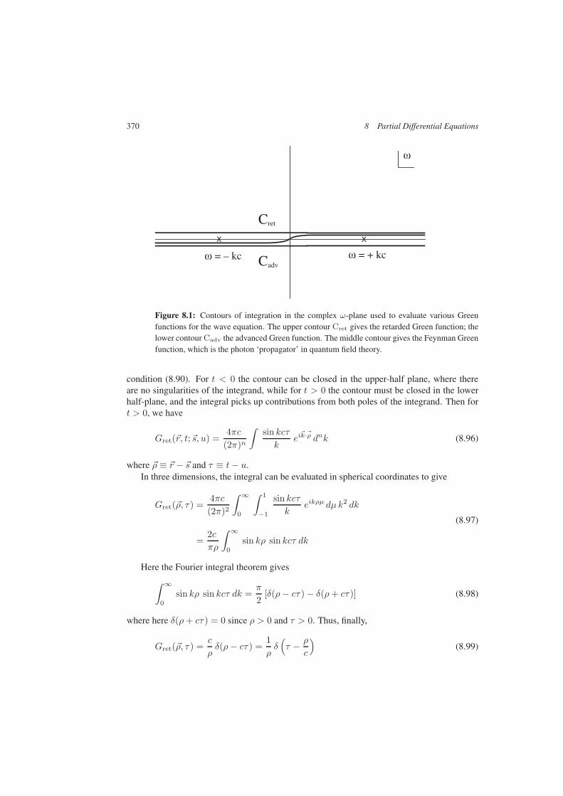
370 8 Partial Differential Equations
X X
Cret
ω
ω = kc ω = + kcCadv
Figure 8.1: Contours of integration in the complex ω-plane used to evaluate various Greenfunctions for the wave equation. The upper contour Cret gives the retarded Green function; thelower contour Cadv the advanced Green function. The middle contour gives the Feynman Greenfunction, which is the photon ‘propagator’ in quantum field theory.
condition (8.90). For t < 0 the contour can be closed in the upper-half plane, where thereare no singularities of the integrand, while for t > 0 the contour must be closed in the lowerhalf-plane, and the integral picks up contributions from both poles of the integrand. Then fort > 0, we have
Gret( r, t; s, u) =4πc(2π)n
∫sin kcτk
eik·ρ dnk (8.96)
where ρ ≡ r − s and τ ≡ t− u.In three dimensions, the integral can be evaluated in spherical coordinates to give
Gret( ρ, τ ) =4πc(2π)2
∫ ∞
0
∫ 1
−1
sin kcτk
eikρµ dµ k2 dk
(8.97)
=2cπρ
∫ ∞
0
sin kρ sin kcτ dk
Here the Fourier integral theorem gives
∫ ∞
0
sin kρ sin kcτ dk =π
2[δ(ρ− cτ ) − δ(ρ+ cτ )] (8.98)
where here δ(ρ+ cτ ) = 0 since ρ > 0 and τ > 0. Thus, finally,
Gret( ρ, τ ) =c
ρδ(ρ− cτ ) =
1ρδ(τ − ρ
c
)(8.99)

8.3 Time-Dependent Partial Differential Equations 371
This result has the natural interpretation that the wave propagates outward from its source withspeed c, with amplitude inversely proportional to the distance from the source.
Remark. The retarded Green function has this sharp form only in an odd number of spatialdimensions. In an even number of dimensions there is a trailing wave in addition to the sharpwave front propagating outward from the source. The interested reader is invited to work thisout for n = 2, which is realized physically by waves emitted from a long linear source.
The advanced Green function Gadv( r, t; s, u) is defined by the condition
Gadv( r, t; s, u) = 0 for t ≥ u. (8.100)
An appropriate contour for this Green function is also shown in Fig. 8.1. The contour be-tween Cret and Cadv defines the Feynman, or causal Green function. This contour gives acontribution to the Green function from the pole at ω = −kc for t < 0, and from the pole atω = +kc for t > 0. This Green function is especially important since it is the “propagator” ofthe photon in quantum electrodynamics. A derivation of this propagator can be found in mosttextbooks on quantum field theory.
If the radiation source is oscillating at a single frequency, so that
ρ( r, t) = ρω( r)e−iωt (8.101)
then the wave amplitude also has the same frequency, so that
φ( r, t) = φω( r)e−iωt (8.102)
and φω( r) must satisfy(
∆ +ω2
c2
)φω( r) = − 4πρω( r) (8.103)
which is the scalar Helmholtz equation.The Green function for this equation is a resolvent of the Laplacian and can be formally
expressed in terms of the eigenfunctions and eigenvalues of ∆. The boundary condition onthe Green function is that the waves should look asymptotically like waves radiating outwardfrom the source; this corresponds to the retarded condition (8.90) on the full Green function.
Example 8.4. In three dimensions, the wave amplitude φω is given by
φω( r)e−iωt =∫
ρω( s)| r − s|δ
(t− u− | r − s|
c
)e−iωu d3s du (8.104)
using the retarded Green function (8.99), so that
φω( r) =∫
eik|r−s|
| r − s| ρω( s) d3s (8.105)
(k = ω/c), corresponding to the Green function
Gω( r, s) =eik|r−s|
| r − s| (8.106)
372 8 Partial Differential Equations
Note that far from the source (which supposes that the source is of finite extent), the am-plitude has the asymptotic form
φω( r) r→∞−→ eikr
r
∫e−ik·sρω( s) d3s (8.107)
where k = kr points radially outward from the source to the point of observation. Thiscorresponds to a wave radiating outward from the source, with amplitude depending ondirection through the spatial Fourier transform of the source density.
From the result of Problem 5.14, we have the expansion
e−ik·s =∞∑
n=0
(−i)n(2n+ 1)jn(ks)Pn cos θ (8.108)
where the jn(ks) are spherical Bessel functions and the Pn are Legendre polynomials.Using the spherical harmonic addition theorem, we have the asymptotic expansion
φω( r) r→∞−→ 4πeikr
r
∞∑
n=0
(−i)nn∑
m=−nqnm(ω)Ynm(θ, φ) (8.109)
where the multipole moments qnm(ω) are here given by
qnm(ω) =∫
Y ∗nm(θs, φs)jn(ks)ρω( s) d3s (8.110)
As with the multipole expansion for the Coulomb potential, there are various normalizationconventions in use.
Remark. The full Green function (8.106) for the scalar Helmholtz equation also has a mul-tipole expansion; for r < s, we have
eik|r−s|
abs r − s= 4πik
∞∑
n=0
(−i)njn(ks)hn(kr)>n∑
m=−nYnm(θ, φ)Y ∗
nm(θs, φs) (8.111)
It is left to the reader to verify this expansion.
Analysis of the Klein–Gordon equation and its Green functions proceeds in a similar way.The details are left to Problem 10. See also Section 8.4.3 for a Klein–Gordon equation withan additional nonlinear term.
8.3 Time-Dependent Partial Differential Equations 373
8.3.3 The Schrödinger Equation
The time-dependent Schrödinger equation for a quantum mechanical system with HamiltonianH is
i∂Ψ(t)∂t
= HΨ(t) (8.112)
The Hamiltonian may be constructed by correspondence with the classical Hamiltonian of thesystem (see Chapter 3), or by other physical principles for a system, such as a spin system,with no classical analog. In any case, physics requires H to be a self-adjoint operator; theeigenstates of the Hamiltonian are states of definite energy of the system, and only energies inthe spectrum of H are possible for the system. A formal solution to Eq. (8.112) can be givenin terms of the resolution of the identity of the Hamiltonian—see Problem 8—but it is purelyformal.
An eigenstate ψ of H satisfies the time-independent Schrödinger equation
Hψ = Eψ (8.113)
Then Ψ(t) = ψ exp(iωt) is a solution of the time-dependent Schrödinger equation (8.112),where
E = ω (8.114)
and is Planck’s constant; Eq. (8.114) is essentially the relation between energy and frequencysuggested by Planck. Since Ψ(t) changes in time only by a phase factor exp(iωt), all matrixelements (Ψ,AΨ) = (ψ,Aψ) are independent of time; hence ψ is a stationary state of thesystem. Equation (8.113) is also known as the (time-independent) Schrödinger equation.
For a particle of mass µ moving in a potential V ( r), the Hamiltonian is
H = − 2
2µ∆ + V ( r) (8.115)
Equation (8.113) is a (partial) differential equation for the particle wave function ψ( r). Thephysical boundary conditions on the wave function are such that If V ( r) is real, then H isa self-adjoint operator whose spectrum is determined by the properties of the solutions ofEq. (8.113).
Example 8.5. For an electron in the Coulomb potential of a point nucleus with chargeZe,we have V (r) = −Ze2/r (again we set 4πε0 = 1). The time-independent Schrödingerequation is then
Hψ( r) =−
2
2me∆ − Ze2
r
ψ( r) = Eψ( r) (8.116)
where me is the mass of the electron. We can separate variables in spherical coordinates,and look for solutions of the form
ψ( r) = RE(r)Ym(θ, φ) (8.117)

374 8 Partial Differential Equations
where Ym(θ, φ) is a spherical harmonic as introduced in Section 6.5.3. We note that isrelated to the angular momentum of the electron, as explained further in Chapter 10.
The radial function RE(r) must then satisfy the equation
− 2
2mer2d
dr
(r2dREdr
)+[(+ 1)2
2mer2− Ze2
r
]RE = ERE (8.118)
This equation has a regular singular point at r = 0 and irregular singular point at ∞,suggesting that it might be related to the confluent hypergeometric equation introduced inChapter 5. To proceed further, we introduce the parameter aZ =
2/Zmee2 to set the
length scale (note that for Z = 1, a = 2/mee
2 = 52.9 pm is the Bohr radius). Thenintroduce the dimensionless variable ρ = 2r/aZ (the reason for the factor two will becomeapparent soon), and let
RE(r) = u(ρ) (8.119)
(we drop the subscripts E and for now). The radial equation (8.118) then becomes
u′′(ρ) +2ρu′(ρ) +
[1ρ− (+ 1)
ρ2
]u(ρ) = −1
4λu(ρ) (8.120)
Here λ = E/EZ , with energy scale EZ defined by
EZ =Ze2
2aZ=Z2mee
4
22= 1
2Z2α2mec
2 (8.121)
where α = e2/c is the dimensionless fine structure constant and c is the speed of light.We will soon see that EZ is the binding energy of the ground state of the electron.
The indices of Eq. (8.120) at ρ = 0 are and −(+ 1), so there are solutions propor-tional to ρ and ρ−−1 for ρ → 0. The second solution is singular at ρ = 0 and must notbe present. Only the first solution is allowed. Thus we let
u(ρ) = ρv(ρ) (8.122)
Then v(ρ) must be a solution of the equation
ρv′′(ρ) + 2(+ 1)v′(ρ) + ( 14λρ+ 1)v(ρ) = 0 (8.123)
For ρ→ ∞, this equation has the asymptotic form
v′′ + 14λv = 0 (8.124)
For positive energy E, we can let λ = κ2 and there are solutions v±(ρ) that have theasymptotic behavior exp(±1
2 iκρ) for ρ → ∞, corresponding to incoming (−) or outgo-ing (+) spherical waves. These solutions have logarithmic phase factors in addition to theusual exp(ikr) and exp(ikz) forms, arising from the long-range nature of the Coulomb po-tential. These subtleties are best seen in parabolic coordinates introduced in Problem 3.9.We leave them for the reader to work out in Problem 9.
8.3 Time-Dependent Partial Differential Equations 375
For E < 0, we let λ = −β2. Then there are solutions with asymptotic behaviorexp(±1
2βρ) for ρ → ∞. Only the exponentially decreasing solution, corresponding toa bound state of the electron, is allowed. In general, the solution v(ρ) that is analytic atr = 0 will not be exponentially decreasing as ρ→ ∞; there will be a discrete set of valuesof β for which this is the case, and the corresponding values of energy E < 0 define thediscrete spectrum of the Hamiltonian (8.116). If we now let
v(ρ) = e−12βρw(ρ) (8.125)
then w(ρ) must satisfy
ρw′′(ρ) + [2(+ 1) − βρ]w′(ρ) + [1 − β(+ 1)]w(ρ) = 0 (8.126)
To transform this to the confluent hypergeometric equation, we now let x = βρ and f(x) =w(ρ). Then f(x) satisfies the equation
xf ′′(x) + [2(+ 1) − x]f ′(x) + (β−1 − − 1)f(x) = 0 (8.127)
This is the confluent hypergeometric equation (5.B38), with
a = + 1 − β−1 and c = 2(+ 1)
The solution F (a|c|x) that is analytic at x = 0 has a part that grows exponentially, unlessa is zero or a negative integer, when there is a polynomial solution. Here that requirementmeans that we must have
1β
= k + + 1 ≡ n (8.128)
with k = 0, 1, 2, . . ., or n = , + 1, + 2, . . .. In this case, the solution is a polynomialof degree k, proportional to an associated Laguerre polynomial defined in Appendix A.Explicitly, we have a solution
f(x) = F (+ 1 − n|2(+ 1)|βρ) = AL2+1n−−1(βρ) (8.129)
where A is a normalization constant. Returning to the original variables, we can write thewave functions ψnm( r) corresponding to energy
En = − Ze2
n2aZ(8.130)
as
ψnm( r) = AL2+1n−−1
(2rnaZ
)exp
(− r
naZ
)Ym(θ, φ) (8.131)
with n = 1, 2, . . ., = 0, 1, . . . , n− 1 and m = , − 1, . . . ,−.

376 8 Partial Differential Equations
8.4 Nonlinear Partial Differential Equations
8.4.1 Quasilinear First-Order Equations
In Section 8.1, we studied a linear first order partial differential equation that describes a wavepropagating in one space dimension with speed s. Suppose now that the speed s depends onthe amplitude of the wave, so that we have a nonlinear wave equation
∂u
∂t+ s(u)
∂u
∂x= 0 (8.132)
This equation can arise from a conservation law for a system described by a density u(x, t)and a flux density Φ, such that
d
dt
∫ b
a
u(x, t) dx = Φ(a) − Φ(b) = −∫ b
a
∂Φ(x, t)dx
dx (8.133)
for any a and b. From this equation it follows that
∂u
∂t+∂Φ∂x
= 0 (8.134)
Equation (8.134) is a equation of continuity similar to Eq. (3.138); it expresses a local versionof conservation of a charge q defined by
q =∫ ∞
−∞u(x, t) dx (8.135)
since Eq. (8.133) means that charge can leave the interval [a, b] only if there is a flux acrossthe endpoints of the interval.
Example 8.6. In the book by Billingham and King cited at the end of the chapter, thisequation appears as a model to describe the flow of traffic on a highway. u(x, t) is thedensity of cars, and the flux Φ(x, t) is expressed as vu(x, t), where v is the speed of thecars. With the empirical assumption that v depends only on the density—there is data thatis consistent with this assumption, at least as a first approximation—the conservation lawleads to Eq. (8.132) with
s(u) = v(u) + uv′(u) (8.136)
Note here that s(u) is not the speed of the cars, but the speed of propagation of fluctuationsin the density of cars.
In general, if the flux Φ is a function of u only, with no explicit dependence on x or t,Eq. (8.134) can be written as
∂u
∂t+ Φ′(u)
∂u
∂x= 0 (8.137)
which is the original Eq. (8.132) with speed s(u) = Φ′(u).

8.4 Nonlinear Partial Differential Equations 377
We want to find solutions to Eq. (8.132) starting from an initial condition
u(x, 0) = u0(x) (8.138)
As with the linear equation with constant s, we can construct characteristics of the partialdifferential equation as curves x = x(t) on which the wave amplitude u is a constant. Alonga characteristic, we have
du =∂u
∂xdx+
∂u
∂tdt =
∂u
∂x[dx− s(u)dt] = 0 (8.139)
Thus the characteristics are straight lines, and the characteristic passing through the point x att = 0 is determined from its slope
dx
dt= s0(x) = s[u0(x)] (8.140)
Then to find the amplitude u at a later time t > 0, we need to solve the implicit equation
u(x, t) = u(x− s(u0)t, 0) (8.141)
as we trace the solution along its characteristic so that
u(x+ s(u0)t, t) = u(x, 0) = u0 (8.142)
However, the solution is not as simple as that in general. If the wave speed depends on theamplitude, then the characteristics are not parallel, and two characteristics will meet, either inthe future or in the past. Since waves are propagating to the right along the X-axis, it is clearthat a faster wave coming from the left will catch up with a slower wave starting to the rightof the fast wave. Thus some characteristics will meet at some time after t = 0 unless s(u0) isa nondecreasing function of x. In that case, the wave is described as a rarefaction wave, sincethere are no faster waves coming from the left; all the intersections of the characteristics lieon the past (i.e., for t < 0).
What happens, then, when two characteristics meet? Consider the characteristics comingfrom x = a and x = b, and suppose the initial conditions are such that
u(a, 0) = ua and u(b, 0) = ub
If sa = s(ua) and sb = s(ub), then the characteristics from a and b will meet
at x =a+ b
2+sa + sb
2a− b
sb − sawhen t =
a− b
sb − sa
The characteristics cannot continue beyond this point, and if they have not already encoun-tered other characteristics, they will form a point of discontinuity in the solution of the partialdifferential equation (8.132). The discontinuities formed by merging characteristics will forma line that is understood as a shock wave or shock front, across which the solution u(x, t) hasa discontinuity in x.
378 8 Partial Differential Equations
We can compute the discontinuity of the solution across a shock using the original partialdifferential equation. If the discontinuity of u(x, t) is at x = X(t), then we can integrateEq. (8.132) from a < X to b > X . This gives
∂
∂t
∫ b
a
u(x, t) dx = Φ(a) − Φ(b) (8.143)
With u± = limε→0+ u(X ± ε, t), we then have
∂
∂t
[(b−X)u+ + (X − a)u−
]= Φ(a) − Φ(b) (8.144)
The velocity of the shock wave is V = dX/dt; if we pass to the limit ε→ 0 we find a relation
V (u− − u+) = Φ(u−) − Φ(u+) (8.145)
between the discontinuities and the velocity of the shock wave. Most often this allows us tocompute V as
V =Φ(u−) − Φ(u+)
u− − u+(8.146)
Problem 12 gives an explicit example of such a shock wave.
8.4.2 KdV Equation
The linear wave equation for a wave with a dispersion relation ω = ks(1 − α2k2) was givenin Eq. (8.16). Now we are interested in the waves that result when the speed of propagationalso depends on the amplitude u of the wave as in the preceding section. Thus we start with ageneral equation of the form
∂u
∂t+ s(u)
∂u
∂x+ sα2 ∂
3u
∂x3= 0 (8.147)
If we consider only the equation when s(u) is a linear function of u, then linear transforma-tions of the variables (u, x and t) allow Eq. (8.147) to be cast in the form
∂u
∂t+ 6u
∂u
∂x+∂3u
∂x3= 0 (8.148)
This is a standard form of the Kortweg–deVries or KdV equation.
Exercise 8.3. Find a set of linear transformations of the variables that change Eq. (8.147)to Eq. (8.148).
One important property of this equation is that it has travelling wave solutions of the form
u(x, t) = U(x− st) ≡ U(ξ) (8.149)
that travel to the right with speed s = κ2; here we have introduced the variable ξ = x − st.The KdV equation requires U(ξ) to satisfy the equation
U ′′′(ξ) + 6U(ξ)U(′(ξ)− κ2U ′(ξ) = 0 (8.150)
8.4 Nonlinear Partial Differential Equations 379
Equation (8.150) can be immediately integrated to give
U ′′(ξ) + 3[U(ξ)]2 − κ2U(ξ) = 0 (8.151)
where a constant of integration on the right-hand side has been set to zero so that U(ξ) tendsto zero for |ξ| → ∞. Then multiply by U ′(ξ) and integrate once more to give
12 [U ′(ξ)]2 + [U(ξ)]3 − 1
2κ2[U(ξ)]2 = 0 (8.152)
where another integration constant has been set to zero so that U(ξ) will vanish for |ξ| → ∞.We now have the differential equation
dU
dξ= U(ξ)
√2U(ξ) − κ2 (8.153)
The integral of this differential equation is not immediately obvious, but it is not too difficultto verify that the solution
U(ξ) =κ2
2sech2( 1
2κξ) =κ2
2 cosh2( 12κξ)
(8.154)
actually satisfies Eq. (8.153).The solution (8.154) is sharply peaked around ξ = 0 and vanishes exponentially for
ξ → ∞. The one parameter κ characterizes both the height and width of the peak, as wellas the speed of the wave—larger κ means a more rapid wave, with a higher and narrowerpeak. The shape of the wave is constant in time, in contrast to linear waves with no disper-sion, i.e., a speed of propagation independent of frequency. The solution is called a solitarywave, or soliton. However, we note that in modern terminology, the term soliton actually im-plies further properties of the equations—especially that there are multisoliton solutions thatcorrespond to solitons that pass through each other maintaining their shape both before andafter interacting. The KdV solitons have all these properties, but we do not discuss them fur-ther here—see the books cited in the bibliography, as well as many others, for further details.
Exercise 8.4. One property of the KdV equation is that it admits an infinite set of conser-vation laws. Show that it follows from the equations of motion that the following quantitiesare conserved:
m =∫ ∞
−∞u dx
P =∫ ∞
−∞u2 dx
E =∫ ∞
−∞( 12u
2x − u3) dx
Assume that u and its derivatives vanish as x → ±∞. We note that these three laws corre-spond to conservation of mass, momentum and energy, and are quite general. It is the lawsbeyond this that are special for the KdV equation.
380 8 Partial Differential Equations
8.4.3 Scalar Field in 1 + 1 Dimensions
The Klein–Gordon equation (8.71) for a scalar field φ(x, t) in one space (+ one time) dimen-sion can be derived from a Lagrangian density
L = 12
(φ2t − φ2
k −m2φ2)
(8.155)
as explained in Appendix A. Here φt = ∂φ/∂t and φt = ∂φ/∂x. As already noted, theKlein–Gordon equation describes the propagation of waves with a dispersion relation
ω2 = k2 +m2 (8.156)
that is associated waves with a free relativistic particle m in units with = c = 1. Thedispersion relation also describes propagation of electromagnetic waves in an ideal plasma,where m is the plasma frequency.
The Lagrangian (8.155) is a special case of the Lagrangian
L = 12
(φ2t − φ2
k
)− U(φ) (8.157)
with potential U(φ)= 12m
2φ2, for which the equation of motion is
∂2φ
∂t2− ∂2φ
∂x2= −dU(φ)
dφ(8.158)
as derived in Appendix A. Also noted there was the energy of the field, which is given by
E[φ] =∫ ∞
−∞
[12
(φ2t + φ2
x
)+ U(φ)
]dx (8.159)
Now assume that the potential U(φ) is non-negative, and that U(φ) = 0 only for a discreteset of values φ = v1, v2, . . . , vN . Then these values of φ are absolute minima of U(φ), and
E[φ] = 0 if and only if φ(x, t) = vk
for some k = 1, . . . , N . These (trivial) static solutions minimize the energy E [φ].If the potential has more than one minimum, there may also be nontrivial static solutions
of the field equation (8.158) that have finite total energy. These solutions must satisfy theequation
d2φ
dx2=dU(φ)dφ
(8.160)
This equation has an integral
W =12
(dφ
dx
)2
− U(φ) (8.161)
W must be constant, independent of x, for any solution of Eq. (8.160). For the solution tohave finite energy, it is necessary that
E[φ] =∫ ∞
−∞dx
[12
(dφ
dx
)2
+ U(φ)
]<∞ (8.162)

8.4 Nonlinear Partial Differential Equations 381
This requires
limx→±∞φ(x) ≡ v± (8.163)
with v+ and v− among the v1, . . . , vN, since Eq. (8.163) implies U(φ) → 0 as well asW → 0 for x → ±∞. Then also W = 0 for all x. However, if N > 1, we need nothave v+ = v−, and there may be nontrivial solutions of W = 0 that interpolate between twominima of U(φ), as well as solutions for which v+ = v−.
Remark. Equation (8.160) has the same form as Newton’s equation of motion for a particlewith potential energy −U(x). A finite energy static solution of the field equation correspondsto a finite action zero-energy solution of the particle equation of motion, in which the particlemoves between two adjacent zeros of U .
Remark. Static finite-energy solutions to the field equations derived from the Lagrang-ian (8.157) can only exist in one space dimension (this result is known as Derrick’s theorem).To see this, consider a field configuration φα(x) ≡ φ(αx) with rescaled spatial coordinates.The energy associated with this configuration in q space dimensions is
Eα ≡ E[φα] =∫ ∞
−∞dqx
[12 (−→∇φα · −→∇φα) + U(φα)
]≡ Kα + Vα
(8.164)
=∫ ∞
−∞dqξ
[12α2−q(
−→∇φα · −→∇φα) + α−qU(φ)]
= α2−qK + α−qV
with ξ = αx. Here K, V are the values of the integrals for α = 1. Since Eα must have anextremum at α = 1, it follows that
(2 − q)K = qV (8.165)
which is consistent with positivity of K and V only for 0 < q < 2.
The equation W = 0 can be solved by quadrature to give
x− x0 = ±∫ φ
φ0
1√U(ψ)
dψ (8.166)
with φ0 = φ(x0). This shows how the solutions interpolate between minima of U(φ), whichby assumption have U(φ) = 0. If U(φ) is O(φ− vk)2 near the minimum at φ = vk, then theintegral diverges as the minimum is approached, corresponding to x→ ±∞.
Example 8.7. For the (1 + 1)-dimensional φ4 field theory, the potential is
U(φ) =12λ
(φ2 − m2
λ
)2
(8.167)
with U(φ) = 0 at the degenerate minima φ = ±v ≡ v±, where v2 = m2/λ. Staticsolutions of the field equations satisfy
d2φ
dx2= 2λφ3 − 2m2φ (8.168)
382 8 Partial Differential Equations
whence
x− x0 = ±√
1λ
∫ φ
φ0
1ψ2 − v2
dψ (8.169)
This equation can be inverted to give
φ(x) = ±v tanh [m(x− x0)] ≡ φ±(x;x0) (8.170)
The solution φ+(x;x0) [φ−(x;x0)] interpolates between −v [+v] as x → −∞ to +v[−v] as x→ +∞, while vanishing at x0. Hence φ+ [φ−] is a known as a kink [antikink].
The energy density of the kink (or antikink) solution is given by
E(x) = 2U(φ) =m4
λ
1cosh4[m(x− x0)]
(8.171)
which is sharply localized near x = x0. The total energy of the kink solution (the classicalmass M∗) of the kink is
E[φ±] ≡M∗ =∫ ∞
−∞E(x)dx =
4m3λ
(8.172)
where we have used the integral∫ ∞
0
dξ
cosh4 ξ=
13
[sinh ξcosh3 ξ
+ 2sinh ξcosh ξ
]∞
0
=23
(8.173)
Since Eq. (8.158) is invariant under Lorentz transformations (in 1 + 1 dimensions),we can transform of the kink and antikink solutions to find solutions that correspond tomoving kinks or antikinks. We have
φu±(x;x0) = ±v tanh
[m(x− x0 − ut)√
(1 − u2)
](8.174)
with energy
E[φu±] = M∗/√
1 − u2 (8.175)
appropriate to a particle of mass M∗ with speed u (note that we have set c = 1).
Remark. For any field φ in 1 + 1 dimensions, there is a topological current density
Kµ ≡ εµν∂φ
∂xν(8.176)
that automatically satisfies ∂Kµ/∂xµ = 0 for nonsingular fields. Hence the topologicalcharge
Q ≡∫ ∞
−∞K0 dx = v+ − v− (8.177)
is conserved. Then the space of nonsingular finite-energy solutions can be divided into topo-logical sectors associated with distinct values of the topological charge.
Exercise 8.5. Find the topological charge (in units of 2v) for the static kink and antikinksolutions. Is this charge the same for the corresponding moving solitons?
8.4 Nonlinear Partial Differential Equations 383
8.4.4 Sine-Gordon Equation
A special potential U(φ) which has applications in nonlinear optics, in addition to its interestas a toy model, is
U(φ) = λv4
[1 − cos
(φ
v
)]= 2λv4 sin2
(φ
2v
)(8.178)
where v is a dimensional constant which we can identify with m/√λ of the φ4 theory. This
potential is bounded, and has zeros for
φ = 2nπv ≡ φn (8.179)
(n = 0,±1,±2, . . .). The field equation for this potential is
∂2φ
∂t2− ∂2φ
∂x2= −λv3 sin
(φ
v
)(8.180)
For small φ, the right-hand side is approximated by −m2φ, and the equation looks like theKlein–Gordon equation in this limit. This has led to the slightly whimsical name sine-Gordonequation for (8.180).
Equation (8.180) has static finite energy solutions obtained from
x− x0 = ±∫ φ
φ0
12√λv2 sin(ψ/2v)
dψ (8.181)
This can be evaluated using the integral∫
dξ
sin ξ= ln
(tan 1
2ξ)
(8.182)
to give
ln(
tanφ
4v
)= ln
(tan
φ0
4v
)±m(x− x0) (8.183)
If we choose x0 such that
φ0 = φ(x0) = (2n+ 1)πv (8.184)
(n = 0,±1,±2, . . .), then we have
φ
4v= (−1)n tan−1
[e±m(x−x0)
](8.185)
where each choice of branch of the arctangent leads to a solution which interpolates betweena different pair of adjacent zeros of U(φ).
Exercise 8.6. If we choose the branch of the arctangent for which tan−1(0) = nπ, findthe limits
φ± = limx→±∞ φ(x)
for each of the choices of sign in the exponent in Eq. (8.185).
384 8 Partial Differential Equations
A Lagrangian Field Theory
In Section 3.5.3, we described the Lagrangian and Hamiltonian dynamics of systems with afinite number of degrees of freedom. Here we present the extension of that theory to systemsof fields, i.e., by functions of space and time coordinates defined on some spacetime manifold.There are some subtleties in that extension, especially when dealing with fields such as theelectromagnetic field with its gauge invariance. However, we will not be concerned with suchpoints here, as we simply present the basic ideas of classical Lagrangian field theory.
Consider first a real scalar field φ(x, t), whose dynamics is to be described by a Lagrangiandensity L that depends on φ and its first derivatives, which we denote by φt for the timederivative ∂φ/∂t and by φk for the spatial derivatives ∂φ/∂xk. The dynamics is based on anextension of Hamilton’s principle (see Section 3.5.3) to require that the action
S[φ(x)] =∫
L(φ, φk, φt) dnx dt (8.A1)
be an extremum relative to nearby fields (n is the number of space dimensions). This leads toa generalization of the Euler–Lagrange equations of motion,
∂
∂t
∂L∂φt
+∂
∂xk∂L∂φk
− ∂L∂φ
= 0 (8.A2)
(summation over k understood) that provides equations of motion for the fields.Canonical momenta for the field can be introduced by
π(x, t) ≡ ∂L∂φt(x, t)
(8.A3)
The Hamiltonian density H defined by
H = π(x, t)∂L
∂φt(x, t)− L(φ, φk, φt) (8.A4)
can often be identified as an energy density of the field. The total field energy is then given by
H = E[φ] =∫ (
π(x, t)∂L
∂φt(x, t)− L(φ, φk, φt)
)dnx (8.A5)
The wave equation for the scalar field φ(x, t) can be derived from the Lagrangian density
L =12
(1c2φ2t − φ2
k
)(8.A6)
(again with implied summation over k), The canonical momentum density is then given byπ(x, t) = φt(x, t) and the Hamiltonian density is
H =12[π(x, t)]2 + [φk(x, t)]2
(8.A7)
A Lagrangian Field Theory 385
Symmetry principles can be enforced by constraining the Lagrangian density to be in-variant under the desired symmetry transformations. This is especially useful in constructingtheories of elementary particles that are supposed to possess certain symmetries, as mentionedin Chapter 10. Here we note that a relativistic field theory can be constructed by requiring Lto be invariant under Lorentz transformations.
Example 8.8. For a relativistic scalar field φ(x, t) in one space dimension, the principleof invariance under Lorentz transformations requires Lagrangian density to have the form
L =12
(1c2φ2t − φ2
x
)− U(φ) 8.157
as already noted in Section 8.4.3. in order to be invariant under Lorentz transformations.Here U(φ) is a functional of φ (and not its derivatives) that is often referred to as thepotential for the field φ. Stability requires U(φ) to be bounded from below, and we willgenerally assume that U(φ) ≥ 0 for all φ. The equation of motion for the field is
1c2∂2φ
∂t2− ∂2φ
∂x2= −dU(φ)
dφ(8.A8)
The conserved energy functional for the field is
E[φ] =∫ ∞
−∞
[12
(φ2t + φ2
x
)+ U(φ)
]dx (8.A9)
The Klein–Gordon equation is the equation of motion derived from a Lagrangian densitywith potential
U(φ) = 12m
2φ (8.A10)
Other potentials U(φ) lead to interesting phenomena, some of which are described inSections 8.4.3 and 8.4.4.
For a scalar field in n space dimensions, the Lorentz invariant Lagrangian density is
L = 12 (φ2
t − φ2k) − U(φ) (8.A11)
with U(φ) a potential that is fairly arbitrary for a classical field, but more constrained in aquantum theory. The canonical momentum is π = φt leading to the Hamiltonian density
H = 12π
2 + 12∇φ · ∇φ+ U(φ) (8.A12)
The momentum and energy can be derived from the stress-energy tensor Tµν defined by
Tµν ≡ ∂φ
∂xµ∂φ
∂xν− Lgµν (8.A13)
We then have
Pµ =∫
T0µ dnx (8.A14)
Conservation of four-momentum follows from the equations of motion (show this).

386 8 Partial Differential Equations
Bibliography and Notes
A monumental treatise with an extensive discussion of methods to find both exact and approx-imate solutions to linear partial differential equations involving the Laplace operator is
Philip M. Morse and Herman Feshbach, Methods of Theoretical Physics, (two vol-umes) McGraw-Hill (1953)
Laplace’s and Poisson’s equations, the scalar Helmholtz equation, the wave equation, theSchrödinger equation, and the diffusion equation are all discussed at length. The method ofseparation of variables, the ordinary differential equations that arise after separating variables,and the special functions that appear as solutions to these equations are thoroughly analyzed.The coordinate systems in which Laplace’s equation and the scalar Helmholtz equation areseparable are analyzed at length. Complex variable methods are thoroughly described, butabstract linear vector space methods are presented only in a very archaic form.
A handbook that has many useful formulas—differential equations, generating functions,recursion relations, integrals and more—is
Milton Abramowitz and Irene Stegun, Handbook of Mathematical Functions, Dover(1972).
This book has extensive graphs and tables of values of the functions, as well as the formulas.While the tables are less important with the availability of high-level programming systemssuch as Matlab and Mathematica, the graphs are still of some use for orientation. It is alsoavailable online as a free download; it was originally created as a project of the (U. S.) NationalBureau of Standards and thus not subject to copyright.
A classic text from the famous Sommerfeld lecture series is
Arnold Sommerfeld, Lectures on Theoretical Physics VI: Partial Differential Equa-tions in Physics, Academic Press (1964)
This book is an outstanding survey of methods for analyzing partial differential equationsthat were available in the 1920s and 1930s. These methods go far beyond the discussion ofseparation of variables given here, and cover many applications that are still interesting today.
A modern survey of various topics in linear and nonlinear wave motion is
J. Billingham and A. C. King, Wave Motion, Cambridge University Press (2000).
This book starts an elementary level, but moves on to describe elastic waves in solids, waterwaves in various limiting cases both linear and nonlinear, electromagnetic waves, and wavesin chemical and biological systems.
Another introduction that emphasized nonlinear partial differential equations that havesolitonic solutions is
P. G. Drazin and R. S. Johnson, Solitons: An Introduction, Cambridge UniversityPress (1989).
This book treats the Kortweg-de Vries equation in great detail, but considers other nonlinearequations as well.
Problems 387
Problems
1. Consider the operator
∆ ≡ ∇2 =(∂2
∂x2+
∂2
∂y2+
∂2
∂z2
)
defined on the (complex) function space L2(Ω), where Ω is three-dimensional regionbounded by a closed surface S. Show that this operator is self-adjoint when defined onthe subspace of twice differentiable functions that satisfy the mixed boundary condition(see Eq. (8.27))
α(r) u(r) + β(r) n · ∇u(r) = α(r) v(r) + β(r) n · ∇ v(r) = 0 on S.
with α(r) and β(r) real functions on S.
2. Evaluate the Green function for the Laplacian in two dimensions, with boundary condi-tion that n · ∇rG( r, s) vanish far from the source, from its Fourier transform
G( r, s) =1
(2π)2
∫eik·(r−s)
k2d2k
and compare this result with the standard result for the electrostatic potential due to aline charge. (Note. The evaluation is tricky. With ρ ≡ | r − s|, you might want to firstevaluate dG/dρ.)
3. Use the continuum eigenvectors defined in Eq. (8.45) to construct an explicit represen-tation of the operators Eλ that define a resolution of the identity (Section 7.3.3) for theoperator ∆ on Rn.
4. Consider the eigenvalue equation
∆u = λu
in a rectangular box characterized by
0 ≤ x ≤ a 0 ≤ y ≤ b 0 ≤ z ≤ c
with periodic boundary conditions
u( r + aex) = u( r) u( r + bey) = u( r) u( r + cez) = u( r)
(here ex, ey, and ez are unit vectors along the coordinate axes, which are parallel to theedges of the box).
(i) Show that ∆ is a self-adjoint operator with the periodic boundary conditions.
(ii) Find a complete orthonormal system of eigenvectors of ∆ with periodic boundaryconditions. What are the corresponding eigenvalues?

388 8 Partial Differential Equations
5. Consider the Laplacian ∆ inside a cylinder of radius R and length L.
(i) Express ∆ in terms of partial derivatives with respect to the standard cylindrical co-ordinates ρ, φ, and z (see Eq. (3.194)).
(ii) Consider solutions to the eigenvalue equation
∆u = λu
of the form
u(ρ, φ, z) = G(ρ)F (φ)Z(z)
Find the differential equations that must be satisfied by the functions G(ρ), F (φ), andZ(z), introducing additional constants as needed.
(iii) Find solutions of these equations that are single valued inside the cylinder and thatvanish on the surface of the cylinder.
(iv) Then describe the spectrum of the Laplacian in the cylinder with these boundaryconditions, and find the corresponding complete orthonormal system of eigenvectors.
6. (i) Show that the retarded Green function for the wave equation (8.70) can be written as
Gret( ρ, τ ) = − c2
(2π)n+1limε→0+
∫1
(ω + iε)2 − k2c2eik·ρ−iωτ dnk dω
with ρ ≡ r − s and τ ≡ t− u.
(ii) Show that the Feynman Green function GF can be written as
GF ( ρ, τ ) = − c2
(2π)n+1limε→0+
∫1
ω2 − k2c2 + iεeik·ρ−iωτ dnk dω
Remark. The problem here is simply to show that each so-called “iε prescription”given here is equivalent to the corresponding contour in Fig. 8.1.
7. Show that the solution (8.99) for the retarded Green function in three dimensions leadsto the potential
φ( r, t) =14π
∫1
| r − s| ρ( s, t− | r − s|
c
)d3s
Remark. This potential is the retarded potential. The potential at the point P = ( r, t)is determined by the sources on the “backward light cone” from P . Draw a picture toexplain this statement.
8. (i) Show that a formal solution to the Schrödinger equation (8.69)
i∂ψ
∂t= Hψ
Problems 389
is given by
ψ(t) = exp(− i
Ht)ψ(0) ≡ U(t)ψ(0) (*)
(ii) If the Hamiltonian H has a resolution of the identity Eω such that
H =
∫ωdEω
then
ψ(t) =∫
e−iωtdEω ψ(0)
(iii) For a particle of mass m with potential energy V ( r) the Hamiltonian is
H = − 2
2m∇2 + V ( r)
The formal solution (∗) can be expressed as
ψ( r, t) =∫
G( r, t; s, 0)ψ( s, 0) d3s
where G( r, t; s, 0) is the Green function for this Schrödinger equation.
(iv) Evaluate the Green function G0( r, t; s, 0) for a free particle (V = 0).
9. Parabolic coordinates ξ, η, φ were introduced in Problem 3.9 in terms of Cartesian coor-dinates x, y, z.
(i) Show that ξ, η can be expressed in terms of the spherical coordinates r and θ as
ξ = r(1 − cos θ) = r − z η = r(1 + cos θ) = r + z
(ii) Show the Laplacian ∆ in parabolic coordinates is
∆ =4
ξ + η
[∂
∂ξ
(ξ∂
∂ξ
)+
∂
∂η
(η∂
∂η
)]+
1ξη
∂2
∂φ2
(iii) Show that the Schrödinger equation (8.116) can be separated in parabolic coordi-nates.
(iv) Find scattering solutions corresponding to an incoming plane wave plus outgoingscattered wave, including the logarithmic corrections to the phase that are related to thelong-range character of the Coulomb potential.
10. (i) Show that the Green function for the Klein–Gordon equation (8.71) in n space di-mensions has the general form
G( ρ, τ ) = − c2
(2π)n+1
∫1
ω2 − k2c2 − (mc2/)2eik·ρ−iωτ dnk dω
390 8 Partial Differential Equations
(again ρ ≡ r− s and τ ≡ t−u) where, as for the wave equation, the contour of integrationin the complex ω-plane must be chosen so that G satisfies the desired initial conditions.
(ii) Show that the contour Cret in Fig. 8.1 again gives a retarded Green function.
(iii) Show that doing the integral over ω gives
Gret( ρ, τ ) =c2
(2π)n
∫sinωkτωk
eik·ρ dnk
with ωk =√k2c2 + (mc2/)2.
11. Show that the Schrödinger equation for a particle of mass m moving in a potential V ( r)can be derived from a Lagrangian
L =i
2(ψ∗ψt − ψ∗
tψ) − 2
2mψ∗kψk − ψ∗V ( r)ψ
Treat ψ and ψ∗ as independent fields.
12. Consider the partial differential equation
∂u
∂t+ (1 + u)
∂u
∂x= 0
with u(x, 0) given by a “hat” function
u(x, 0) =
u0(1 + x) −1 < x ≤ 0u0(1 − x) 0 < t < 10 otherwise
(i) Draw a sketch in the x–t plane of the characteristics of this equation starting from theX-axis at t = 0.
(ii) Find the trajectory of the shock wave associated with these initial conditions.
(iii) Then find the complete solution u(x, t) of the partial differential equation with theseinitial conditions.
13. Derive Eq. (8.175) for the energy of the moving kink solution (8.174).
9 Finite Groups
Symmetries and invariance principles lead to conservation laws that are at the foundation ofphysical theory. The idea that physical laws should be independent of the coordinate systemused to describe spacetime leads to the fundamental conservation laws of classical physics.That laws are independent of the choice of origin of the spatial coordinate system (transla-tion invariance) is equivalent to conservation of momentum; independence of the choice ofinitial time is equivalent to conservation of energy. Rotational invariance of physical laws isequivalent to conservation of angular momentum. Even in systems such as solids, where thefull symmetries of spacetime are not present, there are discrete rotational and translationalsymmetries of the lattice that have consequences for the physical properties of such systems.
Systems of identical particles have special properties in quantum mechanics. All knownelementary particles are classified as either bosons (with integer spin) or fermions (spin 1
2 ).The requirement that any state of a system of bosons (fermions) be symmetric (antisymmetric)under the exchange of any pair of particles leads naturally to study of the properties of per-mutations. Antisymmetry of many-electron states under permutations is the basis of the Pauliexclusion principle, which leads to an elementary qualitative picture of the periodic table ofthe elements. Moreover, the theory of atomic and molecular spectra requires knowledge ofthe constraints on the allowed states of atoms and molecules imposed by the Pauli exclusionprinciple. The allowed states of atomic nuclei are also restricted by the Pauli principle appliedto the constituent protons and neutrons.
These and other symmetries are described by a mathematical structure known as a group,and there is a highly developed theory of groups with physical applications. In this chapter,we introduce some general properties of groups derived from the group axioms that were in-troduced in Chapter 1, and give examples of both finite and continuous groups. These includesymmetry groups of simple geometric objects such as polygons and polyhedra that appear inmolecules and crystal lattices, as well as the group of permutations of N objects, the sym-metric group SN . Space–time symmetries such as rotations and translations are described bycontinuous groups, also known as Lie groups, as are the more abstract symmetries associ-ated with conservation of electric charge and with the fundamental interactions of quarks andleptons. Lie groups are described in detail in Chapter 10.
In this chapter, we study groups with a finite number n of elements (n is the order of thegroup). An important element of this study is to find the (conjugacy) classes of G. Two groupelements a and b are conjugate (a ∼ b) if there is an element g of G such that b = gag−1. Aclass of G contains all the group elements conjugate to any one element of the class. A groupof finite order n has p (≤ n) classes with h1, . . . , hp elements, with
∑hk = n.
Introduction to Mathematical Physics. Michael T. VaughnCopyright c© 2007 WILEY-VCH Verlag GmbH & Co. KGaA, WeinheimISBN: 978-3-527-40627-2
Introduction to Mathematical Physics
Michael T. Vaughn 2007 WILEY-VCH Verlag GmbH & Co.
392 9 Finite Groups
In physical applications, we are most often interested in the representation of a group bylinear operators on a linear vector space, such as the coordinate space of a system of coupledoscillators, or the state space of a quantum mechanical system. A representation is a mapg → D(g) such that the group multiplication is preserved, i.e.,
g = g1g2 if and only if D(g) = D(g1)D(g2)
Of special interest are the irreducible representations, in which the group acts on a vectorspace that has no proper subspace invariant under the action of the entire group. For a finitegroup, any irreducible representation is equivalent to a representation by unitary matrices.
The theory of irreducible representations of finite groups starts from orthogonality re-lations based on two lemmas due to Schur. The first lemma states that any operator thatcommutes with all the operators in an irreducible representation is a multiple of the identityoperator. The second states that if Γ [g → D(g)] and Γ′ [g → D′(g)] are two inequivalentirreducible representations and A is a linear operator such that
AD(g) = D′(g)A
for all g, then A = 0. From these lemmas, we derive the fundamental theorem on represen-tations of finite groups, which states that a finite group G with p classes has exactly p distinctinequivalent irreducible representations, of dimensions m1, . . . ,mp such that
p∑
k=1
m2k = n
We give special attention to the symmetric groups SN , as these are important both for thequantum-mechanical description of systems of identical particles and for the representationtheory of continuous groups. Each class of SN is associated with one of the π(N) partitionsof N and its corresponding Young diagram, as every permutation with a cyclic structure de-scribed by one partition belongs to the same class of SN . Then SN also has π(N) inequivalentirreducible representations, each of which can also be associated with a partition of N and itsYoung diagram.
There is a remarkable generating function, due to Frobenius, for the simple charactersχ
(λ)(m) of SN . This function, derived in Appendix B, allows us to develop graphical methods
based on Young diagrams for computing the characters, for the reduction of tensor productsof irreducible representations of SN , and for the reduction of outer products Γ(µ) Γ(ν) ofirreducible representations of Sm and Sn. The outer products are representations of Sm+n
induced by representations of the subgroup Sm⊗Sm using a standard procedure for obtainingrepresentations of a group from those of its subgroups. These graphical methods can be usedto compute various properties not only of SN , but also of Lie groups and their Lie algebras,as explained in Chapter 10.

9.1 General Properties of Groups 393
9.1 General Properties of Groups
9.1.1 Group Axioms
The essential properties of a group are that (i) multiplication is defined for any two elementsof the group, (ii) there is an identity element that leaves any element unchanged under mul-tiplication, and (iii) for every element of the group, there is an inverse under multiplicationthat brings the group element back to the identity under multiplication. These properties areformalized in the following definition.
Definition 9.1. A group G is a set of elements with a law of composition (multiplication) thatassociates with any ordered pair (g, g′) of elements of G a unique elements gg′, the product ofg and g′, such that
(i) (associative law) for every g, g′, g′′ in G, it is true that
(gg′)g′′ = g(g′g′′); (9.1)
(ii) there is a unique element in G (the identity) denoted by 1 or by e, such that eg = g forevery g in G;
(iii) for every g in G, there is a (unique) element g−1, the inverse of g, such that
g−1g = e = gg−1. (9.2)
The group G is finite if it contains a finite number of elements, otherwise infinite. If G isfinite, the number of elements of G is the order of G. A subset H of G that is a group undermultiplication in G is a subgroup of G, proper unless H = G or H = e.
Definition 9.2. The group G is Abelian if gg′ = g′g for every pair g and g′ in G. The law ofcomposition of an Abelian group is often called addition; the group is additive.
Example 9.1. The set 1,−1 is a group (of order 2) under ordinary multiplication; it isevidently Abelian. This group is denoted by Z2.
Example 9.2. The integers Z = 0,±1,±2, . . . form an (infinite) Abelian group underaddition.
Example 9.3. The permutations of N distinct objects form a group SN , the symmetricgroup, since the result of applying two permutations of the N objects is another permuta-tion. SN is of order N ! (there are N ! distinct permutations of N objects).
Example 9.4. The complex numbers z on the unit circle (|z| = 1) form an Abelian groupunder the usual complex multiplication. The elements of this group depend on a singlereal parameter θ [with z = exp(iθ)] in the range 0 ≤ θ < 2π.
Example 9.5. The n × n unitary matrices U form the unitary group U(n) (recall fromChapter 2 that the product of unitary matrices is unitary). U(n) is non-Abelian for n > 1;U(1) is equivalent to the group of complex numbers on the unit circle. The subgroup ofU(n) containing those matrices U with detU = 1 is the special unitary group SU(n).

394 9 Finite Groups
Example 9.6. The rotations in the plane depicted in Fig. 2.3 form the group SO(2),which is equivalent to the group U(1) in the preceding example. The three-dimensionalrotations depicted in Fig. 2.4 form the group SO(3).
Example 9.7. The orthogonal (real unitary) linear operators in an n-dimensional realvector space form a group O(n). O(n) has a subgroup SO(n) containing the rotationsthat are connected continuously to the identity transformation; reflections are excludedfrom SO(n).
Two groups appearing in different contexts may have the same abstract structure, and arethus equivalent from a mathematical viewpoint. This equivalence is called isomorphism. Forcomputational purposes, we do not need to distinguish between groups that are isomorphic.
Definition 9.3. The groups G and G′ are isomorphic (G ∼= G′) if there is a one-to-one mappingG ↔ G′ that preserves multiplication, so that if a, b in G are mapped to a′, b′ in G′, then
a′b′ = ab
Definition 9.4. A group element g is of order n if n is the smallest integer for which gn = e.If no such integer exists, then g is of infinite order. The group G is periodic if every element isof finite order. G is cyclic if there is an element a in G such that every g in G can be expressedas g = am for some integer m. The cyclic group of order n is denoted by Zn. It containselements e, a, a2, . . . , an−1.
Example 9.8. Zn and Z are cyclic groups. Z is of infinite order.
Example 9.9. The smallest non-Abelian group is the group D3 of order 6 whose elementse, a, b, c, d, d−1 have the properties
a2 = b2 = c2 = e ab = bc = ca = d ac = cb = ba = d−1
The elements a, b, c are evidently of order 2.
Exercise 9.1. (i) For the group D3, show that
aba = c = bab bcb = a = cbc aca = b = cac
(ii) What is the order of d? of d−1?(iii) Show that the elements d and d−1 of D3 can be identified with rotations in a plane
through angles ±2π/3, while the elements a, b, and c can be identified with reflections throughthree axes making angles of 2π/3 with each other.
(iv) Finally, show that these elements contain all six permutations of the three vertices ofan equilateral triangle.
Remark. This exercise shows that the group D3 is isomorphic to S3. D3 is the smallest of aclass known as dihedral groups (see Section 9.2.2).
9.1 General Properties of Groups 395
Definition 9.5. The direct product G1 ⊗ G2 of the groups G1 and G2 contains the orderedpairs (g1, g1) with g1 from G1 and g2 from G2. With a1, b1 from G1 and a2, b2 from G2,multiplication is defined by
(a1, a2)(b1, b2) = (a1b1, a2b2) (9.3)
If G ∼= G1 ⊗ G2, then G is decomposed into the direct product of G1 and G2.
Exercise 9.2. Consider the cyclic groups Z2 = e, a and Z3 = e, b, b2. The directproduct Z2 ⊗ Z3 is a group of order 6, with elements
1 = (e, e), (a, e), (e, b), (e, b2), (a, b), (a, b2) (9.4)
Show that Z2 ⊗ Z3∼= Z6. Hint. Consider the element g = (a, b) and its powers.
9.1.2 Cosets and Classes
Definition 9.6. Suppose G is a group with subgroup H, and g an element of G. The setgH consisting of the elements of G of the form gh with h in H, is a (left) coset of H in G.Similarly, the set Hg is a (right) coset of H in G.
An important property of cosets is that if g1 and g2 are two elements of G, then the cosetsg1H and g2H are either (i) identical, or (ii) contain no common element. To show this, supposeg1H and g2H have a common element. Then there are elements h1 and h2 in H such thatg1h1 = g2h2. Thus g2 = g1h1h
−12 is in g1H, and so is g2h for any h in H. Thus g1H = g2H.
It follows that if G is a group of finite order n with subgroup H of order m, we can findgroup elements g1 = e, g2, . . . , gt such that the cosets g1H, g2H, . . . , gtH are disjoint, butevery element of G is in exactly one of these cosets. Then n = mt, so that the order of H is adivisor of the order of G (Lagrange’s theorem). The integer t is the index of H in G.
An important corollary of Lagrange’s theorem is that if g is an element of order m in thegroup G of finite order n, then m is a divisor of n. Thus, for example, every element g ina group of prime order p has order p (except the identity element, of course), and the groupmust be isomorphic to the cyclic group Zp with elements e, g, g2, . . . , gp−1.
Definition 9.7. Two elements a and b of a group G are conjugate (a ∼ b) if there is an elementg of G such that
b = gag−1 (9.5)
If gag−1 = a for every g in G, then a is self-conjugate.
A group can be divided into (conjugacy) classes, such that each class contains the groupelements conjugate to one member of the class. The identity element is in a class by itself.In an Abelian group, every element is in a class by itself. Every self-conjugate element is inclass by itself. All the elements of a class have the same order (show this).
Remark. Understanding the class structure of a finite group G is especially important, sincethe number of inequivalent irreducible representations of G is equal to the number of distinctclasses of G, as will soon be shown.
396 9 Finite Groups
Example 9.10. In D3, the elements a, b, c form a class, as do the rotations d, d−1.
Example 9.11. The class structure of the rotation group SO(3) is determined by notingthat a rotation in SO(3) can be characterized by a unit vector n defining an axis of rotationand an angle Φ of rotation (0 ≤ Φ ≤ π). Two rotations are conjugate if and only ifthey have the same angle of rotation (see Problem 2.13). Thus the classes of SO(3) arecharacterized by a rotation angle Φ (in [0, π]).
Definition 9.8. If a is self-conjugate, then ga = ag for every g in G, so that self-conjugateelements of G form an Abelian subgroup of G, the center ZG of G.
Example 9.12. The group U(n) of n× n unitary matrices has as its center the group ofmatrices of the form U = exp(iα)1, which is isomorphic to the group U(1).
Definition 9.9. Two subgroups H and H′ of the group G are conjugate if there is an elementg of G such that
H′ = gHg−1 (9.6)
The subgroup H is a invariant subgroup, or normal subgroup, if gHg−1 = H for everyelement g of G. The invariant subgroup H of G is maximal if it is not an (invariant) subgroupof any proper invariant subgroup of G, minimal if it contains no proper subgroup that is aninvariant subgroup of G. G is simple if it contains no proper invariant subgroups, semisimpleif it contains no Abelian invariant subgroups.
Example 9.13. The center ZG of G is an Abelian invariant subgroup of G.
If H is an invariant subgroup of G, then the cosets of H in G form a group under multipli-cation, since we then have
gH = (gHg−1)g = Hg (9.7)
(the left cosets and the right cosets of H coincide), and then
g1Hg2H = g1g2H (9.8)
This group defined by the coset multiplication is the factor group, or quotient group, denotedby G/H (read G mod H).
Example 9.14. The group H ≡ e, d, d−1 ∼= Z3 is an (Abelian) invariant subgroup ofD3, but d, d−1 do not commute with every element of G, so not every Abelian invariantsubgroup of a group G is in the center ZG of G. The factor group D3/Z3
∼= Z2. Note thatit is not true that D3
∼= Z2 ⊗ Z3.
Example 9.15. The group 2Z ≡ 0,±2,±4, . . . of even integers is an invariant sub-group of Z. Note that 2Z is isomorphic to Z (!) Again, the factor group Z/(2Z) = Z2,but it is not true that Z ∼= Z2 ⊗ Z.
9.1 General Properties of Groups 397
Definition 9.10. A mapping f of a group G onto a subgroup H that preserves multiplication
is a homomorphism, written as G f→ H. The elements g in G that are mapped into the identity
on H form a group ker f , the kernel of f . The elements h of H such that gf→ h for some g in
G form a group im f , the image of G (under f ).
Remark. Compare these definitions of kernel and image with those in Chapter 2. Note thata linear vector space V is an Abelian group under vector addition, with identity element θ (thezero vector), and a linear operator can be described as a homomorphism of V into itself.
Exercise 9.3. Show that the kernel of the homomorphism f is an invariant subgroup of G,and im f ∼= G/ ker f .
Exercise 9.4. Show that if H is an invariant subgroup of G, then there is a homomorphism
f with ker f = H such that G f→ G/H.
Definition 9.11. Let G be a group with invariant subgroup H, and K = G/H. Then G is anextension of K by the group H. If H is in the center of G, then G is a covering group of K, orcentral extension of K by H.
Remark. The concept of covering group is important in the discussion of the global proper-ties of Lie groups.
9.1.3 Algebras; Group Algebra
A linear vector space is an Abelian group under addition of vectors, but it has more structure inthe form of multiplication by scalars, and the existence of norm (and scalar product in unitaryspaces). Still more structure is obtained, if there is a rule for multiplication of two vectors toproduce a third vector; such a space is called an algebra. We have the formal
Definition 9.12. An algebra is a linear vector space V on which is defined, in addition tothe usual vector space operations, an operation , multiplication of vectors, that for every pair(x, y) of vectors defines a unique vector x y, the product of x and y. This multiplicationmust satisfy the axioms.
(i) For every scalar α and every pair of vectors x, y,
(αx) y = α(x y) = x (αy) (9.9)
(ii) For every triple of vectors x, y, and z,
(x+ y) z = x z + y z(9.10)
x (y + z) = x y + x z
In addition to these mandatory distributive laws, special types of algebras can be defined byfurther axioms.
Example 9.16. The linear operators on a linear vector space V form an algebra O(V)with multiplication defined as operator multiplication, the operator algebra of V . If V isof finite dimension n, then O(V) has dimension n2.
398 9 Finite Groups
Example 9.17. The linear operators on a linear vector space form another algebra L(V),the Lie algebra of V , with multiplication of two operators A and B defined as the com-mutator,
A B ≡ [A,B] = AB − BA (9.11)
Lie algebras play an important role in the theory of continuous groups.
Example 9.18. The linear operators on a linear vector space form yet another algebraJ(V) with multiplication of two operators A and B defined as the anticommutator,
A B ≡ 12A,B = 1
2 (AB + BA) (9.12)
J(V) is a Jordan algebra. While Jordan algebras are encountered in axiomatic formula-tions of quantum mechanics, they are not discussed at length here.
Definition 9.13. An algebra is commutative if for every pair of vectors x, y we have
x y = y x
Example 9.19. J(V) is commutative; O(V) and L(V) are not.
Definition 9.14.An algebra is associative if for every triple of vectors x, y, and z we have
x (y z) = (x y) z
Example 9.20. O(V) is associative; L(V) and J(V) are not.
Definition 9.15. An algebra has a unit if there is an element 1 of the algebra such that forevery vector x, we have
1 x = c = x 1
Example 9.21. O(V) and J(V) have a unit; L(V) does not.
If G is a finite group, the group algebra A(G) consists of linear combinations of the groupelements with scalar coefficients (complex numbers in general). Multiplication of vectors issimply defined by the group multiplication table, extended by the distributive laws (9.9) and(9.10). If G is of finite order n, then A(G) is of dimension n. A(G) has a unit, the identityelement of G. It is associative since the group multiplication is associative; it is commutativeif and only if the group is Abelian. We use the group algebra of the symmetric group SN toconstruct projection operators onto irreducible representations of SN . The group algebra canalso be used to construct a more abstract theory of representations than required here.
9.2 Some Finite Groups 399
9.2 Some Finite Groups
9.2.1 Cyclic Groups
The cyclic group ZN is generated from a single element a; it has elements 1, a, . . . , aN−1
with aN ≡ 1. A concrete realization of the group ZN is obtained with
a = exp(
2πiN
)(9.13)
using the ordinary rules of complex multiplication.
Exercise 9.5. Show that if p and q are prime (even relatively prime), the cyclic group Zpqcan be factorized into the direct product Zp ⊗ Zq.
As already noted, the only group of prime order p is the cyclic group Zp, which is Abelian.If the integer N is a product of distinct primes p1, . . . , pm, then the only Abelian group oforder N is the cyclic group ZN , for in that case we have
ZN ∼= Zp1 ⊗ Zp2 ⊗ · · · ⊗ Zpm(9.14)
However, if p is prime, then the cyclic group Zpm is not factorizable into the product of smallergroups. Hence there are distinct Abelian groups of order pm of the form
Zpm1 ⊗ Zpm2 ⊗ · · · ⊗ Zpmq
where m1,m2, . . . ,mq is a partition of m into q parts (see the discussion of permutationsbelow for a definition of partitions). The number of such distinct groups is evidently thenumber π(m) of partitions of m.
Example 9.22. The group Z4 has elements 1, a, a2, a3 with a4 = 1. The elementsa, a3 have order 4, while the element a2 is of order 2. On the other hand, the group Z2⊗Z2
has elements 1, a, b, ab = ba, and the elements a, b, ab are each of order 2.
9.2.2 Dihedral Groups
The rotations in the plane that leave a regular N -sided polygon invariant form a group iso-morphic to the cyclic group ZN . Further transformations that leave the polygon invariant are(i) inversion σ of the axis normal to the plane of the polygon, (ii) rotation πk through angle πabout any of N symmetry axes v1, . . . , vN in the plane of the polygon, and (iii) inversions σkof an axis in the plane normal to one of the vk.
Each of the transformations σ, σk, and πk has order 2, and
σπk = σk = πkσ (9.15)
(k − 1, . . . , N ). If a denotes rotation in the plane through angle 2π/N , then also
σkaσk = a−1 = πkaπk σaσ = a (9.16)

400 9 Finite Groups
If we let ρ denote any one of the rotations πk about a symmetry axis, then each of the trans-formations b = ρ, b1 = ρa, . . . , bN−1 = ρaN−1 is of order 2 (show this). The elements 1, a,. . . , aN−1, b = ρ, b1 = ρa, . . . , bN−1 form a group of order 2N , the dihedral group DN .
Remark. Note that if N is odd, the symmetry axes in the plane pass through one vertex ofthe polygon and bisect the opposite edge. On the other hand, if N = 2m is even, then m ofthe axes join opposite vertices, and the other m axes bisect opposite edges of the polygon.
Exercise 9.6. Analyze the class structure of the dihedral group DN . Find the classes, andthe number of elements belonging to each class. Explain geometrically the difference betweenthe structure when N is even and when N is odd.
Exercise 9.7. Show that ZN is an invariant subgroup of the dihedral group DN . What isthe quotient group DN/ZN?
9.2.3 Tetrahedral Group
The tetrahedral group T is the group of rota-tions that transform a regular tetrahedron intoitself. Evidently this group contains rotationsthrough angles ±2π/3 about any of the fouraxes X1,X2,X3,X4 that pass through the cen-ter and one of the four vertices of the tetrahe-dron. These rotations generate three furthertransformations in which the vertices are inter-changed pairwise. Thus T is of order 12; it isin fact isomorphic to the group A4 of even per-mutations of the four vertices (see Problem 8).
•
•
•
•
3
1
4
2
Figure 9.1: A regular tetrahedron viewedfrom above one vertex, here labeled “4.”
The tetrahedron has additional symmetry if reflections are included. There are six planesthat contain one edge of the tetrahedron and bisect the opposite edge. The tetrahedron in in-variant under reflections in each of these planes. Each reflection exchanges a pair of vertices ofthe tetrahedron; denote the reflection exchanging vertices j and k by Rjk. Then more symme-tries are generated by following the reflection Rjk by a rotation through angles ±2π/3 abouteither of the axes j and k. Only six of these combined reflection–rotation transformationsare distinct, so there are a total of 12 new symmetry transformations including the reflections.Thus the complete symmetry group Td of the tetrahedron is of order 24, which is the same asthe order of the group S4 of permutations of the four vertices. This suggests that Td ∼= S4; itis left to Problem 8 to show that this is actually the case.
Remark. In addition to the tetrahedral groups, the symmetry groups of the three-dimensionalcube are important in the theory of solids. These are the octahedral groups O and Od, whichare analyzed in Problems 9 and 10.

9.3 The Symmetric Group SN 401
9.3 The Symmetric Group SN
9.3.1 Permutations and the Symmetric Group SN
Permutations arise directly in the quantum description of systems of identical particles, sincethe states of such systems are required to be either symmetric (Bose–Einstein statistics) orantisymmetric (Fermi–Dirac statistics) under permutations of the particles. Also, the clas-sification of symmetry types is important in the analysis of representations of other groups,especially the classical Lie groups (orthogonal, unitary, and symplectic) described in the nextchapter.
Definition 9.16. A permutation (of degree N ) is a one-to-one mapping of a set ΩN ofN elements onto itself. The permutation is a rearrangement, or reordering, of ΩN . If theelements of ΩN are labeled 1, 2, . . . , N , and the permutation P maps the elements by
P : 1 → i1, 2 → i2, . . . , N → iN (9.17)
then we can write
P = (i1i2 · · · iN ) (9.18)
A longer notation that is useful when considering the product of permutations is to write
P =(
1 2 · · · Ni1 i2 · · · iN
)=(α1 α2 · · · αNiα1 iα2 · · · iαN
)(9.19)
where α1, α2, . . . , αN is an arbitrary reordering of 1, 2, . . . , N .
With this notation, the inverse of the permutation (9.19) is evidently given by
P−1 =(i1 i2 · · · iN1 2 · · · N
)(9.20)
Also, given two permutations
P =(
1 2 · · · Ni1 i2 · · · iN
)Q =
(i1 i2 · · · iNj1 j2 · · · jN
)(9.21)
we have the product
QP =(
1 2 · · · Nj1 j2 · · · jN
)(9.22)
Thus the permutations of ΩN form a group, the symmetric group SN (of degree N). SN is oforder N !, since there are N ! distinct permutations of N objects.
Definition 9.17. A permutation Pjk that interchanges elements (j, k) of ΩN , leaving theother elements in place, is a transposition. A transposition is elementary if the transposedelements are adjacent, i.e., if k ≡ j ± 1 (mod N ).
Every permutation P can be expressed as a product of transpositions, even of elementarytranspositions. If the permutation P is the product of n transpositions, then the parity of P isdefined by εP = (−1)n. P is even if εP = +1, odd if εP = −1.
402 9 Finite Groups
The expression of a permutation P as a product of transpositions is not unique. However,the parity εP of P is unique. To show this, consider the alternant A(x1, . . . , xN ) of the Nvariables x1, . . . , xN , defined by
A(x1, . . . , xN ) ≡∏
j<k
(xj − xk) (9.23)
Under a permutation P = (i1 · · · iN ) of the x1, . . . , xN , the alternant transforms according to
A(x1, . . . , xN ) → A(xi1 , . . . xiN ) ≡ εPA(x1, . . . , xN ) (9.24)
In fact, Eq. (9.24) is an alternate definition of εP. It shows that the parity of the product oftwo permutations P1, P2 is
εP1P2= εP1
εP2= εP2P1
(9.25)
It follows from this that the even permutations form a subgroup of SN , (since the product oftwo even permutations is an even permutation) the alternating group AN . It is an invariantsubgroup as well, since if P is an even permutation, so is QPQ−1 for any permutation Q(even or odd).
Example 9.23. In the group S3, the transpositions are P12 = (213), P13 = (321),P23 = (132). The remaining two permutations (apart from 1) are
(231) = P13P12 = P12P23 = P23P13
(312) = P12P13 = P23P12 = P13P23 (9.26)
The transpositions are odd, while 1, (231), and (312) are even. Note that here the alternat-ing group A3
∼= Z3 is cyclic, and S3/A3∼= Z2. Nevertheless, S3 is not a direct product
Z2 ⊗ Z3.
Exercise 9.8. Express the permutations in S4 as products of the elementary transpositionsP12, P23, P34, P41.
Exercise 9.9. Show that SN/AN∼= Z2.
Definition 9.18. Let P = (i1 · · · iN ) be a permutation of degree N . Associated with P is theN ×N permutation matrix A = A(P) with elements
Ajk = δjik (9.27)
Exercise 9.10. Show that the matrix A is orthogonal, and that detA(P) = εP.
Definition 9.19. A permutation P mapping the elements a1, a2, . . . , ap of ΩN by
a1 → a2 , a2 → a3 , . . . , ap → a1 (9.28)
leaving the other elements fixed, is a cycle of length p, or p-cycle. Such a cycle can berepresented by the abbreviated notation
P = (a1 a2 · · · ap) = (a2 · · · ap a1) = · · · = (ap a1 a2 · · · ap−1)
9.3 The Symmetric Group SN 403
Exercise 9.11. If P is a p-cycle, then εP = (−1)p+1.
Every permutation can be expressed as a product of disjoint cycles, uniquely, apart fromordering of the cycles. For we can choose an element a1 of ΩN and follow the chain a1 →a2 → · · · → ap → a1 to the end of its cycle. Next we choose an element b1 not in theprevious cycle, and follow the chain b1 → b2 → · · · → bq → b1 to the end of its cycle. Thenwe end up with P expressed as
P = (a1 a2 · · · ap)(b1 b2 · · · bq) · · · (9.29)
where, if the degree of P is clear, the 1-cycles can be omitted.
Example 9.24. In cyclic notation, the transpositions of the group S3 are
P12 = (12) P13 = (13) P23 = (23) (9.30)
and the 3-cycles are
(123) = (13)(12) = (12)(23) = (23)(13)(321) = (12)(13) = (23)(12) = (13)(23) (9.31)
Note that the 3-cycles are even, since they are products of two transpositions. Be carefulto distinguish the cyclic notation here and the notation in Example 9.23.
Exercise 9.12. Find the cycle structure for each of the permutations in S4.
Exercise 9.13. If the permutation P in SN is a product of p disjoint cycles, then
εP = (−1)N+p (9.32)
Note explicitly how this works for S3 and S4.
The classes of SN are determined by the cycle structure of permutations, since two per-mutations with the same cycle structure belong to the same class of SN . To see this, note thatif the permutation P is expressed as a product of disjoint cycles,
P = (a1 a2 · · · ap)(b1 b2 · · · bq) · · · (9.33)
and Q is the permutation
Q =(a1 a2 · · · ap b1 b2 · · · bq · · ·a′1 a′2 · · · a′p b′1 b′2 · · · b′q · · ·
)(9.34)
then
P′ ≡ QPQ−1 = (a′1 a′2 · · · a′p)(b′1 b′2 · · · b′q) · · · (9.35)
is a permutation with the same cycle structure as P. Conversely, if P1 and P2 are two per-mutations of degree N with the same cycle structure, then there is a (unique) permutation Qsuch that
P2 = QP1Q−1 (9.36)
Thus any two permutations with the same cycle structure belong to the same class of SN .
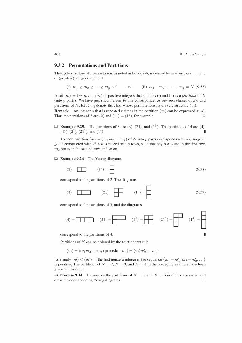
404 9 Finite Groups
9.3.2 Permutations and Partitions
The cycle structure of a permutation, as noted in Eq. (9.29), is defined by a setm1,m2, . . . ,mp
of (positive) integers such that
(i) m1 ≥ m2 ≥ · · · ≥ mp > 0 and (ii) m1 +m2 + · · · +mp = N (9.37)
A set (m) = (m1m2 · · ·mp) of positive integers that satisfies (i) and (ii) is a partition of N(into p parts). We have just shown a one-to-one correspondence between classes of SN andpartitions of N ; let K(m) denote the class whose permutations have cycle structure (m).Remark. An integer q that is repeated r times in the partition (m) can be expressed as qr.Thus the partitions of 2 are (2) and (11) = (12), for example.
Example 9.25. The partitions of 3 are (3), (21), and (13). The partitions of 4 are (4),(31), (22), (212), and (14).
To each partition (m) = (m1m2 · · ·mp) of N into p parts corresponds a Young diagramY(m) constructed with N boxes placed into p rows, such that m1 boxes are in the first row,m2 boxes in the second row, and so on.
Example 9.26. The Young diagrams
(2) = (12) = (9.38)
correspond to the partitions of 2. The diagrams
(3) = (21) = (13) = (9.39)
correspond to the partitions of 3, and the diagrams
(4) = (31) = (22) = (212) = (14) =
correspond to the partitions of 4.
Partitions of N can be ordered by the (dictionary) rule:
(m) = (m1m2 · · ·mp) precedes (m′) = (m′1m
′2 · · ·m′
q)
[or simply (m) < (m′)] if the first nonzero integer in the sequence m1 −m′1,m2 −m′
2, . . .is positive. The partitions of N = 2, N = 3, and N = 4 in the preceding example have beengiven in this order.
Exercise 9.14. Enumerate the partitions of N = 5 and N = 6 in dictionary order, anddraw the corresponding Young diagrams.

9.3 The Symmetric Group SN 405
To each partition (m) of N is associated a conjugate partition (m) whose diagram isobtained from that of (m) by interchanging rows and columns.
Example 9.27. (n) = (1n) (21) = (21) (22) = (22) (31) = (212).
Remark. The partitions (21) and (22) are self-conjugate.
If (m) = (m1m2 · · ·mp) is a partition of N , let νk ≡ mk − mk+1 (k = 1, . . . , p),with mp+1 ≡ 0. Then the conjugate partition (m) can be written in the form (m) =(pνp · · · 2ν21ν1), omitting the term kνk if νk = 0. Conversely, if (m) = (qνq · · · 2ν21ν1)is a partition of N , then the conjugate partition is (m) = (m1m2 · · · mq), with
m1 = ν1 + ν2 + · · · + νq
m2 = ν2 + · · · + νq... (9.40)
mq = νq
These relations are easily verified by drawing a few diagrams.Associated with a Young diagram corresponding to a partition (m) of N is a set of d[(m)]
regular (or standard) tableaux obtained by assigning the numbers 1, 2, . . . , N to the boxesof the Young diagram such that the numbers increase (i) across each row and (ii) down eachcolumn of the diagram. For the diagrams with either a single row or a single column, thereis associated a unique regular tableau, since rules (i) and (ii) require the numbers 1, 2, . . . , Nto appear in order across the row or down the column of the diagram. However, d[(m)] > 1for other Young diagrams, and we shall see that d[(m)] is the dimension of the irreduciblerepresentation of the symmetric group SN corresponding to the partition (m).
Example 9.28. d[(21)] = 2, since
→ 1 23
+ 1 32
Similarly, d[(22)] = 2, since
→ 1 23 4
+ 1 32 4
d[(31)] = 3, since
→ 1 2 34
+ 1 2 43
+ 1 3 42
Computation of the d(m) for partitions of N > 4 is left to the exercises.
Exercise 9.15. Show that d[(m)] = d[(m)] for any conjugate pair (m), (m).
There is also a normal (dictionary) ordering of the standard tableaux associated with a parti-tion. Comparing elements of two standard tableaux while reading across the rows in order, weplace the tableau with the first smaller number ahead of the comparison tableau. The tableauxin the examples above have been written in normal order.
Exercise 9.16. Enumerate the regular tableaux (in normal order) associated with eachpartition (m) of N = 5, 6. Then find the dimension d[(m)] for each (m).
406 9 Finite Groups
9.4 Group Representations
9.4.1 Group Representations by Linear Operators
Of prime importance for physical applications is the study of group representations on a linearvector space V , especially in quantum mechanics, where V is often the space of states of aphysical system. In this and the next section, we develop the general theory of representationsof finite groups; in Section 9.5 we work out the theory of representations of SN in great detail.
Definition 9.20. If G is a group and Γ a group of linear operators on a linear vector space V ,with a homomorphism G → Γ, then Γ is a representation of G. V is the representation space,dimV the dimension of the representation.
In other words, to each element g of G, there corresponds a linear operator DΓ(g) on V suchthat
DΓ(g2)DΓ(g1) = DΓ(g2g1) (9.41)
so that the DΓ(g) follow the multiplication law for the group G. For every group G, the mapg → 1 for every g in G is a representation, the trivial representation, or identity representa-tion. The representation Γ is faithful if every element of G is represented by a distinct linearoperator, so that
DΓ(g2) = DΓ(g1) (9.42)
if and only if g2 = g1.
Definition 9.21. Two representations Γ1 and Γ2 of G on V are equivalent (Γ1 ∼ Γ2) if thereis a nonsingular linear operator S on V such that
DΓ2(g) = SDΓ1(g)S−1 (9.43)
for every g in G; if this is the case, Γ1 and Γ2 differ only by a change of basis in V .
Definition 9.22. If V contains a subspace M invariant under Γ, so that M is an invariantmanifold of DΓ(g) for every group element g, then Γ is reducible. It is fully reducible if M⊥
is also invariant under Γ; in this case the representation Γ can be split into two parts actingon M and M⊥ with no connection between the subspaces. If there is no subspace invariantunder Γ, then Γ is irreducible.
A general problem for any group G is to find all the possible inequivalent irreducible repre-sentations of G. We will find the solution to this problem for finite groups in Theorem 9.4.
Example 9.29. A representation Γm of the cyclic group ZN = 1, a, . . . , aN−1 isdefined by setting
a = exp(
2πimN
)(9.44)
for any m = 0, 1, . . . , N − 1. Each Γm is one-dimensional, hence irreducible, and theN different values of m correspond to inequivalent representations. Γm is faithful unless

9.4 Group Representations 407
either m = 0 (identity representation) or m is a divisor of N . Furthermore, these repre-sentations provide a complete construction of the irreducible representations of Abeliangroups, since we have seen in Section 9.2.1 that every Abelian group can be expressed asa direct product of cyclic groups whose order is a prime number raised to some power,
Example 9.30. The symmetric group SN has two one-dimensional representations, thesymmetric representation Γs with P → 1 for every P, and the antisymmetric representa-tion Γa with P → εP for every P. These representations are inequivalent.
Example 9.31. The action of the permutations of three objects can be represented on C3
by 3 × 3 matrices,
P12 =
0 1 01 0 00 0 1
P13 =
0 0 10 1 01 0 0
P23 =
1 0 00 0 10 1 0
(9.45)
(123) =
0 0 11 0 00 1 0
(321) =
0 1 00 0 11 0 0
1 =
1 0 00 1 00 0 1
(9.46)
that permute the basis vectors of C3. This representation of S3 is reducible, since thevector φ0 = (1, 1, 1) is an eigenvector (eigenvalue +1) of each permutation in S3. ThusM(φ0) is invariant under the representation. However, the representation restricted toM⊥(φ0) is irreducible.
Exercise 9.17. In the three-dimensional space of the preceding example, let
ψ1 ≡√
12 (1,−1, 0) ψ2 ≡
√16 (1, 1,−2) (9.47)
(i) Show that M(ψ1, ψ2) = M⊥(φ0).(ii) Construct the 2 × 2 matrices representing S3 on M(ψ1, ψ2) in the basis ψ1, ψ2.
(iii) Show that this representation is irreducible.
Definition 9.23. If Γ [g → D(g)] is a representation of the group G, then g → D∗(g) definesa representation Γ∗ of G, the complex conjugate of Γ. There are three possibilities:
1. Γ is equivalent to a real representation (Γ is real);
2. Γ ∼ Γ∗, but Γ cannot be transformed to a real representation (Γ is pseudoreal);
3. Γ is not equivalent to Γ∗ (Γ is complex).
Remark. This classification of representations is especially useful in quantum physics, wherecomplex conjugation is related to time reversal and charge conjugation.
Definition 9.24. If Γ [g → D(g)] is a representation of the group G, then g → D†(g−1)defines a representation Γ of G, the dual of Γ. If the D(g) are unitary, then Γ = Γ; in generalthe representation Γ is unitary if it is equivalent to a representation by unitary operators.
Exercise 9.18. Verify that Γ actually is a representation.
408 9 Finite Groups
Theorem 9.1. Any finite-dimensional representation of a group of finite order is equivalentto a unitary representation.
Proof. Suppose G is a group of order n, and Γ a representation of G with g → D(g). Let
H ≡n∑
k=1
D(gk)D†(gk) (9.48)
Then H is positive definite, and if the D(g) are unitary, then H is simply n times the unitmatrix. In any case, however, the matrix ∆ = H1/2 can be chosen to be positive definite. Ifwe now define
U(g) ≡ ∆−1D(g)∆ (9.49)
then the U(g) define a representation of G equivalent to Γ. Now
U(g)U†(g) = ∆−1D(g)HD†(g)∆−1 (9.50)
However,
D(g)HD†(g) = D(g)n∑
k=1
D(gk)D†(gk)D†(g) =n∑
k=1
D(ggk)D†(ggk) (9.51)
and as k runs from 1 to n, the ggk range over the entire group, so that
n∑
k=1
D(ggk)D†(ggk) =n∑
=1
D(g)D†(g) = H (9.52)
It follows that U is unitary, since
U(g)U†(g) = ∆−1D(g)HD†(g)∆−1 = ∆−1H∆−1 = 1
Remark. Since every representation of a finite group is equivalent to a representation byunitary operators, it is no loss of generality to assume that the linear operators are actuallyunitary, unless explicitly stated otherwise.
Definition 9.25. Let Γ be a representation of the group G with g → D(Γ)(g). The characterχ(Γ)(g) of g in Γ is
χ(Γ)(g) ≡ trD(Γ)(g) (9.53)
If g1 and g2 are in the same class of G, then χ(Γ)(g1) = χ(Γ)(g2) in every representation Γ ofG, so the character is a class function. If K is a class in G, then the character χ(Γ)(K) of Kin Γ is the character of any element of K in Γ. The set χ(Γ)(K) of class characters is thecharacter of the representation Γ, simple if Γ is irreducible, otherwise compound.
Example 9.32. Since all the irreducible representations of an Abelian group are one-dimensional, the character of a group element represents the element itself in an irreduciblerepresentation.
9.4 Group Representations 409
Example 9.33. The characters of the classes of S3 (labeled by partitions of 3) in thereducible three-dimensional representation of Example 9.31 are
χ(Γ)(3) = 0 χ(Γ)(21) = 1 χ(Γ)(13) = 3 (9.54)
As an exercise, find these characters in the two-dimensional irreducible representationdefined on M⊥(φ0) (see also Exercise 9.17).
Example 9.34. The character of a rotation through angle θ in the defining representationof SO(2) is
χ(θ) = 2 cos θ (9.55)
since the matrix for rotation through angle θ is
Rz(θ) =(
cos θ − sin θsin θ cos θ
)(9.56)
as given in Eq. (2.107).
Example 9.35. The character of a rotation through angle θ in the defining representationof SO(3) is
χ(θ) = 1 + 2 cos θ (9.57)
To see this, recall the matrix for rotation through angle θ about the Z-axis,
Rz(θ) =
cos θ − sin θ 0sin θ cos θ 0
0 0 1
(9.58)
and note that rotations through angle θ about any axis belong to the same class of SO(3)(see Exercise 2.13).
One observation that can be useful for constructing representations is that if the group Ghas an invariant subgroup H, with factor group F ≡ G/H, then every representation of F isalso a representation of G in which h→ D(h) = 1 for every h in H. Other representations ofG can be constructed from nontrivial representations of H; this is discussed later on.
Example 9.36. The alternating group AN is an invariant subgroup of the symmetricgroup SN , and SN/AN = Z2. The factor group Z2 has two inequivalent irreduciblerepresentations; the corresponding irreducible representations of SN are the symmetric(P → 1) and antisymmetric (P → εP) representations.
410 9 Finite Groups
9.4.2 Schur’s Lemmas and Orthogonality Relations
The basic properties of finite-dimensional unitary representations of groups are derived fromtwo fundamental theorems, both due to Schur.
Theorem 9.2. (Schur’s Lemma I) Let Γ [g → D(g)] be an irreducible representation of thegroup G by unitary operators on the linear vector space V and suppose A is a bounded linearoperator on V such that
AD(g) = D(g)A (9.59)
for every g in G. Then A = α1 for some scalar α.
Remark. In other words, any operator that commutes with every matrix in an irreducibleunitary representation of a group is a multiple of the identity. The restriction to boundedoperators ensures that the theorem also works for infinite-dimensional representations.
Proof. If A commutes with D(g) for every g, so does A†, since Eq. (9.59) implies
A†D†(g) = D†(g)A† (9.60)
and unitarity means that D†(g) = D(g−1) is in Γ for every g. Hence we can take A to beself-adjoint, with a spectral resolution. If the spectrum of A contains more than one point,then V can be decomposed into a direct sum V1 ⊕V2 such that the spectra of A on V1 and V2
are disjoint. But V1 and V2 are invariant under Γ, so that Γ would be reducible. Since it is not,the spectrum of A can contain only one point, i.e., A= α1 for some scalar α.
Theorem 9.3. (Schur’s Lemma II) Let Γ [g → D(g)] and Γ′ [g → D′(g)] be inequivalentunitary irreducible representations of the group G on linear vector spaces V and V ′ of finitedimensions m and m′, respectively. Let A be an m×m′ matrix mapping V ′ to V such that
D(g)A = AD′(g) (9.61)
for every g in G. Then A = 0.
Proof. Suppose m > m′. Then AV ′ defines a linear manifold MA in V of dimensiondimMA ≤ m′ < m. But MA is invariant under Γ if D(g)A = AD′(g), and thus Γ isreducible if dimMA = 0. Hence A = 0. If Γ and Γ′ are irreducible representations of thesame dimension, then either dimMA = 0, in which case A = 0, or dimMA = m, inwhich case Eq. (9.61) implies D(g) = AD′(g)A−1 and thus Γ ∼ Γ′. The latter is contraryto hypothesis, hence A = 0.
Remark. The statements of the two lemmas are valid for an arbitrary group, not necessarilyfinite. However, the lemmas apply to only to finite-dimensional unitary representations, whichmay, or may not, exist for an infinite group.
Two corollaries of Schur’s lemmas lead to a set of orthogonality relations for the represen-tation matrices of finite groups. These relations lead to a fairly complete theory of representa-tions of finite groups, part of which is outlined here.
Corollary 1. Let G be a finite group of order n, Γ [g → D(g)] an irreducible representationof G on the m-dimensional linear vector space V . If X is any linear operator on V , then there
9.4 Group Representations 411
is a scalar α = α(X) such that
A(X) ≡n∑
k=1
D(gk)XD(g−1k ) = α(X) 1 (9.62)
Proof. We have
A(X)D(g) =n∑
k=1
D(gk)XD(g−1k )D(g) = D(g)
n∑
k=1
D(g−1gk)XD(g−1k g) (9.63)
But, as noted earlier, the sum over the elements ggk is equivalent to a sum over all theelements of G, so we have
A(X)D(g) = D(g)A(X) (9.64)
whence A(X) must be a multiple of the identity by Schur’s Lemma I.
Corollary 2. Let Γ [g → D(g)] and Γ′ [g → D′(g)] be inequivalent irreducible representa-tions of the group G of order n on the linear vector spaces V and V ′ of dimension m and m′,respectively. Let X be an m×m′ matrix mapping V ′ to V . Then
F(X) ≡n∑
k=1
D(gk)XD′(g−1k ) = 0 (9.65)
Proof. By the same argument used in the preceding proof, we have
D(g)F(X) = F(X)D′(g) (9.66)
for every g in G. Hence F(X) = 0 by Schur’s Lemma II.Since the results (9.62) and (9.65) are true for any matrix X, we can use the special matri-
ces Xjk with a single nonvanishing matrix element,(Xjk
)j′k′ ≡ δjj′δ
kk′ (9.67)
to derive some useful properties of the representation matrices. In particular, if G is a finitegroup of order n with an m-dimensional representation Γ [g → D(g)], we can treat each setof matrix elements Djk(g) ( = 1, . . . , n) as the components of a vector in an n-dimensionalvector space Vn. Here Vn is exactly the vector space underlying the group algebra A(G)introduced in Section 9.1.3.
In particular, suppose Γ [g → D(g)] is an m-dimensional irreducible representation of G.Then from Eq. (9.62), we have
A(Xkk′) =
n∑
=1
D(g)Xkk′
D(g−1 ) = λkk′1 (9.68)
for some scalar λkk′ , and, since the D(g) are unitary, we then have
n∑
=1
Djk(g)D∗j′k′(g) = λkk′δjj′ (9.69)
412 9 Finite Groups
The scalar λkk′ is evaluated by taking the trace of this equation to give
mλkk′ =n∑
=1
trD(g)X
kk′D(g−1
)
=n∑
=1
trDk′k(g−1
g)
= nδkk′ (9.70)
so that we have, finally,
n∑
=1
Djk(g)D∗j′k′(g) =
n
mδjj′δkk′ (9.71)
Thus the Djk form a set of m2 orthogonal vectors in Vn.Furthermore, if Γa [g → Da(g)] and Γb [g → Db(g)] are two inequivalent finite-
dimensional unitary irreducible representations of G, then Eq. (9.65) tells us that
F(Xkk′) =
n∑
k=1
D(gk)Xkk′
D′(g−1k ) = 0 (9.72)
and then
n∑
=1
Dajk(g)D
b∗j′k′(g) = 0 (9.73)
Thus the Dajk(g), considered as components of vectors Da
jk in Vn, define an orthogonalsystem in Vn. We can then sum over all the inequivalent irreducible representations Γa of Gto obtain
∑
a
m2a ≤ n (9.74)
(ma is the dimension of Γa), since there are at most n orthogonal vectors in Vn, In fact, theequality is always true, as shown in Theorem 9.9.4.
Equations (9.71) and (9.73) can be expressed simply in terms of the characters of therepresentations: If χa(g), χb(g) denote the characters of g in the inequivalent irreduciblefinite-dimensional representations Γa and Γb of G, then
n∑
=1
χa(g)χb∗(g) = n δab (9.75)
The character of g depends only on the class of G to which g belongs. If K1 =e,K2, . . . ,Kp are the classes of G, with h1 = 1, h2, . . . , hp elements, and that χ ak is thecharacter of the class Kk in the irreducible representation Γa. Then Eq. (9.75) is equivalent to
p∑
k=1
hkχakχ
b∗k = n δab (9.76)
9.4 Group Representations 413
Thus the p-dimensional vectors va with components
vak ≡√hknχak (9.77)
(k = 1, . . . , p) form an orthonormal system, so there are at most p inequivalent finite-dimensional irreducible representations of G.
Remark. There are exactly p inequivalent finite-dimensional irreducible representations ofG, and the p× p matrix V = (vak) is unitary, but more work is needed to derive that result.
Now suppose Γ is a finite-dimensional representation of G. In general, Γ is reducible, butwe can express it as a direct sum of inequivalent irreducible representations of G,
Γ = ⊕a cΓa Γa (9.78)
with nonnegative integer coefficients cΓa . If χΓ
k is the character of the classKk of G in Γ, thenwe also have the expansion
χΓk =
∑
a
cΓa χ
ak (9.79)
in terms of the characters of the χak irreducible representations of G. The orthogonality rela-tion (9.76) then gives
p∑
k=1
hkχa∗k χ
Γk = ncΓ
a andp∑
k=1
hk∣∣χΓk
∣∣2 = n∑
a
∣∣cΓa
∣∣2 (9.80)
Hence the representation Γ is irreducible if and only if
p∑
k=1
hk∣∣χΓk
∣∣2 = n (9.81)
Remark. Thus we can reduce any representation Γ of G to a direct sum over the inequivalentirreducible representations using the characters χak once we have the characters χΓ
k of Γ.
Definition 9.26. If G is a group of finite order n, then every element g of G defines a permu-tation Pg (gk → ggk, k = 1, . . . , n). The map g → Pg is a permutation representation of G.If A(Pg) is the permutation matrix associated with Pg (see Eq. (9.27)), then the representationΓR [g → A(Pg)] is a faithful representation, the regular representation, of G.
The characters of ΓR are given by χR1 = n, χRk = 0 (k = 2, . . . , p). From Eq. (9.80) wehave cRa = ma, where ma is the dimension of the irreducible representation Γa. Thus ΓR isexpressed as a direct sum of the inequivalent irreducible representations Γ1, . . . ,Γq of G as
ΓR = ⊕qa=1 maΓa (9.82)
Then alsoq∑
a=1
m2a = n and
q∑
a=1
maχak = 0 (9.83)
414 9 Finite Groups
Now suppose Γ = Γa [g → D(g)] is an irreducible representation of G (dimension ma),and Kk is a class of G with hk elements. Then the class matrix D Γ
k of Kk in Γ is defined by
D Γk ≡
∑
g in Kk
D(g) (9.84)
Since g(Kk) = (Kk)g follows directly from the definition of a class, the class matrix D Γk
commutes with every g in G. Since Γ = Γa is irreducible, we must have
D Γk ≡ Da
k = λak 1 (9.85)
by Schur’s Lemma I; here λak is computed by taking traces on both sides to give
maλak = hkχ
ak (9.86)
In general, the class matrices satisfy
D Γk D Γ
k =p∑
=1
cjkDΓ (9.87)
where the cjk are the class multiplication coefficients of G (see Problem 2). If Γ = Γa, then
hjhk χajχ
ak = ma
p∑
=1
cjkhχa (9.88)
If we now sum Eq. (9.88) over the inequivalent irreducible representations of G, we obtain
hjhk
q∑
a=1
χajχak =
p∑
=1
cjkh
q∑
a=1
maχa = nc1jk (9.89)
in view of Eq. (9.83). Now c1jk is the number of times the identity element appears in theproduct of the classes Kj and Kk. Clearly c1jk = 0 unless Kj is the class Kk inverse to Kk;in that case, c1jk must be the number hk of group elements in the class Kk. Thus we have
c1jk = hkδjk (9.90)
Since Γa is unitary, we also have χak
= χa∗k , and then
hk
q∑
a=1
χa∗j χak = nδjk (9.91)
Thus the q-dimensional vectors uk with components uak = χak (a = 1, . . . , q) form an orthog-onal system. Hence there are at most q classes of G.
The preceding results taken together form the fundamental theorem on the inequivalentirreducible representations of a finite group.

9.4 Group Representations 415
Theorem 9.4. (Fundamental Representation Theorem) Suppose G is a group of finite order ncontaining the classesK1 = e,K2, . . . ,Kp with h1 = 1, h2, . . . , hp elements, respectively.Let Γ1, . . . ,Γq be the inequivalent irreducible representations of G, and let χak be the characterof the class Kk in the irreducible representation Γa. Then
(i) q = p, and(ii) the p× p matrix V = (vak) with matrix elements
vak ≡√hknχak (9.92)
is unitary.
Remark. The characters of the group can then be presented as a p× p matrix, the charactertable of the group, as illustrated in the examples below.
Thus the number of inequivalent irreducible representations of G is equal to the number ofclasses of G. The characters form an orthonormal system (with appropriately chosen weights)considered as vectors with components either along the classes of G, or along the inequivalentirreducible representations of G. Equations (9.76) and (9.88), together with Eq. (9.83), areenough to completely determine the characters and even the representations for small groups,and lead to general methods for computing the characters and representations of larger groups.
Example 9.37. The symmetry group of a square consists of rotations in the planethrough an integer multiple of π/2, and any of these rotations combined with a rotation ρthrough π about a diagonal of the square. This group has elements that we can denote bye, a, a2, a3, ρ, ρa, ρa2, ρa3, with
a4 = e ρ2 = e ρaρ = a3 = a−1 (9.93)
The group is in fact isomorphic to the dihedral group D4 introduced in Section 9.2 (showthis). The classes of the group are easily identified:
K1 = e K2 = a, a3 K3 = a2
K4 = ρ, ρa2 K5 = ρa, ρa3With five classes, there are five inequiva-lent irreducible representations. It is clearfrom Eq. (9.83) that of these, four are one-dimensional and one is two-dimensional.For the one-dimensional representations,we can identify a = ±1 and ρ = ±1 inde-pendently. For the two-dimensional repre-sentation, the requirement ρ2 = e allows
K1 K2 K3 K4 K5
h 1 2 1 2 2
Γ1 1 1 1 1 1
Γ2 1 1 1 −1 −1
Γ3 1 −1 1 1 −1
Γ4 1 −1 1 −1 1
Γ5 2 0 −2 0 0
Character table for D4.
us to identify ρ = σ1; then ρaρ = a−1 leads to the choice a = iσ2, unique up to sign, toobtain a real representation (it is also possible to start with ρ = σ3). The characters of thegroup are then easily computed and can be arranged in the character table shown at theright (check the orthogonality relations as an exercise).
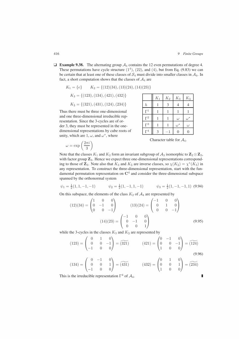
416 9 Finite Groups
Example 9.38. The alternating group A4 contains the 12 even permutations of degree 4.These permutations have cycle structure (14), (22), and (4), but from Eq. (9.83) we canbe certain that at least one of these classes of S4 must divide into smaller classes in A4. Infact, a short computation shows that the classes of A4 are
K1 = e K2 = (12)(34), (13)(24), (14)(23)
K3 = (123), (134), (421), (432)
K3 = (321), (431), (124), (234)
Thus there must be three one-dimensionaland one three-dimensional irreducible rep-resentation. Since the 3-cycles are of or-der 3, they must be represented in the one-dimensional representations by cube roots ofunity, which are 1, ω, and ω∗, where
K1 K2 K3 K3
h 1 3 4 4
Γ1 1 1 1 1
Γ2 1 1 ω ω∗
Γ3 1 1 ω∗ ω
Γ4 3 −1 0 0
Character table for A4.
ω = exp(
2πi3
)
Note that the classesK1 andK2 form an invariant subgroup of A3 isomorphic to Z2⊗Z2,with factor group Z3. Hence we expect three one-dimensional representations correspond-ing to those of Z3. Note also that K3 and K3 are inverse classes, so χ(K3) = χ∗(K3) inany representation. To construct the three-dimensional representation, start with the fun-damental permutation representation on C4 and consider the three-dimensional subspacespanned by the orthonormal system
ψ1 = 12 (1, 1,−1,−1) ψ2 = 1
2 (1,−1, 1,−1) ψ3 = 12 (1,−1,−1, 1) (9.94)
On this subspace, the elements of the class K2 of A4 are represented by
(12)(34) =
1 0 00 −1 00 0 −1
(13)(24) =
−1 0 0
0 1 00 0 −1
(14)(23) =
−1 0 0
0 −1 00 0 1
(9.95)
while the 3-cycles in the classes K3 and K3 are represented by
(123) =
0 1 00 0 −1
−1 0 0
= (321) (421) =
0 −1 00 0 −11 0 0
= (124)
(9.96)
(134) =
0 −1 00 0 1
−1 0 0
= (431) (432) =
0 1 00 0 11 0 0
= (234)
This is the irreducible representation Γ4 of A4.
9.4 Group Representations 417
9.4.3 Kronecker Product of Representations
There are many systems in which we encounter a space that is a tensor product of group rep-resentation spaces. In quantum mechanics, for example, we consider separately the symmetryof a two-electron state under exchange of the spatial and spin coordinates of the two electrons.The combined state must be antisymmetric according to the Pauli principle, but this can beachieved either with symmetric space and antisymmetric spin states, or vice versa. This exam-ple is simple enough, but when more particles are involved, the implementation of the Pauliprinciple requires further analysis.
Definition 9.27. Let Γa [g → Da(g)] and Γb [g → Db(g)] be irreducible representations ofG on Va and on Vb. Then the representation Γa × Γb of G on Va ⊗ Vb defined by
Γa × Γb : g → Da×b ≡ Da ⊗ Db (9.97)
is the Kronecker product (or tensor product) of Γa and Γb.The Kronecker product can be reduced to a sum of irreducible representations of the form
Γa × Γb = ⊕c Cabc Γc (9.98)
The coefficients Cabc in this reduction are called the coefficients of composition of G.The character of Γa × Γb is simply the product of the characters of Γa and Γb,
χa×bk = χakχbk (9.99)
It follows from the orthogonality relation (9.76) that
nCabc =p∑
k=1
hkχakχ
bkχ
c∗k =
p∑
k=1
hkχa∗k χ
b∗k χ
ck (9.100)
Thus the Cabc can be computed directly from the character table.One useful general result can be obtained if we let Γc be the identity representation. Then
Eq. (9.100) becomes
nCab1 =p∑
k=1
hkχakχ
bk = nδab (9.101)
where Γa = Γa∗ is the complex conjugate of Γa, and Γ1 denotes the identity representation.Hence Γ1 appears only in the Kronecker product of an irreducible representation with itscomplex conjugate.
There are also symmetries of the Cabc that follow directly from Eq. (9.100). For example,
Cabc = Cbac = C abc = Cacb (9.102)
These symmetry relations simplify the evaluation of many Kronecker products.
Example 9.39. Consider the group D4 with character table given in Example 9.37. Forthe one-dimensional representations, Kronecker products can be read off directly from thecharacter table to give
Γ2 × Γ3 = Γ4 Γ2 × Γ4 = Γ3 Γ3 × Γ4 = Γ2 (9.103)

418 9 Finite Groups
Note that the characters of the one-dimensional representations themselves form anAbelian group, the character group, here isomorphic to Z2 ⊗ Z2. Also,
Γa × Γ5 = Γ5 (9.104)
(a = 1, . . . , 4), and finally,
Γ5 × Γ5 = Γ1 ⊕ Γ2 ⊕ Γ3 ⊕ Γ4 (9.105)
This result follows directly from the symmetry relations (9.102), though it can also beobtained by calculation using Eq. (9.100) and the character tables.
Exercise 9.19. Compute the reduction of the Kronecker product Γ4 × Γ4 in the group A4
from the character table given in Example 9.38.
9.4.4 Permutation Representations
In Section 9.4.2, we introduced the representation of a group G of order n by the permutationsof the n group elements associated with group multiplication, i.e., if g1 = e, g2, . . . , gn arethe elements of G, then
ggk → gik (9.106)
defines a permutation Pg = (i1, . . . , in) of n. The regular representation ΓR of G was thenintroduced (Definition 9.26) as the representation [g → A(Pg)] of G by the permutationmatrices A(P) corresponding to these permutations.
There are other useful representations of groups by permutations and their associated ma-trices. Every element P of the symmetric group SN corresponds to an N × N permutationmatrix A(P); this is the fundamental (or defining) representation of SN . The fundamentalrepresentation is reducible, since the vector ξ0 = (1, 1, . . . , 1) is transformed into itself byevery permutation of the basis vectors. However, the representation of SN on the (N−1)-dimensional manifold M⊥(ξ0) actually is irreducible, as we now show for the case of S3.
Example 9.40. For the group S3 of permutations of three objects, the fundamental three-dimensional representation was introduced in Example 9.31, with representation matricesgiven in Eq. (9.46). This representation of S3 is reducible, since one-dimensional subspaceM(ξ0) is invariant under S3. We have
A(P)ξ0 = ξ0 (9.107)
for every permutation P in S3. This defines the identity (symmetric) representation of S3.To construct a two-dimensional representation on M⊥(ξ0), note that the vectors
ψ1 ≡√
12 (1,−1, 0) ψ2 ≡
√16 (1, 1,−2) (9.108)
form a complete orthonormal system on M⊥(ξ0). These vectors are chosen so that (i)they are orthogonal to ξ0 and (ii) they are either symmetric (ψ2) or antisymmetric (ψ1)

9.4 Group Representations 419
under the transposition of φ1 and φ2. A short calculation shows that in this basis, thetranspositions are represented by the 2 × 2 matrices
(12) =(−1 00 1
)(13) =
12
(1 −
√3
−√
3 −1
)(23) =
12
(1
√3√
3 −1
)
(9.109)
Then also
(123) = (13)(12) =12
(−1 −
√3√
3 −1
)(321) = (12)(13) =
12
(−1
√3
−√
3 −1
)
(9.110)
This representation is irreducible, since the matrices do not commute with each other, andthus cannot have common eigenvectors.
Remark. The group S3 thus has three inequivalent irreducible representations: Two one-dimensional representations, symmetric (P → 1) and antisymmetric (P → εP), and thetwo-dimensional representation found here, the mixed symmetry representation.
If a group G of order n has a subgroup H of order m, index t = n/m, then permutationsof the cosets of H in G associated with the group multiplication define a permutation represen-tation P(G,H) of G, in which P(g,H) is the permutation of the cosets of H in G associatedwith multiplication by the group element g. To understand this representation, note that thereare elements g1 = e, g2, . . . , gt of G such that g1H, g2H, . . ., gtH are the disjoint cosets of Hin G. Then we can form the t× t matrices σ(g, h) such that
σαβ(g, h) =
1, if ggβ = gαh
0 otherwise(9.111)
These matrices have at most one nonzero element in any row or column, since given g in G,and β = 1, . . . , t, the element ggβ belongs to exactly one coset of H, say gαH. Then let
π(g,H) ≡∑
h∈Hσ(g, h) = A(P(g,H)) (9.112)
where A(P(g,H)) is the permutation matrix associated with the permutation P(g,H).Exercise 9.20. Show that
π(g1,H)π(g2,H) = π(g1g2,H)
so that the π(g,H) actually form a representation of G.
The π(g,H) define the principal representation of G induced by H. Other representationsof G can be constructed from those of H using the matrices σ(g, h). If ∆ [h → D∆(h)] is arepresentation of H, then
DΓ(g) ≡∑
h in Hσ(g, h) ⊗ D∆(h) (9.113)

420 9 Finite Groups
is a representation Γ ≡ ∆ind of G, the representation of G induced by ∆. The principalrepresentation [g → π(g,H)] of G is evidently induced by the identity representation of H.
Example 9.41. Consider the alternating group A4 introduced in Example 9.38. Thisgroup has an Abelian subgroup H isomorphic to Z2 ⊗ Z2 with elements
e a = (12)(34) b = (13)(24) c = (14)(23) (9.114)
with
a2 = b2 = c2 = e and abc = e (9.115)
H has four inequivalent irreducible representations: The identity representation Γ0, andthree representations labeled Γa, Γb, and Γc, in which the elements a, b, c, respectively,are represented by +1 and the other two elements of order 2 by −1. The cosets of H areH = K1 ∪K2, K3, and K3, using the notation of Example 9.38, and we can take thecoset representatives to be e, (123) and (321).
In the principal representation ΓH of A4 induced by H, all the elements of each cosetare represented by the same matrix, and we have
H →
1 0 00 1 00 0 1
K3 →
0 1 00 0 11 0 0
K3 →
0 0 11 0 00 1 0
(9.116)
These matrices have common eigenvectors ψλ = (1, λ, λ2) with λ3 = 1, so that ΓH isreducible; in fact,
ΓH = Γ1 ⊕ Γ2 ⊕ Γ3 (9.117)
where the Γ1,2,3 are the irreducible representations of A4 constructed in Example 9.38.The three-dimensional irreducible representation Γ4 of A4 appears only in the rep-
resentations of A4 induced by one of the representations Γa, Γb, Γc of H. Since theselead to equivalent representations of A4, we can choose Γa. We then find solutions to thefollowing equation
ggβ = gαh (9.118)
as g runs through A4 and gβ runs through the set e, (123), (321). The results are shownin the table, together with the corresponding matrices in the induced representation. Thematrices for the 3-cycles in the class K3 of A4 are not given explicitly; the matrix such a3-cycle is simply the transpose of the matrix for its inverse in the class K3.

9.4 Group Representations 421
Table 9.1: Multiplication table for generating representations of A4 induced by an irreduciblerepresentation of its Z2 ⊗ Z2 subgroup. The rightmost column gives the matrices for the rep-resentation of A4 induced by the representation of Z2 ⊗ Z2 in which the elements e and a arerepresented by +1, the elements b and c by −1.
g gβ gα h∑
h
σαβ D(h)
a e e a
a (123) (123) b
a (321) (321) c
1 0 00 −1 00 0 −1
b e e b
b (123) (123) c
b (321) (321) a
−1 0 0
0 −1 00 0 1
c e e c
c (123) (123) a
c (321) (321) b
−1 0 0
0 1 00 0 −1
(123) e (123) e
(123) (123) (321) e
(123) (321) e e
0 0 11 0 00 1 0
(134) e (123) a
(134) (123) (321) b
(134) (321) e c
0 0 −11 0 00 −1 0
(421) e (123) c
(421) (123) (321) a
(421) (321) e b
0 0 −1
−1 0 00 1 0
(432) e (123) b
(432) (123) (321) c
(432) (321) e a
0 0 1
−1 0 00 −1 0
Remark. The matrices in the table are not exactly the same as those given in Example 9.38.However, the two representations are in fact equivalent, since one can be transformed into theother by a rotation through π/2 in the ψ2-ψ3 plane. The details are left to the reader.
422 9 Finite Groups
9.4.5 Representations of Groups and Subgroups
Any representation of a group G is a representation of a subgroup H, but in general, an irre-ducible representation of G is reducible when restricted to H. As explained in the precedingsection, a representation of H induces a representation of G, which is also reducible in general.The Frobenius reciprocity theorem, explained below and derived in Appendix A, provides afundamental relation between the reduction of irreducible representations of G restricted to asubgroup H and the representations of G induced by irreducible representations of H.
Suppose G is a group of order n, with inequivalent irreducible representations Γ1, . . . ,Γp,of dimensions m1, . . . ,mp, respectively. Also, suppose H is a subgroup of G of order m withinequivalent irreducible representations denoted by ∆1, . . . ,∆q , with µc the dimension of ∆c
(c = 1, . . . , q). A representation Γ of G restricted to H defines the representation Γsub of Hsubduced by Γ. The irreducible representation Γa of G subduces a representation Γasub of Hthat can be reduced to a sum of irreducible representations of H,
Γasub = ⊕c αca∆c (9.119)
with nonnegative integer coefficients αca. On the other hand, the irreducible representation∆c of H induces a representation ∆c
ind of G, also reducible in general,
∆cind = ⊕a βcaΓa (9.120)
with nonnegative integer coefficients βca. The Frobenius reciprocity theorem states that
αca = βca (9.121)
In words, the coefficients that appear in the reduction of an irreducible representation of Grestricted to a subgroup H are equal to the coefficients in the reduction of the representation ofG induced by an irreducible representation of H. A proof of this crucial theorem is presentedin Appendix A for the curious reader.
An important corollary that is extremely useful in practical computations is
Γa × ∆cind = [Γasub × ∆c]ind (9.122)
This allows Kronecker products obtained for a subgroup H to be used to reduce those in G.This result will be applied to the the symmetric group in the next section.
Representations of direct product groups are often useful in constructing representationsof larger groups. If G1 and G2 are groups with representations Γ(1) [g1 → D(1)(g1)] and Γ(2)[g2 → D(2)(g2)], respectively, then
(g1, g2) → D(g1, g2) ≡ D(1)(g1) ⊗ D(2)(g2) (9.123)
is a representation Γ(1) ⊗ Γ(2) of G1 ⊗ G2, irreducible if and only if both Γ(1) and Γ(2)are irreducible. If Γa(1) and Γc(2) are the inequivalent irreducible representations of G1
and G2, then the inequivalent irreducible representations of G1 ⊗ G2 have the form
Γ(a,c) ≡ Γa(1) ⊗ Γc(2) (9.124)
9.4 Group Representations 423
The representations of G induced by those of G1 ⊗ G2 have a special name:
Definition 9.28. If G is a group with subgroup G1 ⊗G2, then the representation of G inducedby the representation Γ(1) ⊗ Γ(2) of G1 ⊗ G2, using the construction of Eq. (9.113), is theouter product [Γ(1) Γ(2)]G of Γ(1) and Γ(2) (with respect to G). The subscript G may beomitted if the group G is understood.
Example 9.42. A rather simple illustration of these ideas can be extracted from the dis-cussion of the alternating group A4 and its Z2 ⊗ Z2 subgroup in examples 9.38 and 9.41.Denote the irreducible representations of Z2 by
ΓS = 1, 1 and ΓA = 1,−1
(S = symmetric, A = antisymmetric), those of Z2 ⊗ Z2 by
Γ0 = ΓS ⊗ ΓS Γa = ΓS ⊗ ΓA Γb = ΓA ⊗ ΓS Γc = ΓA ⊗ ΓA
as in Example 9.41, and those of A4 by Γ1,2,3,4 as in Example 9.38. Under the restrictionof A4 to its Z2 ⊗ Z2 subgroup, we have
Γ1,2,3 → Γ0 Γ4 → Γa ⊕ Γb ⊕ Γc (9.125)
The Frobenius reciprocity theorem then requires that the representations of A4 induced bythose of Z2 ⊗ Z2 satisfy
Γ0ind = ΓS ΓS = Γ1 ⊕ Γ2 ⊕ Γ3 (9.126)
Γa,b,cind = ΓS ΓA = ΓA ΓS = ΓA ΓA = Γ4 (9.127)
as already derived in Example 9.41.
Outer products of representations of SN are especially important, as they play a centralrole in the reduction of Kronecker products of Lie groups. As we shall see in the next chap-ter, irreducible representations of Lie groups are associated with irreducible representationsof SN . For example, consider the group U(n) of unitary operators on an n-dimensional linearvector space Vn. Tensors of rank N are defined on the tensor product ⊗NVn of N identicalcopies of Vn. These tensors define a reducible representation of U(n); irreducible tensors arethose that transform as irreducible representations of SN under permutations of theN indices.
If Γa and Γb are representations of a Lie group corresponding to representations SMand SN , respectively, then the Kronecker product of these representations corresponds to therepresentation of SM+N defined by the outer product ΓaΓb. Thus we are interested in findingthe irreducible representations contained the reduction of outer products of irreducible repre-sentations of SN . Some elegant graphical techniques are available to perform this reduction;these are described in the next section.
424 9 Finite Groups
9.5 Representations of the Symmetric Group SN
9.5.1 Irreducible Representations of SN
The symmetric group SN of permutations of N elements has classes corresponding to parti-tions of N , as described in Section 9.3. Each permutation has a cycle structure that can beidentified with a partition (ξ) of N , and the class K(ξ) of SN consists of all the permutationsin SN with cycle structure characterized by (ξ). Thus there are π(N) classes in SN . It followsthat there are also π(N) inequivalent irreducible representations of SN , and these can also beassociated with partitions of N ; denote the irreducible representation of SN associated withthe partition (λ) of N by Γ(λ).
The simple characters of SN are given by a remarkable generating function due to Frobe-nius. This generating function (Eq. (9.B42)) and the graphical methods that can be used toactually compute the characters are derived in detail in Appendix B. Here we simply notethat the dimension d(λ) of Γ(λ) is given, as already noted in Section 9.3.2, by the number ofregular Young tableaux that can be associated with the Young diagram Y(λ), or by the eleganthook formula (9.B48).
The regular tableaux can be used to define projection operators that act on a general func-tion of N variables to project out functions transforming among themselves under an irre-ducible representation on SN under permutations of the variables. For example, the operatorsS and A defined by
S =∑
P∈SN
P and A =∑
P∈SN
εPP (9.128)
project out the symmetric and antisymmetric components of a function of N variables. Thesecomponents may not be present, of course, in which case the projection gives zero.
For a general regular tableau t associated with a partition (λ) of N , we let Ht (Vt) denotethe subgroup of SN that leaves the rows (columns) of the tableau unchanged. Then define
St =∑
P∈Ht
P and At =∑
P∈Vt
εPP (9.129)
St (At) projects out components of a function that are symmetric (antisymmetric) under per-mutations of variables in the same row (column) of t. We then define the Young symmetrizerassociated with t as
Yt = AtSt (9.130)
Note that if t and t′ are two distinct regular tableaux, there is necessarily at least one pairof elements in some row of t′ that appears in the same column of t. Then St′At = 0,since At projects out the component antisymmetric under exchange of this pair, which is thenannihilated by St′ . Thus
Yt′Yt = 0 (9.131)
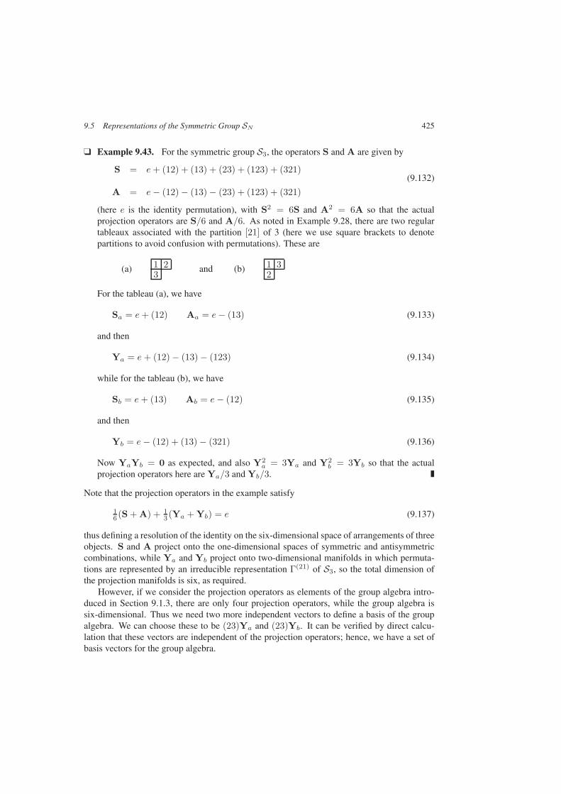
9.5 Representations of the Symmetric Group SN 425
Example 9.43. For the symmetric group S3, the operators S and A are given by
S = e+ (12) + (13) + (23) + (123) + (321)(9.132)
A = e− (12) − (13) − (23) + (123) + (321)
(here e is the identity permutation), with S2 = 6S and A2 = 6A so that the actualprojection operators are S/6 and A/6. As noted in Example 9.28, there are two regulartableaux associated with the partition [21] of 3 (here we use square brackets to denotepartitions to avoid confusion with permutations). These are
(a) 1 23 and (b) 1 3
2
For the tableau (a), we have
Sa = e+ (12) Aa = e− (13) (9.133)
and then
Ya = e+ (12) − (13) − (123) (9.134)
while for the tableau (b), we have
Sb = e+ (13) Ab = e− (12) (9.135)
and then
Yb = e− (12) + (13) − (321) (9.136)
Now YaYb = 0 as expected, and also Y2a = 3Ya and Y2
b = 3Yb so that the actualprojection operators here are Ya/3 and Yb/3.
Note that the projection operators in the example satisfy
16 (S + A) + 1
3 (Ya + Yb) = e (9.137)
thus defining a resolution of the identity on the six-dimensional space of arrangements of threeobjects. S and A project onto the one-dimensional spaces of symmetric and antisymmetriccombinations, while Ya and Yb project onto two-dimensional manifolds in which permuta-tions are represented by an irreducible representation Γ(21) of S3, so the total dimension ofthe projection manifolds is six, as required.
However, if we consider the projection operators as elements of the group algebra intro-duced in Section 9.1.3, there are only four projection operators, while the group algebra issix-dimensional. Thus we need two more independent vectors to define a basis of the groupalgebra. We can choose these to be (23)Ya and (23)Yb. It can be verified by direct calcu-lation that these vectors are independent of the projection operators; hence, we have a set ofbasis vectors for the group algebra.
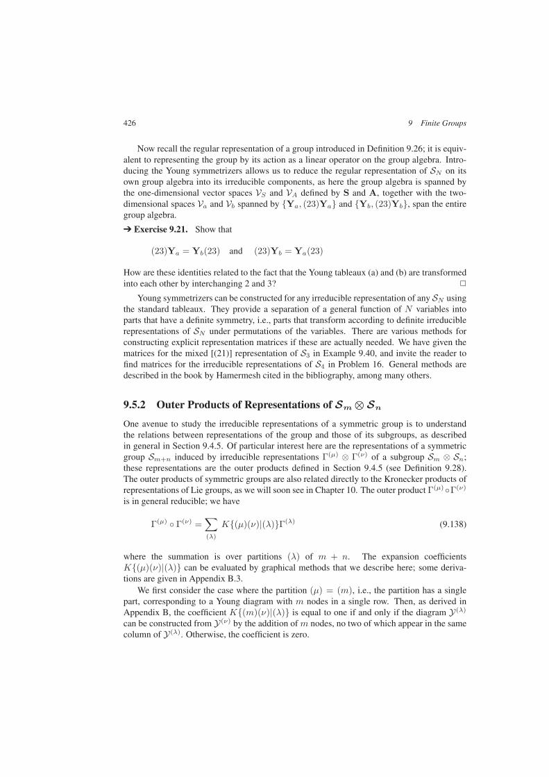
426 9 Finite Groups
Now recall the regular representation of a group introduced in Definition 9.26; it is equiv-alent to representing the group by its action as a linear operator on the group algebra. Intro-ducing the Young symmetrizers allows us to reduce the regular representation of SN on itsown group algebra into its irreducible components, as here the group algebra is spanned bythe one-dimensional vector spaces VS and VA defined by S and A, together with the two-dimensional spaces Va and Vb spanned by Ya, (23)Ya and Yb, (23)Yb, span the entiregroup algebra.
Exercise 9.21. Show that
(23)Ya = Yb(23) and (23)Yb = Ya(23)
How are these identities related to the fact that the Young tableaux (a) and (b) are transformedinto each other by interchanging 2 and 3?
Young symmetrizers can be constructed for any irreducible representation of any SN usingthe standard tableaux. They provide a separation of a general function of N variables intoparts that have a definite symmetry, i.e., parts that transform according to definite irreduciblerepresentations of SN under permutations of the variables. There are various methods forconstructing explicit representation matrices if these are actually needed. We have given thematrices for the mixed [(21)] representation of S3 in Example 9.40, and invite the reader tofind matrices for the irreducible representations of S4 in Problem 16. General methods aredescribed in the book by Hamermesh cited in the bibliography, among many others.
9.5.2 Outer Products of Representations of Sm ⊗ Sn
One avenue to study the irreducible representations of a symmetric group is to understandthe relations between representations of the group and those of its subgroups, as describedin general in Section 9.4.5. Of particular interest here are the representations of a symmetricgroup Sm+n induced by irreducible representations Γ(µ) ⊗ Γ(ν) of a subgroup Sm ⊗ Sn;these representations are the outer products defined in Section 9.4.5 (see Definition 9.28).The outer products of symmetric groups are also related directly to the Kronecker products ofrepresentations of Lie groups, as we will soon see in Chapter 10. The outer product Γ(µ)Γ(ν)
is in general reducible; we have
Γ(µ) Γ(ν) =∑
(λ)
K(µ)(ν)|(λ)Γ(λ) (9.138)
where the summation is over partitions (λ) of m + n. The expansion coefficientsK(µ)(ν)|(λ) can be evaluated by graphical methods that we describe here; some deriva-tions are given in Appendix B.3.
We first consider the case where the partition (µ) = (m), i.e., the partition has a singlepart, corresponding to a Young diagram with m nodes in a single row. Then, as derived inAppendix B, the coefficient K(m)(ν)|(λ) is equal to one if and only if the diagram Y(λ)
can be constructed from Y(ν) by the addition of m nodes, no two of which appear in the samecolumn of Y(λ). Otherwise, the coefficient is zero.
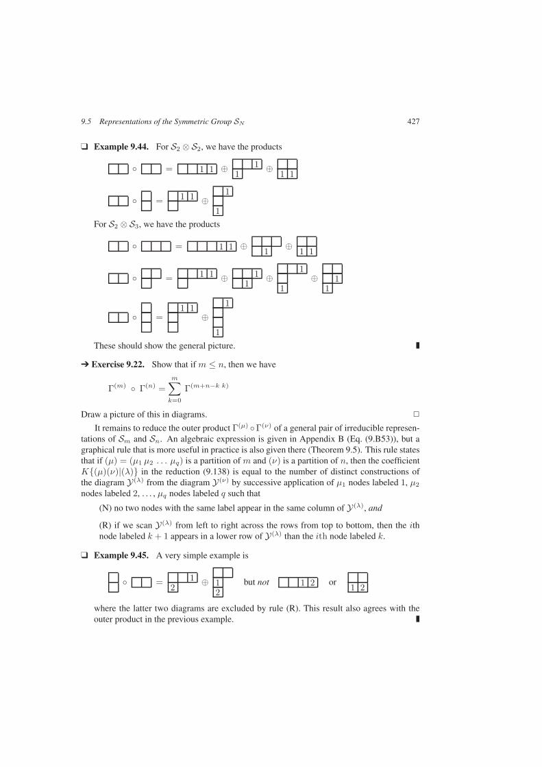
9.5 Representations of the Symmetric Group SN 427
Example 9.44. For S2 ⊗ S2, we have the products
= 1 1 ⊕ 11
⊕1 1
= 1 1 ⊕1
1For S2 ⊗ S3, we have the products
= 1 1 ⊕ 1 ⊕ 1 1
= 1 1 ⊕ 11 ⊕
1
1⊕ 1
1
=1 1
⊕1
1These should show the general picture.
Exercise 9.22. Show that if m ≤ n, then we have
Γ(m) Γ(n) =m∑
k=0
Γ(m+n−k k)
Draw a picture of this in diagrams.
It remains to reduce the outer product Γ(µ) Γ(ν) of a general pair of irreducible represen-tations of Sm and Sn. An algebraic expression is given in Appendix B (Eq. (9.B53)), but agraphical rule that is more useful in practice is also given there (Theorem 9.5). This rule statesthat if (µ) = (µ1 µ2 . . . µq) is a partition of m and (ν) is a partition of n, then the coefficientK(µ)(ν)|(λ) in the reduction (9.138) is equal to the number of distinct constructions ofthe diagram Y(λ) from the diagram Y(ν) by successive application of µ1 nodes labeled 1, µ2
nodes labeled 2, . . . , µq nodes labeled q such that
(N) no two nodes with the same label appear in the same column of Y(λ), and
(R) if we scan Y(λ) from left to right across the rows from top to bottom, then the ithnode labeled k + 1 appears in a lower row of Y(λ) than the ith node labeled k.
Example 9.45. A very simple example is
= 12 ⊕ 1
2but not 1 2 or 1 2
where the latter two diagrams are excluded by rule (R). This result also agrees with theouter product in the previous example.

428 9 Finite Groups
Example 9.46. We have
= 1 1 1 ⊕ 1 11
⊕1 1
1⊕
11
1
The same product in reverse order is given by
= 1 12
⊕ 11 2
⊕1
12
⊕ 1 12
Thus the outer product does not depend on the order of the terms in the product.
Exercise 9.23. Evaluate the outer product Γ(21) Γ(21).
Example 9.47. As a final example, we have
= 1 1 ⊕ 11 ⊕
1
1
⊕ 1 1 ⊕ 11
The evaluation of Γ(2) Γ(22) is left to the reader.
9.5.3 Kronecker Products of Irreducible Representations of SN
Consider now the Kronecker product
Γ(µ) × Γ(ν) =∑
(λ)
C(µ)(ν)|(λ)Γ(λ) (9.139)
of the irreducible representations Γ(µ) and Γ(ν) of SN . A formal expression for the coefficientsC(µ)(ν)|(λ) is
C(µ)(ν)|(λ) =∑
(m)
N(m)
N !χ
(µ)(m)χ
(ν)(m)χ
(λ)(m) (9.140)
which shows that the coefficients C(µ)(ν)|(λ) are symmetric in (µ), (ν) and (λ) (the char-acters of SN are real). Also,
C(µ)(ν)|(λ) = C(µ)(ν)|(λ) (9.141)
so that we can conjugate any two of the partitions in C(µ)(ν)|(λ) and have the same result.Finally,
C(µ)(ν)|(N) = δ(µ)(ν) and C(µ)(ν)|(1N) = δ(µ)(eν) (9.142)
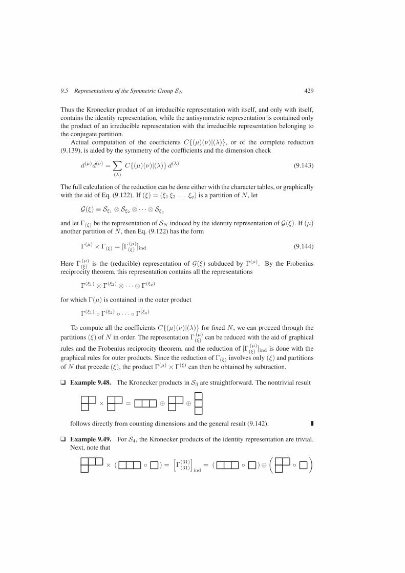
9.5 Representations of the Symmetric Group SN 429
Thus the Kronecker product of an irreducible representation with itself, and only with itself,contains the identity representation, while the antisymmetric representation is contained onlythe product of an irreducible representation with the irreducible representation belonging tothe conjugate partition.
Actual computation of the coefficients C(µ)(ν)|(λ), or of the complete reduction(9.139), is aided by the symmetry of the coefficients and the dimension check
d(µ)d(ν) =∑
(λ)
C(µ)(ν)|(λ) d(λ) (9.143)
The full calculation of the reduction can be done either with the character tables, or graphicallywith the aid of Eq. (9.122). If (ξ) = (ξ1 ξ2 . . . ξq) is a partition of N , let
G(ξ) ≡ Sξ1 ⊗ Sξ2 ⊗ · · · ⊗ Sξq
and let Γ(ξ) be the representation of SN induced by the identity representation of G(ξ). If (µ)another partition of N , then Eq. (9.122) has the form
Γ(µ) × Γ(ξ) = [Γ (µ)(ξ) ]ind (9.144)
Here Γ (µ)(ξ) is the (reducible) representation of G(ξ) subduced by Γ(µ). By the Frobenius
reciprocity theorem, this representation contains all the representations
Γ(ξ1) ⊗ Γ(ξ2) ⊗ · · · ⊗ Γ(ξq)
for which Γ(µ) is contained in the outer product
Γ(ξ1) Γ(ξ2) · · · Γ(ξq)
To compute all the coefficients C(µ)(ν)|(λ) for fixed N , we can proceed through the
partitions (ξ) of N in order. The representation Γ (µ)(ξ) can be reduced with the aid of graphical
rules and the Frobenius reciprocity theorem, and the reduction of [Γ (µ)(ξ) ]ind is done with the
graphical rules for outer products. Since the reduction of Γ(ξ) involves only (ξ) and partitionsof N that precede (ξ), the product Γ(µ) × Γ(ξ) can then be obtained by subtraction.
Example 9.48. The Kronecker products in S3 are straightforward. The nontrivial result
× = ⊕ ⊕
follows directly from counting dimensions and the general result (9.142).
Example 9.49. For S4, the Kronecker products of the identity representation are trivial.Next, note that
× ( ) =[Γ(31)
(31)
]
ind= ( ) ⊕
(
)

430 9 Finite Groups
since
Γ(31)(31) = ( ⊗ ) ⊕
(⊗
)
is computed by noting all the ways in which a single node can be removed from the dia-gram Y(31). Then note that
= ⊕ , = ⊕ ⊕
Since
= −
we then have
× = ⊕ ⊕ ⊕
Note that the dimension check is satisfied. Also
× ( ) =[Γ(31)
(22)
]
ind
Now Γ(31)(22) contains the representations of S3 ⊗ S1 obtained by removing a single node
from the diagram Y(22). Thus
Γ(31)(22) = ⊗
and then
[Γ(31)
(22)
]
ind= ⊕ ⊕
so that
× = ⊕
This actually could have been deduced from the dimension check alone, using the symme-try relation (9.142).
Exercise 9.24. Reduce the Kronecker products
× and ×
using the graphical methods given here.
9.6 Discrete Infinite Groups 431
9.6 Discrete Infinite Groups
The simplest discrete infinite group is the group Z of integers under addition, which corre-sponds to the group of translations of a one-dimensional lattice. If we let T denote the transla-tion of the lattice by one unit, then the group consists of the elements Tn (n = 0,±1,±2, . . .).For every complex number z, there is an irreducible representation Γ(z) of the group, in which
T → z and Tn → zn (9.145)
(n = 0,±1,±2, . . .). The representation is unitary if and only if |z| = 1, in which case letz = exp(ik) and then
Tn → eikn (9.146)
Remark. This example shows that representations of an infinite group need not be unitary,unlike those of a finite group.
For an N -dimensional lattice, there are N fundamental translations T1, . . . ,TN , and thegroup elements have the form
T(x) = T x11 · · · T xN
N (9.147)
with x = (x1, . . . , xN ) and xm = 0,±1,±2, . . . (m = 1, . . . , N ). There is an irreduciblerepresentation Γ(z1, . . . , zN ) for every N -tuple (z1, . . . , zN ) of complex numbers, with
T(x) → z x11 · · · z xN
N (9.148)
The representation is unitary if and only if |zm| = 1 (m = 1, . . . , N ), in which case letzm = exp(ikm) and then
T(x) → eik·x (9.149)
with k = (k1, . . . , kN ), and k · x the usual scalar product of k and x. This representation isalso denoted as Γ(k).Remark. The constraint |zm| = 1 means that km is only definedmodulo 2π. For the infinitelattice, this constrains the vector k to lie on an N -dimensional torus with period 2π/L alongany coordinate axis. Thus in three dimensions, we can restrict k to the cube
− π
L≤ kx ≤ π
L− π
L≤ ky ≤ π
L− π
L≤ kz ≤
π
L(9.150)
with points on opposite faces of the cube identified with the same representation Γ(k). Theconstraints (9.150) define the (first) Brillouin zone for the vector k.
Remark. The vector k is the wave vector of the representation Γ(k), since the functionexp(ik · x) corresponds to a wave propagating in the direction of k with wavelength 2π/ |k|in units of the lattice spacing. In a quantum-mechanical system on the lattice, k is alsointerpreted as the quasi-momentum associated with the representation.

432 9 Finite Groups
Remark. An alternative to using an infinite lattice is to consider a very large lattice withLN points and impose periodic boundary conditions, which is equivalent to the requirementTN = 1. Then the components km are constrained to have the values of the form
km =2πκmL
(9.151)
with κm an integer (κm = 1, . . . , N or κm = −12N,−
12N + 1, . . . , 1
2N − 1, 12N with
κm = ±12N identified as the same point). For practical purposes, this lattice is equivalent to
the infinite lattice if L >> 1.
The full symmetry group of a cubic lattice, denoted here by GC , includes not only trans-lations of the lattice, but also the group Od of rotations and reflections that leave the cubeinvariant. The group GC is not a direct product, since the rotations do not commute with thetranslations. In fact, if R is an element of Od, then
RT(x)R−1 = T(Rx) ⇒ RT(x) = T(Rx)R (9.152)
where Rx is the image of x under the rotationR. Equation (9.152) shows that the translationsare an invariant subgroup of GC , and if |k〉 is an eigenvector of T(x) with
T(x) = |k〉 (9.153)
then D(R)|k〉 will be an eigenvector of T(x) with eigenvalue Rk. This observation leadsto a method for constructing irreducible representations of GC that can be generalized toother groups, notably the group of inhomogeneous Lorentz transformations, also known asthe Poincaré group, whose irreducible representations are constructed in Chapter 10.
We start with fixed k and let Gk denote the subgroup of rotations of the cube that leave thevector k invariant. Gk is the isotropy group, or little group, at k. For a general k, Gk is thetrivial group, but if two (or all three) components of k have the same magnitude, there will benontrivial rotations that leave k invariant. There is even more symmetry if one or more of thecomponents of k is equal to ±π/L (i.e., if k lies on the boundary of the Brillouin zone).
Example 9.50. If k is in the direction of one of the coordinate axes (so that two com-ponents of k vanish), then Gk
∼= D4 is the dihedral group generated by (i) a rotation ρthrough π/2 about the direction of k, and (ii) reflection σ of an axis perpendicular to k,which can be represented as space inversion P combined with rotation through π aboutthe axis of reflection. If further |k| = π/L, so that k is on the boundary of the Brillouinzone, then k and −k are equivalent. In this case, both P and rotations through π aboutany coordinate axis perpendicular to k each leave k invariant, and the isotropy group isenlarged to D4 ⊗ Z2. This group is the largest isotropy group for any nonzero k.
Example 9.51. If k is along one of the main diagonals of the cube,
k = κ (±ex ± ey ± ez)
then Gk∼= Z3 contains the rotations through ±π/3 about the direction of k. If κ = π/L
(so that k is on the boundary of the Brillouin zone), then Gk contains space inversion aswell, and the isotropy group is Z6
∼= Z3 ⊗ Z2.

9.6 Discrete Infinite Groups 433
Exercise 9.25. Other classes of k that have nontrivial isotropy groups are
(i) k1 = ±k2 k3 = 0 and (ii) k1 = ±k2 k3 = 0
Find the largest isotropy group (including reflections) for each of these classes. Describe theextra symmetry if k is on a boundary of the Brillouin zone.
Next choose an irreducible representation of Gk of dimension d, say, and let |k, α〉 (α =1, . . . , d) be a basis for this representation. Then if R is an element of Gk,
D(R)|k, α〉 =∑
β
Dβα(R)|k, β〉 (9.154)
where D(R) is the linear operator representing R in the chosen irreducible representation ofGk. If R is not in Gk, then
D(R)|k, α〉 =∑
β
Cβα(R)|Rk, β〉 (9.155)
with matrix elements Cβα(R) constructed to be consistent with the group multiplication rules.The set of vectors Rk as R runs through the full point symmetry group Od of the cube isthe orbit Λ(k) of k under Od.
Example 9.52. Consider the case k = kez for which the isotropy group Gk is the dihedralgroup D4 generated by the rotation a through π/2 about the Z-axis and the reflection σ ofthe X-axis. Note that
a4 = e σ2 = e σaσ = a−1 (9.156)
As shown in Section 9.4, this group has four one-dimensional representations, in which
a→ ±1 ≡ α σ → ±1 ≡ η (9.157)
and a two-dimensional irreducible representation with
a→ iσy =(
0 1−1 0
)σ → σz =
(1 00 −1
)(9.158)
The orbit of Λ(k) under Od contains the vectors ±kex, ±key , ±kez . Thus if we startwith a one-dimensional representation of the isotropy group, we need to consider a set ofsix basis vectors
| ± kex〉 | ± key〉 | ± kez〉 (9.159)
We then have
P|k〉 = η| − k〉 (9.160)
while the Od rotations Rx(π/2),Ry(π/2), Rz(π/2) act on thesestates as shown in the table at theright. The remaining elements ofOd can be expressed as productsof P and these rotations. Starting
|kex〉 |key〉 |kez〉
Rx(π/2) α|kex〉 α| − kez〉 α|key〉
Ry(π/2) α|kez〉 α|key〉 α| − kex〉
Rz(π/2) α| − key〉 α|kex〉 α|kez〉
Action of rotations on basis vectors.
434 9 Finite Groups
with the two-dimensional irreducible representation of the little group, acting on basisstates |kez,±〉, leads to a twelve-dimensional representation of Od on a space with basisvectors
| ± kex,±〉 | ± key,±〉 | ± kez,±〉 (9.161)
Equation (9.158) corresponds to
Rz
(π2
)|kez,±〉 = ∓|kez,∓〉 and PRx(π)|kez,±〉 = ±|kez,±〉 (9.162)
whence also
Rz(π)|kez,±〉 = −|kez,±〉 (9.163)
For the action of P and Rx(π) separately, it is convenient to take
P|kez,±〉 = ±| − kez,±〉 (9.164)
Rx(π)|kez,±〉 = | − kez,±〉 (9.165)
(this is no more than a phase convention for the basis vector | − kez,−〉). From the groupmultiplication Rx(π)Ry(π) = Rz(π), it then follows that
Ry(π)|kez,±〉 = −| − kez,±〉 (9.166)
It is consistent with Eq. (9.165) to choose
Rx
(π2
)|kez,±〉 = |key,∓〉 Rx
(π2
)|key,±〉 = | − kez,∓〉 (9.167)
It is further consistent with Eq. (9.166) to choose
Ry
(π2
)|kez,±〉 = ±|−kex,∓〉 Ry
(π2
)|−kex,±〉 = ±|−kez,∓〉 (9.168)
The group multiplication rules then lead to a complete construction of the twelve-dimensional representation of Od. The full representation follows from the preceding,and the additional results
Rx
(π2
)|kex,±〉 = ∓|kex,∓〉 Ry
(π2
)|key,±〉 = ∓|key,∓〉 (9.169)
derived from the group multiplication rule
Rx
(π2
)Ry
(π2
)Rx
(−π
2
)= Rz
(π2
)(9.170)
It is an instructive exercise to reduce this six-dimensional representation of Od into irre-ducible components.
A Frobenius Reciprocity Theorem 435
A Frobenius Reciprocity Theorem
In Section 9.4.5, we presented the Frobenius reciprocity theorem, which states that the co-efficients that appear in the reduction of an irreducible representation of G restricted to asubgroup H are equal to the coefficients in the reduction of the representation of G induced byan irreducible representation of H. Here we present a proof of the theorem and an importantcorollary.
Suppose G is a group of finite order n whose classes K1 = e,K2, . . . ,Kp containh1 = 1, h2, . . . , hp elements, respectively. Denote the inequivalent irreducible representationsof G by Γ1, . . . ,Γp, with ma the dimension of Γa and χak the character of the class Kk in Γa.The matrix representing g in Γa is Da(g), with matrix elements Da
jk(g).Now let H be a subgroup of G of order m, index t = n/m. The classes Kk of G split into
classes L1k, . . . , Lnkk of H, with jk elements in the class Ljk (j = 1, . . . , nk). Some classesof G may not be in H, so that k = 1, . . . , s ≤ p, and others may be only partially includedin H, so that
nk∑
j=1
jk ≤ hk (9.A1)
in general. The total number of classes of H is given by
q =s∑
k=1
nk (9.A2)
Then we can denote the inequivalent irreducible representations of H by ∆1, . . . ,∆q , thedimension of ∆c by µc (c = 1, . . . , q), and the character of Ljk in ∆c by φcjk.
The irreducible representation Γa of G subduces a representation Γasub of H, which can bereduced according to
Γasub = ⊕c αca∆c (9.A3)
with nonnegative integer coefficients αca. The character χak can be expressed in terms of thecharacters in H as
χak =q∑
c=1
αcaφcjk (9.A4)
it follows from the orthogonality relation (9.75) that
mαca =∑
k
nk∑
j=1
jkφc∗jkχ
ak (9.A5)
Thus the integers αca are determined from the characters of H and G, as expected. But usingthe second orthogonality relation (9.91), we have
p∑
a=1
αcaχak =
nk∑
j=1
(njkmhk
)φcjk j = 1, . . . , s
0 otherwise
(9.A6)

436 9 Finite Groups
This defines the character of a (reducible) representation Γ of G in terms of the character φcjkof an irreducible representation of H. We shall see that Γ is precisely the representation of Ginduced by Γc of H in the construction of Eq. (9.113).
Now suppose ∆c is an irreducible representation of H. Then the representation ∆cind of G
induced by ∆c is reducible in general,
∆cind = ⊕a βcaΓa (9.A7)
with nonnegative integer coefficients βca. The character ξck of the class Kk of G in ∆cind is
ξck =p∑
a=1
βcaχak (9.A8)
Now recall the definition (Eq. (9.111))
σαβ(g, h) =
1, if ggβ = gαh
0 otherwise(9.A9)
and note that σαα(g, h) = 1 if and only if g = gαhg−1α , i.e., if and only if g and h belong to
the same class of G. Thus
∑
g in Kk
trσ(g, h) =
t (= n/m), if h in Kk
0 otherwise(9.A10)
Also, recall the definition (Eq. (9.113))
DΓ(g) ≡∑
h in Hσ(g, h) ⊗ D∆(h) (9.A11)
Then we have
hkξck =
∑
g in Kk
ξc(g) =∑
g in Kk
∑
h in H[trσ(g, h)]φc(h) = t
nk∑
j=1
jkφcjk (9.A12)
and then
ξck =p∑
a=1
βcaχak =
nk∑
j=1
(njkmhk
)φcjk =
p∑
a=1
αcaχak (9.A13)
where the last equality follows from Eq. (9.A6). Since Eq. (9.A13) is true for all k = 1, . . . , p,it must be that
αca = βca (9.A14)
which is the Frobenius Reciprocity Theorem.
B S-Functions and Irreducible Representations of SN 437
A corollary of this result is
Γa × ∆cind = [Γasub × ∆c]ind (9.A15)
as noted in Eq. (9.122), so that Kronecker products in H can be used to reduce those in G.This corollary is quite useful in practice. To derive the result, note that the character of theclass Kk of G is given in the representation Γa × ∆c
ind by
ξckχak =
nk∑
j=1
(njkhkm
)φcjk
χak =nk∑
j=1
(njkhkm
)[φcjkχ
ak
](9.A16)
But the last expression is the same character of the class Kk in the induced representation[Γasub × ∆c]ind. Hence the two representations must be the same.
B S-Functions and Irreducible Representations of SN
B.1 Frobenius Generating Function for the Simple Characters of SN
In Eq. (9.24), we introduced the alternant A(x1, x2, . . . , xN ) as an antisymmetric function ofthe N variables x1, x2, . . . , xN . Now we can also write
A(x1, x2, . . . , xN ) =∏
j<k
(xj − xk) =∑
P=(i1i2···iN )
εP xN−1i1
xN−2i2
· · ·xiN−1 (9.B17)
where the sum is over all permutations P = (i1i2 · · · iN ) of N . This form shows that thealternant is actually the determinant of the matrix A defined by
A =
1 x1 x21 · · · xN−1
1
1 x2 x22 · · · xN−1
2
......
.... . .
...1 xN x2
N · · · xN−1N
(9.B18)
Note that the alternant is homogeneous of degree 12N(N − 1) in the x1, x2, . . . , xN .
We can also define an antisymmetric polynomial A(λ)(x1, x2, . . . , xN ) associated with apartition (λ) = (λ1 · · ·λs) of N by
A(λ)(x1, x2, . . . , xN ) ≡∑
P=(i1i2···iN )
εP xλ1+N−1i1
xλ2+N−2i2
· · ·xλNiN
(9.B19)
A(λ)(x1, x2, . . . , xN ) is homogeneous of degree dN = 12N(N + 1) in the x1, x2, . . . , xN .
The homogeneous antisymmetric polynomials of degree dN form a linear vector space V ,and the exponents of every monomial in such a polynomial must correspond to the exponentsin Eq. (9.B19) for some partition (λ) of N . Thus the A(λ) define a basis of V , and V hasdimension π(N), the number of distinct partitions of N .

438 9 Finite Groups
Exercise 9.B1. Show that if (λ) = (λ1 · · ·λs) is a partition of N , then the functionA(λ)(x1, x2, . . . , xN ) can be expressed as the determinant of the matrix A(λ) defined by
A =
xλN1 x
λN−1+11 x
λN−2+21 · · · xλ1+N−1
1
xλN2 x
λN−1+12 x
λN−2+22 · · · xλ1+N−1
2
......
.... . .
...xλN
N xλN−1+1N x
λN−2+2N · · · xλ1+N−1
N
(again, if s < N , define λs+1 = · · · = λN = 0).
Now define the symmetric functions
sk = sk(x1, x2, . . . , xN ) ≡N∑
i=1
(xi)k (9.B20)
The functions s1, s2, . . . , sN are functionally independent, since the Jacobian determinant is
det(∂sk∂xi
)= N !
∑
P=(i1i2···iN )
εP xN−1i1
xN−2i2
· · ·xiN−1= N !A(x1, x2, . . . , xN )
(9.B21)
where the sum is over permutations of (1 · · ·N), and the alternantA(x1, x2, . . . , xN ) vanishesonly if two of the variables are equal. Note that powers of the sk are expressed as
(sk)ν =
∑
(ν)
∑
P=(i1i2···iN )
ν!ν1! ν2! · · · νN !
xkν1i1xkν2i2
· · ·xkνN
iN(9.B22)
where the summation is over partitions (ν) of ν; if the number of parts q is less than N , wedefine νq+1 = · · · = νN = 0. Then if (m) = (m1m2 · · ·mt) = (pνp · · · 2ν21ν1) is a partitionof N , define
S(m) = S(m)(x1, x2, . . . , xN ) = sm1sm2 · · · smt=
p∏
k=1
[sk(x1, x2, . . . , xN )]νk (9.B23)
Evidently S(m)(x1, x2, . . . , xN ) is a symmetric, homogeneous polynomial of degree N in thex1, x2, . . . , xN . The S(m) are known as Schur functions, or simply S-functions.
Consider now the product S(m)(x1, . . . , xN )A(x1, . . . , xN ). It is a homogeneous poly-nomial of degree in the variables x1, . . . , xN , antisymmetric under interchange of any pair ofvariables. Thus it must be a linear combination of the polynomials A(λ)(x1, . . . , xN ), and wecan write
S(m)(x1, . . . , xN )A(x1, . . . , xN ) =∑
(λ)
χ(λ)(m)A
(λ)(x1, . . . , xN ) (9.B24)
Remarkably, the coefficients χ (λ)(m) are exactly the simple characters of SN .
B S-Functions and Irreducible Representations of SN 439
To prove this, we will show that the χ (λ)(m) satisfy the orthogonality relations
∑
(m)
N(m)χ(λ)(m)χ
(ξ)(m) = N ! δ(λ)(ξ) (9.B25)
where N(m) is the number of elements in the class K(m).
Remark. In Section 9.3, we identified the classes of SN with the π(N) partitions of N ,and denoted the class whose cycle structure belongs to the partition (m) = (m1m2 · · ·mt) =(pνp · · · 2ν21ν1 by K(m). The number of elements in the class K(m) is given by
N(m) =N !
(1ν1 2ν2 · · · pνp) (ν1! ν2! · · · νp!)≡ N(ν1 ν2 · · · νp) (9.B26)
To see this, note that there are N ! arrangements of 1, . . . , N in the given cycle structure. Butthere are n equivalent expressions of each n-cycle, and νn! arrangements of the νn n-cycles,each of which corresponds to the same permutation in SN .
Remark. Equation (9.B24) serves to define the association of the partition (λ) with a par-ticular irreducible representation. In addition to the orthogonality relations, we need to showthat
χ(λ)
(1N )> 0 (9.B27)
since that character is the dimension of the representation Γ(λ). We also need to verify theidentification of (N) with the symmetric, and (1N ) with the antisymmetric, representation.
Now introduce a second set (y1, . . . , yN ) of N variables, and note that∑
(m)
N(m)S(m)(x1, . . . , xN )S(m)(y1, . . . , yN )(9.B28)
= N !∑
(νk)| Pk kνk=N
p∏
k=1
[sk(x)sk(y)]νk
kνkvk!
where N(m) is the number of elements in the class K(m) of SN given by Eq. (9.B26). Thenkeep the number of variables fixed at n, and sum over N to determine a function S(x, y)defined by
S(x, y) ≡∞∑
N=0
∑
(m)
N(m)
N !S(m)(x1, . . . , xn)S(m)(y1, . . . , yn)
(9.B29)
=∞∏
k=1
∞∑
vk=0
1νk!
[sk(x)sk(y)
k
]νk
= exp
∞∑
k=1
sk(x)sk(y)k
The series in the exponential can be summed in closed form to give
∞∑
k=1
sk(x)sk(y)k
=n∑
i=1
n∑
j=1
∞∑
k=1
(xiyj)k
k= −
n∑
i=1
n∑
j=1
ln(1 − xiyj) (9.B30)
440 9 Finite Groups
and then
S(x, y) = exp
−n∑
i=1
n∑
j=1
ln(1 − xiyj)
=n∏
i=1
n∏
j=1
(1
1 − xiyj
)(9.B31)
Next define the n× n matrix
M = (Mij) =(
11 − xiyj
)(9.B32)
The determinant of M can be evaluated formally by expanding the denominators and usingthe definition of the determinant to obtain
detM =∞∑
µ1=0
· · ·∞∑
µn=0
∑
P=(i1i2···in)
εP (xi1y1)µ1(xi2y2)
µ2 · · · (xinyn)µn (9.B33)
Note that the exponents µ1, µ2, . . . , µn in a single monomial in this series must all be distinct,due to the antisymmetry in the x and y variables enforced by the factor εP. We can reorderthe exponents in each term are so that we always have
µ1 > µ2 > · · · > µn
and the last equation can be written as
detM =∞∑
N=0
∑
(λ)
∑
P=(i)
∑
Q=(j)
εP εQ(xi1yj1)λ1+n−1(xi2yj2)
λ2+n−2 · · · (xinyjn)λn
(9.B34)
where for each N , the sums on P and Q are over permutations i1, i2, . . . , iN andj1, j2, . . . , jN of N , and the sum on (λ) is over the partitions of N . Strictly speaking,the (λ) are partitions into not more than n parts, but the proof of the result (9.B41) for aparticular N only requires n ≥ N , which can always be arranged since n is arbitrary. Fromthe definition of the A(λ)(x) in Eq. (9.B19), it follows that Eq. (9.B34) is equivalent to
detM =∞∑
N=0
∑
(λ)
A(λ)(x)A(λ)(y) (9.B35)
On the other hand, we also have
detM =∥∥∥∥
11 − xiyj
∥∥∥∥ = A(x1, . . . , xn)A(y1, . . . , yn)n∏
i=1
n∏
j=1
(1
1 − xiyj
)(9.B36)
This follows from the observation that after extracting the product of the factors 1/(1− xiyj)from the determinant, there remains a numerator that is a polynomial in the x and y antisym-metric under exchange of any two x or any two y variables, since this exchange corresponds
B S-Functions and Irreducible Representations of SN 441
to exchanging two rows or two columns, respectively, of the matrix M. To evaluate thispolynomial, consider first the 2 × 2 determinant, given by
(1
1 − x1y1
)(1
1 − x2y2
)−(
11 − x1y2
)(1
1 − x2y1
)
(9.B37)
=(x1 − x2)(y1 − y2)
(1 − x1y1)(1 − x1y2)(1 − x2y1)(1 − x2y2)
To generalize this formula to arbitrary n, subtract the ith row of the determinant from the firstrow, and then subtract the jth column of the resulting determinant from the first column. Theresult will be a product of the form
detM =1
1 − x1y1
(n∏
i=2
xi − x1
1 − xiy1
)
n∏
j=2
yj − y11 − x1yj
detM′ (9.B38)
where M′ is the (n− 1)× (n− 1) matrix obtained from M by removing the first row and thefirst column. Thus Eq. (9.B36) is true by induction on n.
Using the result (9.B31) in Eq. (9.B36), and then the definition in Eq. (9.B29), we have
detM = S(x, y)A(x)A(y) =∞∑
N=0
∑
(m)
N(m)
N !S(m)(x)A(x)S(m)(y)A(y) (9.B39)
From definition (9.B24) of the χ (λ)(m), we then have
detM =∞∑
N=0
∑
(λ)
∑
(ξ)
∑
(m)
N(m)
N !χ
(λ)(m)χ
(ξ)(m)A
(λ)(x)A(ξ)(y) (9.B40)
Comparing Eqs. (9.B35) and (9.B40) gives the required orthogonality relation∑
(m)
N(m)χ(λ)(m)χ
(ξ)(m) = N ! δ(λ)(ξ) (9.B41)
The orthogonality relations alone are not quite enough to show that the χ (λ)(m) are simple char-
acters. There is a possible sign ambiguity, since χ (λ)(m) → −χ (λ)
(m) (for all λ) is consistent withorthogonality. But the graphical calculation in Example 9.55 in the next section shows thatthe sign is given correctly.
Anticipating this calculation, we have thus derived the Frobenius generating function
S(m)(x1, . . . , xN )A(x1, . . . , xN ) =∑
(λ)
χ(λ)(m)A
(λ)(x1, . . . , xN ) (9.B42)
for the simple characters χ (λ)(m) of SN . The graphical methods of the next section flow from
this generating function.
442 9 Finite Groups
B.2 Graphical Calculation of the Characters χ(λ)(m)
Suppose (m) = (m1m2 · · ·mt) and (λ) = (λ1 · · ·λs) are two partitions ofN . The Frobenius
generating function (Eq. (9.B42)) tells us that the simple character χ (λ)(m) of the class K(m) of
SN in the irreducible representation Γ(λ) associated with (λ) is given by the coefficient of themonomial
xλ1+N−11 xλ2+N−2
2 · · ·xλN
N (9.B43)
in the product
S(m)(x1, x2, . . . , xN )A(x1, x2, . . . , xN ) =
=
[N∑
i=1
(xi)m1
][N∑
i=1
(xi)m2
]× · · · ×
[N∑
i=1
(xi)mt
](9.B44)
×∑
P=(i1i2···iN )
εP xN−1i1
xN−2i2
· · ·xiN−1
A graphical method to evaluate this coefficient is based on the observation that the product
t∏
j=1
smj
xN−1i1
xN−2i2
· · ·xiN−1
can be depicted as the construction of the Young diagram Y(λ) of the partition (λ) from anempty diagram by successive addition ofm1, . . . ,mt nodes. This construction must be subjectto rules that exclude monomials in which two variables have the same exponent, since suchmonomials disappear from the sum over permutations due to the antisymmetry introduced bythe εP factor.
Now suppose (µ) = (µ1µ2 · · ·µq) is a partition of m, and consider the product
[N∑
i=1
(xi)]A
(µ)(x1, . . . , xN ) ≡∑
(ν)
c(µ)(ν) A
(ν)(x1, . . . , xN ) (9.B45)
where the summation is over partitions (ν) of n = +m. In a term of the form
[N∑
i=1
(xi)]xµ1+N−1
1 xµ2+N−22 · · · xµN
N
there will be nominal contributions from partitions of the form
(µ1 + µ2 · · · µN ), (µ1 µ2 + · · · µN ), . . . , (µ1 µ2 · · · µN + )
However, one or more of these modified partitions may not satisfy the ordering condition(νk ≥ νk+1). If a partition does not satisfy the condition, then either
B S-Functions and Irreducible Representations of SN 443
(i) µk = µk+1 + − 1, in which case two variables have the same exponent in the newmonomial, and the term disappears from the sum, or
(ii) µk < µk+1 + − 1, when the variables xk and xk+1 must be transposed, providing afactor (−1), and the partition modified so that
µ′k = µk+1 + − 1 and µ′
k+1 = µk + 1 (9.B46)
This continues until the partition is in standard order (with an overall sign factor ±1), or thepartition is dropped because condition (i) has been encountered at some stage.
In graphical terms, this analysis leads to the result that the coefficient c(µ)(ν) in Eq. (9.B45)
vanishes unless the diagram Y(ν) can be constructed from the diagram Y(µ) by the regularapplication of nodes, as defined below. If the construction is possible, then c(µ)(ν)
= ±1according to whether the application is even or odd.
Definition 9.29. The addition of nodes to the Young diagram associated with a partition(µ) = (µ1, . . . , µq) of m is a regular application (of nodes) if nodes are added to one row,row r say, until the number of nodes in row r is equal to µr−1 + 1, after which nodes areadded to row r − 1 until the number of nodes in this row is equal to µr−2 + 1. The processcontinues until either the nodes are exhausted at the diagram of a properly ordered partitionor row 1 is reached, in which case the remaining nodes are added to row 1. The parity of theapplication is even (+1) or odd (−1) according to whether nodes are added in an odd or evennumber of rows of the diagram.
The parity rule is based on the fact that changing rows in a diagram during the application ofnodes corresponds to a transposition of variables, with the associated sign factor.
Example 9.53. The product
[N∑
i=1
(xi)3]A(21)(x) (9.B47)
corresponds to adding three nodes to the par-tition (21) of 3. This leads to the four nonva-nishing contributions shown (with appropriatesigns) at the right. Algebraically, we look at aterm of the form (with N = 5 variables)
1 1 1 − 11 1
+ 111
− 11 1
[5∑
i=1
(xi)3]x6
1x42x
23x4
which gives after expansion
x91x
42x
23x4 + x6
1x72x
23x4 + x6
1x42x
53x4 + x6
1x42x
23x
35
(a vanishing term x61x
42x
23x
44 has been dropped). The second and third terms each require
a single transposition to order the exponents correctly, so they require a minus sign, whilethe last term requires two transpositions (x5 → x4 → x3), so it has a positive sign.
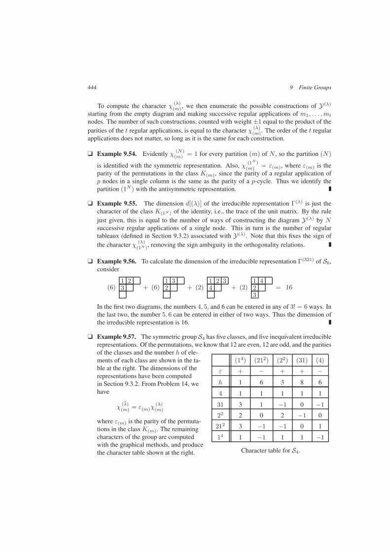
444 9 Finite Groups
To compute the character χ (λ)(m), we then enumerate the possible constructions of Y(λ)
starting from the empty diagram and making successive regular applications of m1, . . . ,mt
nodes. The number of such constructions, counted with weight ±1 equal to the product of theparities of the t regular applications, is equal to the character χ (λ)
(m). The order of the t regularapplications does not matter, so long as it is the same for each construction.
Example 9.54. Evidently χ (N)(m) = 1 for every partition (m) of N , so the partition (N)
is identified with the symmetric representation. Also, χ (1N )(m) = ε(m), where ε(m) is the
parity of the permutations in the class K(m), since the parity of a regular application ofp nodes in a single column is the same as the parity of a p-cycle. Thus we identify thepartition (1N ) with the antisymmetric representation.
Example 9.55. The dimension d[(λ)] of the irreducible representation Γ(λ) is just thecharacter of the class K(1N ) of the identity, i.e., the trace of the unit matrix. By the rulejust given, this is equal to the number of ways of constructing the diagram Y(λ) by Nsuccessive regular applications of a single node. This in turn is the number of regulartableaux (defined in Section 9.3.2) associated with Y(λ). Note that this fixes the sign ofthe character χ (λ)
(1N ), removing the sign ambiguity in the orthogonality relations.
Example 9.56. To calculate the dimension of the irreducible representation Γ(321) of S6,consider
(6)1 23 + (6)
1 32 + (2)
1 2 34 + (2)
1 423
= 16
In the first two diagrams, the numbers 4, 5, and 6 can be entered in any of 3! = 6 ways. Inthe last two, the number 5, 6 can be entered in either of two ways. Thus the dimension ofthe irreducible representation is 16.
Example 9.57. The symmetric group S4 has five classes, and five inequivalent irreduciblerepresentations. Of the permutations, we know that 12 are even, 12 are odd, and the paritiesof the classes and the number h of ele-ments of each class are shown in the ta-ble at the right. The dimensions of therepresentations have been computedin Section 9.3.2. From Problem 14, wehave
χ(eλ)(m) = ε(m)χ
(λ)(m)
where ε(m) is the parity of the permuta-tions in the class K(m). The remainingcharacters of the group are computedwith the graphical methods, and producethe character table shown at the right.
(14) (212) (22) (31) (4)
ε + − + + −h 1 6 3 8 6
4 1 1 1 1 1
31 3 1 −1 0 −1
22 2 0 2 −1 0
212 3 −1 −1 0 1
14 1 −1 1 1 −1
Character table for S4.
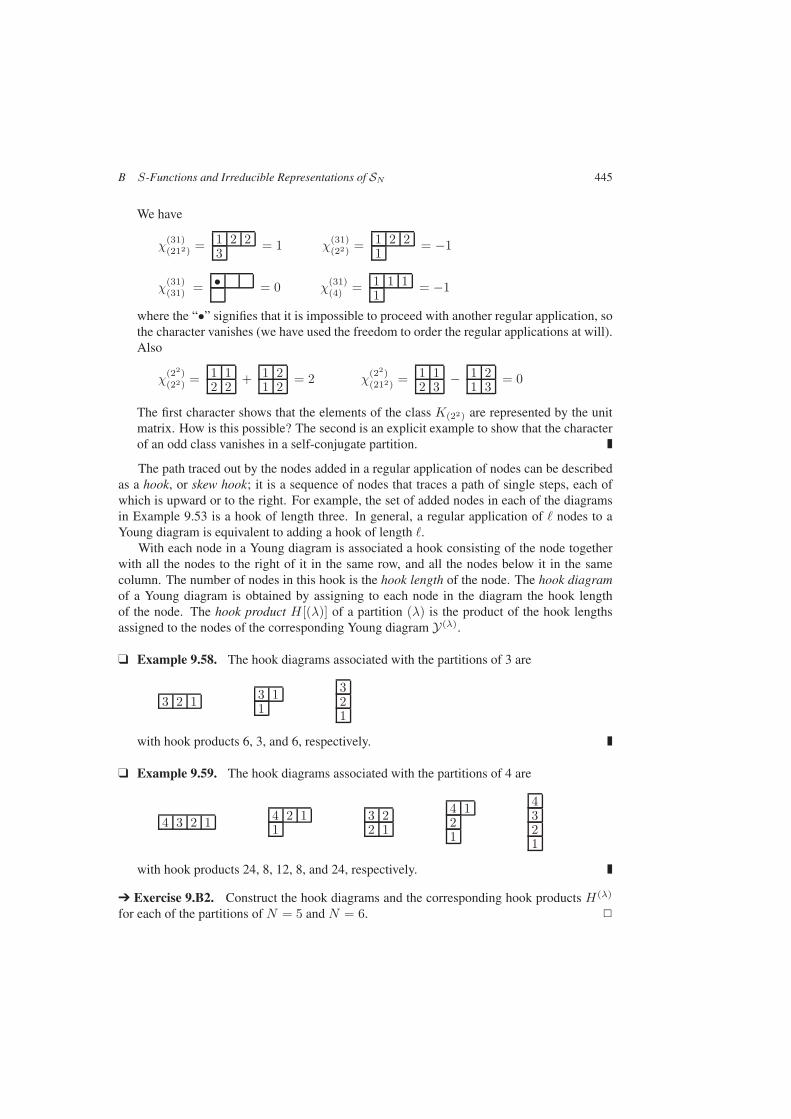
B S-Functions and Irreducible Representations of SN 445
We have
χ(31)(212) = 1 2 2
3 = 1 χ(31)(22) = 1 2 2
1 = −1
χ(31)(31) = • = 0 χ
(31)(4) = 1 1 1
1= −1
where the “•” signifies that it is impossible to proceed with another regular application, sothe character vanishes (we have used the freedom to order the regular applications at will).Also
χ(22)(22) = 1 1
2 2 + 1 21 2 = 2 χ
(22)(212) = 1 1
2 3 − 1 21 3 = 0
The first character shows that the elements of the class K(22) are represented by the unitmatrix. How is this possible? The second is an explicit example to show that the characterof an odd class vanishes in a self-conjugate partition.
The path traced out by the nodes added in a regular application of nodes can be describedas a hook, or skew hook; it is a sequence of nodes that traces a path of single steps, each ofwhich is upward or to the right. For example, the set of added nodes in each of the diagramsin Example 9.53 is a hook of length three. In general, a regular application of nodes to aYoung diagram is equivalent to adding a hook of length .
With each node in a Young diagram is associated a hook consisting of the node togetherwith all the nodes to the right of it in the same row, and all the nodes below it in the samecolumn. The number of nodes in this hook is the hook length of the node. The hook diagramof a Young diagram is obtained by assigning to each node in the diagram the hook lengthof the node. The hook product H[(λ)] of a partition (λ) is the product of the hook lengthsassigned to the nodes of the corresponding Young diagram Y(λ).
Example 9.58. The hook diagrams associated with the partitions of 3 are
3 2 1 3 11
321
with hook products 6, 3, and 6, respectively.
Example 9.59. The hook diagrams associated with the partitions of 4 are
4 3 2 1 4 2 11
3 22 1
4 121
4321
with hook products 24, 8, 12, 8, and 24, respectively.
Exercise 9.B2. Construct the hook diagrams and the corresponding hook products H(λ)
for each of the partitions of N = 5 and N = 6.
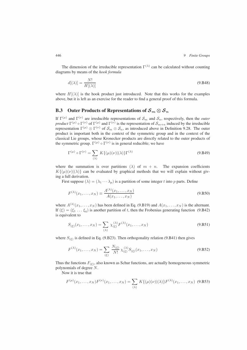
446 9 Finite Groups
The dimension of the irreducible representation Γ(λ) can be calculated without countingdiagrams by means of the hook formula
d[(λ)] =N !
H[(λ)](9.B48)
where H[(λ)] is the hook product just introduced. Note that this works for the examplesabove, but it is left as an exercise for the reader to find a general proof of this formula.
B.3 Outer Products of Representations of Sm ⊗ Sn
If Γ(µ) and Γ(ν) are irreducible representations of Sm and Sn, respectively, then the outerproduct Γ(µ) Γ(ν) of Γ(µ) and Γ(ν) is the representation of Sm+n induced by the irreduciblerepresentation Γ(µ) ⊗ Γ(ν) of Sm ⊗ Sn, as introduced above in Definition 9.28. The outerproduct is important both in the context of the symmetric group and in the context of theclassical Lie groups, whose Kronecker products are directly related to the outer products ofthe symmetric group. Γ(µ) Γ(ν) is in general reducible; we have
Γ(µ) Γ(ν) =∑
(λ)
K(µ)(ν)|(λ)Γ(λ) (9.B49)
where the summation is over partitions (λ) of m + n. The expansion coefficientsK(µ)(ν)|(λ) can be evaluated by graphical methods that we will explain without giv-ing a full derivation.
First suppose (λ) = (λ1 · · ·λp) is a partition of some integer t into p parts. Define
F (λ)(x1, . . . , xN ) ≡ A(λ)(x1, . . . , xN )A(x1, . . . , xN )
(9.B50)
where A(λ)(x1, . . . , xN ) has been defined in Eq. (9.B19) and A(x1, . . . , xN ) is the alternant.If (ξ) = (ξ1 . . . ξq) is another partition of t, then the Frobenius generating function (9.B42)is equivalent to
S(ξ)(x1, . . . , xN ) =∑
(λ)
χ(λ)(ξ) F
(λ)(x1, . . . , xN ) (9.B51)
where S(ξ) is defined in Eq. (9.B23). Then orthogonality relation (9.B41) then gives
F(λ)(x1, . . . , xN ) =
∑
(ξ)
N(ξ)
N !χ
(λ)(ξ) S(ξ)(x1, . . . , xN ) (9.B52)
Thus the functions F(ξ), also known as Schur functions, are actually homogeneous symmetricpolynomials of degree N .
Now it is true that
F (µ)(x1, . . . , xN )F (ν)(x1, . . . , xN ) =∑
(λ)
K(µ)(ν)|(λ)F (λ)(x1, . . . , xN ) (9.B53)
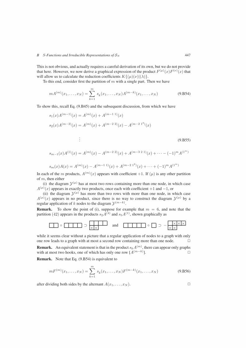
B S-Functions and Irreducible Representations of SN 447
This is not obvious, and actually requires a careful derivation of its own, but we do not providethat here. However, we now derive a graphical expression of the product F (µ)(x)F (ν)(x) thatwill allow us to calculate the reduction coefficients K(µ)(ν)|(λ).
To this end, consider first the partition of m with a single part. Then we have
mA(m)(x1, . . . , xN ) =m∑
k=1
sk(x1, . . . , xN )A(m−k)(x1, . . . , xN ) (9.B54)
To show this, recall Eq. (9.B45) and the subsequent discussion, from which we have
s1(x)A(m−1)(x) = A(m)(x) +A(m−1 1)(x)
s2(x)A(m−2)(x) = A(m)(x) +A(m−2 2)(x) −A(m−2 12)(x)
... (9.B55)
sm−1(x)A(1)(x) = A(m)(x) −A(m−2 2)(x) +A(m−3 2 1)(x) + · · · − (−1)mA(1m)
sm(x)A(x) = A(m)(x) −A(m−1 1)(x) +A(m−2 12)(x) + · · · + (−1)mA(1m)
In each of the m products, A(m)(x) appears with coefficient +1. If (µ) is any other partitionof m, then either
(i) the diagram Y(µ) has at most two rows containing more than one node, in which caseA(µ)(x) appears in exactly two products, once each with coefficient +1 and −1, or
(ii) the diagram Y(µ) has more than two rows with more than one node, in which caseA(µ)(x) appears in no product, since there is no way to construct the diagram Y(µ) by aregular application of k nodes to the diagram Y(m−k).Remark. To show the point of (i), suppose for example that m = 6, and note that thepartition (42) appears in the products s2A(4) and s5A(1), shown graphically as
⊃ × × and ⊃ − × × ×× ×
while it seems clear without a picture that a regular application of nodes to a graph with onlyone row leads to a graph with at most a second row containing more than one node.
Remark. An equivalent statement is that in the product skA(m), there can appear only graphswith at most two hooks, one of which has only one row [A(m−k)].
Remark. Note that Eq. (9.B54) is equivalent to
mF (m)(x1, . . . , xN ) =m∑
k=1
sk(x1, . . . , xN )F (m−k)(x1, . . . , xN ) (9.B56)
after dividing both sides by the alternant A(x1, . . . , xN ).

448 9 Finite Groups
Now consider the product
F (m)(x)F (ν)(x) =∑
(λ)
K(m)(ν)|(λ)F (λ)(x) (9.B57)
The coefficient K(m)(ν)|(λ) is equal to one if and only if the diagram Y(λ) can be con-structed from the diagram Y(ν) by the addition of m nodes, no two of which appear in thesame column of Y(λ). Otherwise, the coefficient is zero.
To show this, note that the result is obviously true for m = 0, 1. Suppose the result is truefor 0, 1, . . . ,m− 1. Then, with Eq. (9.B56) in mind, we have three following possibilities.
(i) Y(λ) can be constructed from Y(ν) by the addition ofm nodes, no two of which appearin the same column of Y(λ). Then F (λ)(x) appears in the product sk(x)F (m−k)(x)F (ν)(x)with coefficient equal to the number of different rows of Y(λ) that contain at least k addednodes. Thus F (λ)(x) appears in the product
mF (m)(x)F (ν)(x) = [s1(x)F (m−1)(x) + · · · + sm(x)F (x)]F (ν)(x)
with total coefficient m, or(ii) Y(λ) is constructed from Y(ν) by the addition ofm nodes, of which at least two appear
in the same column of Y(λ). Then either(a) F (λ)(x) appears in no product sk(x)F (m−k)(x)F (ν)(x), or(b) it appears in exactly two products, once with coefficient +1 and once with coefficient
−1 (an illustration of this is given below), or(iii) Y(λ) cannot be constructed from Y(ν) by the addition of m nodes, in which case
F (λ)(x) appears in no product sk(x)F (m−k)(x)F (ν)(x).Remark. To illustrate the argument in (ii)(b), consider the product of (3) and (312). Wehave
s1F(2) × =
11×
and s2F(1) × = −
1××
since the second product corresponds to a term x23 (x6
1x22x3) that acquires a minus sign when
variables are reordered. Thus the product (3) × (312) does not contain the partition (422).
Thus we have a graphical rule to construct the outer product of the identity representationof Sm with an arbitrary representation of Sn. Some examples were given in Section 9.5.2;here we offer a few more.
Example 9.60. We have
= 1 1 1 ⊕ 1 11
⊕ 11 1
⊕1 1 1
This is a special case of the rule given in Exercise 9.22.
Definition 9.30. Suppose (ν) is a partition of n with Young diagram Y(ν). The constructionof the diagram Y(λ) of a partition (λ) of m+ n by the addition of m nodes to Y(ν), no two ofthat appear in the same column of Y(λ), is a normal application of m nodes to Y(ν).
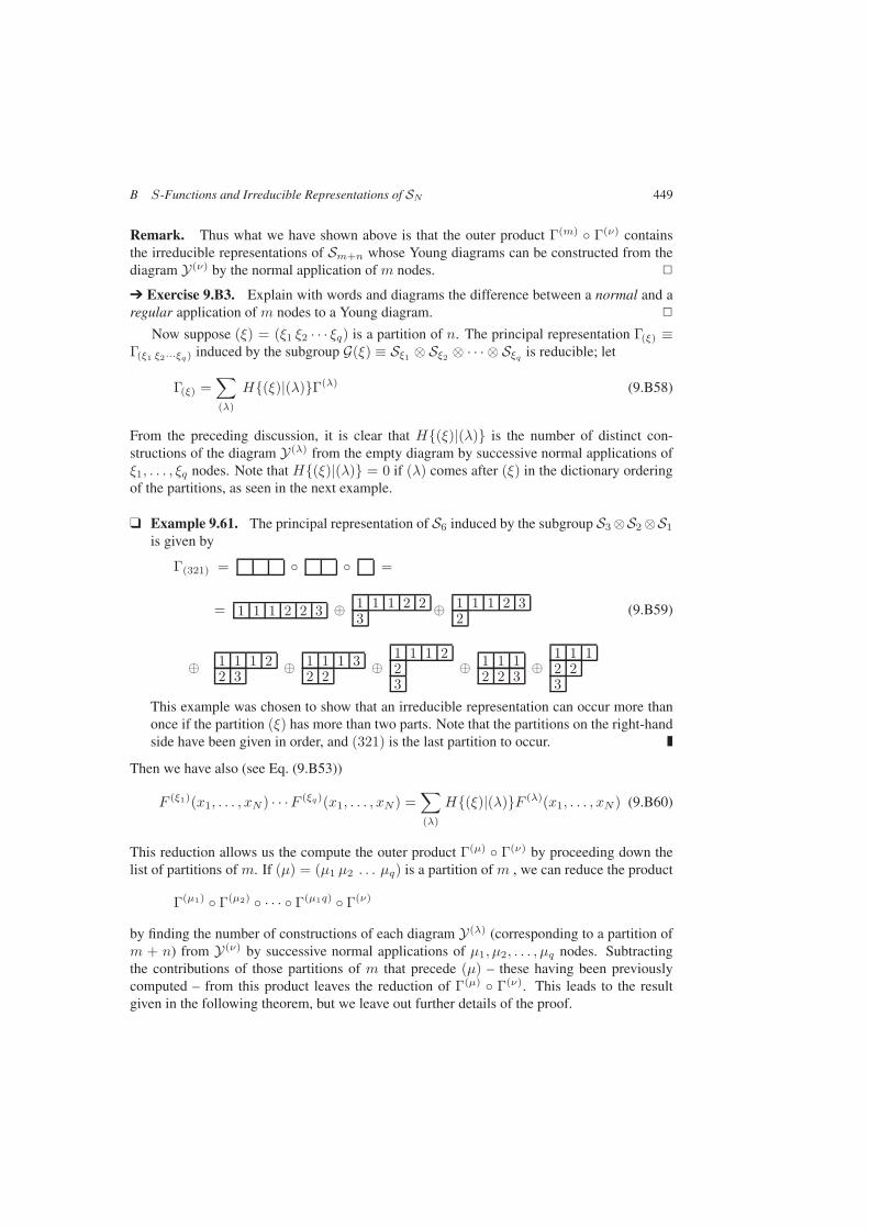
B S-Functions and Irreducible Representations of SN 449
Remark. Thus what we have shown above is that the outer product Γ(m) Γ(ν) containsthe irreducible representations of Sm+n whose Young diagrams can be constructed from thediagram Y(ν) by the normal application of m nodes.
Exercise 9.B3. Explain with words and diagrams the difference between a normal and aregular application of m nodes to a Young diagram.
Now suppose (ξ) = (ξ1 ξ2 · · · ξq) is a partition of n. The principal representation Γ(ξ) ≡Γ(ξ1 ξ2···ξq) induced by the subgroup G(ξ) ≡ Sξ1 ⊗ Sξ2 ⊗ · · · ⊗ Sξq
is reducible; let
Γ(ξ) =∑
(λ)
H(ξ)|(λ)Γ(λ) (9.B58)
From the preceding discussion, it is clear that H(ξ)|(λ) is the number of distinct con-structions of the diagram Y(λ) from the empty diagram by successive normal applications ofξ1, . . . , ξq nodes. Note that H(ξ)|(λ) = 0 if (λ) comes after (ξ) in the dictionary orderingof the partitions, as seen in the next example.
Example 9.61. The principal representation of S6 induced by the subgroup S3⊗S2⊗S1
is given by
Γ(321) = =
= 1 1 1 2 2 3 ⊕ 1 1 1 2 23
⊕ 1 1 1 2 32
(9.B59)
⊕ 1 1 1 22 3
⊕ 1 1 1 32 2
⊕1 1 1 223
⊕ 1 1 12 2 3
⊕1 1 12 23
This example was chosen to show that an irreducible representation can occur more thanonce if the partition (ξ) has more than two parts. Note that the partitions on the right-handside have been given in order, and (321) is the last partition to occur.
Then we have also (see Eq. (9.B53))
F (ξ1)(x1, . . . , xN ) · · ·F (ξq)(x1, . . . , xN ) =∑
(λ)
H(ξ)|(λ)F (λ)(x1, . . . , xN ) (9.B60)
This reduction allows us the compute the outer product Γ(µ) Γ(ν) by proceeding down thelist of partitions of m. If (µ) = (µ1 µ2 . . . µq) is a partition of m , we can reduce the product
Γ(µ1) Γ(µ2) · · · Γ(µ1q) Γ(ν)
by finding the number of constructions of each diagram Y(λ) (corresponding to a partition ofm + n) from Y(ν) by successive normal applications of µ1, µ2, . . . , µq nodes. Subtractingthe contributions of those partitions of m that precede (µ) – these having been previouslycomputed – from this product leaves the reduction of Γ(µ) Γ(ν). This leads to the resultgiven in the following theorem, but we leave out further details of the proof.

450 9 Finite Groups
Theorem 9.5. Suppose (µ) = (µ1 µ2 · · ·µq) is a partition of m and (ν) a partition of n.Then the coefficient K(µ)(ν)|(λ) in the reduction (Eq. (9.B49))
Γ(µ) Γ(ν) =∑
K(µ)(ν)|(λ)Γ(λ)
of Γ(µ) Γ(ν) into a sum of irreducible representations of Sm+n is equal to the number ofdistinct constructions of the diagram Y(λ) from the diagram Y(ν) by successive application ofµ1 nodes labeled 1, . . . , µq nodes labeled q such that
(N) no two nodes with the same label appear in the same column of Y(λ) (the applicationsof the µ1, . . . , µq nodes are normal applications), and
(R) if we scan Y(λ) from left to right across the rows from top to bottom, then the ithnode labeled k + 1 appears in a lower row of Y(λ) than the ith node labeled k.
Exercise 9.B4. Show that
K(µ)(ν)|(λ) = K(µ)(ν)|(λ)
This symmetry relation reduces the number of explicit calculations that need to be done.
Example 9.62. For S2 ⊗ S3, direct application of the graphical rule gives
= 12
⊕1
2⊕ 1
2⊕
12
although this is more easily derived from the result for Γ(2) Γ(λ) given above using thesymmetry relation in Exercise 9.B4. Note that diagrams such as
21
,2
1and 2
1
are eliminated by rule (R).
Example 9.63. For S3 ⊗ S3, we have
= 1 12
⊕1 1
2⊕ 1
1 2
⊕1
12
⊕1
21
⊕1
12
⊕ 11 2
⊕ 112
Note that the partition (321) appears twice, since there are the two distinct constructionsshown of the diagram of (321) from that of (21) consistent with the rule (R).
Exercise 9.B5. Compute the remaining outer products for S3⊗S3. Use the relation givenin Exercise 9.B4 to simplify the calculations.
Bibliography and Notes 451
Bibliography and Notes
An old classic that emphasizes many physical applications is
Morton Hamermesh, Group Theory and its Application to Physical Problems,Addison-Wesley (1962), reprinted by Dover (1989).
Chapter 7 of this book has an especially detailed treatment of the symmetric group SN , uponwhich much of our discussion here is based. There is also a solid discussion of the classicalLie groups, and the connection of the representations of Lie groups with those of SN .
Another classic is
Michael Tinkham, Group Theory and Quantum Mechanics, McGraw-Hill (1964),reprinted by Dover (2003).
This book has a thorough treatment of discrete symmetry groups that are relevant to moleculesand crystal structure. In addition, there is a useful discussion of the full rotational symmetryas applied to atomic systems. The physical relevance of group theory to selection rules and tolevel structure in systems perturbed by external fields is clearly explained.
A brief introduction is
H. F. Jones, Groups, Representations, and Physics, Adam Hilger (1990).
A longer introduction that covers a broad range of applications is
W. Ludwig and C. Falter, Symmetries in Physics: Group Theory Applied to PhysicalProblems (2nd extended edition) , Springer (1996).
A new book that deals with the crystallographic groups is
Richard L. Liboff, Primer for Point and Space Groups, Springer (2004).
There are many other books that combine the analysis of the symmetric group with thestudy of rotational symmetry and the angular momentum algebra to the spectra of atoms,molecules, and nuclei. A sampling of these is listed at the end of Chapter 10.
Problems
1. Show that if K is a class of the group G, then the set K of elements g−1 with g in K isalso a class of G.
Remark. K is the inverse class of K. If K = K, the class K is ambivalent.
2. Suppose the finite group G has classes K1 = e,K2, . . . ,Kp.
(i) Show that the product KkK contains only complete classes of G.
Remark. Thus we can write
KkK =∑
m
cmkKm
with integer coefficients cmk that are the class multiplication coefficients of G.
452 9 Finite Groups
(ii) Show that if Kk denotes the inverse class to Kk, then the cmk satisfy
hmcmk = hc
km
(iii) Find the class multiplication coefficients of S3 and S4.
3. H is an invariant subgroup of G if and only if every class of H is also a class of G.
4. Find the number of distinct Abelian groups of order 720.
5. Consider the group Q with elements 1,−1, a,−a, b,−b, c,−c such that
a2 = b2 = c2 = −1 abc = 1
(i) Complete the multiplication table of Q.
(ii) Find the conjugacy classes of Q.
(iii) Show that an irreducible two-dimensional representation of Q is given by
1 = 1 a = iσx b = iσy c = iσz
where σx, σy, σz are the 2 × 2 Pauli matrices introduced in Eq. (2.81) of Chapter 2.
Remark. This group is the quaternion group discovered by Hamilton. The elements a,b, and c are three independent roots of x2 = −1, but they do not commute under mul-tiplication. The (noncommutative) algebra generated by linear combinations of 1, a, b, cwith multiplication as given here is the quaternion algebra.
6. Describe the inequivalent groups of order 8 (there are five of them).
7. The benzene ring has a hexagonal structure with symmetry group D6 generated by theelements
a—rotation through angle π/3 about an axis normal to the plane of the hexagonpassing through its center, and
σ—reflection of an axis joining two opposite vertices of the hexagon.
These elements satisfy the relations
a6 = 1 σ2 = 1 (σa)2 = 1
(i) Show that D6 is of order 12.
(ii) Find the classes of D6.
(iii) What are the dimensions of the irreducible representations of D6?
(iv) Construct the character table for D6.
(v) Express the matrices for the two-dimensional irreducible representation(s) of D6 interms of the 2 × 2 unit matrix and the Pauli matrices.
Problems 453
8. Consider the symmetries of the tetrahedron (see Section 9.2) as permutations of the fourvertices of the tetrahedron.
(i) Show that the group T is isomorphic to the alternating group A4.
(ii) Show that each of the six reflections corresponds to a transposition in S4, while thecombined reflection–rotations correspond to the 4-cycles.
(iii) Finally, show that the complete symmetry group Td is isomorphic to the symmetricgroup S4.
9. Consider the group of rotational symmetries of the cube in three dimensions. Draw aright-handed set of axes through the center of the cube, with each axis bisecting a pairof opposite faces. Let a, b, c denote rotations through angle π/2 about X , Y , Z axes,respectively.
(i) Show that
a4 = b4 = c4 = e
a2b2c2 = e = c2b2a2
(ab)3 = (bc)3 = (ca)3 = e = (ac)3 = (cb)3 = (ba)3
(ii) Express each element of the group as a (nonunique) product of powers of a, b, c.What is the order of the group?
(iii) Express each element of the group as a permutation of the six faces of the cube.
(iv) Express each element of the group as a permutation of the eight vertices of the cube.
(v) Find the classes of the group.
(vi) Is the group isomorphic to S4?
10. The cube is also symmetric under the operation of reflection through the origin, denotedby P. Show that P commutes with all the rotations of the preceding problem, and thusthat the complete symmetry group of the cube is the direct product O ⊗ Z2 ≡ Od (herethe cyclic group Z2 = 1,P – note that P2 = 1).
Remark. The symmetry group of the cube is the same as the symmetry group of theoctahedron whose vertices are the centers of the six faces of the cube. Hence O and Od
are also known as the octahedral groups.
11. Show that the coefficients of composition of a group G defined by Eq. (9.98) satisfy
p∑
c=1
[Cabc
]2=
p∑
c=1
Caac Cbbc
12. Show that the coefficient an of xn in the formal power series expansion
E(x) ≡∞∏
k=1
(1
1 − xk
)=
∞∑
n=1
anxn

454 9 Finite Groups
is equal to π(n), the number of partitions of n. What is the radius of convergence of thispower series?
Remark. Thus E(x) is a generating function for the π(n).
13. Let P = (i1i2 · · · iN ) be a permutation of degree N . Associated with P is the N × Npermutation matrix A = A(P) with elements
Ajk = δjik
(see Eq. (9.27)). Show that P → A(P) is a reducible representation of SN , and expressit as a direct sum of irreducible representations.
14. If (m) = (m1 · · ·mt) and (λ) are partitions of N , and χ (λ)(m) is the character of the class
K(m) in the irreducible representation Γ(λ) of SN , then
χ(eλ)(m) = ε(m)χ
(λ)(m)
where (λ) is the partition conjugate to (λ), and ε(m) is the parity of the permutations inthe class K(m).
Hint. Show that for every construction of the diagram Y(λ) by regular applications ofm1, . . . ,mt modes to the empty graph, there is a similar construction of the diagramY(eλ), not necessarily of the same parity.
Remark. Thus the character of the irreducible representation associated with the con-jugate partition (λ) is simply related to the character of (λ). Note that this result impliesthat the character of an odd permutation vanishes in an irreducible representation associ-ated with a self-conjugate partition.
15. (i) Compute the characters for the representation of S4 induced by the antisymmetricrepresentation of the S2 ⊗ S2 subgroup.
(ii) Reduce this representation to a sum of irreducible representations of S4.
16. Find a set of matrices representing the transpositions in each of the irreducible represen-tations of S4.
17. (i) Find the parity and the number of elements N(m) for each class K(m) of S6.
(ii) Compute the character table of S6.
18. Let X1 = Ya and X2 = (23)Ya, where
Ya = e+ (12) − (13) − (123)
is the projection operator introduced in Example 9.43.
(i) Find the action of each of the transpositions in S3 on X1 and X2, and thus show thatX1 and X2 form a basis for the two-dimensional representation of S3.
(ii) Transform this basis to that in which the transpositions are represented by orthogonalmatrices.

Problems 455
19. We know from Example 9.48 that the Kronecker product of the mixed symmetry two-dimensional irreducible representation of S3 with itself is given by
× = ⊕ ⊕
Explicit matrices for the two-dimensional irreducible representation were given in Ex-ample 9.40. Now let φ1, φ2 and ψ1, ψ2 be orthonormal bases for copies of this repre-sentation on the vector spaces V1 and V2. Find basis vectors for each of the irreduciblerepresentations in the Kronecker product defined on V1⊗V2 in terms of the basis vectorsφa ⊗ ψb.
20. Reduce the outer products of the irreducible representations of S4 ⊗ S4 in S8.
21. Reduce the Kronecker products of the irreducible representations of S5 and S6

10 Lie Groups and Lie Algebras
It has long been understood that conservation laws of energy, momentum, and angular mo-mentum are related to the invariance of physical laws of a closed system under translationsand rotations of the system. These invariance principles are described by continuous groups(Lie groups), as already noted in Chapter 9, with examples given in Section 9.1. In quantummechanics, the connection between conservation laws and the corresponding symmetries ismade explicit, as the conserved quantities are represented by operators that are directly relatedto the generators of translations and rotations:
P = i∇ and L = ir ×∇
Here Planck’s constant sets a scale for quantum physics. Having introduced it, we followstandard usage and set = 1.
Symmetries other than spacetime symmetries have become increasingly important in mod-ern physics. The special nature of two standard dynamical systems, the harmonic oscillatorand the Kepler–Coulomb problem, is related to the existence of higher symmetries. The har-monic oscillator in n dimensions has a U(n) symmetry associated with rotations in the 2n-dimensional phase space of the oscillator. The Kepler–Coulomb problem of motion in aninverse square potential has an SO(4) symmetry associated with the existence of a secondconserved vector, the Runge–Lenz vector, in addition to the usual angular momentum.
Shell models of atomic and nuclear structure have approximate symmetries associatedwith states of several fermions in a single shell, that are useful in understanding atomic andnuclear spectra of atoms and nuclei. Rotational symmetry also leads to the existence of ro-tational bands in molecular spectra. Applications of group theory to atomic, molecular, andnuclear systems are described in the books cited in the bibliography.
The similarity of proton and neutron, apart from a small difference in mass and the absenceof electric charge on the neutron, led Heisenberg in the 1930s to propose an approximateSU(2) symmetry (isotopic spin, or simply isospin) in which proton and neutron form anelementary doublet. Discovery of exotic (“strange”) baryons and mesons led to attempts togeneralize this symmetry to SU(3) and beyond. The approximate SU(3) symmetry, knowntoday as flavor SU(3), is an important tool for analyzing the spectra of mesons and baryons,and stimulated conjectures in the 1960s about the existence of quarks that eventually led tothe standard model of quarks and leptons as we know it today.
Higher symmetries are also of interest in condensed matter physics. The Hubbard model,in which electrons move freely on a lattice except for a strong repulsion when two electronsoccupy the same site, is used as a starting point for the analysis of many solids, notablyincluding high Tc superconductors as well as antiferromagnetic systems. This model has an
Introduction to Mathematical Physics. Michael T. VaughnCopyright c© 2007 WILEY-VCH Verlag GmbH & Co. KGaA, WeinheimISBN: 978-3-527-40627-2
Introduction to Mathematical Physics
Michael T. Vaughn 2007 WILEY-VCH Verlag GmbH & Co.

458 10 Lie Groups and Lie Algebras
exact SO(4) symmetry that was explicitly recognized only after the model had been studiedfor over twenty years. Further work has led to introduction of groups as large as SO(8) toclassify the spectrum of states in the Hubbard model.
Conservation of electric charge implies a continuity equation for the charge and currentdensities. In quantum mechanics, this is equivalent to invariance under arbitrary phase trans-formations of the wave function of a charged particle. These transformations form a groupU(1), and allowing phase transformations that vary (smoothly) as a function of spacetimepoint (gauge transformations) leads to the principle of gauge invariance, from which followsthe long-range nature of the Coulomb force and the existence of a massless photon.
Yang and Mills extended the idea of local gauge invariance to non-Abelian groups suchas SU(2), later enlarged to larger groups such as SU(3) and beyond. This led to the unifiedgauge theory of the weak and electromagnetic interactions based on a gauge group SU(2) ⊗U(1), after the problem of how to generate masses for the weak gauge fields was solved byHiggs and others. Further work led to the development of quantum chromodynamics as atheory of the strong interactions based on an unbroken gauge group SU(3).
Generalizations of these symmetries are at the center of contemporary attempts to con-struct a unified theory of all interactions, beginning with the grand unified theories of the1970s and early 1980s and continuing with the various string theories that are at the front ofthe stage in the early part of the 21st century. Less obvious symmetries have also been dis-covered in certain nonlinear systems that are described in Chapter 8. The infinite hierarchy ofsymmetries discovered in integrable systems have led to a deeper insight into the structure ofthese systems, and are also relevant to string theory research.
These higher symmetries are examples of Lie groups, which have been studied since themiddle of the 19th century. The classical groups include the groups GL(n,C) [GL(n,R)]of nonsingular linear operators on an n-dimensional linear vector space with complex [real]scalars. Of special importance in physics are the subgroups U(n) and O(n) of unitary andorthogonal operators, and the corresponding subgroups SU(n) and SO(n) of operators whosematrices have determinant +1. Also of interest are the groups Sp(2n) of linear operatorsthat leave invariant the canonical 2-form on the phase space of a Hamiltonian system withn coordinates. There are also exceptional Lie groups that are mentioned only in passing,although they may turn out to be important to elementary particle theory. Beyond that, thereare groups associated with the infinite hierarchies in the integrable systems just mentioned, aswell as with possible string theories, but these are relegated to the problems.
Closely related to a Lie group is its Lie algebra, which is obtained from the structure of thegroup elements near the identity element. The Lie algebra is a linear vector space of operatorswhose commutators are also elements of the vector space. The example best-known in physicsis the algebra of angular momentum operators L = (Lx,Ly,Lz). These operators satisfy thecommutation relations
L× L = iL
They also generate rotations of the coordinate axes in three dimensions.One method to find the irreducible representations of a Lie group is to start from irre-
ducible representations of its Lie algebra. To construct these, we start with a maximal set ofcommuting elements of the algebra (a Cartan subalgebra) and find simultaneous eigenvectors
10 Lie Groups and Lie Algebras 459
of this set. The commutation rules then determine the action of the other elements of the Liealgebra on these eigenvectors. In general, we can find elements that serve as ladder operators,transforming eigenvectors of the Cartan subalegbra into eigenvectors with shifted eigenvalues.In finite-dimensional representations, the chains of states connected by the ladder operatorsmust terminate. This condition leads to a discrete set of finite-dimensional irreducible repre-sentations of the classical groups.
The simplest example of this method is the construction the irreducible representations ofthe algebra of angular momentum operators. We look for eigenstates |m〉 of one component,Lz say, with
Lz|m〉 = m|m〉
Then the operators L± = Lx ± iLy have the property that they shift the eigenvalue of Lz byone unit of :
LzL±|m〉 = (m± 1)L±|m〉
For a finite-dimensional unitary representation, m must have a maximum value, j, say, anda minimum value that must be −j since the operators L must be Hermitian. The fact thatthe ladder operators shift the eigenvalues by integer steps then requires that the number 2j ofsteps from j to −j be an integer.
We work out the application of this method to find some irreducible representations ofthe Lie algebra of the group SU(3), and explain how this method can be extended to otherrepresentations and other Lie algebras. The flavor SU(3) symmetry of baryons and mesons isused as an illustrative example.
The extension of symmetries to local gauge symmetries is important both in classicalelectromagnetic theory and in the SU(3) × SU(2) × U(1) model (the standard model) ofquarks and leptons, as well as further symmetries that are a focus of research in elementaryparticle physics. Here we offer a brief introduction to these symmetries.
An alternative approach to classifying irreducible representations of a Lie group is to re-duce the group representations on tensor products of identical copies of the defining vectorspace. These tensor representations can be reduced according to their symmetry under per-mutations of the spaces in the product, leading to a correspondence between representationsof the Lie group and irreducible representations of the symmetric group with their associatedYoung diagrams. The diagrammatic methods introduced for the symmetric groups can thenbe applied to the study of Lie group representations. For the general linear and unitary groups,this classification actually gives irreducible representations. For the orthogonal and symplec-tic groups, there are further reductions associated with the metric tensors left invariant by thesegroups. These ideas are developed in Appendix A.
An important problem is to reduce the tensor product, or Kronecker product, of irreduciblerepresentations of a Lie group into a sum of irreducible representations. This appears inquantum mechanics as the problem of finding the allowed states of total angular momentumof two or more particles each of which has a definite angular momentum. For the classicalLie groups, the irreducible representations are associated with those of the symmetric groupsSN , and the tensor product corresponds to an outer product of irreducible representations of

460 10 Lie Groups and Lie Algebras
symmetric groups. We show how to use the graphical rules developed in Chapter 9 for theouter products of symmetric groups to reduce these tensor products.
Principles of relativity from Galileo to Einstein have been based on the idea that observersmoving at a constant velocity relative to each other should observe the same physical laws.Application of this idea to Maxwell’s equations led to the Lorentz transformation law relatingthe spacetime coordinates in two coordinate systems moving with a constant relative velocity,and invariance under Lorentz transformations is a key ingredient in constructing theories ofelementary particles. At its deepest level, independence of physics from the coordinate systemused to describe spacetime leads to Einstein’s theory of gravitation (general relativity). In Ap-pendix B, we discuss the Lorentz group and the Poincaré group (the Lorentz group augmentedby translations of the spacetime coordinates) and their representations.
10.1 Lie Groups
In addition to the discrete groups discussed in Chapter 9, there are continuous groups thatare of fundamental importance in physics. Space–time translations, rotations, and transfor-mations between coordinate systems moving with constant relative velocity are all expectedto be symmetries of closed systems; other continuous symmetries mentioned at the top of thechapter have become increasingly important in microscopic physics. These groups are charac-terized by the dependence of group elements on a set of parameters, or coordinates, that varycontinuously as we move through the group. If we denote these parameters collectively by ξ,we can express the group multiplication law in the form
g(ξ) = g′(ξ′)g′′(ξ′′) (10.1)
with a relation
ξ = φ(ξ′, ξ′′) (10.2)
The group is continuous if we can choose coordinates so that the function φ(ξ′, ξ′′) is con-tinuous in each of its variables. The group is a Lie group if we can choose coordinates sothat φ(ξ′, ξ′′) has derivatives of all orders in its variables. Note that the coordinates are takenhere to be real, but there are circumstances in which it is useful to extend the range of thecoordinates into the complex plane.
Example 10.1. The translations of an n-dimensional vector space Vn form a group T n,the translation group in n dimensions. If T(a) denotes translation of the origin by a, thenthe coordinates of a vector are transformed by
T(a) x = x− a (10.3)
Evidently
T(a2)T(a1) = T(a2 + a1) (10.4)
so that T n is an n-parameter Abelian Lie group.
10.2 Lie Algebras 461
Example 10.2. The nonsingular linear operators on an n-dimensional linear vectorspace Vn form a group. This group is the general linear group, denoted by GL(n,R)or GL(n,C) depending on whether the scalars of Vn are real or complex. The groupsGL(n) are non-Abelian for n > 1, since matrix multiplication is noncommutative. Theoperators whose matrix has determinant equal to +1 form an invariant subgroup known asthe special linear group, denoted by SL(n,R) or SL(n,C).
Example 10.3. Linear operators that preserve the vector space scalar product also formgroups, as noted in Section 9.1. In a complex Vn, we have the unitary group U(n) ofunitary operators, and its subgroup SU(n), the special unitary group, of unitary operatorswith determinant +1. On a real vector space, these groups are the orthogonal group O(n)and the special orthogonal group SO(n), since real unitary operators are orthogonal.
Example 10.4. There are spaces with a symplectic (antisymmetric) metric, notably thephase space of classical mechanics introduced in Chapter 3 (Section 3.5.3). These spacesare necessarily even-dimensional due to the antisymmetry of the metric. Linear operatorsthat preserve the symplectic scalar product belong to the symplectic group Sp(2n).
10.2 Lie Algebras
10.2.1 The Generators of a Lie Group
If A is a linear operator on the finite-dimensional vector space Vn that can be reached contin-uously from the identity, then A can be expressed as an exponential
A = exp (iξX) (10.5)
where X is another linear operator on Vn, and ξ is a real parameter.The operators A(ξ) form a one-parameter subgroup, the subgroup generated by X. X
is the generator of the subgroup. The factor i in the exponential is conventional in physics,since it associates unitary operators A with self-adjoint generators X for a real parameter ξ.The factor is sometimes −i, as is the case for the rotation groups presented from the passivepoint of view in Section 2.2 (see Eqs. (2.2.107) and (2.2.113), and Problems 2.16 and 2.18,for example). It is often omitted in the mathematical literature, where unitary group elementsare associated with anti-Hermitian generators.
The collection of operators X such that A = exp(iX) is a group element forms theset of generators of the group. It is clear that a generator multiplied by a scalar is also agenerator. Perhaps less obvious, but true, is that a linear combination of two generators isagain a generator, so that the generators form a linear vector space. For example, a unitarymatrix U on Vn can be expressed as
U = exp[iX] (10.6)
with X Hermitian. But the sum of two Hermitian operators X and Y is also Hermitian, sothat exp[i(X + Y)] is unitary.
462 10 Lie Groups and Lie Algebras
Note however, that
ei(X+Y) = eiX eiY (10.7)
in general. The equality is true if and only if X and Y commute. Also, if
A = exp (iξX) B = exp (iηY) (10.8)
then we can expand the exponentials in formal power series to get
ABA−1B−1 ∼= 1 + 2ξη [X,Y] + · · · (10.9)
where
[X,Y] ≡ XY − YX (10.10)
is the commutator of X and Y.
Exercise 10.1. Show that the terms proportional to ξ2 and η2 in Eq. (10.9) vanish.
10.2.2 The Lie Algebra of a Lie Group
Since the left-hand side of Eq. (10.9) is a group element, the term proportional to the commu-tator on the right-hand side must be a group generator,
[X,Y] = iZ (10.11)
with Z a generator of the group. Thus the set of generators of the group is closed undercommutation, and the generators form a Lie algebra, as defined in Section 9.1.3.
The commutation relations (10.11) can be given a concrete form if we introduce a basisX1, . . . ,XN on the vector space defined by the group generators. Then we have
[Xj ,Xk] = i∑
cjkX (10.12)
which defines the structure constants cjk = −ckj of the Lie algebra, also called the structureconstants of the Lie group. The structure constants are real if the group coordinates are real.
Example 10.5. The operators Sk on V2 defined in terms of the matrices σk by
Sk ≡ 12 σk (10.13)
(k = 1, 2, 3) satisfy the commutation relations
[Sk,S] = i∑
m
εkmSm (10.14)
(see Problem 2.18). These matrices generate the group SU(2) of unitary 2 × 2 matriceswith determinant equal to one (see Problem 2.17).
10.2 Lie Algebras 463
Example 10.6. From Eq. (10.6), it follows that the group U(n) of unitary n×n matricesis generated by the Hermitian n× n matrices. These matrices form a Lie algebra, since ifX and Y are Hermitian, then the operator Z defined by Eq. (10.11) is also Hermitian. Theunit matrix 1 commutes with every element of the algebra; it defines a (one-dimensional)invariant subalgebra as defined in Section 10.2.3.
The exponentiation of a Lie algebra A, as in Eq. (10.5), defines a Lie group G(A), but thismay not be the only Lie group with A as its Lie algebra. For example, the 3 × 3 matrices Lk(k = 1, 2, 3) defined in Problem 2.16 form the Lie algebra of the group SO(3) of rotations inthree (real) dimensions, and satisfy the same commutation relations as the Sk in Example 10.5,so the Lie algebras of SU(2) and SO(3) are isomorphic. However, the groups SU(2) andSO(3) are not quite isomorphic. SU(2) has an invariant subgroup Z2 = 1,−1, the centerof SU(2). The group SO(3) is isomorphic to the factor group SU(2)/Z2. There are twoSU(2) matrices ±U(R) corresponding to each rotation R in SO(3). Rotation about any axisthrough angle 2π, which is the identity in SO(3), corresponds to the matrix −1 in SU(2).
Following Definition 9.20 of a group representation, we have for a Lie algebra:
Definition 10.1. A representation of a Lie algebra A is a one-to-one mapping between theLie algebra and an algebra R of matrices that preserves the commutation relations (10.12).The representation is reducible if R can be expressed a direct sum R1⊕R2 of two commutingsubalgebras, each of which is a representation of A. Otherwise, R is irreducible.
There may be groups other than G(A) that have the same Lie algebra, as seen in theexample just discussed, but the problem of finding representations of a Lie group is essentiallyreduced to finding representations of its Lie algebra. For example, the Lk that generate SO(3)also define a three-dimensional (irreducible) representation of the group SU(2).
Example 10.7. A 3 × 3 generalization of the Pauli matrices is the set λA defined by
λ0 =
√23
1 λA =(σA 00 0
)(A = 1, 2, 3)
λ4 =
0 0 10 0 01 0 0
λ5 =
0 0 −i0 0 0i 0 0
λ6 =
0 0 00 0 10 1 0
λ7 =
0 0 00 0 −i0 i 0
(10.15)
λ8 =
√13
1 0 00 1 00 0 −2
These matrices are Hermitian, and normalized so that
trλAλB = 2δAB (10.16)
consistent with the standard normalization of the Pauli matrices for A = 1, 2, 3.
464 10 Lie Groups and Lie Algebras
Exercise 10.2. (i) Show that any 3 × 3 matrix M can be expressed as
M =8∑
A=0
αAλA with αA = 12 trλAM (A = 0, 1, . . . , 8) (10.17)
(ii) Show that M is Hermitian if and only if all the αA are real.
(iii) Show that any unitary 3 × 3 matrix U can be expressed as
U = exp
(i
8∑
A=0
αAλA
)(10.18)
with the αA real (A = 0, 1, . . . , 8). Express detU in terms of the αA.
It follows from Exercise 10.2 that the λ0, λ1, . . . , λ8 generate the group U(3) of unitary3 × 3 matrices, and the λ1, . . . , λ8 generate the subgroup SU(3) of unitary matrices withdeterminant equal to one. The matrix λ0 commutes with all matrices since it is a multiple ofthe identity; the commutators of the λ1, . . . , λ8 have the form
[λA, λB] = 2i8∑
C=1
fABCλC (10.19)
which defines the structure constants fABC of SU(3)—the factor two on the right-hand sideis to insure that the structure constants for the SU(2) subgroup generated by λ1, λ2, λ3 arethe same as those introduced above (fABC = εABC ). We can introduce generators
FA ≡ 12λA (10.20)
satisfying commutation relations
[FA,FB] = i8∑
C=1
fABCFC (10.21)
by analogy to the SU(2) generators Sk = 12σk.
Exercise 10.3. Show that the structure constants fABC defined in Eq. (10.19) are an-tisymmetric under any permutation of the indices A,B,C. Note that while antisymmetryunder interchange of A,B follows from the antisymmetry of the commutator, the remainingantisymmetry does not. Hint. Use the Jacobi identity introduced in Problem 2.7.
Exercise 10.4. The anticommutators of the λA can be written as
λA, λB = 2
(δAB +
8∑
C=1
dABCλC
)(10.22)
(A,B,C = 0, 1, . . . , 8). Show that the dABC defined here are symmetric under any permuta-tion of the indices A,B,C. Hint. Use Eq. (10.17)
10.2 Lie Algebras 465
Remark. Thus the product λAλB is given by
λAλB = δAB +8∑
C=1
(dABC + ifABC)λC
This is the SU(3) analog of the relation between Pauli matrices in Exercise 2.8.
10.2.3 Classification of Lie Algebras
There are classifications of Lie algebras that are parallel to those of groups. For example,
Definition 10.2. The Lie algebra A is Abelian if
[X,Y] = 0 (10.23)
for every X, Y in A. Evidently the Lie group generated by an Abelian Lie algebra is anAbelian group. A linear subspace B of the Lie algebra A is a subalgebra of A if the commu-tator [X,Y] is in B for every pair (X, Y) in B. It is an invariant subalgebra of A if [X,Y] isin B for every Y in B and every X in A.
If B is a subalgebra of A, then the Lie group L(B) generated by B is a subgroup of the Liegroup L(A) generated by A, and L(B) is an invariant subgroup of L(A) if B is an invariantsubalgebra of A.
Example 10.8. The one-dimensional group with elements of the form (eiα)1, with αreal, is an Abelian invariant subgroup of the group U(n) of unitary n × n matrices. Thecorresponding generator, also proportional to the unit matrix, is an Abelian invariant sub-algebra of the Lie algebra of U(n), since it commutes with all the generators.
Definition 10.3. The Lie algebra A is simple if it is non-Abelian, and contains no properinvariant subalgebra. It is semisimple if it contains no Abelian invariant subalgebra. A Liegroup L(A) is simple (semisimple) if its Lie algebra A is simple (semisimple).
The Lie algebra of U(n) is not simple, or even semisimple, since the unit matrix T1defines a (one-dimensional) Abelian invariant subalgebra. However, the Lie algebra of SU(n)excludes the unit matrix, and is simple for any n ≥ 2. The Lie algebra of SO(n) is also simple,except in the case of SO(4), whose Lie algebra can be expressed as a direct sum
A[SO(4)] ∼ A[SO(3)] ⊕A[SO(3)]
of two SO(3) subalgebras (see Problem 7).Note, however, that a Lie group can be simple even if it contains discrete Abelian invariant
subgroups. For example, the group SU(n) has an Abelian invariant subgroup isomorphic tothe cyclic group Zn with elements of the form U = ω1, with ωn = 1 so that detU = 1. Infact, we have
U(n)/U(1) ∼ SU(n)/Zn (10.24)
466 10 Lie Groups and Lie Algebras
Whether or not a Lie algebra A is semisimple can be determined by direct computationfrom the structure constants. Consider the matrix g = (gjk) with
gjk = 12
∑
,m
cmjcmk (10.25)
A is semisimple if and only if g is nonsingular, though we do not prove that here. If g isnonsingular, it has an inverse
g = g−1 = (gjk) (10.26)
and we can form the (quadratic) Casimir operator
C2 ≡∑
jk
gjkXjXk (10.27)
Exercise 10.5. Show that C2 commutes with every element of the Lie algebra, i.e.,[C2,X] = 0 for every X in A. Thus g serves as a metric tensor on the Lie algebra.
Exercise 10.6. Show that a Casimir operator for the Lie algebra of SU(3) as defined bythe operators FA introduced in Eq. (10.20) is given by
C2 =8∑
A=1
F2A
Hint. Use the commutation relations (10.21) and the results of Exercise 10.3.
The matrix g is real and symmetric. If all its eigenvalues have the same sign (here posi-tive), the algebra A is compact, since a constant value of C2 defines the surface of a general-ized ellipsoid in A. If one or more of the eigenvalues is negative, then A is noncompact, sincea constant C2 then defines the surface of a generalized hyperboloid, which is unbounded.
Example 10.9. For the group SU(2), with generators Sk = 12σk and commutation
relations given by Eq. (10.14), we have
gjk = 12
∑
,m
εjmεmk = δjk (10.28)
Thus the Casimir operator is given by
C2 =−→S · −→S = S2
1 + S22 + S2
3 (10.29)
Hence the Lie algebra is compact. To show that C2 commutes with all the Sk, consider
[Sk,C2] = [Sk,∑
SS] = i∑
,m
εkm (SmS + SSm) = 0 (10.30)
since (SmS + SSm) is symmetric in and m. It is not enough to show that C2 is amultiple of 1 in the defining representation.

10.2 Lie Algebras 467
Example 10.10. A basis of generators of the Lie group SL(2, R) of real unimodular2 × 2 matrices is
K1 = 12 iσ3 K2 = 1
2 iσ1 J3 = 12σ2 (10.31)
Note the generators must be imaginary so that exp(iξX) will be real, and traceless so thedeterminant will be +1. These generators satisfy
[J3,K1] = iK2 [J3,K2] = −iK1 [K1,K2] = −iJ3 (10.32)
These commutation relations are similar to those for the algebra of SU(2), but there is acritical sign difference in the commutator [K1,K2]. As a result of this sign difference, wehave g11 = g22 = −1, g33 = 1, and the quadratic Casimir operator has the form
C2 = J23 − K2
1 − K22 (10.33)
This Lie algebra is simple, but noncompact. It generates homogeneous Lorentz transfor-mations in the plane (see Problem 25).
Example 10.11. Another three-dimensional Lie algebra is defined by elements P1, P2,and J3 that satisfy the commutation relations
[J3,P1] = iP2 [J3,P2] = −iP1 [P1,P2] = 0 (10.34)
The matrix g is singular (g33 = 1, but all other matrix elements vanish), so the Lie algebrais not simple, or even semisimple. Here P1 and P2 generate a two-dimensional Abelianinvariant subalgebra.
Exercise 10.7. Show that the group of rotations and translations in two dimensions hasa Lie algebra defined by generators P1, P2, and J3, with commutators given by Eq. (10.34).In particular, show that J3 generates rotations, while P1 and P2 generate translations in theplane. Then show that
P2 = P21 + P2
2 (10.35)
commutes with all three generators.
Remark. The group of translations and rotations in the plane is the Euclidean group E(2).Its generalization to n dimensions is denoted by E(n).
Remark. P2 is a Casimir operator for the Lie algebra of E(2). In general, any function ofthe generators that commutes with every element of the Lie algebra is a Casimir operator.
Definition 10.4. A Lie group is compact or noncompact according to whether or not its Liealgebra is compact or noncompact.
Definition 10.5. The rank r of a semisimple Lie algebra A is the dimension of a maximalAbelian subalgebra of A (one that is not contained in a larger Abelian subalgebra). Such amaximal Abelian subalgebra is a Cartan subalgebra of A. The rank of a semisimple Lie groupis the same as the rank of its Lie algebra.
468 10 Lie Groups and Lie Algebras
The rank of a semisimple Lie algebra A is the maximum number of linearly independentcommuting elements of the algebra. The rank of the Lie algebra SU(2) is one; any of the Sk(S3, say) commutes with itself, but then S1 and S2 do not commute with S3. The rank of theLie algebra SU(3) is two, since λ3 and λ8 commute, but no independent element commuteswith both of these. In general, the rank of the Lie algebra of SU(n) is n − 1. There are nlinearly independent diagonal n× n matrices. But since
det (exp iX) = exp (i trX)
we must have trX = 0 in order to have det (exp iX) = 1 This eliminates the unit matrix 1,and there are only n− 1 independent diagonal traceless n× n matrices.
Remark. For a compact semisimple Lie algebra of rank r, there are actually r independentCasimir operators. For the Lie algebras of GL(n) and U(n) of rank n, this is equivalent tothe statement that the trace tr(Ak) of any power of a matrix A in invariant under unitarytransformations, and the traces are independent for k = 1, . . . , n.
It is true that every semisimple Lie algebra is a direct sum of simple Lie algebras, thoughwe again omit the proof. The compact simple Lie algebras have been completely classifiedsince the work of E. Cartan in the late 19th century. There are four infinite series:
An (n = 1, 2, . . .) containing the generators of the group SU(n+ 1),
Bn (n = 1, 2, . . .) containing the generators of the group SO(2n+ 1),
Cn (n = 2, 3, . . .) containing the generators of the group Sp(2n), and
Dn (n = 3, 4, . . .) containing the generators of the group SO(2n).
Here Sp(2n) denotes the symplectic group in 2n dimensions, the group of matrices on V2n
that leave invariant an antisymmetric (symplectic) quadratic form
〈x, y〉 ≡n∑
k=1
(x2k−1 y2k − x2k y2k−1) (10.36)
(see also Section 3.5.3 and Problem 3.12). In addition to these infinite series of Lie algebrasassociated with classical groups, there are five exceptional algebras G2, F4, E6, E7, and E8.These are of interest in elementary particle theory and string theory; the report by Slansky andbooks cited in the bibliography contain more details.
Remark. The subscript on the label denotes the rank of the algebra. We have just shown thatthe rank of SU(n) is n− 1. The rank of the orthogonal groups is examined in Problem 6.
Noncompact Lie algebras and groups are also important in physics. The most prominentnoncompact group is the group of Lorentz transformations that appears in the special theoryof relativity. Both the Lorentz group and its extension to include spacetime translations (thePoincaré group), are discussed in Appendix B. Other useful noncompact groups are describedin the book by Wybourne cited in the bibliography.

10.3 Representations of Lie Algebras 469
10.3 Representations of Lie Algebras
Irreducible representations of Lie algebras can be constructed on vector spaces in which thebasis vectors are eigenstates of the Cartan subalgebra. For simple or semisimple algebras, theother independent elements of the Lie algebra can be expressed in terms of ladder operatorsthat transform these eigenstates into eigenstates with new eigenvalues shifted by characteristicvalues (the roots of the algebra) associated with the ladder operators. An example of the useof ladder operators was seen in Problem 7.6, for example. Here we use ladder operators toconstruct irreducible representations of SU(2) and SU(3).
It is also important to reduce the tensor product, or Kronecker product, of irreduciblerepresentations, as introduced in Section 9.4.3. One physical context where this reduction isneeded is in the study of shell models of atoms or nuclei. We want to characterize the allowedstates of multiparticle systems in which each particle has a definite angular momentum interms of states of definite total angular momentum, and also in terms of the symmetry of thestates under permutations of the particles. The ladder operators also play an important role inthis reduction, as we show in examples again chosen from SU(2) and SU(3).
Irreducible representations of any of the simple Lie algebras can be built up from the defin-ing representation using Kronecker products of this representation with itself. Once again weuse SU(2) and SU(3) as examples, but in Appendix A we consider the analysis of irre-ducible representations of the classical Lie algebras in terms of tensors whose componentshave definite symmetry properties under permutations of the indices. This analysis relatesrepresentations of the classical algebras to those of the symmetric groups SN , which allowsus to make use of the graphical methods for the symmetric group introduced in Chapter 9 tostudy the simple Lie algebras.
10.3.1 Irreducible Representations of SU(2)
To see how this method works for the Lie algebra of SU(2) [or SO(3)], consider a standardbasis J1, J2, J3 with commutators
[J3,J1] = iJ2 [J3,J2] = −iJ1 [J1,J2] = iJ3 (10.37)
Introduce the operators
J± ≡ J1 ± iJ2 (10.38)
These satisfy the commutation relations
[J3,J±] = ±J± [J+,J−] = 2J3 (10.39)
If |m〉 is an eigenvector of J3 with eigenvalue m, then the vectors J±|m〉 are, if nonzero,eigenvectors of J3 with eigenvalues m ± 1. That is, the J± act as ladder operators for J3,raising (J+) or lowering (J−) the eigenvalue of J3 by one.
The Casimir operator C2 for the Lie algebra can be expressed as
C2 = J · J = J2 = J21 + J2
2 + J23 = J+J− + J2
3 − J3 = J−J+ + J23 + J3 (10.40)
470 10 Lie Groups and Lie Algebras
Since this operator commutes with the entire algebra, it will be a multiple of the identity onany irreducible representation, by Schur’s lemma. For a unitary representation of the groupSU(2), the Jk must be represented by Hermitian matrices. Then
J− = J†+ (10.41)
so that J+J− and J−J+ are nonnegative operators. Hence the eigenvalues of J3 must bebounded on an irreducible representation. Thus there must be eigenvectors | ± j〉 of J3 witheigenvalues ±j, such that
J+|j〉 = 0 J−| − j〉 = 0 (10.42)
These vectors are also eigenvectors of the Casimir operator, with eigenvalue j(j + 1). Sincewe must be able to reach the vector |j〉 from the vector | − j〉 by repeated application of theoperator J+, the difference 2j must be an integer. Hence j is restricted to the set
j = 0, 12 , 1,
32 , 2, . . . (10.43)
of integer or half-integer values, and the dimension of the representation is 2j + 1. Hence forany dimension n = 2j + 1, there is an irreducible representation Γ(j) of SU(2), with basisvectors |j m〉,m = −j,−j + 1, . . . , j − 1, j such that
J2|j m〉 = j(j + 1)|j m〉 J3|j m〉 = m|j m〉 (10.44)
Also,
J±|j m〉 = C±(j,m)|j m± 1〉 (10.45)
with coefficients C±(jm) determined using Eqs. (10.40) and (10.41). This gives
|C±(j,m)|2 = j(j + 1) −m(m± 1) = (j ∓m)(j ±m+ 1) (10.46)
The standard phase convention is to choose the coefficients C±(jm) to be real and positive,so we have
C±(j,m) =√
(j ∓m)(j ±m+ 1) (10.47)
In the context of quantum mechanics, the operators J correspond to the components of theangular momentum of a system (in units of Planck’s constant ). For a system in a state |jm〉,j is called the angular momentum, or simply spin, of the system. The eigenvalue m of J3
is the Z-component of the angular momentum. It is sometimes called the magnetic quantumnumber, because the energy levels of a system in a magnetic field are split by the interactionof the magnetic moment of the system with the magnetic field, and the interaction energy isproportional to the component of the angular momentum along the magnetic field direction.
10.3 Representations of Lie Algebras 471
10.3.2 Addition of Angular Momenta
Consider two quantum-mechanical systems with angular momentum states belonging to irre-ducible representations Γ(j1) and Γ(j2) of SU(2) defined on vector spaces V(1) and V(2) ofdimension 2j1 + 1 and 2j2 + 1, respectively. Let J(1) and J(2) denote the angular momentumoperators acting on V(1) and V(2). If we now consider these two systems as a single com-pound system defined on the product space V(1)⊗V(2), we want to find states that correspondto definite values of the total angular momentum
J = J(1) + J(2) (10.48)
These states are obtained by reducing the representation Γ(j1) ⊗ Γ(j2) in terms of irreduciblerepresentations of SU(2).
Example 10.12. An elementary example is the problem of combining states of the orbitalangular momentum L of a particle with states of the intrinsic spin S (often s = 1
2 ) to findstates of total angular momentum J = L + S.
Example 10.13. An example often encountered in shell models of atomic or nuclearstructure is the problem of finding the allowed angular momentum states of two or moreparticles with angular momentum j in a single shell, subject to the constraint of the Pauliprinciple that the state be antisymmetric under exchange of any pair of particles.
Suppose then that we start with two sets of states, |j1 m1〉 (m1 = j1, j1 − 1, . . . ,−j1)(angular momentum j1) and |j2 m2〉 (m2 = j2, j2 − 1, . . . ,−j2) (angular momentum j2),on which
J(k) · J(k)|jk mk〉 = jk(jk + 1)|jk mk〉 J(k)3 |jk mk〉 = mk|jk mk〉 (10.49)
(k = 1, 2). In the tensor product space, define states
|j1 j2 ;m1 m2〉 ≡ |j1 m1〉 ⊗ |j2 m2〉 (10.50)
We are looking for states |j1 j2 J ;M〉 that belong to irreducible representations of SU(2),i.e., states of definite total angular momentum. These must satisfy
J · J |j1 j2 J ;M〉 = J(J + 1)|j1 j2 J ;M〉 (10.51)
J3 |j1 j2 J ;M〉 = M |j1 j2 J ;M〉 (10.52)
The |j1 j2 J ;M〉 can be expanded in terms of the |j1 j2 ;m1 m2〉 as
|j1 j2 J ;M〉 =∑
m1,m2
|j1 j2 ;m1 m2〉〈j1 j2 ;m1 m2|j1 j2 J ;M〉 (10.53)
where j1 and j2 are often omitted when their values are clearly understood. The coefficientsin this expansion, also denoted by
C(j1 j2 J ;m1 m2 M) = 〈j1 j2 ;m1 m2|j1 j2 J ;M〉 (10.54)
are called vector coupling coefficients, or Clebsch–Gordan coefficients.

472 10 Lie Groups and Lie Algebras
To determine the allowed values of total angular momentum J , note first that
M = m1 +m2 (10.55)
in view of Eq. (10.48). The largest value of m1 (m2) is j1 (j2); hence the largest value of Mis j1 + j2. Then the largest value of J is also given by
Jmax = j1 + j2 (10.56)
and we have
|Jmax Jmax〉 = |J = Jmax M = Jmax〉 = |j1 j2〉 (10.57)
There are two independent states with M = j1 + j2 − 1, namely |j1 j2 − 1〉 and |j1 − 1 j2〉.One linear combination of these is the state |J = Jmax M = Jmax − 1〉, and it is given by
J−|Jmax Jmax〉 = C−(Jmax, Jmax)|Jmax Jmax − 1〉(10.58)
= C−(j2, j2)|j1 j2 − 1〉 + C−(j1, j1)|j1 − 1 j2〉
where the coefficients C−(J,M) were introduced in Eq. (10.47). The state orthogonal to thismust belong to J = Jmax − 1. It can be constructed either by orthogonality or by noting that
J+|Jmax − 1 Jmax − 1〉 = 0 (10.59)
We can continue to look at states with smaller values of M , and we find that the number ofstates increases by one each time we lower M by one until we reach M = |j1 − j2|. Thus thesmallest value of J is given by
Jmin = |j1 − j2| (10.60)
and the allowed values of J are given by
J = j1 + j2, j1 + j2 − 1, . . . , |j1 − j2| + 1, |j1 − j2| (10.61)
Thus j1, j2 and J must satisfy the triangle inequality even while restricted to integer or half-integer values. As a dimension check, note that (and prove as an exercise).
j1+j2∑
J=|j1−j2|(2J + 1) = (2j1 + 1)(2j2 + 1) (10.62)
Exercise 10.8. Show that
J−|j j〉 =√
2j|j j − 1〉 and J+|j j − 1〉 =√
2j|j j〉
This result is very useful, and it is used in the following examples.
10.3 Representations of Lie Algebras 473
Example 10.14. For two spin-12 particles, the allowed values of total spin are S = 0, 1.
The eigenstates |S M〉 of total spin can be expressed in terms of eigenstates |m1 m2〉 ofindividual spin Z-components as
|1 1〉 = | 1212 〉 |1 0〉 =
√12
(| 12 − 1
2 〉 + | − 12
12 〉)
|1 − 1〉 = | − 12 − 1
2 〉
|0 0〉 =√
12
(| 12 − 1
2 〉 − | − 12
12 〉)
(10.63)
Note that the S = 1 states are symmetric, the S = 0 state antisymmetric.
Example 10.15. Consider a spin-12 particle with orbital angular momentum = 1 (an
electron in an excited state of a hydrogen atom, for example). The total angular momentumj of the particle can be 1
2 or 32 . To construct the states |j m〉 from the states |m ms〉, we
can start with
|3232 〉 = |1 1
2 〉 (10.64)
Then , using Eq. (10.47), we have
J−|3232 〉 =
√3 | 32
12 〉 = |1 − 1
2 〉 +√
2 |0 12 〉 (10.65)
As noted above, the state | 1212 〉 can then be constructed either by orthogonality or by the
requirement that J+|1212 〉 must be zero. The result is
|1212 〉 =
√23 |1 − 1
2 〉 −√
13 |0 1
2 〉) (10.66)
Here we have used the convention (Condon–Shortley convention) that the Clebsch–Gordancoefficient C(j1 j2 J ; j1 J − j1 J) must be positive (provided that j1, j2 and J satisfy thetriangle inequality, of course). The remaining states can then be constructed by applyingthe lowering operator J− to the states already given. The construction of the states forj = ± 1
2 for arbitrary is left to Problem 13.
Example 10.16. The allowed values of total angular momentum from combining j1 = 32
and j2 = 1 are j = 52 ,
32 ,
12 . To construct states |j m〉 in terms of the states |m1 m2〉, we
can follow the line outlined in the previous examples. However, if we only need the state|12
12 〉, for example, then a more direct route is to let
|1212 〉 = a| 32 − 1〉 + b| 12 0〉 + c| − 1
2 1〉 (10.67)
Then J+|1212 〉 = 0 requires
(√
2a+√
3b)|32 0〉 + (√
2b+ 2c)| 12 1〉 = 0 (10.68)
Thus we need
b =√
2c and a =√
3c
so that after normalizing the state, we have
|1212 〉 =
√12 |32 − 1〉 −
√13 |12 0〉 +
√16 | − 1
2 1〉 (10.69)
The remaining states are left to Problem 14.
474 10 Lie Groups and Lie Algebras
10.3.3 SN and the Irreducible Representations of SU(2)
The irreducible representations of SU(2) can also be constructed from tensor products of thefundamental two-dimensional (spin-1
2 ) representation with itself. Example 10.14 shows thatthe product of two spin-1
2 representations leads to the j = 1 and j = 0 representations.For three spin-1
2 particles, the total angular momentum j = 12 ,
32 . It is clear that the
j = 32 representation is symmetric in the three particles. There are two independent j = 1
2representations, one in which the first two particles have total spin j12 = 0 and another inwhich they have j12 = 1. These two representations will transform under the (21) mixedsymmetry representation of S3 under permutations of the three particles.
To see this explicitly, start with the states |m1 m2 m3〉 defined by
|m1 m2 m3〉 = | 12 m1〉 ⊗ |12 m2〉 ⊗ |12 m3〉 (10.70)
(j1 = j2 = j3 = 12 is understood) with m1,m2,m3,= ±1
2 , so there are eight states in total.The states with definite total angular momentum can be denoted by | 32 m〉 (m = ±1
2 ,±32 )
and |12 (j12) m〉 (m = ± 12 ), where we need the extra label j12 = 0, 1 to distinguish the
independent j = 12 states. We have
|3232 〉 = | 12
12
12 〉 |32 − 3
2 〉 = | − 12 − 1
2 − 12 〉
|3212 〉 =
√13
(| 12
12 − 1
2 〉 + | 12 − 12
12 〉 + | 12
12 − 1
2 〉)
(10.71)
|32 − 12 〉 =
√13
(| 12 − 1
2 − 12 〉 + | − 1
212 − 1
2 〉 + | − 12 − 1
212 〉)
Also,
|12 (1) 12 〉 =
√16
(2|12
12 − 1
2 〉 − |12 − 12
12 〉 − |12
12 − 1
2 〉)
(10.72)
|12 (1) − 12 〉 =
√16
(| 12 − 1
2 − 12 〉 + | − 1
212 − 1
2 〉 − 2| − 12 − 1
212 〉)
and finally,
|12 (0) ± 12 〉 =
√12
(| 12 − 1
2 ± 12 〉 − | − 1
212 ± 1
2 〉)
(10.73)
Exercise 10.9. Find the matrices representing the permutations of the three particles inthe two-dimensional space spanned by | 12 (0) 1
2 〉 and | 12 (1) 12 〉
In general, the allowed values of total angular momentum j for N spin-12 particles are
j = 12 N,
12 N − 1, . . . , 0 ( 1
2 ) (10.74)
where j = 0 ( 12 ) is the smallest allowed value for N even (odd). Each value of j corresponds
to a definite irreducible representation of SN and thus to a Young diagram as introducedin Chapter 9. The distinct N -particle states associated with a given Young diagram can beenumerated by counting the number distinct ways of assigning a single-particle label to eachnode of the diagram, noting that the N -particle state must be symmetric (antisymmetric) withrespect to permutations of labels on the same row (column) of the diagram.
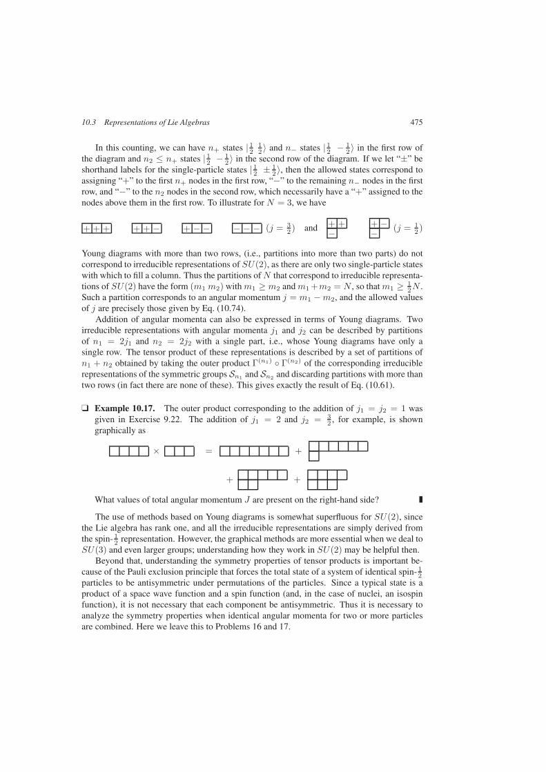
10.3 Representations of Lie Algebras 475
In this counting, we can have n+ states |1212 〉 and n− states | 12 − 1
2 〉 in the first row ofthe diagram and n2 ≤ n+ states | 12 − 1
2 〉 in the second row of the diagram. If we let “±” beshorthand labels for the single-particle states | 12 ± 1
2 〉, then the allowed states correspond toassigning “+” to the first n+ nodes in the first row, “−” to the remaining n− nodes in the firstrow, and “−” to the n2 nodes in the second row, which necessarily have a “+” assigned to thenodes above them in the first row. To illustrate for N = 3, we have
+ + + + + − + − − − − − (j = 32 ) and + +
−+ −− (j = 1
2 )
Young diagrams with more than two rows, (i.e., partitions into more than two parts) do notcorrespond to irreducible representations of SU(2), as there are only two single-particle stateswith which to fill a column. Thus the partitions ofN that correspond to irreducible representa-tions of SU(2) have the form (m1 m2) withm1 ≥ m2 andm1 +m2 = N , so thatm1 ≥ 1
2N .Such a partition corresponds to an angular momentum j = m1 −m2, and the allowed valuesof j are precisely those given by Eq. (10.74).
Addition of angular momenta can also be expressed in terms of Young diagrams. Twoirreducible representations with angular momenta j1 and j2 can be described by partitionsof n1 = 2j1 and n2 = 2j2 with a single part, i.e., whose Young diagrams have only asingle row. The tensor product of these representations is described by a set of partitions ofn1 + n2 obtained by taking the outer product Γ(n1) Γ(n2) of the corresponding irreduciblerepresentations of the symmetric groups Sn1 and Sn2 and discarding partitions with more thantwo rows (in fact there are none of these). This gives exactly the result of Eq. (10.61).
Example 10.17. The outer product corresponding to the addition of j1 = j2 = 1 wasgiven in Exercise 9.22. The addition of j1 = 2 and j2 = 3
2 , for example, is showngraphically as
× = +
+ +
What values of total angular momentum J are present on the right-hand side?
The use of methods based on Young diagrams is somewhat superfluous for SU(2), sincethe Lie algebra has rank one, and all the irreducible representations are simply derived fromthe spin-1
2 representation. However, the graphical methods are more essential when we deal toSU(3) and even larger groups; understanding how they work in SU(2) may be helpful then.
Beyond that, understanding the symmetry properties of tensor products is important be-cause of the Pauli exclusion principle that forces the total state of a system of identical spin-1
2particles to be antisymmetric under permutations of the particles. Since a typical state is aproduct of a space wave function and a spin function (and, in the case of nuclei, an isospinfunction), it is not necessary that each component be antisymmetric. Thus it is necessary toanalyze the symmetry properties when identical angular momenta for two or more particlesare combined. Here we leave this to Problems 16 and 17.

476 10 Lie Groups and Lie Algebras
J3J J+
SU(2)
T3
Y
T T+
U
V+
V
U+
SU(3)
Figure 10.1: Roots and root vectors for the Lie algebras of SU(2) and SU(3). The root vectorsfor SU(2) are defined in Eq. (10.38); those for SU(3) in Eq. (10.76).
10.3.4 Irreducible Representations of SU(3)
The method used in Section 10.3.1 to generate irreducible representations of SU(2) can begeneralized to larger Lie algebras. For example, consider the Lie algebra of SU(3) withstandard generators FA defined by Eq. (10.20) (A = 1, . . . , 8). Here there are two commutinggenerators, and we can choose, for example,
T3 = F3 and Y = 2√3F8 (10.75)
Then we can use simultaneous eigenstates of T3 and Y as basis vectors in a representation;these can be denoted by | T3 Y 〉. The eigenvalue pairs (T3, Y ) of states in a representation arethe weights of the representation. In some irreducible representations there are multiple stateswith the same weight; then further labels are needed to identify the states.
The remaining generators can be rearranged to form ladder operators for the eigenvaluesof T3 and Y. Define
T± = F1 ± iF2 U± = F6 ± iF7 V± = F4 ± iF5 (10.76)
Then
[T3,T±] = ±T± [T3,U±] = ∓12U± [T3,V±] = ±1
2V± (10.77)
and
[Y,T±] = 0 [Y,U±] = ±U± [Y,V±] = ±V± (10.78)
The generators T±,T3 define an SU(2) subalgebra of SU(3) that commutes with Y; hencethe T± change the eigenvalue of T3 by ±1 and leave the eigenvalue of Y unchanged. Thegenerators U± and V± change the eigenvalue of Y by ±1; U− and V+ (U+ and V−)change the eigenvalue of T3 by +1
2 (−12 ). The changes in the eigenvalues induced by the
ladder operators are the roots of the algebra. The ladder operators are also known as rootvectors; there is one for each root. The roots for SU(2) and SU(3) are shown in Fig. 10.1.
Remark. The notation for the generators is based on the historical development of SU(3)as an approximate symmetry of the strong interactions. The SU(2) subalgebra generated
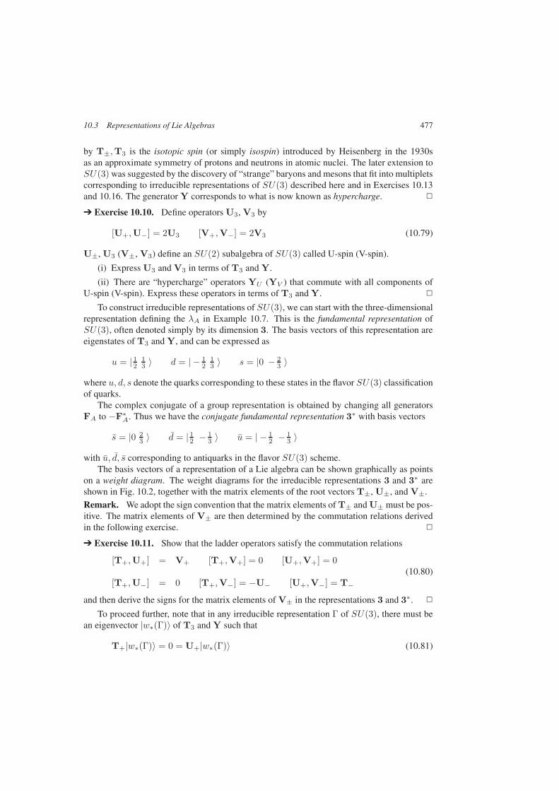
10.3 Representations of Lie Algebras 477
by T±,T3 is the isotopic spin (or simply isospin) introduced by Heisenberg in the 1930sas an approximate symmetry of protons and neutrons in atomic nuclei. The later extension toSU(3) was suggested by the discovery of “strange” baryons and mesons that fit into multipletscorresponding to irreducible representations of SU(3) described here and in Exercises 10.13and 10.16. The generator Y corresponds to what is now known as hypercharge.
Exercise 10.10. Define operators U3, V3 by
[U+,U−] = 2U3 [V+,V−] = 2V3 (10.79)
U±, U3 (V±, V3) define an SU(2) subalgebra of SU(3) called U-spin (V-spin).
(i) Express U3 and V3 in terms of T3 and Y.
(ii) There are “hypercharge” operators YU (YV ) that commute with all components ofU-spin (V-spin). Express these operators in terms of T3 and Y.
To construct irreducible representations of SU(3), we can start with the three-dimensionalrepresentation defining the λA in Example 10.7. This is the fundamental representation ofSU(3), often denoted simply by its dimension 3. The basis vectors of this representation areeigenstates of T3 and Y, and can be expressed as
u = | 1213 〉 d = | − 1
213 〉 s = |0 − 2
3 〉
where u, d, s denote the quarks corresponding to these states in the flavor SU(3) classificationof quarks.
The complex conjugate of a group representation is obtained by changing all generatorsFA to −F∗
A. Thus we have the conjugate fundamental representation 3∗ with basis vectors
s = |0 23 〉 d = |12 − 1
3 〉 u = | − 12 − 1
3 〉
with u, d, s corresponding to antiquarks in the flavor SU(3) scheme.The basis vectors of a representation of a Lie algebra can be shown graphically as points
on a weight diagram. The weight diagrams for the irreducible representations 3 and 3∗ areshown in Fig. 10.2, together with the matrix elements of the root vectors T±, U±, and V±.
Remark. We adopt the sign convention that the matrix elements of T± and U± must be pos-itive. The matrix elements of V± are then determined by the commutation relations derivedin the following exercise.
Exercise 10.11. Show that the ladder operators satisfy the commutation relations
[T+,U+] = V+ [T+,V+] = 0 [U+,V+] = 0(10.80)
[T+,U−] = 0 [T+,V−] = −U− [U+,V−] = T−
and then derive the signs for the matrix elements of V± in the representations 3 and 3∗.
To proceed further, note that in any irreducible representation Γ of SU(3), there must bean eigenvector |w∗(Γ)〉 of T3 and Y such that
T+|w∗(Γ)〉 = 0 = U+|w∗(Γ)〉 (10.81)
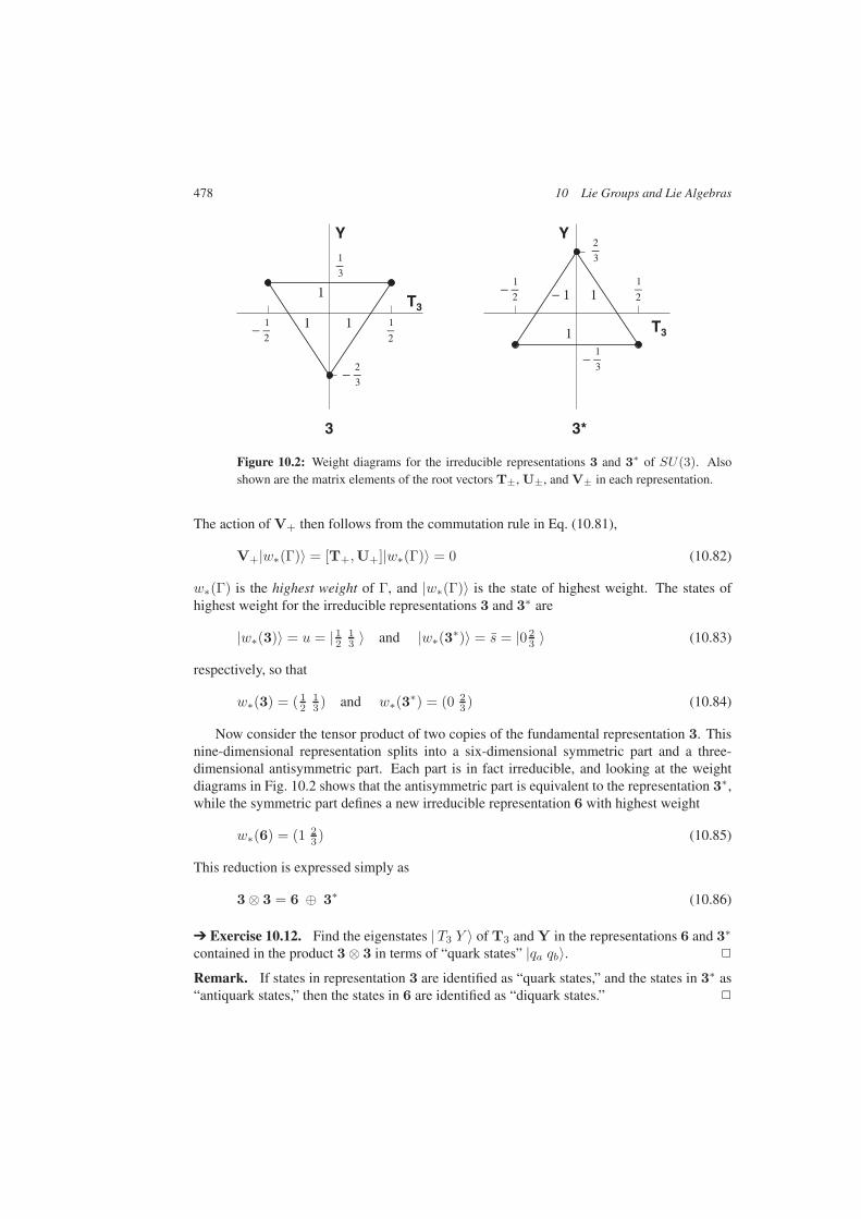
478 10 Lie Groups and Lie Algebras
T3
Y
T3
Y
3 3*
1
11
1
1
− 112_
12__ 1
2_
_ 13_
_ 23_
23_
13_
_ 12_
Figure 10.2: Weight diagrams for the irreducible representations 3 and 3∗ of SU(3). Alsoshown are the matrix elements of the root vectors T±, U±, and V± in each representation.
The action of V+ then follows from the commutation rule in Eq. (10.81),
V+|w∗(Γ)〉 = [T+,U+]|w∗(Γ)〉 = 0 (10.82)
w∗(Γ) is the highest weight of Γ, and |w∗(Γ)〉 is the state of highest weight. The states ofhighest weight for the irreducible representations 3 and 3∗ are
|w∗(3)〉 = u = | 1213 〉 and |w∗(3∗)〉 = s = |0 2
3 〉 (10.83)
respectively, so that
w∗(3) = ( 12
13 ) and w∗(3∗) = (0 2
3 ) (10.84)
Now consider the tensor product of two copies of the fundamental representation 3. Thisnine-dimensional representation splits into a six-dimensional symmetric part and a three-dimensional antisymmetric part. Each part is in fact irreducible, and looking at the weightdiagrams in Fig. 10.2 shows that the antisymmetric part is equivalent to the representation 3∗,while the symmetric part defines a new irreducible representation 6 with highest weight
w∗(6) = (1 23 ) (10.85)
This reduction is expressed simply as
3⊗ 3 = 6 ⊕ 3∗ (10.86)
Exercise 10.12. Find the eigenstates | T3 Y 〉 of T3 and Y in the representations 6 and 3∗
contained in the product 3 ⊗ 3 in terms of “quark states” |qa qb〉.
Remark. If states in representation 3 are identified as “quark states,” and the states in 3∗ as“antiquark states,” then the states in 6 are identified as “diquark states.”
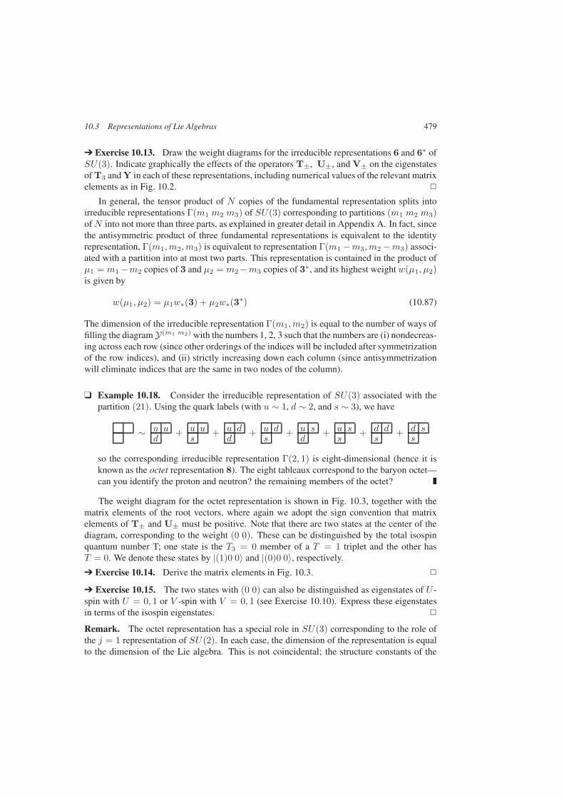
10.3 Representations of Lie Algebras 479
Exercise 10.13. Draw the weight diagrams for the irreducible representations 6 and 6∗ ofSU(3). Indicate graphically the effects of the operators T±, U±, and V± on the eigenstatesof T3 and Y in each of these representations, including numerical values of the relevant matrixelements as in Fig. 10.2.
In general, the tensor product of N copies of the fundamental representation splits intoirreducible representations Γ(m1 m2 m3) of SU(3) corresponding to partitions (m1 m2 m3)ofN into not more than three parts, as explained in greater detail in Appendix A. In fact, sincethe antisymmetric product of three fundamental representations is equivalent to the identityrepresentation, Γ(m1,m2,m3) is equivalent to representation Γ(m1 −m3,m2 −m3) associ-ated with a partition into at most two parts. This representation is contained in the product ofµ1 = m1−m2 copies of 3 and µ2 = m2−m3 copies of 3∗, and its highest weight w(µ1, µ2)is given by
w(µ1, µ2) = µ1w∗(3) + µ2w∗(3∗) (10.87)
The dimension of the irreducible representation Γ(m1,m2) is equal to the number of ways offilling the diagram Y(m1 m2) with the numbers 1, 2, 3 such that the numbers are (i) nondecreas-ing across each row (since other orderings of the indices will be included after symmetrizationof the row indices), and (ii) strictly increasing down each column (since antisymmetrizationwill eliminate indices that are the same in two nodes of the column).
Example 10.18. Consider the irreducible representation of SU(3) associated with thepartition (21). Using the quark labels (with u ∼ 1, d ∼ 2, and s ∼ 3), we have
∼ u ud
+ u us
+ u dd
+ u ds
+ u sd
+ u ss
+ d ds
+ d ss
so the corresponding irreducible representation Γ(2, 1) is eight-dimensional (hence it isknown as the octet representation 8). The eight tableaux correspond to the baryon octet—can you identify the proton and neutron? the remaining members of the octet?
The weight diagram for the octet representation is shown in Fig. 10.3, together with thematrix elements of the root vectors, where again we adopt the sign convention that matrixelements of T± and U± must be positive. Note that there are two states at the center of thediagram, corresponding to the weight (0 0). These can be distinguished by the total isospinquantum number T; one state is the T3 = 0 member of a T = 1 triplet and the other hasT = 0. We denote these states by |(1)0 0〉 and |(0)0 0〉, respectively.
Exercise 10.14. Derive the matrix elements in Fig. 10.3.
Exercise 10.15. The two states with (0 0) can also be distinguished as eigenstates of U -spin with U = 0, 1 or V -spin with V = 0, 1 (see Exercise 10.10). Express these eigenstatesin terms of the isospin eigenstates.
Remark. The octet representation has a special role in SU(3) corresponding to the role ofthe j = 1 representation of SU(2). In each case, the dimension of the representation is equalto the dimension of the Lie algebra. This is not coincidental; the structure constants of the
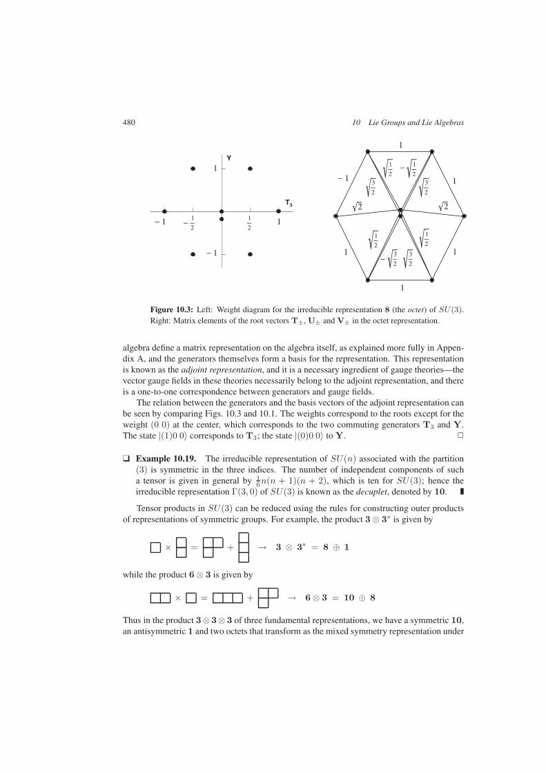
480 10 Lie Groups and Lie Algebras
T3
Y
1
1
1− 1
1
1
2
32_
12__ 1
2_− 1
− 1
1
1
12_
32_
32_ 3
2_
−
−
12_
12_ 1
2_
2
Figure 10.3: Left: Weight diagram for the irreducible representation 8 (the octet) of SU(3).Right: Matrix elements of the root vectors T±, U± and V± in the octet representation.
algebra define a matrix representation on the algebra itself, as explained more fully in Appen-dix A, and the generators themselves form a basis for the representation. This representationis known as the adjoint representation, and it is a necessary ingredient of gauge theories—thevector gauge fields in these theories necessarily belong to the adjoint representation, and thereis a one-to-one correspondence between generators and gauge fields.
The relation between the generators and the basis vectors of the adjoint representation canbe seen by comparing Figs. 10.3 and 10.1. The weights correspond to the roots except for theweight (0 0) at the center, which corresponds to the two commuting generators T3 and Y.The state |(1)0 0〉 corresponds to T3; the state |(0)0 0〉 to Y.
Example 10.19. The irreducible representation of SU(n) associated with the partition(3) is symmetric in the three indices. The number of independent components of sucha tensor is given in general by 1
6n(n + 1)(n + 2), which is ten for SU(3); hence theirreducible representation Γ(3, 0) of SU(3) is known as the decuplet, denoted by 10.
Tensor products in SU(3) can be reduced using the rules for constructing outer productsof representations of symmetric groups. For example, the product 3 ⊗ 3∗ is given by
× = + → 3 ⊗ 3∗ = 8 ⊕ 1
while the product 6⊗ 3 is given by
× = + → 6 ⊗ 3 = 10 ⊕ 8
Thus in the product 3⊗3⊗3 of three fundamental representations, we have a symmetric 10,an antisymmetric 1 and two octets that transform as the mixed symmetry representation under
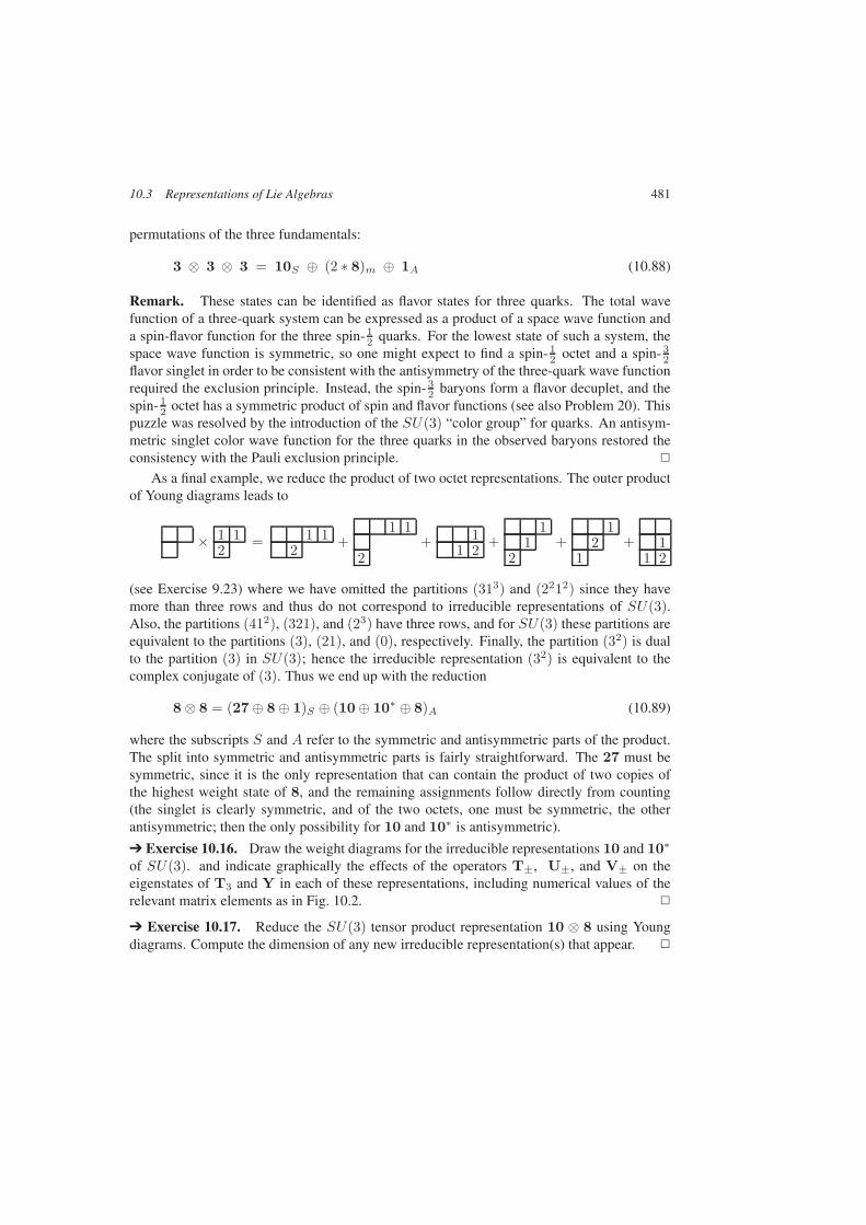
10.3 Representations of Lie Algebras 481
permutations of the three fundamentals:
3 ⊗ 3 ⊗ 3 = 10S ⊕ (2 ∗ 8)m ⊕ 1A (10.88)
Remark. These states can be identified as flavor states for three quarks. The total wavefunction of a three-quark system can be expressed as a product of a space wave function anda spin-flavor function for the three spin-1
2 quarks. For the lowest state of such a system, thespace wave function is symmetric, so one might expect to find a spin-1
2 octet and a spin-32
flavor singlet in order to be consistent with the antisymmetry of the three-quark wave functionrequired the exclusion principle. Instead, the spin- 3
2 baryons form a flavor decuplet, and thespin-1
2 octet has a symmetric product of spin and flavor functions (see also Problem 20). Thispuzzle was resolved by the introduction of the SU(3) “color group” for quarks. An antisym-metric singlet color wave function for the three quarks in the observed baryons restored theconsistency with the Pauli exclusion principle.
As a final example, we reduce the product of two octet representations. The outer productof Young diagrams leads to
× 1 12 = 1 1
2 +1 1
2+ 1
1 2 +1
12
+1
21
+ 11 2
(see Exercise 9.23) where we have omitted the partitions (313) and (2212) since they havemore than three rows and thus do not correspond to irreducible representations of SU(3).Also, the partitions (412), (321), and (23) have three rows, and for SU(3) these partitions areequivalent to the partitions (3), (21), and (0), respectively. Finally, the partition (32) is dualto the partition (3) in SU(3); hence the irreducible representation (32) is equivalent to thecomplex conjugate of (3). Thus we end up with the reduction
8 ⊗ 8 = (27⊕ 8 ⊕ 1)S ⊕ (10⊕ 10∗ ⊕ 8)A (10.89)
where the subscripts S and A refer to the symmetric and antisymmetric parts of the product.The split into symmetric and antisymmetric parts is fairly straightforward. The 27 must besymmetric, since it is the only representation that can contain the product of two copies ofthe highest weight state of 8, and the remaining assignments follow directly from counting(the singlet is clearly symmetric, and of the two octets, one must be symmetric, the otherantisymmetric; then the only possibility for 10 and 10∗ is antisymmetric).
Exercise 10.16. Draw the weight diagrams for the irreducible representations 10 and 10∗
of SU(3). and indicate graphically the effects of the operators T±, U±, and V± on theeigenstates of T3 and Y in each of these representations, including numerical values of therelevant matrix elements as in Fig. 10.2.
Exercise 10.17. Reduce the SU(3) tensor product representation 10 ⊗ 8 using Youngdiagrams. Compute the dimension of any new irreducible representation(s) that appear.
482 10 Lie Groups and Lie Algebras
A Tensor Representations of the Classical Lie Groups
A.1 The Classical Lie Groups
The classical groups are the linear groups GL(n) and SL(n), the unitary groups U(n)andSU(n) defined on a complex n-dimensional linear vector space Vn, the orthogonal groupsO(n) and SO(n) defined on a real n-dimensional space, and the symplectic groups Sp(2n)defined on a 2n-dimensional space. These groups were introduced briefly in Section 10.1.Here we construct representations of these groups using tensor methods whose origins can betraced to the works of Herman Weyl. Another approach is to study representations of the Liealgebras, generalizing the standard treatment of angular momentum in quantum mechanics.This has been worked out in detail for SU(2) and SU(3) in Section 10.3.
The fundamental representation of each of these groups is the defining representation, inwhich each element A of the group is represented by itself in the vector space Vn on which itis defined (Rn for the orthogonal groups and the real linear groups, Cn for the others). Thereare other representations on the same vector space Vn, namely,
A → A∗ A → A−1 A → (A†)−1 (10.A1)
where A∗ denotes the complex conjugate of A (this definition depends on the basis in Vn, butall such representations are evidently equivalent), and A denotes the transpose of A.
For the group SL(2, C), the representation A → A−1 is equivalent to the defining rep-resentation (see Problem 2). We note that the group SL(2, C) is closely related to the groupof homogeneous Lorentz transformations. This relations is similar to the relation betweenSU(2) and the three-dimensional rotations group SO(3), as explained in detail in Appen-dix B. However, for n > 2, Eq. (10.A1) defines four inequivalent irreducible representationsof the groups GL(n,C), and SL(n,C). For the groups GL(n,R) and SL(n,R), the repre-sentation matrices are real (A = A∗), but A → A−1 provides an inequivalent representationexcept in the case of SL(2, R).
For the unitary groups U(n) and SU(n), unitarity of the matrices implies
A = (A†)−1 A∗ = A−1 (10.A2)
so that of the representations in Eq. (10.A1), only the map A → A∗ gives a new inequivalentirreducible representation, the conjugate fundamental representation, that is not equivalent tothe fundamental representation, again apart from the special case of SU(2) (see Problem 1).For the orthogonal groups SO(n), the four representations are identical, since
A = A∗ = A−1 = (A†)−1 (10.A3)
for real orthogonal matrices. For the symplectic groups Sp(2n), the four representations areagain equivalent, though we will not prove that here.
An irreducible representation of the general group GL(n,C) [SL(n,C)] is also irre-ducible for the subgroupU(n) [SU(n)] of unitary matrices, since the Lie algebra ofGL(n,C)is obtained from the real Lie algebra of U(n) by allowing the parameters of the algebra to becomplex. Thus we consider here only the irreducible representations of U(n) and SU(n).The reduction of these irreducible representations under restriction to the subgroups SO(n)or Sp(2n) will also be described.
A Tensor Representations of the Classical Lie Groups 483
A.2 Tensor Representations of U(n) and SU(n)
To construct irreducible representations of U(n) and its subgroup SU(n), we start with abasis for the complex linear vector space Vn on which these groups are defined. Then a linearoperator A has a matrix representation A = (ajk) so that when acting on a vector x withcomponents ξ1, . . . , ξn, it gives the vector Ax with components
[Ax]j ≡ ξ′j = ajkξk (10.A4)
Remark. We recall the (Einstein) summation convention from Chapter 3, which requires usto sum over a repeated pair of indices (one subscript and one superscript) such as the index kin the last equation, unless explicitly instructed not to by writing
S = akbk (no sum)
Since we deal here only with linear manifolds, we do not need the full geometric apparatus ofChapter 3, but we use superscripts to denote the components of a vector in Vn, and subscriptsto denote components of vectors in the dual space to Vn. In Chapter 3, elements of thedual space are identified with the space differential forms on a manifold; here they are linearfunctionals on Vn as introduced in Chapter 2. For a complex vector space, the dual spacecan be envisioned as the “complex conjugate” space, though that identification depends on anexplicit basis. In a real unitary vector space, forms and vectors are equivalent, and we thensum over any pair of repeated indices.
If we now take the tensor product of Vn with itself N times,
⊗NVn ≡ Vn ⊗ · · · ⊗ Vn︸ ︷︷ ︸N times
(10.A5)
we have a representation of U(n) on the space ⊗NVn. The elements X of this space aretensors of rank N 1 whose components ξj1···jN are labeled by a set of N indices. When actedon by a linear operator A from U(n), these components are transformed according to the rule
(AX)j1···jN ≡ ξ′j1···jN = aj1k1· · · ajNkN
ξk1···kN (10.A6)
This representation is reducible, since the transformation coefficients
Aj1···jNk1···kN≡ aj1k1
· · · ajNkN(10.A7)
are unchanged if we apply any permutation of 1, . . . , N to both sets of indices j1 · · · jN andk1 · · · kN . That is, permutations of the indices commute with the tensor transformation law.
Thus we can collect the tensor components into sets that transform among themselvesunder permutations of the indices. For the unitary groups U(n) and SU(n), these sets defineirreducible tensor representations, though we do not prove irreducibility here. An irreducibletensor of rank N is associated with an irreducible representation of the symmetric group SN ,with a partition of N and its Young diagram (see Section 9.5) that define the symmetry typeof the tensor.
1Caution. The rank of a tensor is not the same as the rank of a Lie algebra defined in Definition 10.5.

484 10 Lie Groups and Lie Algebras
Not every partition of N corresponds to an irreducible representation of U(n), however.Since the tensor corresponding to a Young diagram is antisymmetric when we interchangeelements in the same column of the diagram, the partition of N for a U(n) tensor of rank Ncan have no more than n rows. Furthermore, an antisymmetric tensor of rank n is necessarilyproportional to the Levi-Civita symbol
εi1···in =
+1 if i1 · · · in is an even permutation of 1 . . . n−1 if i1 · · · in is an odd permutation of 1 . . . n0 if any two indices are equal
(10.A8)
which is antisymmetric in its n indices. Under transformations of U(n), we have
εi1···in → Ai1···ink1···knεk1···kn = (detA) εi1···in (10.A9)
so the Levi-Civita symbol is transformed into a multiple of itself by an element of U(n). It isa numerical tensor, the ε-tensor, which provides a one-dimensional representation of U(n).Under SU(n), whose elements have detA = 1, the Levi-Civita tensor is transformed exactlyinto itself; it is an invariant of SU(n).
Now suppose (m) = (m1m2 · · ·mp) is a partition of N into p parts. Then
• for p > n, there are no irreducible representations of U(n),
• for p ≤ n, there are two irreducible representations of U(n) on the tensor product space,corresponding to the direct tensor product representation and the conjugate representationintroduced in Eq. (10.A1).
In the case p ≤ n, we can use the Young diagram Y(m) of (m) to compute the dimensionof the corresponding irreducible representation of U(n). Recall that indices are symmetric(antisymmetric) with respect to permuting the elements of a row (column) of the diagram.Then the dimension of the irreducible representation of U(n) corresponding to a partition (m)is equal to the number of ways to fill the boxes of Y(m) with numbers in the range 1, . . . , n,not necessarily distinct, such that
(i) the indices are nondecreasing across each row, and
(ii) the indices are strictly increasing down each column.
This procedure counts the number of independent components of a tensor of the symmetrytype (m); the remaining components are determined by permuting indices of the tensor.
Example 10.20. The irreducible representations of U(n) associated with the partitions(2) and (12) are the symmetric and antisymmetric tensors of rank two, with 1
2n(n + 1)and 1
2n(n−1) independent components, respectively. The diagrammatic rule gives exactlythis result for the dimension of the corresponding irreducible representation.
Example 10.21. In Example 10.18, the dimension of the irreducible representation ofSU(3) associated with the partition (21) and (3) was found to be 8, using the procedurejust described.
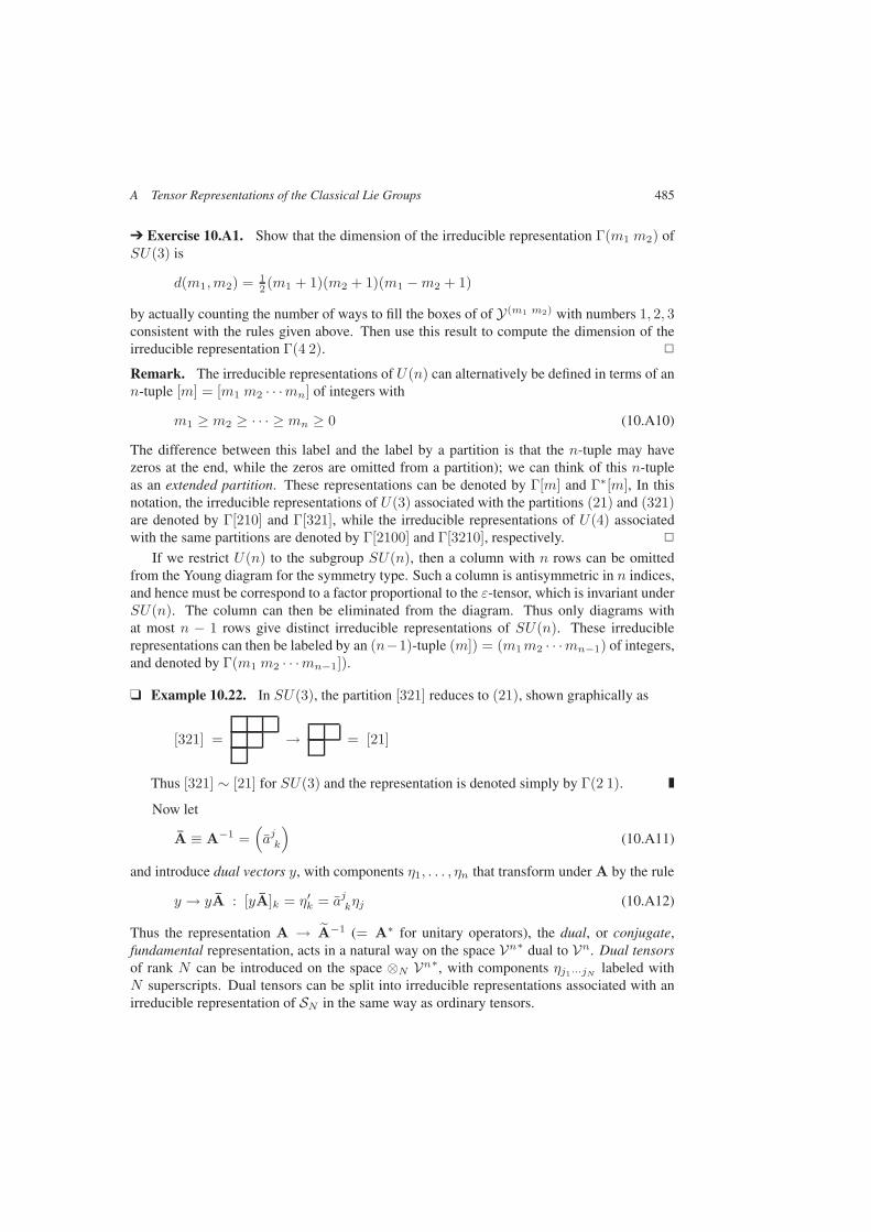
A Tensor Representations of the Classical Lie Groups 485
Exercise 10.A1. Show that the dimension of the irreducible representation Γ(m1 m2) ofSU(3) is
d(m1,m2) = 12 (m1 + 1)(m2 + 1)(m1 −m2 + 1)
by actually counting the number of ways to fill the boxes of of Y(m1 m2) with numbers 1, 2, 3consistent with the rules given above. Then use this result to compute the dimension of theirreducible representation Γ(4 2).
Remark. The irreducible representations of U(n) can alternatively be defined in terms of ann-tuple [m] = [m1 m2 · · ·mn] of integers with
m1 ≥ m2 ≥ · · · ≥ mn ≥ 0 (10.A10)
The difference between this label and the label by a partition is that the n-tuple may havezeros at the end, while the zeros are omitted from a partition); we can think of this n-tupleas an extended partition. These representations can be denoted by Γ[m] and Γ∗[m], In thisnotation, the irreducible representations of U(3) associated with the partitions (21) and (321)are denoted by Γ[210] and Γ[321], while the irreducible representations of U(4) associatedwith the same partitions are denoted by Γ[2100] and Γ[3210], respectively.
If we restrict U(n) to the subgroup SU(n), then a column with n rows can be omittedfrom the Young diagram for the symmetry type. Such a column is antisymmetric in n indices,and hence must be correspond to a factor proportional to the ε-tensor, which is invariant underSU(n). The column can then be eliminated from the diagram. Thus only diagrams withat most n − 1 rows give distinct irreducible representations of SU(n). These irreduciblerepresentations can then be labeled by an (n−1)-tuple (m]) = (m1m2 · · ·mn−1) of integers,and denoted by Γ(m1 m2 · · ·mn−1]).
Example 10.22. In SU(3), the partition [321] reduces to (21), shown graphically as
[321] = → = [21]
Thus [321] ∼ [21] for SU(3) and the representation is denoted simply by Γ(2 1).
Now let
A ≡ A−1 =(ajk
)(10.A11)
and introduce dual vectors y, with components η1, . . . , ηn that transform under A by the rule
y → yA : [yA]k = η′k = ajkηj (10.A12)
Thus the representation A → A−1 (= A∗ for unitary operators), the dual, or conjugate,fundamental representation, acts in a natural way on the space Vn∗ dual to Vn. Dual tensorsof rank N can be introduced on the space ⊗N Vn∗, with components ηj1···jN labeled withN superscripts. Dual tensors can be split into irreducible representations associated with anirreducible representation of SN in the same way as ordinary tensors.

486 10 Lie Groups and Lie Algebras
Tensor indices that are antisymmetric can be raised and lowered using the ε-tensor. If Tis an antisymmetric SU(n) tensor of rank p with components T i1···ip , then there is a corre-sponding antisymmetric dual tensor ∗T of rank (n− p) with components given by
∗Tip+1···in = εi1···in Ti1···ip (10.A13)
where ε i1···in = εi1···in is the completely antisymmetric dual tensor. This dual ∗T is the sameas the Hodge dual introduced in Chapter 3. Conversely, the antisymmetric SU(n) dual tensor∗T of rank (n − p) corresponds to an antisymmetric tensor T of rank p, with componentsrelated by
T i1···ip = εi1···in ∗Tip+1···in (10.A14)
The construction of dual tensors extends to tensors of general symmetry. If T is a SU(n)tensor of rank N , with symmetry associated with the partition (m) = (m1 · · ·mq) of N , thenthe dual tensor has the symmetry of a partition (m)∗ of nm1 − N constructed by assigningto (m)∗ those boxes of a rectangle with n rows and m1 columns that are not in the partition(m), and rotating the diagram to the standard position. Note that (m)∗ depends both on nand (m). The dual representation is equivalent to the (complex) conjugate representation ofSU(n). Tensors whose dual is equivalent to the original tensor are self-dual; the correspond-ing representation of SU(n) is then real.
Example 10.23. The fundamental representation of SU(3) is 3 = (10). The six-dimensional irreducible representation 6 = (20) is a symmetric tensor of rank two; thecorresponding dual tensor is 6∗ = (22). The antisymmetric rank two tensor is associatedwith the partition (11); it is equivalent to the conjugate fundamental 3∗ for SU(3).
Irreducible representations can be denoted simply by their dimension (3, 3∗, . . .) when thecontext is clear. We have shown in Example 10.18 that the irreducible representation (21) ofSU(3) is eight-dimensional; it can be denoted by 8. It is also self-dual, and hence real.
Example 10.24. Consider a rank three tensor of symmetry type (21). For an SU(3)tensor, we can construct the diagram
x xx yy y
→ + = (21) + (21)
so we conclude that the SU(3) tensor dual to (21) also has symmetry type (21) and is thusself-dual. For an SU(4) tensor, on the other hand, we have
x xx yy yy y
→ + = (21) + (221)
Hence the SU(4) tensor dual to (21) has symmetry type (221), and is not self-dual.
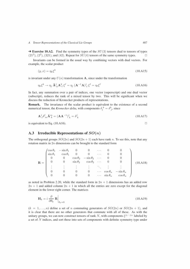
A Tensor Representations of the Classical Lie Groups 487
Exercise 10.A2. Find the symmetry types of the SU(3) tensors dual to tensors of types(212), (22), (321), and (42). Repeat for SU(4) tensors of the same symmetry types.
Invariants can be formed in the usual way by combining vectors with dual vectors. Forexample, the scalar product
(y, x) = ηkξk (10.A15)
is invariant under any U(n) transformation A, since under the transformation
ηkξk → ηj Aj
kAk ξ
= ηj (A−1A)j ξ = ηξ
(10.A16)
In fact, any summation over a pair of indices, one vector (superscript) and one dual vector(subscript), reduces the rank of a mixed tensor by two. This will be significant when wediscuss the reduction of Kronecker products of representations.
Remark. The invariance of the scalar product is equivalent to the existence of a secondnumerical tensor, the Kronecker delta, with components δ kj = δkj , since
AjδmAm
k = (AA−1)jk = δjk (10.A17)
is equivalent to Eq. (10.A16).
A.3 Irreducible Representations of SO(n)
The orthogonal groups SO(2n) and SO(2n+ 1) each have rank n. To see this, note that anyrotation matrix in 2n dimensions can be brought to the standard form
R =
cos θ1 − sin θ1 0 0 · · · 0 0sin θ1 cos θ1 0 0 · · · 0 0
0 0 cos θ2 − sin θ2 · · · 0 00 0 sin θ2 cos θ2 · · · 0 0...
......
.... . .
......
0 0 0 0 · · · cos θn − sin θn0 0 0 0 · · · sin θn cos θn
(10.A18)
as noted in Problem 2.20, while the standard form in 2n + 1 dimensions has an added row2n + 1 and added column 2n + 1 in which all the entries are zero except for the diagonalelement in the lower right corner. The matrices
Hk = i∂
∂θkR∣∣∣∣θk=0
(10.A19)
(k = 1, . . . , n) define a set of n commuting generators of SO(2n) or SO(2n + 1), andit is clear that there are no other generators that commute with all of these. As with theunitary groups, we can now construct tensors of rank N , with components ξj1···jN labeled bya set of N indices, and sort these into sets of components with definite symmetry type under
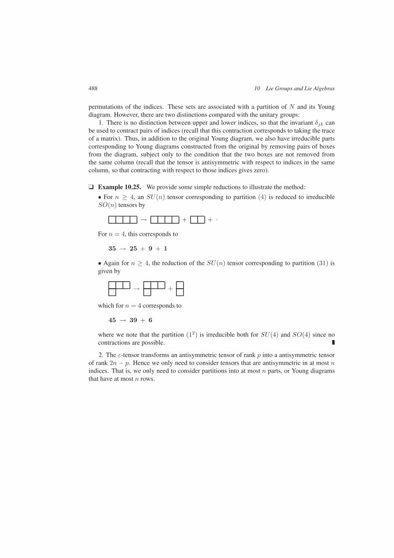
488 10 Lie Groups and Lie Algebras
permutations of the indices. These sets are associated with a partition of N and its Youngdiagram. However, there are two distinctions compared with the unitary groups:
1. There is no distinction between upper and lower indices, so that the invariant δjk canbe used to contract pairs of indices (recall that this contraction corresponds to taking the traceof a matrix). Thus, in addition to the original Young diagram, we also have irreducible partscorresponding to Young diagrams constructed from the original by removing pairs of boxesfrom the diagram, subject only to the condition that the two boxes are not removed fromthe same column (recall that the tensor is antisymmetric with respect to indices in the samecolumn, so that contracting with respect to those indices gives zero).
Example 10.25. We provide some simple reductions to illustrate the method:
• For n ≥ 4, an SU(n) tensor corresponding to partition (4) is reduced to irreducibleSO(n) tensors by
→ + + ·
For n = 4, this corresponds to
35 → 25 + 9 + 1
• Again for n ≥ 4, the reduction of the SU(n) tensor corresponding to partition (31) isgiven by
→ +
which for n = 4 corresponds to
45 → 39 + 6
where we note that the partition (12) is irreducible both for SU(4) and SO(4) since nocontractions are possible.
2. The ε-tensor transforms an antisymmetric tensor of rank p into a antisymmetric tensorof rank 2n − p. Hence we only need to consider tensors that are antisymmetric in at most nindices. That is, we only need to consider partitions into at most n parts, or Young diagramsthat have at most n rows.
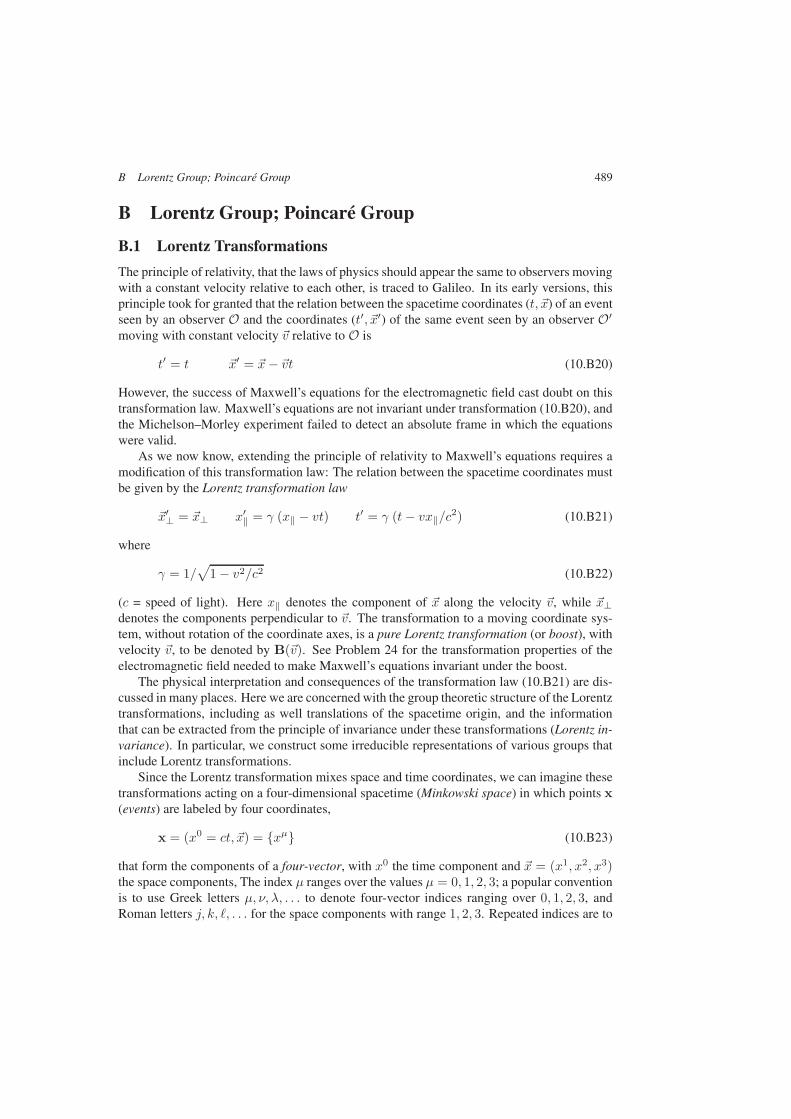
B Lorentz Group; Poincaré Group 489
B Lorentz Group; Poincaré Group
B.1 Lorentz Transformations
The principle of relativity, that the laws of physics should appear the same to observers movingwith a constant velocity relative to each other, is traced to Galileo. In its early versions, thisprinciple took for granted that the relation between the spacetime coordinates (t, x) of an eventseen by an observer O and the coordinates (t′, x′) of the same event seen by an observer O′
moving with constant velocity v relative to O is
t′ = t x′ = x− vt (10.B20)
However, the success of Maxwell’s equations for the electromagnetic field cast doubt on thistransformation law. Maxwell’s equations are not invariant under transformation (10.B20), andthe Michelson–Morley experiment failed to detect an absolute frame in which the equationswere valid.
As we now know, extending the principle of relativity to Maxwell’s equations requires amodification of this transformation law: The relation between the spacetime coordinates mustbe given by the Lorentz transformation law
x′⊥ = x⊥ x′‖ = γ (x‖ − vt) t′ = γ (t− vx‖/c2) (10.B21)
where
γ = 1/√
1 − v2/c2 (10.B22)
(c = speed of light). Here x‖ denotes the component of x along the velocity v, while x⊥denotes the components perpendicular to v. The transformation to a moving coordinate sys-tem, without rotation of the coordinate axes, is a pure Lorentz transformation (or boost), withvelocity v, to be denoted by B(v). See Problem 24 for the transformation properties of theelectromagnetic field needed to make Maxwell’s equations invariant under the boost.
The physical interpretation and consequences of the transformation law (10.B21) are dis-cussed in many places. Here we are concerned with the group theoretic structure of the Lorentztransformations, including as well translations of the spacetime origin, and the informationthat can be extracted from the principle of invariance under these transformations (Lorentz in-variance). In particular, we construct some irreducible representations of various groups thatinclude Lorentz transformations.
Since the Lorentz transformation mixes space and time coordinates, we can imagine thesetransformations acting on a four-dimensional spacetime (Minkowski space) in which points x(events) are labeled by four coordinates,
x = (x0 = ct, x) = xµ (10.B23)
that form the components of a four-vector, with x0 the time component and x = (x1, x2, x3)the space components, The index µ ranges over the values µ = 0, 1, 2, 3; a popular conventionis to use Greek letters µ, ν, λ, . . . to denote four-vector indices ranging over 0, 1, 2, 3, andRoman letters j, k, , . . . for the space components with range 1, 2, 3. Repeated indices are to
490 10 Lie Groups and Lie Algebras
be summed over the appropriate range, following the Einstein summation convention. The useof superscripts rather than subscripts is conventional, but see Chapter 3 for further discussionof the relation between superscripts and subscripts as labels for components.
Linear transformations of the spacetime coordinates will be denoted by Λ, with explicittransformation law
x → x′ = Λx : x′µ = Λµν xν (10.B24)
with the summation convention in effect. Note that when a matrix has one subscript and onesuperscript index, the row index should be placed clearly to the left of the column index.
The difference between four-vectors and vectors in a vector space V4 of Chapter 2 is thathere we define the scalar product of two four-vectors
a = (a0,a ) b = (b0,b ) (10.B25)
as
(a,b) = a · b = aµgµνbν = a0b0 − a ·b (10.B26)
The matrix
g = (gµν) = diag(1,−1,−1,−1) (10.B27)
is a metric tensor, the Minkowski metric, and a · b is a Lorentz scalar. The metric g is notpositive definite, and a four-vector a is
(i) timelike if a · a > 0,
(ii) spacelike if a · a < 0, or
(iii) lightlike if a · a = 0 (a = 0).
Example 10.26. An important four-vector is the four-momentum p of a particle, whichhas components
p = (E/c, p ) (10.B28)
where E is the energy of the particle. We have the Lorentz scalar
p · p = m2c2 (10.B29)
where m is the mass of the particle.
Remark. In the older literature m was often called the “rest mass” of the particle, and E/c2
the “relativistic mass.” The modern view refers to the invariant m simply as the “mass.” Theenergy
E =√
(pc)2 + (mc2)2 (10.B30)
includes a contribution mc2 from the rest energy of the particle.
B Lorentz Group; Poincaré Group 491
The rotations of the spatial coordinate axes, as described in Section 2.2.4, define the ro-tation group. Including the transformations to moving coordinate systems leads to a largergroup, the homogeneous Lorentz group, which contains those linear transformations Λ offour-vectors such that
(Λa,Λb) = (a,b) (10.B31)
for all four-vectors a and b. In terms of the matrix elements of Λ, this requires
Λµα gµν Λνβ = gαβ (10.B32)
Any such transformation is a Lorentz transformation. As already noted, the transformation toa coordinate system moving with constant velocity is a boost, or pure Lorentz transformation.
Exercise 10.B3. (i) Show that the matrix elements of the inverse transformation Λ satisfy
gµα Λα
ν = Λβµ gβν
(ii) Show that the matrix elements Λµν satisfy
∣∣Λ00
∣∣2 − Λ0jΛ
j0 = 1
Remark. Thus∣∣Λ0
0
∣∣ ≥ 1. If∣∣Λ0
0
∣∣ = 1, then Λ is just a rotation of the coordinate axes.
(iii) Show that
det Λ = ±1
for any Lorentz transformation.
The preceding exercise shows that detΛ = ±1 and∣∣Λ0
0
∣∣ ≥ 1, but only restricted Lorentztransformations, those with detΛ = +1 and Λ0
0 ≥ 1, can be reached continuously from theidentity. Other Lorentz transformations are obtained as the product of a restricted Lorentztransformation and one or both of the discrete transformations
space reflection Σ : x→ −x, t→ t
time inversion Θ : x→ x, t→ −t.
Remark. Note that time reversal in quantum mechanics is not simply time inversion. Re-versing the role of initial and final states in a scalar product
〈φ|ψ〉 → 〈ψ|φ〉 = 〈φ|ψ〉∗ (10.B33)
involves complex conjugation as well.
Thus the full Lorentz group L has four connected components:
L↑± : det Λ = ±1 Λ0
0 ≥ 1 and L↓± : detΛ = ∓1 Λ0
0 ≤ −1
and the subgroups L↑+, the restricted Lorentz group, L+ ≡ L↑
+ ∪ L↓+, the proper Lorentz
group, L↑ ≡ L↑+ ∪ L↑
−, the orthochronous Lorentz group, and L0 ≡ L↑+ ∪ L↓
+.

492 10 Lie Groups and Lie Algebras
The restricted Lorentz group is also characterized as SO(3, 1) in a notation whereSO(p, q) denotes the group that leaves invariant a metric of the form
g = diag(1, . . . , 1︸ ︷︷ ︸p times
,−1, . . . ,−1︸ ︷︷ ︸q times
) (10.B34)
The matrix Λ corresponding to a rotation of the coordinate axes has the form
Λ =(
1 00 R(φ, θ, ψ)
)(10.B35)
where R(φ, θ, ψ) is the rotation matrix given in Eq. (2.113), and any Lorentz transformationwith Λ0
0 = 1 is a rotation (proper or improper, as the case may be). For a boost in the directionn with velocity
v = (c tanhχ) n (10.B36)
the matrix elements of Λ ≡ Bn (χ) are given by
Λ00 = coshχ Λj0 = −(sinhχ) nj = Λ0
j(10.B37)
Λjk = δjk + (coshχ− 1) njnk
Remark. The matrix for a boost is symmetric. The converse is almost true: A symmetricLorentz transformation is a pure boost, possibly accompanied by a rotation through a multipleof π about the boost axis. The proof of this statement is left to Problem 26.
The generator Ln for rotations about the axis n are obtained from the rotation matrixRn(Φ) by (see Problem 2.16)
Ln = iR′n(Φ)
∣∣∣∣Φ=0
(10.B38)
Similarly, the generator Kn for boosts in the direction n is given by
Kn = iB′n(χ)
∣∣∣∣χ=0
(10.B39)
The generators satisfy the commutation rules
[Lα,Lβ] = i∑
γ
εαβγLγ [Lα,Kβ] = i∑
γ
εαβγKγ
(10.B40)[Kα,Kβ] = −i
∑
γ
εαβγLγ
where εαβγ is the usual antisymmetric symbol on three indices. The minus sign on the right-hand side of the [Kα,Kβ] commutator distinguishes the Lorentz algebra from that of SO(4)(see Problem 7).

B Lorentz Group; Poincaré Group 493
Exercise 10.B4. (i) Find explicit matrices for the Lα, Kα. Then verify the commuta-tors (10.B40)
(ii) The Lα, Kα span the Lie algebra of the group L↑+. Find quadratic Casimir operators
for the Lie algebra using the results of Section 10.2.3. Is L↑+ compact?
Now introduce the operators
−→M ≡ 1
2 (−→L + i
−→K)
−→N ≡ 1
2 (−→L − i
−→K) (10.B41)
The operators−→M and
−→N each satisfy standard angular momentum commutation rules
[Mα,Mβ ] = i∑
γ
εαβγMγ [Nα,Nβ ] = i∑
γ
εαβγNγ (10.B42)
while commuting with each other ([Mα,Nβ ] = 0).Thus finite-dimensional representations of the homogeneous Lorentz algebra can be con-
structed from the finite-dimensional representations of the angular momentum algebra. Thereare irreducible representations Γ(m,n) of the homogeneous Lorentz algebra with basis vec-tors Φm,nµ,ν such that
−→M · −→M Φm,nµ,ν = m(m+ 1)Φm,nµ,ν
−→N · −→N Φm,nµ,ν = n(n+ 1)Φm,nµ,ν (10.B43)
M3 Φm,nµ,ν = µ Φm,nµ,ν N3 Φm,nµ,ν = ν Φm,nµ,ν (10.B44)
(M1 ± M2) Φm,nµ,ν =√
(m∓ µ)(m± µ+ 1) Φm,nµ±1,ν (10.B45)
(N1 ± N2) Φm,nµ,ν =√
(n∓ ν)(n± ν + 1) Φm,nµ,ν±1 (10.B46)
Here m,n = 0, 12 , 1,
32 , . . . ; µ = −m,−m+1 · · · ,m−1,m ; ν = −n,−n+1, . . . , n−1, n
as worked out in Section 10.3.1.The representations Γ(m,n) do not generate unitary representations of L↑
+, since the rep-resentations of the Kα are not Hermitian. This is consistent with the general rule that anontrivial unitary representation of a noncompact group is necessarily infinite-dimensional (afinite-dimensional unitary representation would be compact). However, these representationsare still useful in constructing representations of the Poincaré group.
B.2 SL(2, C) and the Homogeneous Lorentz Group
The fundamental representation of SL(2, C) is defined on a two-dimensional vector spacewhose elements are two-component spinors
u ≡ (ua) (a = 1, 2 is a spinor index). Under an SL(2, C) transformation A,
u→ u′ = Au : u′a = A ba ub (10.B47)
(summation convention here on spinor indices). There are also conjugate spinors v ≡ (va)(a = 1, 2 is a conjugate spinor index, sometimes called a dotted index and expressed as a).Conjugate spinors transform under the conjugate representation
v → v′ = A∗v : v′a = A∗ ba ub (10.B48)
494 10 Lie Groups and Lie Algebras
These representations can be ntified with the irreducible representations Γ( 12 , 0) and Γ(0, 1
2 )of the L↑
+ once we have derived the equivalence between L↑+ and SL(2, C) transformations.
Under restriction the subgroup SU(2), the representations are both equivalent to the j = 12
representation (see Exercise 1).The analysis of rotations, and more generally Lorentz transformations, is simplified if we
introduce a 2 × 2 matrix representation for four-vectors. Then Lorentz transformations canalso be represented as complex 2 × 2 matrices, which are easier to manipulate than 3 × 3rotation matrices or 4× 4 Lorentz transformation matrices. The representation of rotations by2 × 2 matrices was introduced in Problem 2.18. We can extend the Pauli matrices to form abasis
σ = σµ ≡ (σ0 = 1, σ) ≡ σµ (10.B49)
of four-vectors, and a basis σ of dual four-vectors, with elements
σµ = ζσ∗µζ
−1 = (σ0 = 1,−σ) ≡ σµ (10.B50)
Then to each real four-vector x = (x0, x ) corresponds a Hermitian 2 × 2 matrix
X(x) ≡ σ · x = σµxµ = σ0 x
0 + σ · x =(x0 + x3 x1 − ix2
x1 + ix2 x0 − x3
)(10.B51)
and a dual matrix
X(x) ≡ σ · x = σ0 x0 − σ · x (10.B52)
This correspondence can be inverted: To each Hermitian 2 × 2 matrix X corresponds a four-vectors x(X) and x(X) with components given by
xµ = 12 tr(σµX) xµ = 1
2 tr(σµX) (10.B53)
Exercise 10.B5. Show that
X(x)X(x) = (x · x)1 = X(x)X(x)
detX(x) = x · x = detX(x)
for any four-vector x.
Now suppose A is an element of SL(2, C), that is, a 2 × 2 matrix with detA = 1. Thenthe transformation
X → XA ≡ AXA† (10.B54)
of the 2 × 2 matrix X corresponds to a linear transformation
x = x(X) → xA ≡ x(AXA†) (10.B55)
of four-vectors, with detX = detXA since detA = 1, and hence
x · x = xA · xA (10.B56)
B Lorentz Group; Poincaré Group 495
Thus x → xA is a Lorentz transformation, to be denoted by Λ(A). It follows fromEq. (10.B53) that
xµA = 12 tr(σµAσνA†) xν (10.B57)
so that the Lorentz transformation matrix is given by
Λµν(A) = 12 tr(σµAσνA†) (10.B58)
Remark. In terms of components, the four-vector transformation law (10.B54) is
Xac → A ba Xbd A
∗ dc (10.B59)
with one spinor and one conjugate spinor index. This is exactly the transformation law for theirreducible representation Γ( 1
2 ,12 ) of SL(2, C).
Now
Λ00(A) = 1
2 tr(AA†) ≥ 1 (10.B60)
(see Problem 2.19), so that Λ(A) is orthochronous, and detΛ(A) = 1 since the determinantis a continuous function of A. Thus we have a mapping from SL(2, C) onto the restrictedLorentz group L↑
+. The mapping is two-to-one, since the matrices ±A correspond to the sameLorentz transformation; we have
L↑+ SL(2, C)/Z2 (10.B61)
Note that Λ(A) is a rotation (Λ00 = 1) if and only if AA† = 1, that is, if and only A is
unitary (Problem 2.19 again). We have already noted the relation between SU(2) and SO(3)in Section 10.2.2. Also, if A is Hermitian, then Λ(A) is symmetric, and thus represents aboost in some direction, perhaps with rotation through a multiple of π about the boost axis(see Problem 26).
Exercise 10.B6. Show that the matrix
An(χ) ≡ exp(−1
2σ · nχ)
corresponds to a boost in the direction n with velocity v = (c tanhχ) n.
Remark. Thus in the fundamental representation, the generators are represented by
−→L = 1
2σ−→K = −1
2 iσ (10.B62)
and hence
−→M = 1
2σ−→N = 0 (10.B63)
consistent with the identification of the fundamental representation as Γ( 12 , 0).
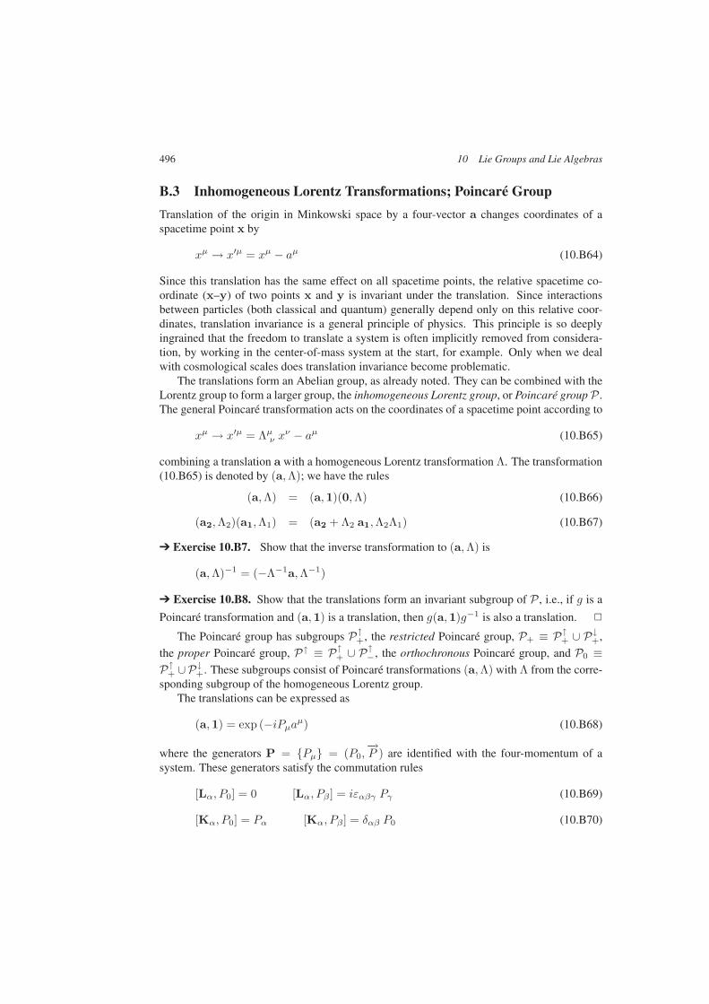
496 10 Lie Groups and Lie Algebras
B.3 Inhomogeneous Lorentz Transformations; Poincaré Group
Translation of the origin in Minkowski space by a four-vector a changes coordinates of aspacetime point x by
xµ → x′µ = xµ − aµ (10.B64)
Since this translation has the same effect on all spacetime points, the relative spacetime co-ordinate (x–y) of two points x and y is invariant under the translation. Since interactionsbetween particles (both classical and quantum) generally depend only on this relative coor-dinates, translation invariance is a general principle of physics. This principle is so deeplyingrained that the freedom to translate a system is often implicitly removed from considera-tion, by working in the center-of-mass system at the start, for example. Only when we dealwith cosmological scales does translation invariance become problematic.
The translations form an Abelian group, as already noted. They can be combined with theLorentz group to form a larger group, the inhomogeneous Lorentz group, or Poincaré group P .The general Poincaré transformation acts on the coordinates of a spacetime point according to
xµ → x′µ = Λµν xν − aµ (10.B65)
combining a translation a with a homogeneous Lorentz transformation Λ. The transformation(10.B65) is denoted by (a,Λ); we have the rules
(a,Λ) = (a,1)(0,Λ) (10.B66)
(a2,Λ2)(a1,Λ1) = (a2 + Λ2 a1,Λ2Λ1) (10.B67)
Exercise 10.B7. Show that the inverse transformation to (a,Λ) is
(a,Λ)−1 = (−Λ−1a,Λ−1)
Exercise 10.B8. Show that the translations form an invariant subgroup of P , i.e., if g is a
Poincaré transformation and (a,1) is a translation, then g(a,1)g−1 is also a translation.
The Poincaré group has subgroups P↑+, the restricted Poincaré group, P+ ≡ P↑
+ ∪ P↓+,
the proper Poincaré group, P↑ ≡ P↑+ ∪ P↑
−, the orthochronous Poincaré group, and P0 ≡P↑
+ ∪P↓+. These subgroups consist of Poincaré transformations (a,Λ) with Λ from the corre-
sponding subgroup of the homogeneous Lorentz group.The translations can be expressed as
(a,1) = exp (−iPµaµ) (10.B68)
where the generators P = Pµ = (P0,−→P ) are identified with the four-momentum of a
system. These generators satisfy the commutation rules
[Lα, P0] = 0 [Lα, Pβ] = iεαβγ Pγ (10.B69)
[Kα, P0] = Pα [Kα, Pβ] = δαβ P0 (10.B70)
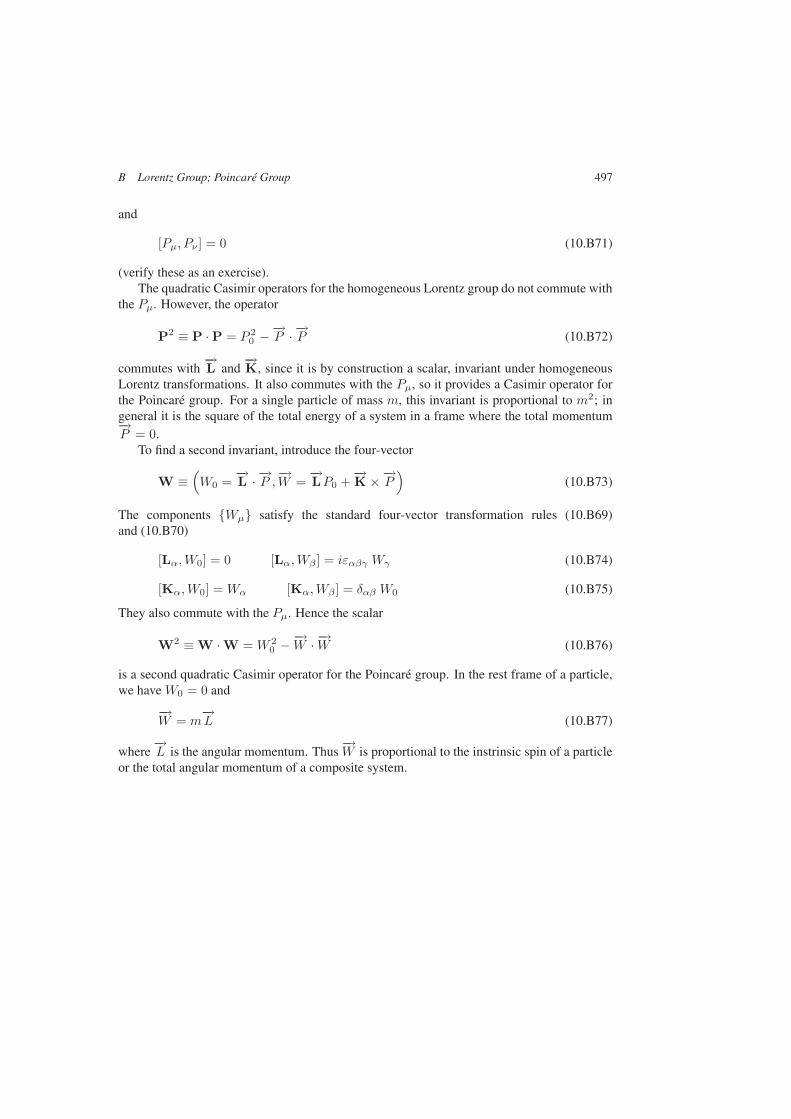
B Lorentz Group; Poincaré Group 497
and
[Pµ, Pν ] = 0 (10.B71)
(verify these as an exercise).The quadratic Casimir operators for the homogeneous Lorentz group do not commute with
the Pµ. However, the operator
P2 ≡ P · P = P 20 −−→
P · −→P (10.B72)
commutes with−→L and
−→K, since it is by construction a scalar, invariant under homogeneous
Lorentz transformations. It also commutes with the Pµ, so it provides a Casimir operator forthe Poincaré group. For a single particle of mass m, this invariant is proportional to m2; ingeneral it is the square of the total energy of a system in a frame where the total momentum−→P = 0.
To find a second invariant, introduce the four-vector
W ≡(W0 =
−→L · −→P ,−→W =
−→LP0 +
−→K ×−→
P)
(10.B73)
The components Wµ satisfy the standard four-vector transformation rules (10.B69)and (10.B70)
[Lα,W0] = 0 [Lα,Wβ ] = iεαβγ Wγ (10.B74)
[Kα,W0] = Wα [Kα,Wβ ] = δαβ W0 (10.B75)
They also commute with the Pµ. Hence the scalar
W2 ≡ W · W = W 20 −−→
W · −→W (10.B76)
is a second quadratic Casimir operator for the Poincaré group. In the rest frame of a particle,we have W0 = 0 and
−→W = m
−→L (10.B77)
where−→L is the angular momentum. Thus
−→W is proportional to the instrinsic spin of a particle
or the total angular momentum of a composite system.

498 10 Lie Groups and Lie Algebras
Bibliography and Notes
Three classic books on the angular momentum algebra and the coupling schemes for additionof angular momenta in atomic and nuclear physics are
A. R. Edmonds, Angular Momentum in Quantum Mechanics (2nd edition), Prince-ton University Press (1960, reissued 1996),
Morris E. Rose, Elementary Theory of Angular Momentum, Wiley (1960), reprintedby Dover (1995),
D. M. Brink and G. R. Satchler, Angular Momentum (3rd edition), Oxford, Claren-don Press (1994).
These have more detail than the book by Tinkham cited in Chapter 9.An unsurpassed pedagogical introduction to Lie algebras and the use of ladder operators
in constructing their representations is
Harry J. Lipkin, Lie Groups for Pedestrians (2nd edition), North-Holland (1966),reprinted by Dover (2002).
Two useful books that cover the classical Lie groups and algebras in physics contexts are
Brian G. Wybourne, Symmetry Principles and Atomic Spectroscopy, Wiley (1970),
Brian G. Wybourne, Classical Groups for Physicists, Wiley (1974).
The first of these has a long description of the properties of the symmetric group and therotational and unitary groups, together with a detailed discussion of the use of these groupsin the classification of atomic states. The second book has a detailed description of both theclassical Lie groups and the exceptional groups, at a somewhat more advanced mathematicallevel, with many applications to physics as of the early 1970s, including atomic and nuclearphysics, but with less emphasis on particle physics. There are also some useful examples ofnoncompact algebras, including the group theory underlying the full spectrum of the hydrogenatom.
A fairly elementary introduction that is focused on applications to particle physics is
Fl. Stancu, "Group Theory in Subnuclear Physics," Oxford University Press (1997).
An excellent review that goes into the more advanced details of working with arbitrary Liealgebras in a particle theory context is
Richard Slansky, Group Theory for Unified Model Building, Physics Reports 79(1981) 1–128.
A recent introduction to group theoretical methods in physics applications is
J. F. Cornwell, Group Theory in Physics: An Introduction, Academic Press (1997)
This is a short and updated version of the more extensive three-volume treatise
J. F. Cornwell, Group Theory in Physics (3 volumes), Academic Press (1984).
The third volume of this series contains an extensive treatment of supersymmetry, which is im-portant in modern particle theory, as well as having some applications in other fields—nucleartheory, for example, as well as some integrable models of interest in condensed matter physics.It also has an extended discussion of infinite-dimensional algebras, which are important bothin string theory and in the study of integrable systems.
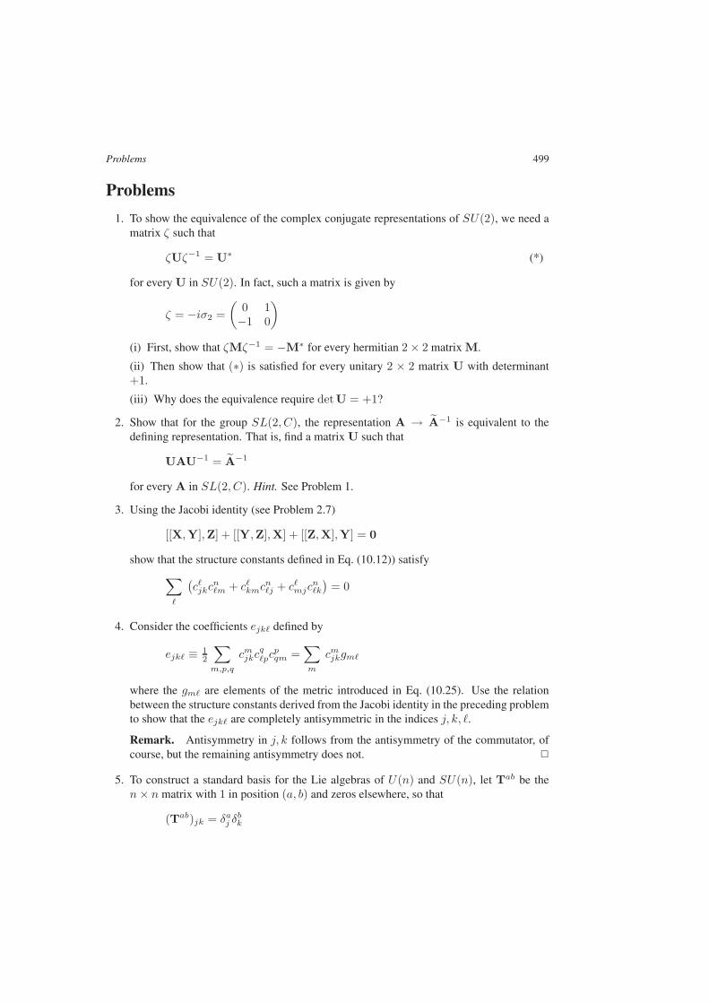
Problems 499
Problems
1. To show the equivalence of the complex conjugate representations of SU(2), we need amatrix ζ such that
ζUζ−1 = U∗ (*)
for every U in SU(2). In fact, such a matrix is given by
ζ = −iσ2 =(
0 1−1 0
)
(i) First, show that ζMζ−1 = −M∗ for every hermitian 2 × 2 matrix M.
(ii) Then show that (∗) is satisfied for every unitary 2 × 2 matrix U with determinant+1.
(iii) Why does the equivalence require detU = +1?
2. Show that for the group SL(2, C), the representation A → A−1 is equivalent to thedefining representation. That is, find a matrix U such that
UAU−1 = A−1
for every A in SL(2, C). Hint. See Problem 1.
3. Using the Jacobi identity (see Problem 2.7)
[[X,Y],Z] + [[Y,Z],X] + [[Z,X],Y] = 0
show that the structure constants defined in Eq. (10.12)) satisfy∑
(cjkc
nm + ckmc
nj + cmjc
nk
)= 0
4. Consider the coefficients ejk defined by
ejk ≡ 12
∑
m,p,q
cmjkcqpc
pqm =
∑
m
cmjkgm
where the gm are elements of the metric introduced in Eq. (10.25). Use the relationbetween the structure constants derived from the Jacobi identity in the preceding problemto show that the ejk are completely antisymmetric in the indices j, k, .
Remark. Antisymmetry in j, k follows from the antisymmetry of the commutator, ofcourse, but the remaining antisymmetry does not.
5. To construct a standard basis for the Lie algebras of U(n) and SU(n), let Tab be then× n matrix with 1 in position (a, b) and zeros elsewhere, so that
(Tab)jk = δaj δbk
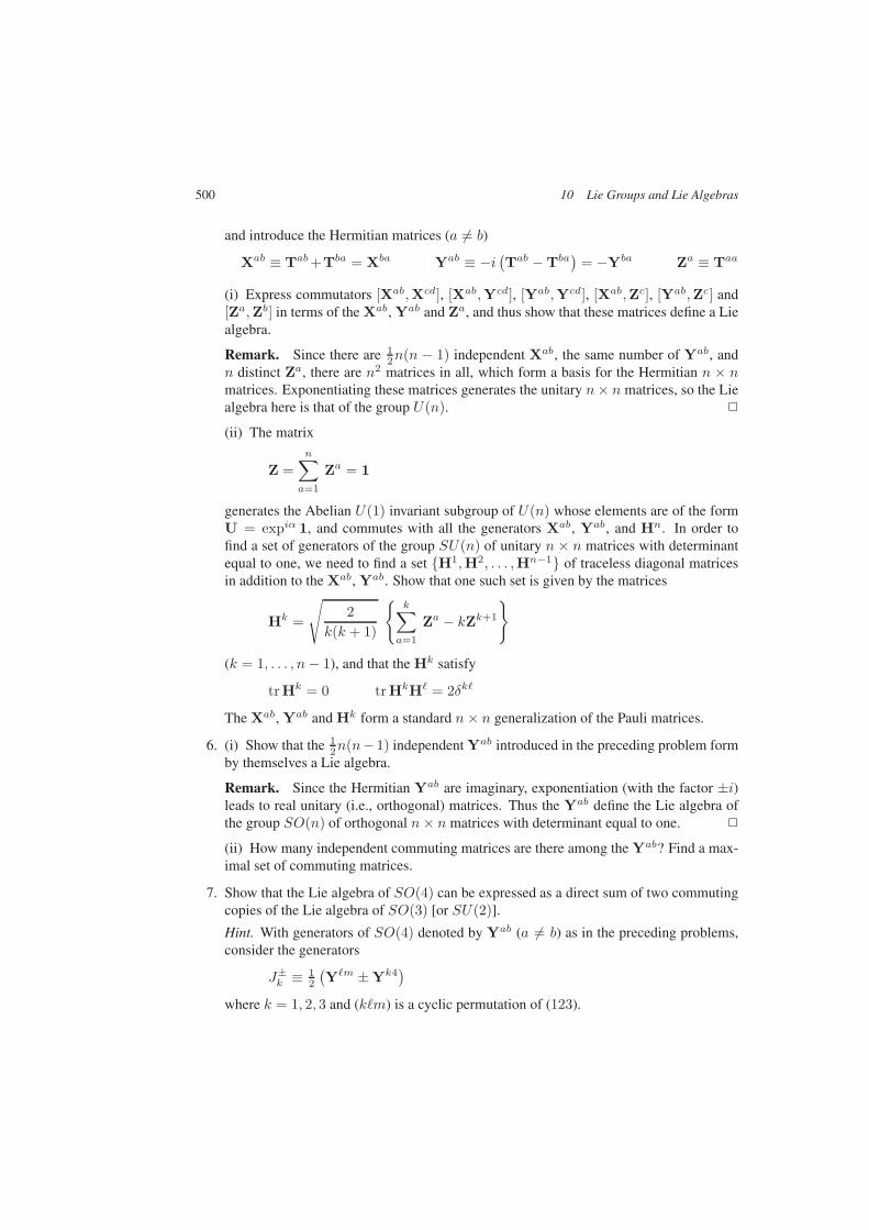
500 10 Lie Groups and Lie Algebras
and introduce the Hermitian matrices (a = b)
Xab ≡ Tab+Tba = Xba Yab ≡ −i(Tab − Tba
)= −Yba Za ≡ Taa
(i) Express commutators [Xab,Xcd], [Xab,Ycd], [Yab,Ycd], [Xab,Zc], [Yab,Zc] and[Za,Zb] in terms of the Xab, Yab and Za, and thus show that these matrices define a Liealgebra.
Remark. Since there are 12n(n − 1) independent Xab, the same number of Yab, and
n distinct Za, there are n2 matrices in all, which form a basis for the Hermitian n × nmatrices. Exponentiating these matrices generates the unitary n× n matrices, so the Liealgebra here is that of the group U(n).
(ii) The matrix
Z =n∑
a=1
Za = 1
generates the Abelian U(1) invariant subgroup of U(n) whose elements are of the formU = expiα 1, and commutes with all the generators Xab, Yab, and Hn. In order tofind a set of generators of the group SU(n) of unitary n × n matrices with determinantequal to one, we need to find a set H1,H2, . . . ,Hn−1 of traceless diagonal matricesin addition to the Xab, Yab. Show that one such set is given by the matrices
Hk =
√2
k(k + 1)
k∑
a=1
Za − kZk+1
(k = 1, . . . , n− 1), and that the Hk satisfy
trHk = 0 trHkH = 2δk
The Xab, Yab and Hk form a standard n× n generalization of the Pauli matrices.
6. (i) Show that the 12n(n− 1) independent Yab introduced in the preceding problem form
by themselves a Lie algebra.
Remark. Since the Hermitian Yab are imaginary, exponentiation (with the factor ±i)leads to real unitary (i.e., orthogonal) matrices. Thus the Yab define the Lie algebra ofthe group SO(n) of orthogonal n× n matrices with determinant equal to one.
(ii) How many independent commuting matrices are there among the Yab? Find a max-imal set of commuting matrices.
7. Show that the Lie algebra of SO(4) can be expressed as a direct sum of two commutingcopies of the Lie algebra of SO(3) [or SU(2)].
Hint. With generators of SO(4) denoted by Yab (a = b) as in the preceding problems,consider the generators
J±k ≡ 1
2
(Ym ± Yk4
)
where k = 1, 2, 3 and (km) is a cyclic permutation of (123).
Problems 501
8. (i) How many independent generators are there for the group SU(4)? How many for thegroup SO(6)?
(ii) Use the results of Problems 5 and 6 to find explicit bases of generators for each ofthese groups.
(iii) Find an isomorphism between these two sets of generators.
Remark. This isomorphism between the Lie algebras of SU(4) and SO(6) is similarto the isomorphism between those of SU(2) and SO(3), but in each case the groups arenot exactly isomorphic because they have different discrete invariant subgroups.
(iv) Does this pattern of isomorphism persist? Is there an isomorphism between the Liealgebras of SU(6) and SO(9)?
9. Consider a particle of mass m moving in a potential
V (r) = − κ
r
The Runge–Lenz vector for the particle is defined by
A = p × L −mκrr
where L = r × p is the angular momentum. In quantum mechanics, r and p are repre-sented by operators that satisfy the canonical commutation relations
[rj , pk] = iδjk
(i) Show that L and A satisfy the commutation relations
[Lj ,Ak] = iεjkA
Remark. This commutation relation with L is actually satisfied by any vector A; it isone definition of a vector.
(ii) With Hamiltonian given by
H =p2
2m+ V (r)
show that
[H,A] = 0
Remark. Thus A is a constant of motion for this Hamiltonian.
(iii) Show that
[Aj ,Ak] = −2imHεjkL

502 10 Lie Groups and Lie Algebras
Remark. From this result it follows that on an eigenmanifold of H with energy E, theoperators
D ≡ A/√
2m |E|
together with the L define a Lie algebra.
(iv) Use the results of Problem 7 to show that for E < 0, the L and D together form aLie algebra of SO(4).
Remark.
Thus the energy levels of the hydrogen atom correspond to representations (irreducIble,in fact) of SO(4). For extra credit, describe these representations.
(v) What is the Lie algebra defined by the L and D for E > 0?
10. Let a†σ, aσ be the creation and annihilation operators for a spin-12 fermion in spin state σ
(σ = ±12 ), as introduced in Problem 7.8. The spin operators for the fermion are
−→S ≡ 1
2
∑
α,β
a†ασαβaβ
(i) Show that the Sk are generators of SU(2) [see Eq. (10.14)].
(ii) Show that the fermion number operator
N =∑
σ
a†σaσ
commutes with the Sk.
11. Introduce fermion pairing operators
B† ≡ 12
∑
α,β
a†αζαβa†β = a†↑a
†↓
B ≡ 12
∑
α,β
aβζαβaα = a†↓a†↑
where ζ = iσ2 has been introduced in Problem 1 (in some contexts, ζ serves as a spinormetric). B† creates a pair of fermions, one with spin up and one with spin down, in thesame mode, while B annihilates a pair.
(i) Show that the fermion number operator
N =∑
σ
a†σaσ
satisfies the commutation rules
[N,B†] = 2B† [N,B] = −2B
Problems 503
(ii) Show that
[B†,B] = N− 1 ≡ 2B3
so that the operators B†, B and B3 generate an SU(2) group (the pairing group).
(iii) Show that this SU(2) pairing algebra commutes with the SU(2) spin algebra justintroduced in Problem 10, so the two algebras can be combined to form an SO(4) Liealgebra.
12. We want to consider the group of 2N × 2N matrices that define linear transformationsof the coordinates q1, . . . , qN and momenta p1, . . . , pN such that the canonical 2-form
ω ≡N∑
k=1
dpk ∧ dqk
is invariant. Such matrices are symplectic matrices, and the corresponding group is thesymplectic group Sp(2N).
(i) For N = 1, use your detailed knowledge of the properties of 2× 2 matrices to give acomplete characterization of Sp(2). Find the subgroups of Sp(2) for which the matricesare (a) orthogonal and (b) unitary.
(ii) For N = 2, try to construct a set of generators of the group Sp(4) (such a set wouldcorrespond to the angular momenta that generate the group of rotation matrices). Notethat symplectic matrices A must satisfy
AT ζA = ζ
where AT is the transpose of A and ζ is the symplectic metric defined by
ζ ≡
0 1 0 0−1 0 0 00 0 0 10 0 −1 0
Find also the generators of the subgroups of Sp(4) for which the matrices are (a) orthog-onal and (b) unitary.
Remark.
Having done the construction for N = 2, you might want to extend it to arbitrary N , butthat is not needed here.
13. Consider a spin-12 particle with orbital angular momentum (the case = 1 was dis-
cussed in Example 10.15). The total angular momentum j of the particle can be ± 12 .
Derive general formulas for the states |j m〉 in terms of the states |m ms〉.
14. Consider the addition of angular momenta j1 = 32 and j2 = 1. Construct the eigenstates
|j m〉 of J · J and J3 in terms of the eigenstates |m1 m2〉 of J(1)3 and J(2)
3 .
Note. In Example 10.16, we gave a direct method to compute the state | 1212 〉. Now we
want all the eigenstates |j m〉.
504 10 Lie Groups and Lie Algebras
15. The interaction between an electron and a nucleus has a relatively small term that can beexpressed as
Hint = aL · S
where L is the orbital angular momentum operator, S the spin, and a is a constant that canbe evaluated with some precision. Show that states of definite total angular momentumj (such as those constructed in Problem 13 are also eigenstates of Hint, and find theeigenvalues of Hint in terms of l, s, j (here we do not require s = 1
2 ).
Remark. Hint is the fine structure Hamiltonian, responsible for splitting atomic energylevels that are degenerate when only the classical Coulomb interaction is considered.
16. Consider the addition of angular momentum for two particles each with j = 1.
(i) What are the allowed values of the total angular momentum J of the two particles?
(ii) Which of these values correspond to symmetric states? antisymmetric states?
Now consider three j = 1 particles.
(iii) What are the allowed values of the total angular momentum J of the three particles,and how many independent states are there for each J?
(iv) Classify the states into irreducible representations of S3.
17. Consider the addition of angular momentum of j = 32 particles.
(i) What are the allowed values of the total angular momentum J of two particles?Which of these values correspond to symmetric (antisymmetric) states?
(ii) What are the allowed values of the total angular momentum J of three particles?Classify these states into irreducible representations of S3. What value(s) of J corre-spond to antisymmetric states?
(iii) What are the allowed values of the total angular momentum J of four particles?Classify these states into irreducible representations of S4. What value(s) of J corre-spond to antisymmetric states?
18. Consider the linear operators Au, Ad, As, Au, Ad, As such that
[Aa, Ab] = δab
(a, b = u, d, s) and introduce the operators
T+ ≡ AuAd , U+ ≡ AdAs , V+ ≡ AuAs
T− ≡ AdAu , U− ≡ AsAd , V− ≡ As Au
as well as
T3 ≡ 12
(AuAu − AdAd
)
Y ≡ 13
(AuAu + AdAd − 2AsAs
)
Problems 505
(i) Show that these eight operators define a Lie algebra, and that T3 and Y can be si-multaneously diagonalized.
(ii) Indicate graphically the effects of the operators T±, U± and V on the eigenvaluesof T3 and Y.
(iii) Show that each of the eight operators commutes with the operator
N ≡ AuAu + AdAd + AsAs
so that subspaces corresponding to definite eigenvalues N of N = Nu + Nd + Ns areinvariant under the Lie algebra. What further subspaces are invariant? (For definiteness,discuss the cases of N = 2 and N = 3.)
(iv) Express the operators introduced in part (i) in terms of the standard generators ofSU(3) introduced in Eq. (10.20).
Remark. This explicit formulation of the SU(3) Lie algebra works just as well if theoperators Aa and Aa satisfy anticommutation rules
Aa, Ab = AaAb + AbAa = δab
(show this). These operators can be visualized as creation and annihilation operators forquarks, and the picture can be extended to describe SU(n) for any value of n.
19. There are eight spin- 12 baryons, including the proton and neutron, that form an octet
under the old flavor SU(3) approximate symmetry of the strong interactions. Draw theweight diagram of the octet (see Fig. 10.3) and label the weights with the symbols for thebaryons.
20. Consider an octet state of three spin-12 quarks u, d, s. Both spin and flavor states have
mixed symmetry under permutations of the three quarks, so the combined spin-flavorstates can be symmetric, antisymmetric or mixed symmetry (see Example 9.48). Thesestates can be denoted by |s j3;T3 Y 〉, where α = S,A, (j12) characterizes the symmetrytype of the product function (j12 identifies a basis vector in the mixed representation).
(i) Construct both symmetric and antisymmetric product states for j3 = 12 in terms of
the basic quark states (see Problem 9.19).
(ii) Suppose the magnetic moment operator µ for quarks is
µ =(
23 + Y
) [( 12 + T3)µu + ( 1
2 − T3)µd]+(
13 − Y
)µsσ
where µu,d,s denote the quark magnetic moments. Compute the magnetic moment matrixelements
〈|α 12 ; (T ) T3 Y | µ3 |α 1
2 ; (T ) T3 Y 〉
between the octet states for possibilities α = S,A.
Remark. The actual baryon magnetic moments can be explained very well if the prod-uct wave function is symmetric. By comparison, the magnetic moments of the nuclei 3H

506 10 Lie Groups and Lie Algebras
and 3He are very close to the values obtained for the antisymmetric wave function withµu and µd replaced by measured proton and neutron magnetic moments. The observedbaryon moments provided another piece of evidence for the existence of an SU(3) colordegree of freedom; as already noted, this allows an antisymmetric singlet color wavefunction to provide the antisymmetry required by the Pauli principle.
21. Compute the dimensions of irreducible representations of SU(4) associated with thepartitions (212) and (22).
22. (i) Find the conjugate representations to the irreducible representations of SU(6) corre-sponding to each of the partitions (2), (12), (3), (21), (13), and (214). Which represen-tations are self-conjugate?
(ii) Find the dimension of each of these irreducible representations.
23. Show that the irreducible representation of SL(n,C) dual to Γ(m1 m2 · · ·mn−1) isΓ(m1 m1 −mn−1 · · · m1 −m2).
24. Consider the behavior of Maxwell’s equations (3.141), (3.142), (3.145), (3.148) underthe Lorentz transformation (10.B21). Find the transformation laws for the electric andmagnetic fields needed for the equations to be invariant under the transformation.
Remark. One hint is to look at the four-vector potential Aµ = (φ,−→A ) as a one-form,
and the electromagnetic field as a two-form F = dA or, with explicit components,
Fµν =∂Aν∂xµ
− ∂Aµ∂xν
The transformation laws for the two-form follow directly from the Lorentz transforma-tion (10.B21).
25. Show that the generators of SL(2, R) introduced in Eq. (10.31), with commutators givenby Eq. (10.32), are suitable generators for the homogeneous Lorentz transformations intwo space dimensions (+time). In particular, J3 generates rotations in the plane, whileK1 and K2 generate transformations to coordinate frames moving with constant velocityin the plane. Show further that the quadratic Casimir operator
C2 = J23 − K2
1 − K22
actually commutes with all three generators.
26. (i) Show that a boost commutes with a rotation about the boost axis.
(ii) Show that a symmetric Lorentz transformation is a boost, possibly accompanied bya rotation through a multiple of π about the boost axis (see also Problem 2.15).
27. Use the fact that the operators−→M and
−→N defined in Appendix B are angular momentum
operators to construct two quadratic Casimir operators for the homogeneous Lorentzgroup in terms of the generators
−→L and
−→K.
Index
AN , see alternating groupAbelian
group, 4, 393Lie algebra, 465
action integral, 142, 384action-angle variables, 148, 164adjoint operator, 56
matrix elements of, 56algebra, 397
associative, 398commutative, 398exterior, 119Fundamental Theorem of, 185Heisenberg, 346Jordan, 398Lie, see Lie algebraof a group, 398operator, 397quaternion, 452
almost everywhere, 265, 272alternant, 402, 437alternating group, 402
A4, 416, 420, 421, 423character table, 416
alternating series, see series, alternatingAmpère’s Law, 127amplitude
Jacobi elliptic function, 252of oscillator, 142
analytic continuation, 179, 181of geometric series, 181uniqueness of, 181
analytic function, 179–190entire, 184meromorphic, 185natural boundary of, 182power series expansion, 180
regular part, 187singular part, 187singular point of, 182
branch point, 173, 183essential singularity, 182pole, 182
singularityresidue at, 187, 190
angular momentum, 87, 144and SU(2), 470in quantum mechanics, 470
addition of, 471–473, 503–504annihilation operator, 347
fermion, 347fermion pair, 502
anticommutator, 55of λA, 464
antikink solution, 382antilinear, 51associative law, 3, 393
vector space, 41asymptotic series, 19–25, 34, 35
Laplace’s method, 23–24, 35atlas, 98attractor, see fixed point, stableautocorrelation function, 285
Bn, 99, 103volume of, 209
balln-dimensional, see Bn
baryonas three-quark state, 481, 505decuplet
in flavor SU(3), 481octet
in flavor SU(3), 479, 505
Introduction to Mathematical Physics. Michael T. VaughnCopyright c© 2007 WILEY-VCH Verlag GmbH & Co. KGaA, WeinheimISBN: 978-3-527-40627-2
Introduction to Mathematical Physics
Michael T. Vaughn 2007 WILEY-VCH Verlag GmbH & Co.
508 Index
basischange of, 57, 105coordinate, 105, 107dual, 50, 107of a linear vector space, 42, 57orthogonal, 44overcomplete, 84
benzene ring, 452Bernoulli
equation, 217numbers, 202, 210
Bernoulli’s principle, 150Bessel function, 237–240
and confluent hypergeometric function,237
asymptotic behavior, 239generating function, 238integral representation, 238, 258modified, 24, 35of first kind, 237of second kind, 238of third kind, 239
asymptotic behavior, 239order of, 237orthogonality relation, 317recursion relation, 238spherical, 240, 317, 365
differential equation, 240integral representation, 258orthogonality relation, 317
Bessel’s equation, 237Laplace transform of, 314
Bessel’s inequality, 44B-function, 203
infinite series, 203integral representation, 203
beta function, see B-functionbifurcation, 28bilinear, 43
concomitant, 336transformation, 172
Bloch’s theorem, 197Bohr radius, 374Boltzmann factor, 33, 35Bolzano-Weierstrass theorem, 7boost, 489, 506
matrix elements, 492boson, 347bound
of functional, 49of linear operator, 53
boundary conditions, 336, 359and Laplacian, 359Dirichlet, 359mixed, 359Neumann, 359periodic, 337, 387self-adjoint, 342, 350
branchcut, 173, 184point, 173, 183, 184
Brillouin zone, 431bundle
cotangent, 108fiber, 106structure group of, 106tangent, 106vector, 106
Cn, 46calculus of variations, 152–153canonical 2-form, 145canonical momentum, see conjugate momen-
tumCantor set, 271Casimir operator, 466
E(2), 467Lorentz group, 506Poincaré group, 497SL(2, R), 467, 506SU(2), 466SU(3), 466
Cauchyintegral formula, 178residue theorem, 191sequence, 5
in Hilbert space, 265of vectors, 49
Cauchy’s theorem, 177, 190Cauchy–Riemann conditions, 169, 177Cayley transform, 76center
of SU(2), 463of group, 396, 397
change of basisactive point of view, 59passive point of view, 59
chaos, 28
Index 509
charactergroup, 418of SO(2), 409of SO(3), 409of group representation, 408table
A4, 416D4, 415for finite group, 415S4, 444
characteristicequation, 64function, 294of PDE, 356, 377polynomial, 64, 72, 74
charge, 126density, 126topological, 382
chart, 98Chebysheff polynomials, 316Christoffel symbols, 136, 137
of first kind, 136of second kind, 136on S2, 137
class (of group), see group, classClebsch-Gordan coefficient, 471
Condon-Shortley convention, 473closed
extension, 324form, 128interval, 7linear manifold
in Hilbert space, 265linear operator
on Hilbert space, 324manifold, 102set, 7vector space, 264
coherent state, 347commutative law, 3
vector space, 41commutator, 55, 112, 114, 462compact
Lie algebra, 466linear operator, 326, 339
self-adjoint, 330manifold, 102support, 303
compactification
one-point, 100of Rn, 100, 103
comparison test, 10complete orthonormal system, 45
in Hilbert space, 265complex
plane, 5, 99unit circle, 9
structure on torus, 197variable, 169
componentscontravariant, 108covariant, 108of a form, 107
transformation law, 107of a tensor, 109of a vector, 42, 104
transformation law, 105compressibility, 157configuration space, 100confluent hypergeometric
equation, 246–248, 350, 375and Coulomb wave functions, 375Laplace transform of, 286polynomial solutions, 289
function, 246, 259and Bessel function, 237integral representation, 247of third kind, 248recursion formulas, 259
series, 246conformal mapping, see map, conformalconjugate
group elements, 395representation, 407, 417, 485subgroups, 396
conjugate momentum, 143, 144in field theory, 384
conjugate partition, see partition, conjugateconservation
of electric charge, 126of energy, 150of mass, 126of matter, 149
constantEuler–Mascheroni, 201Euler-Mascheroni, 19, 34Feigenbaum, 29fine structure, 374
510 Index
of motion, 144Planck, 32, 35, 207, 288, 373, 431, 470Stefan–Boltzmann, 207
contourfor Green function
for wave equation, 369integral, 176
evaluation of real integrals, 191independence of path, 176
keyhole, 193, 194, 209, 210contraction, see tensor, contraction ofcontravariant, 108convergence
absolute, 8conditional, 8, 11in the mean, 270of infinite product, 13of infinite series, 8of sequence, 6
in Hilbert space, 267of linear operators, 75of vectors, 49
pointwise, 14, 276strong, 75, 329uniform, 14, 75, 329weak, 15, 75, 267, 329
convolutionintegral, 284theorem, 284
coordinateatlas, 98basis, 57, 105, 107, 109chart, 98cyclic, 144patch, 97transformation, 98, 159
coordinates, 974-d spherical, 161Cartesian, 132cylindrical, 135generalized, 142oblate spheroidal, 160of a vector, 57on a manifold, 97parabolic, 161polar, 113, 132prolate spheroidal, 160, 163spherical, see spherical coordinates
correlation function, 285
coset, see group, cosetcotangent
bundle, 107, 108space, 107
Coulomb potential, 160, 308, 361, 373in quantum mechanics, 373, 389multipole expansion, 361
covariant, 108creation operator, 347
boson, 347fermion, 347fermion pair, 502
current, 126density, 126displacement, 127
curvature, 132curve
geodesic, 135in a manifold, 104integral, 110
cylinder function, see Bessel function
de Moivre’s formula, 174deficiency index, 329degree of freedom, 100delta-function, see Dirac δ-functionderivative
co-moving, 115directional, 104, 114, 120exterior, 120interior, 122Lie, see Lie derivative
Derrick’s theorem, 381diffeomorphism, 102, 159differential equations
ordinary, see ODEpartial, see PDE
differential form, 107closed, 128exact, 128
differential operator, 336adjoint, 338and boundary conditions, 336boundary term, 336, 338Green function for, 341, 350linear, 336
second order, 338diffusion equation, 366, 367dihedral group, see group, dihedral
Index 511
dimensionof linear vector space, 42of manifold, 98
Diracδ-function, 16bracket, 51quantization condition, 129
Dirichletboundary condition, 359kernel, 275
dispersion relation, 357distance
Euclidean, 133geodesic, 135in linear vector space, 43
distribution, see functionaldistributive law, 4
vector space, 41divergence
of vector field, 122theorem, 125
domainof holomorphy, 182of linear operator, 51
on H, 321dual
basis, 50, 107Hodge-*, 119, 486representation, 407, 485space, 50tensor, 486, 487vector, 485
dynamical system, 26, 139as vector field, 140discrete, 139equations of motion, 139linear, 77–79
E(2), 467Casimir operator, 467
eigenmanifold, 64eigenvalue, 64, 321, 331
algebraic multiplicity, 64, 65, 67degenerate, 65geometric multiplicity, 64, 65, 67multiplicity, 64, 65, 67
eigenvalueslower bound, 71minimax properties, 71–74
upper bound, 71eigenvector, 64, 321
continuum, 362, 387of compact self-adjoint operator, 331
elliptic function, 197, 210, 249–253Jacobi, 249, 252–253order of, 198periods of, 251
elliptic integral, 249, 260analytic continuation of, 250complete, 260
of first kind, 249of second kind, 260
modulus, 260energy
potential, see potential energyenergy levels, see quantum mechanics, energy
levelsfine structure, 504in magnetic field, 470of H atom, 502
energy-momentum relationfreeparticle
nonrelativistic, 288enthalpy, 156entire function, 184ε-neighborhood, 7ε-tensor, 117, 118, 484, 486equation
Bessel, 237confluent hypergeometric, see confluent
hypergeometric equationdifferential, see differential equationhypergeometric, see hypergeometric
equationKlein–Gordon, see Klein–Gordon equa-
tionKortweg-deVries, see KdV equationLaplace, 151, 170Legendre, 231of continuity, 126, 127, 149, 376of motion
Hamilton, 143Lagrange, 142
of state, 100Ricatti, 218Schrödinger, see Schrödinger equation
equilibrium, see fixed pointerror function, 34
512 Index
essential singularity, 182Euclidean
group, 467Euler angles, 59, 87Euler’s equation, 150Euler–Lagrange equations, 136, 142, 153, 165Euler-Mascheroni constant γ, see constant,
Euler-Mascheronievent, 489everywhere dense, 7, 264exact
differential, 220form, 128
exclusion principle, see Pauli, principleexponential integral, 19exterior algebra, 119exterior derivative, see derivative, exteriorexterior product, see product, exterior
Faraday’s law, 127Feigenbaum constant, see constant, Feigen-
baumfermion, 347, 502
pairing operators, 502field, 4
1-form, 114electric, 110electromagnetic, 114
under Lorentz transformation, 506magnetic, 110, 125
of magnetic dipole, 125of monopole, 129
scalar, see scalar, field, 384vector, see vector fieldvelocity, 110, 149
fine structure, 504constant, 374
finite group, see group, finitefixed point, 26, 36, 79, 111
asymptotically stable, 79center, 141hyperbolic, 79of inversion, 171of linear fractional transformation, 172of linear transformation, 171of logistic map, 26stable, 26, 79stable manifold of, 79superstable, 27, 35
unstable, 26, 79unstable manifold of, 79
fluid mechanics, 148–151flux line, 110form
1-form, 107closed, 128differential, 107exact, 128p-form, 117volume, 119
four-vector, 489, 490and 2 × 2 matrix, 494electromagnetic potential, 506energy-momentum, 490, 496lightlike, 490spacelike, 490timelike, 490
Fouriercoefficients, 196, 274integral, 192, 281series, 273–280, 311
convergence, 275cosine, 279Gibbs phenomenon, 278real form, 274sine, 279
transform, 281, 312finite, 85, 313, 314in quantum mechanics, 288multidimensional, 287of ‘hat’ function, 318of convolution, 284of Haar functions, 300
Fourier series, 196in complex plane, 195–197
fraction, 4free energy, 155frequency
angular, 141, 357carrier, 294fundamental, 273, 281natural, 81
Frobeniusgenerating function, 446
for simple characters of SN , 424,438, 441
method for ODEs, 226reciprocity theorem, 422, 435–437
Index 513
functionanalytic, see analytic functionautocorrelation, 285characteristic, 294correlation, 285doubly periodic, 197, 251elliptic, see elliptic functionentire, 184Green, see Green functionmeasurable, 272of a complex variable
analytic, see analytic functiondifferentiable, 169holomorphic at a point, 169meromorphic, 185regular at a point, 169
of a linear operator, 89periodic, 195, 273quasi-periodic, 197rational, 185scaling, 297, 299spline, 302step, 272, 277weight
in scalar product, 268function space, 268
scalar product, 268weight function, 268
functional, 49, 152bounded, 49linear, 49on tangent space, 107
fundamentalfrequency, 273period, 195, 273
second, 197, 198representation
of SU(2), 474of SU(3), 477of classical Lie group, 482of group, 418
wavelet, 299, 301Fundamental Theorem
of algebra, 185of Hilbert Space, 334on finite group representations, 415on normal operators, 68
Γ-function, 22, 25, 199–202, 209
analytic continuation of, 200analytic properties, 200duplication formula, 201infinite product, 200infinite series, 200logarithmic derivative of, 201recursion formula, 200Stirling’s formula, 25Stirling’s series, 202
Gamma function, see Γ-functiongauge
invariance, 125, 129in quantum mechanics, 129
transformation, 125Gauss’ law, 126Gaussian integral, 367Gaussian pulse, 312Gegenbauer polynomials, 306, 316
and Jacobi polynomials, 307properties, 306
general linear group, 461generalized function, see functionalgenerating function
Bessel function, 238for π(N), 453for simple characters of SN , 424, 438,
441Frobenius, 424, 438, 441Legendre polynomials, 233, 257, 290
generatorof Lie group, 461of one-parameter subgroup, 461
generatorsof SU(3), 464
geodesic, 135equation, 137null, 138, 139on S2, 138, 162spacelike, 139timelike, 139
Gibbsfunction, 165phenomenon, 278
GL(n,C), 461, 482GL(n,R), 461, 482gradient, 114, 120Gram–Schmidt process, 289, 290Gram-Schmidt process, 45great circle, 138, 162
514 Index
Green function, 285, 335, 341, 350, 359–362advanced, 371causal, 371Coulomb potential, 361Feynman, 371, 388for damped oscillator, 285for Helmholtz equation, 371for Laplace’s equation, 360for wave equation, 369–371, 388retarded, 369, 388
group, 4A4, 416, 420, 421, 423Abelian, 4, 393additive, 393algebra, 398
of S3, 425alternating, see alternating groupaxioms, 393center, see center, of groupcentral extension, 397class, 395
inverse, 451multiplication, 451
coefficients of composition, 417continuous, 460coset, 395covering, 397cyclic, 394, 399
Zn, 394, 399Z, 394
dihedral, 394, 399D4, 415D6, 452
direct product, 395element
conjugate, 395order, 394self-conjugate, 395
Euclidean, 467extension, 397finite, 393, 399–400
character table of, 415GL(n,C), see GL(n,C)GL(n,R), see GL(n,R)homotopy, 103infinite
discrete, 431isomorphism, 394isotropy, 432
Lie, see Lie group‘little’, see isotropy groupLorentz, see Lorentz, groupO(n), see O(n)octahedral, 400, 453order, 393periodic, 394Poincaré, see Poincaré, groupquaternion, 452renormalization, 209representation, see group representationsimple, 396SL(2), see SL(2)SL(n,C), see SL(n,C)SL(n,R), see SL(n,R)SO(2), see SO(2)SO(3), see SO(3)SO(n), see SO(n)Sp(2n), see Sp(2n)SU(2), see SU(2)SU(3), see SU(3)SU(n), see SU(n)subgroup
conjugate, 396coset, 395index of, 395invariant, 396
symmetric, see symmetric groupsymplectic, 468tetrahedral, 400, 453translation, 460U(n), see U(n)Z, 393, 431
group representation, 406–423character, 408
compound, 408simple, 408
complex, 407complex conjugate, 407
and quantum mechanics, 407defining, 418dimension, 406dual, 407equivalent, 406faithful, 406fully reducible, 406fundamental, 418identity, 406induced by subgroup, 419, 422
Index 515
principal, 419irreducible, 406, 413Kronecker product, 417of finite group
Fundamental Theorem, 415of subgroup
subduced, 422orthogonality relations, 412outer product, 423permutation, 413, 418
induced by subgroup, 419pseudoreal, 407real, 407reducible, 406regular, 413tensor product, 417unitary, 407
group velocity, 358
Haar functions, 294–295Fourier transform, 300
Hamilton’sequations of motion, 143principle, 142
Hamiltonian, 96, 143, 147, 164, 501and Poisson bracket, 164density, 384fine structure, 504for central potential, 143in quantum mechanics, 39, 40, 71, 351,
366, 373, 388energy levels, 71for H atom, 373harmonic oscillator, 351
spectrumfor H atom, 375
system, 100, 108, 143–148Hankel function, 239
and Whittaker function, 239asymptotic behavior, 239
harmonicseries, 9spherical, see spherical harmonics
harmonic oscillatorcoupled, 80damped, 77, 283
Green function for, 285forced, 283nonlinear, 164
one-dimensional, 142, 147quantum, 32, 309, 351
‘hat’ function, 317, 390heat capacity, 156heat equation, see diffusion equationHeaviside function, 277Heisenberg algebra, 346Helmholtz equation, 363, 371Hermite functions, 316, 351Hermite polynomials, 309, 316, 351Hermitian, see linear operator, Hermitianhighest weight
of representation of Lie algebra, 478Hilbert space, 264–268
axioms, 264closed, 264separable, 264, 265
compact self-adjoint operatorspectral representation, 330
complete orthonormal system in, 265convergence of sequences
of linear operators, 329of vectors, 267weak, 267
differential operatorand boundary conditions, 336
linear manifold, 265closed, 265
linear operator, 321–335adjoint, 327bound, 324bounded, 324closed, 324compact, 326, 330continuous, 324deficiency index, 329differential, 336domain, 321, 324essentially unitary, 329extension, 321, 328Hermitian, 328Hilbert–Schmidt norm, 326Hilbert–Schmidt type, 326inverse, 325invertible, 325isometric, 329maximal isometric, 329nonsingular, 325normal, 330
516 Index
of finite rank, 327operator norm, 324resolvent, 335self-adjoint, 328self-adjoint extension, 337separating, 331shift operator, 323, 345spectrum, see spectrumsymmetric, 328unitary, 329
self-adjoint operatorcompact, 330functions of, 335spectral representation, 331
holomorphic, 169holomorphy
domain of, 182homeomorphism, 102homomorphism, 397homotopy group, 103hook, 445
diagram, 445formula for dimension ofSN irreducible
representations, 446length, 445product, 445
hypercharge, 477hypergeometric
confluent, see confluent hypergeometricequation, 241–245, 350
polynomial solutions, 289function, 243, 258
and Legendre function, 234, 235integral representation, 244recursion formulas, 258
series, 242hypergeometric equation, 259
identity, 3image
of homomorphism, 397of linear operator, 52
incompressible flow, 148indicial equation
at regular singular point, 227inequality
Bessel, 44Schwarz, 44triangle, 43
infinite groupdiscrete, 431
infinite product, 13convergence of, 13representation
of Γ-function, 200of analytic functions, 188
infinite series, 8–13convergence of, 8convergence tests, 10–11of functions, 14–18
uniform convergence, 14weak convergence, 15
rearrangement of, 12infinity
in Rn, 100in complex plane, 171, 183in stereographic projection, 99
integralCauchy formula, 178contour, 176, 191–194curve, 110Lebesgue, 271, 272operator, 327, 339–341
adjoint, 340compact, 339degenerate, 352iterated kernel, 340kernel, 339separable, 352
test, 10interval, 7
closed, 7open, 7semi-closed, 7semi-open, 7
invariantmanifold, 61of vector field, 115Poincaré, 147subalgebra, 465subgroup, 396
maximal, 396minimal, 396quotient group, 396
tensor, 484ε-tensor, 484Kronecker delta, 487
topological, 103

Index 517
inverse, 3of linear operator
on Vn, 53on H, 325
permutation, 401inversion, 171island of stability, 28isometry, 47, 58isomorphism, 47
of groups, 394of vector spaces, 47
isospin, 477isotropy group, 432
Jacobi identity, 86, 464, 499Jacobi polynomials, 307
and Gegenbauer polynomials, 307and Legendre polynomials, 307properties, 307
Jacobian determinant, 105, 117, 118
KdV equation, 351, 358, 378–379conservation laws, 379
kernelof homomorphism, 397of integral operator, 339of linear operator, 52
kink solution, 382Klein–Gordon equation, 366, 380, 389
in one space dimension, 380Lagrangian for, 380
Kronecker delta, 487Kronecker product, see tensor product
L2(Ω), 2722(C), 264p, 43ladder operator, 347, 469, 476
for SU(3), 476, 477Lagrange’s theorem, 395Lagrangian, 142
density, 384field theory, 384–385for Klein–Gordon equation, 380, 385for wave equation, 384system, 142–143
Laguerre polynomials, 308, 316associated, 314, 375
Laplace
integraland asymptotic series, 23for Legendre polynomials, 233
operator, see Laplaciantransform, 263, 286, 314
of confluent hypergeometric equation,286
Laplace’s equation, 151, 170, 359Green function for, 360on a sphere, 292separation of variables, 363
Laplace’s method, see asymptotic seriesLaplacian, 134–135, 292, 359
and boundary condtions, 387in cartesian coordinates, 364in cylindrical coordinates, 135, 388in spherical coordinates, 135, 292, 365
lattice, 86, 431dual, 86reciprocal, 86translation, 431
Laurent series, 186–187singular part of, 190
Lebesgue integral, 271, 272Legendre function, 234–236
and hypergeometric function, 234associated, 291
differential equation, 291normalization, 291orthogonality, 291
of first kind, 234of second kind, 235, 236, 257, 258
Legendre polynomials, 231, 257, 290and Jacobi polynomials, 307generating function, 233, 257, 290, 315Laplace integral, 233normalization, 290orthogonality, 290recursion relations, 234, 290Rodrigues’ formula, 232Schläfli integral, 233
Legendre’s equation, 231, 232, 234and hypergeometric equation, 234associated Legendre functions, 291
Leibniz rule, 115Levi-Civita symbol, see ε-tensorLevinson’s theorem, 191Lie algebra, 87, 398, 462–470
Abelian, 465
518 Index
Cartan subalgebra, 467classical, 482classification of, 465–468compact, 466E(2), 467exceptional, 468exponentiation of, 463metric tensor, 466noncompact, 466, 467of a Lie group, 462of rotations in three dimensions, 87rank, 467representation, 463, 469
adjoint, 480irreducible, 463reducible, 463tensor, see tensor, representationweight diagram, 477
root vectors, 476roots, 469, 476semisimple, 465simple, 465SL(2, R), see SL(2, R)SO(n), see SO(n)structure constants, 462SU(2), see SU(2)SU(3), see SU(3)SU(n), see SU(n)subalgebra, 465
invariant, 465U(n), see U(n)
Lie bracket, 113Lie derivative, 104, 122
of vector field, 114Lie group, 460–461
Abelian, 460classical, 482
fundamental representation, 482general linear, 461generator, 461Lie algebra of, 462orthogonal, 461special linear, 461structure constants, 462subgroup
one-parameter, 461symplectic, 461unitary, 461
limit point, 7
linear independence, 41, 223linear manifold, see manifold, linearlinear operator, 51–70
adjoint, 56, 327anticommutator, 55bound, 324bounded, 53, 324Cartesian decomposition, 91characteristic polynomial, 64commutator, 55, 462diagonalizable, 65differential, 221, 336domain, 51, 321, 324eigenmanifold, 64eigenprojectors, 69eigenvalues, 64eigenvectors, 64functions of, 75Hermitian, 57, 328idempotent, 63image, 52integral, 327, 339invariant manifold, 61inverse, 53, 325isometric, 329kernel, 52matrix representation, 54multiplication of, 54negative definite, 70nilpotent, 62non-singular, 52
on Vn, 38nonsingular, 325normal, 68, 330
spectral representation, 67–70null space, 52of finite rank, 327on Hilbert space, see Hilbert space, lin-
ear operatororthogonal, 58polar decomposition, 91positive definite, 70range, 52rank, 52restriction, 61self-adjoint, 57, 328semi-definite, 70sequences of, 75shift, 323, 345

Index 519
singular, 52spectral representation, 331spectrum, 64–70, 330Sturm-Liouville, 339trace, 58unitary, 58, 329
linear vector space, 41–51basis of, 42, 84change of basis in, 57dimension of, 42direct sum, 47distance, 43infinite-dimensional, see Hilbert spacepolynomials, 84tensor product, 48unitary, 43
Liouville’s theorem, 147Lipschitz condition, 111‘little’ group, 432logarithmic derivative, 187, 191
of Γ-function, 201poles of, 187, 191
residue at, 187logistic map, 26, 28, 35Lorentz
group, 468, 491and SL(2, C), 493–495and SO(3, 1), 492homogeneous, 491inhomogeneous, 496–497orthochronous, 491proper, 491restricted, 491
invariance, 489transformation, 467, 489, 491
and SL(2, C), 482boost, 489in 2-d and SL(2, R), 506in one space dimension, 382in two dimensions, 467law, 489pure, see boostrestricted, 491
Lotka-Volterra model, 140–141, 162lower bound, 6
greatest, 6to eigenvalues, 71
magnetic
dipole, 125field, see field, magneticflux, 125moment, 505
of baryons, 505monopole, 129quantum number, 470
magnitude, 5manifold, 97–103
analytic, 98closed, 102closure of, 102compact, 102complex, 98coordinates in, 98differentiable, 97, 98invariant, 61linear, 42orientable, 119product, 101Riemannian, 132stable, see fixed pointsymplectic, 146unstable, see fixed point
mapconformal, 170, 171, 205iterated, 27logistic, see logistic map
mass, 490matrix
adjoint, 56diagonal, 65Jordan canonical form, 67orthogonal, 88Pauli, see Pauli, matricesrotation, 59, 61similarity transformation, 58symplectic, 503trace, 58
matrix elements, 54Maxwell relations, 155Maxwell’s equations, 126, 127, 489measure
of a set, 271measure theory, 271Mellin transform, 315meromorphic, 185metric tensor, 108, 130–134
and distance, 135

520 Index
and volume, 133Euclidean, 132for spinors, 502in spherical coordinates, 133induced, 133nondegenerate, 130of LIe algebra, 466SU(2), 466
of manifold, 132pseudo-Euclidean, 132signature, 130to raise and lower indices, 131vector space, 130
Minkowskimetric, 43, 130, 490space, 139, 489
Mittag–Leffler theorem, 190momentum
in quantum mechanics, 288, 334multiplicity
algebraic, 64, 65, 67geometric, 64, 65, 67of root, 185
multipole expansion, 361for Helmholtz equation, 372
multipole moment, 362multiresolution analysis, 297, 299
N -particle statesspin- 1
2particles, 474
natural frequency, see frequency, naturalneighborhood, 7, 97
ε-, 97Neumann function, 238
asymptotic behavior, 239nonlinear realization
of SL(2), 205norm, 43
vector, 43normal subgroup, see invariant subgroupnumber operator, 347numbers, 3–6
algebraic, 4complex, 4–6irrational, 6prime, 4rational, 4real, 3–4, 6transcendental, 6
O(n), 394, 461ODE, 213–230
and vector fields, 111, 213autonomous, 215factorizable, 219first order, 216–220
exact differential, 220linear, 216
linear, 215, 221–230nth order, 221constant coefficients, 92, 225first order, 216power series solutions, 222second order, 226Wronskian, 223
linear second order, 226–230and Ricatti equation, 219boundary conditions, 338confluence of singularities, 230, 247exponents at singular point, 226, 227indicial equation, 227irregular singular point, 226one regular singular point, 229regular point, 226regular singular point, 226second solution, 228singular point, 226three regular singular points, 241two regular singular points, 229
method of Frobenius, 226order, 213Ricatti equation, 218scale covariant, 215scale invariant, 215Sturm–Liouville equation, 226system of first order, 111, 213
one-parameter subgroup, 461generator of, 461
orbit, 433ordinary differential equations, see ODEorthogonal
complement, 48group, 461
special, 461matrix, 88polynomials, 289
weight function, 289zeroes of, 289
system, 44

Index 521
orthonormal system, 44complete, 45
oscillatoranharmonic, 259harmonic, see harmnic oscillator
outer productfor S3 ⊗ S3, 450for S4 ⊗ S4, 455for SU(2), 475of group representations, 423of representations of SN , 426
and Young diagrams, 426
P -symbol, see Riemann P -symbolpairing
group, 503operators, 502
Papperitz equation, 241parabolic coordinates, 389parity
of permutation, 401, 402Parseval’s theorem, 275partial differential equations, see PDEpartial sum, 8partition
conjugate, 405, 454dual, 506extended, 485of N , 404ordering of, 404self-conjugate, 405Young diagram of, 404
Paulimatrices, 55, 494SU(3) generalization, 463
principle, 347, 348, 481PDE
linear first order, 356method of characteristics, 356nonlinear, 376–383time-dependent, 366–372
period, 195doubling, 28fundamental, 195, 273
permutation, 401cycle, 402cycle structure, 424cyclic representation, 403degree of, 401
inverse, 401matrix, 402, 454parity, 401representation
of group, 413, 418perturbation, 345perturbation theory
classical, 164phase
of oscillator, 142space, 100, 108
phase velocity, 358π(N), 424, 437
classes of SN , 424generating function, 453partitions of N , 424
π2(C), 265Picard’s theorem, 184Planck radiation law, 207plasma frequency, 380Poincaré
1-form, 145group, 432, 468, 496–497
Casimir operator, 497orthochronous, 496proper, 496restricted, 496
invariant, 147lemma, 120, 128
Poisson bracket, 145, 164Poisson’s equation, 359, 360pole, 182
order of, 182residue at, 187
polynomial, 184root of, 184trigonometric, 273
polynomialsorthogonal, see orthogonal polynomials
potentialcentral, 143Coulomb, see Coulomb potentialelectromagnetic, 506electrostatic, see scalar potentialenergy, 80–82, 144, 389for scalar field, 380, 385gravitational, 150inverse square, 457retarded, 388
522 Index
vector, see vector potentialvelocity, 151
potential energy, 176, 259power series, 17–18, 180
circle of convergence, 17expansion of analytic function, 180radius of convergence, 17, 180solutions to linear ODEs, 222
predator-prey system, 140, 162primitive cell, 197probability amplitude, 288
momentum, 288position, 288
productexterior, 116Grassmann, 116infinite, see infinite productinterior, 122manifold, 101of linear operators, 54scalar, see scalar, productvector, 120wedge, 116
projectionoperator, 63orthogonal, 48stereographic, 99, 159
projector, see linear operator, projectionproper length, 139proper time, 139
quadrupole moment, 362quantum mechanics
angular momentum, see angular mo-mentum, in quantum mechanics
energy levels, 39, 71variational bounds, 71, 74
excited states, 74Fourier transform in, 288Hamiltonian, see Hamiltonian, in quan-
tum mechanicslinear operators in, 70momentum operator, 334, 336observables, 70Schrödinger equation, see Schrödinger
equationstates of a system, 70variational principle, 71
quarks
and flavor SU(3), 477quasi-momentum, 431quaternion, 452
R3, 102Rn, 46, 103range
of linear operator, 52rank
of Lie algebra, 467of linear operator, 52of tensor, 109of tensor representation of U(n), 483
ratio test, 10rational function, 185rearrangement, see permutationrenormalization group, 209representation
of group, see group representationof Lie algebra, see Lie algebra, repre-
sentationpermutation, see group representation,
permutationresidue
at singularity, 190resolution of the identity, 332–334, 373, 387,
389response function, see Green functionrest energy, 490Ricatti equation, 218
and second-order linear equation, 219Riemann ζ-function, 9, 206, 210Riemann P -symbol, 241Riemann surface, 173, 205, 208
n-sheeted, 174∞-sheeted, 175of ln(z), 174of n
√w, 174
of√w, 173
of inverse trigonometric functions, 175two-sheeted, 173, 206
Riemannian geometry, 132Riesz–Fischer theorem, 272ring, 4
commutative, 4Rodrigues’ formula
Legendre polynomials, 232root
multiplicity of, 185
Index 523
of SU(2), 476of SU(3), 476of analytic function, 185of characteristic polynomial, 64, 72, 225of Lie algebra, 469of polynomial, 184, 185
with real coefficients, 88test for convergence, 10vectors
of SU(3), 477of Lie algebra, 476
rotationin n dimensions, 89in complex plane, 171in three dimensions, 59, 86, 87
2 × 2 representation, 88axis of rotation, 87Lie algebra, 87
in two dimensions, 59Runge–Lenz vector, 501
S3, see symmetric group, S3
S4, see symmetric group, S4
S5, see symmetric group, S5
S6, see symmetric group, S6
S1, 98S2, 99, 103, 137Sn, 99, 103
volume of, 209SN , see symmetric groupS-function, see Schur functionscalar, 41
field, 102gradient of, 114
potential, 361product, 43, 130
scalar fieldkink solution, 382static solutions, 383
scalar potential, 108, 160Coulomb, 457electrostatic, 161, 359, 362, 387
Schrödinger equation, 288, 373–375for Coulomb potential, 373, 389time-dependent, 366, 373time-independent, 373
Schur function, 438Schur’s lemmas, 410–415Schwarz inequality, 44
self-adjoint, see linear operator, self-adjointsemi-group, 3separation of variables, 363–365
Laplace’s equation, 363sequence, 5
bounded, 5Cauchy, see Cauchy sequencechaotic, 28convergence of, 6logistic map, 26monotonic, 5, 6of functions, 14–16, 269
convergence, 269, 270uniform convergence, 14weak convergence, 15
of linear operators, 75strong convergence, 75uniform convergence, 75weak convergence, 75
of linear operators on Hconvergence, 329
of points in manifoldconvergence, 102
of vectors, 49series
alternating, 11arctangent, 18, 206asymptotic, see asymptotic seriesbinomial, 18confluent hypergeometric, 246exponential, 18Fourier, see Fourier seriesgeometric, 8
analytic continuation of, 181harmonic, 9hypergeometric, 242infinite, see infinite seriesLaurent, 187logarithmic, 18power, see power seriesRiemann ζ-function, 9
set, 7bounded, 7Cantor, 271closed, 7dense, 7measure of, 271of measure zero, 271open, 7
524 Index
shock wave, 377signal processing, 294sine-Gordon equation, 383singular point
at infinity, 183of analytic function, 182of ODE, see ODE, linear second orderof scalar field, 102of vector field, 111
sink, see fixed point, stableSL(2), 205
nonlinear realization of, 205SL(2, C), 493
and Lorentz group, 493–495SL(2, R), 467
and 2-d Lorentz transformation, 467,506
SL(2, C), 482, 499SL(n,C), 461, 482, 506SL(n,R), 461, 482small oscillations, 80–82SO(2), 394SO(3), 103, 394, 396
Lie algebra, 87SO(3, 1), 492
and Lorentz group, 492SO(4)
Lie algebra, 500SO(6), 501SO(n), 394, 461
irreducible representations, 487–488solitary wave, see solitonsoliton, 379source, see fixed point, unstableSp(2n), 461, 503Sp(4), 503space
cotangent, 107fiber, 106functionL2(Ω), 272
linear vector, 41reflection, 491state
thermodynamic, 153tangent, see tangent spacewavelet, 298
speciallinear group, 461
orthogonal group, 461unitary group, 461
spectral density, 285spectral representation
of compact self-adjoint operatoron H, 331
of normal operatoron Vn, 69
of self-adjoint operatoron H, 334
spectrum, 64continuous, 322, 332discrete, 332empty, 323of Laplacian, 363
cartesian coordinates, 364of linear operator
on Vn, 64on H, 323, 330–335
point, 332speed
of light, 130, 207, 374, 489of propagation, 356, 357, 366, 371
spheren-dimensional, see Sn
spherical coordinates, 99, 132, 143in four dimensions, 161volume element, 134
spherical harmonics, 292–293addition theorem for, 293, 361, 372
spin- 12
particle, 347, 473, 474, 502, 503creation and annihilation operators, 502N -particle states, 474pairing operators, 502
spin-orbit coupling, 504spinor, 493
conjugate, 493index
dotted, 493undotted, 493
metric, 502two-component, 493
spline function, 302state space
quantum mechanical, 70thermodynamic, 153
Stefan–Boltzmann law, 207step function, 272Stokes’ theorem, 123–127, 162
Index 525
in two dimensions, 125streamline, 110, 149stress tensor, 150structure constants
of SU(3), 464of Lie algebra, 462
Sturm–Liouvilleequation, 226operator, 339
and boundary conditions, 339SU(2), 102, 462, 499
and angular momentum, 470and rotations in three dimensions, 88Casimir operator, 466irreducible representations, 469–475
and Young diagrams, 475Lie algebra, 462pairing group, 503
SU(3)Casimir operator, 466color, 481flavor, 477
anti-quarks, 477baryon octet, 479, 481, 505diquarks, 478quarks, 477three-quark states, 479, 481
irreducible representations, 476–481dimension formula, 485
Lie algebra, 464, 504representation
conjugate fundamental, 477decuplet, 481fundamental, 477octet, 479
root vectors, 476roots, 476structure constants, 464tensor product
of irreducible representations, 480U -spin, 477, 479, 481V -spin, 477, 479, 481
SU(4), 501, 506SU(6), 506SU(n), 393, 461, 482
invariant tensor, 484Lie algebra, 499representation
conjugate fundamental, 482
irreducible tensor, 483tensor, 483
tensor productof irreducible representations, 483
summation convention (Einstein), 104, 483,490
symmetric group, 393, 401, 424–430and irreducible representations
of SU(2), 474of U(n) and SU(n), 484
charactersimple, 438
classes and cycle structure, 403irreducible representations, 424–430
and Young diagrams, 424–430antisymmetric, 407, 409outer products of, 426–428, 446–450symmetric, 407, 409tensor products of, 428–430
regular representation, 418S3, 402, 403, 407, 409, 418
mixed symmetry representation, 419tensor products in, 429Young symmetrizers, 425
S4
character table, 444irreducible representations, 454tensor products in, 429
S5
tensor products in, 455S6
tensor products in, 455simple characters, 438, 441
and Young diagrams, 442symplectic
group, 461matrix, 503metric, 461
T 2, 103T n, 101tangent
bundle, 106space, 105, 159vector, 104
tensor, 109components, 109contraction of, 110, 122dual, 109
526 Index
inertia, 109metric, see metric tensorrank of, 109representations
of SO(n), 487–488of U(n) and SU(n), 483–487
stress, 150tensor product, 48, 116
in S3, 429in S4, 429in S5, 455in S6, 455in SU(2), 471–473in SU(3), 478, 480in SN , 428
and Young diagrams, 429of group representations, 417, 483of vector spaces, 48
thermodynamics, 153–157time
inversion, 491reversal, 491
topological charge, 382torus, 101
n-dimensional, see T n
trace, 58, 110of linear operator, 326of Pauli matrices, 55
transformCayley, 76Fourier, see Fourier transformLaplace, see Laplace transformMellin, 315
transformationbilinear, 172canonical, 147exponential, 174gauge, 125inversion, 171linear, 171linear fractional, 172, 205
and SL(2), 172, 205Lorentz, see Lorentz, transformationof coordinates, 98orthogonal, 58powers and roots, 172reciprocal, 171rotation, 171scale, 171
similarity, 58symplectic, 147translation, 171unitary, 58
translation, 171, 496group, 460
transposition, 401triangle inequality, 43twin paradox, 163
U -spin, see SU(3), U -spinU(n), 393, 461, 463, 482
Lie algebra, 499representation
conjugate fundamental, 482irreducible tensor, 483tensor, 483
tensor productof irreducible representations, 483
unit circle, 9unitary
groupspecial, 461
operator, 58, 329vector space, 43
upper bound, 6least, 6to eigenvalues, 71
V -spin, see SU(3), V -spinvariational principle
in quantum mechanics, 71vector, 41
bundle, 106component, 42contravariant components, 108cotangent, 107covariant components, 108field, see vector fieldnorm, 43orthogonal, 44Runge-Lenz, 501space, see linear vector spacetangent, 104
vector coupling coefficient, see Clebsch-Gordan coefficient
vector field, 110and differential equations, 111curl of, 125
Index 527
divergence of, 122Hamiltonian, 144integral curves of, 110
vector potential, 125of magnetic dipole, 125of magnetic monopole, 129
velocitygroup, 358phase, 358
velocity potential, 151volume
of Bn, 209of Sn, 209
volume element, 119, 121from metric tensor, 133in spherical coordinates, 134
volume form, see volume elementvorticity, 151, 165
Watson’s lemma, 22wave equation, 366, 369–372
first order, 356characteristics, 356nonlinear, 376
Lagrangian for, 384second order, 369
wave packet, 358wavelet
basis, 301fundamental, 299, 301mother, 299scaling function, 297, 299space, 298
wavelets, 294–305Daubechies, 303with compact support, 303
wedge product, see product, wedgeWeierstrass
approximation theorem, 268, 269
factorization theorem, 189weight diagram
for 3 and 3∗ of SU(3), 478for 8 of SU(3), 480for representation
of Lie algebra, 477weight function, 289
and orthogonal polynomials, 289in scalar product, 268
Whittaker function, 248and Hankel function, 239
winding number, 103Wronskian determinant, 223, 257
Young diagram, 404and irreducible representations
of SU(2), 475of SU(3), 479of U(n) and SU(n), 484of SN , 424–430
and outer products in SN , 426, 446–450and tensor products in SN , 429associated Young tableaux, 405hook diagram of, 445normal application of nodes, 448of partition, 404regular application of nodes to, 443
Young symmetrizer, 424in S3, 425
Young tableau, 405ordering, 405Young symmetrizer for, 424
zero, 3mode, 81of analytic function, see rootvector, 41
ζ-function, see Riemann ζ-function
Related Documents