Introduction to Mathematical Modelling for Bioscientists Workshop 3 · Workshop 3 author: Kyle Wedgwood edited by: Daniel Galvis 24th July 2019 Today’s objectives In the third and

Introduction to Mathematical Modelling for Bioscientists

Workshop 3

author: Kyle Wedgwoodedited by: Daniel Galvis

24th July 2019

Today’s objectives

In the third and final session, we will cover:

• Phase plane analysis

• Bifurcation analysis

1 Mathematical model analysis

In the previous two sessions, we have learned how to write, develop, code and simulate mathematicalmodels. These are the general steps in applying the modelling framework to a given system. Ascomputing power is becoming ever greater, the kinds and sizes of biological system we can represent inthis way continue to grow. However, ultimately, mathematics is a reductionist subject, and its primaryaim is to make predictions about behaviour, rather than just simulating it.

In the biochemical reactions we considered last time, we generally assumed that the system had aunique steady state, in which the concentrations of all reactants were unchanged as time marched on.For these kind of systems, this is a fairly safe assumption to make. However, for other systems, this maynot be true. We have already seen examples of other kinds of behaviour (for example, oscillations inthe Lotka–Volterra model) and transitions between behaviour types (in the Morris–Lecar model). Wewill now explain how simple geometric arguments can be used to understand this behaviour.

For the simple models that we are going to consider in this session, many of the calculations canbe done by hand, however, this is not the case for general, nonlinear models. Since this is a course inmodelling, rather than mathematics, we shall skip some of the finer points on this subject. A greatintroduction to the field for anyone that is interested in learning more about analysis can be found inthe wonderful book by Steven Strogatz.1

Return to population dynamics

Before we present the general framework for performing model analysis, it’s perhaps easiest if we returnto a model we have already spent some time with. As the name of the section suggests, we are going toconsider the Lotka–Volterra model once more. As a reminder the original equations for this system are:

x = αx− βxy, (1.1)

y = γxy − δy. (1.2)

where α, β, γ and δ are all positive constants.

1S. Strogatz. Nonlinear Dynamics and Chaos: With Applications to Physics, Biology, Chemistry, and Engineering.Perseus Books, 2000.

1

2 Phase plane analysis

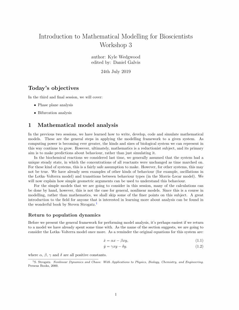
For two-dimensional models, we can understand pretty much everything we need to by looking at thephase plane. This is really just a fancy name for the graph that we get when we plot our state variablesas functions of one another. The full classification of behaviours arises because we know that trajectoriescannot cross one another, and in two-dimensional systems we can observe where all these trajectoriesgo. For example, if we plot y against x for the Lotka–Volterra model, we get

So how do we make sense of this plot?

Nullclines

The first thing we should identify is where the nullclines are for this model. A nullcline is a curve inour phase plane on which one of our state variables is not changing. This implies that either x = 0 ory = 0. Recall when we looked for quasi-steady states in our biochemical reaction experiments that weset C = 0. The idea is essentially the same, although we will go one step further here.

Setting x = 0, we get0 = αx− βxy = x(α− βy).

To satisfy this equation, we either need x = 0, or y = α/β. Note that, if either of these are true, thenthe equation is automatically satisfied. This means that both x = 0 and y = α/β are nullclines of thesystem.

If we now set y = 0, we get0 = γxy − δy = y(γx− δ).

Playing the same game as before, we find that y = 0 and x = δ/γ are both nullclines.

Finding nullclines in xppaut To verify that we have found the correct nullclines, we can search forthem in xppaut. Set the plotting bounds to xlo=0, xhi=12, ylo=0, yhi=8. Now click on Nullcline

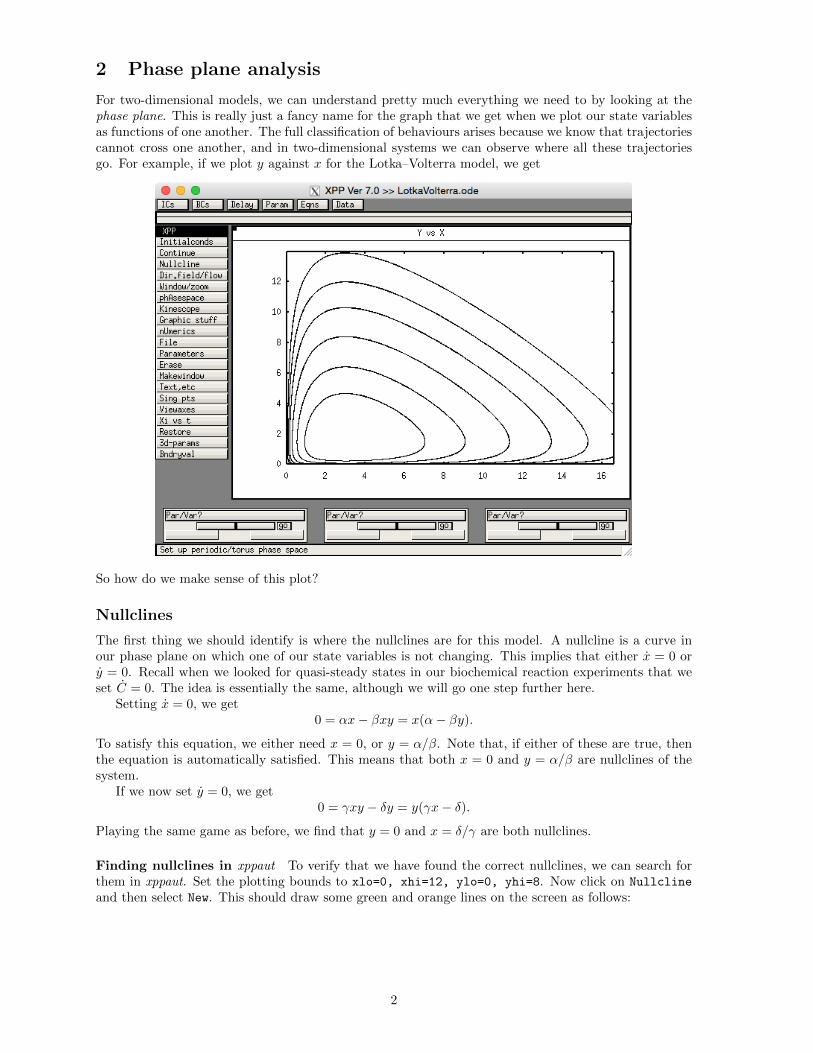
and then select New. This should draw some green and orange lines on the screen as follows:

2

The green lines are the nullclines for the x equation and the orange lines are those for the y variable.In general, xppaut chooses this colour scheme so that green corresponds to the nullcline for the firstvariable and orange to the second variable. In the Nullclines submenu, there are a number of optionsto redraw, freeze and save nullclines, but we typically won’t use these.

So how do nullclines help us in analysing the model? Choose Initialconds, then mIce (KEY-BOARD: press [I] twice) and run some more simulations. There are two things to notice here. Firstly,the trajectories always cross the green line horizontally and the orange line vertically. This makes sensesince we know that across nullclines, one of our state variables must be unchanging and this is truewhen our trajectory is either horizontal or vertical. Secondly, it seems that trajectories ‘wrap around’the intersection of the nullclines. This turns out to be a special point.

Fixed points

At points where the nullclines intersect, neither x nor y are changing. Trajectories starting at thesepoints will remain there indefinitely. Mathematicians call such objects invariant to reflect this. Thisparticular kind of object is known as a fixed point or steady state and they act as very importantorganising centres for the system dynamics. To find a fixed point, we need to find points such that xand y are simultaneously zero. From our earlier considerations, we know that x = 0 and y = 0 arenullclines for the x and y variables respectively. This means that (x, y) = (0, 0), is a fixed point of thesystem. This is called the trivial state and represents a situation in which neither the predator, nor theprey population exist. Similarly, since y = α/β and x = δ/γ are nullclines, then (x, y) = (δ/γ, α/β) isa fixed point of the system.

Stability

We still don’t have a definitive answer about what fixed points really tell us about a system. There isone more piece of information we need to consider: stability. We know that if trajectories start exactlyat a fixed point, they remain there indefinitely, but what happens if they start just next to it? Thestability of a fixed point tells us what happens next.

As a motivating example, consider the pendulum. We know that, over time, due to frictional forces,the pendulum will eventually come to a rest hanging vertically downwards. If you knock the pendulumslightly in this configuration, it will swing back and forth for a bit, but will eventually come to rest

3

Stable UnstableFigure 1: Small perturbations to the pendulum when it is vertically downwards will induce small oscillationsaround this configuration, but the pendulum will eventually come to rest back at the stable fixed point. Whenit is vertically upwards, small perturbations will cause the pendulum to make a large swing so that it eventuallycomes to rest in the downward configuration. This is an example of an unstable fixed point.

vertically downwards again. This configuration is an example of a fixed point, and moreover it is stable,since small perturbations away from it will give rise to trajectories that are attracted back towards it.

There is another fixed point in the pendulum system, namely when the pendulum is verticallyupwards. This may seem counter-intuitive at first, but if you experiment for a bit you can see why it istrue. If you could start a pendulum in exactly this configuration, with no outside interference, it wouldremain there. However, if you now knock the pendulum, it will make a large swing downwards and willswing back and forth around the vertically downward configuration. This is an example of an unstablefixed point: small perturbations will cause trajectories to move away from it.

Very loosely then, we can think of stability as indicating whether trajectories move towards or awayfrom fixed points in the limit of infinite time. Stability can also be understood by examining whathappens to trajectories that are perturbed away from the fixed point.

Returning to the Lotka–Volterra model, it would be useful to examine the stability of the fixed pointswe found earlier. Thankfully, xppaut gives us an easy way to do this.

Finding fixed points in xppaut Graphically, it is easy to see where the fixed points for our systemare, however, we generally need to be more precise when identifying them. xppaut comes prepackagedwith an algorithm to accurately locate them, with a bit of help. Click on the Sing pts menu followedby Mouse (KEYBOARD: Press [S] followed by [M]). The program will now prompt you for an initialguess. We know that there should be a fixed point near the origin, so click here. A dialogue box askingyou if you want to Print eigenvalues will pop up, like so:

4

Select NO and then another box will ask you if you want to Draw invariant sets. Select NO again toarrive at the following window:

There is quite a lot of information in this window, some of which we have not discussed yet, but theimportant information is written at the top and the bottom. At the bottom, we have the coordinates ofthe fixed point. Notice that these are not exactly at (x, y) = (0, 0). This is because the algorithm thatxppaut uses to find the fixed points has an associated stopping tolerance (as do all numerical routines)and the point it has found satisfies this tolerance. For our purposes, it is more than adequate.

The capitalised box at the top of the window tells us that this point is unstable. From a modellingperspective, this means that any perturbation away from the trivial state will lead to population growthin at least one of the predator or prey species. This perturbation could arise, for example, by theintroduction of some species to a deserted island. The numbers underneath this give us more informationabout the type of fixed point the trivial state is. In particular, the fact that r+ and r− both have value1 tells us that trajectories are attracted to the trivial state in one direction and repelled from it inanother. Does this make sense given the trajectories we plotted earlier? Does it make sense for the realsystem?

Aside: Some of you may be wondering about exactly what the values r+,− and c+,− mean. Thesevalues give us vital information about not only the stability, but also the type of the fixed point. Inparticular, they tell us the number of directions that match certain kinds of behaviour near the fixedpoint. Values associated with the + superscript indicate the number of directions moving away from

5

the fixed point, and those associated with the - superscript are the number moving towards the fixedpoint. The letters r and c stand for real and complex. It’s not of great importance to know exactly whatthis means, however, it is useful to note that these tell us about the type of trajectories near the fixedpoint we can expect to see. Directions labelled real support trajectories that move away/towards thefixed point in straight lines, whereas complex ones support oscillatory trajectories that spiral in/out ofthe fixed point. A fixed point is stable if the sum r+ + c+ = 0 (so that there are no directions in whichtrajectories move away from the fixed point). If r+ + c+ > 0, then the fixed point is unstable. As afinal remark, we note that the sum of all directions r+ + r−+ c+ +c− must be equal to the number ofvariables in our system.

In some sense, the trivial steady state is an uninteresting one since it represents the case whereneither population exists. Choose Sing pts and Mouse again and this time click near the nontrivialsteady state. Once more, choose NO when asked to plot the eigenvalues. Note that this time, it doesn’task you to draw the invariant sets. You should now have a window that looks like:

Verify that that coordinates of the fixed point are what they should be. The stability box informs usthat the fixed point is neutrally stable. This is neither stable (in the sense that we have so far discussed),nor is it unstable. In fact, small perturbations to trajectories around the fixed point will neither shrinknor grow, but remain indefinitely. Note that this stability classification only tells us about the dynamicsexponentially close to the fixed point. As we get further away from the fixed point, this analysis breaksdown and perturbations, in general, may ultimately grow. However, for the special model we havechosen, any perturbation away from the fixed point will persist. This is why we see the oscillationsaround this fixed point, no matter where the trajectory starts.

Logistic growth

In the last session, we saw that adding a carrying capacity to the prey population dynamics had asignificant impact on the behaviour of the system. As a reminder, the model we used was

x = αx(

1− x

K

)− βxy, (2.1)

y = γxy − δy, (2.2)

where K is the carrying capacity. Let us now consider the nullclines of this system. The ODE governingthe predator population is the same as before, and so the nullclines will be the same. Setting x = 0 inthe first equation gives us

0 = αx(

1− x

K

)− βxy = x

(α− αx

K− βy

)The nullclines for this equation are thus given by x = 0, as before, and

y =α

β

(1− x

K

).

We thus expect a trivial fixed point (x, y) = (0, 0). To find the other fixed point, we need to set x = δ/γand substitute this in the above equation in order to guarantee that both x = 0 and y = 0 are satisfied.This then tells us that

(x, y) =

(δ

γ,α

β

(1− δ

Kγ

)),

6

is a fixed point of the system.We will now examine the stability of these points in xppaut. Open up the model, or copy and paste

the following and save it as LoktaVolterraLogistic.ode

# Parameters

par alpha=1.5

par beta=1.0

par gamma=1.0

par delta=3.0

par K=10

# Initial conditions

x(0)=5

y(0)=2

# ODEs

x’ = alpha*x*(1-x/K) - beta*x*y

y’ = gamma*x*y - delta*y

# Options

@ bounds=100000000, total=20, meth=qualrk, dt=0.01

@ xp=x, yp=y, xlo=0, xhi=6, ylo=0, yhi=4

done

Plot the nullclines in the same way as before. Simulate the system to get a feel what the trajectorieslook like. You should have a graph that looks something like this:

As expected, we see that the system has nullclines with x = 0, y = 0 and x = δ/γ. The other nullclineis now a line with slope −α/βK and intercept α/β.

Verify that the stability of the trivial steady state is the same as for the case without logistic growthand examine the stability of the other fixed point to get:

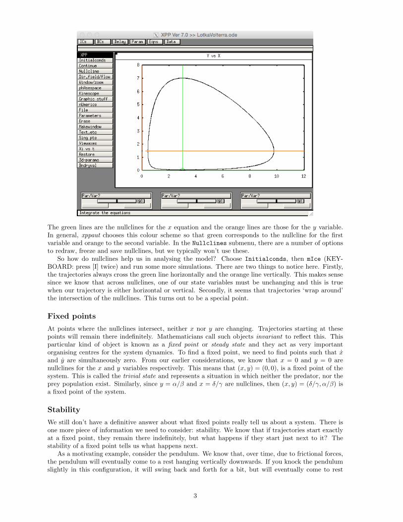
7

First check that the fixed point is where we thought it was. We now see that this fixed point is stable,which explains why trajectories move toward it. The line c−=2 tells us that we should expect trajectoriesto ‘spiral’ towards the fixed point, which is exactly what we observe.

Cooperative inhibition

In the Lotka-Volterra system, we saw that by changing the functional form of the growth rate of theprey species, we could change the stability of the non-trivial fixed point. However, we often don’t needto go to such lengths to alter the stability properties of fixed points. Often, it is enough to changeparameter values to induce such changes.

As an example, consider the biochemical reaction of two species, S1 and S2, with cooperative inhi-bition given by the following system of ODEs:

S1 =k1

1 + (S2/K2)n1− k3S1,

S2 =k2

1 + (S1/K1)n2− k4S2.

The inhibition in this system is reflected by the fact that the reaction rates are dependent on the otherspecies as well as the rates k1 and k2. The parameters k3 and k4 represent the decay rates of the twospecies, whilst K1 and K2 are the dissociation constants for the binding events involved in the reaction.Finally, n1 and n2 are the Hill coefficients capturing the degree of cooperativity.

In the case where n1 > n2, the inhibition by S2 is more effective than that by S1. If all otherparameters are symmetric between the two species (i.e. the parameters that appear in both equationsare the same for each species: k1 = k2, K1 = K2, k3 = k4), we would expect that the fixed point shouldbe one in which the concentration of S1 is low and that of S2 is high. Let’s use xppaut to test this.

Exercise: Write the system of ODEs in code to be simulated in xppaut. Set k1 = k2 = 20,K1 = K2 = 1, k3 = k4 = 5, n1 = 4 and n2 = 1. Plot the concentration of S2 against that of S1. Choosea variety of initial conditions and observe the model behaviour. Plot the nullclines of the system. Doesthis help you understand the dynamics of the model? Find the fixed points of the system and assess theirstability. Does this make sense given the model trajectories? Your phase plane should look somethinglike this:

8

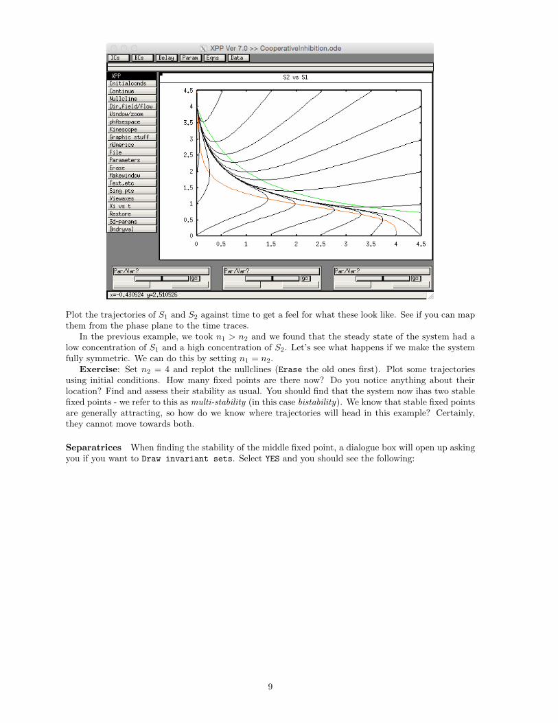
Plot the trajectories of S1 and S2 against time to get a feel for what these look like. See if you can mapthem from the phase plane to the time traces.

In the previous example, we took n1 > n2 and we found that the steady state of the system had alow concentration of S1 and a high concentration of S2. Let’s see what happens if we make the systemfully symmetric. We can do this by setting n1 = n2.

Exercise: Set n2 = 4 and replot the nullclines (Erase the old ones first). Plot some trajectoriesusing initial conditions. How many fixed points are there now? Do you notice anything about theirlocation? Find and assess their stability as usual. You should find that the system now ihas two stablefixed points - we refer to this as multi-stability (in this case bistability). We know that stable fixed pointsare generally attracting, so how do we know where trajectories will head in this example? Certainly,they cannot move towards both.

Separatrices When finding the stability of the middle fixed point, a dialogue box will open up askingyou if you want to Draw invariant sets. Select YES and you should see the following:

9

Now simulate trajectories again and see how their behaviour is dependent on the blue line.You should observe that the blue line separates trajectories that are attracted to the left fixed point

and those that head towards the right fixed point. For this reason, this blue line is called a separatrix.Mathematically speaking, this blue line is called the stable manifold of the middle fixed point (thesedetails are unnecessary). When you examined the stability of the middle fixed point, you should havefound that it had one stable direction and one unstable direction. So, we know that trajectories willmove toward this point, before being repelled away from it. In fact, the direction in which trajectorieswill be attracted to the fixed point is given by this blue line, hence this represents the ‘stable’ directionof the middle fixed point.

Trajectories starting exactly on the blue line will remain on it indefinitely, and so our earlier definitionof invariance applies to curves as well as points in phase space. This means that the blue line is alsoa trajectory of the system, albeit one that is quite hard to simulate. Since we know that trajectoriescannot cross, all other trajectories must stay on either the left or the right of the separatrix. In each ofthese sections, there is only one stable fixed point, so trajectories are attracted to these.

The set of all initial conditions that are attracted to a given stable invariant set (in this case, a fixedpoint), is called its basin of attraction. Separatrices thus delimit the basins of attraction of differentstable solutions. Typically, separatrices are associated with unstable invariant sets or invariant setsassociated with unstable fixed points. They are very useful for predicting the behaviour of a system.For example, perturbations that take trajectories over the separatrix can induce a switch in the systembehaviour. For example, if the system is at a steady state in which S1 is abundant and S2 is not, asufficiently strong perturbation could move it into a state where the concentration of S2 is high andthat of S1 is low.

By changing the value of n2, we have induced a qualitative change in the behaviour of the system.This is called a bifurcation. We encountered these earlier when looking at the Morris–Lecar model, andwe shall do so again very shortly. In particular, since changing n2 away from n1 breaks the symmetryof the system, this is called a symmetry breaking bifurcation.

Gene expression

Gene expression consists of two primary sub-processes: transcription and translation. During transcrip-tion, a coding region of a gene is ‘re-written’ in the form of mRNA. In translation, this mRNA is then‘read off’ by a ribosome to produce a polypeptide chain made up of amino acids. As such, these twoprocesses represent a kind of ‘information transfer’ at both the transcription and translation stage.

10

Regulation of transcription and translation is a complex process that involves a wide variety ofdifferent reactions. As such, a nice mathematical description that fully captures all of the elementaryprocesses is impossible. This is where we turn to phenomenological modelling to capture the essence ofthe biology. One thing we should be aware of is that genes are often present in small numbers in anindividual cell, meaning that our ODE formulation may not always be the most appropriate. However,if we think of our model as an average over many cells, we are generally on safe ground.

Our basic model of gene expression will assume that many of the background molecules needed forvarious processes are available in a fixed quantity. Moreover, we will ignore many significant processes,such as mRNA splicing and nuclear transport. Applying the law of mass action to a population ofmRNA and the protein it encodes gives rise to the following equations:

m = k0 − δmm,p = k1m− δpp,

where m is the concentration of mRNA and p is the concentration of protein. The parameter k0represents the population-averaged transcription rate, which depends on a number of factors includingthe gene copy number, abundance of RNA polymerase, the strength of the gene’s promoter and theavailability of nucleotide building blocks. The parameter k1 is the per-mRNA translation rate, whichalso depends on a host of factors, mostly associated with the ribosomes. Finally, the parameters δm andδp represent the decay of mRNA and protein respectively.

Steady state levels for mRNA and protein are easily found as

mss =k0δm

, pss =k0k1δmδp

.

We often simplify models of gene expression by taking advantage of the fact that mRNA decay (on theorder of minutes) is typically much faster than protein decay (on the order of hours). Thus, as we didfor biochemical reactions, we can assume that the mRNA is in a quasi-steady state. Upon substitutingmss into the ODE for p, we get the reduced model

p =k0k1δm− δpp = α− δpp,

where α = k0k1/δm is called the expression rate.The expression of genes can be regulated at many stages, including RNA polymerase biding, elon-

gation of the mRNA strand, translational initiation and polypeptide elongation. The majority of thisregulation occurs through control of the initiation of transcription, primarily through modifying the asso-ciation of RNA polymerase with gene promoter regions through transcription factors. If a transcriptionfactor increases the rate of RNA polymerase binding, it is called an activator of gene expression. If it in-hibits binding, it is called a repressor. In a similar way to the enzymatic reactions, multiple transcriptionfactors can affect expression of a single gene, and these can act cooperatively or competitively.

Gene regulatory networks

A perhaps more interesting case is when we consider a network of genes that, though the action ofthe proteins they encode, can activate or repress one another. The simplest possible networks are onesin which a gene promotes or inhibits its own expression. If we again treat the mRNA as being inquasi-steady state, a prototypical model for an autoinhibitor is given by

p =α

1 + p/K− δpp,

whereas a similar model for an autoactivator is given by

p =α(p/K)

1 + p/K− δpp.

In 2000, Gardner and colleagues engineered a genetic toggle switch by rewiring elements of existinggene regulatory networks.2 This switch works in a similar way to the cooperative inhibition reaction

2T. S. Gardner, C. R. Cantor, and J. J. Collins. “Construction of a genetic toggle switch in Escherichia coli.” In:Nature 403 (2000), pp. 339–342.

11

we saw earlier: when expression of one gene is high, the other is suppressed, and vice versa. The teamconstructed many examples of the toggle switch using the Lac and Tet repressors in E. coli and cI fromphage lambda. When performing their studies, Gardner are his colleagues developed a simple model3

to explore the behaviour of the switch circuit. This phenomenological model was not intended to fullycharacterise the processes giving rise to the switching behaviour; more to explore the bistability in thenetwork.

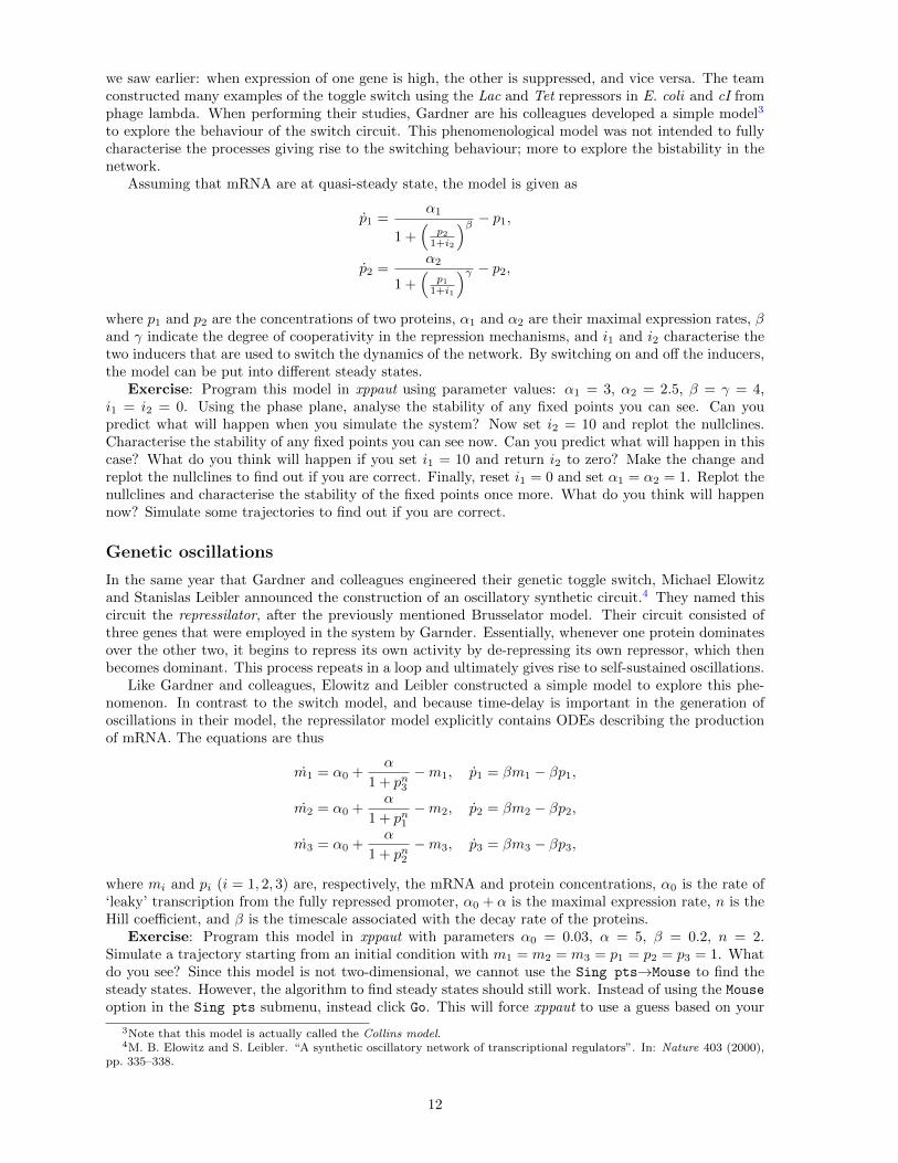
Assuming that mRNA are at quasi-steady state, the model is given as

p1 =α1

1 +(

p21+i2

)β − p1,p2 =

α2

1 +(

p11+i1

)γ − p2,where p1 and p2 are the concentrations of two proteins, α1 and α2 are their maximal expression rates, βand γ indicate the degree of cooperativity in the repression mechanisms, and i1 and i2 characterise thetwo inducers that are used to switch the dynamics of the network. By switching on and off the inducers,the model can be put into different steady states.

Exercise: Program this model in xppaut using parameter values: α1 = 3, α2 = 2.5, β = γ = 4,i1 = i2 = 0. Using the phase plane, analyse the stability of any fixed points you can see. Can youpredict what will happen when you simulate the system? Now set i2 = 10 and replot the nullclines.Characterise the stability of any fixed points you can see now. Can you predict what will happen in thiscase? What do you think will happen if you set i1 = 10 and return i2 to zero? Make the change andreplot the nullclines to find out if you are correct. Finally, reset i1 = 0 and set α1 = α2 = 1. Replot thenullclines and characterise the stability of the fixed points once more. What do you think will happennow? Simulate some trajectories to find out if you are correct.

Genetic oscillations

In the same year that Gardner and colleagues engineered their genetic toggle switch, Michael Elowitzand Stanislas Leibler announced the construction of an oscillatory synthetic circuit.4 They named thiscircuit the repressilator, after the previously mentioned Brusselator model. Their circuit consisted ofthree genes that were employed in the system by Garnder. Essentially, whenever one protein dominatesover the other two, it begins to repress its own activity by de-repressing its own repressor, which thenbecomes dominant. This process repeats in a loop and ultimately gives rise to self-sustained oscillations.

Like Gardner and colleagues, Elowitz and Leibler constructed a simple model to explore this phe-nomenon. In contrast to the switch model, and because time-delay is important in the generation ofoscillations in their model, the repressilator model explicitly contains ODEs describing the productionof mRNA. The equations are thus

m1 = α0 +α

1 + pn3−m1, p1 = βm1 − βp1,

m2 = α0 +α

1 + pn1−m2, p2 = βm2 − βp2,

m3 = α0 +α

1 + pn2−m3, p3 = βm3 − βp3,

where mi and pi (i = 1, 2, 3) are, respectively, the mRNA and protein concentrations, α0 is the rate of‘leaky’ transcription from the fully repressed promoter, α0 + α is the maximal expression rate, n is theHill coefficient, and β is the timescale associated with the decay rate of the proteins.

Exercise: Program this model in xppaut with parameters α0 = 0.03, α = 5, β = 0.2, n = 2.Simulate a trajectory starting from an initial condition with m1 = m2 = m3 = p1 = p2 = p3 = 1. Whatdo you see? Since this model is not two-dimensional, we cannot use the Sing pts→Mouse to find thesteady states. However, the algorithm to find steady states should still work. Instead of using the Mouseoption in the Sing pts submenu, instead click Go. This will force xppaut to use a guess based on your

3Note that this model is actually called the Collins model.4M. B. Elowitz and S. Leibler. “A synthetic oscillatory network of transcriptional regulators”. In: Nature 403 (2000),

pp. 335–338.

12

initial conditions to find a fixed point. Examine the stability of the fixed point you find. You shouldfind a stable fixed point with c−=6. This means that we would expect trajectories to spiral in towardsthe fixed point.

Now, set α = 10, find the fixed point again and assess its stability. You should now find an unstablefixed point, with c+=2, c−=4. This means that we should now have trajectories that spiral away fromthe fixed point. Can you predict what the trajectories will look like? Plot p1, p2 and p3 against time toconfirm this.

In this example, we have seen that changing parameters can not only give rise to changes in steadystate concentrations, but can also induce oscillations. We will now discuss a systematic way to analysethese changes in behaviour further.

3 Bifurcations

We have now seen a number of examples in which changing parameters in a model can give rise todramatic changes in model behaviour. We shall now show how to find specific points at which thisoccurs. Given a steady state solution for a given model, we can use numerical routines to see how thefixed point corresponding to this steady state changes as one of the system parameters varies. Thisprocess is called continuation and the plot of fixed point values against the parameter being varied iscalled the continuation curve. In an experimental setting, this may represent something physiological,such as the size of the response of a system to a given drug. It is standard to refer to the parameter thatis varied as the control parameter. In this example, the control parameter would represent the dose ofthe drug applied to the system. Points along the continuation curve at which the qualitative behaviourof the model changes are known as bifurcation points. Bifurcation points are associated with changes ofstability of invariant sets, and generally also include a change in the number of distinct invariant setsin the phase space.

A continuation curve is often referred to as a branch of solutions, which is parametrised by thecontrol parameter. At bifurcation points, new branches of solutions are often generated, reflecting thechange in the number of invariant sets in the model. This branching behaviour gives bifurcation pointstheir name: bifurcus coming from Latin and meaning to divide into two branches. We can predict thestability of these new invariant sets by analysing the type of bifurcation that occurs at a given valueof the control parameter. This is the power of bifurcation analysis. By understanding the bifurcationtypes that occur in the model, we can predict how the system behaves without ever having to simulateit.

A set of continuation curves in the same figure is known as a bifurcation diagram and the study ofsuch diagrams is called bifurcation analysis. Bifurcation analysis of general nonlinear systems is quitedifficult to do analytically, and so numerical continuation routines must usually be employed to findbranches of solutions. Thankfully, xppaut comes with a built-in, easy-to-use routine.

AUTO

The AUTO package is regarded by many as one of the most sophisticated set of numerical continuationlibraries.5 Indeed, its efficiency and accuracy are still gold standards today. One of the major draw-backs to AUTO, however, is that it is written in Fortran, which has been somewhat eclipsed by otherprogramming languages since its heyday. Interfaces for AUTO have now been written, for example inpython, but in spite of this, the xppaut graphical interface remains one of the easiest ways to access thepower that AUTO offers.

We will now explore how to use AUTO to track branches of solutions in some of the models we havealready met.

5url: http://indy.cs.concordia.ca/auto/.

13

Cooperative inhibition

Recall that our model of cooperative inhibition was given by

S1 =k1

1 + (S2/K2)n1− k3S1,

S2 =k2

1 + (S1/K1)n2− k4S2.

If you haven’t already coded this model, copy and paste the following into a text editor and save itas CooperativeInhibition.ode.

# Parameters

par k1=35,k2=20

par k3=5,k4=5

par Kd1=1,Kd2=1

par n1=2,n2=2

# Initial conditions

S1(0)=1

S2(0)=1

# ODEs

S1’ = k1/(1+(S2/Kd2)^n1)-k3*S1

S2’ = k2/(1+(S1/Kd1)^n2)-k4*S2

# Options

@ bounds=100000000, total=20, meth=qualrk, dt=0.01

@ xp=S1, yp=S2, xlo=0, xhi=4.5, ylo=0, yhi=4.5

done

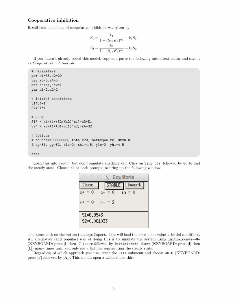
Load this into xppaut, but don’t simulate anything yet. Click on Sing pts, followed by Go to findthe steady state. Choose NO at both prompts to bring up the following window:

This time, click on the button that says Import. This will load the fixed point value as initial conditions.An alternative (and popular) way of doing this is to simulate the system using Initialconds→Go

(KEYBOARD: press [I] then [G]) once followed by Initialconds→Last (KEYBOARD: press [I] then[L]) many times until you only see a flat line representing the steady state.

Regardless of which approach you use, enter the File submenu and choose AUTO (KEYBOARD:press [F] followed by [A]). This should open a window like this:

14

This is the AUTO main window. We will now go through the steps required to set up a continuationrun. We are going to choose k1 as our control parameter and we first need to check that AUTO knowsabout k1’s existence. By default, AUTO can only store eight parameters at once, so we must alsoperform this initial check. To do this, click on the Parameters button (KEYBOARD: press [P]). Thisshould bring up the following window

Here, we can see a list of parameters that AUTO is aware of. The order is unimportant, it only matters

15

that at least one of these stores the value k1, which it does. Close this window and open the submenuAxes, and select hI-lo (KEYBOARD: [A] followed by [I]) to bring up this window:

The Y-axis field tells us what will be plotted in on the y-axis (in this case S1), and the Main Parm

field is the name of the control parameter. This should be set to k1, which it already is. The otheroptions in this window are unimportant, so we can close it now by clicking Ok. Next, we need to setsome options corresponding to the continuation run. These are set from the Numerics window, so openthis now (KEYBOARD: press [N]). The window should look like this:

16

Most of these options are not relevant to our current situation, so we shall ignore them, however, someof them do require changing.

Bounds The first thing to check is the parameter bounds, given by Par Min and Par Max. These setthe parameter range over which the algorithm will compute the continuation curve. Once the algorithmreaches the bound it will stop. If you try to initialise the continuation run using a parameter valueoutside this range, AUTO will fail to converge the first step. In our example, we will let k1 vary from35 to 5, so make the necessary changes in these fields.

Step size Just as our numerical solver for time simulations had a time step, continuation algorithmsalso have a step size. Loosely, you can think of this as scaling how far each step of the numericalprocedure will advance the control parameter. The Dsmin and Dsmax fields set bounds on how small orlarge this step can be, whilst the Ds option sets the initial step size. Since we are starting our simulationat k1 = 35 and ending at k1 = 5, we need this to be negative, so set it to be Ds=-0.02. Often, we donot need to change the other two step size values, since they only control the magnitude of the steps.However, in the later versions of xppaut, it is occasionally necessary to reduce Dsmax to ensure that thecurves that the program plots are nice and smooth. The exact values required for the three optionsassociated with step sizes will depend on the magnitude of the parameter in your model that you wishto vary.

Number of points The Nmax option defines the maximum number of points along the continuationcurve that the numerical routine should produce. The value that should be entered here will dependon the interval over which the control parameter will vary and the maximum and minimum step sizeyou allow the procedure to take. The current value seems like it should suffice here, so we will leave italone. The NPr field sets how often AUTO should label points. Labelling points makes it easier to seewhat the solution is doing, but labelling too many makes the resulting graph difficult to read. This isreally a personal preference, but for now, we can probably leave this as it is.

Note that all of the options required for an AUTO continuation run can be set within the code yousupply to xppaut. For more details of how to set these, please refer to the website.6 We have nowset all of the parameter values we need to run the continuation. Press Run followed by Steady state

(KEYBOARD: press [R], then [S]). At first it may appear that not much has happened. Don’t panic!This is only because the plotting region is not yet set up properly. We can fix this easily by going tothe Axes submenu and selecting Fit (KEYBOARD: [A] followed by [F]). After having done this, youshould be presented with:

6url: http://www.math.pitt.edu/~bard/xpp/help/xppopt.html.

17

Congratulations - you have just successfully performed your first continuation run! So what doesthis tell us? Firstly, you may notice that the curve extends beyond our lower bound for k1 of 5. This isbecause AUTO only checks if we are outside the prescribed control parameter interval after it computesthe point, and it includes this point in the computed curve. The lines on the curve represent fixedpoints of the solution. Bold red curves correspond to stable fixed points, whereas the narrow black linesrepresent unstable fixed points. From left to right then, we see that the system first has a stable fixedpoint with a low concentration of S1. In the middle portion of the diagram, the system possesses threefixed points: two stable and one unstable. Of the two stable fixed points, one has a low concentrationof S1, the other has a high concentration. Remember earlier when we simulated this model in the phaseplane; these three fixed points are essentially the same that we found then and represent bistabilityin the system. Which steady state solutions are ultimately attracted to is dependent on the initialcondition of the trajectory. Finally, for high values of k1, we see that the system only has one, stablefixed point, with a high concentration of S1.

Our earlier analysis suggested that when concentration of S1 was high, that of S2 should be low (atsteady state) and vice versa. Let’s check this now. Go into the Axes menu and select hI-lo again.Replace S1 with S2 in the y-axis field and click Ok. Next, go back into the Axes menu and click Fit

to obtain:

18

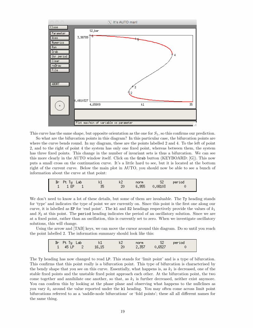
This curve has the same shape, but opposite orientation as the one for S1, so this confirms our prediction.So what are the bifurcation points in this diagram? In this particular case, the bifurcation points are

where the curve bends round. In my diagram, these are the points labelled 2 and 4. To the left of point2, and to the right of point 4 the system has only one fixed point, whereas between them, the systemhas three fixed points. This change in the number of invariant sets is thus a bifurcation. We can seethis more clearly in the AUTO window itself. Click on the Grab button (KEYBOARD: [G]). This nowputs a small cross on the continuation curve. It’s a little hard to see, but it is located at the bottomright of the current curve. Below the main plot in AUTO, you should now be able to see a bunch ofinformation about the curve at that point:

We don’t need to know a lot of these details, but some of them are invaluable. The Ty heading standsfor ‘type’ and indicates the type of point we are currently on. Since this point is the first one along ourcurve, it is labelled as EP for ‘end point’. The k1 and S2 headings respectively provide the values of k1and S2 at this point. The period heading indicates the period of an oscillatory solution. Since we areat a fixed point, rather than an oscillation, this is currently set to zero. When we investigate oscillatorysolutions, this will change.

Using the arrow and [TAB] keys, we can move the cursor around this diagram. Do so until you reachthe point labelled 2. The information summary should look like this:

The Ty heading has now changed to read LP. This stands for ‘limit point’ and is a type of bifurcation.This confirms that this point really is a bifurcation point. This type of bifurcation is characterised bythe bendy shape that you see on this curve. Essentially, what happens is, as k1 is decreased, one of thestable fixed points and the unstable fixed point approach each other. At the bifurcation point, the twocome together and annihilate one another, so that, as k1 is further decreased, neither exist anymore.You can confirm this by looking at the phase plane and observing what happens to the nullclines asyou vary k1 around the value reported under the k1 heading. You may often come across limit pointbifurcations referred to as a ‘saddle-node bifurcations’ or ‘fold points’; these all all different names forthe same thing.

19

We should verify that the point labelled 4 is also a limit point, so do this by moving along thecontinuation curve until you reach it and check that its Ty value is LP. A pair of limit point bifurcationsin this configuration is a classic hallmark of bistability and hysteresis. Hysteresis loops are particularlyuseful for switch design since they only need transient input to move trajectories between fixed points.Suppose that the system is at one fixed point (low S1, high S2), but we want to move it to the oppositefixed point (high S1, low S2). We can apply a transient input to drive the trajectory into the basin ofattraction of the other fixed point. When the input is removed, the trajectory is still in this basin ofattraction of the other fixed point, so we don’t need to keep applying it. We only need to ensure thatthe transient input is strong enough and applied for long enough to make the trajectory cross over theseparatrix of the unperturbed system.

Neural modelling

In the first session, we simulated a model of the Morris–Lecar model. When there was no applied current,the neuron was quiescent with a resting membrane potential of around V = −60 mV. As we increasedthe applied current, the cell depolarised, until the applied current was so high that the neuron startingproducing action potentials. One of the tasks in the first session was to try to identify the minimalapplied current to invoke these action potentials, and to examine how their frequency was dependenton this current. It should come as no surprise that bifurcation analysis and numerical continuation canhelp us to answer both of these questions.

Begin by loading the ML.ode into xppaut. Find the fixed point corresponding to the rest state, eitherby using xppaut’s algorithm to find fixed points and then importing them as initial conditions, or bysimulating the model until you are at a steady state. Now load AUTO as before from the File menu.We are now going to perform a continuation run, using Iapp as our control parameter.

As for the cooperative inhibition model, we need to specify some options for the run. Open theParameter window and set Par1 to iapp. Click Ok and open the Axes submenu and select hI-lo. Inthis menu, simply check that the Y-axis field is set to V and the Main parm field is set to iapp. ClickOk once you are happy with this and then open the Numerics window. There are a few things weneed to change in here. Firstly, we know that the neuron doesn’t start firing until the applied currentis around 90 nA. Furthermore, we know that the neuron stops producing action potentials when theapplied current is around 250 nA, so we should make sure that our parameter range includes theseevents. Set Par max to 250. Since we are choosing quite a range for our control parameters, we shouldmake sure that we choose an appropriate step size - the current one is too small. We can leave the Ds

and Dsmin options as they are, since AUTO will adjust its step size where it can. Instead, simply setthe Dsmax option to 5.

We are now in a position to start the continuation run, so click Run followed by Steady state. Onceagain, we need to adjust the plotting axes, so click Axes followed by Fit to produce:

20

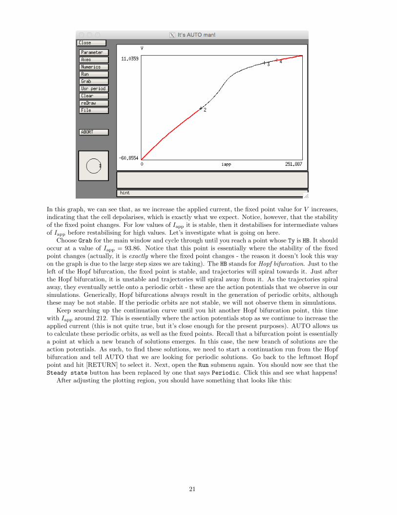
In this graph, we can see that, as we increase the applied current, the fixed point value for V increases,indicating that the cell depolarises, which is exactly what we expect. Notice, however, that the stabilityof the fixed point changes. For low values of Iapp it is stable, then it destabilises for intermediate valuesof Iapp before restabilising for high values. Let’s investigate what is going on here.

Choose Grab for the main window and cycle through until you reach a point whose Ty is HB. It shouldoccur at a value of Iapp = 93.86. Notice that this point is essentially where the stability of the fixedpoint changes (actually, it is exactly where the fixed point changes - the reason it doesn’t look this wayon the graph is due to the large step sizes we are taking). The HB stands for Hopf bifurcation. Just to theleft of the Hopf bifurcation, the fixed point is stable, and trajectories will spiral towards it. Just afterthe Hopf bifurcation, it is unstable and trajectories will spiral away from it. As the trajectories spiralaway, they eventually settle onto a periodic orbit - these are the action potentials that we observe in oursimulations. Generically, Hopf bifurcations always result in the generation of periodic orbits, althoughthese may be not stable. If the periodic orbits are not stable, we will not observe them in simulations.

Keep searching up the continuation curve until you hit another Hopf bifurcation point, this timewith Iapp around 212. This is essentially where the action potentials stop as we continue to increase theapplied current (this is not quite true, but it’s close enough for the present purposes). AUTO allows usto calculate these periodic orbits, as well as the fixed points. Recall that a bifurcation point is essentiallya point at which a new branch of solutions emerges. In this case, the new branch of solutions are theaction potentials. As such, to find these solutions, we need to start a continuation run from the Hopfbifurcation and tell AUTO that we are looking for periodic solutions. Go back to the leftmost Hopfpoint and hit [RETURN] to select it. Next, open the Run submenu again. You should now see that theSteady state button has been replaced by one that says Periodic. Click this and see what happens!

After adjusting the plotting region, you should have something that looks like this:

21

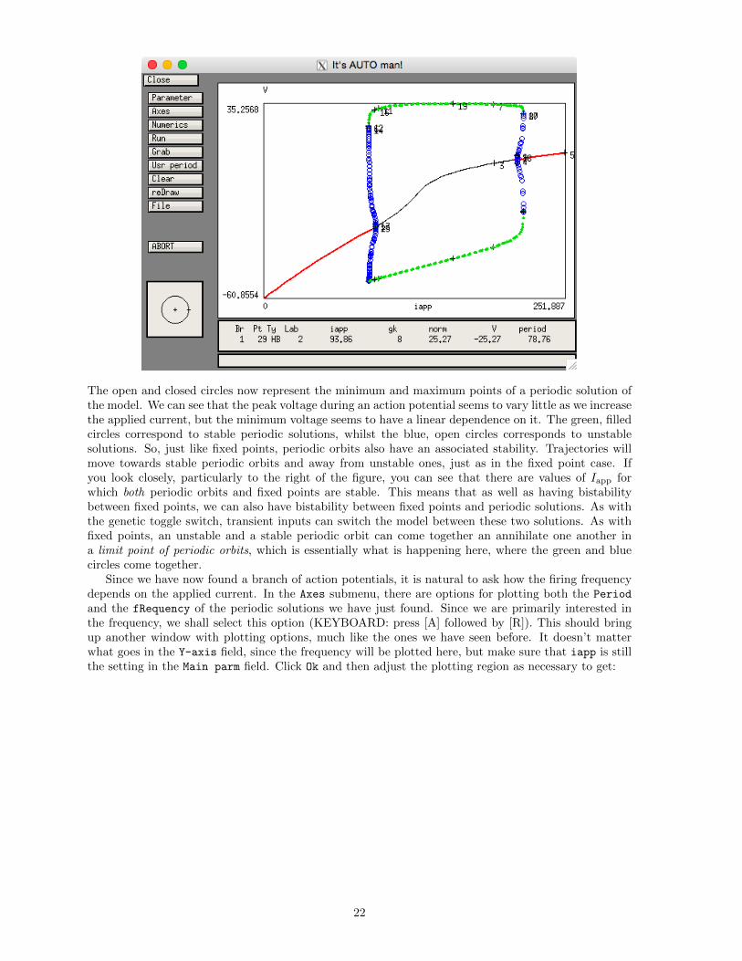
The open and closed circles now represent the minimum and maximum points of a periodic solution ofthe model. We can see that the peak voltage during an action potential seems to vary little as we increasethe applied current, but the minimum voltage seems to have a linear dependence on it. The green, filledcircles correspond to stable periodic solutions, whilst the blue, open circles corresponds to unstablesolutions. So, just like fixed points, periodic orbits also have an associated stability. Trajectories willmove towards stable periodic orbits and away from unstable ones, just as in the fixed point case. Ifyou look closely, particularly to the right of the figure, you can see that there are values of Iapp forwhich both periodic orbits and fixed points are stable. This means that as well as having bistabilitybetween fixed points, we can also have bistability between fixed points and periodic solutions. As withthe genetic toggle switch, transient inputs can switch the model between these two solutions. As withfixed points, an unstable and a stable periodic orbit can come together an annihilate one another ina limit point of periodic orbits, which is essentially what is happening here, where the green and bluecircles come together.

Since we have now found a branch of action potentials, it is natural to ask how the firing frequencydepends on the applied current. In the Axes submenu, there are options for plotting both the Period

and the fRequency of the periodic solutions we have just found. Since we are primarily interested inthe frequency, we shall select this option (KEYBOARD: press [A] followed by [R]). This should bringup another window with plotting options, much like the ones we have seen before. It doesn’t matterwhat goes in the Y-axis field, since the frequency will be plotted here, but make sure that iapp is stillthe setting in the Main parm field. Click Ok and then adjust the plotting region as necessary to get:

22

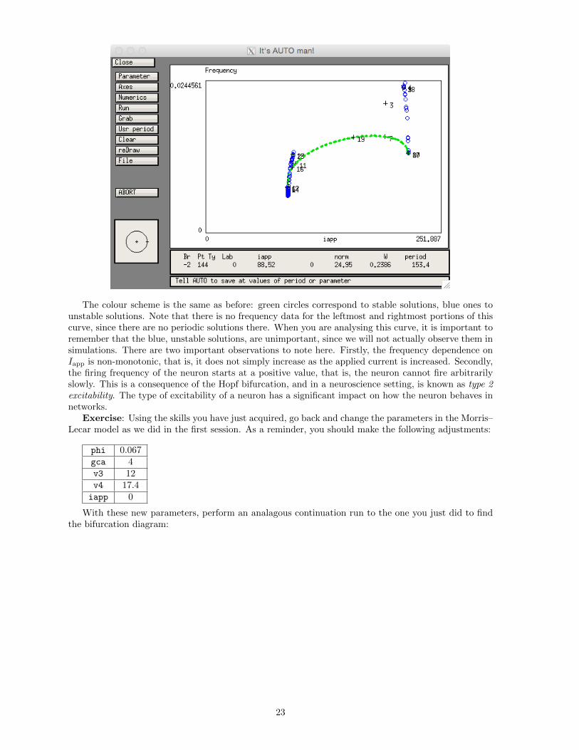
The colour scheme is the same as before: green circles correspond to stable solutions, blue ones tounstable solutions. Note that there is no frequency data for the leftmost and rightmost portions of thiscurve, since there are no periodic solutions there. When you are analysing this curve, it is important toremember that the blue, unstable solutions, are unimportant, since we will not actually observe them insimulations. There are two important observations to note here. Firstly, the frequency dependence onIapp is non-monotonic, that is, it does not simply increase as the applied current is increased. Secondly,the firing frequency of the neuron starts at a positive value, that is, the neuron cannot fire arbitrarilyslowly. This is a consequence of the Hopf bifurcation, and in a neuroscience setting, is known as type 2excitability. The type of excitability of a neuron has a significant impact on how the neuron behaves innetworks.

Exercise: Using the skills you have just acquired, go back and change the parameters in the Morris–Lecar model as we did in the first session. As a reminder, you should make the following adjustments:

phi 0.067gca 4v3 12v4 17.4iapp 0

With these new parameters, perform an analagous continuation run to the one you just did to findthe bifurcation diagram:

23

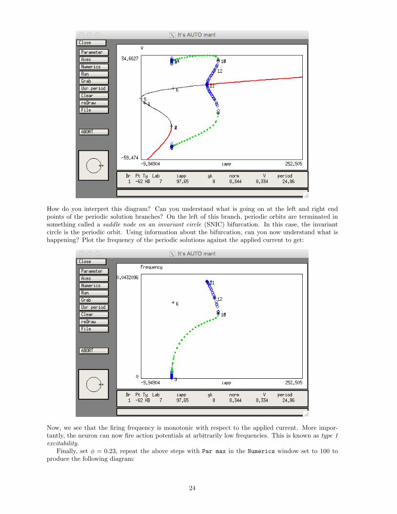
How do you interpret this diagram? Can you understand what is going on at the left and right endpoints of the periodic solution branches? On the left of this branch, periodic orbits are terminated insomething called a saddle node on an invariant circle (SNIC) bifurcation. In this case, the invariantcircle is the periodic orbit. Using information about the bifurcation, can you now understand what ishappening? Plot the frequency of the periodic solutions against the applied current to get:

Now, we see that the firing frequency is monotonic with respect to the applied current. More impor-tantly, the neuron can now fire action potentials at arbitrarily low frequencies. This is known as type 1excitability.

Finally, set φ = 0.23, repeat the above steps with Par max in the Numerics window set to 100 toproduce the following diagram:

24

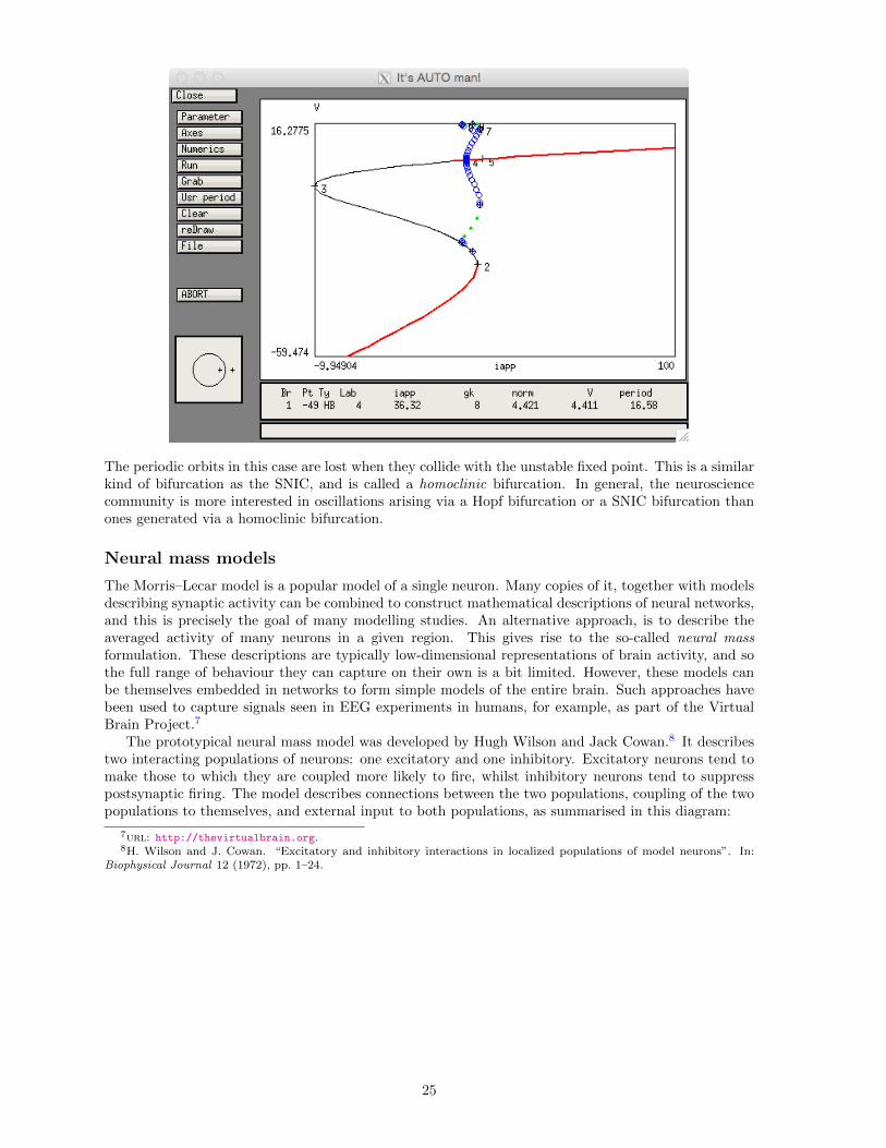
The periodic orbits in this case are lost when they collide with the unstable fixed point. This is a similarkind of bifurcation as the SNIC, and is called a homoclinic bifurcation. In general, the neurosciencecommunity is more interested in oscillations arising via a Hopf bifurcation or a SNIC bifurcation thanones generated via a homoclinic bifurcation.

Neural mass models

The Morris–Lecar model is a popular model of a single neuron. Many copies of it, together with modelsdescribing synaptic activity can be combined to construct mathematical descriptions of neural networks,and this is precisely the goal of many modelling studies. An alternative approach, is to describe theaveraged activity of many neurons in a given region. This gives rise to the so-called neural massformulation. These descriptions are typically low-dimensional representations of brain activity, and sothe full range of behaviour they can capture on their own is a bit limited. However, these models canbe themselves embedded in networks to form simple models of the entire brain. Such approaches havebeen used to capture signals seen in EEG experiments in humans, for example, as part of the VirtualBrain Project.7

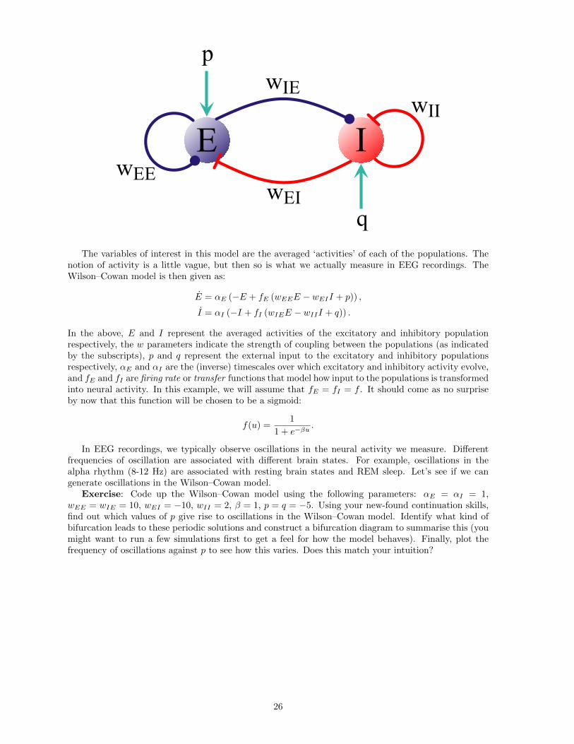
The prototypical neural mass model was developed by Hugh Wilson and Jack Cowan.8 It describestwo interacting populations of neurons: one excitatory and one inhibitory. Excitatory neurons tend tomake those to which they are coupled more likely to fire, whilst inhibitory neurons tend to suppresspostsynaptic firing. The model describes connections between the two populations, coupling of the twopopulations to themselves, and external input to both populations, as summarised in this diagram:

7url: http://thevirtualbrain.org.8H. Wilson and J. Cowan. “Excitatory and inhibitory interactions in localized populations of model neurons”. In:

Biophysical Journal 12 (1972), pp. 1–24.

25

E I

wIE

wEIwEE

wII

p

qThe variables of interest in this model are the averaged ‘activities’ of each of the populations. The

notion of activity is a little vague, but then so is what we actually measure in EEG recordings. TheWilson–Cowan model is then given as:

E = αE (−E + fE (wEEE − wEII + p)) ,

I = αI (−I + fI (wIEE − wIII + q)) .

In the above, E and I represent the averaged activities of the excitatory and inhibitory populationrespectively, the w parameters indicate the strength of coupling between the populations (as indicatedby the subscripts), p and q represent the external input to the excitatory and inhibitory populationsrespectively, αE and αI are the (inverse) timescales over which excitatory and inhibitory activity evolve,and fE and fI are firing rate or transfer functions that model how input to the populations is transformedinto neural activity. In this example, we will assume that fE = fI = f . It should come as no surpriseby now that this function will be chosen to be a sigmoid:

f(u) =1

1 + e−βu.

In EEG recordings, we typically observe oscillations in the neural activity we measure. Differentfrequencies of oscillation are associated with different brain states. For example, oscillations in thealpha rhythm (8-12 Hz) are associated with resting brain states and REM sleep. Let’s see if we cangenerate oscillations in the Wilson–Cowan model.

Exercise: Code up the Wilson–Cowan model using the following parameters: αE = αI = 1,wEE = wIE = 10, wEI = −10, wII = 2, β = 1, p = q = −5. Using your new-found continuation skills,find out which values of p give rise to oscillations in the Wilson–Cowan model. Identify what kind ofbifurcation leads to these periodic solutions and construct a bifurcation diagram to summarise this (youmight want to run a few simulations first to get a feel for how the model behaves). Finally, plot thefrequency of oscillations against p to see how this varies. Does this match your intuition?

26