Introduction to Mathematica – Calculus 2 Page 1 of 90 Introduction To Mathematica For Calculus II Students Mathematica is a math programming language that allows us to do almost any mathematical process you could imagine. In this Tutorial, you will learn how to do the following. 1. How to Get Mathematica as an Olympic College Student. Pages 2 - 5 2. Initial Startup of the Mathematica Program. Pages 6 - 7 3. The Structure and Syntax of Mathematica Commands. Pages 8 - 9 4. Sigma Notation Pages 10 - 13 5. How to Estimate the Area under a curve Numerically. Pages 14 – 29 6. How to calculate the Exact Area under a curve. Pages 30 – 42 7. How to find the Area between two curves. Pages 43 – 45 8. How to find the Indefinite Integral of a function Pages 46 - 50 9. Volumes of Revolution Pages 51 – 54 10.Improper Integrals Pages 55 – 56 11. Arc Length Page 57 12. Surface Area Page 58 13.Application of Integrals Pages 59 – 64 14.Numerical Integration Pages 65 – 71 15.Introduction to Differential Equations Pages 72 – 76 16. Direction Fields Pages 77 – 79 17. Solving Differential Equations Pages 80 – 84 18.Applications of Differential Equations Pages 85 – 90

Welcome message from author
This document is posted to help you gain knowledge. Please leave a comment to let me know what you think about it! Share it to your friends and learn new things together.
Transcript
Introduction to Mathematica – Calculus 2
Page 1 of 90
Introduction To Mathematica For Calculus II Students
Mathematica is a math programming language that allows us to do almost any
mathematical process you could imagine. In this Tutorial, you will learn how to do the
following.
1. How to Get Mathematica as an Olympic College Student. Pages 2 - 5
2. Initial Startup of the Mathematica Program. Pages 6 - 7
3. The Structure and Syntax of Mathematica Commands. Pages 8 - 9
4. Sigma Notation Pages 10 - 13
5. How to Estimate the Area under a curve Numerically. Pages 14 – 29
6. How to calculate the Exact Area under a curve. Pages 30 – 42
7. How to find the Area between two curves. Pages 43 – 45
8. How to find the Indefinite Integral of a function Pages 46 - 50
9. Volumes of Revolution Pages 51 – 54
10. Improper Integrals Pages 55 – 56
11. Arc Length Page 57
12. Surface Area Page 58
13. Application of Integrals Pages 59 – 64
14. Numerical Integration Pages 65 – 71
15. Introduction to Differential Equations Pages 72 – 76
16. Direction Fields Pages 77 – 79
17. Solving Differential Equations Pages 80 – 84
18. Applications of Differential Equations Pages 85 – 90

Introduction to Mathematica – Calculus 2
Page 2 of 90
1. How to Get Mathematica as an Olympic College Student. You can obtain Mathematica as a stand-alone program by following these instructions. First you must Create an Account with Wolfram
1. Create an account with Wolfram.
a. Go to https://user.wolfram.com/portal/login.html
b. Click "Create Wolfram ID"
c. Fill out the “Create a Wolfram ID” form.
d. In the “Your email address (this will be your Wolfram ID)” field, type your Olympic College @student.olympic.edu email address when creating your account.
e. After entering information in all the required fields, click “Create Wolfram ID”
f. You will receive a success message after creating your ID.

Introduction to Mathematica – Calculus 2
Page 3 of 90
2. Check your Olympic College email account.
a. Go to https://mail.student.olympic.edu/owa/ and log into your Olympic College email
account.
b. Open the “Validate your Wolfram ID” email from [email protected].
c. Click the link in the email to verify that your email address is valid.
d. After you have successfully verified your email address, you will receive a thank you
confirmation.

Introduction to Mathematica – Calculus 2
Page 4 of 90
3. Request a Mathematica Activation Key
1. Sign in to the Wolfram account that you created using your @student.olympic.edu email address.
a. Go to https://user.wolfram.com/portal/login.html
b. You will now be logged into the Wolfram User Portal
2. After signing in to the “Wolfram User Portal”, visit the “Wolfram Activation Key Request Form”
for Olympic College.
a. While signed into your “Wolfram User Portal”, copy and paste the following URL into a
new tab in your internet browser:
https://user.wolfram.com/portal/requestAK/b3d8fbb9b1c9930e57fadac88294b36eee36a3f1
b. Fill out the “Wolfram Activation Key Request Form”
c. In the “Email” field of the form, enter your Olympic College @student.olympic.edu email
address.
d. When the form has been completely filled out, click “Submit”
e. An Activation Key will be generated and will display on the screen. Make a note of this
activation key.

Introduction to Mathematica – Calculus 2
Page 5 of 90
4. Download and Install Mathematica
1. Return to the “Wolfram User Portal” webpage: https://user.wolfram.com/portal/login.html
2. Click on the “My Products and Services” tab.
3. Under “My Products and Services”, click on “Mathematica for Students for Sites”
4. Under “Product Information”, click “Get Downloads”
5. Locate your operating system from the list and click "Download"
6. Verify that you have selected the correct version of the software and click “Start Download” when
ready.
7. Depending on the platform selected, you will be prompted to save a file to your local computer.
a. For example, if you selected to download Mathematica 10.1.0 for Windows, you will be
prompted to save a file called “Mathematica_10.1.0_WIN.zip”
8. When the file has finished downloading, unzip or extract the file if necessary.
a. For example, in Windows, right-click the .zip file and select “Extract All…”
b. Once the .zip file has been extracted, a “setup.exe” file will become available. This is the
Mathematica installer file for Windows.
9. Run the installer file on your computer. Follow the on-screen instructions and enter your
Activation Key when prompted.

Introduction to Mathematica – Calculus 2
Page 6 of 90
2. Initial Startup of the Mathematica Program. You will begin by loading up the Mathematica program its icon will look like The program will then load up and you will see a welcome screen similar to this one below. Click on the Tab to start a new notebook and you will have your first program ready to type.
The notebook screen will now look like this.

Introduction to Mathematica – Calculus 2
Page 7 of 90
A very useful addition is to the setup is to add the Basic Math Assistant Palette as this will allow you to
type many math characters and symbols in a more intuitive way.
To do this click on the Palettes Tab and Highlight Basic Math Assistant and click on it.
You will now see on the Right-Hand Corner the Basic Math Assistant.
As can be seen on the Righthand side.
The Basic Math Assistant contains an easy to use set of icons that will
allow you to type in the following items.
Fractions, Powers, Square roots.
Greek letters such as 𝜃 , ∅ , 𝜋.
Special characters such as ∞ , i = √−1 or ! (Factorial).
Common Functions such as Sin , Cos , ArcTan , ex , Log.
It also has Derivative and Integral Commands.
It also has an Advanced Tab that allows for even more choices.

Introduction to Mathematica – Calculus 2
Page 8 of 90
3. The Structure and Syntax of Mathematica Commands.
Mathematica is a specialized programming language and has a very particular structure and the rules of
how you type in command and their Syntax need to be followed carefully.
Rule1: Wolfram Language commands begin with capital letters
and are enclosed by square brackets [.....].
For Example, the Command
Factor[x2 – 5 x + 6] will factor the expression x2 – 5x + 6 and give you the output
(−3 + 𝑥)(−2 + 𝑥)
If however you type factor[x2 – 5 x + 6] or Factor(x2 – 5 x + 6) it will not work.
Also there are many predetermined Functions including Sin[x] , Cos[x], Exp[x], Log[x],
ArcSin[x], Pi, Infinity etc….
These Functions all start with a CAPITOL letter followed by square brackets [……]
So Sin[Pi/4] will give you the exact value of sin( 𝜋
4) =
√2
2
ArcTan[Infinity] will give you the exact value of tan-1(∞) = 𝜋
2
In Mathematica your program commands and output will look like this .
Note 1: If in the above two examples we did not use a Capital letter first such as sin[Pi/4] or
arctan[Infinity] or we did not use Square Brackets such as Sin(Pi/4) or ArcTan{Infinity}
then the command would not work. So, it is important that you get the rule that all
Commands start with a CAPITAL letter followed by square brackets. […..] for if you do
not follow this syntax exactly the programs often fail to work.
Note 2: When you have finished your Mathematica program then you must hit the Numeric
Keypad ENTER button Not the normal Keyboard ENTER button.
The Numeric Keyboard ENTER button tells Mathematica to run the program, while the
normal keyboard ENTER button just jumps to the next line in your program.

Introduction to Mathematica – Calculus 2
Page 9 of 90
Rule 2: All variable names must be in lower case. Variables in Mathematica can have any name you like as long as the variable name does not contain any
spaces and the first letter must always be in lower case.
The following are a list of possible variable names.
These are valid names for variables: x , y , z, max , profit, energy , velocity1, account1a
These are not valid names for variables: X , Max , xvalue 1, Sin
X is not valid as it is a Capitol Letter
Max is not valid as it is a Capitol Letter
xvalue 1 is not valid as it has a space in it.
Sin starts with a Capitol letter and is also a Mathematica command for the sine function.
There are some variable names that are allowed but they should not be used as they tend to cause
confusion when reading and interpreting a program.
For Example :
Don’t use variable names that have a similar name to a command such as using variable names like
factor, print or simplify. For although factor, print and simplify are acceptable variable names they can
easily be mistaken by someone reading your program as the commands Factor , Print and Simplify.
Don’t use variable names that are too long or have no obvious meaning as they make your program
difficult to read.
For Example, don’t use a variable name such as thelargestvalueofafunctionf or xyttppp2. Note: It is a good idea to name your variable, whenever possible, to reflect its meaning or content, so if
a variable is used to store the x coordinate of a point you should call it x or x-coord, if the
variable is the velocity of an object you could call it v or velocity.
So the rule of thumb here is that you should name your variables intelligently so that your
program is easy to read and to understand what your program is doing and the meaning behind
each variables value.
It is also good practice in your program to insert comments next to important parts of your
program such as telling the reader what each variables job is and what the program is doing at
specific points. This can be done by adding on the far right hand side of the same line of the
command the relevant comment, this can be done by using by using the comment feature in
Mathematica the comment feature has the syntax (* put comment here*)

Introduction to Mathematica – Calculus 2
Page 10 of 90
4. Sigma Notation
Sigma Notation allows us to express a sum of terms in a very concise way, in its general form it is
written as
n
i
if1
)( each part of the notation has a specific meaning.
For example we would read as “the sum from k = 1 to n of f(k)” .
∑ 𝑓(𝑘) = 𝑓(1) + 𝑓(2) + 𝑓(3) + ⋯ … 𝑓(𝑛)
𝑛
𝑘=1
In Mathematica, you can do Sigma Notation very intuitively by using the Sigma command.
First, you go to the Basic Math Template and look for 𝑑 ∫ ∑ then choose the Sigma ∑ ∎00=0 icon.
∑ 𝑓(𝑘)
𝑛
𝑘=1
The Sigma Icon

Introduction to Mathematica – Calculus 2
Page 11 of 90
You will now see the following
To complete the Sigma Command, Click on each part of the template above.
index will be replaced by the counting variable, normally k.
start will be replaced by first value of k that sigma starts with.
end will be replaced by the last value of k that sigma ends with.
expr will be replaced by the function f(k) with (……) round it.
So, for example if we wanted to evaluate )20(20
1
2
k
kk we would do the following
Get the sigma template
index will be replaced by k
start will be replaced with 1
end will be replaced by 20
expr will be replaced by (k2 + k + 2)
You then press the Number Pad ENTER Key.
The output will be 3120

Introduction to Mathematica – Calculus 2
Page 12 of 90
Here are some examples of sigma notation being used to simplify repeated addition situations.
(a)
5
1
2
k
k
= 12 +22 + 32 + 42 + 52 = 1 + 4 + 9 + 16 + 25 = 55
(b)
7
3
2
k
k = 32 + 42 + 52 + 62 + 72 = 9 + 16 + 25 + 36 + 49 = 135
(c)
5
0
2 5k
kk = (02 + 5*0) + (12 + 5*1) + (22 + 5*2) + ….. + (52 + 5*5) = 130
Example 1: Use Mathematica to evaluate following sums.
(a)
5
1
2
k
k
(b)
7
3
2
k
k (c)
5
0
2 5k
kk
Input 1(a):
5
1
2
k
k Output 55
Input 1(b):
7
3
2
k
k Output 135
Input 1(c):
5
0
2 )5(k
kk Output 130
Note: In example 1(c) To calculate
5
0
2 5k
kk we needed a set of brackets round the expression
(k2 + 5k) , if you did not do this you would get the correct result. So, for example if you used
5
0
2 5k
kk would get an output of 55 + 5𝑘 this is because Mathematica will interpret
5
0
2 5k
kk as
5
0
2 5)(k
kk .
The syntax rule is if there is more than one term in the expression when you are doing a sigma
sum you must put brackets round the expression.
It is possible to evaluate by hand these sums for extremely large number of terms, but it becomes
impractical in these situations so it is more effective to use Mathematica.
Example 2: Evaluate
100
1
2 153k
kk
Input: )153(100
1
2
k
kk Output 321 700
Introduction to Mathematica – Calculus 2
Page 13 of 90
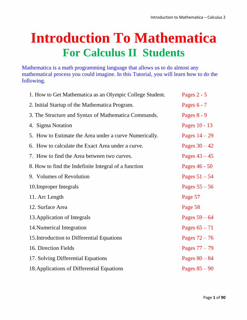
We can generalize the sigma sums by replacing the end term by n
Example 3: Find the general formulas for the following sigma sums.
(a)
n
k 1
1 (b)
n
k
k1
(c)
n
k
k1
2 (d)
n
k
k1
3
Input 1(a):
n
k 1
1 Output 𝑛
Input 1(b):
n
k
k1
Output 1
2𝑛(1 + 𝑛)
Input 1(c):
n
k
k1
2 Output 1
6𝑛(1 + 𝑛)(1 + 2𝑛)
Input 1(d):
n
k
k1
3 0utput 1
4𝑛2(1 + 𝑛)2
It can be shown that the following properties involving the summation of terms using sigma notation are true but we will in this class just accept their validity.
Property 1: For any constant c nccn
k
1
Property 2: For any constant c
n
k
k
n
k
i acca11
Property 3: The addition property
n
k
k
n
k
kk
n
k
k baba111
Property 4: The subtraction property
n
k
k
n
k
kk
n
k
k baba111
Note 1: It is not true that
n
k
k
n
k
kk
n
k
k baba111
Note 2: It is not true that
n
k
k
n
k
kn
k k
k
a
a
b
a
1
1
1
Introduction to Mathematica – Calculus 2
Page 14 of 90
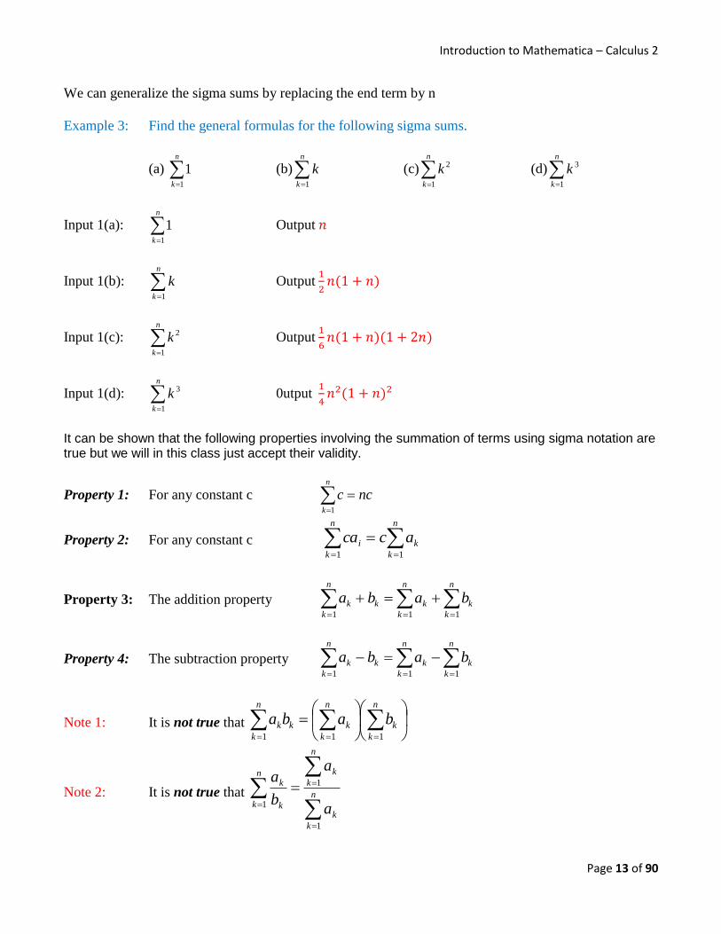
5. How to Estimate the Area under a curve Numerically.
The essential problem here is how to estimate the area under a curve using numerical methods..
Example 4: Estimate the area under the curve f(x) = 5 + 4𝑥 − 𝑥2 − 𝑥3 from x = 0 to 2 using 4 strips.
If you graph f(x) in the Domain [0,2] you get the following curve.
One approach is split the shape into 4 equally spaced strips in the interval [0,2] , We will call the size of
any one of these strips ∆𝑥 = 2−0
4 = 0.5 (∆𝑥 is called delta x). The 4 strips will generate five
x coordinates they will be called x0 = 0 , x1 = 0.5 , x2 = 1 , x3 = 1.5 and x4 = 2
We will then have a diagram that looks like the following.
0.0 0.5 1.0 1.5 2.0
2
4
6
8
0.0 0.5 1.0 1.5 2.0
2
4
6
8

Introduction to Mathematica – Calculus 2
Page 15 of 90
From these 4 strips, we can create 4 rectangles and the total area of these 4 rectangles will give us a
numerical approximation of the area under this curve.
We do however have a choice here because for each strip you could use either the left endpoint or the
right endpoint to define the rectangles heights.
So, the convention is to use the notation L4 to indicate we are using the Left endpoint and R4 to indicate
we are using the Right endpoint to define the heights of the rectangles.
These two choices result in different approximations to the area under the curve.
The value of L4 is an estimate for the area under the curve f(x) = 1 + 6x – x2 – x3 from x = 0 to x = 2
L4 = ∆𝑥𝑓(𝑥0) + ∆𝑥𝑓(𝑥1) + ∆𝑥𝑓(𝑥2) + ∆𝑥𝑓(𝑥3)
= 0.5𝑓(0) + 0.5𝑓(0.5) + 0.5𝑓(1.0) + 0.5𝑓(1.5)
= 0.5(5) + 0.5(6.625) + 0.5(7) + 0.5(5.375)
L4 = 12
Note 1: The width of each strip is found by calculating ∆𝑥 = 2−0
4 this can be generalized to n
strips. So, if you wish to find the width of a single strip ∆𝑥 when the interval from x = a
to x = b is split into n strips we use the formula
∆𝑥 = 𝑏−𝑎
𝑛
Note 2: We ca also generalize the values of the x coordinates x0 , x1 , etc… by using the formula
𝑥𝑘 = 𝑎 + 𝑘∆𝑥
0.0 0.5 1.0 1.5 2.0
2
4
6
8

Introduction to Mathematica – Calculus 2
Page 16 of 90
If we use the Right endpoints and calculate R4 as an estimate for the area under the curve we get the
situation below.
The value of R4 is an estimate for the area under the curve f(x) = 5 + 4𝑥 − 𝑥2 − 𝑥3 from x = 0 to 2.
R4 = ∆𝑥𝑓(𝑥1) + ∆𝑥𝑓(𝑥2) + ∆𝑥𝑓(𝑥3) + ∆𝑥𝑓(𝑥4)
= 0.5𝑓(0.5) + 0.5𝑓(1.0) + 0.5𝑓(1.5) + 0.5𝑓(2)
= 0.5(6.625) + 0.5(7) + 0.5(5.375) + 0.5(1)
R4 = 10
We could reduce the workload by letting Mathematica do most of the number crunching for us
We start by realizing that the general formula for calculating R4 is
R4 =
4
1
][k
kxfx where ∆𝑥 = 𝑏−𝑎
𝑛 and xk = a + ∆𝑥𝑘
In this example R4 =
4
1
]0[k
kxfx as ∆𝑥 = 2−0
4 and xk = 0 + ∆𝑥𝑘
The code for finding R4 is Input: 𝑓[x_]: = 5 + 4𝑥 − 𝑥2 − 𝑥3
deltax =2−0
4;
∑ deltax𝑓[0 + deltax 𝑘]4
𝑘=1
Output: 10
Note : We called the variable ∆x , deltax as all variables need to start with small alphanumeric
letters also we needed to add a space between the variables deltax and k to separate the two
variables.
0.0 0.5 1.0 1.5 2.0
2
4
6
8
Introduction to Mathematica – Calculus 2
Page 17 of 90
In a similar fashion the code for calculating L4 is.
Input: 𝑓[x_]: = 5 + 4𝑥 − 𝑥2 − 𝑥3
deltax =2−0
4;
3
0
]0[k
kdeltaxfdeltax
Output: 12
Note 1: There is a semicolon” ; “after the command deltax =2−0
4; this is just a suppressant
command, it tells Mathematica to do the command but not show the result as part of the
output. This is a useful trick as it can be a distraction to see all the outputs from various
calculations in a Mathematica program, when all you want to see if the final result.
Note 2: The estimates L4 = 12 and R4 = 10 are different, this is very common in using these
estimates and it is often not obvious that any one of the two is a better estimate than the
other.
Note 2: If you want to get a more accurate estimate then you will need to evaluate more
rectangles so instead of n = 4 strips you could use n = 10 strips or n = 400 strips.
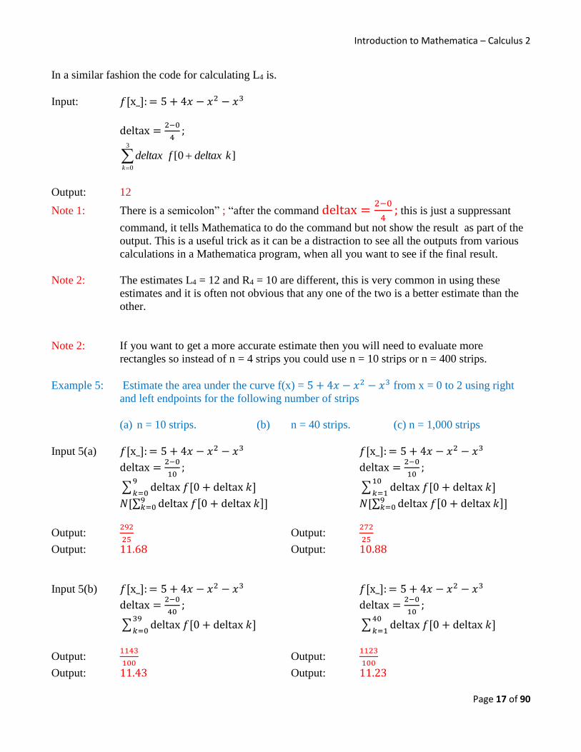
Example 5: Estimate the area under the curve f(x) = 5 + 4𝑥 − 𝑥2 − 𝑥3 from x = 0 to 2 using right
and left endpoints for the following number of strips
(a) n = 10 strips. (b) n = 40 strips. (c) n = 1,000 strips
Input 5(a) 𝑓[x_]: = 5 + 4𝑥 − 𝑥2 − 𝑥3 𝑓[x_]: = 5 + 4𝑥 − 𝑥2 − 𝑥3
deltax =2−0
10; deltax =
2−0
10;
∑ deltax 𝑓[0 + deltax 𝑘]9
𝑘=0 ∑ deltax 𝑓[0 + deltax 𝑘]
10
𝑘=1
𝑁[∑ deltax 𝑓[0 + deltax 𝑘]9𝑘=0 ] 𝑁[∑ deltax 𝑓[0 + deltax 𝑘]9
𝑘=0 ]
Output: 292
25 Output:
272
25
Output: 11.68 Output: 10.88
Input 5(b) 𝑓[x_]: = 5 + 4𝑥 − 𝑥2 − 𝑥3 𝑓[x_]: = 5 + 4𝑥 − 𝑥2 − 𝑥3
deltax =2−0
40; deltax =
2−0
10;
∑ deltax 𝑓[0 + deltax 𝑘]39
𝑘=0 ∑ deltax 𝑓[0 + deltax 𝑘]
40
𝑘=1
Output: 1143
100 Output:
1123
100
Output: 11.43 Output: 11.23

Introduction to Mathematica – Calculus 2
Page 18 of 90
Input 5(c) 𝑓[x_]: = 5 + 4𝑥 − 𝑥2 − 𝑥3 𝑓[x_]: = 5 + 4𝑥 − 𝑥2 − 𝑥3
deltax =2−0
1000; deltax =
2−0
1000;
∑ deltax 𝑓[0 + deltax 𝑘]999
𝑘=0 ∑ deltax 𝑓[0 + deltax 𝑘]
1000
𝑘=1
Output: 708583
62500 Output:
1123
100
Output: 11.3373 Output: 11.3293
Example 6: Estimate the area under the curve f(x) = sin(𝑥) + 𝑥2 from x = 0 to 2𝜋 using 20 strips.
Input: 𝑓[x_]: = Sin[𝑥] + 𝑥2
deltax =2𝜋−0
20;
∑ deltax 𝑓[0 + deltax 𝑘]19
𝑘=0; (*the value of L20 *)
𝑁[∑ deltax 𝑓[0 + deltax 𝑘]9
𝑘=0]
Output: 77.5855
Input: 𝑓[x_]: = Sin[𝑥] + 𝑥2
deltax =2𝜋−0
20;
∑ deltax 𝑓[0 + deltax 𝑘]20
𝑘=1; (*the value of L20 *)
𝑁[∑ deltax 𝑓[0 + deltax 𝑘]20
𝑘=1]
Output: 88.988

Introduction to Mathematica – Calculus 2
Page 19 of 90
Example 7. Estimate the area under the graph f(x) = 9 – x2 from x = – 2 to x = 2 by calculating using 4 approximating rectangles L4 , R4
Solution: If we wish to do it by hand then we will do The following.
We start by calculating a table of values for the function f(x) = 9 – x2
starting with x = – 2 with a ∆x = 𝑏−𝑎
𝑛 =
2−(−2)
4 = 1
The next step is to estimate the area under the curve by calculation L4 , called the Left estimate, this is done by using the 4 left end points as the sample points.
The interval size will be ∆x = 𝑏−𝑎
𝑛 =
2−(−2)
4 = 1
The sample points will be x0 = – 2 x1 = – 1 x2 = 0 and x3 = 1
L4 = ∑ ∆𝑥𝑓(𝑥𝑘)3𝑘=0
= 1f(x0) + 1f(x1) +1f(x2) +1f(x3) = 1f(– 2) + 1f(– 1) + 1f(0) + 1f(1)
= 5 + 8 + 9 + 8 L4 = 30 If we use Mathematica the code will be as follows Input: 𝑓[x_]: = 9 − 𝑥2 𝑎 = −2; (* 𝑎 = −2 *) 𝑏 = 2; (* 𝑏 = 2 *) 𝑛 = 4; (* the number of strips 𝑛 = 4 *)
deltax =𝑏−𝑎
4;
∑ deltax 𝑓[𝑎 + deltax 𝑘]𝑛−1
𝑘=0; (* the value of L4 *)
𝑁[∑ deltax 𝑓[𝑎 + deltax 𝑘]𝑛−1
𝑘=0]
Output: 30 Note 1: We generalized the formula by creating the estimate L4 by using the variables called a , b , n and
delta x this allowed us to create a program that would be adaptable to many other situations. For example, if you wanted 10 strips – just change the value of n to n = 10.
If you wanted to change the start or finish values, just change the values of a and b in the code or you could even change the function by changing f[x_].
Note 2: Notice that for L4 the sigma notation is ∑ … … … . ]𝑛−1
𝑘=0
x0 x1 x2 x3 x4
x – 2 – 1 0 1 2
f(x) 5 8 9 8 5
x0 x1 x2 x3 x4
x – 2 – 1 0 1 2
f(x) 5 8 9 8 5

Introduction to Mathematica – Calculus 2
Page 20 of 90
Solution: We estimate the area under the curve by calculation R4 , called the Right estimate, this is done by using the 4 right end points as the sample points.
The interval size will be ∆x = 𝑏−𝑎
𝑛 =
2−(−2)
4 = 1
The sample points will be x1 = – 1 x2 = 0 x3 = 1 and x4 = 2
R4 = ∑ ∆𝑥𝑓(𝑥𝑘)4𝑘=1
= 1f(x1) +1f(x2) +1f(x3) + 1f(x4) = 1f(– 1) + 1f(0) + 1f(1) + 1f(2)
= 8 + 9 + 8 + 5 = 30 If we use Mathematica the code will be as follows Input: 𝑓[x_]: = 9 − 𝑥2 𝑎 = −2; (* 𝑎 = −2 *) 𝑏 = 2; (* 𝑏 = 2 *) 𝑛 = 4; (* the number of strips 𝑛 = 4 *)
deltax =𝑏−𝑎
4;
∑ deltax 𝑓[𝑎 + deltax 𝑘]𝑛
𝑘=1; (*the value of R4* )
𝑁[∑ deltax 𝑓[𝑎 + deltax 𝑘]𝑛
𝑘=1]
Output: 30 Note 1: We generalized the formula by creating the estimate R4 by using the variables called a , b , n
and delta x this allowed us to create a program that would be adaptable to many other situations. For example, if you wanted 10 strips – just change the value of n to n = 10.
If you wanted to change the start or finish values, just change the values of a and b in the code or you could even change the function by changing f[x_].
Note 2: Notice that for R4 the sigma notation is ∑ … … … . ]𝑛
𝑘=1
Note 3: Both these estimates of the area under the curve are identical , this is very unusual situation
and typically the two estimates will be different values.
x0 x1 x2 x3 x4
x – 2 – 1 0 1 2
f(x) 5 8 9 8 5

Introduction to Mathematica – Calculus 2
Page 21 of 90
Example 8. Estimate the area under the graph f(x) = √𝑥 from x = 0 to x = 8 by calculating the 4 approximating rectangles L4 , R4 and M4
We start by calculating a table of values
for the function f(x) = √𝑥 starting with x = 0
with a ∆x = 𝑏−𝑎
𝑛 =
8−0
4 = 2
Solution: We estimate the area under the curve by calculation L5 , called the Left estimate, this is done by
using the 4 left end points as the sample points. The interval size will be ∆x = 𝑏−𝑎
𝑛 =
8−0
2 = 4
The sample points will be x0 = 0 x1 = 2 x2 = 4 x3 = 6
L4 = ∑ ∆𝑥𝑓(𝑥𝑘−1)3𝑘=0
= 2.f(x0) + 2.f(x1) +2.f(x2) +2.f(x3)
= 2f(0) + 2f(2) + 2f(4) + 2f(6)
= 2[ 0 + √2 + 2 + √6 ] = 2[5.864] = 11.728
If we use Mathematica the code will be as follows
Input: 𝑓[x_]: = √𝑥 𝑎 = 0; (* 𝑎 = 0 *) 𝑏 = 8; (* 𝑏 = 8 *) 𝑛 = 4; (* the number of strips 𝑛 = 4 *)
deltax =𝑏−𝑎
4;
∑ deltax 𝑓[𝑎 + deltax 𝑘]𝑛
𝑘=1; (*the value of R4* )
𝑁[∑ deltax 𝑓[𝑎 + deltax 𝑘]𝑛
𝑘=1]
Output: 11.7274
x0 x1 x2 x3 x4
x 0 2 4 6 8
f(x) 0 √2 2 √6 √8
x0 x1 x2 x3 x4
x 0 2 4 6 8
f(x) 0 √2 2 √6 √8

Introduction to Mathematica – Calculus 2
Page 22 of 90
Solution: We estimate the area under the curve by calculation R4 , called the Right estimate, this is done by using the 4 right end points as the sample points.
The interval size will be ∆x = 𝑏−𝑎
𝑛 =
8−0
2 = 4
The sample points will be x1 = 2 x2 = 4 x3 = 6 x4 = 8
R4 = ∑ ∆𝑥𝑓(𝑥𝑘)4𝑘=1
= 2f(x1) +2f(x2) +2f(x3) + 2f(x4)
= 2[f(2) + f(4) + f(6) + f(8) ]
= 2[ √2 + 2 + √6 + √8 ]
= 2[8.692] = 17.384
If we use Mathematica the code will be as follows
Input: 𝑓[x_]: = √𝑥 𝑎 = 0; (* 𝑎 = 0 *) 𝑏 = 8; (* 𝑏 = 8 *) 𝑛 = 4; (* the number of strips 𝑛 = 4 *)
deltax =𝑏−𝑎
4;
∑ deltax 𝑓[𝑎 + deltax 𝑘]𝑛
𝑘=1; (* the value of R4 * )
𝑁[∑ deltax 𝑓[𝑎 + deltax 𝑘]𝑛
𝑘=1]
Output: 11.3843
x0 x1 x2 x3 x4
x 0 2 4 6 8
f(x) 0 √2 2 √6 √8

Introduction to Mathematica – Calculus 2
Page 23 of 90
Solution: We now estimate the area under the curve by calculation M4 , called the midpoint
estimate, this is done by using the 4 midpoints as the sample points.
The interval size will be ∆x = 𝑏−𝑎
𝑛 =
8−0
2 = 4
For example, the value of 𝑥1∗ is the midpoint between x0 and x1 and is found by
evaluating
𝑥1∗ =
𝑥0 + 𝑥1
2
In general, the kth midpoint 𝑥𝑘∗ will be between xk-1 and xk and its value is 𝑥𝑘
∗ = 𝑥𝑘−1+ 𝑥𝑘
2
Since xk-1 = 𝑎 + ∆𝑥 (𝑘 − 1) xk = 𝑎 + ∆𝑥 𝑘
𝑥𝑘∗ =
𝑎+∆𝑥 𝑘+𝑎+∆𝑥 𝑘(𝑘−1)
2
= 2𝑎+ ∆𝑥(2 𝑘−1)
2
𝑥𝑘∗ = 𝑎 +
∆𝑥(2 𝑘−1)
2
The sample midpoints will be 𝑥1
∗ = 1 𝑥2∗ = 3 𝑥3
∗ = 5 𝑥4∗ = 7
M4 = ∑ ∆𝑥𝑓(𝑥𝑘∗)4
𝑘=1
= 2f(𝑥1∗) +2f(𝑥2
∗) +2f(𝑥3∗) + 2f(𝑥4
∗)
= 2[f(1) + f(3) + f(5) + f(7) ]
= 2[1+ √3 + √5 + √7 ]
= 2[7.614]
= 15.288
If we use Mathematica the code will be as follows
Input: 𝑓[x_]: = √𝑥 𝑎 = 0; (* 𝑎 = 0 *) 𝑏 = 8; (* 𝑏 = 8 *) 𝑛 = 4; (* the number of strips 𝑛 = 4 *)
deltax =𝑏−𝑎
4;
∑ deltax 𝑓[𝑎 +deltax (2𝑘−1)
2]
𝑛
𝑘=1; (* the value of R4 * )
𝑁[∑ deltax 𝑓[𝑎 + deltax 𝑘]𝑛
𝑘=1]
Output: 15.2277
x0 𝑥1∗
x1 𝑥2∗ x2 𝑥3
∗ x3 𝑥4∗ x4
x 0 1 2 3 4 5 6 7 8
f(x) 0 1 √2 √6 2 √5 √6 √7 √8
Introduction to Mathematica – Calculus 2
Page 24 of 90
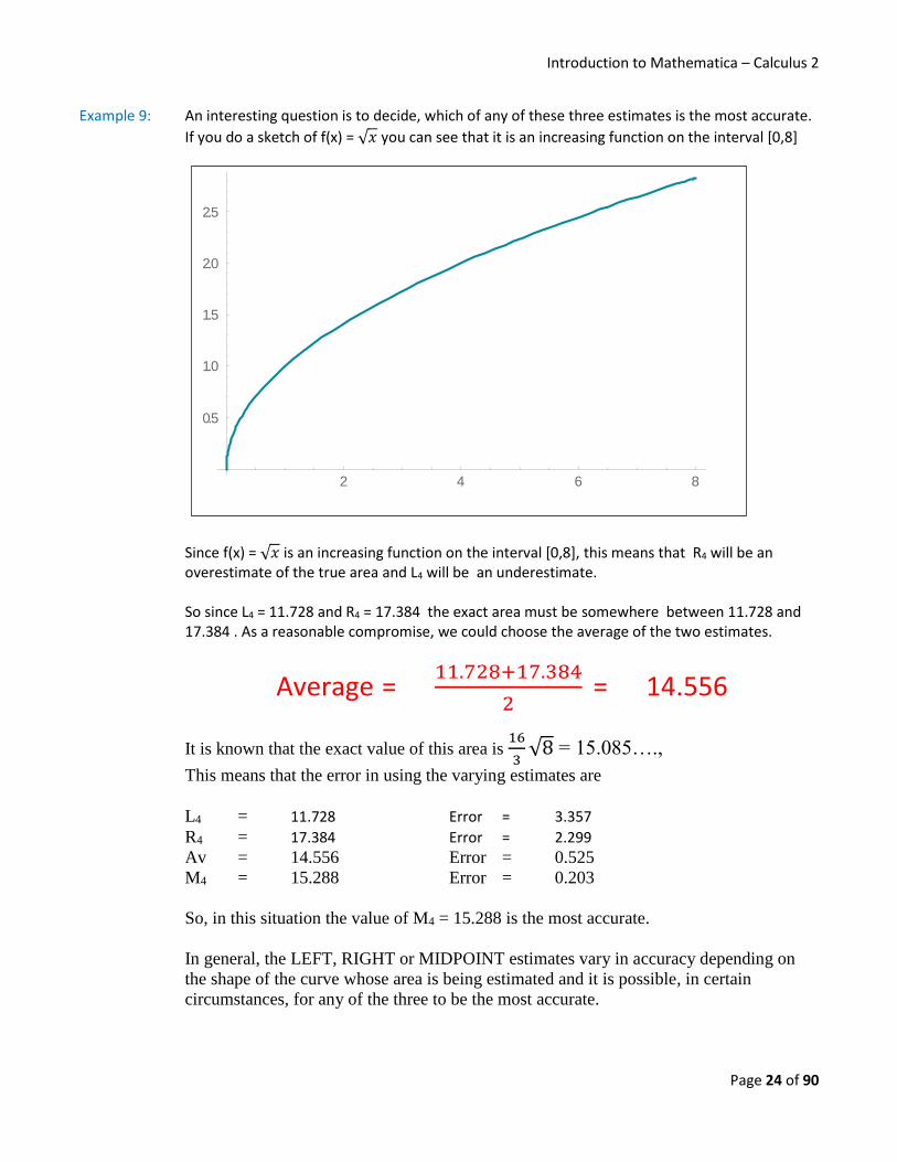
Example 9: An interesting question is to decide, which of any of these three estimates is the most accurate.
If you do a sketch of f(x) = √𝑥 you can see that it is an increasing function on the interval [0,8]
Since f(x) = √𝑥 is an increasing function on the interval [0,8], this means that R4 will be an overestimate of the true area and L4 will be an underestimate. So since L4 = 11.728 and R4 = 17.384 the exact area must be somewhere between 11.728 and 17.384 . As a reasonable compromise, we could choose the average of the two estimates.
Average = 11.728+17.384
2 = 14.556
It is known that the exact value of this area is 16
3√8 = 15.085….,
This means that the error in using the varying estimates are
L4 = 11.728 Error = 3.357
R4 = 17.384 Error = 2.299
Av = 14.556 Error = 0.525
M4 = 15.288 Error = 0.203
So, in this situation the value of M4 = 15.288 is the most accurate.
In general, the LEFT, RIGHT or MIDPOINT estimates vary in accuracy depending on
the shape of the curve whose area is being estimated and it is possible, in certain
circumstances, for any of the three to be the most accurate.
2 4 6 8
0.5
1.0
1.5
2.0
2.5

Introduction to Mathematica – Calculus 2
Page 25 of 90
Example 10: Estimate the area under the curve given by the table of values, using N= 6 (6 strips) and using
(a) L6 (b) R6 (c) M6
Solution: Since we are using n = 6 strips we will have ∆x = 𝑏−𝑎
𝑛 =
12−0
6 = 2 and the sample points in the
table will be. x0 = 0 x1 = 2 x2 = 4 x3 = 6 x4 = 8 x5 = 10 and x6 = 12
We estimate the area under the curve by calculation L6 , called the Left estimate, this is done by using the 6 left end points as the sample points.
The interval size will be ∆x = 𝑏−𝑎
𝑛 =
12−0
6 = 2
The sample points will be x0 = 0 x1 = 2 x2 = 4 x3 = 6 x4 = 8 and x5 = 10
L6 = ∑ ∆𝑥𝑓(𝑥𝑘)5𝑘=0
= 2f(x0) + 2f(x1) +2f(x2) +2f(x3) + 2f(x4) + 2f(x5 = 2f(0) + 2f(2) + 2f(4) + 2f(6) + 2f(8) + 2f(10)
= 2[f(0) +f(2) + f(4) + f(6) + f(8) + f(10) = 2[9 + 8.8 + 8.2 + 7.3 + 5.9 + 4.1] = 2[43.3] L6 = 86.6
The Mathematica code for this calculation is
Input: deltax =12−0
6;
left6 = deltax(9 + 8.8 + 8.2 + 7.3 + 5.9 + 4.1)
Output: 86.6
x0 x1 x2 x3 x4 x5 x6
x 0 1 2 3 4 5 6 7 8 9 10 11 12
f(x) 9 8.9 8.8 8.5 8.2 7.8 7.3 6.6 5.9 5.1 4.1 2.8 1
x0 x1 x2 x3 x4 x5 x6
x 0 1 2 3 4 5 6 7 8 9 10 11 12
f(x) 9 8.9 8.8 8.5 8.2 7.8 7.3 6.6 5.9 5.1 4.1 2.8 1
x 0 1 2 3 4 5 6 7 8 9 10 11 12
f(x) 9 8.9 8.8 8.5 8.2 7.8 7.3 6.6 5.9 5.1 4.1 2.8 1

Introduction to Mathematica – Calculus 2
Page 26 of 90
Solution: We estimate the area under the curve by calculation R6 , called the Right estimate, this is done by using the 6 right end points as the sample points.
The interval size will be ∆x = 𝑏−𝑎
𝑛 =
12−0
6 = 2
The sample points will be x1 = 2 x2 = 4 x3 = 6 x4 = 8 x5 = 10 and x6 = 12
R6 = ∑ ∆𝑥𝑓(𝑥𝑘)6𝑘=1
= 2f(x1) +2f(x2) +2f(x3) + 2f(x4) + 2f(x5) + 2f(x6) = 2f(2) + 2f(4) + 2f(6) + 2f(8) + 2f(10) + 2f(12)
= 2[f(2) + f(4) + f(6) + f(8) + f(10) + f(12) = 2[8.8 + 8.2 + 7.3 + 5.9 + 4.1 + 1] = 2[35.3] = 70.6
The Mathematica code for this calculation is
Input: deltax =12−0
6;
right6 = deltax(9 + 8.8 + 8.2 + 7.3 + 5.9 + 4.1)
Output: 70.6 Note: The Mathematica code for this calculation is not very efficient and the same calculation could
easily be done on a calculator
x0 x1 x2 x3 x4 x5 x6
x 0 1 2 3 4 5 6 7 8 9 10 11 12
f(x) 9 8.9 8.8 8.5 8.2 7.8 7.3 6.6 5.9 5.1 4.1 2.8 1

Introduction to Mathematica – Calculus 2
Page 27 of 90
Solution: We estimate the area under the curve by calculation M6 , called the Mid-point estimate, this is done by using the 6 mid-points as the sample points.
The interval size will be ∆x = 𝑏−𝑎
𝑛 =
12−0
6 = 2
The sample points will be 𝑥1
∗ = 1 𝑥2∗ = 3 𝑥3
∗ = 5 𝑥4∗ = 7 𝑥5
∗ = 9 and 𝑥6∗ = 11
M6 = ∑ ∆𝑥𝑓(𝑥𝑘∗)6
𝑘=1
= 2f(𝑥1∗) +2f(𝑥2
∗) +2f(𝑥3∗) + 2f(𝑥4
∗) + 2f(𝑥5∗) + 2f(𝑥6
∗) = 2f(1) + 2f(3) + 2f(5) + 2f(7) + 2f(9) + 2f(11)
= 2[f(1) + f(3) + f(5) + f(7) + f(9) + f(11)] = 2[8.9 + 8.5 + 7.8 + 6.6 + 5.1 + 2.8] = 2[39.7]
= 79.4 The Mathematica code for this calculation is
Input: deltax =12−0
6;
mid6 = deltax(8.9 + 8.5 + 7.8 + 6.6 + 5.1 + 2.8)
Output: 79.4
Note 1: An interesting question is to decide, which of any of these three estimates is the most
accurate. By looking at the values of f|(x) we can assume that that the function f(x) is
probably decreasing.
This means that L6 is an overestimate since all the rectangles are larger than the area they
are estimating.
While R6 is an underestimate since all the rectangles are smaller than the area they are
estimating.
So, the exact area is probably somewhere between 70.6 and 79.4
Note 2: We could use 70.6+79.4
2 = 75 as another estimate of the true area under the curve.
x0 𝑥1∗
x1 𝑥2∗ x2 𝑥3
∗ x3 𝑥4∗ x4 𝑥5
∗ x5 𝑥6
∗ x6
x 0 1 2 3 4 5 6 7 8 9 10 11 12
f(x) 9 8.9 8.8 8.5 8.2 7.8 7.3 6.6 5.9 5.1 4.1 2.8 1

Introduction to Mathematica – Calculus 2
Page 28 of 90
Example 11: The velocity of a motorcycle over a 60 second period is given in the table below Find an estimate for the distance travelled by the motorcycle over 60 seconds Solution: The distance travelled by the motorcycle over 60 seconds is the same as the area under
the curve in the interval [0,60], as our first estimate we will use L5.
The interval size will be ∆t = 𝑏−𝑎
𝑛 =
60−0
5 =12
The sample points will be t0 = 0 t1 = 12 t2 = 24 t3 = 36 and t4 = 48
distance travelled = d ≈ L5
= ∑ ∆𝑡𝑉(𝑥𝑖−1)5𝑖=0
= 12V(t0) + 12V(t1) +12V(t2) +12V(t3) + 12V(t4)
= 12[V(0) + V(12) + V(24) + V(36) + V(48)] = 12[30 + 28 + 25 + 22 + 24] = 1548 feet
The Mathematica code for this calculation is
Input: deltax =60−0
5;
left5 = deltax(30 + 28 + 25 + 22 + 241)
Output: 1548
t 0 12 24 36 48 60
V(t) 9 8.9 8.8 8.5 8.2 7.8
t0 t1 t2 t3 t4 t5
t 0 12 24 36 48 60
V(t) 9 8.9 8.8 8.5 8.2 7.8
Introduction to Mathematica – Calculus 2
Page 29 of 90
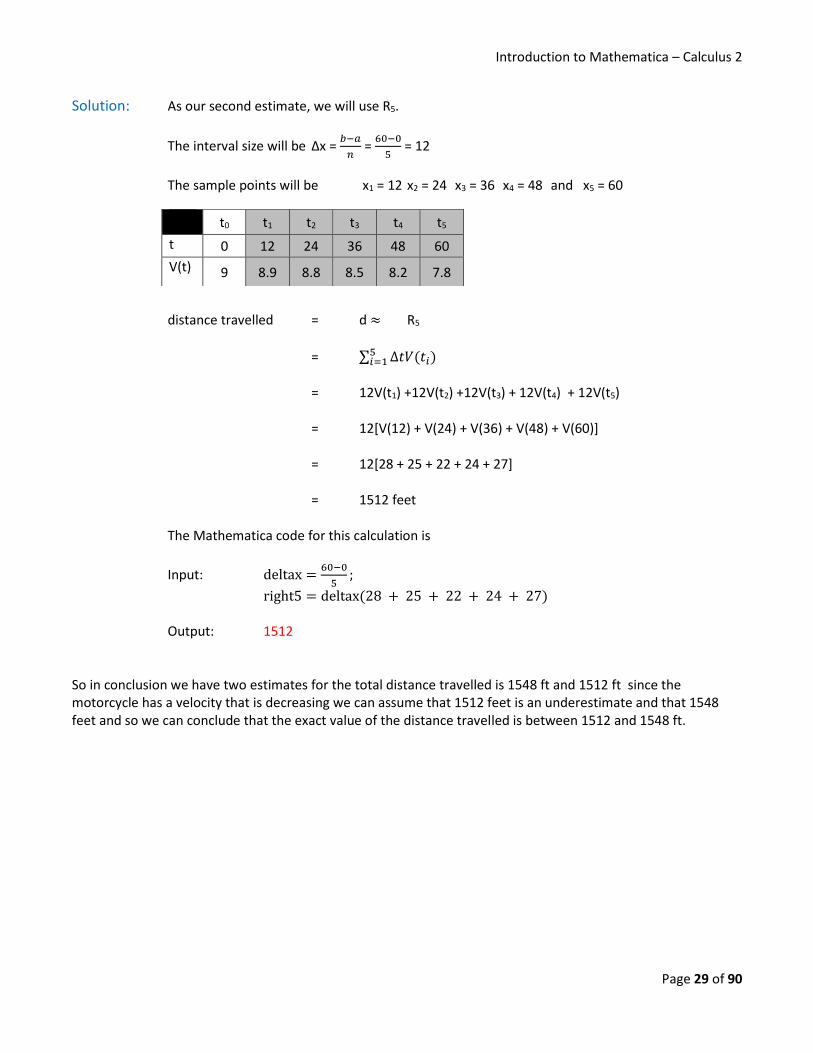
Solution: As our second estimate, we will use R5.
The interval size will be ∆x = 𝑏−𝑎
𝑛 =
60−0
5 = 12
The sample points will be x1 = 12 x2 = 24 x3 = 36 x4 = 48 and x5 = 60
distance travelled = d ≈ R5
= ∑ ∆𝑡𝑉(𝑡𝑖)5𝑖=1
= 12V(t1) +12V(t2) +12V(t3) + 12V(t4) + 12V(t5) = 12[V(12) + V(24) + V(36) + V(48) + V(60)] = 12[28 + 25 + 22 + 24 + 27] = 1512 feet
The Mathematica code for this calculation is
Input: deltax =60−0
5;
right5 = deltax(28 + 25 + 22 + 24 + 27)
Output: 1512 So in conclusion we have two estimates for the total distance travelled is 1548 ft and 1512 ft since the motorcycle has a velocity that is decreasing we can assume that 1512 feet is an underestimate and that 1548 feet and so we can conclude that the exact value of the distance travelled is between 1512 and 1548 ft.
t0 t1 t2 t3 t4 t5
t 0 12 24 36 48 60
V(t) 9 8.9 8.8 8.5 8.2 7.8
Introduction to Mathematica – Calculus 2
Page 30 of 90
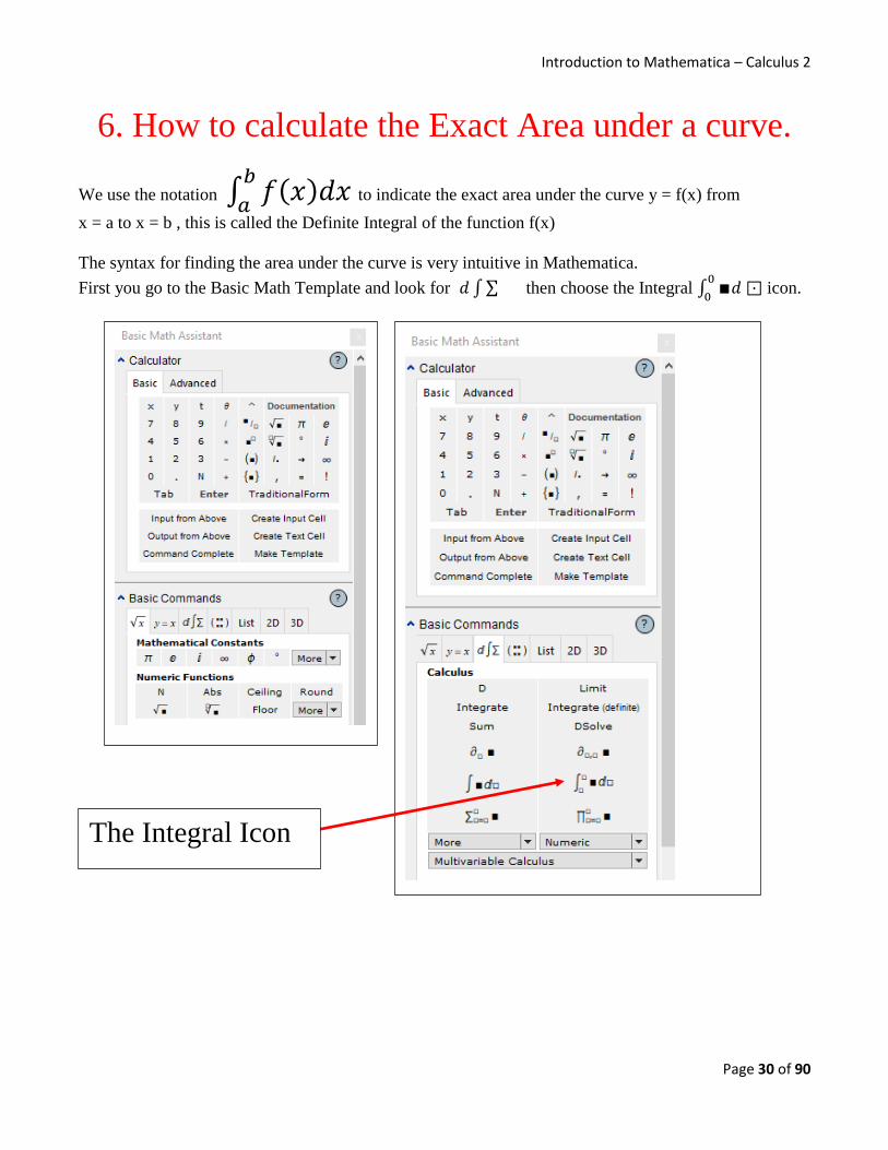
6. How to calculate the Exact Area under a curve.
We use the notation ∫ 𝑓(𝑥)𝑑𝑥𝑏
𝑎 to indicate the exact area under the curve y = f(x) from
x = a to x = b , this is called the Definite Integral of the function f(x)
The syntax for finding the area under the curve is very intuitive in Mathematica.
First you go to the Basic Math Template and look for 𝑑 ∫ ∑ then choose the Integral ∫ ∎𝑑 ⊡0
0 icon.
The Integral Icon

Introduction to Mathematica – Calculus 2
Page 31 of 90
You will now see the following
To complete the Integral Command, Click on each part of the template above.
lower will be replaced by the value of a.
upper will be replaced by the value of b.
expr will be replaced by the function f(x) with (……) round it.
var Will be replaced by the variable (usually x).
Example 12: Find the exact value of ∫ (𝑥3 − 𝑥 + 1)𝑑𝑥5
1
Get the integral template,
lower will be replaced by 1.
upper will be replaced with 5.
expr will be replaced by (x3 – x +1)
var will be replaced by x
You then press the Number Pad ENTER Key. The output will be 148

Introduction to Mathematica – Calculus 2
Page 32 of 90
Example 13: Find the exact area under the curve for the following functions.
(a) ∫ (2𝑥3 − 𝑥2)𝑑𝑥3
1
(b) ∫ (sin(𝑥) + 2cos (𝑥))𝑑𝑥2𝜋
−𝜋
(c) ∫ (𝑥
𝑥+1) 𝑑𝑥
4
0
(d) ∫ (𝑥2 − 9)𝑑𝑥3
−3
Input (a): ∫ (2𝑥3 − 𝑥2) 𝑑𝑥3
1
Output: 94
3
Input (b): ∫ (Sin[𝑥] + 2Cos[𝑥]) 𝑑𝑥𝜋
−𝜋
Output: 0
Input (c): ∫ (𝑥
𝑥+1) 𝑑𝑥
4
0
Output: 4 − Log[5]
Input (d): ∫ (2𝑥3 − 𝑥2) 𝑑𝑥3
1:
Output: −36
Note: The area under a curve can be any value, positive negative or even zero.
This becomes clearer when you see the areas graphically.

Introduction to Mathematica – Calculus 2
Page 33 of 90
Example 14: Graph the area under the curve for the following functions.
(a) ∫ (2𝑥3 − 𝑥2)𝑑𝑥3
1 (b) ∫ (sin(𝑥) + 2cos (𝑥))𝑑𝑥
2𝜋
−𝜋
(c) ∫ (𝑥
𝑥+1) 𝑑𝑥
4
0 (d) ∫ (𝑥2 − 9)𝑑𝑥
3
−3
Input (a): Plot[2𝑥3 − 𝑥2, {𝑥, 1,3}, Filling → Axis]
Output:
Input (b): Plot[Sin[𝑥] + 2Cos[𝑥], {𝑥, −𝜋, 𝜋}, Filling → Axis]
Output:
Notice – that this integral
∫(2𝑥3 − 𝑥2)𝑑𝑥
3
1
Has a positive area as all the curve is above the x-axis
Notice – that this integral
∫ (sin(𝑥) + 2cos (𝑥))𝑑𝑥
2𝜋
−𝜋
Has an area of zero the positive area above the x-axis matches the negative area below the x-axis

Introduction to Mathematica – Calculus 2
Page 34 of 90
Input (c): Plot[𝑥
𝑥+1, {𝑥, 0,4}, Filling → Axis]
Output:
Input (b): Plot[𝑥2 − 9, {𝑥, −3,3}, Filling → Axis]
Output:
Notice – that this integral
∫ (𝑥
𝑥+1) 𝑑𝑥
4
0
Has a positive area as all the curve is above the x-axis
Notice – that this integral
∫(𝑥2 − 9)𝑑𝑥
3
−3
Has a negative area as all of the curve is below the x-axis

Introduction to Mathematica – Calculus 2
Page 35 of 90
A. How to calculate the Errors in Estimating the Area under a curve Numerically.
There are two measurements of error that are typically used they are called the Absolute Error and the
Relative Error they are defined as follows.
Absolute Error = |𝐸𝑥𝑎𝑐𝑡 𝑉𝑎𝑙𝑢𝑒 − 𝐸𝑠𝑡𝑖𝑚𝑎𝑡𝑒𝑑 𝑉𝑎𝑙𝑢𝑒|
Relative Error = |𝐸𝑥𝑎𝑐𝑡 𝑉𝑎𝑙𝑢𝑒−𝐸𝑠𝑡𝑖𝑚𝑎𝑡𝑒𝑑 𝑉𝑎𝑙𝑢𝑒|
𝐸𝑥𝑎𝑐𝑡 𝑉𝑎𝑙𝑢𝑒𝑋 100
Example 15: What are the Absolute and Relative Errors in using L10 and L1000 to estimate the area
∫ (5 + 4𝑥 − 𝑥2 − 𝑥3)2
0dx.
Input: 𝑓[x_]: = 5 + 4𝑥 − 𝑥2 − 𝑥3
exact = ∫ 𝑓[𝑥] 𝑑𝑥2
0;
deltax =2−0
10;
estimate = 𝑁[∑ deltax𝑓[0 + deltax𝑘]9
𝑘=0];
abserror = Abs[exact − estimate]
relerror = Abs[(exact−estimate
exact)100]
Output: 0.346667
Output: 3.05882
Input: 𝑓[x_]: = 5 + 4𝑥 − 𝑥2 − 𝑥3
exact = ∫ 𝑓[𝑥] 𝑑𝑥2
0;
deltax =2−0
1000;
estimate = 𝑁[∑ deltax𝑓[0 + deltax𝑘]999
𝑘=0];
abserror = Abs[exact − estimate]
relerror = Abs[(exact−estimate
exact)100]
Output: 0.0039947
Output: 0.0352471
Note 1: As you increase the number of strips the accuracy of the estimate becomes greater so
L1000 = 11.3373 has only an Absolute error of approximately 0.004 which is a more
accurate estimate than L10 = 11.68 which has an Absolute error of 0.35
Note 2: In general, if you want a very accurate estimate of the area under a curve choose a value
of n as large as is practical.

Introduction to Mathematica – Calculus 2
Page 36 of 90
B. How to Find the Exact Area under a curve using Sigma Notation.
To find the exact under a curve we generalise the concept of splitting the shape into a large number of
rectangular strips and then adding up all these strips together.
For example, suppose we want to know the area under the curve y = f(x) from x = a to x = b.
as shown in the diagram below.
The method used is to approximate this area by splitting the area into n equal strips of width ∆𝑥 .
The width of each rectangle ∆𝑥 =𝑏−𝑎
𝑛 we then construct rectangles using these strips.
We next start with the first point with x coordinate x0 = a
the next point will have x coordinate x1 = a + ∆𝑥
x2 = a + 2∆𝑥
The coordinate of the general x-coordinate xk is xk = a + 𝑘∆𝑥
and so on until we reach the last x coordinate xn = b.
These n + 1 points x0 , x1 , x2 , ……. , xn are called the ordinates.
The distance between any two consecutive ordinates say xk to xk+1 = ∆𝑥
We must now find the area of each strip and then add them all together to get estimated area under the
curve. Each strips area is approximated by using a rectangle and the method we use has three common
variations.
y = f(x)
y
x X=a X=b

Introduction to Mathematica – Calculus 2
Page 37 of 90
The three common choices for which rectangle to use to estimate the area of a strip are, we can either
use the left end point of each subinterval or the right end point or we could use a value in the middle of
the subinterval to calculate the height of the rectangle.
Each choice we make will give a slightly different form to the expression for calculating the area.
Choice 1: If we choose the left end point of each sub-interval we get the following situation.
Notice that the rectangles use the left ordinate for the height of the rectangle. If we then add all
these rectangles together we can obtain an estimate for the area under the curve.
Left End point Area using n strips = ∆𝑥 f(x0) + ∆𝑥 f(x1) + ∆𝑥 f(x2) + ...+∆𝑥 f(xn-1)
Ln = ∆𝑥 [f(x0) + f(x1) + f(x2) + f(x3) + …. + f(xn-1)]
Ln = xxfn
k
k
1
0
)(
The Mathematica code for this last line would be
1
0
)(n
k
kdeltaxafdeltax
y = f(x)
y
x X0=a Xn=b X1 X2 X3 ………………………….
Xn-1 Xn-2 Xn-3
y = f(x)
y
x X0=a Xn=b X1 X2 X3 ………………………….
Xn-1 Xn-2 Xn-3
∆𝑥 ∆𝑥 ∆𝑥 ∆𝑥 ∆𝑥 ∆𝑥 ∆𝑥 ∆𝑥

Introduction to Mathematica – Calculus 2
Page 38 of 90
Choice 2: If we choose the right end point of each sub-interval we get the following situation.
Notice that the rectangles use the right ordinate for the height of the rectangle.
If we then add all these rectangles together we can obtain an estimate for the area under
the curve.
Right End Point Area using n strips = ∆𝑥 f(x1) + ∆𝑥 f(x2) + ∆𝑥 f(x3) + ...+∆𝑥 f(xn)
Rn = ∆𝑥 [f(x1) + f(x2) + f(x3) + f(x4) + ….. + f(xn)]
Rn = xxfn
k
k 1
)(
The Mathematica code for this last line would be
n
k
kdeltaxafdeltax1
)(
y = f(x)
y
x X0=a Xn=b X1 X2 X3 ………………………….
Xn-1 Xn-2 Xn-3
∆𝑥 ∆𝑥 ∆𝑥 ∆𝑥 ∆𝑥 ∆𝑥 ∆𝑥 ∆𝑥
Introduction to Mathematica – Calculus 2
Page 39 of 90
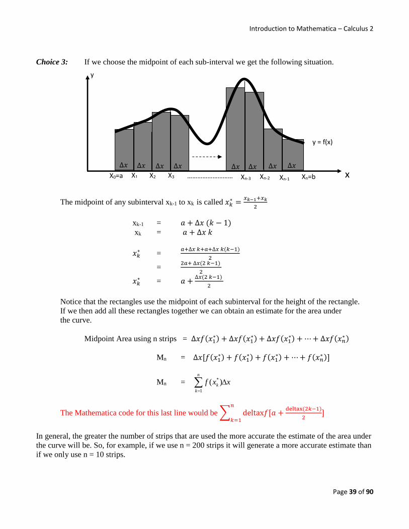
Choice 3: If we choose the midpoint of each sub-interval we get the following situation.
The midpoint of any subinterval xk-1 to xk is called 𝑥𝑘∗ =
𝑥𝑘−1+𝑥𝑘
2
xk-1 = 𝑎 + ∆𝑥 (𝑘 − 1)
xk = 𝑎 + ∆𝑥 𝑘
𝑥𝑘∗ =
𝑎+∆𝑥 𝑘+𝑎+∆𝑥 𝑘(𝑘−1)
2
= 2𝑎+ ∆𝑥(2 𝑘−1)
2
𝑥𝑘∗ = 𝑎 +
∆𝑥(2 𝑘−1)
2
Notice that the rectangles use the midpoint of each subinterval for the height of the rectangle.
If we then add all these rectangles together we can obtain an estimate for the area under
the curve.
Midpoint Area using n strips = ∆𝑥𝑓(𝑥1∗) + ∆𝑥𝑓(𝑥1
∗) + ∆𝑥𝑓(𝑥1∗) + ⋯ + ∆𝑥𝑓(𝑥𝑛
∗ )
Mn = ∆𝑥[𝑓(𝑥1∗) + 𝑓(𝑥1
∗) + 𝑓(𝑥1∗) + ⋯ + 𝑓(𝑥𝑛
∗ )]
Mn = xxfn
k
k 1
* )(
The Mathematica code for this last line would be ∑ deltax𝑓[𝑎 +deltax(2𝑘−1)
2]
𝑛
𝑘=1
In general, the greater the number of strips that are used the more accurate the estimate of the area under
the curve will be. So, for example, if we use n = 200 strips it will generate a more accurate estimate than
if we only use n = 10 strips.
∆𝑥 ∆𝑥 ∆𝑥 ∆𝑥 ∆𝑥 ∆𝑥 ∆𝑥 ∆𝑥
y = f(x)
y
x X0=a Xn=b X1 X2 X3 ………………………….
Xn-1 Xn-2 Xn-3

Introduction to Mathematica – Calculus 2
Page 40 of 90
We can now generalise this problem to come up with the following definitions for finding the area under
the curve A by making the number of strips tend to infinity.
Definition: The area exact area A that lies under the curve y = f(x) from x = a to x = b can be found
by taking an infinite number of strips and using either left, right or midpoints.
So A = lim𝑛→∞
𝐿𝑛 = lim𝑛→∞
∑ 𝑓(𝑥𝑘)∆𝑥𝑛−1𝑖=0
A = lim𝑛→∞
𝑅𝑛 = lim𝑛→∞
∑ 𝑓(𝑥𝑘)∆𝑥𝑛𝑖=1
A = lim𝑛→∞
𝑀𝑛 = lim𝑛→∞
∑ 𝑓(𝑥𝑘∗ )∆𝑥𝑛
𝑖=1
Where ∆𝑥 = 𝑏−𝑎
𝑛
xk = a + ∆𝑥 k
𝑥𝑘∗ = 𝑎 +
∆𝑥(2𝑘−1)
2
Example 16: Find the exact area of the integral ∫ (2𝑥3 − 𝑥2)𝑑𝑥2
0 using Ln , Rn and Mn
Input: 𝑓[x_]: = 2𝑥3 − 𝑥2
deltax =2−0
𝑛;
Limit[∑ deltax𝑓[0 + deltax𝑘]𝑛−1
𝑘=0, 𝑛 → ∞] (* using limit of Ln as 𝑛 → ∞*)
Output: 16
3
Input: 𝑓[x_]: = 2𝑥3 − 𝑥2
deltax =2−0
𝑛;
Limit[∑ deltax𝑓[0 + deltax𝑘]𝑛
𝑘=1, 𝑛 → ∞] (* using limit of Ln as 𝑛 → ∞*)
Output: 16
3
Input: 𝑓[x_]: = 2𝑥3 − 𝑥2
deltax =2−0
𝑛;
Limit[∑ deltax𝑓[0 +deltax(2𝑘−1)
2]
𝑛
𝑘=1, 𝑛 → ∞] (* using limit of Ln as 𝑛 → ∞*)
Output: 16
3
Note: All three methods generate the same result so we typically use Rn in these type of questions as it
has the simplest form

Introduction to Mathematica – Calculus 2
Page 41 of 90
In some situations, it is possible to generalise the process by using the variables a and b.
Example 17: Find the exact area of the integral ∫ (2𝑥3 − 𝑥2)𝑑𝑥𝑏
𝑎 using Rn.
Input: 𝑓[x_]: = 2𝑥3 − 𝑥2
deltax =𝑏−𝑎
𝑛;
Limit[∑ deltax𝑓[0 + deltax𝑘]𝑛
𝑘=1, 𝑛 → ∞] (* using limit of Ln as 𝑛 → ∞*)
Output: 1
6(2𝑎3 − 3𝑎4 + 𝑏3(−2 + 3𝑏))
We can alter the look of the output by using this code
𝑓[x_]: = 2𝑥3 − 𝑥2
deltax =𝑏−𝑎
𝑛;
Expand[
Limit [∑ deltax𝑓[0 + deltax𝑘]
𝑛
𝑘=1
, 𝑛 → ∞]
]
Output: 𝑎3
3−
𝑎4
2−
𝑏3
3+
𝑏4
2

Introduction to Mathematica – Calculus 2
Page 42 of 90
C. Using Your Calculator to calculate areas under a curve We can use our calculator to check our estimates for the area under the curve y = f(x) by using the option
∫ 𝑓(𝑥)𝑑𝑥 on the TI 84 calculator.
Example Use your calculator to find an estimate for ∫ 𝑐𝑜𝑠𝑥. 𝑑𝑥𝜋
20
Solution: We can use our TI 84 calculator to get the area below the curve y = cos x from x = 0 to x = 𝜋
2
In order to do this we follow these steps. 1) Press y = button
2) Type in the desired function in this case Y1 = cos(x) 3) Press the WINDOWS button and choose
Xmin = – 1 Xmax = 2 Xscl = 1 Ymin = – 1 Ymax = 1 Yscl = 1 4) Press 2nd Trace to get the CALC menu 5) choose option 7:∫ 𝑓(𝑥)𝑑𝑥 (this is the numerical integration menu) 6) We tell the computer the Lower Limit by typing 0 and pressing ENTER.
We tell the computer the Lower Limit by typing x =𝜋
2 = 1.57 (or as close as you wish to the true
value 𝜋
2 of ) and pressing ENTER.
The screen will now have the desired area in this case A = 1.0165799 (Approximately)
Example Use your calculator to find an estimate for ∫ ln (𝑥). 𝑑𝑥4
1
Solution: We can use our TI 84 calculator to get the below the curve y = ln(x) from x = 1 to x = 4 In order to do this we follow these steps. 1) Press y = button 2) Type in the desired function in this case Y1 = ln(x) 3) Press the WINDOWS button and choose
Xmin = – 1 Xmax = 5 Xscl = 1 Ymin = – 1 Ymax = 3 Yscl = 1 4) Press 2nd Trace to get the CALC menu 5) choose option 7:∫ 𝑓(𝑥)𝑑𝑥 (this is the numerical integration menu) 6) We tell the computer the Lower Limit by typing 1 and pressing ENTER.
We tell the computer the Lower Limit by typing 4 and pressing ENTER.
The screen will now have the desired area in this case A = 2.6041663 (Approximately)

Introduction to Mathematica – Calculus 2
Page 43 of 90
7. How to find the Area between two curves
To find the area between two curves y = f(x) and y = g(x) from x = a to x = b you
evaluate the integral.
∫(𝑓(𝑥) − 𝑔(𝑥))𝑑𝑥
𝑏
𝑎
Where f(x) is larger than g(x) in the domain [a,b]
Example 18: Find the area between the two curves f(x) = x2 and g(x) = √𝑥
from x = 0 to x = 1
Solution: We can draw a graph of f(x) and g(x) to see which is greater.
Input: 𝑓[x_]: = 𝑥2;
𝑔[x_]: = √𝑥; Plot[{𝑓[𝑥], 𝑔[𝑥]}, {𝑥, 0,1}, PlotLegends → "Expressions"]
Output:
Note: From the graph above we can see that g(x) = √𝑥 is the larger of the two
functions and so we will use (g(x) – f(x)) in evaluating the area
Input: ∫ (𝑔[𝑥] − 𝑓[𝑥]) 𝑑𝑥1
0
Output: 1
3
0.2 0.4 0.6 0.8 1.0
0.2
0.4
0.6
0.8
1.0

Introduction to Mathematica – Calculus 2
Page 44 of 90
It is possible to find the area between two curves that intersect but these situations require
more work.
Example 19: Find the area between the two curves f(x) = sin(x) and g(x) = 𝑐𝑜𝑠(𝑥)
from x = 0 to x = 𝜋
Solution: We start by graphing the functions to see the interaction of the two
functions.
Input: 𝑓[x_]: = Sin[𝑥]; 𝑔[x_]: = Cos[𝑥]; Plot[{𝑓[𝑥], 𝑔[𝑥]}, {𝑥, 0, 𝜋}, PlotLegends → "Expressions"]
Output:
Note: From the graph above we can see that g(x) = cos (𝑥) is larger than
f(x) = sin(x) up to the point of intersection and from that point onwards until x
= 𝜋 that f(x) = sin(x) is larger than g(x) = cos (𝑥).
This means that we need to find the x-coordinate of the point of intersection.
Input: 𝑓[x_]: = Sin[𝑥]; 𝑔[x_]: = Cos[𝑥]; Solve[{Sin[𝑥] == Cos[𝑥]&&0 ≤ 𝑥 ≤ 𝜋}, {𝑥}, Reals]
Output: {{𝑥 → −2ArcTan[1 − √2]}}
The point of intersection is at x = −2ArcTan[1 − √2] = 𝜋
4

Introduction to Mathematica – Calculus 2
Page 45 of 90
So, the area between these two curves will be.
Area = ∫ (𝑔(𝑥) − 𝑓(𝑥)) 𝑑𝑥𝜋
40
+ ∫ (𝑔(𝑥) − 𝑓(𝑥)) 𝑑𝑥𝜋
𝜋
4
= ∫ (𝑐𝑜𝑠(𝑥) − 𝑠𝑖𝑛(𝑥)) 𝑑𝑥𝜋
40
+ ∫ (𝑠𝑖𝑛(𝑥) − 𝑐𝑜𝑠(𝑥)) 𝑑𝑥𝜋
𝜋
4
The Mathematica code is
Input: 𝑓[x_]: = Sin[𝑥]; 𝑔[x_]: = Cos[𝑥];
∫ (𝑔[𝑥] − 𝑓[𝑥]) 𝑑𝑥𝜋
40
+ ∫ (𝑓[𝑥] − 𝑔[𝑥]) 𝑑𝑥𝜋
𝜋
4
Output: 2√2
We can see the area between the curves by using the following code.
Plot[ {𝑓[𝑥], 𝑔[𝑥]}, {𝑥, 0, 𝜋},
Ticks → {{0,𝜋
4,𝜋
2,3𝜋
4, 𝜋} , {−1,0,1}},
Filling → {1 → {2}},
PlotLabels → Expressions
]

Introduction to Mathematica – Calculus 2
Page 46 of 90
8. How to find the Indefinite Integral of a function.
We have already seen how to find the definite integral of a function (see pages 30 – 32)
We use the notation ∫ 𝑓(𝑥)𝑑𝑥𝑏
𝑎 to indicate the exact area under the curve y = f(x) from
x = a to x = b , this is called the Definite Integral of the function f(x)
The syntax for finding the area under the curve is very intuitive in Mathematica.
First you go to the Basic Math Template and look for 𝑑 ∫ ∑ then choose the Integral icon.
The Integral Icon

Introduction to Mathematica – Calculus 2
Page 47 of 90
You will now see the following
To complete the Sigma Command, Click on each part of the template above.
expr will be replaced by the function f(x) with (……) round it.
var Will be replaced by the variable (usually x).
Example 18: Find the Indefinite Integral ∫ (𝑥3 − 2𝑥 + 7) 𝑑𝑥
Get the integral template,
expr will be replaced by (𝑥3 − 2𝑥 + 7)
var will be replaced by x
You then press the Number Pad ENTER Key. The output will be 7𝑥 − 𝑥2 +𝑥4
4
Note 1: You need to put brackets round the function (𝑥3 − 2𝑥 + 7)
Note 2: The output is 7𝑥 − 𝑥2 +𝑥4
4 but technically the proper form as 7𝑥 − 𝑥2 +
𝑥4
4+ 𝐶
Where C is called the Arbitrary constant.

Introduction to Mathematica – Calculus 2
Page 48 of 90
Example 20: Find the following simple Indefinite Integrals.
(a) ∫(𝑥3 − 5𝑥 + 7)𝑑𝑥 (A Polynomial Function)
(b) ∫ (𝑥4−16
2𝑥2+8𝑥) 𝑑𝑥 (A Rational Function)
(c) ∫(√𝑥2 − 6𝑥 + 1)𝑑𝑥 (A Radical Function)
(d) ∫(100𝑒3𝑥+7)𝑑𝑥 (An Exponential Function)
Input (a): ∫ (𝑥3 − 5𝑥 + 7) 𝑑𝑥
Output: 7𝑥 −5𝑥2
2+
𝑥4
4
Input (b): ∫ (𝑥4−16
2𝑥2+8𝑥) 𝑑𝑥
Output: 8𝑥 − 𝑥2 +𝑥3
6− 2Log[𝑥] − 30Log[4 + 𝑥]
Input (c): ∫ (√𝑥2 − 6𝑥 + 1) 𝑑𝑥
Output: 1
2(−3 + 𝑥)√1 − 6𝑥 + 𝑥2 − 4Log[3 − 𝑥 − √1 − 6𝑥 + 𝑥2]
Input (a): ∫ (100𝑒3𝑥+7) 𝑑𝑥
Output: 100
3𝑒7+3𝑥
Note: All of the integrals are missing the arbitrary constant C , so you will need to
remember to add that yourself.
For example, ∫ (𝑥3 − 5𝑥 + 7) 𝑑𝑥 = 7𝑥 −5𝑥2
2+
𝑥4
4+ 𝐶

Introduction to Mathematica – Calculus 2
Page 49 of 90
We can find complex integrals using this command as well as can be seen in the example
below.
Example 21: Find the following complex Indefinite Integrals.
(a) ∫(𝑥3𝑒2𝑥4)𝑑𝑥 (U-Substitution method)
(b) ∫(𝑥2𝐿𝑛(𝑥))𝑑𝑥 (Integration by parts)
(c) ∫(𝑠𝑖𝑛2𝑥 𝑐𝑜𝑠7𝑥)𝑑𝑥 (Trig Integration)
(d) ∫ (1
√𝑥2−25) 𝑑𝑥 (X-Substitution method)
(e) ∫ (24
(𝑥−3)(𝑥+6)) 𝑑𝑥 (Integration by parts)
Input (a): ∫ (𝑥3𝑒2𝑥4) 𝑑𝑥
Output: 𝑒2𝑥4
8
Input (b): ∫ (𝑥2Log[𝑥]) 𝑑𝑥
Output: −𝑥3
9+
1
3𝑥3Log[𝑥]
Input (c): ∫ (Sin[𝑥]^2Cos[𝑥]^7) 𝑑𝑥
Output: 7Sin[𝑥]
128−
1
160Sin[5𝑥] −
5Sin[7𝑥]
1792−
Sin[9𝑥]
2304
Input (d): ∫ (1
√𝑥2−25) 𝑑𝑥
Output: Log[𝑥 + √−25 + 𝑥2]
Input (e): ∫ (24
(𝑥−3)(𝑥+6)) 𝑑𝑥
Output: 24(1
9Log[−3 + 𝑥] −
1
9Log[6 + 𝑥])
Note : The integral ∫(𝑠𝑖𝑛2𝑥 𝑐𝑜𝑠7𝑥)𝑑𝑥 had to be written using the syntax ∫ (Sin[𝑥]^2Cos[𝑥]^7) 𝑑𝑥

Introduction to Mathematica – Calculus 2
Page 50 of 90
Since there are an infinite number of possible functions to Integrate, it will happen, from
time to time that the result of an Indefinite Integral may not be Analytically possible to
find or that the integral may be given in terms of a function that you do not know.
Example 22: Find the following complex Indefinite Integrals.
(a) ∫(𝑒2𝑥4)𝑑𝑥
(b) ∫(𝑒2𝑥4)𝑑𝑥
(c) ∫(𝑒sin (𝑥))𝑑𝑥
Input (a): ∫ (𝑒2𝑥4) 𝑑𝑥
Output: −𝑥Gamma[
1
4,−2𝑥4]
421 4⁄ (−𝑥4)1 4⁄
Note: In this example, the solution is given in terms of the Gamma Function.
Input (b): ∫ (𝑒𝑥2) 𝑑𝑥
Output: 1
2√𝜋Erfi[𝑥]
Note: In this example, the solution is given in terms of the Erfi Function - the imaginary error function
Input (c): ∫ (𝑒Sin[𝑥]) 𝑑𝑥
Output: ∫ 𝑒Sin[𝑥] 𝑑𝑥
Note: In this example, the solution is the original Integral , this means that there is no algebraic
expression that is the integral of esin(x).

Introduction to Mathematica – Calculus 2
Page 51 of 90
9. Volumes of Revolution
A. Volume of Integration (Disk Method)
Example 23: Find the volume of the solid generated when you rotate the curve f(x) = 3x2 + 1 about the
x-axis, from x = 1 to x = 3
Solution: For this situation, we will use the formula. V = dxxf
b
a
2
)(
V = dxx
3
1
22 13
V = dxxx
3
1
24 169
V = dxxx
3
1
24 69
V = 3
1
35 35
9
x
xxxx
V =
)1()1(3)1(
5
9)3()3(3)3(
5
9 3535
V = 5
2448
The Mathematica Code for this question is.
Input: 𝑓[x_]: = 3𝑥2 + 1
𝑎 = 1; 𝑏 = 3;
∫ 𝜋(𝑓[𝑥])2 𝑑𝑥𝑏
𝑎
Output: 2448𝜋
5

Introduction to Mathematica – Calculus 2
Page 52 of 90
Example 24: (a) Find the volume of the solid generated when you rotate the area between the
curves f(x) = 10 – x2 and g(x) = sin(x) about the x-axis, from x = 0 to x = 𝜋
4.
(b) Show this information graphically.
Solution (a): For this situation, we will use the formula. V = dxxgxf
b
a
])()([22
Input: 𝑓[x_]: = 10 − 𝑥2
𝑔[x_]: = Sin[𝑥] 𝑎 = 0;
𝑏 =𝜋
4;
∫ 𝜋((𝑓[𝑥])2 − (𝑔[𝑥])2) 𝑑𝑥𝑏
𝑎
Output: 𝜋
4+
7𝜋2
8−
𝜋4
48+
𝜋6
5120
So, the volume of revolution = 𝜋
4+
7𝜋2
8−
𝜋4
48+
𝜋6
5120
Solution (b): The code to show this information graphically.
Input: 𝑓[x_]: = 10 − 𝑥2
𝑔[x_]: = Sin[𝑥] 𝑎 = 0;
𝑏 =𝜋
4;
Plot[{𝑓[𝑥], 𝑔[𝑥]}, {𝑥, 𝑎, 𝑏}, PlotRange → {−2,2}, PlotLegends → {"f(x) = 2 − "x2"", "Sin[x]"}]
Output:

Introduction to Mathematica – Calculus 2
Page 53 of 90
B. Volumes by Cylindrical Shells.
Example 25: Find the volume created by rotating the curve f(x) = x2 about the y-axis
from x= 0 to x = 1.
Solution: Since we are rotating about the y – axis we use the formula in terms of x.
See diagram below.
V = b
a
dxheightradius ))((2
V = b
a
dxxxf2
= 1
0
2.2 dxxx
= 1
0
3.2 dxx
= 1
0
4
2
1
x
xx
= 𝜋
2
The Mathematica Code for this question is.
Input: 𝑓[x_]: = 𝑥2
𝑎 = 0; 𝑏 = 1;
∫ (2𝜋𝑥𝑓[𝑥]) 𝑑𝑥𝑏
𝑎
Output: 𝜋
2
Note: By setting up the code in this general format it is easy to adapt the code it to other similar
situations. So, if the function was f(x) = x3 + x2 – 1 we only need to change one line of
code , namely we change 𝑓[x_]: = 𝑥2 and replace it with 𝑓[x_] : = 𝑥3 + 𝑥2 − 1
y axis
x = 1 0
y = x2
Radius = x
Height = y = f(x)

Introduction to Mathematica – Calculus 2
Page 54 of 90
Example 26: Find the volume created by rotating the region between the two curves f(x) = 3 + 2x – x2
and g(x) = 3 – x about the y-axis
Solution: Since we are rotating about the y – axis we use the formula in terms of x.
So, radius of a typical shell is x and the
RaDius = x
Height = f(x) – g(x)
= (3 + 2x – x2 ) – (3 – x)
= 3 + 2x – x2 – 3 + x
= 3x – x2
The values of a and b are found by finding where f(x) = 3 + 2x – x2 and g(x) = 3 – x
intersect. In this case, a = 0 and b = 3, See diagram below.
V = b
a
dxheightradius ))((2
V =
b
a
dxxgxfx ))()((2
=
3
0
23.2 dxxxx
=
3
0
32 )2.6( dxxx
= 1
0
43
2
12
x
xxx
V = 27𝜋
2
The Mathematica Code for this question is.
Input: 𝑓[x_]: = 3 + 2𝑥 − 𝑥2
𝑔[x_]: = 3 − 𝑥
Solve[𝑓[𝑥] == 𝑔[𝑥], {𝑥}, Reals]
Output: {{𝑥 → 0}, {𝑥 → 3}}
Input: 𝑓[x_]: = 3 + 2𝑥 − 𝑥2
𝑔[x_]: = 3 − 𝑥
𝑎 = 0; 𝑏 = 3;
∫ (2𝜋𝑥(𝑓[𝑥] − 𝑔[𝑥])) 𝑑𝑥𝑏
𝑎
Output: 27𝜋
2
Radius = x
y axis
3 0 g(x) = 3 – x
f(x) = 3 + 2x – x2
Height = f(x) – g(x)

Introduction to Mathematica – Calculus 2
Page 55 of 90
10. Improper Integrals
There are two types of Improper Integrals – Improper Integrals of Type 1 have the property that at least
one of the two end-points of integration is infinity.
For example, the following three integrals are all Improper Integrals of Type 1.
∫10
𝑥3 𝑑𝑥∞
1 ∫
𝑥
𝑥2+1𝑑𝑥
5
−∞ ∫
4
𝑥2+1𝑑𝑥
∞
−∞
The method used is to use limits to accommodate the infinities.
∫10
𝑥3 𝑑𝑥∞
1 = lim
𝑏→∞(∫
10
𝑥3 𝑑𝑥𝑏
1)
∫𝑥
𝑥2+1𝑑𝑥
5
−∞ = lim
𝑏→−∞(∫
𝑥
𝑥2+1𝑑𝑥
5
𝑏)
∫4
𝑥2+1𝑑𝑥
∞
−∞ = lim
𝑏→∞(∫
𝑥
𝑥2+1𝑑𝑥
𝑏
0) + lim
𝑏→−∞(∫
𝑥
𝑥2+1𝑑𝑥
0
𝑏)
Mathematica copes with Improper Integrals in a very intuitive way as the following examples show
Example 27: Find the value of the following three Type 1 improper Integrals.
(𝑎) ∫10
𝑥3 𝑑𝑥∞
1 (b) ∫
4
𝑥2+1𝑑𝑥
∞
−∞ (𝑐) ∫
𝑥
𝑥2+1𝑑𝑥
5
−∞
Input (a) 𝑓[x_]: =10
𝑥3
∫ 𝑓[𝑥] 𝑑𝑥∞
1 Output: 5
Input (b) 𝑓[x_]: = 𝑓[x_]: =4
𝑥2+1
∫ 𝑓[𝑥] 𝑑𝑥∞
1 Output: 4𝜋
Input (c) 𝑓[x_]: =10
𝑥3
∫ 𝑓[𝑥] 𝑑𝑥∞
1
Output: Integrate: Integral of 𝑥
𝑥2+1 does not converge on {1,∞}.
Note: The Output statement Integrate: Integral of 𝑥
𝑥2+1 does not converge on {1,∞} in this
situation is essentially saying that the area under the curve is infinitely large.
Introduction to Mathematica – Calculus 2
Page 56 of 90
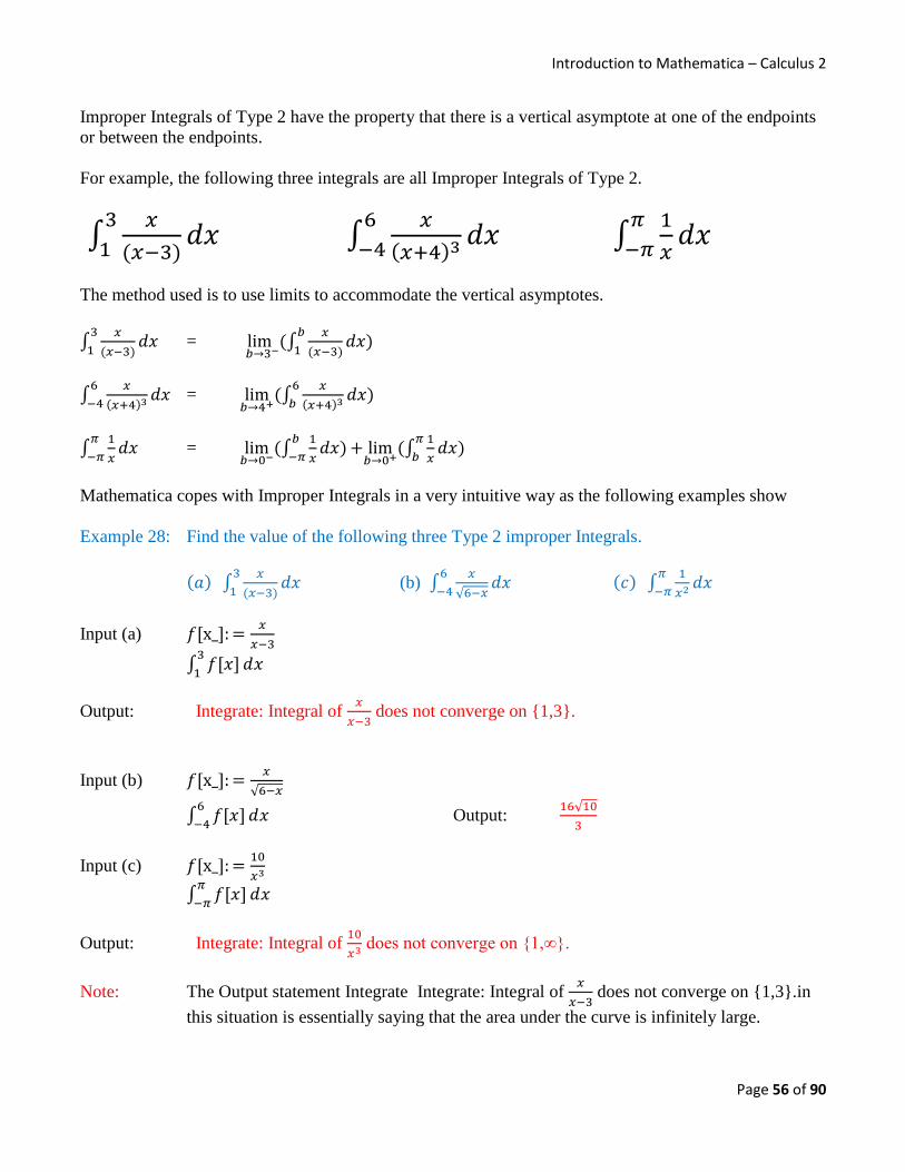
Improper Integrals of Type 2 have the property that there is a vertical asymptote at one of the endpoints
or between the endpoints.
For example, the following three integrals are all Improper Integrals of Type 2.
∫𝑥
(𝑥−3)𝑑𝑥
3
1 ∫
𝑥
(𝑥+4)3 𝑑𝑥6
−4 ∫
1
𝑥𝑑𝑥
𝜋
−𝜋
The method used is to use limits to accommodate the vertical asymptotes.
∫𝑥
(𝑥−3)𝑑𝑥
3
1 = lim
𝑏→3−(∫
𝑥
(𝑥−3)𝑑𝑥
𝑏
1)
∫𝑥
(𝑥+4)3 𝑑𝑥6
−4 = lim
𝑏→4+(∫
𝑥
(𝑥+4)3 𝑑𝑥6
𝑏)
∫1
𝑥𝑑𝑥
𝜋
−𝜋 = lim
𝑏→0−(∫
1
𝑥𝑑𝑥
𝑏
−𝜋) + lim
𝑏→0+(∫
1
𝑥𝑑𝑥
𝜋
𝑏)
Mathematica copes with Improper Integrals in a very intuitive way as the following examples show
Example 28: Find the value of the following three Type 2 improper Integrals.
(𝑎) ∫𝑥
(𝑥−3)𝑑𝑥
3
1 (b) ∫
𝑥
√6−𝑥𝑑𝑥
6
−4 (𝑐) ∫
1
𝑥2 𝑑𝑥𝜋
−𝜋
Input (a) 𝑓[x_]: =𝑥
𝑥−3
∫ 𝑓[𝑥] 𝑑𝑥3
1
Output: Integrate: Integral of 𝑥
𝑥−3 does not converge on {1,3}.
Input (b) 𝑓[x_]: =𝑥
√6−𝑥
∫ 𝑓[𝑥] 𝑑𝑥6
−4 Output:
16√10
3
Input (c) 𝑓[x_]: =10
𝑥3
∫ 𝑓[𝑥] 𝑑𝑥𝜋
−𝜋
Output: Integrate: Integral of 10
𝑥3 does not converge on {1,∞}.
Note: The Output statement Integrate Integrate: Integral of 𝑥
𝑥−3 does not converge on {1,3}.in
this situation is essentially saying that the area under the curve is infinitely large.

Introduction to Mathematica – Calculus 2
Page 57 of 90
11. Arc Length
To find the length of the arc along the curve y = f(x) from x = a to x = b is
L = ∫ √1 + (𝑓′(𝑥))2𝑑𝑥𝑏
𝑎
Example 29: Find the exact value of the arc length for the curve f(x) = 4x + 7 from x = 1 to x = 3
Input: 𝑓[x_]: = 4𝑥 + 7
𝑎 = 1; 𝑏 = 3;
∫ √1 + (𝑓′[𝑥])2 𝑑𝑥𝑏
𝑎
Output: 2√17
Example 30: Find the exact value of arc length for the curve f(x) = 𝑒𝑥 +1
4𝑒−2𝑥 from x = 0 to x = ln(4)
Input: 𝑓[x_]: = 2𝑒𝑥 +1
8𝑒−𝑥
𝑎 = 0; 𝑏 = 𝐿𝑜𝑔[4];
∫ √1 + (𝑓′[𝑥])2 𝑑𝑥𝑏
𝑎
Output: 195
32
Example 31: Find the numerical estimate for the arc length for the curve f(x) = 𝑥 + sin (𝑥)
from x = 0 to x = 1
Input: 𝑓[x ]: = 𝑥 + 𝑆𝑖𝑛[𝑥]
𝑎 = 0; 𝑏 = 1;
𝑁[∫ √1 + (𝑓′[𝑥])2 𝑑𝑥, 4𝑏
𝑎]
Output: 2.097
Note : There are situations where you will not be able to find the exact arc length and in these
situations, you can only find a numerical estimate.
Example 31 is such a situation, in fact it takes Mathematica about 1 minute to perform
this numerical estimate.

Introduction to Mathematica – Calculus 2
Page 58 of 90
12. Surface Area
To find the area of the surface generated by rotating the graph of the function y = f(x) about the x-axis
from x = a to x = b is
S = ∫ 2𝜋𝑓(𝑥)√1 + (𝑓′(𝑥))2𝑑𝑥𝑏
𝑎
Example 32: Find the exact value of the surface area when the graph of f(x) = 6 – 2x is rotated about
the x-axis from x = 0 to x = 3
Input: 𝑓[x_]: = 6 − 2𝑥
𝑎 = 0; 𝑏 = 3;
∫ 2𝜋𝑓[𝑥]√1 + (𝑓′[𝑥])2 𝑑𝑥𝑏
𝑎
Output: 18√5𝜋
Example 33: Find the exact value of arc length for the curve f(x) = 𝑒𝑥 +1
4𝑒−2𝑥 from x = 0 to x = ln(2)
Input: 𝑓[x_]: = 2𝑒𝑥 +1
8𝑒−𝑥
𝑎 = 0; 𝑏 = 𝐿𝑜𝑔[4];
∫ √1 + (𝑓′[𝑥])2 𝑑𝑥𝑏
𝑎
Output: 𝜋(61455
1024+ Log[4])
Example 34: Find the numerical estimate for the arc length for the curve f(x) = 𝑥 + sin (𝑥)
from x = 0 to x =
Input: 𝑓[x_]: = Sin[𝑥] + Cos[𝑥] 𝑎 = 0;
𝑏 =𝜋
2;
𝑁[∫ 2𝜋𝑓[𝑥]√1 + (𝑓′[𝑥])2 𝑑𝑥𝑏
𝑎, 3]
Output: 14.4
Note : There are situations where you will not be able to find the exact value of the Surface
Area. Example 34 is such a situation, in fact it takes Mathematica about 1 minute to
perform this numerical estimate.

Introduction to Mathematica – Calculus 2
Page 59 of 90
13. Application of Integrals
There are many applications of Integrals, here are some practical examples.
A. Finding velocity and position functions
B. Average Value of a Function
C. Work Done Problems
D. Hydrostatic Problems
C. Finding velocity and position functions
Example 35: The acceleration of a moving object is given by the formula a(t) = t2 + 6t , find the
velocity function v(t) and the position function s(t) when v(1) = 5 and s(1) = 0
Solution: We use the fact that v(t) = ∫ 𝑎(𝑡)𝑑𝑡 and that s(t) = ∫ 𝑣(𝑡)𝑑𝑡
v(t) = ∫ 𝑎(𝑡)𝑑𝑡 = ∫(𝑡2 + 6t )𝑑𝑡
Input: ∫ (𝑡2 + 6𝑡) 𝑑𝑡 Output: 3𝑡2 +𝑡3
3
This means that v(t) = 3𝑡2 +𝑡3
3+ 𝐶 so to find the value of C we solve v(1) = 5.
Input: 𝑣[t_]: = 3𝑡2 +𝑡3
3+ 𝐶
Solve[𝑣[1] == 5] Output: {{𝐶 →5
3}}
This means that v(t) = 3𝑡2 +𝑡3
3+
5
3 so to find the value s(t)
We now find s(t) = ∫ 𝑣(𝑡)𝑑𝑡 = ∫(3𝑡2 +𝑡3
3+
5
3)𝑑𝑡
Input: ∫ (3𝑡2 +𝑡3
3+
5
3) 𝑑𝑡 Output:
5𝑡
3+ 𝑡3 +
𝑡4
12
This means that S(t) = 5𝑡
3+ 𝑡3 +
𝑡4
12+ 𝐶 so to find the value of C we solve s(1) = 0.
Input: 𝑠[t_]: =5𝑡
3+ 𝑡3 +
𝑡4
12+ 𝐶
Solve[𝑠[1] == 0] Output: {{𝐶 → −11
4}}
This means that s(t) = 5𝑡
3+ 𝑡3 +
𝑡4
12−
11
4

Introduction to Mathematica – Calculus 2
Page 60 of 90
D. Average Value of a function
Example 36: (a) Find the average value of the function f(x) = 2
√𝑥+1 from x = 0 to x = 3
(b) Find the value(s) of x where the function is equal to the average value.
(c) Show this information graphically.
Solution (a): The formula for the average value of a function f(x) from x = a to x = b is:-
fave = 1
𝑏−𝑎∫ 𝑓(𝑥)𝑑𝑥
𝑏
𝑎
In this question fave = 1
3−0∫ (
2
√𝑥+1) 𝑑𝑥
3
0
Input: 𝑓[x_]: =2
√𝑥+1
𝑎 = 0; 𝑏 = 3;
fave =1
𝑏−𝑎∫ (
2
√𝑥+1) 𝑑𝑥
𝑏
𝑎
Output: 4
3 So, the average value of the function is fave =
4
3
Solution (b): To find the value(s) of x where the function is equal to the average value we need to
solve for what values of x is f(x) = fave
In this question, we need to solve f(x) = 4
3
Input: 𝑓[x_]: =2
√𝑥+1
𝑎 = 0; 𝑏 = 3;
fave =1
𝑏−𝑎∫ (
2
√𝑥+1) 𝑑𝑥
𝑏
𝑎
Solve[𝑓[𝑥] == fave&&𝑎 ≤ 𝑥 ≤ 𝑏, {𝑥}, Reals]
Output: {{𝑥 →5
4}}
So, x = 5
4 is the point where the function f(x) has the same value as the
average value fave.

Introduction to Mathematica – Calculus 2
Page 61 of 90
Solution (c): To show this information graphically we will graph y = f(x) and y = 4
3
Input: 𝑓[x_]: =2
√𝑥+1 (* this is f(x) *)
𝑔[x ]: =4
3 (* this is g(x) *)
Plot[ (* start of Plot Command *)
{𝑓[𝑥], 𝑔[𝑥]}, (* two functions to graph *) {𝑥, 0,3}, (* the range of x- values *)
PlotRange → {0,2}, (* the range of x- values *)
PlotLegends → {"f(x) =2
√x+1", "g(x)=
4
3"} (* legend at side of graph *)
Ticks → {{0,1
4,
1
2,
3
4, 1,
5
4,
3
2,
7
4, 2,
9
4,
5
2,
11
4, 3}, {0,
1
3,
2
3, 1,
4
3,
5
3, 2}} (* scales on x and y-axes *)
GridLines → {{0,1
4,
1
2,
3
4, 1,
5
4,
3
2,
7
4, 2,
9
4,
5
2,
11
4, 3}, {0,
1
3,
2
3, 1,
4
3,
5
3, 2}} (* gridlines on x and y-axes *)
] (* end of Plot Command *)
Output:
Note 1: The point of intersection is at (5
4,
4
3)
Note 2: The code for the graphing of the function contains Plot Options
such as PlotRange , PlotLegends,Ticks and GridLines. These are optional but they do add
some detail to the graphs to help with the overall appearance.

Introduction to Mathematica – Calculus 2
Page 62 of 90
E. Work Done Problems
Example 37: A heavy rope 50ft long, weighs 0.5 pounds per foot and hangs over the edge of a building 120 ft high. How much work is done in pulling the rope to the top of the building?
The total height of the building (200ft ) is not important - only The work done in pulling the rope up is important.
We break the problem into a smaller simpler situation first. Suppose we have the rope at a height of xi above the ground and we raise it up by a small amount called ∆𝑥 then the work done by pulling the rope up this extra ∆𝑥 is given by the formula. W = FD = 0.5xi∆𝑥.
If we sum this up over the entire 50 ft we get
W = lim𝑛→∞
∑ 0.5xi∆𝑥𝑛𝑖=1
which becomes the integral W = ∫ 0.5𝑥𝑑𝑥50
0
W = [0.25𝑥2]𝑥=0𝑥=50
W = 625 ft lb
The Mathematica Code for this question is. Input: 𝑤[x_]: = 0.5𝑥 𝑎 = 0; 𝑏 = 50;
∫ (𝑤[𝑥]) 𝑑𝑥𝑏
𝑎
Output: 625.
Example 38: A cable weighs 2lb per foot is used to lift 800 pounds of coal up a mine shaft 500 ft deep.
Find the work done. Input: 𝑤[x ]: = 800 + 2𝑥 𝑎 = 0; 𝑏 = 500;
∫ (𝑤[𝑥]) 𝑑𝑥𝑏
𝑎
Output: 650000
Note: w(x) is the work function it is made up of a fixed 800 pounds plus x ft of rope that weigh 2 lb per foot so the total weight at point x is w(x) = 800 + 2x
50 ft
xi xi +∆𝑥

Introduction to Mathematica – Calculus 2
Page 63 of 90
F. Hydrostatic Problems
Example 39: Find the hydrostatic pressure on the rectangular plate shown below.
Water has a weight of 62.5 pounds per cubic feet.
Solution: The pressure function p(x) is the pressure at depth xk.
P(xk) = Pressure at depth xk
= 62.5xk (62.5x when feet)
A(xk) = Area of a typical strip at depth xk
= 6∆𝑥
Force Function at xk F(xk) = P(xk)A(xk)
= (62.5xk )( 6∆𝑥)
= 375𝑥𝑘∆𝑥
Total Force F = lim𝑛→∞
∑ 0.5x𝑘 ∆𝑥𝑛𝑘=1
= ∫ 375𝑥𝑑𝑥6
2
= (375
2𝑥2)
𝑥 = 6𝑥 = 2
= 6750 – 750
Total Force F = 6000 lb
The Mathematica Code for this question is.
Input: 𝑎 = 2; 𝑏 = 6; 𝑓[x_]: = 375𝑥
∫ 𝑓[𝑥] 𝑑𝑥𝑏
𝑎
Output: 6000
∆𝑥
xk

Introduction to Mathematica – Calculus 2
Page 64 of 90
Example 40: Find the hydrostatic pressure on the rectangular plate shown below.
Water has a weight of 62.5 pounds per cubic feet.
P(x) = Pressure at depth xk = 62.5x (125
2 x when feet , 9810x when in m)
A(x) = Area of a typical strip at position d = w∆𝑥
We use similar triangles to find w in terms of d the distance from the top of the triangle
3
4 =
3−𝑑
𝑤
3w = 4(3 – d)
3w = 12 – 4d
w = 12 – 4d
3
w = 4 −4
3𝑑
Since d = x – 1 we can calculate the
width of a typical strip in terms of x.
w = 4 −4
3(𝑥𝑘 − 1)
w = 4 −4
3𝑥𝑘 +
4
3
w = 16
3−
4
3𝑥𝑘
Area of a typical strip at depth xk A(xk ) = 𝑤∆𝑥 = (16
3−
4
3𝑥𝑘)∆𝑥
Force Function at xk
F(xk) = P(xk )A(xk ) = (125
2 xk)(
16
3−
4
3𝑥𝑘)∆𝑥 = (
1000
3xk –
250
3𝑥𝑘
2)∆𝑥
Total Force F = lim𝑛→∞
∑1000
3 xk –
250
3 𝑥𝑘
2)∆𝑥𝑛𝑘=1 = ∫ (
1000
3x –
250
3 𝑥2)𝑑𝑥
4
1
= (500
3𝑥2 −
250
9𝑥3)
𝑥 = 4𝑥 = 1
= 750 lb
The Mathematica Code for this question is.
Input: 𝑎 = 1; 𝑏 = 4;
𝑓[x_]: =1000
3𝑥 −
250
3𝑥2
∫ 𝑓[𝑥] 𝑑𝑥𝑏
𝑎
Output: 750
d w ∆𝑥
x

Introduction to Mathematica – Calculus 2
Page 65 of 90
14. Numerical Integration
We have three methods for approximating the Area under a curve the y are Ln , Rn and Mn
These three methods use the technique of splitting the area into rectangles and can be very accurate
if you take enough strips. Two other techniques can also be used to estimate the area under a curve.
These numerical methods are called the Trapezoid Rule and Simpsons Rule.
A. Trapezoid Rule.
We now find a method for getting the approximate area under a curve.
We begin by splitting the area into n strips as shown above, each of width ∆𝑥 = 𝑏−𝑎
𝑛 and xk = a + k∆𝑥 .
To find the area of one these strips we find the area of a trapezium similar to the ones drawn above.
The area of one trapezium AK from xk-1 to xk = 1
2∆𝑥[f(xk-1) + f(xk)]
The estimate of the total Area Tn is
Tn = A1 + A2 + A3 + ….. + An-1 + An
= 1
2∆𝑥[f(x0) + f(x1)]+
1
2∆𝑥[f(x1) + f(x2)] + …….+
1
2∆𝑥[f(xn-1) + f(xn)]
= 1
2∆𝑥[f(x0) + f(x1)+ f(x1) + f(x2) + f(x2) + f(x3) + … + f(xn-1) + f(xn-1) + f(xn)]
= 1
2∆𝑥[f(x0) +2f(x1)+ 2f(x2) + 2f(x3) + ……. + 2f(xn-1) + f(xn)]
Note: This formula is sometimes called the Trapezoidal Rule , and the accuracy of your estimate
depends on the number of strips taken. There are two main situations where we would use this
technique the first is when the information we are given about the function f(x) is not algebraic
but in the form of a table or when f(x) is too complex or is impossible to integrate as in
y
y = f(x)
x xn1 xn2 xn x2 x1 x0 ∆𝑥
𝑓(𝑥0) 𝑓(𝑥1) 𝑓(𝑥2) 𝑓(𝑥𝑛−2)
… … … … … … … ….
𝑓(𝑥𝑛−1) 𝑓(𝑥𝑛)

Introduction to Mathematica – Calculus 2
Page 66 of 90
Example 41: Find an estimate for ∫2
𝑥2+1𝑑𝑥
4
0 using the Trapezoid rule with n = 8 strips.
Solution: The first step is to create a table of values for our function.
Using a = 0 b = 4 n = 8 ∆𝑥 = 𝑏−𝑎
𝑛 =
4−0
8 =
1
2
The Mathematica Code that does this is
Input: 𝑓[x_]: =2
𝑥2+1
𝑎 = 0; 𝑏 = 4; 𝑛 = 8;
deltax =𝑏−𝑎
𝑛;
Table[𝑓[𝑥], {𝑥, 𝑎, 𝑏, deltax}]
Output: {2,8
5, 1,
8
13,
2
5,
8
29,
1
5,
8
53,
2
17}
We then calculate T8 using the following formula.
T8 = 1
2∆𝑥[f(x0) +2f(x1)+ 2f(x2) + 2f(x3)+ 2f(x4) + 2f(x5) + 2f(x6) + 2f(x7) + f(x8)]
T8 = 1
2(
1
2)[2 + 2(
8
5) + 2(1) + 2(
8
13) + 2(
2
5) + 2(
8
29) + 2(
1
5) + 2(
8
53) + 2(
2
17)]
T8 = 1
4[2 +
16
5 + 2 +
16
13 +
4
5 +
16
29 +
2
5 +
16
53 +
4
17]
T8 = 1.32525
The Mathematica Code that does this is
Input: 𝑓[x_]: =1
𝑥2+1
𝑎 = 0; 𝑏 = 4; 𝑛 = 8;
deltax =𝑏−𝑎
𝑛;
area = 𝑁[1
2deltax𝑓[𝑎] + ( ∑
𝑘=1
𝑛−1
deltax𝑓[𝑎 + deltax𝑘]) +1
2deltax𝑓[𝑏]]
Output: 1.32525
x0 x1 x2 x3 x4 x5 x6 x7 x8
Xk 0 0.5 1 1.5 2 2.5 3 3.5 4
f(xk) 2 8
5 1
8
13
2
5
8
29
1
5
8
53
2
17

Introduction to Mathematica – Calculus 2
Page 67 of 90
Example 42: Find the relative error in using the Trapezoid rule to estimate ∫1
𝑥2+1𝑑𝑥
4
0 with
n = 4,8,16,50 and 100 strips.
The Mathematica Code that does this is
Input: 𝑓[x_]: =2
𝑥2+1
𝑎 = 0; 𝑏 = 4; 𝑛 = 4;
deltax =𝑏−𝑎
𝑛;
area = 𝑁[1
2deltax𝑓[𝑎] + ( ∑
𝑘=1
𝑛−1
deltax𝑓[𝑎 + deltax𝑘]) +1
2deltax𝑓[𝑏]]
exactarea = ∫ 𝑓[𝑥] 𝑑𝑥𝑏
𝑎;
rerror = 𝑁[Abs[(exactarea−area
exactarea)100]]
Output: 0.2710856
Input: 𝑓[x_]: =2
𝑥2+1
𝑎 = 0; 𝑏 = 4; 𝑛 = 8;
deltax =𝑏−𝑎
𝑛;
area = 𝑁[1
2deltax𝑓[𝑎] + ( ∑
𝑘=1
𝑛−1
deltax𝑓[𝑎 + deltax𝑘]) +1
2deltax𝑓[𝑏]]
exactarea = ∫ 𝑓[𝑥] 𝑑𝑥𝑏
𝑎;
rerror = 𝑁[Abs[(exactarea−area
exactarea)100]]
Output: 0.0425595
In a similar fashion we get
Change the number of strips to n = 16 the new Output is 0.0108674
Change the number of strips to n = 50 the new Output is 0.00111347
Change the number of strips to n = 100 the new Output is 0.000278381
Note 1: The relative error decreases when the number of strips gets larger
Note 2: The relative error in these examples are given as percentages, so for example when n = 8
strips the relative error is 0.0425595%

Introduction to Mathematica – Calculus 2
Page 68 of 90
Example 43: (a) Find the relative error in using the Trapezoid rule to estimate ∫ sin (𝑥)𝑑𝑥𝜋
0 with
n = 3,4,5,6,7 and 8
(b) Show the results graphically.
Input (a): 𝑓[x_]: = 𝑆𝑖𝑛[𝑥] 𝑎 = 0; 𝑏 = 𝜋; 𝑛 = 2;
deltax =𝑏−𝑎
𝑛;
area = 𝑁[1
2deltax𝑓[𝑎] + ( ∑
𝑘=1
𝑛−1
deltax𝑓[𝑎 + deltax𝑘]) +1
2deltax𝑓[𝑏]]
exactarea = ∫ 𝑓[𝑥] 𝑑𝑥𝜋
0;
rerror = 𝑁[Abs[(exactarea−area
exactarea)100]]
The Results are
Input (b) ListPlot[
{{3,9.31003}, {4,5.19406}, {5,3.31172}, {6,2.29514}, {7,1.68417}, {8,1.28842}},
AxesLabel → {number of strips n,relative error (%)}
]
n 3 4 5 6 7 8
Relative error
9.31003 5.19406 3.31172 2.29514 1.68417 1.28842
3 4 5 6 7 8number of strips n0
2
4
6
8
relative error

Introduction to Mathematica – Calculus 2
Page 69 of 90
A. Simpsons Rule.
The final numerical technique is called Simpsons Rule; we start by splitting the curve into n equal width
strips.
∆𝑥 = 𝑏−𝑎
𝑛 and xk = a + k∆𝑥.
The major difference in Simpsons rule compared to the others is the shape of the strip.
For Left, Right and Midpoints Ln , Rn and Mn the strips will be rectangles.
For the Trapezoid Rule, Tn the strips will be trapezoids.
For Simpsons Rule, Sn the strips will have at the top a quadratic curve joining (xk-1 ,f(xk-1) ) to (xk ,f(xk))
The formula for Simpsons Rule is:-
Sn = 1
3∆𝑥[f(x0) +2f(x1)+ 4f(x2) + 2f(x3)+ 4f(x4) +……… 4f(xn-2) + 2f(xn-1) + f(xn)]
So one strip would look like the diagram shown here.
The blue is the function; The orange is the quadratic curve.
These “quadratic shaped” strips are done for each of the n strips
and their areas are then added together to give an estimate for the
area under the curve.
y
y = f(x)
x xn1 xn2 xn x2 x1 x0 ∆𝑥
𝑓(𝑥0) 𝑓(𝑥1) 𝑓(𝑥2) 𝑓(𝑥𝑛−2)
… … … … … … … ….
𝑓(𝑥𝑛−1) 𝑓(𝑥𝑛)
Xk-1 Xk
∆𝑥
f(Xk)
f(Xk-1)

Introduction to Mathematica – Calculus 2
Page 70 of 90
Example 44: Find an estimate for ∫2
𝑥2+1𝑑𝑥
4
0 using the Simpsons Rule with n = 8 strips.
Solution: The first step is to create a table of values for our function.
Using a = 0 b = 4 n = 8 ∆𝑥 = 𝑏−𝑎
𝑛 =
4−0
8 =
1
2
The Mathematica Code that does this is
Input: 𝑓[x_]: =2
𝑥2+1
𝑎 = 0; 𝑏 = 4; 𝑛 = 8;
deltax =𝑏−𝑎
𝑛;
Table[𝑓[𝑥], {𝑥, 𝑎, 𝑏, deltax}]
Output: {2,8
5, 1,
8
13,
2
5,
8
29,
1
5,
8
53,
2
17}
We then calculate S8 using the following formula.
T8 = 1
3∆𝑥[f(x0) +4f(x1)+ 2f(x2) + 4f(x3)+ 2f(x4) + 4f(x5) + 2f(x6) + 4f(x7) + f(x8)]
T8 = 1
3(
1
2)[2 + 4(
8
5) + 2(1) + 4(
8
13) + 2(
2
5) + 4(
4
29) + 2(
1
5) + 4(
4
53) + 2(
1
17)]
T8 = 1
6[1 +
32
5 + 2 +
32
13 +
4
5 +
16
29 +
2
5 +
16
53 +
2
17]
T8 = 1.59053
The Mathematica Code that does this is
Input: 𝑓[x_]: =1
𝑥2+1
𝑎 = 0; 𝑏 = 4; 𝑛 = 8;
deltax =𝑏−𝑎
𝑛;
area =1
3deltax(𝑓[0] + 2𝑓[0.5] + 4𝑓[1] + 2𝑓[1.5] + 4𝑓[2] + 2𝑓[2.5] + 4𝑓[3] + 2𝑓[3.5] + 𝑓[4])
Output: 1.59053
x0 x1 x2 x3 x4 x5 x6 x7 x8
Xk 0 0.5 1 1.5 2 2.5 3 3.5 4
f(xk) 2 8
5 1
8
13
2
5
8
29
1
5
8
53
2
17

Introduction to Mathematica – Calculus 2
Page 71 of 90
Example 45: Find the relative error in using the Trapezoid rule to estimate ∫1
𝑥2+1𝑑𝑥
4
0 with
n = 4,8 and 16 strips.
The Mathematica Code that does this is
Input: 𝑓[x_]: =1
𝑥2+1
𝑎 = 0; 𝑏 = 4; 𝑛 = 4;
deltax =𝑏−𝑎
𝑛;
area =1
3deltax(𝑓[0] + 4𝑓[1] + 2𝑓[2] + 4𝑓[3] + 𝑓[4]);
exactarea = ∫ 𝑓[𝑥] 𝑑𝑥𝑏
𝑎;
rerror = 𝑁[Abs[(exactarea−area
exactarea)100]]
Output: 2.98255
In a similar fashion, we get:-
Change the number of strips to n = 8 the new Output is 0.1471078
Change the number of strips to n = 16 the new Output is 0.000303374
If we compare the estimates using the Trapezium Rule and Simpsons Rule we get the following.
Note 1: When you compare the two methods, the Trapezium rule is more accurate than Simpsons
Rule for a small number of strips ( n = 4 and n = 8) but when you do a large number of
strips (n = 16) Simpsons Rule is more accurate.
Note 2: In general, as long as there are a reasonably large number of strips, Simpsons Rule will
always give a more accurate result than the Trapezium Rule. For example, if we had used
n = 40 strips the relative error for the Trapezium rule would be 0.00173973% and if we
used Simpsons Rule the relative error is 0.000072225% a factor of 24 times more
accurate!!!
Number of strips 4 8 16
Trapezium Rule
(Relative Error) 0.2710856% 0.0425595% 0.0108674%
Simpsons Rule
(Relative Error) 2.98255% 0.1471078% 0.000303374%

Introduction to Mathematica – Calculus 2
Page 72 of 90
15. Introduction to Differential Equations
A Differential is an equation that contains derivatives.
If the highest derivative is a first derivative the we call this a First Order Differential Equation or for
short a 1st order D.E. and if the highest derivative in the equation is a second derivative then we call it a
2nd order D.E.
So for example, these are all 1st Order D.E. 1. 𝑥𝑑𝑦
𝑑𝑥+ 5𝑦 = 𝑥2
2. 𝑦′(𝑡) + 4𝑦(𝑡) = 0
3. 𝑓′(𝑥) − 7𝑓(𝑥) = sin (𝑥)
So for example, these are all 2nd Order D.E. 4. 𝑑2𝑦
𝑑𝑥2 + 5𝑑𝑦
𝑑𝑥+ 6𝑦 = 2
5. 𝑦′′(𝑡) + 4𝑦′(𝑡) + 3𝑦(𝑡) = 𝑒𝑡
6. 𝑓′′(𝑥) − 7𝑓(𝑥) = 0
When you solve differential equation, you are trying to find any function that satisfies the equation.
It is very often the case that the solution to a D.E. is not unique, many solutions contain arbitrary
constants.
For example, the first order D.E. 𝑥𝑑𝑦
𝑑𝑥− 2𝑥2 − 2𝑥 = 0 has a solution y = x2 + 2x + C where C is any
arbitrary constant.
The solution to the differential equation that contains an arbitrary constant is called the General Solution
to the differential equation
Sometimes you are given a D.E. with some extra information called the initial condition (also called the
boundary condition) and when this happens, you are able to find value(s) of the arbitrary constant C.
The solution to the D.E. will no longer contain any constants and this solution is called the Particular
Solution to the Differential Equation.
For example if we are given the D.E. 𝑥𝑑𝑦
𝑑𝑥− 2𝑥2 − 2𝑥 = 0 and we are also told the initial condition
that y(1) = 5 then we will get the Particular Solution to the D.E. of y = x2 + 2x + 2
In order to solve any differential equation we use the DSolve[…..] Command, the syntax for Solving
D.E. is as follows

Introduction to Mathematica – Calculus 2
Page 73 of 90
DSolve[𝑑𝑖𝑓𝑓𝑒𝑟𝑛𝑡𝑖𝑎𝑙 𝑒𝑞𝑢𝑎𝑡𝑖𝑜𝑛, 𝑦[𝑥], 𝑥]
Where differential equation = The differential equation with == instead of just one =
Example 46: Find the General Solutions to the following 1st Order differential equations.
(a) 𝑥𝑑𝑦
𝑑𝑥+ 5𝑦 = 𝑥2
(b) 𝑦′(𝑡) + 4𝑦(𝑡) = 0
(c) 𝑓′(𝑥) − 7𝑓(𝑥) = sin (𝑥)
Solution (a): Input: ClearAll[𝑦, 𝑥] DSolve[𝑥𝑦′[𝑥] + 5𝑦[𝑥] == 𝑥2, 𝑦[𝑥], 𝑥]
Output: {{𝑦[𝑥] →𝑥2
7+
𝐶[1]
𝑥5 }}
Note: The General Solution to this D.E. is y = 𝑥2
7+
𝐶
𝑥5
Solution (b): Input: ClearAll[𝑦, 𝑡] DSolve[𝑦′[𝑡] + 4𝑦[𝑡] == 0, 𝑦[𝑡], 𝑡]
Output: {{𝑦[𝑡] → 𝑒−4𝑡𝐶[1]}}
Note: The General Solution to this D.E. is y = 𝐶𝑒−4𝑡
Solution (c): Input: ClearAll[𝑦, 𝑥] DSolve[𝑓′[𝑥] − 7𝑓[𝑥] == Sin[𝑥], 𝑓[𝑥], 𝑥]
Output: {{𝑓[𝑥] → 𝑒7𝑥𝐶[1] +1
50(−Cos[𝑥] − 7Sin[𝑥])}}
Note: The General Solution to this D.E. is y = 𝐶𝑒7𝑥 +1
50(−Cos 𝑥 − 7Sin 𝑥)

Introduction to Mathematica – Calculus 2
Page 74 of 90
Example 47: Find the General Solutions to the following 2nd Order differential equations.
(a) 𝑑2𝑦
𝑑𝑥2 + 5𝑑𝑦
𝑑𝑥+ 6𝑦 = 2
(b) 𝑦′′(𝑡) + 4𝑦′(𝑡) + 3𝑦(𝑡) = 𝑒𝑡
(c) 𝑓′′(𝑥) − 7𝑓(𝑥) = 0
Solution (a): Input: ClearAll[𝑦, 𝑥] DSolve[𝑦''[𝑥] + 5𝑦′[𝑥] + 6𝑦[𝑥] == 𝑥2, 𝑦[𝑥], 𝑥]
Output: {{𝑦[𝑥] →1
108(19 − 30𝑥 + 18𝑥2) + 𝑒−3𝑥𝐶[1] + 𝑒−2𝑥𝐶[2]}}
Note: The General Solution to this D.E. is y = 1
108(19 − 30𝑥 + 18𝑥2) + 𝐶𝑒−3𝑥 + 𝐷𝑒−2𝑥
Where C and D are arbitrary Constants.
Solution (b): Input: ClearAll[𝑦, 𝑡] DSolve[𝑦′[𝑡] + 4𝑦[𝑡] + 3𝑦[𝑡] == 𝑒𝑡, 𝑦[𝑡], 𝑡]
Output: {{𝑦[𝑡] →𝑒𝑡
8+ 𝑒−3𝑡𝐶[1] + 𝑒−𝑡𝐶[2]}}
Note: The General Solution to this D.E. is y = 1
8𝑒𝑡 + 𝐶𝑒−3𝑡 + 𝐷𝑒−𝑡
Where C and D are arbitrary Constants.
Solution (c): Input: ClearAll[𝑦, 𝑥] DSolve[𝑓''[𝑥] − 7𝑓[𝑥] == 0, 𝑓[𝑥], 𝑥]
Output: {{𝑓[𝑥] → 𝑒√7𝑥𝐶[1] + 𝑒−√7𝑥𝐶[2]}}
Note: The General Solution to this D.E. is y = 1
8𝑒𝑡 + 𝐶𝑒−3𝑡 + 𝐷𝑒−𝑡
Where C and D are arbitrary Constants.
All of these differential equations have General solutions, in general a 1st order D.E. will have one
arbitrary constant typically called C and 2nd order D.E. will have two arbitrary constants typically called
C and D.
When you are given a D.E. with boundary conditions, we can solve the D.E. BY finding suitable
value(s) for the arbitrary constants and so find Particular Solutions to the given D.E.

Introduction to Mathematica – Calculus 2
Page 75 of 90
In order to solve any differential equation with boundary conditions we use the DSolve[…..] Command,
the syntax for Solving D.E. is as follows
DSolve[{𝑑𝑖𝑓𝑓𝑒𝑟𝑛𝑡𝑖𝑎𝑙 𝑒𝑞𝑢𝑎𝑡𝑖𝑜𝑛, 𝑏𝑜𝑢𝑛𝑑𝑎𝑟𝑦 𝑐𝑜𝑛𝑑𝑖𝑡𝑖𝑜𝑛(𝑠)}, 𝑦[𝑥], 𝑥]
Where differential equation = The differential equation with == instead of just one =
𝑏𝑜𝑢𝑛𝑑𝑎𝑟𝑦 𝑐𝑜𝑛𝑑𝑖𝑡𝑖𝑜𝑛(𝑠) = The given boundary Conditions
Example 48: Find the Particular solutions to the following 1st Order differential equations.
(a) 𝑑𝑦
𝑑𝑥+ 5𝑦 = 2𝑥2 with y(6) = 8
(b) 𝑦′(𝑡) − 𝑦(𝑡) = sin (𝑡) with y(0)=0
(c) 𝑓′(𝑥) − 𝑓(𝑥) = x with y(𝜋) = 1
Solution (a): Input: ClearAll[𝑦, 𝑥] DSolve[{𝑦′[𝑥] + 5𝑦[𝑥] == 2𝑥2, 𝑦[6] == 8}, 𝑦[𝑥], 𝑥]
Output: {{𝑦[𝑥] →2
125𝑒−5𝑥(−342𝑒30 + 2𝑒5𝑥 − 10𝑒5𝑥𝑥 + 25𝑒5𝑥𝑥2)}}
Note: The Particular Solution to this D.E. is
y = 2
125𝑒−5𝑥(−342𝑒30 + 2𝑒5𝑥 − 10𝑒5𝑥𝑥 + 25𝑒5𝑥𝑥2)}}
Solution (b): Input: ClearAll[𝑦, 𝑡] DSolve[{𝑦′[𝑡] − 𝑦[𝑡] == Sin[𝑡], 𝑦[0] == 0}, 𝑦[𝑡], 𝑡]
Output: {{𝑦[𝑡] →1
2(𝑒𝑡 − Cos[𝑡] − Sin[𝑡])}}
Note: The Particular Solution to this D.E. is y = 1
2(𝑒𝑡 − Cos 𝑡 − Sin 𝑡)
Solution (c): Input: ClearAll[𝑦, 𝑥] DSolve[{𝑓′[𝑥] − 𝑓[𝑥] == 𝑥, 𝑓[𝜋] == 1}, 𝑓[𝑥], 𝑥]
Output: {{𝑓[𝑥] → −𝑒−𝜋(𝑒𝜋 − 2𝑒𝑥 − 𝑒𝑥𝜋 + 𝑒𝜋𝑥)}}
Note: The Particular Solution to this D.E. is y =−𝑒−𝜋(𝑒𝜋 − 2𝑒𝑥 − 𝑒𝑥𝜋 + 𝑒𝜋𝑥)

Introduction to Mathematica – Calculus 2
Page 76 of 90
Example 49: Find the Particular Solutions to the following 2nd Order differential equations.
(a) 𝑑2𝑦
𝑑𝑥2 − 2𝑦 = 𝑥 𝑦′(0) = 2 and y(0) = 1
(b) 𝑦′′(𝑡) + 4𝑦′(𝑡) + 3𝑦(𝑡) = 0 𝑦′(1) = 1 and y(0) = 0
(c) 𝑢′′(𝑥) − 𝑢′(𝑥) = sin 𝑥 𝑢′(𝜋) = 2 and u(𝜋) = 1
Solution (a): Input: ClearAll[𝑦, 𝑥] DSolve[{𝑦''[𝑥] − 2𝑦′[𝑥] == 𝑥, 𝑦′[0] == 2, 𝑦[0] == 1}, 𝑦[𝑥], 𝑥]
Output: {{𝑦[𝑥] →1
8(−1 + 9𝑒2𝑥 − 2𝑥 − 2𝑥2)}}
Note: The Particular Solution to this D.E. is y = 1
8(−1 + 9𝑒2𝑥 − 2𝑥 − 2𝑥2)
Solution (b): Input: ClearAll[𝑦, 𝑡] DSolve[{𝑦''[𝑡] + 4𝑦′[𝑡] + 3𝑦[𝑡] == 0, 𝑦′[1] == 1, 𝑦[0] == 0}, 𝑦[𝑡], 𝑡]
Output: {{𝑦[𝑡] → −𝑒3−3𝑡(−1+𝑒2𝑡)
−3+𝑒2 }}
Note: The Particular Solution to this D.E. is y = −𝑒3−3𝑡(−1+𝑒2𝑡)
−3+𝑒2
Solution (c): Input: ClearAll[𝑢, 𝑥] DSolve[{𝑢''[𝑥] − 𝑢′[𝑥] == Sin[𝑥], 𝑢′[𝜋] == 2, 𝑢[𝜋] == 1}, 𝑢[𝑥], 𝑥]
Output: {{𝑢[𝑥] →1
2𝑒−𝜋(3𝑒𝑥 + 𝑒𝜋Cos[𝑥] − 𝑒𝜋Sin[𝑥])}}
Note: The Particular Solution to this D.E. is u(x) =1
2𝑒−𝜋(3𝑒𝑥 + 𝑒𝜋cos 𝑥 − 𝑒𝜋sin 𝑥)
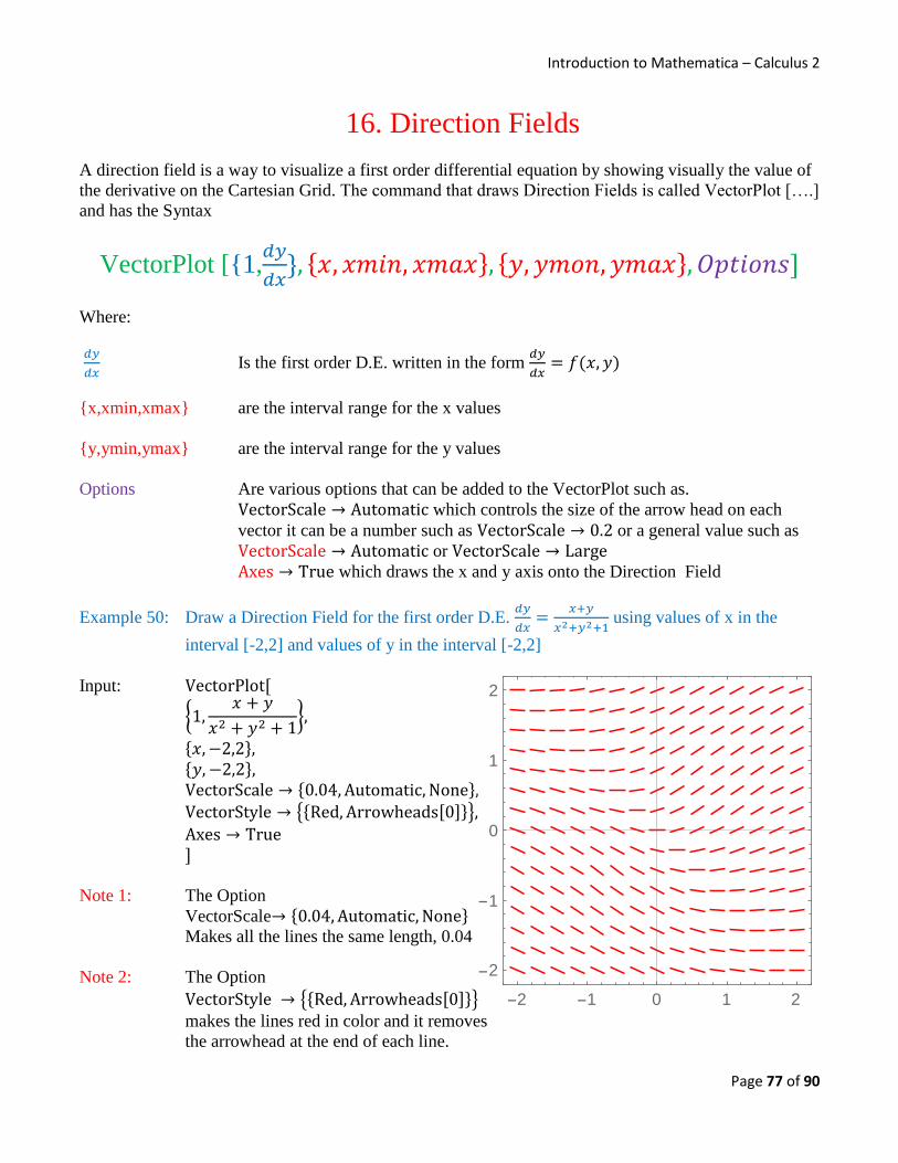
Introduction to Mathematica – Calculus 2
Page 77 of 90
16. Direction Fields
A direction field is a way to visualize a first order differential equation by showing visually the value of
the derivative on the Cartesian Grid. The command that draws Direction Fields is called VectorPlot [….]
and has the Syntax
VectorPlot [{1,𝑑𝑦
𝑑𝑥}, {𝑥, 𝑥𝑚𝑖𝑛, 𝑥𝑚𝑎𝑥}, {𝑦, 𝑦𝑚𝑜𝑛, 𝑦𝑚𝑎𝑥}, 𝑂𝑝𝑡𝑖𝑜𝑛𝑠]
Where:
𝑑𝑦
𝑑𝑥 Is the first order D.E. written in the form
𝑑𝑦
𝑑𝑥= 𝑓(𝑥, 𝑦)
{x,xmin,xmax} are the interval range for the x values
{y,ymin,ymax} are the interval range for the y values
Options Are various options that can be added to the VectorPlot such as.
VectorScale → Automatic which controls the size of the arrow head on each
vector it can be a number such as VectorScale → 0.2 or a general value such as
VectorScale → Automatic or VectorScale → Large
Axes → True which draws the x and y axis onto the Direction Field
Example 50: Draw a Direction Field for the first order D.E. 𝑑𝑦
𝑑𝑥=
𝑥+𝑦
𝑥2+𝑦2+1 using values of x in the
interval [-2,2] and values of y in the interval [-2,2]
Input: VectorPlot[
{1,𝑥 + 𝑦
𝑥2 + 𝑦2 + 1},
{𝑥, −2,2}, {𝑦, −2,2}, VectorScale → {0.04, Automatic, None}, VectorStyle → {{Red, Arrowheads[0]}},
Axes → True
]
Note 1: The Option
VectorScale→ {0.04, Automatic, None}
Makes all the lines the same length, 0.04
Note 2: The Option
VectorStyle → {{Red, Arrowheads[0]}}
makes the lines red in color and it removes
the arrowhead at the end of each line.
2 1 0 1 2
2
1
0
1
2

Introduction to Mathematica – Calculus 2
Page 78 of 90
Example 51: (a) Draw a Direction Field for the first order D.E. 𝑑𝑦
𝑑𝑥=
𝑥+𝑥2
𝑦+1 using values of x in
the interval [−3, 3] and values of y in the interval [-3,3]
(b) Find the Particular Solution to the first order D.E. 𝑑𝑦
𝑑𝑥=
𝑥+𝑥2
𝑦+1 , with y(0)=1
(c) Graph the Direction Field and the Particular Solution on the same diagram.
Input (a): VectorPlot[
{1,𝑥 + 𝑥2
𝑦 + 1},
{𝑥, −3,3}, {𝑦, −3,3}, VectorScale → {0.04, Automatic, None},
VectorStyle → {{Red, Arrowheads[0]}},
Axes → True
]
Note 1: The Option
VectorScale → {0.04, Automatic, None}
Makes all the lines the same length, 0.04
Note 2: The Option
VectorStyle → {{Red, Arrowheads[0]}}
makes the lines red in color and it removes
the arrowhead at the end of each line.
Input (b): ClearAll[𝑦, 𝑥]
DSolve[{𝑦′[𝑥] ==𝑥+𝑥2
𝑦[𝑥]+1, 𝑦[𝜋] == 1}, 𝑦[𝑥], 𝑥]
Output: {{𝑦[𝑥] →1
3(−3 + √3√12 + 3𝑥2 + 2𝑥3)}}
Note 1: The Particular Solution to this D.E is y = 1
3(−3 + √3√12 + 3𝑥2 + 2𝑥3)
Note 2: The output DSolve: For some branches of the general solution, the given boundary
conditions lead to an empty solution. This means that there are some versions of the
General Solution to this D.E. will not exist with the value y(0)=1.
Note 3: There is an interesting feature at the point (−1, −1) the derivative will be
infinite at this point, its like an infinite singularity in the derivative function.
3 2 1 0 1 2 3
3
2
1
0
1
2
3
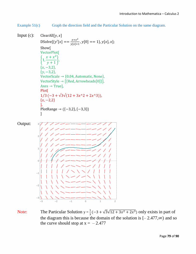
Introduction to Mathematica – Calculus 2
Page 79 of 90
Example 51(c) Graph the direction field and the Particular Solution on the same diagram.
Input (c): ClearAll[𝑦, 𝑥]
DSolve[{𝑦′[𝑥] ==𝑥+𝑥2
𝑦[𝑥]+1, 𝑦[0] == 1}, 𝑦[𝑥], 𝑥];
Show[ VectorPlot[
{1,𝑥 + 𝑥2
𝑦 + 1},
{𝑥, −3,2}, {𝑦, −3,2}, VectorScale → {0.04, Automatic, None},
VectorStyle → {{Red, Arrowheads[0]}},
Axes → True], Plot[
1 3⁄ (−3 + √3√(12 + 3𝑥^2 + 2𝑥^3)), {𝑥, −2,2}
], PlotRange → ({−3,2}, {−3,3}}
]
Output:
Note: The Particular Solution y = 1
3(−3 + √3√12 + 3𝑥2 + 2𝑥3) only exists in part of
the diagram this is because the domain of the solution is [– 2.477,∞) and so
the curve should stop at x = – 2.477
3 2 1 0 1 2
3
2
1
0
1
2
3

Introduction to Mathematica – Calculus 2
Page 80 of 90
17. Solving Differential Equations There are three main types of Differential Equations that we will solve in Calculus II they are
A. Simple Differential Equations
B. Variables Separable Differential Equations
C. Linear Differential Equations
A. Simple Differential Equations
A Simple Differential Equation where you can find the solution by repeated Integration.
The following are all examples of Simple D.E.
1. 𝑑𝑦
𝑑𝑥 = 𝑥3 + 5𝑥 + 7
2. 𝑓′′(𝑥) = 𝑠𝑖𝑛(𝑥) − cos2 (𝑥)
3. 𝑢′′′(𝑡) = 𝑒2𝑡 + ln (t)
To solve a Simple D.E. you integrate until you get to the solution.
In Mathematica we use the DSolve[….] command as seen earlier.
Example 52: Find the General Solutions to the following Simple D.E.
(a) 𝑑𝑦
𝑑𝑥 = 𝑥3 + 5𝑥 + 7
(b) 𝑓′′(𝑥) = 𝑠𝑖𝑛(𝑥) − cos2 (𝑥)
(c) 𝑢′′′(𝑡) = 𝑒2𝑡 + ln (t)
Input (a) DSolve[𝑦′[𝑥] == 𝑥3 + 5𝑥 + 7, 𝑦[𝑥], 𝑥]
Output {{𝑦[𝑥] → 7𝑥 +5𝑥2
2+
𝑥4
4+ 𝐶[1]}}
Solution y = 7𝑥 +5𝑥2
2+
𝑥4
4+ 𝐶
Input (b) DSolve[𝑦''[𝑥] == Sin[𝑥] − Cos[𝑥]^2, 𝑦[𝑥], 𝑥]
Output {{𝑦[𝑥] → −𝑥2
4+ 𝐶[1] + 𝑥𝐶[2] +
Cos[𝑥]2
4− Sin[𝑥]}}
Solution y = −𝑥2
4+ 𝐶 + 𝐷𝑥 +
Cos[𝑥]2
4− Sin 𝑥
Input (c) DSolve[𝑢′[𝑡] == 𝑒2𝑡 + Log[𝑡], 𝑢[𝑡], 𝑡]
Output {{𝑢[𝑡] → 𝐶[1] + 𝑡𝐶[2] + 𝑡2𝐶[3] +1
4(
𝑒2𝑡
2−
11𝑡3
9+
2
3𝑡3Log[𝑡])}}
Solution y = 𝐶 + 𝐷𝑡 + 𝐸𝑡2 +1
4(
𝑒2𝑡
2−
11𝑡3
9+
2
3𝑡3ln 𝑡

Introduction to Mathematica – Calculus 2
Page 81 of 90
Example 53: Find the Particular Solutions to the following Simple D.E.
(a) 𝑑𝑦
𝑑𝑥 = 𝑥3sin (𝑥) y(0) = 1
(b) 𝑓′′(𝑥) = 2𝑥
𝑥2+1 𝑓′(
𝜋
4) = 1 and 𝑓(0) = 0
(c) 𝑢′′′(𝑡) = 𝑒𝑡𝑠𝑖𝑛𝑡 𝑢′′(0) = 2, 𝑢′(0) = 1 𝑎𝑛𝑑 𝑢(0) = −1
Input (a) DSolve[{𝑦′[𝑥] == 𝑥3Sin[𝑥], 𝑦[0] == 1}, 𝑦[𝑥], 𝑥]
Output {{𝑦[𝑥] → 1 + 6𝑥Cos[𝑥] − 𝑥3Cos[𝑥] − 6Sin[𝑥] + 3𝑥2Sin[𝑥]}}
Solution y = 1 + 6𝑥 cos 𝑥 − 𝑥3 cos 𝑥 − 6 sin 𝑥 + 3𝑥2 sin 𝑥
Input (b) DSolve[{𝑦''[𝑥] ==2𝑥
𝑥2+1, 𝑦′[
𝜋
4] == 1, 𝑦[0] == 0}, 𝑦[𝑥], 𝑥]
Output {{𝑦[𝑥] → −𝑥 + 2ArcTan[𝑥] − 𝑥Log[1 +𝜋2
16] + 𝑥Log[1 + 𝑥2]}}
Solution y = −𝑥 + 2 tan−1𝑥 − 𝑥ln(1 +𝜋2
16} + 𝑥ln(1 + 𝑥2)
Input (c) DSolve[{𝑢'''[𝑡] == 𝑒𝑡Sin[𝑡], 𝑢''[0] == 2, 𝑢′[0] == 1, 𝑢[0] == −1}, 𝑢[𝑡], 𝑡]
Output {{𝑢[𝑡] →1
4(−3 + 6𝑡 + 5𝑡2 − 𝑒𝑡Cos[𝑡] − 𝑒𝑡Sin[𝑡])}}
Solution y = 1
4(−3 + 6𝑡 + 5𝑡2 − 𝑒𝑡cos 𝑡 − 𝑒𝑡 sin 𝑡

Introduction to Mathematica – Calculus 2
Page 82 of 90
B. Variables Separable Differential Equations
A Variables Separable Differential Equation is one that can be written in the form 𝑑𝑦
𝑑𝑥 =
𝑓(𝑥)
𝑔(𝑦)
The following are all examples of Variables Separable D.E.
1. 𝑑𝑦
𝑑𝑥 =
4𝑥−7
2𝑦+1
2. 𝑑𝑦
𝑑𝑥 =
𝑥 𝑠𝑖𝑛𝑥
2𝑒𝑦
3. 𝑑𝑢
𝑑𝑡 =
tan 𝑡
√𝑢+1
To solve a Simple D.E. you integrate until you get to the solution.
In Mathematica we use the DSolve[….] command as seen earlier.
Example 54: Find the General Solution to the following Variables Separable D.E.
(a) 𝑑𝑦
𝑑𝑥 =
4𝑥−7
2𝑦+1 (b)
𝑑𝑦
𝑑𝑥 =
𝑥 𝑠𝑖𝑛𝑥
2𝑒𝑦 (c) 𝑑𝑢
𝑑𝑡 =
𝑡2
√𝑢+1
Input (a) DSolve[𝑦′[𝑥] ==4𝑥−7
2𝑦[𝑥]+1, 𝑦[𝑥], 𝑥]
Output {{𝑦[𝑥] →1
2(−1 − √1 − 28𝑥 + 8𝑥2 + 4𝐶[1])}, {𝑦[𝑥] →
1
2(−1 + √1 − 28𝑥 + 8𝑥2 + 4𝐶[1])}}
Solution y = 1
2(−1 ± √1 − 28𝑥 + 8𝑥2 + 4𝐶)
Input (b) DSolve[𝑦''[𝑥] == Sin[𝑥] − Cos[𝑥]^2, 𝑦[𝑥], 𝑥]
Output {{𝑦[𝑥] → Log[𝐶[1] +1
2(−𝑥Cos[𝑥] + Sin[𝑥])]}}
Solution y = ln (𝐶 +1
2(−𝑥 cos 𝑥 + sin 𝑥))
Input (c) DSolve[𝑢′[𝑡] ==𝑡2
√𝑢[𝑡]+1, 𝑢[𝑡], 𝑡]
Output {{𝑢[𝑡] → −1 +(𝑡6+6𝑡3𝐶[1]+9𝐶[1]2)1 3⁄
22 3⁄ }, {𝑢[𝑡] → −1 −(1−𝑖√3)(𝑡6+6𝑡3𝐶[1]+9𝐶[1]2)1 3⁄
222 3⁄ }, {𝑢[𝑡] → −1 −(1+𝑖√3)(𝑡6+6𝑡3𝐶[1]+9𝐶[1]2)1 3⁄
222 3⁄ }}
Solution u = −1 +(𝑡6+6𝑡3𝐶[1]+9𝐶2)1 3⁄
22 3⁄
Note: There is only one Real Function Solution exists for 𝑑𝑢
𝑑𝑡 =
𝑡2
√𝑢+1
u = −1 +(𝑡6+6𝑡3𝐶[1]+9𝐶2)1 3⁄
22 3⁄ the other two are Complex functions as they contain i = √−1

Introduction to Mathematica – Calculus 2
Page 83 of 90
Example 55: Find the Particular Solution to the following Variables Separable D.E.
(a) 𝑑𝑦
𝑑𝑥 =
4𝑥−7
2𝑦+1 with y(0) = 10
(b) 𝑑𝑦
𝑑𝑥 =
𝑥 𝑠𝑖𝑛𝑥
2𝑒𝑦 with y(𝜋) = 0
(b) 𝑑𝑢
𝑑𝑡 =
𝑡2
√𝑢+1 with u(0) = 0
Input (a) DSolve[{𝑦′[𝑥] ==4𝑥−7
2𝑦[𝑥]+1, 𝑦[0] == 0}, 𝑦[𝑥], 𝑥]
Output {{𝑦[𝑥] →1
2(−1 + √1 − 28𝑥 + 8𝑥2)}}
Solution y = 1
2(−1 + √1 − 28𝑥 + 8𝑥2)
Input (b) DSolve[{𝑦′[𝑥] ==𝑥Sin[𝑥]
2𝑒𝑦[𝑥] , 𝑦[𝜋] == 0}, 𝑦[𝑥], 𝑥]
Output {{𝑦[𝑥] → Log[2−𝜋
2+
1
2(−𝑥Cos[𝑥] + Sin[𝑥])]}}
Solution y = ln[2−𝜋
2+
1
2(−𝑥 cos 𝑥 + sin 𝑥)
Input (c) DSolve[{𝑢′[𝑡] ==𝑡2
√𝑢[𝑡]+1, 𝑢[0] == 0}, 𝑢[𝑡], 𝑡]
Output {{𝑢[𝑡] →1
2(−2 + 21 3⁄ ((−2 + 𝑡3)2)1 3⁄ )}, {𝑢[𝑡] →
1
2(−2 + 21 3⁄ ((2 + 𝑡3)2)1 3⁄ )}}
Solution u = 1
2(−2 + 21 3⁄ ((−2 + 𝑡3)2)1 3⁄ )
u = (−2 + 21 3⁄ ((2 + 𝑡3)2)1 3⁄ )
Note: There are two possible Particular solutions to the D.E 𝑑𝑢
𝑑𝑡 =
𝑡2
√𝑢+1 with u(0) = 0

Introduction to Mathematica – Calculus 2
Page 84 of 90
C. Linear Differential Equations
A linear Differential Equation has the form 𝑑𝑦
𝑑𝑥= 𝑘𝑦 + 𝑐
The following are all examples of Variables Separable D.E.
1. 𝑑𝑦
𝑑𝑥 = 5y + 4
2. 𝑦′(𝑡) = 0.03y + 200
3. 𝑝′(𝑡) = – 0.2p + 50
To solve a Simple D.E. you integrate until you get to the solution.
In Mathematica we use the DSolve[….] command as seen earlier.
Example 56: Find the General Solution to the following Linear D.E.
(a) 𝑑𝑦
𝑑𝑥 = 5y + 4
(b) 𝑦′(𝑡) = 0.03y + 200
(c) 𝑝′(𝑡) = – 0.2p + 50
Input (a) DSolve[𝑦′[𝑥] == 5𝑦[𝑥] + 4, 𝑦[𝑥], 𝑥]
Output {{𝑦[𝑥] → −4
5+ 𝑒5𝑥𝐶[1]}}
Solution y = −4
5+ 𝐶𝑒5𝑥
Input (b) DSolve[𝑦′[𝑡] == 0.03𝑦[𝑡] + 4, 𝑦[𝑡], 𝑡]
Output {{𝑦[𝑡] → −133.33333333333334 + 𝑒0.03𝑡𝐶[1]}}
Solution y = −133.333 + 𝐶𝑒0.03𝑡
Input (c) DSolve[𝑝′[𝑡] == −0.2𝑝[𝑡] + 50, 𝑝[𝑡], 𝑡]
Output {{𝑝[𝑡] → 250. + 𝑒−0.2𝑡𝐶[1]}}
Solution u = 250 + 𝐶𝑒−0.2𝑡

Introduction to Mathematica – Calculus 2
Page 85 of 90
18. Applications of Differential Equations There are many practical applications in using Differential Equations , it is by far, the most adaptable
method for modelling situations in Engineering , Sciences , Business etc…. We will use population
models to show the versatility in using Differential equations.
Example 57: Exponential Growth Population Models
(a) A town has population grows at the rate of 2.1% per year , the initial
population of the town is 5000 , find a formula for the population of the
town in t years.
(b) What will the population of the town be in 12 years?
(c) How long before the population reaches 20,000 people.
Solution (a): The D.E. that models this situation is 𝑝′(𝑡) = 0.021𝑝 with p(0) = 500
The Mathematica code that solves this equation is as follows
Input: DSolve[{𝑝′[𝑡] == 0.021𝑝[𝑡], 𝑝[0] == 500}, 𝑝[𝑡], 𝑡]
Output: {{𝑝[𝑡] → 500. 𝑒0.021𝑡}}
The population of this town in t years will be p(t) = 500𝑒0.021𝑡
Solution (b): We need to evaluate p(12)
The Mathematica code that solves this equation is as follows
Input: 𝑝[t_]: = 500𝑒0.021𝑡
Output: 643.298
The population of this town in 12 years will be p(12) = 643 (approx)
Solution (c): We need to solve the equation p(t) = 20,000
The Mathematica code that solves this equation is as follows
Input: 𝑝[t_]: = 500𝑒0.021𝑡
Output: {{𝑡 → 175.66092638637792}}
The population will reach 20,000 in 175.7 years (approx.)

Introduction to Mathematica – Calculus 2
Page 86 of 90
Example 58: Exponential Decay Models
(a) A radioactive element decays at the rate of 0.005% per year , if you start
with 40 grams how much will be left in t years.
(b) What is the half-life of this radioactive material?
(c) Graph this information.
Solution (a): The D.E. that models this situation is 𝑎′(𝑡) = −0.00005𝑎 with a(0) = 40
(0.005% = 0.00005 as a decimal , it is negative since the rate is decreasing)
Input: DSolve[{𝑎′[𝑡] == −0.00005𝑎[𝑡], 𝑎[0] == 40}, 𝑎[𝑡], 𝑡]
Output: {{𝑎[𝑡] → 40. 𝑒−0.00005𝑡}}
The amount of radioactive material left after t years will be p(t) = 40. 𝑒−0.00005𝑡
Solution (b): We now need to solve when is a(t) = 20
Since the half-life is the time it takes to end up with half of the radioactive
material you started with, in this case half of 40 g is 20 g.
Input: DSolve[{𝑎′[𝑡] == −0.00005𝑎[𝑡], 𝑎[0] == 40}, 𝑎[𝑡], 𝑡]
Output: {{𝑡 → 13862.943611198907}}
The half-life of this radioactive material is 13,863 years (approx).
Solution (c): Graph this information.
𝑎[t_]: = 40𝑒−0.00005𝑡
ℎ[t_]: = 20
Plot[{𝑎[𝑡], ℎ[𝑡]}, {𝑡, 0,20000}, AxesLabel → {Time(𝑡years), Amount(𝑎)}]
Output:
5000 10000 15000 20000t Time years
20
25
30
35
40
a Amount
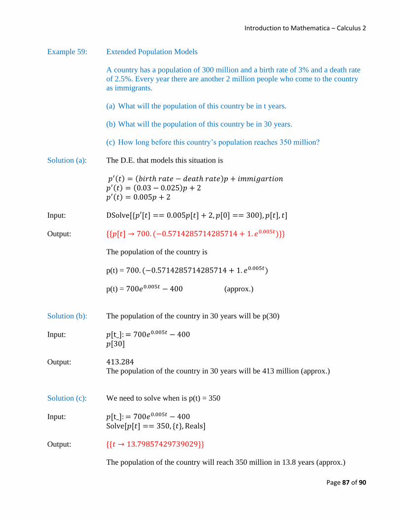
Introduction to Mathematica – Calculus 2
Page 87 of 90
Example 59: Extended Population Models
A country has a population of 300 million and a birth rate of 3% and a death rate
of 2.5%. Every year there are another 2 million people who come to the country
as immigrants.
(a) What will the population of this country be in t years.
(b) What will the population of this country be in 30 years.
(c) How long before this country’s population reaches 350 million?
Solution (a): The D.E. that models this situation is
𝑝′(𝑡) = (𝑏𝑖𝑟𝑡ℎ 𝑟𝑎𝑡𝑒 − 𝑑𝑒𝑎𝑡ℎ 𝑟𝑎𝑡𝑒)𝑝 + 𝑖𝑚𝑚𝑖𝑔𝑎𝑟𝑡𝑖𝑜𝑛
𝑝′(𝑡) = (0.03 − 0.025)𝑝 + 2
𝑝′(𝑡) = 0.005𝑝 + 2
Input: DSolve[{𝑝′[𝑡] == 0.005𝑝[𝑡] + 2, 𝑝[0] == 300}, 𝑝[𝑡], 𝑡]
Output: {{𝑝[𝑡] → 700. (−0.5714285714285714 + 1. 𝑒0.005𝑡)}}
The population of the country is
p(t) = 700. (−0.5714285714285714 + 1. 𝑒0.005𝑡)
p(t) = 700𝑒0.005𝑡 − 400 (approx.)
Solution (b): The population of the country in 30 years will be p(30)
Input: 𝑝[t_]: = 700𝑒0.005𝑡 − 400
𝑝[30]
Output: 413.284
The population of the country in 30 years will be 413 million (approx.)
Solution (c): We need to solve when is p(t) = 350
Input: 𝑝[t_]: = 700𝑒0.005𝑡 − 400
Solve[𝑝[𝑡] == 350, {𝑡}, Reals]
Output: {{𝑡 → 13.79857429739029}}
The population of the country will reach 350 million in 13.8 years (approx.)

Introduction to Mathematica – Calculus 2
Page 88 of 90
Example 60: Logistic Growth Models
(a) An island has enough food to maintain a population of 2000 deer (this number is called the carrying capacity and is usually denoted by K = 2000).
The deer have a growth rate of 12%
(this is usually denoted by r = 0.12).
At present the island has a population of 250 deer
(this is usually called p0 = 250)
What is the population model p(t) for the number of deer in t years.
(b) How many deer will be on the island in 22 years?
Solution (a): This situation is called a logistic model and its D.E. takes the form
𝑝′(𝑡) = 𝑟𝑝(1 −𝑝
𝑘)
The solution to the logistic model is
p(t) = 𝑝0𝑘
𝑝0+(𝑘−𝑝0)𝑒−𝑟𝑡
The population of deer in t years will be p(t) = 𝑝0𝑘
𝑝0+(𝑘−𝑝0)𝑒−𝑟𝑡
p(t) = 250(2000)
250+(2000−250)𝑒−0.12𝑡
p(t) = 500 000
250+1750𝑒−0.12𝑡
Solution (b):
Input: 𝑝[t_]: =500000
250+1750𝑒−0.12𝑡
p[22]
Output: 1333.75
In 22 years there will be 1334 deer on island (approx.)
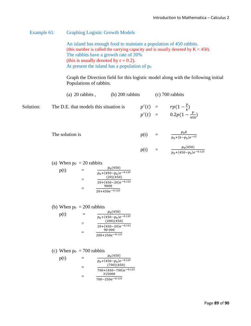
Introduction to Mathematica – Calculus 2
Page 89 of 90
Example 61: Graphing Logistic Growth Models
An island has enough food to maintain a population of 450 rabbits. (this number is called the carrying capacity and is usually denoted by K = 450).
The rabbits have a growth rate of 20%
(this is usually denoted by r = 0.2).
At present the island has a population of p0
Graph the Direction field for this logistic model along with the following initial
Populations of rabbits.
(a) 20 rabbits , (b) 200 rabbits (c) 700 rabbits
Solution: The D.E. that models this situation is 𝑝′(𝑡) = 𝑟𝑝(1 −𝑝
𝑘)
𝑝′(𝑡) = 0.2𝑝(1 −𝑝
450)
The solution is p(t) = 𝑝0𝑘
𝑝0+(𝑘−𝑝0)𝑒−𝑟𝑡
p(t) = 𝑝0(450)
𝑝0+(450−𝑝0)𝑒−0.12𝑡
(a) When p0 = 20 rabbits
p(t) = 𝑝0(450)
𝑝0+(450−𝑝0)𝑒−0.12𝑡
= (20)(450)
20+(450−20)𝑒−0.12𝑡
= 9000
20+430𝑒−0.12𝑡
(b) When p0 = 200 rabbits
p(t) = 𝑝0(450)
𝑝0+(450−𝑝0)𝑒−0.12𝑡
= (200)(450)
20+(450−20)𝑒−0.12𝑡
= 90 000
200+250𝑒−0.12𝑡
(c) When p0 = 700 rabbits
p(t) = 𝑝0(450)
𝑝0+(450−𝑝0)𝑒−0.12𝑡
= (700)(450)
700+(450−700)𝑒−0.12𝑡
= 315000
700−250𝑒−0.12𝑡
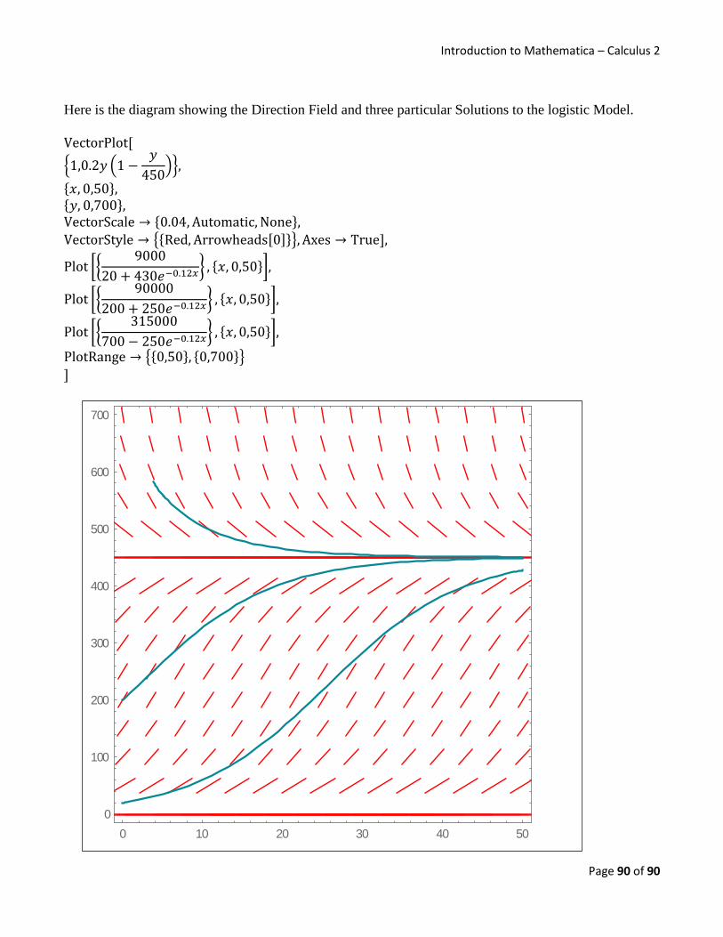
Introduction to Mathematica – Calculus 2
Page 90 of 90
Here is the diagram showing the Direction Field and three particular Solutions to the logistic Model.
VectorPlot[
{1,0.2𝑦 (1 −𝑦
450)},
{𝑥, 0,50}, {𝑦, 0,700}, VectorScale → {0.04, Automatic, None}, VectorStyle → {{Red, Arrowheads[0]}}, Axes → True],
Plot [{9000
20 + 430𝑒−0.12𝑥} , {𝑥, 0,50}],
Plot [{90000
200 + 250𝑒−0.12𝑥} , {𝑥, 0,50}],
Plot [{315000
700 − 250𝑒−0.12𝑥} , {𝑥, 0,50}],
PlotRange → {{0,50}, {0,700}}
]
0 10 20 30 40 50
0
100
200
300
400
500
600
700
Related Documents