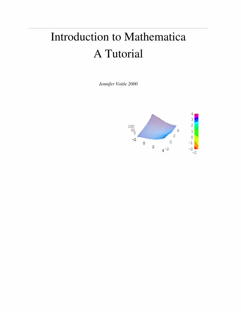
Introduction to Mathematica A Tutorial - QuantCandy · Introductory Programming in Mathematica Pattern Matching with Function Arguments Conditionals Looping Working with Lists Defining

Introduction to Mathematica

A Tutorial

Jennifer Voitle 2000

-20

24-2

0

2

40

50100

-20

24

-2 -1-2

-1

0

1

2

3

4

ContentsIntroduction

Getting Started

Fundamental Arithmetic and Algebraic Operations

Numerics

Matrix Operations

Symbolic Computations

Sequences and Series

Solution of Equations

Vectors

Solution of Nonlinear Equations

Limit of a Function

Differentiation

Taylor Series Expansions

Integration

Solution of Ordinary Differential Equations

Function Interpolation and Approximation

Graphics

Introductory Programming in Mathematica

Pattern Matching with Function Arguments

Conditionals

Looping

Working with Lists

Defining Your Own Rules

Teaching Mathematica New Tricks

Interpolation by Newton's Divided Difference Method

LU Factorization of Matrices

Engineering and Mathematics Applications

Transforms

Financial Applications (coming)

Online Help from Mathematica

2 Mathematica Tutorial.nb

IntroductionMathematica is a system for doing mathematics on the computer.It can do numerics,symbolics,graphics and is

also a programming language.Mathematica has infinite precision.It can plot functions of a single variable; make

contour,surface and density plots with special shading and lighting effects (in plots,the functions may be defined

analytically or in tabular form); perform algebraic manipulations on polynomials; solve linear and nonlinear

equations and systems of equations; compute symbolic and numeric values of total and partial derivatives,and do

animation with Mathematica-generated graphics or with graphics imported from other applications.It has exten-

sive curve-fitting capabilities by regression polynomials,interpolating polynomials,splines and series approxima-

tions.It can work with Laplace and Fourier transforms and solve systems of differential equations,both numeri-

cally and symbolically.It has hundreds of built-in functions such as the Error,Gamma,Bessel and Legendre

functions as well as some rather exotic ones.It can work with both real and complex numbers.Mathematica is also

a rich programming language,containing all of the standard constructs of normal languages such as FORTRAN or

C but with all of the symbolic power of Mathematica.Mathematica functions can be compiled and called from

Excel,C++ or Visual Basic (to name a few).Thus,Mathematica can be taught to do anything that other languages

can do such as neural network analysis,image processing and Finite Element Analysis.Beyond this,the notebook

interface allows creation of truly dynamic documents not possible in any other system.In a notebook,all of the

supporting code,illustrations,hyperlinks and text to support a paper are all self-contained.In addition, Mathemat-

ica documents can be converted to HTML.Although note as of the latest release (v 4.0) there are problems with

the HTML conversion process as you will see if you try to actually upload it to a website.

Getting Started It is very important to follow Mathematica's naming conventions. Mathematica is case-

sensitive. All reserved words begin with uppercase letters, with all other letters lowercase. When two words are

concatenated, an uppercase letter begins each word. These are the only times when uppercase letters are used. A

list of some of the more common function names is provided at the end of this document. Once you understand

Mathematica's syntax, using it becomes almost intuitive. For example, the command for plotting is Plot, and

FindRoot is the function that solves nonlinear equations by the Newton-Raphson or Secant techniques. Mathe-

matica essentially works by pattern-matching, and at the heart of it is this rule:

Given an object, apply transformation rules to it until there are no longer any changes.

Executing a Command Typing commands into Mathematica is very similar to typing with a word processor.

Try typing a command such as the following:

Plot[Sin[x],{x,-2Pi,2Pi}];

Type it exactly as shown above.Note that a times sign is not necessary between the 2 and the symbol Pi; the

multiplication will be performed automatically.If the command Plot[Sin[x],{x,-2Pi,2Pi}]; just beeps and prints

the expression back at you,it means that a syntax error has occurred:Mathematica is unable to understand what

you mean because perhaps you have typed plot instead of Plot,or used round brackets () rather than square.After

typing the command,press the Enter key (or press Shift-Enter.) This will execute your command.Pressing the

return key alone is insufficient as a command may be several lines long,such as when writing a program.You will

press Enter or Shift-Enter each time you wish to ask Mathematica a question.The resulting plot should look like

the following:

Mathematica Tutorial.nb 3

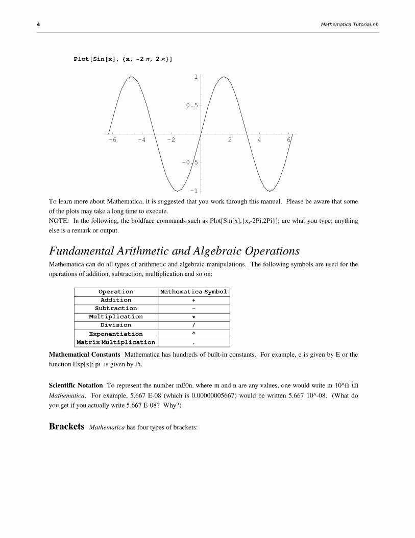
Plot@Sin@xD, 8x, −2 π, 2 π<D

-6 -4 -2 2 4 6

-1

-0.5

0.5

1

To learn more about Mathematica, it is suggested that you work through this manual. Please be aware that some

of the plots may take a long time to execute.

NOTE: In the following, the boldface commands such as Plot[Sin[x],{x,-2Pi,2Pi}]; are what you type; anything

else is a remark or output.

Fundamental Arithmetic and Algebraic Operations Mathematica can do all types of arithmetic and algebraic manipulations. The following symbols are used for the

operations of addition, subtraction, multiplication and so on:

Operation Mathematica Symbol

Addition +

Subtraction −

Multiplication ∗

Division êExponentiation ^

Matrix Multiplication .

Mathematical Constants Mathematica has hundreds of built-in constants. For example, e is given by E or the

function Exp[x]; pi is given by Pi.

Scientific Notation To represent the number mE0n, where m and n are any values, one would write m 10^n inMathematica. For example, 5.667 E-08 (which is 0.00000005667) would be written 5.667 10^-08. (What do

you get if you actually write 5.667 E-08? Why?)

Brackets Mathematica has four types of brackets:


Symbol Explanation

HL Parentheses are used for grouping and ordering operations.

8< Curly brackets are used for elements of lists and arrays

@D Square brackets are used for function arguments

@@DD Double square brackets are used for elements of matrices and lists

Equal Signs Mathematica has several ways of testing equality, but we will mainly be interested in only the

following:

Symbol Meaning

= x = y means set x to the value of y immediately

== x == y means test whether x and y are equal. True or False is returned

:= x := y means set delayed. x is not set equal to y immediately, but the

is remembered and when x is called, the definition y is substituted.

!= x != y tests x not equal to y. True or False is returned.

Logical Operators The logical And, Or are carried out via the && and || operators respectively. x And y would

be written x && y while x Or y would be evaluated x || y. (The || symbol is made by pressing the shift-\ key

twice.)

User-defined Variables Variable names can be any length desired. However, they cannot conflict with Mathe-

matica keywords. Since Mathematica keywords always begin with an uppercase letter, conflict may be avoided

by always beginning user-defined variables with a lowercase letter. (It is possible to override built-in definitions,

but this is usually unnecessary.) Variable names must begin with a letter or $ sign and may combine any combina-

tion of numeric and upper and lowercase alphabetic characters. No spaces may appear in variable names as a

space between symbols usually implies multiplication. You also may not use the letters C, D, E, I, N or O as

these are reserved. note however that the lowercase equivalents c, d, e, i, n and o are valid choices. Variable

names may not include any of the following: .,%^+/*-_#()[]{} | ? to name a few.

Some examples and nonexamples:

(1) x2 is a legal variable name while 2x is not. Since a multiplication symbol is not required between operands

and variables aer not allowed to begin with numerals, 2x will be evaluated as twice the current value of x.

Should you attempt to set 2x to something, such as 10, you will get an error:

2 x = 10

— Set::write : Tag Times in 2 x is Protected.

10

(2) The variable MaxIterations is allowed while neither Max_Iterations nor Max.Iterations are valid.

(3) The variables Tan, Sin, Cos, Sinh, Log, Max and the like are not allowed since they are reserved keywords.

However, valid variable names may include reserved keywords, such as myTan and Tangent.

Mathematica's Built In Symbols To see a list of all of Mathematica's intrinsic keywords, type ?* To see a list

of all key words starting wtih a certain letter, or containing partial phrases, use * as a wildcard character. For


example, all of the keywords that start with Z are

?Z∗

ZeroTest ZeroWidthTimes Zeta ZTransform

More detailed information is available by using the double question mark:

?? ZeroTest

ZeroTest is an option for LinearSolve and other linear algebra functions,

which gives a function to be applied to combinations of matrix

elements to determine whether they should be considered equal to zero.

Attributes@ZeroTestD = 8Protected<Command-completion is very helpful in situations where you don't remember the full name of the function you

want, or don't want to type out a long name. In the Windows environment, type the first few letters of the

function you want and press Ctrl-k. Make your selection from the pop-up list that appears.

Now, let's start exploring!

NumericsEvaluate the product of the two integers 127 and 9721:

127×9721

1234567

A more complicated expression:

2 + H3 + 5L 8ê7 − H2 − PiL^2êH81 − 4L + 7êH14ê3 − 6ê3L − 2

659

56−

1

77H2 − πL2

Note that the answer is left partially evaluated. To convert it to a decimal value, wrap N[ ] around it. You can

use N[%]. % always refers to the most recently evaluated Mathematica expression, wherever it may actually be,

and %% is the next-to last most recently evaluated expression, and so on. So, N[%] means "give the numerical

equivalent of the most recently evaluated expression."

N@%D11.7509

Complex Numbers As an example, simplify 4 + i -(3 - 5i)

4 + I − H3 − 5 IL1 + 6 �


Now for some division:

H4 + ILêH3 − 5 IL7

34+23 �

34

Representation of Numbers Let's get Pi to oh, 800 digits:

N@Pi, 801D3.141592653589793238462643383279502884197169399375105820974944592307�

8164062862089986280348253421170679821480865132823066470938446095505�

8223172535940812848111745028410270193852110555964462294895493038196�

4428810975665933446128475648233786783165271201909145648566923460348�

6104543266482133936072602491412737245870066063155881748815209209628�

2925409171536436789259036001133053054882046652138414695194151160943�

3057270365759591953092186117381932611793105118548074462379962749567�

3518857527248912279381830119491298336733624406566430860213949463952�

2473719070217986094370277053921717629317675238467481846766940513200�

0568127145263560827785771342757789609173637178721468440901224953430�

1465495853710507922796892589235420199561121290219608640344181598136�

2977477130996051870721134999999837297804995105973173281609631860

(Is that really 800 digits?)

Matrix Operations In the following, we show how to invert, evaluate the determinant, transpose, multiply and compute the eigenval-

ues of a matrix.

First, define a matrix A that we can work with:

A = 881, 0, −5<, 87, 3, 0.6<, 8−0.9, 11, 0.725<<881, 0, −5<, 87, 3, 0.6<, 8−0.9, 11, 0.725<<

MatrixForm@AD1 0 −5

7 3 0.6

−0.9 11 0.725

This looks much prettier. The determinant is:

Determinant@ADDeterminant@881, 0, −5<, 87, 3, 0.6<, 8−0.9, 11, 0.725<<D

Fooled you - this is one time that we have a shortcut. The function to compute the determinant is named Det:


Det@AD−402.925

The n by n identity matrix is Identity[n], so for n = 3,

IdentityMatrix@3D êê MatrixForm

1 0 0

0 1 0

0 0 1

Except for roundoff errors, A multiplied by it's inverse should return the identity matrix:

A.Inverse@AD êê MatrixForm

1. 0. 6.93889×10−18

0. 1. 9.54098×10−18

0. −1.38778×10−17 1.

Most of these entries are so close to zero that we can round. The Chop function is used for this purpose:

Chop@%D êê MatrixForm

1. 0 0

0 1. 0

0 0 1.

The transpose of a matrix is obtained by interchanging the rows and columns of a matrix, so a[i,j] = a[j,i]:

Transpose@AD881, 7, −0.9<, 80, 3, 11<, 8−5, 0.6, 0.725<<

[email protected] + 5.80866 �, 5.50702 − 5.80866 �, −6.28904<

Eigenvectors@AD88−0.298534 + 0.384751 �, 0.286874 + 0.409611 �, 0.716077 + 0. �<,8−0.298534 − 0.384751 �, 0.286874 − 0.409611 �, 0.716077 + 0. �<,80.510054, −0.432392, 0.74356<<

Symbolic Computations Mathematica can work with symbols. Let us multiply two polynomials together:


Hx − 1L Hx^4 + x^3 + x^2 + x + 1LH−1 + xL I1 + x + x2 + x3 + x4M

Again, Mathematica leaves the result unevaluated, since this may be what the user wants. To force the expan-

sion, use Expand:

Expand@%D−1 + x5

Factor recovers the original expression.

Factor@%DH−1 + xL I1 + x + x2 + x3 + x4M

The next command performs the polynomial division (x^5 - 1)/(x - 1), which should be x^4 + x^3 + x^2 + x + 1:

Hx^5 − 1LêHx − 1L−1 + x5

−1 + x

Expand@%D

−1

−1 + x+

x5

−1 + x

Hmmmm ... not quite the form we wanted, although still correct. The function PolynomialQuotient is intended

for situations such as this.

PolynomialQuotient@Hx^5 − 1L, Hx − 1L, xD1 + x + x2 + x3 + x4

For fun, let's take the product of (a + b i) to the tenth power. We can use the product operator. Ask for help on

the syntax:

?? Product

Product@f, 8i, imax<D evaluates the product of the expressions f as evaluated

for each i from 1 to imax. Product@f, 8i, imin, imax<D starts with i =

imin. Product@f, 8i, imin, imax, di<D uses steps di. Product@f, 8i, imin,

imax<, 8j, jmin, jmax<, ... D evaluates a product over multiple indices.

Attributes@ProductD = 8HoldAll, Protected, ReadProtected<


Product@a + b I, 8i, 10<DHa + � bL10

Expand@%Da10 + 10 � a9 b − 45 a8 b2 − 120 � a7 b3 + 210 a6 b4 +

252 � a5 b5 − 210 a4 b6 − 120 � a3 b7 + 45 a2 b8 + 10 � a b9 − b10

Can Mathematica recover the original expression? Let's see ...

Factor@%DHa + � bL10

Sequences and Series It is said that Gauss' father made him compute long sums as punishment. One such problem was to compute the

sum 1 + 2 + 3 + ... + 100. Gauss discovered a neat trick for this. We can discover this too by looking at a few

patterns - this is one of the powers of Mathematica! For this problem, let's use the Sum function:

‚i=1

100

i

5050

Alternatively, we can type out the command:

Sum@i, 8i, 100<D5050

Generate a sequence of partial sums by using the Table command. We will just get the first 10 sums:

Table@Sum@i, 8i, j<D, 8j, 1, 10<D81, 3, 6, 10, 15, 21, 28, 36, 45, 55<

You should be able to see the pattern now that would allow you to quickly evaluate the limit of such series.

Now, what is the series 1 + 1/x + 1/x^2 + 1/x^3 + ... + 1/x^n? Carry it out for x = 10:

Sum@1êxî, 8i, 0, 10<D

1 +1

x10+

1

x9+

1

x8+

1

x7+

1

x6+

1

x5+

1

x4+

1

x3+

1

x2+1

x

What is this if x = 0.1? We don't have to redo our work. Just evaluate like this:


% ê. x → 0.1

1.11111×1010

In the above, the /. means replace, and the x Ø 0.1 means use 0.1 anywhere x appears. So the above command

literally means "Take the most recent expression and evaluate it using 0.1 for x." The arrow symbol is created

by pressing the minus key followed by the greater-than key. The /. is created by pressing the backslash key

followed by the period.

Note that products can also be easily evaluated. For example,

‰i=0

10

xi

x55

Solution of Equations

Linear System of Equations To warm up, let's solve the symbolic equation a x +

b = y for x.

Solve@a x + b � y, xD

::x → −b − y

a>>

Note the use of the double equals sign above. This will be discussed more later, but for now,

see what happens if you just use a single equals sign. Do not be surprised when it does not

work.

Mathematica can also solve two equations in two unknowns. For example, the intersection of

the lines 2 x - 3 y = 6 and 8 x + 4/10 y = 11 is

Solve@82 x − 3 y � 6, 8 x + .4 y � 11<, 8x, y<D88x → 1.42742, y → −1.04839<<

We can also use Mathematica's LinearSolve function if we use matrix form:

A = 882, −3<, 88, .4<<;b = 86, 11<;LinearSolve@A, bD81.42742, −1.04839<

In this case we could just as well have solved using the matrix inverse:


[email protected], −1.04839<

Check the solution. We require the product of A and the vector above to give the right hand side b, which it does:

A.%

86., 11.<

% � b

True

Clear@bD8x, y, z<.8a, b, c<a x + b y + c z

Other vector operations are available, and more complex functions are in the package Vector-

Analysis. See the Mathematica book or load the package for more information.

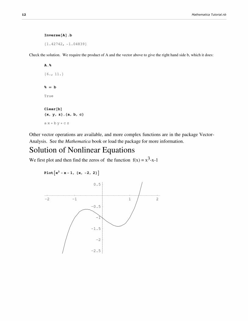
Solution of Nonlinear Equations We first plot and then find the zeros of the function f(x) = x3-x-1

PlotAx3 − x − 1, 8x, −2, 2<E

-2 -1 1 2

-2.5

-2

-1.5

-1

-0.5

0.5


Solve@x^3 − x − 1 � 0, xD

::x →1

3

27

2−3 69

2

1ê3+

I 1

2I9 + 69 MM1ê3

32ê3>,

:x → −1

6I1 + � 3 M 27

2−3 69

2

1ê3−

I1 − � 3 M I 1

2I9 + 69 MM1ê3

2 32ê3>,

:x → −1

6I1 − � 3 M 27

2−3 69

2

1ê3−

I1 + � 3 M I 1

2I9 + 69 MM1ê3

2 32ê3>>

FindRoot@x^3 − x − 1, 8x, 1<D8x → 1.32472<

Nonlinear Systems of Equations The Newton-Raphson method is used to approximate the solution of the system below.

We use the intial guess x = 0, y = 1 and x = 2:

f[x,y,z] = sin(x y) - 3x/z + log(z2)

g[x,y,z] = tan(x2y)+ 8 x y - 11 z

h[x,y,z] = cos(y) + πx+sqrt(zy)

Clear@f, g, hDf@x_, y_, z_D = Sin@x yD − 3 xêz + Log@z^2D;g@x_, y_, z_D = Tan@x^2 yD + 8 x y − 11 z;

h@x_, y_, z_D = Cos@yD + Pi x + Sqrt@z^ yD;

solution = FindRoot@8f@x, y, zD � 0, g@x, y, zD � 0 , h@x, y, zD � 0<,8x, 0<, 8y, 1<, 8z, 2<, MaxIterations → 30D

8x → 0.0592735, y → 17.0133, z → 0.738848<

Check the results by substitution:

8f@x, y, zD , g@x, y, zD , h@x, y, zD < ê. %

9−1.67967×10−8, −4.81571×10−8, 7.99074×10−8=


This is zero as far as the default machine precision is concerned.

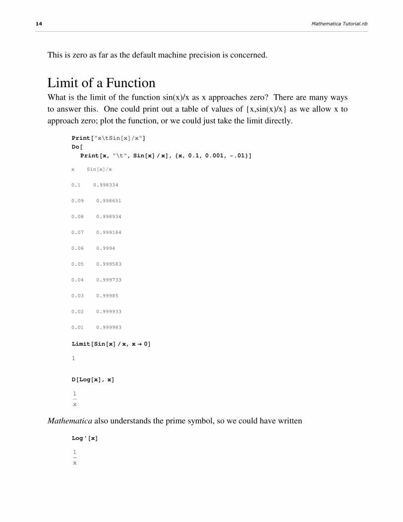
Limit of a Function What is the limit of the function sin(x)/x as x approaches zero? There are many ways

to answer this. One could print out a table of values of {x,sin(x)/x} as we allow x to

approach zero; plot the function, or we could just take the limit directly.

Print@"x\tSin@xDêx"DDo@

Print@x, "\t", Sin@xDêxD, 8x, 0.1, 0.001, −.01<Dx Sin@xDêx

0.1 0.998334

0.09 0.998651

0.08 0.998934

0.07 0.999184

0.06 0.9994

0.05 0.999583

0.04 0.999733

0.03 0.99985

0.02 0.999933

0.01 0.999983

Limit@Sin@xDêx, x → 0D1

D@Log@xD, xD1

x

Mathematica also understands the prime symbol, so we could have written

Log'@xD1

x


What is the derivative of the function f(x) = ax with respect to x?

D@a^x, xDax Log@aD

Partial derivatives are handled in the same way, but care must be taken in specification

of the independent variables. Here is an ugly function:

∂y LogBxyF ArcTanA 1 + x y E

−ArcTanA 1 + x y E

y+

x LogB x

yF

2 1 + x y H2 + x yL

D@Log@xê yD ArcTan@Sqrt@1 + x yDD, yD

−ArcTanA 1 + x y E

y+

x LogB x

yF

2 1 + x y H2 + x yL

Maximum of a Function Which number is larger: eπep or πe pe? (Reference:

The Mathematical Gazette, 1991). To determine which of the values is larger, we

could just evaluate them and take the Max:

Max@8Exp@PiD, PiÊ<Dπ

Alternatively, we could define the function y = exp(x)/xê. If x = 1, then y = e; if x =

e, then y = 1; if x = 10, then y = 42.1369. Clearly y has at least a local minimum on

(1,10).


Clear@yDy@x_D :=

�x

x�;

Plot@y@xD, 8x, 1, 10<D

2 4 6 8 10

1

2

3

4

5

6

7

FindMinimum@y@xD, 8x, 2<D81., 8x → 2.71828<<

This is x=e.Then exp(x)/xê>1 for all positive x,except for x=e.Hence e^pi>piê,since

pi is not equal to e.

Taylor Series Expansions Taylor Series Expansions are obtained with the Series function. To expand the

(assumed n + 1 times differentiable) function f about the point a, with integer n num-

ber of terms, the command is Series[f[x],{x,a,n}]. For example, let us take n = 5:

Clear@fDSeries@f@xD, 8x, a, 5<D

f@aD + f′@aD Hx − aL +1

2f′′@aD Hx − aL2 + 1

6fH3L@aD Hx − aL3 +

1

24fH4L@aD Hx − aL4 + 1

120fH5L@aD Hx − aL5 + O@x − aD6

Now obtain the Taylor Series expansion for Log[x], centered about the point x = 1 (so

we are really doing a Maclaurin expansion), and take four terms.


Series@Log@xD, 8x, 1, 4<D

Hx − 1L −1

2Hx − 1L2 + 1

3Hx − 1L3 − 1

4Hx − 1L4 + O@x − 1D5

Note the O[x-1]^5 term at the end of the result. This represents the truncation error of

the series. To do any calculations with the result, we have to drop this term. This is

done by way of the Normal function:

Normal@%D

−1 −1

2H−1 + xL2 + 1

3H−1 + xL3 − 1

4H−1 + xL4 + x

It is interesting to use other intervals and different degree polynomials in the Taylor

series expansion to see the change in accuracy. One could also use different expansion

points. Since log(x) is not a polynomial, no approximation will match it exactly on the

entire real line, but it is possible to match it as closely as desired on restricted intervals.

Problem: A sharp high-school student showed me the following formula he had read

in a textbook, and asked how it could possibly be correct: how was it possible to

expand something in terms of fractional powers? Use Mathematica to answer the

student's question.

( )8 1

5

9311

323/1 θθθ

θ +−+≅+

Answer: The right-hand side must be the Maclaurin series expansion of the function.

Check this with Series. The result:

Series@H1 + θL^H1ê3L, 8θ, 0, 5<D

1 +θ

3−

θ2

9+5 θ3

81−10 θ4

243+22 θ5

729+ O@θD6


What is the nth term?

Integration Mathematica is capable of computing definite and indefinite integrals, both analyti-

cally and symbolically. The integration routines may require a great deal of memory

depending on the complexity of the function. The syntax for integration is

?? Integrate

Integrate@f, xD gives the indefinite integral of f with respect to x.

Integrate@f, 8x, xmin, xmax<D gives the definite integral of f with

respect to x from xmin to xmax. Integrate@f, 8x, xmin, xmax<, 8y, ymin,

ymax<D gives a multiple definite integral of f with respect to x and y.

Attributes@IntegrateD = 8Protected, ReadProtected<Options@IntegrateD =

8Assumptions → 8<, GenerateConditions→ Automatic, PrincipalValue → False<Now, how does Numerical Integration work??

?? NIntegrate

NIntegrate@f, 8x, xmin, xmax<D gives a numerical approximation

to the integral of f with respect to x from xmin to xmax.

Attributes@NIntegrateD = 8HoldAll, Protected<Options@NIntegrateD = 8AccuracyGoal → ∞, Compiled → True, GaussPoints → Automatic,

MaxPoints → Automatic, MaxRecursion → 6, Method → Automatic, MinRecursion → 0,

PrecisionGoal → Automatic, SingularityDepth→ 4, WorkingPrecision → 16<

Now, compute the integral of ‡ 2 x CosAx2ESinAx2E �x

Integrate@2 x Cos@x^2DêSin@x^2D, xDLogASinAx2EE

Integrate@Exp@−x^2êH2 tauLD, xDπ

2tau ErfB x

2 tau

F

Multiple Integration Double,triple and higher dimension integrals are easily han-

dled.The outer limits appear first in the argument list. The syntax is


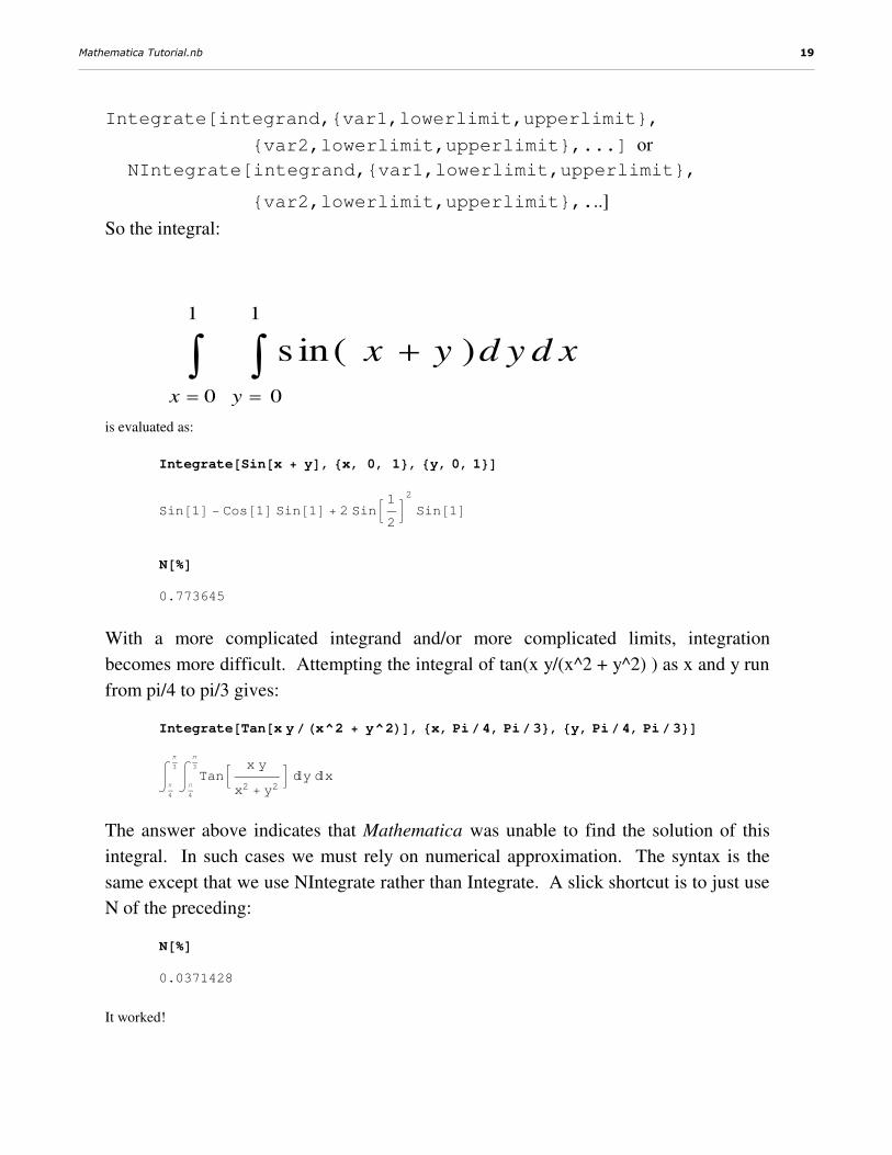
Integrate[integrand,{var1,lowerlimit,upperlimit},

{var2,lowerlimit,upperlimit},...] or

NIntegrate[integrand,{var1,lowerlimit,upperlimit},

{var2,lowerlimit,upperlimit},...] So the integral:

∫ ∫= =

+

1

0

1

0

)s in(

x y

d y d xyx

is evaluated as:

Integrate@Sin@x + yD, 8x, 0, 1<, 8y, 0, 1<D

Sin@1D − Cos@1D Sin@1D + 2 SinB12F2

Sin@1D

N@%D0.773645

With a more complicated integrand and/or more complicated limits, integration

becomes more difficult. Attempting the integral of tan(x y/(x^2 + y^2) ) as x and y run

from pi/4 to pi/3 gives:

Integrate@Tan@x yêHx^2 + y^2LD, 8x, Piê4, Piê3<, 8y, Piê4, Piê3<D

‡π

4

π

3‡π

4

π

3

TanB x y

x2 + y2F �y �x

The answer above indicates that Mathematica was unable to find the solution of this

integral. In such cases we must rely on numerical approximation. The syntax is the

same except that we use NIntegrate rather than Integrate. A slick shortcut is to just use

N of the preceding:

N@%D0.0371428

It worked!


Solution of Ordinary Differential Equations Differential equations are solved by the functions DSolve or NDSolve, and both can also handle systems of

ODEs. The syntax is:

DSolve[lhs == rhs, depvar, indvar] solves the ODE lhs = rhs

for the dependent variable depvar in terms of the independent variable indvar.

NDSolve[lhs == rhs, depvar, {indvar,left, right}] gives a numerical approximation of the

ODE lhs = rhs for the dependent variable depvar in terms of the independent variable indvar on [left,right].

Example: Solve the ODE y''[x] + 2 y'[x] + 5 y = 0 , y[0] = 0, y'[0] = 1, both analytically and numerically. For

the numerical solution, let x run from 0 to 10. Plot.

Clear@x, yDDSolve@y′′@xD + 2 y′@xD + 5 y@xD == 0, y@xD, xD88y@xD → −x C@2D Cos@2 xD − −x C@1D Sin@2 xD<<

To use the initial conditions, call DSolve in this way:

DSolve@8y′′@xD + 2 y′@xD + 5 y@xD == 0, y′@0D == 1, y@0D == 0<, y@xD, xD

::y@xD →1

2−x Sin@2 xD>>

Plot the solution, using a frame to make it fancy:

Plot@%P1, 1, 2T, 8x, 0, 10<, PlotRange → All, Frame → TrueD

0 2 4 6 8 10

-0.05

0

0.05

0.1

0.15

0.2

0.25

The numerical solution Notice that the only difference in the syntax between DSolve

and NDSolve is in specification of the independent variable: here, we provide a

domain.


NDSolve@8y′′@xD + 2 y′@xD + 5 y@xD == 0, y′@0D == 1, y@0D == 0<,y@xD, 8x, 0, 20<D

88y@xD → InterpolatingFunction@880., 20.<<, <>D@xD<<

NDSolve returns the solution as an InterpolatingFunction object. Use Evaluate to

plot the solution:

Plot@Evaluate@y@xD ê. %D, 8x, 0, 20<, PlotRange → All, Frame → TrueD

0 5 10 15 20

-0.05

0

0.05

0.1

0.15

0.2

0.25

Function Interpolation and ApproximationMathematica has several intrinsic functions to perform interpolation and approxima-

tion of data. These include capabilities to perform interpolation, regression and spline

fits of data.

Function Approximation

The syntax for Lagrange Interpolation is:

InterpolatingPolynomial@8data_List<, varD

As an example, we build up a table of six {x,Exp[x]} pairs on the interval [0,4] as the

data_List.

Table@8x, �x<, 8x, 0, 4, 0.8<D880, 1<, 80.8, 2.22554<, 81.6, 4.95303<,82.4, 11.0232<, 83.2, 24.5325<, 84., 54.5982<<


InterpolatingPolynomial@%, xD1 + H1.53193 +

H1.1734 + H0.599187 + H0.229477 + 0.0703085 H−3.2 + xLL H−2.4 + xLLH−1.6 + xLL H−0.8 + xLL x

Regression Regression is performed via the Fit function. The syntax is:

Fit[data_List,{1,var, ... , var^n},var]

where var is the symbol of the desired variable and n is the desired degree of fit. For the preceding {x,Exp[x]}

data, a fifth-degree regression fit is constructed as

FitATable@8x, �x<, 8x, 0, 4, 0.8<D, 91, x, x2, x3, x4, x5=, xE1. + 1.34637 x − 0.449026 x2 + 1.07261 x3 − 0.332991 x4 + 0.0703085 x5

As a shortcut, the variable list {1,x,x2,x3,x4,x5} may be defined by use of Table. In fact, a convenient regres-

sion function is

Clear@regressionDregression@data_List, n_, var_D :=

FitAdata, TableAvari, 8i, 0, n<E, varEregression@Table@8x, �x<, 8x, 0, 4, 0.8<D, 5, xD1. + 1.34637 x − 0.449026 x2 + 1.07261 x3 − 0.332991 x4 + 0.0703085 x5

Of course, this matches the Interpolating polynomial of degree 5 found previously

since the polynomial of degree n interpolating n+1 points is unique.

Multivariate RegressionFit may also be used for multivariate functions. For example,

Fit[data_List,{1,x,y,x y},{x,y}]

will fit z[x,y] = a x + b y + c x y + d to the function defined by data_List.

Using the function 2 x + 4 y - 10, with five points in each direction on the domain 0 £ x £ 1, 0 ≤ y ≤ 1 we obtain

the data as


RegressionData =

Flatten@Table@8x, y, 2 x + 4 y − 10<, 8x, 0, 1, 0.25<,8y, 0, 1, 0.25<D, 1D

880, 0, −10<, 80, 0.25, −9.<, 80, 0.5, −8.<, 80, 0.75, −7.<,80, 1., −6.<, 80.25, 0, −9.5<, 80.25, 0.25, −8.5<, 80.25, 0.5, −7.5<,80.25, 0.75, −6.5<, 80.25, 1., −5.5<, 80.5, 0, −9.<,80.5, 0.25, −8.<, 80.5, 0.5, −7.<, 80.5, 0.75, −6.<, 80.5, 1., −5.<,80.75, 0, −8.5<, 80.75, 0.25, −7.5<, 80.75, 0.5, −6.5<,80.75, 0.75, −5.5<, 80.75, 1., −4.5<, 81., 0, −8.<,81., 0.25, −7.<, 81., 0.5, −6.<, 81., 0.75, −5.<, 81., 1., −4.<<

Now the regression fit is obtained as

Fit@RegressionData, 81, x, y, x y<, 8x, y<D−10. + 2. x + 4. y − 3.10862×10−15 x y

which, as expected, matches the given function. The regression function may be plotted with Plot3D or Contour-

Plot. The discrete RegressionData may be plotted via ListPlot3D or ListContourPlot.

Plot3D@%, 8x, 0, 1<, 8y, 0, 1<D

0

0.2

0.4

0.6

0.8

10

0.2

0.4

0.6

0.8

1

-10

-8

-6

-4

0

0.2

0.4

0.6

0.8

Graphics Mathematica has hundreds of built-in Graphics objects. You can create everything from a simple line plot to

a stellated icosahedron. If what you want is not built in, Mathematica's programming capablity means that

you can easily write code to do your own graphics. There are primitives in Mathematica for drawing such

objects as Circles, Points, Lines and Disks as well.


Plotting

Plot[function,{var,left,right}]

will plot the specified function of a single variable as var runs from left to right.

Plot3D[function,{var1,left,right},{var2,left,right}]

will plot the specified function of two variables var1, var2 on the specified domain.

ContourPlot[function,{var1,left,right},{var2,left,right}]

will make a contour plot of the specified function of two variables var1, var2 on the specified domain.

ListPlot[list]

will plot a set of points given as list. Option: PlotJoined->True will connect the points with lines. The option

Prolog->PointSize[num] will use points of the specified size.

ListPlot3D[list]

will plot a set of 2-D data given as list.

ListContourPlot[list]

will make a contour plot of the tabular data given as list.

Examples

PlotBSin@xDx

, 8x, −10, 10<F

-10 -5 5 10

-0.2

0.2

0.4

0.6

0.8

1

data = Table@8i, RandomReal@D<, 8i, 10<D881, 0.00373923<, 82, 0.224572<, 83, 0.706306<,84, 0.447634<, 85, 0.958863<, 86, 0.73721<,87, 0.000896704<, 88, 0.501372<, 89, 0.6294<, 810, 0.673787<<


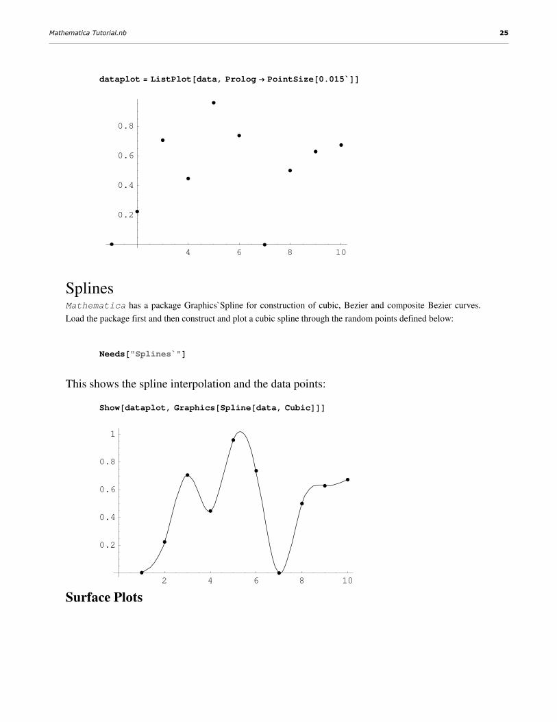
dataplot = ListPlot@data, Prolog → [email protected]`DD

4 6 8 10

0.2

0.4

0.6

0.8

SplinesMathematica has a package Graphics`Spline for construction of cubic, Bezier and composite Bezier curves.

Load the package first and then construct and plot a cubic spline through the random points defined below:

Needs@"Splines`"D

This shows the spline interpolation and the data points:

Show@dataplot, Graphics@Spline@data, CubicDDD

2 4 6 8 10

0.2

0.4

0.6

0.8

1

Surface Plots


Plot3D@Sin@x yD, 8x, 0, 4<, 8y, 0, 4<D

0

1

2

3

40

1

2

3

4

-1

-0.5

0

0.5

1

0

1

2

3

ContourPlot@Sin@x yD, 8x, 0, 4<, 8y, 0, 4<, ColorFunction → HueD

0 1 2 3 4

0

1

2

3

4


DensityPlot@Sin@x yD, 8x, 0, 4<, 8y, 0, 4<D

0 1 2 3 4

0

1

2

3

4

Parametric Plots Mathematica can perform parametric plots of single- or multi-variate functions

with the commands ParametricPlot, ParametricPlot3D. Examples follow.

The Folium of Descartes is defined by the equation

f(x,y) = x^3 + y^3 - 6 x y = 0. Since y cannot be written explicitly as a function of x,

perhaps parametric plotting will work.

Set x = r Cos[t], y = r Sin[t]. (Note that Mathematica could perform these transforma-

tions for us!) Then the function r[t] is as shown below.


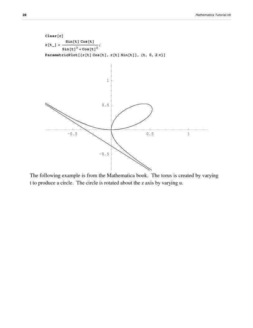
Clear@rDr@t_D =

Sin@tD Cos@tDSin@tD3 + Cos@tD3 ;

ParametricPlot@8r@tD Cos@tD, r@tD Sin@tD<, 8t, 0, 2 π<D

-0.5 0.5 1

-0.5

0.5

1

The following example is from the Mathematica book. The torus is created by varying

t to produce a circle. The circle is rotated about the z axis by varying u.


ParametricPlot3D@8Cos@tD H3 + Cos@uDL, Sin@tD H3 + Cos@uDL, Sin@uD<,8t, 0, 2 π<, 8u, 0, 2 π<D

-4

-2

0

2

4-4

-2

0

2

4

-1-0.5

00.51

-4

-2

0

2

Mathematica has several built-in graphics objects. Load the Graphics`Master pack-

age so that all of the example functions will be available:

Needs@"Graphics`Master`"DWe shall stellate an icosahedron (put star-like points on the faces of the icosahedron):


Show@Graphics3D@Stellate@Icosahedron@DDDD


Show@Graphics3D@DoubleHelix@DDD

Using Show to Combine Graphics ObjectsThe Show command can be used to display a number of graphics objects on the same

set of axes. As an example, to plot the intersection of the curvex^3 + y^3 - 6 x y and

the plane z[x,y] = 0 as x and y run from -2 to 4, we can execute each plot and use

Show to combine them (in plot2, the optional command DisplayFunction->Identity is

used to suppress graphical output, since this graph is not very interesting.)


plot1 = Plot3DAx3 + y3 − 6 x y, 8x, −2, 4<, 8y, −2, 4<E

-2

0

2

4-2

0

2

4

0

50

100

-2

0

2

plot2 = Plot3D@0, 8x, −2, 4<, 8y, −2, 4<,Mesh → False, DisplayFunction → IdentityD;

Show@plot1, plot2D

-2

0

2

4-2

0

2

4

-20

0

20

40

-2

0

2

4

Using GraphicsArray to Combine Graphics ObjectsAnother nice feature in v. 2.0 is GraphicsArray, with which one can show an array

of graphics objects side by side. As an example, surface and contour plots of the


function x^3 + y^3 - 6 x y are shown below. The optional command DisplayFunc-

tion->Identity is used to suppress the plot (to save room.)

plot3 = ContourPlotAx3 + y3 − 6 x y, 8x, −2, 4<, 8y, −2, 4<,DisplayFunction → Identity, ColorFunction → HueE;

Show@GraphicsGrid@88plot1, plot3<<DD

-20

24-2

0

2

40

50100

-20

24

-2 -1 0 1 2 3 4-2

-1

0

1

2

3

4

The Solution Set of an Implicit EquationReference: Mathematica Technical Report, "Guide to Standard Mathematica

Packages", Wolfram Research, p. 97.

Implicit plots are generated from the package GraphicsÌmplicitPlot`. The syntax is

ImplicitPlot@equation, 8x, xmin, xmax<D

As an example, the solution of x^3 + y^3 - 6 x y = 0 will be plotted (this is the Folium

of Descartes). First, load in the package:

Needs@"GraphicsÌmplicitPlot`"D


ImplicitPlotAx3 + y3 − 6 x y == 0, 8x, −2, 4<E;

-2 -1 1 2 3 4

-6

-4

-2

2

Another interesting example, from the "Guide to Standard Mathematica Packages",

p. 98:


ContourPlot@Sin@2 xD + Cos@3 yD � 1,

8x, −2 π, 2 π<, 8y, −2 π, 2 π<, PlotPoints → 30D;

-6 -4 -2 0 2 4 6

-6

-4

-2

0

2

4

6

Pie and Bar ChartsThe package Graphics`Graphics includes routines for creating pie and bar charts of

data. As an example, charts of Mathematica user data are presented:

Needs@"BarCharts`"D; Needs@"Histograms`"D; Needs@"PieCharts`"DUserData =

88.28, "Engineering"<, 8.22, "CS"<, 8.22, "Physical Sciences"<,8.12, "Math Sciences"<, 8.045, "BusinessêFinance"<,8.045, "Life Sciences"<, 8.07, "Other"<<;


PieChart@UserDataD

Engineering

CS

Physical Sciences

Math Sciences

BusinessêFinanceLife Sciences

Other

BarChart@UserData, BarOrientation → HorizontalD

0.05 0.1 0.15 0.2 0.25

Engineering

CS

Physical Sciences

Math Sciences

BusinessêFinanceLife Sciences

Other

Vector FieldsThe package Graphics`PlotField contains capabilities for plotting vector, gradient,

Polya and Hamiltonian fields. The package Graphics`PlotField3D does the same for

3D objects.


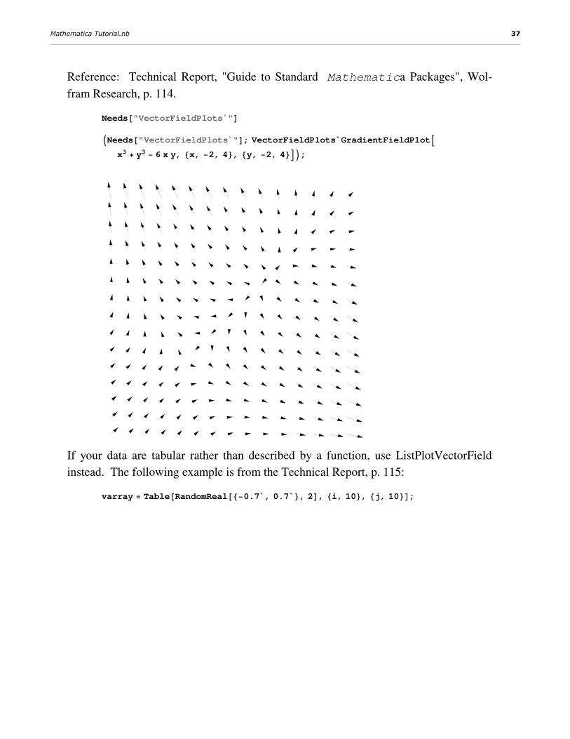
Reference: Technical Report, "Guide to Standard Mathematica Packages", Wol-

fram Research, p. 114.

Needs@"VectorFieldPlots`"DINeeds@"VectorFieldPlots`"D; VectorFieldPlots`GradientFieldPlotA

x3 + y3 − 6 x y, 8x, −2, 4<, 8y, −2, 4<EM;

If your data are tabular rather than described by a function, use ListPlotVectorField

instead. The following example is from the Technical Report, p. 115:

varray = Table@RandomReal@8−0.7`, 0.7`<, 2D, 8i, 10<, 8j, 10<D;


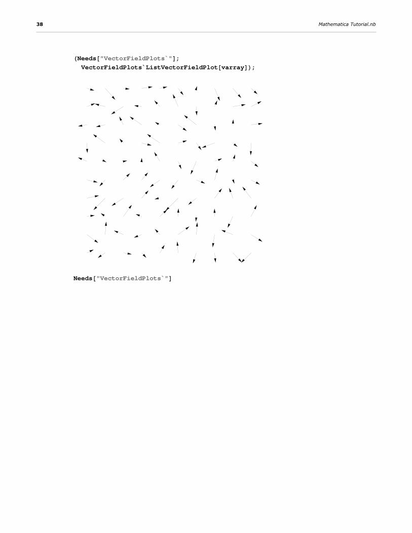
HNeeds@"VectorFieldPlots`"D;VectorFieldPlots`ListVectorFieldPlot@varrayDL;

Needs@"VectorFieldPlots`"D


HNeeds@"VectorFieldPlots`"D;VectorFieldPlots`VectorFieldPlot3D@8x, y, z<, 8x, 0, 2<,8y, 0, 2<, 8z, 0, 2<, PlotPoints → 5, VectorHeads → TrueDL;

Introductory Programming in MathematicaIf Mathematica does not have the function you need, you can always create your

own. In addition, Mathematica is a high-level programming language. In the follow-

ing section, a brief introduction to programming in Mathematica will be presented.

Sorting NumbersUse the Sort command. The argument is a list of numbers. To reverse the order, use

the command Reverse. The minimum of the list is obtained with Min.

Sort@81, 5, 10, −19, 41<D8−19, 1, 5, 10, 41<

Reverse@%D841, 10, 5, 1, −19<


Min@81, 5, 10, −19, 41<D−19

FunctionsThe definition of the function f(x) = x^3 - x - 1 in Mathematica is written as

f[x_] = x^3 - x - 1.

This is equivalent to DEF FNf(x) = x^3 - x - 1 in BASIC.

The underscore _ is required for pattern matching. This means that any argument of f

will match. As a bad example, see what happens when the underscore is omitted in the

definition of f and an attempt is made to evaluate f[1]:

Clear@fDf@xD = x3 − x − 1

f@1D−1 − x + x3

f@1D

The pattern does not match since x ∫ 1. Mathematica has no definition of f[1],

and so f[1] is left unevaluated. The command f[x] = x^3 - x - 1 only gives a definition

for the literal expression f[x]. Thus if we type f[x], x^3 - x- 1 will be returned. But no

other argument of f will match. To make this function work as desired, use the under-

score immediately after the function argument:

Clear@fDf@x_D = x3 − x − 1

f@1D−1 − x + x3

−1

Now the pattern works as desired.

A note about equal signsSometimes it is necessary to use := rather than = . But be careful!

:= means SET DELAYED while = means SET.

Thus LHS := RHS will set LHS equal to RHS only when LHS is called, not when the

definition is made. Conversely, LHS = RHS will make the assignment immediately.


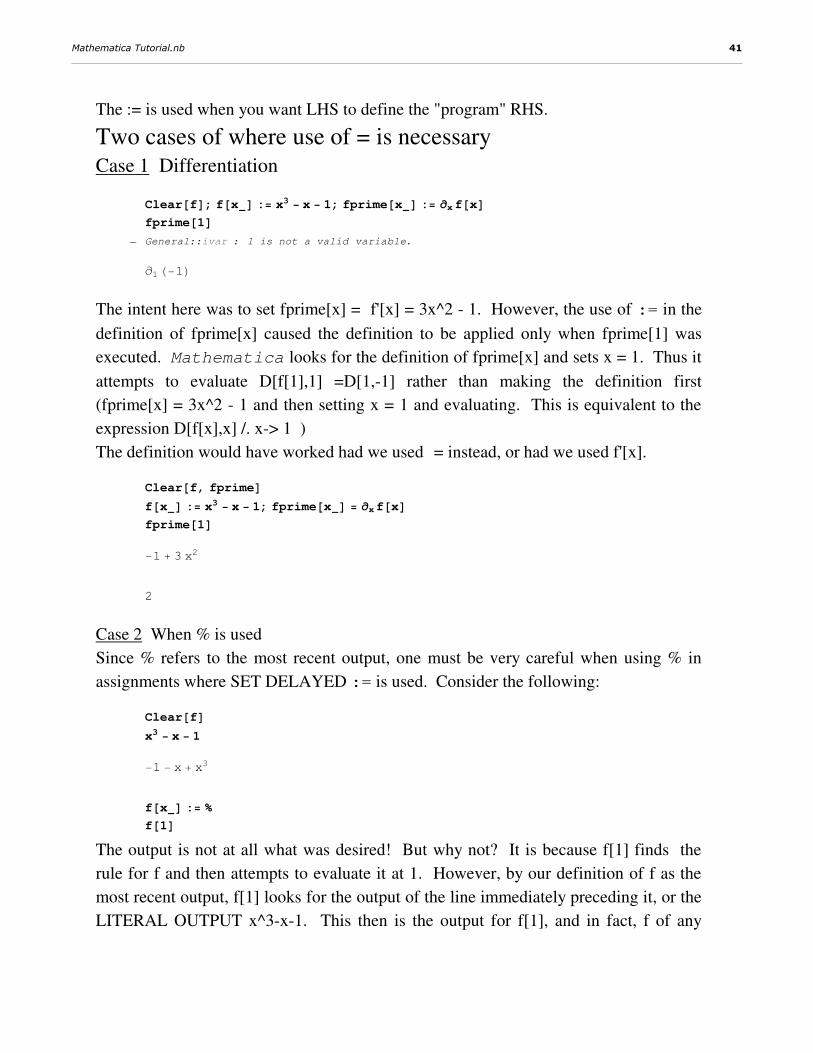
The := is used when you want LHS to define the "program" RHS.

Two cases of where use of = is necessaryCase 1 Differentiation

Clear@fD; f@x_D := x3 − x − 1; fprime@x_D := ∂x f@xDfprime@1D

— General::ivar : 1 is not a valid variable.

∂1H−1L

The intent here was to set fprime[x] = f'[x] = 3x^2 - 1. However, the use of := in the

definition of fprime[x] caused the definition to be applied only when fprime[1] was

executed. Mathematica looks for the definition of fprime[x] and sets x = 1. Thus it

attempts to evaluate D[f[1],1] =D[1,-1] rather than making the definition first

(fprime[x] = 3x^2 - 1 and then setting x = 1 and evaluating. This is equivalent to the

expression D[f[x],x] /. x-> 1 )

The definition would have worked had we used = instead, or had we used f'[x].

Clear@f, fprimeDf@x_D := x3 − x − 1; fprime@x_D = ∂xf@xDfprime@1D−1 + 3 x2

2

Case 2 When % is used

Since % refers to the most recent output, one must be very careful when using % in

assignments where SET DELAYED := is used. Consider the following:

Clear@fDx3 − x − 1

−1 − x + x3

f@x_D := %

f@1DThe output is not at all what was desired! But why not? It is because f[1] finds the

rule for f and then attempts to evaluate it at 1. However, by our definition of f as the

most recent output, f[1] looks for the output of the line immediately preceding it, or the

LITERAL OUTPUT x^3-x-1. This then is the output for f[1], and in fact, f of any


argument will give this result.

Here is the rule that Mathematica has set up for f:

Information@"f", LongForm → FalseDGlobal`f

f@x_D := %

Clear@fD−1 − x + x3

f@x_D = %

f@1D−1 − x + x3

−1

The assignment worked in the desired way. Explain why.

(Hint: look up the rule that Mathematica now has for f.)

Another case where := is necessary rather than = is in our definition of factorial. Try

this example again but define factorial[n_] = n factorial[n-1]

Remember, on the Macintosh, Command-. will abort when Mathematica gets into

an infinite loop. On the IBM, use the Kernel menu and choose Quit Kernel. You will

still be able to save your notebook, but will have to restart the kernel in order to do any

more calculations.

To understand what is happening, remember that the wayMathematica works is to

evaluate an expression until it no longer changes! This is a recursive defintion for

factorial[n] . . . it appears on both sides of the equation. Mathematica trys to

"solve" for factorial[n] but finds that it is equal (by our definition) to n times

factorial[n]! Thus there is no solution and no end to the evaluation. Use of a := makes

the function work perfectly.

Pattern Matching with Function ArgumentsSection 2.3 of the Mathematica book details how to test the arguments of a func-

tion to ascertain that they meet certain criteria. For example, to define array elements


b[i] such that b[i] = odd if i is odd and b[i] = even for even i, use the EvenQ and

OddQ functions. Additionally, the Integer? after i_ below tests that the argument of i

is an integer.

b@i_Integer?EvenQD := even; b@i_Integer?OddQD := odd

b@3Dodd

b@18Deven

[email protected]@5.4D

We can also test whether the arguments are lists, integers, text strings, etc. Built-in

functinos such as PrimeQ, NumberQ, and NameQ will return true or false depending

on the results of the test. Let's test whether the number 113 is prime:

PrimeQ@113DTrue

ConditionalsAs described in Section 2.5.8 of the Mathematica book, Mathematica has the

following conditional structures:

Which /;

If

Switch

The If conditional has the structure

If@test, then, elseD

An implementation of If can be seen in the following example, where the function

TestandSort is defined. This function takes a list of numbers as its input, compares

them to the sorted list, and if these lists are equal, evaluates to true. Otherwise, the

numbers are sorted and returned.


TestandSort@x_ListD :=

If@x == Sort@xD, Print@"Numbers are in ascending order."D,Print@"The sorted numbers are: "D; Sort@xDD

TestandSort@8−16, 117, 49<DThe sorted numbers are:

8−16, 49, 117<

Another implementation of If is the following function, which tests whether an integer

is odd or even:

Clear@TestNumberDTestNumber@i_IntegerD :=

If@EvenQ@iD, Print@"The integer ", i, " is even."D,Print@"The integer ", i, " is odd."DD

TestNumber@6DThe integer 6 is even.

TestNumber@11DThe integer 11 is odd.

One example of a case where Which is very useful is in defining piecewise continu-

ous functions for plotting of splines.

Clear@fDf@x_D := WhichAx < 0, x2, x ≥ 0 && x < 2, x3, True, Tan@xDEPlot@f@xD, 8x, −2, 5<D

-2 -1 1 2 3 4 5

-15

-10

-5

5

10

15

The /; conditional has the syntax


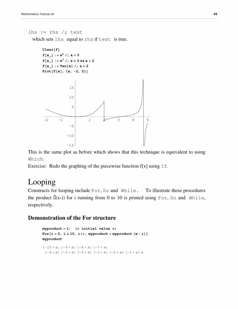
lhs := rhs /; test

which sets lhs equal to rhs if test is true.

Clear@fDf@x_D := x2 ê; x < 0

f@x_D := x3 ê; x ≥ 0 && x < 2

f@x_D := Tan@xD ê; x ≥ 2

Plot@f@xD, 8x, −2, 5<D

-2 -1 1 2 3 4 5

-15

-10

-5

5

10

15

This is the same plot as before which shows that this technique is equivalent to using

Which.

Exercise: Redo the graphing of the piecewise function f[x] using If.

LoopingConstructs for looping include For, Do and While. To illustrate these procedures

the product π(x-i) for i running from 0 to 10 is printed using For, Do and While,

respectively.

Demonstration of the For structure

myproduct = 1; H∗ initial value ∗LFor@i = 0, i 10, i++, myproduct = myproduct Hx − iLDmyproduct

H−10 + xL H−9 + xL H−8 + xL H−7 + xLH−6 + xL H−5 + xL H−4 + xL H−3 + xL H−2 + xL H−1 + xL x


Demonstration of the Do structure

product = 1; Clear@iDDo@product = product Hx − iL, 8i, 0, 10<Dproduct


Demonstration of the While structure

product = 1; H∗ initialization ∗Li = 0;

While@i 10, product = product Hx − iL; i++Dproduct


Working with ListsAs you gain proficiency with Mathematica, you will doubtless find that your opera-

tions are more efficient when you work with lists. As a simple example, the following

function Mean computes the average of a set of numbers. It is then used to compute

the mean of the numbers 1,2, ... , 10.

Mean@x_ListD :=Plus @@ x

Length@xDdata = Table@i, 8i, 10<D81, 2, 3, 4, 5, 6, 7, 8, 9, 10<

Mean@dataD11

2


Defining Your Own Rules

The Factorial Function

myfactorial@1D = 1;

myfactorial@n_D := n myfactorial@n − 1Dmyfactorial@10D3628800

Of course, Mathematica has a built in factorial function, Factorial[x]. Alterna-

tively the symbol ! may be used:

10!

3628800

Fibonacci Numbers The Fibonacci Numbers are the sequence {1,1,2,3,5,8,13, ... }.

The nth number is the sum of the two preceding numbers.

A function, fibonacci[i], can be set up to compute these numbers and a table of results

printed out.

myfibonacci@0D = myfibonacci@1D = 1;

myfibonacci@i_D := myfibonacci@i − 1D + myfibonacci@i − 2DTable@8i, myfibonacci@iD<, 8i, 0, 10<D880, 1<, 81, 1<, 82, 2<, 83, 3<, 84, 5<,85, 8<, 86, 13<, 87, 21<, 88, 34<, 89, 55<, 810, 89<<

Newton's Method Another useful case where this technique could be applied is in

Newton's Method for finding the root of a function, wherein the i-th estimate of the

root x[i] is computed by the scheme xi= xi-1-f(xi-1)/f'(xi-1)

An initial guess x[0] for the root must be provided. As an example, we shall take some

iterations on the root of f[x] = x^3 - x - 1 = 0, with an initial guess x[0] = 1.5.


Clear@f, xDf@x_D = x3 − x − 1;

x@0D = 1.5;

x@i_D := x@i − 1D −f@x@i − 1DDf′@x@i − 1DD

Table@8i, x@iD<, 8i, 0, 5<D880, 1.5<, 81, 1.34783<, 82, 1.3252<,83, 1.32472<, 84, 1.32472<, 85, 1.32472<<

Of course, the built-in function FindRoot performs this but does not print out

the iterations. Try FindRoot[f[x]==0,{x,1.5}] to see the estimate of the root

obtained by Mathematica.

Teaching Mathematica New TricksIf a desired function is not available in Mathematica, you can easily program it.

As an example, the following routine defines a function called NewtonDD that per-

forms interpolation by Newton's Divided Differences. The output will be identical to

that of the intrinsic function InterpolatingPolynomial , but the new function

is valuable for students to check if they are constructing their polynomials correctly.

Interpolation by Newton's Divided DifferencesProcedure NewtonDD takes as input a list of n+1 {x,y} pairs and returns an interpolat-

ing polynomial of degree (at most) n in the variable var.

NewtonDD@data_List, var_SymbolD := BlockB8i, n, poly, x, f<,Do@x@i − 1D = dataPi, 1T; f@i − 1D = dataPi, 2T, 8i, Length@dataD<D;f@i_, 0D := f@iD; f@n_, i_D :=

f@n, i − 1D − f@n − 1, i − 1Dx@nD − x@n − iD ê; i > 0;

‚i=0

Length@dataD−1f@i, iD ‰

j=1

i

Hvar − x@j − 1DLF

Sample Calculations

Construct an interpolating polynomial through the data points

(-6,-60),(-4,-9),(-3,0),(-1,0),(0,-3),(2,0),(3,12) by Newton's Divided Differences.

Compare to the answer obtained by Mathematica's intrinsic function InterpolatingPoly-

nomial.


NewtonDD@88−6, −60<, 8−4, −9<, 8−3, 0<, 8−1, 0<, 80, −3<, 82, 0<, 83, 12<<, xD

−60 +51 H6 + xL

2−11

2H4 + xL H6 + xL +

1

2H3 + xL H4 + xL H6 + xL

mypoly = Expand@%D

−3 −5 x

2+ x2 +

x3

2

?? InterpolatingPolynomial

InterpolatingPolynomial@data, varD gives a polynomial in the variable var

which provides an exact fit to a list of data. The data can have the

forms 88x1, f1<, 8x2, f2<, ... < or 8f1, f2, ... <, where in the second

case, the xi are taken to have values 1, 2, ... . The fi can be replaced

by 8fi, dfi, ddfi, ... <, specifying derivatives at the points xi.

Attributes@InterpolatingPolynomialD = 8Protected<

InterpolatingPolynomial@88−6, −60<, 8−4, −9<, 8−3, 0<, 8−1, 0<, 80, −3<, 82, 0<, 83, 12<<, xD

−60 + H6 + xL 51

2+ H4 + xL −

11

2+3 + x

2

intpoly = Expand@%D

−3 −5 x

2+ x2 +

x3

2

mypoly === intpoly

True

LU-Factorization of Matrices

The code to perform LU factorization of matrices, which is a technique via which we

may solve A.x = b by factorization of A into two triangular matrices L and U is shown

below as a programming example.


Clear@LUFactorization, ConstructLandUD

ConstructLandU@n_D := Block@8i, j<, Unknowns = 8<;u@i_, i_D = 1; Do@Do@l@i, jD = 0, 8i, n<, 8j, i + 1, n<D;Do@u@i, jD = 0, 8i, 2, n<, 8j, 1, i − 1<D;U = Table@u@i, jD, 8i, n<, 8j, n<D; L = Table@l@i, jD, 8i, n<, 8j, n<D;8n<D; Do@Unknowns = Append@Unknowns, l@i, jDD, 8i, n<, 8j, i<D;Do@Unknowns = Append@Unknowns, u@i, jDD, 8i, n<, 8j, i + 1, n<DD

LUFactorization@a_List, b_ListD :=

Block@8n<, EquationList = 8<; n = Length@aD;ConstructLandU@nD; Do@EquationList = Append@EquationList,

[email protected] == Flatten@aDPiTD, 8i, Length@[email protected]<D;solution = Flatten@Solve@EquationList, UnknownsDD;U = U ê. solution; L = L ê. solution; y = LinearSolve@L, bD;x = LinearSolve@U, yD; Print@"The solution x = ", xDD

Let us solve the following system (this arises in 2-point Gaussian Quadrature) by LU-

factorization and compare to the known solution of {1,1}:

LUFactorization@881, 1<, 8−0.57735, 0.57735<<, 82, 0<DThe solution x = 81., 1.<

To check hand calculations, L, U and y can be printed out. For example, L is

MatrixForm@LD

J 1. 0

−0.57735 1.1547N

Online Help From MathematicaTo obtain information about a command, say FindRoot, just type

?FindRoot. For further information, use two ?? as in ??FindRoot. Note that

the file info.m must be loaded. To load, use File, Open, Packages, info.m or configure

the Startup Settings in the Edit menu.

For a list of all symbols beginning (say) with Ja, type ?Ja*

Information@"FindRoot", LongForm → FalseDFindRoot@lhs==rhs, 8x, x0<D searches for a numerical

solution to the equation lhs==rhs, starting with x=x0.

Information about the % symbol


Information@"%", LongForm → FalseD%n or Out@nD is a global object that is assigned to be the value produced on

the nth output line. % gives the last result generated. %% gives the

result before last. %% ... % Hk timesL gives the kth previous result.

To use the online help, pull down the apple on the top left of the screen and select

About Mathematica... then click the HELP button.

During a session if a beep occurs and you want an explanation, select the Why the

Beep?... from the apple menu. The most common errors are syntax errors, such as

using PLOT for Plot or pi for Pi; or having unmatched parentheses. Also watch out

when you define functions.

You should always Clear a function before defining it. Often "old" definitions may

be remembered otherwise, leading to error.

How to find out what version of Mathematica you're running:

Type $Version or $VersionNumber.

$Version

4.0 for Microsoft Windows HJuly 26, 1999L


Introduction to Mathematica A Tutorial - QuantCandy · Introductory Programming in Mathematica Pattern Matching with Function Arguments Conditionals Looping Working with Lists Defining

Documents