Motivation GW BSE Micro-macro Introduction to many-body Green’s functions Matteo Gatti European Theoretical Spectroscopy Facility (ETSF) NanoBio Spectroscopy Group - UPV San Sebastián - Spain [email protected] - http://nano-bio.ehu.es - http://www.etsf.eu ELK school - CECAM 2011

Welcome message from author
This document is posted to help you gain knowledge. Please leave a comment to let me know what you think about it! Share it to your friends and learn new things together.
Transcript

Motivation GW BSE Micro-macro
Introduction to many-body Green’s functions
Matteo Gatti
European Theoretical Spectroscopy Facility (ETSF)
NanoBio Spectroscopy Group - UPV San Sebastián - Spain
[email protected] - http://nano-bio.ehu.es - http://www.etsf.eu
ELK school - CECAM 2011

bg=whiteMotivation GW BSE Micro-macro
Outline
1 Motivation
2 One-particle Green’s functions: GW approximation
3 Two-particle Green’s functions: Bethe-Salpeter equation
4 Micro-macro connection

bg=whiteMotivation GW BSE Micro-macro
References
Francesco SottilePhD thesis, Ecole Polytechnique (2003)http://etsf.polytechnique.fr/system/files/users/francesco/Tesi_dot.pdf
Fabien BrunevalPhD thesis, Ecole Polytechnique (2005)http://theory.polytechnique.fr/people/bruneval/bruneval_these.pdf
Giovanni Onida, Lucia Reining, and Angel RubioRev. Mod. Phys. 74, 601 (2002).
G. StrinatiRivista del Nuovo Cimento 11, (12)1 (1988).

bg=whiteMotivation GW BSE Micro-macro
Outline
1 Motivation
2 One-particle Green’s functions: GW approximation
3 Two-particle Green’s functions: Bethe-Salpeter equation
4 Micro-macro connection

bg=whiteMotivation GW BSE Micro-macro
Motivation
Theoretical spectroscopy
Calculate and reproduceUnderstand and explainPredict
Exp. at 30 K from: P. Lautenschlager et al., Phys. Rev. B 36, 4821 (1987).

bg=whiteMotivation GW BSE Micro-macro
Theoretical Spectroscopy
Which kind of spectra?Which kind of tools?
bg=whiteMotivation GW BSE Micro-macro
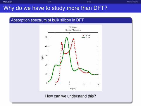
Why do we have to study more than DFT?
Absorption spectrum of bulk silicon in DFT
How can we understand this?

bg=whiteMotivation GW BSE Micro-macro
Why do we have to study more than DFT?
Absorption spectrum of bulk silicon in DFT
Spectroscopy is exciting!

bg=whiteMotivation GW BSE Micro-macro
MBPT vs. TDDFT: different worlds, same physics
MBPTbased on Green’s functionsone-particle G: electron addition and removal - GWtwo-particle L: electron-hole excitation - BSEmoves (quasi)particles aroundis intuitive (easy)
TDDFTbased on the densityresponse function χ: neutral excitationsmoves density aroundis efficient (simple)

bg=whiteMotivation GW BSE Micro-macro
Response functions
External perturbation Vext applied on the sample→ Vtot acting on the electronic system
Potentials
δVtot = δVext + δVind
δVind = vδρ
Dielectric function
ε =δVext
δVtot= 1− v
δρ
δVtot
ε−1 =δVtot
δVext= 1 + v
δρ
δVext

bg=whiteMotivation GW BSE Micro-macro
Response functions
External perturbation Vext applied on the sample→ Vtot acting on the electronic system
Dielectric function
ε =δVext
δVtot= 1− vP
ε−1 =δVtot
δVext= 1 + vχ
P =δρ
δVtotχ =
δρ
δVext
χ = P + Pvχ
P = χ0 + χ0fxcP

bg=whiteMotivation GW BSE Micro-macro
Micro-macro connection
Microscopic-Macroscopic connection: local fields
χG,G′(q, ω) = PG,G′(q, ω) + PG,G1 (q, ω)vG1 (q)χG1,G′(q, ω)
ε−1G,G′(q, ω) = δG,G′ + vG(q)χG,G′(q, ω)
εM(q, ω) =1
ε−1G=0,G′=0(q, ω)
Adler, Phys. Rev. 126 (1962); Wiser, Phys. Rev. 129 (1963).

bg=whiteMotivation GW BSE Micro-macro
Micro-macro connection
Microscopic-Macroscopic connection: local fields
εM(q, ω) = 1− vG=0(q)χG=0,G′=0(q, ω)
χG,G′(q, ω) = PG,G′(q, ω) + PG,G1 (q, ω)vG1 (q)χG1,G′(q, ω)
vG(q) = 0 for G = 0vG(q) = vG(q) for G 6= 0
Hanke, Adv. Phys. 27 (1978).

bg=whiteMotivation GW BSE Micro-macro
Absorption spectra
Absorption spectra
Abs(ω) = limq→0
ImεM(q, ω)
Abs(ω) =− limq→0
Im [vG=0(q)χG=0,G′=0(q, ω)]
Absorption→ response to Vext + V macroind

bg=whiteMotivation GW BSE Micro-macro
Independent particles: Kohn-Sham
Independent transitions:
ε2(ω) =8π2
Ωω2
∑ij
|〈ϕj |e·v|ϕi〉|2δ(εj−εi−ω)

bg=whiteMotivation GW BSE Micro-macro
What is an electron?

bg=whiteMotivation GW BSE Micro-macro
Outline
1 Motivation
2 One-particle Green’s functions: GW approximation
3 Two-particle Green’s functions: Bethe-Salpeter equation
4 Micro-macro connection

bg=whiteMotivation GW BSE Micro-macro
Photoemission
Direct Photoemission Inverse Photoemission

bg=whiteMotivation GW BSE Micro-macro
Why do we have to study more than DFT?
adapted from M. van Schilfgaarde et al., PRL 96 (2006).

bg=whiteMotivation GW BSE Micro-macro
One-particle Green’s function
The one-particle Green’s function G
Definition and meaning of G:
iG(x1, t1; x2, t2) = 〈N|T[ψ(x1, t1)ψ†(x2, t2)
]|N〉
for t1 > t2 ⇒ iG(x1, t1; x2, t2) = 〈N|ψ(x1, t1)ψ†(x2, t2)|N〉for t1 < t2 ⇒ iG(x1, t1; x2, t2) = −〈N|ψ†(x2, t2)ψ(x1, t1)|N〉

bg=whiteMotivation GW BSE Micro-macro
One-particle Green’s function
t1 > t2〈N|ψ(x1, t1)ψ†(x2, t2)|N〉
t1 < t2−〈N|ψ†(x2, t2)ψ(x1, t1)|N〉

bg=whiteMotivation GW BSE Micro-macro
One-particle Green’s function
What is G ?Definition and meaning of G:
G(x1, t1; x2, t2) = −i < N|T[ψ(x1, t1)ψ†(x2, t2)
]|N >
Insert a complete set of N + 1 or N − 1-particle states. This yields
G(x1, t1; x2, t2) = −i∑
j
fj (x1)f ∗j (x2)e−iεj (t1−t2) ×
× [θ(t1 − t2)θ(εj − µ)− θ(t2 − t1)Θ(µ− εj )];
where:
εj =E(N + 1, j)− E(N), εj > µE(N)− E(N − 1, j), εj < µ
fj (x1) =〈N |ψ (x1)|N + 1, j〉 , εj > µ〈N − 1, j |ψ (x1)|N〉 , εj < µ

bg=whiteMotivation GW BSE Micro-macro
One-particle Green’s function
What is G? - Fourier transformFourier Transform:
G(x,x′, ω) =∑
j
fj (x)f ∗j (x′)ω − εj + iηsgn(εj − µ)
.
Spectral function:
A(x,x′;ω) =1π| ImG(x,x′;ω) |=
∑j
fj (x)f ∗j (x′)δ(ω − εj ).

bg=whiteMotivation GW BSE Micro-macro
Photoemission
Direct Photoemission Inverse Photoemission
One-particle excitations→ poles of one-particle Green’s function G

bg=whiteMotivation GW BSE Micro-macro
One-particle Green’s function
One-particle Green’s function
From one-particle G we can obtain:one-particle excitation spectraground-state expectation value of any one-particle operator:e.g. density ρ or density matrix γ:ρ(r, t) = −iG(r, r, t , t+) γ(r, r′, t) = −iG(r, r′, t , t+)
ground-state total energy

bg=whiteMotivation GW BSE Micro-macro
One-particle Green’s function
Straightforward?
G(x, t ; x′, t ′) = −i < N|T[ψ(x, t)ψ†(x′, t ′)
]|N >
|N > = ??? Interacting ground state!
Perturbation Theory?
Time-independent perturbation theories: messy.Textbooks: adiabatically switched on interaction, Gell-Mann-Low
theorem, Wick’s theorem, expansion (diagrams). Lots of diagrams.....

bg=whiteMotivation GW BSE Micro-macro
Functional approach to the MB problem
Equation of motion
To determine the 1-particle Green’s function:
[i∂
∂t1− h0(1)
]G(1,2) = δ(1,2)− i
∫d3v(1,3)G2(1,3,2,3+)
Do the Fourier transform in frequency space:
[ω − h0]G(ω) + i∫
vG2(ω) = 1
where h0 = − 12∇
2 + vext is the independent particle Hamiltonian.The 2-particle Green’s function describes the motion of 2 particles.

bg=whiteMotivation GW BSE Micro-macro
Unfortunately, hierarchy of equationsG1(1,2) ← G2(1,2; 3,4)
G2(1,2; 3,4) ← G3(1,2,3; 4,5,6)...
......

bg=whiteMotivation GW BSE Micro-macro
Self-energy
Perturbation theory starts from what is known to evaluate what is notknown, hoping that the difference is small...Let’s say we know G0(ω) that corresponds to the Hamiltonian h0Everything that is unknown is put in
Σ(ω) = G−10 (ω)−G−1(ω)
This is the definition of the self-energy
Thus,
[ω − h0]G(ω)−∫
Σ(ω)G(ω) = 1
to be compared with
[ω − h0]G(ω) + i∫
vG2(ω) = 1

bg=whiteMotivation GW BSE Micro-macro
One-particle Green’s function
Trick due to Schwinger (1951):introduce a small external potential U(3), that will be made equal tozero at the end, and calculate the variations of G with respect to U
δG(1,2)
δU(3)= −G2(1,3; 2,3) + G(1,2)G(3,3).
bg=whiteMotivation GW BSE Micro-macro
Hedin’s equation
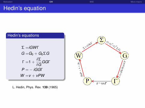
Hedin’s equations
Σ =iGW Γ
G =G0 + G0ΣG
Γ =1 +δΣ
δGGGΓ
P =− iGGΓ
W =v + vPW
L. Hedin, Phys. Rev. 139 (1965)

bg=whiteMotivation GW BSE Micro-macro
GW bandstructure: photoemission
additional charge→

bg=whiteMotivation GW BSE Micro-macro
GW bandstructure: photoemission
additional charge→ reaction: polarization, screening
GW approximation1 polarization made of noninteracting electron-hole pairs (RPA)2 classical (Hartree) interaction between additional charge and
polarization charge

bg=whiteMotivation GW BSE Micro-macro
Hedin’s equation and GW
GW approximation
Σ =iGW Γ
G =G0 + G0ΣGΓ =1P =− iGGΓ
W =v + vPW
L. Hedin, Phys. Rev. 139 (1965)

bg=whiteMotivation GW BSE Micro-macro
Hedin’s equation and GW
GW approximation
Σ =iGWG =G0 + G0ΣGΓ =1P =−iGG
W =v + vPW
L. Hedin, Phys. Rev. 139 (1965)

bg=whiteMotivation GW BSE Micro-macro
GW corrections
Standard perturbative G0W0
H0(r)ϕi (r) + Vxc(r)ϕi (r) = εiϕi (r)
H0(r)φi (r) +
∫dr′ Σ(r, r′, ω = Ei ) φi (r′) = Ei φi (r)
First-order perturbative corrections with Σ = iGW :
Ei − εi = 〈ϕi |Σ− Vxc |ϕi〉
Hybersten and Louie, PRB 34 (1986);Godby, Schlüter and Sham, PRB 37 (1988)

bg=whiteMotivation GW BSE Micro-macro
GW results
M. van Schilfgaarde et al., PRL 96 (2006).

bg=whiteMotivation GW BSE Micro-macro
Independent (quasi)particles: GW
Independent transitions:
ε2(ω) =8π2
Ωω2
∑ij
|〈ϕj |e·v|ϕi〉|2δ(Ej−Ei−ω)

bg=whiteMotivation GW BSE Micro-macro
What is wrong?
What is missing?

bg=whiteMotivation GW BSE Micro-macro
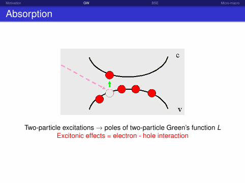
Absorption
Two-particle excitations→ poles of two-particle Green’s function LExcitonic effects = electron - hole interaction
bg=whiteMotivation GW BSE Micro-macro
Absorption
Two-particle excitations→ poles of two-particle Green’s function LExcitonic effects = electron - hole interaction

bg=whiteMotivation GW BSE Micro-macro
Absorption
Two-particle excitations→ poles of two-particle Green’s function LExcitonic effects = electron - hole interaction

bg=whiteMotivation GW BSE Micro-macro
Outline
1 Motivation
2 One-particle Green’s functions: GW approximation
3 Two-particle Green’s functions: Bethe-Salpeter equation
4 Micro-macro connection

bg=whiteMotivation GW BSE Micro-macro
Beyond RPA
P(12) = −iG(12)G(21) = P0(12)
Independent particles (RPA)

bg=whiteMotivation GW BSE Micro-macro
Beyond RPA
P(12) = −iG(13)G(42)Γ(342)
Interacting particles (excitonic effects)

bg=whiteMotivation GW BSE Micro-macro
From Hedin’s equations to BSE
From Hedin...
P = −iGGΓ
Γ = 1 +δΣ
δGGGΓ
The Bethe-Salpeter equation
L = L0 + L0(v + i
δΣ
δG)L

bg=whiteMotivation GW BSE Micro-macro
From Hedin’s equations to BSE
From Hedin...
P = −iGGΓ
Γ = 1 +δΣ
δGGGΓ
...to Bethe-Salpeter
L = L0 + L0(v + i
δΣ
δG)L

bg=whiteMotivation GW BSE Micro-macro
The Bethe-Salpeter equation
Exercise
Formal derivation
L(1234) =− iδG(12)
δVext (34)= +iG(15)
δG−1(56)
δVext (34)G(62)
= + iG(15)δ[G−1
0 (56)− Vext (56)− Σ(56)]
δVext (34)G(62)
=− iG(13)G(42) + iG(15)G(62)[δVH(5)δ(56)
δVext (34)− δΣ(56)
δVext (34)
]=− iG(13)G(42) + iG(15)G(62)
[δVH(5)δ(56)
δG(78)− δΣ(56)
δG(78)
] δG(78)
δVext (34)
L(1234) =L0(1234) + L0(1256)[v(57)δ(56)δ(78) + i
δΣ(56)
δG(78)
]L(7834)

bg=whiteMotivation GW BSE Micro-macro
The Bethe-Salpeter equation
L(1234) = L0(1234) + L0(1256)[v(57)δ(56)δ(78) + i
δΣ(56)
δG(78)
]L(7834)
Polarizabilities
L(1234) = −iδG(12)
δVext (34)χ(12) =
δρ(1)
δVext (2)
L(1122) = χ(12)

bg=whiteMotivation GW BSE Micro-macro
The Bethe-Salpeter equation
Approximations
L = L0 + L0(v + i
δΣ
δG)L
Approximation:
Σ ≈ iGWδ(GW )
δG= W + G
δWδG≈W

bg=whiteMotivation GW BSE Micro-macro
The Bethe-Salpeter equation
Approximations
L = L0 + L0(v + i
δΣ
δG)L
Approximation:
Σ ≈ iGW
δ(GW )
δG= W + G
δWδG≈W

bg=whiteMotivation GW BSE Micro-macro
The Bethe-Salpeter equation
Approximations
L = L0 + L0(v−δ(GW )
δG)L
Approximation:
Σ ≈ iGWδ(GW )
δG= W + G
δWδG≈W

bg=whiteMotivation GW BSE Micro-macro
The Bethe-Salpeter equation
Approximations
Final result:
L = L0 + L0(v −W )L

bg=whiteMotivation GW BSE Micro-macro
The Bethe-Salpeter equation
Bethe-Salpeter equation
L(1234) = L0(1234)+
L0(1256)[v(57)δ(56)δ(78)−W (56)δ(57)δ(68)]L(7834)

bg=whiteMotivation GW BSE Micro-macro
Absorption spectra in BSE
Bulk silicon
G. Onida, L. Reining, and A. Rubio, RMP 74 (2002).

bg=whiteMotivation GW BSE Micro-macro
Solving BSE
L(1234) = L0(1234)+
L0(1256)[v(57)δ(56)δ(78)−W (56)δ(57)δ(68)]L(7834)
Static WSimplification:
W (r1, r2, t1 − t2)⇒W (r1, r2)δ(t1 − t2)
L(1234)⇒ L(r1, r2, r3, r4, t − t ′)⇒ L(r1, r2, r3, r4, ω)

bg=whiteMotivation GW BSE Micro-macro
Solving BSE
L(1234) = L0(1234)+
L0(1256)[v(57)δ(56)δ(78)−W (56)δ(57)δ(68)]L(7834)
Static WSimplification:
W (r1, r2, t1 − t2)⇒W (r1, r2)δ(t1 − t2)
L(1234)⇒ L(r1, r2, r3, r4, t − t ′)⇒ L(r1, r2, r3, r4, ω)

bg=whiteMotivation GW BSE Micro-macro
Solving BSE
L(1234) = L0(1234)+
L0(1256)[v(57)δ(56)δ(78)−W (56)δ(57)δ(68)]L(7834)
Static WSimplification:
W (r1, r2, t1 − t2)⇒W (r1, r2)δ(t1 − t2)
L(1234)⇒ L(r1, r2, r3, r4, t − t ′)⇒ L(r1, r2, r3, r4, ω)

bg=whiteMotivation GW BSE Micro-macro
Solving BSE
Dielectric function
L(r1r2r3r4ω) = L0(r1r2r3r4ω) +
∫dr5dr6dr7dr8 L0(r1r2r5r6ω)×
× [v(r5r7)δ(r5r6)δ(r7r8)−W (r5r6)δ(r5r7)δ(r6r8)]L(r7r8r3r4ω)
εM(ω) = 1− limq→0
[vG=0(q)
∫drdr′e−iq(r−r′)L(r, r, r′, r′, ω)
]

bg=whiteMotivation GW BSE Micro-macro
Solving BSE
L(r1r2r3r4ω) = L0(r1r2r3r4ω) +
∫dr5dr6dr7dr8 L0(r1r2r5r6ω)×
× [v(r5r7)δ(r5r6)δ(r7r8)−W (r5r6)δ(r5r7)δ(r6r8)]L(r7r8r3r4ω)
How to solve it?
Transition space
L(n1n2)(n3n4)(ω) = 〈φ∗n1(r1)φn2 (r2)|L(r1r2r3r4ω)|φ∗n3
(r3)φn4 (r4)〉 = 〈〈L〉〉

bg=whiteMotivation GW BSE Micro-macro
Solving BSE
L(r1r2r3r4ω) = L0(r1r2r3r4ω) +
∫dr5dr6dr7dr8 L0(r1r2r5r6ω)×
× [v(r5r7)δ(r5r6)δ(r7r8)−W (r5r6)δ(r5r7)δ(r6r8)]L(r7r8r3r4ω)
How to solve it?
Transition space
L(n1n2)(n3n4)(ω) = 〈φ∗n1(r1)φn2 (r2)|L(r1r2r3r4ω)|φ∗n3
(r3)φn4 (r4)〉 = 〈〈L〉〉

bg=whiteMotivation GW BSE Micro-macro
Exercise
L0(r1, r2, r3, r4, ω) =∑
ij
(fj − fi )φ∗i (r1)φj (r2)φi (r3)φ∗j (r4)
ω − (Ei − Ej )
Calculate:
〈〈L0〉〉 =fn1 − fn2
ω − (En2 − En1 )δn1n3δn2n4

bg=whiteMotivation GW BSE Micro-macro
Solving BSE
BSE in transition space
We consider only resonant optical transitionsfor a nonmetallic system: (n1n2) = (vkck)⇒ (vc)
L = L0 + L0(v −W )L
L = [1− L0(v −W )]−1L0
L = [L−10 − (v −W )]−1
L(vc)(v ′c′)(ω) = [(Ec − Ev − ω)δvv ′δcc′ + (fv − fc)〈〈v −W 〉〉]−1(fc′ − fv ′)

bg=whiteMotivation GW BSE Micro-macro
Solving BSE
L(vc)(v ′c′)(ω) = [(Ec − Ev − ω)δvv ′δcc′ + (fv − fc)〈〈v −W 〉〉]−1(fc′ − fv ′)
Spectral representation of a hermitian operator
[Hexc − ωI ]−1 =∑λ
|Aλ〉〈Aλ|Eλ − ω
HexcAλ = EλAλ
L(vc)(v ′c′)(ω) =∑λ
A(vc)λ A∗(v
′c′)λ
Eλ − ω(fc′ − fv ′)

bg=whiteMotivation GW BSE Micro-macro
Solving BSE
L(vc)(v ′c′)(ω) = [(Ec − Ev − ω)δvv ′δcc′ + (fv − fc)〈〈v −W 〉〉]−1(fc′ − fv ′)
L→ [Hexc − ωI ]−1
Spectral representation of a hermitian operator
[Hexc − ωI ]−1 =∑λ
|Aλ〉〈Aλ|Eλ − ω
HexcAλ = EλAλ
L(vc)(v ′c′)(ω) =∑λ
A(vc)λ A∗(v
′c′)λ
Eλ − ω(fc′ − fv ′)

bg=whiteMotivation GW BSE Micro-macro
Absorption spectra in BSE
Independent (quasi)particles
Abs(ω) ∝∑vc
|〈v |D|c〉|2δ(Ec − Ev − ω)
Excitonic effects
[Hel + Hhole+Hel−hole] Aλ = EλAλ
Abs(ω) ∝∑λ
∣∣∑vc
A(vc)λ 〈v |D|c〉
∣∣2δ(Eλ − ω)
mixing of transitions: |〈v |D|c〉|2 → |∑
vc A(vc)λ 〈v |D|c〉|
2
modification of excitation energies: Ec − Ev → Eλ

bg=whiteMotivation GW BSE Micro-macro
BSE calculations
A three-step method1 LDA calculation⇒ Kohn-Sham wavefunctions ϕi
2 GW calculation⇒ GW energies Ei and screened Coulomb interaction W
3 BSE calculationsolution of Hexc Aλ = EλAλ with:
H(vc)(v ′c′)exc = (Ec − Ev )δvv ′δcc′ + (fv − fc)〈vc|v −W |v ′c′〉⇒ excitonic eigenstates Aλ,Eλ⇒ spectra εM(ω)

bg=whiteMotivation GW BSE Micro-macro
A bit of history
derivation of the equation (bound state of deuteron)
E. E. Salpeter and H. A. Bethe, PR 84, 1232 (1951).
BSE for exciton calculationsL.J. Sham and T.M. Rice, PR 144, 708 (1966).
W. Hanke and L. J. Sham, PRL 43, 387 (1979).
first ab initio calculationG. Onida, L. Reining, R. W. Godby, R. Del Sole, and W. Andreoni,PRL 75, 818 (1995).
first ab initio calculations in extended systems
S. Albrecht, L. Reining, R. Del Sole, and G. Onida, PRL 80, 4510(1998).
L. X. Benedict, E. L. Shirley, and R. B. Bohn, PRL 80, 4514 (1998).
M. Rohlfing and S. G. Louie, PRL 81, 2312 (1998).

bg=whiteMotivation GW BSE Micro-macro
Continuum excitons
Bulk silicon
G. Onida, L. Reining, and A. Rubio, RMP 74 (2002).

bg=whiteMotivation GW BSE Micro-macro
Bound excitons
Solid argon
F. Sottile, M. Marsili, V. Olevano, and L. Reining, PRB 76 (2007).
bg=whiteMotivation GW BSE Micro-macro
The Wannier model
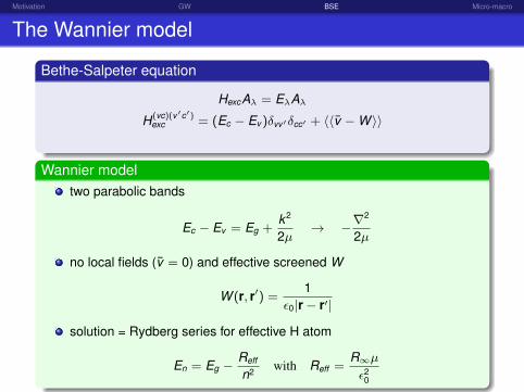
Bethe-Salpeter equation
HexcAλ = EλAλ
H(vc)(v′c′)exc = (Ec − Ev )δvv′δcc′ + 〈〈v −W 〉〉
Wannier modeltwo parabolic bands
Ec − Ev = Eg +k2
2µ→ −∇
2
2µ
no local fields (v = 0) and effective screened W
W (r, r′) =1
ε0|r− r′|
solution = Rydberg series for effective H atom
En = Eg −Reff
n2 with Reff =R∞µε2
0
bg=whiteMotivation GW BSE Micro-macro
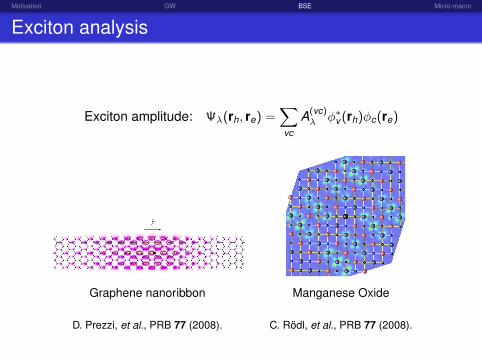
Exciton analysis
Exciton amplitude: Ψλ(rh, re) =∑vc
A(vc)λ φ∗v (rh)φc(re)
Graphene nanoribbon Manganese Oxide
D. Prezzi, et al., PRB 77 (2008). C. Rödl, et al., PRB 77 (2008).

bg=whiteMotivation GW BSE Micro-macro
Outline
1 Motivation
2 One-particle Green’s functions: GW approximation
3 Two-particle Green’s functions: Bethe-Salpeter equation
4 Micro-macro connection

bg=whiteMotivation GW BSE Micro-macro
Micro-macro connection
ObservationAt long wavelength, external fields are slowly varying over the unitcell:
dimension of the unit cell for silicon: 0.5 nmvisible radiation 400 nm < λ < 800 nm
Total and induced fields are rapidly varying: they include thecontribution from electrons in all regions of the cell.Large and irregular fluctuations over the atomic scale.

bg=whiteMotivation GW BSE Micro-macro
Micro-macro connection
ObservationOne usually measures quantities that vary on a macroscopic scale.When we calculate microscopic quantities we need to average overdistances that are
large compared to the cell parametersmall compared to the wavelength of the external perturbation.
The differences between the microscopic fields and the averaged(macroscopic) fields are called the crystal local fields.

bg=whiteMotivation GW BSE Micro-macro
Suppose that we are ableto calculate the microscopic dielectric function ε,
how do we obtain the macroscopic dielectric function εM
that we measure in experiments ?

bg=whiteMotivation GW BSE Micro-macro
Micro-macro connection
Fourier transform
In a periodic medium, every function V (r, ω) can be represented bythe Fourier series
V (r, ω) =∑qG
V (q + G, ω)ei(q+G)r
or:
V (r, ω) =∑
q
eiqr∑
G
V (q + G, ω)eiGr =∑
q
eiqrV (q, r, ω)
where:V (q, r, ω) =
∑G
V (q + G, ω)eiGr
V (q, r, ω) is periodic with respect to the Bravais lattice and hence isthe quantity that one has to average to get the correspondingmacroscopic potential VM(q, ω).

bg=whiteMotivation GW BSE Micro-macro
Micro-macro connection
Averages
VM(q, ω) =1
Ωc
∫drV (q, r, ω)
V (q, r, ω) =∑
G
V (q + G, ω)eiGr
Therefore:
VM(q, ω) =∑
G
V (q + G, ω)1
Ωc
∫dreiGr = V (q + 0, ω)
The macroscopic average VM corresponds tothe G = 0 component of the microscopic V .
Example
Vext (q, ω) = εM(q, ω)Vtot,M(q, ω)

bg=whiteMotivation GW BSE Micro-macro
Micro-macro connection
Fourier transforms
Fourier transform of a function f (r, r′, ω):
f (q + G,q + G′, ω) =
∫drdr′e−i(q+G)rf (r, r′, ω)e+i(q+G′)r′ ≡ fG,G′(q, ω)
Therefore the relation
Vtot (r1, ω) =
∫dr2ε
−1(r1, r2, ω)Vext (r2, ω)
in the Fourier space becomes:
Vtot (q + G, ω) =∑G′
ε−1G,G′(q, ω)Vext (q + G′, ω)

bg=whiteMotivation GW BSE Micro-macro
Micro-macro connection
Example
Vtot,M(q, ω) = ε−1M (q, ω)Vext (q, ω)
Macroscopic dielectric function
Vtot (q + G, ω) =∑G′
ε−1G,G′(q, ω)Vext (q + G′, ω)
VM,tot (q, ω) = Vtot (q + 0, ω)
Vext is a macroscopic quantity:
Vtot,M (q, ω) = ε−1G=0,G′=0(q, ω)Vext (q, ω)
ε−1M (q, ω) = ε−1
G=0,G′=0(q, ω)
εM(q, ω) =1
ε−1G=0,G′=0(q, ω)

bg=whiteMotivation GW BSE Micro-macro
Micro-macro connection
Macroscopic dielectric function
Vext (q + G, ω) =∑G′
εG,G′(q, ω)Vtot (q + G′, ω)
Remember: Vext is a macroscopic quantity:
Vext (q, ω) =∑G′
εG=0,G′(q, ω)Vtot (q + G′, ω)
Vext (q, ω) = εG=0,G′=0(q, ω)Vtot,M(q, ω)+∑G′ 6=0
εG=0,G′(q, ω)Vtot (q+G′, ω)
Vext (q, ω) = εM(q, ω)Vtot,M(q, ω)
εM(q, ω) 6= εG=0,G′=0(q, ω)

bg=whiteMotivation GW BSE Micro-macro
Micro-macro connection
Spectra
εM(q, ω) =1
ε−1G=0,G′=0(q, ω)
Abs(ω) = limq→0
ImεM(ω) = limq→0
Im1
ε−1G=0,G′=0(q, ω)
EELS(ω) = − limq→0
Imε−1M (ω) = − lim
q→0Imε−1
G=0,G′=0(q, ω)

bg=whiteMotivation GW BSE Micro-macro
Micro-macro connection
Spectra
εM(q, ω) =1
ε−1G=0,G′=0(q, ω)
Abs(ω) = limq→0
ImεM(ω) = limq→0
Im1
ε−1G=0,G′=0(q, ω)
EELS(ω) = − limq→0
Imε−1M (ω) = − lim
q→0Imε−1
G=0,G′=0(q, ω)

bg=whiteMotivation GW BSE Micro-macro
BSE vs. TDDFT: what in common ?
BSE
L = L0 + L0(v + Ξ)L
TDDFT
χ = χ0 + χ0(v + fxc)χ

bg=whiteMotivation GW BSE Micro-macro
The Coulomb term v
The Coulomb term
v = v0 + v
bg=whiteMotivation GW BSE Micro-macro
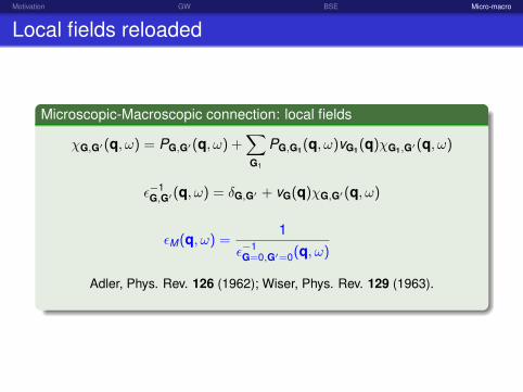
Local fields reloaded
Microscopic-Macroscopic connection: local fields
χG,G′(q, ω) = PG,G′(q, ω) +∑G1
PG,G1 (q, ω)vG1 (q)χG1,G′(q, ω)
ε−1G,G′(q, ω) = δG,G′ + vG(q)χG,G′(q, ω)
εM(q, ω) =1
ε−1G=0,G′=0(q, ω)
Adler, Phys. Rev. 126 (1962); Wiser, Phys. Rev. 129 (1963).
bg=whiteMotivation GW BSE Micro-macro
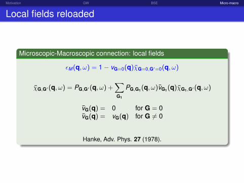
Local fields reloaded
Microscopic-Macroscopic connection: local fields
εM(q, ω) = 1− vG=0(q)χG=0,G′=0(q, ω)
χG,G′(q, ω) = PG,G′(q, ω) +∑G1
PG,G1 (q, ω)vG1 (q)χG1,G′(q, ω)
vG(q) = 0 for G = 0vG(q) = vG(q) for G 6= 0
Hanke, Adv. Phys. 27 (1978).

bg=whiteMotivation GW BSE Micro-macro
Absorption
Abs(ω) = limq→0
ImεM(q, ω)
Abs(ω) =− limq→0
Im [vG=0(q)χG=0,G′=0(q, ω)]
χ = P + Pv χ
Absorption→ response to Vext + V macroind
EELS
Eels(ω) =− limq→0
Im[1/εM(q, ω)]
Eels(ω) =− limq→0
Im [vG=0(q)χG=0,G′=0(q, ω)]
χ = P + P(v0 + v)χ
Eels→ response to Vext

bg=whiteMotivation GW BSE Micro-macro
The Coulomb term v
The Coulomb term
v = v0 + v
long-range v0 ⇒ difference between Abs and Eels

bg=whiteMotivation GW BSE Micro-macro
Coulomb term v0: Abs vs. Eels
F. Sottile, PhD thesis (2003) - Bulk silicon: absorption vs. EELS.

bg=whiteMotivation GW BSE Micro-macro
The Coulomb term v
The Coulomb term
v = v0 + v
long-range v0 ⇒ difference between Abs and Eels
what about v ?

bg=whiteMotivation GW BSE Micro-macro
The Coulomb term v
The Coulomb term
v = v0 + v
long-range v0 ⇒ difference between Abs and Eels
what about v ?
v is responsible for crystal local-field effects

bg=whiteMotivation GW BSE Micro-macro
Coulomb term v : local fields
v : local fields
εM = 1− vG=0χG=0,G′=0
Set v = 0 in:
χG,G′ = χ0G,G′ +
∑G1
χ0G,G1
vG1 χG1,G′
⇒ χG,G′ = χ0G,G′
Result:
εM = 1− vG=0χ0G=0,G′=0
that is: no local-field effects!(equivalent to Fermi’s golden rule)

bg=whiteMotivation GW BSE Micro-macro
Coulomb term v : local fields
v : local fields
εM = 1− vG=0χG=0,G′=0
Set v = 0 in:
χG,G′ = χ0G,G′ +
∑G1
χ0G,G1
vG1 χG1,G′
⇒ χG,G′ = χ0G,G′
Result:
εM = 1− vG=0χ0G=0,G′=0
that is: no local-field effects!(equivalent to Fermi’s golden rule)

bg=whiteMotivation GW BSE Micro-macro
Coulomb term v : local fields
v : local fields
εM = 1− vG=0χG=0,G′=0
Set v = 0 in:
χG,G′ = χ0G,G′ +
∑G1
χ0G,G1
vG1 χG1,G′
⇒ χG,G′ = χ0G,G′
Result:
εM = 1− vG=0χ0G=0,G′=0
that is: no local-field effects!(equivalent to Fermi’s golden rule)

bg=whiteMotivation GW BSE Micro-macro
Coulomb term v : local fields
Bulk silicon: absorption

bg=whiteMotivation GW BSE Micro-macro
Coulomb term v : local fields
A. G. Marinopoulos et al., PRL 89 (2002) - Graphite EELS

bg=whiteMotivation GW BSE Micro-macro
What are local fields?
Effective medium theoryUniform field E0 applied to a dielectric sphere with dielectric constant ε invacuum. From continuity conditions at the interface:
P =3
4πε− 1ε+ 2
E0
Jackson, Classical electrodynamics, Sec. 4.4.
bg=whiteMotivation GW BSE Micro-macro
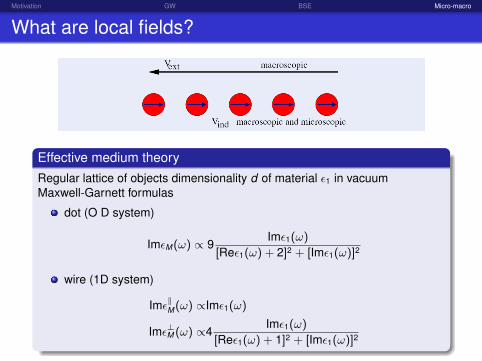
What are local fields?
Effective medium theoryRegular lattice of objects dimensionality d of material ε1 in vacuumMaxwell-Garnett formulas
dot (O D system)
ImεM (ω) ∝ 9Imε1(ω)
[Reε1(ω) + 2]2 + [Imε1(ω)]2
wire (1D system)
Imε‖M (ω) ∝Imε1(ω)
Imε⊥M (ω) ∝4Imε1(ω)
[Reε1(ω) + 1]2 + [Imε1(ω)]2

bg=whiteMotivation GW BSE Micro-macro
What are local fields?
F. Bruneval et al., PRL 94 (2005) -Si nanowires
S. Botti et al., PRB 79 (2009) -SiGe nanodots

bg=whiteMotivation GW BSE Micro-macro
MBPT & TDDFT
MBPT helps improving DFT & TDDFT
DFT & TDDFT help improving MBPT

bg=whiteMotivation GW BSE Micro-macro
Conclusion
(TD)DFT & MBPT...
try to learn both!

bg=whiteMotivation GW BSE Micro-macro
Many thanks!
bg=whiteMotivation GW BSE Micro-macro
Acknowledgements
Silvana BottiFabien BrunevalValerio OlevanoLucia ReiningFrancesco SottileValérie Véniard
Related Documents


