Introduction to Kalman Filters

2458-2

Workshop on GNSS Data Application to Low Latitude Ionospheric Research

John F. Raquet

6 - 17 May 2013

Air Force Institute of Technology USA

Introduction to Kalman Filters

John Raquet, 2012. All Rights Reserved. John Raquet, 2012. All Rights Reserved.

Introduction to Kalman Filters ---

Assumptions and Pitfalls

Dr. John F. Raquet Director, Advanced navigation Technology (ANT) Center

Air Force Institute of Technology

The views expressed in this presentation are those of the author and do not reflect the official policy or position of the United States Air Force, Department of Defense, or the U.S. Government.

2

Kalman Filtering Overview

•  Kalman filtering is an estimation approach that can be applied to navigation –  Many other application areas

•  Concepts to be covered –  Information describing the system

•  State vector •  Covariance matrix

–  Propagating state and covariance forward in time –  Using measurements to update the state and covariance

•  Assumptions/Limitations

3

Kalman Filtering: Information Describing the System (1/2)

•  State vector –  Set of variables that

•  Describe everything you want to know about the system •  Include all of the information needed to determine how the system changes over

time •  Describe systematic errors in the measurements (anything that’s not “noise”)

–  Example: Hot air baloon

–  Does this describe what we want to know? –  Does this describe how the system changes over time? –  Would this be a good state vector for a fighter aircraft? –  Altitude estimation example

⎥⎥⎥⎥⎥⎥⎥⎥

⎦

⎤

⎢⎢⎢⎢⎢⎢⎢⎢

⎣

⎡

=

zyxzyx

x balloon of velocity ENU ,,balloon ofposition ENU ,,

=

=

zyxzyx

4

Kalman Filtering: Information Describing the System (2/2)

•  Covariance matrix –  The covariance matrix basically describes how well the state is

known •  If the system only gives a state output, it’s not that useful. •  If it outputs the state and tells how accurate it is, then you have information

that you can confidently act upon. •  Hot air balloon example: the system state tells me that I’m 300 m above the

ground descending at a rate of 10 m/sec. –  Need to know covariance matrix as well.

»  Case 1: Position accuracy = 10 m 1- σ, velocity accuracy = 1 m/sec 1-σ → probably not in danger until ~30 seconds

»  Case 2: Position accuracy = 400 m 1- σ, velocity accuracy = 15 m/sec 1- σ → you could hit the ground any second!

–  How to interpret covariance matrix

•  Diagonal terms are the error variances of the estimated states •  Off-diagonal terms are cross-covariances, describing the correlations of the

errors between the states

ˆ ˆ[( )( ) ]TP E= − −x x x xEstimated state

True state

5

Kalman Filtering: Propagating Covariance and State Forward in Time

•  State vector and covariance matrix can be propagated forward in time –  If you know the current state estimate, you can determine the state

estimate at a point in the future –  If you know the current covariance matrix, you can determine the

covariance matrix at a point in the future –  Information about how the state and covariance changes over time

is given in •  Dynamics matrix F:

•  State transition matrix Φ:

–  When propagating covariance forward in time, process noise is added to account for

•  Unmodeled dynamics •  Unmodeled system inputs •  Anything else that decreases the ability to predict the future state using the

current state –  Process noise increases uncertainty (i.e., larger covariance values)

Fxx =

)()()( 0011 tttt xΦx −=

6

Kalman Filtering: Measurement Updates

•  A measurement gives information about the state values –  Examples: GPS pseudorange (for position or clock bias) or Doppler (for

velocity or clock drift) •  Effects of a measurement update

–  State values are adjusted to reflect the measurement –  Covariance matrix is adjusted to reflect how well the state is known, now

that the measurement is available •  Measurements always decrease uncertainty (i.e., smaller covariance values)

•  Measurement noise –  Description of how precise the measurement is –  The effect of measurement on state and covariance determined by

tradeoff between •  Measurement noise (how good the measurement is) •  Covariance matrix (how well the state is known at this point)

•  Relationship between measurement and states given by H matrix (same as least-squares)

The Kalman Filter Iteration

7

( )( )

( ) )()(

)(ˆ)(ˆ)(ˆ)()( 1

−+

−−+

−−−

−=

−+=

+=

kk

kkk

Tk

Tk

ttttt

tt

PKHIPxHzKxx

RHHPHPK

Update

dkkT

kkkk

kkkk

tttttttttt

QΦPΦPxΦx

+−−=

−=

−+−−

−

+−−

−

)()()()(

)(ˆ)()(ˆ

111

11

Propagate

0 10 20 30 40 50 60 70 80 90 1000

5

10

15

Time (sec)

Est

imat

ion

Err

or S

td D

ev

Example of Estimation Error Over Time

Measurement Model

8

( )( )

( ) )()(

)(ˆ)(ˆ)(ˆ)()( 1

−+

−−+

−−−

−=

−+=

+=

kk

kkk

Tk

Tk

ttttt

tt

PKHIPxHzKxx

RHHPHPK

Update

dkkT

kkkk

kkkk

tttttttttt

QΦPΦPxΦx

+−−=

−=

−+−−

−

+−−

−

)()()()(

)(ˆ)()(ˆ

111

11

Propagate

vHxz +=measurement state

meas noise

sensitivity matrix

Linear Measurement Model

⎥⎥⎥⎥⎥

⎦

⎤

⎢⎢⎢⎢⎢

⎣

⎡

=

⎥⎥⎥⎥⎥

⎦

⎤

⎢⎢⎢⎢⎢

⎣

⎡

==

21

2212

11221

21

2221

12121

][][

][][][][][

][

nn

n

nn

n

T

vEvvE

vEvvEvvEvvEvE

E

σσ

σσ

σσσ

vvR

Measurement noise is described by the measurement noise covariance matrix:

•  Key assumptions (in semi-nontechnical language) –  Measurement errors v are Gaussian (follow a “bell curve”) –  Measurement errors v are “white” (completely random from measurement to

measurement) –  Measurement model is linear

What if Measurements are Non-Linear

•  Example of non-linear measurements: a range (distance) measurement (such as with GPS)

•  Can use non-linear measurement model

•  Kalman filter is then modified to become an “Extended Kalman Filter” (EKF) –  Requires linearization about the estimated solution –  Because of this, an EKF is not, technically speaking, truly

optimal like the KF –  In many cases it would be “nearly optimal”—depends on the

nature of the linearization

9

vxhz += )( vHxz +=Nonlinear Linear

Dynamics Model

10

( )( )

( ) )()(

)(ˆ)(ˆ)(ˆ)()( 1

−+

−−+

−−−

−=

−+=

+=

kk

kkk

Tk

Tk

ttttt

tt

PKHIPxHzKxx

RHHPHPK

Update

dkkT

kkkk

kkkk

tttttttttt

QΦPΦPxΦx

+−−=

−=

−+−−

−

+−−

−

)()()()(

)(ˆ)()(ˆ

111

11

Propagate

⎥⎥⎥⎥⎥

⎦

⎤

⎢⎢⎢⎢⎢

⎣

⎡

==

][][

][][][][][

][

21

2221

12121

nn

n

Tddd

wEwwE

wEwwEwwEwwEwE

E wwQ

Discrete-Time Dynamics Model

state after propagation

dynamics matrix

process noise

dkk tt wΦxx += +−

− )()( 1

state before propagation

Process noise is described by the measurement noise covariance matrix:

•  Key assumptions (in semi-nontechnical language) –  Process noise wd is Gaussian (follow a “bell curve”) –  Process noise wd is “white” (completely random from epoch to epoch) –  Dynamics model is perfectly known

Initialization and “Time Constant” of a KF

•  Things needed in order to initialize a filter –  Initial state estimate –  Initial covariance matrix –  Measurement model(s) –  Propagation model(s)

•  Time constant (not meant in a precise, technical way) –  Defines how long a measurement will affect the filter –  In theory, every measurement will affect the filter for the rest

of time –  In practice, this may not be the case so much

•  Example: Case in which there is high propagation noise—old measurements are significantly “de-weighted” relative to new measurements

–  Warning: Even in a case where a filter has a “short” time constant (i.e., measurements lose impact fairly quickly), a large measurement error (blunder) can have a devastating impact

11

Kalman Filter Example: Hot Air Balloon

•  Scenario: Want to estimate height of a hot air balloon on a windy day, starting at 800 m

•  What I have –  Radar altimeter to measure height above ground

(assume ground height is known) •  Meas error modeled as Gaussian with 2m standard

deviation

–  Stochastic process model for how the wind affects the height of the balloon

–  Initial uncertainty modeled as Gaussian with standard deviation of 10m (height) and 1m/s (vertical velocity)

•  What I want to know –  Height estimate and standard deviation –  Vertical velocity estimate and standard deviation

12

Stochastic Process Model

•  State vector:

–  h: balloon height (m) –  : baloon vertical velocity (m/s)

•  Continuous time process model:

•  Discrete time process model:

13

hh⎡ ⎤

= ⎢ ⎥⎣ ⎦

x

h

[ ( ) ( )] ( )TE t t Qτ δ τ+ =w w0 00 0.01

Q ⎡ ⎤= ⎢ ⎥⎣ ⎦

Dirac delta

Process noise matrix

0 1( ) ( ) ( )

0 0t t t⎡ ⎤= +⎢ ⎥⎣ ⎦

x x w

Process noise Dynamics matrix F

1( ) ( ) ( ) ( )k k d kt t t t−=Φ Δ +x x w1 1 0.5

( )0 0 0 0

F t tt e Δ Δ⎡ ⎤ ⎡ ⎤

Φ Δ = = =⎢ ⎥ ⎢ ⎥⎣ ⎦ ⎣ ⎦

for 1 0.5seck kt t t −Δ = − =

0.0004 0.0013[ ( ) ( )]

0.0013 0.005T

d k d k dE t t Q ⎡ ⎤= = ⎢ ⎥

⎣ ⎦w w

Kalman Filter Propagation Equations

•  Propagate state: •  Propagate covariance: •  Example

–  Initial conditions:

–  First time step:

14

1ˆ ˆ( ) ( )k kt t −=Φx x1( ) ( ) T

k k dP t P t Q−=Φ Φ +

800ˆ(0)

0⎡ ⎤

= ⎢ ⎥⎣ ⎦

x2

2

10 0(0)

0 1P

⎡ ⎤= ⎢ ⎥⎣ ⎦

1 0.5 800 800ˆ ˆ(0.5) (0)

0 0 0 0⎡ ⎤ ⎡ ⎤ ⎡ ⎤

=Φ = =⎢ ⎥ ⎢ ⎥ ⎢ ⎥⎣ ⎦ ⎣ ⎦ ⎣ ⎦

x x

(0.5) (0)1 0.5 100 0 1 0 0.0004 0.00130 0 0 1 0.5 0 0.0013 0.005

100.25 0.5 0.0004 0.00130.5 1 0.0013 0.005

100.2504 0.50130.5013 1.005

TdP P Q=Φ Φ +

⎡ ⎤ ⎡ ⎤ ⎡ ⎤ ⎡ ⎤= +⎢ ⎥ ⎢ ⎥ ⎢ ⎥ ⎢ ⎥⎣ ⎦ ⎣ ⎦ ⎣ ⎦ ⎣ ⎦

⎡ ⎤ ⎡ ⎤= +⎢ ⎥ ⎢ ⎥⎣ ⎦ ⎣ ⎦

⎡ ⎤= ⎢ ⎥⎣ ⎦

Notice that this is higher (more uncertainty) than when we started!

Propagation Example—No Measurements (Single Run)

15

hh

0 20 40 60 80 100 120 140 160 180 200200

400

600

800

1000

1200

1400

Time (sec)

h (m

)

+/- 2σ

h estimated

h true

0 20 40 60 80 100 120 140 160 180 200-4

-3

-2

-1

0

1

2

3

4

Time (sec)

Ver

tical

Vel

ocity

(h-

dot)

(m

/s)

+/- 2σ

h-dot estimated

h-dot true

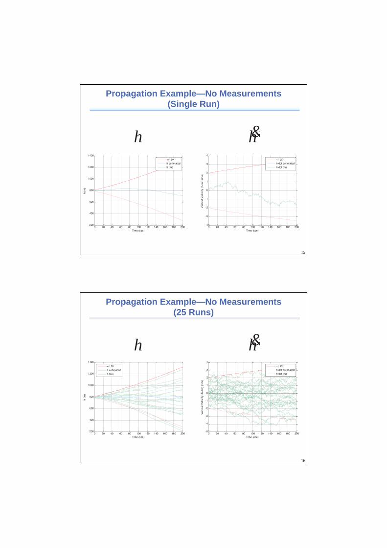
Propagation Example—No Measurements (25 Runs)

16

hh

0 20 40 60 80 100 120 140 160 180 200200

400

600

800

1000

1200

1400

Time (sec)

h (m

)

+/- 2σ

h estimated

h true

0 20 40 60 80 100 120 140 160 180 200-5

-4

-3

-2

-1

0

1

2

3

4

Time (sec)

Ver

tical

Vel

ocity

(h-

dot)

(m

/s)

+/- 2σ

h-dot estimated

h-dot true

Measurement Update at t=40 Sec

•  At t=40 sec, a measurement of 820.97 m is taken (remember, meas error standard deviation is 2 m)

•  Measurement model:

–  In this case:

•  Step 1: Propagate up to measurement time:

17

800ˆ( )

0kt⎡ ⎤

= ⎢ ⎥⎣ ⎦

x1913.3 48

( )48 1.40kP t ⎡ ⎤

= ⎢ ⎥⎣ ⎦

80seckt =

vHxz += [ ]TE=R vv

[ ]1 0meas

H

hz h v v

h⎡ ⎤

= + = +⎢ ⎥⎣ ⎦

x

2 4R E v⎡ ⎤= =⎣ ⎦

(Note that this is a scalar measurement)

These are consistent with previous slides

Measurement Update at t=40 Sec (continued)

•  Step 2: Measurement update

–  In this case, since :

18

[ ]ˆ ˆ ˆ( ) ( ) ( ) ( )k k k kt t K z t H t= + −x x x

1( ) ( )T T

k kK P t H HP t H R−

⎡ ⎤= +⎣ ⎦Kalman gain:

[ ]1 0H =

1,1

1,1

2,1

1,1

1913.30.9981913.3 4

48 0.0253.9917 4

PP R

KP

P R

⎡ ⎤ ⎡ ⎤⎢ ⎥ ⎢ ⎥+ ⎡ ⎤+⎢ ⎥= = =⎢ ⎥ ⎢ ⎥⎢ ⎥ ⎣ ⎦⎢ ⎥⎢ ⎥ ⎢ ⎥+⎣ ⎦+⎢ ⎥⎣ ⎦

[ ]

[ ]

( )

ˆ ˆ ˆ( ) ( ) ( ) ( )

800 0.998820.97 800

0 0.025

820.926ˆ( )

0.525

0.0021 0 1913.3 48 3.992 0.100( )

0.0250 1 48 1.40 0.100 0.198k

k k k k

k

k

I KH P t

t t K z t H t

t

P t

−

= + −

⎡ ⎤ ⎡ ⎤= + −⎢ ⎥ ⎢ ⎥⎣ ⎦ ⎣ ⎦

⎡ ⎤= ⎢ ⎥⎣ ⎦

⎡ ⎤ ⎡ ⎤ ⎡ ⎤= =⎢ ⎥ ⎢ ⎥ ⎢ ⎥−⎣ ⎦ ⎣ ⎦ ⎣ ⎦

x x x

xresidual

1913.3 48( )

48 1.40kP t ⎡ ⎤= ⎢ ⎥⎣ ⎦

from previous slide:

[ ]( ) ( )k kP t I KH P t= −

(Before measurement)

State:

Covariance:

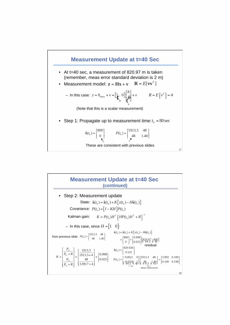
Filter Propagation/Measurement Incorporation Example

19

0 20 40 60 80 100 120 140 160 180 200650

700

750

800

850

900

Time (sec)

h (m

)

+/- 2σ

h estimated

h true

0 20 40 60 80 100 120 140 160 180 200-3

-2

-1

0

1

2

3

Time (sec)

Ver

tical

Vel

ocity

(h-

dot)

(m

/s)

+/- 2σ

h-dot estimated

h-dot true

hh

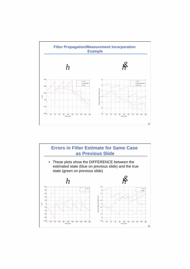
Errors in Filter Estimate for Same Case as Previous Slide

•  These plots show the DIFFERENCE between the estimated state (blue on previous slide) and the true state (green on previous slide)

20

0 20 40 60 80 100 120 140 160 180 200-100

-80

-60

-40

-20

0

20

40

60

80

100

Time (sec)

h (m

)

+/- 2σ

h

0 20 40 60 80 100 120 140 160 180 200-2.5

-2

-1.5

-1

-0.5

0

0.5

1

1.5

2

2.5

Time (sec)

Ver

tical

Vel

ocity

(h-

dot)

(m

/s)

+/- 2σ

h-dot

hh

Errors in Filter Estimate 25 Monte Carlo Runs

21

0 20 40 60 80 100 120 140 160 180 200-100

-80

-60

-40

-20

0

20

40

60

80

100

Time (sec)

h (m

)

+/- 2σ

h

0 20 40 60 80 100 120 140 160 180 200-3

-2

-1

0

1

2

3

Time (sec)

Ver

tical

Vel

ocity

(h-

dot)

(m

/s)

+/- 2σ

h-dot

hh

Modeling Errors

•  In the previous example, the filter had a perfect model •  What happens if there is a process noise modeling error? •  Example:

22 0 20 40 60 80 100 120 140 160 180 200

-100

-80

-60

-40

-20

0

20

40

60

80

100

Time (sec)

h (m

)

+/- 2σ

h

0 20 40 60 80 100 120 140 160 180 200-2.5

-2

-1.5

-1

-0.5

0

0.5

1

1.5

2

2.5

Time (sec)

Ver

tical

Vel

ocity

(h-

dot)

(m

/s)

+/- 2σ

h-dot

hh

0 00 0.001

Q ⎡ ⎤= ⎢ ⎥⎣ ⎦0 00 0.01

Q ⎡ ⎤= ⎢ ⎥⎣ ⎦

True:

Modeled:

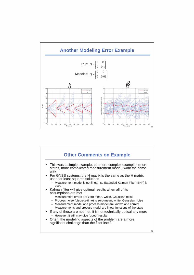
Another Modeling Error Example

23

0 00 0.1

Q ⎡ ⎤= ⎢ ⎥⎣ ⎦0 00 0.01

Q ⎡ ⎤= ⎢ ⎥⎣ ⎦

True:

Modeled:

0 20 40 60 80 100 120 140 160 180 200-150

-100

-50

0

50

100

150

200

Time (sec)

h (m

)

+/- 2σ

h

0 20 40 60 80 100 120 140 160 180 200-6

-4

-2

0

2

4

6

8

Time (sec)

Ver

tical

Vel

ocity

(h-

dot)

(m

/s)

+/- 2σ

h-dot

hh

Other Comments on Example

•  This was a simple example, but more complex examples (more states, more complicated measurement model) work the same way

•  For GNSS systems, the H matrix is the same as the H matrix used for least-squares solutions –  Measurement model is nonlinear, so Extended Kalman Filter (EKF) is

used •  Kalman filter will give optimal results when all of its

assumptions are met –  Measurement errors are zero mean, white, Gaussian noise –  Process noise (discrete-time) is zero mean, white, Gaussian noise –  Measurement model and process model are known and correct –  Measurements and process model are linear functions of the state

•  If any of these are not met, it is not technically optical any more –  However, it still may give “good” results

•  Often, the modeling aspects of the problem are a more significant challenge than the filter itself

24

One Final Thought

25