Introduction to Geophysical Modelling and Inversion - An... · Introduction to Geophysical Modelling and Inversion ... • Depends on the geophysical method, ... A statement of the

@ 2014 Mira Geoscience Ltd.

Introduction to Geophysical Modelling and Inversion

James Reid

GEOPHYSICAL INVERSION FOR

MINERAL EXPLORERS

ASEG-WA, SEPTEMBER 2014

Forward modelling vs. inversion

Forward Modelling: Given a model m and predicting data d

F is an operator representing the governing equations relating the model and data

Model

F

d=F(m)

Data

Inversion

Geophysical inversion refers to the mathematical and statistical

techniques for recovering information on subsurface physical properties

(magnetic susceptibility, density, electrical conductivity etc) from

observed geophysical data.

What is inversion?

Model

m=F-1

(d)

Data

Inversion: Recording data d and predicting model m

F-1

What is inversion?

Forward Modelling: Given a model and predicting data

Model

F

d=F(m)

m=F

-1(d)

Not Possible - Ill Conditioned

Data

Inversion: Recording data and predicting model

F-1

Iterative inversion

Starting model

and acquisition

parameters

Calculate model

response using

forward modelling

algorithm

Compare observed

and model responses,

and calculate

Objective function

Objective function

small, or maximum

no. of iterations

exceeded

Inversion process

is complete:

Output final model

Objective function

large

Alter model

parameters so

as to reduce objective function

Each cycle

through the

inversion process

is called an

iteration

How do inversions work?

This chart summarizes the

requirements for proceeding with

inversion of geophysical data.

Each box has important implications

for successful inversion.

Ability to do forward modelling

calculations is assumed.

Given:

- Field observations

- Error estimates

- Ability to forward model

- Prior knowledge

Choose a suitable

data misfit

Design model

norm

Discretize the Earth

Perform inversion

Evaluate results Iterate

Interpret preferred model(s)

Models

Model Types

Single Physical

Property Value

Parameterized object

(susceptibility, length,

depth, orientation)

Physical property

varies as a function

of depth

Plate in a half space

Plate in a layered

model

Plate in a free-space

(vacuum)

(after: Inversion for Applied Geophysics)

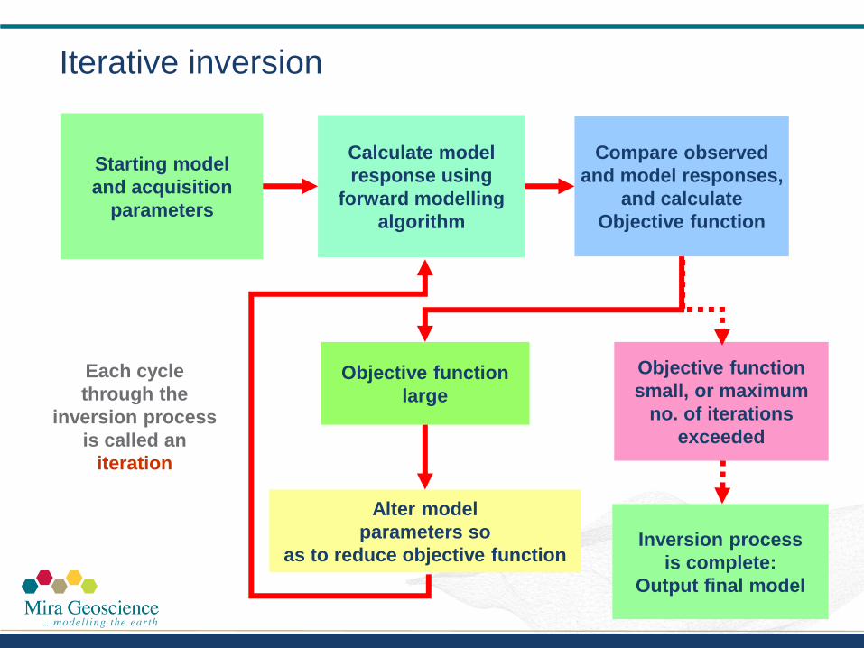
Models

Model Types

2.5D models

2D models

Model is unchanging

perpendicular to

profile section

(after: Inversion for Applied Geophysics)

Model objects have

limited strike length Geologic unit

boundaries adjust

location to create 3D

shapes and bodies.

Physical properties

change in all 3

directions.

Generalized structure

Concatenated 1D

models

Geometry Model

Why invert data?

Helps explain complex data sets

e.g. DCIP, Gravity Gradiometry, AEM, ZTEM, DHEM

Removes topography effects

Explains the data with a model(s) of the earth:

Provides a quantitative model that can be analysed

What is the depth, geometry, volume, physical property of the model features?

More easily relates to geology - easier for interpretation

What geologic features can be determined in the model?

Can QC the data, identify problematic data acquisition problems

Helps separate the noise from the signal in the data estimates the noise levels

estimates depth of penetration

Recovered chargeability Inversion result is more easily

interpretable in terms of geology

Example: Target in presence of geological noise

IP data Data are sometimes difficult to interpret

Shallow anomalies represent

chargeable boulders in till

Subtle responses are important

Know The Data

In order for modelling to occur, all instrument system and survey

acquisition parameters have to be known.

In general, try to do as little as possible to the data to preserve the

information

Obviously erroneous data should be removed prior to inversion.

This includes features/anomalies in the data which are not modelled by the

forward modelling algorithm e.g., IP or SPM effects in EM data etc

RUBBISH IN = RUBBISH OUT

Inverse Modelling

Modelling Styles

• Parametric – few unknowns

15 Data

e.g. TEM decay

time

dB/dt

1D Conductivity model t1

t2

t3

7 unknown

model parameters

(conductivity of each layer;

thickness of upper three layers)

s1

s4

s3

s2

Inverse Modelling

Modelling Styles

• Parametric – few unknowns

• Generalized – many unknowns

15 Data

e.g. TEM decay

time

dB/dt

1D Conductivity model

40 unknown

model parameters

1D Mesh structure predefined

but smaller than expected

structure of geology.

structure inferred from the

resulting model

Inverse Modelling

Modelling Styles

• Lithology based

– VP suite (Fullagar Geophysics)

– Geomodeller (Intrepid)

• Physical Property based

– UBC-GIF codes

– Geosoft Voxi

– VP suite

Inverse Modelling

Physical Property Based Modelling

• Physical property values of many individual cells are adjusted.

• General structure is recovered

e.g. Magnetic Data

3D susceptibility model

(low value cells removed)

Inverse Modelling

Physical Property Based Modelling

• Physical property values of many individual cells are adjusted.

• General structure is recovered.

RESULT IS A PHYSICAL PROPERTY MODEL

CONTAINING STRUCTURE

e.g. Magnetic Data

3D susceptibility model

10,000+ unknown

model parameters

(low value cells removed)

3D Mesh structure predefined

but smaller than expected

structure of geology.

structure inferred from the

resulting model

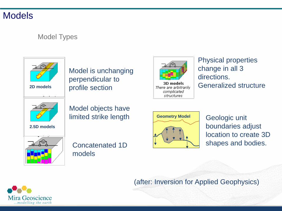
Inverse Modelling

Lithology Based Modelling

• Provide physical properties (single value or distribution) for each

lithology and adjust the geometry to fit the data.

Selected Spectrem EM Channels (Obs - blue, Calc - red)

100 100

1000 1000

10^4 10^4

10^5 10^5

10^6 10^6

Starting Model

450 450

500 500

550 550

600 600

Inverted Model

450 450

500 500

550 550

600 600

RESULT IS A

GEOLOGICAL

MODEL

(courtesy Anglo American)

Inverse Modelling

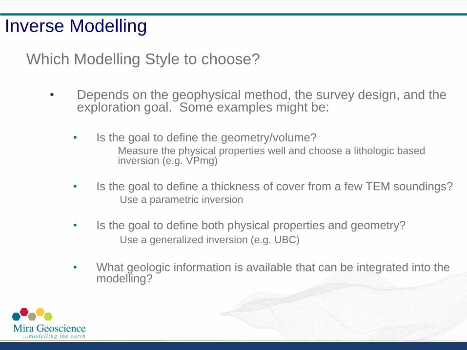
Which Modelling Style to choose?

• Depends on the geophysical method, the survey design, and the

exploration goal. Some examples might be:

• Is the goal to define the geometry/volume?

Measure the physical properties well and choose a lithologic based inversion (e.g. VPmg)

• Is the goal to define a thickness of cover from a few TEM soundings? Use a parametric inversion

• Is the goal to define both physical properties and geometry?

Use a generalized inversion (e.g. UBC)

• What geologic information is available that can be integrated into the modelling?

Acceptable models and non-uniqueness

There are infinitely many models that can explain the observed data

Why is this so?

• Because there are usually more

unknowns (model parameters)

than observed data points

(underdetermined problem)

• Some physically-based non-

uniqueness

• Real data contain noise

Acceptable models and non-uniqueness

There are infinitely many models that can explain the observed data

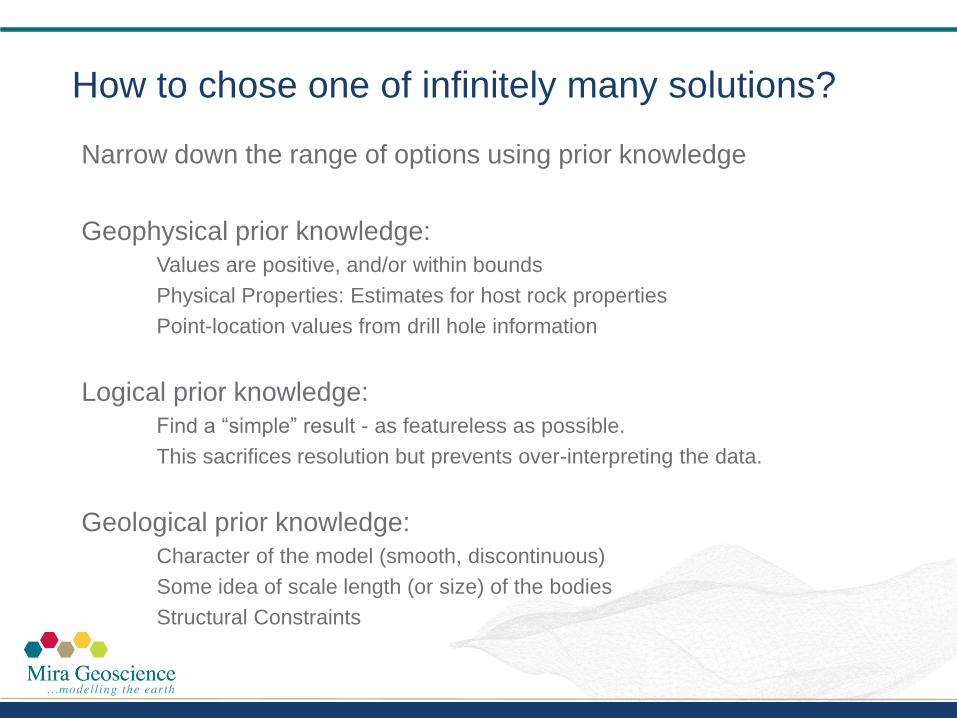
How to chose one of infinitely many solutions?

Narrow down the range of options using prior knowledge

Geophysical prior knowledge:

Values are positive, and/or within bounds

Physical Properties: Estimates for host rock properties

Point-location values from drill hole information

Logical prior knowledge:

Find a “simple” result - as featureless as possible.

This sacrifices resolution but prevents over-interpreting the data.

Geological prior knowledge:

Character of the model (smooth, discontinuous)

Some idea of scale length (or size) of the bodies

Structural Constraints

Model norm

The model norm is a measure of the (mathematical) “size” of a model

The inversion process is an automated decision making scheme

The model norm is a way of encoding prior information in a form suitable

for mathematical optimisation – we seek the “smallest” model

The model norm is part of the solution to nonuniqueness …

Nonuniqueness is addressed by choosing the one model (from

infinitely many) that minimizes the defined model norm

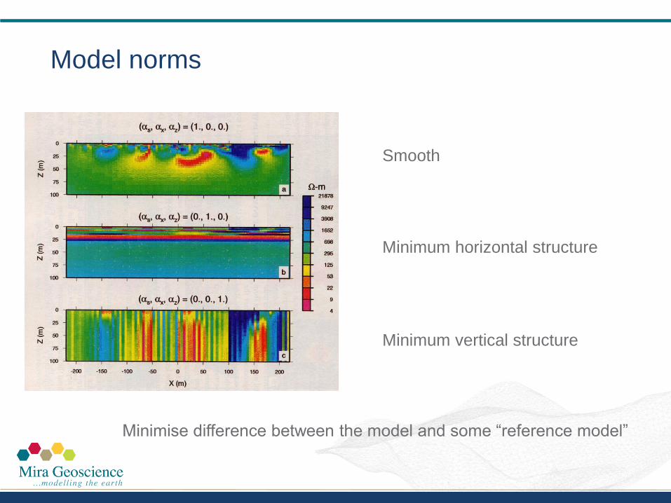
Model norms

Smooth

Minimum horizontal structure

Minimum vertical structure

Minimise difference between the model and some “reference model”

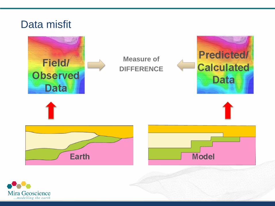
Data misfit

Measure of

DIFFERENCE

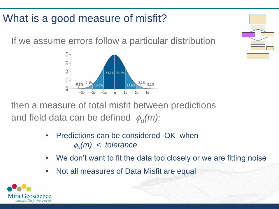
What is a good measure of misfit?

If we assume errors follow a particular distribution

then a measure of total misfit between predictions

and field data can be defined d(m):

• Predictions can be considered OK when

d(m) < tolerance

• We don’t want to fit the data too closely or we are fitting noise

• Not all measures of Data Misfit are equal

What contributes to data noise?

Natural and cultural noise sources

Accuracy and precision in data measurements

Data positioning errors

Approximations made in forward modelling

1D

2D

3D

Plates

Anisotropy

Discretization of topography

Measures of misfit Consider the problem of fitting a straight line to the data shown below:

0

0.5

1

1.5

2

2.5

0 10 20 30 40 50

Depth in drillhole (m)

% C

op

per

y = 0.0285x + 0.3333

0

0.5

1

1.5

2

2.5

0 10 20 30 40 50

Depth in drillhole (m)

% C

u

e11

e28 The residuals are the differences

between the data points and the

best-fit line at each depth

They may be positive or negative

0.3

0.35

0.4

0.45

0.5

0.55

0.6

0.65

0 2 4 6 8 10

Measures of misfit – L1 and L2 norms

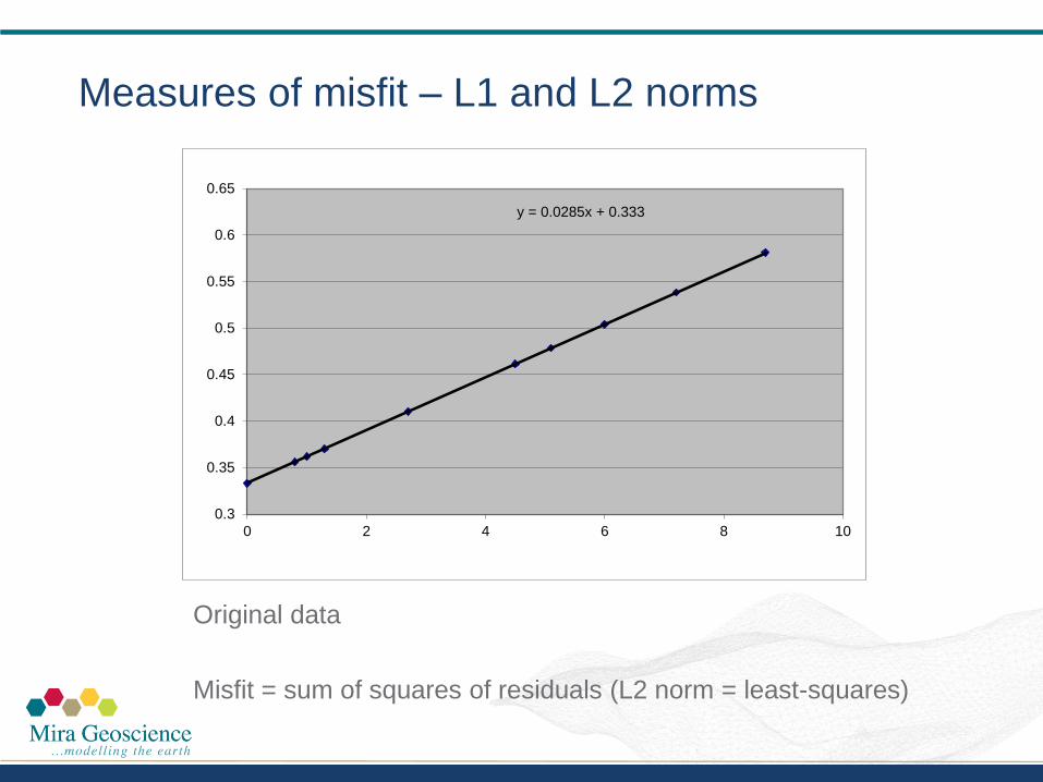
y = 0.0285x + 0.333

0.3

0.35

0.4

0.45

0.5

0.55

0.6

0.65

0 2 4 6 8 10


Original data

Misfit = sum of squares of residuals (L2 norm = least-squares)

0.3

0.35

0.4

0.45

0.5

0.55

0.6

0.65

0 2 4 6 8 10


Original data

Misfit = sum of absolute values of residuals (L1 norm)

y = 0.0285x + 0.333

0.3

0.35

0.4

0.45

0.5

0.55

0.6

0.65

0 2 4 6 8 10


Add an outlying data point

0.3

0.35

0.4

0.45

0.5

0.55

0.6

0.65

0 2 4 6 8 10

y = 0.0298x + 0.342

0.3

0.35

0.4

0.45

0.5

0.55

0.6

0.65

0 2 4 6 8 10


One outlying data point

Misfit = sum of squares of residuals (L2 norm = least-squares)

0.3

0.35

0.4

0.45

0.5

0.55

0.6

0.65

0 2 4 6 8 10


One outlying data point

Misfit = sum of absolute values of residuals (L1 norm)

L1 Less affected by outliers (noise)

Combining model norms and misfit

A statement of the inverse problem is:

Find the model which

Minimises the model norm (M), and

Produces an acceptably small data misfit (D)

Mathematically, this becomes a single optimisation

“Minimise = D + b M ” (subject to d < tolerance)

is the combined objective function

b is the trade off parameter (regularisation parameter)

d

m

*d

b

b 0

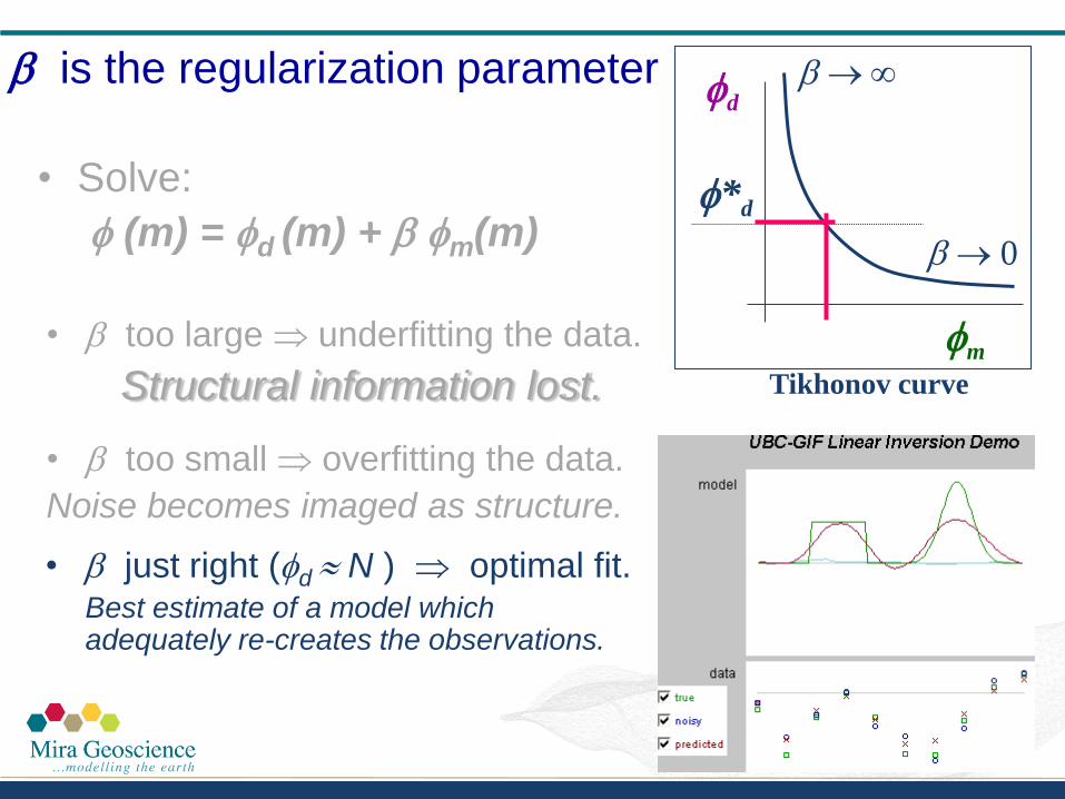
Tikhonov curve

• b just right (d N ) optimal fit. Best estimate of a model which

adequately re-creates the observations.

• b too small overfitting the data.

Noise becomes imaged as structure.

• b too large underfitting the data.

Structural information lost.

b is the regularization parameter

• Solve:

(m) = d (m) + b m(m)

Inverse Modelling

Non-Uniqueness: Solution (partial…)

• Provide explicit geological information

• Constraints

• Combine information from independent geophysical methods

• Joint or Cooperative Inversions

e.g. Gravity with Magnetics, Airborne EM with CSAMT, etc.

Sources of Data

• Geologic Mapping

• DH geological logs

• Interpreted cross-sections

• 3D geological models

• Physical property data per lithology

• Located physical property data measurements

Some information is subjective and some information is objective.

As with the geophysical data we would desire to quantify the uncertainty

associated with this data as an input to the inversion.

Integrated Modelling: Constraints

Rock properties are the link between geology and geophysics

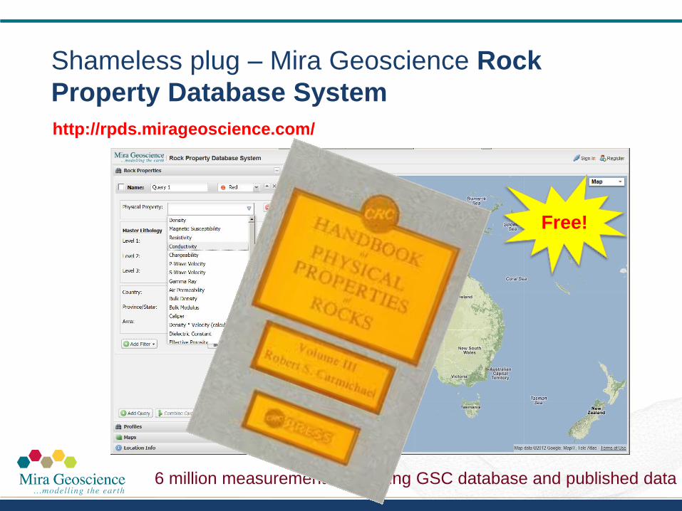
Shameless plug – Mira Geoscience Rock

Property Database System

http://rpds.mirageoscience.com/

6 million measurements, including GSC database and published data

Free!

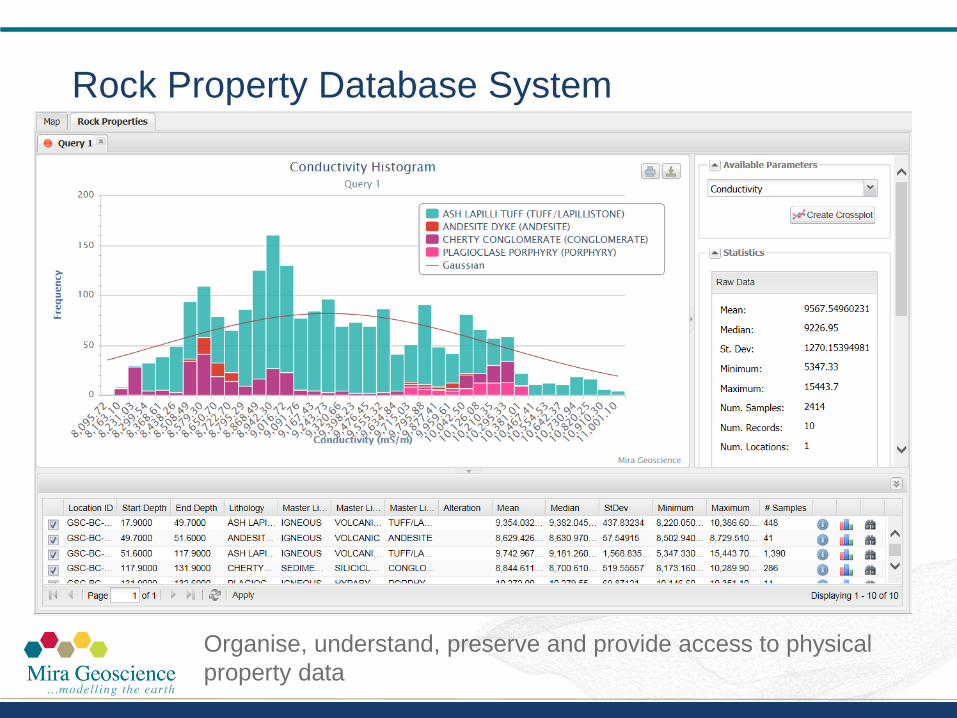
Rock Property Database System

Organise, understand, preserve and provide access to physical

property data

Common Earth Modelling

Goal:

Obtain the most complete representation of the earth.

Benefits:

Improved resolution away from constraints

Allows more precise exploration using quantitative 3D

GIS analysis.

Extending the model to include multiple properties, that honour multiple data sets, on a single model object.

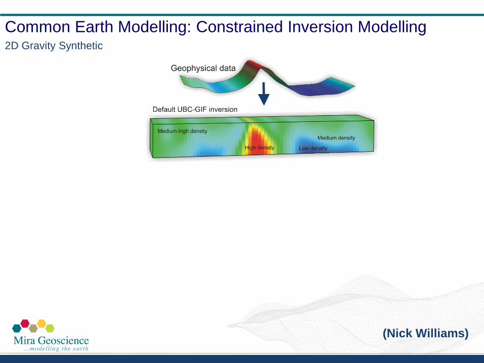
Common Earth Modelling: Constrained Inversion Modelling

(Nick Williams)

2D Gravity Synthetic

Common Earth Modelling: Constrained Inversion Modelling

+

(Nick Williams)

2D Gravity Synthetic

Common Earth Modelling: Constrained Inversion Modelling 2D Gravity Synthetic

+

(Nick Williams)

Common Earth Modelling: Constrained Inversion Modelling 2D Gravity Synthetic

+

(Nick Williams)

Surface constraints

can result in dramatic

improvements

Joint and cooperative inversion

Inversion using more than one geophysical

method

Methods sensitive to same physical

property (e.g., TEM and CSAMT)

Methods sensitive to related properties

(e.g., seismic and gravity)

Joint inversion – single objective function

Cooperative inversion – iterative/sequential

approach

These approaches require that we establish

relationships between the physical properties

each method is sensitive to

Appraisal – How good is our model?

Over-fitting vs under-fitting data

Limits to the data

Limits to the physics

Depth of investigation

Suite of models

Point-spread functions

Model resolution analysis

Sensitivity analysis

Extremal models

Model Covariance Matrix

Co-Kriging error

Summary and conclusion

Inversion has the potential to greatly improve the geological

interpretation of geophysical data

• High quality data is essential for the success of geophysical modelling

• More appropriate/efficient surveys can be designed

• Complex data sets can be understood (DH IP, 3D EM)

Understanding physical property data is the key to successful

inversion interpretation.

• Rock type

• Alteration

• Mineralization


Non uniqueness in inversion is dealt with by imposing constraints

• Provide the constraints or they will be provided for you

• Minimum structure or geological

Interpretation of inversion requires understanding of which parts

of the model are driven by constraints and which parts are driven

by data.

• Requires inspection of multiple models

Inspect observed and predicted data before accepting a model.

• Did the inversion fit the data anomalies you are interested in?

• Beware of over-fitting and under-fitting your data


Geologically constrained inversion will greatly improve your results

• Constraints can be factual or conceptual (hypothesis testing)

• Sparse or detailed

• From different sources

Geological maps

Outcrop samples

Estimates of overburden depth

Detailed drill data

Acknowledgements

Nigel Phillips

Dianne Mitchinson

Scott Napier

Shannon Frey

Thomas Campagne

Ross Brodie - Geoscience Australia

Ken Witherly - Condor Consulting

Regis Neroni - FMGL

Doug Oldenburg - UBC-GIF

- Mira Geoscience, Vancouver

Reference

Inversion for Applied Geophysics

http://www.eos.ubc.ca/research/ubcgif/iag/iag-outline.htm

Introduction to Geophysical Modelling and Inversion - An... · Introduction to Geophysical Modelling and Inversion ... • Depends on the geophysical method, ... A statement of the

Documents