Introduction to Functional Analysis - School of Physicstingyu/functional_analysis.pdf · Chapter I Preliminary Material In functional analysis many different fields of mathematics

Introduction to Functional Analysis

Daniel Daners

School of Mathematics and Statistics

University of Sydney, NSW 2006Australia

Semester 1, 2008 Copyright c©2008 The University of Sydney

Contents

I Preliminary Material 1

1 The Axiom of Choice and Zorn’s Lemma . . . . . . . . . . . . . 1

2 Metric Spaces . . . . . . . . . . . . . . . . . . . . . . . . . . . . 4

3 Limits . . . . . . . . . . . . . . . . . . . . . . . . . . . . . . . . 7

4 Compactness . . . . . . . . . . . . . . . . . . . . . . . . . . . . 11

5 Continuous Functions . . . . . . . . . . . . . . . . . . . . . . . . 14

II Banach Spaces 17

6 Normed Spaces . . . . . . . . . . . . . . . . . . . . . . . . . . . 17

7 Examples of Banach Spaces . . . . . . . . . . . . . . . . . . . . 20

7.1 Elementary Inequalities . . . . . . . . . . . . . . . . . . . 20

7.2 Spaces of Sequences . . . . . . . . . . . . . . . . . . . . 23

7.3 Lebesgue Spaces . . . . . . . . . . . . . . . . . . . . . . 26

7.4 Spaces of Bounded and Continuous Functions . . . . . . 26

8 Basic Properties of Bounded Linear Operators . . . . . . . . . . . 28

9 Equivalent Norms . . . . . . . . . . . . . . . . . . . . . . . . . . 32

10 Finite Dimensional Normed Spaces . . . . . . . . . . . . . . . . . 34

11 Infinite Dimensional Normed Spaces . . . . . . . . . . . . . . . . 36

12 Quotient Spaces . . . . . . . . . . . . . . . . . . . . . . . . . . . 38

III Hilbert Spaces 43

13 Inner Product Spaces . . . . . . . . . . . . . . . . . . . . . . . . 43

14 Projections and Orthogonal Complements . . . . . . . . . . . . . 48

15 Orthogonal Systems . . . . . . . . . . . . . . . . . . . . . . . . . 55

16 Abstract Fourier Series . . . . . . . . . . . . . . . . . . . . . . . 59

IV Linear Operators 67

17 Baire’s Theorem . . . . . . . . . . . . . . . . . . . . . . . . . . . 67

18 The Open Mapping Theorem . . . . . . . . . . . . . . . . . . . . 68

19 The Closed Graph Theorem . . . . . . . . . . . . . . . . . . . . 71

20 The Uniform Boundedness Principle . . . . . . . . . . . . . . . . 72

21 Closed Operators . . . . . . . . . . . . . . . . . . . . . . . . . . 74

22 Closable Operators and Examples . . . . . . . . . . . . . . . . . 76

i

V Duality 81

23 Dual Spaces . . . . . . . . . . . . . . . . . . . . . . . . . . . . . 81

24 The Hahn-Banach Theorem . . . . . . . . . . . . . . . . . . . . 85

25 Reflexive Spaces . . . . . . . . . . . . . . . . . . . . . . . . . . . 90

26 Weak convergence . . . . . . . . . . . . . . . . . . . . . . . . . 91

27 Dual Operators . . . . . . . . . . . . . . . . . . . . . . . . . . . 92

28 Duality in Hilbert Spaces . . . . . . . . . . . . . . . . . . . . . . 94

29 The Lax-Milgram Theorem . . . . . . . . . . . . . . . . . . . . . 96

VI Spectral Theory 99

30 Resolvent and Spectrum . . . . . . . . . . . . . . . . . . . . . . 99

31 Projections, Complements and Reductions . . . . . . . . . . . . . 105

32 The Ascent and Descent of an Operator . . . . . . . . . . . . . . 109

33 The Spectrum of Compact Operators . . . . . . . . . . . . . . . 111

Bibliography 117

ii

Acknowledgement

Thanks to Fan Wu from the 2008 Honours Year for providing an extensive list of

misprints.

iii iv

Chapter I

Preliminary Material

In functional analysis many different fields of mathematics come together. The

objects we look at are vector spaces and linear operators. Hence you need to some

basic linear algebra in general vector spaces. I assume your knowledge of that is

sufficient. Second we will need some basic set theory. In particular, many theorems

depend on the axiom of choice. We briefly discuss that most controversial axiom of

set theory and some equivalent statements. In addition to the algebraic structure

on a vector space, we will look at topologies on them. Of course, these topologies

should be compatible with the algebraic structure. This means that addition and

multiplication by scalars should be continuous with respect to the topology. We will

only look at one class of such spaces, namely normed spaces which are naturally

metric spaces. Hence it is essential you know the basics of metric spaces, and we

provide a self contained introduction of what we need in the course.

1 The Axiom of Choice and Zorn’s Lemma

Suppose that A is a set, and that for each α ∈ A there is a set Xα. We call (Xα)α∈Aa family of sets indexed by A. The set A may be finite, countable or uncountable.

We then consider the Cartesian product of the sets Xα:

∏

α∈A

Xα

consisting of all “collections” (xα)α∈A, where xα ∈ Xα. More formally,∏

α∈AXα is

the set of functions

x : A→⋃

α∈A

Xα

such that x(α) ∈ Xα for all α ∈ A. We write xα for x(α) and (xα)α∈A or simply

(xα) for a given such function x . Suppose now that A 6= ∅ and Xα 6= ∅ for all

α ∈ A. Then there is a fundamental question:

1

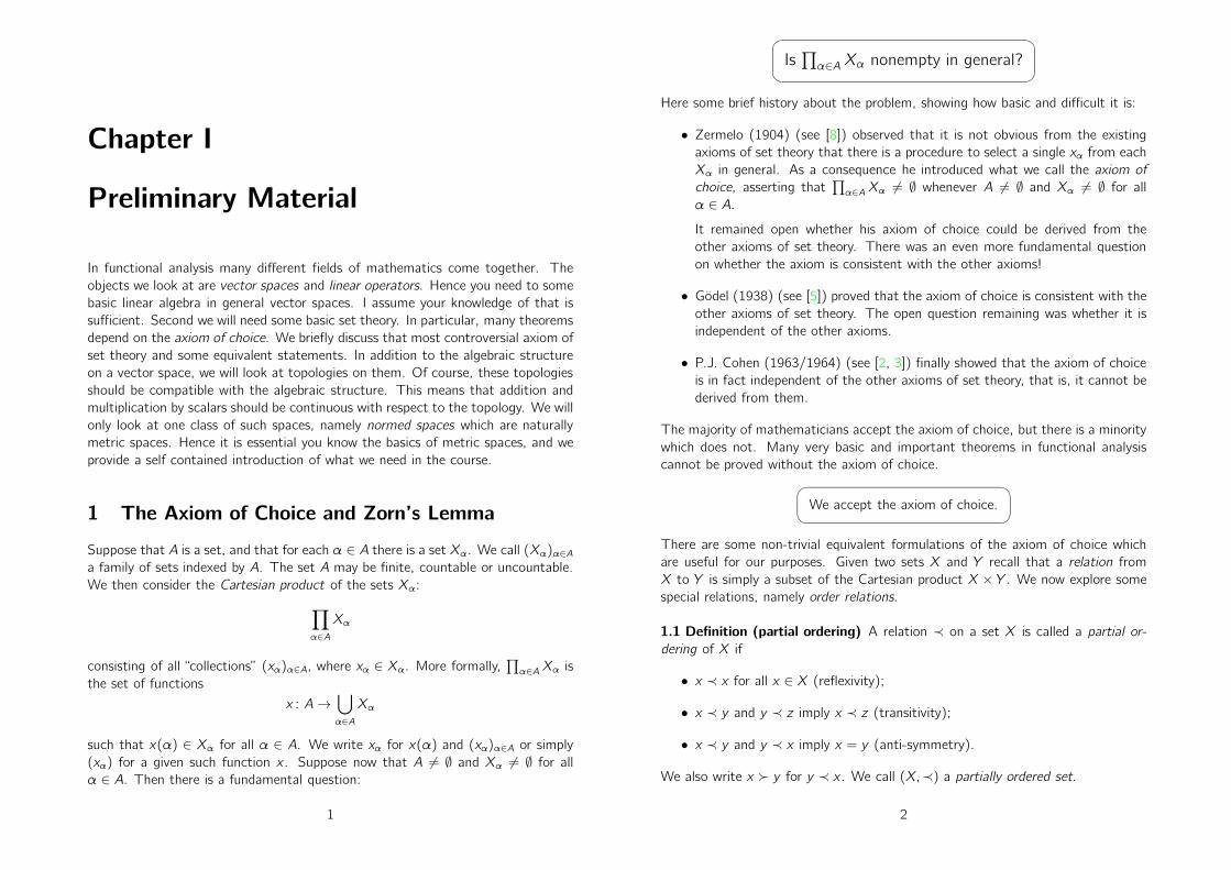
Is

∏

α∈AXα nonempty in general?

Here some brief history about the problem, showing how basic and difficult it is:

• Zermelo (1904) (see [8]) observed that it is not obvious from the existing

axioms of set theory that there is a procedure to select a single xα from each

Xα in general. As a consequence he introduced what we call the axiom of

choice, asserting that∏

α∈AXα 6= ∅ whenever A 6= ∅ and Xα 6= ∅ for all

α ∈ A.

It remained open whether his axiom of choice could be derived from the

other axioms of set theory. There was an even more fundamental question

on whether the axiom is consistent with the other axioms!

• Gödel (1938) (see [5]) proved that the axiom of choice is consistent with the

other axioms of set theory. The open question remaining was whether it is

independent of the other axioms.

• P.J. Cohen (1963/1964) (see [2, 3]) finally showed that the axiom of choice

is in fact independent of the other axioms of set theory, that is, it cannot be

derived from them.

The majority of mathematicians accept the axiom of choice, but there is a minority

which does not. Many very basic and important theorems in functional analysis

cannot be proved without the axiom of choice.

We accept the axiom of choice.

There are some non-trivial equivalent formulations of the axiom of choice which

are useful for our purposes. Given two sets X and Y recall that a relation from

X to Y is simply a subset of the Cartesian product X × Y . We now explore some

special relations, namely order relations.

1.1 Definition (partial ordering) A relation ≺ on a set X is called a partial or-

dering of X if

• x ≺ x for all x ∈ X (reflexivity);

• x ≺ y and y ≺ z imply x ≺ z (transitivity);

• x ≺ y and y ≺ x imply x = y (anti-symmetry).

We also write x ≻ y for y ≺ x . We call (X,≺) a partially ordered set.

2

1.2 Examples (a) The usual ordering ≤ on R is a partial ordering on R.

(b) Suppose S is a collection of subsets of a set X. Then inclusion is a partial

ordering. More precisely, if S, T ∈ S then S ≺ T if and only if S ⊆ T . We say Sis partially ordered by inclusion.

(c) Every subset of a partially ordered set is a partially ordered set by the induced

partial order.

There are more expressions appearing in connection with partially ordered sets.

1.3 Definition Suppose that (X,≺) is a partially ordered set. Then

(a) m ∈ X is called a maximal element in X if for all x ∈ X with x ≻ m we have

x ≺ m;

(b) m ∈ X is called an upper bound for S ⊆ X if x ≺ m for all x ∈ S;

(c) A subset C ⊆ X is called a chain in X if x ≺ y or y ≺ x for all x, y ∈ C;

(d) If a partially ordered set (X,≺) is a chain we call it a totally ordered set.

(e) If (X,≺) is partially ordered and x0 ∈ X is such that x0 ≺ x for all x ∈ X,

then we call x0 a first element.

There is a special class of partially ordered sets playing a particularly important role

in relation to the axiom of choice as we will see later.

1.4 Definition (well ordered set) A partially ordered set (X,≺) is called a well

ordered set if every subset has a first element.

1.5 Examples (a) N is a well ordered set, but Z or R are not well ordered with

the usual order.

(b) Z and R are totally ordered with the usual order.

1.6 Remark Well ordered sets are always totally ordered. To see this assume

(X,≺) is well ordered. Given x, y ∈ X we consider the subset x, y of X. By

definition of a well ordered set we have either x ≺ y or y ≺ x , which shows that

(X,≺) is totally ordered. The converse is not true as the example of Z given above

shows.

There is another, highly non-obvious but very useful statement appearing in con-

nection with partially ordered sets:

1.7 Zorn’s Lemma Suppose that (X,≺) is a partially ordered set such that each

chain in X has an upper bound. Then X has a maximal element.

There is a non-trivial connection between all the apparently different topics we

discussed so far. We state it without proof (see for instance [4]).

3

1.8 Theorem The following assertions are equivalent

(i) The axiom of choice;

(ii) Zorn’s Lemma;

(iii) Every set can be well ordered.

The axiom of choice may seem “obvious” at the first instance. However, the other

two equivalent statements are certainly not. For instance take X = R, which

we know is not well ordered with the usual order. If we accept the axiom of

choice then it follows from the above theorem that there exists a partial ordering

making R into a well ordered set. This is a typical “existence proof” based on the

axiom of choice. It does not give us any hint on how to find a partial ordering

making R into a well ordered set. This reflects Zermelo’s observation that it is

not obvious how to choose precisely one element from each set when given an

arbitrary collection of sets. Because of the non-constructive nature of the axiom

of choice and its equivalent counterparts, there are some mathematicians rejecting

the axiom. These mathematicians have the point of view that everything should

be “constructible,” at least in principle, by some means (see for instance [1]).

2 Metric Spaces

Metric spaces are sets in which we can measure distances between points. We

expect such a “distance function,” called a metric, to have some obvious properties,

which we postulate in the following definition.

2.1 Definition (Metric Space) Suppose X is a set. A map d : X × X → R is

called a metric on X if the following properties hold:

(i) d(x, y) ≥ 0 for all x, y ∈ x ;

(ii) d(x, y) = 0 if and only if x = y ;

(iii) d(x, y) = d(y , x) for all x, y ∈ X.

(iv) d(x, y) ≤ d(x, z) + d(z, y) for all x, y , z ∈ X (triangle inequality).

We call (X, d) a metric space. If it is clear what metric is being used we simply

say X is a metric space.

2.2 Example The simplest example of a metric space is R with d(x, y) := |x −y |.The standard metric used in RN is the Euclidean metric given by

d(x, y) = |x − y |2 :=

√

√

√

√

N∑

i=1

|xi − yi |2

for all x, y ∈ RN.

4

2.3 Remark If (X, d) is a metric space, then every subset Y ⊆ X is a metric space

with the metric restricted to Y . We say the metric on Y is induced by the metric

on X.

2.4 Definition (Open and Closed Ball) Let (X, d) be a metric space. For r > 0

we call

B(x, r) := y ∈ X : d(x, y) < rthe open ball about x with radius r . Likewise we call

B(x, r) := y ∈ X : d(x, y) ≤ r

the closed ball about x with radius r .

Using open balls we now define a “topology” on a metric space.

2.5 Definition (Open and Closed Set) Let (X, d) be a metric space. A subset

U ⊆ X is called open if for every x ∈ X there exists r > 0 such that B(x, r) ⊆ U.

A set U is called closed if its complement X \ U is open.

2.6 Remark For every x ∈ X and r > 0 the open ball B(x, r) in a metric space is

open. To prove this fix y ∈ B(x, r). We have to show that there exists ε > 0 such

that B(y , ε) ⊆ B(x, r). To do so note that by definition d(x, y) < r . Hence we

can choose ε ∈ R such that 0 < ε < r−d(x, y). Thus, by property (iv) of a metric,

for z ∈ B(y , ε) we have d(x, z) ≤ d(x, y) + d(y , z) < d(x, y) + r − d(x, y) = r .Therefore z ∈ B(x, r), showing that B(y , ε) ⊆ B(x, r).

Next we collect some fundamental properties of open sets.

2.7 Theorem Open sets in a metric space (X, d) have the following properties.

(i) X, ∅ are open sets;

(ii) arbitrary unions of open sets are open;

(iii) finite intersections of open sets are open.

Proof. Property (i) is obvious. To prove (ii) let Uα, α ∈ A be an arbitrary family

of open sets in X. If x ∈ ⋃

α∈A Uα then x ∈ Uβ for some β ∈ A. As Uβ is open there

exists r > 0 such that B(x, r) ⊆ Uβ. Hence also B(x, r) ⊆ ⋃

α∈A Uα, showing that⋃

α∈A Uα is open. To prove (iii) let Ui , i = 1, . . . , n be open sets. If x ∈ ⋂ni=1 Ui

then x ∈ Ui for all i = 1, . . . , n. As the sets Ui are open there exist ri > 0 such

that B(x, ri) ⊆ Ui for all i = 1, . . . , n. If we set r := mini=1,...,n ri then obviously

r > 0 and B(x, r) ⊆ ⋂ni=1 Ui , proving (iii).

5

2.8 Remark There is a more general concept than that of a metric space, namely

that of a “topological space.” A collection T of subsets of a set X is called a

topology if the following conditions are satisfied

(i) X, ∅ ∈ T ;

(ii) arbitrary unions of sets in T are in T ;

(iii) finite intersections of sets in T are in T .

The elements of T are called open sets, and (X, T ) a topological space. Hence

the open sets in a metric space form a topology on X.

2.9 Definition (Neighbourhood) Suppose that (X, d) is a metric space (or more

generally a topological space). We call a set U a neighbourhood of x ∈ X if there

exists an open set V ⊆ U with x ∈ V .

Now we define some sets associated with a given subset of a metric space.

2.10 Definition (Interior, Closure, Boundary) Suppose that U is a subset of a

metric space (X, d) (or more generally a topological space). A point x ∈ U is

called an interior point of U if U is a neighbourhood of x . We call

(i) U := Int(U) := x ∈ U : x interior point of U the interior of U;

(ii) U := x ∈ X : U ∩ V 6= ∅ for every neighbourhood V of x the closure of U;

(iii) ∂U := U \ Int(U) the boundary of U.

2.11 Remark A set is open if and only if U = U and closed if and only if U = U.

Moreover, ∂U = U ∩X \ U.

Sometimes it is convenient to look at products of a (finite) number of metric

spaces. It is possible to define a metric on such a product as well.

2.12 Proposition Suppose that (Xi , di), i = 1, . . . , n are metric spaces. Then

X = X1 × X2 × · · · × Xn becomes a metric space with the metric d defined by

d(x, y) :=

n∑

i=1

di(xi , yi)

for all x = (x1, . . . , xn) and y = (y1, . . . , yn) in X.

Proof. Obviously, d(x, y) ≥ 0 and d(x, y) = d(y , x) for all x, y ∈ X. Moreover,

as di(xi , yi) ≥ 0 we have d(x, y) = 0 if and only if di(xi , yi) = 0 for all i = 1, . . . , n.

6

As di are metrics we get xi = yi for all i = 1, . . . , n. For the triangle inequality

note that

d(x, y) =

n∑

i=1

d(xi , yi) ≤n

∑

i=1

(

d(xi , zi) + d(zi , yi))

=

n∑

i=1

d(xi , zi) +

n∑

i=1

d(zi , yi) = d(x, y) + d(z, y)

for all x, y , z ∈ X.

2.13 Definition (Product space) The space and metric introduced in Proposi-

tion 2.12 is called a product space and a product metric, respectively.

3 Limits

Once we have a notion of “closeness” we can discuss the asymptotics of sequences

and continuity of functions.

3.1 Definition (Limit) Suppose (xn)n∈N is a sequence in a metric space (X, d),

or more generally a topological space. We say x0 is a limit of (xn) if for every

neighbourhood U of x0 there exists n0 ∈ N such that xn ∈ U for all n ≥ n0. We

write

x0 = limn→∞xn or xn → x as n →∞.

If the sequence has a limit we say it is convergent, otherwise we say it is divergent.

3.2 Remark Let (xn) be a sequence in a metric space (X, d) and x0 ∈ X. Then

the following statements are equivalent:

(1) limn→∞xn = x0;

(2) for every ε > 0 there exists n0 ∈ N such that d(xn, x0) < ε for all n ≥ n0.

Proof. Clearly (1) implies (2) by choosing neighbourhoods of the form B(x, ε). If

(2) holds and U is an arbitrary neighbourhood of x0 we can choose ε > 0 such that

B(x0, ε) ⊆ U. By assumption there exists n0 ∈ N such that d(xn, x0) < ε for all

n ≥ n0, that is, xn ∈ B(x0, ε) ⊆ U for all n ≥ n0. Therefore, xn → x0 as n →∞.

3.3 Proposition A sequence in a metric space (X, d) has at most one limit.

7

Proof. Suppose that (xn) is a sequence in (X, d) and that x and y are limits of

that sequence. Fix ε > 0 arbitrary. Since x is a limit there exists n1 ∈ N such

that d(xn, x) < ε/2 for all n > n1. Similarly, since y is a limit there exists n2 ∈ Nsuch that d(xn, y) < ε/2 for all n > n2. Hence d(x, y) ≤ d(x, xn) + d(xn, y) ≤ε/2 + ε/2 = ε for all n > maxn1, n2. Since ε > 0 was arbitrary it follows that

d(x, y) = 0, and so by definition of a metric x = y . Thus (xn) has at most one

limit.

We can characterise the closure of sets by using sequences.

3.4 Theorem Let U be a subset of the metric space (X, d) then x ∈ U if and only

if there exists a sequence (xn) in U such that xn → x as n →∞.

Proof. Let U ⊆ X and x ∈ U. Hence B(x, ε)∩U) 6= ∅ for all ε > 0. For all n ∈ Nwe can therefore choose xn ∈ U with d(x, xn) < 1/n. By construction xn → x as

n→∞. If (xn) is a sequence in U converging to x then for every ε > 0 there exists

n0 ∈ N such that xn ∈ B(x, ε) for all n ≥ n0. In particular, B(x, ε) ∩ U 6= ∅ for all

ε > 0, implying that x ∈ U as required.

There is another concept closely related to convergence of sequences.

3.5 Definition (Cauchy Sequence) Suppose (xn) is a sequence in the metric space

(X, d). We call (xn) a Cauchy sequence if for every ε > 0 there exists n0 ∈ N such

that d(xn, xm) < ε for all m, n ≥ n0.Some sequences may not converge, but they accumulate at certain points.

3.6 Definition (Point of Accumulation) Suppose that (xn) is a sequence in a

metric space (X, d) or more generally in a topological space. We say that x0 is a

point of accumulation of (xn) if for every neighbourhood U of x0 and every n0 ∈ Nthere exists n ≥ n0 such that xn ∈ U.

3.7 Remark Equivalently we may say x0 is an accumulation point of (xn) if for

every ε > 0 and every n0 ∈ N there exists n ≥ n0 such that d(xn, x0) < ε. Note

that it follows from the definition that every neighbourhood of x0 contains infinitely

many elements of the sequence (xn).

3.8 Proposition Suppose that (X, d) is a metric space and (xn) a sequence in that

space. Then x ∈ X is a point of accumulation of (xn) if and only if

x ∈∞⋂

k=1

xj : j ≥ k. (3.1)

Proof. Suppose that x ∈ ⋂∞k=1 xj : j ≥ k. Then x ∈ xj : j ≥ k for all k ∈ N.

By Theorem 3.4 we can choose for every k ∈ N an element xnk ∈ xj : j ≥ k such

8

that d(xnk , x) < 1/k . By construction xnk → x as k → ∞, showing that x is a

point of accumulation of (xn). If x is a point of accumulation of (xn) then for all

k ∈ N there exists nk ≥ k such that d(xnk , x) < 1/k . Clearly xnk → x as k → ∞,

so that x ∈ xnj : j ≥ k for all k ∈ N. As xnj : j ≥ k ⊆ xj : j ≥ k for all k ∈ Nwe obtain (3.1).

In the following theorem we establish a connection between Cauchy sequences and

converging sequences.

3.9 Theorem Let (X, d) be a metric space. Then every convergent sequence is a

Cauchy sequence. Moreover, if a Cauchy sequence (xn) has an accumulation point

x0, then (xn) is a convergent sequence with limit x0.

Proof. Suppose that (xn) is a convergent sequence with limit x0. Then for every

ε > 0 there exists n0 ∈ N such that d(xn, x0) < ε/2 for all n ≥ n0. Now

d(xn, xm) ≤ d(xn, x0) + d(x0, xm) = d(xn, x0) + d(xm, x0) <ε

2+ε

2= ε

for all n,m ≥ n0, showing that (xn) is a Cauchy sequence. Now assume that (xn)

is a Cauchy sequence, and that x0 ∈ X is an accumulation point of (xn). Fix ε > 0

arbitrary. Then by definition of a Cauchy sequence there exists n0 ∈ N such that

d(xn, xm) < ε/2 for all n,m ≥ n0. Moreover, since x0 is an accumulation point

there exists m0 ≥ n0 such that d(xm0, x0) < ε/2. Hence

d(xn, x0) ≤ d(xn, xm0) + d(xm0, x0) <ε

2+ε

2= ε

for all n ≥ n0. Hence by Remark 3.2 x0 is the limit of (xn).

In a general metric space not all Cauchy sequences have necessarily a limit, hence

the following definition.

3.10 Definition (Complete Metric Space) A metric space is called complete if

every Cauchy sequence in that space has a limit.

One property of the real numbers is that the intersection of a nested sequence of

closed bounded intervals whose lengths shrinks to zero have a non-empty intersec-

tion. This property is in fact equivalent to the “completeness” of the real number

system. We now prove a counterpart of that fact for metric spaces. There are no

intervals in general metric spaces, so we look at a sequence of nested closed sets

whose diameter goes to zero. The diameter of a set K in a metric space (X, d) is

defined by

diam(K) := supx,y∈K

d(x, y).

9

3.11 Theorem (Cantor’s Intersection Theorem) Let (X, d) be a metric space.

Then the following two assertions are equivalent:

(i) (X, d) is complete;

(ii) For every sequence of closed sets Kn ⊆ X with Kn+1 ⊆ Kn for all n ∈ N

diam(Kn) := supx,y∈Kn

d(x, y)→ 0

as n→∞ we have⋂

n∈NKn 6= ∅.Proof. First assume that X is complete and let Kn be as in (ii). For every n ∈ Nwe choose xn ∈ Kn and show that (xn) is a Cauchy sequence. By assumption

Kn+1 ⊆ Kn for all n ∈ N, implying that xm ∈ Km ⊆ Kn for all m > n. Since

xm, xn ∈ Kn we have

d(xm, xn) ≤ supx,y∈Kn

d(x, y) = diam(Kn)

for all m > n. Since diam(Kn) → 0 as n → ∞, given ε > 0 there exists n0 ∈ Nsuch that diam(Kn0) < ε. Hence, since Km ⊆ Kn ⊆ Kn0 we have

d(xm, xn) ≤ diam(Kn) ≤ diam(Kn0) < ε

for all m > n > n0, showing that (xn) is a Cauchy sequence. By completenes of S,

the sequence (xn) converges to some x ∈ X. We know from above that xm ∈ Knfor all m > n. As Kn is closed x ∈ Kn. Since this is true for all n ∈ N we conclude

that x ∈ ⋂

n∈NKn, so the intersection is non-empty as claimed.

Assume now that (ii) is true and let (xn) be a Cauchy sequence in (X, d). Hence

there exists n0 ∈ X such that d(xn0, xn) < 1/2 for all n ≥ n0. Similarly, there exists

n1 > n0 such that d(xn1, xn) < 1/22 for all n ≥ n1. Continuing that way we

construct a sequence (nk) in N such that for every k ∈ N we have nk+1 > nk and

d(xnk , xn) < 1/2k+1 for all n > nk . We now set Kk := B(xk, 2−k)). If x ∈ Kk+1,

then since nk+1 > nk

d(xnk , x) ≤ d(xnk , xnk+1) + d(xnk+1, x) <1

2k+1+1

2k+1=1

2k.

Hence x ∈ Kk , showing that Kk+1 ⊆ Kk for all k ∈ N. By assumption (ii) we

have⋂

k∈NKk 6= ∅, so choose x ∈ ⋂

k∈NKk 6= ∅. Then x ∈ Kk for all k ∈ N, so

d(xnk , x) ≤ 1/2k for all k ∈ N. Hence xnk → x as k → ∞. By Theorem 3.9 the

Cauchy sequence (xn) converges, proing (i).

We finally look at product spaces defined in Definition 2.13. The rather simple

proof of the following proposition is left to the reader.

3.12 Proposition Suppose that (Xi , di), i = 1, . . . , n are complete metric spaces.

Then the corresponding product space is complete with respect to the product

metric.

10

4 Compactness

We start by introducing some additional concepts, and show that they are all

equivalent in a metric space. They are all generalisations of “finiteness” of a set.

4.1 Definition (Open Cover, Compactness) Let (X, d) be a metric space. We

call a collection of open sets (Uα)α∈A an open cover of X if X ⊆ ⋃

α∈A Uα. The

space X is called compact if for every open cover (Uα)α∈A there exist finitely many

αi ∈ A, i = 1, . . . , m such that (Uαi )i=1,...,m is an open cover of X. We talk about

a finite sub-cover of X.

4.2 Definition (Sequential Compactness) We call a metric space (X, d) sequen-

tially compact if every sequence in X has an point of accumulation.

4.3 Definition (Total Boundedness) We call a metric space X totally bounded

if for every ε > 0 there exist finitely many points xi ∈ X, i = 1, . . . , m, such that

(B(xi , ε))i=1,...,m is an open cover of X.

It turns out that all the above definitions are equivalent, at least in metric spaces

(but not in general topological spaces).

4.4 Theorem For a metric space (X, d) the following statements are equivalent:

(i) X is compact;

(ii) X is sequentially compact;

(iii) X is complete and totally bounded.

Proof. To prove that (i) implies (ii) assume that X is compact and that (xn) is

a sequence in X. We set Cn := xj : j ≥ n and Un := X \ Cn. Then Un is open

for all n ∈ N as Cn is closed. By Proposition 3.8 the sequence (xn) has a point of

accumulation if⋂

n∈N

Cn 6= ∅,

which is equivalent to

⋃

n∈N

Un =⋃

n∈N

X \ Cn = X \⋂

n∈N

Cn 6= X

Clearly C0 ⊃ C1 ⊃ · · · ⊃ Cn 6= ∅ for all n ∈ N. Hence every finite intersection of

sets Cn is nonempty. Equivalently, every finite union of sets Un is strictly smaller

than X, so that X cannot be covered by finitely many of the sets Un. As X is

compact it is impossible that⋃

n∈N Un = X as otherwise a finite number would

cover X already, contradicting what we just proved. Hence (xn) must have a point

of accumulation.

11

Now assume that (ii) holds. If (xn) is a Cauchy sequence it follows from (ii) that

it has a point of accumulation. By Theorem 3.9 we conclude that it has a limit,

showing that X is complete. Suppose now that X is not totally bounded. Then,

there exists ε > 0 such that X cannot be covered by finitely many balls of radius

ε. If we let x0 be arbitrary we can therefore choose x1 ∈ X such that d(x0, x1) > ε.

By induction we may construct a sequence (xn) such that d(xj , xn) ≥ ε for all

j = 1, . . . , n − 1. Indeed, suppose we have x0, . . . , xn ∈ X with d(xj , xn) ≥ ε for

all j = 1, . . . , n − 1. Assuming that X is not totally bounded⋃nj=1B(xj , ε) 6= X,

so we can choose xn+1 not in that union. Hence d(xj , xn+1) ≥ ε for j = 1, . . . , n.

By construction it follows that d(xn, xm) ≥ ε/2 for all n,m ∈ N, showing that (xn)

does not contain a Cauchy subsequence, and thus has no point of accumulation.

As this contradicts (ii), the space X must be totally bounded.

Suppose now that (iii) holds, but X is not compact. Then there exists an open

cover (Uα)α∈A not having a finite sub-cover. As X is totally bounded, for every

n ∈ N there exist finite sets Fn ⊆ X such that

X =⋃

x∈Fn

B(x, 2−n). (4.1)

Assuming that (Uα)α∈A does not have a finite sub-cover, there exists x1 ∈ F1 such

that B(x1, 2−1) and thus K1 := B(x1, 3 · 2−1) cannot be covered by finitely many

Uα. By (4.1) it follows that there exists x2 ∈ F2 such that B(x1, 2−1)∩B(x2, 2−2)

and therefore K2 := B(x2, 3 · 2−2) is not finitely covered by (Uα)α∈A. We can

continue this way and choose xn+1 ∈ Fn+1 such that B(xn, 2−n) ∩B(xn+1, 2−(n+1))

and therefore Kn+1 := B(x2, 3 · 2−(n+1)) is not finitely covered by (Uα)α∈A. Note

that B(xn, 2−n) ∩ B(xn+1, 2−(n+1)) 6= ∅ since otherwise the intersection is finitely

covered by (Uα)α∈A. Hence if x ∈ Kn+1, then

d(xn, x) ≤ d(xn, xn+1) + d(xn+1, x) ≤1

2n+1

2n+1+3

2n+1=6

2n+1=3

2n,

implying that x ∈ Kn. Also diamKn ≤ 3 · 2n−1 → 0. Since X is complete,

by Cantor’s intersection Theorem 3.11 there exists x ∈ ⋂

n∈NKn. As (Uα) is a

cover of X we have x ∈ Uα0 for some α0 ∈ A. Since Uα0 is open there exists

ε > 0 such that B(x, ε) ⊆ Uα0. Choose now n such that 6/2n < ε and fix

y ∈ Kn. Since x ∈ Kn we have d(x, y) ≤ d(x, xn) + d(xn, y) ≤ 6/2n < ε. Hence

Kn ⊆ B(x, ε) ⊆ Uα0, showing that Kn is covered by Uα0. However, by construction

Kn cannot be covered by finitely many Uα, so we have a contradiction. Hence X

is compact, completing the proof of the theorem.

The last part of the proof is modelled on the usual proof of the Heine-Borel the-

orem asserting that bounded and closed sets are the compact sets in RN. Hence

it is not a surprise that the Heine-Borel theorem easily follows from the above

characterisations of compactness.

12

4.5 Theorem (Heine-Borel) A subset of RN is compact if and only if it is closed

and bounded.

Proof. Suppose A ⊆ RN is compact. By Theorem 4.4 the set A is totally bounded,

and thus may be covered by finitely many balls of radius one. A finite union of

such balls is clearly bounded, so A is bounded. Again by Theorem 4.4, the set A

is complete, so in particular it is closed. Now assume A is closed and bounded.

As RN is complete it follows that A is complete. Next we show that A is totally

bounded. We let M be such that A is contained in the cube [−M,M]N . Given

ε > 0 the interval [−M,M] can be covered by m := [2M/ε] + 1 closed intervals

of length ε/2 (here [2M/ε] is the integer part of 2M/ε). Hence [−M,M]N can be

covered by mN cubes with edges ε/2 long. Such cubes are contained in open balls

of radius ε, so we can cover [−M,M]N and thus A by a finite number of balls of

radius ε. Hence A is complete and totally bounded. By Theorem 4.4 the set A is

compact.

We can also look at subsets of metric spaces. As they are metric spaces with the

metric induced on them we can talk about compact subsets of a metric space. It

follows from the above theorem that compact subsets of a metric space are always

closed (as they are complete). Often in applications one has sets that are not

compact, but their closure is compact.

4.6 Definition (Relatively Compact Sets) We call a subset of a metric space

relatively compact if its closure is compact.

4.7 Proposition Closed subsets of compact metric spaces are compact.

Proof. Suppose C ⊆ X is closed and X is compact. If (Uα)α∈A is an open cover

of C then we get an open cover of X if we add the open set X \ C to the Uα. As

X is compact there exists a finite sub-cover of X, and as X \ C ∩ C = ∅ also a

finite sub-cover of C. Hence C is compact.

Next we show that finite products of compact metric spaces are compact.

4.8 Proposition Let (Xi , di), i = 1, . . . , n, be compact metric spaces. Then the

product X := X1×· · ·×Xn is compact with respect to the product metric introduced

in Proposition 2.12.

Proof. By Proposition 3.12 it follows that the product space X is complete.

By Theorem 4.4 is is therefore sufficient to show that X is totally bounded. Fix

ε > 0. Since Xi is totally bounded there exist xik ∈ Xi , k = 1, . . .mi such that

Xi is covered by the balls Bik of radius ε/n and centre xik . Then X is covered

by the balls of radius ε with centres (x1k1, . . . , xiki , . . . xnkn), where ki = 1, . . .mi .

Indeed, suppose that x = (x1, x2, . . . , xn) ∈ X is arbitrary. By assumption, for every

i = 1, . . . n there exist 1 ≤ ki ≤ mi such that d(xi , xiki ) < ε/n. By definition of

13

the product metric the distance between (x1k1, . . . , xnkn) and x is no larger than

d(x1, x1k1) + · · ·+ d(xn, xnkn) ≤ nε/n = ε. Hence X is totally bounded and thus X

is compact.

5 Continuous Functions

We give a brief overview on continuous functions between metric spaces. Through-

out, let X = (X, d) denote a metric space. We start with some basic definitions.

5.1 Definition (Continuous Function) A function f : X → Y between two metric

spaces is called continuous at a point x ∈ X if for every neighbourhood V ⊆ Yof f (x) there exists a neighbourhood U ⊆ X of x such that f (U) ⊆ V . The map

f : X → Y is called continuous if it is continuous at all x ∈ X. Finally we set

C(X, Y ) := f : X → Y | f is continuous.The above is equivalent to the usual ε-δ definition.

5.2 Theorem Let X, Y be metric spaces and f : X → Y a function. Then the

following assertions are equivalent:

(i) f is continuous at x ∈ X;

(ii) For every ε > 0 there exists δ > 0 such that dY(

f (x), f (y))

≤ ε for all y ∈ Xwith dX(x, y) < δ;

(iii) For every sequence (xn) in X with xn → x we have f (xn)→ f (x) as n→∞.

Proof. Taking special neighbourhoods V = B(f (x), ε) and U := B(x, δ) then

(ii) is clearly necessary for f to be continuous. To show the (ii) is sufficient let

V be an arbitrary neighbourhood of f (x). Then there exists ε > 0 such that

B(f (x), ε) ⊆ V . By assumption there exists δ > 0 such that dY(

f (x), f (y))

≤ εfor all y ∈ X with dX(x, y) < δ, that is, f (U) ⊆ V if we let U := B(x, δ). As U

is a neighbourhood of x it follows that f is continuous. Let now f be continuous

and (xn) a sequence in X converging to x . If ε > 0 is given then there exists δ > 0

such that dY (f (x), f (y)) < ε for all y ∈ X with dX(x, y) < δ. As xn → x there

exists n0 ∈ N such that dX(x, xn) < δ for all n ≥ n0. Hence dY (f (x), f (xn)) < ε

for all n ≥ n0. As ε > 0 was arbitrary f (xn)→ f (x) as n →∞. Assume now that

(ii) does not hold. Then there exists ε > 0 such that for each n ∈ N there exists

xn ∈ X with dX(x, xn) < 1/n but dY (f (x), f (xn)) ≥ ε for all n ∈ N. Hence xn → xin X but f (xn) 6→ f (x) in Y , so (iii) does not hold. By contrapositive (iii) implies

(ii), completing the proof of the theorem.

Next we want to give various equivalent characterisations of continuous maps (with-

out proof).

14

5.3 Theorem (Characterisation of Continuity) Let X, Y be metric spaces. Then

the following statements are equivalent:

(i) f ∈ C(X, Y );

(ii) f −1[O] := x ∈ X : f (x) ∈ O is open for every open set O ⊆ Y ;

(iii) f −1[C] is closed for every closed set C ⊆ Y ;

(iv) For every x ∈ X and every neighbourhood V ⊆ Y of f (x) there exists a

neighbourhood U ⊆ X of x such that f (U) ⊆ V ;

(v) For every x ∈ X and every ε > 0 there exists δ > 0 such that dY(

f (x), f (y))

<

ε for all y ∈ X with dX(x, y) < δ.

5.4 Definition (Distance to a Set) Let A be a nonempty subset of X. We define

the distance between x ∈ X and A by

dist(x, A) := infa∈Ad(x, a)

5.5 Proposition For every nonempty set A ⊆ X the map X → R, x 7→ dist(x, A),is continuous.

Proof. By the properties of a metric d(x, a) ≤ d(x, y) + d(y , a). By first

taking an infimum on the left hand side and then on the right hand side we get

dist(x, A) ≤ d(x, y) + dist(y , A) and thus

dist(x, A)− dist(y , A) ≤ d(x, y)

for all x, y ∈ X. Interchanging the roles of x and y we get dist(y , A)−dist(x, A) ≤d(x, y), and thus

| dist(x, A)− dist(y , A)| ≤ d(x, y),implying the continuity of dist(· , A).

We continue to discuss properties of continuous functions on compact sets.

5.6 Theorem If f ∈ C(X, Y ) and X is compact then the image f (X) is compact

in Y .

Proof. Suppose that (Uα) is an open cover of f (X) then by continuity f −1[Uα]

are open sets, and so (f −1[Uα]) is an open cover of X. By the compactness of

X it has a finite sub-cover. Clearly the image of that finite sub-cover is a finite

sub-cover of f (X) by (Uα). Hence f (X) is compact.

Continuous functions on compact sets have other nice properties.

15

5.7 Definition (Uniform Continuity) We say a function f : X → Y is uniformly

continuous if for all ε > 0 there exists δ > 0 such that dY(

f (x), f (y))

< ε for all

x, y ∈ X satisfying dX(x, y) < δ.

The difference to continuity is that δ does not depend on the point x , but can be

chosen to be the same for all x ∈ X, that is uniformly with respect to x ∈ X.

5.8 Theorem If X is compact, then every function f ∈ C(X, Y ) is uniformly con-

tinuous.

Proof. Suppose that X is compact and f not uniformly continuous. Then there

exists ε > 0 such that for all n ∈ N there exist xn, yn ∈ X with d(xn, yn) < 1/n and

d(f (xn), f (yn)) ≥ ε. (5.1)

As X is compact and thus sequentially compact there exists a subsequence xnkconverging to some x ∈ X as k →∞ (see Theorem 4.4). Now

d(x, ynk ) ≤ d(x, xnk) + d(xnk , ynk ) ≤ d(x, xnk) +1

nk

k→∞−−−→ 0,

so that ynk → x as well. By the continuity of f and the triangle inequality

d(f (xnk ), f (ynk )) ≤ d(f (xnk ), f (x)) + d(f (ynk ), f (x))k→∞−−−→ 0,

contradicting our assumption (5.1). Hence f must be uniformly continuous.

One could give an alternative proof of the above theorem using the covering prop-

erty of compact sets. We complete this section by an important property of real

valued continuous functions.

5.9 Theorem Suppose that X is a compact metric space and f ∈ C(X,R). Then

f attains its maximum and minimum, that is, there exist x1, x2 ∈ X such that

f (x1) = inff (x) : x ∈ X and f (x2) = supf (x) : x ∈ X.Proof. By Theorem 5.6 the image of f is compact, and so by the Heine-Borel

theorem (Theorem 4.5) closed and bounded. Hence the image f (X) = f (x) : x ∈X contain its infimum and supremum, that is, x1 and x2 as required exist.

16

Chapter II

Banach Spaces

The purpose of this chapter is to introduce a class of vector spaces modelled on RN.

Besides the algebraic properties we have a “norm” on RN allowing us to measure

distances between points. We generalise the concept of a norm to general vector

spaces and prove some properties of these “normed spaces.” We will see that all

finite dimensional normed spaces are essentially RN or CN. The situation becomes

more complicated if the spaces are infinite dimensional. Functional analysis mainly

deals with infinite dimensional vector spaces.

6 Normed Spaces

We consider a class of vector spaces with an additional topological structure. The

underlying field is always R or C. Most of the theory is developed simultaneously

for vector spaces over the two fields. Throughout, K will be one of the two fields.

6.1 Definition (Normed space) Let E be a vector space. A map E → R, x 7→‖x‖ is called a norm on E if

(i) ‖x‖ ≥ 0 for all x ∈ E and ‖x‖ = 0 if and only if x = 0;

(ii) ‖αx‖ = |α|‖x‖ for all x ∈ E and α ∈ K;

(iii) ‖x + y‖ ≤ ‖x‖+ ‖y‖ for all x, y ∈ E (triangle inequality).

We call (E, ‖·‖) or simply E a normed space.

There is a useful consequence of the above definition.

6.2 Proposition (Reversed triangle inequality) Let (E, ‖·‖) be a normed space.

Then

‖x − y‖ ≥∣

∣‖x‖ − ‖y‖∣

∣

for all x, y ∈ E.

17

Proof. By the triangle inequality ‖x‖ = ‖x − y + y‖ ≤ ‖x − y‖ + ‖y‖, so

‖x − y‖ ≥ ‖x‖ − ‖y‖. Interchanging the roles of x and y and applying (ii) we

get ‖x − y‖ = | − 1|‖(−1)(x − y)‖ = ‖y − x‖ ≥ ‖y‖ − ‖x‖. Combining the two

inequalities, the assertion of the proposition follows.

6.3 Lemma Let (E, ‖·‖) be a normed space and define

d(x, y) := ‖x − y‖

for all x, y ∈ E. Then (E, d) is a metric space.

Proof. By (i) d(x, y) = ‖x − y‖ ≥ 0 for all x ∈ E and d(x, y) = ‖x − y | = 0if and only if x − y = 0, that is, x = y . By (ii) we have d(x, y) = ‖x − y‖ =‖(−1)(y − x)‖ = | − 1|‖y − x‖ = ‖y − x‖ = d(y , x) for all x, y ∈ E. Finally,

for x, y , z it follows from (iii) that d(x, y) = ‖x − y‖ = ‖x − z + z − y‖ ≤‖x − z‖+ ‖z − y‖ = d(x, z) + d(z, y), proving that d(· , ·) satisfies the axioms of

a metric (see Definition 2.1).

We will always equip a normed space with the topology of E generated by the metric

induced by the norm. Hence it makes sense to talk about continuity of functions.

It turns out the that topology is compatible with the vector space structure as the

following theorem shows.

6.4 Theorem Given a normed space (E, ‖·‖), the following maps are continuous

(with respect to the product topologies).

(1) E → R, x 7→ ‖x‖ (continuity of the norm);

(2) E × E → E, (x, y) 7→ x + y (continuity of addition);

(3) K× E → E, (α, x) 7→ αx (continuity of multiplication by scalars).

Proof. (1) By the reversed triangle inequality∣

∣‖x‖ − ‖y‖∣

∣ ≤ ‖x − y‖, implying

that ‖y‖ → ‖y‖ as x → y (that is, d(x, y) = ‖x − y‖ → 0). Hence the norm is

continuous as a map from E to R.

(2) If x, y , a, b ∈ E then ‖(x + y) − (a + b)‖ = ‖(x − a) + (y − b)‖ ≤‖x − a‖+ ‖y − b‖ → 0 as x → a and y → b, showing that x + y → a+ b as x → aand y → b. This proves the continuity of the addition.

(3) For α, ξ ∈ K and a, x ∈ E we have, by using the properties of a norm,

‖ξx − αa‖ = ‖ξ(x − a) + (ξ − α)a‖≤ ‖ξ(x − a)‖+ ‖(ξ − α)x‖ = |ξ|‖x − a‖+ |ξ − α‖x‖.

As the last expression goes to zero as x → a in E and ξ → α in K we have also

proved the continuity of the multiplication by scalars.

18

When looking at metric spaces we discussed a rather important class of metric

spaces, namely complete spaces. Similarly, complete spaces play a special role in

functional analysis.

6.5 Definition (Banach space) A normed space which is complete with respect

to the metric induced by the norm is called a Banach space.

6.6 Example The simplest example of a Banach space is RN or CN with the Eu-

clidean norm.

We give a characterisation of Banach spaces in terms of properties of series. We

recall the following definition.

6.7 Definition (absolute convergence) A series∑∞k=0 ak in E is called absolutely

convergent if∑∞k=0 ‖ak‖ converges.

6.8 Theorem A normed space E is complete if and only every absolutely conver-

gent series in E converges.

Proof. Suppose that E is complete. Let∑∞k=0 ak an absolutely convergent series

in E, that is,∑∞k=0 ‖ak‖ converges. By the Cauchy criterion for the convergence

of a series in R, for every ε > 0 there exists n0 ∈ N such that

n∑

k=m+1

‖ak‖ < ε

for all n > m > n0. (This simply means that the sequence of partial sums∑nk=0 ‖ak‖, n ∈ N is a Cauchy sequence.) Therefore, by the triangle inequality

∥

∥

∥

n∑

k=0

ak −m

∑

k=0

ak

∥

∥

∥=

∥

∥

∥

n∑

k=m+1

ak

∥

∥

∥≤

n∑

k=m+1

‖ak‖ < ε

for all n > m > n0. Hence the sequence of partial sums∑nk=0 ak , n ∈ N is a

Cauchy sequence in E. Since E is complete,

∞∑

k=0

ak = limn→∞

n∑

k=0

ak

exists. Hence if E is complete, every absolutely convergent series converges in E.

Next assume that every absolutely convergent series converges. We have to show

that every Cauchy sequence (xn) in E converges. By Theorem 3.9 it is sufficient

to show that (xn) has a convergent subsequence. Since (xn) is a Cauchy sequence,

for every k ∈ N there exists mk ∈ N such that ‖xn − xm‖ < 2−k for all n,m > mk .

Now set n1 := m1 + 1. Then inductively choose nk such that nk+1 > nk > mk for

all k ∈ N. Then by the above

‖xnk+1 − xnk‖ <1

2k

19

for all k ∈ N. Now observe that

xnk − xn1 =k−1∑

j=1

(xnj+1 − xnj )

for all k ∈ N. Hence (xnk ) converges if and only the series∑∞j=1(xnj+1 − xnj )

converges. By choice of nk we have

∞∑

j=1

‖xnj+1 − xnj‖ ≤∞

∑

j=1

1

2j= 1 <∞.

Hence∑∞j=1(xnj+1 − xnj ) is absolutely convergent. By assumption every absolutely

convergent series converges and therefore (xnk ) converges, completing the proof

of the theorem.

7 Examples of Banach Spaces

In this section we give examples of Banach spaces. They will be used throughout

the course. We start by elementary inequalities and a family of norms in KN. They

serve as a model for more general spaces of sequences or functions.

7.1 Elementary Inequalities

In this section we discuss inequalities arising when looking at a family of norms on

KN. For 1 ≤ p ≤ ∞ we define the p-norms of x := (x1, . . . , xN) ∈ RN by

|x |p :=

(

N∑

i=1

|xi |p)1/p

if 1 ≤ p <∞,

maxi=1,...,N

|xi | if p =∞.(7.1)

At this stage we do not know whether |·|p is a norm. We now prove that the

p-norms are norms, and derive some relationships between them. First we need

Young’s inequality.

7.1 Lemma (Young’s inequality) Let p, p′ ∈ (1,∞) such that

1

p+1

p′= 1. (7.2)

Then

ab ≤ 1pap +

1

p′bp′

for all a, b ≥ 0.

20

Proof. The inequality is obvious if a = 0 or b = 0, so we assume that a, b > 0.

As ln is concave we get from (7.2) that

ln(ab) = ln a + ln b =1

pln ap +

1

p′ln bp

′ ≤ ln(1

pap +

1

p′bp′)

.

Hence, as exp is increasing we have

ab = exp(ln(ab)) ≤ exp(

ln(1

pap +

1

p′bp′))

=1

pap +

1

p′bp′

,

proving our claim.

The relationship (7.2) is rather important and appears very often. We say that p′

is the exponent dual to p. If p = 1 we set p′ :=∞ and if p =∞ we set p′ := 1.

From Young’s inequality we get Hölder’s inequality.

7.2 Proposition Let 1 ≤ p ≤ ∞ and p′ the exponent dual to p. Then for all

x, y ∈ KNN

∑

i=1

|xi ||yi | ≤ |x |p|y |p′.

Proof. If x = 0 or y = 0 then the inequality is obvious. Also if p = 1 or

p =∞ then the inequality is also rather obvious. Hence assume that x, y 6= 0 and

1 < p <∞. By Young’s inequality (Lemma 7.1) we have

1

|x |p|y |p′N

∑

i=1

|xi ||yi | =N

∑

i=1

|xi ||x |p|yi ||y |p′

≤N

∑

i=1

(1

p

( |xi ||x |p

)p

+1

p′

( |yi ||y |p′

)p′)

=1

p

N∑

i=1

( |xi ||x |p

)p

+1

p′

N∑

i=1

( |yi ||y |p′

)p′

=1

p

1

|x |pp

N∑

i=1

|xi |p +1

p′1

|y |p′p′

N∑

i=1

|yi |p′

=1

p

|x |pp|x |pp+1

p′|y |p′p′|y |p′p′

=1

p+1

p′= 1,

from which the required inequality readily follows.

Now we prove the main properties of the p-norms.

7.3 Theorem Let 1 ≤ p ≤ ∞. Then |·|p is a norm on KN . Moreover, if 1 ≤ p ≤q ≤ ∞ then

|x |q ≤ |x |p ≤ Nq−ppq |x |q (7.3)

for all x ∈ KN . (We set (q−p)/pq := 1/p if q =∞.) Finally, the above inequalities

are optimal.

21

Proof. We first prove that |·|p is a norm. The cases p = 1,∞ are easy, and left

to the reader. Hence assume that 1 < p <∞. By definition |x |p ≥ 0 and |x |p = 0if and only if |xi | = 0 for all i = 1, . . . , N, that is, if x = 0. Also, if α ∈ K, then

|αx |p =(

N∑

i=1

|αxi |p)1/p

=(

N∑

i=1

|α|p|xi |p)1/p

= |α||αx |p.

Thus it remains to prove the triangle inequality. For x, y ∈ KN we have, using

Hölder’s inequality (Proposition 7.2), that

|x + y |pp =N

∑

i=1

|xi + yi |p =N

∑

i=1

|xi + yi ||xi + yi |p−1

≤N

∑

i=1

|xi ||xi + yi |p−1 +N

∑

i=1

|yi ||xi + yi |p−1

≤ |x |p(

N∑

i=1

|xi + yi |(p−1)p′)1/p′

+ |y |p(

N∑

i=1

|xi + yi |(p−1)p′)1/p′

=(

|x |p + |y |p)

(

N∑

i=1

|xi + yi |(p−1)p′)1/p′

.

Now, observe that

p′ =(

1− 1p

)−1

=p

p − 1 ,

so we get from the above that

|x + y |pp ≤(

|x |p + |y |p)

(

N∑

i=1

|xi + yi |p)(p−1)/p

=(

|x |p + |y |p)

|x + y |p−1p .

Hence if x + y 6= 0 we get the triangle inequality |x + y |p ≤ |x |p + |y |p. The

inequality is obvious if x + y = 0, so |·|p is a norm on KN .

Next we show the first inequality in (7.3). First let p < q =∞. If x ∈ KN we

pick the component xj of x such that |xj | = |x |∞. Hence |x |∞ = |xj | =(

|xj |p)1/p ≤

|x |p, proving the first inequality in case q =∞. Assume now that 1 ≤ p ≤ q <∞.

If x 6= 0 then |xi |/|x |p ≤ 1 Hence, as 1 ≤ p ≤ q <∞ we have

( |xi ||x |p

)q

≤( |xi ||x |p

)p

for all x ∈ KN \ 0. Therefore,

|x |qq|x |qp=

N∑

i=1

( |xi ||x |p

)q

≤N

∑

i=1

( |xi ||x |p

)p

=|x |pp|x |pp= 1

22

for all x ∈ KN \ 0. Hence |x |q ≤ |x |p for all x 6= 0. For x = 0 the inequality is

trivial. To prove the second inequality in (7.3) assume that 1 ≤ p < q < ∞. We

define s := q/p. The corresponding dual exponent s ′ is given by

s ′ =s

s − 1 =q

q − p .

Applying Hölder’s inequality we get

|x |pp =N

∑

i=1

|xi |p · 1 ≤(

N∑

i=1

|xi |ps)1/s(

N∑

i=1

1s′)1/s ′

= Nq−pq

(

N∑

i=1

|xi |q)p/q

= Nq−pq |x |pq

for all x ∈ KN , from which the second inequality in (7.3) follows. If 1 ≤ p < q =∞and x ∈ KN is given we pick xj such that |xj | = |x |∞. Then

|x |p =(

N∑

i=1

|xi |p)1/p

≤(

N∑

i=1

|xj |p)1/p

= N1/p|xj | = N1/p|x |∞,

covering the last case.

We finally show that (7.3) is optimal. For the first inequality look at the

standard basis of KN , for which we have equality. For the second choose x =

(1, 1, . . . , 1) and observe that |x |p = N1/p. Hence

Nq−ppq |x |q = N

q−ppq N

1q = N

1p = |x |p.

Hence we cannot decrease the constant Nq−ppq in the inequality.

7.2 Spaces of Sequences

Here we discuss spaces of sequences. As most of you have seen this in Metric

Spaces the exposition will be rather brief.

Denote by S the space of all sequences in K, that is, the space of all functions

from N into K. We denote its elements by x = (x0, x1, x2, . . . ) = (xi). We define

vector space operations “component” wise:

• (xi) + (yi) := (xi + yi) for all (xi), (yi) ∈ S;

• α(xi) := (αxi) for all α ∈ K and (xi) ∈ S.

With these operations S becomes a vector space. Given (xi) ∈ S and 1 ≤ p ≤ ∞we define the “p-norms”

|(xi)|p :=

(

∞∑

i=1

|xi |p)1/p

if 1 ≤ p <∞,

supi∈N |xi | if p =∞.(7.4)

These p-norms are not finite for all sequences. We define some subspaces of S in

the following way:

23

• ℓp := ℓp(K) :=

x ∈ S : |x |p <∞

(1 ≤ p ≤ ∞);

• c0 := c0(K) :=

(xi) ∈ S : limi→∞|xi | = 0

.

The p-norms for sequences have similar properties as the p-norms in KN . In fact

most properties follow from the finite version given in Section 7.1.

7.4 Proposition (Hölder’s inequality) For 1 ≤ p ≤ ∞, x ∈ ℓp and y ∈ ℓp′ we

have∞

∑

i=1

|xi ||yi | ≤ |x |p|y |p′,

where p′ is the exponent dual to p defined by (7.2).

Proof. Apply Proposition 7.2 to partial sums and then pass to the limit.

7.5 Theorem Let 1 ≤ p ≤ ∞. Then (ℓp, |·|p) and (c0, , |·|∞) are Banach spaces.

Moreover, if 1 < p < q <∞ then

ℓ1 ℓp ℓq c0 ℓ∞.

Finally, |x |q ≤ |x |p for all x ∈ ℓp if 1 ≤ p < q ≤ ∞.

Proof. It readily follows that |·|p is a norm by passing to the limit from the finite

dimensional case in Theorem 7.3. In particular it follows that ℓp, c0 are subspaces

of S. If |(xi)|p < ∞ for some (xi) ∈ S and p < ∞ then we must have |xi | → 0.Hence ℓp ⊂ c0 for all 1 ≤ p < ∞. Clearly c0 ℓ∞. If 1 ≤ p < q < ∞ then by

Theorem 7.3

supi=1,...,n

|xi | ≤(

n∑

i=1

|xi |q)1/q

≤(

n∑

i=1

|xi |p)1/p

.

Passing to the limit on the right hand side and then taking the supremum on the

left hand side we get

|(xi)|∞ ≤ |(xi)|q ≤ |(xi)|p,proving the inclusions and the inequalities. To show that the inclusions are proper

we use the harmonic series∞

∑

i=1

1

i=∞.

Clearly (1/i) ∈ c0 but not in ℓ1. Similarly, (1/i1/p) ∈ ℓq for q > p but not in ℓp.

We finally prove completeness. Suppose that (xn) is a Cauchy sequence in ℓp.

Then by definition of the p-norm

|xin − xim| ≤ |xn − xm|p

24

for all i , m, n ∈ N. It follows that (xin) is a Cauchy sequence in K for every i ∈ N.

Since K is complete

xi := limn→∞xin (7.5)

exists for all i ∈ N. We set x := (xi). We need to show that xn → x in ℓp, that

is, with respect to the ℓp-norm. Let ε > 0 be given. By assumption there exists

n0 ∈ N such that for all n,m > n0

(

N∑

i=1

|xin − xim|p)1/p

≤ |xn − xm|p <ε

2

if 1 ≤ p <∞ and

maxi=1...,N

|xin − xim| ≤ |xn − xm|∞ <ε

2

if p = ∞. For fixed N ∈ N we can let m → ∞, so by (7.5) and the continuity of

the absolute value, for all N ∈ N and n > n0

(

N∑

i=1

|xin − xi |p)1/p

≤ ε2

if 1 ≤ p <∞ and

maxi=1...,N

|xin − xim| ≤ |xn − x |∞ ≤ε

2

if p =∞. Letting N →∞ we finally get

|xn − x |p ≤ε

2< ε

for all n > n0. Since the above works for every ε > 0 it follows that xn − x → 0in ℓp as n → ∞. Finally, as ℓp is a vector space and xn0, xn0 − x ∈ ℓp we have

x = xn0 − (xn0 − x) ∈ ℓp. Hence xn → x in ℓp, showing that ℓp is complete for

1 ≤ p ≤ ∞. To show that c0 is complete we need to show that x ∈ c0 if xn ∈ c0for all n ∈ N. We know that xn → x in ℓ∞. Hence, given ε > 0 there exists n0 ∈ Nsuch that |xn − x |∞ < ε/2 for all n ≥ n0. Therefore

|xi | ≤ |xi − xin0 |+ |xin0| ≤ |x − xn0|∞ + |xin0| <ε

2+ |xin0|

for all i ∈ N. Since xn0 ∈ c0 there exists i0 ∈ N such that |xin0 | < ε/2 for all i > i0.

Hence |xi | ≤ ε/2+ ε/2 = ε for all i > i0, so x ∈ c0 as claimed. This completes the

proof of completeness of ℓp and c0.

7.6 Remark The proof of completeness in many cases follows similar steps as the

one above.

25

(1) Take a an arbitrary Cauchy sequence (xn) in the normed space E and show

that (xn) converges not in the norm of E, but in some weaker sense. (In the

above proof it is, “component-wise,” that is xin converges for each i ∈ N to

some x);

(2) Show that ‖xn − x‖E → 0;

(3) Show that x ∈ E by using that E is a vector space.

7.3 Lebesgue Spaces

The Lebesgue or simply Lp-spaces are familiar to all those who have taken “Lebesgue

Integration and Fourier Analysis.” We give an outline on the main properties of

these spaces. They are some sort of continuous version of the ℓp-spaces.

Suppose that X ⊂ RN is an open (or simply measurable) set. If u : X → K is

a measurable function we set

‖u‖p :=

(

∫

X

|u(x)|p dx)1/p

if 1 ≤ p <∞,

ess-supx∈X

|u(x)| if p =∞.(7.6)

We then let Lp(X,K) = Lp(X) be the space of all measurable functions on X

for which ‖u‖p is finite. Two such functions are equal if they are equal almost

everywhere.

7.7 Proposition (Hölder’s inequality) Let 1 ≤ p ≤ ∞. If u ∈ Lp(X) and v ∈Lp′(X) then

∫

X

|u||v | dx ≤ ‖u‖p‖v‖p′.

Moreover there are the following facts.

7.8 Theorem Let 1 ≤ p ≤ ∞. Then (Lp(X), ‖·‖p) is a Banach space. If X has

finite measure then

L∞(X) ⊂ Lq(X) ⊂ Lp(X) ⊂ L1(X)

if 1 < p < q <∞. If X has infinite measure there are no inclusions between Lp(X)

and Lq(X) for p 6= q.

7.4 Spaces of Bounded and Continuous Functions

Suppose that X is a set and E = (E, ‖·‖) a normed space. For a function u : X → Ewe let

‖u‖∞ := supx∈X‖u(x)‖

26

We define the space of bounded functions by

B(X,E) := u : X → E | ‖u‖∞ <∞.

This space turns out to be a Banach space if E is a Banach space. Completeness

of B(X,E) is equivalent to the fact that the uniform limit of a bounded sequence

of functions is bounded. The proof follows the steps outlined in Remark 7.6.

7.9 Theorem If X is a set and E a Banach space, then B(X,E) is a Banach space

with the supremum norm.

Proof. Let (un) be a Cauchy sequence in B(X,E). As

‖un(x)− um(x)‖E ≤ ‖un − um‖∞ (7.7)

for all x ∈ X and m, n ∈ N it follows that(

un(x))

is a Cauchy sequence in E for

every x ∈ X. Since E is complete

u(x) := limn→∞un(x)

exists for all x ∈ X. We need to show that un → u in B(X,E), that is, with

respect to the supremum norm. Let ε > 0 be given. Then by assumption there

exists n0 ∈ N such that ‖un − um‖∞ < ε/2 for all m, n > n0. Using (7.7) we get

‖un(x)− um(x)‖ <ε

2

for all m, n > n0 and x ∈ X. For fixed x ∈ X we can let m → ∞, so by the

continuity of the norm

‖un(x)− u(x)‖ <ε

2

for all x ∈ X and all n > n0. Hence ‖un − u‖∞ ≤ ε/2 < ε for all n > n0. Since the

above works for every ε > 0 it follows that un − u → 0 in E as n→∞. Finally, as

B(X,E) is a vector space and un0 , un0−u ∈ B(X,E) we have u = un0−(un0−u) ∈B(X,E). Hence un → u in B(X,E), showing that B(X,E) is complete.

If X is a metric space we denote the vector space of all continuous functions by

C(X,E). This space does not carry a topology or norm in general. However,

BC(X,E) := B(X,E) ∩ C(X,E)

becomes a normed space with norm ‖·‖∞. Note that if X is compact then

C(X,E) = BC(X,E). The space BC(X,E) turns out to be a Banach space

if E is a Banach space. Note that the completeness of BC(X,E) is equivalent

to the fact that the uniform limit of continuous functions is continuous. Hence

the language of functional analysis provides a way to rephrase standard facts from

analysis in a concise and unified way.

27

7.10 Theorem If X is a metric space and E a Banach space, then BC(X,E) is a

Banach space with the supremum norm.

Proof. Let un be a Cauchy sequence in BC(X,E). Then it is a Cauchy sequence

in B(X,E). By completeness of that space un → u in B(X,E), so we only need

to show that u is continuous. Fix x0 ∈ X arbitrary. We show that f is continuous

at x0. Clearly

‖u(x)−u(x0)‖E ≤ ‖u(x)−un(x)‖E+‖un(x)−un(x0)‖E+‖un(x0)−u(x0)‖E (7.8)

for all x ∈ X and n ∈ N. Fix now ε > 0 arbitrary. Since un → u in B(X,E) there

exists n0 ∈ N such that ‖un(x) − u(x)‖E < ε/4 for all n > n0 and x ∈ X. Hence

(7.8) implies that

‖u(x)− u(x0)‖E <ε

2+ ‖un(x)− un(x0)‖E. (7.9)

Since un0+1 is continuous at x0 there exists δ > 0 such that ‖un0+1(x)−un0+1(x0)‖E <ε/2 for all x ∈ X with d(x, x0) < δ and n > n0. Using (7.9) we get ‖u(x) −u(x0)‖E < ε/2 + ε/2 if d(x, x0) < δ and so u is continuous at x0. As x0 was

arbitrary, u ∈ C(X,E) as claimed.

Note that the above is a functional analytic reformulation of the fact that a uni-

formly convergent sequence of bounded functions is bounded, and similarly that a

uniformly convergent sequence of continuous functions is continuous.

8 Basic Properties of Bounded Linear Operators

One important aim of functional analysis is to gain a deep understanding of prop-

erties of linear operators. We start with some definitions.

8.1 Definition (bounded sets) A subset U of a normed space E is called bounded

if there exists M > 0 such that U ⊂ B(0,M).We next define some classes of linear operators.

8.2 Definition Let E, F be two normed spaces.

(a) We denote by Hom(E, F ) the set of all linear operators from E to F .

(“Hom” because linear operators are homomorphisms between vector spaces.) We

also set Hom(E) := Hom(E,E).

(b) We set

L(E, F ) := T ∈ Hom(E, F ) : T continuous

and L(E) := L(E,E).(c) We call T ∈ Hom(E, F ) bounded if T maps every bounded subset of E

onto a bounded subset of F .

28

In the following theorem we collect the main properties of continuous and bounded

linear operators. In particular we show that a linear operator is bounded if and only

if it is continuous.

8.3 Theorem For T ∈ Hom(E, F ) the following statements are equivalent:

(i) T is uniformly continuous;

(ii) T ∈ L(E, F );

(iii) T is continuous at x = 0;

(iv) T is bounded;

(v) There exists α > 0 such that ‖Tx‖F ≤ α‖x‖E for all x ∈ E.

Proof. The implications (i)⇒(ii) and (ii)⇒(iii) are obvious. Suppose now that T

is continuous at x = 0 and that U is an arbitrary bounded subset of E. As T is

continuous at x = 0 there exists δ > 0 such that ‖Tx‖F ≤ 1 whenever ‖x‖E ≤ δ.Since U is bounded M := supx∈U ‖x‖E <∞, so for every x ∈ U

∥

∥

∥

δ

Mx∥

∥

∥

E=δ

M‖x‖E ≤ δ.

Hence by the linearity of T and the choice of δ

δ

M‖Tx‖F =

∥

∥

∥T

( δ

Mx)∥

∥

∥

F≤ 1,

showing that

‖Tx‖F ≤M

δ

for all x ∈ U. Therefore, the image of U under T is bounded, showing that (iii)

implies (iv). Suppose now that T is bounded. Then there exists α > 0 such that

‖Tx‖F ≤ α whenever ‖x‖E ≤ 1. Hence, using the linearity of T

1

‖x‖E‖Tx‖F =

∥

∥

∥T

( x

‖x‖E

)∥

∥

∥

F≤ α

for all x ∈ E with x 6= 0. Since T0 = 0 it follows that ‖Tx‖F ≤ α‖x‖E for all

x ∈ E. Hence (iv) implies (v). Suppose now that there exists α > 0 such that

‖Tx‖F ≤ α‖x‖E for all x ∈ E. Then by the linearity of T

‖Tx − Ty‖F = ‖T (x − y)‖F ≤ α‖x − y‖E,

showing the uniform continuity of T . Hence (v) implies (i), completing the proof

of the theorem.

Obviously, L(E, F ) is a vectors space. We will show that it is a normed space if

we define an appropriate norm.

29

8.4 Definition (operator norm) For T ∈ L(E, F ) we define

‖T ‖L(E,F ) := infα > 0: ‖Tx‖F ≤ α‖x‖E for all x ∈ E

We call ‖T ‖L(E,F ) the operator norm of E.

8.5 Remark We could define ‖T ‖L(E,F ) for all T ∈ Hom(E, F ), but Theorem 8.3

shows that T ∈ L(E, F ) if and only if ‖T ‖L(E,F ) <∞.

Before proving that the operator norm is in fact a norm, we first give other char-

acterisations.

8.6 Proposition Suppose that T ∈ L(E, F ). Then ‖Tx‖F ≤ ‖T ‖L(E,F )‖x‖E for

all x ∈ E. Moreover,

‖T ‖L(E,F ) = supx∈E\0

‖Tx‖F‖x‖E

= sup‖x‖E=1

‖Tx‖F = sup‖x‖E<1

‖Tx‖F = sup‖x‖E≤1

‖Tx‖F .(8.1)

Proof. Fix T ∈ L(E, F ) and set A := α > 0: ‖Tx‖F ≤ α‖x‖E for all x ∈ E.By definition ‖T ‖L(E,F ) = inf A. If α ∈ A, then ‖Tx‖F ≤ α‖x‖E for all x ∈ E.

Hence, for every x ∈ E we have ‖Tx‖F ≤ (inf A)‖x‖E, proving the first claim. Set

now

λ := supx∈E\0

‖Tx‖F‖x‖E

.

Then, ‖Tx‖F ≤ λ‖x‖E for all x ∈ E, and so λ ≥ inf A = ‖T ‖L(E,F ). By the above

we have ‖Tx‖F ≤ ‖T ‖L(E,F )‖x‖E and thus

‖Tx‖F‖x‖E

≤ ‖T ‖L(E,F )

for all x ∈ E \ 0, implying that λ ≤ ‖T ‖L(E,F ). Combining the inequalities

λ = ‖T ‖L(E,F ), proving the first equality in (8.1). Now by the linearity of T

supx∈E\0

‖Tx‖F‖x‖E

= supx∈E\0

∥

∥

∥Tx

‖x‖E

∥

∥

∥

F= sup‖x‖E=1

‖Tx‖F ,

proving the second equality in (8.1). To prove the third equality note that

β := sup‖x‖E<1

‖Tx‖F ≤ sup‖x‖E<1

‖Tx‖F‖x‖E

≤ supx∈E\0

‖Tx‖F‖x‖E

= λ.

On the other hand, we have for every x ∈ E and ε > 0

∥

∥

∥Tx

‖x‖E + ε∥

∥

∥

F≤ β

30

and thus ‖Tx‖F ≤ β(‖x‖E + ε) for all ε > 0 and x ∈ E. Hence ‖Tx‖F ≤ β‖x‖Efor all x ∈ E, implying that β ≥ λ. Combining the inequalities β = λ, which is the

third inequality in (8.1). For the last equality note that ‖Tx‖F ≤ ‖T ‖L(E,F )‖x‖E ≤‖T ‖L(E,F ) whenever ‖x‖E ≤ 1. Hence

sup‖x‖E≤1

‖Tx‖F ≤ ‖T ‖L(E,F ) = sup‖x‖E=1

‖Tx‖F ≤ sup‖x‖E≤1

‖Tx‖F ,

implying the last inequality.

We next show that ‖·‖L(E,F ) is a norm.

8.7 Proposition The space(

L(E, F ), ‖·‖L(E,F ))

is a normed space.

Proof. By definition ‖T ‖L(E,F ) ≥ 0 for all T ∈ (E, F ). Let now ‖T ‖L(E,F ) = 0.Then by (8.1) we have

supx∈E\0

‖Tx‖F‖x‖E

= 0,

so in particular ‖Tx‖F = 0 for all x ∈ E. Hence T = 0 is the zero operator. If

λ ∈ K, then by (8.1)

‖λT ‖L(E,F ) = sup‖x‖E=1

‖λTx‖F = sup‖x‖E=1

|λ|‖Tx‖F

= |λ| sup‖x‖E=1

‖Tx‖F = |λ|‖T ‖L(E,F ).

If S, T ∈ L(E, F ), then again by (8.1)

‖S + T ‖L(E,F ) = sup‖x‖E=1

‖(S + T )x‖F ≤ sup‖x‖E=1

(

‖Sx‖F + ‖Tx‖F)

≤ sup‖x‖E=1

(

‖S‖L(E,F ) + ‖T ‖L(E,F ))

‖x‖E = ‖S‖L(E,F ) + ‖T ‖L(E,F ),

completing the proof of the proposition.

From now on we will always assume that L(E, F ) is equipped with the operator

norm. Using the steps outlined in Remark 7.6 we prove that L(E, F ) is complete

if F is complete.

8.8 Theorem If F is a Banach space, then L(E, F ) is a Banach space with respect

to the operator norm.

Proof. To simplify notation we let ‖T ‖ := ‖T ‖L(E,F ) for all T ∈ L(E, F ).Suppose that F is a Banach space, and that (Tn) is a Cauchy sequence in L(E, F ).By Proposition 8.6 we have

‖Tnx − Tmx‖F = ‖(Tn − Tm)x‖F ≤ ‖Tn − Tm‖‖x‖E

31

for all x ∈ E and n,m ∈ N. As (Tn) is a Cauchy sequence in L(E, F ) it follows

that (Tnx) is a Cauchy sequence in F for all x ∈ E. As F is complete

Tx := limn→∞Tnx

exists for all x ∈ E. If x, y ∈ E and λ, µ ∈ K, then

Tn(λx + µy) = λTnx + µTny

yn→∞

yn→∞

T (λx + µy) = λTx + µTy.

Hence, T : E → F is a linear operator. It remains to show that T ∈ L(E, F ) and

that Tn → T in L(E, F ). As (Tn) is a Cauchy sequence, for every ε > 0 there

exists n0 ∈ N such that

‖Tnx − Tmx‖F ≤ ‖Tn − Tm‖‖x‖E ≤ ε‖x‖Efor all n,m ≥ n0 and all x ∈ E. Letting m → ∞ and using the continuity of the

norm we see that

‖Tnx − Tx‖F ≤ ε‖x‖Efor all x ∈ E and n ≥ n0. By definition of the operator norm ‖Tn − T ‖ ≤ ε for

all n ≥ n0. In particular, Tn − T ∈ L(E, F ) for all n ≥ n0. Since ε > 0 was

arbitrary, ‖Tn − T ‖ → 0 in L(E, F ). Finally, since L(E, F ) is a vector space and

Tn0, Tn0 − T ∈ L(E, F ), we have T = Tn0 − (Tn0 − T ) ∈ L(E, F ), completing the

proof of the theorem.

9 Equivalent Norms

Depending on the particular problem we look at, it may be convenient to work with

different norms. Some norms generate the same topology as the original norm,

others may generate a different topology. Here are some definitions.

9.1 Definition (Equivalent norms) Suppose that E is a vector space, and that

‖·‖1 and ‖·‖2 are norms on E.

• We say that ‖·‖1 is stronger than ‖·‖2 if there exists a constant C > 0 such

that

‖x‖2 ≤ C‖x‖1for all x ∈ E. In that case we also say that ‖·‖2 is weaker than ‖·‖1.

• We say that the norms ‖·‖1 and ‖·‖2 are equivalent if there exist two constants

c, C > 0 such that

c‖x‖1 ≤ ‖x‖2 ≤ C‖x‖1for all x ∈ E.

32

9.2 Examples (a) Let |·|p denote the p-norms on KN, where 1 ≤ p ≤ ∞ as defined

in Section 7.2. We proved in Theorem 7.3 that

|x |q ≤ |x |p ≤ Nq−ppq |x |q

for all x ∈ KN if 1 ≤ p ≤ q ≤ ∞. Hence all p-norms on KN are equivalent.

(b) Consider ℓp for some p ∈ [1,∞). Then by Theorem 7.5 we have |x |q ≤ |x |pfor all x ∈ ℓp if 1 ≤ p < q ≤ ∞. Hence the p-norm is stronger than the q-norm

considered as a norm on ℓp. Note that in contrast to the finite dimensional case

considered in (a) there is no equivalence of norms!

The following worthwhile observations are easily checked.

9.3 Remarks (a) Equivalence of norms is an equivalence relation.

(b) Equivalent norms generate the same topology on a space.

(c) If ‖·‖1 is stronger than ‖·‖2, then the topology T1 on E induced by ‖·‖1 is

stronger than the topology T2 induced by ‖·‖2. This means that T1 ⊇ T2, that is,

sets open with respect to ‖·‖1 are open with respect to ‖·‖2 but not necessarily

vice versa.

(d) Consider the two normed spaces E1 := (E, ‖·‖1) and E2 := (E, ‖·‖2).Clearly E1 = E2 = E as sets, but not as normed (or metric) spaces. By Theo-

rem 8.3 it is obvious that ‖·‖1 is stronger than ‖·‖2 if and only if the linear map

i(x) := x is a bounded linear operator i ∈ L(E1, E2). If the two norms are equiva-

lent then also i−1 = i ∈ L(E2, E1).

9.4 Lemma If ‖·‖1 and ‖·‖2 are two equivalent norms, then E1 := (E, ‖·‖1) is

complete if and only if E2 := (E, ‖·‖2) is complete.

Proof. Let (xn) be a sequence in E. Since ‖·‖1 and ‖·‖2 are equivalent there

exists c, C > 0 such that

c‖xn − xm‖1 ≤ ‖xn − xm‖2 ≤ C‖xn − xm‖1

for all n,m ∈ N. Hence (xn) is a Cauchy sequence in E1 if and only if it is a Cauchy

sequence in E2. Denote by i(x) := x the identity map. If xn → x in E1, then

xn → x in E2 since i ∈ L(E1, E2) by Remark 9.3(d). Similarly xn → x in E1 if

xn → x in E2 since i ∈ L(E2, E1).

Every linear operator between normed spaces induces a norm on its domain. We

show under what circumstances it is equivalent to the original norm.

9.5 Definition (Graph norm) Suppose that E, F are normed spaces and T ∈Hom(E, F ). We call

‖u‖T := ‖u‖E + ‖Tu‖Fthe graph norm on E associated with T .

33

Let us now explain the term “graph norm.”

9.6 Remark From the linearity of T it is rather evident that ‖·‖T is a norm on E.

It is called the “graph norm” because it really is a norm on the graph of T . The

graph of T is the set

graph(T ) := (u, Tu) : u ∈ E ⊂ E × F.

By the linearity of T that graph is a linear subspace of E × F , and ‖·‖T is a norm,

making graph(T ) into a normed space. Hence the name graph norm.

Since ‖u‖E ≤ ‖u‖E + ‖Tu‖F = ‖u‖T for all u ∈ E the graph norm of any linear

operator is stronger than the norm on E. We have equivalence if and only if T is

bounded!

9.7 Proposition Let T ∈ Hom(E, F ) and denote by ‖·‖T the corresponding graph

norm on E. Then T ∈ L(E, F ) if and only if ‖·‖T is equivalent to ‖·‖E.

Proof. If T ∈ L(E, F ), then

‖u‖E ≤ ‖u‖T = ‖u‖E + ‖Tu‖F ≤ ‖u‖E + ‖T ‖L(E,F )‖u‖E =(

1 + ‖T ‖L(E,F ))

‖u‖E

for all u ∈ E, showing that ‖·‖T and ‖·‖E are equivalent. Now assume that the

two norms are equivalent. Hence there exists C > 0 such that ‖u‖T ≤ C‖u‖E for

all u ∈ E. Therefore,

‖Tu‖F ≤ ‖u‖E + ‖Tu‖F = ‖u‖T ≤ C‖u‖E

for all u ∈ E. Hence T ∈ L(E, F ) by Theorem 8.3.

10 Finite Dimensional Normed Spaces

In the previous section we did not make any assumption on the dimension of a

vector space. We prove that all norms on such spaces are equivalent.

10.1 Theorem Suppose that E is a finite dimensional vector space. Then all norms

on E are equivalent. Moreover, E is complete with respect to every norm.

Proof. Suppose that dimE = N. Given a basis (e1, . . . , eN), for every x ∈ Ethere exist unique scalars ξ1, . . . , ξN ∈ K such that

x =

N∑

i=1

ξiei .

34

In other words, the map T : KN → E, given by

Tξ :=

N∑

i=1

ξiei (10.1)

for all ξ = (ξ1, . . . , ξN), is an isomorphism between KN and E. Let now ‖·‖E be a

norm on E. Because equivalence of norms is an equivalence relation, it is sufficient

to show that the graph norm of T−1 on E is equivalent to ‖·‖E. By Proposition 9.7

this is the case if T−1 ∈ L(E,KN). First we show that T ∈ L(KN, E). Using the

properties of a norm and the Cauchy-Schwarz inequality for the dot product in KN

(see also Proposition 7.2 for p = q = 2) we get

‖Tξ‖E =∥

∥

∥

N∑

n=1

ξiei

∥

∥

∥

E≤

N∑

n=1

|ξi |‖ei‖E ≤(

N∑

n=1

‖ei‖2E)1/2

|ξ|2 = C|ξ|2

for all ξ ∈ KN if we set C :=(

∑Nn=1 ‖ei‖2E

)1/2

. Hence, T ∈ L(KN, E). By

the continuity of a norm the map ξ 7→ ‖Tξ‖E is a continuous map from KN to

R. In particular it is continuous on the unit sphere S = ξ ∈ KN : |ξ|2 = 1.Clearly S is a compact subset of KN . We know from Theorem 5.9 that continuous

functions attain a minimum on such a set. Hence there exists β ∈ S such that

‖Tβ‖E ≤ ‖Tξ‖E for all ξ ∈ S. Since ‖β‖ = 1 6= 0 and T is an isomorphism,

property (i) of a norm (see Definition 6.1) implies that c := ‖Tβ‖E > 0. If ξ 6= 0,then since ξ/|ξ|2 ∈ S,

c ≤∥

∥

∥Tξ

|ξ|2

∥

∥

∥

E.

Now by the linearity of T and property (ii) of a norm c |ξ|2 ≤ ‖Tξ‖E and therefore

|T−1x |2 ≤ c−1‖x‖E for all x ∈ E. Hence T−1 ∈ L(E,KN) as claimed. We finally

need to prove completeness. Given a Cauchy sequence in E with respect to ‖·‖Ewe have from what we just proved that

|T−1xn − T−1xm|2 ≤ c‖xn − xm‖E,

showing that (T−1xn) is a Cauchy sequence in KN. By the completeness of KN we

have T−1xn → η in KN. By continuity of T proved above we get xn → Tη, so (xn)

converges. Since the above arguments work for every norm on E, this shows that

E is complete with respect to every norm.

There are some useful consequences to the above theorem. The first is concerned

with finite dimensional subspaces of an arbitrary normed space.

10.2 Corollary Every finite dimensional subspace of a normed space E is closed

and complete in E.

35

Proof. If F is a finite dimensional subspace of E, then F is a normed space with

the norm induced by the norm of E. By the above theorem F is complete with

respect to that norm, so in particular it is closed in E.

The second shows that any linear operator on a finite dimensional normed space is

continuous.

10.3 Corollary Let E, F be normed spaces and dimE <∞. If T : E → F is linear,

then T is bounded.

Proof. Consider the graph norm ‖x‖T := ‖x‖E + ‖Tx‖F , which is a norm on E.

By Theorem 10.1 that norm is equivalent to ‖·‖E. Hence by Proposition 9.7 we

conclude that T ∈ L(E, F ) as claimed.

We finally prove a counterpart to the Heine-Borel Theorem (Theorem 4.5) for

general finite dimensional normed spaces. In the next section we will show that the

converse is true as well, providing a topological characterisation of finite dimensional

normed spaces.

10.4 Corollary (General Heine-Borel Theorem) Let E be a finite dimensional

normed space. Then A ⊂ E is compact if and only if A is closed and bounded.

Proof. Suppose that dimE = N. Given a basis (e1, . . . , eN) define T ∈ L(KN, E)as in (10.1). We know from the above that T and T−1 are continuous and therefore

map closed sets onto closed sets (see Theorem 5.3). Also T and T−1 map bounded

sets onto bounded sets (see Theorem 8.3) and compact sets onto compact sets

(see Theorem 5.6). Hence the assertion of the corollary follows.

11 Infinite Dimensional Normed Spaces

The purpose of this section is to characterise finite and infinite dimensional vector

spaces by means of topological properties.

11.1 Theorem (Almost orthogonal elements) Suppose E is a normed space and

M a proper closed subspace of E. Then for every ε ∈ (0, 1) there exists xε ∈ Ewith ‖xε‖ = 1 and

dist(xε,M) := infx∈M‖x − xε‖ ≥ 1− ε.

Proof. Fix an arbitrary x ∈ E \M which exists since M is a proper subspace of

E. As M is closed dist(x,M) := α > 0 as otherwise x ∈ M = M. Let ε ∈ (0, 1)be arbitrary and note that (1− ε)−1 > 1. Hence by definition of an infimum there

exists mε ∈ M such that

‖x −mε‖ ≤α

1− ε. (11.1)

36

We define

xε :=x −mε‖x −mε‖

.

Then clearly ‖xε‖ = 1 and by (11.1) we have

‖xε −m‖ =∥

∥

∥

x −mε‖x −mε‖

−m∥

∥

∥=

1

‖x −mε‖∥

∥

∥x −

(

mε + ‖x −mε‖m)

∥

∥

∥

≥ 1− εα

∥

∥

∥x −(

mε + ‖x −mε‖m)

∥

∥

∥

for all m ∈ M. As mε ∈ M and M is a subspace of E we clearly have

mε + ‖x −mε‖m ∈ M

for all m ∈ M. Thus by our choice of x

‖xε −m‖ ≥1− εαα = 1− ε

for all m ∈ M. Hence xε is as required in the theorem.

11.2 Corollary Suppose that E has closed subspaces Mi , i ∈ N. If

M1 M2 M3 · · · Mn Mn+1

for all n ∈ N then there exist mn ∈ Mn such that ‖mn‖ = 1 and dist(mn,Mn−1) ≥1/2 for all n ∈ N. Likewise, if

M1 ! M2 ! M3 ! · · · ! Mn ! Mn+1

for all n ∈ N, then there exist mn ∈ Mn such that ‖mn‖ = 1 and dist(mn,Mn+1) ≥1/2 for all n ∈ N.

Proof. Consider the first case. As Mn−1 is a proper closed subspace of Mn we can

apply Theorem 11.1 and select mn ∈ Mn such that dist(mn,Mn−1) ≥ 1/2. Doing

so inductively for all n ∈ N we get the required sequence (mn). In the second case

we proceed similarly: There exists m1 ∈ M1 such that dist(m1,M2) ≥ 1/2. Next

choose m2 ∈ M2 such that dist(m2,M3) ≥ 1/2, and so on.

With the above we are able to give a topological characterisation of finite and

infinite dimensional spaces.

11.3 Theorem A normed space E is finite dimensional if and only if the unit sphere

S = x ∈ E : ‖x‖ = 1 is compact.

37

Proof. First assume that dimE = N < ∞. Since the unit sphere is closed

and bounded, by the general Heine-Borel Theorem (Corollary 10.4) it is com-

pact. Now suppose that E is infinite dimensional. Then there exists a countable

linearly independent set en : n ∈ N. We set Mn := spanek : k = 1, . . . , n.Clearly dimMn = n and thus by Corollary 10.2 Mn is closed for all n ∈ N Mn. As

dimMn+1 > dimMn the sequence (Mn) satisfies the assumptions of Corollary 11.2.

Hence there exist mn ∈ Mn such that ‖mn‖ = 1 and dist(mn,Mn−1) ≥ 1/2 for all

n ∈ N. However, this implies that ‖mn−mk‖ ≥ 1/2 whenever n 6= k , showing that

there is a sequence in S which does not have a convergent subsequence. Hence S

cannot be compact, completing the proof of the theorem.

11.4 Corollary Let E be a normed vector space. Then the following assertions are

equivalent:

(i) dimE <∞;

(ii) The unit sphere in E is compact;

(iii) The unit ball in E is relatively compact;

(iv) Every closed and bounded set in E is compact.

Proof. Assertions (i) and (ii) are equivalent by Theorem 11.3. Suppose that (ii)

is true. Denote the unit sphere in E by S. Define a map f : [0, 1] × S → E by

setting f (t, x) := tx . Then by Theorem 6.4 the map f is continuous and its image

is the closed unit ball in E. By Proposition 4.8 the set [0, 1]×S is compact. Since

the image of a compact set under a continuous function is compact it follows that

the closed unit ball in E is compact, proving (iii). Now assume that (iii) holds. Let

M be an arbitrary closed and bounded set in E. Then there exists R > 0 such that

M ⊂ B(0, R). Since the map x → Rx is continuous on E and the closed unit ball

is compact it follows that B(0, R) is compact. Now M is compact because it is a

closed subset of a compact set (see Proposition 4.7), so (iv) follows. If (iv) holds,

then in particular the unit sphere is compact, so (ii) follows.

12 Quotient Spaces

Consider a vector space E and a subspace F . We define an equivalence relation ∼between elements x, y in E by x ∼ y if and only if x − y ∈ F . Denote by [x ] the

equivalence class of x ∈ E and set

E/F := [x ] : x ∈ E.

38

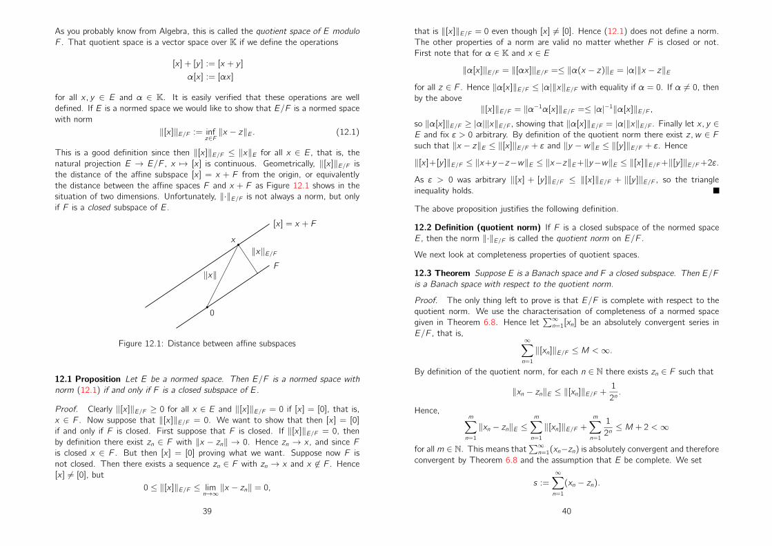
As you probably know from Algebra, this is called the quotient space of E modulo

F . That quotient space is a vector space over K if we define the operations

[x ] + [y ] := [x + y ]

α[x ] := [αx ]

for all x, y ∈ E and α ∈ K. It is easily verified that these operations are well

defined. If E is a normed space we would like to show that E/F is a normed space

with norm

‖[x ]‖E/F := infz∈F‖x − z‖E. (12.1)

This is a good definition since then ‖[x ]‖E/F ≤ ‖x‖E for all x ∈ E, that is, the

natural projection E → E/F , x 7→ [x ] is continuous. Geometrically, ‖[x ]‖E/F is

the distance of the affine subspace [x ] = x + F from the origin, or equivalently

the distance between the affine spaces F and x + F as Figure 12.1 shows in the

situation of two dimensions. Unfortunately, ‖·‖E/F is not always a norm, but only

if F is a closed subspace of E.

0

F

[x ] = x + F

x

‖x‖

‖x‖E/F

Figure 12.1: Distance between affine subspaces

12.1 Proposition Let E be a normed space. Then E/F is a normed space with

norm (12.1) if and only if F is a closed subspace of E.

Proof. Clearly ‖[x ]‖E/F ≥ 0 for all x ∈ E and ‖[x ]‖E/F = 0 if [x ] = [0], that is,

x ∈ F . Now suppose that ‖[x ]‖E/F = 0. We want to show that then [x ] = [0]

if and only if F is closed. First suppose that F is closed. If ‖[x ]‖E/F = 0, then

by definition there exist zn ∈ F with ‖x − zn‖ → 0. Hence zn → x , and since F

is closed x ∈ F . But then [x ] = [0] proving what we want. Suppose now F is

not closed. Then there exists a sequence zn ∈ F with zn → x and x 6∈ F . Hence

[x ] 6= [0], but

0 ≤ ‖[x ]‖E/F ≤ limn→∞‖x − zn‖ = 0,

39

that is ‖[x ]‖E/F = 0 even though [x ] 6= [0]. Hence (12.1) does not define a norm.

The other properties of a norm are valid no matter whether F is closed or not.

First note that for α ∈ K and x ∈ E

‖α[x ]‖E/F = ‖[αx ]‖E/F =≤ ‖α(x − z)‖E = |α|‖x − z‖Efor all z ∈ F . Hence ‖α[x ]‖E/F ≤ |α|‖x‖E/F with equality if α = 0. If α 6= 0, then

by the above

‖[x ]‖E/F = ‖α−1α[x ]‖E/F =≤ |α|−1‖α[x ]‖E/F ,so ‖α[x ]‖E/F ≥ |α|‖x‖E/F , showing that ‖α[x ]‖E/F = |α|‖x‖E/F . Finally let x, y ∈E and fix ε > 0 arbitrary. By definition of the quotient norm there exist z, w ∈ Fsuch that ‖x − z‖E ≤ ‖[x ]‖E/F + ε and ‖y − w‖E ≤ ‖[y ]‖E/F + ε. Hence

‖[x ]+[y ]‖E/F ≤ ‖x+y−z−w‖E ≤ ‖x−z‖E+‖y−w‖E ≤ ‖[x ]‖E/F+‖[y ]‖E/F+2ε.

As ε > 0 was arbitrary ‖[x ] + [y ]‖E/F ≤ ‖[x ]‖E/F + ‖[y ]‖E/F , so the triangle

inequality holds.

The above proposition justifies the following definition.

12.2 Definition (quotient norm) If F is a closed subspace of the normed space

E, then the norm ‖·‖E/F is called the quotient norm on E/F .

We next look at completeness properties of quotient spaces.

12.3 Theorem Suppose E is a Banach space and F a closed subspace. Then E/F

is a Banach space with respect to the quotient norm.

Proof. The only thing left to prove is that E/F is complete with respect to the

quotient norm. We use the characterisation of completeness of a normed space

given in Theorem 6.8. Hence let∑∞n=1[xn] be an absolutely convergent series in

E/F , that is,∞

∑

n=1

‖[xn]‖E/F ≤ M <∞.

By definition of the quotient norm, for each n ∈ N there exists zn ∈ F such that

‖xn − zn‖E ≤ ‖[xn]‖E/F +1

2n.

Hence,m

∑

n=1

‖xn − zn‖E ≤m

∑

n=1

‖[xn]‖E/F +m

∑

n=1

1

2n≤ M + 2 <∞

for allm ∈ N. This means that∑∞n=1(xn−zn) is absolutely convergent and therefore

convergent by Theorem 6.8 and the assumption that E be complete. We set

s :=

∞∑

n=1

(xn − zn).

40

Now by choice of zn and the definition of the quotient norm

∥

∥

∥

(

m∑

n=1

[xn])

− [s]∥

∥

∥

E/F=

∥

∥

∥

(

m∑

n=1

[xn − zn])

− [s]∥

∥

∥

E/F≤

∥

∥

∥

(

m∑

n=1

(xn − zn))

− s∥

∥

∥

E→ 0

as m → ∞ by choice of s. Hence∑∞n=1[xn] = [s] converges with respect to the

quotient norm, and so by Theorem 6.8 E/F is complete.

Next we look at factorisations of bounded linear operators. Given normed spaces

E, F and an operator T ∈ L(E, F ) it follows from Theorem 5.3 that ker T := x ∈E : Tx = 0 is a closed subspace of E. Hence we E/ ker T is a normed space with

the quotient norm. We then define a linear operator T : E/ ker T → F by setting

T [x ] := Tx

for all x ∈ E. It is easily verified that this operator is well defined and lin-

ear. Moreover, if we set π(x) := [x ], then by definition of the quotient norm

‖π(x)‖E/ ker T ≤ ‖x‖E, so π ∈ L(E,E/ kerT ) with ‖π‖L(E,E/ kerT ) ≤ 1. Moreover,

we have the factorisation

T = T π,meaning that the following diagram is commutative.

E F

E/ kerT

T

π T

We summarise the above in the following Theorem.

12.4 Theorem Suppose that E, F are normed spaces and that T ∈ L(E, F ). If

T , π are defined as above, then T ∈ L(E/ kerT, F ), ‖T ‖L(E,F ) = ‖T‖L(E/ ker T,F )and we have the factorisation T = T π.Proof. The only thing left to prove is that T ∈ L(E/ kerT, F ), and that ‖T ‖ :=‖T ‖L(E,F ) = ‖T‖L(E/ ker T,F ) =: ‖T‖. First note that

‖T [x ]‖F = ‖Tx‖F = ‖T (x − z)‖F ≤ ‖T ‖‖x − z‖Efor all z ∈ kerT . Hence by definition of the quotient norm

‖T [x ]‖F ≤ ‖T ‖‖[x ]‖E/ kerT .Now by definition of the operator norm ‖T‖ ≤ ‖T ‖ < ∞. In particular, T ∈L(E/ kerT, F ). To show equality of the operator norms observe that

‖Tx‖F = ‖T [x ]‖F ≤ ‖T‖‖[x ]‖E/ kerT ≤ ‖T‖‖x‖Eby definition of the operator and quotient norms. Hence ‖T ‖ ≤ ‖T‖, showing that

‖T ‖ = ‖T‖.

41 42

Chapter III

Hilbert Spaces

Hilbert spaces are in some sense a direct generalisation of finite dimensional Eu-

clidean spaces, where the norm has some geometric meaning and angles can be

defined by means of the dot product. The dot product can be used to define the

norm and prove many of its properties. Hilbert space theory is doing this in a similar

fashion, where an inner product is a map with properties similar to the dot product

in Euclidean space. We will emphasise the analogies and see how useful they are

to find proofs in the general context of inner product spaces.

13 Inner Product Spaces

Throughout we let E denote a vector space over K.

13.1 Definition (Inner product, inner product space) A function (· | ·) : E ×E → K is called an inner product or scalar product if

(i) (u | v) = (v | u) for u, v ∈ E,

(ii) (u | u) ≥ 0 for all u ∈ E and (u | u) = 0 if and only if u = 0.

(iii) (αu + βv | w) = α(u | w) + β(v | w) for all u, v , w ∈ E and α, β ∈ K,

We say that E equipped with (· | ·) is an inner product space.

13.2 Remark As an immediate consequence of the above definition, inner products

have the following properties:

(a) By property (i) we have (u | u) = (u | u) and therefore (u | u) ∈ R for all

u ∈ E. Hence property (ii) makes sense.

(b) Using (i) and (iii) we have

(u | αv + βw) = α(u | v) + β(u | w)

43

for all u, v , w ∈ E and α, β ∈ K. In particular we have

(u | λv) = λ(u | v)

for all u, v ∈ E and λ ∈ K.

Next we give some examples of Banach and Hilbert spaces.

13.3 Examples (a) The space CN equipped with the Euclidean scalar product given

by

(x | y) := x · y =N

∑

i=1

xiy i

for all x := (x1, . . . , xN), y := (y1, . . . , yN) ∈ CN is an inner product space. More

generally, if we take a positive definite Hermitian matrix A ∈ CN×N , then

(x | y)A := xTAy

defines an inner product on CN.

(b) An infinite dimensional version is ℓ2 defined in Section 7.2. An inner product

is defined by

(x | y) :=∞

∑

i=1

xiy i

for all (xi), (yi) ∈ ℓ2. The series converges by Hölder’s inequality (Proposition 7.4).

(c) For u, v ∈ L2(X) we let

(u | v) :=∫

X

u(x)v(x)dx.

By Hölder’s inequality Proposition 7.7 the integral is finite and easily shown to be

an inner product.

The Euclidean norm on CN is defined by means of the dot product, namely by

‖x‖ = √x · x for x ∈ CN. We make a similar definition in the context of general

inner product spaces.

13.4 Definition (induced norm) If E is an inner product space with inner product

(· | ·) we define

‖u‖ :=√

(u | u) (13.1)

for all u ∈ E.

Note that from Remark 13.2 we always have (x | x) ≥ 0, so ‖x‖ is well defined.

We call ‖·‖ a “norm,” but at the moment we do not know whether it really is a

norm in the proper sense of Definition 6.1. We now want to work towards a proof

that ‖·‖ is a norm on E. On the way we look at some geometric properties of inner

products and establish the Cauchy-Schwarz inequality.

44

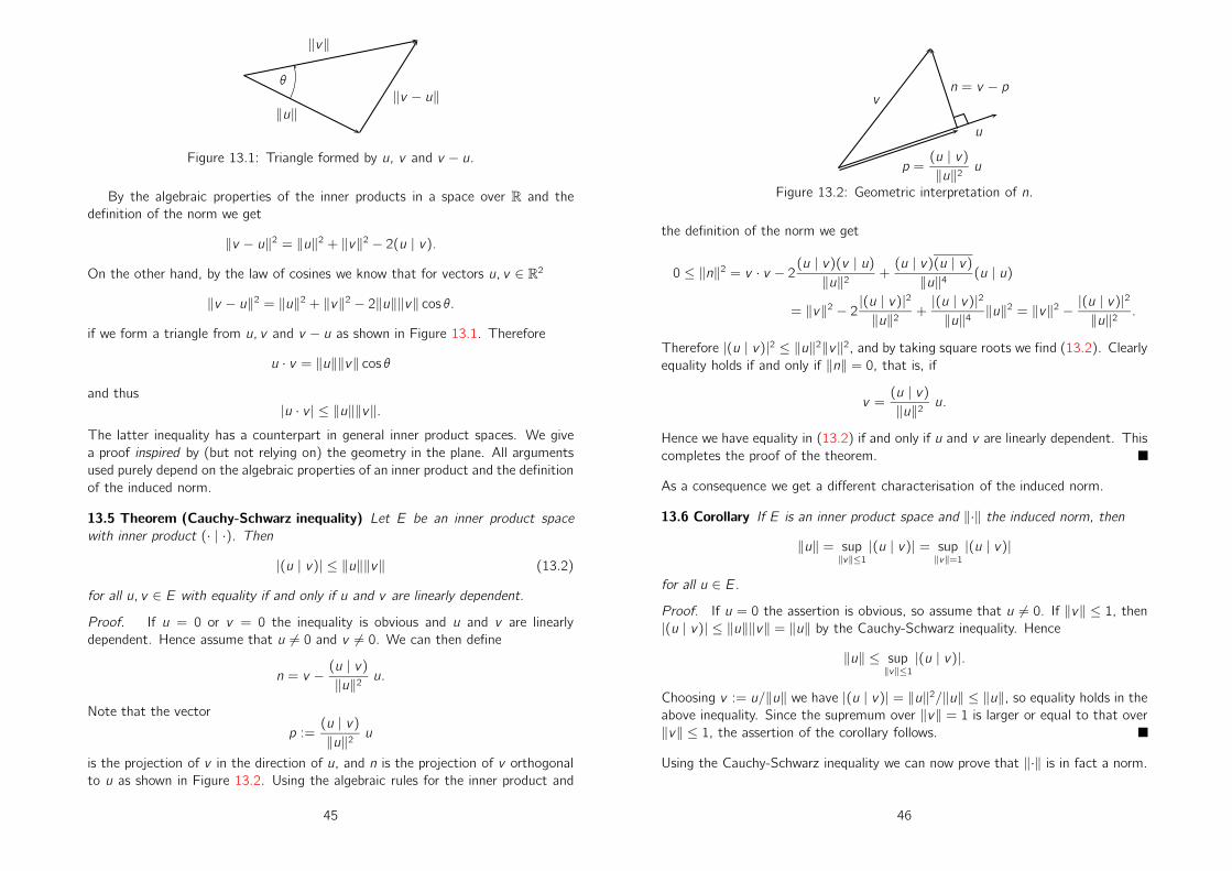
‖u‖

‖v‖

‖v − u‖θ

Figure 13.1: Triangle formed by u, v and v − u.

By the algebraic properties of the inner products in a space over R and the

definition of the norm we get

‖v − u‖2 = ‖u‖2 + ‖v‖2 − 2(u | v).

On the other hand, by the law of cosines we know that for vectors u, v ∈ R2

‖v − u‖2 = ‖u‖2 + ‖v‖2 − 2‖u‖‖v‖ cos θ.

if we form a triangle from u, v and v − u as shown in Figure 13.1. Therefore

u · v = ‖u‖‖v‖ cos θ

and thus

|u · v | ≤ ‖u‖‖v‖.The latter inequality has a counterpart in general inner product spaces. We give

a proof inspired by (but not relying on) the geometry in the plane. All arguments

used purely depend on the algebraic properties of an inner product and the definition

of the induced norm.

13.5 Theorem (Cauchy-Schwarz inequality) Let E be an inner product space

with inner product (· | ·). Then

|(u | v)| ≤ ‖u‖‖v‖ (13.2)

for all u, v ∈ E with equality if and only if u and v are linearly dependent.

Proof. If u = 0 or v = 0 the inequality is obvious and u and v are linearly

dependent. Hence assume that u 6= 0 and v 6= 0. We can then define

n = v − (u | v)‖u‖2 u.

Note that the vector

p :=(u | v)‖u‖2 u

is the projection of v in the direction of u, and n is the projection of v orthogonal

to u as shown in Figure 13.2. Using the algebraic rules for the inner product and

45

u

vn = v − p

p =(u | v)‖u‖2 u

Figure 13.2: Geometric interpretation of n.

the definition of the norm we get

0 ≤ ‖n‖2 = v · v − 2(u | v)(v | u)‖u‖2 +(u | v)(u | v)‖u‖4 (u | u)

= ‖v‖2 − 2 |(u | v)|2

‖u‖2 +|(u | v)|2‖u‖4 ‖u‖

2 = ‖v‖2 − |(u | v)|2

‖u‖2 .

Therefore |(u | v)|2 ≤ ‖u‖2‖v‖2, and by taking square roots we find (13.2). Clearly

equality holds if and only if ‖n‖ = 0, that is, if

v =(u | v)‖u‖2 u.

Hence we have equality in (13.2) if and only if u and v are linearly dependent. This

completes the proof of the theorem.

As a consequence we get a different characterisation of the induced norm.

13.6 Corollary If E is an inner product space and ‖·‖ the induced norm, then

‖u‖ = sup‖v‖≤1

|(u | v)| = sup‖v‖=1

|(u | v)|

for all u ∈ E.

Proof. If u = 0 the assertion is obvious, so assume that u 6= 0. If ‖v‖ ≤ 1, then

|(u | v)| ≤ ‖u‖‖v‖ = ‖u‖ by the Cauchy-Schwarz inequality. Hence

‖u‖ ≤ sup‖v‖≤1

|(u | v)|.

Choosing v := u/‖u‖ we have |(u | v)| = ‖u‖2/‖u‖ ≤ ‖u‖, so equality holds in the

above inequality. Since the supremum over ‖v‖ = 1 is larger or equal to that over

‖v‖ ≤ 1, the assertion of the corollary follows.

Using the Cauchy-Schwarz inequality we can now prove that ‖·‖ is in fact a norm.

46

13.7 Theorem If E is an inner product space, then (13.1) defines a norm on E.

Proof. By property (ii) of an inner product (see Definition 13.1 we have ‖u‖ =√

(u | u) ≥ 0 with equality if and only if u = 0. If u ∈ E and λ ∈ K, then

‖λu‖ =√

(λu | λu) =√

λλ(u | u) =√

|λ|2‖u‖2 = |λ|‖u‖as required. To prove the triangle inequality let u, v ∈ E. By the algebraic proper-

ties of an inner product and the Cauchy-Schwarz inequality we have

‖u + v‖2 = (u + v | u + v) = ‖u‖2 + (u | v) + (v | u) + ‖v‖2

≤ ‖u‖2 + 2|(u | v)|2 + ‖v‖2 ≤ ‖u‖2 + 2‖u‖2‖v‖2 + ‖v‖2 =(

‖u‖+ ‖v‖)2.

Taking square roots the triangle inequality follows. Hence ‖·‖ defines a norm.

As a matter of convention we always consider inner product spaces as normed

spaces.

13.8 Convention Since every inner product induces a norm we will always assume

that an inner product space is a normed space with the norm induced by the inner

product.

Once we have a norm we can talk about convergence and completeness. Note that

not every inner product space is complete, but those which are play a special role.

13.9 Definition (Hilbert space) An inner product space which is complete with

respect to the induced norm is called a Hilbert space.

The inner product is a map on E × E. We show that this map is continuous with

respect to the induced norm.

13.10 Proposition (Continuity of inner product) Let E be an inner product space.

Then the inner product (· | ·) : E×E → K is continuous with respect to the induced

norm.

Proof. If xn → x and yn → y in E (with respect to the induced norm), then using

the Cauchy-Schwarz inequality

|(xn | yn)− (x | y)| = |(xn − x | yn) + (x | yn − y)|≤ |(xn − x | yn)|+ |(x | yn − y)| ≤ ‖xn − x‖‖yn‖+ ‖x‖‖yn − y‖ → 0

as n→∞. Note that we also use the continuity of the norm in the above argument

to conclude that ‖yn‖ → ‖y‖ (see Theorem 6.4). Hence the inner product is

continuous.

The lengths of the diagonals and edges of a parallelogram in the plane satisfy a

relationship. The norm in an inner product space satisfies a similar relationship,

called the parallelogram identity. The identity will play an essential role in the next

section.

47

13.11 Proposition (Parallelogram identity) Let E be an inner product space and

‖·‖ the induced norm. Then

‖u + v‖2 + ‖u − v‖2 = 2‖u‖2 + 2‖v‖2 (13.3)

for all u, v ∈ E.

Proof. By definition of the induced norm and the properties of an inner product

‖u + v‖2 + ‖u − v‖2 = ‖u‖2 + (u | v) + (v | u) + ‖v‖2+ ‖u‖2 − (u | v)− (v | u) + ‖v‖2 = 2‖u‖2 + 2‖v‖2

for all u, v ∈ E as required.

It turns out that the converse is true as well. More precisely, if a norm satisfies

(13.3) for all u, v ∈ E, then there is an inner product inducing that norm (see [7,

Section I.5] for a proof).

14 Projections and Orthogonal Complements

In this section we discuss the existence and properties of “nearest point projections”

from a point onto a set, that is, the points that minimise the distance from a closed

set to a given point.

14.1 Definition (Projection) Let E be a normed space andM a non-empty closed

subset. We define the set of projections of x onto M by

PM(x) := m ∈ M : ‖x −m‖ = dist(x,M).

The meaning of PM(x) is illustrated in Figure 14.1 for the Euclidean norm in the

plane. If the set is not convex, PM(x) can consist of several points, if it is convex,

it is precisely one.

x

M

Figure 14.1: The set of nearest point projections PM(x).

We now look at some example. First we look at subsets of RN, and show that

then PM(x) is never empty.

48

14.2 Example Suppose that M ⊂ RN is non-empty and closed and x ∈ M. If we

fix α > dist(x,M) and x ∈ RN, then the set K := M ∩ B(x, α) is a closed and

bounded, and dist(x,M) = dist(x,K). We know from Proposition 5.5 that the

distance function x 7→ dist(x,K) is continuous. Since K is compact by the Heine-

Borel theorem, the continuous map y 7→ d(x, y) attains a minimum on K. Hence

there exists y ∈ K such that d(x, y) = infz∈K d(y , z) = dist(x,K) = dist(x,M),

which means that y ∈ PM(x). Hence PM(x) is non-empty if M ⊂ RN. The same

applies to any finite dimensional space.

The argument to prove that PM(x) is non-empty used above very much depends

on the set K to be compact. In the following example we show that PM(x) can

be empty. It is evident that PM(x) can be empty if E is not complete. It may be

more surprising and counter intuitive that even if E is complete, PM(x) may be

empty! There is no mystery about this, it just shows how much our intuition relies

on bounded and closed sets to be compact.

14.3 Example Let E := C([0, 1]) with norm ‖u‖ := ‖u‖∞ + ‖u‖1. We claim that

E is complete. Clearly ‖u‖∞ ≤ ‖u‖ for all u ∈ E. Also

‖u‖1 =∫ 1

0

|u(x)| dx ≤ ‖u‖∞∫ 1

0

1 dx = ‖u‖∞

for all x ∈ E. Hence ‖·‖ is equivalent to the supremum norm ‖·‖∞, so convergence

with respect to ‖·‖ is uniform convergence. By Section 7.4 and Lemma 9.4 the

space E is complete with respect to the norm ‖·‖. Now look at the subspace

M := u ∈ C([0, 1]) : u(0) = 0.

Since uniform convergence implies pointwise convergence M is closed. (Note that

by closed we mean closed as a subset of the metric space E, not algebraically

closed.) Denote by 1 the constant function with value 1. If u ∈ M, then

‖1− u‖ ≥ ‖1− u‖∞ ≥ |1− u(0)| = 1, (14.1)

so dist(1,M) ≥ 1. If we set un(x) :=n√x , then 0 ≤ 1−un(x)→ 0 for all x ∈ (0, 1],

so by the dominated convergence theorem

‖1− un‖ = ‖1− un‖∞ +∫ 1

0

1− un(x) dx ≥ 1 +∫ 1

0

1− un(x) dx → 1

as n→∞. Hence dist(1,M) = 1. We show now that PM(1) = ∅, that is, there is

no nearest element in M from 1. If u ∈ M, then u(0) = 0 and thus by continuity

of u there exists an interval [0, δ] such that |1 − u(x)| > 1/2 for all x ∈ [0, δ].Hence for all u ∈ M we have ‖1− u‖1 > 0. Using (14.1) we have

‖1− u‖ = ‖1− u‖∞ + ‖1− u‖1 ≥ 1 + ‖1− u‖1 > 1

for all u ∈ M, so PM(1) is empty.

49

In the light of the above example it is a non-trivial fact that PM(x) is not empty in

a Hilbert space, at least if M is closed and convex. By a convex set, as usual, we

mean a subset M such that tx + (1− t)y ∈ M for all x, y ∈ M and t ∈ [0, 1]. In

other words, if x, y are inM, so is the line segment connecting them. The essential

ingredient in the proof is the parallelogram identity from Proposition 13.11.

14.4 Theorem (Existence and uniqueness of projections) Let H be a Hilbert

space and M ⊂ H non-empty, closed and convex. Then PM(x) contains precisely

one element which we also denote by PM(x).

Proof. Let M ⊂ H be non-empty, closed and convex. If x ∈ M, then PM(x) = x ,

so there is existence and also uniqueness of an element of PM(x). Hence we assume

that x 6∈ M and set

α := dist(x,M) = infm∈M‖x −m‖.

Since M is closed and x 6∈ M we have α > 0. From the parallelogram identity

Proposition 13.11 we get

‖m1 −m2‖2 = ‖(m1 − x)− (m2 − x)‖2= 2‖m1 − x‖2 + 2‖m1 − x‖2 − ‖(m1 − x) + (m2 − x)‖2.

If m1, m2 ∈ M, then ‖mi − x‖ ≥ α for i = 1, 2 and by the convexity of M we have

(m1 +m2)/2 ∈ M. Hence

‖(m1 − x) + (m2 − x)‖ = ‖m1 +m2 − 2x‖ = 2∥

∥

∥

m1 +m22

− x∥

∥

∥≥ 2α.

and by using the above

‖m1 −m2‖2 ≤ 2‖m1 − x‖2 + 2‖m1 − x‖2 − 4α2. (14.2)

for all m1, m2 ∈ M. We can now prove uniqueness. Given m1, m2 ∈ PM(x) we have

by definition ‖mi − x‖ = α (i = 1, 2), and so by (14.2)

‖m1 −m2‖2 ≤ 4α2 − 4α2 = 0.

Hence ‖m1 − m2‖ = 0, that is, m1 = m2 proving uniqueness. As a second step

we prove the existence of an element in PM(x). By definition of an infimum there

exists a sequence (xn) in M such that

‖xn − x‖ → α := dist(x,M).

This obviously implies that (xn) a bounded sequence in H, but since H is not

necessarily finite dimensional, we cannot conclude it is converging without further

investigation. We show that (xn) is a Cauchy sequence and therefore converges

50

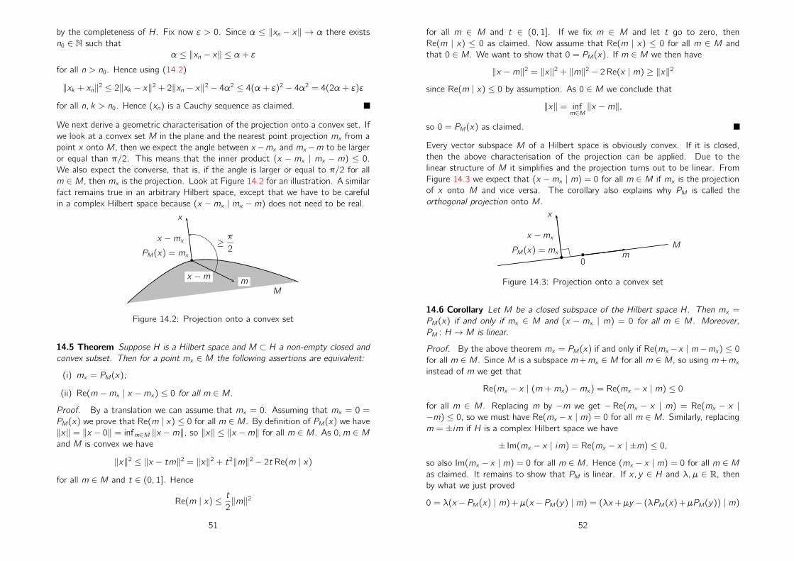
by the completeness of H. Fix now ε > 0. Since α ≤ ‖xn − x‖ → α there exists

n0 ∈ N such that

α ≤ ‖xn − x‖ ≤ α+ εfor all n > n0. Hence using (14.2)

‖xk + xn‖2 ≤ 2‖xk − x‖2 + 2‖xn − x‖2 − 4α2 ≤ 4(α+ ε)2 − 4α2 = 4(2α+ ε)ε

for all n, k > n0. Hence (xn) is a Cauchy sequence as claimed.

We next derive a geometric characterisation of the projection onto a convex set. If

we look at a convex set M in the plane and the nearest point projection mx from a

point x onto M, then we expect the angle between x −mx and mx−m to be larger

or equal than π/2. This means that the inner product (x − mx | mx − m) ≤ 0.We also expect the converse, that is, if the angle is larger or equal to π/2 for all

m ∈ M, then mx is the projection. Look at Figure 14.2 for an illustration. A similar

fact remains true in an arbitrary Hilbert space, except that we have to be careful

in a complex Hilbert space because (x −mx | mx −m) does not need to be real.

bPM(x) = mx

x

m

x −mx

x −mM

≥ π2

Figure 14.2: Projection onto a convex set

14.5 Theorem Suppose H is a Hilbert space and M ⊂ H a non-empty closed and

convex subset. Then for a point mx ∈ M the following assertions are equivalent:

(i) mx = PM(x);

(ii) Re(m −mx | x −mx) ≤ 0 for all m ∈ M.

Proof. By a translation we can assume that mx = 0. Assuming that mx = 0 =

PM(x) we prove that Re(m | x) ≤ 0 for all m ∈ M. By definition of PM(x) we have

‖x‖ = ‖x − 0‖ = infm∈M ‖x −m‖, so ‖x‖ ≤ ‖x −m‖ for all m ∈ M. As 0, m ∈ Mand M is convex we have

‖x‖2 ≤ ‖x − tm‖2 = ‖x‖2 + t2‖m‖2 − 2t Re(m | x)

for all m ∈ M and t ∈ (0, 1]. Hence

Re(m | x) ≤ t2‖m‖2

51

for all m ∈ M and t ∈ (0, 1]. If we fix m ∈ M and let t go to zero, then

Re(m | x) ≤ 0 as claimed. Now assume that Re(m | x) ≤ 0 for all m ∈ M and

that 0 ∈ M. We want to show that 0 = PM(x). If m ∈ M we then have

‖x −m‖2 = ‖x‖2 + ‖m‖2 − 2Re(x | m) ≥ ‖x‖2

since Re(m | x) ≤ 0 by assumption. As 0 ∈ M we conclude that

‖x‖ = infm∈M‖x −m‖,

so 0 = PM(x) as claimed.

Every vector subspace M of a Hilbert space is obviously convex. If it is closed,

then the above characterisation of the projection can be applied. Due to the

linear structure of M it simplifies and the projection turns out to be linear. From

Figure 14.3 we expect that (x −mx | m) = 0 for all m ∈ M if mx is the projection

of x onto M and vice versa. The corollary also explains why PM is called the

orthogonal projection onto M.

PM(x) = mx

x

m

x −mx

0

M

Figure 14.3: Projection onto a convex set

14.6 Corollary Let M be a closed subspace of the Hilbert space H. Then mx =

PM(x) if and only if mx ∈ M and (x − mx | m) = 0 for all m ∈ M. Moreover,

PM : H → M is linear.

Proof. By the above theorem mx = PM(x) if and only if Re(mx−x | m−mx) ≤ 0for all m ∈ M. Since M is a subspace m+mx ∈ M for all m ∈ M, so using m+mxinstead of m we get that

Re(mx − x | (m +mx)−mx) = Re(mx − x | m) ≤ 0for all m ∈ M. Replacing m by −m we get −Re(mx − x | m) = Re(mx − x |−m) ≤ 0, so we must have Re(mx − x | m) = 0 for all m ∈ M. Similarly, replacing

m = ±im if H is a complex Hilbert space we have

± Im(mx − x | im) = Re(mx − x | ±m) ≤ 0,so also Im(mx − x | m) = 0 for all m ∈ M. Hence (mx − x | m) = 0 for all m ∈ Mas claimed. It remains to show that PM is linear. If x, y ∈ H and λ, µ ∈ R, then

by what we just proved

0 = λ(x −PM(x) | m)+µ(x −PM(y) | m) = (λx +µy − (λPM(x)+µPM(y)) | m)

52

for all m ∈ M. Hence again by what we proved PM(λx+µy) = λPM(x)+µPM(y),

showing that PM is linear.

We next connect the projections discussed above with the notion of orthogonal

complements.

14.7 Definition (Orthogonal complement) For an arbitrary non-empty subsetM

of an inner product space H we set

M⊥ := x ∈ H : (x | m) = 0 for all m ∈ M.We call M⊥ the orthogonal complement of M in H.

We now establish some elementary but very useful properties of orthogonal com-

plements.

14.8 Lemma Suppose M is a non-empty subset of the inner product space H.

Then M⊥ is a closed subspace of H and M⊥ = M⊥= (spanM)⊥ = (spanM)⊥.

Proof. If x, y ∈ M⊥ and λ, µ ∈ K, then

(λx + µy | m) = λ(x | m) + µ(y | m) = 0,for all m ∈ M, so M⊥ is a subspace of H. If x is from the closure of M⊥, then

there exist xn ∈ M⊥ with xn → x . By the continuity of the inner product

(x | m) = limn→∞(xn | m) = lim

n→∞0 = 0

for all m ∈ M. Hence x ∈ M⊥, showing that M⊥ is closed. We next show

that M⊥ = M⊥. Since M ⊂ M we have M

⊥ ⊂ M⊥ by definition the orthogonal

complement. Fix x ∈ M⊥ and m ∈ M. Then there exist mn ∈ M with mn → m.

By the continuity of the inner product

(x | m) = limn→∞(x | mn) = lim

n→∞0 = 0.

Hence x ∈ M⊥ and thus M⊥ ⊃ M⊥, showing that M

⊥= M⊥. Next we show that

M⊥ = (spanM)⊥. Clearly (spanM)⊥ ⊂ M⊥ since M ⊂ spanM. Suppose now

that x ∈ M⊥ and m ∈ spanM. Then there exist mi ∈ M and λi ∈ K, i = 1, . . . , n,

such that m =∑ni=1 λimi . Hence

(x | m) = λin

∑

i=1

(x | mi) = 0,

and thus x ∈ (spanM)⊥. Therefore (spanM)⊥ ⊃ M⊥ and so (spanM)⊥ = M⊥ as

claimed. The last assertion of the lemma follows by what we have proved above.

Indeed we know that M⊥ = M⊥

and that M⊥= (spanM)⊥.

We are now ready to prove the main result on orthogonal projections. It is one of

the most important and useful facts on Hilbert spaces.

53

14.9 Theorem (orthogonal complements) Suppose that M is a closed subspace

of the Hilbert space H. Then

(i) H = M ⊕M⊥;

(ii) PM is the projection of H onto M parallel to M⊥ (that is, PM(M⊥) = 0)

(iii) PM ∈ L(H,M) with ‖PM‖L(H,M) ≤ 1.

Proof. (i) By Corollary 14.6 we have (x − PM(x) | m) = 0 for all x ∈ H and

m ∈ M. Hence x − PM(x) ∈ M⊥ for all x ∈ H and therefore

x = PM(x) + (I − PM)(x) ∈ M +M⊥,

and thus H = M +M⊥. If x ∈ M ∩M⊥, then (x | x) = 0, so x = 0, showing that

H = M ⊕M⊥ is a direct sum.

(ii) By Corollary 14.6 the map PM is linear. Since PM(x) = x for x ∈ M we

have P 2M = PM and PM(M⊥) = 0. Hence PM is a projection.

(iii) By (i) we have (PM(x) | x − PM(x)) = 0 and so

‖x‖2 = ‖PM(x) + (I − PM)(x)‖2= ‖PM(x)‖2 + ‖x − PM(x)‖2 + 2Re(PM(x) | x − PM(x)) ≥ ‖PM(x)‖2

for all x ∈ H. Hence PM ∈ L(H,M) with ‖PM‖L(H,M) ≤ 1 as claimed.

14.10 Remark The above theorem in particular implies that for every closed sub-

space M of a Hilbert space H there exists a closed subspace N such that H =

M ⊕ N. We call M a complemented subspace. The proof used the existence of a

projection. We know from Example 14.3 that projections onto closed subspaces do

not necessarily exist in a Banach space, so one may not expect every subspace of a

Banach space to be complemented. A rather recent result [6] shows that if every

closed subspace of a Banach space is complemented, then its norm is equivalent to

a norm induced by an inner product! Hence the above theorem provides a unique

property of Hilbert spaces.

The above theorem can be used to prove some properties of orthogonal comple-

ments. The first is a very convenient criterion for a subspace of a Hilbert space to

be dense.

14.11 Corollary A subspace M of a Hilbert space H is dense in H if and only if

M⊥ = 0.

Proof. Since M⊥ = M⊥

by Lemma 14.8 it follows from Theorem 14.9 that

H = M ⊕M⊥

54

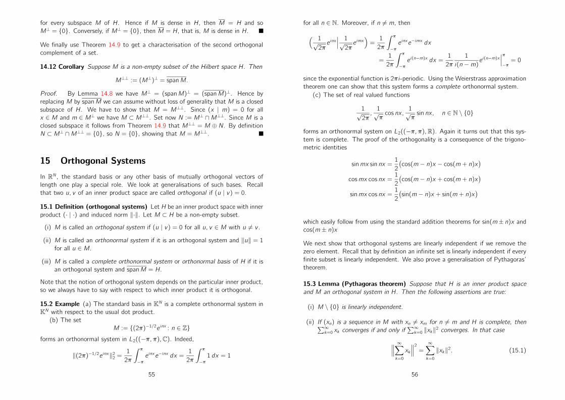
for every subspace M of H. Hence if M is dense in H, then M = H and so

M⊥ = 0. Conversely, if M⊥ = 0, then M = H, that is, M is dense in H.

We finally use Theorem 14.9 to get a characterisation of the second orthogonal

complement of a set.

14.12 Corollary Suppose M is a non-empty subset of the Hilbert space H. Then

M⊥⊥ := (M⊥)⊥ = spanM.

Proof. By Lemma 14.8 we have M⊥ = (spanM)⊥ = (spanM)⊥. Hence by

replacing M by spanM we can assume without loss of generality that M is a closed

subspace of H. We have to show that M = M⊥⊥. Since (x | m) = 0 for all

x ∈ M and m ∈ M⊥ we have M ⊂ M⊥⊥. Set now N := M⊥ ∩M⊥⊥. Since M is a

closed subspace it follows from Theorem 14.9 that M⊥⊥ = M ⊕ N. By definition

N ⊂ M⊥ ∩M⊥⊥ = 0, so N = 0, showing that M = M⊥⊥.

15 Orthogonal Systems

In RN, the standard basis or any other basis of mutually orthogonal vectors of

length one play a special role. We look at generalisations of such bases. Recall

that two u, v of an inner product space are called orthogonal if (u | v) = 0.

15.1 Definition (orthogonal systems) Let H be an inner product space with inner

product (· | ·) and induced norm ‖·‖. Let M ⊂ H be a non-empty subset.

(i) M is called an orthogonal system if (u | v) = 0 for all u, v ∈ M with u 6= v .

(ii) M is called an orthonormal system if it is an orthogonal system and ‖u‖ = 1for all u ∈ M.

(iii) M is called a complete orthonormal system or orthonormal basis of H if it is

an orthogonal system and spanM = H.

Note that the notion of orthogonal system depends on the particular inner product,

so we always have to say with respect to which inner product it is orthogonal.

15.2 Example (a) The standard basis in KN is a complete orthonormal system in

KN with respect to the usual dot product.

(b) The set

M := (2π)−1/2e inx : n ∈ Zforms an orthonormal system in L2((−π, π),C). Indeed,

‖(2π)−1/2e inx‖22 =1

2π

∫ π

−π

e inxe−inx dx =1

2π

∫ π

−π

1 dx = 1

55

for all n ∈ N. Moreover, if n 6= m, then

( 1√2πe inx

∣

∣

∣

1√2πe imx

)

=1

2π

∫ π

−π

e inxe−imx dx

=1

2π

∫ π

−π

e i(n−m)x dx =1

2π

1

i(n −m)ei(n−m)x

∣

∣

∣

π

−π= 0

since the exponential function is 2πi-periodic. Using the Weierstrass approximation

theorem one can show that this system forms a complete orthonormal system.

(c) The set of real valued functions

1√2π,1√πcos nx,

1√πsin nx, n ∈ N \ 0

forms an orthonormal system on L2((−π, π),R). Again it turns out that this sys-

tem is complete. The proof of the orthogonality is a consequence of the trigono-

metric identities

sinmx sin nx =1

2

(

cos(m − n)x − cos(m + n)x)

cosmx cos nx =1

2

(

cos(m − n)x + cos(m + n)x)

sinmx cos nx =1

2

(

sin(m − n)x + sin(m + n)x)

which easily follow from using the standard addition theorems for sin(m± n)x and

cos(m ± n)x

We next show that orthogonal systems are linearly independent if we remove the

zero element. Recall that by definition an infinite set is linearly independent if every

finite subset is linearly independent. We also prove a generalisation of Pythagoras’

theorem.

15.3 Lemma (Pythagoras theorem) Suppose that H is an inner product space

and M an orthogonal system in H. Then the following assertions are true:

(i) M \ 0 is linearly independent.

(ii) If (xn) is a sequence in M with xn 6= xm for n 6= m and H is complete, then∑∞k=0 xk converges if and only if

∑∞k=0 ‖xk‖2 converges. In that case

∥

∥

∥

∞∑

k=0

xk

∥

∥

∥

2

=

∞∑

k=0

‖xk‖2. (15.1)

56

Proof. (i) We have to show that every finite subset of M \ 0 is linearly indepen-

dent. Hence let xk ∈ M \0, k = 1, . . . , n be a finite number of distinct elements.

Assume that λk ∈ K are such that

n∑

k=0

λkxk = 0.

If we fix xm, m ∈ 0, . . . , n, then by the orthogonality

0 =(

n∑

k=0

λkxk

∣

∣

∣xm

)

=

n∑

k=0

λk(xk | xm) = λm‖xm‖2.

Since xm 6= 0 it follows that λm = 0 for all m ∈ 0, . . . , n, showing that M \ 0is linearly independent.

(ii) Let (xn) be a sequence in M with xn 6= xm. (We only look at the case

of an infinite set because otherwise there are no issues on convergence). We

set sn :=∑nk=1 xk and tn :=

∑nk=1 ‖xk‖2 the partial sums of the series under

consideration. If 1 ≤ m < n, then by the orthogonality

‖sn − sm‖2 =∥

∥

∥

n∑

k=m+1

xk

∥

∥

∥

2

=(

n∑

k=m+1

xk

∣

∣

∣

n∑

j=m+1

xj

)

=

n∑

k=m+1

n∑

j=m+1

(xk | xj) =n

∑

k=m+1

‖xk‖2 = |tn − tm|.

Hence (sn) is a Cauchy sequence in H if and only if tn is a Cauchy sequence in R,

and by the completeness they either both converge or diverge. The identity (15.1)

now follows by setting m = 0 in the above calculation and then letting n →∞.

In the case of H = KN and the standard basis ei , i = 1, . . . , N, we call xi = (x | ei)the components of x ∈ KN . The Euclidean norm is given by

‖x‖2 =n

∑

k=1

|xi |2 =n

∑

k=1

|(x | ei)|2.

If we do not sum over the full standard basis we may only get an inequality, namely

m∑

k=1

|(x | ei)|2 ≤n

∑

k=1

|(x | ei)|2 ≤ ‖x‖2.

if m ≤ n. We now prove a similar inequality replacing the standard basis by an

arbitrary orthonormal system M in an inner product space H. From the above

reasoning we expect that∑

m∈M

|(x | m)|2 ≤ ‖x‖

57

for all x ∈ M. The definition of an orthonormal system M does not make any

assumption on the cardinality of M, so it may be uncountable. However, if M is

uncountable, it is not clear what the series above means. To make sense of the

above series we define∑

m∈M

|(x | m)|2 := supN ⊂ M finite

∑

m∈N

|(x | m)|2 (15.2)

We now prove the expected inequality.

15.4 Theorem (Bessel’s inequality) Let H be an inner product space and M an

orthonormal system in H. Then∑

m∈M

|(x | m)|2 ≤ ‖x‖2 (15.3)

for all x ∈ H. Moreover, the set m ∈ M : (x | m) 6= 0 is at most countable for

every x ∈ H.

Proof. Let N = mk : k = 1, . . . n be a finite subset of the orthonormal set M

in H. Then, geometrically,n

∑

k=1

(x | mk)mk

is the projection of x onto the span of N. By Pythagoras theorem (Lemma 15.3)

and since ‖mk‖ = 1 we have

∥

∥

∥

n∑

k=1

(x | mk)mk∥

∥

∥

2

=

n∑

k=1

|(x | mk)|2‖mk‖2 =n

∑

k=1

|(x | mk)|2.

We expect the norm of the projection to be smaller than the norm of ‖x‖. To see

that we use the properties of the inner product and the above identity to get

0 ≤∥

∥

∥x −

n∑

k=1

(x | mk)mk∥

∥

∥

2

= ‖x‖2 +∥

∥

∥

n∑

k=1

(x | mk)mk∥

∥

∥

2

−n

∑

k=1

(x | mk)(x | mk)−n

∑

k=1

(x | mk)(mk | x)

= ‖x‖2 +n

∑

k=1

|(x | mk)|2 − 2n

∑

k=1

|(x | mk)|2

= ‖x‖2 −n

∑

k=1

|(x | mk)|2.

Hence we have shown that∑

m∈N

|(x | m)|2 ≤ ‖x‖2

58

for every finite set N ⊂ M. Taking the supremum over all such finite sets (15.3)

follows. To prove the second assertion note that for every given x ∈ H the sets

Mn := m ∈ M : |(x | m)| ≥ 1/n is finite for every n ∈ N as otherwise (15.3)

could not be true. Since countable unions of finite sets are countable, the set

m ∈ M : (x | m) 6= 0 =⋃

n∈N

Mn

is countable as claimed.

15.5 Remark Since for every x the set m ∈ M : (x | m) 6= 0 is countable we

can choose an arbitrary enumeration and write Mx := m ∈ M : (x | m) 6= 0 =mk : k ∈ N. Since the series

∑∞k=1 |(x | mk)|2 has non-negative terms and every

such sequence is unconditionally convergent we have

∞∑

m∈M

|(x | m)|2 =∞

∑

k=1

|(x | mk)|2

no matter which enumeration we take. Recall that unconditionally convergent

means that a series converges, and every rearrangement also converges to the

same limit. We make this more precise in the next section.

16 Abstract Fourier Series

If x is a vector in KN and ei the standard basis, then we know that

n∑

k=1

(x | ek)ek

is the orthogonal projection of x onto the subspace spanned by e1, . . . , en if n ≤ N,

and that

x =

N∑

k=1

(x | ek)ek .

We might therefore expect that the analogous expression∑

m∈M

(x | m)m (16.1)

is the orthogonal projection onto spanM if M is an orthonormal system in a Hilbert

space H. However, there are some difficulties. First of all, M does not need to be

countable, so the sum does not necessarily make sense. Since we are not working

in R, we cannot use a definition like (15.2). On the other hand, we know from

Theorem 15.4 that the set

Mx := m ∈ M : (x | M) 6= 0 (16.2)

59

is at most countable. Hence Mx is finite or its elements can be enumerated. If Mxis finite (16.1) makes perfectly good sense. Hence let us assume that mk , k ∈ Nis an enumeration of Mx . Hence, rather than (16.1), we could write

∞∑

k=0

(x | mk)mk .

This does still not solve all our problems, because the limit of the series may depend

on the particular enumeration chosen. The good news is that this is not the case,

and that the series is unconditionally convergent, that is, the series converges and

for every bijection σ : N→ N we have

∞∑

k=0

(x | mk)mk =∞

∑

k=0

(x | mσ(k))mσ(k).

Recall that the series on the right hand side is called a rearrangement of the series

on the left. We now show that (16.1) is actually a projection, not onto spanM,

but onto its closure.

16.1 Theorem Suppose that M is an orthonormal system in a Hilbert space H

and set N := spanM. Let x ∈ H and mk , k ∈ N an enumeration of Mx . Then∑∞k=0(x | mk)mk is unconditionally convergent, and

PN(x) =

∞∑

k=0

(x | mk)mk , (16.3)

where PN(x) is the orthogonal projection onto N as defined in Section 14.

Proof. Fix x ∈ H. By Theorem 15.4 the set Mx is either finite or countable. We

let mk , k ∈ N an enumeration of Mx , setting for convenience mk := 0 for k larger

than the cardinality of Mx if Mx is finite. Again by Theorem 15.4

∞∑

k=0

|(x | mk)|2 ≤ ‖x‖2,

so by Lemma 15.3 the series

y :=

∞∑

k=0

(x | mk)mk

converges in H since H is complete. We now use the characterisation of projections

from Corollary 14.6 to show that y = PN(x). For m ∈ M we consider

sn(m) :=(

n∑

k=0

(x | mk)mk − x∣

∣

∣m)

=

n∑

k=0

(x | mk)(mk | m)− (x | m).

60

Since the series is convergent, the continuity of the inner product shows that

(y − x | m) = limn→∞sn(m) =

∞∑

k=0

(x | mk)(mk | m)− (x | m)

exists for all m ∈ M. If m ∈ Mx , that is, m = mj for some j ∈ N, then by the

orthogonality

(y − x | m) = (x | mj)− (x | mj) = 0.If m ∈ M \Mx , then (x | m) = (mk | m) = 0 for all k ∈ N by definition of Mxand the orthogonality. Hence again (y − x | m) = 0, showing that y − x ∈ M⊥.

By Lemma 14.8 it follows that y − x ∈ spanM⊥. Now Corollary 14.6 implies

that y = PN(x) as claimed. Since we have worked with an arbitrary enumeration

of Mx and PN(x) is independent of that enumeration, it follows that the series is

unconditionally convergent.

We have just shown that (16.3) is unconditionally convergent. For this reason we

can make the following definition, giving sense to (16.1).

16.2 Definition (Fourier series) Let M be an orthonormal system in the Hilbert

space H. If x ∈ H we call (x | m), m ∈ M, the Fourier coefficients of x with

respect to M. Given an enumeration mk , k ∈ N of Mx as defined in (16.2) we set

∑

m∈M

(x | m)m :=∞

∑

k=0

(x | mk)mk

and call it the Fourier series of x with respect to M. (For convenience here we let

mk = 0 for k larger than the cardinality of Mx if it is finite.)

With the above definition, Theorem 16.1 shows that

∑

m∈M

(x | m)m = PN(x)

for all x ∈ H if N := spanM. As a consequence of the above theorem we get the

following characterisation of complete orthonormal systems.

16.3 Theorem (orthonormal bases) Suppose that M is an orthonormal system

in the Hilbert space H. Then the following assertions are equivalent:

(i) M is complete;

(ii) x =∑

m∈M

(x | m)m for all x ∈ H (Fourier series expansion);

(iii) ‖x‖2 =∑

m∈M

|(x | m)|2 for all x ∈ H (Parseval’s identity).

61

Proof. (i)⇒(ii): If M is complete, then by definition N := spanM = H and so by

Theorem 16.1

x = PN(x) =∑

m∈M

(x | m)m

for all x ∈ H, proving (ii).

(ii)⇒(iii): By Lemma 15.3 and since Mx is countable we have

‖x‖2 =∥

∥

∥

∑

m∈M

(x | m)m∥

∥

∥

2

=∑

m∈M

|(x | m)|2

if (ii) holds, so (iii) follows.

(iii)⇒(i): Let N := spanM and fix x ∈ N⊥. By assumption, Theorem 14.9

and 16.1 as well as Lemma 15.3 we have

0 = ‖PN(x)‖2 =∥

∥

∥

∑

m∈M

(x | m)m∥

∥

∥

2

=∑

m∈M

|(x | m)|2 = ‖x‖2.

Hence x = 0, showing that spanM⊥= 0. By Corollary 14.11 spanM = H, that

is, M is complete, proving (i).

We next provide the connection of the above “abstract Fourier series” to the “classi-

cal” Fourier series you may have seen elsewhere. To do so we look at the expansions

with respect to the orthonormal systems considered in Example 15.2.

16.4 Example (a) Let ei be the standard basis in KN . The Fourier “series” of

x ∈ KN with respect to ei is

x =

N∑

i=1

(x | ei)ei .

Of course we do not usually call this a “Fourier series” but say xi := (x | ei) are

the components of the vector x and the above sum the representation of x with

respect to the basis ei . The example should just illustrate once more the parallels

of Hilbert space theory to various properties of Euclidean spaces.

(b) The Fourier coefficients of u ∈ L2((−π, π),C) with respect to the orthonor-

mal system1√2πe inx , n ∈ Z,

are given by

cn :=1√2π

∫ π

−π

e−inxu(x) dx.

Hence the Fourier series of u with respect to the above system is

u =∑

n∈Z

cneinx =

∑

n∈Z

1√2π

∫ π

−π

e−inxu(x) dxe inx .

62

This is precisely the complex form of the classical Fourier series of u. Our the-

ory tells us that the series converges in L2((−π, π),C), but we do not get any

information on pointwise or uniform convergence.

(c) We now look at u ∈ L2((−π, π),R) and its expansion with respect to the

orthonormal system given by

1√2π,1√πcos nx,

1√πsin nx, n ∈ N \ 0.

The Fourier coefficients are

a0 =1√2π

∫ π

−π

u(x) dx

an =1√π

∫ π

−π

u(x) cos nx dx

bn =1√π

∫ π

−π

u(x) sin nx dx

Hence the Fourier series with respect to the above system is

u = a0 +

∞∑

n=0

(an cos nx + bn sin nx),

which is the classical cosine-sine Fourier series. Again convergence is guaranteed

in L2((−π, π),R), but not pointwise or uniform.

Orthonormal bases in linear algebra come from diagonalising symmetric matrices

associated with a particular problem from applications or otherwise. Similarly,

orthogonal systems of functions come by solving partial differential equations by

separation of variables. There are many such systems like Legendre and Laguerre

polynomials, spherical Harmonics, Hermite functions, Bessel functions and so on.

They all fit into the framework discussed in this section if we choose the right

Hilbert space of functions with the appropriate inner product.

16.5 Remark One can also get orthonormal systems from any finite or countable

set of linearly independent elements of an inner product space by means of the

Gram-Schmidt orghogonalisation process as seen in second year algebra.

We have mentioned the possibility of uncountable orthonormal systems or bases.

They can occur, but in practice all orthogonal bases arising from applications (like

partial differential equations) are countable. Recall that a metric space is separable

if it has a countable dense subset.

16.6 Theorem A Hilbert space is separable if and only if it has a countable or-

thonormal basis.

63

Proof. If the space H is finite dimensional and ei , i = 1, . . . N, is an orthonormal

basis of H, then the set

spanQe1, . . . , eN :=

N∑

k=1

λkek : λk ∈ Q(+iQ)

is dense in H since Q is dense in R, so every finite dimensional Hilbert space is

separable. Now assume that H is infinite dimensional and that H has a complete

countable orthonormal system M = ek : k ∈ N. For every N ∈ N we let HN :=

spane1, . . . , eN. Then dimHN = N and by what we just proved, HN is separable.

Since countable unions of countable sets are countable it follows that countable

unions of separable sets are separable. Hence

spanM =⋃

N∈N

HN

is separable. Since M is complete spanM is dense. Hence any dense subset of

spanM is dense in H as well, proving that H is separable. Assume now that H is a

separable Hilbert space and let D := xk : k ∈ N be a dense subset of H. We set

Hn := spanxk : k = 1, . . . , n. Then Hn is a nested sequence of finite dimensional

subspaces of H whose union contains D and therefore is dense in H. We have

dimHn ≤ dimHn+1, possibly with equality. We inductively construct a basis for

spanD by first choosing a basis of H1. Given a basis for Hn we extend it to a

basis of Hn+1 if dimHn+1 > dimHn, otherwise we keep the basis we had. Doing

that inductively from n = 1 will give a basis for Hn for each n ∈ N. The union of

all these bases is a countable linearly independent set spanning spanD. Applying

the Gram-Schmidt orthonormalisation process we can get a countable orthonormal

system spanning spanD. Since spanD is dense, it follows that H has a complete

countable orthonormal system.

Using the above theorem we show that there is, up to an isometric isomorphism,

there is only one separable Hilbert space, namely ℓ2. Hence ℓ2 plays the same role

as KN is isomorphic to an arbitrary N-dimensional space.

16.7 Corollary Every separable infinite dimensional Hilbert space is isometrically

isomorphic to ℓ2.

Proof. Let H be a separable Hilbert space. Then by Theorem 16.6 H has a

countable orthonormal basis ek : k ∈ N. We define a linear map T : H → ℓ2 by

setting

(Tx)i := (x | ei)for x ∈ H and i ∈ N. (This corresponds to the components of x in case H = KN.)

By Parseval’s identity from Theorem 16.3 we have

‖x‖2 =∞

∑

i=1

|(x | ei)|2 = |Tx |22

64

Hence T is an isometry. Hence it remains to show that T is surjective. Let (ξi) ∈ ℓ2and set

x :=

∞∑

i=1

ξkei

Since (ξi) ∈ ℓ2 we have

∞∑

i=1

|ξi |2‖ei‖2 =∞

∑

i=1

|ξi |2 <∞

By Lemma 15.3 the series defining x converges in H. Also, by orthogonality,

(x | ei) = ξi , so Tx = (ξi). Hence T is surjective and thus an isometric isomorphism

between H and ℓ2.

65 66

Chapter IV

Linear Operators

We have discussed basic properties of linear operators already in Section 8. Here

we want to prove some quite unexpected results on bounded linear operator on

Banach spaces. The essential ingredient to prove these results is Baire’s Theorem

from topology.

17 Baire’s Theorem

To prove some fundamental properties of linear operators on Banach spaces we

need Baire’s theorem on the intersection of dense open sets.

17.1 Theorem (Baire’s Theorem) Suppose that X is a complete metric space

and that On, n ∈ N, are open dense subsets of X. Then⋂

n∈NOn is dense in X.

Proof. We want to show that for every x ∈ X and ε > 0 the ball B(x, ε) and⋂

n∈NOn have non-empty intersection. Fix x ∈ X and ε > 0. We show that there

exist sequences (xn) in X and (εn) in R such that x1 = x , ε1 = ε, εn → 0 and

B(xn+1, εn+1) ⊆ B(xn, εn) ∩On; (17.1)

for all n ∈ N. We prove the existence of such sequences inductively. Fix x ∈ X and

ε > 0. We set x1 := x and ε1 := min1, ε. Suppose that we have chosen xn and

εn already. Since On is open and dense in X the set B(xn, εn) ∩ On is non-empty

and open. Hence we can choose xn+1 ∈ B(xn, εn) and 0 < εn+1 < minεn, 1/nsuch that (17.1) is true.

From the construction we have B(xn+1, εn+1) ⊆ B(xn, εn) for all n ∈ N and

εn → 0. Since X is complete Cantor’s intersection theorem (Theorem 3.11) implies

that⋂

n∈NB(xn, εn) is non-empty and so we can choose y ∈ ⋂

n∈NB(xn, εn). By

(17.1) we have

y ∈ B(xn+1, εn+1) ⊆ B(xn, εn) ∩On

67

for every n ∈ N and therefore y ∈ On for all n ∈ N. Hence y ∈ ⋂

n∈NOn. By

construction B(xn, εn) ⊆ B(x, ε) for all n ∈ N and so y ∈ B(x, ε) as well. Since x

and ε > 0 were chosen arbitrarily we conclude that⋂

n∈NOn is dense in X.

17.2 Remark In Baire’s Theorem it is essential that the sets On be open in X (or

satisfy a suitable other condition). If we set O1 = Q and O2 = R \Q, then O1 and

O2 are dense subsets of R, but O1 ∩O2 = ∅.We can also reformulate Baire’s theorem in terms of properties of closed sets.

17.3 Corollary Suppose that X is a non-empty complete metric space and that

Cn, n ∈ N, is a family of closed sets in X with X =⋃

n∈N Cn. Then there exists

n ∈ N such that Cn has non-empty interior.

Proof. If Cn has non-empty interior for all n ∈ N, then On := X \ Cn is open and

dense in X for all n ∈ N. By Baire’s Theorem the intersection⋂

n∈NOn is dense in

X. Hence⋃

n∈N

Cn =⋃

n∈N

(X \On) = X \(

⋂

n∈N

On

)

6= X.

Therefore, Cn must have non-empty interior for some n ∈ N.

18 The Open Mapping Theorem

We know that a map between metric spaces is continuous if and only pre-images

of open sets are open. We do not want to look at pre-images, but the images of

open sets and look at maps for which such images are open.

18.1 Definition (open map) Suppose that X, Y are metric spaces. We call a map

f : X → Y open if f maps every open subset of X onto an open subset of Y .

18.2 Remark To be open is a very strong property of a map. Homeomorphisms are

open because the inverse function is continuous. On the other hand, if a continuous

function is not surjective such as the constant function, we do not expect it to be

open. However, even surjective continuous functions are not necessarily open. As

an example consider f (x) := x(x2 − 1) which is surjective from R to R. Indeed,

f ((−1, 1)) = [−2/3√3, 2/3

√3] is closed since the function has a maximum and a

minimum in (−1, 1).Our aim is to show that linear surjective maps are open. We start by proving a

characterisation of open linear maps.

18.3 Proposition Suppose E is a Banach space and F a normed space. For T ∈L(E, F ) the following assertions are equivalent:

68

(i) T is open;

(ii) There exists r > 0 such that B(0, r) ⊆ T(

B(0, 1))

;

(iii) There exists r > 0 such that B(0, r) ⊆ T(

B(0, 1))

.

Proof. We prove (i) implies (ii) and hence also (iii). As B(0, 1) is open, the set

T(

B(0, 1))

is open in F by (i). Since 0 ∈ T (B(0, 1)) there exists r > 0 such that

B(0, r) ⊆ T (B(0, 1)) ⊆ T(

B(0, 1))

⊆ T(

B(0, 1))

,

so (iii) follows.

We next prove that (iii) implies (ii). This is the most difficult part of the proof.

Assume that there exists r > 0 such that

B(0, r) ⊆ T(

B(0, 1))

.

We show that B(0, r/2) ⊆ T(

B(0, 1))

which proves (ii). Hence let y ∈ B(0, r/2).Then 2y ∈ B(0, r) and since B(0, r) ⊆ T

(

B(0, 1))

there exists x1 ∈ B(0, 1) such

that

‖2y − Tx1‖ ≤r

2.

Hence 4y − 2Tx1 ∈ B(0, r) and by the same argument as before there exists

x2 ∈ B(0, 1) such that

‖4y − 2Tx1 − Tx2‖ ≤r

2.

Continuing this way we can construct a sequence (xn) in B(0, 1) such that

‖2ny − 2n−1Tx1 − · · · − 2Txn−1 − Txn‖ ≤r

2

for all n ∈ N. Dividing by 2n we get

∥

∥

∥y −

n∑

k=1

2−kTxk

∥

∥

∥≤ r

2n+1

for all n ∈ N. Hence

y =

∞∑

k=1

2−kTxk.

Since ‖xk‖ ≤ 1 for all k ∈ N we have that

∞∑

k=1

2−k‖xk‖ ≤∞

∑

k=1

2−k = 1

and so the series

x :=

∞∑

k=1

2−kxk

69

converges absolutely in E because E is complete. Moreover, ‖x‖ ≤ 1 and so

x ∈ B(0, 1). Because T is continuous we have

Tx = limn→∞T

(

n∑

k=1

2−kxk

)

= limn→∞

n∑

k=1

2−kTxk = y

by construction of x . Hence y ∈ T(

B(0, 1))

and (ii) follows.

We finally prove that (ii) implies (i). By (ii) and the linearity of T we have

T(

B(0, ε))

= εT(

B(0, 1))

for every ε > 0. Because the map x → εx is a homeomorphism on F the set

T(

B(0, ε))

is a neighbourhood of zero for every ε > 0. Let now U ⊆ E be open

and y ∈ T (U). As U is open there exists ε > 0 such that

B(x, ε) = x + B(0, ε) ⊆ U,

where y = Tx . Since z → x + z is a homeomorphism and T is linear we get

T(

B(x, ε))

= Tx + T(

B(0, ε))

= y + T(

B(0, ε))

⊆ T (U).

Hence T(

B(x, ε))

is a neighbourhood of y in T (U). As y was an arbitrary point

in T (U) it follows that T (U) is open.

We next prove a lemma on convex “balanced” sets.

18.4 Lemma Let E be a normed space and S ⊆ E convex with S = −S :=−x : x ∈ S. If S has non-empty interior, then S is a neighbourhood of zero.

Proof. We first show that S is convex. If x, y ∈ S and xn, yn ∈ S with xn → x and

yn → x , then txn + (1− t)yn ∈ S for all n ∈ N and all t ∈ [0, 1]. Letting n → ∞we get tx +(1− t)y ∈ S for all t ∈ [0, 1], so S is convex. Also, if −xn ∈ −S, then

passing to the limit −x ∈ −S. Hence also S = −S. If S has non-empty interior,

then there exist z ∈ S and ε > 0 such that B(z, ε) ⊆ S. Therefore z ± h ∈ Swhenever ‖h‖ < ε and since S = −S we also have −(z ±h) ∈ S. By the convexity

of S we have

y =1

2

(

(x + h) + (−x + h))

∈ S

whenever ‖h‖ < ε. Hence B(0, ε) ⊆ S, so S is a neighbourhood of zero.

We can now prove our main theorem of this section.

18.5 Theorem (open mapping theorem) Suppose that E and F are Banach spaces.

If T ∈ L(E, F ) is surjective, then T is open.

70

Proof. As T is surjective we have

F =⋃

n∈N

T(

B(0, n))

with T(

B(0, n))

closed for all n ∈ N. Since F is complete, by Corollary 17.3 to

Baire’s theorem there exists n ∈ N such that T(

B(0, n))

has non-empty interior.

Since the map x → nx is a homeomorphism and T is linear, the set T(

B(0, 1))

has non-empty interior as well. Now B(0, 1) is convex and B(0, 1) = −B(0, 1).The linearity of T implies that

T(

B(0, 1))

= −T(

B(0, 1))

is convex as well. Since we already know that T(

B(0, 1))

has non-empty interior,

Lemma 18.4 implies that T(

B(0, 1))

is a neighbourhood of zero, that is, there

exists r > 0 such that

B(0, r) ⊆ T(

B(0, 1))

.

Since E is complete Proposition 18.3 implies that T is open.

18.6 Corollary (bounded inverse theorem) Suppose that E and F are Banach

spaces and that T ∈ L(E, F ) is bijective. Then T−1 ∈ L(F, E).Proof. We know that T−1 : F → E is linear. If U ⊆ E is open, then by the open

mapping theorem (T−1)−1(U) = T (U) is open in F since T is surjective. Hence

T−1 is continuous by Theorem 5.3, that is, T−1 ∈ L(F, E).

18.7 Corollary Suppose E is a Banach space with respect to the norms ‖·‖1 and

‖·‖2. If ‖·‖2 is stronger than ‖·‖1, then the two norms are equivalent.

Proof. Let E1 := (E, ‖·‖1) and E2 := (E, ‖·‖2). Since ‖·‖2 is stronger than ‖·‖1the map I : x 7→ x is bounded and bijective from E2 into E1. Since E1 and E2are Banach spaces the inverse map I−1 : x 7→ x is bounded as well by the bounded

inverse theorem (Corollary 18.6). Hence there exists c > 0 such that ‖x‖2 ≤ c‖x‖1for all x ∈ E, proving that the two norms are equivalent.

19 The Closed Graph Theorem

Suppose that T : E → F is a linear map between the normed spaces E and F .

Consider the graph

G(T ) = (x, T x) : x ∈ E ⊆ E × F

71

which is a vector space with norm

‖(x, T x)‖T = ‖x‖+ ‖Tx‖.

If T is continuous, then G(T ) is closed as a subset of E×F . The question is whether

the converse is true as well. The answer is no in general. An example was given in

Assignment 1. In that example we had E := C1([−1, 1]) to F := C([−1, 1]) both

with the supremum norm and Tu = u′ was a differential operator. We also saw

in that assignment that E was not complete with respect to the supremum norm.

We now show that this non-completeness makes it possible that an operator with

closed graph is unbounded (discontinuous). We prove that this cannot happen if

E is complete! The proof is based on the open mapping theorem.

19.1 Theorem (closed graph theorem) Suppose that E and F are Banach spaces

and that T ∈ Hom(E, F ). Then T ∈ L(E, F ) if and only if T has closed graph.

Proof. If T ∈ L(E, F ) and (xn, T xn)→ (x, y) then by the continuity Txn → Tx =y , so (x, y) = (x, T x) ∈ G(T ). This shows that G(T ) is closed. Now suppose

that G(T ) is closed. We define linear maps

ES−→ G(T ) P−→ F, x 7→ (x, T x) 7→ Tx.

Then obviously

‖P (x, T x)‖F = ‖Tx‖F ≤ ‖(x, T x)‖T .Hence P ∈ L(G(T ), F ). Next we note that S : E → G(T ) is an isomorphism

because clearly S is surjective and also injective since Sx = (x, T x) = (0, 0)

implies that x = 0. Moreover, S−1(x, T x) = x , and therefore

‖S−1(x, T x)‖E = ‖x‖E ≤ ‖(x, T x)‖T

for all x ∈ E. Hence S−1 ∈ L(G(T ), E). Since every closed subspace of a Banach

space is a Banach space, G(T ) is a Banach space with respect to the graph norm.

By the bounded inverse theorem (Corollary 18.6) S = (S−1)−1 ∈ L(E,G(T )) and

so T = P S ∈ L(E, F ) as claimed.

20 The Uniform Boundedness Principle

We show that pointwise boundedness of a family of bounded linear operators be-

tween Banach spaces implies the boundedness of the operator norms.

20.1 Theorem (uniform boundedness principle) Suppose that E and F are Ba-

nach spaces. Let (Tα)α∈A be a family of linear operators in L(E, F ) such that

supα∈A ‖Tαx‖F <∞ for all x ∈ E. Then supα∈A ‖Tα‖L(E,F ) <∞.

72

Proof. For every x ∈ E we define a map S(x) : A → F by setting (S(x))(α) :=

Tα(x) for all α ∈ A. By assumption

‖(S(x))(α)‖F = ‖Tα(x)‖F ≤ supα∈A‖Tαx‖F <∞

for all α ∈ A. Hence, S(x) ∈ B(A, F ) for all x ∈ E and so S : E → B(A, F ). By

definition of S we have

(

S(λx + µy))

(α) = Tα(λx + µy) = λTαx + µTαy = λ(S(x))(α) + µ(S(y))(α)

for all x, y ∈ E and λ, µ ∈ K. Hence S : E → B(A, F ) is linear. We show that S

has closed graph. To do so let xn → x and S(xn) → L and show that S(x) = L.

For α ∈ A fixed we have

∥

∥(S(xn)(α)− (S(x))(α)∥

∥

F= ‖Tαxn − Tαx‖F → 0

because Tα is continuous. Since by assumption also (S(xn))(α) = Tα(xn)→ Tαx =(S(x))(α) we conclude that (S(x))(α) = L(α) for all α ∈ A and thus S(x) = L

as desired. Hence S ∈ Hom(

E,B(A, F ))

has closed graph. By Theorem 7.9 the

space B(A, F ) is a Banach space since F is a Banach space. Since also E is a

Banach space by assumption, the closed graph theorem (Theorem 19.1) implies

that S ∈ L(

E,B(A, F ))

. By definition of the operator norm there exists a constant

M > 0 such that

‖S(x)‖∞ = supα∈A‖Tαx‖F ≤ M‖x‖E

for all x ∈ E. In particular

‖Tαx‖F ≤ M‖x‖Efor all x ∈ E and all α ∈ A, so ‖Tα‖L(E,F ) ≤ M for all α ∈ A. This completes the

proof of the theorem.

We can apply the above to countable families of linear operators, and in particu-

lar for sequences which converge pointwise. We prove that the limit operator is

bounded if it is the pointwise limit of bounded linear operators between Banach

spaces. Note that in general, the pointwise limit of continuous functions is not

continuous.

20.2 Corollary Suppose that E and F are Banach spaces and that (Tn) is a

sequence in L(E, F ) such that Tx := limn→∞ Tnx exists for all x ∈ E. Then

T ∈ L(E, F ) and

‖T ‖L(E,F ) ≤ lim infn→∞

‖Tn‖L(E,F ) <∞. (20.1)

Proof. T is linear because for x, y ∈ E and λ, µ ∈ K we have

T (λx + µy) = limn→∞Tn(λx + µy) = lim

n→∞(λTnx + µTny) = λTx + µTy.

73

By assumption the sequence (Tnx) is bounded in F for every x ∈ E. Hence

the uniform boundedness principle (Theorem 20.1) implies that(

‖Tn‖L(E,F ))

is a

bounded sequence as well. By definition of the limit inferior we get

‖Tx‖ = limn→∞‖Tnx‖F = lim inf

n→∞‖Tnx‖F = lim

n→∞

(

infk≥n‖Tkx‖F

)

≤ limn→∞

(

infk≥n‖Tk‖L(E,F )

)

‖x‖E =(

lim infn→∞

‖Tn‖L(E,F ))

‖x‖E <∞

for all x ∈ E. Hence by definition of the operator norm (20.1) follows.

Note that in the above proof we cannot in general replace the limit inferior by a

limit because we only know that the sequence ‖Tn‖ is bounded.

21 Closed Operators

In this section we look at a class of operators which are not necessarily bounded,

but still sharing many properties with bounded operators.

21.1 Definition (closed operator) Let E, F be Banach spaces. We call A a closed

operator from E to F with domain D(A) if D(A) is a subspace of E and the graph

G(A) := (x, Ax) : x ∈ D(A) ⊆ E × F

is closed in E × F . We write A : D(A) ⊆ E → F .

21.2 Remark (a) The graph of a linear operator A : D(A) ⊆ E → F is closed if

and only if xn → x in E and Axn → y in F imply that x ∈ D(A) and Ax = y . The

condition looks similar to continuity. The difference is that continuity means that

xn → x in E implies that the sequence (Axn) automatically converges, whereas this

is assumed in case of a closed operator.

(b) Note that A : D(A)→ F is always continuous if we consider D(A) with the

graph norm ‖x‖A := ‖x‖E + ‖Ax‖F .Classical examples of closed but unbounded operators are differential operators.

We demonstrate this with the simplest possible example.

21.3 Example Consider the vector space of continuous functions E = C([0, 1]).

Define the operator Au := u′ with domain

D(A) := C1([0, 1]) := u : [0, 1]→ R | u′ ∈ C([0, 1]).

We show that A : D(A) ⊆ E → E is a closed operator which is not bounded.

A standard result from analysis asserts that if un → u pointwise and u′n → vuniformly, then u is differentiable with u′ = v ∈ C([0, 1]). Suppose that un → u and

Aun → v in E. Since convergence in the supremum norm is the same as uniform

74

convergence we have in particular that un → u pointwise and Aun = u′n → v

uniformly. Hence u ∈ C1([0, 1]) = D(A) and Au = u′ = v . Hence A is a closed

operator. We next show that A is not bounded. To do so let un(x) := xn.

Then ‖un‖∞ = 1 for all n ∈ N, but ‖u′n‖∞ = n →∞ as n →∞. Hence A maps a

bounded set of D(A) onto an unbounded set in E and therefore A is not continuous

by Theorem 8.3.

We next prove some basic properties of closed operators:

21.4 Theorem Suppose that E and F are Banach spaces and that A : D(A) ⊆E → F is an injective closed operator.

(i) Then A−1 : im(A) ⊆ F → E is a closed operator with domain D(A−1) =

im(A).

(ii) If im(A) = F , then A−1 ∈ L(F, E) is bounded.

(iii) If im(A) = F and A−1 : im(A) ⊆ F → E is bounded, then im(A) = F and

A−1 ∈ L(F, E).Proof. (i) Note that

G(A) = (x, Ax) : x ∈ D(A) = (A−1y , y) : y ∈ im(A)

is closed in E×F . Since the map (x, y)→ (y , x) is an isometric isomorphism from

E × F to F × E, the graph of A−1 is closed in F × E.

(ii) By part (i) the operator A−1 : im(A) = F → E is closed. Since E, F

are Banach spaces, the closed graph theorem (Theorem 19.1) implies that A−1 ∈L(F, E).

(iii) Suppose y ∈ F . Since im(A) is dense there exist yn ∈ im(A) such that

yn → y in F . If we set xn := A−1yn, then by the boundedness of A−1 we have

‖xn − xm‖F ≤ ‖A−1‖L(im(A),E)‖yn − ym‖E for all n,m ∈ N. Since yn → y it follows

that (xn) is a Cauchy sequence in E, so by completeness of E we have xn =

A−1yn → x in E. Since A−1 is closed by (i) we get that y ∈ D(A−1) = im(A) and

A−1y = x . Since y ∈ F was arbitrary we get im(A) = F .

We can also characterise closed operators in terms of properties of the graph norm

on D(A) as introduced in Definition 9.5.

21.5 Proposition Suppose that E and F are Banach spaces. Then, the operator

A : D(A) ⊆ E → F is closed if and only if D(A) is a Banach space with respect to

the graph norm ‖x‖A := ‖x‖E + ‖Ax‖F .Proof. We first assume that A is closed and show that D(A) is complete with

respect to the graph norm. Let (xn) be a Cauchy sequence in (D(A), ‖·‖A). Fix

ε > 0. Then there exists n0 ∈ N such that

‖xn − xm‖A = ‖xn − xm‖E + ‖Axn − Axm‖F < ε

75

for all m, n > n0. Hence (xn) and (Axn) are Cauchy sequences in E and F ,

respectively. By the completeness of E and F we conclude that xn → x and

Axn → y . Since A is closed we have x ∈ D(A) and Ax = y , so

‖xn − x‖A = ‖xn − x‖E + ‖Axn − Ax‖F → 0.

Hence, xn → x in (D(A), ‖·‖A), proving that (D(A), ‖·‖A) is a Banach space.

Suppose now that (D(A), ‖·‖A) is a Banach space. Suppose that xn → x in

E and Axn → y in F . Since (xn) is a Cauchy sequence in E and (Axn) a Cauchy

sequence in F , the definition of the graph norm

‖xn − xm‖A = ‖xn − xm‖E + ‖Axn − Axm‖F

implies that (xn) is a Cauchy sequence with respect to the graph norm in D(A).

By the completeness of D(A) with respect to the graph norm we have xn → xin the graph norm. By the definition of the graph norm this in particular implies

x ∈ D(A) and Axn → Ax , so Ax = y . Hence A is closed.

In the following corollary we look at the relationship between continuous and closed

operators. Continuous means with respect to the norm on D(A) induced by the

norm in E.

21.6 Corollary Suppose that E, F are Banach spaces and that A : D(A) ⊆ E → Fis a linear operator. Then A ∈ L(D(A), F ) is closed if and only if D(A) is closed

in E.

Proof. Suppose that A ∈ L(D(A), F ). By Proposition 9.7, the graph norm on

D(A) is equivalent to the norm of E restricted to D(A). Since A is closed we know

from Proposition 21.5 that D(A) is complete with respect to the graph norm, and

therefore with respect to the norm in E. Hence D(A) is closed in E. Suppose now

that D(A) is closed in E. Since E is a Banach space, also D(A) is a Banach space.

Hence, the closed graph theorem (Theorem 19.1) implies that A ∈ L(D(A), F ).

As a consequence of the above result the domain of a closed and unbounded

operator A : D(A) ⊆ E → F is never a closed subset of E.

22 Closable Operators and Examples

Often operators are initially defined on a relatively small domain with the disad-

vantage that they are not closed. We show now that under a suitable assumption

there exists a closed operator extending such a linear operator.

22.1 Definition (extension/closure of a linear operator) (i) Suppose A : D(A) ⊆E → F is a linear operator. We call the linear operator B : D(B) ⊆ E → F and

76

extension of A if D(A) ⊆ D(B) and Ax = Bx for all x ∈ D(A). We write B ⊇ Aif that is the case.

(ii) The linear operator A : D(A) ⊆ E → F is called closable if there exists a

closed operator B : D(B) ⊆ E → F with B ⊇ A.

(iii) We call A the closure of A if A is closed, A ⊇ A, and B ⊇ A for every

closed operator with B ⊇ A.

22.2 Theorem (closure of linear operator) Suppose that A : D(A) ⊆ E → F is

a linear operator. Then the following assertions are equivalent:

(i) A is closable.

(ii) If xn → 0 in E and Axn → y in F , then y = 0.

In that case G(A) = G(A) ⊆ E × F is the graph of the closure A, and D(A) =

x ∈ E : (x, y) ∈ G(A) its domain.

Proof. Suppose that (i) is true and that B is a closed operator with B ⊇ A. If

xn ∈ D(A), xn → 0 and Axn → y , then x ∈ D(B) and Bxn = Axn → y as well.

Since B is closed B0 = 0 = y , so (ii) follows.

Suppose now that (ii) holds. We show that G(A) is the graph of a linear

operator. To do so we let (x, y), (x, y) ∈ G(A) and show that y = y . By choice

of (x, y) there exist xn ∈ D(A) such that xn → x in E and Axn → y in F .

Similarly there exist zn ∈ D(A) with zn → x and Azn → y . Then xn − zn → 0 and

A(xn − zn) → (y − y ). By assumption (ii) we conclude that y − y = 0, that is,

y = y . Hence we can define an operator A by setting Ax := y for all (x, y) ∈ G(A).Its domain is given by

D(A) := x ∈ E : (x, y) ∈ G(A)and its graph by G(A) = G(A). If x, z ∈ D(A), then by the above construction

there exist sequences (xn) and (zn) in D(A) with Axn → Ax and Azn → Az . Hence

A(λxn + µzn) = λAxn + µAzn → λAx + µAzSince λxn+µzn → λx+µz , by definition of A we get (λx+µz, λAx+µAz) ∈ G(A)and so A(λx +µz) = λAx +µAz . Hence D(A) is a subspace of E and A is linear.

Because G(A) = G(A) is closed, it follows that A is a closed operator. Moreover,

A is the closure of A because G(A) must be contained in the graph of any closed

operator extending A.

We can use the above in particular to construct extensions of bounded linear op-

erators defined on dense subspaces.

22.3 Corollary (Extension of linear operators) Suppose that E, F are Banach

spaces, and that E0 is a dense subspace of E. If T0 : L(E0, F ), then there ex-

ists a unique operator T ∈ L(E, F ) such that Tx = T0x for all x ∈ E0. Moreover,

‖T0‖L(E0,F ) = ‖T ‖L(E,F ).

77

Proof. We consider T0 as a linear operator on E with domain D(T0) = E0.

Suppose that xn ∈ E0 with xn → 0 and T0xn → y . Since T0 is bounded we have

‖T0xn‖F ≤ ‖T0‖L(E0,F )‖xn‖E → 0, so y = 0. By Theorem 22.2 T0 has a closure

which we denote by T . We show that D(T ) = E and that T is bounded. If xn ∈ E0and xn → x in E, then by definition of Tx we have

‖Tx‖ = limn→∞‖T0xn‖F ≤ ‖T0‖L(E0,F ) lim

n→∞‖xn‖E ≤ ‖T0‖L(E0,F )‖x‖E.

Hence ‖T ‖L(E,F ) ≤ ‖T0‖L(E0,F ). Since clearly ‖T ‖L(E,F ) ≥ ‖T0‖L(E0,F ), the equality

of the operator norms follow. Now Corollary 21.6 implies that D(T ) is closed in

E, and since E0 ⊆ D(T ) is dense in E we get D(T ) = E.

We complete this section by an example of a closable operator arising in reformu-

lating a Sturm-Liouville boundary value problem in a Hilbert space setting. The

approach can be used for much more general boundary value problems for partial

differential equations. We need one class of functions to deal with such problems.

22.4 Definition (support/test function) Let Ω ⊆ RN be an open set and u : Ω→K a function. The set

supp(u) := x ∈ Ω: u(x) 6= 0

is called the support of u. We let

C∞(Ω) := u : Ω→ K : u has partial derivatives of all orders

and

C∞c (Ω) := u ∈ C∞(Ω) : supp(u) ⊆ Ω is compact.The elements of C∞c (Ω) are called test functions.

22.5 Example Let I = [a, b] be a compact interval, p ∈ C1(I), q ∈ C(I) with

p(x) > 0 for all x ∈ I and αi , βi ∈ R with α2i + β2i 6= 0 (i = 1, 2). We want to

reformulate the Sturm-Liouville boundary value problem

−(pu′)′ + qu = f in (a, b),

α1u(a)− β1u′(a) = 0α2u(a) + β2u

′(a) = 0

(22.1)

in a Hilbert space setting as a problem in L2((a, b),R). Functions in L2((a, b),R)

are not generally differentiable, so we first define a linear operator on a smaller

domain by setting

A0 := −(pu′)′ + qu

78

for all u ∈ D(A0), where

D(A0) := u ∈ C∞(I) : α1u(a)− β1u′(a) = α2u(a) + β2u′(a) = 0.

The idea is to deal with the boundary conditions by incorporating them into the

definition of the domain of the differential operator. We note that if A0u = f with

u ∈ D(A0), then u is a solution of (22.1).

We would like to deal with a closed operator, but unfortunately, A0 is not

closed. We will show that A0 is closable as an operator in L2((a, b),R). Clearly

D(A0) ⊆ L2((a, b),R). Moreover, C∞c ((a, b)) ⊆ D(A0). Using integration by parts

twice we see that

∫ b

a

ϕA0u dx =

∫ b

a

uA0ϕdx + p(uϕ′ − ϕu′)

∣

∣

∣

b

a=

∫ b

a

uA0ϕdx (22.2)

for all u ∈ D(A0) and ϕ ∈ C∞c ((a, b)) because ϕ(a) = ϕ′(a) = ϕ(b) = ϕ′(b) = 0.

Suppose now that un ∈ D(A0) such that un → 0 in L2((a, b),R) and A0un → v in

L2((a, b),R). Using (22.2) we and the Cauchy-Schwarz inequality we get

∣

∣

∣

∫ b

a

ϕA0un dx∣

∣

∣ =∣

∣

∣

∫ b

a

unA0ϕdx∣

∣

∣ ≤ ‖un‖2‖A0ϕ‖2 → 0

as n →∞. Therefore,

∫ b

a

ϕA0un dx →∫ b

a

ϕv dx = 0

for all ϕ ∈ C∞c ((a, b)). One can show that C∞c ((a, b)) is dense in L2((a, b),R), so

that v = 0 in L2((a, b),R). By Theorem 22.2 the operator A0 is closable. Denote

its closure by A with domain D(A). Since C∞c ((a, b)) is dense in L2((a, b),R) and

C∞c ((a, b)) ⊆ D(A0) it follows that D(A) is a dense subset of L2((a, b),R).

Instead of (22.1) it is common to study the abstract equation

Au = f

in L2((a, b),R). The solutions may not be differentiable, but if they are, then

they are solutions to (22.1). We call solutions of the abstract equation generalised

solutions of (22.1). The advantage of that setting is that we can use all the Hilbert

space theory including Fourier series expansions of solutions.

79 80

Chapter V

Duality

23 Dual Spaces

In this section we discuss the space of linear operators from a normed space over

K into K. This is called the “dual space” and plays an important role in many

applications. We give some precise definition and then examples.

23.1 Definition (Dual space) If E is a normed vector space over K, then we call

E ′ := L(E,K)

the dual space of E. The elements of E ′ are often referred to as bounded linear

functionals on E. The operator norm on L(E,K) is called the dual norm on E ′

and is denoted by ‖·‖E′. If f ∈ E ′, then we define

〈f , x〉 := f (x).

23.2 Remark (a) As K (= R or C) is complete it follows from Theorem 8.8 that

E ′ is a Banach space, even if E is not complete.

(b) For fixed x ∈ E, the map

E ′ → K, f → 〈f , x〉

is obviously linear. Hence

〈· , ·〉 : E ′ × E → K

is a bilinear map. It is called the duality map on E. Despite the similarity in

notation, 〈· , ·〉 is not an inner product, and we want to use different notation for

the two concepts.

(c) By definition of the operator norm, the dual norm is given by

‖f ‖E′ = supx∈E\0

|〈f , x〉|‖x‖E

= sup‖x‖E≤1

|〈f , x〉|

81

and as a consequence

|〈f , x〉| ≤ ‖f ‖E′‖x‖Efor all f ∈ E ′ and x ∈ E. Hence the duality map 〈· , ·〉 : E ′×E → K is continuous.

We next give some examples of dual spaces. We also look at specific represen-

tations of dual spaces and the associated duality map, which is useful in many

applications. These representations are often not easy to get.

23.3 Example Let E = KN. Then the dual space is given by all linear maps from

KN to K. Such maps can be represented by a 1×N matrix. Hence the elements of

KN are column vectors, and the elements of (KN)′ are row vectors, and the duality

map is simply matrix multiplication. More precisely, if

f = [f1, . . . , fN] ∈ (KN)′ and x =

x1...

xN

∈ KN ,

then

〈f , x〉 = [f1, . . . , fN]

x1...

xN

=

N∑

k=1

fkxk ,

which is almost like the dot product except for the complex conjugate in the second

argument. By identifying the row vector f with the column vector f T we can

identify the dual of KN with itself.

Note however, that the dual norm depends by definition on the norm of the

original space. We want to compute the dual norm for the above identification by

looking at Ep = KN with the p-norm as defined in (7.1). We are going to show

that, with the above identification,

E ′p = Ep′(1

p+1

p′= 1

)

with equal norms. By Hölder’s inequality (Proposition 7.2)

|〈f , x〉| ≤ |f |p′ |x |p, (23.1)

for all x ∈ KN and 1 ≤ p ≤ ∞. Hence by definition of the dual norm ‖f ‖E′p ≤ |f |p′.We show that there is equality for 1 ≤ p ≤ ∞, that is,

‖f ‖E′p = |f |p′. (23.2)

We do this by choosing a suitable x in (23.1). Let λk ∈ K such that |λk | = 1 and

|fk | = λk fk . First assume that p ∈ (1,∞]. For k = 1, . . . , N we set

xk :=

λk |fk |1/(p−1) if p ∈ (1,∞)λk if p =∞.

82

Then, noting that p′ = p/(p − 1) if p ∈ (1,∞) and p′ = 1 if p =∞, we have

fkxk =

fkλk |fk |1/(p−1) = |fk |p/(p−1) = |fk |p′ if p ∈ (1,∞),fkλk = |fk | = |fk |p′ if p =∞,

and hence for that choice of x

〈f , x〉 =n

∑

k=1

|fk |p′

= |f |p′ |f |p′−1p′ .

Now if p = ∞ then |f |p′−1p′ = |f |01 = 1, so ‖f ‖E′p = |f |1. If p ∈ (1,∞) then, by

definition of x and since p′ = p/(p − 1), we have

|fk |p′−1 = |fk |1/(p−1) = |xk |

and so

|f |p′−1p′ =(

N∑

k=1

|fk |p/(p−1))1−1/p′

=(

N∑

k=1

|xk |p)1/p

= |x |p.

Together with (23.1) we conclude that (23.2) is true if 1 < p ≤ ∞. In case p = 1

we let j ∈ 1, . . . , N such that |fj | = maxk=1,...,N |fk |. Then set xj := λj (λj as

defined above) and xk = 0 otherwise. Then

〈f , x〉 = λj fj = |fj | = maxk=1,...,N

|fk | = |f |∞,

so ‖f ‖E′p = |f |∞ if p = 1 as well.

We next look at an infinite dimensional analogue to the above example, namely

the sequence spaces ℓp from Section 7.2.

23.4 Example For two sequences x = (xk) and y = (yk) in K we set

〈x, y〉 :=∞

∑

k=0

xkyk

whenever the series converges. By Hölder’s inequality (see Proposition 7.4)

|〈x, y〉| ≤ |x |p|y |p′

for all x ∈ ℓp and y ∈ ℓp′ , where and 1 ≤ p ≤ ∞. This means that for every fixed

y ∈ ℓp′, the linear functional x 7→ 〈y , x〉 is bounded, and therefore an element of

the dual space (ℓp)′. Hence, if we identify y ∈ ℓp′ with the map x 7→ 〈y , x〉, then

we naturally have

ℓp′ ⊆ ℓ′pfor 1 ≤ p ≤ ∞. The above identification is essentially the same as the one in the

previous example on finite dimensional spaces. We prove now that

83

(i) ℓ′p = ℓp′ if 1 ≤ p <∞ with equal norm;

(ii) c ′0 = ℓ1 with equal norm.

Most of the proof works for (i) and (ii). Given f ∈ ℓ′p we need to find y ∈ ℓp′ such

that 〈f , x〉 =∑∞k=0 ykxk for all x ∈ ℓp. We set ek := (δjk) ∈ ℓp. We define

yk := 〈f , ek〉

and show that y := (yk) ∈ ℓp′. Further we define fn ∈ ℓ′p by

〈fn, x〉 :=n

∑

k=0

ykxk

If we set x (n) :=∑nk=0 xkek , then we get

〈f , x (n)〉 =⟨

f ,

n∑

k=0

xkek

⟩

=

n∑

k=0

xk〈f , ek〉 =n

∑

k=0

ykxk = 〈fn, x〉

by definition of yk for all n ∈ N. If we prove that x (n) → x in ℓp, then we get

∞∑

k=0

xkyk = limn→∞〈fn, x〉 = lim

n→∞〈f , x (n)〉 = 〈f , x〉,

and so 〈y , x〉 = 〈f , x〉. Hence by the uniform boundedness principle (Corollary 20.2)

we get

lim infn→∞

‖fn‖ℓ′p ≤ ‖f ‖ℓ′p <∞.

By the previous example on finite dimensional spaces, the dual norm of fn is given

by ‖fn‖ℓ′p = |(y0, . . . , yn)|p′, and so

lim infn→∞

‖fn‖ℓ′p = limn→∞ |(y0, . . . , yn)|p′ = |y |p′ ≤ ‖f ‖ℓ′p .

By Hölder’s inequality |〈f , x〉| = |〈y , x〉| ≤ |y |p′|x |p, and so ‖f ‖ℓ′p ≤ |y |p′. Combin-

ing the two inequalities we get ‖f ‖ℓ′p = |y |p′. Hence the only thing to prove is that

x (n) → x in ℓp. If 1 ≤ p <∞ and x ∈ ℓp this follows since

|x (n) − x |pp =∞

∑

k=n+1

|xk |p → 0

as n →∞. If p =∞ and x ∈ c0, then also

|x (n) − x |∞ = supk≥n|xk | → 0

as n →∞, so x (n) → x in c0. Hence (i) and (ii) follow.

84

We finally mention an even more general version of the above, namely the dual

spaces of the Lp spaces. Proofs can be found in [7, Section IV.9].

23.5 Example If Ω ⊆ RN is an open set we can consider Lp(Ω). By Hölder’s

inequality we have∣

∣

∣

∫

Ω

f (x)g(x) dx∣

∣

∣≤ ‖f ‖p′‖g‖p

for 1 ≤ p ≤ ∞. Hence, if we identify f ∈ Lp′(Ω) with the linear functional

g →∫

Ω

f (x)g(x) dx,

then we have f ∈(

Lp(Ω))′

. With that identification Lp′(Ω) ⊆(

Lp(Ω))′

for 1 ≤p ≤ ∞. Using the Radon-Nikodym Theorem from measure theory one can show

that(

Lp(Ω))′= Lp′(Ω)

if 1 ≤ p <∞ and

L1(Ω) ⊂(

L∞(Ω))′

with proper inclusion.

24 The Hahn-Banach Theorem

We have introduced the dual space to a normed vector space, but do not know how

big it is in general. The Hahn-Banach theorem in particular shows the existence

of many bounded linear functionals on every normed vector space. For the most

basic version for vector spaces over R we do not even need to have a norm on the

vector space, but just a semi-norm.

24.1 Theorem (Hahn-Banach, R-version) Suppose that E is a vector space over

R and that p : E → R is a map satisfying

(i) p(x + y) ≤ p(x) + p(y) for all x ∈ E (sub-additivity);

(ii) p(αx) = αp(x) for all x ∈ E and α ≥ 0 (positive homogeneity).

Let M be a subspace and f0 ∈ Hom(M,R) with f0(x) ≤ p(x) for all x ∈ M. Then

there exists an extension f ∈ Hom(E,R) such that f |M = f0 and f (x) ≤ p(x) for

all x ∈ E.

Proof. (a) We first show that f0 can be extended as required ifM has co-dimension

one. More precisely, let x0 ∈ E \M and assume that span(M ∪ x0) = E. As

x0 6∈ M we can write every x ∈ E in the form

x = m + αx0

85

with α ∈ R and m ∈ M uniquely determined by x . Hence for every c ∈ R, the map

fc ∈ Hom(E,R) given by

fc(m + αx) := f0(m) + cα

is well defined, and fc(m) = f0(m) for all m ∈ M. We want to show that it is

possible to choose c ∈ R such that fc(x) ≤ p(x) for all x ∈ E. Equivalently

f0(m) + cα ≤ p(m + αx0)

for all m ∈ M and α ∈ R. By the positive homogeneity of p and the linearity of f

the above is equivalent to

f0(m/α) + c ≤ p(x0 +m/α) if α > 0,

f0(−m/α)− c ≤ p(−x0 −m/α) if α < 0.

Hence we need to show that we can choose c such that

c ≤ p(x0 +m/α)− f0(m/α)c ≥ −p(−x0 −m/α) + f0(−m/α)

for all m ∈ M and α ∈ R. Note that ±m/α is just an arbitrary element of M, so

the above conditions reduce to

c ≤ p(x0 +m)− f0(m)c ≥ −p(−x0 +m) + f0(m)

for all m ∈ M. Such a choice of c is therefore possible if

−p(−x0 +m1) + f0(m1) ≤ p(x0 +m2)− f0(m2)

for all m1, m2 ∈ M. By the linearity of f0 this is equivalent to

f0(m1 +m2) = f0(m1) + f0(m2) ≤ p(−x0 +m1) + p(x0 +m2)

for all m1, m2 ∈ M. Using the sub-additivity of p we can verify this condition since

f0(m1 +m2) ≤ p(m1 +m2) = p(m1 − x0 +m2 + x0) ≤ p(m1 − x0) + p(m2 + x0)

for all m1, m2 ∈ M. Hence c can be chosen as required.

(b) To prove the assertion of the theorem in the general case we use Zorn’s

Lemma discussed in Section 1. We consider the set X of all extensions g of f0such that g(x) ≤ p(x) for all x in the domain D(g) of g. We write g2 ⊇ g1 if g2an extension g1. Then ⊆ defines a partial ordering of X. Moreover, f0 ∈ X, so

that X 6= ∅. Suppose now that C = gα : α ∈ A is an arbitrary chain in X and

set D(g) :=⋃

α∈AD(gα) and g(x) := gα(x) if x ∈ D(gα). Then g is an upper

bound of C in X. By Zorn’s Lemma (Theorem 1.7) X has a maximal element f

86

with domain D(f ). We claim that D(f ) = E. If not, then by part (a) of this proof

f has a proper extension in X, so f was not maximal. Hence D(f ) = E, and f is

a functional as required.

We next want to get a version of the Hahn-Banach theorem for vector spaces over

C. To do so we need to strengthen the assumptions on p.

24.2 Definition (semi-norm) Suppose that E is a vector space over K. A map

p : E → R is called a semi-norm on E if

(i) p(x + y) ≤ p(x) + p(y) for all x, y ∈ E;

(ii) p(αx) = |α|p(x) for all x ∈ E and all α ∈ K.

24.3 Lemma Let p be a semi-norm on E. Then p(x) ≥ 0 for all x ∈ E and

p(0) = 0. Moreover, |p(x) − p(y)| ≤ p(x − y) for all x, y ∈ E (reversed triangle

inequality).

Proof. Firstly by (ii) we have p(0) = p(0x) = 0p(x) = 0 for all x ∈ E, so

p(0) = 0. If x, y ∈ E, then by (i)

p(x) = p(x − y + y) ≤ p(x − y) + p(y),

so that

p(x)− p(y) ≤ p(x − y).Interchanging the roles of x and y and using (ii) we also have

p(y) − p(x) ≤ p(y − x) = p(−(x − y)) = p(x − y).

Combining the two inequalities we get |p(x) − p(y)| ≤ p(x − y) for all x, y ∈ E.

Choosing y = 0 we get 0 ≤ |p(x)| ≤ p(x), so p(x) ≥ 0 for all x ∈ E.

We can now prove a version of the Hahn-Banach Theorem for vector spaces over

C.

24.4 Theorem (Hahn-Banach, C-version) Suppose that p is a semi-norm on the

vector space E over K and let M be a subspace of E. If f0 ∈ Hom(M,K) is such

that |f0(x)| ≤ p(x) for all x ∈ M, then there exists an extension f ∈ Hom(E,K)such that f |M = f0 and |f (x)| ≤ p(x) for all x ∈ E

Proof. If K = R, then the assertion of the theorem follows from Lemma 24.3 and

Theorem 24.1. Let now E be a vector space over C. We split f0 ∈ Hom(M,C)into real and imaginary parts

f0(x) := g0(x) + ih0(x)

87

with g0, h0 real valued and g0, h0 ∈ Hom(MR,R), where MR is M considered as a

vector space over R. Due to the linearity of f0 we have

0 = i f0(x)− f0(ix) = ig0(x)− h0(x)− g0(ix)− ih0(ix)= −

(

g0(ix) + h0(x))

+ i(

g0(x)− h0(ix))

for all x ∈ M. In particular, h0(x) = −g0(ix) and so g0(ix) + h0(x) = 0 for all

x ∈ M. Therefore,

f0(x) = g0(x)− ig0(ix) (24.1)

for all x ∈ M. We now consider E as a vector space over R. We denote that

vector space by ER. We can consider MR as a vector subspace of ER. Now clearly

g0 ∈ Hom(MR,R) and by assumption

g0(x) ≤ |f0(x)| ≤ p(x)

for all x ∈ MR. By Theorem 24.1 there exists g ∈ Hom(ER,R) such that g|MR = g0and

g(x) ≤ p(x)for all x ∈ ER. We set

f (x) := g(x)− ig(ix)for all x ∈ ER, so that f |M = f0 by (24.1). To show that f is linear from E to C

we only need to look at multiplication by i because f is linear over R. We have

f (ix) = g(ix)− ig(i2x) = g(ix)− ig(−x)= g(ix) + ig(x) = i

(

g(x)− ig(ix))

= i f (x)

for all x ∈ E. It remains to show that |f (x)| ≤ p(x). For fixed x ∈ E we choose

λ ∈ C with |λ| = 1 such that λf (x) = |f (x)|. Then since |f (x)| ∈ R and using

the definition of f

|f (x)| = λf (x) = f (λx) = g(λx) ≤ p(λx) = |λ|p(x) = p(x).

This completes the proof of the theorem.

From the above version of the Hahn-Banach theorem we can prove the existence

of bounded linear functionals with various special properties.

24.5 Corollary Suppose that E is a normed space. Then for every x ∈ E, x 6= 0,there exists f ∈ E ′ such that ‖f ‖E′ = 1 and 〈f , x〉 = ‖x‖E.Proof. Fix x ∈ E with x 6= 0 and set M := spanx. Define f0 ∈ Hom(M,K) by

setting 〈f0, αx〉 := α‖x‖E for all α ∈ K. Setting p(y) := ‖y‖ we have

|〈f0, αx〉| = |α|‖x‖E = ‖αx‖E = p(αx)

88

for all α ∈ K. By Theorem 24.4 there exists f ∈ Hom(E,K) such that f (αx) =

f0(αx) for all α ∈ K and |〈f , y〉| ≤ p(y) = ‖y‖E for all y ∈ E. Hence f ∈ E ′ and

‖f ‖E′ ≤ 1. Since |〈f , x〉| = ‖x‖E by definition of f we have ‖f ‖E′ = 1, completing

the proof of the corollary.

24.6 Remark By the above corollary E ′ 6= 0 for all normed spaces E 6= 0.Theorem 24.4 also allows us to get continuous extensions of linear functionals.

24.7 Theorem (extension of linear functionals) Let E be normed space andM ⊂E a proper subspace. Then for every f0 ∈ M ′ there exists f ∈ E ′ such that f |M = f0and ‖f ‖E′ = ‖f0‖M′.Proof. The function p : E → R given by p(x) := ‖f0‖M′‖x‖E defines a semi-norm

on E. Clearly

|〈f0, x〉| ≤ ‖f0‖M′‖x‖Efor all x ∈ M, so by Theorem 24.4 there exists f ∈ Hom(E,K) with f |M = f0 and

|〈f , x〉| ≤ p(x) = ‖f0‖M′‖x‖Efor all x ∈ E. In particular f ∈ E ′ and ‖f ‖E′ ≤ ‖f0‖M′. Moreover,

‖f ‖M′ = supx∈M‖x‖E≤1

|〈f , x〉| ≤ supx∈E‖x‖E≤1

|〈f , x〉| = ‖f ‖E′,

so that ‖f ‖E′ = ‖f0‖M′.

We can use the above theorem to obtain linear functionals with special properties.

24.8 Corollary Let E be a normed space and M ⊂ E a proper closed subspace.

Then for every x0 ∈ E \M there exists f ∈ E ′ such that f |M = 0 and 〈f , x0〉 = 1.Proof. Fix x0 ∈ E\M be arbitrary and let M1 := M⊕spanx0. For m+αx0 ∈ M1define

〈f0, m + αx0〉 := α.for all α ∈ K and m ∈ M. Then clearly 〈f0, x0〉 = 1 and 〈f0, m〉 = 0 for all m ∈ M.

Moreover, since M is closed d := dist(x0,M) > 0 and

infm∈M‖m + αx0‖ = |α| inf

m∈M‖ − α−1m − x0‖ = |α| inf

m∈M‖m − x0‖ = d |α|.

Hence

|〈f0, m + αx0〉| = |α| ≤ d−1‖m + αx0‖for all m ∈ M and α ∈ K. Hence f0 ∈ M ′1. Now we can apply Theorem 24.7 to

conclude the proof.

89

25 Reflexive Spaces

The dual of a normed space is again a normed space. Hence we can look at the

dual of that space as well. The question is whether or not the second dual coincides

with the original space.

25.1 Definition (Bi-dual space) If E is a normed space we call

E ′′ := (E ′)′

the Bi-dual or second dual space of E.

We have seen that for every fixed x ∈ E the map f → 〈f , x〉 is linear and

|〈f , x〉| ≤ ‖f ‖E′‖x‖Efor all f ∈ E ′. Hence we can naturally identify x ∈ E with 〈·, x〉 ∈ E ′′. With that

canonical identification we have E ⊆ E ′′ and

‖〈·, x〉‖E′′ ≤ ‖x‖E.

By the Hahn-Banach Theorem (Corollary 24.5) there exists f ∈ E ′ such that

〈f , x〉 = ‖x‖, so we have

‖〈·, x〉‖E′′ = ‖x‖E.This proves the following proposition. It also turns out that the norms are the

same.

25.2 Proposition The map x → 〈·, x〉 is an isometric embedding of E into E ′′,

that is, E ⊆ E ′′ with equal norms.

For some spaces there is equality.

25.3 Definition (reflexive space) We say that a normed space E is reflexive if

E = E ′′ with the canonical identification x → 〈·, x〉.

25.4 Remark (a) As dual spaces are always complete (see Remark 23.2(a)), every

reflexive space is a Banach space.

(b) Not every Banach space is reflexive. We have shown in Example 23.4 that

c ′0 = ℓ1 and ℓ′1 = ℓ∞, so that

c ′′0 = ℓ′1 = ℓ∞ 6= c0

Other examples of non-reflexive Banach spaces are L1(Ω), L∞(Ω) and BC(Ω).

25.5 Examples (a) Every finite dimensional normed space is reflexive.

(b) ℓp is reflexive for p ∈ (1,∞) as shown in Example 23.4.

(c) Lp(Ω) is reflexive for p ∈ (1,∞) as shown in Example 23.5.

(d) Every Hilbert space is reflexive as we will show in Section 28.

90

26 Weak convergence

So far, in a Banach space we have only looked at sequences converging with respect

to the norm in the space. Since we work in infinite dimensions there are more

notions of convergence of a sequence. We introduce one involving dual spaces.

26.1 Definition (weak convergence) Let E be a Banach space and (xn) a se-

quence in E. We say (xn) converges weakly to x in E if

limn→∞〈f , xn〉 = 〈f , x〉

for all f ∈ E ′. We write xn x in that case.

26.2 Remark (a) Clearly, if xn → x with respect to the norm, then xn x weakly.

(b) The converse is not true, that is, weak convergence does not imply con-

vergence with respect to the norm. As an example consider the sequence en :=

(δkn)k∈N ∈ ℓ2. Then |en|2 = 1 and 〈f , en〉 = fn for all f = (fk)k∈N ∈ ℓ′2 = ℓ2. Hence

for all f ∈ ℓ′2〈f , en〉 = fn → 0

as n → ∞, so en 0 weakly. However, (en) does not converge with respect to

the norm.

(c) The weak limit of a sequence is unique. To see this note that if 〈f , x〉 = 0 for

all f ∈ E ′, then x = 0 since otherwise the Hahn-Banach Theorem (Corollary 24.5)

implies the existence of f ∈ E ′ with 〈f , x〉 6= 0.

From the example in Remark 26.2 we see that in general ‖xn‖ 6→ ‖x‖ if xn x

weakly. However, we can still get an upper bound for ‖x‖E using the uniform

boundedness principle.

26.3 Proposition Suppose that E is a Banach space and that xn x weakly in

E. Then (xn) is bounded and

‖x‖E ≤ lim infn→∞

‖xn‖E.

Proof. We consider xn as an element of E ′′. By assumption 〈f , xn〉 → 〈f , x〉for all f ∈ E ′. Hence by the uniform boundedness principle (Corollary 20.2) and

Proposition 25.2

‖x‖E = ‖x‖E′′ ≤ lim infn→∞

‖xn‖E′′ = lim infn→∞

‖xn‖E <∞.

as claimed.

91

27 Dual Operators

For every linear operator T from a normed space E into a normed space F we can

define an operator from the dual F ′ into E ′ by composing a linear functional on f

with T to get a linear functional on E.

27.1 Definition Suppose that E and F are Banach spaces and that T ∈ L(E, F ).We define the dual operator T ′ : F ′ → E ′ by

T ′f := f T

for all f ∈ F ′.Note that for f ∈ F ′ and x ∈ E by definition

〈T ′f , x〉 = 〈f , T x〉.

The situation is also given in the following diagram:

E F

K

T

fT ′f=f T

27.2 Remark We can also look at the second dual of an operator T ∈ L(E, F ).Then T ′′ = (T ′)′ : E ′′ → F ′′. By definition of T ′′ and the canonical embedding of

E ⊆ E ′′ we always haven T ′′|E = T . If E and F are reflexive, then T ′′ = T .

We next show that an operator and its dual have the same norm.

27.3 Theorem Let E and F be normed spaces and T ∈ L(E, F ). Then T ′ ∈L(F ′, E ′) and ‖T ‖L(E,F ) = ‖T ′‖L(F ′,E′).Proof. By definition of the dual norm we have

‖T ′f ‖E′ = sup‖x‖E≤1

|〈T ′f , x〉| = sup‖x‖E≤1

|〈f , T x〉|

≤ sup‖x‖E≤1

‖f ‖F ′‖Tx‖F = ‖T ‖L(E,F )‖f ‖F ′,

so ‖T ′‖L(F ′,E′) ≤ ‖T ‖L(E,F ). For the opposite inequality we use the Hahn-Banach

Theorem (Corollary 24.5) which guarantees that for every x ∈ E there exists f ∈ F ′such that ‖f ‖F ′ = 1 and 〈f , T x〉 = ‖Tx‖F . Hence, for that choice of f we have

‖Tx‖F = 〈f , T x〉 = 〈T ′f , x〉 ≤ ‖T ′f ‖E′‖x‖E≤ ‖T ′‖L(F ′,E′)‖f ‖F ′‖x‖E = ‖T ′‖L(F ′,E′)‖x‖E.

92

Hence ‖T ′‖L(F ′,E′) ≥ ‖T ‖L(E,F ) and the assertion of the theorem follows.

We can use the dual operator to obtain properties of the original linear operator.

27.4 Proposition Let E and F be normed spaces and T ∈ L(E, F ). Then the

image of T is dense in F if and only if kerT ′ = 0.Proof. Suppose that im(T ) = F and that f ∈ ker T ′. Then

0 = 〈T ′f , x〉 = 〈f , T x〉

for all x ∈ E. Since im(T ) is dense in F we conclude that f = 0, so ker T ′ = 0.We prove the converse by contrapositive, assuming that M := im(T ) is a proper

subspace of F . By the Hahn-Banach Theorem (Corollary 24.8) there exists f ∈ F ′with ‖f ‖F ′ = 1 and 〈f , y〉 = 0 for all y ∈ M. In particular

〈T ′f , x〉 = 〈f , T x〉 = 0

for all x ∈ E. Hence T ′f = 0 but f 6= 0 and so kerT ′ 6= 0 as claimed.

We apply the above to show that the dual of an isomorphism is also an isomorphism.

27.5 Proposition Let E and F be normed spaces and T ∈ L(E, F ) is an iso-

morphism with T−1 ∈ L(F, E). Then T ′ ∈ L(F ′, E ′) is an isomorphism and

(T−1)′ = (T ′)−1.

Proof. By Proposition 27.4 the dual T ′ is injective since im(T ) = F . For given

g ∈ E ′ we set f := (T−1)′g. Then

〈T ′f , x〉 = 〈f , T x〉 = 〈(T−1)′g, T x〉 = 〈g, T−1Tx〉 = 〈g, x〉

for all x ∈ E. Hence T ′ is surjective and (T ′)−1 = (T−1)′ as claimed.

We can apply the above to “embeddings” of spaces.

27.6 Definition (continuous embedding) Suppose that E and F are normed spaces

and that E ⊆ F . If the natural injection i : E → F , x 7→ i(x) := x is continuous,

then we write E → F . We say E is continuously embedded into F . If in addition

E is dense in F , then we write Ed→ F and say E is densely embedded into F .

If E → F and i ∈ L(E, F ) is the natural injection, then the dual is given by

〈i ′(f ), x〉 = 〈f , i(x)〉

for all f ∈ F ′ and x ∈ E. Hence i ′(f ) = f |E is the restriction of f to E. Hence F ′

in some sense is a subset of E ′. However, i ′ is an injection if and only if Ed→ F

by Proposition 27.4. Hence we can prove the following proposition.

93

27.7 Proposition Suppose that Ed→ F . Then F ′ → E ′. If E and F are reflexive,

then F ′d→ E ′.

Proof. The first statement follows from the comments before. If E and F

are reflexive, then i ′′ = i by Remark 27.2. Hence (i ′)′ = i is injective, so by

Proposition 27.4 i ′ has dense range, that is, F ′d→ E ′.

28 Duality in Hilbert Spaces

Suppose now that H is a Hilbert space. By the Cauchy-Schwarz inequality

|(x | y)| ≤ ‖x‖‖y‖

for all x, y ∈ H. As a consequence

J(y) := (· | y) ∈ H′

is naturally in the dual space of H and ‖J(y)‖H′ ≤ ‖y‖ for every y ∈ H.

28.1 Proposition The map J : H → H′ defined above has the following properties:

(i) J(λx + µy) = λJ(x) + µJ(y) for all x, y ∈ H and λ, µ ∈ K. We say J is

conjugate linear.

(ii) ‖J(y)‖H′ = ‖y‖H for all y ∈ H.

(iii) J : H → H′ is continuous.

Proof. (i) is obvious from the definition of J and the properties of an inner product.

(ii) follows from Corollary 13.6 and the definition of the dual norm. Finally (iii)

follows from (ii) since ‖J(x)− J(y)‖H′ = ‖J(x − y)‖H′ = ‖x − y‖H.

We now show that J is bijective, that is, H = H′ if we identify y ∈ H with

J(y) ∈ H′.

28.2 Theorem (Riesz representation theorem) The map J : H → H′ is a conju-

gate linear isometric isomorphism. It is called the Riesz isomorphism.

Proof. By the above proposition, J is a conjugate linear isometry. To show that

J is surjective let f ∈ H′ with f 6= 0. By continuity of f the kernel ker f is a proper

closed subspace of H, and so by Theorem 14.9 we have

H = ker f ⊕ (ker f )⊥

94

and there exists z ∈ (ker f )⊥ with ‖z‖ = 1. Clearly

−〈f , x〉z + 〈f , z〉x ∈ ker f

for all x ∈ H. Since z ∈ (ker f )⊥ we get

0 =(

−〈f , x〉z+ 〈f , z〉x∣

∣z)

= −〈f , x〉(z | z)+ 〈f , z〉(x | z) = −〈f , x〉+ 〈f , z〉(x | z)

for all x ∈ H. Hence

〈f , x〉 = 〈f , z〉(x | z) =(

x∣

∣〈f , z〉z)

for all x ∈ H, so J(y) = f if we set y = 〈f , z〉z .

We use the above to show that Hilbert spaces are reflexive.

28.3 Corollary (reflexivity of Hilbert spaces) If H is a Hilbert space, then H′ is

a Hilbert space with inner product (f | g)H′ := (J−1(g) | J−1(f ))H. The latter

inner product induces the the dual norm. Moreover, H is reflexive.

Proof. By the properties of J, (f | g)H′ := (J−1(g) | J−1(f ))H clearly defines an

inner product on H′. Moreover, again by the properties of J

(f | f )H′ = (J−1(f ) | J−1(f ))H = ‖f ‖2H′,

so H′ is a Hilbert space. To prove that H is reflexive let x ∈ H′′ and denote the

Riesz isomorphisms on H and H′ by JH and JH′ , respectively. Then by the definition

of the inner product on H′ and JH

〈f , x〉H = 〈x, f 〉H′ = (f | J−1H′ (x))H′ = (J−1H J−1H′ (x) | J−1H (f ))H = 〈f , J−1H J−1H′ (x)〉

for all f ∈ H′. Hence by definition of reflexivity H is reflexive.

Let finally H1 and H2 be Hilbert spaces and T ∈ L(H1, H2). Moreover, let J1 and

J2 be the Riesz isomorphisms on H1 and H2, respectively. If T ′ is the dual operator

of T , then we set

T ∗ = J−11 T ′ J2 ∈ L(H2, H1).The situation is depicted in the commutative diagram below:

H′2 H′1

H2 H1

T ′

T ∗

J2 J1

95

28.4 Definition (adjoint operators) The operator T ∗ ∈ L(H2, H1) as defined

above is called the adjoint operator of T . If H1 = H2 and T = T ∗, then T is

called self-adjoint, and if TT ∗ = T ∗T , then T is called normal.

28.5 Remark If T ∈ L(H1, H2) and T ∗ its adjoint, then by definition

(Tx | y)H2 = (x | T ∗y)H1

for all x ∈ H1 and y ∈ H2. To see this we use the definition of T ∗:

(Tx | y) = (J2y | J2Tx) = (J2y | T ′J1x) = (y | J−11 T ′J1x) = (y | T ∗x)

for all x ∈ H1 and y ∈ H2.

29 The Lax-Milgram Theorem

In the previous section we looked at the representation of linear functionals on a

Hilbert space by means of the scalar product. Now we look at sesqui-linear forms.

29.1 Definition (sesqui-linear form) Let H be a Hilbert space over K. A map

b : H × H → K is called a sesqui-linear form on H if

(i) u 7→ b(u, v) is linear for all v ∈ H;

(ii) v 7→ b(u, v) is conjugate linear for all u ∈ H.

The sesqui-linear form b(· , ·) is called a Hermitian form if

(iii) b(u, v) = b(v , u) for all u, v ∈ H.

Moreover, the sesqui-linear form b(· , ·) is called bounded if there exists M > 0

such that

|b(u, v)| ≤ M‖u‖H‖v‖H (29.1)

for all u, v ∈ H and coercive if there exists α > 0 such that

α‖u‖2H ≤ Re b(u, u) (29.2)

for all u ∈ H.

If A ∈ L(H), then

b(u, v) := (u | Av) (29.3)

defines a bounded sesqui-linear form on H. We next show that the converse is

also true, that is, for every bounded sesqui-linear form there exists a linear operator

such that (29.3) holds for all u, v ∈ H.

96

29.2 Proposition For every bounded sesqui-linear form b(· , ·) there exists a unique

linear operator A ∈ L(H) such that (29.3) holds for all u, v ∈ H. Moreover,

‖A‖L(H) ≤ M, where M is the constant in (29.1).

Proof. By (29.1) it follows that for every fixed v ∈ H the map u → b(u, v) is

a bounded linear functional on H. The Riesz representation theorem implies that

there exists a unique element Av in H such that (29.3) holds. The map v → Avis linear because

(w | A(λu + µv)) = b(w, λu + µv) = λb(w, u) + µb(w, v)= λ(w | Au) + µ(w | Av) = (w | λAu + µAv)

for all u, v , w ∈ H and λ, µ ∈ K, and so by definition of A we get A(λu + µv) =

λAu+µAv . To show that A is bounded we note that by Corollary 13.6 and (29.1)

we have

‖Av‖H = sup‖u‖H=1

|(u | Av)| = sup‖u‖H=1

|b(u, v)| ≤ sup‖u‖H=1

M‖u‖H‖v‖H = M‖v‖H

for all v ∈ H. Hence A ∈ L(H) and ‖A‖L(H) ≤ M as claimed.

We next show that if the form is coercive, then the operator constructed above is

invertible.

29.3 Theorem (Lax-Milgram theorem) Suppose b(· , ·) is a bounded coercive

sesqui-linear form and A ∈ L(H) the corresponding operator constructed above.

Then A is invertible and A−1 ∈ L(H) with ‖A−1‖L(H) ≤ α−1, where α > 0 is the

constant from (29.2).

Proof. By the coercivity of b(· , ·) we have

α‖u‖2H ≤ Re b(u, u) ≤ |b(u, u)| = |(u | Au)| ≤ ‖u‖H‖Au‖H

for all u ∈ H. Therefore α‖u‖H ≤ ‖Au‖H for all u ∈ H and so A is injective,

A−1 ∈ L(im(A), H) with ‖A−1‖L(H) ≤ α−1. We next show that im(A) is dense in

H by proving that its orthogonal complement is trivial. If u ∈ (im(A))⊥, then in

particular

0 = (u | Au) = b(u, u) ≥ α‖u‖2Hby definition of A and the coercivity of b(· , ·). Hence u = 0 and so Corollary 14.11

implies that im(A) is dense in H. Since A is in particular a closed operator with

bounded inverse, Theorem 21.4(iii) implies that im(A) = H.

97 98

Chapter VI

Spectral Theory

Spectral theory is a generalisation of the theory of eigenvalues and eigenvectors of

matrices to operators on infinite dimensional spaces.

30 Resolvent and Spectrum

Consider an N×N matrix A. The set of λ ∈ C for which (λI−A) is not invertible is

called the set of eigenvalues of A. Due to the fact that dim(im(A))+dim(ker(A)) =

N the matrix (λI − A) is only invertible if it has a trivial kernel. It turns out that

there are at most N such λ called the eigenvalues of A. We consider a similar set

of λ for closed operators on a Banach space E over C.

30.1 Definition (resolvent and spectrum) Let E be a Banach space over C and

A : D(A) ⊆ E → E a closed operator. We call

(i) (A) := λ ∈ C | (λI − A) : D(A)→ E is bijective and (λI − A)−1 ∈ L(E)the resolvent set of A;

(ii) R(λ, A) := (λI − A)−1 the resolvent of A at λ ∈ (A);

(iii) σ(A) := C \ (A) the spectrum of A.

30.2 Remarks (a) If A : D(A) ⊆ E → E is closed, then (λI−A) : D(A) ⊆ E → Eis closed as well for all λ ∈ K. To see this assume that xn ∈ D(A) with xn → xand (λI − A)xn → y in E. Then Axn = λxn − (λI − A)xn → λx − y in E. Since

A is closed x ∈ D(A) and Ax = λx − y , that is, (λI − A)x = y . Hence λI − A is

closed.

(b) The graph norms of (λI − A) are equivalent for all λ ∈ K. This follows

since for every x ∈ D(A) and λ ∈ K

‖x‖λI−A = ‖x‖+ ‖(λI − A)x‖ ≤ (1 + |λ|)(‖x‖+ ‖Ax‖) = (1 + |λ|)‖x‖A

99

and

‖x‖A = ‖x‖+ ‖Ax‖ = ‖x‖+ ‖λx − (λI − A)x‖≤ (1 + |λ|)(‖x‖+ ‖(λx − A)x‖) = (1 + |λ|)‖x‖λI−A.

We next get some characterisations of the points in the resolvent set.

30.3 Proposition Let A : D(A) ⊆ E → E be a closed operator on the Banach

space E. Then the following assertions are equivalent.

(i) λ ∈ (A);

(ii) λI − A : D(A)→ E is bijective;

(iii) λI − A is injective, im(λI − A) = E and (λI − A)−1 ∈ L(im(λI − A), E).

Proof. By definition of the resolvent set (i) implies (ii). Since λI − A is a

closed operator by the above remark, the equivalence of (i) to (iii) follows from

Theorem 21.4.

We now want to derive properties of R(λ, A) = (λI−A)−1 as a function of λ. If A

is not an operator but a complex number we can use the geometric series to find

various series expansions for1

λ− a = (λ−a)−1. To get a more precise formulation

we need a lemma.

30.4 Lemma Let T ∈ L(E). Then

r := limn→∞‖T n‖1/n (30.1)

exists and r ≤ ‖T ‖.Proof. First note that

‖T n+mx‖ = ‖T nTmx‖ ≤ ‖T n‖‖Tmx‖ ≤ ‖T n‖‖Tm‖‖x‖

for all x ∈ E, so by definition of the operator norm

‖T n+m‖ ≤ ‖T n‖‖Tm‖ (30.2)

for all n,m ≥ 0. Fix now m ∈ N, m > 1. If n > m, then there exist qn, rn ∈ N with

n = mqn + rn and 0 ≤ rn < m. Hence

qnn=1

m

(

1 +rnn

)

→ 1

m

as n → ∞. From (30.2) we conclude that ‖T n‖1/n ≤ ‖Tm‖qn/n‖T ‖rn/n for all

n > m. Hence

lim infn→∞

‖T n‖1/n ≤ ‖Tm‖1/m

100

for all m ∈ N and so

lim infn→∞

‖T n‖1/n ≤ lim supn→∞

‖T n‖1/n ≤ ‖T ‖.

Hence the limit (30.1) exists, and our proof is complete.

We now look at an analogue of the “geometric series” for bounded linear operators.

30.5 Proposition (Neumann series) Let T ∈ L(E) and set

r := limk→∞‖T k‖1/k .

Then the following assertions are true.

(i)∑∞k=0 T

k converges absolutely in L(E) if r < 1 and diverges if r > 1.

(ii) If∑∞k=0 T

k converges, then∑∞k=0 T

k = (I − T )−1.

Proof. Part (i) is a consequence of the root test for the absolute convergence of

a series. For part (ii) we use a similar argument as in case of the geometric series.

Clearly

(I − T )n

∑

k=0

T k =

n∑

k=0

T k(I − T ) =n

∑

k=0

T k −n+1∑

k=0

T k = I − T n+1

for all n ∈ N. Since the series∑nk=0 T

k converges, in particular T n → 0 in L(E)and therefore

(I − T )∞

∑

k=0

T kx =

∞∑

k=0

T k(I − T )x = x

for all x ∈ E. Hence (ii) follows.

We next use the above to show that the resolvent is analytic on (A). The series

expansions we find are very similar to corresponding expansions of (λ− a)−1 based

on the geometric series.

30.6 Definition (analytic function) Let E be a Banach space over C and U ⊆ Can open set. A map f : U → E is called analytic (or holomorphic) if for every

λ0 ∈ U there exists r > 0 and ak ∈ E such that

f (λ) =

∞∑

k=0

ak(λ− λ0)k

for all λ ∈ U with |λ− λ0| < r .

101

30.7 Theorem Let E be a Banach space over C and A : D(A) ⊆ E → E a closed

operator.

(i) The resolvent set (A) is open in C and the resolvent R(· , A) : (A)→ L(E)is analytic;

(ii) For all λ0 ∈ (A) we have ‖R(λ0, A)‖L(E) ≥1

dist(λ0, σ(A)).

(iii) For all λ, µ ∈ (A)

R(λ, A)−R(µ,A) = (µ− λ)R(λ, A)R(µ,A)

(resolvent equation);

(iv) For all λ, µ ∈ (A)

R(λ, A)R(µ,A) = R(µ,A)R(λ, A)

and

AR(λ, A)x = R(λ, A)Ax = (λR(λ, A)− I)xfor all x ∈ D(A).

Proof. (i) If (A) = ∅, then (A) is open. Hence suppose that (A) 6= ∅ and fix

λ0 ∈ (A). Then

λI − A = (λ− λ0) + (λ0I − A)for all λ ∈ C. Hence

(λI − A) = (λ0I − A)(

I + (λ− λ0)R(λ0, A))

(30.3)

for all λ ∈ C. Now fix r ∈ (0, 1) and suppose that

|λ− λ0| ≤r

‖R(λ0, A)‖L(E).

Then |λ− λ0|‖R(λ0, A)‖L(E) < 1 and by Proposition 30.5 I + (λ− λ0)R(λ0, A) is

invertible and

(

I + (λ− λ0)R(λ0, A))−1=

∞∑

k=0

(−1)kR(λ0, A)k(λ− λ0)k .

Hence by (30.3) the operator (λI − A) : D(A)→ E has a bounded inverse and

R(λ, A) = (λI − A)−1 =(

I + (λ− λ0)R(λ0, A))−1R(λ0, A)

=

∞∑

k=0

(−1)kR(λ0, A)k+1(λ− λ0)k

102

for all λ ∈ C with

|λ− λ0| <1

‖R(λ0, A)‖L(E).

Therefore (A) is open and the map λ 7→ R(λ, A) analytic on (A).

(ii) From the proof of (i) we have

|λ− λ0| ≥1

‖R(λ0, A)‖L(E).

for all λ ∈ σ(A). Hence

dist(λ0, σ(A)) = infλ∈σ(A)

|λ− λ0| ≥1

‖R(λ0, A)‖L(E).

and so (ii) follows.

(iii) If λ, µ ∈ (A), then

(µI − A) = (λI − A) + (µ− λ)I.

If we multiply by R(λ, A) from the left and by R(µ,A) from the right we get

R(λ, A) = R(µ,A) + (µ− λ)R(λ, A)R(µ,A).

from which our claim follows.

(iv) The first identity follows from (iii) since we can interchange the roles of λ

and µ to get the same result. The last identity follows since

A = λI − (λI − A)

by applying R(λ, A) from the left and from the right.

30.8 Remarks (a) Because (A) is closed, the spectrum σ(A) is always a closed

subset of C.

(b) Part (ii) if the above theorem shows that (A) is the natural domain of the

resolvent R(· , A).Next we look at the spectrum of bounded operators.

30.9 Definition Let E be a Banach space and T ∈ L(E). We call

spr(T ) := sup|λ| : λ ∈ σ(T )

the spectral radius of T .

30.10 Theorem Suppose that E is a Banach space and T ∈ L(E). Then σ(T ) is

non-empty and bounded. Moreover, spr(T ) = limn→∞ ‖T n‖1/n ≤ ‖T ‖.

103

Proof. Using Proposition 30.5 we see that

R(λ, T ) = (λI − T )−1 = 1λ

(

I − 1λT

)−1

=

∞∑

k=0

1

λk+1T k (30.4)

if |λ| > r := limn→∞ ‖T n‖1/n. The above is the Laurent expansion of R(· , T )about zero for |λ| large. We know that such an expansion converges in the largest

annulus contained in the domain of the analytic function. Hence r = spr(T ) as

claimed. We next prove that σ(T ) is non-empty. We assume σ(T ) is empty and

derive a contradiction. If σ(T ) = ∅, then the function

g : C→ C, λ 7→ 〈f , R(λ, T )x〉is analytic on C for every x ∈ E and f ∈ E ′. By (30.4) we get

|g(λ)| ≤ 1|λ|

∞∑

k=0

‖T ‖k2k‖T ‖k ‖f ‖E′‖x‖E =

‖f ‖E′‖x‖E|λ|

for all |λ| ≥ 2‖T ‖. In particular, g is bounded and therefore by Liouville’s theorem

g is constant. Again from the above g(λ)→ 0 as |λ| → ∞, and so that constant

must be zero. Hence

〈f , R(λ, T )x〉 = 0for all x ∈ E and f ∈ E ′. Hence by the Hahn-Banach theorem (Corollary 24.5)

R(λ, T )x = 0 for all x ∈ E, which is impossible since R(λ, T ) is bijective. This

proves that σ(T ) 6= ∅.

Note that λI − A may fail to have a continuous inverse defined on E for several

reasons. We split the spectrum up accordingly.

30.11 Definition Let A : D(A) ⊆ E → E be a closed operator. We call

• σp(A) := λ ∈ C : λI − A not injective the point spectrum of A;

• σc(A) := λ ∈ C : λI − A injective, im(λI − A) = E, (λI − A)−1 unboundedthe continuous spectrum of A;

• σr(A) := λ ∈ C : λI − A injective, im(λI − A) 6= E the residual spectrum

of A;

30.12 Remarks (a) By definition of σ(A) and Proposition 30.3

σ(A) = σp(A) ∪ σc(A) ∪ σr(A)is clearly a disjoint union.

(b) The elements of σp(A) are called the eigenvalues of A, and the non-zero

elements of ker(λI − A) the corresponding eigenvectors.

(c) If dimE = N < ∞ the spectrum consists of eigenvalues only. This follows

since dim(im(λI−A))+dim(ker(λI−A)) = N and therefore λI−A is not invertible

if and only if it has non-trivial kernel.

104

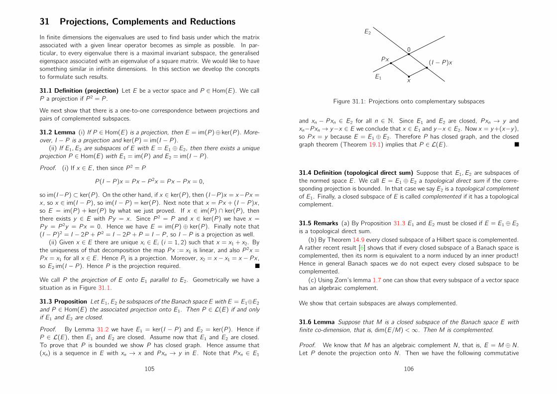
31 Projections, Complements and Reductions

In finite dimensions the eigenvalues are used to find basis under which the matrix

associated with a given linear operator becomes as simple as possible. In par-

ticular, to every eigenvalue there is a maximal invariant subspace, the generalised

eigenspace associated with an eigenvalue of a square matrix. We would like to have

something similar in infinite dimensions. In this section we develop the concepts

to formulate such results.

31.1 Definition (projection) Let E be a vector space and P ∈ Hom(E). We call

P a projection if P 2 = P .

We next show that there is a one-to-one correspondence between projections and

pairs of complemented subspaces.

31.2 Lemma (i) If P ∈ Hom(E) is a projection, then E = im(P )⊕ ker(P ). More-

over, I − P is a projection and ker(P ) = im(I − P ).(ii) If E1, E2 are subspaces of E with E = E1 ⊕ E2, then there exists a unique

projection P ∈ Hom(E) with E1 = im(P ) and E2 = im(I − P ).Proof. (i) If x ∈ E, then since P 2 = P

P (I − P )x = Px − P 2x = Px − Px = 0,

so im(I−P ) ⊂ ker(P ). On the other hand, if x ∈ ker(P ), then (I−P )x = x−Px =x , so x ∈ im(I − P ), so im(I − P ) = ker(P ). Next note that x = Px + (I − P )x ,so E = im(P ) + ker(P ) by what we just proved. If x ∈ im(P ) ∩ ker(P ), then

there exists y ∈ E with Py = x . Since P 2 = P and x ∈ ker(P ) we have x =

Py = P 2y = Px = 0. Hence we have E = im(P ) ⊕ ker(P ). Finally note that

(I − P )2 = I − 2P + P 2 = I − 2P + P = I − P , so I − P is a projection as well.

(ii) Given x ∈ E there are unique xi ∈ Ei (i = 1, 2) such that x = x1 + x2. By

the uniqueness of that decomposition the map Px := x1 is linear, and also P 2x =

Px = x1 for all x ∈ E. Hence P1 is a projection. Moreover, x2 = x − x1 = x − Px ,so E2 im(I − P ). Hence P is the projection required.

We call P the projection of E onto E1 parallel to E2. Geometrically we have a

situation as in Figure 31.1.

31.3 Proposition Let E1, E2 be subspaces of the Banach space E with E = E1⊕E2and P ∈ Hom(E) the associated projection onto E1. Then P ∈ L(E) if and only

if E1 and E2 are closed.

Proof. By Lemma 31.2 we have E1 = ker(I − P ) and E2 = ker(P ). Hence if

P ∈ L(E), then E1 and E2 are closed. Assume now that E1 and E2 are closed.

To prove that P is bounded we show P has closed graph. Hence assume that

(xn) is a sequence in E with xn → x and Pxn → y in E. Note that Pxn ∈ E1

105

b0

b

b

b

Px

x

(I − P )x

E1

E2

Figure 31.1: Projections onto complementary subspaces

and xn − Pxn ∈ E2 for all n ∈ N. Since E1 and E2 are closed, Pxn → y and

xn−Pxn → y−x ∈ E we conclude that x ∈ E1 and y−x ∈ E2. Now x = y+(x−y),so Px = y because E = E1 ⊕ E2. Therefore P has closed graph, and the closed

graph theorem (Theorem 19.1) implies that P ∈ L(E).

31.4 Definition (topological direct sum) Suppose that E1, E2 are subspaces of

the normed space E. We call E = E1 ⊕ E2 a topological direct sum if the corre-

sponding projection is bounded. In that case we say E2 is a topological complement

of E1. Finally, a closed subspace of E is called complemented if it has a topological

complement.

31.5 Remarks (a) By Proposition 31.3 E1 and E2 must be closed if E = E1 ⊕ E2is a topological direct sum.

(b) By Theorem 14.9 every closed subspace of a Hilbert space is complemented.

A rather recent result [6] shows that if every closed subspace of a Banach space is

complemented, then its norm is equivalent to a norm induced by an inner product!

Hence in general Banach spaces we do not expect every closed subspace to be

complemented.

(c) Using Zorn’s lemma 1.7 one can show that every subspace of a vector space

has an algebraic complement.

We show that certain subspaces are always complemented.

31.6 Lemma Suppose that M is a closed subspace of the Banach space E with

finite co-dimension, that is, dim(E/M) <∞. Then M is complemented.

Proof. We know that M has an algebraic complement N, that is, E = M ⊕ N.

Let P denote the projection onto N. Then we have the following commutative

106

diagram.

E N

E/M

P

π P

Since M is a closed subspace, by Theorem 12.3 E/M is a Banach space and P is

an isomorphism. Since dim(E/M) <∞ the operator P is continuous, and so it is

continuous. Therefore P is continuous as well as a composition of two continuous

operators. Hence we can apply Proposition 31.3 to conclude the proof.

Suppose now that E is a vector space and E1 and E2 are subspaces such that

E = E1⊕E2. Denote by P1 and P2 the corresponding projections. If A ∈ Hom(E),then

Ax = P1Ax + P2Ax = P1A(P1x + P2x) + P2A(P1x + P2x)

= P1AP1x + P1AP2x + P2AP1x + P2AP2x

for all x ∈ E. Setting

Ai j := PiAPj ,

we have Ai j ∈ Hom(Ej , Ei). If we identify x ∈ E with (x1, x2) := (P1x, P2x) ∈E1 × E2, then we can write

Ax =

[

A11 A12A21 A22

] [

x1x2

]

31.7 Definition (complete reduction) We say E = E1 ⊕ E2 completely reduces

A if A12 = A21 = 0, that is,

A ∼[

A11 0

0 A22

]

If that is the case we set Ai := Ai i and write A = A1 ⊕ A2.

We next characterise the reductions by means of the projections.

31.8 Proposition Suppose that E = E1 ⊕ E2 and that P1 and P2 are the corre-

sponding projections. Let A ∈ Hom(E). Then E = E1 ⊕ E2 completely reduces A

if and only if P1A = AP1.

Proof. Suppose that E = E1 ⊕ E2 completely reduces A. Then

P1Ax = P1AP1x + P1AP2x = P1AP1x = P1AP1x + P2AP1x = AP1x.

107

To prove the converse Note that P1P2 = P2P1 = 0. Hence A12 = P1AP2 =

AP1P2 = 0 and also A21 = P2AP1 = P2P1A = 0, so E = E1 ⊕ E2 completely

reduces A.

Of course we could replace interchange the roles of P1 and P2 in the above propo-

sition.

31.9 Proposition Suppose that E = E1 ⊕ E2 completely reduces A ∈ Hom(E).Let A = A1 ⊕ A2 be this reduction. Then

(i) kerA = kerA1 ⊕ kerA2;

(ii) imA = imA1 ⊕ imA2;

(iii) A is injective (surjective) if and only if A1 and A2 are injective (surjective);

(iv) if A is bijective, then E = E1 ⊕ E2 completely reduces A−1 and A−1 =

A−11 ⊕ A−12 .

Proof. (i) If x = x1+ x2 with x1 ∈ E1 and x2 ∈ E2, then 0 = Ax = A1x1 +A2x2 if

and only if A1x1 = 0 and A2x2 = 0. Hence (i) follows.

(ii) If x = x1+x2 with x1 ∈ E1 and x2 ∈ E2, then y = Ax = A1x1+A2x2 = y1+y2if and only if A1x1 = y1 and A2x2 = y2. Hence (ii) follows.

(iii) follows directly from (i) and (ii), and (iv) follows from the argument given

in the proof of (ii).

We finally look at resolvent and spectrum of the reductions. It turns out that the

spectral properties of A can can be completely described by the operators A1 and

A2.

31.10 Proposition Suppose that E is a Banach space and that E = E1 ⊕ E2 a

topological direct sum completely reducing A ∈ L(E). Let A = A1 ⊕ A2 be this

reduction. Then

(i) Ai ∈ L(Ei) (i = 1, 2);

(ii) σ(A) = σ(A1) ∪ σ(A2);

(iii) σp(A) = σp(A1) ∪ σp(A2).

Proof. By Proposition 31.3 the projections P1, P2 associated with E = E1 ⊕ E2are bounded. Hence Ai = PiAPi is bounded for i = 1, 2. The equality in (ii) follows

from Proposition 31.9(iv) which shows that (A) = (A1) ∩ (A2). Finally (iii)

follows since by Proposition 31.9(i) shows that ker(λI − A) = 0 if and only if

ker(λIE1 − A1) = ker(λIE2 − A2) = 0.

108

32 The Ascent and Descent of an Operator

Let E be a vector space over K and T ∈ Hom(E). We then consider two nested

sequences of subspaces:

0 = ker T 0 ⊆ ker T ⊆ ker T 2 ⊆ ker T 3 ⊆ . . .and

E = imT 0 ⊇ imT ⊇ imT 2 ⊇ imT 3 ⊇ . . . .We are interested in n such that there is equality.

32.1 Lemma If kerT n = kerT n+1, then ker T n = ker T n+k for all k ∈ N. More-

over, if imT n = imT n+1, then imT n = imT n+k for all k ∈ N.

Proof. If k ≥ 1 and x ∈ kerT n+k , then 0 = T n+kx = T n+1(T k−1x) and so

T k−1x ∈ ker T n. By assumption kerT n = kerT n+1 and therefore T n+k−1x =

T n(T k−1x) = 0. Hence kerT n+k = kerT n+k−1 for all k ≥ 1 from which the

first assertion follows. The second assertion is proved similarly. If k ≥ 1 and

x ∈ imT n+k−1, then there exists y ∈ E with x = T n+k−1y = T k−1(T ny) and

so T ny ∈ imT n. By assumption imT n = imT n+1 and therefore there exists

z ∈ imT n+1 with T n+1z = T ny . Thus T n+kz = T k−1(T n+1z) = T k−1(T ny) =

T n+k−1y = x which implies that imT n+k−1 = imT n+k for all k ≥ 1. This completes

the proof of the lemma.

The above lemma motivates the following definition.

32.2 Definition (ascent and descent) We call

α(T ) := infn ≥ 1: ker T n = kerT n+1the ascent of T and

δ(T ) := infn ≥ 1: imT n = imT n+1the descent of T

If dimE = N <∞, then ascent and descent are clearly finite and since dim(kerT n)+

dim(im(T n)) = N for all n ∈ N, ascent and descent are always equal. We now

show that they are equal provided they are both finite. The arguments we use

are similar to those to prove the Jordan decomposition theorem for matrices. The

additional complication is that in infinite dimensions there is no dimension formula.

32.3 Theorem Suppose that α(T ) and δ(T ) are both finite. Then α(T ) = δ(T ).

Moreover, if we set n := α(T ) = δ(T ), then

E = ker T n ⊕ imT n

and the above direct sum completely reduces T .

109

Proof. Let α := α(T ) and δ := δ(T ). The plan is to show that

imT α ∩ kerT k = 0 (32.1)

and that

imT k + ker T δ = E (32.2)

for all k ≥ 1. Choosing k = δ in (32.1) and k = α in (32.2) we then get

imT α ⊕ ker T δ = E. (32.3)

To show that α = δ assume that x ∈ ker T δ+1. By (32.3) there is a unique

decomposition x = x1 + x2 with x1 ∈ imT α and x2 ∈ ker T δ. Because kerT δ ⊆kerT δ+1 we get x1 = x − x2 ∈ ker T δ+1. We also have x1 ∈ imT α, so by (32.1)

we conclude that x1 = 0. Hence x = x2 ∈ ker T δ, so that ker T δ = ker T δ+1. By

definition of the ascent we have α ≤ δ. Assuming that α < δ, then by definition

of the descent imT δ ( imT α. By (32.2) we still have imT δ + kerT δ = E,

contradicting (32.3). Hence α = δ.

To prove (32.1) fix k ≥ 1 and let x ∈ imT α ∩ ker T k . Then x = T αy for some

y ∈ E and 0 = T kx = T α+ky . As ker T α = ker T α+k we also have x = T αy = 0.

To prove (32.2) fix k ≥ 1 and let x ∈ E. As imT δ = imT δ+k there exists y ∈ Ewith T δx = T δ+ky . Hence T δ(x−T ky) = 0, proving that x−T ky ∈ ker T δ. Hence

we can write x = T ky + (x − T ky) from which (32.2) follows.

We finally prove that (32.3) completely reduces T . By definition of n = α = δ

we have T (kerT n) ⊆ kerT n+1 = kerT n and T (imT n) ⊆ imT n+1 = imT n. This

completes the proof of the theorem.

We well apply the above to the operator λI − A, where A is a bounded operator

on a Banach space and λ ∈ σp(A).

32.4 Definition (algebraic multiplicity) Let E be a Banach space and over C. If

A ∈ L(E) and λ ∈ σp(A) is an eigenvalue we call

dim ker(λI − A)

the geometric multiplicity of λ and

dim(

⋃

n∈N

ker(λI − A)n)

the algebraic multiplicity of λ. The ascent α(λI − A) is called the Riesz index of

the eigenvalue λ.

Note that the definitions here are consistent with the ones from linear algebra.

As it turns out the algebraic multiplicity of the eigenvalue of a matrix as defined

above coincides with the multiplicity of λ as a root of the characteristic polynomial.

110

In infinite dimensions there is no characteristic polynomial, so we use the above

as the algebraic multiplicity. The only question now is whether there are classes

of operators for which ascent and descent of λI − A are finite for every or some

eigenvalues. It turns out that such properties are connected to compactness. This

is the topic of the next section.

33 The Spectrum of Compact Operators

We want to study a class of operators appearing frequently in the theory of partial

differential equations and elsewhere. They share many properties with operators

on finite dimensional spaces.

33.1 Definition (compact operator) Let E and F be Banach spaces. Then T ∈Hom(E, F ) is called compact if T (B) is compact for all bounded sets B ⊂ E. We

set

K(E, F ) := T ∈ Hom(E, F ) : T is compact

and K(E) := L(E,E).

33.2 Remark By the linearity T is clearly compact if and only if T (B(0, 1)) is

compact.

33.3 Proposition Let E, F be Banach spaces. Then K(E, F ) is a closed subspace

of L(E, F ).

Proof. If B ⊂ E is bounded, then by assumption the closure of T (B) is compact,

and therefore bounded. To show that K(E, F ) is a subspace of L(E, F ) let T, S ∈K(E, F ) and λ, µ ∈ K. Let B ⊂ E be bounded and let (yn) be a sequence in

(λT + µS)(B). Then there exist xn ∈ B with yn = λTxn + µSxn. Since B is

bounded the sequence (xn) is bounded as well. By the compactness of T there

exists a subsequence (xnk ) with Txnk → y . By the compactness of S we can select a

further subsequence (xnkj ) with Sxnkj → z . Hence ynkj = λTxnkj+µSxnkj → λy+µz .This shows that every sequence in (λT+µS)(B) has a convergent subsequence, so

by Theorem 4.4 the closure of that set is compact. Hence λT + µS is a compact

operator.

Suppose finally that Tn ∈ K(E, F ) with Tn → T in T ∈ L(E, F ). It is sufficient

to show that T (B) is compact if B = B(0, 1) is the unit ball. We show that T (B)

is totally bounded. To do so fix ǫ > 0. Since Tn → T there exists n ∈ N such that

‖Tn − T ‖L(E,F ) <ε

4. (33.1)

111

By assumption Tn is compact and so Tn(B) is compact. Therefore there exist

yk ∈ Tn(B), k = 1, . . . , m, such that

Tn(B) ⊆m⋃

k=1

B(yk , ε/4). (33.2)

If we let y ∈ T (B), then y = Tx for some x ∈ B. By (33.2) there exists

k ∈ 1, . . . , m such that Tnx ∈ B(yk , ε/4). By (33.1) and since ‖x‖ ≤ 1 we get

‖yk − y‖ = ‖yk − Tny‖+ ‖Tny − Tx‖ ≤ε

4+ε

4‖x‖ ≤ ε

2,

so that y ∈ B(yk , ε/2). Since y ∈ B was arbitrary this shows that

T (B) ⊆m⋃

k=1

B(yk, ε/2)

and therefore

T (B) ⊆m⋃

k=1

B(yk, ε/2) ⊆m⋃

k=1

B(yk, ε).

Since ε > 0 was arbitrary T (B) is totally bounded. Since F is complete Theo-

rem 4.4 implies that T (B) is compact.

We now look at compositions of operators.

33.4 Proposition Let E, F, G be Banach spaces. If K ∈ K(F, G), then KT ∈K(E, F ) for all T ∈ L(E, F ). Likewise, if K ∈ K(E, F ), then TK ∈ K(E,G) for

all T ∈ L(F, G).Proof. If K ∈ K(F, G), T ∈ L(E, F ) and B ⊂ E bounded, then T (B) is

bounded in F and therefore KT (B) is compact in G. Hence KT is compact.

If K ∈ K(E, F ), T ∈ L(F, G) and B ⊂ E bounded, then K(B) is compact in

F . Since T is continuous T (K(B)) is compact in G, so TK(B) ⊂ T (K(B)) is

compact. Hence TK is a compact operator.

33.5 Remark If we define multiplication of operators in L(E) to be composition of

operators, then L(E) becomes a non-commutative algebra. The above propositions

show that K(E) is a closed ideal in that algebra.

The next theorem will be useful to characterise the spectrum of compact operators.

33.6 Theorem Let T ∈ K(E) and λ ∈ K \ 0. Then for all k ∈ N

(i) dim(

ker(λI − T )k)

<∞;

112

(ii) im(λI − T )k is closed in E.

Proof. Since ker(λI − T )k = ker(I − λ−1T )k and im(λI − T )k = im(I − λ−1T )kwe can assume without loss of generality that λ = 1 by replacing T by λT . Also,

we can reduce the proof to the case k = 1 because

(I −K)k =k

∑

j=0

(−1)j(

k

j

)

T j = I −k

∑

j=1

(−1)j−1(

k

j

)

T j = I − T

if we set T :=∑kj=1(−1)j−1

(

kj

)

T j . Note that by Proposition 33.4 the operator T

is compact.

(i) If x ∈ ker(I − T ), then x = Tx and so

S := x ∈ ker(I − T ) : ‖x‖ = 1 ⊆ T (B(0, 1)).

Since T is compact S is compact as well. Note that S is the unit sphere in

ker(I − T ), so by Theorem 11.3 the kernel of I − T is finite dimensional.

(ii) Set S := I − T . As kerS is closed M := E/ kerS is a Banach space by

Theorem 12.3 with norm ‖x‖M := infy∈kerS ‖y − x‖. Now set F := im(S). Let

S ∈ L(M,F ) be the map induced by S. We show that S−1 is bounded on im(S).

If not, then there exist yn ∈ im(S) such that yn → 0 but ‖S−1yn‖M = 1 for all

n ∈ N. By definition of the quotient norm there exist xn ∈ E with 1 ≤ ‖xn‖E ≤ 2such that

S[xn] = xn − Txn = yn → 0.Since T is compact there exists a subsequence such that Txnk → z . Hence from

the above

xnk = ynk + Txnk → z.By the continuity of T we have Txnk → Tz , so that z = Tz . Hence z ∈ ker(I−T )and [xnk ] → [z ] = [0] in M. Since ‖[xn‖M = 1 for all n ∈ N this is not possible.

Hence S−1 ∈ L(im(S),M) and by Proposition 21.4 it follows that F = im(S) =

im(I − T ) is closed.

We next prove that the ascent and descent of λI − T is finite if T is compact and

λ 6= 0.

33.7 Theorem Let T ∈ K(E) and λ ∈ K \ 0. Then n := α(λI − T ) = δ(λI −T ) <∞ and

E = ker(λI − T )n ⊕ im(λI − T )n

is a topological direct sum completely reducing µI − T for all µ ∈ C.

Proof. Replacing T by λT we can assume without loss of generality that λ = 1.

Suppose that α(λI − T ) = ∞. Then Nk := ker(I − T )k is closed in E for every

k ∈ N and

N0 ⊂ N1 ⊂ N2 ⊂ N3 ⊂ . . . ,

113

where all inclusions are proper inclusions. By Corollary 11.2 there exist xk ∈ Nksuch that

‖xk‖ = 1 and dist(xk, Nk−1) ≥1

2for all k ≥ 1. Now

Txk − Txℓ = (I − T )xℓ − (I − T )xk + xk − xℓ= xk −

(

xℓ − (I − T )xℓ + (I − T )xk)

= xk − z,where z := xℓ− (I−T )xℓ+(I−T )xk ∈ ker(I−T )k−1 = Nk−1 if 1 ≤ ℓ < k . Hence

by choice of (xk) we get

‖Txk − Txℓ‖ = ‖xk − z‖ ≥1

2

for all 1 ≤ ℓ < k . Therefore the bounded sequence Txk does not have a convergent

subsequence, so T is not compact. As a consequence, if T ∈ K(E, F ) is compact,

then α(I − T ) <∞.

The proof for the descent works quite similarly. We assume that δ(I−T ) =∞.

Then by Theorem 33.6 Mk := im(I − T )k is closed in E for every k ∈ N and

M0 ⊃ M1 ⊃ M2 ⊃ M3 ⊃ . . . ,where all inclusions are proper inclusions. By Corollary 11.2 there exist xk ∈ Mksuch that

‖xk‖ = 1 and dist(xk ,Mk+1) ≥1

2for all k ≥ 1. Now

Txk − Txℓ = (I − T )xℓ − (I − T )xk − xk + xℓ= xℓ −

(

xk − (I − T )xℓ + (I − T )xk)

= xk − z,where z := xk − (I−T )xℓ+(I−T )xk ∈ im(I−T )k+1 = Mk+1 if 1 ≤ k < ℓ. Hence

by choice of (xk) we get

‖Txk − Txℓ‖ = ‖xℓ − z‖ ≥1

2

for all 1 ≤ k < ℓ. Therefore the bounded sequence Txk does not have a convergent

subsequence, so T is not compact. As a consequence, if T ∈ K(E, F ) is compact,

then δ(I − T ) <∞.

By Theorem 32.3 n := α(I−T ) = δ(I −T ) and E = ker(I −T )n⊕ im(I −T )nis a direct sum completely reducing I − T and therefore µI − T for all µ ∈ K. By

Theorem 33.6 the subspaces ker(I−T )n and im(I−T )n are closed, so by 31.3 the

above is a topological direct sum

As a consequence of the above theorem we prove that compact operators behave

quite similarly to operators on finite dimensional spaces. The following corollary

would be proved by the dimension formula in finite dimensions.

114

33.8 Corollary Suppose that T ∈ K(E) and λ 6= 0. Then λI − T is injective if

and only if it is surjective.

Proof. If λI − T is injective, then 0 = ker(λI − T ) = ker(λI − T )2, and by

Theorem 33.7 we get

E = ker(λI − T )⊕ im(λI − T ) = 0 ⊕ im(λI − T ) = im(λI − T ). (33.3)

On the other hand, if E = im(λI − T ), then im(λI − T ) = im(λI − T )2, so that

δ(λI − T ) = 1. Hence ker(λI − T ) = 0 by Theorem 33.7 and (33.3).

We finally derive a complete description of the spectrum of closed operators.

33.9 Theorem (Riesz-Schauder) Let E be a Banach space over C and T ∈ K(E)compact. Then σ(T ) \ 0 consists of at most countably many isolated eigenval-

ues of finite algebraic multiplicity. The only possible accumulation point of these

eigenvalues is zero.

Proof. By Corollary 33.8 and Proposition 30.3 every λ ∈ σ(T ) \ 0 is an

eigenvalue of T . By Theorems 33.6 and 33.7 these eigenvalues have finite algebraic

multiplicity. Hence it remains to show that they are isolated. Fix λ ∈ σ(T ) \ 0and let n its Riesz index (see Definition 32.4). Then by Theorem 33.7

E = ker(λI − T )n ⊕ im(λI − T )n

is a topological direct sum completely reducing µI −T for all µ ∈ C. We set N :=

ker(λI−T )n and M := im(λI−T )n. Let T = TN⊕TM be the reduction associated

with the above direct sum decomposition. By construction λI − TN is nilpotent,

so by Theorem 30.10 spr(λI − TN) = 0. In particular this means that σ(TN) =

λ. Moreover, by construction, λI − TM is injective and so by Proposition 30.3

and Corollary 33.8 λ ∈ (TM). As (TM) is open by Theorem 30.7 there exists

r > 0 such that B(λ, r) ⊂ (TM). By Theorem 31.10 (T ) = (TN) ∩ (TM), so

B(λ, r) \ λ ⊂ (T ), showing that λ is an isolated eigenvalue. Since the above

works for every λ ∈ σ(T ) \ 0 the assertion of the theorem follows.

33.10 Remarks (a) If T ∈ K(E) and dimE = ∞, then 0 ∈ σ(T ). If not, then

by Proposition 33.4 the identity operator I = TT−1 is compact. Hence the unit

sphere in E is compact and so by Theorem 11.3 E is finite dimensional.

(b) The above theorem allows us to decompose a compact operator T ∈ L(E)in the following way. Let λk ∈ σp(T ) \ 0, k = 1, . . . , m, and let nk be the

corresponding Riesz indices. Then set

Nk := ker(λI − T )nk

115

and Tk := T |Nk . Then there exists a closed subspace M ⊂ E which is invariant

under T such that

E = N1 ⊕ N2 ⊕ · · · ⊕ Nm ⊕Mcompletely reduces T = T1 ⊕ T2 ⊕ · · · ⊕ Tm ⊕ TM . To get this reduction apply

Theorem 33.9 inductively.

The above theory is also useful for certain classes of closed operators A : D(A) ⊆E → E, namely those for which R(λ, A) is compact for some λ ∈ (A). In that case

the resolvent identity from Theorem 30.7 and Proposition 33.4 imply that R(λ, A)

is compact for all λ ∈ (A). It turns out that σ(A) = σp(A) consist of isolated

eigenvalues, and the only possible point of accumulation is infinity. Examples of

such a situation include boundary value problems for partial differential equations

such as the one in Example 22.5.

116

Bibliography

[1] E. Bishop and D. Bridges, Constructive analysis, Grundlehren der Mathema-

tischen Wissenschaften, vol. 279, Springer-Verlag, Berlin, 1985.

[2] P. Cohen, The independence of the continuum hypothesis, Proc. Nat. Acad.

Sci. U.S.A. 50 (1963), 1143–1148.

[3] P. J. Cohen, The independence of the continuum hypothesis. II, Proc. Nat.

Acad. Sci. U.S.A. 51 (1964), 105–110.

[4] J. Dugundji, Topology, Allyn and Bacon Inc., Boston, Mass., 1966.

[5] K. Gödel, The consistency of the axiom of choice and of the generalized

continuum-hypothesis, Proc. Nat. Acad. Sci. U.S.A. 24 (1938), 556–557.

[6] J. Lindenstrauss and L. Tzafriri, On the complemented subspaces problem,

Israel J. Math. 9 (1971), 263–269.

[7] K. Yosida, Functional analysis, 6th ed., Grundlehren der Mathematischen Wis-

senschaften, vol. 123, Springer-Verlag, Berlin, 1980.

[8] E. Zermelo, Beweis, daß jede Menge wohlgeordnet werden kann, Math. Ann.

59 (1904), 514–516.

117