CHAPTER 5 Introduction to Fractals Larry S. Liebovitch Center for Complex Systems and Brain Sciences, Center for Molecular Biology and Biotechnology, & Departments of Psychology and Biomedical Sciences Florida Atlantic University 777 Glades Road Boca Raton, FL 33431 U. S. A. E-mail: [email protected] http://walt.ccs.fau.edu/~liebovitch/larry.html Lina A. Shehadeh Center for Complex Systems and Brain Sciences Florida Atlantic University 777 Glades Road Boca Raton, FL 33431 U. S. A.

Welcome message from author
This document is posted to help you gain knowledge. Please leave a comment to let me know what you think about it! Share it to your friends and learn new things together.
Transcript
CHAPTER 5
Introduction to Fractals
Larry S. Liebovitch
Center for Complex Systems and Brain Sciences, Center for MolecularBiology and Biotechnology, & Departments of Psychology andBiomedical SciencesFlorida Atlantic University777 Glades RoadBoca Raton, FL 33431U. S. A.E-mail: [email protected]://walt.ccs.fau.edu/~liebovitch/larry.html
Lina A. Shehadeh
Center for Complex Systems and Brain SciencesFlorida Atlantic University777 Glades RoadBoca Raton, FL 33431U. S. A.
digitstaff
Text Box
Notice: This author provided manuscript is a chapter that appears as part of a text, Tutorials in Contemporary Nonlinear Methods for the Behavioral Sciences Web Book, Edited by M.A. Riley & G.C. Van Orden Courtesy of the US government public domain website National Science Foundation available at http://www.nsf.gov/sbe/bcs/pac/nmbs/nmbs.pdf

Liebovitch & Shehadeh
179
INTRODUCTION
This chapter is a Word version of the PowerPoint presentation
given by Dr. Larry S. Liebovitch at the NSF Nonlinear Methods in
Psychology Workshop, October 24-25, 2003 at George Mason
University, Fairfax, VA. The PowerPoint presentation itself is also
available as a part of this web book. Here the notes which can be seen
on the PowerPoint presentation by using “Normal View” are presented
as text around their respective PowerPoint slides. The concept here is
to try to reproduce the look and feel of the presentation at the
workshop. Therefore, this is not, and is not meant to be, your usual
“print” article. The form of the language here is more typical of
spoken, rather than written, English. The form of the graphics is
sparser, larger pictures captioned with larger fonts, that is more typical
of PowerPoint presentations than printed illustrations. We hope that
this experimental format may provide a simpler introduction to fractals
than that of a more formal presentation. We also hope that the
availability of the PowerPoint file will be of use in teaching these
materials and may also serve as a starting point for others to customize
these slides for their own applications.
This chapter is about “fractals”. Objects in space can have fractal
properties. Time series of values can have fractal properties. Sets of
numbers can have fractal properties. Much of the statistics that you are
familiar with deals with the “linear” properties of data. Fractals can
help us describe some “non-linear” properties of data.
Introduction to Fractals
180
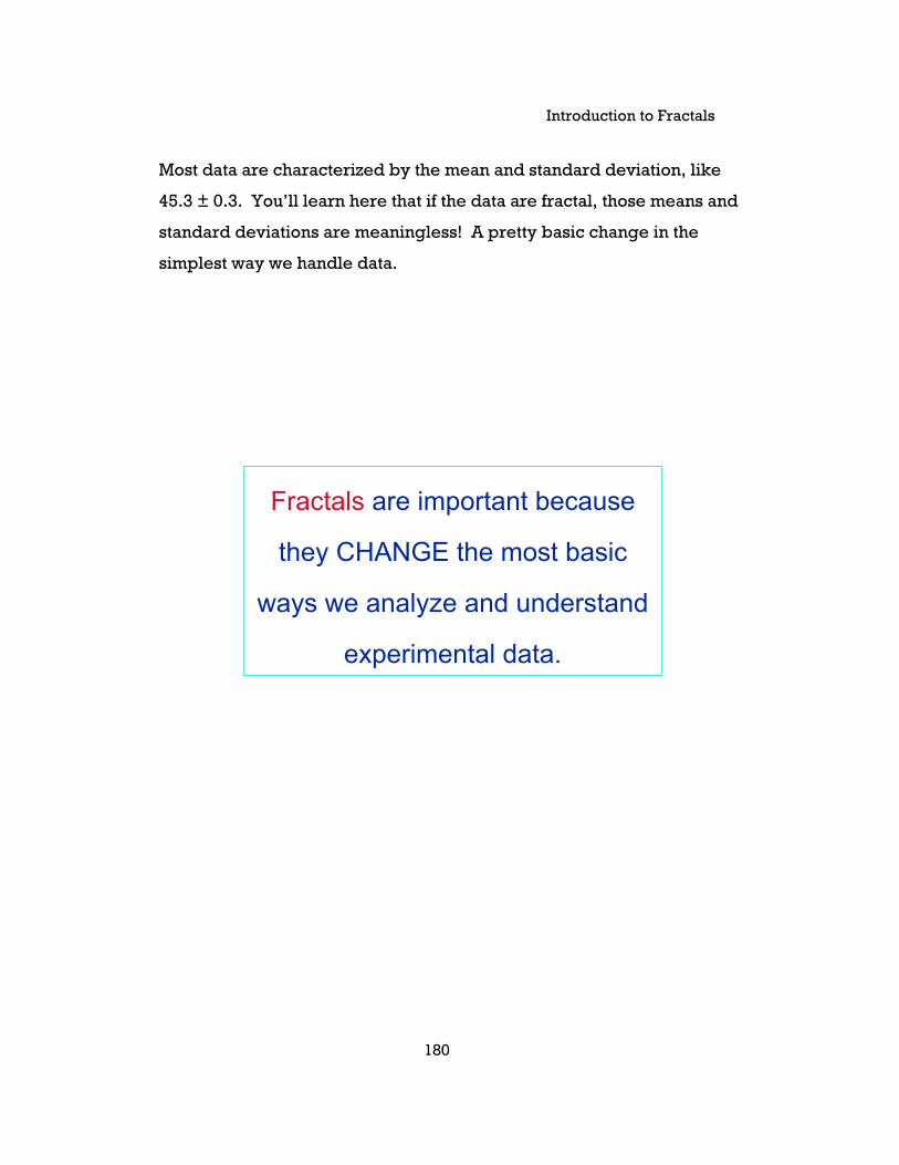
Most data are characterized by the mean and standard deviation, like
45.3 ± 0.3. You’ll learn here that if the data are fractal, those means and
standard deviations are meaningless! A pretty basic change in the
simplest way we handle data.
Fractals are important because
they CHANGE the most basic
ways we analyze and understand
experimental data.
Liebovitch & Shehadeh
181
We’ll start with objects. Let’s first see the difference between the non-
fractal and fractal objects.
Properties of Objectsin Space
Non-Fractal and Fractal Objects are different.
Introduction to Fractals
182
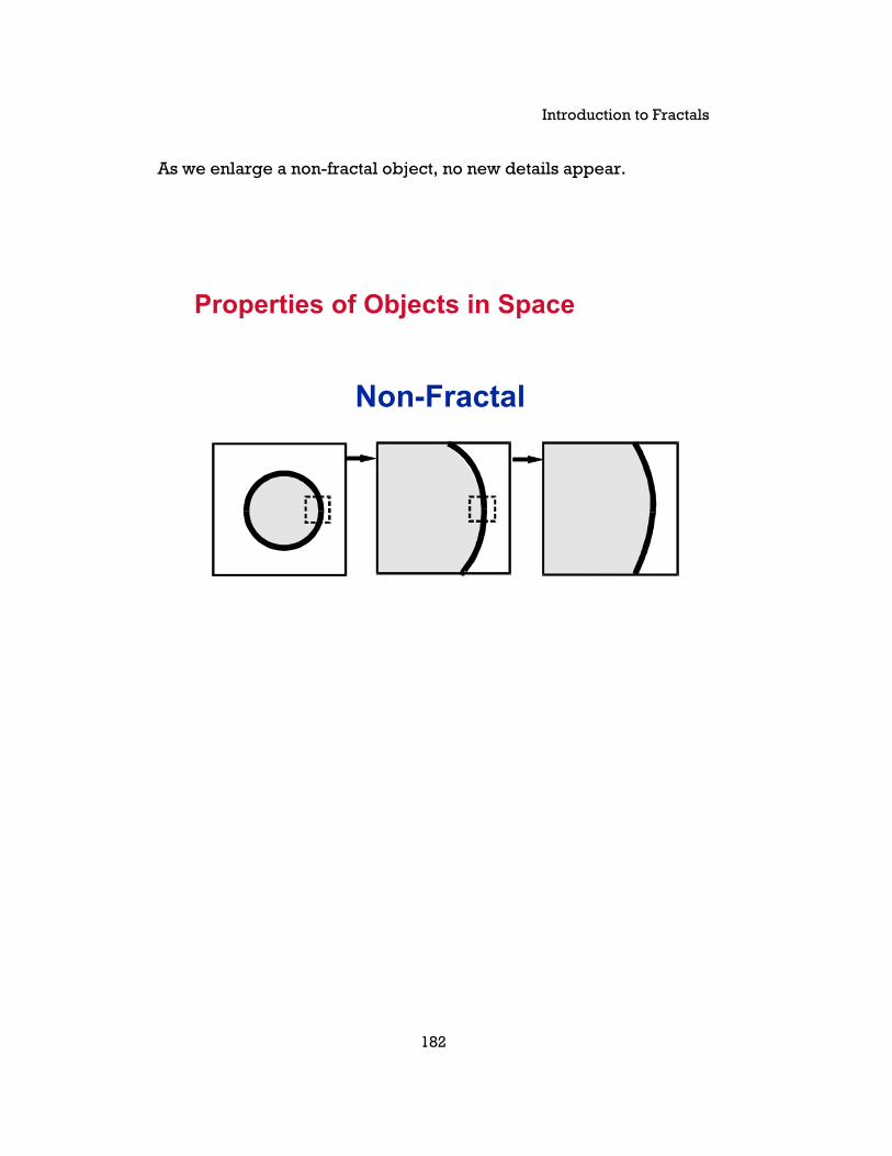
As we enlarge a non-fractal object, no new details appear.
Non-Fractal
Properties of Objects in Space
Liebovitch & Shehadeh
183
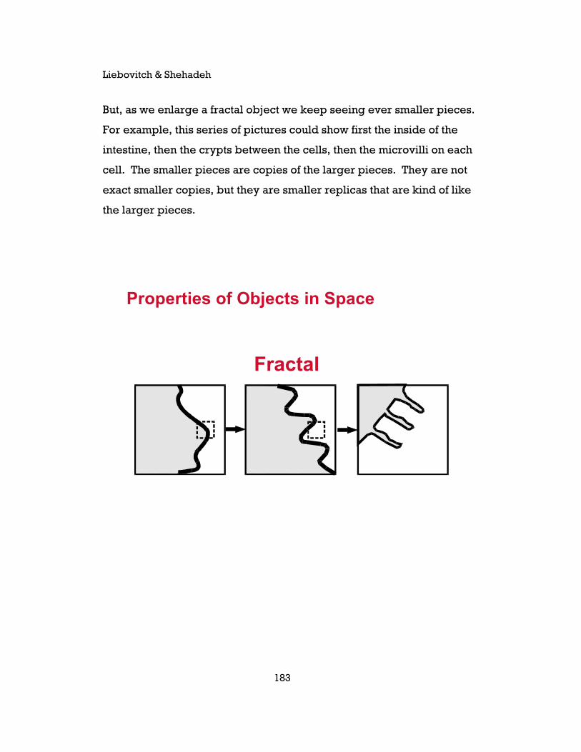
But, as we enlarge a fractal object we keep seeing ever smaller pieces.
For example, this series of pictures could show first the inside of the
intestine, then the crypts between the cells, then the microvilli on each
cell. The smaller pieces are copies of the larger pieces. They are not
exact smaller copies, but they are smaller replicas that are kind of like
the larger pieces.
Fractal
Properties of Objects in Space
Introduction to Fractals
184
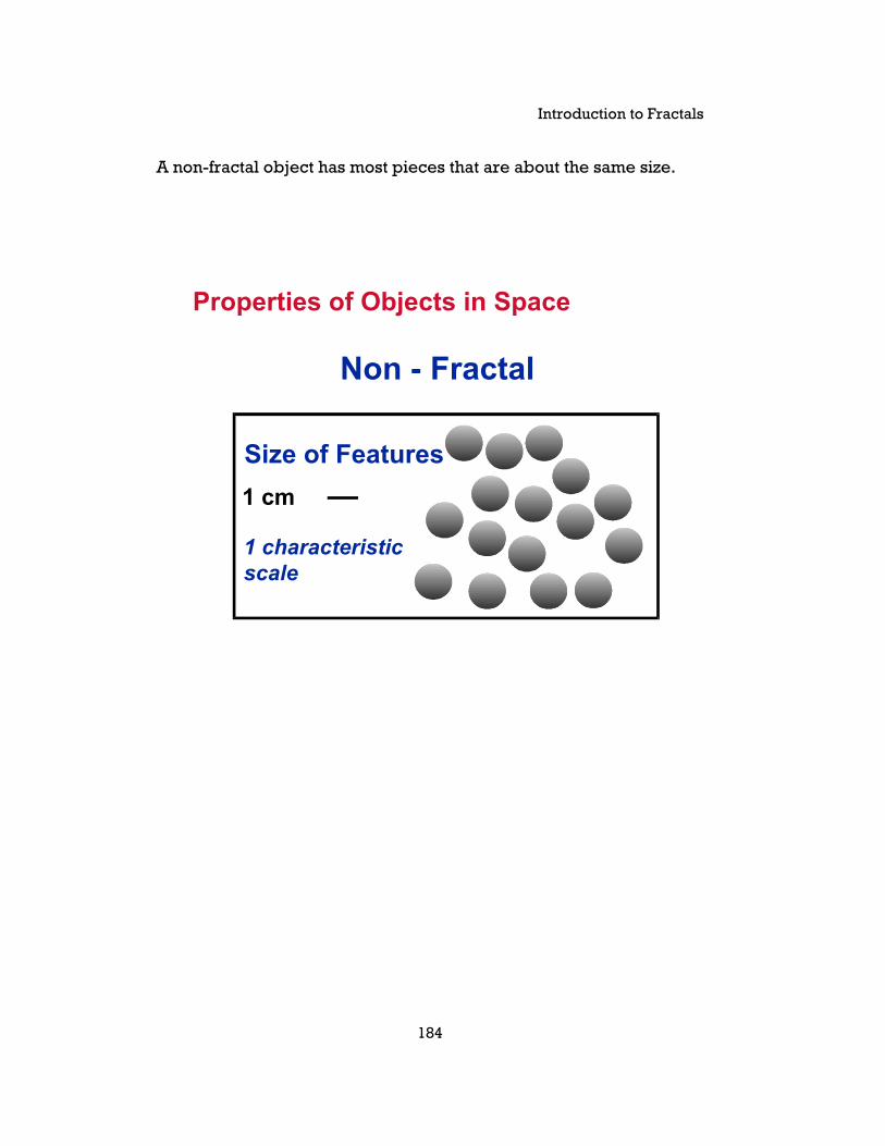
A non-fractal object has most pieces that are about the same size.
Non - Fractal
Size of Features
1 cm
1 characteristicscale
Properties of Objects in Space
Liebovitch & Shehadeh
185
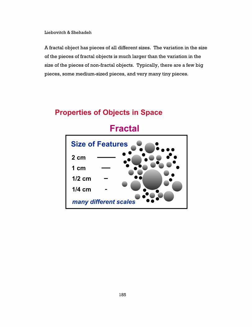
A fractal object has pieces of all different sizes. The variation in the size
of the pieces of fractal objects is much larger than the variation in the
size of the pieces of non-fractal objects. Typically, there are a few big
pieces, some medium-sized pieces, and very many tiny pieces.
Fractal
Size of Features
2 cm
1 cm
1/2 cm
1/4 cm
many different scales
Properties of Objects in Space

Introduction to Fractals
186
Fractal objects have interesting properties. Here we describe those
properties very briefly. Then later, we will describe them in more
detail.
Properties of Fractal Objects
Self-Similarity.The little pieces are smaller copies of the larger pieces.
Scaling.The values measured depend on the resolution used tomake the measurement.
Statistics.The “average” size depends on the resolution used tomake the measurement.

Liebovitch & Shehadeh
187
A tree is fractal. It has a few large branches, some medium-sized
branches, and very many small branches. A tree is self-similar: The
little branches are smaller copies of the larger branches. There is a
scaling: The length and thickness of each branch depends on which
branch we measure. There is no average size of a branch: The greater
the number of smaller branches we include, the smaller is the
“average” length and thickness.
This tree is from http://www.feebleminds-gifs.com/trees23.jpg.
Example of a Fractal
A tree is fractal
from http://www.feebleminds-gifs.com/trees23.jpg
Introduction to Fractals
188
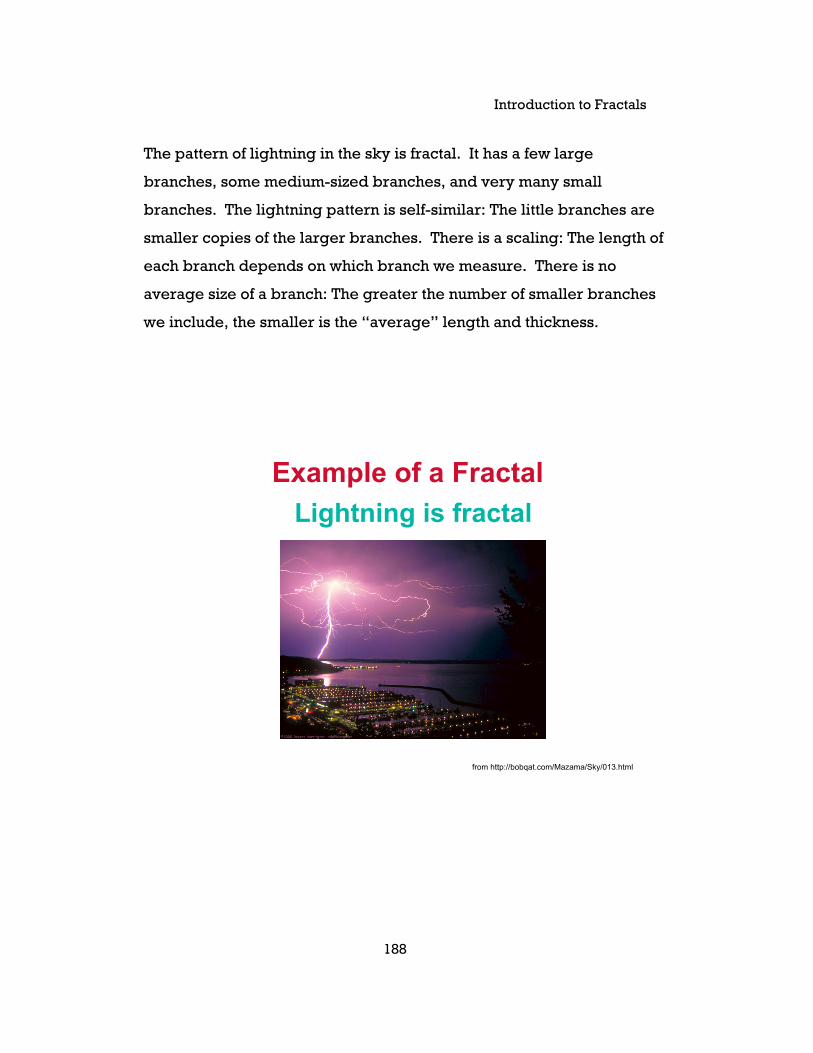
The pattern of lightning in the sky is fractal. It has a few large
branches, some medium-sized branches, and very many small
branches. The lightning pattern is self-similar: The little branches are
smaller copies of the larger branches. There is a scaling: The length of
each branch depends on which branch we measure. There is no
average size of a branch: The greater the number of smaller branches
we include, the smaller is the “average” length and thickness.
from http://bobqat.com/Mazama/Sky/013.html
Example of a Fractal
Lightning is fractal

Liebovitch & Shehadeh
189
The pattern of clouds in the sky is fractal. They are made up of a few
big clouds, some medium-sized clouds, and very many small clouds.
The cloud pattern is self-similar: The little clouds are smaller copies of
the larger clouds. There is a scaling: The size of each cloud depends
on which cloud we measure. There is no average size of a cloud: The
greater the number of smaller clouds we include, the smaller is the
“average” size of a cloud.
Example of a Fractal
Clouds are fractal
From http://www.feebleminds-gifs.com/cloud-13.jpg

Introduction to Fractals
190
The pattern of paint colors in a Jackson Pollack painting is fractal. The
pattern is made up of a few big swirls, some medium-sized swirls, and
very many small swirls. The pattern is self-similar: The little swirls are
smaller copies of the larger swirls. There is a scaling: The size of each
swirl depends on which swirl we measure. There is no average size of
a swirl: The greater the number of smaller swirls we include, the
smaller is the “average” size of a swirl.
Example of a Fractal
A Pollock Painting is Fractal
From R. P. Taylor. 2002. Order in Pollock’s Chaos, Sci. Amer. Dec. 2002
Liebovitch & Shehadeh
191
Fractals
Self-Similarity
Self-similarity: Objects or processes whose small pieces resemble the
whole.
Introduction to Fractals
192
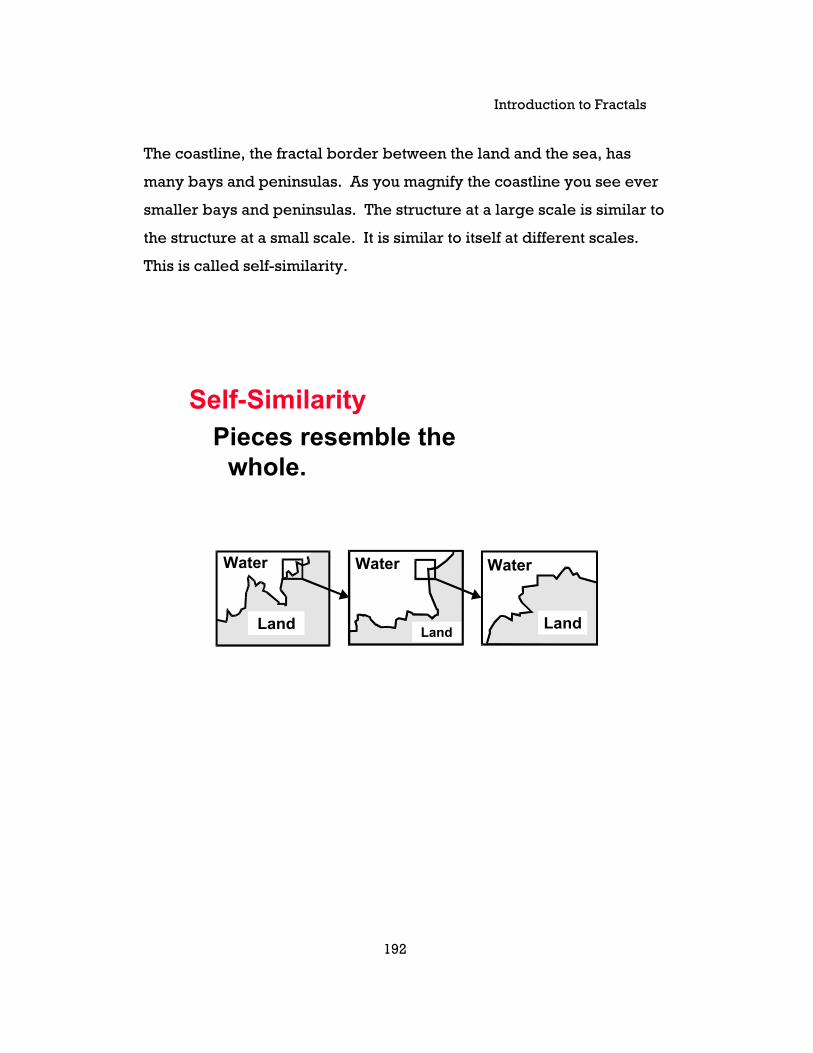
The coastline, the fractal border between the land and the sea, has
many bays and peninsulas. As you magnify the coastline you see ever
smaller bays and peninsulas. The structure at a large scale is similar to
the structure at a small scale. It is similar to itself at different scales.
This is called self-similarity.
Water
Land
Water
Land
Water
Land
Self-SimilarityPieces resemble the
whole.

Liebovitch & Shehadeh
193
This is the Sierpinski Triangle. In this mathematical object each little
piece is an exact smaller copy of the whole object.
Sierpinski Triangle

Introduction to Fractals
194
The blood vessels in the retina are self-similar. The branching of the
larger vessels is like the branching of the smaller vessels. The airways
in the lung are self-similar. The branching of the larger airways is like
the branching of the smaller airways. In real biological objects like
these, each little piece is not an exact copy of the whole object. It is
kind of like the whole object which is known as statistical self-similarity.
Branching Patternsblood vessels
Family, Masters, and Platt 1989Physica D38:98-103Mainster 1990 Eye 4:235-241
in the retinaair waysin the lungsWest and Goldberger 1987Am. Sci. 75:354-365

Liebovitch & Shehadeh
195
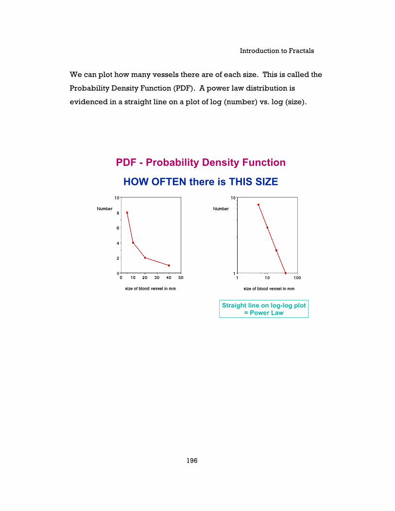
Let’s try to understand statistical self-similarity. Here is an
unrealistically simplified picture of the blood vessels in the retina. If
we ask how many vessels are there of each different size we see that
there is one that is 40mm long, two that are 20mm long, four that are
10mm long, and eight that are 5 mm long.
Blood Vessels in the Retina
Introduction to Fractals
196
We can plot how many vessels there are of each size. This is called the
Probability Density Function (PDF). A power law distribution is
evidenced in a straight line on a plot of log (number) vs. log (size).
PDF - Probability Density Function
HOW OFTEN there is THIS SIZE
Straight line on log-log plot= Power Law

Liebovitch & Shehadeh
197
The PDF of the large vessels is a straight line on a plot of log (number)
vs. log(size). There are a few big-big vessels, many medium-big
vessels, and a huge number of small-big vessels.
The PDF of the small vessels is also a straight line on a plot of
log(Number) vs. Log(size). There are a few big-small vessels, many
medium-small vessels, and a huge number of small-small vessels.
The PDF of the big vessels has the same shape (i.e., is similar to) the
PDF of the small vessels. The PDF is a measure of the statistics of the
vessels. So, the PDF (the statistics) of the large vessels is similar to the
PDF (the statistics) of the small vessels. This is statistical self-similarity.
The small pieces are not exact copies of the large pieces, but the
statistics of the small pieces are similar to the statistics of the large
pieces.
Statistical Self-Similarity
The statistics of the big pieces is the sameas the statistics of the small pieces.
Number
10001001011
10
100
1000
10001001011
10
100
1000
size in µm size in mm
NumberSMALLblood
vessels
BIGblood
vessels
Introduction to Fractals
198
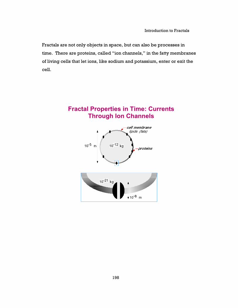
Fractals are not only objects in space, but can also be processes in
time. There are proteins, called “ion channels,” in the fatty membranes
of living cells that let ions, like sodium and potassium, enter or exit the
cell.
Fractal Properties in Time: CurrentsThrough Ion Channels
Liebovitch & Shehadeh
199
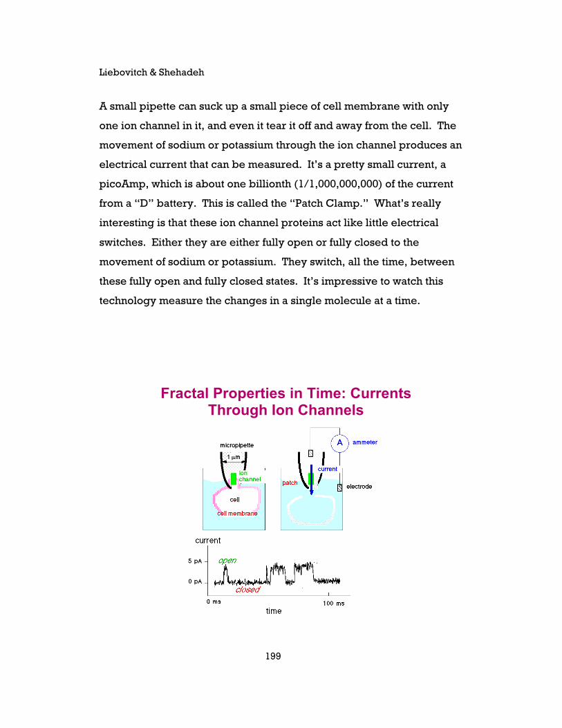
A small pipette can suck up a small piece of cell membrane with only
one ion channel in it, and even it tear it off and away from the cell. The
movement of sodium or potassium through the ion channel produces an
electrical current that can be measured. It’s a pretty small current, a
picoAmp, which is about one billionth (1/1,000,000,000) of the current
from a “D” battery. This is called the “Patch Clamp.” What’s really
interesting is that these ion channel proteins act like little electrical
switches. Either they are either fully open or fully closed to the
movement of sodium or potassium. They switch, all the time, between
these fully open and fully closed states. It’s impressive to watch this
technology measure the changes in a single molecule at a time.
Fractal Properties in Time: CurrentsThrough Ion Channels

Introduction to Fractals
200
These open and closed times are fractal! If you record them and play
them back slowly you see a sequences of open and closed times. But if
you take one segment of time, and play it back at higher resolution, you
see that it actually consists of many briefer open and closed times. It is
self-similar in time.
Currents Through Ion Channels
ATP sensitive potassium channel incell from the pancreas
Gilles, Falke, and Misler (Liebovitch 1990 Ann. N.Y. Acad. Sci. 591:375-391)
5 sec
5 msec
5 pA
FC = 10 Hz
FC = 1k Hz

Liebovitch & Shehadeh
201
Here is a histogram of the times (in ms) that one channel was closed.
The recording was made at the fastest time resolution, allowing the
briefest closed times to be recorded. The PDF is mostly a straight line
on this log (number) versus time (t) plot, but with an occasional longer
closed time. Data with fractal properties often have unusual events that
occur more often than expected from the usual “Bell Curve.” Those
occasional longer closed times are a hint that these data might be
fractal.
Closed Time Histogramspotassium channel in the
corneal endothelium
NumberofclosedTimesperTimeBin intheRecord
Liebovitch et al. 1987 Math. Biosci. 84:37-68
Closed Time in ms

Introduction to Fractals
202
Here is another histogram of the closed times (in ms) of that same ion
channel. This recording was made at a little slower time resolution and
so longer closed times were recorded. The PDF is mostly a straight line
on this log (number) versus time (t) plot, but with an occasional longer
closed time.
Closed Time Histogramspotassium channel in the
corneal endothelium
NumberofclosedTimesperTimeBin intheRecord
Liebovitch et al. 1987 Math. Biosci. 84:37-68
Closed Time in ms
Liebovitch & Shehadeh
203
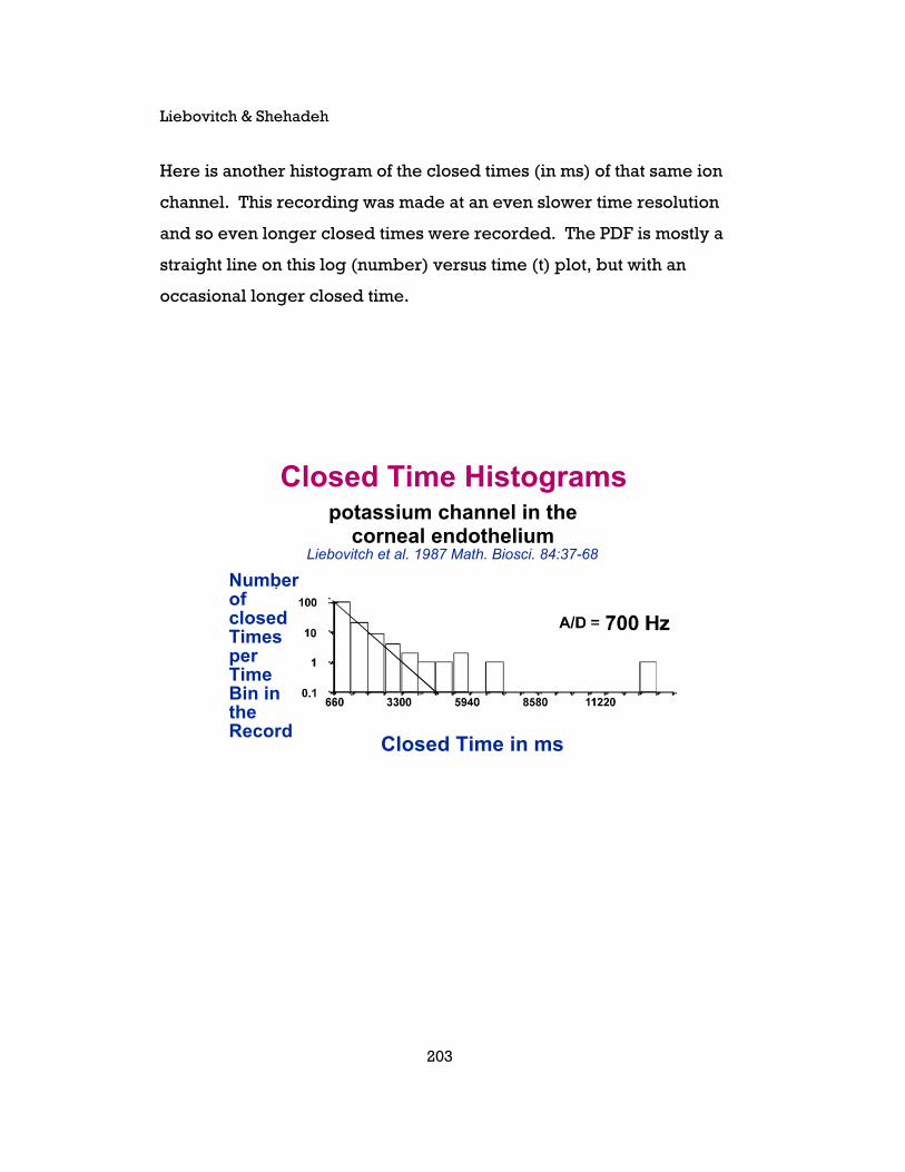
Here is another histogram of the closed times (in ms) of that same ion
channel. This recording was made at an even slower time resolution
and so even longer closed times were recorded. The PDF is mostly a
straight line on this log (number) versus time (t) plot, but with an
occasional longer closed time.
Closed Time in ms
NumberofclosedTimesperTimeBin intheRecord
Closed Time Histogramspotassium channel in the
corneal endotheliumLiebovitch et al. 1987 Math. Biosci. 84:37-68

Introduction to Fractals
204
Here is another histogram of the closed times (in ms) of that same ion
channel. This recording was made at a much lower time resolution and
so only the longest closed times were recorded. The PDF is mostly a
straight line on this log (number) versus time (t) plot, but with an
occasional longer closed time. The PDF looks similar at different time
resolutions. The PDF is a measure of the statistics. So, the statistics is
similar to itself at different time resolutions. This is statistical self-
similarity in time.
Closed Time Histogramspotassium channel in the
corneal endothelium
NumberofclosedTimesperTimeBin intheRecord
Liebovitch et al. 1987 Math. Biosci. 84:37-68
Closed Time in ms
Liebovitch & Shehadeh
205
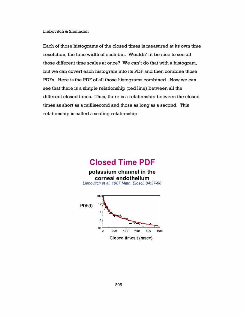
Each of those histograms of the closed times is measured at its own time
resolution, the time width of each bin. Wouldn’t it be nice to see all
those different time scales at once? We can’t do that with a histogram,
but we can covert each histogram into its PDF and then combine those
PDFs. Here is the PDF of all those histograms combined. Now we can
see that there is a simple relationship (red line) between all the
different closed times. Thus, there is a relationship between the closed
times as short as a millisecond and those as long as a second. This
relationship is called a scaling relationship.
Closed Time PDFpotassium channel in the
corneal endotheliumLiebovitch et al. 1987 Math. Biosci. 84:37-68

Introduction to Fractals
206
Fractals
Scaling
Scaling: The value measured depends upon the resolution used to
make the measurement.

Liebovitch & Shehadeh
207
If we measure the length of the west coast of Britain with a large ruler,
we get a certain value for the length of the coastline. If we now
measure it again with a smaller ruler, we catch more of the smaller bays
and peninsulas that we missed before, and so the coastline
measurement is longer. The value we measure for the coastline
depends on the size of the ruler that we use to measure it.
Scaling The value measured depends
on the resolution used to dothe measurement.

Introduction to Fractals
208
Here is a plot of how the length of the west coast of Britain depends
upon the resolution that we use to measure it. There is no one value
that best describes the length of the west coast of Britain. It depends
upon the scale (resolution) at which we measure it. As we measure it at
a finer scale, we include the segments of the smaller bays and
peninsulas, and the coastline is longer. This is one of the surprising
way in which fractals change the most basic way that we analyze and
understand our data. There is no one number that best describes the
length of the west coast of Britain. Instead, what is important is how the
length depends upon the resolution that we use to measure it. The
more smaller bays and peninsulas, the more the length of the coast
increases when it is measured at a finer resolution, and the steeper the
slope on this plot. This plot therefore shows that the coast of Britain is
rougher than that of Australia, which is rougher than that of South
Africa, which is rougher than that of a plain circle.
How Long is the Coastline of Britain?Richardson 1961 The problem of contiguity: An Appendix to Statistics of
Deadly Quarrels General Systems Yearbook 6:139-187
Lo
g10
(T
ota
l Len
gth
in K
m)
AUSTRIALIAN COAST
CIRCLE
SOUTH AFRICAN COAST
GERMAN LAND-FRONTIER, 1900WEST COAST OF BRITIAN
LAND-FRONTIER OF PORTUGAL
4.0
3.5
3.0
1.0 1.5 2.0 2.5 3.0 3.5
LOG10 (Length of Line Segments in Km)
Liebovitch & Shehadeh
209
Iannaccone and his colleagues study how organisms develop in order
to understand and cure cancer in kids. They mix cells from another
animal into an embryo so that the fate of these marker cells can be
traced out as the animal develops. The cells that are added have a
different enzyme, which attaches to a radioactive marker that blackens
a photographic film to make a picture. On the following page are some
of those pictures of the liver. Look, the added cells are not in one
clump. They are in islands of all different sizes.
There is no one area that best describes the size of these islands. The
area measured depends on the resolution used. This scaling
relationship is a straight line on a plot of log (area) versus log
(resolution).
There is no one perimeter that best describes the size of these islands.
The perimeter measured depends on the resolution used. This scaling
relationship is also a straight line on a plot of log (perimeter) versus log
(resolution).
This is one of the surprising way in which fractals change the most basic
way that we analyze and understand our data. There is no one number
that best describes the area or perimeter of these islands. Instead,
what is important is how the area or perimeter depends upon the
resolution that we use to measure it.

Introduction to Fractals
210
Genetic Mosaics in the LiverP. M. Iannaccone. 1990. FASEB J. 4:1508-1512.
Y.-K. Ng and P. M. Iannaccone. 1992. Devel. Biol. 151:419-430.

Liebovitch & Shehadeh
211
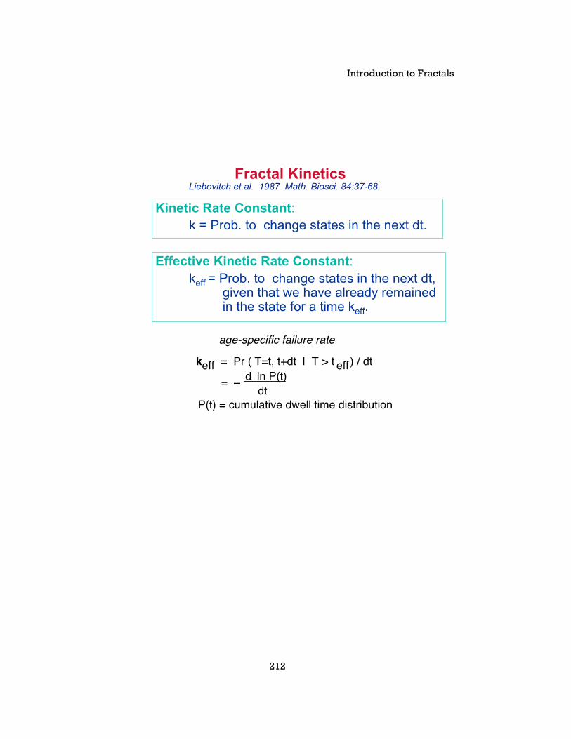
So far, we’ve seen fractal scaling in space. There are also fractal
scaling in time. The usual way to measure the switching of an ion
channel is the “kinetic rate constant.” That tells us the probability that
the ion channel switches between open and closed states. But the ion
channel must be closed (or open) long enough for us to see it as closed
(or open). A more appropriate measure is the probability that the ion
channel switches between open and closed states, given that it has
already remained in a state for a certain amount of time. That certain
amount of time defines the time resolution at which we measure the
switching probability. We called that probability the “effective kinetic
rate constant” (keff),
keff = Pr (T=t, t+Δt | T > teff) / Δt, [5.1]
which is the probability (Pr) for the ion channel to open (or close)
during the time interval T = (t, t+Δt), given that it has already remained
closed (or open) for a time T ≥ teff. In the branch of statistics called
renewal theory, keff is called the “age specific failure rate,” for
example, the probability that a light bulb fails in the next second given
it has already burned for teff hours. In the branch of statistics used in
epidemiology and insurance, keff is called the “survival rate,” for
example, the probability that a patient dies of cancer this year, if they
have already had cancer for teff years.
Introduction to Fractals
212
Kinetic Rate Constant:k = Prob. to change states in the next dt.
Effective Kinetic Rate Constant:keff = Prob. to change states in the next dt,
given that we have already remainedin the state for a time keff.
k = Pr ( T=t, t+dt | T > t ) / dteff eff
age-specific failure rate
= – ddtln P(t)
P(t) = cumulative dwell time distribution
Fractal KineticsLiebovitch et al. 1987 Math. Biosci. 84:37-68.

Liebovitch & Shehadeh
213
We measured the open and closed times for an ion channel in the cells
in the cornea, the clear part in the front of the eye that you look through
to see these words. The effective kinetic rate constant is a straight line
on a plot of log (effective kinetic rate constant) versus log (effective
time used to measure it). This is a fractal scaling relationship in time.
The faster we could look, the briefer open and closed times we would
see.
70 pS K+ ChannelCorneal Endothelium
Liebovitch et al. 1987 Math. Biosci. 84:37-68.
effk in Hz
effective time scaleteff in msec
effectivekineticrate
constant100
1000
10
11 10 100 1000
keff = A teff1-D
Introduction to Fractals
214
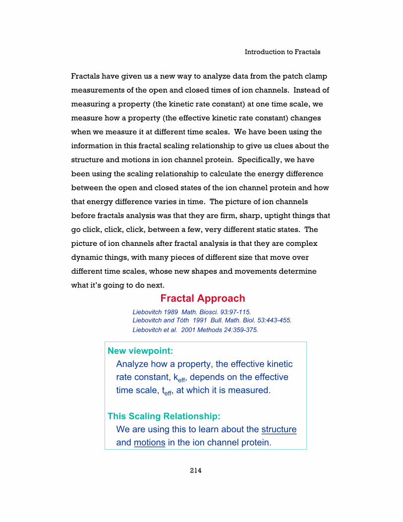
Fractals have given us a new way to analyze data from the patch clamp
measurements of the open and closed times of ion channels. Instead of
measuring a property (the kinetic rate constant) at one time scale, we
measure how a property (the effective kinetic rate constant) changes
when we measure it at different time scales. We have been using the
information in this fractal scaling relationship to give us clues about the
structure and motions in ion channel protein. Specifically, we have
been using the scaling relationship to calculate the energy difference
between the open and closed states of the ion channel protein and how
that energy difference varies in time. The picture of ion channels
before fractals analysis was that they are firm, sharp, uptight things that
go click, click, click, between a few, very different static states. The
picture of ion channels after fractal analysis is that they are complex
dynamic things, with many pieces of different size that move over
different time scales, whose new shapes and movements determine
what it’s going to do next.
Fractal Approach
New viewpoint:
Analyze how a property, the effective kinetic
rate constant, keff, depends on the effective
time scale, teff, at which it is measured.
This Scaling Relationship:
We are using this to learn about the structure
and motions in the ion channel protein.
Liebovitch 1989 Math. Biosci. 93:97-115.Liebovitch and Tóth 1991 Bull. Math. Biol. 53:443-455.
Liebovitch et al. 2001 Methods 24:359-375.
Liebovitch & Shehadeh
215
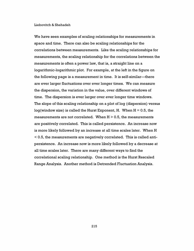
We have seen examples of scaling relationships for measurements in
space and time. There can also be scaling relationships for the
correlations between measurements. Like the scaling relationships for
measurements, the scaling relationship for the correlations between the
measurements is often a power law, that is, a straight line on a
logarithmic-logarithmic plot. For example, at the left in the figure on
the following page is a measurement in time. It is self-similar—there
are ever larger fluctuations over ever longer times. We can measure
the dispersion, the variation in the value, over different windows of
time. The dispersion is ever larger over ever longer time windows.
The slope of this scaling relationship on a plot of log (dispersion) versus
log(window size) is called the Hurst Exponent, H. When H = 0.5, the
measurements are not correlated. When H > 0.5, the measurements
are positively correlated. This is called persistence. An increase now
is more likely followed by an increase at all time scales later. When H
< 0.5, the measurements are negatively correlated. This is called anti-
persistence. An increase now is more likely followed by a decrease at
all time scales later. There are many different ways to find the
correlational scaling relationship. One method is the Hurst Rescaled
Range Analysis. Another method is Detrended Fluctuation Analysis.
Introduction to Fractals
216
Correlations
window 1window 2window 3
disp
ersio
n 1
disp
ersio
n 2
disp
ersio
n 3
Measures of disperson:Hurst Rescaled Range Analysis: R/SDetrended Fluctuation Analysis: DFA
log (window size)
H = 1/2no correlation
anti-persistent
H < 1/2
persistentH > 1/2
log (dispersion)
Liebovitch & Shehadeh
217
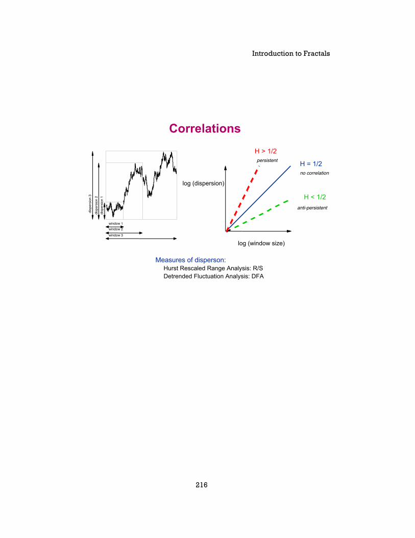
On the left, the Hurst rescaled range analysis was used to measure the
correlations in the open and closed times of an ion channel protein
(open circles). At short times, H = 0.6, and at along times H = 0.9.
These are very persistent correlations. The correlations disappear
(black circles) when the order of the open and closed times was
randomly shuffled. This means that there is a long term “memory,”
which gets stronger with time, in how the shape of the ion channel
protein changes in time. Previous models of ion channels, as shown on
the right, assumed that the channel switched between a few, discrete
shapes, without any memory. This fractal analysis tells us that ion
channels do not behave that way. Instead, the fractal analysis has
enabled us to see that there are important, continuous dynamical
processes, with memory, going on inside the ion channel protein.
C8 C7 C6 C5 C4Ca++ Ca++ Ca++ Ca++
C3 C2 C1Ca++ Ca++
8-state Markovian Model
“memoryless”H = 0.5
Data
“a process with memory”
H = 0.6
H = 0.9
Kochetkov, et al. 1999. J. Biol. Phys. 25:211-222.
Fractal Kinetics
Introduction to Fractals
218
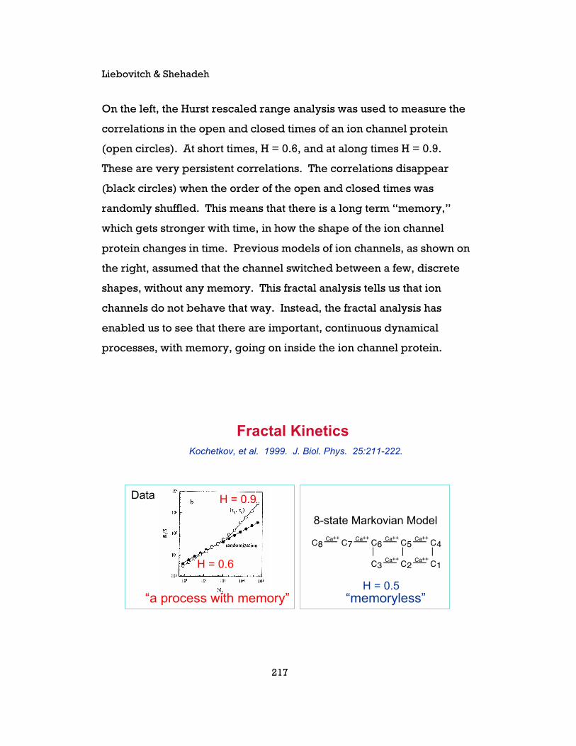
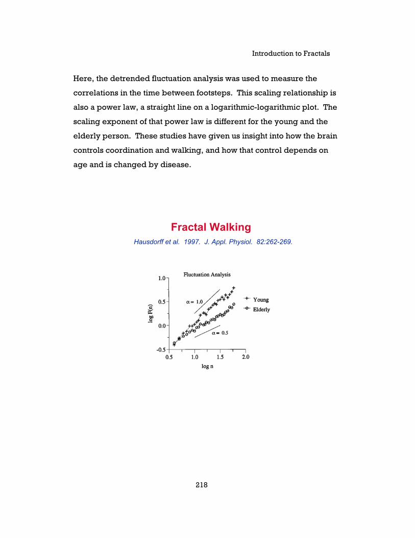
Here, the detrended fluctuation analysis was used to measure the
correlations in the time between footsteps. This scaling relationship is
also a power law, a straight line on a logarithmic-logarithmic plot. The
scaling exponent of that power law is different for the young and the
elderly person. These studies have given us insight into how the brain
controls coordination and walking, and how that control depends on
age and is changed by disease.
Fractal WalkingHausdorff et al. 1997. J. Appl. Physiol. 82:262-269.
Liebovitch & Shehadeh
219
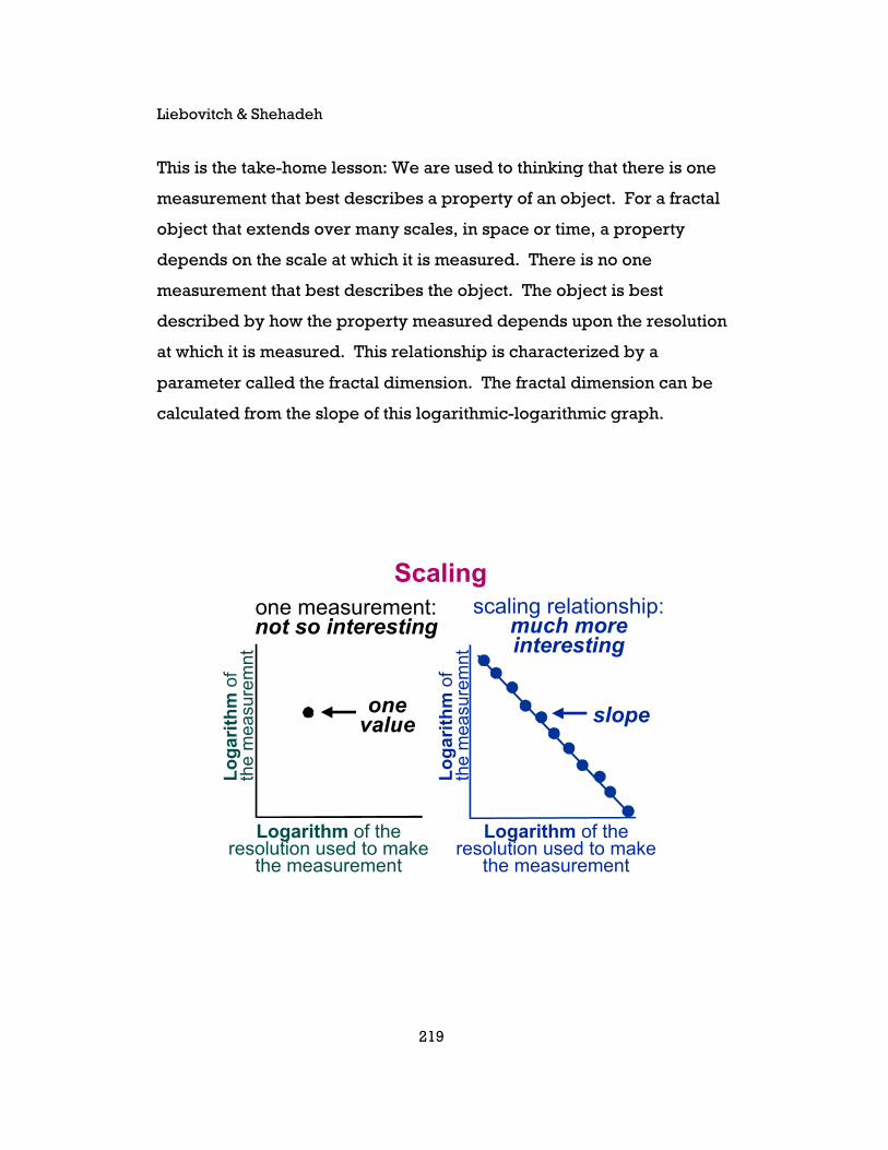
This is the take-home lesson: We are used to thinking that there is one
measurement that best describes a property of an object. For a fractal
object that extends over many scales, in space or time, a property
depends on the scale at which it is measured. There is no one
measurement that best describes the object. The object is best
described by how the property measured depends upon the resolution
at which it is measured. This relationship is characterized by a
parameter called the fractal dimension. The fractal dimension can be
calculated from the slope of this logarithmic-logarithmic graph.
one measurement:not so interesting
slope
Scaling
Lo
gar
ith
m o
f th
e m
easu
rem
nt
Lo
gar
ith
m o
f th
e m
easu
rem
nt
onevalue
Logarithm of theresolution used to make
the measurement
Logarithm of theresolution used to make
the measurement
scaling relationship:much moreinteresting
Introduction to Fractals
220
Fractals
Statistics
Fractals have some unique statistical properties. The “average” size
depends on the resolution used to make the measurement. What is
important is not the average, but how the average depends on the
resolution used to make the measurement.

Liebovitch & Shehadeh
221
Here is a set of numbers; maybe they are the values measured from an
experiment. I have drawn a circle to represent each number. The
diameter of the circle is proportional to the magnitude of the number.
Here is a non-fractal set of numbers. Most of them are about the size of
an average number. A few are a bit smaller than the average. A few
are bit larger than the average.
Not Fractal

Introduction to Fractals
222
Here is the PDF of theoe non-fractal numbers. The PDF is how many
numbers there are of each size. The PDF here is called a “Bell Curve,”
a “Gaussian Distribution,” or a “Normal Distribution.” It’s strange that
someone chose to call this a “normal” distribution. We are about to see
that much of the world is definitely not like this kind of “normal.”
Not Fractal

Liebovitch & Shehadeh
223
Here is a picture of Gauss on the old 10 Deustche Mark German bill. He
has now been replaced by the 5 Euro. You can see his curve and even
the equation for it on this bill! There are no equations on American
money. (There is a scientist on American money. Do you know who it
is?)
GaussianBell Curve“Normal Distribution”

Introduction to Fractals
224
Here is a set of numbers from a fractal distribution. The diameter of
each circle is proportional to the size of the number. These numbers
could be from the room around you. Look around your room. There
are few big things (people and chairs), many medium-sized things
(pens and coins), and a huge number of tiny things (dust and bacteria).
It is not at all like that “Normal” distribution. Sets of data from many
things in the real world are just like this. We call this a fractal
distribution of numbers because it has the same statistical properties as
the sizes of the pieces in fractal objects.
Fractal

Liebovitch & Shehadeh
225
Here is the PDF of these fractal numbers. The PDF is how many
numbers there are of each size. There are a few big numbers, many
medium sized numbers, and a huge amount of tiny numbers. The PDF
is a straight line on a plot of log(How Many Numbers; the PDF) versus
log(value of the numbers).
Fractal

Introduction to Fractals
226
The statistics of a fractal set of numbers is very different from the
statistics of “normal” numbers that they taught you about in Statistics
101. The statistics you learned in Statistics 101 is only about non-fractal
numbers. Take the average of a sample of non-fractal numbers. This is
called the Sample Mean. As you include ever more data, the sample
means, shown here as µ, get ever closer to one value. We call that
value the Population Mean, shown here as µpop. We think that the
population mean is the “real” value of the mean.
Mean
Non - Fractal
More Data
pop
Liebovitch & Shehadeh
227
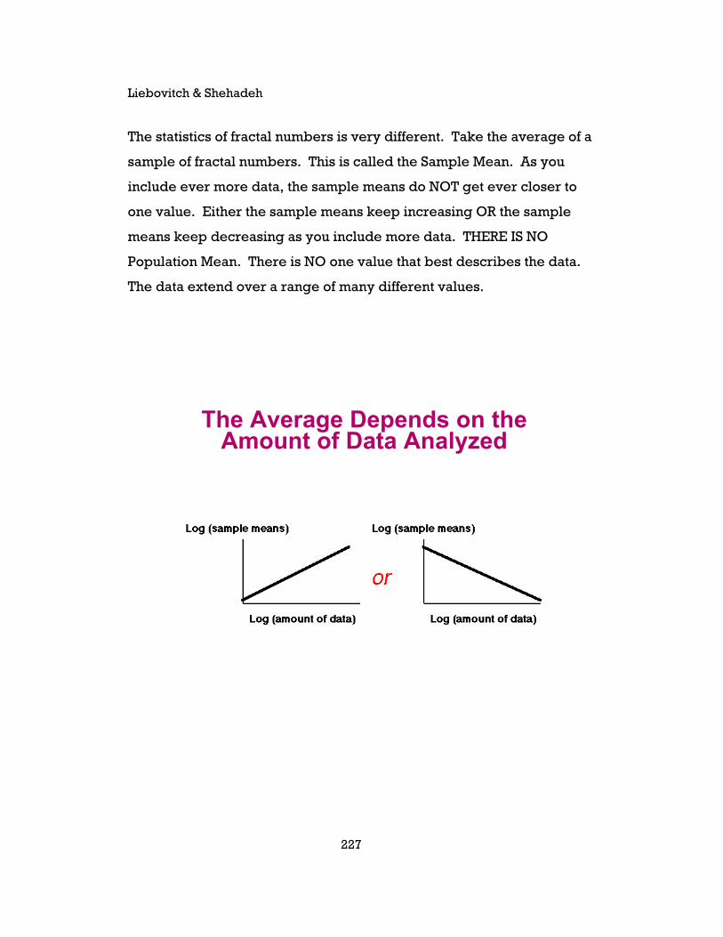
The statistics of fractal numbers is very different. Take the average of a
sample of fractal numbers. This is called the Sample Mean. As you
include ever more data, the sample means do NOT get ever closer to
one value. Either the sample means keep increasing OR the sample
means keep decreasing as you include more data. THERE IS NO
Population Mean. There is NO one value that best describes the data.
The data extend over a range of many different values.
The Average Depends on theAmount of Data Analyzed

Introduction to Fractals
228
Here is why that happens. Again, here is a set of fractal numbers. The
diameter of the circles are proportional to the size of the numbers. As
you include ever more numbers one of two things will happen:
1. If there is an excess of many small values, the sample means
get smaller and smaller.
2. If there is an excess of a few big values, the sample means get
larger and larger
Whether 1 or 2 happens depends on the ratio of the amount of small
numbers to the amount of big numbers. That ratio is characterized by a
parameter called the Fractal Dimension.
The Average Depends on theAmount of Data Analyzed
each piece

Liebovitch & Shehadeh
229
Let’s play a non-fractal game of chance. Toss a coin, if it comes up tails
we win nothing, if it comes up heads we win $1. The average winnings
are the probability of each outcome times how much we win on that
outcome. The average winnings are (1/2) x ($0) + (1/2) x ($1) = 50¢.
Let’s go to a fair casino to play this game. Fair casinos exist only in
math textbooks; “fair” means the bank is willing only to break even and
not make a profit. We and the casino think it’s fair for us to be charged
50¢ to play one game. That seems reasonable; half the time we win
nothing, half the time we win $1, so if it costs 50¢ to play each time, on
average, we and the casino will break even.
Ordinary Coin Toss
Toss a coin. If it is tails win$0, If it is heads win $1.
The average winnings are:2-1.1 = 0.5
1/2
Non-Fractal
Introduction to Fractals
230
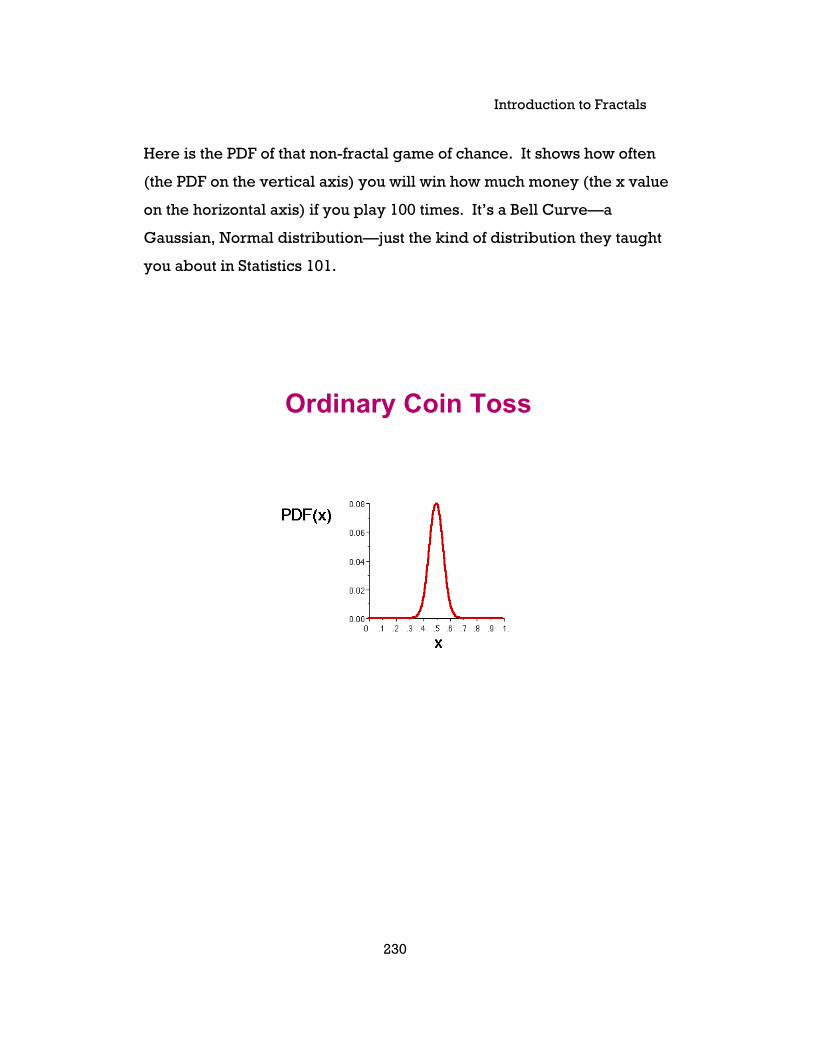
Here is the PDF of that non-fractal game of chance. It shows how often
(the PDF on the vertical axis) you will win how much money (the x value
on the horizontal axis) if you play 100 times. It’s a Bell Curve—a
Gaussian, Normal distribution—just the kind of distribution they taught
you about in Statistics 101.
Ordinary Coin Toss

Liebovitch & Shehadeh
231
Here’s what happens when I played that non-fractal game, over and
over again. A computer (actually a Macintosh Plus running Microsoft
BASIC!) picked a random number to simulate flipping the coin. Here,
the average winnings per game is shown after n games. For a while I
(the Mac) was lucky. I was winning more than an average 50¢ in each
game. But, as you might suspect (this is called the Law of Large
Numbers), after a while my luck ran out. In the long run, I was winning
exactly an average of 50¢ in each game.
Ordinary Coin Toss
Introduction to Fractals
232
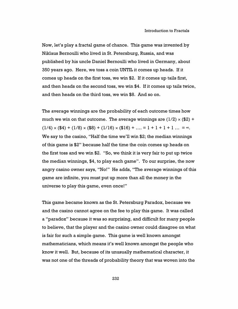
Now, let’s play a fractal game of chance. This game was invented by
Niklaus Bernoulli who lived in St. Petersburg, Russia, and was
published by his uncle Daniel Bernoulli who lived in Germany, about
350 years ago. Here, we toss a coin UNTIL it comes up heads. If it
comes up heads on the first toss, we win $2. If it comes up tails first,
and then heads on the second toss, we win $4. If it comes up tails twice,
and then heads on the third toss, we win $8. And so on.
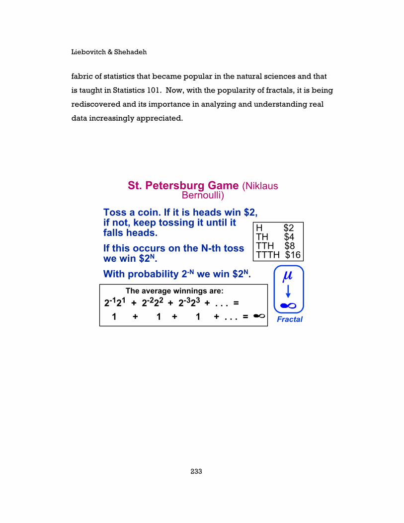
The average winnings are the probability of each outcome times how
much we win on that outcome. The average winnings are (1/2) × ($2) +
(1/4) × ($4) + (1/8) × ($8) + (1/16) × ($16) + …. = 1 + 1 + 1 + 1 … = ∞.
We say to the casino, “Half the time we’ll win $2; the median winnings
of this game is $2” because half the time the coin comes up heads on
the first toss and we win $2. “So, we think it is very fair to put up twice
the median winnings, $4, to play each game”. To our surprise, the now
angry casino owner says, “No!” He adds, “The average winnings of this
game are infinite, you must put up more than all the money in the
universe to play this game, even once!”
This game became known as the St. Petersburg Paradox, because we
and the casino cannot agree on the fee to play this game. It was called
a “paradox” because it was so surprising, and difficult for many people
to believe, that the player and the casino owner could disagree on what
is fair for such a simple game. This game is well known amongst
mathematicians, which means it’s well known amongst the people who
know it well. But, because of its unusually mathematical character, it
was not one of the threads of probability theory that was woven into the
Liebovitch & Shehadeh
233
fabric of statistics that became popular in the natural sciences and that
is taught in Statistics 101. Now, with the popularity of fractals, it is being
rediscovered and its importance in analyzing and understanding real
data increasingly appreciated.
St. Petersburg Game (NiklausBernoulli)
Toss a coin. If it is heads win $2,if not, keep tossing it until itfalls heads.
If this occurs on the N-th tosswe win $2N.
With probability 2-N we win $2N.
H $2TH $4TTH $8TTTH $16
The average winnings are:
2-121 + 2-222 + 2-323 + . . . =
1 + 1 + 1 + . . . = Fractal
Introduction to Fractals
234
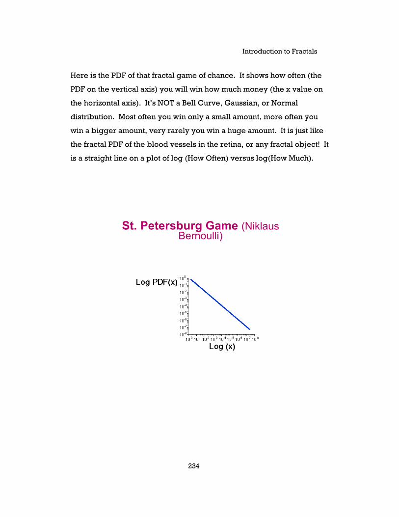
Here is the PDF of that fractal game of chance. It shows how often (the
PDF on the vertical axis) you will win how much money (the x value on
the horizontal axis). It’s NOT a Bell Curve, Gaussian, or Normal
distribution. Most often you win only a small amount, more often you
win a bigger amount, very rarely you win a huge amount. It is just like
the fractal PDF of the blood vessels in the retina, or any fractal object! It
is a straight line on a plot of log (How Often) versus log(How Much).
St. Petersburg Game (NiklausBernoulli)

Liebovitch & Shehadeh
235
Here’s what happens when I played that fractal game over and over
again. Here, the average winnings per game is shown after n games.
The more I played, the more often there was sometimes a lot of tails
before that first head. When there are a lot of those tails, I won a huge
jackpot. As more and more of those jackpots happened, the average
winnings per game kept increasing. There is no average (population
mean) for this game. The more I played, the more the average kept
changing. They told you in Statistics 101 that the more data you have,
the closer the sample means are to the population mean. Not here!
There is no population mean. The more data we have (the more games
I played) the more the sample means keep changing. The few
exponentially large wins keep pushing the sample mean up, which is
very different than what you learned in Statistics 101. Welcome to
fractals.
St. Petersburg Game (NiklausBernoulli)

Introduction to Fractals
236
Here is a non-fractal object. It is a checkerboard. Actually, I’m only
showing you a piece of it; it should really extend forever in each
direction. Place a circle on it. Count all the black pixels in that circle,
and divide by the total number of pixels. That is the average density
within that circle. The graph shows how that density changes as the
circles get bigger and bigger. The average density fluctuates a bit;
after all, we are putting a round circle over a square grid. But, as the
circles get bigger and bigger, the average density gets closer and
closer to 1/2. This seems reasonable because the checkerboard is 1/2
black and 1/2 white.
Non-Fractal
Log avgdensity within
radius r
Log radius r
Liebovitch & Shehadeh
237
The figure on the next page is a fractal object. It is called a Diffusion
Limited Aggregation (DLA). It is statistically self-similar. It has little
spaces between its little arms, medium spaces between its medium-
sized arms, and large spaces between its large arms. We’re only
showing you a piece of it, but it should also really extend forever in
each direction. Place a circle on it. Count all the black pixels in that
circle, and divide by the total number of pixels. That gives the average
density within that circle. The graph shows how that density changes as
the circles get bigger and bigger. As the circles get bigger we catch
more of the ever larger spaces between the arms, and so the density
gets smaller. As the circles get ever bigger, the density gets ever
smaller. There is no one density that describes this object. What’s
more, the local density on a big arm is very high. The local density
between big arms is very low. Yet, the same mechanism makes the
arms and the spaces between them. Based upon our Statistics 101
training, we are used to thinking that when the local average changes,
when there is a difference in the mean value between an experiment
and a control, or between now and then, that the system must have
changed. Here, fractals, with infinite variance, have moments, such as
the mean, that can be very different in space and time or between
experiments and controls, even though the basic process has not
changed at all!

Introduction to Fractals
238
Fractal
Log avgdensity within radius r
Log radius r
.5
-1.0
-2.0
-1.5
.5 1.0 1.5 2.0 2.5 3.0 3.5 4.0 4.5 5.0 5.5 6.00-2.5
0
Meakin 1986 In On Growthand Form: Fractal and Non-Fractal Patterns inPhysics Ed. Stanley & Ostrowsky, Martinus Nijoff Pub., pp. 111-135

Liebovitch & Shehadeh
239
Here is yet another example of fractal data. Data from many
experiments have fractal properties. Here are the action potentials, the
little electrical sparks, that encode information sent down the nerves in
your body. Teich et al. measured them in the auditory nerve, which
brings information about sounds from your ear to your brain.
Electrical Activity of Auditory NerveCells
Teich, Jonson, Kumar, and Turcott 1990 Hearing Res. 46:41-52
voltage
time
action potentials
Introduction to Fractals
240
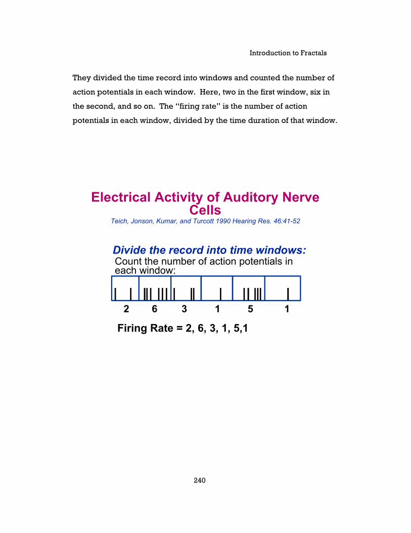
They divided the time record into windows and counted the number of
action potentials in each window. Here, two in the first window, six in
the second, and so on. The “firing rate” is the number of action
potentials in each window, divided by the time duration of that window.
Electrical Activity of Auditory NerveCells
Teich, Jonson, Kumar, and Turcott 1990 Hearing Res. 46:41-52
2
Count the number of action potentials ineach window:
6 3 1 5 1
Firing Rate = 2, 6, 3, 1, 5,1
Divide the record into time windows:
Liebovitch & Shehadeh
241
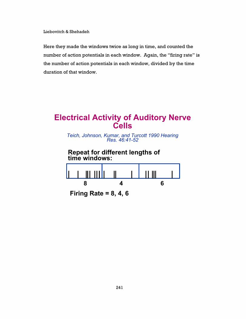
Here they made the windows twice as long in time, and counted the
number of action potentials in each window. Again, the “firing rate” is
the number of action potentials in each window, divided by the time
duration of that window.
Electrical Activity of Auditory NerveCells
Teich, Johnson, Kumar, and Turcott 1990 HearingRes. 46:41-52
Repeat for different lengths oftime windows:
8 4 6
Firing Rate = 8, 4, 6

Introduction to Fractals
242
In Statistics 101 they taught you that as you collect more data, the
fluctuations average out. You were taught to expect that the fluctuations
in the firing rate should be less as the time windows get longer. But
look here—the variations don’t change much as the time windows go
from 0.5 s to 5.0 s to 50.0 s! [Actually, the real deal here is that the
variance of the fluctuations falls much slower than 1/sqrt(n)]. You
include more data, but you don’t get any closer to the real firing rate.
There is no one single value, like a population mean, that best
describes the firing rate. The increase in variation at longer time
windows is real. It represents correlations in the action potentials
which may tell how information is encoded in the timing of the action
potentials.
Electrical Activity of Auditory Nerve CellsTeich, Jonson, Kumar, and Turcott 1990 Hearing Res. 46:41-52
0
Thevariationin thefiring ratedoes notdecreaseat longertimewindows.
4 8 12 16 20 24 28
70
60
80
90
100
120
130
140
110
150
T = 50.0 sec T = 5.0 sec
T = 0.5 sec
FIR
ING
RA
TE
SAMPLE NUMBER (each of duration T sec)
Liebovitch & Shehadeh
243
Fractals
Power Law PDFs
PDFs: Fractal data have a characteristic PDF form called a Power Law.
Introduction to Fractals
244
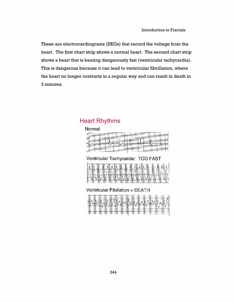
These are electrocardiograms (EKGs) that record the voltage from the
heart. The first chart strip shows a normal heart. The second chart strip
shows a heart that is beating dangerously fast (ventricular tachycardia).
This is dangerous because it can lead to ventricular fibrillation, where
the heart no longer contracts in a regular way and can result in death in
3 minutes.
Heart Rhythms
Liebovitch & Shehadeh
245
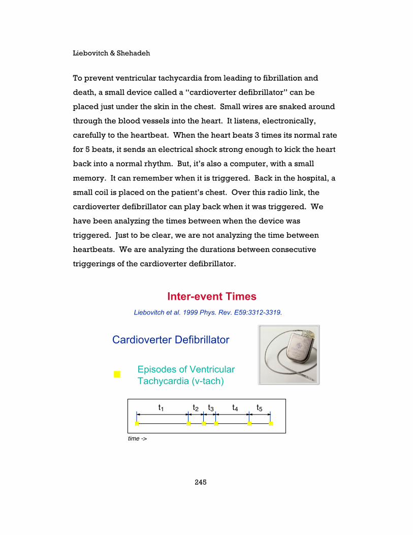
To prevent ventricular tachycardia from leading to fibrillation and
death, a small device called a “cardioverter defibrillator” can be
placed just under the skin in the chest. Small wires are snaked around
through the blood vessels into the heart. It listens, electronically,
carefully to the heartbeat. When the heart beats 3 times its normal rate
for 5 beats, it sends an electrical shock strong enough to kick the heart
back into a normal rhythm. But, it’s also a computer, with a small
memory. It can remember when it is triggered. Back in the hospital, a
small coil is placed on the patient’s chest. Over this radio link, the
cardioverter defibrillator can play back when it was triggered. We
have been analyzing the times between when the device was
triggered. Just to be clear, we are not analyzing the time between
heartbeats. We are analyzing the durations between consecutive
triggerings of the cardioverter defibrillator.
Inter-event Times
Episodes of VentricularTachycardia (v-tach)
t1 t2 t3 t4 t5
time ->
Cardioverter Defibrillator
Liebovitch et al. 1999 Phys. Rev. E59:3312-3319.
Introduction to Fractals
246
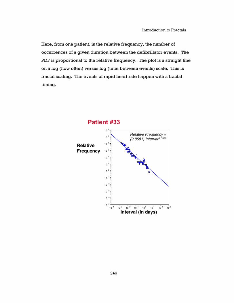
Here, from one patient, is the relative frequency, the number of
occurrences of a given duration between the defibrillator events. The
PDF is proportional to the relative frequency. The plot is a straight line
on a log (how often) versus log (time between events) scale. This is
fractal scaling. The events of rapid heart rate happen with a fractal
timing.
Interval (in days)
RelativeFrequency
10 310 210 110 010 -110 -210 -310 -410 -5
10 -4
10 -3
10 -2
10 -1
10 0
10 1
10 2
10 3
10 4
10 5
10 6
Relative Frequency =(9.8581) Interval-1.0988
Patient #33
Liebovitch & Shehadeh
247
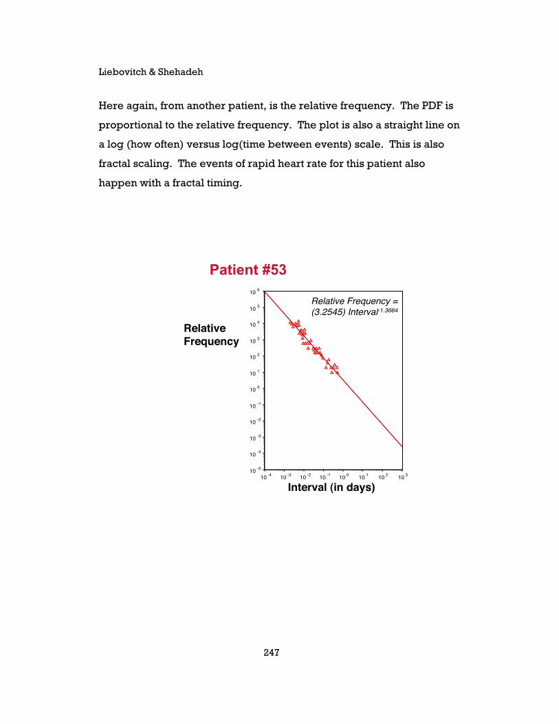
Here again, from another patient, is the relative frequency. The PDF is
proportional to the relative frequency. The plot is also a straight line on
a log (how often) versus log(time between events) scale. This is also
fractal scaling. The events of rapid heart rate for this patient also
happen with a fractal timing.
Interval (in days)
RelativeFrequency
Relative Frequency =(3.2545) Interval-1.3664
10 310 210 110 010 -110 -210 -310 -410 -5
10 -4
10 -3
10 -2
10 -1
10 0
10 1
10 2
10 3
10 4
10 5
10 6
Patient #53
Introduction to Fractals
248
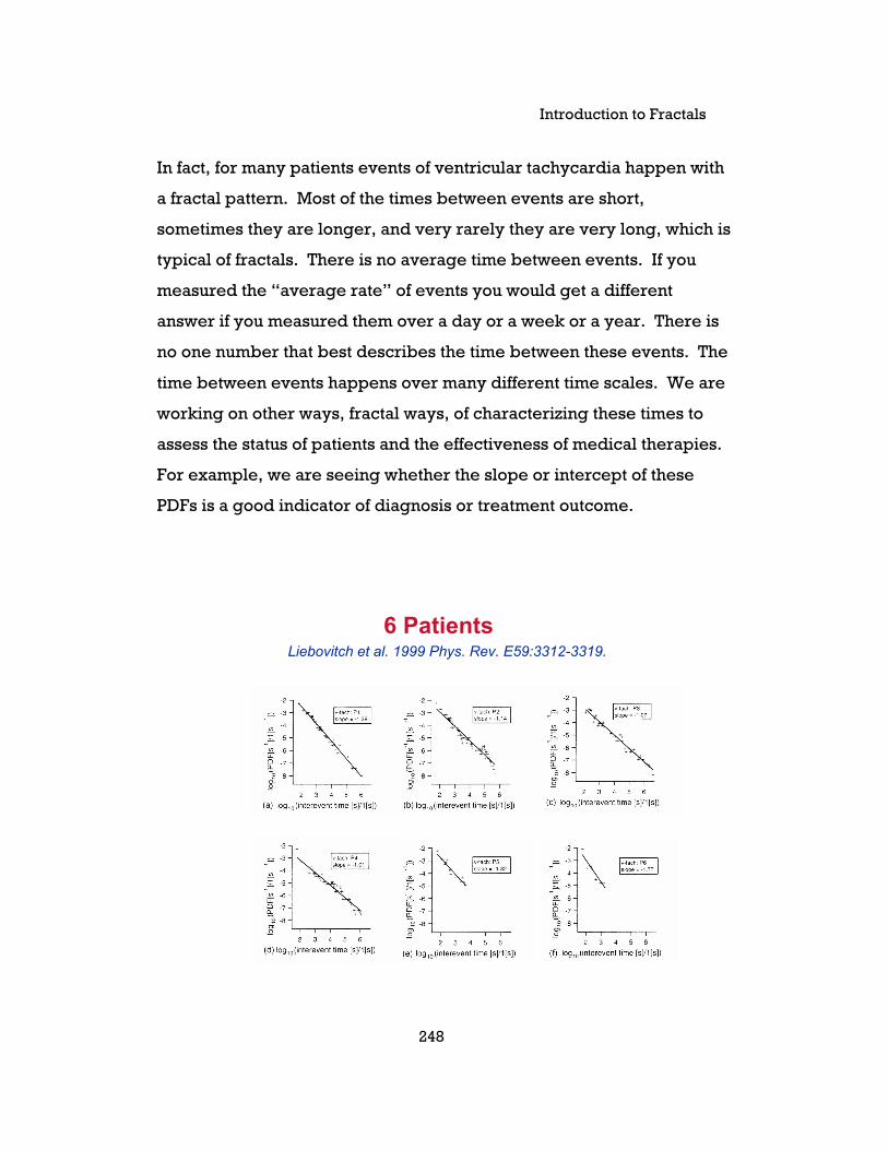
In fact, for many patients events of ventricular tachycardia happen with
a fractal pattern. Most of the times between events are short,
sometimes they are longer, and very rarely they are very long, which is
typical of fractals. There is no average time between events. If you
measured the “average rate” of events you would get a different
answer if you measured them over a day or a week or a year. There is
no one number that best describes the time between these events. The
time between events happens over many different time scales. We are
working on other ways, fractal ways, of characterizing these times to
assess the status of patients and the effectiveness of medical therapies.
For example, we are seeing whether the slope or intercept of these
PDFs is a good indicator of diagnosis or treatment outcome.
6 PatientsLiebovitch et al. 1999 Phys. Rev. E59:3312-3319.
Liebovitch & Shehadeh
249
We are also analyzing the times at which different e-mail viruses arrive
at the gateway into an internet service provider. On the picture on the
following page are the events—the arrival times of e-mail viruses. We
are looking at the duration of times between the arrival of each virus.
We have studied 4 viruses:
1. AnnaKournikova doesn’t have a picture of her, it’s a file that
you wouldn’t want to open.
2. Magistr can erase sectors on your hard disk or your
cmos/bios. If you don’t know what the cmos/bios is, you don’t
want us to tell you what happens if it gets erased.
3. Klez puts together messages by joining fragments of phrases
that it contains.
4. Sircam tempts you to open and execute its attached file.
Much is known about the structure of the Internet. Less is known about
the dynamics of the Internet. The arrival times of these viruses depend
on both the structure and dynamics of the Internet. We are hoping that
our study of these arrival times will tell us how the structure interacts
with the dynamics if the Internet.

Introduction to Fractals
250
Inter-arrival Times of E-mail Viruses
t1 t2 t3 t4 t5
time ->
Liebovitch and Schwartz 2003 Phys. Rev. E68:017101.
AnnaKournikova"Hi: Check This!” AnnaKournikova.jpg vbs.
MagistrSubject, body, attachment from other files: erase disk, cmos/bios.
KlezE-mail from its own phrases: infect by just viewing in Outlook Express.
Sircam“I send you this file in order to have your advice.”
Liebovitch & Shehadeh
251
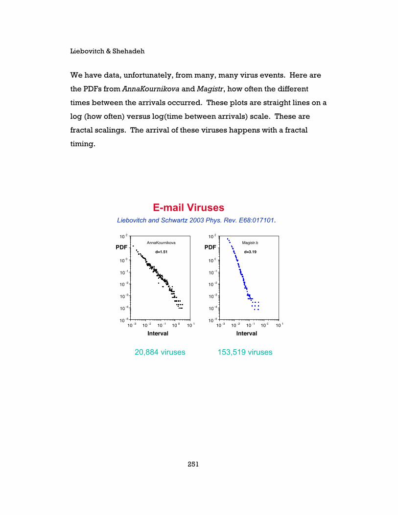
We have data, unfortunately, from many, many virus events. Here are
the PDFs from AnnaKournikova and Magistr, how often the different
times between the arrivals occurred. These plots are straight lines on a
log (how often) versus log(time between arrivals) scale. These are
fractal scalings. The arrival of these viruses happens with a fractal
timing.
E-mail Viruses
10 110 010 -110 -210 -310 -5
10 -4
10 -3
10 -2
10 -1
10 0
10 1
10 2
Interval
PDFAnnaKournikova
10 110 010 -110 -210 -310 -5
10 -4
10 -3
10 -2
10 -1
10 0
10 1
10 2
Interval
PDFMagistr.b
d=1.51 d=3.19
20,884 viruses 153,519 viruses
Liebovitch and Schwartz 2003 Phys. Rev. E68:017101.
Introduction to Fractals
252
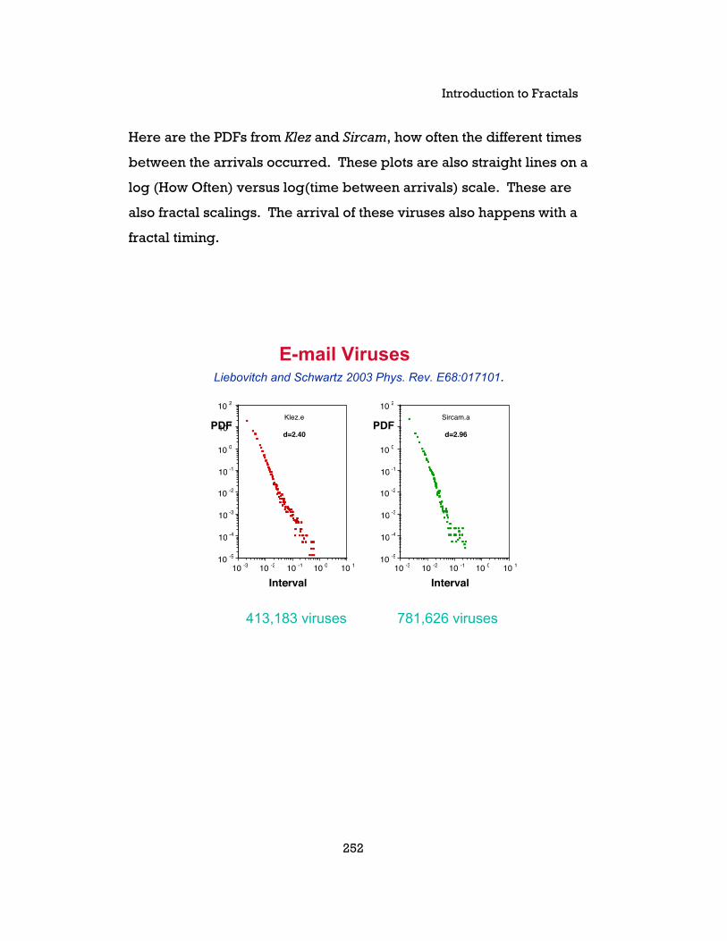
Here are the PDFs from Klez and Sircam, how often the different times
between the arrivals occurred. These plots are also straight lines on a
log (How Often) versus log(time between arrivals) scale. These are
also fractal scalings. The arrival of these viruses also happens with a
fractal timing.
E-mail Viruses
413,183 viruses 781,626 viruses
10 110 010 -110 -210 -310 -5
10 -4
10 -3
10 -2
10 -1
10 0
10 1
10 2
Interval
PDFKlez.e
10 110 010 -110 -210 -310 -5
10 -4
10 -3
10 -2
10 -1
10 0
10 1
10 2
Interval
PDFSircam.a
d=2.40 d=2.96
Liebovitch and Schwartz 2003 Phys. Rev. E68:017101.
Liebovitch & Shehadeh
253
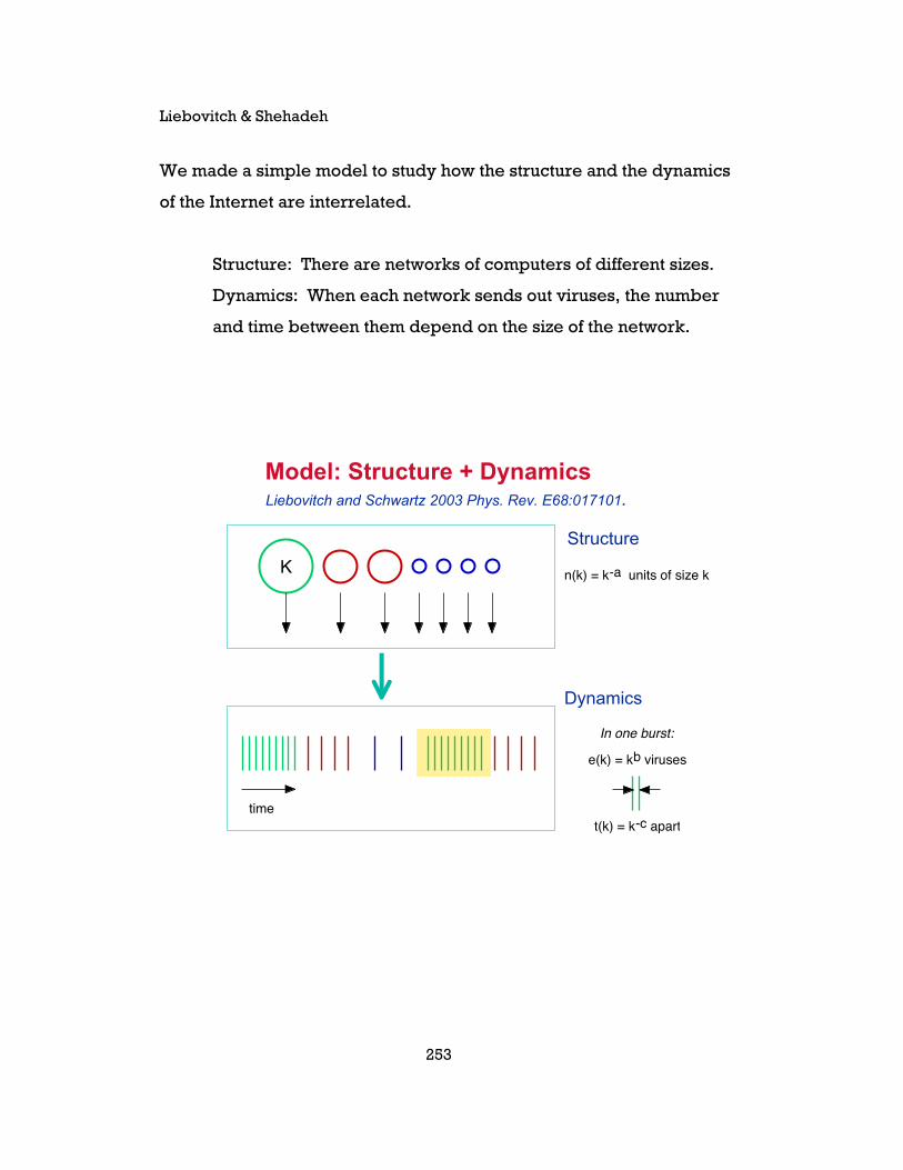
We made a simple model to study how the structure and the dynamics
of the Internet are interrelated.
Structure: There are networks of computers of different sizes.
Dynamics: When each network sends out viruses, the number
and time between them depend on the size of the network.
Model: Structure + Dynamics
Structure
Dynamics
K n(k) = k-a units of size k
e(k) = kb viruses
t(k) = k-c apart
In one burst:
time
Liebovitch and Schwartz 2003 Phys. Rev. E68:017101.
Introduction to Fractals
254
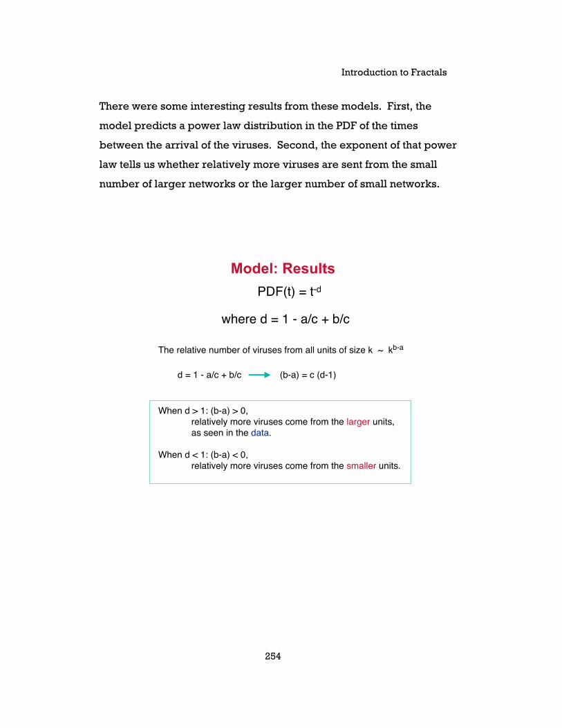
There were some interesting results from these models. First, the
model predicts a power law distribution in the PDF of the times
between the arrival of the viruses. Second, the exponent of that power
law tells us whether relatively more viruses are sent from the small
number of larger networks or the larger number of small networks.
Model: Results
The relative number of viruses from all units of size k ~ kb-a
(b-a) = c (d-1)
When d > 1: (b-a) > 0,relatively more viruses come from the larger units,as seen in the data.
When d < 1: (b-a) < 0,relatively more viruses come from the smaller units.
d = 1 - a/c + b/c
PDF(t) = t-d
where d = 1 - a/c + b/c

Liebovitch & Shehadeh
255
Fractals
Methods for Determiningthe PDFs
The PDF is an important tool in determining if experimental data have
fractal properties. A power law PDF is characteristic of fractal
behavior. The standard method for evaluating the PDF is to make a
histogram of the data. That method is very good at determining the
PDF when the data are not fractal. It is less good at determining the
PDF when the data are fractal. Next, we’ll see other ways of
determining the PDF, and how they compare to the histogram method.
Introduction to Fractals
256
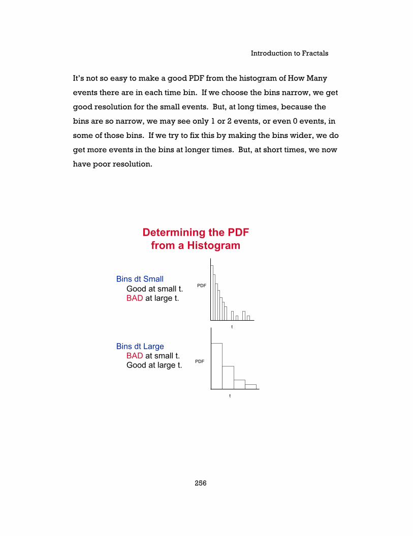
It’s not so easy to make a good PDF from the histogram of How Many
events there are in each time bin. If we choose the bins narrow, we get
good resolution for the small events. But, at long times, because the
bins are so narrow, we may see only 1 or 2 events, or even 0 events, in
some of those bins. If we try to fix this by making the bins wider, we do
get more events in the bins at longer times. But, at short times, we now
have poor resolution.
Determining the PDFfrom a Histogram
Bins dt SmallGood at small t.BAD at large t.
t
Bins dt LargeBAD at small t.Good at large t.
t

Liebovitch & Shehadeh
257
We figured out a nice algorithm to get a better PDF. Narrow bins are
good at short times. Wide bins are good at long times. So, we make
histograms of different bin sizes. But, we cannot combine histograms of
different bin sizes. However, we can compute the PDF from each
histogram and then combine the PDFs. For each histogram, the PDF(t)
is N(t), the number of values in the bin that covers (t, t+dt), divided by
Nt, the total number of values in that histogram, divided by dt, the width
of the bins in that histogram. The histograms with narrow bins give us
good resolution in the PDF at short times. The histograms with wide
bins give us good values in the PDF at long times. We’ve found that this
method yields accurate and reliable PDFs for tails of many different
kinds of distributions. See Liebovitch et al. 1999 for details.
Determining the PDFLiebovitch et al. 1999 Phys. Rev. E59:3312-3319.
Solution:Make ONE PDFFrom SEVERAL Histograms of DIFFERENT Bin Size
Choose dt = 1, 2, 4, 8, 16 … seconds
PDF = N(t)Ntotdt
N(t) = number in [t, t+dt]
Ntot = total number in each histogramdt = bin size

Introduction to Fractals
258
Here, PDFs were measured from a set of fractal data. The red boxes
indicate the PDF made in the usual way from one histogram. You can
see where there are only 1 or 2 events in the largest bins. The black
boxes indicate the PDF generated from the same data using the new
multi-histogram method to make the PDF. Pretty impressive difference.
New multi-histogram
Standard fixed dt
10 410 310210 110 010 -110 -210 -6
10 -5
10 -4
10 -3
10 -2
10 -1
10 0
10 1
Values
Determining the PDF
Liebovitch & Shehadeh
259
Fractals
Summary

Introduction to Fractals
260
SELF-SIMILARITY
Definition: Pieces of an object in space, or parts of a process in time, are
smaller versions of the whole object or process.
Examples: The Sierpinski Triangle in space and the times between the
arrival of e-mail viruses.
Methods: A power law distribution of the PDF of the pieces of an object
in space or the parts of a process in time is indicative of fractal
behavior.
Importance for data analysis: There is no single scale, in space or time,
that characterizes such data that extends over many scales.
Summary of Fractal PropertiesSummary of Fractal Properties
Self-SimilarityPieces resemble the
whole.
Liebovitch & Shehadeh
261
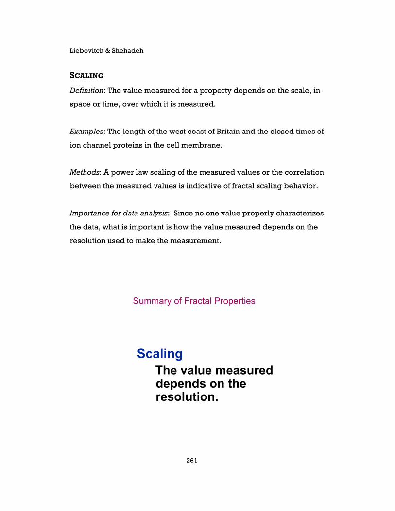
SCALING
Definition: The value measured for a property depends on the scale, in
space or time, over which it is measured.
Examples: The length of the west coast of Britain and the closed times of
ion channel proteins in the cell membrane.
Methods: A power law scaling of the measured values or the correlation
between the measured values is indicative of fractal scaling behavior.
Importance for data analysis: Since no one value properly characterizes
the data, what is important is how the value measured depends on the
resolution used to make the measurement.
Summary of Fractal PropertiesSummary of Fractal Properties
Scaling The value measured
depends on theresolution.

Introduction to Fractals
262
STATISTICS
Definition: The PDF is a power law. The population mean and
population standard deviation don’t exist.
Examples: The winnings in the St. Petersburg game and the variation in
the times between action potentials recorded from auditory nerve cells
in the ear.
Methods: A power law distribution of the PDF or a power law scaling
relationship for the moments is indicative of fractal behavior.
Importance for data analysis: When the mean depends on the spatial
scale, the temporal scale, or how much data we analyze, then the mean
is meaningless. What is meaningful is how the sample means, or
another scaling property, depend on the spatial scale, the temporal
scale, or how much data we analyze, which is described by the fractal
dimension.
Summary of Fractal PropertiesSummary of Fractal Properties
Statistical Properties Moments may be zero
or infinite.

Liebovitch & Shehadeh
263
Probability theory started from solving gambling problems about 400
years ago. About 200 years ago, those results were used to develop
basic statistics. Most of the statistical tests we use were developed less
than 100 years ago. We show you this to emphasize that statistics is
NOT a dead science, although it’s often presented like that in Statistics
101. It has changed a lot. It is still changing. It will change even more
in the future. The statistical properties of fractals are examples of new
ideas that are now being incorporated into and are changing statistics.
400 years ago:Gambling Problems Probability Theory
200 years ago:Statistics How we do experiments.
100 years ago:Student’s t-test, F-test, ANOVA
Now:Still changing
Statistics is NOT a dead science.

Introduction to Fractals
264
The take-home lesson here is not that fractals some arcane super-
sophisticated mathematical tool that only needs to be used in some
strange circumstance. Fractals change the most basic way we look at
experimental data. They allow us to analyze and make sense out of the
huge amount of real data that “just ain’t a bell curve.” The most
common use of mathematics and statistics in all science is means ±
s.e.m. Fractals tell us that if the data are fractal, those means are
meaningless! That’s a pretty basic change in the simplest way we
handle data. That’s what revolutions in science are about—not about
changing the complex stuff, but about changing the simplest stuff. The
stuff that we were taught so firmly that we never thought it would
change.
Fractals CHANGE the most basic ways weanalyze and understand experimental data.
Fractals
Measurements over many scales.
What is real is not one number, but how the measured
values change with the scale at which they are measured
(fractal dimension).
No Bell CurvesNo Moments
No mean ± s.e.m.

Liebovitch & Shehadeh
265
TO LEARN MORE ABOUT FRACTALS
1. A book called Fractals and Chaos Simplified for the Life Sciences
(Liebovitch, 1998). This book consists of facing pages, where the left
page is text and the right page is a picture. It leads you, one concept at
a time, through the material.
2. A CD-ROM of curricula materials for a mathematics course for
college students who never liked and never did well in math (funded,
in part, by the National Science Foundation, Division of Undergraduate
Education). The materials emphasize what mathematics is, how
mathematicians do mathematics, and how mathematics is used in
science. We’re almost finished with it and would be happy to send you
a free demo (contact information is on the first page of this chapter).References:References:
Fractals and Chaos and
Simplified for the Life
Sciences
Larry S. Liebovitch
Oxford Univ. Press, 1998
The Mathematics and
Science of Fractals
Larry S. Liebovitch and
Lina Shehadehwww.ccs.fau.edu/~liebovitch/
larry.html
CD ROM
NSFDUE-9752226DUE-9980715
Introduction to Fractals
266
We have concentrated here (and in the references noted on the
previous page) on providing an introduction to fractal concepts, their
importance, and what can be learned from them. Here are some books
that describe the mathematical details of these methods and give
examples of how scientists have used them.
Technical Details
J. Feder. 1988. Fractals. Plenum Press.t.
J. B. Bassingthwaighte, L. S. Liebovitch and B. J. West.1994. Fractal Physiology. Oxford University Press.
P. M. Iannaccone and M. Khokha. 1996. FractalGeometry in Biological Systems. CRC Press.
A. Bunde and S. Havlin, eds. 1994. Fractals inScience. Springer-Verlag.
ACKNOWLEDGEMENTS
The development of some of these materials was supported, in part, by
NSF grants DUE-9752226 and DUE-9980715.
Related Documents