Chapter 1 Introduction to Fluid Mechanics

Welcome message from author
This document is posted to help you gain knowledge. Please leave a comment to let me know what you think about it! Share it to your friends and learn new things together.
Transcript
Chapter 1
Introduction to Fluid Mechanics
Definition
Mechanics is the oldest physical science that deals with
both stationary and moving bodies under the influence of
forces.
The branch of mechanics that deals with bodies at rest is
called statics, while the branch that deals with bodies in
motion is called dynamics.
The subcategory fluid mechanics is defined as the science
that deals with the behavior of fluids at rest (fluid statics)
or in motion (fluid dynamics), and the interaction of fluids
with solids or other fluids at the boundaries.
The study of fluids at rest is called fluid statics.
2

Definition
The study of f1uids in motion, where pressure forces are
not considered, is called fluid kinematics and if the
pressure forces are also considered for the fluids in
motion. that branch of science is called fluid dynamics.
Fluid mechanics itself is also divided into several
categories.
The study of the motion of fluids that are practically
incompressible (such as liquids, especially water, and
gases at low speeds) is usually referred to as
hydrodynamics.
A subcategory of hydrodynamics is hydraulics, which
deals with liquid flows in pipes and open channels.
3

Gas dynamics deals with the flow of fluids that undergo
significant density changes, such as the flow of gases
through nozzles at high speeds.
The category aerodynamics deals with the flow of gases
(especially air) over bodies such as aircraft, rockets, and
automobiles at high or low speeds.
Some other specialized categories such as meteorology,
oceanography, and hydrology deal with naturally
occurring flows.
Definition
4
What is a Fluid?
A substance exists in three primary phases: solid, liquid,
and gas. A substance in the liquid or gas phase is referred
to as a fluid.
Distinction between a solid and a fluid is made on the basis
of the substance’s ability to resist an applied shear (or
tangential) stress that tends to change its shape.
A solid can resist an applied shear stress by deforming,
whereas a fluid deforms continuously under the influence
of shear stress, no matter how small.
In solids stress is proportional to strain, but in fluids stress
is proportional to strain rate.
5

What is a Fluid?
When a constant
shear force is
applied, a solid
eventually stops
deforming, at some
fixed strain angle,
whereas a fluid
never stops
deforming and
approaches a certain
rate of strain.
Figure.
Deformation of a rubber eraser
placed between two parallel plates
under the influence of a shear force.
6

In a liquid, molecules can move
relative to each other, but the volume
remains relatively constant because of
the strong cohesive forces between the
molecules.
As a result, a liquid takes the shape of
the container it is in, and it forms a
free surface in a larger container in a
gravitational field.
A gas, on the other hand, expands until
it encounters the walls of the container
and fills the entire available space.
This is because the gas molecules are
widely spaced, and the cohesive forces
between them are very small.
Unlike liquids, gases cannot form a
free surface7
What is a Fluid?

8
Differences between liquid and gases
Liquid Gases
Difficult to compress and
often regarded as
incompressible
Easily to compress – changes of
volume is large, cannot normally
be neglected and are related to
temperature
Occupies a fixed volume
and will take the shape of
the container
No fixed volume, it changes
volume to expand to fill the
containing vessels
A free surface is formed if
the volume of container is
greater than the liquid.
Completely fill the vessel so that
no free surface is formed.
What is a Fluid?

Application areas of Fluid Mechanics
Mechanics of fluids is extremely important in many areas of engineering and science. Examples are:
Biomechanics
Blood flow through arteries and veins
Airflow in the lungs
Flow of cerebral fluid
Households
Piping systems for cold water, natural gas, and sewage
Piping and ducting network of heating and air-conditioning systems
refrigerator, vacuum cleaner, dish washer, washingmachine, water meter, natural gas meter, air conditioner,radiator, etc.
Meteorology and Ocean Engineering
Movements of air currents and water currents9

Application areas of Fluid Mechanics
Mechanical Engineering Design of pumps, turbines, air-conditioning equipment,
pollution-control equipment, etc.
Design and analysis of aircraft, boats, submarines,
rockets, jet engines, wind turbines, biomedical devices,
the cooling of electronic components, and the
transportation of water, crude oil, and natural gas.
Civil Engineering
Transport of river sediments
Pollution of air and water
Design of piping systems
Flood control systems
Chemical Engineering
Design of chemical processing equipment10

Turbomachines: pump, turbine, fan, blower, propeller, etc.
Military: Missile, aircraft, ship, underwater vehicle, dispersion
of chemical agents, etc.
Automobile: IC engine, air conditioning, fuel flow, external
aerodynamics, etc.
Medicine: Heart assist device, artificial heart valve, Lab-on-a-
Chip device, glucose monitor, controlled drug delivery, etc.
Electronics: Convective cooling of generated heat.
Energy: Combuster, burner, boiler, gas, hydro and wind
turbine, etc.
Oil and Gas: Pipeline, pump, valve, offshore rig, oil spill
cleanup, etc.
Almost everything in our world is either in contact with a fluid
or is itself a fluid.11
Application areas of Fluid Mechanics

The number of fluid engineering applications is enormous:
breathing, blood flow, swimming, pumps, fans, turbines,
airplanes, ships, rivers, windmills, pipes, missiles, icebergs,
engines, filters, jets, and sprinklers, to name a few.
When you think about it, almost everything on this planet
either is a fluid or moves within or near a fluid.
Application areas of Fluid Mechanics
12
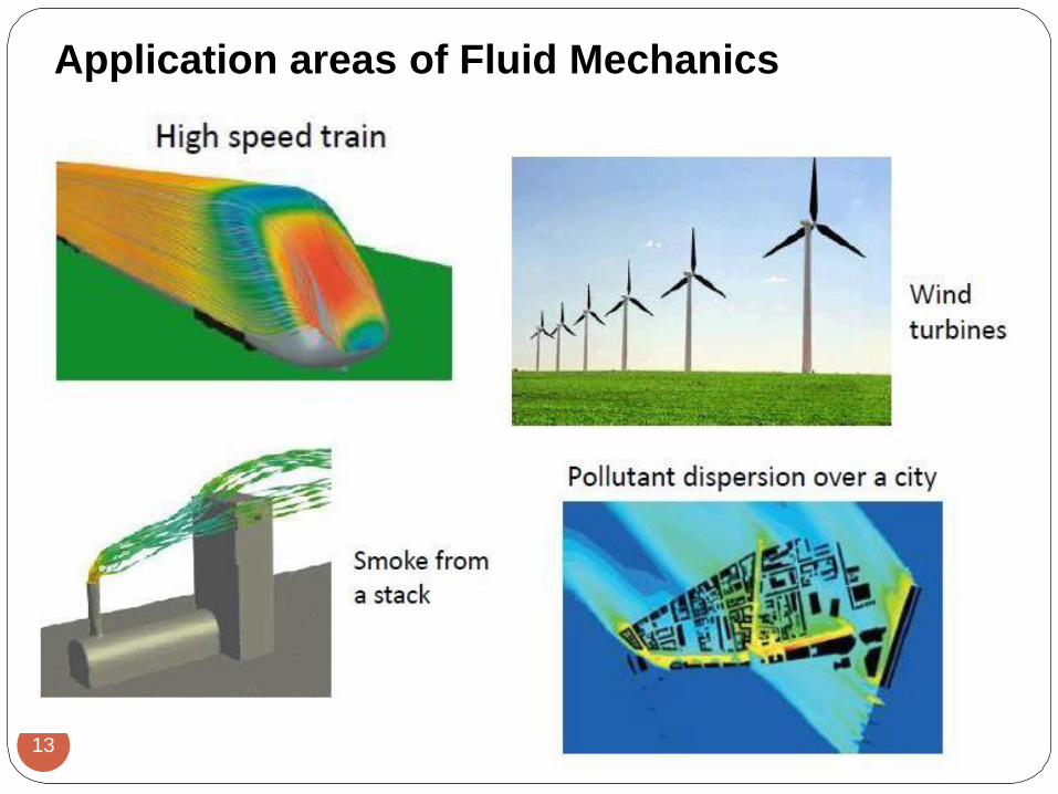
Application areas of Fluid Mechanics
13
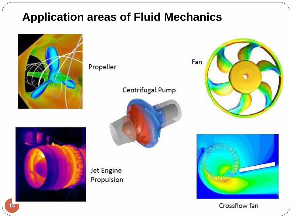
Application areas of Fluid Mechanics
14
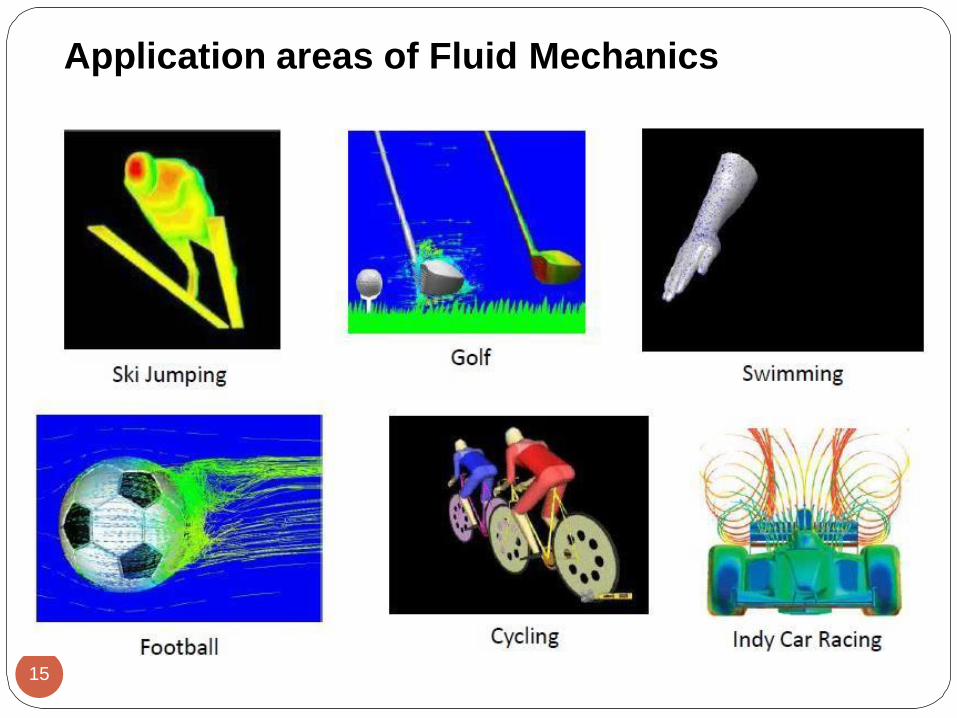
Application areas of Fluid Mechanics
15
Classification of Fluid Flows
There is a wide variety of fluid flow problems encountered
in practice, and it is usually convenient to classify them on
the basis of some common characteristics to make it
feasible to study them in groups.
Viscous versus Inviscid Regions of Flow
When two fluid layers move relative to each other, a
friction force develops between them and the slower layer
tries to slow down the faster layer.
This internal resistance to flow is quantified by the fluid
property viscosity, which is a measure of internal stickiness
of the fluid.
Viscosity is caused by cohesive forces between the
molecules in liquids and by molecular collisions in gases.
16
Viscous versus Inviscid Regions of Flow…
There is no fluid with zero viscosity, and thus all fluid
flows involve viscous effects to some degree.
Flows in which the frictional effects are significant are
called viscous flows.
However, in many flows of practical interest, there are
regions (typically regions not close to solid surfaces) where
viscous forces are negligibly small compared to inertial or
pressure forces.
Neglecting the viscous terms in such inviscid flow regions
greatly simplifies the analysis without much loss in
accuracy.
Classification of Fluid Flows
17

Viscous versus Inviscid Regions of Flow
Classification of Fluid Flows
18
Internal versus External Flow
A fluid flow is classified as being internal or external,
depending on whether the fluid is forced to flow in a
confined channel or over a surface.
The flow of an unbounded fluid over a surface such as a
plate, a wire, or a pipe is external flow.
The flow in a pipe or duct is internal flow if the fluid is
completely bounded by solid surfaces.
Water flow in a pipe, for example, is internal flow, and
airflow over a ball or over an exposed pipe during a windy
day is external flow .
Classification of Fluid Flows
19

Compressible versus Incompressible Flow
A flow is classified as being compressible or
incompressible, depending on the level of variation of
density during flow.
Incompressibility is an approximation, and a flow is said to
be incompressible if the density remains nearly constant
throughout.
Therefore, the volume of every portion of fluid remains
unchanged over the course of its motion when the flow (or
the fluid) is incompressible.
The densities of liquids are essentially constant, and thus
the flow of liquids is typically incompressible. Therefore,
liquids are usually referred to as incompressible substances.
Classification of Fluid Flows
20

Compressible versus Incompressible Flow…
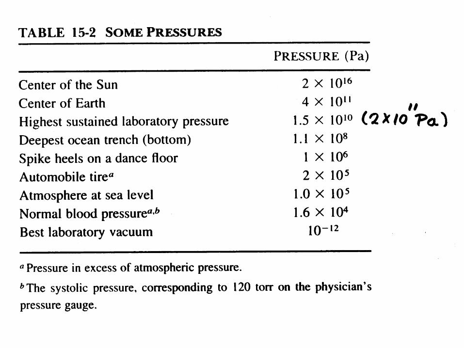
A pressure of 210 atm, for example, causes the density of
liquid water at 1 atm to change by just 1 percent.
Gases, on the other hand, are highly compressible. A
pressure change of just 0.01 atm, for example, causes a
change of 1 percent in the density of atmospheric air.
Gas flows can often be approximated as incompressible if
the density changes are under about 5 percent.
The compressibility effects of air can be neglected at
speeds under about 100 m/s.
Classification of Fluid Flows
21
Classification of Fluid Flows
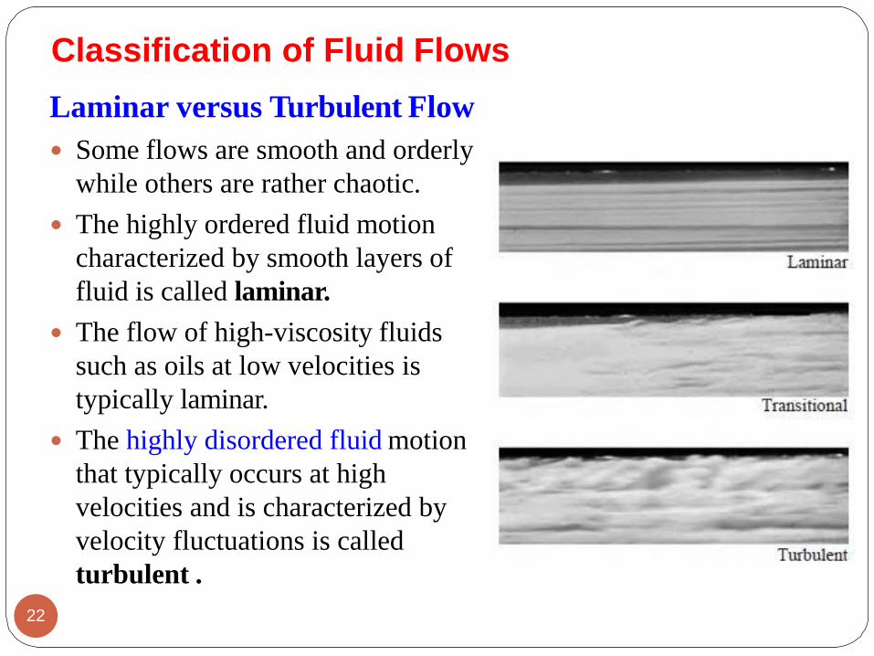
Laminar versus Turbulent Flow
Some flows are smooth and orderly
while others are rather chaotic.
The highly ordered fluid motion
characterized by smooth layers of
fluid is called laminar.
The flow of high-viscosity fluids
such as oils at low velocities is
typically laminar.
The highly disordered fluid motion
that typically occurs at high
velocities and is characterized by
velocity fluctuations is called
turbulent .
22

Classification of Fluid Flows
Laminar versus Turbulent Flow
The flow of low-viscosity fluids
such as air at high velocities is
typically turbulent.
A flow that alternates between
being laminar and turbulent is
called transitional.
23

Natural (or Unforced) versus Forced Flow
A fluid flow is said to be natural or forced, depending on
how the fluid motion is initiated.
In forced flow, a fluid is forced to flow over a surface or in
a pipe by external means such as a pump or a fan.
In natural flows, any fluid motion is due to natural means
such as the buoyancy effect, which manifests itself as the
rise of the warmer (and thus lighter) fluid and the fall of
cooler (and thus denser) fluid .
In solar hot-water systems, for example, the
thermosiphoning effect is commonly used to replace pumps
by placing the water tank sufficiently above the solar
collectors.
Classification of Fluid Flows
24
Steady versus Unsteady Flow
The terms steady and uniform are used frequently in
engineering, and thus it is important to have a clear
understanding of their meanings.
The term steady implies no change at a point with time.
The opposite of steady is unsteady.
The term uniform implies no change with location
over a specified region.
Classification of Fluid Flows
25

Properties of Fluids
Any characteristic of a system is called a property.
Some familiar properties are pressure P, temperature T,
volume V, and massm.
Other less familiar properties include viscosity, thermal
conductivity, modulus of elasticity, thermal expansion
coefficient, electric resistivity, and even velocity and
elevation.
Properties are considered to be either intensive or extensive.
Intensive properties are those that are independent of the mass
of a system, such as temperature, pressure, and density.
Extensive properties are those whose values depend on the
size—or extent—of the system. Total mass, total volume V, and
total momentum are some examples of extensive properties.
26
Properties of Fluids
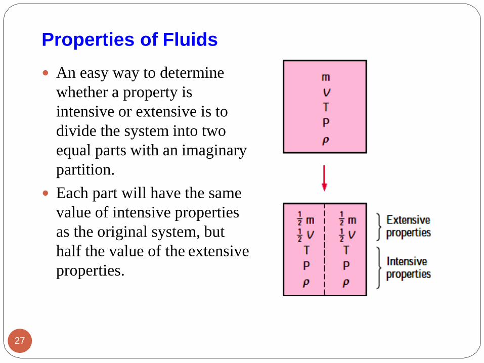
An easy way to determine
whether a property is
intensive or extensive is to
divide the system into two
equal parts with an imaginary
partition.
Each part will have the same
value of intensive properties
as the original system, but
half the value of the extensive
properties.
27
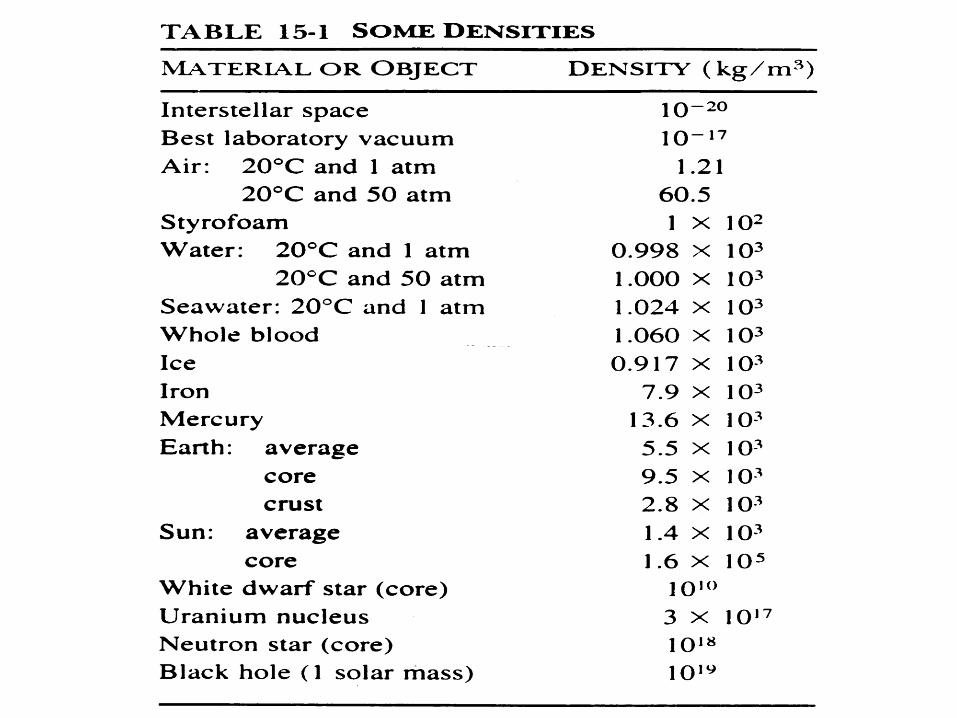
Properties of Fluids
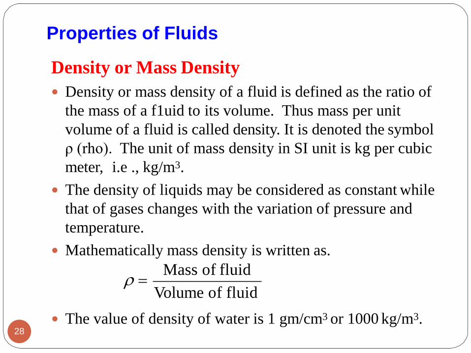
Density or Mass Density
Density or mass density of a fluid is defined as the ratio of
the mass of a f1uid to its volume. Thus mass per unit
volume of a fluid is called density. It is denoted the symbol
ρ (rho). The unit of mass density in SI unit is kg per cubic
meter, i.e ., kg/m3.
The density of liquids may be considered as constant while
that of gases changes with the variation of pressure and
temperature.
Mathematically mass density is written as.
The value of density of water is 1 gm/cm3 or 1000 kg/m3.
Volume of fluid
28
Mass of fluid =

Density or Mass Density
The density of a substance, in general, depends on
temperature and pressure.
The density of most gases is proportional to pressure and
inversely proportional to temperature.
Liquids and solids, on the other hand, are essentially
incompressible substances, and the variation of their
density with pressure is usually negligible.
Properties of Fluids
29

Properties of Fluids
Specific weight or Weight Density
Specific weight or weight density of a fluid is the ratio
between the weight of a fluid to its volume.
Thus weight per unit volume of a fluid is called weight
density and it is denoted by the symbol w.
Mathematically,
w =Weight of fluid
=(Mass of fluid) x Acceleration due to gravity
Volume of fluid Volume of fluid
=Mass of fluid x g
Volume of fluid
= x g
w = g
30

Properties of Fluids
Specific Volume
Specific volume of a fluid is defined as the volume of a
fluid occupied by a unit mass or volume per unit mass of a
fluid is called specific volume.
Mathematically, it is expressed as
Thus specific volume is the reciprocal of mass density. It is
expressed as m3/kg.
It is commonly applied to gases.
1
Mass of fluid
Volume
Mass of fluid=
1Specific volume =
Volume offluid =
31

Properties of Fluids
32
Weight density (density)of air
Thus weight density of a liquid = S x Weight densityof water
= S x 1000x 9.81N/m3
Thus density of a liquid = S x Densityof water
= S x 1000kg/m3
Specific Gravity.
Specific gravity is defined as the ratio of the weight density (or
density) of a fluid to the weight density (or density) of a standard
fluid.
For liquids, the standard fluid is taken water and for gases, the
standard fluid is taken air. Specific gravity is also called relative
density. It is dimensionless quantity and is denoted by the symbol S.
S(for liquids) =Weight density (density)of liquid
Weight density (density)of water
S(for gases) =Weight density (density)of gas
Properties of Fluids
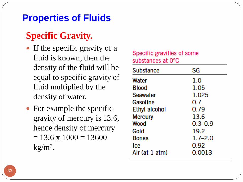
Specific Gravity.
If the specific gravity of a
fluid is known, then the
density of the fluid will be
equal to specific gravity of
fluid multiplied by the
density of water.
For example the specific
gravity of mercury is 13.6,
hence density of mercury
= 13.6 x 1000 = 13600
kg/m3.
33
Properties of Fluids
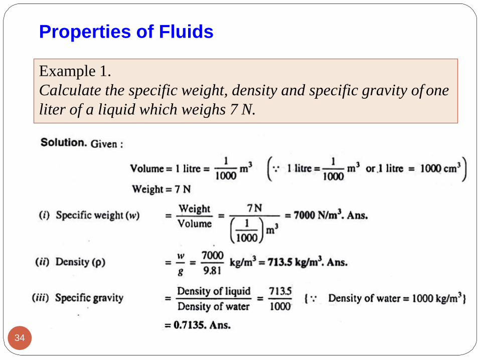
Example 1.
Calculate the specific weight, density and specific gravity of one
liter of a liquid which weighs 7 N.
34

Example 2. Calculate the density, specific weight and weight of
one liter of petrol of specific gravity = 0.7
35

Viscosity
Viscosity is defined as the property of a fluid which offers
resistance to the movement of one layer of fluid over another
adjacent layer of the fluid.
When two layers of a fluid, a distance 'dy' apart move one over
the other at different velocities say u and u+ du as shown in Fig.
1.1 , the viscosity together with relative velocity causes a shear
stress acting between the fluid layers:
Properties of Fluids
36

Properties of Fluids
Viscosity
The top layer causes a shear stress on the adjacent lower
layer while the lower layer causes a shear stress on the
adjacent top layer.
This shear stress is proportional to the rate of change of
velocity with respect to y. It is denoted by symbol τ called
Tau.
Mathematically,
or
(1.2)dy
= du
37

represents the rate of shear strain or rate of shear
deformation or velocity gradient.
From equation (1.2) we have
Thus viscosity is also defined as the shear stress
required to produce unit rate of shear strain.
dy
Properties of Fluids
where μ (called mu) is the constant of proportionality
and is known as the coefficient of dynamic viscosity or
only viscosity.
du
(1.3)du
dy
=
38

Unit of Viscosity.
The unit of viscosity is obtained by putting the
dimension of the quantities in equation ( 1.3)
Properties of Fluids
SI unit of viscosity =Newton second
=Ns
m2 m2
39

Properties of Fluids
Kinematic Viscosity.
It is defined as the ratio between the dynamic viscosity and
density of fluid.lt is denoted by the Greek symbol (ν) called
'nu' . Thus, mathematically,
=Viscosity
=
Density
The SI unit of kinematic viscosity is m2/s.
Newton's Law of Viscosity.
It states that the shear stress (τ) on a fluid element layer is
directly proportional to the rate of shear strain. The constant
of proportionality is called the co-efficient viscosity.
Mathematically, it is expressed as given by equation (1 . 2).
40

Properties of Fluids
Fluids which obey the above relation are known as
Newtonian fluids and the fluids which do not obey the
above relation are called Non-newtonian fluids.
Variation of Viscosity with Temperature
Temperature affects the viscosity.
The viscosity of liquids decreases with the increase of
temperature while the viscosity of gases increases with
increase of temperature. This is due to reason that the
viscous forces in a fluid are due to cohesive forces and
molecular momentum transfer.
In liquids the cohesive forces predominates the molecular
momentum transfer due to closely packed molecules and
with the increase in temperature, the cohesive forces
decreases with the result of decreasing viscosity.41

Properties of Fluids
But in the case of gases the cohesive force are small and
molecular momentum transfer predominates. With the
increase in temperature, molecular momentum transfer
increases and hence viscosity increases. The relation between
viscosity and temperature for liquids and gases are:
42
o
2
(ii) For a gas,
1
where for air o = 0.000017, = 0.000000056, = 0.1189x 10⁻⁹
, = are constants for theliquidFor water, μo = 1.79 x 10 poise, = 0.03368and =0.000221
-3
(i) For liquids, =
= o + t −t2
where =Viscosityof liquid at t oC, in poise
o = Viscosity of liquid at 0 C,in poise
10 m21poise=
1 Ns
o 1+t + t

Types of Fluids
1. Ideal Fluid. A fluid, which is incompressible and is
having no viscosity, is known as an ideal fluid. Ideal
fluid is only an imaginary fluid as all the fluids, which
exist, have some viscosity.
2. Real fluid. A fluid, which possesses viscosity, is knownas
real fluid. All the fluids: in actual practice, are real fluids.
3. Newtonian Fluid. A real fluid, in which the shear stressis
directly, proportional to the rate of shear strain (or
velocity gradient), is known as a Newtonian fluid.
4. Non-Newtonian fluid. A real fluid, in which shear stress
is not proportional to the rate of shear strain (or velocity
gradient), known as a Non-Newtonian fluid.
43
Types of Fluids
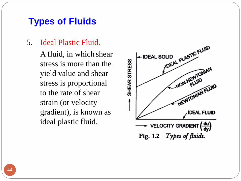
5. Ideal Plastic Fluid.
A fluid, in which shear
stress is more than the
yield value and shear
stress is proportional
to the rate of shear
strain (or velocity
gradient), is known as
ideal plastic fluid.
44
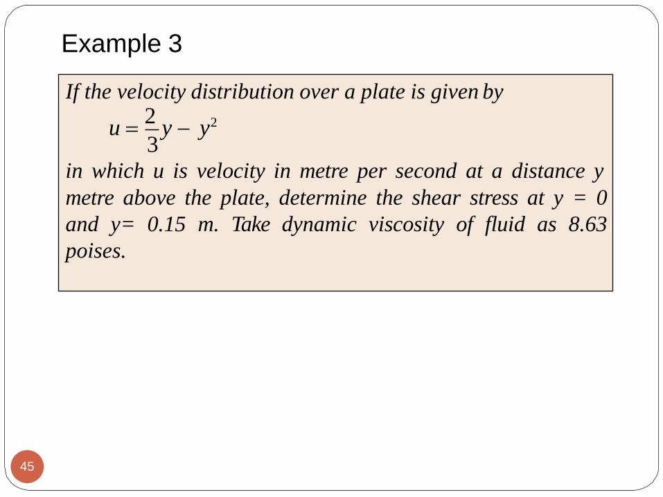
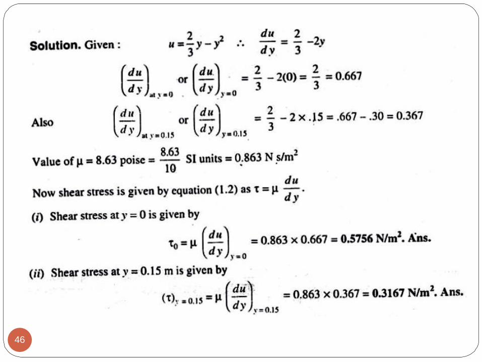
Example 3
If the velocity distribution over a plate is given by
metre above the plate, determine the shear stress at y = 0
and y= 0.15 m. Take dynamic viscosity of fluid as 8.63
poises.
3in which u is velocity in metre per second at a distance y
45
u =2
y − y2
46

Example 4
Calculate the dynamic viscosity of an oil, which is used for
lubrication between a square plate of size 0.8 m x 0.8 m and an
inclined plane with angle of inclination 30o as shown in Fig. 1.4.
The weight of the square plate is 300 N and it slides down the
inclined plane with a uniform velocity of 0.3 m/s. The thickness
of oil film is 1.5 mm.
Fig.1.4
47

48

Example 5
The space between two square flat parallel plates is filled with
oil. Each side of the plate is 60 cm. The thickness of the oil
film is 12.5 mm. The upper plate, which moves at 2.5 metre per
sec requires a force of 98.1 N to maintain the speed.
Determine : ·
i.the dynamic viscosity of the oil, and
ii.the kinematic viscosity of the oil if the specific gravity of the
oil is 0.95.
Solution. Given:
Each side of a square plate = 60 cm = 0.6 m
Area A= 0.6 x 0.6 = 0.36 m2
49
Thickness of oil film
Velocity of upper plate
dy = 12.5 mm = 12.5 x 10⁻³ m
u = 2.5 m/s

50
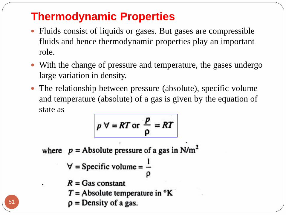
Thermodynamic Properties
Fluids consist of liquids or gases. But gases are compressible
fluids and hence thermodynamic properties play an important
role.
With the change of pressure and temperature, the gases undergo
large variation in density.
The relationship between pressure (absolute), specific volume
and temperature (absolute) of a gas is given by the equation of
state as
51

Isothermal Process. If the changes in density occurs at
constant temperature, then the process is called isothermal
and relationship between pressure (p) and density (ρ) is
given by
J
kg.K The value of gas constant R is R = 287
Thermodynamic Properties
ρ
Adiabatic Process. If the change in density occurs with no
heat exchange to and from the gas, the process is called
adiabatic. And if no heat is generated within the gas due to
friction, the relationship between pressure and density is
given by
p = constant
p
52ρk
= constant

where k = Ratio of specific heat of a gas at constant
pressure and constant volume.
k = 1.4 for air
Thermodynamic Properties
53
Compressibility and Bulk Modulus
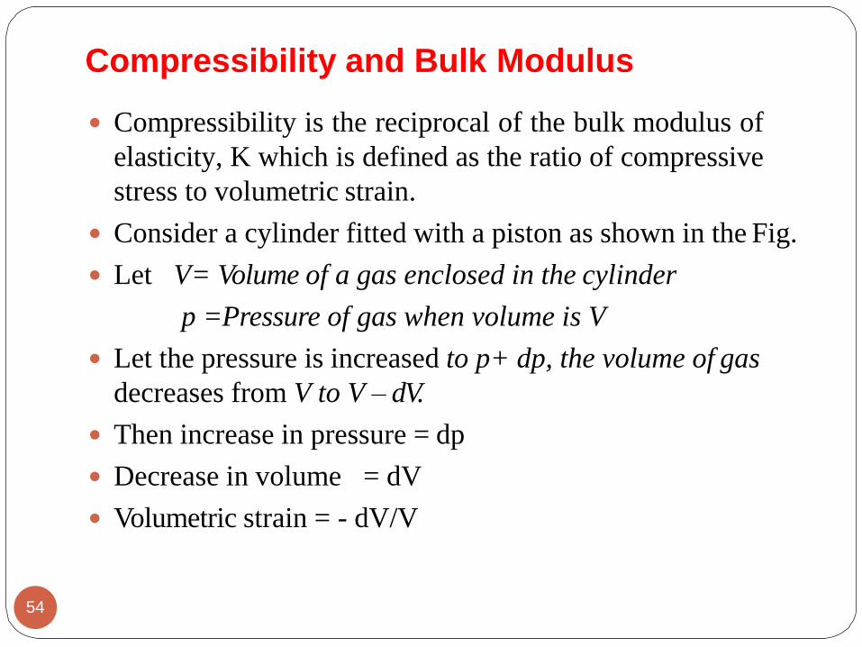
Compressibility is the reciprocal of the bulk modulus of
elasticity, K which is defined as the ratio of compressive
stress to volumetric strain.
Consider a cylinder fitted with a piston as shown in the Fig.
Let V= Volume of a gas enclosed in the cylinder
p =Pressure of gas when volume is V
Let the pressure is increased to p+ dp, the volume of gas
decreases from V to V – dV.
Then increase in pressure = dp
Decrease in volume = dV
Volumetric strain = - dV/V
54

- ve sign means the volume
decreases with increase of pressure.
dV= −
dpV=
V
Compressibility is given by = 1/K
dp
-dV
VolumetricstrainK =
Increase of pressureBulk modules
Compressibility and Bulk Modulus
55

Surface Tension and Capillarity
Surface tension is defined as the tensile force acting on the
surface of a liquid in contact with a gas or on the surface
between two immiscible liquids such that the contact
surface behaves like a membrane under tension.
Surface tension is created due to the unbalanced cohesive
forces acting on the liquid molecules at the fluid surface.
Molecules in the interior of the fluid mass are surrounded
by molecules that are attracted to each other equally.
However, molecules along the surface are subjected to a net
force toward the interior.
The apparent physical consequence of this unbalanced
force along the surface is to create the hypothetical skin or
membrane.56
Surface Tension and Capillarity
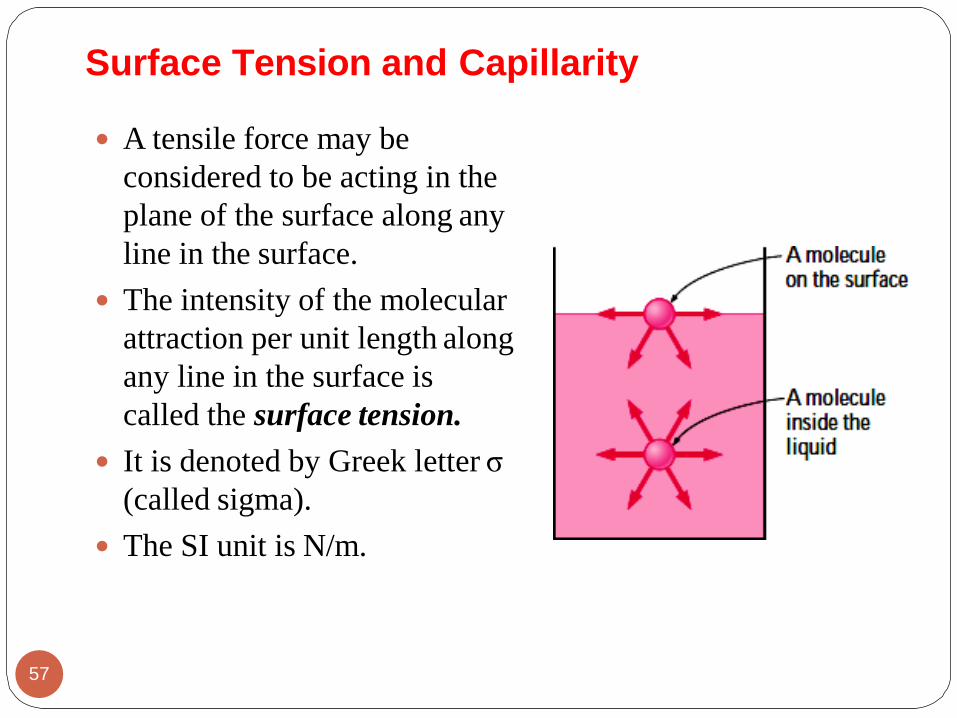
A tensile force may be
considered to be acting in the
plane of the surface along any
line in the surface.
The intensity of the molecular
attraction per unit length along
any line in the surface is
called the surface tension.
It is denoted by Greek letter σ
(called sigma).
The SI unit is N/m.
57

Surface Tension and Capillarity
Surface Tension on liquid Droplet and
Bubble
Consider a small spherical droplet of a
liquid of radius ‘R'. On the entire
surface of the droplet, the tensile force
due to surface tension will be acting.
Let σ = surface tension of the liquid
P= Pressure intensity inside the
droplet (in excess of the outside
pressure intensity)
R= Radius of droplet.
Let the droplet is cut into two halves.
The forces acting on one half (say left
half) will be58
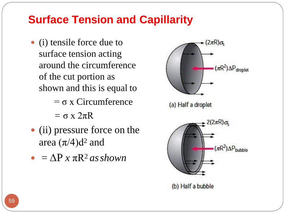
(i) tensile force due to
surface tension acting
around the circumference
of the cut portion as
shown and this is equal to
= σ x Circumference
= σ x 2πR
(ii) pressure force on the
area (π/4)d2 and
= P x πR2 asshown
Surface Tension and Capillarity
59

These two forces will be equal and opposite under
equilibrium conditions, i.e.,
A hollow bubble like a soap bubble in air has two surfaces
in contact with air, one inside and other outside. Thus two
surfaces are subjected surface tension.
Surface Tension and Capillarity
60

Surface Tension……. Example 1
Find the surface tension in a soap bubble of 40 mm
diameter when the inside pressure is 2.5 N/m2 above
atmospheric pressure.
61

Surface Tension……. Example 2
The pressure outside the droplet of water of diameter
0.04 mm is 10.32 N/cm2 (atmospheric pressure).
Calculate the pressure within the droplet if surface
tension is given as 0.0725 N/m of water.
62

Surface Tension and Capillarity
Capillarity
Capillarity is defined as a phenomenon of rise or fall of a
liquid surface in a small tube relative to the adjacent general
level of liquid when the tube is held vertically in the liquid.
The rise of liquid surface is known as capillary rise while
the fall of the liquid surface is known as capillary
depression.
The attraction (adhesion) between the wall of the tube and
liquid molecules is strong enough to overcome the mutual
attraction (cohesion) of the molecules and pull them up the
wall. Hence, the liquid is said to wet the solid surface.
It is expressed in terms of cm or mm of liquid. Its value
depends upon the specific weight of the liquid, diameter of
the tube and surface tension of the liquid.
63

Surface Tension and Capillarity
Expression for Capillary Rise
Consider a glass tube of small
diameter ‘d’ opened at both ends
and is inserted in a liquid, say water.
The liquid will rise in the tube
above the level of the liquid.
Let h = the height of the liquid in
the tube . Under a state of
equilibrium, the weight of the liquid
of height h is balanced by the force
at the surface of the liquid in the
tube. But the force at the surface of
the liquid in the tube is due to
surface tension.64
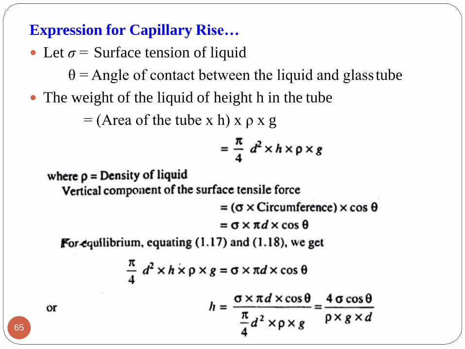
Expression for Capillary Rise…
Let σ = Surface tension of liquid
θ = Angle of contact between the liquid and glass tube
The weight of the liquid of height h in the tube
= (Area of the tube x h) x ρ x g
65
Expression for Capillary Rise…
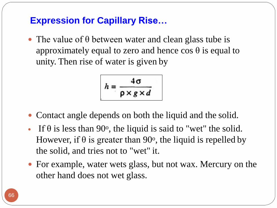
The value of θ between water and clean glass tube is
approximately equal to zero and hence cos θ is equal to
unity. Then rise of water is given by
Contact angle depends on both the liquid and the solid.
If θ is less than 90o, the liquid is said to "wet" the solid.
However, if θ is greater than 90o, the liquid is repelled by
the solid, and tries not to "wet" it.
For example, water wets glass, but not wax. Mercury on the
other hand does not wet glass.
66
Capillarity
Expression for Capillary Fall
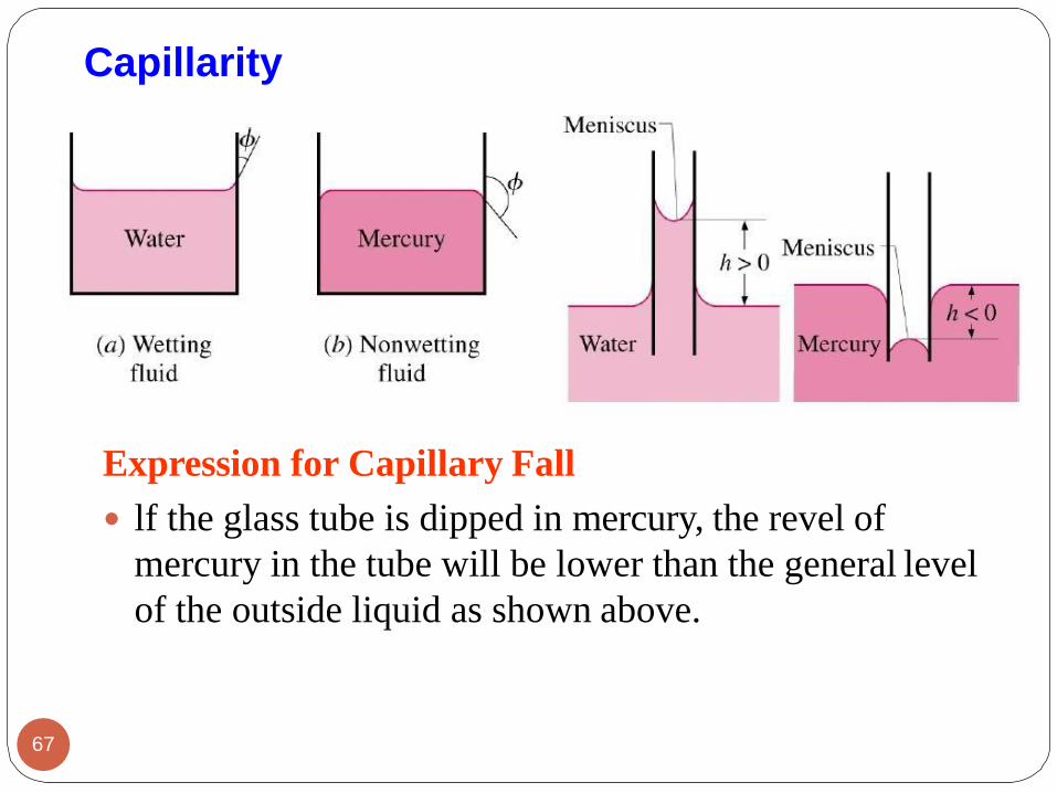
lf the glass tube is dipped in mercury, the revel of
mercury in the tube will be lower than the general level
of the outside liquid as shown above.
67
Capillarity
Expression for Capillary Fall
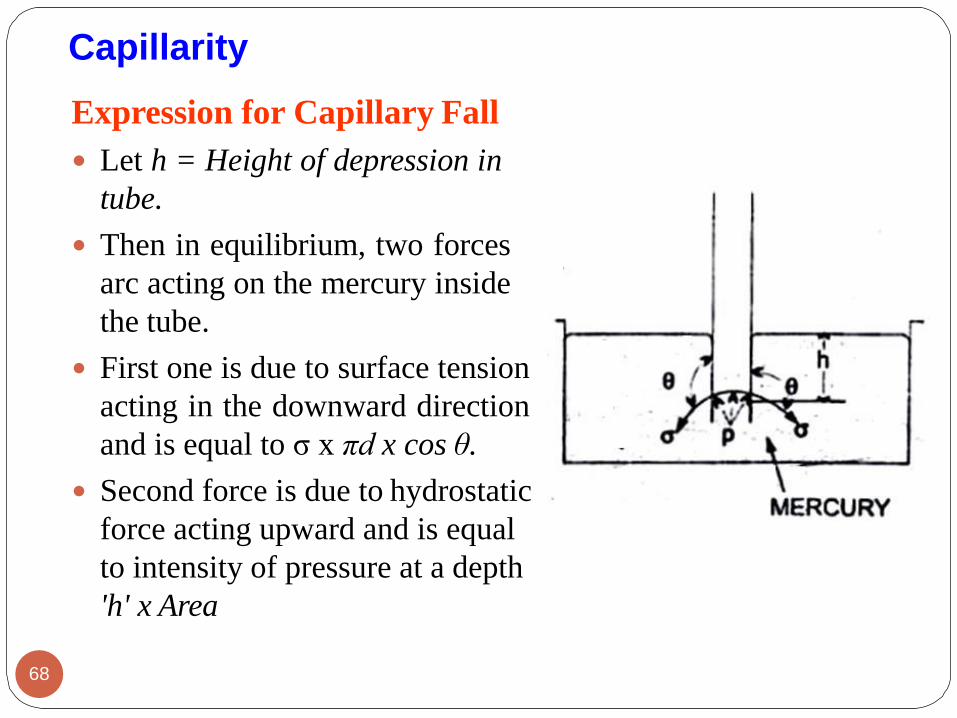
Let h = Height of depression in
tube.
Then in equilibrium, two forces
arc acting on the mercury inside
the tube.
First one is due to surface tension
acting in the downward direction
and is equal to σ x πd x cos θ.
Second force is due to hydrostatic
force acting upward and is equal
to intensity of pressure at a depth
'h' x Area
68
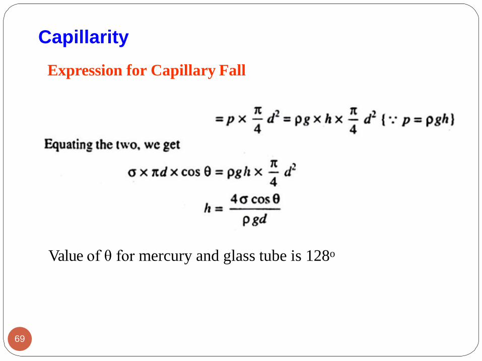
Expression for Capillary Fall
69
Capillarity
Value of θ for mercury and glass tube is 128o
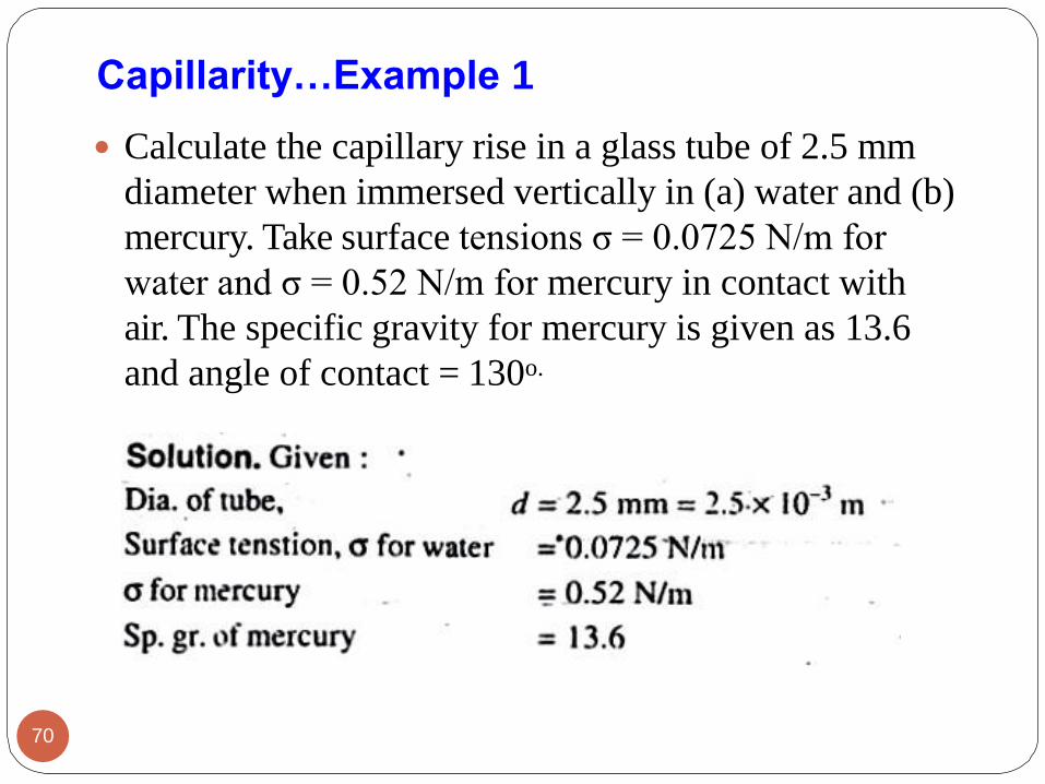
Capillarity…Example 1
Calculate the capillary rise in a glass tube of 2.5 mm
diameter when immersed vertically in (a) water and (b)
mercury. Take surface tensions σ = 0.0725 N/m for
water and σ = 0.52 N/m for mercury in contact with
air. The specific gravity for mercury is given as 13.6
and angle of contact = 130o.
70

Capillarity…Example 1
71
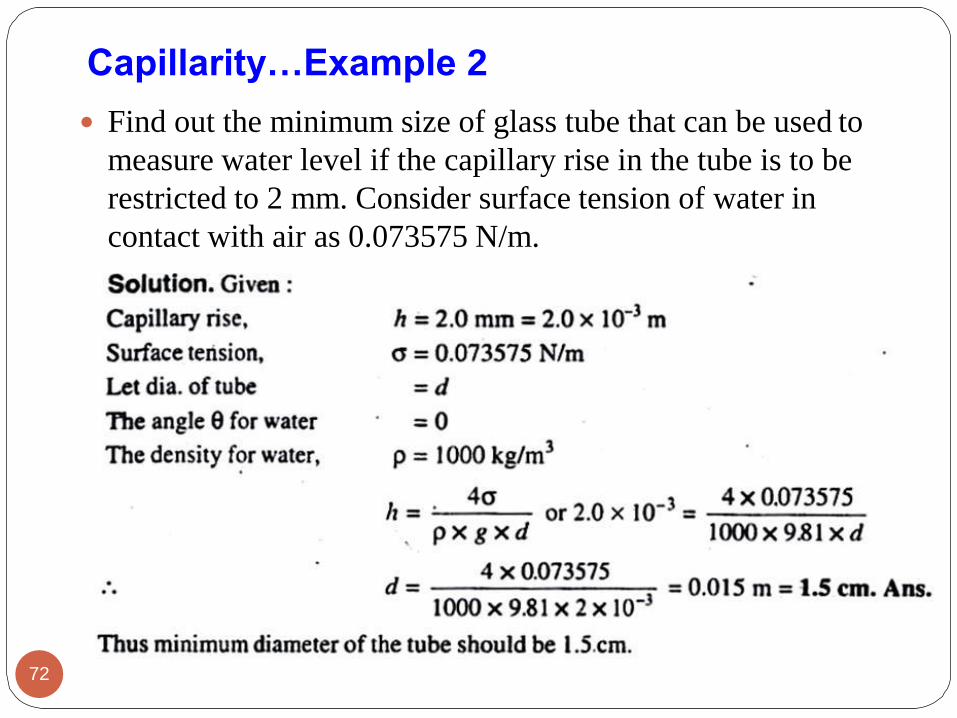
Find out the minimum size of glass tube that can be used to
measure water level if the capillary rise in the tube is to be
restricted to 2 mm. Consider surface tension of water in
contact with air as 0.073575 N/m.
Capillarity…Example 2
72

Flow Analysis Techniques
In analyzing fluid motion,
we might take one of two
paths:
1. Seeking an estimate of
gross effects (mass flow,
induced force, energy
change) over a finite
region or control volume
or
2. Seeking the point-by-
point details of a flow
pattern by analyzing an
infinitesimal region of
the flow.73

The control volume technique is useful when we are
interested in the overall features of a flow, such as mass
flow rate into and out of the control volume or net forces
applied to bodies.
Differential analysis, on the other hand, involves
application of differential equations of fluid motion to any
and every point in the flow field over a region called the
flow domain.
When solved, these differential equations yield details
about the velocity, density, pressure, etc., at every point
throughout the entire flow domain.
Flow Analysis Techniques
74
Flow Patterns
Fluid mechanics is a highly visual subject. The patterns of flow
can be visualized in a dozen different ways, and you can view
these sketches or photographs and learn a great deal
qualitatively and often quantitatively about the flow.
Four basic types of line patterns are used to visualize flows:
1. A streamline is a line everywhere tangent to the velocity
vector at a given instant.
2. A pathline is the actual path traversed by a given fluid
particle.
3. A streakline is the locus of particles that have earlierpassed
through a prescribed point.
4. A timeline is a set of fluid particles that form a line at a
given instant.
75

The streamline is convenient to calculate mathematically,
while the other three are easier to generate experimentally.
Note that a streamline and a timeline are instantaneous lines,
while the pathline and the streakline are generated by the
passage of time.
A streamline is a line that is everywhere tangent to the
velocity field. If the flow is steady, nothing at a fixed point
(including the velocity direction) changes with time, so the
streamlines are fixed lines in space.
For unsteady flows the streamlines may change shape with
time.
A pathline is the line traced out by a given particle as it flows
from one point to another.
Flow Patterns
76

A streakline consists of all particles in a flow that have
previously passed through a common point. Streaklines are
more of a laboratory tool than an analytical tool.
They can be obtained by taking instantaneous photographs of
marked particles that all passed through a given location in
the flow field at some earlier time.
Such a line can be produced by continuously injecting
marked fluid (neutrally buoyant smoke in air, or dye in water)
at a given location.
If the flow is steady, each successively injected particle
follows precisely behind the previous one forming a steady
streakline that is exactly the same as the streamline through
the injection point.
Flow Patterns
77

Flow Patterns
(a) Streamlines
78
(b) Streaklines

Streaklines are often confused with streamlines or pathlines.
While the three flow patterns are identical in steady flow, they
can be quite different in unsteady flow.
The main difference is that a streamline represents an
instantaneous flow pattern at a given instant in time, while a
streakline and a pathline are flow patterns that have some age
and thus a time history associated with them.
If the flow is steady, streamlines, pathlines, and streaklines are
identical
Flow Patterns
79
Dimensions and Units
Fluid mechanics deals with the measurement of many
variables of many different types of units. Hence we need
to be very careful to be consistent.
Dimensions and Base Units
The dimension of a measure is independent of any
particular system of units. For example, velocity may be
inmetres per second or miles per hour, but dimensionally, it
is always length per time, or L/T = LT−1 .
The dimensions of the relevant base units of the Système
International (SI) system are:
80

Dimensions and Units
Derived Units
81
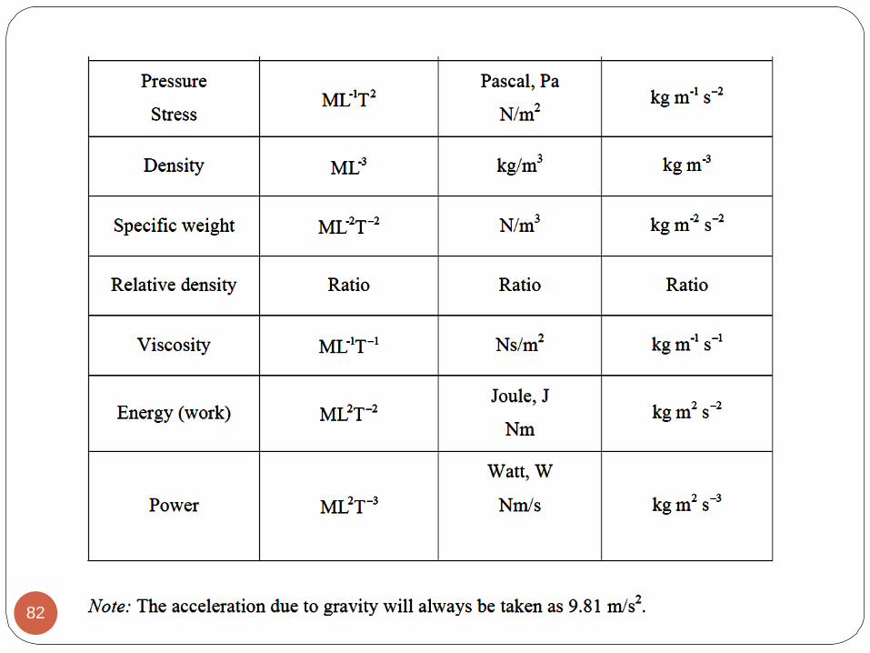
82

Unit Table
Quantity SI Unit English Unit
Length (L) Meter (m) Foot (ft)
Mass (m) Kilogram (kg) Slug (slug) =
lb*sec2/ft
Time (T) Second (s) Second (sec)
Temperature ( ) Celcius (oC) Farenheit (oF)
Force Newton
(N)=kg*m/s2
Pound (lb)
83

Dimensions and Units…
1 Newton – Force required to accelerate a 1 kg of mass
to 1 m/s2
1 slug – is the mass that accelerates at 1 ft/s2 when acted
upon by a force of 1 lb
To remember units of a Newton use F=ma (Newton’s 2nd
Law)
[F] = [m][a]= kg*m/s2 = N
To remember units of a slug also use F=ma => m = F / a
[m] = [F] / [a] = lb / (ft / sec2) = lb*sec2 / ft
84

End of Chapter 1
Next Lecture
Chapter 2: Fluid Statics
85

Fluids and Fluid Mechanics


Measuring Pressure


Bernoulli
Along a Streamline
ji
z
y
x
ks
n
ˆp g − = +a kSeparate acceleration due to gravity. Coordinate
system may be in any orientation!
k is vertical, s is in direction of flow, n is normal.
s
zp
ss
d
da g
− = +
Component of g in s direction
Note: No shear forces!
Therefore flow must be
frictionless.
Steady state (no change in
p wrt time)

Bernoulli
Along a Streamline
s
dV Va
dt s
= =
s
p dza
s ds
− = +
p pdp ds dn
s n
= +
0 (n is constant along streamline, dn=0)
dp dV dzV
ds ds ds − = +
Write acceleration as derivative wrt s
Chain rule
ds
dt=
dp ds p s = dV ds V s= and
Can we eliminate the partial derivative?
VV
s

Integrate F=ma Along a
Streamline
0dp VdV dz + + =
0dp
VdV g dz+ + =
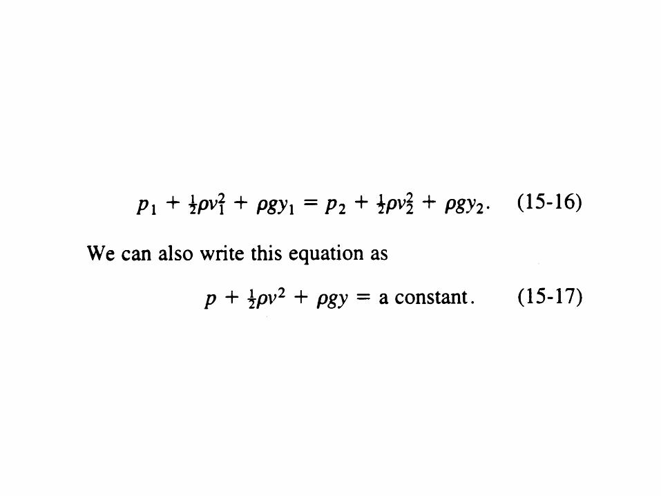
21
2p
dpV gz C
+ + =
2
'
1
2pp V z C + + =
If density is constant…
But density is a function
of ________.pressure
Eliminate ds
Now let’s integrate…
dp dV dzV
ds ds ds − = +
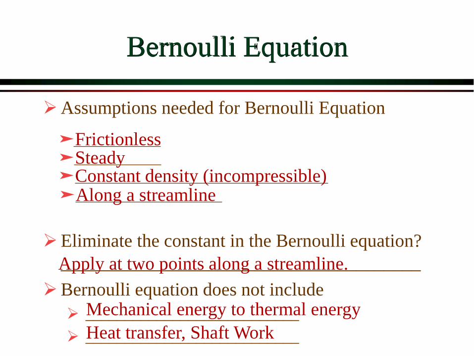
➢Assumptions needed for Bernoulli Equation
➢Eliminate the constant in the Bernoulli equation?
_______________________________________
➢Bernoulli equation does not include
➢ ___________________________
➢ ___________________________
Bernoulli Equation
Apply at two points along a streamline.
Mechanical energy to thermal energy
Heat transfer, Shaft Work
FrictionlessSteadyConstant density (incompressible)Along a streamline
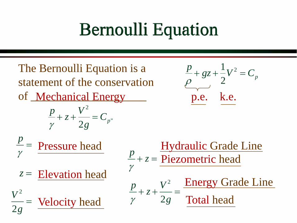
Bernoulli Equation
The Bernoulli Equation is a
statement of the conservation
of ____________________Mechanical Energy p.e. k.e.
21
2p
pgz V C
+ + =
2
"2
p
p Vz C
g+ + =
Pressure headp
=
z =
pz
+ =
2
2
V
g=
Elevation head
Velocity head
Piezometric head
2
2
p Vz
g+ + =
Total head
Energy Grade Line
Hydraulic Grade Line

Bernoulli Equation: Simple Case
(V = 0)
➢Reservoir (V = 0)
➢Put one point on the surface,
one point anywhere else
z
Elevation datum
21 2
pz z
g- =
Pressure datum 1
2
Same as we found using statics
2
"2
p
p Vz C
g+ + =
1 21 2
p pz z
+ = +
We didn’t cross any streamlines
so this analysis is okay!
Mechanical Energy
Conserved
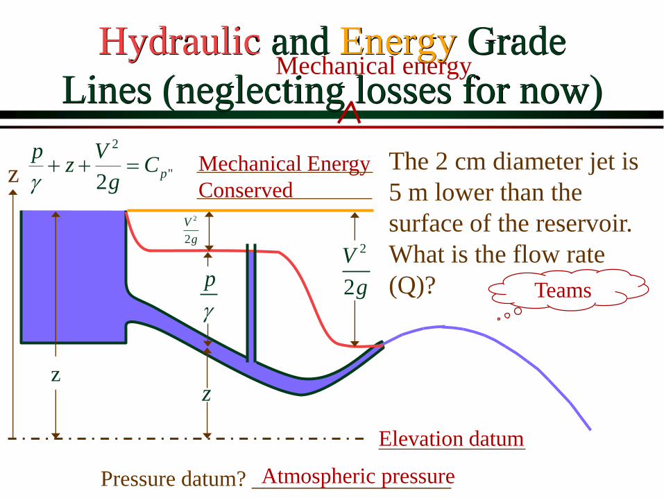
Hydraulic and Energy Grade
Lines (neglecting losses for now)
The 2 cm diameter jet is
5 m lower than the
surface of the reservoir.
What is the flow rate
(Q)?p
z
2
2
V
g
Elevation datum
z
Pressure datum? __________________Atmospheric pressure
Teams
z
2
2
V
g
2
"2
p
p Vz C
g+ + =
Mechanical energy

Bernoulli Equation: Simple Case
(p = 0 or constant)
➢What is an example of a fluid experiencing
a change in elevation, but remaining at a
constant pressure? ________2 2
1 1 2 21 2
2 2
p V p Vz z
g g + + = + +
( ) 2
2 1 2 12V g z z V= - +
2 2
1 21 2
2 2
V Vz z
g g+ = +
Free jet
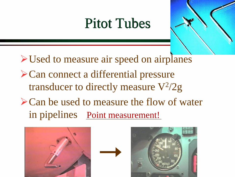
Pitot Tubes
➢Used to measure air speed on airplanes
➢Can connect a differential pressure
transducer to directly measure V2/2g
➢Can be used to measure the flow of water
in pipelines Point measurement!
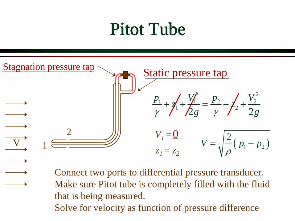
Pitot Tube
VV1 =
1
2
Connect two ports to differential pressure transducer.
Make sure Pitot tube is completely filled with the fluid
that is being measured.
Solve for velocity as function of pressure difference
z1 = z2
( )1 2
2V p p
= −
Static pressure tapStagnation pressure tap
0
2 2
1 1 2 21 2
2 2
p V p Vz z
g g + + = + +

Relaxed Assumptions for
Bernoulli Equation
➢Frictionless (velocity not influenced by viscosity)
➢Steady
➢Constant density (incompressible)
➢Along a streamline
Small energy loss (accelerating flow, short distances)
Or gradually varying
Small changes in density
Don’t cross streamlines
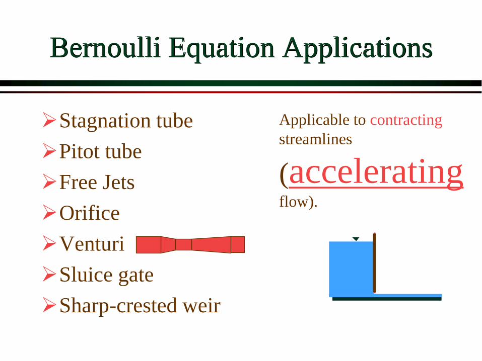
Bernoulli Equation Applications
➢Stagnation tube
➢Pitot tube
➢Free Jets
➢Orifice
➢Venturi
➢Sluice gate
➢Sharp-crested weir
Applicable to contracting
streamlines
(acceleratingflow).

Summary
➢By integrating F=ma along a streamline we found…
➢That energy can be converted between pressure, elevation, and velocity
➢That we can understand many simple flows by applying the Bernoulli equation
➢However, the Bernoulli equation can not be applied to flows where viscosity is large, where mechanical energy is converted into thermal energy, or where there is shaft work.
mechanical

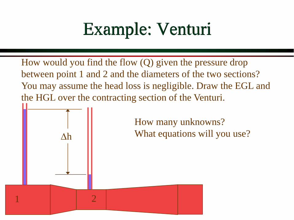
Example: Venturi
How would you find the flow (Q) given the pressure drop
between point 1 and 2 and the diameters of the two sections?
You may assume the head loss is negligible. Draw the EGL and
the HGL over the contracting section of the Venturi.
1 2
Dh
How many unknowns?
What equations will you use?

Example Venturi
2 2
1 1 2 21 2
1 22 2
p V p Vz z
g g + + = + +
g
V
g
Vpp
22
2
1
2
221 −=−
−=−
4
1
2
2
221 12 d
d
g
Vpp
( ) 4
12
212
1
)(2
dd
ppgV
−
−=
( ) 4
12
212
1
)(2
dd
ppgACQ v
−
−=
VAQ =
2211 AVAV =
44
2
22
2
11
dV
dV
=
2
22
2
11 dVdV =
2
1
2
221
d
dVV =

Chapter 5
Dimensional Analysis And Similitude
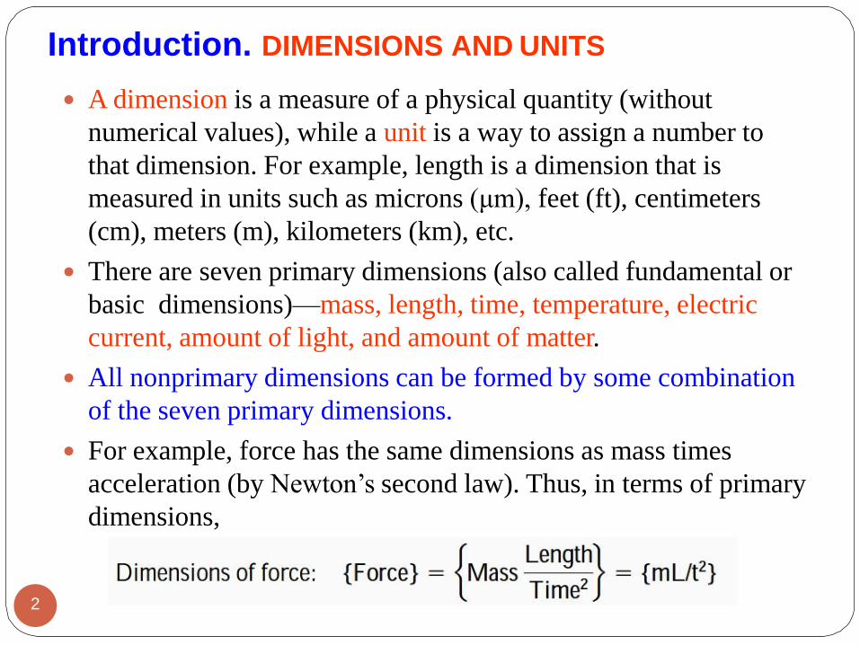
Introduction. DIMENSIONS AND UNITS
A dimension is a measure of a physical quantity (without
numerical values), while a unit is a way to assign a number to
that dimension. For example, length is a dimension that is
measured in units such as microns (μm), feet (ft), centimeters
(cm), meters (m), kilometers (km), etc.
There are seven primary dimensions (also called fundamental or
basic dimensions)—mass, length, time, temperature, electric
current, amount of light, and amount of matter.
All nonprimary dimensions can be formed by some combination
of the seven primary dimensions.
For example, force has the same dimensions as mass times
acceleration (by Newton’s second law). Thus, in terms of primary
dimensions,
2
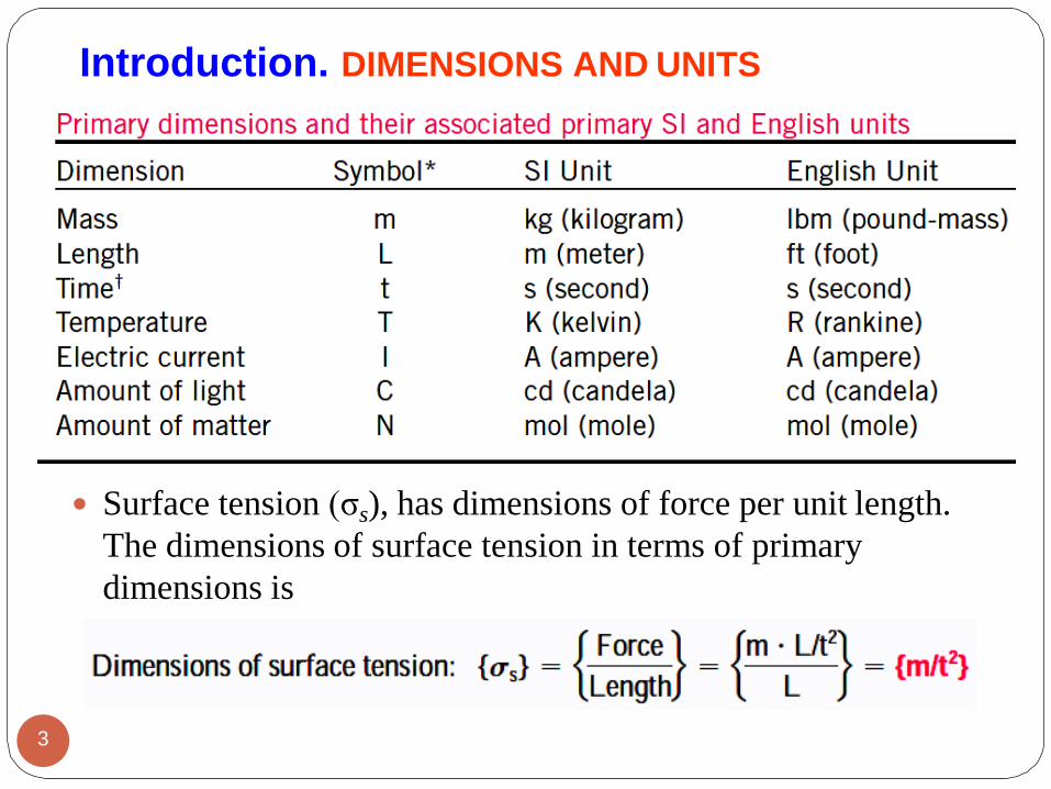
Surface tension (σs), has dimensions of force per unit length.
The dimensions of surface tension in terms of primary
dimensions is
Introduction. DIMENSIONS AND UNITS
3

DIMENSIONAL HOMOGENEITY
Law of dimensional homogeneity: Every additive term in an
equation must have the same dimensions.
Consider, for example, the change in total energy of a simple
compressible closed system from one state and/or time (1) to
another (2), as shown in the figure
The change in total energy of the
system (∆E) is given by
where E has three components:
internal energy (U), kinetic energy
(KE), and potential energy (PE).
4

These components can be written in terms of the system mass (m);
measurable quantities and thermodynamic properties at each of the
two states, such as speed (V), elevation (z), and specific internal
energy (u); and the known gravitational acceleration constant (g),
It is straightforward to verify that the left side of the change in
Energy equation and all three additive terms on the right side have
the same dimensions—energy.
DIMENSIONAL HOMOGENEITY
5

In addition to dimensional homogeneity, calculations are valid
only when the units are also homogeneous in each additive term.
For example, units of energy in the above terms may be J, N·m ,
or kg·m2/s2, all of which are equivalent.
Suppose, however, that kJ were used in place of J for one of the
terms. This term would be off by a factor of 1000 compared to
the other terms.
It is wise to write out all units when performing mathematical
calculations in order to avoid such errors.
DIMENSIONAL HOMOGENEITY
6
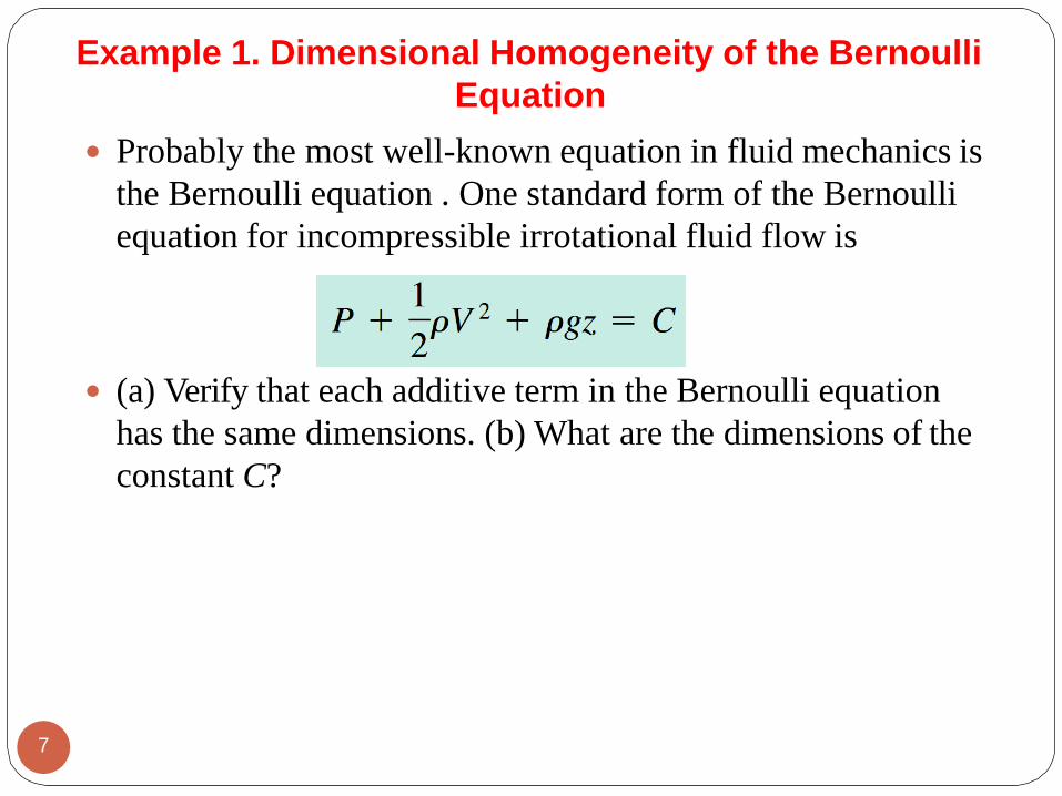
Example 1. Dimensional Homogeneity of the Bernoulli
Equation
Probably the most well-known equation in fluid mechanics is
the Bernoulli equation . One standard form of the Bernoulli
equation for incompressible irrotational fluid flow is
(a) Verify that each additive term in the Bernoulli equation
has the same dimensions. (b) What are the dimensions of the
constant C?
7

8

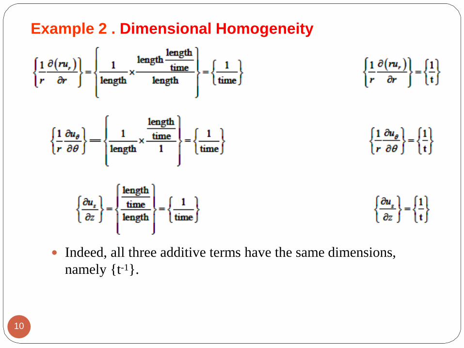
Example 2 . Dimensional Homogeneity
In Chap. 4 we discussed the differential equation for conservation
of mass, the continuity equation. In cylindrical coordinates, and for
steady flow,
9
Write the primary dimensions of each additive term in the equation,
and verify that the equation is dimensionally homogeneous.
Solution. We are to determine the primary dimensions of each
additive term, and we are to verify that the equation is dimensionally
homogeneous.
Analysis .The primary dimensions of the velocity components are
length/time. The primary dimensions of coordinates r and z are
length, and the primary dimensions of coordinate θ are unity (it is a
dimensionless angle). Thus each term in the equation can be written
in terms of primary dimensions,
10
Example 2 . Dimensional Homogeneity
Indeed, all three additive terms have the same dimensions,
namely {t-1}.

Nondimensionalization of Equations
The law of dimensional
homogeneity guarantees that
every additive term in an
equation has the same
dimensions.
It follows that if we divide
each term in the equation by a
collection of variables and
constants whose product has
those same dimensions, the
equation is rendered
nondimensional.
11
If, in addition, the nondimensional terms in the equation are of
order unity, the equation is called normalized.
Each term in a nondimensional equation is dimensionless.
A nondimensionalized form of the
Bernoulli equation is formed by
dividing each additive term by a
pressure (here we use ). Each
resulting term is dimensionless
(dimensions of {1}).

In the process of nondimensionalizing an equation of motion,
nondimensional parameters often appear—most of which are
named after a notable scientist or engineer (e.g., the Reynolds
number and the Froude number).
This process is sometimes called inspectional analysis.
As a simple example, consider the equation of motion
describing the elevation z of an object falling by gravity
through a vacuum (no air drag).
The initial location of the object is z0 and its initial velocityis
w0 in the z-direction. From high school physics,
……………… (1)
Dimensional variables are defined as dimensional quantities
that change or vary in the problem.
Nondimensionalization of Equations
12
For the simple differential equation given in Eq. 1, there are
two dimensional variables: z (dimension of length) and t
(dimension of time).
Nondimensional (or dimensionless) variables are defined as
quantities that change or vary in the problem, but have no
dimensions; an example is angle of rotation, measured in
degrees or radians which are dimensionless units. Gravitational
constant g, while dimensional, remains constant and is called a
dimensional constant.
Other dimensional constants are relevant to this particular
problem are initial location z0 and initial vertical speedw0.
While dimensional constants may change from problem to
problem, they are fixed for a particular problem and are thus
distinguished from dimensional variables.
Nondimensionalization of Equations
13

We use the term parameters for the combined set of
dimensional variables, nondimensional variables, and
dimensional constants in the problem.
Equation 1 is easily solved by integrating twice and
applying the initial conditions. The result is an expression
for elevation z at any time t:
……………(2)
The constant ½ and the exponent 2 in Eq. 2 are
dimensionless results of the integration. Such constants are
called pure constants. Other common examples of pure
constants are Π and e.
Nondimensionalization of Equations
14
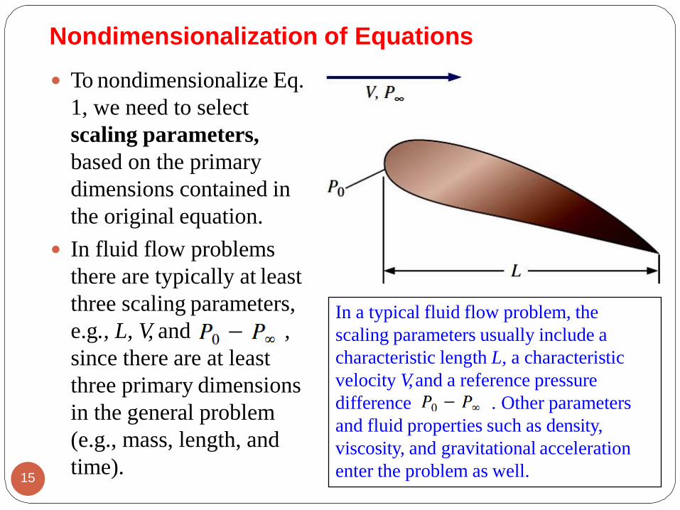
To nondimensionalize Eq.
1, we need to select
scaling parameters,
based on the primary
dimensions contained in
the original equation.
In fluid flow problems
there are typically at least
three scaling parameters,
e.g., L, V, and ,
since there are at least
three primary dimensions
in the general problem
(e.g., mass, length, and
time).15
Nondimensionalization of Equations
In a typical fluid flow problem, the
scaling parameters usually include a
characteristic length L, a characteristic
velocity V, and a reference pressure
difference . Other parameters
and fluid properties such as density,
viscosity, and gravitational acceleration
enter the problem as well.
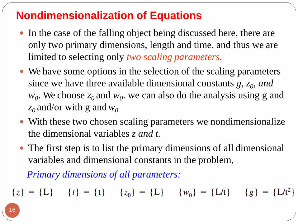
In the case of the falling object being discussed here, there are
only two primary dimensions, length and time, and thus we are
limited to selecting only two scaling parameters.
We have some options in the selection of the scaling parameters
since we have three available dimensional constants g, z0, and
w0. We choose z0 and w0. we can also do the analysis using g and
z0 and/or with g and w0
With these two chosen scaling parameters we nondimensionalize
the dimensional variables z and t.
The first step is to list the primary dimensions of all dimensional
variables and dimensional constants in the problem,
Primary dimensions of all parameters:
16
Nondimensionalization of Equations

The second step is to use our two scaling parameters to
nondimensionalize z and t (by inspection) into nondimensional
variables z* and t*,
Nondimensionalized variables:
………………(3)
Substitution of Eq. 3 into Eq. 1 gives
…...(4)
which is the desired nondimensional equation. The grouping of
dimensional constants in Eq. 4 is the square of a well-known
nondimensional parameter or dimensionless group called the
Froude number,17
Nondimensionalization of Equations
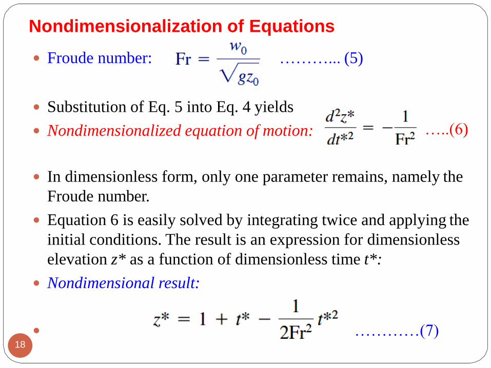
Froude number: ………... (5)
Substitution of Eq. 5 into Eq. 4 yields
Nondimensionalized equation of motion: …..(6)
In dimensionless form, only one parameter remains, namely the
Froude number.
Equation 6 is easily solved by integrating twice and applying the
initial conditions. The result is an expression for dimensionless
elevation z* as a function of dimensionless time t*:
Nondimensional result:
…………(7)
Nondimensionalization of Equations
18

There are two key advantages of nondimensionalization
First, it increases our insight about the relationships between
key parameters. Equation 5 reveals, for example, that doubling
w0 has the same effect as decreasing z0 by a factor of 4.
Second, it reduces the number of parameters in the problem.
For example, the original problem contains one dependent
variable, z; one independent variable, t; and three additional
dimensional constants, g, w0, and z0. The nondimensionalized
problem contains one dependent parameter, z*; one
independent parameter, t*; and only one additional parameter,
namely the dimensionless Froude number, Fr. The number of
additional parameters has been reduced from three to one!
Nondimensionalization of Equations
19

Dimensional Analysis and Similarity
Nondimensionalization of an equation by inspection is useful
only when we know the equation to begin with.
However, in many cases in real-life engineering, the equations
are either not known or too difficult to solve; often times
experimentation is the only method of obtaining reliable
information.
In most experiments, to save time and money, tests are
performed on a geometrically scaled model, rather than on the
full-scale prototype. In such cases, care must be taken to
properly scale the results. We introduce here a powerful
technique called dimensional analysis.
20

The three primary purposes of dimensional analysis are
✓To generate nondimensional parameters that help in the
design of experiments (physical and/or numerical) and in
the reporting of experimental results
✓To obtain scaling laws so that prototype performance can
be predicted from model performance
✓To (sometimes) predict trends in the relationship between
parameters
There are three necessary conditions for complete similarity
between a model and a prototype.
The first condition is geometric similarity—the model must
be the same shape as the prototype, but may be scaled by
some constant scale factor.
Dimensional Analysis and Similarity
21
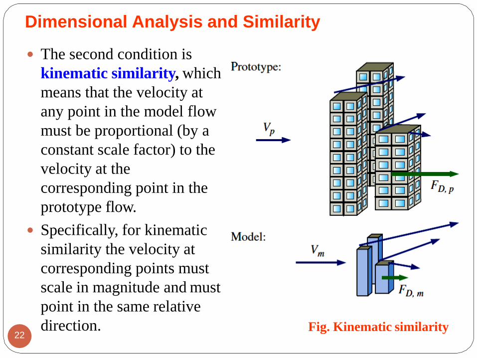
The second condition is
kinematic similarity, which
means that the velocity at
any point in the model flow
must be proportional (by a
constant scale factor) to the
velocity at the
corresponding point in the
prototype flow.
Specifically, for kinematic
similarity the velocity at
corresponding points must
scale in magnitude and must
point in the same relative
direction.
Dimensional Analysis and Similarity
Fig. Kinematic similarity22

Kinematic similarity is achieved when, at all locations, the speed in
the model flow is proportional to that at corresponding locations in
the prototype flow, and points in the same direction.
Geometric similarity is a prerequisite for kinematic similarity
Just as the geometric scale factor can be less than, equal to, or
greater than one, so can the velocity scale factor.
In Fig. above, for example, the geometric scale factor is less than
one (model smaller than prototype), but the velocity scale is greater
than one (velocities around the model are greater than those around
the prototype).
The third and most restrictive similarity condition is that of
dynamic similarity. Dynamic similarity is achieved when all
forces in the model flow scale by a constant factor to corresponding
forces in the prototype flow (force-scale equivalence).
23
Dimensional Analysis and Similarity
As with geometric and kinematic similarity, the scale factor for
forces can be less than, equal to, or greater than one.
In Fig. shown in slide 20 above for example, the force-scale
factor is less than one since the force on the model building is
less than that on the prototype.
Kinematic similarity is a necessary but insufficient condition
for dynamic similarity.
It is thus possible for a model flow and a prototype flow to
achieve both geometric and kinematic similarity, yet not
dynamic similarity. All three similarity conditions must exist for
complete similarity to be ensured.
In a general flow field, complete similarity between a model
and prototype is achieved only when there is geometric,
kinematic, and dynamic similarity.
Dimensional Analysis and Similarity
24
We let uppercase Greek letter Pi (Π) denote a nondimensional
parameter. We have already discussed one Π, namely the
Froude number, Fr.
In a general dimensional analysis problem, there is one Π that
we call the dependent Π, giving it the notation Π1. The
parameter Π1 is in general a function of several other Π’s,
which we call independent Π’s. The functional relationship is
Functional relationship between Π’s:
where k is the total number of Π’s.
Consider an experiment in which a scale model is tested to
simulate a prototype flow.
Dimensional Analysis and Similarity
25

To ensure complete similarity between the model and the
prototype, each independent P of the model (subscript m) must
be identical to the corresponding independent Π of the prototype
(subscript p),
i.e., Π2, m = Π2, p , Π3, m = Π3, p, . . . .., Πk, m = Πk, p.
To ensure complete similarity, the model and prototype must be
geometrically similar, and all independent Π groups must match
between model and prototype.
Under these conditions the dependent Π of the model (Π1, m) is
guaranteed to also equal the dependent Π of the prototype (Π1, p).
Mathematically, we write a conditional statement for achieving
similarity,
Dimensional Analysis and Similarity
26

Consider, for example, the
design of a new sports car, the
aerodynamics of which is to
be tested in a wind tunnel. To
save money, it is desirable to
test a small, geometrically
scaled model of the car rather
than a full-scale prototype of
the car.
In the case of aerodynamic
drag on an automobile, it
turns out that if the flow is
approximated as
incompressible, there are only
two Π’s in the problem,
Dimensional Analysis and Similarity
27

Where
The procedure used to generate these Π’s will be discussed
later in this chapter.
In the above equation FD is the magnitude of the aerodynamic
drag on the car, ρ is the air density, V is the car’s speed (or the
speed of the air in the wind tunnel), L is the length of the car,
and μ is the viscosity of the air. Π1 is a nonstandard form of the
drag coefficient, and Π2 is the Reynolds number, Re.
The Reynolds number is the most well known and useful
dimensionless parameter in all of fluid mechanics
Dimensional Analysis and Similarity
28

In the problem at hand there is only one independent Π, and
the above Eq. ensures that if the independent Π’s match (the
Reynolds numbers match: Π2, m = Π2, p ), then the dependent
Π’s also match (Π1, m = Π1, p).
This enables engineers to measure the aerodynamic drag on
the model car and then use this value to predict the
aerodynamic drag on the prototype car.
Dimensional Analysis and Similarity
29
Example 3: Similarity between Model and Prototype Cars
The aerodynamic drag of a new sports car is to be predicted at a
speed of 50.0 mi/h at an air temperature of 25°C. Automotive
engineers build a one fifth scale model of the car to test in a wind
tunnel. It is winter and the wind tunnel is located in an unheated
building; the temperature of the wind tunnel air is only about
5°C. Determine how fast the engineers should run the wind
tunnel in order to achieve similarity between the model and the
prototype.
Solution:
We are to utilize the concept of similarity to determine the speed
of the wind tunnel.
Assumptions:
The model is geometrically similar to the prototype
The wind tunnel walls are far enough away so as to not interfere
with the aerodynamic drag on the model car.30

Example 3: Similarity between Model and Prototype Cars
The wind tunnel has a moving belt to simulate the ground under
the car. (The moving belt is necessary in order to achieve
kinematic similarity everywhere in the flow, in particular
underneath the car.)
A drag balance is a device
used in a wind tunnel to
measure the aerodynamic
drag of a body. When
testing automobile models,
a moving belt is often
added to the floor of the
wind tunnel to simulate the
moving ground
(from the car’s frame of
reference).31
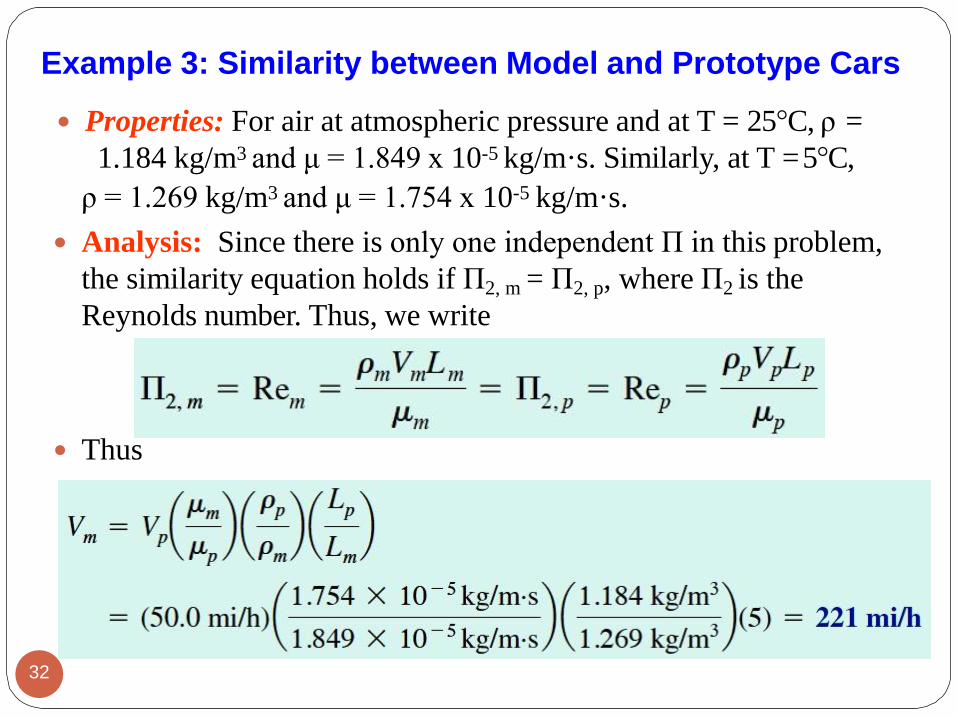
Properties: For air at atmospheric pressure and at T = 25°C, ρ =
1.184 kg/m3 and μ = 1.849 x 10⁻⁵ kg/m·s. Similarly, at T =5°C,
ρ = 1.269 kg/m3 and μ = 1.754 x 10⁻⁵ kg/m·s.
Analysis: Since there is only one independent Π in this problem,
the similarity equation holds if Π2, m = Π2, p, where Π2 is the
Reynolds number. Thus, we write
Thus
Example 3: Similarity between Model and Prototype Cars
32

The power of using dimensional analysis and similarity to
supplement experimental analysis is further illustrated by the fact
that the actual values of the dimensional parameters (density,
velocity, etc.) are irrelevant. As long as the corresponding
independent Π’s are set equal to each other, similarity is achieved
even if different fluids are used.
This explains why automobile or aircraft performance can be
simulated in a water tunnel, and the performance of a submarine can
be simulated in a wind tunnel.
Suppose, for example, that the engineers in Example above use a
water tunnel instead of a wind tunnel to test their one-fifth scale
model. Using the properties of water at room temperature (20°C is
assumed), the water tunnel speed required to achieve similarity is
easily calculated as
Example 3: Similarity between Model and Prototype Cars
33
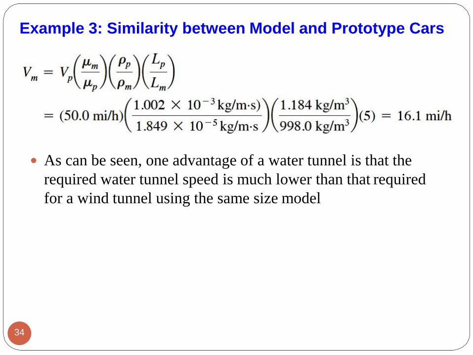
As can be seen, one advantage of a water tunnel is that the
required water tunnel speed is much lower than that required
for a wind tunnel using the same size model
Example 3: Similarity between Model and Prototype Cars
34
The Method of Repeating Variables and the
Buckingham Pi Theorem
In this section we will learn how to generate the nondimensional
parameters, i.e., the Π’s.
There are several methods that have been developed for this
purpose, but the most popular (and simplest) method is the method
of repeating variables, popularized by Edgar Buckingham (1867–
1940).
We can think of this method as a step-by-step procedure or
“recipe” for obtaining nondimensional parameters. There are six
steps in this method as described below in detail
35

The Method of Repeating Variables and the
Buckingham Pi Theorem
36
The Method of Repeating Variables and the
Buckingham Pi Theorem
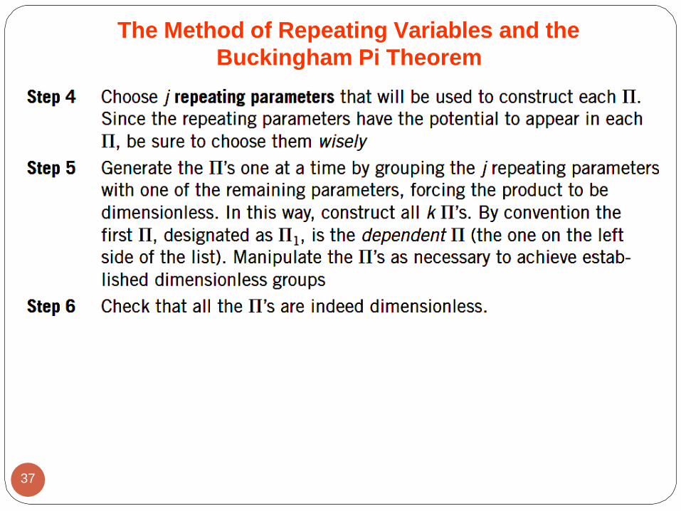
37

Fig. A concise
summary of the six
steps that comprise
the method of
repeating variables
The Method of Repeating Variables and the
Buckingham Pi Theorem
38
The Method of Repeating Variables and the
Buckingham Pi Theorem
As a simple first example, consider a ball falling in a vacuum. Let
us pretend that we do not know that Eq. 1 is appropriate for this
problem, nor do we know much physics concerning falling objects.
In fact, suppose that all we know is that the instantaneous
elevation z of the ball must be a function of time t, initial vertical
speed w0, initial elevation z0, and gravitational constant g.
The beauty of dimensional analysis is that the only other thing we
need to know is the primary dimensions of each of these
quantities.
As we go through each step of the method of repeating variables,
we explain some of the subtleties of the technique in more detail
using the falling ball as an example.
39

The Method of Repeating Variables
Step 1
There are five parameters
(dimensional variables,
nondimensional
variables, and
dimensional constants) in
this problem; n = 5. They
are listed in functional
form, with the dependent
variable listed as a
function of the
independent variables
and constants:
List of relevant
parameters:
Fig. Setup for dimensional analysis of a ball falling
in a vacuum. Elevation z is a function of time t,
initial vertical speed w0, initial elevation z0, and
gravitational constant g.
40
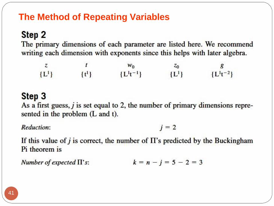
The Method of Repeating Variables
41

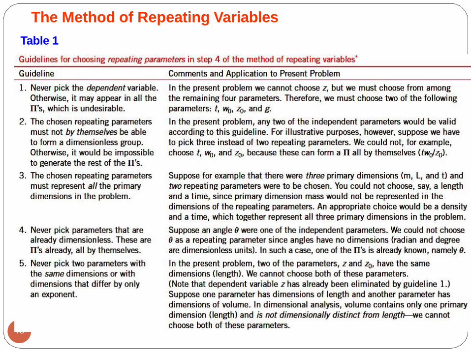
Step 4
We need to choose two repeating parameters since j = 2. Since
this is often the hardest (or at least the most mysterious) part of
the method of repeating variables, several guidelines about
choosing repeating parameters are listed in Table 1.
Following the guidelines of Table 1 on the next page, the wisest
choice of two repeating parameters is w0 and z0.
Repeating parameters: w0 and z0
Step 5
Now we combine these repeating parameters into products with
each of the remaining parameters, one at a time, to create the Π’s.
The first Π is always the dependent Π and is formed with the
dependent variable z.
Dependent Π : ……………….(1)
where a1 and b1 are constant exponents that need to be determined.42
The Method of Repeating Variables

We apply the primary dimensions of step 2 into Eq. 1 and force
the Π to be dimensionless by setting the exponent of each
primary dimension to zero:
Dimensions of Π1:
Since primary dimensions are by definition independent of each
other, we equate the exponents of each primary dimension
independently to solve for exponents a1 and b1
Thus
The Method of Repeating Variables
43
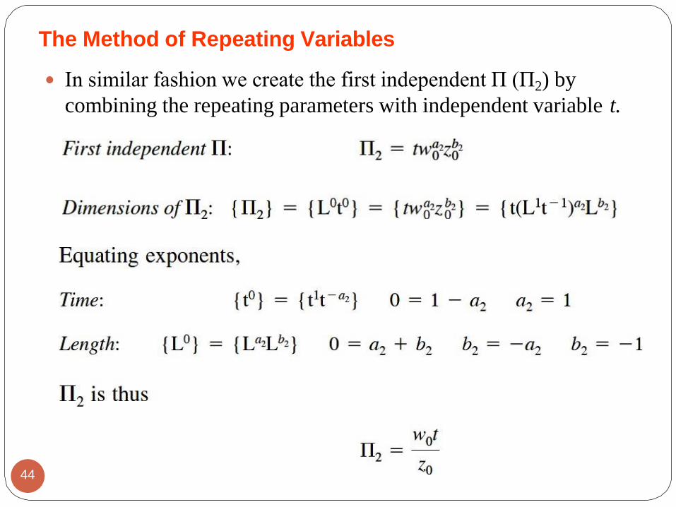
In similar fashion we create the first independent Π (Π2) by
combining the repeating parameters with independent variable t.
The Method of Repeating Variables
44
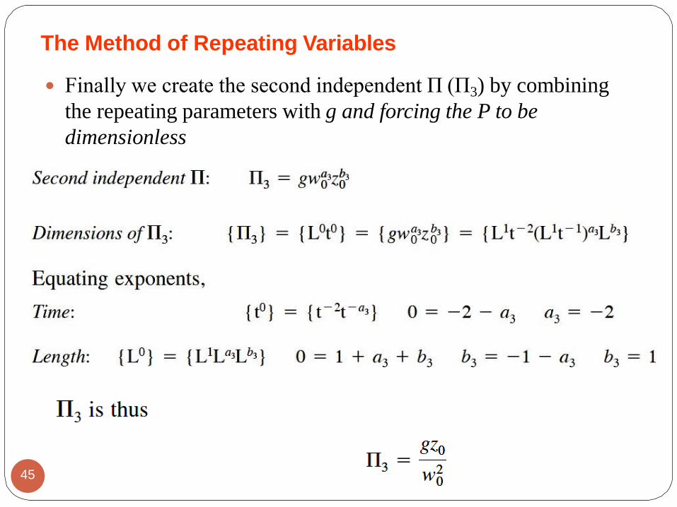
The Method of Repeating Variables
Finally we create the second independent Π (Π3) by combining
the repeating parameters with g and forcing the P to be
dimensionless
45

We can see that Π1 and Π2 are the same as the nondimensionalized
variables z* and t* defined by Eq. 3 (See slide number 15)—no
manipulation is necessary for these.
However, we recognize that the third P must be raised to the power
of -1/2 to be of the same form as an established dimensionless
parameter, namely the Froude number of
Such manipulation is often necessary to put the Π’s into proper
established form (“socially acceptable form” since it is a named,
established nondimensional parameter that is commonly used in
the literature.
The Method of Repeating Variables
46

Step 6
We should double-check that the Π’s are indeed dimensionless
We are finally ready to write the functional relationship between
the nondimensional parameters
Relationship between Π’s:
The method of repeating variables properly predicts the functional
relationship between dimensionless groups.
However, the method of repeating variables cannot predict the
exact mathematical form of the equation. This is a fundamental
limitation of dimensional analysis and the method of repeating
variables.
The Method of Repeating Variables
47
48
The Method of Repeating Variables
Table 1

The Method of Repeating Variables
49
The Method of Repeating Variables
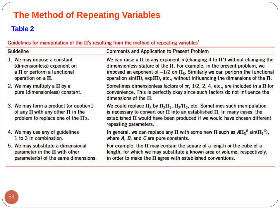
59
Table 2

Table 3. Some common established nondimensional parameters
51

52

53

54

EXAMPLE 4. Pressure in a Soap Bubble
Some children are playing with soap
bubbles, and you become curious as to the
relationship between soap bubble radius and
the pressure inside the soap bubble. You
reason that the pressure inside the soap
bubble must be greater than atmospheric
pressure, and that the shell of the soap
bubble is under tension, much like the skin
of a balloon. You also know that the
property surface tension must be important
in this problem. Not knowing any other
physics, you decide to approach the
problem using dimensional analysis.
Establish a relationship between pressure
difference
soap bubble radius R, and the surface
tension σs of the soap film.55
The pressure inside a soap
bubble is greater than that
surrounding the soap
bubble due to surface tension
in the soap film.
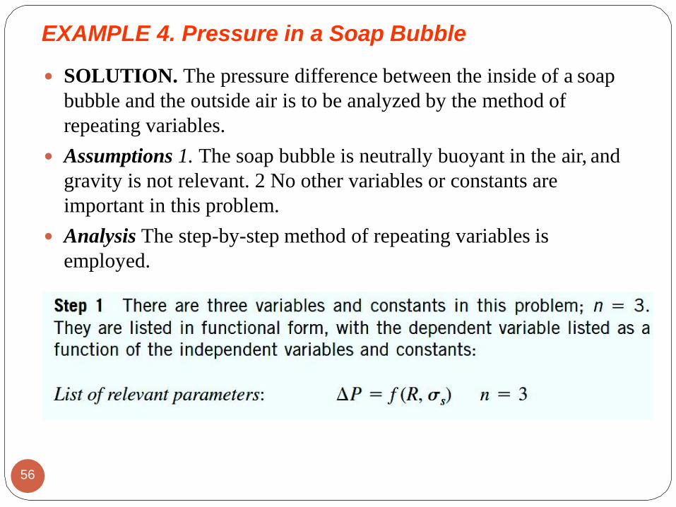
SOLUTION. The pressure difference between the inside of a soap
bubble and the outside air is to be analyzed by the method of
repeating variables.
Assumptions 1. The soap bubble is neutrally buoyant in the air, and
gravity is not relevant. 2 No other variables or constants are
important in this problem.
Analysis The step-by-step method of repeating variables is
employed.
EXAMPLE 4. Pressure in a Soap Bubble
56
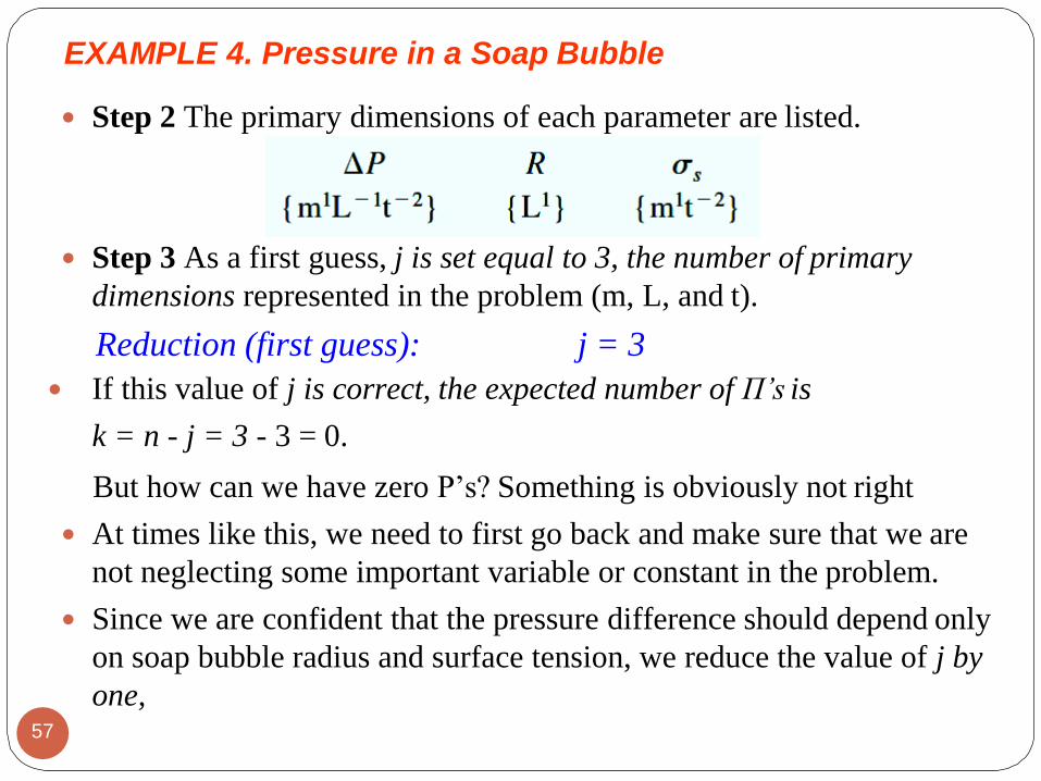
Step 2 The primary dimensions of each parameter are listed.
Step 3 As a first guess, j is set equal to 3, the number of primary
dimensions represented in the problem (m, L, and t).
Reduction (first guess): j = 3
If this value of j is correct, the expected number of Π’s is
k = n - j = 3 - 3 = 0.
But how can we have zero P’s? Something is obviously not right
At times like this, we need to first go back and make sure that we are
not neglecting some important variable or constant in the problem.
Since we are confident that the pressure difference should depend only
on soap bubble radius and surface tension, we reduce the value of j by
one,
EXAMPLE 4. Pressure in a Soap Bubble
57

EXAMPLE 4. Pressure in a Soap Bubble
Reduction (second guess): j = 2
If this value of j is correct, k = n - j = 3 - 2 = 1. Thus we expect one
Π, which is more physically realistic than zero Π’s.
Step 4 We need to choose two repeating parameters since j = 2.
Following the guidelines of Table 1, our only choices are R and σs,
since ∆P is the dependent variable.
Step 5 We combine these repeating parameters into a product with
the dependent variable ∆P to create the dependent Π,
Dependent Π: ………(1)
We apply the primary dimensions of step 2 into Eq. 1 and force the
Π to be dimensionless.
58
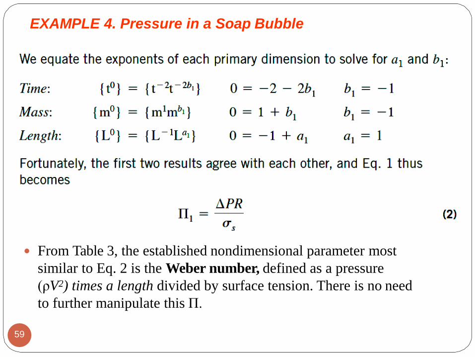
From Table 3, the established nondimensional parameter most
similar to Eq. 2 is the Weber number, defined as a pressure
(ρV2) times a length divided by surface tension. There is no need
to further manipulate this Π.
EXAMPLE 4. Pressure in a Soap Bubble
59

This is an example of how we can sometimes predict trends with
dimensional analysis, even without knowing much of the physics
of the problem. For example, we know from our result that if the
radius of the soap bubble doubles, the pressure difference
decreases by a factor of 2. Similarly, if the value of surface
tension doubles, ∆P increases by a factor of 2.
Dimensional analysis cannot predict the value of the constant in
Eq. 3; further analysis (or one experiment) reveals that the
constant is equal to 4 (Chap. 1).
EXAMPLE 4. Pressure in a Soap Bubble
Step 6 We write the final functional relationship. In the case at
hand, there is only one Π, which is a function of nothing. This is
possible only if the Π is constant.
Relationship between Π’s:
60
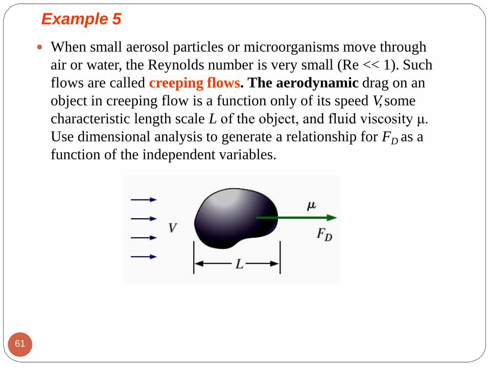
Example 5
When small aerosol particles or microorganisms move through
air or water, the Reynolds number is very small (Re << 1). Such
flows are called creeping flows. The aerodynamic drag on an
object in creeping flow is a function only of its speed V, some
characteristic length scale L of the object, and fluid viscosity μ.
Use dimensional analysis to generate a relationship for FD as a
function of the independent variables.
61

62

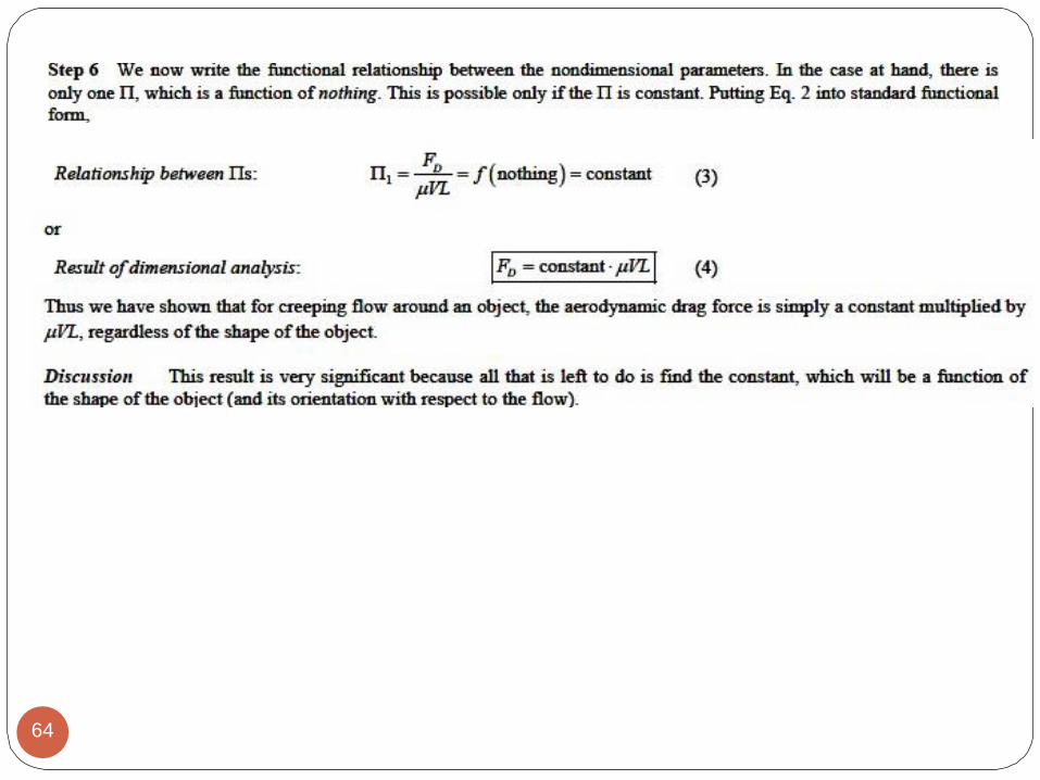
63
64

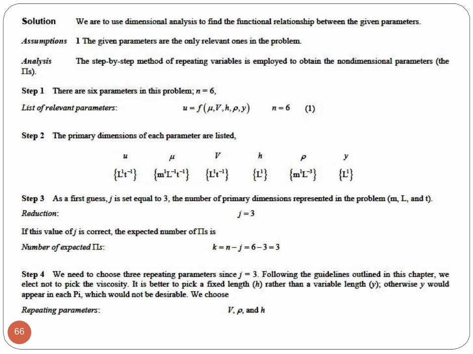
Example 6
Consider fully developed Couette flow—flow between two infinite
parallel plates separated by distance h, with the top plate moving
and the bottom plate stationary as illustrated in the Fig. shown. The
flow is steady, incompressible, and two-dimensional in the xy-plane.
Use the method of repeating variables to generate a dimensionless
relationship for the x component of fluid velocity u as a function of
fluid viscosity μ, top plate speed V, distance h, fluid density ρ, and
distance y.
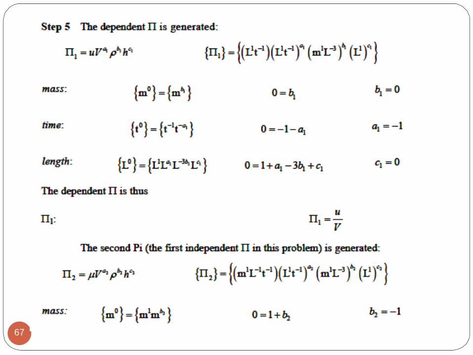
65
66
67

68
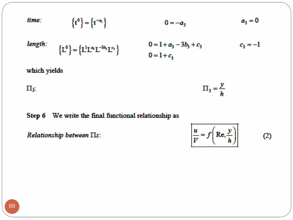
69
Related Documents