Fundamentals of Data Mining Typical Data Mining Tasks Data Mining Using R Introduction to Data Mining Jie Yang Department of Mathematics, Statistics, and Computer Science University of Illinois at Chicago February 3, 2014

Welcome message from author
This document is posted to help you gain knowledge. Please leave a comment to let me know what you think about it! Share it to your friends and learn new things together.
Transcript

Fundamentals of Data Mining Typical Data Mining Tasks Data Mining Using R
Introduction to Data Mining
Jie Yang
Department of Mathematics, Statistics, and Computer ScienceUniversity of Illinois at Chicago
February 3, 2014
Fundamentals of Data Mining Typical Data Mining Tasks Data Mining Using R
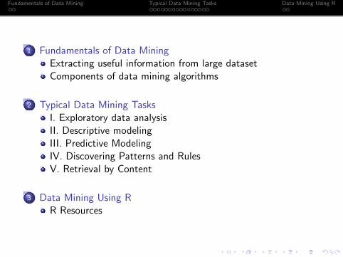
1 Fundamentals of Data MiningExtracting useful information from large datasetComponents of data mining algorithms
2 Typical Data Mining TasksI. Exploratory data analysisII. Descriptive modelingIII. Predictive ModelingIV. Discovering Patterns and RulesV. Retrieval by Content
3 Data Mining Using RR Resources
Fundamentals of Data Mining Typical Data Mining Tasks Data Mining Using R
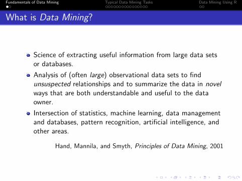
What is Data Mining?
Science of extracting useful information from large data setsor databases.
Analysis of (often large) observational data sets to findunsuspected relationships and to summarize the data in novelways that are both understandable and useful to the dataowner.
Intersection of statistics, machine learning, data managementand databases, pattern recognition, artificial intelligence, andother areas.
Hand, Mannila, and Smyth, Principles of Data Mining, 2001
Fundamentals of Data Mining Typical Data Mining Tasks Data Mining Using R
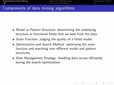
Components of data mining algorithms
Model or Pattern Structure: determining the underlyingstructure or functional forms that we seek from the data.
Score Function: judging the quality of a fitted model.
Optimization and Search Method: optimizing the scorefunction and searching over different model and patternstructures.
Data Management Strategy: handling data access efficientlyduring the search/optimization.
Fundamentals of Data Mining Typical Data Mining Tasks Data Mining Using R
I. Exploratory data analysis
Explore the data without any clear ideas of what we arelooking for.
Typical techniques are interactive and visual.
Projection techniques (such as principal components analysis)can be very useful for high-dimensional data.
Small-proportion or lower resolution samples can be displayedor summarized for large numbers of cases.
Fundamentals of Data Mining Typical Data Mining Tasks Data Mining Using R
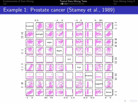
Example 1: Prostate cancer (Stamey et al., 1989)
lcavol
2.5 −1 2 −1 2 0 80
−12
4
2.54.0 lweight
age
4060
80
−11 lbph
svi
0.00.6
−11
3
lcp
gleason
6.08.0
060 pgg45
−1 3 40 70 0.0 1.0 6.0 9.0 0 4
03lpsa
Fundamentals of Data Mining Typical Data Mining Tasks Data Mining Using R
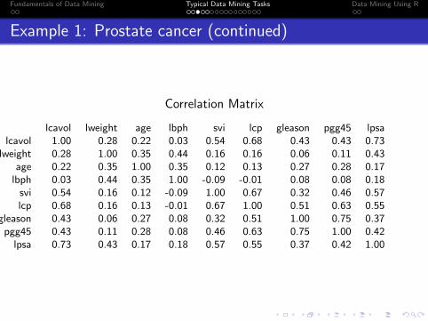
Example 1: Prostate cancer (continued)
Correlation Matrix
lcavol lweight age lbph svi lcp gleason pgg45 lpsalcavol 1.00 0.28 0.22 0.03 0.54 0.68 0.43 0.43 0.73
lweight 0.28 1.00 0.35 0.44 0.16 0.16 0.06 0.11 0.43age 0.22 0.35 1.00 0.35 0.12 0.13 0.27 0.28 0.17
lbph 0.03 0.44 0.35 1.00 -0.09 -0.01 0.08 0.08 0.18svi 0.54 0.16 0.12 -0.09 1.00 0.67 0.32 0.46 0.57lcp 0.68 0.16 0.13 -0.01 0.67 1.00 0.51 0.63 0.55
gleason 0.43 0.06 0.27 0.08 0.32 0.51 1.00 0.75 0.37pgg45 0.43 0.11 0.28 0.08 0.46 0.63 0.75 1.00 0.42
lpsa 0.73 0.43 0.17 0.18 0.57 0.55 0.37 0.42 1.00
Fundamentals of Data Mining Typical Data Mining Tasks Data Mining Using R
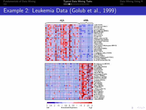
Example 2: Leukemia Data (Golub et al., 1999)
Fundamentals of Data Mining Typical Data Mining Tasks Data Mining Using R
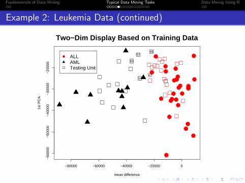
Example 2: Leukemia Data (continued)
−80000 −60000 −40000 −20000 0
−60
000
−50
000
−40
000
−30
000
−20
000
mean difference
1st P
CA
Two−Dim Display Based on Training Data
ALLAMLTesting Unit
54
57
60
66
67
Fundamentals of Data Mining Typical Data Mining Tasks Data Mining Using R
II. Descriptive modeling
Describe all of the data or the process generating the data.
Density estimation —- for overall probability distribution.
Cluster analysis and segmentation —- partition samples intogroups.
Dependency modeling —- describe the relationship betweenvariables.
Fundamentals of Data Mining Typical Data Mining Tasks Data Mining Using R
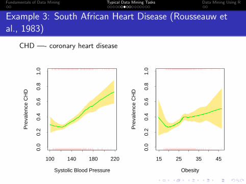
Example 3: South African Heart Disease (Rousseauw etal., 1983)
CHD —- coronary heart disease
6.5 Local Likelihood and Other Models 207
Systolic Blood Pressure
Pre
vale
nce
CH
D
100 140 180 220
0.0
0.2
0.4
0.6
0.8
1.0
Obesity
Pre
vale
nce
CH
D
15 25 35 45
0.0
0.2
0.4
0.6
0.8
1.0
FIGURE 6.12. Each plot shows the binary response CHD (coronary heart dis-ease) as a function of a risk factor for the South African heart disease data.For each plot we have computed the fitted prevalence of CHD using a local linearlogistic regression model. The unexpected increase in the prevalence of CHD atthe lower ends of the ranges is because these are retrospective data, and some ofthe subjects had already undergone treatment to reduce their blood pressure andweight. The shaded region in the plot indicates an estimated pointwise standarderror band.
This model can be used for flexible multiclass classification in moderatelylow dimensions, although successes have been reported with the high-dimensional ZIP-code classification problem. Generalized additive models(Chapter 9) using kernel smoothing methods are closely related, and avoiddimensionality problems by assuming an additive structure for the regres-sion function.As a simple illustration we fit a two-class local linear logistic model to
the heart disease data of Chapter 4. Figure 6.12 shows the univariate locallogistic models fit to two of the risk factors (separately). This is a usefulscreening device for detecting nonlinearities, when the data themselves havelittle visual information to offer. In this case an unexpected anomaly isuncovered in the data, which may have gone unnoticed with traditionalmethods.Since CHD is a binary indicator, we could estimate the conditional preva-
lence Pr(G = j|x0) by simply smoothing this binary response directly with-out resorting to a likelihood formulation. This amounts to fitting a locallyconstant logistic regression model (Exercise 6.5). In order to enjoy the bias-correction of local-linear smoothing, it is more natural to operate on theunrestricted logit scale.Typically with logistic regression, we compute parameter estimates as
well as their standard errors. This can be done locally as well, and so
Fundamentals of Data Mining Typical Data Mining Tasks Data Mining Using R
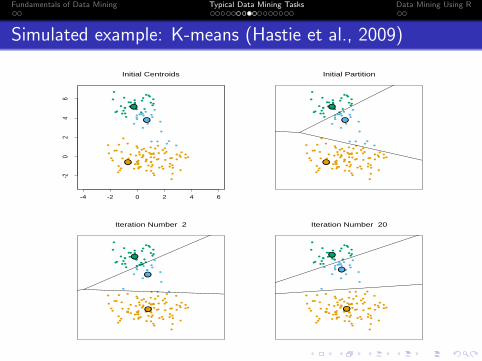
Simulated example: K-means (Hastie et al., 2009)
14.3 Cluster Analysis 511
-4 -2 0 2 4 6
-20
24
6Initial Centroids
• • •
•
••
••
•••
•
•
•
• •• ••
•• • •
•
••
•
•
•
••
•
••
•••••
• ••
• •••
•
•
•
••
••
•••
•
••
••
•
•
••••
•
•
• •••
••
•• •
•• •• •
•
• •• •
••
•
• •
•
• ••••
••
•
•
•• • •
•• •• •
• ••
•
••• •
•••
•
•• •
•
••
••
•
•
••
••
••
•
••
• •
••• ••
•
••
•
••
• • •
•
••
••
•••
•
•
•
• •• ••
•• • •
•
••
•
•
•
••
•
••
•••••
• ••
• •••
•
•
•
••
••
•••
•
••
••
•
•
••••
•
•
• •••
••
•• •
•• •• •
•
• •• •
••
•
• •
•
• ••••
••
•
•
•• • •
•• •• •
• ••
•
••• •
•••
•
•• •
•
••
••
•
•
••
••
••
•
••
• •
••• ••
•
••
•
••
Initial Partition
• • •
•
••
••
•••
•
•
•
• •• ••
•• • •
•
••
•
•
••
•
••
•••••
• ••
•
• •••
•
•
•
••
•
••
•••
•
••
•
•
•
•
•
••••
•
•
• •••
••
•• •
•• •• •
•
• •• •
••
•
• •
•• ••
••
•
••
•• •• •
••
••• •
••
•
•
•
•
• •• •
•
••
••
•
•
••
••
•
•
•
••
••
• •
••• ••
Iteration Number 2
•
••
•
••
• • •
•
••
••
•••
•
•
•
• •• ••
•• • •
•
••
•
•
••
•
••
•••••
• ••
•
• •••
•
•
•
••
••
••
•••
•
••
•
•
•
•
•
•
••••
•
•
• •••
••
•• •
•• •• •
•
• •• •
••
•
• •
••
••• •
•
•• • •
•• •• •
•• ••
•
•••
•••
•
•• •
•
••
••
•
•
••
••
••••
• •
••• ••
Iteration Number 20
•
••
•
••
FIGURE 14.6. Successive iterations of the K-means clustering algorithm forthe simulated data of Figure 14.4.
Fundamentals of Data Mining Typical Data Mining Tasks Data Mining Using R
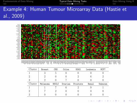
Example 4: Human Tumour Microarray Data (Hastie etal., 2009)
61.
Introduction
SID42354SID31984SID301902SIDW
128368SID375990SID360097SIDW
325120ESTsChr.10SIDW
365099SID377133SID381508SIDW
308182SID380265SIDW
321925ESTsChr.15SIDW
362471SIDW
417270SIDW
298052SID381079SIDW
428642TUPLE1TUP1ERLUMENSIDW
416621SID43609ESTsSID52979SIDW
357197SIDW
366311ESTsSMALLNUCSIDW
486740ESTsSID297905SID485148SID284853ESTsChr.15SID200394SIDW
322806ESTsChr.2SIDW
257915SID46536SIDW
488221ESTsChr.5SID280066SIDW
376394ESTsChr.15SIDW
321854W
ASWiskott
HYPOTHETICALSIDW
376776SIDW
205716SID239012SIDW
203464HLACLASSISIDW
510534SIDW
279664SIDW
201620SID297117SID377419SID114241ESTsCh31SIDW
376928SIDW
310141SIDW
298203PTPRCSID289414SID127504ESTsChr.3SID305167SID488017SIDW
296310ESTsChr.6SID47116MITOCHONDRIAL60ChrSIDW
376586HomosapiensSIDW
487261SIDW
470459SID167117SIDW
31489SID375812DNAPOLYMERSID377451ESTsChr.1MYBPROTOSID471915ESTsSIDW
469884HumanmRNASIDW
377402ESTsSID207172RASGTPASESID325394H.sapiensmRNAGNALSID73161SIDW
380102SIDW
299104
BREASTRENAL
MELANOMAMELANOMA
MCF7D-reproCOLONCOLON
K562B-reproCOLONNSCLC
LEUKEMIARENAL
MELANOMABREAST
CNSCNS
RENALMCF7A-repro
NSCLCK562A-repro
COLONCNS
NSCLCNSCLC
LEUKEMIACNS
OVARIANBREAST
LEUKEMIAMELANOMAMELANOMA
OVARIANOVARIAN
NSCLCRENAL
BREASTMELANOMA
OVARIANOVARIAN
NSCLCRENAL
BREASTMELANOMA
LEUKEMIACOLON
BREASTLEUKEMIA
COLONCNS
MELANOMANSCLC
PROSTATENSCLCRENALRENALNSCLCRENAL
LEUKEMIAOVARIAN
PROSTATECOLON
BREASTRENAL
UNKNOWN
FIG
URE
1.3.DNA
microarray
data:expression
matrix
of6830
genes(rows)
and64
samples
(columns),
forthe
human
tumor
data.Only
arandom
sample
of100
rowsare
shown.The
displayis
aheat
map,
rangingfrom
brightgreen
(negative,underexpressed)tobrightred
(positive,overexpressed).Missing
valuesare
gray.Therows
andcolum
nsare
displayedin
arandom
lychosen
order.
14.3 Cluster Analysis 513
Number of Clusters K
Su
m o
f S
qu
are
s
2 4 6 8 101
60
00
02
00
00
02
40
00
0
•
•
••
••
• •• •
FIGURE 14.8. Total within-cluster sum of squares for K-means clustering ap-plied to the human tumor microarray data.
TABLE 14.2. Human tumor data: number of cancer cases of each type, in eachof the three clusters from K-means clustering.
Cluster Breast CNS Colon K562 Leukemia MCF7
1 3 5 0 0 0 02 2 0 0 2 6 23 2 0 7 0 0 0
Cluster Melanoma NSCLC Ovarian Prostate Renal Unknown
1 1 7 6 2 9 12 7 2 0 0 0 03 0 0 0 0 0 0
The data are a 6830 × 64 matrix of real numbers, each representing anexpression measurement for a gene (row) and sample (column). Here wecluster the samples, each of which is a vector of length 6830, correspond-ing to expression values for the 6830 genes. Each sample has a label suchas breast (for breast cancer), melanoma, and so on; we don’t use these la-bels in the clustering, but will examine posthoc which labels fall into whichclusters.
We applied K-means clustering with K running from 1 to 10, and com-puted the total within-sum of squares for each clustering, shown in Fig-ure 14.8. Typically one looks for a kink in the sum of squares curve (or itslogarithm) to locate the optimal number of clusters (see Section 14.3.11).Here there is no clear indication: for illustration we chose K = 3 giving thethree clusters shown in Table 14.2.
Fundamentals of Data Mining Typical Data Mining Tasks Data Mining Using R
III. Predictive modeling: classification and regression
Predict the value of one variable from the known values ofother variables.
Classification —- the predicted variable is categorical.
Regression —- the predicted variable is quantitative.
Subset Selection and Shrinkage Methods – for cases of toomany variables.
Fundamentals of Data Mining Typical Data Mining Tasks Data Mining Using R
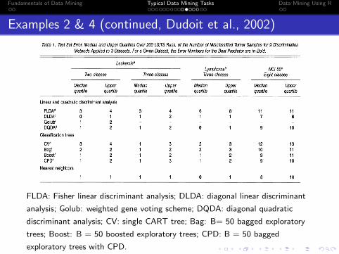
Examples 2 & 4 (continued, Dudoit et al., 2002)
Dudoit, Fridlyand, and Speed: Discrimination Methods for the Classification of Tumors
terry/zarray/Html for figures for the NCI 60 and lymphoma data.)
5.1.2 Fisher Linear Discriminant Analysis. On the oppo- site end of the performance spectrum is FLDA. The most likely reason for the poor performance of FLDA is that with a limited number of tumor samples and a fairly large number of genes p, the matrices of between-group and within-group sums of squares and cross-products are quite unstable and pro- vide poor estimates of the corresponding population quantities. The performance of FLDA dramatically improves and reaches error rates comparable to DLDA when the number of genes is decreased to p = 10, especially when the genes are selected according to the "smarter" BW criterion of Section 4 (see web supplement). Note also that FLDA is a "global" method, that is, it makes use of all of the data for each prediction, and as a result, some tumor samples may not be well represented by the discriminant variables. (There is only one discriminant variable for the two-class leukemia dataset and two discrimi- nant variables for the three-class lymphoma dataset.) In con- trast, NN methods are "local."
5.1.3 Maximum Likelihood Discriminant Rules. The simple DLDA rule produced impressively low misclassifica- tion rates compared with more sophisticated predictors, such as bagged classification trees. With the exception of the lym- phoma dataset, linear classifiers (i.e., DLDA), that assume a common covariance matrix for the different classes, yielded lower error rates than quadratic classifiers (i.e., DQDA), that allow for different class covariance matrices. Thus for the datasets considered here, gains in accuracy were obtained
by ignoring correlations between genes. DLDA classifiers are sometimes called "naive Bayes" because they arise in a
Bayesian setting, where the predicted tumor class is the one with maximum posterior probability pr(y = klx).
5.1.4 Weighted Gene Voting Scheme. For the binary class leukemia dataset, the performance of the variant of DLDA
implemented by Golub et al. (1999) was also examined. This method performed similarly to boosting, CPD, and DQDA, but was inferior to NN and especially to DLDA, which had a median error rate of 0. Note that in contrast to the aggregated predictors in bagging and boosting, the "voting" is over vari- ables (here genes) rather than over classifiers. Furthermore, the gene voting scheme as defined by Golub et al. (1999) is
applicable to binary classes only; the closest generalization of it to multiple classes is the standard DLDA predictor, which was applied to the other datasets.
5.1.5 Classification Trees. CART-based predictors had
performance intermediate between the best classifiers (DLDA, NN) and the worst classifier (FLDA). Aggregated tree pre- dictors were generally more accurate than a single cross- validated tree, with CPD and boosting performing better than standard bagging. Several values of the parameter d, d =
.05, .1,.25,.5,.75, were tried for the CPD method. For each
dataset, the best value turned out to be between .5 and 1, sug- gesting that the performance of CPD was not very sensitive to the parameter d controlling the degree of smoothing. A value of d = .75 was used in Table 1.
Table 1. Test Set Error. Median and Upper Quartiles Over 200 LSITS Runs, of the Number of Misclassified Tumor Samples for 9 Discrimination Methods Applied to 3 Datasets. For a Given Dataset, the Error Numbers for the Best Predictor are in Bold.
Leukemiaa Lymphomab NCI 60C
Two classes Three classes Three classes Eight classes
Median Upper Median Upper Median Upper Median Upper quartile quartile quartile quartile quartile quartile quartile quartile
Linear and quadratic discriminant analysis FLDAd 3 4 3 4 6 8 11 11 DLDAe 0 1 1 2 1 1 7 8 Golubf 1 2 - - - - - DQDA9 1 2 1 2 0 1 9 10
Classification trees
CVh 3 4 1 3 2 3 12 13 Bag' 2 2 1 2 2 3 10 11 Boost/ 1 2 1 2 1 2 9 11 CPDk 1 2 1 3 1 2 9 10
Nearest neighbors 1 1 1 1 0 1 8 10
a Leukemia dataset from Golub et al. (1999), test set size nTS = 24, p = 40 genes. b Lymphoma dataset from Alizadeh et al. (2000), test set size nTS = 27, p = 50 genes. c NCI 60 dataset from Ross et al. (2000), test set size nTS = 21, p = 30 genes. dFLDA: Fisher linear discriminant analysis. eDLDA: diagonal linear discriminant analysis. fGolub: weighted gene voting scheme of Golub et al. (1999). 9DQDA: diagonal quadratic discriminant analysis. hCV:single CART tree with pruning by 10-fold cross-validation. 'Bag:B = 50 bagged exploratory trees. Boost: B = 50 boosted exploratory trees.
kCPD: B = 50 bagged exploratory trees with CPD, d = .75.
83
FLDA: Fisher linear discriminant analysis; DLDA: diagonal linear discriminant
analysis; Golub: weighted gene voting scheme; DQDA: diagonal quadratic
discriminant analysis; CV: single CART tree; Bag: B= 50 bagged exploratory
trees; Boost: B = 50 boosted exploratory trees; CPD: B = 50 bagged
exploratory trees with CPD.
Fundamentals of Data Mining Typical Data Mining Tasks Data Mining Using R
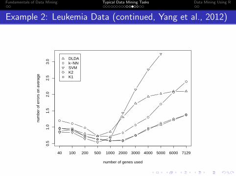
Example 2: Leukemia Data (continued, Yang et al., 2012)
0.5
1.0
1.5
2.0
2.5
3.0
number of genes used
num
ber
of e
rror
s on
ave
rage
40 100 200 500 1000 2000 3000 4000 5000 6000 7129
DLDAk−NNSVMK2K1
Fundamentals of Data Mining Typical Data Mining Tasks Data Mining Using R
Example 1: Prostate cancer (continued, Hastie et al.,2009)
50 3. Linear Methods for Regression
TABLE 3.1. Correlations of predictors in the prostate cancer data.
lcavol lweight age lbph svi lcp gleason
lweight 0.300age 0.286 0.317lbph 0.063 0.437 0.287svi 0.593 0.181 0.129 −0.139lcp 0.692 0.157 0.173 −0.089 0.671
gleason 0.426 0.024 0.366 0.033 0.307 0.476pgg45 0.483 0.074 0.276 −0.030 0.481 0.663 0.757
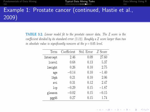
TABLE 3.2. Linear model fit to the prostate cancer data. The Z score is thecoefficient divided by its standard error (3.12). Roughly a Z score larger than twoin absolute value is significantly nonzero at the p = 0.05 level.
Term Coefficient Std. Error Z Score
Intercept 2.46 0.09 27.60lcavol 0.68 0.13 5.37lweight 0.26 0.10 2.75
age −0.14 0.10 −1.40lbph 0.21 0.10 2.06svi 0.31 0.12 2.47lcp −0.29 0.15 −1.87
gleason −0.02 0.15 −0.15pgg45 0.27 0.15 1.74
example, that both lcavol and lcp show a strong relationship with theresponse lpsa, and with each other. We need to fit the effects jointly tountangle the relationships between the predictors and the response.
We fit a linear model to the log of prostate-specific antigen, lpsa, afterfirst standardizing the predictors to have unit variance. We randomly splitthe dataset into a training set of size 67 and a test set of size 30. We ap-plied least squares estimation to the training set, producing the estimates,standard errors and Z-scores shown in Table 3.2. The Z-scores are definedin (3.12), and measure the effect of dropping that variable from the model.A Z-score greater than 2 in absolute value is approximately significant atthe 5% level. (For our example, we have nine parameters, and the 0.025 tailquantiles of the t67−9 distribution are ±2.002!) The predictor lcavol showsthe strongest effect, with lweight and svi also strong. Notice that lcp isnot significant, once lcavol is in the model (when used in a model withoutlcavol, lcp is strongly significant). We can also test for the exclusion ofa number of terms at once, using the F -statistic (3.13). For example, weconsider dropping all the non-significant terms in Table 3.2, namely age,
Fundamentals of Data Mining Typical Data Mining Tasks Data Mining Using R
Example 1: Prostate cancer (continued, Hastie et al.,2009)
3.4 Shrinkage Methods 63
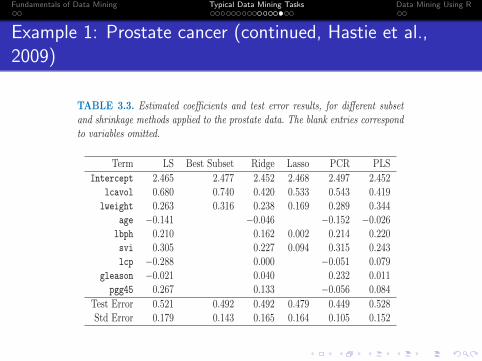
TABLE 3.3. Estimated coefficients and test error results, for different subsetand shrinkage methods applied to the prostate data. The blank entries correspondto variables omitted.
Term LS Best Subset Ridge Lasso PCR PLS
Intercept 2.465 2.477 2.452 2.468 2.497 2.452lcavol 0.680 0.740 0.420 0.533 0.543 0.419lweight 0.263 0.316 0.238 0.169 0.289 0.344
age −0.141 −0.046 −0.152 −0.026lbph 0.210 0.162 0.002 0.214 0.220svi 0.305 0.227 0.094 0.315 0.243lcp −0.288 0.000 −0.051 0.079
gleason −0.021 0.040 0.232 0.011pgg45 0.267 0.133 −0.056 0.084
Test Error 0.521 0.492 0.492 0.479 0.449 0.528Std Error 0.179 0.143 0.165 0.164 0.105 0.152
squares,
β̂ridge = argminβ
{ N∑
i=1
(yi − β0 −
p∑
j=1
xijβj)2
+ λ
p∑
j=1
β2j
}. (3.41)
Here λ ≥ 0 is a complexity parameter that controls the amount of shrink-age: the larger the value of λ, the greater the amount of shrinkage. Thecoefficients are shrunk toward zero (and each other). The idea of penaliz-ing by the sum-of-squares of the parameters is also used in neural networks,where it is known as weight decay (Chapter 11).
An equivalent way to write the ridge problem is
β̂ridge = argminβ
N∑
i=1
(yi − β0 −
p∑
j=1
xijβj
)2,
subject to
p∑
j=1
β2j ≤ t,
(3.42)
which makes explicit the size constraint on the parameters. There is a one-to-one correspondence between the parameters λ in (3.41) and t in (3.42).When there are many correlated variables in a linear regression model,their coefficients can become poorly determined and exhibit high variance.A wildly large positive coefficient on one variable can be canceled by asimilarly large negative coefficient on its correlated cousin. By imposing asize constraint on the coefficients, as in (3.42), this problem is alleviated.
The ridge solutions are not equivariant under scaling of the inputs, andso one normally standardizes the inputs before solving (3.41). In addition,
Fundamentals of Data Mining Typical Data Mining Tasks Data Mining Using R
IV. Discovering patterns and rules
Pattern detection: Examples includespotting fraudulent behavior,detection of unusual stars or galaxies.
Association rules: For example, to find combinations of itemsthat occur frequently in transaction databases (e.g., groceryproducts that are often purchased together).
Fundamentals of Data Mining Typical Data Mining Tasks Data Mining Using R
V. Retrieval by content
Find similar patterns in the data set.
For text (e.g., Web pages), the pattern may be a set ofkeywords.
For images, the user may have a sample image, a sketch of animage, or a description of an image, and wish to find similarimages from a large set of images.
The definition of similarity is critical, but so are the details ofthe search strategy.
Fundamentals of Data Mining Typical Data Mining Tasks Data Mining Using R
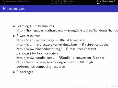
R resources
Learning R in 15 minuteshttp://homepages.math.uic.edu/∼jyang06/stat486/handouts/handout3.pdf
R web resourceshttp://cran.r-project.org/ – Official R websitehttp://cran.r-project.org/other-docs.html – R reference bookshttp://www.bioconductor.org/ – R resources (dataset,packages) for bioinformaticshttp://www.rstudio.com/ – RStudio, a convenient R editorhttp://accc.uic.edu/service/argo-cluster – UIC highperformance computing resource
R packages
Fundamentals of Data Mining Typical Data Mining Tasks Data Mining Using R
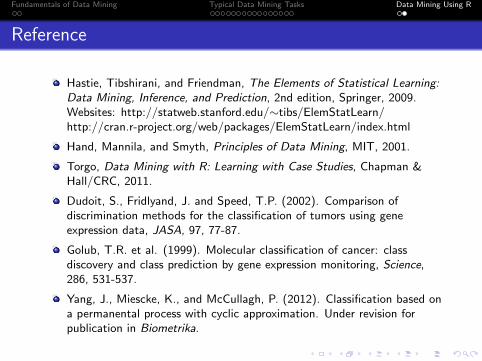
Reference
Hastie, Tibshirani, and Friendman, The Elements of Statistical Learning:Data Mining, Inference, and Prediction, 2nd edition, Springer, 2009.Websites: http://statweb.stanford.edu/∼tibs/ElemStatLearn/http://cran.r-project.org/web/packages/ElemStatLearn/index.html
Hand, Mannila, and Smyth, Principles of Data Mining, MIT, 2001.
Torgo, Data Mining with R: Learning with Case Studies, Chapman &Hall/CRC, 2011.
Dudoit, S., Fridlyand, J. and Speed, T.P. (2002). Comparison ofdiscrimination methods for the classification of tumors using geneexpression data, JASA, 97, 77-87.
Golub, T.R. et al. (1999). Molecular classification of cancer: classdiscovery and class prediction by gene expression monitoring, Science,286, 531-537.
Yang, J., Miescke, K., and McCullagh, P. (2012). Classification based ona permanental process with cyclic approximation. Under revision forpublication in Biometrika.
Related Documents