Introduction to Compressible Computational Fluid …educ.jmu.edu/~sochacjs/navierstokes.pdf · compressible ow equations. The incompressible ow equations model uids whose density

Introduction to Compressible Computational Fluid DynamicsJames S. Sochacki

Department of MathematicsJames Madison University

[email protected]

Abstract

This document is intended as an introduction to computational fluid dynamics atthe upper undergraduate level. It is assumed that the student has had courses throughthree dimensional calculus and some computer programming experience with numer-ical algorithms. A course in differential equations is recommended. This documentis intended to be used by undergraduate instructors and students to gain an under-standing of computational fluid dynamics. The document can be used in a classroomor research environment at the undergraduate level. The idea of this work is to havethe students use the modules to discover properties of the equations and then relatethis to the physics of fluid dynamics. Many issues, such as rarefactions and shocksare left out of the discussion because the intent is to have the students discover theseconcepts and then study them with the instructor. The document is used in part ofthe undergraduate MATH 365 - Computation Fluid Dynamics course at James Madi-son University (JMU) and is part of the joint NSF Grant between JMU and NorthCarolina Central University (NCCU): A Collaborative Computational Sciences Pro-gram.

This document introduces the full three-dimensional Navier Stokes equations. As-sumptions to these equations are made to derive equations that are accessible to un-dergraduates with the above prerequisites. These equations are approximated usingfinite difference methods. The development of the equations and finite differencemethods are contained in this document. Software modules and their correspondingdocumentation in Fortran 90, Maple and Matlab can be downloaded from the web-site: http://www.math.jmu.edu/~jim/compressible.html. The software modulesand their corresponding documentation are mentioned in this document.

Introduction

Computational fluid dynamics (CFD) usually involves working with some formof the Navier-Stokes equations. These forms are usually obtained by making someassumptions that simplify the equations. The next step is to develop a numericalalgorithm for solving these equations.

The Navier-Stokes equations are commonly expressed in one of two forms. Oneform is known as the incompressible flow equations and the other is known as thecompressible flow equations. The incompressible flow equations model fluids whosedensity does not change over time. The compressible flow equations allow the densityof the fluid to change with the flow.

1

http://www.math.jmu.edu/~jim/compressible.html

This document will consider the compressible flow equations. The compressibleNavier-Stokes equations are intimidating partial differential equations (PDE’s) andrightfully so. They are extremely difficult mathematical equations that describe themotion of a fluid in three dimensions (3D). The equations allow for velocity changes,density changes, energy changes and viscous effects. To appreciate the complexityof these equations think about the flow of water down a rocky incline. These equa-tions can be simplified by making some assumptions about the flow of the fluid thatturns the problem into a two dimensional (2D) or sometimes a one dimensional (1D)problem.

The discussions in this document are meant to help you understand some of thecomplexities of the Navier-Stokes equations. Of course, there are whole industriesworking on these equations and no industry understands them completely. Thereare, of course, many mathematical questions that have not been answered regardingthe full 3D Navier-Stokes equations.

If assumptions can be made about the fluid being studied the Navier-Stokes equa-tions can be converted into 1D and 2D problems. Many mathematical properties areknown about some of these 1D and 2D PDE’s. You can study some of these PDE’snumerically in the equation documents described in this work.

We now present the full 3D Navier-Stokes equations. The equations are obtainedby applying Newton’s force laws, the conservation of mass principle and conservationof energy principle to the motion of a fluid. In this document we will assume that youhave seen this development in a physics course or have considered the modules at theJames Madison University Computational Science site that develop these equations.

2

The (3D) Navier-Stokes equations are

[1] The Momentum Equation or The Momentum Balance Equation

ρ(∂

∂tU + (U · ∇)U) +∇p− δ∆U − (η +

1

3µ)∇∇ · U = G

[2] The Continuity Equation or The Mass Balance Equation

∂∂tρ+∇ · (ρU) = 0

[3] The Energy Equations or The Energy Balance Equations

(E1) ∂∂tρ(1

2U · U + ε) +∇ · (ρU(1

2U · U + ω) = 0

(E2) ∂∂tE +∇ · ((E + p)U) = 0

[4] The Equations of State

(S1) p = c2ρ (Acoustics - sound waves)

(S2) p = (γ − 1)(E − 12ρU · U) (Gas Dynamics)

(S3) p = αρk (Gas Dynamics)

The momentum equation is really 3 equations since

U =

u1

u2

u3

=

u1(x1, x2, x3, t)u2(x1, x2, x3, t)u3(x1, x2, x3, t)

or

U =

uvw

=

u(x, y, z, t)v(x, y, z, t)w(x, y, z, t)

.

Newton’s force law is applied in all three dimensions. Since U = (u1, u2, u3) orU = (u, v, w), the u1 (or u) component is the velocity of the fluid in the x1 (or x)direction, the u2 (or v) component is the velocity of the fluid in the x2 (or y) directionand the u3 (or w) component is the velocity of the fluid in the x3 (or z) direction.(We will use both of these notations for our space dimensions.) Under the energyequations we have listed two energy equations because both forms of these equationsare commonly used. We have also listed some equations of state. The equationsof state are experimentally derived equations and allow us to eliminate one of theunknowns so that we have 5 PDE’s and 5 unknowns. That is, the (3D) Navier-Stokesequations are a system of 5 PDE’s. In this document, the documents describing thesoftware modules and the software modules will only use the energy equation (E2)

3

and one of the two state equations (S1) or (S2). (In (E1) ε is the internal energy andω is the enthalpy.)

We now explain the notation used in the Navier-Stoke’s equations; ρ = ρ(x, y, z, t)is the density of the fluid at a point (x, y, z) at time t, p = p(x, y, z, t) is the pressure onthe fluid at a point (x, y, z) at time t. The symbol ∇ represents the gradient (column)vector ( ∂

∂x1, ∂∂x2, ∂∂x3

) or ( ∂∂x, ∂∂y, ∂∂z

). By ∇p we mean the (column) vector (px, py, pz),where the subscript indicates partial differentiation with respect to that variable. Thesymbol ∆ represents the Laplacian and is given by ∇ · ∇ or ∂2

∂x2+ ∂2

∂y2+ ∂2

∂z2and is

applied to each component of U = (u, v, w). The parameters δ, η and µ are functionsof (x, y, z) that describe the viscosity of the fluid. The function G is the (column)vector (g1(x, y, z, t), g2(x, y, z, t), g3(x, y, z, t)) and models external forces acting onthe fluid. In the modules we set G = 0. You can easily modify the codes to seewhat effects external forces have on the fluid flow and the mathematical equations.The internal energy of the fluid is modeled by ε = ε(x, y, z, t) and the total energyof the fluid is modeled by E = E(x, y, z, t). The speed of sound in the fluid is givenby c = c(x, y, z). The functions c, α, k and γ are determined experimentally. In thesoftware modules c, α, k and γ are constant.

4

THE EULER EQUATIONS

The Euler equations are obtained from the Navier-Stokes equations by assumingthe fluid is viscous-free. Dropping these terms from the Navier-Stokes equations givesus the (3D) Euler equations

[1] Momentum Equation or Momentum Balance

ρ( ∂∂tU + (U · ∇)U) +∇p = G

[2] Continuity equation or Mass Balance

∂∂tρ+∇ · (ρU) = 0

[3] The Energy Equations or The Energy Balance Equations

(E1) ∂∂tρ(1

2U · U + ε) +∇ · (ρU(1

2U · U + w) = 0

(E2) ∂∂tE +∇ · ((E + p)U) = 0



(S2) p = (γ − 1)(E − 12ρU · U) (Gas Dynamics)

(S3) p = αρk (Gas Dynamics)

As an exercise you should carry out the differentiation and vector operations inthe Navier-Stokes and Euler equations and express the PDE’s for these equations interms of the components of U using either the

U =

u1

u2

u3

=

u1(x1, x2, x3, t)u2(x1, x2, x3, t)u3(x1, x2, x3, t)

or

U =

uvw

=

u(x, y, z, t)v(x, y, z, t)w(x, y, z, t)

notation.

5

THE 1D NAVIER-STOKES AND EULER EQUATIONS

In the modules we will only consider the (1D) equations. A study of the (1D)equations will give you an insight into the difficulties of studying fluid mechanics andof simulating fluid flow on a computer. Many of the problems arising in (1D) have tobe considered in both (2D) and (3D). Of course, more problems arise in (2D) than(1D) and in (3D) than (2D). The modules are meant to give you an understanding ofthe complexities of computational science and of what computational science is andhow it is used in CFD. Although, we are studying fluid flow the ideas of developinga system of equations that describe a phenomena, numerically approximating theseequations and their solutions with algorithms, using computers to run the algorithmsand using computers to visualize the results make up computational science. Ofcourse, studying each of these steps and the difficulties of each step also make upcomputational science.

A physical interpretation of the 1D equations is to think of the flow of a fluid ina thin tube or a narrow channel and how the properties of the fluid; velocity, densityand energy change only along the tube or the channel. Of course, problems like thisoccur all the time. Drinking straws, ditches and blood veins are some examples.

We will write the (1D) Navier-Stokes equations as


ρ( ∂∂tu+ u ∂

∂xu) + ∂

∂xp− δ ∂2

∂x2u− (η + 1

3µ) ∂2

∂x2u = g(x, t)


∂∂tρ+ ∂

∂x(ρu) = 0

[3] The Energy Equation or The Energy Balance Equation

∂

∂tE +

∂

∂x((E + p)u) = 0



(S2) p = (γ − 1)(E − 12ρu2) (Gas Dynamics)

Note that the momentum equation can be written as

ρut + ρuux + px − αuxx = g

or

6

ρ(ut + (12u2)x) + px − αuxx = g

where α = δ + η + 13µ. If the pressure does not depend on x this equation reduces to

ρ(ut + uux)− αuxx = g

or

ρ(ut + (12u2)x)− αuxx = g.

Now suppose the fluid density, ρ is a constant. Dividing by ρ gives us

(B1) ut + uux − νuxx = G

or

(B2) ut + (12u2)x − νuxx = G.

where ν = αρ

and G(x, t) = g(x,t)ρ

. These PDE’s are known as Burger’s equation with

viscosity. Equation (B1) is known as the non-conservation form of Burger’s equationand equation (B2) is known as the conservation form of Burger’s equation. A studyof these equations will help you to understand fluid velocity in the Navier-Stokesequations. You can click on the Burger’s Modules Description Document link tolearn how to do a numerical study of these equations through the software modules.A good discovery project is to modify the modules to include viscosity and then studywhat happens as ν → 0 and compare this with the numerical solution to Burger’sequation with ν = 0. After this study return to equation (B2) and see how you couldverify your numerical results analytically.

We now consider the Continuity Equation PDE. If the fluid velocity u is a constantthis PDE reduces to

(W) ∂∂tρ+ u ∂

∂x(ρ) = 0.

We leave it as an exercise for you to use the chain rule of differentiation to showthat ρ(x, t) = f(x−ut) is a general solution to this PDE for an arbitrary differentiablefunction f and a constant fluid velocity u. Note that ρ(x, 0) = f(x). Therefore,physically f is the fluid density at time 0 or the initial fluid density. Also, note thatthe graph of f(x − ut) is a translation of the graph of f(x) to the right or left by adistance |ut| depending on the sign of u. Therefore, the general solution to equation(W) is a translation of the initial density by |ut|. We see that over time the initialdensity moves to the right or left by an amount |ut|. That is, as the time t increasesthe initial density moves further to the right or to the left. This is known as a wave.Since |ut| can be thought of as the distance the initial density moves, we will call |u|the speed of the wave. To do a numerical study of advection diffusion equation clickon the Advection Diffusion Modules Description Document link. This document willdescribe the software modules for this equation. You will observe the phenomenadescribed above in these software modules.

Note that equation (B1) and equation (W) are similar to the PDE

7

(AD) wt + cwx + dwxx = h(x, t).

This PDE is known as the advection-diffusion equation. In order to get (B1) from(AD) we replace u by w in the partial derivative expressions, u with no derivativesby c and α by d. In order to get (W) from (AD) we replace ρ by w, u by c and dwould equal 0. In the software modules you will see that c is the speed (or advection)of the wave and d is the diffusion of the system.

We now consider the (1D) Euler equations. An understanding of these equationsis essential to understanding the (1D) Navier-Stokes equations. After completing themodules associated with the (1D) Euler equations you should be able to write yourown codes for the (1D) Navier-Stokes equations.

The (1D) Euler equations which we will denote as (E1) are


ρ( ∂∂tu+ u ∂

∂xu) + ∂

∂xp = g(x, t)


∂∂tρ+ ∂

∂x(ρu) = 0


∂

∂tE +

∂

∂x((E + p)u) = 0




We now consider another form of the (1D) Euler equations. From the productrule we have that

(ρu)t = ρtu+ ρut

and that

ρut = (ρu)t − ρtu.

From the continuity equation we have that −ρt = ∂∂x

(ρu). Using this in the lastequation we obtain

ρut = (ρu)t + u∂

∂x(ρu).

8

Substituting this into the momentum equation we see that

ρut + ρu∂

∂xu+

∂

∂xp =

(ρu)t + u∂

∂x(ρu) + ρu

∂

∂xu+

∂

∂xp =

(ρu)t +∂

∂x(uρu) +

∂

∂xp = g

where in the last equality we used the product rule. From the last line we now obtainthe following form for the momentum equation

(ρu)t +∂

∂x(u2ρ+ p) = g.

Using this form of the momentum equation the (1D) Euler equations (with thismomentum equation) which we will denote as (E2) are


∂∂t

(ρu) + ∂∂x

(u2ρ+ p) = g


∂∂tρ+ ∂

∂x(ρu) = 0


∂

∂tE +

∂

∂x((E + p)u) = 0




If we use (S1) in the momentum equation and the continuity equation we obtainthe following system of equations for u and ρ which we will denote as (E3)


∂∂t

(ρu) + ∂∂x

((u2 + c2)ρ) = g


9

∂∂tρ+ ∂

∂x(ρu) = 0

or the following system of equations for u and p which we will denote as (E4)


∂∂t

( pc2u) + ∂

∂x(u

2+c2

c2p) = g


∂∂t

pc2

+ ∂∂x

( pc2u) = 0

Since the speed of sound in the fluid is usually known, we see that both of these formsare two equations in two unknowns. We leave it as an exercise for you to show thatthese two equations can be written in the form

∂

∂tv1 +

∂

∂xf1(v1, v2) = g(x)

∂

∂tv2 +

∂

∂xf2(v1, v2) = 0.

(You need to determine v1, v2, f1 and f2.) Equations of this form are called conser-vation equations. You will find that the functions f1 and f2 are similar for (E3) and(E4). If you solve (E3) you can get the pressure from p = c2ρ and if you solve (E4) youcan get the density from this same relationship. The software modules allow you todo a numerical study of equation (E3). To learn how to do this study click on the linkOne Dimensional Density Velocity Equations Modules Description Document. Thisdocument will describe the software modules dealing with this equation. Later, wewill use the acoustic condition S2 (p = c2ρ) to generate a linear equation for pressuredisturbances.

10

If we use (S2) in the energy equation we obtain the following system of equationsfor u, ρ and E which we will denote as (E5)


∂∂t

(ρu) + ∂∂x

((γ − 1)(E − 12ρu2)) = g


∂∂tρ+ ∂

∂x(ρu) = 0


∂

∂tE +

∂

∂x((γE − (1− γ)

2ρu2)u) = 0

Note these equations can be put in the form

∂

∂tv1 +

∂

∂xf1(v1, v2, v3) = 0

∂

∂tv2 +

∂

∂xf2(v1, v2, v3) = 0

∂

∂tv3 +

∂

∂xf3(v1, v2, v3) = 0

where v1 = (ρu), v2 = ρ and v3 = E and where

f1(v1, v2, v3) =v21v2

+ (γ − 1)(v3 − 12

v21v2

)

f2(v1, v2, v3) = v1

f3(v1, v2, v3) = (γv3 − (1−γ)2

v21v2

)v1v2

.

We leave it as an exercise for you to carry out the process we did to get these con-servation equations from (E1) and (S2) to get the conservation equation form for the(3D) Euler equations. To do a numerical study of the (1D) Euler equations clickon the link One Dimensional Euler Equations Modules Description Document. Thisdocument will describe the software modules associated with this equation.

We could have substituted (S1) or (S2) directly into (E1) and used these equationsin the modules. We leave this as an exercise for you. You can compare and contrastyour codes for these systems with the codes in the modules.

11

The 1D Linearized Pressure Equation or Acoustic Equation

We will assume c is a constant in our derivation. To model the propagation ofsound (acoustic or pressure) waves we will linearize the following two equations.


∂∂t

( pc2u) + ∂

∂x(u2 p

c2+ p) = 0


∂∂t

pc2

+ ∂∂x

( pc2u) = 0.

In acoustic (sound) waves the particle velocity u is small. That is, |u| << 1 implyingu2 << u. Therefore, we linearize the Momentum Equation by dropping the nonlinearterms containing u2. This gives us


∂∂t

( pc2u) + ∂

∂xp = 0


∂∂t

pc2

+ ∂∂x

( pc2u) = 0.

We differentiate the Momentum Equation with respect to x and the Continuity Equa-tion with respect to t and equate the mixed partial derivative term ( p

c2u)xt to get

(LP) ptt − c2pxx = 0.

We leave it for you to show that

p(x, t) = f(x− ct) + g(x+ ct)

for arbitrary functions f and g is a solution to (LP). That is, the linearized pressureequation has solutions made up waves traveling to the left and to the right with speedc.

12

THE NUMERICAL SOLUTIONS

Introduction

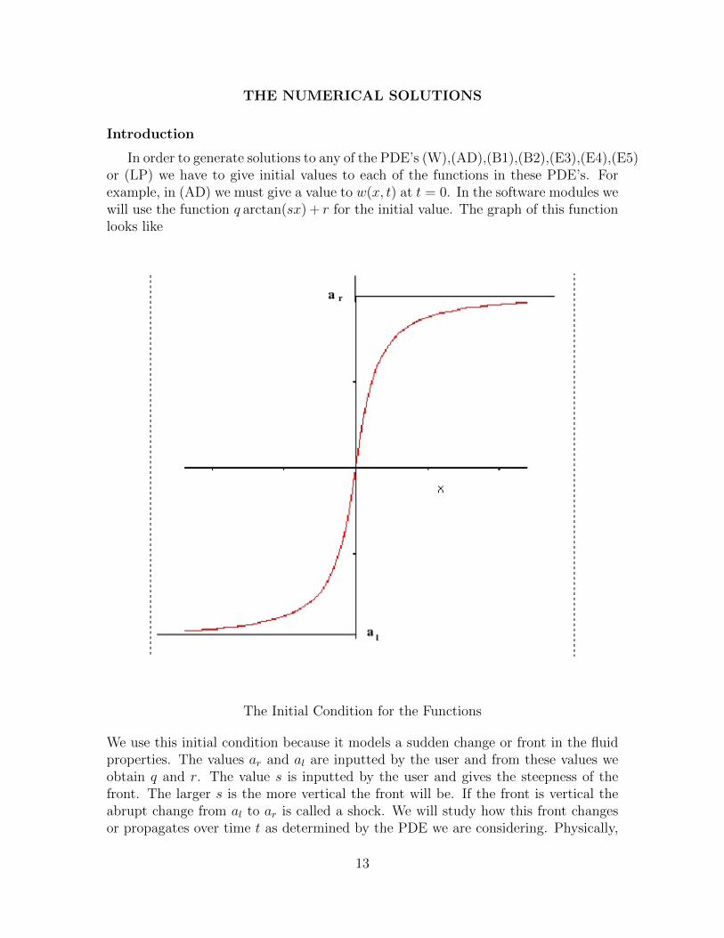
In order to generate solutions to any of the PDE’s (W),(AD),(B1),(B2),(E3),(E4),(E5)or (LP) we have to give initial values to each of the functions in these PDE’s. Forexample, in (AD) we must give a value to w(x, t) at t = 0. In the software modules wewill use the function q arctan(sx) + r for the initial value. The graph of this functionlooks like

The Initial Condition for the Functions

We use this initial condition because it models a sudden change or front in the fluidproperties. The values ar and al are inputted by the user and from these values weobtain q and r. The value s is inputted by the user and gives the steepness of thefront. The larger s is the more vertical the front will be. If the front is vertical theabrupt change from al to ar is called a shock. We will study how this front changesor propagates over time t as determined by the PDE we are considering. Physically,

13

one can think of having a glass tube of length 20 meters and at the midpoint there isa filament that blocks air from traveling down the tube. However, this filament canbe removed to allow the air to flow down the tube. Smoke filled air is put in the glasstube on the left. The right is filled with clean air. The filament is then removed.Intuitively, one would think the smoke would move to the right into the clean air. Wewill look to see if this happens in our modules that simulate fluid flow.

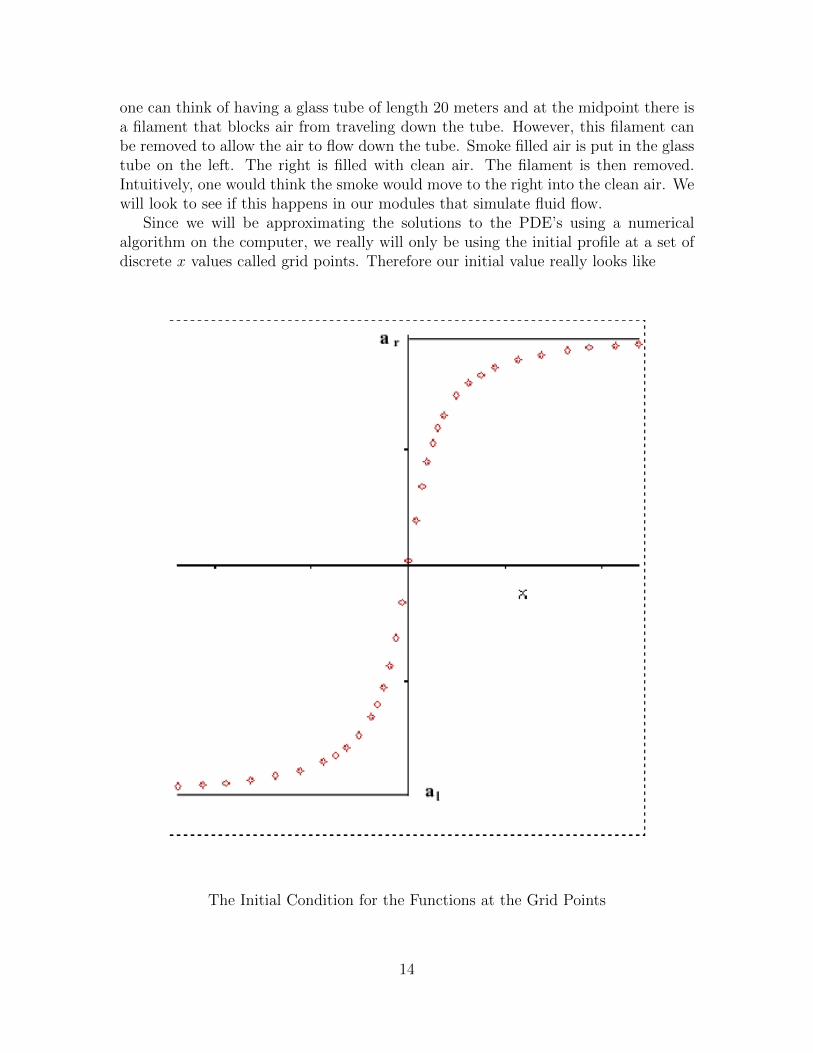
Since we will be approximating the solutions to the PDE’s using a numericalalgorithm on the computer, we really will only be using the initial profile at a set ofdiscrete x values called grid points. Therefore our initial value really looks like

The Initial Condition for the Functions at the Grid Points

14

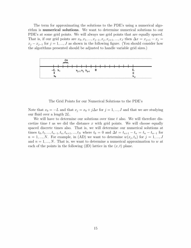
The term for approximating the solutions to the PDE’s using a numerical algo-rithm is numerical solutions. We want to determine numerical solutions to ourPDE’s at some grid points. We will always use grid points that are equally spaced.That is, if our grid points are x0, x1, ..., xj−1, xj, xj+1, ..., xJ then ∆x = xj+1 − xj =xj − xj−1 for j = 1, ..., J as shown in the following figure. (You should consider howthe algorithms presented should be adjusted to handle variable grid sizes.)

The Grid Points for our Numerical Solutions to the PDE’s

Note that x0 = −L and that xj = x0 + j∆x for j = 1, ..., J and that we are studyingour fluid over a length 2L.

We will have to determine our solutions over time t also. We will therefore dis-cretize time t as we did the distance x with grid points. We will choose equallyspaced discrete times also. That is, we will determine our numerical solutions attimes t0, t1, ..., tn−1, tn, tn+1, ..., tN where t0 = 0 and ∆t = tn+1 − tn = tn − tn−1 forn = 1, ..., N . For example, in (AD) we want to determine w(xj, tn) for j = 1, ..., Jand n = 1, ..., N . That is, we want to determine a numerical approximation to w ateach of the points in the following (2D) lattice in the (x, t) plane.

15

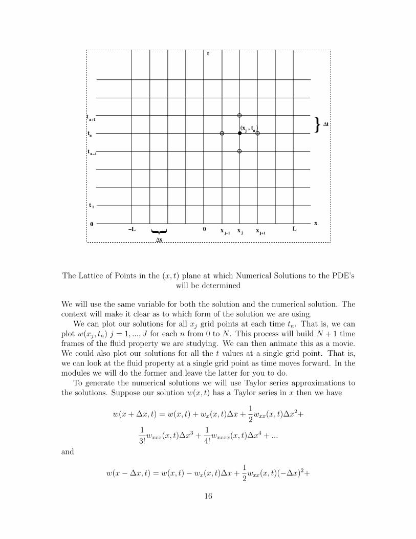
The Lattice of Points in the (x, t) plane at which Numerical Solutions to the PDE’swill be determined

We will use the same variable for both the solution and the numerical solution. Thecontext will make it clear as to which form of the solution we are using.

We can plot our solutions for all xj grid points at each time tn. That is, we canplot w(xj, tn) j = 1, ..., J for each n from 0 to N . This process will build N + 1 timeframes of the fluid property we are studying. We can then animate this as a movie.We could also plot our solutions for all the t values at a single grid point. That is,we can look at the fluid property at a single grid point as time moves forward. In themodules we will do the former and leave the latter for you to do.

To generate the numerical solutions we will use Taylor series approximations tothe solutions. Suppose our solution w(x, t) has a Taylor series in x then we have

w(x+ ∆x, t) = w(x, t) + wx(x, t)∆x+1

2wxx(x, t)∆x

2+

1

3!wxxx(x, t)∆x

3 +1

4!wxxxx(x, t)∆x

4 + ...

and

w(x−∆x, t) = w(x, t)− wx(x, t)∆x+1

2wxx(x, t)(−∆x)2+

16

1

3!wxxx(x, t)(−∆x3) +

1

4!wxxxx(x, t)(−∆x)4 + ...

We call the first Taylor series the forward series and the latter Taylor series thebackward series. From the forward series we have

wx(x, t) =w(x+ ∆x, t)− w(x, t)

∆x− 1

2wxx(x, t)∆x−

1

3!wxxx(x, t)∆x

2 − 1

4!wxxxx(x, t)∆x

3 − ...

and from the backward series we have

wx(x, t) =w(x, t)− w(x−∆x, t)

∆x+

1

2wxx(x, t)∆x−

1

3!wxxx(x, t)∆x

2 +1

4!wxxxx(x, t) + ∆x3...

We will call the approximation

(FD) w(x+∆x,t)−w(x,t)∆x

to wx(x, t) the forward difference in space approximation to wx(x, t) and we will call

(BD) w(x,t)−w(x−∆x,t)∆x

the backward difference in space approximation to wx(x, t). The error in both of theseapproximations is seen to depend on ∆x and wxx. If we subtract the backward seriesfrom the forward series we have

wx(x, t) =w(x+ ∆x, t)− w(x−∆x, t)

2∆x− 1

3!wxxx(x, t)∆x

2 − ...

We call

(CD) w(x+∆x,t)−w(x−∆x,t)2∆x

the centered difference in space approximation to wx(x, t). We see that the error inthis approximation depends on wxxx and ∆x2. If ∆x << 1 then we would expectusing (CD) to give us better results than using (FD) or (BD). In the modules youwill learn that this is not always the case.

If we add the forward and backward series we find that

wxx(x, t) =w(x+ ∆x, t)− 2w(x, t) + w(x−∆x, t)

∆x2+

1

4!wxxxx(x, t)∆x

2 + ...

We call

(SCD) w(x+∆x,t)−2w(x,t)+w(x−∆x,t)∆x2

17

the second centered difference in space approximation to wxx(x, t).

Advection Diffusion Equation

Consider the equation (AD) (with h = 0)

wt(xj, t) = w′(xj, t) = −cwx(xj, t)− dwxx(xj, t) for j = 1, .., J − 1

If we apply (FD),(BD) and (CD) to this equation we obtain the following numer-ical schemes

(ADF)

wt(xj, t) = w′(xj, t) = −c(w(xj+∆x,t)−w(xj ,t)

∆x)− d(

w(xj+∆x,t)−2w(xj ,t)+w(xj−∆x,t)

∆x2)

for j = 1, .., J − 1

(ADB)

wt(xj, t) = w′(xj, t) = −c(w(xj ,t)−w(xj−∆x,t)

∆x)− d(


∆x2)

for j = 1, .., J − 1

(ADC)

wt(xj, t) = w′(xj, t) = −c(w(xj+∆x,t)−w(xj−∆x,t)

2∆x)− d(


∆x2)

for j = 1, .., J − 1

respectively. We can rewrite these equations as

(ADF) wt(xj, t) = w′(xj, t) = −c(w(xj+1,t)−w(xj ,t)

∆x)− d(

w(xj+1,t)−2w(xj ,t)+w(xj−1,t)

∆x2)

for j = 1, .., J − 1

(ADB) wt(xj, t) = w′(xj, t) = −c(w(xj ,t)−w(xj−1,t)

∆x)− d(


∆x2)

for j = 1, .., J − 1

(ADC) wt(xj, t) = w′(xj, t) = −c(w(xj+1,t)−w(xj−1,t)

2∆x)− d(


∆x2)

for j = 1, .., J − 1

Note that each of these is a system of ordinary differential equations for J − 1functions wj(t) = w(xj, t). Note that in (ADF) when J = 1 we need w(x0, t) andthat in (ADB) when j = J − 1 we need w(xJ , t). In our modules we will always use

w(x0, t) = qarctan(sx0) + r.

andw(xJ , t) = qarctan(sxJ) + r.

That is, we will keep w(x0, t) and w(xJ , t) constant over time. We will not solvesystems of ordinary differential equations in this document. The reader can solvethese systems.

We now replace the wt(xj, t) = w′(xj, t) by forward, backward and centered dif-ferences in time. For example, consider (ADF) we have

18

(ADFF)w(xj ,tn+1)−w(xj ,tn)

∆t= −c(w(xj+1,tn)−w(xj ,tn)

∆x)− d(

w(xj+1,tn)−2w(xj ,tn)+w(xj−1,tn)

∆x2)

for j = 1, .., J − 1

(ADFB)w(xj ,tn)−w(xj ,tn−1)

∆t= −c(w(xj+1,tn)−w(xj ,tn)

∆x)− d(


∆x2)

for j = 1, .., J − 1

(ADFC)w(xj ,tn+1)−w(xj ,tn−1)

2∆t= −c(w(xj+1,tn)−w(xj ,tn)

∆x)− d(


∆x2)

for j = 1, .., J − 1

as the forward in time, backward in time and centered in time approximationsfor (ADF), respectively. The schemes (ADFF) and (ADFC) are known as explicitschemes because we can solve explicitly for w(xj, tn+1) for j = 1, .., J−1. The scheme(ADFB) is known as an implicit scheme because we have to solve all the equationsat once for w(xj, tn) for j = 1, .., J − 1. We have to write (ADFB) as a system ofJ−1 equations and solve the resulting matrix equation. We will only consider explicitschemes in the modules. Solving for w(xj, tn+1) in (ADFF) and (ADFC) we obtain

(ADFF) w(xj, tn+1) =w(xj, tn)− c∆t

∆x(w(xj+1, tn)− w(xj, tn))− d∆t

∆x2(w(xj+1, tn)− 2w(xj, tn) + w(xj−1, tn))

for j = 1, .., J − 1

(ADFC) w(xj, tn+1) =w(xj, tn−1)− 2c∆t

∆x(w(xj+1, tn)−w(xj, tn))− 2d∆t

∆x2(w(xj+1, tn)−2w(xj, tn)+w(xj−1, tn))

for j = 1, .., J − 1

Let’s now consider (ADFF). Suppose n = 0 then we have

w(xj, t1) =w(xj, 0)− c∆t

∆x(w(xj+1, 0)− w(xj, 0))− d∆t

∆x2(w(xj+1, 0)− 2w(xj, 0) + w(xj−1, 0))

for j = 1, .., J − 1

since t0 = 0. We can see that in order to find w(xj, t1) for j = 1, .., J − 1 we need toknow w(xj, 0) for j = 1, .., J − 1. Of course, we do know this since w(xj, 0) is givenby our initial condition. We now have an approximation to w at the next time step.Letting n = 1 in (ADFF) gives us

19

w(xj, t2) =w(xj, t1)− c∆t

∆x(w(xj+1, t1)− w(xj, t1))− d∆t

∆x2(w(xj+1, t1)− 2w(xj, t1) + w(xj−1, t1))

for j = 1, .., J − 1.

Since we solved for w(xj, t1) for j = 1, .., J−1 when n = 0, we can determine w(xj, t2)for j = 1, .., J − 1. We proceed in this fashion.

Note that to get w(xj, t2) for j = 1, .., J − 1 we do not need to know w(xj, 0).Therefore, in our codes we will write w(xj, t0) for j = 1, .., J − 1 to a file and replacew(xj, 0) for j = 1, .., J − 1 by w(xj, t1) for j = 1, .., J − 1. We will then solve forw(xj, t2) for j = 1, .., J − 1. We then write w(xj, t2) for j = 1, .., J − 1 to a file andreplace w(xj, 0) for j = 1, .., J − 1 by w(xj, t2) for j = 1, .., J − 1. We continue thisprocess for each time step we solve for w(xj, tn). This is a common practice since itreduces the amount of computer memory our program will need. Since we put the wvalues in a file, we can use the w values in these files for analysis and visualization.

In the module where we study (AD) we use

(ADFF) w(xj, tn+1) =w(xj, tn)− c∆t

∆x(w(xj+1, tn)− w(xj, tn))− d∆t


for j = 1, .., J − 1,

(ADBF) w(xj, tn+1) =w(xj, tn)− c∆t

∆x(w(xj, tn)− w(xj−1, tn))− d∆t


for j = 1, .., J − 1

and

(ADCC) w(xj, tn+1) =w(xj, tn−1)− c∆t

∆x(w(xj+1, tn)−w(xj−1, tn))− 2d∆t

∆x2(w(xj+1, tn)−2w(xj, tn)+w(xj−1, tn))

for j = 1, .., J − 1.

Schemes (ADFF) and (ADBF) are called upwind schemes and (ADCC) is called aleap frog scheme. To see where these names come from we let d = 0. We then have

(ADFF) w(xj, tn+1) = w(xj, tn)− c∆t∆x

(w(xj+1, tn)− w(xj, tn))

for j = 1, .., J − 1,

(ADBF) w(xj, tn+1) = w(xj, tn)− c∆t∆x

(w(xj, tn)− w(xj−1, tn))

for j = 1, .., J − 1

and

20

(ADCC) w(xj, tn+1) = w(xj, tn−1)− c∆t∆x

(w(xj+1, tn)− w(xj−1, tn))

for j = 1, .., J − 1.

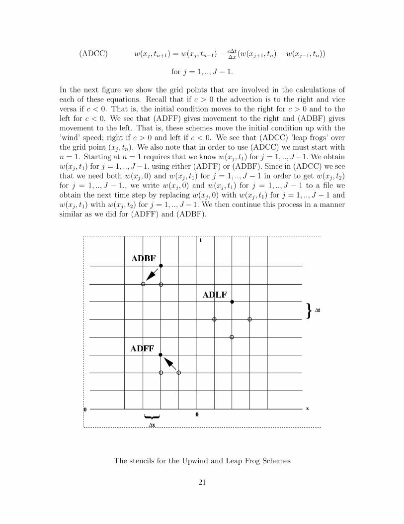
In the next figure we show the grid points that are involved in the calculations ofeach of these equations. Recall that if c > 0 the advection is to the right and viceversa if c < 0. That is, the initial condition moves to the right for c > 0 and to theleft for c < 0. We see that (ADFF) gives movement to the right and (ADBF) givesmovement to the left. That is, these schemes move the initial condition up with the’wind’ speed; right if c > 0 and left if c < 0. We see that (ADCC) ’leap frogs’ overthe grid point (xj, tn). We also note that in order to use (ADCC) we must start withn = 1. Starting at n = 1 requires that we know w(xj, t1) for j = 1, .., J−1. We obtainw(xj, t1) for j = 1, .., J−1. using either (ADFF) or (ADBF). Since in (ADCC) we seethat we need both w(xj, 0) and w(xj, t1) for j = 1, .., J − 1 in order to get w(xj, t2)for j = 1, .., J − 1., we write w(xj, 0) and w(xj, t1) for j = 1, .., J − 1 to a file weobtain the next time step by replacing w(xj, 0) with w(xj, t1) for j = 1, .., J − 1 andw(xj, t1) with w(xj, t2) for j = 1, .., J − 1. We then continue this process in a mannersimilar as we did for (ADFF) and (ADBF).

The stencils for the Upwind and Leap Frog Schemes

21

Note that if c∆t∆x

= 1 and d = 0 in (ADBF) we have

w(xj, tn+1) = w(xj−1, tn).

That is, the value of w at the point (xj, tn+1) is equal to the value of w at a point∆x back in space and a point ∆t back in time. Since c = ∆x

∆tin this case, we see that

the values of w are moving forward in time at the speed c. Therefore, this schemegives the exact solution since we know that this is what happens in the PDE whend = 0. We leave it for you to show that a similar phenomenon occurs in (ADFF)under these same conditions. You can test this in the modules. You should then testwhat happens if c∆t

∆x< 1 and then what happens if c∆t

∆x> 1. The phenomenon you

will observe is called the Courant-Friedrichs-Lewy condition.

Burger’s Equation

We now proceed to the viscous Burger equations (B1) and (B2). We first considerthe leap frog schemes. That is, we use centered differences on the equations

(B1) ut + uux − νuxx = G

and

(B2) ut + (12u2)x − νuxx = G.

We will only do these equations for ν = 0 and G = 0. We leave the viscous case foryou. For (B1) we have

(B1LF) u(xj, tn+1) = u(xj, tn−1)− ( ∆t∆x

)u(xj, tn)(u(xj+1, tn)− u(xj−1, tn))

for j = 1, .., J − 1.

(B2LF) u(xj, tn+1) = u(xj, tn−1)− ( ∆t∆x

)(u(xj+1, tn)2/2− u(xj−1, tn)2/2)

for j = 1, .., J − 1.

The scheme (B1LF) depends on the differentiated (non-conservation) form of theBurger’s equation and (B2LF) depends on the undifferentiated (conservation) form ofthe Burger’s equation. If our initial condition has a steep slope the derivative will belarge and we expect larger errors. We should check for this in the Burger’s equationmodules.

The last numerical approximation we consider for the solutions to our PDE’s isthe Lax-Wendroff scheme. In the Lax-Wendroff scheme we look at the Taylor seriesof w(x, t) in t. We have

w(x, t+ ∆t) = w(x, t) + ∆twt(x, t) +1

2∆t2wtt(x, t)+

1

3!∆t3wttt(x, t) +

1

4!∆t4wtttt(x, t) + ...

22

If we truncate after the wt(x, t) term we call the approximation the first order Lax-Wendroff scheme, if we truncate after the wtt(x, t) term we call the approximationthe second order Lax-Wendroff scheme and so on. We replace the t derivatives by thePDE. For example, if we apply the second order Lax-Wendroff scheme to (B2) (withν = 0 and G = 0) we have

ut = −(12u2)x

and

utt = (−(12u2)x)t = −((1

2u2)t)x.

In the last equation we assumed that we could switch the order of differentiation.Carrying out the differentiation we have

utt = −((12u2)t)x = −(uut)x.

Now replacing ut by the PDE we have

utt = −(uut)x = (u(12u2)x)x.

We now have our second order Lax-Wendroff approximation

u(x, t+ ∆t) = u(x, t) + ut(x, t)∆t+1

2utt(x, t)∆t

2 =

u(x, t)− (1

2u2)x∆t+

1

2(u(

1

2u2)x)x∆t

2.

We now replace the outside x derivatives by centered differences in the following way

(B2LW) u(xj, t+ ∆t) = u(xj, t)− ( ∆t2∆x

)(u(xj+1, t)2/2− u(xj−1, t)

2/2) +12

∆t2

∆x(u(xj+1/2, t)(

12u(xj+1/2, t)

2)x − u(xj−1/2, t)(12u(xj−1/2, t)

2)x).

Note that we used centered differences on the last term with ∆x at the points(xj−1/2, t) and (xj+1/2, t). We now replace

u(xj+1/2, t) and u(xj−1/2, t)

by

u(xj−1/2, t) ≈ (u(xj, t) + u(xj−1, t))/2 and u(xj+1/2, t) ≈ (u(xj+1, t) + u(xj, t))/2.

That is, we approximate these values by the average value of adjacent grid points.We then do centered differences on u(xj−1/2, t)

2x and u(xj+1/2, t)

2x to get

u(xj−1/2, t)2x ≈

(u(xj ,t)2−u(xj−1,t)

2)

∆xand u(xj+1/2, t)

2x ≈

(u(xj+1,t)2−u(xj ,t)

2)

∆x.

23

Substituting these into (B2LW) gives us

(B2LW)u(xj, tn+1) = u(xj, tn)− ( ∆t

∆x)(u(xj+1, tn)2/2− u(xj−1, tn)2/2) + 1

2∆t2

∆x[(u(xj+1, tn) +

u(xj, tn))/2](12

(u(xj+1,tn)2−u(xj ,tn)2)

∆x)− [(u(xj, tn)+u(xj−1, tn))/2](1

2

(u(xj ,tn)2−u(xj−1,tn)2)

∆x).

We leave it as an exercise for you to apply Lax-Wendroff to (B1).We use leap frog and Lax-Wendroff on (E3) or (E4) and (E5). These are done in

the software for the 1D Density Velocity Equations and 1D Euler Equations, respec-tively. To apply leap frog or Lax-Wendroff to a system of PDE’s you apply it to eachequation in the system. For example, consider the numerical solutions to (E4) (withg = 0)

∂∂tm+ ∂

∂x(m

2

w+ c2w) = 0

∂∂tw + ∂

∂xm = 0

using leap frog. (We have made the substitutions w = pc2

and m = uw in (E4).)Applying centered differences to the derivatives we obtain

m(xj ,tn+1)−m(xj ,tn−1)

2∆t= −

m(xj+1,tn)2

w(xj+1,tn)−

m(xj−1,tn)2

w(xj−1,tn)+c(xj+1)2w(xj+1,tn)−c(xj−1)2w(xj−1,tn)

2∆x

w(xj ,tn+1)−w(xj ,tn−1)

2∆t= −m(xj+1,tn)−m(xj−1,tn)

2∆x.

Of course, in the first equation we solve for m(xj, tn+1) and in the second equation wesolve for w(xj, tn+1). Notice that we must solve for both of these for j = 1, .., J − 1before we go on to solve for m(xj, tn+2) and w(xj, tn+2). To get the pressure weuse p(xj, tn+1) = c(xj)

2w(xj, tn+1) and to get the fluid velocity we use u(xj, tn+1) =m(xj, tn+1)/w(xj, tn+1).

The 1D Linear Pressure Equation

We now numerically solve the 1D linear pressure equation (LP). We use centereddifferences in time and space to get

p(xj, tn+1)− 2p(xj, tn) + p(xj, tn−1)

∆t2= c2p(xj+1, tn)− 2p(xj, tn)− p(xj−1, tn)

∆x2.

Solving this equation for p(xj, tn+1) we have

(NLP)p(xj, tn+1) = 2p(xj, tn)− p(xj, tn−1) + c2 ∆t2

∆x2(p(xj+1, tn)− 2p(xj, tn)− p(xj−1, tn)).

24

Note that in order to obtain p(xj, t2) for j = 1, .., J − 1 we must substitute n = 1on the right hand side of the above equation. Doing this we see that we need bothp(xj, t1) and p(xj, t0). Since t0 = 0, we get p(xj, t0) from the initial condition p(x, 0).To get p(xj, t1) we require that pt(xj, 0) be given. Suppose p(x, 0) = p0(x) andpt(x, 0) = q0(x) for given p0(x) and q0(x). Then we have p(xj, 0) from p0(x) and weobtain p(xj, t1) from a forward difference in time approximation on pt(xj, 0). That is,

p(xj, t1)− p(xj, 0)

∆t= q0(xj)

so that

p(xj, t1) = p(xj, 0) + q0(xj)∆t.

Now that we have p(xj, 0) and a numerical approximation for p(xj, t1) we can use(NLP) to get a numerical approximation for p(xj, t2) for j = 1, .., J − 1. We thenoutput p(xj, 0) for j = 1, .., J − 1 to a file and replace p(xj, 0) with p(xj, t1) andreplace p(xj, t1) with p(xj, t2) and then use (NLP) with n = 1 to get p(xj, t3) forj = 1, .., J − 1. We output p(xj, t1) for j = 1, .., J − 1 to a file and continue theprocess as usual.

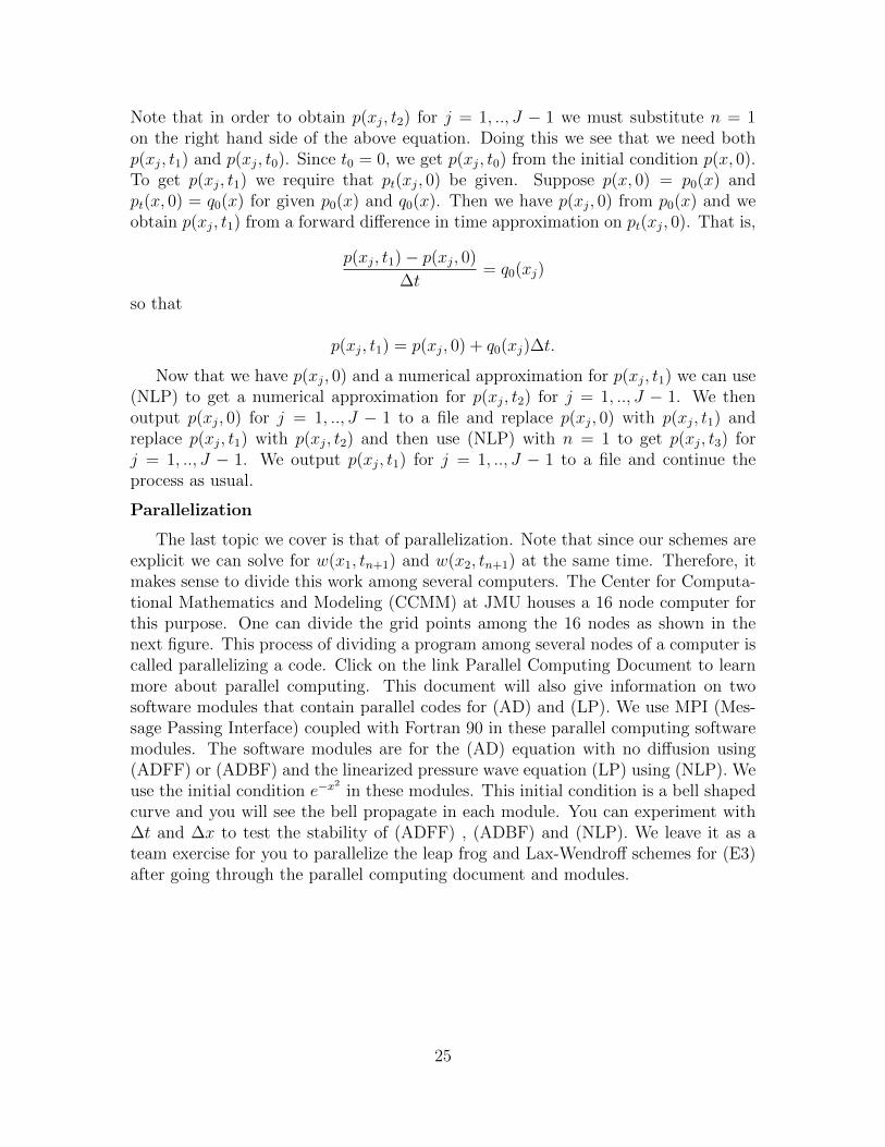
Parallelization

The last topic we cover is that of parallelization. Note that since our schemes areexplicit we can solve for w(x1, tn+1) and w(x2, tn+1) at the same time. Therefore, itmakes sense to divide this work among several computers. The Center for Computa-tional Mathematics and Modeling (CCMM) at JMU houses a 16 node computer forthis purpose. One can divide the grid points among the 16 nodes as shown in thenext figure. This process of dividing a program among several nodes of a computer iscalled parallelizing a code. Click on the link Parallel Computing Document to learnmore about parallel computing. This document will also give information on twosoftware modules that contain parallel codes for (AD) and (LP). We use MPI (Mes-sage Passing Interface) coupled with Fortran 90 in these parallel computing softwaremodules. The software modules are for the (AD) equation with no diffusion using(ADFF) or (ADBF) and the linearized pressure wave equation (LP) using (NLP). Weuse the initial condition e−x

2in these modules. This initial condition is a bell shaped

curve and you will see the bell propagate in each module. You can experiment with∆t and ∆x to test the stability of (ADFF) , (ADBF) and (NLP). We leave it as ateam exercise for you to parallelize the leap frog and Lax-Wendroff schemes for (E3)after going through the parallel computing document and modules.

25

A schematic showing how to divide the grid points among the nodes of a parallelcomputer

We recommend that you have this document handy as you go through the modulesso that you can refer back to the appropriate equations and numerical schemes foreach module. The Maple routines have a lot of the mathematical manipulations toget the equations and schemes in them, but that they are slower computationally.The Matlab routines allow movie output choices for visualizing the fluid ’flow’. TheFortran 90 routines are faster computationally, but the data sets have to be loadedinto Maple or Matlab for viewing. Maple and Matlab routines for viewing the datasets are with the Fortran software modules.

26

Introduction to Compressible Computational Fluid …educ.jmu.edu/~sochacjs/navierstokes.pdf · compressible ow equations. The incompressible ow equations model uids whose density

Documents