Introduction to climate modeling Peter Guttorp University of Washington [email protected] .

Introduction toclimate modeling

Peter Guttorp

University of Washington

[email protected]://www.stat.washington.edu/peter

Acknowledgements

ASA climate consensus workshopKevin Trenberth

Ben Santer

Myles Allen

IPCC Fourth Assessment Reports

Steve Sain

NCAR IMAGe/GSP

Weather and climate

Climate is –average weather

WMO 30 years (1961-1990)

–marginal distribution of weathertemperature

wind

precipitation

–classification of weather typestate of the climate system

Weather is–current activity in troposphere

Models of climate and weather

Numerical weather prediction:–Initial state is critical–Don’t care about entire distribution, just most likely event

–Need not conserve mass and energy

Climate models:–Independent of initial state–Need to get distribution of weather right

–Critical to conserve mass and energy

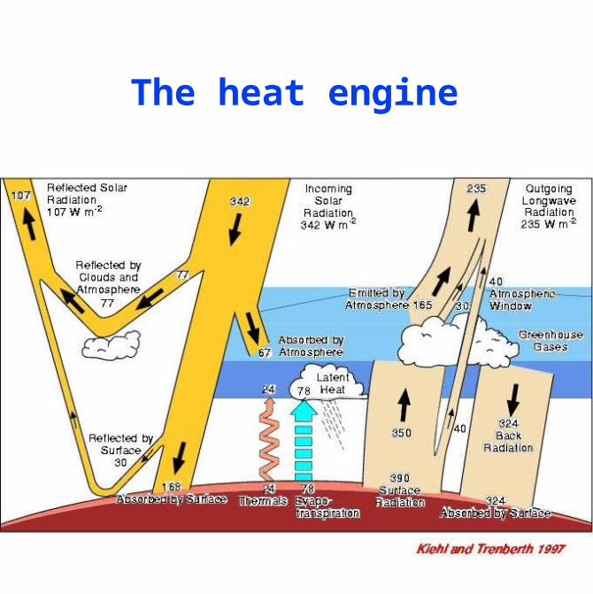
The heat engine

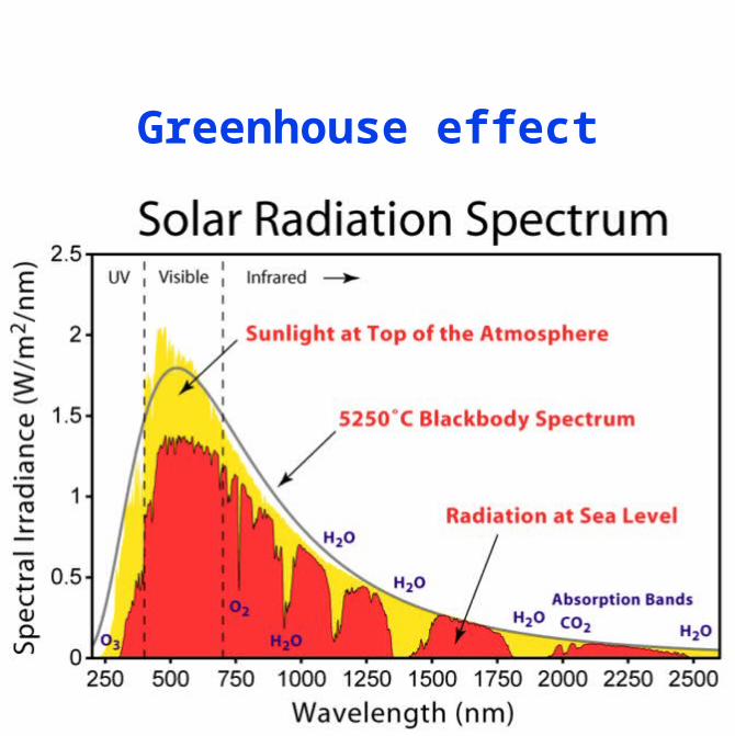
Greenhouse effect

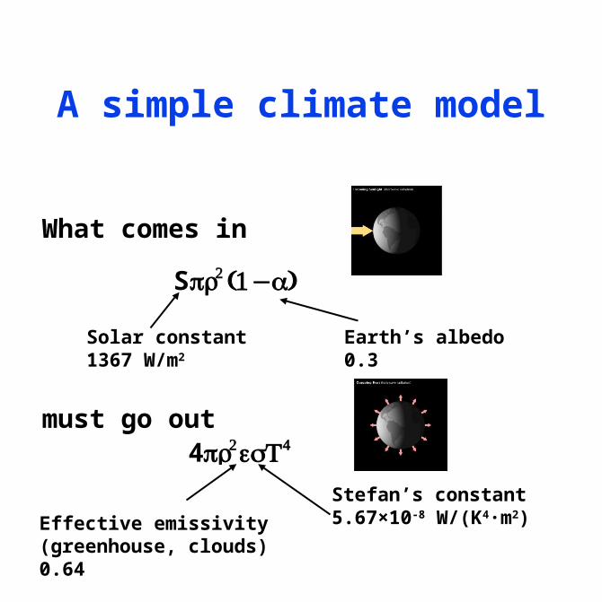
A simple climate model

What comes in

must go out

Sπr2 (1−a)

4πr2εσT4

Solar constant1367 W/m2

Earth’s albedo0.3

Effective emissivity(greenhouse, clouds)0.64

Stefan’s constant5.67×10-8 W/(K4·m2)

Solution

Average earth temperature is T=285K (12°C)

One degree Celsius change in average earth temperature is obtained by changing

solar constant by 1.4%

Earth’s albedo by 3.3%

effective emissivity by 1.4%

But in reality…

The solar constant is not constantThe albedo changes with land use changes, ice melting and cloudinessThe emissivity changes with greenhouse gas changes and cloudinessNeed to model the three-dimensional (at least) atmosphereBut the atmosphere interacts with land surfaces……and with oceans!

Historically

mid 70s Atmosphere models

mid-80s Interactions with land

early 90s Coupled with sea & ice

late 90s Added sulphur aerosols

2000 Other aerosols and carbon cycle

2005 Dynamic vegetation and atmospheric chemistry

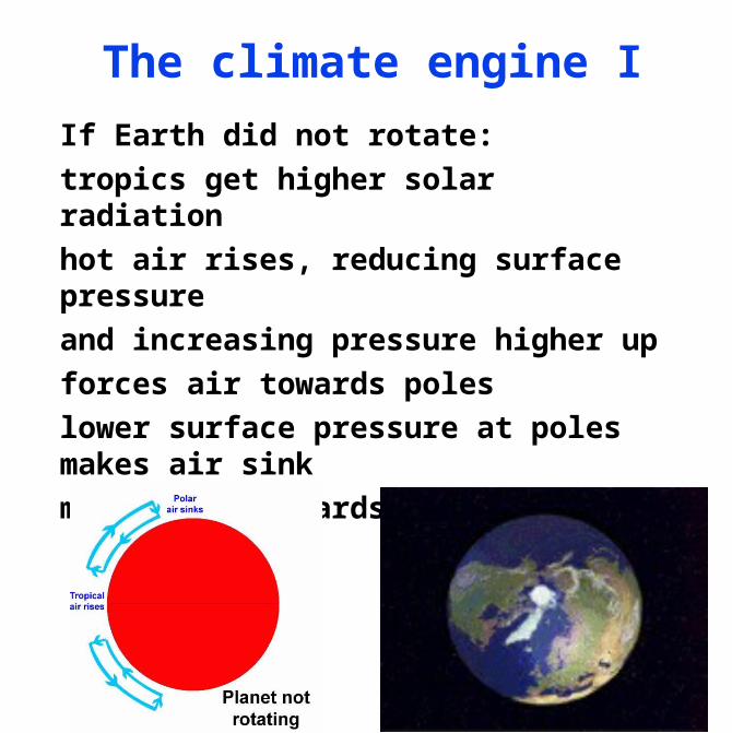
The climate engine I

If Earth did not rotate:

tropics get higher solar radiation

hot air rises, reducing surface pressure

and increasing pressure higher up

forces air towards poles

lower surface pressure at poles makes air sink

moves back towards tropics

The climate engine II

Since earth does rotate, air packets do not follow longitude lines (Coriolis effect)

Speed of rotation highest at equator

Winds travelling polewards get a bigger and bigger westerly speed (jet streams)

Air becomes unstable

Waves develop in the westerly flow (low pressure systems over Northern Europe)

Mixes warm tropical air with cold polar air

Net transport of heat polewards

Modeling the atmosphere

Coupled partial differential equations describing

Conservation of massConservation of momentumConservation of waterThermodynamicsHydrostatic equilibrium

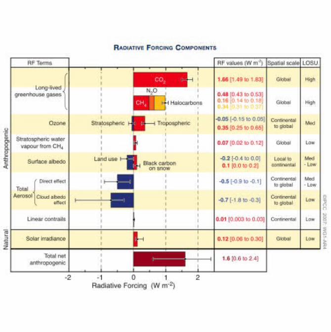
Boundary valuesRadiative forcings

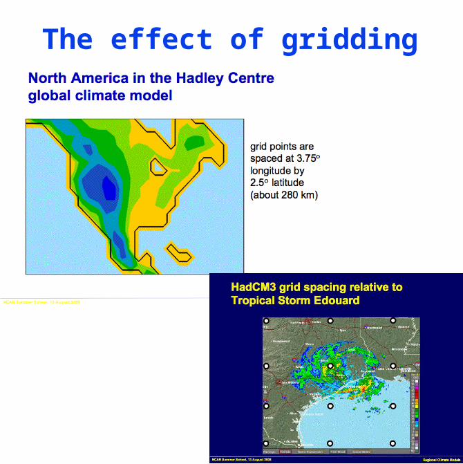
The effect of gridding

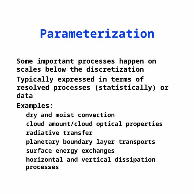
Parameterization

Some important processes happen on scales below the discretization

Typically expressed in terms of resolved processes (statistically) or data

Examples:dry and moist convection

cloud amount/cloud optical properties

radiative transfer

planetary boundary layer transports

surface energy exchanges

horizontal and vertical dissipation processes

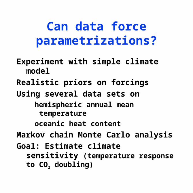
Can data force parametrizations?

Experiment with simple climate model

Realistic priors on forcings

Using several data sets onhemispheric annual mean temperature

oceanic heat content

Markov chain Monte Carlo analysis

Goal: Estimate climate sensitivity (temperature response to CO2 doubling)

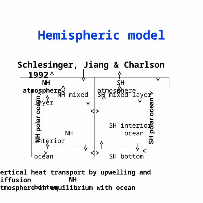
Hemispheric model

Schlesinger, Jiang & Charlson 1992

NH atmosphere SH atmosphere

NH mixed layer

NH interior ocean

NH bottom

SH mixed layer

SH interior ocean

SH bottom

Vertical heat transport by upwelling and diffusionAtmosphere in equilibrium with ocean

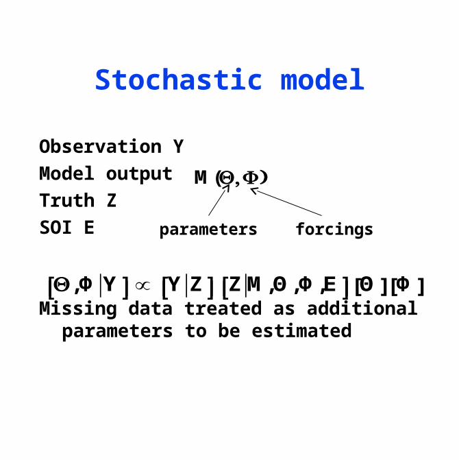
Stochastic model

Observation Y

Model output

Truth Z

SOI E

Missing data treated as additional parameters to be estimated

M(Θ,Φ)

Θ,Φ Y⎡⎣ ⎤⎦∝ Y Z⎡⎣ ⎤⎦ Z M,Θ,Φ,E⎡⎣ ⎤⎦ Θ[ ] Φ[ ]

parameters forcings

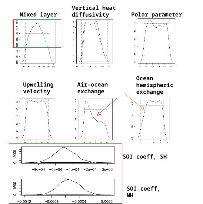
Mixed layerVertical heatdiffusivity Polar parameter

Upwellingvelocity

Air-oceanexchange

Ocean hemisphericexchange

SOI coeff, SH

SOI coeff, NH

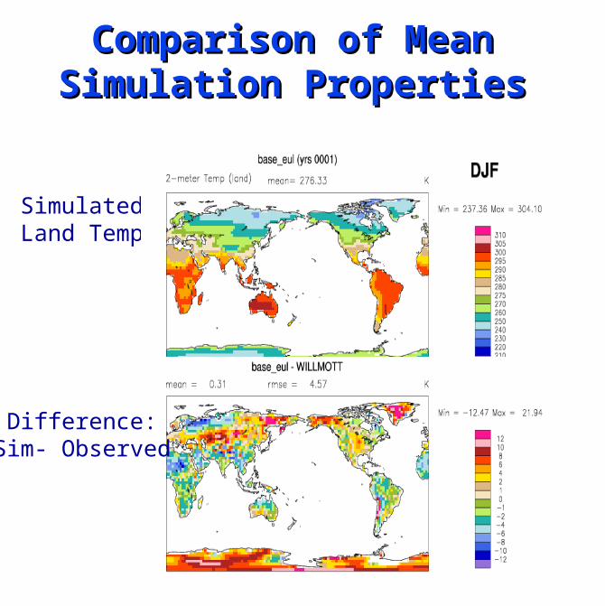
Comparison of Mean Comparison of Mean Simulation PropertiesSimulation Properties

SimulatedLand Temp

Difference:Sim- Observed

Sources of uncertainty

ForcingsSea surface temperature is uncertain, especially for early years

Greenhouse gases vague estimates for early part

DataGlobal mean temperature is not measured

Uncertainty in estimates may be as big as 1°C

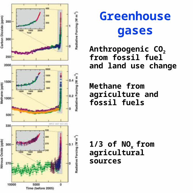
Greenhouse gases

Anthropogenic CO2 from fossil fuel and land use change

Methane from agriculture and fossil fuels

1/3 of NOx from agricultural sources

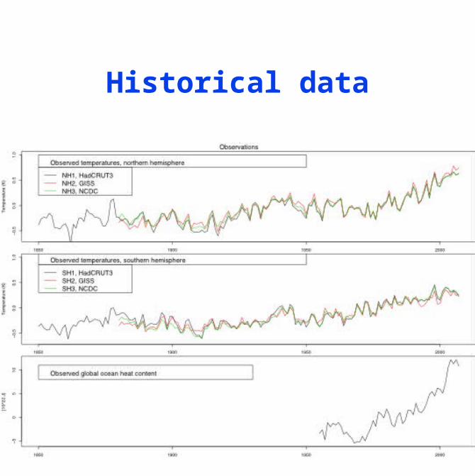
Historical data

Sensitivity

Reasonable climate models must reproduce

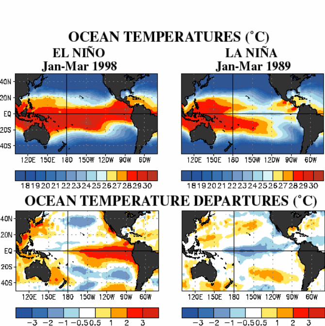
El Niño

Pacific Decadal Oscillation

Dust bowl, Sahel drought etc.

El Niño simulations

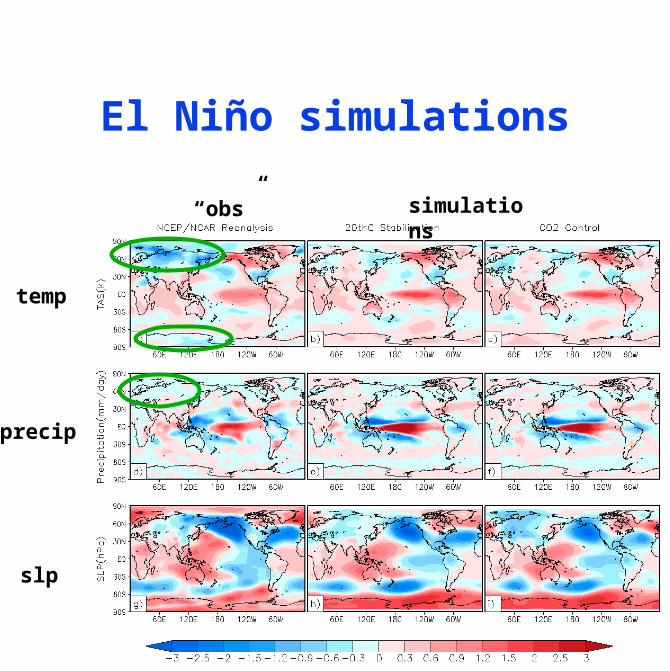
El Niño simulations

“obs” simulations

temp

precip

slp

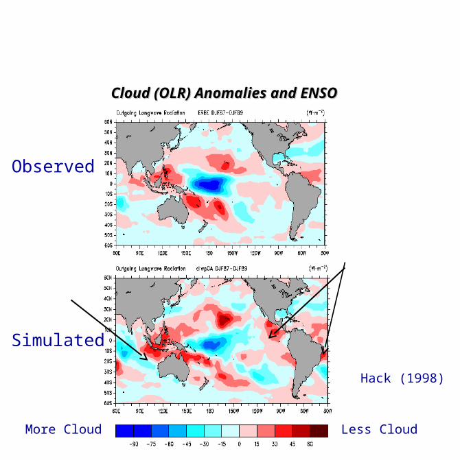
Cloud (OLR) Anomalies and ENSOCloud (OLR) Anomalies and ENSO

Hack (1998)

Observed

Simulated

More Cloud Less Cloud

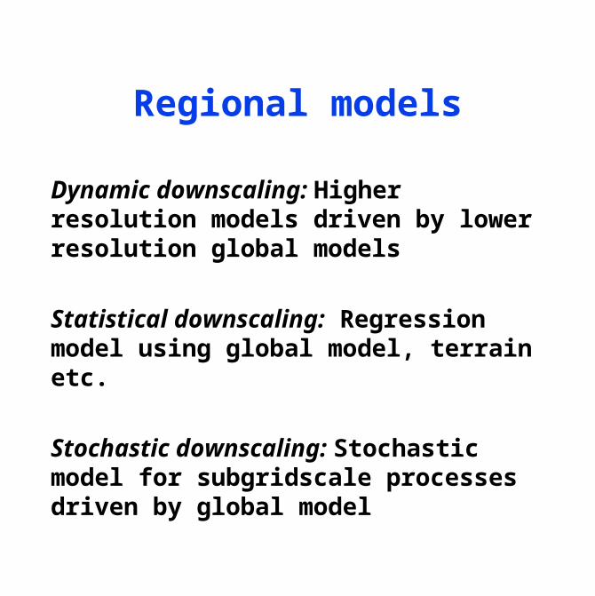
Regional models

Dynamic downscaling: Higher resolution models driven by lower resolution global models

Statistical downscaling: Regression model using global model, terrain etc.

Stochastic downscaling: Stochastic model for subgridscale processes driven by global model

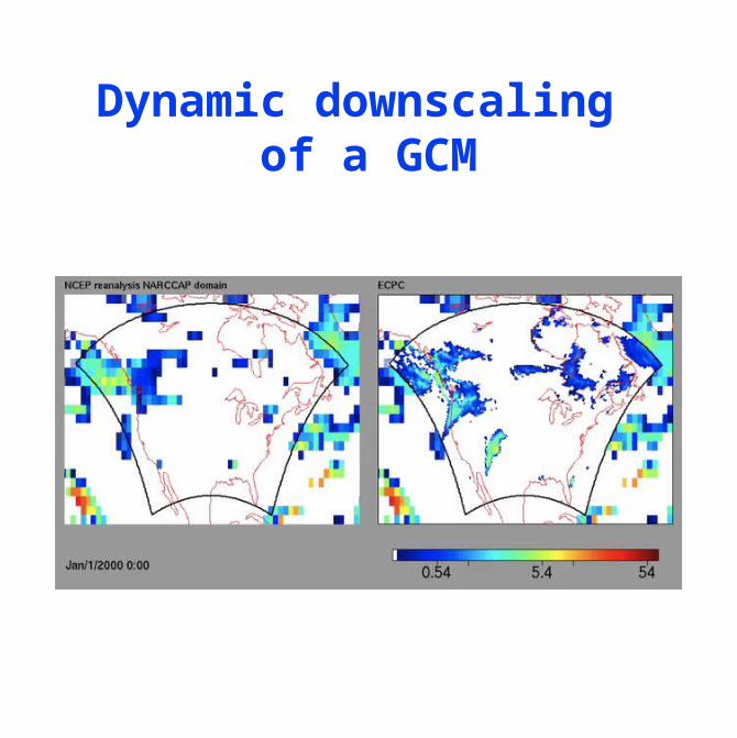
Dynamic downscaling of a GCM

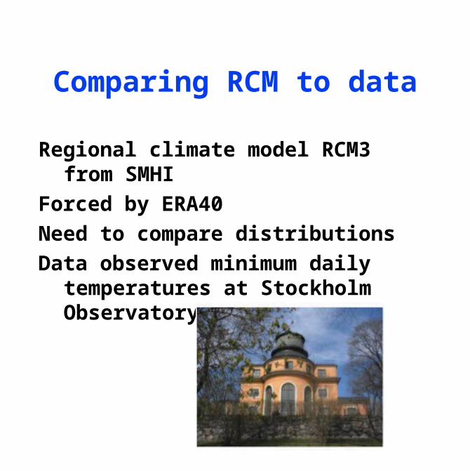
Comparing RCM to data

Regional climate model RCM3 from SMHI

Forced by ERA40

Need to compare distributions

Data observed minimum daily temperatures at Stockholm Observatory

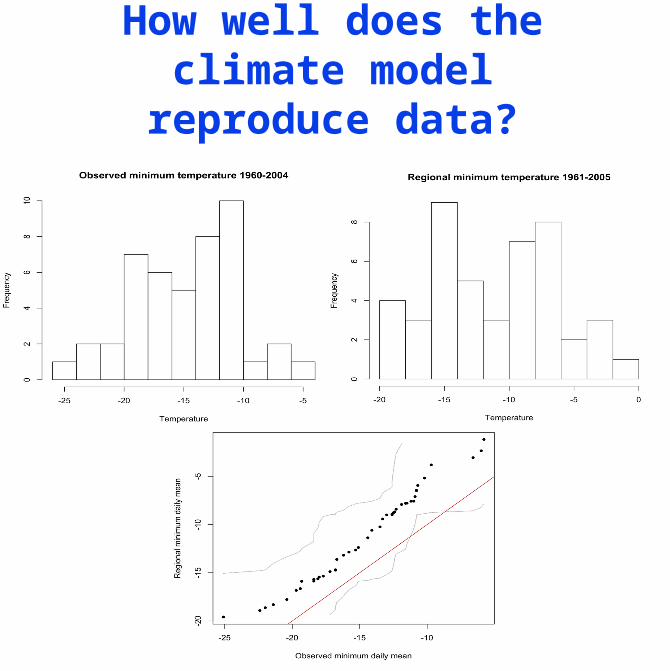
How well does the climate model reproduce data?

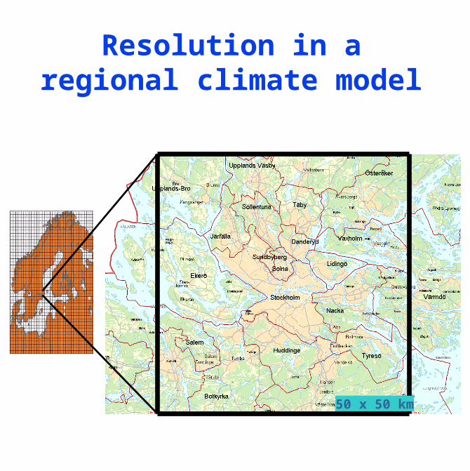
Resolution in a regional climate model

50 x 50 km

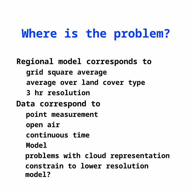
Where is the problem?

Regional model corresponds to grid square average

average over land cover type

3 hr resolution

Data correspond topoint measurement

open air

continuous time

Model

problems with cloud representation

constrain to lower resolution model?

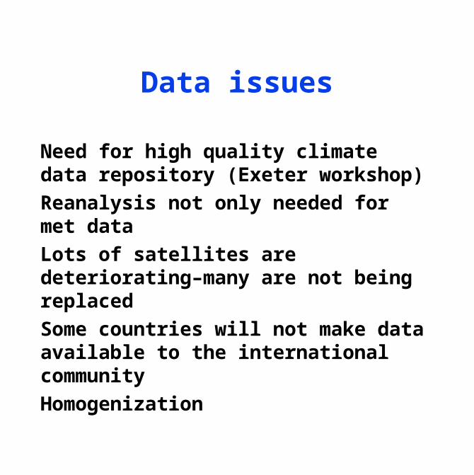
Data issues

Need for high quality climate data repository (Exeter workshop)

Reanalysis not only needed for met data

Lots of satellites are deteriorating–many are not being replaced

Some countries will not make data available to the international community

Homogenization

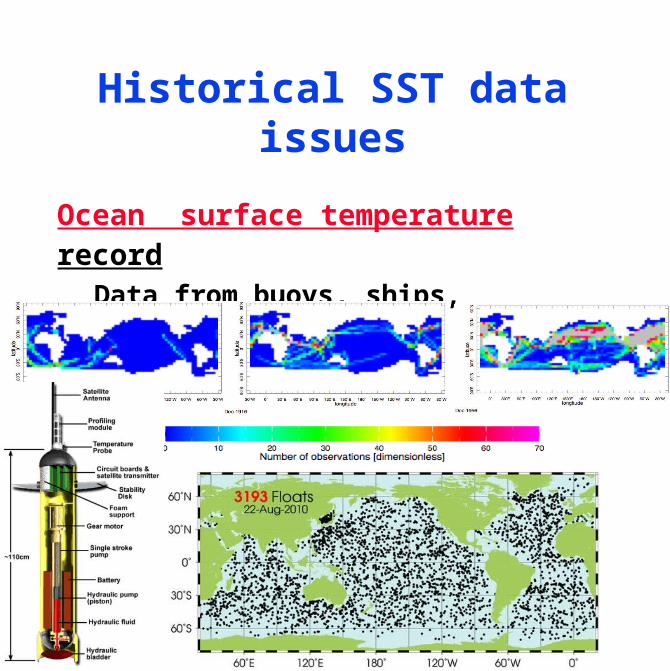
Historical SST data issues

Ocean surface temperature recordData from buoys, ships, satellites, floats

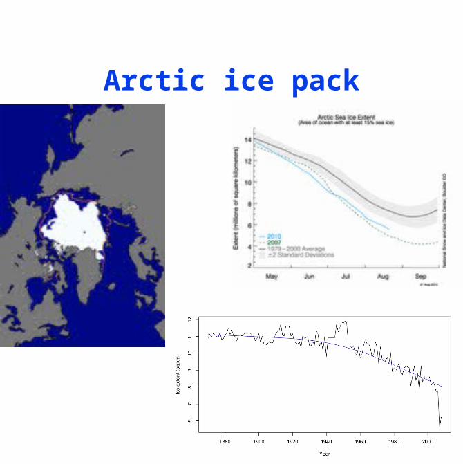
Arctic ice pack