Introduction to BEST Viewpoints - · PDF fileIntroduction to BEST Viewpoints This is not all but just one of the documentation files included in BEST Viewpoints. Introduction ... and

Introduction to BEST ViewpointsThis is not all but just one of the documentation files included in BEST Viewpoints.

Introduction

BEST Viewpoints is a user friendly data manipulation and analysis application which can be used to

automate common data manipulation procedures and analysis tasks.

Summarizing data using bar charts, Pareto analysis, box plots, bubble charts or line plots are some of

the basic features users will be able to quickly access and use efficiently. Additionally the application

provides data exploration and statistical analysis tools like summary statistics, histograms, scatter plots,

confidence intervals, hypothesis testing, data modeling, statistical control charts and process capability

analysis.

More advanced capabilities of BEST Viewpoints can be used for association analysis like market basket

analysis and for calculating and graphically representing retail analytics. Additionally, basic text mining

capabilities like string pattern counting are also available for datasets that contain text or string columns.

Furthermore, users are empowered by the full library of Mathematica functions to symbolically represent

and perform calculations in datasets of multiple data types. To enable communication with other sys-

tems and to enable the portability of results, many data formats are available for importing data and

exporting results. Additionally, a graphical user interface is provided to read data and create queries

from databases without the need of typing SQL scripts.

Workflow

The software is designed for data importing, manipulation, and analysis by means of two main sections:

1. Data, for data importing and manipulation, and 2. Analysis for applying analysis methodologies and

graphically representing information contained in the imported dataset.

The image below shows the application in its initial state with the dataset loaded by default. Note the

"Quick Start Guide" which should help the user quickly getting started using the application.

A quick description of the main navigation controls should help understand how the application is

designed. As shown in the image below the arrow wrapping the working section number is a menu with

the available working options. Note that there are three subsections in each of the main working modes.

These subsections can also be accessed by clicking on any of the circles at the right of the main section

names (see images below). Thus, there are indeed two ways to navigate the working sections; the

menu with all the options which might be easier to understand, and the 'single-click circles' which might

be preferred for a more efficient navigation.

The next paragraphs briefly describe the capabilities BEST Viewpoints provide in each of its main

working sections.

1. Data

Section 1. Data provides a data importing and modification interface to prepare data for section 2.

Analysis. The main objective of this section is to simplify the process of uploading and preparing data

2

for analysis. For this purpose the following external data sources are available: databases, files

(spreadsheets, text files, csv files, etc.) user defined variables, and Mathematica scripts.

The image below shows section 1.1 Import displaying the sources available for data importing. Note

that the application will always charge a default dataset of sale transactions such that the user can

quickly test the application in any of its sections. This default dataset can be used as a model for the

new datasets the user will use for analysis. Note that it is required that the data imported must be in

tabular form with string headers for each column.

Section 1.1 Import is where data is uploaded. Some of the features of this section include the selection

of spreadsheet tab names and the automatic dataset corner point identifications when the file is a

spreadsheet. Importing spreadsheet data in cross-tab format is also possible. The image below shows

some of the tools that become available when a spreadsheet file is selected.

To read data from a database a graphical user interface is provided to create queries without the need

of typing SQL scripts. The image below shows a simple example of the user interface provided for

selecting tables from a database and creating queries. The table Sales is selected and a simple query

3

has been created and applied. The yellow color is used to highlight the preview of results before for-

mally applying the query and loading the resulting dataset.

The two data modification sections are named 1.2 Modify 1.1, and 1.3 Modify 1.1 or 1.2. These

sections are useful for data transformation visualization and manipulation. In these sections the user

can calculate new fields, transform existing fields, summarize data, query data, and sort by one or more

columns. All data transformation procedures defined in these sections can be saved as Analysis Tem-

plates for future use in different datasets that have the same column headers.

The image below shows Modify 1.1 in the Transform module. Note that a dummy data transformation

was applied to MonthNo.

2. Analysis

4

Section 2. Analysis contains three data analysis interfaces named 2.1 Summarize, 2.2 Explore, and

2.3. Associate. These modules are designed to facilitate the application of many data analysis method-

ologies visualizing and extracting the information contained in one or more data columns (or fields)

grouping by one or more categorical fields.

Section 2.1 Summarize is designed to summarize data in form of Pivot Tables or Cross Tabs of any of

the following formats: Bar Charts, Pie Charts, Pareto Plots, Box Plots, Confidence Intervals and Line

Plots. The image below shows a simple example of this section in use: calculating Total Sales grouped

by CountryID and then by Product.

Section 2.2 Explore facilitates the creation of Summary Statistics, Histograms, Scatter Plots, Bubble

Charts, Statistical Control Charts, Capability Analysis, Hypothesis Tests (including goodness of fit

tests), Box Plots, Distribution Charts, Mean Confidence Intervals, Standard Deviation Confidence

Intervals, 3D Plots, Line Plots, Quantile Plots, and Probability Plots among other. The image below

shows a simple example of this section in use: Bundle of box plots and line plots of Sales by CountryID.

5

Finally, section 2.3. Associate is for identifying associations between one or more analysis variables.

This way of analyzing and portraying the information in data is sometimes referred as Market Basket

Analysis , Affinity Analysis or Association Analysis. Additionally, this section provides an easy way of

performing Retail Analytics with calculations like Penetration, Footprint, Average Transaction Revenue,

and Sole Purchase Count, among other. Finally, basket statistics like Total Baskets, Min, Max, and

Mean Basket Size, are also calculated. The image below shows a simple example of this section in

use: count of strongest associations of products sold together in purchase orders (represented by

OrderID).

Additionally, a well documented library of functions for data processing and analysis is provided for

Mathematica users. This Mathematica package named MXL Plus (data Miners eXtensible Library) is

intended to be used by programmers who would not only use this program for analyzing data, but that

would also like to create Mathematica scripts using some of the functions used by BEST Viewpoints.

Startup

6

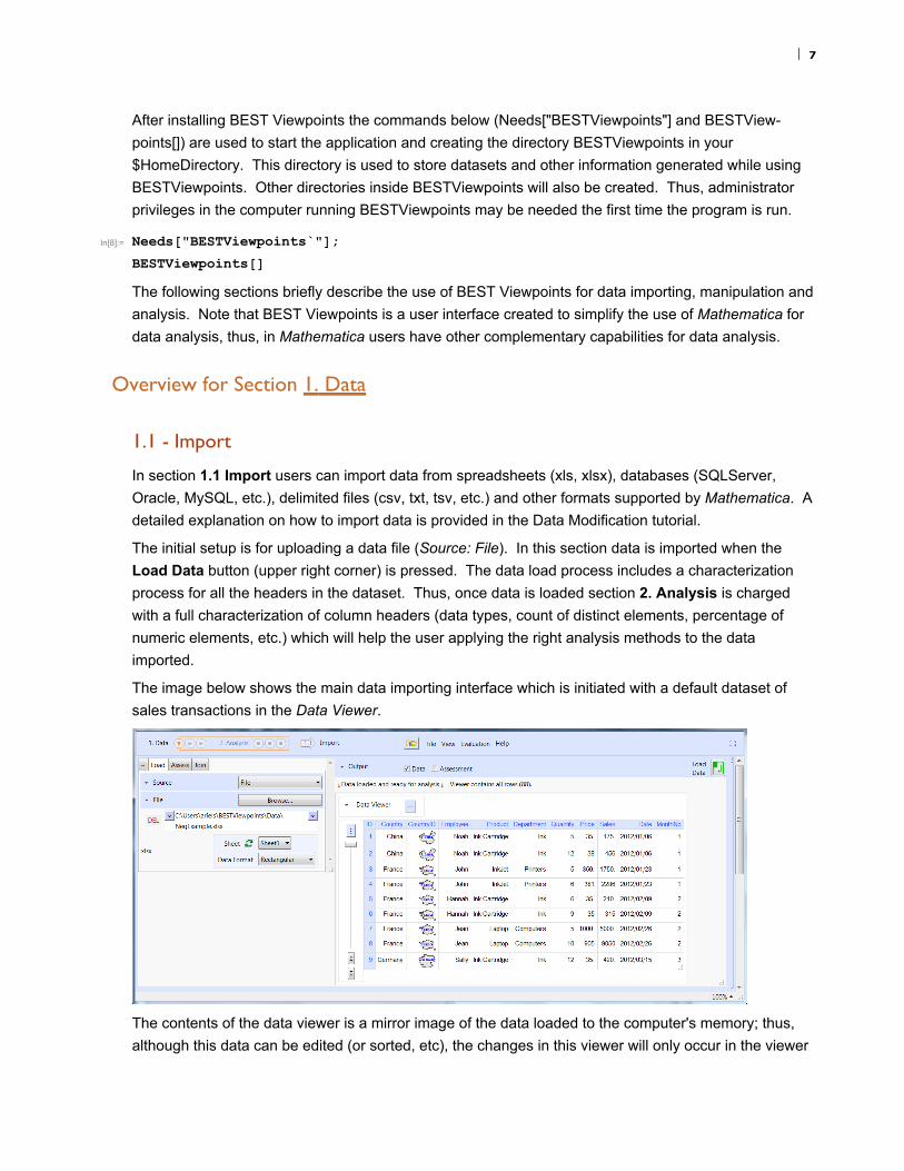
After installing BEST Viewpoints the commands below (Needs["BESTViewpoints"] and BESTView-

points[]) are used to start the application and creating the directory BESTViewpoints in your

$HomeDirectory. This directory is used to store datasets and other information generated while using

BESTViewpoints. Other directories inside BESTViewpoints will also be created. Thus, administrator

privileges in the computer running BESTViewpoints may be needed the first time the program is run.

In[8]:= Needs["BESTViewpoints`"];

BESTViewpoints[]

The following sections briefly describe the use of BEST Viewpoints for data importing, manipulation and

analysis. Note that BEST Viewpoints is a user interface created to simplify the use of Mathematica for

data analysis, thus, in Mathematica users have other complementary capabilities for data analysis.

Overview for Section 1. Data

1.1 - Import

In section 1.1 Import users can import data from spreadsheets (xls, xlsx), databases (SQLServer,

Oracle, MySQL, etc.), delimited files (csv, txt, tsv, etc.) and other formats supported by Mathematica. A

detailed explanation on how to import data is provided in the Data Modification tutorial.

The initial setup is for uploading a data file (Source: File). In this section data is imported when the

Load Data button (upper right corner) is pressed. The data load process includes a characterization

process for all the headers in the dataset. Thus, once data is loaded section 2. Analysis is charged

with a full characterization of column headers (data types, count of distinct elements, percentage of

numeric elements, etc.) which will help the user applying the right analysis methods to the data

imported.

The image below shows the main data importing interface which is initiated with a default dataset of

sales transactions in the Data Viewer.

The contents of the data viewer is a mirror image of the data loaded to the computer's memory; thus,

although this data can be edited (or sorted, etc), the changes in this viewer will only occur in the viewer

7

unless the user uses the option File: Send to Viewpoints which uploads the edited data in the viewer

as a new dataset. In any case, this Data Viewer is just that, a viewer, and the right way to modify the

data imported is by using the Data Modification tools provided in sections 1.2 and 1.3.

This viewer can Compress data such that large text lines or images are displayed as a representative

object like Ink Cartri... for Ink Cartridge. This can be very useful when the contents of the data cells are

lists, graphics or any other data type which content may need large cells for a full display.

1.2 and 1.3 - Modifying Imported Data

Sections 1.2 Modify 1.1 and 1.3 Modify 1.1 or 1.2 provide users the capability of performing data

transformation operations like, transforming columns, calculation of new fields and summaries, select-

ing/deselecting fields, sorting data by one or more fields or columns, and querying datasets. A detailed

explanation on the use of the two data modification sections is available in the Data Modification tutorial.

After defining any combination of the data modification operations (Transform, Calculate, Select, Sort,

Query) the user can save a Template where all transformations, calculations, queries, etc are saved for

future use in similar datasets. Note that operations are always executed in the order shown (i.e. 1-

Transform, 2-Calculate, 3-Select, 4-Sort, and 5-Query), and should also be defined in this order.

In general these two sections are similar but section 1.3 can operate on the output of either section 1.1

or 1.2 and can also group calculations by levels of one or more categorical variables. After data is

modified it can be selected for analysis from any of the analysis modules or imported again from section

1.1.

The basic appearance of these sections is shown above. In this interfaces the Auto Update checkbox

can be used to enable or disable automatic analysis. It is recommended to always leave automatic

8

analysis on unless the dataset is so large that the application slows down significantly. In this case the

user may prefer to define the commands first and then evaluate them by pressing the green return

button.

The Summaries checkbox on top is useful for displaying the calculated summaries only. This is particu-

larly convenient when displaying grouped data summaries in section 1.3.

The Output options in the opener (see image below) are used to define some characteristics of the

Data Viewer. For example the Compress checkbox can be used to view data in compressed form to

avoid displaying cells which content is too wide or too long.

The Display options are used to define the size of the viewer (15X11) and the maximum number of

records displayed (5,000). Note that the data viewer does not need to contain all the data loaded (or in

memory), but the viewer is there to help the user understand or evaluate how the dataset is being

modified by means of the user actions in the user interface. Displaying all data records when the

dataset is large may significantly increase rendering time of the data in the viewer.

The Assess checkbox enables the assessment of the data types and performs some basic analysis of

the data.

Overview for Section 2. Analysis

When the program is started the main interface looks as shown below. The applications loads a default

dataset which can be used for testing purposes. Note that the program starts at section 2. Analysis.

Section 1. Data shows the preloaded dataset. In this section the user may select whether data will be

imported from a file, a database, or other sources as shown in the image below. This section will be

discussed later in this tutorial.

9

Back in section 2.1 Summarize, the Aim menu allows selecting data fields in two different modes.

Selecting at least one data "Field" or column that the user wants to Analyze followed by selecting at

least one Group By or categorical field is enough to start analyzing data. Thie Aim menu is present in

all analysis subsections 2.1, 2.2, and 2.3 and is the main set of tools used to start any analysis session.

The image below shows the results of selecting "Sales" as the analysis field and the categorical fields

"Country" followed by "Product". The total sales were calculated for each Country, then the information

for each Country was grouped by Product and the results were displayed graphically. Note that Brazil

was excluded using the Categories menu. Finally note that the Image Size width has also been set to

10 (inches). This is just an introductory example to show how data can be easily summarized using the

Summarize section.

Section 2.2 Explore provides access to many data analysis methodologies. The image below is just an

example of a basic exploration of the information in the field "Sales" when grouped by the countries

China and Germany. Note that the bundle shown in the output can be modified by the user by selecting

other options from the Bundle menu.

10

In section 1.3 Associate BEST Viewpoints provides the capability of finding associations between

elements of the data fields selected in Analyze by the groups created by the selected Group By fields.

The image below shows the result of using this section to graphically display how events (A-1) that

occurred in a particular time can be analyzed to understand flow, and thus associations, between

different process states.

When a retail transactions dataset is being analyzed in this section users can also calculate Retail

Analytics and perform Market Basket Analysis . The image below shows results for analyzing supermar-

ket transactions for identifying associations between product departments. In this particular case the

dataset was filtered to include only baskets that contain items from Dairy or Grocery departments, and

that are processed through express checkout (baskets size <=10).

11

While using BEST Viewpoints the File Menu will enable the user to print, save, extract or send by email

the results displayed on the screen. These options are available in the File menu.

The next section is about the main features provided by the interface of all analysis sections.

User Interface for Section 2. Analysis

Sections 2.1, 2.2, and 2.3 provide interfaces with controls that will help use different methodologies to

analyze data. Some of the analyses provided are Pareto plots, Cross Tabs, Box and Whisker Plots,

Bubble Plots, Scatter Plots, Confidence Intervals, Hypothesis Testing, Line Plots, and Histograms.

Also, association or affinity analysis and retail analytics are also provided.

There are many controls and features provided to work on all these analysis sections and, although

there are differences from section to section, a common set of tools with similar appearance is present

in each section. Thus, the following documentation is about those common features in the user inter-

face of sections 2.1, 2.2, and 2.3.

General Controls

Note that in the image below two left pane menus are open: Aim and Build. The amount of menus is

controlled with the "+" and "-" tabs. The content of the Build tab dynamically changes as the user

makes changes in the Output menu. In general the Build menu provides many options to adjust the

output results to the user preferences.

12

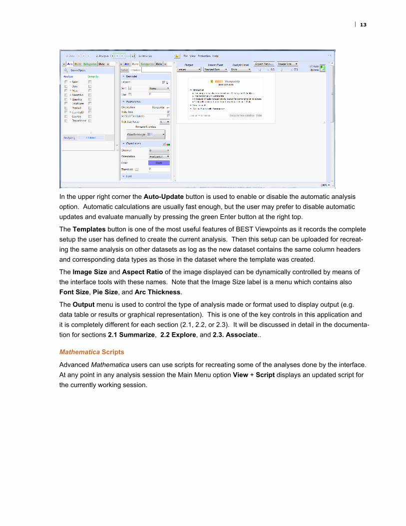
In the upper right corner the Auto-Update button is used to enable or disable the automatic analysis

option. Automatic calculations are usually fast enough, but the user may prefer to disable automatic

updates and evaluate manually by pressing the green Enter button at the right top.

The Templates button is one of the most useful features of BEST Viewpoints as it records the complete

setup the user has defined to create the current analysis. Then this setup can be uploaded for recreat-

ing the same analysis on other datasets as log as the new dataset contains the same column headers

and corresponding data types as those in the dataset where the template was created.

The Image Size and Aspect Ratio of the image displayed can be dynamically controlled by means of

the interface tools with these names. Note that the Image Size label is a menu which contains also

Font Size, Pie Size, and Arc Thickness.

The Output menu is used to control the type of analysis made or format used to display output (e.g.

data table or results or graphical representation). This is one of the key controls in this application and

it is completely different for each section (2.1, 2.2, or 2.3). It will be discussed in detail in the documenta-

tion for sections 2.1 Summarize, 2.2 Explore, and 2.3. Associate..

Mathematica Scripts

Advanced Mathematica users can use scripts for recreating some of the analyses done by the interface.

At any point in any analysis session the Main Menu option View + Script displays an updated script for

the currently working session.

13

Analysis Templates

One of the most attractive capabilities of this application is the possibility of saving Analysis Templates

at any point. These templates work as bookmarks that the user may use to repeat or come back to

exactly the state of analysis defined in any analysis session. These templates are available for data

manipulation as well as for the analysis sections.

The image below shows the Templates Manager window which is activated using the Templates button

. By pressing the return button the template shown in the image can be uploaded to get the

same analysis performed. Note that the templates will replicate the desired analysis only if the dataset

loaded has the required data columns or fields used to create the plot. Additionally, the data types must

also match accordingly. That is not only the data column must exist, but also it must contain the same

type of information (e.g. numbers in the Sales example below).

14

Note that templates can be organized by projects to simplify its use. It is recommended to define

projects associated to the data being analyzed to simplify the search and use, and to make sure that

templates will match the currently loaded dataset.

Aim Menu

The basic layout of the Analysis interface is shown below. Usually analysis is started by selecting one

ore more Analysis field (e.g. Sales), then the user may Group By one or more categorical fields (e.g.

CountryID, Product) by just selecting the field names from the Aim menu. The order in which analysis

fields and categories are selected is used to create the selected analysis type (Leaves Chart in this

case). This order can be changed in several places: In the plot, when the mouse is over the field label,

or at the bottom of the left menu interface.

15

Note that the fields selected are placed at the bottom of the Aim menu (e.g. under Grouping By) as

tools such that the user can change the selection order or even replace the selected fields by any other

field.

Build Menu

Once the Analysis and Group By fields are selected the Build menu will provide many dynamically

available options for modifying the analysis in course. Most of the options in this menu are designed to

be easy to understand thus, only when considered necessary some of these options will be discussed

further in the documentation. The Mathematica documentation for the selected type of analysis is

fundamental to understand the Build menu. For example, "Element Function" is an option for many

types of charts. Thus, it is expected that the user will make reference to the Mathematica documenta-

tion for complementing this documentation and understand how to use some of the options made

available in the interface.

Categories Menu

The Categories menu is used for selecting which values of the categorical fields being analyzed should

be used for analysis. The Categories menu in the Hierarchical Viewpoints module provides particular

options that will be discussed later. Just as an example, the image below shows the Total Sales by

Product and CountryID after deselecting Germany.

16

The Analysis Level is used to fold the analysis created in the Root level by means of Cross Tabs or

Multi Dimensional Cross Tabs.

Once the analysis is finished the File menu can be used to Save, or Print results (see image below).

The Output To Notebook option can also be used to take current results to a new window for further

manipulation using Mathematica.

Data Menu

Input Data Source

The user may also control the Source of input Data for analysis. For example, if Section 1.2 has been

used to calculate a new field, then user may want to set the output of that section as the target data for

analysis. Additionally, a Sample from the data can be analyzed instead of the full dataset. This may be

useful for large datasets or for statisticians which want to explore different analyses by sampling from

17

data.

One common and key element to these sections is that the input data for analysis can either be the

originally loaded dataset (output in Section 1.1), the output of Section 1.2, the output of Section 1.3 or

the Summaries from Section 1.3. This creates an extremely flexible data manipulation and analysis

environment where analysts can generate many different types of analyses in parallel.

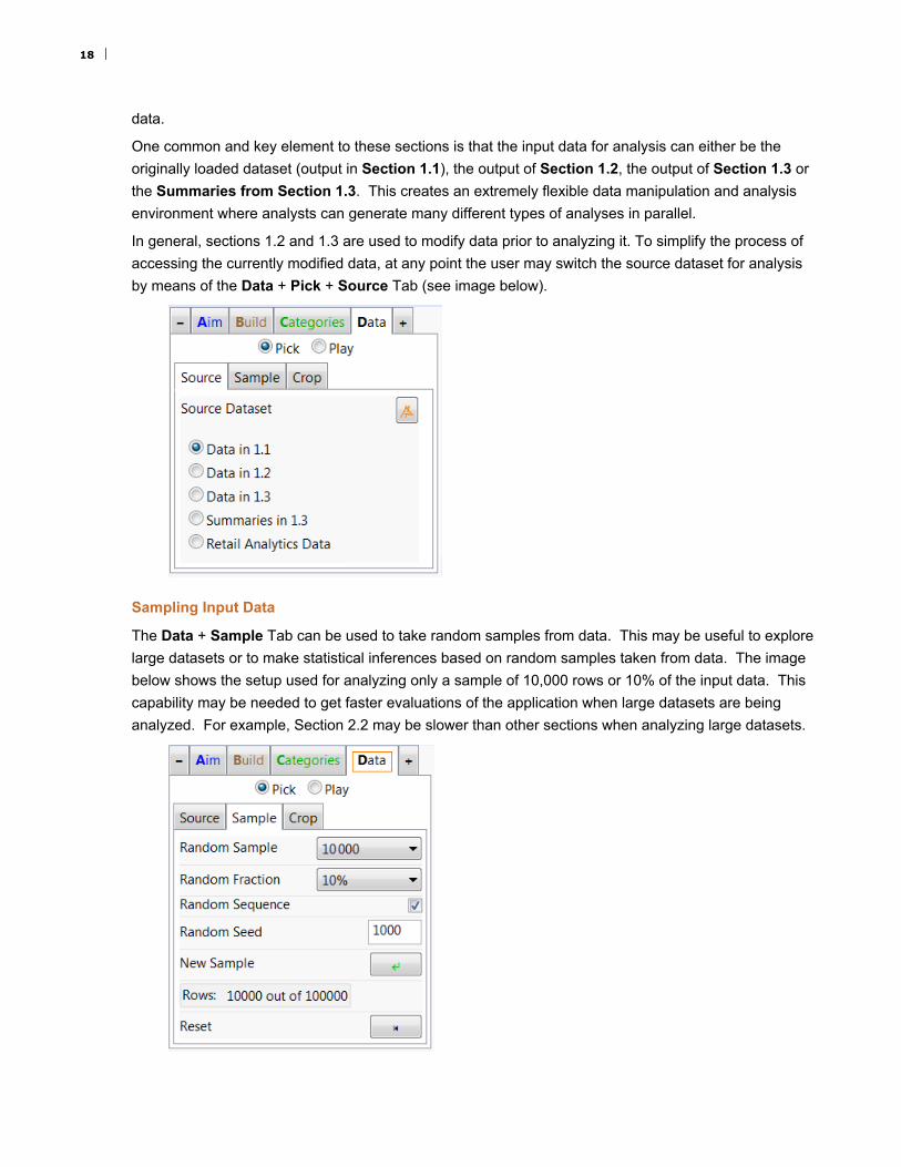
In general, sections 1.2 and 1.3 are used to modify data prior to analyzing it. To simplify the process of

accessing the currently modified data, at any point the user may switch the source dataset for analysis

by means of the Data + Pick + Source Tab (see image below).

Sampling Input Data

The Data + Sample Tab can be used to take random samples from data. This may be useful to explore

large datasets or to make statistical inferences based on random samples taken from data. The image

below shows the setup used for analyzing only a sample of 10,000 rows or 10% of the input data. This

capability may be needed to get faster evaluations of the application when large datasets are being

analyzed. For example, Section 2.2 may be slower than other sections when analyzing large datasets.

18

Cropping Input Data

The Data + Crop Tab can be used to extract a data region or to crop data. This may be useful when

there are obvious outliers in the target analysis field(s) data. The image below shows that simply

selecting the region of interest in data is enough to crop data at the user's convenience. Once the

region is selected pressing Apply crops the data to the selected region (the data points in the second

scatter plot). Note that a maximum of 25,000 points are included in the scatter plot to ensure a fast

response time of the data cropping tool.

19