Introduction to Alpha Shapes - Computer graphics · 2.2 Alpha Shapes and the Delaunay Triangulation Thissectionwillshowthattheboundary@Sfi ofthefi-shapeis,foranyvalue...

Introduction to Alpha Shapes

SUMMARY

WARNING: MAY CONTAIN ERRORS!

Kaspar Fischer ([email protected])

Contents

1 Introduction 1

2 Definition 2

2.1 Alpha Shapes and the Convex Hull . . . . . . . . . . . . . . . . . 42.2 Alpha Shapes and the Delaunay Triangulation . . . . . . . . . . 5

3 Alpha Complexes 6

3.1 The Alpha Complex of a Point Set . . . . . . . . . . . . . . . . . 63.2 The Link Between the Complex and the Shape . . . . . . . . . . 73.3 The Interior of the Alpha Shape . . . . . . . . . . . . . . . . . . 103.4 Edelsbrunner’s Algorithm . . . . . . . . . . . . . . . . . . . . . . 11

4 Limitation of “Classical” Alpha Shapes and Improvements 14

4.1 Limitations . . . . . . . . . . . . . . . . . . . . . . . . . . . . . . 144.2 Extensions . . . . . . . . . . . . . . . . . . . . . . . . . . . . . . . 15

1 Introduction

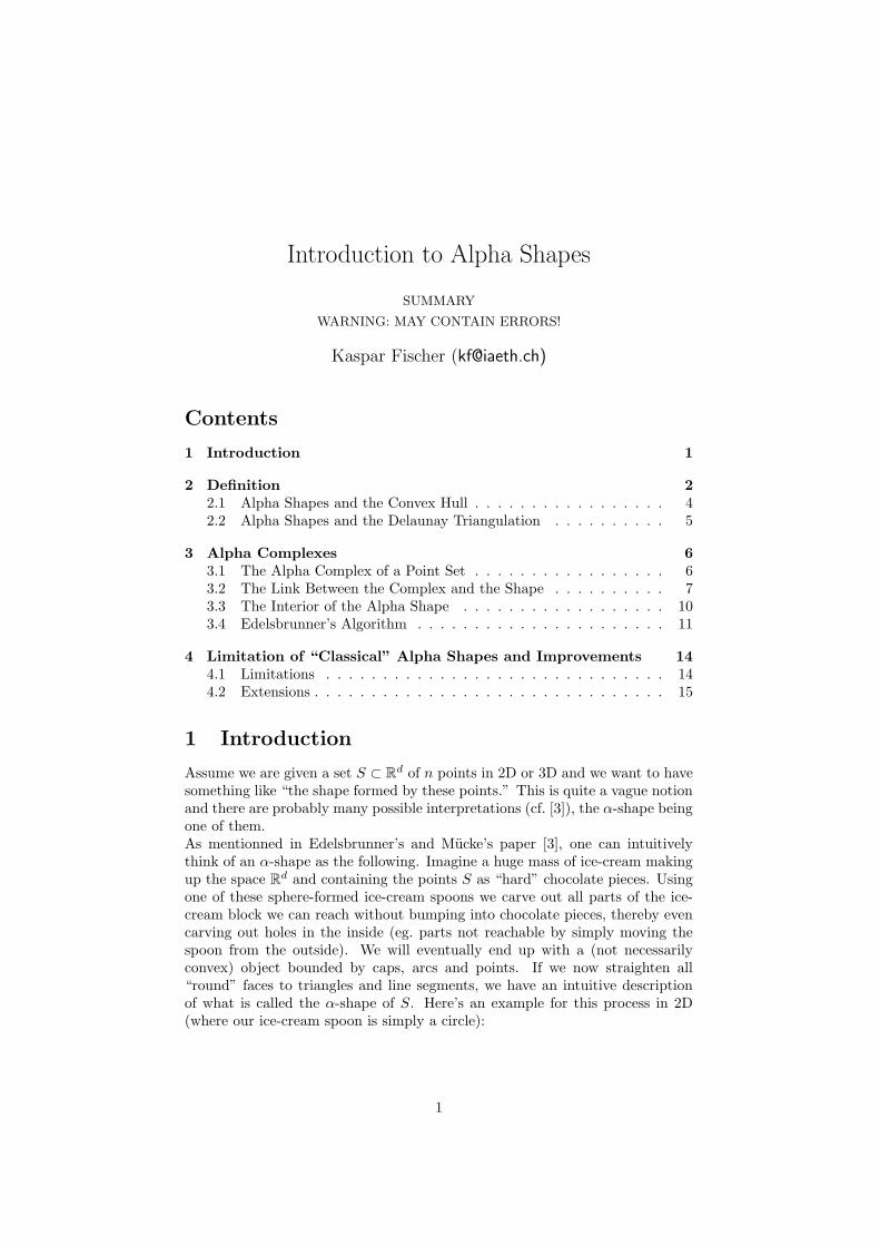
Assume we are given a set S ⊂ Rd of n points in 2D or 3D and we want to havesomething like “the shape formed by these points.” This is quite a vague notionand there are probably many possible interpretations (cf. [3]), the α-shape beingone of them.As mentionned in Edelsbrunner’s and Mucke’s paper [3], one can intuitivelythink of an α-shape as the following. Imagine a huge mass of ice-cream makingup the space Rd and containing the points S as “hard” chocolate pieces. Usingone of these sphere-formed ice-cream spoons we carve out all parts of the ice-cream block we can reach without bumping into chocolate pieces, thereby evencarving out holes in the inside (eg. parts not reachable by simply moving thespoon from the outside). We will eventually end up with a (not necessarilyconvex) object bounded by caps, arcs and points. If we now straighten all“round” faces to triangles and line segments, we have an intuitive descriptionof what is called the α-shape of S. Here’s an example for this process in 2D(where our ice-cream spoon is simply a circle):

1

And what is α in the game? α is the radius of the carving spoon. A very smallvalue will allow us to eat up all of the ice-cream except the chocolate pointsS themselves. Thus we already see that the α-shape of S degenerates to thepoint-set S for α → 0. On the other hand, a huge value of α will prevent useven from moving the spoon between two points since it’s way too large. So wewill never spoon up ice-cream lying in the inside of the convex hull of S, andhence the α-shape for α→∞ is the convex hull of S.

In the following I will (i) summarize the definitons from [3] to state the aboveconcepts (spoon, etc.) more precisely and (ii) present a result from [1] whichallows one to easily compute α-shapes from the Delaunay triangulation of S.Finally, I will very briefly give an overview of the problems and approaches withα-shapes when applied to surface reconstruction.

2 Definition

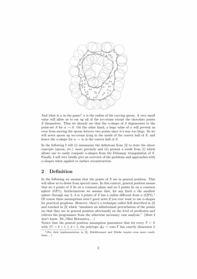
In the following we assume that the points of S are in general position. Thiswill allow us to desist from special cases. In this context, general position meansthat no 4 points of S lie on a common plane and no 5 points lie on a commonsphere (GP1); furthermorewe we assume that, for any fixed α the smallestsphere through any 2, 3 or 4 points of S has a radius different from α (GP2).1

Of course these assumptions aren’t good news if you ever want to use α-shapesfor practical proplems. However, there’s a technique called SoS described in [2]and touched in [3] which “simulates an infinitesimal perturbation of the points[so that they are in general position afterwards] on the level of predicates andrelieves the programmer from the otherwise necessary case analysis.” (More Idon’t know, Mr./Miss Britannica. . . )Notice that the general position assumption guarantees that for every T ⊂ S

with |T | = k + 1 ≤ d + 1, the polytope ∆T = conv T has exactly dimension k

1(For their implementation in [3], Edelsbrunner and Mucke require even more condi-tions. . . )

2

and therefore is a k-simplex. (By the way: Whenever I talk about a “k-simplex”in the following, I mean a k-simplex ∆T for some T ⊂ S such that |T | = k+1.)

First, we need the notion of a λ-ball which will stand for the ice-cream spoonmentioned in the introduction.

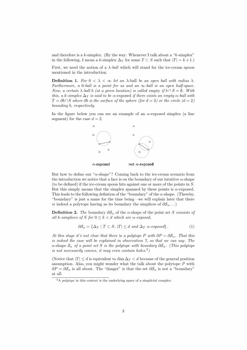
Definition 1. For 0 < λ < ∞ let an λ-ball be an open ball with radius λ.Furthermore, a 0-ball is a point for us and an ∞-ball is an open half-space.Now, a certain λ-ball b (at a given location) is called empty if b ∩ S = ∅. Withthis, a k-simplex ∆T is said to be α-exposed if there exists an empty α-ball withT = ∂b∩S where ∂b is the surface of the sphere (for d = 3) or the circle (d = 2)bounding b, respectively.

In the figure below you can see an example of an α-exposed simplex (a linesegment) for the case d = 2.

����������� ��� ���������������� ���

But how to define our “α-shape”? Coming back to the ice-cream scenario fromthe introduction we notice that a face is on the boundary of our intuitive α-shape(to be defined) if the ice-cream spoon hits against one or more of the points in S.But this simply means that the simplex spanned by these points is α-exposed.This leads to the following defintion of the “boundary” of the α-shape. (Thereby,“boundary” is just a name for the time being—we will explain later that thereis indeed a polytope having as its boundary the simplices of ∂Sα. . . )

Definition 2. The boundary ∂Sα of the α-shape of the point set S consists ofall k-simplices of S for 0 ≤ k < d which are α-exposed,

∂Sα = {∆T | T ⊂ S, |T | ≤ d and ∆T α-exposed} . (1)

At this stage it’s not clear that there is a polytope P with ∂P = ∂Sα. That thisis indeed the case will be explained in observation 7, so that we can say: Theα-shape Sα of a point set S is the polytope with boundary ∂Sα. (This polytopeis not necessarily convex, it may even contain holes.2)

(Notice that |T | ≤ d is equivalent to dim∆T < d because of the general positionassumption. Also, you might wonder what the talk about the polytope P with∂P = ∂Sα is all about. The “danger” is that the set ∂Sα is not a “boundary”at all.

2A polytope in this context is the underlying space of a simplicial complex.

3

�������������� �� ������������������� �!�#"%$��'&��(�)"��+*�,

The above figure for instance shows a set of (d − 1)-simplices in R2 which donot represent a boundary since one line-segment is contained in a “closed” area.In our case of the set ∂Sα, observation 7 will clarify that things like the abovesituation cannot occur here. Another question is whether there is more than onepolytope with boundary ∂Sα. But here the answer is relatively simple, thereare but two such polytopes: If P is one, so is Rd\P as you can easily verify.But we’re not really interested in the unbounded one among these two, sinceour point set “spans a bounded object.” So we will choose the other.)Finally, here’s another example of (the boundary of) an α-shape.

-/.10

2.1 Alpha Shapes and the Convex Hull

Since an infinitely small ball exposes any point in S but none of the higher-dimensional simplices, and since an α-ball with α greater than the radius of thesmallest enclosing circle of the points S doesn’t allow an interior simplex to beα-exposed, we get limα→0 ∂Sα = S and limα→∞ ∂Sα = ∂ convS, respectively.And thus it’s plausible:

Observation 1. limα→0 Sα = S and limα→∞ Sα = convS.

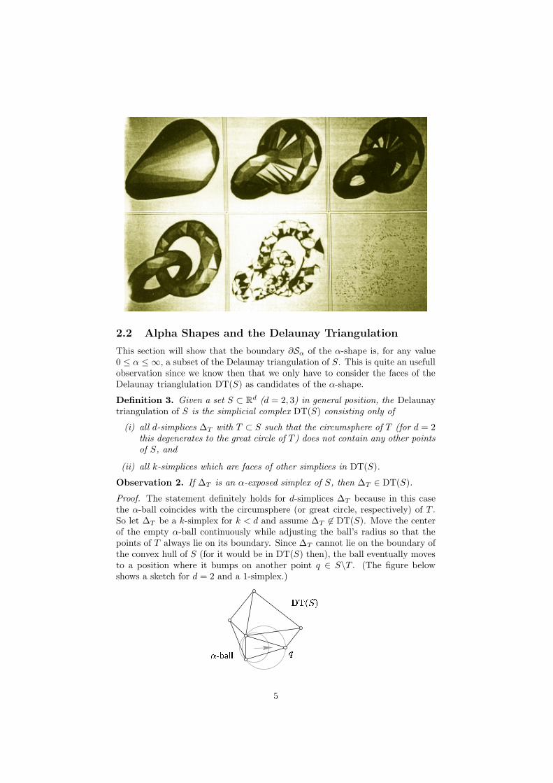
The following figure (originally published in [3] I think) illustrates some α-shapesfor different values of α for a three-dimensional point set. The first image showsthe ∞-shape, the last one the 0-shape.

4

2.2 Alpha Shapes and the Delaunay Triangulation

This section will show that the boundary ∂Sα of the α-shape is, for any value0 ≤ α ≤ ∞, a subset of the Delaunay triangulation of S. This is quite an usefullobservation since we know then that we only have to consider the faces of theDelaunay trianglulation DT(S) as candidates of the α-shape.

Definition 3. Given a set S ⊂ Rd (d = 2, 3) in general position, the Delaunaytriangulation of S is the simplicial complex DT(S) consisting only of

(i) all d-simplices ∆T with T ⊂ S such that the circumsphere of T (for d = 2this degenerates to the great circle of T ) does not contain any other pointsof S, and

(ii) all k-simplices which are faces of other simplices in DT(S).

Observation 2. If ∆T is an α-exposed simplex of S, then ∆T ∈ DT(S).

Proof. The statement definitely holds for d-simplices ∆T because in this casethe α-ball coincides with the circumsphere (or great circle, respectively) of T .So let ∆T be a k-simplex for k < d and assume ∆T 6∈ DT(S). Move the centerof the empty α-ball continuously while adjusting the ball’s radius so that thepoints of T always lie on its boundary. Since ∆T cannot lie on the boundary ofthe convex hull of S (for it would be in DT(S) then), the ball eventually movesto a position where it bumps on another point q ∈ S\T . (The figure belowshows a sketch for d = 2 and a 1-simplex.)

���������

��� ������

5

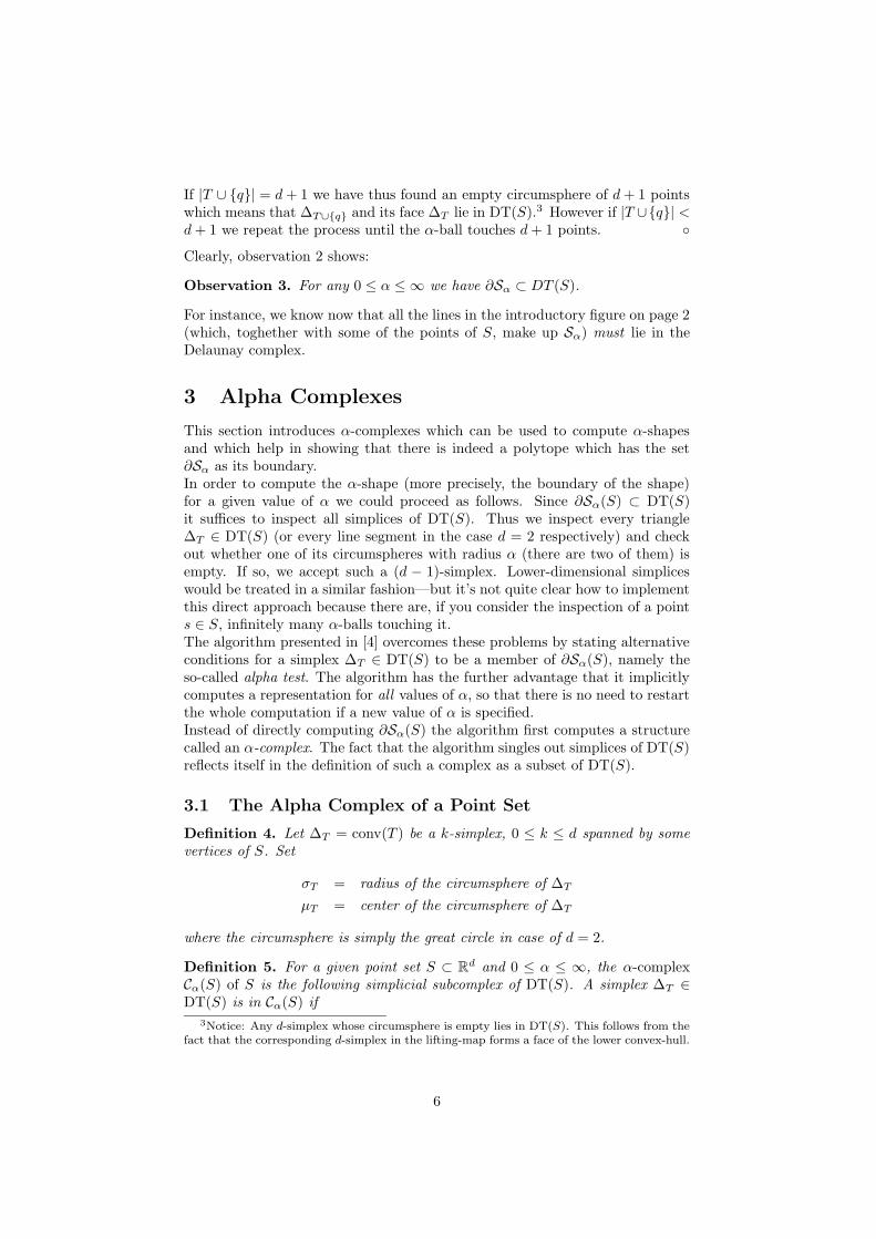
If |T ∪ {q}| = d+ 1 we have thus found an empty circumsphere of d+ 1 pointswhich means that ∆T∪{q} and its face ∆T lie in DT(S).3 However if |T ∪{q}| <d+ 1 we repeat the process until the α-ball touches d+ 1 points. ◦

Clearly, observation 2 shows:

Observation 3. For any 0 ≤ α ≤ ∞ we have ∂Sα ⊂ DT (S).

For instance, we know now that all the lines in the introductory figure on page 2(which, toghether with some of the points of S, make up Sα) must lie in theDelaunay complex.

3 Alpha Complexes

This section introduces α-complexes which can be used to compute α-shapesand which help in showing that there is indeed a polytope which has the set∂Sα as its boundary.In order to compute the α-shape (more precisely, the boundary of the shape)for a given value of α we could proceed as follows. Since ∂Sα(S) ⊂ DT(S)it suffices to inspect all simplices of DT(S). Thus we inspect every triangle∆T ∈ DT(S) (or every line segment in the case d = 2 respectively) and checkout whether one of its circumspheres with radius α (there are two of them) isempty. If so, we accept such a (d − 1)-simplex. Lower-dimensional simpliceswould be treated in a similar fashion—but it’s not quite clear how to implementthis direct approach because there are, if you consider the inspection of a points ∈ S, infinitely many α-balls touching it.The algorithm presented in [4] overcomes these problems by stating alternativeconditions for a simplex ∆T ∈ DT(S) to be a member of ∂Sα(S), namely theso-called alpha test. The algorithm has the further advantage that it implicitlycomputes a representation for all values of α, so that there is no need to restartthe whole computation if a new value of α is specified.Instead of directly computing ∂Sα(S) the algorithm first computes a structurecalled an α-complex. The fact that the algorithm singles out simplices of DT(S)reflects itself in the definition of such a complex as a subset of DT(S).

3.1 The Alpha Complex of a Point Set

Definition 4. Let ∆T = conv(T ) be a k-simplex, 0 ≤ k ≤ d spanned by somevertices of S. Set

σT = radius of the circumsphere of ∆T

µT = center of the circumsphere of ∆T

where the circumsphere is simply the great circle in case of d = 2.

Definition 5. For a given point set S ⊂ Rd and 0 ≤ α ≤ ∞, the α-complexCα(S) of S is the following simplicial subcomplex of DT(S). A simplex ∆T ∈DT(S) is in Cα(S) if

3Notice: Any d-simplex whose circumsphere is empty lies in DT(S). This follows from thefact that the corresponding d-simplex in the lifting-map forms a face of the lower convex-hull.

6

(C1) σT < α and the σT -ball located at µT is empty, or

(C2) ∆T is a face of another simplex in Cα(S).

Notice that this is actually the set of all simplices in DT(S) satisfying (C1),enlarged by as many faces of the latter as needed to make the set a simplicialcomplex. The condition (C1) is called the alpha test here. And: In contrast to∂Sα, the α-complex can contain d-dimensional simplices; on the other hand, Cαcontains all points S by definition (which need not be the case for Sα.)

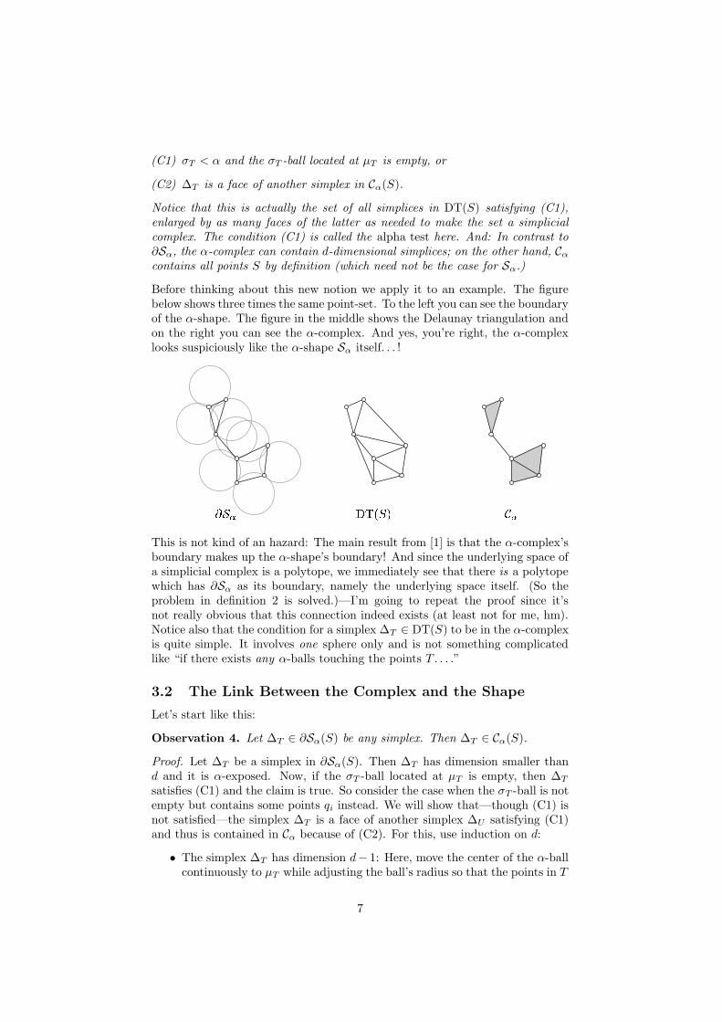
Before thinking about this new notion we apply it to an example. The figurebelow shows three times the same point-set. To the left you can see the boundaryof the α-shape. The figure in the middle shows the Delaunay triangulation andon the right you can see the α-complex. And yes, you’re right, the α-complexlooks suspiciously like the α-shape Sα itself. . . !

����� ������ ���

This is not kind of an hazard: The main result from [1] is that the α-complex’sboundary makes up the α-shape’s boundary! And since the underlying space ofa simplicial complex is a polytope, we immediately see that there is a polytopewhich has ∂Sα as its boundary, namely the underlying space itself. (So theproblem in definition 2 is solved.)—I’m going to repeat the proof since it’snot really obvious that this connection indeed exists (at least not for me, hm).Notice also that the condition for a simplex ∆T ∈ DT(S) to be in the α-complexis quite simple. It involves one sphere only and is not something complicatedlike “if there exists any α-balls touching the points T . . . .”

3.2 The Link Between the Complex and the Shape

Let’s start like this:

Observation 4. Let ∆T ∈ ∂Sα(S) be any simplex. Then ∆T ∈ Cα(S).

Proof. Let ∆T be a simplex in ∂Sα(S). Then ∆T has dimension smaller thand and it is α-exposed. Now, if the σT -ball located at µT is empty, then ∆T

satisfies (C1) and the claim is true. So consider the case when the σT -ball is notempty but contains some points qi instead. We will show that—though (C1) isnot satisfied—the simplex ∆T is a face of another simplex ∆U satisfying (C1)and thus is contained in Cα because of (C2). For this, use induction on d:

• The simplex ∆T has dimension d− 1: Here, move the center of the α-ballcontinuously to µT while adjusting the ball’s radius so that the points in T

7

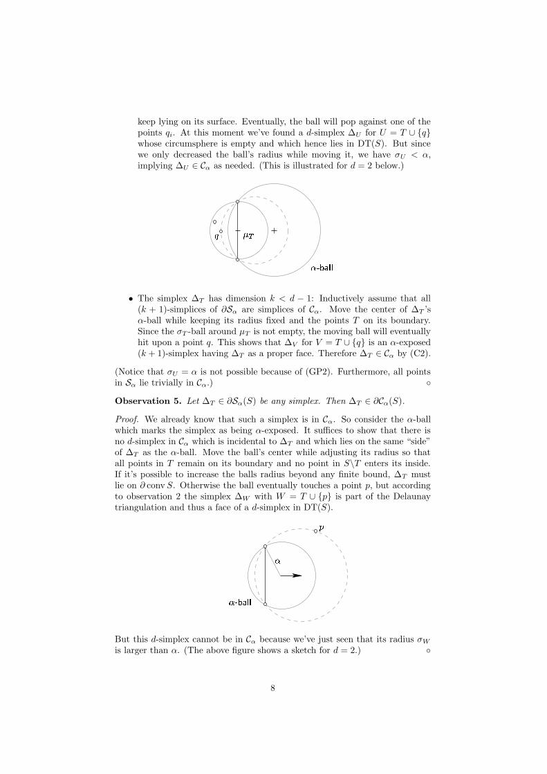
keep lying on its surface. Eventually, the ball will pop against one of thepoints qi. At this moment we’ve found a d-simplex ∆U for U = T ∪ {q}whose circumsphere is empty and which hence lies in DT(S). But sincewe only decreased the ball’s radius while moving it, we have σU < α,implying ∆U ∈ Cα as needed. (This is illustrated for d = 2 below.)

����������

��

• The simplex ∆T has dimension k < d − 1: Inductively assume that all(k + 1)-simplices of ∂Sα are simplices of Cα. Move the center of ∆T ’sα-ball while keeping its radius fixed and the points T on its boundary.Since the σT -ball around µT is not empty, the moving ball will eventuallyhit upon a point q. This shows that ∆V for V = T ∪ {q} is an α-exposed(k + 1)-simplex having ∆T as a proper face. Therefore ∆T ∈ Cα by (C2).

(Notice that σU = α is not possible because of (GP2). Furthermore, all pointsin Sα lie trivially in Cα.) ◦

Observation 5. Let ∆T ∈ ∂Sα(S) be any simplex. Then ∆T ∈ ∂Cα(S).

Proof. We already know that such a simplex is in Cα. So consider the α-ballwhich marks the simplex as being α-exposed. It suffices to show that there isno d-simplex in Cα which is incidental to ∆T and which lies on the same “side”of ∆T as the α-ball. Move the ball’s center while adjusting its radius so thatall points in T remain on its boundary and no point in S\T enters its inside.If it’s possible to increase the balls radius beyond any finite bound, ∆T mustlie on ∂ convS. Otherwise the ball eventually touches a point p, but accordingto observation 2 the simplex ∆W with W = T ∪ {p} is part of the Delaunaytriangulation and thus a face of a d-simplex in DT(S).

����������

�

�

But this d-simplex cannot be in Cα because we’ve just seen that its radius σWis larger than α. (The above figure shows a sketch for d = 2.) ◦

8

The other direction is proved similarly. A principal k-simplex of Cα is a sim-plex which is not a proper face of another one in Cα. Every principal simplexmust fullful (C1) (though the reverse is not always true). (Btw: Notice that aprincipal simplex ∈ Cα of dimension < d has to lie on the boundary of Cα.)

Observation 6. Let ∆T ∈ ∂Cα(S). Then ∆T ∈ ∂Sα(S).

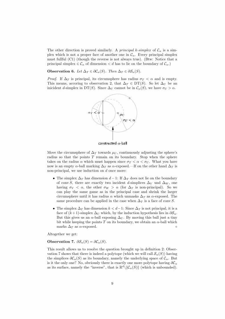
Proof. If ∆T is principal, its circumsphere has radius σT < α and is empty.This means, accoring to observation 2, that ∆T ∈ DT(S). So let ∆U be aninicident d-simplex in DT(S). Since ∆U cannot be in Cα(S), we have σU > α.

������������� �����������������

��� � �

�"!#� � $ �

Move the circumsphere of ∆T towards µU , continuously adjusting the sphere’sradius so that the points T remain on its boundary. Stop when the spheretakes on the radius α which must happen since σT < α < σU . What you havenow is an empty α-ball marking ∆T as α-exposed.—If on the other hand ∆T isnon-principal, we use induction on d once more:

• The simplex ∆T has dimension d− 1: If ∆T does not lie on the boundaryof convS, there are exactly two incident d-simplices ∆V und ∆W , onehaving σV < α, the other σW > α (for ∆T is non-principal). So wecan play the same game as in the principal case and shrink the largercircumsphere until it has radius α which unmasks ∆T as α-exposed. Thesame procedure can be applied in the case when ∆T is a face of convS.

• The simplex ∆T has dimension k < d−1: Since ∆T is not principal, it is aface of (k+1)-simplex ∆U which, by the induction hypothesis lies in ∂Sα.But this gives us an α-ball exposing ∆U . By moving this ball just a tinybit while keeping the points T on its boundary, we obtain an α-ball whichmarks ∆T as α-exposed. ◦

Altogether we get:

Observation 7. ∂Sα(S) = ∂Cα(S).

This result allows us to resolve the question brought up in definition 2: Obser-vation 7 shows that there is indeed a polytope (which we will call Sα(S)) havingthe simplices ∂Cα(S) as its boundary, namely the underlying space of Cα. Butis it the only one? No, obviously there is exactly one more polytope having ∂Cαas its surface, namely the “inverse”, that is Rd\‖Cα(S)‖ (which is unbounded).

9

But since we’re definitely interested in a bounded object we4 “set”

Sα(S) := ‖Cα(S)‖. (2)

(If you want to, you can see this as an alternative definition of the α-shape.)

3.3 The Interior of the Alpha Shape

Relax, we’re over the hill, haha! There’s just two more little things I’d like tomention. The first bit is that there’s an easy way to find out on which side of afacet ∆T ∈ ∂Cα the interior of the α-shape lies. What I mean is the following:

���������� ��

�� ��

The line segment on the right does obviously not bound the interior of the shape,so the interior of the α-shape is on neither of its sides. The same holds for theline in the middle of the figure. The remaining four lines (on the left of theimage) however do bound the interior of the shape, so one side of aff(∆T ) is“inside” and the other “outside”.Of course we could solve the problem by simply inspecting the α-complex (check-ing whether there is a d-simplex in the complex containing ∆T ). But here’sanother way:

Observation 8. Let ∆T ∈ ∂Cα be a facet on the boundary of the α-shape.Then: ∆T bounds the interior of the α-shape iff but one of the two α-balls b

with T = ∂b ∩ S is empty.

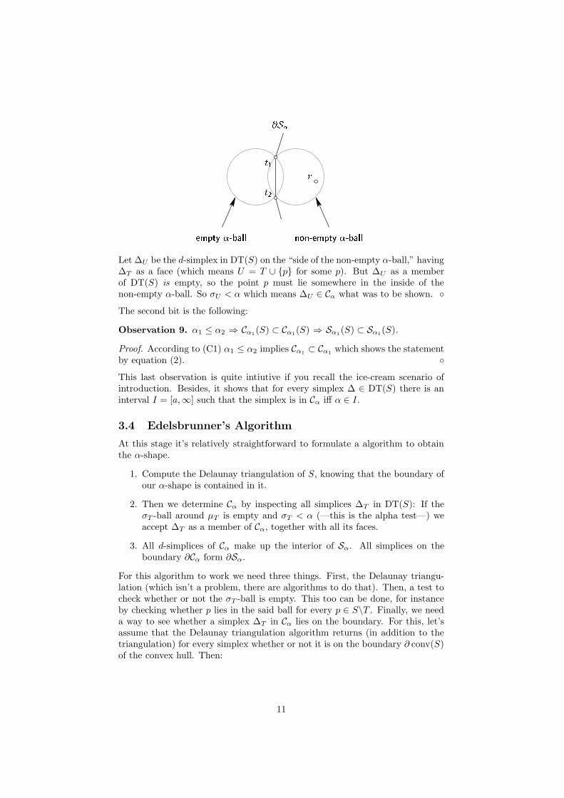
Proof. The direction (⇒) can be shown as follows. Since ∆T ∈ ∂Cα = ∂Sα,one of the two α-balls in question must be empty. So we’ll have to show thatthe other is not. But if ∆T bounds the interior then there is a d-simplex ∆U inthe α-complex having ∆T as a face. Consequently, the circumsphere of ∆U hasradius σU < α which already shows that the α-ball “on the side of ∆U” cannotbe empty.The other direction is shown similarly, so take a look at the figure below. Asalready mentioned, one of the α-balls must be empty. So we assume that theother is not, but contains a point r instead.

4Zwei moeglichkeiten???

10

������������ ������ ��������������������� ������

���

� �

!#"%$

&

Let ∆U be the d-simplex in DT(S) on the “side of the non-empty α-ball,” having∆T as a face (which means U = T ∪ {p} for some p). But ∆U as a memberof DT(S) is empty, so the point p must lie somewhere in the inside of thenon-empty α-ball. So σU < α which means ∆U ∈ Cα what was to be shown. ◦

The second bit is the following:

Observation 9. α1 ≤ α2 ⇒ Cα1(S) ⊂ Cα1

(S) ⇒ Sα1(S) ⊂ Sα1

(S).

Proof. According to (C1) α1 ≤ α2 implies Cα1⊂ Cα1

which shows the statementby equation (2). ◦

This last observation is quite intiutive if you recall the ice-cream scenario ofintroduction. Besides, it shows that for every simplex ∆ ∈ DT(S) there is aninterval I = [a,∞] such that the simplex is in Cα iff α ∈ I.

3.4 Edelsbrunner’s Algorithm

At this stage it’s relatively straightforward to formulate a algorithm to obtainthe α-shape.

1. Compute the Delaunay triangulation of S, knowing that the boundary ofour α-shape is contained in it.

2. Then we determine Cα by inspecting all simplices ∆T in DT(S): If theσT -ball around µT is empty and σT < α (—this is the alpha test—) weaccept ∆T as a member of Cα, together with all its faces.

3. All d-simplices of Cα make up the interior of Sα. All simplices on theboundary ∂Cα form ∂Sα.

For this algorithm to work we need three things. First, the Delaunay triangu-lation (which isn’t a problem, there are algorithms to do that). Then, a test tocheck whether or not the σT -ball is empty. This too can be done, for instanceby checking whether p lies in the said ball for every p ∈ S\T . Finally, we needa way to see whether a simplex ∆T in Cα lies on the boundary. For this, let’sassume that the Delaunay triangulation algorithm returns (in addition to thetriangulation) for every simplex whether or not it is on the boundary ∂ conv(S)of the convex hull. Then:

11

Observation 10. Let ∆T be a simplex in Cα(S). If ∆T ∈ ∂ conv(S), then it isobviously on the boundary of Cα. Otherwise, it is in the interior of Cα iff all ofthe simplices in DT(S) properly containing ∆T lie in Cα, too.

5

The algorithm presented in [1] and [3] is an efficient implementation of the aboveprocedure, with two additional advantages: First of all the algorithm does notrun for a single value α but computes an implicit representation instead whichcan be used to deduce Sα for any value of α. More precisely, the algorithmcomputes for every simplex ∆T ∈ DT(S) an intervall I = [a,∞] with theinterpretation that ∆T ∈ Sα iff α ∈ I.6 (That there is such an interval is aconsequence of observation 9, as already mentionned.) Second, the algorithmnot only distinguishes among interior and non-interior simplices of Cα (as wehave done above), but makes three distinctions instead, one more among thenon-interior simplices. (I didn’t get why though, probably it’s just useful to havethe algorithm output some more information about the individual simplicesof the α-shape’s boundary. . . ?) In the following I will not make this finerdifferentiation.When we increase α continuously from 0 towards∞ and consider a simplex ∆T ∈DT(S), we see (using observation 9) that there are two (possibly empty) inter-vals (a, b) and (b,∞) (with 0 ≤ a ≤ b ≤ ∞) such that

∆T is

not in Cα (for α < a)in ∂Cα (for α ∈ (a, b))

interior to Cα (for α ∈ (b,∞)). (3)

(Notice that there is no need to consider the boundaries of the intervall (eg.the situations α = a, b) because of the general position assumption: Since thecomplex Cα only changes when a simplex is picked up by condition (C1), andsince there are by assumption (GP2) no circumspheres with radius α, we seethat the complex cannot change when α passes the values a and b.)Our aim is to find a, b (eg. the intervals in (3)) for every simplex ∆T ∈ DT(S).For a d-simplex in DT(S) the story is simple: Its circumsphere is empty bydefinition and the alpha-test indicates that it is in the α-complex iff σT < α.And since a d-simplex is always interior to Cα we get a = b = σT . We can thuswrite down the head of the algorithm as follows:

procedure AlphaShape(S,d);{Given a point-set S ⊂ Rd, computes a list R of simplices ∆T and}{two lists B, I of intervals such that ∆T ∈ ∂Sα if and only if α ∈ BT }{and ∆T ∈ int(Sα) if and only if α ∈ IT .}begin

R:= DT(S);for each d-simplex ∆T ∈ R do

BT := ∅; IT := (σi,∞);end for;...

5Reason: Every simplex in the complex DT(S) is a face of a d-simplex, and thus, if onesuper-simplex of ∆T does not lie in Cα there’s also a d-simplex containing ∆T not lying inCα which means that ∆T is on the boundary.

6Notice that it’s not really obvious how to alter our above procedure to output such animplicit representation. That’s why we need another way. . .

12

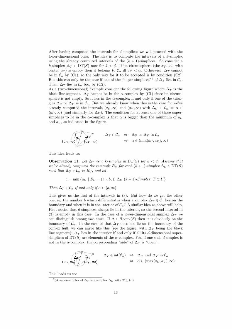
After having computed the intervals for d-simplices we will proceed with thelower-dimensional ones. The idea is to compute the intervals of a k-simplexusing the already computed intervals of the (k + 1)-simplices. So consider ak-simplex ∆T ∈ DT(S) now for k < d. If its circumsphere (the σT -ball withcenter µT ) is empty then it belongs to Cα iff σT < α. Otherwise, ∆T cannotbe in Cα by (C1), so the only way for it to be accepted is by condition (C2).But this can only be the case if one of the “super-simplices”7 of ∆T lies in Cα.Then, ∆T lies in Cα too, by (C2).As a (two-dimensional) example consider the following figure where ∆T is theblack line-segment. ∆T cannot be in the α-complex by (C1) since its circum-sphere is not empty. So it lies in the α-complex if and only if one of the trian-gles ∆U or ∆V is in Cα. But we already know when this is the case for we’vealready computed the intervals (aU ,∞) and (aV ,∞) with ∆U ∈ Cα ⇔ α ∈(aU ,∞) (and similarly for ∆V ). The condition for at least one of these super-simplices to lie in the α-complex is that α is bigger than the minimum of aUand aV , as indicated in the figure.

��� ������ �������� � � ��

∆T ∈ Cα ⇔ ∆U or ∆V in Cα

⇔ α ∈ (min(aU , aV ),∞)

This idea leads to:

Observation 11. Let ∆T be a k-simplex in DT(S) for k < d. Assume thatwe’ve already computed the intervals BU for each (k + 1)-simplex ∆U ∈ DT(S)such that ∆U ∈ Cα ⇔ BU , and let

a = min {aU | BU = (aU , bu), ∆U (k + 1)-Simplex, T ⊂ U}

Then ∆T ∈ Cα if and only if α ∈ (a,∞).

This gives us the first of the intervals in (3). But how do we get the otherone, eg. the number b which differentiates when a simplex ∆T ∈ Cα lies on theboundary and when it is in the interior of Cα? A similar idea as above will help.First notice that d-simplices always lie in the interior, so the second interval in(3) is empty in this case. In the case of a lower-dimensional simplex ∆T wecan distinguish among two cases. If ∆ ∈ ∂ conv(S) then it is obviously on theboundary of Cα. In the case of that ∆T does not lie on the boundary of theconvex hull, we can argue like this (see the figure, with ∆T being the blackline segment): ∆T lies in the interior if and only if all its d-dimensional super-simplices of DT(S) are elements of the α-complex. For, if one such d-simplex isnot in the α-complex, the corresponding “side” of ∆T is “open”.

��� ������ ��������� � � ���

∆T ∈ int(Cα) ⇔ ∆U und ∆V in Cα

⇔ α ∈ (max(aU , aV ),∞)

This leads us to:

7(A super-simplex of ∆T is a simplex ∆U with T ( U .)

13

Observation 12. Let ∆T be a k-simplex in Cα for k < d. Assume that we’vealready computed the intervals BU for each d-simplex ∆U ∈ DT(S) such that∆U ∈ Cα ⇔ BU , and let

b = max {aU | BU = (aU , bu), BU d-Simplex mit T ⊂ U}

Then ∆T ∈ ∂Cα if and only if α ∈ (b,∞).

Altogether we get the following algorithm:

procedure AlphaShape(S,d);{Given a point-set S ⊂ Rd, computes a list R of simplices ∆T and}{two lists B, I of intervals such that ∆T ∈ ∂Sα if and only if α ∈ BT }{and ∆T ∈ int(Sα) if and only if α ∈ IT .}begin

R:= DT(S);for each d-simplex ∆T ∈ R do

BT := ∅; IT := (σi,∞);end for;for k := d− 1 to 0 by −1 do

for each k-simplex ∆T ∈ R do

if bT is empty thena:= σT ;

else

a:= min {aU | BU = (aU , bu), ∆U (k + 1)-Simplex, T ⊂ U};if ∆T ∈ ∂ conv(S) then

b:= ∞;else

b:= max {aU | BU = (aU , bu), BU d-Simplex mit T ⊂ U};BT := (a, b); IT := (b,∞);

end for;end for;return (R,B, I);

end AlphaShape;

(Notice that the test ∆T ∈ ∂ conv(S) can be achieved by “flagging” the simpliceson ∂ conv(S) during the calculation of the Delaunay triangulation.)

4 Limitation of “Classical” Alpha Shapes and

Improvements

4.1 Limitations

The main application of α-shapes is the reconstruction of objects which havebeen sampled by points. For instance, a 3D-scanner provides points on thesurface of a human-being or so. The main problems with α-shapes in surfacereconstruction are (as mentionned in [5]):

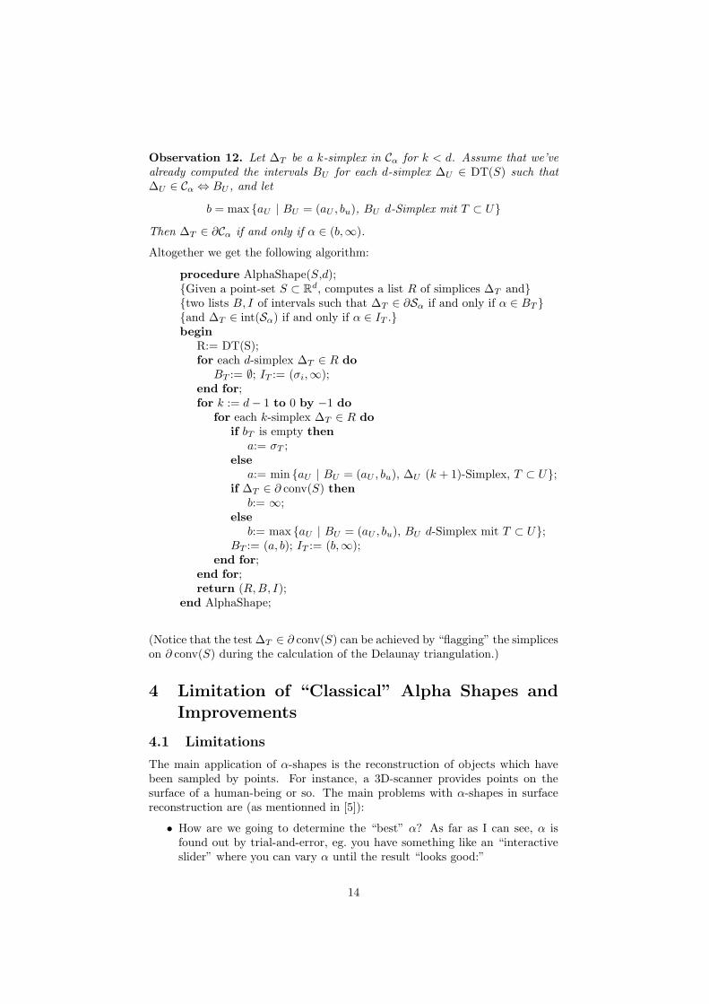
• How are we going to determine the “best” α? As far as I can see, α isfound out by trial-and-error, eg. you have something like an “interactiveslider” where you can vary α until the result “looks good:”

14

The figure, taken from [5], shows some α-shapes; we would chose themiddle one, intuitively.

• There are point-sets for which there is no satisfying α, eg. all α-shapesdon’t give intuitively good approximations of the object’s surface. Thisis mostly the case when the points S are not uniformly sampled. Thereasan for the unsatisfactory result is that α-shapes are based on distancesbetween points in order to decide which points to connect by triangles orlines. Non-uniform point-set are thus relatively inappropriate.

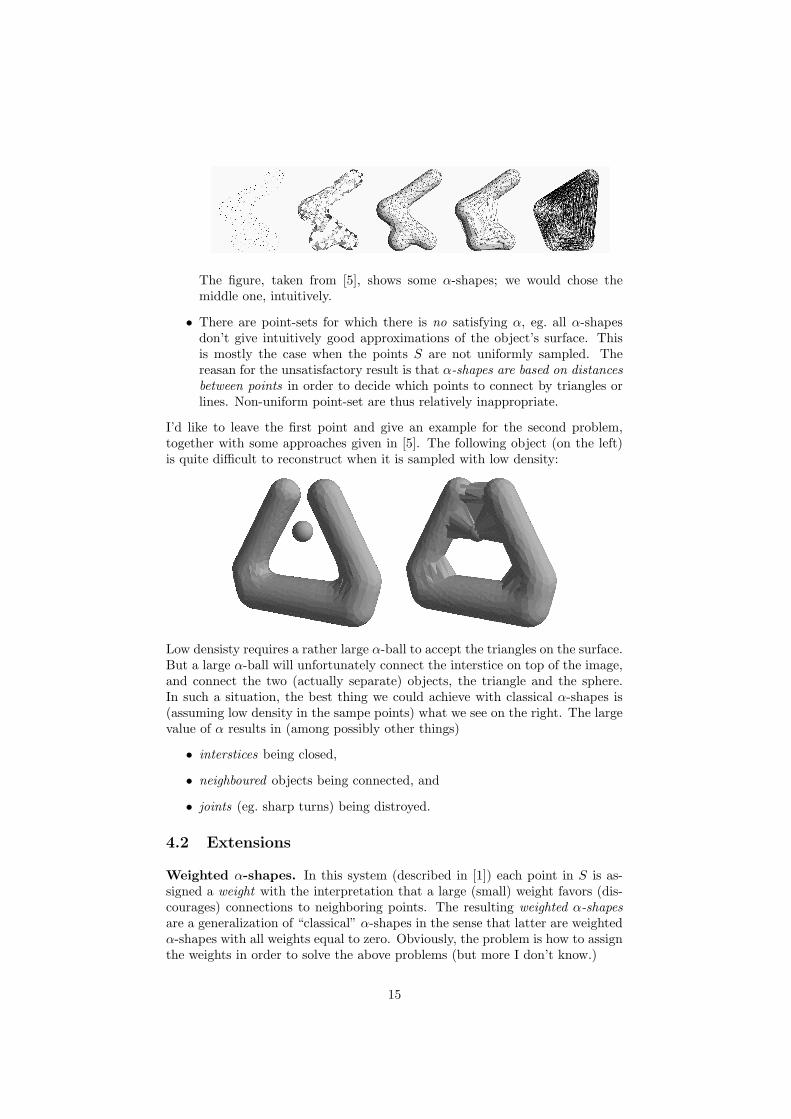
I’d like to leave the first point and give an example for the second problem,together with some approaches given in [5]. The following object (on the left)is quite difficult to reconstruct when it is sampled with low density:

Low densisty requires a rather large α-ball to accept the triangles on the surface.But a large α-ball will unfortunately connect the interstice on top of the image,and connect the two (actually separate) objects, the triangle and the sphere.In such a situation, the best thing we could achieve with classical α-shapes is(assuming low density in the sampe points) what we see on the right. The largevalue of α results in (among possibly other things)

• interstices being closed,

• neighboured objects being connected, and

• joints (eg. sharp turns) being distroyed.

4.2 Extensions

Weighted α-shapes. In this system (described in [1]) each point in S is as-signed a weight with the interpretation that a large (small) weight favors (dis-courages) connections to neighboring points. The resulting weighted α-shapesare a generalization of “classical” α-shapes in the sense that latter are weightedα-shapes with all weights equal to zero. Obviously, the problem is how to assignthe weights in order to solve the above problems (but more I don’t know.)

15

Density-scaling. In [5], “density-scaled α-shapes” are presented. Briefly, onecomputes the point-density of each point and uses this to get an approximationof the point-density of a triangle (for instance by avering the point-densities ofthe triangle’s points or by taking the maximum of these densities and so on).Then, the α-ball is reduced in size in areas where the triangle’s point-densityis higher than average. By computing the density of the triangle in differentways (avering, taking the maximum, and so on), one can achieve a finer level ofdetail in higher density areas, or detect (that is, separate) neightboured objectsif they have different point densities.

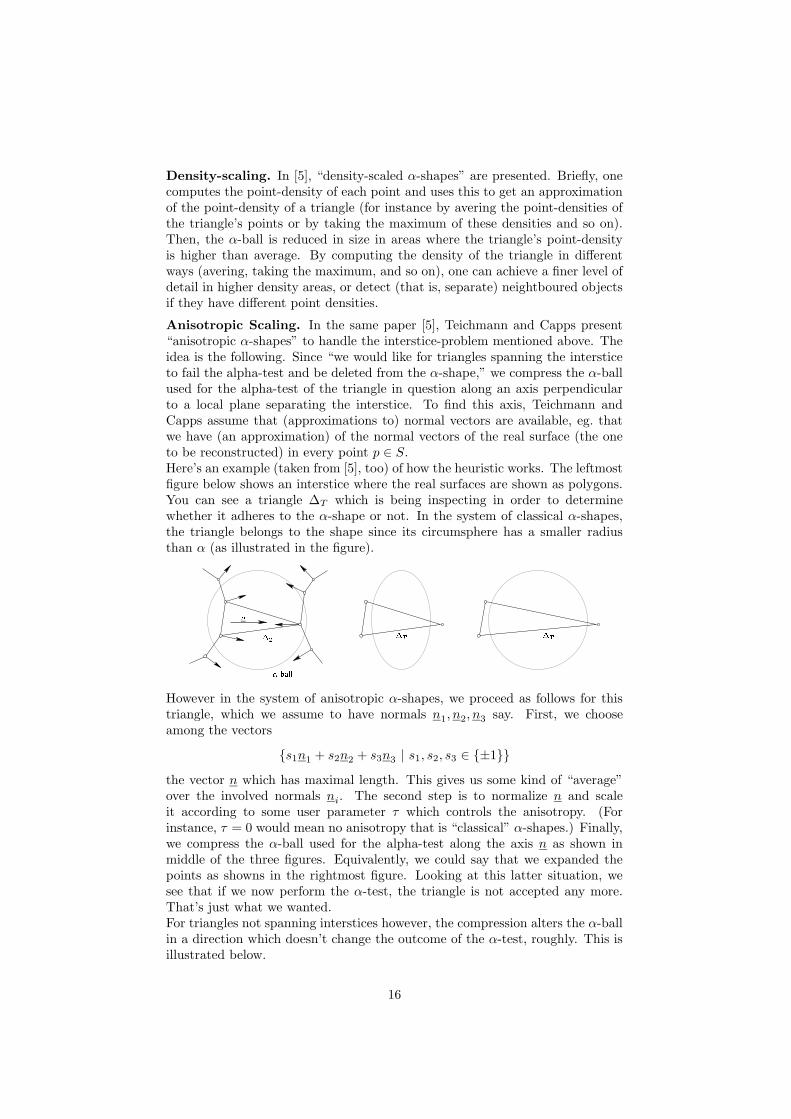
Anisotropic Scaling. In the same paper [5], Teichmann and Capps present“anisotropic α-shapes” to handle the interstice-problem mentioned above. Theidea is the following. Since “we would like for triangles spanning the intersticeto fail the alpha-test and be deleted from the α-shape,” we compress the α-ballused for the alpha-test of the triangle in question along an axis perpendicularto a local plane separating the interstice. To find this axis, Teichmann andCapps assume that (approximations to) normal vectors are available, eg. thatwe have (an approximation) of the normal vectors of the real surface (the oneto be reconstructed) in every point p ∈ S.Here’s an example (taken from [5], too) of how the heuristic works. The leftmostfigure below shows an interstice where the real surfaces are shown as polygons.You can see a triangle ∆T which is being inspecting in order to determinewhether it adheres to the α-shape or not. In the system of classical α-shapes,the triangle belongs to the shape since its circumsphere has a smaller radiusthan α (as illustrated in the figure).

��������� �

�

�

However in the system of anisotropic α-shapes, we proceed as follows for thistriangle, which we assume to have normals n1, n2, n3 say. First, we chooseamong the vectors

{s1n1 + s2n2 + s3n3 | s1, s2, s3 ∈ {±1}}

the vector n which has maximal length. This gives us some kind of “average”over the involved normals ni. The second step is to normalize n and scaleit according to some user parameter τ which controls the anisotropy. (Forinstance, τ = 0 would mean no anisotropy that is “classical” α-shapes.) Finally,we compress the α-ball used for the alpha-test along the axis n as shown inmiddle of the three figures. Equivalently, we could say that we expanded thepoints as showns in the rightmost figure. Looking at this latter situation, wesee that if we now perform the α-test, the triangle is not accepted any more.That’s just what we wanted.For triangles not spanning interstices however, the compression alters the α-ballin a direction which doesn’t change the outcome of the α-test, roughly. This isillustrated below.

16

��������� �

References

[1] H. Edelsbrunner. Weighted alpha shapes. Technical Report UIUCDCS-R-92-1760, Dept. Comput. Sci., Univ. Illinois, Urbana, IL, 1992.

[2] H. Edelsbrunner and E. P. Mucke. Simulation of simplicity: A techniqueto cope with degeneratcases in geometric algorithms. ACM Trans. Graph.,9(1):66–104, 1990.

[3] H. Edelsbrunner and E. P. Mucke. Three-dimensional alpha shapes.Manuscript UIUCDCS-R-92-1734, Dept. Comput. Sci., Univ. Illinois,Urbana-Champaign, IL, 1992.

[4] H. Edelsbrunner and E. P. Mucke. Three-dimensional alpha shapes. ACMTrans. Graph., 13(1):43–72, January 1994.

[5] M. Teichmann and M. Capps. Surface reconstruction with anisotropicdensity-scaled alpha-shapes. In IEEE Visualization ’98 Proceedings, pages67–72, San Francisco, CA, October 1998. ACM/SIGGRAPH Press.

The pictures on page 2 and 5 have been taken from [3] and from Walter Luh’shomepage at http://www.stanford.edu/˜wluh/cs448b/alphashapes.html. The im-ages in section 4 have been taken from [5].

Kaspar Fischer, [email protected]—26. V. 2000

17