Introduction to Adaptive Control

Chapter 1Introduction to Adaptive Control

1.1 Adaptive Control—Why?

Adaptive Control covers a set of techniques which provide a systematic approach forautomatic adjustment of controllers in real time, in order to achieve or to maintaina desired level of control system performance when the parameters of the plantdynamic model are unknown and/or change in time.

Consider first the case when the parameters of the dynamic model of the plantto be controlled are unknown but constant (at least in a certain region of operation).In such cases, although the structure of the controller will not depend in generalupon the particular values of the plant model parameters, the correct tuning of thecontroller parameters cannot be done without knowledge of their values. Adaptivecontrol techniques can provide an automatic tuning procedure in closed loop forthe controller parameters. In such cases, the effect of the adaptation vanishes astime increases. Changes in the operation conditions may require a restart of theadaptation procedure.

Now consider the case when the parameters of the dynamic model of the plantchange unpredictably in time. These situations occur either because the environ-mental conditions change (ex: the dynamical characteristics of a robot arm or of amechanical transmission depend upon the load; in a DC-DC converter the dynamiccharacteristics depend upon the load) or because we have considered simplified lin-ear models for nonlinear systems (a change in operation condition will lead to adifferent linearized model). These situations may also occur simply because the pa-rameters of the system are slowly time-varying (in a wiring machine the inertia ofthe spool is time-varying). In order to achieve and to maintain an acceptable level ofcontrol system performance when large and unknown changes in model parametersoccur, an adaptive control approach has to be considered. In such cases, the adap-tation will operate most of the time and the term non-vanishing adaptation fullycharacterizes this type of operation (also called continuous adaptation).

Further insight into the operation of an adaptive control system can be gained ifone considers the design and tuning procedure of the “good” controller illustratedin Fig. 1.1. In order to design and tune a good controller, one needs to:

I.D. Landau et al., Adaptive Control, Communications and Control Engineering,DOI 10.1007/978-0-85729-664-1_1, © Springer-Verlag London Limited 2011

1

2 1 Introduction to Adaptive Control

Fig. 1.1 Principles ofcontroller design

Fig. 1.2 An adaptive controlsystem

(1) Specify the desired control loop performances.(2) Know the dynamic model of the plant to be controlled.(3) Possess a suitable controller design method making it possible to achieve the

desired performance for the corresponding plant model.

The dynamic model of the plant can be identified from input/output plant mea-surements obtained under an experimental protocol in open or in closed loop. Onecan say that the design and tuning of the controller is done from data collected onthe system. An adaptive control system can be viewed as an implementation of theabove design and tuning procedure in real time. The tuning of the controller will bedone in real time from data collected in real time on the system. The correspondingadaptive control scheme is shown in Fig. 1.2.

The way in which information is processed in real time in order to tune the con-troller for achieving the desired performances will characterize the various adapta-tion techniques. From Fig. 1.2, one clearly sees that an adaptive control system isnonlinear since the parameters of the controller will depend upon measurements ofsystem variables through the adaptation loop.

The above problem can be reformulated as nonlinear stochastic control with in-complete information. The unknown parameters are considered as auxiliary states(therefore the linear models become nonlinear: x = ax =⇒ x1 = x1x2, x2 = v

where v is a stochastic process driving the parameter variations). Unfortunately,the resulting solutions (dual control) are extremely complicated and cannot be im-plemented in practice (except for very simple cases). Adaptive control techniquescan be viewed as approximation for certain classes of nonlinear stochastic controlproblems associated with the control of processes with unknown and time-varyingparameters.

1.2 Adaptive Control Versus Conventional Feedback Control 3

1.2 Adaptive Control Versus Conventional Feedback Control

The unknown and unmeasurable variations of the process parameters degrade theperformances of the control systems. Similarly to the disturbances acting upon thecontrolled variables, one can consider that the variations of the process parametersare caused by disturbances acting upon the parameters (called parameter distur-bances). These parameter disturbances will affect the performance of the controlsystems. Therefore the disturbances acting upon a control system can be classifiedas follows:

(a) disturbances acting upon the controlled variables;(b) (parameter) disturbances acting upon the performance of the control system.

Feedback is basically used in conventional control systems to reject the effect ofdisturbances upon the controlled variables and to bring them back to their desiredvalues according to a certain performance index. To achieve this, one first measuresthe controlled variables, then the measurements are compared with the desired val-ues and the difference is fed into the controller which will generate the appropriatecontrol.

A similar conceptual approach can be considered for the problem of achievingand maintaining the desired performance of a control system in the presence ofparameter disturbances. We will have to define first a performance index (IP) forthe control system which is a measure of the performance of the system (ex: thedamping factor for a closed-loop system characterized by a second-order transferfunction is an IP which allows to quantify a desired performance expressed in termsof “damping”). Then we will have to measure this IP. The measured IP will becompared to the desired IP and their difference (if the measured IP is not acceptable)will be fed into an adaptation mechanism. The output of the adaptation mechanismwill act upon the parameters of the controller and/or upon the control signal in orderto modify the system performance accordingly. A block diagram illustrating a basicconfiguration of an adaptive control system is given in Fig. 1.3.

Associated with Fig. 1.3, one can consider the following definition for an adap-tive control system.

Definition 1.1 An adaptive control system measures a certain performance index(IP) of the control system using the inputs, the states, the outputs and the knowndisturbances. From the comparison of the measured performance index and a setof given ones, the adaptation mechanism modifies the parameters of the adjustablecontroller and/or generates an auxiliary control in order to maintain the performanceindex of the control system close to the set of given ones (i.e., within the set ofacceptable ones).

Note that the control system under consideration is an adjustable dynamic systemin the sense that its performance can be adjusted by modifying the parameters of thecontroller or the control signal. The above definition can be extended straightfor-wardly for “adaptive systems” in general (Landau 1979).

A conventional feedback control system will monitor the controlled variablesunder the effect of disturbances acting on them, but its performance will vary (it


Fig. 1.3 Basic configuration for an adaptive control system

is not monitored) under the effect of parameter disturbances (the design is doneassuming known and constant process parameters).

An adaptive control system, which contains in addition to a feedback control withadjustable parameters a supplementary loop acting upon the adjustable parametersof the controller, will monitor the performance of the system in the presence ofparameter disturbances.

Consider as an example the case of a conventional feedback control loop de-signed to have a given damping. When a disturbance acts upon the controlled vari-able, the return of the controlled variable towards its nominal value will be char-acterized by the desired damping if the plant parameters have their known nominalvalues. If the plant parameters change upon the effect of the parameter disturbances,the damping of the system response will vary. When an adaptation loop is added,the damping of the system response will be maintained when changes in parametersoccur.

Comparing the block diagram of Fig. 1.3 with a conventional feedback controlsystem, one can establish the correspondences which are summarized in Table 1.1.

While the design of a conventional feedback control system is oriented firstlytoward the elimination of the effect of disturbances upon the controlled variables,the design of adaptive control systems is oriented firstly toward the elimination ofthe effect of parameter disturbances upon the performance of the control system. Anadaptive control system can be interpreted as a feedback system where the controlledvariable is the performance index (IP).

One can view an adaptive control system as a hierarchical system:

• Level 1: conventional feedback control;• Level 2: adaptation loop.

In practice often an additional “monitoring” level is present (Level 3) which decideswhether or not the conditions are fulfilled for a correct operation of the adaptationloop.


Table 1.1 Adaptive controlversus conventional feedbackcontrol

Conventional feedbackcontrol system

Adaptive control system

Objective: monitoring ofthe “controlled”variables according to acertain IP for the case ofknown parameters

Objective: monitoring of theperformance (IP) of thecontrol system for unknownand varying parameters

Controlled variable Performance index (IP)

Transducer IP measurement

Reference input Desired IP

Comparison block Comparison decision block

Controller Adaptation mechanism

Fig. 1.4 Comparison of an adaptive controller with a conventional controller (fixed parameters),(a) fixed parameters controller, (b) adaptive controller

Figure 1.4 illustrates the operation of an adaptive controller. In Fig. 1.4a, a changeof the plant model parameters occurs at t = 150 and the controller used has constantparameters. One can see that poor performance results from this parameter change.In Fig. 1.4b, an adaptive controller is used. As one can see, after an adaptationtransient the nominal performance is recovered.


1.2.1 Fundamental Hypothesis in Adaptive Control

The operation of the adaptation loop and its design relies upon the following fun-damental hypothesis: For any possible values of plant model parameters there is acontroller with a fixed structure and complexity such that the specified performancescan be achieved with appropriate values of the controller parameters.

In the context of this book, the plant models are assumed to be linear and thecontrollers which are considered are also linear.

Therefore, the task of the adaptation loop is solely to search for the “good” valuesof the controller parameters.

This emphasizes the importance of the control design for the known parametercase (the underlying control design problem), as well as the necessity of a prioriinformation about the structure of the plant model and its characteristics which canbe obtained by identification of a model for a given set of operational conditions.

In other words, an adaptive controller is not a “black box” which can solve acontrol problem in real time without an initial knowledge about the plant to be con-trolled. This a priori knowledge is needed for specifying achievable performances,the structure and complexity of the controller and the choice of an appropriate de-sign method.

1.2.2 Adaptive Control Versus Robust Control

In the presence of model parameter variations or more generally in the presence ofvariations of the dynamic characteristics of a plant to be controlled, robust controldesign of the conventional feedback control system is a powerful tool for achievinga satisfactory level of performance for a family of plant models. This family is oftendefined by means of a nominal model and a size of the uncertainty specified in theparameter domain or in the frequency domain.

The range of uncertainty domain for which satisfactory performances can beachieved depends upon the problem. Sometimes, a large domain of uncertainty canbe tolerated, while in other cases, the uncertainty tolerance range may be very small.If the desired performances cannot be achieved for the full range of possible param-eter variations, adaptive control has to be considered in addition to a robust controldesign. Furthermore, the tuning of a robust design for the true nominal model usingan adaptive control technique will improve the achieved performance of the robustcontroller design. Therefore, robust control design will benefit from the use of adap-tive control in terms of performance improvements and extension of the range of op-eration. On the other hand, using an underlying robust controller design for buildingan adaptive control system may drastically improve the performance of the adaptivecontroller. This is illustrated in Figs. 1.5, 1.6 and 1.7, where a comparison betweenconventional feedback control designed for the nominal model, robust control de-sign and adaptive control is presented. To make a fair comparison the presence ofunmodeled dynamics has been considered in addition to the parameter variations.


Fig. 1.5 Frequency characteristics of the true plant model for ω0 = 1 and ω0 = 0.6 and of theidentified model for ω0 = 1

For each experiment, a nominal plant model is used in the first part of the recordand a model with different parameters is used in the second part.

The plant considered for this example is characterized by a third order modelformed by a second-order system with a damping factor of 0.2 and a natural fre-quency varying from ω0 = 1 rad/sec to ω0 = 0.6 rad/sec and a first order system.The first order system corresponds to a high-frequency dynamics with respect to thesecond order. The change of the damping factor occurs at t = 150.

The nominal system (with ω0 = 1) has been identified using a second-ordermodel (lower order modeling). The frequency characteristics of the true model forω0 = 1, ω0 = 0.6 and of the identified model for ω0 = 1 are shown in Fig. 1.5.

Based on the second-order model identified for ω0 = 1 a conventional fixed con-troller is designed (using pole placement—see Chap. 7 for details). The performanceof this controller is illustrated in Fig. 1.6a. One can see that the performance of theclosed-loop system is seriously affected by the change of the natural frequency. Fig-ure 1.6b shows the performance of a robust controller designed on the basis of thesame identified model obtained for ω0 = 1 (for this design pole placement is com-bined with the shaping of the sensitivity functions—see Chap. 8 for details). Onecan observe that the nominal performance is slightly lower (slower step response)than for the previous controller but the performance remains acceptable when thecharacteristics of the plant change.


Fig. 1.6 Comparison of conventional feedback control and robust control, (a) conventional designfor the nominal model, (b) robust control design

Figure 1.7a shows the response of the control system when the parameters ofthe conventional controller used in Fig. 1.6a are adapted, based on the estimationin real time of a second-order model for the plant. A standard parameter adaptationalgorithm is used to update the model parameters. One observes that after a tran-sient, the nominal performances are recovered except that a residual high-frequencyoscillation is observed. This is caused by the fact that one estimates a lower ordermodel than the true one (but this is often the situation in practice). To obtain a satis-factory operation in such a situation, one has to “robustify” the adaptation algorithm(in this example, the “filtering” technique has been used—see Chap. 10 for details)and the results are shown in Fig. 1.7b. One can see that the residual oscillation hasdisappeared but the adaptation is slightly slower.

Figure 1.7c shows the response of the control system when the parameters of therobust controller used in Fig. 1.6b are adapted using exactly the same algorithm asfor the case of Fig. 1.7a. In this case, even with a standard adaptation algorithm,residual oscillations do not occur and the transient peak at the beginning of theadaptation is lower than in Fig. 1.7a. However, the final performance will not bebetter than that of the robust controller for the nominal model.

After examining the time responses, one can come to the following conclusions:

1. Before using adaptive control, it is important to do a robust control design.2. Robust control design improves in general the adaptation transients.

1.3 Basic Adaptive Control Schemes 9

Fig. 1.7 Comparison of adaptive controller, (a) adaptation added to the conventional controller(Fig. 1.6a), (b) robust adaptation added to the conventional controller (Fig. 1.6a), (c) adaptationadded to the robust controller (Fig. 1.6b)

3. A robust controller is a “fixed parameter” controller which instantaneously pro-vides its designed characteristics.

4. The improvement of performance via adaptive control requires the introductionof additional algorithms in the loop and an “adaptation transient” is present (thetime necessary to reach the desired performance from a degraded situation).

5. A trade-off should be considered in the design between robust control and robustadaptation.

1.3 Basic Adaptive Control Schemes

In the context of various adaptive control schemes, the implementation of the threefundamental blocks of Fig. 1.3 (performance measurement, comparison-decision,adaptation mechanism) may be very intricate. Indeed, it may not be easy to decom-pose the adaptive control scheme in accordance with the basic diagram of Fig. 1.3.Despite this, the basic characteristic which allows to decide whether or not a sys-tem is truly “adaptive” is the presence or the absence of the closed-loop control ofa certain performance index. More specifically, an adaptive control system will useinformation collected in real time to improve the tuning of the controller in order


Fig. 1.8 Open-loop adaptive control

to achieve or to maintain a level of desired performance. There are many controlsystems which are designed to achieve acceptable performance in the presence ofparameter variations, but they do not assure a closed-loop control of the performanceand, as such, they are not “adaptive”. The typical example is the robust control de-sign which, in many cases, can achieve acceptable performances in the presence ofparameter variations using a fixed controller.

We will now go on to present some basic schemes used in adaptive control.

1.3.1 Open-Loop Adaptive Control

We shall consider next as an example the “gain-scheduling” scheme which is anopen-loop adaptive control system. A block diagram of such a system is shown inFig. 1.8. The adaptation mechanism in this case is a simple look-up table storedin the computer which gives the controller parameters for a given set of environ-ment measurements. This technique assumes the existence of a rigid relationshipbetween some measurable variables characterizing the environment (the operatingconditions) and the parameters of the plant model. Using this relationship, it is thenpossible to reduce (or to eliminate) the effect of parameter variations upon the per-formance of the system by changing the parameters of the controller accordingly.

This is an open-loop adaptive control system because the modifications of thesystem performance resulting from the change in controller parameters are not mea-sured and feedback to a comparison-decision block in order to check the efficiencyof the parameter adaptation. This system can fail if for some reason or another therigid relationship between the environment measurements and plant model parame-ters changes.

Although such gain-scheduling systems are not fully adaptive in the sense of Def-inition 1.1, they are widely used in a variety of situations with satisfactory results.Typical applications of such principles are:

1. adjustments of autopilots for commercial jet aircrafts using speed and altitudemeasurements,


2. adjustment of the controller in hot dip galvanizing using the speed of the steelstrip and position of the actuator (Fenot et al. 1993),

and many others.Gain-scheduling schemes are also used in connection with adaptive control

schemes where the gain-scheduling takes care of rough changes of parameters whenthe conditions of operation change and the adaptive control takes care of the finetuning of the controller.

Note however that in certain cases, the use of this simple principle can be verycostly because:

1. It may require additional expensive transducers.2. It may take a long time and numerous experiments in order to establish the de-

sired relationship between environment measurements and controller parameters.

In such situations, an adaptive control scheme can be cheaper to implement since itwill not use additional measurements and requires only additional computer power.

1.3.2 Direct Adaptive Control

Consider the basic philosophy for designing a controller discussed in Sect. 1.1 andwhich was illustrated in Fig. 1.1.

One of the key points is the specification of the desired control loop performance.In many cases, the desired performance of the feedback control system can be spec-ified in terms of the characteristics of a dynamic system which is a realization ofthe desired behavior of the closed-loop system. For example, a tracking objectivespecified in terms of rise time, and overshoot, for a step change command can bealternatively expressed as the input-output behavior of a transfer function (for ex-ample a second-order with a certain resonance frequency and a certain damping).A regulation objective in a deterministic environment can be specified in terms ofthe evolution of the output starting from an initial disturbed value by specifying thedesired location of the closed-loop poles. In these cases, the controller is designedsuch that for a given plant model, the closed-loop system has the characteristics ofthe desired dynamic system.

The design problem can in fact be equivalently reformulated as in Fig. 1.9. Thereference model in Fig. 1.9 is a realization of the system with desired performances.The design of the controller is done now in order that:

(1) the error between the output of the plant and the output of the reference modelis identically zero for identical initial conditions;

(2) an initial error will vanish with a certain dynamic.

When the plant parameters are unknown or change in time, in order to achieveand to maintain the desired performance, an adaptive control approach has to beconsidered and such a scheme known as Model Reference Adaptive Control (MRAC)is shown in Fig. 1.10.


Fig. 1.9 Design of a linearcontroller in deterministicenvironment using an explicitreference model forperformance specifications

Fig. 1.10 Model ReferenceAdaptive Control scheme

This scheme is based on the observation that the difference between the outputof the plant and the output of the reference model (called subsequently plant-modelerror) is a measure of the difference between the real and the desired performance.This information (together with other information) is used by the adaptation mech-anism (subsequently called parameter adaptation algorithm) to directly adjust theparameters of the controller in real time in order to force asymptotically the plant-model error to zero. This scheme corresponds to the use of a more general conceptcalled Model Reference Adaptive Systems (MRAS) for the purpose of control. SeeLandau (1979). Note that in some cases, the reference model may receive measure-ments from the plant in order to predict future desired values of the plant output.

The model reference adaptive control scheme was originally proposed byWhitaker et al. (1958) and constitutes the basic prototype for direct adaptive control.

The concept of model reference control, and subsequently the concept of directadaptive control, can be extended for the case of operation in a stochastic environ-ment. In this case, the disturbance affecting the plant output can be modeled as anARMA process, and no matter what kind of linear controller with fixed parameterwill be used, the output of the plant operating in closed loop will be an ARMAmodel. Therefore the control objective can be specified in terms of a desired ARMAmodel for the plant output with desired properties. This will lead to the concept ofstochastic reference model which is in fact a prediction reference model. See Lan-dau (1981). The prediction reference model will specify the desired behavior of thepredicted output. The plant-model error in this case is the prediction error which


Fig. 1.11 Indirect adaptivecontrol (principle)

is used to directly adapt the parameters of the controller in order to force asymp-totically the plant-model stochastic error to become an innovation process. The selftuning minimum variance controller (Åström and Wittenmark 1973) is the basic ex-ample of direct adaptive control in a stochastic environment. More details can befound in Chaps. 7 and 11.

Despite its elegance, the use of direct adaptive control schemes is limited by thehypotheses related to the underlying linear design in the case of known parameters.While the performance can in many cases be specified in terms of a reference model,the conditions for the existence of a feasible controller allowing for the closed loopto match the reference model are restrictive. One of the basic limitations is that onehas to assume that the plant model has in all the situations stable zeros, which in thediscrete-time case is quite restrictive.1 The problem becomes even more difficult inthe multi-input multi-output case. While different solutions have been proposed toovercome some of the limitations of this approach (see for example M’Saad et al.1985; Landau 1993a), direct adaptive control cannot always be used.

1.3.3 Indirect Adaptive Control

Figure 1.11 shows an indirect adaptive control scheme which can be viewed as areal-time extension of the controller design procedure represented in Fig. 1.1. Thebasic idea is that a suitable controller can be designed on line if a model of the plantis estimated on line from the available input-output measurements. The scheme istermed indirect because the adaptation of the controller parameters is done in twostages:

(1) on-line estimation of the plant parameters;(2) on-line computation of the controller parameters based on the current estimated

plant model.

1Fractional delay larger than half sampling periods leads to unstable zeros. See Landau (1990a).High-frequency sampling of continuous-time systems with difference of degree between denomi-nator and numerator larger or equal to two leads to unstable zeros. See Åström et al. (1984).


Fig. 1.12 Basic scheme foron-line parameter estimation

This scheme uses current plant model parameter estimates as if they are equal tothe true ones in order to compute the controller parameters. This is called the ad-hoccertainty equivalence principle.2

The indirect adaptive control scheme offers a large variety of combinations ofcontrol laws and parameter estimation techniques. To better understand how theseindirect adaptive control schemes work, it is useful to consider in more detail theon-line estimation of the plant model.

The basic scheme for the on-line estimation of plant model parameters is shownin Fig. 1.12. The basic idea is to build an adjustable predictor for the plant outputwhich may or may not use previous plant output measurements and to compare thepredicted output with the measured output. The error between the plant output andthe predicted output (subsequently called prediction error or plant-model error)is used by a parameter adaptation algorithm which at each sampling instant willadjust the parameters of the adjustable predictor in order to minimize the predictionerror in the sense of a certain criterion. This type of scheme is primarily an adaptivepredictor which will allow an estimated model to be obtained asymptotically givingthereby a correct input-output description of the plant for the given sequence ofinputs.

This technique is successfully used for the plant model identification in open-loop (see Chap. 5). However, in this case special input sequences with a rich fre-quency content will be used in order to obtain a model giving a correct input-outputdescription for a large variety of possible inputs.

The situation in indirect adaptive control is that in the absence of external rich ex-citations one cannot guarantee that the excitation will have a sufficiently rich spec-trum and one has to analyze when the computation of the controller parametersbased on the parameters of an adaptive predictor will allow acceptable performanceto be obtained asymptotically.

Note that on-line estimation of plant model parameters is itself an adaptive sys-tem which can be interpreted as a Model Reference Adaptive System (MRAS). Theplant to be identified represents the reference model. The parameters of the ad-justable predictor (the adjustable system) will be driven by the PAA (parameter

2For some designs a more appropriate term will be ad-hoc separation theorem.


Table 1.2 Duality of modelreference adaptive controland adaptive prediction

Model reference adaptive control Adaptive predictor

Reference model Plant

Adjustable system (plant + controller) Adjustable predictor

Fig. 1.13 Indirect adaptive control (detailed scheme)

adaptation algorithm) in order to minimize a criterion in terms of the adaptationerror (prediction error).

The scheme of Fig. 1.12 is the dual of Model Reference Adaptive Control be-cause they have a similar structure but they achieve different objectives. Note thatone can pass from one configuration to the other by making the following substitu-tions (Landau 1979) (see Table 1.2).

Introducing the block diagram for the plant model parameter estimation givenin Fig. 1.12 into the scheme of Fig. 1.11, one obtains the general configuration ofan indirect adaptive control shown in Fig. 1.13. Using the indirect adaptive controlschemes shown in Fig. 1.13, one can further elaborate on the ad-hoc use of the“certainty equivalence” or “separation theorem” which hold for the linear case withknown parameters.

In terms of separation it is assumed that the adaptive predictor gives a good pre-diction (or estimation) of the plant output (or states) when the plant parameters areunknown, and that the prediction error is independent of the input to the plant (this isfalse however during adaptation transients). The adjustable predictor is a system forwhich full information is available (parameters and states). An appropriate controlfor the predictor is computed and this control is also applied to the plant. In termsof certainty equivalence, one considers the unknown parameters of the plant modelas additional states. The control applied to the plant is the same as the one appliedwhen all the “states” (i.e., parameters and states) are known exactly, except that the“states” are replaced by their estimates. The indirect adaptive control was originallyintroduced by Kalman (1958).


However, as mentioned earlier, the parameters of the controller are calculated us-ing plant parameter estimates and there is no evidence, therefore, that such schemeswill work (they are not the exact ones, neither during adaptation, nor in general,even asymptotically). A careful analysis of the behavior of these schemes should bedone. In some cases, external excitation signals may be necessary to ensure the con-vergence of the scheme toward desired performances. As a counterpart adaptationhas to be stopped if the input of the plant whose model has to be estimated is notrich enough (meaning a sufficiently large frequency spectrum).

Contributions by Gevers (1993), Van den Hof and Schrama (1995) have led tothe observation that in indirect adaptive control the objective of the plant parame-ter estimation is to provide the best prediction for the behavior of the closed loopsystem, for given values of the controller parameters (in other words this allows toassess the performances of the controlled system). This can be achieved by eitherusing appropriate data filters on plant input-output data or by using adaptive predic-tors for the closed-loop system parameterized in terms of the controller parametersand plant parameters. See Landau and Karimi (1997b), Chaps. 9 and 16.

1.3.4 Direct and Indirect Adaptive Control: Some Connections

Comparing the direct adaptive control scheme shown in Fig. 1.10 with the indirectadaptive control scheme shown in Fig. 1.13, one observes an important difference.In the scheme of Fig. 1.10, the parameters of the controller are directly estimated(adapted) by the adaptation mechanism. In the scheme of Fig. 1.13, the adaptationmechanism 1 tunes the parameters of an adjustable predictor and these parametersare then used to compute the controller parameters.

However, in a number of cases, related to the desired control objectives andstructure of the plant model, by an appropriate parameterization of the adjustablepredictor (reparameterization), the parameter adaptation algorithm of Fig. 1.13 willdirectly estimate the parameter of the controller yielding to a direct adaptive controlscheme. In such cases the adaptation mechanism 2 (the design block) disappearsand one gets a direct adaptive control scheme. In these schemes, the output of theadjustable predictor (whose parameters are known at each sampling) will behave asthe output of a reference model. For this reason, such schemes are also called “im-plicit model reference adaptive control” (Landau 1981; Landau and Lozano 1981;Egardt 1979). This is illustrated in Fig. 1.14.

To illustrate the idea of “reparameterization” of the plant model, consider thefollowing example. Let the discrete-time plant model be:

y(t + 1) = −a1y(t) + u(t) (1.1)

where y is the plant output, u is the plant input and a is an unknown parameter.Assume that the desired objective is to find u(t) such that:

y(t + 1) = −c1y(t) (1.2)


Fig. 1.14 Implicit model reference adaptive control

(The desired closed-loop pole is defined by c1). The appropriate control law whena1 is known has the form:

u(t) = −r0y(t); r0 = c1 − a1 (1.3)

However, (1.1) can be rewritten as:

y(t + 1) = −c1y(t) + r0y(t) + u(t) (1.4)

and the estimation of the unknown parameter r0 will directly give the parameter ofthe controller. Using an adjustable predictor of the form:

y(t + 1) = −c1y(t) + r0(t)y(t) + u(t) (1.5)

and a control law derived from (1.3) in which r0 is replaced by its estimates:

u(t) = −r0(t)y(t) (1.6)

one gets:

y(t + 1) = −c1y(t) (1.7)

which is effectively the desired output at (t + 1) (i.e., the output of the implicitreference model made from the combination of the predictor and the controller).

A number of well known adaptive control schemes (minimum variance self-tuning control—Åström and Wittenmark 1973, generalized minimum variance self-tuning control—Clarke and Gawthrop 1975) have been presented as indirect adap-tive control schemes, however in these schemes one directly estimates the controllerparameters and therefore they fall in the class of direct adaptive control schemes.


1.3.5 Iterative Identification in Closed Loopand Controller Redesign

In indirect adaptive control, the parameters of the controller are generally updated ateach sampling instant based on the current estimates of the plant model parameters.

However, nothing forbids us to update the estimates of the plant model parame-ters at each sampling instant, and to update the controller parameters only every N

sampling instants. Arguments for choosing this procedure are related to:

• the possibility of getting better parameter estimates for control design;• the eventual reinitialization of the plant parameters estimation algorithm after

each controller updating;• the possibility of using a more sophisticated control design procedure (in partic-

ular robust control design) requiring a large amount of computation.

If the plant to be controlled has constant parameters over a large time horizon, onecan consider a large horizon N for plant parameters estimation, followed by theredesign of the controller based on the results of the identification in closed loop.Of course, this procedure can be repeated. The important feature of this approach isthat identification in closed loop is done in the presence of a linear fixed controller(which is not the case in indirect adaptive control where plant parameter estimatesand controller parameters are updated at each sampling instant).

This approach to indirect adaptive control is called iterative identification inclosed loop and controller redesign. See Gevers (1993), Bitmead (1993), Van denHof and Schrama (1995).

This technique can be used for:

• retuning and redesign of an existing controller without opening the loop;• retuning of a controller from time to time in order to take into account possible

change in the model parameters.

It has been noticed in practice that this technique often allows to improve the per-formances of a controller designed on the basis of a model identified in open loop.See Bitmead (1993), Van den Hof and Schrama (1995), Langer and Landau (1996)and Chap. 9.

The explanation is that identification in closed loop is made with an effectiveplant input which corresponds to the external excitation filtered by a sensitivity func-tion. This sensitivity function will enhance the signal energy in the frequency rangearound the band pass of the closed loop and therefore will allow a more accuratemodel to be obtained in this region, which is critical for the design.

This technique emphasizes the role of identification in closed loop as a basic stepfor controller tuning based on data obtained in closed-loop operation.


Fig. 1.15 Schematic diagramof the multiple-modeladaptive control approach

1.3.6 Multiple Model Adaptive Control with Switching

When large and rapid variations of the plant model parameters occur, the adaptationtransients in classical indirect adaptive control schemes are often unsatisfactory. Toimprove the adaption transients the use of the so called “multiple model adaptivecontrol” offers a very appealing solution. The basic idea of this approach is to selectin real time the best model of the plant from an a priori known set of models andapply the output of the corresponding predesigned controller to the plant. The per-formance can be improved by on-line adaptation of an adjustable model in order tofind a more accurate plant model. The block diagram of such a system is presentedin Fig. 1.15. The system contains a bank of fixed models (G1,G2,G3), an adaptivemodel estimator G (using a closed-loop type parameter estimation scheme) and anadjustable controller.

The system operates in two steps:

Step 1: The best available fixed model (with respect to an error criterion) is selectedby a switching procedure (implemented in the supervisor).

Step 2: The parameters of an adjustable plant model are updated. When its perfor-mance in term of the error criterion is better than the best fixed model, oneswitches to this model and one computes a corresponding controller.

This approach has been developed in Morse (1995), Narendra and Balakrishnan(1997), Karimi and Landau (2000) among other references.

1.3.7 Adaptive Regulation

Up to now we have considered that the plant model parameters are unknown andtime varying and implicitly it was assumed the disturbance (and its model) is known.


However, there are classes of applications (active vibration control, active noise con-trol, batch reactors) where the plant model can be supposed to be known (obtainedby system identification) and time invariant and where the objective is to reject theeffect of disturbances with unknown and time varying characteristics (for example:multiple vibrations with unknown and time varying frequencies). To reject distur-bances (asymptotically), the controller should incorporate the model of the distur-bance (the internal model principle). Therefore in adaptive regulation, the internalmodel in the controller should be adapted in relation with the disturbance model.Direct and indirect adaptive regulation solutions have been proposed. For the indi-rect approach the disturbance model is estimated and one computes the controlleron the basis of the plant and disturbance model. In the direct approach, through anappropriate parametrization of the controller, one adapts directly the internal model.These techniques are discussed in Chap. 14. Among the first references on this ap-proach (which include applications) see Amara et al. (1999a, 1999b), Valentinotti(2001), Landau et al. (2005).

1.3.8 Adaptive Feedforward Compensation of Disturbances

In a number of applications (including active vibration control, active noise con-trol) it is possible to get a measurement highly correlated with the disturbance (animage of the disturbance). Therefore one can use an (adaptive) feedforward filterfor compensation of the disturbance (eventually on top of a feedback system). Thisis particularly interesting for the case of wide band disturbances where the perfor-mance achievable by feed back only may be limited (limitations introduced by theBode “integral” of the output sensitivity function).

The feedforward filter should be adapted with respect to the characteristics of thedisturbance. It is important to mention that despite its “open-loop character”, thereis an inherent positive feedback in the physical system, between the actuator and themeasurement of the image of the disturbance. Therefore the adaptive feedforwardfilter operates in closed loop with positive feedback. The adaptive feedforward filtershould stabilize this loop while simultaneously compensating the effect of the dis-turbance. The corresponding block diagram is shown in Fig. 1.16. These techniquesare discussed in Chap. 15.

1.3.9 Parameter Adaptation Algorithm

The parameter adaptation algorithm (PAA) forms the essence of the adaptationmechanism used to adapt either the parameter of the controller directly (in directadaptive control), or the parameters of the adjustable predictor of the plant output.

The development of the PAA which will be considered in this book and which isused in the majority of adaptive control schemes assumes that the “models are linear


Fig. 1.16 Schematic diagram of the adaptive feedforward disturbance compensation

in parameters”,3 i.e., one assumes that the plant model admits a representation of theform:

y(t + 1) = θT φ(t) (1.8)

where θ denotes the vector of (unknown) parameters and φ(t) is the vector of mea-surements. This form is also known as a “linear regression”. The objective will beto estimate the unknown parameter vector θ given in real time y and φ. Then, theestimated parameter vector denoted θ will be used for controller redesign in indi-rect adaptive control. Similarly, for direct adaptive control it is assumed that thecontroller admits a representation of the form:

y∗(t + 1) = −θTc φ(t) (1.9)

where y∗(t + 1) is a desired output (or filtered desired output), θc is the vector ofthe unknown parameters of the controller and φ(t) is a vector of measurements andthe objective will be to estimate θc given in real time y∗ and φ.

The parameter adaptation algorithms will be derived with the objective of min-imizing a criterion on the error between the plant and the model, or between thedesired output and the true output of the closed-loop system.

The parameter adaptation algorithms have a recursive structure, i.e., the newvalue of the estimated parameters is equal to the previous value plus a correctingterm which will depend on the most recent measurements.

The general structure of the parameter adaptation algorithm is as follows:⎡⎣

New estimatedparameters(vector)

⎤⎦ =

⎡⎣

Previous estimatedparameters(vector)

⎤⎦+

⎡⎣

Adaptationgain

(matrix)

⎤⎦

×⎡⎣

Measurementfunction(vector)

⎤⎦×

⎡⎣

Prediction errorfunction(scalar)

⎤⎦

3The models may be linear or nonlinear but linear in parameters.


which translates to:

θ (t + 1) = θ (t) + F(t)φ(t)ν(t + 1) (1.10)

where θ denotes the estimated parameter vector, F(t) denotes the adaptation gain,φ(t) is the observation (regressor) vector which is a function of the measurementsand ν(t + 1) denotes the adaptation error which is the function of the plant-modelerror.

Note that the adaptation starts once the latest measurements on the plant out-put y(t + 1) is acquired (which allows to generate the plant-model error at t + 1).Therefore θ (t +1) will be only available after a certain time δ within t +1 and t +2,where δ is the computation time associated with (1.10).

1.4 Examples of Applications

1.4.1 Open-Loop Adaptive Control of Deposited Zincin Hot-Dip Galvanizing

Hot-dip galvanizing is an important technology for producing galvanized steelstrips. However, the demand, particularly from automotive manufacturers, becamemuch sharper in terms of the coating uniformity required, both for use in exposedskin panels and for better weldability. Furthermore, the price of zinc rose drasticallysince the eighties and a tight control of the deposited zinc was viewed as a meansof reducing the zinc consumption (whilst still guaranteeing the minimum zinc de-posit). Open-loop adaptive control is one of the key elements in the Sollac hot-dipgalvanizing line at Florange, France (Fenot et al. 1993).

The objective of the galvanizing line is to obtain galvanized steel with forma-bility, surface quality and weldability equivalent to uncoated cold rolled steel. Thevariety of products is very large in terms of deposited zinc thickness and steel stripthickness. The deposited zinc may vary between 50 to 350 g/m2 (each side) and thestrip speed may vary from 30 to 180 m/mn.

The most important part of the process is the hot-dip galvanizing. The principleof the hot-dip galvanizing is illustrated in Fig. 1.17. Preheated steel strip is passedthrough a bath of liquid zinc and then rises vertically out of the bath through thestripping “air knives” which remove the excess zinc. The remaining zinc on the stripsurface solidifies before it reaches the rollers, which guide the finished product. Themeasurement of the deposited zinc can be made only on the cooled finished strip andthis introduces a very large and time-varying pure time delay. The effect of air knivesdepends on the air pressure, the distance between the air knives and the strip, and thespeed of the strip. Nonlinear static models have been developed for computing theappropriate pressure, distance and speed for a given value of the desired depositedzinc.

The objective of the control is to assure a good uniformity of the deposited zincwhilst guaranteeing a minimum value of the deposited zinc per unit area. Tight

1.4 Examples of Applications 23

Fig. 1.17 Hot-dip galvanizing process

control (i.e., small variance of the controlled variable) will allow a more uniformcoating and will reduce the average quantity of deposited zinc per unit area. As aconsequence, in addition to quality improvement, a tight control on the depositedzinc per unit area has an important commercial impact since the average consump-tion for a modern galvanizing line is of the order of 40 tons per day.

The pressure in the air knives, which is the control variable, is itself regulatedthrough a pressure loop, which can be approximated by a first order system. Thedelay of the process will depend linearly on the speed. Therefore a continuous-time linear dynamic model relating variations of the pressure to variations of thedeposited mass, of the form:

H(s) = Ge−sτ

1 + sT; τ = L

V

can be considered, where L is the distance between the air knives and the transduc-ers and V is the strip speed. When discretizing this model, the major difficulty comesfrom the variable time-delay. In order to obtain a controller with a fixed number ofparameters, the delay of the discrete-time model should remain constant. Therefore,the sampling period TS is tied to the strip speed using the formula:

Ts =LV

+ δ

d; (d = integer)

where δ is an additional small time-delay corresponding to the equivalent time-delayof the industrial network and of the programmable controller used for pressure reg-ulation and d is the discrete-time delay (integer). A linearized discrete-time modelcan be identified.

However, the parameters of the model will depend on the distance between theair knives and the steel strip and on the speed V .

In order to assure satisfactory performances for all regions of operation an “open-loop adaptation” technique has been considered. The open-loop adaptation is madewith respect to:


• steel strip speed;• distance between the air knives and the steel strip.

The speed range and the distance range have been split into three regions giving atotal of nine operating regions. For each of these operating regions, an identificationhas been performed and robust controllers based on the identified models have beendesigned for all the regions and stored in a table.

A reduction of the dispersion of coating is noticed when closed-loop digital con-trol is used. This provides a better quality finished product (extremely importantin the automotive industry, for example). The average quantity of deposited zinc isalso reduced by 3% when open-loop adaptive digital control is used, still guaran-teeing the specifications for minimum zinc deposit and this corresponds to a verysignificant economic gain.

1.4.2 Direct Adaptive Control of a Phosphate Drying Furnace

This application has been done at the O.C.P., Beni-Idir Factory, Morocco (Dahhouet al. 1983). The phosphate, independently of the extraction method, has about 15%humidity. Before being sold its humidity should be reduced to about 1.5% using arotary drying furnace. The drying process requires a great consumption of energy.The objective is to keep the humidity of the dried phosphate close to the desiredvalue (1.5%) independently of the raw material humidity variations (between 7 and20%), feedflow variations (100 to 240 t/h) and other perturbations that may affectthe drying process.

The dynamic characteristics of the process vary as a consequence of the variablemoisture and the nature of the damp product. A direct adaptive control approach hasbeen used to achieve the desired performances over the range of possible changesin the process characteristics.

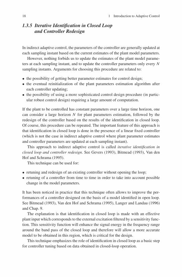
A block diagram of the system is shown in Fig. 1.18. The drying furnace consistsof a:

• feeding system,• combustion chamber,• rotary drying tube,• dust chamber,• ventilator and chimney.

The combustion chamber produces the hot gas needed for the drying process. Thehot gas and the phosphate mix in the rotary drying tube. In the dust chamber, onerecaptures the phosphate fine particles which represent approximately 30% of thedried phosphate. The final product is obtained on the bottom of the dust chamberand recovered on a conveyor. The temperature of the final product is used as anindirect measure of its humidity. The control action is the fuel flow while the othervariable for the burner (steam, primary air) are related through conventional loopsto the fuel flow.


Fig. 1.18 Phosphate drying furnace

Significant improvement in performance was obtained with respect to a standardPID controller (the system has a delay of about 90 s). The improved regulation hasas a side effect an average reduction of the fuel consumption and a reduction of thethermal stress on the combustion chamber walls allowing to increase the averagetime between two maintenance operations.

1.4.3 Indirect and Multimodel Adaptive Controlof a Flexible Transmission

The flexible transmission built at GIPSA-LAB, Control Dept. (CNRS-INPG-UJF),Grenoble, France, consists of three horizontal pulleys connected by two elastic belts(Fig. 1.19). The first pulley is driven by a D.C. motor whose position is controlledby local feedback. The third pulley may be loaded with disks of different weight.The objective is to control the position of the third pulley measured by a positionsensor. The system input is the reference for the axis position of the first pulley.A PC is used to control the system. The sampling frequency is 20 Hz.

The system is characterized by two low-damped vibration modes subject to alarge variation in the presence of load. Fig. 1.20 gives the frequency characteristicsof the identified discrete-time models for the case without load, half load (1.8 kg)and full load (3.6 kg). A variation of 100% of the first vibration mode occurs whenpassing from the full loaded case to the case without load. In addition, the systemfeatures a delay and unstable zeros. The system was used as a benchmark for robustdigital control (Landau et al. 1995a), as well as a test bed for indirect adaptive con-trol, multiple model adaptive control, identification in open-loop and closed-loopoperation, iterative identification in closed loop and control redesign. The use ofvarious algorithms for real-time identification and adaptive control which will bediscussed throughout the book will be illustrated on this real system (see Chaps. 5,9, 12, 13 and 16).


Fig. 1.19 The flexibletransmission (GIPSA-LAB,Grenoble), (a) block diagram,(b) view of the system

1.4.4 Adaptive Regulation in an Active Vibration Control System

The active vibration control system built at GIPSA-LAB, Control Dept. (CNRS-INPG-UJF), Grenoble, France for benchmarking of control strategies is shown inFig. 1.21 and details are given in Fig. 1.22. For suppressing the effect of vibra-tional disturbances one uses an inertial actuator which will create vibrational forcesto counteract the effect of vibrational disturbances (inertial actuators use a similarprinciple as loudspeakers). The load is posed on a passive damper and the inertialactuator is fixed to the chassis where the vibrations should be attenuated. A shakerposed on the ground is used to generate the vibration. The mechanical constructionof the load is such that the vibrations produced by the shaker, are transmitted to theupper side of the system. The controller will act (through a power amplifier) on the


Fig. 1.20 Frequency characteristics of the flexible transmission for various loads

position of the mobile part of the inertial actuator in order to reduce the residualforce. The sampling frequency is 800 Hz.

The system was used as a benchmark for direct and indirect adaptive regulationstrategies. The performance of the algorithms which will be presented in Chap. 14will be evaluated on this system.

1.4.5 Adaptive Feedforward Disturbance Compensationin an Active Vibration Control System

The system shown in Fig. 1.23 is representative of distributed mechanical structuresencountered in practice where a correlated measurement with the disturbance (animage of the disturbance) is made available and used for feedforward disturbancecompensation (GIPSA-LAB, Control Dept., Grenoble, France). A detailed schemeof the system is shown in Fig. 1.24. It consists on five metal plates connected bysprings. The second plate from the top and the second plate from the bottom areequipped with an inertial actuator. The first inertial actuator will excite the structure(disturbances) and the second will create vibrational forces which can counteract theeffect of these vibrational disturbances. Two accelerometers are used to measure thedisplacement of vibrating plates. The one posed on the second plate on the bottommeasures the residual acceleration which has to be reduced. The one posed above


Fig. 1.21 Active vibrationcontrol system using aninertial actuator (photo)

Fig. 1.22 Active vibration control using an inertial actuator (scheme)


Fig. 1.23 An active vibration control using feedforward compensation (photo)

Fig. 1.24 An active vibration control using feedforward compensation (scheme)

gives an image of the disturbance to be used for feedforward compensation. As itresults clearly from Figs. 1.23 and 1.24, the actuator located down side will com-pensate vibrations at the level of the lowest plate but will induce forces upstreambeyond this plate an therefore a positive feedback is present in the system whichmodifies the effective measurement of the image of the disturbance. The algorithmswhich will be presented in Chap. 15 will be evaluated on this system.


1.5 A Brief Historical Note

This note is not at all a comprehensive account of the evolution of the adaptivecontrol field which is already fifty years old. Its objective is to point out some ofthe moments in the evolution of the field which we believe were important. In par-ticular, the evolution of discrete-time adaptive control of SISO systems (which isthe main subject of this book) will be emphasized (a number of basic references tocontinuous-time adaptive control are missed).

The formulation of adaptive control as a stochastic control problem (dual con-trol) was given in Feldbaum (1965). However, independently more ad-hoc adaptivecontrol approaches have been developed.

Direct adaptive control appeared first in relation to the use of a model referenceadaptive system for aircraft control. See Whitaker et al. (1958). The indirect adap-tive control was probably introduced by Kalman (1958) in connection with digitalprocess control.

Earlier work in model reference adaptive systems has emphasized the impor-tance of stability problems for these schemes. The first approach for synthesizingstable model reference adaptive systems using Lyapunov functions was proposed inButchart and Shakcloth (1966) and further generalized in Parks (1966). The impor-tance of positive realness of some transfer functions for the stability of MRAS waspointed out for the first time in Parks (1966). The fact that model reference adaptivesystems can be represented as an equivalent feedback system with a linear time in-variant feedforward block and a nonlinear time-varying feedback block was pointedout in Landau (1969a, 1969b) where an input-output approach based on hypersta-bility (passivity) concepts was proposed for the design. For detailed results alongthis line of research see Landau (1974, 1979). While initially direct adaptive con-trol schemes have only been considered in continuous time, synthesis of discrete-time direct adaptive schemes and applications appeared in the seventies. See Landau(1971, 1973), Bethoux and Courtiol (1973), Ionescu and Monopoli (1977). For anaccount of these earlier developments see Landau (1979).

The indirect adaptive control approach was significantly developed starting withÅström and Wittenmark (1973) where the term “self-tuning” was coined. The result-ing scheme corresponded to an adaptive version of the minimum variance discrete-time control. A further development appeared in Clarke and Gawthrop (1975). Infact, the self-tuning minimum variance controller and its extensions are a directadaptive control scheme since one estimates directly the parameters of the con-troller. It took a number of years to understand that discrete-time model referenceadaptive control systems and stochastic self-tuning regulators based on minimiza-tion of the error variance belong to the same family. See Egardt (1979), Landau(1982a).

Tsypkin (1971) also made a very important contribution to the development andanalysis of discrete-time parameter adaptation algorithms.

Despite the continuous research efforts, it was only at the end of the 1970’s thatfull proofs for the stability of discrete-time model reference adaptive control andstochastic self-tuning controllers (under some ideal conditions) became available.

1.5 A Brief Historical Note 31

See Goodwin et al. (1980b, 1980a) (for continuous-time adaptive control see Morse1980; Narendra et al. 1980).

The progress of the adaptive control theory on the one hand and the availabilityof microcomputers on the other hand led to a series of successful applications ofdirect adaptive controllers (either deterministic or stochastic) in the late 1970’s andearly 1980’s. However, despite a number of remarkable successes in the same pe-riod a number of simple counter-examples have since shown the limitation of theseapproaches.

On the one hand, the lack of robustness of the original approaches with respectto noise, unmodeled dynamics and disturbances has been emphasized. On the otherhand, the experience with the various applications has shown that one of the ma-jor assumptions in these schemes (i.e., the plant model is a discrete-time modelwith stable zeros and a fixed delay) is not a very realistic one (except in specialapplications). Even successful applications have required a careful selection of thesampling frequency (since fractional delay larger than half of the sampling periodgenerates a discrete-time unstable zero). The industrial experiences and variouscounter-examples were extremely beneficial for the evolution of the field. A sig-nificant research effort has been dedicated to robustness issues and development ofrobust adaptation algorithms. Egardt (1979), Praly (1983c), Ortega et al. (1985),Ioannou and Kokotovic (1983) are among the basic references. A deeper analysis ofthe adaptive schemes has also been done in Anderson et al. (1986). An account ofthe work on robustness of adaptive control covering both continuous and discrete-time adaptive control can be found in Ortega and Tang (1989). For continuous-timeonly, see also Ioannou and Datta (1989, 1996).

The other important research direction was aimed towards adaptive control ofdiscrete-time models with unstable zeros which led to the development of indirectadaptive control schemes and their analysis. The problems of removing the need ofpersistence of excitation and of the eventual singularities which may occur whencomputing a controller based on plant model parameter estimates have been ad-dressed, as well as the robustness issues (see Lozano and Zhao 1994 for detailsand a list of references). Various underlying linear control strategies have been con-sidered: pole placement (de Larminat 1980 is one of the first references), linearquadratic control (Samson 1982 is the first reference) and generalized predictivecontrol (Clarke et al. 1987). Adaptive versions of pole placement and generalizedpredictive control are the most popular ones.

The second half of the nineties has seen the emergence of two new ap-proaches to adaptive control. On one hand there is the development of plantmodel identification in closed loop (Gevers 1993; Van den Hof and Schrama 1995;Landau and Karimi 1997a, 1997b) leading to the strategy called “iterative identi-fication in closed loop and controller redesign” (see Chap. 9). On the other handthe “multiple model adaptive control” emerged as a solution for improving the tran-sients in indirect adaptive control. See Morse (1995), Narendra and Balakrishnan(1997), Karimi and Landau (2000) and Chap. 13.

End of the nineties and beginning of the new century have seen the emergence ofa new paradigm: adaptive regulation. In this context the plant model is assumed to


be known and invariant and adaptation is considered with respect to the disturbancemodel which is unknown and time varying (Amara et al. 1999a; Valentinotti 2001;Landau et al. 2005 and Chap. 14). In the mean time it was pointed out that adaptivefeedforward compensation of disturbances which for a long time has been consid-ered as an “open-loop” problem has in fact a hidden feedback structure bringing thissubject in the context of adaptive feedback control. New solutions are emerging, seeJacobson et al. (2001), Zeng and de Callafon (2006), Landau and Alma (2010) andChap. 15.

1.6 Further Reading

It is not possible in a limited number of pages to cover all the aspects of adaptivecontrol. In what follows we will mention some references on a number of issues notcovered by this book.

• Continuous Time Adaptive Control (Ioannou and Sun 1996; Sastry and Bodson1989; Anderson et al. 1986; Åström and Wittenmark 1995; Landau 1979; Datta1998)

• Multivariable Systems (Dugard and Dion 1985; Goodwin and Sin 1984; Dionet al. 1988; Garrido-Moctezuma et al. 1993; Mutoh and Ortega 1993; de Mathelinand Bodson 1995)

• Systems with Constrained Inputs (Zhang and Evans 1994; Feng et al. 1994;Chaoui et al. 1996a, 1996b; Sussmann et al. 1994; Suarez et al. 1996; Åströmand Wittenmark 1995)

• Input and Output Nonlinearities (Tao and Kokotovic 1996; Pajunen 1992)• Adaptive Control of Nonlinear Systems (Sastry and Isidori 1989; Marino and

Tomei 1995; Krstic et al. 1995; Praly et al. 1991; Lozano and Brogliato 1992a;Brogliato and Lozano 1994; Landau et al. 1987)

• Adaptive Control of Robot Manipulators (Landau 1985; Landau and Horowitz1988; Slotine and Li 1991; Arimoto and Miyazaki 1984; Ortega and Spong 1989;Nicosia and Tomei 1990; Lozano 1992; Lozano and Brogliato 1992b, 1992c)

• Adaptive Friction Compensation (Gilbart and Winston 1974; Canudas et al. 1995;Armstrong and Amin 1996; Besançon 1997)

• Adaptive Control of Asynchronous Electric Motors (Raumer et al. 1993; Marinoet al. 1996; Marino and Tomei 1995; Espinoza-Perez and Ortega 1995)

1.7 Concluding Remarks

In this chapter we have presented a number of concepts and basic adaptive controlstructures. We wish to emphasize the following basic ideas:

1. Adaptive control provides a set of techniques for automatic adjustment of thecontrollers in real time in order to achieve or to maintain a desired level of con-trol system performance, when the parameters of the plant model are unknownand/or change in time.

1.7 Concluding Remarks 33

2. While a conventional feedback control is primarily oriented toward the elim-ination of the effect of disturbances acting upon the controlled variables, anadaptive control system is mainly oriented toward the elimination of the effectof parameter disturbances upon the performances of the control system.

3. A control system is truly adaptive if, in addition to a conventional feedback, itcontains a closed-loop control of a certain performance index.

4. Robust control design is an efficient way to handle known parameter uncertaintyin a certain region around a nominal model and it constitutes a good underlyingdesign method for adaptive control, but it is not an adaptive control system.

5. Adaptive control can improve the performance of a robust control design byproviding better information about the nominal model and expanding the un-certainty region for which the desired performances can be guaranteed.

6. One distinguishes adaptive control schemes with direct adaptation of the pa-rameters of the controller or with indirect adaptation of the parameters of thecontroller (as a function of the estimates of plant parameters).

7. One distinguishes between adaptive control schemes with non-vanishing adap-tation (also called continuous adaptation) and adaptive control schemes withvanishing adaptation. Although in the former, adaptation operates most of thetime, in the latter, its effect vanishes in time.

8. The use of adaptive control is based on the assumption that for any possiblevalues of the plant parameters there is a controller with a fixed structure andcomplexity such that the desired performances can be achieved with appropriatevalues of the controller parameters. The task of the adaptation loop is to searchfor the good values of the controller parameters.

9. There are two control paradigms: (1) adaptive control where the plant model pa-rameters are unknown an time varying while the disturbance model is assumedto be known; and (2) adaptive regulation where the plant model is assumed tobe known and the model of the disturbance is unknown and time varying.

10. Adaptive control systems are nonlinear time-varying systems and specific toolsfor analyzing their properties are necessary.

http://www.springer.com/978-0-85729-663-4

Introduction to Adaptive Control

Documents