Introduction Exponential functions are ideal for modeling growth and decay phenomena. Equations derived from given information, such as observations, can.

IntroductionExponential functions are ideal for modeling growth and decay phenomena. Equations derived from given information, such as observations, can be used to solve problems that involve forecasting and decision-making based on future events. Equations for modeling growth and decay can also be derived from a general exponential growth model, which is a standard equation that has been proven to work for many cases. In addition to equations, graphs are also helpful because they allow predictions to be made about data.

1

6.1.3: Creating Exponential and Logarithmic Equations

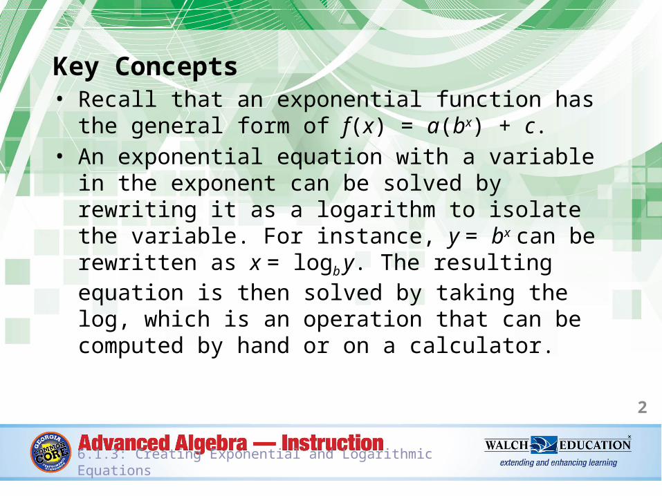
Key Concepts• Recall that an exponential function has the general

form of f(x) = a(bx) + c. • An exponential equation with a variable in the

exponent can be solved by rewriting it as a logarithm to isolate the variable. For instance, y = bx can be rewritten as x = logb y. The resulting equation is then solved by taking the log, which is an operation that can be computed by hand or on a calculator.

2

6.1.3: Creating Exponential and Logarithmic Equations

Key Concepts, continued

3

6.1.3: Creating Exponential and Logarithmic Equations

• Logarithmic functions of the form f(x) = log x are the inverses of exponential functions and vice versa. Their graphs are mirror images of each other.

Key Concepts, continued• To solve an exponential equation where the exponent

is a variable, write an equivalent logarithmic equation and use it to solve for the exponent variable.

• Often, rewriting a logarithmic equation as an exponential equation makes it easier to solve.

• Recall that e is an irrational number with an approximate value of 2.71828.

4

6.1.3: Creating Exponential and Logarithmic Equations

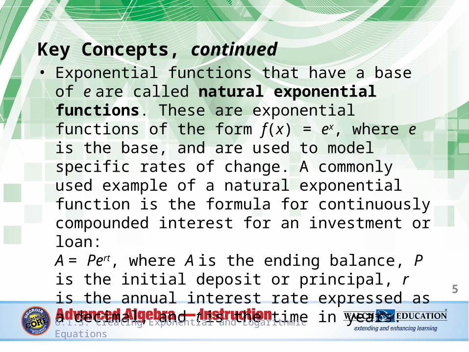
Key Concepts, continued• Exponential functions that have a base of e are called

natural exponential functions. These are exponential functions of the form f(x) = ex, where e is the base, and are used to model specific rates of change. A commonly used example of a natural exponential function is the formula for continuously compounded interest for an investment or loan:A = Pert, where A is the ending balance, P is the initial deposit or principal, r is the annual interest rate expressed as a decimal, and t is the time in years.

5

6.1.3: Creating Exponential and Logarithmic Equations

Key Concepts, continued• Natural exponential functions are solved in the same

manner as exponential functions with bases other than e. Similarly, logarithmic functions with a base of e are called natural logarithms. Natural logarithms are usually written in the form “ln,” which means “loge.” The natural log of x can be written as ln x or loge x.

• Natural logarithm functions are solved in the same manner as other logarithmic functions.

6

6.1.3: Creating Exponential and Logarithmic Equations

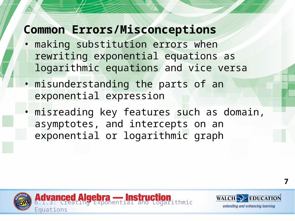
Common Errors/Misconceptions• making substitution errors when rewriting exponential

equations as logarithmic equations and vice versa

• misunderstanding the parts of an exponential expression

• misreading key features such as domain, asymptotes, and intercepts on an exponential or logarithmic graph

7

6.1.3: Creating Exponential and Logarithmic Equations

Guided Practice

Example 1The demand for a particular flat-panel television at a store is given by the exponential function d(x) = 500 – 0.5e0.004x, where d(x) represents the number of TVs sold that week, and x represents the price in dollars. What is the demand level when the TV is priced at $450 versus when it is priced at $400? Which price level will result in higher demand for this TV? Which of the two price levels will yield the most revenue?

8

6.1.3: Creating Exponential and Logarithmic Equations

Guided Practice: Example 1, continued

1. Determine the demand for the TV at the price level of $450.

Recall that the demand is the number of TVs sold at the given price.

Substitute x = 450 into the original exponential function and solve for d(x).

9

6.1.3: Creating Exponential and Logarithmic Equations

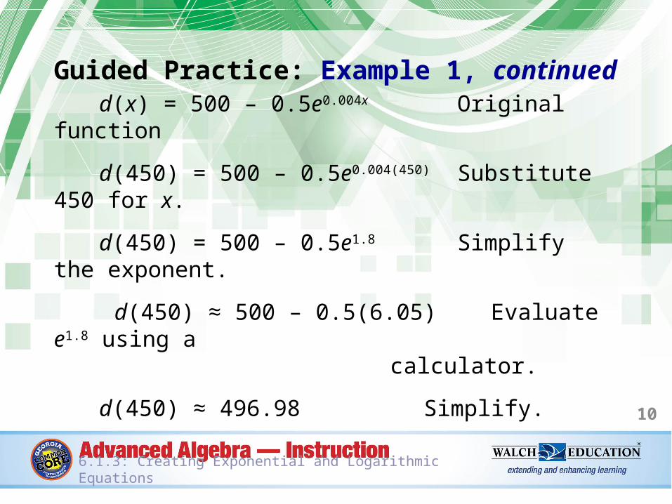
Guided Practice: Example 1, continued d(x) = 500 – 0.5e0.004x Original

function

d(450) = 500 – 0.5e0.004(450) Substitute 450 for x.

d(450) = 500 – 0.5e1.8 Simplify the exponent.

d(450) ≈ 500 – 0.5(6.05) Evaluate e1.8 using a

calculator.

d(450) ≈ 496.98 Simplify.

10

6.1.3: Creating Exponential and Logarithmic Equations

Guided Practice: Example 1, continuedThe demand at the price level of $450 is approximately 496.98.

Since the number of TVs needs to be a whole number, round up so the demand at the price level of $450 is approximately 497 TVs.

11

6.1.3: Creating Exponential and Logarithmic Equations

Guided Practice: Example 1, continued

2. Determine the demand for the TV at the price level of $400.Substitute x = 400 into the original exponential function and solve for d(x).

12

6.1.3: Creating Exponential and Logarithmic Equations

d(x) = 500 – 0.5e0.004x Original function

d(400) = 500 – 0.5e0.004(400) Substitute 400 for x.

d(400) = 500 – 0.5e1.6 Simplify the exponent.

d(400) ≈ 500 – 0.5(4.95)Evaluate e1.6 using

a calculator.

d(400) ≈ 497.52Simplify.

Guided Practice: Example 1, continuedThe demand at the price level of $400 is approximately 497.52. Rounded to the nearest whole TV, the demand at $400 is approximately 498 TVs.

13

6.1.3: Creating Exponential and Logarithmic Equations

Guided Practice: Example 1, continued

3. Determine which price level results in a higher demand.

When comparing the results of steps 1 and 2, we see the demand at the $400 price level is slightly higher (498) than the demand at $450 (497).

14

6.1.3: Creating Exponential and Logarithmic Equations

Guided Practice: Example 1, continued

4. Which of the two price levels will yield the most revenue?

To determine the revenue for each price level, multiply each price by the number of TVs sold at that price (the demand) and then find the difference.

450 • 497 = 223,650 

400 • 498 = 199,200 

15

6.1.3: Creating Exponential and Logarithmic Equations

Guided Practice: Example 1, continuedThough a lower price results in higher demand, the resulting revenue is much lower when the TVs are priced at $400 than when they are priced at $450. The price level of $450 yields higher revenue.

16

6.1.3: Creating Exponential and Logarithmic Equations

✔

Guided Practice: Example 1, continued

17

6.1.3: Creating Exponential and Logarithmic Equations

Guided Practice

Example 4It is predicted that the annual rate of inflation will average about 3% for each of the next 10 years. The estimated cost of goods in any of those years can be written as C(t) = P(1.03)t, where P is the current cost of goods and t is the time in years. If the price of 8 gallons of gas is currently $25, use the function to find the cost of 8 gallons of gas 10 years from now. Graph the original function and use it to verify your calculation.

18

6.1.3: Creating Exponential and Logarithmic Equations

Guided Practice: Example 4, continued

1. Determine the cost of 8 gallons of gas 10 years from now.

Substitute the known information into the given cost function, C(t) = P(1.03)t, and then solve the resulting equation to determine the price of gas 10 yearsfrom now.

19

6.1.3: Creating Exponential and Logarithmic Equations

Guided Practice: Example 4, continued

Let P (the current cost) equal 25, and let t equal 10.

C(t) = P(1.03)t

Original function

C(10) = (25)(1.03)(10) Substitute 25 for P

and 10 for t.

C(10) ≈ 33.60 Simplify.

The cost of 8 gallons of gas will be approximately $33.60 in 10 years.

20

6.1.3: Creating Exponential and Logarithmic Equations

Guided Practice: Example 4, continued

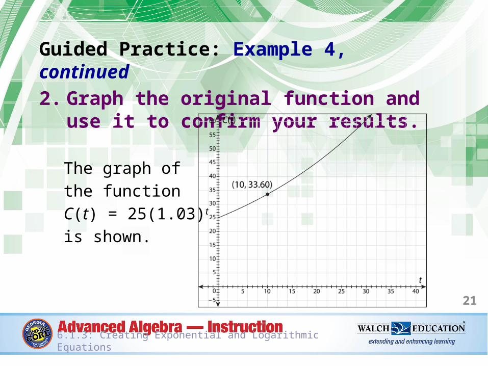
2. Graph the original function and use it to confirm your results.The graph of

the function

C(t) = 25(1.03)t

is shown.

21

6.1.3: Creating Exponential and Logarithmic Equations

Guided Practice: Example 4, continuedThe x-axis represents time in years, and the y-axis represents the cost of gas in dollars. Note that wheret = 10, C(t) ≈ 33.60, as shown. Therefore, the graph confirms our calculation that after 10 years of inflation at an average of 3% per year, 8 gallons of gas will cost approximately $33.60.

22

6.1.3: Creating Exponential and Logarithmic Equations

✔

Guided Practice: Example 4, continued

23

6.1.3: Creating Exponential and Logarithmic Equations