119 1 This chapter should be cited as: Cubasch, U., D. Wuebbles, D. Chen, M.C. Facchini, D. Frame, N. Mahowald, and J.-G. Winther, 2013: Introduction. In: Climate Change 2013: The Physical Science Basis. Contribution of Working Group I to the Fifth Assessment Report of the Intergovernmental Panel on Climate Change [Stocker, T.F., D. Qin, G.-K. Plattner, M. Tignor, S.K. Allen, J. Boschung, A. Nauels, Y. Xia, V. Bex and P.M. Midgley (eds.)]. Cambridge University Press, Cambridge, United Kingdom and New York, NY, USA. Coordinating Lead Authors: Ulrich Cubasch (Germany), Donald Wuebbles (USA) Lead Authors: Deliang Chen (Sweden), Maria Cristina Facchini (Italy), David Frame (UK/New Zealand), Natalie Mahowald (USA), Jan-Gunnar Winther (Norway) Contributing Authors: Achim Brauer (Germany), Lydia Gates (Germany), Emily Janssen (USA), Frank Kaspar (Germany), Janina Körper (Germany), Valérie Masson-Delmotte (France), Malte Meinshausen (Australia/Germany), Matthew Menne (USA), Carolin Richter (Switzerland), Michael Schulz (Germany), Uwe Schulzweida (Germany), Bjorn Stevens (Germany/USA), Rowan Sutton (UK), Kevin Trenberth (USA), Murat Türkeş (Turkey), Daniel S. Ward (USA) Review Editors: Yihui Ding (China), Linda Mearns (USA), Peter Wadhams (UK) Introduction

Welcome message from author
This document is posted to help you gain knowledge. Please leave a comment to let me know what you think about it! Share it to your friends and learn new things together.
Transcript

119
1
This chapter should be cited as:Cubasch, U., D. Wuebbles, D. Chen, M.C. Facchini, D. Frame, N. Mahowald, and J.-G. Winther, 2013: Introduction. In: Climate Change 2013: The Physical Science Basis. Contribution of Working Group I to the Fifth Assessment Report of the Intergovernmental Panel on Climate Change [Stocker, T.F., D. Qin, G.-K. Plattner, M. Tignor, S.K. Allen, J. Boschung, A. Nauels, Y. Xia, V. Bex and P.M. Midgley (eds.)]. Cambridge University Press, Cambridge, United Kingdom and New York, NY, USA.
Coordinating Lead Authors:Ulrich Cubasch (Germany), Donald Wuebbles (USA)
Lead Authors:Deliang Chen (Sweden), Maria Cristina Facchini (Italy), David Frame (UK/New Zealand), Natalie Mahowald (USA), Jan-Gunnar Winther (Norway)
Contributing Authors:Achim Brauer (Germany), Lydia Gates (Germany), Emily Janssen (USA), Frank Kaspar (Germany), Janina Körper (Germany), Valérie Masson-Delmotte (France), Malte Meinshausen (Australia/Germany), Matthew Menne (USA), Carolin Richter (Switzerland), Michael Schulz (Germany), Uwe Schulzweida (Germany), Bjorn Stevens (Germany/USA), Rowan Sutton (UK), Kevin Trenberth (USA), Murat Türkeş (Turkey), Daniel S. Ward (USA)
Review Editors:Yihui Ding (China), Linda Mearns (USA), Peter Wadhams (UK)
Introduction
1
120
Table of Contents
Executive Summary ..................................................................... 121
1.1 Chapter Preview .............................................................. 123
1.2 Rationale and Key Concepts of the WGI Contribution ............................................................ 123
1.2.1 Setting the Stage for the Assessment ........................ 123
1.2.2 Key Concepts in Climate Science ............................... 123
1.2.3 Multiple Lines of Evidence for Climate Change ......... 129
1.3 Indicators of Climate Change ...................................... 130
1.3.1 Global and Regional Surface Temperatures ............... 131
1.3.2 Greenhouse Gas Concentrations ............................... 132
1.3.3 Extreme Events ......................................................... 134
1.3.4 Climate Change Indicators ........................................ 136
1.4 Treatment of Uncertainties .......................................... 138
1.4.1 Uncertainty in Environmental Science ....................... 138
1.4.2 Characterizing Uncertainty ........................................ 138
1.4.3 Treatment of Uncertainty in IPCC .............................. 139
1.4.4 Uncertainty Treatment in This Assessment................. 139
1.5 Advances in Measurement and Modelling Capabilities ....................................................................... 142
1.5.1 Capabilities of Observations ..................................... 142
1.5.2 Capabilities in Global Climate Modelling .................. 144
Box 1.1: Description of Future Scenarios ............................... 147
1.6 Overview and Road Map to the Rest of the Report ......................................................................... 151
1.6.1 Topical Issues ............................................................ 151
References .................................................................................. 152
Appendix 1.A: Notes and Technical Details on Figures Displayed in Chapter 1 ............................................................... 155
Frequently Asked Questions
FAQ 1.1 If Understanding of the Climate System Has Increased, Why Hasn’t the Range of Temperature Projections Been Reduced? ........... 140
1
Introduction Chapter 1
121
Executive Summary
Human Effects on Climate
Human activities are continuing to affect the Earth’s energy budget by changing the emissions and resulting atmospheric concentrations of radiatively important gases and aerosols and by changing land surface properties. Previous assessments have already shown through multiple lines of evidence that the climate is changing across our planet, largely as a result of human activities. The most compelling evidence of climate change derives from observations of the atmosphere, land, oceans and cryosphere. Unequivocal evidence from in situ observations and ice core records shows that the atmos-pheric concentrations of important greenhouse gases such as carbon dioxide (CO2), methane (CH4), and nitrous oxide (N2O) have increased over the last few centuries. {1.2.2, 1.2.3}
The processes affecting climate can exhibit considerable natural variability. Even in the absence of external forcing, periodic and chaotic variations on a vast range of spatial and temporal scales are observed. Much of this variability can be represented by simple (e.g., unimodal or power law) distributions, but many components of the climate system also exhibit multiple states—for instance, the gla-cial–interglacial cycles and certain modes of internal variability such as El Niño-Southern Oscillation (ENSO). Movement between states can occur as a result of natural variability, or in response to external forc-ing. The relationship among variability, forcing and response reveals the complexity of the dynamics of the climate system: the relationship between forcing and response for some parts of the system seems rea-sonably linear; in other cases this relationship is much more complex. {1.2.2}
Multiple Lines of Evidence for Climate Change
Global mean surface air temperatures over land and oceans have increased over the last 100 years. Temperature measure-ments in the oceans show a continuing increase in the heat content of the oceans. Analyses based on measurements of the Earth’s radi-ative budget suggest a small positive energy imbalance that serves to increase the global heat content of the Earth system. Observations from satellites and in situ measurements show a trend of significant reductions in the mass balance of most land ice masses and in Arctic sea ice. The oceans’ uptake of CO2 is having a significant effect on the chemistry of sea water. Paleoclimatic reconstructions have helped place ongoing climate change in the perspective of natural climate var-iability. {1.2.3; Figure 1.3}
Observations of CO2 concentrations, globally averaged temper-ature and sea level rise are generally well within the range of the extent of the earlier IPCC projections. The recently observed increases in CH4 and N2O concentrations are smaller than those assumed in the scenarios in the previous assessments. Each IPCC assessment has used new projections of future climate change that have become more detailed as the models have become more advanced. Similarly, the scenarios used in the IPCC assessments have themselves changed over time to reflect the state of knowledge. The range of climate projections from model results provided and assessed in the first IPCC assessment in 1990 to those in the 2007 AR4 provides an opportunity to compare the projections with the actually observed changes, thereby examining the deviations of the projections from the observations over time. {1.3.1, 1.3.2, 1.3.4; Figures 1.4, 1.5, 1.6, 1.7, 1.10}
Climate change, whether driven by natural or human forcing, can lead to changes in the likelihood of the occurrence or strength of extreme weather and climate events or both. Since the AR4, the observational basis has increased substantially, so that some extremes are now examined over most land areas. Furthermore, more models with higher resolution and a greater number of regional models have been used in the simulations and projections of extremes. {1.3.3; Figure 1.9}
Treatment of Uncertainties
For AR5, the three IPCC Working Groups use two metrics to com-municate the degree of certainty in key findings: (1) Confidence is a qualitative measure of the validity of a finding, based on the type, amount, quality and consistency of evidence (e.g., data, mechanis-tic understanding, theory, models, expert judgment) and the degree of agreement1; and (2) Likelihood provides a quantified measure of uncertainty in a finding expressed probabilistically (e.g., based on sta-tistical analysis of observations or model results, or both, and expert judgement)2. {1.4; Figure 1.11}
Advances in Measurement and Modelling Capabilities
Over the last few decades, new observational systems, especial-ly satellite-based systems, have increased the number of obser-vations of the Earth’s climate by orders of magnitude. Tools to analyse and process these data have been developed or enhanced to cope with this large increase in information, and more climate proxy data have been acquired to improve our knowledge of past chang-es in climate. Because the Earth’s climate system is characterized on multiple spatial and temporal scales, new observations may reduce the uncertainties surrounding the understanding of short timescale
1 In this Report, the following summary terms are used to describe the available evidence: limited, medium, or robust; and for the degree of agreement: low, medium, or high. A level of confidence is expressed using five qualifiers: very low, low, medium, high, and very high, and typeset in italics, e.g., medium confidence. For a given evidence and agreement statement, different confidence levels can be assigned, but increasing levels of evidence and degrees of agreement are correlated with increasing confidence (see Section 1.4 and Box TS.1 for more details).
2 In this Report, the following terms have been used to indicate the assessed likelihood of an outcome or a result: Virtually certain 99–100% probability, Very likely 90–100%, Likely 66–100%, About as likely as not 33–66%, Unlikely 0–33%, Very unlikely 0–10%, Exceptionally unlikely 0–1%. Additional terms (Extremely likely: 95–100%, More likely than not >50–100%, and Extremely unlikely 0–5%) may also be used when appropriate. Assessed likelihood is typeset in italics, e.g., very likely (see Section 1.4 and Box TS.1 for more details).
1
Chapter 1 Introduction
122
processes quite rapidly. However, processes that occur over longer timescales may require very long observational baselines before much progress can be made. {1.5.1; Figure 1.12}
Increases in computing speed and memory have led to the development of more sophisticated models that describe phys-ical, chemical and biological processes in greater detail. Model-ling strategies have been extended to provide better estimates of the uncertainty in climate change projections. The model comparisons with observations have pushed the analysis and development of the models. The inclusion of ‘long-term’ simulations has allowed incorporation of information from paleoclimate data to inform projections. Within uncertainties associated with reconstructions of past climate variables from proxy record and forcings, paleoclimate information from the Mid Holocene, Last Glacial Maximum, and Last Millennium have been used to test the ability of models to simulate realistically the magnitude and large-scale patterns of past changes. {1.5.2; Figures 1.13, 1.14}
As part of the process of getting model analyses for a range of alter-native images of how the future may unfold, four new scenarios for future emissions of important gases and aerosols have been developed for the AR5, referred to as Representative Concentration Pathways (RCPs). {Box 1.1}
1
Introduction Chapter 1
123
1.1 Chapter Preview
This introductory chapter serves as a lead-in to the science presented in the Working Group I (WGI) contribution to the Intergovernmental Panel on Climate Change (IPCC) Fifth Assessment Report (AR5). Chapter 1 in the IPCC Fourth Assessment Report (AR4) (Le Treut et al., 2007) provid-ed a historical perspective on the understanding of climate science and the evidence regarding human influence on the Earth’s climate system. Since the last assessment, the scientific knowledge gained through observations, theoretical analyses, and modelling studies has contin-ued to increase and to strengthen further the evidence linking human activities to the ongoing climate change. In AR5, Chapter 1 focuses on the concepts and definitions applied in the discussions of new findings in the other chapters. It also examines several of the key indicators for a changing climate and shows how the current knowledge of those indicators compares with the projections made in previous assess-ments. The new scenarios for projected human-related emissions used in this assessment are also introduced. Finally, the chapter discusses the directions and capabilities of current climate science, while the detailed discussion of new findings is covered in the remainder of the WGI contribution to the AR5.
1.2 Rationale and Key Concepts of the WGI Contribution
1.2.1 Setting the Stage for the Assessment
The IPCC was set up in 1988 by the World Meteorological Organiza-tion and the United Nations Environment Programme to provide gov-ernments with a clear view of the current state of knowledge about the science of climate change, potential impacts, and options for adaptation and mitigation through regular assessments of the most recent information published in the scientific, technical and socio-eco-nomic literature worldwide. The WGI contribution to the IPCC AR5 assesses the current state of the physical sciences with respect to cli-mate change. This report presents an assessment of the current state of research results and is not a discussion of all relevant papers as would be included in a review. It thus seeks to make sure that the range of scientific views, as represented in the peer-reviewed literature, is considered and evaluated in the assessment, and that the state of the science is concisely and accurately presented. A transparent review process ensures that disparate views are included (IPCC, 2012a).
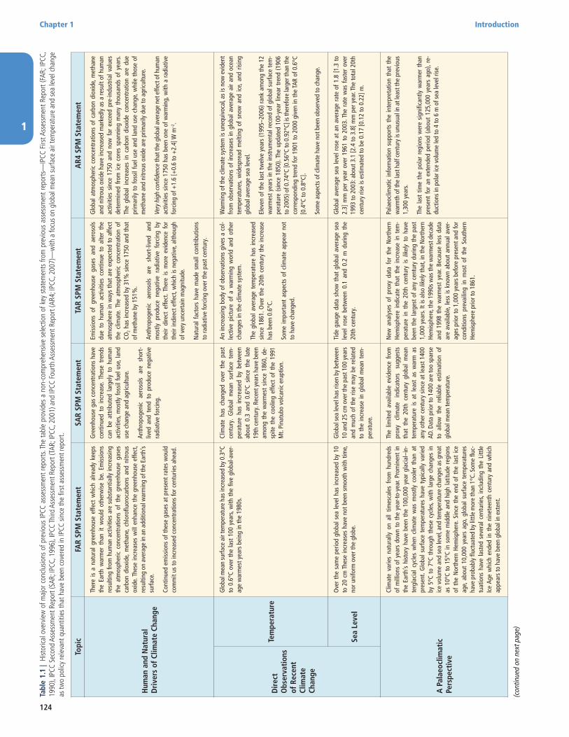
As an overview, Table 1.1 shows a selection of key findings from earlier IPCC assessments. This table provides a non-comprehensive selection of key assessment statements from previous assessment reports— IPCC First Assessment Report (FAR, IPCC, 1990), IPCC Second Assess-ment Report (SAR, IPCC, 1996), IPCC Third Assessment Report (TAR, IPCC, 2001) and IPCC Fourth Assessment Report (AR4, IPCC, 2007)—with a focus on policy-relevant quantities that have been evaluated in each of the IPCC assessments.
Scientific hypotheses are contingent and always open to revision in light of new evidence and theory. In this sense the distinguishing fea-tures of scientific enquiry are the search for truth and the willingness to subject itself to critical re-examination. Modern research science
conducts this critical revision through processes such as the peer review. At conferences and in the procedures that surround publica-tion in peer-reviewed journals, scientific claims about environmental processes are analysed and held up to scrutiny. Even after publication, findings are further analysed and evaluated. That is the self-correcting nature of the scientific process (more details are given in AR4 Chapter 1 and Le Treut et al., 2007).
Science strives for objectivity but inevitably also involves choices and judgements. Scientists make choices regarding data and models, which processes to include and which to leave out. Usually these choices are uncontroversial and play only a minor role in the production of research. Sometimes, however, the choices scientists make are sources of disagreement and uncertainty. These are usually resolved by fur-ther scientific enquiry into the sources of disagreement. In some cases, experts cannot reach a consensus view. Examples in climate science include how best to evaluate climate models relative to observations, how best to evaluate potential sea level rise and how to evaluate prob-abilistic projections of climate change. In many cases there may be no definitive solution to these questions. The IPCC process is aimed at assessing the literature as it stands and attempts to reflect the level of reasonable scientific consensus as well as disagreement.
To assess areas of scientific controversy, the peer-reviewed literature is considered and evaluated. Not all papers on a controversial point can be discussed individually in an assessment, but every effort has been made here to ensure that all views represented in the peer-reviewed literature are considered in the assessment process. A list of topical issues is given in Table 1.3.
The Earth sciences study the multitude of processes that shape our environment. Some of these processes can be understood through idealized laboratory experiments, by altering a single element and then tracing through the effects of that controlled change. However, as in other natural and the social sciences, the openness of environmental systems, in terms of our lack of control of the boundaries of the system, their spatially and temporally multi-scale character and the complexity of interactions, often hamper scientists’ ability to definitively isolate causal links. This in turn places important limits on the understand-ing of many of the inferences in the Earth sciences (e.g., Oreskes et al., 1994). There are many cases where scientists are able to make inferences using statistical tools with considerable evidential support and with high degrees of confidence, and conceptual and numerical modelling can assist in forming understanding and intuition about the interaction of dynamic processes.
1.2.2 Key Concepts in Climate Science
Here, some of the key concepts in climate science are briefly described; many of these were summarized more comprehensively in earlier IPCC assessments (Baede et al., 2001). We focus only on a certain number of them to facilitate discussions in this assessment.
First, it is important to distinguish the meaning of weather from cli-mate. Weather describes the conditions of the atmosphere at a cer-tain place and time with reference to temperature, pressure, humid-ity, wind, and other key parameters (meteorological elements); the
1
Chapter 1 Introduction
124
Topi
cFA
R SP
M S
tate
men
tSA
R SP
M S
tate
men
tTA
R SP
M S
tate
men
tA
R4 S
PM S
tate
men
t
Hum
an a
nd N
atur
al
Dri
vers
of C
limat
e Ch
ange
Ther
e is
a n
atur
al g
reen
hous
e ef
fect
whi
ch a
lread
y ke
eps
the
Eart
h w
arm
er t
han
it w
ould
oth
erw
ise
be.
Emis
sion
s re
sulti
ng fr
om h
uman
act
iviti
es a
re s
ubst
antia
lly in
crea
sing
th
e at
mos
pher
ic c
once
ntra
tions
of
the
gree
nhou
se g
ases
ca
rbon
dio
xide
, met
hane
, chl
orofl
uoro
carb
ons
and
nitr
ous
oxid
e. T
hese
incr
ease
s w
ill e
nhan
ce t
he g
reen
hous
e ef
fect
, re
sulti
ng o
n av
erag
e in
an
addi
tiona
l war
min
g of
the
Eart
h’s
surfa
ce.
Cont
inue
d em
issi
ons
of th
ese
gase
s at
pre
sent
rate
s w
ould
co
mm
it us
to in
crea
sed
conc
entr
atio
ns fo
r cen
turie
s ah
ead.
Gre
enho
use
gas
conc
entr
atio
ns h
ave
cont
inue
d to
inc
reas
e. T
hese
tre
nds
can
be a
ttrib
uted
lar
gely
to
hum
an
activ
ities
, mos
tly fo
ssil
fuel
use
, lan
d us
e ch
ange
and
agr
icul
ture
.
Anth
ropo
geni
c ae
roso
ls
are
shor
t-liv
ed a
nd t
end
to p
rodu
ce n
egat
ive
radi
ativ
e fo
rcin
g.
Emis
sion
s of
gre
enho
use
gase
s an
d ae
roso
ls
due
to h
uman
act
iviti
es c
ontin
ue t
o al
ter
the
atm
osph
ere
in w
ays
that
are
exp
ecte
d to
affe
ct
the
clim
ate.
The
atm
osph
eric
con
cent
ratio
n of
CO
2 has
incr
ease
d by
31%
sin
ce 1
750
and
that
of
met
hane
by
151%
.
Anth
ropo
geni
c ae
roso
ls
are
shor
t-liv
ed
and
mos
tly p
rodu
ce n
egat
ive
radi
ativ
e fo
rcin
g by
th
eir
dire
ct e
ffect
. The
re i
s m
ore
evid
ence
for
th
eir i
ndire
ct e
ffect
, whi
ch is
neg
ativ
e, a
lthou
gh
of v
ery
unce
rtai
n m
agni
tude
.
Nat
ural
fac
tors
hav
e m
ade
smal
l con
trib
utio
ns
to ra
diat
ive
forc
ing
over
the
past
cen
tury
.
Glo
bal a
tmos
pher
ic c
once
ntra
tions
of
carb
on d
ioxi
de, m
etha
ne
and
nitr
ous
oxid
e ha
ve in
crea
sed
mar
kedl
y as
a re
sult
of h
uman
ac
tiviti
es s
ince
175
0 an
d no
w f
ar e
xcee
d pr
e-in
dust
rial
valu
es
dete
rmin
ed f
rom
ice
core
s sp
anni
ng m
any
thou
sand
s of
yea
rs.
The
glob
al i
ncre
ases
in
carb
on d
ioxi
de c
once
ntra
tion
are
due
prim
arily
to
foss
il fu
el u
se a
nd la
nd u
se c
hang
e, w
hile
tho
se o
f m
etha
ne a
nd n
itrou
s ox
ide
are
prim
arily
due
to a
gric
ultu
re.
Very
hig
h co
nfide
nce
that
the
glob
al a
vera
ge n
et e
ffect
of h
uman
ac
tiviti
es s
ince
175
0 ha
s be
en o
ne o
f war
min
g, w
ith a
radi
ativ
e fo
rcin
g of
+1.
6 [+
0.6
to +
2.4]
W m
–2.
Dir
ect
O
bser
vati
ons
of R
ecen
t
Clim
ate
Chan
ge
Tem
pera
ture
Glo
bal m
ean
surfa
ce a
ir te
mpe
ratu
re h
as in
crea
sed
by 0
.3°C
to
0.6
°C o
ver
the
last
100
yea
rs, w
ith t
he fi
ve g
loba
l-ave
r-ag
e w
arm
est y
ears
bei
ng in
the
1980
s.
Clim
ate
has
chan
ged
over
the
pas
t ce
ntur
y. G
loba
l m
ean
surfa
ce t
em-
pera
ture
has
inc
reas
ed b
y be
twee
n ab
out
0.3
and
0.6°
C si
nce
the
late
19
th c
entu
ry. R
ecen
t yea
rs h
ave
been
am
ong
the
war
mes
t si
nce
1860
, de-
spite
the
coo
ling
effe
ct o
f th
e 19
91
Mt.
Pina
tubo
vol
cani
c er
uptio
n.
An in
crea
sing
bod
y of
obs
erva
tions
giv
es a
col
-le
ctiv
e pi
ctur
e of
a w
arm
ing
wor
ld a
nd o
ther
ch
ange
s in
the
clim
ate
syst
em.
The
glob
al a
vera
ge t
empe
ratu
re h
as in
crea
sed
sinc
e 18
61. O
ver
the
20th
cen
tury
the
incr
ease
ha
s be
en 0
.6°C
.
Som
e im
port
ant
aspe
cts
of c
limat
e ap
pear
not
to
hav
e ch
ange
d.
War
min
g of
the
clim
ate
syst
em is
une
quiv
ocal
, as
is n
ow e
vide
nt
from
obs
erva
tions
of i
ncre
ases
in g
loba
l ave
rage
air
and
ocea
n te
mpe
ratu
res,
wid
espr
ead
mel
ting
of s
now
and
ice
, and
ris
ing
glob
al a
vera
ge s
ea le
vel.
Elev
en o
f the
last
twel
ve y
ears
(199
5–20
06) r
ank
amon
g th
e 12
w
arm
est y
ears
in th
e in
stru
men
tal r
ecor
d of
glo
bal s
urfa
ce te
m-
pera
ture
(sin
ce 1
850)
. The
upd
ated
100
-yea
r lin
ear
tren
d (1
906
to 2
005)
of 0
.74°
C [0
.56°
C to
0.9
2°C]
is th
eref
ore
larg
er th
an th
e co
rres
pond
ing
tren
d fo
r 190
1 to
200
0 gi
ven
in th
e TA
R of
0.6
°C
[0.4
°C to
0.8
°C].
Som
e as
pect
s of
clim
ate
have
not
bee
n ob
serv
ed to
cha
nge.
Sea
Leve
l
Ove
r th
e sa
me
perio
d gl
obal
sea
leve
l has
incr
ease
d by
10
to 2
0 cm
The
se in
crea
ses
have
not
bee
n sm
ooth
with
tim
e,
nor u
nifo
rm o
ver t
he g
lobe
.
Glo
bal s
ea le
vel h
as ri
sen
by b
etw
een
10 a
nd 2
5 cm
ove
r the
pas
t 100
yea
rs
and
muc
h of
the
ris
e m
ay b
e re
late
d to
the
incr
ease
in g
loba
l mea
n te
m-
pera
ture
.
Tide
gau
ge d
ata
show
tha
t gl
obal
ave
rage
sea
le
vel
rose
bet
wee
n 0.
1 an
d 0.
2 m
dur
ing
the
20th
cen
tury
.
Glo
bal a
vera
ge s
ea le
vel r
ose
at a
n av
erag
e ra
te o
f 1.
8 [1
.3 t
o 2.
3] m
m p
er y
ear
over
196
1 to
200
3. T
he r
ate
was
fas
ter
over
19
93 to
200
3: a
bout
3.1
[2.4
to 3
.8] m
m p
er y
ear.
The
tota
l 20t
h ce
ntur
y ris
e is
est
imat
ed to
be
0.17
[0.1
2 to
0.2
2] m
.
A P
alae
oclim
atic
Pe
rspe
ctiv
e
Clim
ate
varie
s na
tura
lly o
n al
l tim
esca
les
from
hun
dred
s of
mill
ions
of y
ears
dow
n to
the
yea
r-to-
year
. Pro
min
ent
in
the
Eart
h’s
hist
ory
have
bee
n th
e 10
0,00
0 ye
ar g
laci
al–i
n-te
rgla
cial
cyc
les
whe
n cl
imat
e w
as m
ostly
coo
ler
than
at
pres
ent.
Glo
bal s
urfa
ce t
empe
ratu
res
have
typ
ical
ly v
arie
d by
5°C
to
7°C
thro
ugh
thes
e cy
cles
, with
larg
e ch
ange
s in
ic
e vo
lum
e an
d se
a le
vel,
and
tem
pera
ture
cha
nges
as
grea
t as
10°
C to
15°
C in
som
e m
iddl
e an
d hi
gh la
titud
e re
gion
s of
the
Nor
ther
n He
mis
pher
e. S
ince
the
end
of
the
last
ice
age,
abo
ut 1
0,00
0 ye
ars
ago,
glo
bal s
urfa
ce t
empe
ratu
res
have
pro
babl
y flu
ctua
ted
by li
ttle
mor
e th
an 1
°C. S
ome
fluc-
tuat
ions
hav
e la
sted
sev
eral
cen
turie
s, in
clud
ing
the
Litt
le
Ice
Age
whi
ch e
nded
in t
he n
inet
eent
h ce
ntur
y an
d w
hich
ap
pear
s to
hav
e be
en g
loba
l in
exte
nt.
The
limite
d av
aila
ble
evid
ence
fro
m
prox
y cl
imat
e in
dica
tors
su
gges
ts
that
the
20t
h ce
ntur
y gl
obal
mea
n te
mpe
ratu
re i
s at
lea
st a
s w
arm
as
any
othe
r cen
tury
sin
ce a
t lea
st 1
400
AD. D
ata
prio
r to
1400
are
too
spar
se
to a
llow
the
rel
iabl
e es
timat
ion
of
glob
al m
ean
tem
pera
ture
.
New
ana
lyse
s of
pro
xy d
ata
for
the
Nor
ther
n He
mis
pher
e in
dica
te t
hat
the
incr
ease
in
tem
-pe
ratu
re i
n th
e 20
th c
entu
ry i
s lik
ely
to h
ave
been
the
larg
est o
f any
cen
tury
dur
ing
the
past
1,
000
year
s. It
is a
lso
likel
y th
at, i
n th
e N
orth
ern
Hem
isph
ere,
the
1990
s was
the
war
mes
t dec
ade
and
1998
the
war
mes
t ye
ar. B
ecau
se le
ss d
ata
are
avai
labl
e, le
ss is
kno
wn
abou
t an
nual
ave
r-ag
es p
rior t
o 1,
000
year
s be
fore
pre
sent
and
for
cond
ition
s pr
evai
ling
in m
ost
of t
he S
outh
ern
Hem
isph
ere
prio
r to
1861
.
Pala
eocl
imat
ic in
form
atio
n su
ppor
ts t
he in
terp
reta
tion
that
the
w
arm
th o
f the
last
hal
f cen
tury
is u
nusu
al in
at l
east
the
prev
ious
1,
300
year
s.
The
last
tim
e th
e po
lar
regi
ons
wer
e si
gnifi
cant
ly w
arm
er t
han
pres
ent
for
an e
xten
ded
perio
d (a
bout
125
,000
yea
rs a
go),
re-
duct
ions
in p
olar
ice
volu
me
led
to 4
to 6
m o
f sea
leve
l ris
e.
Tabl
e 1.
1 |
Hist
orica
l ove
rvie
w o
f maj
or c
onclu
sions
of p
revi
ous
IPCC
ass
essm
ent r
epor
ts. T
he ta
ble
prov
ides
a n
on-c
ompr
ehen
sive
sele
ctio
n of
key
sta
tem
ents
from
pre
viou
s as
sess
men
t rep
orts
—IP
CC F
irst A
sses
smen
t Rep
ort (
FAR;
IPCC
, 19
90),
IPCC
Sec
ond
Asse
ssm
ent R
epor
t (SA
R; IP
CC, 1
996)
, IPC
C Th
ird A
sses
smen
t Rep
ort (
TAR;
IPCC
, 200
1) a
nd IP
CC F
ourth
Ass
essm
ent R
epor
t (AR
4; IP
CC, 2
007)
—w
ith a
focu
s on
glob
al m
ean
surfa
ce a
ir te
mpe
ratu
re a
nd se
a le
vel c
hang
e as
two
polic
y re
leva
nt q
uant
ities
that
hav
e be
en c
over
ed in
IPCC
sin
ce th
e fir
st a
sses
smen
t rep
ort.
(con
tinue
d on
nex
t pag
e)

1
Introduction Chapter 1
125
(Tab
le 1
.1 c
ontin
ued)
Topi
cFA
R SP
M S
tate
men
tSA
R SP
M S
tate
men
tTA
R SP
M S
tate
men
tA
R4 S
PM S
tate
men
t
Und
erst
andi
ng a
nd
Att
ribu
ting
Clim
ate
Ch
ange
The
size
of t
his
war
min
g is
bro
adly
con
sist
ent
with
pre
dic-
tions
of c
limat
e m
odel
s, bu
t it i
s als
o of
the
sam
e m
agni
tude
as
nat
ural
clim
ate
varia
bilit
y. T
hus
the
obse
rved
inc
reas
e co
uld
be la
rgel
y du
e to
this
nat
ural
var
iabi
lity;
alte
rnat
ivel
y th
is v
aria
bilit
y an
d ot
her
hum
an f
acto
rs c
ould
hav
e of
fset
a
still
larg
er h
uman
-indu
ced
gree
nhou
se w
arm
ing.
The
un-
equi
voca
l det
ectio
n of
the
enha
nced
gre
enho
use
effe
ct fr
om
obse
rvat
ions
is n
ot li
kely
for a
dec
ade
or m
ore.
The
bala
nce
of e
vide
nce
sugg
ests
a
disc
erni
ble
hum
an in
fluen
ce o
n gl
ob-
al c
limat
e. S
imul
atio
ns w
ith c
oupl
ed
atm
osph
ere–
ocea
n m
odel
s ha
ve p
ro-
vide
d im
port
ant
info
rmat
ion
abou
t de
cade
to
cent
ury
times
cale
nat
ural
in
tern
al c
limat
e va
riabi
lity.
Ther
e is
new
and
str
onge
r ev
iden
ce t
hat
mos
t of
the
war
min
g ob
serv
ed o
ver t
he la
st 5
0 ye
ars
is a
ttrib
utab
le t
o hu
man
act
iviti
es. T
here
is
a lo
nger
and
mor
e sc
rutin
ized
tem
pera
ture
reco
rd
and
new
mod
el e
stim
ates
of v
aria
bilit
y. R
econ
-st
ruct
ions
of
clim
ate
data
for
the
pas
t 1,
000
year
s in
dica
te th
is w
arm
ing
was
unu
sual
and
is
unlik
ely
to b
e en
tirel
y na
tura
l in
orig
in.
Mos
t of
the
obs
erve
d in
crea
se in
glo
bal a
vera
ge t
empe
ratu
res
sinc
e th
e m
id-2
0th
cent
ury
is v
ery
likel
y du
e to
the
obs
erve
d in
crea
se
in
anth
ropo
geni
c gr
eenh
ouse
ga
s co
ncen
trat
ions
. Di
scer
nibl
e hu
man
infl
uenc
es n
ow e
xten
d to
oth
er a
spec
ts o
f cl
imat
e, in
clud
ing
ocea
n w
arm
ing,
cont
inen
tal-a
vera
ge te
mpe
ra-
ture
s, te
mpe
ratu
re e
xtre
mes
and
win
d pa
tter
ns.
Proj
ecti
ons
of F
utur
e Ch
ange
s in
Cl
imat
e
Tem
pera
ture
Und
er th
e IP
CC B
usin
ess-
as-U
sual
em
issi
ons
of g
reen
hous
e ga
ses,
a ra
te o
f inc
reas
e of
glo
bal m
ean
tem
pera
ture
dur
ing
the
next
cen
tury
of a
bout
0.3
°C p
er d
ecad
e (w
ith a
n un
cer-
tain
ty r
ange
of
0.2°
C to
0.5
°C p
er d
ecad
e); t
his
is g
reat
er
than
that
see
n ov
er th
e pa
st 1
0,00
0 ye
ars.
Clim
ate
is e
xpec
ted
to c
ontin
ue t
o ch
ange
in
the
futu
re.
For
the
mid
-ra
nge
IPCC
em
issi
on s
cena
rio, I
S92a
, as
sum
ing
the
‘bes
t est
imat
e’ v
alue
of
clim
ate
sens
itivi
ty a
nd in
clud
ing
the
effe
cts o
f fut
ure
incr
ease
s in
aero
sols,
m
odel
s pr
ojec
t an
incr
ease
in g
loba
l m
ean
surfa
ce a
ir te
mpe
ratu
re r
ela-
tive
to 1
990
of a
bout
2°C
by
2100
.
Glo
bal
aver
age
tem
pera
ture
and
sea
lev
el a
re
proj
ecte
d to
rise
und
er a
ll IP
CC S
RES
scen
ario
s. Th
e gl
obal
ly a
vera
ged
surfa
ce t
empe
ratu
re i
s pr
ojec
ted
to in
crea
se b
y 1.
4°C
to 5
.8°C
ove
r the
pe
riod
1990
to 2
100.
Confi
denc
e in
the
abi
lity
of m
odel
s to
pro
ject
fu
ture
clim
ate
has
incr
ease
d.
Anth
ropo
geni
c cl
imat
e ch
ange
will
per
sist
for
m
any
cent
urie
s.
For t
he n
ext t
wo
deca
des,
a w
arm
ing
of a
bout
0.2
°C p
er d
ecad
e is
pro
ject
ed fo
r a ra
nge
of S
RES
emis
sion
sce
nario
s. Ev
en if
the
conc
entr
atio
ns o
f al
l gre
enho
use
gase
s an
d ae
roso
ls h
ad b
een
kept
con
stan
t at
yea
r 20
00 le
vels,
a f
urth
er w
arm
ing
of a
bout
0.
1°C
per d
ecad
e w
ould
be
expe
cted
.
Ther
e is
now
hig
her
confi
denc
e in
pro
ject
ed p
atte
rns
of w
arm
-in
g an
d ot
her r
egio
nal-s
cale
feat
ures
, inc
ludi
ng c
hang
es in
win
d pa
tter
ns, p
reci
pita
tion
and
som
e as
pect
s of
ext
rem
es a
nd o
f ice
.
Anth
ropo
geni
c w
arm
ing
and
sea
leve
l ris
e w
ould
con
tinue
for
ce
ntur
ies,
even
if
gree
nhou
se g
as c
once
ntra
tions
wer
e to
be
stab
ilise
d.
Sea
Leve
lAn
ave
rage
rate
of g
loba
l mea
n se
a le
vel r
ise
of a
bout
6 c
m
per d
ecad
e ov
er th
e ne
xt c
entu
ry (w
ith a
n un
cert
aint
y ra
nge
of 3
to 1
0 cm
per
dec
ade)
is p
roje
cted
.
Mod
els
proj
ect
a se
a le
vel r
ise
of 5
0 cm
from
the
pres
ent t
o 21
00.
Glo
bal
mea
n se
a le
vel
is p
roje
cted
to
rise
by
0.09
to 0
.88
m b
etw
een
1990
and
210
0.
Glo
bal s
ea le
vel r
ise
for
the
rang
e of
sce
nario
s is
pro
ject
ed a
s 0.
18 to
0.5
9 m
by
the
end
of th
e 21
st c
entu
ry.
1
Chapter 1 Introduction
126
SWR
SWR, LWR SWR, LWR
SWR
SWR
LWR
IncomingShortwave
Radiation (SWR)
SWR Absorbed bythe Atmosphere
Aerosol/cloudInteractions
SWR Re�ected bythe Atmosphere
Outgoing LongwaveRadiation (OLR)
SWR Absorbed bythe Surface SWR Re�ected by
the Surface
LatentHeat Flux
SensibleHeat Flux
BackLongwaveRadiation
(LWR)
LWREmitted
fromSurface
ChemicalReactions
ChemicalReactions
Emission ofGases
and Aerosols
Vegetation Changes
Ice/Snow Cover
Ocean Color
Wave Height SurfaceAlbedo
Changes
AerosolsClouds Ozone Greenhouse
Gases andLarge Aerosols
NaturalFluctuations in
Solar Output
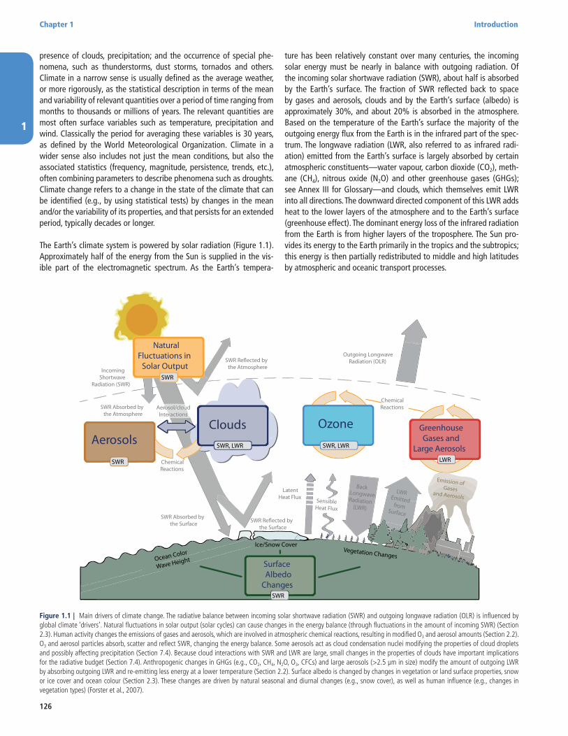
Figure 1.1 | Main drivers of climate change. The radiative balance between incoming solar shortwave radiation (SWR) and outgoing longwave radiation (OLR) is influenced by global climate ‘drivers’. Natural fluctuations in solar output (solar cycles) can cause changes in the energy balance (through fluctuations in the amount of incoming SWR) (Section 2.3). Human activity changes the emissions of gases and aerosols, which are involved in atmospheric chemical reactions, resulting in modified O3 and aerosol amounts (Section 2.2). O3 and aerosol particles absorb, scatter and reflect SWR, changing the energy balance. Some aerosols act as cloud condensation nuclei modifying the properties of cloud droplets and possibly affecting precipitation (Section 7.4). Because cloud interactions with SWR and LWR are large, small changes in the properties of clouds have important implications for the radiative budget (Section 7.4). Anthropogenic changes in GHGs (e.g., CO2, CH4, N2O, O3, CFCs) and large aerosols (>2.5 μm in size) modify the amount of outgoing LWR by absorbing outgoing LWR and re-emitting less energy at a lower temperature (Section 2.2). Surface albedo is changed by changes in vegetation or land surface properties, snow or ice cover and ocean colour (Section 2.3). These changes are driven by natural seasonal and diurnal changes (e.g., snow cover), as well as human influence (e.g., changes in vegetation types) (Forster et al., 2007).
presence of clouds, precipitation; and the occurrence of special phe-nomena, such as thunderstorms, dust storms, tornados and others. Climate in a narrow sense is usually defined as the average weather, or more rigorously, as the statistical description in terms of the mean and variability of relevant quantities over a period of time ranging from months to thousands or millions of years. The relevant quantities are most often surface variables such as temperature, precipitation and wind. Classically the period for averaging these variables is 30 years, as defined by the World Meteorological Organization. Climate in a wider sense also includes not just the mean conditions, but also the associated statistics (frequency, magnitude, persistence, trends, etc.), often combining parameters to describe phenomena such as droughts. Climate change refers to a change in the state of the climate that can be identified (e.g., by using statistical tests) by changes in the mean and/or the variability of its properties, and that persists for an extended period, typically decades or longer.
The Earth’s climate system is powered by solar radiation (Figure 1.1). Approximately half of the energy from the Sun is supplied in the vis-ible part of the electromagnetic spectrum. As the Earth’s tempera-
ture has been relatively constant over many centuries, the incoming solar energy must be nearly in balance with outgoing radiation. Of the incoming solar shortwave radiation (SWR), about half is absorbed by the Earth’s surface. The fraction of SWR reflected back to space by gases and aerosols, clouds and by the Earth’s surface (albedo) is approximately 30%, and about 20% is absorbed in the atmosphere. Based on the temperature of the Earth’s surface the majority of the outgoing energy flux from the Earth is in the infrared part of the spec-trum. The longwave radiation (LWR, also referred to as infrared radi-ation) emitted from the Earth’s surface is largely absorbed by certain atmospheric constituents—water vapour, carbon dioxide (CO2), meth-ane (CH4), nitrous oxide (N2O) and other greenhouse gases (GHGs); see Annex III for Glossary—and clouds, which themselves emit LWR into all directions. The downward directed component of this LWR adds heat to the lower layers of the atmosphere and to the Earth’s surface (greenhouse effect). The dominant energy loss of the infrared radiation from the Earth is from higher layers of the troposphere. The Sun pro-vides its energy to the Earth primarily in the tropics and the subtropics; this energy is then partially redistributed to middle and high latitudes by atmospheric and oceanic transport processes.
1
Introduction Chapter 1
127
Changes in the global energy budget derive from either changes in the net incoming solar radiation or changes in the outgoing longwave radiation (OLR). Changes in the net incoming solar radiation derive from changes in the Sun’s output of energy or changes in the Earth’s albedo. Reliable measurements of total solar irradiance (TSI) can be made only from space, and the precise record extends back only to 1978. The generally accepted mean value of the TSI is about 1361 W m−2 (Kopp and Lean, 2011; see Chapter 8 for a detailed discussion on the TSI); this is lower than the previous value of 1365 W m−2 used in the earlier assessments. Short-term variations of a few tenths of a percent are common during the approximately 11-year sunspot solar cycle (see Sections 5.2 and 8.4 for further details). Changes in the outgoing LWR can result from changes in the temperature of the Earth’s surface or atmosphere or changes in the emissivity (measure of emission effi-ciency) of LWR from either the atmosphere or the Earth’s surface. For the atmosphere, these changes in emissivity are due predominantly to changes in cloud cover and cloud properties, in GHGs and in aerosol concentrations. The radiative energy budget of the Earth is almost in balance (Figure 1.1), but ocean heat content and satellite measure-ments indicate a small positive imbalance (Murphy et al., 2009; Tren-berth et al., 2009; Hansen et al., 2011) that is consistent with the rapid changes in the atmospheric composition.
In addition, some aerosols increase atmospheric reflectivity, whereas others (e.g., particulate black carbon) are strong absorbers and also modify SWR (see Section 7.2 for a detailed assessment). Indirectly, aer-osols also affect cloud albedo, because many aerosols serve as cloud condensation nuclei or ice nuclei. This means that changes in aerosol types and distribution can result in small but important changes in cloud albedo and lifetime (Section 7.4). Clouds play a critical role in climate because they not only can increase albedo, thereby cooling the planet, but also because of their warming effects through infra-red radiative transfer. Whether the net radiative effect of a cloud is one of cooling or of warming depends on its physical properties (level of occurrence, vertical extent, water path and effective cloud particle size) as well as on the nature of the cloud condensation nuclei pop-ulation (Section 7.3). Humans enhance the greenhouse effect direct-ly by emitting GHGs such as CO2, CH4, N2O and chlorofluorocarbons (CFCs) (Figure 1.1). In addition, pollutants such as carbon monoxide (CO), volatile organic compounds (VOC), nitrogen oxides (NOx) and sulphur dioxide (SO2), which by themselves are negligible GHGs, have an indirect effect on the greenhouse effect by altering, through atmos-pheric chemical reactions, the abundance of important gases to the amount of outgoing LWR such as CH4 and ozone (O3), and/or by acting as precursors of secondary aerosols. Because anthropogenic emission sources simultaneously can emit some chemicals that affect climate and others that affect air pollution, including some that affect both, atmospheric chemistry and climate science are intrinsically linked.
In addition to changing the atmospheric concentrations of gases and aerosols, humans are affecting both the energy and water budget of the planet by changing the land surface, including redistributing the balance between latent and sensible heat fluxes (Sections 2.5, 7.2, 7.6 and 8.2). Land use changes, such as the conversion of forests to culti-vated land, change the characteristics of vegetation, including its colour, seasonal growth and carbon content (Houghton, 2003; Foley et al., 2005). For example, clearing and burning a forest to prepare agricultural
land reduces carbon storage in the vegetation, adds CO2 to the atmos-phere, and changes the reflectivity of the land (surface albedo), rates of evapotranspiration and longwave emissions (Figure 1.1).
Changes in the atmosphere, land, ocean, biosphere and cryosphere—both natural and anthropogenic—can perturb the Earth’s radiation budget, producing a radiative forcing (RF) that affects climate. RF is a measure of the net change in the energy balance in response to an external perturbation. The drivers of changes in climate can include, for example, changes in the solar irradiance and changes in atmospheric trace gas and aerosol concentrations (Figure 1.1). The concept of RF cannot capture the interactions of anthropogenic aerosols and clouds, for example, and thus in addition to the RF as used in previous assess-ments, Sections 7.4 and 8.1 introduce a new concept, effective radi-ative forcing (ERF), that accounts for rapid response in the climate system. ERF is defined as the change in net downward flux at the top of the atmosphere after allowing for atmospheric temperatures, water vapour, clouds and land albedo to adjust, but with either sea surface temperatures (SSTs) and sea ice cover unchanged or with global mean surface temperature unchanged.
Once a forcing is applied, complex internal feedbacks determine the eventual response of the climate system, and will in general cause this response to differ from a simple linear one (IPCC, 2001, 2007). There are many feedback mechanisms in the climate system that can either amplify (‘positive feedback’) or diminish (‘negative feedback’) the effects of a change in climate forcing (Le Treut et al., 2007) (see Figure 1.2 for a representation of some of the key feedbacks). An example of a positive feedback is the water vapour feedback whereby an increase in surface temperature enhances the amount of water vapour pres-ent in the atmosphere. Water vapour is a powerful GHG: increasing its atmospheric concentration enhances the greenhouse effect and leads to further surface warming. Another example is the ice albedo feedback, in which the albedo decreases as highly reflective ice and snow surfaces melt, exposing the darker and more absorbing surfaces below. The dominant negative feedback is the increased emission of energy through LWR as surface temperature increases (sometimes also referred to as blackbody radiation feedback). Some feedbacks oper-ate quickly (hours), while others develop over decades to centuries; in order to understand the full impact of a feedback mechanism, its timescale needs to be considered. Melting of land ice sheets can take days to millennia.
A spectrum of models is used to project quantitatively the climate response to forcings. The simplest energy balance models use one box to represent the Earth system and solve the global energy bal-ance to deduce globally averaged surface air temperature. At the other extreme, full complexity three-dimensional climate models include the explicit solution of energy, momentum and mass conservation equations at millions of points on the Earth in the atmosphere, land, ocean and cryosphere. More recently, capabilities for the explicit sim-ulation of the biosphere, the carbon cycle and atmospheric chemistry have been added to the full complexity models, and these models are called Earth System Models (ESMs). Earth System Models of Interme-diate Complexity include the same processes as ESMs, but at reduced resolution, and thus can be simulated for longer periods (see Annex III for Glossary and Section 9.1).
1
Chapter 1 Introduction
128
An equilibrium climate experiment is an experiment in which a cli-mate model is allowed to adjust fully to a specified change in RF. Such experiments provide information on the difference between the initial and final states of the model simulated climate, but not on the time-de-pendent response. The equilibrium response in global mean surface air temperature to a doubling of atmospheric concentration of CO2 above pre-industrial levels (e.g., Arrhenius, 1896; see Le Treut et al., 2007 for a comprehensive list) has often been used as the basis for the concept of equilibrium climate sensitivity (e.g., Hansen et al., 1981; see Meehl et al., 2007 for a comprehensive list). For more realistic simulations of climate, changes in RF are applied gradually over time, for example, using historical reconstructions of the CO2, and these simulations are called transient simulations. The temperature response in these tran-sient simulations is different than in an equilibrium simulation. The transient climate response is defined as the change in global surface temperature at the time of atmospheric CO2 doubling in a global cou-pled ocean–atmosphere climate model simulation where concentra-tions of CO2 were increased by 1% yr–1. The transient climate response
is a measure of the strength and rapidity of the surface temperature response to GHG forcing. It can be more meaningful for some problems as well as easier to derive from observations (see Figure 10.20; Sec-tion 10.8; Chapter 12; Knutti et al., 2005; Frame et al., 2006; Forest et al., 2008), but such experiments are not intended to replace the more realistic scenario evaluations.
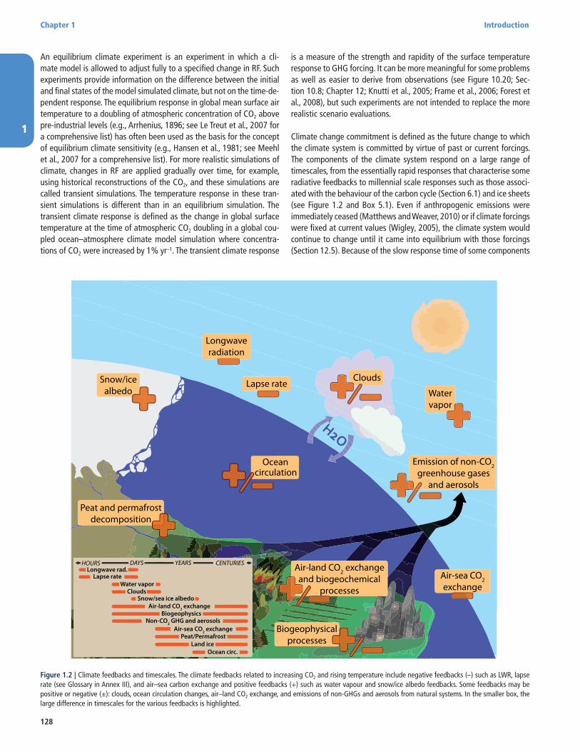
Climate change commitment is defined as the future change to which the climate system is committed by virtue of past or current forcings. The components of the climate system respond on a large range of timescales, from the essentially rapid responses that characterise some radiative feedbacks to millennial scale responses such as those associ-ated with the behaviour of the carbon cycle (Section 6.1) and ice sheets (see Figure 1.2 and Box 5.1). Even if anthropogenic emissions were immediately ceased (Matthews and Weaver, 2010) or if climate forcings were fixed at current values (Wigley, 2005), the climate system would continue to change until it came into equilibrium with those forcings (Section 12.5). Because of the slow response time of some components
Snow/icealbedo
Longwaveradiation
Lapse rateClouds
Watervapor
Emission of non-CO2greenhouse gases
and aerosols
Air-sea CO2exchange
Air-land CO2 exchangeand biogeochemical
processes
Biogeophysicalprocesses
Peat and permafrostdecomposition
Oceancirculation
HOURS DAYS YEARS CENTURIESLongwave rad.
Snow/sea ice albedo
Lapse rateWater vapor
Clouds
Air-land CO2 exchangeBiogeophysics
Non-CO2 GHG and aerosolsAir-sea CO2 exchange
Peat/PermafrostLand ice
Ocean circ.
Figure 1.2 | Climate feedbacks and timescales. The climate feedbacks related to increasing CO2 and rising temperature include negative feedbacks (–) such as LWR, lapse rate (see Glossary in Annex III), and air–sea carbon exchange and positive feedbacks (+) such as water vapour and snow/ice albedo feedbacks. Some feedbacks may be positive or negative (±): clouds, ocean circulation changes, air–land CO2 exchange, and emissions of non-GHGs and aerosols from natural systems. In the smaller box, the large difference in timescales for the various feedbacks is highlighted.
1
Introduction Chapter 1
129
of the climate system, equilibrium conditions will not be reached for many centuries. Slow processes can sometimes be constrained only by data collected over long periods, giving a particular salience to paleo-climate data for understanding equilibrium processes. Climate change commitment is indicative of aspects of inertia in the climate system because it captures the ongoing nature of some aspects of change.
A summary of perturbations to the forcing of the climate system from changes in solar radiation, GHGs, surface albedo and aerosols is pre-sented in Box 13.1. The energy fluxes from these perturbations are bal-anced by increased radiation to space from a warming Earth, reflection of solar radiation and storage of energy in the Earth system, principally the oceans (Box 3.1, Box 13.1).
The processes affecting climate can exhibit considerable natural var-iability. Even in the absence of external forcing, periodic and chaotic variations on a vast range of spatial and temporal scales are observed. Much of this variability can be represented by simple (e.g., unimodal or power law) distributions, but many components of the climate system also exhibit multiple states—for instance, the glacial-interglacial cycles and certain modes of internal variability such as El Niño-South-ern Oscillation (ENSO) (see Box 2.5 for details on patterns and indices of climate variability). Movement between states can occur as a result of natural variability, or in response to external forcing. The relation-ship between variability, forcing and response reveals the complexity of the dynamics of the climate system: the relationship between forc-ing and response for some parts of the system seems reasonably linear; in other cases this relationship is much more complex, characterised by hysteresis (the dependence on past states) and a non-additive combi-nation of feedbacks.
Related to multiple climate states, and hysteresis, is the concept of irreversibility in the climate system. In some cases where multiple states and irreversibility combine, bifurcations or ‘tipping points’ can been reached (see Section 12.5). In these situations, it is difficult if not impossible for the climate system to revert to its previous state, and the change is termed irreversible over some timescale and forcing range. A small number of studies using simplified models find evidence for global-scale ‘tipping points’ (e.g., Lenton et al., 2008); however, there is no evidence for global-scale tipping points in any of the most com-prehensive models evaluated to date in studies of climate evolution in the 21st century. There is evidence for threshold behaviour in certain aspects of the climate system, such as ocean circulation (see Section 12.5) and ice sheets (see Box 5.1), on multi-centennial-to-millennial timescales. There are also arguments for the existence of regional tip-ping points, most notably in the Arctic (e.g., Lenton et al., 2008; Duarte et al., 2012; Wadhams, 2012), although aspects of this are contested (Armour et al., 2011; Tietsche et al., 2011).
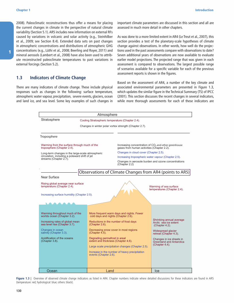
1.2.3 Multiple Lines of Evidence for Climate Change
While the first IPCC assessment depended primarily on observed changes in surface temperature and climate model analyses, more recent assessments include multiple lines of evidence for climate change. The first line of evidence in assessing climate change is based on careful analysis of observational records of the atmosphere, land, ocean and cryosphere systems (Figure 1.3). There is incontroverti-
ble evidence from in situ observations and ice core records that the atmospheric concentrations of GHGs such as CO2, CH4, and N2O have increased substantially over the last 200 years (Sections 6.3 and 8.3). In addition, instrumental observations show that land and sea sur-face temperatures have increased over the last 100 years (Chapter 2). Satellites allow a much broader spatial distribution of measurements, especially over the last 30 years. For the upper ocean temperature the observations indicate that the temperature has increased since at least 1950 (Willis et al., 2010; Section 3.2). Observations from satellites and in situ measurements suggest reductions in glaciers, Arctic sea ice and ice sheets (Sections 4.2, 4.3 and 4.4). In addition, analyses based on measurements of the radiative budget and ocean heat content sug-gest a small imbalance (Section 2.3). These observations, all published in peer-reviewed journals, made by diverse measurement groups in multiple countries using different technologies, investigating various climate-relevant types of data, uncertainties and processes, offer a wide range of evidence on the broad extent of the changing climate throughout our planet.
Conceptual and numerical models of the Earth’s climate system offer another line of evidence on climate change (discussions in Chapters 5 and 9 provide relevant analyses of this evidence from paleoclimat-ic to recent periods). These use our basic understanding of the cli-mate system to provide self-consistent methodologies for calculating impacts of processes and changes. Numerical models include the cur-rent knowledge about the laws of physics, chemistry and biology, as well as hypotheses about how complicated processes such as cloud formation can occur. Because these models can represent only the existing state of knowledge and technology, they are not perfect; they are, however, important tools for analysing uncertainties or unknowns, for testing different hypotheses for causation relative to observations, and for making projections of possible future changes.
One of the most powerful methods for assessing changes occurring in climate involves the use of statistical tools to test the analyses from models relative to observations. This methodology is generally called detection and attribution in the climate change community (Section 10.2). For example, climate models indicate that the temperature response to GHG increases is expected to be different than the effects from aerosols or from solar variability. Radiosonde measurements and satellite retrievals of atmospheric temperature show increases in tropospheric temperature and decreases in stratospheric tempera-tures, consistent with the increases in GHG effects found in climate model simulations (e.g., increases in CO2, changes in O3), but if the Sun was the main driver of current climate change, stratospheric and tropospheric temperatures would respond with the same sign (Hegerl et al., 2007).
Resources available prior to the instrumental period—historical sources, natural archives, and proxies for key climate variables (e.g., tree rings, marine sediment cores, ice cores)—can provide quantita-tive information on past regional to global climate and atmospheric composition variability and these data contribute another line of evi-dence. Reconstructions of key climate variables based on these data sets have provided important information on the responses of the Earth system to a variety of external forcings and its internal variabil-ity over a wide range of timescales (Hansen et al., 2006; Mann et al.,
1
Chapter 1 Introduction
130
2008). Paleoclimatic reconstructions thus offer a means for placing the current changes in climate in the perspective of natural climate variability (Section 5.1). AR5 includes new information on external RFs caused by variations in volcanic and solar activity (e.g., Steinhilber et al., 2009; see Section 8.4). Extended data sets on past changes in atmospheric concentrations and distributions of atmospheric GHG concentrations (e.g., Lüthi et al., 2008; Beerling and Royer, 2011) and mineral aerosols (Lambert et al., 2008) have also been used to attrib-ute reconstructed paleoclimate temperatures to past variations in external forcings (Section 5.2).
1.3 Indicators of Climate Change
There are many indicators of climate change. These include physical responses such as changes in the following: surface temperature, atmospheric water vapour, precipitation, severe events, glaciers, ocean and land ice, and sea level. Some key examples of such changes in
important climate parameters are discussed in this section and all are assessed in much more detail in other chapters.
As was done to a more limited extent in AR4 (Le Treut et al., 2007), this section provides a test of the planetary-scale hypotheses of climate change against observations. In other words, how well do the projec-tions used in the past assessments compare with observations to date? Seven additional years of observations are now available to evaluate earlier model projections. The projected range that was given in each assessment is compared to observations. The largest possible range of scenarios available for a specific variable for each of the previous assessment reports is shown in the figures.
Based on the assessment of AR4, a number of the key climate and associated environmental parameters are presented in Figure 1.3, which updates the similar figure in the Technical Summary (TS) of IPCC (2001). This section discusses the recent changes in several indicators, while more thorough assessments for each of these indicators are
Ocean Land Ice
Troposphere
Near Surface
Stratosphere Cooling Stratospheric temperature (Chapter 2.4).
Changes in winter polar vortex strength (Chapter 2.7).
Increasing concentration of CO2 and other greenhousegases from human activities (Chapter 2.2).Changes in cloud cover (Chapter 2.5).Increasing tropospheric water vapour (Chapter 2.5). Changes in aerosole burden and ozone concentrations (Chapter 2.2)
Rising global average near surfacetemperature (Chapter 2.4).
Increasing surface humidity (Chapter 2.5).
Warming throughout much of theworlds ocean (Chapter 3.2).
Increasing rates of global mean sea level rise (Chapter 3.7).
Changes in ocean salinity (Chapter 3.3).
Acidification of the oceans (Chapter 3.8).
More frequent warm days and nights. Fewer cold days and nights (Chapter 2.6).
Reductions in the number of frost days (Chapter 2.6).
Decreasing snow cover in most regions (Chapter 4.5).
Degrading permafrost in areal extent and thickness (Chapter 4.6).
Large scale precipitation changes (Chapter 2.5).
Increase in the number of heavy precipitation events (Chapter 2.6).
Shrinking annual average Arctic sea ice extent (Chapter 4.2).
Widespread glacier retreat (Chapter 4.3).
Changes in ice sheets in Greenland and Antarctica (Chapter 4.4).
Warming from the surface through much of the troposphere (Chapter 2.4).
Long-term changes in the large-scale atmospheric circulation, including a poleward shift of jet streams (Chapter 2.7).
Atmosphere
Warming of sea surface temperatures (Chapter 2.4).
Observations of Climate Changes from AR4 (points to AR5)
Figure 1.3 | Overview of observed climate change indicators as listed in AR4. Chapter numbers indicate where detailed discussions for these indicators are found in AR5 (temperature: red; hydrological: blue; others: black).
1
Introduction Chapter 1
131
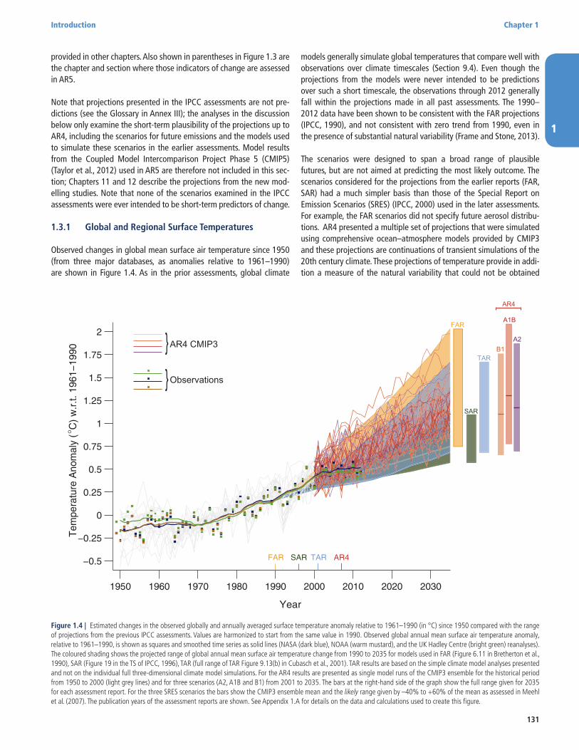
Figure 1.4 | Estimated changes in the observed globally and annually averaged surface temperature anomaly relative to 1961–1990 (in °C) since 1950 compared with the range of projections from the previous IPCC assessments. Values are harmonized to start from the same value in 1990. Observed global annual mean surface air temperature anomaly, relative to 1961–1990, is shown as squares and smoothed time series as solid lines (NASA (dark blue), NOAA (warm mustard), and the UK Hadley Centre (bright green) reanalyses). The coloured shading shows the projected range of global annual mean surface air temperature change from 1990 to 2035 for models used in FAR (Figure 6.11 in Bretherton et al., 1990), SAR (Figure 19 in the TS of IPCC, 1996), TAR (full range of TAR Figure 9.13(b) in Cubasch et al., 2001). TAR results are based on the simple climate model analyses presented and not on the individual full three-dimensional climate model simulations. For the AR4 results are presented as single model runs of the CMIP3 ensemble for the historical period from 1950 to 2000 (light grey lines) and for three scenarios (A2, A1B and B1) from 2001 to 2035. The bars at the right-hand side of the graph show the full range given for 2035 for each assessment report. For the three SRES scenarios the bars show the CMIP3 ensemble mean and the likely range given by –40% to +60% of the mean as assessed in Meehl et al. (2007). The publication years of the assessment reports are shown. See Appendix 1.A for details on the data and calculations used to create this figure.
provided in other chapters. Also shown in parentheses in Figure 1.3 are the chapter and section where those indicators of change are assessed in AR5.
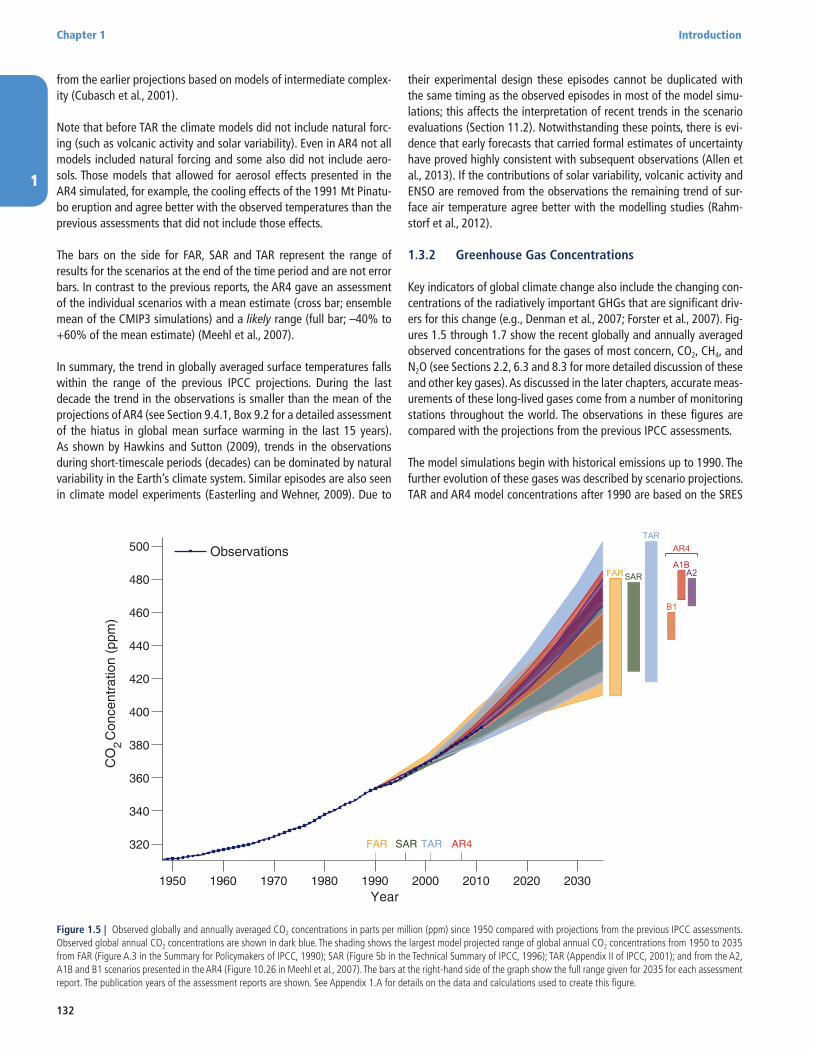
Note that projections presented in the IPCC assessments are not pre-dictions (see the Glossary in Annex III); the analyses in the discussion below only examine the short-term plausibility of the projections up to AR4, including the scenarios for future emissions and the models used to simulate these scenarios in the earlier assessments. Model results from the Coupled Model Intercomparison Project Phase 5 (CMIP5) (Taylor et al., 2012) used in AR5 are therefore not included in this sec-tion; Chapters 11 and 12 describe the projections from the new mod-elling studies. Note that none of the scenarios examined in the IPCC assessments were ever intended to be short-term predictors of change.
1.3.1 Global and Regional Surface Temperatures
Observed changes in global mean surface air temperature since 1950 (from three major databases, as anomalies relative to 1961–1990) are shown in Figure 1.4. As in the prior assessments, global climate
models generally simulate global temperatures that compare well with o bservations over climate timescales (Section 9.4). Even though the projections from the models were never intended to be predictions over such a short timescale, the observations through 2012 generally fall within the projections made in all past assessments. The 1990–2012 data have been shown to be consistent with the FAR projections (IPCC, 1990), and not consistent with zero trend from 1990, even in the presence of substantial natural variability (Frame and Stone, 2013).
The scenarios were designed to span a broad range of plausible futures, but are not aimed at predicting the most likely outcome. The scenarios considered for the projections from the earlier reports (FAR, SAR) had a much simpler basis than those of the Special Report on Emission Scenarios (SRES) (IPCC, 2000) used in the later assessments. For example, the FAR scenarios did not specify future aerosol distribu-tions. AR4 presented a multiple set of projections that were simulated using comprehensive ocean–atmosphere models provided by CMIP3 and these projections are continuations of transient simulations of the 20th century climate. These projections of temperature provide in addi-tion a measure of the natural variability that could not be obtained
1
Chapter 1 Introduction
132
from the earlier projections based on models of intermediate complex-ity (Cubasch et al., 2001).
Note that before TAR the climate models did not include natural forc-ing (such as volcanic activity and solar variability). Even in AR4 not all models included natural forcing and some also did not include aero-sols. Those models that allowed for aerosol effects presented in the AR4 simulated, for example, the cooling effects of the 1991 Mt Pinatu-bo eruption and agree better with the observed temperatures than the previous assessments that did not include those effects.
The bars on the side for FAR, SAR and TAR represent the range of results for the scenarios at the end of the time period and are not error bars. In contrast to the previous reports, the AR4 gave an assessment of the individual scenarios with a mean estimate (cross bar; ensemble mean of the CMIP3 simulations) and a likely range (full bar; –40% to +60% of the mean estimate) (Meehl et al., 2007).
In summary, the trend in globally averaged surface temperatures falls within the range of the previous IPCC projections. During the last decade the trend in the observations is smaller than the mean of the projections of AR4 (see Section 9.4.1, Box 9.2 for a detailed assessment of the hiatus in global mean surface warming in the last 15 years). As shown by Hawkins and Sutton (2009), trends in the observations during short-timescale periods (decades) can be dominated by natural variability in the Earth’s climate system. Similar episodes are also seen in climate model experiments (Easterling and Wehner, 2009). Due to
their experimental design these episodes cannot be duplicated with the same timing as the observed episodes in most of the model simu-lations; this affects the interpretation of recent trends in the scenario evaluations (Section 11.2). Notwithstanding these points, there is evi-dence that early forecasts that carried formal estimates of uncertainty have proved highly consistent with subsequent observations (Allen et al., 2013). If the contributions of solar variability, volcanic activity and ENSO are removed from the observations the remaining trend of sur-face air temperature agree better with the modelling studies (Rahm-storf et al., 2012).
1.3.2 Greenhouse Gas Concentrations
Key indicators of global climate change also include the changing con-centrations of the radiatively important GHGs that are significant driv-ers for this change (e.g., Denman et al., 2007; Forster et al., 2007). Fig-ures 1.5 through 1.7 show the recent globally and annually averaged observed concentrations for the gases of most concern, CO2, CH4, and N2O (see Sections 2.2, 6.3 and 8.3 for more detailed discussion of these and other key gases). As discussed in the later chapters, accurate meas-urements of these long-lived gases come from a number of monitoring stations throughout the world. The observations in these figures are compared with the projections from the previous IPCC assessments.
The model simulations begin with historical emissions up to 1990. The further evolution of these gases was described by scenario projections. TAR and AR4 model concentrations after 1990 are based on the SRES
Figure 1.5 | Observed globally and annually averaged CO2 concentrations in parts per million (ppm) since 1950 compared with projections from the previous IPCC assessments. Observed global annual CO2 concentrations are shown in dark blue. The shading shows the largest model projected range of global annual CO2 concentrations from 1950 to 2035 from FAR (Figure A.3 in the Summary for Policymakers of IPCC, 1990); SAR (Figure 5b in the Technical Summary of IPCC, 1996); TAR (Appendix II of IPCC, 2001); and from the A2, A1B and B1 scenarios presented in the AR4 (Figure 10.26 in Meehl et al., 2007). The bars at the right-hand side of the graph show the full range given for 2035 for each assessment report. The publication years of the assessment reports are shown. See Appendix 1.A for details on the data and calculations used to create this figure.
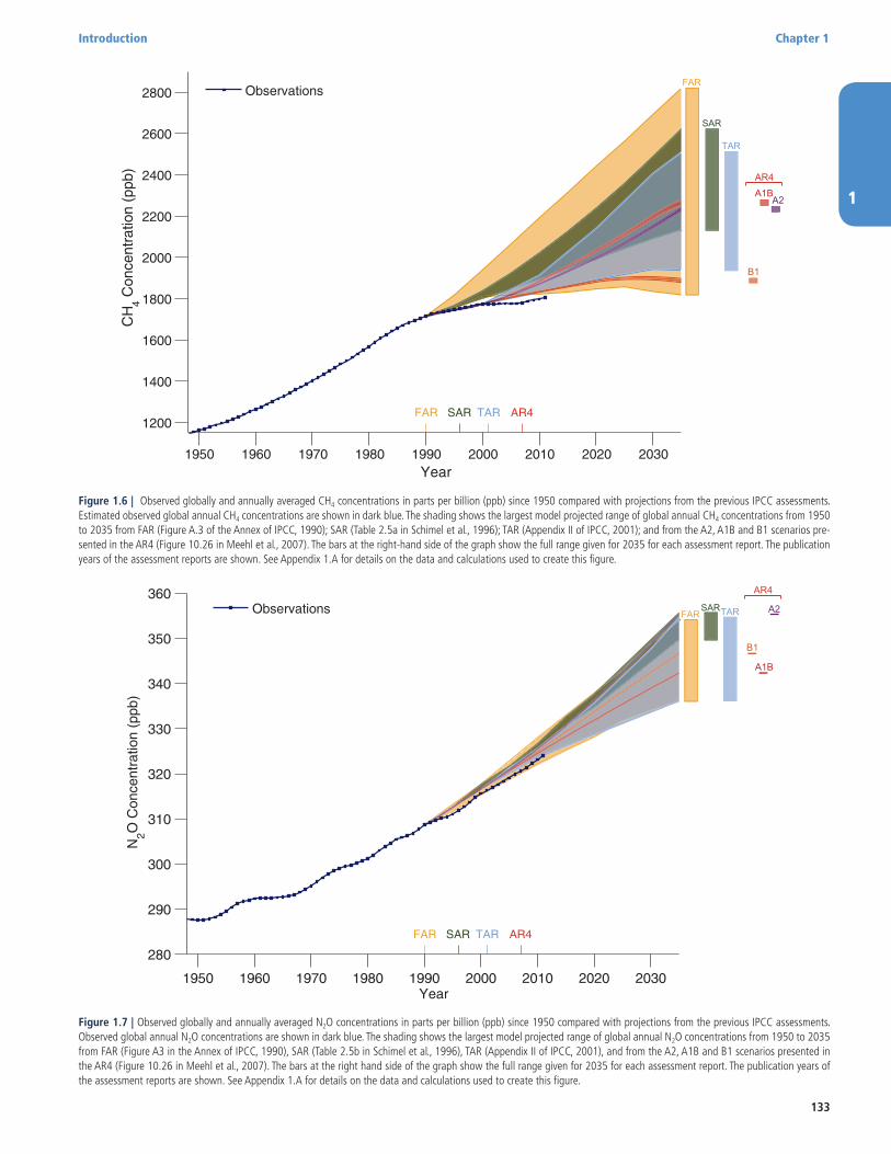
1
Introduction Chapter 1
133
Figure 1.7 | Observed globally and annually averaged N2O concentrations in parts per billion (ppb) since 1950 compared with projections from the previous IPCC assessments. Observed global annual N2O concentrations are shown in dark blue. The shading shows the largest model projected range of global annual N2O concentrations from 1950 to 2035 from FAR (Figure A3 in the Annex of IPCC, 1990), SAR (Table 2.5b in Schimel et al., 1996), TAR (Appendix II of IPCC, 2001), and from the A2, A1B and B1 scenarios presented in the AR4 (Figure 10.26 in Meehl et al., 2007). The bars at the right hand side of the graph show the full range given for 2035 for each assessment report. The publication years of the assessment reports are shown. See Appendix 1.A for details on the data and calculations used to create this figure.
Figure 1.6 | Observed globally and annually averaged CH4 concentrations in parts per billion (ppb) since 1950 compared with projections from the previous IPCC assessments. Estimated observed global annual CH4 concentrations are shown in dark blue. The shading shows the largest model projected range of global annual CH4 concentrations from 1950 to 2035 from FAR (Figure A.3 of the Annex of IPCC, 1990); SAR (Table 2.5a in Schimel et al., 1996); TAR (Appendix II of IPCC, 2001); and from the A2, A1B and B1 scenarios pre-sented in the AR4 (Figure 10.26 in Meehl et al., 2007). The bars at the right-hand side of the graph show the full range given for 2035 for each assessment report. The publication years of the assessment reports are shown. See Appendix 1.A for details on the data and calculations used to create this figure.
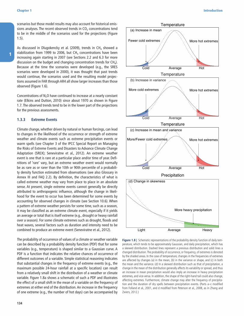
1
Chapter 1 Introduction
134
scenarios but those model results may also account for historical emis-sions analyses. The recent observed trends in CO2 concentrations tend to be in the middle of the scenarios used for the projections (Figure 1.5).
As discussed in Dlugokencky et al. (2009), trends in CH4 showed a stabilization from 1999 to 2006, but CH4 concentrations have been increasing again starting in 2007 (see Sections 2.2 and 6.3 for more discussion on the budget and changing concentration trends for CH4). Because at the time the scenarios were developed (e.g., the SRES scenarios were developed in 2000), it was thought that past trends would continue, the scenarios used and the resulting model projec-tions assumed in FAR through AR4 all show larger increases than those observed (Figure 1.6).
Concentrations of N2O have continued to increase at a nearly constant rate (Elkins and Dutton, 2010) since about 1970 as shown in Figure 1.7. The observed trends tend to be in the lower part of the projections for the previous assessments.
1.3.3 Extreme Events
Climate change, whether driven by natural or human forcings, can lead to changes in the likelihood of the occurrence or strength of extreme weather and climate events such as extreme precipitation events or warm spells (see Chapter 3 of the IPCC Special Report on Managing the Risks of Extreme Events and Disasters to Advance Climate Change Adaptation (SREX); Seneviratne et al., 2012). An extreme weather event is one that is rare at a particular place and/or time of year. Defi-nitions of ‘rare’ vary, but an extreme weather event would normally be as rare as or rarer than the 10th or 90th percentile of a probabili-ty density function estimated from observations (see also Glossary in Annex III and FAQ 2.2). By definition, the characteristics of what is called extreme weather may vary from place to place in an absolute sense. At present, single extreme events cannot generally be directly attributed to anthropogenic influence, although the change in likeli-hood for the event to occur has been determined for some events by accounting for observed changes in climate (see Section 10.6). When a pattern of extreme weather persists for some time, such as a season, it may be classified as an extreme climate event, especially if it yields an average or total that is itself extreme (e.g., drought or heavy rainfall over a season). For some climate extremes such as drought, floods and heat waves, several factors such as duration and intensity need to be combined to produce an extreme event (Seneviratne et al., 2012).
The probability of occurrence of values of a climate or weather variable can be described by a probability density function (PDF) that for some variables (e.g., temperature) is shaped similar to a Gaussian curve. A PDF is a function that indicates the relative chances of occurrence of different outcomes of a variable. Simple statistical reasoning indicates that substantial changes in the frequency of extreme events (e.g., the maximum possible 24-hour rainfall at a specific location) can result from a relatively small shift in the distribution of a weather or climate variable. Figure 1.8a shows a schematic of such a PDF and illustrates the effect of a small shift in the mean of a variable on the frequency of extremes at either end of the distribution. An increase in the frequency of one extreme (e.g., the number of hot days) can be accompanied by
Figure 1.8 | Schematic representations of the probability density function of daily tem-perature, which tends to be approximately Gaussian, and daily precipitation, which has a skewed distribution. Dashed lines represent a previous distribution and solid lines a changed distribution. The probability of occurrence, or frequency, of extremes is denoted by the shaded areas. In the case of temperature, changes in the frequencies of extremes are affected by changes (a) in the mean, (b) in the variance or shape, and (c) in both the mean and the variance. (d) In a skewed distribution such as that of precipitation, a change in the mean of the distribution generally affects its variability or spread, and thus an increase in mean precipitation would also imply an increase in heavy precipitation extremes, and vice-versa. In addition, the shape of the right-hand tail could also change, affecting extremes. Furthermore, climate change may alter the frequency of precipita-tion and the duration of dry spells between precipitation events. (Parts a–c modified from Folland et al., 2001, and d modified from Peterson et al., 2008, as in Zhang and Zwiers, 2012.)
Precipitation
Temperature
Temperature
Temperature
AverageLight
Average HotCold
HotAverageCold
HotAverageCold
Heavy
(d) Change in skewness
(c) Increase in mean and variance
(b) Increase in variance
(a) Increase in mean
More heavy precipitation
More hot extremesFewer cold extremes
More hot extremesMore cold extremes
More hot extremesMore/Fewer cold extremes
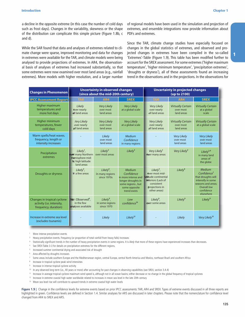
1
Introduction Chapter 1
135
Figure 1.9 | Change in the confidence levels for extreme events based on prior IPCC assessments: TAR, AR4 and SREX. Types of extreme events discussed in all three reports are highlighted in green. Confidence levels are defined in Section 1.4. Similar analyses for AR5 are discussed in later chapters. Please note that the nomenclature for confidence level changed from AR4 to SREX and AR5.
a decline in the opposite extreme (in this case the number of cold days such as frost days). Changes in the variability, skewness or the shape of the distribution can complicate this simple picture (Figure 1.8b, c and d).
While the SAR found that data and analyses of extremes related to cli-mate change were sparse, improved monitoring and data for changes in extremes were available for the TAR, and climate models were being analysed to provide projections of extremes. In AR4, the observation-al basis of analyses of extremes had increased substantially, so that some extremes were now examined over most land areas (e.g., rainfall extremes). More models with higher resolution, and a larger number
of regional models have been used in the simulation and projection of extremes, and ensemble integrations now provide information about PDFs and extremes.
Since the TAR, climate change studies have especially focused on changes in the global statistics of extremes, and observed and pro-jected changes in extremes have been compiled in the so-called ‘Extremes’-Table (Figure 1.9). This table has been modified further to account for the SREX assessment. For some extremes (‘higher maximum temperature’, ‘higher minimum temperature’, ‘precipitation extremes’, ‘droughts or dryness’), all of these assessments found an increasing trend in the observations and in the projections. In the observations for
1 More intense precipitation events² Heavy precipitation events. Frequency (or proportion of total rainfall from heavy falls) increases³ Statistically significant trends in the number of heavy precipitation events in some regions. It is likely that more of these regions have experienced increases than decreases. 4 See SREX Table 3-3 for details on precipitation extremes for the different regions.5 Increased summer continental drying and associated risk of drought6 Area affected by droughts increases7 Some areas include southern Europe and the Mediterranean region, central Europe, central North America and Mexico, northeast Brazil and southern Africa8 Increase in tropical cyclone peak wind intensities9 Increase in intense tropical cyclone activity 10 In any observed long-term (i.e., 40 years or more) after accounting for past changes in observing capabilities (see SREX, section 3.4.4) 11 Increase in average tropical cyclone maximum wind speed is, although not in all ocean basins; either decrease or no change in the global frequency of tropical cyclones12 Increase in extreme coastal high water worldwide related to increases in mean sea level in the late 20th century13 Mean sea level rise will contribute to upward trends in extreme coastal high water levels
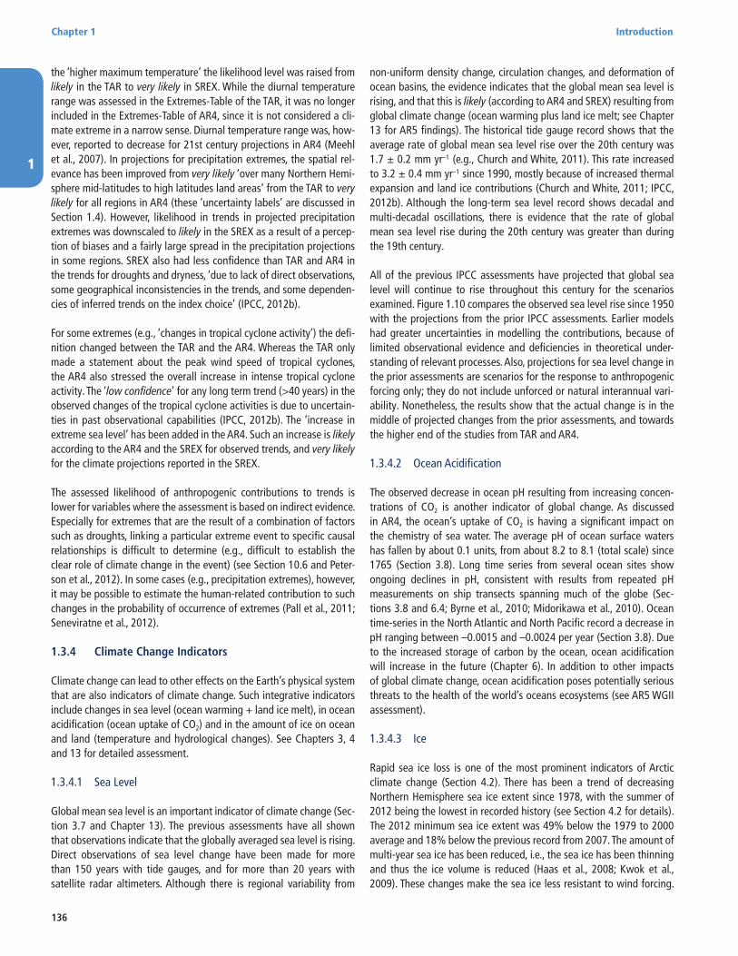
1
Chapter 1 Introduction
136
the ‘higher maximum temperature’ the likelihood level was raised from likely in the TAR to very likely in SREX. While the diurnal temperature range was assessed in the Extremes-Table of the TAR, it was no longer included in the Extremes-Table of AR4, since it is not considered a cli-mate extreme in a narrow sense. Diurnal temperature range was, how-ever, reported to decrease for 21st century projections in AR4 (Meehl et al., 2007). In projections for precipitation extremes, the spatial rel-evance has been improved from very likely ‘over many Northern Hemi-sphere mid-latitudes to high latitudes land areas’ from the TAR to very likely for all regions in AR4 (these ‘uncertainty labels’ are discussed in Section 1.4). However, likelihood in trends in projected precipitation extremes was downscaled to likely in the SREX as a result of a percep-tion of biases and a fairly large spread in the precipitation projections in some regions. SREX also had less confidence than TAR and AR4 in the trends for droughts and dryness, ‘due to lack of direct observations, some geographical inconsistencies in the trends, and some dependen-cies of inferred trends on the index choice’ (IPCC, 2012b).
For some extremes (e.g., ‘changes in tropical cyclone activity’) the defi-nition changed between the TAR and the AR4. Whereas the TAR only made a statement about the peak wind speed of tropical cyclones, the AR4 also stressed the overall increase in intense tropical cyclone activity. The ‘low confidence’ for any long term trend (>40 years) in the observed changes of the tropical cyclone activities is due to uncertain-ties in past observational capabilities (IPCC, 2012b). The ‘increase in extreme sea level’ has been added in the AR4. Such an increase is likely according to the AR4 and the SREX for observed trends, and very likely for the climate projections reported in the SREX.
The assessed likelihood of anthropogenic contributions to trends is lower for variables where the assessment is based on indirect evidence. Especially for extremes that are the result of a combination of factors such as droughts, linking a particular extreme event to specific causal relationships is difficult to determine (e.g., difficult to establish the clear role of climate change in the event) (see Section 10.6 and Peter-son et al., 2012). In some cases (e.g., precipitation extremes), however, it may be possible to estimate the human-related contribution to such changes in the probability of occurrence of extremes (Pall et al., 2011; Seneviratne et al., 2012).
1.3.4 Climate Change Indicators
Climate change can lead to other effects on the Earth’s physical system that are also indicators of climate change. Such integrative indicators include changes in sea level (ocean warming + land ice melt), in ocean acidification (ocean uptake of CO2) and in the amount of ice on ocean and land (temperature and hydrological changes). See Chapters 3, 4 and 13 for detailed assessment.
1.3.4.1 Sea Level
Global mean sea level is an important indicator of climate change (Sec-tion 3.7 and Chapter 13). The previous assessments have all shown that observations indicate that the globally averaged sea level is rising. Direct observations of sea level change have been made for more than 150 years with tide gauges, and for more than 20 years with satellite radar altimeters. Although there is regional variability from
non-uniform density change, circulation changes, and deformation of ocean basins, the evidence indicates that the global mean sea level is rising, and that this is likely (according to AR4 and SREX) resulting from global climate change (ocean warming plus land ice melt; see Chapter 13 for AR5 findings). The historical tide gauge record shows that the average rate of global mean sea level rise over the 20th century was 1.7 ± 0.2 mm yr–1 (e.g., Church and White, 2011). This rate increased to 3.2 ± 0.4 mm yr–1 since 1990, mostly because of increased thermal expansion and land ice contributions (Church and White, 2011; IPCC, 2012b). Although the long-term sea level record shows decadal and multi-decadal oscillations, there is evidence that the rate of global mean sea level rise during the 20th century was greater than during the 19th century.
All of the previous IPCC assessments have projected that global sea level will continue to rise throughout this century for the scenarios examined. Figure 1.10 compares the observed sea level rise since 1950 with the projections from the prior IPCC assessments. Earlier models had greater uncertainties in modelling the contributions, because of limited observational evidence and deficiencies in theoretical under-standing of relevant processes. Also, projections for sea level change in the prior assessments are scenarios for the response to anthropogenic forcing only; they do not include unforced or natural interannual vari-ability. Nonetheless, the results show that the actual change is in the middle of projected changes from the prior assessments, and towards the higher end of the studies from TAR and AR4.
1.3.4.2 Ocean Acidification
The observed decrease in ocean pH resulting from increasing concen-trations of CO2 is another indicator of global change. As discussed in AR4, the ocean’s uptake of CO2 is having a significant impact on the chemistry of sea water. The average pH of ocean surface waters has fallen by about 0.1 units, from about 8.2 to 8.1 (total scale) since 1765 (Section 3.8). Long time series from several ocean sites show ongoing declines in pH, consistent with results from repeated pH measurements on ship transects spanning much of the globe (Sec-tions 3.8 and 6.4; Byrne et al., 2010; Midorikawa et al., 2010). Ocean time-series in the North Atlantic and North Pacific record a decrease in pH ranging between –0.0015 and –0.0024 per year (Section 3.8). Due to the increased storage of carbon by the ocean, ocean acidification will increase in the future (Chapter 6). In addition to other impacts of global climate change, ocean acidification poses potentially serious threats to the health of the world’s oceans ecosystems (see AR5 WGII assessment).
1.3.4.3 Ice
Rapid sea ice loss is one of the most prominent indicators of Arctic climate change (Section 4.2). There has been a trend of decreasing Northern Hemisphere sea ice extent since 1978, with the summer of 2012 being the lowest in recorded history (see Section 4.2 for details). The 2012 minimum sea ice extent was 49% below the 1979 to 2000 average and 18% below the previous record from 2007. The amount of multi-year sea ice has been reduced, i.e., the sea ice has been thinning and thus the ice volume is reduced (Haas et al., 2008; Kwok et al., 2009). These changes make the sea ice less resistant to wind forcing.
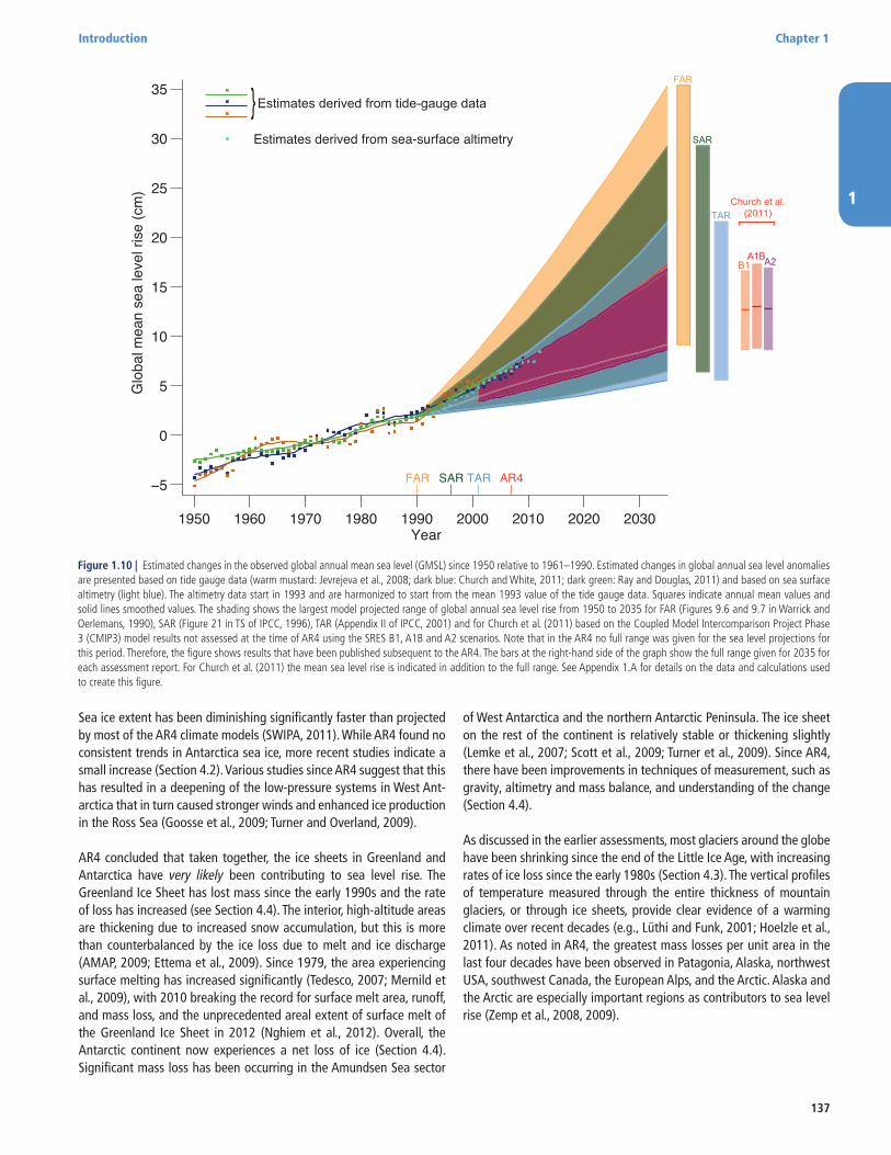
1
Introduction Chapter 1
137
AR4TARSARFAR
1950 1960 1970 1980 1990 2000 2010 2020 2030
−5
0
5
10
15
20
25
30
35
Year
Glo
bal m
ean
sea
leve
l ris
e (c
m)
FAR
SAR
TAR
A1BA2B1
Church et al.(2011)
Estimates derived from sea-surface altimetry
Estimates derived from tide-gauge data}
Figure 1.10 | Estimated changes in the observed global annual mean sea level (GMSL) since 1950 relative to 1961–1990. Estimated changes in global annual sea level anomalies are presented based on tide gauge data (warm mustard: Jevrejeva et al., 2008; dark blue: Church and White, 2011; dark green: Ray and Douglas, 2011) and based on sea surface altimetry (light blue). The altimetry data start in 1993 and are harmonized to start from the mean 1993 value of the tide gauge data. Squares indicate annual mean values and solid lines smoothed values. The shading shows the largest model projected range of global annual sea level rise from 1950 to 2035 for FAR (Figures 9.6 and 9.7 in Warrick and Oerlemans, 1990), SAR (Figure 21 in TS of IPCC, 1996), TAR (Appendix II of IPCC, 2001) and for Church et al. (2011) based on the Coupled Model Intercomparison Project Phase 3 (CMIP3) model results not assessed at the time of AR4 using the SRES B1, A1B and A2 scenarios. Note that in the AR4 no full range was given for the sea level projections for this period. Therefore, the figure shows results that have been published subsequent to the AR4. The bars at the right-hand side of the graph show the full range given for 2035 for each assessment report. For Church et al. (2011) the mean sea level rise is indicated in addition to the full range. See Appendix 1.A for details on the data and calculations used to create this figure.
Sea ice extent has been diminishing significantly faster than projected by most of the AR4 climate models (SWIPA, 2011). While AR4 found no consistent trends in Antarctica sea ice, more recent studies indicate a small increase (Section 4.2). Various studies since AR4 suggest that this has resulted in a deepening of the low-pressure systems in West Ant-arctica that in turn caused stronger winds and enhanced ice production in the Ross Sea (Goosse et al., 2009; Turner and Overland, 2009).
AR4 concluded that taken together, the ice sheets in Greenland and Antarctica have very likely been contributing to sea level rise. The Greenland Ice Sheet has lost mass since the early 1990s and the rate of loss has increased (see Section 4.4). The interior, high-altitude areas are thickening due to increased snow accumulation, but this is more than counterbalanced by the ice loss due to melt and ice discharge (AMAP, 2009; Ettema et al., 2009). Since 1979, the area experiencing surface melting has increased significantly (Tedesco, 2007; Mernild et al., 2009), with 2010 breaking the record for surface melt area, runoff, and mass loss, and the unprecedented areal extent of surface melt of the Greenland Ice Sheet in 2012 (Nghiem et al., 2012). Overall, the Antarctic continent now experiences a net loss of ice (Section 4.4). Significant mass loss has been occurring in the Amundsen Sea sector
of West Antarctica and the northern Antarctic Peninsula. The ice sheet on the rest of the continent is relatively stable or thickening slightly (Lemke et al., 2007; Scott et al., 2009; Turner et al., 2009). Since AR4, there have been improvements in techniques of measurement, such as gravity, altimetry and mass balance, and understanding of the change (Section 4.4).
As discussed in the earlier assessments, most glaciers around the globe have been shrinking since the end of the Little Ice Age, with increasing rates of ice loss since the early 1980s (Section 4.3). The vertical profiles of temperature measured through the entire thickness of mountain glaciers, or through ice sheets, provide clear evidence of a warming climate over recent decades (e.g., Lüthi and Funk, 2001; Hoelzle et al., 2011). As noted in AR4, the greatest mass losses per unit area in the last four decades have been observed in Patagonia, Alaska, northwest USA, southwest Canada, the European Alps, and the Arctic. Alaska and the Arctic are especially important regions as contributors to sea level rise (Zemp et al., 2008, 2009).
1
Chapter 1 Introduction
138
1.4 Treatment of Uncertainties
1.4.1 Uncertainty in Environmental Science
Science always involves uncertainties. These arise at each step of the scientific method: in the development of models or hypotheses, in measurements and in analyses and interpretation of scientific assump-tions. Climate science is not different in this regard from other areas of science. The complexity of the climate system and the large range of processes involved bring particular challenges because, for example, gaps in direct measurements of the past can be filled only by recon-structions using proxy data.
Because the Earth’s climate system is characterized by multiple spatial and temporal scales, uncertainties do not usually reduce at a single, predictable rate: for example, new observations may reduce the uncer-tainties surrounding short-timescale processes quite rapidly, while longer timescale processes may require very long observational base-lines before much progress can be made. Characterization of the inter-action between processes, as quantified by models, can be improved by model development, or can shed light on new areas in which uncer-tainty is greater than previously thought. The fact that there is only a single realization of the climate, rather than a range of different climates from which to draw, can matter significantly for certain lines of enquiry, most notably for the detection and attribution of causes of climate change and for the evaluation of projections of future states.
1.4.2 Characterizing Uncertainty
‘Uncertainty’ is a complex and multifaceted property, sometimes orig-inating in a lack of information, and at other times from quite funda-mental disagreements about what is known or even knowable (Moss and Schneider, 2000). Furthermore, scientists often disagree about the best or most appropriate way to characterize these uncertainties: some can be quantified easily while others cannot. Moreover, appropriate characterization is dependent on the intended use of the information and the particular needs of that user community.
Scientific uncertainty can be partitioned in various ways, in which the details of the partitioning usually depend on the context. For instance, the process and classifications used for evaluating observational uncertainty in climate science is not the same as that employed to evaluate projections of future change. Uncertainty in measured quan-tities can arise from a range of sources, such as statistical variation, variability, inherent randomness, inhomogeneity, approximation, sub-jective judgement, and linguistic imprecision (Morgan et al., 1990), or from calibration methodologies, instrumental bias or instrumental limitations (JCGM, 2008).
In the modelling studies that underpin projections of future climate change, it is common to partition uncertainty into four main catego-ries: scenario uncertainty, due to uncertainty of future emissions of GHGs and other forcing agents; ‘model uncertainty’ associated with climate models; internal variability and initial condition uncertainty; and forcing and boundary condition uncertainty for the assessment of historical and paleoclimate simulations (e.g., Collins and Allen, 2002; Yip et al., 2011).
Model uncertainty is an important contributor to uncertainty in cli-mate predictions and projections. It includes, but is not restricted to, the uncertainties introduced by errors in the model’s representation of dynamical and physical and bio-geochemical aspects of the climate system as well as in the model’s response to external forcing. The phrase ‘model uncertainty’ is a common term in the climate change literature, but different studies use the phrase in different senses: some use it to represent the range of behaviours observed in ensembles of climate model (model spread), while others use it in more comprehen-sive senses (see Sections 9.2, 11.2 and 12.2). Model spread is often used as a measure of climate response uncertainty, but such a measure is crude as it takes no account of factors such as model quality (Chap-ter 9) or model independence (e.g., Masson and Knutti, 2011; Pennell and Reichler, 2011), and not all variables of interest are adequately simulated by global climate models.
To maintain a degree of terminological clarity this report distinguishes between ‘model spread’ for this narrower representation of climate model responses and ‘model uncertainty’ which describes uncertainty about the extent to which any particular climate model provides an accurate representation of the real climate system. This uncertainty arises from approximations required in the development of models. Such approximations affect the representation of all aspects of the cli-mate including the response to external forcings.
Model uncertainty is sometimes decomposed further into parametric and structural uncertainty, comprising, respectively, uncertainty in the values of model parameters and uncertainty in the underlying model structure (see Section 12.2). Some scientific research areas, such as detection and attribution and observationally-constrained model pro-jections of future climate, incorporate significant elements of both observational and model-based science, and in these instances both sets of relevant uncertainties need to be incorporated.
Scenario uncertainty refers to the uncertainties that arise due to limita-tions in our understanding of future emissions, concentration or forcing trajectories. Scenarios help in the assessment of future developments in complex systems that are either inherently unpredictable, or that have high scientific uncertainties (IPCC, 2000). The societal choices defining future climate drivers are surrounded by considerable uncer-tainty, and these are explored by examining the climate response to a wide range of possible futures. In past reports, emissions scenarios from the SRES (IPCC, 2000) were used as the main way of exploring uncertainty in future anthropogenic climate drivers. Recent research has made use of Representative Concentration Pathways (RCP) (van Vuuren et al., 2011a, 2011b).
Internal or natural variability, the natural fluctuations in climate, occur in the absence of any RF of the Earth’s climate (Hawkins and Sutton, 2009). Climate varies naturally on nearly all time and space scales, and quantifying precisely the nature of this variability is challenging, and is characterized by considerable uncertainty. The analysis of internal and forced contributions to recent climate is discussed in Chapter 10. The fractional contribution of internal variability compared with other forms of uncertainty varies in time and in space, but usually diminish-es with time as other sources of uncertainty become more significant (Hawkins and Sutton, 2009; see also Chapter 11 and FAQ 1.1).
1
Introduction Chapter 1
139
In the WGI contribution to the AR5, uncertainty is quantified using 90% uncertainty intervals unless otherwise stated. The 90% uncer-tainty interval, reported in square brackets, is expected to have a 90% likelihood of covering the value that is being estimated. The value that is being estimated has a 5% likelihood of exceeding the upper end-point of the uncertainty interval, and the value has a 5% likelihood of being less than that the lower endpoint of the uncertainty interval. A best estimate of that value is also given where available. Uncertainty intervals are not necessarily symmetric about the corresponding best estimate.
In a subject as complex and diverse as climate change, the information available as well as the way it is expressed, and often the interpreta-tion of that material, varies considerably with the scientific context. In some cases, two studies examining similar material may take different approaches even to the quantification of uncertainty. The interpretation of similar numerical ranges for similar variables can differ from study to study. Readers are advised to pay close attention to the caveats and conditions that surround the results presented in peer- reviewed studies, as well as those presented in this assessment. To help readers in this complex and subtle task, the IPCC draws on specific, calibrat-ed language scales to express uncertainty (Mastrandrea et al., 2010), as well as specific procedures for the expression of uncertainty (see Table 1.2). The aim of these structures is to provide tools through which chapter teams might consistently express uncertainty in key results.
1.4.3 Treatment of Uncertainty in IPCC
In the course of the IPCC assessment procedure, chapter teams review the published research literature, document the findings (including uncertainties), assess the scientific merit of this information, identify the key findings, and attempt to express an appropriate measure of the uncertainty that accompanies these findings using a shared guid-ance procedure. This process has changed over time. The early Assess-ment Reports (FAR and SAR) were largely qualitative. As the field has grown and matured, uncertainty is being treated more explicitly, with a greater emphasis on the expression, where possible and appropriate, of quantified measures of uncertainty.
Although IPCC’s treatment of uncertainty has become more sophis-ticated since the early reports, the rapid growth and considerable diversity of climate research literature presents ongoing challenges. In the wake of the TAR the IPCC formed a Cross-Working Group team charged with identifying the issues and compiling a set of Uncertainty Guidance Notes that could provide a structure for consistent treatment of uncertainty across the IPCC’s remit (Manning et al., 2004). These expanded on the procedural elements of Moss and Schneider (2000) and introduced calibrated language scales designed to enable chap-ter teams to use the appropriate level of precision to describe find-ings. These notes were revised between the TAR and AR4 and again between AR4 and AR5 (Mastrandrea et al., 2010).
Recently, increased engagement of social scientists (e.g., Patt and Schrag, 2003; Kandlikar et al., 2005; Risbey and Kandlikar, 2007; Broomell and Budescu, 2009; Budescu et al., 2009; CCSP, 2009) and expert advisory panels (CCSP, 2009; InterAcademy Council, 2010) in the area of uncertainty and climate change has helped clarify issues
and procedures to improve presentation of uncertainty. Many of the recommendations of these groups are addressed in the revised Guid-ance Notes. One key revision relates to clarification of the relation-ship between the ‘confidence’ and ‘likelihood’ language, and pertains to demarcation between qualitative descriptions of ‘confidence’ and the numerical representations of uncertainty that are expressed by the likelihood scale. In addition, a finding that includes a probabilistic measure of uncertainty does not require explicit mention of the level of confidence associated with that finding if the level of confidence is high or very high. This is a concession to stylistic clarity and readabil-ity: if something is described as having a high likelihood, then in the absence of additional qualifiers it should be inferred that it also has high or very high confidence.
1.4.4 Uncertainty Treatment in This Assessment
All three IPCC Working Groups in the AR5 have agreed to use two met-rics for communicating the degree of certainty in key findings (Mas-trandrea et al., 2010):
• Confidence in the validity of a finding, based on the type, amount, quality, and consistency of evidence (e.g., data, mechanistic under-standing, theory, models, expert judgment) and the degree of agreement. Confidence is expressed qualitatively.
• Quantified measures of uncertainty in a finding expressed proba-bilistically (based on statistical analysis of observations or model results, or expert judgement).
A level of confidence synthesizes the Chapter teams’ judgements about the validity of findings as determined through evaluation of the availa-ble evidence and the degree of scientific agreement. The evidence and agreement scale underpins the assessment, as it is on the basis of evi-dence and agreement that statements can be made with scientific con-fidence (in this sense, the evidence and agreement scale replaces the ‘level of scientific understanding’ scale used in previous WGI assess-ments). There is flexibility in this relationship; for a given evidence and agreement statement, different confidence levels could be assigned, but increasing levels of evidence and degrees of agreement are cor-related with increasing confidence. Confidence cannot necessarily be assigned for all combinations of evidence and agreement, but where key variables are highly uncertain, the available evidence and scientific agreement regarding that variable are presented and discussed. Confi-dence should not be interpreted probabilistically, and it is distinct from ‘statistical confidence’.
The confidence level is based on the evidence (robust, medium and limited) and the agreement (high, medium and low). A combination of different methods, e.g., observations and modelling, is important for evaluating the confidence level. Figure 1.11 shows how the combined evidence and agreement results in five levels for the confidence level used in this assessment.
The qualifier ‘likelihood’ provides calibrated language for describ-ing quantified uncertainty. It can be used to express a probabilistic e stimate of the occurrence of a single event or of an outcome, for example, a climate parameter, observed trend, or projected change
1
Chapter 1 Introduction
140
Frequently Asked Questions
FAQ 1.1 | If Understanding of the Climate System Has Increased, Why Hasn’t the Range of Temperature Projections Been Reduced?
The models used to calculate the IPCC’s temperature projections agree on the direction of future global change, but the projected size of those changes cannot be precisely predicted. Future greenhouse gas (GHG) emission rates could take any one of many possible trajectories, and some underlying physical processes are not yet completely understood, making them difficult to model. Those uncertainties, combined with natural year-to-year climate variability, produce an ‘uncertainty range’ in temperature projections.
The uncertainty range around projected GHG and aerosol precursor emissions (which depend on projections of future social and economic conditions) cannot be materially reduced. Nevertheless, improved understanding and climate models—along with observational constraints—may reduce the uncertainty range around some factors that influence the climate’s response to those emission changes. The complexity of the climate system, however, makes this a slow process. (FAQ1.1, Figure 1)
Climate science has made many important advances since the last IPCC assessment report, thanks to improvements in measurements and data analysis in the cryosphere, atmosphere, land, biosphere and ocean systems. Scientists also have better understanding and tools to model the role of clouds, sea ice, aerosols, small-scale ocean mixing, the carbon cycle and other processes. More observations mean that models can now be evaluated more thoroughly, and projections can be better constrained. For example, as models and observational analysis have improved, projections of sea level rise have become more accurate, balancing the current sea level rise budget.
Despite these advances, there is still a range in plausible projections for future global and regional climate—what scientists call an ‘uncertainty range’. These uncertainty ranges are specific to the variable being considered (precipitation vs. temperature, for instance) and the spatial and temporal extent (such as regional vs. global averages). Uncertainties in climate projections arise from natural variability and uncertainty around the rate of future emissions and the climate’s response to them. They can also occur because representations of some known processes are as yet unrefined, and because some processes are not included in the models.
There are fundamental limits to just how precisely annual temperatures can be projected, because of the chaotic nature of the climate system. Furthermore, decadal-scale projections are sensitive to prevailing conditions—such as the temperature of the deep ocean—that are less well known. Some natural variability over decades arises from interactions between the ocean, atmosphere, land, biosphere and cryosphere, and is also linked to phenomena such as the El Niño-Southern Oscillation (ENSO) and the North Atlantic Oscillation (see Box 2.5 for details on patterns and indices of climate variability).
Volcanic eruptions and variations in the sun’s output also contribute to natural variability, although they are externally forced and explainable. This natural variability can be viewed as part of the ‘noise’ in the climate record, which provides the backdrop against which the ‘signal’ of anthropogenic climate change is detected.
Natural variability has a greater influence on uncertainty at regional and local scales than it does over continental or global scales. It is inherent in the Earth system, and more knowledge will not eliminate the uncertainties it brings. However, some progress is possible—particularly for projections up to a few years ahead—which exploit advances in knowledge of, for instance, the cryosphere or ocean state and processes. This is an area of active research. When climate variables are averaged over decadal timescales or longer, the relative importance of internal variability diminishes, making the long-term signals more evident (FAQ1.1, Figure 1). This long-term perspective is consistent with a common definition of climate as an average over 30 years.
A second source of uncertainty stems from the many possible trajectories that future emission rates of GHGs and aerosol precursors might take, and from future trends in land use. Nevertheless, climate projections rely on input from these variables. So to obtain these estimates, scientists consider a number of alternative scenarios for future human society, in terms of population, economic and technological change, and political choices. They then estimate the likely emissions under each scenario. The IPCC informs policymaking, therefore climate projections for different emissions scenarios can be useful as they show the possible climatic consequences of different policy choices. These scenarios are intended to be compatible with the full range of emissions scenarios described in the current scientific literature, with or without climate policy. As such, they are designed to sample uncertainty in future scenarios. (continued on next page)
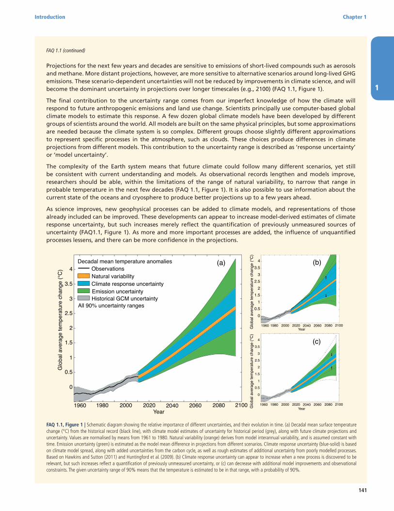
1
Introduction Chapter 1
141
FAQ 1.1 (continued)
Projections for the next few years and decades are sensitive to emissions of short-lived compounds such as aerosols and methane. More distant projections, however, are more sensitive to alternative scenarios around long-lived GHG emissions. These scenario-dependent uncertainties will not be reduced by improvements in climate science, and will become the dominant uncertainty in projections over longer timescales (e.g., 2100) (FAQ 1.1, Figure 1).
The final contribution to the uncertainty range comes from our imperfect knowledge of how the climate will respond to future anthropogenic emissions and land use change. Scientists principally use computer-based global climate models to estimate this response. A few dozen global climate models have been developed by different groups of scientists around the world. All models are built on the same physical principles, but some approximations are needed because the climate system is so complex. Different groups choose slightly different approximations to represent specific processes in the atmosphere, such as clouds. These choices produce differences in climate projections from different models. This contribution to the uncertainty range is described as ‘response uncertainty’ or ‘model uncertainty’.
The complexity of the Earth system means that future climate could follow many different scenarios, yet still be consistent with current understanding and models. As observational records lengthen and models improve, researchers should be able, within the limitations of the range of natural variability, to narrow that range in probable temperature in the next few decades (FAQ 1.1, Figure 1). It is also possible to use information about the current state of the oceans and cryosphere to produce better projections up to a few years ahead.
As science improves, new geophysical processes can be added to climate models, and representations of those already included can be improved. These developments can appear to increase model-derived estimates of climate response uncertainty, but such increases merely reflect the quantification of previously unmeasured sources of uncertainty (FAQ1.1, Figure 1). As more and more important processes are added, the influence of unquantified processes lessens, and there can be more confidence in the projections.
Year1960 1980 2000 2020 2040 2060 2080 2100
0
0.5
1
1.5
2
2.5
3
3.5
4
Glo
bal a
vera
ge te
mpe
ratu
re c
hang
e (°
C)
Decadal mean temperature anomaliesObservationsNatural variabilityClimate response uncertaintyEmission uncertaintyHistorical GCM uncertainty
All 90% uncertainty ranges
(a)
Year1960 1980 2000 2020 2040 2060 2080 2100
(b)
00.5
11.5
22.5
33.5
4
Glo
bal a
vera
ge te
mpe
ratu
re c
hang
e (°
C)
Year1960 1980 2000 2020 2040 2060 2080 2100
(c)
0
0.5
1
1.5
2
2.5
3
3.5
4
Glo
bal a
vera
ge te
mpe
ratu
re c
hang
e (°
C)
FAQ 1.1, Figure 1 | Schematic diagram showing the relative importance of different uncertainties, and their evolution in time. (a) Decadal mean surface temperature change (°C) from the historical record (black line), with climate model estimates of uncertainty for historical period (grey), along with future climate projections and uncertainty. Values are normalised by means from 1961 to 1980. Natural variability (orange) derives from model interannual variability, and is assumed constant with time. Emission uncertainty (green) is estimated as the model mean difference in projections from different scenarios. Climate response uncertainty (blue-solid) is based on climate model spread, along with added uncertainties from the carbon cycle, as well as rough estimates of additional uncertainty from poorly modelled processes. Based on Hawkins and Sutton (2011) and Huntingford et al. (2009). (b) Climate response uncertainty can appear to increase when a new process is discovered to be relevant, but such increases reflect a quantification of previously unmeasured uncertainty, or (c) can decrease with additional model improvements and observational constraints. The given uncertainty range of 90% means that the temperature is estimated to be in that range, with a probability of 90%.
1
Chapter 1 Introduction
142
lying in a given range. Statements made using the likelihood scale may be based on statistical or modelling analyses, elicitation of expert views, or other quantitative analyses. Where sufficient information is available it is preferable to eschew the likelihood qualifier in favour of the full probability distribution or the appropriate probability range. See Table 1.2 for the list of ‘likelihood’ qualifiers to be used in AR5.
Many social sciences studies have found that the interpretation of uncertainty is contingent on the presentation of information, the con-text within which statements are placed and the interpreter’s own lexical preferences. Readers often adjust their interpretation of prob-abilistic language according to the magnitude of perceived potential consequences (Patt and Schrag, 2003; Patt and Dessai, 2005). Further-more, the framing of a probabilistic statement impinges on how it is interpreted (Kahneman and Tversky, 1979): for example, a 10% chance of dying is interpreted more negatively than a 90% chance of surviving.
In addition, work examining expert judgement and decision making shows that people—including scientific experts—are prone to a range of heuristics and biases that affect their judgement (e.g., Kahneman et al., 1982). For example, in the case of expert judgements there is a tendency towards overconfidence both at the individual level (Morgan et al., 1990) and at the group level as people converge on a view and draw confidence in its reliability from each other. However, in an assessment of the state of scientific knowledge across a field
such as climate change—characterized by complexity of process and heterogeneity of data constraints—some degree of expert judgement is inevitable (Mastrandrea et al., 2010).
These issues were brought to the attention of chapter teams so that contributors to the AR5 might be sensitized to the ways presentation, framing, context and potential biases might affect their own assess-ments and might contribute to readers’ understanding of the infor-mation presented in this assessment. There will always be room for debate about how to summarize such a large and growing literature. The uncertainty guidance is aimed at providing a consistent, cali-brated set of words through which to communicate the uncertainty, confidence and degree of consensus prevailing in the scientific litera-ture. In this sense the guidance notes and practices adopted by IPCC for the presentation of uncertainties should be regarded as an inter-disciplinary work in progress, rather than as a finalized, comprehensive approach. Moreover, one precaution that should be considered is that translation of this assessment from English to other languages may lead to a loss of precision.
1.5 Advances in Measurement and Modelling Capabilities
Since AR4, measurement capabilities have continued to advance. The models have been improved following the progress in the understand-ing of physical processes within the climate system. This section illus-trates some of those developments.
1.5.1 Capabilities of Observations
Improved understanding and systematic monitoring of Earth’s climate requires observations of various atmospheric, oceanic and terrestrial parameters and therefore has to rely on various technologies (ranging from ground-based instruments to ships, buoys, ocean profilers, bal-loons, aircraft, satellite-borne sensors, etc.). The Global Climate Observ-ing System (GCOS, 2009) defined a list of so-called Essential Climate Variables, that are technically and economically feasible to observe, but some of the associated observing systems are not yet operated in a systematic manner. However, during recent years, new observational systems have increased the number of observations by orders of mag-nitude and observations have been made at places where there have been no data before (see Chapters 2, 3 and 4 for an assessment of changes in observations). Parallel to this, tools to analyse and process the data have been developed and enhanced to cope with the increase of information and to provide a more comprehensive picture of the Earth’s climate. At the same time, it should be kept in mind that there has been some limited progress in developing countries in filling gaps in their in situ observing networks, but developed countries have made little progress in ensuring long-term continuity for several important observing systems (GCOS, 2009). In addition, more proxy (non-instru-mental) data have been acquired to provide a more comprehensive picture of climate changes in the past (see Chapter 5). Efforts are also occurring to digitize historic observations, mainly of ground-station data from periods prior to the second half of the 20th century (Brunet and Jones, 2011).
High agreementLimited evidence
High agreementMedium evidence
High agreementRobust evidence
Medium agreementRobust evidence
Medium agreementMedium evidence
Medium agreementLimited evidence
Low agreementLimited evidence
Low agreementMedium evidence
Low agreementRobust evidence
Evidence (type, amount, quality, consistency)
Agr
eem
ent
Confidence Scale
Figure 1.11 | The basis for the confidence level is given as a combination of evidence (limited, medium, robust) and agreement (low, medium and high) (Mastrandrea et al., 2010).
Term Likelihood of the Outcome
Virtually certain 99−100% probability
Very likely 90−100% probability
Likely 66−100% probability
About as likely as not 33−66% probability
Unlikely 0−33% probability
Very unlikely 0−10% probability
Exceptionally unlikely 0−1% probability
Notes:Additional terms that were used in limited circumstances in the AR4 (extremely likely = 95−100% probability, more likely than not = >50−100% probability, and extremely unlikely = 0−5% probability) may also be used in the AR5 when appropriate.
Table 1.2 | Likelihood terms associated with outcomes used in the AR5.
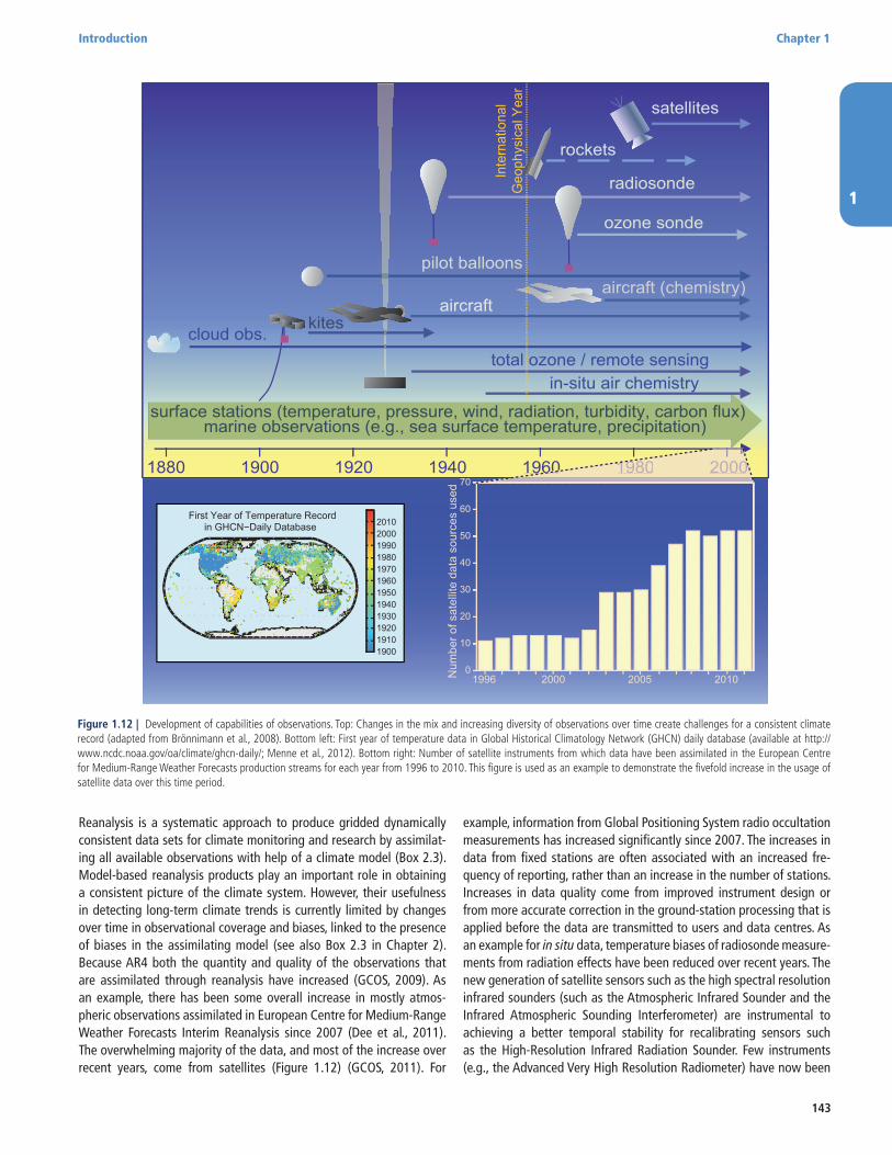
1
Introduction Chapter 1
143
19601940192019001880
satellites
rockets
radiosondeInte
rnat
iona
l G
eoph
ysic
al Y
ear
ozone sonde
aircraftaircraft (chemistry)
kites
pilot balloons
total ozone / remote sensingin-situ air chemistry
cloud obs.
surface stations (temperature, pressure, wind, radiation, turbidity, carbon flux)marine observations (e.g., sea surface temperature, precipitation)
1980 2000
First Year of Temperature Recordin GHCN−Daily Database
190019101920193019401950196019701980199020002010
1996 0
10
20
30
40
50
60
70
2000 2005 2010 Num
ber o
f sat
ellit
e da
ta s
ourc
es u
sed
60 1980 200096 060 199
Figure 1.12 | Development of capabilities of observations. Top: Changes in the mix and increasing diversity of observations over time create challenges for a consistent climate record (adapted from Brönnimann et al., 2008). Bottom left: First year of temperature data in Global Historical Climatology Network (GHCN) daily database (available at http://www.ncdc.noaa.gov/oa/climate/ghcn-daily/; Menne et al., 2012). Bottom right: Number of satellite instruments from which data have been assimilated in the European Centre for Medium-Range Weather Forecasts production streams for each year from 1996 to 2010. This figure is used as an example to demonstrate the fivefold increase in the usage of satellite data over this time period.
Reanalysis is a systematic approach to produce gridded dynamically consistent data sets for climate monitoring and research by assimilat-ing all available observations with help of a climate model (Box 2.3). Model-based reanalysis products play an important role in obtaining a consistent picture of the climate system. However, their usefulness in detecting long-term climate trends is currently limited by changes over time in observational coverage and biases, linked to the presence of biases in the assimilating model (see also Box 2.3 in Chapter 2). Because AR4 both the quantity and quality of the observations that are assimilated through reanalysis have increased (GCOS, 2009). As an example, there has been some overall increase in mostly atmos-pheric observations assimilated in European Centre for Medium-Range Weather Forecasts Interim Reanalysis since 2007 (Dee et al., 2011). The overwhelming majority of the data, and most of the increase over recent years, come from satellites (Figure 1.12) (GCOS, 2011). For
example, information from Global Positioning System radio occultation measurements has increased significantly since 2007. The increases in data from fixed stations are often associated with an increased fre-quency of reporting, rather than an increase in the number of stations. Increases in data quality come from improved instrument design or from more accurate correction in the ground-station processing that is applied before the data are transmitted to users and data centres. As an example for in situ data, temperature biases of radiosonde measure-ments from radiation effects have been reduced over recent years. The new generation of satellite sensors such as the high spectral resolution infrared sounders (such as the Atmospheric Infrared Sounder and the Infrared Atmospheric Sounding Interferometer) are instrumental to achieving a better temporal stability for recalibrating sensors such as the High-Resolution Infrared Radiation Sounder. Few instruments (e.g., the Advanced Very High Resolution Radiometer) have now been
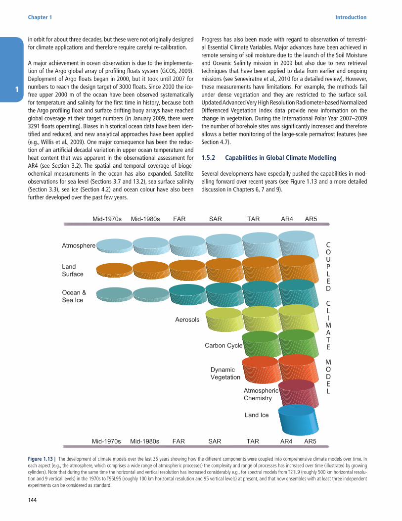
1
Chapter 1 Introduction
144
in orbit for about three decades, but these were not originally designed for climate applications and therefore require careful re-calibration.
A major achievement in ocean observation is due to the implementa-tion of the Argo global array of profiling floats system (GCOS, 2009). Deployment of Argo floats began in 2000, but it took until 2007 for numbers to reach the design target of 3000 floats. Since 2000 the ice-free upper 2000 m of the ocean have been observed systematically for temperature and salinity for the first time in history, because both the Argo profiling float and surface drifting buoy arrays have reached global coverage at their target numbers (in January 2009, there were 3291 floats operating). Biases in historical ocean data have been iden-tified and reduced, and new analytical approaches have been applied (e.g., Willis et al., 2009). One major consequence has been the reduc-tion of an artificial decadal variation in upper ocean temperature and heat content that was apparent in the observational assessment for AR4 (see Section 3.2). The spatial and temporal coverage of bioge-ochemical measurements in the ocean has also expanded. Satellite observations for sea level (Sections 3.7 and 13.2), sea surface salinity (Section 3.3), sea ice (Section 4.2) and ocean colour have also been further developed over the past few years.
Progress has also been made with regard to observation of terrestri-al Essential Climate Variables. Major advances have been achieved in remote sensing of soil moisture due to the launch of the Soil Moisture and Oceanic Salinity mission in 2009 but also due to new retrieval techniques that have been applied to data from earlier and ongoing missions (see Seneviratne et al., 2010 for a detailed review). However, these measurements have limitations. For example, the methods fail under dense vegetation and they are restricted to the surface soil. Updated Advanced Very High Resolution Radiometer-based Normalized Differenced Vegetation Index data provide new information on the change in vegetation. During the International Polar Year 2007–2009 the number of borehole sites was significantly increased and therefore allows a better monitoring of the large-scale permafrost features (see Section 4.7).
1.5.2 Capabilities in Global Climate Modelling
Several developments have especially pushed the capabilities in mod-elling forward over recent years (see Figure 1.13 and a more detailed discussion in Chapters 6, 7 and 9).
Atmosphere
LandSurface
Ocean & Sea Ice
Aerosols
Carbon Cycle
Dynamic Vegetation
AtmosphericChemistry
Mid-1970s Mid-1980s TARSARFAR AR4
COUPLED
CLI
MATE
MODEL
Land Ice
AR5
Mid-1970s Mid-1980s TARSARFAR AR4 AR5
Figure 1.13 | The development of climate models over the last 35 years showing how the different components were coupled into comprehensive climate models over time. In each aspect (e.g., the atmosphere, which comprises a wide range of atmospheric processes) the complexity and range of processes has increased over time (illustrated by growing cylinders). Note that during the same time the horizontal and vertical resolution has increased considerably e.g., for spectral models from T21L9 (roughly 500 km horizontal resolu-tion and 9 vertical levels) in the 1970s to T95L95 (roughly 100 km horizontal resolution and 95 vertical levels) at present, and that now ensembles with at least three independent experiments can be considered as standard.
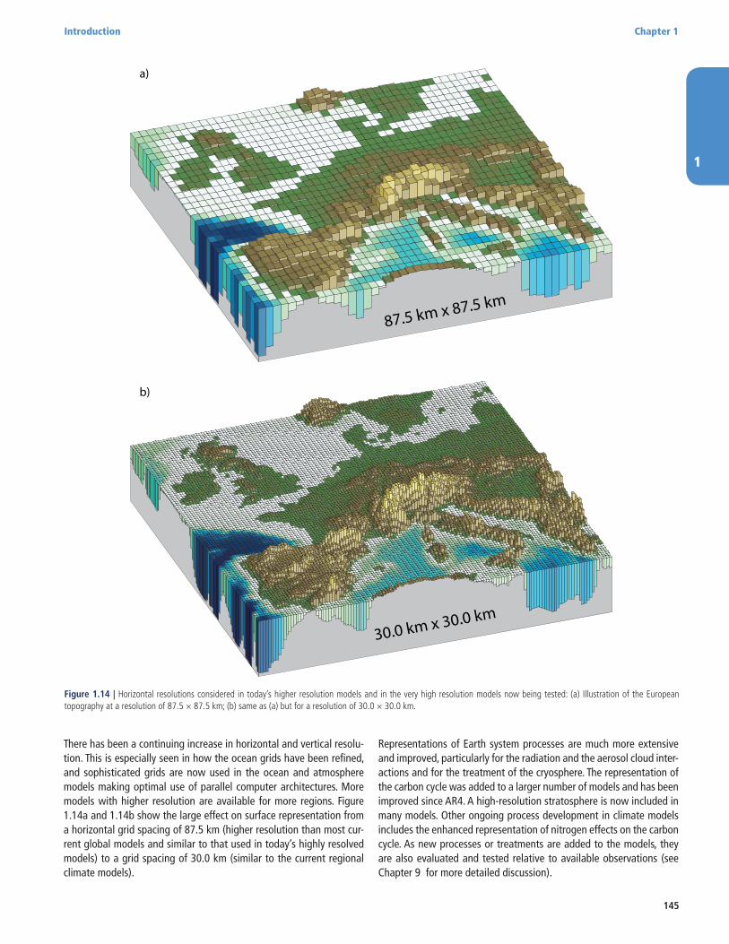
1
Introduction Chapter 1
145
87.5 km x 87.5 km
30.0 km x 30.0 km
a)
b)
Figure 1.14 | Horizontal resolutions considered in today’s higher resolution models and in the very high resolution models now being tested: (a) Illustration of the European topography at a resolution of 87.5 × 87.5 km; (b) same as (a) but for a resolution of 30.0 × 30.0 km.
There has been a continuing increase in horizontal and vertical resolu-tion. This is especially seen in how the ocean grids have been refined, and sophisticated grids are now used in the ocean and atmosphere models making optimal use of parallel computer architectures. More models with higher resolution are available for more regions. Figure 1.14a and 1.14b show the large effect on surface representation from a horizontal grid spacing of 87.5 km (higher resolution than most cur-rent global models and similar to that used in today’s highly resolved models) to a grid spacing of 30.0 km (similar to the current regional climate models).
Representations of Earth system processes are much more extensive and improved, particularly for the radiation and the aerosol cloud inter-actions and for the treatment of the cryosphere. The representation of the carbon cycle was added to a larger number of models and has been improved since AR4. A high-resolution stratosphere is now included in many models. Other ongoing process development in climate models includes the enhanced representation of nitrogen effects on the carbon cycle. As new processes or treatments are added to the models, they are also evaluated and tested relative to available observations (see Chapter 9 for more detailed discussion).
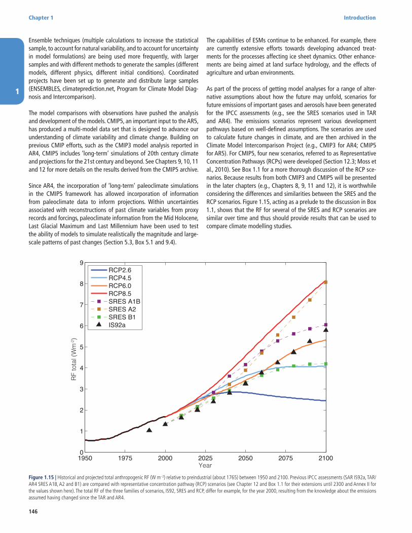
1
Chapter 1 Introduction
146
Ensemble techniques (multiple calculations to increase the statistical sample, to account for natural variability, and to account for uncertainty in model formulations) are being used more frequently, with larger samples and with different methods to generate the samples (different models, different physics, different initial conditions). Coordinated projects have been set up to generate and distribute large samples (ENSEMBLES, climateprediction.net, Program for Climate Model Diag-nosis and Intercomparison).
The model comparisons with observations have pushed the analysis and development of the models. CMIP5, an important input to the AR5, has produced a multi-model data set that is designed to advance our understanding of climate variability and climate change. Building on previous CMIP efforts, such as the CMIP3 model analysis reported in AR4, CMIP5 includes ‘long-term’ simulations of 20th century climate and projections for the 21st century and beyond. See Chapters 9, 10, 11 and 12 for more details on the results derived from the CMIP5 archive.
Since AR4, the incorporation of ‘long-term’ paleoclimate simulations in the CMIP5 framework has allowed incorporation of information from paleoclimate data to inform projections. Within uncertainties associated with reconstructions of past climate variables from proxy records and forcings, paleoclimate information from the Mid Holocene, Last Glacial Maximum and Last Millennium have been used to test the ability of models to simulate realistically the magnitude and large-scale patterns of past changes (Section 5.3, Box 5.1 and 9.4).
The capabilities of ESMs continue to be enhanced. For example, there are currently extensive efforts towards developing advanced treat-ments for the processes affecting ice sheet dynamics. Other enhance-ments are being aimed at land surface hydrology, and the effects of agriculture and urban environments.
As part of the process of getting model analyses for a range of alter-native assumptions about how the future may unfold, scenarios for future emissions of important gases and aerosols have been generated for the IPCC assessments (e.g., see the SRES scenarios used in TAR and AR4). The emissions scenarios represent various development pathways based on well-defined assumptions. The scenarios are used to calculate future changes in climate, and are then archived in the Climate Model Intercomparison Project (e.g., CMIP3 for AR4; CMIP5 for AR5). For CMIP5, four new scenarios, referred to as Representative Concentration Pathways (RCPs) were developed (Section 12.3; Moss et al., 2010). See Box 1.1 for a more thorough discussion of the RCP sce-narios. Because results from both CMIP3 and CMIP5 will be presented in the later chapters (e.g., Chapters 8, 9, 11 and 12), it is worthwhile considering the differences and similarities between the SRES and the RCP scenarios. Figure 1.15, acting as a prelude to the discussion in Box 1.1, shows that the RF for several of the SRES and RCP scenarios are similar over time and thus should provide results that can be used to compare climate modelling studies.
1950 1975 2000 2025 2050 2075 21000
1
2
3
4
5
6
7
8
9
Year
RF
tota
l (W
m-2)
RCP2.6RCP4.5RCP6.0RCP8.5SRES A1BSRES A2SRES B1IS92a
Figure 1.15 | Historical and projected total anthropogenic RF (W m–2) relative to preindustrial (about 1765) between 1950 and 2100. Previous IPCC assessments (SAR IS92a, TAR/AR4 SRES A1B, A2 and B1) are compared with representative concentration pathway (RCP) scenarios (see Chapter 12 and Box 1.1 for their extensions until 2300 and Annex II for the values shown here). The total RF of the three families of scenarios, IS92, SRES and RCP, differ for example, for the year 2000, resulting from the knowledge about the emissions assumed having changed since the TAR and AR4.
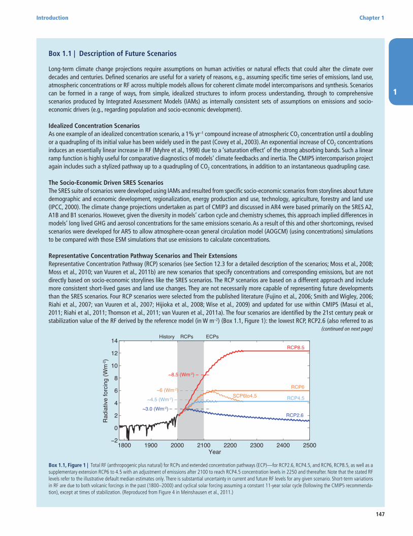
1
Introduction Chapter 1
147
Box 1.1 | Description of Future Scenarios
Long-term climate change projections require assumptions on human activities or natural effects that could alter the climate over decades and centuries. Defined scenarios are useful for a variety of reasons, e.g., assuming specific time series of emissions, land use, atmospheric concentrations or RF across multiple models allows for coherent climate model intercomparisons and synthesis. Scenarios can be formed in a range of ways, from simple, idealized structures to inform process understanding, through to comprehensive scenarios produced by Integrated Assessment Models (IAMs) as internally consistent sets of assumptions on emissions and socio-economic drivers (e.g., regarding population and socio-economic development).
Idealized Concentration ScenariosAs one example of an idealized concentration scenario, a 1% yr–1 compound increase of atmospheric CO2 concentration until a doubling or a quadrupling of its initial value has been widely used in the past (Covey et al., 2003). An exponential increase of CO2 concentrations induces an essentially linear increase in RF (Myhre et al., 1998) due to a ‘saturation effect’ of the strong absorbing bands. Such a linear ramp function is highly useful for comparative diagnostics of models’ climate feedbacks and inertia. The CMIP5 intercomparison project again includes such a stylized pathway up to a quadrupling of CO2 concentrations, in addition to an instantaneous quadrupling case.
The Socio-Economic Driven SRES ScenariosThe SRES suite of scenarios were developed using IAMs and resulted from specific socio-economic scenarios from storylines about future demographic and economic development, regionalization, energy production and use, technology, agriculture, forestry and land use (IPCC, 2000). The climate change projections undertaken as part of CMIP3 and discussed in AR4 were based primarily on the SRES A2, A1B and B1 scenarios. However, given the diversity in models’ carbon cycle and chemistry schemes, this approach implied differences in models’ long lived GHG and aerosol concentrations for the same emissions scenario. As a result of this and other shortcomings, revised scenarios were developed for AR5 to allow atmosphere-ocean general circulation model (AOGCM) (using concentrations) simulations to be compared with those ESM simulations that use emissions to calculate concentrations.
Representative Concentration Pathway Scenarios and Their ExtensionsRepresentative Concentration Pathway (RCP) scenarios (see Section 12.3 for a detailed description of the scenarios; Moss et al., 2008; Moss et al., 2010; van Vuuren et al., 2011b) are new scenarios that specify concentrations and corresponding emissions, but are not directly based on socio-economic storylines like the SRES scenarios. The RCP scenarios are based on a different approach and include more consistent short-lived gases and land use changes. They are not necessarily more capable of representing future developments than the SRES scenarios. Four RCP scenarios were selected from the published literature (Fujino et al., 2006; Smith and Wigley, 2006; Riahi et al., 2007; van Vuuren et al., 2007; Hijioka et al., 2008; Wise et al., 2009) and updated for use within CMIP5 (Masui et al., 2011; Riahi et al., 2011; Thomson et al., 2011; van Vuuren et al., 2011a). The four scenarios are identified by the 21st century peak or stabilization value of the RF derived by the reference model (in W m–2) (Box 1.1, Figure 1): the lowest RCP, RCP2.6 (also referred to as
Box 1.1, Figure 1 | Total RF (anthropogenic plus natural) for RCPs and extended concentration pathways (ECP)—for RCP2.6, RCP4.5, and RCP6, RCP8.5, as well as a supplementary extension RCP6 to 4.5 with an adjustment of emissions after 2100 to reach RCP4.5 concentration levels in 2250 and thereafter. Note that the stated RF levels refer to the illustrative default median estimates only. There is substantial uncertainty in current and future RF levels for any given scenario. Short-term variations in RF are due to both volcanic forcings in the past (1800–2000) and cyclical solar forcing assuming a constant 11-year solar cycle (following the CMIP5 recommenda-tion), except at times of stabilization. (Reproduced from Figure 4 in Meinshausen et al., 2011.)
1800 1900 2000 2100 2200 2300 2400 2500−2
0
2
4
6
8
10
12
14History RCPs ECPs
~3.0 (Wm-2)
~4.5 (Wm-2)
~6 (Wm-2)
~8.5 (Wm-2)
RCP2.6
RCP4.5
RCP6
RCP8.5
SCP6to4.5
Year
Rad
iativ
e fo
rcin
g (W
m-2)
(continued on next page)
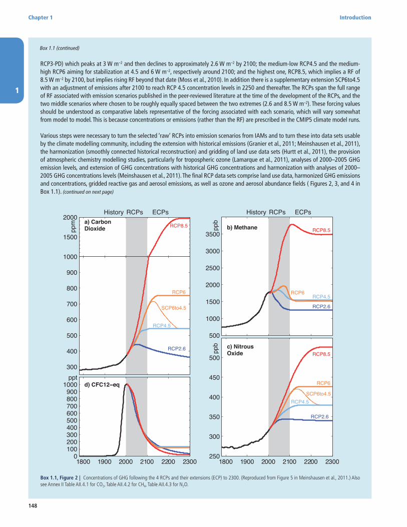
1
Chapter 1 Introduction
148
RCP3-PD) which peaks at 3 W m–2 and then declines to approximately 2.6 W m–2 by 2100; the medium-low RCP4.5 and the medium-high RCP6 aiming for stabilization at 4.5 and 6 W m–2, respectively around 2100; and the highest one, RCP8.5, which implies a RF of 8.5 W m–2 by 2100, but implies rising RF beyond that date (Moss et al., 2010). In addition there is a supplementary extension SCP6to4.5 with an adjustment of emissions after 2100 to reach RCP 4.5 concentration levels in 2250 and thereafter. The RCPs span the full range of RF associated with emission scenarios published in the peer-reviewed literature at the time of the development of the RCPs, and the two middle scenarios where chosen to be roughly equally spaced between the two extremes (2.6 and 8.5 W m–2). These forcing values should be understood as comparative labels representative of the forcing associated with each scenario, which will vary somewhat from model to model. This is because concentrations or emissions (rather than the RF) are prescribed in the CMIP5 climate model runs.
Various steps were necessary to turn the selected ‘raw’ RCPs into emission scenarios from IAMs and to turn these into data sets usable by the climate modelling community, including the extension with historical emissions (Granier et al., 2011; Meinshausen et al., 2011), the harmonization (smoothly connected historical reconstruction) and gridding of land use data sets (Hurtt et al., 2011), the provision of atmospheric chemistry modelling studies, particularly for tropospheric ozone (Lamarque et al., 2011), analyses of 2000–2005 GHG emission levels, and extension of GHG concentrations with historical GHG concentrations and harmonization with analyses of 2000–2005 GHG concentrations levels (Meinshausen et al., 2011). The final RCP data sets comprise land use data, harmonized GHG emissions and concentrations, gridded reactive gas and aerosol emissions, as well as ozone and aerosol abundance fields ( Figures 2, 3, and 4 in Box 1.1). (continued on next page)
Box 1.1, Figure 2 | Concentrations of GHG following the 4 RCPs and their extensions (ECP) to 2300. (Reproduced from Figure 5 in Meinshausen et al., 2011.) Also see Annex II Table AII.4.1 for CO2, Table AII.4.2 for CH4, Table AII.4.3 for N2O.
1500
2000
ppm a) Carbon
Dioxide
History RCPs ECPs
RCP8.5
300
400
500
600
700
800
900
1000
RCP2.6
RCP4.5
RCP6
SCP6to4.5
1800 1900 2000 2100 2200 23000
100200300400500600700800900
1000ppt
d) CFC12−eq
1800 1900 2000 2100 2200 2300250
300
350
400
450
500
ppb c) Nitrous
Oxide RCP8.5
RCP2.6
RCP4.5
RCP6
SCP6to4.5
500
1000
1500
2000
2500
3000
3500
ppb
b) Methane
History RCPs ECPs
RCP8.5
RCP2.6
RCP4.5RCP6
Box 1.1 (continued)
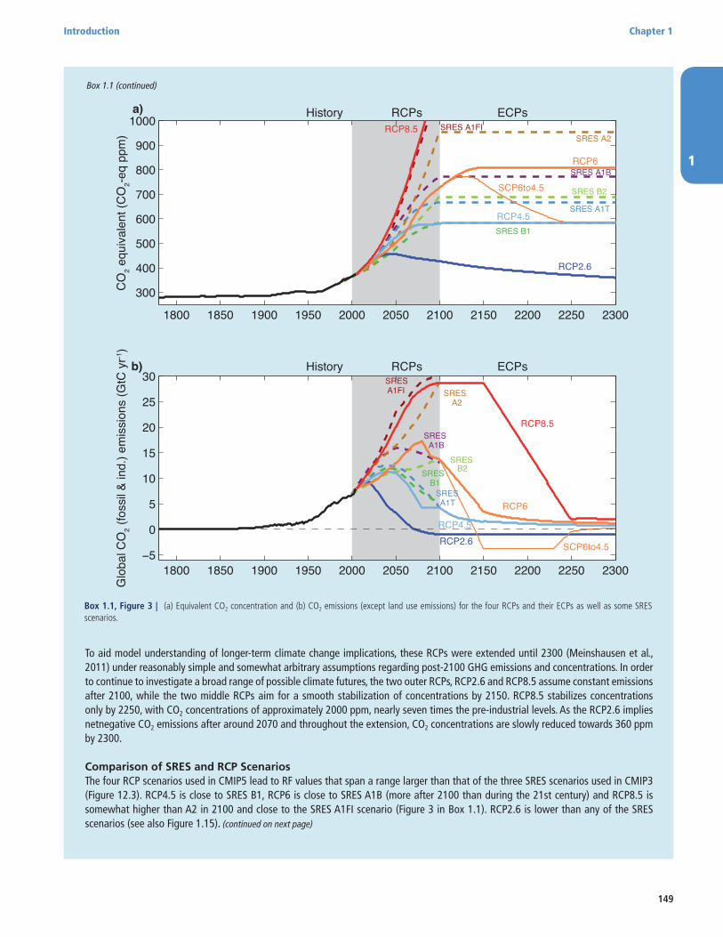
1
Introduction Chapter 1
149
To aid model understanding of longer-term climate change implications, these RCPs were extended until 2300 (Meinshausen et al., 2011) under reasonably simple and somewhat arbitrary assumptions regarding post-2100 GHG emissions and concentrations. In order to continue to investigate a broad range of possible climate futures, the two outer RCPs, RCP2.6 and RCP8.5 assume constant emissions after 2100, while the two middle RCPs aim for a smooth stabilization of concentrations by 2150. RCP8.5 stabilizes concentrations only by 2250, with CO2 concentrations of approximately 2000 ppm, nearly seven times the pre-industrial levels. As the RCP2.6 implies netnegative CO2 emissions after around 2070 and throughout the extension, CO2 concentrations are slowly reduced towards 360 ppm by 2300.
Comparison of SRES and RCP ScenariosThe four RCP scenarios used in CMIP5 lead to RF values that span a range larger than that of the three SRES scenarios used in CMIP3 (Figure 12.3). RCP4.5 is close to SRES B1, RCP6 is close to SRES A1B (more after 2100 than during the 21st century) and RCP8.5 is somewhat higher than A2 in 2100 and close to the SRES A1FI scenario (Figure 3 in Box 1.1). RCP2.6 is lower than any of the SRES scenarios (see also Figure 1.15). (continued on next page)
Box 1.1 (continued)
Box 1.1, Figure 3 | (a) Equivalent CO2 concentration and (b) CO2 emissions (except land use emissions) for the four RCPs and their ECPs as well as some SRES scenarios.
1800 1850 1900 1950 2000 2050 2100 2150 2200 2250 2300
300
400
500
600
700
800
900
1000a) History RCPs ECPs
RCP2.6
RCP4.5
RCP6
RCP8.5
SCP6to4.5SRES A1B
SRES A1FI
SRES A1T
SRES A2
SRES B1
SRES B2
CO
2 equ
ival
ent (
CO
2-eq
ppm
)
1800 1850 1900 1950 2000 2050 2100 2150 2200 2250 2300−5
0
5
10
15
20
25
30b) History RCPs ECPs
RCP2.6RCP4.5
RCP6
RCP8.5
SCP6to4.5
SRESA1B
SRESA1FI
SRESA1T
SRESA2
SRESB1
SRESB2
Glo
bal C
O2 (
foss
il &
ind.
) em
issi
ons
(GtC
yr-1
)
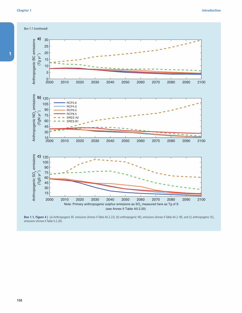
1
Chapter 1 Introduction
150
Box 1.1 (continued)
Box 1.1, Figure 4 | (a) Anthropogenic BC emissions (Annex II Table AII.2.22), (b) anthropogenic NOx emissions (Annex II Table AII.2.18), and (c) anthropogenic SOx emissions (Annex II Table II.2.20).
2000 2010 2020 2030 2040 2050 2060 2070 2080 2090 21000
5
10
15
20
25
30a)An
thro
poge
nic
BC e
mis
sion
s
2000 2010 2020 2030 2040 2050 2060 2070 2080 2090 2100153045607590
105120b)
Ant
hrop
ogen
ic N
OX e
mis
sion
s(T
gN y
r-1)
(Tg
yr-1)
(TgS
yr-1
)
RCP2.6RCP4.5RCP6.0RCP8.5SRES A2SRES B1
2000 2010 2020 2030 2040 2050 2060 2070 2080 2090 2100
153045607590
105120c)
Anth
ropo
geni
c SO
X em
issi
ons
Note: Primary anthropogenic sulphur emissions as SO2 measured here as Tg of S (see Annex II Table AII.2.20)
1
Introduction Chapter 1
151
1.6 Overview and Road Map to the Rest of the Report
As this chapter has shown, understanding of the climate system and the changes occurring in it continue to advance. The notable scientific advances and associated peer-reviewed publications since AR4 provide the basis for the assessment of the science as found in Chapters 2 to 14. Below a quick summary of these chapters and their objectives is provided.
Observations and Paleoclimate Information (Chapters 2, 3, 4 and 5): These chapters assess information from all climate system compo-nents on climate variability and change as obtained from instrumental records and climate archives. This group of chapters covers all relevant aspects of the atmosphere including the stratosphere, the land surface, the oceans and the cryosphere. Information on the water cycle, includ-ing evaporation, precipitation, runoff, soil moisture, floods, drought, etc. is assessed. Timescales from daily to decades (Chapters 2, 3 and 4) and from centuries to many millennia (Chapter 5) are considered.
Process Understanding (Chapters 6 and 7): These chapters cover all relevant aspects from observations and process understanding, to projections from global to regional scale. Chapter 6 covers the carbon cycle and its interactions with other biogeochemical cycles, in particular the nitrogen cycle, as well as feedbacks on the climate system. Chapter 7 treats in detail clouds and aerosols, their interactions and chemistry, the role of water vapour, as well as their role in feedbacks on the cli-mate system.
From Forcing to Attribution of Climate Change (Chapters 8, 9 and 10): In these chapters, all the information on the different drivers (natural and anthropogenic) of climate change is collected, expressed in terms of RF, and assessed (Chapter 8). As part of this, the science of metrics commonly used in the literature to compare radiative effects from a range of agents (Global Warming Potential, Global Temperature Change Potential and others) is covered. In Chapter 9, the hierarchy of climate models used in simulating past and present climate change is assessed. Information regarding detection and attribution of changes on global to regional scales is assessed in Chapter 10.
Future Climate Change and Predictability (Chapters 11 and 12): These chapters assess projections of future climate change derived from climate models on timescales from decades to centuries at both global and regional scales, including mean changes, variability and extremes. Fundamental questions related to the predictability of climate as well as long-term climate change, climate change commitments and inertia in the climate system are addressed.
Integration (Chapters 13 and 14): These chapters integrate all rel-evant information for two key topics in WGI AR5: sea level change (Chapter 13) and climate phenomena across the regions (Chapter 14). Chapter 13 assesses information on sea level change ranging from observations and process understanding to projections from global to regional scales. Chapter 14 assesses the most important modes of variability in the climate system and extreme events. Furthermore, this chapter deals with interconnections between the climate phenome-na, their regional expressions, and their relevance for future regional
climate change. Maps produced and assessed in Chapter 14, together with Chapters 11 and 12, form the basis of the Atlas of Global and Regional Climate Projections in Annex I. RFs and estimates of future atmospheric concentrations from Chapters 7, 8, 11 and 12 form the basis of the Climate System Scenario Tables in Annex II.
1.6.1 Topical Issues
A number of topical issues are discussed throughout the assessment. These issues include those of areas where there is contention in the peer-reviewed literature and where questions have been raised that are being addressed through ongoing research. Table 1.3 provides a non-comprehensive list of many of these and the chapters where they are discussed.
Topic Section
Abrupt change and irreversibility 5.7, 12.5, 13.4
Aerosols 6.4, 7.3, 7.4, 7.5, 7.6, 8.3, 11.3, 14.1
Antarctic climate change 5.8, 9.4, 10.3, 13.3
Arctic sea ice change 4.2, 5.5, 9.4, 10.3, 11.3, 12.4
Hydrological cycle changes 2.5, 2.6, 3.3, 3.4, 3.5, 7.6, 10.3, 12.4
Carbon-climate feedbacks 6.4, 12.4
Climate sensitivity 5.3, 9.7, 10.8, 12.5
Climate stabilization 6.3, 6.4, 12.5
Cloud feedbacks 5.3, 7.2, 9.7, 11.3, 12.4
Cosmic ray effects on clouds 7.4
Decadal climate variability 5.3, 9.5, 10.3
Earth’s Energy (trends, distribution and budget)
2.3, 3.2, 13.3
El Niño-Southern Oscillation 2.7, 5.4, 9.4, 9.5, 14.4
Geo-engineering 6.4, 7.7
Glacier change 4.3, 5.5, 10.5, 13.3
Ice sheet dynamics and mass balance assessment
4.4, 5.3, 5.6, 10.5, 13.3
Monsoons 2.7, 5.5, 9.5, 14.2
Ocean acidification 3.8, 6.4
Permafrost change 4.7, 6.3, 10.5
Solar effects on climate change 5.2, 8.4
Sea level change, including regional effects 3.7, 5.6, 13.1
Temperature trends since 1998 2.4, 3.2, 9.4
Tropical cyclones 2.6, 10.6, 14.6
Upper troposphere temperature trends 2.4, 9.4
Table 1.3 | Key topical issues discussed in the assessment.
1
Chapter 1 Introduction
152
References
Allen, M. R., J. F. B. Mitchell, and P. A. Stott, 2013: Test of a decadal climate forecast. Nature Geosci., 6, 243–244.
AMAP, 2009: Summary – The Greenland Ice Sheet in a Changing Climate: Snow, Water, Ice and Permafrost in the Arctic (SWIPA). Arctic Monitoring and Assess-ment Programme (AMAP), 22 pp.
Armour, K. C., I. Eisenman, E. Blanchard-Wrigglesworth, K. E. McCusker, and C. M. Bitz, 2011: The reversibility of sea ice loss in a state-of-the-art climate model. Geophys. Res. Lett., 38.
Arrhenius, S., 1896: On the influence of carbonic acid in the air upon the temperature of the ground. Philos. Mag., 41, 237–276.
Baede, A. P. M., E. Ahlonsou, Y. Ding, and D. Schimel, 2001: The climate system: An overview. In: Climate Change 2001: The Scientific Basis. Contribution of Work-ing Group I to the Third Assessment Report of the Intergovernmental Panel on Climate Change [J. T. Houghton, Y. Ding, D. J. Griggs, M. Noquer, P. J. van der Linden, X. Dai, K. Maskell and C. A. Johnson (eds.)]. Cambridge University Press, Cambridge, United Kingdom and New York, NY, USA.
Beerling, D. J., and D. L. Royer, 2011: Convergent Cenozoic CO2 history. Nature Geosci., 4, 418–420.
Bretherton, F. P., K. Bryan, and J. D. Woodes, 1990: Time-dependent greenhouse-gas-induced climate change. In: Climate Change: The IPCC Scientific Assessment [J. T. Houghton, G. J. Jenkins and J. J. Ephraums (eds.)]. Cambridge University Press, Cambridge, United Kingdom and New York, NY, USA, 177–193.
Brönnimann, S., T. Ewen, J. Luterbacher, H. F. Diaz, R. S. Stolarski, and U. Neu, 2008: A focus on climate during the past 100 years. In: Climate Variability and Extremes during the Past 100 Years [S. Brönnimann, J. Luterbacher, T. Ewen, H. F. Diaz, R. S. Stolarski and U. Neu (eds.)]. Springer Science+Business Media, Heidelberg, Germany and New York, NY, USA, pp. 1–25.
Broomell, S., and D. Budescu, 2009: Why are experts correlated? Decomposing cor-relations between judges. Psychometrika, 74, 531–553.
Brunet, M., and P. Jones, 2011: Data rescue initiatives: Bringing historical climate data into the 21st century. Clim. Res., 47, 29–40.
Budescu, D., S. Broomell, and H.-H. Por, 2009: Improving communication of uncer-tainty in the reports of the Intergovernmental Panel on Climate Change. Psychol. Sci., 20, 299–308.
Byrne, R., S. Mecking, R. Feely, and X. Liu, 2010: Direct observations of basin-wide acidification of the North Pacific Ocean. Geophys. Res. Lett., 37.
CCSP, 2009: Best Practice Approaches for Characterizing, Communicating, and Incor-porating Scientific Uncertainty in Climate Decision Making. U.S. Climate Change Science Program, Washington, DC, USA, 96 pp.
Church, J. A., and N. J. White, 2011: Sea-level rise from the late 19th to the early 21st century. Surv. Geophys., 32, 585–602.
Church, J. A., J. M. Gregory, N. J. White, S. M. Platten, and J. X. Mitrovica, 2011: Understanding and projecting sea level change. Oceanography, 24, 130–143.
Cleveland, W. S., 1979: Robust locally weighted regression and smoothing scatter-plots. J. Am. Stat. Assoc., 74, 829–836.
Collins, M., and M. R. Allen, 2002: Assessing the relative roles of initial and bound-ary conditions in interannual to decadal climate predictability. J. Clim., 15, 3104–3109.
Covey, C., et al., 2003: An overview of results from the Coupled Model Intercompari-son Project. Global Planet. Change, 37, 103–133.
Cubasch, U., et al., 2001: Projections of future climate change. In: Climate Change 2001: The Scientific Basis. Contribution of Working Group I to the Third Assess-ment Report of the Intergovernmental Panel on Climate Change [J. T. Houghton, Y. Ding, D. J. Griggs, M. Noquer, P. J. van der Linden, X. Dai, K. Maskell and C. A. Johnson (eds.)]. Cambridge University Press, Cambridge, United Kingdom and New York, NY, USA, 527–582.
Dee, D. P., et al., 2011: The ERA-Interim reanalysis: Configuration and performance of the data assimilation system. Q. J. R. Meteorol. Soc., 137, 553–597.
Denman, K. L., et al., 2007: Couplings between changes in the climate system and biogeochemistry. In: Climate Change 2007: The Physical Science Basis. Contribu-tion of Working Group I to the Fourth Assessment Report of the Intergovern-mental Panel on Climate Change [Solomon, S., D. Qin, M. Manning, Z. Chen, M. Marquis, K. B. Averyt, M. Tignor and H. L. Miller (eds.)]. Cambridge University Press, Cambridge, United Kingdom and New York, NY, USA, 501–587.
Dlugokencky, E. J., et al., 2009: Observational constraints on recent increases in the atmospheric CH4 burden. Geophys. Res. Lett., 36, L18803.
Duarte, C. M., T. M. Lenton, P. Wadhams, and P. Wassmann, 2012: Commentary: Abrupt climate change in the Arctic. Nature Clim. Change, 2, 60–62.
Easterling, D. R., and M. F. Wehner, 2009: Is the climate warming or cooling? Geo-phys. Res. Lett., 36, L08706.
Elkins, J., and G. Dutton, 2010: Nitrous oxide and sulfur hexaflouride. Section in State of the Climate in 2009. Bull. Am. Meteorol. Soc., 91, 44–45.
Ettema, J., M. R. van den Broeke, E. van Meijgaard, W. J. van de Berg, J. L. Bamber, J. E. Box, and R. C. Bales, 2009: Higher surface mass balance of the Greenland ice sheet revealed by high-resolution climate modeling. Geophys. Res. Lett., 36, L12501.
Foley, J., et al., 2005: Global consequences of land use. Science, 309, 570–574.Folland, C. K., et al., 2001: Observed climate variability and change. In: Climate
Change 2001: The Scientific Basis. Contribution of Working Group I to the Third Assessment Report of the Intergovernmental Panel on Climate Change [J. T. Houghton, Y. Ding, D. J. Griggs, M. Noquer, P. J. van der Linden, X. Dai, K. Maskell and C. A. Johnson (eds.)]. Cambridge University Press, Cambridge, United King-dom and New York, NY, USA, 101–181.
Forest, C. E., P. H. Stone, and A. P. Sokolov, 2008: Constraining climate model param-eters from observed 20th century changes. Tellus A, 60, 911–920.
Forster, P., et al., 2007: Changes in atmospheric constituents and in radiative forcing. In: Climate Change 2007: The Physical Science Basis. Contribution of Working Group I to the Fourth Assessment Report of the Intergovernmental Panel on Climate Change [Solomon, S., D. Qin, M. Manning, Z. Chen, M. Marquis, K. B. Averyt, M. Tignor and H. L. Miller (eds.)]. Cambridge University Press, Cambridge, United Kingdom and New York, NY, USA, 131–234.
Frame, D. J., and D. A. Stone, 2013: Assessment of the first consensus prediction on climate change. Nature Clim. Change, 3, 357–359.
Frame, D. J., D. A. Stone, P. A. Stott, and M. R. Allen, 2006: Alternatives to stabilization scenarios. Geophys. Res. Lett., 33.
Fujino, J., R. Nair, M. Kainuma, T. Masui, and Y. Matsuoka, 2006: Multi-gas mitiga-tion analysis on stabilization scenarios using aim global model. Energy J., 0, 343–353.
GCOS, 2009: Progress Report on the Implementation of the Global Observing System for Climate in Support of the UNFCCC 2004–2008, GCOS-129 (WMO/TD-No. 1489; GOOS-173; GTOS-70) , Geneva, Switzerland.
GCOS , 2011: Systematic Observation Requirements for Satellite-based Products for Climate Supplemental details to the satellite-based component of the Imple-mentation Plan for the Global Observing System for Climate in Support of the UNFCCC – 2011 Update, (GCOS-154) – December 2011, Geneva, Switzerland.
Goosse, H., W. Lefebvre, A. de Montety, E. Crespin, and A. H. Orsi, 2009: Consistent past half-century trends in the atmosphere, the sea ice and the ocean at high southern latitudes. Clim. Dyn., 33, 999–1016.
Granier, C., et al., 2011: Evolution of anthropogenic and biomass burning emissions of air pollutants at global and regional scales during the 1980–2010 period. Clim. Change, 109, 163–190.
Haas, C., A. Pfaffling, S. Hendricks, L. Rabenstein, J. L. Etienne, and I. Rigor, 2008: Reduced ice thickness in Arctic Transpolar Drift favors rapid ice retreat. Geophys. Res. Lett., 35, L17501.
Hansen, J., D. Johnson, A. Lacis, S. Lebedeff, P. Lee, D. Rind, and G. Russell, 1981: Cli-mate impact of increasing atmospheric carbon dioxide. Science, 213, 957–966.
Hansen, J., M. Sato, R. Ruedy, K. Lo, D. W. Lea, and M. Medina-Elizade, 2006: Global temperature change. Proc. Natl. Acad. Sci. U.S.A., 103, 14288–14293.
Hansen, J., R. Ruedy, M. Sato, and K. Lo, 2010: Global surface temperature change. Rev. Geophys., 48, RG4004.
Hansen, J., M. Sato, P. Kharecha, and K. von Schuckmann, 2011: Earth’s energy imbalance and implications. Atmos. Chem. Phys., 11, 13421–13449.
Hawkins, E., and R. Sutton, 2009: The potential to narrow uncertainty in regional climate predictions. Bull. Am. Meteorol. Soc., 90, 1095–1107.
Hawkins, E., and R. Sutton, 2011: The potential to narrow uncertainty in projections of regional precipitation change. Clim. Dyn., 37, 407–418.
1
Introduction Chapter 1
153
Hegerl, G. C., et al., 2007: Understanding and attributing climate change. In: Climate Change 2007: The Physical Science Basis. Contribution of Working Group I to the Fourth Assessment Report of the Intergovernmental Panel on Climate Change [Solomon, S., D. Qin, M. Manning, Z. Chen, M. Marquis, K. B. Averyt, M. Tignor and H. L. Miller (eds.)]. Cambridge University Press, Cambridge, United Kingdom and New York, NY, USA, 665–745.
Hijioka, Y., Y. Matsuoka, H. Nishomoto, M. Masui, and M. Kainuma, 2008: Global GHG emission scenarios under GHG concentration stabilization targets. JGEE, 13, 97–108.
Hoelzle, M., G. Darms, M. P. Lüthi, and S. Suter, 2011: Evidence of accelerated engla-cial warming in the Monte Rosa area, Switzerland/Italy. Cryosphere, 5, 231–243.
Houghton, R., 2003: Revised estimates of the annual net flux of carbon to the atmo-sphere from changes in land use and land management 1850–2000. Tellus B, 55, 378–390.
Huntingford, C., J. Lowe, B. Booth, C. Jones, G. Harris, L. Gohar, and P. Meir, 2009: Contributions of carbon cycle uncertainty to future climate projection spread. Tellus B, doi:10.1111/j.1600–0889.2009.00414.x, 355–360.
Hurtt, G. C., et al., 2011: Harmonization of land-use scenarios for the period 1500–2100: 600 years of global gridded annual land-use transitions, wood harvest, and resulting secondary lands. Clim. Change, 109, 117–161.
InterAcademy Council, 2010: Climate change assessments. In: Review of the Pro-cesses and Procedures of the IPCC, Amsterdam, The Netherlands.
IPCC, 1990: Climate Change: The IPCC Scientific Assessment [J. T. Houghton, G. J. Jen-kins and J. J. Ephraums (eds.)]. Cambridge University Press, Cambridge, United Kingdom and New York, NY, USA, 212 pp.
IPCC , 1996: Climate Change 1995: The Science of Climate Change. Contribution of Working Group I to the Second Assessment Report of the Intergovernmental Panel on Climate Change. Cambridge University Press, Cambridge, United King-dom and New York, NY, USA, 584 pp.
IPCC , 2000: IPCC Special Report on Emissions Scenarios. Prepared by Working Group III of the Intergovernmental Panel on Climate Change, Cambridge Univer-sity Press, Cambrudge, United Kingdom, pp 570.
IPCC , 2001: Climate Change 2001: The Scientific Basis. Contribution of Working Group I to the Third Assessment Report of the Intergovernmental Panel on Cli-mate Change [J. T. Houghton, Y. Ding, D. J. Griggs, M. Noquer, P. J. van der Linden, X. Dai, K. Maskell and C. A. Johnson (eds.)]. Cambridge University Press, Cam-bridge, United Kingdom and New York, NY, USA, 881 pp.
IPCC , 2007: Climate Change 2007: The Physical Science Basis. Contribution of Work-ing Group I to the Fourth Assessment Report of the Intergovernmental Panel on Climate Change (IPCC) [Solomon, S., D. Qin, M. Manning, Z. Chen, M. Marquis, K. B. Averyt, M. Tignor and H. L. Miller (eds.)]. Cambridge University Press, 996 pp.
IPCC , 2012a: Procedures for the preparation, review, acceptance, adoption, approv-al and publication of IPCC reports. Appendix A to the Principles Governing IPCC Work, Geneva, Switzerland, 6-9 June 2012, 29 pp.
IPCC , 2012b: Managing the Risks of Extreme Events and Disasters to Advance Cli-mate Change Adaptation. Special Report of the Intergovernmental Panel on Cli-mate Change. [ Field, C. B., V. Barros, T. F. Stocker, D. Qin, D. J. Dokken, K. L. Ebi, M. D. Mastrandrea, K. J. Mach, G.-K. Plattner, S. K. Allen, M. Tignor, and P. M. Midgley (Eds.)]. Cambridge University Press, Cambridge, United Kingdom, 582 pp.
JCGM, 2008: JCGM 100: 2008. GUM 1995 with minor corrections. Evaluation of measurement data—Guide to the expression of uncertainty in measurement. Joint Committee for Guides in Metrology.
Jevrejeva, S., J. C. Moore, A. Grinsted, and P. L. Woodworth, 2008: Recent global sea level acceleration started over 200 years ago? Geophys. Res. Lett., 35, L08715.
Kahneman, D., and A. Tversky, 1979: Prospect theory: An analysis of decision under risk. Econometrica, 47, 263–291.
Kahneman, D., P. Slovic, and A. Tversky, Eds., 1982: Judgment under Uncertainty: Heuristics and Biases. Cambridge University Press, Cambridge, United Kingdom and New York, NY, USA, 544 pp.
Kandlikar, M., J. Risbey, and S. Dessai, 2005: Representing and communicating deep uncertainty in climate-change assessments. C. R. Geosci., 337, 443–455.
Knutti, R., F. Joos, S. A. Müller, G. K. Plattner, and T. F. Stocker, 2005: Probabilistic climate change projections for CO2 stabilization profiles. Geophys. Res. Lett., 32, L20707.
Knutti, R., et al., 2008: A review of uncertainties in global temperature projections over the twenty-first century. J. Clim., 21, 2651–2663.
Kopp, G., and J. L. Lean, 2011: A new, lower value of total solar irradiance: Evidence and climate significance. Geophys. Res. Lett., 38, L01706.
Kwok, R., G. F. Cunningham, M. Wensnahan, I. Rigor, H. J. Zwally, and D. Yi, 2009: Thinning and volume loss of the Arctic Ocean sea ice cover: 2003–2008. J. Geo-phys. Res. Oceans, 114, C07005.
Lamarque, J. F., et al., 2011: Global and regional evolution of short-lived radiatively-active gases and aerosols in the Representative Concentration Pathways. Clim. Change, 109, 191–212.
Lambert, F., et al., 2008: Dust-climate couplings over the past 800,000 years from the EPICA Dome C ice core. Nature, 452, 616–619.
Lemke, P., et al., 2007: Observations: Changes in snow, ice and frozen ground. In: Cli-mate Change 2007: The Physical Science Basis. Contribution of Working Group I to the Fourth Assessment Report of the Intergovernmental Panel on Climate Change [Solomon, S., D. Qin, M. Manning, Z. Chen, M. Marquis, K. B. Averyt, M. Tignor and H. L. Miller (eds.)]. Cambridge University Press, Cambridge, United Kingdom and New York, NY, USA, 339–383.
Lenton, T., H. Held, E. Kriegler, J. Hall, W. Lucht, S. Rahmstorf, and H. Schellnhuber, 2008: Tipping elements in the Earth’s climate system. Proc. Natl. Acad. Sci.U.S.A., 105, 1786–1793.
Le Treut, H., et al., 2007: Historical Overview of Climate Change. In: Climate Change 2007: The Physical Science Basis. Contribution of Working Group I to the Fourth Assessment Report of the Intergovernmental Panel on Climate Change [Solo-mon, S., D. Qin, M. Manning, Z. Chen, M. Marquis, K. B. Averyt, M. Tignor and H. L. Miller (eds.)]. Cambridge University Press, Cambridge, United Kingdom and New York, NY, USA, pp. 94–127.
Lüthi, M., and M. Funk, 2001: Modelling heat flow in a cold, high-altitude glacier: Interpretation of measurements from Colle Gnifetti, Swiss Alps. J. Glaciol., 47, 314–324.
Lüthi, D., et al., 2008: High-resolution carbon dioxide concentration record 650,000–800,000 years before present. Nature, 453, 379–382.
Mann, M., Z. Zhang, M. Hughes, R. Bradley, S. Miller, S. Rutherford, and F. Ni, 2008: Proxy-based reconstructions of hemispheric and global surface temperature variations over the past two millennia. Proc. Natl. Acad. Sci. U.S.A., 105, 13252–13257.
Manning, M., et al., 2004: IPCC workshop Report: Describing scientific uncertainties in climate change to support analysis of risk and of options [IPCC IPCC Working Group I Technical Support Unit (ed.)]. Available at http://www.ipcc.ch/ (accessed 07-10-2013), 138.
Masson, D., and R. Knutti, 2011: Climate model genealogy. Geophys. Res. Lett., 38, L08703.
Mastrandrea, M. D., et al., 2010: Guidance notes for lead authors of the IPCC Fifth Assessment Report on Consistent Treatment of Uncertainties. Available at http://www.ipcc.ch (accessed 07-10-2013).
Masui, T., et al., 2011: An emission pathway for stabilization at 6 Wm−2 radiative forcing. Clim. Change, 109, 59–76.
Matthews, H. D., and A. J. Weaver, 2010: Committed climate warming. Nature Geosci., 3, 142–143.
Meehl, G. A., et al., 2007: Global climate projections. In: Climate Change 2007: The Physical Science Basis. Contribution of Working Group I to the Fourth Assess-ment Report of the Intergovernmental Panel on Climate Change [Solomon, S., D. Qin, M. Manning, Z. Chen, M. Marquis, K. B. Averyt, M. Tignor and H. L. Miller (eds.)]. Cambridge University Press, Cambridge, United Kingdom and New York, NY, USA, 749–845.
Meinshausen, M., et al., 2011: The RCP greenhouse gas concentrations and their extensions from 1765 to 2300. Clim. Change, 109, 213–241.
Menne, M. J., I. Durre, R. S. Vose, B. E. Gleason, and T. G. Houston, 2012: An overview of the Global Historical Climatology Network-Daily Database. J. Atmos. Ocean. Technol., 29, 897–910.
Mernild, S. H., G. E. Liston, C. A. Hiemstra, K. Steffen, E. Hanna, and J. H. Christensen, 2009: Greenland ice sheet surface mass-balance modelling and freshwater flux for 2007, and in a 1995–2007 perspective. Hydrol. Proc,, 23, 2470–2484.
Midorikawa, T., et al., 2010: Decreasing pH trend estimated from 25-yr time series of carbonate parameters in the western North Pacific. Tellus B, 62, 649–659.
Morgan, M. G., M. Henrion, and M. Small, 1990: Uncertainty: A Guide to Dealing with Uncertainty in Quantitative Risk and Policy Analysis. Cambridge University Press, Cambridge, United Kingdom and New York, NY, USA, 332 pp.
Morice, C. P., J. J. Kennedy, N. A. Rayner, and P. D. Jones, 2012: Quantifying uncertain-ties in global and regional temperature change using an ensemble of observa-tional estimates: The HadCRUT4 data set. J. Geophys. Res. Atmos., 117, D08101.
1
Chapter 1 Introduction
154
Moss, R. H., and S. H. Schneider, 2000: Uncertainties in the IPCC TAR: Recommenda-tions to lead authors for more consistent assessment and reporting. In: Guid-ance Papers on the Cross Cutting Issues of the Third Assessment Report of the IPCC. World Meteorological Organization, Geneva, pp. 33–51.
Moss, R., et al., 2008: Towards New Scenarios for Analysis of Emissions, Climate Change, Impacts, and Response Strategies. Geneva, Intergovernmental Panel on Climate Change, 132 pp.
Moss, R., et al., 2010: The next generation of scenarios for climate change research and assessment. Nature, 463, 747–756.
Murphy, D., S. Solomon, R. Portmann, K. Rosenlof, P. Forster, and T. Wong, 2009: An observationally based energy balance for the Earth since 1950. J. Geophys. Res. Atmos., 114, D17107.
Myhre, G., E. Highwood, K. Shine, and F. Stordal, 1998: New estimates of radiative forcing due to well mixed greenhouse gases. Geophys. Res. Lett., 25, 2715–2718.
Nghiem, S. V., et al., 2012: The extreme melt across the Greenland ice sheet in 2012. Geophys. Res. Lett., 39, L20502.
Oreskes, N., K. Shrader-Frechette, and K. Belitz, 1994: Verification, validation, and confirmation of numerical models in the earth sciences. Science, 263, 641–646.
Pall, P., et al., 2011: Anthropogenic greenhouse gas contribution to flood risk in Eng-land and Wales in autumn 2000. Nature, 470, 382–385.
Patt, A. G., and D. P. Schrag, 2003: Using specific language to describe risk and prob-ability. Clim. Change, 61, 17–30.
Patt, A. G., and S. Dessai, 2005: Communicating uncertainty: Lessons learned and suggestions for climate change assessment. C. R. Geosci., 337, 425–441.
Pennell, C., and T. Reichler, 2011: On the effective number of climate models. J. Clim., 24, 2358–2367.
Peterson, T. C., P. A. Stott, and S. Herring, 2012: Explaining extreme events of 2011 from a climate perspective. Bull. Am. Meteorol. Soc., 93, 1041–1067.
Peterson, T. C., et al., 2008: Why weather and climate extremes matter. In: Weather and Climate Extremes in a Changing Climate. Regions of Focus: North America, Hawaii, Caribbean, and U.S. Pacific Islands, [Karl, T. R., G. A. Meehl, C. D. Miller, S. J. Hassol, A. M. Waple, and W. L. Murray (eds.)]. A Report by the U.S.Climate Change Science Program and the Subcommittee on Global Change Research, Washington, DC., USA, 11–33.
Rahmstorf, S., G. Foster, and A. Cazenave, 2012: Comparing climate projections to observations up to 2011. Environ. Res. Lett., 7, 044035.
Ray, R. D., and B. C. Douglas, 2011: Experiments in reconstructing twentieth-century sea levels. Prog. Oceanogr., 91, 496–515.
Riahi, K., A. Grübler, and N. Nakicenovic, 2007: Scenarios of long-term socio-eco-nomic and environmental development under climate stabilization. Technol. ForecastSoc Change, 74, 887–935.
Riahi, K., et al., 2011: RCP 8.5–A scenario of comparatively high greenhouse gas emissions. Clim. Change, 109, 33–57.
Risbey, J. S., and M. Kandlikar, 2007: Expressions of likelihood and confidence in the IPCC uncertainty assessment process. Clim. Change, 85, 19–31.
Schimel, D., et al., 1996: Radiative forcing of climate change. In: Climate Change 1995: The Science of Climate Change, Contribution of Working Group I to the Second Assessment Report of the Intergovernmental Panel on Climate Change [J. T. Houghton, L. G. Meiro Filho, B. A. Callander, N. Harris, A. Kattenburg and K. Maskell (eds.)]. Cambridge University Press, Cambridge, United Kingdom and New York, NY, USA, 69–131.
Scott, J. T. B., G. H. Gudmundsson, A. M. Smith, R. G. Bingham, H. D. Pritchard, and D. G. Vaughan, 2009: Increased rate of acceleration on Pine Island Glacier strongly coupled to changes in gravitational driving stress. The Cryosphere, 3, 125–131.
Seneviratne, S., et al., 2010: Investigating soil moisture-climate interactions in a changing climate: A review. Earth-Sci. Rev., 99, 125–161.
Seneviratne, S. I., et al., 2012: Chapter 3: Changes in climate extremes and their Impacts on the Natural Physical Environment. In: SREX: Special Report on Man-aging the Risks of Extreme Events and Disasters to Advance Climate Change Adaptation [C. B. Field, et al. (eds.]. Cambridge University Press, Cambridge, United Kingdom and New York, NY, USA, pp.109–230.
Smith, S., and T. Wigley, 2006: Multi-gas forcing stabilization with Minicam. Energy J., 373–391.
Smith, T. M., R. W. Reynolds, T. C. Peterson, and J. Lawrimore, 2008: Improvements to NOAA’s historical merged land-ocean surface temperature analysis (1880–2005). J. Clim., 21, 2283–2296.
Steinhilber, F., J. Beer, and C. Fröhlich, 2009: Total solar irradiance during the Holo-cene. Geophys. Res. Lett., 36, L19704.
SWIPA, 2011: Snow, water, ice and permafrost in the Arctic. SWIPA 2011 Executive Summary. AMAP, Oslo, Norway, 16 pp.
Taylor, K. E., R. J. Stouffer, and G. A. Meehl, 2012: An overview of CMIP5 and the experiment design. Bull. Am. Meteorol. Soc., 93, 485–498.
Tedesco, M., 2007: A new record in 2007 for melting in Greenland. EOS, Trans. Am. Geophys. Union, 88, 383.
Thomson, A. M., et al., 2011: RCP4.5: A pathway for stabilization of radiative forcing by 2100. Clim. Change, 109, 77–94.
Tietsche, S., D. Notz, J. H. Jungclaus, and J. Marotzke, 2011: Recovery mechanisms of Arctic summer sea ice. Geophys. Res. Lett., 38, L02707.
Trenberth, K. E., J. T. Fasullo, and J. Kiehl, 2009: Earth’s global energy budget. Bull. Am. Meteorol. Soc., 90, 311–323.
Turner, J., and J. E. Overland, 2009: Contrasting climate change in the two polar regions. Polar Res., 28, 146–164.
Turner, J., et al., 2009: Antarctic Climate Change and the environment. Scientific Committee on Antarctic Research, Cambridge, United Kingdom, 526 pp.
van Vuuren, D., et al., 2007: Stabilizing greenhouse gas concentrations at low levels: An assessment of reduction strategies and costs. Clim. Change, 81, 119–159.
van Vuuren, D. P., et al., 2011a: RCP2.6: Exploring the possibility to keep global mean temperature increase below 2°C. Clim. Change, 109, 95–116.
van Vuuren, D. P., et al., 2011b: The representative concentration pathways: An over-view. Clim. Change, 109, 5–31.
Wadhams, P., 2012: Arctic ice cover, ice thickness and tipping points. Ambio, 41, 23–33.
Warrick, R., and J. Oerlemans, 1990: Sea level rise. In: Climate Change: The IPCC Scientific Assessment [J. T. Houghton, G. J. Jenkins and J. J. Ephraums (eds.)]. Cambridge University Press, Cambridge, United Kingdom and New York, NY, USA, 261–281.
Wigley, T. M. L., 2005: The climate change commitment. Science, 307, 1766–1769.Willis, J. K., J. M. Lyman, G. C. Johnson, and J. Gilson, 2009: In situ data biases and
recent ocean heat content variability. J. Atmos. Ocean. Technol., 26, 846–852.Willis, J., D. Chambers, C. Kuo, and C. Shum, 2010: Global sea level rise recent prog-
ress and challenges for the decade to come. Oceanography, 23, 26–35.Wise, M., et al., 2009: Implications of limiting CO2 concentrations for land use and
energy. Science, 324, 1183–1186.Yip, S., C. A. T. Ferro, D. B. Stephenson, and E. Hawkins, 2011: A simple, coherent
framework for partitioning uncertainty in climate predictions. J. Climate, 24, 4634–4643.
Zemp, M., I. Roer, A. Kääb, M. Hoelzle, F. Paul, and W. Haeberli, 2008: Global glacier changes: Facts and figures. United Nations Environment Programme and World Glacier Monitoring Service, 88 pp.
Zemp, M., M. Hoelzle, and W. Haeberli, 2009: Six decades of glacier mass-balance observations: A review of the worldwide monitoring network. Ann. Glaciol., 50, 101–111.
Zhang, X., and F. Zwiers, 2012: Statistical indices for the diagnosing and detect-ing changes in extremes. In: Extremes in a Changing Climate: Detection, Analy-sis and Uncertainty [A. AghaKouchak, D. Easterling, K. Hsu, S. Schubert, and S. Sorooshian (eds.)]. Springer Science+Business Media, Heidelberg, Germany and New York, NY, USA, 1–14.
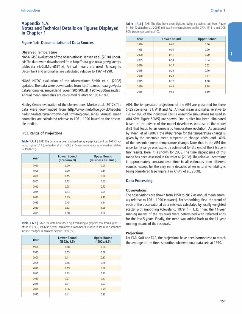
1
Introduction Chapter 1
155
Appendix 1.A: Notes and Technical Details on Figures Displayed in Chapter 1
Figure 1.4: Documentation of Data Sources
Observed TemperatureNASA GISS evaluation of the observations: Hansen et al. (2010) updat-ed: The data were downloaded from http://data.giss.nasa.gov/gistemp/tabledata_v3/GLB.Ts+dSST.txt. Annual means are used (January to December) and anomalies are calculated relative to 1961–1990.
NOAA NCDC evaluation of the observations: Smith et al. (2008) updated: The data were downloaded from ftp://ftp.ncdc.noaa.gov/pub/data/anomalies/annual.land_ocean.90S.90N.df_1901–2000mean.dat. Annual mean anomalies are calculated relative to 1961–1990.
Hadley Centre evaluation of the observations: Morice et al. (2012): The data were downloaded from http://www.metoffice.gov.uk/hadobs/hadcrut4/data/current/download.html#regional_series. Annual mean anomalies are calculated relative to 1961–1990 based on the ensem-ble median.
IPCC Range of Projections
Table 1.A.1 | FAR: The data have been digitized using a graphics tool from FAR Chap-ter 6, Figure 6.11 (Bretherton et al., 1990) in 5-year increments as anomalies relative to 1990 (°C).
Year Lower Bound(Scenario D)
Upper Bound(Business as Usual)
1990 0.00 0.00
1995 0.09 0.14
2000 0.15 0.30
2005 0.23 0.53
2010 0.28 0.72
2015 0.33 0.91
2020 0.39 1.11
2025 0.45 1.34
2030 0.52 1.58
2035 0.58 1.86
Year Lower Bound(IS92c/1.5)
Upper Bound(IS92e/4.5)
1990 0.00 0.00
1995 0.05 0.09
2000 0.11 0.17
2005 0.16 0.28
2010 0.19 0.38
2015 0.23 0.47
2020 0.27 0.57
2025 0.31 0.67
2030 0.36 0.79
2035 0.41 0.92
Table 1.A.2 | SAR: The data have been digitized using a graphics tool from Figure 19 of the TS (IPCC, 1996) in 5-year increments as anomalies relative to 1990. The scenarios include changes in aerosols beyond 1990 (°C).
Table 1.A.3 | TAR: The data have been digitized using a graphics tool from Figure 9.13(b) (Cubasch et al., 2001) in 5-year increments based on the GFDL_R15_a and DOE PCM parameter settings (°C).
Year Lower Bound Upper Bound
1990 0.00 0.00
1995 0.05 0.09
2000 0.11 0.20
2005 0.14 0.34
2010 0.17 0.52
2015 0.22 0.70
2020 0.28 0.87
2025 0.37 1.08
2030 0.43 1.28
2035 0.52 1.50
AR4: The temperature projections of the AR4 are presented for three SRES scenarios: B1, A1B and A2. Annual mean anomalies relative to 1961–1990 of the individual CMIP3 ensemble simulations (as used in AR4 SPM Figure SPM5) are shown. One outlier has been eliminated based on the advice of the model developers because of the model drift that leads to an unrealistic temperature evolution. As assessed by Meehl et al. (2007), the likely range for the temperature change is given by the ensemble mean temperature change +60% and –40% of the ensemble mean temperature change. Note that in the AR4 the uncertainty range was explicitly estimated for the end of the 21st cen-tury results. Here, it is shown for 2035. The time dependence of this range has been assessed in Knutti et al. (2008). The relative uncertainty is approximately constant over time in all estimates from different sources, except for the very early decades when natural variability is being considered (see Figure 3 in Knutti et al., 2008).
Data Processing
ObservationsThe observations are shown from 1950 to 2012 as annual mean anom-aly relative to 1961–1990 (squares). For smoothing, first, the trend of each of the observational data sets was calculated by locally weighted scatter plot smoothing (Cleveland, 1979; f = 1/3). Then, the 11-year running means of the residuals were determined with reflected ends for the last 5 years. Finally, the trend was added back to the 11-year running means of the residuals.
ProjectionsFor FAR, SAR and TAR, the projections have been harmonized to match the average of the three smoothed observational data sets at 1990.
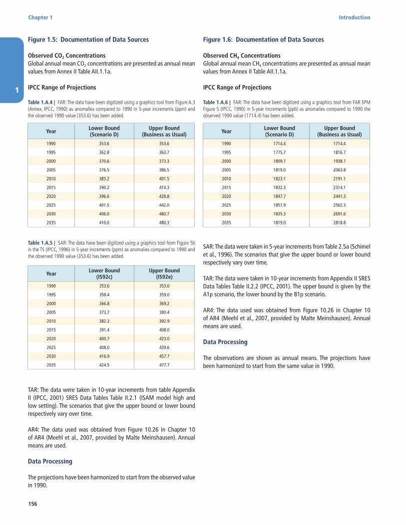
1
Chapter 1 Introduction
156
Figure 1.5: Documentation of Data Sources
Observed CO2 ConcentrationsGlobal annual mean CO2 concentrations are presented as annual mean values from Annex II Table AII.1.1a.
IPCC Range of Projections
Table 1.A.4 | FAR: The data have been digitized using a graphics tool from Figure A.3 (Annex, IPCC, 1990) as anomalies compared to 1990 in 5-year increments (ppm) and the observed 1990 value (353.6) has been added.
Year Lower Bound (Scenario D)
Upper Bound(Business as Usual)
1990 353.6 353.6
1995 362.8 363.7
2000 370.6 373.3
2005 376.5 386.5
2010 383.2 401.5
2015 390.2 414.3
2020 396.6 428.8
2025 401.5 442.0
2030 406.0 460.7
2035 410.0 480.3
Year Lower Bound (IS92c)
Upper Bound(IS92e)
1990 353.6 353.6
1995 358.4 359.0
2000 366.8 369.2
2005 373.7 380.4
2010 382.3 392.9
2015 391.4 408.0
2020 400.7 423.0
2025 408.0 439.6
2030 416.9 457.7
2035 424.5 477.7
Table 1.A.5 | SAR: The data have been digitized using a graphics tool from Figure 5b in the TS (IPCC, 1996) in 5-year increments (ppm) as anomalies compared to 1990 and the observed 1990 value (353.6) has been added.
TAR: The data were taken in 10-year increments from table Appendix II (IPCC, 2001) SRES Data Tables Table II.2.1 (ISAM model high and low setting). The scenarios that give the upper bound or lower bound respectively vary over time.
AR4: The data used was obtained from Figure 10.26 in Chapter 10 of AR4 (Meehl et al., 2007, provided by Malte Meinshausen). Annual means are used.
Data Processing
The projections have been harmonized to start from the observed value in 1990.
Figure 1.6: Documentation of Data Sources
Observed CH4 ConcentrationsGlobal annual mean CH4 concentrations are presented as annual mean values from Annex II Table AII.1.1a.
IPCC Range of Projections
Table 1.A.6 | FAR: The data have been digitized using a graphics tool from FAR SPM Figure 5 (IPCC, 1990) in 5-year increments (ppb) as anomalies compared to 1990 the observed 1990 value (1714.4) has been added.
Year Lower Bound(Scenario D)
Upper Bound(Business as Usual)
1990 1714.4 1714.4
1995 1775.7 1816.7
2000 1809.7 1938.7
2005 1819.0 2063.8
2010 1823.1 2191.1
2015 1832.3 2314.1
2020 1847.7 2441.3
2025 1857.9 2562.3
2030 1835.3 2691.6
2035 1819.0 2818.8
SAR: The data were taken in 5-year increments from Table 2.5a (Schimel et al., 1996). The scenarios that give the upper bound or lower bound respectively vary over time.
TAR: The data were taken in 10-year increments from Appendix II SRES Data Tables Table II.2.2 (IPCC, 2001). The upper bound is given by the A1p scenario, the lower bound by the B1p scenario.
AR4: The data used was obtained from Figure 10.26 in Chapter 10 of AR4 (Meehl et al., 2007, provided by Malte Meinshausen). Annual means are used.
Data Processing
The observations are shown as annual means. The projections have been harmonized to start from the same value in 1990.
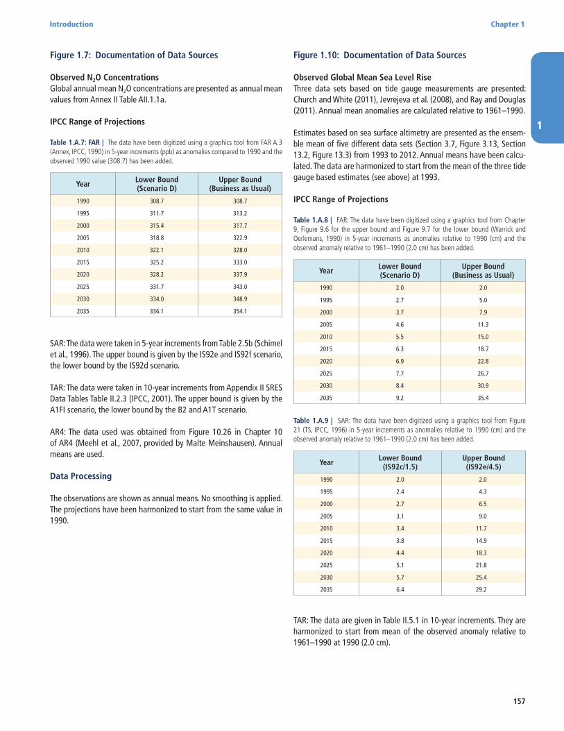
1
Introduction Chapter 1
157
Figure 1.7: Documentation of Data Sources
Observed N2O ConcentrationsGlobal annual mean N2O concentrations are presented as annual mean values from Annex II Table AII.1.1a.
IPCC Range of Projections
Table 1.A.7: FAR | The data have been digitized using a graphics tool from FAR A.3 (Annex, IPCC, 1990) in 5-year increments (ppb) as anomalies compared to 1990 and the observed 1990 value (308.7) has been added.
Year Lower Bound(Scenario D)
Upper Bound(Business as Usual)
1990 308.7 308.7
1995 311.7 313.2
2000 315.4 317.7
2005 318.8 322.9
2010 322.1 328.0
2015 325.2 333.0
2020 328.2 337.9
2025 331.7 343.0
2030 334.0 348.9
2035 336.1 354.1
SAR: The data were taken in 5-year increments from Table 2.5b (Schimel et al., 1996). The upper bound is given by the IS92e and IS92f scenario, the lower bound by the IS92d scenario.
TAR: The data were taken in 10-year increments from Appendix II SRES Data Tables Table II.2.3 (IPCC, 2001). The upper bound is given by the A1FI scenario, the lower bound by the B2 and A1T scenario.
AR4: The data used was obtained from Figure 10.26 in Chapter 10 of AR4 (Meehl et al., 2007, provided by Malte Meinshausen). Annual means are used.
Data Processing
The observations are shown as annual means. No smoothing is applied. The projections have been harmonized to start from the same value in 1990.
Figure 1.10: Documentation of Data Sources
Observed Global Mean Sea Level RiseThree data sets based on tide gauge measurements are presented: Church and White (2011), Jevrejeva et al. (2008), and Ray and Douglas (2011). Annual mean anomalies are calculated relative to 1961–1990.
Estimates based on sea surface altimetry are presented as the ensem-ble mean of five different data sets (Section 3.7, Figure 3.13, Section 13.2, Figure 13.3) from 1993 to 2012. Annual means have been calcu-lated. The data are harmonized to start from the mean of the three tide gauge based estimates (see above) at 1993.
IPCC Range of Projections
Table 1.A.8 | FAR: The data have been digitized using a graphics tool from Chapter 9, Figure 9.6 for the upper bound and Figure 9.7 for the lower bound (Warrick and Oerlemans, 1990) in 5-year increments as anomalies relative to 1990 (cm) and the observed anomaly relative to 1961–1990 (2.0 cm) has been added.
Table 1.A.9 | SAR: The data have been digitized using a graphics tool from Figure 21 (TS, IPCC, 1996) in 5-year increments as anomalies relative to 1990 (cm) and the observed anomaly relative to 1961–1990 (2.0 cm) has been added.
Year Lower Bound(Scenario D)
Upper Bound(Business as Usual)
1990 2.0 2.0
1995 2.7 5.0
2000 3.7 7.9
2005 4.6 11.3
2010 5.5 15.0
2015 6.3 18.7
2020 6.9 22.8
2025 7.7 26.7
2030 8.4 30.9
2035 9.2 35.4
Year Lower Bound(IS92c/1.5)
Upper Bound(IS92e/4.5)
1990 2.0 2.0
1995 2.4 4.3
2000 2.7 6.5
2005 3.1 9.0
2010 3.4 11.7
2015 3.8 14.9
2020 4.4 18.3
2025 5.1 21.8
2030 5.7 25.4
2035 6.4 29.2
TAR: The data are given in Table II.5.1 in 10-year increments. They are harmonized to start from mean of the observed anomaly relative to 1961–1990 at 1990 (2.0 cm).
1
Chapter 1 Introduction
158
AR4: The AR4 did not give a time-dependent estimate of sea level rise. These analyses have been conducted post AR4 by Church et al. (2011) based on the CMIP3 model results that were available at the time of AR4. Here, the SRES B1, A1B and A2 scenarios are shown from Church et al. (2011). The data start in 2001 and are given as anomalies with respect to 1990. They are displayed from 2001 to 2035, but the anoma-lies are harmonized to start from mean of the observed anomaly rela-tive to 1961–1990 at 1990 (2.0 cm).
Data Processing
The observations are shown from 1950 to 2012 as the annual mean anomaly relative to 1961–1990 (squares) and smoothed (solid lines). For smoothing, first, the trend of each of the observational data sets was calculated by locally weighted scatterplot smoothing (Cleveland, 1979; f = 1/3). Then, the 11-year running means of the residuals were determined with reflected ends for the last 5 years. Finally, the trend was added back to the 11-year running means of the residuals.
Related Documents