Introduction 2 Qm

1

Introduction to Quantum Mechanic

A) RadiationB) Light is made of particles. The need for a quantification

1) Black-body radiation (1860-1901) 2) Atomic Spectroscopy (1888-) 3) Photoelectric Effect (1887-1905)

C) Wave–particle duality 1) Compton Effect (1923).2) Electron Diffraction Davisson and Germer (1925).3) Young's Double Slit Experiment

D) Louis de Broglie relation for a photon from relativityE) A new mathematical tool: Wavefunctions and operatorsF) Measurable physical quantities and associated operators - Correspondence principle G) The Schrödinger Equation (1926)H) The Uncertainty principle

2

When you find this image, you may skip this part

This is less important

3

The idea of duality is rooted in a debate over the nature of light and matter dating back to the 1600s, when competing theories of light were proposed by Huygens and Newton.

Christiaan Huygens Dutch 1629-1695light consists of waves

Sir Isaac Newton1643 1727 light consists of particles

4

Radiations, terminology

5

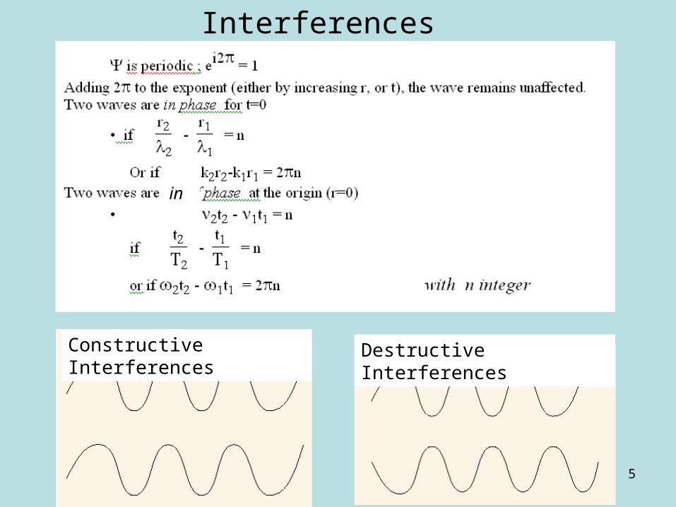
Interferences

Constructive Interferences Destructive Interferences

in

6

Phase speed or velocity

7

Introducing new variables

• At the moment, let consider this just a formal change, introducing

and

we obtain

8

Introducing new variables

At the moment, h is a simple constant

Later on, h will have a dimension and the p and E will be physical quantities

Then

9

2 different velocities, v and v

10

If h is the Planck constant J.s

Then

Louis de BROGLIEFrench (1892-1987)

Max Planck (1901)Göttingen

11

- Robert Millikan (1910) showed that it was quantified.

-Rutherford (1911) showed that the negative part was diffuse while the positive part was concentrated.

Soon after theelectron discovery in 1887- J. J. Thomson (1887) Some negative part could be extracted from the atoms

12

Gustav Kirchhoff (1860). The light emitted by a black body is called black-body radiation]

black-body radiation

At room temperature, black bodies emit IR light, but as the temperature increases past a few hundred degrees Celsius, black bodies start to emit at visible wavelengths, from red, through orange, yellow, and white before ending up at blue, beyond which the emission includes increasing amounts of UV

RED WHITESmall Large

Shift of

13

black-body radiationClassical TheoryFragmentation of the surface.One large area (Small Large smaller pieces (Large Small ) Vibrations associated to the size, N2 or N3

14

Kirchhoff

black-body radiation

RED WHITESmall Large

Shift of Radiation is emitted when a solid after receiving energy goes back to the most stable state (ground state). The energy associated with the radiation is the difference in energy between these 2 states. When T increases, the average E*Mean is higher and intensity increases. E*Mean- E = kT. k is Boltzmann constant (k= 1.38 10-23 Joules K-1).

15

black-body radiation

Max Planck (1901)Göttingen

Why a decrease for small ? Quantification

Numbering rungs of ladder introduces quantum numbers (here equally spaced)

16

Quantum numbers

In mathematics, a natural number (also called counting number) has two main purposes: they can be used for counting ("there are 6 apples on the table"), and they can be used for ordering ("this is the 3rd largest city in the country").

17

black-body radiation

Max Planck (1901)Göttingen

Why a decrease for small ? Quantification

18

black-body radiation, quantification

Max Planck

Steps too hard to climb Easy slope, rampPyramid nowadays Pyramid under construction

19

Max Planck

20

Johannes Rydberg 1888Swedish

n1 → n2 name Converges to (nm)

1 → ∞ Lyman 91

2 → ∞ Balmer 365

3 → ∞ Pashen 821

4 → ∞ Brackett 1459

5 → ∞ Pfund 2280

6 → ∞ Humphreys

3283

Atomic Spectroscopy

Absorption or Emission

21

Johannes Rydberg 1888Swedish

IR

VISIBLE

UV

Atomic Spectroscopy

Absorption or Emission

Emission

-R/12

-R/22

-R/32

-R/42

-R/52

-R/62-R/72

Quantum numbers n, levels are not equally spaced R = 13.6 eV

22

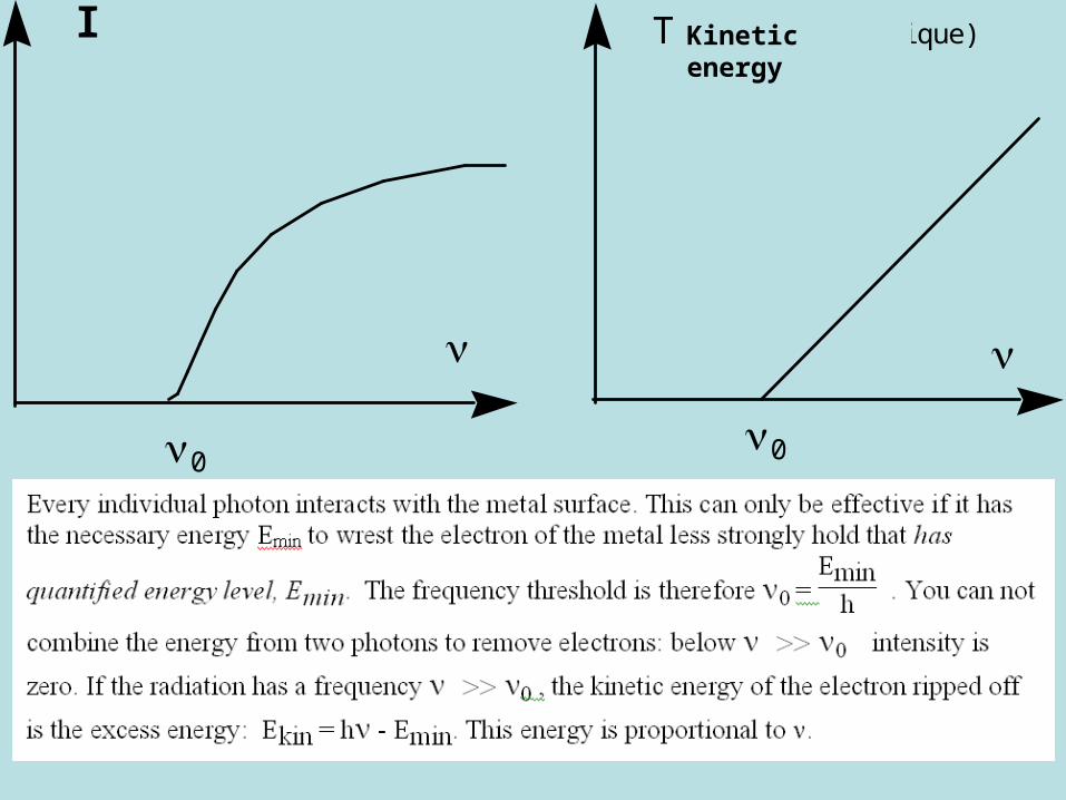
Photoelectric Effect (1887-1905)discovered by Hertz in 1887 and explained in 1905 by Einstein.

Vide

I

i

e

ee

Vacuum

Heinrich HERTZ (1857-1894)

Albert EINSTEIN(1879-1955)

23

I

00

T (énergie cinétique)Kinetic energy

24

Compton effect 1923playing billiards assuming =h/p

p

h/ '

h/

p2/2m

h'

h

Arthur Holly ComptonAmerican 1892-1962

25

Davisson and Germer 1925

Clinton DavissonLester GermerIn 1927

d

2d sin = k

Diffraction is similarly observed using a mono-energetic electron beam

Bragg law is verified assuming =h/p

26

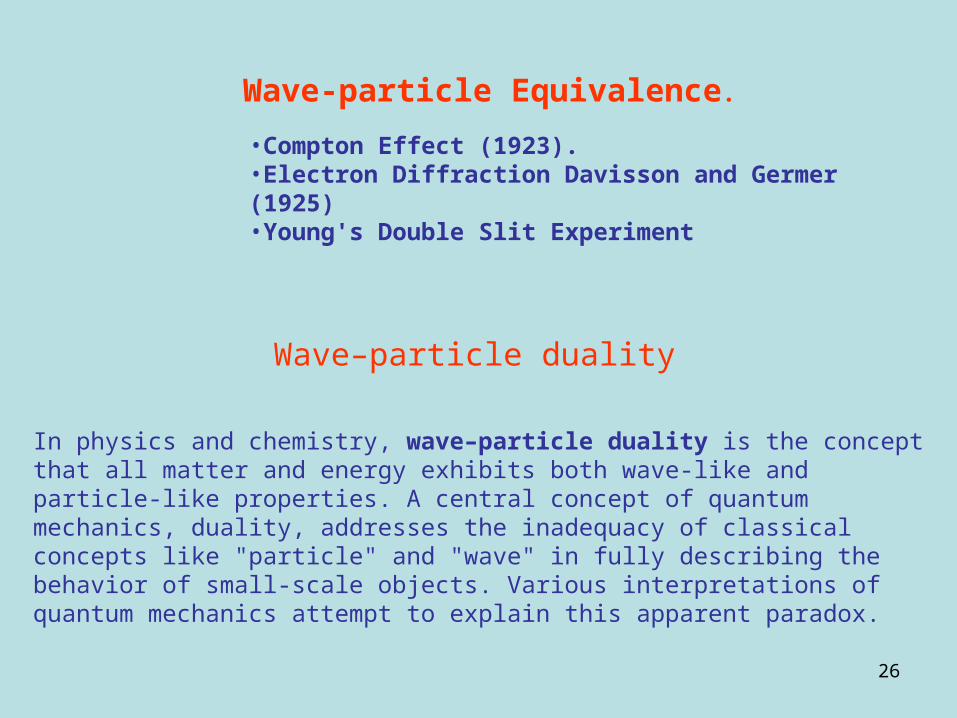
Wave-particle Equivalence.

•Compton Effect (1923).•Electron Diffraction Davisson and Germer (1925)•Young's Double Slit Experiment

In physics and chemistry, wave–particle duality is the concept that all matter and energy exhibits both wave-like and particle-like properties. A central concept of quantum mechanics, duality, addresses the inadequacy of classical concepts like "particle" and "wave" in fully describing the behavior of small-scale objects. Various interpretations of quantum mechanics attempt to explain this apparent paradox.

Wave–particle duality

27

Thomas Young 1773 – 1829 English, was born into a family of Quakers.

At age 2, he could read. At 7, he learned Latin, Greek and maths. At 12, he spoke Hebrew, Persian and could handle optical instruments. At 14, he spoke Arabic, French, Italian and Spanish, and soon the Chaldean Syriac. "… He is a PhD to 20 years "gentleman, accomplished flute player and minstrel (troubadour). He is reported dancing above a rope." He worked for an insurance company, continuing research into the structure of the retina, astigmatism ... He is the rival Champollion to decipher hieroglyphics.He is the first to read the names of Ptolemy and Cleopatra which led him to propose a first alphabet of hieroglyphic scriptures (12 characters).

28

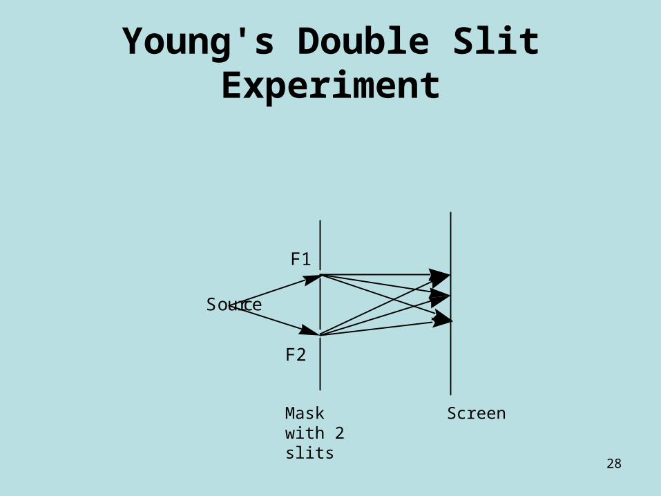
Young's Double Slit Experiment

Ecran Plaque photo

F2

F1

Source

ScreenMask with 2 slits

29

Young's Double Slit Experiment

This is a typical experiment showing the wave nature of light and interferences.

What happens when we decrease the light intensity ?If radiation = particles, individual photons reach one spot and there will be no interferences

If radiation particles there will be no spots on the screen

The result is ambiguousThere are spots

The superposition of all the impacts make interferences

30

Young's Double Slit Experiment

Assuming a single electron each timeWhat means interference with itself ?

What is its trajectory?If it goes through F1, it should ignore the presence of F2

Ecran Plaque photo

F2

F1

Source

ScreenMask with 2 slits

31

Young's Double Slit ExperimentThere is no possibility of knowing through which split the photon went!

If we measure the crossing through F1, we have to place a screen behind.Then it does not go to the final screen.

We know that it goes through F1 but we do not know where it would go after.These two questions are not compatible

Ecran Plaque photo

F2

F1

Source

ScreenMask with 2 slits

Two important differences with classical physics:

• measurement is not independent from observer

• trajectories are not defined; h goes through F1 and F2 both! or through them with equal probabilities!

32

Macroscopic world:A basket of cherriesMany of them (identical) We can see them and taste othersTaking one has negligible effectCherries are both red and good

Microscopic world:A single cherryEither we look at it without eatingIt is redOr we eat it, it is goodYou can not try both at the same timeThe cherry could not be good and red at the same time

33

Slot machine “one-arm bandit”

After introducing a coin, you have 0 coin or X coins.

A measure of the profit has been made: profit = X

34

de Broglie relation from relativityPopular expressions of relativity:m0 is the mass at rest, m in motion

E like to express E(m) as E(p) with p=mv

Ei + T + Erelativistic + ….

35

de Broglie relation from relativity

Application to a photon (m0=0)

To remember

To remember

36

Max Planck

Useful to remember to relate energy

and wavelength

37

A New mathematical tool: Wave functions and Operators

Each particle may be described by a wave function (x,y,z,t), real or complex,having a single value when position (x,y,z) and time (t) are defined.If it is not time-dependent, it is called stationary.The expression =Aei(pr-Et) does not represent one molecule but a flow of particles: a plane wave

38

Wave functions describing one particle

To represent a single particle (x,y,z) that does not evolve in time, (x,y,z) must

be finite (0 at ∞). In QM, a particle is not localized but has a probability to be in a given volume:dP= * dV is the probability of finding the particle in the volume dV. Around one point in space, the density of probability is dP/dV= * has the dimension of L-1/3 Integration in the whole space should give oneis said to be normalized.

39

Operators associated to physical quantities

We cannot use functions (otherwise we would end with classical mechanics)

Any physical quantity is associated with an operator.An operator O is “the recipe to transform into ’ ”We write: O = ’ If O = o(o is a number, meaning that O does not modify , just a scaling factor), we say that is an eigenfunction of O and o is the eigenvalue.We have solved the wave equation O = oby finding simultaneously and o that satisfy the equation.o is the measure of O for the particle in the state described by .

40

Slot machine (one-arm bandit)

Introducing a coin, you have 0 coin or X coins.

A measure of the profit has been made: profit = X

O is a Vending machine (cans)

Introducing a coin, you get one can.

No measure of the gain is made unless you sell the can (return to coins)

41

Examples of operators in mathematics : P parity

Even function : no change after x → -x Odd function : f changes sign after x → -x

y=x2 is even y=x3 is odd

y= x2 + x3 has no parity: P(x2 + x3) = x2 - x3

Pf(x) = f(-x)

42

Examples of operators in mathematics : A

y is an eigenvector; the eigenvalue is -1

43

Linearity

The operators are linear:

O (a1+ b1) = O (a1 ) + O( b1)

44

Normalization

An eigenfunction remains an eigenfunction when multiplied by a constant

O()= o() thus it is always possible to normalize a finite function

Dirac notations <I>

45

Mean value

• If 1 and 2 are associated with the same eigenvalue o: O(a1 +b2)=o(a1 +b2)

• If not O(a1 +b2)=o1(a1 )+o2(b2)

we define ō = (a2o1+b2o2)/(a2+b2)

Dirac notations

46

Sum, product and commutation of operators

(A+B)=A+B(AB)=AB

y1=e4x y2=x2 y3=1/x

d/dx 4 -- --

x3 3 3 3

x d/dx -- 2 -1

operators

wavefunctions

eigenvalues

47

Sum, product and commutation of operators

y1=e4x y2=x2 y3=1/x

A = d/dx 4 -- --

B = x3 3 3 3

C= x d/dx -- 2 -1

not compatibleoperators

[A,C]=AC-CA0

[A,B]=AB-BA=0[B,C]=BC-CB=0

48

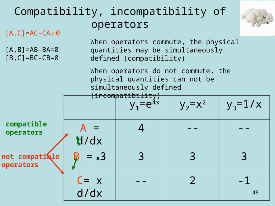
Compatibility, incompatibility of operators

y1=e4x y2=x2 y3=1/x

A = d/dx 4 -- --

B = x3 3 3 3

C= x d/dx -- 2 -1

not compatibleoperators

[A,C]=AC-CA0

[A,B]=AB-BA=0[B,C]=BC-CB=0

When operators commute, the physical quantities may be simultaneously defined (compatibility)

When operators do not commute, the physical quantities can not be simultaneously defined (incompatibility)

compatibleoperators

49

x and d/dx do not commute, are incompatible

Translation and inversion do not commute, are incompatible

A T(A)I(T(A))

I(A) AT(I(A))

vecteur de translation

O

Centre d'inversion

O

Translation vector

Inversion center

50

Introducing new variables

Now it is time to give a physical meaning.

p is the momentum, E is the Energy

H=6.62 10-34 J.s

51

Plane waves

This represents a (monochromatic) beam, a continuous flow of particles with the same velocity (monokinetic).

k, , , p and E are perfectly definedR (position) and t (time) are not defined.*=A2=constant everywhere; there is no

localization.If E=constant, this is a stationary state,

independent of t which is not defined.

52

Niels Henrik David Bohr Danish1885-1962

Correspondence principle 1913/1920

For every physical quantity one can define an operator. The definition uses formulae from classical physics replacing quantities involved by the corresponding operators

QM is then built from classical physics in spite of demonstrating its limits

53

Operators p and H

We use the expression of the plane wave which allows defining exactly p and E.

54

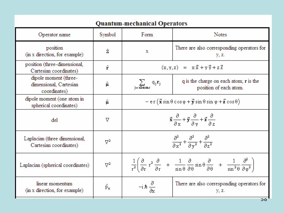
Momentum and Energy Operators

Remember during this chapter

55

Stationary state E=constant

Remember for 3 slides after

56

Kinetic energy

Classical quantum operator

In 3D :

Calling the laplacian

Pierre Simon, Marquis de Laplace (1749 -1827)

57

Correspondence principleangular momentum

Classical expression Quantum expression

lZ= xpy-ypx

58

59

60

61

62

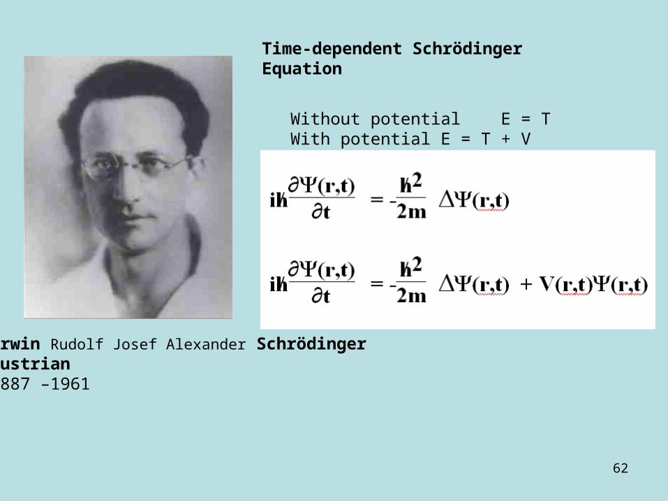
Erwin Rudolf Josef Alexander SchrödingerAustrian 1887 –1961

Without potential E = TWith potential E = T + V

Time-dependent Schrödinger Equation

63

Schrödinger Equation for stationary states

Kinetic energyTotal energy

Potential energy

64

Schrödinger Equation for stationary states

H is the hamiltonian

Sir William Rowan Hamilton Irish 1805-1865

Half penny bridge in Dublin

Remember

65

Chemistry is nothing but an application of Schrödinger Equation (Dirac)

Paul Adrien Dirac 1902 – 1984Dirac’s mother was British and his father was Swiss.

<I> < IOI >

Dirac notations

66

Uncertainty principle

the Heisenberg uncertainty principle states that locating a particle in a small region of space makes the momentum of the particle uncertain; and conversely, that measuring the momentum of a particle precisely makes the position uncertain

We already have seen incompatible operators

Werner HeisenbergGerman1901-1976

67

It is not surprising to find that quantum mechanics does not predict the position of an electron exactly. Rather, it provides only a probability as to where the electron will be found. We shall illustrate the probability aspect in terms of the system of an electron confined to motion along a line of length L. Quantum mechanical probabilities are expressed in terms of a distribution function.For a plane wave, p is defined and the position is not.With a superposition of plane waves, we introduce an uncertainty on p and we localize. Since, the sum of 2 wavefucntions is neither an eigenfunction for p nor x, we have average values.With a Gaussian function, the localization below is 1/2

68

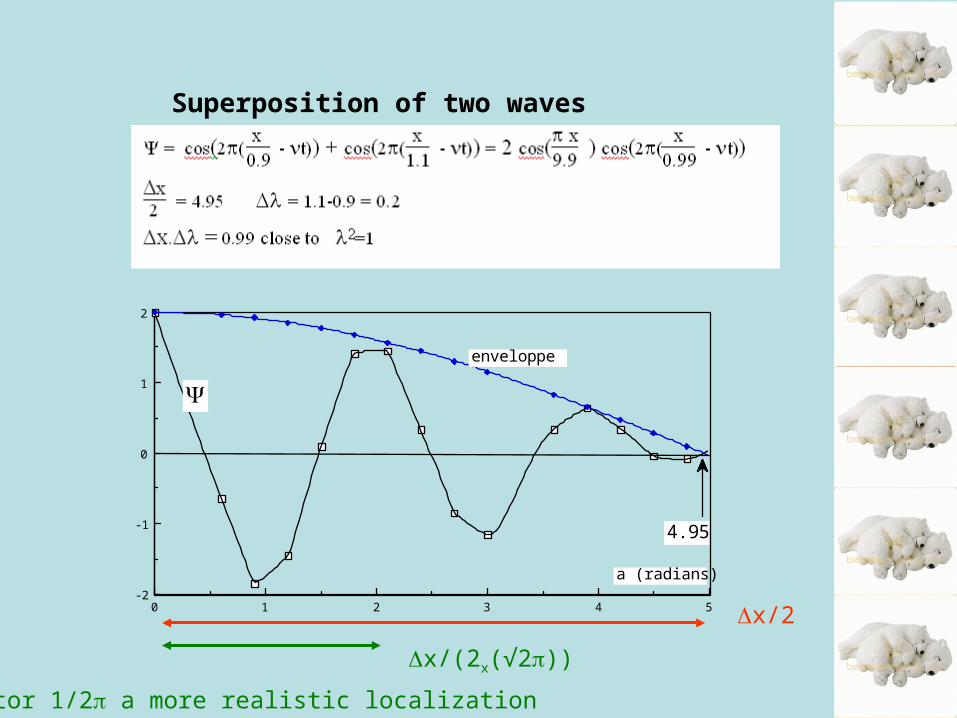
p and x do not commute and are incompatibleFor a plane wave, p is known and x is not (*=A2 everywhere)Let’s superpose two waves… this introduces a delocalization for p and may be localize x

At the origin x=0 and at t=0 we want to increase the total amplitude, so the two waves 1 and 2 are taken in phaseAt ± x/2 we want to impose them out of phaseThe position is therefore known for x ± x/2 the waves will have wavelengths

69

Superposition of two waves

0 1 2 3 4 5-2

-1

0

1

2

a (radians)

4.95

enveloppe

x/2

x/(2x(√2))

Factor 1/2 a more realistic localization

70

Uncertainty principle

Werner HeisenbergGerman1901-1976

A more accurate calculation localizes more(1/2 the width of a gaussian) therefore one gets

x and p or E and t play symmetric roles in the plane wave expression;Therefore, there are two main uncertainty principles