Introducing Non-Normality of Latent Psychological Constructs in Choice Modeling with an Application to Bicyclist Route Choice Chandra R. Bhat* The University of Texas at Austin Department of Civil, Architectural and Environmental Engineering 301 E. Dean Keeton St. Stop C1761, Austin TX 78712 Phone: 512-471-4535; Fax: 512-475-8744 Email: [email protected] and King Abdulaziz University, Jeddah 21589, Saudi Arabia Subodh K. Dubey The University of Texas at Austin Department of Civil, Architectural and Environmental Engineering 301 E. Dean Keeton St. Stop C1761, Austin TX 78712 Phone: 512-471-4535, Fax: 512-475-8744 E-mail: [email protected] Kai Nagel Institute for Land and Sea Transport (ILS) Transport System Planning and Traffic Telematics TU Berlin Secr SG 12 Salzufer 17-19 D-10587 Berlin Phone: +49-30-314-23308, Fax: +49-30-314-26269 E-mail: [email protected] *corresponding author Original version: July 25, 2014 Revised version: April 15, 2015

Welcome message from author
This document is posted to help you gain knowledge. Please leave a comment to let me know what you think about it! Share it to your friends and learn new things together.
Transcript

Introducing Non-Normality of Latent Psychological Constructs in Choice Modeling with an Application to Bicyclist Route Choice
Chandra R. Bhat* The University of Texas at Austin
Department of Civil, Architectural and Environmental Engineering 301 E. Dean Keeton St. Stop C1761, Austin TX 78712
Phone: 512-471-4535; Fax: 512-475-8744 Email: [email protected]
and King Abdulaziz University, Jeddah 21589, Saudi Arabia
Subodh K. Dubey The University of Texas at Austin
Department of Civil, Architectural and Environmental Engineering 301 E. Dean Keeton St. Stop C1761, Austin TX 78712
Phone: 512-471-4535, Fax: 512-475-8744 E-mail: [email protected]
Kai Nagel Institute for Land and Sea Transport (ILS)
Transport System Planning and Traffic Telematics TU Berlin Secr SG 12
Salzufer 17-19 D-10587 Berlin
Phone: +49-30-314-23308, Fax: +49-30-314-26269 E-mail: [email protected]
*corresponding author
Original version: July 25, 2014 Revised version: April 15, 2015

ABSTRACT
In the current paper, we propose the use of a multivariate skew-normal (MSN) distribution
function for the latent psychological constructs within the context of an integrated choice and
latent variable (ICLV) model system. The multivariate skew-normal (MSN) distribution that we
use is tractable, parsimonious in parameters that regulate the distribution and its skewness, and
includes the normal distribution as a special interior point case (this allows for testing with the
traditional ICLV model). Our procedure to accommodate non-normality in the psychological
constructs exploits the latent factor structure of the ICLV model, and is a flexible, yet very
efficient approach (through dimension-reduction) to accommodate a multivariate non-normal
structure across all indicator and outcome variables in a multivariate system through the
specification of a much lower-dimensional multivariate skew-normal distribution for the
structural errors. Taste variations (i.e., heterogeneity in sensitivity to response variables) can also
be introduced efficiently and in a non-normal fashion through interactions of explanatory
variables with the latent variables. The resulting model we develop is suitable for estimation
using Bhat’s (2011) maximum approximate composite marginal likelihood (MACML) inference
approach. The proposed model is applied to model bicyclists’ route choice behavior using a web-
based survey of Texas bicyclists. The results reveal evidence for non-normality in the latent
constructs. From a substantive point of view, the results suggest that the most unattractive
features of a bicycle route are long travel times (for commuters), heavy motorized traffic volume,
absence of a continuous bicycle facility, and high parking occupancy rates and long lengths of
parking zones along the route.
Keywords: Multivariate skew-normal distribution, multinomial probit, ICLV models, MACML
estimation approach, bicyclist route choice.

1
1. INTRODUCTION
Economic choice modeling has continually seen improvements and refinements in specification,
partly because of the availability of new techniques to estimate models. One such development is
the incorporation of random taste heterogeneity (i.e., taste variations in response to explanatory
variables) across decision makers using discrete (non-parametric) or continuous (parametric) or
mixture (combination of discrete and continuous) random distributions for model coefficients.
Such a specification also leads to correlations across alternative utilities when one or more
random coefficients appear in the utility specifications of multiple alternatives. Early examples
included studies by Revelt and Train (1996) and Bhat (1997), and there have now been many
applications of this approach, using (primarily) latent-class multinomial logit and mixed
multinomial logit formulations. A second development is the explicit consideration of latent
psychological constructs (such as attitudes, perceptions, values and beliefs) within the context of
economic choice models, which has the advantage (over the random taste heterogeneity
approach) that it imparts more structure to the underlying choice process based on theoretical
concepts and notions drawn from the psychology field. Additionally, it provides the opportunity
to efficiently introduce random taste variations and the concomitant correlations across
alternative utilities (we will come back to this latter point, which we believe has been less
discussed and less exploited in the literature to date). This second development, commonly
referred to as integrated choice and latent variable (ICLV) models (Ben-Akiva et al., 2002, and
Bolduc et al., 2005), may be viewed as a variation of the traditional structural equation methods
(SEMs) (see, for example, Muthen, 1978 and Muthen, 1984) to accommodate an unordered-
response outcome. Specifically, the traditional SEM includes a structural equation model for the
latent variables (as a function of exogenous variables) as well as a measurement equation model
that relates latent variables to observed continuous, binary, or ordered-response indicator
variables. The ICLV model, conceptually speaking, adds an unordered-response outcome
variable that may be considered as another indicator variable in the measurement component of
the traditional SEM (except that the measurement component typically does not include
exogenous variables, while the unordered-response choice variable is modeled as a function of
exogenous variables).
Another area of intense research in the recent past, but originating more from the
statistical field, is the consideration of non-normal distributions in modeling data. This has been
2
spurred by the increasing presence of multi-dimensional data that potentially exhibit non-normal
features such as asymmetry, heavy tails, and even multimodality. Parametric approaches to
accommodate non-normality span the gamut from finite mixtures of normal distributions to
skew-normal distributions (and more general skew-elliptical distributions) to mixtures of skew-
normal distributions (and mixtures of more general skew-elliptical distributions). Some recent
applications include Pyne et al. (2009), Lachos et al. (2010), Contreras-Reyes and Arellano-
Valle (2013), Riggi and Ingrassia (2013), Lin et al. (2013), and Vrbik and McNicholas (2014).
Many of these recent studies use either a multivariate skew-normal or a skew-t distribution as the
basis for accommodating non-normality, with different proposals on how to characterize these
skew distributions (see Lee and McLachlan (2013) for a recent review and synthesis of the many
different proposals). In the context of the multivariate skew-normal distribution, broadly
speaking, there are two forms – restricted and unrestricted, with what Lee and McLachlan
characterize as “extended” and “generalized” being relatively minor generalizations of the
restricted and unrestricted forms. However, it is well recognized now that the underlying basis
for all of the different proposals for the multivariate skew-normal distribution originate in the
pioneering work of Azzalini and Dalla Valle (1996). Arellano-Valle and Azzalini (2006)
provided a unified framework to characterize the many other proposals since Azzalini and Dalla
Valle (1996), and showed how their unified skew-normal (SUN) distribution includes all other
proposals as special cases. Thus, in this research, we will maintain notations that correspond to
the SUN distribution.
In the current paper, we bring together the two developments discussed above – the ICLV
model structure and the treatment of non-normality through a multivariate skew-normal or MSN
distribution specification. In particular, we allow the latent constructs in the ICLV model to be
skew-normal. After all, there is no theoretical basis for specifying these constructs as normal (as
is typically assumed in the literature); thus, there is substantial appeal in specifying a more
general non-normal specification that is then characterized empirically. To our knowledge, this
is the first probit-kernel based ICLV model proposed in the econometric literature, which has
several important features.1 First, it recognizes the very real possibility that latent variables are
1 Brey and Walker (2011) is the only other study we are aware of that considers a non-normal distribution within an ICLV model. However, they use a single latent variable, and their approach adds to convergence problems to what is already a difficult convergence problem in the context of a logit-kernel based formulation. Specifically, the integrand in their integration involves an increasingly complicated mixing. Even in the typical normally-mixed
3
non-normally distributed after conditioning on exogenous variables. Imposing normality when
the structural errors in the latent variable relationship with exogenous variables are non-normal
can render the parameter estimates inconsistent in the measurement equations corresponding to
binary or ordinal indicators, as well as in the unordered outcome model (this is because of the
non-linear nature of the relationship with the latent variable; see Geweke and Keane, 1999, Caffo
et al., 2007, and Wall et al., 2012). Of course, this inconsistency will permeate into the
coefficients of the structural component (relating the latent variables to exogenous variables)
because these structural coefficients are being implicitly estimated through the relationship
embedded in the measurement equations. Incorrectly imposing normality will also lead, in
general, to inefficient estimation in all of the ICLV model components and can lead to incorrect
inferences. Second, our proposal to include non-normality exploits the latent factor structure of
the ICLV model. That is, our approach constitutes a flexible, yet very efficient approach
(through dimension-reduction) to accommodate a multivariate non-normal structure across all
indicator and outcome variables through the specification of a much lower-dimensional
multivariate skew-normal distribution for the structural errors. This leads to parsimony in the
additional parameters introduced because of non-normality. Third, taste variations (i.e.,
heterogeneity in sensitivity to response variables) can also be introduced efficiently and in a non-
normal fashion through interactions of explanatory variables with the latent variables. Thus, for
example, in a bicyclist route choice model, bicyclists who are more safety conscious (say a latent
variable) than their peers may be more sensitive to motorized traffic volumes and on-street
parking. By interacting safety consciousness with exogenous variables corresponding to
motorized traffic volumes and on-street parking, we then allow non-normal taste variation in
response to both these exogenous attributes, but originating from a single skew-normal
distribution associated with the safety conscious latent variable. Fourth, the multivariate skew-
normal (MSN) distribution that we use has properties that make it an ideal one for incorporation
into the ICLV model. In particular, the MSN distribution is tractable, parsimonious in parameters
that regulate the distribution and its skewness, and includes the normal distribution as a special
interior point case (this allows for testing with the traditional ICLV model). It also is flexible,
latent variables, convergence is not easy and it is not uncommon for the estimation to simply not converge (see Alvarez-Daziano and Bolduc, 2013, and Bhat and Dubey, 2014). On the other hand, our flexible skew-normal distribution, combined with our proposed estimation technique, does make the estimation simpler and easier in a probit-based kernel context, even with multiple latent variables.
4
allowing a continuity of shapes from normality to non-normality, including skews to the left or
right and sharp versus flat peaking toward the mode (see Bhat and Sidharthan, 2012). Besides,
the MSN generates skew by shifting mass to the left or right of the mean of the normal
distribution, thus generating asymmetry and flexibility, but keeping the tails thin as in the
normal density function (which makes estimation of the parameters of the MSN distribution
easier than other asymmetric distributions such as the log-normal that have long tails).
Additionally, the MSN distribution immediately accommodates correlation across the latent
variables because of its multivariate structure. Finally, the MSN distribution has specific
properties that enable the use of Bhat’s (2011) maximum approximate composite marginal
likelihood (MACML) inference approach for estimation of the resulting model. This
substantially simplifies the estimation approach because the dimensionality of integration in the
composite marginal likelihood (CML) function that needs to be maximized to obtain a consistent
estimator (under standard regularity conditions) for the model parameters is independent of the
number of latent variables and the number of ordinal indicator variables in the model system.
The rest of this paper is structured as follows. Section 2 presents a general discussion of
the multivariate skew normal distribution and some of its properties that are particularly relevant
to this paper. Section 3 presents the model formulation and estimation approach. Section 4
presents an application of the proposed model to bicyclist route choice, and Section 5
summarizes the findings of the paper.
2. THE MULTIVARIATE SKEW-NORMAL DISTRIBUTION FUNCTION
2.1. Overview
As indicated earlier, in this paper, we use the multivariate skew distribution (MVSN) version
originally proposed by Azzalini and Dalla Valle (1996) for a number of reasons (this is also
referred to by Lee and McLachlan, 2013 as the restricted multivariate skew normal distribution,
though we will drop the label “restricted” in the rest of this paper for ease in presentation).
Specifically, the MVSN version used here is (1) efficient in the number of additional parameters
to be estimated, (2) allows independence between skew-normally distributed and normally-
distributed elements in a multivariate vector (useful in the ICLV context where the structural
equation errors of the latent psychological constructs are considered independent of the
measurement equation errors), (3) is closed under any affine transformation of the skew-
5
normally distributed vector (is the key to the MACML estimation of the skew-ICLV model), and
(4) is closed under the sum of independent skew-normally distributed and normally distributed
vectors of the same dimensions (is the key to mixing non-normally distributed latent variables
with normally distributed measurement equation errors). At the same time, the cumulative
distribution function of an L-variate skew normally distributed variable of the Azzalini and Dalla
Valle type requires only the evaluation of an )1( L -dimensional multivariate cumulative
normal distribution function.
Consider an MVSN distributed random variable vector )',,,,( 321 L η with an
)1( L -location parameter vector L0 (that is, an )1( L vector with all elements being zero) and
an )( LL -symmetric positive-definite correlation matrix *Γ . Then, the MVSN distribution for
η implies that η is obtained through a latent conditioning mechanism on an )1( L -variate
normally distributed vector ,),( 1*0 *CC where *
0C is a latent )11( -vector and *C 1 is an )1( L -
vector:
. 1
where, , 0
~ **1
1
*
*Γρ
ρΩΩ
0Lo MVN
C*C
(1)
ρ is an )1( L -vector, each of whose elements may lie between –1 and +1. The matrix *Ω is
also a positive-definite correlation matrix. Then, )0(| *01 C*Cη has the standard multivariate
skew-normal (SMVSN) density function shown below:
2/11
1**
)(1
)(where),() ;(2) ;(
~
ρΓρ
ρΓαzαΩzΩzη
*
*
LL , (2)
where (.)L and (.) represent the standard multivariate normal density function of L
dimensions and the standard univariate cumulative distribution function, respectively. We write
).(SMVSN~ *Ωη To obtain the density function of the non-standardized multivariate skew-
normal distribution, consider the distribution of .ωηY ζ This MVSN distribution for Y
implies that Y is obtained through a latent conditioning mechanism on an )1( L -variate
normally distributed vector ,),( 10 CC where 0C is a latent )11( -vector and 1C is an )1( L -
vector:
6
ωΓωΓωρΓ
ΩΩ *
and, ,
1 where, ,
0~ 1
1
0σ
σ
σ
ζCLMVN
C. (3)
Specifically, we write ),,,(MVSN~ *ΩωY ζ and the conditioning-type stochastic representation
of Y is obtained as )0(| 01 CCY . The probability density function of the random variable Y
may be written in terms of the SMVSN density function above as (see Bhat and Sidharthan,
2012):
),(where),;(~
),,;(
1
1
ζζ
yωzΩzΩωyY 1**
L
L
jjLf (4)
and j is the jth diagonal element of the matrix ω .
The cumulative distribution function for η may be obtained as:
. 1
);,,(2);(~
)(*
**1
*
Ωρ
ρΩΩz0Ωzzη LLP (5)
The corresponding cumulative distribution function for Y is:
. ,,2;~
)( *1
*
Ω)(yω0Ω)(yωyY 11 ζζ LLP (6)
2.2. Properties of the MVSN Distribution
The close correspondence of the MVSN distribution with the normal distribution leads to several
desirable properties. The three properties that are key to the formulation of the SN-ICLV model
proposed in this paper are listed below. The proofs for the first two properties are available in
Arellano-Valle and Azzalini (2006) and Bhat and Sidharthan (2012). The proof for the third
property, which is critical for the current paper, is based on the marginal and conditional
distribution properties of the multivariate normal distribution.
Property 1: The sum of a MVSN distributed vector Y (dimension 1L ) )],,(MVSN~[ *ΩωY ζ
and an independently distributed multivariate normally (MVN) distributed vector W
(dimension 1L ) )] ,[ ΣMVN(μ~W is still MVSN distributed:
7
),~
,~ ,(MVSN~ *ΩωμWY ζ where , ~
,~~~~, ~~
~1~ΣΩΩ)ω(Ω)ω(Ω
Ωρ
ρΩ 11*
*
*
ωρ)ω(ρ 1 ~~ , and ω~ is the diagonal matrix of standard deviations of Ω~
.
Property 2: The affine transformation of the MVSN distributed vector Y (dimension 1L )
)] , ,(MVSN~[ *ΩωY ζ as BYa , where B is a )( Lh matrix, is also an MVSN distributed
vector of dimension 1h :
)],~
,~ , (MVSN~ *ΩωBaBYa ζ where ,~
,~~~~,~~
~~
BBΩΩ)ω(Ω)ω(ΩΩρ
ρ1Ω 11*
*
*
, ~~ ρBω)ω(ρ 1 and ω~ is the diagonal matrix of standard deviations of Ω~
.
Property 3: Partition the MVSN vector Y into sub-vectors 1Y of dimension 11L and 2Y of
dimension 12L , so that the conditioning type representation for Y (of dimension
)1)( 21 LLL in Equation (3) may be written as follows:
222111
2122
1211
21
2
11
2
1
0
,,
1
where,,
0
MVN~ ρωρω
ΓΓ
ΓΓΩΩ
σσ
σ
σ
σσ
ζ
ζ
C
C L
C
, (7)
and .,, 11221222221111 ωΓωΓωΓωΓωΓωΓ ***
Then, the marginal distribution of 1Y is also MVSN distributed: ),,,(MVSN~ 1111*ΩωY ζ where
11
11
1
ΓΩ
σ
σ and
*Γρ
ρΩ
11
1*1
1. A similar result holds for the marginal distribution of 2Y .
The proofs for the marginal distributions are straightforward given the conditioning
representation above. For future reference, we also note that, with a re-arrangement of the
vectors 210 and,, CCC in Equation (7) and using the properties of the multivariate normally
distributed vector, the conditional density function of 2C and0C given 11 yC is also
multivariate normally distributed. Specifically, define the following:
8
),(~
),(~
111
11222111
110 ζyζζζyσζ -- ΓΓΓ 11
11220211
110 ,1Θ σσσσ -- ΓΓΘΓ and
121
11222 ΓΓΓΓΘ - . Then, the conditional density function of 20 and C C given 11 yC is
.Θ
and~
~~
where, ,~
MVN~202
020
2
0111
2
0
2
ΘΘ
ΘΘΘ
ζ
ζζζyC
C L
C (8)
The above property will be used to derive the conditional (cumulative) distribution function of
.2Y given 1Y , which will be important in the estimation of the proposed SN-ICLV model (as
discussed later in Section 3.4, we are not aware of any earlier and explicit derivation of the
conditional distribution function of a sub-vector of an MVSN distributed vector given another
subvector).
3. THE SN-ICLV MODEL FORMULATION
There are three components of the SN-ICLV model: (1) the latent variable structural equation
model; (2) the latent variable measurement equation model; and (3) the choice model. In the
following presentation, we will use the index l for latent variables (l=1,2,…,L), and the index i
for alternatives (i=1,2,…,I). In the current set-up, we assume a stated preference exercise (as in
the empirical context of the paper) in which each respondent provides a single set of indicators
(of the latent variables) in the measurement equation model, but is presented with multiple
choice scenarios for the choice component estimation. So, we will use the index t for choice
occasion (t=1,2,…,T). Note also that the presence of individual-specific latent variables
immediately engenders a covariance pattern among the multiple choice instances of the same
individual, because the individual-specific (stochastic and MVSN-distributed) latent variables
enter into the utility functions of each choice instance from the same individual. Finally, we will
use the index q for individuals (q=1,2,…,Q), though, as appropriate and convenient, we will
suppress this index in parts of the presentation.
3.1. Latent Variable Structural Equation Model
For the latent variable structural equation model, we will assume that the latent variable *lz is a
linear function of covariates as follows:
,*ll ηz wαl (9)

9
where w is a )1~
( D vector of observed individual-specific covariates (not including a constant),
lα is a corresponding )1~
( D vector of coefficients, and l is a random error term. In our
notation, the same exogenous vector w is used for all latent variables; however, this is in no way
restrictive, since one may place the value of zero in the appropriate row of lα if a specific
variable does not impact *lz . Next, define the )
~( DL matrix ),...,( 21 Lαααα , and
)1( L vectors ),...,,( **2
*1 Lzzz*z and )'.,,,,( 321 L η To allow correlation among the
latent variables, η is assumed to be standard multivariate skew-normally distributed:
),(SMVSN~ *Ωη
Γρ
ρΩ
1* , where Γ is a correlation matrix of size )( LL (we assume
the matrix Γ to be a correlation matrix rather than a covariance matrix due to identification
considerations as discussed later in the paper). In matrix form, Equation (9) may be written as:
η αwz* . (10)
3.2. Latent Variable Measurement Equation Model
For the latent variable measurement equation model, let there be H continuous variables
) ..., , ,( 21 HSSS with an associated index h ) ..., ,2 ,1( Hh . Let hhhh δS *zd in the usual
linear regression fashion, where hδ is a scalar constant, hd is an )1( L vector of latent variable
loadings on the hth continuous indicator variable, and h is a normally distributed measurement
error term. Stack the H continuous variables into a )1( H vector S, the H constants hδ into a
)1( H vector δ , and the H error terms into another )1( H vector ) ..., , ,( 21 Hξ . Also, let
sΣ be the covariance matrix of ξ . And define the )( LH matrix of latent variable loadings
.,...,, 21 Hdddd Then, one may write, in matrix form, the following measurement equation for
the continuous indicator variables:
ξdzδS * . (11)
Similar to the continuous variables, let there also be G ordinal indicator variables, and let
g be the index for the ordinal variables ) ..., ,2 ,1( Gg . Let the index for the ordinal outcome
category for the gth ordinal variable be represented by gj . For notational ease only, assume that
10
the number of ordinal categories is the same across the ordinal indicator variables, so that
. ..., ,2 ,1 Jjg Let *gS be the latent underlying variable whose horizontal partitioning leads to
the observed outcome for the gth ordinal indicator variable, and let the individual under
consideration choose the gn th ordinal outcome category for the gth ordinal indicator variable.
Then, in the usual ordered response formulation, we may write the following for the individual:
gggg δS ~~~* *zd , gg nggng S ,
*1, , where gδ
~ is a scalar constant, gd
~ is an )1( L vector of
latent variable loadings on the underlying variable for the gth indicator variable, and g~
is a
standard normally distributed measurement error term (the normalization on the error term is
needed for identification, as in the usual ordered-response model; see McKelvey and Zavoina,
1975). Note also that, for each ordinal indicator variable,
JgggNNgggg gg ,1,0,1,2,1,0, and,0 , ;... . For later use, let
.),...,,(and,),...,,( 211,3,2, Gg ψψψψψ Jggg Stack the G underlying continuous
variables *gS into a )1( G vector *S and the G constants gδ
~ into a )1( G vector δ
~. Also,
define the )( LG matrix of latent variable loadings ,~
,...,~
,~~
21
Gdddd and let *s
Σ be the
correlation matrix of )~
..., ,~
,~
(~
21 Gξ . Stack the lower thresholds Gggng ..., ,2 ,11,
into a
)1( G vector lowψ and the upper thresholds Gggng ..., ,2 ,1, into another vector upψ .
Then, in matrix form, the measurement equation for the ordinal indicators may be written as:
up*
low** ψSψξzdδS ,
~~~. (12)
Define .)~
,(and,)~
,( ,)~
,( , , ξξξdddδδδSSS *
Then, the continuous parts of
Equations (11) and (12) may be combined into a single equation as:
**
*
)(Var and ,~~)E(with,sss
sss
ΣΣ
ΣΣΣ '
ξ
zdδ
dzδsξzdδS
*
** . (13)
3.3. Choice Model
Assume a typical random utility-maximizing model, and let i be the index for alternatives (i =1,
2,3,…,I). Note that some alternatives may not be available to some individuals during some
11
choice instances, but the modification to allow this is quite trivial. So, for presentation
convenience, we will assume that all alternatives are available to all individuals at all choice
instances. The utility for alternative i at time period t (t=1,2,…,T) for individual q is then written
as (suppressing the index q):
,)( titititi εU *i zγxβ (14)
where tix is a (D×1)-column vector of exogenous attributes. β is a (D×1)-column vector of
corresponding coefficients, ti is an )( LN i -matrix of exogenous variables interacting with
latent variables to influence the utility of alternative i, iγ is an )1( iN -column vector of
coefficients capturing the effects of latent variables and its interaction effects with other
exogenous variables, and ti is a normal error term that is independent and identically normally
distributed across individuals and choice occasions. The notation above is very general. Thus, if
each of the latent variables impacts the utility of alternative i purely through a constant shift in
the utility function, ti will be an identity matrix of size L, and each element of iγ will capture
the effect of a latent variable on the constant specific to alternative i. Alternatively, if the first
latent variable is the only one relevant for the utility of alternative i, and it affects the utility of
alternative i through both a constant shift as well as an exogenous variable, then iN =2, and ti
will be a )2( L -matrix, with the first row having a ‘1’ in the first column and ‘0’ entries
elsewhere, and the second row having the exogenous variable value in the first column and ‘0’
entries elsewhere.2
Next, let the variance-covariance matrix of the vertically stacked vector of errors
]) ..., , ,([ 21 tIttt εεεε be Λ and let ) vector1( ) ..., , ,( 21 TITεεεε . The covariance of ε is
2 In the empirical context of the current paper, we use unlabeled alternatives and thus the individual-specific demographic and latent variables are introduced purely as interaction terms to alternative-specific attributes. In the notation of Equation (14), individual-specific demographic variables are introduced by interacting them with alternative attributes as part of the xti vector, while the individual-specific latent variables are introduced by specifying φti as a matrix containing only alternative-specific attributes (that is, by interacting the latent variables with alternative-specific attributes with no constant shift effect, because of the unlabeled nature of the alternatives). Indeed, in this case, φti is of the same size across all alternatives, and γi is the same across all alternatives. However, in the presentation here, we will maintain a more general notation that includes the case of labeled alternatives.
12
ΛIDEN T , where TIDEN is an identity matrix of size T.3 Define the following vectors and
matrices: matrix), ( ),...,,( 21 DIItttt xxxx matrix), ( ),...,,( 21 DTI Txxxx
),...,,( 21 tIttt UUUU vector)1( I , ),...,,( 21 TUUUU ) vector1( TI ,
),...,, 21 tIttt
LNI
ii
1
matrix, ),...,, 21 T
LNTI
ii
1
. Also, define the
I
iiNI
1
matrix γ , which is initially filled with all zero values. Then, position the )1( 1N
row vector 1γ in the first row to occupy columns 1 to 1N , position the )1( 2N row vector 2γ
in the second row to occupy columns 1N +1 to ,21 NN and so on until the )1( IN row vector
Iγ is appropriately positioned. Then, in matrix form, we may write the following equation for
the vector of utilities across all choice instances of the individual:
)matrix ()(where,)( LTITT γλελzxβεzγxβU ** IDENIDEN . (15)
As in the case of any choice model, for the case of labeled alternatives, one of the
alternatives has to be used as the base when introducing alternative-specific constants and
variables that do not vary across the I alternatives. Also, only the covariance matrix of the error
differences is estimable. Taking the difference with respect to the first alternative, only the
elements of the covariance matrix Λ
of ),,...,,( 32 I
where 1 ii ( 1i ), are
estimable. Λ is constructed from Λ
by adding an additional row on top and an additional
column to the left. All elements of this additional row and column are filled with values of
zeroes. In addition, an additional scale normalization needs to be imposed on Λ
, which may be
accomplished by normalizing the first element of Λ
to the value of one. Third, in MNP models,
when only individual-specific covariates are used, exclusion restrictions are needed in the form
of at least one individual characteristic being excluded from each alternative’s utility in addition
to being excluded from a base alternative (but appearing in some other utilities; (see Keane, 1992
and Munkin and Trivedi, 2008).
3 For the unlabeled alternatives case of our empirical context, there is no meaning to having a general covariance matrix Λ for the error terms across alternatives. Thus, Λ is specified to be an identity matrix of size I. But, for completeness, we will formulate the model with a general Λ matrix that may be specified for labeled alternatives.
13
3.4. Overall Model System Identification and Estimation
Let θ be the collection of parameters to be estimated:
, ]Vech( ),Vech( , ),Vech( , ),(Vech,),Vech( ),(Vech),Vech([ )ΛγΣψδρΓαθ
βd
where
)(Vech α , )Vech(ρ , )(Vech d
, and )(Vech γ represent vectors of the elements of the α , ρ , d
,
and γ , respectively, to be estimated, and Γ)(Vech represents the vector of the non-zero upper
triangle elements of Γ (and similarly for other covariance matrices). For future use, define
,TIGHE and .1)1(~ TIGE
To develop the reduced form equations, we define some additional notations as follows:
matrix) ( ),( LE λdπ
,
vector)1( ),( Eεξ
,
where Σ0Λ0
0Σ0 ,MVN~,MVN~ EEE
.
Now, replace the right side of Equation (10) for *z in Equations (13) and (15) to obtain the
following system:
ξηdαwdδξηwdδξzdδS *
)(α (16)
εληαwλxβεηαwλxβεzλxβU * )( . (17)
Next, consider the )1( E vector USSU ,
. Define
πηαwλxβ
αwdδSU
. (18)
Then, by successive application of properties 1 and 2 from Section 2.2, we obtain
),~
,,~
( *~ ΩωMVSNΓ
B ~SU E (19)
where ,
~~ matrix, )1()1(~~
~1~ vector,)1(
~~~
* 1-Γ
1-Γ
*
*ωΓωΓ
Γρ
ρΩ
EEEαwλxβ
αwdδB
,~,~
~ ρωρΣΓΓ -1Γπππ and
Γω~ is the diagonal matrix of the standard deviations of Γ
~.
General and necessary identification conditions for ICLV models have yet to be
developed, but good discussions of sufficiency conditions may be found in Stapleton (1978), Vij
and Walker (2014), Alvarez-Daziano and Bolduc (2013), and Bhat and Dubey (2014). So we

14
will only list the sufficiency conditions here: (1) Identification of each of the ordinal
measurement equation system and the choice model hold, as discussed in Sections 3.2 and 3.3,
respectively, (2) Γ is a correlation matrix, and the measurement equation error term covariance
matrix Σ
is strictly diagonal, (3) For each latent construct or variable (that is for each *lz ), there
is at least one indicator variable that loads only on that latent variable and no other latent variable
(that is, there is at least one factor complexity one indicator variable for each latent variable), (4)
If a specific variable (or specific interaction variable of an individual-specific attribute and an
alternative-specific attribute in the case of unlabeled alternatives) impacts the utility of an
alternative in the choice model through the x vector, the utility of that alternative not depend on
any latent variable that contains that specific variable (or specific interaction variable in the case
of unlabeled alternatives) as a covariate in the structural equation system.
Next, to estimate the model, we need to develop the distribution of the vector
*uSSu ,
, where ,,...,,,,...,, **2
*121
ttt tImmtmt
** uuu*t
*T
* uuuuu
),(*ttmtitim miUUu
tt
and tm indicates the chosen alternative at choice occasion t. To obtain the vector Su from SU ,
define a matrix M of size TIGHTIGH *)1( . Fill this matrix with values of zero.
Then, insert an identity matrix of size HG into the first HG rows and HG columns of the
matrix M . Next, consider the last TI *)1( rows and TI columns of the matrix M . Position a
block-diagonal matrix in these rows and columns, each block diagonal being of size
))()( I1-I and containing the matrix tM , which itself is an identity matrix of size )1( I with
an extra column of ‘-1’ values added at the thtm column. Then, )(SUSu M , and we can write
),,,(*)1(*Ω
ωBMVSN ~Su TIGH where BB
~M
and
.)( and ,~
,)( )( ,1 111 πρωρωωρ
ρ *
*
*
MMΓMΓΓΓΓ
Ω *
*
*
(20)
where ω is the diagonal matrix of standard deviation of Γ
.
In the conditioning representation for MVSN variables (see Section 2), we may write:
ωΓωΓρωΓ
ΩΩ *
and,,
1where,,
0MVN~ *
~
1
0 σσ
σ
BC EH
C. (21)
15
Next, partition Su into a component corresponding to the continuous observed indicators
(captured in the vector S) and another component corresponding to the continuous latent
underlying constructs manifested in the form of the ordinal indicators and the utility differentials
in the choice model: ,)~,( uSSu where .])(,)[(~ ** usu Correspondingly, also partition B
into components for the mean of the vectors S and u~ ,, ~
uS BBB
and appropriately
partition the covariance elements Γ
and σ in Ω :
uuS
uS
~~
~
ΓΓ
ΓΓΓ
and .),( ~ uS σσσ Then,
using Equation (21), we may write:
uuSu
uSS
uS
u
S
u
S
B
B
C
C
~~~
~
~
~
~
~
0 1
where,,
0
MVN~
ΓΓσ
ΓΓσ
σσ
ΩΩ
VEH
C
(22)
Also, using Property 3 in Section 2.2, define the following for a specific value of sS :
,),(1Θ),(),(μ ~~~00~~~0 SuSSSuuSS σσBsσBsBBsσ -1SuS
-1S
-1SuS
-1S ΓΓΘΓΓΓμΓ
u
and .~~~~ uS-1SuSu ΓΓΓΓΘ
u Then, the conditional density function of uC ~0 andC given sCS is
multivariate normally distributed:
).~~
(Θ
and)1~
(μ
where,,MVN~~~0
~00
~
0~
~
0 EEEC
uu
u
E
ΘΘ
ΘΘ
μμΘμ
uS
u
sCC
(23)
That is,
)(|)~,~
( ~0, ~0sCgC SuCu
hCfC 111~
1~
1r
];~,~
[( ---E
E
r hω ΘΘΘΘ Θωωμω
)g . (24)
Next, supplement the threshold vectors defined earlier as follows:
,,~
*)1( TIlowlow ψψ ,
and
TIup *)1(,~ 0ψψup , where TI *)1( is an 1*)1( TI -column vector of negative
infinities, and TI *)1( 0 is another 1*)1( TI -column vector of zeroes ( lowψ~ and upψ~ are
1)1~
( E vectors). Then the likelihood function may be written as:
16
,)(|]0[Prob
~~)(|)~,
~(
),,;(
|),...,,,...,,Pr(),,;()(
0
0~
~0,~
212211
0
~
'
sC
gsCgC
ωBsS
sSωBsS
S
SuC
Dg
SS
SS
u
g
C
dhdhCf
f
mmmnjnjnjfL
h
C
S
TGGS
*Γ
*Γ
Ω
Ωθ
S
S
(25)
where gD~ is the region of integration such that ~~~:~~ uplow ψψ ggDg ,
),,;( *Γ
ΩS SS ωBsS
Sf is the MVSN density function of dimension H (number of continuous
indicators in the measurement equation) given by (see Property 3 of Section 2.2):
,1
),(where),;(~
),,;( 1
1
1
SΓ
*Γ
*Γ Γ
ΩsΩΩSSS
S
S
S*
S*
SSσ
σBωssωωBsS SH
H
jSf and
11
SS ΓΓ
* ΩΩ ωωS S . (26)
The denominator in the expression in Equation (25) is given by:
0
00
Θ
μ)(|]0[Prob sCSC . (27)
The likelihood function in Equation (25) involves the evaluation of a 1)1(~ TIGE
dimensional rectangular integral, which can be cumbersome and difficult as the number of
ordinal indicators or the number of alternatives or the number of choice occasions per individual
increases. Hence, we use Maximum Approximate Composite Marginal Likelihood (MACML)
approach proposed by Bhat (2011), as it only involves the computation of univariate and
bivariate cumulative distribution functions.
3.5. The MACML Estimation Approach
The MACML approach, similar to the parent CML approach (see Varin et al., 2011, Lindsay et
al., 2011, Yi et al., 2011, and Bhat, 2014, for recent reviews of CML approaches), maximizes a
surrogate likelihood function that compounds much easier-to-compute, lower-dimensional,
marginal likelihoods. The CML approach, which belongs to the more general class of composite
likelihood function approaches (see Lindsay, 1988, and Bhat, 2014), may be explained in a
simple manner as follows. In the SN-ICLV model, instead of developing the likelihood function
component for the joint probability of the observed ordinal indicators and the observed choice
outcome conditional on the observed continuous variable vector (the second component of
17
Equation (25)), one may compound (multiply) the probabilities of each pair of observed ordinal
indicators, and each combination of an ordinal indicator with the choice outcome, conditional on
the observed continuous variable vector. The CML estimator (in this instance, the pairwise CML
estimator) is then the one that maximizes the resulting surrogate likelihood function. The
properties of the CML estimator may be derived using the theory of estimating equations (see
Cox and Reid, 2004, Yi et al., 2011, and Bhat, 2014). Specifically, under usual regularity
assumptions (Molenberghs and Verbeke, 2005, page 191, Xu and Reid, 2011), the CML
estimator is consistent and asymptotically normally distributed (this is because of the
unbiasedness of the CML score function, which is a linear combination of proper score functions
associated with the marginal event probabilities forming the composite likelihood; for a formal
proof, see Xu and Reid, 2011 and Bhat, 2014).
In the context of the proposed SN-ICLV model, consider the following (pairwise)
composite marginal likelihood function for an individual q as follows:
)(
),Pr(
);Pr(),Pr(
),,;()(
1
1 1
1 1
1
1 1
,
sS
ωBsS SS
T
t
T
tttt
G
g
T
ttgg
G
g
G
gggggg
SqCML
mm
mnjnjnj
fL *Γ
ΩθS
(28)
In the above CML approach, the MVNCD function appearing in the CML function is of
dimension equal to three for ),Pr( gggg njnj (corresponding to the probability of each pair
of observed ordinal indicators), equal to 1I for );Pr( tgg mnj (corresponding to each
combination of an ordinal indicator and the observed choice outcome at a specific time period t),
and equal to 1)1(2 I for ),Pr( tt mm (corresponding to each combination of observed choice
outcomes at time period t and time period t ). To write out the CML function explicitly, define
the following matrices: (1) A selection matrix gtA (g=1,2,…,G and t=1,2,…,T) of
dimension EI~
)1( : Fill this matrix with values of zero for all elements and position an
element of ‘1’ in the first row and first column. Then, position an element of ‘1’ in the second
row and the (g+1)th column. Also, position an identity matrix of size 1I in the last 1I rows
and columns from 2)1)(1( tIG to 1)1( tIG ; (2) A selection matrix gg N

18
( gg , =1,2,…,G, )gg of dimension E~
3 : Fill this matrix with values of zero for all elements
and position an element of ‘1’ in the first row and first column. Then, position an element of ‘1’
in the second row and the (g+1)th column, as well as an element of ‘1’ in the third row and the
( 1g )th column; (3) A selection matrix tt R ( tt , =1,2,…,T, )tt of dimension
EI~
]1)1(*2[ : Fill this matrix with values of zero for all elements and position an element
of ‘1’ in the first row and first column. Then, insert an identity matrix of size 1I in rows 2 to
1)1( I and columns 2)1)(1( tIG to 1)1( tIG . Similarly, position another
identity matrix of size 1I in the rows 2)1( I to 1)1(*2 I and columns
2)1)(1( tIG to 1)1( tIG ; (4) EEuu
u ~~(
Θ
~~0
~00
ΘΘ
ΘΘ matrix);
(5) ,,,0 gg upupugg ψψψ
,,,0 gg lowlowlgg ψψψ
,,,0 gg lowupulgg ψψψ
gg uplowlugg ψψψ ,,0
(all )13( vectors), and
)1(,0 Ig
0,ψψ upupg,
and
11,,0 )1(
IIg lowlowg, ψψ
, where g][ upψ refers to the gth element of upψ and glowψ
refers to the gth element of lowψ ; (6) );33(),13( gggggggggg NΘNΘμNμ
(7) ],1)1[( Igtgt μAμ
)]1()1[( IIgtgtgt AΘAΘ
; and
(8) .)1)1(2()1)1(2(~
and1)1)1(2(~ III tttttttttt RΘRΘμRμ
With the above definitions, we may write:
19
,~
);~)((2
;2;2
(29)
;2
;2
;2
;2
)(|]0[Prob
),,;()(
1
1 1
1~
1~
1~1)1(*2
1 1
111,1
111,1
1113
1113
1113
1113
1
1 1
0
T
t
T
tt
-tt
-tt
-
G
g
T
t
-gt
--gt
-gt
--gt
-gg
--gg
-gg
--gg
-gg
--gg
-gg
--gg
G
g
G
gg
S
CML
tttttt
gtgtgtgtgtgt
gggggg
gggggg
gggggg
gggggg
C
fL
ΘΘΘ
ΘΘΘΘΘΘ
ΘΘΘ
ΘΘΘ
ΘΘΘ
ΘΘΘ
*Γ
ωΘωμω
ωΘωωμωΘωωμ
ωΘωωμ
ωΘωωμ
ωΘωωμ
ωΘωωμ
Ωθ S
lowgupg
lgg
lugg
ulgg
ugg
S
SS
ψψ
ψ
ψ
ψ
ψ
sC
ωBsS
where ),,;( *Γ
ΩS SS ωBsS
Sf and )(|]0[Prob 0 sCS C are as provided in Equations (26) and
(27), respectively.
In the above expression, an analytic approximation approach is used to evaluate the
MVNCD functions in the second, third, and fourth elements (this analytic approach is embedded
within the MACML approach of Bhat, 2011). Specifically, the logarithm of Equation (29) is
computed for each of the individuals q in the sample using the MACML approach
( )( log , θqMACMLL ) and the MACML estimator is then obtained by maximizing the following
function:
.)(log)(log1
,
Q
qqMACMLMACML LL θθ (30)
The covariance matrix of the parameters θ may be estimated by the inverse of Godambe’s
(1960) sandwich information matrix (see Zhao and Joe, 2005).
1)()( θθ GVMACML11 )]()][([)]([ θθθ HJH ,
where )(θH and )(θJ can be estimated in a straightforward manner at the MACML estimate
MACMLθ as follows:

20
.)(log)(log
)ˆ(ˆ
and ,)(log
)ˆ(ˆ
ˆ
,,
1
ˆ
,2
1
MACMLθ
θ
θ
θ
θ
θθ
θθ
θθ
qMACMLqMACMLQ
q
qMACMLQ
q
LLJ
LH
MACML (31)
3.6. Ensuring the Positive-Definiteness of Matrices
The covariance matrices in the CML function need to be positive definite. This can be assured by
ensuring that the covariance matrix Θ in Equation (23) is positive definite, which itself requires
that
Γρ
ρΩ
1* in the structural equation system be positive definite and the covariance
matrix of utility differentials in the choice model, Λ
, also be positive definite. The simplest way
to ensure the positive-definiteness of these matrices is to use a Cholesky-decomposition and
parameterize the CML function in terms of the Cholesky parameters (rather than the original
covariance matrices). For ,*Ω we also need to ensure that the Cholesky decomposition *ΩL
is
such that *Ω is a correlation matrix. This is done by parameterizing the diagonal terms of *ΩL
as
follows:
2,1
22,1
21,13,12,11,1
22121
1
001
0001
LLLLLLL llllll
ll
*ΩL . (32)
In the estimation, the Cholesky elements in the matrix *ΩL
are estimated, guaranteeing that *Ω
is indeed a correlation matrix. In addition, the top diagonal element of Λ
has to be normalized to
one (as discussed earlier), which implies that the first element of the Cholesky matrix of Λ
is
fixed to the value of one.
4. APPLICATION TO BICYCLIST ROUTE CHOICE
4.1. Background
Americans are less dependent on motorized vehicles today and are driving less than in 2005.
This trend is particularly being led by millennials (those born between 1983 and 2000) who wait
21
longer to obtain a driver’s license and who drive significantly fewer miles than previous
generations of young Americans (see Dutzik and Baxandall, 2013). The decrease in driving, not
surprisingly, has been associated with an increase in travel by other means of transportation. For
instance, the number of workers commuting by the bicycle mode has increased by 39 percent
between 2005 and 2011. At an absolute level, 18 percent of the U.S. population age 16 or older
rode a bicycle at least once during the summer of 2012, according to the 2012 National Survey of
Bicyclist and Pedestrian Attitudes and Behavior (Schroeder and Wilbur, 2013). These trends of
decreasing driving and the increasing use of non-motorized forms of travel has not gone
unnoticed by planners and policy leaders. In particular, there is increasing attention today on
designing built environments that promote the use of non-motorized travel modes of
transportation, as part of an integrated land use-transportation approach to address traffic
congestion issues (see, for example, Metropolitan Transportation Commission, 2009, and
Southern California Association of Governments, 2012). This is as opposed to the predominantly
one-dimensional and resource-intensive solution in the past of building additional roadway
capacity, which is becoming increasingly more difficult to sustain from a financial and
environmental perspective.
Even as transportation professionals view the promotion of non-motorized forms of
transportation as an element of a multidimensional toolbox of strategies to address traffic
congestion issues (and consequent air pollution and greenhouse gas emissions considerations),
health scientists view walking and bicycling as a means to build up a “health capital” from
physical activity participation. Specifically, it is now well established in the epidemiological
literature that physical activity is important for the health and well-being of individuals. In
addition to reducing the incidence of obesity and its several concomitant adverse mental and
physical health consequences, physical activity presents benefits even to non-obese and non-
overweight individuals from the standpoint of increasing cardiovascular fitness, improving
mental health, and decreasing heart disease, diabetes, high blood pressure, and several forms of
cancer side effects (National Center for Health Statistics, 2010).
In the context of the above discussion, the empirical focus of this paper is on bicycle
route choice. This emphasis is motivated by the fact that designing good routes for bicycling
(with desired facilities along the way) is an important component of promoting bicycling in the
first place. Besides, with limited funds, policy makers need to identify the best pathways along
22
which to invest in bicycle facilities. Additionally, a good knowledge of bicyclist route choice
decisions can help design vibrant and physically active cities. At its core, route choice entails an
analysis of how individuals perceive, and trade-off among, a host of route attributes such as
travel distances, travel times, traffic volumes, terrain grade, parking presence and type (no
parking allowed or parallel parking or angled parking), speed limits, number of cross-streets, and
the type and number of traffic control devices along a route.
To be sure, there have been many studies in the recent past that have examined bicyclist
route choice decisions. These studies have used revealed preference data (that is, collecting route
choice in a natural setting and then developing a set of non-chosen alternatives) or stated
preference data (that is, providing a hypothetical set of two to three routes characterized by
specific attributes, and asking the individual to make a route choice between the presented
routes).4 Some recent examples of revealed preference-based bicyclist route choice models
include Menghini et al., 2010, Hood et al., 2011, Broach et al., 2012, and Rendell et al., 2012),
while some recent examples of stated preference-based bicyclist route choice models include
Sener et al., 2009, Caulfield et al., 2012, and Chen and Chen, 2013. These earlier studies have
made important contributions to our understanding of bicyclist route choice decisions, and have
underscored the fact that bicyclists do indeed consider a range of route attributes when making
their route choices (in contrast to the typical practice in travel demand modeling that assumes
that distance is the sole criterion in bicyclist route choice decisions; see also Menghini et al.,
2010 and Rendell et al., 2012). Earlier studies have also indicated that the valuation of route
attributes differ according to trip purpose (commuting versus non-commuting) and demographic
characteristics. But none of these earlier route choice studies have explicitly considered
bicycling attitudes and perceptions. In fact, except for Sener et al. (2009) and Chen and Chen
(2013), earlier studies have not even considered potential taste (sensitivity) variations across
4 There are advantages and disadvantages of using revealed preference and stated preference data for bicyclist route choice analysis. Revealed preference data are naturalistic and provide information on the actual chosen alternative. However, they are relatively cumbersome to collect, provide limited variation in relevant route attributes and also require the generation of non-chosen paths (and inappropriate generation of non-chosen paths can lead to biased estimation results). Stated preference data are easier to collect, provide variation over a range of potentially relevant attributes (since the routes are constructed by the analyst) to provide rich trade-off information, obviate the need to generate choice sets, and can examine attributes/attribute levels that are not manifested in current bicycling routes. Limitations of stated preference data include comprehension difficulties in the hypothetical scenarios, and exaggeration effects to attempt to influence policy decisions. Stinson and Bhat (2003) and Hood et al. (2011) discuss the advantages and disadvantages of revealed and stated preference data in more detail. In this paper, as we will discuss in the next section, a stated preference survey is used in the analysis.
23
individuals to route attributes due to unobserved individual characteristics. For instance, some
individuals may be avid and intense pro-bicycle enthusiasts (relative to their otherwise
observationally equivalent peers), and this may translate to increased sensitivity to such route
operational characteristics as number of cross-streets (because pro-bicyclists may see cross-
streets as a nuisance). Of course, it is also possible that pro-bicycle enthusiasts have a decreased
sensitivity to the number of cross-streets because they take things in stride. Similarly, some
bicyclists may be very safety conscious (say an unobserved variable to the analyst) relative to
their observationally equivalent peers, which can then get manifested in the form of increased
sensitivity to on-street parking attributes, bikeway facility characteristics (such as a continuous
versus discontinuous facility), and roadway functional characteristics (such as motorized traffic
volumes along route and speed limit on roadway). But even Sener et al. (2009) and Chen and
Chen (2013) consider the effects of unobserved characteristics only implicitly, by allowing
continuous (in the case of Sener et al., 2009) or discrete (in the case of Chen and Chen, 2013)
random distributions to capture sensitivity variations across individuals to route attributes (that
is, taste heterogeneity). This random distribution approach, while better than assuming the
absence of the moderating effects of unobserved factors, still treats unobserved psychological
preliminaries of choice (i.e., attitudes and preferences) as being contained in a “black box” to be
integrated out. On the other hand, the ICLV approach allows a deeper understanding into the
route choice decision process of bicyclists by developing a conceptual structural model for the
“soft” psychometric measures associated with individual attitudes and perceptions. Specifically,
the latent constructs of attitudes and perceptions are related to observed individual-specific
covariates in the structural equation model, and these latent constructs then are interacted with
the “hard” observed route attribute variables to explain route choice. In doing so, a parsimonious
and behavioral structure is provided to the nature of heterogeneity (across individuals) in route
attribute effects. Importantly, this specification immediately considers both observed and
unobserved heterogeneity in route attribute effects (because the latent constructs are related to
observed individual variables), as well as accommodates covariance in the route attribute effects
(because the same latent variable may be interacted with multiple route attributes; thus, for
example, safety consciousness can lead to increased sensitivity to multiple route attributes at
once). Finally, our specification immediately allows non-normal distribution effects for the
heterogeneity effects of route attributes, rather than a priori imposing a normal distribution.
24
To our knowledge, this is the first application of an ICLV structure to bicycle route
choice modeling, in addition to this being the first application of the SN-ICLV model in the
econometric literature. In addition, we apply the SN-ICLV model to a repeated choice data case,
rather than the cross-sectional analysis of some other ICLV studies (such as Prato et al., 2012).
4.2. Data and Sample Formation
The data for this study is drawn from a 2009 web based survey conducted by the University of
Texas at Austin. Details of the survey procedures are provided in Sener et al. (2009), and so only
a brief overview of the survey is provided here. The focus of the survey effort was on obtaining
information from individuals (aged 18 years or above) who have had some experience in
bicycling, since the objective was to elicit useful information for an assessment of bicycle
facilities and an analysis of bicycling concerns/reasons. Further, given the focus on bicyclists, the
route choice model estimates are valid even though we do not have a representative sample of
bicyclists. This is due to Manski and Lerman’s (1977) result for exogenous samples, which is
applicable here because the alternatives in the route choice analysis are unlabeled alternatives
constructed by the analyst. In this sense, we do not have a choice-based sample because
respondents are not chosen based on their route choice.
The survey collected limited information on demographic (age, gender, education, and
household size) and employment-related characteristics (commute distance, work schedule
flexibility), along with much more comprehensive information on the bicycling characteristics of
the respondents (in the rest of this paper, we will refer to the demographic and employment-
related characteristics as individual-specific attributes). In addition, the survey solicited
respondent views on three psychological construct indicators related to the overall quality of
bicycle facilities, bicycling safety from traffic crashes, and the frequency of non-commute
bicycling during the year. All these three indicator variables were measured on a 4-point ordinal
scale, as follows: (1) overall quality of bicycle facilities (very inadequate, inadequate, adequate,
very adequate), (2) bicycle safety from traffic crashes (very dangerous, somewhat dangerous,
somewhat safe, and very safe), and (3) frequency of non-commute bicycling (about once or twice
a month, about once a week, 2-3 days per week, and 4-5 days (or more) per week). We
hypothesize that individuals with a “pro-bicycle” attitude (the first latent construct we use) will
be more positive about the quality of bicycle facilities (the first indicator variable) and will
25
undertake more bicycling for non-commuting purposes (the third indicator variable). Also, we
propose that a “safety-conscious” personality (the second latent construct we use) will tend to
have a lower evaluation of bicycle safety from traffic crashes (the second indicator variable).
The route choice stated preference (SP) scenarios were presented in the form of a table
with three columns and five rows (each column representing a hypothetical route, and each row
representing a certain level of an attribute; respondents were asked to choose the route they
would use from the three routes presented). The route attributes included the following:
On-street parking – Parking type (none, angled, or parallel), parking turnover rate, length
of parking area, and parking occupancy rate.
Bicycle facility characteristics – On-road bicycle lane (a designated portion of the
roadway striped for bicycle use) or shared roadway (a shared roadway open to both
bicycle and motor vehicle travel), width of bicycle lane if present or overall roadway
width if shared roadway, and bicycle facility continuity.
Roadway physical characteristics – Roadway grade, and number of stop signs, red lights
and cross streets.
Roadway functional characteristics – Motorized traffic volume and speed limit.
Roadway operational characteristics – Travel time.
The route attribute levels corresponding to the attributes listed above, except travel time, are
available in Sener et al. (2009), and reproduced in Table 1 for completeness. Before discussing
the generation of travel time attribute levels in the experiments, we should note that separate
experimental designs were developed for commuter bicyclists (those who bicycle for commuting
purposes, some of whom may also bicycle for non-commuting reasons) and non-commuter
bicyclists (designated to be those who bicycle only for non-commuting purposes). The
identification of respondents into these two bicyclist groups was based on questions before the
SP experiments were presented. Further, travel time was included as an attribute only for
commuter bicyclists, since non-commute travel is mainly for recreation pursuits with no specific
destination in mind. The travel time attribute level for each route (for commuter bicyclists) in the
SP experiments was designed to be pivoted off the actual commute time by bicycle as reported
by the individual. This was done to preserve some amount of realism in presenting alternative
routes in the stated choice experiments.
26
In total, there are 11 route attributes for commuting-related SP experiments, and 10 route
attributes for non-commuting-related experiments. To reduce respondent burden when evaluating
routes, we used a partitioning mechanism where only five attributes were used to characterize
routes for any single respondent. At the same time, the selection of the five attributes for any
individual was undertaken in a carefully designed rotating and overlapping fashion to enable the
capture of all variable effects when the responses from the different SP choice scenarios across
different individuals are brought together. Each respondent is presented with four choice
questions (or choice experiments) in the survey.
The survey included a total of 1689 respondents. After screening for missing data and
other inconsistencies, the final sample size included a total of 1429 respondents with a total
sample size of 5716 (1429 individuals with 4 choice occasions each). Further, we split the
sample into 70% for estimation and 30% for prediction. Thus, the estimation and prediction
samples included 1000 respondents (with 4000 choice occasions) and 429 respondents (with
1716 choice instances), respectively.
4.3. Impact of Latent Variables
The route choice experiments involve unlabeled route alternatives, in which each route is
represented by a set of attributes. Thus, the impact of the latent variables on route choice is
characterized by moderating the effect of these route attributes on route choice. Based on the
discussion in the previous section, we expect that pro-bicycle enthusiasts will be less sensitive to
route physical and operational characteristics, while safety conscious bicyclists will be highly
sensitive to on-street parking attributes, bikeway facility characteristics, and roadway functional
characteristics. The overall conceptual diagram for the model system is provided in Figure 1.
First, both the latent constructs, pro-bicycle and safety consciousness, are specified as a function
of the individual-specific characteristics of cyclists in a structural equation model (see the center
of Figure 1). The two latent constructs are mapped to cyclists’ perceptions through indicator
variables in a measurement equation model (shown separately at the bottom of Figure 1). As
discussed in the previous section, the “pro-bicycle” attitude is mapped to the ordinal indicators
related to the overall quality of bicycle facilities and the frequency of non-commute bicycling,
while the “safety conscious” personality is mapped to the ordinal indicator related to bicycling
safety from traffic crashes. The latent constructs and individual-specific variables (subject to the
27
identification issues discussed in Section 3.4) are then interacted with the route attributes to
formulate the utility of each unlabeled route alternative. The utility of a route is manifested in the
actual observed route choice in the stated preference experiments.
4.4. Explanatory Variables in Route Choice Model
In the route choice model, we consider all the route attributes described in Table 1. In the
discussion below, we discuss our general expectations of the effects of these route attributes as
well as the interaction effects with latent variables. For the parking related variables (parking
type, parking turnover rate, length of parking area and parking occupancy rate), we expect to
observe a negative coefficient, as routes with parking facilities, high parking turnover rate, high
parking area length, and high parking occupancy rate are likely to cause ride discomfort to
bicyclists and at the same time increase the likelihood of crashes between motorized vehicles and
bicyclists (due to the presence of blind spots, reduction in sight distance and limited lateral space
for maneuverability). We also allow interaction effects with the latent variable “safety
consciousness”. Second, for the bicycle facility variables (on-road bicycle lane rather than a
shared roadway, bikeway facility width, and continuous bicycle facility indicator variable), we
expect positive coefficients, as the presence of a separate bicycle lane or a large facility width or
a continuous bicycle facility along a route is likely to encourage the use of the route due to better
maneuvering and cushion space, lower chances of accidents, and less interruptions in bicycling.
We consider interactions among the bicycle facility variables and the latent variable ‘pro-
bicycle’ to test the hypothesis that individuals who are more “pro-bicycle” would be more
accommodating of limited bicycle facilities relative to those who are less “pro-bicycle”. Third,
we expect the physical characteristics of the roadway (terrain grade and number of stop signs,
red lights, and cross streets) to impact route choice. For terrain grade, one may observe positive
or negative effects on bicyclists’ route choice decisions. Thus, bicyclists may prefer flat terrains
for the commute (relative to non-commute travel purposes), so that they do not overexert and
they arrive at work in a presentable way. But, for non-commute bicycling, respondents may
prefer a moderate grade over no grade as they may prefer some level of physical activity benefit.
Further, assuming that “pro-bicycle” individuals are likely to be fitter, we hypothesize that they
are more likely to prefer moderate to high grades over flat terrains. For the number of stop signs,
red lights, and cross-streets, we anticipate a negative influence on route choice because of the
28
travel disruption, and we hypothesize that this negative influence will be particularly pronounced
for avid “pro-bicycle” individuals who bicycle often. Fourth, for roadway functional
characteristics (traffic volume and speed limit), we also expect negative coefficients, as high
motorized traffic volumes and high speed limits increase the likelihood of accidents and the
consequences of an accident. We allow an interaction between the ‘safety’ latent variable and
roadway functional characteristics, with the expectation that individuals who are safety
conscious would particularly shy away from routes with high motorized traffic volumes and high
speed limits. Finally, we expect a negative coefficient on the travel time variable for commute
bicycling route choice.
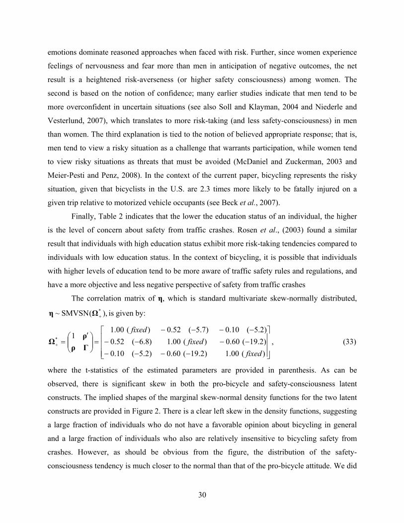
4.5. Structural Equation Model Results
Table 2 provides the results for the effects of individual-specific variables on the two latent
constructs in the structural equation model, each of which is discussed in turn in the subsequent
sections. But before doing so, a couple of issues. For the effects of the age variable on the latent
constructs, we attempted continuous functional forms as well as spline effects (that is, piecewise
linear effects), but the dummy variable specification as in Table 2 provided the best results.
Second, we have introduced the specification for all the dummy variables in Table 2 in such a
way that the estimated coefficients are all positive. This is accomplished by choosing the base
category for each exogenous variable such that the base category has the lowest value on the
latent constructs. This is done so that the location values of the latent constructs (that is, the αw
component in Equation (10)) is always positive, which helps when we interpret the moderating
effects of the latent constructs on the sensitivity to route attributes in the route choice model (see
Section 4.7).
4.5.1. Pro-Bicycle Attitude
The results in Table 2 indicate that the pro-bicyclist tendency is the highest for individuals in the
18-24 years age group (the youngest age group) and progressively decreases thereafter. This
result may be a reflection of the increasing acceptance and use of alternatives modes of
transportation (other than driving alone) by young individuals (the so-called millennials), a trend
that started to surface in about 2008 (Pucher et al., 2011). This trend has been associated with
factors such as higher environmental consciousness in the younger generation, the high costs of
29
insurance and fuel at a time when the economy has been weak, and substitution of in-person
“hangouts” by virtual “hangouts” using social mobile devices. The steady decrease in pro-
bicyclist attitudes with age may also be an indirect manifestation of the fact that bicycling
requires physical effort, and the participation levels and intensity of physical activity, in general,
tend to decrease with age (Pucher and Renne, 2003).
The pro-bicycle attitude also has a clear gender association, with men more likely to have
pro-bicyclist tendencies than women (see Pucher et al., 2011). This may reflect a preference for
less strenuous forms of physical activity among women or may be attributable to less
discretionary time available to invest in bicycling and recreation because of women’s traditional
work-family responsibilities (Garrard et al., 2008). In addition, Table 2 shows a higher pro-
bicycling attitude among single person households relative to other types of households,
consistent with some earlier studies (for example, Handy et al., 2010) that have found a higher
propensity to bicycle among people living alone.
4.5.2. Safety-Conscious Personality
For the ‘safety-conscious’ latent variable, we observe that individuals in the middle age group
(between 25-44 years of age) and beyond (more than 44 years of age) are more safety conscious
than younger individuals (between 18-24 years of age, which is the base age category). This may
be reflective of humans tending to be opportunistic and less risk-averse when young (between
18-24 years of age) due to sensation-seeking and a feeling of invincibility, but becoming less
adventurous and more risk-averse in their late 20’s and beyond when child-rearing and career-
building take center stage (Turner and McClure, 2003 and Dohmen et al., 2010). In the bicycling
context, it may also be related to the worry about slower reflexes and recovering from bicycle-
related crash injuries, combined with family responsibilities, when individuals are beyond 44
years of age (which makes this group of individuals the most safety conscious).
The gender variable also affects the ‘safety-conscious’ latent construct; women are more
safety-conscious than men in the context of bicycling safety from traffic crashes, a finding
generally consistent with the psychological literature (see Akar et al., 2013). For example,
Croson and Gneezy (2009) offer three explanations for the gender difference in risk-taking
(which is on the reverse scale of safety-consciousness). The first is based on the notion of “risk
as feelings” (see also Loewenstein et al., 2001), which states that our instinctive and intuitive
30
emotions dominate reasoned approaches when faced with risk. Further, since women experience
feelings of nervousness and fear more than men in anticipation of negative outcomes, the net
result is a heightened risk-averseness (or higher safety consciousness) among women. The
second is based on the notion of confidence; many earlier studies indicate that men tend to be
more overconfident in uncertain situations (see also Soll and Klayman, 2004 and Niederle and
Vesterlund, 2007), which translates to more risk-taking (and less safety-consciousness) in men
than women. The third explanation is tied to the notion of believed appropriate response; that is,
men tend to view a risky situation as a challenge that warrants participation, while women tend
to view risky situations as threats that must be avoided (McDaniel and Zuckerman, 2003 and
Meier-Pesti and Penz, 2008). In the context of the current paper, bicycling represents the risky
situation, given that bicyclists in the U.S. are 2.3 times more likely to be fatally injured on a
given trip relative to motorized vehicle occupants (see Beck et al., 2007).
Finally, Table 2 indicates that the lower the education status of an individual, the higher
is the level of concern about safety from traffic crashes. Rosen et al., (2003) found a similar
result that individuals with high education status exhibit more risk-taking tendencies compared to
individuals with low education status. In the context of bicycling, it is possible that individuals
with higher levels of education tend to be more aware of traffic safety rules and regulations, and
have a more objective and less negative perspective of safety from traffic crashes
The correlation matrix of η, which is standard multivariate skew-normally distributed,
),(SMVSN~ *Ωη is given by:
)(00.1)2.19(60.0)2.5(10.0
)2.19(60.0)(00.1)8.6(52.0
)2.5(10.0)7.5(52.0)(00.11*
fixed
fixed
fixed
Γρ
ρΩ , (33)
where the t-statistics of the estimated parameters are provided in parenthesis. As can be
observed, there is significant skew in both the pro-bicycle and safety-consciousness latent
constructs. The implied shapes of the marginal skew-normal density functions for the two latent
constructs are provided in Figure 2. There is a clear left skew in the density functions, suggesting
a large fraction of individuals who do not have a favorable opinion about bicycling in general
and a large fraction of individuals who also are relatively insensitive to bicycling safety from
crashes. However, as should be obvious from the figure, the distribution of the safety-
consciousness tendency is much closer to the normal than that of the pro-bicycle attitude. We did
31
not have any a priori hypotheses about these distributions, since these can be context-specific.
However, we should note that the left skew for safety consciousness is rather consistent with the
longer right tail generally observed in the social-psychological literature for risk-taking (see, for
example, Bakshi and Madan, 2006). That is, relative to the normal distribution, the effects of
unobserved characteristics make a larger fraction of individuals less safety conscious (more risk-
taking), according to the left skew distribution on the safety consciousness variable. In any case,
the important point is that the empirical fit shows that the latent constructs (and especially the
pro-bicycling attitude) are not symmetric and are not normally distributed. Statistically speaking,
the skew parameters in the ρ vector (see the first column of the covariance matrix *Ω of
Equation (33)) are different from zero, indicating that the latent constructs are statistically
different from normal distributions. Finally, there is a significant negative correlation between
the pro-bicycle and safety-conscious latent constructs, which is quite intuitive. That is,
individuals who are more pro-bicycle than their observationally equivalent peers are also less
concerned about the dangers of bicycle-related crashes.
4.6. Measurement Equation Model Results
The measurement equation model provides the loading of the latent constructs on the indicator
variables (see the bottom of Figure 1). In our empirical context, all the three indicator variables
are of an ordinal nature, and Equation (12) in Section 3.2 applies. In this equation, the parameter
vectors δ~
and ψ do not have any substantive interpretations, and simply map the scale of the
underlying latent variable vector *z to the observed ordinal indicators (we do not present the δ~
and ψ estimates here to conserve on space, but these are available from the authors). More
important are the estimates of the vector d~
in Equation (12). The estimated values for this vector
are as follows: (1) The loading of the “pro-bicycle” latent variable on the overall quality of
bicycle facilities is 1.71 (t-statistic of 8.96), showing that respondents with a high pro-bicycle
attitude also have a favorable opinion of the quality of bicycle facilities, (2) The loading of the
“safety consciousness” personality on bicycling experience from the perspective of safety from
traffic crashes is -1.10 (t-statistic of -15.01), reflecting the expected lower evaluation of traffic
safety during bicycling by safety-conscious bicyclists, and (3) The loading of the “pro-bicycle”
attitude on the frequency of non-commute bicycling throughout the year is 0.27 (t-statistic of
32
11.23), showing the positive impact of a favorable bicycle attitude on non-commute bicycling
frequency.
4.7. Route Choice Model Results
Table 3 provides the parameter estimates for the route choice model parameters of the SN-ICLV
model. In arriving at the final specification, we attempted a number of interaction effects of route
attributes with individual-specific observed variables, in addition to interaction effects of route
attributes with the two latent constructs (whenever the two effects can be identified based on the
sufficiency conditions discussed in Section 3.4). However, none of the individual-specific
observed variable interaction effects turned out to be statistically significant (except for trip
purpose interacted with terrain grade) when the latent construct interaction effects were also
included. That is, our results essentially showed that individual-specific observed variables
impact route choice through the latent constructs and not directly, providing substantial support
for the ICLV model structure and the specification used in the paper.
In the discussion of Table 3 below, and purely for interpretation ease, we will interpret
the coefficients on the latent constructs as though the latent constructs were deterministic
(technically, the latent constructs are skew-normally distributed, engendering unobserved
heterogeneity in the moderating effects of the latent constructs on the sensitivity to route
attributes). Specifically, we will assume that the latent constructs are at their location value of
αw , which, by specification of the structural equation model, is always positive (see Section
4.5.1 and 4.5.2). Also, we note here that the parameters in Table 3 provide the effects of
variables on the utility valuation of routes. Interaction effects of route attributes with the latent
constructs/bicyclist characteristics are shown in Table 3 by indenting the labels for latent
constructs/bicyclist characteristics under the route attributes.
The effects of on-street parking characteristics indicate that all bicyclists prefer no
parking rather than any form of parking on their route (note that the base category for parking
type is “absence of parking”, and the signs of all the parking type-related variables are negative).
Parking presents a general hindrance to bicycle movement and restricts the cushion between
motorized traffic and bicyclists. The results also indicate that angled parking is preferred to
parallel parking, presumably because of better visibility and line of sight for bicyclists as cars
pull out from an angled parking configuration. On the other hand, parallel parking (a) presents
33
more disruption to bicyclists as motorists maneuver into or out of a parallel parking spot, and (b)
poses a “dooring” problem to bicyclists. As importantly, and intuitively, bicyclists who are
safety-conscious are more concerned about (and stay away from) routes with parking,
particularly those with parallel parking. The effects of the remaining parking variables are also as
expected, and reveal that routes with high parking turnover rate, length of parking area, and
parking occupancy rate reduces the attractiveness of bicycling routes, particularly so for safety
conscious individuals. All of these parking attributes present disruptions to the movement of
bicyclists because of more potential conflict occasions and conflict durations during a bicyclist’s
trip.
The effects of bicycle facility characteristics reveal that routes with a continuous bicycle
facility (the whole route has a bicycle lane or wide outside lane) are preferred relative to those
with a discontinuous facility (see also Caulfied et al., 2012). Further, bicyclists prefer routes with
no bicycle lane and a wide outside lane of width greater than or equal to 10.5 feet to routes with
a bicycle lane of width less than 6.75 feet (we did not find statistically significant differences in
preferences between a 3.75 feet bicycle lane and a 6.25 feet bicycle lane, and so both of these
levels form the base category). That is, bicyclists appear to prefer wide bicycle facilities (even if
not explicitly demarcated and separated from motorist lanes) to demarcated but narrow bicycle
lanes. Bernhoft and Carstensen (2008) also found a similar result. While this result may seem
counterintuitive, it is suggestive of the notion that facility width is a better representation of
space cushion in the mental perception map of bicyclists than is facility separation. Interestingly,
we did not find any statistically significant interaction effect of a safety conscious personality
with bicycle facility characteristics.
The effects of roadway physical characteristics provide some surprising results in the
context of terrain grade. To interpret the coefficients, we should note first that the location of the
pro-bicycle latent construct varies (across individuals) from a value of zero to the value of 0.637
(mean of 0.158), while the location of the safety consciousness construct varies from a value of
zero to the value of 0.372 (mean of 0.126). Then, the results in Table 3 indicate that all
individuals (technically in the location) most prefer moderate hills to flat grades, especially for
non-commuting bicycling (as can be observed from the negative coefficient on commuting
bicycling). This trend may be attributed to the preference for a bicycle route that is not
monotonous in landscape or physical effort, especially for bicycling for recreation/leisure (see
34
Stinson and Bhat, 2003 for a similar result). The results for “steep hills” are a little more tricky.
At the mean location value for the pro-bicycle attitude of 0.158, the coefficient of steep hills is
0.047 (=0.087-0.252*0.158) for non-commuting bicyclists and -0.072 (=0.087-0.252*0.158-
0.119) for commuting bicyclists. That is, non-commuting bicyclists prefer steep hills to a flat
grade, while commuting bicyclists prefer flat grades to steep hills. The latter effect is intuitive,
because individuals would like to arrive at work in a reasonably presentable fashion. However,
surprisingly and when examining the coefficient on the pro-bicycling variable, the results show
that individuals who are higher on the pro-bicycle scale have a lower preference for moderate
and steep grades relative to individuals who are lower on the pro-bicycle scale. This is contrary
to our hypothesis presented in Section 4.4. Perhaps this reflects a pre-trip underestimation of the
strenuousness of bicycling along moderate to steep grades by individuals who are lower on the
pro-bicycle scale, because they bicycle lesser and have less experience. The second variable in
the category of roadway physical characteristics reflects the reduced likelihood of using routes
with a higher number of traffic controls and cross-streets, particularly for individuals who are
pro-bicycle and potentially see traffic controls as very annoying and disruptive (see also
Menghini et al., 2010 and Prato et al., 2012).
Next, the effects of roadway functional characteristics show that bicyclists prefer routes
with low volumes of motorized traffic to routes with moderate and high volumes of motorized
traffic (see also Prato et al., 2012 for a similar result). This is likely to be a combination of a
larger space cushion over the stretch of the route when there is only light traffic as well as a
lower likelihood of crashes. As one may expect, safety-conscious bicyclists, in particular, shy
away from routes with moderate to high motorized traffic volumes. Similar safety related issues
extend to the effect of speed limit on route choice (as also found by Caulfied et al., 2012), with
bicyclists (and particularly safety-conscious bicyclists) preferring routes with a speed limit of
less than or equal to 35 miles per hour to routes with speed limits exceeding 35 miles per hour.
Finally, the coefficient for travel time (relevant only for commute travel) is negative, suggesting
that cyclists prefer routes with lower travel times. We did not find statistically significant effects
of the latent constructs on the travel time effect.
35
4.8. Measures of Data Fit
In this section, we provide measures of fit for the route choice predictions from our proposed
SN-ICLV model, the corresponding ICLV model that imposes normal distributions for the latent
constructs, as well as an MNP model that ignores the latent constructs but considers observed
and unobserved heterogeneity in the effects of route attributes. We would like to note here that,
unlike many earlier ICLV-based studies that compare the ICLV model with a simple discrete
choice model without any accommodation of observed or unobserved heterogeneity, we consider
both observed and unobserved heterogeneity in the “strawman” MNP specification. We believe
this is only fair, and that many earlier ICLV studies have not used an appropriate non-ICLV
discrete choice model yardstick to compare the estimated ICLV model with. In developing our
MNP specification, we extensively tested for observed and unobserved heterogeneity. At the
end, only the random (normal) distributions for terrain grade and motorized traffic volumes
turned out to be statistically significant. This is as opposed to the SN-ICLV specification in
which the error terms in the structural equation system for the latent constructs permeates into
unobserved heterogeneity effects for all route attributes that are interacted with one or both latent
constructs. Thus, in Table 3, unobserved heterogeneity appears for 12 route attribute effects
(angle parking, parallel parking, parking turnover rate, length of parking area, parking occupancy
rate, moderate hills, steep hills, moderate # and high # of stop signs, red lights and cross streets,
moderate and heavy traffic volumes, and high speed limit), and in a very parsimonious manner
because all these effects originate from only two latent constructs.
The predictions from the route choice models in the SN-ICLV, ICLV, and MNP models
are compared as follows. For the SN-ICLV and ICLV models, the model system is estimated as
discussed in Section 3 (for ICLV model, we simply fix the skew parameters to zero in the
structural equation). For the MNP model, we use a MACML estimation procedure as described
on Bhat (2011) (the detailed estimation results for the ICLV and MNP models are not presented
here to conserve on space, but may be obtained from the authors). Then, using Equation (17) and
the estimated parameters from the MACML estimation for the three different models, one can
obtain the logarithm of the probability of the sequence of observed choices for each respondent
from each model, which is the predictive log-likelihood function of the route choice model at
convergence )ˆ(θ L . Then, the SN-ICLV and the ICLV models can be compared using the

36
familiar likelihood ratio test. For the test between the SN-ICLV and MNP models, one can
compute the adjusted likelihood ratio index with respect to the log-likelihood at equal shares:
)(
)ˆ(12
c
M
L
L
θ , (33)
where )ˆ(θ L and )(c L are the log-likelihood functions at convergence and at equal shares (at
each choice instance), respectively, and M is the number of parameters estimated in the model.
To test the performance of the two non-nested models (i.e. the SN-ICLV and MNP models)
statistically, the non-nested adjusted likelihood ratio test may be used. This test determines if the
adjusted likelihood ratio indices of two non-nested models are significantly different. In
particular, if the difference in the indices is )( 21
22 , then the probability that this
difference could have occurred by chance is no larger than 5.012 )]()(2[ MMc L in
the asymptotic limit. A small value of the probability of chance occurrence indicates that the
difference is statistically significant and that the model with the higher value of adjusted
likelihood ratio index is to be preferred.
The above predictive likelihood ratio test (for the comparison of the SN-ICLV and ICLV
models) and non-nested adjusted likelihood ratio test (for the comparison of the SN-ICLV and
MNP models) are undertaken both in the estimation sample and the validation sample. We also
evaluate the performance of the three models intuitively and informally by computing the
average probability of correct prediction across all choice instances, in both the estimation and
validation samples. The use of testing on both the estimation and validation samples is to ensure
that there is no over-fitting effects during evaluation.
The results for the estimation sample are presented in the second main column of Table 4.
The first row provides the log-likelihood at equal shares, which is, of course, the same across the
three models. The second row indicates the superior performance of the SN-ICLV model in
terms of the predictive log-likelihood value, as does the adjusted likelihood ratio index in the
fifth row. The sixth row formally shows the predictive likelihood ratio test result of the
comparison of the SN-ICLV model over the ICLV model, indicating the clear dominance of the
SN-ICLV data fit. The same result is obtained in the next row through a non-nested adjusted
likelihood ratio test comparing the SN-ICLV model with the MNP model; the probability that the
adjusted likelihood ratio index difference between the SN-ICLV and MNP models could have
37
occurred by chance is literally zero. The average probability of correct prediction (see the last
row of the table) reinforces the results from the statistical tests. Similar results are obtained in the
validation sample. In summary, the SN-ICLV model clearly outperforms the other two models
from a statistical standpoint.
One can also examine the results from the SN-ICLV and ICLV models behaviorally. Of
course, the use of an incorrect distribution for the latent constructs will, in general, lead to
inconsistent parameter estimation in all components of the model system. Intuitively speaking,
assuming similar estimated coefficients in the SN-ICLV and ICLV models (as was the case in
our estimations), the left-skew manifested in the latent constructs in our model system indicate
that the effects of unobserved factors lead to a smaller fraction of pro-bicyclists and a smaller
fraction of safety-conscious individuals than what is specified by the normal distribution. So,
with similar estimated coefficients in the choice model between the SN-ICLV and ICLV models,
we should expect that the negative effects of pro-bicycling and safety consciousness on specific
design features should lead to a smaller aggregate magnitude of effect on route choice from our
SN-ICLV model relative to the ICLV model. To examine this issue, we created two routes (A
and B) with exactly the same values for the design attributes, the value for each design attribute
corresponding to the base category for the route attribute in Table 2 (we assigned the average
travel time across all individuals as the travel time for each of the two routes). Next, we changed
the value of each design attribute in turn from the base category to a non-base category for route
B so that the value of only one design attribute was different between the two routes each time.
We then computed a pseudo-elasticity for each design attribute as the percentage difference in
the choice probability for route B from the base case (0.5 probability for both routes A and B),
assuming the group of commuter bicyclists who are 18-24 years of age, male, single, and with an
associate degree/some college degree. Here, we do not provided these elasticity measures for
each attribute, but provide a flavor of the differences between the different models. Thus, for
example, the presence of a high number of stop-signs, red lights, and cross-streets reduced the
probability of route B by 75% according to our SN-ICLV model, but by 88% in the ICLV model.
Similarly, a high speed limit reduced the probability of route B by 76% according to our model,
but by 88% according to the ICLV model. Overall, the effects of design features that degrade
route attractiveness are exaggerated by the simple ICLV model relative to our SN-ICLV model.
While it is more difficult to intuit the differences between these latent variable models and the
38
simple MNP model, our results indicated that the MNP model even further exaggerates the
negative consequences of parking, discontinuous bicycle facility, steep hills, high number of
stop-signs, red lights, and cross-streets, heavy traffic volumes, high speed limits, and travel time
increases.
4.9. Relative Effects of Route Attributes
All the route attributes in Table 4 are dummy (discrete) variables (or switches), except for travel
time for commute-related route choice, and so one can readily obtain the relative importance of
the route attributes. While one cannot technically compare the relative effects of the dummy
variables and the travel time variable for commute-related route choice, one approach to get an
order of magnitude effect is to compute the (dis-)utility effect of travel time at the mean bicycle
commute travel time value of 30 minutes in the sample. This yields a value of -0.93, which may
be compared with the coefficients on the route attribute dummy variables.
The magnitudes of the coefficients in Table 3 indicate that routes with long travel times
(for commuters) and heavy motorized traffic volume are, by far, the most unlikely to be chosen.
Other route attributes with a high impact include whether the route has a continuous bicycle
facility or not, high parking occupancy rates and long lengths of parking when parking is
allowed, and a high speed limit (more than 35 mph) on the route. On the other hand, bicycle
facility width (if a bicycle lane exists) or width of wide outside lane (if a bicycle lane does not
exist) are the least important attributes in bicyclist route choice evaluation, while the impact of
terrain grade and angle parking are also quite small. These relative magnitude effects were also
reflected in the pseudo-elasticity measures computed in the previous section.
The results above have at least four general implications for bicycling infrastructure
investments. First, the results suggest that providing some kind of a continuous facility (either in
the form of a wide outside lane or in the form of an exclusive bicycle lane) is more important
than the specific type of facility provided (whether a wide outside lane or whether an exclusive
bicycle lane). Second, there is a suggestion that providing a wide outside lane (without any
demarcation in motorized vehicle and bicycle movement) may be somewhat better than
providing a relatively narrow but exclusive bicycle lane (from the perspective of the
attractiveness of a route to bicyclists). This is consistent with the concept of vehicular bicycling,
which is based on the notion that bicycling safety is improved by sharing of the roadway
39
between motorists and bicyclists, and educating motorists to recognize bicyclists as legitimate
users of roadways (see Sener et al., 2009 and Pucher et al., 2011). However, we must emphasize
again here that the precise form of the bicycle facility pales in comparison to providing a
continuous facility of some form in the first place. Third, our results imply that disallowing
parking on potential routes would be a good strategy to attract bicyclists to use these routes. If
parking has to be allowed due to other considerations, restricting the length of parking and the
hours of parking may be an approach to reduce the deterrent effects on bicycling along the route.
Additionally, the notion of limiting the duration of parking for a specific vehicle, while may be
helpful from other transportation considerations, does seem to discourage bicycling along the
route (since limiting parking duration results in frequent vehicle turnovers). Planners may want
to consider these parking-related effects on bicyclist route choice when designing and investing
in bicycle facilities. Doing so also has the potential to promote bicycling, since safety conscious
bicyclists (and by extension, individuals who may not be bicycling because of their worry about
safety when bicycling) are particularly sensitive to parking-related attributes. Fourth, other
important issues that planners need to consider in designing bicycle facilities are speed limit
restrictions and ways to control motorized traffic volumes.
5. CONCLUSIONS
Integrated choice and latent variable (ICLV) models enable researchers to provide a structure to
unobserved effects in choice modeling, and are gaining popularity as a means to unravel the
decision process of individuals in choice situations. However, a substantial limitation of
traditional ICLV models is that they impose a normal distribution assumption for the unobserved
latent constructs. But there is no theoretical basis for making such an assumption. Besides,
imposing this assumption when the structural errors are non-normal can render all parameter
estimates inconsistent. In the current paper, we have proposed a skew-normal distribution form
for the latent constructs. To our knowledge, this is the first such ICLV model proposed in the
econometric literature. The multivariate skew-normal (MSN) distribution that we use is
tractable, parsimonious in parameters that regulate the distribution and its skewness, and includes
the normal distribution as a special interior point case (this allows for testing with the traditional
ICLV model). It also is flexible, allowing a continuity of shapes from normality to non-
normality, including skews to the left or right and sharp versus flat peaking toward the mode (see
40
Bhat and Sidharthan, 2012). It also immediately accommodates correlation across the latent
variables because of its multivariate structure. The resulting skew normal ICLV model we
develop is suitable for estimation using Bhat’s (2011) maximum approximate composite
marginal likelihood (MACML) inference approach.
The proposed model was applied to model bicyclists’ route choice behavior. In this study,
two latent variables - pro-bicycle attitude and safety consciousness in the context of traffic
crashes - were specified to moderate the effect of route attributes in bicyclist route choice
decisions. These latent variables were assumed to be manifested in three ordinal indicator
variables associated with (a) perceptions about the overall quality of bicycle facilities, (b)
bicycling experience from the perspective of safety from traffic crashes, and (c) how often the
respondent bicycles throughout the year for non-commuting reasons. A stated preference
methodology using a web-based survey of Texas bicyclists provided the route choice data to
implement the model. The results showed that individual-specific observed variables impact
route choice through the latent constructs we developed and not directly, providing substantial
support for the ICLV model structure and the specification used in the paper. Importantly, the
results showed evidence for non-normality in the latent constructs, with the proposed model
soundly rejecting the traditional ICLV model (with normal latent constructs) and a multinomial
probit model (with unstructured heterogeneity in the influence of unobserved factors on the
sensitivity to route attributes) based on data fit considerations. Further, the results suggest that
the most unattractive features of a bicycle route are long travel times (for commuters), heavy
motorized traffic volume, absence of a continuous bicycle facility, and high parking occupancy
rates and long lengths of parking zones along the route.
In conclusion, from a methodological standpoint, this paper has developed an extension
of the typical ICLV models to incorporate potential non-linearity in the latent constructs. The
resulting model should be applicable in a variety of choice contexts. From a substantive
standpoint, the model developed here may be used by planners to assess and improve existing
bicycle routes as well as to plan better routes by understanding trade-offs among route attributes.
ACKNOWLEDGMENTS
This research was partially supported by the U.S. Department of Transportation through the
Data-Supported Transportation Operations and Planning (D-STOP) Tier 1 University

41
Transportation Center. The first author would like to acknowledge support from a Humboldt
Research Award from the Alexander von Humboldt Foundation, Germany. The authors are
grateful to Lisa Macias for her help in formatting this document, and to anonymous reviewers for
helpful comments on an earlier version of the document.
42
REFERENCES
Alvarez-Daziano, R., Bolduc, D., 2013. Incorporating pro-environmental preferences towards green automobile technologies through a Bayesian hybrid choice model. Transportmetrica A: Transport Science 9(1), 74-106.
Akar, G., Fischer, N., Namgung, M., 2013. Bicycling choice and gender case study: the Ohio State University. International Journal of Sustainable Transportation 7(5), 347-365.
Arellano-Valle, R.B., Azzalini, A., 2006. On the unification of families of skew-normal distributions. Scandinavian Journal of Statistics 33(3), 561-574.
Azzalini, A., Dalla Valle, A., 1996. The multivariate skew-normal distribution. Biometrica 83(4), 715-726.
Bakshi, G., Madan, D., 2006. The distribution of risk aversion. Available at SSRN 890270.
Beck, L.F., Dellinger, A.M., O'Neil, M.E., 2007. Motor vehicle crash injury rates by mode of travel, United States: using exposure-based methods to quantify differences. American Journal of Epidemiology 166(2), 212-218.
Ben-Akiva, M., Walker, J., Bernardino, A.T., Gopinath, D.A., Morikawa, T., Polydoropoulou, A., 2002. Integration of choice and latent variable models. In: Mahmassani, H. (ed.) In Perpetual Motion: Travel Behavior Research Opportunities and Application Challenges, Pergamon, Elsevier Science, 431-470.
Bernhoft, I.M., Carstensen, G., 2008. Preferences and behaviour of pedestrians and cyclists by age and gender. Transportation Research Part F 11(2), 83-95.
Bhat, C.R., 1997. Endogenous segmentation mode choice model with an application to intercity travel. Transportation Science 31(1), 34-48.
Bhat, C.R., 2011. The maximum approximate composite marginal likelihood (MACML) estimation of multinomial probit-based unordered response choice models. Transportation Research Part B 45(7), 923-939.
Bhat, C.R., 2014. The composite marginal likelihood (CML) inference approach with applications to discrete and mixed dependent variable models. Foundations and Trends in Econometrics 7(1), 1-117.
Bhat, C.R., Dubey S.K., 2014. A new estimation approach to integrate latent psychological constructs in choice modeling. Transportation Research Part B, 67, 68-85.
Bhat, C.R., Sidharthan, R., 2012. A new approach to specify and estimate non-normally mixed multinomial logit models. Transportation Research Part B 46(7), 817-833.
Bolduc, D., Ben-Akiva, M., Walker, J., Michaud, A., 2005. Hybrid choice models with logit kernel: applicability to large scale models. In: Lee-Gosselin, M., Doherty, S. (eds.) Integrated Land-Use and Transportation Models: Behavioral Foundations, Elsevier, Oxford, 275-302.
Brey, R., Walker, J.L., 2011. Latent temporal preferences: An application to airline travel. Transportation Research Part A 45(9), 880-895.
43
Broach, J., Dill, J., Gliebe, J., 2012. Where do cyclists ride? A route choice model developed with revealed preference GPS data. Transportation Research Part A 46(10), 1730-1740.
Caffo, B., An, M.W., Rohde, C., 2007. Flexible random intercept models for binary outcomes using mixtures of normals. Computational Statistics & Data Analysis 51(11), 5220-5235.
Caulfield, B., Brick, E., McCarthy, O.T., 2012. Determining bicycle infrastructure preferences-A case study of Dublin. Transportation Research Part D 17(5), 413-417.
Chen, C.F., Chen, P.C., 2013. Estimating recreational cyclists’ preferences for bicycle routes-Evidence from Taiwan. Transport Policy 26, 23-30.
Contreras-Reyes, J.E., Arellano-Valle, R.B., 2013. Growth estimates of cardinalfish (Epigonus crassicaudus) based on scale mixtures of skew-normal distributions. Fisheries Research 147, 137-144.
Cox, D.R., Reid, N., 2004. A note on pseudolikelihood constructed from marginal densities. Biometrika 91(3), 729–737.
Croson, R., Gneezy, U., 2009. Gender differences in preferences. Journal of Economic Literature 47(2), 448-474.
Dohmen, T.J., Falk, A., Huffman, D., Sunde, U., 2010. Are risk aversion and impatience related to cognitive ability? American Economic Review, 100(3), 1238-1260.
Dutzik, T., Baxandall, P., 2013. A new direction: Our changing relationship with driving and the implications for America’s future. U.S. Public Interest Research Group Education Fund, Boston, MA.
Garrard, J., Rose, G., Lo, S.K., 2008. Promoting transportation cycling for women: the role of bicycle infrastructure. Preventive medicine 46(1), 55-59.
Geweke, J., Keane, M., 1999. Mixture of normals probit models. In: Hsiao, Lahiri, Lee and Pesaran (eds.), Analysis of Panels and Limited Dependent Variable Models, Cambridge University Press, 49-78.
Godambe, V.P., 1960. An optimum property of regular maximum likelihood estimation. The Annals of Mathematical Statistics 31(4), 1208-1211.
Handy, S.L., Xing, Y., Buehler, T.J., 2010. Factors associated with bicycle ownership and use: A study of six small U.S. cities. Transportation 37(6), 967-985.
Hood, J., Sall, E., Charlton, B., 2011. A GPS-based bicycle route choice model for San Francisco, California. Transportation Letters 3(1), 63-75.
Keane, M.P., 1992. A note on identification in the multinomial probit model. Journal of Business & Economic Statistics 10(2), 193-200.
Lachos, V.H., Ghosh, P., Arellano-Valle, R.B., 2010. Likelihood based inference for skew normal independent linear mixed models. Statistica Sinica 20(1), 303–322
Lee, S., McLachlan, G.J., 2013. Finite mixtures of multivariate skew t-distributions: Some recent and new results. Statistics and Computing 24(2), 181-202
Lin, T.I., Ho, H.J., Lee, C.R., 2013. Flexible mixture modelling using the multivariate skew-t-normal distribution. Statistics and Computing 24(4), 531-546.
44
Lindsay, B.G., 1988. Composite likelihood methods. Contemporary Mathematics 80, 221-239.
Lindsay, B.G., Yi, G.Y., Sun, J., 2011. Issues and strategies in the selection of composite likelihoods. Statistica Sinica 21(1), 71-105.
Loewenstein, G.F., Weber, E.U., Hsee, C.K., Welch, N., 2001. Risk as feelings. Psychological Bulletin 127(2), 267-286.
Manski, C.F., Lerman, S.R., 1977. The estimation of choice probabilities from choice based samples. Econometrica 45(8), 1977-1988.
McDaniel, S.R., Zuckerman, M., 2003. The relationship of impulsive sensation seeking and gender to interest and participation in gambling activities. Personality and Individual Differences 35(6), 1385-1400.
McKelvey, R.D., Zavoina, W., 1975. A statistical model for the analysis of ordinal level dependent variables. Journal of Mathematical Sociology 4(1), 103-120.
Meier-Pesti, K., Penz, E., 2008. Sex or gender? Expanding the sex-based view by introducing masculinity and femininity as predictors of financial risk taking. Journal of Economic Psychology 29(2), 180-196.
Menghini, G., Carrasco, N., Schüssler, N., Axhausen, K.W., 2010. Route choice of cyclists in Zurich. Transportation Research Part A 44(9), 754-765.
Metropolitan Transportation Commission, 2009. Regional Bicycle Plan for the San Francisco Bay Area: 2009 Update. March.
Molenberghs, G., Verbeke, G., 2005. Models for Discrete Longitudinal Data. Springer Series in Statistics. Springer Science + Business Media, Inc., New York.
Munkin, M.K., Trivedi, P.K., 2008. Bayesian analysis of the ordered probit model with endogenous selection. Journal of Econometrics 143(2), 334-348.
Muthen, B., 1978. Contributions to factor analysis of dichotomous variables. Psychometrika 43(4), 551-560.
Muthen, B., 1984. A general structural equation model with dichotomous, ordered categorical, and continuous latent variable indicators. Psychometrika 49(1), 115-132.
National Center for Health Statistics, 2010. Health, United States, 2009: With Special Feature on Medical Technology. Hyattsville, MD. http://www.cdc.gov/nchs/data/hus/hus09.pdf
Niederle, M., Vesterlund, L., 2007. Do women shy away from the competition? Do men compete too much? Quarterly Journal of Economics 122(3), 1067-1101.
Prato, C.G., Bekhor, S., Pronello, C., 2012. Latent variables and route choice behavior. Transportation 39(2), 299-319.
Pucher, J., Renne, J.L., 2003. Socioeconomics of urban travel: evidence from the 2001 NHTS. Transportation Quarterly 57(3), 49-77.
Pucher, J., Buehler, R., Seinen, M., 2011. Bicycling renaissance in North America? An update and re-appraisal of cycling trends and policies. Transportation Research Part A 45(6), 451-475.

45
Pyne, S., Hu, X., Wang, K., Rossin, E., Lin, T.I., Maier, L.M., Baecher-Allan, C., McLachlan, G.J., Tamayo, P., Hafler, D.A., De-Jager, P.L., Mesirow, J.P., 2009. Automated high-dimensional flow cytometric data analysis. Proceedings of the National Academy of Sciences of the United States of America 106(21), 8519-8524.
Rendall, S., Rose, P., Janssen, K., 2012. Delivering effective cycle facilities: Modelling bicycle route choice in New Zealand. Institution of Professional Engineers New Zealand (IPENZ) Transportation Group Conference, March.
Revelt, D., Train, K., 1996. Incentives for appliance efficiency in a competitive energy environment. ACEEE Summer Study Proceedings Paper, Panel 3, Paper 15, August.
Riggi, S., Ingrassia, S.. 2013. Modeling high energy cosmic rays mass composition data via mixtures of multivariate skew-t distributions. arXiv: 13011178 [astro-phHE].
Rosen, A.B., Tsai, J.S., Downs, S.M., 2003. Variations in risk attitude across race, gender, and education. Medical Decision Making 23(6), 511-517.
Schroeder, P., Wilbur, M., 2013. 2012 National Survey of Bicyclist and Pedestrian Attitudes and Behavior, Volume 2: Findings Report. Report No. DOT HS 811 841 B, National Highway Traffic Safety Administration, Washington, DC.
Sener, I.N., Eluru, N., Bhat, C.R., 2009. An analysis of bicycle route choice preferences in Texas, U.S. Transportation 36(5), 511-539.
Soll, J.B., Klayman, J., 2004. Overconfidence in interval estimates. Journal of Experimental Psychology: Learning, Memory, and Cognition 30(2), 299-314.
Southern California Association of Governments, 2012. 2012-2035 Regional Transportation Plan/Sustainable Communities Strategy (RTP/SCS): Towards a Sustainable Future, Active Transportation Appendix. Available at: http://rtpscs.scag.ca.gov/Documents/2012/final/SR/2012fRTP_ActiveTransportation.pdf.
Stapleton, D.C., 1978. Analyzing political participation data with a MIMIC Model. Sociological Methodology 9, 52-74.
Stinson, M.A., Bhat C.R., 2003. An analysis of commuter bicyclist route choice using a stated preference survey. Transportation Research Record 1828, 107-115.
Turner, C., McClure, R., 2003. Age and gender differences in risk-taking behaviour as an explanation for high incidence of motor vehicle crashes as a driver in young males. Injury Control and Safety Promotion 10(3), 123-130.
Varin, C., Reid, N., Firth, D., 2011. An overview of composite likelihood methods. Statistica Sinica 21(1), 5-42.
Vij, A., Walker, J., 2014. Hybrid choice models: The identification problem. In: Hess, S., Daly, A. (eds.) Handbook of Choice Modelling, Edward Elgar Publishing, 519-564.
Vrbik, I., McNicholas, P.D., 2014. Parsimonious skew mixture models for model-based clustering and classification. Computational Statistics and Data Analysis 71, 196-210.
Wall, M.M., Guo, J., Amemiya, Y., 2012. Mixture factor analysis for approximating a non-normally distributed continuous latent factor with continuous and dichotomous observed variables. Multivariate Behavioral Research 47(2), 276-313.

46
Xu, X., Reid, N., 2011. On the robustness of maximum composite likelihood estimate. Journal of Statistical Planning and Inference 141(9), 3047-3054.
Yi, G.Y., Zeng, L., Cook, R.J., 2011. A robust pairwise likelihood method for incomplete longitudinal binary data arising in clusters. The Canadian Journal of Statistics 39(1), 34-51.
Zhao, Y., Joe, H., 2005. Composite likelihood estimation in multivariate data analysis. The Canadian Journal of Statistics 33(3), 335-356.

47
Figure 1: Conceptual Diagram for Considering Psychological Constructs in Bicyclists’ Route Choice Analysis
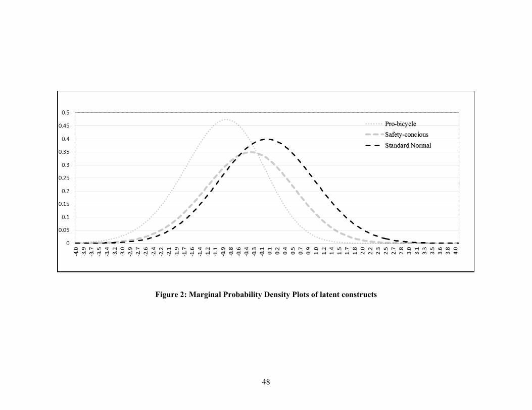
48
Figure 2: Marginal Probability Density Plots of latent constructs
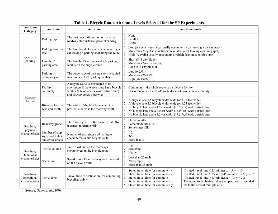
49
Table 1. Bicycle Route Attribute Levels Selected for the SP Experiments Attribute Category
Attribute Attribute Attribute levels
On-street parking
Parking type The parking configuration on a shared roadway (for instance, parallel parking)
1. None 2. Parallel 3. Angle
Parking turnover rate
The likelihood of a cyclist encountering a car leaving a parking spot along the route
1. Low (A cyclist very occasionally encounters a car leaving a parking spot) 2. Moderate (A cyclist sometimes encounters a car leaving a parking spot) 3. High (A cyclist usually encounters a vehicle leaving a parking spot)
Length of parking area
The length of the motor vehicle parking facility on the bicycle route
1. Short (½-1 city block) 2. Moderate (2-4 city blocks) 3. Long (5-7 city blocks)
Parking occupancy rate
The percentage of parking spots occupied in a motor vehicle parking facility
1. Low (0-25%) 2. Moderate (26-75%) 3. High (76-100%)
Bikeway facility
Facility continuity
A bicycle route is considered to be continuous if the whole route has a bicycle facility (a bike lane or wide outside lane) and discontinuous otherwise
1. Continuous – the whole route has a bicycle facility 2. Discontinuous – the whole route does not have a bicycle facility
Bikeway facility type and width
The width of the bike lane when it is present; otherwise the roadway width
1. A bicycle lane 1.5 bicycle width wide (or 3.75 feet wide) 2. A bicycle lane 2.5 bicycle width wide (or 6.25 feet wide) 3. No bicycle lane and a 1.5 car width (10.5 feet) wide outside lane 4. No bicycle lane and a 2.0 car width (14.0 feet) wide outside lane 5. No bicycle lane and a 2.5 car width (17.5 feet) wide outside lane
Roadway physical
characteristics
Roadway grade The terrain grade of the bicycle route (for instance, moderate hills)
1. Flat – no hills 2. Some moderate hills 3. Some steep hills
Number of stop signs, red lights and cross streets
Number of stop signs and red lights encountered on the bicycle route
1. 1-2 2. 3-5 3. More than 5
Roadway functional
characteristics
Traffic volume Traffic volume on the roadways encountered on the bicycle route
1. Light 2. Moderate 3. Heavy
Speed limit Speed limit of the roadways encountered on the bicycle route
1. Less than 20 mph 2. 20-35 mph 3. More than 35 mph
Roadway operational
characteristics Travel time
Travel time to destination (for commuting bicyclists only)
1. Stated travel time for commute – y 2. Stated travel time for commute – x 3. Stated travel time for commute 4. Stated travel time for commute + x 5. Stated travel time for commute + y
If stated travel time ≤ 25 minutes x = 5, y = 10; If stated travel time > 25 and ≤ 45 minutes x = 5, y = 15; If stated travel time > 45 minutes x = 10, y = 20; The travel time obtained after the operations is rounded off to the nearest multiple of 5
Source: Sener et al., 2009.
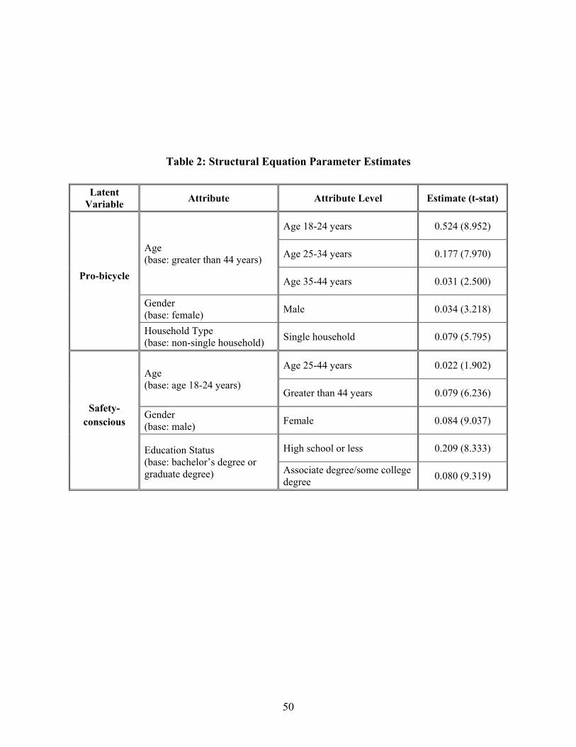
50
Table 2: Structural Equation Parameter Estimates
Latent Variable
Attribute Attribute Level Estimate (t-stat)
Pro-bicycle
Age (base: greater than 44 years)
Age 18-24 years 0.524 (8.952)
Age 25-34 years 0.177 (7.970)
Age 35-44 years 0.031 (2.500)
Gender (base: female)
Male 0.034 (3.218)
Household Type (base: non-single household)
Single household 0.079 (5.795)
Safety-conscious
Age (base: age 18-24 years)
Age 25-44 years 0.022 (1.902)
Greater than 44 years 0.079 (6.236)
Gender (base: male)
Female 0.084 (9.037)
Education Status (base: bachelor’s degree or graduate degree)
High school or less 0.209 (8.333)
Associate degree/some college degree
0.080 (9.319)
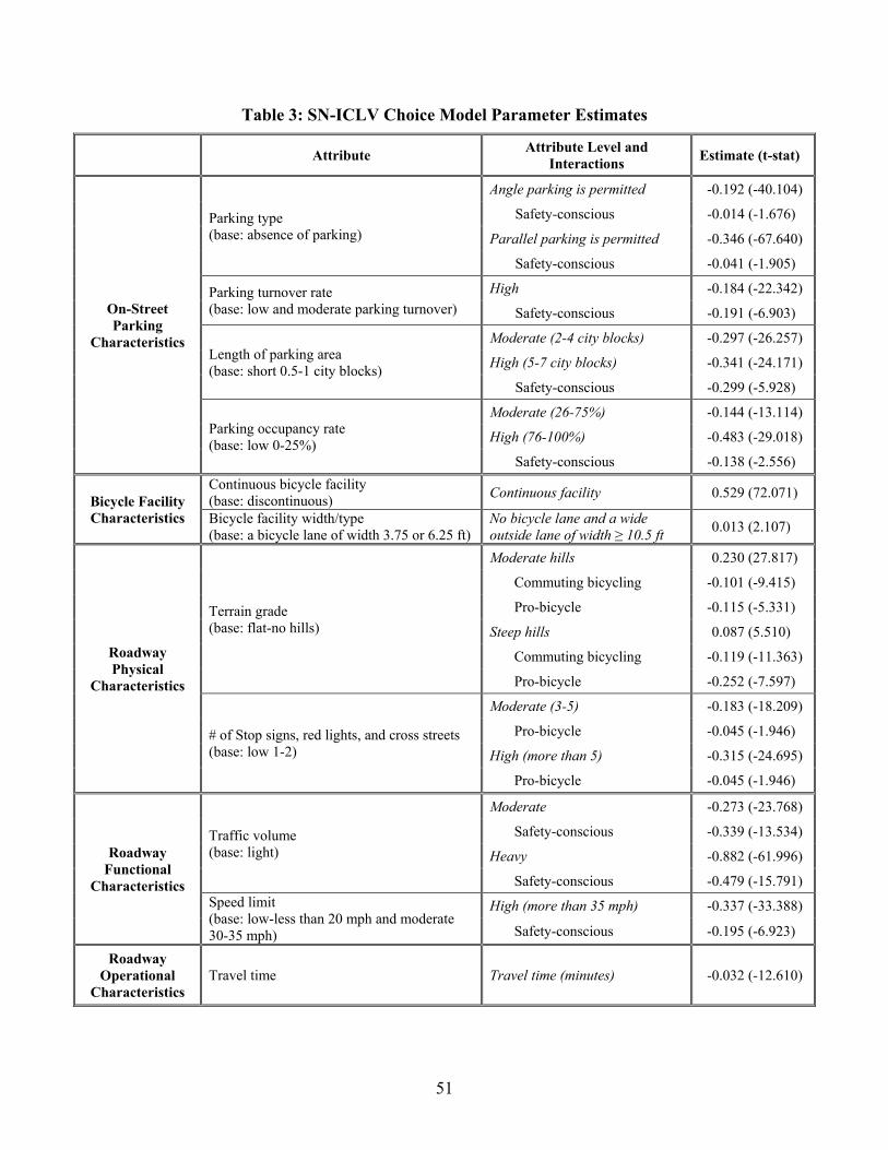
51
Table 3: SN-ICLV Choice Model Parameter Estimates
Attribute
Attribute Level and Interactions
Estimate (t-stat)
On-Street Parking
Characteristics
Parking type (base: absence of parking)
Angle parking is permitted -0.192 (-40.104)
Safety-conscious -0.014 (-1.676)
Parallel parking is permitted -0.346 (-67.640)
Safety-conscious -0.041 (-1.905)
Parking turnover rate (base: low and moderate parking turnover)
High -0.184 (-22.342)
Safety-conscious -0.191 (-6.903)
Length of parking area (base: short 0.5-1 city blocks)
Moderate (2-4 city blocks) -0.297 (-26.257)
High (5-7 city blocks) -0.341 (-24.171)
Safety-conscious -0.299 (-5.928)
Parking occupancy rate (base: low 0-25%)
Moderate (26-75%) -0.144 (-13.114)
High (76-100%) -0.483 (-29.018)
Safety-conscious -0.138 (-2.556)
Bicycle Facility Characteristics
Continuous bicycle facility (base: discontinuous)
Continuous facility 0.529 (72.071)
Bicycle facility width/type (base: a bicycle lane of width 3.75 or 6.25 ft)
No bicycle lane and a wide outside lane of width ≥ 10.5 ft
0.013 (2.107)
Roadway Physical
Characteristics
Terrain grade (base: flat-no hills)
Moderate hills 0.230 (27.817)
Commuting bicycling -0.101 (-9.415)
Pro-bicycle -0.115 (-5.331)
Steep hills 0.087 (5.510)
Commuting bicycling -0.119 (-11.363)
Pro-bicycle -0.252 (-7.597)
# of Stop signs, red lights, and cross streets (base: low 1-2)
Moderate (3-5) -0.183 (-18.209)
Pro-bicycle -0.045 (-1.946)
High (more than 5) -0.315 (-24.695)
Pro-bicycle -0.045 (-1.946)
Roadway Functional
Characteristics
Traffic volume (base: light)
Moderate -0.273 (-23.768)
Safety-conscious -0.339 (-13.534)
Heavy -0.882 (-61.996)
Safety-conscious -0.479 (-15.791)
Speed limit (base: low-less than 20 mph and moderate 30-35 mph)
High (more than 35 mph) -0.337 (-33.388)
Safety-conscious -0.195 (-6.923)
Roadway Operational
Characteristics Travel time Travel time (minutes) -0.032 (-12.610)

52
Table 4. Measures of Fit of Route Choice Model in Estimation and Validation Sample
Summary Statistic Estimation Sample Validation Sample
SN-ICLV ICLV MNP SN-ICLV ICLV MNP
Log-likelihood at equal shares for choice model -13183.35 -5655.66
Predictive log-likelihood at convergence -3091.77 -3121.36 -3416.18 -1441.78 -1492.38 -1584.30
Number of parameters 32 30 31 32 30 31
Number of observations 4000 1729
Predictive adjusted likelihood ratio index 0.763 0.761 0.739 0.740 0.731 0.714
Predictive likelihood ratio test between SN-ICLV and ICLV models
Test statistic [-2*(LLICLV-LLSN-ICLV)]=59.18 > Chi-Squared statistics with 3 degrees of
freedom at any reasonable level of significance
Test statistics [-2*(LLICLV-LLSN-ICLV)]=99.20 > Chi-Squared statistics with 3 degrees of
freedom at any reasonable level of significance
Non-nested adjusted likelihood ratio test between the SN-ICLV and MNP models (validation)
0001.000.23 0001.045.18
Average probability of correct prediction 0.75 0.73 0.69 0.69 0.66 0.64
Related Documents