INTRODUCING LEVEL OF DETAIL TO 3D THEMATIC MAPS

INTRODUCING LEVEL OF DETAIL TO 3D THEMATIC MAPS

Billur Engin, Burcin Bozkaya, Selim Balcisoy

{ [email protected], [email protected], [email protected] }

Abstract

This study investigates 3D

visualization of geography related statistical

data, organized in different abstraction levels

considering their distance to a virtual camera.

User has the freedom to visualize her dataset

with respect to one of three different

distribution models, for investigating and

developing hypothesis from the input data.

Representations may be generated with classed

or unclassed data. Up to two data sets are

intuitively embedded in 3D environments

produced in real time.

If the aim is to tell a story linked with

geography, thematic maps are said to be one

of the most generic methods. With the help of

texturing technology, two dimensional

thematic maps are generated in real time and

projected on a predefined terrain. Introducing

level of detail for data abstraction with respect

to camera movements has advanced the system

into a multiscale visualization.

The contributions of this paper are: to

observe data in a 3D environment and

visualize spatial data in its original 3D

geography leading to a much faster

understanding while avoiding confusions; the

ability to choose between different statistical

visualizations and decide which one of them

best fits the distribution of input data; the

ability to display the relationship between

statistical data and geography in an intuitive

way; and to introduce details on demand to

thematic maps, where details are automatically

visualized when the viewpoint gets closer to

the terrain.

Keywords--- Geographical Information

Visualization, Thematic Maps, Level of Detail,

Cartography

Introduction

Visualizing statistical data in

relationship with geography is a complex task.

The complexity lies in the expanded

information density of the statistical data.

Defining a visual language for successful

representation of multiple data layers in 3D is

the starting point of the problem handled in

this paper. The methodology we propose in

this paper can easily be applicable to 2D

thematic maps. We choose to include height

data to achieve 3D visualization mainly

because 3D maps reinforce the spatial

statistical information, enhance perception and

improve navigation. As a result, a 3D terrain is

generated as a reference point and base for the

information being visualized.

A successful representation requires

balancing the information represented with the

geographical area shown in the scene at that

particular moment. We propose a level of

detail algorithm to handle this issue.

Our approach is to construct a thematic

map from the input data, then assign detail

levels on it and to change those detail levels

due to the position of camera, by preserving a

constant information density. As a displayed

region gets distant to camera, representation of

data becomes increasingly simplified.

Simplifying means enlarging the unit

subdivision area of the region automatically,

ensuring that the information is still readable.

As the distance between a region and camera

decreases, unit subdivision area gets smaller,

leading to a more detailed depiction.

Figure 1. San Francisco’s demographic data

(maintained from U.S. Census Bureau)

represented on 3D terrain.

After the production process, a 2D

thematic map is wrapped on the 3D terrain as

texture. With the aid of advanced computer

graphics technology, namely using frame

buffer objects, performing flexible off-screen

rendering is possible at run time.

Some examples of present

geographical visualization systems and their

comparisons with the proposed system are

presented in motivation and related work

section. System section describes details of the

proposed system and explains its technical

aspects. Case study section demonstrates the

visualization of demographic data of San

Francisco city with the developed method and

a multiscale visualization example. Results,

discussions and further study section denotes

the accomplishments and limitations of the

work. It also refers to further works and

possible improvements for the method.

Motivation and Related Work

3D terrain visualization is a topic

studied in depth [1, 2, 3, 4]. Recently it is

possible to visualize a large scale landscape

and interact with it in real time, on a regular

notebook.

Geography, has such an influence in

cognition of information that in most of

representations, terrain is included as a

reference point for the data. When geographic

mapping of the data is achievable, visualizing

data in relation to its spatial values will guide

the system to an intuitive depiction.

When exploring large datasets,

analysts often work through a process of

“Overview first, zoom and filter, then details-

on-demand” [5]. This principle is the key

motivation for multi-scale visualizations. As

the user navigates through the scene, system

switches between icon sets and data

frequencies in order to keep the density of

information constant. In an “overview” state

whole data must be visualized and to avoid

overwhelming the reader with an

unrecognizable amount of information, details

must be omitted, and the data must be highly

abstracted. Too much detail will hinder the

overview. In the proceeding levels (as the user

zooms in the scene) while the area displayed

gets closer to the camera, density of

information will get lower. In these levels

more detail must be represented to adjust the

information density. Level of detail algorithms

are produced in order to gain speed, while

maintaining the most detailed view for the

places nearest to the camera, showing less

features for regions away from camera and not

drawing at all the regions placed outside the

scene [6, 7].

There are two techniques to handle

changes in information density in multi-scale

visualizations. One is processing data (filter,

aggregate, etc.) before visualization process.

The other one is leaving the data untouched

and changing the symbology, such as showing

a city in the overview level with a polygon,

while letting the labels (city names) appear as

the user zooms in.

An example of processing data for the

visualization of changes in data density is

Legible Cities [8]. Geographical data have a

multiresolution character, since they are

structured from blocks, tracts, counties, states

and so on. Multiscale systems are suitable with

their flexibility to make observations in

different scales without breaking the

interrelations. Legible Cities is an urban

visualization system making benefit of this

concept. Users have both the opportunity to

observe relationships of neighborhoods and the

ability to look at individual buildings.

Abstraction of data is done via clustering

algorithms. There are two views available in

Legible Cities: a 3D model view and a matrix

of multidimensional data which is displayed in

a separate window. Although the interrelation

between buildings and geographical regions

are visualized in a self explaining way, the data

window of the application is rather

complicated and needs some extra effort.

Cartography is one of the most suitable

application areas for multi-scale information

visualizations. It has scale-specific properties

and in-between scale properties. Since there

are many attributes, relations and details in a

map, mapmaker decides for each layer what to

include and not to include in the representation

to highlight the underlying pattern of the

subject.

Cartograms are geographical data

visualizations, produced by the principle of

distorting a map according to the statistical

factor represented. Although geometric regions

are resized, the objective of a cartogram is to

resemble the original geography. Cartograms

maintain a special representation of

geographical data. They lay emphasis on the

raw data instead of the area involved. For

example in a population-based choropleth map

densely populated areas may be less than the

low populated areas, thus the general pattern of

the corresponding map will be drawing

attention to the lower values. Since the

cartograms demonstrate the areas in relation

with a parameter, the cartogram of the same

data will reveal a completely different

impression.

Adoption of non-photorealistic

techniques of computer graphics, to

geographical visualization results in depictions

which are familiar from paper-based

cartography. Buchin et al. [9] improved a

technique for computer-generated reproduction

of traditional terrain illustration. Terrain

surface is visualized effectively with tonal

variations and slope lines. Using a texture

based approach, they developed a system

which computes the surface measures and

slope lines of the terrain, given a digital

elevation model. This approach is suitable for

producing reference maps more than thematic

maps.

Recently with the vast spread of

Google Maps and Google Earth usage,

geographical visualization systems with easy

to use interfaces are increasing. Some of these

systems are featured below.

After Google released their Google

Maps Application Programming interface,

which enables users to develop their own

application, called mash–ups (Purvis et al,

2006 [10]), feeding from Google’s streamed

data, combining geographical data from other

sources, doing analysis and serving their

outcome as a layer through Google map

interface. One of the mash-up examples is

GMapCreator1 [11], a freeware application

developed for 2D thematic mapping in Google

Maps. It can read shapefiles [12] and generate

thematic maps based on a field in its attribute

table. These thematic maps are rendered as a

series of raster image data and for different

zoom levels these raster images are stored in a

quadtree. In other words, this application

produces raster images from shapefiles and

displays them on Google Maps as an additional

layer. An example of thematic mapping

through GMapCreator1 can be tested online

[13] .

Jürgen Döllner, combining

multiresolution texture models with

geographical visualization, improved many

innovative methods. He uses image pyramid

and texture tree structures for storage and

organization of texture layers [14]. With the

addition of a luminance texture on a

cartographic or topographic texture, a system

for highlighting a region of interest is

maintained in one of his studies. [15] For a

level of detail as the layer resolutions get

lower, details of terrain get lost accordingly. In

order to prevent this side effect, in one of his

other studies shading is based on a topographic

texture. [15] For visualizing thematic data, a

2D texture of thematic data is constructed and

projected on 3D terrain. Multiple layers are

produced with this approach and they can be

turned on or off. 3D objects are included in

thematic maps to visualize data in a different

way. [14]

The System

Thematic maps are said to be one of

the most generic methods to represent spatial

data. Consequently, we decided to present

statistical datasets using thematic maps in our

study.

The program flow starts with reading

the inputs and storing them. Then the

visualization process begins with partitioning

the geographical area into smaller

subdivisions. These subdivisions are shaded

according to their distance to camera and the

resulting screen image is saved as a texture.

Respectively, the terrain is constructed from

the elevation grid and previously generated

texture is wrapped on it. As the camera moves,

the texture is modified and patched on the

terrain.

Statistical Foundations:

In an effort to find out the

characteristics of data, descriptive statistical

methods are used. After getting an overview of

the data with a raw table, a need emerges to

discover the distribution pattern of data. As an

initial attack, producing a pie chart and box

plot of data values is suitable. They are good

visual displays for detecting the data in

predetermined intervals.

Lastly, the dataset is prepared for the

visualization process. There are two types of

data arrangements used in our system, classed

and unclassed mapping. Classifying the raw

data by combining them into classes or groups,

with each class represented by a unique

symbol results in a classed map; in contrast, if

each raw data value is depicted by a unique

symbol, an unclassed map results. [16] There

are major advantages for both classed and

unclassed maps. While unclassed maps portray

the data distribution more precisely, classed

maps, having narrow number of categories,

makes the depiction easier to understand.

Two options are available in our study

for data classification; equal intervals method

and quintiles method, each suitable for

different purposes. Unclassed maps are

abstracted via normalization process.

Equal Intervals: Equal intervals (or equal

steps) method is about forming up classes

which occupy same width along the number

line.

By making a pie chart we can observe

which classes are empty, which are

overcrowded and get a sense about the

distribution of data. In equal intervals method,

some ranges may be blank areas and some

ranges may get overcrowded. Those limits will

be meaningless. Pie chart of data will reveal

the utility of a legend prepared for equal

interval limits.

Box-plot: One technique representative of

Tukey’s work is the box plot. Here, a

rectangular box represents the interquartile

range, and the middle line within the box

represents the median, or 50th percentile. The

position of the median, relative to the 75th

(upper quartile) and 25th (lower quartile)

percentiles, is an indicator of whether the

distribution is symmetric or skewed. [16]

The following quantities (called

fences) are needed for identifying extreme

values in the tails of the distribution: [17]

lower inner fence: lower quartile - 1.5 * inter quartile

upper inner fence: upper quartile + 1.5 * inter quartile

lower outer fence: lower quartile - 3 * inter quartile

upper outer fence: upper quartile + 3 * inter quartile

A point beyond an inner fence on

either side is considered a mild outlier. A point

beyond an outer fence is considered an extreme

outlier. [17]

We used the box-plot approach to

visualize the extreme and mild outliers in our

dataset and to envision the distribution

characteristics of it.

Normalization: In order to diminish the effect

of dispersity in data, instead of using raw

values, data points’ distance to minimum of

input set, is divided into the range of data.

𝐍𝐨𝐫𝐦𝐚𝐥𝐢𝐳𝐞𝐝 𝐕𝐚𝐥𝐮𝐞 =𝐫𝐚𝐰 𝐝𝐚𝐭𝐚 −𝐦𝐢𝐧.𝐨𝐟 𝐝𝐚𝐭𝐚

𝐦𝐚𝐱 𝐨𝐟 𝐝𝐚𝐭𝐚 −𝐦𝐢𝐧 𝐨𝐟 𝐝𝐚𝐭𝐚

This way the relativity of data with

respect to its range is visualized. This

technique also has an inefficiency: if there are

extreme values in a dataset and the remaining

members of the set is distributed in a narrow

range, differentiation of values will be

difficult.

Visualization:

Visualization process of our study is

simply about generating a thematic map from

input statistical data sets according to level of

detail. The system is composed of three steps:

Partitioning the geography into smaller

subdivisions.

Filtering the information according to

subdivisions’ size.

Colorization of these subdivisions.

In uniform subdivisions, partitions are

equal to squares. Switching between different

resolution levels is maintained by changing the

size of squares. For each detail level,

precalculated abstract data are used. Here are

the 3 resolution levels of data and how they are

estimated:

Highest Resolution: Terrain is partitioned into

square-shaped enumeration units.

Corresponding to a unique point in data grid.

Squares are assumed to have the value of the

corresponding grid point.

Figure 2. Unit subdivision area for highest

resolution.

Medium Resolution : As the distance between

a point and the camera gets larger, details

become less recognizable and the number of

points displayed increases, and so does the

density of information. To avoid a crowded

visualization, clusters are formed from grid

points. For medium resolution, terrain is

separated into squares containing four grid

points. Each square’s value is the average of

corresponding four data points’ values.

Figure 3. Unit subdivision area for medium

resolution, consisting of 4 grid points.

Lowest Resolution: This phase is the lowest

resolution state. This time terrain is separated

into relatively bigger squares which cover 16

grid points. Average of each 16 grid points is

the value of corresponding subdivision area.

Figure 4. Unit subdivision area for the lowest

resolution consisting of 16 grid points, where Pij

is a grid point and a is 1/8 of unit square’s edge

Figure 5. Different levels of details in the

same thematic map.

In the uniform subdivisions case, detail

level of an individual height point is decided

according to its distance to the camera. Since

different levels of detail may be generated due

different height points of subregions, a

terrain’s regions that are closer to the camera

may end up with a higher level of detail

compared to regions that are further away

(Figure5). Thematic maps are dynamically

generated in real time to sustain this property.

Figure 6. Different levels of details and their

subdivision areas.

In non-uniform (vectoral) subdivisions, the

first thing to do is to find how many population

points lay inside the subdivision, which is in

fact a polygon. Value of each subdivision area

is evaluated by taking the average of points

inside it.

Figure 7. Shading of nonuniform subdivisons.

Colorization:

The primary aim of producing a choropleth

texture is to give a sense about the data density

of a place. To represent another dimension,

color is used here. There are two different

methods we used to colorize produced

choropleth maps: shading and hatching.

Shading:

Data were mapped to a legend of colors,

which varies from lighter to darker. Areas

where information density is high are shaded

with darker colors and the less dense areas are

shaded with lighter colors. Subdivisions are

shaded based on their values calculated in the

previous step. There are three choices that the

user can switch between at runtime.

First method uses unclassed maps:

RGB values of each region are assigned in

relation to the normalized value mentioned

before. All regions have full intensity of red

while intensities of green and blue changes due

to normalized values of regions.The outcome

is a color-ramp from red through white.

Figure 8. Legend for visualization of

unclassed data.

Second and third methods produce classed

maps:

In these two methods, before shading

subdivisions, data are classified into groups

using equal intervals and box-plot methods

respectively. Subsequent to classification step,

each group is mapped to a color. While

seeking for the appropriate color set for a

choropleth map, Color Brewer website was

very helpful, [18]

Hatching:

This mode is an attempt to visualize

the data density with hatches, which is a

method frequently used in paper based maps.

Differentiation of different classes is the key

idea of this concept. While continuity is

preserved with the parallel alignment of the

lines, contrast is maintained with the additional

strokes.

Figure 9. Introduction of automated

details on demand to thematic maps. The details

are automatically visualized when the viewpoint

gets closer to the terrain.

More densely populated squares are

hatched with more lines and there are 3

population classes. The same method of

hatching is applied to all sizes of squares, in

different level of details.

Since dredging is applied to classes of

points, unclassed data can’t be represented

using this method.

Terrain Visualizer :

While modeling a geography-related

information visualization system, drawing the

corresponding landscape is vital. The terrain

forms a base for the structure and acts as a

reference point for the displayed spatial data.

Generally speaking, including the landscape

improves the comprehension of representations

and provides useful insights.

The structure of digital terrain model

used in this study is based on regular

rectangular grid coordinates. The data consists

of elevation values measured in equal

distances, through X and Y directions. Thus

each grid point has X, Y and Z coordinates.

Figure 10. wire model of the terrain.

For the purpose of forming a

continuous surface, triangulation technique

was performed. Each point, except the ones on

the edges, is shared by 6 triangle shaped

around it. Each triangle shares vertices and

edges with its neighbors, thus the continuity of

surface is maintained and possible crack

formations are prevented.

While visualizing the terrain, gray is

used as a neutral color, and hence a colorful

depiction is avoided which would complicate

the visual language.

Case Study

Population Data of San Francisco:

San Francisco, being a city with hills and

seaboard, has a wide elevation range. Thus it is

suitable for a 3D visualization system.

Input Data :

Height Map: Height map of San

Francisco is downloaded from USGS

(United States Geological Survey)

website [19]. Data were maintained in

NED format, which is a raster file with

1 arc second resolution. Boundaries of

input were latitudes -122.52 and -

122.35, longitudes 37.59 and 37.82.

Statistical Data Set: Demographics of

California State are downloaded from

U.S. Census Bureau website [19]. This

dataset is based on year 2000 U.S.

census and has a resolution of 7.5 arc

seconds. Since downloaded files covered the

whole state, the region of interest was

extracted with the help of ArcGIS [20].

Road Data: Road data is maintained from

ESRI resources. [21]

Polygon Data: Block and tract subdivision

data, which are based on year 2000 U.S.

census, are maintained again from U.S. Census

Bureau website [19].

Data Analysis :

Since the characteristics of data aren’t

known in order to develop an hypothesis about

data, population data of San Francisco are

investigated carefully.

Raw table: From this initial attack, minimum,

maximum, median, mean and range of data are

obtained: Minimum population = 0 Maximum

population = 3363.54 Range = 3363.54

Median = 42.14 Mean = 201.96.

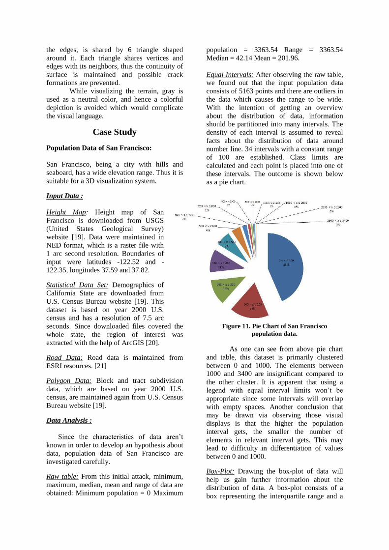
Equal Intervals: After observing the raw table,

we found out that the input population data

consists of 5163 points and there are outliers in

the data which causes the range to be wide.

With the intention of getting an overview

about the distribution of data, information

should be partitioned into many intervals. The

density of each interval is assumed to reveal

facts about the distribution of data around

number line. 34 intervals with a constant range

of 100 are established. Class limits are

calculated and each point is placed into one of

these intervals. The outcome is shown below

as a pie chart.

Figure 11. Pie Chart of San Francisco

population data.

As one can see from above pie chart

and table, this dataset is primarily clustered

between 0 and 1000. The elements between

1000 and 3400 are insignificant compared to

the other cluster. It is apparent that using a

legend with equal interval limits won’t be

appropriate since some intervals will overlap

with empty spaces. Another conclusion that

may be drawn via observing those visual

displays is that the higher the population

interval gets, the smaller the number of

elements in relevant interval gets. This may

lead to difficulty in differentiation of values

between 0 and 1000.

Box-Plot: Drawing the box-plot of data will

help us gain further information about the

distribution of data. A box-plot consists of a

box representing the interquartile range and a

line, representing the median, passing through

this box.

Figure 12. Box-plot of San Francisco population

data.

Colorization:

Shading

Figure 13. legend for the box-plot

method.

After intervals are decided for uniform

subdivisions via box-plot method, this color

legend is mapped to relevant classes. Since

there aren’t any elements in the first interval

(Lower Inner Fence < x ≤ Lower Quartile), it

isn’t included in this legend.

Figure 14. legend for equal intervals method.

In non-uniform subdivisions mode,

interval limits are decided by equal intervals

method or quintiles method, too. After class

limits are determined, color legend of the map

is generated manually. RGB values of the

legend is given on the left.

Road Network:

The road network of San Francisco

reinforces the population density transitions.

As a general pattern in highly populated

regions, road network is denser, while in

regions with less population, road network is

less crowded.

Figure 15. Road network of San Francisco

reinforces the population density transitions.

Multiple Data Visualization:

In order to test the performance of our system,

in multivariate data visualization, a synthetic

data layer is added to the existing San

Francisco case study. All inputs are identical to

the previous case study’s inputs, except an

additional randomly generated statistical data

set.

Figure 16. Visualization of multiple data layers.

Symbology:

This time instead of using both

hatching and shading options for visualization

of one data set, hatching technique is used to

visualize San Francisco’s demographic data

while the additional data set is classified and

shaded due to both equal intervals and box-plot

legends.

The output is an efficient multivariate

data representation. Since the colorization of

two layers created a contrast, information of

different layers are easily distinguished.

Road Network:

When the road network layer is turned

on, visualization becomes too crowded and

complicated. This is because hatches and roads

are both represented as lines. Therefore the

dimension of data layers should be kept up to

2; any layers more than that make it

complicated, in this state.

Comparison with ArcScene :

ArcScene is a 3D visualization

application that allows you to view your GIS

data in three dimensions [22]. In order to

compare our study with the state of art in

geographical information visualization

systems, we chose to visualize our data in

ArcScene. Some major advantages of using

our software are observed during this

comparison:

Since our study uses level of detail

approach while visualizing thematic data, as

the camera zooms out of the scene depiction of

information is simplified and the system

switches to a less detailed visualization.

ArcScene uses the same detail level regardless

of camera position, thus as the camera gets

away from representation region, information

density increases.

Figure 17. Via using level of detail information

density of the depiction is kept constant, so

observing the data from a distant point is

possible in the proposed system.

Figure 18. Due to unvarying size of squares,

information density increases as camera gets

away from the representation region.

Besides, observation of thematic data

from a distant point is nearly impossible with

ArcScene due to clustering of unvarying size

of squares and those squares’ borders creates

anti aliasing as a side effect .

Figure 19. Visualization of geographical data

with ArcScene(a) and with the proposed system

(b).

Finally, our program rendered more

realistic illustrations of the landscape, when

compared to ArcScene. We chose to create 2D

textures of thematic data and wrap it on a more

detailed 3D terrain, that’s why height changes

are smoother. Via making use of light, 3D

effects are highlighted.

Results, Discussions and Further

Study

Visualization of geographical data is

vital for conveying the underlying information

patterns. Since geographical databases consist

of great amount of spatial data, without

attaching these data to some spatial references,

it is impossible for human mind to pick the

essence of information among loads of

meaningless numerical data.

The proposed system produces 3D

environments in which up to two data sets are

intuitively embedded into, in real time. As the

user navigates through the scene, she has the

opportunity to observe data in different scales.

Introduction of automated details-on-demand

to thematic maps is one of the significant

contributions of this work. The details are

automatically visualized when the viewpoint

gets closer to the terrain. Real time

modification of produced thematic map

enables great user interactivity when combined

with 3D the navigation. Abstraction of data,

due to the distance between observer and data

prevents visualization of unreadable details

and clusters the data through larger unit

representation regions (lower resolutions).

Both individual data and the overall pattern of

information are depicted with the introduction

of level of detail technique to 3D thematic

maps.

For investigating and developing

hypothesis from the input data, user has the

freedom to visualize her dataset in three

different distribution models. Representations

may be generated with classed or unclassed

data. Two different interval determining

methods are implemented, which is a fine tool

for understanding the divisions of data over

number line.

There are some issues in this system

which need further study: Some parameters

have to be input by the user, which in the

future can be decided by the system itself, such

as the interval limits of data. Even the most

suitable statistical classification method for

input data can be determined via some

intelligent algorithm by the computer itself.

Decreasing the manual work done by

implementing more elaborate analytic tools

will increase the usability of software.

Although our system has a consistent

visual language of its own, it isn’t efficient for

visualizing more than two datasets, which are

represented as separate layers. Increasing the

displayed data layers will be the subject to be

investigated next, in the near future.

An alternative to uniform subdivisions,

consitituting levels of detail from categorical

data (e.g. for viewing demographic distribution

due to ethnicity, gender, religion) may also be

implemented as part of our future research. In

this case, different levels of detail will induce

dynamic borders between different categories

being visualized. This improvement would let

us generalize our system to visualize both

numeric and categorical data.

While creating visualizations that

appeal to the eye, letting the user choose her

own color set and generating their texture

patterns instead of hatching will help the

diversity of depictions produced. Thus a valid

user interface should be designed with

additional options.

Last but not least; even though this

system is found to be “good-looking” and easy

to understand by users, with the intention of

finding out its success about being informative

and naming the strong and weak sides, a

complete usability study is required. Such a

usability study will also guide us through

choosing more legitimate breakpoints between

levels of detail, which are currently constant

points that we have chosen.

References

[1] D. Cohen-Or, and Y. Levanoni, “Temporal

continuity of levels of detail in delaunay

triangulated terrain” Proceedings of the 7th

conference on Visualization '96, ,pp. 37–42,

San Francisco, California, Oct. 1996.

[2] F. Losasso, and H. Hoppe, “Geometry

Clipmaps: terrain rendering using nested

regular grids”, ACM Transactions on

Graphics, ACM Press, vol. 23, 2004.

[3] M. Clasen and H. C. Hege, “Terrain

Rendering using Spherical Clipmaps” ,

EuroVis 2006 – Proc. Eurographics / IEEE

VGTC Symposium on Visualization, pp. 91-

98, 2006.

[4] J. Schneider and R. Westermann, "GPU-

Friendly High-Quality Terrain Rendering,"

Journal of WSCG, vol. 14, pp. 49-56, 2006.

[5] Human Computer Interaction Lab ,

University of Maryland, Available from:

www.cs.umd.edu/hcil/research/visualization.sh

tml,retrieved 23.02.2009.

[6] A. Asirvatham and H. Hoppe, "Terrain

rendering using GPU-based geometry

clipmaps," GPU Gems, vol. 2, pp. 109–122,

2005.

[7] A. Brodersen, "Real-time visualization of

large textured terrains," in Proceedings of the

3rd international conference on Computer

graphics and interactive techniques in

Australasia and South East Asia Dunedin,

ACM Press, New Zeland, 2005.

[8] R. Chang, G. Wessel, R. Kosara, E. Sauda,

W. Ribarsky, "Legible Cities: Focus-

Dependent Multi-Resolution Visualization of

Urban Relationships", IEEE Transactions on

Visualizationand Computer Graphics, vol. 13,

no. 6, 2007.

[9] K. Buchin, M. C. Sousa, J. Döllner, F.

Samavati, M. Walther, “Illustrating Terrains

using Direction of Slope and Lighting” , 4th

ICA Mountain Cartography Workshop, Vall de

Nuria, Spain, 2004.

[10]Purvis M., Sambells J., Turner C. (2006).

Beginning Google Maps Applications with

PHP and Ajax. Berkeley: APress.

[11] M. Gibin, A. Singleton, R. Milton, P.

Mateos, P. Longley, "An Exploratory

Cartographic Visualisation of London through

the Google Maps API", Applied Spatial

Analysis and Policy, vol. 1, no. 2, Springer,

2008.

[12] ESRI ShapeFile, Available from:

http://www.esri.com/library/whitepapers/pdfs/s

hapefile.pdf, retrieved 23.02.2009.

[13] London Profiler, Accessed from:

www.londonprofiler.org , retrieved

20.07.2008.

[14] J. Döllner, K. Hinrichs, "Dynamic 3D

Maps and Their Texture-Based Design",

Proceedings of Computer Graphics

International, 2000.

[15] K. Baumann, J. Döllner, K. Hinrichs,

“Integrated Multiresolution Geometry and

Texture Models for Terrain Visualization”,

Joint Eurographics-IEEE TCVG Symposium

on Visualization, 2000.

[16] R. Fawcett-Tang, W. Owen, "Mapping –

an illustrative guide to graphic navigational

systems", Rockport Publishers, 2002. [23] T.

A. Slocum, R. B. McMaster, F. C. Kessler, H.

H. Howard, "Thematic Cartography and

Geographic Visualization",

Pearson/PrenticeHall,2004.

[17] The Free Encyclopedia, Available from:

www.wikipedia.org/, retrieved 23.02.2009. 54

[18] C. A. Brewer," ColorBrewer - Selecting

Good Color Schemes for Maps [online]",

2002. Available from:

www.personal.psu.edu/cab38/ColorBrewer/Co

lorBrewer.html, retrieved Accessed

23.02.2009.

[19] U.S. Census Bureau, Available from:

www.usgs.gov/ retrieved 20.08.2008.

[20] ESRI’ s ArcGIS, Available from:

www.esri.com/products.hml, retrieved

23.02.2009.

[21] ] ESRI Data & Maps library

[22] ESRI’s ArcScene, 3D display

environment Available from:

http://webhelp.esri.com/arcgisdesktop/9.2/inde

x.cfm?TopicName=ArcScene_3D_display_env

ironment, retrieved 23.02.2009.