INTRO TO PATH ANALYSIS AND STRUCTURAL EQUATION MODELING · INTRO TO PATH ANALYSIS AND STRUCTURAL EQUATION MODELING NICOLE MICHEL [email protected] 9 OCTOBER, 2014 Alsterberg

INTRO TO PATH ANALYSIS

AND STRUCTURAL

EQUATION MODELING

NICOLE MICHEL

[email protected]

9 OCTOBER, 2014

Alsterberg et al. 2013

Outline

1. What are path analysis and structural equation

modeling?

2. When to use path analysis and/or SEM?

3. How to create, evaluate, and revise models

4. How to do path analysis/SEM in R

http://jarrettbyrnes.info/ubc_sem/

What is path analysis?

• Modeling that lets you test hypotheses about causation

(both direction and strength)

• Multivariate technique

• Identifies directed dependencies between a set of

variables

• Closely related to multiple regression, but lets you look at

multiple predictor and dependent variables at once (like

many regression models put together back-to-back)

• Developed ~1918 by geneticist Sewell Wright

What is path analysis?

Equation:

Y1 =α + βX1 + ε

X1 Y1

ε

Now add more levels

Orcas

oTters

Urchins

Kelp

Equations: T =α1 + β1O + ε1 U =α2 + β2T + ε2 K =α3 + β3U + ε2

Now make it more complex

Humans

oTters Urchins

Kelp

Equations: T =α1 + β1H + ε1 U =α2 + β2T + β3H + ε2 K =α3 + β4U + β5H + ε2

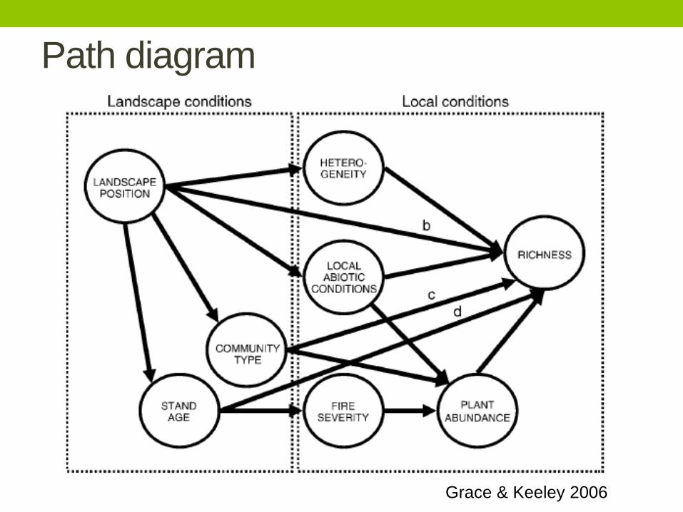
Path diagram

Grace & Keeley 2006

Time for some jargon

• Exogenous variable: variables that affect other variables,

but are not affected themselves

• Endogenous variable: variables that are causally

affected by other variables. May or may not have causal

effects on other variables.

• Recursive model: a model in which all causality flows in

one direction

• Non-recursive model: a model in which causality flows in

more than one direction (i.e., that includes at least one

loop or reciprocal effect)

• Saturated model: has paths between all variables

Exogenous?

Grace & Keeley 2006

Endogenous?

Grace & Keeley 2006

Exogenous Endogenous Recursive

Grace & Keeley 2006

Non-recursive - keep it simple (stupid)

Grace & Keeley 2006

How do you figure

out what’s going on

here?

Humans

oTters Urchins

Kelp

Humans

oTters Urchins

Kelp

Saturated

model

Unsaturated

model

Correlations = curved lines

Grace 2005

Unexplained correlations

(between residual variance) could

represent uncertain causal driver,

common driver, etc.

Path coefficients

Grace & Bollen 2005

Swope & Parker 2012

Alsterberg et al. 2013

So what’s the difference between PA and

SEM? • Path analysis is a special case of structural equation

modeling

• Path analysis includes only measured variables that act

singly (e.g., tarsus length, abundance, CORT)

• Structural equation modeling includes latent and/or

composite variables.

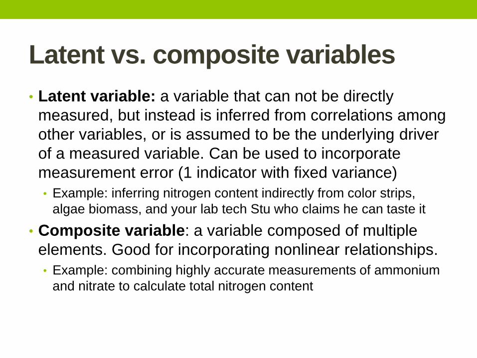
Latent vs. composite variables

• Latent variable: a variable that can not be directly

measured, but instead is inferred from correlations among

other variables, or is assumed to be the underlying driver

of a measured variable. Can be used to incorporate

measurement error (1 indicator with fixed variance)

• Example: inferring nitrogen content indirectly from color strips,

algae biomass, and your lab tech Stu who claims he can taste it

• Composite variable: a variable composed of multiple

elements. Good for incorporating nonlinear relationships.

• Example: combining highly accurate measurements of ammonium

and nitrate to calculate total nitrogen content

Structural equation model with latent

variables

Grace & Keeley 2006

Structural equation model

Composite

variable

SEM as a unifying process

When to use PA/SEM

• When you’re interested in identifying and quantifying

cause/effect relationships (and have the ability to do so)

• When you’re interested in quantifying indirect effects (e.g.,

trophic cascades)

• When you’re working with observational or (more

recently) experimental data

• When you have sufficient sample size

• No “set” number. Some proposed rules of thumb:

• 5-20 samples per parameter (often 10)

• 75-200 cases (200 may be unreasonable for many cases)

• Many PA/SEM models have far lower sample size – e.g., 7 (Feeley &

Terborgh 2008)

Model identification

• Can your model be fit?

3 = a + b

4 = 2a + b

a & b have unique solutions

Identified

3 = a + b + c

4 = 2a + b + 3c

a, b, & c have no unique

solutions

Underidentified

3 = a + b

4 = 2a + b

7 = 3b + a

Overidentified

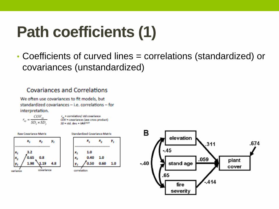
Path coefficients (1)

• Coefficients of curved lines = correlations (standardized) or

covariances (unstandardized)

Aside: standardized vs. unstandardized

variables path coefficients • Unstandardized variables – presented in the original units of

the explanatory and predictor variables. Represent the slope of

the relationship between the predictor and response variable.

Not useful when comparing strength of paths between

variables on different scales (e.g., rainfall in mm, liana

frequency (0-1))

• Standardized variables – standardized based on SDs (z-

scored). Allows direct comparisons, but measured in SD units,

often misinterpreted.

• Alternative: standardize based on “relative ranges”

• See, e.g.: Grace, J.B. and K.A. Bollen 2005. Interpreting the

results from multiple regression and structural equation

models. Bulletin of the ESA 86:283-295. (and many more!)

Path coefficients (2)

• Coefficients of single paths = regression coefficients (βs),

standardized (interpretation) or unstandardized (fit)

Plant cover =

elevation*0.311 + 0.674

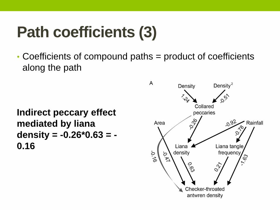
Path coefficients (3)

• Coefficients of compound paths = product of coefficients

along the path

Indirect peccary effect

mediated by liana

density = -0.26*0.63 = -

0.16

Path coefficients (4)

• When variables are connected by more than one causal

pathway, the path coefficients are “partial” regression

coefficients (=controlling for

other effects)

Path coefficients (5)

• Paths from error variables represent prediction error

(influences from other forces)

Path coefficients (6)

• Total effect of one variable on another is the sum of its

direct and indirect effects

Total peccary effect =

-1.60 + -1.68 = -3.28

How to get started

• Start with the big ideas/theory

• Expand the conceptual model to hone in on details (what

measurements represent theoretical processes?)

• Prune unnecessary details (identification!)

• Create alternative models to test

• Confront your pretty models with

cold, hard data

Software

• Commercial software (AMOS, LISREL, MPLUS)

• SAS PROC CALIS/TCALIS

• R

• sem (2001)

• OpenMX (solver not currently open-source)

• lavaan (2010; built on sem, robust, multifunctional, supports

complex models including latent and/or composite variables, uses

syntax similar to linear models)

• lavaan extensions: lavaan.survey, semTools, semPlot

SEM assumptions

• Observations are independent of one another

• Variables are unstandardized (special methods for

standardized variables exist)

• Exogenous variables are measured without error

• Endogenous variables are continuous and multivariate

normally distributed (robust to violations, and methods to

correct for nonnormality exist)

• Incomplete data ok, models can impute using Full

Information Maximum Likelihood or Multiple Imputation

How lavaan fits models

• Default: maximum likelihood (ML)

• Alternatively, can use various least squares methods

• Robust estimators with adjusted test statistics (e.g.,

Satterthwaite, Satorra-Bentler) available for complete

and/or incomplete data

So you’ve drawn your model, now what?

• Check to make sure it’s identifiable:

• Should have >1 df = 1+ more observed variables than

estimated parameters (including path coefficients,

covariances, etc.)

• Make sure you have sufficient indicators for any latent

variables

• Make sure there are no negative variances or

correlations > 1.0

• Go to R!

About the data

• Data and code compiled from Jarrett Byrnes’ “An introduction to structural equation modeling for ecology and evolutionary biology” lecture series, available online here: http://jarrettbyrnes.info/ubc_sem/

• Five-year study of wildfires in southern California, 90 plots (20 x 50m). Data from Jon Keeley et al.

• Objectives: understand post-fire recovery of plant species richness

About the data

• Response variables: plant cover, species richness

• Predictor variables: age of burned stand, distance from

coast, elevation, abiotic conditions (aspect, soils), spatial

heterogeneity, fire severity (index based on condition of

remnant shrubs)

Some useful references

• Grace, JB 2006. Structural Equation Modeling and Natural Systems. Cambridge University Press.

• Shipley, B. 2000. Cause and Correlation in Biology. Cambridge University Press.

• Kline (2005) Principles and Practice of Structural Equation Modeling. (2nd Edition) Guilford Press.

• Hancock & Muller (2006) Structural Equation Modeling: A Second Course. Information Age Publishing, Greenwich, CT.

• Bollen (1989) Structural Equations with Latent Variables. John Wiley and Sons.

• Lee (2007) Structural Equation Modeling: A Bayesian Approach. John Wiley and Sons.

• Grace, J.B. and K.A. Bollen. 2005. Interpreting the results from multiple regression and structural equation models. Bull. Ecol. Soc. Amer. 86:283-295

• Structuralequations.org (James Grace’s website)

• http://jarrettbyrnes.info/ubc_sem/ (Jarrett Byrnes’ website. More PPTs, examples and code available)