Intro to econometrics

Introduction to Econometrics

Gaetan “Guy” Lion

June 2015

1

Table of Content

1) Linear Regression.

2) Multiple Regression. Multiple Regression as an

Optimization.

3) Building an Econometrics model. Stepwise

Regression, Autoregressive Regression.

4) Model testing. Multicollinearity, Autocorrelation,

Heteroskedasticity, Robust Standard Errors, Outliers testing, Normality, Scenario testing.

2

1) Linear Regression

3

The Basic Linear Regression Equation

4

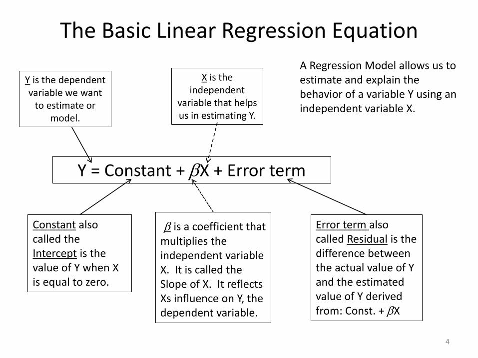
Y = Constant + bX + Error term

Y is the dependent variable we want

to estimate or model.

b is a coefficient that multiplies the independent variable X. It is called the Slope of X. It reflects Xs influence on Y, the dependent variable.

X is the independent

variable that helps us in estimating Y.

Constant also called the Intercept is the value of Y when X is equal to zero.

Error term also called Residual is the difference between the actual value of Y and the estimated value of Y derived from: Const. + bX

A Regression Model allows us to estimate and explain the behavior of a variable Y using an independent variable X.

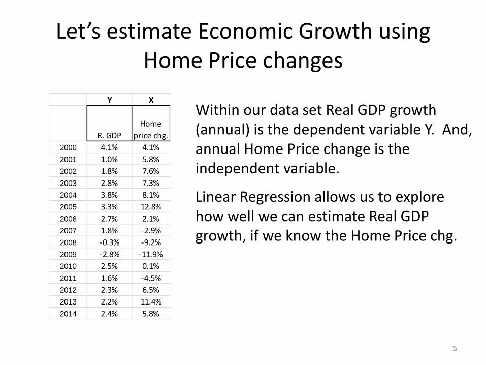
Let’s estimate Economic Growth using Home Price changes

5

Y X

R. GDP

Home

price chg.

2000 4.1% 4.1%

2001 1.0% 5.8%

2002 1.8% 7.6%

2003 2.8% 7.3%

2004 3.8% 8.1%

2005 3.3% 12.8%

2006 2.7% 2.1%

2007 1.8% -2.9%

2008 -0.3% -9.2%

2009 -2.8% -11.9%

2010 2.5% 0.1%

2011 1.6% -4.5%

2012 2.3% 6.5%

2013 2.2% 11.4%

2014 2.4% 5.8%

Within our data set Real GDP growth (annual) is the dependent variable Y. And, annual Home Price change is the independent variable.

Linear Regression allows us to explore how well we can estimate Real GDP growth, if we know the Home Price chg.

Excel Scatter Plot = Regression the easy way

6

H:\Abilities\Projects\2015\Econometrics\Basics.xlsx\Linear regression

Running a Linear Regression visually is very easy in three easy steps: 1) Do a Scatter Plot with your independent variable X (Home price chg.) on the X-axis and your dependent variable Y (Real GDP growth) on the Y-axis;2) Add a Trendline to your Scatter Plot. That is actually your Regression line that best fit the data;3) Format your Trendline by adding the actual regression equation and the R^2 measure that tells how much the variable X explains of the variance of variable Y.

The regressed equation solution: Real GDP Growth = 1.44% + 0.177(Home price chg.)

Step 1: Do a Scatter Plot with X var. on X-axis; Y var. on Y-Axis Step 2: Add a Trendline Step 3: Format Trendline by adding equation and R^2

-4%

-3%

-2%

-1%

0%

1%

2%

3%

4%

5%

-15% -10% -5% 0% 5% 10% 15%

R G

DP

gro

wth

Home price change

R GDP growth vs Home Price change

-4%

-3%

-2%

-1%

0%

1%

2%

3%

4%

5%

-15% -10% -5% 0% 5% 10% 15%

R G

DP

gro

wth

Home price change


y = 0.1771x + 0.0144R² = 0.5674

-4%

-3%

-2%

-1%

0%

1%

2%

3%

4%

5%

-15% -10% -5% 0% 5% 10% 15%

R G

DP

gro

wth

Home price change


The Geometry of Linear Regression

7

Constant or Intercept = value of Y when X = 0Beta coefficient or Slope = Chg. in Y/Chg. in X

-4%

-3%

-2%

-1%

0%

1%

2%

3%

4%

5%

-15% -10% -5% 0% 5% 10% 15%

R G

DP

gro

wth

Home price change


Intercept

-4%

-3%

-2%

-1%

0%

1%

2%

3%

4%

5%

-15% -10% -5% 0% 5% 10% 15%

R G

DP

gro

wth

Home price change


Chg. in Y

Chg. in X

H:\Abilities\Projects\2015\Econometrics\Basics.xlsx\Linear regression

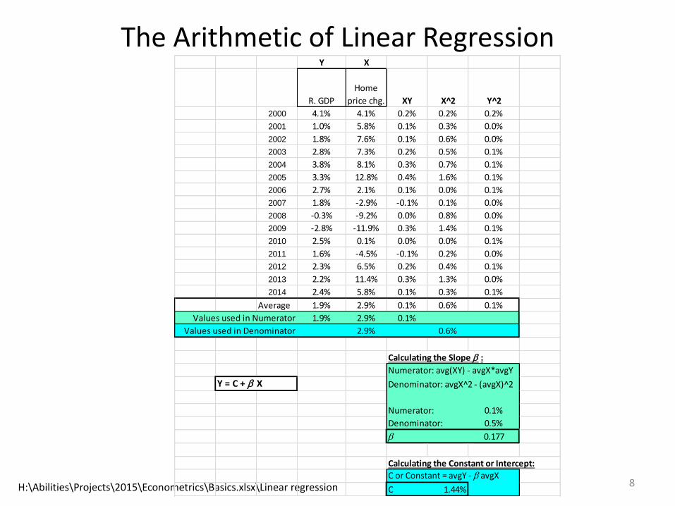
The Arithmetic of Linear Regression

8H:\Abilities\Projects\2015\Econometrics\Basics.xlsx\Linear regression

Y X

R. GDP

Home

price chg. XY X^2 Y^2

2000 4.1% 4.1% 0.2% 0.2% 0.2%

2001 1.0% 5.8% 0.1% 0.3% 0.0%

2002 1.8% 7.6% 0.1% 0.6% 0.0%

2003 2.8% 7.3% 0.2% 0.5% 0.1%

2004 3.8% 8.1% 0.3% 0.7% 0.1%

2005 3.3% 12.8% 0.4% 1.6% 0.1%

2006 2.7% 2.1% 0.1% 0.0% 0.1%

2007 1.8% -2.9% -0.1% 0.1% 0.0%

2008 -0.3% -9.2% 0.0% 0.8% 0.0%

2009 -2.8% -11.9% 0.3% 1.4% 0.1%

2010 2.5% 0.1% 0.0% 0.0% 0.1%

2011 1.6% -4.5% -0.1% 0.2% 0.0%

2012 2.3% 6.5% 0.2% 0.4% 0.1%

2013 2.2% 11.4% 0.3% 1.3% 0.0%

2014 2.4% 5.8% 0.1% 0.3% 0.1%

Average 1.9% 2.9% 0.1% 0.6% 0.1%

Values used in Numerator 1.9% 2.9% 0.1%

Values used in Denominator 2.9% 0.6%

Calculating the Slope b :

Numerator: avg(XY) - avgX*avgY

Y = C + b X Denominator: avgX^2 - (avgX)^2

Numerator: 0.1%

Denominator: 0.5%

b 0.177

Calculating the Constant or Intercept:

C or Constant = avgY - b avgX

C 1.44%

A 2nd Arithmetic ApproachSlope b = Covariance (X, Y)/Variance(X)

9

Covar(X,Y) Var(X)

R GDP Home price A B A x B B^2

Y X Y - Avg. X - Avg.

2000 4.1% 4.1% 2.1% 1.2% 0.0% 0.0%

2001 1.0% 5.8% -1.0% 2.9% 0.0% 0.1%

2002 1.8% 7.6% -0.2% 4.7% 0.0% 0.2%

2003 2.8% 7.3% 0.9% 4.4% 0.0% 0.2%

2004 3.8% 8.1% 1.8% 5.3% 0.1% 0.3%

2005 3.3% 12.8% 1.4% 9.9% 0.1% 1.0%

2006 2.7% 2.1% 0.7% -0.8% 0.0% 0.0%

2007 1.8% -2.9% -0.2% -5.8% 0.0% 0.3%

2008 -0.3% -9.2% -2.2% -12.0% 0.3% 1.4%

2009 -2.8% -11.9% -4.7% -14.8% 0.7% 2.2%

2010 2.5% 0.1% 0.6% -2.7% 0.0% 0.1%

2011 1.6% -4.5% -0.3% -7.4% 0.0% 0.5%

2012 2.3% 6.5% 0.4% 3.6% 0.0% 0.1%

2013 2.2% 11.4% 0.3% 8.6% 0.0% 0.7%

2014 2.4% 5.8% 0.4% 2.9% 0.0% 0.1%

Average 1.9% 2.9% 1.3% 7.3% Sum

0.09% 0.49% Sum/n

Slope = Covar(X,Y)/Var(X)

Numerator 0.09%

Denominator 0.49%

Slope 0.177

H:\Abilities\Projects\2015\Econometrics\Basics.xlsx\Linear regression2

Linear Regression Excel Basics

10

R GDP Home price

Y Y est. X

2000 4.1% 2.2% 4.1%

2001 1.0% 2.5% 5.8%

2002 1.8% 2.8% 7.6%

2003 2.8% 2.7% 7.3%

2004 3.8% 2.9% 8.1%

2005 3.3% 3.7% 12.8%

2006 2.7% 1.8% 2.1%

2007 1.8% 0.9% -2.9%

2008 -0.3% -0.2% -9.2%

2009 -2.8% -0.7% -11.9%

2010 2.5% 1.5% 0.1%

2011 1.6% 0.6% -4.5%

2012 2.3% 2.6% 6.5%

2013 2.2% 3.5% 11.4%

2014 2.4% 2.5% 5.8%

Basic formulas

SLOPE() 0.177

INTERCEPT() 1.44%

RSQ () 0.567

STYX() 1.2%RSQ() = R Square. is the square of correlation between Y and Y est. It tells how well the model’s estimates fit the actual data. It also tells what is the % of the dependent variable’s variance explained by the model. This value ranges from 0 (a terrible model that does not fit or explain the data) to 1 (a perfect model that fits the data identically and explains 100% of the variance of the dependent variable).

STYX () = Standard Error of Model. Assuming that the Errors are normally distributed, one can assume that about 2/3ds of data observations fall within + or – 1 Standard Error from the model’s estimate. And, 95% of them fall within + or –1.96 Standard Errors away from the model’s estimate.

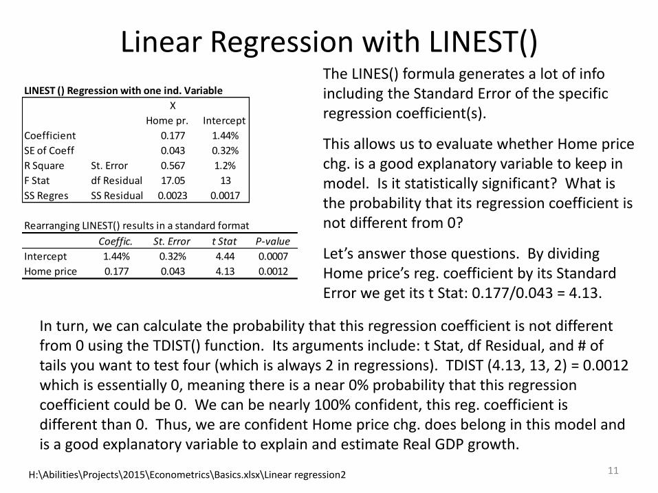
Linear Regression with LINEST()

11H:\Abilities\Projects\2015\Econometrics\Basics.xlsx\Linear regression2

LINEST () Regression with one ind. Variable

X

Home pr. Intercept

Coefficient 0.177 1.44%

SE of Coeff 0.043 0.32%

R Square St. Error 0.567 1.2%

F Stat df Residual 17.05 13

SS Regres SS Residual 0.0023 0.0017

Rearranging LINEST() results in a standard format

Coeffic. St. Error t Stat P-value

Intercept 1.44% 0.32% 4.44 0.0007

Home price 0.177 0.043 4.13 0.0012

The LINES() formula generates a lot of info including the Standard Error of the specific regression coefficient(s).

This allows us to evaluate whether Home price chg. is a good explanatory variable to keep in model. Is it statistically significant? What is the probability that its regression coefficient is not different from 0?

Let’s answer those questions. By dividing Home price’s reg. coefficient by its Standard Error we get its t Stat: 0.177/0.043 = 4.13.

In turn, we can calculate the probability that this regression coefficient is not different from 0 using the TDIST() function. Its arguments include: t Stat, df Residual, and # of tails you want to test four (which is always 2 in regressions). TDIST (4.13, 13, 2) = 0.0012 which is essentially 0, meaning there is a near 0% probability that this regression coefficient could be 0. We can be nearly 100% confident, this reg. coefficient is different than 0. Thus, we are confident Home price chg. does belong in this model and is a good explanatory variable to explain and estimate Real GDP growth.

Depicting 95% Confidence Interval

12

-4.0%

-3.0%

-2.0%

-1.0%

0.0%

1.0%

2.0%

3.0%

4.0%

5.0%

6.0%

7.0%

Real GDP Growth Actual, Est, 95% C.I.

Y Y est. CI Low CI High

-4.0%

-3.0%

-2.0%

-1.0%

0.0%

1.0%

2.0%

3.0%

4.0%

5.0%

6.0%

7.0%

-15.0% -10.0% -5.0% 0.0% 5.0% 10.0% 15.0%

Re

al G

DP

gro

wth

Home Price change

Real GDP Growth vs Home price chg, 95% C.I.

Y Y est. CI Low CI High

H:\Abilities\Projects\2015\Econometrics\Basics.xlsx\Linear regression2

Depicting 95% C.I. over time Depicting 95% C.I. vs. Home Price chg.

A 95% Confidence Interval means that we would expect that about 1 observation out of 20 would fall outside the Confidence Interval. The graphs look about right. We have only 15 observations. But, two of them are just within the C.I. All others are well within.

The C.I. Low range is 1.96 Standard Error of the model below Y estimate. The C.I. High range is 1.96 Standard Error above Y estimate.

2) Multiple Regression as an Optimization

13

Those two methods are identical. The only difference is that the Regression statistical output gives you a lot of very valuable information about a model that Optimization does not.

The Basic Multiple Regression Equation

14

Y = Constant + b1X1 + b2X2 + Error term

Y is the dependent variable we want

to estimate or model.

b1 is a coefficient that multiplies the independent variable X1. It reflects X1’s influence on Y, the dependent variable.

X1 is the 1st

independent variable that helps us in estimating Y.

X2 is the 2nd independent

variable that helps us in estimating Y.

Constant also called the Intercept is the value of Y when X1 and X2 are equal to zero.

b2 same explanation as b1.

Error term also called Residual is the difference between the actual value of Y and the estimated value of Y derived from: Const. + b1X1 + b2X2.

Such Regressions can have many more independent variables X3, X4, X5, …

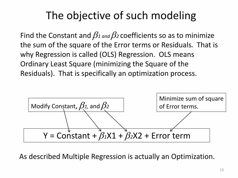
The objective of such modeling

15


Find the Constant and b1 and b2 coefficients so as to minimize the sum of the square of the Error terms or Residuals. That is why Regression is called (OLS) Regression. OLS means Ordinary Least Square (minimizing the Square of the Residuals). That is specifically an optimization process.

Modify Constant, b1, and b2

Minimize sum of square of Error terms.

As described Multiple Regression is actually an Optimization.

An Optimization Example

16


Real GDP Growth = Constant + b1Home Price chg + b2S&P 500 chg + Error term

We are going to model or estimate annual Real GDP Growth with two independent variables: Home Price yearly change and S&P 500 yearly change.

Optimization starting point

17

What to change

Constant 2%

b 1 Home price 0.1

b 2 S&P 500 0.1

Y Y est. Error Error^2 X1 X2

R. GDP Estimate Residual Residual^2

Home

price S&P 500

2000 4.1% 3.2% -0.9% 0.0% 4.1% 7.6%

2001 1.0% 0.9% 0.0% 0.0% 5.8% -16.4%

2002 1.8% 1.1% -0.7% 0.0% 7.6% -16.5%

2003 2.8% 2.4% -0.4% 0.0% 7.3% -3.2%

2004 3.8% 4.5% 0.8% 0.0% 8.1% 17.3%

2005 3.3% 4.0% 0.6% 0.0% 12.8% 6.8%

2006 2.7% 3.1% 0.4% 0.0% 2.1% 8.6%

2007 1.8% 3.0% 1.2% 0.0% -2.9% 12.7%

2008 -0.3% -0.6% -0.4% 0.0% -9.2% -17.3%

2009 -2.8% -1.4% 1.3% 0.0% -11.9% -22.5%

2010 2.5% 4.0% 1.5% 0.0% 0.1% 20.3%

2011 1.6% 2.7% 1.1% 0.0% -4.5% 11.4%

2012 2.3% 3.5% 1.2% 0.0% 6.5% 8.7%

2013 2.2% 5.0% 2.8% 0.1% 11.4% 19.1%

2014 2.4% 4.3% 1.9% 0.0% 5.8% 17.5%

What to minimize: Sum E.^2 0.2%

H:\Abilities\Projects\2015\Econometrics\Basics.xlsx\Optimization

R. GDP gr. in 2000 = 2% + 0.1(4.1%) + 0.1(7.6%) = 3.2%

Using Excel Solver to run the Optimization

18

What to change

Constant 1.37%

b 1 Home price 0.133

b 2 S&P 500 0.054

Y Y est. Error Error^2 X1 X2

R. GDP Estimate Residual Residual^2

Home

price S&P 500

2000 4.1% 2.3% -1.8% 0.0% 4.1% 7.6%

2001 1.0% 1.3% 0.3% 0.0% 5.8% -16.4%

2002 1.8% 1.5% -0.3% 0.0% 7.6% -16.5%

2003 2.8% 2.2% -0.6% 0.0% 7.3% -3.2%

2004 3.8% 3.4% -0.4% 0.0% 8.1% 17.3%

2005 3.3% 3.4% 0.1% 0.0% 12.8% 6.8%

2006 2.7% 2.1% -0.6% 0.0% 2.1% 8.6%

2007 1.8% 1.7% -0.1% 0.0% -2.9% 12.7%

2008 -0.3% -0.8% -0.5% 0.0% -9.2% -17.3%

2009 -2.8% -1.4% 1.3% 0.0% -11.9% -22.5%

2010 2.5% 2.5% 0.0% 0.0% 0.1% 20.3%

2011 1.6% 1.4% -0.2% 0.0% -4.5% 11.4%

2012 2.3% 2.7% 0.4% 0.0% 6.5% 8.7%

2013 2.2% 3.9% 1.7% 0.0% 11.4% 19.1%

2014 2.4% 3.1% 0.7% 0.0% 5.8% 17.5%


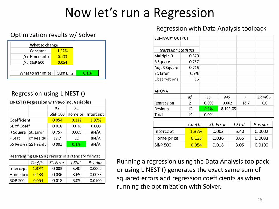
Now let’s run a Regression

19

What to change

Constant 1.37%

b 1 Home price 0.133

b 2 S&P 500 0.054


LINEST () Regression with two ind. Variables

X2 X1

S&P 500 Home pr. Intercept

Coefficient 0.054 0.133 1.37%

SE of Coeff 0.018 0.036 0.003

R Square St. Error 0.757 0.009 #N/A

F Stat df Residual 18.7 12 #N/A

SS Regres SS Residual 0.003 0.1% #N/A

Rearranging LINEST() results in a standard format


Intercept 1.37% 0.003 5.40 0.0002

Home price 0.133 0.036 3.65 0.0033

S&P 500 0.054 0.018 3.05 0.0100

Optimization results w/ SolverRegression with Data Analysis toolpack

Regression using LINEST ()

Running a regression using the Data Analysis toolpack or using LINEST () generates the exact same sum of squared errors and regression coefficients as when running the optimization with Solver.

SUMMARY OUTPUT

Regression Statistics

Multiple R 0.870

R Square 0.757

Adj. R Square 0.716

St. Error 0.9%

Observations 15

ANOVA

df SS MS F Signif. F

Regression 2 0.003 0.002 18.7 0.0

Residual 12 0.1% 8.19E-05

Total 14 0.004


Intercept 1.37% 0.003 5.40 0.0002

Home price 0.133 0.036 3.65 0.0033

S&P 500 0.054 0.018 3.05 0.0100

Regression = Optimization

20

Both methods do the exact same thing by minimizing the sum of the square of the Errors or Residuals. Consequently, they generate the exact same overall model with identical independent variable coefficients.

The big difference is that the standard Regression output generates a lot of information about the model that Optimization does not do.


Multiple R 0.870

R Square 0.757

Adj. R Square 0.716

St. Error 0.9%

Observations 15

R Square: same meaning as defined within Linear Regression section.

Adjusted R Square: it adjusts R Square downward for using more variables. So, Adj. R Square is always a bit smaller than R Square. Unlike R Square, Adj. R Square can have negative values (for really bad fitting models).

Standard Error: same meaning as defined within Linear Regression section.

So whenever you can you should use Regression instead of Optimization. But, Optimization is more flexible, as it can handle constraints on the independent variables (maybe one of the Xs coeff. should be negative or < 1 for some reason). Regression can’t handle such constraints.

More Regression info: statistical significance of independent variables

21

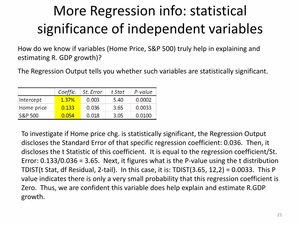
How do we know if variables (Home Price, S&P 500) truly help in explaining and estimating R. GDP growth)?

The Regression Output tells you whether such variables are statistically significant.

To investigate if Home price chg. is statistically significant, the Regression Output discloses the Standard Error of that specific regression coefficient: 0.036. Then, it discloses the t Statistic of this coefficient. It is equal to the regression coefficient/St. Error: 0.133/0.036 = 3.65. Next, it figures what is the P-value using the t distribution TDIST(t Stat, df Residual, 2-tail). In this case, it is: TDIST(3.65, 12,2) = 0.0033. This P value indicates there is only a very small probability that this regression coefficient is Zero. Thus, we are confident this variable does help explain and estimate R.GDP growth.

A Visual Summary. Two Independent Variables for one Model

22-4.0%

-3.0%

-2.0%

-1.0%

0.0%

1.0%

2.0%

3.0%

4.0%

5.0%

-2.0% -1.0% 0.0% 1.0% 2.0% 3.0% 4.0% 5.0%

Act

ual

Estimate

R GDP growth Actual vs Estimate

-4.0%

-3.0%

-2.0%

-1.0%

0.0%

1.0%

2.0%

3.0%

4.0%

5.0%

-15.0% -10.0% -5.0% 0.0% 5.0% 10.0% 15.0%

R G

DP

gro

wth

Home price change


-4.0%

-3.0%

-2.0%

-1.0%

0.0%

1.0%

2.0%

3.0%

4.0%

5.0%

-30.0% -20.0% -10.0% 0.0% 10.0% 20.0% 30.0%

R G

DP

gro

wth

S&P 500 change

R GDP growth vs S&P 500 change

3) Building an Econometrics Model

23

Do Leading Indicators lead Real GDP growth? Are they good predictors of Real GDP growth?

• We will build econometric models to address those questions.

• We will test those models using state-of-the-art peer-review practices.

24

The Leading Indicators

1 Hours Avg. Weekly Hours - Manufacturing, (Hours)

2 Un_claim Average Weekly Initial Claims - Unemployment Insurance, (Ths.)

3 New_orders Manufacturers' New Orders - Consumer Goods and Materials, (Mil. 1982 $)

4 Nondef1 Manufact. New Orders - Nondefense capital goods exclud. aircraft, (Mil. 1982 $)

5 Nondef2 Manufacturers' New Orders - Nondefense Capital Goods, (Mil. Ch. 1982 $)

6 Building_permits Building Permits for New Private Housing Units, (Ths.)

7 S&P 500 Index of stock prices - 500 common stocks, (1941-43=10, NSA)

8 M2 Money supply - M2, (Bil. 2009 $, NSA)

9 Spread Interest rate spread 10-year Treasury bonds less federal funds, (%, NSA)

10 Expectations Consumer Expectations - from the University of Michigan, (1966Q1=100, NSA)

Original source: Conference Board, BEA, Federal Reserve, BLS. Actual source: Moody's Economy.com

25

\2015\Econometrics\Leading indicators.xlsx\Leading indicators

We are using a data set going back to 1982. This will allow us to explore the out-of-sample issue later on with earlier data prior to 1982.

How to structure the Dependent Variable, Real GDP Growth?

26

Unit root test (nonstationary): Unit root test (nonstationary): Unit root test (nonstationary):

tau Stat Critic. val. Type tau Stat Critic. val. Type tau Stat Critic. val. Type

Dickey-Fuller -1.12 -3.15 with Constant, with Trend Dickey-Fuller -0.83 -3.15 with Constant, with Trend Dickey-Fuller -6.79 -2.58 with Constant, no Trend

Augmented DF -4.74 -2.58 with Constant, no Trend

$-

$2,000

$4,000

$6,000

$8,000

$10,000

$12,000

$14,000

$16,000

$18,000

19

82q

1

19

83q

3

19

85q

1

19

86q

3

19

88q

1

19

89q

3

19

91q

1

19

92q

3

19

94q

1

19

95q

3

19

97q

1

19

98q

3

20

00q

1

20

01q

3

20

03q

1

20

04q

3

20

06q

1

20

07q

3

20

09q

1

20

10q

3

20

12q

1

20

13q

3

Real GDP in 2009 $mm

8.20

8.40

8.60

8.80

9.00

9.20

9.40

9.60

9.80

19

82q

1

19

83q

3

19

85q

1

19

86q

3

19

88q

1

19

89q

3

19

91q

1

19

92q

3

19

94q

1

19

95q

3

19

97q

1

19

98q

3

20

00q

1

20

01q

3

20

03q

1

20

04q

3

20

06q

1

20

07q

3

20

09q

1

20

10q

3

20

12q

1

20

13q

3

LN(Real GDP in 2009 $)

-10.0%

-8.0%

-6.0%

-4.0%

-2.0%

0.0%

2.0%

4.0%

6.0%

8.0%

10.0%

12.0%

19

82q

1

19

83q

3

19

85q

1

19

86q

3

19

88q

1

19

89q

3

19

91q

1

19

92q

3

19

94q

1

19

95q

3

19

97q

1

19

98q

3

20

00q

1

20

01q

3

20

03q

1

20

04q

3

20

06q

1

20

07q

3

20

09q

1

20

10q

3

20

12q

1

20

13q

3

Real GDP Growth quarterly % chg. annualized

A unit root test tests if a variable is nonstationary. If it is, the Average and Variance of the time series are unstable across subsections of the data. Here, we can see the Avg. is ever increasing. The Variance is most probably too. Those properties will render all statistical significance inferences flawed.

We used the Dickey-Fuller (DF) test with a Constant, because the Average > 0, and a Trend because the data clearly trends. The DF test confirms this variable has a unit root because its tau Stat of -1.12 is not negative enough vs. the Critical value of - 3.15.

Many practitioners believe that taking the log of a level variable is an effective way to fix this problem. It rarely is. The DF test suggests this logged variable is even more nonstationary than the original level variable.

Transforming the variable intoa % change from one period to the next effectively renders it stationary (mean-reverting). We can see now that both the Avg. and Variance are likely to remain more stable across various timeframes.

The DF test confirms that is the case as the tau State of -6.79 is much more negative than the Critical value of - 2.58 (for a variable with an Avg. greater than zero and no trend). In this case we also used the Augmented DF to double check that this variable is stationary. It is.

To avoid unit root issues (nonstationary), we will structure the Leading Indicators in a similar fashion (% change from one period to the next); except for the Spread (10 Year Treasury – FF) that is already pretty mean-reverting.

Level: has Unit RootNot mean-reverting Nonstationary

LN(Level): has Unit RootNot mean-reverting Nonstationary

% Chg: No Unit Root Mean-reverting Stationary

\2015\Econometrics\Leading indicators.xlsx\Visuals

Selecting independent variables

27

1) Select independent variables that are correlated with the dependent variable at a statistically significant level.

Correlation stat significance

n 123

St. error 0.09 SQRT(1/(n-1))

a level 0.05 Stat. sign. threshold

Correlation 0.18 St. error x 1.96

Within our data associated with 123 quarterly observations, and using a statistical significance level of 0.05, this corresponds to a minimum absolute Correlation of 0.18. For good measure, let’s round up this minimum Correlation to 0.20.

2) Select the variable lag (spot, lag 1-, lag 2-, lag 3-, lag 4-quarters) associated with the highest correlation with the dependent variable.

The independent variables are Leading Indicators. Given that, we expect that some of the quarterly lags will have the highest correlations.

\2015\Econometrics\Econometric models.xlsx\Variable Selection

Correlation with Real GDP Growth

28


Hours Un_claim New_orders Nondef1 Nondef2 Building_permits S&P 500 M2 Spread Expectations

Spot 0.50 -0.60 0.68 0.58 0.37 0.43 0.32 -0.21 0.04 0.16

Lag 1 0.33 -0.47 0.52 0.36 0.33 0.44 0.38 0.01 0.09 0.17

Lag 2 0.25 -0.39 0.33 0.26 0.26 0.39 0.34 0.07 0.12 0.18

Lag 3 0.12 -0.22 0.26 0.04 0.04 0.40 0.28 0.10 0.16 0.18

Lag 4 0.17 -0.22 0.12 0.02 -0.01 0.27 0.15 0.14 0.18 0.17


We can in part answer the first question regarding how much the Leading Indicators lead economic growth… Apparently, not by much. In six out of the eight Leading Indicators with statistically significant correlations, the Spot correlation is the highest.

Selecting the variables

29


Hours Un_claim New_orders Nondef1 Nondef2 Building_permits S&P 500 M2 Spread Expectations

Spot 0.50 -0.60 0.68 0.58 0.37 0.43 0.32 -0.21 0.04 0.16

Lag 1 0.33 -0.47 0.52 0.36 0.33 0.44 0.38 0.01 0.09 0.17

Lag 2 0.25 -0.39 0.33 0.26 0.26 0.39 0.34 0.07 0.12 0.18

Lag 3 0.12 -0.22 0.26 0.04 0.04 0.40 0.28 0.10 0.16 0.18

Lag 4 0.17 -0.22 0.12 0.02 -0.01 0.27 0.15 0.14 0.18 0.17


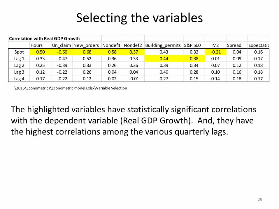
The highlighted variables have statistically significant correlations with the dependent variable (Real GDP Growth). And, they have the highest correlations among the various quarterly lags.

30

-10.0%

-8.0%

-6.0%

-4.0%

-2.0%

0.0%

2.0%

4.0%

6.0%

8.0%

10.0%

12.0%

-10.0% -5.0% 0.0% 5.0% 10.0%

R G

DP

gro

wth

Quarterly change in New Orders

New Orders vs R GDP

-10.0%

-8.0%

-6.0%

-4.0%

-2.0%

0.0%

2.0%

4.0%

6.0%

8.0%

10.0%

12.0%

-2.0% -1.5% -1.0% -0.5% 0.0% 0.5% 1.0% 1.5% 2.0%

R G

DP

gro

wth

Quarterly change in Hours

Hours vs R GDP

-10.0%

-8.0%

-6.0%

-4.0%

-2.0%

0.0%

2.0%

4.0%

6.0%

8.0%

10.0%

12.0%

-20.0% -10.0% 0.0% 10.0% 20.0% 30.0%

R G

DP

gro

wth

Quarterly change in Unemployment Claims

Unemployment Claims vs R GDP

-10.0%

-8.0%

-6.0%

-4.0%

-2.0%

0.0%

2.0%

4.0%

6.0%

8.0%

10.0%

12.0%

-20.0% -15.0% -10.0% -5.0% 0.0% 5.0% 10.0%

R G

DP

gro

wth

Quarterly change in Nondef Spending1

Nondefense Spending1 vs R GDP

-10.0%

-8.0%

-6.0%

-4.0%

-2.0%

0.0%

2.0%

4.0%

6.0%

8.0%

10.0%

12.0%

-30.0% -20.0% -10.0% 0.0% 10.0% 20.0%

R G

DP

gro

wth

Quarterly change in Nondef Spending2

Nondefense Spending2 vs R GDP

-10.0%

-8.0%

-6.0%

-4.0%

-2.0%

0.0%

2.0%

4.0%

6.0%

8.0%

10.0%

12.0%

-30.0% -20.0% -10.0% 0.0% 10.0% 20.0%

R G

DP

gro

wth

Quarterly change in Building Permits Lag1

Building Permits Lag1 vs R GDP

-10.0%

-8.0%

-6.0%

-4.0%

-2.0%

0.0%

2.0%

4.0%

6.0%

8.0%

10.0%

12.0%

-30.0% -20.0% -10.0% 0.0% 10.0% 20.0%

R G

DP

gro

wth

Quarterly change in S&P 500 Lag1

S&P 500 Lag1 vs R GDP

-10.0%

-8.0%

-6.0%

-4.0%

-2.0%

0.0%

2.0%

4.0%

6.0%

8.0%

10.0%

12.0%

-2.0% -1.0% 0.0% 1.0% 2.0% 3.0% 4.0% 5.0% 6.0%

R G

DP

gro

wth

Quarterly change in M2

M2 vs R GDP

Scatter Plots illustrating the relationship between the independent variables and the dependent one (R GDP growth).

Econometrics\Econometric models.xlsx\Plots

Building the Model manually: Forward Stepwise Regression, 1st step

31

Correlation with Residual of Step 1

0.00 (0.02) 0.12 (0.26) (0.05) (0.12) (0.07) (0.03)

X

New_orders Hours Un_claim Nondef1 Nondef2 Building_permits Lag1S&P 500 Lag1 M2

5.0% 1.4% -4.1% 6.6% 8.9% 17.2% 8.0% 1.6%

5.0% 1.2% -10.8% 5.2% 2.7% 14.4% 10.2% 0.3%

5.0% 0.4% -7.6% 4.4% 6.0% 1.8% 1.7% 1.1%

1.4% 0.6% -10.2% 5.8% 9.6% -1.6% 0.1% 1.1%

-1.4% -0.2% 5.1% 2.7% 1.4% 8.9% -3.2% 1.2%

0.0% -0.4% 5.4% -0.8% -2.2% -3.6% -2.9% 0.5%

Y X

Real GDP Y est. Residual New_orders

1983q2 9.4% 6.7% -2.8% 5.0%

1983q3 8.1% 6.7% -1.4% 5.0%

1983q4 8.5% 6.7% -1.8% 5.0%

1984q1 8.2% 3.8% -4.4% 1.4%

1984q2 7.2% 1.5% -5.7% -1.4%

1984q3 4.0% 2.7% -1.3% 0.0%

1984q4 3.2% 2.1% -1.1% -0.7%

First step: build a simple linear regression model with the independent variable with the highest absolute correlation with the dependent one. In this case, it is New_orders with a correlation of 0.68.

Next, select a 2nd independent variable with the highest correlation with the residual of this first linear regression. As shown it is Nondef1 with a correlation of -0.26.

Econometrics\Econometric models.xlsx\Step1

Forward Stepwise Regression, 2nd step

32

Y Y est X1 X2

Real GDP Estimate Residual New_orders Nondef1

1983q2 9.4% 7.0% -2.5% 5.0% 6.6%

1983q3 8.1% 6.7% -1.4% 5.0% 5.2%

1983q4 8.5% 6.6% -1.9% 5.0% 4.4%

1984q1 8.2% 4.6% -3.6% 1.4% 5.8%

1984q2 7.2% 2.3% -4.9% -1.4% 2.7%

1984q3 4.0% 2.5% -1.5% 0.0% -0.8%

1984q4 3.2% 2.2% -1.0% -0.7% 0.1%

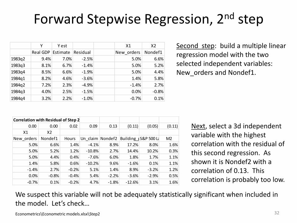
Second step: build a multiple linear regression model with the two selected independent variables: New_orders and Nondef1.

Correlation with Residual of Step 2

0.00 0.00 0.02 0.09 0.13 (0.11) (0.05) (0.11)

X1 X2

New_orders Nondef1 Hours Un_claim Nondef2 Building_permits Lag1S&P 500 Lag1 M2

5.0% 6.6% 1.4% -4.1% 8.9% 17.2% 8.0% 1.6%

5.0% 5.2% 1.2% -10.8% 2.7% 14.4% 10.2% 0.3%

5.0% 4.4% 0.4% -7.6% 6.0% 1.8% 1.7% 1.1%

1.4% 5.8% 0.6% -10.2% 9.6% -1.6% 0.1% 1.1%

-1.4% 2.7% -0.2% 5.1% 1.4% 8.9% -3.2% 1.2%

0.0% -0.8% -0.4% 5.4% -2.2% -3.6% -2.9% 0.5%

-0.7% 0.1% -0.2% 4.7% -1.8% -12.6% 3.1% 1.6%

Next, select a 3d independent variable with the highest correlation with the residual of this second regression. As shown it is Nondef2 with a correlation of 0.13. This correlation is probably too low.

We suspect this variable will not be adequately statistically significant when included in the model. Let’s check…


Forward Stepwise Regression, 3d step

33

Coefficients St. Error t Stat

Intercept 2.6% 0.2% 15.8

X1 New_orders 0.643 0.091 7.1

X2 Nondef1 0.286 0.069 4.2

X3 Nondef2 -0.087 0.041 (2.1)

Actually, the issue with X3 Nondef2 is not that it is not statistically significant, but that its regression coefficient has the wrong sign relative to its original correlation with the dependent variable. That’s a concern.

Let’s redo this 3d step with the next independent variable that had the 2nd highest absolute correlation with the residual from the regression in the 2nd step. It was Building_permits Lag 1 with a correlation of (0.11). That correlation appears too low. We suspect again this variable will not be adequately statistically significant. But, let’s give it a try to find out…


Forward Stepwise Regression, 3d step, 2nd try

34

Coefficients St. Error t Stat P-value

Intercept 2.6% 0.2% 15.7 0.00

X1 New_orders 0.556 0.100 5.6 0.00

X2 Nondef1 0.192 0.054 3.5 0.00

X3 Building_permits Lag10.040 0.028 1.4 0.16

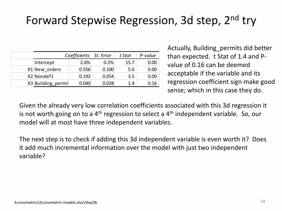
Actually, Building_permits did better than expected. t Stat of 1.4 and P-value of 0.16 can be deemed acceptable if the variable and its regression coefficient sign make good sense; which in this case they do.

Econometrics\Econometric models.xlsx\Step3b

Given the already very low correlation coefficients associated with this 3d regression it is not worth going on to a 4th regression to select a 4th independent variable. So, our model will at most have three independent variables.

The next step is to check if adding this 3d independent variable is even worth it? Does it add much incremental information over the model with just two independent variable?

Comparing model with two vs. three independent variables

35

Hold out performance

2 var 3 var

Actual Model Model

2014q1 -2.1% 2.2% 2.5%

2014q2 4.6% 4.0% 3.7%

2014q3 5.0% 3.9% 4.0%

2014q4 2.6% 1.7% 1.8%

2014 2.5% 2.9% 3.0%

Regression Stats 2 var. 3 var.

Multiple R 0.718 0.724

R Square 0.516 0.524

Adj. R Square 0.508 0.512

Standard Error 1.83% 1.83%

Observations 123 123

Regression coefficients. 2 variable model


Intercept 2.6% 0.2% 15.5 0.00

New_orders 0.616 0.091 6.8 0.00

Nondef1 0.197 0.054 3.6 0.00

Regression coefficients. 3 variable model


Intercept 2.6% 0.2% 15.7 0.00

New_orders 0.556 0.100 5.6 0.00

Nondef1 0.192 0.054 3.5 0.00

Building_permits Lag10.040 0.028 1.4 0.16

The two models are just about even on Goodness-of-fit measures.

In the two-variable model both variables are very statistically significant.

In the three-variable model, the 3d one, as mentioned is not statistically significant.

In the Hold Out, the 2- var. model performs just as well if not better than the 3-var. one.

All of the above suggests the 2-var. model is the winner as the 3d variable does not add enough incremental information.

Econometrics\Econometric models.xlsx\Compare 2 vs 3b

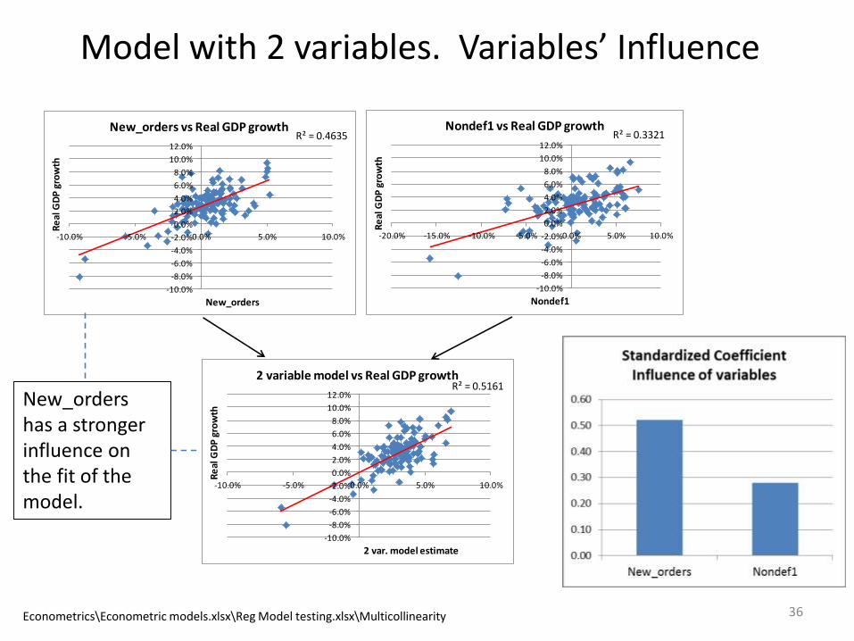
Model with 2 variables. Variables’ Influence

36

R² = 0.4635

-10.0%

-8.0%

-6.0%

-4.0%

-2.0%

0.0%

2.0%

4.0%

6.0%

8.0%

10.0%

12.0%

-10.0% -5.0% 0.0% 5.0% 10.0%

Re

al G

DP

gro

wth

New_orders

New_orders vs Real GDP growthR² = 0.3321

-10.0%

-8.0%

-6.0%

-4.0%

-2.0%

0.0%

2.0%

4.0%

6.0%

8.0%

10.0%

12.0%

-20.0% -15.0% -10.0% -5.0% 0.0% 5.0% 10.0%

Re

al G

DP

gro

wth

Nondef1

Nondef1 vs Real GDP growth

R² = 0.5161

-10.0%

-8.0%

-6.0%

-4.0%

-2.0%

0.0%

2.0%

4.0%

6.0%

8.0%

10.0%

12.0%

-10.0% -5.0% 0.0% 5.0% 10.0%

Re

al G

DP

gro

wth

2 var. model estimate

2 variable model vs Real GDP growth

Econometrics\Econometric models.xlsx\Reg Model testing.xlsx\Multicollinearity

New_orders has a stronger influence on the fit of the model.

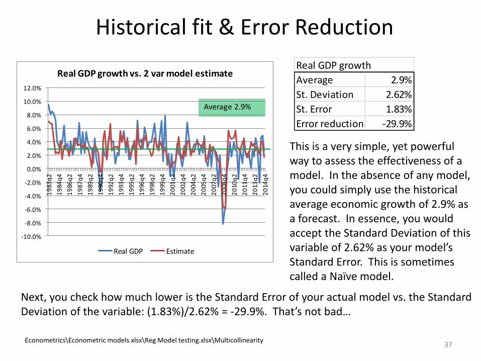
Historical fit & Error Reduction

37

Real GDP growth

Average 2.9%

St. Deviation 2.62%

St. Error 1.83%

Error reduction -29.9%

-10.0%

-8.0%

-6.0%

-4.0%

-2.0%

0.0%

2.0%

4.0%

6.0%

8.0%

10.0%

12.0%

19

83q

2

19

84q

4

19

86q

2

19

87q

4

19

89q

2

19

90q

4

19

92q

2

19

93q

4

19

95q

2

19

96q

4

19

98q

2

19

99q

4

20

01q

2

20

02q

4

20

04q

2

20

05q

4

20

07q

2

20

08q

4

20

10q

2

20

11q

4

20

13q

2

20

14q

4

Real GDP growth vs. 2 var model estimate

Real GDP Estimate

Average 2.9%

Econometrics\Econometric models.xlsx\Reg Model testing.xlsx\Multicollinearity

This is a very simple, yet powerful way to assess the effectiveness of a model. In the absence of any model, you could simply use the historical average economic growth of 2.9% as a forecast. In essence, you would accept the Standard Deviation of this variable of 2.62% as your model’s Standard Error. This is sometimes called a Naïve model.

Next, you check how much lower is the Standard Error of your actual model vs. the Standard Deviation of the variable: (1.83%)/2.62% = -29.9%. That’s not bad…

Adding an Autoregressive Variable (Y Lag 4)

38

Model

Model 2-var

2-var + Y Lag 4

Regression Stats

Multiple R 0.718 0.750

R Square 0.516 0.563

Adj. R Square 0.508 0.552

St. Error 1.83% 1.75%

Observations 123 123

Coefficient

Intercept 2.6% 2.0%

New_orders 0.62 0.65

Nondef1 0.20 0.18

Y Lag 4 0.21

Standardized coefficient


Nondef1 0.28 0.25

Y Lag 4 0.22

T Stat

Intercept 15.5 8.4

New_orders 6.8 7.4

Nondef1 3.6 3.4

Y Lag 4 3.6

P value

Intercept 0.00 0.00


Nondef1 0.00 0.00

Y Lag 4 0.00

Model

Model 2-var

Actual 2-var + Y Lag 4

2014q1 -2.1% 2.2% 2.1%

2014q2 4.6% 4.0% 3.7%

2014q3 5.0% 3.9% 4.2%

2014q4 2.6% 1.7% 1.8%

2014 2.5% 2.9% 3.0%

If you know economic growth 4 quarters ago, it does provide marginally additional incremental info on estimating economic growth in current quarter.

Coefficients for New_orders and Nondef1 have remained surprisingly stable and so have their influence as measured with Standardized coefficients.

Statistical significance of variables is very similar for both models.

Hold Out performance is pretty much even

Econometrics\Econometric models.xlsx\Model finalists

Visual comp.: Regression vs Autoregressive model

39

-10.0%

-8.0%

-6.0%

-4.0%

-2.0%

0.0%

2.0%

4.0%

6.0%

8.0%

10.0%1

983

q2

19

84q

4

19

86q

2

19

87q

4

19

89q

2

19

90q

4

19

92q

2

19

93q

4

19

95q

2

19

96q

4

19

98q

2

19

99q

4

20

01q

2

20

02q

4

20

04q

2

20

05q

4

20

07q

2

20

08q

4

20

10q

2

20

11q

4

20

13q

2

20

14q

4

Qu

arte

rly

Re

al G

DP

ch

ange

, an

nu

aliz

ed

Reg model: Actual vs Estimate

Actual Estimate

-10.0%

-8.0%

-6.0%

-4.0%

-2.0%

0.0%

2.0%

4.0%

6.0%

8.0%

10.0%

12.0%

19

83q

2

19

84q

4

19

86q

2

19

87q

4

19

89q

2

19

90q

4

19

92q

2

19

93q

4

19

95q

2

19

96q

4

19

98q

2

19

99q

4

20

01q

2

20

02q

4

20

04q

2

20

05q

4

20

07q

2

20

08q

4

20

10q

2

20

11q

4

20

13q

2

20

14q

4

Qu

arte

rly

Re

al G

DP

ch

ange

, an

nu

aliz

ed

Autoreg model: Actual vs Estimate

Actual Estimate

-3.0%

-2.0%

-1.0%

0.0%

1.0%

2.0%

3.0%

4.0%

5.0%

6.0%

2014q1 2014q2 2014q3 2014q4 Average

Hold Out Performance

Actual Reg est. Autoreg est.

0.00

0.10

0.20

0.30

0.40

0.50

0.60

New_orders Nondef1 Y Lag 4

# o

f St

and

ard

de

viat

ion

s

Standardized Regression coefficient

Reg Autoreg

Econometric models.xlsx\Graphs.xlsx\Comparison

The Pros & Cons of Autoregressive Models

40

The pros: 1) It often reduce the autocorrelation of residuals; 2) It improves the overall Goodness-of-fit of a model;3) It often improves the forecasting up to the Lag used in the model (Lag 4

quarters will allow you to forecast potentially better up to 4 quarters out).

The cons: 1) The autoregressive variable can grab away explanatory information from the

macroeconomic variables and weaken their statistical significance;2) It can weaken the forecasting beyond the Lag used in the model. If you use

Lag 4 quarters, the model forecasting may weaken beyond 4 quarters.

Thus, depending on what is your objective and the issues associated with a model, an autoregressive model may add value or not. You may decide to keep both models and use them in different circumstances.

In this specific example, the autoregressive model does not add much value.

4) Model Testing

41

Linear Regression underlying assumptions: 1) No near-exact linear relationships between independent variables. Multicollinearity issue.2) Error terms (Residuals) are independent. Autocorrelation issue.3) Residuals have a constant variance. Heteroskedasticity issue.

We will test the regular Regression model with two variables for all of the above assumptions, and conduct additional tests related to model specification.

Multicollinearity

42

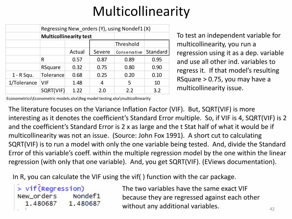
To test an independent variable for multicollinearity, you run a regression using it as a dep. variable and use all other ind. variables to regress it. If that model’s resulting RSquare > 0.75, you may have a multicollinearity issue.

The literature focuses on the Variance Inflation Factor (VIF). But, SQRT(VIF) is more interesting as it denotes the coefficient’s Standard Error multiple. So, if VIF is 4, SQRT(VIF) is 2 and the coefficient’s Standard Error is 2 x as large and the t Stat half of what it would be if multicollinearity was not an issue. (Source: John Fox 1991). A short cut to calculating SQRT(VIF) is to run a model with only the one variable being tested. And, divide the Standard Error of this variable’s coeff. within the multiple regression model by the one within the linear regression (with only that one variable). And, you get SQRT(VIF). (EViews documentation).

In R, you can calculate the VIF using the vif( ) function with the car package.

The two variables have the same exact VIF because they are regressed against each other without any additional variables.

Econometrics\Econometric models.xlsx\Reg model testing.xlsx\multicollinearity

Regressing New_orders (Y), using Nondef1 (X)

Multicollinearity test

Threshold

Actual Severe Conservative Standard

R 0.57 0.87 0.89 0.95

RSquare 0.32 0.75 0.80 0.90

1 - R Squ. Tolerance 0.68 0.25 0.20 0.10

1/Tolerance VIF 1.48 4 5 10

SQRT(VIF) 1.22 2.0 2.2 3.2

2-variable Model Residuals

43

Econometric models.xlsx\Reg model testing.xlsx\autocorrelation

Unless the residual pattern is extremely obvious, it is difficult to visually accurately assess whether residuals are autocorrelated or heteroskedastic. You have to statistically test for those properties to get an accurate diagnostic. However, we can speculate that the residuals are probably not very heteroskedastic (right hand side scatter plot).

-6.0%

-4.0%

-2.0%

0.0%

2.0%

4.0%

6.0%

-8.0% -6.0% -4.0% -2.0% 0.0% 2.0% 4.0% 6.0% 8.0%

Re

sid

ual

Estimate

2-var model: Residual l vs Estimate

Econometric models.xlsx\Graphs.xlsx\Regression model

Autocorrelation Lag 1 test: Durbin Watson (DW)

44

In R with lmtest package.

> dwtest(Regression, order.by = NULL, exact = NULL)

Durbin-Watson test

data: Regression

DW = 1.7189, p-value = 0.05316

alternative hypothesis: true autocorrelation is greater than 0

P-value Interpretation

0.05 We can reject alternative hypothesis that true autocorrelation is >0.

0.95 We can't reject the alternative hypothesis that the true autocorrelation is >0.

Durbin Watson

Numerator 6.94% sum(Residual - Residual t-1)^2

Denominator 4.04% sum(Residual^2)

DW score 1.719

n 123

k 2

dL 1.634

dU 1.715

Value from DW table

Value from DW table

number of observations

number of independent variables

The 1.719 DW score falls just outside the zone of uncertainty for positive autocorrelation (1.634 – 1.715). So, we can be pretty sure those residuals are not positively autocorrelated with Lag 1 residuals.

The R output says the same thing. There is only a 0.05 chance that such residuals are autocorrelated. In R, watch for the direction of this test.

Econometrics\Econometric models.xlsx\Reg model testing.xlsx\autocorrelation

Two better tests than DW: Ljung-Box & Breusch-Godfrey

45

Comparing Ljung-Box and Breusch-Godfrey tests using R

Ljung-Box test Breusch-Godfrey test.

You don't need to load any extra library for this test. In R with lmtest package.

Testing for Lag 1 or AR(1) Testing for Lag 1 or AR(1)

> bgtest(Regression, order = 1, type = c("Chisq"))

Breusch-Godfrey test for serial correlation of order up to 1

data: Regression

LM test = 2.2148, df = 1, p-value = 0.1367

Testing up to Lag 4 or AR(4) Testing up to Lag 4 or AR(4)

> Box.test(Regression$res,lag = 4, type = c("Ljung-Box"),fitdf = 0) > bgtest(Regression, order = 4, type = c("Chisq"))

Box-Ljung test Breusch-Godfrey test for serial correlation of order up to 4

data: Regression$res data: Regression

X-squared = 37.1735, df = 4, p-value = 1.659e-07 LM test = 24.7465, df = 4, p-value = 5.657e-05

2015\Econometrics\Reg Model testing.xlsx\Autocorrelation

Autocorrelation related p-value

LB BG Interpretation

AR(1) 0.1355 0.1367 Not stat. significant

AR(4) 0.0000 0.0000 Very stat. significant

The LB and BG tests are better than DW for two reasons. They can test for more than one lag. They can also test a model with an autoregressive variable. Meanwhile, DW can’t.

The LB and BG tests diagnostics were nearly identical. Residuals do not have an AR(1) process. But, they have an AR(4) one.

Autocorrelations statistical significance

46Econometrics\Econometric models.xlsx\Reg model testing.xlsx\autocorrelation

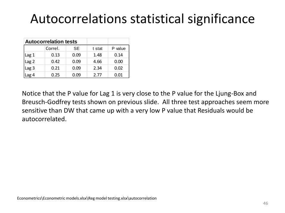
Autocorrelation tests

Correl. SE t stat P value

Lag 1 0.13 0.09 1.48 0.14

Lag 2 0.42 0.09 4.66 0.00

Lag 3 0.21 0.09 2.34 0.02

Lag 4 0.25 0.09 2.77 0.01

Notice that the P value for Lag 1 is very close to the P value for the Ljung-Box and Breusch-Godfrey tests shown on previous slide. All three test approaches seem more sensitive than DW that came up with a very low P value that Residuals would be autocorrelated.

Autocorrelation: Regular model vs Autoregressive one

47

Regular model

Autocorrelation statistical significance


Lag 1 0.13 0.09 1.48 0.14

Lag 2 0.42 0.09 4.66 0.00

Lag 3 0.21 0.09 2.34 0.02

Lag 4 0.25 0.09 2.77 0.01

Autoregressive Model

Autocorrelation statistical significance


Lag 1 0.01 0.09 0.13 0.90

Lag 2 0.27 0.09 2.95 0.00

Lag 3 0.10 0.09 1.08 0.28

Lag 4 0.02 0.09 0.20 0.84

Econometrics\Econometric models.xlsx\Reg model testing.xlsx\autocorrelation

By adding a Y Lag 4 variable, the Autoregressive model reduced all autocorrelations (from Lag 1 to Lag 4) vs. the Regular model. This is a common phenomenon in modeling. Notice the Autoregressive Model would not entirely circumvent the autocorrelation of residual issue. The Lag 2 is clearly statistically significant.

Heteroskedasticity test: Breusch-Pagan

48

Y X1 X2

Residual^2 New_ordersNondef1

1983q2 0.1% 5.0% 6.6%

1983q3 0.0% 5.0% 5.2%

1983q4 0.0% 5.0% 4.4%

1984q1 0.1% 1.4% 5.8%

1984q2 0.2% -1.4% 2.7%

Breusch-Pagan LM Chi dist. P value

Lagrange Multiplier (LM) 0.8

DF (# variables) 2.0

Chi Dist. P value 0.68


Multiple R 0.079

R Square 0.006

Adj. R Square -0.010

Standard Error 0.000

Observations 123

ANOVA


Regression 2 1.75E-07 8.77E-08 0.38 0.68

Residual 120 2.77E-05 2.31E-07

Total 122 2.78E-05

In R with lmtest package.

> bptest(Regression,varformula = NULL, studentize = FALSE)

Breusch-Pagan test

data: Regression

BP = 0.8135, df = 2, p-value = 0.6658

Econometrics\Econometric models.xlsx\Reg model testing.xlsx\heteroskedasticity

The BP test tests for linear heteroskedasticity. It suggests that residuals are not heteroskedastic because the LM Chi distribution P value at 0.68 is far from being statistically significant. In most cases, the ANOVA F test generates very similar values.

Heteroskedasticity test: White Test

49

Y

Residual^2 X1 X2 X1^2 X2^2

1983q2 0.1% 5.0% 6.6% 0.2% 0.4%

1983q3 0.0% 5.0% 5.2% 0.2% 0.3%

1983q4 0.0% 5.0% 4.4% 0.3% 0.2%

1984q1 0.1% 1.4% 5.8% 0.0% 0.3%

1984q2 0.2% -1.4% 2.7% 0.0% 0.1%

ANOVA

df SS MS F Signific. F

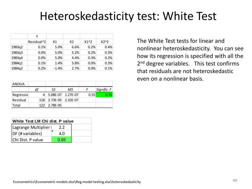
Regression 4 5.08E-07 1.27E-07 0.55 0.70

Residual 118 2.73E-05 2.32E-07

Total 122 2.78E-05

White Test LM Chi dist. P value

Lagrange Multiplier (LM)2.2

DF (# variables) 4.0



The White Test tests for linear and nonlinear heteroskedasticity. You can see how its regression is specified with all the 2nd degree variables. This test confirms that residuals are not heteroskedastic even on a nonlinear basis.

Heteroskedasticity test: Autoregressive Conditional Heteroskedasticity (ARCH)

50

Y X1 X2 X3 X4

Resid^2 Resid^2 t-1 Resid^2 t-2 Resid^2 t-3 Resid^2 t-4

1983q2 0.1%

1983q3 0.0% 0.1%

1983q4 0.0% 0.0% 0.1%

1984q1 0.1% 0.0% 0.0% 0.1%

1984q2 0.2% 0.1% 0.0% 0.0% 0.1%

1984q3 0.0% 0.2% 0.1% 0.0% 0.0%

1984q4 0.0% 0.0% 0.2% 0.1% 0.0%

ANOVA

df SS MS F Sign. F

Regression 4 5.21E-07 1.3E-07 0.56 0.69

Residual 114 2.63E-05 2.31E-07

Total 118 2.68E-05

ARCH LM Chi dist. P value

Lagrange Multiplier (LM) 2.3

DF (# lags) 4



This heteroskedasticity test checks whether the variance of an error term is a function of the size of the previous error terms.

In plain English, are large residuals followed by large residuals and small ones by small ones.

As indicated with the high value for Significance of F and Chi distribution P value, this model’s residuals do not suffer from this type of heteroskedasticity.

Where does heteroskedasticity come from?

51

-6.0%

-4.0%

-2.0%

0.0%

2.0%

4.0%

6.0%

-8.0% -6.0% -4.0% -2.0% 0.0% 2.0% 4.0% 6.0% 8.0%

Re

sid

ual

Estimate

Reg model: Residual l vs Estimate

-6.0%

-4.0%

-2.0%

0.0%

2.0%

4.0%

6.0%

-10.0% -8.0% -6.0% -4.0% -2.0% 0.0% 2.0% 4.0% 6.0%

Re

sid

ual

New_orders

Reg model: Residual vs New_orders

-6.0%

-4.0%

-2.0%

0.0%

2.0%

4.0%

6.0%

-16.0% -11.0% -6.0% -1.0% 4.0% 9.0%

Re

sid

ual

Nondef1

Reg model: Residual vs Nondef1

Econometric models.xlsx\Graphs.xlsx\Regression model

We already know the overall model does not demonstrate heteroskedastic residuals. But if it is some model reviewers fit a quadratic regression line to the residuals vs. each of the independent variables to identify heteroskedasticity at the variable level. In this case, the resulting quadratic regression lines are pretty flat reflecting unlikely heteroskedasticity issues.

Testing Heteroskedasticity at the variable level: Park Test

52

ANOVA


Regression 1 0.000 0.000 0.233 0.63

Residual 121 0.000 0.000

Total 122 0.000

Coeff. St. Error t Stat P-value

Intercept 0.00 0.00 7.42 0.00

New_orders 0.00 0.00 0.48 0.63

Econometrics\Econometric models.xlsx\Reg model testing.xlsx\heteroskedasticity variable

The most common form of the Park test is to log all the variables. But, you can’t log negative values. So, the Park test has also a linear form described here. Notice that this version of the Park test is nearly identical to the Breusch-Pagan test except it tests for one single variable at a time to identify where the heteroskedasticity comes from.

Using linear form of the Park test.

Y X1

Residual^2 New_orders

1983q2 0.06% 5.0%

1983q3 0.02% 5.0%

1983q4 0.04% 5.0%

1984q1 0.13% 1.4%

We ran the same test for Nondef1, and got P values of 0.38. So, in both cases the residuals are not heteroskedastic relative to the level of either independent variables.

Residual autocorrelation & heteroskedasticity recap

53

Residuals are not heteroskedastic. Note that all the heteroskedasticity tests (BP, White, ARCH) for the overall model generated almost the same Sign. of F and Chi Square dist. P-value (all near 0.7). That’s even though they tested for different shapes of heteroskedasticity.

Residuals are autocorrelated when looking beyond Lag 1. There too a couple of the tests (Ljung-Box, Breusch-Pagan) gave us nearly identical results in terms of respective P values.

There are several ways to resolve autocorrelation and heteroskedasticity issues as shown on the next slide.

How to resolve Autocorrelation & Heteroskedasticity

54

C:\Users\liongc\Desktop\Econometrics\Model Guidance\Model guidance map.xlsx\Simple Map

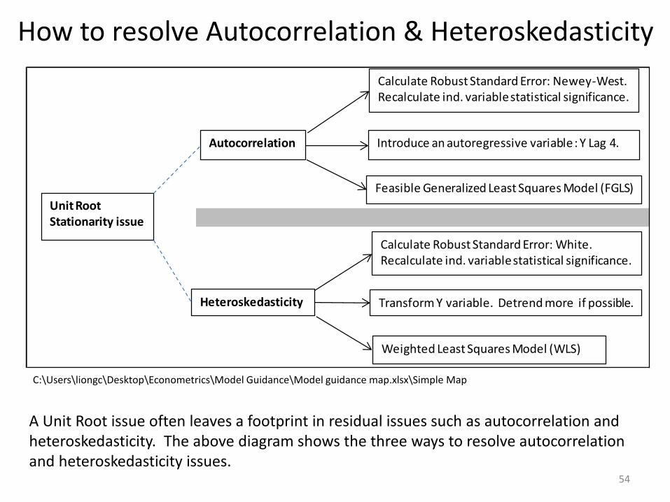
A Unit Root issue often leaves a footprint in residual issues such as autocorrelation and heteroskedasticity. The above diagram shows the three ways to resolve autocorrelation and heteroskedasticity issues.

Calculate Robust Standard Error: Newey-West. Recalculate ind. variable statistical significance.

Introduce an autoregressive variable : Y Lag 4.

Feasible Generalized Least Squares Model (FGLS)

Calculate Robust Standard Error: White. Recalculate ind. variable statistical significance.

Transform Y variable. Detrend more if possible.

Weighted Least Squares Model (WLS)

Autocorrelation

Heteroskedasticity

Unit Root Stationarity issue

Mapping the Robust Standard Error Path

55C:\Users\liongc\Desktop\Econometrics\Model Guidance\Model guidance map.xlsx\Map 2

The diagram below fleshes out what it means to calculate Robust Standard Error and test ind. variables statistical significance.

Yes

No Yes

No

Yes

No

Are residuals heteroskedastic (White test, Breusch-Pagan)and/or autocorrelated (DW, Ljung)?

Calculate Robust Standard Error: White for heteros.;Newey-West for autocor.Recalculate independent variables statistical significance.

Are independent variables still statistically significant?

Good, you are done with heteroskedasticity and autocorrelation testing.

Good, you are done with resolvingheteroskedasticity and autocorrelation issues.

Confirm that a variable that is not stat. significant is supported by economic theory. If not, consider removing variable.

Is your dependent variable stationary [Unit Root ] (Dickey-Fuller test)?

Consider transforming Y to % change or First-Difference .

White SEs = Newey-West SEs w/ zero lag with R

56

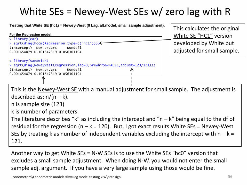
Testing that White SE (hc1) = Newey-West (0 Lag, alt.model, small sample adjustment).

For the Regression model.

> library(car)

> sqrt(diag(hccm(Regression,type=c("hc1"))))

(Intercept) New_orders Nondef1

0.001654879 0.101647319 0.056301194

> library(sandwich)

> sqrt(diag(NeweyWest(Regression,lag=0,prewhite=FALSE,adjust=123/121)))

(Intercept) New_orders Nondef1

0.001654879 0.101647319 0.056301194

This calculates the original White SE “HC1” version developed by White but adjusted for small sample.

This is the Newey-West SE with a manual adjustment for small sample. The adjustment is described as: n/(n – k). n is sample size (123)k is number of parameters. The literature describes “k” as including the intercept and “n – k” being equal to the df of residual for the regression (n – k = 120). But, I got exact results White SEs = Newey-West SEs by treating k as number of independent variables excluding the intercept with n – k = 121.

Econometrics\Econometric models.xlsx\Reg model testing.xlsx\Stat sign.

Another way to get White SEs = N-W SEs is to use the White SEs “hc0” version that excludes a small sample adjustment. When doing N-W, you would not enter the small sample adj. argument. If you have a very large sample using those would be fine.

White SE = Newey-West SE summary

57

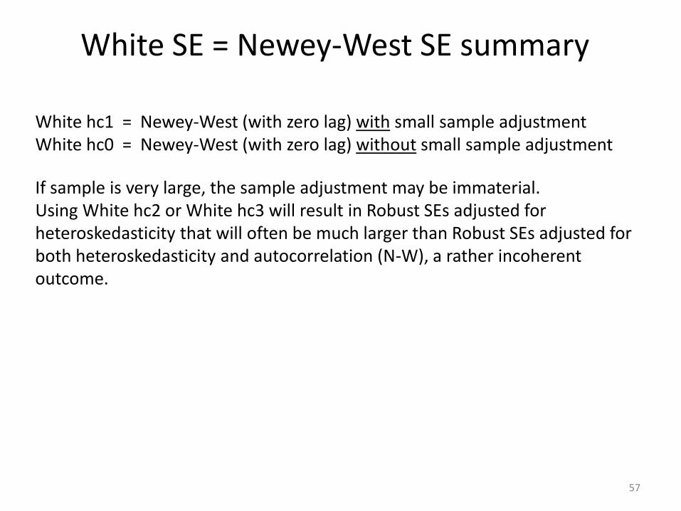
White hc1 = Newey-West (with zero lag) with small sample adjustmentWhite hc0 = Newey-West (with zero lag) without small sample adjustment

If sample is very large, the sample adjustment may be immaterial. Using White hc2 or White hc3 will result in Robust SEs adjusted for heteroskedasticity that will often be much larger than Robust SEs adjusted for both heteroskedasticity and autocorrelation (N-W), a rather incoherent outcome.

Recalculating variables stat. significance

58

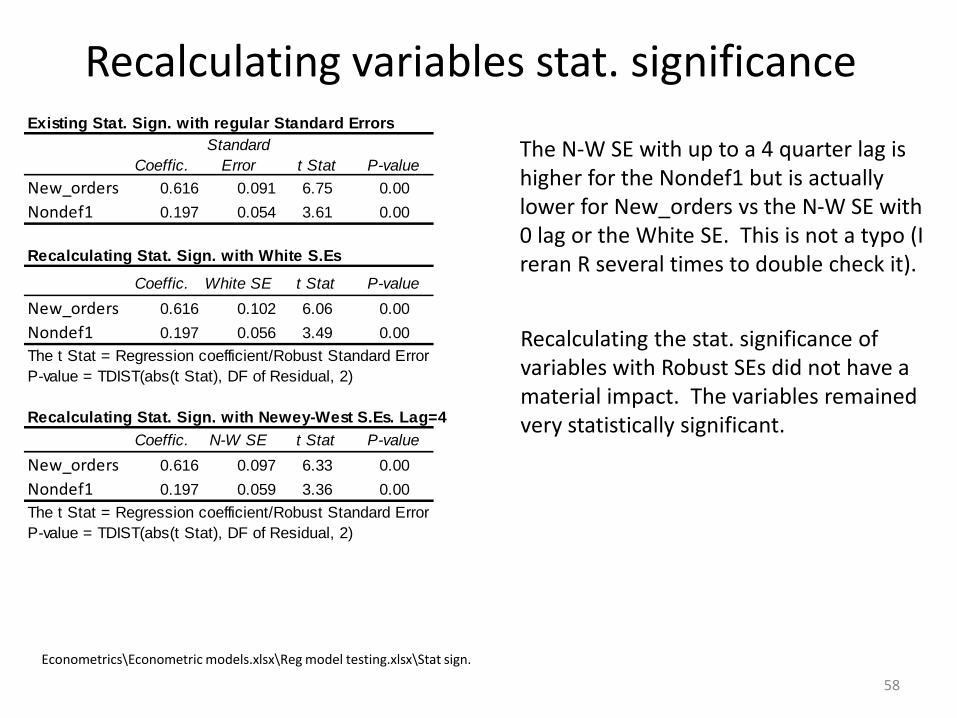
The N-W SE with up to a 4 quarter lag is higher for the Nondef1 but is actually lower for New_orders vs the N-W SE with 0 lag or the White SE. This is not a typo (I reran R several times to double check it).

Econometrics\Econometric models.xlsx\Reg model testing.xlsx\Stat sign.

Existing Stat. Sign. with regular Standard Errors

Coeffic.

Standard

Error t Stat P-value

New_orders 0.616 0.091 6.75 0.00

Nondef1 0.197 0.054 3.61 0.00

Recalculating Stat. Sign. with White S.Es

Coeffic. White SE t Stat P-value

New_orders 0.616 0.102 6.06 0.00

Nondef1 0.197 0.056 3.49 0.00

The t Stat = Regression coefficient/Robust Standard Error

P-value = TDIST(abs(t Stat), DF of Residual, 2)

Recalculating Stat. Sign. with Newey-West S.Es. Lag=4

Coeffic. N-W SE t Stat P-value

New_orders 0.616 0.097 6.33 0.00

Nondef1 0.197 0.059 3.36 0.00

The t Stat = Regression coefficient/Robust Standard Error

P-value = TDIST(abs(t Stat), DF of Residual, 2)

Recalculating the stat. significance of variables with Robust SEs did not have a material impact. The variables remained very statistically significant.

Testing coefficient stability across different

time series

59

Regression Coefficient X2 X1

Nondef1 New_ordersIntercept

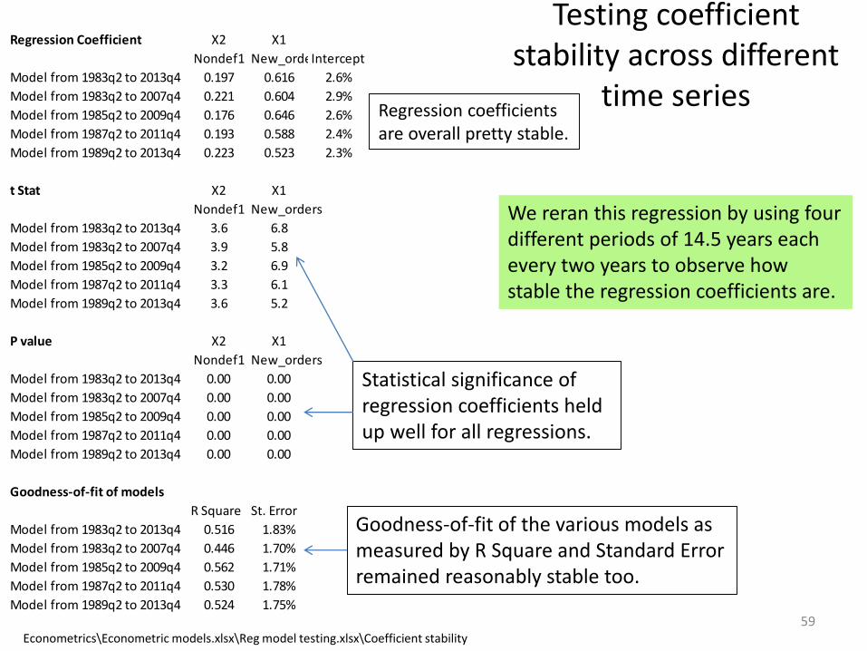
Model from 1983q2 to 2013q4 0.197 0.616 2.6%

Model from 1983q2 to 2007q4 0.221 0.604 2.9%

Model from 1985q2 to 2009q4 0.176 0.646 2.6%

Model from 1987q2 to 2011q4 0.193 0.588 2.4%

Model from 1989q2 to 2013q4 0.223 0.523 2.3%

t Stat X2 X1

Nondef1 New_orders

Model from 1983q2 to 2013q4 3.6 6.8

Model from 1983q2 to 2007q4 3.9 5.8

Model from 1985q2 to 2009q4 3.2 6.9

Model from 1987q2 to 2011q4 3.3 6.1

Model from 1989q2 to 2013q4 3.6 5.2

P value X2 X1

Nondef1 New_orders

Model from 1983q2 to 2013q4 0.00 0.00

Model from 1983q2 to 2007q4 0.00 0.00

Model from 1985q2 to 2009q4 0.00 0.00

Model from 1987q2 to 2011q4 0.00 0.00

Model from 1989q2 to 2013q4 0.00 0.00

Goodness-of-fit of models

R Square St. Error

Model from 1983q2 to 2013q4 0.516 1.83%

Model from 1983q2 to 2007q4 0.446 1.70%

Model from 1985q2 to 2009q4 0.562 1.71%

Model from 1987q2 to 2011q4 0.530 1.78%

Model from 1989q2 to 2013q4 0.524 1.75%

We reran this regression by using four different periods of 14.5 years each every two years to observe how stable the regression coefficients are.

Regression coefficients are overall pretty stable.

Statistical significance of regression coefficients held up well for all regressions.

Goodness-of-fit of the various models as measured by R Square and Standard Error remained reasonably stable too.

Econometrics\Econometric models.xlsx\Reg model testing.xlsx\Coefficient stability

Exploring Outliers (why R can be really cool)

60

> influencePlot(Regression, id.n=6) Cook's D (bubble size)

It measures the change to the estimates that results from deleting an observation. Its calculation combines a measure of Outlierness (like Stud. Residuals) and Leverage. Threshold:> 4/n

Studentized Residuals (y-axis)

Dependent variable outliers

Large error. Unusual dependent variable value given the independent variable’s input. This means an actual datapoint is two standard deviations (scaled on a t distribution) of the Residual away from the regressed line. Fairly similar to being two model's Standard Errors away (small differences due to dfs). Threshold: + or - 2.

Hat-Leverage (x-axis)

Independent variable outliers

Leverage measures how far an independent variable deviates from its Mean. Threshold: >(2k + 2)/n

Econometrics\Graphs.xlsx\R Graphs

Using the car package

Outliers

61

> influencePlot(Regression, id.n=6)

StudRes Hat CookD

5 2.81192728 0.026683421 0.261387671

9 1.31478653 0.060466331 0.191990916

23 1.43797317 0.068965131 0.224956383

33 -0.79884290 0.066833211 0.123615536

69 2.63048375 0.038623597 0.297165815

100 -2.14789027 0.029868097 0.214386600

102 -0.01900992 0.070398888 0.003032988

103 -1.58568051 0.176556380 0.421266201

104 0.30230346 0.199567139 0.087481253

106 -2.44084923 0.025118592 0.221672137

112 -2.57586760 0.008165951 0.131880907

119 -2.14938212 0.011899339 0.134171528

2 var Regression Model

A B A x B Rank Rank

Observ. StudRes Hat-Lev. CookD Influence CookD Influence

103 -1.586 0.177 0.421 0.280 1 1

69 2.630 0.039 0.297 0.102 2 2

5 2.812 0.027 0.261 0.075 3 5

23 1.438 0.069 0.225 0.099 4 3

106 -2.441 0.025 0.222 0.061 5 7

100 -2.148 0.030 0.214 0.064 6 6

9 1.315 0.060 0.192 0.080 7 4

119 -2.149 0.012 0.134 0.026 8 10

112 -2.576 0.008 0.132 0.021 9 11

33 -0.799 0.067 0.124 0.053 10 9

104 0.302 0.200 0.087 0.060 11 8

102 -0.019 0.070 0.003 0.001 12 12

Correlation 0.87

Econometrics\Graphs.xlsx\R Graphs

The most important and encompassing outlier-measure is Cook’s D because it pretty much aggregates the information from Studentized Residuals and Leverage.

Impact of Outliers on regression coefficients

62

> Regression103<-lm(Real.GDP~New_orders + Nondef1, econdata,subset=-c(103,124,125,126,127))

> summary(Regression103)

Regression testing for outliers

without without without

All data 103 69 5

Coeffic.

Intercept 0.026 0.027 0.026 0.026

New_orders 0.616 0.575 0.648 0.647

Nondef1 0.197 0.186 0.173 0.179

t Stat

New_orders 6.75 6.11 7.21 7.24

Nondef1 3.61 3.40 3.20 3.36

Adj. R Sq. 0.508 0.433 0.522 0.528

Econometrics\Econometric models.xlsx\Reg model testing.xlsx\Outliers

Here we reran the regression by taking out one at a time each of the top three observations ranked by Cook’s D measure (the more encompassing measure of influence).

As shown, the coefficients and their statistical respective statistical significance remained pretty stable.

Does Cook’s D really work?

63

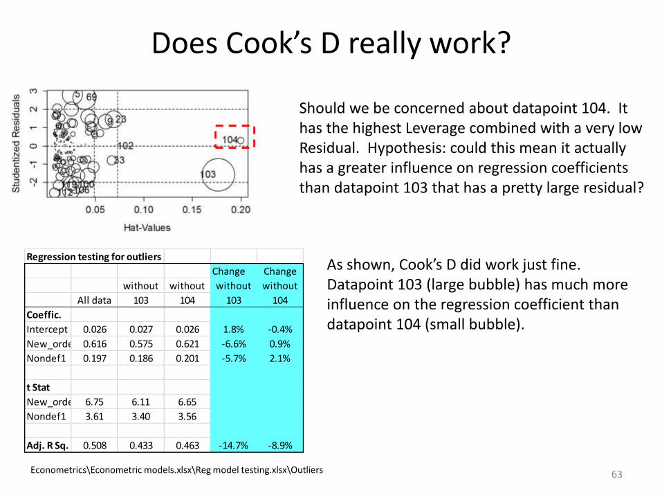
Should we be concerned about datapoint 104. It has the highest Leverage combined with a very low Residual. Hypothesis: could this mean it actually has a greater influence on regression coefficients than datapoint 103 that has a pretty large residual?

Regression testing for outliers

Change Change

without without without without

All data 103 104 103 104

Coeffic.

Intercept 0.026 0.027 0.026 1.8% -0.4%

New_orders 0.616 0.575 0.621 -6.6% 0.9%

Nondef1 0.197 0.186 0.201 -5.7% 2.1%

t Stat

New_orders 6.75 6.11 6.65

Nondef1 3.61 3.40 3.56

Adj. R Sq. 0.508 0.433 0.463 -14.7% -8.9%

As shown, Cook’s D did work just fine. Datapoint 103 (large bubble) has much more influence on the regression coefficient than datapoint 104 (small bubble).

Econometrics\Econometric models.xlsx\Reg model testing.xlsx\Outliers

Are Residuals Normally distributed?

64

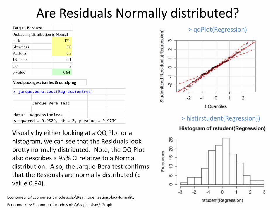
Jarque- Bera test.

Probability distribution is Normal

n - k 121

Skewness 0.0

Kurtosis 0.2

JB score 0.1

DF 2

p-value 0.94

Econometrics\Econometric models.xlsx\Reg model testing.xlsx\Normality

> qqPlot(Regression)

> hist(rstudent(Regression))

Econometrics\Econometric models.xlsx\Graphs.xlsx\R Graph

Visually by either looking at a QQ Plot or a histogram, we can see that the Residuals look pretty normally distributed. Note, the QQ Plot also describes a 95% CI relative to a Normal distribution. Also, the Jarque-Bera test confirms that the Residuals are normally distributed (p value 0.94).

Need packages: tseries & quadprog

> jarque.bera.test(Regression$res)

Jarque Bera Test

data: Regression$res

X-squared = 0.0529, df = 2, p-value = 0.9739

Scenario Testing: Can the Model break down?

65Econometrics\Econometric models.xlsx\Reg model testing.xlsx\Scenario testing

If we use inputs (yellow), we get output (pink).

Scenarios: Real GDP quarterly change annualized

New_orders

Min Median Max

3.1% -11.4% -7.3% -3.3% 0.7% 3.1% 5.5% 7.9%

Min -20.6% -8.4% -5.9% -3.5% -1.0% 0.5% 1.9% 3.4%

-13.4% -7.0% -4.5% -2.1% 0.4% 1.9% 3.4% 4.8%

-6.2% -5.6% -3.1% -0.7% 1.8% 3.3% 4.8% 6.2%

Nondef1 Median 0.9% -4.2% -1.7% 0.8% 3.2% 4.7% 6.2% 7.6%

6.3% -3.1% -0.7% 1.8% 4.3% 5.8% 7.2% 8.7%

11.7% -2.1% 0.4% 2.9% 5.4% 6.8% 8.3% 9.8%

Max 17.1% -1.0% 1.5% 3.9% 6.4% 7.9% 9.4% 10.8%

Regression Model Model data from 1982 From beginning of series in 1959

Coefficient Min Median Max Min Median Max

Intercept 2.6%

New_orders 0.616 0.5% -9.3% 0.5% 5.2% -11.4% 0.7% 7.9%

Nondef1 0.197 0.9% -15.7% 0.9% 7.5% -20.6% 0.9% 17.1%

Output estimate

Real GDP 3.1%

Median R GDP

Learning sample 3.1%

Since 1947 3.2%

We then sensitize the values of both New_orders and Nondef1 based on historical ranges going back to 1959. We then generate 49 different scenarios of GDP growth.

Are the scenario estimates reasonable?

66

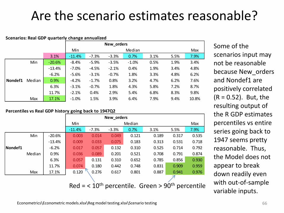
Scenarios: Real GDP quarterly change annualizedNew_orders

Min Median Max

3.1% -11.4% -7.3% -3.3% 0.7% 3.1% 5.5% 7.9%

Min -20.6% -8.4% -5.9% -3.5% -1.0% 0.5% 1.9% 3.4%

-13.4% -7.0% -4.5% -2.1% 0.4% 1.9% 3.4% 4.8%

-6.2% -5.6% -3.1% -0.7% 1.8% 3.3% 4.8% 6.2%

Nondef1 Median 0.9% -4.2% -1.7% 0.8% 3.2% 4.7% 6.2% 7.6%

6.3% -3.1% -0.7% 1.8% 4.3% 5.8% 7.2% 8.7%

11.7% -2.1% 0.4% 2.9% 5.4% 6.8% 8.3% 9.8%

Max 17.1% -1.0% 1.5% 3.9% 6.4% 7.9% 9.4% 10.8%

Percentiles vs Real GDP history going back to 1947Q2

New_orders

Min Median Max

-11.4% -7.3% -3.3% 0.7% 3.1% 5.5% 7.9%

Min -20.6% 0.003 0.014 0.049 0.121 0.189 0.317 0.535

-13.4% 0.009 0.033 0.075 0.183 0.313 0.531 0.718

Nondef1 -6.2% 0.017 0.057 0.132 0.310 0.525 0.714 0.792

Median 0.9% 0.036 0.089 0.201 0.521 0.708 0.791 0.874

6.3% 0.057 0.131 0.310 0.652 0.785 0.856 0.930

11.7% 0.074 0.180 0.442 0.748 0.831 0.909 0.959

Max 17.1% 0.120 0.276 0.617 0.801 0.887 0.941 0.976

Econometrics\Econometric models.xlsx\Reg model testing.xlsx\Scenario testing

Some of the scenarios input may not be reasonable because New_orders and Nondef1 are positively correlated (R = 0.52). But, the resulting output of the R GDP estimates percentiles vs entire series going back to 1947 seems pretty reasonable. Thus, the Model does not appear to break down readily even with out-of-sample variable inputs.

Red = < 10th percentile. Green > 90th percentile

Is the Model well specified? Link test

67

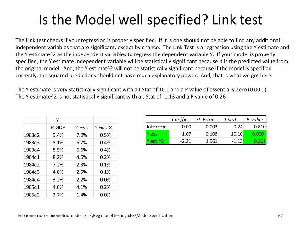
Y

R GDP Y est. Y est. 2̂

1983q2 9.4% 7.0% 0.5%

1983q3 8.1% 6.7% 0.4%

1983q4 8.5% 6.6% 0.4%

1984q1 8.2% 4.6% 0.2%

1984q2 7.2% 2.3% 0.1%

1984q3 4.0% 2.5% 0.1%

1984q4 3.2% 2.2% 0.0%

1985q1 4.0% 4.1% 0.2%

1985q2 3.7% 1.4% 0.0%


Intercept 0.00 0.003 0.24 0.810

Y est. 1.07 0.106 10.10 0.000

Y est.^2 -2.21 1.961 -1.13 0.261

The Link test checks if your regression is properly specified. If it is one should not be able to find any additional independent variables that are significant, except by chance. The Link Test is a regression using the Y estimate and the Y estimate^2 as the independent variables to regress the dependent variable Y. If your model is properly specified, the Y estimate independent variable will be statistically significant because it is the predicted value from the original model. And, the Y estimat^2 will not be statistically significant because if the model is specified correctly, the squared predictions should not have much explanatory power. And, that is what we got here.

The Y estimate is very statistically significant with a t Stat of 10.1 and a P value of essentially Zero (0.00...).The Y estimate^2 is not statistically significant with a t Stat of -1.13 and a P value of 0.26.

Econometrics\Econometric models.xlsx\Reg model testing.xlsx\Model Specification

Intro to econometrics

Data & Analytics