Article 1 Intratumor Heterogeneity and 2 Circulating Tumor Cell Clusters 3 Zafarali Ahmed 1 , Simon Gravel 2* 4 1 Department of Biology, McGill University, 5 Montreal, Quebec, Canada 6 2 Department of Human Genetics, McGill 7 University, Montreal, Quebec, Canada 8 * [email protected] 9 Summary 10 Genetic diversity plays a central role in tumor 11 progression, metastasis, and resistance to treat- 12 ment. Experiments are shedding light on this 13 diversity at ever finer scales, but interpretation 14 is challenging. Using recent progress in numer- 15 ical models, we simulate macroscopic tumors to 16 investigate the interplay between growth dynam- 17 ics, microscopic composition, and circulating tu- 18 mor cell cluster diversity. We find that modest 19 differences in growth parameters can profoundly 20 change microscopic diversity. Simple outwards 21 expansion leads to spatially segregated clones 22 and low diversity, as expected. However, a mod- 23 est cell turnover can result in an increased num- 24 ber of divisions and mixing among clones result- 25 ing in increased microscopic diversity in the tu- 26 mor core. Using simulations to estimate power 27 to detect such spatial trends, we find that multi- 28 region sequencing data from contemporary stud- 29 ies is marginally powered to detect the predicted 30 effects. Slightly larger samples, improved detec- 31 tion of rare variants, or sequencing of smaller 32 biopsies or circulating tumor cell clusters would 33 allow one to distinguish between leading models 34 of tumor evolution. The genetic composition of 35 circulating tumor cell clusters, which can be ob- 36 tained from non-invasive blood draws, is there- 37 fore informative about tumor evolution and its 38 metastatic potential. 39 Highlights 40 1. Numerical and theoretical models show in- 41 teraction of front expansion, mutation, and 42 clonal mixing in shaping tumor heterogene- 43 ity. 44 2. Cell turnover increases intratumor hetero- 45 geneity. 46 3. Simulated circulating tumor cell clusters 47 and microbiopsies exhibit substantial diver- 48 sity with strong spatial trends. 49 4. Simulations suggest attainable sampling 50 schemes able to distinguish between preva- 51 lent tumor growth models. 52 Introduction 53 Most cancer deaths are due to metastasis of 54 the primary tumor, which complicates treatment 55 and promotes relapse (Holohan et al. 2013; Van- 56 haranta and Massagu´ e 2013; Quail and Joyce 57 2013; Steeg 2016). Circulating tumor cells 58 (CTC) are bloodborne enablers of metastasis 59 that were first detected in the blood of patients 60 after death (Ashworth 1869) and can now be cap- 61 tured using a variety of devices (Joosse, Gorges, 62 and Pantel 2014; Sarioglu et al. 2015; Glynn et 63 al. 2015; Siravegna et al. 2017) allowing us to 64 study their origins and implications for metasta- 65 sis (Massagu´ e and Obenauf 2016; Lambert, Pat- 66 tabiraman, and Weinberg 2017). Counts of sin- 67 gle CTCs have been used to predict tumor pro- 68 gression (Cristofanilli et al. 2005; Krebs, Sloane, 69 et al. 2011; Siravegna et al. 2017) and monitor 70 curative and palliative therapies in a vast array 71 of cancer types (D. Hayes et al. 2002; W¨ ulfing 72 et al. 2006; Aceto, Toner, et al. 2015; Siravegna 73 et al. 2017). CTCs have also been isolated in 74 clusters of up to 100 cells (Marrinucci et al. 75 2012; Aceto, Bardia, et al. 2014; Glynn et al. 76 2015; Au et al. 2017). These CTC clusters, 77 though rare, are associated with more aggressive 78 metastatic cancer and poorer survival rates in 79 mice and breast and prostate cancer patients (Li- 80 otta, Kleinerman, and Saldel 1976; Glaves 1983; 81 Aceto, Bardia, et al. 2014; Cheung et al. 2016). 82 Cellular growth within tumors follows Dar- 83 winian evolution with sequential accumulation 84 of mutations and selection resulting in subclones 85 of different fitness (Nowell 1976; Burrell et al. 86 2013; Williams et al. 2016). Certain classes of 87 mutations are known to give cancer cells advan- 88 1 . CC-BY 4.0 International license peer-reviewed) is the author/funder. It is made available under a The copyright holder for this preprint (which was not . http://dx.doi.org/10.1101/113480 doi: bioRxiv preprint first posted online Mar. 3, 2017;

Intratumor Heterogeneity and Circulating Tumor Cell Clusters · 9 * [email protected] 10 Summary ... 29 region sequencing data from contemporary stud- ... lent tumor growth models.
Jul 23, 2018
Welcome message from author
This document is posted to help you gain knowledge. Please leave a comment to let me know what you think about it! Share it to your friends and learn new things together.
Transcript

Article1
Intratumor Heterogeneity and2
Circulating Tumor Cell Clusters3
Zafarali Ahmed1, Simon Gravel2*4
1 Department of Biology, McGill University,5
Montreal, Quebec, Canada6
2 Department of Human Genetics, McGill7
University, Montreal, Quebec, Canada8
Summary10
Genetic diversity plays a central role in tumor11
progression, metastasis, and resistance to treat-12
ment. Experiments are shedding light on this13
diversity at ever finer scales, but interpretation14
is challenging. Using recent progress in numer-15
ical models, we simulate macroscopic tumors to16
investigate the interplay between growth dynam-17
ics, microscopic composition, and circulating tu-18
mor cell cluster diversity. We find that modest19
differences in growth parameters can profoundly20
change microscopic diversity. Simple outwards21
expansion leads to spatially segregated clones22
and low diversity, as expected. However, a mod-23
est cell turnover can result in an increased num-24
ber of divisions and mixing among clones result-25
ing in increased microscopic diversity in the tu-26
mor core. Using simulations to estimate power27
to detect such spatial trends, we find that multi-28
region sequencing data from contemporary stud-29
ies is marginally powered to detect the predicted30
effects. Slightly larger samples, improved detec-31
tion of rare variants, or sequencing of smaller32
biopsies or circulating tumor cell clusters would33
allow one to distinguish between leading models34
of tumor evolution. The genetic composition of35
circulating tumor cell clusters, which can be ob-36
tained from non-invasive blood draws, is there-37
fore informative about tumor evolution and its38
metastatic potential.39
Highlights40
1. Numerical and theoretical models show in-41
teraction of front expansion, mutation, and42
clonal mixing in shaping tumor heterogene-43
ity.44
2. Cell turnover increases intratumor hetero- 45
geneity. 46
3. Simulated circulating tumor cell clusters 47
and microbiopsies exhibit substantial diver- 48
sity with strong spatial trends. 49
4. Simulations suggest attainable sampling 50
schemes able to distinguish between preva- 51
lent tumor growth models. 52
Introduction 53
Most cancer deaths are due to metastasis of 54
the primary tumor, which complicates treatment 55
and promotes relapse (Holohan et al. 2013; Van- 56
haranta and Massague 2013; Quail and Joyce 57
2013; Steeg 2016). Circulating tumor cells 58
(CTC) are bloodborne enablers of metastasis 59
that were first detected in the blood of patients 60
after death (Ashworth 1869) and can now be cap- 61
tured using a variety of devices (Joosse, Gorges, 62
and Pantel 2014; Sarioglu et al. 2015; Glynn et 63
al. 2015; Siravegna et al. 2017) allowing us to 64
study their origins and implications for metasta- 65
sis (Massague and Obenauf 2016; Lambert, Pat- 66
tabiraman, and Weinberg 2017). Counts of sin- 67
gle CTCs have been used to predict tumor pro- 68
gression (Cristofanilli et al. 2005; Krebs, Sloane, 69
et al. 2011; Siravegna et al. 2017) and monitor 70
curative and palliative therapies in a vast array 71
of cancer types (D. Hayes et al. 2002; Wulfing 72
et al. 2006; Aceto, Toner, et al. 2015; Siravegna 73
et al. 2017). CTCs have also been isolated in 74
clusters of up to 100 cells (Marrinucci et al. 75
2012; Aceto, Bardia, et al. 2014; Glynn et al. 76
2015; Au et al. 2017). These CTC clusters, 77
though rare, are associated with more aggressive 78
metastatic cancer and poorer survival rates in 79
mice and breast and prostate cancer patients (Li- 80
otta, Kleinerman, and Saldel 1976; Glaves 1983; 81
Aceto, Bardia, et al. 2014; Cheung et al. 2016). 82
Cellular growth within tumors follows Dar- 83
winian evolution with sequential accumulation 84
of mutations and selection resulting in subclones 85
of different fitness (Nowell 1976; Burrell et al. 86
2013; Williams et al. 2016). Certain classes of 87
mutations are known to give cancer cells advan- 88
1
.CC-BY 4.0 International licensepeer-reviewed) is the author/funder. It is made available under aThe copyright holder for this preprint (which was not. http://dx.doi.org/10.1101/113480doi: bioRxiv preprint first posted online Mar. 3, 2017;

tages beyond local growth rates. For example,89
acquiring mutations in ANGPTL4 in breast tu-90
mors does not appear to provide a growth advan-91
tage to cells in the primary, however it enhances92
metastatic potential to the lungs (Padua et al.93
2008). Similarly, breast tumors are more likely94
to metastasize into the lung or brain if they ac-95
quire mutations in TGFβ or ST6GALNAC5, re-96
spectively (Padua et al. 2008; Bos et al. 2009;97
Peinado et al. 2017). These genes are referred98
to as metastasis progression genes or metastasis99
virulence genes (Lorusso and Ruegg 2012).100
Mutations, including those in metastasis pro-101
gression and virulence genes, are not uniformly102
distributed in the tumor. Tumors show substan-103
tial intratumoral heterogeneity (ITH) (Navin et104
al. 2010; Gerlinger, Rowan, et al. 2012; Sottoriva105
et al. 2015; McGranahan and Swanton 2015; Mc-106
Granahan and Swanton 2017) where subclones107
have private mutations that can lead to sub-108
clonal phenotypes (J. Zhang et al. 2014; Ger-109
linger, Horswell, et al. 2014; Yates et al. 2015;110
Morrissy et al. 2017; Peinado et al. 2017). A high111
degree of ITH can allow tumors to explore a wide112
range of phenotypes relevant to metastatic out-113
look. Additionally, ITH can contribute to ther-114
apy resistance and relapse (Holohan et al. 2013;115
Hiley et al. 2014). Studying ITH is therefore116
important for understanding cancer progression117
and improving therapeutic and prognostic deci-118
sions (Hiley et al. 2014; Jamal-Hanjani, Hack-119
shaw, et al. 2014; Alizadeh et al. 2015; Andor120
et al. 2016). To capture the complete mutational121
spectrum of a primary tumor, multiple study de-122
signs have been proposed that divide the tumor123
into regionally representative samples, known as124
multiregion sequencing (Gerlinger, Rowan, et al.125
2012; Gerlinger, Horswell, et al. 2014; J. Zhang126
et al. 2014; Yates et al. 2015; Ling et al. 2015).127
Next-generation sequencing (NGS) and molec-128
ular profiling has shown that CTCs have simi-129
lar genetic composition to both the primary and130
metastatic lesions (Heitzer et al. 2013; Brouwer131
et al. 2016; Siravegna et al. 2017). Sequencing132
of CTCs can therefore be used as a non-invasive133
liquid biopsy to study tumors and tumor hetero-134
geneity, monitor response to therapy, and deter-135
mine patient-specific course of treatment (Powell 136
et al. 2012; Heitzer et al. 2013; Krebs, Metcalf, 137
et al. 2014; Hodgkinson et al. 2014). 138
Here we use simulations to assess whether ge- 139
netic heterogeneity within individual circulat- 140
ing tumor cell clusters can be informative about 141
solid tumor progression. Because CTC clusters 142
are thought to originate from neighboring cells 143
in the tumor (Aceto, Bardia, et al. 2014), het- 144
erogeneity within CTC clusters is closely related 145
to cellular-scale genetic heterogeneity within tu- 146
mors. We therefore interpret our simulation re- 147
sults as informative about both micro-biopsies 148
and circulating tumor cell clusters. 149
We used an extension1 of the simulator de- 150
scribed in Waclaw et al. (2015) to study the 151
interplay of tumor dynamics, CTC cluster di- 152
versity, and metastatic outlook. We first con- 153
sider tumor-wide heterogeneity patterns, and 154
find that the overall distribution of common al- 155
lele frequencies is well described by a recent an- 156
alytical model of tumor growth (Fusco et al. 157
2016) that assumes neutrality and no turnover: 158
the global patterns of diversity are relatively ro- 159
bust to modest departures from these assump- 160
tions. We then show that fine-scale tumor het- 161
erogeneity, and therefore CTC cluster composi- 162
tion, depend more sensitively on the turnover dy- 163
namics of the tumor. We discuss consequences 164
for metastatic outlook and, by simulating multi- 165
region sequencing studies of micro-biopsies, show 166
that currently achievable sample sizes would be 167
well powered to identify spatial trends and dis- 168
tinguish between leading models of tumor evolu- 169
tion. 170
Simulation Model 171
To simulate the growth of solid tumors, we use 172
TumorSimulator2 (Waclaw et al. 2015). The 173
software is able to simulate a tumor contain- 174
ing 108 cells, or roughly 1 cubic centimeter (Del 175
Monte 2009), in less than 24 core-hours. The tu- 176
mor consists of cells that occupy points on a 3D 177
lattice. Cells do not move in this model: The 178
tumor evolves through cell division and death. 179
1https://github.com/zafarali/tumorheterogeneity2http://www2.ph.ed.ac.uk/ bwaclaw/cancer-code/
2
.CC-BY 4.0 International licensepeer-reviewed) is the author/funder. It is made available under aThe copyright holder for this preprint (which was not. http://dx.doi.org/10.1101/113480doi: bioRxiv preprint first posted online Mar. 3, 2017;

Empty lattice sites are assumed to contain nor-180
mal cells which are not modelled in TumorSim-181
ulator.182
Each cell has an associated list of genetic al-183
terations which represent single nucleotide poly-184
morphisms (SNPs) that can be either passenger185
or driver. Driver mutations increase the growth186
rate by a factor 1 + s, where s ≥ 0 is the average187
selective advantage of a driver mutation.188
The simulation begins with a single cell that189
already has an unlimited growth potential. Tu-190
mor growth then proceeds by selecting a mother191
cell randomly. It then divides with a probability192
proportional to b0(1 + s)k (rescaled by the maxi-193
mal birth rate of all cells in the tumor, such that194
this probability is≤ 1) where b0 is the inital birth195
rate and k is the number of driver mutations in196
that cell. New cells are given new passenger and197
driver mutations according to two independent198
Poisson distributions parameterized by haploid199
mutation rates µp and µd so that the maximal200
frequency in a tumor is one. The mother cell201
dies with a probability proportional to the death202
rate d (rescaled in a similar manner as the birth203
rate), independent of whether it succesfully re-204
produced. The simulation ends when there are205
108 cells in the tumor, unless otherwise speci-206
fied. To facilitate comparison, we first set pa-207
rameters b0, s, µp, and µd to match those used208
in Waclaw et al. (2015). When comparing to209
experimental data in Ling et al. (2015), we ad-210
just the passenger mutation rate to match em-211
pirical observations (See further details of the212
algorithm and complete description of parame-213
ters in Supplemental Information and Table S2214
respectively).215
We consider three turnover scenarios corre-216
sponding to three models for the death rate d:217
(i) No turnover (d = 0), corresponding to sim-218
ple clonal growth (Hallatschek et al. 2007; Fusco219
et al. 2016); (ii) Surface Turnover (d(x, y, z) > 0220
only if x, y, z is on the surface), corresponding to221
a quiescent core model (Shweiki et al. 1995) (iii)222
Turnover (d > 0 everywhere), a model favored223
in Waclaw et al. 2015 to explore ITH.224
Results 225
Global composition 226
To determine the effect of the growth dynam- 227
ics on global intratumor heterogeneity, we first 228
consider the distribution of allele frequencies 229
(or allele frequency spectra, AFS) for different 230
turnover models (Fig 1, S1). In all cases, a ma- 231
jority of driver and passenger genetic variants are 232
at frequency less than 1%, as expected from the- 233
oretical and empirical observations (e.g., Wang 234
et al. 2014; Fusco et al. 2016). Passenger muta- 235
tions represent the bulk of ITH independently of 236
the selection coefficient (Fig S2), consistent with 237
the theoretical and experimental evidence that 238
neutral evolution drives most ITH (Williams et 239
al. 2016). For simulations with low to moderate 240
death rate, d ∈ {0.05, 0.1, 0.2} and s = 1%, we 241
find that the frequency spectra are very similar 242
across the three turnover models (Fig 1, S1, S2): 243
A low death rate has little impact on the global 244
composition of a tumor. 245
When the death rate is increased to d = 0.65, 246
as in Waclaw et al. (2015), the different mod- 247
els produce distinct frequency spectra (Fig 1b). 248
Waclaw et al (2015) considered the number of 249
high-frequency driver mutations as a measure of 250
diversity, which is a simple summary statistic of 251
the AFS. As in Waclaw et al., we find that the 252
number of high-frequency drivers is higher in the 253
turnover model than in the no turnover model. 254
Waclaw et al. interpreted this observation as 255
an indication that turnover reduces diversity, be- 256
cause high frequencies suggest a larger number 257
of dominant clones. However, we find that di- 258
versity, as measured by the number of polymor- 259
phic sites, is in fact increased for all types of 260
variants and at all frequencies. The number of 261
somatic mutations in the turnover model is 3.4 262
times higher than in the surface turnover model 263
and 6.2 times higher than in the no turnover 264
model. This is primarily due to a higher number 265
of cell divisions required to reach a given tumor 266
size when cell death occurs throughout the tu- 267
mor (Table S1). The Waclaw et al. model uses 268
a death rate of d = 0.65, which is a staggering 269
95% of the birth rate. The turnover model there- 270
3
.CC-BY 4.0 International licensepeer-reviewed) is the author/funder. It is made available under aThe copyright holder for this preprint (which was not. http://dx.doi.org/10.1101/113480doi: bioRxiv preprint first posted online Mar. 3, 2017;

4.0 3.5 3.0 2.5 2.0 1.5 1.0 0.5 0.0log10(frequency)
0
2
4
6
8
10
log 1
0(co
unt d
ensit
y)(a) d=0.05
No Turnover S=3730.56No Turnover (Drivers) Sd=10.25Surface Turnover S=3771.31Surface Turnover (Drivers) Sd=9.23Turnover S=3863.33Turnover (Drivers) Sd=10.07Fusco et al. (Passengers)Fusco et al. (Drivers)Deterministic Result
4.0 3.5 3.0 2.5 2.0 1.5 1.0 0.5 0.0log10(frequency)
0
2
4
6
8
10
log 1
0(co
unt d
ensit
y)
(b) d=0.65No Turnover S=3730.56No Turnover (Drivers) Sd=10.25Surface Turnover S=6901.27Surface Turnover (Drivers) Sd=51.73Turnover S=22990.25Turnover (Drivers) Sd=2277.83Fusco et al. (Passengers)Fusco et al. (Drivers)Deterministic Result
Figure 1: Frequency Spectra for the Primary Tumor at (a) low death rate and (b) high death ratefor all mutations (circles) and driver mutations (triangles). At low death rate, the frequency spectra arenearly indistinguishable, whereas for higher death rate, the turnover model produces elevated diversity across thefrequency spectrum for both driver and neutral mutations. The total number of somatic mutations, S, and the totalnumber of driver mutations, Sd, in the tumor is shown in the legend (average of 15 simulations). The vertical graydotted line shows the minimum frequency of mutations returned by TumorSimulator. The black dotted line shows theasymptotic result of a geometric model with a scaling of ζ = 30 and is described in Supplementary Section S.5. Theblue and oranged dashed lines shows the result from Fusco et al.. Fig S1 and S2 show simulations with intermediatevalues of d and different values of s.
fore has 8.3 times more cell divisions to reach a271
given size, and the surface turnover has 4 times272
more cell divisions than the no turnover model273
(Table S1).274
Fig 1a exhibits two distinct power-law be-275
haviors, a high-frequency power-law distribution276
φ(f) of mutations with frequency f scaling as277
φ(f) ∼ f−2.5, and a low-frequency scaling as278
φ(f) ∼ f−1.61. This scaling is present in the279
neutral case with no turnover (Fig S2a). Scal-280
ing laws in the distribution of allele frequen-281
cies have attracted considerable interest, harking282
back to the Wright-Fisher model for a constant-283
sized population (the “standard neutral model”)284
which predicts φ(f) ∼ f−1(Wright 1931; R. A.285
Fisher 1999). Population growth leads to an ex-286
cess of rare variants: Tumor models that account287
for exponential population growth in a coales-288
cent or branching process framework (Ohtsuki289
and Innan 2017) predict φ(f) ∼ f−1 to φ(f) ∼290
f−2, depending on model parameters. A more291
directly applicable theoretical model was devel-292
oped in Fusco et al. (2016) to model outwards293
growth of a bacterial colony or tumor, without 294
turnover. Based on experimental and simulation 295
data, also showing two scaling regimes, Fusco 296
et al. considered a low-frequency regime con- 297
taining “bubbles” (mutations that are cut off 298
from the surface) and a high-frequency regime 299
consisting of “sectors” (mutations that kept on 300
with surface growth). They then used a Kardar- 301
Parisi-Zhang model (Kardar, Parisi, and Y.-C. 302
Zhang 1986) of surface growth that predicts scal- 303
ing laws of φ(f) ∼ f−1.55 at low frequencies, and 304
of φ(f) ∼ f−3.3 at high frequencies (assuming 305
a rough tumor surface). Supplementary Section 306
S.5 also provides a simplified deterministic and 307
neutral geometric model for sectors which pre- 308
dicts a decay for common variants φ(f) ∼ f−2.5 309
(Figs 1 and S2). 310
We adapted the continuity matching from 311
Fusco et al. for distributions of allele frequencies 312
(Fig S3), leading to predicted transition at fre- 313
quency fc = 10−1.7. Both scaling laws and transi- 314
tion point are in excellent agreement with obser- 315
vations, with no fitting parameters (Fig 1). How- 316
4
.CC-BY 4.0 International licensepeer-reviewed) is the author/funder. It is made available under aThe copyright holder for this preprint (which was not. http://dx.doi.org/10.1101/113480doi: bioRxiv preprint first posted online Mar. 3, 2017;

ever some departures are visible at extremely low317
frequencies (Fig S4a).318
Even though the Fusco et al. model assumes319
no turnover, it is relatively robust to modest320
turnover. For d = 0.2, there is a 20% increase of321
the overall number of segregating sites, but no322
difference in the overall scaling of common vari-323
ants (Fig S2). Even in the large turnover regime324
(d = 0.65), the two distinct scaling laws are325
still clearly visible, suggesting that the distinc-326
tion between bubbles and sectors is a useful con-327
struct despite the massive turnover. Similarly,328
selection has a weak effect on global patterns of329
passenger diversity except under the presence of330
extremely strong turnover (Fig S2). Turnover331
does increase the discrepancy between simula-332
tions and the Fusco et al. model for very rare333
variants (Fig S4). Supplementary section S.9334
presents an extension to the Fusco et al model335
that accounts for the role of cell turnover in in-336
creasing the number of mutations in the tumor337
core (Fig. S4b).338
Cluster diversity depends on sampling339
position and turnover rate340
To study the effect of cluster size, position of341
origin, and evolutionary model on CTC cluster342
composition, we sampled groups of cells across343
tumors (More details in Supplementary Section344
‘CTC cluster synthesis’). To assess genetic het-345
erogeneity within clusters, we consider the num-346
ber of distinct somatic mutations, S(n), among347
cells in clusters of size n.348
As expected, we find that larger CTC clus-349
ters have more somatic mutations (Fig 2, S5).350
Whereas moderate turnover had little impact351
on the tumor-wide number or frequency dis-352
tribution of segregating sites, it can lead to353
a 5-fold increase in the number of segregating354
sites observed in small clusters: Clusters from355
models with low turnover have many more so-356
matic mutations than in the no turnover model357
(Fig 2a,b). Surface turnover with low death rates358
d ∈ {0, 0.05, 0.1, 0.2} has little effect on cluster359
diversity (Fig S5).360
Fig 2 also shows the relationship between a361
CTC cluster’s shedding location (i.e. its distance362
to the tumor center-of-mass when it was sam- 363
pled) and its genetic content. No turnover and 364
surface turnover models show similar trends of 365
increasing diversity with distance (Fig S5). Full 366
turnover models show an opposite trend of de- 367
creasing diversity with distance in clusters of in- 368
termediate size (Fig 2b-d and S6 for d = 0.1, 0.2, 369
and 0.65, respectively). 370
The number of distinct somatic mutations per 371
cluster S(n) shows a dip near the tumor surface 372
where the cell density has not yet reached equi- 373
librium (Fig 2 and S6). This is the result of 374
two transient effects. First, the earliest cells to 375
populate the expansion front have experienced 376
fewer divisions than the later cells, thus the av- 377
erage number of mutations in cells at a given 378
distance from the tumor center increases as the 379
front progresses. Second, the cells that first pop- 380
ulate empty areas in the expansion front are 381
more closely related to each other: If a cell has 382
only one neighbor, it must descend directly from 383
that neighbor; if a cell has 26 neighbors, it only 384
has a 1/26 chance of descending directly from 385
any given immediate neighbor — the time to the 386
most recent common ancestor between neighbors 387
increases as space fills up. Fig S8, which shows 388
how S(n) changes as the tumor expands from 389
size 106 to 108, also shows that this dip travels 390
with the expansion front. 391
Fig S8 also shows how S(n) changes within 392
the core of the tumor as it expands to eventu- 393
ally generate the patterns seen in Fig 2. Two 394
processes increase cluster diversity within the 395
core: new mutations and mixing among exist- 396
ing clones. To disentangle the effect of these two 397
processes, we produce an equivalent time-course 398
simulation where new mutations are turned off 399
when the tumor reaches 106 cells, leaving only 400
clone mixing to increase genetic diversity. Fig S9 401
shows contrasting effects in the core and edge 402
of the tumor: the diversity in edge clusters de- 403
creases over time because of serial founder ef- 404
fects. By contrast, the number of somatic mu- 405
tations in clusters near the centre of the tumor 406
increases: Mixing causes an increase in the num- 407
ber of distinct somatic mutations present in a 408
cluster of a given size by bringing together cells 409
5
.CC-BY 4.0 International licensepeer-reviewed) is the author/funder. It is made available under aThe copyright holder for this preprint (which was not. http://dx.doi.org/10.1101/113480doi: bioRxiv preprint first posted online Mar. 3, 2017;

100 200 300Distance from Centre
of Tumor (cells)
0
10
20
30M
ean
S(n)
(a) No Turnover
0.0
0.5
1.0
Tumor Cell Density
100 200 300Distance from Centre
of Tumor (cells)
10
20
Mea
n S(
n)
(b) Turnover, d=0.05
0.0
0.5
1.0
Tumor Cell Density
100 200 300Distance from Centre
of Tumor (cells)
10
20
30
Mea
n S(
n)
(c) Turnover, d=0.1
0.0
0.5
1.0
Tumor Cell Density
100 200 300Distance from Centre
of Tumor (cells)
20
40
Mea
n S(
n)
(d) Turnover, d=0.2
0.0
0.5
1.0Tum
or Cell Density
1 2-7 8-1213-17
18-2223-30
Cluster Sizes
Figure 2: Number of somatic mutations per cluster as a function of cluster size and position for a model withdeath rate set to (a) d = 0 (no turnover) (b) d = 0.05, (c) d = 0.1 and (d) d = 0.2. The number of mutations insingle CTCs increases at the edge, reflecting the larger number of cell divisions. The trend is reversed for largerclusters with at higher death rate. The shaded gray area represents the density of tumor cells at each position. Thesmoothed curves were obtained by a Gaussian weighted average using weight wi(x) = exp(−(x − xi)
2), where xi isthe distance from the centre of the tumor. See Fig S5 and S6 for the surface turnover model and turnover modelwith d = 0.65 respectively.
from more distant backgrounds, increasing the410
effective population size. This leads to a roughly411
linear increase of cluster diversity with distance412
from the tumor edge. For d = 0.1 and clusters of413
20 cells, the number of somatic mutations at the414
tumor centre increases from 5 to 8 as the tumor415
grows from 106 to 108 cells (Fig S9). The num-416
ber of somatic mutations further increases to 13417
if mutations are allowed in the core of the tumor418
(Fig S8): new mutations in this case contribute419
more to diversity in the core than clonal mixing.420
Fig S10 show an alternate representation of421
this effect: we visualize the coalescence trees422
for neighbourhoods of 30 cells at the center423
and edges of the tumor. Neighbourhoods near424
the center of the tumor have longer terminal425
branches as there was more time for additional426
mutations to accumulate. This effect is partic-427
ularly pronounced as the death rate increases.428
Neighbourhoods near the edge share a larger pro-429
portion of the trunk indicating that the cells have430
a recent common ancestor as a consequence of431
the serial founder effect: the height of the trees432
are higher at the edge, but the sum of branch433
lengths (i.e., S(n)) are higher in the center for434
the turnover model.435
Comparison with multi-region sequenc-436
ing data437
We did not have access to large-scale sequencing438
data for micro-biopsies. To illustrate predictions439
of our model, we therefore used multi-region se- 440
quencing data from a Hepatocellular Carcinoma 441
(HCC) patient presented in Ling et al. (2015) 442
(Fig 3a). The HCC data contained 23 sequenced 443
samples from a single tumor each with ≈ 20, 000 444
cells. We therefore used our sampling scheme to 445
simulate 23 biopsies of comparable sizes (20, 000 446
cells). The distance measurements were made 447
using ImageJ (Schneider, Rasband, and Eliceiri 448
2012) and Fig S1 from Ling et al. 2015. Since 449
Ling et al. (2015) could only reliably call vari- 450
ants at more than 10% frequency, we used a sim- 451
ilar frequency cutoff in our simulations. The 452
HCC data does not show a clear spatial trend 453
(Fig 3a) whereas simulations with and without 454
turnover had detectable trends at comparable 455
sample size (Fig 3c,d). 456
We therefore investigated the study design 457
that would be needed to effectively distinguish 458
between the different models proposed here. 459
Based on simulations, power depends on cluster 460
size, number of clusters sampled, and the choice 461
of frequency cutoff (Fig 3b and S11). For a sam- 462
ple of 23 biopsies with ≈ 20, 000 cells each and 463
a frequency cutoff of > 10%, we only have 50% 464
power to detect a spatial trend in both turnover 465
and no turnover models (Fig S11). 466
Spatial trends observed in Figs 2 and S5 are 467
barely detectable with the current sample size 468
but could be detected with modest increases in 469
sample size or decreases in the frequency cut- 470
off (Fig 3b). The choice of frequency cutoff can 471
6
.CC-BY 4.0 International licensepeer-reviewed) is the author/funder. It is made available under aThe copyright holder for this preprint (which was not. http://dx.doi.org/10.1101/113480doi: bioRxiv preprint first posted online Mar. 3, 2017;

0.0 0.5 1.0 1.5Distance from Centre of Tumor (cm)
0
5
10
15
20
25
# So
mat
ic M
utat
ions
(a) HCC Patient (>10% frequency)
Regression (p=0.463)Raw Counts 0.0
0.2
0.4
0.6
0.8
1.0
Tumor Purity
0 100 200 300Distance from Centre of Tumor (cells)
5
10
15
20
25
30
# So
mat
ic M
utat
ions
(c) No Turnover (>10% frequency)
Regression (p=0.007)Raw Counts
0.0
0.2
0.4
0.6
0.8
1.0
Tumor Cell Density
0 100 200 300Distance from Centre of Tumor (cells)
10152025303540
# So
mat
ic M
utat
ions
(d) Turnover (>10% frequency)
Regression (p=0.074)Raw Counts
0.0
0.2
0.4
0.6
0.8
1.0
Tumor Cell Density
0 10 20 30 40 50 60Number of samples
1.0
0.5
0.0
0.5
1.0
Sign
ed P
ropo
rtion
of
Sign
ifica
nt R
egre
ssio
ns
(b) Power Analysis (d=0.2, p<0.01)
1(2,7)(8,12)(13,17)(18,22)(23,30)10010001000020000
Figure 3: Comparison of simulated multi-region NGS with empirical hepatocellular carcinoma. (a)Spatial distribution and regression of the number of somatic mutations of 23 samples (20,000 cells each) in hepato-cellular carcinoma patient. (b) Power to identify spatial trends in diversity as a function of cluster size and samplesize (biopsies with over 100 cells have a frequency cutoff of > 10%, while smaller clusters have no frequency cutoff).The signed proportion of significant regressions counts the number of regressions that were significant (p < 0.01)for positive and negative slopes (See Supplementary Section S.3). Spatial trends in simulated tumors with samplingschemes as in (a), without turnover (c) and with turnover (d). The shaded gray area of (a) represents the tumorpurity of the samples at each position. The shaded gray area of (c) and (d) represents the density of tumor cells ateach position. See also Fig S11 for power analyses for the no turnover and different cell death rats d.
qualitatively affect spatial trends. Biopsies con-472
taining tens of thousands of cells with a 10% fre-473
quency cutoff show an increase in diversity at474
the edge of the tumor across all turnover models,475
with the number of spatially distributed samples476
needed to detect the trend reliably close to 40,477
roughly twice the size of the HCC dataset. If all478
mutations could be reliably detected, including479
at frequencies below 1%, spatial patterns should480
be apparent with only 10 biopsies, and these481
would highlight qualitative differences between482
the models, with increased diversity in the core483
for turnover models (Fig S11). 484
Small cluster sequencing, by focusing on glob- 485
ally rare but locally common variation, eas- 486
ily captures such differences in growth models. 487
Approximately 30 deep sequenced small cluster 488
(23-30 cells) samples are sufficient to reliably 489
reveal qualitative difference between turnover 490
models that neither single cells nor large biop- 491
sies capture, even at low (1%) frequency cutoffs 492
(Fig S11). 493
7
.CC-BY 4.0 International licensepeer-reviewed) is the author/funder. It is made available under aThe copyright holder for this preprint (which was not. http://dx.doi.org/10.1101/113480doi: bioRxiv preprint first posted online Mar. 3, 2017;

CTC clusters derived from turnover494
models are more likely to contain viru-495
lent mutations496
Metastasis is an inefficient process (Massague497
and Obenauf 2016) in that most CTCs are elim-498
inated from the circulatory system or fail to sur-499
vive in the new microenvironment. We hypoth-500
esize that the genetic composition of CTC clus-501
ters influences the likelihood of implantation into502
a new microenvironment. More specifically, ge-503
netic heterogeneity within a cluster may con-504
tribute to implantation by increasing the like-505
lihood that a metastasis progression mutation is506
present. If a cluster has S somatic mutations,507
and each mutation has a small probability p� 1508
of being a metastasis progression or virulence509
gene, the probability of having at least one such510
metastasis virulence gene is 1− (1− p)S ≈ Sp.511
Diverse CTC clusters do not carry more vir-512
ulent mutations, on average, than homogeneous513
ones, but they are more likely to carry some vir-514
ulent mutations because of the increased diver-515
sity. Unless implantation probability is exactly516
proportional to the number of cells carrying viru-517
lent mutations in a cluster, which seems unlikely,518
diversity will impact implantation rate.519
To compare the increased likelihood that CTC520
clusters possess metastatic progression genes521
compared to single CTCs, we determine the rel-522
ative increase in the number of distinct somatic523
mutations in a CTC cluster versus a single CTC524
and refer to it as the cluster advantage, A(n).525
To disentangle the contributions from the micro-526
scopic and macroscopic diversity, as well as clus-527
ter size effects, we compute the cluster advan-528
tage for clusters composed of neighboring cells,529
as well as for random sets of cells sampled across530
the tumor (Fig 4).531
Whereas randomly sampled sets of cells show532
similar and almost linear increase of the cluster533
advantage with sample size, cell clusters show534
more variability. Turnover models have the535
highest cluster advantage, followed by the sur-536
face turnover model, and the no turnover model537
(Fig 4). Higher turnover increases the cluster538
advantage (Fig S12). Even low turnover with539
a death rate of d = 0.05 doubles the cluster ad-540
100 101 102
CTC Cluster Size, n
10 1
100
101
Clus
ter A
dvan
tage
, S(n)
S(1)
1
d=0.2No Turnover (Cluster)No Turnover (Random Set)Surface Turnover (Cluster)Surface Turnover (Random Set)Turnover (Cluster)Turnover (Random Set)Standard Neutral Model
Figure 4: Cluster advantage, A(n), or the increasein number of distinct somatic mutations in a CTCcluster relative to single CTC, as a function of clustersize for a random subset of 500 clusters drawn uniformlyacross the tumor. A law of diminishing returns appliesto all models because of redundancy of mutations. Theturnover model shows a 2-fold increase in the cluster ad-vantage over the no turnover model. See also Fig S12 ford ≤ 0.1.
vantage compared to the no turnover and surface 541
turnover model (Fig S12). 542
Discussion 543
Global diversity 544
Even though tumor-wide distribution of allele 545
frequencies in our simulations are consistent with 546
Waclaw et al. (Waclaw et al. 2015), we reach 547
opposite conclusions about the effect of cell 548
turnover on genetic diversity. Waclaw et al. ar- 549
gued that turnover reduces diversity based on 550
the observation that more high-frequency vari- 551
ants were observed in the tumor with turnover: 552
A small number of clones make up a larger pro- 553
portion of the tumor. Even though we can re- 554
produce the observation, we find that turnover 555
models in fact vastly increase diversity accord- 556
ing to more conventional metrics, for example by 557
increasing the number of somatic mutations (by 558
≈ 6.2× for d = 0.65) across the frequency spec- 559
trum. Both the increase in the number of dom- 560
inant clonal mutations and the increased over- 561
all number of polymorphic sites have the same 562
8
.CC-BY 4.0 International licensepeer-reviewed) is the author/funder. It is made available under aThe copyright holder for this preprint (which was not. http://dx.doi.org/10.1101/113480doi: bioRxiv preprint first posted online Mar. 3, 2017;
simple origin: A tumor model with turnover re-563
quires more cell divisions to reach a given size.564
Even though an early driver mutation has more565
time to realize a selective advantage and oc-566
cupy a higher fraction of the tumor, carrier cells567
are also more likely to accumulate new muta-568
tions along the way leading to increased poly-569
morphism (Fig 1 and Table S1). In other words,570
the Waclaw et al. metric of diversity (i.e., the571
number of clones above 10% in frequency) can572
reflect a higher concentration of common clones,573
but it is also confounded by changes in the mu-574
tation rate or in the number of cell divisions (i.e.,575
an increase in the neutral mutation rate would576
counterintuitively result in a reduced measure of577
diversity).578
At low rates of turnover, the global distribu-579
tion of allele frequencies above 10−4 is well de-580
scribed by the Fusco et al. model assuming neu-581
trality without turnover. With low turnover, the582
tumor is almost completely occupied, weakening583
the effect of selection (Fig S2): favorable muta-584
tions trapped within the tumor are hindered by585
spatial constraints (Fusco et al. 2016; Enriquez-586
Navas et al. 2016), whereas the effect of selec-587
tion along the tumor edge is limited by the ex-588
cess drift at the frontier (Excoffier, Foll, and Pe-589
tit 2009). However, when turnover is increased590
to d = 0.65, the tumor is largely unoccupied591
(Fig S6) allowing for the release of the growth592
potential in fitter clones in the core.593
Spatial patterns in small clusters594
The impact of turnover on cellular heterogene-595
ity is more pronounced when considering small596
cell clusters (Figs 2 and S5). These fine-scale597
patterns can be interpreted by considering the598
expansion dynamics of each model and their im-599
pact on cell division and clonal mixing.600
In all turnover models, the number of somatic601
mutations in a given cell is ≈ 3.0× higher at the602
edges than at the centre of the tumor, reflect-603
ing the higher number of divisions to reach the604
edge: The centre of the tumor is occupied early,605
which slows down cell division. Cells keep divid-606
ing due to turnover, however: For example, cells607
at the centre of the tumor with d = 0.2 have608
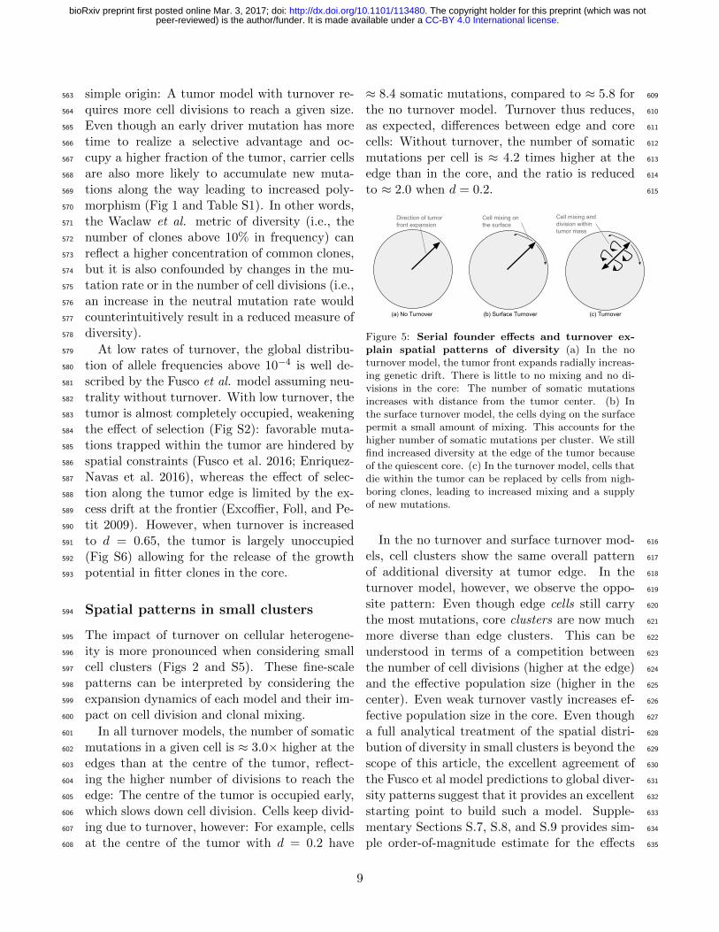
≈ 8.4 somatic mutations, compared to ≈ 5.8 for 609
the no turnover model. Turnover thus reduces, 610
as expected, differences between edge and core 611
cells: Without turnover, the number of somatic 612
mutations per cell is ≈ 4.2 times higher at the 613
edge than in the core, and the ratio is reduced 614
to ≈ 2.0 when d = 0.2. 615
(a) No Turnover (b) Surface Turnover (c) Turnover
Direction of tumor front expansion
Cell mixing on the surface
Cell mixing and division within tumor mass
Figure 5: Serial founder effects and turnover ex-plain spatial patterns of diversity (a) In the noturnover model, the tumor front expands radially increas-ing genetic drift. There is little to no mixing and no di-visions in the core: The number of somatic mutationsincreases with distance from the tumor center. (b) Inthe surface turnover model, the cells dying on the surfacepermit a small amount of mixing. This accounts for thehigher number of somatic mutations per cluster. We stillfind increased diversity at the edge of the tumor becauseof the quiescent core. (c) In the turnover model, cells thatdie within the tumor can be replaced by cells from nigh-boring clones, leading to increased mixing and a supplyof new mutations.
In the no turnover and surface turnover mod- 616
els, cell clusters show the same overall pattern 617
of additional diversity at tumor edge. In the 618
turnover model, however, we observe the oppo- 619
site pattern: Even though edge cells still carry 620
the most mutations, core clusters are now much 621
more diverse than edge clusters. This can be 622
understood in terms of a competition between 623
the number of cell divisions (higher at the edge) 624
and the effective population size (higher in the 625
center). Even weak turnover vastly increases ef- 626
fective population size in the core. Even though 627
a full analytical treatment of the spatial distri- 628
bution of diversity in small clusters is beyond the 629
scope of this article, the excellent agreement of 630
the Fusco et al model predictions to global diver- 631
sity patterns suggest that it provides an excellent 632
starting point to build such a model. Supple- 633
mentary Sections S.7, S.8, and S.9 provides sim- 634
ple order-of-magnitude estimate for the effects 635
9
.CC-BY 4.0 International licensepeer-reviewed) is the author/funder. It is made available under aThe copyright holder for this preprint (which was not. http://dx.doi.org/10.1101/113480doi: bioRxiv preprint first posted online Mar. 3, 2017;
of clone mixing and late mutations (i.e., muta-636
tions in the core) observed on diversity patterns,637
including an extension of the Fusco et al model638
that accounts for late mutations. In addition to639
turnover rate, a key parameter that controls mix-640
ing is the expected distance between mother and641
daughter cells. In TumorSimulator, cells are al-642
lowed to reproduce to neighboring positions ac-643
cording to a Moore neighborhood, which leads644
to relatively diffuse small clusters. A challenge645
in building models for fine-scale diversity will be646
to implement realistic models of cell-cell interac-647
tions.648
Metastatic potential649
The difference in somatic diversity between sin-650
gle CTCs and CTC clusters, measured through651
the cluster advantage, follows the expected law652
of diminishing returns: The more cells in the653
cluster, the fewer the number of unique mu-654
tations per cell. However, the trends vary by655
growth model and cluster origin. Cell mixing656
and rare, late mutations caused by turnover re-657
duces neighboring cell similarity and increases658
cluster advantage.659
Under the assumption that the presence or ab-660
sence of a metastatic progression allele modu-661
lates metastatic potential of tumor cell clusters,662
the proportion of metastatic lesions that derive663
from circulating tumor cell clusters is highest in664
the turnover model. We can think of this as in-665
terference occurring between cells within a clus-666
ter. Alternately, this is an illustration of the ad-667
vantage of not putting all one’s egg in the same668
basket, applied to tumor metastasis: Assuming669
that there is a chance component to cluster im-670
plantation, mixing due to turnover increases the671
likelihood that at least one virulence cell makes672
it to a hospitable site. Such an effect should be673
robust to details of the growth model.674
In experiments, CTC clusters derived from675
primary breast and prostate tumors produced676
more aggressive metastatic tumors (Aceto, Bar-677
dia, et al. 2014) compared to single CTCs. This678
is likely due to differences in mechanical proper-679
ties of the cluster or the creation of a locally fa-680
vorable environment by the cluster, rather than681
by genetic differences. However, the present 682
analysis suggests that this advantage can be en- 683
hanced by diversity within the cluster. 684
Statistical power 685
Both fine-scale mixtures of cell phenotypes and 686
clonally constrained mutations have been ob- 687
served experimentally in tumors (Navin et al. 688
2010; Yates et al. 2015). Similarly, multi-region 689
sequencing revealed high tumor heterogeneity in 690
clear cell renal carcinoma (ccRCC) (Gerlinger, 691
Horswell, et al. 2014) and esophageal squamous 692
cell carcinoma (Hao et al. 2016), but low levels 693
in lung adenocarcinomas (J. Zhang et al. 2014). 694
This strongly suggests that the amount of mix- 695
ing and late mutations varies substantially across 696
tumors, with ccRCC data being better described 697
by a model with turnover, whereas lung adeno- 698
carcinoma data more closely resembles a model 699
with low or no turnover. 700
In practice, distinguishing between mixing, 701
turnover, mutations, and tumor growth idiosyn- 702
crasies will be challenging. Among limitations of 703
our model, we note the assumption of spherical 704
tumor shape and the absence of complex phys- 705
ical contraints (which HCC tumors may experi- 706
ence). Another limitation of the present model 707
is the rigid computational grid which prevents 708
cells from pushing each other out of the way, 709
which constrains growth in the center of the tu- 710
mor. This constraint plays a role in reducing di- 711
versity at the center of the tumor, but it may not 712
be realistic in the earlier stages of tumor growth. 713
The importance of such effects is largely un- 714
known, and it is likely to vary between tumors 715
and tumor types. Fortunately, we have shown 716
that we are at the cusp of being able to test 717
such models quantitatively. A sampling experi- 718
ment with twice as many samples than were col- 719
lected in the HCC patient studied above would 720
enable us to either validate or reject the current 721
state-of-the-art models confidently (Fig 3b). Al- 722
ternatively, sequencing of small clusters would 723
further allow us to discriminate between the dif- 724
ferent models of turnover. 725
In either case, the use of frequency cutoffs can 726
strongly affect inferred spatial patterns of diver- 727
10
.CC-BY 4.0 International licensepeer-reviewed) is the author/funder. It is made available under aThe copyright holder for this preprint (which was not. http://dx.doi.org/10.1101/113480doi: bioRxiv preprint first posted online Mar. 3, 2017;

sity: a focus on common variants means a focus728
on old branches of the tree (Fig S10). This em-729
phasizes the mean number of divisions per cell,730
which is larger at the edge, but fails to capture731
recent mutations and clonal mixing, which have732
larger impact at the core. Thus spatial patterns733
inferred using variants at frequency above 1% are734
more similar across models, and can be opposite735
to those including all mutations (Fig S11).736
Data collection schemes including the lung737
TRACERx study (Jamal-Hanjani, Hackshaw, et738
al. 2014; Jamal-Hanjani, Wilson, et al. 2017)739
will help us put the state-of-the-art models to740
the test and identify such important parameters741
of tumor growth. Given our power analysis, we742
find that sequencing small contiguous cell clus-743
ters provides a richer picture of tumor dynamics744
compared to larger biopsies, with little to no loss745
in power, assuming that few-cell sequencing can746
be performed accurately.747
Conclusion748
This work set out to answer two simple ques-749
tions: First, should we expect substantial hetero-750
geneity at the cellular scale within tumors and751
within circulating tumor cell clusters? The an-752
swer to the first question is most likely yes, as753
even the models with no turnover exhibit mea-754
surable cluster heterogeneity.755
The second question was whether this het-756
erogeneity, sampled through liquid biopsies or757
multi-region sequencing, is informative about tu-758
mor dynamics. Given that state-of-the-art mod-759
els produce very different predictions about the760
level of cluster heterogeneity, the answer is also761
positive. This work identified some of the key762
factors that determine cluster diversity, espe-763
cially the interaction between range expansion764
and cell turnover leading to late mutations and765
mixing. Even if no diversity were observed at all766
in CTC clusters, it would enable us to reject the767
present models in favor of models including addi-768
tional biological factors that favor the clustering769
of genetically similar cells. Measuring diversity,770
or the lack of diversity, within circulating tumor771
cell clusters or fine-scale multi-region sequencing772
is therefore a promising tool for both fundamen- 773
tal and medical oncology. 774
Author Contributions 775
Conceptualization, S.G.; Methodology, S.G.; 776
Software, Z.A.; Investigation, Z.A. and S.G.; 777
Writing Original Draft, Z.A.; Data Curation 778
Z.A.; Review & Editing, Z.A & S.G.; Visualiza- 779
tion, Z.A.; Funding Acquisition, Z.A. and S.G.; 780
Resources, S.G.; Supervision, S.G. 781
Acknowledgments 782
We thank Julien Jouganous, Hamid Nikbakht,Yasser Riazalhosseini, Aaron Ragsdale andRobert Sladek for useful discussions. This re-search was made possible thanks to a Cana-dian Institutes of Health Undergraduate Re-search Award in computational biology, fundingreference numbers 139962 and 145987 and Fred-erick Banting and Charles Best Canada Gradu-ate Scholarship. This research was undertaken,in part, thanks to funding from the Canada Re-search Chairs program and a Sloan research fel-lowship.
References
Aceto, N., A. Bardia, et al. (2014). “Circulatingtumor cell clusters are oligoclonal precursorsof breast cancer metastasis”. Cell 158.5, 1110–1122.
Aceto, N., M. Toner, et al. (2015). “En route tometastasis: circulating tumor cell clusters andepithelial-to-mesenchymal transition”. Trendsin Cancer 1.1, 44–52.
Alizadeh, A. A. et al. (2015). “Toward under-standing and exploiting tumor heterogeneity”.Nature Medicine 21.8, 846–853.
Andor, N. et al. (2016). “Pan-cancer analysisof the extent and consequences of intratumorheterogeneity”. Nature Medicine 22.1, 105.
Ashworth, T. (1869). “A case of cancer in whichcells similar to those in the tumours were seenin the blood after death”. Aust Med J. 14, 146.
11
.CC-BY 4.0 International licensepeer-reviewed) is the author/funder. It is made available under aThe copyright holder for this preprint (which was not. http://dx.doi.org/10.1101/113480doi: bioRxiv preprint first posted online Mar. 3, 2017;

Au, S. H. et al. (2017). “Microfluidic isolationof circulating tumor cell clusters by size andasymmetry”. Scientific Reports 7.1, 2433.
Bos, P. D. et al. (2009). “Genes that mediatebreast cancer metastasis to the brain”. Nature459.7249, 1005–1009.
Brouwer, A. et al. (2016). “Evaluation andconsequences of heterogeneity in the circu-lating tumor cell compartment”. Oncotarget7.30, 48625.
Burrell, R. A. et al. (2013). “The causes and con-sequences of genetic heterogeneity in cancerevolution”. Nature 501.7467, 338.
Cheung, K. J. et al. (2016). “Polyclonal breastcancer metastases arise from collective dis-semination of keratin 14-expressing tumorcell clusters”. Proceedings of the NationalAcademy of Sciences 113.7, E854–E863.
Cristofanilli, M. et al. (2005). “Circulating tu-mor cells: a novel prognostic factor for newlydiagnosed metastatic breast cancer”. Journalof Clinical Oncology 23.7, 1420–1430.
Del Monte, U. (2009). “Does the cell number 109
still really fit one gram of tumor tissue?” CellCycle 8.3, 505–506.
Durrett, R. (2008). Probability models for DNAsequence evolution. Springer Science & Busi-ness Media.
Enriquez-Navas, P. M. et al. (2016). “Exploit-ing evolutionary principles to prolong tumorcontrol in preclinical models of breast can-cer”. Science Translational Medicine 8.327,327ra24–327ra24.
Excoffier, L., M. Foll, and R. J. Petit (2009).“Genetic consequences of range expansions”.Annual Review of Ecology, Evolution, and Sys-tematics 40, 481–501.
Fisher, R. A. (1999). The genetical theory of nat-ural selection: a complete variorum edition.Oxford University Press.
Fusco, D. et al. (2016). “Excess of muta-tional jackpot events in expanding popula-tions revealed by spatial Luria–Delbruck ex-periments”. Nature Communications 7, 12760.
Gerlinger, M., S. Horswell, et al. (2014). “Ge-nomic architecture and evolution of clear cell
renal cell carcinomas defined by multiregionsequencing”. Nature Genetics 46.3, 225–233.
Gerlinger, M., A. J. Rowan, et al. (2012). “In-tratumor heterogeneity and branched evolu-tion revealed by multiregion sequencing”. NewEngland Journal of Medicine 2012.366, 883–892.
Glaves, D. (1983). “Correlation between circulat-ing cancer cells and incidence of metastases”.British Journal of Cancer 48.5, 665.
Glynn, M. et al. (2015). “Cluster size distribu-tion of cancer cells in blood using stopped-flowcentrifugation along scale-matched gaps of aradially inclined rail”. Microsystems & Nano-engineering 1, 15018.
Hallatschek, O. et al. (2007). “Genetic drift atexpanding frontiers promotes gene segrega-tion”. Proceedings of the National Academy ofSciences 104.50, 19926–19930.
Hao, J.-J. et al. (2016). “Spatial intratumoralheterogeneity and temporal clonal evolution inesophageal squamous cell carcinoma”. NatureGenetics 48.12, 1500.
Hayes, D. et al. (2002). “Monitoring expressionof HER-2 on circulating epithelial cells in pa-tients with advanced breast cancer”. Interna-tional Journal of Oncology 21.5, 1111–1117.
Heitzer, E. et al. (2013). “Complex tumorgenomes inferred from single circulating tumorcells by array-CGH and next-generation se-quencing”. Cancer Research 73.10, 2965–2975.
Hiley, C. et al. (2014). “Deciphering intratu-mor heterogeneity and temporal acquisitionof driver events to refine precision medicine”.Genome Biology 15.8, 453.
Hodgkinson, C. L. et al. (2014). “Tumorigenicityand genetic profiling of circulating tumor cellsin small-cell lung cancer”. Nature Medicine20.8, 897–903.
Holohan, C. et al. (2013). “Cancer drug resis-tance: an evolving paradigm”. Nature ReviewsCancer 13.10, 714–726.
Hou, J. M. et al. (2012). “Clinical significanceand molecular characteristics of circulating tu-mor cells and circulating tumor microemboliin patients with small-cell lung cancer”. Jour-nal of Clinical Oncology 30.5, 525–532.
12
.CC-BY 4.0 International licensepeer-reviewed) is the author/funder. It is made available under aThe copyright holder for this preprint (which was not. http://dx.doi.org/10.1101/113480doi: bioRxiv preprint first posted online Mar. 3, 2017;
Jamal-Hanjani, M., A. Hackshaw, et al. (2014).“Tracking genomic cancer evolution for pre-cision medicine: the lung TRACERx study”.PLoS Biology 12.7, e1001906.
Jamal-Hanjani, M., G. A. Wilson, et al. (2017).“Tracking the evolution of non–small-cell lungcancer”. New England Journal of Medicine376.22, 2109–2121.
Joosse, S. A., T. M. Gorges, and K. Pantel(2014). “Biology, detection, and clinical im-plications of circulating tumor cells”. EMBOMolecular Medicine, e201303698.
Jouganous, J. et al. (2017). “Inferring the jointdemographic history of multiple populations:beyond the diffusion approximation”. Genet-ics, 117.
Kardar, M., G. Parisi, and Y.-C. Zhang (1986).“Dynamic scaling of growing interfaces”.Physical Review Letters 56.9, 889.
Korolev, K. S. et al. (2010). “Genetic demixingand evolution in linear stepping stone mod-els”. Reviews of Modern Physics 82.2, 1691.
Krebs, M. G., R. L. Metcalf, et al. (2014).“Molecular analysis of circulating tumourcells-biology and biomarkers.” Nature ReviewsClinical Oncology 11.3, 129–44.
Krebs, M. G., R. Sloane, et al. (2011). “Evalu-ation and prognostic significance of circulat-ing tumor cells in patients with non–small-cell lung cancer”. Journal of Clinical Oncology29.12, 1556–1563.
Lambert, A. W., D. R. Pattabiraman, and R. A.Weinberg (2017). “Emerging biological princi-ples of metastasis”. Cell 168.4, 670–691.
Ling, S. et al. (2015). “Extremely high geneticdiversity in a single tumor points to prevalenceof non-Darwinian cell evolution”. Proceedingsof the National Academy of Sciences 112.47.
Liotta, L. A., J. Kleinerman, and G. M. Saldel(1976). “The significance of hematogenous tu-mor cell clumps in the metastatic process”.Cancer research 36.3, 889–894.
Lorusso, G. and C. Ruegg (2012). “New insightsinto the mechanisms of organ-specific breastcancer metastasis”. Seminars in Cancer Biol-ogy. Vol. 22. 3. Elsevier, 226–233.
Lyons, R., R. Pemantle, and Y. Peres (1995).“Conceptual proofs of L log L criteria for meanbehavior of branching processes”. The Annalsof Probability, 1125–1138.
Marrinucci, D. et al. (2012). “Fluid biopsyin patients with metastatic prostate, pan-creatic and breast cancers”. Physical Biology9.1, 016003.
Massague, J. and A. C. Obenauf (2016).“Metastatic colonization by circulating tu-mour cells”. Nature 529.7586, 298–306.
McGranahan, N. and C. Swanton (2015). “Bi-ological and therapeutic impact of intratu-mor heterogeneity in cancer evolution”. Can-cer Cell 27.1, 15–26.
– (2017). “Clonal heterogeneity and tumor evo-lution: past, present, and the future”. Cell168.4, 613–628.
Morrissy, A. S. et al. (2017). “Spatial hetero-geneity in medulloblastoma”. Nature Genetics49.5, 780.
Navin, N. et al. (2010). “Inferring tumor progres-sion from genomic heterogeneity”. GenomeResearch 20.1, 68–80.
Nowell, P. C. (1976). “The clonal evolution oftumor cell populations”. Science 194.4260, 23–28.
Ohtsuki, H. and H. Innan (2017). “Forward andbackward evolutionary processes and allelefrequency spectrum in a cancer cell popula-tion”. Theoretical Population Biology 117, 43–50.
Padua, D. et al. (2008). “TGFβ primes breasttumors for lung metastasis seeding throughangiopoietin-like 4”. Cell 133.1, 66–77.
Peinado, H. et al. (2017). “Pre-metastatic niches:organ-specific homes for metastases”. NatureReviews Cancer 17.5, 302.
Powell, A. A. et al. (2012). “Single cell profil-ing of circulating tumor cells: transcriptionalheterogeneity and diversity from breast cancercell lines”. PloS ONE 7.5, e33788.
Quail, D. F. and J. A. Joyce (2013). “Microenvi-ronmental regulation of tumor progression andmetastasis”. Nature Medicine 19.11, 1423.
Sarioglu, A. F. et al. (2015). “A microfluidicdevice for label-free, physical capture of cir-
13
.CC-BY 4.0 International licensepeer-reviewed) is the author/funder. It is made available under aThe copyright holder for this preprint (which was not. http://dx.doi.org/10.1101/113480doi: bioRxiv preprint first posted online Mar. 3, 2017;

culating tumor cell clusters”. Nature Methods12.7, 685.
Schneider, C. A., W. S. Rasband, and K. W. Eli-ceiri (2012). “NIH Image to ImageJ: 25 yearsof image analysis”. Nature Methods 9.7, 671.
Shweiki, D. et al. (1995). “Induction of vascu-lar endothelial growth factor expression by hy-poxia and by glucose deficiency in multicellspheroids: implications for tumor angiogene-sis”. Proceedings of the National Academy ofSciences 92.3, 768–772.
Siravegna, G. et al. (2017). “Integrating liquidbiopsies into the management of cancer”. Na-ture Reviews Clinical Oncology 14.9, 531.
Sottoriva, A. et al. (2015). “A Big Bang model ofhuman colorectal tumor growth”. Nature Ge-netics 47.3, 209–216.
Steeg, P. S. (2016). “Targeting metastasis”. Na-ture Reviews Cancer 16.4, 201.
Vanharanta, S. and J. Massague (2013). “Originsof metastatic traits”. Cancer Cell 24.4, 410–421.
Waclaw, B. et al. (2015). “A spatial modelpredicts that dispersal and cell turnoverlimit intratumour heterogeneity”. Nature525.7568, 261–264.
Wang, Y. et al. (2014). “Clonal evolutionin breast cancer revealed by single nucleusgenome sequencing”. Nature 512.7513, 155–160.
Weinstein, B. T. et al. (2017). “Genetic drift andselection in many-allele range expansions”.PLoS Computational Biology 13.12, e1005866.
Williams, M. J. et al. (2016). “Identification ofneutral tumor evolution across cancer types”.Nature Genetics 48, 238–244.
Wright, S. (1931). “Evolution in Mendelian pop-ulations”. Genetics 16.2, 97–159.
Wulfing, P. et al. (2006). “HER2-positive circu-lating tumor cells indicate poor clinical out-come in stage I to III breast cancer patients”.Clinical Cancer Research 12.6, 1715–1720.
Yates, L. R. et al. (2015). “Subclonal diver-sification of primary breast cancer revealedby multiregion sequencing”. Nature Medicine21.7, 751–759.
Zhang, J. et al. (2014). “Intratumor hetero-geneity in localized lung adenocarcinomas de-lineated by multiregion sequencing”. Science346.6206, 256–259.
14
.CC-BY 4.0 International licensepeer-reviewed) is the author/funder. It is made available under aThe copyright holder for this preprint (which was not. http://dx.doi.org/10.1101/113480doi: bioRxiv preprint first posted online Mar. 3, 2017;

S Supplemental Information
S.1 Tumor growth model
The tumor consists of cells that occupy points on a 3D lattice. Empty lattice sites are assumed tocontain normal cells which are not modelled explicitly in TumorSimulator.
Each cell has an associated list of genetic alterations which represent single nucleotide polymor-phisms (SNPs) that can be either passenger or driver. Driver mutations increase the growth rateby a factor 1 + s, where s ≥ 0 is the selective advantage of a driver mutation.
At t = 0, the simulation begins with a single cell that already has an unlimited growth potential.The TumorSimulator algorithm then proceeds to grow the tumor through the following steps:
1. Select a random cell to be the mother cell.
2. Set the cell birth rate to b′ = b0(1 + s)k−kmax , where b0 is the initial tumor birth rate, s is theaverage selective advantage of a driver mutation, k is the number of driver mutations presentin the mother cell and kmax is the maximum number of drivers in any cell.
3. Randomly select a lattice point adjacent to the mother cell. If empty, create a geneticallyidentical daughter cell at that position with a probability b′. If no cell created, or no emptysites are found proceed to 5.
4. Independently give mother and daughter cells additional passenger and driver mutations. Thenumber of passenger and driver mutations are drawn according to Poisson distributions withmean µp and µd, respectively, and are drawn independently for the mother and daughter cell.Each mutation is unique and there is no back-mutations or recurrent mutations.
5. Kill (i.e., remove) the mother cell with probability d(1 + s)−kmax .
In our analysis, we consider three turnover scenarios corresponding to three values of the deathrate d: (i) No turnover (d = 0), corresponding to simple clonal growth (Hallatschek et al. 2007);(ii) Surface Turnover (d(x, y, z) > 0 only if x, y, z is on the surface), corresponding to a quiescentcore model (Shweiki et al. 1995) (iii) Turnover (d > 0 everywhere), a model favored in Waclawet al. 2015 to explore ITH.
The initial birth rate (b0 = ln(2)), driver mutation rate µd = 2 × 10⁻⁵, and selective advantage(s = 1%) were kept consistent with Waclaw et al. 2015 except where otherwise noted. In additionto varying the turnover model (full, surface, or none), we vary its intensity by controlling the deathrate, d ∈ {0.05, 0.1, 0.2, 0.65}. TumorSimulator also has a parameter that controls migration of cellsto form new independent cancer lesions. We did not allow such local migrations, as they wouldhave little effect on the very fine-scale diversity in the primary tumor. We used two values for thepassenger mutation rate: µp = 0.01 to facilitate comparison with simulations from Waclaw et al.2015 (Waclaw et al. simulated with µp = 0.01, but reported a mutation rate of 0.02 to accountfor an equivalent rate per diploid genome), and µp = 0.01875 to match experimental observationsfrom Ling et al. 2015 (Since the number of passenger mutations grows linearly with the mutationrate, we simply scaled µp based on the difference between predictions using µp = 0.01 and the datafrom Fig 3a.) All tumors were grown until they had 108 cells except where otherwise stated.
TumorSimulator (Waclaw et al. 2015) is available at http://www2.ph.ed.ac.uk/ bwaclaw/cancer-code/.
15
.CC-BY 4.0 International licensepeer-reviewed) is the author/funder. It is made available under aThe copyright holder for this preprint (which was not. http://dx.doi.org/10.1101/113480doi: bioRxiv preprint first posted online Mar. 3, 2017;

S.2 CTC cluster synthesis
Experimental evidence suggests that CTC clusters are formed from neighboring cells in the primarytumor and not by agglomeration or proliferation of single CTCs in the blood (J. M. Hou et al.2012; Aceto, Bardia, et al. 2014). To represent circulating tumor cell clusters, we therefore sampledspherical clusters (with a large radius) of cells in different areas of the tumor produced by theWaclaw et al. model. To get a fixed number of cells in the cluster, n, we picked the n closest cellsto the center-of-mass of this sphere. We varied the number of cells in the cluster from n = 2 ton = 30 to represent the range of empirical findings (Marrinucci et al. 2012).
S.3 Power Analysis
To establish the effectiveness of sequencing CTC clusters versus larger biopsies at detecting a trendand distinguishing between models, we conduct a power analysis. We use linear regression on thenumber of somatic mutations per cluster (or biopsy) of size n as a function of distance r from thetumor center-of-mass (i.e, S(n, r) = mr + c where m and c are regression coefficients). Clustersand biopsies to regress are sampled at random from a previously generated set of 1000 samples.Given a sample size and cluster size, we resample 100 subsets from these 1000 samples to estimateproportion of regressions that were significant (p < 0.01). To capture the direction of the slope, wecalculate the sign of the coefficient m and report the signed proportion of significant regressions.For larger biopsies, we apply a frequency cutoff and only includes a mutation in the analysis if itis above a certain cluster-wide frequency, thus simulating the mutant allele frequency cutoff fromsequencing experiments (Ling et al. 2015).
S.4 Standard Neutral Model for Cluster Advantage
The relative increase in the number of distinct somatic mutations in a CTC cluster versus a singleCTC is given by the cluster advantage, i.e., A(n) = S(n)−S(1)
S(1) = S(n)S(1) −1, where S(n) is the number
of somatic mutations in a cluster of size n and S(1) is the number of somatic mutations in thecell closest to the center-of-mass of the cluster (as described in Section CTC cluster synthesis). Ahigher cluster advantage indicates that a CTC cluster is more potent relative to a single CTC fromthe same tumor. In other words, a higher cluster advantage means less genetic redundancy withina cluster. Under the standard neutral model (infinite sites, neutral evolution, random mixing), andtherefore the expected number of somatic mutations is E(S(n)) = µH(n−1) (Durrett 2008), whereH(n) is the n-th harmonic number,
∑ni=1
1i .
S.5 A geometric model
To estimate the frequency distribution of common variants, we model the tumor as a continuouslygrowing sphere where only surface cells divide. If a mutation appears in a cell at the surface ofthe tumor at a time when the tumor has radius r, we suppose that this mutation occupies a cross-section area a2 of the tumor surface. It therefore occupies a fraction a2
4πr2of the surface of the tumor
at that point. If the tumor grows radially outwards and reaches a radius of R, the descendants ofthis cell occupy a fraction a2
4πr2of the space yet to be occupied, and the mutation itself will occupy
a fraction
f(r) =a2
4πr2
(1− r3
R3
)of the final tumor, which is the volume of a spherical cone with its tip removed. We can thenintegrate over all possible radii r where mutations occur. The density ρ(r) of mutations occurring
16
.CC-BY 4.0 International licensepeer-reviewed) is the author/funder. It is made available under aThe copyright holder for this preprint (which was not. http://dx.doi.org/10.1101/113480doi: bioRxiv preprint first posted online Mar. 3, 2017;

at radius r is proportional to the density of cells at that locus
ρ(r) ' µ4πr2
a3,
with µ the mutation rate per cell. The frequency spectrum is therefore
φ(f) =
∫ R
0drρ(r)δ(f − f(r))
If we focus on common mutations, which occurred at r � R, we can approximate f(r) ' a2
4πr2,
leading to
φ(f) ' µ
4√πf
52
.
We show in the next section that a model accounting for stochastic fluctuations in the earlyreproductive success of a mutation, or weak changes in selection, preserves this scaling behavior,but with an overall scale factor ζ that depends on details of the growth model, i.e.
φ(f) ' ζµ
4√πf
52
.
Fig 1 shows the agreement of simulation results to the geometric model with ζ = 30 for highfrequency mutants. As mentioned above, variants at less than 1% frequency follow a distinct powerlaw with slope closer to our estimate of 1.61, which is similar to the theoretical value of 1.55described in Fusco et al. (2016).
S.6 Allele frequency distribution under a stochastic spherical growth model
The deterministic model presented above does not take into account the stochastic variation in thefate of cells, which is especially important in the first few generations after a mutation appears. Toaccount for this, we can imagine that the initial frequency of each new mutation gets multipliedby a random factor i to account for the random differences in success in the original cells overthe first few generations. In other words, i is the number of descendants produced by the originalcell divided by the expected number of descendants for other cells at the same radius. If we onlyconsider mutations with given i, we find
fi(r) =ia2
4πr2
and
φi(f) ' µi32
4√πf
52
.
If we assume that multipliers are drawn from a probability distribution P (i) that is independentof r, we get an expected frequency spectrum
φ(f) '∑i
P (i)φi(f) =µE[i32
]4√πf
52
.
Even though the 5/2 scaling behavior is maintained, the expectation E[i32
]can be much larger
than 1, as there is an early settler advantage in this model. However, the value of this scaling factordepends on the details of the growth model (Fig 1 and S2).
17
.CC-BY 4.0 International licensepeer-reviewed) is the author/funder. It is made available under aThe copyright holder for this preprint (which was not. http://dx.doi.org/10.1101/113480doi: bioRxiv preprint first posted online Mar. 3, 2017;
More generally, the f−52 asymptotic result is derived under an extremely simple model. The
Fusco et al. model (Fusco et al. 2016) captures a very similar scaling, but with a much moredetailed model of stochastic fluctuations that captures both rare and common variant scaling.Neither models take into account selection and turnover. Analytical results under selection aredifficult to obtain because moment-based approaches that close under neutrality do not close underselection (see, e.g.,Weinstein et al. 2017; Korolev et al. 2010; Jouganous et al. 2017).
S.7 Expected frequency of a mutation in a given cell
Following the Fusco et al model, the distribution of allele frequencies can be approximated by itsasymptotic values
φ(f) = Πcχ(ξ),
where Πc = N−α(β−1)
β−α , ξ = ffc
and fc = N− 1−αβ−α is the transition point between the two asymptotic
regimes. Finally
χ(ξ) '
{αξ−(α+1) if ξ ≤ 1
βξ−(β+1), ξ > 1,(1)
where N is the number of cells in the tumor and α = 0.55 and β = 2.3 are scaling factors thatdepend on the geometry of tumor growth.
Using this approximation, we can compute basic statistics for the expected frequency of sampledalleles. For example, the expected allele frequency of a mutation selected uniformly at random is
〈f〉u = Πcfcα
α− 1
[(Nfc)
α−1 − 1]
+ Πcfcβ
β − 1
(1− fβ−1c
)' 1.4× 10⁻⁵. (2)
If we sample mutations proportionally to their population frequency, we get
〈f〉freq =Πcf
2c
〈f〉u×(
α
α− 2
[(Nfc)
α−2 − 1]
+β
β − 2
(1− fβ−2c
))' 0.018 (3)
so that the expected frequency of a mutation observed in a given cell is at reasonably high frequency.That is to say that the typical clone size, in a tumor of size 108, is approximately 1.8× 10⁶.
Similarly, the the probability of drawing a mutation at frequency f , given that mutations aresampled according to their frequency, is
φfreq(f) =fφ(f)∫ 1
0 f′φ(f ′)df ′
and the cumulative distribution function of the allele frequencies for mutation drawn proportionallyto the allele frequency is
CDFfreq(f) =
∫ f0 fφ(f ′)df ′∫ 1
0 f′′φ(f ′′)df ′′
=
∫ f0 fφ(f ′)df ′
〈f〉u,
from which we infer that less than 2% of variants in a cell drawn at random are derived from cloneswith frequency below 10−5: Over 98% of cells derive from clones of size over 1000.
18
.CC-BY 4.0 International licensepeer-reviewed) is the author/funder. It is made available under aThe copyright holder for this preprint (which was not. http://dx.doi.org/10.1101/113480doi: bioRxiv preprint first posted online Mar. 3, 2017;

S.8 Number of cell divisions, and properties of the tumor core
We would like to estimate the average number of divisions since tumor beginning that cells at agiven position in the tumor have undergone. We consider a two-stage model, wherein we first havestraightforward tumor expansion which can be described by the Fusco et al ‘bubble and sector’model, and subsequent alteration of this state under a steady-state model. In the first stage, themain effect of turnover is to increase the number of divisions necessary for the tumor necessaryto reach a given radius R. Under turnover, it takes more divisions for the tumor to reach agiven radius, and we find empirically that the number of divisions required to reach a given radiusincreases approximately by a factor (1 + d) for low turnover.
We’ll distinguish between ‘early’ and ‘late’ mutations according to whether a mutation occurredon the expansion front (early), or behind the front (late). To estimate the rate of division withinthe tumor core, we must first estimate the unoccupied cell density e within the tumor. This canbe estimated as close to e ' d
b by assuming that growth due to births eb is offset by death d. (It isapproximate because it assumes that the probability of drawing an empty cell next to the selectedmother cell is e — this is not exact if there are spatial correlations in cell occupancies.)
The final radius of the tumor is therefore approximately Rf =(
3N4π(1−e)
) 13. This is close enough
to the observed values in Fig 2 (for example, this predicts Rf = 288 for d = 0 and Rf = 323 ford = 0.2).
To estimate the number of late mutations, we first need to compute the expected number ofdivisions occurring along a given lineage after the tumor front has passed. This can be estimatedby first considering the expected number of times a given core cell is selected while the tumor growsfrom radius R to R+1. In a model where the tumor has a smooth boundary, a cell on the boundaryhas probability γb of reproducing successfully (i.e., we have a probability γ ' 1/2 of drawing anempty site nearby, and probability b of successfully reproducing on that site).
Now, while growing from size R to size R+1, we consider that each cell on a surface of area 4πR
must successfully reproduce on average (R+1)2
R2 ' 1 times. It must therefore be selected 1γb times,
on average, for the tumor to move forth one unit. Since cells are chosen at random, each cell insidethe tumor must be picked, on average, the same number of times as edge cells. This leads to, onaverage, d
γb deaths (and, at equilibrium, the same number of births).
Thus the total number of births/deaths per occupied cell at distance R0 after the front has passedis
D =
∫ Rf
R0
dRd
γb' (Rf −R0)
d
γb.
For d = 0.2, and Rf = 323 this means approximately 188 deaths and birth per occupied cell. Theexpected number of mutations on a lineage increases by µ ' ×10−2 with each birth/death cycle.Thus each lineage gains order of two new mutations in the core. This is consistent with the lineagesdrawn on Fig S10, and with the increase in the number of clones per cell in Fig 2.
Clones derived from these mutations are extremely unlikely to reach frequencies comparableto the bubble and sector clones contributing to diversity in the Fusco et al. model. Thus weakturnover therefore induces a third, distinct regime of late clones, in addition to the bubbles andthe sectors, which will remain very rare. Late clones will have a higher relative impact near thecenter of the tumor, given the additional time for late clones to develop, and the reduced numberof early clones.
Because the core is near birth-death equilibrium, the expected number of descendants of a givencell (and therefore of a new mutation) is one. Thus the expected number of late mutations in acell at distance R of the core is simply µ(Rf −R) dγb .
19
.CC-BY 4.0 International licensepeer-reviewed) is the author/funder. It is made available under aThe copyright holder for this preprint (which was not. http://dx.doi.org/10.1101/113480doi: bioRxiv preprint first posted online Mar. 3, 2017;

S.9 Mean frequency of late clones and cluster diversity
If we suppose that late clones remain very small, we can model each cell division as independent ofeach other. That is, we can neglect the probability that mutant cells replace each other and modelclone growth as a critical Galton-Watson branching process a probability d of dying or branching.This apparently coarse approximation is reasonable here because TumorSimulator uses a Mooreneighborhood with 26 neighbors: the fact that a mother cell occupies one of these 26 neighborhoodcells has a low impact on the probability of the daughter cell to divide. Further divisions willnot crowd out space as long as the clusters remain relatively small: a cell’s daughter will be atapproximate mean squared distance 3 ∗ (18/26) = 2.1 (the factor of three accounts for the threedimensions, and 18/26 is the mean squared displacement in each direction. This is approximatebecause displacement along the three directions is not independent). The grand-daughter will beat mean squared distance 4.15, and so forth. A simple toy model where cells carrying a mutationare allowed to divide into neighboring grid points with probability e, irrespective of occupancy (i.e.,grid points can carry multiple cells), shows relatively little overlap for the parameter ranges studiedhere: For a mutation occurring at the founding of the tumor with parameters d = 0.1, e = 0.14,and Rf = 303, there is only 6% overlap on average by the time the tumor has size 108 (i.e., themean number of occupied gridpoints is only 6% lower than the number of cells, including thosejointly occupying a grid-point.)
A very crude estimate of the number of segregating sites in small clusters can therefore beobtained by assuming that late clones are in fact so diffuse that is is unlikely that a small clusterwill capture more than one clone cell – this will naturally overestimate S(n) for large clones andlarge clusters but we find that it is an appropriate approximation for small clusters, or for partsof the tumor that experienced relatively few late divisions (Fig S7). In Fig S7, predictions areobtained by using the empirical number of early mutations observed in single cells under no turnover(Sd=0,n=1(R)), shown as a dotted line, scaling it by the empirical factor (1 + d) discussed in theprevious section, and adding the predicted number of late mutations nµ (Rf (d)−R) d
γb .
We computed above D ' (Rf −R0)dγb , the estimated number of cell divisions per occupied site
between the front passage and present. Mutations accumulate at a constant rate during this time,and so the typical late mutation at this position will only have D
2 generations to experience geneticdrift. For d = 0.2, and Rf = 323, this means 94 cycles.
To model the distribution of clone size, we consider the Galton-Watson model with variance2d(1 − d). The variance in clone size in the Galton-Watson model after j generations is simply2d(1− d)j.
We can estimate the distribution of surviving sizes using Yaglom’s asymptotic limit (Lyons, Pe-mantle, and Peres 1995), and find that the size distribution of surviving lineages after j generationsis
P (Zjj
= m|Zj > 0) ' 2
σ2e
−2m
σ2 ,
and
P (Zj = k|Zj > 0) ' 2
jσ2e
−2k
jσ2 .
The expected size of a surviving clone is approximately
E =σ2j
2
and the asymptotic survival probability is simply 1/E, per Kolmogorov’s estimate.
20
.CC-BY 4.0 International licensepeer-reviewed) is the author/funder. It is made available under aThe copyright holder for this preprint (which was not. http://dx.doi.org/10.1101/113480doi: bioRxiv preprint first posted online Mar. 3, 2017;

Thus the overall probability of having a clone of size k > 0 given j steps is
P (Zj = k > 0) ' 4
j2σ4e
−2k
jσ2 .
Finally, we must add contributions from all mutations appearing at all positions in the tumor. Ifwe imagine that each cell in the tumor contributes mutations at constant rate µ, from the momentthe front crosses it, then the number of mutations with an expected j death cycles is
4πR3j
3σ(1− e),
where Rj is the maximal radius for which mutations can have an expectation of going through jdeath-birth cycles.
Thus we simply need to sum the number of late mutations occurring over all positions in thetumor. Through each cycle R to R+ 1, there are 4πR3(1− e)/3 cells in the tumor, and an averageof ν = d
γbµ mutations that will appear, each of which will survive on average j = D = (Rf −R) dγbgenerations. Thus
P (k) =
∫dR
4πR3ν(1− e)3
e− 2kjσ2
j2σ4,
=
∫dR
4πR3ν(1− e)3
e− 2k
(Rf−R) dσ2
γb
((Rf −R) dγbσ2)2
,
=
∫dR
4π(Rf −R)3ν(1− e)3
e− k
R dγbσ2
(R dγbσ
2)2,
=4πν(1− e)
3
∫dR(Rf −R)3
e− k
R dγbσ2
(R dγbσ
2)2.
This can be integrated using Mathematica
P (k) =πbγµ
((1− d
b
)24(d− 1)4d7
×((
b2γ2k2 − 12bγ(d− 1)d2kRf + 24(d− 1)2d4R2f
)Ei
(bkγ
2(d− 1)d2Rf
)
−2(d− 1)d2Rfe
bγk
2(d−1)d2Rf
(b2γ2k2 − 10bγ(d− 1)d2kRf + 8(d− 1)2d4R2
f
)bγk
).
(4)
This provides a good estimate for the excess of rare variants observed in d = 0.1 and d = 0.2compared to d (Fig S4b).
S.10 Code Availability
The code to reproduce simulations, analyses and figures can be found athttps://github.com/zafarali/tumorheterogeneity. Parameters for each simulations and details ofhow to reproduce results and figures are specified in Table S2.
21
.CC-BY 4.0 International licensepeer-reviewed) is the author/funder. It is made available under aThe copyright holder for this preprint (which was not. http://dx.doi.org/10.1101/113480doi: bioRxiv preprint first posted online Mar. 3, 2017;

Table 1: Average number of generations for a cell in each model (estimated from the number ofsomatic mutations per cell divided by the mutation rate, µ = 0.01). Standard deviation in brackets.The number of divisions increases with the death rate.
Average Number of Divisions in Model(mutation rate = 0.02, birth rate = 0.69)
Death Rate (d) No Turnover Surface Turnover Turnover
0.05 220.82± 12.35 225.28± 13.43 235.74± 14.34
0.1 220.82± 12.35 229.15± 15.92 245.45± 11.06
0.2 220.82± 12.35 231.01± 21.14 283.06± 18.66
0.65 220.82± 12.35 418.90± 17.49 1791.84± 62.19
4.0 3.5 3.0 2.5 2.0 1.5 1.0 0.5 0.0log10(frequency)
0
2
4
6
8
10
log 1
0(co
unt d
ensit
y)
d=0.1No Turnover S=3730.56No Turnover (Drivers) Sd=10.25Surface Turnover S=3766.25Surface Turnover (Drivers) Sd=11.75Turnover S=4053.4Turnover (Drivers) Sd=9.53Fusco et al. (Passengers)Fusco et al. (Drivers)Deterministic Result
4.0 3.5 3.0 2.5 2.0 1.5 1.0 0.5 0.0log10(frequency)
0
2
4
6
8
10
log 1
0(co
unt d
ensit
y)
d=0.2No Turnover S=3730.56No Turnover (Drivers) Sd=10.25Surface Turnover S=3886.27Surface Turnover (Drivers) Sd=9.64Turnover S=4467.4Turnover (Drivers) Sd=13.0Fusco et al. (Passengers)Fusco et al. (Drivers)Deterministic Result
Supplemental Figure 1: Allele frequency spectra for low death rates, d ∈ {0.1, 0.2} show similarscaling laws. Total allele frequency distribution is shown using circles and driver frequency distri-bution using triangle. The total number of somatic mutations, S, and the total number of drivermutations, Sd, in the tumor is shown in the legend (average of 15 simulations). The vertical graydotted line shows the minimum frequency of mutations returned by TumorSimulator. The blackdotted line shows the asymptotic result of a geometric model with a scaling of ζ = 30 and is de-scribed in Supplementary Section S.5. The blue and oranged dashed lines shows the result fromFusco et al.. See Fig 1 for d = 0.05 and d = 0.65.
22
.CC-BY 4.0 International licensepeer-reviewed) is the author/funder. It is made available under aThe copyright holder for this preprint (which was not. http://dx.doi.org/10.1101/113480doi: bioRxiv preprint first posted online Mar. 3, 2017;

4 3 2 1 0log10(frequency)
0
2
4
6
8
10
log 1
0(co
unt d
ensit
y)
(a) No Selection
d=0 S=3722.6d=0.05 S=3891.2d=0.1 S=4074.8d=0.2 S=4404.4d=0.65 S=22599.33Fusco et al.Deterministic Result
4 3 2 1 0log10(frequency)
0
2
4
6
8
10
log 1
0(co
unt d
ensit
y)
(b) Selection = 1%d=0 S=3730.56d=0 (Drivers) Sd=10.25d=0.05 S=3863.33d=0.05 (Drivers) Sd=10.07d=0.1 S=4053.4d=0.1 (Drivers) Sd=9.53d=0.2 S=4467.4d=0.2 (Drivers) Sd=13.0d=0.65 S=22990.25d=0.65 (Drivers) Sd=2277.83Fusco et al. (Passengers)Fusco et al. (Drivers)Deterministic Result
4 3 2 1 0log10(frequency)
0
2
4
6
8
10
log 1
0(co
unt d
ensit
y)
(c) Selection = 10%d=0 S=3734.2d=0 (Drivers) Sd=40.73d=0.05 S=3839.87d=0.05 (Drivers) Sd=50.73d=0.1 S=3992.07d=0.1 (Drivers) Sd=59.86d=0.2 S=4385.57d=0.2 (Drivers) Sd=100.64d=0.65 S=7821.5d=0.65 (Drivers) Sd=1789.5Fusco et al. (Passengers)Fusco et al. (Drivers)Deterministic Result
Supplemental Figure 2: Comparison of the allele frequency spectra for simulations with selectionrates (a) s = 0, (b) s = 1% and (c) s = 10% for different death rates d. The allele frequencyspectra are similar across selection coefficients at d ∈ {0, 0.5, 0.1, 0.2}. Only under high turnover(d = 0.65) is there a departure from the no turnover scaling result of Fusco et al.
4.0 3.5 3.0 2.5 2.0 1.5 1.0 0.5 0.0log10(frequency)
0
1
2
3
4
5
6
7
8
9
log 1
0(co
unt d
ensit
y)
SimulationFusco et al. (CDF Matching)Fusco et al. (PDF Matching)Deterministic Result
Supplemental Figure 3: Continuity matching in probability space. Blue dotted line representsthe solution from Fusco et al. with two scaling regimes described by the powers α = 0.55 andβ = 2.3. Fusco et al. imposed continuity matching on the cumulative distributions of frequencies(CDF), leading to fc = 10−2.06. The resulting probability distribution of afrequencies (PDF) is thederivative of the cumulative function and thus discontinuous. Continuity matching in frequency
space leads to f ′c = fc(αβ
) 1β−α = 10−1.70, where α = 0.55 and β = 2.3 are the low and high frequency
scaling factors respectively. Gray circles show results from a simulation with a neutral selectioncoefficient and no turnover. The green solid line shows the deterministic geometric model with ascaling of ζ = 30.
23
.CC-BY 4.0 International licensepeer-reviewed) is the author/funder. It is made available under aThe copyright holder for this preprint (which was not. http://dx.doi.org/10.1101/113480doi: bioRxiv preprint first posted online Mar. 3, 2017;

(a) (b)
6 5 4 3 2 1 0log10(frequency)
0
2
4
6
8
10
12
log 1
0(co
unt d
ensi
ty)
s = 0, N = 106, d = 0 S=9970.6
s = 0, N = 106, d = 0. 1 S=19320.6
s = 0, N = 106, d = 0. 2 S=27738.4
s = 0, N = 106, d = 0. 65 S=250339.0Fusco et al. (With Correction)
-5 -4 -3 -2 -1 00
2
4
6
8
10
log10(frequency)
log 10(countdensity)
d=0, observed
d=0.1, observed
d=0.2, observed
d=0.1, theory
d=0.2,theory
Supplemental Figure 4: (a) Effect of turnover on rare variant frequency distribution, showingdeparture from the (no turnover) Fusco et. al analytical model. We simulate a smaller tumor withN = 106 to make it computationally tractable to list all mutations in the tumor. (b) Validation ofthe theoretical model from Section S.9: the excess of rare variants for d = 0.1 and d = 0.2 can beestimated using a Galton-Watson model of clonal growth. The dashed lines are obtained by addingthe prediction for the distribution of late clones from Eq 4 to the observation with d = 0.
100 200 300Distance from Centre
of Tumor (cells)
0
10
20
30
Mea
n S(
n)
(a) Surface Turnover, d=0.05
0.0
0.5
1.0
Tumor Cell Density
100 200 300Distance from Centre
of Tumor (cells)
5
10
15
Mea
n S(
n)
(b) Surface Turnover, d=0.1
0.0
0.5
1.0
Tumor Cell Density
100 200 300Distance from Centre
of Tumor (cells)
10
20
Mea
n S(
n)
(c) Surface Turnover, d=0.2
0.0
0.5
1.0
Tumor Cell Density
100 200 300Distance from Centre
of Tumor (cells)
20
40
60
Mea
n S(
n)
(d) Surface Turnover, d=0.65
0.0
0.5
1.0
Tumor Cell Density
1 2-7 8-1213-17
18-2223-30
Cluster Sizes
Supplemental Figure 5: Spatial distribution of the number of somatic mutations percluster in the surface turnover model with death rates (a) d = 0.05, (b) d = 0.1, (c)d = 0.2 and (d) d = 0.65. Trends are similar to the no turnover model indicating that a majorityof the effects seen in the turnover models is due to the fact that cell death and mixing can occurthroughout the tumor. See Fig 2a for d = 0 and Fig 2b-d for the corresponding turnover models.
24
.CC-BY 4.0 International licensepeer-reviewed) is the author/funder. It is made available under aThe copyright holder for this preprint (which was not. http://dx.doi.org/10.1101/113480doi: bioRxiv preprint first posted online Mar. 3, 2017;
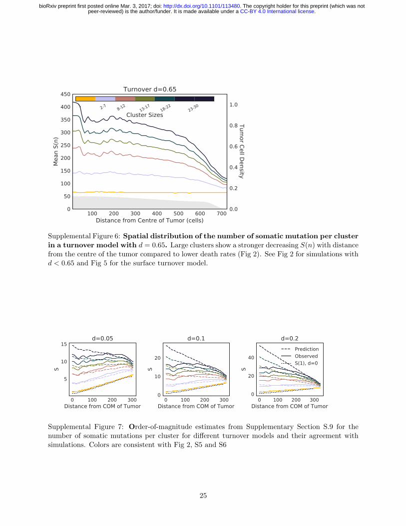
100 200 300 400 500 600 700Distance from Centre of Tumor (cells)
0
50
100
150
200
250
300
350
400
450
Mea
n S(
n)
Turnover d=0.65
0.0
0.2
0.4
0.6
0.8
1.0
Tumor Cell Density
1 2-7 8-1213-17
18-2223-30
Cluster Sizes
Supplemental Figure 6: Spatial distribution of the number of somatic mutation per clusterin a turnover model with d = 0.65. Large clusters show a stronger decreasing S(n) with distancefrom the centre of the tumor compared to lower death rates (Fig 2). See Fig 2 for simulations withd < 0.65 and Fig 5 for the surface turnover model.
0 100 200 300Distance from COM of Tumor
5
10
15
S
d=0.05
0 100 200 300Distance from COM of Tumor
0
10
20
S
d=0.1
0 100 200 300Distance from COM of Tumor
0
20
40
S
d=0.2PredictionObservedS(1), d=0
Supplemental Figure 7: Order-of-magnitude estimates from Supplementary Section S.9 for thenumber of somatic mutations per cluster for different turnover models and their agreement withsimulations. Colors are consistent with Fig 2, S5 and S6
25
.CC-BY 4.0 International licensepeer-reviewed) is the author/funder. It is made available under aThe copyright holder for this preprint (which was not. http://dx.doi.org/10.1101/113480doi: bioRxiv preprint first posted online Mar. 3, 2017;
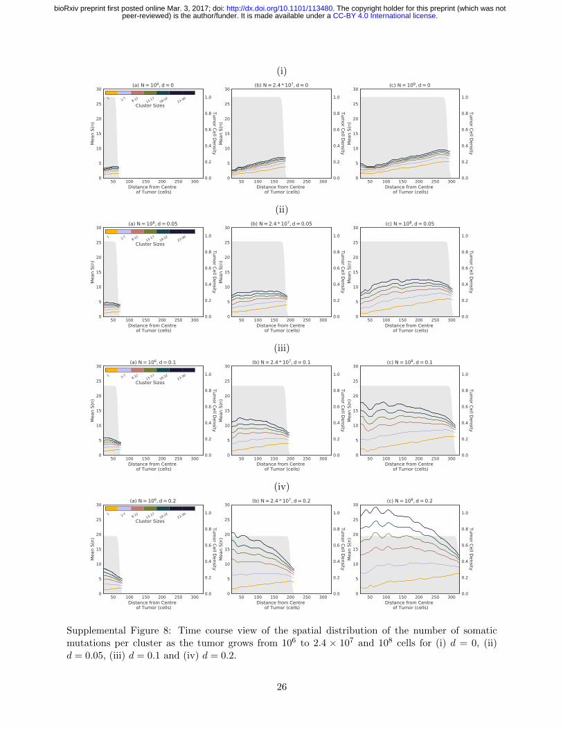
(i)
50 100 150 200 250 300Distance from Centre
of Tumor (cells)
0
5
10
15
20
25
30M
ean
S(n)
(a) N = 106, d = 0
0.0
0.2
0.4
0.6
0.8
1.0
Tumor Cell Density
50 100 150 200 250 300Distance from Centre
of Tumor (cells)
0
5
10
15
20
25
30
Mea
n S(
n)
(b) N = 2.4 * 107, d = 0
0.0
0.2
0.4
0.6
0.8
1.0
Tumor Cell Density
50 100 150 200 250 300Distance from Centre
of Tumor (cells)
0
5
10
15
20
25
30
Mea
n S(
n)
(c) N = 108, d = 0
0.0
0.2
0.4
0.6
0.8
1.0Tum
or Cell Density1 2-7 8-12
13-1718-22
23-30
Cluster Sizes
(ii)
50 100 150 200 250 300Distance from Centre
of Tumor (cells)
0
5
10
15
20
25
30
Mea
n S(
n)
(a) N = 106, d = 0.05
0.0
0.2
0.4
0.6
0.8
1.0
Tumor Cell Density
50 100 150 200 250 300Distance from Centre
of Tumor (cells)
0
5
10
15
20
25
30M
ean
S(n)
(b) N = 2.4 * 107, d = 0.05
0.0
0.2
0.4
0.6
0.8
1.0
Tumor Cell Density
50 100 150 200 250 300Distance from Centre
of Tumor (cells)
0
5
10
15
20
25
30
Mea
n S(
n)
(c) N = 108, d = 0.05
0.0
0.2
0.4
0.6
0.8
1.0
Tumor Cell Density
1 2-7 8-1213-17
18-2223-30
Cluster Sizes
(iii)
50 100 150 200 250 300Distance from Centre
of Tumor (cells)
0
5
10
15
20
25
30
Mea
n S(
n)
(a) N = 106, d = 0.1
0.0
0.2
0.4
0.6
0.8
1.0
Tumor Cell Density
50 100 150 200 250 300Distance from Centre
of Tumor (cells)
0
5
10
15
20
25
30
Mea
n S(
n)
(b) N = 2.4 * 107, d = 0.1
0.0
0.2
0.4
0.6
0.8
1.0
Tumor Cell Density
50 100 150 200 250 300Distance from Centre
of Tumor (cells)
0
5
10
15
20
25
30
Mea
n S(
n)
(c) N = 108, d = 0.1
0.0
0.2
0.4
0.6
0.8
1.0
Tumor Cell Density
1 2-7 8-1213-17
18-2223-30
Cluster Sizes
(iv)
50 100 150 200 250 300Distance from Centre
of Tumor (cells)
0
5
10
15
20
25
30
Mea
n S(
n)
(a) N = 106, d = 0.2
0.0
0.2
0.4
0.6
0.8
1.0
Tumor Cell Density
50 100 150 200 250 300Distance from Centre
of Tumor (cells)
0
5
10
15
20
25
30
Mea
n S(
n)
(b) N = 2.4 * 107, d = 0.2
0.0
0.2
0.4
0.6
0.8
1.0
Tumor Cell Density
50 100 150 200 250 300Distance from Centre
of Tumor (cells)
0
5
10
15
20
25
30
Mea
n S(
n)
(c) N = 108, d = 0.2
0.0
0.2
0.4
0.6
0.8
1.0
Tumor Cell Density
1 2-7 8-1213-17
18-2223-30
Cluster Sizes
Supplemental Figure 8: Time course view of the spatial distribution of the number of somaticmutations per cluster as the tumor grows from 106 to 2.4 × 10⁷ and 108 cells for (i) d = 0, (ii)d = 0.05, (iii) d = 0.1 and (iv) d = 0.2.
26
.CC-BY 4.0 International licensepeer-reviewed) is the author/funder. It is made available under aThe copyright holder for this preprint (which was not. http://dx.doi.org/10.1101/113480doi: bioRxiv preprint first posted online Mar. 3, 2017;

(i)
50 100 150 200 250 300Distance from Centre
of Tumor (cells)
0
5
10
15
20
25
30M
ean
S(n)
(a) N = 106, d = 0No new mutations after N = 106
0.0
0.2
0.4
0.6
0.8
1.0
Tumor Cell Density
50 100 150 200 250 300Distance from Centre
of Tumor (cells)
0
5
10
15
20
25
30
Mea
n S(
n)
(b) N = 2.4 * 107, d = 0No new mutations after N = 106
0.0
0.2
0.4
0.6
0.8
1.0
Tumor Cell Density
50 100 150 200 250 300Distance from Centre
of Tumor (cells)
0
5
10
15
20
25
30
Mea
n S(
n)
(c) N = 108, d = 0No new mutations after N = 106
0.0
0.2
0.4
0.6
0.8
1.0
Tumor Cell Density
1 2-7 8-1213-17
18-2223-30
Cluster Sizes
(ii)
50 100 150 200 250 300Distance from Centre
of Tumor (cells)
0
5
10
15
20
25
30
Mea
n S(
n)
(a) N = 106, d = 0.05No new mutations after N = 106
0.0
0.2
0.4
0.6
0.8
1.0
Tumor Cell Density
50 100 150 200 250 300Distance from Centre
of Tumor (cells)
0
5
10
15
20
25
30
Mea
n S(
n)(b) N = 2.4 * 107, d = 0.05
No new mutations after N = 106
0.0
0.2
0.4
0.6
0.8
1.0
Tumor Cell Density
50 100 150 200 250 300Distance from Centre
of Tumor (cells)
0
5
10
15
20
25
30
Mea
n S(
n)
(c) N = 108, d = 0.05No new mutations after N = 106
0.0
0.2
0.4
0.6
0.8
1.0
Tumor Cell Density
1 2-7 8-1213-17
18-2223-30
Cluster Sizes
(iii)
50 100 150 200 250 300Distance from Centre
of Tumor (cells)
0
5
10
15
20
25
30
Mea
n S(
n)
(a) N = 106, d = 0.1No new mutations after N = 106
0.0
0.2
0.4
0.6
0.8
1.0
Tumor Cell Density
50 100 150 200 250 300Distance from Centre
of Tumor (cells)
0
5
10
15
20
25
30
Mea
n S(
n)
(b) N = 2.4 * 107, d = 0.1No new mutations after N = 106
0.0
0.2
0.4
0.6
0.8
1.0
Tumor Cell Density
50 100 150 200 250 300Distance from Centre
of Tumor (cells)
0
5
10
15
20
25
30
Mea
n S(
n)
(c) N = 108, d = 0.1No new mutations after N = 106
0.0
0.2
0.4
0.6
0.8
1.0
Tumor Cell Density
1 2-7 8-1213-17
18-2223-30
Cluster Sizes
(iv)
50 100 150 200 250 300Distance from Centre
of Tumor (cells)
0
5
10
15
20
25
30
Mea
n S(
n)
(a) N = 106, d = 0.2No new mutations after N = 106
0.0
0.2
0.4
0.6
0.8
1.0
Tumor Cell Density
50 100 150 200 250 300Distance from Centre
of Tumor (cells)
0
5
10
15
20
25
30
Mea
n S(
n)
(b) N = 2.4 * 107, d = 0.2No new mutations after N = 106
0.0
0.2
0.4
0.6
0.8
1.0
Tumor Cell Density
50 100 150 200 250 300Distance from Centre
of Tumor (cells)
0
5
10
15
20
25
30
Mea
n S(
n)
(c) N = 108, d = 0.2No new mutations after N = 106
0.0
0.2
0.4
0.6
0.8
1.0
Tumor Cell Density
1 2-7 8-1213-17
18-2223-30
Cluster Sizes
Supplemental Figure 9: Time course view of the spatial distribution of the number of somaticmutations per cluster as the tumor grows from 106 to 2.4× 10⁷ and 108 cells for for (i) d = 0, (ii)d = 0.05, (iii) d = 0.1 and (iv) d = 0.2 if no new mutations are created when the tumor reaches106 cells, thus revealing the contributions of clonal mixing and genetic drift.
27
.CC-BY 4.0 International licensepeer-reviewed) is the author/funder. It is made available under aThe copyright holder for this preprint (which was not. http://dx.doi.org/10.1101/113480doi: bioRxiv preprint first posted online Mar. 3, 2017;
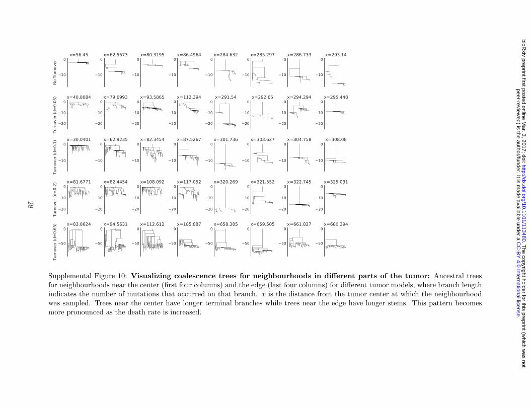
10
0No
Tur
nove
rx=56.45
10
0x=62.5673
10
0x=80.3195
10
0x=86.4964
10
0x=284.632
10
0x=285.297
10
0x=286.733
10
0x=293.14
20
10
0
Turn
over
(d=0
.05) x=40.8084
20
10
0x=79.6993
20
10
0x=93.5865
20
10
0x=112.394
20
10
0x=291.54
20
10
0x=292.65
20
10
0x=294.294
20
10
0x=295.448
10
0
Turn
over
(d=0
.1) x=30.0401
10
0x=62.9235
10
0x=82.3454
10
0x=87.5267
10
0x=301.736
10
0x=303.627
10
0x=304.758
10
0x=308.08
20
10
0
Turn
over
(d=0
.2) x=81.6771
20
10
0x=82.4454
20
10
0x=108.092
20
10
0x=117.052
20
10
0x=320.269
20
10
0x=321.552
20
10
0x=322.745
20
10
0x=325.031
50
0
Turn
over
(d=0
.65) x=83.8624
50
0x=94.5631
50
0x=112.612
50
0x=185.887
50
0x=658.385
50
0x=659.505
50
0x=661.827
50
0x=680.394
Supplemental Figure 10: Visualizing coalescence trees for neighbourhoods in different parts of the tumor: Ancestral treesfor neighbourhoods near the center (first four columns) and the edge (last four columns) for different tumor models, where branch lengthindicates the number of mutations that occurred on that branch. x is the distance from the tumor center at which the neighbourhoodwas sampled. Trees near the center have longer terminal branches while trees near the edge have longer stems. This pattern becomesmore pronounced as the death rate is increased.
28
.C
C-B
Y 4.0 International license
peer-reviewed) is the author/funder. It is m
ade available under aT
he copyright holder for this preprint (which w
as not.
http://dx.doi.org/10.1101/113480doi:
bioRxiv preprint first posted online M
ar. 3, 2017;
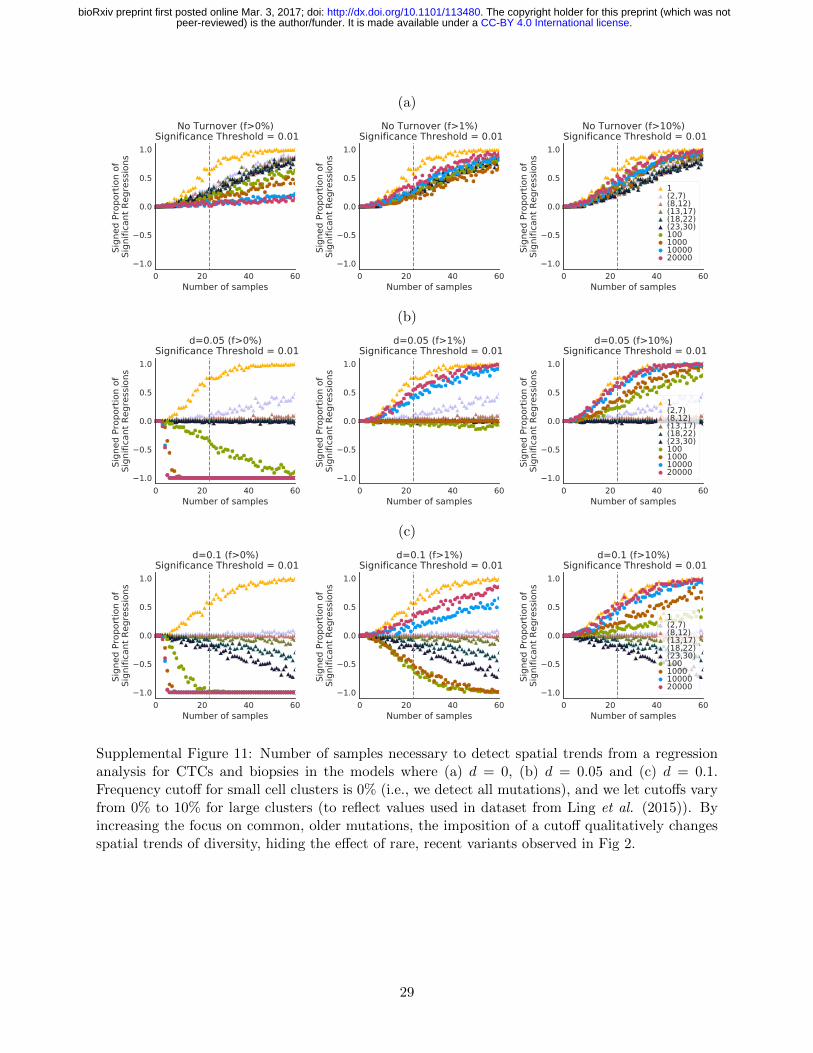
(a)
0 20 40 60Number of samples
1.0
0.5
0.0
0.5
1.0
Sign
ed P
ropo
rtion
of
Sign
ifica
nt R
egre
ssio
nsNo Turnover (f>0%)
Significance Threshold = 0.01
0 20 40 60Number of samples
1.0
0.5
0.0
0.5
1.0
Sign
ed P
ropo
rtion
of
Sign
ifica
nt R
egre
ssio
ns
No Turnover (f>1%) Significance Threshold = 0.01
0 20 40 60Number of samples
1.0
0.5
0.0
0.5
1.0
Sign
ed P
ropo
rtion
of
Sign
ifica
nt R
egre
ssio
ns
No Turnover (f>10%) Significance Threshold = 0.01
1(2,7)(8,12)(13,17)(18,22)(23,30)10010001000020000
(b)
0 20 40 60Number of samples
1.0
0.5
0.0
0.5
1.0
Sign
ed P
ropo
rtion
of
Sign
ifica
nt R
egre
ssio
ns
d=0.05 (f>0%) Significance Threshold = 0.01
0 20 40 60Number of samples
1.0
0.5
0.0
0.5
1.0
Sign
ed P
ropo
rtion
of
Sign
ifica
nt R
egre
ssio
nsd=0.05 (f>1%)
Significance Threshold = 0.01
0 20 40 60Number of samples
1.0
0.5
0.0
0.5
1.0
Sign
ed P
ropo
rtion
of
Sign
ifica
nt R
egre
ssio
ns
d=0.05 (f>10%) Significance Threshold = 0.01
1(2,7)(8,12)(13,17)(18,22)(23,30)10010001000020000
(c)
0 20 40 60Number of samples
1.0
0.5
0.0
0.5
1.0
Sign
ed P
ropo
rtion
of
Sign
ifica
nt R
egre
ssio
ns
d=0.1 (f>0%) Significance Threshold = 0.01
0 20 40 60Number of samples
1.0
0.5
0.0
0.5
1.0
Sign
ed P
ropo
rtion
of
Sign
ifica
nt R
egre
ssio
ns
d=0.1 (f>1%) Significance Threshold = 0.01
0 20 40 60Number of samples
1.0
0.5
0.0
0.5
1.0
Sign
ed P
ropo
rtion
of
Sign
ifica
nt R
egre
ssio
ns
d=0.1 (f>10%) Significance Threshold = 0.01
1(2,7)(8,12)(13,17)(18,22)(23,30)10010001000020000
Supplemental Figure 11: Number of samples necessary to detect spatial trends from a regressionanalysis for CTCs and biopsies in the models where (a) d = 0, (b) d = 0.05 and (c) d = 0.1.Frequency cutoff for small cell clusters is 0% (i.e., we detect all mutations), and we let cutoffs varyfrom 0% to 10% for large clusters (to reflect values used in dataset from Ling et al. (2015)). Byincreasing the focus on common, older mutations, the imposition of a cutoff qualitatively changesspatial trends of diversity, hiding the effect of rare, recent variants observed in Fig 2.
29
.CC-BY 4.0 International licensepeer-reviewed) is the author/funder. It is made available under aThe copyright holder for this preprint (which was not. http://dx.doi.org/10.1101/113480doi: bioRxiv preprint first posted online Mar. 3, 2017;

100 101 102
CTC Cluster Size, n
10 1
100
101
Clus
ter A
dvan
tage
, S(n)
S(1)
1
d=0.05
No Turnover (Cluster)No Turnover (Random Set)Surface Turnover (Cluster)Surface Turnover (Random Set)Turnover (Cluster)Turnover (Random Set)Standard Neutral Model
100 101 102
CTC Cluster Size, n
10 1
100
101
Clus
ter A
dvan
tage
, S(n)
S(1)
1
d=0.1
100 101 102
CTC Cluster Size, n
10 1
100
101
Clus
ter A
dvan
tage
, S(n)
S(1)
1
d=0.65
Supplemental Figure 12: Cluster advantage for weak turnover models: even weak mixing (turnovermodel with d = 0.05) can lead to substantial differences in the cluster advantage.
30
.CC-BY 4.0 International licensepeer-reviewed) is the author/funder. It is made available under aThe copyright holder for this preprint (which was not. http://dx.doi.org/10.1101/113480doi: bioRxiv preprint first posted online Mar. 3, 2017;

Table S2: Parameters for all reported simulations The code to run all simulations presented here can be found at this online repository. These parameters must be specified in params.h . Alternatively, all parameters are pre-written into the repository and can be compiled in one command using compile_all_experiments.sh . Driver mutation rate (driver_prob ) is fixed to 2e-5. Tumors are grown to size 108, unless specified. To toggle between surface turnover models, core turnover column is specified to be either ON or OFF. If ON, the line DEATH_ON_SURFACE must be uncommented in the params file. Initial birth rate is specified as growth0 and is set to 0.69. Parameters for individual simulations are reported below.
Passenger Mutation Rate 1e-2 Figure Experiment Name Death Rate
(death0 ) Selection Coefficient (driver_adv )
Core Turnover (DEATH_ON_SURFACE )
Executable name on repository once compiled
Fig 1 Frequency Spectra
d=0.05, no turnover 0 0.01 OFF 1_0_0
d=0.05, surface turnover
0.05 0.01 ON 1_1_005
d=0.05, turnover 0.05 0.01 OFF 1_0_01
d=0.65, no turnover 0 0.01 OFF 1_0_0
d=0.65, surface turnover
0.65 0.01 ON 1_1_065
d=0.65, turnover 0.65 0.01 OFF 1_0_065
Fig S1 Frequency Spectra
d=0.1, no turnover 0 0.01 OFF 1_0_0
“Intratumor Heterogeneity and Circulating Tumor Cell Clusters” (Ahmed and Gravel, 2018)
.CC-BY 4.0 International licensepeer-reviewed) is the author/funder. It is made available under aThe copyright holder for this preprint (which was not. http://dx.doi.org/10.1101/113480doi: bioRxiv preprint first posted online Mar. 3, 2017;

d=0.1, surface turnover
0.1 0.01 ON 1_1_01
d=0.1, turnover 0.1 0.01 OFF 1_0_01
d=0.2, no turnover 0 0.01 OFF 1_0_0
d=0.2, surface turnover
0.2 0.01 ON 1_1_02
d=0.2, turnover 0.2 0.01 OFF 1_0_02
Fig S2(a), Frequency spectra vs selection rate
No Selection, d=0.0 0 0.0 OFF 0_0_0
No Selection, d=0.05 0.05 0.0 ON 0_0_005
No Selection, d=0.1 0.1 0.0 OFF 0_0_01
No Selection, d=0.2 0.2 0.0 OFF 0_0_02
No Selection, d=0.65 0.65 0.0 ON 0_0_065
Fig S2(c), frequency spectra vs selection rate
Selection 10%, d=0.0 0 0.1 OFF 10_0_0
Selection 10%, d=0.05
0.05 0.1 ON 10_0_005
Selection 10%, d=0.1 0.1 0.1 OFF 10_0_01
Selection 10%, d=0.2 0.2 0.1 OFF 10_0_02
Selection 10%, d=0.65
0.65 0.1 ON 10_0_065
“Intratumor Heterogeneity and Circulating Tumor Cell Clusters” (Ahmed and Gravel, 2018)
.CC-BY 4.0 International licensepeer-reviewed) is the author/funder. It is made available under aThe copyright holder for this preprint (which was not. http://dx.doi.org/10.1101/113480doi: bioRxiv preprint first posted online Mar. 3, 2017;
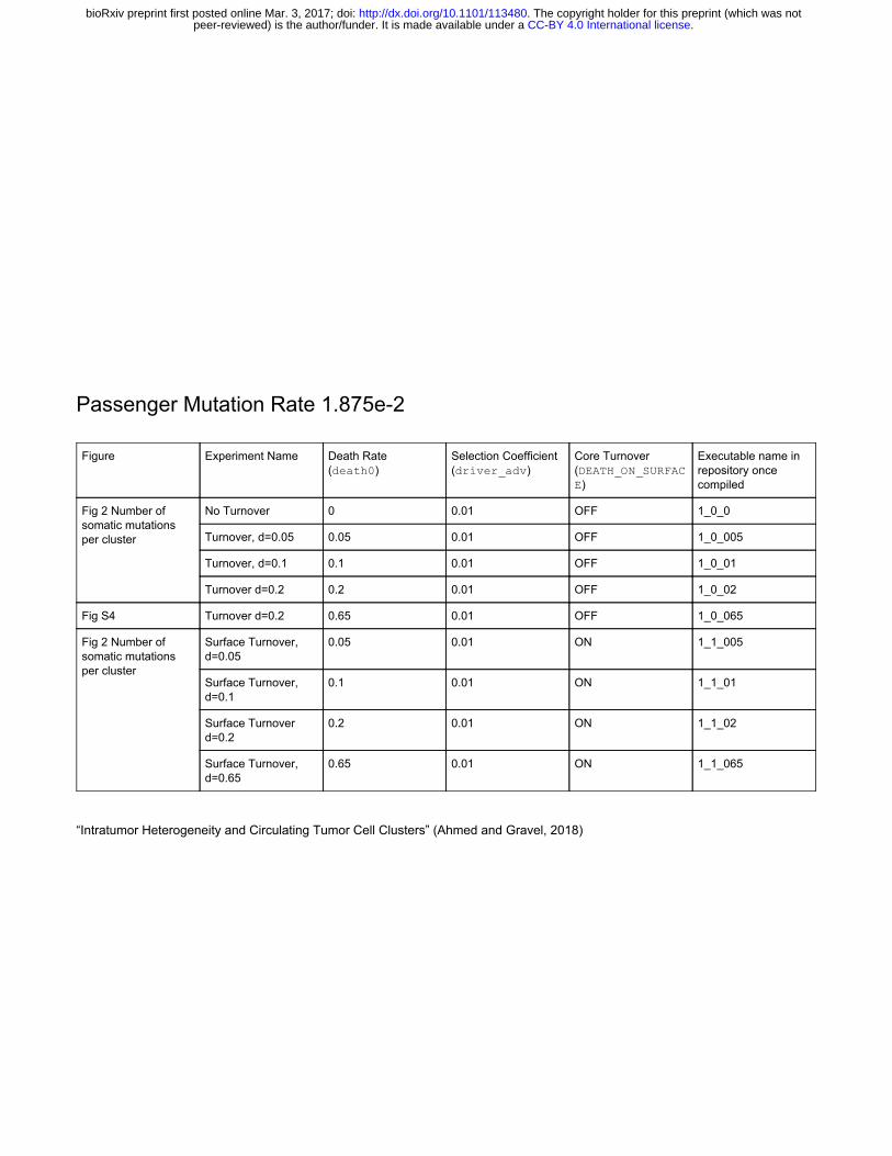
Passenger Mutation Rate 1.875e-2
Figure Experiment Name Death Rate (death0 )
Selection Coefficient (driver_adv )
Core Turnover (DEATH_ON_SURFACE )
Executable name in repository once compiled
Fig 2 Number of somatic mutations per cluster
No Turnover 0 0.01 OFF 1_0_0
Turnover, d=0.05 0.05 0.01 OFF 1_0_005
Turnover, d=0.1 0.1 0.01 OFF 1_0_01
Turnover d=0.2 0.2 0.01 OFF 1_0_02
Fig S4 Turnover d=0.2 0.65 0.01 OFF 1_0_065
Fig 2 Number of somatic mutations per cluster
Surface Turnover, d=0.05
0.05 0.01 ON 1_1_005
Surface Turnover, d=0.1
0.1 0.01 ON 1_1_01
Surface Turnover d=0.2
0.2 0.01 ON 1_1_02
Surface Turnover, d=0.65
0.65 0.01 ON 1_1_065
“Intratumor Heterogeneity and Circulating Tumor Cell Clusters” (Ahmed and Gravel, 2018)
.CC-BY 4.0 International licensepeer-reviewed) is the author/funder. It is made available under aThe copyright holder for this preprint (which was not. http://dx.doi.org/10.1101/113480doi: bioRxiv preprint first posted online Mar. 3, 2017;

Simulation Compilation and Submission The script compile_all_experiments.sh will compile all the experiments according to the above parameters. If you are on a cluster you can use submit_all_experiments.sh to submit all of them to a queue. This script is called multiple times with different mutation rates u0.01 and u0.01875 and seeds: ['10','100','102','15','3','3318','33181','33185','33186','34201810','342018101','342018102','8','9','9
9’]
Analysis Pipeline: See https://github.com/zafarali/tumorheterogeneity/blob/mixing-parallel/analysis/__init__.py
Code Module Purpose
load_tumor Loads the tumor into memory
create_kdsampler Creates the sampler to search for SNPs in the tumor
marginal_counts_unordered Used for the advantage plots with random sampling
marginal_counts_ordered Used for the advantage plots with ordered sampling
density_plot Density plot in the background
big_samples Gets the big samples from the tumor (upwards of 10k)
perform_mixing_analysis Performs mixing analysis
“Intratumor Heterogeneity and Circulating Tumor Cell Clusters” (Ahmed and Gravel, 2018)
.CC-BY 4.0 International licensepeer-reviewed) is the author/funder. It is made available under aThe copyright holder for this preprint (which was not. http://dx.doi.org/10.1101/113480doi: bioRxiv preprint first posted online Mar. 3, 2017;

Pipeline for figures: See run_figure_pipeline.sh
PATH_TO_ALL_SIMS="../model/experiments/u0.01875/"
SELECTED_TUMOR="10" # seed of the selected tumor for analysis
python2 do_power_analysis.py $PATH_TO_ALL_SIMS $SELECTED_TUMOR
python2 create_AFS_figures.py
python2 create_number_of_divisions_table.py > S1table.txt
python2 create_Splots_figures.py $SELECTED_TUMOR
python2 create_cluster_advantage_plots.py
python2 create_fanning_plots_v2.py
python2 create_trees.py $PATH_TO_ALL_SIMS $SELECTED_TUMOR
python2 create_analytic_plot.py
Recreating Experiments in S7 and S8 Switch to the branch TRANSITION_EXPERIMENT and run the compile script compile_transition_experiments.sh You can then use submit_all_experiments.sh (bash submit_all_experiments.sh u0.01transition SEED DRY) to submit them to a cluster. The seeds used for this experiment are [6, 7, 8]
Recreating Experiments in S4 Switch to branch new-death-models and run the compile script. You can then use submit_all_experiments.sh (bash submit_all_experiments.sh u0..01lowcutoff SEED DRY) to submit them to a cluster. The seeds used for this experiment are [1, 2, 3, 4, 5]
“Intratumor Heterogeneity and Circulating Tumor Cell Clusters” (Ahmed and Gravel, 2018)
.CC-BY 4.0 International licensepeer-reviewed) is the author/funder. It is made available under aThe copyright holder for this preprint (which was not. http://dx.doi.org/10.1101/113480doi: bioRxiv preprint first posted online Mar. 3, 2017;
Related Documents


![Tumor evolution and intratumor heterogeneity of an ...s-space.snu.ac.kr/bitstream/10371/100516/1/12885... · smoothed and segmented using the ‘DNAcopy’ R package [17] with alpha=0.01,](https://static.cupdf.com/doc/110x72/5f6c8ce9a8f7e53c5a49f921/tumor-evolution-and-intratumor-heterogeneity-of-an-s-spacesnuackrbitstream10371100516112885.jpg)


