Interval-valued Time Series: Model Estimation based on ...

Interval-valued Time Series:

Model Estimation based on Order Statistics

Wei Lin†

†International School of Economics and Management

Capital University of Economics and Business

Beijing, China 100070

Gloria Gonzalez-Rivera∗

∗Department of Economics

University of California, Riverside

Riverside, CA 92521

September 12, 2014

Abstract

The current regression models for interval-valued data ignore the extreme nature of thelower and upper bounds of intervals. We propose a new estimation approach that considers thebounds of the interval as realizations of the max/min order statistics coming from a sampleof nt random draws from the conditional density of an underlying stochastic process Yt.This approach is important for data sets for which the relevant information is only available ininterval format, e.g., low/high prices, but nevertheless we are interested in the characterizationof the latent process as well as in the modeling of the bounds themselves. We estimate adynamic model for the conditional mean and conditional variance of the latent process, whichis assumed to be normally distributed, and for the conditional intensity of the discrete processnt, which follows a negative binomial density function. Under these assumptions, togetherwith the densities of order statistics, we obtain maximum likelihood estimates of the parametersof the model, which are needed to estimate the expected value of the bounds of the interval. Weimplement this approach with the time series of livestock prices, of which only low/high pricesare recorded making the price process itself a latent process. We find that the proposed modelprovides an excellent fit of the intervals of low/high returns with an average coverage rate of83%.

Key Words: Interval-valued Data, Order Statistics, Intensity, Maximum Likelihood Estimation,Commodity Prices.

JEL Classification: C01, C13, C32.

1 Introduction

Since the work on symbolic data by Billard and Diday (2003, 2006), a variety of regression mod-

els have been proposed to fit interval-valued data, see the survey article by Arroyo, Gonzalez-

Rivera and Mate (2011) for an extensive review. A first approach proposed by Billard and

Diday was to regress the centers of the intervals of the dependent variable on the centers of the

intervals of the regressors. Subsequent approaches considered two separate regressions, one for

the lower bound and another for the upper bound of intervals (Brito, 2007), or one regression

for the center and another for the range of the interval (Lima Neto and de Carvalho, 2010).

None of these approaches guarantees that the fitted values from the regressions will satisfy the

natural order of an interval, i.e., by yl ≤ yu, for all observations in the sample. A solution

came from Lima Neto and de Carvalho (2010) who modified the previous regression models

by imposing non-negative constraints on the regression coefficients of the model for the range.

Gonzalez-Rivera and Lin (2013) argued that these ad hoc constraints limit the usefulness of

the model and proposed a constrained regression model that generalizes the previous regression

models for lower/upper bounds or center/radius of intervals, and naturally guarantees that the

proper order of the fitted intervals is satisfied.

A common thread to these approaches is that they consider the lower and upper bound as

distinct stochastic processes. In this paper we propose an alternative approach and argue that

there is only one stochastic process, say Yt, that generates the upper and lower bounds of

the interval. When we analyze interval-valued data, we only observe the bounds and these are

extreme realizations of a latent random variable. This is our conceptual setup. At a fixed time

t, we consider a random variable Yt with a given conditional density function from which we

draw randomly nt realizations. The lower and upper bounds of the interval, i.e. (ylt and yut)

are the realized minimum and maximum values coming from the set of realizations associated

with the nt draws. As such, our interest moves towards the analysis of these two order statistics

and their probability density functions. As an example, consider a time series of daily prices.

In a given day t, from opening to closing time, there are nt transactions, each one generating

a market price. If we consider the daily number of trades as the nt random draws, their

corresponding intra daily prices are the realizations of the random variable daily price Yt, and

the highest/lowest prices are the realizations of the max/min order statistics of Yt. Observe

that we are not interested in the dynamics of the intra daily prices, only the lowest/highest

prices carry information on the daily market activity.To start the modeling exercise, we require

a set of assumptions regarding the density of the underlying stochastic process and the density

1

of the number of draws. We will assume that the first process is continuous and it follows

a conditional normal density function, and that the second process is naturally discrete and

it follows a negative binomial density. Under these assumptions, we will obtain the expected

values of the lower and upper bounds of the interval.

However, this modeling approach will also provide information on the latent process because

we will be able to model its conditional mean and conditional variance. This is an advantage in

those instances in which there are not records of opening or closing prices, typically the object

of analysis, or when those prices are not very representative of the state of the market. In

this paper, we model such a time series: agricultural and livestock prices provided by the US

Department of Agriculture. We look into beef sales prices; the daily information provided is

low price, high price, weighted average price, number of trades and total pounds traded. We

could model the weighted average price but this is not very informative for potential sellers

and buyers. Instead, we construct the daily interval-valued time series of low/high beef prices,

which we manually dig from several archives provided by the US Department of Agriculture,

and implement our approach to discover the characteristics of the latent price as well as the

expected values of the low and high prices.

The paper is organized as follows. In Section 2, we discuss the key ideas of our modeling

approach and implementation under a set of assumptions. In Section 3, we use Monte Carlo

simulation to investigate the properties of the proposed maximum likelihood estimator. In

Section 4, we model the dynamics of the daily beef sales and prices, and in Section 5, we

conclude by summarizing our findings.

2 General Framework

We assume that there is an underlying stochastic process for the interval-valued time series,

and in a given time t, e.g. day, month, etc. the high/low values of intervals are the realized

highest and lowest order statistics based on the random draws from the conditional densities of

the underlying stochastic process. Formally,

Assumption 1. (DGP) Let Yt : t = 1, · · · , T be the underlying stochastic process. The latent

random variable Yt at time t has a conditional probability density function ft(yt|Ft). At each

time t, from the conditional density of Yt we draw nt observations. The number of draws has

a discrete density function ht(nt|Ft). Let ylt and yut be the smallest and largest value of the

2

random sample St ≡ yit : i = 1, 2, · · · , nt:

ylt ≡ miniSt = min

1≤i≤nt

yit,

yut ≡ maxiSt = max

1≤i≤nt

yit.

Then, (ylt, yut, nt) : t = 1, · · · , T forms the observed interval time series and number of

random draws, and Ft ≡ (yls, yus, ns) : s = 1, · · · , t − 1 is the information set available at

time t.

At time t, the low and high observations (ylt and yut) are the lowest and highest ranked

order statistics of the random sample St formed by the nt draws or trades. The joint conditional

probability density of (ylt, yut) given nt and information set Ft is,

gt(ylt, yut|nt,Ft) = nt(nt − 1) [Ft(yut|Ft)− Ft(ylt|Ft)]nt−2

×ft(ylt|Ft)ft(yut|Ft)

where Ft(·|Ft) is the cumulative distribution function corresponding to the conditional density

ft(·|Ft). Then, the joint probability density of (ylt, yut, nt) conditional on information set Ft is,

pt(ylt, yut, nt|Ft) = gt(ylt, yut|nt,Ft)ht(nt|Ft).

We still need to specify the conditional densities ft(yt|Ft) and ht(nt|Ft) and their dependence

on the information set. Therefore, we have Assumptions 2 and 3.

Assumption 2. (Distributions) The conditional densities of the underlying stochastic process

Yt and of the number of random draws nt are normal and negative binomial respectively, i.e.,

ft(yt|Ft) ≡1√

2πσ2t

exp

−(yt − µt)2

2σ2t

,

ht(nt|Ft) ≡Γ(nt + d− 2)

(nt − 2)!Γ(d)

(d

λt + d

)d( λtλt + d

)nt−2

,

where µt and σ2t are the conditional mean and conditional variance of Yt; and λt and d are the

intensity function and dispersion parameter of the discrete process nt.

We assume negative binomial distribution as a robust alternative to the Poisson distribution

because the additional dispersion parameter d will capture potential over dispersion in the data.

When d goes to infinity, the negative binomial converges to Poisson.

Assumption 3. (Dependence) The conditional mean, variance and intensity of the underlying

3

random processes yt and the discrete process nt are parametric functions of the information set,

i.e.,

µt(α) = fµ(wt; α), (2.1)

log σ2t (β) = fσ(wt; β), (2.2)

λt(γ) = fλ(wt; γ). (2.3)

The functions fµ(·), fσ(·), and fλ(·) represent the dependence on the information set, and the

parameters α, β, and γ will be estimated. The random vector wt is a subset of information set

Ft, i.e., wt ⊂ Ft.

The information set w will consists of past low/high intervals and past number of draws

(trades). With this information, it makes sense to model the conditional mean µt(α) mainly as

a function of the past centers of the intervals, i.e. (yl+yh)/2 and the conditional variance σ2t (β)

as a function of the past ranges of the intervals, i.e (yh−yl). The conditional intensity λt will be

a function of the past number of draws. It is also possible that there will be interactions among

the three functions, for instance, the number of draws may influence volatility. Eventually, the

final specifications will be driven by the characteristics of the data.

Let θ1 ≡ (α, β) and θ2 ≡ (γ, d). Given Assumptions 2 and 3, the joint density of (ylt, yut, nt)

can be explicitly written as,

p(ylt, yut, nt|wt; θ) = g(ylt, yut|nt,wt; θ1)h(nt|wt; θ2)

= nt(nt − 1)

[Φ

(yut − µt(α)

σt(β)

)− Φ

(ylt − µt(α)

σt(β)

)]nt−2

× 1

σt(β)φ

(ylt − µt(α)

σt(β)

)1

σt(β)φ

(yut − µt(α)

σt(β)

)×Γ(nt + d− 2)

(nt − 2)!Γ(d)

(d

λt + d

)d( λtλt + d

)nt−2

, (2.4)

where φ(·) and Φ(·) are the standard normal probability density and cumulative distribution

functions.

The estimation of the model proceeds by maximum likelihood (ML). For a sample (ylt, yut, nt) :

t = 1, 2, · · · , T, the ML function is

L(θ|yu,yl,n) = L1(θ1|yu,yl,n) + L2(θ2|n)

4

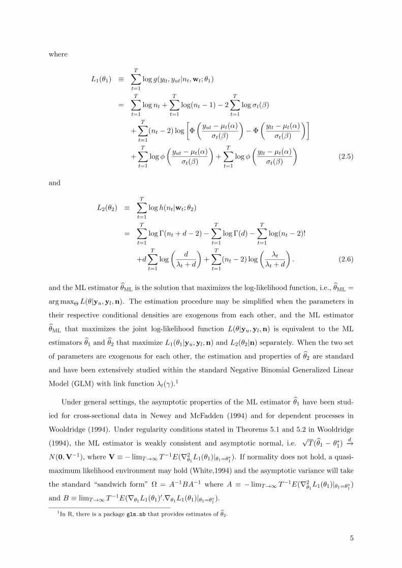
where

L1(θ1) ≡T∑t=1

log g(ylt, yut|nt,wt; θ1)

=

T∑t=1

log nt +

T∑t=1

log(nt − 1)− 2

T∑t=1

log σt(β)

+

T∑t=1

(nt − 2) log

[Φ

(yut − µt(α)

σt(β)

)− Φ

(ylt − µt(α)

σt(β)

)]

+T∑t=1

log φ

(yut − µt(α)

σt(β)

)+

T∑t=1

log φ

(ylt − µt(α)

σt(β)

)(2.5)

and

L2(θ2) ≡T∑t=1

log h(nt|wt; θ2)

=T∑t=1

log Γ(nt + d− 2)−T∑t=1

log Γ(d)−T∑t=1

log(nt − 2)!

+dT∑t=1

log

(d

λt + d

)+

T∑t=1

(nt − 2) log

(λt

λt + d

). (2.6)

and the ML estimator θML is the solution that maximizes the log-likelihood function, i.e., θML =

arg maxΘ L(θ|yu,yl,n). The estimation procedure may be simplified when the parameters in

their respective conditional densities are exogenous from each other, and the ML estimator

θML that maximizes the joint log-likelihood function L(θ|yu,yl,n) is equivalent to the ML

estimators θ1 and θ2 that maximize L1(θ1|yu,yl,n) and L2(θ2|n) separately. When the two set

of parameters are exogenous for each other, the estimation and properties of θ2 are standard

and have been extensively studied within the standard Negative Binomial Generalized Linear

Model (GLM) with link function λt(γ).1

Under general settings, the asymptotic properties of the ML estimator θ1 have been stud-

ied for cross-sectional data in Newey and McFadden (1994) and for dependent processes in

Wooldridge (1994). Under regularity conditions stated in Theorems 5.1 and 5.2 in Wooldridge

(1994), the ML estimator is weakly consistent and asymptotic normal, i.e.√T (θ1 − θ∗1)

d−→

N(0,V−1), where V ≡ − limT→∞ T−1E(∇2

θ1L1(θ1)|θ1=θ∗1

). If normality does not hold, a quasi-

maximum likelihood environment may hold (White,1994) and the asymptotic variance will take

the standard “sandwich form” Ω = A−1BA−1 where A ≡ − limT→∞ T−1E(∇2

θ1L1(θ1)|θ1=θ∗1

)

and B ≡ limT→∞ T−1E(∇θ1L1(θ1)′.∇θ1L1(θ1)|θ1=θ∗1

).

1In R, there is a package glm.nb that provides estimates of θ2.

5

Given the model specification and the density of the order statistics, and by calling the law

of iterated expectations, we obtain the conditional means of the lower and upper bounds of

interval, µlt and µut respectively, as follows

µlt ≡ E(ylt|Ft) = E[E(ylt|Ft, nt)|Ft]

= E

[nt

∫ +∞

−∞s

(1− Φ

(s− µt(α)

σt(β)

))nt−1 1

σt(β)φ

(s− µt(α)

σt(β)

)ds

∣∣∣∣∣Ft]

=∞∑nt=2

[nt

∫ +∞

−∞s

(1− Φ

(s− µt(α)

σt(β)

))nt−1 1

σt(β)φ

(s− µt(α)

σt(β)

)ds · h(nt|Ft)

]

and

µut ≡ E(yut|Ft)

=∞∑nt=2

[nt

∫ +∞

−∞s

(Φ

(s− µt(α)

σt(β)

))nt−1 1

σt(β)φ

(s− µt(α)

σt(β)

)ds · h(nt|Ft)

](2.7)

Similarly, the conditional variances of lower and upper bounds of the interval are as follows,

σ2lt ≡ E(y2

lt|Ft)− E(ylt|Ft)2

=∞∑nt=2

[nt

∫ +∞

−∞s2

(1− Φ

(s− µt(α)

σt(β)

))nt−1 1

σt(β)φ

(s− µt(α)

σt(β)

)ds · h(nt|Ft)

]− µ2

lt

and

σ2ut ≡ E(y2

ut|Ft)− E(yut|Ft)2 (2.8)

=

∞∑nt=2

[nt

∫ +∞

−∞s2

(Φ

(s− µt(α)

σt(β)

))nt−1 1

σt(β)φ

(s− µt(α)

σt(β)

)ds · h(nt|Ft)

]− µ2

ut

After estimation, we plug the ML estimates θ into expressions (2.7) – (2.8) and obtain

the estimates of conditional means and conditional variances of the lower and upper bounds,

denoted as ylt, yut, σ2lt, and σ2

ut, which in turn permits the construction of confidence bands for

the bounds.

3 Simulation

We perform Monte Carlo simulations to assess the finite sample performance of the proposed

maximum likelihood estimators. The data generating processes (DGP) satisfy Assumptions 1

6

– 3 and the conditional moments are specified as follows

µt = α0 +∑i

αliyl,t−i +∑i

αhiyh,t−i +∑i

αni log nt−i, (3.1)

log σ2t = β0 +

∑i

βri log(yh,t−i − yl,t−i)2 +∑i

βni log nt−i, (3.2)

log λt = γ0 +∑i

γri log(yh,t−i − yl,t−i)2 +∑i

γni log nt−i. (3.3)

In Table 1 we summarize all the DGPs specifications. We consider three specifications for

each conditional moment, mean, variance, and intensity. DGP1 has no dependence in yt or in

nt. DGP2 has higher persistence than DGP3 but with less number of lagged regressors. For

each DGP, we consider both small (200 observations) and large (2,000 observations) sample

sizes 2. Finally, we replicate each DGP 5,000 times.

[TABLE 1] [TABLE 2]

In Table 2, we report the average of the absolute bias of the ML estimates and their average

mean squared error (AMSE). For all DGPs, the average absolute bias and the AMSE are very

close to zero even for small samples, and they go to zero when the sample size increases from

200 to 2,000. We observe that for DGP2 and DGP3, the estimates of the constant terms i.e.,

α0, β0, and γ0, are less accurate (large AMSEs) than those of the slope coefficients, in particular

for small samples.

We also test the normality of the ML estimates (with 5000 replications) by implementing

the Anderson-Darling (AD) test and the popular Jarque-Bera test (JB). The AD test asseses the

distance between the empirical distribution function Fn(x) and the hypothesized distribution

function F0(x) under the null hypothesis, i.e.,

AD = n

∫ ∞−∞

(Fn(x)− F0(x))2

[F0(x)(1− F0(x))]dx.

The asymptotic distribution of the AD statistic is nonstandard and its critical values or p-values

are available in Pearson and Hartley (1972, Table 54). Stephens (1974) found that the AD test

is a powerful statistic to detect most departures from normality.

[TABLE 3]

In Table 3 we report both the AD and JB statistics with their p-values. Those statistics with

p-values less than 1% are written in bold. For DGP1 both statistics fail to reject normality for

2When generating the sample, we produce additional 100 observations and use only the last 200 or 2,000observations as the effective sample for estimation.

7

all estimates in small and large samples except for the dispersion estimate with a small sample

size. For DGP2 and DGP3, there is rejection of normality for a few estimates when the sample

size is small but, as the sample becomes large, both statistics fail to reject normality. Overall,

AD and JB provide the same decision. These results are in agreement with the asymptotic

properties of the ML estimators discussed above.

4 Modeling Interval-valued Beef Prices

The Agriculture Marketing Service (AMS) within the United States Department of Agriculture

(USDA) provides current, unbiased price and sales information to assist in the orderly marketing

and distribution of farm commodities. Its daily market news reports include information on

prices, volume, quality, condition, and other market data on farm products in specific markets

and marketing areas. Reports cover both domestic and international markets.

4.1 Description of the Data

The specific data set that we analyze is the national daily boxed beef cuts negotiated sales

prices. The historical data are archived and it is downloaded from the following website:3

http://goo.gl/76WYQ. The name of the daily beef report is “Boxed Beef Cutout & Cuts-

Negotiated Sales PM CSV”, coded as “LM XB403”. In the daily report, sales prices of different

parts (choice cuts) of beef are provided, and we select item “109E”. The available information

includes number of trades, total pounds, low price, high price, and weighted average price,

where prices reflect U.S. dollars per 100 pounds.

There is not special reason to work with this particular commodity. Our interest is to show

that there are time series for which the relevant information is not given by a single number,

in this case, a daily price. The weighted price is not very informative for potential sellers and

buyers as includes sales volume and it is not representative of any given transaction. If we

are interested in the forecasting of beef prices, we are bound to work with the low and high

prices, and thus the importance of modeling the interval. To this end, we apply the estimation

methodology proposed in the previous sections. There are other areas within economics and

other sciences where the relevant and only format of the data is the interval format. For

instance, electricity prices, fair market price within real estate markets, bid/ask prices in the

bond markets, low/high temperature records in a given location, blood pressure measurements

3We shorten the original url by Google url shortener.

8

in health records, etc. all these are examples of data sets where a point-valued format does not

exist because in most cases it would be meaningless.

The AMS archives are very rich in data and, as we did with beef prices, sales data on any

other livestock or farm products can be retrieved though it requires a non-trivial manual effort.

We construct a daily time series that ranges form January 4th, 2010 to September 30th 2013

for a total of 950 observations. In Figures 1a and 1b, we plot the time series of daily low/high

prices and number of trades, respectively.

[FIGURE 1a] [FIGURE 1b]

The prices are nonstationary, they have an upward trend, thus we need to work with returns.

To preserve the interval format, we calculate daily returns with respect to the previous day

weighted average price, that is,

rht =Phigh,t − Pavg,t−1

Pavg,t−1× 100%

rlt =Plow,t − Pavg,t−1

Pavg,t−1× 100%.

In Figure 1c, we plot the low and high returns. In Table 4, we report the descriptive statistics

for the three series: low percentage change rlt, high percentage change rht and number of trades

nt. The median low return is -3.41% and the median high return is 5.83%. Both series have

similar standard deviation of about 3.5%, and both are skewed and leptokurtic. The median

number of daily trades is 30. We observe that over dispersion is present, i.e. the variance

166.92 is much larger than the mean 31.54, so that the assumed negative binomial distribution

for number of trades is a plausible assumption.

[TABLE 4]

In Figures 2 and 3, we plot the autocorrelation and partial autocorrelation functions for each

of the three times series. Both returns series, rlt and rht, exhibit moderate but significant

autocorrelation, in contrast with the zero autocorrelation customarily found in financial returns.

The dependence observed in the series log nt is predominantly weekly seasonality (5-day week).

[FIGURE 2] [FIGURE 3]

9

4.2 Model Selection and Estimation

We propose a specification search going from a rather general to a more parsimonious model.

The general model involves an autoregressive representation for the conditional mean, condi-

tional variance, and conditional intensity. The starting most general specification is as follows,

µt = α0 +

p1∑ξ=1

αlξrl,t−ξ +

p1∑ξ=1

αhξrh,t−ξ

+s1µ log nt−5 + s2µ log nt−10 + s3µ log nt−15

+(1 + s1µL

5 + s2µL10 + s3µL

15) p2∑ξ=1

αnξ log nt−ξ (4.1)

log σ2t = β0 +

q1∑ξ=1

βrξ log(rh,t−ξ − rl,t−ξ)2

+s1σ log nt−5 + s2σ log nt−10 + s3σ log nt−15

+(1 + s1σL

5 + s2σL10 + s3σL

15) q2∑ξ=1

βnξ log nt−ξ (4.2)

log λt = γ0 +

k1∑ξ=1

γrξ log(rh,t−ξ − rl,t−ξ)2

+s1λ log nt−5 + s2λ log nt−10 + s3λ log nt−15

+(1 + s1λL

5 + s2λL10 + s3λL

15) k2∑ξ=1

γnξ log nt−ξ, (4.3)

According to the information contained in the autocorrelation functions, the number of

trades exhibits marked weekly seasonality of order 2 or 3 4. As a starting point, we choose

order 3 and we include the non-seasonal and seasonal component (in a multiplicative fashion)

of the number of trades as regressors in the conditional mean and variance. In the conditional

mean, we include the past centers of the interval in an unrestricted format, i.e. rl,t−ξ and rh,t−ξ

separately. The conditional variance and conditional intensity are assumed to be a function of

the range of past intervals. Our task is to find the order of the several polynomial lags in the

three equations.

We estimate jointly by maximum likelihood the mean and variance equations, (4.1) and

(4.2). The order of the polynomial lags are restricted to the following large set

p1, p2, q1, q2 ∈ A ≡ 0, 1, 2, 3, 4, 5, 6, 7, 8, 9,4Since we consider a 5-day week, autoregressive seasonality of order 1, 2, and 3 means a 5-period, 10-period

and 15-period lag, respectively i.e., L5, L10,L15.

10

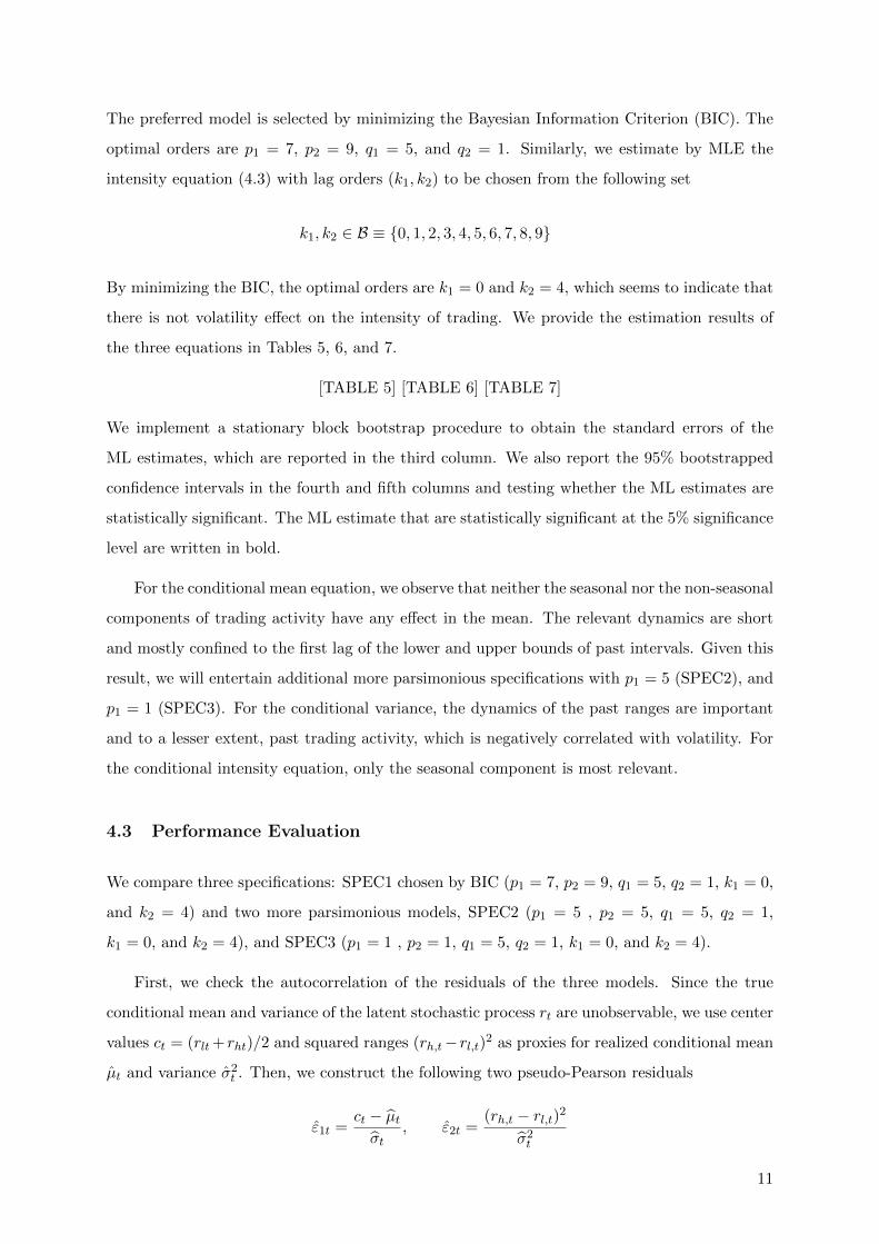
The preferred model is selected by minimizing the Bayesian Information Criterion (BIC). The

optimal orders are p1 = 7, p2 = 9, q1 = 5, and q2 = 1. Similarly, we estimate by MLE the

intensity equation (4.3) with lag orders (k1, k2) to be chosen from the following set

k1, k2 ∈ B ≡ 0, 1, 2, 3, 4, 5, 6, 7, 8, 9

By minimizing the BIC, the optimal orders are k1 = 0 and k2 = 4, which seems to indicate that

there is not volatility effect on the intensity of trading. We provide the estimation results of

the three equations in Tables 5, 6, and 7.

[TABLE 5] [TABLE 6] [TABLE 7]

We implement a stationary block bootstrap procedure to obtain the standard errors of the

ML estimates, which are reported in the third column. We also report the 95% bootstrapped

confidence intervals in the fourth and fifth columns and testing whether the ML estimates are

statistically significant. The ML estimate that are statistically significant at the 5% significance

level are written in bold.

For the conditional mean equation, we observe that neither the seasonal nor the non-seasonal

components of trading activity have any effect in the mean. The relevant dynamics are short

and mostly confined to the first lag of the lower and upper bounds of past intervals. Given this

result, we will entertain additional more parsimonious specifications with p1 = 5 (SPEC2), and

p1 = 1 (SPEC3). For the conditional variance, the dynamics of the past ranges are important

and to a lesser extent, past trading activity, which is negatively correlated with volatility. For

the conditional intensity equation, only the seasonal component is most relevant.

4.3 Performance Evaluation

We compare three specifications: SPEC1 chosen by BIC (p1 = 7, p2 = 9, q1 = 5, q2 = 1, k1 = 0,

and k2 = 4) and two more parsimonious models, SPEC2 (p1 = 5 , p2 = 5, q1 = 5, q2 = 1,

k1 = 0, and k2 = 4), and SPEC3 (p1 = 1 , p2 = 1, q1 = 5, q2 = 1, k1 = 0, and k2 = 4).

First, we check the autocorrelation of the residuals of the three models. Since the true

conditional mean and variance of the latent stochastic process rt are unobservable, we use center

values ct = (rlt+ rht)/2 and squared ranges (rh,t− rl,t)2 as proxies for realized conditional mean

µt and variance σ2t . Then, we construct the following two pseudo-Pearson residuals

ε1t =ct − µtσt

, ε2t =(rh,t − rl,t)2

σ2t

11

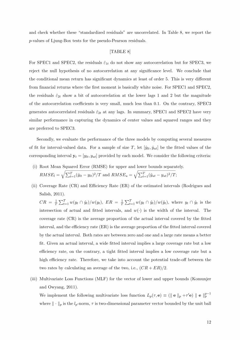
and check whether these “standardized residuals” are uncorrelated. In Table 8, we report the

p-values of Ljung-Box tests for the pseudo-Pearson residuals.

[TABLE 8]

For SPEC1 and SPEC2, the residuals ε1t do not show any autocorrelation but for SPEC3, we

reject the null hypothesis of no autocorrelation at any significance level. We conclude that

the conditional mean return has significant dynamics at least of order 5. This is very different

from financial returns where the first moment is basically white noise. For SPEC1 and SPEC2,

the residuals ε2t show a bit of autocorrelation at the lower lags 1 and 2 but the magnitude

of the autocorrelation coefficients is very small, much less than 0.1. On the contrary, SPEC3

generates autocorrelated residuals ε2t at any lags. In summary, SPEC1 and SPEC2 have very

similar performance in capturing the dynamics of center values and squared ranges and they

are preferred to SPEC3.

Secondly, we evaluate the performance of the three models by computing several measures

of fit for interval-valued data. For a sample of size T , let [ylt, yut] be the fitted values of the

corresponding interval yt = [ylt, yut] provided by each model. We consider the following criteria:

(i) Root Mean Squared Error (RMSE) for upper and lower bounds separately.

RMSEl =√∑T

t=1(ylt − ylt)2/T and RMSEu =√∑T

t=1(yut − yut)2/T ;

(ii) Coverage Rate (CR) and Efficiency Rate (ER) of the estimated intervals (Rodrigues and

Salish, 2011).

CR = 1T

∑Tt=1w(yt ∩ yt)/w(yt), ER = 1

T

∑Tt=1w(yt ∩ yt)/w(yt), where yt ∩ yt is the

intersection of actual and fitted intervals, and w(·) is the width of the interval. The

coverage rate (CR) is the average proportion of the actual interval covered by the fitted

interval, and the efficiency rate (ER) is the average proportion of the fitted interval covered

by the actual interval. Both rates are between zero and one and a large rate means a better

fit. Given an actual interval, a wide fitted interval implies a large coverage rate but a low

efficiency rate, on the contrary, a tight fitted interval implies a low coverage rate but a

high efficiency rate. Therefore, we take into account the potential trade-off between the

two rates by calculating an average of the two, i.e., (CR+ ER)/2.

(iii) Multivariate Loss Functions (MLF) for the vector of lower and upper bounds (Komunjer

and Owyang, 2011).

We implement the following multivariate loss function Lp(τ, e) ≡ (‖ e ‖p +τ ′e) ‖ e ‖p−1p

where ‖ · ‖p is the lp-norm, τ is two-dimensional parameter vector bounded by the unit ball

12

Bq in R2 with lq-norm (where p and q satisfy 1/p+1/q = 1), and e = (el, eu) is the bivariate

residual interval (ylt − ylt, yut − yut). We consider two norms, p = 1 and p = 2 and their

corresponding τ parameter vectors within the unit balls B∞ and B2 respectively, MLF1 =∫τ∈B∞(|el|+ |eu|+ τ1el + τ2eu)dτ , MLF2 =

∫τ∈B2

[e2l + e2

u + (τ1el + τ2eu)(e2l + e2

u)1/2]dτ .

(iv) Mean Distance Error (MDE) between the fitted and actual intervals (Arroyo et al., 2011).

Let Dq(yt, yt) be a distance measure of order q between the fitted and the actual intervals,

the mean distance error is defined as MDEq(yt, yt) = [∑T

t=1Dq(yt, yt)/T ]1/q. We

consider q = 1 and q = 2, with a distance measure such as D(yt, yt) = 1√2[(ylt − ylt)2 +

(yut − yut)2]1/2.

The evaluation results for the three specifications considered are reported in Table 9.

[TABLE 9]

Across the four measures, SPEC1 offers the best fit though it is only marginally better than

SPEC2. Both specifications dominate SPEC3. In summary, SPEC2 (p1 = 5 , p2 = 5, q1 = 5,

q2 = 1, k1 = 0, and k2 = 4) provides a more parsimonious specification than SPEC1 without

sacrificing a good data fit. The following figures offer a visual aspect of the fitting of the data.

Based on the estimation results, we calculate the estimated conditional mean µt, conditional

variance σ2t and conditional intensity λt . In addition, we calculate the estimated expected low

and high returns (rlt and rht) and their corresponding estimated conditional variances (σ2lt and

σ2ht) according to expressions (2.7)- (2.8). The time series of all these estimates and of the actual

values are plotted in Figure 4]

[FIGURE 4]

In Figure 4a, we observe that µt lies very much around the center of the actual intervals. The

estimated expected low and high returns also follow very closely the profiles of the actual low

and high returns. According to their RMSEs, we find a better fit for the upper bounds than

for the lower bounds across the three specifications considered. The average coverage rate is

about 83% and the average efficiency rate about 76%, which is a very good fitting. In Figure

4b, we plot the estimated variance, which shows that there is substantial heteroskedasticity in

the series. The three most prominent bursts of volatility corresponds to those instances where

the ranges of the intervals are the widest. In Figure 4c, we plot the actual number of trades nt

and the estimated intensity λt. Although these two series are not directly comparable, we see

that λt as a measure of the expected number of trades follows very closely the actual number.

13

5 Conclusion

By focusing on the lower and upper bound of an interval as two different stochastic processes,

the current literature on model estimation has ignored the extreme nature of such bounds. Our

main contribution is a modeling approach that exploits such extreme property. At the core,

we have argued that there is only one stochastic process Yt from which the lower and upper

bounds of the intervals (ylt and yut) are the realized extreme observations (minima and maxima)

coming from the nt random draws from the conditional density of the process. A key point is

to understand that the researcher is interested in the characterization of this latent stochastic

process as much as in the modeling of the bounds themselves. This question is important

because there are time series data sets for which the relevant information is only available in

interval format e.g. low/high prices. Yet in these instances, it is of interest to know the expected

price or any other conditional moment of the price process, e.g. variance. skewness, etc. We

have introduced a data set of daily beef prices and sales for which the opening or closing prices

are not reported because they are not very informative to potential sellers and buyers, and

consequently we are restricted to work with the interval low/high prices.

The modelling approach is based on the theory of order statistics. For implementation

purposes, we need to assume a conditional density for the latent stochastic process. We have

assumed normality as a first approximation but this assumption can be refined according to

the researcher’s needs. One advantage of the data set that we have analyzed is that contains

information on the daily number of trades, so that we are able to model the conditional intensity

of trading in addition to the modeling of the conditional mean and variance. The standard

distributional assumption for counts is a Poisson density but we have assumed a more robust

alternative, the Negative Binomial, as it takes into account potential over dispersion of the data.

Given these distributions, we have estimated the model by maximum likelihood. Monte Carlo

simulations indicate that the estimators are well-behaved and, in large samples, they do not

show any apparent biases and they seem to be normally distributed.

The modeling of beef prices shows interesting features. The conditional mean of the corre-

sponding returns exhibits relevant dynamics in contrast to financial returns. The return process

is heteroskedastic and the dynamics of the conditional variance are driven by the range of past

intervals and the past number of trades. The conditional intensity function is mainly driven

by the seasonal component of the number of trades. We have also estimated the expected low

and high returns to construct the fitted intervals. When these are compared with the actual

intervals, we find that the model provides a very good fitting with an average coverage rate of

14

83% and an average efficiency rate of about 76%.

15

References

[1] Anderson, T.W. and Darling, D.A. (1954), “A Test of Goodness-of-Fit,” Journal of the

American Statistical Association. Vol. 49, pp. 765-769.

[2] Arroyo, J., Gonzalez-Rivera, G, and Mate, C. (2011), “Forecasting with Interval and His-

togram Data. Some Financial Applications,” in Handbook of Empirical Economics and

Finance, A. Ullah and D. Giles (eds.). Chapman and Hall, pp. 247-280.

[3] Billard, L., and Diday, E. (2003), “From the statistics of data to the statistics of knowledge:

symbolic data analysis,” Journal of the American Statistical Association. Vol. 98, pp. 470-

487.

[4] Billard, L., and Diday E. (2006), Symbolic Data Analysis: Conceptual Statistics and Data

Mining, 1st ed., Wiley and Sons, Chichester.

[5] Brito, P. (2007), “Modelling and analysing interval data,” Proceedings of the 30th Annual

Conference of GfKl. Springer, Berlin, pp. 197-208.

[6] Gonzalez-Rivera, G., and Lin, W. (2013), “Constrained Regression for Interval-valued

Data,” Journal of Business and Economic Statistics, Vol. 31, No. 4, pp. 473-490.

[7] Jarque, Carlos M.; Bera, Anil K. (1980), “Efficient Tests for Normality, Homoscedasticity

and Serial Independence of Regression Residuals,” Economics Letters. Vol. 6 (3), pp. 255-

259.

[8] Komunjer, I., and Owyang, M. (2012), “Multivariate Forecast Evaluation and Rationality

Testing,” Review of Economics and Statistics. Vol. 94, No. 4, pp. 1066-1080.

[9] Lima Neto, E., and de Carvalho, F. (2010), “Constrained linear regression models for

symbolic interval-valued variables,” Computational Statistics and Data Analysis. Vol. 54,

pp. 333-347.

[10] Newey, W., and MacFadden, D. (1994), “Large Sample Estimation and Hypothesis Test-

ing,” in Handbook of Econometrics, Vol. IV, R. Engle and D. McFadden, (eds.). North

Holland, Amsterdam, pp. 2111-2245.

[11] Rodrigues, P.M.M., and Salish, N. (2014), “Modeling and Forecasting Interval Time Series

with Threshold Models”, Advances in Data Analysis and Classification, pp. 1-17.

[12] Stephens, M. A. (1974), “EDF Statistics for Goodness of Fit and Some Comparisons”

Journal of the American Statistical Association, Vol 69: 730737.

16

[13] White, H. (1994). Estimation, Inference and Specification Analysis. Cambridge University

Press, Cambridge.

[14] Wooldridge, Jeffrey M., (1986). “Estimation and inference for dependent processes,” in

Handbook of Econometrics, R. F. Engle & D. McFadden (ed.) Edition 1, Vol 4, Chapter 45,

pp. 2639-2738 Elsevier.

17

Table 1: Specification of Data Generating Processes

Parameters DGP1 DGP2 DGP3

α0 1 1 1αl1 – 0.6 0.2αh1 – 0.6 0.2αl2 – −0.3 −0.2αh2 – −0.3 −0.2αl3 – – 0.1αh3 – – 0.1αl4 – – −0.1αh4 – – −0.1αl5 – – 0.1αh5 – – 0.1αn1 – 0.6 0.2αn2 – −0.3 −0.2αn3 – – 0.1αn4 – – −0.1αn5 – – 0.1

β0 1 1 1βr1 – 0.6 0.2βr2 – −0.3 −0.2βr3 – – 0.1βr4 – – −0.1βr5 – – 0.1βn1 – 0.6 0.2βn2 – −0.3 −0.2βn3 – – 0.1βn4 – – −0.1βn5 – – 0.1

γ0 5 1 1γr1 – 0.6 0.2γr2 – −0.3 −0.2γr3 – – 0.1γr4 – – −0.1γr5 – – 0.1γn1 – 0.6 0.2γn2 – −0.3 −0.2γn3 – – 0.1γn4 – – −0.1γn5 – – 0.11/d 0.1 0.1 0.1

Sample Size 200/2,000 200/2,000 200/2,000Replications 5,000 5,000 5,000

18

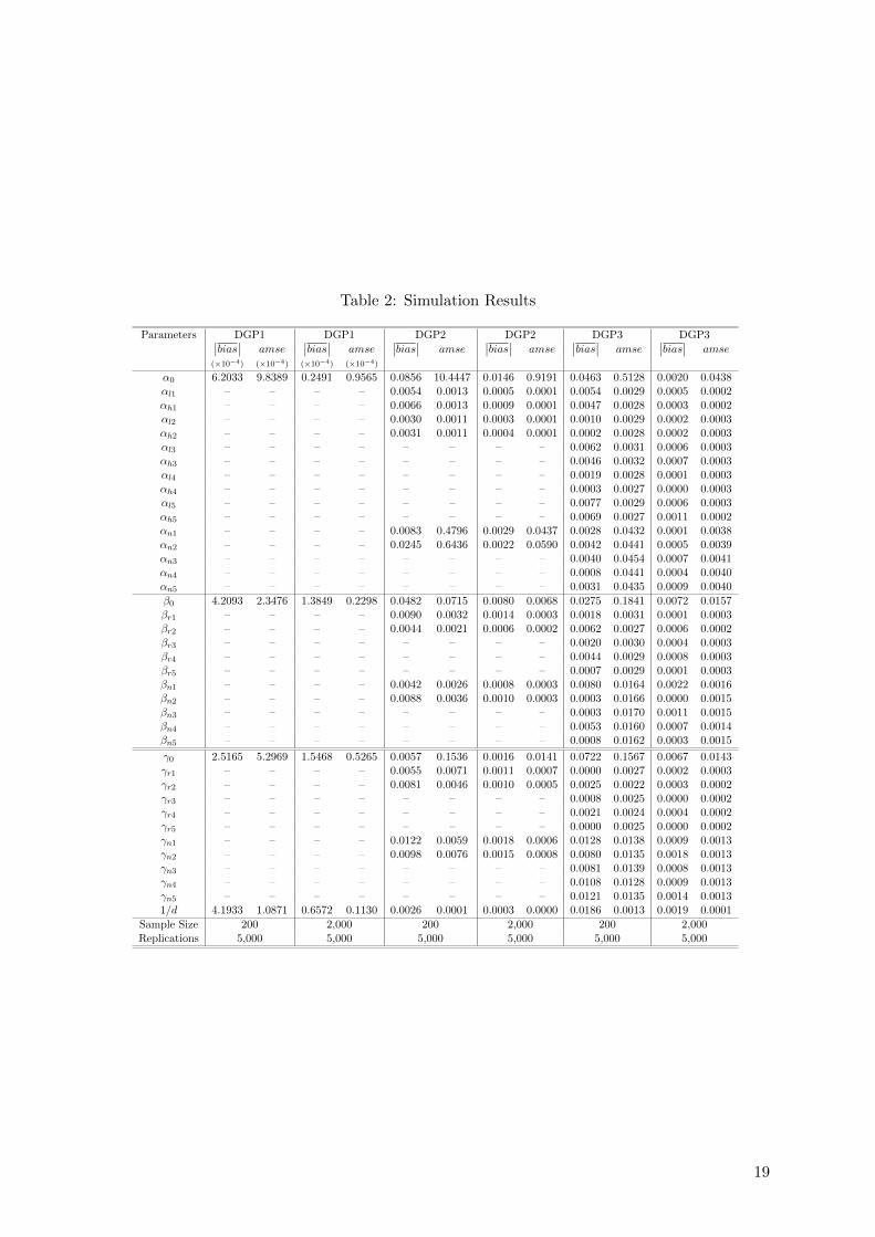
Table 2: Simulation Results

Parameters DGP1 DGP1 DGP2 DGP2 DGP3 DGP3∣∣bias∣∣ amse∣∣bias∣∣ amse

∣∣bias∣∣ amse∣∣bias∣∣ amse

∣∣bias∣∣ amse∣∣bias∣∣ amse

(×10−4) (×10−4) (×10−4) (×10−4)

α0 6.2033 9.8389 0.2491 0.9565 0.0856 10.4447 0.0146 0.9191 0.0463 0.5128 0.0020 0.0438αl1 – – – – 0.0054 0.0013 0.0005 0.0001 0.0054 0.0029 0.0005 0.0002αh1 – – – – 0.0066 0.0013 0.0009 0.0001 0.0047 0.0028 0.0003 0.0002αl2 – – – – 0.0030 0.0011 0.0003 0.0001 0.0010 0.0029 0.0002 0.0003αh2 – – – – 0.0031 0.0011 0.0004 0.0001 0.0002 0.0028 0.0002 0.0003αl3 – – – – – – – – 0.0062 0.0031 0.0006 0.0003αh3 – – – – – – – – 0.0046 0.0032 0.0007 0.0003αl4 – – – – – – – – 0.0019 0.0028 0.0001 0.0003αh4 – – – – – – – – 0.0003 0.0027 0.0000 0.0003αl5 – – – – – – – – 0.0077 0.0029 0.0006 0.0003αh5 – – – – – – – – 0.0069 0.0027 0.0011 0.0002αn1 – – – – 0.0083 0.4796 0.0029 0.0437 0.0028 0.0432 0.0001 0.0038αn2 – – – – 0.0245 0.6436 0.0022 0.0590 0.0042 0.0441 0.0005 0.0039αn3 – – – – – – – – 0.0040 0.0454 0.0007 0.0041αn4 – – – – – – – – 0.0008 0.0441 0.0004 0.0040αn5 – – – – – – – – 0.0031 0.0435 0.0009 0.0040

β0 4.2093 2.3476 1.3849 0.2298 0.0482 0.0715 0.0080 0.0068 0.0275 0.1841 0.0072 0.0157βr1 – – – – 0.0090 0.0032 0.0014 0.0003 0.0018 0.0031 0.0001 0.0003βr2 – – – – 0.0044 0.0021 0.0006 0.0002 0.0062 0.0027 0.0006 0.0002βr3 – – – – – – – – 0.0020 0.0030 0.0004 0.0003βr4 – – – – – – – – 0.0044 0.0029 0.0008 0.0003βr5 – – – – – – – – 0.0007 0.0029 0.0001 0.0003βn1 – – – – 0.0042 0.0026 0.0008 0.0003 0.0080 0.0164 0.0022 0.0016βn2 – – – – 0.0088 0.0036 0.0010 0.0003 0.0003 0.0166 0.0000 0.0015βn3 – – – – – – – – 0.0003 0.0170 0.0011 0.0015βn4 – – – – – – – – 0.0053 0.0160 0.0007 0.0014βn5 – – – – – – – – 0.0008 0.0162 0.0003 0.0015

γ0 2.5165 5.2969 1.5468 0.5265 0.0057 0.1536 0.0016 0.0141 0.0722 0.1567 0.0067 0.0143γr1 – – – – 0.0055 0.0071 0.0011 0.0007 0.0000 0.0027 0.0002 0.0003γr2 – – – – 0.0081 0.0046 0.0010 0.0005 0.0025 0.0022 0.0003 0.0002γr3 – – – – – – – – 0.0008 0.0025 0.0000 0.0002γr4 – – – – – – – – 0.0021 0.0024 0.0004 0.0002γr5 – – – – – – – – 0.0000 0.0025 0.0000 0.0002γn1 – – – – 0.0122 0.0059 0.0018 0.0006 0.0128 0.0138 0.0009 0.0013γn2 – – – – 0.0098 0.0076 0.0015 0.0008 0.0080 0.0135 0.0018 0.0013γn3 – – – – – – – – 0.0081 0.0139 0.0008 0.0013γn4 – – – – – – – – 0.0108 0.0128 0.0009 0.0013γn5 – – – – – – – – 0.0121 0.0135 0.0014 0.00131/d 4.1933 1.0871 0.6572 0.1130 0.0026 0.0001 0.0003 0.0000 0.0186 0.0013 0.0019 0.0001

Sample Size 200 2,000 200 2,000 200 2,000Replications 5,000 5,000 5,000 5,000 5,000 5,000

19

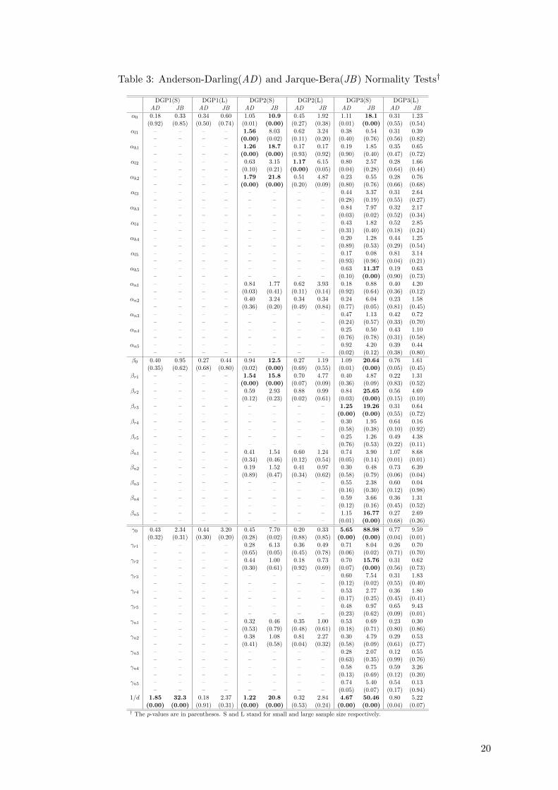
Table 3: Anderson-Darling(AD) and Jarque-Bera(JB) Normality Tests†

DGP1(S) DGP1(L) DGP2(S) DGP2(L) DGP3(S) DGP3(L)AD JB AD JB AD JB AD JB AD JB AD JB

α0 0.18 0.33 0.34 0.60 1.05 10.9 0.45 1.92 1.11 18.1 0.31 1.23(0.92) (0.85) (0.50) (0.74) (0.01) (0.00) (0.27) (0.38) (0.01) (0.00) (0.55) (0.54)

αl1 – – – – 1.56 8.03 0.62 3.24 0.38 0.54 0.31 0.39– – – – (0.00) (0.02) (0.11) (0.20) (0.40) (0.76) (0.56) (0.82)

αh1 – – – – 1.26 18.7 0.17 0.17 0.19 1.85 0.35 0.65– – – – (0.00) (0.00) (0.93) (0.92) (0.90) (0.40) (0.47) (0.72)

αl2 – – – – 0.63 3.15 1.17 6.15 0.80 2.57 0.28 1.66– – – – (0.10) (0.21) (0.00) (0.05) (0.04) (0.28) (0.64) (0.44)

αh2 – – – – 1.79 21.8 0.51 4.87 0.23 0.55 0.28 0.76– – – – (0.00) (0.00) (0.20) (0.09) (0.80) (0.76) (0.66) (0.68)

αl3 – – – – – – – – 0.44 3.37 0.31 2.64– – – – – – – – (0.28) (0.19) (0.55) (0.27)

αh3 – – – – – – – – 0.84 7.97 0.32 2.17– – – – – – – – (0.03) (0.02) (0.52) (0.34)

αl4 – – – – – – – – 0.43 1.82 0.52 2.85– – – – – – – – (0.31) (0.40) (0.18) (0.24)

αh4 – – – – – – – – 0.20 1.28 0.44 1.25– – – – – – – – (0.89) (0.53) (0.29) (0.54)

αl5 – – – – – – – – 0.17 0.08 0.81 3.14– – – – – – – – (0.93) (0.96) (0.04) (0.21)

αh5 – – – – – – – – 0.63 11.37 0.19 0.63– – – – – – – – (0.10) (0.00) (0.90) (0.73)

αn1 – – – – 0.84 1.77 0.62 3.93 0.18 0.88 0.40 4.20– – – – (0.03) (0.41) (0.11) (0.14) (0.92) (0.64) (0.36) (0.12)

αn2 – – – – 0.40 3.24 0.34 0.34 0.24 6.04 0.23 1.58– – – – (0.36) (0.20) (0.49) (0.84) (0.77) (0.05) (0.81) (0.45)

αn3 – – – – – – – – 0.47 1.13 0.42 0.72– – – – – – – – (0.24) (0.57) (0.33) (0.70)

αn4 – – – – – – – – 0.25 0.50 0.43 1.10– – – – – – – – (0.76) (0.78) (0.31) (0.58)

αn5 – – – – – – – – 0.92 4.20 0.39 0.44– – – – – – – – (0.02) (0.12) (0.38) (0.80)

β0 0.40 0.95 0.27 0.44 0.94 12.5 0.27 1.19 1.09 20.64 0.76 1.61(0.35) (0.62) (0.68) (0.80) (0.02) (0.00) (0.69) (0.55) (0.01) (0.00) (0.05) (0.45)

βr1 – – – – 1.54 15.8 0.70 4.77 0.40 4.87 0.22 1.31– – – – (0.00) (0.00) (0.07) (0.09) (0.36) (0.09) (0.83) (0.52)

βr2 – – – – 0.59 2.93 0.88 0.99 0.84 25.65 0.56 4.69– – – – (0.12) (0.23) (0.02) (0.61) (0.03) (0.00) (0.15) (0.10)

βr3 – – – – – – – – 1.25 19.26 0.31 0.64– – – – – – – – (0.00) (0.00) (0.55) (0.72)

βr4 – – – – – – – – 0.30 1.95 0.64 0.16– – – – – – – – (0.58) (0.38) (0.10) (0.92)

βr5 – – – – – – – – 0.25 1.26 0.49 4.38– – – – – – – – (0.76) (0.53) (0.22) (0.11)

βn1 – – – – 0.41 1.54 0.60 1.24 0.74 3.90 1.07 8.68– – – – (0.34) (0.46) (0.12) (0.54) (0.05) (0.14) (0.01) (0.01)

βn2 – – – – 0.19 1.52 0.41 0.97 0.30 0.48 0.73 6.39– – – – (0.89) (0.47) (0.34) (0.62) (0.58) (0.79) (0.06) (0.04)

βn3 – – – – – – – – 0.55 2.38 0.60 0.04– – – – – – – – (0.16) (0.30) (0.12) (0.98)

βn4 – – – – – – – – 0.59 3.66 0.36 1.31– – – – – – – – (0.12) (0.16) (0.45) (0.52)

βn5 – – – – – – – – 1.15 16.77 0.27 2.69– – – – – – – – (0.01) (0.00) (0.68) (0.26)

γ0 0.43 2.34 0.44 3.20 0.45 7.70 0.20 0.33 5.65 88.98 0.77 9.59(0.32) (0.31) (0.30) (0.20) (0.28) (0.02) (0.88) (0.85) (0.00) (0.00) (0.04) (0.01)

γr1 – – – – 0.28 6.13 0.36 0.49 0.71 8.04 0.26 0.70– – – – (0.65) (0.05) (0.45) (0.78) (0.06) (0.02) (0.71) (0.70)

γr2 – – – – 0.44 1.00 0.18 0.73 0.70 15.76 0.31 0.62– – – – (0.30) (0.61) (0.92) (0.69) (0.07) (0.00) (0.56) (0.73)

γr3 – – – – – – – – 0.60 7.54 0.31 1.83– – – – – – – – (0.12) (0.02) (0.55) (0.40)

γr4 – – – – – – – – 0.53 2.77 0.36 1.80– – – – – – – – (0.17) (0.25) (0.45) (0.41)

γr5 – – – – – – – – 0.48 0.97 0.65 9.43– – – – – – – – (0.23) (0.62) (0.09) (0.01)

γn1 – – – – 0.32 0.46 0.35 1.00 0.53 0.69 0.23 0.30– – – – (0.53) (0.79) (0.48) (0.61) (0.18) (0.71) (0.80) (0.86)

γn2 – – – – 0.38 1.08 0.81 2.27 0.30 4.79 0.29 0.53– – – – (0.41) (0.58) (0.04) (0.32) (0.58) (0.09) (0.61) (0.77)

γn3 – – – – – – – – 0.28 2.07 0.12 0.55– – – – – – – – (0.63) (0.35) (0.99) (0.76)

γn4 – – – – – – – – 0.58 0.75 0.59 3.26– – – – – – – – (0.13) (0.69) (0.12) (0.20)

γn5 – – – – – – – – 0.74 5.40 0.54 0.13– – – – – – – – (0.05) (0.07) (0.17) (0.94)

1/d 1.85 32.3 0.18 2.37 1.22 20.8 0.32 2.84 4.67 50.46 0.80 5.22(0.00) (0.00) (0.91) (0.31) (0.00) (0.00) (0.53) (0.24) (0.00) (0.00) (0.04) (0.07)

† The p-values are in parentheses. S and L stand for small and large sample size respectively.

20

Table 4: Descriptive Statistics

low % change high % change # of tradesStatistics (rlt) (rht) (nt)

Minimum −29.000 −2.984 61st Quartile −5.565 3.999 22

Median −3.415 5.832 303rd Quartile −1.604 8.211 40Maximum 24.480 44.750 130

Mean −3.8380 6.3350 31.540Variance 12.7687 11.7219 166.92

Correlation 0.3750 ——–Skewness −0.7585 2.0796 0.8657Kurtosis 11.9538 19.5875 5.9716

Table 5: Estimation Results of Conditional Mean Equation

Conditional Mean Equation

95% C.I.estimate s.e.† lower upper

α0 -1.57 1.82 -5.14 2.31αl1 -0.35 0.04 -0.41 -0.26αl2 0.07 0.03 0.00 0.14αl3 0.06 0.03 -0.01 0.11αl4 0.11 0.03 0.04 0.15αl5 0.03 0.03 -0.04 0.07αl6 0.07 0.03 -0.01 0.11αl7 0.03 0.04 -0.05 0.10αh1 0.22 0.04 0.13 0.28αh2 0.04 0.04 -0.05 0.09αh3 0.02 0.03 -0.04 0.07αh4 -0.01 0.03 -0.08 0.05αh5 0.07 0.03 0.00 0.11αh6 -0.02 0.03 -0.07 0.04αh7 -0.03 0.03 -0.08 0.03αn1 0.18 0.21 -0.29 0.52αn2 0.12 0.17 -0.29 0.40αn3 0.19 0.16 -0.24 0.40αn4 -0.14 0.17 -0.37 0.32αn5 0.31 0.41 -0.67 0.86αn6 -0.44 0.23 -0.78 0.11αn7 0.47 0.22 -0.15 0.74αn8 -0.08 0.20 -0.43 0.38αn9 0.46 0.22 -0.11 0.75s1µ -0.30 0.38 -0.79 0.64s2µ 0.25 0.23 -0.22 0.69s3µ -0.29 0.20 -0.52 0.29†Standard errors are obtainedby stationary block bootstrap-ping.

21

Table 6: Estimation Results of Conditional Variance Equation

Conditional Variance Equation

95% C.I.estimate s.e.† lower upper

β0 -0.43 0.39 -1.15 0.34βr1 0.42 0.08 0.28 0.56βr2 0.08 0.04 -0.01 0.15βr3 0.08 0.05 0.00 0.18βr4 0.09 0.03 0.01 0.14βr5 0.12 0.05 -0.01 0.20βn1 -0.10 0.06 -0.2 0.02s1σ -0.21 0.09 -0.37 -0.04s2σ 0.02 0.07 -0.11 0.15s3σ -0.11 0.07 -0.20 0.07†Standard errors are obtainedby stationary block bootstrap-ping.

Table 7: Estimation Results of Conditional Intensity Equation

Conditional Intensity Equation

95% C.I.estimate s.e.† lower upper

γ0 1.01 0.25 1.05 1.97γn1 -0.04 0.03 -0.07 0.02γn2 -0.04 0.02 -0.08 0.00γn3 0.02 0.02 -0.03 0.05γn4 0.08 0.02 0.02 0.12s1λ 0.37 0.03 0.30 0.42s2λ 0.18 0.04 0.05 0.20s3λ 0.11 0.03 -0.02 0.111/d 0.10 0.01 0.10 0.14†Standard errors are obtainedby stationary block bootstrap-ping.

22

Table 8: Ljung-Box Tests for pseudo-Pearson Residuals ε1t and ε2t

ε1t (p-values) ε2t (p-values)lags SPEC1 SPEC2 SPEC3 lags SPEC1 SPEC2 SPEC3

1 0.60 0.62 0.12 1 0.01 0.01 0.002 0.82 0.74 0.00 2 0.02 0.01 0.003 0.88 0.88 0.00 3 0.04 0.03 0.014 0.95 0.95 0.00 4 0.08 0.06 0.025 0.98 0.96 0.00 5 0.14 0.10 0.046 0.99 0.76 0.00 6 0.21 0.15 0.077 0.96 0.75 0.00 7 0.23 0.17 0.088 0.98 0.75 0.00 8 0.11 0.08 0.049 0.81 0.50 0.00 9 0.12 0.08 0.0410 0.87 0.60 0.00 10 0.14 0.10 0.0511 0.61 0.45 0.00 11 0.12 0.08 0.0412 0.67 0.52 0.00 12 0.15 0.10 0.0513 0.73 0.58 0.00 13 0.12 0.08 0.0414 0.69 0.53 0.00 14 0.11 0.07 0.0415 0.75 0.60 0.00 15 0.08 0.05 0.0316 0.78 0.61 0.00 16 0.09 0.06 0.0317 0.71 0.49 0.00 17 0.11 0.08 0.0418 0.76 0.54 0.00 18 0.14 0.10 0.0619 0.61 0.41 0.00 19 0.18 0.13 0.0820 0.66 0.47 0.00 20 0.22 0.16 0.10

Table 9: Measures of Goodness of Fit

RMSE CR & ER MLF MDE

Lower Upper CR ER CR+ER2 p = 1 p = 2 q = 1 q = 2

Spec 1 3.3226 2.8191 0.8388 0.7648 0.8018 4.5586 18.9874 2.5054 3.0812Spec 2 3.3385 2.8397 0.8385 0.7624 0.8005 4.5903 19.2095 2.5204 3.0992Spec 3 3.4431 2.8886 0.8356 0.7568 0.7962 4.7041 20.1987 2.5808 3.1779

23

0 200 400 600 800

400

500

600

700

800 High Price

Weighted AverageLow Price

(a) Daily Low and High Prices, and Weighted Average Price

0 200 400 600 800

2040

6080

100

120

Number of Trades

(b) Daily Number of Trades

0 200 400 600 800

-20

020

40

High Percentage ChangeLow Percentage Change

(c) Daily Low and High Returns

Figure 1: Daily Prices and Returns and Number of Trades

24

0 5 10 15 20 25 30

0.0

0.2

0.4

0.6

0.8

1.0

Lag

ACF

rlt

0 5 10 15 20 25 30

-0.15

-0.05

0.05

0.15

Lag

Par

tial A

CF

rlt

0 5 10 15 20 25 30

0.0

0.2

0.4

0.6

0.8

1.0

Lag

ACF

rht

0 5 10 15 20 25 30

-0.05

0.05

0.10

0.15

0.20

Lag

Par

tial A

CF

rht

Figure 2: ACF and PACF of Low/High Daily Returns

0 5 10 15 20 25 30

0.0

0.4

0.8

Lag

ACF

log(nt)

0 5 10 15 20 25 30

-0.1

0.1

0.3

0.5

Lag

Par

tial A

CF

log(nt)

Figure 3: ACF and PACF of Logarithm of Number of Trades

25

0 200 400 600 800

-20

020

40

Actual HighActual LowEst.HighEst.MeanEst.Low

(a) Estimated Daily Returns: µt, rlt, rht

0 200 400 600 800

05

1015

2025

30

Est.Variance

(b) Estimated Variance: σ2t

0 200 400 600 800

2040

6080

100

120

# of TradesEst. Intensity

(c) Estimated Intensity: λt

Figure 4: Estimated Conditional Mean/Variance/Intensity

26