Intersection Graphs and Geometric Objects in the Plane vorgelegt von M. Sc. Mathematik Udo Hoffmann geb. in Mönchengladbach Von der Fakultät II – Mathematik und Naturwissenschaften der Technischen Universität Berlin zur Erlangung des akademischen Grades Doktor der Naturwissenschaften – Dr. rer. nat. – genehmigte Dissertation Promotionsausschuss Vorsitzender: Prof. Dr. Boris Springborn Berichter: Prof. Dr. Stefan Felsner Prof. Dr. Wolfgang Mulzer Prof. Jean Cardinal Tag der wissenschaftlichen Aussprache: 24. März 2016 Berlin 2016

Welcome message from author
This document is posted to help you gain knowledge. Please leave a comment to let me know what you think about it! Share it to your friends and learn new things together.
Transcript
Intersection Graphs and GeometricObjects in the Plane
vorgelegt vonM. Sc. Mathematik
Udo Hoffmanngeb. in Mönchengladbach
Von der Fakultät II – Mathematik und Naturwissenschaftender Technischen Universität Berlin
zur Erlangung des akademischen Grades
Doktor der Naturwissenschaften– Dr. rer. nat. –
genehmigte Dissertation
Promotionsausschuss
Vorsitzender: Prof. Dr. Boris SpringbornBerichter: Prof. Dr. Stefan Felsner
Prof. Dr. Wolfgang MulzerProf. Jean Cardinal
Tag der wissenschaftlichen Aussprache: 24. März 2016
Berlin 2016


Acknowledgements
This work was mainly done in the Diskrete Mathematik working group. I would liketo thank all current and former members, I had the pleasure of working and discussingwith. We had a nice working atmosphere. Many thanks to: Stefan Felsner, Linda Kleist,Veit Wiechert, Nieke Aerts, Steven Chaplick, Piotr Micek, Irina Mustaţă, Daniel Heldt,Thomas Hixon, and Kolja Knauer.Especially, thanks to Stefan, for always giving advice how to improve my work, andfor always giving the possibility to talk to.I want to thank Jean Cardinal for hosting me in Brussels, and giving many ideas forthe second part of this thesis.Many thanks to Linda, Veit, Steven, and Axel for proofreading parts of this work.I want to mention that this work had not been possible without the funding of theDFG research training group Methods for Discrete Structures.Finally, I want to thank Stefan, Jean, and Wolfgang Mulzer for agreeing to read thisthesis.
Thank you!Udo

Contents
What is this thesis about? 1
0. Notations and definitions 50.1. Graphs . . . . . . . . . . . . . . . . . . . . . . . . . . . . . . . . . . . . . 5
0.1.1. Graph drawings . . . . . . . . . . . . . . . . . . . . . . . . . . . . 60.1.2. Intersection graphs in the plane . . . . . . . . . . . . . . . . . . . 70.1.3. Visibility graphs . . . . . . . . . . . . . . . . . . . . . . . . . . . 8
0.2. Partial orders . . . . . . . . . . . . . . . . . . . . . . . . . . . . . . . . . 90.3. Complexity theory . . . . . . . . . . . . . . . . . . . . . . . . . . . . . . 100.4. Projective geometry . . . . . . . . . . . . . . . . . . . . . . . . . . . . . 120.5. (Abstract) order types and (pseudo)line arrangements. . . . . . . . . . . 130.6. Geometry and topology . . . . . . . . . . . . . . . . . . . . . . . . . . . 15
I. Combinatorial properties of intersection graphs 17
1. The dimension of bipartite intersection graphs 191.1. Background of subclasses of grid intersection graphs. . . . . . . . . . . . 19
1.1.1. Definitions of subclasses of grid intersection graphs . . . . . . . . 201.2. Containment relations between the classes . . . . . . . . . . . . . . . . . 231.3. Dimension . . . . . . . . . . . . . . . . . . . . . . . . . . . . . . . . . . . 271.4. Vertex-edge incidence posets . . . . . . . . . . . . . . . . . . . . . . . . . 301.5. Separating examples . . . . . . . . . . . . . . . . . . . . . . . . . . . . . 35
1.5.1. 4-dimensional graphs . . . . . . . . . . . . . . . . . . . . . . . . 361.5.2. Constructions . . . . . . . . . . . . . . . . . . . . . . . . . . . . 381.5.3. Stabbability . . . . . . . . . . . . . . . . . . . . . . . . . . . . . . 43
1.6. The dimension of bipartite segment intersection graphs . . . . . . . . . . 49
2. The slope number of segment intersection graphs 532.1. Background . . . . . . . . . . . . . . . . . . . . . . . . . . . . . . . . . . 542.2. Segment intersection graphs and Hamiltonian paths . . . . . . . . . . . . 542.3. Behavior of the slope number . . . . . . . . . . . . . . . . . . . . . . . . 612.4. Computational complexity . . . . . . . . . . . . . . . . . . . . . . . . . . 65
i
Contents
2.5. Odd slope number and bipartite graphs . . . . . . . . . . . . . . . . . . 72
II. Realizability problems and the existential theory of the reals 77
3. Realizability of circular sequences 793.1. Background . . . . . . . . . . . . . . . . . . . . . . . . . . . . . . . . . . 793.2. Arithmetics with order types . . . . . . . . . . . . . . . . . . . . . . . . 803.3. The reduction for circular sequences . . . . . . . . . . . . . . . . . . . . 813.4. Realizable order types with non-realizable circular sequences . . . . . . . 86
4. Slopes of segment intersection graphs revisited 97
5. Recognition of point visibility graphs 1015.1. Background . . . . . . . . . . . . . . . . . . . . . . . . . . . . . . . . . . 1015.2. Point visibility graphs preserving collinearities . . . . . . . . . . . . . . . 1025.3. ∃R-completeness of PVG recognition . . . . . . . . . . . . . . . . . . . . 1055.4. Point visibility graphs on a grid . . . . . . . . . . . . . . . . . . . . . . . 107
5.4.1. Irrational coordinates . . . . . . . . . . . . . . . . . . . . . . . . 1075.4.2. Large grid size . . . . . . . . . . . . . . . . . . . . . . . . . . . . 1085.4.3. Recognition of point visibility graphs on a grid . . . . . . . . . . 109
6. The planar slope number 1136.1. Background . . . . . . . . . . . . . . . . . . . . . . . . . . . . . . . . . . 1136.2. Computational complexity . . . . . . . . . . . . . . . . . . . . . . . . . . 113
7. Open problems, questions, conjectures 117
Bibliography 118
Abstract 127
Zusammenfassung 129
ii
What is this thesis about?
This thesis deals with geometric representations of graphs in the plane. Three mainproblems connected with geometric representations of graphs are:
• Which graphs admit a certain representation? (Characterization problem)
• Does a given graph admit a representation of a certain type? (Recognition prob-lem)
• How complex are the representations?
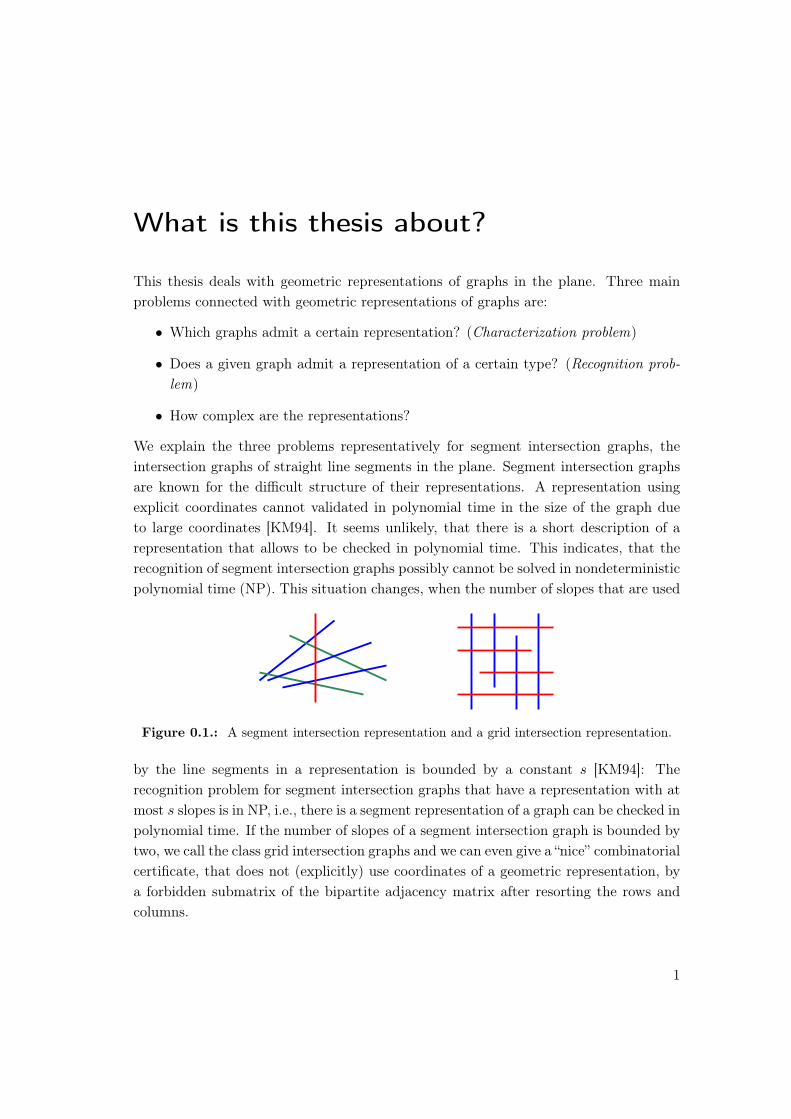
We explain the three problems representatively for segment intersection graphs, theintersection graphs of straight line segments in the plane. Segment intersection graphsare known for the difficult structure of their representations. A representation usingexplicit coordinates cannot validated in polynomial time in the size of the graph dueto large coordinates [KM94]. It seems unlikely, that there is a short description of arepresentation that allows to be checked in polynomial time. This indicates, that therecognition of segment intersection graphs possibly cannot be solved in nondeterministicpolynomial time (NP). This situation changes, when the number of slopes that are used
Figure 0.1.: A segment intersection representation and a grid intersection representation.
by the line segments in a representation is bounded by a constant s [KM94]: Therecognition problem for segment intersection graphs that have a representation with atmost s slopes is in NP, i.e., there is a segment representation of a graph can be checked inpolynomial time. If the number of slopes of a segment intersection graph is bounded bytwo, we call the class grid intersection graphs and we can even give a “nice” combinatorialcertificate, that does not (explicitly) use coordinates of a geometric representation, bya forbidden submatrix of the bipartite adjacency matrix after resorting the rows andcolumns.
1

In the first part of this thesis, we work with graph representations that have a combi-natorial description, while the second part deals with the existential theory of the reals(∃R), a complexity class, which is connected to “complex” geometric representations.
In Chapter 1, we point out a connection of the order dimension of partial orders togrid intersection graphs that are comparability graphs the partial orders. We show, thatthe order dimension of grid intersection graphs is bounded by four. This observation isused to study the containment relation on many subclasses of grid intersection graphs.We argue that the order dimension is a useful tool for this purpose. We also show thatthe order dimension of bipartite intersection graphs of segments is not bounded, but wecan give an upper bounds on the dimension that is linear in the number of slopes thatis used in the representation. This leads to the study of the slope number of segmentintersection graphs, the minimal number k, such that there is a segment intersectionrepresentation using k slopes.
In Chapter 2, we construct a class of intersection graphs of segments from planar graphs(with Hamiltonian path). The slope number of these segments intersection graphs is twoif and only if the planar graph has a Hamiltonian cycle. We show that the Hamiltoniancycle problem in planar triangulations is NP-complete, even if a Hamiltonian path isgiven. This way we prove, that computing the slope number of a segment intersectiongraph is NP-hard. We use this connection to show that the slope number of a graphdoes not change “continuously”: The slope number may drop from a linear number innumber of vertices down to two, upon the removal of a single vertex.
Chapter 3, the beginning of the second part, deals with the realizability of circularsequences. Mnëv [Mnë88] has shown that for each semialgebraic set S, there is an ordertype (combinatorial descriptions of point sets), that has a realization space with the“the same geometric structure” as S. A consequence of this result is, that deciding therealizability of an order type is as hard as deciding the emptiness of a semialgebraicset. This problem is complete in the existential theory of the reals. We give a modifiedproof for this complexity result. Our modified proof allows to show, that deciding therealizability of a circular sequence of an order type is complete in ∃R, even if the ordertype is realizable and a realization is given.
In Chapter 4, we use the proof we presented in Chapter 3 to show, that determiningthe slope number of a segment intersection graph is hard in ∃R.In Chapter 5, we use the hardness result for circular sequences from Chapter 3 to showthat the recognition problem of point visibility graphs is hard in the existential theoryof the reals. We also show that there are point visibility graphs that have at least oneirrational coordinate in each representation. We show that deciding the existence ofa representation with rational coordinates is possibly undecidable, depending on the(un)decidability of the “existential theory of the rationals”.
2

Chapter 6 deals with the planar slope number of planar graphs. The planar slopenumber of a planar graph G is defined as the minimum number k, such that G hasa straight line drawing with k slopes used for drawing the edges. We show that thisproblem is also hard in the existential theory of the reals, and point out consequencesfor drawings that minimize the planar slope number.We conclude by pointing out some open questions that appeared in this thesis inChapter 7.
3

0. Notations and definitions
0.1. Graphs
Throughout this thesis we use the following notations.By G = (V ;E) we denote a graph G on the vertex set V with edges E ⊆
(V2
). Usually
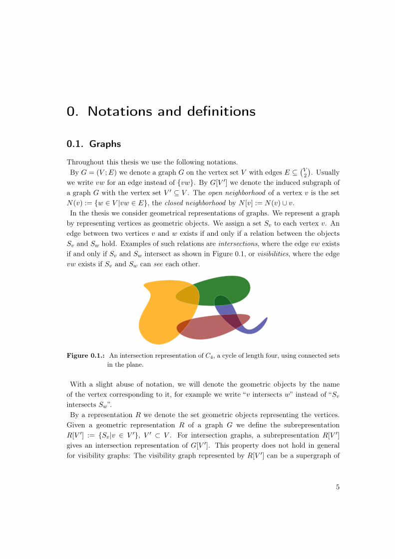
we write vw for an edge instead of vw. By G[V ′] we denote the induced subgraph ofa graph G with the vertex set V ′ ⊆ V . The open neighborhood of a vertex v is the setN(v) := w ∈ V |vw ∈ E, the closed neighborhood by N [v] := N(v) ∪ v.In the thesis we consider geometrical representations of graphs. We represent a graphby representing vertices as geometric objects. We assign a set Sv to each vertex v. Anedge between two vertices v and w exists if and only if a relation between the objectsSv and Sw hold. Examples of such relations are intersections, where the edge vw existsif and only if Sv and Sw intersect as shown in Figure 0.1, or visibilities, where the edgevw exists if Sv and Sw can see each other.
Figure 0.1.: An intersection representation of C4, a cycle of length four, using connected setsin the plane.
With a slight abuse of notation, we will denote the geometric objects by the nameof the vertex corresponding to it, for example we write “v intersects w” instead of “Sv
intersects Sw”.By a representation R we denote the set geometric objects representing the vertices.Given a geometric representation R of a graph G we define the subrepresentationR[V ′] := Sv|v ∈ V ′, V ′ ⊂ V . For intersection graphs, a subrepresentation R[V ′]
gives an intersection representation of G[V ′]. This property does not hold in generalfor visibility graphs: The visibility graph represented by R[V ′] can be a supergraph of
5
0. Notations and definitions
G[V ′], because the objects of R[V \ V ′] may have blocked visibilities between objects ofR[V ′] in the original representation R[V ]. An induced subgraph of a visibility graph isnot necessarily a visibility graph again. For example an independent set is not a visibil-ity graph (with the usual definitions of visibility), since a non-edge requires a blockedvisibility, which requires another vertex which is seen instead.The two main graph classes we study in this thesis are segment intersection graphs andpoint visibility graphs in the plane. In the rest of this section we give an overview onrepresentations of graphs that are used in this thesis.
0.1.1. Graph drawings
We discuss “classical” drawings of graphs: The vertices of a graph are represented aspoints and the edges as curves between the incident vertices. Such a drawing is astraight-line drawing if the curves representing the edges are line segments.We call a drawing planar if it has a drawing with non-crossing edges. A planar drawingis outerplanar if all vertices are incident to the unbounded face.Outerplanar graphs are exactly the graphs that have a 1-page book embedding, a planardrawing where all points lie in one line ` and the edges lie in one half-space that isbounded by `. In general, a k-page book embedding of a graph G is an ordering of thevertices along with the partition of the edges into k sets, such that each of the k setshas a 1-page book embedding with the given vertex ordering. This can be seen as adrawing of a graph with the vertices on the spine of a book, where the edges of one ofthe k blocks are drawn on only one page of the book.
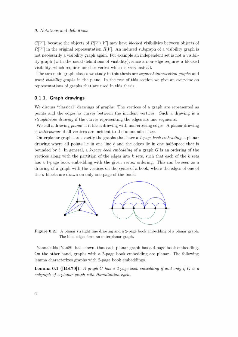
Figure 0.2.: A planar straight line drawing and a 2-page book embedding of a planar graph.The blue edges form an outerplanar graph.
Yannakakis [Yan89] has shown, that each planar graph has a 4-page book embedding.On the other hand, graphs with a 2-page book embedding are planar. The followinglemma characterizes graphs with 2-page book embeddings.
Lemma 0.1 ([BK79]). A graph G has a 2-page book embedding if and only if G is asubgraph of a planar graph with Hamiltonian cycle.
6

0.1. Graphs
0.1.2. Intersection graphs in the plane
While every graph can be represented as intersection graph of a collection of general setswe focus on subclasses of intersection graphs of connected sets in the plane, which oftenhave a rich structure from connections to planarity. The most general class here is theclass of string graphs, the intersection graphs of curves in the plane. This is equivalentto the intersection graph of connected regions. Not every graph is a string graph. Aclass of non-string graphs is given by full subdivisions (every edge is subdivided) ofnon-planar graphs [EET76].
Lemma 0.2 ([Sin66, HNZ91]). The full subdivision PG of a graph G is a string graphif and only if G is planar. If G is planar then PG is even a segment contact graph ofhorizontal and vertical segments.
A graph G that has a string representation, such that each pair of curves intersects atmost once, then G is called pseudosegment intersection graph.A contact graph is a special kind of intersection graphs where the sets are interiorlydisjoint. The existence of a segment contact representation of PG for planar G followsfrom the following more general theorem.
Lemma 0.3 ([HNZ91]). A planar bipartite graph is a segment contact graph of ver-tical and horizontal segments.
Such a contact representation of PG for a planar graph G can also be considered as weakbar visibility representation, where the vertices are represented by vertical segments andthe edges by horizontal segments (sight lines). If the lower endpoint of each verticalsegment lies on a common horizontal line we call the representation a weak semi-barvisibility representation.
Lemma 0.4. A graph G has a weak semi-bar visibility representation if and only if Gis outerplanar.
The semi-bar visibility representations of a graph G have a close connection to 1-page book embeddings: The possible orders of the semi-bars coincide with the order ofvertices in a 1-page book embedding. Those orders are the possible (cyclic) orders ofthe outer-face cycle in an outerplanar drawing.A large part of this thesis deals with segment intersection graphs (SEG) the inter-section graphs of line segments in the plane. We consider only SEG representationswithout intersections of parallel segments. Those representations are often called purerepresentations. Every SEG graph has a pure representation. We denote the class ofgraphs with a pure representation using at most k directions/slopes is denoted by k-dir.
7

0. Notations and definitions
The class of graphs that can be realized using a prescribed set of slopes α1, . . . , αk isdenoted by k-dir(α1, . . . , αk). The class of graphs that can be represented by the slopesα1, . . . , αk and β1, . . . , βk is the same if and only if the directions can be transformedinto each other by a linear transformation [ČKNP02]. This is always possible for k ≤ 3.For larger k, we can pick three directions, say α1, α2, α3, and map them on arbitraryother directions β1, β2, β3 by a linear transformation. The image of all other directionsis determined by the choice of this maps.Pure 2-dir representations (grid intersection representations) have a simple combina-torial description using its bipartite adjacency matrix.
Lemma 0.5 ([HNZ91]). A bipartite graph G is a grid intersection graph if and onlyif its bipartite adjacency matrix has a cross-free ordering, i.e., an ordering of the rowsand columns, such that the matrix does not contain a submatrix of the following kind: 1
1 0 1
1
.
For general SEG representations no simple combinatorial characterization is known.Many properties of segment intersection graphs are easier to show, when we can fixa segment representation. A tool that allows us to construct a graph from a segmentrepresentation, such that each representation of the graph contains a copy of the oldrepresentation, is given by the following lemma.
Lemma 0.6 (order forcing lemma, [KM94]). Let R be a simple segment represen-tation of a graph G. There exists a segment intersection graph GR on O(|V (G)|2)
vertices, such that any segment representation of GR contains a copy of the segmentrepresentation R. Moreover, GR has a segment representation using s slopes (s ≥ 2) ifand only if G can be realized using at most s slopes. The graph GR can be constructedfrom R in polynomial time.
0.1.3. Visibility graphs
Next to bar- and semi-bar visibility representations, we consider point visibility graphs.Given a set of objects S in the plane, we say two objects p and q in the plane seeeach other if there is a lines segment that intersects exactly p and q. The edges ofthe visibility graph of S are the pairs of objects in S that can see each other. A pointvisibility graph is a graph that is the visibility graph of some point set. For an overviewon different visibility graphs considered in literature we refer to Chapter 5.
8
0.2. Partial orders
0.2. Partial orders
A partially ordered set (poset) P = (X,≤P ) is a binary relation that is
• reflexive: a ≤P a for all a ∈ X,
• antisymmetric: a ≤P b and b ≤P a implies a = b for all a, b ∈ X,
• transitive: a ≤P b and b ≤P c implies a ≤P c for all a, b, c ∈ X.
Two elements a and b are comparable if a ≤P b or b ≤P a. The incomparable pairsinc(P ) of P are all pairs (a, b) ∈ X ×X that are not comparable. The set of maximaMax(P ) is the set of elements x with no y such that x <P y. Similarly, the set ofminima Min(P ) is defined.A linear order L = (X,≤L) on X is a linear extension of P when x ≤P y impliesx ≤L y. A family R of linear extensions of P is a realizer of P if P =
⋂i∈R Li, i.e.,
x ≤P y if and only if x ≤L y for every L ∈ R. The dimension of P , denoted dim(P ),is the minimum size of a realizer of P . This notion of dimension for partial orders wasdefined by Dushnik and Miller [DM41]. The dimension of P can also be defined asthe minimum t, such that P admits an order preserving embedding into the dominanceorder on Rt, i.e., we can associate a vector x = (x1, . . . , xt) ∈ Rt with each elementx ∈ X, such that X ≤P y if and only if xi ≤ yi for i = 1, . . . , t. We denote this order onvectors as the dominance order and denote it by x ≤dom y. We can construct t linearextensions from an embedding of the order in Rt by the orthogonal projection of thepoints onto the t coordinate axes.A poset can be considered as a directed graph. The undirected graph we obtain bydropping the orientation of the edges is called the comparability graph. In this thesis weconsider mainly bipartite posets or posets of height 2, which are the posets where eachelement is minimum or maximum. Equivalently, bipartite posets are the posets withbipartite comparability graph. For a bipartite graph G = (A,B;E), we define the posetQG where A = Max(QG) and B = Min(QG) and a > b if a ∈ A, b ∈ B and ab ∈ E.An interval order is a partial order P = (X,≤P ) admitting an interval representation,i.e., a mapping x→ [ax, bx] from the elements of P to intervals in R such that x ≤P y
iff bx ≤ ay. The interval dimension of P , denoted idim(P ), is the minimum number tsuch that there exist t interval orders Ii with P =
⋂ti=1 Ii. Equivalently, the interval
dimension can be defined as the smallest t, such that P is represented as dominanceorder of boxes (the Cartesian product of the different intervals of one element) in Rt.Since every linear order is an interval order idim(P ) ≤ dim(P ) for all P . If P isbipartite, then dimension and interval dimension differ by at most one, i.e., dim(P ) ≤idim(P ) + 1, [Tro92, p.47].
9
0. Notations and definitions
For the sake of brevity we define the dimension of a bipartite graph G to be equal tothe dimension of QG. The freedom that we have in defining QG, i.e., the choice of thecolor classes, does not affect the dimension. This is an easy instance of the fact thatdimension is a comparability invariant (see [TMS76]).The prime example for (bipartite) posets of large dimension is the standard example Snof dimension n, the poset QG, where G is the complete bipartite Kn,n with one perfectmatching removed [Tro92, p.12].
0.3. Complexity theory
In this section we remind the reader of some widely known concepts in complexitytheory and give a short introduction on some infrequently used complexity classes. Foran overview we refer to [AB09].By P we denote the class of problems that can be solved by algorithms in polynomialtime in the input size by a touring machine. Problems that lie in the complexity classNP are those that can be solved in nondeterministic polynomial time, i.e., a givensolution (a certificate) of the problem can be verified by an algorithm in polynomialtime.Next to these classic complexity classes, we consideration is the existential theory ofthe reals, which we abbreviate by ∃R. The existential theory of the reals is characterizedby the following problem: Given a quantifier-free formula F (x1, . . . , xn) using the num-bers 0 and 1, addition and multiplication operations, strict and non-strict comparisonoperators, Boolean operators, and the variables x1, . . . , xn and we are asked whetherthere exists an assignment of real values to x1, . . . , xn, such that F is satisfied. Thisamounts to deciding, whether a system of polynomial inequalities admits a solution overthe reals.It is known from the Tarski-Seidenberg Theorem that ∃R (and even a more generalclass, the first-order theory over a real closed field) is decidable. Only much morerecently, a polynomial space (PSPACE) algorithm for problems in ∃R has been proposedby Canny [Can88].We call a problem complete in ∃Rif it is polynomially equivalent to a ∃R-completeproblem.Some geometric problems have been shown to be complete in ∃R, many based on thefundamental work by Mnëv [Mnë88]. The notation ∃R has been proposed more recentlyby Schaefer [Sch09].Some geometric problems ∃R-complete (resp. hard for optimization problems) include.
• abstract order type realizability/stretchability of pseudoline arrangements [Mnë88],
10

0.3. Complexity theory
• recognition of segment intersection graphs [KM94],
• computing the rectilinear (straight line) crossing number of a graph [Bie91],
• algorithmic Steinitz problem [RGZ95],
• recognition of unit distance graphs and realizability of planar linkages [Sch12],
• simultaneous geometric (i.e., straight line) graph embedding [Kyn11],
• recognition of d-dimensional Delauney triangulations [APT14].
The following “non-geometrical” decision problems are also complete in ∃R.
• solvability of a strict polynomial inequality system,
• solvability of a polynomial equation in several variables.
For some of the geometric problems above, the question for a representation on the grid(i.e., with integer coordinates) arises. For polytopes and order types the complexity ofthis is a longstanding open problem [Stu87]: Asking for integer solutions to the formulawhich certify a problem to be hard in ∃R do not capture that a rational solution leadsto a representation on the integer grid by scaling. Thus, a representation on the integergrid exists if we find a rational solution. Similar to ∃R we denote the existential theoryof the rationals by ∃Q. The decidability of ∃Q is a longstanding open problem. Effortshave been made to define the integers via rational logic. For example Poonen [Poo09]characterized the integers using a formula with only two universal quantifiers. Eliminat-ing those quantifiers would imply that the computational complexity of the existentialtheory of the integers and the rationals is polynomially equivalent.Furthermore, we use the notion of decidablility. Roughly speaking, a decision problemis decidable if there exists an algorithm that solves the problem and terminates after afinite number of steps. We call an algorithm that terminates after a finite number ofsteps and always gives the correct answer to a decision problem an effective algorithm.If there is no effective algorithm for a problem it is called undecidable. Some of the mostprominent examples of undecidable problems are
• the halting problem, which asks whether a program will terminate or run foreveron a given input,
• Hilbert’s tenth problem, which asks whether a Diophantine equation, i.e., a poly-nomial equation in several variables, has a solution over the integers.
11
0. Notations and definitions
Both problems above are positive semi-decidable: If “yes” instances of the problems aregiven there exists an algorithm gives the correct answer after a finite number of steps.For example, a given polynomial equation can be checked for roots in the integers bytesting combinations of integers with an absolute value that is bounded by a constantM . Increasing M after testing all combinations leads to an algorithm that finds asolution after a finite number of steps. However, we cannot give an upper bound on theconstant M and thus the algorithm cannot correctly answer “no”.
0.4. Projective geometry
For many geometric problems it is useful to use projective geometry instead of Euclideangeometry. We refer to [RG11] for further reading. A projective plane satisfies thefollowing axioms:
1. Any two distinct points are contained in exactly one line.
2. Any two distinct lines intersect in exactly one point.
3. There are four points such that no line is incident to more than two points.
We call a map f a projective transformation if it preserves point-line incidences, i.e.,each line `, which is spanned by two points p and q, is mapped onto the line spannedby f(p) and f(q).We will use two models for the real projective plane, the extended Euclidean plane andhomogeneous coordinates.For the extended Euclidean plane, we add a new point at infinity for each class ofparallel lines. Parallel lines intersect in this point. The new points lie on the line atinfinity.A way to give coordinates to the extended Euclidean plane are homogeneous coordi-nates: We consider points as 1-dimensional subspaces of the vector space R3. A linethrough two distinct points is represented by the 2-dimensional subspace containing thetwo points/subspaces. In this model, projective transformations correspond exactly tolinear transformations of R3.To obtain “a plane” from homogeneous coordinates we consider an affine plane A thatdoes not intersect the origin. We consider the intersection of the points and lines withA. The 1-dimensional subspaces (points), that are not parallel to A, intersect A ina point. The 2-dimensional subspaces (lines), that are not parallel to A, intersect Ain a line. The 2-dimensional subspace L, that is parallel to A, represents the line atinfinity. The 2-dimensional subspaces that correspond to parallel lines on A intersect ina 1-dimensional subspace that is contained in L, i.e., on a point on the line at infinity.
12
0.5. (Abstract) order types and (pseudo)line arrangements.
This way, the extended Euclidean plane is contained in the model using homogeneouscoordinates.We usually choose A to be given by z = 1. Thus, we can assume that points(1-dimensional subspaces), that do not lie on the line at infinity, are given by p =
λ(a, b, 1), λ ∈ R, and its coordinate in the extended Euclidean plane by p = (a, b).An important invariant of a 4-tuple of points under projective transformation is thecross-ratio. The cross-ratio (a, b; c, d) of four points a, b, c, d ∈ R2 is defined as
(a, b; c, d) :=|a, c| · |b, d||a, d| · |b, c| ,
where |x, y| is the determinant of the matrix obtained by writing the two vectors ascolumns. For four points a, b, c, d on a line, the cross-ratio is given by
−→ac·−→bd−→
ad·−→bc, where −→xy
denotes the oriented distance between x and y.
0.5. (Abstract) order types and (pseudo)line arrangements.
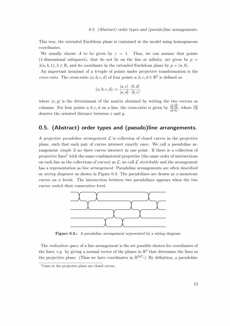
A projective pseudoline arrangement L is collection of closed curves in the projectiveplane, such that each pair of curves intersect exactly once. We call a pseudoline ar-rangement simple if no three curves intersect in one point. If there is a collection ofprojective lines1 with the same combinatorial properties (the same order of intersectionson each line as the collections of curves) as L, we call L stretchable and the arrangementhas a representation as line arrangement. Pseudoline arrangements are often describedas wiring diagrams as shown in Figure 0.3: The pseudolines are drawn as x-monotonecurves on n levels. The intersection between two pseudolines appears when the twocurves switch their consecutive level.
Figure 0.3.: A pseudoline arrangement represented by a wiring diagram.
The realization space of a line arrangement is the set possible choices for coordinates ofthe lines, e.g. by giving a normal vector of the planes in R3 that determine the lines inthe projective plane. (Thus we have coordinates in R3|L|.) By definition, a pseudoline
1Lines in the projective plane are closed curves.
13

0. Notations and definitions
arrangement is stretchable if and only if its realization space is non-empty. Usually therealization space is considered modulo projective transformations.The model of representing the lines by the normal vector of the planes allows for asimple definition of a dual map Dproj : A projective line (plane in R3) is mapped ontothe 1-dimensional subspace that is spanned by a normal vector of its plane and viceversa. This map is an involution (self-inverse). Due to nicer mapping we usually usethe duality on a parabola D. The map D maps the line given by y = ax − b onto thepoint (a, b). It can be obtained by applying a projective transformation before applyingthe projective duality, thus it also preserves incidences and the cross-ratio. A point pthat lies on the intersection of the two lines `1 and `2 is mapped onto the line D(p),that is spanned by the points D(`1) and D(`2). It also preserves the orientation of eachtriple of intersecting lines: As shown in Figure 0.4, three lines that do not intersectin one point in the extended Euclidean plane are mapped by D onto three points ingeneral position, i.e., the points are not collinear. The triangle, that is bounded by the
D
D
Figure 0.4.: Duality preserves the orientation of triples and the order on lines.
three lines, gives an orientation of the lines by considering the clockwise order of thelines on the boundary (`1, `2, `3). This is the same orientation of points of the dualtriangle spanned by the dual points (D(`1),D(`2),D(`3)). In the case of three lines thatintersect in one point (or are parallel) the dual points points are collinear. The order ofthe lines around their intersection point coincides with the order of the points on theircommon dual line.The information of the orientation of each triple and the order of points on a line fullydetermines the combinatorial information of the pseudoline arrangement. On the otherhand, the orientation of each triangle encodes the full the pseudoline arrangement.Thus, a pseudoline arrangement can be dualized by giving the orientation of each tripleof points, such that the triples satisfy certain axioms, see for example [BLVS+99]. The
14
0.6. Geometry and topology
axioms come from dualizing the restrictions on curves to be a pseudoline arrangement.The orientation of each triple of points is called an abstract order type. An abstractorder type is realizable if there is a point set with this orientation. This is the case ifand only if its dual pseudoline arrangement is stretchable. An abstract order type iscalled simple if and only if the dual pseudoline arrangement is simple. This is the caseif and only if no three points are collinear.We often drop the word “abstract” and only use the term “order type” when we aremainly interested in the realizability.Abstract order types are also known as rank 3 oriented matroids. The orientation of atriple of points (p1, p2, p3) in homogeneous coordinates can also be determined by themap
χ : R3×3 → −, 0,+(p1, p2, p3) 7→ sign (det ((p1, p2, p3))) .
If the points are given with positive z-coordinate, then the triple is oriented counter-clockwise if the determinant is positive, clockwise if the determinant is negative, andthey are collinear if the determinant is zero. The map χ is called the chirotope.For an order type we can consider the circular sequence. Given a point set that real-izes an order type, we define the circular sequence as the sequence of orders of pointsthat appear as the orthogonal projection of the point set onto a rotating, directed line.This leads to a sequence of
(n2
)+ 1 permutations (assuming general position) of the
points while rotating by an angle of π. The sequence of permutations is called allow-able or circular sequence. An allowable sequence describes a unique abstract order typearrangement [GP80], whereas an order type usually has several allowable sequences.A circular sequence can be uniquely described by the order of switches, the sequenceof transpositions that appear between consecutive permutations in the allowable se-quence [GP80]. The sequence of the switches is the order of the slopes of the linesthat are spanned by the pairs of points of the order type. In the dual line arrangementthe order of switches describes the order of intersection points of lines in x-direction (ifthe rotating line starts and ends at vertical position). A circular sequence describes aunique order type [GP80]. On the other hand, one abstract order type can be realizedby many circular sequences.
0.6. Geometry and topology
While describing realization spaces of order types, line arrangements or other geometricobjects we need some basic definitions from algebraic geometry and topology.
15
0. Notations and definitions
A semialgebraic set is a set that can be described as the solution set of a polyno-mial inequality system consisting of strict and non-strict inequalities and equations. Asemialgebraic set is called primary if it has a description only by gstrict polynomialinequalities and equations. Note that a primary semialgebraic set is an open set.Two sets in Rn are homotopy equivalent if they can be continuously deformed into eachother (they have the same topological structure).Two semialgebraic sets V and W are stably equivalent if there is a homeomorphismf : V × Rs → W × Rt, where both maps f and f−1 are polynomial maps. Stableequivalence of two sets implies homotopy equivalence.
16

Part I.
Combinatorial properties ofintersection graphs
17


1. The dimension of bipartiteintersection graphs
In this chapter we study bipartite intersection graphs in the plane from the perspective oforder dimension. We start with the observation that partial orders of height two whosecomparability graph is a grid intersection graph have order dimension at most four.Starting from this observation we provide a comprehensive study of classes of graphsbetween grid intersection graphs and bipartite permutation graphs and the containmentrelation on these classes. Order dimension plays a role in many arguments.This chapter is based on [CFHW15].
1.1. Background of subclasses of grid intersection graphs.
Subclasses of GIGs appear in several technical applications. For example in nano PLA-design [STS11] and in biology [HATI11].Other restrictions on the geometry of the representation are used to study algorithmicproblems. For example, stabbability has been used to study hitting sets and indepen-dent sets in families of rectangles [CF13]. Additionally, computing the jump numberof a poset, which is NP-hard in general, has been shown solvable in polynomial timefor bipartite posets with interval dimension two using their restricted GIG representa-tion [TS11].Beyond these graph classes that have been motivated by applications and algorithmicconsiderations, we also study several other natural intermediate graph classes. All thesegraph classes and properties are defined in Subsection 1.1.1.The main contribution of this work is to establish the strict containment and incompa-rability relations depicted in Figure 1.1. We additionally relate these classes to incidenceposets of planar and outerplanar graphs.In Section 1.2 we use the geometric representations to establish the containment re-lations between the graph classes as shown in Figure 1.1. The maximal dimension ofgraphs in these classes is the topic of Section 1.3. In Section 1.4 we use vertex-edgeincidence posets of planar graphs to separate some of these classes from each other.Specifically, we show that the vertex-edge incidence posets of planar graphs are a sub-class of stabbable GIG (StabGIG), and that vertex-edge incidence posets of outerplanar
19
1. The dimension of bipartite intersection graphs
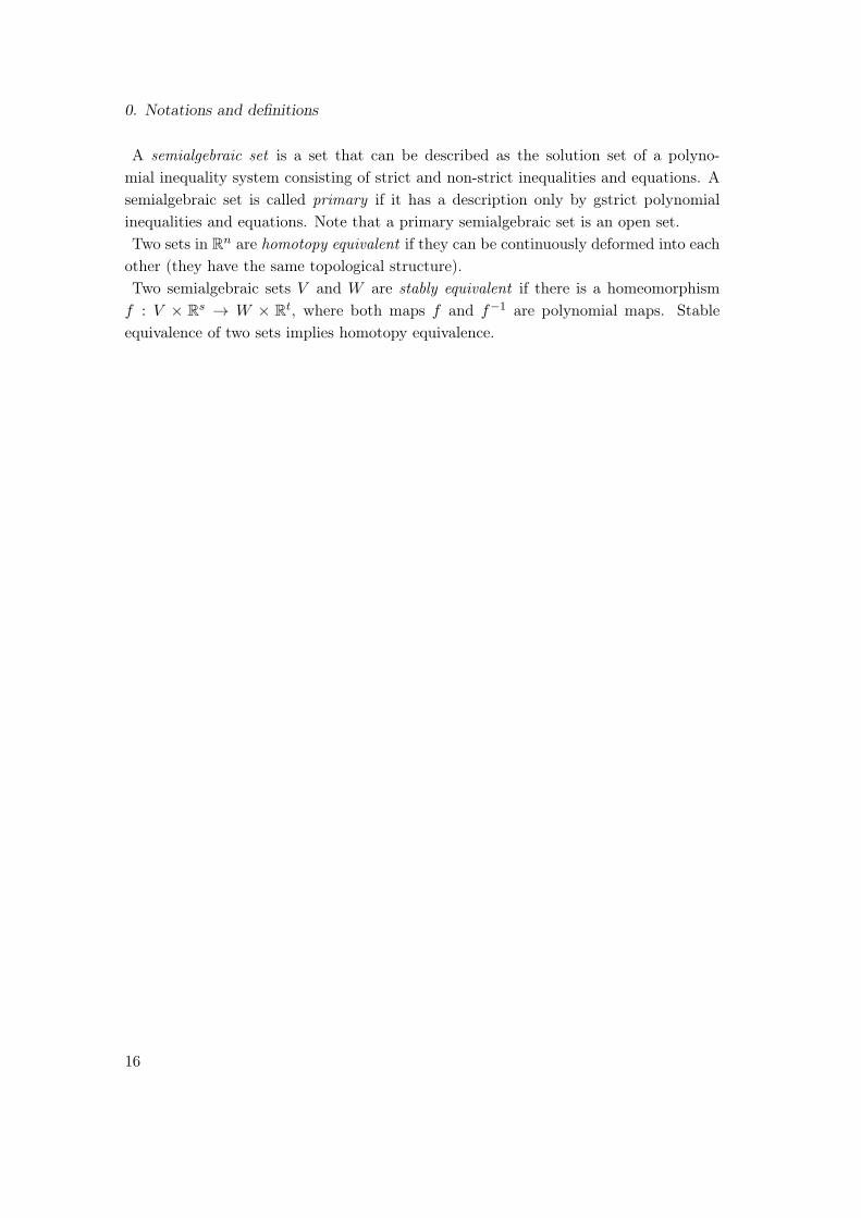
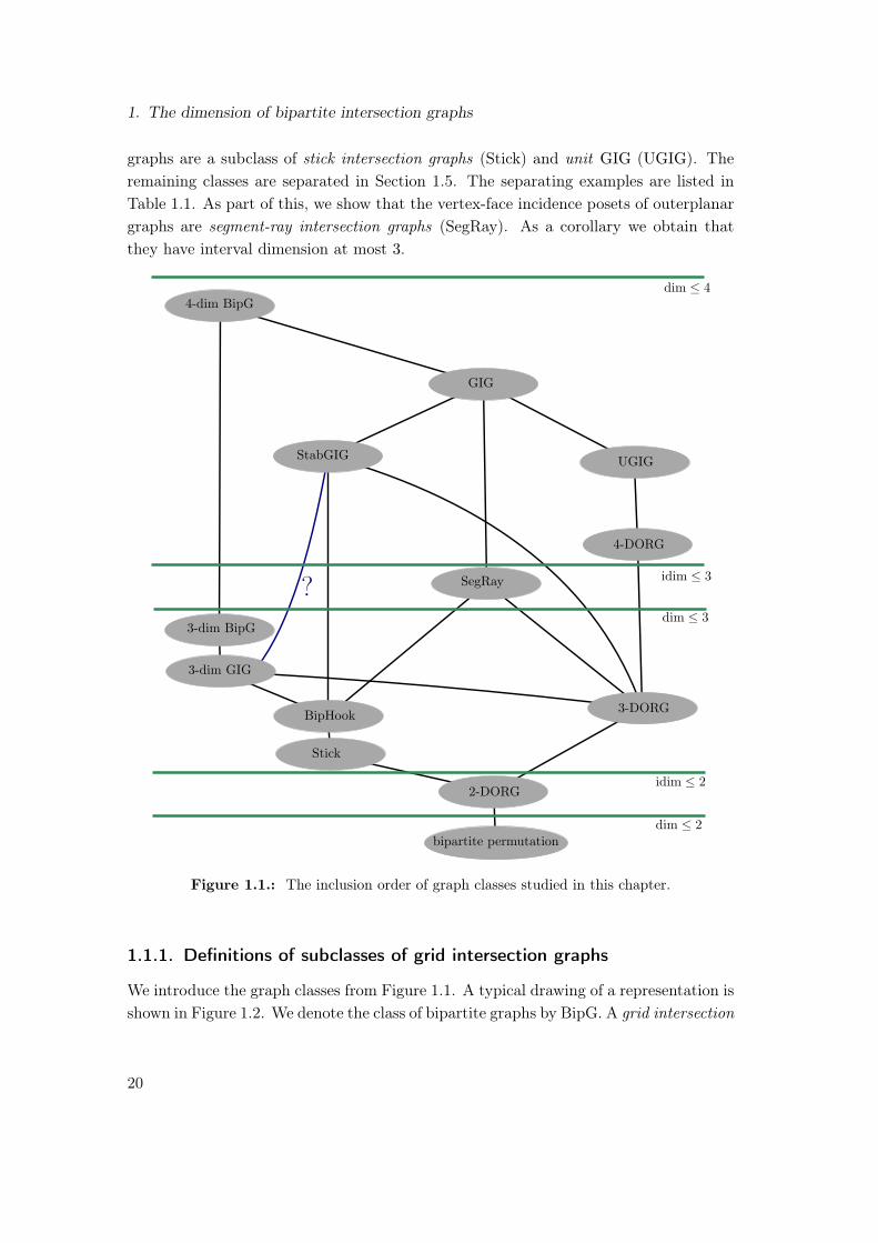
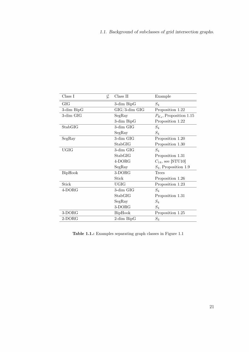
graphs are a subclass of stick intersection graphs (Stick) and unit GIG (UGIG). Theremaining classes are separated in Section 1.5. The separating examples are listed inTable 1.1. As part of this, we show that the vertex-face incidence posets of outerplanargraphs are segment-ray intersection graphs (SegRay). As a corollary we obtain thatthey have interval dimension at most 3.
4-dim BipG
GIG
UGIG
4-DORG
3-DORG
3-dim BipG
StabGIG
SegRay
3-dim GIG
BipHook
2-DORG
bipartite permutation
Stick
dim ≤ 4
?idim ≤ 3
dim ≤ 3
idim ≤ 2
dim ≤ 2
Figure 1.1.: The inclusion order of graph classes studied in this chapter.
1.1.1. Definitions of subclasses of grid intersection graphs
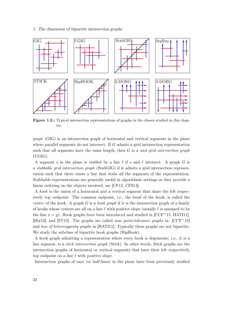
We introduce the graph classes from Figure 1.1. A typical drawing of a representation isshown in Figure 1.2. We denote the class of bipartite graphs by BipG. A grid intersection
20
1.1. Background of subclasses of grid intersection graphs.
Class I 6⊆ Class II Example
GIG 3-dim BipG S4
3-dim BipG GIG/3-dim GIG Proposition 1.223-dim GIG SegRay PK4 , Proposition 1.15
3-dim BipG Proposition 1.22StabGIG 3-dim GIG S4
SegRay S4
SegRay 3-dim GIG Proposition 1.20StabGIG Proposition 1.30
UGIG 3-dim GIG S4
StabGIG Proposition 1.314-DORG C14, see [STU10]SegRay S4, Proposition 1.9
BipHook 3-DORG TreesStick Proposition 1.26
Stick UGIG Proposition 1.234-DORG 3-dim GIG S4
StabGIG Proposition 1.31SegRay S4
3-DORG S4
3-DORG BipHook Proposition 1.252-DORG 2-dim BipG S3
Table 1.1.: Examples separating graph classes in Figure 1.1
21
1. The dimension of bipartite intersection graphs
SegRay
3-DORG2-DORGBipHOOKSTICK
UGIG StabGIGGIG
Figure 1.2.: Typical intersection representations of graphs in the classes studied in this chap-ter.
graph (GIG) is an intersection graph of horizontal and vertical segments in the planewhere parallel segments do not intersect. If G admits a grid intersection representationsuch that all segments have the same length, then G is a unit grid intersection graph(UGIG).A segment s in the plane is stabbed by a line ` if s and ` intersect. A graph G isa stabbable grid intersection graph (StabGIG) if it admits a grid intersection represen-tation such that there exists a line that stabs all the segments of the representation.Stabbable representations are generally useful in algorithmic settings as they provide alinear ordering on the objects involved, see [CF13, CFS14].A hook is the union of a horizontal and a vertical segment that share the left respec-tively top endpoint. The common endpoint, i.e., the bend of the hook, is called thecenter of the hook. A graph G is a hook graph if it is the intersection graph of a familyof hooks whose centers are all on a line ` with positive slope (usually ` is assumed to bethe line x = y). Hook graphs have been introduced and studied in [CCF+15, HATI11],[Hix13], and [ST15]. The graphs are called max point-tolerance graphs in [CCF+15]and loss of heterozygosity graphs in [HATI11]. Typically these graphs are not bipartite.We study the subclass of bipartite hook graphs (BipHook).A hook graph admitting a representation where every hook is degenerate, i.e., it is aline segment, is a stick intersection graph (Stick). In other words, Stick graphs are theintersection graphs of horizontal or vertical segments that have their left respectivelytop endpoint on a line ` with positive slope.Intersection graphs of rays (or half-lines) in the plane have been previously studied
22
1.2. Containment relations between the classes
in the context of their chromatic number [KN98] and the clique problem [CCL13]. Weconsider some natural bipartite subclasses of this class. Consider a set of axis-alignedrays in the plane. If the rays are restricted into two orthogonal directions, e.g. upand right, their intersection graph is called a two directional orthogonal ray graph (2-DORG). This class has been studied in [STU10] and [TS11]. Analogously, if three orfour directions are allowed for the rays, we talk about 3-DORGs or 4-DORGs. Theclass of 4-DORGs was introduced in connection with defect tolerance schemes for nano-programmable logic arrays [STS11].Finally, segment-ray graphs (SegRay) are the intersection graphs of horizontal segmentsand vertical rays directed in the same direction. SegRay graphs (and closely relatedgraph classes) have been previously discussed in the context of covering and hitting setproblems (see e.g., [KMN05, CG14, CCM13]).In the representations defining graphs in all these classes we can assume the x and they-coordinate of endpoints of any two different segments are distinct. This property canbe established by appropriate perturbations of the segments.For the sake of brevity we define the dimension of a bipartite graph G to be equal to thedimension of its comparability graph. The freedom that we have in defining the partialorder on G, i.e., the choice of the color classes for minima and maxima, does not affectthe dimension. This is an easy instance of the fact that dimension is a comparabilityinvariant, i.e., independent of the choice of partial order on the comparability graph, asshown in [TMS76].
1.2. Containment relations between the classes
The diagram shown in Figure 1.1 has 19 non-transitive inclusions represented by theedges. In this section we show the inclusion between the respective classes of graphs.The inclusion 2-dim BipG ⊆ 2-DORG was already noted as a consequence of Proposi-tion 1.6. The next 8 inclusions follow directly from the definition of the classes:
UGIG ⊆ GIG StabGIG ⊆ GIG
2-DORG ⊆ 3-DORG 3-DORG ⊆ 4-DORG
3-dim GIG ⊆ 3-dim BipG 3-dim BipG ⊆ 4-dim BipG
Stick ⊆ BipHook 3-dim GIG ⊆ GIG.
The following less trivial inclusions follow from geometric modifications of the represen-tation. The proofs are given in the following two propositions.
BipHook ⊆ StabGIG 2-DORG ⊆ Stick.
Proposition 1.1. Each bipartite hook graph is a stabbable GIG.
23
1. The dimension of bipartite intersection graphs
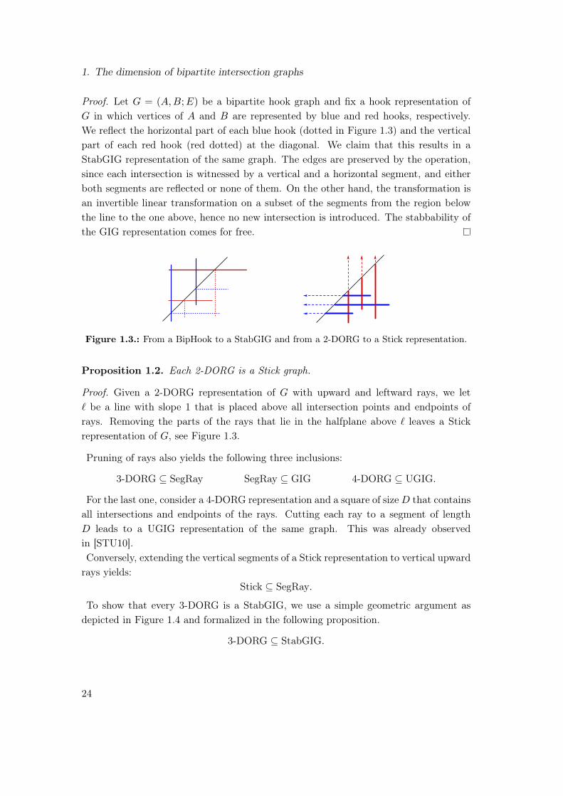
Proof. Let G = (A,B;E) be a bipartite hook graph and fix a hook representation ofG in which vertices of A and B are represented by blue and red hooks, respectively.We reflect the horizontal part of each blue hook (dotted in Figure 1.3) and the verticalpart of each red hook (red dotted) at the diagonal. We claim that this results in aStabGIG representation of the same graph. The edges are preserved by the operation,since each intersection is witnessed by a vertical and a horizontal segment, and eitherboth segments are reflected or none of them. On the other hand, the transformation isan invertible linear transformation on a subset of the segments from the region belowthe line to the one above, hence no new intersection is introduced. The stabbability ofthe GIG representation comes for free.
Figure 1.3.: From a BipHook to a StabGIG and from a 2-DORG to a Stick representation.
Proposition 1.2. Each 2-DORG is a Stick graph.
Proof. Given a 2-DORG representation of G with upward and leftward rays, we let` be a line with slope 1 that is placed above all intersection points and endpoints ofrays. Removing the parts of the rays that lie in the halfplane above ` leaves a Stickrepresentation of G, see Figure 1.3.
Pruning of rays also yields the following three inclusions:
3-DORG ⊆ SegRay SegRay ⊆ GIG 4-DORG ⊆ UGIG.
For the last one, consider a 4-DORG representation and a square of sizeD that containsall intersections and endpoints of the rays. Cutting each ray to a segment of lengthD leads to a UGIG representation of the same graph. This was already observedin [STU10].Conversely, extending the vertical segments of a Stick representation to vertical upwardrays yields:
Stick ⊆ SegRay.
To show that every 3-DORG is a StabGIG, we use a simple geometric argument asdepicted in Figure 1.4 and formalized in the following proposition.
3-DORG ⊆ StabGIG.
24

1.2. Containment relations between the classes
`
s
Figure 1.4.: From a 3-DORG to a StabGIG representation
Proposition 1.3. Each 3-DORG is a stabbable GIG.
Proof. Consider a 3-DORG representation of a graph G. We assume that vertical rayspoint up or down while horizontal rays point right. Let s be a vertical line to the rightof all the intersections. We prune the horizontal rays at s to make them segments andthen reflect the segments at s, this doubles the length of the segments (see Figure 1.4).Now take all upward rays and move them to the right via a reflection at s. This resultsin an intersection representation with vertical rays in both directions and horizontalsegments such that all rays pointing down are left of s and all rays pointing up are tothe right of s. Due to this property we find a line ` of positive slope that stabs all therays and segments of the representation. Pruning the rays above, respectively belowtheir intersection with ` yields a StabGIG representation of G.
A non-geometric modification of a representation gives the 16th of the 19 non-transitiveinclusions from Figure 1.1:
BipHook ⊆ SegRay.
Proposition 1.4. Each bipartite hook graph is a SegRay graph.
Proof. Consider a BipHook representation of G = (A,B;E). We construct a SegRayrepresentation where A is represented by vertical rays and B by horizontal segments.Let a1, . . . , a|A| be the order of the vertices of A that we get by the centers of the hookson the diagonal, read from bottom-left to top-right. The y-coordinates of the horizontalsegments and the endpoints of the rays in our SegRay representation of G will be givenin the following way.
25
1. The dimension of bipartite intersection graphs
We initialize a list R = [a1, . . . , a|A|] and a set S = B of active vertices, and an emptylist Y . We apply one of the following steps repeatedly:
1. If there is an active a ∈ R such that N(a) ∩ S = ∅, then remove a from R andappend it to Y .
2. If there is an active b ∈ S such that vertices of N(b) appear consecutively in R,then remove b from S and append it to Y .
Suppose that R and S are empty after the iteration. Then we can construct a Seg-Ray representation of G. The endpoint of the ray representing ai receives i as thex-coordinate and the position of ai in Y as the y-coordinate. The segment representingb ∈ B also obtains the y-coordinate according to its position in Y . Its x-coordinates aredetermined by its neighbourhood. Now it is straight-forward to verify that this definesa SegRay representation of G. It remains to show that one of the steps can always
b1
aj
ai a′′
a′
bi
bi+1
Figure 1.5.: Left: b1 is not involved in a forward pair. Right: A forbidden configuration for abipartite hook graph.
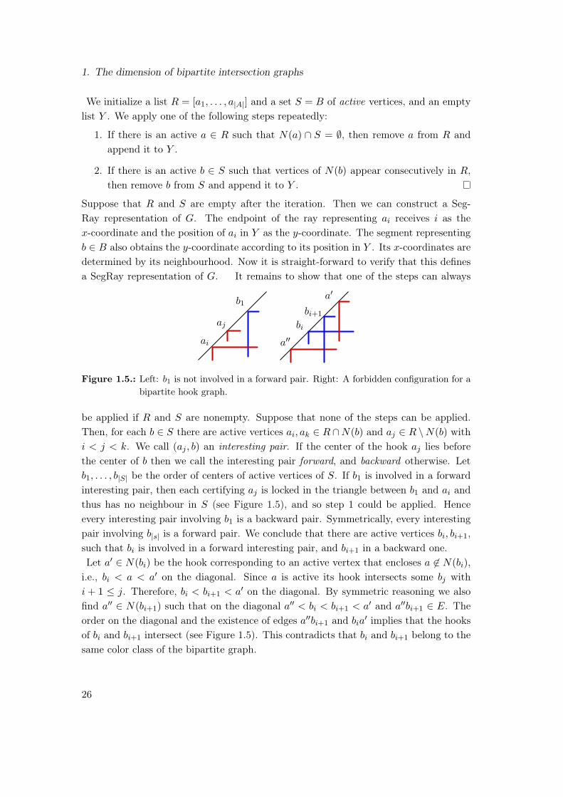
be applied if R and S are nonempty. Suppose that none of the steps can be applied.Then, for each b ∈ S there are active vertices ai, ak ∈ R∩N(b) and aj ∈ R \N(b) withi < j < k. We call (aj , b) an interesting pair. If the center of the hook aj lies beforethe center of b then we call the interesting pair forward, and backward otherwise. Letb1, . . . , b|S| be the order of centers of active vertices of S. If b1 is involved in a forwardinteresting pair, then each certifying aj is locked in the triangle between b1 and ai andthus has no neighbour in S (see Figure 1.5), and so step 1 could be applied. Henceevery interesting pair involving b1 is a backward pair. Symmetrically, every interestingpair involving b|s| is a forward pair. We conclude that there are active vertices bi, bi+1,such that bi is involved in a forward interesting pair, and bi+1 in a backward one.Let a′ ∈ N(bi) be the hook corresponding to an active vertex that encloses a 6∈ N(bi),i.e., bi < a < a′ on the diagonal. Since a is active its hook intersects some bj withi + 1 ≤ j. Therefore, bi < bi+1 < a′ on the diagonal. By symmetric reasoning we alsofind a′′ ∈ N(bi+1) such that on the diagonal a′′ < bi < bi+1 < a′ and a′′bi+1 ∈ E. Theorder on the diagonal and the existence of edges a′′bi+1 and bia′ implies that the hooksof bi and bi+1 intersect (see Figure 1.5). This contradicts that bi and bi+1 belong to thesame color class of the bipartite graph.
26
1.3. Dimension
1.3. Dimension
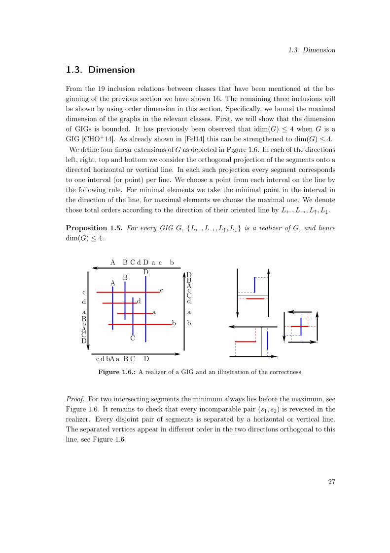
From the 19 inclusion relations between classes that have been mentioned at the be-ginning of the previous section we have shown 16. The remaining three inclusions willbe shown by using order dimension in this section. Specifically, we bound the maximaldimension of the graphs in the relevant classes. First, we will show that the dimensionof GIGs is bounded. It has previously been observed that idim(G) ≤ 4 when G is aGIG [CHO+14]. As already shown in [Fel14] this can be strengthened to dim(G) ≤ 4.We define four linear extensions of G as depicted in Figure 1.6. In each of the directionsleft, right, top and bottom we consider the orthogonal projection of the segments onto adirected horizontal or vertical line. In each such projection every segment correspondsto one interval (or point) per line. We choose a point from each interval on the line bythe following rule. For minimal elements we take the minimal point in the interval inthe direction of the line, for maximal elements we choose the maximal one. We denotethose total orders according to the direction of their oriented line by L←, L→, L↑, L↓.
Proposition 1.5. For every GIG G, L←, L→, L↑, L↓ is a realizer of G, and hencedim(G) ≤ 4.
A B C d D a c b
dC
ab
DCBaAbdc
da
b
A Acc
C
dc
aBb
DB
DB
DCA
Figure 1.6.: A realizer of a GIG and an illustration of the correctness.
Proof. For two intersecting segments the minimum always lies before the maximum, seeFigure 1.6. It remains to check that every incomparable pair (s1, s2) is reversed in therealizer. Every disjoint pair of segments is separated by a horizontal or vertical line.The separated vertices appear in different order in the two directions orthogonal to thisline, see Figure 1.6.
27
1. The dimension of bipartite intersection graphs
It is known that a bipartite graph is a bipartite permutation graph if and only if thedimension of the poset is at most 2. Thus, by Proposition 1.5, the maximal dimensionof the graphs in the other classes that we consider must be 3 or 4.The class of 2-DORGs is characterized by the interval dimension of the graph.
Proposition 1.6. 2-DORGs are exactly the bipartite graphs of interval dimension 2.
This has been shown in [STU10] using a characterization of 2-DORGs as the complementof co-bipartite circular arc graphs. Below we give a simple direct proof.To explain it we recall the geometric version of interval dimension: Vectors a, b ∈ Rd
with a ≤dom b define a standard box [a, b] = v : a ≤dom v ≤dom b in Rd. LetP = (X,≤P ) be a poset. A family of standard boxes [ax, bx] ⊆ Rd : x ∈ X is a boxrepresentation of P in Rd if it holds that x <P y if and only if bx ≤dom ay. Then theinterval dimension of P is the minimum d for which there is a box representation ofP in Rd. Note that if P has height 2 with A = Min(P ) and B = Max(P ), then in abox representation the lower corner ax for each x ∈ A and the upper corner by for eachy ∈ B are irrelevant, in the sense that they can uniformly be chosen as (−c, . . . ,−c)respectively (c, . . . , c) for a large enough constant c.
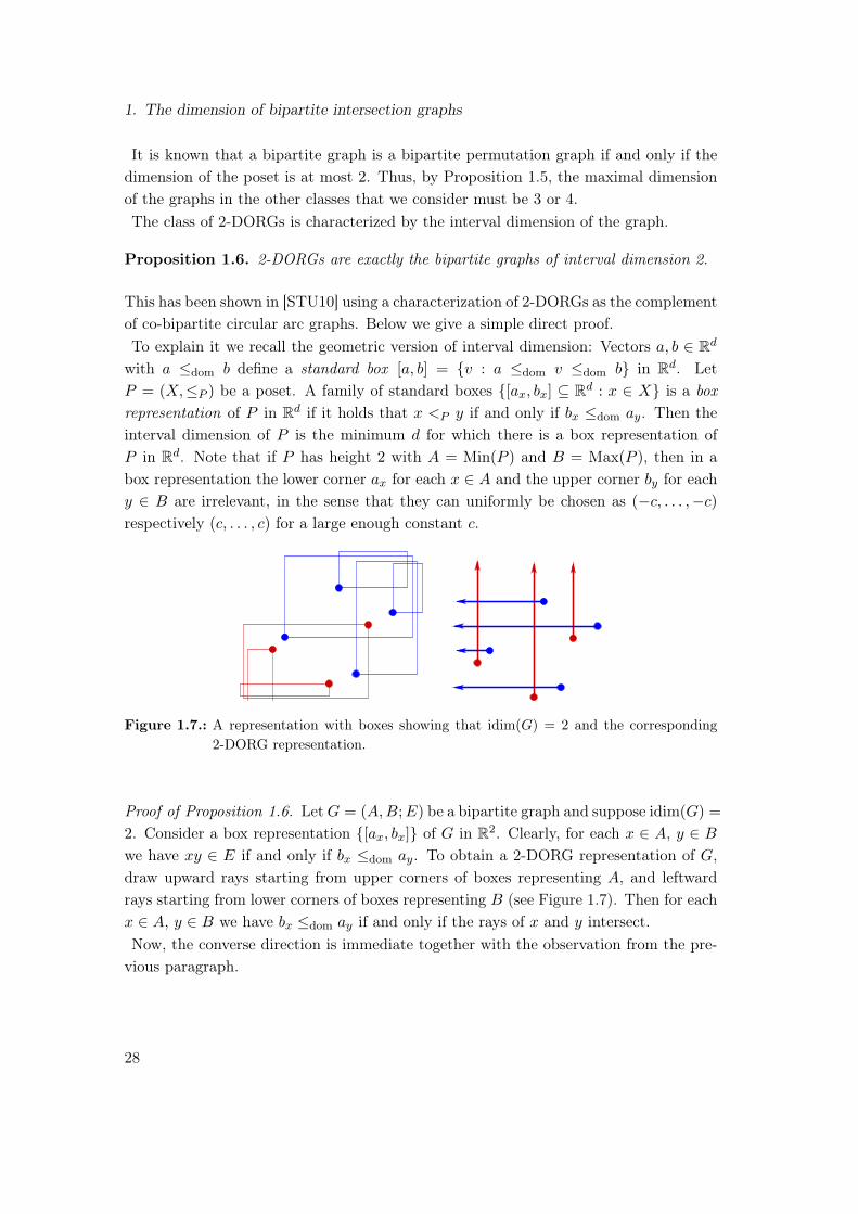
Figure 1.7.: A representation with boxes showing that idim(G) = 2 and the corresponding2-DORG representation.
Proof of Proposition 1.6. LetG = (A,B;E) be a bipartite graph and suppose idim(G) =
2. Consider a box representation [ax, bx] of G in R2. Clearly, for each x ∈ A, y ∈ Bwe have xy ∈ E if and only if bx ≤dom ay. To obtain a 2-DORG representation of G,draw upward rays starting from upper corners of boxes representing A, and leftwardrays starting from lower corners of boxes representing B (see Figure 1.7). Then for eachx ∈ A, y ∈ B we have bx ≤dom ay if and only if the rays of x and y intersect.Now, the converse direction is immediate together with the observation from the pre-vious paragraph.
28

1.3. Dimension
Since the 2-DORGs are exactly the bipartite graphs of interval dimension 2, and in-terval dimension is bounded by dimension, we obtain
2-dim BipG ⊆ 2-DORG.
In the following we show that BipHooks and 3-DORGs have dimension at most 3. Forthese results we note that graphs with a special SegRay representation have dimensionat most 3 and that the interval dimension of SegRay graphs is bounded by 3. Thislatter result was shown previously by a different argument in [CHO+14].
Lemma 1.7. For a SegRay graph G, dim(G) ≤ 3 when G has a SegRay representationsatisfying the following: whenever two horizontal segments are such that the x-projectionof one is included in the other one, then the smaller segment lies below the bigger one.
Proof. Consider such a SegRay representation ofG with horizontal segments as maximaland downward rays as minimal elements of QG. The linear extensions L→, L←, and L↓defined for Proposition 1.5 form a realizer of QG.
Corollary 1.8. For every 3-DORG G, dim(G) ≤ 3.
Proof. Consider a 3-DORG representation of G where the horizontal rays use two di-rections. We cut the horizontal rays so that they have the same length D. When D islarge enough, this yields a SegRay representation of the same graph. Note that such arepresentation has no nested segments. Thus, Lemma 1 implies dim(QG) ≤ 3.
Proposition 1.9. For every SegRay graph G, idim(G) ≤ 3.
Proof. Suppose that the rays correspond to minimal elements of QG. By Lemma 1.7the linear extensions L→, L← and L↓ reverse all incomparable pairs except some thatconsist of two maximal elements. We convert these linear extensions to interval ordersand extend the intervals (originally points) of maximal elements in L→ far to the rightto make them intersect. In this way we obtain three interval orders whose intersectiongives rise to QG.
Proposition 1.10. For every bipartite hook graph G, dim(G) ≤ 3.
Proof. Let A and B be the color classes of G. We construct the graph G′ by addingprivate neighbours to vertices of B. Then G′ is also a BipHook graph as we can easilyadd hooks intersecting a single hook in a representation of G. By Proposition 1.4 weknow that G′ has a SegRay representation R with downward rays representing A. Byconstruction, each horizontal segment in R must have its private ray intersecting it.Thus, R satisfies the property of Lemma 1.7 and dim(QG′) ≤ 3. Since QG is an inducedsubposet of QG′ we conclude dim(QG) ≤ 3.
29

1. The dimension of bipartite intersection graphs
Since Stick ⊂ BipHook we know that dim(QG) ≤ 3 if G is a Stick graph. However, anicer realizer for a Stick graph is obtained by Proposition 1.5, since L← and L↓ coincidein a Stick representation.In Section 1.5 we will show that these bounds are tight.
1.4. Vertex-edge incidence posets
We proceed by investigating the relations between the classes of GIGs and incidenceposets of graphs.For a graph G, PG denotes the vertex-edge incidence poset of G, and the comparabilitygraph of PG is the graph obtained by subdividing each edge of G once. The vertex-edgeincidence posets of dimension 3 are characterised by Schnyder’s Theorem.
Theorem 1.11 ([Sch89]). A graph G is planar if and only if dim(PG) ≤ 3.
Even though some GIGs have poset dimension 4, we will see that the vertex-edgeincidence posets with a GIG representation are precisely the vertex-edge incidence posetsof planar graphs. A weak bar visibility representation of G gives a GIG representationof PG. On the other hand, a GIG representation of PG can be transformed into a weakbar visibility representation of G. In particular, since the segments representing edgesof G intersect two segments representing incident vertices, they can be shortened untiltheir intersections become contacts. Hence PG is a GIG if and only if G is planar. Wenext show the stronger result, that there is a StabGIG representation of PG for everyplanar graph G.
Proposition 1.12. A graph G is planar if and only if PG is a stabbable GIG.
We use the following definitions. A generic floorplan is a partition of a rectangle into afinite set of interiorly disjoint rectangles that have no point where four rectangles meet.Two floorplans are weakly equivalent if there exist bijections ΦH between the horizontalsegments and ΦV between the vertical segments, such that a segment s has an endpointon t in F if and only if Φ(s) has an endpoint on Φ(t). A floorplan F covers a set ofpoints P if and only if every segment contains exactly one point of P and no point iscontained in two segments. The following theorem has been conjectured by Ackerman,Barequet and Pinter [ABP06], who have also shown it for the special case of separablepermutations. It has been shown by Felsner [Fel13] for general permutations.
Theorem 1.13 ([Fel13]). Let P be a set of n points in the plane, such that no twopoints have the same x- or y-coordinate and F a generic floorplan with n segments.Then there exists a floorplan F ′, such that F and F ′ are weakly equivalent and F ′
covers P .
30
1.4. Vertex-edge incidence posets
Proof of Proposition 1.12. Consider a weak bar-visibility representation of G. The low-est and highest horizontal segments hb and ht can be extended, such that their left aswell as their right endpoints can be connected by new vertical segments vl and vr. Thesegments hb, ht, vl and vr are the boundary of a rectangle. Extending every horizontalsegment until its left and right endpoints touch vertical segments leads to a floorplanF . By Theorem 1.13 there exists an equivalent floorplan F ′ that covers a pointset Pconsisting of n points on the diagonal of the the big rectangle with positive slope. Short-ening the horizontal segments and extending the vertical segments of F ′ by ε > 0 oneach end leads to a GIG representation of PG that can be stabbed by the line throughthe diagonal.On the other hand, every GIG representation of PG leads to a weak bar-visibilityrepresentation, and hence G is planar.
We will now show that PG is in the classes of Stick and bipartite hook graphs if andonly if G is outerplanar.
Proposition 1.14. PG is a Stick graph if and only if G is outerplanar.
Proof. Outerplanar graphs have been characterized by linear orderings of their verticesby Felsner and Trotter [FT05]: A graph G = (V,E) is outerplanar if and only if thereexist linear orders L1, L2, L3 of the vertices with L2 =
←−L1, i.e., L2 is the reverse of L1,
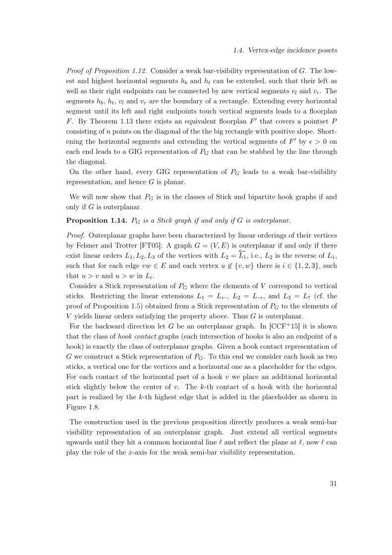
such that for each edge vw ∈ E and each vertex u 6∈ v, w there is i ∈ 1, 2, 3, suchthat u > v and u > w in Li.Consider a Stick representation of PG where the elements of V correspond to verticalsticks. Restricting the linear extensions L1 = L←, L2 = L→, and L3 = L↑ (cf. theproof of Proposition 1.5) obtained from a Stick representation of PG to the elements ofV yields linear orders satisfying the property above. Thus G is outerplanar.For the backward direction let G be an outerplanar graph. In [CCF+15] it is shownthat the class of hook contact graphs (each intersection of hooks is also an endpoint of ahook) is exactly the class of outerplanar graphs. Given a hook contact representation ofG we construct a Stick representation of PG. To this end we consider each hook as twosticks, a vertical one for the vertices and a horizontal one as a placeholder for the edges.For each contact of the horizontal part of a hook v we place an additional horizontalstick slightly below the center of v. The k-th contact of a hook with the horizontalpart is realized by the k-th highest edge that is added in the placeholder as shown inFigure 1.8.
The construction used in the previous proposition directly produces a weak semi-barvisibility representation of an outerplanar graph. Just extend all vertical segmentsupwards until they hit a common horizontal line ` and reflect the plane at `, now ` canplay the role of the x-axis for the weak semi-bar visibility representation.
31

1. The dimension of bipartite intersection graphs
Figure 1.8.: A hook contact representation of G transformed into a Stick representation ofPG.
Proposition 1.15. A graph G is outerplanar if and only if the graph PG has a SegRayrepresentation where the vertices of G are represented as rays.
Proof. Cutting the rays of a SegRay representation with rays pointing downwards some-where below all horizontal segments leads to a weak semi-bar visibility representationof G and vice versa. Thus, Lemma 0.4 gives the result.
Proposition 1.16. A graph G is outerplanar if and only if the graph PG has a hookrepresentation.
Proof. If G is outerplanar then PG has a hook representation by Proposition 1.14. Onthe other hand, assume that PG has a hook representation for a graph G. According toProposition 1.4 we construct a SegRay representation with vertices as rays and edgesas segments. This representation shows that G is outerplanar by Proposition 1.15.
Proposition 1.17. If G is outerplanar, then the graph PG has a SegRay representationwhere the vertices of G are represented as segments.
Proof. Consider a hook representation R′ of PG. According to the proof Proposition 1.4we can transform PG into a SegRay representation with a free choice of the colorclassthat is represented by rays. Choosing the subdivision vertices as rays leads to therequired representation.
In contrast to Proposition 1.15, the backward direction of Proposition 1.17 does nothold: Figure 1.9 shows a SegRay representation of PK2,3 with vertices being representedas horizontal segments, but K2,3 is not outerplanar. Together with Proposition 1.15this also shows that the class of SegRay graphs is not symmetric in its color classes.In the following we construct a UGIG representation of PG for an outerplanar graphG.
32

1.4. Vertex-edge incidence posets
Figure 1.9.: A SegRay representation of PK2,3.
Proposition 1.18. If G is outerplanar then PG is a UGIG.
Proof. We construct a UGIG representation of PG for a maximal outerplanar graphG = (V,E) with outer-face cycle v0, . . . , vn. The vertices of V are drawn as verticalsegments. Starting from v0 we iteratively draw the vertices of breadth-first-search layers(BFS-layers). Each BFS-layer has a natural order inherited from the order on the outer-face, i.e., the increasing order of indices. When the i-th layer Li has been drawn thefollowing invariants hold:
1. Segments for all vertices and edges of G[L0, . . . , Li−1], all vertices of Li, and alledges connecting vertices of Li−1 to vertices of Li have been placed.
2. The upper endpoints of the segments representing vertices in Li lie on a strictmonotonically decreasing curve Ci. Their order on Ci agrees with the order of thecorresponding vertices in Li. Their x-coordinates differ by at most one.
3. No segment intersects the region above Ci.
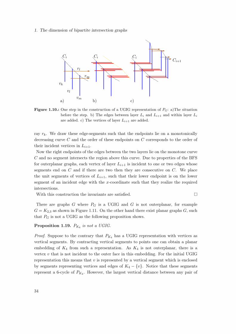
We start the construction with the vertical segment corresponding to v0. The curveC0 is chosen as a line with negative slope that intersects the upper endpoint of v0.We start the (i+ 1)-th step by adding segments for the edges within vertices of layerLi. Afterwards we add the segments for edges between vertices in layer Li and Li+1 andthe segments for the vertices of layer Li+1. The construction is indicated in Figure 1.10.First we draw unit segments for the edges within layer Li. Since the graph is outerpla-nar such edges only occur between consecutive vertices of the layer. For a vertex vk ofLi which is not the first vertex of Li we define a horizontal ray rk whose start is on thesegment of the predecessor of vk on this layer such that the only additional intersectionof rk is with the segment of vk. The initial unit segment of ray rk can be used for theedge between vk and its predecessor.All segments that will represent edges between layer Li and Li+1 are placed as hor-izontal segments that intersect the segment of the incident vertex vk ∈ Li above the
33
1. The dimension of bipartite intersection graphs
Ci+1
CiCiCi
a) b) c)
rl
rm
vl
vk
vm
Figure 1.10.: One step in the construction of a UGIG representation of PG: a)The situationbefore the step. b) The edges between layer Li and Li+1 and within layer Li
are added. c) The vertices of layer Li+1 are added.
ray rk. We draw these edge-segments such that the endpoints lie on a monotonicallydecreasing curve C and the order of these endpoints on C corresponds to the order oftheir incident vertices in Li+1.Now the right endpoints of the edges between the two layers lie on the monotone curveC and no segment intersects the region above this curve. Due to properties of the BFSfor outerplanar graphs, each vertex of layer Li+1 is incident to one or two edges whosesegments end on C and if there are two then they are consecutive on C. We placethe unit segments of vertices of Li+1, such that their lower endpoint is on the lowersegment of an incident edge with the x-coordinate such that they realize the requiredintersections.With this construction the invariants are satisfied.
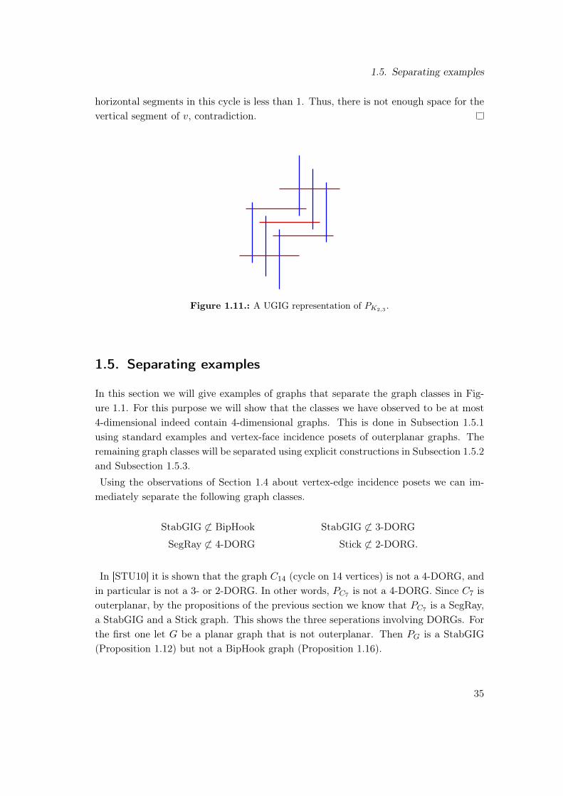
There are graphs G where PG is a UGIG and G is not outerplanar, for exampleG = K2,3 as shown in Figure 1.11. On the other hand there exist planar graphs G, suchthat PG is not a UGIG as the following proposition shows.
Proposition 1.19. PK4 is not a UGIG.
Proof. Suppose to the contrary that PK4 has a UGIG representation with vertices asvertical segments. By contracting vertical segments to points one can obtain a planarembedding of K4 from such a representation. As K4 is not outerplanar, there is avertex v that is not incident to the outer face in this embedding. For the initial UGIGrepresentation this means that v is represented by a vertical segment which is enclosedby segments representing vertices and edges of K4 − v. Notice that these segmentsrepresent a 6-cycle of PK4 . However, the largest vertical distance between any pair of
34
1.5. Separating examples
horizontal segments in this cycle is less than 1. Thus, there is not enough space for thevertical segment of v, contradiction.
Figure 1.11.: A UGIG representation of PK2,3 .
1.5. Separating examples
In this section we will give examples of graphs that separate the graph classes in Fig-ure 1.1. For this purpose we will show that the classes we have observed to be at most4-dimensional indeed contain 4-dimensional graphs. This is done in Subsection 1.5.1using standard examples and vertex-face incidence posets of outerplanar graphs. Theremaining graph classes will be separated using explicit constructions in Subsection 1.5.2and Subsection 1.5.3.Using the observations of Section 1.4 about vertex-edge incidence posets we can im-mediately separate the following graph classes.
StabGIG 6⊂ BipHook StabGIG 6⊂ 3-DORG
SegRay 6⊂ 4-DORG Stick 6⊂ 2-DORG.
In [STU10] it is shown that the graph C14 (cycle on 14 vertices) is not a 4-DORG, andin particular is not a 3- or 2-DORG. In other words, PC7 is not a 4-DORG. Since C7 isouterplanar, by the propositions of the previous section we know that PC7 is a SegRay,a StabGIG and a Stick graph. This shows the three seperations involving DORGs. Forthe first one let G be a planar graph that is not outerplanar. Then PG is a StabGIG(Proposition 1.12) but not a BipHook graph (Proposition 1.16).
35

1. The dimension of bipartite intersection graphs
`
Figure 1.12.: The poset S4 and a stabbable 4-DORG representation of it.
1.5.1. 4-dimensional graphs
First of all, some graph classes are already separated by their maximal dimension. Thestandard example Sn of an n-dimensional poset, cf. [Tro92], is the poset on n minimalelements a1, . . . , an and n maximal elements b1, . . . , bn, such that ai < bj in Sn if andonly if i 6= j. To separate most of the 4-dimensional classes from the 3-dimensional ones,the standard example S4 is sufficient. As shown in Figure 1.12 it has as a stabbable4-DORG representation. From this it follows that:
StabGIG 6⊂ BipHook StabGIG 6⊂ 3-DORG
4-DORG 6⊂ 3-DORG StabGIG 6⊂ 3-dim GIG
Since the interval dimension of Sn is n we get the following relations from Proposi-tion 1.9.
StabGIG 6⊂ SegRay 4-DORG 6⊂ SegRay
We will now show that the vertex-face incidence poset of an outerplanar graph has aSegRay representation. In [FN11] it has been shown that there are outerplanar mapswith a vertex-face incidence poset of dimension 4. Together with Proposition 1.20 belowthis shows that there are SegRay graphs of dimension 4. We obtain
SegRay 6⊂ 3-dim GIG.
Proposition 1.20. If G is an outerplanar map then the vertex-face incidence poset ofG is a SegRay graph.
Proof. Let G be a graph with a fixed outerplanar embedding. First we argue that wemay assume that G is 2-connected. If G is not connected then we can add a single edgebetween two components without changing the vertex-face poset. Now consider addingan edge between two neighbours of a cut vertex on the outer face cycle, i.e., two verticesof distance 2 on this cycle. This adds a new face to the vertex-face-poset, but keeps
36

1.5. Separating examples
f
v2
v1
v2 v1fv1 v2
f
Figure 1.13.: Illustration for the induction step in Proposition 1.20
the old vertex-face-poset as an induced subposet. Therefore, we may assume that G is2-connected.By induction on the number of bounded faces we show that G has a SegRay represen-tation in which the cyclic order of the vertices on the outer face agrees with the left-rightorder (cyclically) of rays representing these vertices. If G has one bounded face then theclaim is straight-forward. If G has more bounded faces then consider the dual graphof G without the outer face, which is a tree. Let f be a face that corresponds to aleaf of that tree. Define G′ to be the plane graph obtained by removing f and incidentdegree-2 vertices from G. Then exactly two vertices v1, v2 of f are still in G′, and theyare adjacent via an edge at the outer face of G′. Note that G′ is 2-connected. Applyinginduction on G′ we obtain a SegRay representation in which the two rays representingv1 and v2 are either consecutive, or left- and rightmost ray.In the first case we insert rays for the removed vertices between v1 and v2 with endpointsbeing below all other horizontal segments. Then a segment representing f can easilybe added to obtain a SegRay representation with the required properties of G, see themiddle of Figure 1.13.If the rays of v1 and v2 are the left- and rightmost ones, then observe that the endpointsof both rays can be extended upwards to be above all other endpoints. We can insertthe new rays to the left of all the other rays and the segment for f as indicated inFigure 1.13 on the right. This concludes the proof.
Propositions 1.20 and 1.9 also give the following interesting result about vertex-faceincidence posets of outerplanar maps which complements the fact that they can havedimension 4 [FN11].
Corollary 1.21. The interval dimension of a vertex-face incidence poset of an outer-planar map is bounded by 3.
We have separated all the graph classes which involve dimension except for the twoclasses of 3-dimensional GIGs and stabbable GIGs. As indicated in Figure 1.1 it remainsopen whether 3-dim GIG is a subclass of StabGIG or not. More comments on this canbe found at the end of Subsection 1.5.3.
37

1. The dimension of bipartite intersection graphs
1.5.2. Constructions
In this subsection we give explicit constructions for the remaining separations of classesnot involving StabGIG.In the introduction we mentioned that every 2-dimensional order of height 2, i.e.,every bipartite permutation graph, is a GIG. We show now that this does not hold for3-dimensional orders of height 2.
Proposition 1.22. There is a 3-dimensional bipartite graph that is not a GIG.
a
Figure 1.14.: The drawing on the left defines an inclusion order of homothetic triangles. Thisheight-2 order does not have a pseudosegment representation.
Proof. The left drawing in Figure 1.14 defines a poset P by ordering the homothetictriangles by inclusion. Some of the triangles are so small that we refer to them as pointsfrom now on. Each inclusion in P is witnessed by a point and a triangle, and hence Phas height 2. To see that it is 3-dimensional we use the drawing and the three directionsdepicted in Figure 1.14. By applying the same method as we did for Proposition 1.5 weobtain three linear extensions forming a realizer of P .We claim that P is not a pseudosegment intersection graph , and hence not a GIG.Suppose to the contrary that it has a pseudosegment representation. The six greentriangles together with the three green and the three blue points form a cycle of length12 in G. Hence, the union of the corresponding pseudosegments in the representationcontains a closed curve in R2. Without loss of generality assume that the pseudosegmentrepresenting the yellow point lies inside this closed curve (we may change the outer faceusing a stereographic projection). The pseudosegments of the three large blue triangles
38

1.5. Separating examples
intersect the yellow pseudosegment and one blue pseudosegment (corresponding to ablue point) each. The yellow and the blue pseudosegments divide the interior of theclosed curve into three regions. We show that each of these regions contains one of thepseudosegments representing black points.Each purple pseudosegment intersects the cycle in a point that is incident to one ofthe three bounded regions. Now, each black pseudosegment intersects a purple one. Ifsuch an intersection lies in the unbounded region, then the whole black pseudosegmentis contained in this region. This is not possible as for each of the black pseudosegmentsthere is a blue pseudosegment representing a small blue triangle that connects it tothe enclosed yellow pseudosegment without intersecting the cycle. Thus, the threeintersections of purple and black pseudosegments have to occur in the bounded regions,and in each of them one. It follows that each of the three bounded regions contains oneblack pseudosegment.Now, the red pseudosegment intersects each of the three black pseudosegments. Sincethey lie in three different regions whose boundary it may only traverse through the yellowpseudosegment, it has to intersect the yellow pseudosegment twice. This contradictsthe existence of a pseudosegment representation.
In the following we give constructions to show that
Stick 6⊂ UGIG UGIG 6⊂ Stick
BipHook 6⊂ 3-DORG BipHook 6⊂ Stick
Proposition 1.23. The Stick graph shown in Figure 1.15 is not a UGIG.
Figure 1.15.: A stick representation of a graph that is not a UGIG.
39

1. The dimension of bipartite intersection graphs
Proof. Let G be the graph represented in Figure 1.15. Let v and h be the two adjacentvertices of G that are drawn as black sticks in the figure. There are five pairs of inter-secting blue vertical and red horizontal segments v1, h1, . . . , v5, h5. Each vi intersectsh and each hi intersects v. Four of the pairs vi, hi form a 4-cycle with a pair of greensegments qi, ri.Suppose that G has a UGIG representation. We claim that in any such representationthe intersection points pi of vi and hi form a chain in <dom after a suitable rotation ofthe representation. Note that one quadrant formed by the segments v and h (withoutloss of generality the upper right one) contains at least two of the pi’s by the pigeonholeprinciple. Assume without loss of generality that p1 and p2 lie in this quadrant. If p1 andp2 are incomparable in <dom, then the horizontal segment h1 of the lower intersectionpoint has a forbidden intersection with the vertical segment v2 of the higher one, seeFigure 1.16 left.
h
v2
h2
v
v1
vi
v1
v1
hj
v2
hi
h1
h1h2
vv2
h
qj
rj
vj
v
h
h1
h2
Figure 1.16.: Left: The intersection points p1, p2 in the upper right quadrant form a chain in<dom. Middle: pi does not dominate p2 in <dom. Right: The green segmentsqj , rj for the middle pair of segments hj , vj cannot be added.
So p1 and p2 are comparable in <dom. We may assume that v2, h2 is the pair ofsegments whose intersection point is dominated in <dom by all other intersection pointsin the upper right quadrant. We observe that the lower endpoint of v2 lies below thelower endpoint of v, and the left endpoint of h2 lies to the left of the left endpoint of has shown in the middle of Figure 1.16. It follows that if an intersection point pi doesnot dominate p2, then pi lies below h2 and to the left of v2, but not in the upper rightquadrant by our choice of p2 (see Figure 1.16 for an example). It is easy to see that theremaining two intersection points pj (j 6∈ 1, 2, i) then have to dominate p2 in <dom,as otherwise we would see forbidden intersections among the blue and red segments.We conclude that, in each case, four of the points p1, . . . , p5 lie in the upper rightquadrant and that they form a chain with respect to <dom. Thus at least one pair ofsegments vj , hj with pj being in the middle of the chain has neighbours qj , rj . However,as indicated in the right of Figure 1.16, qj and rj cannot be added without introducing
40
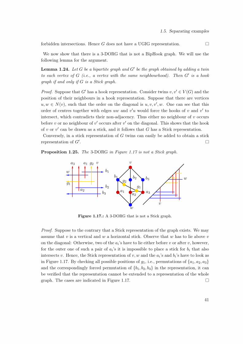
1.5. Separating examples
forbidden intersections. Hence G does not have a UGIG representation.
We now show that there is a 3-DORG that is not a BipHook graph. We will use thefollowing lemma for the argument.
Lemma 1.24. Let G be a bipartite graph and G′ be the graph obtained by adding a twinto each vertex of G (i.e., a vertex with the same neighbourhood). Then G′ is a hookgraph if and only if G is a Stick graph.
Proof. Suppose that G′ has a hook representation. Consider twins v, v′ ∈ V (G) and theposition of their neighbours in a hook representation. Suppose that there are verticesu,w ∈ N(v), such that the order on the diagonal is u, v, v′, w. One can see that thisorder of centres together with edges uw and v′u would force the hooks of v and v′ tointersect, which contradicts their non-adjacency. Thus either no neighbour of v occursbefore v or no neighbour of v′ occurs after v′ on the diagonal. This shows that the hookof v or v′ can be drawn as a stick, and it follows that G has a Stick representation.Conversely, in a stick representation of G twins can easily be added to obtain a stickrepresentation of G′.
Proposition 1.25. The 3-DORG in Figure 1.17 is not a Stick graph.
v
w
a1 a3
b2
w
va1
b1
b2
b3a2
a2
b3
g1
b1g2
a3
g1
g2
w
v
Figure 1.17.: A 3-DORG that is not a Stick graph.
Proof. Suppose to the contrary that a Stick representation of the graph exists. We mayassume that v is a vertical and w a horizontal stick. Observe that w has to lie above von the diagonal: Otherwise, two of the ai’s have to lie either before v or after v, however,for the outer one of such a pair of ai’s it is impossible to place a stick for bi that alsointersects v. Hence, the Stick representation of v, w and the ai’s and bi’s have to look asin Figure 1.17. By checking all possible positions of g1, i.e., permutations of a1, a2, a3and the correspondingly forced permutation of b1, b2, b3 in the representation, it canbe verified that the representation cannot be extended to a representation of the wholegraph. The cases are indicated in Figure 1.17.
41

1. The dimension of bipartite intersection graphs
As a consequence, there is a 3-DORG that is not a bipartite hook graph. Indeed, if weadd a twin to each vertex of the graph shown in Figure 1.17 then the obtained graph isstill a 3-DORG. It can not be a BipHook graph as otherwise by Lemma 1.24 we wouldconclude that the graph in Figure 1.17 is a Stick graph.We next show a construction of a bipartite hook graph that is not a Stick graph. Arelated construction was also presented in [Hix13].
x
y
Figure 1.18.: The graph Φ and the two possible positions of x and y in a Stick representationof G.
Proposition 1.26. There is a bipartite hook graph that is not a Stick graph.
Proof. The proof is based on the graph Φ shown in Figure 1.18. The vertices x and yare the connectors of Φ. Let G be a graph that contains an induced Φ and a path pxyfrom x to y such that there is no adjacency between inner vertices of pxy and the 6-cycleof Φ. Observe that the Stick representation of the 6-cycle is essentially unique. Now itis easy to check that in a Stick representation of G the sticks for the connectors haveto be placed like the two blue sticks or like the two red sticks in Figure 1.18, otherwisethe sticks of x and y would be separated by the 6-cycle, whence one of the sticksrepresenting inner vertices of pxy and a stick of the 6-cycle would intersect. Dependingon the placement the connectors are of type inner (blue) or outer (red).Consider the graph Φ4 depicted in Figure 1.19 together with a hook representationof it. Suppose for contradiction that Φ4 has a Stick representation. It contains fourcopies Φ1, . . . ,Φ4 of the graph Φ with connectors x1, . . . , x5. By our observation above,the connectors of each Φi are either of inner or outer type. We claim that for eachi ∈ 1, 2, 3, connecters of Φi and Φi+1 are of different type. If the type of bothconnectors of Φi and Φi+1 is inner, then such a placement would force extra edges,specifically an edge between the two 6-cycles of Φi and Φi+1. And if both are outerthen such a placement would separate xi and xi+2, see Figure 1.20 on the left.It follows that the connector type of the Φi’s is alternating. In particular, there isi ∈ 1, 2 such that the connectors of Φi,Φi+1,Φi+2 are of type inner–outer–inner in
42
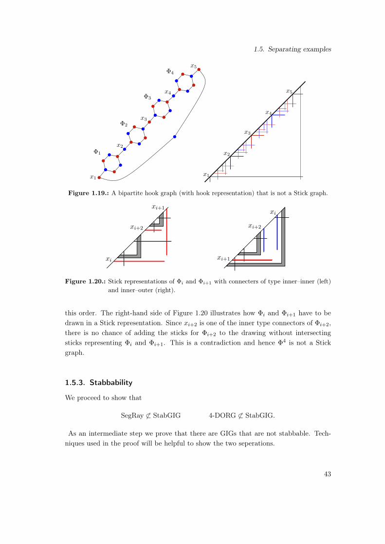
1.5. Separating examples
x1
x2
x3
x4
x5
x1
x2
x3
x4
x5
Φ1
Φ2
Φ3
Φ4
Figure 1.19.: A bipartite hook graph (with hook representation) that is not a Stick graph.
xi+2
xi+1
xi
xi
xi+2
xi+1
Figure 1.20.: Stick representations of Φi and Φi+1 with connecters of type inner–inner (left)and inner–outer (right).
this order. The right-hand side of Figure 1.20 illustrates how Φi and Φi+1 have to bedrawn in a Stick representation. Since xi+2 is one of the inner type connectors of Φi+2,there is no chance of adding the sticks for Φi+2 to the drawing without intersectingsticks representing Φi and Φi+1. This is a contradiction and hence Φ4 is not a Stickgraph.
1.5.3. Stabbability
We proceed to show that
SegRay 6⊂ StabGIG 4-DORG 6⊂ StabGIG.
As an intermediate step we prove that there are GIGs that are not stabbable. Tech-niques used in the proof will be helpful to show the two seperations.
43

1. The dimension of bipartite intersection graphs
Proposition 1.27. There exists a GIG that is not a StabGIG.
Proof. Consider a GIG representation of a complete bipartite graph Kn,n. The GIGrepresentation forms a grid in the plane. Now we add segments such that for every pairof cells in the same row or in the same column there is a segment that has endpointsin both of the cells. Furthermore, those segments can be drawn in such way that ahorizontal and a vertical segment intersect if and only if both intersect a common cellcompletely, that is, they do not have an endpoint in this cell. Denote the resulting GIGrepresentation by Rn and the corresponding GIG by Gn.Suppose for contradiction that Gn has a stabbable GIG representation R′n for all n ∈ N.By the Erdős-Szekeres theorem for monotone subsequences, for every k ∈ N there existsn ∈ N such that in Rn there are subsets H and V consisting of k horizontal and k
vertical segments that represent vertices of the Kn,n in Gn, such that they appear inthe same order (up to reflection) as segments in Rn representing the same set of vertices.In Rn those segments induce a subgrid to which we added the blue segments depictedin Figure 1.21. That is, for each cell c in the subgrid we have a horizontal segment hcand a vertical one vc such that hc and vc intersect only each other and the segmentsbuilding the boundary of c.
Figure 1.21.: Partial representation of Rn on the left. Replaced cell segments in R′n on theright.
It is easy to see that this partial representation in Rn is not stabbable if k is large.Since the segments of the subgrid appear in the same order (up to reflection) in R′n,we only have to consider the placement of cell segments hc and vc. We restrict ourattention to cells not lying on the boundary of the grid and fix a stabbing line ` for R′n.There are two possibilities for the placement of hc and vc in R′n. One case is that theintersection point pc of hc and vc lies in c or in one of the eight cells surrounding c.Then the segments hc and vc can only be stabbed by ` if at least one of those eight cellsaround c is intersected by `. The cells intersected by ` in R′n are only O(k) many, so
44
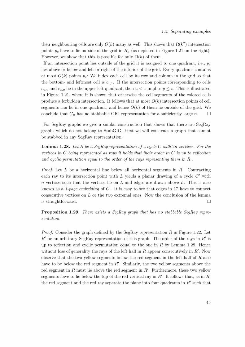
1.5. Separating examples
their neighbouring cells are only O(k) many as well. This shows that Ω(k2) intersectionpoints pc have to lie outside of the grid in R′n (as depicted in Figure 1.21 on the right).However, we show that this is possible for only O(k) of them.If an intersection point lies outside of the grid it is assigned to one quadrant, i.e., pclies above or below and left or right of the interior of the grid. Every quadrant containsat most O(k) points pc: We index each cell by its row and column in the grid so thatthe bottom- and leftmost cell is c1,1. If the intersection points corresponding to cellscu,v and cx,y lie in the upper left quadrant, then u < x implies y ≤ v. This is illustratedin Figure 1.21, where it is shown that otherwise the cell segments of the colored cellsproduce a forbidden intersection. It follows that at most O(k) intersection points of cellsegments can lie in one quadrant, and hence O(k) of them lie outside of the grid. Weconclude that Gn has no stabbable GIG representation for a sufficiently large n.
For SegRay graphs we give a similar construction that shows that there are SegRaygraphs which do not belong to StabGIG. First we will construct a graph that cannotbe stabbed in any SegRay representation.
Lemma 1.28. Let R be a SegRay representation of a cycle C with 2n vertices. For thevertices in C being represented as rays it holds that their order in C is up to reflectionand cyclic permutation equal to the order of the rays representing them in R .
Proof. Let L be a horizontal line below all horizontal segments in R. Contractingeach ray to its intersection point with L yields a planar drawing of a cycle C ′ withn vertices such that the vertices lie on L and edges are drawn above L. This is alsoknown as a 1-page embedding of C ′. It is easy to see that edges in C ′ have to connectconsecutive vertices on L or the two extremal ones. Now the conclusion of the lemmais straightforward.
Proposition 1.29. There exists a SegRay graph that has no stabbable SegRay repre-sentation.
Proof. Consider the graph defined by the SegRay representation R in Figure 1.22. LetR′ be an arbitrary SegRay representation of this graph. The order of the rays in R′ isup to reflection and cyclic permutation equal to the one in R by Lemma 1.28. Hencewithout loss of generality the rays of the left half in R appear consecutively in R′. Nowobserve that the two yellow segments below the red segment in the left half of R alsohave to be below the red segment in R′. Similarly, the two yellow segments above thered segment in R must lie above the red segment in R′. Furthermore, these two yellowsegments have to lie below the top of the red vertical ray in R′. It follows that, as in R,the red segment and the red ray seperate the plane into four quadrants in R′ such that
45

1. The dimension of bipartite intersection graphs
Figure 1.22.: A SegRay graph with no stabbable SegRay representation.
each quadrant contains exactly one of the considered yellow segments. Any line in theplane can intersect at most three of the quadrants and thus will miss a yellow segmentin R′. Therefore, R′ is not stabbable and the conlusion follows.
We add a vertex h to the graph in Figure 1.22 that is adjacent to all rays. Thisgraph is still a SegRay graph. We call this graph a bundle and the set of horizontalsegments its head. The bundle is not stabbable in any SegRay representation by theproposition above. This means, in any StabGIG representation of a bundle there is onehorizontal segment above the segment representing h and one below. Indeed, otherwisethe representation of the bundle can be modified by extending vertical segments to raysin one direction to obtain a stabbed SegRay representation. Using this property of abundle we can show the following.
Proposition 1.30. There exists a SegRay graph that is not a stabbable GIG.
Figure 1.23.: Illustration of a SegRay graph that is not a StabGIG
46
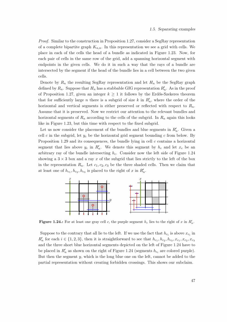
1.5. Separating examples
Proof. Similar to the construction in Proposition 1.27, consider a SegRay representationof a complete bipartite graph Kn,n. In this representation we see a grid with cells. Weplace in each of the cells the head of a bundle as indicated in Figure 1.23. Now, foreach pair of cells in the same row of the grid, add a spanning horizontal segment withendpoints in the given cells. We do it in such a way that the rays of a bundle areintersected by the segment if the head of the bundle lies in a cell between the two givencells.Denote by Rn the resulting SegRay representation and let Hn be the SegRay graphdefined by Rn. Suppose thatHn has a stabbable GIG representation R′n. As in the proofof Proposition 1.27, given an integer k ≥ 1 it follows by the Erdős-Szekeres theoremthat for sufficiently large n there is a subgrid of size k in R′n, where the order of thehorizontal and vertical segments is either preserved or reflected with respect to Rn.Assume that it is preserved. Now we restrict our attention to the relevant bundles andhorizontal segments of Rn according to the cells of the subgrid. In Rn again this lookslike in Figure 1.23, but this time with respect to the fixed subgrid.Let us now consider the placement of the bundles and blue segments in R′n. Given acell c in the subgrid, let yc be the horizontal grid segment bounding c from below. ByProposition 1.29 and its consequences, the bundle lying in cell c contains a horizontalsegment that lies above yc in R′n. We denote this segment by hc and let xc be anarbitrary ray of the bundle intersecting hc. Consider now the left side of Figure 1.24showing a 3 × 3 box and a ray x of the subgrid that lies strictly to the left of the boxin the representation Rn. Let c1, c2, c3 be the three shaded cells. Then we claim thatat least one of hc1 , hc2 , hc3 is placed to the right of x in R′n.
x x
y
Figure 1.24.: For at least one gray cell c, the purple segment hc lies to the right of x in R′n.
Suppose to the contrary that all lie to the left. If we use the fact that hci is above xci inR′n for each i ∈ 1, 2, 3, then it is straightforward to see that hc1 , hc2 , hc3 , xc1 , xc2 , xc3
and the three short blue horizontal segments depicted on the left of Figure 1.24 have tobe placed in R′n as shown on the right of Figure 1.24 (segments hci are colored purple).But then the segment y, which is the long blue one on the left, cannot be added to thepartial representation without creating forbidden crossings. This shows our subclaim.
47
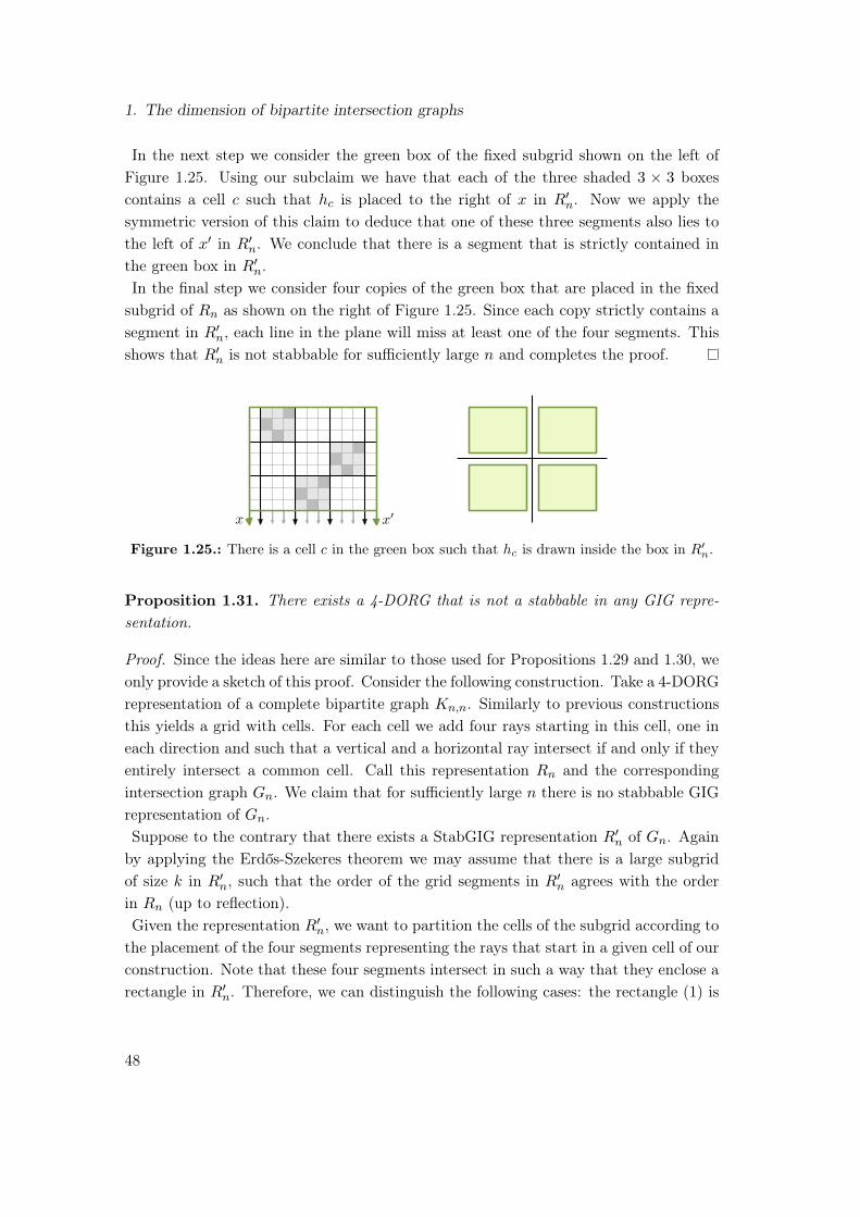
1. The dimension of bipartite intersection graphs
In the next step we consider the green box of the fixed subgrid shown on the left ofFigure 1.25. Using our subclaim we have that each of the three shaded 3 × 3 boxescontains a cell c such that hc is placed to the right of x in R′n. Now we apply thesymmetric version of this claim to deduce that one of these three segments also lies tothe left of x′ in R′n. We conclude that there is a segment that is strictly contained inthe green box in R′n.In the final step we consider four copies of the green box that are placed in the fixedsubgrid of Rn as shown on the right of Figure 1.25. Since each copy strictly contains asegment in R′n, each line in the plane will miss at least one of the four segments. Thisshows that R′n is not stabbable for sufficiently large n and completes the proof.
x x′
Figure 1.25.: There is a cell c in the green box such that hc is drawn inside the box in R′n.
Proposition 1.31. There exists a 4-DORG that is not a stabbable in any GIG repre-sentation.
Proof. Since the ideas here are similar to those used for Propositions 1.29 and 1.30, weonly provide a sketch of this proof. Consider the following construction. Take a 4-DORGrepresentation of a complete bipartite graph Kn,n. Similarly to previous constructionsthis yields a grid with cells. For each cell we add four rays starting in this cell, one ineach direction and such that a vertical and a horizontal ray intersect if and only if theyentirely intersect a common cell. Call this representation Rn and the correspondingintersection graph Gn. We claim that for sufficiently large n there is no stabbable GIGrepresentation of Gn.Suppose to the contrary that there exists a StabGIG representation R′n of Gn. Againby applying the Erdős-Szekeres theorem we may assume that there is a large subgridof size k in R′n, such that the order of the grid segments in R′n agrees with the orderin Rn (up to reflection).Given the representation R′n, we want to partition the cells of the subgrid according tothe placement of the four segments representing the rays that start in a given cell of ourconstruction. Note that these four segments intersect in such a way that they enclose arectangle in R′n. Therefore, we can distinguish the following cases: the rectangle (1) is
48
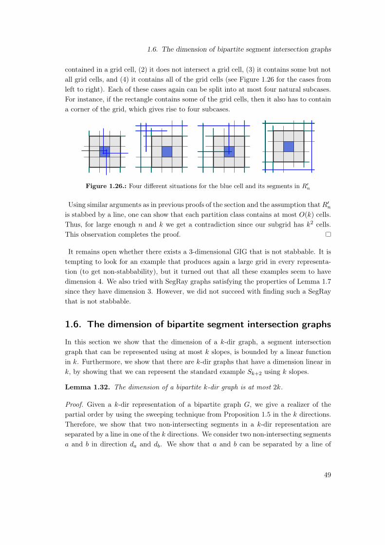
1.6. The dimension of bipartite segment intersection graphs
contained in a grid cell, (2) it does not intersect a grid cell, (3) it contains some but notall grid cells, and (4) it contains all of the grid cells (see Figure 1.26 for the cases fromleft to right). Each of these cases again can be split into at most four natural subcases.For instance, if the rectangle contains some of the grid cells, then it also has to containa corner of the grid, which gives rise to four subcases.
Figure 1.26.: Four different situations for the blue cell and its segments in R′n
Using similar arguments as in previous proofs of the section and the assumption thatR′nis stabbed by a line, one can show that each partition class contains at most O(k) cells.Thus, for large enough n and k we get a contradiction since our subgrid has k2 cells.This observation completes the proof.
It remains open whether there exists a 3-dimensional GIG that is not stabbable. It istempting to look for an example that produces again a large grid in every representa-tion (to get non-stabbability), but it turned out that all these examples seem to havedimension 4. We also tried with SegRay graphs satisfying the properties of Lemma 1.7since they have dimension 3. However, we did not succeed with finding such a SegRaythat is not stabbable.
1.6. The dimension of bipartite segment intersection graphs
In this section we show that the dimension of a k-dir graph, a segment intersectiongraph that can be represented using at most k slopes, is bounded by a linear functionin k. Furthermore, we show that there are k-dir graphs that have a dimension linear ink, by showing that we can represent the standard example Sk+2 using k slopes.
Lemma 1.32. The dimension of a bipartite k-dir graph is at most 2k.
Proof. Given a k-dir representation of a bipartite graph G, we give a realizer of thepartial order by using the sweeping technique from Proposition 1.5 in the k directions.Therefore, we show that two non-intersecting segments in a k-dir representation areseparated by a line in one of the k directions. We consider two non-intersecting segmentsa and b in direction da and db. We show that a and b can be separated by a line of
49

1. The dimension of bipartite intersection graphs
direction da or db. We apply a linear transformation T such that T (da) and T (db) areboth vertical or horizontal segments. The vertical or horizontal segments are separatedby a vertical or a horizontal line ` as shown in the proof of Proposition 1.5. Invertingthe linear transformation leads to a line T−1(`) of direction da or db, which separatesthe segments a and b.This implies that the dimension of a bipartite k-dir graph is at most 2k.
After showing that the dimension of bipartite k-dir graphs is bounded linearly in k, weshow that this bound is up to a constant factor tight.
Theorem 1.33. The standard example Sk+2 for even k has a segment representationusing k different slopes.
Proof. We construct a segment representation of Sk+2, for even n, iteratively. Westart with the representation of S4 that is shown in Figure 1.27. The constructionwill be symmetric to the horizontal line `. We keep the following invariant during the
a1b1
b2a2
`
Figure 1.27.: A symmetric representation of S4.
construction: Removing the segment b2 leads to segment representation, such that theminima (blue) can be extended to rays into the upper half-plane without creating newintersections. Symmetrically, removing the segment a1 from the representation, suchthat the maxima (red) can be extended to rays into the lower half-plane without creatingnew intersections. In addition, the segments a1 and b2 share the leftmost or rightmostintersection point on `.We use the invariant to construct a segment representation of Sk for even k, withk − 2 slopes from a representation of Sk−2 using k − 4 slopes. The construction will besymmetric with respect to a horizontal line `. Note that the representation of S4 shownin Figure 1.27 satisfies all those invariants. We describe the construction in the casethat b2 and a1 share the rightmost intersection point on `.First, we add two parallel lines with a positive slope that is smaller than all slopesof the segments in the representation of Sk−2. The lines intersect ` to the left of therepresentation of Sk−2 and do not intersect the representation. We extend the blue
50

1.6. The dimension of bipartite segment intersection graphs
b2
a2
b1
a1
`
Figure 1.28.: A segment representation of S6.
segments, such that all segments except for a2 intersect the upper of the two new lines,which is possible since we assumed the slope of the new segments is small. The segmenta2 ends after intersecting the lower of the new lines. The upper of the new lines isthe supporting line for the new segment b2. We fix a position of the new segment b2,such that it contains all intersection points of segments and the new line. For now, weconsider b2 as a ray pointing in the lower left direction of the line. The lower of the newlines supports a segment that contains all but the rightmost intersection points withthe blue segments and is also considered as a ray to the left direction of its supportingline. The representation in the half-plane below ` is symmetric to the representationabove `.We show that this construction gives a segment representation of Sk, i.e., we have toshow that segments of one color do not intersect and that each segment intersects k− 1
other segments.Note, that the segments of one color do not intersect by construction and the invariant:The invariant states that we can extend the blue segments in the upper half-plane andthe red segments in the lower half-plane without creating new intersections.
51
1. The dimension of bipartite intersection graphs
The two new red segments intersect all but one blue segment by construction. Therightmost blue that does not intersect the new segment on the lower line lies on thesupporting line of the former segment a1, the segment which could not be extendedwithout creating a new intersection. Thus this segment intersects k − 1 segments, allbut the red segment on the lower line. The segment a2 intersects all except the newsegment b2. The modifications of all other blue segments cause two new intersectionswith the segments on the new lines. Thus, the number of intersections is k − 1 for thered segments on the new supporting lines and the blue segments on the old supportinglines. This implies the correct number of intersections for each segment by symmetry.We added two new directions which gives a k− 2-dir representation of Sk inductively.
52

2. The slope number of segmentintersection graphs
In this chapter, we investigate the slope number of segment intersection graphs. Wedefine the slope number of a segment intersection graph G to be the minimal k, suchthat G has a k-dir representation.
The main tool is a connection between Hamiltonian cycles in maximal planar graphs Gand grid intersection representations of a graph P ∗G associated with G. A similar connec-tion exists between Hamiltonian cycles in G and segment intersection representationsof P ∗G. This is presented in Section 2.2. In Section 2.3 we consider the behaviour of theslope number under removal of vertices. We use the methods from Section 2.2 to showthat there are graphs with a slope number that is linear in the number of vertices (andedges), and the removal of one special vertex leads to a grid intersection representation,i.e., the slope number drops down to two. Another consequence of Section 2.2 is thatthe recognition of grid and of segment intersection graphs is NP-hard. This follows fromknown NP-hardness results for the Hamiltonian cycle and the Hamiltonian path prob-lem in maximal planar graphs [Wid82, AG11]. In Section 2.4 we extend this by showingthat the Hamiltonian cycle problem in maximal planar graphs with given Hamiltonianpath is NP-complete. With our tools this corresponds to the problem of finding a gridrepresentation of a graph with a given segment representation. This implies that theproblem of determining the slope number of a graph is NP-hard. The input graphs inthe reduction have at most slope number four and thus it is NP-hard to determine if a4-dir graph has a 2-dir (GIG) representation.
The bipartite k-dir graphs we consider in the first sections always use an even numberof directions k. In Section 2.5 we raise the question whether there is a bipartite SEG
with an odd slope number. We answer this question affimatively and show that the classof bipartite 3-dir graphs that do not have a 2-dir representation has no monochromaticdirection, that is, all segments of one slope have the same color in a proper two coloring.
Parts of this chapter appeared in [Hof15].
53
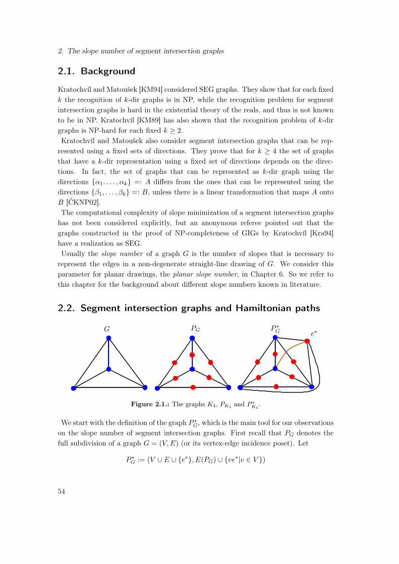
2. The slope number of segment intersection graphs
2.1. Background
Kratochvíl and Matoušek [KM94] considered SEG graphs. They show that for each fixedk the recognition of k-dir graphs is in NP, while the recognition problem for segmentintersection graphs is hard in the existential theory of the reals, and thus is not knownto be in NP. Kratochvíl [KM89] has also shown that the recognition problem of k-dirgraphs is NP-hard for each fixed k ≥ 2.Kratochvíl and Matoušek also consider segment intersection graphs that can be rep-resented using a fixed sets of directions. They prove that for k ≥ 4 the set of graphsthat have a k-dir representation using a fixed set of directions depends on the direc-tions. In fact, the set of graphs that can be represented as k-dir graph using thedirections α1. . . . , αk =: A differs from the ones that can be represented using thedirections β1, . . . , βk =: B, unless there is a linear transformation that maps A ontoB [ČKNP02].The computational complexity of slope minimization of a segment intersection graphshas not been considered explicitly, but an anonymous referee pointed out that thegraphs constructed in the proof of NP-completeness of GIGs by Kratochvíl [Kra94]have a realization as SEG.Usually the slope number of a graph G is the number of slopes that is necessary torepresent the edges in a non-degenerate straight-line drawing of G. We consider thisparameter for planar drawings, the planar slope number, in Chapter 6. So we refer tothis chapter for the background about different slope numbers known in literature.
2.2. Segment intersection graphs and Hamiltonian paths
e∗P ∗GG PG
Figure 2.1.: The graphs K4, PK4 and P ∗K4.
We start with the definition of the graph P ∗G, which is the main tool for our observationson the slope number of segment intersection graphs. First recall that PG denotes thefull subdivision of a graph G = (V,E) (or its vertex-edge incidence poset). Let
P ∗G := (V ∪ E ∪ e∗, E(PG) ∪ ve∗|v ∈ V )
54
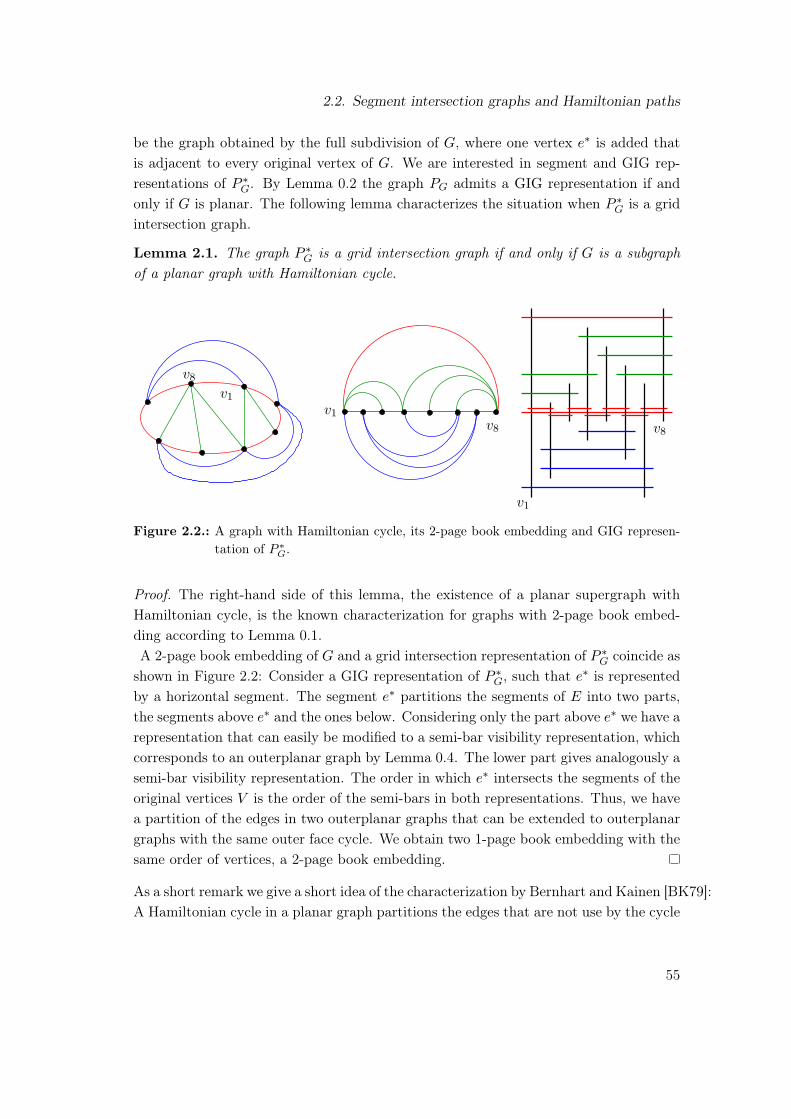
2.2. Segment intersection graphs and Hamiltonian paths
be the graph obtained by the full subdivision of G, where one vertex e∗ is added thatis adjacent to every original vertex of G. We are interested in segment and GIG rep-resentations of P ∗G. By Lemma 0.2 the graph PG admits a GIG representation if andonly if G is planar. The following lemma characterizes the situation when P ∗G is a gridintersection graph.
Lemma 2.1. The graph P ∗G is a grid intersection graph if and only if G is a subgraphof a planar graph with Hamiltonian cycle.
v1
v8
v1
v8
v8
v1
Figure 2.2.: A graph with Hamiltonian cycle, its 2-page book embedding and GIG represen-tation of P ∗G.
Proof. The right-hand side of this lemma, the existence of a planar supergraph withHamiltonian cycle, is the known characterization for graphs with 2-page book embed-ding according to Lemma 0.1.A 2-page book embedding of G and a grid intersection representation of P ∗G coincide asshown in Figure 2.2: Consider a GIG representation of P ∗G, such that e∗ is representedby a horizontal segment. The segment e∗ partitions the segments of E into two parts,the segments above e∗ and the ones below. Considering only the part above e∗ we have arepresentation that can easily be modified to a semi-bar visibility representation, whichcorresponds to an outerplanar graph by Lemma 0.4. The lower part gives analogously asemi-bar visibility representation. The order in which e∗ intersects the segments of theoriginal vertices V is the order of the semi-bars in both representations. Thus, we havea partition of the edges in two outerplanar graphs that can be extended to outerplanargraphs with the same outer face cycle. We obtain two 1-page book embedding with thesame order of vertices, a 2-page book embedding.
As a short remark we give a short idea of the characterization by Bernhart and Kainen [BK79]:A Hamiltonian cycle in a planar graph partitions the edges that are not use by the cycle
55
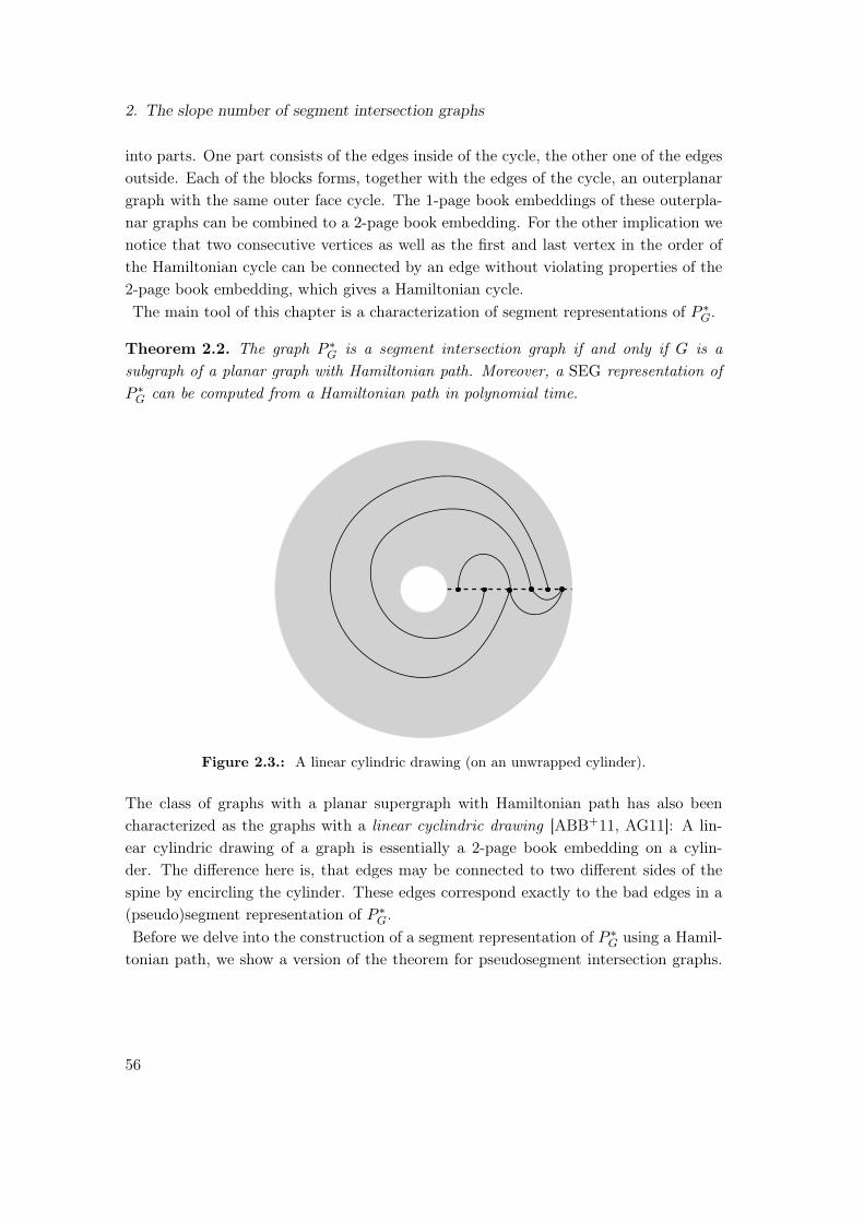
2. The slope number of segment intersection graphs
into parts. One part consists of the edges inside of the cycle, the other one of the edgesoutside. Each of the blocks forms, together with the edges of the cycle, an outerplanargraph with the same outer face cycle. The 1-page book embeddings of these outerpla-nar graphs can be combined to a 2-page book embedding. For the other implication wenotice that two consecutive vertices as well as the first and last vertex in the order ofthe Hamiltonian cycle can be connected by an edge without violating properties of the2-page book embedding, which gives a Hamiltonian cycle.The main tool of this chapter is a characterization of segment representations of P ∗G.
Theorem 2.2. The graph P ∗G is a segment intersection graph if and only if G is asubgraph of a planar graph with Hamiltonian path. Moreover, a SEG representation ofP ∗G can be computed from a Hamiltonian path in polynomial time.
Figure 2.3.: A linear cylindric drawing (on an unwrapped cylinder).
The class of graphs with a planar supergraph with Hamiltonian path has also beencharacterized as the graphs with a linear cyclindric drawing [ABB+11, AG11]: A lin-ear cylindric drawing of a graph is essentially a 2-page book embedding on a cylin-der. The difference here is, that edges may be connected to two different sides of thespine by encircling the cylinder. These edges correspond exactly to the bad edges in a(pseudo)segment representation of P ∗G.Before we delve into the construction of a segment representation of P ∗G using a Hamil-tonian path, we show a version of the theorem for pseudosegment intersection graphs.
56

2.2. Segment intersection graphs and Hamiltonian paths
Theorem 2.3. The graph P ∗G is a pseudosegment intersection graph if and only if G isa subgraph of a planar graph with Hamiltonian path.
Proof. We first show, that we can add edges to G such that we obtain a planar graphwith Hamiltonian path if P ∗G has a pseudosegment representation: The pseudosegmentof e∗ gives a linear order of the vertices v1, . . . , vn. We add a pseudosegment parallel toe∗, that intersects exactly vi and vi+1 in the representation for each i ∈ 1, . . . , n− 1.The modified representation is a pseudosegment representation P ∗G′ for a graph G′ thathas the Hamiltonian path (v1, . . . , vn). The planarity of G′ follows from Lemma 0.2.To show that P ∗G has a pseudosegment representation if G has a Hamiltonian path,we start with a planar straight line drawing of G, see Figure 2.4. We can interpretthis drawing as contact representation of PG, where the edges are represented by linesegments ending on circles which correspond to the vertices. We can obtain a pseu-dosegment contact representation of PG by removing a small part from the circles suchthat the contacts are preserved. We decide which part we remove after drawing e∗ in thefollowing way: Let v1, . . . , vn be the order of the vertices along the Hamiltonian path.Then, we draw a pseudosegment for e∗ starting inside of the cycle of v1. Iteratively, weleave the cycle of vi into a face that is incident to vi+1 and enter circle vi+1 withoutintersecting any other segment or cycle. A face with this property exists because vivi+1
is an edge of G. We finish the construction by removing a segment of each circle, suchthat the pseudosegment representing e∗ intersects each circle exactly once.
v1v2
v1
v2
v3 v4
v4
v3
Figure 2.4.: A pseudosegment and a segment representation of P ∗K4
We continue by considering the differences between a GIG representation and a SEG
representation of P ∗G. Let R be a SEG representation of P ∗G with horizontal segmente∗. We call the part of a segment that lies above e∗ the upper part, the one below e∗
the lower part. In contrast to a GIG representation, a segment representation may haveedge segments that intersect the lower part of one vertex segment and the upper part ofanother vertex segment as shown in Figure 2.4 right. We call those edges the bad edges.Recall, that a segment representation of P ∗G gives an embedding of G. The bad edges
57

2. The slope number of segment intersection graphs
vw are exactly those, such the unique closed curve Cvw on the segments v, w, vw ande∗ separates the first vertex of the Hamiltonian path v1 from the last one vn. The curveCvw corresponds to the cycle consisting of the Hamiltonian path and the bad edge inthe graph G. This implies that removing all bad edges leads to a planar graph in whichv1 and vn lie in the same face.
Observation 2.4. Removing the bad edges from G leads to graph that is a subgraph ofa planar graph with Hamiltonian cycle.
Note, that fixing a Hamiltonian path in a planar graph also fixes the bad edges. The badedges can be partitioned into several types: We call a bad edge vivj with i < j an upwardedge if its segment connects the lower part of vi with the upper part of vj . Otherwiseit is called downward edge. We call a bad edge vw a front back edge if v1 lies in thebounded region of Cvw. A vertex incident to a bad front edge is a bad front vertex, anda bad back vertex if it is incident to a bad back edge. The partition of the bad edges inupward and downward edges depends (up to interchanging the types of all edges) onlyon the Hamiltonian path. Whether a bad edge is a front or a back edge is determinedby the choice of the outer face in the embedding of G. With these definitions we canmake the following observation on the slopes of a segment representation of P ∗G. Notethat we only consider normal representations, where e∗ is represented by a horizontalsegment and all other segments have positive slope.
Observation 2.5. If the edge vivj is a front upward edge or a back downward edge,then s(vi) < s(vj). In the case that vivj is a front downward or a back upward edge, wehave s(vj) < s(vi). The slopes of the bad edge vivj lies strictly between the slopes of itsincident vertices.
Proof of Theorem 2.2. We give a construction of a segment representation of P ∗G from anembedding of G where the end of the Hamiltonian path lies on the outer face, i.e., all badedges are front bad edges. By symmetry, we only show how to construct a representationthat has only upward bad edges. We can assume without loss of generality, that G is amaximal planar graph.We start to build the representation with the segment e∗ has a horizontal ray inpositive x-direction. We construct a representation such that all slopes of segments arenon-negative. We first add the part of the vertices incident to bad edges and the badedges to the representation.We will choose the slopes, such that the following properties and the conditions fromObservation 2.5 are satisfied.
a. For each pair of upward bad edges of the form vivk and vjvl with i ≤ j < k ≤ l
we have s(vivk) ≤ s(vjvl) (see Figure 2.5).
58

2.2. Segment intersection graphs and Hamiltonian paths
b. For each pair of upward bad edges of the form vivk and vjvk with i < j < k, wehave s(i) ≤ s(j) < s(k) and s(vivj) ≤ s(vjvk).
e∗
vivj
vivkvjvl
Figure 2.5.: Forbidden configuration of Property a.
With these properties, we construct a representation by adding vj and all bad edgesvivj with i < j to the representation in step j. We keep the following invariants for therepresentation Rj after step j.
1. If vivk with i ≤ j < k is a bad upward edge, then there is an interval on the lowerpart of vi, such that a ray starting from this interval in positive s(vivk) directiondoes not intersect any segment of Rj .
2. If vivk with i ≤ j < k is a bad downward edge, then there is an interval on theupper part of vi, such that a ray starting from this interval in negative s(vivk)
direction does not intersect any segment of Rj .
In step j, we pick a point pj on e∗ right of the intersections with all other vertices viwith i < j, such that a line `j of slope s(vj) through the point does not intersect anyother segment of the representation Rj−1 than e∗. This can be done by choosing thepoint far enough to the right on e∗. For each incident bad upward edge vivj of vj weextend the lower part of vj until it sees the upper part of vi with by a sight line of slopes(vivj). If for each bad upward edge vjvk we further extend the lower part of vj until aline of slope s(vjvk) starting from an interval on vj does not intersect any other segmentof the representation Rj−1. Symmetrically, we extend the upper part of vj until all itsneighbors vi with a bad upward edge vivj can be seen by a sight line of slope s(vivj),or until a line of slope s(vjvk) does not intersect the rest of the representation throughan interval on the upper part of vj if vjvk is a bad downward edge. After determiningthe ends of vj on `j this way we can draw the bad edges vivj on the constructed sightlines. These sight lines do not cross which follows from Property b.
59
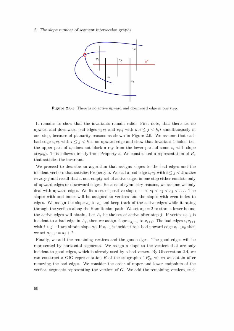
2. The slope number of segment intersection graphs
e∗vi
vl
vh
vk
vj
Figure 2.6.: There is no active upward and downward edge in one step.
It remains to show that the invariants remain valid. First note, that there are noupward and downward bad edges vhvk and vivl with h, i ≤ j < k, l simultaneously inone step, because of planarity reasons as shown in Figure 2.6. We assume that eachbad edge vivk with i ≤ j < k is an upward edge and show that Invariant 1 holds, i.e.,the upper part of vj does not block a ray from the lower part of some vi with slopes(vivk). This follows directly from Property a. We constructed a representation of Rj
that satisfies the invariant.
We proceed to describe an algorithm that assigns slopes to the bad edges and theincident vertices that satisfies Property b. We call a bad edge vivk with i ≤ j < k activein step j and recall that a non-empty set of active edges in one step either consists onlyof upward edges or downward edges. Because of symmetry reasons, we assume we onlydeal with upward edges. We fix a set of positive slopes · · · < s1 < s2 < s3 < . . . . Theslopes with odd index will be assigned to vertices and the slopes with even index toedges. We assign the slope s1 to v1 and keep track of the active edges while iteratingthrough the vertices along the Hamiltonian path. We set a1 := 2 to store a lower boundthe active edges will obtain. Let Aj be the set of active after step j. If vertex vj+1 isincident to a bad edge in Aj , then we assign slope saj+1 to vj+1. The bad edges vivj+1
with i < j+ 1 are obtain slope aj . If vj+1 is incident to a bad upward edge vj+1vk thenwe set aj+1 := aj + 2.
Finally, we add the remaining vertices and the good edges. The good edges will berepresented by horizontal segments. We assign a slope to the vertices that are onlyincident to good edges, which is already used by a bad vertex. By Observation 2.4, wecan construct a GIG representation R of the subgraph of P ∗G, which we obtain afterremoving the bad edges. We consider the order of upper and lower endpoints of thevertical segments representing the vertices of G. We add the remaining vertices, such
60
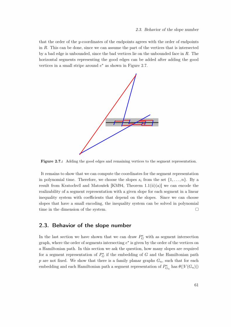
2.3. Behavior of the slope number
that the order of the y-coordinates of the endpoints agrees with the order of endpointsin R. This can be done, since we can assume the part of the vertices that is intersectedby a bad edge is unbounded, since the bad vertices lie on the unbounded face in R. Thehorizontal segments representing the good edges can be added after adding the goodvertices in a small stripe around e∗ as shown in Figure 2.7.
Figure 2.7.: Adding the good edges and remaining vertices to the segment representation.
It remains to show that we can compute the coordinates for the segment representationin polynomial time. Therefore, we choose the slopes si from the set 1, . . . , n. By aresult from Kratochvíl and Matoušek [KM94, Theorem 1.1(ii)(a)] we can encode therealizability of a segment representation with a given slope for each segment in a linearinequality system with coefficients that depend on the slopes. Since we can chooseslopes that have a small encoding, the inequality system can be solved in polynomialtime in the dimension of the system.
2.3. Behavior of the slope number
In the last section we have shown that we can draw P ∗G with as segment intersectiongraph, where the order of segments intersecting e∗ is given by the order of the vertices ona Hamiltonian path. In this section we ask the question, how many slopes are requiredfor a segment representation of P ∗G if the embedding of G and the Hamiltonian pathp are not fixed. We show that there is a family planar graphs Gn, such that for eachembedding and each Hamiltonian path a segment representation of P ∗Gn
has θ(|V (Gn)|)
61

2. The slope number of segment intersection graphs
slopes. First we consider the number of slopes of P ∗G for a fixed Hamiltonian path underdifferent embeddings of G.Let wiwi+1, wi+1wi+2, . . . , wi+k−1wi+k be bad edges of the same type (upwards/down-wards). We call the vertices a chain of length k. If all the edges of the chain are of thesame front or back type the chain is called monotone.
Lemma 2.6. Let p be a Hamiltonian path in G and C be a chain of bad edges. Anysegment representation of P ∗G, whose vertex order along e
∗ is given by p, requires at least2(d |C|2 e+ 1) slopes.
Proof. Consider a segment representation of P ∗G. Without loss of generality, let C ′ be achain of front upward bad edges. For a bad front edge we know that the segment with theupper part has a larger slope then the segment with the lower part. By Observation 2.5,the bad edges connecting vertices in the chain have slopes that lie between the slopes oftheir incident vertices. Thus the segment representation uses at least 2(|C ′|+ 1) slopes;|C ′|+ 1 slopes for the vertices incident to the bad edges, |C ′| for the bad edges, and onefor e∗.
e∗
Figure 2.8.: No good edge separates the ends of e∗ from the unbounded face.
Therefore, we only have to show that a chain of bad edges of length |C| leads to amonotone chain of bad edges C ′ of length d|C|/2e. We observe that the unbounded faceof P ∗G −B, where B is the set of bad edges, is the face that is incident to the two endsof the Hamiltonian path: Otherwise we have good edge that separates both ends of e∗
from the unbounded face, which is not possible as shown in Figure 2.8.On the other hand, we can obtain a pseudosegment representation of each such em-bedding by flipping one front bad edge over to a back bad as shown in Figure 2.9. Thisflipping splits the chain into two chains, one of which has the claimed length.
We show that there is a family of planar triangulations that have only Hamiltonianpaths including long chains of bad edges. This way, we prove that there are graphsGn, such that P ∗G requires a large number of slopes in any segment representation.Therefore, we need the following tools.
62
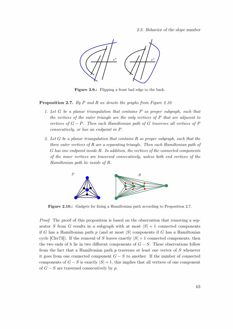
2.3. Behavior of the slope number
e∗ e∗
Figure 2.9.: Flipping a front bad edge to the back.
Proposition 2.7. By P and R we denote the graphs from Figure 2.10.
1. Let G be a planar triangulation that contains P as proper subgraph, such thatthe vertices of the outer triangle are the only vertices of P that are adjacent tovertices of G − P . Then each Hamiltonian path of G traverses all vertices of Pconsecutively, or has an endpoint in P .
2. Let G be a planar triangulation that contains R as proper subgraph, such that thethree outer vertices of R are a separating triangle. Then each Hamiltonian path ofG has one endpoint inside R. In addition, the vertices of the connected componentsof the inner vertices are traversed consecutively, unless both end vertices of theHamiltonian path lie inside of R.
P R
Figure 2.10.: Gadgets for fixing a Hamiltonian path according to Proposition 2.7.
Proof. The proof of this proposition is based on the observation that removing a sep-arator S from G results in a subgraph with at most |S| + 1 connected componentsif G has a Hamiltonian path p (and at most |S| components if G has a Hamiltoniancycle [Chv73]). If the removal of S leaves exactly |S| + 1 connected components, thenthe two ends of h lie in two different components of G − S. These observations followfrom the fact that a Hamiltonian path p traverses at least one vertex of S wheneverit goes from one connected component G − S to another. If the number of connectedcomponents of G− S is exactly |S|+ 1, this implies that all vertices of one componentof G− S are traversed consecutively by p.
63
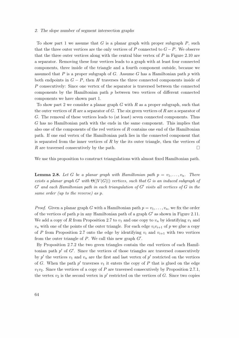
2. The slope number of segment intersection graphs
To show part 1 we assume that G is a planar graph with proper subgraph P , suchthat the three outer vertices are the only vertices of P connected to G−P . We observethat the three outer vertices along with the central blue vertex of P in Figure 2.10 area separator. Removing these four vertices leads to a graph with at least four connectedcomponents, three inside of the triangle and a fourth component outside, because weassumed that P is a proper subgraph of G. Assume G has a Hamiltonian path p withboth endpoints in G − P , then H traverses the three connected components inside ofP consecutively: Since one vertex of the separator is traversed between the connectedcomponents by the Hamiltonian path p between two vertices of different connectedcomponents we have shown part 1.To show part 2 we consider a planar graph G with R as a proper subgraph, such thatthe outer vertices of R are a separator of G. The six green vertices of R are a separator ofG. The removal of these vertices leads to (at least) seven connected components. ThusG has no Hamiltonian path with the ends in the same component. This implies thatalso one of the components of the red vertices of R contains one end of the Hamiltonianpath. If one end vertex of the Hamiltonian path lies in the connected component thatis separated from the inner vertices of R by the its outer triangle, then the vertices ofR are traversed consecutively by the path.
We use this proposition to construct triangulations with almost fixed Hamiltonian path.
Lemma 2.8. Let G be a planar graph with Hamiltonian path p = v1, . . . , vn. Thereexists a planar graph G′ with Θ(|V (G)|) vertices, such that G is an induced subgraph ofG′ and each Hamiltonian path in each triangulation of G′ visits all vertices of G in thesame order (up to the reverse) as p.
Proof. Given a planar graph G with a Hamiltonian path p = v1, . . . , vn, we fix the orderof the vertices of path p in any Hamiltonian path of a graph G′ as shown in Figure 2.11.We add a copy of R from Proposition 2.7 to v1 and one copy to vn by identifying v1 andvn with one of the points of the outer triangle. For each edge vivi+1 of p we glue a copyof P from Proposition 2.7 onto the edge by identifying vi and vi+1 with two verticesfrom the outer triangle of P . We call this new graph G′.By Proposition 2.7.2 the two green triangles contain the end vertices of each Hamil-tonian path p′ of G′. Since the vertices of those triangles are traversed consecutivelyby p′ the vertices v1 and vn are the first and last vertex of p′ restricted on the verticesof G. When the path p′ traverses v1 it enters the copy of P that is glued on the edgev1v2. Since the vertices of a copy of P are traversed consecutively by Proposition 2.7.1,the vertex v2 is the second vertex in p′ restricted on the vertices of G. Since two copies
64
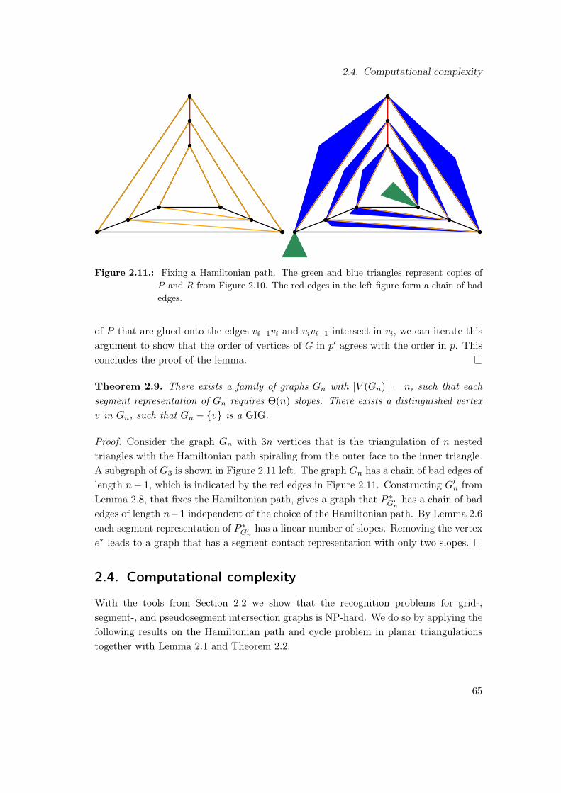
2.4. Computational complexity
Figure 2.11.: Fixing a Hamiltonian path. The green and blue triangles represent copies ofP and R from Figure 2.10. The red edges in the left figure form a chain of badedges.
of P that are glued onto the edges vi−1vi and vivi+1 intersect in vi, we can iterate thisargument to show that the order of vertices of G in p′ agrees with the order in p. Thisconcludes the proof of the lemma.
Theorem 2.9. There exists a family of graphs Gn with |V (Gn)| = n, such that eachsegment representation of Gn requires Θ(n) slopes. There exists a distinguished vertexv in Gn, such that Gn − v is a GIG.
Proof. Consider the graph Gn with 3n vertices that is the triangulation of n nestedtriangles with the Hamiltonian path spiraling from the outer face to the inner triangle.A subgraph of G3 is shown in Figure 2.11 left. The graph Gn has a chain of bad edges oflength n− 1, which is indicated by the red edges in Figure 2.11. Constructing G′n fromLemma 2.8, that fixes the Hamiltonian path, gives a graph that P ∗G′
nhas a chain of bad
edges of length n−1 independent of the choice of the Hamiltonian path. By Lemma 2.6each segment representation of P ∗G′
nhas a linear number of slopes. Removing the vertex
e∗ leads to a graph that has a segment contact representation with only two slopes.
2.4. Computational complexity
With the tools from Section 2.2 we show that the recognition problems for grid-,segment-, and pseudosegment intersection graphs is NP-hard. We do so by applying thefollowing results on the Hamiltonian path and cycle problem in planar triangulationstogether with Lemma 2.1 and Theorem 2.2.
65
2. The slope number of segment intersection graphs
Theorem 2.10. The Hamiltonian cycle problem [Wid82, Chv85] and the Hamiltonianpath problem [AG11] in planar triangulations is NP-complete.
Corollary 2.11. The recognition problem of grid intersection graphs, segment intersec-tion graphs, and pseudosegment intersection graphs is NP-hard.
We show that minimizing the slope number of a segment intersection graph is NP-hard.
Theorem 2.12. Computing the slope number of a segment intersection graph is NP-hard.
The theorem above follows from the following theorem, Lemma 2.1 and Theorem 2.2:Consider planar triangulations G that have a Hamiltonian path. Then the graph P ∗G hasa 4-dir representation. It has a 2-dir representation if and only if G has a Hamiltoniancycle. To determine this is NP-complete.
Theorem 2.13. The Hamiltonian cycle problem in planar triangulations with Hamil-tonian path is NP-complete, even if the Hamiltonian path is given.
The idea to show this theorem is the following: We follow the proof by Chvátal [Chv85]who shows that the Hamiltonian cycle problem in maximal planar graphs is NP-complete.The proof builds upon the reduction of the 3SAT problem to the Hamiltonian cycleproblem in planar, cubic bipartite graphs by Akiyama, Nishizeki, and Saito [ANS80].We apply their reduction on certain 3SAT instances. These instances guarantee tofind a Hamiltonian path in the resulting maximal planar graph. The NP-hardness ofthe Hamiltonian cycle problem in maximal planar graphs with Hamiltonian path fol-lows from the fact that the satisfiability problem on our special 3SAT instances is stillNP-hard.The 3SAT instances we consider are the almost satisfiable 3SAT instances. We call a3SAT instance almost satisfiable if there exists a truth assignment, such that all butone clause is satisfied. To my knowledge, almost satisfiable instances have not beenconsidered before.
Lemma 2.14. The problem of deciding the satisfiability of almost satisfiable 3SAT withgiven almost satisfying truth assignment is NP-complete.
Proof. We give a reduction from the 3SAT problem. Given a 3SAT instance we modifyall clauses in the following way. We replace each literal in each clause with a newvariable, so each variable appears only once. In addition we introduce a variable x andthe clause x. For each pair of variables y1, y2, where both variables corresponded to a
66

2.4. Computational complexity
literal of the same variable, we add the clauses x∨ y1 ∨ y2 and x∨ y1 ∨ y2 to make themequivalent if they are both non-negated or both negated, or x ∨ y1 ∨ y2 and x ∨ y1 ∨ y2
if exactly one literal is negated. The constructed 3SAT is satisfiable if and only if theoriginal is: In a satisfying truth assignment x is false, hence the introduced clauses givethe equivalence between y1 and y2, or their negation respectively. Thus a satisfyinginstance of the almost satisfiable 3SAT results in a satisfying truth assignment for theoriginal 3SAT. On the other hand, a truth assignment satisfying all but one clause isgiven by setting x and all other variables true. The size of the new 3SAT is polynomialin the size of the original one. This concludes the proof that almost satisfiable 3SAT isNP-complete.
e1
e2e3
P
Q′e1
e2e2
e1
e2e3
Q
v
Figure 2.12.: Gadgets used in Theorem 2.13
Proof of Theorem 2.13. In order to show Theorem 2.13 we have to delve into the proof ofthe NP-hardness of the Hamiltonian cycle problem in planar triangulations. Therefore,we first explain a construction that reduces the Hamiltonian path problem in planar,cubic, bipartite graphs to the Hamiltonian path problem in maximal planar graphs byChvátal [Chv85]. Wigderson [Wid82] gave a similar but more involved construction toreduce the Hamiltonian cycle problem in planar, cubic (and not necessarily bipartite)graphs to the Hamiltonian cycle problem in planar triangulations. In a given planar,cubic, bipartite graph G = (A,B;E) we subdivide each edge. We glue a copy Pa of thegraph P shown in Figure 2.12 on each vertex a ∈ A. Here the middle vertex representsa and the three vertices e1, e2, e3 of P are identified with the subdivision vertices of thethree edges incident to a. The vertices of B are replaced in the same way with a copy ofthe graph Q that is shown in Figure 2.12. The graph we constructed is denoted by G′.
Claim 2.15. For each triangulation G′′ of G′ the following holds: The graph G′′ has aHamiltonian cycle if and only if G has a Hamiltonian cycle.
Proof. We first observe that a Hamiltonian cycle in G′′ does not traverse two verticesof B without traversing a vertex of A in between. This follows from Proposition 2.7.1:
67
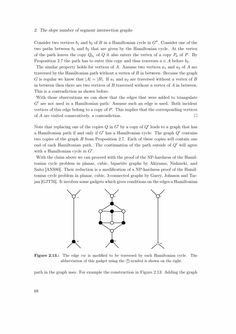
2. The slope number of segment intersection graphs
Consider two vertices b1 and b2 of B in a Hamiltonian cycle in G′′. Consider one of thetwo paths between b1 and b2 that are given by the Hamiltonian cycle. At the vertexof the path leaves the copy Qb1 of Q it also enters the vertex of a copy Pa of P . ByProposition 2.7 the path has to enter this copy and thus traverses a ∈ A before b2.The similar property holds for vertices of A. Assume two vertices a1 and a2 of A aretraversed by the Hamiltonian path without a vertex of B in between. Because the graphG is regular we know that |A| = |B|. If a1 and a2 are traversed without a vertex of Bin between then there are two vertices of B traversed without a vertex of A in between.This is a contradiction as shown before.With those observations we can show that the edges that were added to triangulateG′ are not used in a Hamiltonian path: Assume such an edge is used. Both incidentvertices of this edge belong to a copy of P . This implies that the corresponding verticesof A are visited consecutively, a contradiction.
Note that replacing one of the copies Q in G′ by a copy of Q′ leads to a graph that hasa Hamiltonian path if and only if G′ has a Hamiltonian cycle: The graph Q′ containstwo copies of the graph R from Proposition 2.7. Each of these copies will contain oneend of each Hamiltonian path. The continuation of the path outside of Q′ will agreewith a Hamiltonian cycle in G′.With the claim above we can proceed with the proof of the NP-hardness of the Hamil-tonian cycle problem in planar, cubic, bipartite graphs by Akiyama, Nishizeki, andSaito [ANS80]. Their reduction is a modification of a NP-hardness proof of the Hamil-tonian cycle problem in planar, cubic, 3-connected graphs by Garey, Johnson and Tar-jan [GJT76]. It involves some gadgets which gives conditions on the edges a Hamiltonian
©↑
v
w
v
w
v
w
Figure 2.13.: The edge vw is modified to be traversed by each Hamiltonian cycle. Theabbreviation of this gadget using the ©↑ -symbol is shown on the right.
path in the graph uses. For example the construction in Figure 2.13: Adding the graph
68
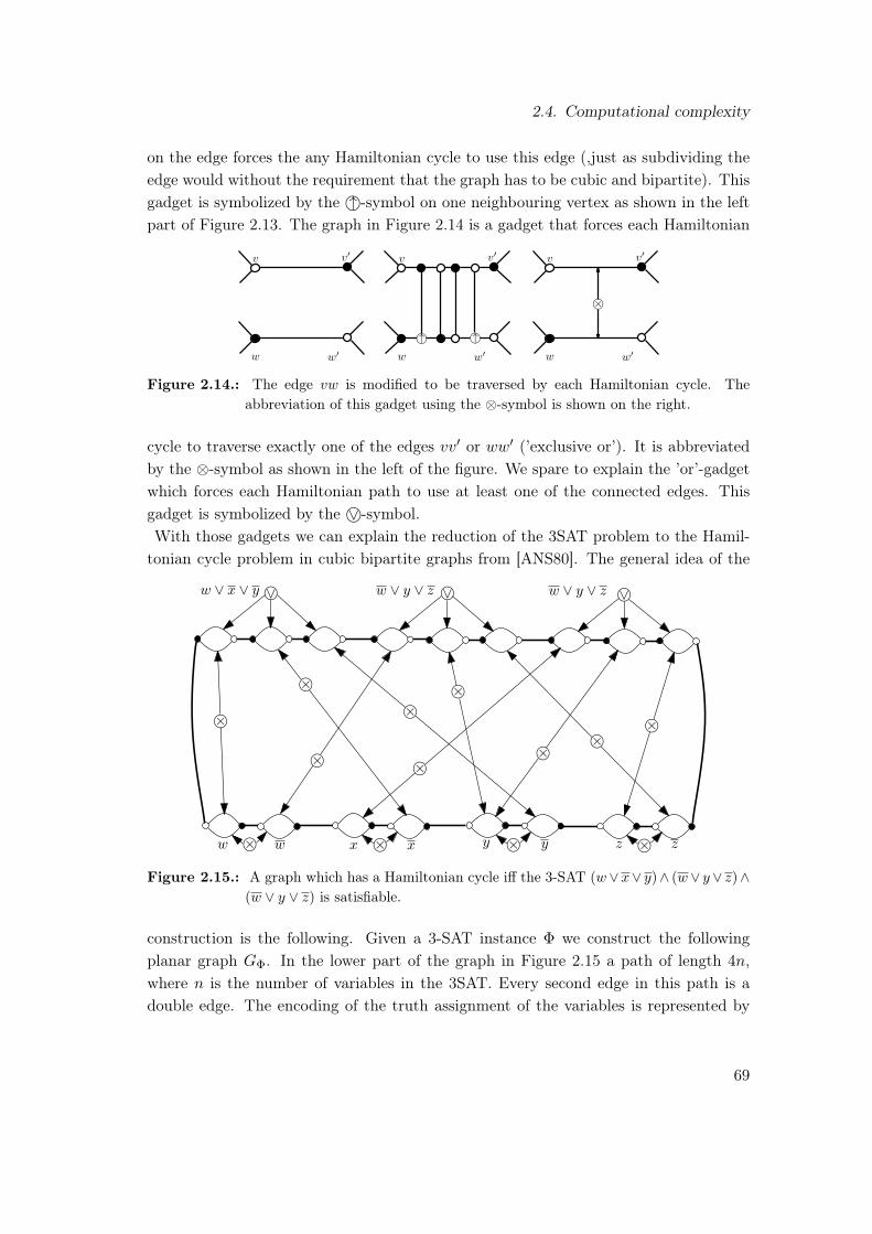
2.4. Computational complexity
on the edge forces the any Hamiltonian cycle to use this edge (,just as subdividing theedge would without the requirement that the graph has to be cubic and bipartite). Thisgadget is symbolized by the ©↑ -symbol on one neighbouring vertex as shown in the leftpart of Figure 2.13. The graph in Figure 2.14 is a gadget that forces each Hamiltonian
v′v
©×
w w′
v′v
w w′©↑ ©↑
v′v
w w′
Figure 2.14.: The edge vw is modified to be traversed by each Hamiltonian cycle. Theabbreviation of this gadget using the ⊗-symbol is shown on the right.
cycle to traverse exactly one of the edges vv′ or ww′ (’exclusive or’). It is abbreviatedby the ⊗-symbol as shown in the left of the figure. We spare to explain the ’or’-gadgetwhich forces each Hamiltonian path to use at least one of the connected edges. Thisgadget is symbolized by the ©∨ -symbol.With those gadgets we can explain the reduction of the 3SAT problem to the Hamil-tonian cycle problem in cubic bipartite graphs from [ANS80]. The general idea of the
©∨
w w x x y y z z
©×
©×
©×©×
©×
©×
©×©×
©×
©∨ ©∨w ∨ x ∨ y w ∨ y ∨ z w ∨ y ∨ z
©× ©× ©× ©×
Figure 2.15.: A graph which has a Hamiltonian cycle iff the 3-SAT (w∨x∨ y)∧ (w∨ y∨ z)∧(w ∨ y ∨ z) is satisfiable.
construction is the following. Given a 3-SAT instance Φ we construct the followingplanar graph GΦ. In the lower part of the graph in Figure 2.15 a path of length 4n,where n is the number of variables in the 3SAT. Every second edge in this path is adouble edge. The encoding of the truth assignment of the variables is represented by
69
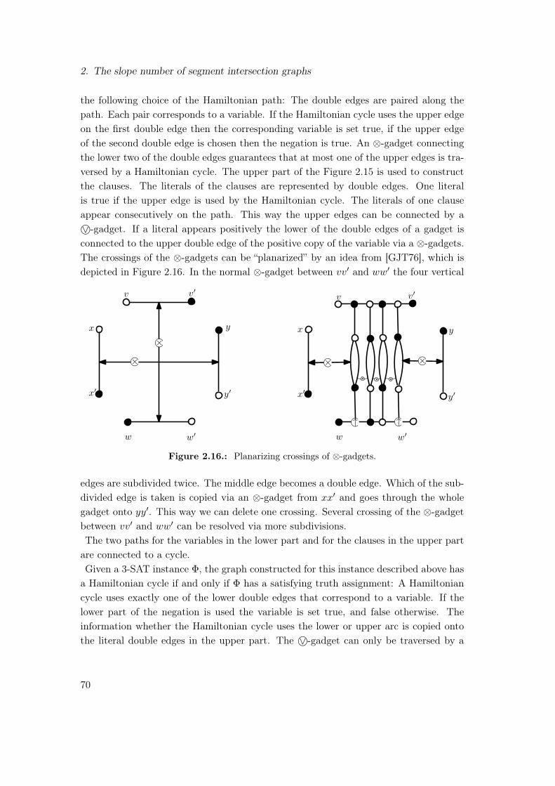
2. The slope number of segment intersection graphs
the following choice of the Hamiltonian path: The double edges are paired along thepath. Each pair corresponds to a variable. If the Hamiltonian cycle uses the upper edgeon the first double edge then the corresponding variable is set true, if the upper edgeof the second double edge is chosen then the negation is true. An ⊗-gadget connectingthe lower two of the double edges guarantees that at most one of the upper edges is tra-versed by a Hamiltonian cycle. The upper part of the Figure 2.15 is used to constructthe clauses. The literals of the clauses are represented by double edges. One literalis true if the upper edge is used by the Hamiltonian cycle. The literals of one clauseappear consecutively on the path. This way the upper edges can be connected by a©∨ -gadget. If a literal appears positively the lower of the double edges of a gadget isconnected to the upper double edge of the positive copy of the variable via a ⊗-gadgets.The crossings of the ⊗-gadgets can be “planarized” by an idea from [GJT76], which isdepicted in Figure 2.16. In the normal ⊗-gadget between vv′ and ww′ the four vertical
©×
©×
v′v
w w′
©↑ ©↑
©× ©×
v′v
w w′
x
x′
y
y′
x
x′
y
y′
Figure 2.16.: Planarizing crossings of ⊗-gadgets.
edges are subdivided twice. The middle edge becomes a double edge. Which of the sub-divided edge is taken is copied via an ⊗-gadget from xx′ and goes through the wholegadget onto yy′. This way we can delete one crossing. Several crossing of the ⊗-gadgetbetween vv′ and ww′ can be resolved via more subdivisions.The two paths for the variables in the lower part and for the clauses in the upper partare connected to a cycle.Given a 3-SAT instance Φ, the graph constructed for this instance described above hasa Hamiltonian cycle if and only if Φ has a satisfying truth assignment: A Hamiltoniancycle uses exactly one of the lower double edges that correspond to a variable. If thelower part of the negation is used the variable is set true, and false otherwise. Theinformation whether the Hamiltonian cycle uses the lower or upper arc is copied ontothe literal double edges in the upper part. The ©∨ -gadget can only be traversed by a
70
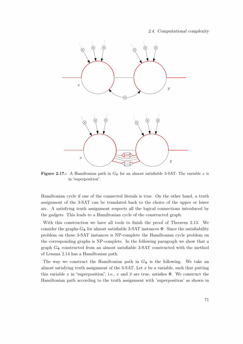
2.4. Computational complexity
©× ©× ©× ©× ©× ©×
©×
xx
©× ©× ©× ©× ©× ©×
xx
Figure 2.17.: A Hamiltonian path in GΦ for an almost satisfiable 3-SAT: The variable x isin “superposition”.
Hamiltonian cycle if one of the connected literals is true. On the other hand, a truthassignment of the 3-SAT can be translated back to the choice of the upper or lowerarc. A satisfying truth assignment respects all the logical connections introduced bythe gadgets. This leads to a Hamiltonian cycle of the constructed graph.
With this construction we have all tools to finish the proof of Theorem 2.13. Weconsider the graphs GΦ for almost satisfiable 3-SAT instances Φ. Since the satisfiabilityproblem on those 3-SAT instances is NP-complete the Hamiltonian cycle problem onthe corresponding graphs is NP-complete. In the following paragraph we show that agraph GΦ constructed from an almost satisfiable 3-SAT constructed with the methodof Lemma 2.14 has a Hamiltonian path.
The way we construct the Hamiltonian path in GΦ is the following. We take analmost satisfying truth assignment of the 3-SAT. Let x be a variable, such that puttingthis variable x in “superposition”, i.e., x and x are true, satisfies Φ. We construct theHamiltonian path according to the truth assignment with ’superposition’ as shown in
71
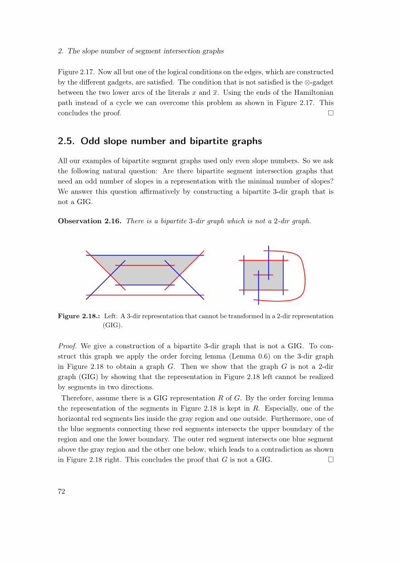
2. The slope number of segment intersection graphs
Figure 2.17. Now all but one of the logical conditions on the edges, which are constructedby the different gadgets, are satisfied. The condition that is not satisfied is the ⊗-gadgetbetween the two lower arcs of the literals x and x. Using the ends of the Hamiltonianpath instead of a cycle we can overcome this problem as shown in Figure 2.17. Thisconcludes the proof.
2.5. Odd slope number and bipartite graphs
All our examples of bipartite segment graphs used only even slope numbers. So we askthe following natural question: Are there bipartite segment intersection graphs thatneed an odd number of slopes in a representation with the minimal number of slopes?We answer this question affirmatively by constructing a bipartite 3-dir graph that isnot a GIG.
Observation 2.16. There is a bipartite 3-dir graph which is not a 2-dir graph.
Figure 2.18.: Left: A 3-dir representation that cannot be transformed in a 2-dir representation(GIG).
Proof. We give a construction of a bipartite 3-dir graph that is not a GIG. To con-struct this graph we apply the order forcing lemma (Lemma 0.6) on the 3-dir graphin Figure 2.18 to obtain a graph G. Then we show that the graph G is not a 2-dirgraph (GIG) by showing that the representation in Figure 2.18 left cannot be realizedby segments in two directions.Therefore, assume there is a GIG representation R of G. By the order forcing lemmathe representation of the segments in Figure 2.18 is kept in R. Especially, one of thehorizontal red segments lies inside the gray region and one outside. Furthermore, one ofthe blue segments connecting these red segments intersects the upper boundary of theregion and one the lower boundary. The outer red segment intersects one blue segmentabove the gray region and the other one below, which leads to a contradiction as shownin Figure 2.18 right. This concludes the proof that G is not a GIG.
72

2.5. Odd slope number and bipartite graphs
In contrast to the previous examples none of the directions in the last lemma ismonochromatic. We show that this is the case in general by showing that one monochro-matic direction in a bipartite 3-dir representation allows us to transform the graph toa grid intersection graph.
Lemma 2.17. Let G be a bipartite graph with 3-dir representation, such that one di-rection is monochromatic. Then G is a GIG.
Proof. We use the 3-dir representation with one monochromatic direction to constructa GIG representation of G. Therefore, we assume without loss of generality that themonochromatic direction is horizontal, and the other two have slopes 1 and −1. This canbe assumed since a 3-dir representation R can be transformed by a linear transformationto a 3-dir representation R′ that uses three prescribed slopes s1, s2, s3 [ČKNP02]. Let Abe the color class using three directions. First we define a linear order on the segmentsof A by augmenting the segments to piecewise linear, bi-infinite curves that do notintersect and use the three slopes 0, 1 and −1 as shown in Figure 2.19. We call thosecurves a laminar family of curves. The order of intersection of a vertical line with thelaminar family gives an order on those curves, which will correspond to a cross-freematrix order of the vertices in A. The existence of the extension of A to a laminar
1
2
4
3
Figure 2.19.: The segments of A extended to a laminar family of curves.
family can be proven as follows. Let ε be the minimal distance between two segmentsof A. Consider a ball of radius ε/2 at the left endpoint of a segment a ∈ A. We let theball roll by a horizontal force to the left. The other segments are considered as walls.Since the ball has radius ε/2 and there is no horizontal wall it does not get stuck on itsway to the left. Thus the trajectory of the midpoint of the ball gives a piecewise linearcurve to the left that consists of horizontal segments and segments that are parallel tothe walls, i.e., they have slope 0, 1, or −1. Similarly, the trajectory of a ball rolling fromthe right endpoint of a to the right extends this curve to a bi-infinite curve. We extendall curves by repeating the procedure for the other segments with a ball of radius ε/2i
for the i-th segment.
73
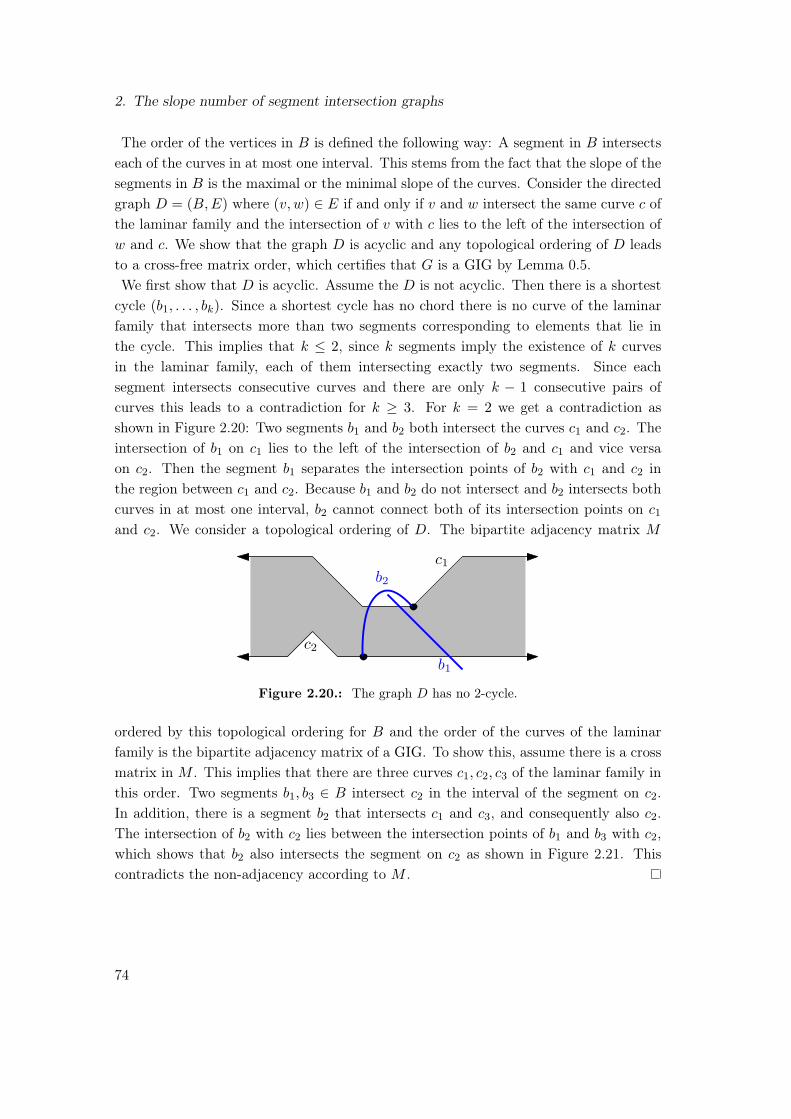
2. The slope number of segment intersection graphs
The order of the vertices in B is defined the following way: A segment in B intersectseach of the curves in at most one interval. This stems from the fact that the slope of thesegments in B is the maximal or the minimal slope of the curves. Consider the directedgraph D = (B,E) where (v, w) ∈ E if and only if v and w intersect the same curve c ofthe laminar family and the intersection of v with c lies to the left of the intersection ofw and c. We show that the graph D is acyclic and any topological ordering of D leadsto a cross-free matrix order, which certifies that G is a GIG by Lemma 0.5.We first show that D is acyclic. Assume the D is not acyclic. Then there is a shortestcycle (b1, . . . , bk). Since a shortest cycle has no chord there is no curve of the laminarfamily that intersects more than two segments corresponding to elements that lie inthe cycle. This implies that k ≤ 2, since k segments imply the existence of k curvesin the laminar family, each of them intersecting exactly two segments. Since eachsegment intersects consecutive curves and there are only k − 1 consecutive pairs ofcurves this leads to a contradiction for k ≥ 3. For k = 2 we get a contradiction asshown in Figure 2.20: Two segments b1 and b2 both intersect the curves c1 and c2. Theintersection of b1 on c1 lies to the left of the intersection of b2 and c1 and vice versaon c2. Then the segment b1 separates the intersection points of b2 with c1 and c2 inthe region between c1 and c2. Because b1 and b2 do not intersect and b2 intersects bothcurves in at most one interval, b2 cannot connect both of its intersection points on c1
and c2. We consider a topological ordering of D. The bipartite adjacency matrix M
b1
b2
c1
c2
Figure 2.20.: The graph D has no 2-cycle.
ordered by this topological ordering for B and the order of the curves of the laminarfamily is the bipartite adjacency matrix of a GIG. To show this, assume there is a crossmatrix in M . This implies that there are three curves c1, c2, c3 of the laminar family inthis order. Two segments b1, b3 ∈ B intersect c2 in the interval of the segment on c2.In addition, there is a segment b2 that intersects c1 and c3, and consequently also c2.The intersection of b2 with c2 lies between the intersection points of b1 and b3 with c2,which shows that b2 also intersects the segment on c2 as shown in Figure 2.21. Thiscontradicts the non-adjacency according to M .
74

2.5. Odd slope number and bipartite graphs
c1
c2
c3
b1
b2
b3
Figure 2.21.: The adjacency matrix is cross-free.
75

Part II.
Realizability problems and theexistential theory of the reals
77


3. Realizability of circular sequences
In this Chapter we sketch and simplify the idea of a proof of Mnëv’s universality theo-rem [Mnë88] for order types. We extend the theorem for circular sequences.
Theorem 3.1. [Mnëv’s universality theorem] Let S be a semialgebraic set defined by apolynomial inequality system with integer coefficients. Then there exists an order typeO, such that S is stably equivalent to the realization space of O.
The order type O of the theorem above can be constructed from the description of thesemialgebraic set in form of an (in)equality system. The proof of Theorem 3.1 leadsto a polynomial time algorithm to construct the order type O from the description ofS given by the polynomial inequality system. This leads to the following complexityresult for the problem of deciding the realizability of an order type.
Corollary 3.2. The problem of deciding the realizability of an order type is completein ∃R.
We first give an overview over the results on circular sequences in Section 3.1. Then weshow how to implement and store arithmetic operations in order types in Section 3.2. Af-terwards, we give a modified version of the ∃R-reduction for the order type realizabilityproblem based on work by Shor [Sho91], Richter-Gebert [RG95] and Matoušek [Mat14]in Section 3.3. These three papers are simplifications of the proof by Mnëv [Mnë88].With the help of our modification we prove that the realizability of circular sequencesis hard in ∃R, even if the order type is known to be realizable.
3.1. Background
Circular sequences have been studied by Perrin [Per81] (1881), who claimed that eachcircular sequence defining a certain set of axioms is realizable. This claim was provenfalse by Goodman and Pollack [GP80] by showing that the circular sequence of a pointset of five points in convex position, the bad pentagon shown in Figure 3.1, is not real-izable. Pilz [Pil14] considered the complexity of the realizability of a circular sequence.He notices that the NP-hardness proof of Shor [Sho91] does not generalize to circularsequences. We show ∃R-hardness, even if the order type is realizable.
79

3. Realizability of circular sequences
Figure 3.1.: The bad pentagon of Goodman and Pollak.
3.2. Arithmetics with order types
In order to reduce the order type realizability problem to solvability of a system of strictpolynomial inequalities, we simulate arithmetic operations with order types. This usesstandard constructions introduced by von Staudt in his “algebra of throws” [Sta47]. Theconstructions are well described in [RG11].To carry out arithmetic operations using orientation predicates, we associate numberswith points on a line `. We use the cross-ratio to encode the values in the followingway: We fix two points on a line and associate them with 0 and 1. On the line throughthose points we call the point at infinity ∞. For a point x on this line the cross-ratio(x, 1; 0,∞) results in the distance between 0 and x scaled by the distance between 0
and 1. Because the cross-ratio is a projective invariant we can fix one line and use thepoint x for representing its value. In this way, we have established the coordinates onone line.
ab
c
d
∞ 0 x y x+ y`
`∞ `∞
`0 x y1∞
a b
c
x · y
d
Figure 3.2.: Gadgets for addition (left) and multiplication (right) on a line.
For computing on this line we use the gadgets for addition and multiplication that are
80
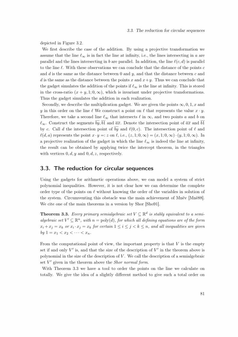
3.3. The reduction for circular sequences
depicted in Figure 3.2.We first describe the case of the addition. By using a projective transformation weassume that the line `∞ is in fact the line at infinity, i.e., the lines intersecting in a areparallel and the lines intersecting in b are parallel. In addition, the line `(c, d) is parallelto the line `. With these observations we can conclude that the distance of the points cand d is the same as the distance between 0 and y, and that the distance between c andd is the same as the distance between the points x and x+y. Thus we can conclude thatthe gadget simulates the addition of the points if `∞ is the line at infinity. This is storedin the cross-ratio (x + y, 1; 0,∞), which is invariant under projective transformations.Thus the gadget simulates the addition in each realization.Secondly, we describe the multiplication gadget. We are given the points∞, 0, 1, x andy in this order on the line ` We construct a point on ` that represents the value x · y.Therefore, we take a second line `∞ that intersects ` in ∞, and two points a and b on`∞. Construct the segments by, b1 and ax. Denote the intersection point of ax and b1by c. Call d the intersection point of by and `(0, c). The intersection point of ` and`(d, a) represents the point x · y =: z on `, i.e., (z, 1; 0,∞) = (x, 1; 0,∞) · (y, 1; 0,∞). Ina projective realization of the gadget in which the line `∞ is indeed the line at infinity,the result can be obtained by applying twice the intercept theorem, in the triangleswith vertices 0, d, y and 0, d, z, respectively.
3.3. The reduction for circular sequences
Using the gadgets for arithmetic operations above, we can model a system of strictpolynomial inequalities. However, it is not clear how we can determine the completeorder type of the points on ` without knowing the order of the variables in solution ofthe system. Circumventing this obstacle was the main achievement of Mnëv [Mnë88].We cite one of the main theorems in a version by Shor [Sho91].
Theorem 3.3. Every primary semialgebraic set V ⊆ Rd is stably equivalent to a semi-algebraic set V ′ ⊆ Rn, with n = poly(d), for which all defining equations are of the formxi +xj = xk or xi ·xj = xk for certain 1 ≤ i ≤ j < k ≤ n, and all inequalities are givenby 1 = x1 < x2 < · · · < xn.
From the computational point of view, the important property is that V is the emptyset if and only V ′ is, and that the size of the description of V ′ in the theorem above ispolynomial in the size of the description of V . We call the description of a semialgebraicset V ′ given in the theorem above the Shor normal form.With Theorem 3.3 we have a tool to order the points on the line we calculate ontotally. We give the idea of a slightly different method to give such a total order on
81

3. Realizability of circular sequences
the points on this line by Richter-Gebert [RG95]. For details we refer to Matoušek’smanuscript [Mat14]. We start with possible assumptions on the form of the descriptionthe semialgebraic set.
1. The values of all variables can be assumed to be larger than 1. This can beachieved by replacing each variable xi by x+
i − x−i , where x+i and x−i are new
variables which can be assumed to be larger than 1.
2. All coefficients are positive. The sign of a coefficient can be changed by bringingthe term on the other side of the inequality.
x2 + 2xy + y2 < z
Vx2+2xy + Vy2 = Vx2+2xy+y2
Vx2 + V2xy = Vx2+2xy y · y = Vy2
x · x = Vx2 V2 · Vxy = V2xy
1 + 1 = V2 x · y = Vxy
Vx2+2xy+y2
Figure 3.3.: Decomposing a formula in elementary operations.
Now we decompose both sides of the (in)equalities recursively into two subformulas asshown for the left-hand side of the equation in Figure 3.3. The result of each subfor-mula f is stored in a new variable Vf .The resulting decomposition tree gives an order on the variables that lie on directedpaths, but not a total order on the variables. To obtain a total order we use the ideaof Richter-Gebert [RG95] to introduce several scales. We take a topological ordering ofthe constructed decomposition tree. In each node of the tree we realize one calculation,an addition or a multiplication. We realize this calculation using the order types in thefollowing way. First assume the first i − 1 calculations of the topological ordering arealready realized on the horizontal line `. For calculation i, we introduce a new scale Si.In this scale, we add a new point 0i to the right of all already existing points. Thispoint takes the role of the point 0 in scale i. We now copy the input variables of gadgeti into the scale using the addition gadget: If the variable Vx is used for a computationin Si already exists in a scale Sh with h < i, we add the difference between 0h and Vxonto 0i (using an addition gadget) to create a copy of Vx in scale Si. This guaranteesthat variable x has the same value in each scale. After copying all required variables
82
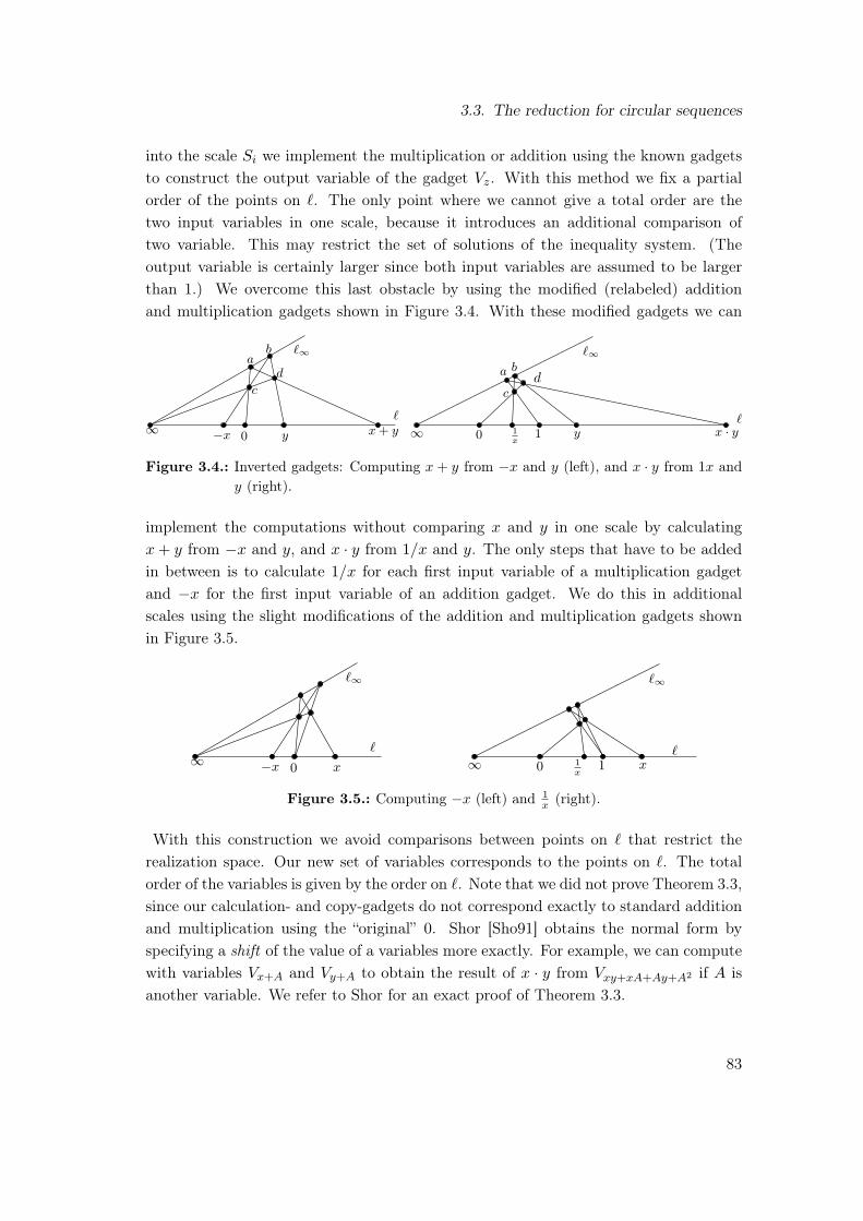
3.3. The reduction for circular sequences
into the scale Si we implement the multiplication or addition using the known gadgetsto construct the output variable of the gadget Vz. With this method we fix a partialorder of the points on `. The only point where we cannot give a total order are thetwo input variables in one scale, because it introduces an additional comparison oftwo variable. This may restrict the set of solutions of the inequality system. (Theoutput variable is certainly larger since both input variables are assumed to be largerthan 1.) We overcome this last obstacle by using the modified (relabeled) additionand multiplication gadgets shown in Figure 3.4. With these modified gadgets we can
ab
c
d
∞ −x 0 y x+ y`
`∞ `∞
`0 1 y1
x∞
a b
c
x · y
d
Figure 3.4.: Inverted gadgets: Computing x+ y from −x and y (left), and x · y from 1x andy (right).
implement the computations without comparing x and y in one scale by calculatingx+ y from −x and y, and x · y from 1/x and y. The only steps that have to be addedin between is to calculate 1/x for each first input variable of a multiplication gadgetand −x for the first input variable of an addition gadget. We do this in additionalscales using the slight modifications of the addition and multiplication gadgets shownin Figure 3.5.
∞ −x 0 x
`
`∞ `∞
`0 1 x1
x∞
Figure 3.5.: Computing −x (left) and 1x (right).
With this construction we avoid comparisons between points on ` that restrict therealization space. Our new set of variables corresponds to the points on `. The totalorder of the variables is given by the order on `. Note that we did not prove Theorem 3.3,since our calculation- and copy-gadgets do not correspond exactly to standard additionand multiplication using the “original” 0. Shor [Sho91] obtains the normal form byspecifying a shift of the value of a variables more exactly. For example, we can computewith variables Vx+A and Vy+A to obtain the result of x · y from Vxy+xA+Ay+A2 if A isanother variable. We refer to Shor for an exact proof of Theorem 3.3.
83
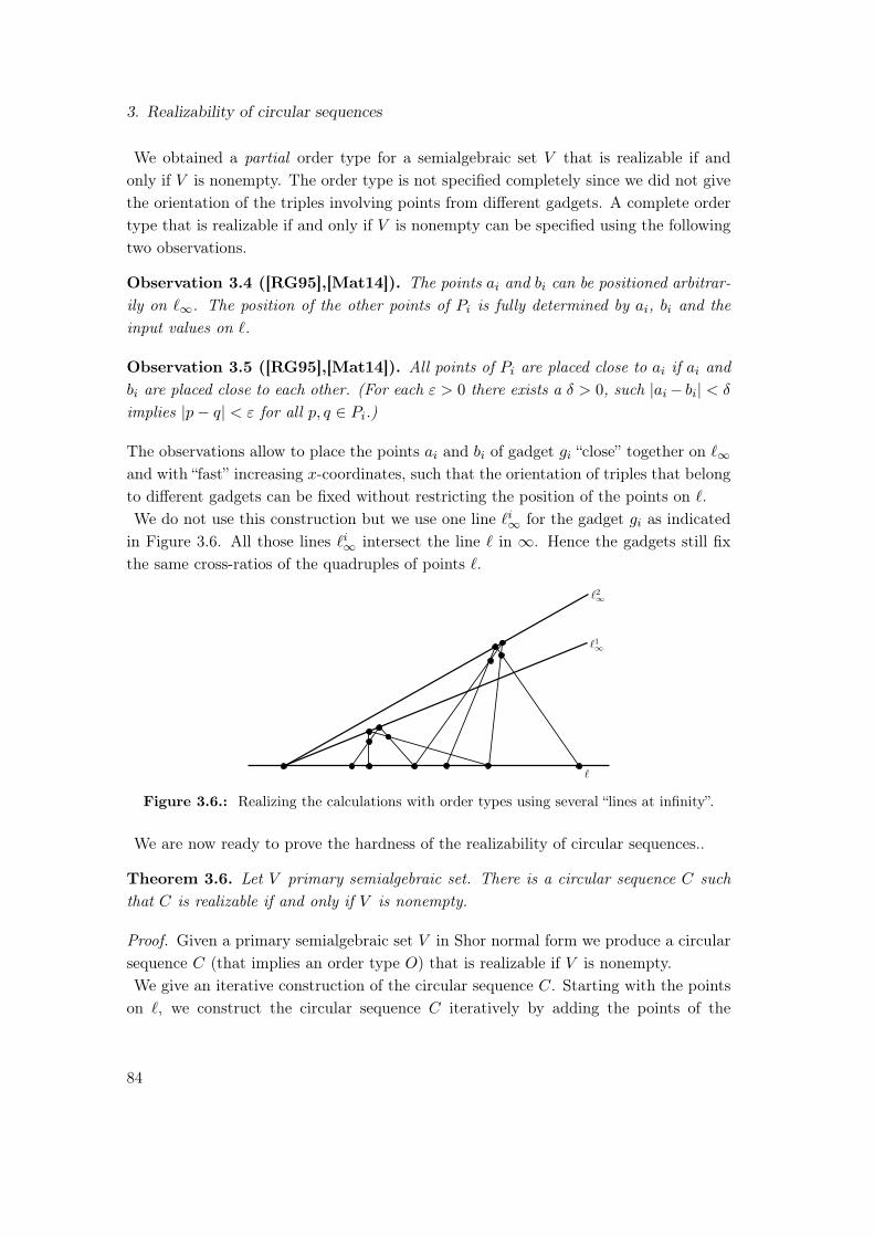
3. Realizability of circular sequences
We obtained a partial order type for a semialgebraic set V that is realizable if andonly if V is nonempty. The order type is not specified completely since we did not givethe orientation of the triples involving points from different gadgets. A complete ordertype that is realizable if and only if V is nonempty can be specified using the followingtwo observations.
Observation 3.4 ([RG95],[Mat14]). The points ai and bi can be positioned arbitrar-ily on `∞. The position of the other points of Pi is fully determined by ai, bi and theinput values on `.
Observation 3.5 ([RG95],[Mat14]). All points of Pi are placed close to ai if ai andbi are placed close to each other. (For each ε > 0 there exists a δ > 0, such |ai− bi| < δ
implies |p− q| < ε for all p, q ∈ Pi.)
The observations allow to place the points ai and bi of gadget gi “close” together on `∞and with “fast” increasing x-coordinates, such that the orientation of triples that belongto different gadgets can be fixed without restricting the position of the points on `.We do not use this construction but we use one line `i∞ for the gadget gi as indicatedin Figure 3.6. All those lines `i∞ intersect the line ` in ∞. Hence the gadgets still fixthe same cross-ratios of the quadruples of points `.
`
`1∞
`2∞
Figure 3.6.: Realizing the calculations with order types using several “lines at infinity”.
We are now ready to prove the hardness of the realizability of circular sequences..
Theorem 3.6. Let V primary semialgebraic set. There is a circular sequence C suchthat C is realizable if and only if V is nonempty.
Proof. Given a primary semialgebraic set V in Shor normal form we produce a circularsequence C (that implies an order type O) that is realizable if V is nonempty.We give an iterative construction of the circular sequence C. Starting with the pointson `, we construct the circular sequence C iteratively by adding the points of the
84
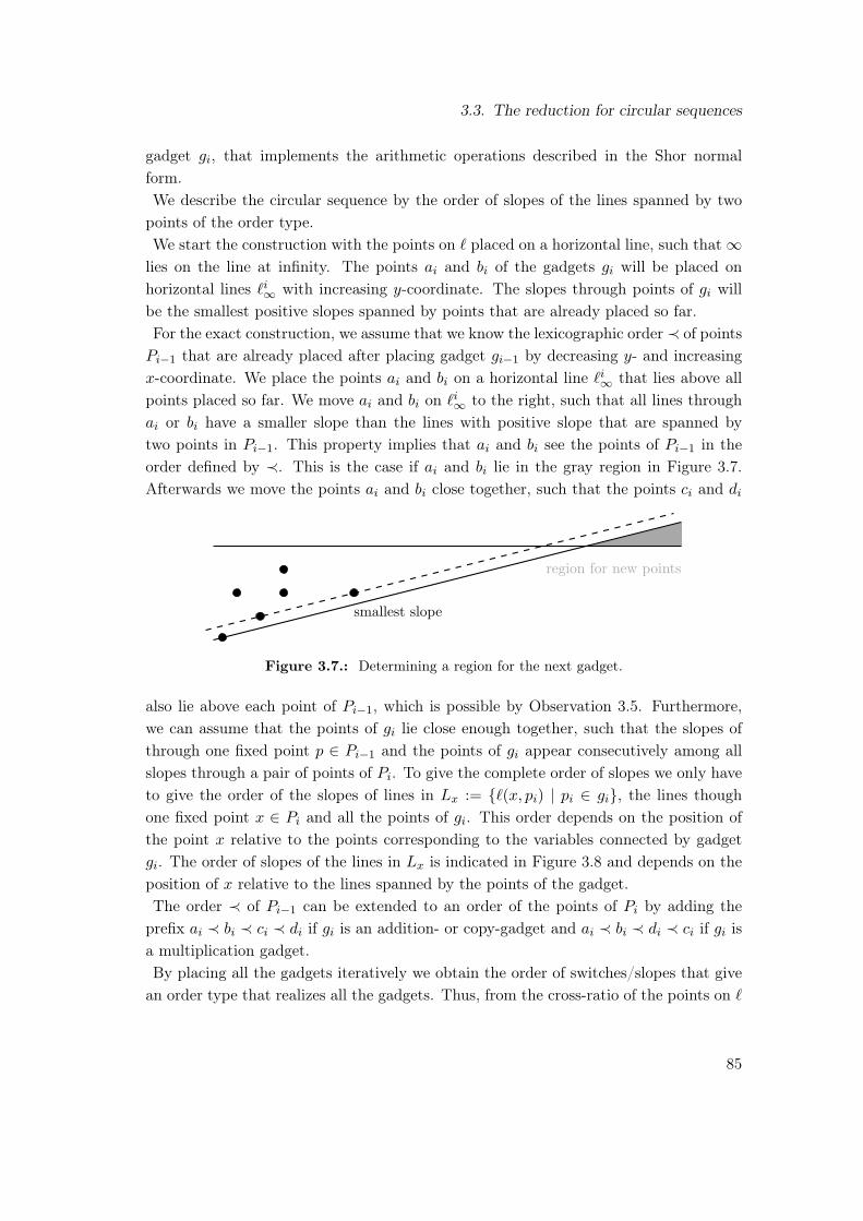
3.3. The reduction for circular sequences
gadget gi, that implements the arithmetic operations described in the Shor normalform.We describe the circular sequence by the order of slopes of the lines spanned by twopoints of the order type.We start the construction with the points on ` placed on a horizontal line, such that∞lies on the line at infinity. The points ai and bi of the gadgets gi will be placed onhorizontal lines `i∞ with increasing y-coordinate. The slopes through points of gi willbe the smallest positive slopes spanned by points that are already placed so far.For the exact construction, we assume that we know the lexicographic order ≺ of pointsPi−1 that are already placed after placing gadget gi−1 by decreasing y- and increasingx-coordinate. We place the points ai and bi on a horizontal line `i∞ that lies above allpoints placed so far. We move ai and bi on `i∞ to the right, such that all lines throughai or bi have a smaller slope than the lines with positive slope that are spanned bytwo points in Pi−1. This property implies that ai and bi see the points of Pi−1 in theorder defined by ≺. This is the case if ai and bi lie in the gray region in Figure 3.7.Afterwards we move the points ai and bi close together, such that the points ci and di
smallest slope
region for new points
Figure 3.7.: Determining a region for the next gadget.
also lie above each point of Pi−1, which is possible by Observation 3.5. Furthermore,we can assume that the points of gi lie close enough together, such that the slopes ofthrough one fixed point p ∈ Pi−1 and the points of gi appear consecutively among allslopes through a pair of points of Pi. To give the complete order of slopes we only haveto give the order of the slopes of lines in Lx := `(x, pi) | pi ∈ gi, the lines thoughone fixed point x ∈ Pi and all the points of gi. This order depends on the position ofthe point x relative to the points corresponding to the variables connected by gadgetgi. The order of slopes of the lines in Lx is indicated in Figure 3.8 and depends on theposition of x relative to the lines spanned by the points of the gadget.The order ≺ of Pi−1 can be extended to an order of the points of Pi by adding theprefix ai ≺ bi ≺ ci ≺ di if gi is an addition- or copy-gadget and ai ≺ bi ≺ di ≺ ci if gi isa multiplication gadget.By placing all the gadgets iteratively we obtain the order of switches/slopes that givean order type that realizes all the gadgets. Thus, from the cross-ratio of the points on `
85

3. Realizability of circular sequences
a b
c
d
(a, b, d, c) (c, d, a, b)
(a, b, c, d)
(a, c, b, d)
(c, a, b, d) (c, a, d, b)
Figure 3.8.: The clockwise rotation of the lines through x (blue) and the different points ofa gadget is indicated by the tuples.
in a realization of C we can compute a point in the semialgebraic set V . On the otherhand, a point x in V leads to a realization of C by placing the points on ` such thatthey encode x in the cross-ratio and repeating the construction for the positioning ofthe gadgets above. Consequently, C is realizable if and only if V is nonempty.
3.4. Realizable order types with non-realizable circularsequences
In this section we strengthen this result and show that deciding the realizability of acircular sequence is hard in ∃R, even if the order type is known to be realizable.
Theorem 3.7. Deciding the realizability of a (non-simple) circular sequence that in-duces a realizable order type is complete in ∃R.
Proof. We prove this theorem by a reduction of the solvability of a strict polynomialinequality system to the realizability of the circular sequence. The idea to prove thistheorem is to make the order type constructed above realizable by removing the point∞,the intersection point of ` and `∞. The orientations of the triples including ∞ will beforced by the circular sequence.We will slightly modify the order type constructed in the proof of Theorem 3.6 by notusing the Shor normal form directly. Instead we plug in the construction by Richter-Gebert, which we sketched as proof of the Shor normal form. This means we decomposethe calculations in single computations. Each computation is done using one gadgets ina single scale. The order of the scales on the line ` is the following, see Figure 3.9. Firstwe add a scale for each variable. Afterwards we add the scales for the computationsin the order they appear in the decomposition of the formulas in single computations,i.e., from the leaves to the root in Figure 3.3. After the computation scales we add a
86
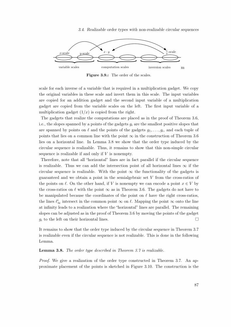
3.4. Realizable order types with non-realizable circular sequences
variable scales
computation scales
inversion scales
x · yx-scale y-scale1y -scale
m
Figure 3.9.: The order of the scales.
scale for each inverse of a variable that is required in a multiplication gadget. We copythe original variables in these scale and invert them in this scale. The input variablesare copied for an addition gadget and the second input variable of a multiplicationgadget are copied from the variable scales on the left. The first input variable of amultiplication gadget (1/x) is copied from the right.The gadgets that realize the computations are placed as in the proof of Theorem 3.6,i.e., the slopes spanned by a points of the gadgets gi are the smallest positive slopes thatare spanned by points on ` and the points of the gadgets g1, . . . , gi, and each tuple ofpoints that lies on a common line with the point ∞ in the construction of Theorem 3.6lies on a horizontal line. In Lemma 3.8 we show that the order type induced by thecircular sequence is realizable. Thus, it remains to show that this non-simple circularsequence is realizable if and only if V is nonempty.Therefore, note that all “horizontal” lines are in fact parallel if the circular sequenceis realizable. Thus we can add the intersection point of all horizontal lines ∞ if thecircular sequence is realizable. With the point ∞ the functionality of the gadgets isguaranteed and we obtain a point in the semialgebraic set V from the cross-ratios ofthe points on `. On the other hand, if V is nonempty we can encode a point x ∈ V bythe cross-ratios on ` with the point ∞ as in Theorem 3.6. The gadgets do not have tobe manipulated because the coordinates of the point on ` have the right cross-ratios,the lines `i∞ intersect in the common point ∞ on `. Mapping the point ∞ onto the lineat infinity leads to a realization where the “horizontal” lines are parallel. The remainingslopes can be adjusted as in the proof of Theorem 3.6 by moving the points of the gadgetgi to the left on their horizontal lines.
It remains to show that the order type induced by the circular sequence in Theorem 3.7is realizable even if the circular sequence is not realizable. This is done in the followingLemma.
Lemma 3.8. The order type described in Theorem 3.7 is realizable.
Proof. We give a realization of the order type constructed in Theorem 3.7. An ap-proximate placement of the points is sketched in Figure 3.10. The construction is the
87
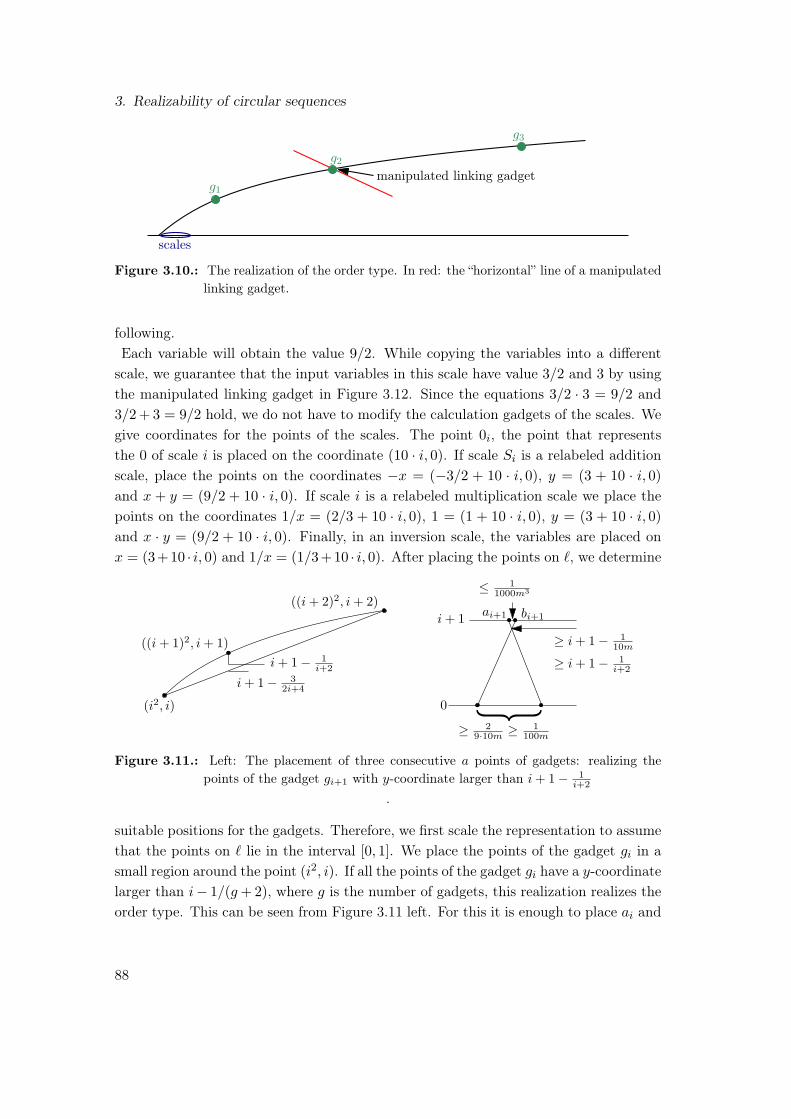
3. Realizability of circular sequences
scales
g1
g2
g3
manipulated linking gadget
Figure 3.10.: The realization of the order type. In red: the “horizontal” line of a manipulatedlinking gadget.
following.Each variable will obtain the value 9/2. While copying the variables into a differentscale, we guarantee that the input variables in this scale have value 3/2 and 3 by usingthe manipulated linking gadget in Figure 3.12. Since the equations 3/2 · 3 = 9/2 and3/2 + 3 = 9/2 hold, we do not have to modify the calculation gadgets of the scales. Wegive coordinates for the points of the scales. The point 0i, the point that representsthe 0 of scale i is placed on the coordinate (10 · i, 0). If scale Si is a relabeled additionscale, place the points on the coordinates −x = (−3/2 + 10 · i, 0), y = (3 + 10 · i, 0)
and x + y = (9/2 + 10 · i, 0). If scale i is a relabeled multiplication scale we place thepoints on the coordinates 1/x = (2/3 + 10 · i, 0), 1 = (1 + 10 · i, 0), y = (3 + 10 · i, 0)
and x · y = (9/2 + 10 · i, 0). Finally, in an inversion scale, the variables are placed onx = (3 + 10 · i, 0) and 1/x = (1/3 + 10 · i, 0). After placing the points on `, we determine
(i2, i)
((i+ 1)2, i+ 1)
((i+ 2)2, i+ 2)
i+ 1− 32i+4
i+ 1− 1i+2
≥ 29·10m ≥ 1
100m
0
i+ 1
≤ 11000m3
ai+1 bi+1
≥ i+ 1− 110m
≥ i+ 1− 1i+2
Figure 3.11.: Left: The placement of three consecutive a points of gadgets: realizing thepoints of the gadget gi+1 with y-coordinate larger than i+ 1− 1
i+2
.
suitable positions for the gadgets. Therefore, we first scale the representation to assumethat the points on ` lie in the interval [0, 1]. We place the points of the gadget gi in asmall region around the point (i2, i). If all the points of the gadget gi have a y-coordinatelarger than i− 1/(g+ 2), where g is the number of gadgets, this realization realizes theorder type. This can be seen from Figure 3.11 left. For this it is enough to place ai and
88

3.4. Realizable order types with non-realizable circular sequences
bi in a distance smaller than 1/(1000m3), where m is the number of scales, as indicatedin Figure 3.11 right using the interception theorem. Now we only have to show that
0i 0jxik xj
k
scale i scale j
c
d
Figure 3.12.: A manipulated linking gadget where the value in the left scale is larger thanthe value in the right scale.
the orientation of triples with two points from one gadget and one point from anothergadget are correct.Here, we make the following observation: Each linking gadget links a larger variable onthe left to a smaller variable on the right. This follows from the fact that the variablesof value 9/2 are linked from the left to points of distance 3/2 or 3 from 0i to the right,and the inverse variables are linked from 2/9 on the right to 1/3 on the left. This hasthe effect that the points ci and di of a manipulated linking gadget gi lie on a line whichis rotated clockwise from the original horizontal line as shown in Figure 3.12. This lineof negative slope still separates the points of the later gadgets gj with j > i from thegadgets with smaller index as shown by the red line in Figure 3.10.
We have shown that the realizability problem for non-simple circular sequences thatinduce a realizable order type is hard in ∃R. We now show that this result even holdsfor simple circular sequences.
Theorem 3.9. The realizability problem for simple circular sequences with given real-ization of the induced order type is ∃R-hard.
For the proof of the theorem above we need the following definition. An abstract ordertype P is constructible if there exists a ordering of the points (p1, . . . , pn), such that
1. no three points among p1, . . . , p4 are collinear, and
2. each pi lies on at most two of the lines spanned by the points p1, . . . , pi−1.
89

3. Realizability of circular sequences
We describe the basic idea of how to construct a simple order type from a constructibleorder type, such that the simple order type is realizable if and only if the constructibleone is realizable. As shown in Figure 3.13, a simple order type is constructed by re-
pi
Figure 3.13.: Replacing pi, that lies on two lines, by four points that reserve a convex regionaround the intersection point of the two lines.
placing each point pi (starting from i = n), that lies on two lines spanned by points inp1, . . . , pi−1, with points in convex position, which enclose the original point pi andbehave “similar” to the point pi in the order type. From the new order type we canreconstruct the old one by placing the point pi on the intersection points of the twospanned lines. The order type with the new points encodes, that the intersection pointof the two lines lies inside the convex region Ci. The new order type constructed thisway is realizable if and only if the old order type that contained pi is realizable: Theconvex region Ci in the new order type is empty and thus the point pi can be placed onthe intersection point of the lines pi lies on. This is the step where the constructabilityof the order type is necessary: The new order type encodes that the pairwise intersec-tion of the lines lie in the convex region Ci. Since the order type is constructible thereare at most two lines that determine the position of pi, which allow to place pi in theconvex region. A non-constructible order type forces one pi to be placed on the pairwiseintersection points of three lines in Ci. These three points might not coincide in eachrealization.Applying this replacement iteratively to the point pi for i = n, . . . , 5 leads to a sequenceof constructible order types P = Pn, . . . , P4 = P , where Pt is the order type beforereplacing point pt by points that span a convex region. In order type Pt all collinearitiesof at least three points appear in the first t points of the sequence of points shows theconstructability. Since the first four points of a constructible order type are in generalposition the order type P = P4 is simple.With the following observation we obtain the ∃R-hardness for the realizability of simpleorder types.
90

3.4. Realizable order types with non-realizable circular sequences
Proposition 3.10 ([Mat14]). The order type constructed in the proof of Theorem 3.6is constructible.
Proof. We give an order that certifies that the order type in Theorem 3.6 is constructible.Therefore, let g1, . . . , gk be an order of the gadgets, that respects the order of thecalculations from Figure 3.3. We give an iterative construction by adding the pointsof the gadgets iteratively to the sequence P . Assume the input points of the gadget giare already constructed. We append the points of gi in the order of the labels shown inFigure 3.14 to the sequence of points. We observe that none of the points of the gadgetlies on more than two lines when the point is constructed, thus Item 2 is satisfied bythe sequence.
0 x y x+ y
1 2 3
4
5
6
7
80 1 x y x · y1 2 3 4
5
6
7
8
9
Figure 3.14.: The constructability sequence of points within one gadget.
As a corollary from the above proposition, we obtain the ∃R-completeness of simpleorder type realizability.
Corollary 3.11. Deciding the realizability of simple order types is ∃R-complete.
To apply a similar construction to the non-simple circular sequence, we need a slightlystronger condition than the constructability of the order type to overcome the followingproblem: If the points pi and pj lie on same parallel class of lines (which is encoded inthe non-simple circular sequence) as another line that is already constructed, then theline through pi and pj is also already constructed. In other words, the common point ofthe parallel class on the line at infinity is already constructed. Since the only parallelclass of lines in the circular sequence we constructed in Theorem 3.6 are the horizontallines and the point ∞ is constructed in the beginning, this is not an obstacle for us.Hence we are ready to prove Theorem 3.9.
91

3. Realizability of circular sequences
Proof of Theorem 3.9. We reduce the realizability problem of the circular sequencesconstructed in the proof of Theorem 3.6 to the realizability for simple circular sequences.Let (p1, . . . , pn) be a sequence of the points that certifies the constructibility of theorder type/circular sequence. We iteratively construct a simple order type O and acircular sequence C that is realizable if and only if O is realizable with circular sequenceC. We set On+1 = O and Cn+1 = C, where C is the circular sequence constructed inTheorem 3.6. For t = n, . . . , 5 we apply one of the following steps.If pt does not lie in a line spanned by the points in p1, . . . , pt−1, we keep pt.If pt lies on two lines spanned by the points in p1, . . . , pt−1 we do the following. Wereplace the point pt by the set of four points Pt in convex position around pt as indicatedin Figure 3.15. The positions of these points relative to the position pt and the lines
pt
v
h
p1t
p2tp3t
p4t
Figure 3.15.: Replacing a point on two lines by point in convex position: The lines definedby the new points are almost parallel to v or h
v and h are indicated according to the following rules, which indicate the order of theslopes through the new points.
• The points below h are very close to h compared to the points above h.
• The points to the right of v lie very close to v compared to the points on the leftside of v.
The first item has the effect that the absolute value of the slope of a line through apoint on h and a point of Pt that lies above h is larger than any slope of a line throughany point on h and a point of Pt that lies below h if h is assumed to be horizontal. For
92
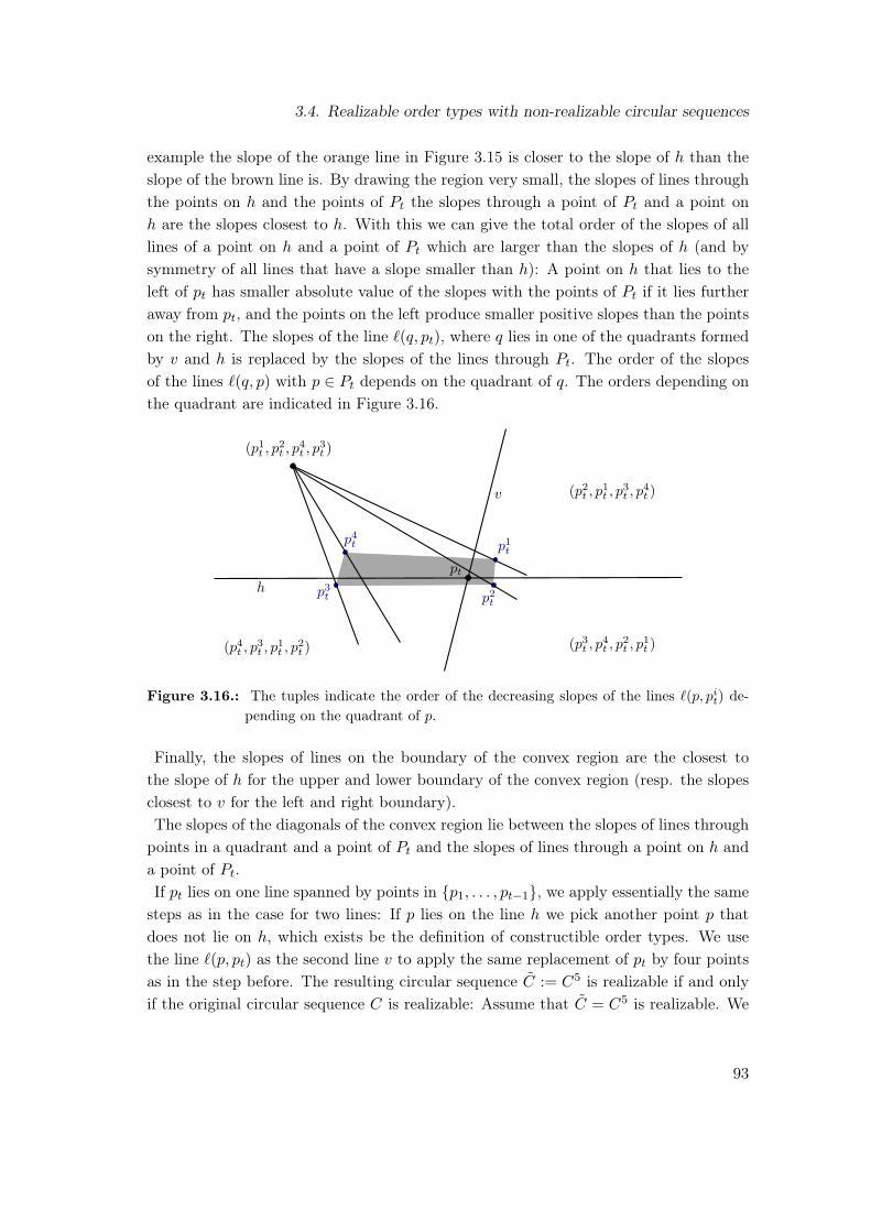
3.4. Realizable order types with non-realizable circular sequences
example the slope of the orange line in Figure 3.15 is closer to the slope of h than theslope of the brown line is. By drawing the region very small, the slopes of lines throughthe points on h and the points of Pt the slopes through a point of Pt and a point onh are the slopes closest to h. With this we can give the total order of the slopes of alllines of a point on h and a point of Pt which are larger than the slopes of h (and bysymmetry of all lines that have a slope smaller than h): A point on h that lies to theleft of pt has smaller absolute value of the slopes with the points of Pt if it lies furtheraway from pt, and the points on the left produce smaller positive slopes than the pointson the right. The slopes of the line `(q, pt), where q lies in one of the quadrants formedby v and h is replaced by the slopes of the lines through Pt. The order of the slopesof the lines `(q, p) with p ∈ Pt depends on the quadrant of q. The orders depending onthe quadrant are indicated in Figure 3.16.
pt
v
h
p1t
p2tp3t
p4t
(p1t , p2t , p
4t , p
3t )
(p2t , p1t , p
3t , p
4t )
(p3t , p4t , p
2t , p
1t )(p4t , p
3t , p
1t , p
2t )
Figure 3.16.: The tuples indicate the order of the decreasing slopes of the lines `(p, pit) de-pending on the quadrant of p.
Finally, the slopes of lines on the boundary of the convex region are the closest tothe slope of h for the upper and lower boundary of the convex region (resp. the slopesclosest to v for the left and right boundary).The slopes of the diagonals of the convex region lie between the slopes of lines throughpoints in a quadrant and a point of Pt and the slopes of lines through a point on h anda point of Pt.If pt lies on one line spanned by points in p1, . . . , pt−1, we apply essentially the samesteps as in the case for two lines: If p lies on the line h we pick another point p thatdoes not lie on h, which exists be the definition of constructible order types. We usethe line `(p, pt) as the second line v to apply the same replacement of pt by four pointsas in the step before. The resulting circular sequence C := C5 is realizable if and onlyif the original circular sequence C is realizable: Assume that C = C5 is realizable. We
93

3. Realizability of circular sequences
show inductively that if Ct is realizable then Ct+1 is realizable.In the first case, where we did not replace the point pt, the statement is true. In thesecond case, let R be a realization of the circular sequence Ct. We delete the points ofPt from R and add the point pt at the intersection point of h and v, which lies in theconvex region spanned by the points of Pt. We replace the points of Pt by the point pt,intersection point of h and v. The point pt has the same orientation in each triple asany of the points in Pt.Since the slopes of the lines through a point p 6∈ Pt, which does not lie on v or h, andthe points of Pt appear consecutively among all slopes, and the slope of `(p, pt) lies inthis interval, the new realization is a realization of Ct+1 as constructed.In the third case we use the same arguments: We replace points of Pt by one point ptthat lies on its original line h inside the convex hull of points of Pt, which results in arealization of Ct+1.
ptB
pWp
Figure 3.17.: The double wedge Wp defined by a ball around pt.
On the other hand, we have to show that C is realizable if C is realizable. Therefore,we construct a realization of Ct from Ct+1. We first determine ball B around pt. LetWp be the smallest double wedge originating at point p that contains the ball B asshown in Figure 3.17. We choose the radius of B, such that no point is contained inanother double wedge and the intersection of two cones is bounded, unless the origins ofthe double wedges are collinear with pt. This has the effect that placing the points of Pt
inside the ball B leads to a realization, where the lines through a point p and the pointsof Pt lie inside of the double wedge Wp. Since the double wedges are disjoint outside ofa bounded region the slopes of the lines through points of Pt form an interval, whichlies inside of the wedge. Afterwards, we determine a small angle, such that the onlyslope in this angle is the slope of h. We construct a parallelogram around pt inside B,with the sides parallel to v and h, such that the slopes of the diagonals lie in this angle.We place the points of Pt on the vertices of the parallelogram. Finally, we perturb thepoints slightly, such that the sides of the parallelogram are not parallel to v and h,without changing the circular sequence otherwise. This results in a realization of thecircular sequence Ct.The circular sequence Ct does not contain any parallel lines spanned by points including
94
3.4. Realizable order types with non-realizable circular sequences
pt, . . . , pn. Thus C5 is a simple circular sequence. In this way, we have reduced therealizability of constructible circular sequences to the realizability of simple circularsequences, which shows that realizability of simple circular sequences is hard in ∃R.
Note that Property 2 of the constructible order type is necessary in the construction:The point pt is replaced by a convex region. This region reserves space for the uniqueintersection point pt of some lines. If pt is forced to be the intersection point of morethan two lines, then the order type guarantees that the pairwise intersection point oftwo of the lines lies in the convex region, but not that all three lines have a commonintersection point, which is forced by the original point pt.Via projective duality we obtain the following result for line arrangements, which weuse in Chapter 5 for point visibility graphs.
Theorem 3.12. Deciding the realizability of simple allowable sequences of simple linearrangements is complete in ∃R.
Proof. A simple allowable sequence of a line arrangement corresponds to a simple cir-cular sequence of an abstract order type via projective duality. Thus, a given abstractorder O type with circular sequence C is realizable if and only if the dual pseudolinearrangement L is stretchable with allowable sequence C. This shows that deciding therealizability of a pseudoline arrangement with given allowable sequence is complete in∃R.
95


4. Slopes of segment intersectiongraphs revisited
In Chapter 2 we proved that minimizing the slope number of a segment intersectiongraph is NP-hard. Now, we show that the problem is even hard in the existentialtheory of the reals.The proof is composed of the following steps. First we show that the problem ofminimizing the slope number of a partial, simple line arrangements is hard in ∃R. By apartial line arrangement we mean the arrangement of segments in a connected region,where each of the segments has both ends on the boundary of the region. For examplethe gray part of the lines in Figure 4.1 that intersect the gray region are a partial linearrangement.
Figure 4.1.: The part of the lines intersecting the gray shaded region is a partial line arrange-ment.
We can use the order forcing lemma of Kratochvíl and Matoušek [KM94] to fix thepartial, simple arrangement in a segment intersection graph to show that the slopeminimization problem for segment intersection graphs is hard ∃R.
97
4. Slopes of segment intersection graphs revisited
Theorem 4.1. Minimizing the slope number of a partial, simple line arrangements ishard in the existential theory of the reals.
Proof. We start to describe the basic idea. Again, we use duality to prove the corre-sponding results for order types instead of line arrangements. Here we basically1 usethe standard dual map D given by
D : L → P, y = Ax−B 7→ (B,A).
The problem of minimizing the number of different slopes of the lines translates into theproblem of realizing the order type O using as few as possible different y-coordinatesof the points. We consider the order type constructed in the proof of Theorem 3.9. Inthis order type we removed the point ∞ to make the order type realizable. However,it is hard in ∃R to check whether the point ∞ can be added, which is forced by thecircular sequence. In this proof we force the point ∞, the common intersection pointof all “horizontal lines”, by using as few horizontal lines as possible to position thepoints of the order type on. Therefore, let s be the number of lines through ∞ in thesimple order type that points lie on. Before removing∞ we add points on each of theselines, such that each line contains at least s+ 1 points. The resulting order type has arealization using at most s different y-coordinates if and only if the modelled inequalitysystem describes a non-empty set: Since we have at least s + 1 points on each linewhich contained the point ∞ before the modification, we know that each of those linesis horizontal in a realization using at most s different y-coordinates. This shows thatwe can add the point∞ again to obtain a realization of an order type that contains theoriginal order type O.
As in [KM94], we use the order forcing lemma to force a copy of the partial line arrange-ment in a segment intersection graph to transfer the properties of the line arrangementon the segment intersection graph.
Theorem 4.2. Determining the slope number of a segment intersection graph is hardin ∃R.
Proof. We reduce the slope number problem of simple, partial line arrangements to theslope number problem of segment intersection graphs. Let L be a partial, simple linearrangement. For this simple segment representation we construct the graph GL fromLemma 0.6. Then GL has a segment representation using s slopes if and only if L can
1The standard dual map is given by y = Ax − B 7→ (A,B). To keep the orientation of our figuresaligned to the figures used in the last section we reverse x and y-coordinate of the order type. Thedifferent choice of the duality map reverses all orientations of triples, which does not influence therealizability.
98
be realized using at most s slopes. A segment representation of GL can be constructedfrom L in polynomial time. This concludes the proof that minimizing the slope numberof segment intersection graphs is hard in ∃R.
99

5. Recognition of point visibility graphs
In this chapter, we consider the recognition problem for point visibility graphs. InSection 5.1, we provide background on previous work on point visibility graphs andvisibility graphs in general. In Section 5.2, we show simple visibility graph constructions,the fan and the generalized fan, all geometric realizations of which are guaranteed topreserve a specified collection of subsets of collinear points. The proofs are elementaryand only require a series of basic observations. The main result, the ∃R-hardness of pointvisibility graph recognition, is given in Section 5.3. The proof is based on the uniquenessof the representation of a fan and the ∃R-hardness of the realizability of simple allowablesequences of line arrangements (Theorem 3.12). In Section 5.4, we give two applicationsof the fan construction. In the first, we show that there exists a point visibility graphthat does not have any geometric realization on the integer grid. In other words, allgeometric realizations of this point visibility graph are such that at least one of the pointshas an irrational coordinate. Another application of the fan construction follows, wherewe show that there are point visibility graphs, such that each grid realization requirescoordinates of values 22
3√n where n denotes the number of vertices of the point visibilitygraph. We conclude the section by discussing upper bounds on a grid representationof a graph. This question is closely related to the decidability of the existence of agrid representation of a PVG. We show that this problem is decidable if and only ifthe existential theory of the rationals (∃Q) is decidable. The decidability of ∃Q is alongstanding open problem.
5.1. Background
The recognition problem for point visibility graphs has been explicitly stated as animportant open problem by various authors [KPW05], and is listed as the first openproblem in a recent survey from Ghosh and Goswami [GG13].For planar point visibility graphs, a linear-time recognition algorithm has been pro-posed by Ghosh and Roy [GR14]. For general point visibility graphs they showed thatrecognition problem lies in ∃R. More recently, Roy [Roy14] published an ingenious andrather involved NP-hardness proof for recognition of arbitrary point visibility graphs.Since ∃R contains NP the ∃R-hardness implies the NP-hardness.
101
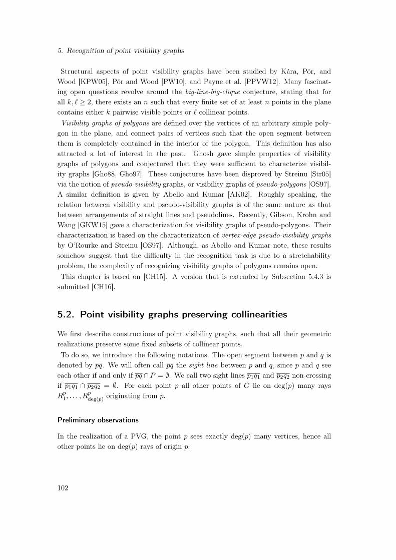
5. Recognition of point visibility graphs
Structural aspects of point visibility graphs have been studied by Kára, Pór, andWood [KPW05], Pór and Wood [PW10], and Payne et al. [PPVW12]. Many fascinat-ing open questions revolve around the big-line-big-clique conjecture, stating that forall k, ` ≥ 2, there exists an n such that every finite set of at least n points in the planecontains either k pairwise visible points or ` collinear points.Visibility graphs of polygons are defined over the vertices of an arbitrary simple poly-gon in the plane, and connect pairs of vertices such that the open segment betweenthem is completely contained in the interior of the polygon. This definition has alsoattracted a lot of interest in the past. Ghosh gave simple properties of visibilitygraphs of polygons and conjectured that they were sufficient to characterize visibil-ity graphs [Gho88, Gho97]. These conjectures have been disproved by Streinu [Str05]via the notion of pseudo-visibility graphs, or visibility graphs of pseudo-polygons [OS97].A similar definition is given by Abello and Kumar [AK02]. Roughly speaking, therelation between visibility and pseudo-visibility graphs is of the same nature as thatbetween arrangements of straight lines and pseudolines. Recently, Gibson, Krohn andWang [GKW15] gave a characterization for visibility graphs of pseudo-polygons. Theircharacterization is based on the characterization of vertex-edge pseudo-visibility graphsby O’Rourke and Streinu [OS97]. Although, as Abello and Kumar note, these resultssomehow suggest that the difficulty in the recognition task is due to a stretchabilityproblem, the complexity of recognizing visibility graphs of polygons remains open.This chapter is based on [CH15]. A version that is extended by Subsection 5.4.3 issubmitted [CH16].
5.2. Point visibility graphs preserving collinearities
We first describe constructions of point visibility graphs, such that all their geometricrealizations preserve some fixed subsets of collinear points.To do so, we introduce the following notations. The open segment between p and q isdenoted by pq. We will often call pq the sight line between p and q, since p and q seeeach other if and only if pq ∩ P = ∅. We call two sight lines p1q1 and p2q2 non-crossingif p1q1 ∩ p2q2 = ∅. For each point p all other points of G lie on deg(p) many raysRp
1, . . . , Rpdeg(p) originating from p.
Preliminary observations
In the realization of a PVG, the point p sees exactly deg(p) many vertices, hence allother points lie on deg(p) rays of origin p.
102
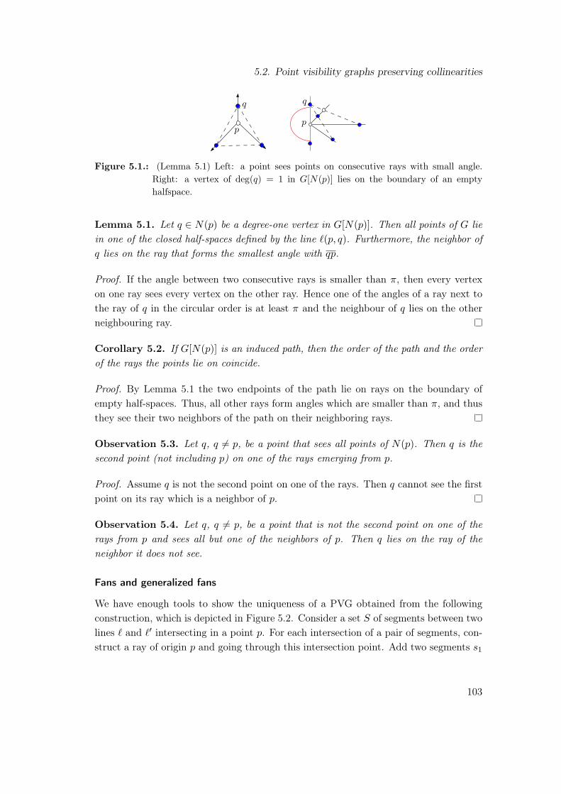
5.2. Point visibility graphs preserving collinearities
pp
Figure 5.1.: (Lemma 5.1) Left: a point sees points on consecutive rays with small angle.Right: a vertex of deg(q) = 1 in G[N(p)] lies on the boundary of an emptyhalfspace.
Lemma 5.1. Let q ∈ N(p) be a degree-one vertex in G[N(p)]. Then all points of G liein one of the closed half-spaces defined by the line `(p, q). Furthermore, the neighbor ofq lies on the ray that forms the smallest angle with qp.
Proof. If the angle between two consecutive rays is smaller than π, then every vertexon one ray sees every vertex on the other ray. Hence one of the angles of a ray next tothe ray of q in the circular order is at least π and the neighbour of q lies on the otherneighbouring ray.
Corollary 5.2. If G[N(p)] is an induced path, then the order of the path and the orderof the rays the points lie on coincide.
Proof. By Lemma 5.1 the two endpoints of the path lie on rays on the boundary ofempty half-spaces. Thus, all other rays form angles which are smaller than π, and thusthey see their two neighbors of the path on their neighboring rays.
Observation 5.3. Let q, q 6= p, be a point that sees all points of N(p). Then q is thesecond point (not including p) on one of the rays emerging from p.
Proof. Assume q is not the second point on one of the rays. Then q cannot see the firstpoint on its ray which is a neighbor of p.
Observation 5.4. Let q, q 6= p, be a point that is not the second point on one of therays from p and sees all but one of the neighbors of p. Then q lies on the ray of theneighbor it does not see.
Fans and generalized fans
We have enough tools to show the uniqueness of a PVG obtained from the followingconstruction, which is depicted in Figure 5.2. Consider a set S of segments between twolines ` and `′ intersecting in a point p. For each intersection of a pair of segments, con-struct a ray of origin p and going through this intersection point. Add two segments s1
103

5. Recognition of point visibility graphs
`
`′
s2s1
ab
c d
ep
Figure 5.2.: A fan: a vertex is placed on each intersection of two lines/segments.
and s2 between ` and `′, such the first intersection point on ` and `′ lie on s1 and thesecond on s2.We now put a point on each intersection of the segments and rays and construct thePVG of this set of points. We call this graph the fan of S and denote it by fan(S).Since we have the choice of the position of the segments s1 and s2, we can avoid anycollinearity between a point on s1 or s2 and points on other segments, except for theobvious collinearities on one ray. Thus, every point sees all points on s1 except for theone of the ray it lies on.
Lemma 5.5. All realizations of a fan preserve collinearities between points that lie onone segment and between points that lie on one ray.
Proof. We first show that the distribution of the points onto the rays of p is unique. Byconstruction the points on s2 see all the points on s1, which are exactly the neighborsof p. Thus, by Observation 5.3, the points from s2 are the second points of a ray. Sincethere is exactly one point for each ray on s2, all the other points are not second pointson a ray. By construction each of the remaining points sees all but one point of s1.Observation 5.4 gives a unique ray a point lies on. The order of the rays is unique byCorollary 5.2. On each ray the order of the points is as constructed, since the PVG ofpoints on one ray is an induced path. Now, we have to show that the points originatingfrom one segment are still collinear. Consider three consecutive rays R1, R2, R3. Weconsider a visibility between a point p1 on R1 and one point p3 on R3 that has to beblocked by a point on R2. Let p2 be the original blocker from the construction. Foreach point on R2 that lies closer to p, there is a sight line blocked by this point, and foreach point that lies further away from p there is a sight line blocked by this point. Foreach of these points we pick one sight line that corresponds to an original segment andp1p3. This set of sight lines is non-crossing, since the segments only intersect on raysby assumption. So we have a set of non-crossing sight lines and the same number ofblockers available. Since the order on each ray is fixed, and the sight lines intersect R2
in a certain order, the blocker for each sight line is uniquely determined and has to bethe original blocker. By transitivity of collinearity all points from the segments remain
104
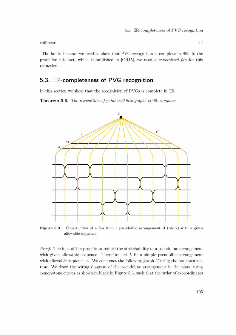
5.3. ∃R-completeness of PVG recognition
collinear.
The fan is the tool we need to show that PVG recognition is complete in ∃R. In theproof for this fact, which is published in [CH15], we used a generalized fan for thisreduction.
5.3. ∃R-completeness of PVG recognition
In this section we show that the recognition of PVGs is complete in ∃R.
Theorem 5.6. The recognition of point visibility graphs is ∃R-complete.
``′
p
s1s2
Figure 5.3.: Construction of a fan from a pseudoline arrangement A (black) with a givenallowable sequence.
Proof. The idea of the proof is to reduce the stretchability of a pseudoline arrangementwith given allowable sequence. Therefore, let L be a simple pseudoline arrangementwith allowable sequence A. We construct the following graph G using the fan construc-tion: We draw the wiring diagram of the pseudoline arrangement in the plane usingx-monotone curves as shown in black in Figure 5.3, such that the order of x-coordinates
105
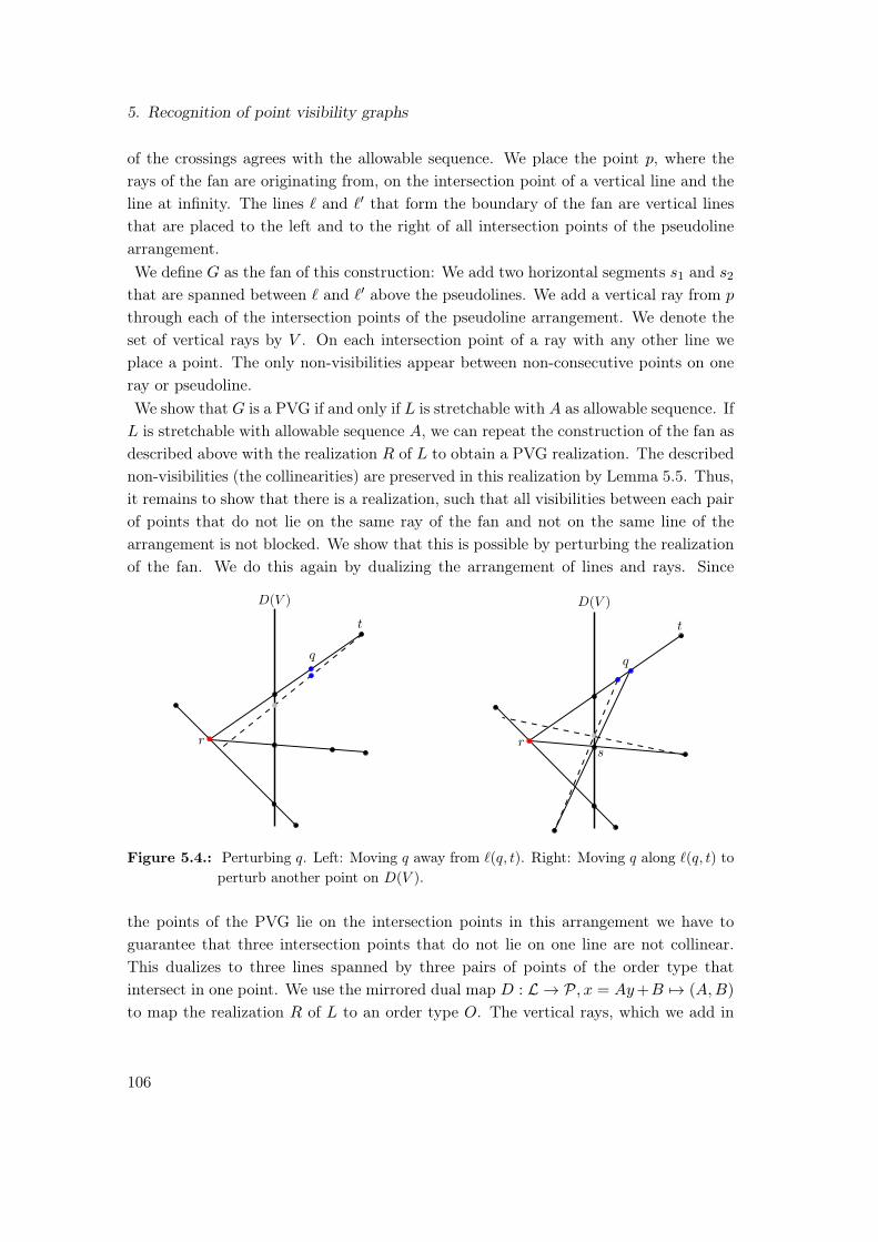
5. Recognition of point visibility graphs
of the crossings agrees with the allowable sequence. We place the point p, where therays of the fan are originating from, on the intersection point of a vertical line and theline at infinity. The lines ` and `′ that form the boundary of the fan are vertical linesthat are placed to the left and to the right of all intersection points of the pseudolinearrangement.We define G as the fan of this construction: We add two horizontal segments s1 and s2
that are spanned between ` and `′ above the pseudolines. We add a vertical ray from p
through each of the intersection points of the pseudoline arrangement. We denote theset of vertical rays by V . On each intersection point of a ray with any other line weplace a point. The only non-visibilities appear between non-consecutive points on oneray or pseudoline.We show that G is a PVG if and only if L is stretchable with A as allowable sequence. IfL is stretchable with allowable sequence A, we can repeat the construction of the fan asdescribed above with the realization R of L to obtain a PVG realization. The describednon-visibilities (the collinearities) are preserved in this realization by Lemma 5.5. Thus,it remains to show that there is a realization, such that all visibilities between each pairof points that do not lie on the same ray of the fan and not on the same line of thearrangement is not blocked. We show that this is possible by perturbing the realizationof the fan. We do this again by dualizing the arrangement of lines and rays. Since
D(V )
r
q
t
D(V )
r
q
t
s
Figure 5.4.: Perturbing q. Left: Moving q away from `(q, t). Right: Moving q along `(q, t) toperturb another point on D(V ).
the points of the PVG lie on the intersection points in this arrangement we have toguarantee that three intersection points that do not lie on one line are not collinear.This dualizes to three lines spanned by three pairs of points of the order type thatintersect in one point. We use the mirrored dual map D : L → P, x = Ay+B 7→ (A,B)
to map the realization R of L to an order type O. The vertical rays, which we add in
106
5.4. Point visibility graphs on a grid
the construction of the fan, dualize to points on the y-axis; one for each intersection ofthe y-axis with a line spanned by two points of the order type. Now, assume that inthe order type D(L ∪ V ) there are three independent pairs that span lines intersectingin one point r. We consider a point q of in D(L) that is contained in a pair that spansa line, which intersects two other spanned lines in one common point. Note that we canmove q in an ε-neighborhood without creating new non-simple points in the spannedarrangement, and without changing the circular sequence, by continuity arguments.When we move q, we also move some points of D(V ) to obtain the order type asindicated in Figure 5.4. If none of the independent pairs that create r contains a pointon D(V ) whose position depends on q, then we can move q away from the line `(q, t),where t is the point collinear with q and r, such that one line less intersects r. Otherwise,if there is a point s ∈ D(V ) whose position depends on q, then we move q along theline `(q, t). This has the effect that the line spanned by s and one other point doesnot intersect r any more. This step reduces the number of lines that intersect in thepoint r. This perturbation reduces the number of triples of independent pairs whosespanned lines intersect in a common point. Thus, repeating this step leads to an ordertype without such triples. Placing points on the intersection points of the dual linearrangement leads to a realization of the PVG G.
5.4. Point visibility graphs on a grid
In this section we show that there are PVGs that cannot be represented on a grid, i.e.,that cannot be represented with rational coordinates. In addition we show that thereare PVGs that can be represented on a grid, but each representation on a grid requiresa doubly exponential grid size. Afterwards we show that deciding whether a PVG has arepresentation on a grid is decidable if and only if the existential theory of the rationals(∃Q) is decidable. The decidability of ∃Q is a longstanding open problem. We point outthat the undecidability of ∃Q would imply that the grid size for PVGs with n verticescannot be bounded from above by a computable function in n.
5.4.1. Irrational coordinates
First, we present a point visibility graph that has no representation, such that all pointsuse rational coordinates.
Theorem 5.7. There exists a point visibility graph, such that every PVG realizationhas at least one point with an irrational coordinate.
Proof. We use the so-called Perles configuration of 9 points on 9 lines illustrated inFigure 5.5. It is known that for every geometric realization of this configuration in the
107

5. Recognition of point visibility graphs
Figure 5.5.: The Perles configuration.
Euclidean plane, one of the points has an irrational coordinate [Grü03]. We combinethis construction with the fan construction described in Section 5.2. Hence, we pick twolines ` and `′ intersecting in a point p, such that all lines of the configuration intersectboth ` and `′ in the same wedge. Note that up to a projective transformation, the pointp may be considered to be on the line at infinity and ` and `′ are parallel. We addtwo non-intersecting segments s1 and s2 close to p, that do not intersect any line of theconfiguration. Then, we construct a ray from p through each of the points, and constructthe visibility graph of the original points together with all the intersections of the rayswith the lines and the two segments s1, s2. From Lemma 5.5, all the collinearities ofthe original configuration are preserved, and every realization of the graph contains acopy of the Perles configuration.
5.4.2. Large grid size
Here we give a simple construction for point visibility graphs where all its integer real-izations require a superexponential grid size, thus a (binary) encoding of the coordinateshas superpolynomial size.
With the following simple construction we encode a line arrangement in a fan as shownin Figure 5.3. Consider a line arrangement A, and add a point p in an unbounded faceof the arrangement, such that all intersections of lines are visible in an angle aroundp that is smaller than π. Construct rays ` and `′ through the extremal intersectionpoints of the arrangement and p. By Lemma 5.5, the fan of this construction gives aPVG that fixes A. Since there are line arrangements that require integer coordinates ofvalues 22Θ(|A|) [GPS90] and the fan has Θ(|A|3) points we get the following lower boundon the coordinates of points in any realization of this PVG.
Corollary 5.8. There exists a point visibility graph with n vertices every realization ofwhich requires coordinates of values 22Θ( 3√n).
108

5.4. Point visibility graphs on a grid
5.4.3. Recognition of point visibility graphs on a grid
We now prove that the recognition problem for visibility graphs on a grid is decidableif and only if the existential theory of the rationals is decidable . The computationalcomplexity of answering the question “Does this object have a realization on a grid?”(rational realization problem) is unknown for various types of objects. Most prominently,it is unknown for polytopes and oriented matroids and (non-simple) order types andthus (non-simple) line arrangements. Matiyasevich [Mat70] showed that the existentialtheory of the integers is undecidable by giving a negative solution to Hilbert’s tenthproblem: Deciding whether a diophantine equation has a solution is undecidable. Thiscannot be applied to a grid realization of a PVG, since a realization of a PVG withrational coordinates, which can be obtained by a rational solution of the inequalitysystem, leads to a grid realization by scaling. Hence for those geometric realizationson the grid the decidability of Hilbert’s tenth problem over the rationals is of interest.Grünbaum [Grü72] conjectured in 1972 that there is no algorithm that enumerates allarrangements in the rational projective plane, which is equivalent to the recognitionproblem of order types that can be represented on a grid. This conjecture is still open.Poonen [Poo09] tried to define the integers using rational logic, i.e., to give a formulaF (w) over the rationals that is satisfiable if and only if w is an integer. These formulasare known, but they involve existential and universal quantifiers. The existence ofsuch a formula using only existential quantifiers would show the undecidability of theexistential theory of the rationals.Similar to work a of Sturmfels [Stu87] for oriented matroids and polytopes, we showthe following theorem.
Theorem 5.9. The realization problem for visibility graphs of points on a grid is de-cidable if and only if the existential theory of the rationals is decidable.
Before proving this theorem, we point out a connection of this question to finding anupper bound on the grid size of a PVG that is realizable on a grid.
Corollary 5.10. Assume the recognition problem for PVG on a grid is undecidable.Then there is no computable function f : N→ N such that each PVG with n points thatis realizable on a grid can be drawn on a grid of size f(n)× f(n).
Proof. We suppose that a computable function f : N → N exists, such that everyPVG that is realizable on a grid with n vertices can be represented on a grid of sizef(n) × f(n). Using this function, we can give an algorithm that decides whether agraph G with |V (G)| = n has a realization as a PVG on a grid.We first compute f(n), then for each x ∈ [f(n)]2n we check whether G is the PVG ofthe point set (x(v1), y(v1), . . . , x(vn), y(vn)) = x. If there is such an x, the algorithmreturns the realization, otherwise no realization exists.
109
5. Recognition of point visibility graphs
This algorithm is clearly an effective decision procedure, and thus the recognitionproblem for PVG on a grid is decidable – a contradiction to the assumption.
If we try to use the reduction of Theorem 5.6 in order to prove Theorem 5.9, the mainobstacle is that we cannot reduce to a strict inequality system. This leads to an openrealization space, and we can always find a rational point in an non-empty open set.If we do not have an open realization space we do not know if we can perturb thelines/points as in the proof of Theorem 5.6 to get rid of collinearities of points of thePVG that do not lie on a common line of the arrangement. However, since we are onlyconcerned with the decidability of the problem, we use a (non-polynomial) computablereduction.
Proof of Theorem 5.9. We give a computable reduction from the rational realizationproblem for (non-simple) line arrangements to the rational realization problem forPVGs. Given a line arrangement L of n lines, we construct a finite set of graphs GL,such that L has a rational realization if and only if at least one graph in GL has arational PVG realization.We construct the set of graphs GL as follows. We want to encode L in a fan. Thus, wepick one unbounded face fp of L as the face to place the point p, the origin of all rays ofthe fan. Since we do not know the circular order of the vertices of L around p we createa set of graphs GA for each possible circular order A of vertices of L around p, namelyfor each possible allowable sequence A with p in the fixed unbounded face fp. The setof graphs GA contains possible fans with circular order A of the vertices of L around p:Depending on a realization of L (with A) the visibility of two points of the fan that donot lie on the same line of L or the same ray of the fan can be blocked by another point.For each combination of additional blocked edges we create a single graph. Therefore,note that the only edges we require to keep the unique representation (all lines of L arepreserved) of a fan (Lemma 5.5) are the edges of one vertex to the vertices on differentrays on the segment s1 (the segment that is added closest to p in the construction ofthe fan), and the edges of the path on one ray and the path on the segment s1. Allother optional edges can be removed (which may lead to a non-realizable graph) to keepthe points on the lines of L collinear in each PVG representation of the fan. For eachsubset S of optional edges, the set of graphs GA contains the fans forcing the circularorder A around p, where exactly the optional edges contained in S are also containedin the fan.Now, L has a rational realization if and only if there is a graph G ∈ GL that has arational PVG realization:First assume L has a rational realization R. From R we construct a fan as beforeby placing p in the same unbounded face. The PVG realization obtained by this fan
110
5.4. Point visibility graphs on a grid
construction is a rational realization of some graph G contained in GA, where A is thecircular order around p in this realization.On the other hand, a rational PVG realization of one of the graphs in GL leads to arational realization of L, since each graph in GL preserves the collinearities of points onL in each PVG realization.The set GL can be computed from L. Thus, an effective decision algorithm for therational realization problem for PVGs leads to an effective decision algorithm for therational realization problem for line arrangements by applying the algorithm on eachgraph in GL. This shows that if the rational realization problem for PVGs is decidable,then the rational realization problem for line arrangements is decidable. On the otherhand, we can encode the realization problem for PVGs in an existential formula as donein [GR14]. A rational solution of this formula leads to a rational realization of the PVG,because the variables encode the coordinates of the points.
111

6. The planar slope number
The slope number of a graph G is defined to be the minimum number of distinct edgeslopes in a non-degenerate straight line drawing of G. Similarly, the planar slope numberof a graph is the minimum number of distinct edge slopes in a planar straight linedrawing of G.In this section, we consider the computational complexity of computing the slopenumber. We show that determining the planar slope number of a graph is hard in ∃R.
6.1. Background
A simple lower bound for the slope number of a graph G is d∆(G)/2e, where ∆(G)
denotes the maximum degree of G, since at most two edges of the same slope areincident to one vertex. The main work in this area deals with the question whetherthe slope number of a planar graph is also bounded from above by a function in themaximum degree. This was answered negatively [BMW06, PP06, DSW07] by examplesof families of graphs of maximum degree 5 with arbitrarily large slope number. Incontrast, Keszegh, Pach, and Pálvölgyi have shown that the planar slope number isbounded by an exponential function in the maximum degree [KPP13]. For partialplanar 3-trees [JJK+13] this has been improved to a polynomial upper bound of O(∆5)
and for outerplanar graphs [KMW14] to a linear upper bound of ∆ − 1 (for ∆ ≥ 4),even for outerplanar drawings.It is NP-complete to decide whether a graph has slope number 2 [FHH+93], and it isNP-complete to decide whether a graph has planar slope number 2 [GT01]. Thus bothproblems, computing the slope number and the planar slope number are NP-hard. Inthe following subsection we show that computing the planar slope number is even hardin ∃R.
6.2. Computational complexity
Theorem 6.1. Deciding if the planar slope number of a planar graph with maximumdegree ∆ is d∆/2e is complete in ∃R.
113

6. The planar slope number
Proof. We prove the theorem by reducing the stretchability of a pseudoline arrangementto the realizability of a planar graph using d∆/2e slopes. Let L be an arrangement ofn − 3 pseudolines. From L we construct a arrangement L′ by adding three lines to L,such that all intersections of L lie in the triangle formed by these new lines. This canbe done in a way, such that L′ is stretchable if and only L is stretchable, for example asshown in Figure 6.1. This has the effect that all intersections of L are inner intersection
Figure 6.1.: Adding three lines (green) to a (pseudo)line arrangement L, such that all verticesof L are inner vertices.
points of L′. We construct the following planar graph GL′ : First take the intersectionpoints of L′ vertices of GL′ and the line segments between the vertices as edges G. Tothis graph, we add a cycle Cf in each bounded face f . We determine the length of thiscycle in the following way: Note that the (cyclic) order of the slopes of lines of a linearrangement is already encoded in the line arrangement. Consider a vertex v that isincident to a face f of the arrangement L′. Let ` and `′ be the pseudolines in clockwiseorder that form the boundary of the face f close to v. We define w(v, f) as the numberof (pseudo)lines of L′, whose slopes lie clockwise between ` and `′. The length of thecycle Cf , which we add in face f , is
1 +∑
v incident to f
(2w(v, f) + 1) .
We connect each v, that is incident to f , to 2w(v, f) + 1 consecutive vertices of thecycle. We do this in a way, such that GL′ stays planar.The graph GL′ we just constructed has a straight line drawing with ∆(GL′)/2 = 2n
slopes if and only if L is stretchable.We first show that L is stretchable if GL′ has a planar drawing with 2n slopes. Notethat the graph GL′ is, after contracting the two edges incident to the degree two vertexin each face, 3-connected and thus has, up to the choice of the outer face, a unique
114

6.2. Computational complexity
embedding. Thus, the cyclic order of the neighbours around a vertex is the order whichwe constructed in the planar drawing. The inner vertices of the arrangement havedegree 4n. Thus, in a realization using 2n slopes, the opposite edges have the sameslope. Since the edges coming from a pseudoline are opposite we obtain a realization ofL by drawing each line on the path of the edges originating from its pseudoline.
subdivisionvertex
v1
v2
e1
e4
v4v3
f
v1
v4
e4
Figure 6.2.: Left: Drawing the cycle in the face. Green segments indicate slopes of thearrangement, gray segments intermediate slopes. Right: Using the subdivisionvertex to close the polygon.
On the other hand, GL′ admits a straight line drawing with 2n slopes if L is stretchable:Consider a realization R of L′, which exists if L is stretchable. We construct a planardrawing of the graph GL′ on R. We draw the vertices of L′ on this realization.
Between two consecutive slopes used by the realization of L′ we fix one additionalslope. Through each vertex of L′ we draw a line of each of the slopes. In each of thebounded faces we construct a polygon in the face that almost fills the whole face. Thevertices of the cycle in the face are basically placed on the intersection points of thelines through the vertices of the face and the polygon. Starting from the vertex thatfollows the degree two vertex of the cycle clockwise, we enumerate the vertices and edgesclockwise by v1, . . . , vdeg(f) and e1, . . . , edeg(f). We pick a point close to v1 on the mostcounterclockwise line through v1 in f . From this point we draw the first edge of thepolygon parallel to the edge e1. We end on the clockwise last line through v2 that liesin the face f . Iteratively, we proceed to draw edges of the polygon from the endpointof the last edge close to vi, parallel to the edge ei, to the clockwise last line throughvi+1 until we reach vdeg(f). If the vertices of the polygon close to v1 and vdeg(f) canbe connected by a segment parallel to en we do so and add the subdivision vertex onthis edge. Otherwise, we use the degree two vertex to extend the edge parallel to e1
115

6. The planar slope number
or edeg(f)−1 to close the polygon as depicted in Figure 6.2, by placing the subdivisionvertex on the vertex of the polygon that is not intersected by a line through a vertex.By construction the placement of the vertices on the polygons and the arrangementleads to a drawing of GL using 2n slopes.The graph GL′ can be constructed from L in polynomial time. Consequently, decidingif GL′ can be drawn using 2n slopes is hard in ∃R.
As a consequence of this reduction, we can carry over the result from non-simple linearrangements, as we already did for point visibility graphs in the previous section.
Corollary 6.2. There are planar graphs, such that each planar drawing that minimizesthe number of slopes has at least one vertex with an irrational coordinate.
Corollary 6.3. The problem of deciding whether a graph G has a planar straight linedrawing on the grid with d∆(G)/2e slopes is decidable if and only if ∃Q is decidable.
Determining the computational complexity of computing the non-planar slope numberremains an open problem. We conjecture that it is also hard in ∃R.
116
7. Open problems, questions,conjectures
In this chapter we list some open problems that occured in this thesis.
Chapter 1
The main open problems of Chapter 1 are the recognition problems for many subclassesof grid intersection graphs.
Problem 7.1. Determine the complexity of the recognition problem for the subclassesof grid intersection graphs mentioned in Chapter 1.
The following table lists the current state of these problems.
Class recognition complexity reference
GIG NP-complete [Kra94]UGIG NP-complete [MP13]3-dim BipG NP-complete [FMP15]3-dim GIG OpenStabGIG OpenSegRay OpenBipHook OpenStick Open4-DORG Open3-DORG Open2-DORG Polynomial [STU10],[Cog82]bipartite permutation Polynomial [DM41]
Chapter 2 and Chapter 4
Problem 7.2. Determine the complexity of approximating the slope number.
117
7. Open problems, questions, conjectures
Chapter 3
Problems that are complete in ∃R have instances, where the obvious certificate hassuperpolynomial size. However, this does not imply that the problems cannot be solvedin NP. For example, there are string graphs that have an exponential number of crossingsin each repesentation, but string graph recognition is in NP [SSŠ03].
Open question 7.3. Is the existential theory of the reals contained in NP?
Open question 7.4. Is the existential theory of the rationals decidable?
Chapter 5
The recognition problem for many classes of visibility graph is open. We refer toGhosh [GG13] for an overview.
Problem 7.5. Determine the complexity of the recognition of segment visibility graphsin the plane.
Open question 7.6. Gibson, Krohn, and Wang recently gave a characterization ofvisibility graphs of pseudo-polygons [GKW15]. Does this characterization lead to a poly-nomial algorithm?
Problem 7.7. Determine the complexity of polygon visibility graph recognition.
Beside this recognition questions, the following question has also been considered [Mat09].
Open question 7.8. Consider a PVG G with an independent set of size k that can berepresented by a point set in general position. How many vertices does G have at least?
Chapter 6
Open question 7.9. Is determining the slope number of a graph hard in ∃R?
The planar slope number of a graph is bounded in its maximum degree [KPP13]. Thebest known bound is exponential in the maximum degree.
Open question 7.10. Is the planar slope number of a planar graph polynomially boundedin its maximum degree?
118
Bibliography
[AB09] Sanjeev Arora and Boaz Barak. Computational complexity: a modern ap-proach. Cambridge University Press, 2009.
[ABB+11] Christopher Auer, Christian Bachmaier, Franz Josef Brandenburg, Wolf-gang Brunner, and Andreas Gleißner. Plane drawings of queue and dequegraphs. In International Symposium on Graph Drawing (GD), volume 6502of LNCS, pages 68–79. Springer, 2011.
[ABP06] Eyal Ackerman, Gill Barequet, and Ron Y. Pinter. On the number ofrectangulations of a planar point set. Journal of Combinatorial Theory,Series A, 113:1072–1091, 2006.
[AG11] Christopher Auer and Andreas Gleißner. Characterizations of deque andqueue graphs. In Graph-Theoretic Concepts in Computer Science (WG),volume 6986 of LNCS, pages 35–46. Springer, 2011.
[AK02] James Abello and Krishna Kumar. Visibility graphs and oriented matroids.Discrete & Computational Geometry, 28:449–465, 2002.
[ANS80] Takanori Akiyama, Takao Nishizeki, and Nobuji Saito. NP-completeness ofthe Hamiltonian cycle problem for bipartite graphs. Journal of InformationProcessing, 3:73–76, 1980.
[APT14] Karim A. Adiprasito, Arnau Padrol, and Louis Theran. Universality theo-rems for inscribed polytopes and delaunay triangulations. arXiv:1406.7831,2014.
[Bie91] Daniel Bienstock. Some provably hard crossing number problems. Discrete& Computational Geometry, 6:443–459, 1991.
[BK79] Frank R. Bernhart and Paul C. Kainen. The book thickness of a graph.Journal of Combinatorial Theory, Series B, 27:320–331, 1979.
[BLVS+99] Anders Björner, Michel Las Vergnas, Bernd Sturmfels, Neil White, andGünter M. Ziegler. Oriented Matroids. Cambridge University Press, secondedition, 1999.
119

Bibliography
[BMW06] János Barát, Jirı Matoušek, and David R. Wood. Bounded-degree graphshave arbitrarily large geometric thickness. European Journal of Combina-torics, 13:R3, 2006.
[Can88] John Canny. Some algebraic and geometric computations in PSPACE. InSymposium on Theory of Computing (STOC), pages 460–467. ACM, 1988.
[CCF+15] Daniele Catanzaro, Steven Chaplick, Stefan Felsner, Bjarni V. Halldórsson,Magnus. M. Halldórsson, Thomas Hixon, and Juraj Stacho. Max-point-tolerance graphs. Discrete Applied Mathematics, to appear, 2015.
[CCL13] Sergio Cabello, acceptedJean Cardinal, and Stefan Langerman. The cliqueproblem in ray intersection graphs. Discrete & Computational Geometry,50:771–783, 2013.
[CCM13] Steven Chaplick, Elad Cohen, and Gila Morgenstern. Stabbing polygonalchains with rays is hard to approximate. In Canadian Conference on Com-putational Geometry (CCCG), 2013.
[CF13] Victor Chepoi and Stefan Felsner. Approximating hitting sets of axis-parallel rectangles intersecting a monotone curve. Computational Geometry,46:1036–1041, 2013.
[CFHW15] Steven Chaplick, Stefan Felsner, Udo Hoffmann, and Veit Wiechert. Gridintersection graphs and order dimension. arXiv:1512.02482, 2015.
[CFS14] José R. Correa, Laurent Feuilloley, and José Soto. Independent and hittingsets of rectangles intersecting a diagonal line. In Latin American Theoret-ical Informatics Symposium (LATIN), volume 8392 of LNCS, pages 35–46.Springer, 2014.
[CG14] Timothy M. Chan and Elyot Grant. Exact algorithms and APX-hardnessresults for geometric packing and covering problems. Computational Geom-etry, 47:112–124, 2014.
[CH15] Jean Cardinal and Udo Hoffmann. Recognition and complexity of pointvisibility graphs. In Symposium on Computational Geometry (SoCG), vol-ume 34 of LIPIcs, pages 171–185. Schloss Dagstuhl–Leibniz-Zentrum fürInformatik, 2015.
[CH16] Jean Cardinal and Udo Hoffmann. Recognition and complexity of pointvisibility graphs. Discrete & Computational Geometry, 2016. accepted.
120
Bibliography
[CHO+14] Steven Chaplick, Pavol Hell, Yota Otachi, Toshiki Saitoh, and Ryuhei Ue-hara. Intersection dimension of bipartite graphs. In Theory and Applicationsof Models of Computation, volume 8402 of LNCS, pages 323–340. Springer,2014.
[Chv73] Vašek Chvátal. Tough graphs and Hamiltonian circuits. Discrete Mathe-matics, 5:215–228, 1973.
[Chv85] Vašek Chvátal. Hamiltonian cycles. In Eugene L. Lawler, Jan K. Lenstra,Alexander H.G. Rinnoy Kan, and David B. Shmoys, editors, The travelingsalesman problem: a guided tour of combinatorial optimization, pages 403–429. Wiley New York, 1985.
[ČKNP02] Jakub Černy, Daniel Král, Helena Nyklová, and Ondřej Pangrác. On inter-section graphs of segments with prescribed slopes. In International Sym-posium on Graph Drawing (GD), volume 2265 of LNCS, pages 261–271.Springer, 2002.
[Cog82] Olivier Cogis. On the Ferrers dimension of a digraph. Discrete Mathematics,38:47–52, 1982.
[DM41] Ben Dushnik and Edwin W. Miller. Partially ordered sets. American Jour-nal of Mathematics, 63:600–610, 1941.
[DSW07] Vida Dujmović, Matthew Suderman, and David R. Wood. Graph drawingswith few slopes. Computational Geometry, 38:181–193, 2007.
[EET76] Gideon Ehrlich, Shimon Even, and Robert E. Tarjan. Intersection graphsof curves in the plane. Journal of Combinatorial Theory, Series B, 21:8–20,1976.
[Fel13] Stefan Felsner. Exploiting air-pressure to map floorplans on point sets. InInternational Symposium on Graph Drawing (GD), volume 8242 of LNCS,pages 196–207. Springer, 2013.
[Fel14] Stefan Felsner. The order dimension of planar maps revisited. SIAM Journalon Discrete Mathematics, 28:1093–1101, 2014.
[FHH+93] Michael Formann, Torben Hagerup, James Haralambides, Michael Kauf-mann, Frank T. Leighton, Antonios Symvonis, Emo Welzl, and Gerhard J.Woeginger. Drawing graphs in the plane with high resolution. SIAM Jour-nal on Computing, 22:1035–1052, 1993.
121
Bibliography
[FMP15] Stefan Felsner, Irina Mustaţă, and Martin Pergel. The complexity of thepartial order dimension problem – closing the gap. arXiv:1306.1855, 2015.
[FN11] Stefan Felsner and Johan Nilsson. On the order dimension of outerplanarmaps. Order, 28:415–435, 2011.
[FT05] Stefan Felsner and William T. Trotter. Posets and planar graphs. Journalof Graph Theory, 49(4):273–284, 2005.
[GG13] Subir K. Ghosh and Partha P. Goswami. Unsolved problems in visibilitygraphs of points, segments, and polygons. ACM Computing Surveys, 46:22,2013.
[Gho88] Subir K. Ghosh. On recognizing and characterizing visibility graphs ofsimple polygons. In Scandinavian Workshop on Algorithm Theory (SWAT),volume 8503 of LNCS, pages 96–104. Springer, 1988.
[Gho97] Subir K. Ghosh. On recognizing and characterizing visibility graphs ofsimple polygons. Discrete & Computational Geometry, 17:143–162, 1997.
[GJT76] Michael R. Garey, David S. Johnson, and Robert E. Tarjan. The planarHamiltonian circuit problem is NP-complete. SIAM Journal on Computing,5:704–714, 1976.
[GKW15] Matt Gibson, Erik Krohn, and Qing Wang. A characterization of visibilitygraphs for pseudo-polygons. In European Symposium on Algorithms (ESA),volume 9294 of LNCS, pages 607–618. Springer, 2015.
[GP80] Jacob E. Goodman and Richard Pollack. On the combinatorial classificationof nondegenerate configurations in the plane. Journal of CombinatorialTheory, Series A, 29:220–235, 1980.
[GPS90] Jacob E. Goodman, Richard Pollack, and Bernd Sturmfels. The intrinsicspread of a configuration in Rd. Journal of the American MathematicalSociety, 3:639–651, 1990.
[GR14] Subir K. Ghosh and Bodhayan Roy. Some results on point visibility graphs.In Workshop on Algorithms and Computing (WALCOM), volume 8344 ofLNCS, pages 163–175. Springer, 2014.
[Grü72] Branko Grünbaum. Arrangements and Spreads, volume 10 of Regional Con-ference Series in Mathematics. AMS, 1972.
122

Bibliography
[Grü03] Branko Grünbaum. Convex Polytopes, volume 221 of Graduate Texts inMathematics. Springer-Verlag, 2003.
[GT01] Ashim Garg and Roberto Tamassia. On the computational complexity ofupward and rectilinear planarity testing. SIAM Journal on Computing,31:601–625, 2001.
[HATI11] Bjarni V. Halldórsson, Derek Aguiar, Ryan Tarpine, and Sorin Istrail. TheClark phaseable sample size problem: Long-range phasing and loss of het-erozygosity in GWAS. Journal of Computational Biology, 18:323–333, 2011.
[Hix13] Thomas Hixon. Hook graphs and more: some contributions to geometricgraph theory. Master’s thesis, TU Berlin, 2013.
[HNZ91] Irith Ben-Arroyo Hartman, Ilan Newman, and Ran Ziv. On grid intersectiongraphs. Discrete Mathematics, 87:41–52, 1991.
[Hof15] Udo Hoffmann. The slope number of segment intersection graphs. In Eu-ropean Workshop on Computational Geometry (EuroCG), pages 109–112,2015.
[JJK+13] Vít Jelínek, Eva Jelínková, Jan Kratochvíl, Bernard Lidicky, Marek Tesař,and Tomáš Vyskočil. The planar slope number of planar partial 3-trees ofbounded degree. Graphs and Combinatorics, 29:981–1005, 2013.
[KM89] Jan Kratochvíl and Jirí Matoušek. NP-hardness results for intersectiongraphs. Commentationes Mathematicae Universitatis Carolinae, 30:761–773, 1989.
[KM94] Jan Kratochvíl and Jirí Matoušek. Intersection graphs of segments. Journalof Combinatorial Theory, Series B, 62:289–315, 1994.
[KMN05] Matthew J. Katz, Joseph S.B. Mitchell, and Yuval Nir. Orthogonal segmentstabbing. Computational Geometry, 30:197–205, 2005.
[KMW14] Kolja Knauer, Piotr Micek, and Bartosz Walczak. Outerplanar graph draw-ings with few slopes. Computational Geometry, 47:614–624, 2014.
[KN98] Alexandr V. Kostochka and Jaroslav Nešetřil. Coloring relatives of inter-vals on the plane, I: chromatic number versus girth. European Journal ofCombinatorics, 19:103–110, 1998.
[KPP13] Balázs Keszegh, János Pach, and Dömötör Pálvölgyi. Drawing planargraphs of bounded degree with few slopes. SIAM Journal on Discrete Math-ematics, 27:1171–1183, 2013.
123
Bibliography
[KPW05] Jan Kára, Attila Pór, and David R. Wood. On the chromatic number of thevisibility graph of a set of points in the plane. Discrete & ComputationalGeometry, 34:497–506, 2005.
[Kra94] Jan Kratochvíl. A special planar satisfiability problem and a consequenceof its NP-completeness. Discrete Applied Mathematics, 52:233–252, 1994.
[Kyn11] Jan Kynčl. Simple realizability of complete abstract topological graphs inP. Discrete & Computational Geometry, 45:383–399, 2011.
[Mat70] Yuri V. Matiyasevich. Enumerable sets are diophantine. Doklady AkademiiNauk SSSR, 191:279–282, 1970.
[Mat09] Jiří Matoušek. Blocking visibility for points in general position. Discrete &Computational Geometry, 42:219–223, 2009.
[Mat14] Jiří Matoušek. Intersection graphs of segments and ∃R. arXiv:1406.2636,2014.
[Mnë88] Nicolai E. Mnëv. The universality theorems on the classification problemof configuration varieties and convex polytopes varieties. In Topology andGeometry – Rohlin Seminar, LNM, pages 527–543. Springer, 1988.
[MP13] Irina Mustaţă and Martin Pergel. Unit grid intersection graphs: Recognitionand properties. arXiv:1306.1855, 2013.
[OS97] Joseph O’Rourke and Ileana Streinu. Vertex-edge pseudo-visibility graphs:Characterization and recognition. In Symposium on Computational Geom-etry (SoCG), pages 119–128. ACM, 1997.
[Per81] Raoul Perrin. Sur le problème des aspects. Bulletin de la Société Mathé-matique de France, 10:103–127, 1881.
[Pil14] Alexander Pilz. On the complexity of problems on order types and geometricgraphs. PhD thesis, TU Graz, 2014.
[Poo09] Bjorn Poonen. Characterizing integers among rational numbers with auniversal-existential formula. American Journal of Mathematics, 131:675–682, 2009.
[PP06] János Pach and Dömötör Pálvölgyi. Bounded-degree graphs can have ar-bitrarily large slope numbers. European Journal of Combinatorics, 13:N1,2006.
124

Bibliography
[PPVW12] Michael S. Payne, Attila Pór, Pavel Valtr, and David R. Wood. On the con-nectivity of visibility graphs. Discrete & Computational Geometry, 48:669–681, 2012.
[PW10] Attila Pór and David R. Wood. On visibility and blockers. Journal ofCoputational Geometry, 1:29–40, 2010.
[RG95] Jürgen Richter-Gebert. Mnëv’s universality theorem revisited. In SéminaireLotharingien de Combinatoire, volume 34, pages 211–225, 1995.
[RG11] Jürgen Richter-Gebert. Perspectives on projective geometry: a guided tourthrough real and complex geometry. Springer, 2011.
[RGZ95] Jürgen Richter-Gebert and Günter M. Ziegler. Realization spaces of 4-polytopes are universal. Bulletin of the American Mathematical Society,32:403–412, 1995.
[Roy14] Bodhayan Roy. Point visibility graph recognition is NP-hard.arXiv:1406.2428, 2014.
[Sch89] Walter Schnyder. Planar graphs and poset dimension. Order, 5:323–343,1989.
[Sch09] Marcus Schaefer. Complexity of some geometric and topological prob-lems. In International Symposium on Graph Drawing (GD), volume 5849of LNCS, pages 334–344. Springer, 2009.
[Sch12] Marcus Schaefer. Realizability of graphs and linkages. In János Pach, editor,Thirty Essays on Geometric Graph Theory. Springer, 2012.
[Sho91] Peter W. Shor. Stretchability of pseudolines is NP-hard. Applied Geometryand Discrete Mathematics: The Victor Klee Festschrift, 4:531–554, 1991.
[Sin66] Frank W. Sinden. Topology of thin film RC circuits. Bell System TechnicalJournal, 45:1639–1662, 1966.
[SSŠ03] Marcus Schaefer, Eric Sedgwick, and Daniel Štefankovič. Recognizing stringgraphs in NP. Journal of Computer and System Sciences, 67:365–380, 2003.
[ST15] Maurice Soto and Christopher Thraves. p-box: A new graph model. Dis-crete Mathematics and Theoretical Computer Science, 17:179–186, 2015.
[Sta47] Karl Georg Christian Staudt. Geometrie der Lage. 1847.
125
Bibliography
[Str05] Ileana Streinu. Non-stretchable pseudo-visibility graphs. ComputationalGeometry, 31:195–206, 2005.
[STS11] Anish Man Singh Shrestha, Asahi Takaoka, and Tayu Satoshi. On two prob-lems of nano-PLA design. IEICE transactions on information and systems,94:35–41, 2011.
[Stu87] Bernd Sturmfels. On the decidability of diophantine problems in combinato-rial geometry. Bulletin of the American Mathematical Society, 17:121–124,1987.
[STU10] Anish Man Singh Shrestha, Satoshi Tayu, and Shuichi Ueno. On orthogonalray graphs. Discrete Applied Mathematics, 158:1650–1659, 2010.
[TMS76] William T. Trotter, John I. Moore, and David P. Sumner. The dimension ofa comparability graph. Proceedings of the American Mathematical Society,60:35–38, 1976.
[Tro92] William T. Trotter. Combinatorics and Partially Ordered Sets: DimensionTheory. Johns Hopkins Series in the Mathematical Sciences. The JohnsHopkins University Press, 1992.
[TS11] Claudio Telha and José Soto. Jump number of two-directional orthogo-nal ray graphs. In Integer Programming and Combinatorial Optimization(IPCO), volume 6655 of LNCS, pages 389–403. Springer, 2011.
[Wid82] Avi Widgerson. The complexity of the Hamiltonian circuit problem formaximal planar graphs. Technical report, Princeton University, ElectricalEngineering and Computer Science Department, 1982.
[Yan89] Mihalis Yannakakis. Embedding planar graphs in four pages. Journal ofComputer and System Sciences, 38:36–67, 1989.
126

Abstract
In this thesis, we consider several aspects of representations of graphs in the plane. Weconsider mainly intersection and visibility representations of graphs. In both kind ofrepresentations, the vertices are represented by sets in the plane. Intersection represen-tations represent the edges by the intersection of two sets. In visibility graphs, an edgecorresponds to a visibility between the sets.In the first part, we consider connections between representations of bipartite segmentintersection graphs and their order dimension. In Chapter 1, we show that the orderdimension of grid intersection graphs, the intersection graphs of horizontal and verticalsegments, is at most four. We use this observation to study the containment relation ofmany subclasses of grid intersection graphs. We generalize the observation on the orderdimension of grid intersection graphs, by showing that the order dimension of bipartitesegment intersection graphs is at most linear in the number of slopes that is used ina representation. This leads to the study of the slope number of segment intersectiongraphs, the minimal number of slopes that is sufficient to represent an intersectiongraph. In Chapter 2, we show that the slope number of segment intersection graphs isNP-hard to compute, and that it behaves “non-continuously”, i.e., it may drop, from alinear number in the number of segments down to two, upon the removal of a singlevertex.The proofs in the first part are based on combinatorial properties of the graphs. Inthe second part, we deal with the realizability problem and the complexity class exis-tential theory of the reals (∃R). Many geometric representation problems for graphs arecomplete in ∃R, for example the recognition of segment intersection graphs. We showthat computing the slope number of segment intersection graphs (Chapter 4) and therecognition of point visibility graphs (Chapter 5) is complete in ∃R. Both proofs arebased on the ∃R-hardness of the realizability of circular sequences, the order of slopesof lines that are spanned by a point sets, which we present in Chapter 3. We finish inChapter 6, by showing that determining the minimum number of slopes that is sufficientfor a planar straight line drawing of a graph, the planar slope number of a graph, isalso complete in ∃R. We discuss consequences the ∃R-hardness for properties of therepresentation.
127

Zusammenfassung
In dieser Arbeit beschäftigen wir uns mit verschiedenen Darstellungsarten von Graphenin der Ebene. Hauptsächlich behandeln wir dabei Schnitt- und Sichtbarkeitsdarstel-lungen. Bei beiden Darstellungsarten werden die Knoten durch Mengen in der Ebenedargestellt. Bei Schnittgraphen existiert eine Kante zwischen zwei Knoten wenn diezugehörigen Mengen sich schneiden. Kanten in Sichtbarkeitsgraphen existieren, wennMengen zweier Knoten sich sehen können, also eine Verbindungsstrecke zwischen zweiPunkten der Mengen existiert, die nicht von einer anderen Menge geschnitten wird.Im ersten Teil dieser Arbeit untersuchen wir einen Zusammenhang zwischen bipar-titen Schnittgraphen von Segmenten und der Ordnungsdimension der zugehörigen par-tiellen Ordnung. In Kapitel 1 zeigen wir, dass die Ordnungsdimension von Gitter-schnittgraphen, den Schnittgraphen horizontaler und vertikaler Segmente, höchstensvier ist. Wir verwenden diese Beobachtung um das Verhältnis vieler Unterklassenvon Gitterschnittgraphen zu bestimmen. Wir verallgemeinern die Beobachtung überdie Dimension von Gitterschnittgraphen und zeigen, dass die Ordnungsdimension vonbipartiten Segmentschnittgraphen unbegrenzt ist, sie jedoch höchstens linear in derAnzahl der Steigungen ist. Dies führt zu einer Untersuchung der Steigungszahl vonSegmentschnittgraphen, der minimalen Anzahl von Steigungen, die für die Darstellungeines Segmentschnittgraphen benötigt wird. In Kapitel 2 zeigen wir, dass das Berech-nen der Steigungszahl NP-schwer ist. Außerdem zeigen wir, dass die Steigungszahlsich “unstetig” verhält: Das Entfernen eines Knoten von einem Graphen mit linearerSteigungszahl kann zu einem Gitterschnittgraphen führen.Während die Beweise im ersten Teil eher kombinatorisch sind, betrachten wir imzweiten Teil Realisierbarkeitsprobleme und die Komplexitätsklasse existential theoryof the reals (∃R). Viele geometrische Probleme sind ∃R-vollständig, wie zum Beispieldie Erkennung von Segmentschnittgraphen. Wir zeigen, dass die Berechnung der Stei-gungszahl von Segmentschnittgraphen (Kapitel 4) und die Erkennung von Sichtbarkeits-graphen von Punktmengen (Kapitel 5) ∃R-schwer ist. Beide Beweise basieren auf der∃R-Schwere der Realisierbarkeit von circular sequences, der Reihenfolge der Steigungender durch eine Punktmenge aufgespannter Menge von Geraden. Dieser Beweis basiertaufMnëvs universality theorem und wird in Kapitel 3 präsentiert. Zum Abschluss zeigenwir, dass die Berechnung der minimalen Anzahl von Steigungen in einer planaren, ger-adlinigen Zeichnung, der planaren Steigunszahl eines planaren Graphen, ∃R-schwer ist.
129
Related Documents