Interpreting, analysing and modelling COVID-19 mortality data

Nonlinear Dyn (2020) 101:1751–1776https://doi.org/10.1007/s11071-020-05966-z

ORIGINAL PAPER

Interpreting, analysing and modelling COVID-19 mortalitydata

Didier Sornette · Euan Mearns ·Michael Schatz · Ke Wu · Didier Darcet

Received: 28 April 2020 / Accepted: 16 September 2020 / Published online: 1 October 2020© The Author(s) 2020

Abstract We present results on the mortality statis-tics of the COVID-19 epidemic in a number of coun-tries. Our data analysis suggests classifying countriesin five groups, (1) Western countries, (2) East Block,(3) developed Southeast Asian countries, (4) North-

A preprint of this article was uploaded to https://ssrn.com/abstract=3586411.

Didier Sornette, Euan Mearns, Michael Schatz and Ke Wuthese authors have contributed equally.

Electronic supplementary material The online version ofthis article (https://doi.org/10.1007/s11071-020-05966-z)contains supplementary material, which is available toauthorized users.

D. SornetteTokyo Tech World Research Hub Initiative (WRHI),Institute of Innovative Research, Tokyo Institute ofTechnology, Yokohama 226-8502, Japan

D. Sornette · K. WuInstitute of Risk Analysis, Prediction and Management(Risks-X), Academy for Advanced InterdisciplinaryStudies, Southern University of Science and Technology(SUSTech), Shenzhen 518055, Chinae-mail: [email protected]

D. Sornette · M. Schatz (B)· E. Mearns · K. WuDepartment of Management, Technology and Economics,ETH Zurich, Scheuchzerstrasse 7, 8092, Zurich,Switzerlande-mail: [email protected]

D. DarcetGavekal Intelligence Software, 75016 Paris, France

ern Hemisphere developing countries and (5) South-ern Hemisphere countries. Comparing the number ofdeaths per million inhabitants, a pattern emerges inwhich the Western countries exhibit the largest mor-tality rate. Furthermore, comparing the running cumu-lative death tolls as the same level of outbreak progressin different countries reveals several subgroups withintheWestern countries and further emphasises the differ-ence between the five groups. Analysing the relation-ship between deaths per million and life expectancy indifferent countries, taken as a proxy of the preponder-ance of elderly people in the population, a main reasonbehind the relatively more severe COVID-19 epidemicin theWestern countries is found to be their larger pop-ulation of elderly people, with exceptions such as Nor-way and Japan, for which other factors seem to dom-inate. Our comparison between countries at the samelevel of outbreak progress allows us to identify andquantify a measure of efficiency of the level of strin-gency of confinementmeasures.Wefind that increasingthe stringency from 20 to 60 decreases the death countby about 50 lives per million in a time window of 20days. Finally, we perform logistic equation analyses ofdeaths as ameans of tracking the dynamics of outbreaksin the “first wave” and estimating the associated ulti-mate mortality, using four different models to identifymodel error and robustness of results. This quantitativeanalysis allows us to assess the outbreak progress indifferent countries, differentiating between those thatare at a quite advanced stage and close to the end ofthe epidemic from those that are still in the middle of

123

http://crossmark.crossref.org/dialog/?doi=10.1007/s11071-020-05966-z&domain=pdf

http://orcid.org/0000-0003-1691-5558

https://ssrn.com/abstract=3586411


https://doi.org/10.1007/s11071-020-05966-z

1752 D. Sornette et al.

it. This raises many questions in terms of organisation,preparedness, governance structure and so on.

Keywords COVID-19 epidemic · Mortality · Lifeexpectancy · Stringency of confinement measures ·Logistic equation · Outbreak progress

Contents

1 Introduction . . . . . . . . . . . . . . . . . . . . . 17522 Mortality data: understanding its nature and biases . 17523 Analysing key factors of international mortality rates 1755

3.1 Caveats . . . . . . . . . . . . . . . . . . . . . 17553.2 Transforming mortality data for cross-country com-

parison . . . . . . . . . . . . . . . . . . . . . . 17563.2.1 Population normalised death rates and rough

geographic grouping . . . . . . . . . . . 17563.2.2 Quantitative comparison by defining a suit-

able reference time . . . . . . . . . . . . 17563.3 Quantifying key factors of COVID-19 mortality 1757

3.3.1 Age dependence and life expectancy . . . 17573.3.2 Lockdown policies and mortality in Europe

and the USA . . . . . . . . . . . . . . . 17583.4 A short discussion of other factors . . . . . . . 1762

4 Logistic projections of ultimate mortality in selectedcountries . . . . . . . . . . . . . . . . . . . . . . . 17624.1 Models . . . . . . . . . . . . . . . . . . . . . . 17624.2 Methodology . . . . . . . . . . . . . . . . . . 17644.3 Results . . . . . . . . . . . . . . . . . . . . . . 1764

5 Discussion . . . . . . . . . . . . . . . . . . . . . . 1768A Appendix . . . . . . . . . . . . . . . . . . . . . . . 1770

A.1 Choice of reference time . . . . . . . . . . . . 1770A.2 Impact of lockdownpolicies in individual countries. 1771A.3 Reporting delay and additional noise in daily

reported data. . . . . . . . . . . . . . . . . . . 1773References . . . . . . . . . . . . . . . . . . . . . . . . 1774

1 Introduction

Since first identified in December 2019 in Wuhan,China, a novel coronavirus disease (COVID-19) causedby the SARS-CoV-2 virus has been spreading in Chinain Jan–Feb 2020, and then was declared a global pan-demic on March 11, 2020, by the World Health Organ-isation (WHO). As of 24 April 2020 when the first ver-sion of this paper was finalised, despite various start-ing times of the outbreak among different countries,more than 2.7million cases of COVID-19 have beenreported worldwide with 190K acknowledged deaths.As of 19th July 2020 when the revised version of thispaper was finalised, according to the European Centrefor Disease Prevention andControl (in accordancewiththe applied case definitions and testing strategies in the

affected countries), 14.3million cases of COVID-19have been reported, including approximately 602,000deaths.

An immediate qualitative observation of the cur-rent epidemic is the wide range of mortality outcomesamong various countries and regions, suggesting anumber of entangled factors affecting the statistics.It was clear from the start that mortality data wereimpacted by two key variables, namely the size ofpopulation and the degree of progression of the out-break. We developed methodology to normalise forboth of these variables that we describe below. Forexample, Japan, South Korea and Singapore seemed tohave much lower death rates compared to West Euro-pean economic peers. Hubei Province in China seemedto have much higher mortality than all other Chineseprovinces. Germany and Norway seemed to be per-forming a lot better than West European peers. EasternEurope seemed to be performing much better than theWest. And Mexico seemed to perform better than theneighbouring USA. Why was it that poorer countriesseemed to be performing so much better than the richcountries of the OECD with their high performancehealth services?

In this paper, we try to untangle some of these ques-tions by dissecting mortality statistics in details. InSect. 2, we demonstrate how mortality statistics aregenerated and discuss the potential reliability and con-sistency issues. In Sect. 3, we transform the mortal-ity data to partly account for the normalisation prob-lem across country and time, and then analyse the twokey variables: age distribution and lockdown strate-gies. In Sect. 4, we provide a top-down modellingapproach to analyse the current stage of the epidemicin different countries and project future scenarios.In Sect. 5, we discuss potential implications of ourresults.

2 Mortality data: understanding its nature andbiases

In order to understand the mortality data of COVID-19, it is vital to first analyse the characteristics of thedisease and how it leads to a death. SARS-CoV-2 is apositive-sense single-stranded RNA virus, with a sin-gle linear RNA segment, belonging to the broad fam-ily of viruses known as coronaviruses. It is uniqueamong known betacoronaviruses in its incorporation

123

Interpreting, analysing and modelling COVID-19 mortality data 1753

of a polybasic cleavage site, a characteristic knownto increase pathogenicity and transmissibility in otherviruses [1–3]. Common symptoms include fever, coughand shortness of breath. Other symptoms may includefatigue, muscle pain, diarrhoea, sore throat, loss ofsmell and abdominal pain [4]. The elderly and thosewith underlying medical problems like chronic bron-chitis, emphysema, heart disease or diabetes are morelikely to develop serious illness [5–7]. There has beenan increasing number of reports of COVID-19 out-breaks in long-term care homes across Europe withhigh associatedmortality, highlighting the extreme vul-nerability of the elderly in this setting [8]. It is impor-tant to stress the characteristics of infections by SARS-CoV-2, which is mainly dangerous for the elderly andpersons with co-morbidity, in contrast with many pre-vious epidemics (including the Spanish flu of 1918–19,the Asian flu of 1957) for which a large proportion ofdeaths were teenagers and young people [9–11].

The five stages of COVID-19 progression as weunderstand them are:

– Stage1 (asymptomatic or presymptomatic):Asymp-tomatic infection with SARS-CoV-2 where theinfected person does not know they have the diseasebut could probably transmit it to others [12–14]. Itis this feature of SARS-CoV-2 that makes it partic-ularly difficult to contain. A recent modelling studysuggested that asymptomatic individuals might bemajor drivers for the growth of the COVID-19 pan-demic [15]. It is possible that asymptomatic casesmay never develop symptoms [16], but if they do,the time between exposure to COVID-19 and theonset of symptoms is commonly around five to sixdays but can range from 1 to 14days [17–19]. Wenote however that the WHO did not accept theclaim of asymptomatic infections and even chal-lenges this claim on its website; see also the pointsraised by Beda M Stadler, former director of theInstitute for Immunology at the University of Bern[20] against this claim of “healthy sicks”.

– Stage 2 (mild): An unknown number of personsprogress from Stage 1 to develop symptoms. Basedon data from China, the WHO estimate that 75%asymptomatic cases continue to develop symptomsafter testing positive, 80% of laboratory confirmedpatients have had mild to moderate disease and themedian time from onset to clinical recovery formild cases is approximately 2weeks [21]. The two

key symptoms are a mild fever accompanied bya chesty cough. The severity of these symptomsvaries widely from case to case.

– Stage 3 (moderate): A small but unknown fractionof those who develop symptoms do not recover andbegin to develop more serious pathological condi-tions. Many who contract this secondary infectionremain at home and manage to recover.

– Stage 4 (severe): A small but unknown fractionfromStage 3 becomemore seriously ill and developrespiratory distress, requiring admission to hos-pital. In China and the USA, hospitalisation hasoccurred in 10.6% and 20.7 to 31.4% of casesreported, respectively [8]. Lungs lose their abilityto absorb sufficient amount of oxygen. The admin-istration of oxygen buys the patient time and aidsrecovery. Autopsies have revealed severe violationofmicrocirculation in the lungs in a number of deadpatients [22].

– Stage 5 (critical): A small but unknown fraction donot recover at Stage 4, become critically ill, andare admitted to an intensive care unit where manyare placed on invasive mechanical ventilation. TheEuropean Centre for Disease Prevention and Con-trol (ECDC) estimates that 7% hospitalised casesare admitted to intensive care units (ICU) based ondata from 13 countries [8]. Median length of stay inICU has been reported to be around seven days forsurvivors and eight days for non-survivors, thoughevidence is still limited [23,24]. At this stage, anunknown fraction dies while the remainder recoverwith potential lung damage and viral damage to awide range of organs including kidneys, liver andheart [22].

Stage 1 makes COVID-19 a particularly infectiousdisease since an infected and contagious person maypass the disease on to others without even knowingthey had it. Compared to seasonal influenzawith a basicreproduction number R0 ∼ 1.1 to 2.0 [25,26], COVID-19 is estimated to have a much higher R0 ∼ from 1.4 to6.5 [17,19,27–29]. In fact, there is no unique numbersince transmission is heavily dependent upon popula-tion density and structure as well as the biological char-acteristics. Large cities with underground trains willhave higher R0 than remote rural areas. Family tradi-tion may also play a role since this is mainly a diseaseof the very old. If the family tradition is to have grand-parents in the family home (Italy and Iran), or staying

123


in care homes, then there is a higher possibility of theelderly getting infected.

Before tackling these entangled factors, we needto first understand what is behind the numbers. Usu-ally, we have an absolute measure and relative mea-sure of mortality statistics. For the absolute measure,i.e. the number of COVID-19 deaths, it is importantto acknowledge different standards of death reportingsystem among countries. The WHO guidelines man-dated that the death be recorded as COVID-19 if it is aprobable or confirmed COVID-19 case, unless there isa clear alternative cause of death that cannot be relatedto COVID-19 disease [30].

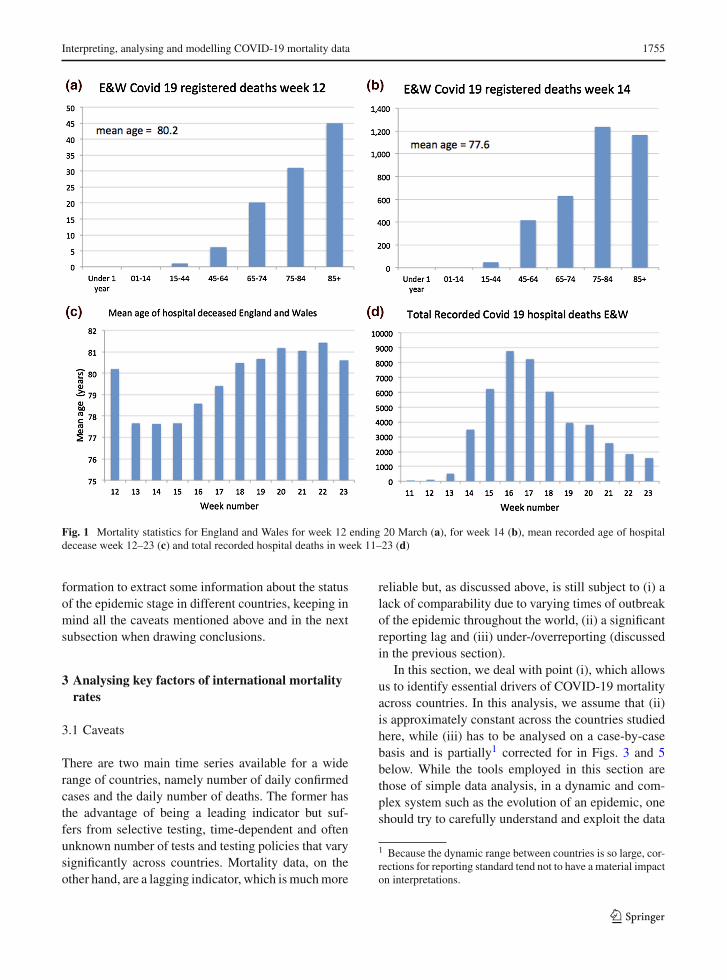
As illustrations of the heterogeneity of reportingstandards, it is useful to review the case of the UKand of New York. The UK Office of National Statis-tics (ONS) began publishing data on the number ofUK deaths from COVID-19 that began to occur duringweek 11, i.e. the week ending 13 March 2020. Fig-ure 1 shows details on the UK reported mortality inhospitals. (A) shows the age profile of hospital deathsfrom Covid-19 in England andWales. Like other coun-tries, the mortality profile shows that the disease wasmost lethal in the ageing 65+ cohorts and increasedexponentially with age; (B) in week 14, the age profilehad changed reflecting a change in policy where (1)elderly patients in hospitals were sent back to their carehomes and (2) doctors became more selective send-ing very elderly Covid-19 patients from care homesto hospital since it was recognised that the survivalof the very old was not good and hospital capacitywas reserved for younger patients; (C) shows how theplunge in age of the hospital deceased was reversed inweek 16 [the peak of mortality, see panel (D)], pre-sumably because it was now recognised that hospitalcapacity was not over-stretched and an increasing num-ber of elderly were admitted, many of whom died astestified by the statistics; (D) the profile of hospitaldeaths from Covid-19 in England and Wales showingthe huge peaks of more than 8000 deaths in weeks16 and 17. These huge peaks in part reflect failureto protect the most vulnerable from infection in carehomes.

OnApril 14,NewYork’smortality statistics includedpeople who died at homewithout getting tested, or whodied in nursing homes or at hospitals, but did not havea confirmed positive test result. The New York Times[31], The Economist [32] and The Financial Times[33] estimated there might be up to 100% more deaths

not included in the current statistics in some countriesbased on an analysis of the excess deaths, although theydid not correct for the significant short-term reportinglag in mortality data (see section A.3 in the “appendix”for a visualisation of this reporting delay). On April 17,authorities inWuhan revised the local death toll upwardby 50%.

Regarding the relative measure of mortality statis-tics, most media and reports only use case fatality rate(CFR), the number of deaths divided by the numberof confirmed cases, to compare status of the epidemicamong different countries. Let alone the reliability ofthe absolute number of deaths (the numerator men-tioned above), the denominator—number of confirmedcases—is also subject to a number of biases. For exam-ple, China’s national health commission issued sevenversions of a case definition for COVID-19 between15 January and 3 March, and a recent study foundeach of the first four changes increased the propor-tion of cases detected and counted by between 2.8and 7.1 times [34]. Furthermore, the number of casesis usually on the basis of testing, which is biasedtowards severe cases in some countries, health carestaff in others (the UK) while towards a larger groupin some other countries implementing massive testingprograms, such as SouthKorea and Iceland. The testingprotocols and accuracy may also have a large impacton the results.

Relating positive test results to real levels of infec-tion is also subject to a large number of biases. It isimportant to note that the real number of infections isfar higher than those recorded in positive tests sinceonly a tiny fraction of any population has been tested.This relates to another concept: Infection Fatality Rate(number of deaths divided by total infections includingasymptomatic cases). The commonly cited death ratesfor seasonal flu of 0.1% to 0.2% are usually reported interms of a version of the CFR (deaths among the popu-lationwho have visible symptoms of the disease), whileseveral recent studies on seroprevalence of antibodiesto SARS-CoV-2 in the general population [35,36] haveused IFR. These IFR cannot be directly compared withthe CFR of seasonal flu. If, say, 50% of the infectedpopulation is asymptomatic, this implies that CFR = 2IFR.

It is not realistic to wait for all the reliable statisticsbeforewe start tomodel and understand the progressionof the COVID-19 epidemic. In the following section,wewill use the existing statisticswith appropriate trans-

123


Fig. 1 Mortality statistics for England and Wales for week 12 ending 20 March (a), for week 14 (b), mean recorded age of hospitaldecease week 12–23 (c) and total recorded hospital deaths in week 11–23 (d)

formation to extract some information about the statusof the epidemic stage in different countries, keeping inmind all the caveats mentioned above and in the nextsubsection when drawing conclusions.

3 Analysing key factors of international mortalityrates

3.1 Caveats

There are two main time series available for a widerange of countries, namely number of daily confirmedcases and the daily number of deaths. The former hasthe advantage of being a leading indicator but suf-fers from selective testing, time-dependent and oftenunknown number of tests and testing policies that varysignificantly across countries. Mortality data, on theother hand, are a lagging indicator, which ismuchmore

reliable but, as discussed above, is still subject to (i) alack of comparability due to varying times of outbreakof the epidemic throughout the world, (ii) a significantreporting lag and (iii) under-/overreporting (discussedin the previous section).

In this section, we deal with point (i), which allowsus to identify essential drivers of COVID-19 mortalityacross countries. In this analysis, we assume that (ii)is approximately constant across the countries studiedhere, while (iii) has to be analysed on a case-by-casebasis and is partially1 corrected for in Figs. 3 and 5below. While the tools employed in this section arethose of simple data analysis, in a dynamic and com-plex system such as the evolution of an epidemic, oneshould try to carefully understand and exploit the data

1 Because the dynamic range between countries is so large, cor-rections for reporting standard tend not to have a material impacton interpretations.

123


along several dimensions before applyingmore sophis-ticatedmodels. Analysing themost influential explana-tory factors allows us to identify anomalies and put ourprediction results of Sect. 4 in perspective.

Below, we use mortality data from Johns HopkinsUniversity Centre for Systems Science and Engineer-ing [37].

3.2 Transforming mortality data for cross-countrycomparison

3.2.1 Population normalised death rates and roughgeographic grouping

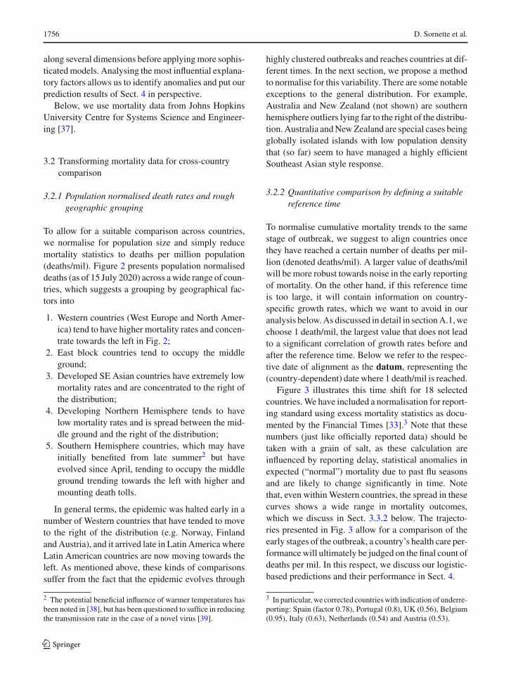
To allow for a suitable comparison across countries,we normalise for population size and simply reducemortality statistics to deaths per million population(deaths/mil). Figure 2 presents population normaliseddeaths (as of 15 July 2020) across awide range of coun-tries, which suggests a grouping by geographical fac-tors into

1. Western countries (West Europe and North Amer-ica) tend to have higher mortality rates and concen-trate towards the left in Fig. 2;

2. East block countries tend to occupy the middleground;

3. Developed SE Asian countries have extremely lowmortality rates and are concentrated to the right ofthe distribution;

4. Developing Northern Hemisphere tends to havelow mortality rates and is spread between the mid-dle ground and the right of the distribution;

5. Southern Hemisphere countries, which may haveinitially benefited from late summer2 but haveevolved since April, tending to occupy the middleground trending towards the left with higher andmounting death tolls.

In general terms, the epidemic was halted early in anumber of Western countries that have tended to moveto the right of the distribution (e.g. Norway, Finlandand Austria), and it arrived late in Latin America whereLatin American countries are now moving towards theleft. As mentioned above, these kinds of comparisonssuffer from the fact that the epidemic evolves through

2 The potential beneficial influence of warmer temperatures hasbeen noted in [38], but has been questioned to suffice in reducingthe transmission rate in the case of a novel virus [39].

highly clustered outbreaks and reaches countries at dif-ferent times. In the next section, we propose a methodto normalise for this variability. There are some notableexceptions to the general distribution. For example,Australia and New Zealand (not shown) are southernhemisphere outliers lying far to the right of the distribu-tion. Australia andNewZealand are special cases beingglobally isolated islands with low population densitythat (so far) seem to have managed a highly efficientSoutheast Asian style response.

3.2.2 Quantitative comparison by defining a suitablereference time

To normalise cumulative mortality trends to the samestage of outbreak, we suggest to align countries oncethey have reached a certain number of deaths per mil-lion (denoted deaths/mil). A larger value of deaths/milwill be more robust towards noise in the early reportingof mortality. On the other hand, if this reference timeis too large, it will contain information on country-specific growth rates, which we want to avoid in ouranalysis below.As discussed in detail in sectionA.1,wechoose 1 death/mil, the largest value that does not leadto a significant correlation of growth rates before andafter the reference time. Below we refer to the respec-tive date of alignment as the datum, representing the(country-dependent) date where 1 death/mil is reached.

Figure 3 illustrates this time shift for 18 selectedcountries.We have included a normalisation for report-ing standard using excess mortality statistics as docu-mented by the Financial Times [33].3 Note that thesenumbers (just like officially reported data) should betaken with a grain of salt, as these calculation areinfluenced by reporting delay, statistical anomalies inexpected (“normal”) mortality due to past flu seasonsand are likely to change significantly in time. Notethat, even withinWestern countries, the spread in thesecurves shows a wide range in mortality outcomes,which we discuss in Sect. 3.3.2 below. The trajecto-ries presented in Fig. 3 allow for a comparison of theearly stages of the outbreak, a country’s health care per-formancewill ultimately be judged on the final count ofdeaths per mil. In this respect, we discuss our logistic-based predictions and their performance in Sect. 4.

3 In particular,we corrected countrieswith indication of underre-porting: Spain (factor 0.78), Portugal (0.8), UK (0.56), Belgium(0.95), Italy (0.63), Netherlands (0.54) and Austria (0.53).

123


Fig. 2 Deaths per million population for 55 countries selectedto represent five main socioeconomic and geo-political groupsfrom around the world. Sweden, Brazil and Belarus are high-lighted as countries that have pursued a policy of no lockdown.

The two graphs differ only in the logarithmic versus linear scaleof their vertical axis, allowing us to put in perspective the relativedeath toll across different countries

3.3 Quantifying key factors of COVID-19 mortality

3.3.1 Age dependence and life expectancy

For most, the SARS-CoV-2 infection goes unnoticed(stage 1), for some, it leads to mild symptoms (stage2). For a tiny minority of vulnerable people, it developsinto a lethal disease (stages 4– 5). The relatively highR0 produces a flood of hospital admissions giving anamplified sense of seriousness at the whole populationlevel.

As noted in [23,40] and evident from country-specific mortality statistics, there is clear evidence ofthose most susceptible to progression to Stage 5. Fig-ure 4 shows the total number of deaths as recordedin Italy and the population structure of India. Mortal-ity is highest in the older cohorts, with a median age of80years, while India has a small number of the very oldin its population. This observation informs the hypoth-

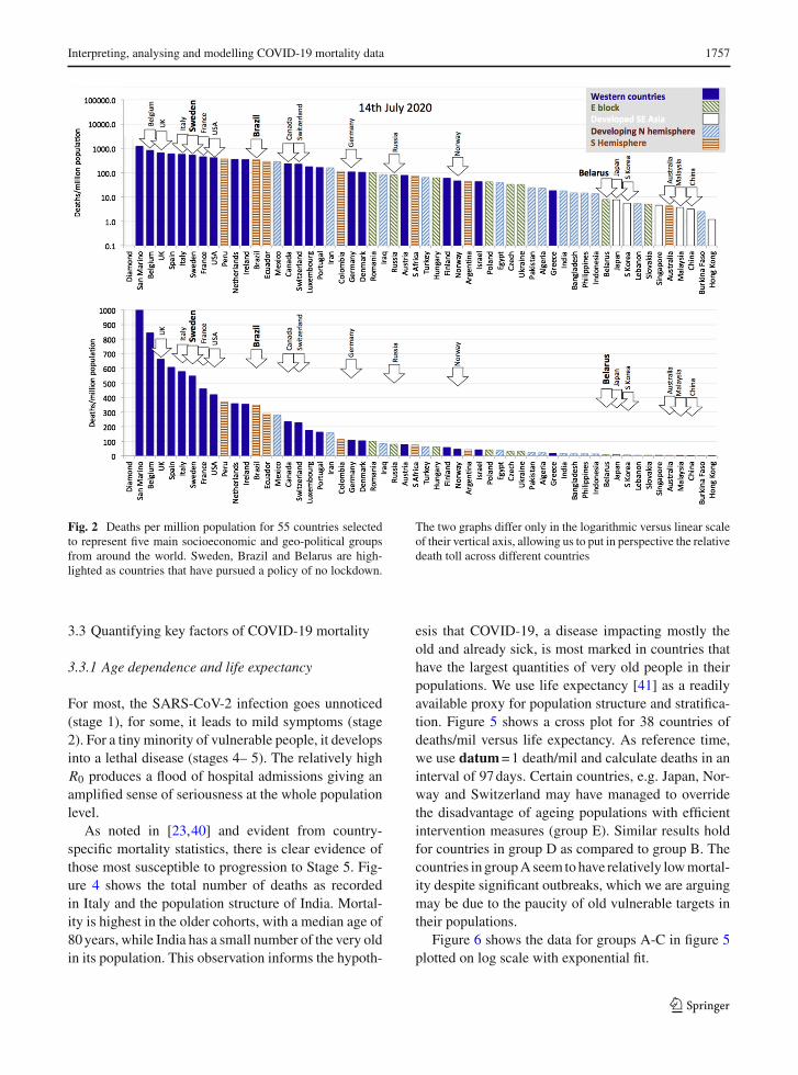
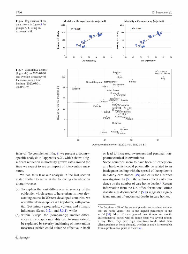
esis that COVID-19, a disease impacting mostly theold and already sick, is most marked in countries thathave the largest quantities of very old people in theirpopulations. We use life expectancy [41] as a readilyavailable proxy for population structure and stratifica-tion. Figure 5 shows a cross plot for 38 countries ofdeaths/mil versus life expectancy. As reference time,we use datum=1 death/mil and calculate deaths in aninterval of 97days. Certain countries, e.g. Japan, Nor-way and Switzerland may have managed to overridethe disadvantage of ageing populations with efficientintervention measures (group E). Similar results holdfor countries in group D as compared to group B. Thecountries in groupAseem tohave relatively lowmortal-ity despite significant outbreaks, which we are arguingmay be due to the paucity of old vulnerable targets intheir populations.

Figure 6 shows the data for groups A-C in figure 5plotted on log scale with exponential fit.

123


Fig. 3 Cumulative mortality curves for selected countries. Thedatum marks the point where each country reached 1/mil deathsas explained in the text. Lower panel is corrected for potentialunderreporting according to [33], see text for details. The dashedbox in the upper panel represents the data reported in an earlierversion of this paper

Based on the trends we identified here, we areinclined to draw the following conclusions (mind thespecial cases of Australia, South Korea and Japan iden-

tified above). We hypothesise that a key driver behindthe large COVID-19 epidemic in the Western coun-tries is because these rich countries have spent largeamounts on healthcare with a focus on extending thelives of the elderly, through a rangeofmedical andphar-maceutical interventions. Moreover, if there is a rela-tion of climate/temperature to the outbreak severity ofCOVID-19, it is rather weak and does not seem signifi-cant as compared to the demographic structure. Finally,there is a substantial variation even within the Westerncountries that is unexplained by (minor) demographic,climatic or geographical differences. We analyse thesecountries in the next section.

3.3.2 Lockdown policies and mortality in Europe andthe USA

As outlined above, looking at population, normalisedmortality statistics allows us to compare the progres-sion of the epidemic across countries: in particular,we can quantify what is the shift in time needed tobest make comparable the mortality curves of variouscountries. The analysis here can be understood as top-down complementary to studies such as [42–45], whichare subject to additional assumptions and do not allowfor a straightforward comparison across countries. Thevalue of this time-shifted dataset is to allow us, forinstance, to analyse the potential efficiency of interven-tion and lockdown policies across a number ofWesterncountries.Stringency index

The authors in [46] collect and update an exhaustivelist of government responses to COVID-19. In partic-ular, they calculate a Stringency Index as a daily time

Fig. 4 Mortality statisticsfor Italy until July 12(Median age: 82years) andthe population structure ofItaly and India

123


Fig. 5 Cross plot showing the relationship between lifeexpectancy and mortality expressed as deaths/mil. As referencetime,we use datum=1 death/mil and calculate deaths in an inter-val of 97days. Lower panel is corrected for potential underreport-ing according to [33], see Sect. 3.2.2 for details

series of numbers in [0, 100], based on an average ofthe following policies:

1. School closure,2. Workplace closure,3. Canceling public events,4. Closing public transport,5. Public info campaigns,6. Restrictions on internal movement,7. International travel controls.

For a detailed explanation and weighting of variouspolicies, we refer to [46]. Note that, this index doesnot cover personal non-pharmaceutical interventionssuch as increased personal hygiene or voluntary socialdistancing.

Cumulative mortality and lockdownA first pass examination of this data is to look at

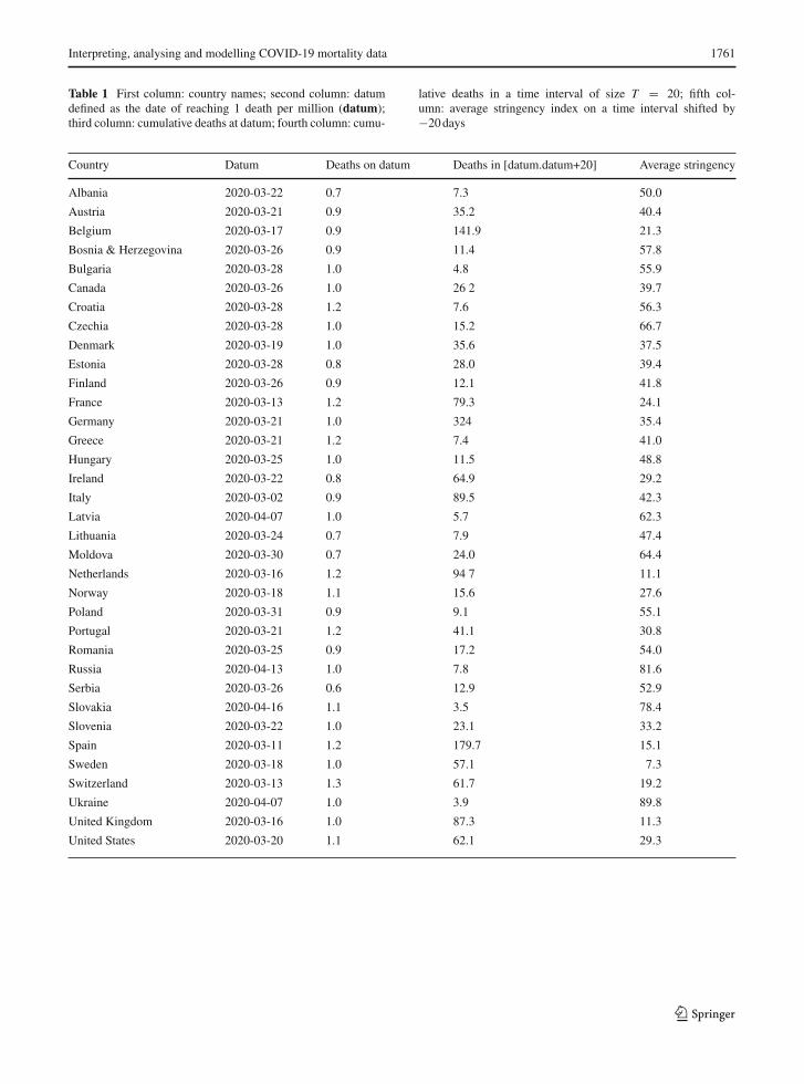
cumulative mortality in a range of countries and theirrelation to the stringency index. For this, we fix adate t = 2020/04/20 and compare the cumulativedeaths per 1million population on this date. Usingthe results from [47,48], who report an average timefrom infection to death of roughly 20 days,4 we cal-culate the average Stringency Index on a time interval[2020/03/01, t − 20] and plot against total deaths att , see Fig. 7. Here, the initial time point is chosen adhoc. It would seem that the stringency index has littleinfluence on the number of deaths in a country. How-ever, as we have discussed above, the epidemic arrivedin various countries at different times, so one needs tocarefully account for this time lag.

To get amore robust result on efficiency of lockdownstrategies, we conduct the following steps to transformthe data, as recorded in Table 1:

1. For each country, we choose the beginning of theepidemic to be at

datum=1 deaths per million (1)

and record for each country the time where thisnumber was reached (to be precise, we choose theday where the reported number was closest to 1deaths per million)

2. Next, we choose some time frame T , restricted bythe country being the latest to have reached 1 deathsper million. In our example below, we set T =20days.

3. For each country, we calculate the number of deathsin a time interval [datum, datum + T ].

4. Finally, we calculate the average stringency indexin a time interval shifted backwards by 20 days toaccount for the average time of infection to death[47,48].

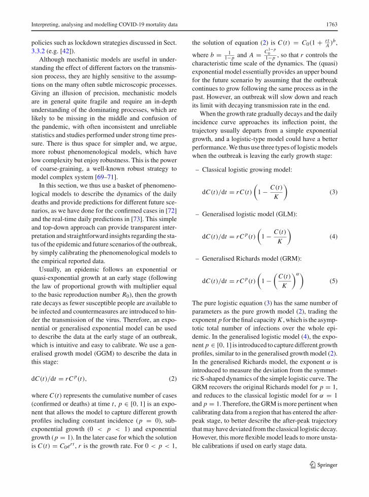
Figure 8 shows the number of cumulative deathswith respect to lockdown strategies in European coun-tries, using the methodology outlined above. We notea rather convincing negative correlation between strin-gency during the beginning of the epidemic and thelogarithm of the number of deaths in a subsequent time

4 Below we consider averages on intervals, and the exact distri-bution is not essential here.

123


Fig. 6 Regressions of thedata shown in figure 5 forgroups A–C using anexponential fit

Fig. 7 Cumulative deaths(log scale) on 2020/04/20and average stringency oflockdown over a timehorizon [2020/03/01,2020/03/26]

interval. To complement Fig. 8, we present a country-specific analysis in “appendix A.2”, which shows a sig-nificant reduction in mortality growth rates around thetime we expect to see an impact of intervention mea-sures.

We can thus take our analysis in the last sectiona step further to arrive at the following classificationalong two axes:

(a) To explain the vast differences in severity of theepidemic, which seems to have taken its most dev-astating course inWestern developed countries, wenoted that demographics is a key driver, with poten-tial (but minor) geographic, cultural and climaticinfluences (Sects. 3.2.1 and 3.3.1), while

(b) within Europe, the (comparably) smaller differ-ences in per-capita mortality can, to some extend,be explained by severity and timing of interventionmeasures (which could either be effective in itself

or lead to increased awareness and personal non-pharmaceutical interventions).Some countries seem to have been hit exception-ally hard, which could potentially be related to aninadequate dealing with the spread of the epidemicin elderly care homes [49] and calls for a furtherinvestigation. In [50], the authors collect early evi-dence on the number of care home deaths.5 Recentinformation from the UK office for national officestatistics (as documented in [50]) suggests a signif-icant amount of uncounted deaths in care homes.

5 In Belgium, 46% of the general practitioners-patient encoun-ters are home visits. This is the highest percentage in theworld [51]. Most of these general practitioners are mobileentrepreneurial nurses who do home visits via several roundsa day. Thus, they have high incentives to do what theirclients/patients at home demand, whether or not it is reasonablefrom a professional point of view [52].

123


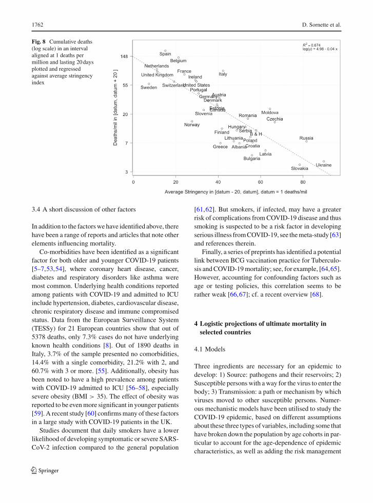
Table 1 First column: country names; second column: datumdefined as the date of reaching 1 death per million (datum);third column: cumulative deaths at datum; fourth column: cumu-

lative deaths in a time interval of size T = 20; fifth col-umn: average stringency index on a time interval shifted by−20days

Country Datum Deaths on datum Deaths in [datum.datum+20] Average stringency

Albania 2020-03-22 0.7 7.3 50.0

Austria 2020-03-21 0.9 35.2 40.4

Belgium 2020-03-17 0.9 141.9 21.3

Bosnia & Herzegovina 2020-03-26 0.9 11.4 57.8

Bulgaria 2020-03-28 1.0 4.8 55.9

Canada 2020-03-26 1.0 26 2 39.7

Croatia 2020-03-28 1.2 7.6 56.3

Czechia 2020-03-28 1.0 15.2 66.7

Denmark 2020-03-19 1.0 35.6 37.5

Estonia 2020-03-28 0.8 28.0 39.4

Finland 2020-03-26 0.9 12.1 41.8

France 2020-03-13 1.2 79.3 24.1

Germany 2020-03-21 1.0 324 35.4

Greece 2020-03-21 1.2 7.4 41.0

Hungary 2020-03-25 1.0 11.5 48.8

Ireland 2020-03-22 0.8 64.9 29.2

Italy 2020-03-02 0.9 89.5 42.3

Latvia 2020-04-07 1.0 5.7 62.3

Lithuania 2020-03-24 0.7 7.9 47.4

Moldova 2020-03-30 0.7 24.0 64.4

Netherlands 2020-03-16 1.2 94 7 11.1

Norway 2020-03-18 1.1 15.6 27.6

Poland 2020-03-31 0.9 9.1 55.1

Portugal 2020-03-21 1.2 41.1 30.8

Romania 2020-03-25 0.9 17.2 54.0

Russia 2020-04-13 1.0 7.8 81.6

Serbia 2020-03-26 0.6 12.9 52.9

Slovakia 2020-04-16 1.1 3.5 78.4

Slovenia 2020-03-22 1.0 23.1 33.2

Spain 2020-03-11 1.2 179.7 15.1

Sweden 2020-03-18 1.0 57.1 7.3

Switzerland 2020-03-13 1.3 61.7 19.2

Ukraine 2020-04-07 1.0 3.9 89.8

United Kingdom 2020-03-16 1.0 87.3 11.3

United States 2020-03-20 1.1 62.1 29.3

123


Fig. 8 Cumulative deaths(log scale) in an intervalaligned at 1 deaths permillion and lasting 20daysplotted and regressedagainst average stringencyindex

3.4 A short discussion of other factors

In addition to the factorswe have identified above, therehave been a range of reports and articles that note otherelements influencing mortality.

Co-morbidities have been identified as a significantfactor for both older and younger COVID-19 patients[5–7,53,54], where coronary heart disease, cancer,diabetes and respiratory disorders like asthma weremost common. Underlying health conditions reportedamong patients with COVID-19 and admitted to ICUinclude hypertension, diabetes, cardiovascular disease,chronic respiratory disease and immune compromisedstatus. Data from the European Surveillance System(TESSy) for 21 European countries show that out of5378 deaths, only 7.3% cases do not have underlyingknown health conditions [8]. Out of 1890 deaths inItaly, 3.7% of the sample presented no comorbidities,14.4% with a single comorbidity, 21.2% with 2, and60.7% with 3 or more. [55]. Additionally, obesity hasbeen noted to have a high prevalence among patientswith COVID-19 admitted to ICU [56–58], especiallysevere obesity (BMI > 35). The effect of obesity wasreported to be evenmore significant in younger patients[59].A recent study [60] confirmsmany of these factorsin a large study with COVID-19 patients in the UK.

Studies document that daily smokers have a lowerlikelihood of developing symptomatic or severe SARS-CoV-2 infection compared to the general population

[61,62]. But smokers, if infected, may have a greaterrisk of complications fromCOVID-19 disease and thussmoking is suspected to be a risk factor in developingserious illness fromCOVID-19, see themeta-study [63]and references therein.

Finally, a series of preprints has identified a potentiallink between BCG vaccination practice for Tuberculo-sis andCOVID-19mortality; see, for example, [64,65].However, accounting for confounding factors such asage or testing policies, this correlation seems to berather weak [66,67]; cf. a recent overview [68].

4 Logistic projections of ultimate mortality inselected countries

4.1 Models

Three ingredients are necessary for an epidemic todevelop: 1) Source: pathogens and their reservoirs; 2)Susceptible personswith away for the virus to enter thebody; 3) Transmission: a path or mechanism by whichviruses moved to other susceptible persons. Numer-ous mechanistic models have been utilised to study theCOVID-19 epidemic, based on different assumptionsabout these three types of variables, including some thathave broken down the population by age cohorts in par-ticular to account for the age-dependence of epidemiccharacteristics, as well as adding the risk management

123


policies such as lockdown strategies discussed in Sect.3.3.2 (e.g. [42]).

Although mechanistic models are useful in under-standing the effect of different factors on the transmis-sion process, they are highly sensitive to the assump-tions on the many often subtle microscopic processes.Giving an illusion of precision, mechanistic modelsare in general quite fragile and require an in-depthunderstanding of the dominating processes, which arelikely to be missing in the middle and confusion ofthe pandemic, with often inconsistent and unreliablestatistics and studies performed under strong time pres-sure. There is thus space for simpler and, we argue,more robust phenomenological models, which havelow complexity but enjoy robustness. This is the powerof coarse-graining, a well-known robust strategy tomodel complex system [69–71].

In this section, we thus use a basket of phenomeno-logical models to describe the dynamics of the dailydeaths and provide predictions for different future sce-narios, as we have done for the confirmed cases in [72]and the real-time daily predictions in [73]. This simpleand top-down approach can provide transparent inter-pretation and straightforward insights regarding the sta-tus of the epidemic and future scenarios of the outbreak,by simply calibrating the phenomenological models tothe empirical reported data.

Usually, an epidemic follows an exponential orquasi-exponential growth at an early stage (followingthe law of proportional growth with multiplier equalto the basic reproduction number R0), then the growthrate decays as fewer susceptible people are available tobe infected and countermeasures are introduced to hin-der the transmission of the virus. Therefore, an expo-nential or generalised exponential model can be usedto describe the data at the early stage of an outbreak,which is intuitive and easy to calibrate. We use a gen-eralised growth model (GGM) to describe the data inthis stage:

dC(t)/dt = rC p(t), (2)

where C(t) represents the cumulative number of cases(confirmed or deaths) at time t , p ∈ [0, 1] is an expo-nent that allows the model to capture different growthprofiles including constant incidence (p = 0), sub-exponential growth (0 < p < 1) and exponentialgrowth (p = 1). In the later case for which the solutionis C(t) = C0ert , r is the growth rate. For 0 < p < 1,

the solution of equation (2) is C(t) = C0(1 + r tA )b,

where b = 11−p and A = C1−p

01−p , so that r controls the

characteristic time scale of the dynamics. The (quasi)exponential model essentially provides an upper boundfor the future scenario by assuming that the outbreakcontinues to grow following the same process as in thepast. However, an outbreak will slow down and reachits limit with decaying transmission rate in the end.

When the growth rate gradually decays and the dailyincidence curve approaches its inflection point, thetrajectory usually departs from a simple exponentialgrowth, and a logistic-type model could have a betterperformance.We thus use three types of logisticmodelswhen the outbreak is leaving the early growth stage:

– Classical logistic growing model:

dC(t)/dt = rC(t)

(1 − C(t)

K

)(3)

– Generalised logistic model (GLM):

dC(t)/dt = rC p(t)

(1 − C(t)

K

)(4)

– Generalised Richards model (GRM):

dC(t)/dt = rC p(t)

(1 −

(C(t)

K

)α)(5)

The pure logistic equation (3) has the same number ofparameters as the pure growth model (2), trading theexponent p for thefinal capacity K ,which is the asymp-totic total number of infections over the whole epi-demic. In the generalised logistic model (4), the expo-nent p ∈ [0, 1] is introduced to capture different growthprofiles, similar to in the generalised growth model (2).In the generalised Richards model, the exponent α isintroduced to measure the deviation from the symmet-ric S-shaped dynamics of the simple logistic curve. TheGRM recovers the original Richards model for p = 1,and reduces to the classical logistic model for α = 1and p = 1. Therefore, theGRM ismore pertinent whencalibrating data from a region that has entered the after-peak stage, to better describe the after-peak trajectorythatmayhave deviated from the classical logistic decay.However, this more flexible model leads to more unsta-ble calibrations if used on early stage data.

123


4.2 Methodology

Scenarios. As we have demonstrated in [72], logistic-type models tend to under-estimate the final capacityK and thus could serve as lower bounds for the futurescenarios.We define thepositive scenario as themodelwith the second lowest predicted final total deaths Kamong the three logistic models, and themedium sce-nario as the model with the highest predicted finaltotal deaths among the three logisticmodels. Both posi-tive and medium scenarios could underestimate largelythe final capacity. The negative scenario is describedby the generalised growth model, which should onlydescribe the early stage of the epidemic outbreak and istherefore least reliable for countries in the more maturestage as it does not include a finite population capacity.

Calibration. For the calibration, we use the standardLevenberg-Marquardt algorithm to solve the non-linearleast square optimisation. To estimate the uncertainty ofour model estimates, we use a bootstrap approach witha negative binomial error structure N B(μ, σ 2), whereμ and σ 2 are the mean and variance of the distribution,estimated from the empirical data.

Data. The reported death data are from the EuropeanCentre for Disease Prevention and Control (ECDC)[8]up to July 17.

4.3 Results

We define the outbreak progress as the latest cumu-lative number of deaths per million divided by the pre-dicted final total death toll. As the epidemic progresses,the outbreak progress increases and finally saturates to1 when the epidemic ends. Note that, in a classicallogistic curve, an outbreak progress of 50% indicatesthat the total number of deaths has reached its inflectionpoint, which is also the time of the peak of the dailyincidence curve. If the inflection point has been passed,the worst of the outbreak is over. The fitted trajectory,and thus the position of the inflection point and thepredicted final death toll depends on country-specificfactors identified in Sect. 3,most notably demographicsand (early) intervention measures. Therefore, the out-break progress can measure how mature the outbreakis in a country, and is more conservative than the same

analysis based on confirmed cases, as the number ofdeaths is a lagging indicator behind confirmed cases.

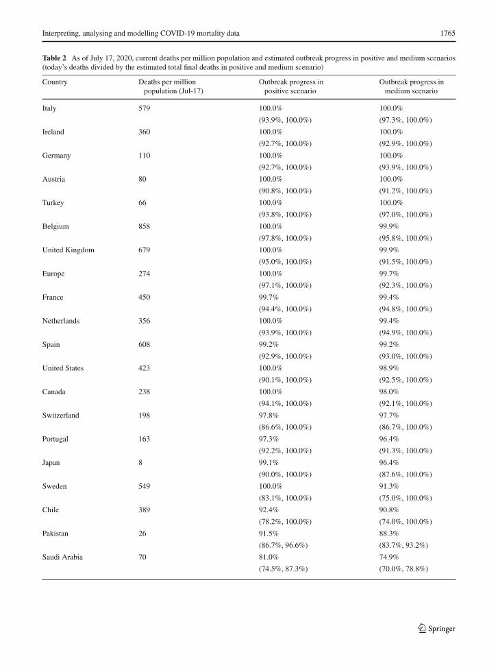
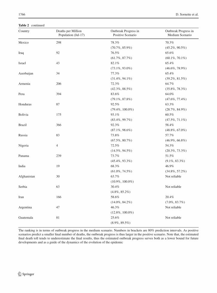
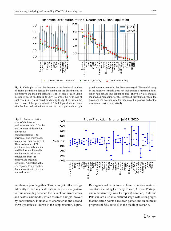
In Table 2, we list the cumulative numbers of deathsper million population as of July 17, 2020, and the out-break progress (death) in positive and medium scenar-ios. In Fig. 9, we plot the ensemble distribution of thefinal total number of deaths per million population foreach country, which are based on the aggregation of thesimulations in positive and medium scenarios. Thosecountries with a non-converged distributions are dis-played in the left panel, while those with a convergeddistribution are in the right panel. The left side of eachviolin in cyan is based on data up to July 17, while theright side of each violin in grey is based on data upto April 24, when the first version of this paper wassubmitted. Note that, the logistic-type models are usu-ally useful for understanding the short-term dynamicsextending over a few days, but may become inadequatefor long-term predictions due to the change of the fun-damental dynamics resulting from government inter-ventions, a second wave of outbreaks or other factors,as showed by large shifts of distributions in severalcountries.

To have a view of the performance of short-term pre-dictions, we present the latest 7-day prediction errorsfor the total number of deaths in Fig. 10, based on posi-tive and medium scenarios. One can see that our 7-daypredictions based on data up to July 10th are correctin all matured countries and enjoy narrow predictionintervals. In contrast, our 7-day predictions underesti-mate the true numbers in immature countries, includingIndia, Argentina, Iraq and Honduras. Until May 24, weuploaded a daily update of our projections and an anal-ysis of forecasting errors online, and then shifted toa weekly update until July 3 [73]. We have now dis-continued it as the epidemic enters second waves andother regimes with highly dependent country-specificcharacteristics.

As of July 17, 2020, the epidemic in Italy, Ireland,Germany, Austria, Turkey, Belgium, the United King-dom, France, Netherlands, Spain, the USA, Canada,Switzerland, Portugal and Japan have almost ended,with the outbreak progress approaching 100%.Most ofthese countries have the earliest starts of the outbreaks,with Italy and Spain being the first two hotspots inEurope.However, theUSAhas started a secondwave ofoutbreak with the daily confirmed cases keeping break-ing records recently. This is likely due to the easing ofthe lockdown and street demonstrations where large

123


Table 2 As of July 17, 2020, current deaths per million population and estimated outbreak progress in positive and medium scenarios(today’s deaths divided by the estimated total final deaths in positive and medium scenario)

Country Deaths per millionpopulation (Jul-17)

Outbreak progress inpositive scenario

Outbreak progress inmedium scenario

Italy 579 100.0% 100.0%

(93.9%, 100.0%) (97.3%, 100.0%)

Ireland 360 100.0% 100.0%

(92.7%, 100.0%) (92.9%, 100.0%)

Germany 110 100.0% 100.0%

(92.7%, 100.0%) (93.9%, 100.0%)

Austria 80 100.0% 100.0%

(90.8%, 100.0%) (91.2%, 100.0%)

Turkey 66 100.0% 100.0%

(93.8%, 100.0%) (97.0%, 100.0%)

Belgium 858 100.0% 99.9%

(97.8%, 100.0%) (95.8%, 100.0%)

United Kingdom 679 100.0% 99.9%

(95.0%, 100.0%) (91.5%, 100.0%)

Europe 274 100.0% 99.7%

(97.1%, 100.0%) (92.3%, 100.0%)

France 450 99.7% 99.4%

(94.4%, 100.0%) (94.8%, 100.0%)

Netherlands 356 100.0% 99.4%

(93.9%, 100.0%) (94.9%, 100.0%)

Spain 608 99.2% 99.2%

(92.9%, 100.0%) (93.0%, 100.0%)

United States 423 100.0% 98.9%

(90.1%, 100.0%) (92.5%, 100.0%)

Canada 238 100.0% 98.0%

(94.1%, 100.0%) (92.1%, 100.0%)

Switzerland 198 97.8% 97.7%

(86.6%, 100.0%) (86.7%, 100.0%)

Portugal 163 97.3% 96.4%

(92.2%, 100.0%) (91.3%, 100.0%)

Japan 8 99.1% 96.4%

(90.0%, 100.0%) (87.6%, 100.0%)

Sweden 549 100.0% 91.3%

(83.1%, 100.0%) (75.0%, 100.0%)

Chile 389 92.4% 90.8%

(78.2%, 100.0%) (74.0%, 100.0%)

Pakistan 26 91.5% 88.3%

(86.7%, 96.6%) (83.7%, 93.2%)

Saudi Arabia 70 81.0% 74.9%

(74.5%, 87.3%) (70.0%, 78.8%)

123


Table 2 continued

Country Deaths per MillionPopulation (Jul-17)

Outbreak Progress inPositive Scenario

Outbreak Progress inMedium Scenario

Mexico 298 78.3% 70.3%

(70.7%, 85.9%) (45.2%, 90.5%)

Iraq 92 76.5% 65.6%

(61.7%, 87.7%) (60.1%, 70.1%)

Israel 43 82.1% 65.4%

(73.1%, 93.0%) (46.6%, 78.9%)

Azerbaijan 34 77.3% 65.4%

(31.4%, 94.1%) (39.2%, 81.5%)

Armenia 206 72.3% 64.7%

(42.3%, 88.5%) (35.8%, 78.3%)

Peru 394 83.6% 64.0%

(79.1%, 87.8%) (47.6%, 77.4%)

Honduras 87 92.5% 63.3%

(79.4%, 100.0%) (28.7%, 84.9%)

Bolivia 175 93.1% 60.5%

(83.4%, 99.7%) (47.5%, 71.1%)

Brazil 366 92.3% 58.4%

(87.1%, 98.6%) (48.8%, 67.0%)

Russia 83 73.8% 57.7%

(67.5%, 80.7%) (46.9%, 66.8%)

Nigeria 4 72.5% 54.3%

(14.5%, 94.5%) (20.3%, 73.3%)

Panama 239 73.7% 51.5%

(45.4%, 93.3%) (9.1%, 83.3%)

India 19 68.3% 46.9%

(61.0%, 74.5%) (34.8%, 57.2%)

Afghanistan 30 63.7% Not reliable

(10.9%, 100.0%)

Serbia 63 30.4% Not reliable

(4.8%, 85.2%)

Iran 166 58.6% 20.4%

(14.0%, 84.2%) (7.0%, 83.7%)

Argentina 47 46.3% Not reliable

(12.8%, 100.0%)

Guatemala 81 25.6% Not reliable

(8.9%, 89.5%)

The ranking is in terms of outbreak progress in the medium scenario. Numbers in brackets are 80% prediction intervals. As positivescenarios predict a smaller final number of deaths, the outbreak progress is thus larger in the positive scenario. Note that, the estimatedfinal death toll tends to underestimate the final results, thus the estimated outbreak progress serves both as a lower bound for futuredevelopments and as a guide of the dynamics of the evolution of the epidemic

123


Fig. 9 Violin plot of the distributions of the final total numberof deaths per million derived by combining the distributions ofthe positive and medium scenarios. The left side of each violinin cyan is based on data up to July 17, while the right side ofeach violin in grey is based on data up to April 24, when thefirst version of this paper submitted. The left panel shows coun-tries that have a distribution that has not converged, and the right

panel presents countries that have converged. The model setupin the negative scenario does not incorporate a maximum satu-ration number and thus cannot be used. The yellow dots indicatethe median prediction for the combined distribution, while thegreen and red dots indicate the median of the positive and of themedium scenarios, respectively

Fig. 10 7-day predictionerror of the forecastperformed on July 10 for thetotal number of deaths forthe variouscountries/regions. Thehorizontal line correspondsto empirical data on July 17.The errorbars are 80%prediction intervals and themiddle dots are the medianpredictions based on thepredictions from thepositive and mediumscenarios. A negative valuecorresponds to a predictionthat underestimated the truerealised value

numbers of people gather. This is not yet reflected sig-nificantly in the daily death data as there is usually a twoto four weeks lag between the data of confirmed casesand deaths. Our model, which assumes a single “wave”by construction, is unable to characterise the secondwave dynamics as shown in the supplementary figure.

Resurgences of cases are also found in several maturedcountries includingGermany, France,Austria, Portugaland others (mostlyWest European). Sweden, Chile andPakistan are also in a matured stage with strong signsthat inflection points have been passed and an outbreakprogress of 85% to 95% in the medium scenario.

123


The next less matured group of countries are SaudiArabia, Mexico, Iraq, Israel, Azerbaijan, Armenia,Peru, Honduras and Bolivia, which have their outbreakprogress in the range of 60%-80%. They just have con-firmed signals that their inflection points have beenpassed, and the shapes of their distribution are settlingto the after-peak trajectory. Saudi Arabia and Israel arealso in a second wave of outbreaks, which may changethe previous inflection points and reduce the outbreakprogress.

Brazil, Russia, Nigeria and Panama are in the thirdmost matured group of countries, which are just at theinflection points and have higher uncertainties regard-ing their future scenarios. This is confirmed by the non-converged (Nigeria and Panama) or highly dispersed(Brazil and Russia) distribution of final deaths per mil-lion as shown in Fig. 9.

The remaining group includes India, Afghanistan,Serbia, Iran, Argentina and Guatemala, whose mor-tality curves have not significantly departed from theexponential or sub-exponential growth trajectory, indi-cating the early stage of the outbreak and high uncer-tainties for the future projections, as evidenced by theirnon-converged distributions of the final deaths in Fig. 9.

5 Discussion

The SARS-CoV-2 / Covid-19 pandemic began inWuhan, China, in January 2020. By 25 April 2020,when we submitted the present paper, it had spreadto every country in the world and killed an esti-mated ∼ two hundred thousand people worldwide.As of 19 July 2020, 14.3 million cases of COVID-19have been reported, including approximately 602,000deaths. Mortality trends showed that it has been killingmore people (normalised for population size) in West-ern countries than anywhere else outside of Wuhan.We set out to solve the riddle of whyWestern countrieswith their lavish healthcare systems were hardest hit.We also set out to understand why the impacts as mea-sured by deaths per million population varied so muchbetween the various Western countries.

Contrary to many early media reports, COVID-19is quite specific about the individuals who are mostsusceptible and die. The largest group of casualties isfound in the elderly, specifically the over 65-year-oldcohorts. The mean age of the dead in the UK is about80 similar to the mean age of the dead in Italy. Many ofthe dead are aged 80 or more and arguably were close

to end of life, exhibiting comorbidities such as respira-tory disorders, cancer and heart disease. In the UK, the65+ group comprises 87% of all deaths. In the under65 group that comprises 13% of all deaths, numerousreports suggest that it is the clinically obese who aremost at risk. The deceased obese are also described ashaving comorbidities of diabetes, high blood pressureand atherosclerosis.

We have presented results on the mortality statisticsof the COVID-19 epidemic in a number of countries.After drawing attention to many data quality issues,we have proposed a classification of countries in fivegroups, 1) Western countries, 2) East Block , 3) devel-oped Southeast Asian countries, 4) Northern Hemi-sphere developing countries and 5) Southern Hemi-sphere countries. Comparing the number of deaths permillion inhabitants, a pattern emerges in which theWestern countries exhibit the largest mortality rate.Furthermore, comparing the running cumulative deathtolls at the same level of outbreak progress in differentcountries reveals several subgroups within the West-ern countries and further emphasises the differencebetween the five groups. Rationalising the drastic dif-ferences in performance goes beyond the present arti-cle, but visualising these differences calls for in-depthinvestigations of causative or correlated factors suchas preparedness, development and organisation of thehealth-care system (public-private, governance struc-ture, etc), culture (close physical contacts versus socialdistance, hygiene, etc), stringency of the reactions tocontrol the epidemic, temperature, geography, popula-tion density, general health and age distribution and soon.

Inspired by a number of reports, we presented a syn-thetic plot of the relationship between deaths per mil-lion and life expectancy in different countries, taken asa proxy of the preponderance of elderly people in thepopulation. Our analysis strongly suggests that a mainreason behind the relatively more severe COVID-19epidemic in the Western countries is their larger pop-ulation of elderly people, with the exceptions such asNorway and Japan, for which other factors seem todominate. Following the outcomes of the epidemic inthese countries and extending the comparative analysisthat we present will provide important insights to learnand implement as much as possible the procedures thathave been successful.

Within theWestern countries,we report a large rangeof outcomes, despite similar demographics. Our com-

123


parison between countries at the same level of outbreakprogress also allowed us to identify and quantify amea-sure of efficiency of the level of stringency of confine-ment measures. This delicate and controversial subjectfinds here an objective analysis, which confirms thatstronger stringency on confinement measures duringthe early stages of the epidemic are significantly neg-atively correlated with deaths per million. We founda correlation between mortality and a stringency met-ric that quantifies 7 different measures such as closureof schools, bans on large public meetings and lockingdown populations.

Looking at Fig. 8 (and extending the time window)shows that increasing the stringency from 20 to 60during the onset of the epidemic decreases the deathcount by about 50 lives per million within two weeks,or roughly 350 lives per million until July, i.e. about20’000-25’000 lives for the UK. Thus, unsurprisingly,preventing people from meeting and moving aroundprovides a barrier against the propagation of the virus.But the effect up to date is arguably small, and largelydepends on when the confinement measures were putin place. As argued by the epidemiologist behind Swe-den’s trust-based approach to tackling the epidemic,closedown, lockdown, closing borders, none of thesemeasures may have historical scientific basis when theepidemic is already well advanced 6. Moreover, thelockdown strategy faces the paradoxical desires of, onthe one hand, having the least number of infected peo-ple.On the other hand, the governments of locked downcountries worry that only a tiny percentage of the pop-ulation has been exposed to the virus (at the time ofwriting, estimations vary from a few percent to 10 per-cent), so that any deconfinement may lead immediatelyto a second epidemicwave, barring achieving a fractionof about 60%of the population7 being protected by pre-vious infections or vaccination. Recent studies suggestthat the herd immunity threshold could be lower, per-haps even as lowas 20%as a result of partial preexistingimmunity and strong heterogeneity of R0 [74,75].

We have also performed logistic equation analysesof deaths as a means of tracking the maturity of out-breaks and estimating ultimate mortality. We use four

6 https://www.nature.com/articles/d41586-020-01098-x.7 This fraction of 60% is derived from an assumed averageinfection factor R0 = 2.5, so that the effective infection fac-tor Reff when a fraction p of the population is immune becomesReff = R0(1 − p). Then, solving for p such that Reff ≤ 1 givesp ≥ 60%.

different models to identify model error and robust-ness of results. This quantitative analysis allowed us toassess the outbreak progress in different countries, dif-ferentiating between those that are at a quite advancedstage and close to the end of the epidemic from thosethat are still in the middle of it.

Western governments will be judged on two met-rics. First, they will be judged on the ultimate num-ber of deaths per million people. Second, they willbe judged on the economic and social costs of theiractions. With only one exception (Sweden), Westerngovernments have taken extreme actions to combatCOVID-19, with different levels of stringency acrosscountries (with the case of Asian countries needing adifferent discussion). These actions include confiningwhole populations at home, shutting down large sec-tors of their economies, throwing tens ofmillions out ofwork and running up massive debts. The common esti-mationof the economic cost of thesemeasures iswidelyestimated around 10% of GDP, and is likely to grow astime passes. Strict confinement can also have seriousconsequences in terms of mental illness and neglectof other conditions. The breakdown of supply chainsthreatens famines of ‘biblical proportions’, accordingto a recent UN report.

Given these conclusions, and with the perspectiveand experience of the epidemics of the past, we have toask whether the extraordinary response levels, with noequivalent in history, are justified by the threats posedby the SARS-CoV-2 virus. Was it worth putting theprosperity of whole nations at risk in this way? In a col-umn entitled “Coronavirus, watch out for danger, butnot the one you think”, Professor Gilbert Deray, fromthe Pitié-Salpêtrière Hospital in Paris summarises theproblem as follows: For 30 years, from my hospitalobservatory, I have lived through many health crises,HIV, SARS, MERS, resurgence of tuberculosis, multi-resistant bacteria, we have managed them calmly andvery effectively. None of them have given rise to thecurrent panic. I have never experienced such a level ofconcern for an infectious disease.

This is the first time that people’s health has been putahead of economic interests at such a global level. Butwas this well thought out? A society cannot save everylife, it has to make reasonable choices. A wise pol-icy requires intelligent calculations that arbitrate andbalance medical, social, economic, equity and inter-generational considerations. Have we been collectively

123

https://www.nature.com/articles/d41586-020-01098-x


blinded by short-sighted medical considerations andbeen overwhelmed by a pandemic of fear [76]?

What could have been done better? Without doubt,many studies will be published on this question.It seems to us that the well-conceived PandemicInfluenza Plan elaborated by nations in collabora-tion with the WHO have been superseded by a pan-demic of fear. For example, translating from thelatest Swiss Pandemic Influenza Plan (2018), weread that the pandemic management strategies aredesigned to reduce at the very least deleterious con-sequences of the pandemic and the priority objec-tives are: (i) to protect and preserve the life, well-being and health of the population; (ii) keep casu-alties to a minimum and (iii) prevent the occur-rence of subsequent economic damage. Further, theSwiss-WHO based plan continues with the follow-ing statement (www.bag.admin.ch/bag/fr/home/das-bag/publikationen/broschueren/publikationen-uebertragbare-krankheiten/pandemieplan-2018.html): “Pre-venting aninfluenza pandemic by means of contain-ment measures seems, according to current knowledge,unrealistic both nationally and internationally.Applica-tion of selective measures as part of containment inter-ventions can be used to prevent the spread of disease,limit local outbreaks during the initial phase and thusreduce transmission, and thus providing targeted pro-tection for vulnerable people. These measures will notprevent the spread of the pandemic, but they will even-tually help to slow it down and thus gain time. Contain-ment measures therefore have local operational objec-tives and contribute to the mitigation strategy”. Theseclear instructions have the further benefit of removinguncertainty, which has been a major cause of stress inaffected population [77]. The science of epidemics iswell-established and dictates that at the very beginningof an epidemic, stringent measures must been put inplace to isolate the local clusters and to protect the vul-nerable. It thus seems to us that the undifferentiatedand unprecedented global and complete lockdown inmany countries has not been rooted in sound scientificthinking based on the calm assessment based on all pre-vious knowledge, but has fallen trap to quickly cookedmodels that catalysed an atmosphere of fear amplifiedby the social media and media machine as sellers ofattention [78].

Acknowledgements Open access funding provided by SwissFederal Institute of Technology Zurich. We thank Clive Best,

Peter Cauwels, Katharina Fellnhofer, Pengcheng Li and YixuanZhang for useful feedbacks.

Compliance with ethical standards

Conflict of interest The authors declare that they have no con-flict of interest.

Open Access This article is licensed under a Creative Com-mons Attribution 4.0 International License, which permitsuse, sharing, adaptation, distribution and reproduction in anymedium or format, as long as you give appropriate credit to theoriginal author(s) and the source, provide a link to the CreativeCommons licence, and indicate if changes were made. Theimages or other third party material in this article are includedin the article’s Creative Commons licence, unless indicatedotherwise in a credit line to the material. If material is notincluded in the article’s Creative Commons licence and yourintended use is not permitted by statutory regulation or exceedsthe permitted use, you will need to obtain permission directlyfrom the copyright holder. To view a copy of this licence, visithttp://creativecommons.org/licenses/by/4.0/.

A Appendix

A.1 Choice of reference time

As discussed in Sect. 3.2.2, to allow for a suitable com-parison of mortality curves for countries of differentpopulation, we align countries at a suitable referencetime of reaching a certain number of deaths/mil. Here,we need to take the following into account.

1. Due to the considerable variance reported in timeof infection to death and potential early importedcases, we expect a larger value of deaths/mil to bemore robust towards noise in the early reported dataof COVID-19 deaths.

2. If the reference time is too large, it may beinfluenced considerably by country-specific growthrates, which can lead to spurious results in Sect.3.3.2 on lockdown policies.

To address this, we look at growth rates before andafter a range of reference times T ∗ ∈ {T0.8, T0.9, T1,T1.1, · · · , T4}, where Tx , for each country, denotes thetime when x deaths/mil was reached.We then calculateaverage weekly growth rates for cumulative mortalityC(t),

1

7log

(C(T ∗)

C(T ∗ − 7)

)and

1

7log

(C(T ∗ + 7)

C(T ∗)

),

(6)

123

www.bag.admin.ch/bag/fr/home/das-bag/publikationen/broschueren/publikationen-uebertragbare-krankheiten/pandemieplan-2018.html



http://creativecommons.org/licenses/by/4.0/


Fig. 11 Significance ofnon-zero linear relationshipof average weekly growthrates (6) before and after thereference times Tx when xdeaths/mil was reached;using all countries in Table1 with CT0.8−7 > 0 (n = 20)

and test for a significant linear relationship across coun-tries, see Fig. 11. We exclude reference times with asignificant correlation and choose 1 death/mil for ouranalysis.8

A.2 Impact of lockdown policies in individual coun-tries.

To complement our analysis in Sect. 3.3.2 above, westudy the potential impact of intervention and lock-down policies on mortality growth rates. To this end,we denote by C(t) the cumulative number of COVID-19 deaths in a fixed country. As discussed in Sect.4, the growth rate of C can be adequately describedby logistic-type models, which capture the (combined)influence of lockdown policies, increased awarenessand personal hygiene, a reducing number of suscepti-ble individuals and other potential factors. While thesemodels are suitable to capture a full epidemic outbreak,it has been noted in [72] for the number of confirmedcases that the reduction in the daily growth rate canbe approximated by a simpler exponential decay on

8 Note that this does not indicate the absence of such correlationfor T1, we merely avoid using reference times where the null ofno correlation can be rejected.

shorter time intervals.9. More specifically, on an inter-val [t, t], we fit a segmented linear regression

log

(log

(C(t + 1)

C(t)

))= a − γ1(t − t), t ∈ [t, t∗]

log

(log

(C(t + 1)

C(t)

))= a − γ1(t

∗ − t) − γ2(t − t∗), t ∈ [t∗, t]

(7)

with exponential decay parameters γ1 and γ2. To quan-tify the potential impact of lockdown policies, we com-pare the decay parameter before and after the time weexpect to see a reduction in mortality growth rates. Inparticular, using the Stringency Index of [46] as above,we set

t∗ = [time Stringency Index of 60 was first reached]

+20days, (8)

and compare the exponential decay parameters beforeand after t∗.

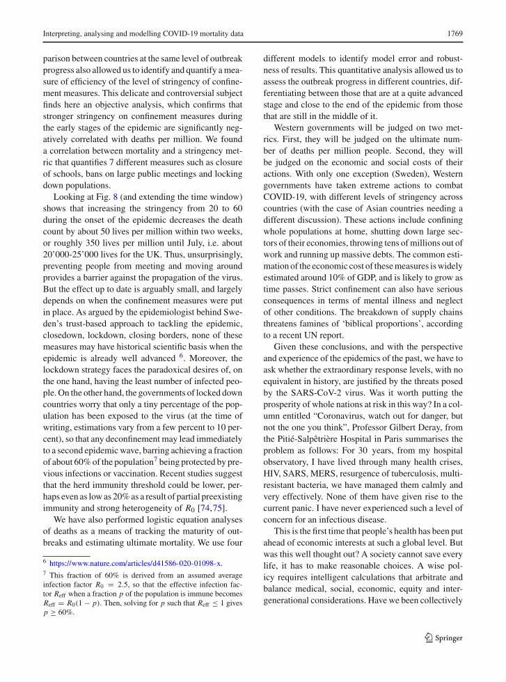
As an example, Fig. 12 shows exponential decayrates for Belgium and Portugal. For Belgium, we find asignificant increase in γ , indicating a decrease in infec-tivity around the time lockdown policies were imple-mented. For Portugal, in comparison10, we first note asubstantially larger initial rate of decay, which couldbe due to increased awareness and voluntary social

9 Contrary to the analysis in [79], which looks at linear fits tothe growth rate, we find that it is essential to consider log-growthrates to be able to draw conclusions.10 For cross-country comparison it is not sufficient to considerexponential decay rates alone, but in combination with the inter-cept a of the respective fits as given by 7.

123


Fig. 12 Daily growth rate of mortality in Belgium and Portugal (log scale) and linear fits according to 7. The solid and dashed linesindicate the date where increasing levels of stringency were reached, shifted by 20 days (average time lag of infection to death)

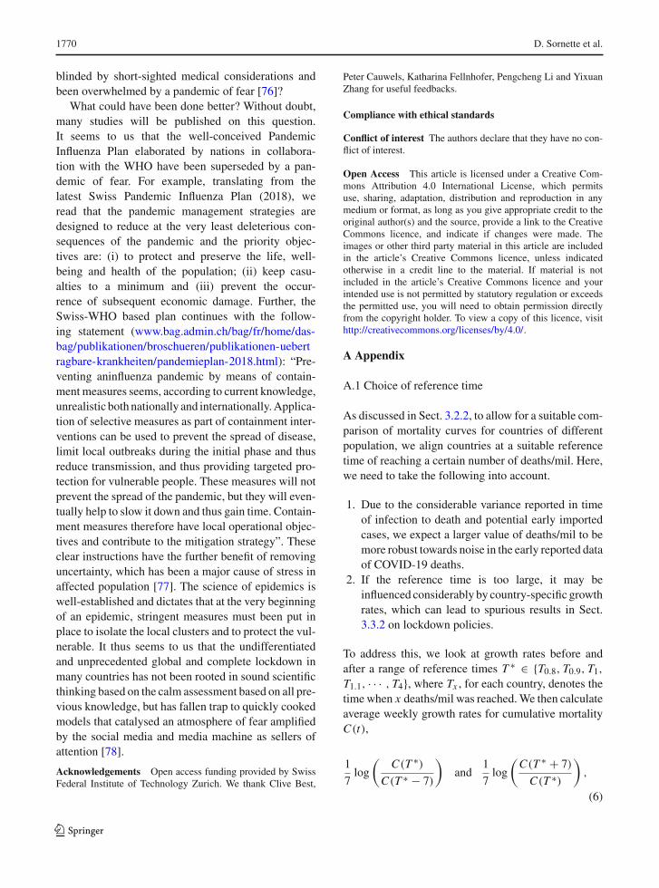
distancing, efficiency of early intervention measuresor other country-specific factors. Moreover, we see adecrease of the decay parameter at t∗, which one wouldexpect to see from the evolution of an epidemic withconstant infectivity (as predicted by a standard SIRmodel), andwecannot deduce that additional lockdownmeasures were particularly effective. Figure 13 showsthe result of this analysis for the countries analysed inSect. 3.3.2.Wenote that amajority of countries showan

increasing or approximately constant rate of exponen-tial decay γ around the time of lockdown (lower rightcorner of the figure), indicating a decrease in infectiv-ity. Plots for individual countries can be found in thesupplements. This analysiswould benefit fromdata col-lected with actual date of death, see section A.3.

123


Fig. 13 Exponential decayparameters γ in (7) beforeand after t∗ defined in (8).The solid line indicates aconstant rate of decay

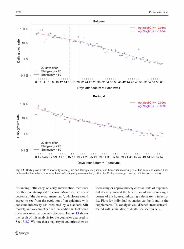
Fig. 14 Reported versusactual mortality in Belgium.Cumulative mortality C(t)shows a reporting delay ofaround 3 days (left) andsignificant reduction innoise of the daily loggrowth ratelog (log (C(t + 1)/C(t)))(right)

A.3 Reporting delay and additional noise in dailyreported data.

The extensive data base of Johns Hopkins Universitycollects mortality data as reported by governments andhealth agencies worldwide. In most cases, death fromCOVID-19 gets reported with several days delay, andthis reporting introduces additional noise to the data. InFig. 14, we show cumulative mortality and its growthrate in the first two months of the epidemic in Belgium,using both reported data from JHU [37] as well as dailyupdate data sorted by actual date of death from pressconferences and reports of Belgian officials [80]. We

note a significant delay of roughly 3days in the report-ing of deaths, as well as a significant reduction of noisein the data, even after accounting for weekly season-ality in both time series. Availability of this data fora wide range of countries would significantly improvemodelling and statistical analysis, for example, detect-ing change points in the log growth rate of Fig. 12 toconfirm the choice of partition at t∗ in (8).

123


References

1. Andersen, K.G., Rambaut, A., Lipkin, W.I., Holmes, E.C.,Garry, R.F.: The proximal origin of SARS-CoV-2. Nat.Med.26(4), 450 (2020)

2. Walls, A.C., Park, Y.J., Tortorici, M.A., Wall, A., McGuire,A.T., Veesler, D.: Structure, function, and antigenicity of theSARS-CoV-2 spike glycoprotein. Cell 181(2), 281 (2020)

3. Coutard, B., Valle, C., de Lamballerie, X., Canard, B., Sei-dah, N., Decroly, E.: The spike glycoprotein of the new coro-navirus 2019-nCoVcontains a furin-like cleavage site absentin CoV of the same clade. Antivir. Res. 176, 104742 (2020)

4. U.S. Centers for Disease Control and Prevention(CDC). Symptoms of coronavirus. https://www.cdc.gov/coronavirus/2019-ncov/symptoms-testing/symptoms.html (2020)

5. Guo, Y.R., Cao, Q.D., Hong, Z.S., Tan, Y.Y., Chen, S.D.,Jin, H.J., Tan, K.S., Wang, D.Y., Yan, Y.: The origin, trans-mission and clinical therapies on coronavirus disease 2019(COVID-19) outbreak-an update on the status. Mil. Med.Res. 7(1), 1 (2020)

6. Wang, D., Hu, B., Hu, C., Zhu, F., Liu, X., Zhang, J.,Wang, B., Xiang, H., Cheng, Z., Xiong, Y., et al.: Clinicalcharacteristics of 138 hospitalized patients with 2019 novelcoronavirus-infected pneumonia in Wuhan, China. JAMA323(11), 1061 (2020)

7. Guan, W.J., Ni, Z.Y., Hu, Y., Liang, W.H., Ou, C.G., He,J.X., Liu, L., Shan, H., Lei, C.l., Hui, D.S., et al.: Clini-cal characteristics of coronavirus disease 2019 in China. N.Engl. J. Med. 382, 1708 (2020)

8. European Centre for Disease Prevention and Con-trol (ECDC). Coronavirus disease 2019 (COVID-19) in the EU/EEA and the UK - ninth update.https://www.ecdc.europa.eu/en/publications-data/rapid-risk-assessment-coronavirus-disease-2019-covid-19-pandemic-ninth-update(23 Apr 2020)

9. Gagnon,A.,Miller,M.S., Hallman, S.A., Bourbeau, R., Her-ring, D.A., Earn, D.J., Madrenas, J.: Age-specific mortalityduring the 1918 influenza pandemic: unravelling the mys-tery of high young adult mortality. PLoS One 8(8), e69586(2013)

10. Viboud, C., Simonsen, L., Fuentes, R., Flores, J., Miller,M.A., Chowell, G.: Global mortality impact of the 1957–1959 influenza pandemic. J. Infect. Dis. 213(5), 738 (2016)

11. Lee, P.I., Hu, Y.L., Chen, P.Y., Huang, Y.C., Hsueh, P.R.:Are children less susceptible to COVID-19? J. Microbiol.Immunol. Infect. 53(3), 371 (2020)

12. Rothe, C., Schunk, M., Sothmann, P., Bretzel, G., Froeschl,G., Wallrauch, C., Zimmer, T., Thiel, V., Janke, C., Gugge-mos, W., et al.: Transmission of 2019-nCoV infection froman asymptomatic contact in Germany. N. Engl. J. Med.382(10), 970 (2020)

13. Zou,L.,Ruan, F.,Huang,M., Liang,L.,Huang,H.,Hong,Z.,Yu, J., Kang, M., Song, Y., Xia, J., et al.: SARS-CoV-2 viralload in upper respiratory specimens of infected patients. N.Engl. J. Med. 382(12), 1177 (2020)

14. Wei, W.E., Li, Z., Chiew, C.J., Yong, S.E., Toh, M.P.,Lee, V.J.: Presymptomatic Transmission of SARS-CoV-2-Singapore, January 23-March 16, 2020.Morbidity andMor-tality Weekly Report 69(14), 411 (2020)

15. Aguilar, J.B., Faust, J.S., Westafer, L.M., Gutierrez, J.B.:Investigating the Impact of Asymptomatic Carriers onCOVID-19 Transmission. medRxiv preprint (2020). https://doi.org/10.1101/2020.03.18.20037994. URL https://www.medrxiv.org/content/early/2020/03/31/2020.03.18.20037994

16. Hu, Z., Song, C., Xu, C., Jin, G., Chen, Y., Xu, X., Ma,H., Chen, W., Lin, Y., Zheng, Y., et al.: Clinical characteris-tics of 24 asymptomatic infectionswithCOVID-19 screenedamong close contacts in Nanjing, China. Sci. China Life Sci.63, 1–6 (2020)

17. Wu, J.T., Leung, K., Bushman, M., Kishore, N., Niehus,R., de Salazar, P.M., Cowling, B.J., Lipsitch, M., Leung,G.M.: Estimating clinical severity of COVID-19 from thetransmission dynamics in Wuhan, China. Nat. Med. 26, 1–5(2020)

18. Lauer, S.A., Grantz, K.H., Bi, Q., Jones, F.K., Zheng, Q.,Meredith, H.R., Azman, A.S., Reich, N.G., Lessler, J.: Theincubation period of coronavirus disease 2019 (COVID-19) from publicly reported confirmed cases: estimation andapplication. Ann. Internal Med. 172, 577–582 (2020)

19. Lai, C.C., Shih, T.P., Ko, W.C., Tang, H.J., Hsueh, P.R.:Severe acute respiratory syndrome coronavirus 2 (SARS-CoV-2) and corona virus disease-2019 (COVID-19): the epi-demic and the challenges. Int. J. Antimicrob. Agents 55(3),105924 (2020)

20. Stadler, B.: Coronavirus:Why everyonewaswrong. Englishtranslation from the Swiss magazine Weltwoche (WorldWeek) on June 10th (2020)

21. World Health Organization (WHO). Report ofthe WHO-China joint mission on coronavirusdisease 2019 (COVID-19). https://www.who.int/docs/default-source/coronaviruse/who-china-joint-mission-on-covid-19-final-report.pdf (2020)

22. Varga, Z., Flammer,A.J., Steiger, P., Haberecker,M., Ander-matt, R., Zinkernagel, A.S., Mehra, M.R., Schuepbach,R.A., Ruschitzka, F., Moch, H.: Endothelial cell infectionand endotheliitis in COVID-19. Lancet 395, 1417–1418(2020)

23. Zhou, F., Yu, T., Du, R., Fan, G., Liu, Y., Liu, Z., Xiang,J.: Clinical course and risk factors for mortality of adultinpatients with COVID-19 inWuhan, China: a retrospectivecohort study. Lancet 295, 1054 (2020)

24. Young, B.E., Ong, S.W.X., Kalimuddin, S., Low, J.G., Tan,S.Y., Loh, J., Ng, O.T., Marimuthu, K., Ang, L.W., Mak,T.M., et al.: Epidemiologic features and clinical course ofpatients infected with SARS-CoV-2 in Singapore. JAMA323, 1054–1062 (2020)

25. Coburn, B.J., Wagner, B.G., Blower, S.: Modeling influenzaepidemics and pandemics: insights into the future of swineflu (H1N1). BMC Med. 7(1), 30 (2009)

26. Biggerstaff, M., Cauchemez, S., Reed, C., Gambhir, M.,Finelli, L.: Estimates of the reproduction number for sea-sonal, pandemic, and zoonotic influenza: a systematicreview of the literature. BMC Infect. Dis. 14(1), 480 (2014)

27. Liu, Y., Gayle, A.A., Wilder-Smith, A., Rocklöv, J.: Thereproductive number of COVID-19 is higher compared toSARS coronavirus. J. Travel Med. 27(2), 1 (2020)

28. Park, M., Cook, A.R., Lim, J.T., Sun, Y., Dickens, B.L.:A systematic review of COVID-19 epidemiology based oncurrent evidence. J. Clin. Med. 9(4), 967 (2020)

123

https://www.cdc.gov/coronavirus/2019-ncov/symptoms-testing/symptoms.html



https://www.ecdc.europa.eu/en/publications-data/rapid-risk-assessment-coronavirus-disease-2019-covid-19-pandemic-ninth-update



https://doi.org/10.1101/2020.03.18.20037994

https://doi.org/10.1101/2020.03.18.20037994

https://www.medrxiv.org/content/early/2020/03/31/2020.03.18.20037994



https://www.who.int/docs/default-source/coronaviruse/who-china-joint-mission-on-covid-19-final-report.pdf




29. Sanche, S., Lin, Y., Xu, C., Romero-Severson, E., Hengart-ner, N., Ke, R.: High contagiousness and rapid spread ofsevere acute respiratory syndrome coronavirus 2. Emerg.Infect. Dis. 26(7), 1470 (2020)

30. World Health Organization (WHO). International guide-lines for certification and classification (coding) of covid-19as cause of death. https://www.who.int/classifications/icd/Guidelines_Cause_of_Death_COVID-19.pdf (2020)

31. Wu, J., McCann, A., Katz, J., Peltier, E.: 36,000missing deaths: Tracking the true toll of the coro-navirus crisis. https://www.nytimes.com/interactive/2020/04/21/world/coronavirus-missing-deaths.html (2020)

32. Economist. Tracking covid-19 excess deaths across coun-tries. https://www.economist.com/graphic-detail/2020/04/16/tracking-covid-19-excess-deaths-across-countries(2020)

33. Financial Times. Tracking covid-19 excess deathsacross countries. https://www.ft.com/content/a26fbf7e-48f8-11ea-aeb3-955839e06441 (2020)

34. Tsang, T.K., Wu, P., Lin, Y., Lau, E.H.Y., Leung, G.M.L.,Cowling, B.J.: Effect of changing case definitions forCOVID-19 on the epidemic curve and transmission param-eters in mainland China: a modelling study. Lancet PublicHealth 5(5), 289 (2020)

35. Streeck, H., Schulte, B., Kuemmerer, B., Richter, E.,Hoeller, T., Fuhrmann, C., Bartok, E., Dolscheid, R., Berger,M., Wessendorf, L., Eschbach-Bludau, M., Kellings, A.,Schwaiger, A., Coenen,M., Hoffmann, P., Noethen,M., Eis-Huebinger, A.M., Exner, M., Schmithausen, R., Schmid,M., Hartmann, G.: Infection fatality rate of SARS-CoV-2infection in a German community with a super-spreadingevent. medRxiv preprint https://doi.org/10.1101/2020.05.04.20090076 (2020)

36. Bendavid, E., Mulaney, B., Sood, N., Shah, S., Ling, E.,Bromley-Dulfano, R., Lai, C., Weissberg, Z., Saavedra, R.,Tedrow, J., et al.: COVID-19 Antibody Seroprevalence inSanta Clara County, California. medRxiv preprint, https://doi.org/10.1101/2020.04.14.20062463 (2020)

37. Johns Hopkins University Center for Systems Scienceand Engineering (JHU CSSE). 2019 novel coronaviruscovid-19 (2019-ncov) data repository. https://github.com/CSSEGISandData/COVID-19/tree/master/csse_covid_19_data (2020)

38. Neher, R.A., Dyrdak, R., Druelle, V., Hodcroft, E.B., Albert,J.: Potential impact of seasonal forcing on a SARS-CoV-2 pandemic., medRxiv preprint, https://doi.org/10.1101/2020.02.13.20022806 (2020)

39. Chowell, G., Mizumoto, K.: The COVID-19 pandemic inthe USA: what might we expect? Lancet 395(10230), 1093–1094 (2020)

40. Verity, R., Okell, L.C., Dorigatti, I., Winskill, P., Whittaker,C., Ferguson, N.M.: Estimates of the severity of coronavirusdisease 2019: amodel-based analysis. Lancet Infect. Dis. 20,669 (2020)

41. The World Bank. Life expectancy at birth, total (years).https://data.worldbank.org/indicator/SP.DYN.LE00.IN

42. Prem, K., Liu, Y., Russell, T.W., Kucharski, A.J., Eggo,R.M., Davies, N., Flasche, S., Clifford, S., Pearson, C.A.,Munday, J.D., et al.: The effect of control strategies to reducesocial mixing on outcomes of the COVID-19 epidemic in

Wuhan,China: amodelling study.Lancet PublicHealth 5(5),261 (2020)

43. Flaxman, S.,Mishra, S., Gandy, A., N. Ferguson, S.B. et. al.:Estimating the number of infections and the impact of non-pharmaceutical interventions on COVID-19 in 11 Europeancountries. Published online: https://doi.org/10.25561/77731(2020)

44. Dehning, J., Zierenberg, J., Spitzner, F.P., WIbral, M., Neto,J.P., Wilczek, M., Priesmann, V.: Inferring change points inthe spread of COVID-19 reveals the effecitveness of inter-ventions. Science 369(6500) (2020)

45. Banholzer, N., van Weenen, E., Kratzwald, B., Seel-iger, A., Tschernutter, D., Bottrighi, P., Cenedese, A.,Salles, J.P., Vach, W., Feuerriegel, S.: Impact of non-pharmaceutical interventions on documented cases ofCOVID-19. medRxiv preprint, https://doi.org/10.1101/2020.04.16.20062141. (2020)

46. Hale, T., Petherick, A., Phillips, T., Webster, S.:Oxford COVID-19 Government Response Tracker,Blavatnik School of Government. Online data set,https://www.bsg.ox.ac.uk/research/research-projects/coronavirus-government-response-tracker (2020)

47. Sanche, S., Lin, Y.T., Xu, C., Romero-Severson, E., Hen-gartner, N., Ke, R.: High contagiousness and rapid spreadof severe acute respiratory syndrome coronavirus 2. Emerg.Infect. Dis. 26(7), 1470 (2020)

48. Linton, N.M., Kobayashi, T., Yang, Y., et al.: Incubationperiod and other epidemiological characteristics of 2019novel coronavirus infections with right truncation: a statis-tical analysis of publicly available case data. J. Clin. Med.9(2), 538 (2020)

49. Gardner,W., States, D., Bagley, N.: The corona virus and therisks to the elderly in long-term care. J. Aging Soc. Policy32(4–5), 310 (2020)

50. Comas-Herrera, A., Zalakain, J., C.L. C, A. Hsu, J.L.Fernandez-Plotka, Mortality associated with COVID-19outbreaks in care homes: early international evidence(accessed: 21 April). https://ltccovid.org/2020/04/12/mortality-associated-with-covid-19-outbreaks-in-care-homes-early-international-evidence/ (2020)

51. De Maeseneer, J., De Prins, L., Heyerick, J.: Home visits inBelgium: a multivariate analysis. Eur. J. Gen. Pr. 5(1), 11(1999)

52. Salman, R., Busse, R., Mossialos, E.: editors, Regulatingentrepreneurial behaviour in European health care systems.The European Journal of General Practice, Buckingham,Philadelphia, World Health Organisation (2002)

53. Richardson, S., Hirsch, J., Narasimhan,M., et al.: PresentingCharacteristics, Comorbidities, and Outcomes Among 5700Patients HospitalizedWith COVID-19 in the NewYork CityArea. JAMA. Published online April 22. https://doi.org/10.1001/jama.2020.6775 (2020)

54. Brurberg, A.F.K.: COVID-19: The Relationship BetweenAge, Comorbidity and Disease Severity—A Rapid Review.Norwegian Institute of Public Health, Oslo (2020)

55. EpiCentro - Istituto Superiore di Sanità. Characteristicsof SARS-CoV-2 patients dying in Italy Report based onavailable data on April 20th. https://www.epicentro.iss.it/en/coronavirus/bollettino/Report-COVID-2019_20_april_2020.pdf (2020)

123

https://www.who.int/classifications/icd/Guidelines_Cause_of_Death_COVID-19.pdf

https://www.who.int/classifications/icd/Guidelines_Cause_of_Death_COVID-19.pdf

https://www.nytimes.com/interactive/2020/04/21/world/coronavirus-missing-deaths.html

https://www.nytimes.com/interactive/2020/04/21/world/coronavirus-missing-deaths.html

https://www.economist.com/graphic-detail/2020/04/16/tracking-covid-19-excess-deaths-across-countries

https://www.economist.com/graphic-detail/2020/04/16/tracking-covid-19-excess-deaths-across-countries

https://www.ft.com/content/a26fbf7e-48f8-11ea-aeb3-955839e06441

https://www.ft.com/content/a26fbf7e-48f8-11ea-aeb3-955839e06441

https://doi.org/10.1101/2020.05.04.20090076

https://doi.org/10.1101/2020.05.04.20090076

https://doi.org/10.1101/2020.04.14.20062463

https://doi.org/10.1101/2020.04.14.20062463

https://github.com/CSSEGISandData/COVID-19/tree/master/csse_covid_19_data



https://doi.org/10.1101/2020.02.13.20022806

https://doi.org/10.1101/2020.02.13.20022806

https://data.worldbank.org/indicator/SP.DYN.LE00.IN

https://doi.org/10.25561/77731

https://doi.org/10.1101/2020.04.16.20062141

https://doi.org/10.1101/2020.04.16.20062141

https://www.bsg.ox.ac.uk/research/research-projects/coronavirus-government-response-tracker

https://www.bsg.ox.ac.uk/research/research-projects/coronavirus-government-response-tracker

https://ltccovid.org/2020/04/12/mortality-associated-with-covid-19-outbreaks-in-care-homes-early-international-evidence/



https://doi.org/10.1001/jama.2020.6775

https://doi.org/10.1001/jama.2020.6775

https://www.epicentro.iss.it/en/coronavirus/bollettino/Report-COVID-2019_20_april_2020.pdf




56. Simonnnet, A., Chetbourn, M., Pattou, F., Jourdain, M.,et al.: High prevalence of obesity in severe acute respiratorysyndrome coronavirus-2 (SARS-CoV-2) requiring invasivemechanical ventilation. Obesity (2020). https://doi.org/10.1002/oby.22831

57. Dietz, W., Santos-Burgoa, C.: Obesity and its Implicationsfor COVID-19Mortality. Obesity (2020). https://doi.org/10.1002/oby.22818

58. Qingxian, C., Fengjuan, C., Fang, L., Xiaohui, L., Tao, W.,Qikai, W., Qing, H., Zhaoqin,W., Yingxia, L., Jun, C., et al.:Obesity and COVID-19 severity in a designated hospitalin Shenzhen, China. Available at SSRN: https://ssrn.com/abstract=3556658 (2020)

59. Lighter, J., Phillips, M., Hochman, S., Sterling, S., Johnson,D., Francois, F., Stachel, A.: Obesity in patients youngerthan 60 years is a risk factor for Covid-19 hospital admis-sion. Clinical Infectious Diseases, ciaa415, https://doi.org/10.1093/cid/ciaa415 (2020)

60. Williamson, E.J., Walker, A.J., Bhaskaran, K., et al.: Open-SAFELY: factors associated with COVID-19 death in 17million patients. Nature (2020). https://doi.org/10.1038/s41586-020-2521-4(2020)

61. Guan, Wj, et al.: Clinical characteristics of coronavirus dis-ease 2019 in China. N. Engl. J. Med. 382, 1708 (2020)

62. Changeux, J.P., Amoura, Z., Rey, F.,Miyara,M.: A nicotinichypothesis for Covid-19 with preventive and therapeuticimplications - Preprint v1. Qeios, https://www.qeios.com/read/article/571 (2020)

63. Vardavas, C.I., Nikitara, K.: COVID-19 and smoking: a sys-tematic review of the evidence. Tob. Induc. Dis. 18, 20(2020)

64. Shet, A., Ray, D., Malavige, N., Santosham, M., Bar-Zeev,N.: Differential COVID-19-attributable mortality and BCGvaccine use in countries. medRxiv preprint, https://doi.org/10.1101/2020.04.01.20049478 (2020)

65. Berg, M., Yu, Q., et al.: Mandated Bacillus Calmette-Guérin(BCG) vaccination predicts flattened curves for the spreadof COVID-19. medRxiv preprint, https://doi.org/10.1101/2020.04.05.20054163 (2020)

66. Kirov, S.: Association Between BCG Policy is SignificantlyConfounded by Age and is Unlikely to Alter Infection orMortality Rates. medRxiv preprint, https://doi.org/10.1101/2020.04.06.20055616 (2020)

67. Szigeti, R., Kellermayer, D., Kellermayer, R.: BCG protectsagainst COVID-19? A word of caution. medRxiv preprint,https://doi.org/10.1101/2020.04.09.20056903. (2020)

68. Soliman, R., Brassey, J., Plüddemann, A., Heneghan,C.: Does BCG vaccination protect against acute res-piratory infections and COVID-19? A rapid reviewof current evidence. https://www.cebm.net/covid-19/does-bcg-vaccination-protect-against-acute-respiratory-infections-and-covid-19-a-rapid-review-of-current-evidence(2020)

69. Sornette, D.: Predictability of catastrophic events: mate-rial rupture, earthquakes, turbulence, financial crashes andhuman birth. Proc. Natl. Acad. Sci. USA 99(Suppl. 1), 2522(2002)

70. Sornette, D.: Critical Phenomena in Natural Sciences, vol.2. Springer Series in Synergetics, Heidelberg (2004)

71. Israeli, N., Goldenfeld, N.: Computational irreducibility andthe predictability of complex physical systems. Phys. Rev.Lett. 92, 074105 (2004)

72. Wu, K., Darcet, D., Wang, Q., Sornette, D.: Generalizedlogistic growth modeling of the COVID-19 outbreak in 29provinces inChina and in the rest of theworld. arXiv preprintarXiv:2003.05681 (2020)

73. Chair of Entreprenerial Risks ETH Zurich. Covid-19 con-firmed cases and cumulative mortality predictions. https://er.ethz.ch/Covid-19/Dailyforecasts.html (2020)

74. Gomes, G., Corder, R., King, J., Langwig, K., Souto-Maior,C., Carneiro, J., Goncalves, G., Penha-Goncalves, C., Fer-reira, M., Aguas, R.: Individual variation in susceptibility orexposure to SARS-CoV-2 lowers the herd immunity thresh-old. medRxiv preprint, https://doi.org/10.1101/2020.04.27.20081893 (2020)

75. Brennan, P., Brennan, L.: Susceptibility-adjusted herdimmunity threshold model and potential R0 distri-bution fitting the observed Covid-19 data in Stock-holm. medRxiv preprint, https://doi.org/10.1101/2020.05.19.20104596 (2020)

76. Miles, D., Stedman, M., Heald, A.: Living with COVID-19: balancing costs against benefits in the face of the virus.forthcoming in the National Institute Economic Review,August (available at http://www.imperial.ac.uk/people/d.miles (2020)

77. Pellegrino, G., Ravenna, F., Züllig, G.: The effects ofCOVID-19-Induced Uncertainty in the Euro Area: The RoleofPessimisms.CEPRCovidEconomics, 18:2020https://bit.ly/3dUHYcP (2020)

78. Wu, T.: TheAttentionMerchants, Borzoi Book published byA.A. Knopf, a division of Penguin Random House (2016)

79. Meunier, T.A.J.: Full lockdown policies in Western Europecountries have no evident impacts on the COVID-19 epi-demic. medRxiv preprint, https://doi.org/10.1101/2020.04.24.20078717 (2020)

80. Sciensano. Daily updates of belgian health authorities.https://covid-19.sciensano.be/nl/covid-19-epidemiologische-situatie (2020)

Publisher’s Note Springer Nature remains neutral with regardto jurisdictional claims in published maps and institutional affil-iations.

123

https://doi.org/10.1002/oby.22831






https://doi.org/10.1093/cid/ciaa415

https://doi.org/10.1093/cid/ciaa415

https://doi.org/10.1038/s41586-020-2521-4(2020)

https://doi.org/10.1038/s41586-020-2521-4(2020)

https://www.qeios.com/read/article/571

https://www.qeios.com/read/article/571

https://doi.org/10.1101/2020.04.01.20049478

https://doi.org/10.1101/2020.04.01.20049478

https://doi.org/10.1101/2020.04.05.20054163

https://doi.org/10.1101/2020.04.05.20054163

https://doi.org/10.1101/2020.04.06.20055616

https://doi.org/10.1101/2020.04.06.20055616

https://doi.org/10.1101/2020.04.09.20056903

https://www.cebm.net/covid-19/does-bcg-vaccination-protect-against-acute-respiratory-infections-and-covid-19-a-rapid-review-of-current-evidence



http://arxiv.org/abs/2003.05681

https://er.ethz.ch/Covid-19/Dailyforecasts.html

https://er.ethz.ch/Covid-19/Dailyforecasts.html

https://doi.org/10.1101/2020.04.27.20081893

https://doi.org/10.1101/2020.04.27.20081893

https://doi.org/10.1101/2020.05.19.20104596

https://doi.org/10.1101/2020.05.19.20104596

http://www.imperial.ac.uk/people/d.miles

http://www.imperial.ac.uk/people/d.miles

https://bit.ly/3dUHYcP

https://bit.ly/3dUHYcP

https://doi.org/10.1101/2020.04.24.20078717

https://doi.org/10.1101/2020.04.24.20078717

https://covid-19.sciensano.be/nl/covid-19-epidemiologische-situatie

https://covid-19.sciensano.be/nl/covid-19-epidemiologische-situatie

Interpreting, analysing and modelling COVID-19 mortality data

Documents