Interpretation of the self-potential anomaly over a 2D inclined plate using a moving average window curves method

Special Section

Assessing uncertainty in geophysical problems — Introduction

Aime Fournier1, Klaus Mosegaard2, Henning Omre3, Malcolm Sambridge4, and Luis Tenorio5

Uncertainty is an important component of all geophysical studies,which is ever present but often ignored. There is uncertainty at everystage in geophysical applications: from errors and biases in themeasurements, through the models and methods that connect thephysics to the data, to the final decision-making based on estimatedparameters. In some cases the meaning of uncertainty is itselfuncertain.Uncertainty quantification (UQ) has many important applications

and is now becoming an essential component of geosciences.Methods for uncertainty quantification play an important role in,for example, propagating errors of input parameters in geophysicalsimulations and forward calculations, determining uncertaintiesof inversion results, in risk assessment, and in decision andpolicymaking.The objective of this special GEOPHYSICS section is to expose a

wide audience to current developments in UQ in applications re-lated to: (1) uncertainty quantification in diverse geophysical appli-cations; (2) visualization of uncertainty in complex multiparameterproblems; (3) interpretation of uncertainty estimates in complex in-verse problems; (4) quantitative risk analysis; (5) elicitation of priordistributions for different types of geophysical information; (6)uncertainty quantification in nonlinear and high dimensional prob-lems, and (7) uncertainty estimation via optimization or samplingbased approaches.We are excited to report that many excellent papers were submitted

concerning various aspects of uncertainty. We hope that this specialsection will serve as a comprehensive contemporary overview of thelongstanding effort to assess uncertainty in geophysical problems.Biswas and Sharma report an interpretation study of self-

potential anomaly over a 2D inclined structure using very fast

simulated-annealing global optimization. A bimodel ambiguityhas been observed in the interpretation for a sheet–type structureand an appropriate procedure is demonstrated to find the actual sub-surface structure.Coles et al. explore DN-optimization, a recently introduced

method in optimal experimental design theory, as a tool to minimizethe forecasted postinversion model uncertainty in marine boreholeseismic applications. TheDN-criterion is a design objective functioncrafted specifically for nonlinear data-model relationships and,when used in conjunction with greedy, sequential optimizationalgorithms, is among the first of its kind to be computationallyefficient enough for industrial-scale applications.Majdański describes an analytical estimation of errors in layered

models based on wide-angle seismic traveltimes and their propaga-tion during the inversion. Comparing the final uncertainties for bothstrategies the author suggests using a multiparameter simultaneousinversion in place of a typical layer-stripping approach.Molnar et al. examine the uncertainty in predicted linear 1D site

amplification due to uncertainty in shear-wave velocity (VS) struc-ture quantified from Bayesian (probabilistic) inversion of microtre-mor array dispersion data. Determination of the VS-depth profilemarginal probability distribution indicates which portions of theresulting VS-depth profiles are most reliable for accurate siteresponse prediction.Young et al. present a novel method of uncertainty analysis us-

ing a two-stage hierarchal, transdimensional, Bayesian tomographicinversion scheme that allows the number and distribution of modelparameters to be implicitly controlled by the data and the data noiseto be treated as an unknown. The method is applied to ambient seis-mic noise data recorded in southeast Australia, and the resulting 3D

Published online 22 May 2013.1Schlumberger, Houston, Texas, USA. E-mail: [email protected] University of Denmark, Kogens Lyngby, Denmark. E-mail: [email protected] University of Science and Technology, Department of Mathematical Sciences, Trondheim, Norway. E-mail: [email protected] National University, Canberra, Australia. E-mail: [email protected] School of Mines, Applied Mathematics and Statistics, Golden, Colorado, USA. E-mail: [email protected].

© 2013 Society of Exploration Geophysicists. All rights reserved.

WB1

GEOPHYSICS, VOL. 78, NO. 3 (MAY-JUNE 2013); P. WB1–WB2.10.1190/GEO2013-0425-SPSEIN.1

Dow

nloa

ded

05/2

9/13

to 2

03.1

10.2

46.2

2. R

edis

trib

utio

n su

bjec

t to

SEG

lice

nse

or c

opyr

ight

; see

Ter

ms

of U

se a

t http

://lib

rary

.seg

.org

/

shear velocity model has strong geophysical implications for thecurrent debate concerning the tectonic history of Tasmania andits relationship with mainland Australia.Dettmer et al. apply probabilistic inversion using a transdimen-

sional hierarchical model to ocean-acoustic reflection measurementsto recover shallow sediment structure including sound-velocitydispersion, frequency-dependent attenuation, and their uncertain-ties. Results at two sites indicate dispersive sediments at somedepths where the variability of velocity and attenuation as a functionof frequency clearly exceeds the estimated uncertainties.By computing and ranking contributions of uncertain reservoir

parameters to the predicted variance of the measurements, Chugu-nov et al. apply global sensitivity analysis (GSA) to quantitativelylink uncertainty in crosswell seismic monitoring and neutron-capture logging to the underlying reservoir variability. CalculatedGSA indices are shown to provide a quantitative basis for the mon-itoring program design in a CO2 storage project.Reading and Gallagher give an illustration of how the outputs

of a transdimensional Bayesian Markov chain Monte Carlo infer-

ence procedure can be used to quantify uncertainty in geophysicalborehole logs. The modeled changepoints, borehole log parameters,and the variance of the noise distribution of each log are comparedwith the observed lithology classes down the borehole to make anappraisal of the uncertainty due to different components of variationin the observed data (geologic process, geologic noise, andanalytic noise).Wessling et al. provide an in-depth investigation of uncertainty

associated with manual steps in a pore pressure modeling approachand provides a means to quantify uncertainty from estimatingtrendline envelopes from porosity-indicating logs. The presentedapproach is beneficial for a more reliable determination of the pres-sure window for safe drilling operations.Cracknell and Reading provide a practical example of the “up-

side” of uncertainty in identifying zones of geologic interest fromremote sensing data. Uncertainty is calculated from class member-ship probabilities output in conjunction with categorical predictionsgenerated by two inductive machine leaning algorithms using air-borne geophysics and satellite data.

WB2 Assessing uncertainty in geophysical problems — Introduction

Dow

nloa

ded

05/2

9/13

to 2

03.1

10.2

46.2

2. R

edis

trib

utio

n su

bjec

t to

SEG

lice

nse

or c

opyr

ight

; see

Ter

ms

of U

se a

t http

://lib

rary

.seg

.org

/

Interpretation of self-potential anomaly over a 2D inclined structureusing very fast simulated-annealing global optimization — An insightabout ambiguity

Shashi Prakash Sharma1 and Arkoprovo Biswas1

ABSTRACT

A very fast simulated-annealing (VFSA) global optimizationprocedure is developed for the interpretation of self-potential(SP) anomaly measured over a 2D inclined sheet-type structure.Model parameters such as electric current dipole density (k),horizontal and vertical locations of the center of the causativebody (x0 and h), half-width (a), and polarization/inclinationangle (α) of the sheet are optimized. VFSA optimizationyields a large number of well-fitting solutions in a vast modelspace. Even though the assumed model space (minimum andmaximum limits for each model parameter) is appropriate, ithas been observed that models obtained by the VFSA processin the predefined model space could also be geologically

erroneous. This offers new insight into the interpretation of self-potential data. Our optimization results indicate that there existat least two sets of solutions that can fit the observed dataequally well. The first set of solutions represents a local opti-mum and is geologically inappropriate. The second set of solu-tions represents the actual subsurface structure. The mean modelestimated from the latter models represents the global solution.The efficacy of the developed approach has been demonstratedusing various synthetic examples. Field data from the Surda areaof Rakha Mines, India and the Bavarian woods, Germany arealso interpreted. The computation time for finding this versatilesolution is very short (52 s on a simple PC) and the proposedapproach is found to be more advantageous than otherapproaches.

INTRODUCTION

The self-potential (SP) method deals with the measurement of theelectrical potential that develops on the earth’s surface due to flowof the natural electrical current on the subsurface. Natural currentflows mainly in the vicinity of massive sulfide or graphite bodiesdue to electrochemical activity. A large negative SP anomaly isusually observed in the vicinity of mineralization. Some potentialanomaly of small magnitude (negative and positive) also developson the earth’s surface due to electrokinetic flow, temperature andpressure gradient, bioelectrical activity, etc. (Telford et al., 1990).The SP method is routinely used for the investigation of sulfideand graphite bodies (Sundararajan et al., 1998; Mendonca, 2008;Ramazi et al., 2009). Apart from the conventional mineral explora-tion work, the SP method is also used for groundwater investigation(Monteiro Santos et al., 2002), geothermal investigation (Corwinand Hoover, 1979; Fitterman and Corwin, 1982), seepage detection

(Panthulu et al., 2001), and cavity detection (Vichabian andMorgan, 2002).Interpretation of data is a very important and crucial step in geo-

physical exploration. Accurate and unambiguous interpretation ofSP anomalies is equally important. Therefore, development and im-provement in interpretation techniques for SP data are essential.Several approaches have been developed in the past for the inter-pretation of SP anomaly using analytical expressions for simplegeometrical structures (sphere, cylinder, and sheet). Mathematicalexpressions used for the modeling and inversion of SP anomaliesare similar to the expressions used in gravity prospecting, assumingthe body is of simple geometrical shape (El-Araby, 2004; El-Kaliouby and Al-Garni, 2009). Initial interpretation approachesdeal with characteristic points (Paul, 1965; Paul et al., 1965;Rao et al., 1970), logarithmic-curve matching (Meiser, 1962;Murthy and Haricharan, 1984) and nomograms (Murthy and Har-icharan, 1985). Sundararajan et al. (1990) proposed the Hilbert

Manuscript received by the Editor 21 June 2012; revised manuscript received 22 February 2013; published online 22 May 2013.1IIT Kharagpur, Department of Geology and Geophysics, India. E-mail: [email protected]; [email protected].

© 2013 Society of Exploration Geophysicists. All rights reserved.

WB3

GEOPHYSICS, VOL. 78, NO. 3 (MAY-JUNE 2013); P. WB3–WB15, 14 FIGS., 6 TABLES.10.1190/GEO2012-0233.1

Dow

nloa

ded

05/2

7/13

to 2

03.1

10.2

46.2

2. R

edis

trib

utio

n su

bjec

t to

SEG

lice

nse

or c

opyr

ight

; see

Ter

ms

of U

se a

t http

://lib

rary

.seg

.org

/

transform approach to interpret SP anomalies. Linearized inversionschemes have also been developed (El-Araby, 2004; Abdelrahmanet al., 2008) for interpretation. More recently, El-Kaliouby and Al-Garni (2009) developed a modular neural networks (MNN) methodand Monteiro Santos (2010) used the particle swarm optimization(PSO) method for the interpretation of SP anomaly.Various linearized and nonlinear inversions require either a priori

knowledge about the initial model or a suitable search range foreach model parameter. These are mainly predicted from the mea-sured data. However, field SP anomalies do not reveal most ofthe model parameters. For example, in a sheet-type structure, dipoledensity k can vary over a large range and cannot be determinedbased on field observations. Similarly, the depth of the center ofthe sheet may also vary over a large range. Information about shal-low and deep structures can be obtained from the width and mag-nitude of the anomaly. Shallow structures show high magnitudeand small wavelength (sharp) anomaly and vice versa. Further, itis rather difficult to get estimates of half-width from the anomaly.The polarization angle can also vary either from 0° to 90° or90°–180°. The direction of polarization can be inferred to be either0°–90° or 90°–180° by looking at the anomaly, but the exact dipmust be optimized. Several nonlinear inversion methods used inthe optimization of self-potential data have utilized a very limitedsearch range (El-Kaliouby and Al-Garni, 2009; Monteiro Santos,2010). Under the condition when most of the model parameters can-not be easily assumed, a large search range is required for globaloptimization. Use of PSO and MNN may not yield the desiredresolution in a wide search range.Further, a large search range for various model parameters may

result in equivalent solutions that fit the observed response verywell. This is because ambiguity or nonuniqueness is inherent inevery geophysical interpretation.The investigation of nonuniqueness in the interpretation of SP

data is missing in literature. In the present work, the very fastsimulated-annealing (VFSA) global optimization method is usedto interpret the SP anomaly over sheet-type structures that addressthe above concern. VFSA optimization had been widely used inmany geophysical applications (Chunduru et al., 1995; Sen andStoffa, 1995; Zhao et al., 1996; Sharma and Kaikkonen, 1999;

Sharma and Baranwal, 2005; Monteiro Santos et al., 2006; Sharma,2012). VFSA can find multiple solutions within a large search rangewithout compromising the resolution. Further, in a large searchrange, one may explore equivalent solutions to get an insight aboutpossible ambiguity in interpretation. VFSA yields mathematicallyconverging solutions. It is not necessary that various model param-eters obtained during the VFSA process form geologically relevantmodels, such that the sheet model always lies within the subsurface.In a random selection process, VFSA yields geologically relevantand irrelevant models in a vast model space to fit the observed data.Only geologically relevant models have been used for the estima-tion of the actual subsurface structure and uncertainty. The objectiveof the study is to investigate possible ambiguity in the interpretationof self-potential data and develop an appropriate interpretationapproach for a 2D sheet-type structure.

FORMULATION OF FORWARD PROBLEMAND MISFIT

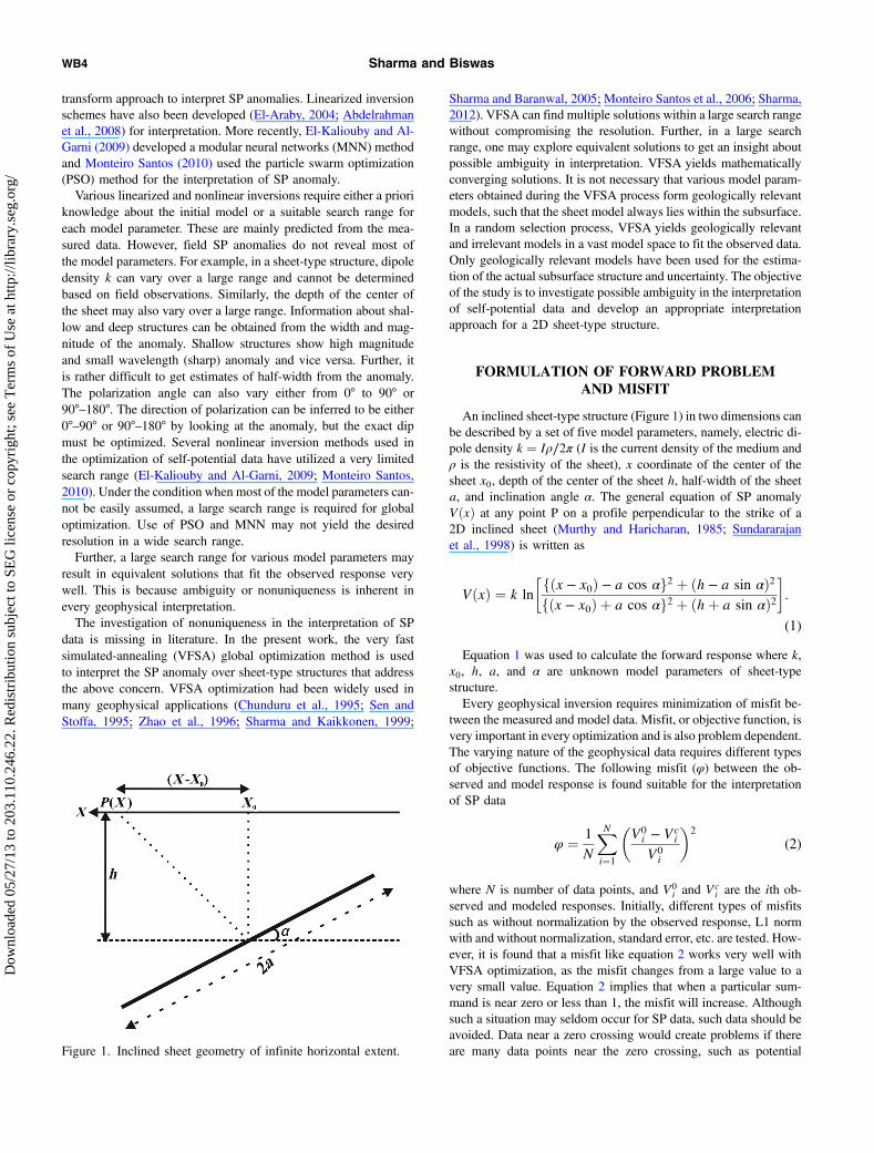
An inclined sheet-type structure (Figure 1) in two dimensions canbe described by a set of five model parameters, namely, electric di-pole density k ¼ Iρ∕2π (I is the current density of the medium andρ is the resistivity of the sheet), x coordinate of the center of thesheet x0, depth of the center of the sheet h, half-width of the sheeta, and inclination angle α. The general equation of SP anomalyVðxÞ at any point P on a profile perpendicular to the strike of a2D inclined sheet (Murthy and Haricharan, 1985; Sundararajanet al., 1998) is written as

VðxÞ ¼ k ln

�fðx − x0Þ − a cos αg2 þ ðh − a sin αÞ2fðx − x0Þ þ a cos αg2 þ ðhþ a sin αÞ2

�:

(1)

Equation 1 was used to calculate the forward response where k,x0, h, a, and α are unknown model parameters of sheet-typestructure.Every geophysical inversion requires minimization of misfit be-

tween the measured and model data. Misfit, or objective function, isvery important in every optimization and is also problem dependent.The varying nature of the geophysical data requires different typesof objective functions. The following misfit (φ) between the ob-served and model response is found suitable for the interpretationof SP data

φ ¼ 1

N

XNi¼1

�V0i − Vc

i

V0i

�2

(2)

where N is number of data points, and V0i and Vc

i are the ith ob-served and modeled responses. Initially, different types of misfitssuch as without normalization by the observed response, L1 normwith and without normalization, standard error, etc. are tested. How-ever, it is found that a misfit like equation 2 works very well withVFSA optimization, as the misfit changes from a large value to avery small value. Equation 2 implies that when a particular sum-mand is near zero or less than 1, the misfit will increase. Althoughsuch a situation may seldom occur for SP data, such data should beavoided. Data near a zero crossing would create problems if thereare many data points near the zero crossing, such as potentialFigure 1. Inclined sheet geometry of infinite horizontal extent.

WB4 Sharma and Biswas

Dow

nloa

ded

05/2

7/13

to 2

03.1

10.2

46.2

2. R

edis

trib

utio

n su

bjec

t to

SEG

lice

nse

or c

opyr

ight

; see

Ter

ms

of U

se a

t http

://lib

rary

.seg

.org

/

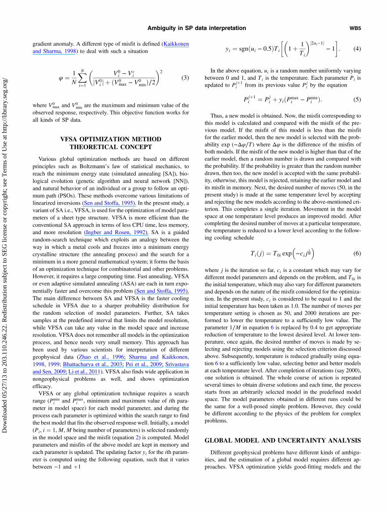
gradient anomaly. A different type of misfit is defined (Kaikkonenand Sharma, 1998) to deal with such a situation

φ ¼ 1

N

XNi¼1

�V0i − Vc

i

jV0i j þ ðV0

max − V0minÞ∕2

�2

(3)

where V0max and V0

min are the maximum and minimum value of theobserved response, respectively. This objective function works forall kinds of SP data.

VFSA OPTIMIZATION METHODTHEORETICAL CONCEPT

Various global optimization methods are based on differentprinciples such as Boltzmann’s law of statistical mechanics, toreach the minimum energy state (simulated annealing [SA]), bio-logical evolution (genetic algorithm and neural network [NN]),and natural behavior of an individual or a group to follow an opti-mum path (PSOs). These methods overcome various limitations oflinearized inversions (Sen and Stoffa, 1995). In the present study, avariant of SA i.e., VFSA, is used for the optimization of model para-meters of a sheet type structure. VFSA is more efficient than theconventional SA approach in terms of less CPU time, less memory,and more resolution (Ingber and Rosen, 1992). SA is a guidedrandom-search technique which exploits an analogy between theway in which a metal cools and freezes into a minimum energycrystalline structure (the annealing process) and the search for aminimum in a more general mathematical system; it forms the basisof an optimization technique for combinatorial and other problems.However, it requires a large computing time. Fast annealing, VFSAor even adaptive simulated annealing (ASA) are each in turn expo-nentially faster and overcome this problem (Sen and Stoffa, 1995).The main difference between SA and VFSA is the faster coolingschedule in VFSA due to a sharper probability distribution forthe random selection of model parameters. Further, SA takessamples at the predefined interval that limits the model resolution,while VFSA can take any value in the model space and increaseresolution. VFSA does not remember all models in the optimizationprocess, and hence needs very small memory. This approach hasbeen used by various scientists for interpretation of differentgeophysical data (Zhao et al., 1996; Sharma and Kaikkonen,1998, 1999; Bhattacharya et al., 2003; Pei et al., 2009; Srivastavaand Sen, 2009; Li et al., 2011). VFSA also finds wide application innongeophysical problems as well, and shows optimizationefficacy.VFSA or any global optimization technique requires a search

range (Pmini and Pmax

i , minimum and maximum value of ith para-meter in model space) for each model parameter, and during theprocess each parameter is optimized within the search range to findthe best model that fits the observed response well. Initially, a model(Pi, i ¼ 1,M,M being number of parameters) is selected randomlyin the model space and the misfit (equation 2) is computed. Modelparameters and misfits of the above model are kept in memory andeach parameter is updated. The updating factor yi for the ith param-eter is computed using the following equation, such that it variesbetween −1 and þ1

yi ¼ sgnðui − 0.5ÞTi

��1þ 1

Ti

�j2ui−1j− 1

�. (4)

In the above equation, ui is a random number uniformly varyingbetween 0 and 1, and Ti is the temperature. Each parameter Pi isupdated to Pjþ1

i from its previous value Pji by the equation

Pjþ1i ¼ Pj

i þ yiðPmaxi − Pmin

i Þ: (5)

Thus, a new model is obtained. Now, the misfit corresponding tothis model is calculated and compared with the misfit of the pre-vious model. If the misfit of this model is less than the misfitfor the earlier model, then the new model is selected with the prob-ability exp (−Δφ∕T) where Δφ is the difference of the misfits ofboth models. If the misfit of the new model is higher than that of theearlier model, then a random number is drawn and compared withthe probability. If the probability is greater than the random numberdrawn, then too, the new model is accepted with the same probabil-ity, otherwise, this model is rejected, retaining the earlier model andits misfit in memory. Next, the desired number of moves (50, in thepresent study) is made at the same temperature level by acceptingand rejecting the new models according to the above-mentioned cri-terion. This completes a single iteration. Movement in the modelspace at one temperature level produces an improved model. Aftercompleting the desired number of moves at a particular temperature,the temperature is reduced to a lower level according to the follow-ing cooling schedule

TiðjÞ ¼ T0i exp�−cij

1M

�(6)

where j is the iteration so far, ci is a constant which may vary fordifferent model parameters and depends on the problem, and T0i isthe initial temperature, which may also vary for different parametersand depends on the nature of the misfit considered for the optimiza-tion. In the present study, ci is considered to be equal to 1 and theinitial temperature has been taken as 1.0. The number of moves pertemperature setting is chosen as 50, and 2000 iterations are per-formed to lower the temperature to a sufficiently low value. Theparameter 1∕M in equation 6 is replaced by 0.4 to get appropriatereduction of temperature to the lowest desired level. At lower tem-perature, once again, the desired number of moves is made by se-lecting and rejecting models using the selection criterion discussedabove. Subsequently, temperature is reduced gradually using equa-tion 6 to a sufficiently low value, selecting better and better modelsat each temperature level. After completion of iterations (say 2000),one solution is obtained. The whole course of action is repeatedseveral times to obtain diverse solutions and each time, the processstarts from an arbitrarily selected model in the predefined modelspace. The model parameters obtained in different runs could bethe same for a well-posed simple problem. However, they couldbe different according to the physics of the problem for complexproblems.

GLOBAL MODEL AND UNCERTAINTY ANALYSIS

Different geophysical problems have different kinds of ambigu-ities, and the estimation of a global model requires different ap-proaches. VFSA optimization yields good-fitting models and the

Ambiguity in SP data interpretation WB5

Dow

nloa

ded

05/2

7/13

to 2

03.1

10.2

46.2

2. R

edis

trib

utio

n su

bjec

t to

SEG

lice

nse

or c

opyr

ight

; see

Ter

ms

of U

se a

t http

://lib

rary

.seg

.org

/

global model can be predicted using different approaches. Variousmodel parameters (k, x0, h, a, α) of good-fitting models may differfrom each other and could lie in a wide range in the multidimen-sional model space. It is important to sample the region of modelspace where clustering occurs (where a large number of models arelocated). Different sampling techniques have been used to predictthe global model and minimize uncertainty in the final model(Mosegaard and Tarantola, 1995; Sen and Stoffa, 1996).To obtain the best-fit model after a single VFSA run, computa-

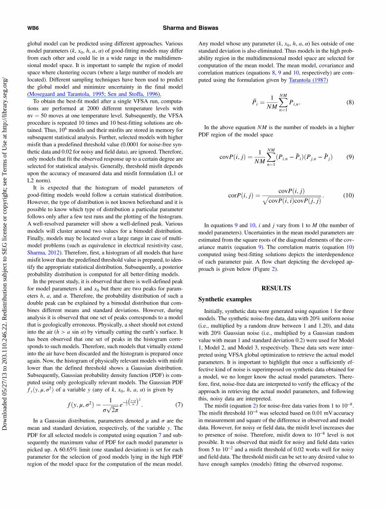
tions are performed at 2000 different temperature levels withnv ¼ 50 moves at one temperature level. Subsequently, the VFSAprocedure is repeated 10 times and 10 best-fitting solutions are ob-tained. Thus, 106 models and their misfits are stored in memory forsubsequent statistical analysis. Further, selected models with highermisfit than a predefined threshold value (0.0001 for noise-free syn-thetic data and 0.02 for noisy and field data), are ignored. Therefore,only models that fit the observed response up to a certain degree areselected for statistical analysis. Generally, threshold misfit dependsupon the accuracy of measured data and misfit formulation (L1 orL2 norm).It is expected that the histogram of model parameters of

good-fitting models would follow a certain statistical distribution.However, the type of distribution is not known beforehand and it ispossible to know which type of distribution a particular parameterfollows only after a few test runs and the plotting of the histogram.A well-resolved parameter will show a well-defined peak. Variousmodels will cluster around two values for a bimodel distribution.Finally, models may be located over a large range in case of multi-model problems (such as equivalence in electrical resistivity case,Sharma, 2012). Therefore, first, a histogram of all models that havemisfit lower than the predefined threshold value is prepared, to iden-tify the appropriate statistical distribution. Subsequently, a posteriorprobability distribution is computed for all better-fitting models.In the present study, it is observed that there is well-defined peak

for model parameters k and x0 but there are two peaks for param-eters h, a, and α. Therefore, the probability distribution of such adouble peak can be explained by a bimodal distribution that com-bines different means and standard deviations. However, duringanalysis it is observed that one set of peaks corresponds to a modelthat is geologically erroneous. Physically, a sheet should not extendinto the air (h > a sin α) by virtually cutting the earth’s surface. Ithas been observed that one set of peaks in the histogram corre-sponds to such models. Therefore, such models that virtually extendinto the air have been discarded and the histogram is prepared onceagain. Now, the histogram of physically relevant models with misfitlower than the defined threshold shows a Gaussian distribution.Subsequently, Gaussian probability density function (PDF) is com-puted using only geologically relevant models. The Gaussian PDFfyðy; μ; σ2Þ of a variable y (any of k, x0, h, a, α) is given by

fðy; μ; σ2Þ ¼ 1

σffiffiffiffiffi2π

p e−12

�y−μσ

2

. (7)

In a Gaussian distribution, parameters denoted μ and σ are themean and standard deviation, respectively, of the variable y. ThePDF for all selected models is computed using equation 7 and sub-sequently the maximum value of PDF for each model parameter ispicked up. A 60.65% limit (one standard deviation) is set for eachparameter for the selection of good models lying in the high PDFregion of the model space for the computation of the mean model.

Any model whose any parameter (k, x0, h, a, α) lies outside of onestandard deviation is also eliminated. Thus models in the high prob-ability region in the multidimensional model space are selected forcomputation of the mean model. The mean model, covariance andcorrelation matrices (equations 8, 9 and 10, respectively) are com-puted using the formulation given by Tarantola (1987)

P̄i ¼1

NM

XNM

n¼1

Pi;n. (8)

In the above equation NM is the number of models in a higherPDF region of the model space

covPði; jÞ ¼ 1

NM

XNM

n¼1

ðPi;n − P̄iÞðPj;n − P̄jÞ (9)

corPði; jÞ ¼ covPði; jÞffiffiffiffiffiffiffiffiffiffiffiffiffiffiffiffiffiffiffiffiffiffiffiffiffiffiffiffiffiffiffiffiffiffiffiffiffiffifficovPði; iÞcovPðj; jÞp : (10)

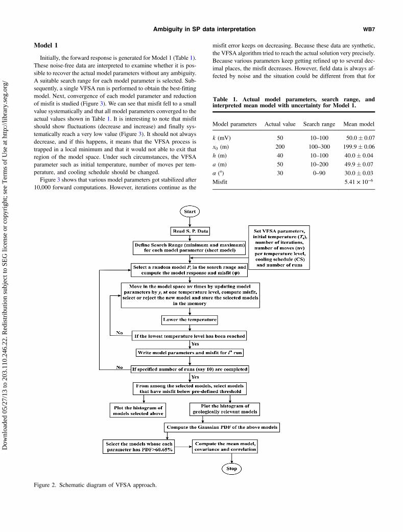
In equations 9 and 10, i and j vary from 1 to M (the number ofmodel parameters). Uncertainties in the mean model parameters areestimated from the square roots of the diagonal elements of the cov-ariance matrix (equation 9). The correlation matrix (equation 10)computed using best-fitting solutions depicts the interdependenceof each parameter pair. A flow chart depicting the developed ap-proach is given below (Figure 2).

RESULTS

Synthetic examples

Initially, synthetic data were generated using equation 1 for threemodels. The synthetic noise-free data, data with 20% uniform noise(i.e., multiplied by a random draw between 1 and 1.20), and datawith 20% Gaussian noise (i.e., multiplied by a Gaussian randomvalue with mean 1 and standard deviation 0.2) were used for Model1, Model 2, and Model 3, respectively. These data sets were inter-preted using VFSA global optimization to retrieve the actual modelparameters. It is important to highlight that once a sufficiently ef-fective kind of noise is superimposed on synthetic data obtained fora model, we no longer know the actual model parameters. There-fore, first, noise-free data are interpreted to verify the efficacy of theapproach in retrieving the actual model parameters, and followingthis, noisy data are interpreted.The misfit (equation 2) for noise-free data varies from 1 to 10−8.

The misfit threshold 10−4 was selected based on 0.01 mVaccuracyin measurement and square of the difference in observed and modeldata. However, for noisy or field data, the misfit level increases dueto presence of noise. Therefore, misfit down to 10−8 level is notpossible. It was observed that misfit for noisy and field data variesfrom 5 to 10−2 and a misfit threshold of 0.02 works well for noisyand field data. The threshold misfit can be set to any desired value tohave enough samples (models) fitting the observed response.

WB6 Sharma and Biswas

Dow

nloa

ded

05/2

7/13

to 2

03.1

10.2

46.2

2. R

edis

trib

utio

n su

bjec

t to

SEG

lice

nse

or c

opyr

ight

; see

Ter

ms

of U

se a

t http

://lib

rary

.seg

.org

/

Model 1

Initially, the forward response is generated for Model 1 (Table 1).These noise-free data are interpreted to examine whether it is pos-sible to recover the actual model parameters without any ambiguity.A suitable search range for each model parameter is selected. Sub-sequently, a single VFSA run is performed to obtain the best-fittingmodel. Next, convergence of each model parameter and reductionof misfit is studied (Figure 3). We can see that misfit fell to a smallvalue systematically and that all model parameters converged to theactual values shown in Table 1. It is interesting to note that misfitshould show fluctuations (decrease and increase) and finally sys-tematically reach a very low value (Figure 3). It should not alwaysdecrease, and if this happens, it means that the VFSA process istrapped in a local minimum and that it would not able to exit thatregion of the model space. Under such circumstances, the VFSAparameter such as initial temperature, number of moves per tem-perature, and cooling schedule should be changed.Figure 3 shows that various model parameters got stabilized after

10,000 forward computations. However, iterations continue as the

misfit error keeps on decreasing. Because these data are synthetic,the VFSA algorithm tried to reach the actual solution very precisely.Because various parameters keep getting refined up to several dec-imal places, the misfit decreases. However, field data is always af-fected by noise and the situation could be different from that for

Table 1. Actual model parameters, search range, andinterpreted mean model with uncertainty for Model 1.

Model parameters Actual value Search range Mean model

k (mV) 50 10–100 50.0� 0.07

x0 (m) 200 100–300 199.9� 0.06

h (m) 40 10–100 40.0� 0.04

a (m) 50 10–200 49.9� 0.07

α (°) 30 0–90 30.0� 0.03

Misfit 5.41 × 10−6

Figure 2. Schematic diagram of VFSA approach.

Ambiguity in SP data interpretation WB7

Dow

nloa

ded

05/2

7/13

to 2

03.1

10.2

46.2

2. R

edis

trib

utio

n su

bjec

t to

SEG

lice

nse

or c

opyr

ight

; see

Ter

ms

of U

se a

t http

://lib

rary

.seg

.org

/

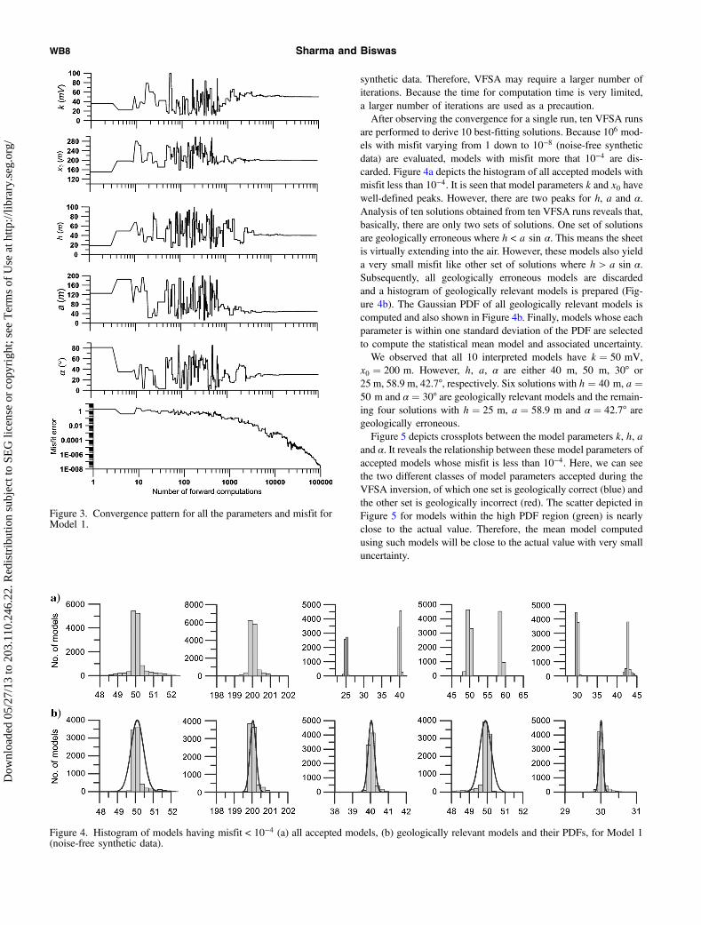
synthetic data. Therefore, VFSA may require a larger number ofiterations. Because the time for computation time is very limited,a larger number of iterations are used as a precaution.After observing the convergence for a single run, ten VFSA runs

are performed to derive 10 best-fitting solutions. Because 106 mod-els with misfit varying from 1 down to 10−8 (noise-free syntheticdata) are evaluated, models with misfit more that 10−4 are dis-carded. Figure 4a depicts the histogram of all accepted models withmisfit less than 10−4. It is seen that model parameters k and x0 havewell-defined peaks. However, there are two peaks for h, a and α.Analysis of ten solutions obtained from ten VFSA runs reveals that,basically, there are only two sets of solutions. One set of solutionsare geologically erroneous where h < a sin α. This means the sheetis virtually extending into the air. However, these models also yielda very small misfit like other set of solutions where h > a sin α.Subsequently, all geologically erroneous models are discardedand a histogram of geologically relevant models is prepared (Fig-ure 4b). The Gaussian PDF of all geologically relevant models iscomputed and also shown in Figure 4b. Finally, models whose eachparameter is within one standard deviation of the PDF are selectedto compute the statistical mean model and associated uncertainty.We observed that all 10 interpreted models have k ¼ 50 mV,

x0 ¼ 200 m. However, h, a, α are either 40 m, 50 m, 30° or25 m, 58.9 m, 42.7°, respectively. Six solutions with h ¼ 40 m, a ¼50 m and α ¼ 30° are geologically relevant models and the remain-ing four solutions with h ¼ 25 m, a ¼ 58.9 m and α ¼ 42.7° aregeologically erroneous.Figure 5 depicts crossplots between the model parameters k, h, a

and α. It reveals the relationship between these model parameters ofaccepted models whose misfit is less than 10−4. Here, we can seethe two different classes of model parameters accepted during theVFSA inversion, of which one set is geologically correct (blue) andthe other set is geologically incorrect (red). The scatter depicted inFigure 5 for models within the high PDF region (green) is nearlyclose to the actual value. Therefore, the mean model computedusing such models will be close to the actual value with very smalluncertainty.

Figure 3. Convergence pattern for all the parameters and misfit forModel 1.

Figure 4. Histogram of models having misfit < 10−4 (a) all accepted models, (b) geologically relevant models and their PDFs, for Model 1(noise-free synthetic data).

WB8 Sharma and Biswas

Dow

nloa

ded

05/2

7/13

to 2

03.1

10.2

46.2

2. R

edis

trib

utio

n su

bjec

t to

SEG

lice

nse

or c

opyr

ight

; see

Ter

ms

of U

se a

t http

://lib

rary

.seg

.org

/

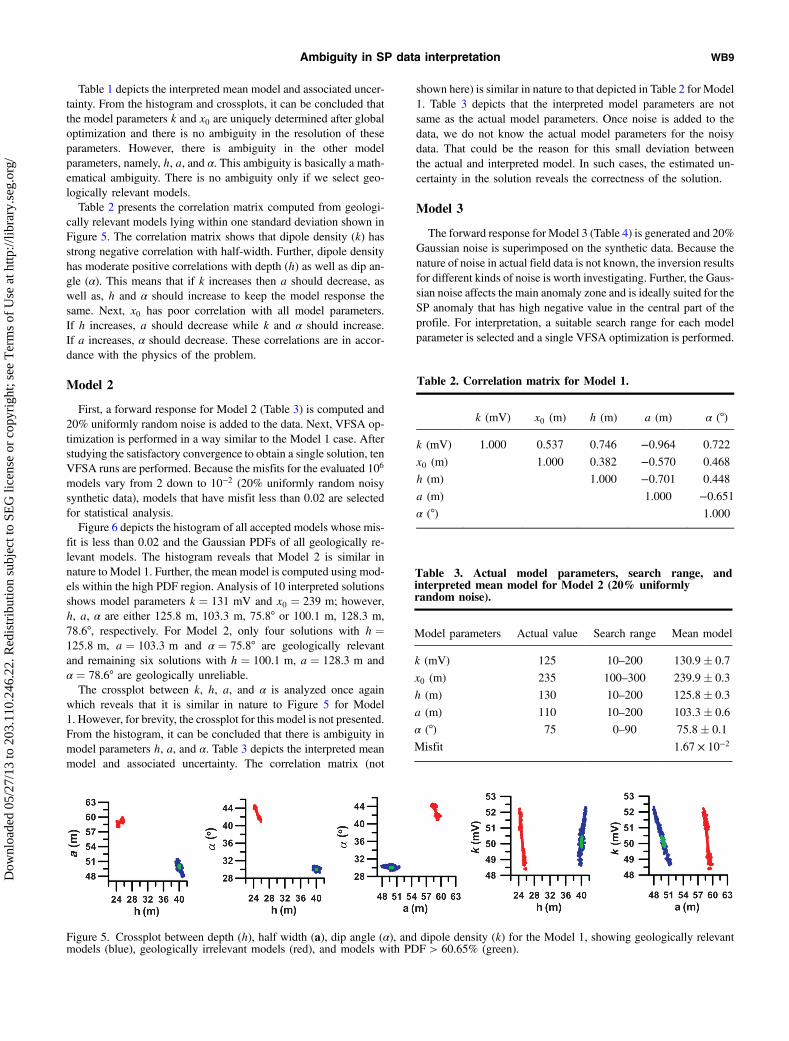
Table 1 depicts the interpreted mean model and associated uncer-tainty. From the histogram and crossplots, it can be concluded thatthe model parameters k and x0 are uniquely determined after globaloptimization and there is no ambiguity in the resolution of theseparameters. However, there is ambiguity in the other modelparameters, namely, h, a, and α. This ambiguity is basically a math-ematical ambiguity. There is no ambiguity only if we select geo-logically relevant models.Table 2 presents the correlation matrix computed from geologi-

cally relevant models lying within one standard deviation shown inFigure 5. The correlation matrix shows that dipole density (k) hasstrong negative correlation with half-width. Further, dipole densityhas moderate positive correlations with depth (h) as well as dip an-gle (α). This means that if k increases then a should decrease, aswell as, h and α should increase to keep the model response thesame. Next, x0 has poor correlation with all model parameters.If h increases, a should decrease while k and α should increase.If a increases, α should decrease. These correlations are in accor-dance with the physics of the problem.

Model 2

First, a forward response for Model 2 (Table 3) is computed and20% uniformly random noise is added to the data. Next, VFSA op-timization is performed in a way similar to the Model 1 case. Afterstudying the satisfactory convergence to obtain a single solution, tenVFSA runs are performed. Because the misfits for the evaluated 106

models vary from 2 down to 10−2 (20% uniformly random noisysynthetic data), models that have misfit less than 0.02 are selectedfor statistical analysis.Figure 6 depicts the histogram of all accepted models whose mis-

fit is less than 0.02 and the Gaussian PDFs of all geologically re-levant models. The histogram reveals that Model 2 is similar innature to Model 1. Further, the mean model is computed using mod-els within the high PDF region. Analysis of 10 interpreted solutionsshows model parameters k ¼ 131 mV and x0 ¼ 239 m; however,h, a, α are either 125.8 m, 103.3 m, 75.8° or 100.1 m, 128.3 m,78.6°, respectively. For Model 2, only four solutions with h ¼125.8 m, a ¼ 103.3 m and α ¼ 75.8° are geologically relevantand remaining six solutions with h ¼ 100.1 m, a ¼ 128.3 m andα ¼ 78.6° are geologically unreliable.The crossplot between k, h, a, and α is analyzed once again

which reveals that it is similar in nature to Figure 5 for Model1. However, for brevity, the crossplot for this model is not presented.From the histogram, it can be concluded that there is ambiguity inmodel parameters h, a, and α. Table 3 depicts the interpreted meanmodel and associated uncertainty. The correlation matrix (not

shown here) is similar in nature to that depicted in Table 2 for Model1. Table 3 depicts that the interpreted model parameters are notsame as the actual model parameters. Once noise is added to thedata, we do not know the actual model parameters for the noisydata. That could be the reason for this small deviation betweenthe actual and interpreted model. In such cases, the estimated un-certainty in the solution reveals the correctness of the solution.

Model 3

The forward response for Model 3 (Table 4) is generated and 20%Gaussian noise is superimposed on the synthetic data. Because thenature of noise in actual field data is not known, the inversion resultsfor different kinds of noise is worth investigating. Further, the Gaus-sian noise affects the main anomaly zone and is ideally suited for theSP anomaly that has high negative value in the central part of theprofile. For interpretation, a suitable search range for each modelparameter is selected and a single VFSA optimization is performed.

Figure 5. Crossplot between depth (h), half width (a), dip angle (α), and dipole density (k) for the Model 1, showing geologically relevantmodels (blue), geologically irrelevant models (red), and models with PDF > 60.65% (green).

Table 2. Correlation matrix for Model 1.

k (mV) x0 (m) h (m) a (m) α (°)

k (mV) 1.000 0.537 0.746 −0.964 0.722

x0 (m) 1.000 0.382 −0.570 0.468

h (m) 1.000 −0.701 0.448

a (m) 1.000 −0.651α (°) 1.000

Table 3. Actual model parameters, search range, andinterpreted mean model for Model 2 (20% uniformlyrandom noise).

Model parameters Actual value Search range Mean model

k (mV) 125 10–200 130.9� 0.7

x0 (m) 235 100–300 239.9� 0.3

h (m) 130 10–200 125.8� 0.3

a (m) 110 10–200 103.3� 0.6

α (°) 75 0–90 75.8� 0.1

Misfit 1.67 × 10−2

Ambiguity in SP data interpretation WB9

Dow

nloa

ded

05/2

7/13

to 2

03.1

10.2

46.2

2. R

edis

trib

utio

n su

bjec

t to

SEG

lice

nse

or c

opyr

ight

; see

Ter

ms

of U

se a

t http

://lib

rary

.seg

.org

/

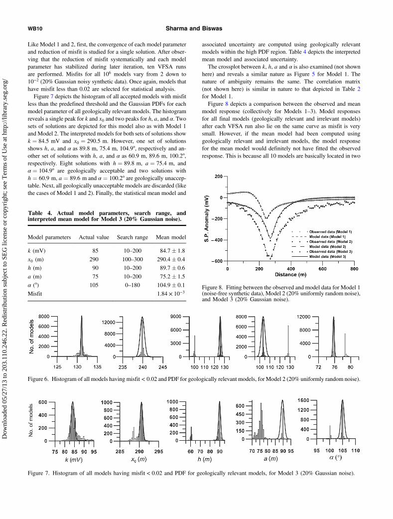
Like Model 1 and 2, first, the convergence of each model parameterand reduction of misfit is studied for a single solution. After obser-ving that the reduction of misfit systematically and each modelparameter has stabilized during later iteration, ten VFSA runsare performed. Misfits for all 106 models vary from 2 down to10−2 (20% Gaussian noisy synthetic data). Once again, models thathave misfit less than 0.02 are selected for statistical analysis.Figure 7 depicts the histogram of all accepted models with misfit

less than the predefined threshold and the Gaussian PDFs for eachmodel parameter of all geologically relevant models. The histogramreveals a single peak for k and x0 and two peaks for h, a, and α. Twosets of solutions are depicted for this model also as with Model 1and Model 2. The interpreted models for both sets of solutions showk ¼ 84.5 mV and x0 ¼ 290.5 m. However, one set of solutionsshows h, a, and α as 89.8 m, 75.4 m, 104.9°, respectively and an-other set of solutions with h, a, and α as 60.9 m, 89.6 m, 100.2°,respectively. Eight solutions with h ¼ 89.8 m, a ¼ 75.4 m, andα ¼ 104.9° are geologically acceptable and two solutions withh ¼ 60.9 m, a ¼ 89.6 m and α ¼ 100.2° are geologically unaccep-table. Next, all geologically unacceptable models are discarded (likethe cases of Model 1 and 2). Finally, the statistical mean model and

associated uncertainty are computed using geologically relevantmodels within the high PDF region. Table 4 depicts the interpretedmean model and associated uncertainty.The crossplot between k, h, a and α is also examined (not shown

here) and reveals a similar nature as Figure 5 for Model 1. Thenature of ambiguity remains the same. The correlation matrix(not shown here) is similar in nature to that depicted in Table 2for Model 1.Figure 8 depicts a comparison between the observed and mean

model response (collectively for Models 1–3). Model responsesfor all final models (geologically relevant and irrelevant models)after each VFSA run also lie on the same curve as misfit is verysmall. However, if the mean model had been computed usinggeologically relevant and irrelevant models, the model responsefor the mean model would definitely not have fitted the observedresponse. This is because all 10 models are basically located in two

Figure 6. Histogram of all models havingmisfit < 0.02 and PDF for geologically relevant models, for Model 2 (20% uniformly random noise).

Table 4. Actual model parameters, search range, andinterpreted mean model for Model 3 (20% Gaussian noise).

Model parameters Actual value Search range Mean model

k (mV) 85 10–200 84.7� 1.8

x0 (m) 290 100–300 290.4� 0.4

h (m) 90 10–200 89.7� 0.6

a (m) 75 10–200 75.2� 1.5

α (°) 105 0–180 104.9� 0.1

Misfit 1.84 × 10−3

Figure 7. Histogram of all models having misfit < 0.02 and PDF for geologically relevant models, for Model 3 (20% Gaussian noise).

Figure 8. Fitting between the observed and model data for Model 1(noise-free synthetic data), Model 2 (20% uniformly random noise),and Model 3 (20% Gaussian noise).

WB10 Sharma and Biswas

Dow

nloa

ded

05/2

7/13

to 2

03.1

10.2

46.2

2. R

edis

trib

utio

n su

bjec

t to

SEG

lice

nse

or c

opyr

ight

; see

Ter

ms

of U

se a

t http

://lib

rary

.seg

.org

/

different regions of the model space. Therefore, only geologicallyrelevant models are used to compute the mean model. The com-puted response for a mean model of this nature also fits the observedresponse very precisely, just as does each of the individual modelresponses. Moreover, the mean models, whose responses shown inFigure 8, are computed from models lying in the high PDF region ofthe model space. It is interesting to note that uncertainty estimatedfor such a mean model suggests that the actual model locates withinthe estimated uncertainty. The model response for any model se-lected randomly within the estimated uncertainty will be close tothe observed response; however, it may not fit precisely like a finalmodel depicted by the individual VFSA solution.

FIELD EXAMPLE 1 (BAVARIAN WOODSANOMALY, GERMANY)

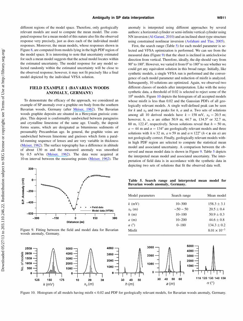
To demonstrate the efficacy of the approach, we considered anexample of SP anomaly over a graphite ore body from the southernBavarian woods, Germany (after Meiser, 1962). The Bavarianwoods graphite deposits are situated in a Hercynian gneissic com-plex. This deposit is conformably sandwiched between paragneissand crystalline limestone of the same age. Usually, the depositforms seams, which are designated as bituminous sediments ofpresumably Precambrian age. In general, the graphite veins aresandwiched between limestone and gneisses which form a paral-lel-running sequence of lenses and are very variable in thickness(Meiser, 1962). The surface topography has a difference in altitudeof about 130 m and the measured anomaly was smoothedby 0.5 mV/m (Meiser, 1962). The data were acquired at10-m interval between the measuring points (Meiser, 1962). The

anomaly is interpreted using different approaches by severalauthors: a horizontal cylinder or semi-infinite vertical cylinder usingNN inversion (Al-Garaní, 2010) and an inclined sheet-type structureusing constrained nonlinear inversion (Asfahani and Tlas, 2005).First, the search range (Table 5) for each model parameter is se-

lected and VFSA optimization is performed. We can see from themeasured data (Figure 9) that the sheet is inclined in anticlockwisedirection from vertical. Therefore, ideally, the dip should vary from90° to 180°. However, we varied it from 0° to 180° to see whether wecould get any equivalent solution in this broad range. Initially, likesynthetic models, a single VFSA run is performed and the conver-gence of each model parameter and reduction of misfit is analyzed.Subsequently, 10 solutions are optimized. Again, we observed twodifferent classes of models after interpretation. Like with the noisysynthetic data, a threshold of 0.02 is selected to reject some of the106 models. Figure 10 depicts the histogram of all accepted modelswhose misfit is less than 0.02 and the Gaussian PDFs of all geo-logically relevant models. A single well-defined peak can be seenfor k and x0 and two peaks for h, a and α. Two sets of solutionsamong all 10 derived models have k ¼ 158 mV, x0 ¼ 20.5 m;however, h, a, α are either 50.9 m, 44.7 m, 134.5° or 32.7 m,60 m, 122.4°, respectively. Seven solutions reveal that h ¼ 50 m,a ¼ 44 m and α ¼ 134° are geologically relevant models and threesolutions with h ≈ 32 m, a ≈ 59 m and α ≈ 122° (h < a sin α) arenot geologically correct. Finally, geologically relevant models with-in high PDF region are selected to compute the statistical meanmodel and associated uncertainty. A comparison between the ob-served and mean model data is shown in Figure 9. Table 5 depictsthe interpreted mean model and associated uncertainty. The inter-pretation of field data is in accordance with the synthetic data indepicting two sets of solutions that fit the observed data well.

Table 5. Search range and interpreted mean model forBavarian woods anomaly, Germany.

Model parameters Search range Mean model

k (mV) 10–300 158.3� 3.1

x0 (m) −50 − 50 20.5� 0.4

h (m) 10–100 50.9� 0.3

a (m) 10–200 44.6� 0.8

α (°) 0–180 134.3� 0.2

Misfit 8.01 × 10−3Figure 9. Fitting between the field and model data for Bavarianwoods anomaly, Germany.

Figure 10. Histogram of all models having misfit < 0.02 and PDF for geologically relevant models, for Bavarian woods anomaly, Germany.

Ambiguity in SP data interpretation WB11

Dow

nloa

ded

05/2

7/13

to 2

03.1

10.2

46.2

2. R

edis

trib

utio

n su

bjec

t to

SEG

lice

nse

or c

opyr

ight

; see

Ter

ms

of U

se a

t http

://lib

rary

.seg

.org

/

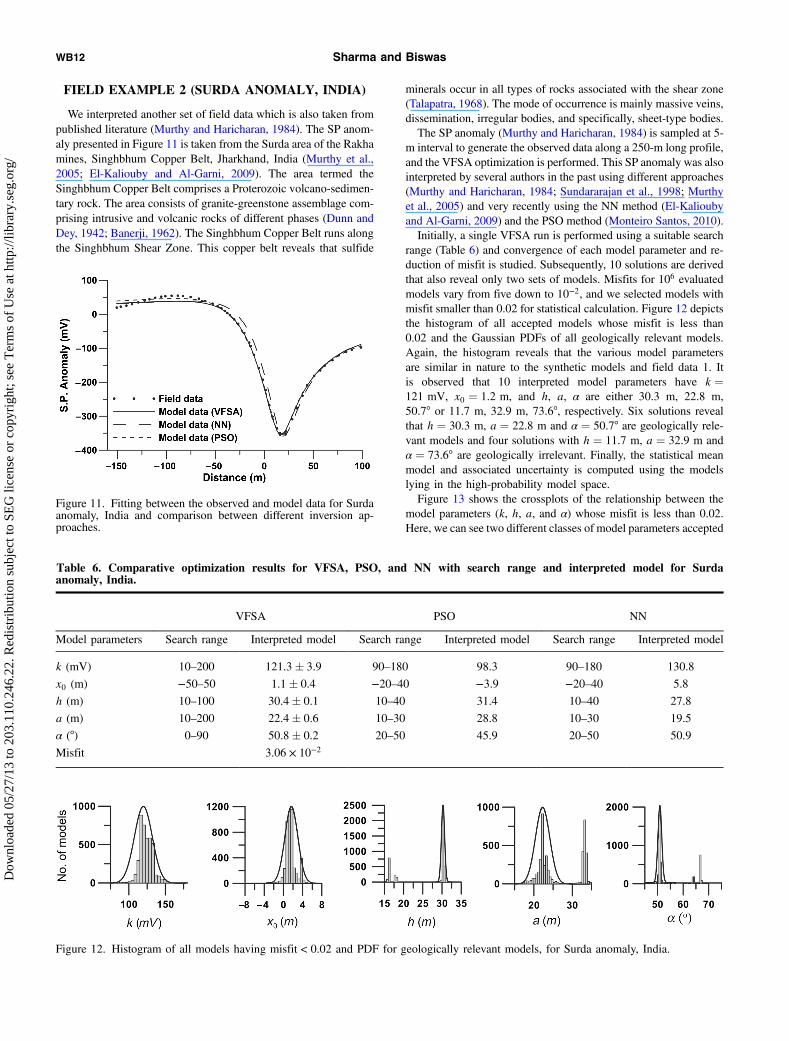
FIELD EXAMPLE 2 (SURDA ANOMALY, INDIA)

We interpreted another set of field data which is also taken frompublished literature (Murthy and Haricharan, 1984). The SP anom-aly presented in Figure 11 is taken from the Surda area of the Rakhamines, Singhbhum Copper Belt, Jharkhand, India (Murthy et al.,2005; El-Kaliouby and Al-Garni, 2009). The area termed theSinghbhum Copper Belt comprises a Proterozoic volcano-sedimen-tary rock. The area consists of granite-greenstone assemblage com-prising intrusive and volcanic rocks of different phases (Dunn andDey, 1942; Banerji, 1962). The Singhbhum Copper Belt runs alongthe Singhbhum Shear Zone. This copper belt reveals that sulfide

minerals occur in all types of rocks associated with the shear zone(Talapatra, 1968). The mode of occurrence is mainly massive veins,dissemination, irregular bodies, and specifically, sheet-type bodies.The SP anomaly (Murthy and Haricharan, 1984) is sampled at 5-

m interval to generate the observed data along a 250-m long profile,and the VFSA optimization is performed. This SP anomaly was alsointerpreted by several authors in the past using different approaches(Murthy and Haricharan, 1984; Sundararajan et al., 1998; Murthyet al., 2005) and very recently using the NN method (El-Kalioubyand Al-Garni, 2009) and the PSO method (Monteiro Santos, 2010).Initially, a single VFSA run is performed using a suitable search

range (Table 6) and convergence of each model parameter and re-duction of misfit is studied. Subsequently, 10 solutions are derivedthat also reveal only two sets of models. Misfits for 106 evaluatedmodels vary from five down to 10−2, and we selected models withmisfit smaller than 0.02 for statistical calculation. Figure 12 depictsthe histogram of all accepted models whose misfit is less than0.02 and the Gaussian PDFs of all geologically relevant models.Again, the histogram reveals that the various model parametersare similar in nature to the synthetic models and field data 1. Itis observed that 10 interpreted model parameters have k ¼121 mV, x0 ¼ 1.2 m, and h, a, α are either 30.3 m, 22.8 m,50.7° or 11.7 m, 32.9 m, 73.6°, respectively. Six solutions revealthat h ¼ 30.3 m, a ¼ 22.8 m and α ¼ 50.7° are geologically rele-vant models and four solutions with h ¼ 11.7 m, a ¼ 32.9 m andα ¼ 73.6° are geologically irrelevant. Finally, the statistical meanmodel and associated uncertainty is computed using the modelslying in the high-probability model space.Figure 13 shows the crossplots of the relationship between the

model parameters (k, h, a, and α) whose misfit is less than 0.02.Here, we can see two different classes of model parameters accepted

Figure 11. Fitting between the observed and model data for Surdaanomaly, India and comparison between different inversion ap-proaches.

Table 6. Comparative optimization results for VFSA, PSO, and NN with search range and interpreted model for Surdaanomaly, India.

VFSA PSO NN

Model parameters Search range Interpreted model Search range Interpreted model Search range Interpreted model

k (mV) 10–200 121.3� 3.9 90–180 98.3 90–180 130.8

x0 (m) −50–50 1.1� 0.4 −20–40 −3.9 −20–40 5.8

h (m) 10–100 30.4� 0.1 10–40 31.4 10–40 27.8

a (m) 10–200 22.4� 0.6 10–30 28.8 10–30 19.5

α (°) 0–90 50.8� 0.2 20–50 45.9 20–50 50.9

Misfit 3.06 × 10−2

Figure 12. Histogram of all models having misfit < 0.02 and PDF for geologically relevant models, for Surda anomaly, India.

WB12 Sharma and Biswas

Dow

nloa

ded

05/2

7/13

to 2

03.1

10.2

46.2

2. R

edis

trib

utio

n su

bjec

t to

SEG

lice

nse

or c

opyr

ight

; see

Ter

ms

of U

se a

t http

://lib

rary

.seg

.org

/

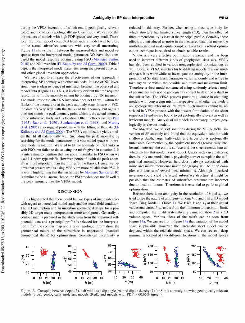
during the VFSA inversion, of which one is geologically relevant(blue) and the other is geologically irrelevant (red). We can see thatthe scatters of models with high PDF (green) are very small. There-fore, the mean model computed from such a model will be closeto the actual subsurface structure with very small uncertainty.Figure 11 shows the fit between the measured data and model re-sponse from the interpreted model parameter. We have also com-pared the model response obtained using PSO (Monteiro Santos,2010) and NN inversion (El-Kaliouby and Al-Garni, 2009). Table 6depicts the interpreted model parameter using the present approachand other global inversion approaches.We have tried to compare the effectiveness of our approach in

interpreting SP anomaly with other methods. In case of NN inver-sion, there is clear evidence of mismatch between the observed andmodel data (Figure 11). Thus, it is clearly evident that the requiredresolution to fit the anomaly cannot be obtained by NN inversion.The model response after NN inversion does not fit well within theflanks of the anomaly or at the peak anomaly zone. In case of PSO,the data fits very well with the flanks of the anomaly, but again itdoes not match the peak anomaly point which is the actual anomalyof the subsurface body and its location. Other methods used by Paul(1965), Rao et al. (1970), Sundararajan et al. (1998), and Murthyet al. (2005) also suggest problems with the fitting of the data (El-Kaliouby and Al-Garni, 2009). The VFSA optimization yields mod-els that fit all data equally well (including the peak anomaly) bysearching for the model parameters in a vast model space with pre-cise model resolution. We tried to fit the anomaly on the flanks aswith PSO, but failed to do so using the misfit given in equation 2. Itis interesting to mention that we got a fit similar to PSO when weused L1-norm type misfit. However, perfect fit with the peak anom-aly is more important than the fittings at the flanks. Hence, we be-lieve that present results using VFSA are more reliable than PSO. Itis worth highlighting that the misfit used by Monteiro Santos (2010)is similar to the L1-norm. Hence, the PSO model does not fit well atthe peak anomaly like the VFSA model.

DISCUSSION

It is highlighted that there could be two types of inconsistencieswith regard to theoretical model study and the actual field condition.The 2D assumption and an uncertain geometrical shape for a pos-sibly 3D target make interpretation more ambiguous. Generally, acontour map is prepared in the study area from the measured self-potential data and a principal profile is selected for the interpreta-tion. From the contour map and a priori geologic information, thegeometrical nature of the subsurface is understood (standardgeometrical shape) for optimization. Geometrical uncertainty is

reduced in this way. Further, when using a sheet-type body forwhich structure has limited strike length (3D), then the effect ofthree-dimensionality is least at the principal profile. Certainly theseeffects are introduced as noise in the measured data that makes themultidimensional misfit quite complex. Therefore, a robust optimi-zation technique is required to obtain reliable results.VFSA is a very effective optimization approach and has been

used to interpret different kinds of geophysical data sets. VFSAhas also been applied in various nongeophysical optimizations aswell. Because VFSA searches for best-fitting models in a vast mod-el space, it is worthwhile to investigate the ambiguity in the inter-pretation of SP data. Each parameter varies randomly and is free totake any value within the possible minimum and maximum limit.Therefore, a sheet model constructed using randomly selected mod-el parameters may not be geologically correct to describe a sheet inthe subsurface. The VFSA process provides guidance in obtainingmodels with converging misfit, irrespective of whether the modelsare geologically relevant or irrelevant. Such models cannot be re-stricted in VFSA process with the present formulation of the sheet(equation 1) and we are bound to get geologically relevant as well asirrelevant models. Analysis of all models is necessary to reject geo-logically irrelevant models.We observed two sets of solutions during the VFSA global in-

version of SP anomaly and found that the equivalent solution withshallower depth, larger half-width, and larger dip is geologicallyunfeasible. Geometrically, the equivalent model (geologically irre-levant) intersects the earth’s surface and the sheet extends into airwhich means this model is not correct. Under such circumstances,there is only one model that is physically correct to explain the self-potential anomaly. However, field data is always associated withnoise and multidimensional misfit topography will be quite com-plex and consist of several local minimums. Although linearizedinversion could yield the actual subsurface structure, it might bepossible that the estimates of subsurface structure are incorrectdue to local minimums. Therefore, it is essential to perform globaloptimization.Because there is no ambiguity in the resolution of k and x0, we

tried to see the nature of ambiguity among h, a and α in a 3D modelspace using Model 1 (Table 1). We fixed k and x0 at their actualvalues and varied h, a, and α from the minimum to maximum limit,and computed the misfit systematically using equation 2 in a 3Dvolume space. Various slices of the misfit can be seen fromFigure 14a. We can see from Figure 14a that variation of the modelspace is plausible; however, the unrealistic sheet model can bedepicted within the realistic model space. We can see two deepminimums located at two different locations in the model spaces

Figure 13. Crossplot between depth (h), half width (a), dip angle (α), and dipole density (k) for Surda anomaly, showing geologically relevantmodels (blue), geologically irrelevant models (Red), and models with PDF > 60.65% (green).

Ambiguity in SP data interpretation WB13

Dow

nloa

ded

05/2

7/13

to 2

03.1

10.2

46.2

2. R

edis

trib

utio

n su

bjec

t to

SEG

lice

nse

or c

opyr

ight

; see

Ter

ms

of U

se a

t http

://lib

rary

.seg

.org

/

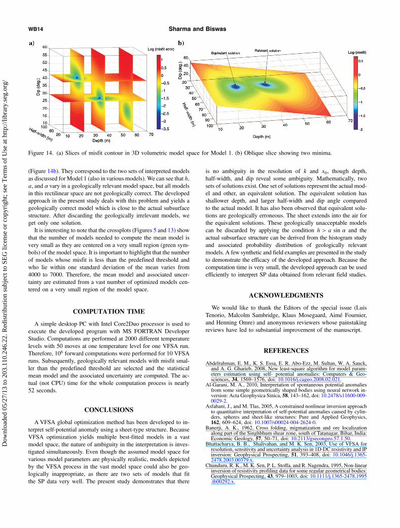
(Figure 14b). They correspond to the two sets of interpreted modelsas discussed for Model 1 (also in various models). We can see that h,a, and α vary in a geologically relevant model space, but all modelsin this rectilinear space are not geologically correct. The developedapproach in the present study deals with this problem and yields ageologically correct model which is close to the actual subsurfacestructure. After discarding the geologically irrelevant models, weget only one solution.It is interesting to note that the crossplots (Figures 5 and 13) show

that the number of models needed to compute the mean model isvery small as they are centered on a very small region (green sym-bols) of the model space. It is important to highlight that the numberof models whose misfit is less than the predefined threshold andwho lie within one standard deviation of the mean varies from4000 to 7000. Therefore, the mean model and associated uncer-tainty are estimated from a vast number of optimized models cen-tered on a very small region of the model space.

COMPUTATION TIME

A simple desktop PC with Intel Core2Duo processor is used toexecute the developed program with MS FORTRAN DeveloperStudio. Computations are performed at 2000 different temperaturelevels with 50 moves at one temperature level for one VFSA run.Therefore, 106 forward computations were performed for 10 VFSAruns. Subsequently, geologically relevant models with misfit smal-ler than the predefined threshold are selected and the statisticalmean model and the associated uncertainty are computed. The ac-tual (not CPU) time for the whole computation process is nearly52 seconds.

CONCLUSIONS

AVFSA global optimization method has been developed to in-terpret self-potential anomaly using a sheet-type structure. BecauseVFSA optimization yields multiple best-fitted models in a vastmodel space, the nature of ambiguity in the interpretation is inves-tigated simultaneously. Even though the assumed model space forvarious model parameters are physically realistic, models depictedby the VFSA process in the vast model space could also be geo-logically inappropriate, as there are two sets of models that fitthe SP data very well. The present study demonstrates that there

is no ambiguity in the resolution of k and x0, though depth,half-width, and dip reveal some ambiguity. Mathematically, twosets of solutions exist. One set of solutions represent the actual mod-el and other, an equivalent solution. The equivalent solution hasshallower depth, and larger half-width and dip angle comparedto the actual model. It has also been observed that equivalent solu-tions are geologically erroneous. The sheet extends into the air forthe equivalent solutions. These geologically unacceptable modelscan be discarded by applying the condition h > a sin α and theactual subsurface structure can be derived from the histogram studyand associated probability distribution of geologically relevantmodels. A few synthetic and field examples are presented in the studyto demonstrate the efficacy of the developed approach. Because thecomputation time is very small, the developed approach can be usedefficiently to interpret SP data obtained from relevant field studies.

ACKNOWLEDGMENTS

We would like to thank the Editors of the special issue (LuisTenorio, Malcolm Sambridge, Klaus Mosegaard, Aimé Fournier,and Henning Omre) and anonymous reviewers whose painstakingreviews have led to substantial improvement of the manuscript.

REFERENCES

Abdelrahman, E. M., K. S. Essa, E. R. Abo-Ezz, M. Sultan, W. A. Sauck,and A. G. Gharieb, 2008, New least-square algorithm for model param-eters estimation using self- potential anomalies: Computers & Geo-sciences, 34, 1569–1576, doi: 10.1016/j.cageo.2008.02.021.

Al-Garani, M. A., 2010, Interpretation of spontaneous potential anomaliesfrom some simple geometrically shaped bodies using neural network in-version: Acta Geophysica Sinica, 58, 143–162, doi: 10.2478/s11600-009-0029-2.

Asfahani, J., and M. Tlas, 2005, A constrained nonlinear inversion approachto quantitative interpretation of self-potential anomalies caused by cylin-ders, spheres and sheet-like structures: Pure and Applied Geophysics,162, 609–624, doi: 10.1007/s00024-004-2624-0.

Banerji, A. K., 1962, Cross folding, migmatization and ore localizationalong part of the Singhbhum shear zone, south of Tatanagar, Bihar, India:Economic Geology, 57, 50–71, doi: 10.2113/gsecongeo.57.1.50.

Bhattacharya, B. B., Shalivahan, and M. K. Sen, 2003, Use of VFSA forresolution, sensitivity and uncertainty analysis in 1D-DC resistivity and IPinversion: Geophysical Prospecting, 51, 393–408, doi: 10.1046/j.1365-2478.2003.00379.x.

Chunduru, R. K., M. K. Sen, P. L. Stoffa, and R. Nagendra, 1995, Non-linearinversion of resistivity profiling data for some regular geometrical bodies:Geophysical Prospecting, 43, 979–1003, doi: 10.1111/j.1365-2478.1995.tb00292.x.

Figure 14. (a) Slices of misfit contour in 3D volumetric model space for Model 1. (b) Oblique slice showing two minima.

WB14 Sharma and Biswas

Dow

nloa

ded

05/2

7/13

to 2

03.1

10.2

46.2

2. R

edis

trib

utio

n su

bjec

t to

SEG

lice

nse

or c

opyr

ight

; see

Ter

ms

of U

se a

t http

://lib

rary

.seg

.org

/

Corwin, R. F., and D. B. Hoover, 1979, The self-potential method in geother-mal exploration: Geophysics, 44, 226–245, doi: 10.1190/1.1440964.

Dunn, J. A., and A. K. Dey, 1942, The geology and petrology of easternSinghbhum and surrounding areas. Memoir: Geological Survey of India,69, 281–450.

El-Araby, H. M., 2004, A new method for complete quantitative interpreta-tion of self-potential anomalies: Journal of Applied Geophysics, 55, 211–224, doi: 10.1016/j.jappgeo.2003.11.002.

El-Kaliouby, H. M., and M. A. Al-Garni, 2009, Inversion of self-potentialanomalies caused by 2D inclined sheets using neural networks: Journal ofGeophysics and Engineering, 6, 29–34, doi: 10.1088/1742-2132/6/1/003.

Fitterman, D. V., and R. F. Corwin, 1982, Inversion of self-potential datafrom the Cerro-Prieto geothermal field Mexico: Geophysics, 47, 938–945, doi: 10.1190/1.1441361.

Ingber, L., and B. Rosen, 1992, Genetic algorithms and very fast simulatedreannealing—A comparison: Mathematical and Computer Modeling, 16,87–100, doi: 10.1016/0895-7177(92)90108-W.

Kaikkonen, P., and S. P. Sharma, 1998, 2-D nonlinear joint inversion of VLFand VLF-R data using simulated annealing: Journal of Applied Geo-physics, 39, 155–176, doi: 10.1016/S0926-9851(98)00025-1.

Li, J. H., D. S. Feng, J. P. Xiao, and L. X. Peng, 2011, Calculation of all-timeapparent resistivity of large loop transient electromagnetic method withvery fast simulated annealing: Journal of Central South University ofTechnology, 18, 1235–1239, doi: 10.1007/s11771-011-0827-y.

Meiser, P., 1962, A method of quantitative interpretation of self-potentialmeasurements: Geophysical Prospecting, 10, 203–218, doi: 10.1111/j.1365-2478.1962.tb02009.x.

Mendonca, C. A., 2008, Forward and inverse self-potential modeling inmineral exploration: Geophysics, 73, no. 1, F33–F43, doi: 10.1190/1.2821191.

Monteiro Santos, F. A., 2010, Inversion of self-potential of idealized bodies’anomalies using particle swarm optimization: Computers & Geosciences,36, 1185–1190, doi: 10.1016/j.cageo.2010.01.011.

Monteiro Santos, F. A., E. P. Almeida, R. Castro, M. Nolasco, and L.Mendes-Victor, 2002, A hydrogeological investigation using EM34and SP surveys: Earth, Planets and Space, 54, 655–662.

Monteiro Santos, F. A., S. A. Sultan, P. Represas, and A. L. El Sorady, 2006,Joint inversion of gravity and geoelectrical data for groundwater andstructural investigation: Application to the northwestern part of Sinai,Egypt: Geophysical Journal International, 165, 705–718, doi: 10.1111/j.1365-246X.2006.02923.x.

Mosegaard, K., and A. Tarantola, 1995, Monte Carlo sampling of solutionsto inverse problems: Journal of Geophysical Research, 100, 12431–12447, doi: 10.1029/94JB03097.

Murthy, B. V. S., and P. Haricharan, 1984, Self-potential anomaly over dou-ble line of poles — interpretation through log curves: Proceedings of theIndian Academy of Science (Earth and Planetary Science), 93, 437–445.

Murthy, B. V. S., and P. Haricharan, 1985, Nomograms for the completeinterpretation of spontaneous potential profiles over sheet like and cylind-rical 2D structures: Geophysics, 50, 1127–1135, doi: 10.1190/1.1441986.

Murthy, I. V. R., K. S. Sudhakar, and P. R. Rao, 2005, A new method ofinterpreting self- potential anomalies of two-dimensional inclined sheets:Computers & Geosciences, 31, 661–665, doi: 10.1016/j.cageo.2004.11.017.

Panthulu, T. V., C. Krishnaiah, and J. M. Shirke, 2001, Detection of seepagepaths in earth dams using self-potential and electrical resistivity methods:Engineering Geology, 59, 281–295, doi: 10.1016/S0013-7952(00)00082-X.

Paul, M. K., 1965, Direct interpretation of self-potential anomalies causedby inclined sheets of infinite extension: Geophysics, 30, 418–423, doi: 10.1190/1.1439596.

Paul, M. K., S. Data, and B. Banerjee, 1965, Interpretation of SP anomaliesdue to localized causative bodies: Pure and Applied Geophysics, 61, 95–100, doi: 10.1007/BF00875765.

Pei, D. H., J. A. Quirein, B. E. Cornish, D. Quinn, and N. R. Warpinski,2009, Velocity calibration of microseismic monitoring: A very vast simu-lated annealing (VFSA) approach for joint-objective optimization: Geo-physics, 74, no. 6, WCB47–WCB55, doi: 10.1190/1.3238365.

Ramazi, H., M. R. H. Nejad, and A. A. Firoozi, 2009, Application ofintegrated geoelectrical methods in Khenadarreh (Arak, Iran) graphitedeposit exploration: Journal of the Geological Society of India, 74,260–266, doi: 10.1007/s12594-009-0126-5.

Rao, B. S. R., I. V. R. Murthy, and S. J. Reddy, 1970, Interpretation of self-potential anomalies of some simple geometrical bodies: Pure and AppliedGeophysics, 78, 60–77, doi: 10.1007/BF00874774.

Sen, M. K., and P. L. Stoffa, 1995, Global optimization methods in geo-physical inversion: Elsevier.

Sen, M. K., and P. L. Stoffa, 1996, Bayesian inference, Gibbs sampler anduncertainty estimation in geophysical inversion: Geophysical Prospecting,44, 313–350, doi: 10.1111/j.1365-2478.1996.tb00152.x.

Sharma, S. P., 2012, VFSARES — A very fast simulated annealingFORTRAN program for interpretation of 1-D DC resistivity soundingdata from various electrode array: Computers & Geosciences, 42,177–188, doi: 10.1016/j.cageo.2011.08.029.

Sharma, S. P., and V. C. Baranwal, 2005, Delineation of groundwater-bearing fracture zones in a hard rock area integrating very low frequencyelectromagnetic and resistivity data: Journal of Applied Geophysics, 57,155–166, doi: 10.1016/j.jappgeo.2004.10.003.

Sharma, S. P., and P. Kaikkonen, 1998, Two-dimensional nonlinear in-version of VLF-R data using simulated annealing: Geophysical JournalInternational, 133, 649–668, doi: 10.1046/j.1365-246X.1998.00523.x.

Sharma, S. P., and P. Kaikkonen, 1999, Appraisal of equivalence and sup-pression problems in 1-D EM and DC measurements using global opti-mization and joint inversion: Geophysical Prospecting, 47, 219–249, doi:10.1046/j.1365-2478.1999.00121.x.

Srivastava, R. P., and M. K. Sen, 2009, Fractal-based stochastic inversion ofpoststack seismic data using very fast simulated annealing: Journal ofGeophysics and Engineering, 6, 412–425, doi: 10.1088/1742-2132/6/4/009.

Sundararajan, N., I. Arun Kumar, N. L. Mohan, and S. V. SeshagiriRao,1990, Use of Hilbert transform to interpret self potential anomaliesdue to two dimensional inclined sheets: Pure and Applied Geophysics,133, 117–126, doi: 10.1007/BF00876706.

Sundararajan, N., P. Srinivasa Rao, and V. Sunitha, 1998, An analyticalmethod to interpret self-potential anomalies caused by 2D inclined sheets:Geophysics, 63, 1551–1555, doi: 10.1190/1.1444451.

Talapatra, A. K., 1968, Sulphide minerlalization associated with migmatiza-tion in the southern part of the Singhbhum shear zone, Bihar, India: Eco-nomic Geology, 63, 156–165, doi: 10.2113/gsecongeo.63.2.156.

Tarantola, A., 1987,. Inverse problem theory, methods of data fitting andmodel parameter estimation: Elsevier Publishing Company, 630.

Telford, W. M., L. P. Geldart, and R. E. Sheriff, 1990, Applied geophysics:Cambridge University Press, 792.

Vichabian, Y., and F. D. Morgan, 2002, Self potentials in cave detection: TheLeading Edge, 866–871, doi: 10.1190/1.1508953.

Zhao, L. S., M. K. Sen, P. Stoffa, and C. Frohlich, 1996, Application of veryfast simulated annealing to the determination of the crustal structurebeneath Tibet: Geophysical Journal International, 125, 355–370, doi:10.1111/j.1365-246X.1996.tb00004.x.

Ambiguity in SP data interpretation WB15

Dow

nloa

ded

05/2

7/13

to 2

03.1

10.2

46.2

2. R

edis

trib

utio

n su

bjec

t to

SEG

lice

nse

or c

opyr

ight

; see

Ter

ms

of U

se a

t http

://lib

rary

.seg

.org

/