INTERPRETATION OF SYNTHETIC SEISMOGRAMS

GEOPHYSICS, VOL. XXVI, NO. 2 (APRIL, 1961), PP. 13G5-157, 22 FIGS.

INTERPRETATION OF SYNTHETIC SEISMOGRAMS*

R. L. SENGBUSH,? P. L. LAWRENCE,t F. J. McDONALi

AZ&act: A linear filter model of the complicated seismic process can be formulated by assuming that (1) the layering of the earth is described by the continuous velocity log, (2) the shot pulse is time-invariant and propagates as a plane wave with normal incidence, and (3) all multiples, ghosts, and other noise are negligible. Then, the model earth with discrete layers can be considered a filter whose impulse response is the set of reflection coefficients. The set of reflection coefficients becomes the reflectivity function when the model earth has a continuously varying velocity. By definition, the reflectivity function is the derivative of the logarithm of velocity, where both are functions of two-way travel time The input to this filter is the time-invariant shot pulse. The output is a synthetic seismogram that contains the reflectivity function filtered by the shot pulse; in other words, it consists of primary reflections only. Since the filter is linear, the input and the filter may be Interchanged, the reflectivity function becoming the input and the shot pulse becoming the filter.

A non-mathematical discussion of the reflecttons from simple, ideal velocity layering shows that: (1) The reflection from a step velocity function is the shot pulse itself. (2) Thin beds produce a differentiated shot pulse. (3) Beds which approximate a square pulse in velocity produce a pair of shot pulses, with the second delayed in time and reversed in phase with respect to the first. The composite reflection has its greatest amplitude when the layer thickness (in two-way travel time) is one-half the basic period of the shot pulse. This situation is called “tuning.” The strongest reflections on field records result when the shot pulse is tuned to the velocity layering. (4) Ramp-transition zones (linear increase in the logarithm of velocity) produce integrated shot pulses at the changes in slope of the velocity function.

A correspondence can be established between the velocity function and the synthetic seismogram by shifting the velocity function later in time The shift is required because of “filter delay.” The amount of filter delay is related to the impulse response waveform, which, in the case of the synthetic seismogram, is given by the reflection from a step velocity function.

IN-TRODUCTION-

This paper presents a treatment of the funda- mentals of synthetic seismograms from the view of linear filter theory. It gives a detailed description of a linear filter model of the seismic process in the earth, and discusses reflections from simple velocity layering. The paper also contains a discussion of depth-time correspondence between the earth and the related seismogram, and some examples comparing field records and synthetic seismograms.

The paper is written for the benefit of seismic interpreters. We want it to be of practical value to them, as we believe a thorough understanding of synthetic seismograms will contribute to a better interpretation of field records. For this reason, we have chosen a descriptive rather than a mathematical treatment of the subject, and have em-

phasized the qualitative, and in some instances

quantitative usefulness of the model in assisting

in the interpretation of field records. For those

who are interested in the mathematical treat-

ment, an appendix containing the pertinent steps

and formulae is given at the end of the paper.

THE LINEAR FILTER MODEL OF THE SEISMIC

REFLECTION PROCESS

This paper presents a linear filter model’ of the

actual seismic process in the real earth. The linear

filter model is a mathematical model, and has

the two characteristics common to all mathe-

matical models:

1. The models are precisely defined mathemati-

cally.

r The model is a linear, passive, time-invariant filter, which for simplicity we will call a linear filter.

* Presented at the 29th Annual Meeting of the Society of Exploration Geophysicists, Los Angeles, November 10, 1959. Manuscript received by the Editor March 3, 1960.

t Socony Mobil Oil Co., Inc., Dallas, Texas.

138

INTERPRETATION OF SYNTHETIC SEISMOGRAMS 139

2. The models are only approximations to reality; that is, while the mathematical rela- tions are precise, they do not correspond to reality under all conditions.

The primary purpose of a model is to answer some questions, but not all questions about the “thing” that is being modelled. The usefulness of a particular model lies in its success in giving correct answers. The answers may be quantitatively inaccurate, but qualitatively useful. Even when the answers are partially wrong, the model is useful as it provides a framework for the description of deviations from ideality-and we may be led to a better model. Models are important from another standpoint-and this is very important in the case of the linear filter model of the actual seismic process-in that they force a certain pre- cision of thought on the part of the problem formulator that had not been demanded by the relatively nebulous sort of thinking that pre- ceded the model.

The linear filter model that is discussed in this paper was first presented in a very significant paper by Peterson, Fillipone, and Coker (1955). The Peterson model is defined by the following properties:

1.

2.

3.

4.

5.

The model earth is transversely isotropic, and is characterized in the z-direction by a continuous velocity function u(z) that is obtained from a continuous velocity log. The density function p(z) of the model is related to v(z) by p(z) =k[~(z)]~, where k and m are constants. In the special case where m=O, p(z)=k. The shot pulse propagates in the z-direction as a plane wave, thus striking the layers at normal incidence. Reflections result exclusively from velocity changes due to the assumed relationship between density and velocity. Only primary reflections’are allowed-all types of “noise” such as ground roll, ghosts, and multiples are excluded. The shot pulse waveform is time-invariant; that is, its shape and amplitude are constant and do not change with travel time

Peterson called the output of his model the synthetic seismogram. The fact that the synthetic2 is similar to the field record to a marked degree in many instances means that the model frequently gives the correct answers, which is an indication that the model approaches reality. This is suffi- cient reason to study the model in detail.

* The noun, synthetic, is used for brevity in place of synthetic seismogram.

We will digress briefly and review the well- known properties of a linear, passive, time-invariant filter. Taking the adjectives in order:

1. Linear means that the output is linearily related to the input; that is, if the input ,fl(t) produces an output ol(t), and if another input_lz(t) produces the output oz(l), then the input jr(t)+f2(t) will produce the output ol(f)+oz(t). Also, if the input is Af,(t), where A is a constant, the output will be Aol(t).

2. Passive means that the fiiter has no internai

sources; that is, it responds only when it has an input.

3. Time-invariant means that the properties of the filter are independent of time that is, if jr(t) produces or(t), then jr(t+r) gives Ol(t+r).

A standard method of characterizing a filter is by its impulse response (Figure 1). An impulse3 as an input will produce a characteristic transient waveform as an output-this waveform is called the impulse response, g(t). There are two restric- tions on g(l) in any physically realizable filter (meaning one that can be constructed with physi- cal elements) :

1. g(t) =0 for t <O. 2. g(t)-+0 for t+m.

In other words, a physically realizable filter can- not respond before the impulse is applied, and the effect of the impulse must eventually die out.

Thus, a linear filter is a black box with an input and an output. The impulse response g(t) is a characteristic of the filter, and as such, belongs in the box. Any given input f(t) will be modified in passing through the box, and the output will be a function of bothf(Q and g(t). Mathematically the output will be given by convolving j(t) with g(t). The mathematical operation of convolution is

3 An impulse 6(t) has the following properties:

1. a(t) = ;’ 1 ,

t=o t # 0.

s +* 2. s(t)& = 1.

-Cc

Thus, an impulse is infinite at the only point where it is not zero, and it approaches infinity in such a way that its area remains finite. Impulses are useful mathematical concepts, but they are not physically realizable. However, it is possible to approximate an impulse with functions that are realizable, such as a tall, thin square pulse.

140 R. L. SENGBUSH, P. L. LAWRENCE, F. J. McDONAL

designated by a star, and is defined by the integral relationship of equation (1))

(1) 44 =f(d *go.= J tfb)g(t - TW,

0

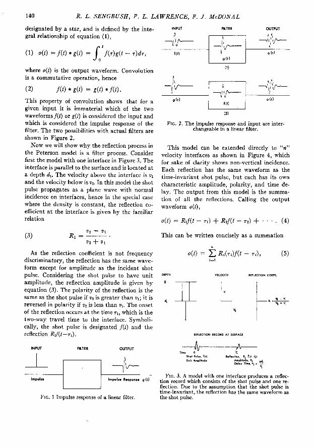
where o(t) is the output waveform. Convolution is a commutative operation, hence

i2> I@> * g(4 = go> *fit)-

This property of convolution shows that for a given input it is imma~terial~ which of the two waveformsf(t) or g(l) is considered the input and which is considered the impulse response of the filter. The two possibilities -with acttual filters ares shown in Figure 2.

Now we will show why the reflection process in the Peterson model is a filter process. Consider first the model with one interface in Figure 3. The interface is parallel to the surface and is located at a depth dl. The velocity above the interface is Q and the velocity below is v2. In this model the shot pulse propagates as a plane wave with normal incidence on interfaces, hence in the special case where the density is constant, the reflection coefficient at the interface is given by the familiar relation

v2 - Vl R1=.-.-.

82 + 81

As the reflection coefficient is not frequency discriminatory, the reflection has the same waveform except for amplitude as the incident shot pulse. Considering the shot pulse to have unit amplitude, the reflection amplitude is given by equation (3). The polarity of the reflection is the same as the shot pulse if v2 is greater than vl; it is reversed in polarity if vz is less than ~1. The onset of the reflection occurs at the time ~1, which is the two-way travel time to the interface. Symboli- cally, the shot pulse is designated ,f((t) and the reflection Rlf(t-~~).

INPUT FILTER OUTPUT

d&-r*

FIG. 1 Impulse response of a linear filter.

INPUT FILTER OUTPUT

(2)

FIG. 2. The impulse response and input are inter- changeable in a linear filter.

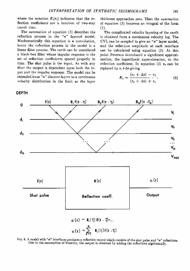
This model can be extended directly to “n” velocity interfaces as shown in Figure 4, which for sake of clarity shows non-vertical incidence. Each reflection has the same waveform as the time-invariant shot pulse, but each has its own characteristic amplitude, polarity, and time delay. The output from this model is the summation of all the reflections. Calling the output waveform o(t),

o(t) = R?f(l - 71) + Rzj(s - 72) + . . . . (4)

This can be written concisely as a summation

n o(t) = 2 Ri(7;)j(l - pi), (5)

i=l

FIG. 3. A model with one interface produces a reflection record which consists of the shot pulse and one re- Section. Due to the assumption that the shot pulse is time-invariant, the reflection has the same waveform as the shot pulse.


where the notation Ri(Ti) indicates that the reflection coefficients are a function of two-way travel time

The summation of equation (5) describes the reflection process in the ‘W’ layered model. Mathematically this equation is a convolution, hence the reflection process in the model is a linear filter process. The earth can be considered a black-box filter whose impulse response is the set of reflection coefficients spaced properly in time The shot pulse is the input. As with any filter the output is dependent upon both the input and the impulse response. The model can be extended from “n” discrete layers to a continuous velocity distribution in the limit as the layer

thickness approaches zero. Then the summation of equation (5) becomes an integral of the form

(1). The complicated velocity layering of the earth

is obtained from a continuous velocity log. The CVL can be sampled to give an “II” layer model, and the reflection amplitude at each interface can be calculated using equation (3). At this point Peterson introduced a significant approximation, the logarithmic approximation, to the reflection coefficient. In equation (3) vz can be replaced by vl+Av giving

R 1 = (VI + Av> - VI ,

(~1 + Av) + vl (6)

DEPTH

d,

4

4

v3 . . .

%I

Vntl

f(t) R(t) 0 (t)

Shot pulse Reflection coeff. output

o(t) = R,(T) f(t -3;3+...

0 (t) =$ Ri(X)f(t -X)

FIG. 4. A model with ‘W interfaces produces a reflection record which consists of the shot pulse and “n” reflections. Due to the assumption of linearity, the output is obtained by adding the reflections algebraically.


Av RI =

2vl+ Av

If Av is small compared to vi, which will be true if the CVL is sampled at close enough intervals, equation (7) can be written as an approximation

(8) 1 Av

R,---, 2 Vl

1 A log VI.

R1 = 2

The approximation is very good for reflection coefficients less than 0.3.

If density variations are considered in the model, v must be replaced in equation (9) by the acoustic impedance pv, where p is the density. However, if the density is related to the velocity by the general expression, p = kv”, where k and m are constants, the acoustic impedance becomes

(10) pv = kvm+l.

In equation (9) the reflection coefficient becomes

(11) R = f A log kvm+l,

R = -:_[Alogk+ (m+ l)Alogv],

(12) R = F A log v.

In this case also, the reflection coefficient is proportional to the change in the logarithm of velocity.

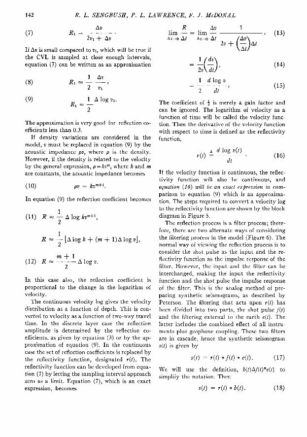
The continuous velocity log gives the velocity distribution as a function of depth. This is con- verted to velocity as a function of two-way travel time In the discrete layer case the reflection amplitude is determined by the reflection coefficients, as given by equation (3) or by the approximation of equation (9). In the continuous case the set of reflection coefficients is replaced by the reflectivity function, designated r(t). The reflectivity function can be developed from equation (7) by letting the sampling interval approach zero as a limit. Equation (7), which is an exact expression, becomes

Az+o At Ai-0 At

\At/

1 dv

= 0 2v dt ’ (14)

1 d 10s~ v (15)

The coefficient of 3 is merely a gain factor and can be ignored. The logarithm of velocity as a function of time will be called the velocity function. Then the derivative of the velocity function with respect to time is defined as the reflectivity function,

(16)

If the velocity function is continuous, the reflectivity function will also be continuous, and equation (16) will be a?z exact expression in comparison to equation (9) which is an approximation. The steps required to convert a velocity log to the reflectivity function are shown by the block diagram in Figure 5.

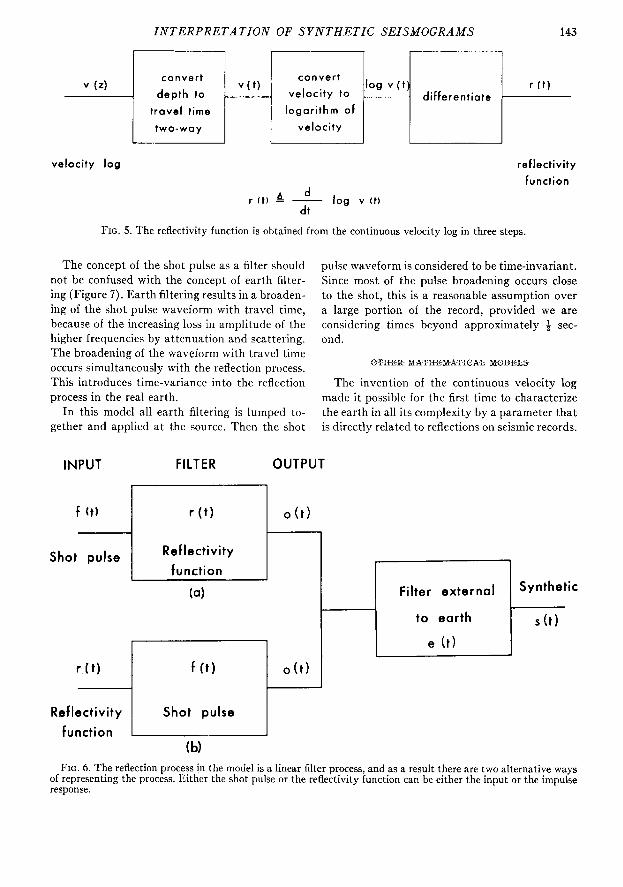
The reflection process is a filter process; therefore, there are two alternate ways of considering the filtering process in the model (Figure 6). The normal way of viewing the reflection process is to consider the shot pulse as the input and the reflectivity function as the impulse response of the filter. However, the input and the filter can be interchanged, making the input the reflectivity function and the shot pulse the impulse response of the filter. This is the analog method of pre- paring synthetic seismograms, as described by Peterson. The filtering that acts upon r(t) has been divided into two parts, the shot pulse j(t) and the filtering external to the earth e(t). The latter includes the combined effect of all instru- ments plus geophone coupling. These two filters are in cascade, hence the synthetic seismogram s(t) is given by

s(t) = r(t) *f(l) * e(t). (17)

We will use the definition, b(t)Af(t)*e(t) to simplify the notation. Then

s(t) = r(t) * b(l). (18)


v (4 convert convert

depth to _ v(t)

velocity to log v(t) r It)

differentiate

travel time logarithm of

two-way velocity

velocity log reflectivity

function d

r ft) P - dt

log v (t)

FIG. 5. The reflectivity function is obtained from the continuous velocity log in three steps.

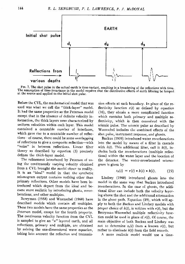
The concept of the shot pulse as a filter should not be confused with the concept of earth filtering (Figure 7). Earth filtering results in a broadening of the shot pulse waveform with travel timebecause of the increasing loss in amplitude of the higher frequencies by attenuation and scattering. The broadening of the waveform with travel timeoccurs simultaneously with the reflection process. This introduces time-variance into the reflection process in the real earth.

In this model all earth filtering is lumped to- gether and applied at the source. Then the shot

INPUT

F (t)

Shot pulse

r(t)

Reflectivity

function

FILTER

r (t)

Reflectivity

function

(a)

f (t)

Shot pulse

(b)

OUTPUT

pulse waveform is considered to be time-invariant. Since most of the pulse broadening occurs close to the shot, this is a reasonable assumption over a large portion of the record, provided we are considering times beyond approximately 4 second.

The invention of the continuous velocity log made it possible for the first time to characterize the earth in all its complexity by a parameter that is directly related to reflections on seismic records.

0 (t)

0 (t)

Filter external Synthetic

FIG. 6. The reflection process in the model is a linear filter process, and as a result there are two alternative ways of representing the process. Either the shot pulse or the reflectivity function can be either the input or the impulse response.


Initial shot pulse

-7 4 4

EARTH

de 4

A/- Reflections from >

various depths

FIG. i’. The shot pulse in the actual earth is time-variant, resulting in a broadening of the reflections with timeThe assumption of time-invariance in the model requires that the distributive effects of earth filtering be lumped at the source and applied to the initial shot pulse.

Before the CVL, the mathematical model that was used was what we call the “thick-layer” model. It had the same properties as the Peterson model except that in the absence of definite velocity information, the thick layers were characterized by uniform velocities within each layer. This model contained a countable number of interfaces, which gave rise to a countable number of reflections-of course, there could be some overlapping of reflections to give a composite reflection-with “noise” in between reflections. Linear filter theory as described by equation (5) precisely defines the thick-layer model.

The refinement introduced by Peterson of using the continuously varying velocity obtained from a CVL brought the model closer to reality. It is an “ideal” model in that the synthetic seismogram output contains nothing other than primary reflections. Other models hare been introduced which depart from the ideal and be- come more realistic by introducing ghosts, reverberations, and other multiples.

Berryman (1958) and Wuenschel (1960) have described models which contain all multiples. These two models have the same properties as the Peterson model, except for the fourth property. The continuous velocity function from the CVL is sampled to give an “n” layered earth, and all reflections, primary and multiple, are obtained by solving the one-dimensional wave equation, taking into account the reflection and transmis-

sion effects at each boundary. In place of the reflectivity function r(t) as defined by equation (16), they obtain a more complicated function which contains both primary and multiple reflectivity, which is then convolved with the seismic pulse. The seismic pulse as described by Wuenschel includes the combined effects of the shot pulse, instrument response, and ghosts.

Backus (1959) introduced water reverberations into the model by means of a filter in cascade with b(t). This additional filter, call it It(t), includes both the reverberations (multiple reflections) within the water layer and the location of the detector. The water-reverberated seismogram is given by

s/&(t) = r(t) * f?(t) * h(t). (19)

Lindsey (1960) introduced ghosts into the mode! in the same way that Backus introduced reverberations. In the case of ghosts, the additional filter can include both the velocity layering above the shot and the additional attenuation in the ghost path. Equation (19), which will ap- ply to both the Backus and Lindsey models with proper choice of h(t), is written with r(t), but the Berryman-Wuenschel multiple reflectivity function could be used in place of r(t). Of course, the main objective of both Backus and Lindsey was not to determine sh(l) from a known r(l), but rather to eliminate h(t) from the field records.

A more realistic model would use a time-

INTERPRETATION OF SYNTHETIC SEISMOGRAMS

variant shot pulse. The mathematics is only slightly more complicated, and time-variant synthetics could be easily calculated using digital computers. With analog equipment, an adequate approximation to time-variance can be accom- plished piece-wise by using different filters for different sections of the record if the time- variance is slow with respect to the time constants of b(t).

We do not intend to discuss further any of the models other than the Peterson model. We will continue with a discussion of the reflections from some simple velocity functions as a basis for the more general velocity functions obtained from CVL’S.

SIMPLE VELOCITY FUNCTIONS

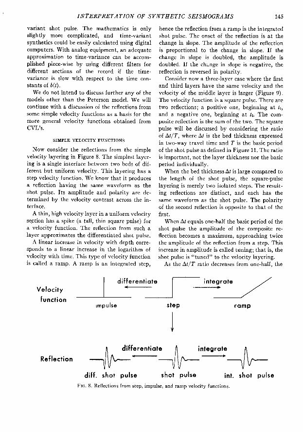
Now consider the reflections from the simple velocity layering in Figure 8. The simplest layering is a single interface between two beds of different but uniform velocity. This layering has a step velocity function. We know that it produces a reflection having the same waveform as the shot pulse. Its amplitude and polarity are determined by the velocity contrast across the interface.

A thin, high velocity layer in a uniform velocity section has a spike (a tall, thin square pulse) for a velocity function. The reflection from such a layer approximates the differentiated shot pulse.

A linear increase in velocity with depth corre- sponds to a linear increase in the logarithm of velocity with time This type of velocity function is called a ramp. A ramp is an integrated step,

I. /

Velocity

function

/ differentiate 1 interate /

Impulse step ramp

hence the reflection from a ramp is the integrated shot pulse. The onset of the reflection is at the change in slope. The amplitude of the reflection is proportional to the change in slope. If the change in slope is doubled, the amplitude is doubled. If the change in slope is negative, the reflection is reversed in polarity.

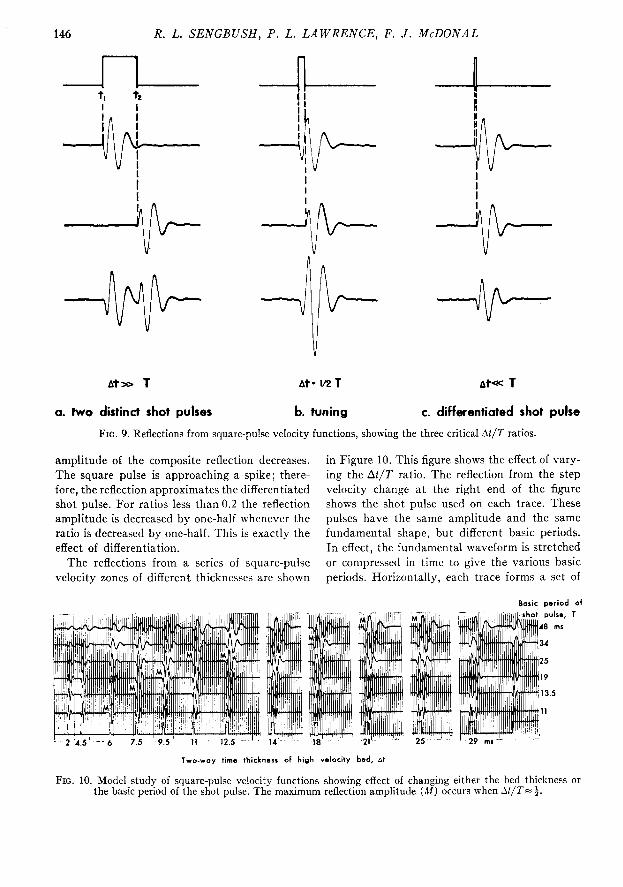
Consider now a three-layer case where the first and third layers have the same velocity and the velocity of the middle layer is larger (Figure 9). The velocity function is a square pulse. There are two reflections; a positive one, beginning at t,, and a negative one, beginning at tz. The composite reflection is the sum of the two. The square pulse will be discussed by considering the ratio of At/T, where At is the bed thickness expressed in two-way travel time and T is the basic period of the shot pulse as defined in Figure 11. The ratio is important, not the layer thickness nor the basic period individually.

When the bed thickness At is large compared to the length of the shot pulse, the square-pulse layering is merely two isolated steps. The resulting reflections are distinct, and each has the same waveform as the shot pulse. The polarity of the second reflection is opposite to that of the first.

When At equals one-half the basic period of the shot pulse the amplitude of the composite reflection becomes a maximum, approaching twice the amplitude of the reflection from a step. This increase in amplitude is called tuning; that is, the shot pulse is “tuned” to the velocity layering.

As the A.t/T ratio decreases from one-half, the

Reflection

diff. shot pulse shot pulse int. shot pulse

FIG. 8. Reflections from step, impulse, and ramp velocity functions.


i ik-

&t=+ T

a. two distinct shot pulses

At= t/2T

b. tuning

Ata T

c. differentiated shot pulse

FIG. 9. Reflections from square-pulse velocity functions, showing the three critical At/T ratios.

amplitude of the composite reflection decreases. in Figure 10. This figure shows the effect of vary- The square pulse is approaching a spike; there- ing the At/T ratio. The reflection from the step fore, the reflection approximates the differentiated velocity change at the right end of the figure shot pulse. For ratios less than 0.2 the reflection shows the shot pulse used on each trace. These amplitude is decreased by one-half whenever the pulses have the same amplitude and the same ratio is decreased by one-half. This is exactly the fundamental shape, but different basic periods. effect of differentiation. In effect, the fundamental waveform is stretched

The reflections from a series of square-pulse or compressed in time to give the various basic velocity zones of different thicknesses are shown periods. Horizontally, each trace forms a set of

Two-way time thickness of high velocity bed, it

Boric period of

T

FIG. 10. Model study of square-pulse velocity functions showing effect of changing either the bed thickness or the basic period of the shot pulse. The maximum reflection amplitude (M) occurs when At/T-f.


reflections where the basic period of the shot pulse is held constant and the bed thickness is varied. Vertically, there is another set of reflections where the bed thickness is held constant and the basic period is varied. The tuning effect can be seen by following either a horizontal or a vertical set of reflections. As the ratio approaches one-half, the reflection amplitude becomes a maximum. The largest reflections for each horizontal and vertical set are labeled M on the figure.

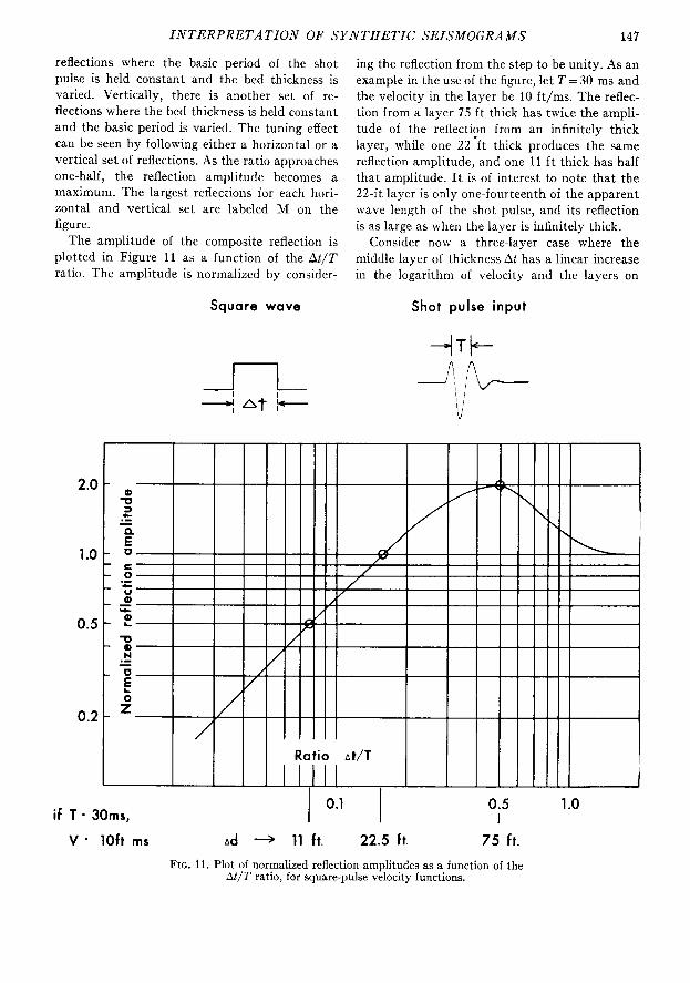
The amplitude of the composite reflection is plotted in Figure 11 as a function of the At/T ratio. The amplitude is normalized by consider-

Square wuve

ing the reflection from the step to be unity. As an example in the use of the figure, let T = 30 ms and the velocity in the layer be 10 ft/ms. The reflection from a layer 75 ft thick has twiLe the amplitude of the reflection from an infinitely thick layer, while one 22 *ft thick produces the same reflection amplitude, and one 11 ft thick has half that amplitude. It is of interest to note that the 22-ft layer is only one-fourteenth of the apparent wave length of the shot pulse, and its reflection is as large as when the layer is infinitely thick.

Consider now a three-layer case where the middle layer of thickness At has a linear increase in the logarithm of velocity and the layers on

Shot pulse input

FIG. 11. Plot of normalized reflection amplitudes as a function of the At/P’ ratio, for square-pulse velocity functions.


-A-- t, 6 I I I I

At>> T At' l/Z T At - T

a; two distinct b. tuning of c. shot pulse

integrated shot pulses integrated shot pulses

FIG. 12. Reflection from ramp-transition velocity functions, showing the three critical At/T ratios.

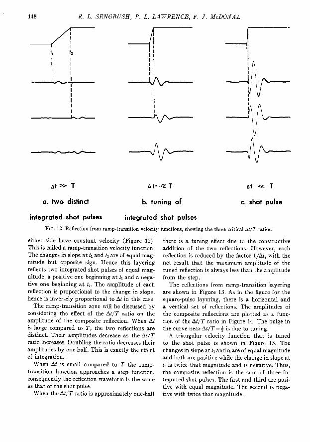
either side have constant velocity (Figure 12). This is called a ramp-transition velocity function. The changes in slope at tr and tz are of equal magnitude but opposite sign. Hence this layering reflects two integrated shot pulses of equal magnitude, a positive one beginning at tl and a negative one beginning at tz. The amplitude of each reflection is proportional to the change in slope, hence is inversely proportional to Al in this case.

The ramp-transition zone will be discussed by considering the effect of the At/T ratio on the amplitude of the composite reflection. When At is large compared to T, the two reflections are distinct. Their amplitudes decrease as the At/T ratio increases. Doubling the ratio decreases their amplitudes by one-half. This is exactly the effect of integration.

When At is small compared to T the ramp- transition function approaches a step function, consequently the reflection waveform is the same as that of the shot pulse.

When the At/T ratio is approximately one-half

there is a tuning effect due to the constructive addition of the two reflections. However, each reflection is reduced by the factor l/At, with the net result that the maximum amplitude of the tuned reflection is always less than the amplitude from the step.

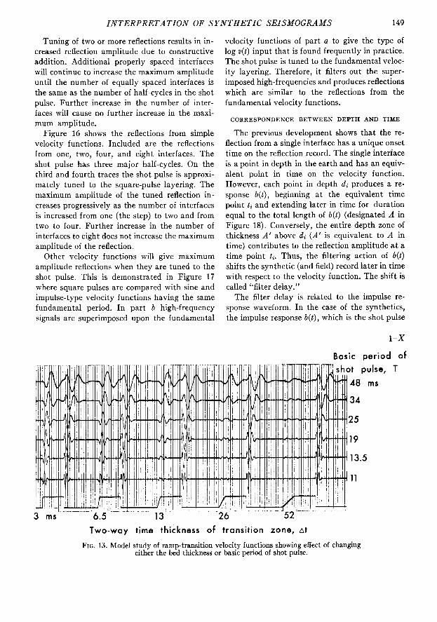
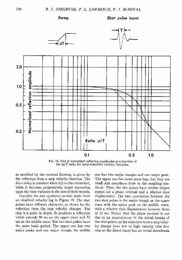
The reflections from ramp-transition layering are shown in Figure 13. As in the figure for the square-pulse layering, there is a horizontal and a vertical set of reflections. The amplitudes of the composite reflections are plotted as a function of the At/T ratio in Figure 14. The bulge in the curve near At/T = 4 is due to tuning.

A triangular velocity function that is tuned to the shot pulse is shown in Figure 1.5. The changes in slope at tl and t3 are of equal magnitude and both are positive while the change in slope at 1~ is twice that magnitude and is negative. Thus, the composite reflection is the sum of three integrated shot pulses. The first and third are positive with equal magnitude. The second is negative with twice that magnitude.


Tuning of two or more reflections results in increased reflection amplitude due to constructive addition. Additional properly spaced interfaces will continue to increase the maximum amplitude until the number of equally spaced interfaces is the same as the number of half-cycles in the shot pulse. Further increase in the number of interfaces will cause no further increase in the maximum amplitude.

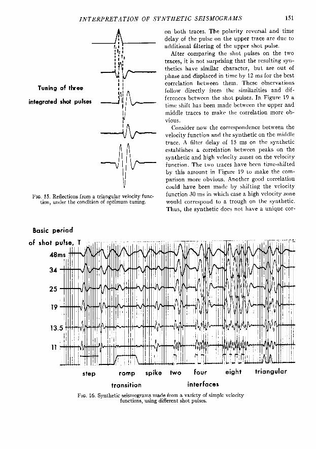
Figure 16 shows the reflections from simple velocity functions. Included are the reflections from one, two, four, and eight interfaces. The shot pulse has three major half-cycles. On the third and fourth traces the shot pulse is approximately tuned to the square-pulse layering. The maximum amplitude of the tuned reflection increases progressively as the number of interfaces is increased from one (the step) to two and from two to four. Further increase in the number of interfaces to eight does not increase the maximum amplitude of the reflection.

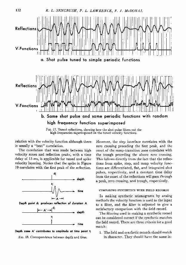
Other velocity functions will give maximum amplitude reflections when they are tuned to the shot pulse. This is demonstrated in Figure 17 where square pulses are compared with sine and impulse-type velocity functions having the same fundamental period. In part b high-frequency signals are superimposed upon the fundamental

velocity functions of part a to give the type of log v(t) input that is found frequently in practice. The shot pulse is tuned to the fundamental velocity layering. Therefore, it filters out the superimposed high-frequencies and produces reflections which are similar to the reflections from the fundamental velocity functions.

CORRESPONDENCE BETWEEN DEPTH AND time

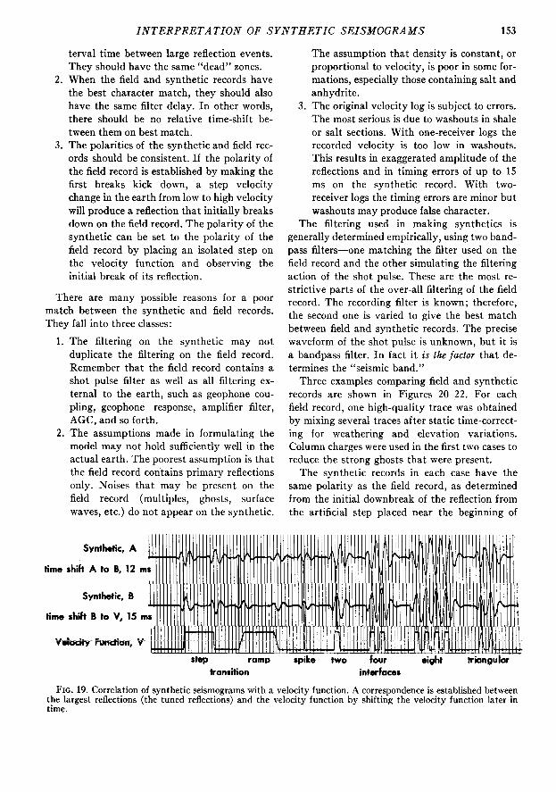
The previous development shows that the reflection from a single interface has a unique onset time on the reflection record. The single interface is a point in depth in the earth and has an equivalent point in time on the velocity function. However, each point in depth di produces a response b(t), beginning at the equivalent timepoint t, and extending later in time for duration equal to the total length of b(t) (designated A in Figure 18). Conversely, the entire depth zone of thickness A’ above di (A’ is equivalent to A in time) contributes to the reflection amplitude at a time point ti. Thus, the filtering action of b(t) shifts the synthetic (and_fIeld) record~later in timewith respect to the velocity function. The shift is called “filter delay.”

The filter delay is related to the impulse response waveform. In the case of the synthetics, the impulse response b(t), which is the shot pulse

1-X

Basic period of

Two-way time thickness of transition zone, At

FIG. 13. Model study of ramp-transition velocity functions showing effect of changing either the bed thickness or basic period of shot pulse.

T


Ramp Shot pulse input

-

-

- - - - -

-

-

-

-

-

Ratio At/T

0.1

FIG. 14. Plot of normalized reflection amplitudes as a function of the At/T ratio, for ramp-transition velocity functions.

as modified by the external filtering, is given by the reflection from a step velocity function. The filter delay is constant when b(l) is time-invariant, while it becomes progressively larger depending upon the time-variance in the case of field records.

Consider the two synthetic records made from an idealized velocity log in Figure 19. The shot pulses have different character, as shown by the reflection from the step velocity changes. The step is a point in depth. It produces a reflection which extends 70 ms on the upper trace and 5.5 ms on the middle trace. The two shot pulses have the same basic period. The upper one has two major peaks and one major trough; the middle

one has two major troughs and one major peak. The upper one has some extra legs, but they are small and contribute little to the resulting synthetic. Thus, the two pulses have similar shapes except for a phase reversal and a relative timedisplacement. The best correlation between the two shot pulses is the major trough on the upper trace with the major peak on the middle trace, with a relative time displacement between them of 12 ms. Notice that the phase reversal is not due to an inconsistency in the initial breaks of the shot pulses, as the reflection from a step velocity change from low to high velocity (the first step on the direct trace) has an initial downbreak


Tuning of three

integrated shot pulses

FIG. 15. Reflections from a triangular velocity function, under the condition of optimum tuning.

Basic period

on both traces. The polarity reversal and timedelay of the pulse on the upper trace are due to additional filtering of the upper shot pulse.

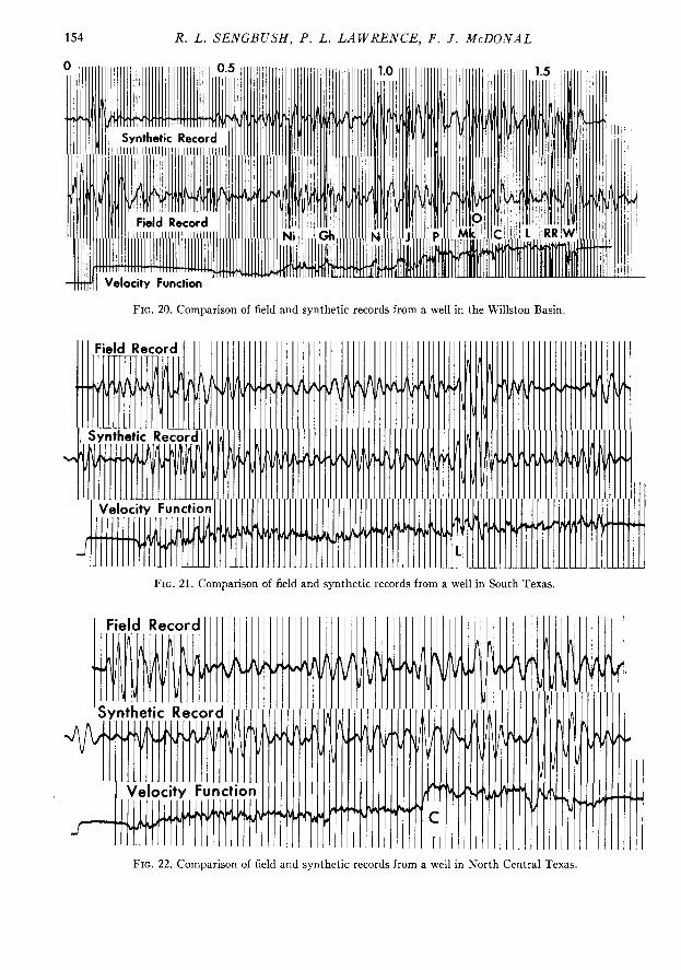
After comparing the shot pulses on the two traces, it is not surprising that the resulting synthetics have similar character, but are out of phase and displaced in time by 12 ms for the best correlation between them. These observations follow directly from the similarities and dif- ferences between the shot pulses. In Figure 19 a time shift has been made between the upper and middle traces to make the correlation more obvious.

Consider now the correspondence between the velocity function and the synthetic on the middle trace. A filter delay of 15 ms on the synthetic establishes a correlation between peaks on the synthetic and high velocity zones on the velocity function. The two traces have been tiple-shifted by this amount in Figure 19 to make the comparison more obvious. Another good correlation could have been made by shifting the velocity function 30 ms in which case a high velocity zone would correspond to a trough on the synthetic. Thus, the synthetic does not have a unique cor-

step ramp spike two four eight triangular

transition interfaces

FIG. 16. Synthetic seismograms made from a variety of simple velocity functions, using different shot pulses.


Reflections

V-Functions

a. Shot pulse tuned to simple periodic functions

II Reflections

V-Functions ! 1

b. Same shot pulse and same periodic functions with random

high frequency function superimposed

FIG. 17. Tuned reflections, showing how the shot pulse filters out the high frequencies superimposed on the tuned-velocity functions.

relation with the velocity function although there is usually a “best” correlation.

The correlation that was made between high velocity zones and reflection peaks, with a timedelay of 15 ms, is applicable for tuned and spike velocity layering. Notice that the spike in Figure 19 correlates with the first peak of the reflection.

4 L depth

However, the step interface correlates with the zero crossing preceding the first peak, and the onset of the ramp-transition zone correlates with the trqugh preceding the above zero crossing. This follows directly from the fact that the reflections from spike, step, and ramp velocity functions are differentiated, flat, and integrated shot pulses, respectively, and a constant time delay from the onset of the reflections will pass through a peak, zero crossing, and trough, respectively.

time COMPARING SYNTHETICS WITH FIELD RECORDS

IcA-4

Depth point di produces reflection of dumtion A

kAA.+di - deph

;I time

Depth zone A’ contributes to amplitude at time point $

FIG. 18. Correspondence between depth and time

In making synthetic seismograms by analog methods the velocity function is used as the input to a filter, and the filter is adjusted to give a satisfactory comparison with the field record.

The filtering used in making a synthetic record can be considered correct if the synthetic ma~tches the field record. There are three criteria for a good match:

1. The field and synthetic records should match in character, They should have the same in-


terval time between large reflection events. They should have the same “dead” zones.

2. When the field and synthetic records have the best character match, they should also have the same filter delay. In other words, there should be no relative time-shift between them on best match.

3. The polarities of the synthetic and field records should be consistent. If the polarity of the field record is established by making the first breaks kick down, a step velocity change in the earth from low to high velocity will produce a reflection that initially breaks down on the field record. The polarity of the synthetic can be set to the polarity of the field record by placing an isolated step on the velocity function and observing the initial break of its reflection.

There are many possible reasons for a poor match between the synthetic and field records. They fall into three classes:

. The filtering on the synthetic may not duplicate the filtering on the field record. Remember that the field record contains a shot pulse filter as well as all filtering external to the earth, such as geophone coupling, geophone response, amplifier filter, AGC, and so forth.

2. The assumptions made in formulating the model may not hold sufficiently well in the actual earth. The poorest assumption is that the field record contains primary reflections only. Noises that may be present on the field record (multiples, ghosts, surface waves, etc.) do not appear on the synthetic.

3.

The assumption that density is constant, or proportional to velocity, is poor in some for- mations, especially those containing salt and anhydrite. The original velocity log is subject to errors. The most serious is due to washouts in shale or salt sections. With one-receiver logs the recorded velocity is too low in washouts. This results in exaggerated amplitude of the reflections and in timing errors of up to 15 ms on the synthetic record. With two- receiver logs the timing errors are minor but washouts may produce false character.

The filtering used in making synthetics is generally determined empirically, using two bandpass filters-one matching the filter used on the field record and the other simulating the filtering action of the shot pulse. These are the most re- strictive parts of the over-all filtering of the field record. The recording filter is known; therefore, the second one is varied to give the best match between field and synthetic records. The precise waveform of the shot pulse is unknown, but it is a bandpass filter. In fact it is the factor that de- termines the “seismic band.”

Three examples comparing field and synthetic records are shown in Figures 20-22. For each field record, one high-quality trace was obtained by mixing several traces after static time-correct- ing for weathering and elevation variations. Column charges were used in the first two cases to reduce the strong ghosts that were present.

The synthetic records in each case have the same polarity as the field record, as determined from the initial downbreak of the reflection from the artificial step placed near the beginning of

Synthetic, A

time shift A to B, 12

Synthetic, B

time shift B to V, 15

step romp

transition spike two four eight triongukr

interfaces

FIG. 19. Correlation of synthetic seismograms with a velocity function. A correspondence is established between the largest reflections (the tuned reflections) and the velocity function by shifting the velocity function later in time

154 R. L. SENGBUSH, P. L. LAWRENCE, F. J. McDO‘VAL

ll1llllMl Synthetic Record lllnlnllll1lIl~

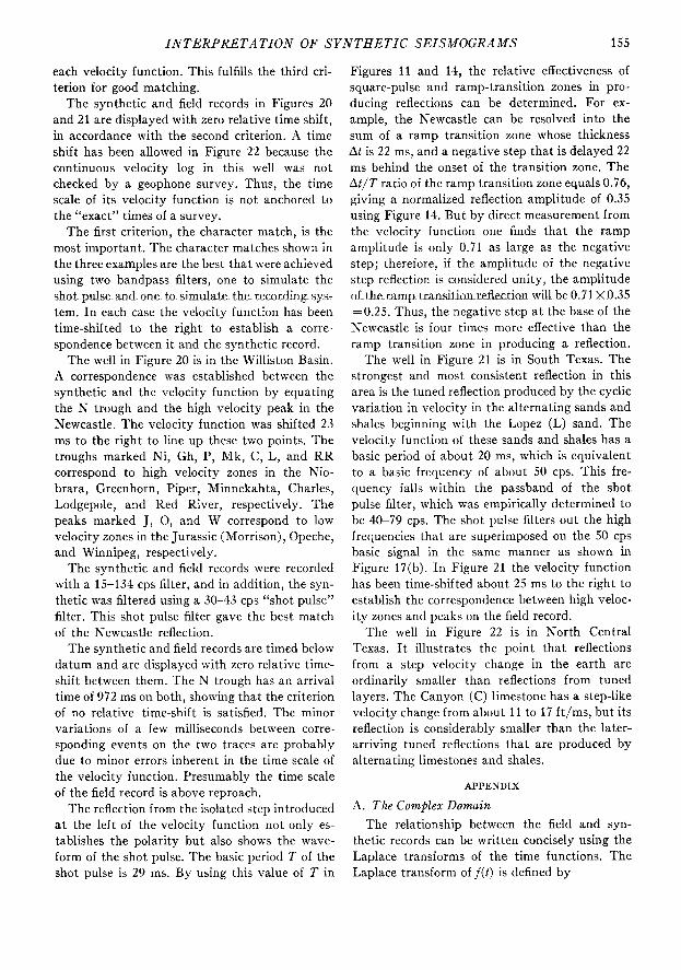
FIG. 20. Comparison of field and synthetic records from a well in the Willston Basin

FIG. 21. Comparison of field and synthetic records from a well in South Texas.

FIG. 22. Comparison of field and synthetic records from a well in North Central Texas.

INTERPRETATION OF SYNTHETIC SEISMOGRAMS 15.5

each velocity function. This fulfills the third criterion for good matching.

The synthetic and field records in Figures 20 and 21 are displayed with zero relative time shift, in accordance with the second criterion. A timeshift has been allowed in Figure 22 because the continuous velocity log in this well was not checked by a geophone survey. Thus, the timescale of its velocity function is not anchored to the “exact” times of a survey.

The first criterion, the character match, is the most important. The character matches shown in the three examples are the best that were achieved using two bandpass filters, one to simulate the shot pulse and one to simulate the recor~ding sys- tem. In each case the velocity function has been time-shifted to the right to establish a correspondence between it and the synthetic record.

The well in Figure 20 is in the Williston Basin. A correspondence was established between the synthetic and the velocity function by equating the K trough and the high velocity peak in the Newcastle. The velocity function was shifted 23 ms to the right to line up these two points. The troughs marked Ni, Gh, P, Mk, C, L, and RR correspond to high velocity zones in the Nio- brara, Greenhorn, Piper, Minnekahta, Charles, Lodgepole, and Red River, respectively. The peaks marked J, 0, and W correspond to low velocity zones in the Jurassic (Morrison), Opeche, and Winnipeg, respectively.

The synthetic and field records were recorded with a 15-134 cps filter, and in addition, the synthetic was filtered using a 30-43 cps “shot pulse” filter. This shot pulse filter gave the best match of the Newcastle reflection.

The synthetic and field records are timed below datum and are displayed with zero relative time- shift between them. The N trough has an arrival time of 972 ms on both, showing that the criterion of no relative time-shift is satisfied. The minor variations of a few milliseconds between corresponding events on the two traces are probably due to minor errors inherent in the time scale of the velocity function. Presumably the time scale of the field record is above reproach.

The reflection from the isolated step introduced at the left of the velocity function not only establishes the polarity but also shows the waveform of the shot pulse. The basic period T of the shot pulse is 29 ms. By using this value of T in

Figures 11 and 14, the relative effectiveness of square-pulse and ramp-transition zones in producing reflections can be determined. For example, the Newcastle can be resolved into the sum of a ramp transition zone whose thickness At is 22 ms, and a negative step that is delayed 22 ms behind the onset of the transition zone. The At/T ratio of the ramp transition zone equals 0.76, giving a normalized reflection amplitude of 0.35 using Figure 14. But by direct measurement from the velocity function one finds that the ramp amplitude is only 0.71 as large as the negative step; therefore, if the amplitude of the negative step reflection is considered unity, the amplitude oftheramp transidonretlection will be 0.71 X0.35 =0.25. Thus, the negative step at the base of the Newcastle is four times more effective than the ramp transition zone in producing a reflection.

The well in Figure 21 is in South Texas. The strongest and most consistent reflection in this area is the tuned reflection produced by the cyclic variation in velocity in the alternating sands and shales beginning with the Lopez (L) sand. The velocity function of these sands and shales has a basic period of about 20 ms, which is equivalent to a basic frequency of about 50 cps. This frequency falls within the passband of the shot pulse filter, which was empirically determined to be 40-79 cps. The shot pulse filters out the high frequencies that are superimposed on the 50 cps basic signal in the same manner as shown in Figure 17(b). In Figure 21 the velocity function has been time-shifted about 25 ms to the right to establish the correspondence between high velocity zones and peaks on the field record.

The well in Figure 22 is in Korth Central Texas. It illustrates the point that reflections from a step velocity change in the earth are ordinarily smaller than reflections from tuned layers. The Canyon (C) limestone has a step-like velocity change from about 11 to 17 ft/ms, but its reflection is considerably smaller than the later- arriving tuned reflections that are produced by alternating limestones and shales.

APPENDIX

A. The Complex Domain

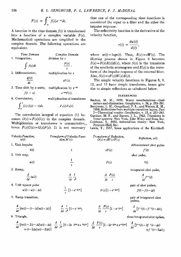
The relationship between the field and synthetic records can be written concisely using the Laplace transforms of the time functions. The Laplace transform of f(t) is defined by


F(s) = s

-f(l),-w. 0

A function in the time domainf(t) is transformed into a function of a complex variable F(s). Mathematical operations are simplified in the complex domain. The following operations are equivalent:

time Domain 1. Integration;

Complex Domain division by s

s fW F(s) -.

s

2. Differentiation;

d!(t) dl

multiplication by s

3. time shift by a units; multiplication by e-~*

f@ - a) c=*F(s).

4. Convolution; multiplication of transforms

s O>&)j& - z)dT Fh)Fz(s).

The convolution integral of equation (1) becomes O(S) =F(s)G(s) in the complex domain. Multiplication of transforms is commutative,, hence F(s)G(s)=G(s)F(s). It is not necessary

V&city ~~unclion, 4)

1. Unit impulse

60) 2. Unit step,

3. Ramp,

4. Unit square pulse

u(t)--(l-At)

5. Ramp transition,

Transform of Velocity Func- tion, W(s)

1 -

A 1 -- Al s2

f [l_e-Ata]

% [lu(t)-((t-A6)u(6-AQ] $ ; [lee-At6,

6. Triangle,

that one of the corresponding time functions is considered the input to a filter and the other the impulse response.

The reflectivity function is the derivative of the velocity function,

Wt) r(t) = ~

40 ’ where w(t) =logs(t). Thus, R(s) =sW(s). The filtering process shown in Figure 6 becomes S(S) =F(s)R(s)E(s), where S(S) is the transform of the synthetic seismogram and E(s) is the transform of the impulse response of the external filter. Also, S(S) =sF(s)W(s)E(s).

The simple velocity functions in Figures 8, 9, 12, and 15 have simple transforms, hence give rise to simple reflections as tabulated below.

REFERENCES

Backus, M. M., 1959, Water reverberations-their nature and elimination: Geophysics, v. 24, p. 233-261.

Berryman, L. H., Goupillaud, P. L., and Waters, I(. H., 19.58, Reflections from multiple transition layers. Part I-Theoretical results: Geophysics, v. 23, p. 223-243.

Gardner, M. F., and Barnes, J. I,., 1942, Transients in linear systems: New York, John Wiley and Sons, Inc.

Goldman, S., 1953, Information theory: New York, Prentice-Hall, Inc.

Lewis, T., 1937, Some applications of the Kirchhoff-

Transform of Rejeclion, O(s) =sW(s)F(s)

SF(S)

A F(s) --- A6 s

F(s) [ 1 -e-At*]

; +! [l_e-A’s]

RejEection, o(6)

differentiated shot pulse,

f’(t)

shot pulse,

f(6)

integrated shot pulse,

$ f-‘(6)

pair of shot pulses,

f(t)-f(t--6)

pair of integrated shot pulses,

; b-l(t)-f-l(t-At)]

three integrated shot upl&s,

% [lu(t)-2(6-At)w(t-A6) $ $ [1-2e-A’*+e*@]

+(6--2A6)u(&2At)]

6 y [1-2e-Ati+e-zA’a] 2 [f-l(6)-2f-‘(t-At)

+f-‘(t-2At) J

interpretation OF SYNTHETIC SEISMOGRAMS 157

Dirac function in problems involving solutions of the classical wave equation: Philosophical Magazine, v. 7, p. 329-360.

Lindsey, J. P., 1960, Elimination of seismic ghost reflections by means of a linear filter: Geophysics, v. 25, p. 130-140.

Peterson, R. A., Fillipone, W. R., and Coker, F. B., 1955, The synthesis of seismograms from well log data: Geophysics, v. 20, p. 516-538.

Piety,. R. G., 1942, Interpretation of the transient be- pr of the reflection seismograph: Geophysics, v. , p. 123-132.

Smith, M. K., 1958, A review of methods of filtering seismic data: Geophysics, v. 23, p. 44-57.

Swartz, C. A., and Sokoloff, V. M., 1954, Filtering as-

sociated with selective sampling of geophysical data: Geophysics, v. 19, p. 402-419.

Truxal, J. G., 1955, Automatic feedback control synthesis: McGraw-Hill, Inc., New York.

Widess, M. B., and Taylor, G. L., 1959, Seismic reflections from layering within the Precambrian basement complex, Oklahoma: Geophysics, v. 24, p. 417-425.

Wolf, A.! 1937, The reflection of elastrc waves from transitron layers of variable velocity: Geophysics, v. 2. D. 357-363.

Wobhs, J. P., 1956, The composition of reflections: Geo- physrcs, v. 21, p. 261-276.

Wuenschel, P. C., 1960, Seismogram synthesis including multiples and transmission coefficients: Geophysics, v. 25. p. 106-129.

INTERPRETATION OF SYNTHETIC SEISMOGRAMS

Documents