INTERPRETATION OF MINI-FRAC AND FLOWBACK PRESSURE RESPONSE: APPLICATION TO UNCONVENTIONAL RESERVOIRS IN THE UAE by Omar T. Khaleel

Welcome message from author
This document is posted to help you gain knowledge. Please leave a comment to let me know what you think about it! Share it to your friends and learn new things together.
Transcript

INTERPRETATION OF MINI-FRAC AND FLOWBACK PRESSURE
RESPONSE: APPLICATION TO UNCONVENTIONAL
RESERVOIRS IN THE UAE
by
Omar T. Khaleel

© Copyright by Omar T. Khaleel, 2019
All Rights Reserved

ii
A thesis submitted to the faculty and the board of trustees of the Colorado School of Mines in
partial fulfillment of the requirements for the degree of Doctor of Philosophy (Petroleum
Engineering)
Golden, Colorado
Date: _________________________
Signed: _________________________
Omar T. Khaleel
Signed: _________________________
Dr. Hossein Kazemi
Thesis Advisor
Signed: _________________________
Dr. Waleed AlAmeri
Thesis Co-Advisor
Golden, Colorado
Date: _________________________
Signed: _________________________
Dr. Jennifer Miskimins
Associate Professor and Interim Head
Department of Petroleum Engineering
iii
ABSTRACT
The main objective of the thesis was to develop a working knowledge of the underlying
concepts for developing unconventional shale in the UAE Diyab formation. To achieve this
objective, I identified four broad subsets as listed: (1) Reservoir engineering evaluation of the UAE
Diyab (Upper Jurassic, gas condensate) and Shilaif (Middle Cretaceous, light oil) unconventional
shale development. (2) Conduct laboratory experiments in Diyab cores to determine benchtop
permeability of cores with and without fractures. (3) Understand the mini-frac pressure fall-off
analysis as the major method for determining in-situ matrix permeability for use in reservoir
evaluation, modeling, and forecasting performance of stimulated shale reservoirs. (4) Determine
permeability enhancement in a Diyab stimulated well using rate transient analysis (RTA). This
permeability is the effective permeability composed of matrix rock permeability and microfracture
permeability of the stimulated reservoir section.
In regard to reservoir evaluation, I constructed a compositional reservoir model of Shilaif
light oil in a small sector surrounding an exploration well. To obtain the stimulated reservoir
permeability, and permeability of imbedded fracture system, I performed rate transient analysis
(RTA) using the Shilaif exploration well production data. Finally, I used this permeability in the
compositional model of the reservoir to forecast the well’s future performance.
In regard to laboratory experiments, I measured permeability of fractured and unfractured
core samples from Diyab. Finally, much of my time was spent on evaluating the mini-frac pressure
fall-off theory, and determining the effect of hydraulic fracture filtrate on the magnitude of the
stress changes near the two surfaces of the hydraulic fracture which provided information about
the extent of micro-fracture creation and re-stimulation.
iv
Among the four objectives, evaluation of the mini-frac theory and its interpretation
consumed most of my research effort. Mini-frac injection tests, commonly known as Diagnostic
Fracture Injection Test (DFIT), are of great value in determining the minimum horizontal stress
and permeability of the matrix rock under reservoir conditions. This permeability can be compared
with the permeability of core samples from the same formation to determine how closely
laboratory-measured permeabilities reflect the formation permeability under reservoir stress
conditions.
In this thesis, (1) I present both analytical and numerical modeling of single- and two-phase
flow in support of the interpretation of the pressure falloff from field DFIT data, and (2) I analyze
the pressure falloff data of a laboratory conducted DFIT in a granite core by Luke Frash (Ph.D.
Thesis, CSM, 2014). I applied my interpretative procedures used on the laboratory DFIT data to a
mini-frac test from Diyab formation.
Finally, I determined the depth of filtrate invasion and depth of formation cooling. I used
the quantitative information of filtrate invasion, formation cooling, and rock deformation at
fracture surface to determine the net stress change near the surface of the fracture, which is
commonly referred to as the ‘stress shadow’ effect.
v
TABLE OF CONTENTS
ABSTRACT ................................................................................................................................... iii
LIST OF FIGURES ..................................................................................................................... xiii
LIST OF TABLES .......................................................................................................................xxv
NOMENCLATURE .................................................................................................................. xxix
ACKNOWLEDGMENT.......................................................................................................... xxxiii
CHAPTER 1 INTRODUCTION .....................................................................................................1
1.1 Background ....................................................................................................................... 1
1.2 Methodology and Problem Statement ............................................................................. 10
1.3 Organization of the Thesis .............................................................................................. 12
CHAPTER 2 LITERATURE REVIEW .......................................................................................13
2.1 Hydraulic Fracturing ....................................................................................................... 13
2.2 Fracture Mechanics ......................................................................................................... 14
2.3 Fracture Propagation Models .......................................................................................... 18
2.3.1 PKN Model ............................................................................................................ 19
2.3.2 KGD Model ........................................................................................................... 20

vi
2.3.3 Radial Model .......................................................................................................... 21
2.4 Stress Shadow .................................................................................................................. 21
2.4.1 Poroelastic Effect ................................................................................................... 23
2.4.2 Thermoelastic Effect .............................................................................................. 24
2.4.3 Fracture Expansion ................................................................................................ 24
2.4.4 Total Effect ............................................................................................................ 25
2.5 Diagnostic Fracture Injection Test .................................................................................. 26
2.5.1 G-Function Analysis .............................................................................................. 30
2.5.2 Barree et al. Square-Root of Time Analysis .......................................................... 31
2.5.3 Log-Log Pressure Derivative ................................................................................. 32
2.5.4 After Closure Analysis ........................................................................................... 33
2.6 United Arab Emirates Petroleum Systems ...................................................................... 33
2.6.1 Shilaif Formation ................................................................................................... 36
2.6.2 Diyab Formation .................................................................................................... 39
CHAPTER 3 GEOLOGY, PETROPHYSICS AND GEOCHEMISTRY .....................................41
vii
3.1 Sedimentology ................................................................................................................. 41
3.1.1 Thin Section Analysis ............................................................................................ 41
3.1.2 Scanning Electron Microscopy .............................................................................. 44
3.2 Integration of Geology and Well Logs ............................................................................ 47
3.2.1 FMI ........................................................................................................................ 47
3.2.2 Lithoscanner and GEOFLEX Mineralogy Logs .................................................... 51
3.3 Geochemistry ................................................................................................................... 51
3.3.1 Total Organic Carbon ............................................................................................ 52
3.3.2 Vitrinite reflectance ............................................................................................... 57
3.4 Geomechanics ................................................................................................................. 59
3.4.1 Mohr-Coulomb failure envelope ........................................................................... 61
3.4.2 Brazilian Test ......................................................................................................... 62
3.5 Sample Description ......................................................................................................... 63
CHAPTER 4 MATHEMATICAL MODELS ..............................................................................65
4.1 Geomechanical Model Description ................................................................................. 65

viii
4.1.1 Fracture Propagation Model .................................................................................. 66
4.1.2 Depth of Filterate Invasion and Associated Pore Pressure Increase ...................... 73
4.1.3 Filterate Cooling and Thermoelastic Stress ........................................................... 78
4.2 Numerical Model ............................................................................................................. 86
4.3 Hydraulic Fracturing Experiment .................................................................................... 90
4.3.1 Hydraulic Fracturing Experiment Pressure Transient Analysis ............................ 92
4.3.2 Hydraulic Fracturing Experiment G-function Analysis ......................................... 99
4.4 Hydraulic Fracturing Experiment Modeling ................................................................. 103
4.4.1 Numerical Simulation Model for Frash Experiment ........................................... 104
4.4.2 Numerical code validation using CMG model .................................................... 106
4.5 Pressure Falloff Leakoff Theory ................................................................................... 111
4.5.1 Numerical Model Verification ............................................................................. 124
4.6 Field DFIT Analysis ...................................................................................................... 129
4.6.1 Actual Field DFIT Rate Transient Analysis ........................................................ 129
4.6.2 Field G-function analysis ..................................................................................... 134
ix
4.7.1 Field Example Pressure Transient Analysis ........................................................ 137
4.7.2 Field Example G-function Analysis .................................................................... 141
CHAPTER 5 COMPOSITIONAL MODELING .......................................................................143
5.1 Static Model and Grid Setup ......................................................................................... 143
5.2 Model Parameters .......................................................................................................... 145
5.2.1 Petrophysical Parameters ..................................................................................... 145
5.2.2 Initialization ......................................................................................................... 146
5.2.3 PVT Analysis ....................................................................................................... 148
5.2.4 Relative Permeability ........................................................................................... 151
5.2.5 Well Properties .................................................................................................... 154
5.2.6 Hydraulic Fracture Design ................................................................................... 156
5.3 Results and Analysis ..................................................................................................... 160
5.3.1 Rate Transient Analysis ....................................................................................... 160
5.3.2 Pressure Transient Analysis ................................................................................. 163
5.3.3 Production Forecast and History Match .............................................................. 166
x
CHAPTER 6 LABORATORY EXPERIMENTS ......................................................................169
6.1 Core Cleaning ................................................................................................................ 169
6.1.1 Core Preparation .................................................................................................. 169
6.1.2 Soxhlet Extractor ................................................................................................. 170
6.1.3 Procedure ............................................................................................................. 171
6.2 Porosity and Permeability Experiments ........................................................................ 172
6.2.1 Core Measurement System 300 ........................................................................... 172
6.2.2 Procedure ............................................................................................................ 175
6.2.3 Results and Discussion........................................................................................ 175
6.3 Capillary Pressure, Relative Permeability and Residual Saturation Experiments ........ 189
6.3.1 Ultra-High Speed Centrifuge ............................................................................... 189
6.3.2 Procedure ............................................................................................................. 191
6.3.2.1 Saturation ........................................................................................................ 192
6.3.2.2 Calibration ....................................................................................................... 192
6.3.2.3 First Drainage Cycle ....................................................................................... 193
xi
6.3.2.4 Spontaneous Imbibition Cycle ........................................................................ 194
6.3.2.5 Forced Imbibition Cycle ................................................................................. 194
6.4 Results and Discussion .................................................................................................. 195
CHAPTER 7 CONCLUSIONS, RECOMMENDATIONS AND FUTURE WORK .................196
7.1 Conclusions ................................................................................................................... 196
7.2 Recommendations and future work ............................................................................... 197
REFERENCES ............................................................................................................................199
APPENDIX A GEOLOGY..........................................................................................................204
A.1 Sedimentology ..................................................................................................................204
A.1.1 Thin Section Analysis ............................................................................................204
A.1.2 Scanning Electron Microscopy ..............................................................................210
APPENDIX B WELL LOGS.......................................................................................................219
B.1 Integration of Geology and Well Logs .............................................................................219
B.1.1 FMI .........................................................................................................................221
B.1.2 Lithoscanner and GEOFLEX Mineralogy Logs ....................................................226
APPENDIX C GEOCHEMISTRY ..............................................................................................229
xii
C.1 Geochemistry ....................................................................................................................229
C.1.1 Total Organic Carbon .............................................................................................229
C.1.2 Vitrinite Reflectance ..............................................................................................235
APPENDIX D GEOMECHANICS .............................................................................................242
D.1 Geomechanics ..................................................................................................................242
D.1.1 Static vs. Dynamic Elastic Properties ....................................................................245
D.1.2 Mohr-Coulomb failure envelope ............................................................................248
D.1.3 Brazilian Test .........................................................................................................252
D.1.4 Sample Description ................................................................................................253
xiii
LIST OF FIGURES
Figure 1.1 Comparative oil and gas resource triangle (White 2017). ....................................... 2
Figure 1.2 Hydraulic fractured wells contribution to U.S. total oil and gas production
(EIA 2016). ............................................................................................................. 3
Figure 1.3 U.S. gas production over time (EIA 2018b). ........................................................... 4
Figure 1.4 U.S. net gas trade. (EIA 2018b). ............................................................................. 5
Figure 1.5 U.S. history oil production (EIA 2018b). ................................................................ 5
Figure 1.6 U.S. net oil trade (EIA 2018b)................................................................................. 6
Figure 1.7 Structural features of major fields in UAE (EIA 2015). ......................................... 7
Figure 2.1 Cartoon showing a complex fracture network (Michael et al. 2018). ................... 14
Figure 2.2 Schematic drawing illustrating the three fundamental modes of fracture.
A: mode I, tensile or opening; B: mode II, in-plane shear or sliding mode;
C: mode III, anti-plane shear or tearing mode (Pollard and Segall 1987). ........... 16
Figure 2.3 Three in-situ stress regimes (Tutuncu 2015). ........................................................ 17
Figure 2.4 Fracture propagation relative to the in-situ stresses (Salah et al. 2016). ............... 18
Figure 2.5 PKN 2-D fracture model (Ge and Ghassemi 2018)............................................... 19
Figure 2.6 KGD 2-D fracture model (Ge and Ghassemi 2018). ............................................. 20
Figure 2.7 Radial 2-D fracture model (Ge and Ghassemi 2018). .......................................... 21
Figure 2.8 Stress reversal area around hydraulic fracture (Asala et al. 2016). ...................... 22
xiv
Figure 2.9 Plan view showing that the shape of the cooled region controls the ratio of
principal stresses within the cooled region (Perkins and Gonzalez 1985). ........... 22
Figure 2.10 Plane view of two-winged hydraulic fracture (Perkins and Gonzalez 1985). ....... 24
Figure 2.11 Stresses change due to fracture expansion (Pollard and Segall 1987). ................. 25
Figure 2.12 Idealized pressure profile during hydraulic fracture treatment (Cramer and
Nguyen 2013)........................................................................................................ 26
Figure 2.13 Generic DFIT plot illustrating injection rate in black and bottom hole
pressure in red (Barree et al. 2015). ...................................................................... 27
Figure 2.14 A typical misinterpretation of closure pressure from G-function plot
(Baree et al. 2015). ................................................................................................ 29
Figure 2.15 Gas entry effect in real operation (Baree et al. 2015). ........................................... 29
Figure 2.16 Ideal G-Function analysis plot (Baree et al. 2009). ............................................... 30
Figure 2.17 Ideal SQRT(t) analysis plot (Baree et al. 2009). ................................................... 31
Figure 2.18 Ideal Log-Log analysis plot (Baree et al. 2009). ................................................... 32
Figure 2.19 Ideal ACA analysis plot (Baree et al. 2009). ......................................................... 33
Figure 2.20 UAE percentage of world proven reserve (EIA 2018a). ....................................... 34
Figure 2.21 Simplified UAE stratigraphic sequence and hydrocarbon habitat distribution
through time (Alsharhan et al. 2014). ................................................................... 35
Figure 2.22 Sequence stratigraphic framework of the Shilaif formation
(Alsharhan et al. 2014). ......................................................................................... 37
xv
Figure 2.23 Location map of UAE showing oil major oil fields (Alsharhan et al. 2014). ....... 38
Figure 2.24 Sequence stratigraphic correlation of the Diyab/Tuwaiq Mountain/ Hadriya/
Hanifa/ Jubaila formations (Alsharhan et al. 2014). ............................................. 40
Figure 3.1 Sample A thin section images with indicative arrows (ADNOC). ........................ 42
Figure 3.2 Sample A XRD results in bar chart (ADNOC). .................................................... 43
Figure 3.3 Sample B thin section images with indicative arrows (ADNOC). ........................ 43
Figure 3.4 Sample B XRD results in bar chart (ADNOC). .................................................... 44
Figure 3.5 Sample A standard SEM image with analysis (ADNOC). .................................... 45
Figure 3.6 Sample A ion-Milled SEM image with analysis (ADNOC). ................................ 45
Figure 3.7 Sample B standard SEM image with analysis (ADNOC). .................................... 46
Figure 3.8 Sample B ion-Milled SEM image with analysis (ADNOC). ................................ 46
Figure 3.9 Composite log layout showing different datasets integrated in the Diyab
(Jubaila) Formation (ADNOC). ............................................................................ 48
Figure 3.10 Integrating FMI -Feature Intensity –OH Logs (GR Spectroscopy) (ADNOC). .... 49
Figure 3.11 Larger healed (resistive) DRF fractures in Diyab with strike (ADNOC). ............ 50
Figure 3.12 Stubby conductive fractures in Diyab with strike (ADNOC). .............................. 50
Figure 3.13 Lithoscanner mineralogy in Diyab (Jubaila) formation (ADNOC). ..................... 51
Figure 3.14 TOC computed from logs in the Jubaila source rock (ADNOC). ......................... 53
xvi
Figure 3.15 S2 vs TOC % for Diyab samples (ADNOC). ........................................................ 54
Figure 3.16 HI vs OI for Diyab samples (ADNOC). ................................................................ 55
Figure 3.17 HI vs Tmax for Diyab samples (ADNOC). ........................................................... 56
Figure 3.18 Vitrinite reflectance for sample A (ADNOC). ...................................................... 58
Figure 3.19 Solid bitumen reflectance for sample A (ADNOC). ............................................. 58
Figure 3.20 Photomicrographs of sample A (ADNOC). .......................................................... 59
Figure 3.21 Diyab formation geomechanical log (ADNOC). ................................................... 60
Figure 3.22 Failure envelope for Diyab formation sample at shallower depth (ADNOC). ...... 62
Figure 3.23 Core sample before and after Brazilian loading test, (ADNOC). .......................... 63
Figure 3.24 Diyab core sample CT scans illustrating the presence of natural fractures,
(ADNOC). ............................................................................................................. 64
Figure 4.1 Idealization of a two-wing hydraulic fracture with fluid leakoff from the
fracture faces (Charoenwongsa 2012). ................................................................. 66
Figure 4.2 PKN 2-D fracture model (Ge and Ghassemi 2018)............................................... 67
Figure 4.3 Plane view of two-winged hydraulic fracture (Perkins and Gonzalez 1985). ....... 76
Figure 4.4 Stresses change due to fracture expansion (Pollard and Segall 1987). ................. 82
Figure 4.5 Hydraulic fracturing experiment well dimensions (Frash 2014). .......................... 91
Figure 4.6 Granite slab post fracture (Frash 2014). ................................................................ 91
xvii
Figure 4.7 Pressure Profile in an Experiment Conducted in a Granite Slab (Frash 2014) ..... 92
Figure 4.8 Diagnostic p vs. t log-log plot for hydraulic fracturin experiment in a
granite slab. The plot clearly shows a straight line with a slope of 0.5 ............... 93
Figure 4.9 p vs. t plot for L. Frash hydraulic fracturing experiment in a granite
slab. The plot clearly shows a straight line with a slope of 0.5 ............................ 93
Figure 4.10 p vs. pt t t+ − plot for L. Frash hydraulic fracturing experiment
in a granite slab. The plot clearly shows a straight line with a slope of 0.5 ......... 94
Figure 4.11 Frash (2014) G-function pressure profile .............................................................. 99
Figure 4.12 Numerical model logarithmic grid. ..................................................................... 104
Figure 4.13 Numerical model pressure profile. ...................................................................... 105
Figure 4.14 Numerical model code diagnostic plot. ............................................................... 105
Figure 4.15 Numerical model linear flow analysis. ................................................................ 106
Figure 4.16 Three-dimension structural model. ...................................................................... 107
Figure 4.17 Hydraulic fracture in CMG model with refinement of 3-3-1. ............................. 108
Figure 4.18 CMG model pressure profile. .............................................................................. 109
Figure 4.19 CMG model linear and bi-linear flow regimes.................................................... 110
Figure 4.20 CMG model linear flow analysis. ........................................................................ 110
Figure 4.21 CMG model #2 full model grid. .......................................................................... 112
Figure 4.22 CMG model #2 zoomed model grid. ................................................................... 112
xviii
Figure 4.23 CMG model #2 5 micron constant rate case. ...................................................... 113
Figure 4.24 CMG model #2 5 micron constant pressure case. ............................................... 114
Figure 4.25 Schematic showing the leakoff rate from fracture face. ...................................... 121
Figure 4.26 Idealized DFIT presenting the leakoff rate exponential decay. ........................... 123
Figure 4.27 Frash, 2014 experiment pressure profile with the calculated leakoff rate. .......... 124
Figure 4.28 CMG model #2 5000 micron constant pressure case. ......................................... 125
Figure 4.29 CMG model #2 5000 micron constant pressure case diagnostic plot. ................ 125
Figure 4.30 Variable shut-in rates numerical model pressure profile. .................................... 127
Figure 4.31 Variable shut-in rates numerical model Diagnostic plot. .................................... 127
Figure 4.32 Field DFIT. .......................................................................................................... 129
Figure 4.33 Actual field diagnostic plot. ................................................................................ 130
Figure 4.34 p
q
vs. t plot for actual field linear flow analysis (ADNOC). ..................... 130
Figure 4.35 p
q
vs.
pt t t+ − plot for actual field linear flow analysis (ADNOC). ... 131
Figure 4.36 Actual field G-function plot. ............................................................................... 134
Figure 4.37 Economides and Nolte (1989) fall-off pressure vs. time. .................................... 137
Figure 4.38 Field data diagnostic plot by (Economides and Nolte1989). .............................. 137
xix
Figure 4.39 p vs. t plot for actual field example (Economides and Nolte 1989). .......... 138
Figure 4.40 p vs. pt t t+ − plot for actual field example (Economides and
Nolte 1989). ........................................................................................................ 138
Figure 4.41 Economides and Nolte (1989) G-function plot. .................................................. 141
Figure 5.1 Three-dimensional structural model. ................................................................... 144
Figure 5.2 Bar chart of lumped components ......................................................................... 149
Figure 5.3 WinProp generated phase envelope. .................................................................... 150
Figure 5.4 Oil viscosity change with production time. ......................................................... 151
Figure 5.5 Oil/Water matrix relative permeability. .............................................................. 152
Figure 5.6 Gas/Liquid matrix relative permeability. ............................................................ 152
Figure 5.7 Oil/Water fracture relative permeability. ............................................................ 153
Figure 5.8 Gas/Liquid fracture relative permeability. .......................................................... 153
Figure 5.9 CMG well schematic. .......................................................................................... 155
Figure 5.10 Perforation number 10 (the blue fill color means perforation is open). .............. 155
Figure 5.11 Hydraulic fracture and well in a block in the compositional model. ................... 157
Figure 5.12 Zoomed in hydraulic fracture block presenting refinement. ............................... 158
Figure 5.13 Three-dimensional hydraulic fractures. ............................................................... 159
Figure 5.14 Illustration of the SRV and Non-SRV regions. ................................................... 160
xx
Figure 5.15 Diagnostic rate transient analysis plot, showing the bilinear and linear flows
by the slopes ¼ and ½ respectively. .................................................................... 161
Figure 5.16 Rate transient linear flow analysis. ...................................................................... 161
Figure 5.17 Diagnostic pressure transient analysis plot, showing the linear flow regime
by the slope ½. .................................................................................................... 163
Figure 5.18 Pressure transient linear flow analysis. ............................................................... 164
Figure 5.19 Actual and numerical model (CMG) oil production data. ................................... 167
Figure 5.20 Actual and numerical model (CMG) gas production data. .................................. 167
Figure 5.21 Numerical model (CMG) oil production forecast. .............................................. 168
Figure 5.22 Numerical model (CMG) gas production forecast. ............................................. 168
Figure 6.1 Schematic of the Soxhlet extractor (Uzun 2018). ............................................... 171
Figure 6.2 The Core Measurement System (CMS 300). ...................................................... 174
Figure 6.3 Core Laboratories CMS-300 unsteady-state permeameter/porosimeter
(Mcphee et al. 2015). .......................................................................................... 174
Figure 6.4 Core from Diyab unconventional formation from UAE (sample 1). .................. 177
Figure 6.5 Permeability of uncleaned Diyab core sample 1. ................................................ 177
Figure 6.6 Permeability of cleaned Diyab core sample 1. .................................................... 178
Figure 6.7 Porosity of uncleaned Diyab core sample 1. ....................................................... 178
Figure 6.8 Porosity of cleaned Diyab core sample 1. ........................................................... 179
xxi
Figure 6.9 Core from Diyab unconventional formation in UAE (sample 2). ....................... 179
Figure 6.10 Permeability of uncleaned Diyab core sample 2. ................................................ 180
Figure 6.11 Permeability of cleaned Diyab core sample 2. .................................................... 180
Figure 6.12 Porosity of uncleaned Diyab core sample 2. ....................................................... 181
Figure 6.13 Porosity of cleaned Diyab core sample 2. ........................................................... 181
Figure 6.14 Sample 2 second half artificial fracture. (A) Sample 2 intact core, (B) Core
cut into two halves, and (C) Teflon tape used to hold the cores together. .......... 182
Figure 6.15 Diyab artificially fractured core permeability (sample 2). .................................. 183
Figure 6.16 Diyab artificially fractured core porosity (sample 2). ......................................... 183
Figure 6.17 Core from Diyab unconventional formation in UAE (sample 3). ....................... 187
Figure 6.18 Permeability of uncleaned Diyab core sample 3. ................................................ 187
Figure 6.19 Permeability of cleaned Diyab core sample 3. .................................................... 188
Figure 6.20 Porosity of uncleaned Diyab core sample 3. ....................................................... 188
Figure 6.21 Porosity of cleaned Diyab core sample 3. ........................................................... 189
Figure 6.22 ACES-200 Automated Centrifuge from Core Laboratories. ............................... 191
Figure 6.23 Oil-replacing-water (gravity drainage) in a 100% brine-saturated core,
1st drainage cycle (AlSumaiti 2011)................................................................... 193
Figure 6.24 Imbibition experiment setup showing core hanging beneath a mass-balance
and completely submersed inside an imbibition fluid while mass change vs.
time is recorded (Khaleel et al. 2019). ................................................................ 194
xxii
Figure 6.25 Brine-replacing-oil in oil saturated core (AlSumaiti 2011). ............................... 195
Figure A.1 Sample A thin section images with indicative arrows (ADNOC). ..................... 196
Figure A.2 Sample A XRD results in bar chart (ADNOC). ................................................. 197
Figure A.3 Sample B thin section images with indicative arrows (ADNOC). ..................... 198
Figure A.4 Sample B XRD results in bar chart (ADNOC)................................................... 199
Figure A.5 Sample A standard SEM image with analysis (ADNOC). ................................. 200
Figure A.6 Sample A ion-Milled SEM image with analysis (ADNOC). ............................. 200
Figure A.7 Sample B standard SEM image with analysis (ADNOC). ................................. 201
Figure A.8 Sample B ion-Milled SEM image with analysis (ADNOC)............................... 201
Figure B.1 Composite log layout showing different datasets integrated in the Diyab
(Jubaila) Formation (ADNOC). .......................................................................... 202
Figure B.2 Integrating FMI -Feature Intensity –OH Logs (GR Spectroscopy) (ADNOC). . 202
Figure B.3 Larger healed (resistive) DRF fractures in Diyab with strike (ADNOC). .......... 203
Figure B.4 Stubby conductive fractures in Diyab with strike (ADNOC). ............................ 204
Figure B.4 Stubby resistive fractures in Diyab with strike (ADNOC). ................................ 206
Figure B.6 Drilling induced fractures (DIF) and breakouts (BO) examples in Diyab
with trends (ADNOC). ........................................................................................ 207
Figure B.7 FMI Caliper data showing deterioration of borehole along Break Out
interval (ADNOC). ............................................................................................. 208
xxiii
Figure B.8 Image texture types with description observed in Diyab formation (ADNOC). 210
Figure B.9 Lithoscanner mineralogy in Diyab (Jubaila) formation (ADNOC). ................... 211
Figure B.10 GEOFLEX mineralogy in Diyab (Jubaila) formation. ..................................... 214
Figure C.1 Total organic carbon computed from LithoScanner (ADNOC). ........................ 216
Figure C.2 TOC computed from logs in the Jubaila source rock (ADNOC). ...................... 218
Figure C.3 S2 vs TOC % for Diyab samples (ADNOC). ..................................................... 219
Figure C.4 HI vs OI for Diyab samples (ADNOC). ............................................................. 220
Figure C.5 HI vs Tmax for Diyab samples (ADNOC). ........................................................ 222
Figure C.6 Vitrinite reflectance for sample A (ADNOC)..................................................... 223
Figure C.7 Solid bitumen reflectance for sample A (ADNOC)............................................ 226
Figure C.8 Photomicrographs of sample A (ADNOC). ........................................................ 227
Figure C.9 Vitrinite reflectance for sample B (ADNOC). .................................................... 229
Figure C.10 Solid bitumen reflectance for sample B (ADNOC). ........................................... 231
Figure C.11 Photomicrographs of sample B (ADNOC). ........................................................ 235
Figure D.1 Diyab formation geomechanical log (ADNOC). ................................................ 238
Figure D.2 Failure envelope for Diyab formation sample at shallower depth (ADNOC). ... 240
Figure D.3 Failure envelope for Diyab formation sample at deeper depth (ADNOC). ........ 242
xxiv
Figure D.4 MCFE criterion followed.................................................................................... 246
Figure D.5 Typical Brazilian tensile test loading configurations: (a) flat loading
platens, (b) flat loading platens with two small-diameter steel rods, (c) flat
loading platens with cushion, and (d) curved loading jaws (Li, 2013). .............. 250
Figure D.6 Core sample before and after Brazilian loading test, (ADNOC). ....................... 252
Figure D.7 Diyab core sample CT scans illustrating the presence of natural fractures,
(ADNOC). ........................................................................................................... 253
xxv
LIST OF TABLES
Table 1.1 Unconventional oil reservoir properties and resources of UAE. (EIA 2015). ........ 7
Table 1.2 Unconventional gas reservoir properties and resources of UAE (EIA 2015). ........ 7
Table 1.3 Comparison of Shilaif formation and USA major unconventional formation...... 10
Table 4.1 Actual field hydraulic fracturing job; PKN model Inputs and results summary. . 74
Table 4.2 Mini-frac PKN model Inputs and results summary. ............................................. 75
Table 4.3 Field hydraulic fracture job; pore pressure distribution model Inputs and
results summary. ................................................................................................... 79
Table 4.4 Mini-frac job; pore pressure distribution model Inputs and results summary. ..... 79
Table 4.5 Actual field hydraulic fracture job; thermoelastic effect results........................... 81
Table 4.6 Mini-frac thermoelastic effect results. .................................................................. 81
Table 4.7 Actual field hydraulic fracture job; poroelastic effect calculation results. ........... 83
Table 4.8 Mini-frac poroelastic effect calculation results. ................................................... 83
Table 4.9 Actual field hydraulic fracture job; fracture expansion effect results. ................. 86
Table 4.10 Mini-frac fracture expansion effect results. .......................................................... 86
Table 4.11 Actual hydraulic fracture job; total stress field effect results. .............................. 88
xxvi
Table 4.12 Mini-frac total stress field effect results. .............................................................. 88
Table 4.13 Calculations performed on data obtained by Frash (2014) using 1D linear
flow pressure transient analysis (PTA) t method. .............................................. 98
Table 4.14 Calculations performed on data obtained by Frash (2014) using 1D linear
flow pressure falloff pt t t+ − method..................................................... 99
Table 4.15 Calculations performed on data obtained by Frash (2014) using Nolte
G-function method using pc. ............................................................................... 103
Table 4.16 Calculations performed on data obtained by Frash(2014) using Nolte
G-function method using pR . .............................................................................. 104
Table 4.17 Numerical model PTA Inputs and results summary. ......................................... 107
Table 4.18 CMG model Inputs. ............................................................................................ 109
Table 4.19 CMG model RTA Inputs and results summary. ................................................. 112
Table 4.20 CMG model #2 Inputs. ....................................................................................... 114
Table 4.21 Leakoff rate calculation. ..................................................................................... 123
Table 4.22 CMG model #2 PTA results. .............................................................................. 127
Table 4.23 CMG model #2 variable shut-in rate PTA results. ............................................. 129
Table 4.24 Calculations performed on data obtained by ADNOC DFIT using 1D linear
flow pressure transient analysis (PTA) method ( p vs. t plot). ...................... 133
xxvii
Table 4.25 Calculations performed on data obtained by ADNOC DFIT 1D linear flow
pressure falloff pt t t+ − method. .......................................................... 134
Table 4.26 Calculations performed on data obtained by ADNOC DFIT using Nolte
G-function method using pc. ............................................................................... 135
Table 4.27 Calculations performed on data obtained by ADNOC DFIT using Nolte
G-function method using pR . .............................................................................. 136
Table 4.28 Calculations performed on data obtained by Actual field example
(Economides and Nolte 1989) using 1D linear flow pressure transient
analysis (PTA) method ( p vs. t plot). ............................................................ 139
Table 4.29 Calculations performed on data obtained by Actual field example
(Economides and Nolte 1989) 1D linear flow pressure falloff
pt t t+ − method. .................................................................................... 140
Table 4.30 Calculations performed on data obtained by Actual field example
(Economides and Nolte 1989) using Nolte G-function method using pc . ......... 142
Table 4.31 Calculations performed on data obtained by Actual field example
(Economides and Nolte 1989) using Nolte G-function method using pR. .......... 143
Table 5.1 Petrophysical properties for SRV region. ........................................................... 146
Table 5.2 Petrophysical properties for non-SRV region. .................................................... 147
Table 5.3 Shape factor inputs.............................................................................................. 148
Table 5.4 Model initialization parameters. ......................................................................... 148
Table 5.5 Lumped fluid component. ................................................................................... 150

xxviii
Table 5.6 Critical well properties........................................................................................ 156
Table 5.7 Hydraulic fracture assumed properties. .............................................................. 159
Table 5.8 Model inputs and permeability calculation for RTA. ......................................... 165
Table 5.9 Model inputs and permeability calculation for PTA. ......................................... 168
Table 6.1 Diyab artificial fractured core measurement results. .......................................... 189
Table 6.2 Middle Bakken artificial fractured core measurement results (Cho 2017). ........ 189
Table A.1 Sample A thin section interpretation summary. .................................................. 194
Table A.2 Sample B thin section interpretation summary. .................................................. 195
Table A.3 Sample A standard SEM image interpretation summary. ................................... 197
Table A.4 Sample A ion-milled SEM image interpretation summary. ................................ 200
Table A.5 Sample B standard SEM image interpretation summary. ................................... 201
Table A.6 Sample B ion-milled SEM image interpretation summary. ................................ 204
Table C.1 Vitrinite reflectance percentage and the reflected hydrocarbon generation
zone and maturity level. ...................................................................................... 205
Table D.1 Comparison of dynamic and static Young’s moduli and Poisson’s ratios.......... 208
Table D.2 Tensile strength obtained from the Brazilian testing for Diyab formation. ........ 210
xxix
NOMENCLATURE
a0 Cooled region perpendicular distance from fracture [ft]
b0 Cooled region parallel distance from fracture [ft]
a1 Water flooded region perpendicular distance from fracture [ft]
b1 Water flooded region parallel distance from fracture [ft]
c Compressibility [psi-1]
cf Fracture compliance [ft/psi]
ct Total compressibility [psi]
CL Leakoff coefficient [ft/√min ]
E Young’s modulus [psi]
G Shear modulus [psi]
G(ΔtD) Dimensionless G-function [-]
kfeff Stimulated formation permeability [md]
km Matrix permeability [md]
kr Relative permeability [fraction]
KI Mode I stress intensity factor [ft/√in.] KIc Fracture toughness [psi√in.] nhf Number of hydraulic fracture stages

xxx
pc Closure stress [psi]
pf Formation pressure [psi]
pR Reservoir pressure [psi]
q Fluid rate [bbl/min]
r Distance from fracture tip [in.]
s Saturation [fraction]
shf Apparent skin [-]
sp Spurt loss [-]
Vc Volume of the cooled region [ft3]
Vwt Volume of the water flooded region [in.]
wf Fracture width [in.]
yf Fracture half-length [ft]
δ Kronecker delta
β Linear coefficient of thermal expansion [in./(in. °F)]
Δp Pressure difference [psi]
Δp1 Pressure difference between the water/oil flood front and the hot/cold Front [psi]
Δp2 Pressure difference between the hot/cold front and fracture [psi]

xxxi
ΔpL Difference between shut-in pressure and pressure at a shut-in time equal to the
injection time [psi]
Δσ1F Stress change due to fracture compression perpendicular to the fracture [psi]
Δσ2F Stress change due to fracture pressure difference parallel to the fracture [psi]
Δσ1p Stress change due to pore pressure difference perpendicular to the fracture [psi]
Δσ2p Stress change due to pore pressure difference parallel to the fracture [psi]
Δσ1T Stress change due to temperature difference perpendicular to the fracture [psi]
Δσ2T Stress change due to temperature difference parallel to the fracture [psi]
Δσh Minimum horizontal stress [psi]
ΔσH Maximum horizontal stress [psi]
Δσh Minimum horizontal stress [psi]
Δσxx New maximum horizontal stress [psi]
Δσyy New minimum horizontal stress [psi]
θ Angle measured from the fracture [degrees]
λ Mobility [md/cp]
μ Viscosity [cp]
ν Poisson’s ratio [-]
σx Stress in x direction [psi]
σy Stress in y direction [psi]

xxxii
τxy Shear stress in x-y plane [psi]
ρ Density [lbm/ft3]
ϕ Porosity [fraction]
∇ Gradient operator
∇ ∙ Divergence operator

xxxiii
ACKNOWLEDGMENT
First and foremost, I would like to thank GOD (ALLAH) the exalted most gracious and
merciful for giving me the motivation, guidance, and patience toward my pursuit. The one who is
most deserving of thanks and praise from people is Allah, may He be glorified and exalted, because
of the great favors and blessings that He has bestowed upon me and my family.
I would like to express my special appreciation and profound gratitude to my advisor Dr.
Hossein Kazemi, you have been a tremendous advisor for me. I would like to thank you for all the
guidance, support, encouragement, and allowing me to grow. Your advice on both research as well
as on my career and life have been priceless. I am also thankful for encouraging me to use shorter,
clear sentences in my writings and for carefully reading and commenting on countless revisions of
this manuscript. I have been amazingly fortunate to work with you over the years.
Dr. Erdal Ozkan, I am deeply grateful for all the support, your advice, and long discussions
that helped me sort out the technical details of my work. I am also thankful for reading my thesis,
commenting on my views and helping me understand and enrich my ideas. Thank you for being
there for me always.
Dr. Waleed Alameri, thank you is not enough for all the support and help you gave me as a
brother even before becoming my co-advisor, you spent much time to figure my research with
ADNOC and guide me through Skype.
I would also like to thank my committee members, Dr. Mansur Ermila, Dr. Stephen
Sonnenberg, and Dr. Ali Tura for serving as my committee members even at hardship. I also want
to thank you for letting my defense be an enjoyable moment, and for your brilliant comments and
suggestions.

xxxiv
Dr. Ilkay Eker, I cannot express my gratitude and thanks to you. You were always there to help
in technical and non-technical means. Thank you is not enough for all the support and help you
gave me, and the time you spent for me.
Dr. Luke Frash, your help is always appreciated and will continue to be. Thank you for
providing the experimental results performed by you and the authorization to validate my theory
using it. You had a busy schedule, yet you were always helpful and replying to my emails and
question.
Ozan Uzun, thank you for your presence and support in laboratory work, you were patient with
me all over this journey and I learned a lot from you.
I would like to thank my colleagues Nick Fetta, Muhannad Abokhamseen, Ashtiwi Bahri,
Saleh Alhaidary, Kaveh Amini, and Abdelrahim Almulhim. Thanks to Thanh Nguyen from CMG
for all the support. Special thanks to ADNOC for their financial support during my journey.
I would like to thank my parents, my father Mr. Tariq Khalil and my mother Mrs. Khalil, you
both are the most amazing parents, thank you for unconditional love, and may God (Allah) always
bless you. My Siblings, I love all of you, and thank you for the constant encouragement and
support.
Finally, last but not least, my wife Mahasen, how can I thank you enough, you have been so
supportive and loving. You have always been there and kept strong with me, and always support
me as I was away, You have helped me in pursuit of this milestone (it is ours), I am so grateful for
your love, support, encouragement.

xxxv
This work is dedicated in memory of H.H. Sheikh Zayed Bin Sultan Al-Nahyan,
former President of the United Arab Emirates, and to H.H. Sheikh Khalifa Bin Zayed Al-
Nahyan, the current President of the United Arab Emirates, and to H.H. Sheikh Mohamed Bin
Zayed Al-Nahyan, the Crown Prince of the Emirate of Abu Dhabi and Deputy Supreme
Commander of the United Arab Emirates Armed Forces, for their deep belief in importance of
education in improving the quality of life for the citizens, country and world community. Their
noble belief in access to quality education is a global vision that extends far beyond the borders
of our country. I would like also to dedicate this thesis to my family and my country.

1
CHAPTER 1
1. INTRODUCTION
There are four objectives in the research presented in this thesis: (1) Reservoir engineering
evaluation of the UAE Diyab (Upper Jurassic, gas condensate) and Shilaif (Middle Cretaceous,
light oil) unconventional shale development. (2) Conduct laboratory experiments in Diyab cores
to determine benchtop permeability of cores with and without fractures. (3) Improve our
understanding of the mini-frac pressure fall-off data as the major source of in-situ matrix
permeability measurement for use in reservoir evaluation and modeling of stimulated shale
reservoirs. (4) Calculate enhanced permeability of a Diyab stimulated well using rate transient
analysis (RTA). The permeability from RTA is the effective permeability composed of matrix rock
permeability and microfracture permeability of the stimulated reservoir section.
In this chapter, I provide an introduction to unconventional shale technology, field
development in the US and recent activities in the UAE, pertinent literature material, methodology
used in the thesis, and organization of the thesis.
1.1 Background
The use of both terms “conventional” and “unconventional” in the oil and gas industry extends
for decades, yet no standard definitions exist. The definition at its simplest form that in a
“conventional” resource, fluids will flow to the wellbore on its own, while an “unconventional”
resource will not. In order to enable fluid flow from unconventional resources the application of
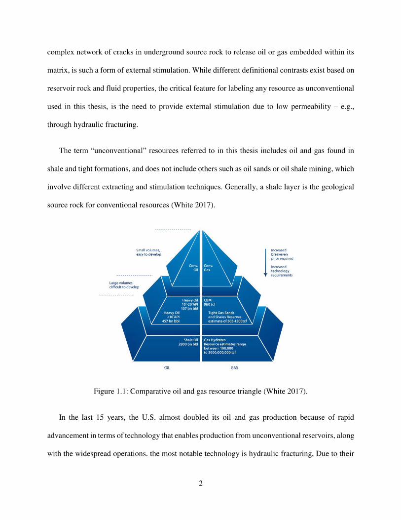
external stimulation is required. Figure 1.1 illustrates an easier comparison of both resources.
Hydraulic fracturing, by injecting a mixture of fluids and proppants at high pressure, creates a
2
complex network of cracks in underground source rock to release oil or gas embedded within its
matrix, is such a form of external stimulation. While different definitional contrasts exist based on
reservoir rock and fluid properties, the critical feature for labeling any resource as unconventional
used in this thesis, is the need to provide external stimulation due to low permeability – e.g.,
through hydraulic fracturing.
The term “unconventional” resources referred to in this thesis includes oil and gas found in
shale and tight formations, and does not include others such as oil sands or oil shale mining, which
involve different extracting and stimulation techniques. Generally, a shale layer is the geological
source rock for conventional resources (White 2017).
Figure 1.1: Comparative oil and gas resource triangle (White 2017).
In the last 15 years, the U.S. almost doubled its oil and gas production because of rapid
advancement in terms of technology that enables production from unconventional reservoirs, along
with the widespread operations. the most notable technology is hydraulic fracturing, Due to their

3
low permeabilities, this technology along with horizontal drilling allowed economic production
from unconventional resources, serving the world especially North America by reducing oil net
imports and making it a gas net exporter. In 2015, almost half of U.S. gas and oil production is
from hydraulic fractured wells as shown in Figure 1.2 (a) And (b) respectively.
(a)
(b)
Figure 1.2: Hydraulic fractured wells contribution to U.S. total oil and gas production (EIA
2016).

4
U.S. successful story lies where it was able to become an exporter of gas, the era of
unconventional development started before that but the optimized production started in 2008
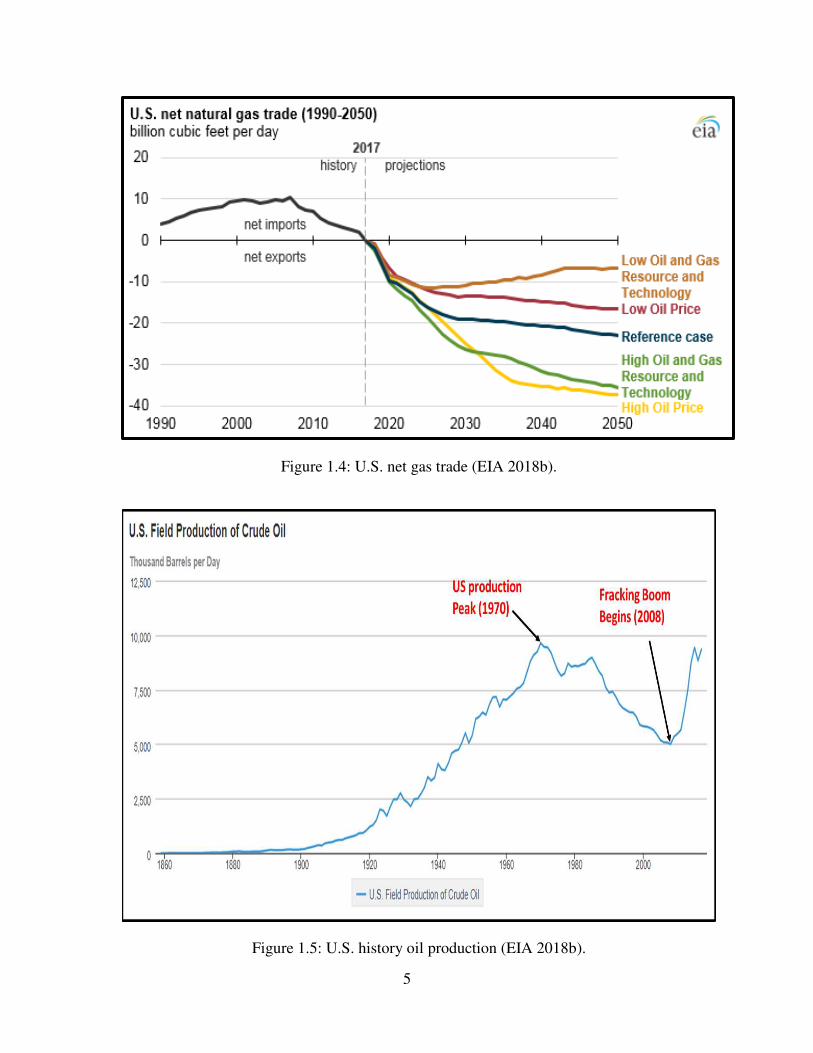
(Figure 1.3). Histrionic increase started since then, currently as shown in Figure 1.4. U.S. is a net
gas exporter and projected to be in all five reference cases created. A similar phenomenon is seen
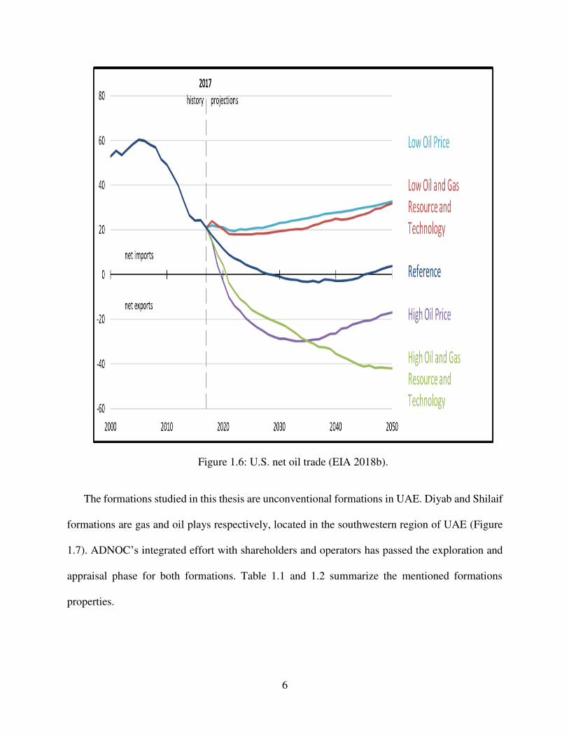
in oil (Figures 1.5 and 1.6), where the dramatic increase started in 2008. Yet, the U.S. is a net oil
importer except for two cases when exports begin in 2020. This successful story made many
countries interested in unconventional development, one of them is UAE.
Figure 1.3: U.S. gas production over time (EIA 2018b).
Fracking Boom Begins (2008)
5
Figure 1.4: U.S. net gas trade (EIA 2018b).
Figure 1.5: U.S. history oil production (EIA 2018b).
6
Figure 1.6: U.S. net oil trade (EIA 2018b).
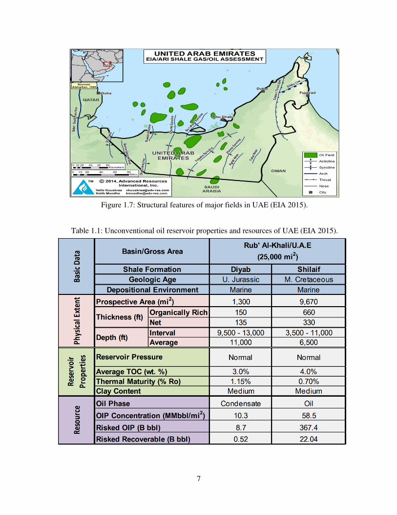
The formations studied in this thesis are unconventional formations in UAE. Diyab and Shilaif
formations are gas and oil plays respectively, located in the southwestern region of UAE (Figure
1.7). ADNOC’s integrated effort with shareholders and operators has passed the exploration and
appraisal phase for both formations. Table 1.1 and 1.2 summarize the mentioned formations
properties.
7
Figure 1.7: Structural features of major fields in UAE (EIA 2015).
Table 1.1: Unconventional oil reservoir properties and resources of UAE (EIA 2015).
8
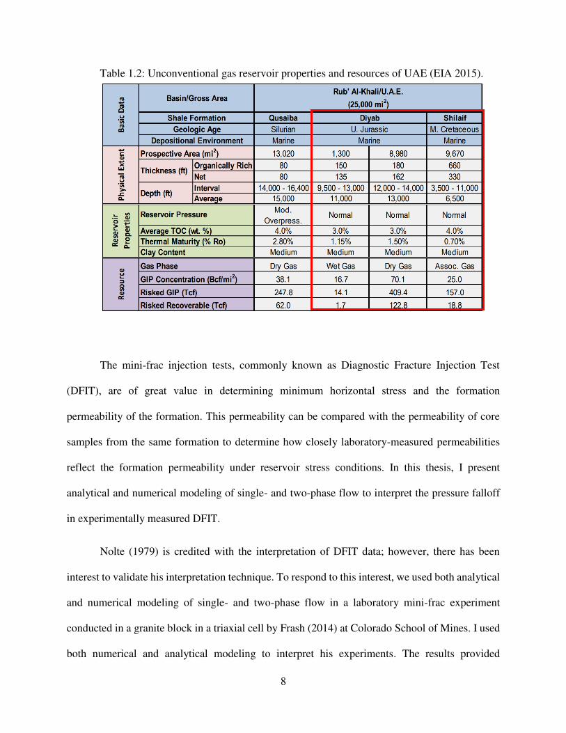
Table 1.2: Unconventional gas reservoir properties and resources of UAE (EIA 2015).
The mini-frac injection tests, commonly known as Diagnostic Fracture Injection Test
(DFIT), are of great value in determining minimum horizontal stress and the formation
permeability of the formation. This permeability can be compared with the permeability of core
samples from the same formation to determine how closely laboratory-measured permeabilities
reflect the formation permeability under reservoir stress conditions. In this thesis, I present
analytical and numerical modeling of single- and two-phase flow to interpret the pressure falloff
in experimentally measured DFIT.
Nolte (1979) is credited with the interpretation of DFIT data; however, there has been
interest to validate his interpretation technique. To respond to this interest, we used both analytical
and numerical modeling of single- and two-phase flow in a laboratory mini-frac experiment
conducted in a granite block in a triaxial cell by Frash (2014) at Colorado School of Mines. I used
both numerical and analytical modeling to interpret his experiments. The results provided

9
information on hydraulic fracture propagation and flow characteristics when air, inside the rock,
was displaced by the water as fracturing fluid. The same technique was applied to the production
data from Diyab formation in UAE.
Quantifying the success of hydraulic fracturing requires a reliable method to calculate the
formation matrix permeability before stimulation and the effective formation permeability after
fracturing. Our analytical and numerical solution methods provided a simple and reliable method
to interpret both mini-frac flow tests before hydraulic fracturing and production data after
fracturing operations are completed. The analytical method uses a simple mathematical solution
of flow toward high permeability fractures. In addition, validation of the stress shadow was
conducted in this research for better understanding of the formed fracture network.
Thus, the method is not ambiguous and easy to understand. Finally, we have successfully
applied our method to DFIT and production data from Diyab formation in UAE. Our solution
technique uses the conventional flow of single and two-phase flow to develop analytical
interpretation technique, sheds light on the Nolte's method, and provides a method to calculate in-
situ formation matrix permeability before stimulation and the permeability enhancement
(formation of microfractures) of the formation resulting from hydraulic fracturing operations.
Microfractures form because of rock deformation during fracturing operations—especially, in
multi-stage hydraulic fracture operations.
Second, an experimental study was also part of this research, to evaluate the UAE
formation Diyab for unconventional development. From reservoir and geological perspective. Last
but not least compositional modeling of the UAE developed shale from Shilaif formation, to
evaluate the reservoir performance and predict future reservoir response.
10
1.2 Methodology and Problem Statement
Hydraulic fracturing is the most notable and enabling technology for unconventional reservoir
production, despite the advances in technology, the Oil recovery from unconventional resources
remains low (4% to 10%) and Gas recovery (12% to 20%). In order to produce from these
formations efficiently the physics of fracture propagation and stresses redistribution should be
studied thoroughly. Thus, understanding the underlying physics of hydraulic fracture propagation
and stress redistribution will enhance further understanding of reservoir characteristics, and means
for enhancing production.
U.S. leads production of oil and gas from unconventional shale resources, the astonishing
increase in U.S. oil and gas production towards energy dependence made many countries interested
in unconventional development and most are in the pursuit. I believe UAE has tremendous first-
class unconventional resources that allow it to join the race with the U.S. in unconventional oil
and gas production.
This thesis focuses on UAE unconventional gas formation “Diyab”, considered to be a major
source of gas with almost 500 Tcf GIP. The other formation studied in this thesis is the “Shilaif”,
which is an oil play of almost 400 bbl of OIP. In this research, the focus is on unconventional gas
resources. UAE holds almost 6% of the world reserve (EIA 2015) yet it is a natural gas net
importer.
The reason behind that is the fact that natural gas produced is high sulphur which makes
processing expensive, so the company tends to re-inject the gas into conventional oil fields as EOR
technique to extend the life of oil fields. The source rocks mentioned above are believed to be
world-class source rocks; a comparison with USA major unconventional formations is presented
11
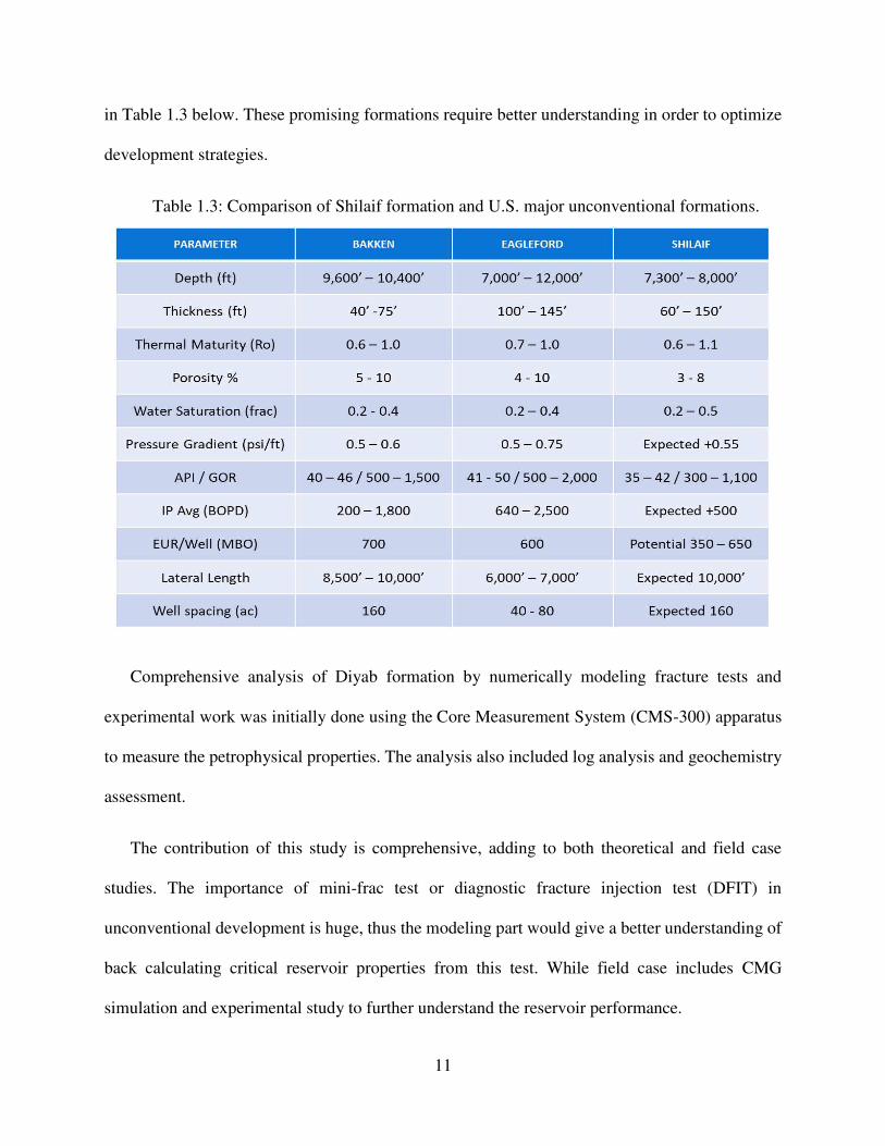
in Table 1.3 below. These promising formations require better understanding in order to optimize
development strategies.
Table 1.3: Comparison of Shilaif formation and U.S. major unconventional formations.
Comprehensive analysis of Diyab formation by numerically modeling fracture tests and
experimental work was initially done using the Core Measurement System (CMS-300) apparatus
to measure the petrophysical properties. The analysis also included log analysis and geochemistry
assessment.
The contribution of this study is comprehensive, adding to both theoretical and field case
studies. The importance of mini-frac test or diagnostic fracture injection test (DFIT) in
unconventional development is huge, thus the modeling part would give a better understanding of
back calculating critical reservoir properties from this test. While field case includes CMG
simulation and experimental study to further understand the reservoir performance.
12
1.3 Organization of the Thesis
This thesis has seven chapters.
Chapter 1 is the introduction, which covered the background, objective and problem statement.
Chapter 2 is the literature review of the theory followed in the methodology and the formation
studied.
Chapter 3 is a brief summary of Diyab geology, geochemistry, and geomechanical analysis of
the studied formation.
Chapter 4 is the numerical and analytical models conducted equations, explanations, and the
model results and discussion.
Chapter 5 is the field case CMG modeling history match results and forecast.
Chapter 6 is the experimental procedure and apparatus explanation, along with its results and
discussion.
Chapter 7 is the research observed conclusions, recommendations and future work
recommended.
Appendices present the same as Chapter 3 but with details and discussion.
13
CHAPTER 2
2. LITERATURE REVIEW
This chapter presents a literature review, which includes (1) an overview of hydraulic fracture
models, (2) mechanics of hydraulic fracturing, (3) Stress shadow effect (stress reversal) on further
fracture propagation, and (4) geologic description of the studied formation.
2.1 Hydraulic Fracturing
A multitude number of studies have been previously conducted in pursuit of understanding
hydraulic fracturing and to validate associated theories. The main approach was through laboratory
scale experiments as they are the most common physical studies due to convenience in sample
size, greater control over variables, rapid execution and ability to test innovative stimulation
methodologies with lower costs compared to field scale studies. A literature review was performed
to evaluate the current hydraulic fracturing state-of-the-art, identify other good stimulation
technologies and identify focus areas for this research effort.
Hydraulic fracturing is a form of stimulation applied in unconventional tight reservoirs to aid
hydrocarbon production. In general, the hydraulic fracture is created by injecting fracturing fluid
at high rate building up pressure that yields to formation breakdown. This process creates a bi-
wing fracture, propagating from the wellbore into the reservoir. In unconventional formations the
induced hydraulic fracture can rejuvenate the existing natural fractures (Warpinski et al. 2009).
Hence, creating a complex network exposing more contact with the reservoirs as shown in Figure
2.1, indicating a larger stimulated area than a simple planar fracture (Fisher et al. 2002; and
Warpinski et al. 2009). Water-based fluids are used the most in hydraulic fracturing operations as
it is the least expensive. The most commonly used fluid in the industry nowadays is “slick-water”,
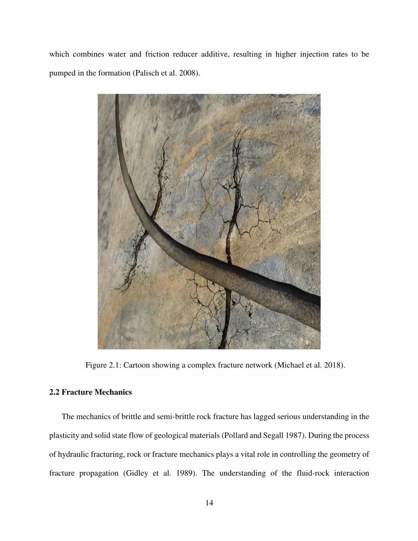
14
which combines water and friction reducer additive, resulting in higher injection rates to be
pumped in the formation (Palisch et al. 2008).
Figure 2.1: Cartoon showing a complex fracture network (Michael et al. 2018).
2.2 Fracture Mechanics
The mechanics of brittle and semi-brittle rock fracture has lagged serious understanding in the
plasticity and solid state flow of geological materials (Pollard and Segall 1987). During the process
of hydraulic fracturing, rock or fracture mechanics plays a vital role in controlling the geometry of
fracture propagation (Gidley et al. 1989). The understanding of the fluid-rock interaction
15
mechanisms in the hydraulic fracturing will allow optimizing the operation and achieving the
anticipated reservoir contact. Where in real operations, fractures induced are far more complicated
in geometry and direction compared with the available theories, and we can have complex fracture
network (Smith and Montgomery 2015).
Irwin and de Wit (1983) define fracture mechanics as describing: “. . . the fracture of materials
in terms of the laws of applied mechanics and the macroscopic properties of materials. It provides
a quantitative treatment, based on stress analysis, which relates fracture strength to the applied
load and structural geometry of a component containing defects”. Fracture mechanics was
formerly introduced to understand what happens when fracture occurs rather than why it occurs
(Lawn 1983).
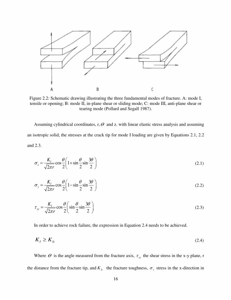
Irwin (1957) introduced the theory of linear elastic fracture mechanics, which is an alternative
technique to the energy balance approach. The method quantifies the stress state near the fracture
tip by stress intensity factors: ,I IIK K andIIIK , allowing to measure the real forces on the crack
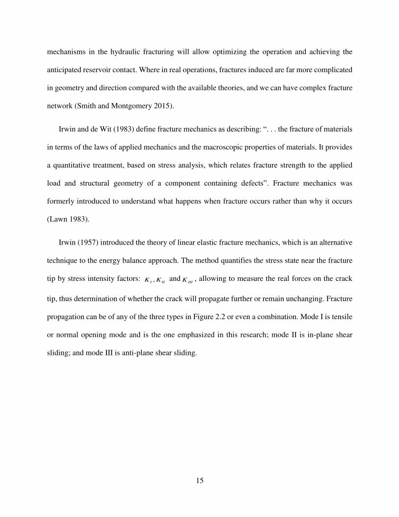
tip, thus determination of whether the crack will propagate further or remain unchanging. Fracture
propagation can be of any of the three types in Figure 2.2 or even a combination. Mode I is tensile
or normal opening mode and is the one emphasized in this research; mode II is in-plane shear
sliding; and mode III is anti-plane shear sliding.
16
Figure 2.2: Schematic drawing illustrating the three fundamental modes of fracture. A: mode I,
tensile or opening; B: mode II, in-plane shear or sliding mode; C: mode III, anti-plane shear or
tearing mode (Pollard and Segall 1987).
Assuming cylindrical coordinates, r, and z. with linear elastic stress analysis and assuming
an isotropic solid, the stresses at the crack tip for mode I loading are given by Equations 2.1, 2.2
and 2.3.
3cos 1 sin sin
2 2 22
Ix
K
r
= +
(2.1)
3cos 1 sin sin
2 2 22
Iy
K
r
= −
(2.2)
3cos sin sin
2 2 22
Ixy
K
r
=
(2.3)
In order to achieve rock failure, the expression in Equation 2.4 needs to be achieved.
I IcK K (2.4)
Where is the angle measured from the fracture axis, xy the shear stress in the x-y plane, r
the distance from the fracture tip, and IcK the fracture toughness, x stress in the x-direction in
17
psi, y
stress in the y-direction in psi, IK the mode I stress intensity factor in psi in. , r the
distance from crack tip in inch.
Multiple laboratory techniques might be followed to measure the fracture toughness; most
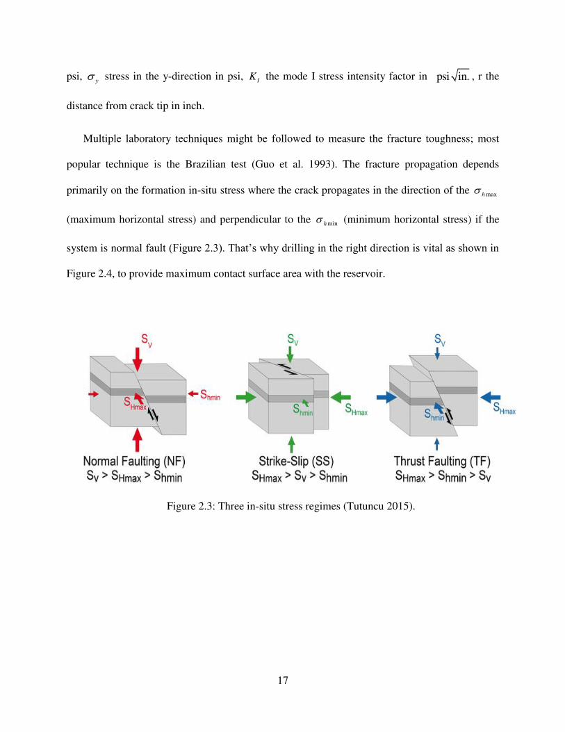
popular technique is the Brazilian test (Guo et al. 1993). The fracture propagation depends
primarily on the formation in-situ stress where the crack propagates in the direction of the maxh
(maximum horizontal stress) and perpendicular to the minh (minimum horizontal stress) if the
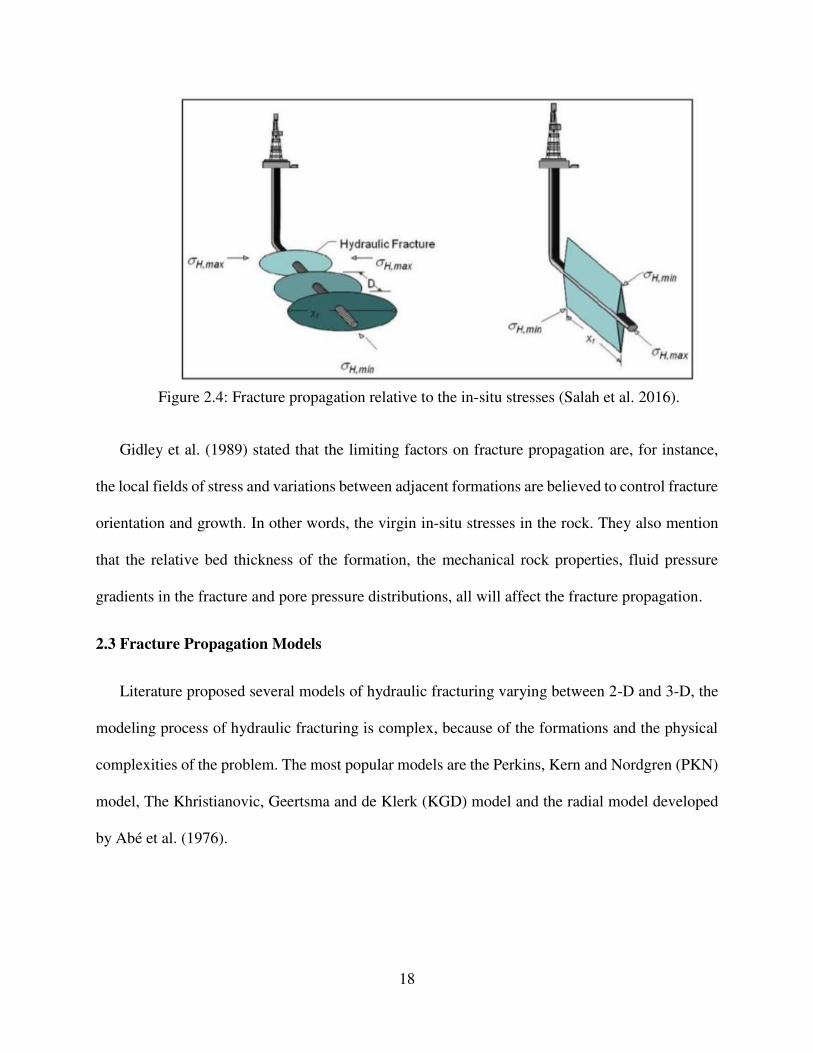
system is normal fault (Figure 2.3). That’s why drilling in the right direction is vital as shown in
Figure 2.4, to provide maximum contact surface area with the reservoir.
Figure 2.3: Three in-situ stress regimes (Tutuncu 2015).
18
Figure 2.4: Fracture propagation relative to the in-situ stresses (Salah et al. 2016).
Gidley et al. (1989) stated that the limiting factors on fracture propagation are, for instance,
the local fields of stress and variations between adjacent formations are believed to control fracture
orientation and growth. In other words, the virgin in-situ stresses in the rock. They also mention
that the relative bed thickness of the formation, the mechanical rock properties, fluid pressure
gradients in the fracture and pore pressure distributions, all will affect the fracture propagation.
2.3 Fracture Propagation Models
Literature proposed several models of hydraulic fracturing varying between 2-D and 3-D, the
modeling process of hydraulic fracturing is complex, because of the formations and the physical
complexities of the problem. The most popular models are the Perkins, Kern and Nordgren (PKN)
model, The Khristianovic, Geertsma and de Klerk (KGD) model and the radial model developed
by Abé et al. (1976).
19
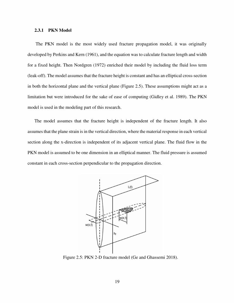
2.3.1 PKN Model
The PKN model is the most widely used fracture propagation model, it was originally
developed by Perkins and Kern (1961), and the equation was to calculate fracture length and width
for a fixed height. Then Nordgren (1972) enriched their model by including the fluid loss term
(leak-off). The model assumes that the fracture height is constant and has an elliptical cross-section
in both the horizontal plane and the vertical plane (Figure 2.5). These assumptions might act as a
limitation but were introduced for the sake of ease of computing (Gidley et al. 1989). The PKN
model is used in the modeling part of this research.
The model assumes that the fracture height is independent of the fracture length. It also
assumes that the plane strain is in the vertical direction, where the material response in each vertical
section along the x-direction is independent of its adjacent vertical plane. The fluid flow in the
PKN model is assumed to be one dimension in an elliptical manner. The fluid pressure is assumed
constant in each cross-section perpendicular to the propagation direction.
Figure 2.5: PKN 2-D fracture model (Ge and Ghassemi 2018).
20
2.3.2 KGD Model
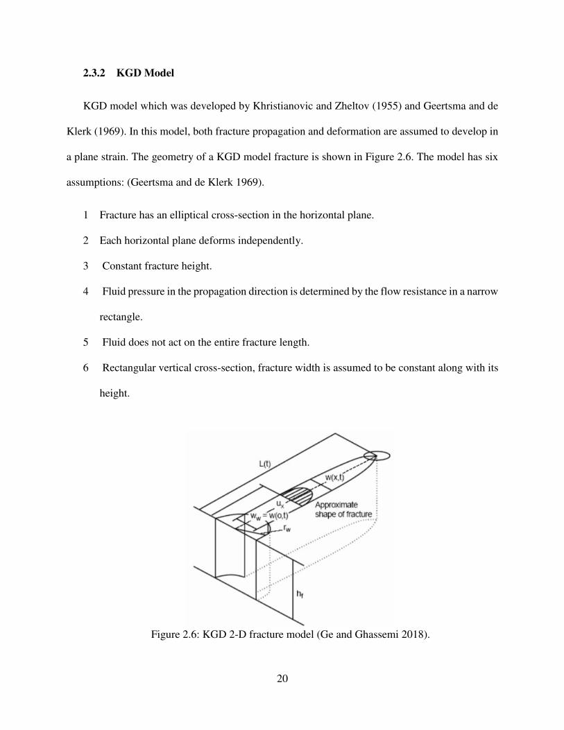
KGD model which was developed by Khristianovic and Zheltov (1955) and Geertsma and de
Klerk (1969). In this model, both fracture propagation and deformation are assumed to develop in
a plane strain. The geometry of a KGD model fracture is shown in Figure 2.6. The model has six
assumptions: (Geertsma and de Klerk 1969).
1 Fracture has an elliptical cross-section in the horizontal plane.
2 Each horizontal plane deforms independently.
3 Constant fracture height.
4 Fluid pressure in the propagation direction is determined by the flow resistance in a narrow
rectangle.
5 Fluid does not act on the entire fracture length.
6 Rectangular vertical cross-section, fracture width is assumed to be constant along with its
height.
Figure 2.6: KGD 2-D fracture model (Ge and Ghassemi 2018).
21
2.3.3 Radial Model
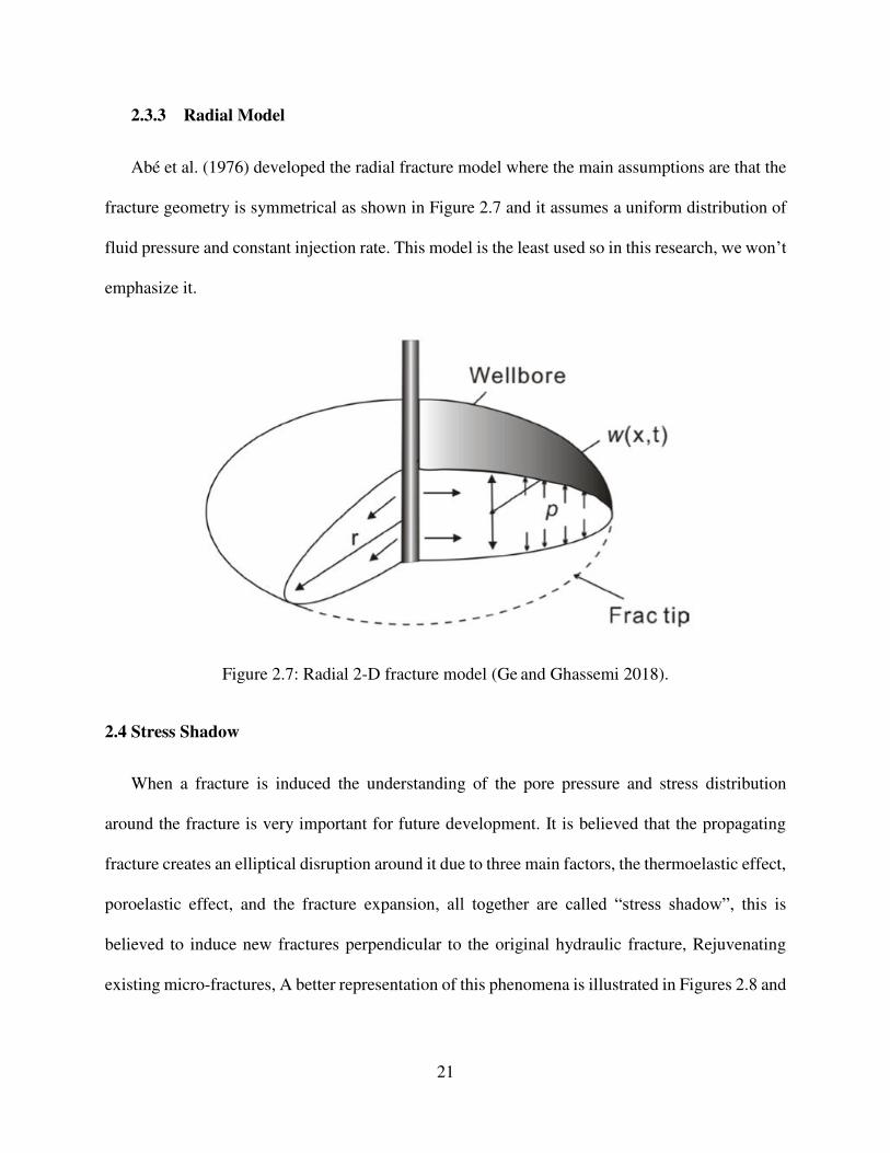
Abé et al. (1976) developed the radial fracture model where the main assumptions are that the
fracture geometry is symmetrical as shown in Figure 2.7 and it assumes a uniform distribution of
fluid pressure and constant injection rate. This model is the least used so in this research, we won’t
emphasize it.
Figure 2.7: Radial 2-D fracture model (Ge and Ghassemi 2018).
2.4 Stress Shadow
When a fracture is induced the understanding of the pore pressure and stress distribution
around the fracture is very important for future development. It is believed that the propagating
fracture creates an elliptical disruption around it due to three main factors, the thermoelastic effect,
poroelastic effect, and the fracture expansion, all together are called “stress shadow”, this is
believed to induce new fractures perpendicular to the original hydraulic fracture, Rejuvenating
existing micro-fractures, A better representation of this phenomena is illustrated in Figures 2.8 and
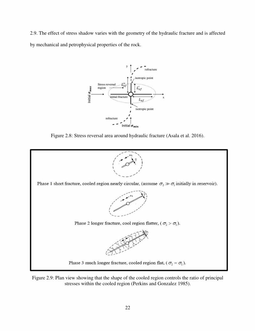
22
2.9. The effect of stress shadow varies with the geometry of the hydraulic fracture and is affected
by mechanical and petrophysical properties of the rock.
Figure 2.8: Stress reversal area around hydraulic fracture (Asala et al. 2016).
Figure 2.9: Plan view showing that the shape of the cooled region controls the ratio of principal
stresses within the cooled region (Perkins and Gonzalez 1985).
23
2.4.1 Poroelastic Effect
Fracture induction in a formation causes fluid loss into the microfractures and matrix. The
effect of feeding the formation is an increase in the pore pressure, this effect is called “poroelastic”.
The pore pressure change will result in a change in the stresses around the fracture induced. The
theory behind this effect was first presented by Biot (1941).
Perkins and Gonzalez (1985) and Konning (1985) extended the poroelastic effect equation to
include more realistic parameters, like anisotropy and heterogeneity. In their model the length and
width of the extent of both cooled and flooded regions, it also includes fluid leak off to the
formation in two dimensions, all are done in elliptical coordinates. The poroelastic effect
understanding aids in the designs of hydraulic fracturing treatment by taking into account the pore
pressure increase.
The theory has time dependent fluid flow combined with the fluid mass conservation with
Darcy's law; the main outcome of the equations is relating the total stress to the effective stress
from deformation of the rock matrix and the pore pressure increase from fluid leak-off. Biot’s
theory of poroelasticity has been developed by (Geertsma and de Klerk 1957).
Geertsma (1966) studied the poroelastic effect for a hydraulically induced fracture. He had a
two phase oil-wet rock system. Nevertheless, Geertsma concluded that the effect of pore pressure
to be insignificant in real life situation. Rice and Cleary (1976) did a similar model except that
they named the poroelastic effect as “back-stress”.
Detournay et al. 1990 studied the poroelastic effect in a PKN hydraulic fracture model, using
an explicit solving method. The pore pressure increase effect from fluid leakoff was within the
assumption of the PKN model.

24
2.4.2 Thermoelastic Effect
Thermoelastic effect means the effect of temperature variation between the injected fluid into
the fracture and reservoir temperature. It is also developed by Perkins and Gonzalez (1985). With
a similar idea to poroelastic effect. Where the volume of the cooled and waterflooded region and
the effect of cooling the formation on stresses and further fracture induction. The main idea behind
this concept is that the cooling effect would cause shrinkage in the pores which eventually increase
the effective pore pressure.
Figure 2.10 provides a better visual representation of the major and minor semi-axis of the
elliptical cool region and the water-flooded region.
Figure 2.10: Plan view of two-winged hydraulic fracture (Perkins and Gonzalez 1985).
2.4.3 Fracture Expansion
Pollard and Segall (1987) presented the effect of inducing hydraulic fracture in the media
around it, where the induced fracture would occupy space in the confined media, hence
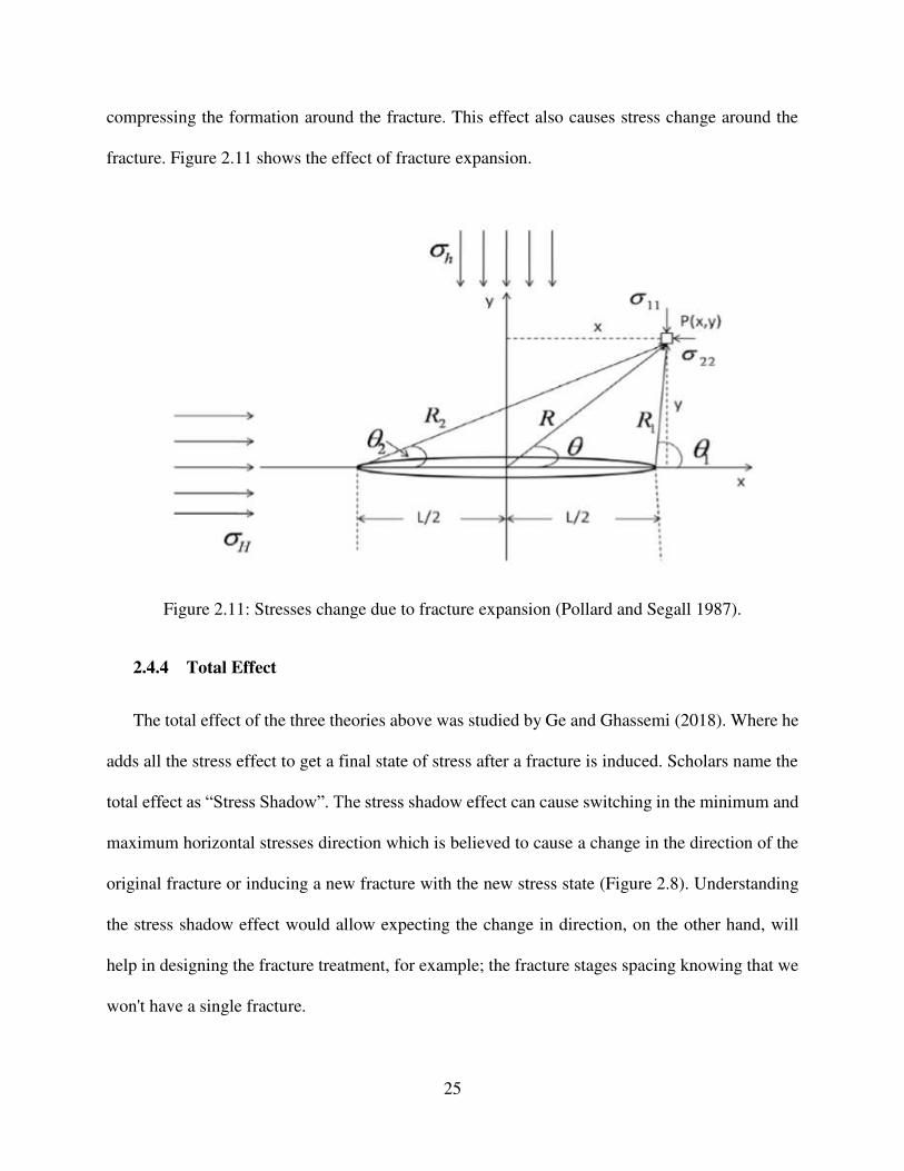
25
compressing the formation around the fracture. This effect also causes stress change around the
fracture. Figure 2.11 shows the effect of fracture expansion.
Figure 2.11: Stresses change due to fracture expansion (Pollard and Segall 1987).
2.4.4 Total Effect
The total effect of the three theories above was studied by Ge and Ghassemi (2018). Where he
adds all the stress effect to get a final state of stress after a fracture is induced. Scholars name the
total effect as “Stress Shadow”. The stress shadow effect can cause switching in the minimum and
maximum horizontal stresses direction which is believed to cause a change in the direction of the
original fracture or inducing a new fracture with the new stress state (Figure 2.8). Understanding
the stress shadow effect would allow expecting the change in direction, on the other hand, will
help in designing the fracture treatment, for example; the fracture stages spacing knowing that we
won't have a single fracture.
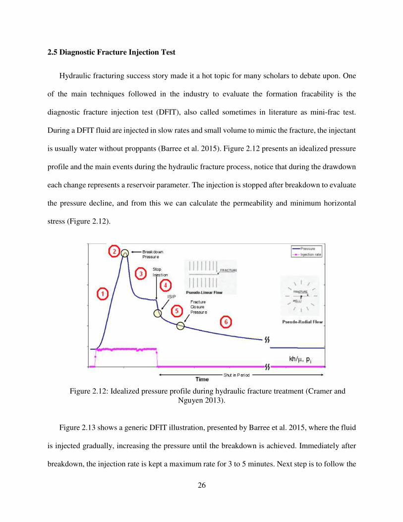
26
2.5 Diagnostic Fracture Injection Test
Hydraulic fracturing success story made it a hot topic for many scholars to debate upon. One
of the main techniques followed in the industry to evaluate the formation fracability is the
diagnostic fracture injection test (DFIT), also called sometimes in literature as mini-frac test.
During a DFIT fluid are injected in slow rates and small volume to mimic the fracture, the injectant
is usually water without proppants (Barree et al. 2015). Figure 2.12 presents an idealized pressure
profile and the main events during the hydraulic fracture process, notice that during the drawdown
each change represents a reservoir parameter. The injection is stopped after breakdown to evaluate
the pressure decline, and from this we can calculate the permeability and minimum horizontal
stress (Figure 2.12).
Figure 2.12: Idealized pressure profile during hydraulic fracture treatment (Cramer and
Nguyen 2013).
Figure 2.13 shows a generic DFIT illustration, presented by Barree et al. 2015, where the fluid
is injected gradually, increasing the pressure until the breakdown is achieved. Immediately after
breakdown, the injection rate is kept a maximum rate for 3 to 5 minutes. Next step is to follow the
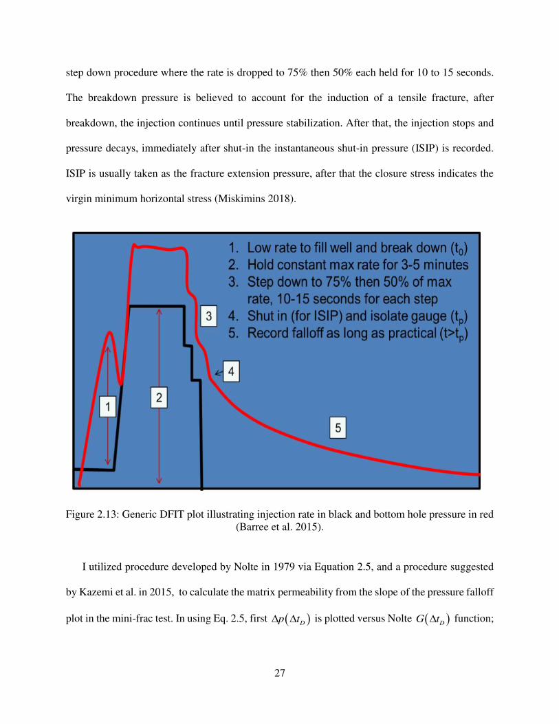
27
step down procedure where the rate is dropped to 75% then 50% each held for 10 to 15 seconds.
The breakdown pressure is believed to account for the induction of a tensile fracture, after
breakdown, the injection continues until pressure stabilization. After that, the injection stops and
pressure decays, immediately after shut-in the instantaneous shut-in pressure (ISIP) is recorded.
ISIP is usually taken as the fracture extension pressure, after that the closure stress indicates the
virgin minimum horizontal stress (Miskimins 2018).
Figure 2.13: Generic DFIT plot illustrating injection rate in black and bottom hole pressure in red
(Barree et al. 2015).
I utilized procedure developed by Nolte in 1979 via Equation 2.5, and a procedure suggested
by Kazemi et al. in 2015, to calculate the matrix permeability from the slope of the pressure falloff
plot in the mini-frac test. In using Eq. 2.5, first ( )Dp t is plotted versus Nolte ( )D
G t function;
28
then, leakoff coefficient LC is calculated from the late straight-line slope of the plot; finally
permeability is calculated from Equation 2.6 .
( )
2
L p D
f
C t G tp
c
= (2.5)
2
2(0.00118( ))
Lm
t L
Ck
c p
=
(2.6)
Where, LC the leakoff coefficient in ft min ,
pt the total pumping time in min, ( )DG t
dimensionless G-function,f
c fracture compliance in ft/psi , mk matrix permeability in md, cp
closure stress in psi ,and cp is the leakoff driving pressure in psi. The exact nature of cp is highly
debatable! It is bound by two quantities: ( )0f c
p p t p = = − and ( )0f R
p p t p = = − . In the
later, Rp is the asymptotic value of the shut-in fall-off pressure at long shut-in times.
The most common mistake in DFIT analysis (discussed below) is the incorrect acquisition of
the instantaneous shut-in pressure (ISIP). This usually leads to wrong interpretation of the
formation/fracture parameter, consequently a bad treatment design is ended with. The second most
common mistake is wrong closure pressure, this leads to several wrong interpretations, for
example, permeability is calculated wrong and net pressure estimation. Figure 2.14 shows the
typical mistake that can be made in choosing the closure point due to high noise data. The third
most common mistake is the gas entry which will result in an increase in pressure in perforations,
and this can increase the leak-off rate (Miskimins 2018).
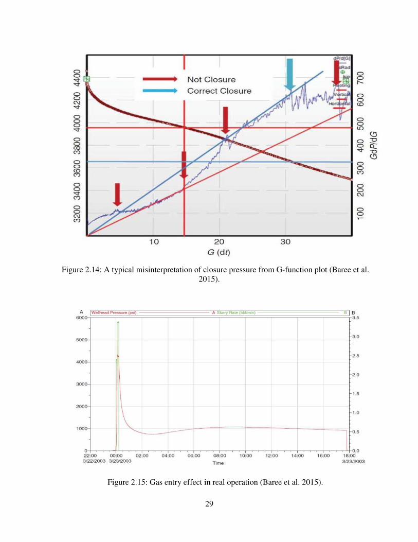
29
Figure 2.14: A typical misinterpretation of closure pressure from G-function plot (Baree et al.
2015).
Figure 2.15: Gas entry effect in real operation (Baree et al. 2015).

30
2.5.1 G-Function Analysis
G-function analysis was first introduced by Nolte (1979). The G-function is a dimensionless
function plotted with pressure, pressure derivative and G-function multiply the pressure derivative
are plotted versus the G-time as shown in Figure 2.16. Although multiple analysis are used and all
have the same findings, the G-function analysis is the most commonly used compared with the
other analysis. Yet most of the time all three are used together to eliminate error as much as
possible.
Briefly, the G-function analysis draws a tangent line from the bottom of /Gdp dG until the
deviation from a straight line, at this point a straight line is drawn where the intersection with the
pressure curve is recorded as closure pressure.
Figure 2.16: Ideal G-Function analysis plot (Baree et al. 2009).
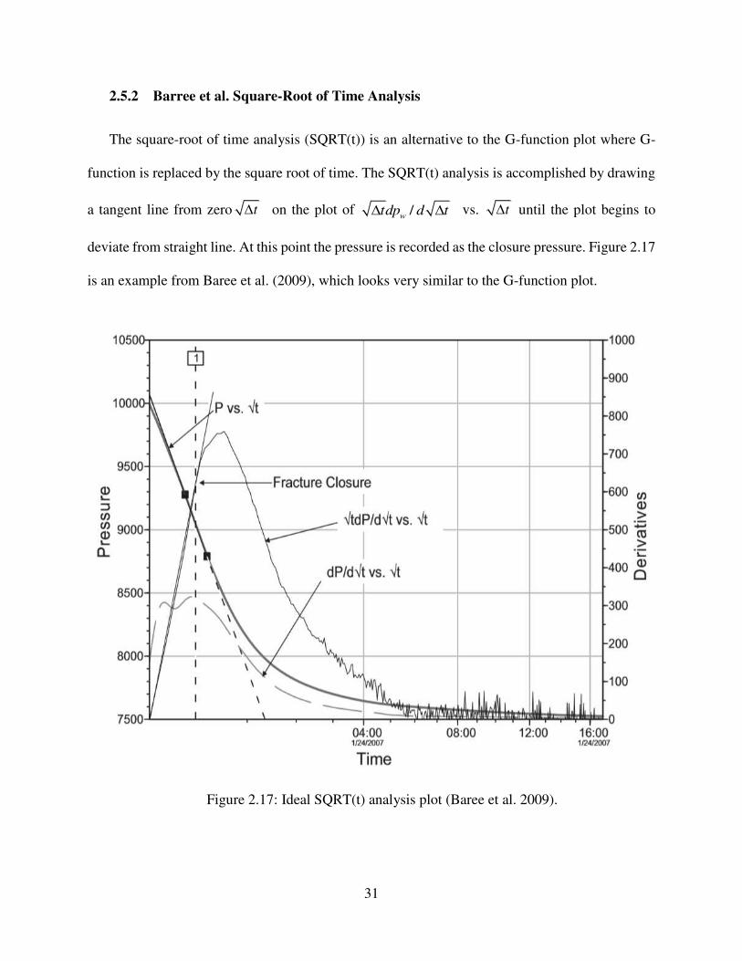
31
2.5.2 Barree et al. Square-Root of Time Analysis
The square-root of time analysis (SQRT(t)) is an alternative to the G-function plot where G-
function is replaced by the square root of time. The SQRT(t) analysis is accomplished by drawing
a tangent line from zero t on the plot of /w
tdp d t vs. t until the plot begins to
deviate from straight line. At this point the pressure is recorded as the closure pressure. Figure 2.17
is an example from Baree et al. (2009), which looks very similar to the G-function plot.
Figure 2.17: Ideal SQRT(t) analysis plot (Baree et al. 2009).
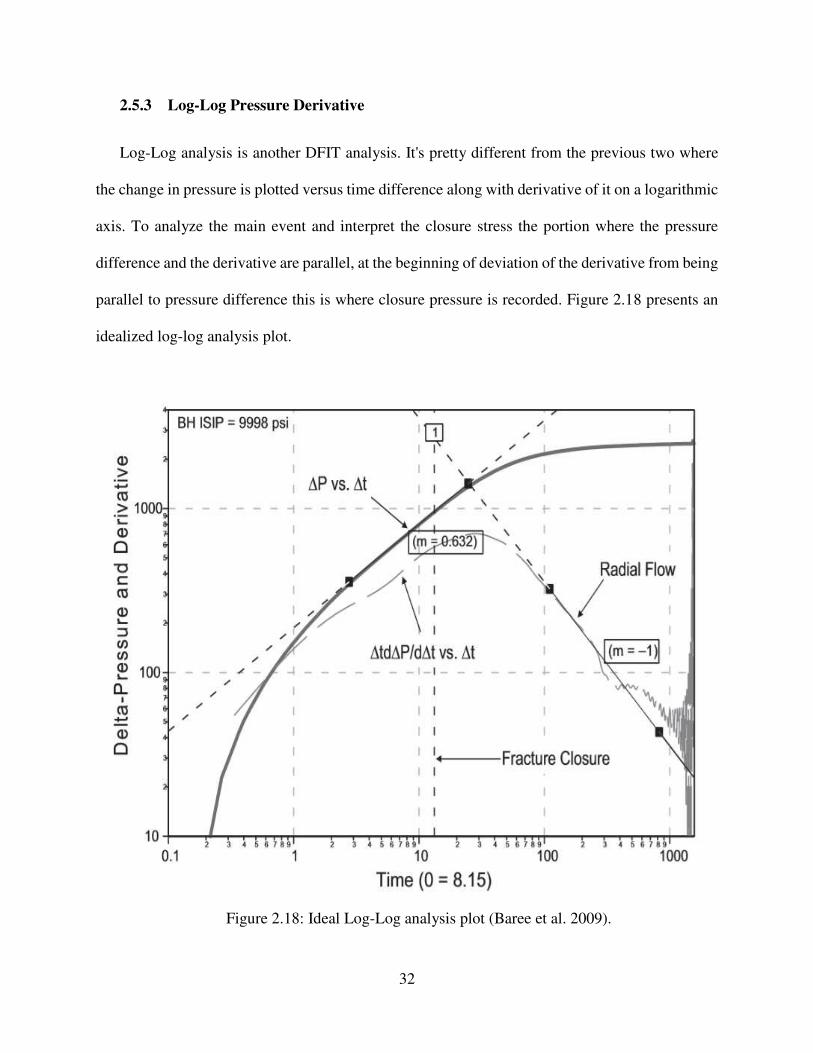
32
2.5.3 Log-Log Pressure Derivative
Log-Log analysis is another DFIT analysis. It's pretty different from the previous two where
the change in pressure is plotted versus time difference along with derivative of it on a logarithmic
axis. To analyze the main event and interpret the closure stress the portion where the pressure
difference and the derivative are parallel, at the beginning of deviation of the derivative from being
parallel to pressure difference this is where closure pressure is recorded. Figure 2.18 presents an
idealized log-log analysis plot.
Figure 2.18: Ideal Log-Log analysis plot (Baree et al. 2009).

33
2.5.4 After Closure Analysis
The after closure analysis (ACA) is the fourth analysis of DFIT explained. It is usually used to
extrapolate the flow regime by finding the slope of the pressure difference curve. The pressure
difference is plotted along with the derivative versus the square linear flow function. Figure 2.19
presents an idealized ACA analysis plot.
Figure 2.19: Ideal ACA analysis plot (Baree et al. 2009).
2.6 United Arab Emirates Petroleum Systems
According to OPEC (2018), 82% of the world's proven oil reserves are located in OPEC
member countries, with almost 65.36% of the OPEC total oil reserves are located in the Middle
East. Holding this gigantic reserve of conventional oil has to have world-class source rock.
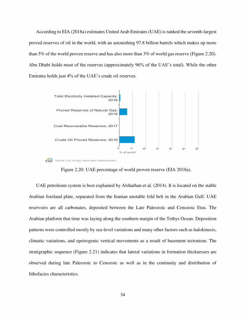
34
According to EIA (2018a) estimates United Arab Emirates (UAE) is ranked the seventh-largest
proved reserves of oil in the world, with an astonishing 97.8 billion barrels which makes up more
than 5% of the world proven reserve and has also more than 3% of world gas reserve (Figure 2.20).
Abu Dhabi holds most of the reserves (approximately 96% of the UAE’s total). While the other
Emirates holds just 4% of the UAE’s crude oil reserves.
Figure 2.20: UAE percentage of world proven reserve (EIA 2018a).
UAE petroleum system is best explained by Alsharhan et al. (2014). It is located on the stable
Arabian foreland plate, separated from the Iranian unstable fold belt in the Arabian Gulf. UAE
reservoirs are all carbonates, deposited between the Late Paleozoic and Cenozoic Eras. The
Arabian platform that time was laying along the southern margin of the Tethys Ocean. Deposition
patterns were controlled mostly by sea-level variations and many other factors such as halokinesis,
climatic variations, and epeirogenic vertical movements as a result of basement tectonism. The
stratigraphic sequence (Figure 2.21) indicates that lateral variations in formation thicknesses are
observed during late Paleozoic to Cenozoic as well as in the continuity and distribution of
lithofacies characteristics.
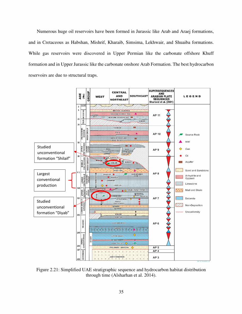
35
Numerous huge oil reservoirs have been formed in Jurassic like Arab and Araej formations,
and in Cretaceous as Habshan, Mishrif, Kharaib, Simsima, Lekhwair, and Shuaiba formations.
While gas reservoirs were discovered in Upper Permian like the carbonate offshore Khuff
formation and in Upper Jurassic like the carbonate onshore Arab Formation. The best hydrocarbon
reservoirs are due to structural traps.
Figure 2.21: Simplified UAE stratigraphic sequence and hydrocarbon habitat distribution
through time (Alsharhan et al. 2014).
Largest
conventional
production
Studied
unconventional
formation “Shilaif”
Studied
unconventional
formation “Diyab”
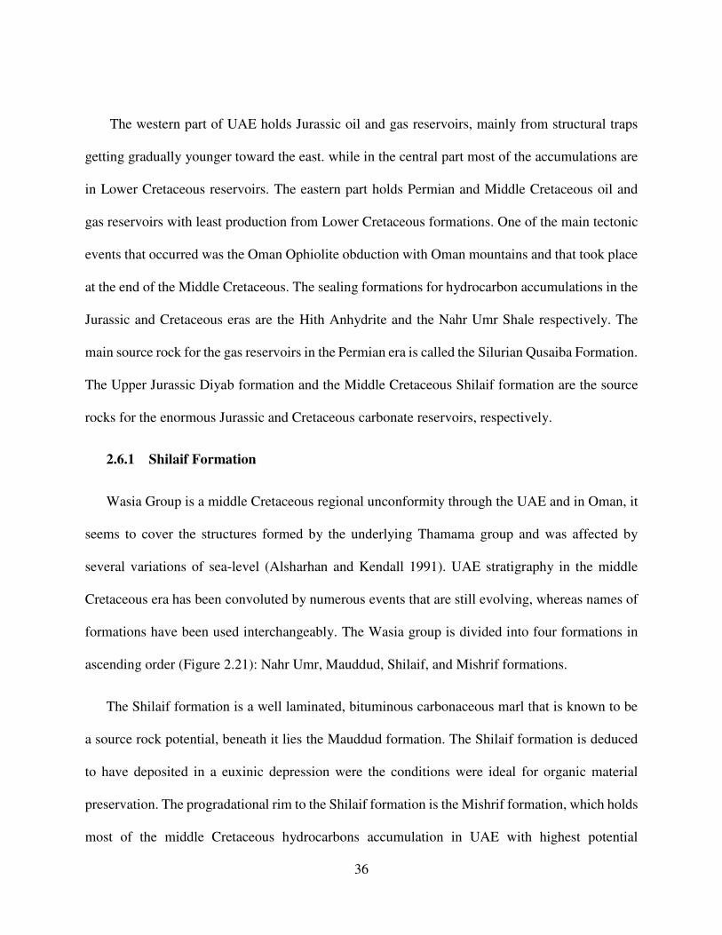
36
The western part of UAE holds Jurassic oil and gas reservoirs, mainly from structural traps
getting gradually younger toward the east. while in the central part most of the accumulations are
in Lower Cretaceous reservoirs. The eastern part holds Permian and Middle Cretaceous oil and
gas reservoirs with least production from Lower Cretaceous formations. One of the main tectonic
events that occurred was the Oman Ophiolite obduction with Oman mountains and that took place
at the end of the Middle Cretaceous. The sealing formations for hydrocarbon accumulations in the
Jurassic and Cretaceous eras are the Hith Anhydrite and the Nahr Umr Shale respectively. The
main source rock for the gas reservoirs in the Permian era is called the Silurian Qusaiba Formation.
The Upper Jurassic Diyab formation and the Middle Cretaceous Shilaif formation are the source
rocks for the enormous Jurassic and Cretaceous carbonate reservoirs, respectively.
2.6.1 Shilaif Formation
Wasia Group is a middle Cretaceous regional unconformity through the UAE and in Oman, it
seems to cover the structures formed by the underlying Thamama group and was affected by
several variations of sea-level (Alsharhan and Kendall 1991). UAE stratigraphy in the middle
Cretaceous era has been convoluted by numerous events that are still evolving, whereas names of
formations have been used interchangeably. The Wasia group is divided into four formations in
ascending order (Figure 2.21): Nahr Umr, Mauddud, Shilaif, and Mishrif formations.
The Shilaif formation is a well laminated, bituminous carbonaceous marl that is known to be
a source rock potential, beneath it lies the Mauddud formation. The Shilaif formation is deduced
to have deposited in a euxinic depression were the conditions were ideal for organic material
preservation. The progradational rim to the Shilaif formation is the Mishrif formation, which holds
most of the middle Cretaceous hydrocarbons accumulation in UAE with highest potential
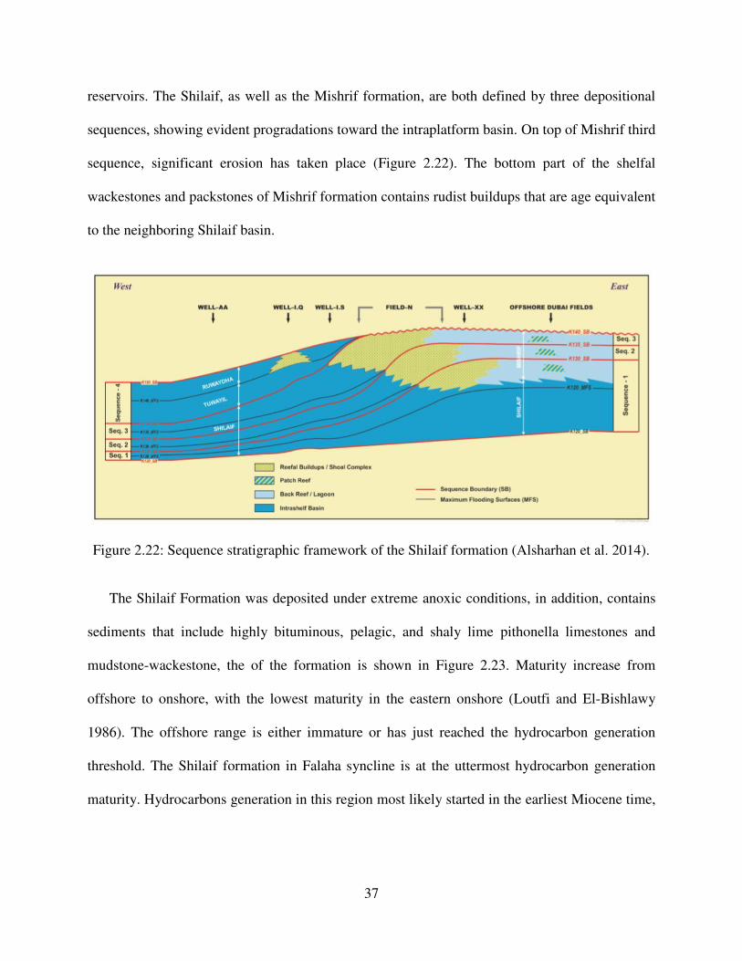
37
reservoirs. The Shilaif, as well as the Mishrif formation, are both defined by three depositional
sequences, showing evident progradations toward the intraplatform basin. On top of Mishrif third
sequence, significant erosion has taken place (Figure 2.22). The bottom part of the shelfal
wackestones and packstones of Mishrif formation contains rudist buildups that are age equivalent
to the neighboring Shilaif basin.
Figure 2.22: Sequence stratigraphic framework of the Shilaif formation (Alsharhan et al. 2014).
The Shilaif Formation was deposited under extreme anoxic conditions, in addition, contains
sediments that include highly bituminous, pelagic, and shaly lime pithonella limestones and
mudstone-wackestone, the of the formation is shown in Figure 2.23. Maturity increase from
offshore to onshore, with the lowest maturity in the eastern onshore (Loutfi and El-Bishlawy
1986). The offshore range is either immature or has just reached the hydrocarbon generation
threshold. The Shilaif formation in Falaha syncline is at the uttermost hydrocarbon generation
maturity. Hydrocarbons generation in this region most likely started in the earliest Miocene time,
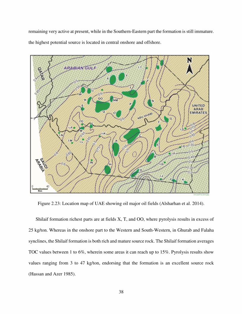
38
remaining very active at present, while in the Southern-Eastern part the formation is still immature.
the highest potential source is located in central onshore and offshore.
Figure 2.23: Location map of UAE showing oil major oil fields (Alsharhan et al. 2014).
Shilaif formation richest parts are at fields X, T, and OO, where pyrolysis results in excess of
25 kg/ton. Whereas in the onshore part to the Western and South-Western, in Ghurab and Falaha
synclines, the Shilaif formation is both rich and mature source rock. The Shilaif formation averages
TOC values between 1 to 6%, wherein some areas it can reach up to 15%. Pyrolysis results show
values ranging from 3 to 47 kg/ton, endorsing that the formation is an excellent source rock
(Hassan and Azer 1985).
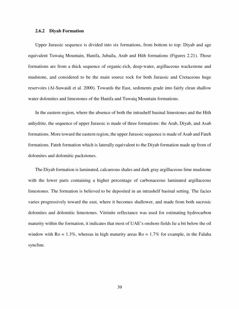
39
2.6.2 Diyab Formation
Upper Jurassic sequence is divided into six formations, from bottom to top: Diyab and age
equivalent Tuwaiq Mountain, Hanifa, Jubaila, Arab and Hith formations (Figures 2.21). Those
formations are from a thick sequence of organic-rich, deep-water, argillaceous wackestone and
mudstone, and considered to be the main source rock for both Jurassic and Cretaceous huge
reservoirs (Al-Suwaidi et al. 2000). Towards the East, sediments grade into fairly clean shallow
water dolomites and limestones of the Hanifa and Tuwaiq Mountain formations.
In the eastern region, where the absence of both the intrashelf basinal limestones and the Hith
anhydrite, the sequence of upper Jurassic is made of three formations: the Arab, Diyab, and Asab
formations. More toward the eastern region, the upper Jurassic sequence is made of Asab and Fateh
formations. Fateh formation which is laterally equivalent to the Diyab formation made up from of
dolomites and dolomitic packstones.
The Diyab formation is laminated, calcareous shales and dark gray argillaceous lime mudstone
with the lower parts containing a higher percentage of carbonaceous laminated argillaceous
limestones. The formation is believed to be deposited in an intrashelf basinal setting. The facies
varies progressively toward the east, where it becomes shallower, and made from both sucrosic
dolomites and dolomitic limestones. Vitrinite reflectance was used for estimating hydrocarbon
maturity within the formation, it indicates that most of UAE’s onshore fields lie a bit below the oil
window with Ro = 1.3%, whereas in high maturity areas Ro = 1.7% for example, in the Falaha
syncline.

40
The southern eastern part experience lower maturities, which is explained by the less deep
sediments buried, due to the incidence of the Mender Lekhwair high. The offshore Diyab
formation is in the late stage of hydrocarbon generation with Ro = 1.3%. Diyab is world-class
potential source rock in western onshore and offshore parts and ranges from moderate to good.
Figure 2.24 illustrates the sequence stratigraphic correlation for the upper Jurassic depositions.
Figure 2.24: Sequence stratigraphic correlation of the Diyab/Tuwaiq Mountain/ Hadriya/ Hanifa/
Jubaila formations (Alsharhan et al. 2014).
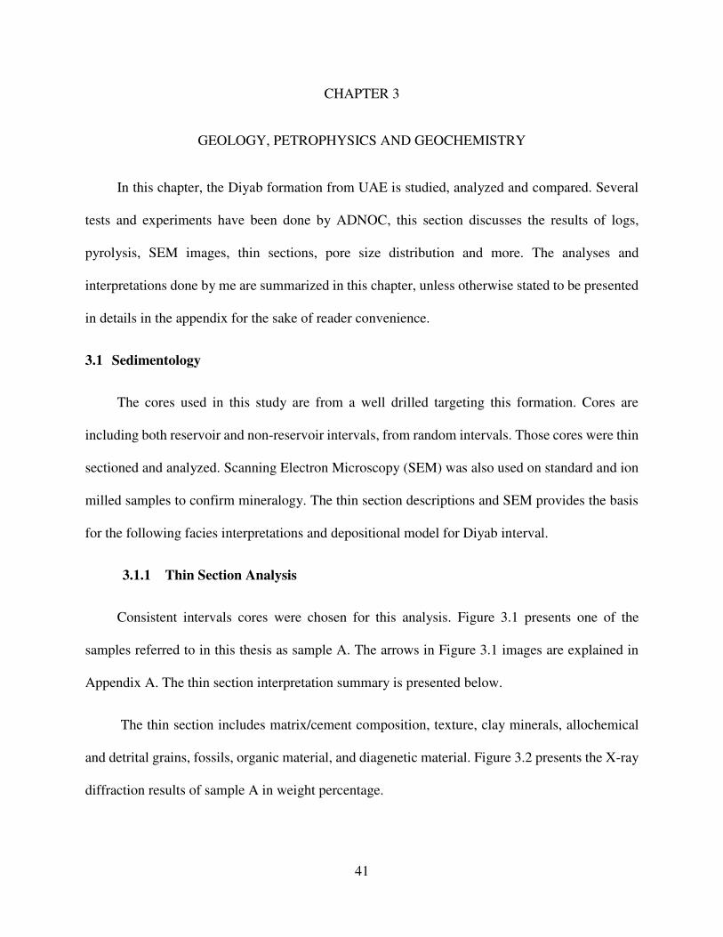
41
CHAPTER 3
3. GEOLOGY, PETROPHYSICS AND GEOCHEMISTRY
In this chapter, the Diyab formation from UAE is studied, analyzed and compared. Several
tests and experiments have been done by ADNOC, this section discusses the results of logs,
pyrolysis, SEM images, thin sections, pore size distribution and more. The analyses and
interpretations done by me are summarized in this chapter, unless otherwise stated to be presented
in details in the appendix for the sake of reader convenience.
3.1 Sedimentology
The cores used in this study are from a well drilled targeting this formation. Cores are
including both reservoir and non-reservoir intervals, from random intervals. Those cores were thin
sectioned and analyzed. Scanning Electron Microscopy (SEM) was also used on standard and ion
milled samples to confirm mineralogy. The thin section descriptions and SEM provides the basis
for the following facies interpretations and depositional model for Diyab interval.
3.1.1 Thin Section Analysis
Consistent intervals cores were chosen for this analysis. Figure 3.1 presents one of the
samples referred to in this thesis as sample A. The arrows in Figure 3.1 images are explained in
Appendix A. The thin section interpretation summary is presented below.
The thin section includes matrix/cement composition, texture, clay minerals, allochemical
and detrital grains, fossils, organic material, and diagenetic material. Figure 3.2 presents the X-ray
diffraction results of sample A in weight percentage.
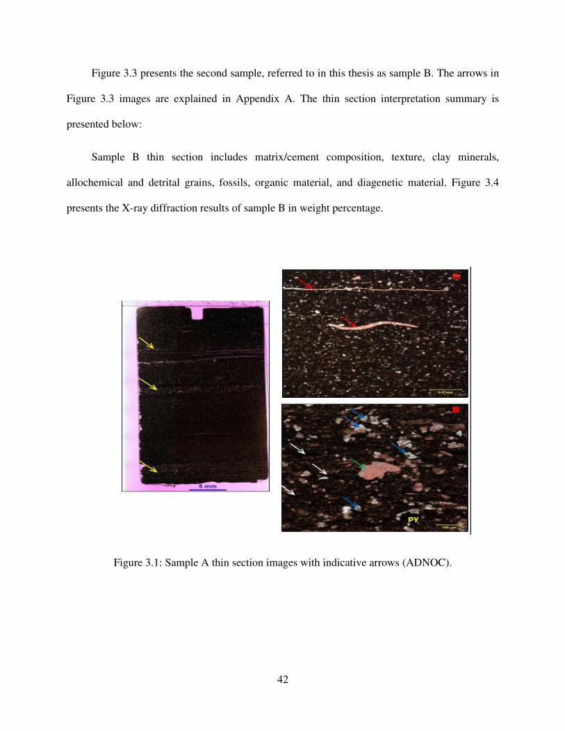
42
Figure 3.3 presents the second sample, referred to in this thesis as sample B. The arrows in
Figure 3.3 images are explained in Appendix A. The thin section interpretation summary is
presented below:
Sample B thin section includes matrix/cement composition, texture, clay minerals,
allochemical and detrital grains, fossils, organic material, and diagenetic material. Figure 3.4
presents the X-ray diffraction results of sample B in weight percentage.
Figure 3.1: Sample A thin section images with indicative arrows (ADNOC).
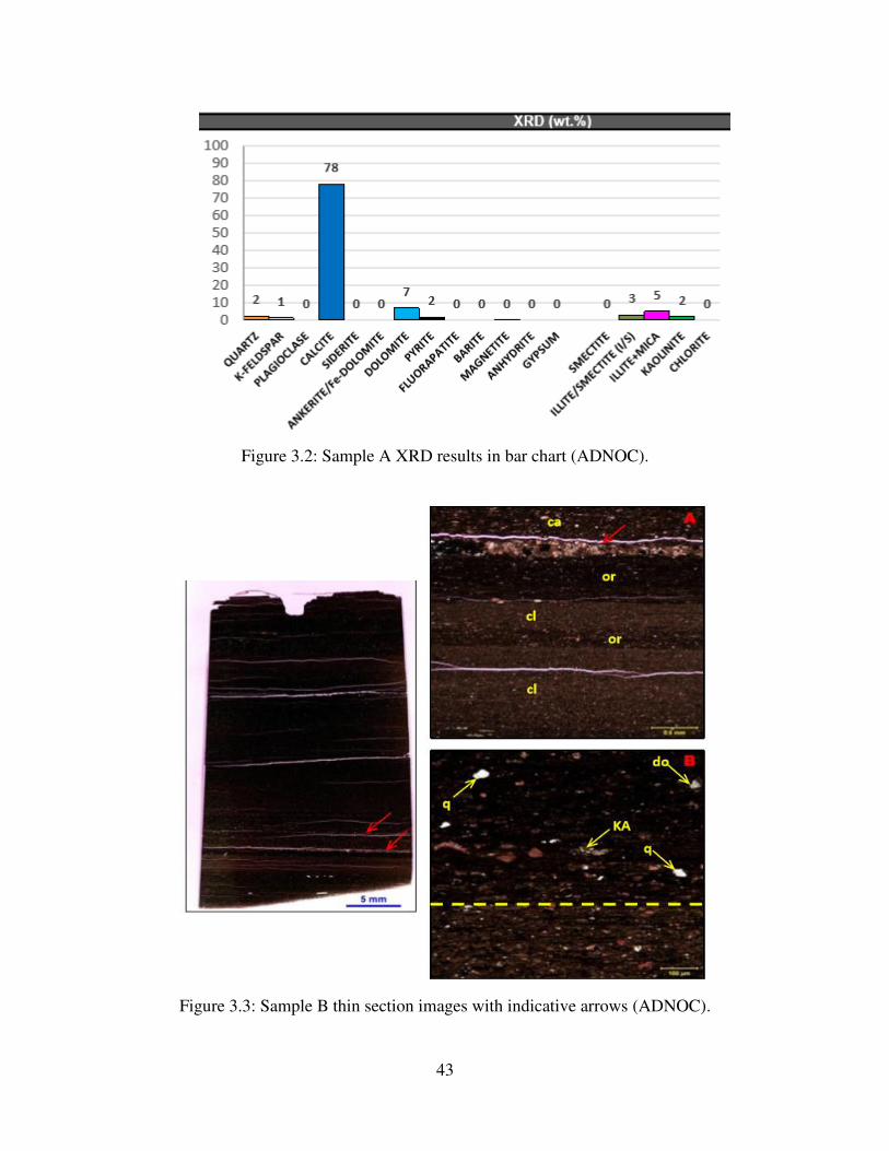
43
Figure 3.2: Sample A XRD results in bar chart (ADNOC).
Figure 3.3: Sample B thin section images with indicative arrows (ADNOC).
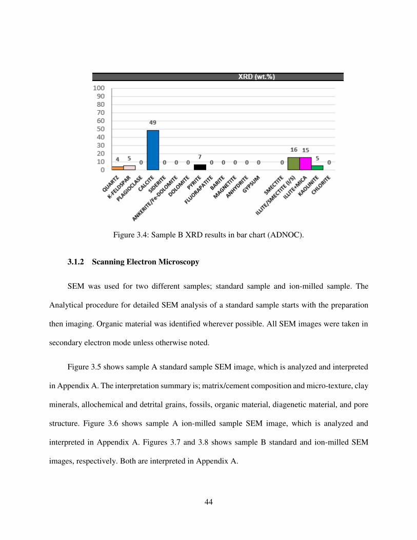
44
Figure 3.4: Sample B XRD results in bar chart (ADNOC).
3.1.2 Scanning Electron Microscopy
SEM was used for two different samples; standard sample and ion-milled sample. The
Analytical procedure for detailed SEM analysis of a standard sample starts with the preparation
then imaging. Organic material was identified wherever possible. All SEM images were taken in
secondary electron mode unless otherwise noted.
Figure 3.5 shows sample A standard sample SEM image, which is analyzed and interpreted
in Appendix A. The interpretation summary is; matrix/cement composition and micro-texture, clay
minerals, allochemical and detrital grains, fossils, organic material, diagenetic material, and pore
structure. Figure 3.6 shows sample A ion-milled sample SEM image, which is analyzed and
interpreted in Appendix A. Figures 3.7 and 3.8 shows sample B standard and ion-milled SEM
images, respectively. Both are interpreted in Appendix A.
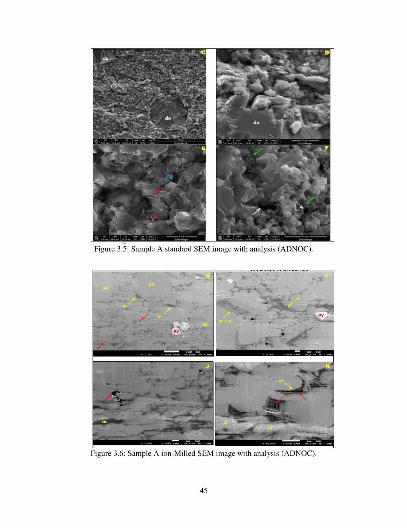
45
Figure 3.5: Sample A standard SEM image with analysis (ADNOC).
Figure 3.6: Sample A ion-Milled SEM image with analysis (ADNOC).
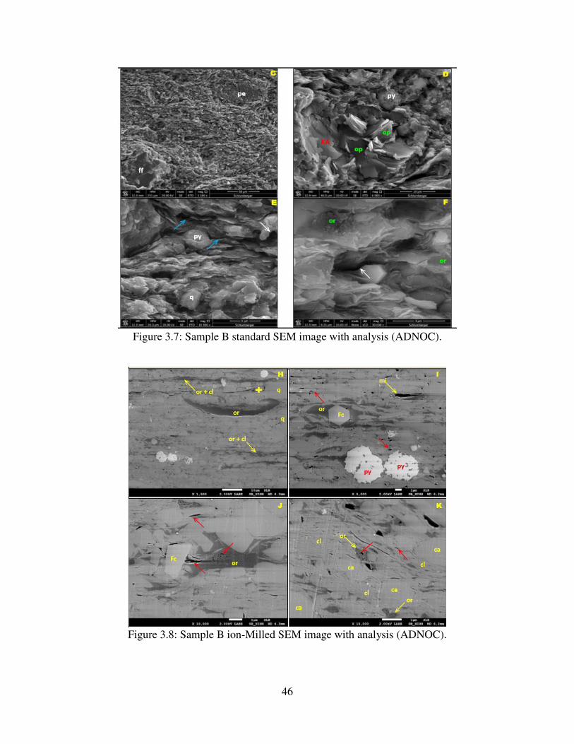
46
Figure 3.7: Sample B standard SEM image with analysis (ADNOC).
Figure 3.8: Sample B ion-Milled SEM image with analysis (ADNOC).
47
3.2 Integration of Geology and Well Logs
This section integrates wireline log data, Formation MicroImager (FMI), SonicScanner,
Lithoscanner and triple-combo logs with Geoflex (cuttings) and mud log data to characterize the
Diyab (Jubaila), Hanifa and Araej Formations. Data quality is impressive and facilitates a
confident interpretation. Again, the sections presented in this chapter are the important ones from
the writer point of view, if any of the tests mentioned above aren’t presented here will be in
Appendix B.
Natural fractures are observed in the imaged interval. Both resistive (healed) and conductive
(possibly open) fractures are interpreted. The latter category of fractures comprises the majority
observed. Arab D hosts most of the ‘sinusoidal’ (larger) natural fractures. Attributes have been
extracted for Continuous Conductive Fractures (CCF), Discontinuous Conductive Fractures (DCF)
and Enhanced Fractures (EF) – the larger and more continuous fractures which maybe possibly
open.
Insitu stress around the borehole is noted in the FMI in the form of drilling induced fractures
and breakouts. Induced fractures mostly occur in Arab D while breakouts are seen mainly in Diyab.
No evidence of faulting is observed in the imaged interval. An image based visual textural
catalogue for Diyab is created using FMI and other allied logs. It is observed that drilling induced
features may have a facies/texture control.
3.2.1 FMI
The FMI image shows the Diyab Formation to be well bedded. Layering intensity decreases
on moving up the section. Layering comprises bed boundaries and solution seams (Figure 3.9).
Structural dip is low. Fracture types observed are the stubby /segment conductive (SCF) and
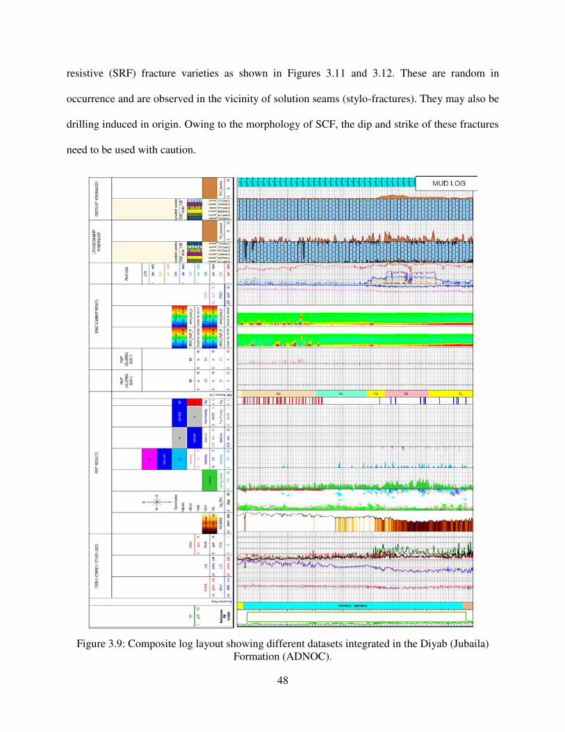
48
resistive (SRF) fracture varieties as shown in Figures 3.11 and 3.12. These are random in
occurrence and are observed in the vicinity of solution seams (stylo-fractures). They may also be
drilling induced in origin. Owing to the morphology of SCF, the dip and strike of these fractures
need to be used with caution.
Figure 3.9: Composite log layout showing different datasets integrated in the Diyab (Jubaila)
Formation (ADNOC).
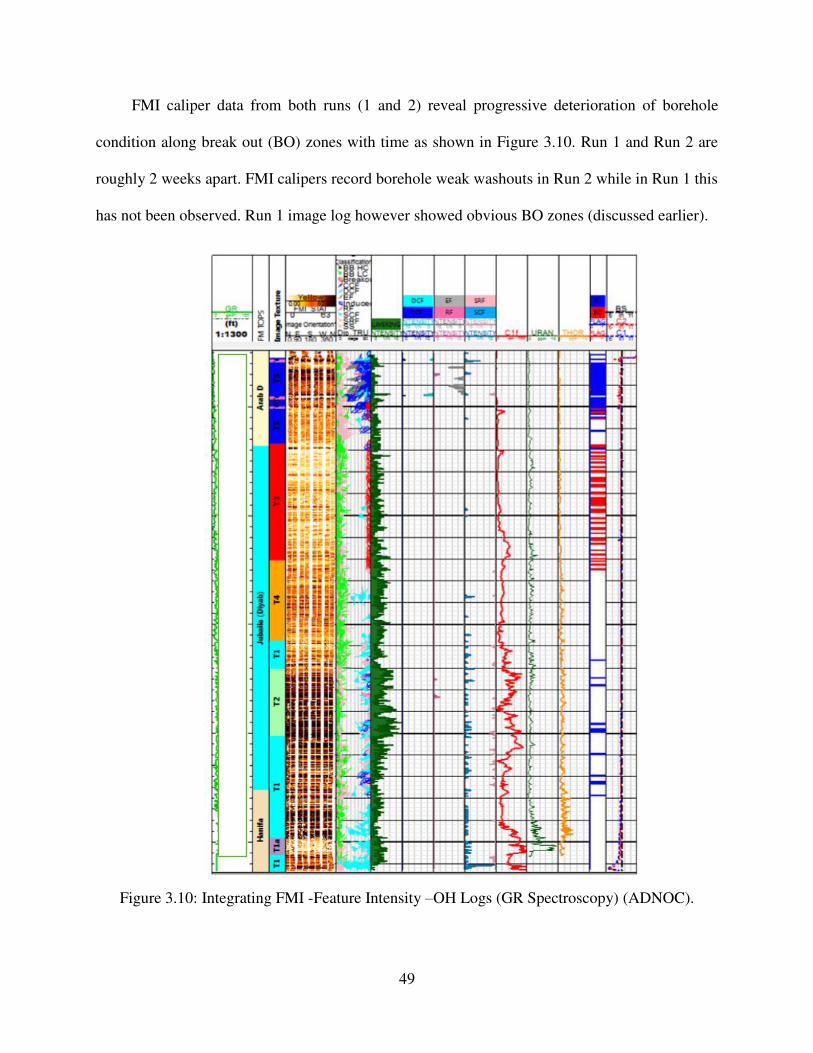
49
FMI caliper data from both runs (1 and 2) reveal progressive deterioration of borehole
condition along break out (BO) zones with time as shown in Figure 3.10. Run 1 and Run 2 are
roughly 2 weeks apart. FMI calipers record borehole weak washouts in Run 2 while in Run 1 this
has not been observed. Run 1 image log however showed obvious BO zones (discussed earlier).
Figure 3.10: Integrating FMI -Feature Intensity –OH Logs (GR Spectroscopy) (ADNOC).
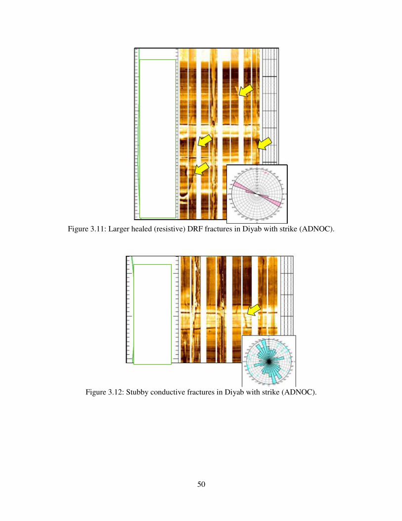
50
Figure 3.11: Larger healed (resistive) DRF fractures in Diyab with strike (ADNOC).
Figure 3.12: Stubby conductive fractures in Diyab with strike (ADNOC).
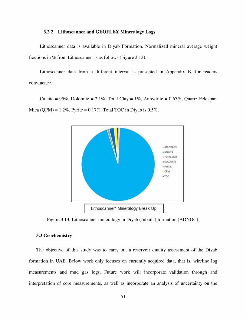
51
3.2.2 Lithoscanner and GEOFLEX Mineralogy Logs
Lithoscanner data is available in Diyab Formation. Normalized mineral average weight
fractions in % from Lithoscanner is as follows (Figure 3.13):
Lithoscanner data from a different interval is presented in Appendix B, for readers
convinence.
Calcite = 95%, Dolomite = 2.1%, Total Clay = 1%, Anhydrite = 0.67%, Quartz-Feldspar-
Mica (QFM) = 1.2%, Pyrite = 0.17%. Total TOC in Diyab is 0.5%.
Figure 3.13: Lithoscanner mineralogy in Diyab (Jubaila) formation (ADNOC).
3.3 Geochemistry
The objective of this study was to carry out a reservoir quality assessment of the Diyab
formation in UAE. Below work only focuses on currently acquired data, that is, wireline log
measurements and mud gas logs. Future work will incorporate validation through and
interpretation of core measurements, as well as incorporate an analysis of uncertainty on the
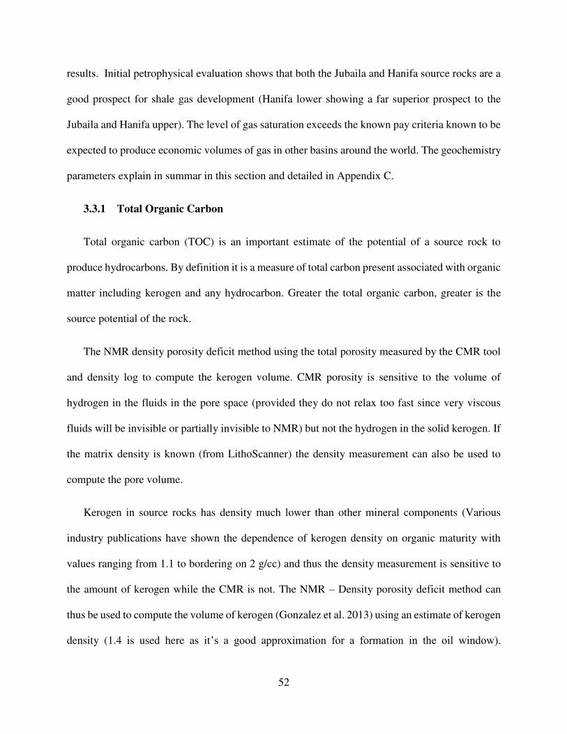
52
results. Initial petrophysical evaluation shows that both the Jubaila and Hanifa source rocks are a
good prospect for shale gas development (Hanifa lower showing a far superior prospect to the
Jubaila and Hanifa upper). The level of gas saturation exceeds the known pay criteria known to be
expected to produce economic volumes of gas in other basins around the world. The geochemistry
parameters explain in summar in this section and detailed in Appendix C.
3.3.1 Total Organic Carbon
Total organic carbon (TOC) is an important estimate of the potential of a source rock to
produce hydrocarbons. By definition it is a measure of total carbon present associated with organic
matter including kerogen and any hydrocarbon. Greater the total organic carbon, greater is the
source potential of the rock.
The NMR density porosity deficit method using the total porosity measured by the CMR tool
and density log to compute the kerogen volume. CMR porosity is sensitive to the volume of
hydrogen in the fluids in the pore space (provided they do not relax too fast since very viscous
fluids will be invisible or partially invisible to NMR) but not the hydrogen in the solid kerogen. If
the matrix density is known (from LithoScanner) the density measurement can also be used to
compute the pore volume.
Kerogen in source rocks has density much lower than other mineral components (Various
industry publications have shown the dependence of kerogen density on organic maturity with
values ranging from 1.1 to bordering on 2 g/cc) and thus the density measurement is sensitive to
the amount of kerogen while the CMR is not. The NMR – Density porosity deficit method can
thus be used to compute the volume of kerogen (Gonzalez et al. 2013) using an estimate of kerogen
density (1.4 is used here as it’s a good approximation for a formation in the oil window).
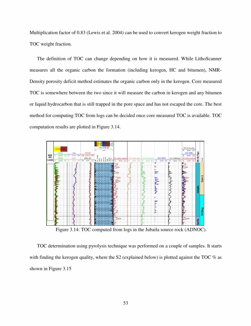
53
Multiplication factor of 0.83 (Lewis et al. 2004) can be used to convert kerogen weight fraction to
TOC weight fraction.
The definition of TOC can change depending on how it is measured. While LithoScanner
measures all the organic carbon the formation (including kerogen, HC and bitumen), NMR-
Density porosity deficit method estimates the organic carbon only in the kerogen. Core measured
TOC is somewhere between the two since it will measure the carbon in kerogen and any bitumen
or liquid hydrocarbon that is still trapped in the pore space and has not escaped the core. The best
method for computing TOC from logs can be decided once core measured TOC is available. TOC
computation results are plotted in Figure 3.14.
Figure 3.14: TOC computed from logs in the Jubaila source rock (ADNOC).
TOC determination using pyrolysis technique was performed on a couple of samples. It starts
with finding the kerogen quality, where the S2 (explained below) is plotted against the TOC % as
shown in Figure 3.15
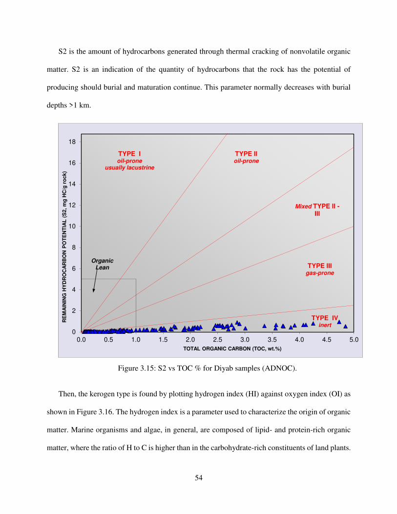
54
S2 is the amount of hydrocarbons generated through thermal cracking of nonvolatile organic
matter. S2 is an indication of the quantity of hydrocarbons that the rock has the potential of
producing should burial and maturation continue. This parameter normally decreases with burial
depths >1 km.
Figure 3.15: S2 vs TOC % for Diyab samples (ADNOC).
Then, the kerogen type is found by plotting hydrogen index (HI) against oxygen index (OI) as
shown in Figure 3.16. The hydrogen index is a parameter used to characterize the origin of organic
matter. Marine organisms and algae, in general, are composed of lipid- and protein-rich organic
matter, where the ratio of H to C is higher than in the carbohydrate-rich constituents of land plants.
0
2
4
6
8
10
12
14
16
18
0.0 0.5 1.0 1.5 2.0 2.5 3.0 3.5 4.0 4.5 5.0
RE
MA
ININ
G H
YD
RO
CA
RB
ON
PO
TE
NT
IAL
(S
2, m
g H
C/g
ro
ck)
TOTAL ORGANIC CARBON (TOC, wt.%)
TYPE IIoil-prone
Mixed TYPE II -III
TYPE IIIgas-prone
OrganicLean
TYPE IVinert
TYPE Ioil-prone
usually lacustrine
55
HI typically ranges from ~100 to 600 in geological samples. Where, oxygen index is a parameter
that correlates with the ratio of O to C, which is high for polysacharride-rich remains of land plants
and inert organic material (residual organic matter) encountered as background in marine
sediments. OI values range from near 0 to ~150.
Figure 3.16: HI vs OI for Diyab samples (ADNOC).
The last step in the conducted pyrolysis test is to link the kerogen type and maturity by plotting
HI against Tmax as shown in Figure 3.17. Tmax is the temperature at which the maximum release
of hydrocarbons from cracking of kerogen occurs during pyrolysis (top of S2 peak). Tmax is an
indication of the stage of maturation of the organic matter.
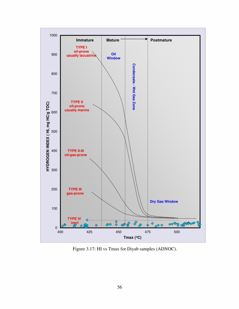
56
Figure 3.17: HI vs Tmax for Diyab samples (ADNOC).
0
100
200
300
400
500
600
700
800
900
1000
400 425 450 475 500
HY
DR
OG
EN
IN
DE
X (
HI,
mg
HC
/g T
OC
)
Tmax (oC)
TYPE Ioil-prone
usually lacustrine
TYPE IIoil-prone
usually marine
TYPE II-IIIoil-gas-prone
Co
nd
en
sa
te -
We
t Ga
s Z
on
e
Dry Gas Window
Immature Postmature
TYPE IIIgas-prone
TYPE IVinert
Mature
OilWindow
57
3.3.2 Vitrinite reflectance
Samples from Diyab formation were analyzed for thermal maturity level based on the
reflectance values measured on vitrinite (%VRo) and/or solid bitumen (%BRo). Fluorescent
macerals from the liptinite group (alginite and/or sporinite) were not present to complement the
thermal maturity assessment. Sufficient number of reflectance measurements (≥20) was collected
on solid bitumen macerals in all samples to satisfy the standard test method and return the results
with a high confidence level. Measurements collected on solid bitumen were then re-calculated to
vitrinite reflectance equivalent (%VRE), based on the equation by Jacob (1989).
Sedimentary rocks often contain low amount of terrestrial organic matter (such as vitrinite),
as well as small, reworked or oxidized grains with granulated/mottled surface, or particles with
suppressed reflectance, which are not considered to be representative as maturity indicators and
are omitted from the statistics. When the vitrinite is absent, which may be the case in marine source
rocks or the pre-Silurian rocks, the reflectance is measured on solid bitumen (%BRo, secondary
maceral) or graptolites/chitinozoans/scolecodonts (%Ro, organic fossil remains), which also
express a regular change with maturity. These data are used to present thermal maturity level as
the vitrinite reflectance equivalent (%VRE).
The vitrinite reflectance for sample A is presented in Figure 3.18, the interpretation of
Figures 3.18, 3.19 and 3.20 are presented Appendix C. A second sample with its analysis is also
presented in Appendix C.

58
Figure 3.18: Vitrinite reflectance for sample A (ADNOC).
Figure 3.19: Solid bitumen reflectance for sample A (ADNOC).
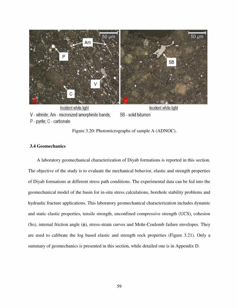
59
Figure 3.20: Photomicrographs of sample A (ADNOC).
3.4 Geomechanics
A laboratory geomechanical characterization of Diyab formations is reported in this section.
The objective of the study is to evaluate the mechanical behavior, elastic and strength properties
of Diyab formations at different stress path conditions. The experimental data can be fed into the
geomechanical model of the basin for in-situ stress calculations, borehole stability problems and
hydraulic fracture applications. This laboratory geomechanical characterization includes dynamic
and static elastic properties, tensile strength, unconfined compressive strength (UCS), cohesion
(So), internal friction angle (ϕ), stress-strain curves and Mohr-Coulomb failure envelopes. They
are used to calibrate the log based elastic and strength rock properties (Figure 3.21). Only a
summary of geomechanics is presented in this section, while detailed one is in Appendix D.
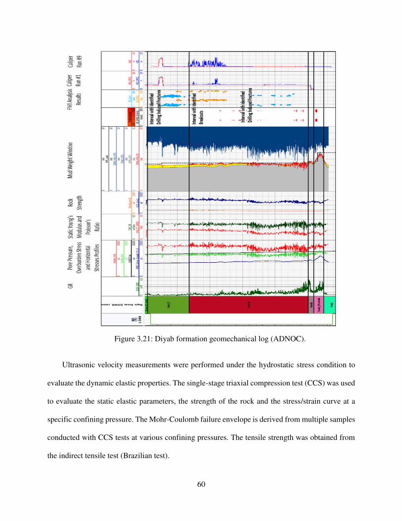
60
Figure 3.21: Diyab formation geomechanical log (ADNOC).
Ultrasonic velocity measurements were performed under the hydrostatic stress condition to
evaluate the dynamic elastic properties. The single-stage triaxial compression test (CCS) was used
to evaluate the static elastic parameters, the strength of the rock and the stress/strain curve at a
specific confining pressure. The Mohr-Coulomb failure envelope is derived from multiple samples
conducted with CCS tests at various confining pressures. The tensile strength was obtained from
the indirect tensile test (Brazilian test).
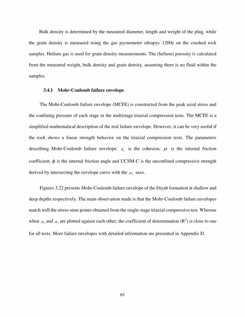
61
Bulk density is determined by the measured diameter, length and weight of the plug, while
the grain density is measured using the gas pycnometer ultrapyc 1200e on the crushed rock
samples. Helium gas is used for grain density measurements. The (helium) porosity is calculated
from the measured weight, bulk density and grain density, assuming there is no fluid within the
samples.
3.4.1 Mohr-Coulomb failure envelope
The Mohr-Coulomb failure envelope (MCFE) is constructed from the peak axial stress and
the confining pressure of each stage in the multistage triaxial compression tests. The MCFE is a
simplified mathematical description of the real failure envelope. However, it can be very useful if
the rock shows a linear strength behavior on the triaxial compression tests. The parameters
describing Mohr-Coulomb failure envelope: oS is the cohesion, is the internal friction
coefficient, 𝜙 is the internal friction angle and UCSM-C is the unconfined compressive strength
derived by intersecting the envelope curve with the 1 axes.
Figures 3.22 presents Mohr-Coulomb failure envelope of the Diyab formation at shallow and
deep depths respectively. The main observation made is that the Mohr-Coulomb failure envelopes
match well the stress-state points obtained from the single-stage triaxial compressive test. Whereas
when 1 and
3 are plotted against each other, the coefficient of determination (R2) is close to one
for all tests. More failure envelopes with detailed information are presented in Appendix D.

62
Figure 3.22: Failure envelope for Diyab formation sample at shallower depth (ADNOC).
3.4.2 Brazilian Test
Brazilian test is a simple, yet indirect assessment method to find the tensile strength of any
brittle solid such as rock and concrete. The test procedure starts with compressing a thin circular
disc across the diameter until failure is achieved. The compression force applied induces tensile
stresses perpendicular to the vertical diameter, allowing equal distribution over the region around
the center. It is referred to earlier as an indirect tensile strength test, because it is calculated based
on the assumption that the occurrence of failure is at the point of maximum tensile stress, i.e., the
disc center. Figure 3.23 presents the core status before and after Brazilian test while the tensile
strength results are presented in Appendix D.
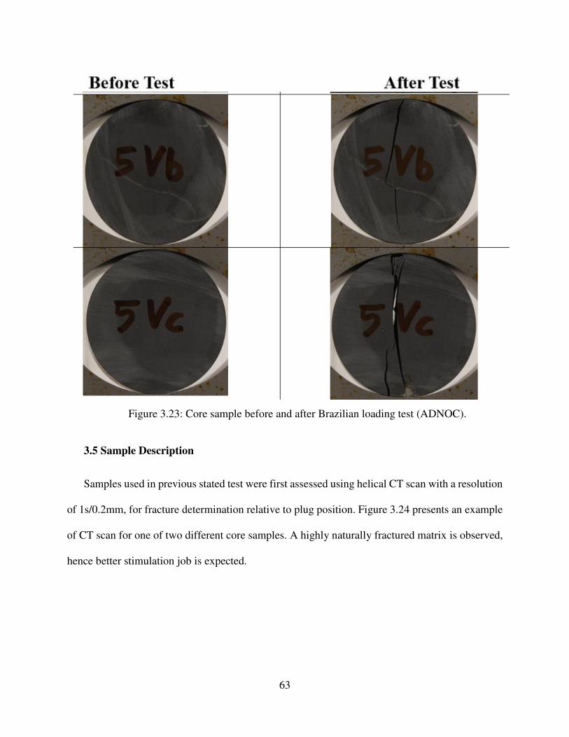
63
Figure 3.23: Core sample before and after Brazilian loading test (ADNOC).
3.5 Sample Description
Samples used in previous stated test were first assessed using helical CT scan with a resolution
of 1s/0.2mm, for fracture determination relative to plug position. Figure 3.24 presents an example
of CT scan for one of two different core samples. A highly naturally fractured matrix is observed,
hence better stimulation job is expected.
64
Figure 3.24: Diyab core sample CT scans illustrating the presence of natural fractures (ADNOC).

65
CHAPTER 4
4 MATHEMATICAL MODELS
In this chapter, the model of fracture propagation and pressure falloff in a mini-frac test are
presented for an unconventional reservoir. For readers’ convenience this chapter is simplified to
four sections, the first section, in brief, describes the system modeled. The second section includes
the governing equations and mathematical formulations developed as part of this research. Finally,
the model’s numerical solution description followed by the validation and capability of the model.
4.1 Geomechanical Model Description
The model includes a single two wing vertical hydraulic fracture propagating in porous and
permeable media (Figure 4.1). The fluid system in the model is set to be single phase, and the well
is hydraulically stimulated with slickwater. The model is set to be in a normal fault system (Figure
2.3) where the overburden stress is the maximum (z-axis) resulting in the induction of vertical
fracture propagating from the well in the maximum horizontal direction (x-axis) and perpendicular
to minimum horizontal stress (y-axis).
The fracture induced in the rock would result in stress reversal region (stress shadow) which
is a result of poroelastic, thermoelastic and fracture expansion in the media. Fracture propagation
is computed with respect to time and calculating the new minimum and maximum horizontal
stresses simultaneously from pore pressure, temperature and expansion effects, all are done in
elliptical coordinate.
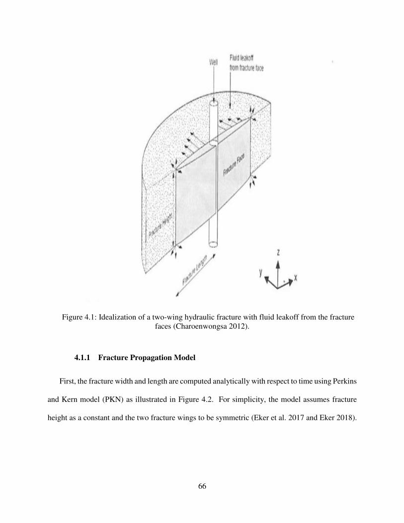
66
Figure 4.1: Idealization of a two-wing hydraulic fracture with fluid leakoff from the fracture
faces (Charoenwongsa 2012).
4.1.1 Fracture Propagation Model
First, the fracture width and length are computed analytically with respect to time using Perkins
and Kern model (PKN) as illustrated in Figure 4.2. For simplicity, the model assumes fracture
height as a constant and the two fracture wings to be symmetric (Eker et al. 2017 and Eker 2018).
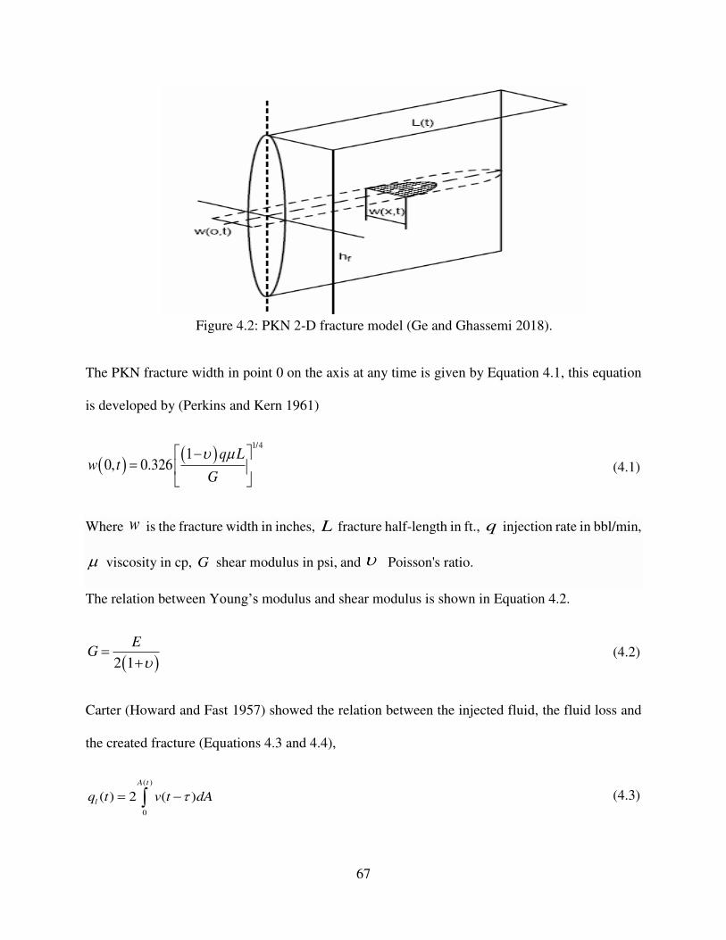
67
Figure 4.2: PKN 2-D fracture model (Ge and Ghassemi 2018).
The PKN fracture width in point 0 on the axis at any time is given by Equation 4.1, this equation
is developed by (Perkins and Kern 1961)
( ) ( ) 1/4
10, 0.326
q Lw t
G
− =
(4.1)
Where w is the fracture width in inches, L fracture half-length in ft., q injection rate in bbl/min,
viscosity in cp, G shear modulus in psi, and Poisson's ratio.
The relation between Young’s modulus and shear modulus is shown in Equation 4.2.
( )2 1
EG
=
+ (4.2)
Carter (Howard and Fast 1957) showed the relation between the injected fluid, the fluid loss and
the created fracture (Equations 4.3 and 4.4),
( )
0
( ) 2 ( )
A t
lq t v t dA= − (4.3)
68
( )( ) ( 2 )f f p
dA tq t w s
dt= + (4.4)
where inj
q is the injection fluid rate, lq fluid loss rate, f
q fracture creation fluid rate, v velocity
of the leaking filtrate, ( )A t surface area of one wing fracture, and exposure time of the fracturing
fluid to the fracture tip. Summing Equations 4.3 and 4.4 gives us the total injected fluid rate in
Equation 4.5.
( )
0
( )( ) 2 ( ) ( 2 )
A t
inj f p
dA tq t v t dA w s
dt= − + + (4.5)
Applying Laplace transformation to Equation 4.5 yields in Equation 4.6,
( ) 2
2
5.6146 2 2( ) 1
8
p x
f
L
q w s xL e erfc x
hC
+ = + − (4.6)
where E Young’s modulus in psi, h fracture height in ft, p
s spurt loss in 3 2ft ft , and LC leakoff
coefficient in ft min .
The error function in Equation 4.6 is solved by (Burger et al. 1985) approximation shown in
Equation 4.7, this applies when the error is between 3% and 20%
222
( ) 11 0.85
x x xe erfc x
x + − = +
(4.7)
Where:
2
2
L
p
Cx t
w s=
+ (4.8)
69
Reservoir controlled fluid injection occurs when the injected fluid is the same as formation fluid,
then it can be shown, using the solution of single-phase flow into a fracture, the leakoff coefficient
is:
1/2
Res Cont Fluid
1 tL L
k cC p
=
(4.9)
And,
( ) ( )L w i w Rp p t p p t p = − − (4.10)
As indicated, the above equation was based on the 1D flow at constant rate injection for
single-phase flow into formation containing the same fluid. For situations where fracturing fluid
is liquid (e.g., water), and formation fluids is either gas or very light oil as in unconventional shale,
then the exact nature of Lp is debatable! We believe, that another formulation based on injection
of a more viscous fluid to create fracture will apply. The derivation of such a formulation is referred
to as the “viscosity controlled leakoff”.
Viscosity controlled leakoff coefficient case, we begin with the equation for the interstitial frontal
velocity of the injected viscous fluid:
1 k dpu
dx = − (4.11)
Knowing thatdx
udt
= , and assuming that the injection pressure differential Lp (a positive number)
remains constant over the distance x that injected fluid travels, then we can re-write frontal velocity
as:
70
1L
k p dxu
x dt
= = (4.12)
Or,
1L
kxdx p dt
=
(4.13)
0 0
1ptL
L
kxdx p dt
=
(4.14)
2 12 L p
kL p t
=
(4.15)
12 L p
kL p t
=
(4.16)
1/2
1 1
212
L
BC L
p
L p C
k p k p k pv
L tkp t
= = =
(4.17)
1/2
Vis Cont Fluid
1
2
LL
k pC
=
(4.18)
In field units, given earlier, Equation 4.18 is:
Vis Cont Fluid
1/2
3 0
1.48 10 x
L
k pC
− =
=
(4.19)
Where, Lp is bounded by the following limits:
( ) ( )L w i w Rp p t p p t p = − − (4.20)
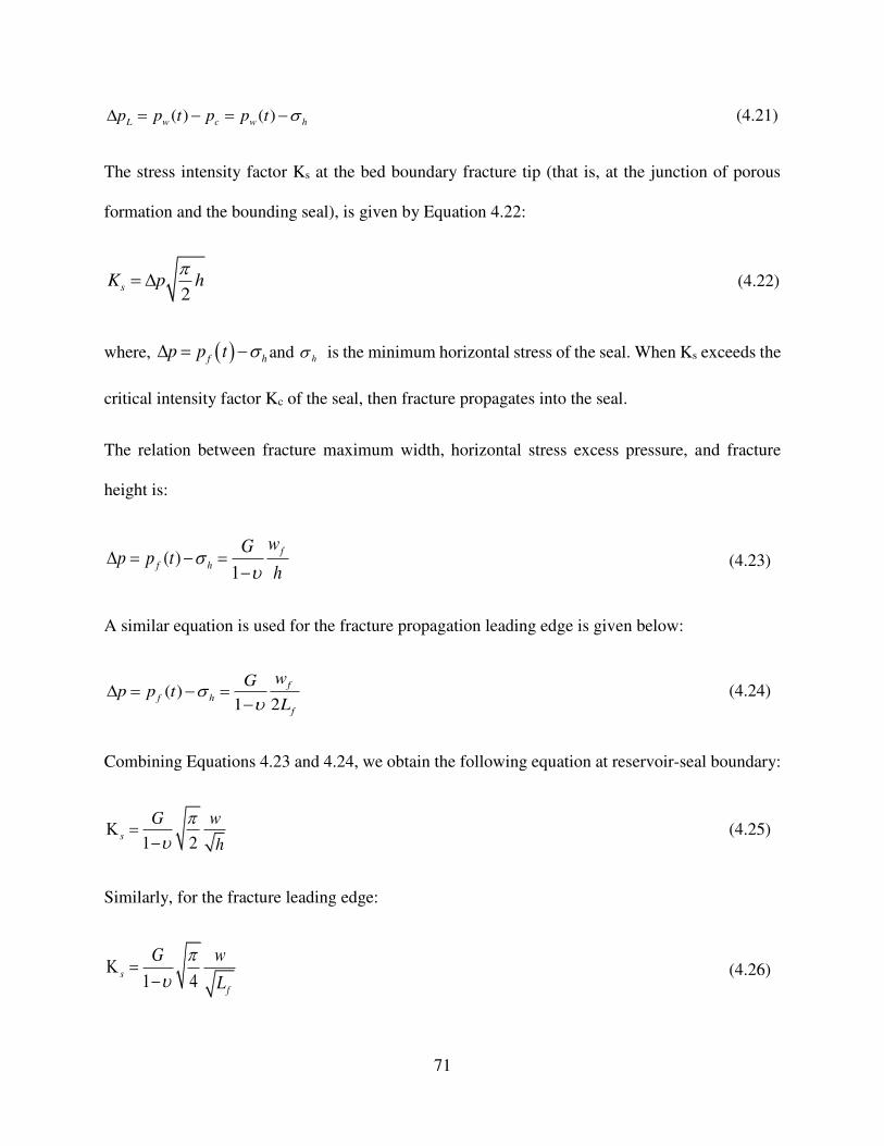
71
( ) ( )L w c w hp p t p p t = − = − (4.21)
The stress intensity factor Ks at the bed boundary fracture tip (that is, at the junction of porous
formation and the bounding seal), is given by Equation 4.22:
2sK p h
= (4.22)
where, ( )f hp p t = − and h is the minimum horizontal stress of the seal. When Ks exceeds the
critical intensity factor Kc of the seal, then fracture propagates into the seal.
The relation between fracture maximum width, horizontal stress excess pressure, and fracture
height is:
( )1
f
f h
wGp p t
h
= − =
− (4.23)
A similar equation is used for the fracture propagation leading edge is given below:
( )1 2
f
f h
f
wGp p t
L
= − =
− (4.24)
Combining Equations 4.23 and 4.24, we obtain the following equation at reservoir-seal boundary:
1 2s
G w
h
=−
(4.25)
Similarly, for the fracture leading edge:
1 4s
f
G w
L
=−
(4.26)
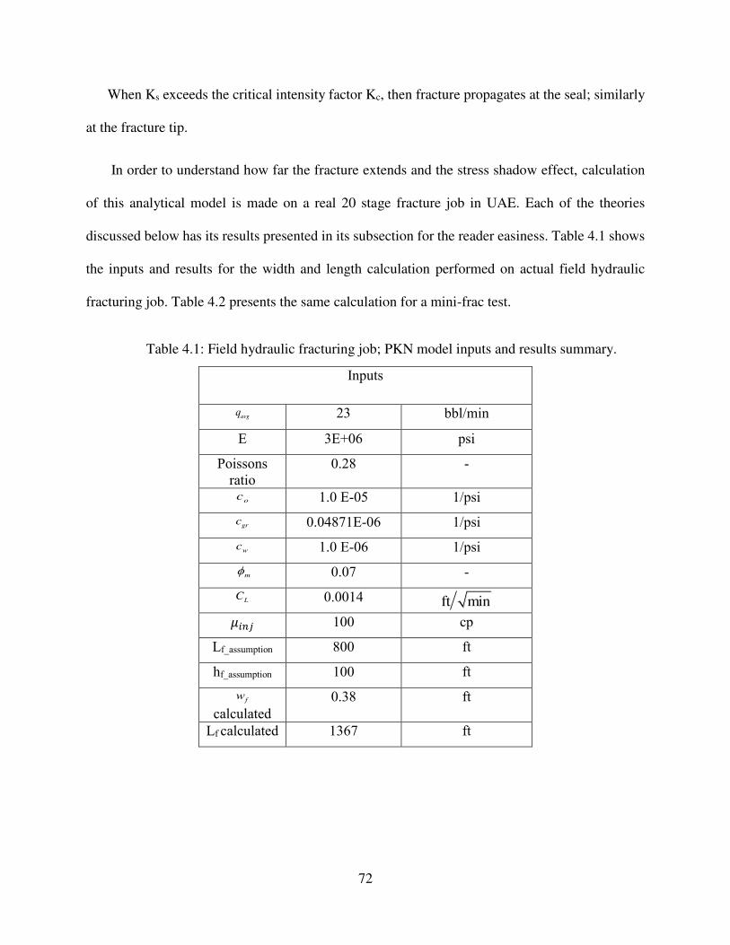
72
When Ks exceeds the critical intensity factor Kc, then fracture propagates at the seal; similarly
at the fracture tip.
In order to understand how far the fracture extends and the stress shadow effect, calculation
of this analytical model is made on a real 20 stage fracture job in UAE. Each of the theories
discussed below has its results presented in its subsection for the reader easiness. Table 4.1 shows
the inputs and results for the width and length calculation performed on actual field hydraulic
fracturing job. Table 4.2 presents the same calculation for a mini-frac test.
Table 4.1: Field hydraulic fracturing job; PKN model inputs and results summary.
Inputs
avgq 23 bbl/min
E 3E+06 psi
Poissons ratio
0.28 -
oc 1.0 E-05 1/psi
grc 0.04871E-06 1/psi
wc 1.0 E-06 1/psi
m 0.07 -
LC 0.0014 ft min 𝜇𝑖𝑛𝑗 100 cp
Lf_assumption 800 ft
hf_assumption 100 ft
fw
calculated
0.38 ft
Lf calculated 1367 ft
73
Table 4.2: Mini-frac; PKN model inputs and results summary.
Inputs
avgq 10 bbl/min
E 2.5E+06 psi
Poissons ratio
0.3 -
grc 0.04871E-06 1/psi
wc 1.0 E-06 1/psi
m 0.07 -
LC 0.0014 ft min 𝜇𝑖𝑛𝑗 100 cp
Lf_assumption 500 ft
hf_assumption 100 ft
fw
calculated
0.18 ft
Lf calculated
133 ft
4.1.2 Depth of Filtrate Invasion and Associated Pore Pressure Increase
After calculating the width and length of the fracture, Perkins and Gonzalez (1985) showed
that the volume of the cooled region and waterflooded region are determined by an energy balance
as presented in Equations 4.27 and 4.28 respectively:
(1 ) (1 )
w w ic
gr gr w w or o o or
C WV
C C S C S
=− + − +
(4.27)
(1 )
iwt
or wi
WV
S S=
− − (4.28)
74
Where, cV volume of the cooled region in 3ft , wtV volume of the water flooded region in
3ft , w
water density in 3lbm/ft , wC specific heat in °Btu/(lbm. F) , iW volume of water injected in bbl,
gr rock grain density in
3lbm/ft , gr
C specific heat in °Btu/(lbm. F) , porosity in fraction, and
orS residual oil saturation.
Knowing the volumes stated above allows the computation of the flowing bottomhole water
injection pressure as shown in Equation 4.29 (Perkins and Gonzalez 1985).
2 3iwf RP p p p= + + (4.29)
Where, iwf
P is the flowing bottomhole injection pressure, and Rp reservoir fluid pressure.
The pressure increase between the water/oil flood front and the hot/cold front 2p (neglecting
compressibility effects in this region) is presented in Equation 4.30, and pressure increase between
the hot/cold front and the fracture 3p (neglecting compressibility effects in this region) is
presented in Equation 4.31.
1 1
0 0
2
ln
141.2( )
inj w
rw
a bq
a bp
kk h
+ + =
(4.30)
0 0
3
ln
141.2( )
inj w
f
rw
a bq
Lp
kk h
+ =
(4.31)

75
Thus, the major and minor semi-axis of the elliptical cool region are shown in Equation
4.32 and Equation 4.33 respectively. While the major and minor semi-axis of the elliptical water
flooded region are shown in Equations 4.34 and 4.35 respectively
1
1
0
1
2
fL F
Fa
+
= (4.32)
1
1
0
1
2
fL F
Fb
−
= (4.33)
2
2
1
1
2
fL F
Fa
+
= (4.34)
2
2
1
1
2
fL F
Fb
−
= (4.35)
Where:
2
1 2 2
2 414
2
c c
f f
V VF
L h L h
= + + (4.36)
2
2 2 2
2 414
2
wt wt
f f
V VF
L h L h
= + + (4.37)
1F and 2F are the intermediate terms defined in Equations 4.36 and 4.37 that are used in
computing the semiaxes of the cooled and waterflooded ellipses respectively. Figure 4.3 provides
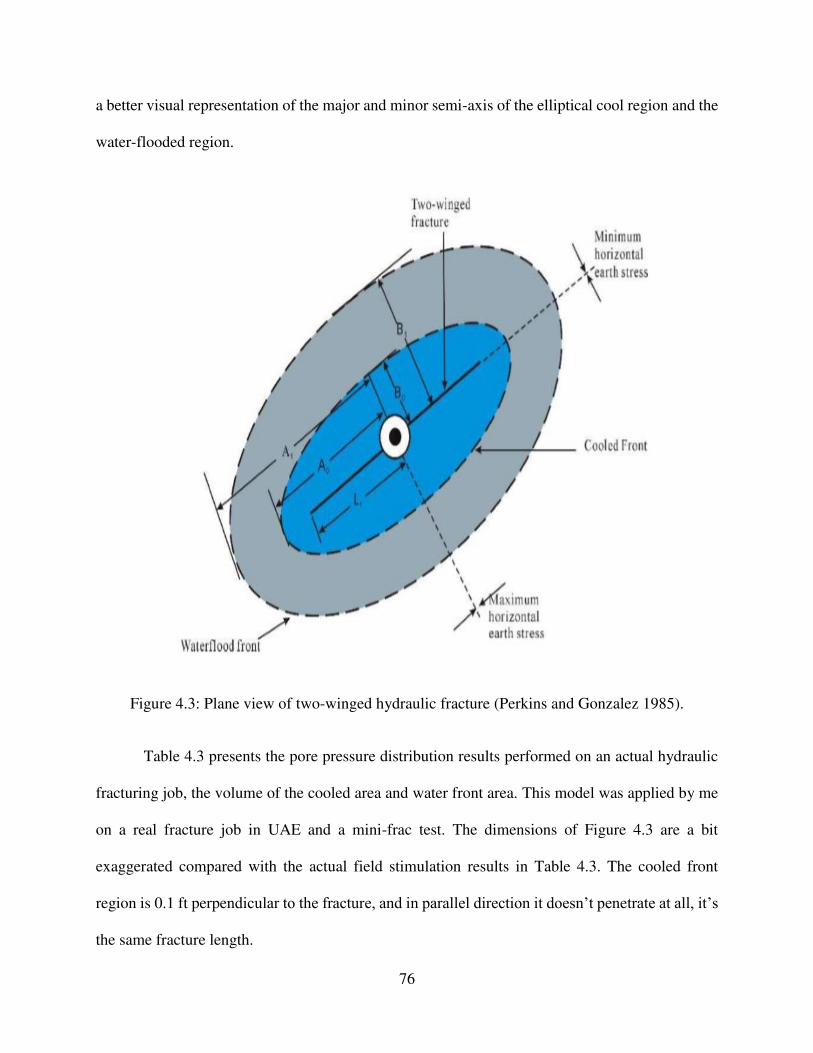
76
a better visual representation of the major and minor semi-axis of the elliptical cool region and the
water-flooded region.
Figure 4.3: Plane view of two-winged hydraulic fracture (Perkins and Gonzalez 1985).
Table 4.3 presents the pore pressure distribution results performed on an actual hydraulic
fracturing job, the volume of the cooled area and water front area. This model was applied by me
on a real fracture job in UAE and a mini-frac test. The dimensions of Figure 4.3 are a bit
exaggerated compared with the actual field stimulation results in Table 4.3. The cooled front
region is 0.1 ft perpendicular to the fracture, and in parallel direction it doesn’t penetrate at all, it’s
the same fracture length.
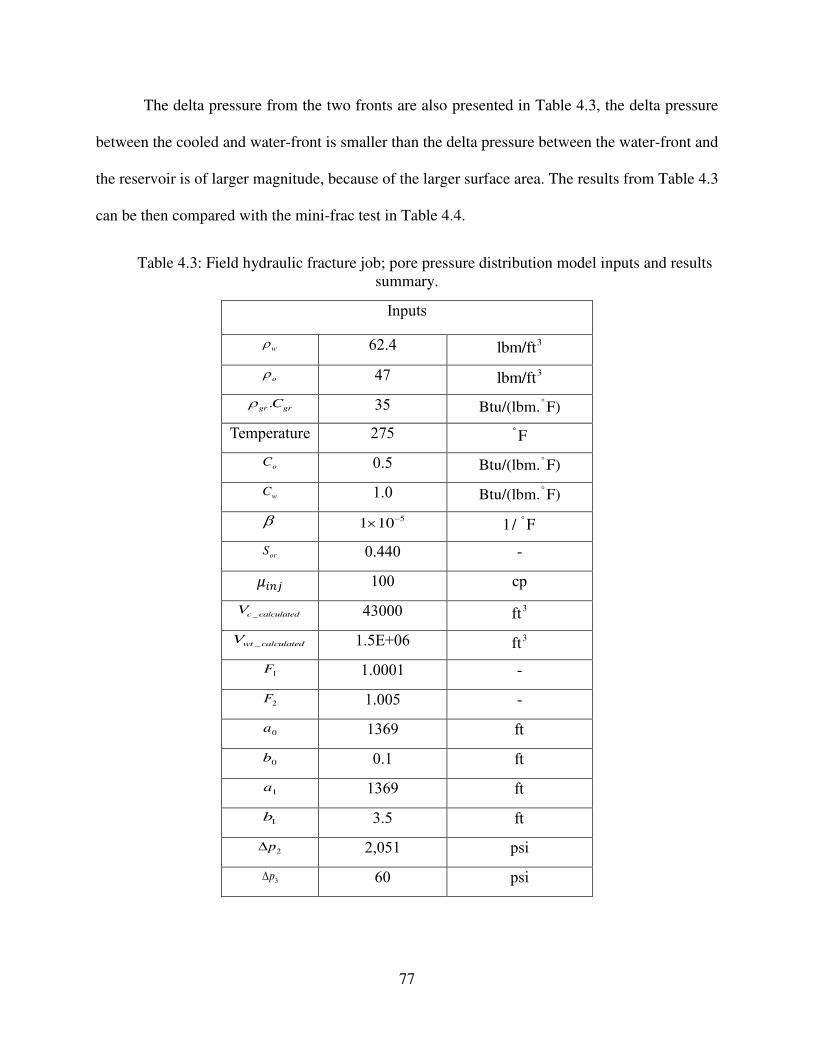
77
The delta pressure from the two fronts are also presented in Table 4.3, the delta pressure
between the cooled and water-front is smaller than the delta pressure between the water-front and
the reservoir is of larger magnitude, because of the larger surface area. The results from Table 4.3
can be then compared with the mini-frac test in Table 4.4.
Table 4.3: Field hydraulic fracture job; pore pressure distribution model inputs and results
summary.
Inputs
w 62.4 3lbm/ft
o 47 3lbm/ft
.gr gr
C 35 °Btu/(lbm. F)
Temperature 275 ° F
oC 0.5 °Btu/(lbm. F)
wC 1.0 °Btu/(lbm. F)
51 10− °1/ F
orS 0.440 - 𝜇𝑖𝑛𝑗 100 cp
_c calculatedV 43000 3ft
_wt calculatedV 1.5E+06 3ft
1F 1.0001 -
2F 1.005 -
0a 1369 ft
0b 0.1 ft
1a 1369 ft
1b 3.5 ft
2p 2,051 psi
3p 60 psi
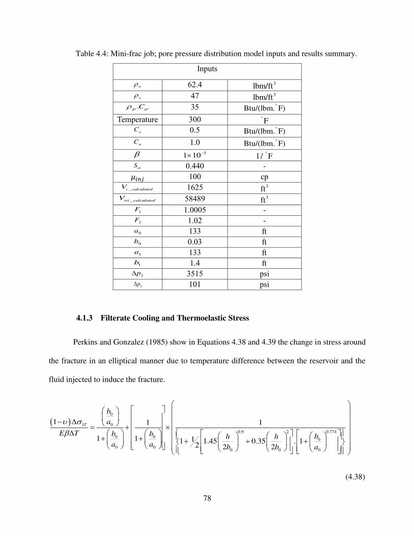
78
Table 4.4: Mini-frac job; pore pressure distribution model inputs and results summary.
Inputs
w 62.4 3lbm/ft
o 47 3lbm/ft
.gr gr
C 35 °Btu/(lbm. F)
Temperature 300 ° F
oC 0.5 °Btu/(lbm. F)
wC 1.0 °Btu/(lbm. F)
51 10− °1/ F
orS 0.440 - 𝜇𝑖𝑛𝑗 100 cp
_c calculatedV 1625 3ft
_wt calculatedV 58489 3ft
1F 1.0005 - 2F 1.02 - 0a 133 ft
0b 0.03 ft
1a 133 ft
1b 1.4 ft
2p 3515 psi 3p 101 psi
4.1.3 Filterate Cooling and Thermoelastic Stress
Perkins and Gonzalez (1985) show in Equations 4.38 and 4.39 the change in stress around
the fracture in an elliptical manner due to temperature difference between the reservoir and the
fluid injected to induce the fracture.
( )0
01
0.9 2 0.7740 0
0
0 00 0 0
1 1 1
1 1 11 1.45 0.35 . 12 2 2
T
b
a
E T b b bh ha a b b a
− = + + + + + +
(4.38)
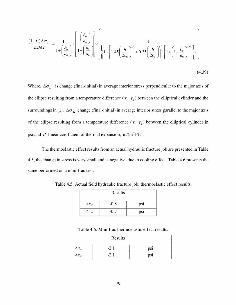
79
( )0
02
0.9 2 1.360 0
0
0 00 0 0
1 1 1
1 1 1 1.45 0.35 . 1 12 2
T
b
a
E T b b bh ha a b b a
− = + + + + + + −
(4.39)
Where, 1T is change (final-initial) in average interior stress perpendicular to the major axis of
the ellipse resulting from a temperature difference (RT T− ) between the elliptical cylinder and the
surroundings in psi , 2T change (final-initial) in average interior stress parallel to the major axis
of the ellipse resulting from a temperature difference (RT T− ) between the elliptical cylinder in
psi,and linear coefficient of thermal expansion, °in/(in F) .
The thermoelastic effect results from an actual hydraulic fracture job are presented in Table
4.5, the change in stress is very small and is negative, due to cooling effect. Table 4.6 presents the
same performed on a mini-frac test.
Table 4.5: Actual field hydraulic fracture job; thermoelastic effect results.
Results
1T -0.8 psi
2T -0.7 psi
Table 4.6: Mini-frac thermoelastic effect results.
Results
1T -2.1 psi
2T -2.1 psi

80
4.1.4 Filterate Invasion and Poroelastic Effect
Perkins and Gonzalez (1985) also shows in Equations 4.40 and 4.41 the change in stress
around the fracture in an elliptical manner due to pore pressure difference.
( )0
1 0
0.9 2 0.7740 0
0
0 00 0 0
1 1 1
1 1 11 1.45 0.35 . 12 2 2
p
b
a
EJ p b b bh ha a b b a
− = + + + + + +
(4.40)
( )0
2 0
0.9 2 1.360 0
0
0 00 0 0
1 1 1
1 1 1 1.45 0.35 . 1 12 2
p
b
a
EJ p b b bh ha a b b a
− = + + + + + + −
(4.41)
1 2
3
grc
JE
−= − (4.42)
Where, 1p
is change (final-initial) in average interior stress perpendicular to the major axis of
the ellipse resulting from a pressure difference ( RP P− ) between the elliptical cylinder and the
surroundings, psi [MPa], 2 p change (final-initial) in average interior stress parallel to the major
axis of the ellipse resulting from a pressure difference ( RP P− ) between the elliptical cylinder and
the surroundings, psi [MPa], and J linear coefficient of pore pressure expansion.
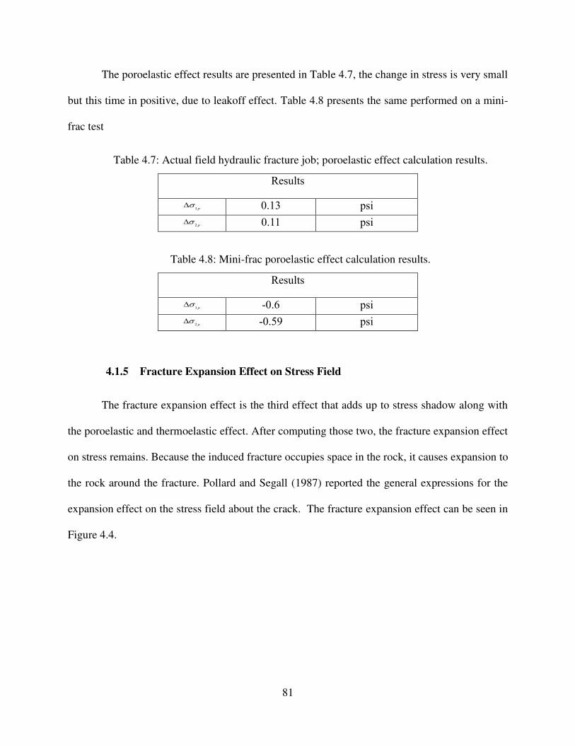
81
The poroelastic effect results are presented in Table 4.7, the change in stress is very small
but this time in positive, due to leakoff effect. Table 4.8 presents the same performed on a mini-
frac test
Table 4.7: Actual field hydraulic fracture job; poroelastic effect calculation results.
Results
1 p 0.13 psi
2 p 0.11 psi
Table 4.8: Mini-frac poroelastic effect calculation results.
Results
1 p -0.6 psi
2 p -0.59 psi
4.1.5 Fracture Expansion Effect on Stress Field
The fracture expansion effect is the third effect that adds up to stress shadow along with
the poroelastic and thermoelastic effect. After computing those two, the fracture expansion effect
on stress remains. Because the induced fracture occupies space in the rock, it causes expansion to
the rock around the fracture. Pollard and Segall (1987) reported the general expressions for the
expansion effect on the stress field about the crack. The fracture expansion effect can be seen in
Figure 4.4.
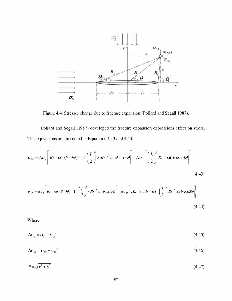
82
Figure 4.4: Stresses change due to fracture expansion (Pollard and Segall 1987).
Pollard and Segall (1987) developed the fracture expansion expressions effect on stress.
The expressions are presented in Equations 4.43 and 4.44.
2 2
1 3 3
1 cos( ) 1 sin sin 3 sin cos32 2
F I II
L LRr Rr Rr − − − = − − + +
(4.43)
2 2
1 3 1 3
2 cos( ) 1 sin sin 3 2 sin( ) sin cos32 2
F I II
L LRr Rr Rr Rr − − − − = − − − + − −
(4.44)
Where:
11 11
c
I = − (4.45)
12 12
c
II = − (4.46)
2 2R x y= + (4.47)
83
1tany
x − =
(4.48)
2
2
12
LR x y
= − +
(4.49)
1
1 tan
2
y
Lx
−
= −
(4.50)
2
2
22
LR x y
= + +
(4.51)
1
2 tan
2
y
Lx
−
= +
(4.52)
1 2( )r R R= (4.53)
( )1 2
2
+ = (4.54)
Where, 1F is change (final-initial) in average interior stress perpendicular to the major axis of
the ellipse resulting from the space occupied by the induced fracture between the elliptical cylinder
and the surrounding in psi. 2F is change (final-initial) in average interior stress parallel to the
major axis of the ellipse resulting from the space occupied by the induced fracture between the
elliptical cylinder and the surrounding in psi. is the angle between the fracture and point of
interest, in radians. R is the distance between the fracture and point of interest, in ft. 11 is the

84
remote stress perpendicular to the fracture ( h ) in psi. 22 is the remote stress parallel to the
fracture ( H ) in psi. 12 is the remote shear stress to the fracture in psi. 11
c is normal stress on
the fracture internal surface (f
p ) in psi. 12
c is the shear stress to the fracture internal surface in
psi.
The fracture expansion effect results are presented in Table 4.9, the change in stress is the
largest in magnitude compared with the temperature and pore pressure, due to the low
compressibility of the formation. Table 4.10 presents the expansion effect on a mini-frac test.
Table 4.9: Actual field hydraulic fracture job; fracture expansion effect results.
Results
x 100 ft
y 100 ft
1F 2202 psi
2 F 441 psi
Table 4.10: Mini-frac fracture expansion effect results.
Results
x 100 ft
y 100 ft
1F 492 psi
2 F -564 psi
85
4.1.6 Total stress field
The total stress field around the fracture is simply the sum of the in-situ original stress, and
the stresses induced by thermoelasticity, poroelasticity and fracture expansion. Summing up each
direction as shown in Equations 4.55 and 4.56 yields with the new stress redistribution around the
fracture.
1 1 1yy h p T F = + + + (4.55)
2 2 2xx H p T F = + + + (4.56)
Where, yy
is the new normal stress after fracture induction. h is the minimum horizontal stress
before fracture induction. H is the maximum horizontal stress before fracture induction. 1p
and 2 p
are the poroelastic stress effect after fracture induction. 1T and 2T are the
thermoelastic stress effect after fracture induction. 1F and 2F are the stress effect due to
fracture expansion, all in psi.
The total stress field results around the fracture are presented in Table 4.11, the effect of
all the models, did alter the minimum horizontal stress to maximum and the maximum to
minimum. Proving the fracture changes direction, hence creating complex one. yy
is the
minimum horizontal stress after the total stress field is applied to it, while xx is the maximum
horizontal stress after the total stress field is applied to it. The difference in magnitude of both is
associated with new fracture induction. The exact same conclusion is made on the mini-frac test
calculation presented in Table 4.12.
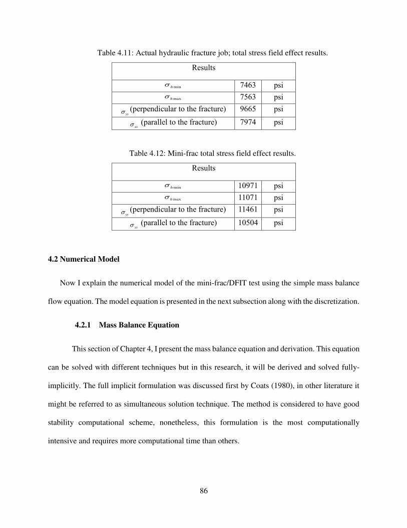
86
Table 4.11: Actual hydraulic fracture job; total stress field effect results.
Results
minh 7463 psi maxh 7563 psi
yy (perpendicular to the fracture) 9665 psi
xx (parallel to the fracture) 7974 psi
Table 4.12: Mini-frac total stress field effect results.
Results
minh 10971 psi maxh 11071 psi
yy (perpendicular to the fracture) 11461 psi
xx (parallel to the fracture) 10504 psi
4.2 Numerical Model
Now I explain the numerical model of the mini-frac/DFIT test using the simple mass balance
flow equation. The model equation is presented in the next subsection along with the discretization.
4.2.1 Mass Balance Equation
This section of Chapter 4, I present the mass balance equation and derivation. This equation
can be solved with different techniques but in this research, it will be derived and solved fully-
implicitly. The full implicit formulation was discussed first by Coats (1980), in other literature it
might be referred to as simultaneous solution technique. The method is considered to have good
stability computational scheme, nonetheless, this formulation is the most computationally
intensive and requires more computational time than others.
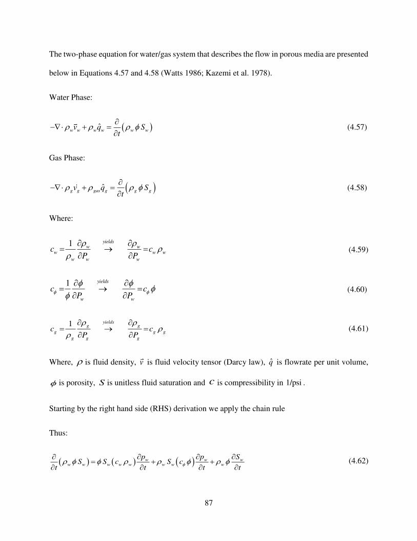
87
The two-phase equation for water/gas system that describes the flow in porous media are presented
below in Equations 4.57 and 4.58 (Watts 1986; Kazemi et al. 1978).
Water Phase:
( )ˆ w w w w w wv q St
− + =
(4.57)
Gas Phase:
( )ˆ g g gas g g gv q St
− + =
(4.58)
Where:
1
yiel
ww w
ds
w w
w w w
c cP P
= → =
(4.59)
1
yiel
w
ds
w
c cP P
= → =
(4.60)
1
yiel
g
g gds
g g
g g g
c cP P
= → =
(4.61)
Where, is fluid density, v is fluid velocity tensor (Darcy law), q̂ is flowrate per unit volume,
is porosity, S is unitless fluid saturation and c is compressibility in 1/psi .
Starting by the right hand side (RHS) derivation we apply the chain rule
Thus:
( ) ( ) ( ) w w ww w w w w w w w
p p SS S c S c
t t t t
= + +
(4.62)
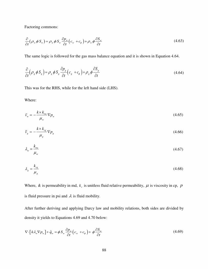
88
Factoring commons:
( ) ( ) w ww w w w w w
p SS S c c
t t t
= + +
(4.63)
The same logic is followed for the gas mass balance equation and it is shown in Equation 4.64.
( ) ( ) g g
g g g g g g
p SS S c c
t t t
= + +
(4.64)
This was for the RHS, while for the left hand side (LHS).
Where:
rww
w
w
k kv p
= − (4.65)
rg
g
g
g
k kv p
= − (4.66)
rww
w
k
= (4.67)
rg
g
g
k
= (4.68)
Where, k is permeability in md, rk is unitless fluid relative permeability, is viscosity in cp, p
is fluid pressure in psi and is fluid mobility.
After further deriving and applying Darcy law and mobility relations, both sides are divided by
density it yields to Equations 4.69 and 4.70 below:
( ) ˆ w ww ww ww
p Sk p q S c c
t t
+ = + +
(4.69)
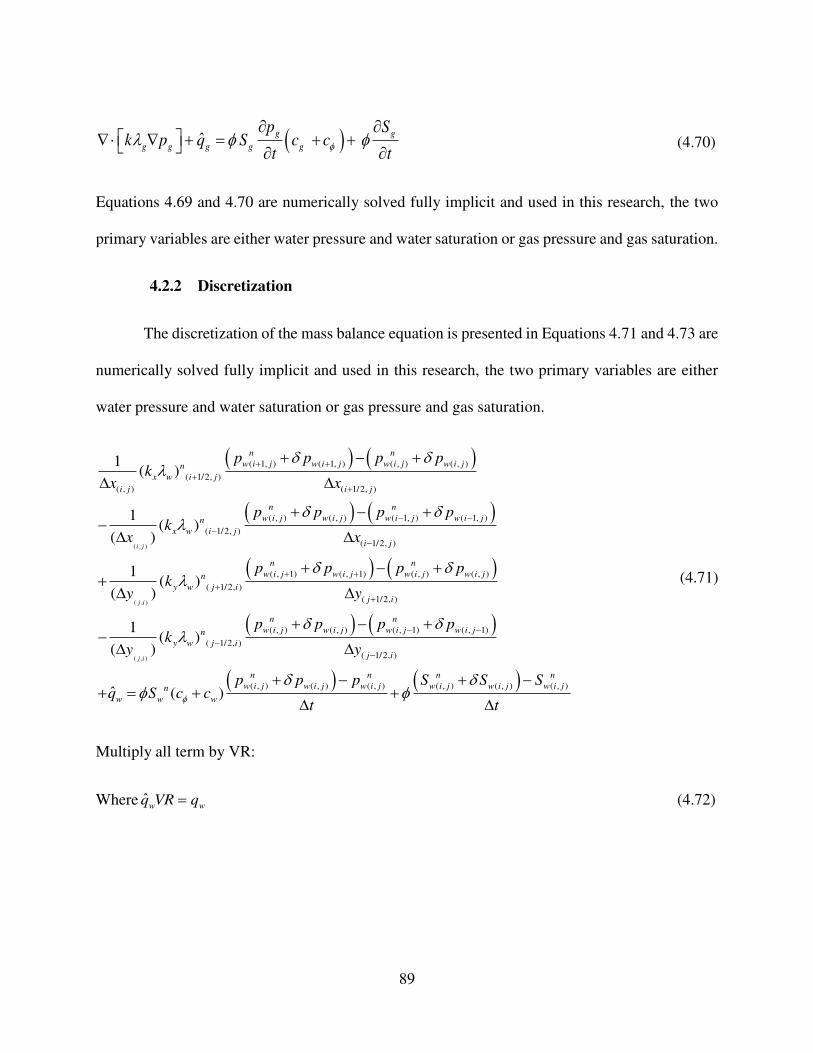
89
( ) ˆ g g
g g g g g
p Sk p q S c c
t t
+ = + +
(4.70)
Equations 4.69 and 4.70 are numerically solved fully implicit and used in this research, the two
primary variables are either water pressure and water saturation or gas pressure and gas saturation.
4.2.2 Discretization
The discretization of the mass balance equation is presented in Equations 4.71 and 4.73 are
numerically solved fully implicit and used in this research, the two primary variables are either
water pressure and water saturation or gas pressure and gas saturation.
( ) ( )
( ) ( )
( ))
( )
( ,
,
( 1, ) ( 1, ) ( , ) ( , )
( 1/2, )
( , ) ( 1/2, )
( , ) ( , ) ( 1, ) ( 1, )
( 1/2, )
( , 1
(
) ( , 1)
(
2
1/2
1 )
,
,
)
/
1
(
( )
1(
(
1)
))
( )j
i j
i
w i j i j w i j i jn
x i j
i j i j
w i j i j w i j i j
n n
w w
w
n n
w w
w
n
w
ix
i
j
n
j
i j
j w i jn
y w i
p pk
x x
p p
p p
p p
p pk
y
kx x
+ ++
+
− −
+
−
+
−
+
−
−−
+−
+ +
+ +
+
( )
( ) ( )
( ) ( )( , )
( , ) ( , )
( 1/2, )
( , ) ( , ) ( , 1) ( , 1)
( 1/2, )
( 1/2, )
( , ) ( , ) ( , ) ( , ) ( , ) ( , )
1( )
( )
ˆ ( )
j i
n
w i j w i j
j i
n n
w i j w i j w i j w i jn
y w j i
j i
n n n n
w i j w i j w i j w i j w i j w i jn
w w w
p p
y
p p p pk
y y
p p p S S Sq S c c
t t
+
− −−
−
+
+ − +−
+ − + −+ = + +
(4.71)
Multiply all term by VR:
Where ˆw wq VR q= (4.72)
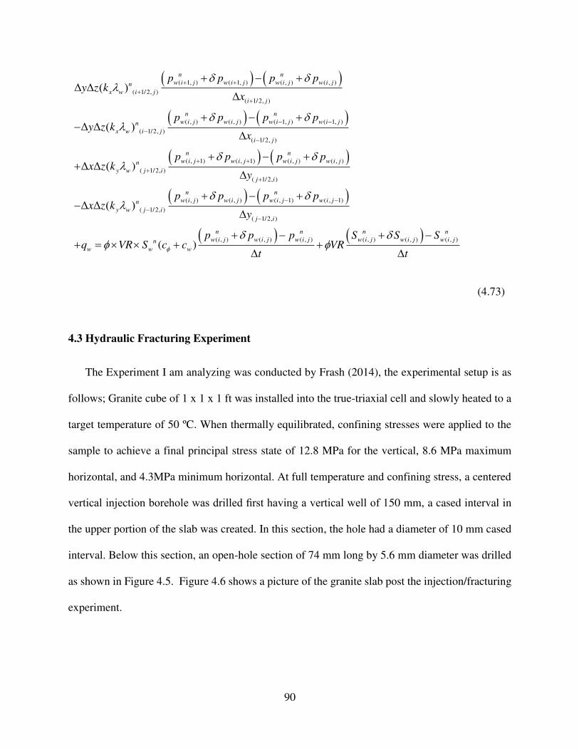
90
( ) ( )
( ) ( )
( )
( 1, ) ( 1, ) ( , ) ( , )
( 1/2, )
( 1/2, )
( , ) ( , ) ( 1, ) ( 1, )
( 1
)
( , 1) ( , 1) ( , ) ( ,
( 1/
2
2, )
/ , )
( 1/2,
Δ )
Δ Δ (
Δ (
)
Δ (
Δ )
n n
w w
w
n n
w w
w
n n
w i j w i j w i j w i j
w i j i j w i j i jn
x i j
i j
w i j i
w
j w i j i jn
x i
j
n
y j
j
i
i
p py z k
x
p p
p p
p p
k
p p
p
x
p
z k
y zx
+ ++
+
−
+
−
+
−
+
−
−
−−
++
+ +
+ +
+ − ( )
( ) ( )
( ) ( )
)
( 1/2, )
( , ) ( , ) ( , 1) ( , 1)
( 1/2, )
( 1/2, )
( , ) ( , ) ( , ) ( , ) ( , ) ( , )
Δ Δ ( )
( )
j i
n n
w i j w i j w i j w i jn
y w j i
j i
n n n n
w i j w i j w i j w i j w i j w i jn
w w w
y
p p p px z k
y
p p p S S Sq VR S c c VR
t t
+
− −−
−
+ − +−
+ − + −+ = + +
(4.73)
4.3 Hydraulic Fracturing Experiment
The Experiment I am analyzing was conducted by Frash (2014), the experimental setup is as
follows; Granite cube of 1 x 1 x 1 ft was installed into the true-triaxial cell and slowly heated to a
target temperature of 50 ºC. When thermally equilibrated, confining stresses were applied to the
sample to achieve a final principal stress state of 12.8 MPa for the vertical, 8.6 MPa maximum
horizontal, and 4.3MPa minimum horizontal. At full temperature and confining stress, a centered
vertical injection borehole was drilled first having a vertical well of 150 mm, a cased interval in
the upper portion of the slab was created. In this section, the hole had a diameter of 10 mm cased
interval. Below this section, an open-hole section of 74 mm long by 5.6 mm diameter was drilled
as shown in Figure 4.5. Figure 4.6 shows a picture of the granite slab post the injection/fracturing
experiment.

91
Figure 4.5: Hydraulic fracturing experiment well dimensions (Frash 2014).
Figure 4.6: Granite slab post fracture (Frash 2014).
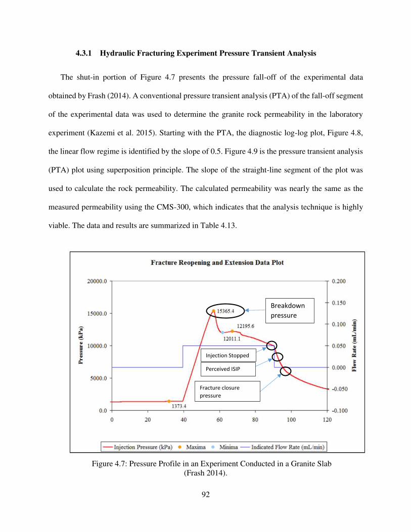
92
4.3.1 Hydraulic Fracturing Experiment Pressure Transient Analysis
The shut-in portion of Figure 4.7 presents the pressure fall-off of the experimental data
obtained by Frash (2014). A conventional pressure transient analysis (PTA) of the fall-off segment
of the experimental data was used to determine the granite rock permeability in the laboratory
experiment (Kazemi et al. 2015). Starting with the PTA, the diagnostic log-log plot, Figure 4.8,
the linear flow regime is identified by the slope of 0.5. Figure 4.9 is the pressure transient analysis
(PTA) plot using superposition principle. The slope of the straight-line segment of the plot was
used to calculate the rock permeability. The calculated permeability was nearly the same as the
measured permeability using the CMS-300, which indicates that the analysis technique is highly
viable. The data and results are summarized in Table 4.13.
Figure 4.7: Pressure Profile in an Experiment Conducted in a Granite Slab
(Frash 2014).
Breakdown
pressure
Perceived ISIP
Fracture closure
pressure
Injection Stopped
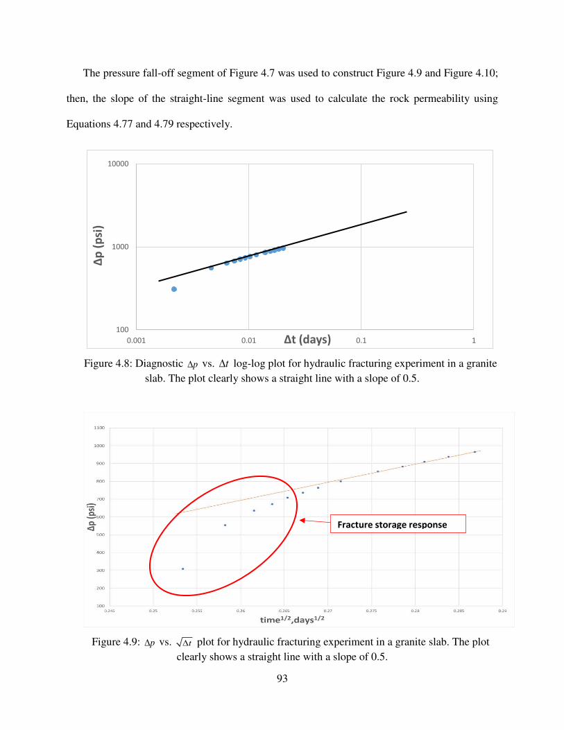
93
The pressure fall-off segment of Figure 4.7 was used to construct Figure 4.9 and Figure 4.10;
then, the slope of the straight-line segment was used to calculate the rock permeability using
Equations 4.77 and 4.79 respectively.
Figure 4.8: Diagnostic p vs. t log-log plot for hydraulic fracturing experiment in a granite
slab. The plot clearly shows a straight line with a slope of 0.5.
Figure 4.9: p vs. t plot for hydraulic fracturing experiment in a granite slab. The plot
clearly shows a straight line with a slope of 0.5.
100
1000
10000
0.001 0.01 0.1 1
∆p (p
si)
∆t (days)
Fracture storage response
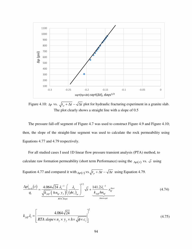
94
Figure 4.10: p vs. pt t t+ − plot for hydraulic fracturing experiment in a granite slab.
The plot clearly shows a straight line with a slope of 0.5
The pressure fall-off segment of Figure 4.7 was used to construct Figure 4.9 and Figure 4.10;
then, the slope of the straight-line segment was used to calculate the rock permeability using
Equations 4.77 and 4.79 respectively.
For all studied cases I used 1D linear flow pressure transient analysis (PTA) method, to
calculate raw formation permeability (short term Performance) using the ( )p t vs. t using
Equation 4.77 and compared it with ( )p t vspt t t+ − using Equation 4.79.
( )( ) ( )
1/21 1
0
4.064 24 141.2 facex t t thf
t t feff hffeff hf f m
InterceptRTA Slope
p tt s
q c k hnk hn y
− −=
= +
(4.74)
2
4.064 24
feff t
f f t
kRTA slope n y h c
=
(4.75)
100
200
300
400
500
600
700
800
900
1000
1100
-0.3 -0.25 -0.2 -0.15 -0.1 -0.05 0
∆p (p
si)
sqrt(tp+Δt)-sqrt(Δt), days1/2
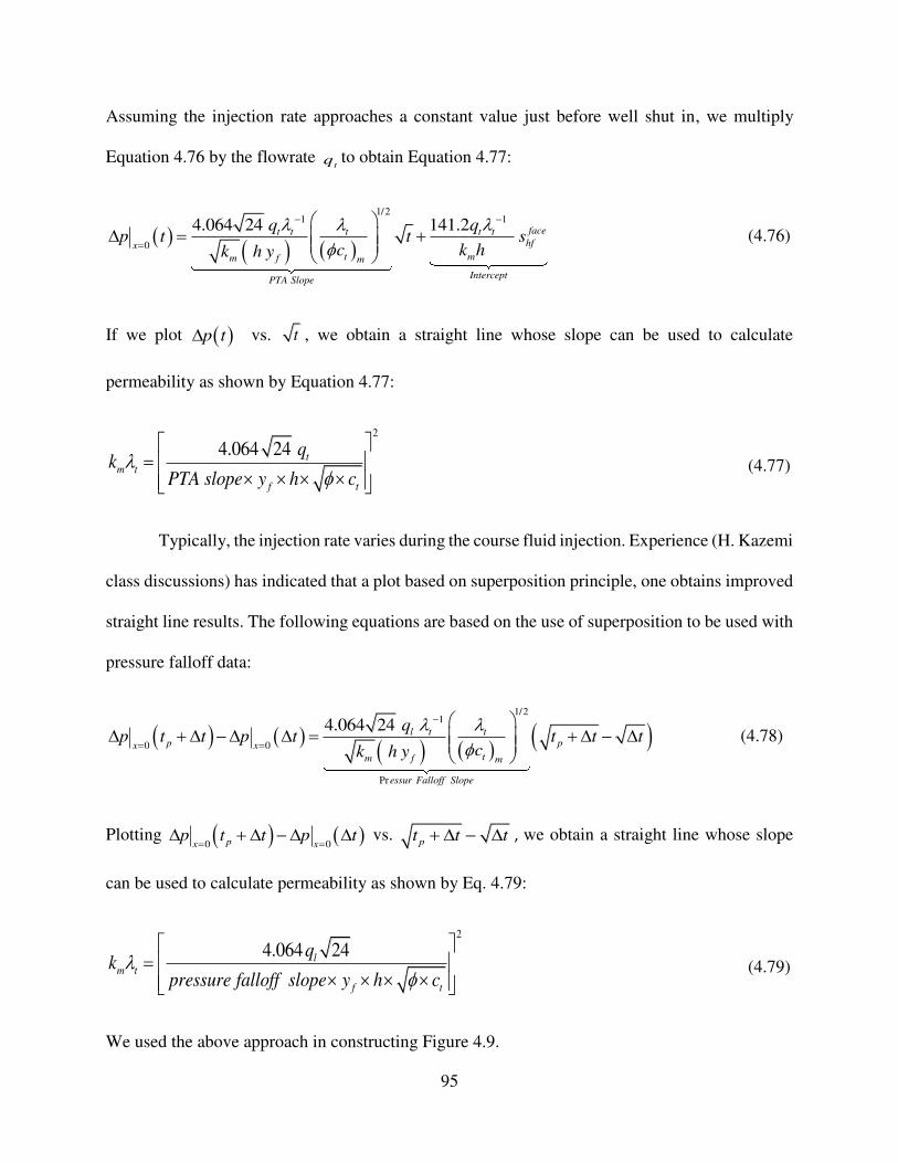
95
Assuming the injection rate approaches a constant value just before well shut in, we multiply
Equation 4.76 by the flowrate tq to obtain Equation 4.77:
( ) ( ) ( )
1/21 1
0
4.064 24 141.2 facet t t t thfx
t mm f m
InterceptPTA Slope
q qp t t s
c k hk h y
− −
=
= +
(4.76)
If we plot ( )p t vs. t , we obtain a straight line whose slope can be used to calculate
permeability as shown by Equation 4.77:
2
4.064 24
tm t
f t
qk
PTA slope y h c
=
(4.77)
Typically, the injection rate varies during the course fluid injection. Experience (H. Kazemi
class discussions) has indicated that a plot based on superposition principle, one obtains improved
straight line results. The following equations are based on the use of superposition to be used with
pressure falloff data:
( ) ( ) ( ) ( ) ( )1/2
1
0 0
Pr
4.064 24 l t tp px x
tm f m
essur Falloff Slope
qp t t p t t t t
ck h y
−
= =
+ − = + −
(4.78)
Plotting ( ) ( )0 0px x
p t t p t= =
+ − vs. pt t t+ − , we obtain a straight line whose slope
can be used to calculate permeability as shown by Eq. 4.79:
2
4.064 24
lm t
f t
qk
pressure falloff slope y h c
=
(4.79)
We used the above approach in constructing Figure 4.9.
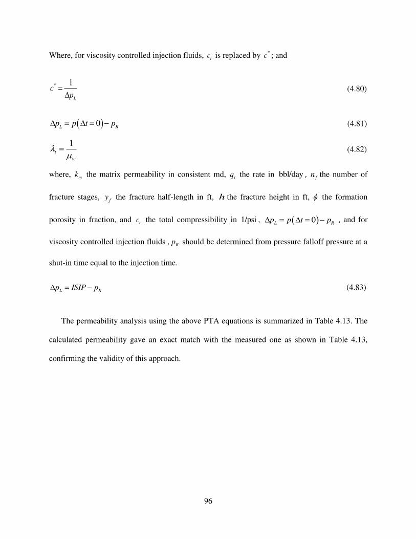
96
Where, for viscosity controlled injection fluids, tc is replaced by *
c ; and
* 1
L
cp
=
(4.80)
( )0 L R
p p t p = = − (4.81)
1t
w
= (4.82)
where, mk the matrix permeability in consistent md, tq the rate in bbl/day , f
n the number of
fracture stages, f
y the fracture half-length in ft, h the fracture height in ft, the formation
porosity in fraction, and tc the total compressibility in 1/psi , ( )0 L R
p p t p = = − , and for
viscosity controlled injection fluids , Rp should be determined from pressure falloff pressure at a
shut-in time equal to the injection time.
L Rp ISIP p = − (4.83)
The permeability analysis using the above PTA equations is summarized in Table 4.13. The
calculated permeability gave an exact match with the measured one as shown in Table 4.13,
confirming the validity of this approach.
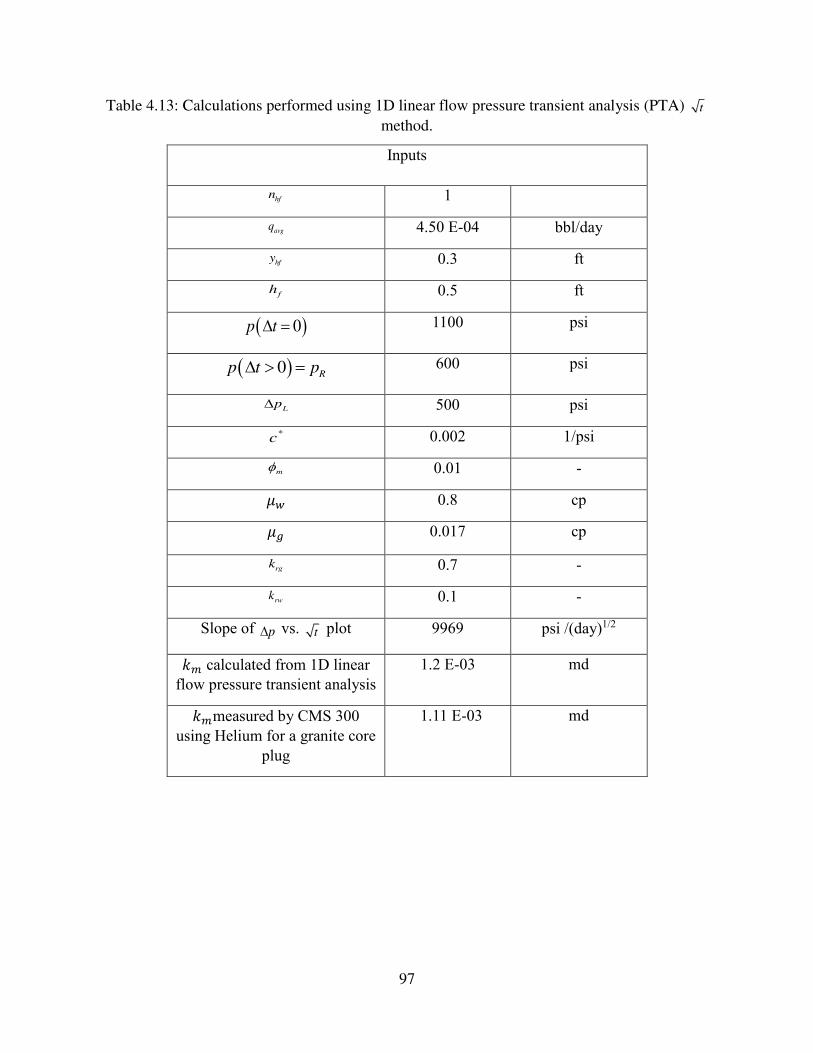
97
Table 4.13: Calculations performed using 1D linear flow pressure transient analysis (PTA) t
method.
Inputs
hfn 1
avgq 4.50 E-04 bbl/day
hfy 0.3 ft
fh 0.5 ft
( )0p t = 1100 psi
( )0R
p t p = 600 psi
Lp 500 psi *
c 0.002 1/psi
m 0.01 - 𝜇𝑤 0.8 cp 𝜇𝑔 0.017 cp
rgk 0.7 -
rwk 0.1 -
Slope of p vs. t plot 9969 psi /(day)1/2 𝑘𝑚 calculated from 1D linear flow pressure transient analysis
1.2 E-03
md
𝑘𝑚measured by CMS 300 using Helium for a granite core
plug
1.11 E-03
md
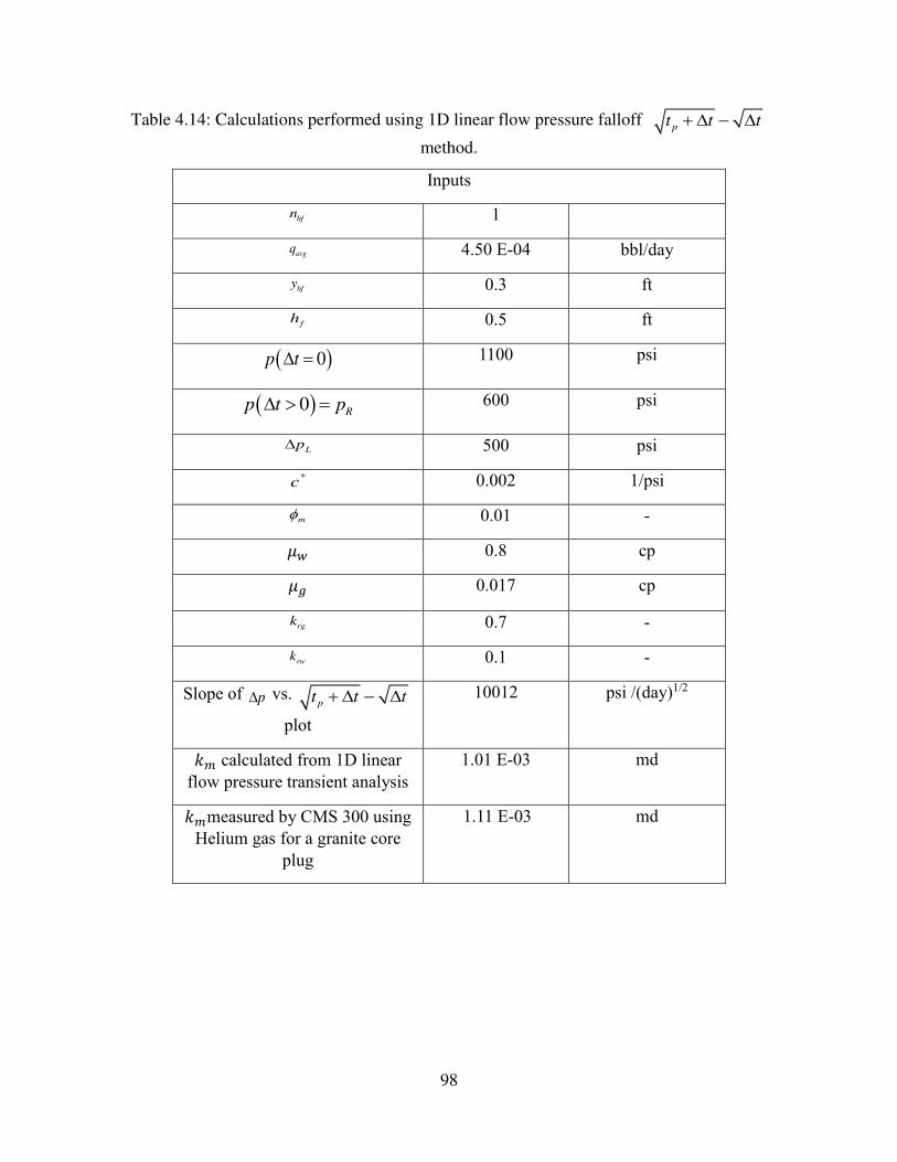
98
Table 4.14: Calculations performed using 1D linear flow pressure falloff pt t t+ −
method.
Inputs
hfn 1
avgq 4.50 E-04 bbl/day
hfy 0.3 ft
fh 0.5 ft
( )0p t = 1100 psi
( )0R
p t p = 600 psi
Lp 500 psi *
c 0.002 1/psi
m 0.01 - 𝜇𝑤 0.8 cp 𝜇𝑔 0.017 cp
rgk 0.7 -
rwk 0.1 -
Slope of p vs. pt t t+ −
plot
10012 psi /(day)1/2
𝑘𝑚 calculated from 1D linear flow pressure transient analysis
1.01 E-03
md
𝑘𝑚measured by CMS 300 using Helium gas for a granite core
plug
1.11 E-03
md
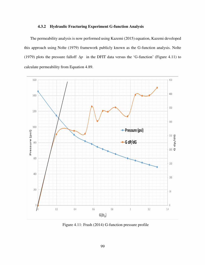
99
4.3.2 Hydraulic Fracturing Experiment G-function Analysis
The permeability analysis is now performed using Kazemi (2015) equation, Kazemi developed
this approach using Nolte (1979) framework publicly known as the G-function analysis. Nolte
(1979) plots the pressure falloff p in the DFIT data versus the ‘G-function’ (Figure 4.11) to
calculate permeability from Equation 4.89.
Figure 4.11: Frash (2014) G-function pressure profile
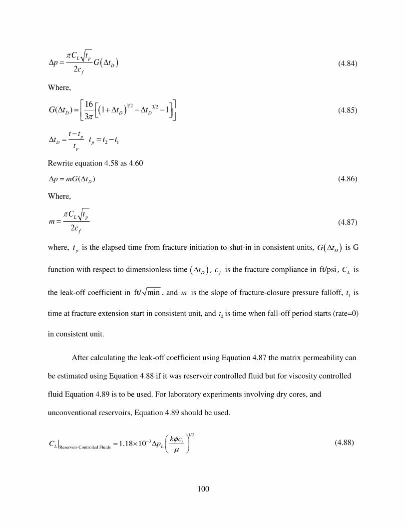
100
( )2
L p
D
f
C tp G t
c
= (4.84)
Where,
( )3 2 3 216( ) 1 1
3D D D
G t t t
= + − − (4.85)
p
D
p
t tt
t
− =
2 1pt t t= −
Rewrite equation 4.58 as 4.60
( )Dp mG t = (4.86)
Where,
2
L p
f
C tm
c
= (4.87)
where, p
t is the elapsed time from fracture initiation to shut-in in consistent units, ( )DG t is G
function with respect to dimensionless time ( )Dt ,
fc is the fracture compliance in ft/psi , LC is
the leak-off coefficient in ft/ min , and m is the slope of fracture-closure pressure falloff, 1t is
time at fracture extension start in consistent unit, and 2t is time when fall-off period starts (rate=0)
in consistent unit.
After calculating the leak-off coefficient using Equation 4.87 the matrix permeability can
be estimated using Equation 4.88 if it was reservoir controlled fluid but for viscosity controlled
fluid Equation 4.89 is to be used. For laboratory experiments involving dry cores, and
unconventional reservoirs, Equation 4.89 should be used.
1/2
3
Reservoir-Controlled Fluids1.18 10 t
L L
k cC p
− =
(4.88)
101
1/2
3
Viscosity-Controlled Fluids1.48 10 L
L
k pC
− =
(4.89)
Where, p in psi, k in md, tc in 1/psi, and in cp. ( )0 L R
p p t p = = − , and Rp hould be
determined from pressure falloff pressure at a shut-in time equal to the injection time.
L Rp ISIP p = − (4.90)
( )' fracture compliance
2f
hc
E
=
( )( )
'
'
'
2 2
2 3
Where, is Nolte pessure gradient coefficient in fracture
= Power law exponent for viscosity model
Viscosity degradation coefficient; zero for Newtonian fluids such as water
= 0.8
n
n a
n
a
+=
+ +
=
for Newtoninan fluids such as water
( ) ( )'
2 plane strain modulus
1
EE
=
−
To get the permeability to slope from the plot ( )Dp t vs. ( )DG t , shown in Figure 4.8.
G can be calculated using Equation 4.85, which is done in this analysis and calculated
permeability is presented in Table 4.15. Which again gave almost the same permeability value as
the measured one, confirming the validity of this technique.
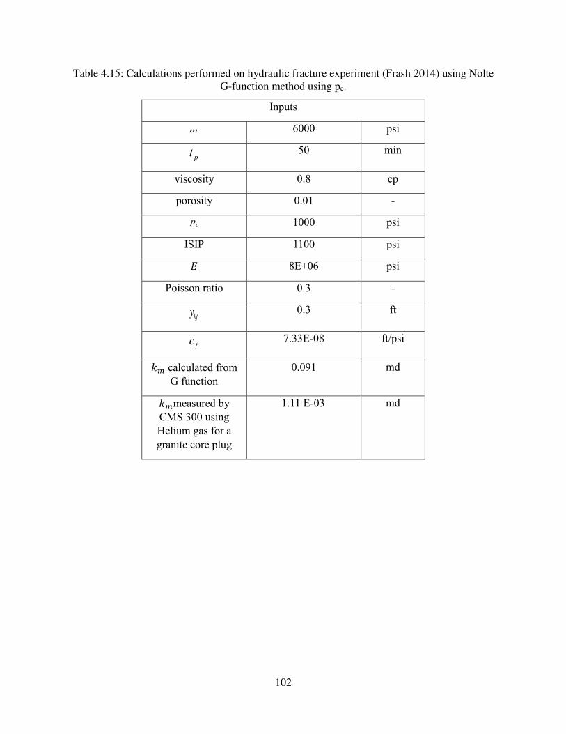
102
Table 4.15: Calculations performed on hydraulic fracture experiment (Frash 2014) using Nolte
G-function method using pc.
Inputs
m 6000 psi
pt 50 min
viscosity 0.8 cp
porosity 0.01 -
cp 1000 psi
ISIP 1100 psi 𝐸 8E+06 psi
Poisson ratio 0.3 -
hfy 0.3 ft
fc 7.33E-08 ft/psi 𝑘𝑚 calculated from
G function
0.091
md
𝑘𝑚measured by CMS 300 using Helium gas for a granite core plug
1.11 E-03
md
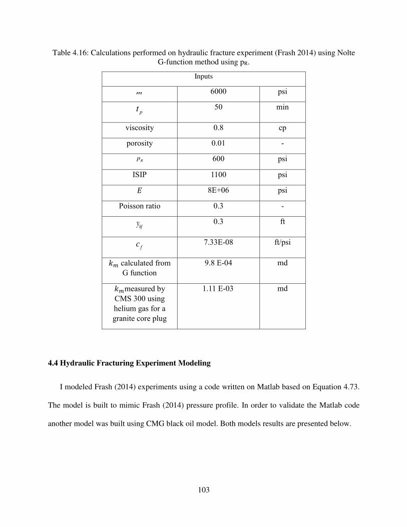
103
Table 4.16: Calculations performed on hydraulic fracture experiment (Frash 2014) using Nolte
G-function method using pR.
Inputs
m 6000 psi
pt 50 min
viscosity 0.8 cp
porosity 0.01 -
Rp 600 psi
ISIP 1100 psi 𝐸 8E+06 psi
Poisson ratio 0.3 -
hfy 0.3 ft
fc 7.33E-08 ft/psi 𝑘𝑚 calculated from
G function
9.8 E-04
md
𝑘𝑚measured by CMS 300 using helium gas for a granite core plug
1.11 E-03
md
4.4 Hydraulic Fracturing Experiment Modeling
I modeled Frash (2014) experiments using a code written on Matlab based on Equation 4.73.
The model is built to mimic Frash (2014) pressure profile. In order to validate the Matlab code
another model was built using CMG black oil model. Both models results are presented below.

104
4.4.1 Numerical Simulation Model for Frash Experiment
A numerical model, using a Matlab code, was developed based on Equation 4.73 to model
Frash experiments (2014) and to validate the effectiveness of the numerical model theory. The
numerical code gridding is illustrated in Figure 4.12. Figure 4.13 is the numerical model pressure
profile during injection and fall-off. The pressure profile was then analyzed using the PTA method,
to indicate the linear flow regime through the diagnostic plot (Figure 4.14). Hence, back calculate
permeability by the linear flow analysis (Figure 4.15) using Equation 4.77. The main inputs and
calculated permeability are presented in Table 4.17, and again the approach is validated with the
permeability similarity.
Figure 4.12: Numerical model logarithmic grid.

105
Figure 4.13: Numerical model pressure profile.
Figure 4.14: Numerical model code Diagnostic plot.
Fracture storage response
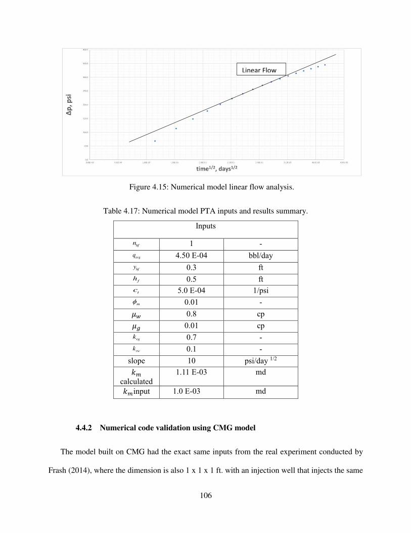
106
Figure 4.15: Numerical model linear flow analysis.
Table 4.17: Numerical model PTA inputs and results summary.
Inputs
hfn 1 -
avgq 4.50 E-04 bbl/day
hfy 0.3 ft
fh 0.5 ft
tc 5.0 E-04 1/psi m 0.01 - 𝜇𝑤 0.8 cp 𝜇𝑔 0.01 cp
rgk 0.7 -
rwk 0.1 - slope 10 psi/day 1/2 𝑘𝑚
calculated
1.11 E-03
md 𝑘𝑚input 1.0 E-03
md
4.4.2 Numerical code validation using CMG model
The model built on CMG had the exact same inputs from the real experiment conducted by
Frash (2014), where the dimension is also 1 x 1 x 1 ft. with an injection well that injects the same
Linear Flow
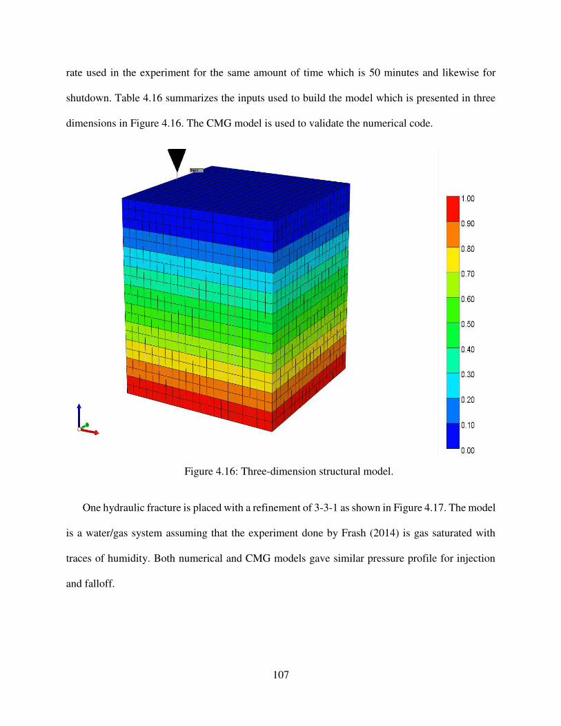
107
rate used in the experiment for the same amount of time which is 50 minutes and likewise for
shutdown. Table 4.16 summarizes the inputs used to build the model which is presented in three
dimensions in Figure 4.16. The CMG model is used to validate the numerical code.
Figure 4.16: Three-dimension structural model.
One hydraulic fracture is placed with a refinement of 3-3-1 as shown in Figure 4.17. The model
is a water/gas system assuming that the experiment done by Frash (2014) is gas saturated with
traces of humidity. Both numerical and CMG models gave similar pressure profile for injection
and falloff.
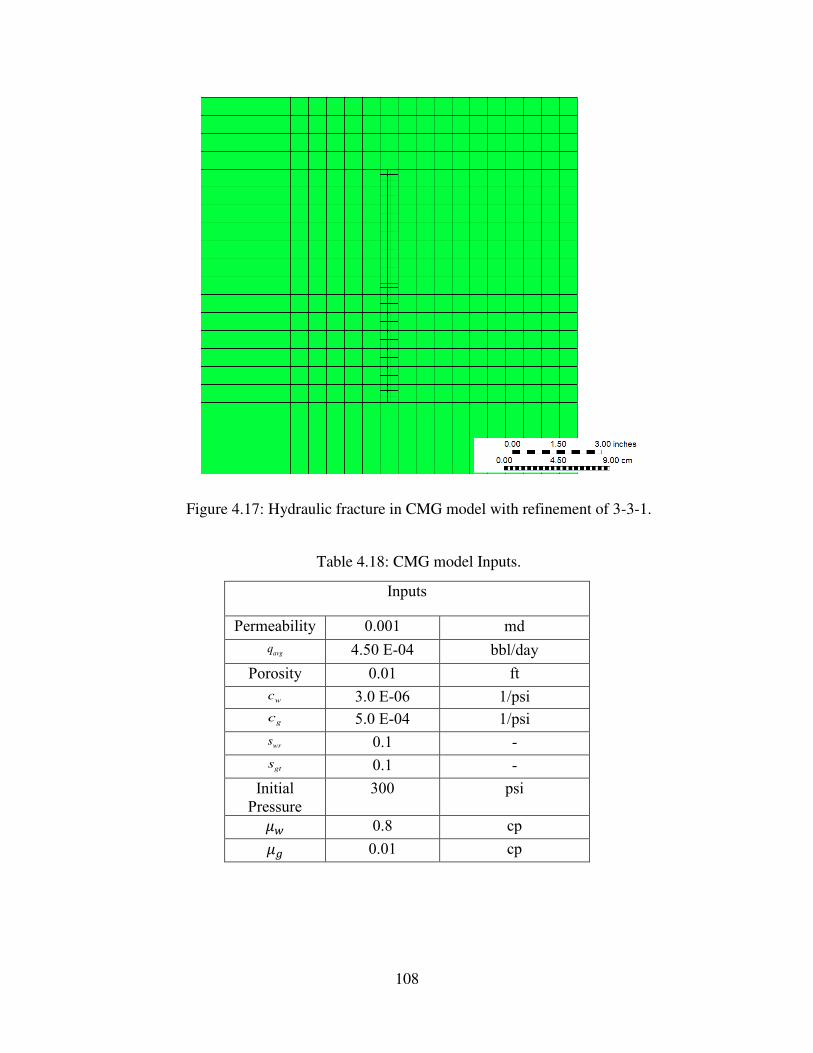
108
Figure 4.17: Hydraulic fracture in CMG model with refinement of 3-3-1.
Table 4.18: CMG model Inputs.
Inputs
Permeability 0.001 md
avgq 4.50 E-04 bbl/day
Porosity 0.01 ft wc 3.0 E-06 1/psi g
c 5.0 E-04 1/psi wrs 0.1 - gt
s 0.1 - Initial
Pressure
300 psi 𝜇𝑤 0.8 cp 𝜇𝑔 0.01 cp
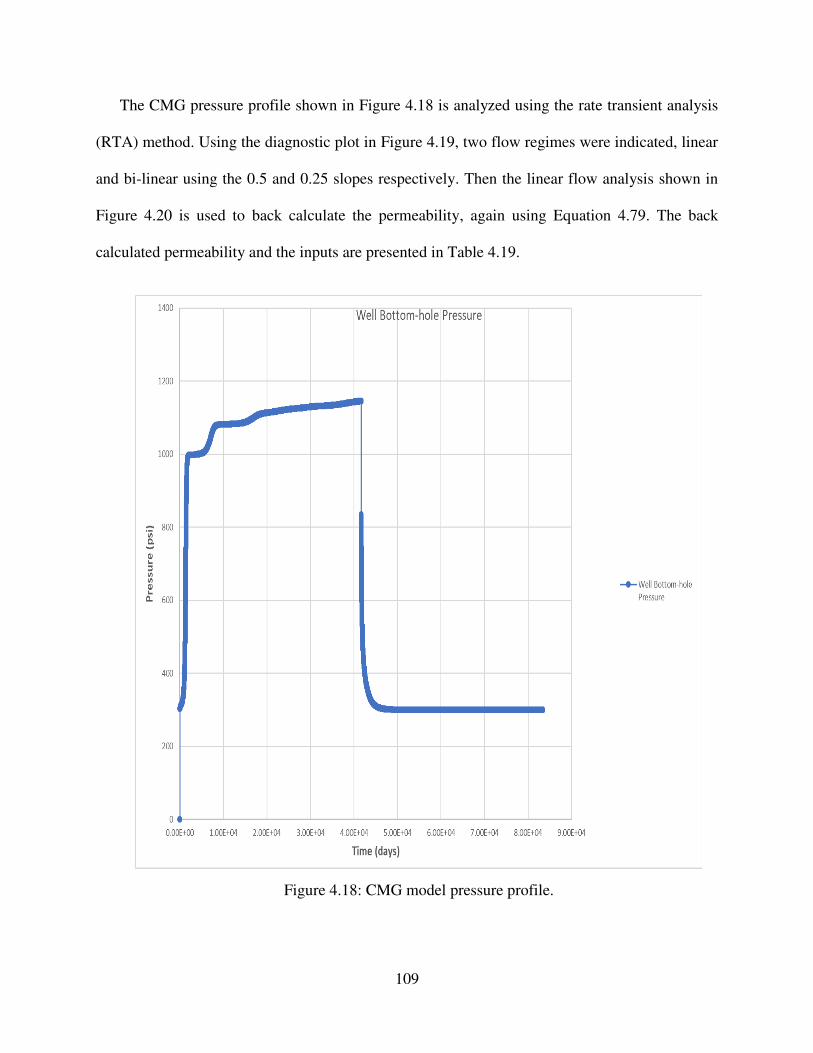
109
The CMG pressure profile shown in Figure 4.18 is analyzed using the rate transient analysis
(RTA) method. Using the diagnostic plot in Figure 4.19, two flow regimes were indicated, linear
and bi-linear using the 0.5 and 0.25 slopes respectively. Then the linear flow analysis shown in
Figure 4.20 is used to back calculate the permeability, again using Equation 4.79. The back
calculated permeability and the inputs are presented in Table 4.19.
Figure 4.18: CMG model pressure profile.
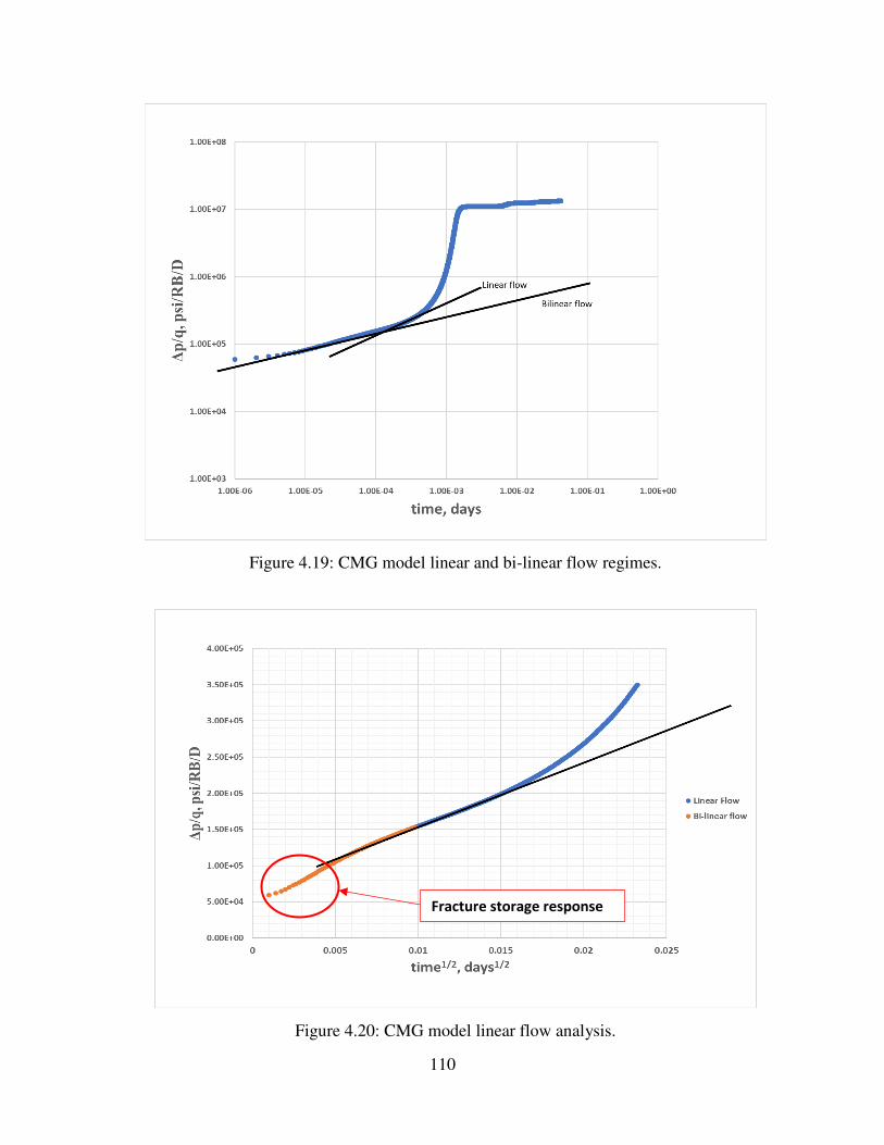
110
Figure 4.19: CMG model linear and bi-linear flow regimes.
Figure 4.20: CMG model linear flow analysis.
Fracture storage response

111
Table 4.19: CMG model RTA Inputs and results summary.
Inputs
hfn 1 -
avgq 4.50 E-04 bbl/day
hfy 0.3 ft
fh 0.5 ft
m 0.01 - 𝜇𝑤 0.8 cp 𝜇𝑔 0.01 cp
rgk 0.7 -
rwk 0.1 - slope 5.0 E+06 psi/bbl/day/(day)1/2 𝑘𝑚
calculated
1.13 E-03
md 𝑘𝑚input 1.0 E-03
md
4.5 Pressure Falloff Leakoff Theory
The previous CMG model was using a constant rate to validate the numerical code written.
This sub-section discusses the leakoff theory during the mini-frac falloff. The model first was built
as 1-D constant rate case ignoring the wellbore storage effect during the shut-in of the well. Again
using Frash, 2014, experiment to validate this theory, the model was built with the same input
parameters of the experiment (Frash 2014).
This model will be referred to as CMG model #2 to prevent any confusion. The grid for this
model is of total of 246 grids, the size of the middle 200 grids is 5 micron, and fine gridding is
used to study the water front. Then the grid size increases logarithmically in each direction until
they equal the same size of the granite block used by (Frash 2014). The grid is presented in Figure
4.21 and zoomed in Figure 4.22 for a better visual presentation. Table 4.20 presents the inputs for
this model.
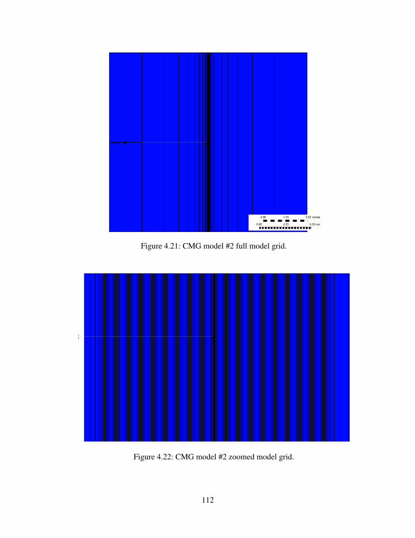
112
Figure 4.21: CMG model #2 full model grid.
Figure 4.22: CMG model #2 zoomed model grid.
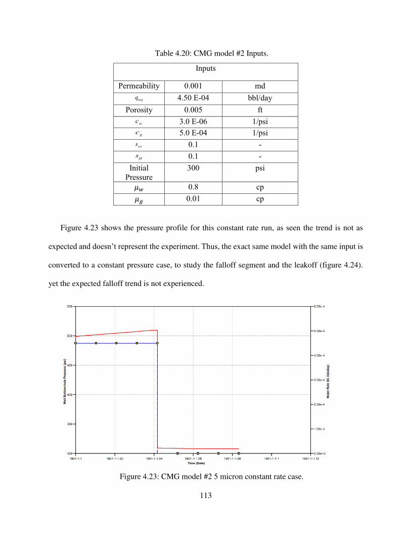
113
Table 4.20: CMG model #2 Inputs.
Inputs
Permeability 0.001 md
avgq 4.50 E-04 bbl/day
Porosity 0.005 ft wc 3.0 E-06 1/psi g
c 5.0 E-04 1/psi wrs 0.1 - gt
s 0.1 - Initial
Pressure
300 psi 𝜇𝑤 0.8 cp 𝜇𝑔 0.01 cp
Figure 4.23 shows the pressure profile for this constant rate run, as seen the trend is not as
expected and doesn’t represent the experiment. Thus, the exact same model with the same input is
converted to a constant pressure case, to study the falloff segment and the leakoff (figure 4.24).
yet the expected falloff trend is not experienced.
Figure 4.23: CMG model #2 5 micron constant rate case.

114
Figure 4.24: CMG model #2 5 micron constant pressure case.
Thus, the following derivation was made for the leakoff theory. And was then verified using
the numerical model. Starting with simple mass balance at shut-in in Equation 4.91
The mass balance equation in the fracture, at the shut-in time, is:
( )w f
w i w l
d Vq q
d t
= −
(4.91)
Where, the fracture volume based on Perkins, Kern, and Nordgren (PKN) model is:
( ) 4 f f f
V t hL w = (4.92)
The average width for a 2D elliptic fracture used in the PKN model is:
( ) ( )22 1
4
f
f f c
Lw p t p
E
− = − (4.93)

115
Thus, the fracture volume is:
( ) ( )2 22 1
( ) 4 f
f f f f c
hLV t hL w p t p
E
− = = −
(4.94)
Expanding Eq. 4.94, we obtain:
( ) ( )f w
w f w i w l
d V dV q q
d t d t
+ = −
( ) ( )f f
w f w w w i w l
d V d pV c q q
d t d t + = −
( ) ( )f f
f w i l
d V d pV c q q
d t d t+ = −
(4.95)
The equation for the rate of water entering the fracture during water injection equals the rate of
expansion of wellbore fluid column:
f
i sur w w w
pq q B V c
t
= −
(4.96)
At shut-in, surface flow rate surq is zero; thus, during fracture shut-in period, the rate of fluid
entering the fracture is:
f
i w w
pq V c
t
= −
(4.97)
Substituting Equation 4.97 in Equation 4.95:
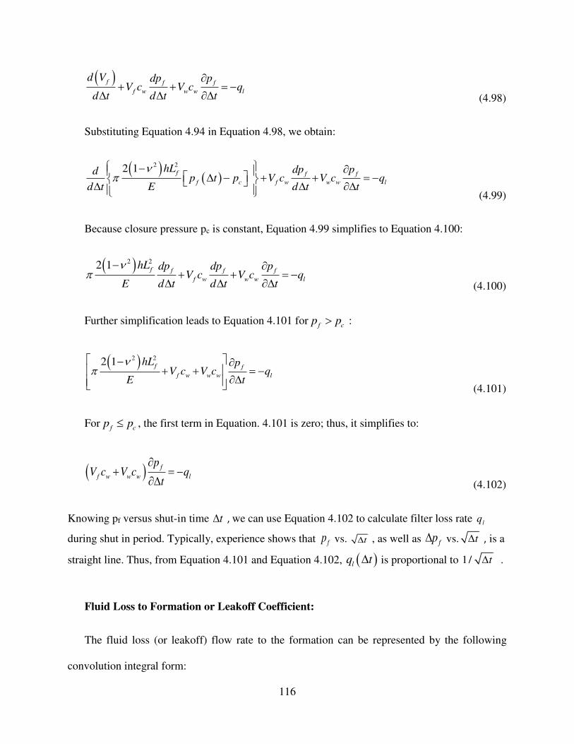
116
( )f f f
f w w w l
d V dp pV c V c q
d t d t t
+ + = −
(4.98)
Substituting Equation 4.94 in Equation 4.98, we obtain:
( ) ( )2 22 1
f f f
f c f w w w l
hL dp pdp t p V c V c q
d t E d t t
− − + + = − (4.99)
Because closure pressure pc is constant, Equation 4.99 simplifies to Equation 4.100:
( )2 22 1f f f f
f w w w l
hL dp dp pV c V c q
E d t d t t
− + + = −
(4.100)
Further simplification leads to Equation 4.101 forf c
p p :
( )2 22 1f f
f w w w l
hL pV c V c q
E t
− + + = −
(4.101)
Forf c
p p , the first term in Equation. 4.101 is zero; thus, it simplifies to:
( ) f
f w w w l
pV c V c q
t
+ = −
(4.102)
Knowing pf versus shut-in time t , we can use Equation 4.102 to calculate filter loss rate lq
during shut in period. Typically, experience shows that fp vs. t , as well as f
p vs. t , is a
straight line. Thus, from Equation 4.101 and Equation 4.102, ( )lq t is proportional to 1/ t .
Fluid Loss to Formation or Leakoff Coefficient:
The fluid loss (or leakoff) flow rate to the formation can be represented by the following
convolution integral form:
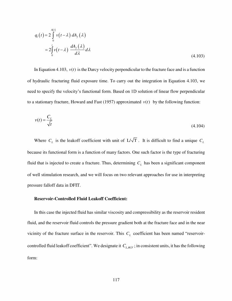
117
( ) ( )( )
( )
( ) ( )0
0
2
2
A t
l f
tf
q t v t dA
dAv t d
d
= −
= −
(4.103)
In Equation 4.103, ( )v t is the Darcy velocity perpendicular to the fracture face and is a function
of hydraulic fracturing fluid exposure time. To carry out the integration in Equation 4.103, we
need to specify the velocity’s functional form. Based on 1D solution of linear flow perpendicular
to a stationary fracture, Howard and Fast (1957) approximated ( )v t by the following function:
( ) LCv t
t=
(4.104)
Where LC is the leakoff coefficient with unit of L/ T . It is difficult to find a unique LC
because its functional form is a function of many factors. One such factor is the type of fracturing
fluid that is injected to create a fracture. Thus, determining LC has been a significant component
of well stimulation research, and we will focus on two relevant approaches for use in interpreting
pressure falloff data in DFIT.
Reservoir-Controlled Fluid Leakoff Coefficient:
In this case the injected fluid has similar viscosity and compressibility as the reservoir resident
fluid, and the reservoir fluid controls the pressure gradient both at the fracture face and in the near
vicinity of the fracture surface in the reservoir. This LC coefficient has been named “reservoir-
controlled fluid leakoff coefficient”. We designate it ,L RCFC ; in consistent units, it has the following
form:
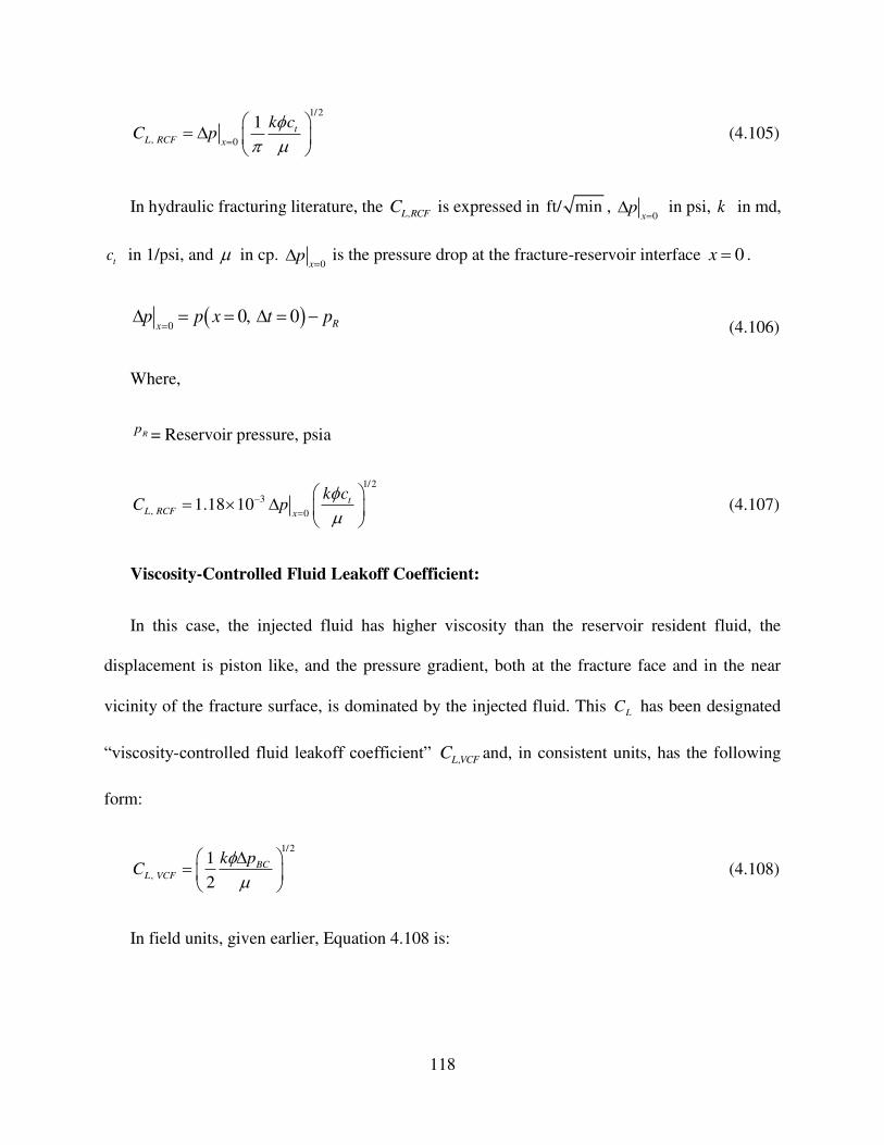
118
1/2
, 0
1 tL RCF x
k cC p
=
=
(4.105)
In hydraulic fracturing literature, the ,L RCF
C is expressed in ft/ min , 0x
p=
in psi, k in md,
tc in 1/psi, and in cp. 0x
p=
is the pressure drop at the fracture-reservoir interface 0x = .
( )0
0, 0 Rx
p p x t p=
= = = − (4.106)
Where,
Rp = Reservoir pressure, psia
1/2
3
, 01.18 10 t
L RCF x
k cC p
−=
=
(4.107)
Viscosity-Controlled Fluid Leakoff Coefficient:
In this case, the injected fluid has higher viscosity than the reservoir resident fluid, the
displacement is piston like, and the pressure gradient, both at the fracture face and in the near
vicinity of the fracture surface, is dominated by the injected fluid. This LC has been designated
“viscosity-controlled fluid leakoff coefficient” ,L VCF
C and, in consistent units, has the following
form:
1/2
,
1
2
BCL VCF
k pC
=
(4.108)
In field units, given earlier, Equation 4.108 is:
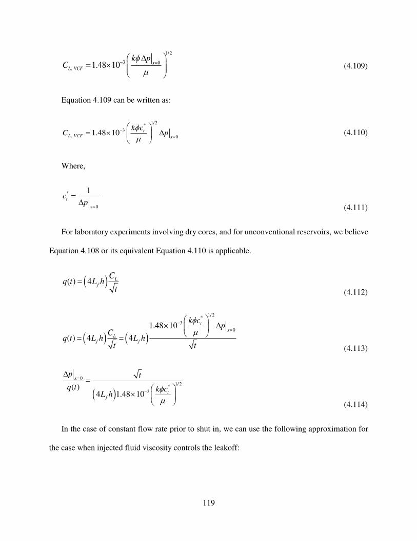
119
1/2
3 0, 1.48 10 x
L VCF
k pC
− =
=
(4.109)
Equation 4.109 can be written as:
1/2*
3
, 01.48 10 t
L VCF x
k cC p
−=
=
(4.110)
Where,
*
0
1t
x
cp
=
=
(4.111)
For laboratory experiments involving dry cores, and for unconventional reservoirs, we believe
Equation 4.108 or its equivalent Equation 4.110 is applicable.
( )( ) 4 Lf
Cq t L h
t=
(4.112)
( ) ( )
1/ 2*
3
01.48 10
( ) 4 4
t
x
Lf f
k cp
Cq t L h L h
t t
−=
= = (4.113)
( )0
1/2*
3( )
4 1.48 10
x
tf
p t
q t k cL h
=
−
=
(4.114)
In the case of constant flow rate prior to shut in, we can use the following approximation for
the case when injected fluid viscosity controls the leakoff:

120
( )
( )1/2
*3
4 1.48 10 tf
p t t
q k cL h
−
=
(4.115)
Where,
( ) ( ) 1* 0t pc p t p t t
− = = − =
Where, t in min, q in 3ft /min , k in md *
tc in 1/psi, and in cp.
For multi-phase flow and constant flow rate injection, one can extend the reservoir-controlled,
single phase flow equations to the following multi-phase form:
( ) ( ) ( )
1/21 1
0
4.064 24 141.2 facet t t t thfx
tf
InterceptPTA Slope
q qp t t s
c khk h L
− −
=
= +
(4.116)
2
1 4.064 24
tt
f t
qk
PTA slope L h c
−
= (4.117)
In the above equation, we set tc equal to *
tc , for which we generate a hybrid of viscosity-
controlled formulation.
Applying superposition principle to the shut-in period, we obtain:
( ) ( )( )
( ) ( ) ( )0
0 0
1/ 21
Pressur Falloff Slope
4.064 24
x
px x
p t
l t tp
tf
p t t p t
qt t t
ck h L
=
= =
−
+ − =
+ −
(4.118)
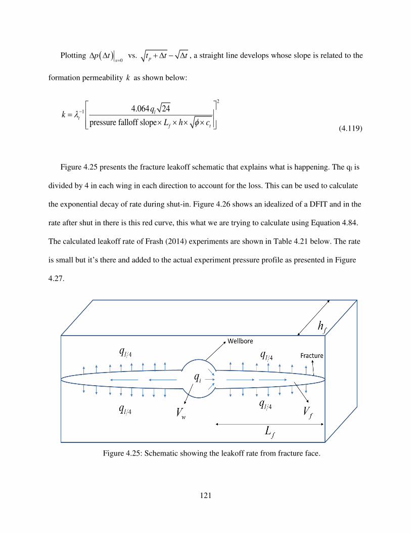
121
Plotting ( )0x
p t=
vs. pt t t+ − , a straight line develops whose slope is related to the
formation permeability k as shown below:
2
1 4.064 24
pressure falloff slope
lt
f t
qk
L h c
−
= (4.119)
Figure 4.25 presents the fracture leakoff schematic that explains what is happening. The ql is
divided by 4 in each wing in each direction to account for the loss. This can be used to calculate
the exponential decay of rate during shut-in. Figure 4.26 shows an idealized of a DFIT and in the
rate after shut in there is this red curve, this what we are trying to calculate using Equation 4.84.
The calculated leakoff rate of Frash (2014) experiments are shown in Table 4.21 below. The rate
is small but it’s there and added to the actual experiment pressure profile as presented in Figure
4.27.
Figure 4.25: Schematic showing the leakoff rate from fracture face.

122
Table 4.21: Leakoff rate calculation.
lq f
dp d t
3cm /min psi/min
0.00109 98.9
0.00091 82.7
0.00077 69.4
0.00069 62.6
0.00065 58.7
0.00060 54.8
0.00057 51.7
0.00053 47.7
0.00047 42.4
0.00044 39.4
0.00041 37.3
0.00039 35.2
0.00036 33.1
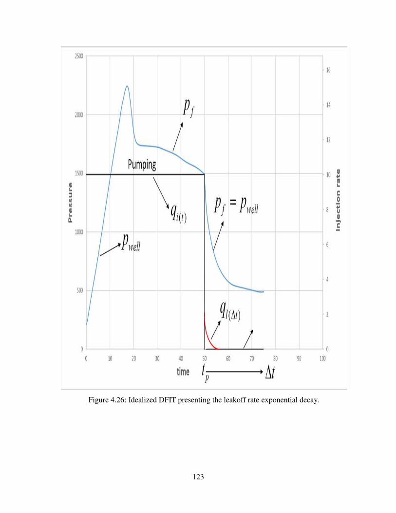
123
Figure 4.26: Idealized DFIT presenting the leakoff rate exponential decay.
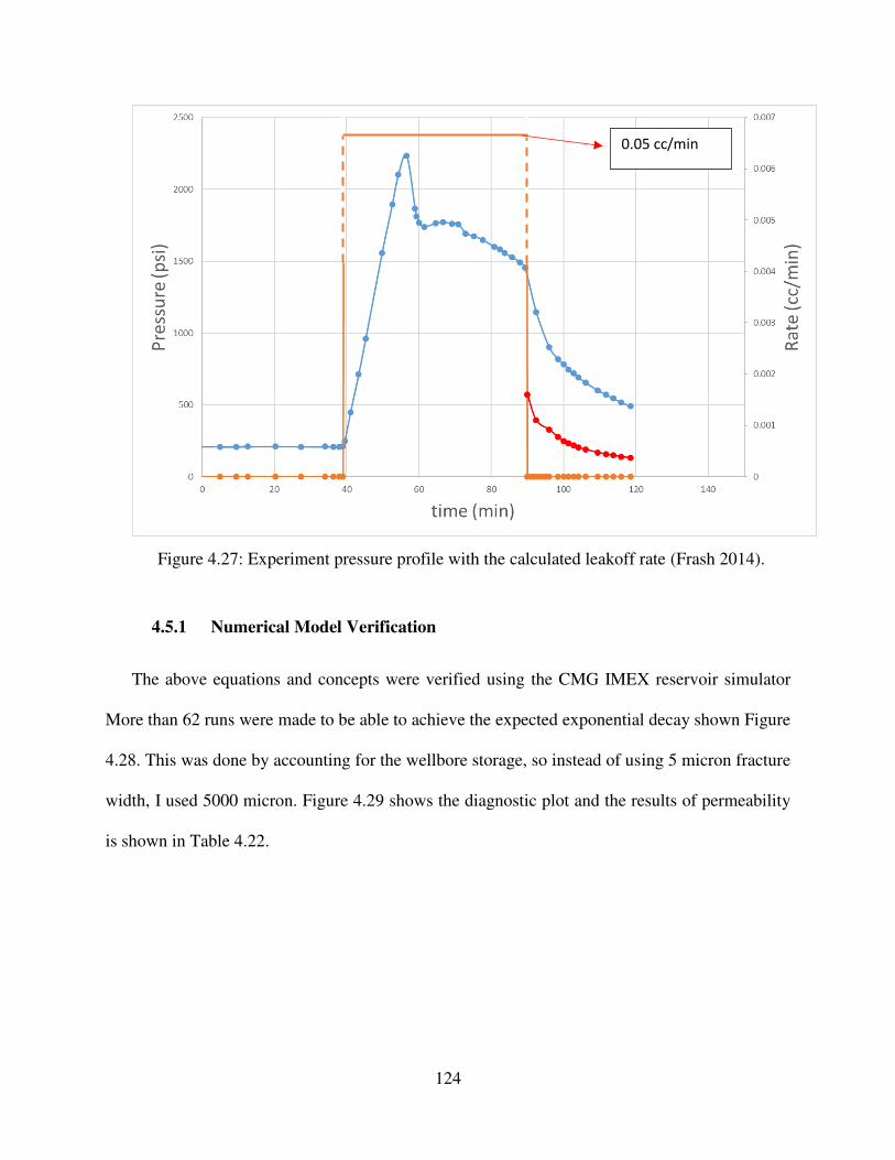
124
Figure 4.27: Experiment pressure profile with the calculated leakoff rate (Frash 2014).
4.5.1 Numerical Model Verification
The above equations and concepts were verified using the CMG IMEX reservoir simulator
More than 62 runs were made to be able to achieve the expected exponential decay shown Figure
4.28. This was done by accounting for the wellbore storage, so instead of using 5 micron fracture
width, I used 5000 micron. Figure 4.29 shows the diagnostic plot and the results of permeability
is shown in Table 4.22.
0.05 cc/min
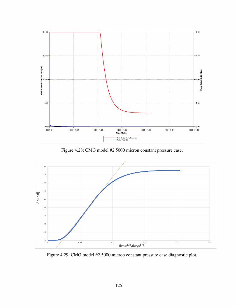
125
Figure 4.28: CMG model #2 5000 micron constant pressure case.
Figure 4.29: CMG model #2 5000 micron constant pressure case diagnostic plot.

126
Table 4.22: CMG model #2 PTA results.
Inputs
hfn 1
avgq 0.00045 bbl/day
fw 1.6 x10⁻³ ft
hfy 0.3 ft
fh 0.5 ft
( )0p t = 1100 psi
( )0R
p t p = 900 psi
Lp 200 psi *
c 0.005 1/psi
m 0.0014 -
hf 100 % 𝜇𝑤 0.8 cp 𝜇𝑔 0.017 cp
rgk 0.7 -
rwk 0.1 -
Slope of p vs. t plot 1352 psi /(day)1/2
Calculated 𝑘𝑚 from 1D linear flow pressure transient analysis
1.21 E-03
md
Input 𝑘𝑚 1 E-03
md
Using Equation 4.97 to calculate the leakoff rate during shut-in showed that not only pressure
has the exponential decay trend but the rate also. Figure 4.30 shows the numerical model result
with the variable shut-in rates. The falloff segment was then analyzed using the PTA analysis as
shown in Figure 4.31. The trend of the plot shows a very similar one to the real experiment. The
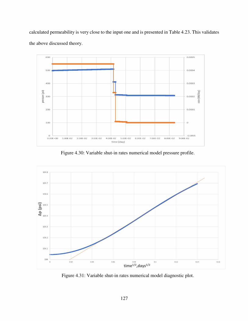
127
calculated permeability is very close to the input one and is presented in Table 4.23. This validates
the above discussed theory.
Figure 4.30: Variable shut-in rates numerical model pressure profile.
Figure 4.31: Variable shut-in rates numerical model diagnostic plot.
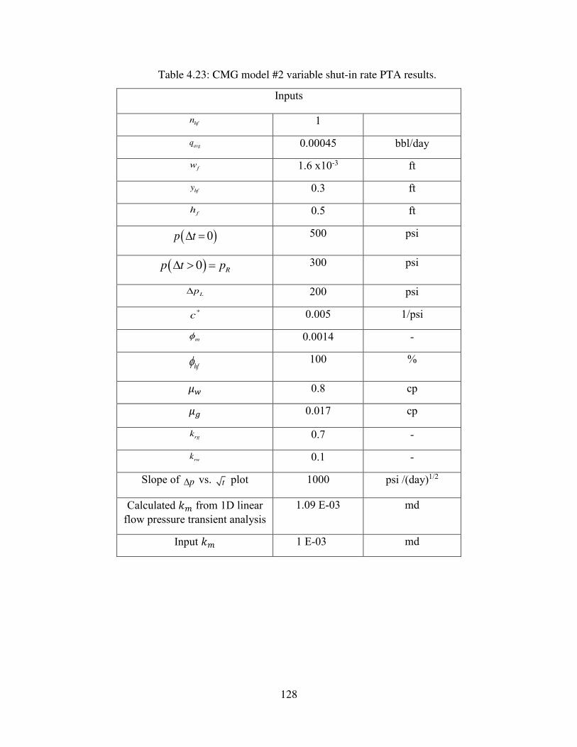
128
Table 4.23: CMG model #2 variable shut-in rate PTA results.
Inputs
hfn 1
avgq 0.00045 bbl/day
fw 1.6 x10⁻³ ft
hfy 0.3 ft
fh 0.5 ft
( )0p t = 500 psi
( )0R
p t p = 300 psi
Lp 200 psi *
c 0.005 1/psi
m 0.0014 -
hf 100 % 𝜇𝑤 0.8 cp 𝜇𝑔 0.017 cp
rgk 0.7 -
rwk 0.1 -
Slope of p vs. t plot 1000 psi /(day)1/2
Calculated 𝑘𝑚 from 1D linear flow pressure transient analysis
1.09 E-03
md
Input 𝑘𝑚 1 E-03
md
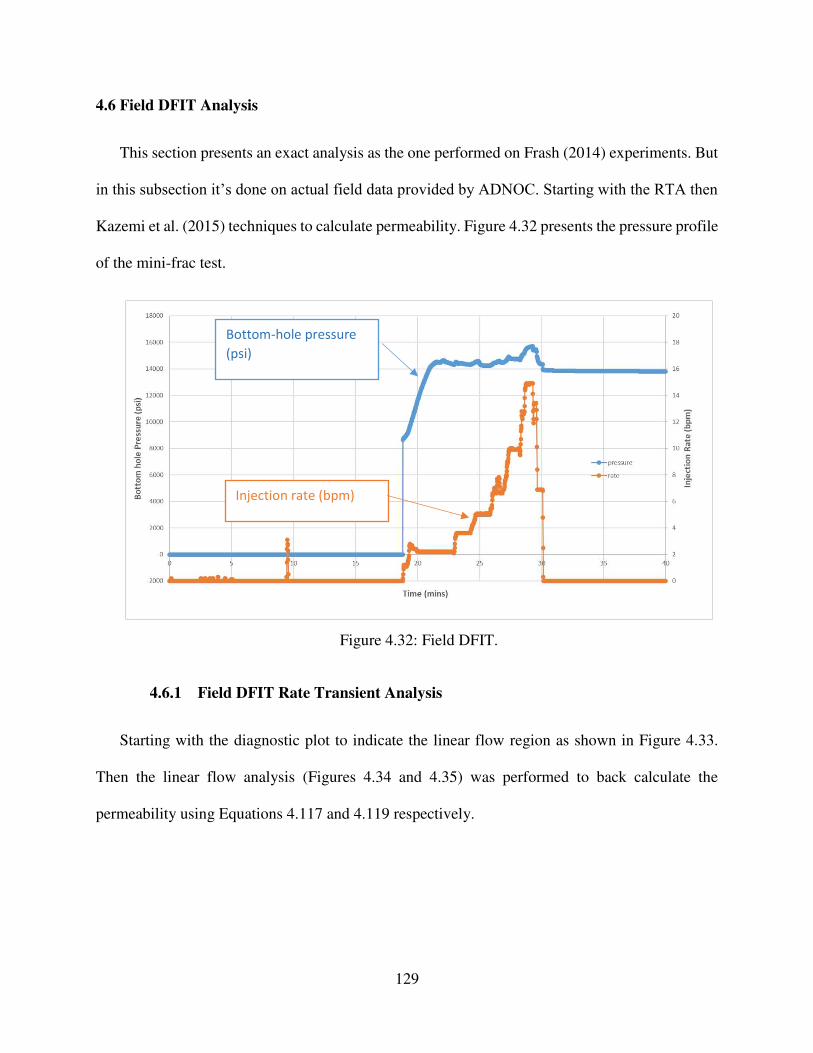
129
4.6 Field DFIT Analysis
This section presents an exact analysis as the one performed on Frash (2014) experiments. But
in this subsection it’s done on actual field data provided by ADNOC. Starting with the RTA then
Kazemi et al. (2015) techniques to calculate permeability. Figure 4.32 presents the pressure profile
of the mini-frac test.
Figure 4.32: Field DFIT.
4.6.1 Field DFIT Rate Transient Analysis
Starting with the diagnostic plot to indicate the linear flow region as shown in Figure 4.33.
Then the linear flow analysis (Figures 4.34 and 4.35) was performed to back calculate the
permeability using Equations 4.117 and 4.119 respectively.
Bottom-hole pressure
(psi)
Injection rate (bpm)
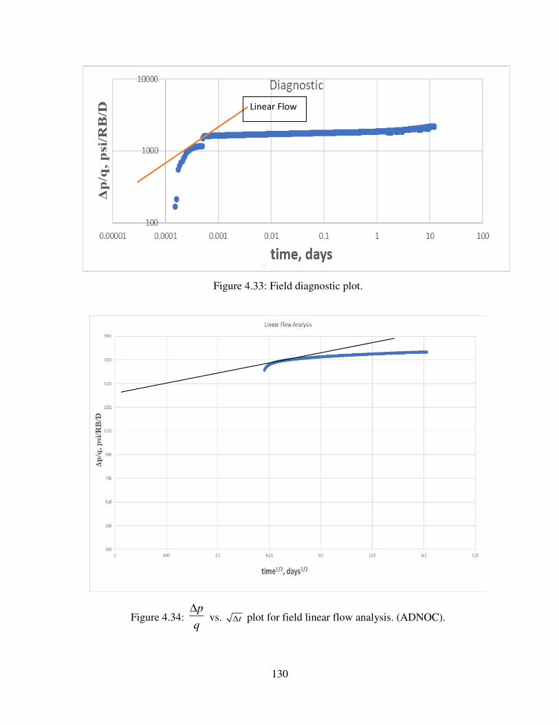
130
Figure 4.33: Field diagnostic plot.
Figure 4.34: p
q
vs. t plot for field linear flow analysis. (ADNOC).
Linear Flow
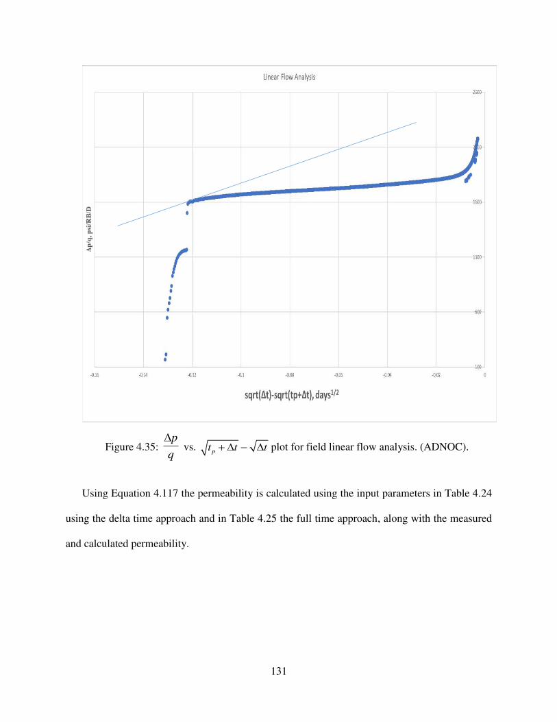
131
Figure 4.35: p
q
vs.
pt t t+ − plot for field linear flow analysis. (ADNOC).
Using Equation 4.117 the permeability is calculated using the input parameters in Table 4.24
using the delta time approach and in Table 4.25 the full time approach, along with the measured
and calculated permeability.
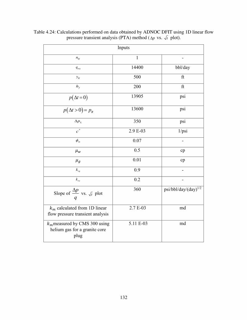
132
Table 4.24: Calculations performed on data obtained by ADNOC DFIT using 1D linear flow
pressure transient analysis (PTA) method ( p vs. t plot).
Inputs
hfn 1 -
avgq 14400 bbl/day
hfy 500 ft
fh 200 ft
( )0p t = 13905 psi
( )0R
p t p = 13600 psi
Lp 350 psi *
c 2.9 E-03 1/psi
m 0.07 - 𝜇𝑤 0.5 cp 𝜇𝑔 0.01 cp
rgk 0.9 -
rwk 0.2 -
Slope of p
q
vs. t plot
360 psi/bbl/day/(day)1/2
𝑘𝑚 calculated from 1D linear flow pressure transient analysis
2.7 E-03
md
𝑘𝑚measured by CMS 300 using helium gas for a granite core
plug
5.11 E-03
md
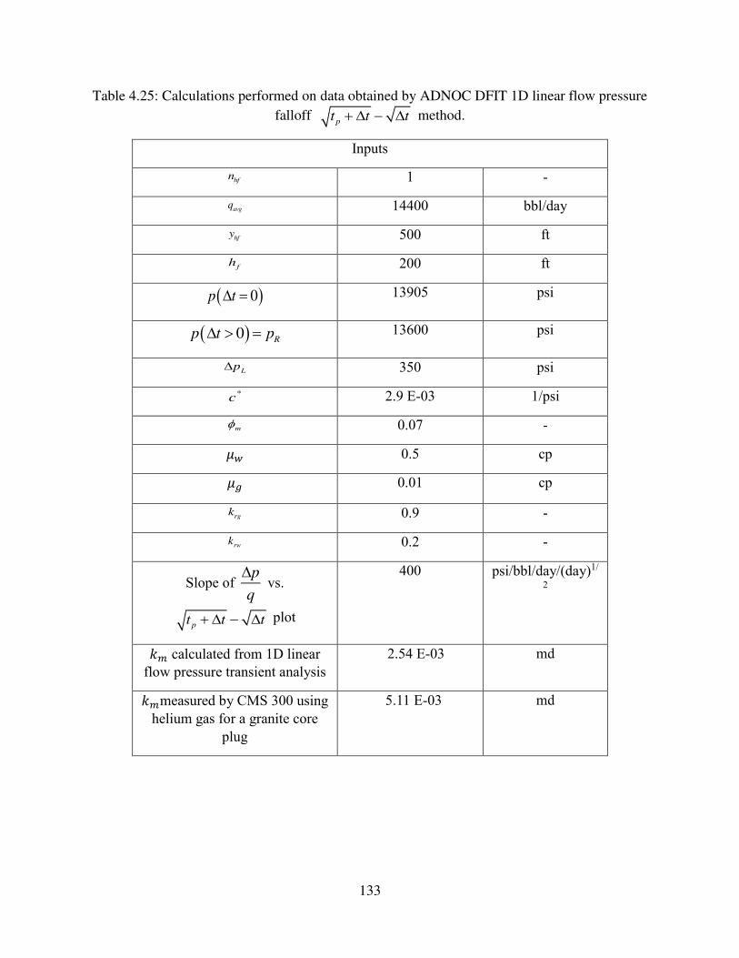
133
Table 4.25: Calculations performed on data obtained by ADNOC DFIT 1D linear flow pressure
falloff pt t t+ − method.
Inputs
hfn 1 -
avgq 14400 bbl/day
hfy 500 ft
fh 200 ft
( )0p t = 13905 psi
( )0R
p t p = 13600 psi
Lp 350 psi *
c 2.9 E-03 1/psi
m 0.07 - 𝜇𝑤 0.5 cp 𝜇𝑔 0.01 cp
rgk 0.9 -
rwk 0.2 -
Slope of p
q
vs.
pt t t+ − plot
400 psi/bbl/day/(day)1/
2
𝑘𝑚 calculated from 1D linear flow pressure transient analysis
2.54 E-03
md
𝑘𝑚measured by CMS 300 using helium gas for a granite core
plug
5.11 E-03
md
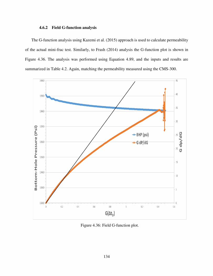
134
4.6.2 Field G-function analysis
The G-function analysis using Kazemi et al. (2015) approach is used to calculate permeability
of the actual mini-frac test. Similarly, to Frash (2014) analysis the G-function plot is shown in
Figure 4.36. The analysis was performed using Equation 4.89, and the inputs and results are
summarized in Table 4.2. Again, matching the permeability measured using the CMS-300.
Figure 4.36: Field G-function plot.
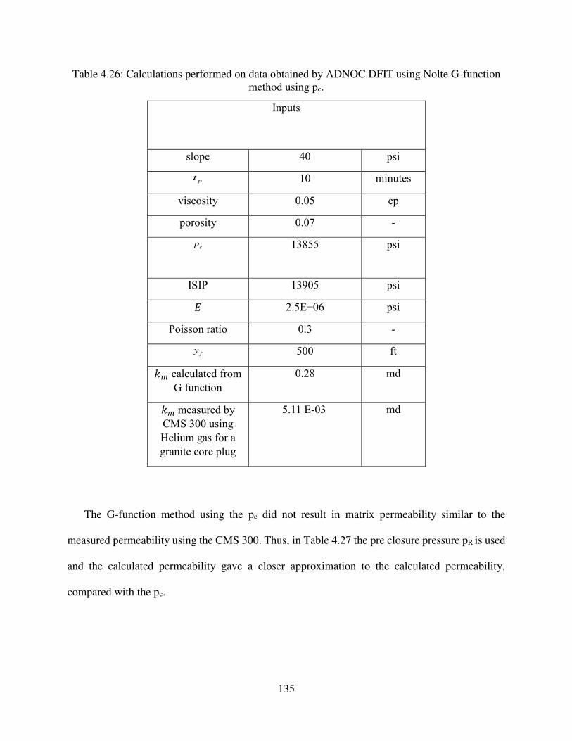
135
Table 4.26: Calculations performed on data obtained by ADNOC DFIT using Nolte G-function
method using pc.
Inputs
slope 40 psi
pt 10 minutes
viscosity 0.05 cp
porosity 0.07 -
cp 13855 psi
ISIP 13905 psi 𝐸 2.5E+06 psi
Poisson ratio 0.3 -
fy 500 ft 𝑘𝑚 calculated from
G function
0.28
md
𝑘𝑚 measured by CMS 300 using Helium gas for a granite core plug
5.11 E-03
md
The G-function method using the pc did not result in matrix permeability similar to the
measured permeability using the CMS 300. Thus, in Table 4.27 the pre closure pressure pR is used
and the calculated permeability gave a closer approximation to the calculated permeability,
compared with the pc.

136
Table 4.27: Calculations performed on data obtained by ADNOC DFIT using Nolte G-function
method using pR.
Inputs
slope 40 psi
pt 10 minutes
viscosity 0.05 cp
porosity 0.07 -
Rp 13600 psi
ISIP 13905 psi 𝐸 2.5E+06 psi
Poisson ratio 0.3 -
fy 500 ft 𝑘𝑚 calculated from
G function
2.6 E-04
md
𝑘𝑚measured by CMS 300 using Helium gas for a granite core plug
5.11 E-03
md
4.7 Analysis of a Reliable Field Data (Economides and Nolte 1989):
In Economides and Nolte (1989), Chapter 7 contains an example of a fall-off in a mini-frac
test. This example was analyzed in this thesis by the G-function analysis using Kazemi et al. (2015)
approach and the PTA analysis. The reason is to further verify the approaches with an example
from the equation’s main developer Kenneth Nolte. The fall-off part is shown in Figure 4.37.
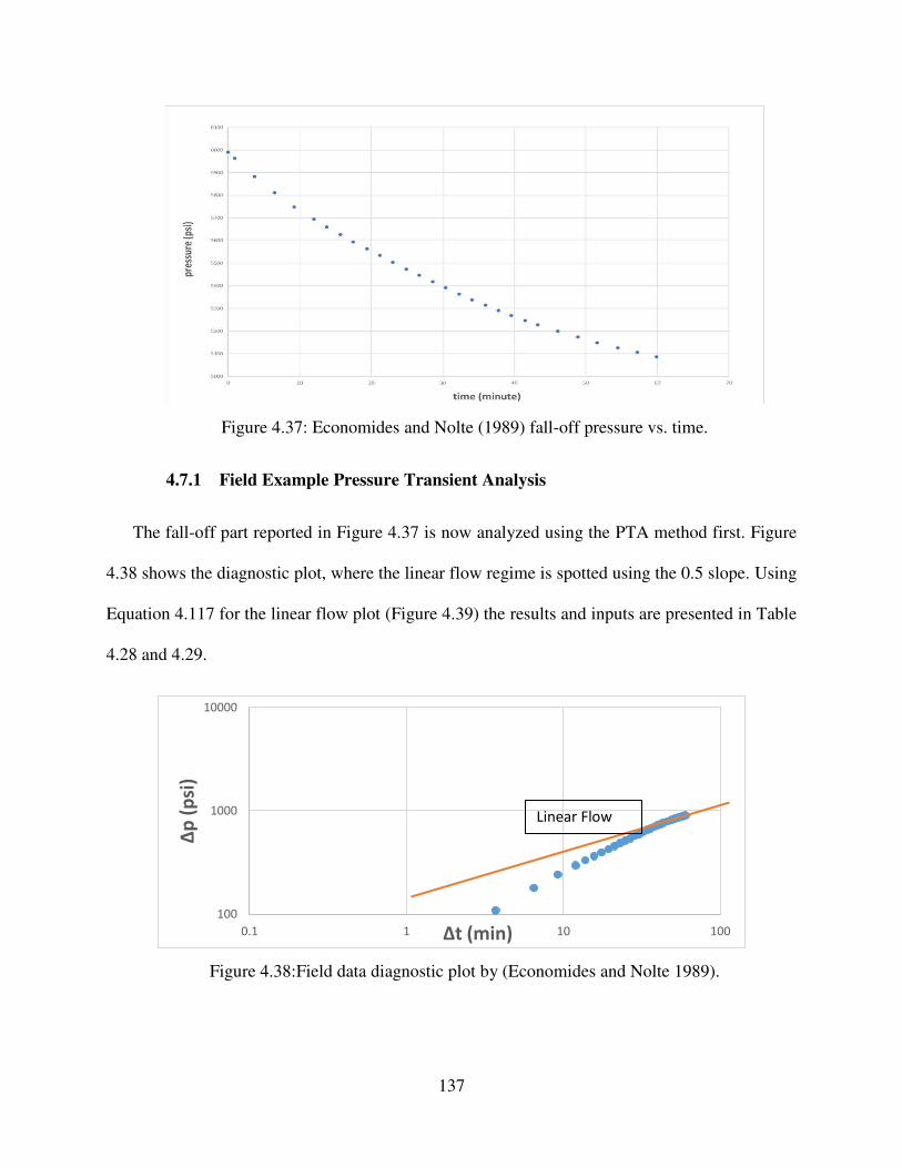
137
Figure 4.37: Economides and Nolte (1989) fall-off pressure vs. time.
4.7.1 Field Example Pressure Transient Analysis
The fall-off part reported in Figure 4.37 is now analyzed using the PTA method first. Figure
4.38 shows the diagnostic plot, where the linear flow regime is spotted using the 0.5 slope. Using
Equation 4.117 for the linear flow plot (Figure 4.39) the results and inputs are presented in Table
4.28 and 4.29.
Figure 4.38:Field data diagnostic plot by (Economides and Nolte 1989).
100
1000
10000
0.1 1 10 100
∆p (p
si)
∆t (min)
Linear Flow
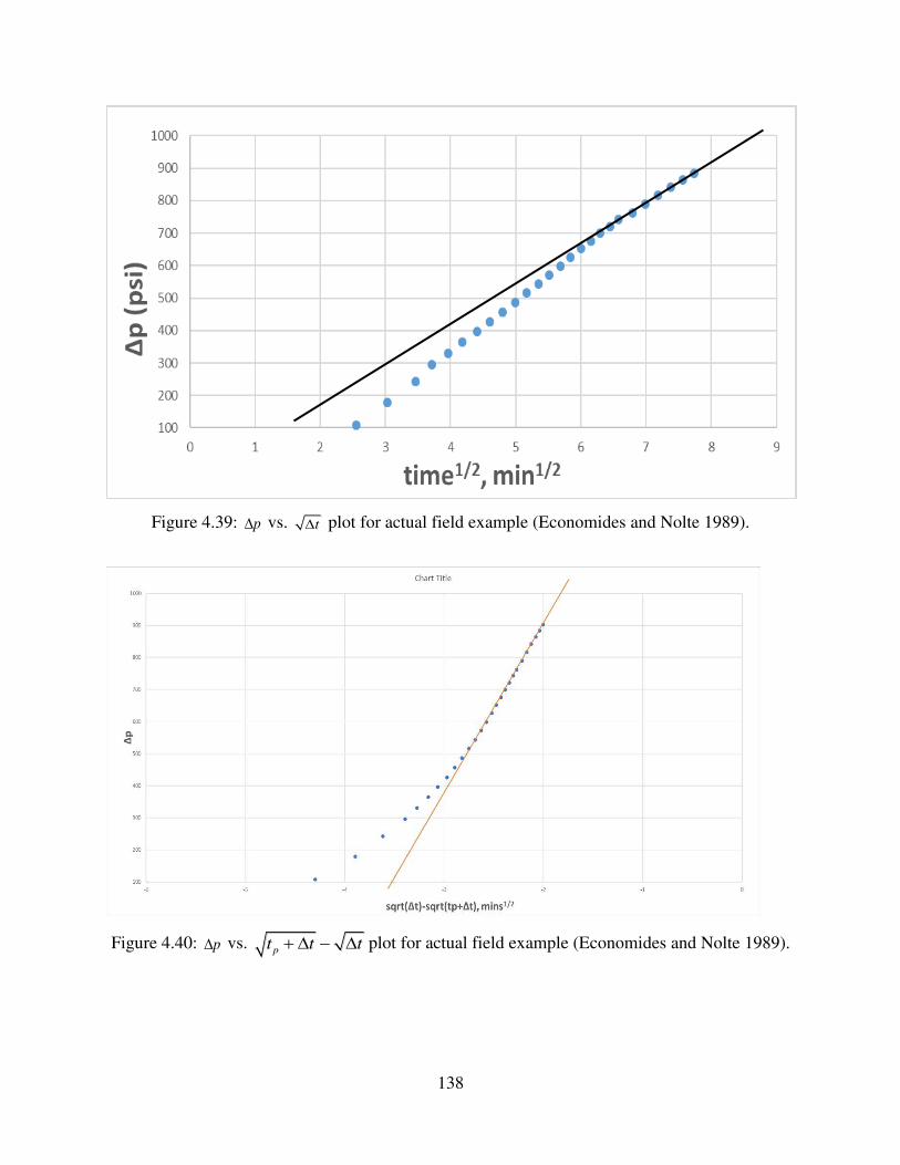
138
Figure 4.39: p vs. t plot for actual field example (Economides and Nolte 1989).
Figure 4.40: p vs. pt t t+ − plot for actual field example (Economides and Nolte 1989).
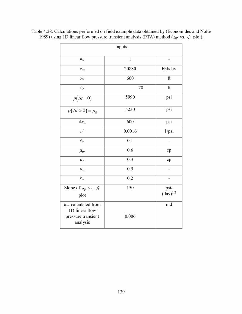
139
Table 4.28: Calculations performed on field example data obtained by (Economides and Nolte
1989) using 1D linear flow pressure transient analysis (PTA) method ( p vs. t plot).
Inputs
hfn 1 -
avgq 20880 bbl/day
hfy 660 ft
fh 70 ft
( )0p t = 5990 psi
( )0R
p t p = 5230 psi
Lp 600 psi *
c 0.0016 1/psi
m 0.1 - 𝜇𝑤 0.6 cp 𝜇𝑜 0.3 cp
rok 0.5 -
rwk 0.2 -
Slope of p vs. t plot
150 psi/ (day)1/2 𝑘𝑚 calculated from
1D linear flow pressure transient
analysis
0.006
md
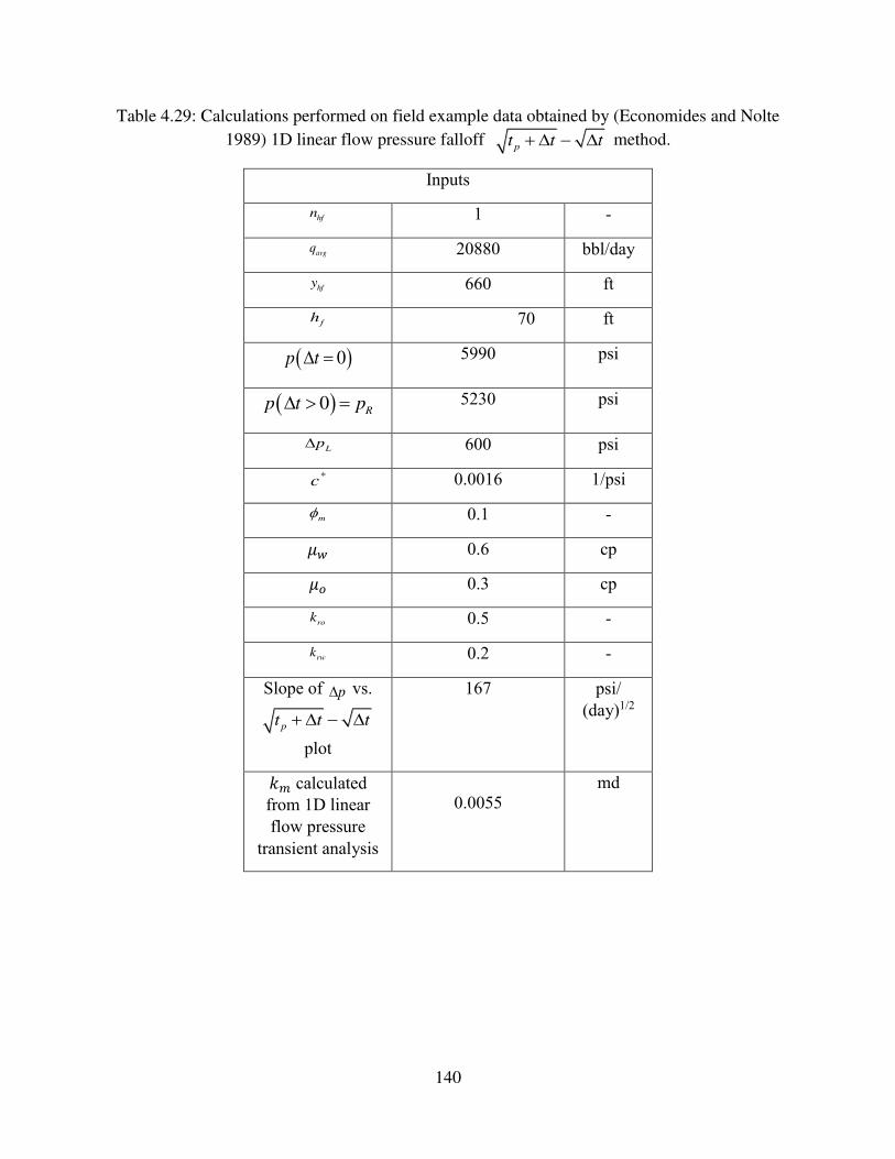
140
Table 4.29: Calculations performed on field example data obtained by (Economides and Nolte
1989) 1D linear flow pressure falloff pt t t+ − method.
Inputs
hfn 1 -
avgq 20880 bbl/day
hfy 660 ft
fh 70 ft
( )0p t = 5990 psi
( )0R
p t p = 5230 psi
Lp 600 psi *
c 0.0016 1/psi
m 0.1 - 𝜇𝑤 0.6 cp 𝜇𝑜 0.3 cp
rok 0.5 -
rwk 0.2 -
Slope of p vs.
pt t t+ −
plot
167 psi/ (day)1/2
𝑘𝑚 calculated from 1D linear flow pressure
transient analysis
0.0055
md
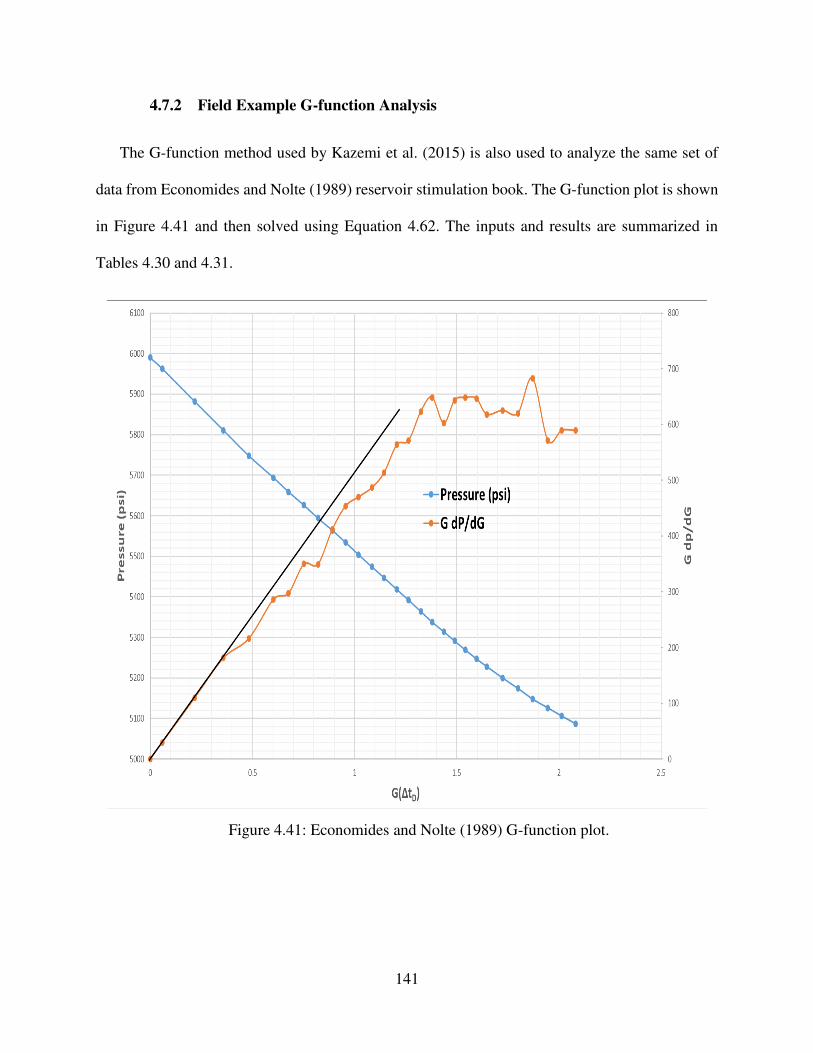
141
4.7.2 Field Example G-function Analysis
The G-function method used by Kazemi et al. (2015) is also used to analyze the same set of
data from Economides and Nolte (1989) reservoir stimulation book. The G-function plot is shown
in Figure 4.41 and then solved using Equation 4.62. The inputs and results are summarized in
Tables 4.30 and 4.31.
Figure 4.41: Economides and Nolte (1989) G-function plot.
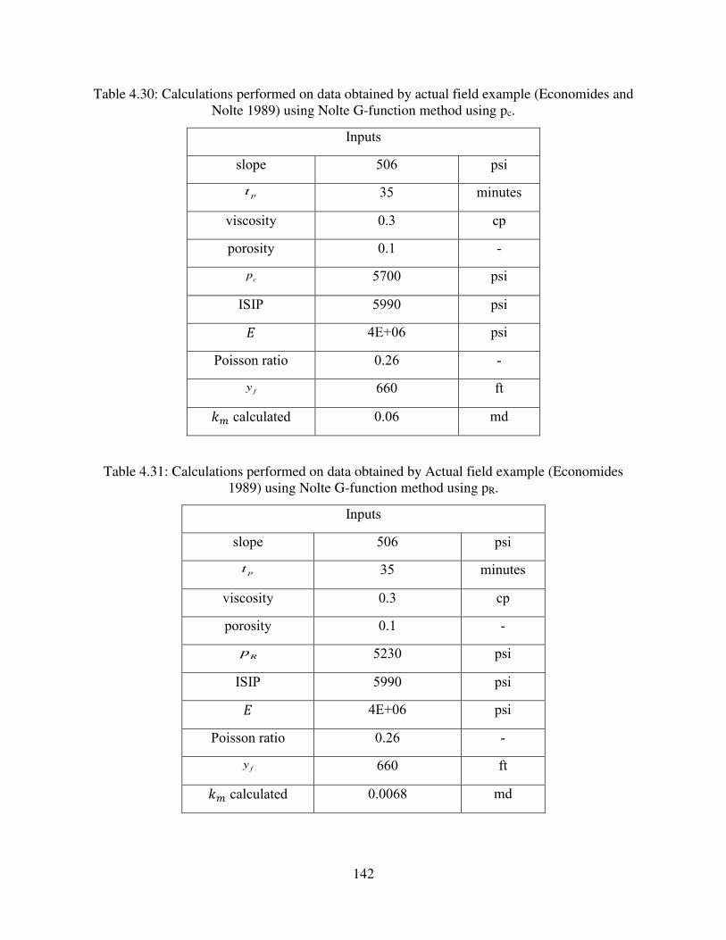
142
Table 4.30: Calculations performed on data obtained by actual field example (Economides and
Nolte 1989) using Nolte G-function method using pc.
Inputs
slope 506 psi
pt 35 minutes
viscosity 0.3 cp
porosity 0.1 -
cp 5700 psi
ISIP 5990 psi 𝐸 4E+06 psi
Poisson ratio 0.26 -
fy 660 ft 𝑘𝑚 calculated 0.06
md
Table 4.31: Calculations performed on data obtained by Actual field example (Economides
1989) using Nolte G-function method using pR.
Inputs
slope 506 psi
pt 35 minutes
viscosity 0.3 cp
porosity 0.1 -
Rp 5230 psi
ISIP 5990 psi 𝐸 4E+06 psi
Poisson ratio 0.26 -
fy 660 ft 𝑘𝑚 calculated 0.0068
md
143
CHAPTER 5
5 COMPOSITIONAL MODELING
This chapter presents a dual-porosity compositional model of Shilaif formation, using
simulator GEMTM developed by Computer Modeling Group (CMG) software to match and
forecast reservoir production of the Shilaif formation. All data was supplied by ADNOC. In the
model, other than forecasting also rate transient analysis (RTA) is made to check for linear flow
regime and back calculate the permeabilities. The flow simulation incorporates both geologic
model and production data to create a history match.
The model construction starts by building a dual porosity static model. After creating the grid
parameters are plugged in, then a pressure-volume-temperature analysis (PVT) model is created
using the CMG PVT software package “WinProp” and it is then imported to the flow model. A
hydraulic fracture treatment is then included to mimic the operation from the provided data. The
sub-sections below will explain the steps followed in order to get to the results.
5.1 Static Model and Grid Setup
CMG dual porosity system also includes the permeability for matrix and natural fractures,
relative to the natural fracture the matrix permeability is of less permeability but larger storage
capacity. Warren and Root (1963) showed that the storage capacity is a function of compressibility,
porosity and thickness. The larger the magnitude of compressibility and porosity the larger the
storage capacity would yield. Interporosity flow within the simulation is modeled using the shape
factor, the interporosity flow is the interaction of fluids in both fractures and matrix.
Gillman and Kazemi (1983) presented an equation for the shape factor for a matrix block, with
varied geometrical configurations, surrounded partially or fully by conductive fractures. For
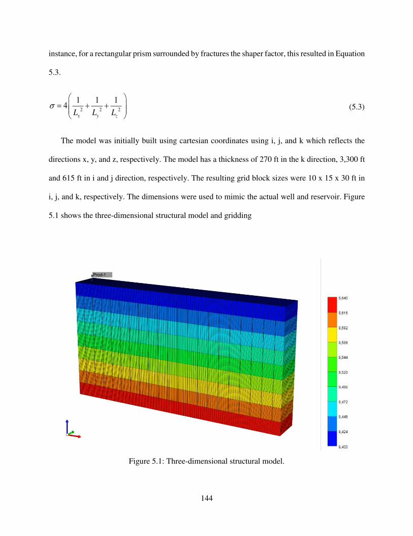
144
instance, for a rectangular prism surrounded by fractures the shaper factor, this resulted in Equation
5.3.
2 2 2
1 1 14
x y zL L L
= + +
(5.3)
The model was initially built using cartesian coordinates using i, j, and k which reflects the
directions x, y, and z, respectively. The model has a thickness of 270 ft in the k direction, 3,300 ft
and 615 ft in i and j direction, respectively. The resulting grid block sizes were 10 x 15 x 30 ft in
i, j, and k, respectively. The dimensions were used to mimic the actual well and reservoir. Figure
5.1 shows the three-dimensional structural model and gridding
Figure 5.1: Three-dimensional structural model.
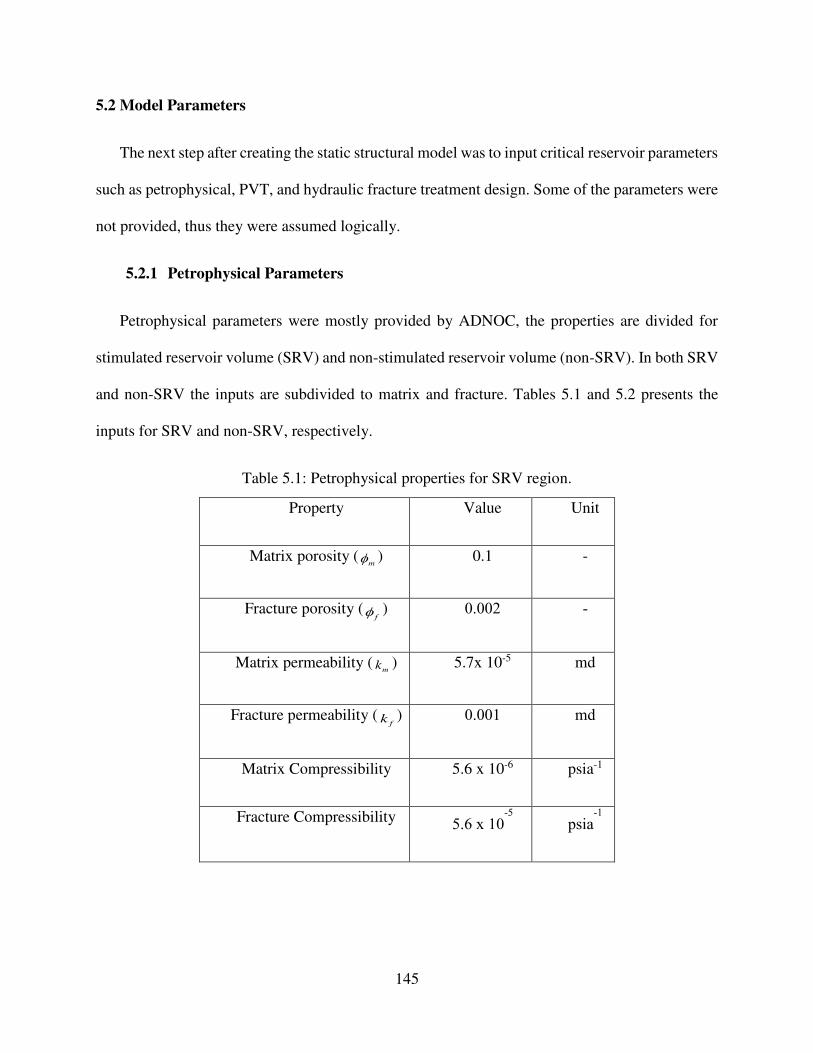
145
5.2 Model Parameters
The next step after creating the static structural model was to input critical reservoir parameters
such as petrophysical, PVT, and hydraulic fracture treatment design. Some of the parameters were
not provided, thus they were assumed logically.
5.2.1 Petrophysical Parameters
Petrophysical parameters were mostly provided by ADNOC, the properties are divided for
stimulated reservoir volume (SRV) and non-stimulated reservoir volume (non-SRV). In both SRV
and non-SRV the inputs are subdivided to matrix and fracture. Tables 5.1 and 5.2 presents the
inputs for SRV and non-SRV, respectively.
Table 5.1: Petrophysical properties for SRV region.
Property Value Unit
Matrix porosity (m ) 0.1 -
Fracture porosity (f
) 0.002 -
Matrix permeability (mk ) 5.7x 10⁻⁵ md
Fracture permeability (f
k ) 0.001 md
Matrix Compressibility 5.6 x 10⁻⁶ psia-1
Fracture Compressibility 5.6 x 10⁻⁵
psia-1
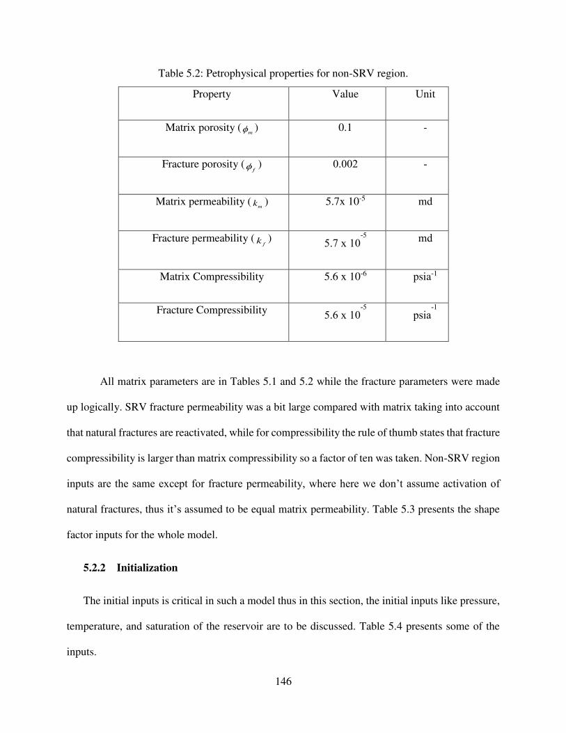
146
Table 5.2: Petrophysical properties for non-SRV region.
Property Value Unit
Matrix porosity (m ) 0.1 -
Fracture porosity (f
) 0.002 -
Matrix permeability (mk ) 5.7x 10⁻⁵ md
Fracture permeability (f
k ) 5.7 x 10⁻⁵
md
Matrix Compressibility 5.6 x 10⁻⁶ psia-1
Fracture Compressibility 5.6 x 10⁻⁵
psia-1
All matrix parameters are in Tables 5.1 and 5.2 while the fracture parameters were made
up logically. SRV fracture permeability was a bit large compared with matrix taking into account
that natural fractures are reactivated, while for compressibility the rule of thumb states that fracture
compressibility is larger than matrix compressibility so a factor of ten was taken. Non-SRV region
inputs are the same except for fracture permeability, where here we don’t assume activation of
natural fractures, thus it’s assumed to be equal matrix permeability. Table 5.3 presents the shape
factor inputs for the whole model.
5.2.2 Initialization
The initial inputs is critical in such a model thus in this section, the initial inputs like pressure,
temperature, and saturation of the reservoir are to be discussed. Table 5.4 presents some of the
inputs.
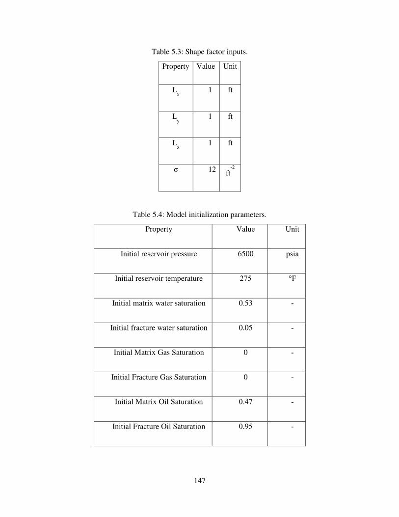
147
Table 5.3: Shape factor inputs.
Property Value Unit
Lx 1 ft
Ly 1 ft
Lz 1 ft
σ 12 ft-2
Table 5.4: Model initialization parameters.
Property Value Unit
Initial reservoir pressure 6500 psia
Initial reservoir temperature 275 °F
Initial matrix water saturation 0.53 -
Initial fracture water saturation 0.05 -
Initial Matrix Gas Saturation 0 -
Initial Fracture Gas Saturation 0 -
Initial Matrix Oil Saturation 0.47 -
Initial Fracture Oil Saturation 0.95 -

148
Reservoir pressure and temperature are both provided by ADNOC performed logs. The
saturation endpoints where a combination of provided mercury injection capillary pressure (MICP)
and Eker et al. (2017) analysis.
5.2.3 PVT Analysis
The compositional mode requires a reliable PVT data, in order to accurately characterize the
multicomponent fluid and understand the phase behavior effect as reservoir depletes. The
compositional model uses Peng-Robinson equation of state to properly integrate both
thermodynamics and volumetric properties with PVT.
The lack of technically right PVT data was the main missing piece from ADNOC, the only
PVT report provided had only separator fluids, not in bottomhole conditions. The report stated that
the oil properties are closest to Bakken oil, thus the framework data of Eker et al. (2017) was used.
The oil viscosity and gravity were mentioned in one of the reports to be 0.28 cp and 34 API.
Using Bakken oil composition and the provided MICP data, WinProp was used to create the
fluid model and then imported to the main model. The fluid composition is lumped in WinProp,
the reason behind that is speeding up the simulator. Table 5.5 presents the lumped component
percentages, while Figure 5.2 presents a bar chart for visual distribution comparison.
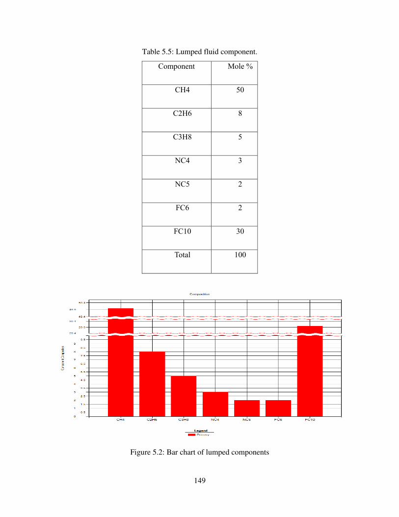
149
Table 5.5: Lumped fluid component.
Component Mole %
CH4 50
C2H6 8
C3H8 5
NC4 3
NC5 2
FC6 2
FC10 30
Total 100
Figure 5.2: Bar chart of lumped components
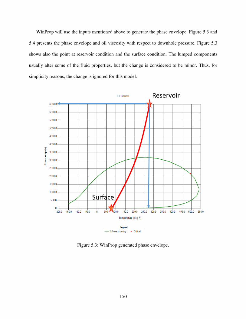
150
WinProp will use the inputs mentioned above to generate the phase envelope. Figure 5.3 and
5.4 presents the phase envelope and oil viscosity with respect to downhole pressure. Figure 5.3
shows also the point at reservoir condition and the surface condition. The lumped components
usually alter some of the fluid properties, but the change is considered to be minor. Thus, for
simplicity reasons, the change is ignored for this model.
Figure 5.3: WinProp generated phase envelope.
Reservoir
Surface
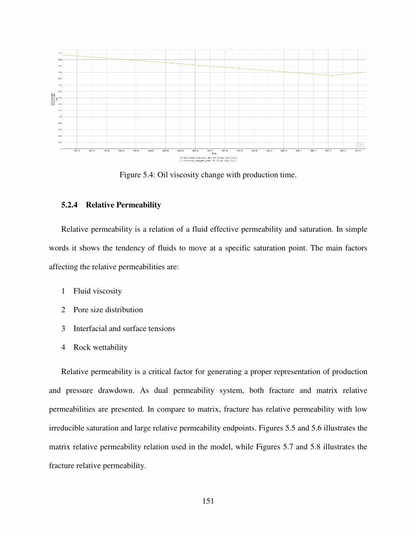
151
Figure 5.4: Oil viscosity change with production time.
5.2.4 Relative Permeability
Relative permeability is a relation of a fluid effective permeability and saturation. In simple
words it shows the tendency of fluids to move at a specific saturation point. The main factors
affecting the relative permeabilities are:
1 Fluid viscosity
2 Pore size distribution
3 Interfacial and surface tensions
4 Rock wettability
Relative permeability is a critical factor for generating a proper representation of production
and pressure drawdown. As dual permeability system, both fracture and matrix relative
permeabilities are presented. In compare to matrix, fracture has relative permeability with low
irreducible saturation and large relative permeability endpoints. Figures 5.5 and 5.6 illustrates the
matrix relative permeability relation used in the model, while Figures 5.7 and 5.8 illustrates the
fracture relative permeability.
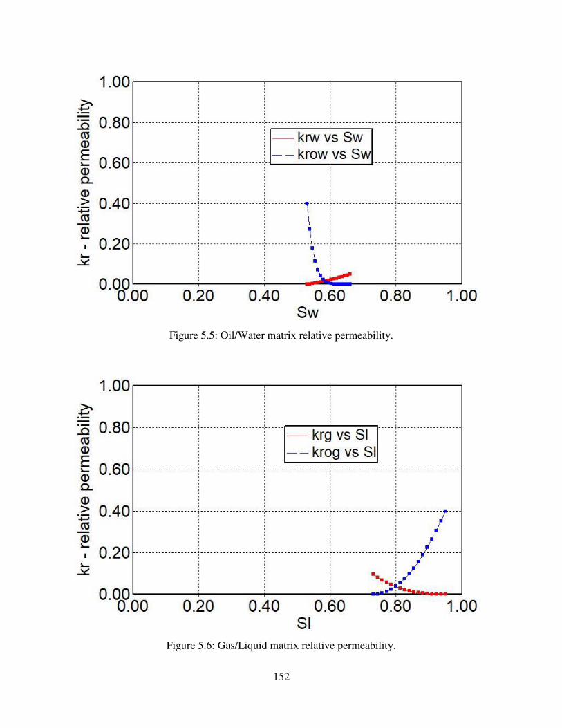
152
Figure 5.5: Oil/Water matrix relative permeability.
Figure 5.6: Gas/Liquid matrix relative permeability.

153
Figure 5.7: Oil/Water fracture relative permeability.
Figure 5.8: Gas/Liquid fracture relative permeability.
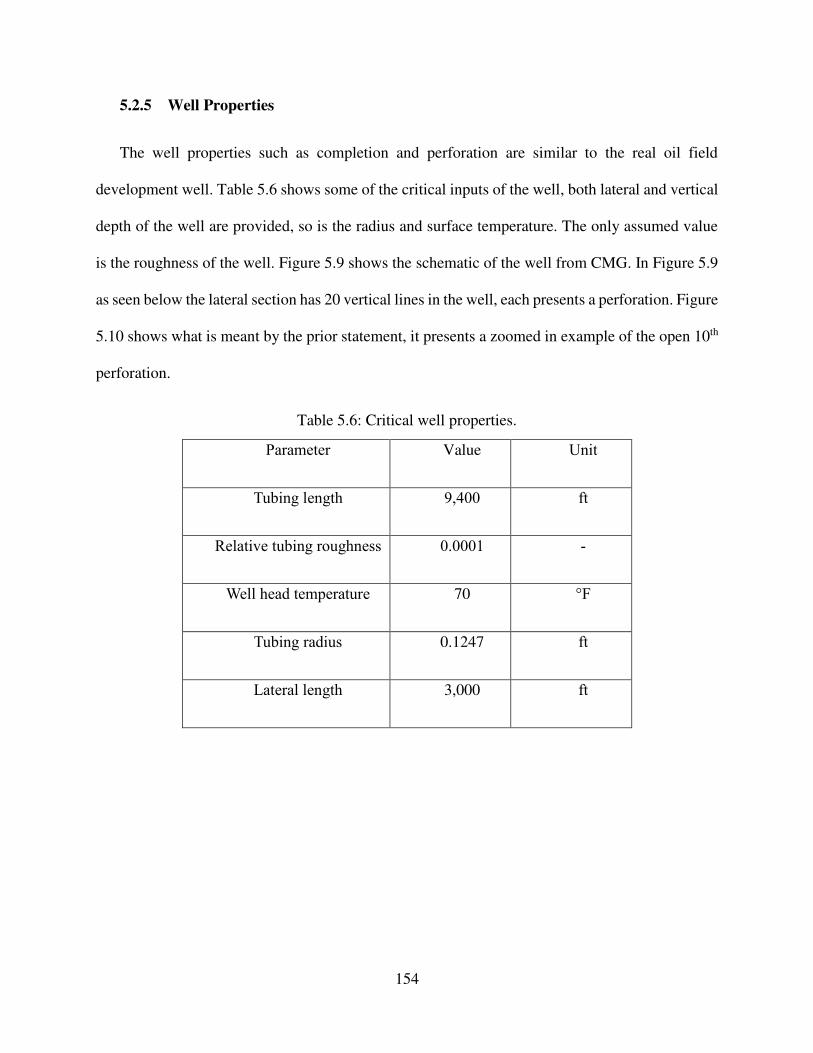
154
5.2.5 Well Properties
The well properties such as completion and perforation are similar to the real oil field
development well. Table 5.6 shows some of the critical inputs of the well, both lateral and vertical
depth of the well are provided, so is the radius and surface temperature. The only assumed value
is the roughness of the well. Figure 5.9 shows the schematic of the well from CMG. In Figure 5.9
as seen below the lateral section has 20 vertical lines in the well, each presents a perforation. Figure
5.10 shows what is meant by the prior statement, it presents a zoomed in example of the open 10th
perforation.
Table 5.6: Critical well properties.
Parameter Value Unit
Tubing length 9,400 ft
Relative tubing roughness 0.0001 -
Well head temperature 70 °F
Tubing radius 0.1247 ft
Lateral length 3,000 ft
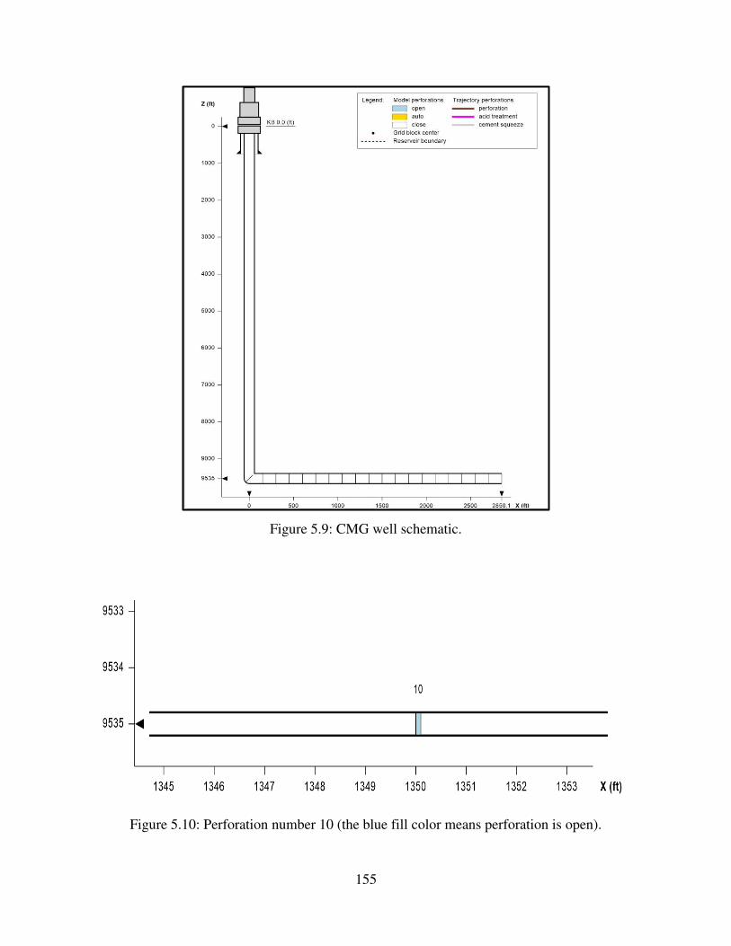
155
Figure 5.9: CMG well schematic.
Figure 5.10: Perforation number 10 (the blue fill color means perforation is open).
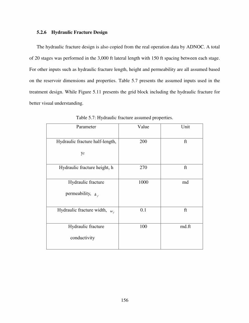
156
5.2.6 Hydraulic Fracture Design
The hydraulic fracture design is also copied from the real operation data by ADNOC. A total
of 20 stages was performed in the 3,000 ft lateral length with 150 ft spacing between each stage.
For other inputs such as hydraulic fracture length, height and permeability are all assumed based
on the reservoir dimensions and properties. Table 5.7 presents the assumed inputs used in the
treatment design. While Figure 5.11 presents the grid block including the hydraulic fracture for
better visual understanding.
Table 5.7: Hydraulic fracture assumed properties.
Parameter Value Unit
Hydraulic fracture half-length,
yf
200 ft
Hydraulic fracture height, h 270 ft
Hydraulic fracture
permeability, f
k
1000 md
Hydraulic fracture width, f
w 0.1 ft
Hydraulic fracture
conductivity
100 md.ft
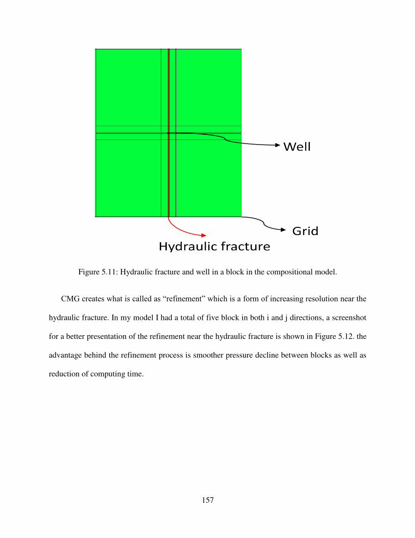
157
Figure 5.11: Hydraulic fracture and well in a block in the compositional model.
CMG creates what is called as “refinement” which is a form of increasing resolution near the
hydraulic fracture. In my model I had a total of five block in both i and j directions, a screenshot
for a better presentation of the refinement near the hydraulic fracture is shown in Figure 5.12. the
advantage behind the refinement process is smoother pressure decline between blocks as well as
reduction of computing time.
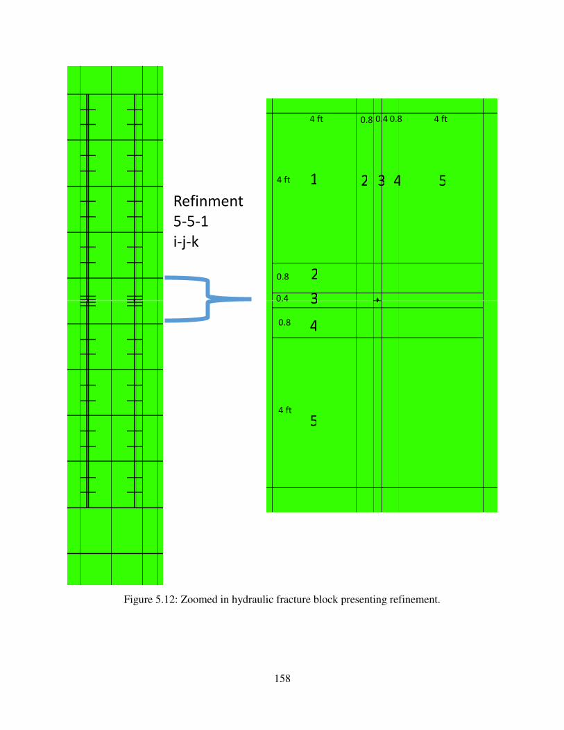
158
Figure 5.12: Zoomed in hydraulic fracture block presenting refinement.
1 4 3 5 2
4
3
5
2
Refinment
5-5-1
i-j-k
4 ft
4 ft
0.8
ft
0.4
ft 0.8
ft 4 ft
0.8
ft 0.4
ft 0.8
ft
4 ft

159
The hydraulic fracturing treatment was copied for the real operation in terms of spacing and
stages chosen. Figure 5.13 presents the hydraulic fracturing treatment, total of 20 stages, single
cluster each, where applied with fracture spacing of 150 ft between each stage.
Figure 5.13: Three-dimensional hydraulic fractures.
For more realistic condition and depletion effect, the option “Null Blocks” was used to
represent boundary conditions, the nulled blocks were, Figure 5.14 below shows a better
representation of is simply having zero properties in the grid. In Figure 5.14 the blocks labelled
“Non-SRV” are the nulled blocks, 105 ft. in both i and j directions.

160
Figure 5.14: Illustration of the SRV and Non-SRV regions.
5.3 Results and Analysis
The Model was set to produce for a year and then build up for three months to study the flow
regimes and match with the real well production data. For the flow regime analysis, rate transient
analysis (RTA) and pressure transient analysis (PTA) are used, thereby the model is validated by
back calculating the permeability and matching it with the input.
5.3.1 Rate Transient Analysis
Rate transient analysis is used in well testing, most commonly in unconventionals to determine
the linear flow regime, hence calculate critical reservoir properties like permeability. Figure 5.15
shows the Log-Log plot of the rate normalized pressure against time, indicating that the linear flow
is achieved, which will be used for plotting the linear flow analysis hence back calculate effective
permeability.
In order to back calculate effective permeability, linear flow analysis is plotted (Figure 5.16),
which is Cartesian plot of the rate normalized pressure against square root of time. The next step
is model verification, by back calculating the affective formation permeability using Equation 5.4.
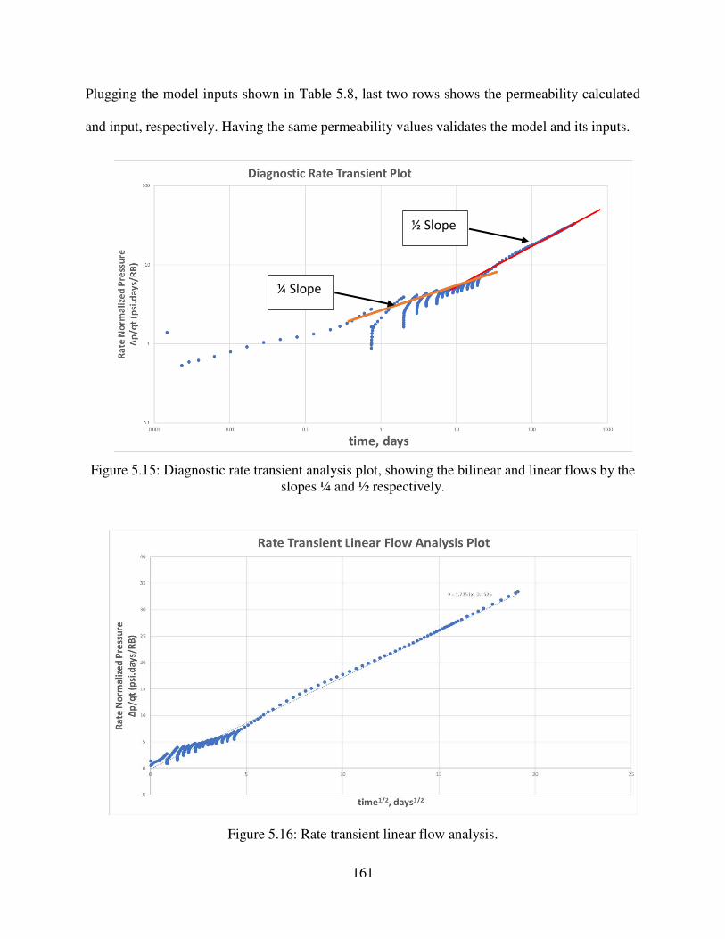
161
Plugging the model inputs shown in Table 5.8, last two rows shows the permeability calculated
and input, respectively. Having the same permeability values validates the model and its inputs.
Figure 5.15: Diagnostic rate transient analysis plot, showing the bilinear and linear flows by the
slopes ¼ and ½ respectively.
Figure 5.16: Rate transient linear flow analysis.
½ Slope
¼ Slope
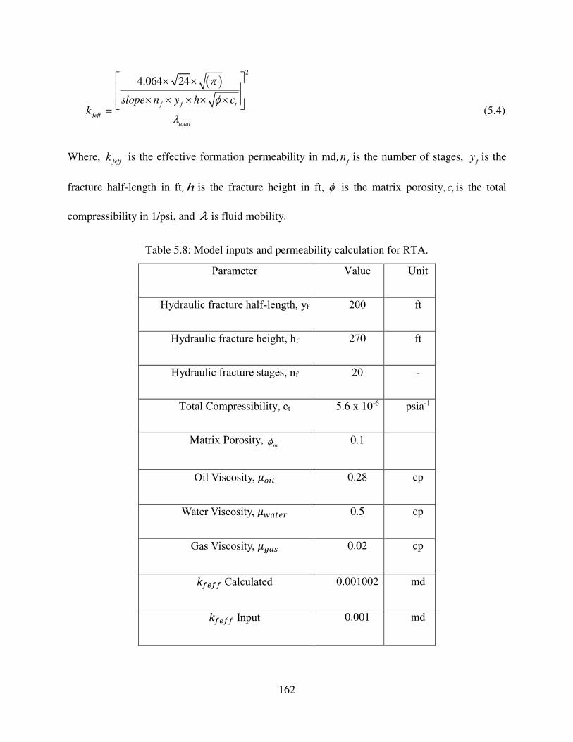
162
( )2
4.064 24
f f t
feff
total
slope n y h ck
= (5.4)
Where, feff
k is the effective formation permeability in md,f
n is the number of stages, f
y is the
fracture half-length in ft, h is the fracture height in ft, is the matrix porosity, tc is the total
compressibility in 1/psi, and is fluid mobility.
Table 5.8: Model inputs and permeability calculation for RTA.
Parameter Value Unit
Hydraulic fracture half-length, yf 200 ft
Hydraulic fracture height, hf 270 ft
Hydraulic fracture stages, nf 20 -
Total Compressibility, ct 5.6 x 10⁻⁶ psia-1
Matrix Porosity, m 0.1
Oil Viscosity, 𝜇𝑜𝑖𝑙 0.28 cp
Water Viscosity, 𝜇𝑤𝑎𝑡𝑒𝑟 0.5 cp
Gas Viscosity, 𝜇𝑔𝑎𝑠 0.02 cp
𝑘𝑓𝑒𝑓𝑓 Calculated 0.001002 md
𝑘𝑓𝑒𝑓𝑓 Input 0.001 md
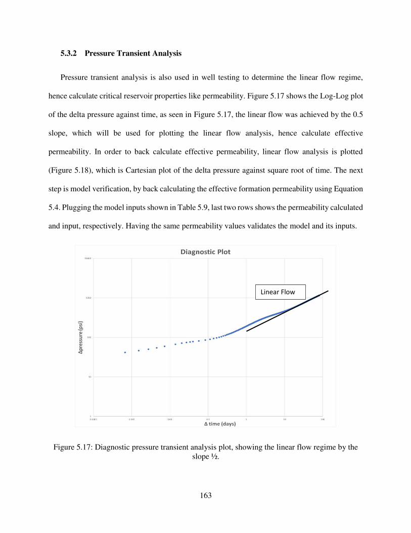
163
5.3.2 Pressure Transient Analysis
Pressure transient analysis is also used in well testing to determine the linear flow regime,
hence calculate critical reservoir properties like permeability. Figure 5.17 shows the Log-Log plot
of the delta pressure against time, as seen in Figure 5.17, the linear flow was achieved by the 0.5
slope, which will be used for plotting the linear flow analysis, hence calculate effective
permeability. In order to back calculate effective permeability, linear flow analysis is plotted
(Figure 5.18), which is Cartesian plot of the delta pressure against square root of time. The next
step is model verification, by back calculating the effective formation permeability using Equation
5.4. Plugging the model inputs shown in Table 5.9, last two rows shows the permeability calculated
and input, respectively. Having the same permeability values validates the model and its inputs.
Figure 5.17: Diagnostic pressure transient analysis plot, showing the linear flow regime by the
slope ½.
Linear Flow
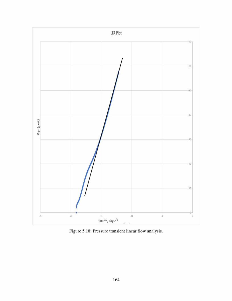
164
Figure 5.18: Pressure transient linear flow analysis.
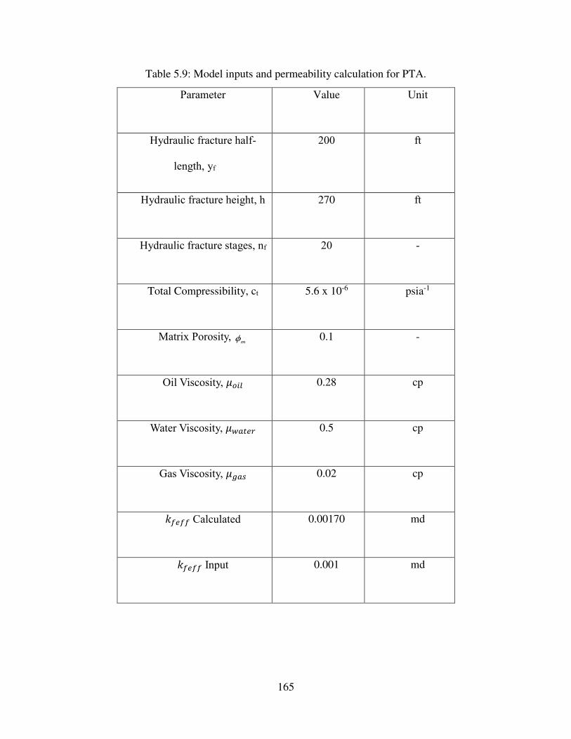
165
Table 5.9: Model inputs and permeability calculation for PTA.
Parameter Value Unit
Hydraulic fracture half-
length, yf
200 ft
Hydraulic fracture height, h 270 ft
Hydraulic fracture stages, nf 20 -
Total Compressibility, ct 5.6 x 10⁻⁶ psia-1
Matrix Porosity, m 0.1 -
Oil Viscosity, 𝜇𝑜𝑖𝑙 0.28 cp
Water Viscosity, 𝜇𝑤𝑎𝑡𝑒𝑟 0.5 cp
Gas Viscosity, 𝜇𝑔𝑎𝑠 0.02 cp
𝑘𝑓𝑒𝑓𝑓 Calculated 0.00170 md
𝑘𝑓𝑒𝑓𝑓 Input 0.001 md
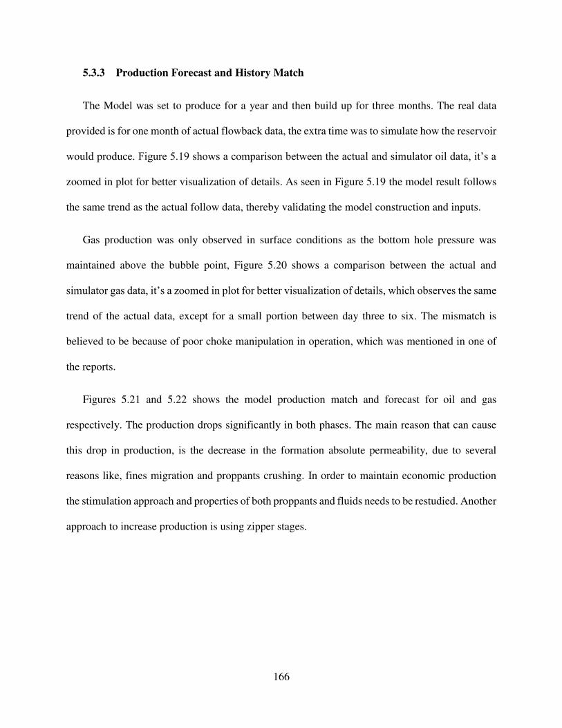
166
5.3.3 Production Forecast and History Match
The Model was set to produce for a year and then build up for three months. The real data
provided is for one month of actual flowback data, the extra time was to simulate how the reservoir
would produce. Figure 5.19 shows a comparison between the actual and simulator oil data, it’s a
zoomed in plot for better visualization of details. As seen in Figure 5.19 the model result follows
the same trend as the actual follow data, thereby validating the model construction and inputs.
Gas production was only observed in surface conditions as the bottom hole pressure was
maintained above the bubble point, Figure 5.20 shows a comparison between the actual and
simulator gas data, it’s a zoomed in plot for better visualization of details, which observes the same
trend of the actual data, except for a small portion between day three to six. The mismatch is
believed to be because of poor choke manipulation in operation, which was mentioned in one of
the reports.
Figures 5.21 and 5.22 shows the model production match and forecast for oil and gas
respectively. The production drops significantly in both phases. The main reason that can cause
this drop in production, is the decrease in the formation absolute permeability, due to several
reasons like, fines migration and proppants crushing. In order to maintain economic production
the stimulation approach and properties of both proppants and fluids needs to be restudied. Another
approach to increase production is using zipper stages.
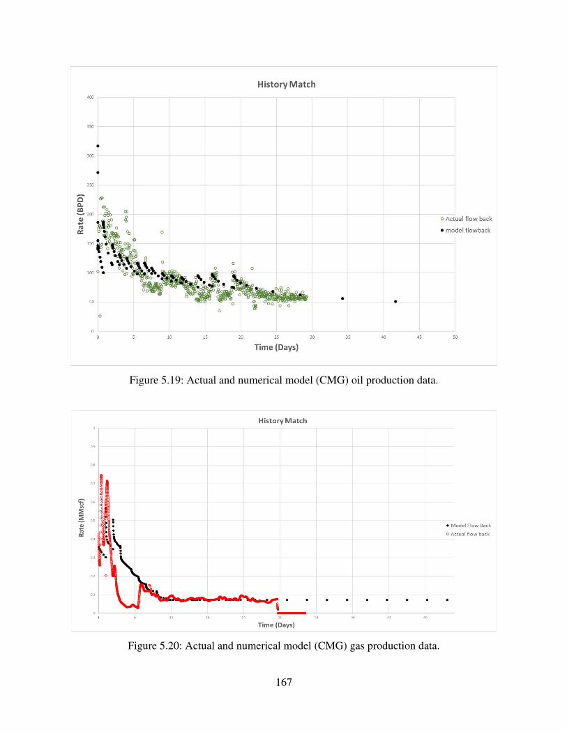
167
Figure 5.19: Actual and numerical model (CMG) oil production data.
Figure 5.20: Actual and numerical model (CMG) gas production data.
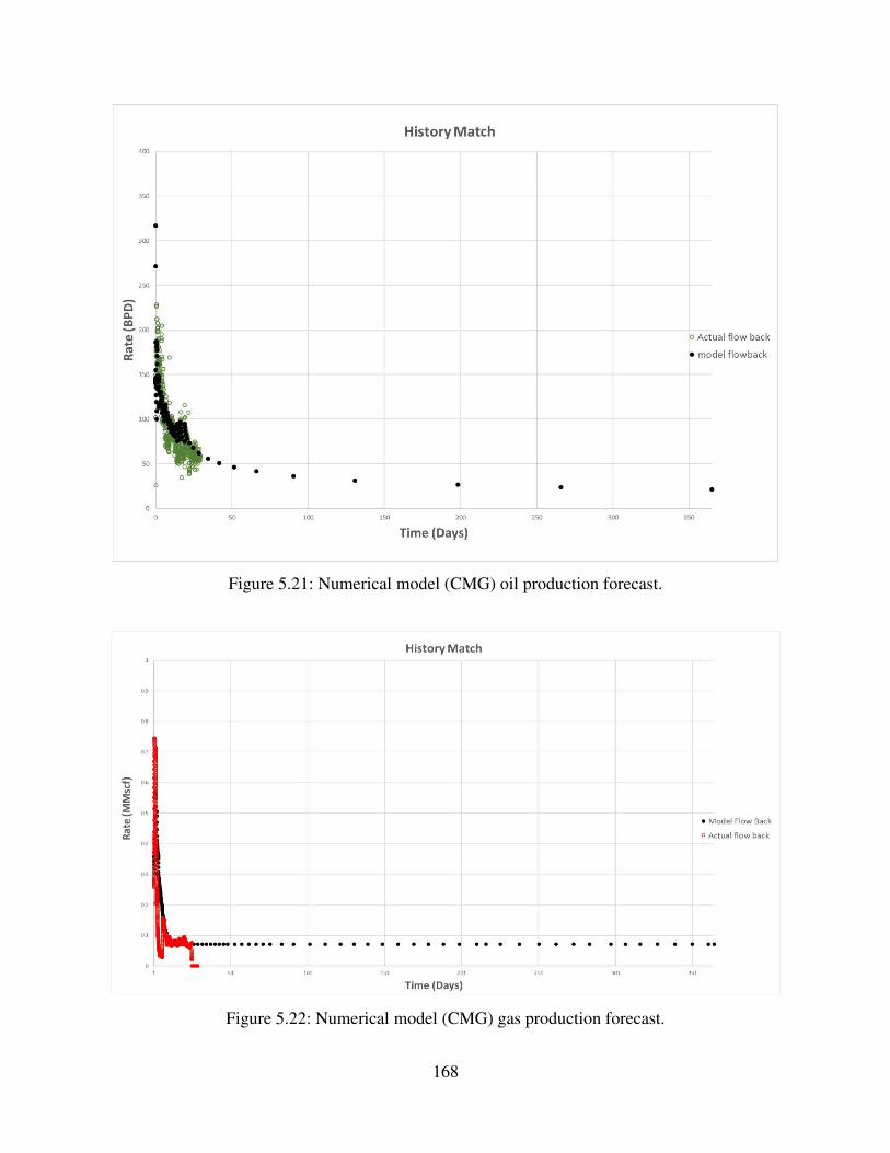
168
Figure 5.21: Numerical model (CMG) oil production forecast.
Figure 5.22: Numerical model (CMG) gas production forecast.
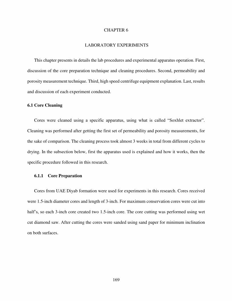
169
CHAPTER 6
6 LABORATORY EXPERIMENTS
This chapter presents in details the lab procedures and experimental apparatus operation. First,
discussion of the core preparation technique and cleaning procedures. Second, permeability and
porosity measurement technique. Third, high speed centrifuge equipment explanation. Last, results
and discussion of each experiment conducted.
6.1 Core Cleaning
Cores were cleaned using a specific apparatus, using what is called “Soxhlet extractor”.
Cleaning was performed after getting the first set of permeability and porosity measurements, for
the sake of comparison. The cleaning process took almost 3 weeks in total from different cycles to
drying. In the subsection below, first the apparatus used is explained and how it works, then the
specific procedure followed in this research.
6.1.1 Core Preparation
Cores from UAE Diyab formation were used for experiments in this research. Cores received
were 1.5-inch diameter cores and length of 3-inch. For maximum conservation cores were cut into
half’s, so each 3-inch core created two 1.5-inch core. The core cutting was performed using wet
cut diamond saw. After cutting the cores were sanded using sand paper for minimum inclination
on both surfaces.
170
6.1.2 Soxhlet Extractor
Soxhlet extractor (Figure 6.1) is an apparatus invented by Franz von Soxhlet in 1879.
Originally designed for lipids extraction from solid test material, but scientists use it whenever
there is difficulty in any extraction from solids. In general, dry solid is placed inside the extractor
chamber above heating flask. The extractor is attached to the flask containing the required solvent
and a condenser.
The heater evaporates the solvent into the column where the hot solvent vapor travels up
towards the condenser, which cools it, hence drips down onto the test material. The extractor
chamber containing the solid material slowly fills with drips of the warm solvent, until the liquid
level in the chamber reaches a specific level (almost full), where the chamber is emptied by siphon
action, and circulating back down to the flask.
This cycle is repeated as long as the heater is on, which is as many times as desired for
extraction, note that the solvent used has to be less dense (lower boiling temperature than the
dissolvent). During each cycle, a portion of the intended dissolvent dissolves in the solvent.
Nonetheless, the dissolvent that reaches the solvent heating flask stays there, because of difference
in boiling temperatures. This is considered the main advantage of this type of extractor. Which
makes it more efficient when compared with simply heating up the solid in a flask with the solvent.
After extraction is over the solvent used can be re-used as long as the dissolvent doesn’t evaporate.
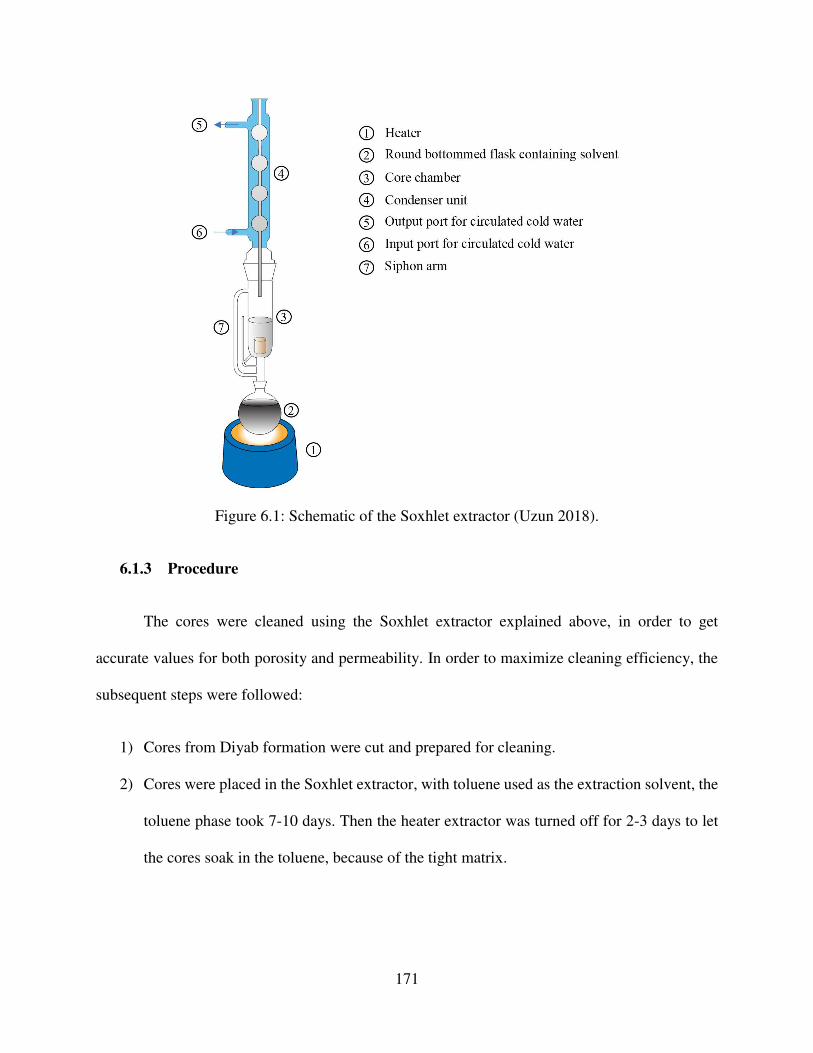
171
Figure 6.1: Schematic of the Soxhlet extractor (Uzun 2018).
6.1.3 Procedure
The cores were cleaned using the Soxhlet extractor explained above, in order to get
accurate values for both porosity and permeability. In order to maximize cleaning efficiency, the
subsequent steps were followed:
1) Cores from Diyab formation were cut and prepared for cleaning.
2) Cores were placed in the Soxhlet extractor, with toluene used as the extraction solvent, the
toluene phase took 7-10 days. Then the heater extractor was turned off for 2-3 days to let
the cores soak in the toluene, because of the tight matrix.
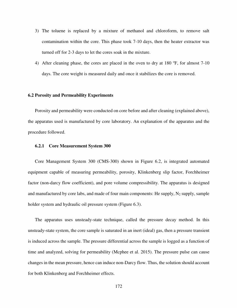
172
3) The toluene is replaced by a mixture of methanol and chloroform, to remove salt
contamination within the core. This phase took 7-10 days, then the heater extractor was
turned off for 2-3 days to let the cores soak in the mixture.
4) After cleaning phase, the cores are placed in the oven to dry at 180 oF, for almost 7-10
days. The core weight is measured daily and once it stabilizes the core is removed.
6.2 Porosity and Permeability Experiments
Porosity and permeability were conducted on core before and after cleaning (explained above),
the apparatus used is manufactured by core laboratory. An explanation of the apparatus and the
procedure followed.
6.2.1 Core Measurement System 300
Core Management System 300 (CMS-300) shown in Figure 6.2, is integrated automated
equipment capable of measuring permeability, porosity, Klinkenberg slip factor, Forchheimer
factor (non-darcy flow coefficient), and pore volume compressibility. The apparatus is designed
and manufactured by core labs, and made of four main components: He supply, N2 supply, sample
holder system and hydraulic oil pressure system (Figure 6.3).
The apparatus uses unsteady-state technique, called the pressure decay method. In this
unsteady-state system, the core sample is saturated in an inert (ideal) gas, then a pressure transient
is induced across the sample. The pressure differential across the sample is logged as a function of
time and analyzed, solving for permeability (Mcphee et al. 2015). The pressure pulse can cause
changes in the mean pressure, hence can induce non-Darcy flow. Thus, the solution should account
for both Klinkenberg and Forchheimer effects.

173
This system uses Helium for porosity/permeability measurement and Nitrogen for confining.
In the permeability measurement, the core sample is loaded hydraulically via a carousel into the
test core holder, then confined at the specified confining stress (maximum of 10,000 psi
confinement). The source chamber is filled with helium and a valve isolates the core holder from
the helium tank. For porosity measurement, the downstream valve of the plug sample is closed
while, for permeability measurement, it is left open as helium flows from the reference tank
through the sample.
The instantaneous flow rates are calculated from the recorded sample volume, and the rate of
pressure decay. The instantaneous delta pressures across the plug are equal to the readings of
upstream pressure. The differential or upstream pressure across the core sample is recorded as a
function of time until a pressure stabilization criterion is been reached.
Since the mean pressure in the core sample is continually decreasing, where the initial rates
are rapid, the computer analytical solution must take account of both Forchheimer (inertial) and
Klinkenberg (viscous) effects. The instrument is capable of measuring permeability within the
range of 15 Darcy all the way to super tight nano-Darcy. A schematic is shown in Figure 6.3 that
give a better visual explanation.
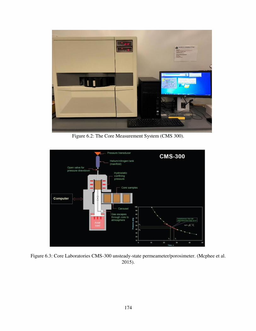
174
Figure 6.2: The Core Measurement System (CMS 300).
Figure 6.3: Core Laboratories CMS-300 unsteady-state permeameter/porosimeter. (Mcphee et al.
2015).
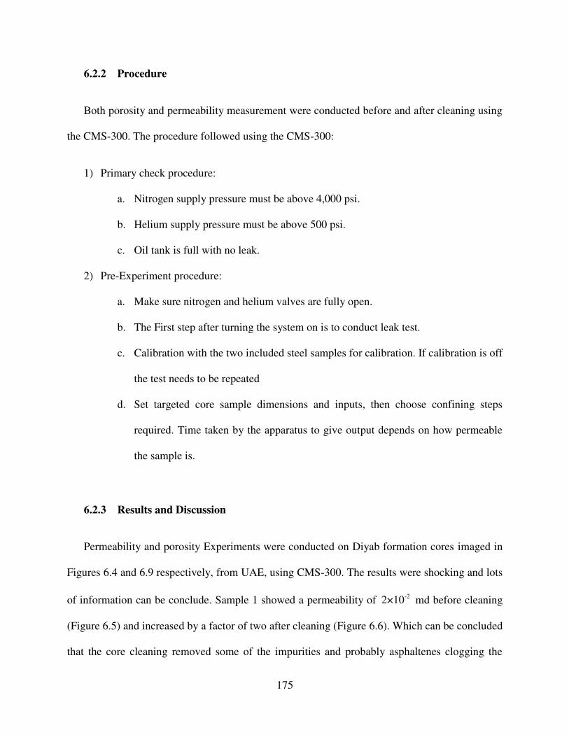
175
6.2.2 Procedure
Both porosity and permeability measurement were conducted before and after cleaning using
the CMS-300. The procedure followed using the CMS-300:
1) Primary check procedure:
a. Nitrogen supply pressure must be above 4,000 psi.
b. Helium supply pressure must be above 500 psi.
c. Oil tank is full with no leak.
2) Pre-Experiment procedure:
a. Make sure nitrogen and helium valves are fully open.
b. The First step after turning the system on is to conduct leak test.
c. Calibration with the two included steel samples for calibration. If calibration is off
the test needs to be repeated
d. Set targeted core sample dimensions and inputs, then choose confining steps
required. Time taken by the apparatus to give output depends on how permeable
the sample is.
6.2.3 Results and Discussion
Permeability and porosity Experiments were conducted on Diyab formation cores imaged in
Figures 6.4 and 6.9 respectively, from UAE, using CMS-300. The results were shocking and lots
of information can be conclude. Sample 1 showed a permeability of -22×10 md before cleaning
(Figure 6.5) and increased by a factor of two after cleaning (Figure 6.6). Which can be concluded
that the core cleaning removed some of the impurities and probably asphaltenes clogging the

176
channels. Porosity measurement for Sample 1 showed a porosity of 2%, the result didn’t change
before and after cleaning as shown in Figures 6.7 and 6.8 respectively. In summary Sample 1 had
promising permeability, while porosity was disappointing low.
Sample 2 (Figure 6.9) permeability measurements showed tighter core, the result was almost
-31×10 md before cleaning in Figure 6.10, which increased by almost factor if two after cleaning
in Figure 6.11, thereby the same conclusion is drawn as Sample 1. While having a very tight matrix
in Sample 2 the porosity was promising, the core results showed an average of 8% porosity
(Figures 6.12 and 6.13), which is opposite to Sample 1 where we had high permeability and low
porosity. Nonetheless, this proofs the Unconventionals (source rock) heterogeneity.
The main question asked is why such incompatibility between permeability and porosity in
both samples. The interesting conclusion drawn from personal and expert analysis for Sample 1 is
that the porosity and permeability measured are fracture dominant, as seen in Figure 6.4 the core
highly fractured which reflects the high permeability. The matrix is too tight and the time taken by
the equipment to measure matrix permeability and porosity didn’t leave chance for the response
to be reflected from the matrix, and equipment cannot distinguish whether the results are for matrix
or fracture. Sample 2 (Figure 6.9) is less naturally fractured and this is why it showed more tight
permeability results at the same time larger pore volume compared with Sample 1, as the results
are matrix dominant.
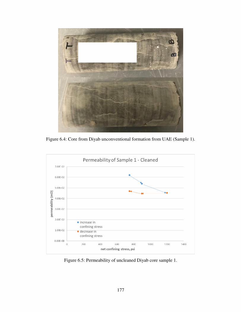
177
Figure 6.4: Core from Diyab unconventional formation from UAE (Sample 1).
Figure 6.5: Permeability of uncleaned Diyab core sample 1.
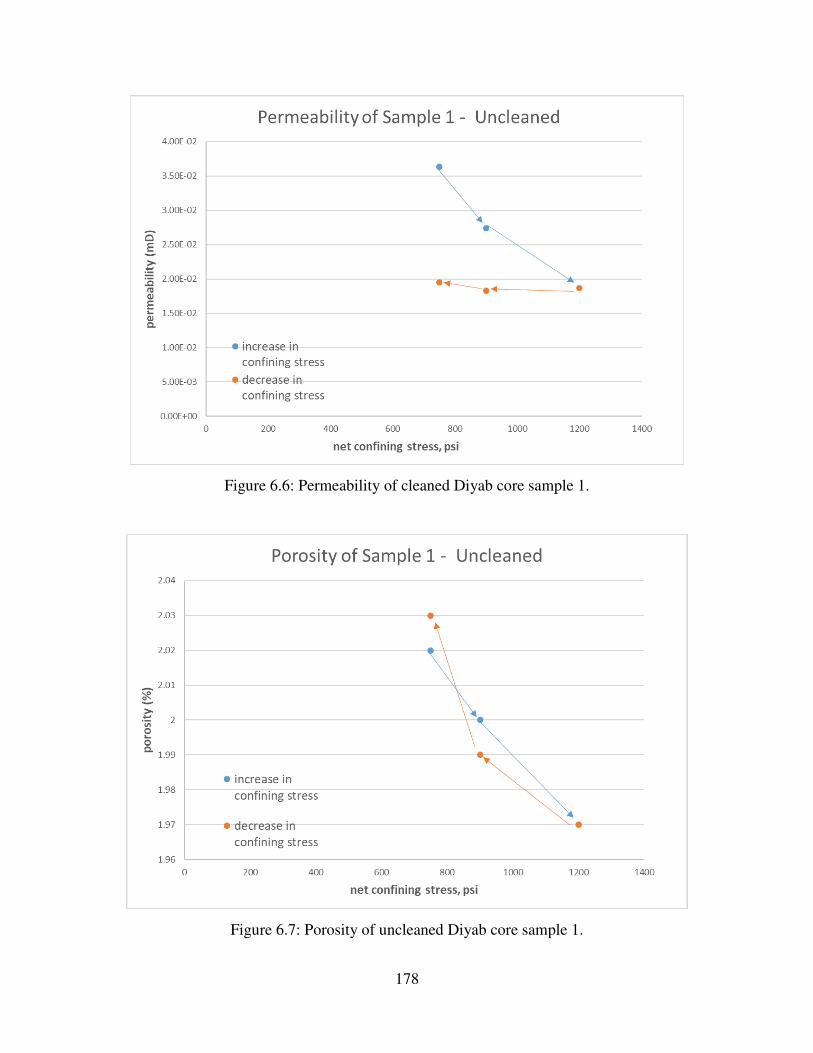
178
Figure 6.6: Permeability of cleaned Diyab core sample 1.
Figure 6.7: Porosity of uncleaned Diyab core sample 1.
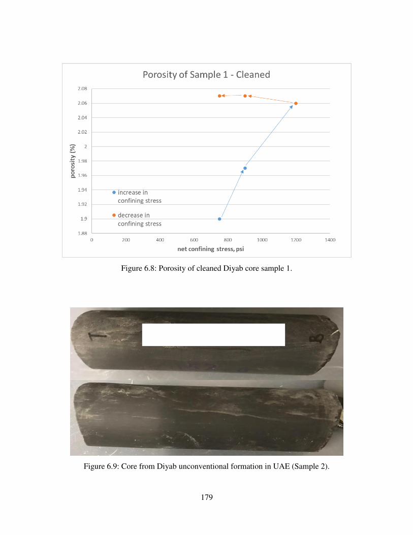
179
Figure 6.8: Porosity of cleaned Diyab core sample 1.
Figure 6.9: Core from Diyab unconventional formation in UAE (Sample 2).

180
Figure 6.10: Permeability of uncleaned Diyab core sample 2.
Figure 6.11: Permeability of cleaned Diyab core sample 2.
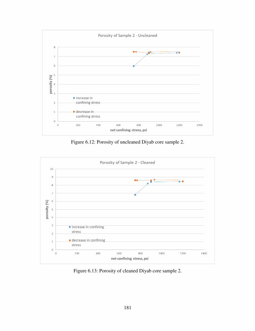
181
Figure 6.12: Porosity of uncleaned Diyab core sample 2.
Figure 6.13: Porosity of cleaned Diyab core sample 2.
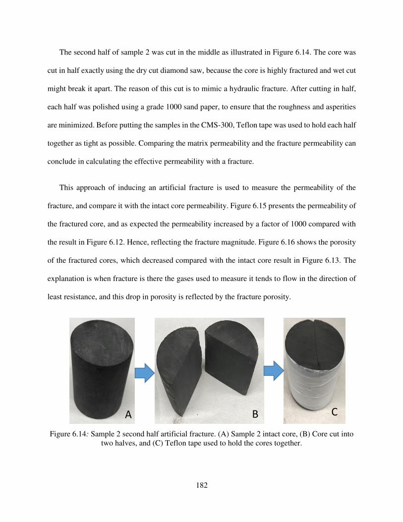
182
The second half of sample 2 was cut in the middle as illustrated in Figure 6.14. The core was
cut in half exactly using the dry cut diamond saw, because the core is highly fractured and wet cut
might break it apart. The reason of this cut is to mimic a hydraulic fracture. After cutting in half,
each half was polished using a grade 1000 sand paper, to ensure that the roughness and asperities
are minimized. Before putting the samples in the CMS-300, Teflon tape was used to hold each half
together as tight as possible. Comparing the matrix permeability and the fracture permeability can
conclude in calculating the effective permeability with a fracture.
This approach of inducing an artificial fracture is used to measure the permeability of the
fracture, and compare it with the intact core permeability. Figure 6.15 presents the permeability of
the fractured core, and as expected the permeability increased by a factor of 1000 compared with
the result in Figure 6.12. Hence, reflecting the fracture magnitude. Figure 6.16 shows the porosity
of the fractured cores, which decreased compared with the intact core result in Figure 6.13. The
explanation is when fracture is there the gases used to measure it tends to flow in the direction of
least resistance, and this drop in porosity is reflected by the fracture porosity.
Figure 6.14: Sample 2 second half artificial fracture. (A) Sample 2 intact core, (B) Core cut into
two halves, and (C) Teflon tape used to hold the cores together.
A B C
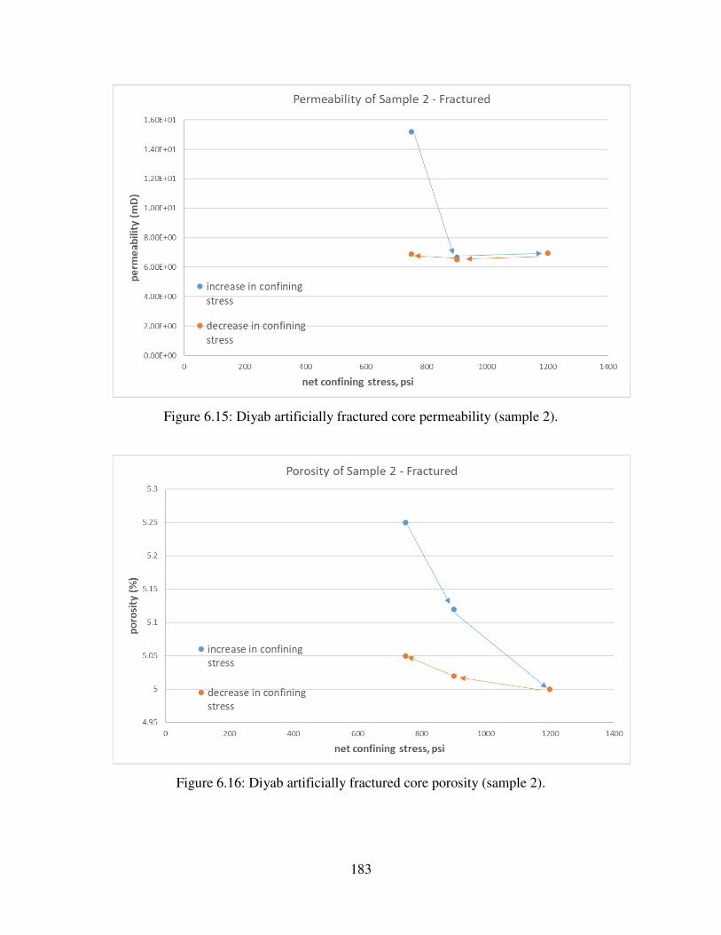
183
Figure 6.15: Diyab artificially fractured core permeability (sample 2).
Figure 6.16: Diyab artificially fractured core porosity (sample 2).
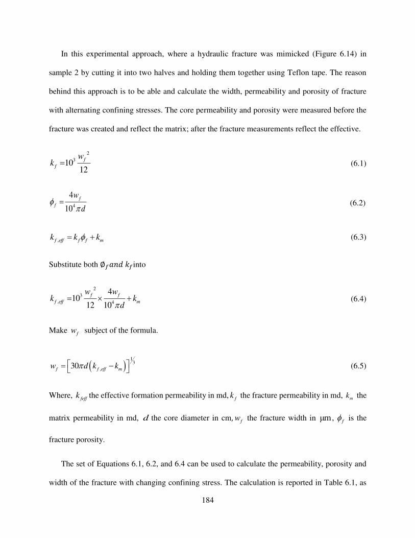
184
In this experimental approach, where a hydraulic fracture was mimicked (Figure 6.14) in
sample 2 by cutting it into two halves and holding them together using Teflon tape. The reason
behind this approach is to be able and calculate the width, permeability and porosity of fracture
with alternating confining stresses. The core permeability and porosity were measured before the
fracture was created and reflect the matrix; after the fracture measurements reflect the effective.
2
31 0 12
f
fkw
= (6.1)
4
4 10
f
f
w
d
= (6.2)
,f eff f f mkk k= + (6.3)
Substitute both ∅𝑓𝑎𝑛𝑑 𝑘𝑓into
2
3
, 4
41 0
12 10
f f
f eff mkw w
kd
= + (6.4)
Make fw subject of the formula.
( )13
,30f f eff mw kd k = − (6.5)
Where, feff
k the effective formation permeability in md,f
k the fracture permeability in md, mk the
matrix permeability in md, d the core diameter in cm,f
w the fracture width in μm , f
is the
fracture porosity.
The set of Equations 6.1, 6.2, and 6.4 can be used to calculate the permeability, porosity and
width of the fracture with changing confining stress. The calculation is reported in Table 6.1, as

185
seen all the properties of the fracture decreases with increasing confining stress. From these results
the following conclusion is made; the fracture reported had almost 13 microns, yet is able to
increase the permeability of the system almost 400000 times.
Cho (2017) reported similar hydraulic fracture experiment as the one presented in Figure
6.14 but he performed it on middle Bakken formation. His results are presented in Table 6.2. The
fracture width again never comes to zero even with almost 3000 psi of confining stress, which is
very close to the reservoir condition.
Table 6.1: Diyab artificial fractured core measurement results.
Matrix Fractures
Confining
Stress
Measured
mk
Confining
Stress
Measured
,f effk
fk
fw
f
psia md psia md md μm fraction
A 750 2.16E-03 750 1.52E+01 25830 17.6 0.0005
B 900 1.95E-03 900 6.66E+00 14900 13.3 0.0004
C 1200 1.50E-03 1200 6.36E+00 14449 13.1 0.0004
D 900 1.55E-03 900 6.53E+00 14706 13.2 0.0004
E 750 1.63E-03 750 6.89E+00 15242 13.5 0.0004
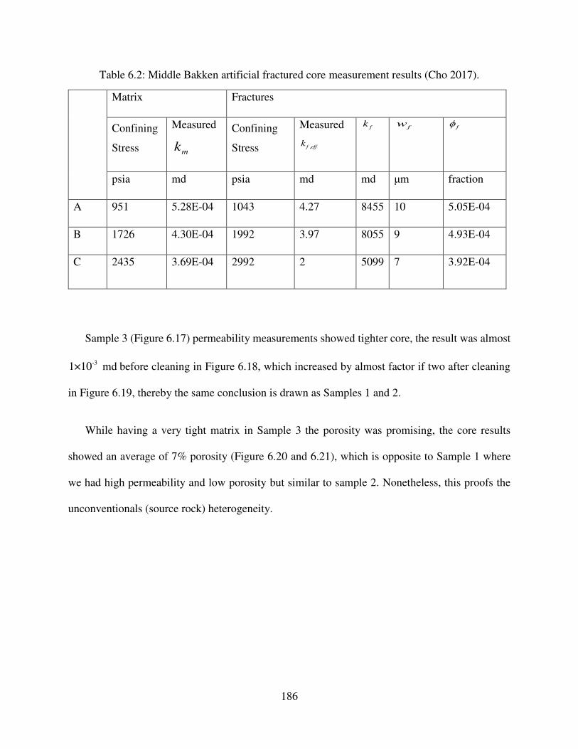
186
Table 6.2: Middle Bakken artificial fractured core measurement results (Cho 2017).
Matrix Fractures
Confining
Stress
Measured
mk
Confining
Stress
Measured
,f effk
fk
fw
f
psia md psia md md μm fraction
A 951 5.28E-04 1043 4.27 8455 10 5.05E-04
B 1726 4.30E-04 1992 3.97 8055 9 4.93E-04
C 2435 3.69E-04 2992 2 5099 7 3.92E-04
Sample 3 (Figure 6.17) permeability measurements showed tighter core, the result was almost
-31×10 md before cleaning in Figure 6.18, which increased by almost factor if two after cleaning
in Figure 6.19, thereby the same conclusion is drawn as Samples 1 and 2.
While having a very tight matrix in Sample 3 the porosity was promising, the core results
showed an average of 7% porosity (Figure 6.20 and 6.21), which is opposite to Sample 1 where
we had high permeability and low porosity but similar to sample 2. Nonetheless, this proofs the
unconventionals (source rock) heterogeneity.
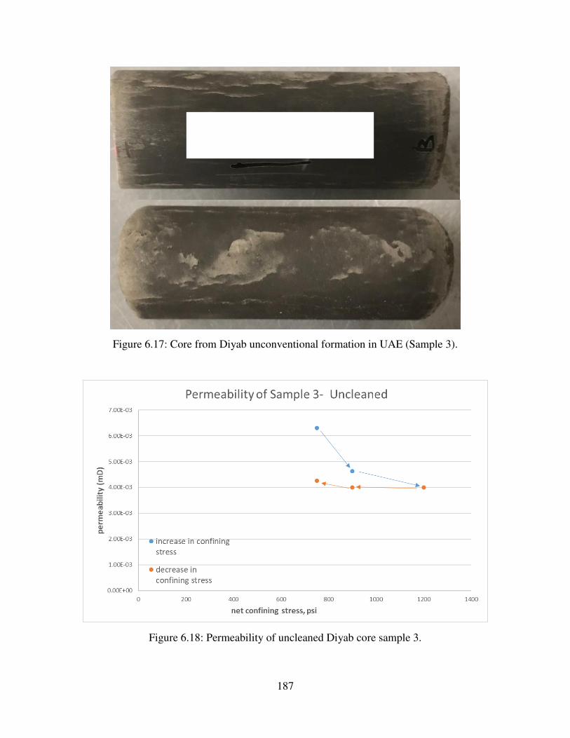
187
Figure 6.17: Core from Diyab unconventional formation in UAE (Sample 3).
Figure 6.18: Permeability of uncleaned Diyab core sample 3.
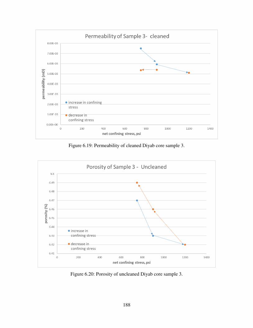
188
Figure 6.19: Permeability of cleaned Diyab core sample 3.
Figure 6.20: Porosity of uncleaned Diyab core sample 3.
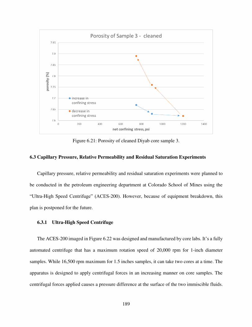
189
Figure 6.21: Porosity of cleaned Diyab core sample 3.
6.3 Capillary Pressure, Relative Permeability and Residual Saturation Experiments
Capillary pressure, relative permeability and residual saturation experiments were planned to
be conducted in the petroleum engineering department at Colorado School of Mines using the
“Ultra-High Speed Centrifuge” (ACES-200). However, because of equipment breakdown, this
plan is postponed for the future.
6.3.1 Ultra-High Speed Centrifuge
The ACES-200 imaged in Figure 6.22 was designed and manufactured by core labs. It’s a fully
automated centrifuge that has a maximum rotation speed of 20,000 rpm for 1-inch diameter
samples. While 16,500 rpm maximum for 1.5 inches samples, it can take two cores at a time. The
apparatus is designed to apply centrifugal forces in an increasing manner on core samples. The
centrifugal forces applied causes a pressure difference at the surface of the two immiscible fluids.
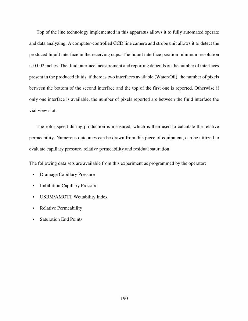
190
Top of the line technology implemented in this apparatus allows it to fully automated operate
and data analyzing. A computer-controlled CCD line camera and strobe unit allows it to detect the
produced liquid interface in the receiving cups. The liquid interface position minimum resolution
is 0.002 inches. The fluid interface measurement and reporting depends on the number of interfaces
present in the produced fluids, if there is two interfaces available (Water/Oil), the number of pixels
between the bottom of the second interface and the top of the first one is reported. Otherwise if
only one interface is available, the number of pixels reported are between the fluid interface the
vial view slot.
The rotor speed during production is measured, which is then used to calculate the relative
permeability. Numerous outcomes can be drawn from this piece of equipment, can be utilized to
evaluate capillary pressure, relative permeability and residual saturation
The following data sets are available from this experiment as programmed by the operator:
▪ Drainage Capillary Pressure
▪ Imbibition Capillary Pressure
▪ USBM/AMOTT Wettability Index
▪ Relative Permeability
▪ Saturation End Points
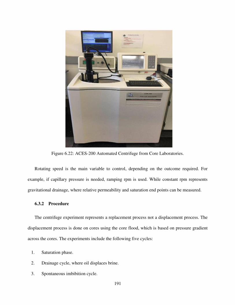
191
Figure 6.22: ACES-200 Automated Centrifuge from Core Laboratories.
Rotating speed is the main variable to control, depending on the outcome required. For
example, if capillary pressure is needed, ramping rpm is used. While constant rpm represents
gravitational drainage, where relative permeability and saturation end points can be measured.
6.3.2 Procedure
The centrifuge experiment represents a replacement process not a displacement process. The
displacement process is done on cores using the core flood, which is based on pressure gradient
across the cores. The experiments include the following five cycles:
1. Saturation phase.
2. Drainage cycle, where oil displaces brine.
3. Spontaneous imbibition cycle.
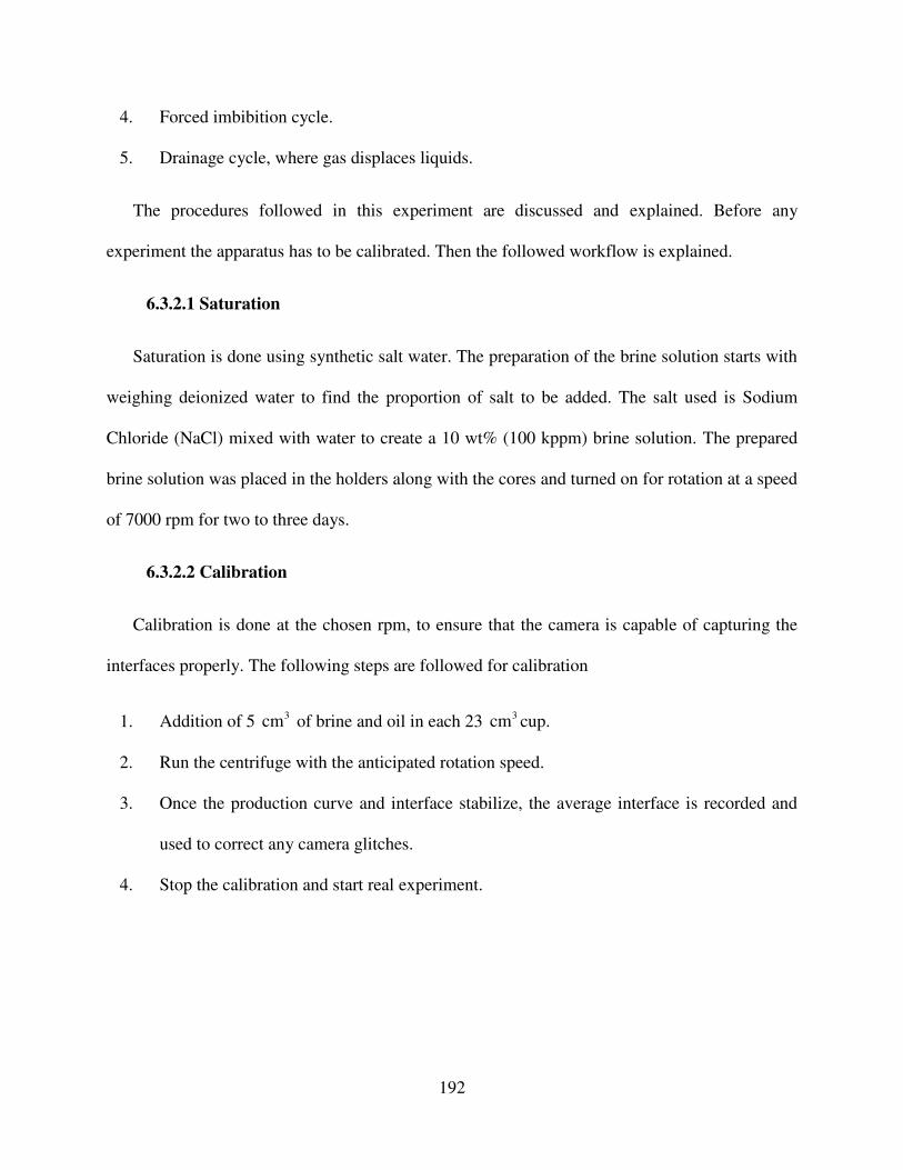
192
4. Forced imbibition cycle.
5. Drainage cycle, where gas displaces liquids.
The procedures followed in this experiment are discussed and explained. Before any
experiment the apparatus has to be calibrated. Then the followed workflow is explained.
6.3.2.1 Saturation
Saturation is done using synthetic salt water. The preparation of the brine solution starts with
weighing deionized water to find the proportion of salt to be added. The salt used is Sodium
Chloride (NaCl) mixed with water to create a 10 wt% (100 kppm) brine solution. The prepared
brine solution was placed in the holders along with the cores and turned on for rotation at a speed
of 7000 rpm for two to three days.
6.3.2.2 Calibration
Calibration is done at the chosen rpm, to ensure that the camera is capable of capturing the
interfaces properly. The following steps are followed for calibration
1. Addition of 5 3cm of brine and oil in each 23
3cm cup.
2. Run the centrifuge with the anticipated rotation speed.
3. Once the production curve and interface stabilize, the average interface is recorded and
used to correct any camera glitches.
4. Stop the calibration and start real experiment.
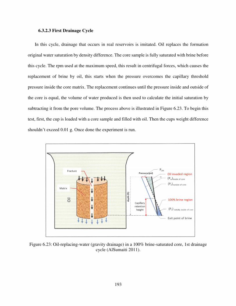
193
6.3.2.3 First Drainage Cycle
In this cycle, drainage that occurs in real reservoirs is imitated. Oil replaces the formation
original water saturation by density difference. The core sample is fully saturated with brine before
this cycle. The rpm used at the maximum speed, this result in centrifugal forces, which causes the
replacement of brine by oil, this starts when the pressure overcomes the capillary threshold
pressure inside the core matrix. The replacement continues until the pressure inside and outside of
the core is equal, the volume of water produced is then used to calculate the initial saturation by
subtracting it from the pore volume. The process above is illustrated in Figure 6.23. To begin this
test, first, the cup is loaded with a core sample and filled with oil. Then the cups weight difference
shouldn’t exceed 0.01 g. Once done the experiment is run.
Figure 6.23: Oil-replacing-water (gravity drainage) in a 100% brine-saturated core, 1st drainage
cycle (AlSumaiti 2011).
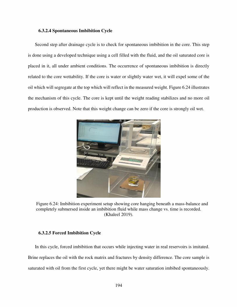
194
6.3.2.4 Spontaneous Imbibition Cycle
Second step after drainage cycle is to check for spontaneous imbibition in the core. This step
is done using a developed technique using a cell filled with the fluid, and the oil saturated core is
placed in it, all under ambient conditions. The occurrence of spontaneous imbibition is directly
related to the core wettability. If the core is water or slightly water wet, it will expel some of the
oil which will segregate at the top which will reflect in the measured weight. Figure 6.24 illustrates
the mechanism of this cycle. The core is kept until the weight reading stabilizes and no more oil
production is observed. Note that this weight change can be zero if the core is strongly oil wet.
Figure 6.24: Imbibition experiment setup showing core hanging beneath a mass-balance and
completely submersed inside an imbibition fluid while mass change vs. time is recorded.
(Khaleel 2019).
6.3.2.5 Forced Imbibition Cycle
In this cycle, forced imbibition that occurs while injecting water in real reservoirs is imitated.
Brine replaces the oil with the rock matrix and fractures by density difference. The core sample is
saturated with oil from the first cycle, yet there might be water saturation imbibed spontaneously.
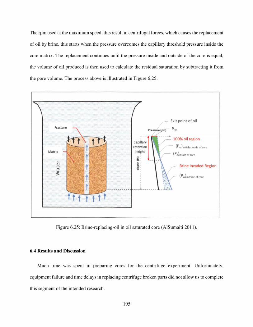
195
The rpm used at the maximum speed, this result in centrifugal forces, which causes the replacement
of oil by brine, this starts when the pressure overcomes the capillary threshold pressure inside the
core matrix. The replacement continues until the pressure inside and outside of the core is equal,
the volume of oil produced is then used to calculate the residual saturation by subtracting it from
the pore volume. The process above is illustrated in Figure 6.25.
Figure 6.25: Brine-replacing-oil in oil saturated core (AlSumaiti 2011).
6.4 Results and Discussion
Much time was spent in preparing cores for the centrifuge experiment. Unfortunately,
equipment failure and time delays in replacing centrifuge broken parts did not allow us to complete
this segment of the intended research.
196
CHAPTER 7
CONCLUSIONS, RECOMMENDATIONS AND FUTURE WORK
7.1 Conclusions
The main effort in this thesis is focused on finding a reliable method to obtain reservoir
permeability under reservoir conditions for use in multi-phase and multi-component numerical
models. The first and second conclusions pertain this issue:
1. The use of conventional pressure transient analysis (PTA), rate transient analysis (RTA), and
Nolte G-function technique to analyze several field and experimental data proves that the
pressure transient analysis and rate transient analysis, both are reliable and easier to use
compared with Nolte’s G-function. Nonetheless, the calculated permeability from three
methods yield similar results. However, PTA and RTA do not require the use of
geomechanical properties while the G-function requires Young’s modulus and Poisson's ratio.
2. Applying PTA and G-function to the experimental data obtained by Frash (2014) to calculate
permeability, and comparing with core measured permeability, we obtained excellent
agreement.
3. The two transient analysis require reliable data especially in unconventional reservoirs,
because the injectant fluid is basically water (Newtonian fluid). As the conventional pressure
transient analysis and rate transient analysis assumes Newtonian fluids.
4. Wellbore and fracture storage needs to be included in models to better reflect the pressure
decline.
5. Leakoff coeffecient calculation depends on the difference between the injectant fluid and
reservoir resident fluids. If the injected fluid has similar viscosity and compressibility as the
197
reservoir resident fluid it is called reservoir controlled fluid case. If the injected fluid has
higher viscosity than the reservoir resident fluid it is called viscosity controlled case. Each
case uses a different equation for permeability calculation.
6. I investigated the effect of fluid invasion from hydraulic fracture to the formation during
reservoir stimulation, in order to determine the depth of penetration of fluid and cooling effect
and the effect of rock deformation (fracture expansion) on the state of stress of the formation.
I discovered that the depth of penetration of the water front is almost 4 ft and the cooled front
is only 0.2 ft.
7. The CMG compositional model is used to match and forecast the field performance. The
permeability calculated using the transient techniques, provided reliable permeability which
adds to validating the technique reliability.
8. I conducted core experiments to measure the permeability and width of the fracture at the
‘perceived’ closure pressure. At this fracture closure, the width was between 10 and 20
microns. The permeability of the core in the presence of the fracture was two orders of
magnitude higher than the permeability of the core without fracture. A major conclusion of
this experiment is that fracture never closes completely.
7.2 Recommendations and Future Work
The recommendations after this research:
1. I recommend that a full geomechanics model for fracture propagation and closure to be built
on this, which is an ongoing effort at the Colorado School of Mines.
2. The above discussed techniques were also applied on a field example by ADNOC, however
the results were noisy and was hard to analyze. The techniques require quality DFIT data to

198
use for permeability calculation. ADNOC needs to have reliable DFIT results, to get a more
reliable analysis.
3. Perform high speed centrifuge experiment on Diyab cores to get reliable capillary pressure and
relative permeability curve for better understanding of saturation endpoints and residual
saturation. It can be used as an input in numerical model.
4. Perform core flood experiment on Diyab cores using different fluids and study the improved
oil recovery.
199
REFERENCES
Abé, H., Mura, T. and Keer, L. 1976. Growth-Rate of a Penny-Shaped Crack in Hydraulic
Fracturing Of Rocks. J. Geophys. Res. 81 (29), pp. 5335–5340.
Alsharhan A. and Kendall C. 1991. Cretaceous Chronostratigraphy, Unconformities and Eustatic
Sea Level Changes in the Sediments of Abu Dhabi, United Arab Emirates. Cretaceous
Research. 12, pp. 379-401.
Alsharhan, A., Strohmenger, C. and Al-Mansoori, A. 2014. Mesozoic Petroleum Systems of Abu
Dhabi, United Arab Emirates. In Petroleum Systems of the Tethyan Region. pp. 679-711.
Chapter 18, ed. L. Marlow, C. Kendall and L. Yose. The American Association of
Petroleum Geologists. DOI: 10.1036/13431869M106483.
AlSumaiti A. 2011. Numerical and Experimental Modeling of Double Displacement Oil Recovery
in Fractured Carbonate Reservoirs. PhD thesis, Petroleum Engineering Department,
Colorado School of Mines.
Al-Suwaidi, AS., Taher, A.K., Alsharhan, A. and Salah, M. 2000. Stratigraphy and Geo-chemistry
of Upper Jurassic Diyab Formation, Abu Dhabi, UAE. Middle East models of
Jurassic/Cretaceous Carbonate Systems. SEPM Special Publication 69, 249-271.
Asala, H., Ahmadi, M. and Taleghani, A. 2016. Why Re-Fracturing Works and Under What
Conditions. Paper presented at the SPE Annual Technical Conference and Exhibition, 26-
28 September, Dubai, UAE. SPE- 181516 -MS. https://doi.org/10.2118/181516-MS.
ASTM International. 2005. Standard Test Method for Laboratory Determination of Pulse
Velocities and Ultrasonic Elastic Constants of Rock. West Conshohocken: IHS.
Barree, R., Barree, V. and Craig, D. 2009. Holistic Fracture Diagnostics: Consistent Interpretation
of Prefrac Injection Tests Using Multiple Analysis Methods. SPE Prod and Oper 24 (3):
396-406. http:// dx.doi.org/10.2118/107877-PA.
Barree, R., Gilbert, J. and Miskimins, J. 2015. Diagnostic Fracture Injection Tests: Common
Mistakes, Misfires, and Misdiagnoses. SPE Production and Operations 30 (2): 1-15. SPE-
169539-PA. https://doi.org/10.2118/169539-PA.
Biot, M. 1941. “General theory of three-dimensional consolidation.” Journal of Applied Physics, 12, 155–164.
Burger, J., Sourieau, P. and Combarnous, M. 1985. Thermal Methods of Oil Recovery. Houston,
Texas: Gulf Publishing Company.
200
Charoenwongsa, S. 2012. Numerical Simulation of the 3-D Hydraulic Fracturing Process, Cleanup
and Relevant Physics. PhD thesis, Petroleum Engineering Department, Colorado School
of Mines.
Cho, Y. 2017. Experimental Measurement and Numerical Modeling of Multiphase Flow in
Middle Bakken. PhD thesis, Petroleum Engineering Department, Colorado School of
Mines.
Cramer, D. and Nguyen, D. 2013. Diagnostic Fracture Injection Testing Tactics in Unconventional
Reservoirs. Paper presented at the SPE Hydraulic Fracturing Technology Conference, The
Woodlands, Texas, 4-6 February. SPE-163863-MS. http://dx.doi.org/102118/ 163863-MS.
Coats, K. 1980. An Equation of State Compositional Model. Soc. Petrol. Eng. J. 20, 363-376.
https://doi.org/10.2118/8284-PA.
Detournay, E., Cheng, A., McLennan, J., 1990. A Poroelastic PKN Hydraulic Fracture Model
Based on an Explicit Moving Mesh Algorithm. J. Energy Resour. Technol. 112, 224–230.
https://doi.org/10.1115/1.2905762.
Economides, M. and Nolte, K. 1989. Reservoir Stimulation, second edition. Upper Saddle River,
New Jersey: Prentice Hall.
Eker, E., Uzun, I., Kazemi, H., and Rutledge, J., 2017. Hydraulic Fracture Propagation Modeling
for Well Performance Analysis: Eagle Ford Formation Case Study. Presented at the SPE
Western Regional Meeting, Bakersfield, California, 23-27 April 2017. SPE-186087-MS.
https://doi.org/10.2118/186087-MS.
Eker E. 2018. Numerical Simulation of Poroelasticity and Multiphase Flow in Matrix-Fracture
System: Application to Niobrara Formation, DJ Basin. PhD thesis, Petroleum Engineering
Department, Colorado School of Mines.
Energy Information Administration (EIA). 2015. Technically Recoverable Shale Oil and Shale
Gas Resources: United Arab Emirates.
https://www.eia.gov/analysis/studies/worldshalegas/pdf/UAE_2014.pdf (accessed
January 2019)
Energy Information Administration (EIA). 2016. Hydraulic Fracturing Accounts for About Half
of Current U.S. Crude Oil Production.
https://www.eia.gov/todayinenergy/detail.php?id=25372 (accessed January 2019).
Energy Information Administration (EIA). 2018a. Country Analysis Brief: United Arab Emirates.
https://www.eia.gov/beta/international/analysis.php?iso=ARE (accessed February 2019).
201
Energy Information Administration (EIA). 2018b. Annual Energy Outlook with projection to
2050. https://www.eia.gov/outlooks/aeo/pdf/aeo2019.pdf (accessed December 2018).
Fisher, M., Wright, C., Davidson, B., Goodwin, A., Fielder, E., Buckler, M. and Steinsberger, N.
2002. Integrating fracture mapping technologies to optimize stimulations in the Barnett
shale. Presented at the SPE Annual Technical Conference and Exhibition, San Antonio,
Texas, USA. SPE-77441-MS. https://doi.org/10.2118/77441-MS.
Frash. L. 2014. Laboratory-Scale Study of Hydraulic Fracturing In Heterogeneous Media for
Enhanced Geothermal Systems and General Well Stimulation. PhD thesis, Civil
Engineering Department, Colorado School of Mines.
Ge, J., and Ghassemi, A. 2018. Sensitivity Study on the Poroelastic and Thermoelastic Effects on
the Stress Reversal nearby an Existing Hydraulic Fracture. Paper ARMA 18-0287
presented at 52nd US Rock Mechanics / Geomechanics Symposium held in Seattle,
Washington, USA, 17–20 June 2018.
Geertsma, J. 1957. The Effect of Fluid-Pressure Decline on Volumetric Changes of Porous Rocks.
Trans AIME 210:331–339.
Geertsma, J. 1966. Problems of Rock Mechanics in Petroleum Production Engineering, Proc., First
Cong. Intl. Sot. of Mech., Lisbon I, 585.
Geertsma, J. and de Klerk, F. 1969. A Rapid Method of Predicting Width and Extent of
Hydraulically Induced Fractures. Journal of Petroleum Technology, 21 (12), pp.1-571.
Gidley, J., Holditch, S., Nierode, D. and Veatch, R. 1989. Recent Advances in Hydraulic
Fracturing. SPE Monograph Series. Richardson, Texas, 12, pp 89–90.
Gonzalez, J., Lewis, R., Hemingway, J., Grau, J., Rylander, E. and Schmitt, R. 2013.
Determination of Formation Organic Carbon Content Using New Neutron-Induced
Gamma Ray Spectroscopy Service that Directly Measures Carbon. Presented at the
Unconventional Resources Technology Conference, Denver, Colorado, USA. SPE
168711.
Guo, H., Aziz, N. and Schmidt, L. 1993. Rock Fracture-Toughness Determination by the Brazilian
Test. Eng. Geol., 33: 177-188.
Hassan, T. and Azer, S. 1985. The Occurrence and Origin of Oil in Offshore Abu Dhabi.
Presented at the SPE Fourth Middle East on Technical Conference and Expedition,
Bahrain. SPE-13696-MS. https://doi.org/10.2118/13696-MS.
202
Howard, G. and Fast, C. 1957. Optimum Fluid Characteristics for Fracture Extension. Drilling
and Production Practices, pp. 261-270. American Petroleum Institute, Tulsa, OK.
Irwin, G. 1957. Analysis of Stresses and Strains near The End of a Crack Traversing a Plate. J. of
App Mech 24:361-364.
Irwin, G. and de Wit, R. 1983. A Summary of Fracture Mechanics Concepts. J. test eval. 56-65.
https://doi.org/10.1520/JTE11586J.
ISRM. 1978. Suggested Methods for Determining Tensile Strength of Rock Materials.
International Journal of Rock Mechanics and Mining Sciences, Vol. 15, No. 3, P. 99-103.
Jacob, H. 1989. Classification, Structure, Genesis and Practical Importance of Natural Solid Oil
Bitumen (‘‘migrabitumen’’). International Journal of Coal Geology 11, 65–79.
Kazemi, H., Vestal, C.A., Shank, D.G., 1978. An Efficient Multicomponent Numerical Simulator.
Soc. Petrol. Eng. J. 18, 355-368. https://doi.org/10.2118/6890-PA.
Kazemi, H., Eker, I., Torcuk, M. A. and Kurtoglu, B. 2015. Performance Analysis of
Unconventional Shale Reservoirs. In Fundamentals of Gas Shale Reservoirs, pp. 283-300,
ed. R. Rezaee, Chap 13. Hoboken, New Jersey: John Wiley and Sons.
Khaleel, O. 2017. Selecting an Optimal Surfactant for Use in EOR: An Experimental Study. MSc
Thesis, Petroleum Engineering Department, Colorado School of Mines, Golden, Colorado.
Khaleel, O., Teklu, T., Alameri, W., Abass, H. and Kazemi, H., 2019. Wettability Alteration of
Carbonate Reservoir Cores—Laboratory Evaluation Using Complementary Techniques.
SPE Res Eval and Eng 23 (1): 578–593. SPE-194483-PA. https://doi.org/10.2118/194483-
PA.
Khristianovic, S., and Zheltov, Y. 1955. Formation of vertical fractures by means of highly viscous
fluids. Proc., 4th World Petroleum Congress, Rome, II, 579–586.
Lawn, B. 1983. Physics of Fracture. Journal of the American Ceramic Society. 66(2): 83-91.
Lewis, R., Ingraham, D., Pearcy, M., Williamson, J., Sawyer, W. and Frantz, J. 2004. New
evaluation techniques for gas shale reservoirs. Presented in Reservoir Symposium (pp. 1-
11).
Li, D., and Wong, L. 2013. The Brazilian Disc Test For Rock Mechanics Applications: Review
And New Insights. Rock Mech. Rock. Eng. 46, 269–287. https://doi.org/10.1007/s00603-
012-0257-7.
203
Loutfi, G., and El Bishlawy, S. 1986. Habitat of hydrocarbon in Abu Dhabi, UAE. Presented at
the Symposium on Hydrocarbon Potential of Intense Thrust Zones, Abu Dhabi,
December 1986, p. 63-124.
Mcphee, C., Reed, J. and Zubizarreta, I. 2015, Routine Core Analysis: Developments in Petroleum
Science, v. 64, p. 181–268, doi:10.1016/B978-0-444-63533-4.00005-6.
Michael, A., Habibi A., and Lloyds R. 2018. Three Stress-Shadowing Mitigation Techniques for
Hydraulic Fracturing Operations: An Overview. The way ahead, SPE.
https://pubs.spe.org/en/twa/twa-article-detail/?art=4671 (accessed March 2019)
Miskimins J., 2018. PEGN522: Reservoir stimulation lecture notes. Fall 2018. Colorado School
of Mines.
Nolte, K.G. 1979. Determination of Fracture Parameters from Fracturing Pressure Decline.
Presented at the SPE 54th Annual Technical Conference and Exhibition, Las Vegas, Sept.
23-26. SPE-8341-MS. https://doi.org/10.2118/8341-MS
Nordgren, R. 1972. Propagation of vertical hydraulic fractures. J. Pet. Technol., 253, 306–314.
OPEC. 2018. Annual Statistical Bulletin.
https://www.opec.org/opec_web/en/publications/202.htm (accessed March 2019)
Palisch, T., Vincent, M. and Handren, P. 2008. Slickwater Fracturing: Food For Thought.
Presented at the SPE Annual Technical Conference and Exhibition in Denver, Colorado.
SPE-115766-MS. https://doi.org/10.2118/115766-MS.
Perkins, T. and Kern, L. 1961. Widths of hydraulic fractures. Journal of Petroleum Technology,
13 (09), pp.937-949.
Perkins, T. and Gonzalez, J. 1985. The Effect of Thermoelastic Stresses on Injection Well
Fracturing. SPE J. 25 (1): 78-88. SPE-11332-PA. https://doi.org/10.2118/11332-PA.
Pollard, D. and Segall, P. 1987. Theoretical Displacements and Stresses near Fractures Rock: With
Applications to Faults, Joints, Veins, Dikes, and Solution Surfaces. In Atkinson, B.K., ed.,
Fracture Mechanics of Rocks, New York: Academic Press.
Salah, M., Orr, D., Meguid, A., Crane, B. and Squires, S. 2016. Multistage Horizontal Hydraulic
Fracture Optimization through an Integrated Design and Workflow in Apollonia Tight
Chalk, Egypt from the Laboratory to the Field. SPE-183068-MS.
https://doi.org/10.2118/183068-MS.
204
Smith, M. and Montgomery, C. 2015. Hydraulic Fracturing Boca Raton, FL. CRC Press, Taylor
& Francis Group.
Tutuncu, A. 2015. PEGN590: Reservoir Geomechanics lecture notes. Fall 2015. Colorado School
of Mines.
Uzun, O. 2018. Determining Osmotic Pressure in Niobrara Chalk and Codell Sandstone Using
High-Speed Centrifuge. MSc Thesis, Petroleum Engineering Department, Colorado
School of Mines, Golden, Colorado.
Rice, J., and Cleary, M. 1976. Basic Stress Diffusion Solutions for Fluid-Saturated Elastic Porous
Media with Compressible Constituents: Reviews of Geophysics and Space Physics, v. 14,
no. 2, p. 227–241.
Warpinski, N. Mayerhofer, M., Vincent, M., Cipolla, C. and Lolon, E. 2009. Stimulating
Unconventional Reservoirs: Maximizing Network Growth While Optimizing Fracture
Conductivity. Can Pet Technol 48 (10): 39-51. SPE-114173-PA.
https://doi.org/10.2118/114173-PA.
Warren. J. and Root. P. 1963. The Behavior of Naturally Fractured Reservoirs. SPE J. 3 (3): 245-
256. SPE-426-PA. https://doi.org/10.2118/426-PA.
Watts, J. 1986. A compositional formulation of the pressure and saturation equations. SPE
Reservoir Engineering J. 1(03):243–252. http://dx.doi.org/10.2118/12244-PA.
White, D. 2017. Chesapeake Energy Looks Like A Screaming Buy. Seeking Alpha.
https://seekingalpha.com/article/4084236-chesapeake-energy-looks-like-screaming-buy.
(acsessed January 2019).
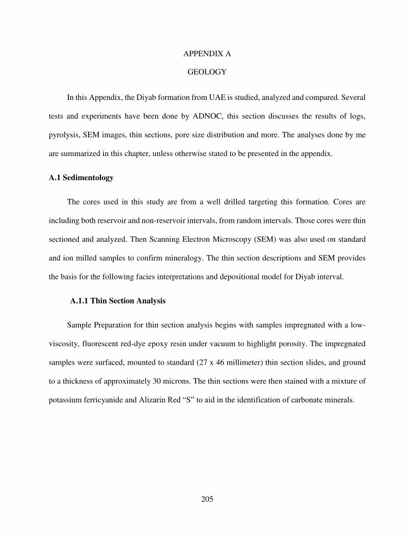
205
APPENDIX A
A. GEOLOGY
In this Appendix, the Diyab formation from UAE is studied, analyzed and compared. Several
tests and experiments have been done by ADNOC, this section discusses the results of logs,
pyrolysis, SEM images, thin sections, pore size distribution and more. The analyses done by me
are summarized in this chapter, unless otherwise stated to be presented in the appendix.
A.1 Sedimentology
The cores used in this study are from a well drilled targeting this formation. Cores are
including both reservoir and non-reservoir intervals, from random intervals. Those cores were thin
sectioned and analyzed. Then Scanning Electron Microscopy (SEM) was also used on standard
and ion milled samples to confirm mineralogy. The thin section descriptions and SEM provides
the basis for the following facies interpretations and depositional model for Diyab interval.
A.1.1 Thin Section Analysis
Sample Preparation for thin section analysis begins with samples impregnated with a low-
viscosity, fluorescent red-dye epoxy resin under vacuum to highlight porosity. The impregnated
samples were surfaced, mounted to standard (27 x 46 millimeter) thin section slides, and ground
to a thickness of approximately 30 microns. The thin sections were then stained with a mixture of
potassium ferricyanide and Alizarin Red “S” to aid in the identification of carbonate minerals.

206
Sample imaging, is done using a Nikon polarizing microscope, the prepared thin sections
were examined and digitally imaged under transmitted plane-polarized, transmitted cross-
polarized, and/or reflected UV light. The microscope is equipped with a spot insight digital camera,
reflected light source, and various UV filters. All thin section images were taken in plane-polarized
light unless otherwise noted.
Consistent intervals cores were chosen for this analysis. Figure A.1 presents two images
(image A and B) of the same sample referred to in this thesis as sample A. The arrows in Figure
A.1 images are explained in Table A.1.
The thin section interpretation summary is presented in Table A.1, which include
matrix/cement composition, texture, clay minerals, allochemical and detrital grains, fossils,
organic material, and diagenetic material. Figure A.2 presents the X-ray diffraction results of
sample A in weight percentage.
Figure A.3 presents two images (image A and B) of the same sample referred to in this thesis
as sample B. The arrows in Figure A.3 images are explained in Table A.2. The thin section
interpretation summary is presented in Table A.2, which include matrix/cement composition,
texture, clay minerals, allochemical and detrital grains, fossils, organic material, and diagenetic
material. Figure A.4 presents the X-ray diffraction results of sample B in weight percentage.
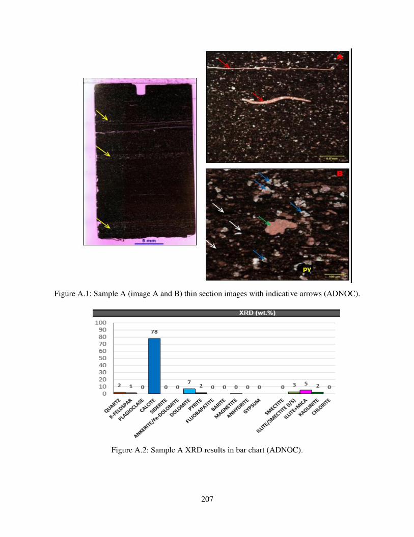
207
Figure A.1: Sample A (image A and B) thin section images with indicative arrows (ADNOC).
Figure A.2: Sample A XRD results in bar chart (ADNOC).
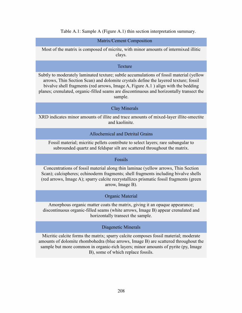
208
Table A.1: Sample A (Figure A.1) thin section interpretation summary.
Matrix/Cement Composition
Most of the matrix is composed of micrite, with minor amounts of intermixed illitic clays.
Texture
Subtly to moderately laminated texture; subtle accumulations of fossil material (yellow arrows, Thin Section Scan) and dolomite crystals define the layered texture; fossil bivalve shell fragments (red arrows, Image A, Figure A.1 ) align with the bedding
planes; crenulated, organic-filled seams are discontinuous and horizontally transect the sample.
Clay Minerals
XRD indicates minor amounts of illite and trace amounts of mixed-layer illite-smectite and kaolinite.
Allochemical and Detrital Grains
Fossil material; micritic pellets contribute to select layers; rare subangular to subrounded quartz and feldspar silt are scattered throughout the matrix.
Fossils
Concentrations of fossil material along thin laminae (yellow arrows, Thin Section Scan); calcispheres; echinoderm fragments; shell fragments including bivalve shells (red arrows, Image A); sparry calcite recrystallizes prismatic fossil fragments (green
arrow, Image B).
Organic Material
Amorphous organic matter coats the matrix, giving it an opaque appearance; discontinuous organic-filled seams (white arrows, Image B) appear crenulated and
horizontally transect the sample.
Diagenetic Minerals
Micritic calcite forms the matrix; sparry calcite composes fossil material; moderate amounts of dolomite rhombohedra (blue arrows, Image B) are scattered throughout the sample but more common in organic-rich layers; minor amounts of pyrite (py, Image
B), some of which replace fossils.
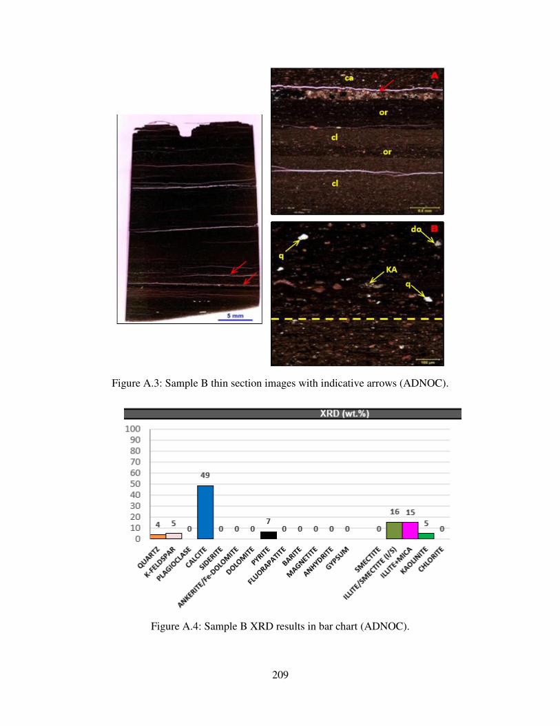
209
Figure A.3: Sample B thin section images with indicative arrows (ADNOC).
Figure A.4: Sample B XRD results in bar chart (ADNOC).
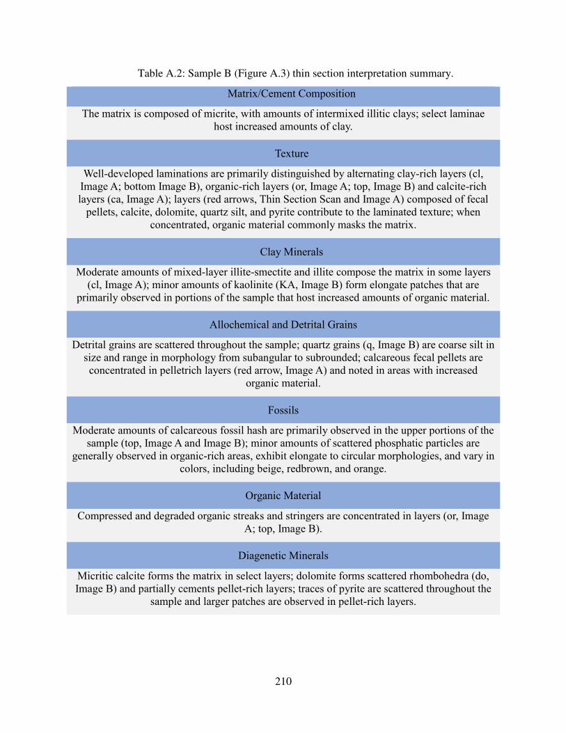
210
Table A.2: Sample B (Figure A.3) thin section interpretation summary.
Matrix/Cement Composition
The matrix is composed of micrite, with amounts of intermixed illitic clays; select laminae host increased amounts of clay.
Texture
Well-developed laminations are primarily distinguished by alternating clay-rich layers (cl, Image A; bottom Image B), organic-rich layers (or, Image A; top, Image B) and calcite-rich layers (ca, Image A); layers (red arrows, Thin Section Scan and Image A) composed of fecal
pellets, calcite, dolomite, quartz silt, and pyrite contribute to the laminated texture; when concentrated, organic material commonly masks the matrix.
Clay Minerals
Moderate amounts of mixed-layer illite-smectite and illite compose the matrix in some layers (cl, Image A); minor amounts of kaolinite (KA, Image B) form elongate patches that are
primarily observed in portions of the sample that host increased amounts of organic material.
Allochemical and Detrital Grains
Detrital grains are scattered throughout the sample; quartz grains (q, Image B) are coarse silt in size and range in morphology from subangular to subrounded; calcareous fecal pellets are concentrated in pelletrich layers (red arrow, Image A) and noted in areas with increased
organic material.
Fossils
Moderate amounts of calcareous fossil hash are primarily observed in the upper portions of the sample (top, Image A and Image B); minor amounts of scattered phosphatic particles are
generally observed in organic-rich areas, exhibit elongate to circular morphologies, and vary in colors, including beige, redbrown, and orange.
Organic Material
Compressed and degraded organic streaks and stringers are concentrated in layers (or, Image A; top, Image B).
Diagenetic Minerals
Micritic calcite forms the matrix in select layers; dolomite forms scattered rhombohedra (do, Image B) and partially cements pellet-rich layers; traces of pyrite are scattered throughout the
sample and larger patches are observed in pellet-rich layers.
211
A.1.2 Scanning Electron Microscopy
SEM was used for two different samples; standard sample and ion-milled sample. The
Analytical procedure for detailed SEM analysis of a standard sample starts with the preparation
then imaging. The procedure is that a small, freshly broken portion of each sample was mounted
on a standard SEM mount and sputter-coated with platinum/palladium for approximately 60
seconds. Then the samples were analyzed and imaged in an FEI Quanta 650 FEG field emission
scanning electron microscope equipped with an EDAX energy dispersive X-ray spectrometer
(EDX). A range of image magnifications documents the morphology of the rock fabric and the
pore system. Organic material was identified wherever possible. All SEM images were taken in
secondary electron mode unless otherwise noted.
While for the ion-milled, a small, freshly broken portion of each sample was shaped into a
rectangular prism and mounted to a molybdenum mount. Then the sample was placed in JEOL
Cross-Section Polisher for approximately 10 hours to obtain a polished surface of approximately
1000x500 microns in size. The samples were analyzed and imaged in a JEOL JSM 7500F cold
cathode field emission scanning electron microscope equipped with an EDAX energy dispersive
X-ray spectrometer (EDX). Images document the rock fabric, focusing on the pore system and the
morphology of organic matter. All images were taken in backscattered electron mode.
Figure A.5 shows four standard SEM images (images A, B, C and D) of sample A, which is
analyzed and interpreted in Table A.3, which include matrix/cement composition and micro-
texture, clay minerals, allochemical and detrital grains, fossils, organic material, diagenetic
material, and pore structure. Figure A.6 shows four ion–milled SEM images (images A, B, C and
D) of sample A ion-milled sample SEM image, which is analyzed and interpreted in Table A.4.
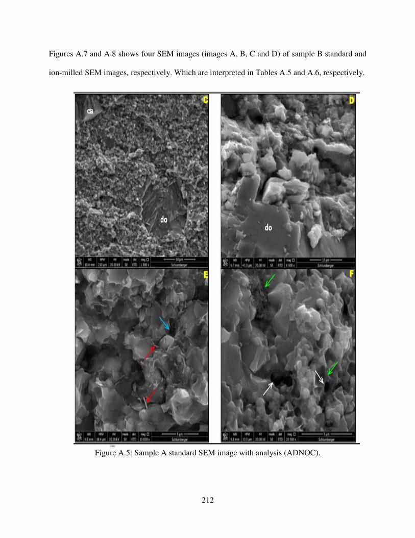
212
Figures A.7 and A.8 shows four SEM images (images A, B, C and D) of sample B standard and
ion-milled SEM images, respectively. Which are interpreted in Tables A.5 and A.6, respectively.
Figure A.5: Sample A standard SEM image with analysis (ADNOC).
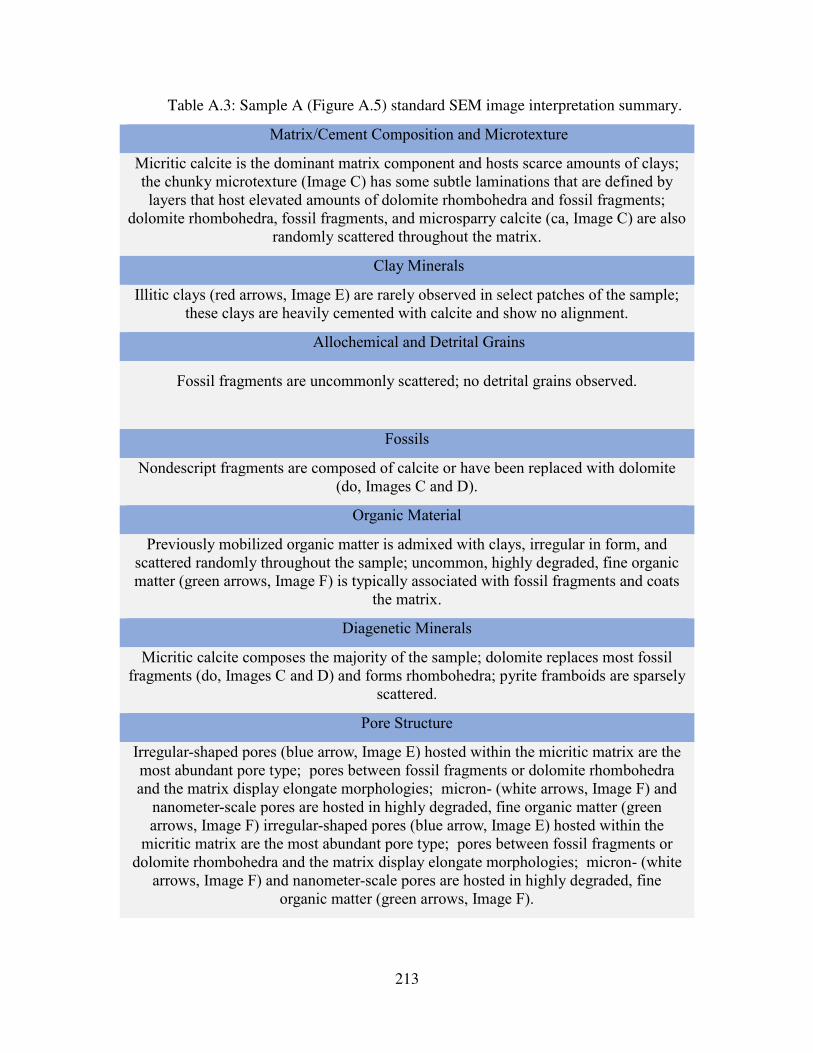
213
Table A.3: Sample A (Figure A.5) standard SEM image interpretation summary.
Matrix/Cement Composition and Microtexture
Micritic calcite is the dominant matrix component and hosts scarce amounts of clays; the chunky microtexture (Image C) has some subtle laminations that are defined by layers that host elevated amounts of dolomite rhombohedra and fossil fragments;
dolomite rhombohedra, fossil fragments, and microsparry calcite (ca, Image C) are also randomly scattered throughout the matrix.
Clay Minerals
Illitic clays (red arrows, Image E) are rarely observed in select patches of the sample; these clays are heavily cemented with calcite and show no alignment.
Allochemical and Detrital Grains
Fossil fragments are uncommonly scattered; no detrital grains observed.
Fossils
Nondescript fragments are composed of calcite or have been replaced with dolomite (do, Images C and D).
Organic Material
Previously mobilized organic matter is admixed with clays, irregular in form, and scattered randomly throughout the sample; uncommon, highly degraded, fine organic matter (green arrows, Image F) is typically associated with fossil fragments and coats
the matrix.
Diagenetic Minerals
Micritic calcite composes the majority of the sample; dolomite replaces most fossil fragments (do, Images C and D) and forms rhombohedra; pyrite framboids are sparsely
scattered.
Pore Structure
Irregular-shaped pores (blue arrow, Image E) hosted within the micritic matrix are the most abundant pore type; pores between fossil fragments or dolomite rhombohedra and the matrix display elongate morphologies; micron- (white arrows, Image F) and
nanometer-scale pores are hosted in highly degraded, fine organic matter (green arrows, Image F) irregular-shaped pores (blue arrow, Image E) hosted within the
micritic matrix are the most abundant pore type; pores between fossil fragments or dolomite rhombohedra and the matrix display elongate morphologies; micron- (white
arrows, Image F) and nanometer-scale pores are hosted in highly degraded, fine organic matter (green arrows, Image F).

214
Figure A.6: Sample A ion-milled SEM image with analysis (ADNOC).
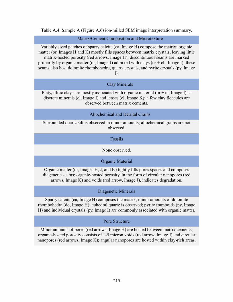
215
Table A.4: Sample A (Figure A.6) ion-milled SEM image interpretation summary.
Matrix/Cement Composition and Microtexture
Variably sized patches of sparry calcite (ca, Image H) compose the matrix; organic matter (or, Images H and K) mostly fills spaces between matrix crystals, leaving little
matrix-hosted porosity (red arrows, Image H); discontinuous seams are marked primarily by organic matter (or, Image J) admixed with clays (or + cl , Image I); these seams also host dolomite rhombohedra, quartz crystals, and pyrite crystals (py, Image
I).
Clay Minerals
Platy, illitic clays are mostly associated with organic material (or + cl, Image I) as discrete minerals (cl, Image I) and lenses (cl, Image K); a few clay floccules are
observed between matrix cements.
Allochemical and Detrital Grains
Surrounded quartz silt is observed in minor amounts; allochemical grains are not observed.
Fossils
None observed.
Organic Material
Organic matter (or, Images H, J, and K) tightly fills pores spaces and composes diagenetic seams; organic-hosted porosity, in the form of circular nanopores (red
arrows, Image K) and voids (red arrow, Image J), indicates degradation.
Diagenetic Minerals
Sparry calcite (ca, Image H) composes the matrix; minor amounts of dolomite rhombohedra (do, Image H); euhedral quartz is observed; pyrite framboids (py, Image H) and individual crystals (py, Image I) are commonly associated with organic matter.
Pore Structure
Minor amounts of pores (red arrows, Image H) are hosted between matrix cements; organic-hosted porosity consists of 1-5 micron voids (red arrow, Image J) and circular nanopores (red arrows, Image K); angular nanopores are hosted within clay-rich areas.

216
Figure A.7: Sample B standard SEM image with analysis (ADNOC).

217
Table A.5: Sample B (Figure A.7) standard SEM image interpretation summary.
Matrix/Cement Composition and Microtexture
Dominant micritic calcite is intermixed with a minor amount of aligned clays, lending to a moderately well-laminated microtexture (Image C); randomly distributed calcite crystals, fossil fragments (ff, Image C), and potential pellets (pe, Image C) disrupt the
clay layers; most fossils and elongate organic matter align to bedding planes;
Clay Minerals
Clays align to bedding planes (center, Image E); illite and mixed-layer illite-smectite are most common; kaolinite (KA, Image D) is typically associated with organic
material.
Allochemical and Detrital Grains
Fossils are both scattered and concentrated in poorly defined layers; no detrital grains observed.
Fossils
Calcareous bivalve shells, nondescript fossil fragments (ff, Image C), and pellets (pe, Image C) typically align with bedding.
Organic Material
Previously mobilized organic matter is commonly observed; this matter is typically intermixed with clays, is associated with fine matter, and has irregular or
discontinuous, elongate morphologies; fine organic matter (or, Image F) commonly coats pore throats; sparsely observed organic particles (op, Image D) are moderately
degraded;
Diagenetic Minerals
Calcareous micrite and microsparite overprint the clay matrix; pyrite framboids (py, Images D and E) are commonly observed throughout the matrix and in association with organic material; pyrite crystals are uncommonly associated with bivalve fragments;
sparse quartz crystals (q, Image E) are observed.
Pore Structure
Shaped pores hosted within micrite are the dominant pore type; elongate matrix pores (blue arrows, Image E) are common in clay-rich areas; elongate, interparticle pores
(white arrows, Images E and F) are commonly observed between fossils and the matrix, or between crystals of pyrite or calcite; nanometer scale porosity is hosted
within fine organic matter (or, Image F) ovate to irregular-shaped pores hosted within micrite are the dominant pore type;
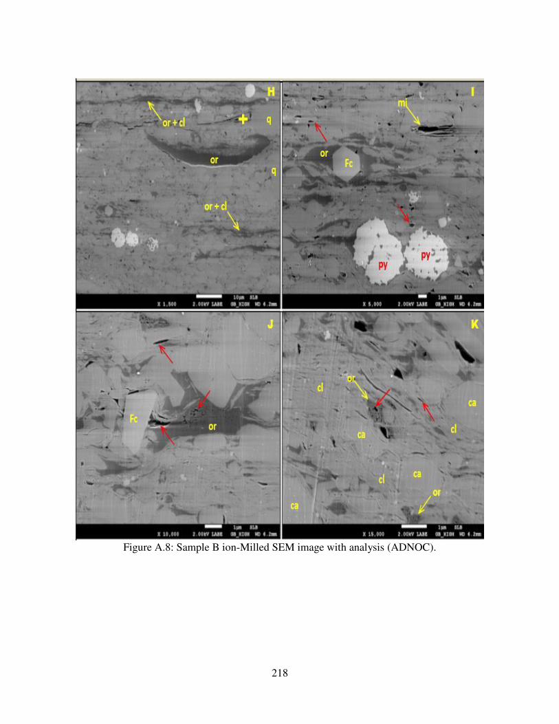
218
Figure A.8: Sample B ion-Milled SEM image with analysis (ADNOC).
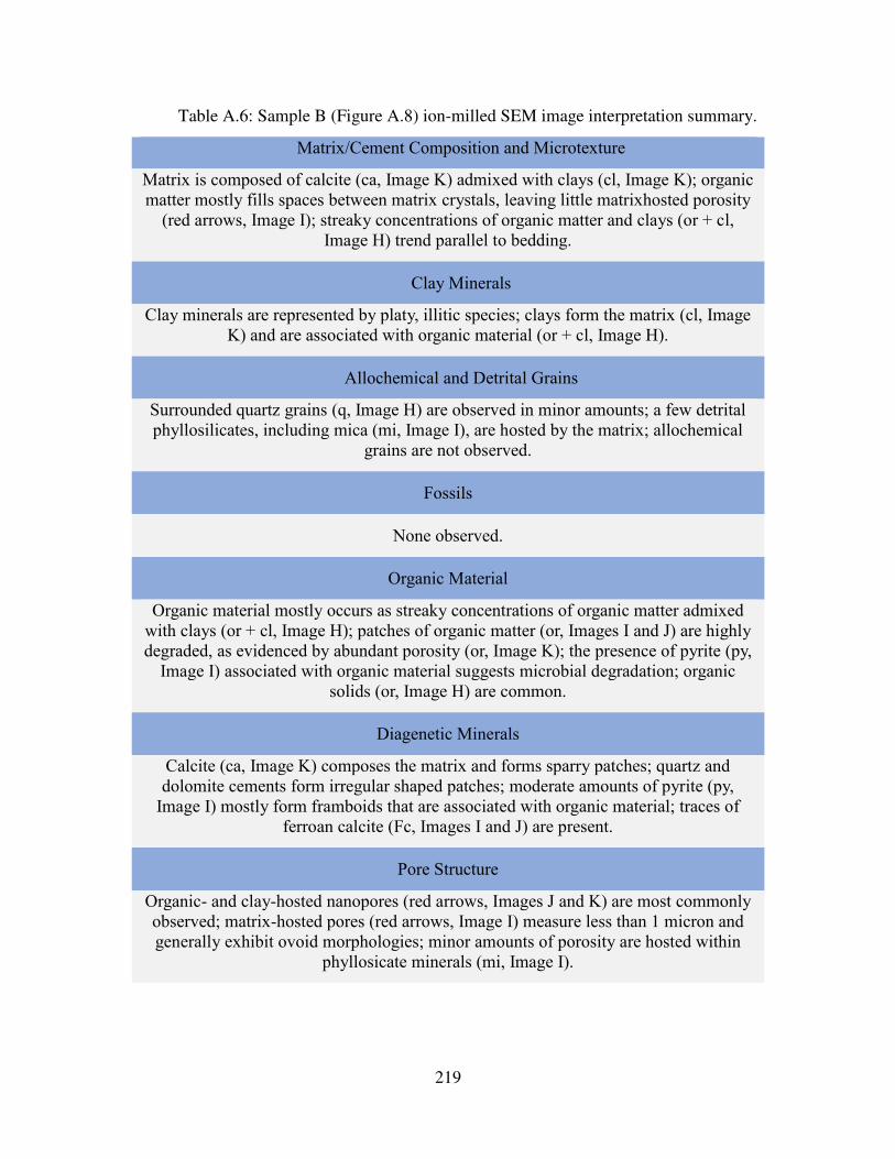
219
Table A.6: Sample B (Figure A.8) ion-milled SEM image interpretation summary.
Matrix/Cement Composition and Microtexture
Matrix is composed of calcite (ca, Image K) admixed with clays (cl, Image K); organic matter mostly fills spaces between matrix crystals, leaving little matrixhosted porosity
(red arrows, Image I); streaky concentrations of organic matter and clays (or + cl, Image H) trend parallel to bedding.
Clay Minerals
Clay minerals are represented by platy, illitic species; clays form the matrix (cl, Image K) and are associated with organic material (or + cl, Image H).
Allochemical and Detrital Grains
Surrounded quartz grains (q, Image H) are observed in minor amounts; a few detrital phyllosilicates, including mica (mi, Image I), are hosted by the matrix; allochemical
grains are not observed.
Fossils
None observed.
Organic Material
Organic material mostly occurs as streaky concentrations of organic matter admixed with clays (or + cl, Image H); patches of organic matter (or, Images I and J) are highly degraded, as evidenced by abundant porosity (or, Image K); the presence of pyrite (py,
Image I) associated with organic material suggests microbial degradation; organic solids (or, Image H) are common.
Diagenetic Minerals
Calcite (ca, Image K) composes the matrix and forms sparry patches; quartz and dolomite cements form irregular shaped patches; moderate amounts of pyrite (py,
Image I) mostly form framboids that are associated with organic material; traces of ferroan calcite (Fc, Images I and J) are present.
Pore Structure
Organic- and clay-hosted nanopores (red arrows, Images J and K) are most commonly observed; matrix-hosted pores (red arrows, Image I) measure less than 1 micron and generally exhibit ovoid morphologies; minor amounts of porosity are hosted within
phyllosicate minerals (mi, Image I).
220
APPENDIX B
B. WELL LOGS
B.1 Integration of Geology and Well Logs
This geology section integrates wireline log data, Formation MicroImager (FMI),
SonicScanner, Lithoscanner and triple-combo logs with Geoflex (cuttings) and mud log data to
characterize the Diyab (Jubaila), Hanifa and Araej Formations. Data quality is impressive and
facilitates a confident interpretation.
In the studied well, it reveals structural dip to be low and mean dip range computed is 0.6 -
1.6 / WSW-W over the entire logged interval. No obvious changes in structural dip magnitude and
azimuth are noted in the logged section indicating the absence of any major structural events.
Diagenesis is manifested in the form of solution seams (including stylolites) on image log.
Natural fractures are observed in the imaged interval. Both resistive (healed) and conductive
(possibly open) fractures are interpreted. The latter category of fractures comprises the majority
observed. Arab D hosts most of the ‘sinusoidal’ (larger) natural fractures. Attributes have been
extracted for Continuous Conductive Fractures (CCF), Discontinuous Conductive Fractures (DCF)
and Enhanced Fractures (EF) – the larger and more continuous fractures which maybe possibly
open. For CCF and DCF a maximum hydraulic aperture of 0.9 mm and maximum fracture porosity
of 0.41 % is noted. For EF, a maximum hydraulic aperture of 0.18 mm and maximum fracture
porosity of 0.15 % is noted.
Insitu stress around the borehole is noted in the FMI in the form of drilling induced fractures
and breakouts. Induced fractures mostly occur in Arab D while breakouts are seen mainly in Diyab.
No evidence of faulting is observed in the imaged interval. An image based visual textural
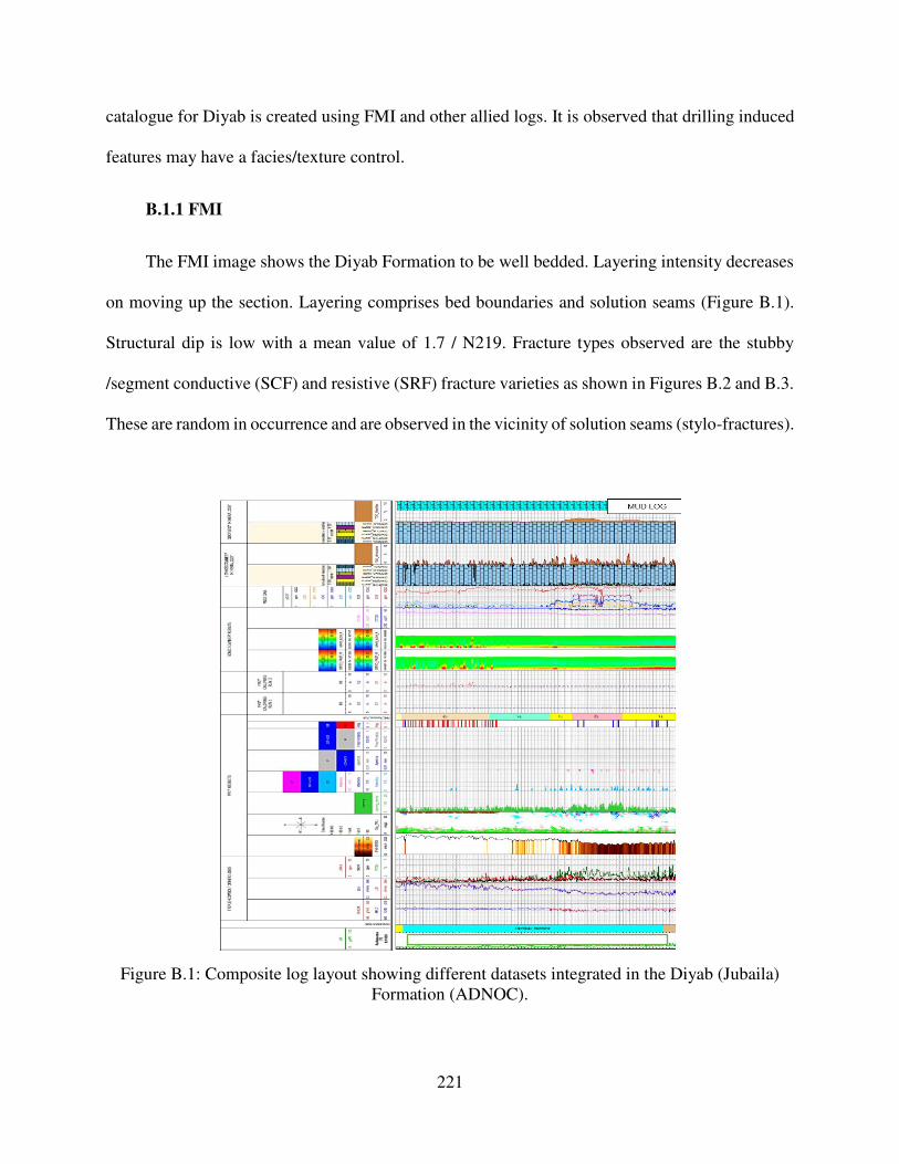
221
catalogue for Diyab is created using FMI and other allied logs. It is observed that drilling induced
features may have a facies/texture control.
B.1.1 FMI
The FMI image shows the Diyab Formation to be well bedded. Layering intensity decreases
on moving up the section. Layering comprises bed boundaries and solution seams (Figure B.1).
Structural dip is low with a mean value of 1.7 / N219. Fracture types observed are the stubby
/segment conductive (SCF) and resistive (SRF) fracture varieties as shown in Figures B.2 and B.3.
These are random in occurrence and are observed in the vicinity of solution seams (stylo-fractures).
Figure B.1: Composite log layout showing different datasets integrated in the Diyab (Jubaila)
Formation (ADNOC).
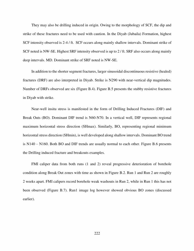
222
They may also be drilling induced in origin. Owing to the morphology of SCF, the dip and
strike of these fractures need to be used with caution. In the Diyab (Jubaila) Formation, highest
SCF intensity observed is 2-4 / ft. SCF occurs along mainly shallow intervals. Dominant strike of
SCF noted is NW-SE. Highest SRF intensity observed is up to 2 / ft. SRF also occurs along mainly
deep intervals. MD. Dominant strike of SRF noted is NW-SE.
In addition to the shorter segment fractures, larger sinusoidal discontinuous resistive (healed)
fractures (DRF) are also interpreted in Diyab. Strike is N290 with near-vertical dip magnitudes.
Number of DRFs observed are six (Figure B.4). Figure B.5 presents the stubby resistive fractures
in Diyab with strike.
Near-well insitu stress is manifested in the form of Drilling Induced Fractures (DIF) and
Break Outs (BO). Dominant DIF trend is N60-N70. In a vertical well, DIF represents regional
maximum horizontal stress direction (SHmax). Similarly, BO, representing regional minimum
horizontal stress direction (SHmin), is well developed along shallow intervals. Dominant BO trend
is N140 – N160. Both BO and DIF trends are usually normal to each other. Figure B.6 presents
the Drilling induced fracture and breakouts examples.
FMI caliper data from both runs (1 and 2) reveal progressive deterioration of borehole
condition along Break Out zones with time as shown in Figure B.2. Run 1 and Run 2 are roughly
2 weeks apart. FMI calipers record borehole weak washouts in Run 2, while in Run 1 this has not
been observed (Figure B.7). Run1 image log however showed obvious BO zones (discussed
earlier).

223
Figure B.2: Integrating FMI -Feature Intensity –OH Logs (GR Spectroscopy) (ADNOC).
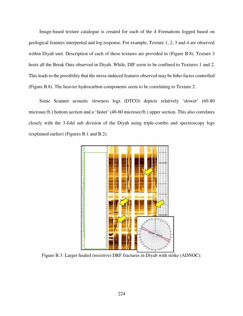
224
Image-based texture catalogue is created for each of the 4 Formations logged based on
geological features interpreted and log response. For example, Texture 1, 2, 3 and 4 are observed
within Diyab unit. Description of each of these textures are provided in (Figure B.8). Texture 3
hosts all the Break Outs observed in Diyab. While, DIF seem to be confined to Textures 1 and 2.
This leads to the possibility that the stress-induced features observed may be litho-facies controlled
(Figure B.8). The heavier hydrocarbon components seem to be correlating to Texture 2.
Sonic Scanner acoustic slowness logs (DTCO) depicts relatively ‘slower’ (60-80
microsec/ft.) bottom section and a ‘faster’ (40-60 microsec/ft.) upper section. This also correlates
closely with the 3-fold sub division of the Diyab using triple-combo and spectroscopy logs
(explained earlier) (Figures B.1 and B.2).
Figure B.3: Larger healed (resistive) DRF fractures in Diyab with strike (ADNOC).
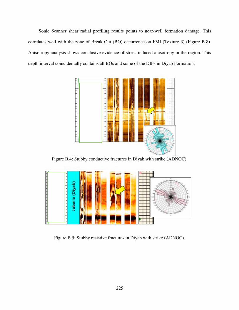
225
Sonic Scanner shear radial profiling results points to near-well formation damage. This
correlates well with the zone of Break Out (BO) occurrence on FMI (Texture 3) (Figure B.8).
Anisotropy analysis shows conclusive evidence of stress induced anisotropy in the region. This
depth interval coincidentally contains all BOs and some of the DIFs in Diyab Formation.
Figure B.4: Stubby conductive fractures in Diyab with strike (ADNOC).
Figure B.5: Stubby resistive fractures in Diyab with strike (ADNOC).
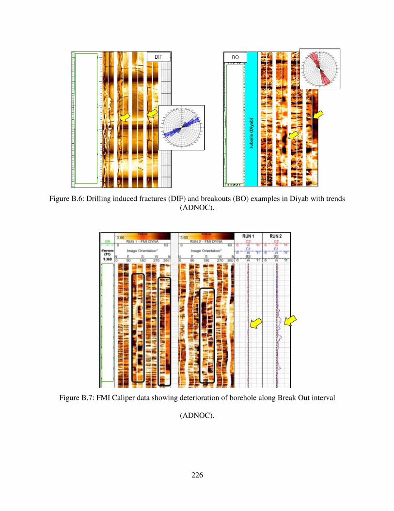
226
Figure B.6: Drilling induced fractures (DIF) and breakouts (BO) examples in Diyab with trends
(ADNOC).
Figure B.7: FMI Caliper data showing deterioration of borehole along Break Out interval
(ADNOC).
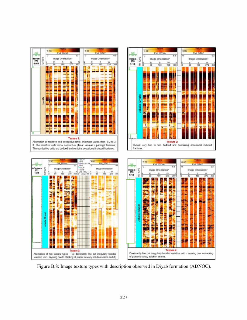
227
Figure B.8: Image texture types with description observed in Diyab formation (ADNOC).

228
B.1.2 Lithoscanner and GEOFLEX Mineralogy Logs
Lithoscanner data is available in Diyab Formation. Normalized mineral average weight
fractions in % from Lithoscanner is as follows (Figure B.9):
Calcite = 95%, Dolomite = 2.1%, Total Clay = 1%, Anhydrite = 0.67%, Quartz-Feldspar-
Mica (QFM) = 1.2%, Pyrite = 0.17%. Total TOC in Diyab is 0.5%.
Figure B.9: Lithoscanner mineralogy in Diyab (Jubaila) formation (ADNOC).
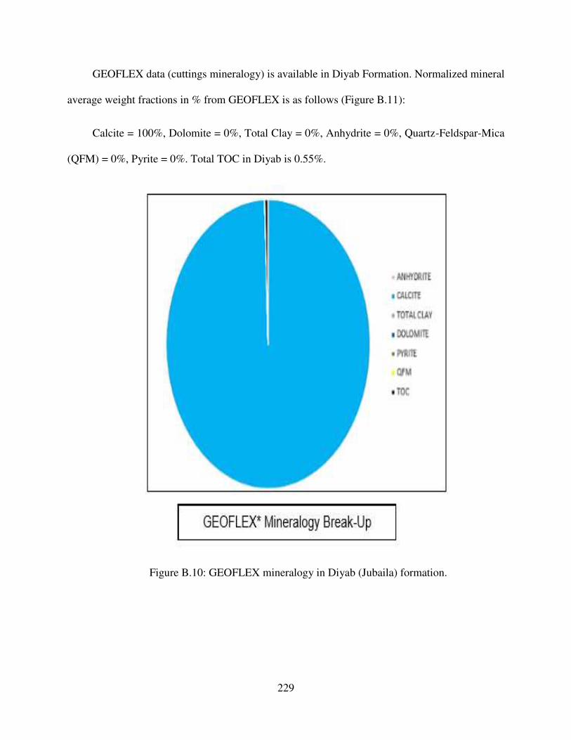
229
GEOFLEX data (cuttings mineralogy) is available in Diyab Formation. Normalized mineral
average weight fractions in % from GEOFLEX is as follows (Figure B.11):
Calcite = 100%, Dolomite = 0%, Total Clay = 0%, Anhydrite = 0%, Quartz-Feldspar-Mica
(QFM) = 0%, Pyrite = 0%. Total TOC in Diyab is 0.55%.
Figure B.10: GEOFLEX mineralogy in Diyab (Jubaila) formation.
230
APPENDIX C
C. GEOCHEMISTRY
C.1 Geochemistry
The objective of this study was to carry out a reservoir quality assessment of the Diyab
formation in UAE. Below work only focuses on currently acquired data, that is, wireline log
measurements and mud gas logs. Future work will incorporate validation through and
interpretation of core measurements, as well as incorporate an analysis of uncertainty on the
results. Initial petrophysical evaluation shows that both the Jubaila and Hanifa source rocks are a
good prospect for Shale Gas development (with Hanifa lower showing a far superior prospect to
the Jubaila and Hanifa upper). The level of gas saturation exceeds the known pay criteria known
to be expected to produce economic volumes of gas in other basins around the world.
C.1.1 Total Organic Carbon
Total organic carbon (TOC) is an important estimate of the potential of a source rock to
produce hydrocarbons. By definition it is a measure of total carbon present associated with organic
matter including kerogen and any hydrocarbon. Greater the total organic carbon, greater is the
source potential of the rock.
TOC was computed from logs using
1. Uranium concentration measured using spectral gamma-ray
2. Passey Delta Log R technique
3. Schmoker’s density-based method
4. Modified Schmoker method – uses matrix density as input
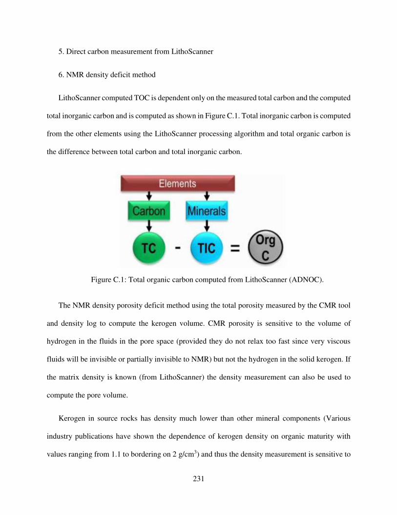
231
5. Direct carbon measurement from LithoScanner
6. NMR density deficit method
LithoScanner computed TOC is dependent only on the measured total carbon and the computed
total inorganic carbon and is computed as shown in Figure C.1. Total inorganic carbon is computed
from the other elements using the LithoScanner processing algorithm and total organic carbon is
the difference between total carbon and total inorganic carbon.
Figure C.1: Total organic carbon computed from LithoScanner (ADNOC).
The NMR density porosity deficit method using the total porosity measured by the CMR tool
and density log to compute the kerogen volume. CMR porosity is sensitive to the volume of
hydrogen in the fluids in the pore space (provided they do not relax too fast since very viscous
fluids will be invisible or partially invisible to NMR) but not the hydrogen in the solid kerogen. If
the matrix density is known (from LithoScanner) the density measurement can also be used to
compute the pore volume.
Kerogen in source rocks has density much lower than other mineral components (Various
industry publications have shown the dependence of kerogen density on organic maturity with
values ranging from 1.1 to bordering on 2 g/cm3) and thus the density measurement is sensitive to
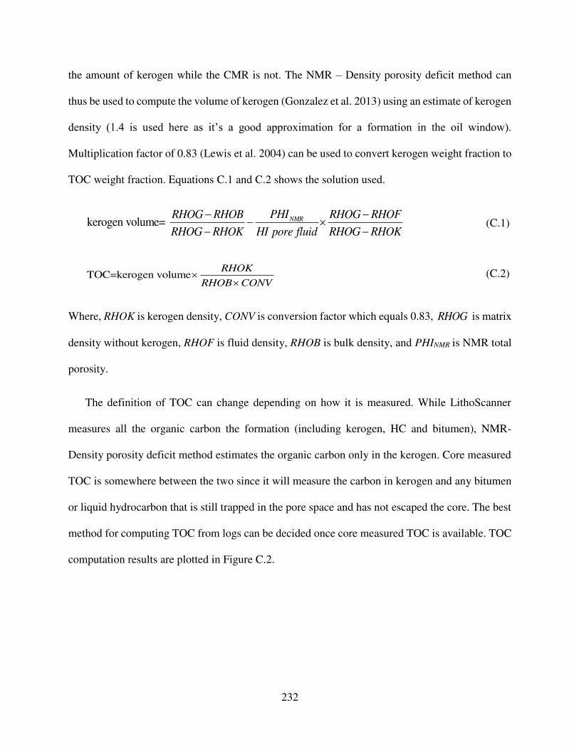
232
the amount of kerogen while the CMR is not. The NMR – Density porosity deficit method can
thus be used to compute the volume of kerogen (Gonzalez et al. 2013) using an estimate of kerogen
density (1.4 is used here as it’s a good approximation for a formation in the oil window).
Multiplication factor of 0.83 (Lewis et al. 2004) can be used to convert kerogen weight fraction to
TOC weight fraction. Equations C.1 and C.2 shows the solution used.
kerogen volume= NMRPHIRHOG RHOB RHOG RHOF
RHOG RHOK HI pore fluid RHOG RHOK
− −−
− − (C.1)
TOC=kerogen volumeRHOK
RHOB CONV
(C.2)
Where, RHOK is kerogen density, CONV is conversion factor which equals 0.83, RHOG is matrix
density without kerogen, RHOF is fluid density, RHOB is bulk density, and PHINMR is NMR total
porosity.
The definition of TOC can change depending on how it is measured. While LithoScanner
measures all the organic carbon the formation (including kerogen, HC and bitumen), NMR-
Density porosity deficit method estimates the organic carbon only in the kerogen. Core measured
TOC is somewhere between the two since it will measure the carbon in kerogen and any bitumen
or liquid hydrocarbon that is still trapped in the pore space and has not escaped the core. The best
method for computing TOC from logs can be decided once core measured TOC is available. TOC
computation results are plotted in Figure C.2.
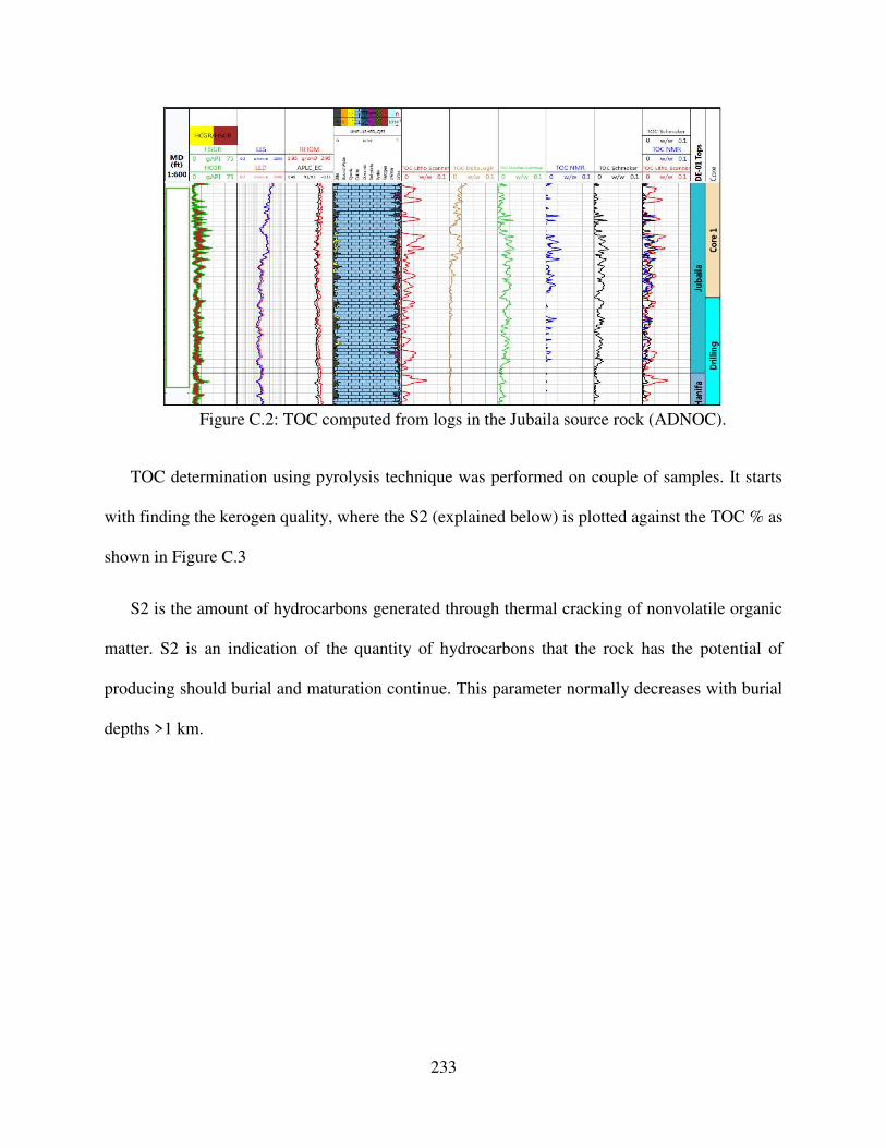
233
Figure C.2: TOC computed from logs in the Jubaila source rock (ADNOC).
TOC determination using pyrolysis technique was performed on couple of samples. It starts
with finding the kerogen quality, where the S2 (explained below) is plotted against the TOC % as
shown in Figure C.3
S2 is the amount of hydrocarbons generated through thermal cracking of nonvolatile organic
matter. S2 is an indication of the quantity of hydrocarbons that the rock has the potential of
producing should burial and maturation continue. This parameter normally decreases with burial
depths >1 km.
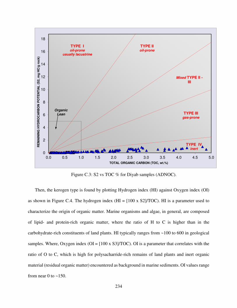
234
Figure C.3: S2 vs TOC % for Diyab samples (ADNOC).
Then, the kerogen type is found by plotting Hydrogen index (HI) against Oxygen index (OI)
as shown in Figure C.4. The hydrogen index (HI = [100 x S2]/TOC). HI is a parameter used to
characterize the origin of organic matter. Marine organisms and algae, in general, are composed
of lipid- and protein-rich organic matter, where the ratio of H to C is higher than in the
carbohydrate-rich constituents of land plants. HI typically ranges from ~100 to 600 in geological
samples. Where, Oxygen index (OI = [100 x S3]/TOC). OI is a parameter that correlates with the
ratio of O to C, which is high for polysacharride-rich remains of land plants and inert organic
material (residual organic matter) encountered as background in marine sediments. OI values range
from near 0 to ~150.
0
2
4
6
8
10
12
14
16
18
0.0 0.5 1.0 1.5 2.0 2.5 3.0 3.5 4.0 4.5 5.0
RE
MA
ININ
G H
YD
RO
CA
RB
ON
PO
TE
NT
IAL
(S
2, m
g H
C/g
ro
ck)
TOTAL ORGANIC CARBON (TOC, wt.%)
TYPE IIoil-prone
Mixed TYPE II -III
TYPE IIIgas-prone
OrganicLean
TYPE IVinert
TYPE Ioil-prone
usually lacustrine
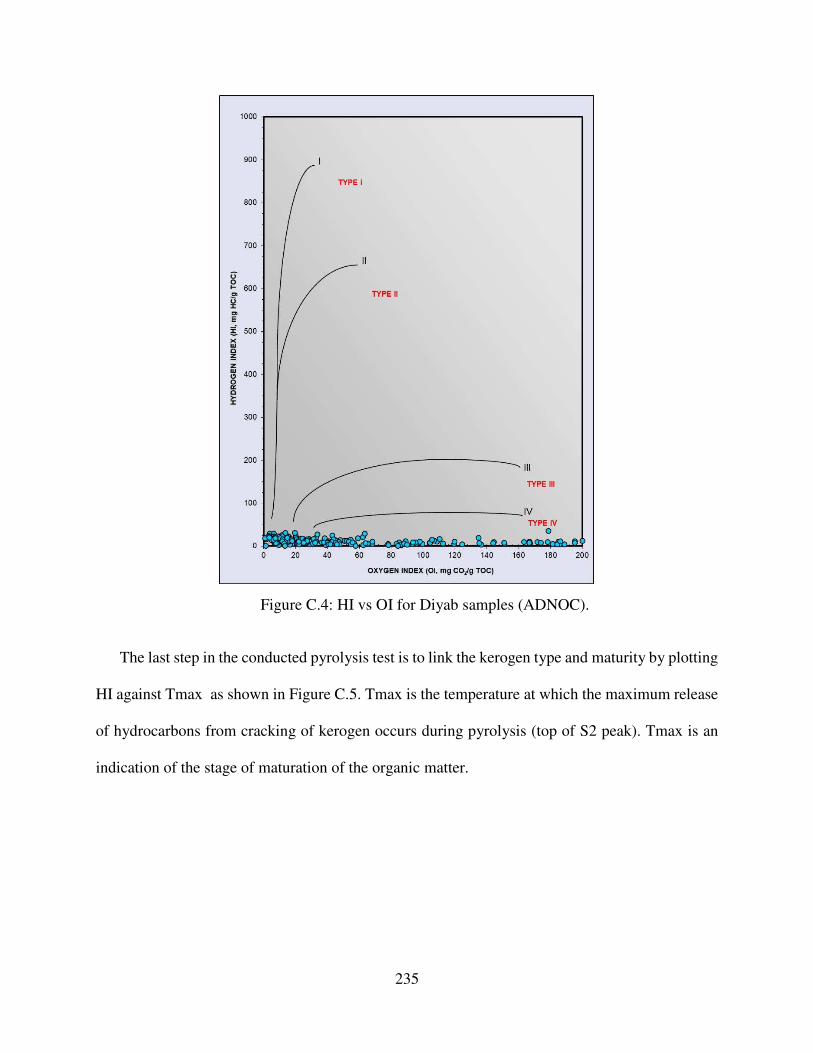
235
Figure C.4: HI vs OI for Diyab samples (ADNOC).
The last step in the conducted pyrolysis test is to link the kerogen type and maturity by plotting
HI against Tmax as shown in Figure C.5. Tmax is the temperature at which the maximum release
of hydrocarbons from cracking of kerogen occurs during pyrolysis (top of S2 peak). Tmax is an
indication of the stage of maturation of the organic matter.
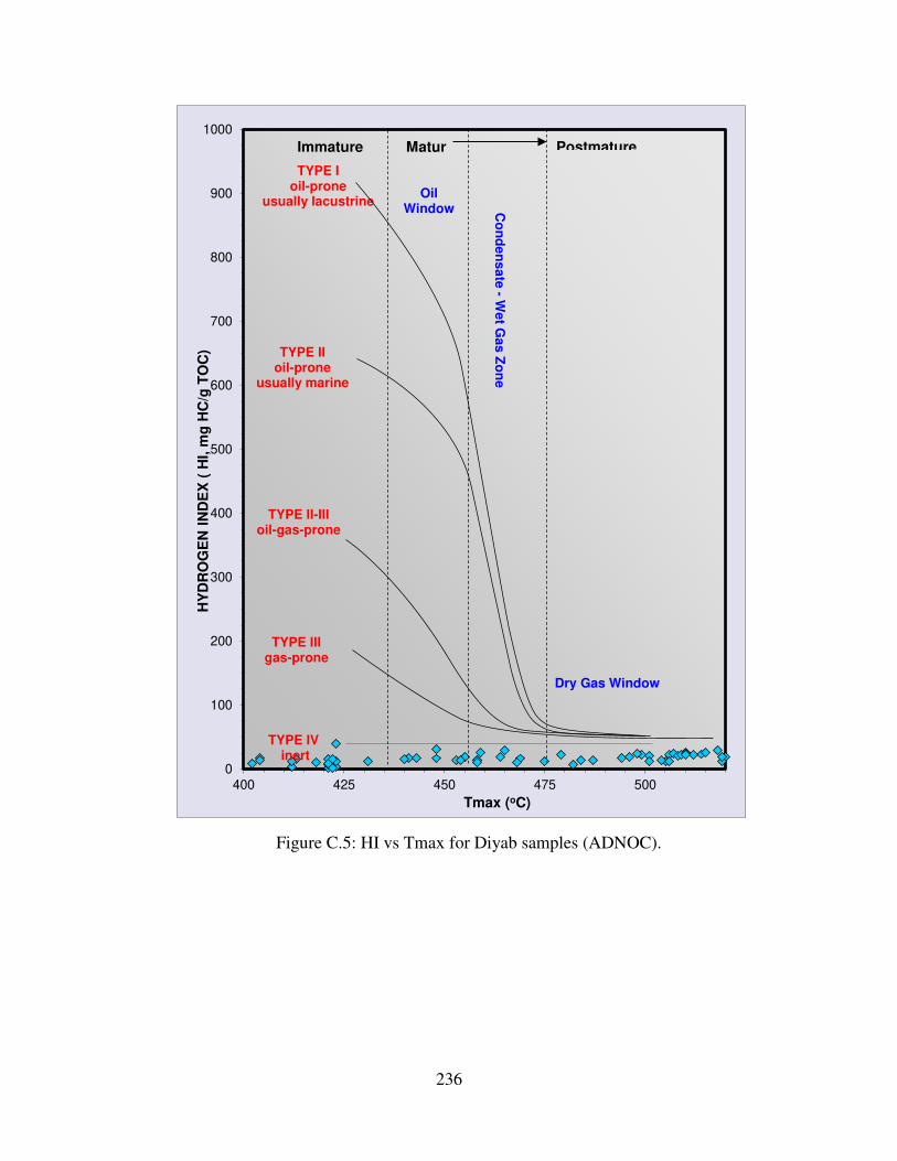
236
Figure C.5: HI vs Tmax for Diyab samples (ADNOC).
0
100
200
300
400
500
600
700
800
900
1000
400 425 450 475 500
HY
DR
OG
EN
IN
DE
X (
HI,
mg
HC
/g T
OC
)
Tmax (oC)
TYPE Ioil-prone
usually lacustrine
TYPE IIoil-prone
usually marine
TYPE II-IIIoil-gas-prone
Co
nd
en
sa
te -
We
t Ga
s Z
on
e
Dry Gas Window
Immature Postmature
TYPE IIIgas-prone
TYPE IVinert
Matur
OilWindow

237
C.1.2 Vitrinite Reflectance
Samples from Diyab formation were analyzed for thermal maturity level based on the
reflectance values measured on vitrinite (%VRo) and/or solid bitumen (%BRo). Fluorescent
macerals from the liptinite group (alginite and/or sporinite) were not present to complement the
thermal maturity assessment. Sufficient number of reflectance measurements (≥20) was collected
on solid bitumen macerals in all samples to satisfy the standard test method and return the results
with a high confidence level. Measurements collected on solid bitumen were then re-calculated to
vitrinite reflectance equivalent (%VRE), based on the equation by Jacob (1989).
Sample Preparation starts with crushing the sample, the crushed rock sample (one sample
requires 6g of >12 mesh diameter grains) and thermoplastic ‘Lucite’ powder are placed in the Leco
Hydraulic Mounting Press PR36 chamber. The applied temperature and pressure melt the ‘Lucite’
and binds the components together. After curing and water-cooling, the thick-section is removed
from the chamber and is ready for a grinding-polishing step using the Leco Grinder Polisher
GPX200. Prior to analysis, polished blocks are first air dried and then stored overnight in a
desiccator in order to remove any moisture. Polished thick-sections, prepared in accordance with
specifications described in the ASTM D2797 standard, are used for organic matter (OM)
examination with an optical microscope using reflected light illumination and oil immersion.
Sedimentary rocks often contain low amount of terrestrial organic matter (such as vitrinite),
as well as small, reworked or oxidized grains with granulated/mottled surface, or particles with
suppressed reflectance, which are not considered to be representative as maturity indicators and
are omitted from the statistics. When the vitrinite is absent, which may be the case in marine source
rocks or the pre-Silurian rocks, the reflectance is measured on solid bitumen (%BRo, secondary
maceral) or graptolites/chitinozoans/scolecodonts (%Ro, organic fossil remains), which also
238
express a regular change with maturity. These data are used to present thermal maturity level as
the vitrinite reflectance equivalent (%VRE).
Interpretations of thermal maturity level and hydrocarbons generation zone are made base
on the %Ro measurements and overall microscopic observations of OM under incident white and
UV fluorescent light. The given confidence level is often related to the quantity and quality of OM
particles and solid bitumen concentrations in rock. An explanation with additional information
related to data in the report helps the reader to understand the provided information is presented
below, Table C.1 shows the reference of the vitrinite reflectance and concluded information.
Table C.1: Vitrinite reflectance percentage and the reflected hydrocarbon generation zone
and maturity level.
The vitrinite reflectance for sample A is presented in Figure C.6, where it shows a maximum
of 1.20 % and minimum of 1.00 %. Concluded from the bar chart the average percentage is 1.12
%. Figure C.7 shows the solid bitumen reflectance for sample A with a maximum and minimum
of 1.70 % and 1.00 % respectively. The mean of solid bitumen reflectance is concluded to be 1.36,
and this mean was used to calculate the vitrinite reflectance equivalent, this mean was used to
calculate the vitrinite reflectance equivalent using Jacob (1989) equation, which calculated 1.24
%. Which in reference to Table C.1 means the thermal maturity level is late mature, the
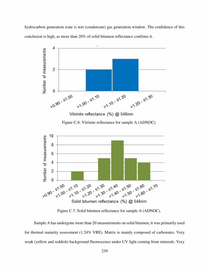
239
hydrocarbon generation zone is wet (condensate) gas generation window. The confidence of this
conclusion is high, as more than 20% of solid bitumen reflectance confirms it.
Figure C.6: Vitrinite reflectance for sample A (ADNOC).
Figure C.7: Solid bitumen reflectance for sample A (ADNOC).
Sample A has undergone more than 20 measurements on solid bitumen, it was primarily used
for thermal maturity assessment (1.24% VRE). Matrix is mainly composed of carbonates. Very
weak (yellow and reddish) background fluorescence under UV light coming from minerals. Very
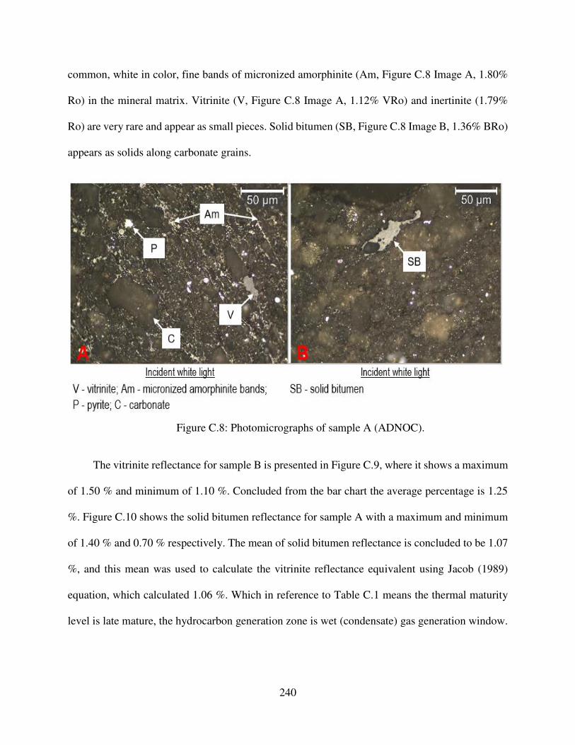
240
common, white in color, fine bands of micronized amorphinite (Am, Figure C.8 Image A, 1.80%
Ro) in the mineral matrix. Vitrinite (V, Figure C.8 Image A, 1.12% VRo) and inertinite (1.79%
Ro) are very rare and appear as small pieces. Solid bitumen (SB, Figure C.8 Image B, 1.36% BRo)
appears as solids along carbonate grains.
Figure C.8: Photomicrographs of sample A (ADNOC).
The vitrinite reflectance for sample B is presented in Figure C.9, where it shows a maximum
of 1.50 % and minimum of 1.10 %. Concluded from the bar chart the average percentage is 1.25
%. Figure C.10 shows the solid bitumen reflectance for sample A with a maximum and minimum
of 1.40 % and 0.70 % respectively. The mean of solid bitumen reflectance is concluded to be 1.07
%, and this mean was used to calculate the vitrinite reflectance equivalent using Jacob (1989)
equation, which calculated 1.06 %. Which in reference to Table C.1 means the thermal maturity
level is late mature, the hydrocarbon generation zone is wet (condensate) gas generation window.
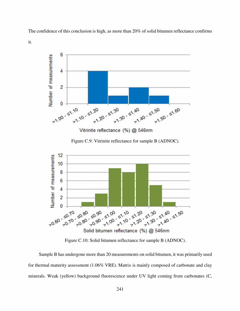
241
The confidence of this conclusion is high, as more than 20% of solid bitumen reflectance confirms
it.
Figure C.9: Vitrinite reflectance for sample B (ADNOC).
Figure C.10: Solid bitumen reflectance for sample B (ADNOC).
Sample B has undergone more than 20 measurements on solid bitumen, it was primarily used
for thermal maturity assessment (1.06% VRE). Matrix is mainly composed of carbonate and clay
minerals. Weak (yellow) background fluorescence under UV light coming from carbonates (C,
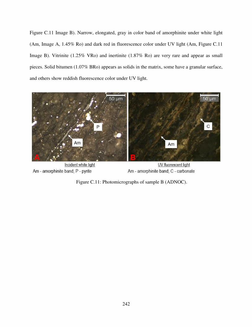
242
Figure C.11 Image B). Narrow, elongated, gray in color band of amorphinite under white light
(Am, Image A, 1.45% Ro) and dark red in fluorescence color under UV light (Am, Figure C.11
Image B). Vitrinite (1.25% VRo) and inertinite (1.87% Ro) are very rare and appear as small
pieces. Solid bitumen (1.07% BRo) appears as solids in the matrix, some have a granular surface,
and others show reddish fluorescence color under UV light.
Figure C.11: Photomicrographs of sample B (ADNOC).
243
APPENDIX D
D. GEOMECHANICS
D.1 Geomechanics
A laboratory geomechanical characterization of Diyab formations is reported in this section.
The objective of the study is to evaluate the mechanical behavior, elastic and strength properties
of Diyab formations at different stress path conditions. The experimental data can be fed into the
geomechanical model of the basin for in-situ stress calculations, borehole stability problems and
hydraulic fracture applications.
This laboratory geomechanical characterization includes dynamic and static elastic properties,
tensile strength, unconfined compressive strength (UCS), cohesion (So), internal friction angle (ϕ),
stress-strain curves and Mohr-Coulomb failure envelopes. Which are used to calibrate the log
based elastic and strength rock properties (Figure D.1).
The laboratory geomechanics experiments were conducted in ADNOC facilities. The reason
behind the geomechanical analysis is to create a clear picture of UAE Diyab unconventional
formation and create a better understanding for interested parties. Geomechanical description is an
important tool used when designing hydraulic fracture treatment in unconventional development.

244
Figure D.1: Diyab formation geomechanical log (ADNOC).
Ultrasonic velocity measurements were performed under the hydrostatic stress condition to
evaluate the dynamic elastic properties. The single-stage triaxial compression test (CCS) was used
to evaluate the static elastic parameters, the strength of the rock and the stress/strain curve at a
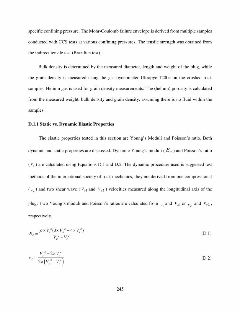
245
specific confining pressure. The Mohr-Coulomb failure envelope is derived from multiple samples
conducted with CCS tests at various confining pressures. The tensile strength was obtained from
the indirect tensile test (Brazilian test).
Bulk density is determined by the measured diameter, length and weight of the plug, while
the grain density is measured using the gas pycnometer Ultrapyc 1200e on the crushed rock
samples. Helium gas is used for grain density measurements. The (helium) porosity is calculated
from the measured weight, bulk density and grain density, assuming there is no fluid within the
samples.
D.1.1 Static vs. Dynamic Elastic Properties
The elastic properties tested in this section are Young’s Moduli and Poisson’s ratio. Both
dynamic and static properties are discussed. Dynamic Young’s moduli ( dE ) and Poisson’s ratio
( dv ) are calculated using Equations D.1 and D.2. The dynamic procedure used is suggested test
methods of the international society of rock mechanics, they are derived from one compressional
(p
v ) and two shear wave ( 1sv and 2sv ) velocities measured along the longitudinal axis of the
plug: Two Young’s moduli and Poisson’s ratios are calculated from p
v and 1sv or p
v and 2sv ,
respectively.
2 2 2
2 2
(3 4 )s p s
d
p s
V V VE
V V
− =
− (D.1)
( )2 2
2 2
2
2
p s
d
p s
V Vv
V V
− =
− (D.2)
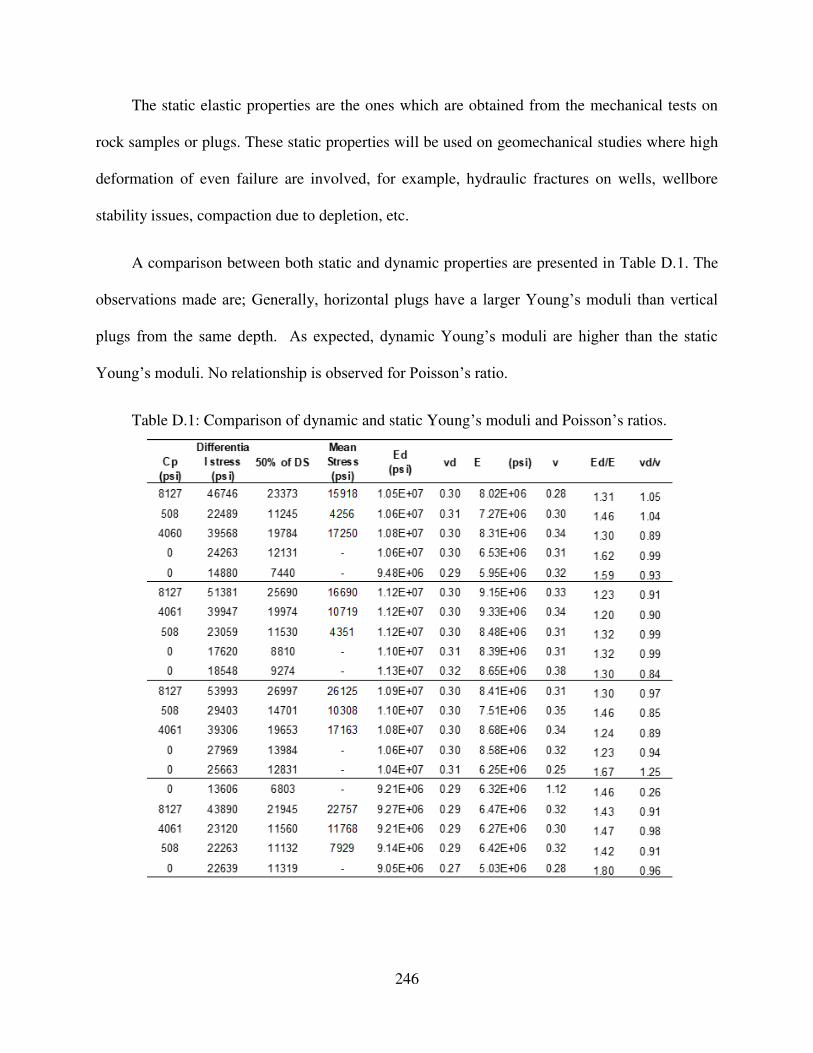
246
The static elastic properties are the ones which are obtained from the mechanical tests on
rock samples or plugs. These static properties will be used on geomechanical studies where high
deformation of even failure are involved, for example, hydraulic fractures on wells, wellbore
stability issues, compaction due to depletion, etc.
A comparison between both static and dynamic properties are presented in Table D.1. The
observations made are; Generally, horizontal plugs have a larger Young’s moduli than vertical
plugs from the same depth. As expected, dynamic Young’s moduli are higher than the static
Young’s moduli. No relationship is observed for Poisson’s ratio.
Table D.1: Comparison of dynamic and static Young’s moduli and Poisson’s ratios.
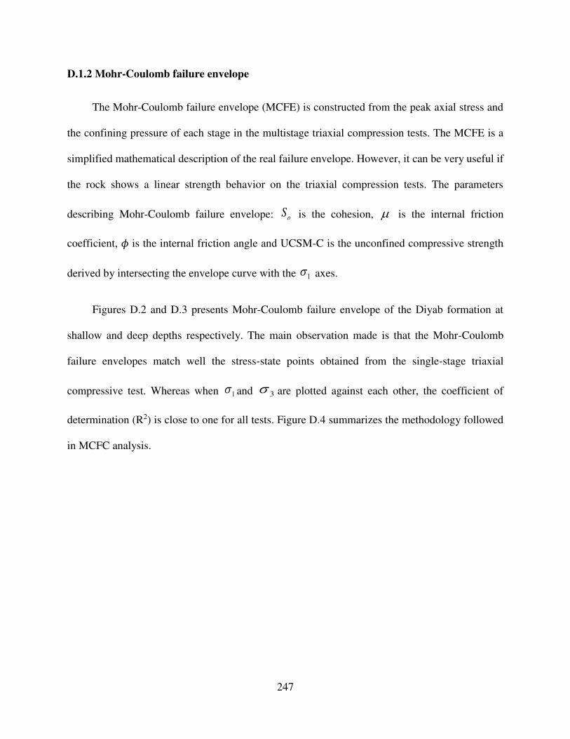
247
D.1.2 Mohr-Coulomb failure envelope
The Mohr-Coulomb failure envelope (MCFE) is constructed from the peak axial stress and
the confining pressure of each stage in the multistage triaxial compression tests. The MCFE is a
simplified mathematical description of the real failure envelope. However, it can be very useful if
the rock shows a linear strength behavior on the triaxial compression tests. The parameters
describing Mohr-Coulomb failure envelope: oS is the cohesion, is the internal friction
coefficient, 𝜙 is the internal friction angle and UCSM-C is the unconfined compressive strength
derived by intersecting the envelope curve with the 1 axes.
Figures D.2 and D.3 presents Mohr-Coulomb failure envelope of the Diyab formation at
shallow and deep depths respectively. The main observation made is that the Mohr-Coulomb
failure envelopes match well the stress-state points obtained from the single-stage triaxial
compressive test. Whereas when 1 and 3 are plotted against each other, the coefficient of
determination (R2) is close to one for all tests. Figure D.4 summarizes the methodology followed
in MCFC analysis.
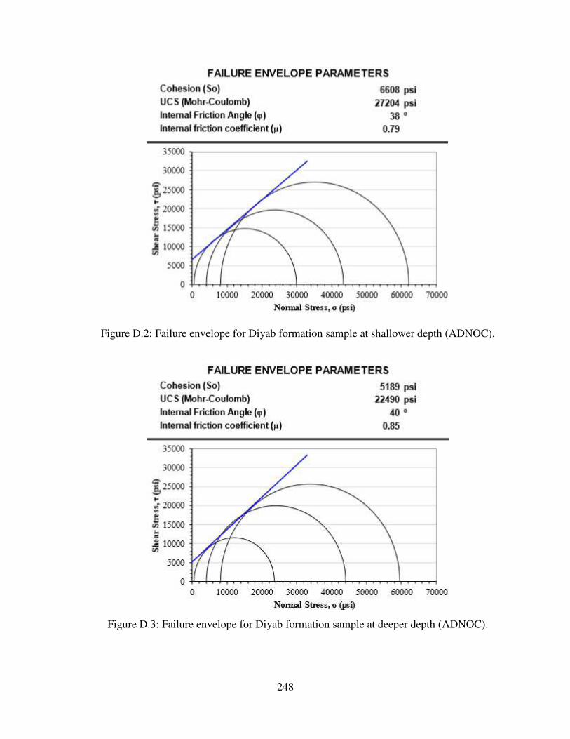
248
Figure D.2: Failure envelope for Diyab formation sample at shallower depth (ADNOC).
Figure D.3: Failure envelope for Diyab formation sample at deeper depth (ADNOC).
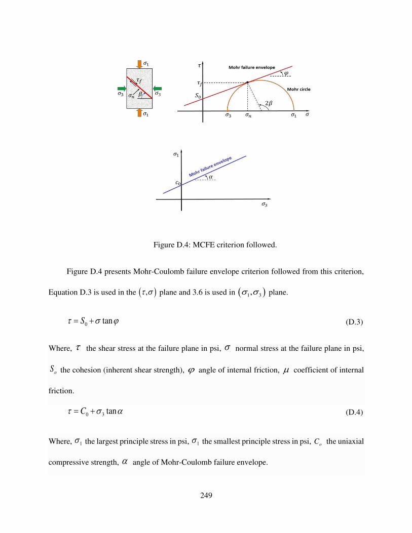
249
Figure D.4: MCFE criterion followed.
Figure D.4 presents Mohr-Coulomb failure envelope criterion followed from this criterion,
Equation D.3 is used in the ( ), plane and 3.6 is used in ( )1 3, plane.
0 tanS = + (D.3)
Where, the shear stress at the failure plane in psi, normal stress at the failure plane in psi,
oS the cohesion (inherent shear strength), angle of internal friction, coefficient of internal
friction.
0 3 tanC = + (D.4)
Where, 1 the largest principle stress in psi, 1 the smallest principle stress in psi, oC the uniaxial
compressive strength, angle of Mohr-Coulomb failure envelope.
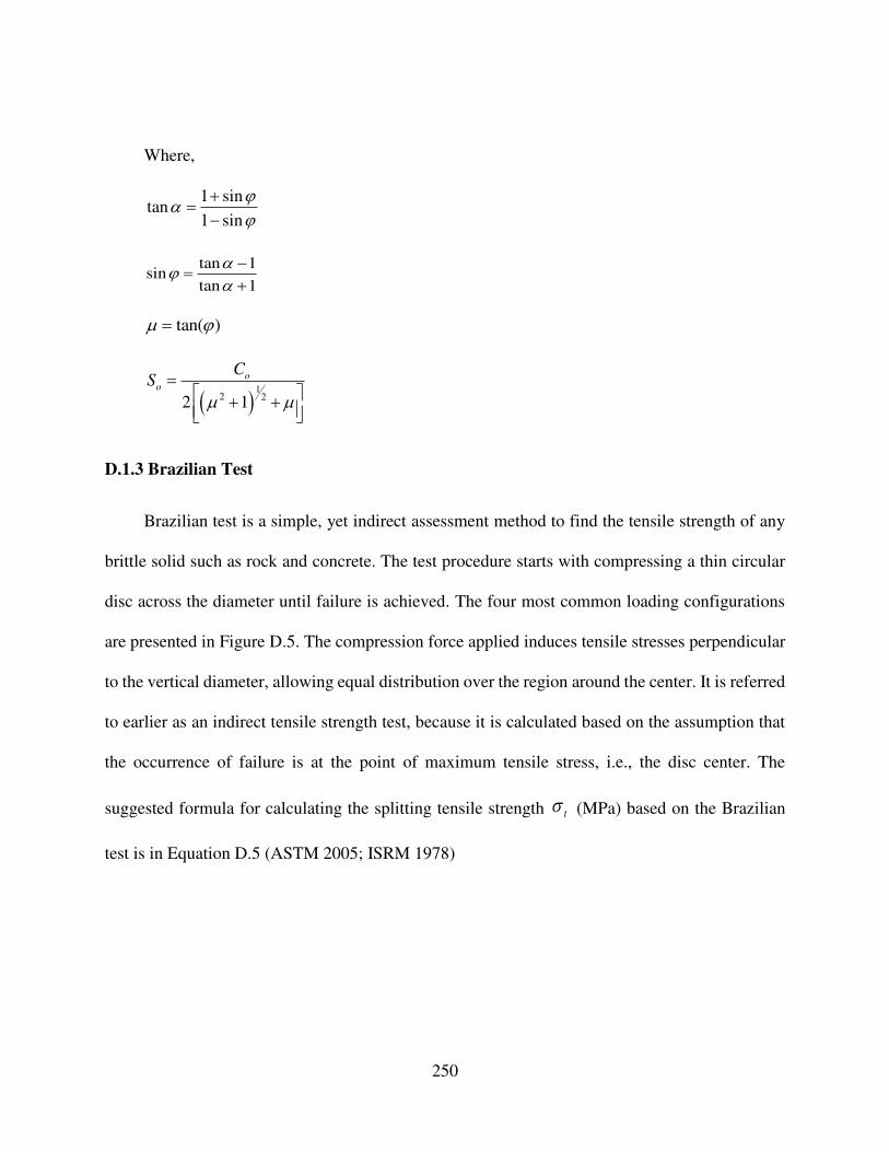
250
Where,
1 sintan
1 sin
+=
−
tan 1sin
tan 1
−
=+
tan( ) =
( )1
2 22 1
oo
CS
=
+ +
D.1.3 Brazilian Test
Brazilian test is a simple, yet indirect assessment method to find the tensile strength of any
brittle solid such as rock and concrete. The test procedure starts with compressing a thin circular
disc across the diameter until failure is achieved. The four most common loading configurations
are presented in Figure D.5. The compression force applied induces tensile stresses perpendicular
to the vertical diameter, allowing equal distribution over the region around the center. It is referred
to earlier as an indirect tensile strength test, because it is calculated based on the assumption that
the occurrence of failure is at the point of maximum tensile stress, i.e., the disc center. The
suggested formula for calculating the splitting tensile strength t (MPa) based on the Brazilian
test is in Equation D.5 (ASTM 2005; ISRM 1978)
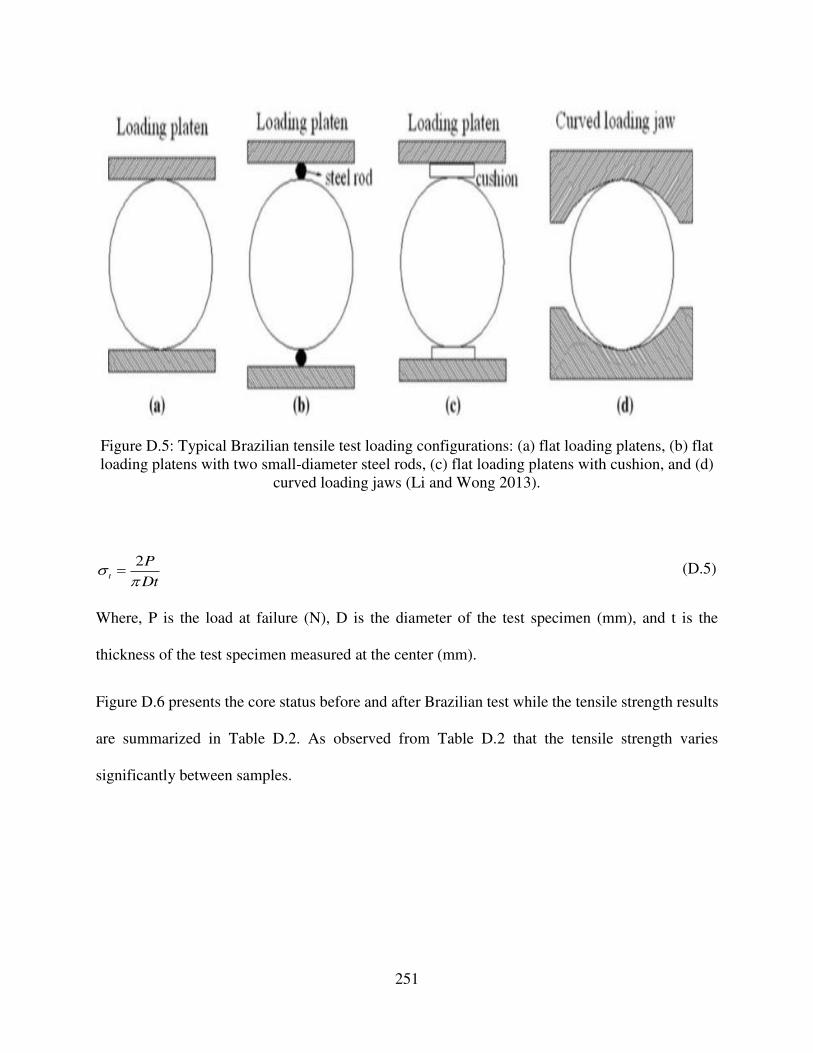
251
Figure D.5: Typical Brazilian tensile test loading configurations: (a) flat loading platens, (b) flat
loading platens with two small-diameter steel rods, (c) flat loading platens with cushion, and (d)
curved loading jaws (Li and Wong 2013).
2t
P
Dt
= (D.5)
Where, P is the load at failure (N), D is the diameter of the test specimen (mm), and t is the
thickness of the test specimen measured at the center (mm).
Figure D.6 presents the core status before and after Brazilian test while the tensile strength results
are summarized in Table D.2. As observed from Table D.2 that the tensile strength varies
significantly between samples.
252
Figure D.6: Core sample before and after Brazilian loading test (ADNOC).
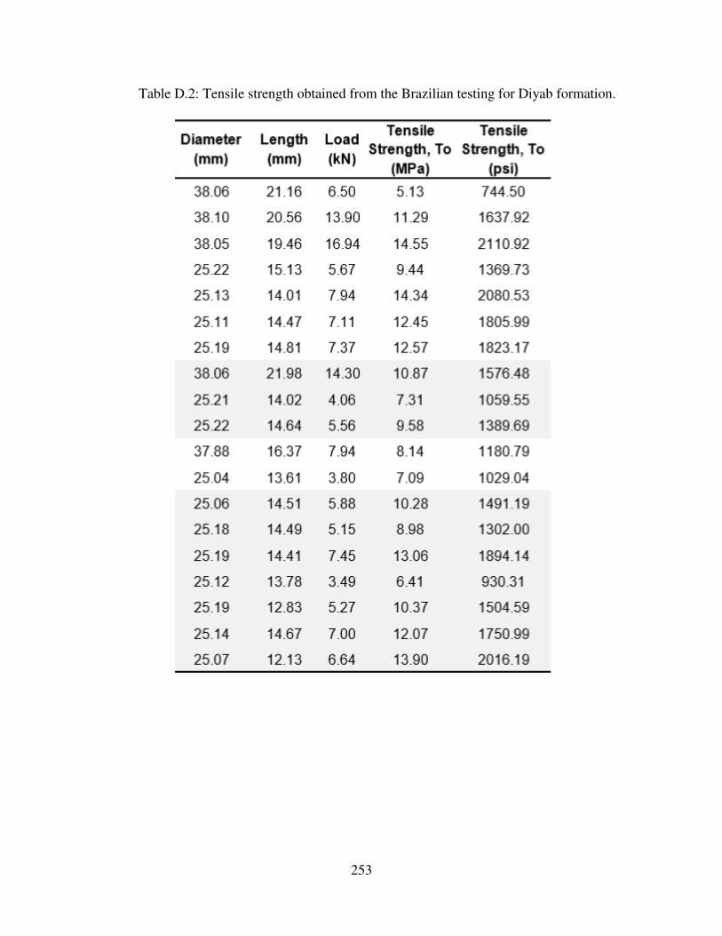
253
Table D.2: Tensile strength obtained from the Brazilian testing for Diyab formation.
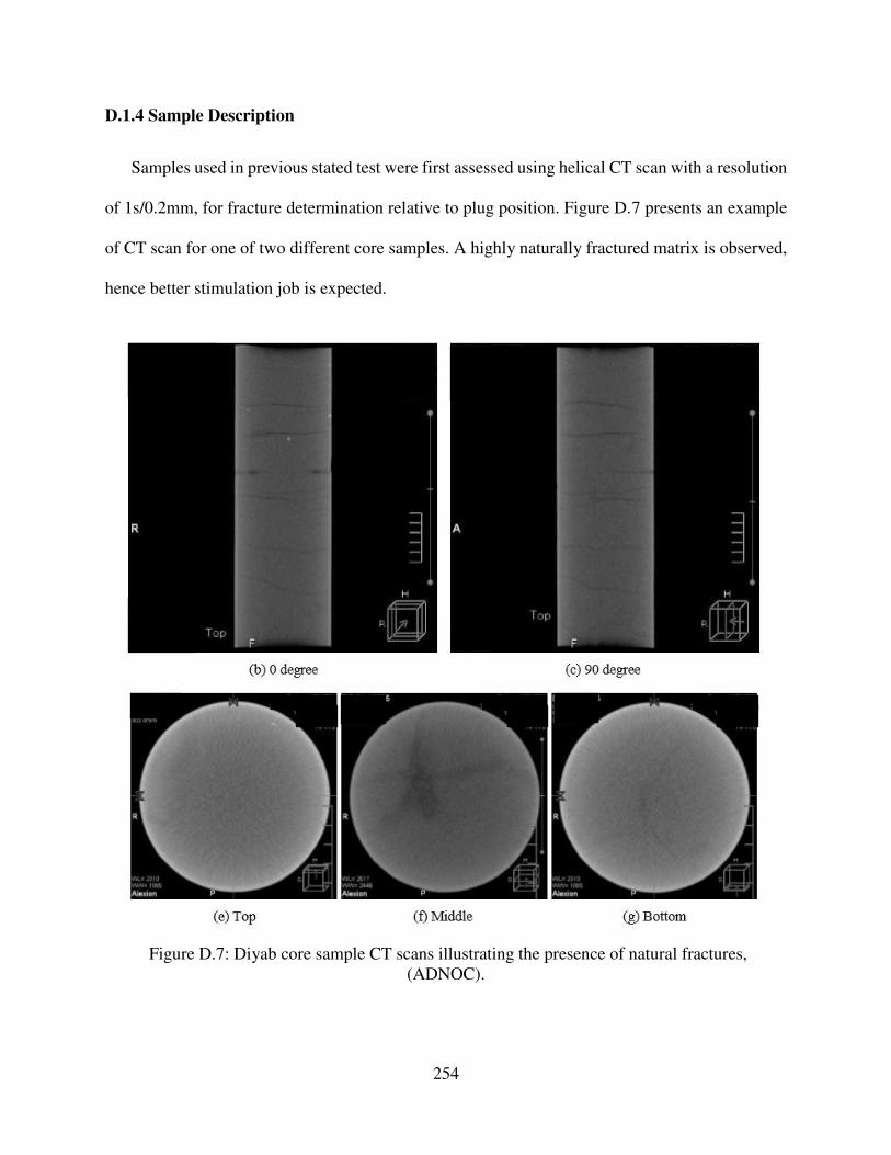
254
D.1.4 Sample Description
Samples used in previous stated test were first assessed using helical CT scan with a resolution
of 1s/0.2mm, for fracture determination relative to plug position. Figure D.7 presents an example
of CT scan for one of two different core samples. A highly naturally fractured matrix is observed,
hence better stimulation job is expected.
Figure D.7: Diyab core sample CT scans illustrating the presence of natural fractures,
(ADNOC).
Related Documents