Interpretation and mining of statistical machine learning (Q)SAR models for toxicity prediction by Samuel Jonathan Webb Submitted for the degree of Doctor of Philosophy in Computing Faculty of Engineering and Physical Sciences University of Surrey February 2015 © Samuel Jonathan Webb 2015

Welcome message from author
This document is posted to help you gain knowledge. Please leave a comment to let me know what you think about it! Share it to your friends and learn new things together.
Transcript

Interpretation and mining of statistical
machine learning (Q)SAR models for
toxicity prediction
by
Samuel Jonathan Webb
Submitted for the degree of Doctor of Philosophy in Computing
Faculty of Engineering and Physical Sciences
University of Surrey
February 2015
© Samuel Jonathan Webb 2015


i
Acknowledgements
The financial support from the Technology Strategy Board (TSB) for funding of the KTP
project 6875 and Lhasa Limited’s initial and ongoing funding of the PhD is gratefully
acknowledged, without which this project couldn’t have been completed.
The work in this thesis would not have been possible without the support of many only some
of which can be mentioned here. I would like to thank my supervisors BH, PK and JV for
their support and guidance throughout (and before) this postgraduate study began.
Additionally, I would like to thank all those Lhasa Limited staff who provided feedback on
publications, software and presentations throughout the undertaking of the PhD.
Finally, I would like to thank MW, LW, ZI, TH, CB, JK and JT for their support whether
academic, personal or both.
ii
Abstract
Structure Activity Relationship (SAR) modelling capitalises on techniques developed within
the computer science community, particularly in the fields of machine learning and data
mining. These machine learning approaches are often developed for the optimisation of
model accuracy which can come at the expense of the interpretation of the prediction.
Highly predictive models should be the goal of any modeller, however, the intended users of
the model and all factors relating to usage of the model should be considered. One such
aspect is the clarity, understanding and explanation for the prediction. In some cases black
box models which do not provide an interpretation can be disregarded regardless of their
predictive accuracy. In this thesis the problem of model interpretation has been tackled in the
context of models to predict toxicity of drug like molecules.
Firstly a novel algorithm has been developed for the interpretation of binary classification
models where the endpoint meets defined criteria: activity is caused by the presence of a
feature and inactivity by the lack of an activating feature or the deactivation of all such
activating features. This algorithm has been shown to provide a meaningful interpretation of
the model’s cause(s) of both active and inactive predictions for two toxicological endpoints:
mutagenicity and skin irritation. The algorithm shows benefits over other interpretation
algorithms in its ability to not only identify the causes of activity mapped to fragments and
physicochemical descriptors but also in its ability to account for combinatorial effects of the
descriptors. The interpretation is presented to the user in the form of the impact of features
and can be visualised as a concise summary or in a hierarchical network detailing the full
elucidation of the models behaviour for a particular query compound.
The interpretation output has been capitalised on and incorporated into a knowledge mining
strategy. The knowledge mining is able to extract the learned structure activity relationship
trends from a model such as a Random Forest, decision tree, k Nearest Neighbour or support
vector machine. These trends can be presented to the user focused around the feature
responsible for the assessment such as ACTIVATING or DEACTIVATING. Supporting
examples are provided along with an estimation of the models predictive performance for a
given SAR trend.
Both the interpretation and knowledge mining has been applied to models built for the
prediction of Ames mutagenicity and skin irritation. The performance of the developed
models is strong and comparable to both academic and commercial predictors for these two
toxicological activities.
iii
Contribution of work to publications
Some of the work in this thesis has contributed or formed the focus of external publications.
The various communications cover the algorithms described in chapters 6 and 7 along with
their application to Ames mutagenicity and skin irritation for model interpretation and
knowledge mining.
Articles
1. S. J. Webb, T. Hanser, B. Howlin, P. Krause, and J. D. Vessey, Feature combination
networks for the interpretation of statistical machine learning models: application to
Ames mutagenicity., J. Cheminform., vol. 6, no. 1, p. 8, Jan. 2014.
Oral presentations
1. S. J. Webb, Interpretation of statistical machine learning models: application to
Ames mutagenicity prediction, MGMS Young Modellers’ Forum 2013, London UK,
November 2013.
2. S. J. Webb, Feature combination networks with statistical (Q)SAR models:
interpretation and knowledge mining. UK-QSAR autumn meeting 2014. CCDC,
Cambridge UK, September 2014.
Posters
1. S. J. Webb, T. Hanser, B. Howlin, P. Krause, and J. D. Vessey, Interpretable Ames
mutagenicity predictions using statistical learning techniques, QSAR2012, Tallin
Estonia, June 2012.
2. S. J. Webb, T. Hanser, B. Howlin, P. Krause, and J. D. Vessey, Interpretation of
statistical machine learning models for Ames mutagenicity, 6th Joint Sheffield
Conference on Chemoinformatics, Sheffield UK, July 2013 (represented at UK-
QSAR Spring meeting, Eli Lilly 2014).
3. S. J. Webb, T. Hanser, B. Howlin, P. Krause, and J. D. Vessey, Knowledge
extraction from the interpetation fo SAR models by feature networks, QSAR2014,
Milan Italy.

iv
Contents
1 Introduction ...................................................................................................................... 1
2 Computational toxicology: (Q)SAR and macine learning ............................................... 4
2.1 (Q)SAR and regulatory submission.......................................................................... 5
2.2 Learning and algorithms ........................................................................................... 6
2.2.1 Supervised learning .......................................................................................... 6
2.2.2 Ensembles, bagging and boosting .................................................................... 9
2.2.3 Unsupervised learning .................................................................................... 11
2.2.4 Instance based learning................................................................................... 12
2.2.5 Read across ..................................................................................................... 13
2.2.6 Expert and rule based systems ........................................................................ 14
2.3 Practical considerations .......................................................................................... 15
2.3.1 Dealing with activity imbalance ..................................................................... 15
2.3.2 OECD principles ............................................................................................ 16
2.3.3 Applicability domains .................................................................................... 17
2.4 Performance metrics ............................................................................................... 18
2.5 Validation ............................................................................................................... 19
2.6 Summary ................................................................................................................ 20
3 Interpretation and knowledge mining ............................................................................. 21
3.1 The need and use case for interpretation ................................................................ 21
3.2 Interpretable predictions (white box models) ......................................................... 23
3.2.1 Expert / alert based systems ........................................................................... 23
3.2.2 Purpose designed interpretable models .......................................................... 25
3.3 Interpretation of black box (Q)SAR models .......................................................... 26
3.3.1 Visualising relevant training structures .......................................................... 27
3.3.2 Identifying the importance of features: globally and locally .......................... 28
3.3.3 Identifying the behaviour of atoms and/or fragments .................................... 30
3.4 Knowledge mining ................................................................................................. 34
3.4.1 Mining from datasets ...................................................................................... 34
3.4.2 Mining from models ....................................................................................... 37
3.4.3 Impact of this work to knowledge mining ...................................................... 38
3.5 Current need in model interpretation ...................................................................... 38
4 Cheminformatics: Software, data, descriptors and fragmentation ................................. 39
v
4.1 Software ................................................................................................................. 39
4.1.1 Chemical engines ........................................................................................... 39
4.1.2 Coralie ............................................................................................................ 39
4.1.3 KNIME .......................................................................................................... 39
4.2 Data ........................................................................................................................ 39
4.2.1 Dataset size .................................................................................................... 41
4.2.2 Data quality and curation ............................................................................... 41
4.3 Chemical structures, chemical space and similarity .............................................. 42
4.3.1 Structural similarity........................................................................................ 44
4.4 Descriptors ............................................................................................................. 45
4.4.1 Fingerprints .................................................................................................... 46
4.4.2 Physicochemical descriptors .......................................................................... 49
4.4.3 Descriptor selection........................................................................................ 50
4.4.4 Descriptor discretisation ................................................................................ 50
4.5 Fragmentation ........................................................................................................ 51
4.5.1 Retrosynthesis guided fragmentation ............................................................. 51
4.5.2 Bond cutting and functional unit based fragmentation .................................. 52
4.5.3 Reduced graph fragmentation ........................................................................ 53
4.5.4 Usage .............................................................................................................. 54
4.6 Summary ................................................................................................................ 54
5 Endpoints ....................................................................................................................... 55
5.1 Mutagenicity .......................................................................................................... 55
5.1.1 Endpoint ......................................................................................................... 55
5.1.2 Mechanisms of mutagenicity ......................................................................... 57
5.1.3 Experimental tests for mutagenicity............................................................... 58
5.1.4 Structural alerts and models ........................................................................... 59
5.1.5 Data ................................................................................................................ 61
5.1.6 Machine learning models ............................................................................... 63
5.2 Skin irritation ......................................................................................................... 68
5.2.1 Endpoint ......................................................................................................... 68
5.2.2 Experimental tests .......................................................................................... 69
5.2.3 Mechanisms, alerts and models ..................................................................... 70
5.2.4 Data and curation ........................................................................................... 71
vi
5.2.5 Machine learning models ............................................................................... 72
5.3 Summary ................................................................................................................ 77
6 Enumerated Combination Relationships (ENCORE) for the interpretation of binary
statistical models .................................................................................................................... 79
6.1 Algorithm ............................................................................................................... 79
6.1.1 Overview ......................................................................................................... 79
6.1.2 Technology and code ...................................................................................... 82
6.1.3 Feature networks: definition and organisation .............................................. 82
6.1.4 Network generation ....................................................................................... 88
6.1.5 Network assessment ...................................................................................... 90
6.1.6 Limitations and practical implementations .................................................... 94
6.2 Practical applications of modelling ........................................................................ 96
6.2.1 Learning algorithms ....................................................................................... 96
6.2.2 Descriptors choice for model building ........................................................... 96
6.3 Interpretations ......................................................................................................... 97
6.3.1 Overview of ENCORE interpretation .............................................................. 97
6.3.2 Example prediction and interpretation differences for mutagenicity ......... 100
6.3.3 Comparison with other models and algorithms ........................................... 104
6.3.4 Example prediction and interpretation differences for skin irritation ......... 109
6.4 Conclusion ............................................................................................................ 112
7 Enumerated Combination Relationships (ENCORE) for knowledge mining .............. 115
7.1 Knowledge mining ............................................................................................... 115
7.1.1 Feature dictionary ......................................................................................... 115
7.1.2 Iterative mining approach ............................................................................. 116
7.1.3 Extracting SAR trends from the feature dictionary ...................................... 117
7.2 Implementation ..................................................................................................... 119
7.2.1 Software implementations ............................................................................ 119
7.2.2 Fragmentation ............................................................................................... 120
7.3 Strategies for comparison with existing rule sets ................................................ 121
7.4 Application of ENCORE for knowledge mining ................................................. 122
7.4.1 Mutagenicity ................................................................................................. 122
7.4.2 Skin irritation ................................................................................................ 143
7.5 Conclusion ............................................................................................................ 150
8 Conclusions .................................................................................................................. 151

vii
8.1.1 Advancement of the area .............................................................................. 151
8.2 Real world application ......................................................................................... 152
8.3 Future work .......................................................................................................... 153
9 Appendix ...................................................................................................................... 155
10 Bibliography ............................................................................................................ 166
Abbreviations
ADME adsorption, distribution, metabolism and excretion
ACC accuracy
ANN artificial neural network
AUC area under curve
BAC balanced accuracy
BRICS
breaking of retrosynthetically interesting chemical
substructures
CBOS cluster-based oversampling
CDK chemistry development kit
CSC cost sensitive clasisifcation
DM distance to model
DNA deoxyribonucleic acid
DT decition tree
ECFP extended connectivity fingerprints
ECHA european chemicals agency
ECVAM european centre for the validation of alternative
ENCORE enumerated combination networks
EP emerging pattern
ESSR extended smallest set of smallest rings
FDA food and drug administration
FN false negative
FP false positive
GHS globally harmonized system
GLP good lab practice
JEP jumping emerging pattern
KNIME konstanz information miner
kNN k nearest neighbours
MACCS molecular access system
MCC matthews correlation coefficient
MoA mechanism of action
OECD organisation for economic co-operation and development
OOB out of bag
OSS one sided selection
PART partial decision trees
PLS partial least squares

viii
PPV positive predictive value
QSAR quantitative structure activity relationship
QSPR quantitative structure property relationship
REACH
registration, evaluation, authorisation & restriction of
chemicals
RECAP retrosynthetic combinatorial analysis procedure
RF random forest
RHE reconstructed human epidermis
RIPPER repeated incremental pruning to produce error reduction
ROS random oversampling
RUS random undersampling
SEN sensitivity
SMARTS smiles arbitrary target specification
SMILES simplified molecular-input line-entry system
SMOTE synthetic minority oversampling technique
SOHN self organising hypothesis networks
SOM self organised maps
SPEC specificity
SVM support vector machine
TMACC topological maximum cross correlation
TN true negative
TP true positive
TTC threshold of toxicological concern
WE wilsons editing
WoE weight of evidence

ix
List of figures
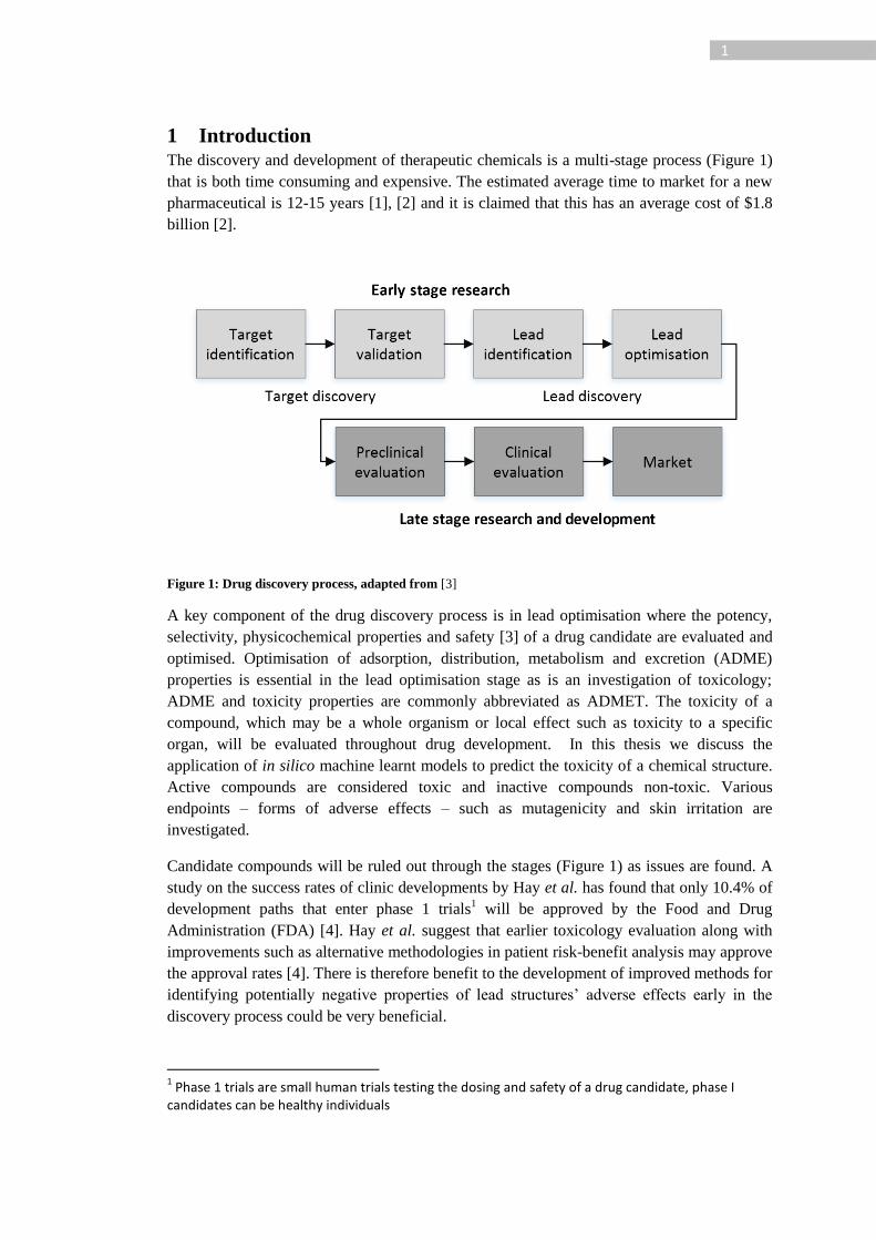
Figure 1: Drug discovery process, adapted from [3] ................................................................ 1
Figure 2: Impurities Classification with Respect to Mutagenic and Carcinogenic, reproduced
from [16] .................................................................................................................................. 5
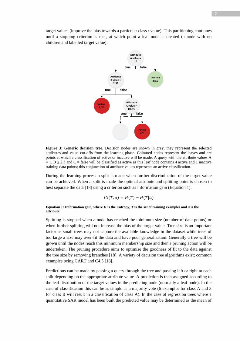
Figure 3: Generic decision tree. Decision nodes are shown in grey, they represent the
selected attributes and value cut-offs from the learning phase. Coloured nodes represent the
leaves and are points at which a classification of active or inactive will be made. A query
with the attribute values A = 1, B ≤ 2.5 and C = false will be classified as active as this leaf
node contains 4 active and 1 inactive training data points; this conjunction of attribute values
represents an active classification. ........................................................................................... 7
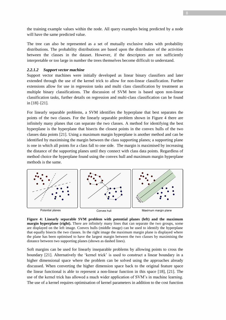
Figure 4: Linearly separable SVM problem with potential planes (left) and the maximum
margin hyperplane (right). There are infinitely many lines that can separate the two groups,
some are displayed on the left image. Convex hulls (middle image) can be used to identify
the hyperplane that equally bisects the two classes. In the right image the maximum margin
plane is displayed where the plane has been optimised to have the largest margin between the
two classes by maximising the distance between two supporting planes (shown as dashed
lines). ........................................................................................................................................ 8
Figure 5: Random Forest algorithm high level workflow, where <x> is the sample size and i
is the ith element of m iterations. For each tree built a selection of the descriptors is chosen
adding the second level of randomisation. ............................................................................. 10
Figure 6: k Nearest Neighbour example, k = 8, supporting training instances represented by
full line. Class indicated by colour coding. ............................................................................ 13
Figure 7: Derek Nexus expert system example ..................................................................... 14
Figure 8: Derek alert 331: Halogenated alkene...................................................................... 24
Figure 9: SOHN modelling overview, adapted from content in [60]..................................... 26
Figure 10: SOHN relationships, where ei represents an example structure, red colouring
represents active and green inactive ....................................................................................... 26
Figure 11: Similarity map example highlight, reproduced from [71] .................................... 32
Figure 12: Emerging pattern mining, left hand represents the bits present in the 7 data point,
the middle represents the bits identified in the emerging pattern and the right shows the
supporting examples for the emerging pattern ....................................................................... 36
Figure 13: Example chemical structure formats .................................................................... 43
Figure 14: Atom centred and linear path fragmentation for distances 0-2 commencing at the
nitrogen atom ......................................................................................................................... 47
Figure 15: Example hashed fingerprint process; red represents bit collisions and orange bits
exceeding the max fingerprint length (1023) ......................................................................... 48
Figure 16: RECAP bond cleavage types [142] ...................................................................... 52
Figure 17: Bond cutting based fragmentation where all combinations of bond cleavages are
undertaken .............................................................................................................................. 52
Figure 18: Reduced graph fragmentation. Step 1 involves identification of the reduced units
using a functional reducer (green units) and a ring reducer (orange units). The reduced graph
represents the reduced units with R6 being a six membered ring and F3 being a 3 membered
functional group. In step 3 the path is enumerated from depths 0 to 2 (representing the full
reduced graph), as the connections are kept the reduced graphs can be expanded back into
fragments................................................................................................................................ 53

x
Figure 19: DNA/RNA bases................................................................................................... 56
Figure 20: DNA mutations ..................................................................................................... 57
Figure 21: Reaction of an amine with a Michael acceptor, reproduced from [150] ............... 57
Figure 22: Bromouracil tautomers. Left representing thymine like and right cytosine like
[148] ....................................................................................................................................... 58
Figure 23: Distribution of the mean (bottom) and max (top) Tanimoto similarity (Ceres
fingerprint) within the datasets ............................................................................................... 63
Figure 24: Testing and evaluation strategy for dermal irritation/corrosion, OECD guideline
404 [171]; assessment steps shown in light blue boxes and possible conclusions in dark blue.
................................................................................................................................................ 70
Figure 25: Balanced accuracy of IBk, DT and RF models with various weights for the
majority class .......................................................................................................................... 76
Figure 26: Stages for the generation of a prediction with interpretation for a query structure.
In the developed implementation the descriptor generation, prediction and enumeration are
handled by pre-existing libraries. These libraries have been used to provide functionality
required for (Q)SAR modelling. The interpretation algorithm has been developed a as a new
standalone library. The complete functionality has then been bundled into full applications.
................................................................................................................................................ 79
Figure 27: SAR elucidation example; where the numbered structure highlights represent the
component being queried. Highlighting of green represents inactive and red active. The
lower structure represents the elucidated SAR with orange representing the deactivated
component and the green the deactivating component. .......................................................... 80
Figure 28: Interpretation high level workflow. The top path consisting of the training data,
model and outputting a prediction and a confidence is independent code (limitations do apply
regarding selection and representation of descriptors). The interpretation algorithm consists
of the bottom path where a feature network is generated, predicted and then the ENCORE
decision tree is used to assess the network and then various summary algorithms can be used
to extract the interpretation. .................................................................................................... 81
Figure 29: ENCORE technology overview. .............................................................................. 82
Figure 30: Directed acyclic graph. Node 0 is a parent of nodes {1,2} and an ascendant of
nodes {1,2,3,4,5}. Node 1 is a parent and ascendant of nodes {3,4}. Node 2 is not a parent of
node 3. .................................................................................................................................... 83
Figure 31: Hierarchical organisation of the features for bitstring {1,3,4} ............................. 85
Figure 32: Fragment feature hierarchy for 1-nitronapthalene. The smallest fragments are at
the bottom (D-F) which combine as the network is traversed upwards towards the original
structure at node A. The atoms are labelled with their original position on the structure
showing how the hierarchy can be generated from atom and bond numbers (not shown)..... 86
Figure 33: Enumerated fragments (left) and theoretical description (right). The bits set in the
fingerprint represent the contribution of the fragments atoms and bonds to the parent
structures fingerprint. A fragment will generate a subset of the bits set in the parent (or the
full set). The numbered fragments on the left represent a numbered row on the right table,
e.g. the benzene fragments 5 and 6 generate the following fingerprint subset: {5,6,7}
whereas the 4th fragment the nitro just generates {0}. ............................................................ 87
Figure 34: Features and their hierarchy. Dashed lines indicate original network for structural
bits only, full lines indicate additional nodes and connections involving the physicochemical
xi
fingerprint. Bits 1, 3 and 4 are a component of the structural fingerprint. Bits 7 and 8 are
components of a single physicochemical property fingerprint .............................................. 88
Figure 35: Node classification rules represented as a decision tree. Each coloured node
represents an assessment type and the questions are asked about the given node or
ascendants/descendants. ......................................................................................................... 90
Figure 36: Network example. The prediction network is coloured according to activity (red =
active, green = inactive), the assessment network is coloured according to assessment type
(red = activating, pink = activity identified, blue = ignore, green = deactivating, orange =
deactivated, purple = negated). .............................................................................................. 92
Figure 37: Network summary variations. Left - explicit, middle - implicit top and right -
implicit bottom. Additional colours indicate: light grey for no incorporation in any summary,
dark grey for incorporation in a different summary, full colour for the nodes utilised in the
specific summary. Arrow indicates a direct parent-child relationship. .................................. 93
Figure 38: Combination enumeration count with pruning. Where the pruning level indicates
the maximum k (number of bits) allowed for the enumeration and all levels below are
included .................................................................................................................................. 95
Figure 39: Discretisation fingerprint vs discretised variable classes where ( is inclusive and ]
is exclusive ............................................................................................................................. 97
Figure 40: Example of interpretation visualisation in Coralie for 1-bromo-2-chloroethane.
The top left shows the structure editor where the query can be drawn, the top right shows the
prediction with the confidence and a textual representation of the interpretation. The lower
section shows the specific information regarding the extracted activations and ID 67802 is
highlighted on the bottom right. Under visualisation the summary mode can be selected,
EXPLICIT_DEACTIVATION is the current method. The ACTIVATING – 14% refers to
the confidence of the model for the selected feature prediction. ........................................... 98
Figure 41: 1-bromo-2-chloroethane assessed feature network. The left network represents the
fragments present in the network shown on the right. Node 1 = Br, node 4 = bromo-alkyl
(single carbon) etc… .............................................................................................................. 99
Figure 42: Model interpretations for 1-(chloromethyl)-4-nitrobenzene using the explicit top
methodology, single red highlight represents an ACTIVATING feature, a coupled orange-
green highlight represents a deactivation where the orange component is the deactivated
feature the green components represents the novel atoms and bonds in the deactivating
feature. ................................................................................................................................. 100
Figure 43: Model assessed networks for 1-(chloromethyl)-4-nitrobenzene. The fragment
network is displayed on the left with the smallest fragments on the bottom and combined as
the network is traversed up to the full query. The various assessments are shown in the
coloured networks on the right where: red = ACTIVATING, pink =
ACTIVITY_IDENTIFIED, blue = IGNORE, green = DEACTIVATING and orange =
DEACTIVATED. ................................................................................................................ 101
Figure 44: Model interpretations for 1-bromo-3-chloropropane, the red highlight represents
the activating motif using any summary methodology ........................................................ 102
Figure 45: Interpretation of 3-methyl-butyl nitrite for all models using any summary
methodology ........................................................................................................................ 102
Figure 46: Interpretation for 2‐hydroxy‐5‐[(E)‐2‐(4‐nitrophenyl)diazen‐1‐yl]benzoate using
the explicit top summary methodology ................................................................................ 103
xii
Figure 47: Interpretation for 2‐hydroxy‐5‐[(E)‐2‐(4‐nitrophenyl)diazen‐1‐yl]benzoate using
the implicit bottom summary methodology. Purple represents the first node predictive active
in a deactivation path. ........................................................................................................... 104
Figure 48: Derek Nexus alert matches for 1-(chloromethyl)-4-nitrobenzene ...................... 104
Figure 49: SOHN model hypothesis matches for 1-(chloromethyl)-4-nitrobenzene ........... 105
Figure 50: Similarity Maps based interpretation for 1-(chloromethyl)-4-nitrobenzene for RF-
C model ................................................................................................................................ 105
Figure 51: Derek Nexus alert matches for 1-bromo-3-chloropropane ................................. 106
Figure 52: SOHN hypotheses matches for 1-bromo-3-chloropropane ................................. 106
Figure 53: Similarity maps interpretation for 1-bromo-3-chloropropane RF-C prediction . 106
Figure 54: Similarity maps interpretation of 3-methyl-butyl nitrite RF-C model ................ 107
Figure 55: Derek Nexus alert matches for 2‐hydroxy‐5‐[(E)‐2‐(4‐nitrophenyl)diazen‐1‐
yl]benzoate ........................................................................................................................... 107
Figure 56: SOHN hypotheses matches for 2‐hydroxy‐5‐[(E)‐2‐(4‐nitrophenyl)diazen‐1‐
yl]benzoate ........................................................................................................................... 107
Figure 57: Similarity maps interpretation of 2‐hydroxy‐5‐[(E)‐2‐(4‐nitrophenyl)diazen‐1‐
yl]benzoate for RF-C ............................................................................................................ 108
Figure 58: Isocyanate identification, Derek Alert, SOHN hypothesis and extracted feature
from IBk, RF, DT ................................................................................................................. 109
Figure 59: 2-ethyloxirane interpretation from RF, IBk and DT models .............................. 110
Figure 60: (bromomethyl)benzene interpretations from RF, IBk and DT ........................... 111
Figure 61: inactive 5-amino-2,4,5-triiodobenzene-1,3-dicarbonyl dichloride ..................... 111
Figure 62: Iterative knowledge mining overview. A dataset is divided into folds and an
iterative approach used to predict each structure and then store the interpretation in a
dictionary .............................................................................................................................. 116
Figure 63: Theoretical representation of a SAR trend tree. The virtual root covers entire
support set, nodes 1-3 coverer level 1 ACTIVATING features. Descendants from a level 1
node (e.g. 1.1, 1.2, 1.1.1) cover specifications of the ACTIVATING feature. The fragments
increase in size as the network descends. ............................................................................. 117
Figure 64: Example SAR trend representation, red indicates active and green inactive ...... 118
Figure 65: Example deactivating child feature with supporting examples and assessment
counts ................................................................................................................................... 119
Figure 66: Coralie high level extension overview. The Coralie application has a number of
core libraries (grouped to Coralie core). ENCORE core builds on top of these Core libraries
to extend both UI and back end functionality (data processing). A modelling API has been
developed extended Weka and using the chemical engine for descriptor calculation.
ENCORE core, the modelling API and the interpretation algorithm are bundled into
ENCORE Coralie plugin. Green represents Lhasa Limited development, blue external
development and orange development undertaken for the ENCORE algorithm. ................ 120
Figure 67: Impact of depth value on hierarchical network size. Blue node represents full
query structure, red lines indicate cut-off points resulting in the left and middle networks. 121
Figure 68: Example dataset profiling of a set of alerts (left) and a set of features (right) .... 122
Figure 69: Distribution of number of ACTIVATING examples per feature for the range of 5
and 50, x axis represents the number of ACTIVATING examples per feature and the y axis
represents the frequency of that count .................................................................................. 126

xiii
Figure 70: Example activating fragment features ................................................................ 126
Figure 71: Top left: frequency of accuracy in ACTIVATING examples, top right: frequency
of accuracy in all supporting examples, bottom: supporting example sensitivity vs supporting
example specificity. ............................................................................................................. 127
Figure 72: Activating support signal vs full support signal ................................................. 128
Figure 73: Subset of epoxide motif SAR extraction. The fragments contained in the feature
are shown on the left with their majority assessment. The tree on the right represents the
relationship between the features in the 4 levels. The features all represent a specification of
the epoxide structural motif, the relationship between the features in shown in node 7 where
the deactivated component is shown in orange and the deactivating component in green. . 130
Figure 74: Supporting example set for epoxide deactivation (node 7), label indicates
concordance of the prediction, red label indicates experimentally active and a green label
experimentally inactive ........................................................................................................ 130
Figure 75: Quinoline SAR tree subsection. The fragments displayed relate to the full feature
and all represent a peri substitution on the quinoline fragment ........................................... 132
Figure 76: Supporting example set for sulphonamide deactivation of quinoline, green label
indicates experimentally inactive, label indicates concordance of the prediction. All
supporting examples are true negatives. .............................................................................. 132
Figure 77: ENCORE feature accuracy vs Derek Nexus accuracy for activating supporting
examples; a triangle indicate a higher accuracy in ENCORE and a circle a higher accuracy in
Derek Nexus......................................................................................................................... 134
Figure 78 thiochromone derived motif and thioxanethone derived motif ........................... 134
Figure 79: Support set of thiochromone subset ................................................................... 135
Figure 80: Histogram of difference between Derek Nexus accuracy and ENCORE accuracy
for feature support sets: positive values indicate higher performance in Derek Nexus and
lower higher performance in of the ENCORE models ........................................................ 135
Figure 81: Example of a Tversky(1,0) and Tversky(0,1) value of 1 and impact for knowledge
mining .................................................................................................................................. 136
Figure 82: Derek Nexus alert vs max similarity to 159 extracted features .......................... 137
Figure 83: Features similar to the N-Nitroso Derek Nexus alert ......................................... 137
Figure 84: Acid halide Derek Nexus pattern and similar feature ......................................... 137
Figure 85: Example perception of aromaticity on xanthone and non-aromaticity in xanthene
containing supporting examples, upper half represent no aromaticity on central ring
(xanthenes), lower half show aromaticity on central ring (xanthones) ................................ 139
Figure 86: Xanthone derived ring features and experimental signals .................................. 139
Figure 87: EP vs feature Tanimoto similarity and Tversky index overview ....................... 140
Figure 88: Example ENCORE feature and EP with a Tversky(1,0) index of 1 ................... 141
Figure 89: Novel features to ENCORE mining (compared with EP mining) ...................... 141
Figure 90: SARpy vs feature similarity overview................................................................ 142
Figure 91: Signal comparison of SARpy alerts with average signal of features with
Tversky(1,0) = 1. Circle for a higher signal in the ENCORE feature, triangle for equal signal
and square for higher signal in SARpy ................................................................................ 143
Figure 92: Performance of features based on cross validationTable 30 shows the manually
extracted features from the SAR tree for the 10 fold cross validation model; ACTIVATING
features that have a signal ≥0.5 have been selected. Additionally, ACTIVITY_IDENTIFIED

xiv
features have been included where the signal is higher than the parent feature such as F5
(unsaturated ester, acid, alcohol motif) with a signal of 0.640 and its child feature F6
(unsaturated ester motif) with a signal of 0.750. .................................................................. 146
Figure 93: Example of extracted ACTIVATING features ................................................... 148
xv
List of equations
Equation 1: Information gain, where H is the Entropy, T is the set of training examples and a
is the attribute ........................................................................................................................... 7
Equation 2: Unweighted average for combining model predictions in bagging [19], where M
represents the number of models, and ym(x) the prediction for a given model ........................ 9
Equation 3: kNN for binary classification, where y(x) is the predicted class of the query, wj
is the weight for instance j and yσ(j) is the class of instance j and k is the number of instances.
wj is 1 for all j in the unweighted approach ........................................................................... 12
Equation 4: Accuracy (ACC) ................................................................................................. 18
Equation 5: Balanced accuracy (BAC) .................................................................................. 18
Equation 6: Sensitivity (SEN) ................................................................................................ 18
Equation 7: Specificity (SPEC) ............................................................................................. 18
Equation 8 Matthew’s correlation coefficient (MCC) ........................................................... 18
Equation 9 Positive predictive value (PPV) ........................................................................... 18
Equation 10: Franke et al. feature importance [60], where x is a fingerprint with the presence
(fi = 1) or absence (fi = 0) of feature fi. ................................................................................. 31
Equation 11: Determination of fragment contribution, two component structures [73] ........ 32
Equation 12: Determination of fragment contribution in multi component structures [73],
where .. indicates a multi component fragment (A is not connected to C in the graph) ........ 33
Equation 13: Interpretation of a three component structure with two activating causes (A,C)
............................................................................................................................................... 33
Equation 14: Equation 6 Emerging pattern support [90]. ...................................................... 35
Equation 15 Emerging pattern growth rate [90], where pat is the emerging patter, D1 is the
first class and D2 is the second class. ..................................................................................... 35
Equation 16: SARpy likelihood ratio [94], true positives (TP) are active structures
containing the fragments and false positives (FP) are inactive structures containing the
fragment. ................................................................................................................................ 36
Equation 17: Tanimoto similarity for binary features, where XA represents the bits set in A,
XB represents the bits set in B. [117] ..................................................................................... 44
Equation 18: Tversky index for binary features, where XA represents the bits set in A, XB
represents the bits set in B. α and β represent weightings for XA and XB and \ represents the
relative complement [117] ..................................................................................................... 44
Equation 19: Potts and Guy equation for logKp[133], MW = molecular weight .................. 50
Equation 20: Class weight for given class C .......................................................................... 73
Equation 21: Combinations without repetition where n is the number of items and k is the
desired number of items ......................................................................................................... 84
Equation 22: Total number of enumerable combinations where n is the total number of
components (bits) ................................................................................................................... 84
Equation 23: Signal calculation for a given feature ............................................................. 128

xvi
List of code snippets
Code snippet 1: Similarity maps atom weight calculation pseudo code, reproduced from [71]
................................................................................................................................................ 32
Code snippet 2: Identifying identical structures with fingerprints ......................................... 49
Code snippet 3: Network generation pseudo-code for generating a network utilising a
structural fingerprint and physicochemical descriptors .......................................................... 88
Code snippet 4: Pseudo-code for identifying descendant relationship. Atoms, bonds and
physchem represent the number of each element in the current node after removing the
elements present in the compare node. ................................................................................... 89
Code snippet 5: Hierarchy generation .................................................................................... 89
Code snippet 6: Pseudo-code for the extraction of explicit and implicit top interpretation
summary ................................................................................................................................. 94
Code snippet 7: Pseudo-code for explicit bottom summary interpretation extraction ........... 94
Code snippet 8: Iterative knowledge mining approach ........................................................ 117

xvii
List of tables
Table 1: Example of read across on artificial data points ...................................................... 13
Table 2: Physicochemical descriptor applicability domains [25] .......................................... 17
Table 3: Performance metrics ................................................................................................ 18
Table 4: ToxAlerts literature sources for Mutagenicity and Skin sensitisation ..................... 24
Table 5: Examples of publicly available toxicity data partially reproduced from [110] ....... 40
Table 6: Selection of descriptor calculation packages ........................................................... 45
Table 7: Ames mutagenicity strain details [153] ................................................................... 58
Table 8 Ashby and Tennant structural alerts [52] .................................................................. 60
Table 9: Learning algorithm details ....................................................................................... 65
Table 10: Cross validation performance of the selected model from each algorithm +
descriptor combination ........................................................................................................... 66
Table 11: Test set performance of the selected model from each algorithm + descriptor
combination............................................................................................................................ 66
Table 12: Performance of selected models and external models against validation data ...... 67
Table 13: GHS classifications for skin irritation and corrosion [168] ................................... 68
Table 14: Skin irritation datasets ........................................................................................... 72
Table 15: Descriptor details ................................................................................................... 72
Table 16: Class weights ......................................................................................................... 74
Table 17: Cross validation performance of Ceres + logKp fingerprint models ..................... 75
Table 18: Best two models from each learning algorithm (cross validation) and Ceres
fingerprint only model ........................................................................................................... 76
Table 19: Model performance of PaDEL external validation set .......................................... 77
Table 20: Assessment rules. The jagged line indicates the node with the assessment type
described, + represents an active prediction and – a negative prediction. ............................. 91
Table 21: Descriptor limitation .............................................................................................. 96
Table 22 Change in model performance as a result of removing logKp bits from validation
set ......................................................................................................................................... 112
Table 23 Changes as a result of removing LogKp bits ........................................................ 112
Table 24: Coverage of dataset with various knowledge mining parameterisation
configurations ...................................................................................................................... 124
Table 25: Node details for epoxide SAR tree subset ........................................................... 129
Table 26 Quinoline feature tree node details ....................................................................... 131
Table 27: Similarity parameterisation and meaning ............................................................ 136
Table 28: Derek Nexus fired alerts and performance against PaDEL training set .............. 144
Table 29: SOHN extracted active hypotheses from PaDEL harmonised skin irritation hazard
training set ............................................................................................................................ 145
Table 30: Selected features from PaDEL skin irritation hazard training set, depth = 3, rings =
true, functions = true, fusions = false, cross validation folds = 10 ...................................... 147
Table 31: Comparison of ENCORE features to Derek Nexus alerts and SOHN hypotheses
............................................................................................................................................. 147
Table 32: ACTIVATING feature counts from the LogKP RF, IBk and DT mining ........... 149

1
1 Introduction The discovery and development of therapeutic chemicals is a multi-stage process (Figure 1)
that is both time consuming and expensive. The estimated average time to market for a new
pharmaceutical is 12-15 years [1], [2] and it is claimed that this has an average cost of $1.8
billion [2].
Figure 1: Drug discovery process, adapted from [3]
A key component of the drug discovery process is in lead optimisation where the potency,
selectivity, physicochemical properties and safety [3] of a drug candidate are evaluated and
optimised. Optimisation of adsorption, distribution, metabolism and excretion (ADME)
properties is essential in the lead optimisation stage as is an investigation of toxicology;
ADME and toxicity properties are commonly abbreviated as ADMET. The toxicity of a
compound, which may be a whole organism or local effect such as toxicity to a specific
organ, will be evaluated throughout drug development. In this thesis we discuss the
application of in silico machine learnt models to predict the toxicity of a chemical structure.
Active compounds are considered toxic and inactive compounds non-toxic. Various
endpoints – forms of adverse effects – such as mutagenicity and skin irritation are
investigated.
Candidate compounds will be ruled out through the stages (Figure 1) as issues are found. A
study on the success rates of clinic developments by Hay et al. has found that only 10.4% of
development paths that enter phase 1 trials1 will be approved by the Food and Drug
Administration (FDA) [4]. Hay et al. suggest that earlier toxicology evaluation along with
improvements such as alternative methodologies in patient risk-benefit analysis may approve
the approval rates [4]. There is therefore benefit to the development of improved methods for
identifying potentially negative properties of lead structures’ adverse effects early in the
discovery process could be very beneficial.
1 Phase 1 trials are small human trials testing the dosing and safety of a drug candidate, phase I
candidates can be healthy individuals
2
A Structure Activity Relationship (SAR) model is an in silico model built to map trends in
data that can be used to link molecular structures to a target activity, when this is done in a
quantitative manner the model is considered to be a Quantitative Structure Activity
Relationship, QSAR; together SAR and QSAR are referred to as (Q)SAR. There is some
debate between the terms SAR and QSAR in that there is disagreement over what makes a
model a QSAR instead of a SAR. The Organisation of Economic Co-operation and
Development (OECD) define the term (Q)SAR to refer to either qualitative structure activity
relationships or quantitative structure activity relationships where the qualitative models are
derived from non-continuous data such as binary activity and qualitative models are derived
from continuous data such as potency [5]. Models can be built using a variety of descriptors
and learning techniques. Data and descriptors are discussed in chapter 4 and various
modelling techniques in chapter 2. In this thesis (Q)SAR refers to the prediction of a
quantitative value and SAR refers to the prediction of a qualitative value such as
active/inactive.
The focus of this thesis is on the application of qualitative SAR models for toxicity
prediction, specifically on the improvement of the interpretability of machine learned models
and their utilisation in knowledge mining. The interpretability of (Q)SAR models is a
limitation of many models [6], [7]. Interpretable models lend themselves to better utilisation
both in drug discovery and regulatory acceptance [6], [8]. The interpretability of a (Q)SAR
model is commonly attributed to an appropriate choice in descriptors involving statistical
descriptor selection as well as chemically meaningful choices accounting for believed
mechanisms of action [8], [9]. However, even with sufficiently interpretable descriptors if an
algorithm provides no transparency for the prediction that has been made it is not possible to
understand the prediction provided by the model.
Predictive models for toxicity – and ADME – rely on the similarity principle; similar
structures exhibit similar activity [1]. There are three main methods for predicting the
toxicity of compounds: grouping approaches such as read across, (Quantitative/Qualitative)
Structure Activity/Property Relationships (Q)SARs / (Q)SPRs built using machine
learning/statistical modelling and expert systems. Weight of evidence (WoE) approaches
may use multiple of each of these techniques. In the machine learning approach a learning
algorithm is used to identify trends in training sets which can then be used in the prediction
of the property of interest for new structures. These methods vary in accuracy and
interpretation depending on the learning algorithm used and descriptors chosen. Among the
most interpretable are white-box model. All these methods rely on statistical relationships
within the training set between descriptors and the property of interest. In chapter 2 we
discuss computational toxicology introducing various machine learning concepts and
algorithms. Practical considerations of (Q)SAR modelling are highlighted and factors
affecting the acceptance of the resultant models are introduced. In chapter 3 we discuss
existing algorithms for both (Q)SAR modelling and rule extraction / knowledge mining from
both data and models.
The work discussed throughout this thesis focusses on the development of interpretation
strategies for (Q)SAR models where an interpretable learning algorithm (white box) has not
been used in the development of a model. The reasons for using such modelling approaches
are discussed in chapter 2 and various existing interpretation strategies in chapter 3. The
work aims to provide a universal type interpretation that allows for the use of the best
3
performing model regardless of the algorithm’s ability to provide transparent reasoning. The
novel algorithm for model interpretation is detailed in chapter 6 along with its application to
Ames mutagenicity and harmonised hazard code for skin irritation prediction.
The addition of an interpretation methodology to the prediction process could aid in the
regulatory approval by helping move towards meeting the interpretable requirement of the
OECD guidelines [10]. Where the interpretation does not meet the mechanistic component of
OECD principle 5 it will still aid towards better utilisation of the predictions from a (Q)SAR.
A parallel benefit is in aiding the depth of utilisation of predictions from (Q)SAR models.
In addition to the interpretation of (Q)SAR models the work discussed here aims to further
the usability of in silico models by providing a methodology for extracting SAR rules from
learnt (Q)SAR models and providing strategies for their use with the development of
knowledge based expert systems. To set the scene, we detail in Chapter 2 the background
material on computational toxicology together with a discussion of a variety of machine
learning and (Q)SAR techniques. We then move on to a review of the current state of
interpretable (Q)SAR modelling, in Chapter 3. Various cheminformatic concepts, software
and approaches relevant to the understanding of the subsequent chapters are discussed in
Chapter 4. The research contribution will be demonstrated and evaluated in the context of
two toxicological endpoints: mutagenicity and skin irritation. These will be introduced
Chapter 5, which then focuses on the model building activities for the respective end points.
The new interpretation algorithm is then presented in Chapter 6. This interpretation
algorithm is then used in the development of the knowledge mining algorithm that is
presented in Chapter 7 and applied to the same mutagenicity and skin data. Finally, a
conclusion of the thesis is provided in Chapter 8.
4
2 Computational toxicology: (Q)SAR and macine learning In this chapter we outline and discuss concepts within cheminformatics (informatics in the
domain of chemistry) covering machine learning and (Q)SAR modelling. Algorithms used in
model building in later chapters are detailed along with general strategies used in the model
building process. The endpoints and models are discussed in chapter 5, with the
interpretation algorithm theory and application in chapter 6 and then the knowledge mining
algorithm and results in chapter 7.
As stated in chapter 1 (Q)SAR and (Q)SPR modelling can be considered the application of
statistical techniques and machine learning to the modelling of structural activities or
properties. The goal of the modelling is to derive relationships between the training data
(chemical dataset) and the target value of interest so that the models may be applied to
predict the properties or activities of new compounds. To this end descriptors are used to
describe the structures in the training set and a learning algorithm is used to develop a model
which captures the relationships between the descriptors and the target value such as
solubility or mutagenicity.
“Essentially, all models are wrong, but some are useful” (George E. P.
Box)2
A model will not be a perfect predictor. However, if it predicts accurately a large amount of
the time, provides a meaningful measure of confidence and supports the purpose for which is
it built the model will provide benefit. Predictive error can occur for a number of reasons.
Chemicals that are far from the chemical space of the training set represent an area of space
where knowledge is sparse or non-existent; when extrapolating to form a prediction the
accuracy of the predictions is lower than when the prediction is interpolated (query falls
within the space of the training set). Trends in the training set may be biased resulting in the
training of the model biasing the predictions for a particular class and or region on a
continuous variable. Over training may occur resulting in a model that is highly predictive of
similar/training compounds but fails to generalise and achieve high external predictivity.
A model is limited by the data used for training; models built for toxicity prediction will not
be exempt from the garbage in, garbage out issue. If a model is built on erroneous data
(garbage in) then we cannot expect the model to produce sensible output (garbage out).
Further issues are exhibited where the activity is caused by a large number of independent
features such as with mutagenicity. Uneven distribution of features or classes in the dataset
can lead to some knowledge being missed due to sparseness. Local modelling strategies are
likely appropriate where an endpoint relies on multiple independent causes.
Good overviews of cheminformatics and (Q)SAR modelling as well as historical
perspectives can be found in Tropha et al. [8], Gasteiger and Engel [11], Gillet and Leach
[12], Varnek and Baskin [7] and Cherkasov et al. [8].
2 George E. P. Box was a Professor Emeritus of Statistics at the University of Wisconsin, the quotation
is taken from Empirical Model-Building and Response Surfaces (1987)
5
2.1 (Q)SAR and regulatory submission
(Q)SAR models are currently under investigation for usage in regulatory submission of
drugs and cosmetics and in some cases are approved for use in the assessment of specific
toxicological concerns.
REACH (Registration, Evaluation, Authorisation & restriction of Chemicals) is a European
Union regulation that came into force in 2007. Reach covers substances such as human and
veterinary medicines, food, agrochemicals and other substances which are manufactured or
imported into the EU in quantities of 1 tonne or more per year [13]. Annex XI states that a
(Q)SAR model may be used instead of testing given the following conditions are met [14]:
1) Results are derived from a (Q)SAR model whose scientific validity has been
established
2) The substance falls within the applicability domain (see section 2.3.3) of the model
3) Results are adequate for the purpose of classification and labelling and/or risk
assessment
4) Adequate and reliable documentation of the applied method is provided.
The European Chemicals Agency (ECHA) allow under the REACH regulation submissions
from read across models where the approach is deemed to be adequate so as to avoid
unnecessary testing in addition to supporting WoE conclusions [15]. The utilisation of
(Q)SAR models for alternatives to testing are supported by being transparent and detailed.
Providing an explanation of the reason behind a model’s prediction will likely support
regulatory submission of (Q)SAR predictions.
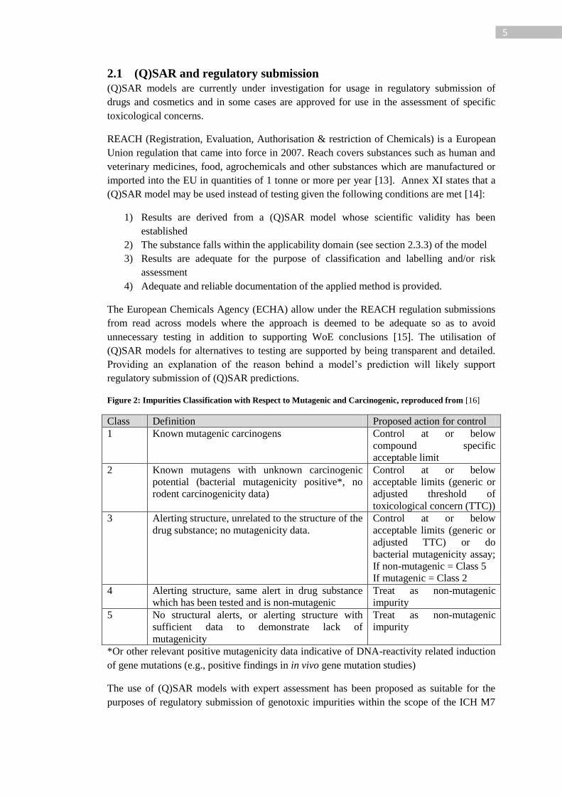
Figure 2: Impurities Classification with Respect to Mutagenic and Carcinogenic, reproduced from [16]
Class Definition Proposed action for control
1 Known mutagenic carcinogens Control at or below
compound specific
acceptable limit
2 Known mutagens with unknown carcinogenic
potential (bacterial mutagenicity positive*, no
rodent carcinogenicity data)
Control at or below
acceptable limits (generic or
adjusted threshold of
toxicological concern (TTC))
3 Alerting structure, unrelated to the structure of the
drug substance; no mutagenicity data.
Control at or below
acceptable limits (generic or
adjusted TTC) or do
bacterial mutagenicity assay;
If non-mutagenic = Class 5
If mutagenic = Class 2
4 Alerting structure, same alert in drug substance
which has been tested and is non-mutagenic
Treat as non-mutagenic
impurity
5 No structural alerts, or alerting structure with
sufficient data to demonstrate lack of
mutagenicity
Treat as non-mutagenic
impurity
*Or other relevant positive mutagenicity data indicative of DNA-reactivity related induction
of gene mutations (e.g., positive findings in in vivo gene mutation studies)
The use of (Q)SAR models with expert assessment has been proposed as suitable for the
purposes of regulatory submission of genotoxic impurities within the scope of the ICH M7

6
[16] guidelines for genotoxocity hazard detection [17]. The draft guidelines propose that a
classification under five classes can be undertaken with the support of (Q)SAR
methodologies.
If data is not available to classify compounds based on database, literature and bacterial
mutagenicity experimental data (classes 1, 2 or 5) (Q)SAR models can be utilised to support
the classification of classes 3, 4 or 5 [16]. Models developed for the prediction of bacterial
mutagenicity assays can be utilised in a combination of an expert rule-based approach and a
complementary statistical based approach; the models should conform to the OECD
guidelines [16], for more detail on the OECD guidelines see section 2.3.2. Although the
predictions from (Q)SAR models can be used, they should be supplemented with expert
assessment to support the given predictions and help to clarify where results conflict [16].
Given a sufficiently developed and transparent model two independent negative predictions
for mutagenicity allow for the classification of a compound as a non-mutagenic impurity.
2.2 Learning and algorithms
There exists a large variety of learning algorithms each with their own benefits and
disadvantages. There is also a variety of classification systems of grouping the learning
algorithms such as: kernel methods, neural networks, recursive partitioning. At a high level
two groupings are utilised here: white box vs black box and supervised vs unsupervised.
The terms white box and black box are used to indicate the level of
interpretability/transparency of a model and/or prediction generated from the use of the
algorithm. A white box model is considered to be interpretable whereas a black box model is
considered uninterpretable, i.e. the user does not know why the resultant prediction was
made. The focus of this research effort is to improve the interpretability of black box SAR
models as applied to toxicity prediction.
2.2.1 Supervised learning
Supervised learning aims to discover relationships between descriptors and the prediction
target and for this the target value and descriptors of every training structure is provided to
the algorithm. Many algorithms exist with varying complexity and degree of interpretation.
The complexity of the training set dictates to some degree the complexity of machine
learning algorithm used.
Simple problems may be linearly separable and allow for the use of learning algorithms such
as linear regression or least squares. For more complex problems algorithms such as decision
trees, random forests, neural networks or support vector machines may be required. A
selection of learning algorithms has been utilised in this work to allow for a comparison
across a section of the learning strategies.
2.2.1.1 Decision tree (recursive partitioning)
Decision trees fall into the white box model category as the path through the tree gives the
cause of the prediction. A decision tree is built from a dataset of attributes and target values
and can represent classification tasks when the target is a list of classes or regression when
presented with a continuous target value.
Decision tree methods divide the dataset based on attribute values via recursive partitioning
[18], the split points’ are chosen to improve the discrimination between the training data
7
target values (improve the bias towards a particular class / value). This partitioning continues
until a stopping criterion is met, at which point a leaf node is created (a node with no
children and labelled target value).
Figure 3: Generic decision tree. Decision nodes are shown in grey, they represent the selected
attributes and value cut-offs from the learning phase. Coloured nodes represent the leaves and are
points at which a classification of active or inactive will be made. A query with the attribute values A
= 1, B ≤ 2.5 and C = false will be classified as active as this leaf node contains 4 active and 1 inactive
training data points; this conjunction of attribute values represents an active classification.
During the learning process a split is made when further discrimination of the target value
can be achieved. When a split is made the optimal attribute and splitting point is chosen to
best separate the data [18] using a criterion such as information gain (Equation 1).
( ) ( ) ( )
Equation 1: Information gain, where H is the Entropy, T is the set of training examples and a is the
attribute
Splitting is stopped when a node has reached the minimum size (number of data points) or
when further splitting will not increase the bias of the target value. Tree size is an important
factor as small trees may not capture the available knowledge in the dataset while trees of
too large a size may over-fit the data and have poor generalisation. Generally a tree will be
grown until the nodes reach this minimum membership size and then a pruning action will be
undertaken. The pruning procedure aims to optimise the goodness of fit to the data against
the tree size by removing branches [18]. A variety of decision tree algorithms exist; common
examples being CART and C4.5 [18].
Predictions can be made by passing a query through the tree and passing left or right at each
split depending on the appropriate attribute value. A prediction is then assigned according to
the leaf distribution of the target values in the predicting node (normally a leaf node). In the
case of classification this can be as simple as a majority vote (6 examples for class A and 3
for class B will result in a classification of class A). In the case of regression trees where a
quantitative SAR model has been built the predicted value may be determined as the mean of
8
the training example values within the node. All query examples being predicted by a node
will have the same predicted value.
The tree can also be represented as a set of mutually exclusive rules with probability
distributions. The probability distributions are based upon the distribution of the activities
between the classes in the dataset. However, if the descriptors are not sufficiently
interpretable or too large in number the trees themselves become difficult to understand.
2.2.1.2 Support vector machine
Support vector machines were initially developed as linear binary classifiers and later
extended through the use of the kernel trick to allow for non-linear classification. Further
extensions allow for use in regression tasks and multi class classification by treatment as
multiple binary classifications. The discussion of SVM here is based upon non-linear
classification tasks, further details on regression and multi-class classification can be found
in [18]–[21].
For linearly separable problems, a SVM identifies the hyperplane that best separates the
points of the two classes. For the linearly separable problem shown in Figure 4 there are
infinitely many planes that can separate the two classes. A method for identifying the best
hyperplane is the hyperplane that bisects the closest points in the convex hulls of the two
classes data points [21]. Using a maximum margin hyperplane is another method and can be
identified by maximising the margin between the class supporting planes; a supporting plane
is one in which all points for a class fall to one side. The margin is maximised by increasing
the distance of the supporting planes until they connect with class data points. Regardless of
method choice the hyperplane found using the convex hull and maximum margin hyperplane
methods is the same.
Figure 4: Linearly separable SVM problem with potential planes (left) and the maximum
margin hyperplane (right). There are infinitely many lines that can separate the two groups, some
are displayed on the left image. Convex hulls (middle image) can be used to identify the hyperplane
that equally bisects the two classes. In the right image the maximum margin plane is displayed where
the plane has been optimised to have the largest margin between the two classes by maximising the
distance between two supporting planes (shown as dashed lines).
Soft margins can be used for linearly inseparable problems by allowing points to cross the
boundary [21]. Alternatively the ‘kernel trick’ is used to construct a linear boundary in a
higher dimensional space where the problem can be solved using the approaches already
discussed. When converting the higher dimension space back to the original feature space
the linear functional is able to represent a non-linear function in this space [18], [21]. The
use of the kernel trick has allowed a much wider application of SVM’s in machine learning.
The use of a kernel requires optimisation of kernel parameters in addition to the cost function
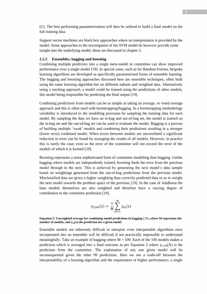
9
(C). The best performing parameterisation will then be utilised to build a final model on the
full training data.
Support vector machines are black box approaches where no interpretation is provided by the
model. Some approaches to the investigation of the SVM model do however provide some
insight into the underlying model; these are discussed in chapter 3.
2.2.2 Ensembles, bagging and boosting
Combining multiple predictors into a single meta-model or committee can show improved
performance over a single model [19]. In special cases, such as for Random Forests, bespoke
learning algorithms are developed as specifically parameterised forms of ensemble learning.
The bagging and boosting approaches discussed here are ensemble techniques, often built
using the same learning algorithm but on different subsets and weighted data. Alternatively
using a stacking approach, a model could be trained using the predictions of other models;
this model being responsible for predicting the final output [19].
Combining predictions from models can be as simple as taking an average, or voted average
approach and this is often used with bootstrapping/bagging. In a bootstrapping methodology
variability is introduced to the modelling processes by sampling the training data for each
model. By sampling the data we have an in-bag and out-of-bag set, the model is trained on
the in-bag set and the out-of-bag set can be used to evaluate the model. Bagging is a process
of building multiple ‘weak’ models and combining their predictions resulting in a stronger
(lower error) combined model. When errors between models are uncorrelated a significant
reduction in error can be found by averaging the results of all models. However, in practice
this is rarely the case; even so the error of the committee will not exceed the error of the
models of which it is formed [19].
Boosting represents a more sophisticated form of committee modelling than bagging. Unlike
bagging where models are independently trained, boosting feeds the error from the previous
model through to the next. This is achieved by generating the next model’s data sample
based on weightings generated from the out-of-bag predictions from the previous model.
Misclassified data are given a higher weighting than correctly predicted data so as to weight
the next model towards the problem space of the previous [19]. In the case of AdaBoost the
base models themselves are also weighted and therefore have a varying degree of
contribution to the committee prediction [19].
( )
∑ ( )
Equation 2: Unweighted average for combining model predictions in bagging [19], where M represents the
number of models, and ym(x) the prediction for a given model
Ensemble models are inherently difficult to interpret; even interpretable algorithms once
incorporated into an ensemble will be difficult if not practically impossible to understand
meaningfully. Take an example of bagging where M = 100. Each of the 100 models makes a
prediction which is averaged into a final outcome as per Equation 2 where yCOM(X) is the
prediction from the committee. The explanation of any one given model will be
inconsequential given the other 99 predictions. Here we see a trade-off between the
interpretability of a learning algorithm and the requirement of higher performance; a single
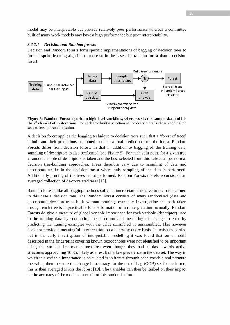
10
model may be interpretable but provide relatively poor performance whereas a committee
built of many weak models may have a high performance but poor interpretability.
2.2.2.1 Decision and Random forests
Decision and Random forests form specific implementations of bagging of decision trees to
form bespoke learning algorithms, more so in the case of a random forest than a decision
forest.
Figure 5: Random Forest algorithm high level workflow, where <x> is the sample size and i is
the ith
element of m iterations. For each tree built a selection of the descriptors is chosen adding the
second level of randomisation.
A decision forest applies the bagging technique to decision trees such that a ‘forest of trees’
is built and their predictions combined to make a final prediction from the forest. Random
Forests differ from decision forests in that in addition to bagging of the training data,
sampling of descriptors is also performed (see Figure 5). For each split point for a given tree
a random sample of descriptors is taken and the best selected from this subset as per normal
decision tree-building approaches. Trees therefore vary due to sampling of data and
descriptors unlike in the decision forest where only sampling of the data is performed.
Additionally pruning of the trees is not performed. Random Forests therefore consist of an
averaged collection of de-correlated trees [18].
Random Forests like all bagging methods suffer in interpretation relative to the base learner,
in this case a decision tree. The Random Forest consists of many randomised (data and
descriptors) decision trees built without pruning; manually investigating the path taken
through each tree is impracticable for the formation of an interpretation manually. Random
Forests do give a measure of global variable importance for each variable (descriptor) used
in the training data by scrambling the descriptor and measuring the change in error by
predicting the training examples with the value scrambled vs unscrambled. This however
does not provide a meaningful interpretation on a query-by-query basis. In activities carried
out in the early investigation of interpretable modelling it was found that some motifs
described in the fingerprint covering known toxicophores were not identified to be important
using the variable importance measures even though they had a bias towards active
structures approaching 100%; likely as a result of a low prevalence in the dataset. The way in
which this variable importance is calculated is to iterate through each variable and permute
the value, then measure the change in accuracy for the out of bag (OOB) set for each tree;
this is then averaged across the forest [18]. The variables can then be ranked on their impact
on the accuracy of the model as a result of this randomisation.
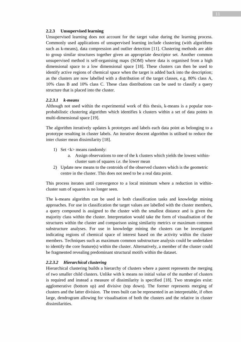
11
2.2.3 Unsupervised learning
Unsupervised learning does not account for the target value during the learning process.
Commonly used applications of unsupervised learning include clustering (with algorithms
such as k-means), data compression and outlier detection [11]. Clustering methods are able
to group similar structures together given an appropriate descriptor set. Another common
unsupervised method is self-organising maps (SOM) where data is organised from a high
dimensional space to a low dimensional space [18]. These clusters can then be used to
identify active regions of chemical space when the target is added back into the description;
as the clusters are now labelled with a distribution of the target classes, e.g. 80% class A,
10% class B and 10% class C. These class distributions can be used to classify a query
structure that is placed into the cluster.
2.2.3.1 k-means
Although not used within the experimental work of this thesis, k-means is a popular non-
probabilistic clustering algorithm which identifies k clusters within a set of data points in
multi-dimensional space [19].
The algorithm iteratively updates k prototypes and labels each data point as belonging to a
prototype resulting in cluster labels. An iterative descent algorithm is utilised to reduce the
inter cluster mean dissimilarity [18].
1) Set <k> means randomly:
a. Assign observations to one of the k clusters which yields the lowest within-
cluster sum of squares i.e. the lower mean
2) Update new means to the centroids of the observed clusters which is the geometric
centre in the cluster. This does not need to be a real data point.
This process iterates until convergence to a local minimum where a reduction in within-
cluster sum of squares is no longer seen.
The k-means algorithm can be used in both classification tasks and knowledge mining
approaches. For use in classification the target values are labelled with the cluster members,
a query compound is assigned to the cluster with the smallest distance and is given the
majority class within the cluster. Interpretation would take the form of visualisation of the
structures within the cluster and comparison using similarity metrics or maximum common
substructure analyses. For use in knowledge mining the clusters can be investigated
indicating regions of chemical space of interest based on the activity within the cluster
members. Techniques such as maximum common substructure analysis could be undertaken
to identify the core feature(s) within the cluster. Alternatively, a member of the cluster could
be fragmented revealing predominant structural motifs within the dataset.
2.2.3.2 Hierarchical clustering
Hierarchical clustering builds a hierarchy of clusters where a parent represents the merging
of two smaller child clusters. Unlike with k means no initial value of the number of clusters
is required and instead a measure of dissimilarity is specified [18]. Two strategies exist:
agglomerative (bottom up) and divisive (top down). The former represents merging of
clusters and the latter division. The trees built can be represented in an interpretable, if often
large, dendrogram allowing for visualisation of both the clusters and the relative in cluster
dissimilarities.
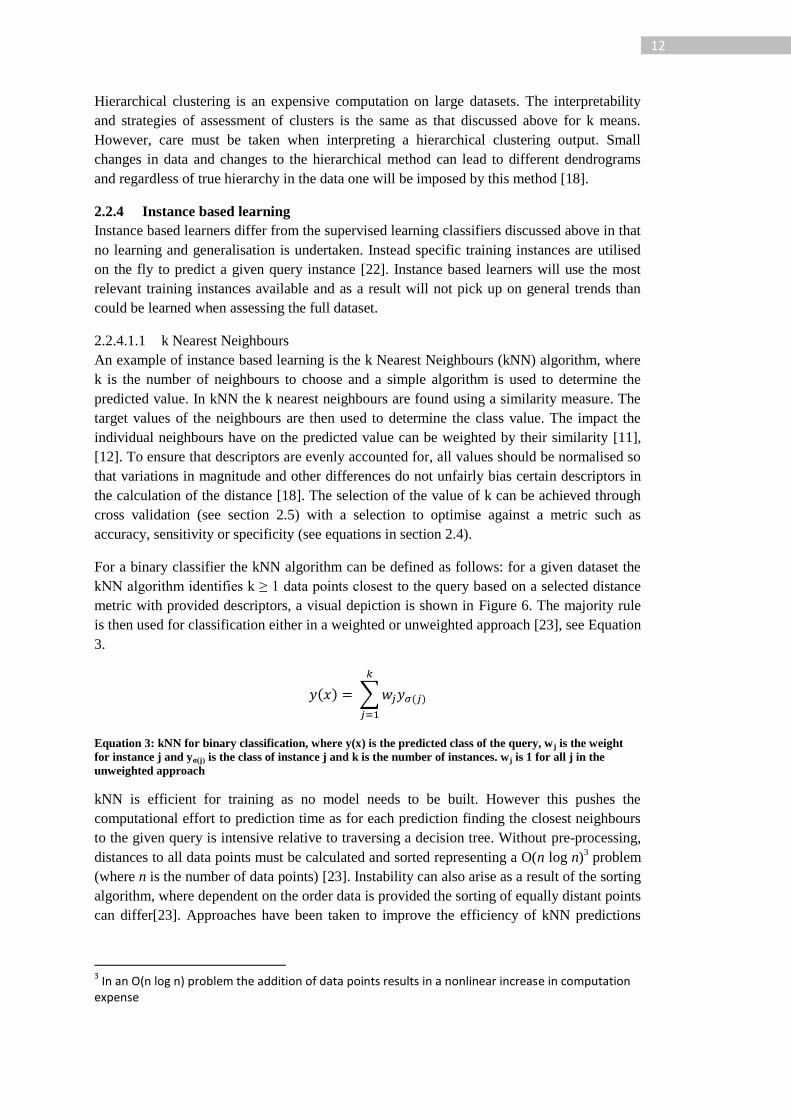
12
Hierarchical clustering is an expensive computation on large datasets. The interpretability
and strategies of assessment of clusters is the same as that discussed above for k means.
However, care must be taken when interpreting a hierarchical clustering output. Small
changes in data and changes to the hierarchical method can lead to different dendrograms
and regardless of true hierarchy in the data one will be imposed by this method [18].
2.2.4 Instance based learning
Instance based learners differ from the supervised learning classifiers discussed above in that
no learning and generalisation is undertaken. Instead specific training instances are utilised
on the fly to predict a given query instance [22]. Instance based learners will use the most
relevant training instances available and as a result will not pick up on general trends than
could be learned when assessing the full dataset.
2.2.4.1.1 k Nearest Neighbours
An example of instance based learning is the k Nearest Neighbours (kNN) algorithm, where
k is the number of neighbours to choose and a simple algorithm is used to determine the
predicted value. In kNN the k nearest neighbours are found using a similarity measure. The
target values of the neighbours are then used to determine the class value. The impact the
individual neighbours have on the predicted value can be weighted by their similarity [11],
[12]. To ensure that descriptors are evenly accounted for, all values should be normalised so
that variations in magnitude and other differences do not unfairly bias certain descriptors in
the calculation of the distance [18]. The selection of the value of k can be achieved through
cross validation (see section 2.5) with a selection to optimise against a metric such as
accuracy, sensitivity or specificity (see equations in section 2.4).
For a binary classifier the kNN algorithm can be defined as follows: for a given dataset the
kNN algorithm identifies k ≥ 1 data points closest to the query based on a selected distance
metric with provided descriptors, a visual depiction is shown in Figure 6. The majority rule
is then used for classification either in a weighted or unweighted approach [23], see Equation
3.
( ) ∑ ( )
Equation 3: kNN for binary classification, where y(x) is the predicted class of the query, wj is the weight
for instance j and yσ(j) is the class of instance j and k is the number of instances. wj is 1 for all j in the
unweighted approach
kNN is efficient for training as no model needs to be built. However this pushes the
computational effort to prediction time as for each prediction finding the closest neighbours
to the given query is intensive relative to traversing a decision tree. Without pre-processing,
distances to all data points must be calculated and sorted representing a O(n log n)3 problem
(where n is the number of data points) [23]. Instability can also arise as a result of the sorting
algorithm, where dependent on the order data is provided the sorting of equally distant points
can differ[23]. Approaches have been taken to improve the efficiency of kNN predictions
3 In an O(n log n) problem the addition of data points results in a nonlinear increase in computation
expense
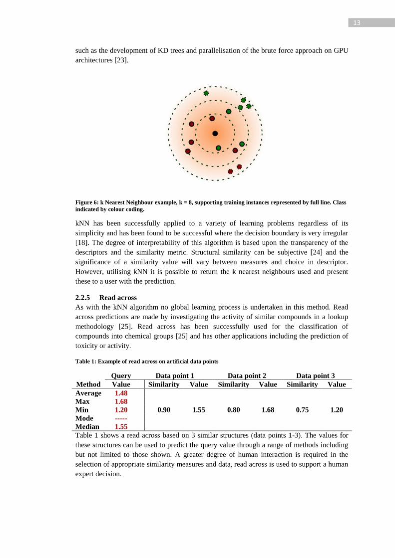
13
such as the development of KD trees and parallelisation of the brute force approach on GPU
architectures [23].
Figure 6: k Nearest Neighbour example, k = 8, supporting training instances represented by full line. Class
indicated by colour coding.
kNN has been successfully applied to a variety of learning problems regardless of its
simplicity and has been found to be successful where the decision boundary is very irregular
[18]. The degree of interpretability of this algorithm is based upon the transparency of the
descriptors and the similarity metric. Structural similarity can be subjective [24] and the
significance of a similarity value will vary between measures and choice in descriptor.
However, utilising kNN it is possible to return the k nearest neighbours used and present
these to a user with the prediction.
2.2.5 Read across
As with the kNN algorithm no global learning process is undertaken in this method. Read
across predictions are made by investigating the activity of similar compounds in a lookup
methodology [25]. Read across has been successfully used for the classification of
compounds into chemical groups [25] and has other applications including the prediction of
toxicity or activity.
Table 1: Example of read across on artificial data points
Method
Query Data point 1 Data point 2 Data point 3
Value Similarity Value Similarity Value Similarity Value
Average 1.48
0.90 1.55 0.80 1.68 0.75 1.20
Max 1.68
Min 1.20
Mode -----
Median 1.55
Table 1 shows a read across based on 3 similar structures (data points 1-3). The values for
these structures can be used to predict the query value through a range of methods including
but not limited to those shown. A greater degree of human interaction is required in the
selection of appropriate similarity measures and data, read across is used to support a human
expert decision.
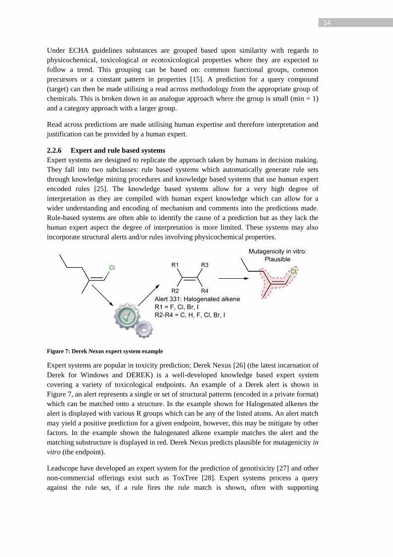
14
Under ECHA guidelines substances are grouped based upon similarity with regards to
physicochemical, toxicological or ecotoxicological properties where they are expected to
follow a trend. This grouping can be based on: common functional groups, common
precursors or a constant pattern in properties [15]. A prediction for a query compound
(target) can then be made utilising a read across methodology from the appropriate group of
chemicals. This is broken down in an analogue approach where the group is small (min = 1)
and a category approach with a larger group.
Read across predictions are made utilising human expertise and therefore interpretation and
justification can be provided by a human expert.
2.2.6 Expert and rule based systems
Expert systems are designed to replicate the approach taken by humans in decision making.
They fall into two subclasses: rule based systems which automatically generate rule sets
through knowledge mining procedures and knowledge based systems that use human expert
encoded rules [25]. The knowledge based systems allow for a very high degree of
interpretation as they are compiled with human expert knowledge which can allow for a
wider understanding and encoding of mechanism and comments into the predictions made.
Rule-based systems are often able to identify the cause of a prediction but as they lack the
human expert aspect the degree of interpretation is more limited. These systems may also
incorporate structural alerts and/or rules involving physicochemical properties.
Figure 7: Derek Nexus expert system example
Expert systems are popular in toxicity prediction; Derek Nexus [26] (the latest incarnation of
Derek for Windows and DEREK) is a well-developed knowledge based expert system
covering a variety of toxicological endpoints. An example of a Derek alert is shown in
Figure 7, an alert represents a single or set of structural patterns (encoded in a private format)
which can be matched onto a structure. In the example shown for Halogenated alkenes the
alert is displayed with various R groups which can be any of the listed atoms. An alert match
may yield a positive prediction for a given endpoint, however, this may be mitigate by other
factors. In the example shown the halogenated alkene example matches the alert and the
matching substructure is displayed in red. Derek Nexus predicts plausible for mutagenicity in
vitro (the endpoint).
Leadscope have developed an expert system for the prediction of genotixicity [27] and other
non-commercial offerings exist such as ToxTree [28]. Expert systems process a query
against the rule set, if a rule fires the rule match is shown, often with supporting
15
documentation in the form of details of the alert and supporting example structures, see
Figure 8 in section 3.2.1.
2.3 Practical considerations
A fundamental component of a modelling exercise is the data (both training and validation,
see section 4.2). Without data of sufficient quality and size we cannot hope to build good
models with high statistical accuracy, large domains of applicability and enough robustness
to apply to new data.
Data for toxicity prediction can come from many sources, the raw data will often need to be
processed into a model friendly format and decisions may need to be taken over class
boundaries. For example an in vitro study may be repeated or carried out under a number of
different protocols, even for a single compound. This format is unlikely to be model
appropriate and pre-processing steps must be taken before any model building activity can be
undertaken. In this example it may be appropriate to define a procedure for assigning an
overall call to the data. This could be in the form of: if any protocol returns an active
response then the overall call is active. All pre-processing steps must not irreversibly change
the raw data as other pre-processing procedures may be desired for future activities. To aid
in the development of a high quality dataset the experimental data would be taken from the
same lab and under the same protocol [29] as these results are likely to be more comparable
but in practice is rarely achieved.
2.3.1 Dealing with activity imbalance
Activity imbalance refers to datasets where the division of the target activity across the range
(continuous) or classes (classification) is uneven. This imbalance is normally in the form of a
large bias towards inactive [30], [31].
Having imbalance in the target value can result in models that are highly predictive of the
majority class with poor performance against the minority class. If a learning algorithm
optimises by reducing the error within the model the misclassification of the minority data is
less costly than the majority data. As the bias increases the cost in misclassifying the
minority data will decrease. This issue can be dealt with during pre-processing steps or
through the utilisation of a function in the learning accounting for the bias. In addition to the
class imbalance it is often seen that the minority class will cover a much more diverse set of
compounds [30]. Common procedures for dealing with class imbalance are random under
sampling (RUS) where the majority class is under sampled, random over sampling (ROS)
where the majority class is over sampled, cost sensitive classification (CSC) where different
costs in misclassification are assigned (more costly to misclassify the minority class) and the
generation of synthetic data using methods such as the (borderline-) Synthetic Minority
Oversampling Technique (b-)SMOTE which uses the k nearest neighbours algorithm (where
k is the number of data points) to identify k nearest neighbours for each minority example
and then generate new examples at theoretical points.
Methods producing synthetic data such as SMOTE are inappropriate for interpretable
machine learning models. If a model was to provide reasoning for the prediction to the user
based upon example compounds from the training set, theoretical descriptor values may be
misleading and no chemical structure is available for these theoretical points. For these
reasons methods such as these are not discussed in depth further.

16
Sampling and cost sensitive techniques are of significant interest to (Q)SAR building
methodologies. Given that there is often a class imbalance (which may have been addressed
when using a pre-built dataset) it is important to have strategies to tackle the issues that arise.
A comprehensive study by Van Hulse et al. [31] has shown that of 7 sampling techniques
(RUS, ROS, SMOTE, b-SMOTE, one-sided selection (OSS), Wilsons editing (WE), cluster-
based oversampling (CBOS)) random under sampling resulted in the highest performance
increase across 35 independent datasets with random over sampling resulting in the second
best performance increase.
These results are favourable for work in the toxicity prediction domain where capturing the
knowledge of the training set in an interpretable and explainable manner is of benefit.
However, Tropsha [30] recommends a more chemically meaningful approach to addressing
class imbalance. First a similarity matrix is calculated between compounds from the two
classes, dissimilar structures from the majority set below a threshold are then discarded. The
model is then developed on the balanced set which has an active and inactive set of a closer
chemical space.
2.3.2 OECD principles
The Organisation of Economic Co-operation and Development (OECD) have published
guidelines for the validation of (Q)SAR models [10]. These guidelines cover a number of
stages of the model building processes such as algorithm choice as well as covering steps to
ensure that a prediction being made falls within the remit of the model. The guidelines are:
1) The model should cover a defined endpoint;
2) The model should use an unambiguous algorithm;
3) The model should have a defined domain of applicability (region the model is
interpolating and where the most reliable predictions will be made);
4) The model should have appropriate measures of goodness-of-fit, robustness and
predictivity;
5) The model should have a mechanistic interpretation if possible.
The modelling reported in the later chapters meet points 1 to 4: the endpoint is defined down
to a specific assay or global toxicity, the algorithms utilised are well described, the domains
of the models are identified using a fragment based methodology and validation studies have
been carried out to assess the performance. The algorithms utilised are also able to provide a
confidence for each prediction. The models however do not have a mechanistic interpretation
and models that are not rule based containing human expert knowledge are unlikely to have
such an interpretation. The ENCORE algorithm as described in chapter 6 has been applied to
all models and therefore all predictions provide an interpretation suitable for human expert
analysis of the output.
The addition of an interpretation methodology to the model building process could aid in the
regulatory approval by helping move towards meeting the interpretable requirement of the
OECD guidelines [10]. Where the interpretation does not meet the mechanistic component of
OECD principle 5 it will still aid towards better utilisation of the predictions from a (Q)SAR.
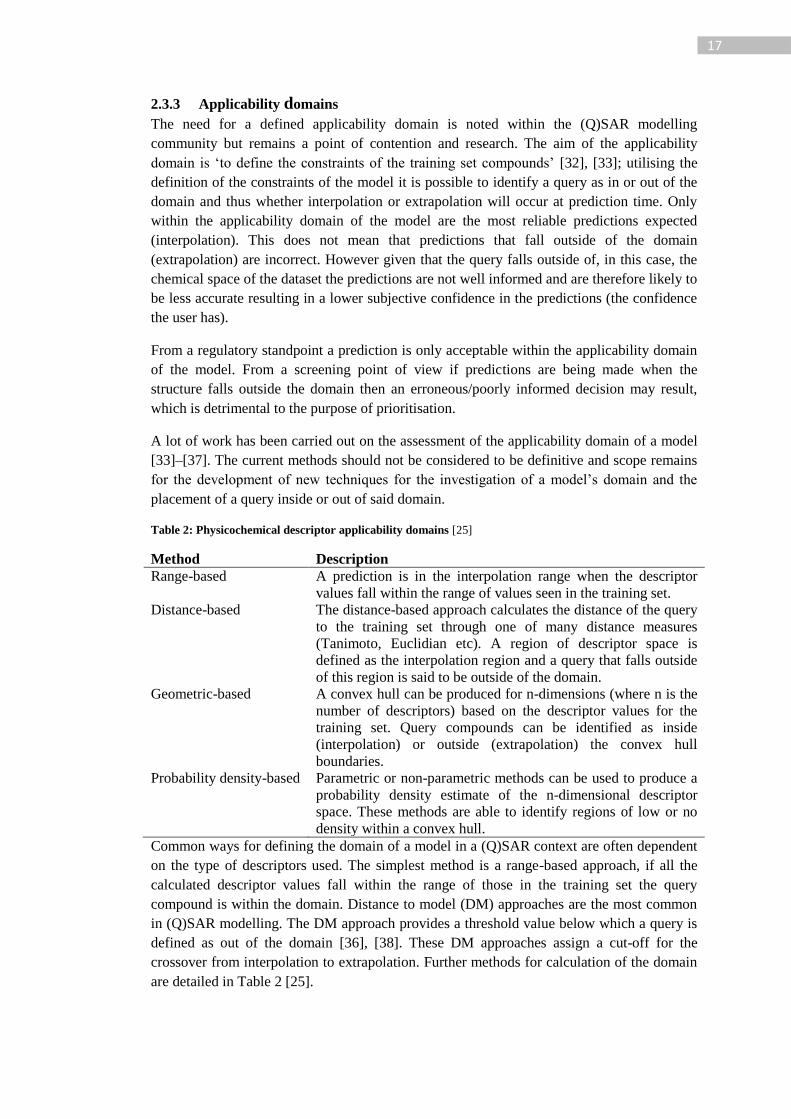
17
2.3.3 Applicability domains
The need for a defined applicability domain is noted within the (Q)SAR modelling
community but remains a point of contention and research. The aim of the applicability
domain is ‘to define the constraints of the training set compounds’ [32], [33]; utilising the
definition of the constraints of the model it is possible to identify a query as in or out of the
domain and thus whether interpolation or extrapolation will occur at prediction time. Only
within the applicability domain of the model are the most reliable predictions expected
(interpolation). This does not mean that predictions that fall outside of the domain
(extrapolation) are incorrect. However given that the query falls outside of, in this case, the
chemical space of the dataset the predictions are not well informed and are therefore likely to
be less accurate resulting in a lower subjective confidence in the predictions (the confidence
the user has).
From a regulatory standpoint a prediction is only acceptable within the applicability domain
of the model. From a screening point of view if predictions are being made when the
structure falls outside the domain then an erroneous/poorly informed decision may result,
which is detrimental to the purpose of prioritisation.
A lot of work has been carried out on the assessment of the applicability domain of a model
[33]–[37]. The current methods should not be considered to be definitive and scope remains
for the development of new techniques for the investigation of a model’s domain and the
placement of a query inside or out of said domain.
Table 2: Physicochemical descriptor applicability domains [25]
Method Description
Range-based A prediction is in the interpolation range when the descriptor
values fall within the range of values seen in the training set.
Distance-based The distance-based approach calculates the distance of the query
to the training set through one of many distance measures
(Tanimoto, Euclidian etc). A region of descriptor space is
defined as the interpolation region and a query that falls outside
of this region is said to be outside of the domain.
Geometric-based A convex hull can be produced for n-dimensions (where n is the
number of descriptors) based on the descriptor values for the
training set. Query compounds can be identified as inside
(interpolation) or outside (extrapolation) the convex hull
boundaries.
Probability density-based Parametric or non-parametric methods can be used to produce a
probability density estimate of the n-dimensional descriptor
space. These methods are able to identify regions of low or no
density within a convex hull.
Common ways for defining the domain of a model in a (Q)SAR context are often dependent
on the type of descriptors used. The simplest method is a range-based approach, if all the
calculated descriptor values fall within the range of those in the training set the query
compound is within the domain. Distance to model (DM) approaches are the most common
in (Q)SAR modelling. The DM approach provides a threshold value below which a query is
defined as out of the domain [36], [38]. These DM approaches assign a cut-off for the
crossover from interpolation to extrapolation. Further methods for calculation of the domain
are detailed in Table 2 [25].

18
The use of structural fragments to define the applicability domain is conceptually simple. If
the fragments present in the query structure are also present in the training set then the model
is interpolating and the query is in the domain. If an exotic fragment is present on the query
structure that has not been seen in the training set then the model is extrapolating [25].
Similarity measures can be utilised to identify in and out of domain structures on a global
level. The similarity of a query to the training set can be calculated. By utilising methods
such as atom centred fragments it is possible to get a measure of similarity based on the
global arrangement of features [25].
A comparison of various applicability domains methods is available in references [32], [33].
The conclusion by Sahigara et al. [32] is that no single applicability domain method is
sufficient for the assessment of the domain of a new model and all contain their own benefits
and disadvantages. Even within the same dataset different methods of AD will result in
varying improvements to the performance of the model through the removal of unreliable
predictions [32].
2.4 Performance metrics
Binary classification model performance can be assessed using a number of performance
measures.
Table 3: Performance metrics
Measure Equation Equation 4: Accuracy (ACC)
Equation 5: Balanced accuracy (BAC)
Equation 6: Sensitivity (SEN)
Equation 7: Specificity (SPEC)
Equation 8 Matthew’s correlation coefficient
(MCC)
√( )( )( )( )
Equation 9 Positive predictive value (PPV)
19
These measures are calculated using the counts of true positives (TP), true negatives (TN),
false positive (FP) and false negatives (FN). Balanced accuracy (Equation 5) is preferential
to accuracy (Equation 4) as the accuracy measure can be misleading if the validation set
(data which has not been used for modelling and is used to assess the external predictivity of
the model) is biased towards a particular class; for example with a data bias of 1:10 a good
accuracy can be achieved by predicting everything to be the majority class. Sensitivity
(Equation 6) gives a representation of a model’s ability to correctly identify the positive class
and specificity (Equation 7) represents a model’s ability to correctly identify the negative
class. Many more performance measures exist and the measures for regression models differ
to those of classification; only those used within this work are discussed here.
Biased validation data can result in a perceived accurate model even if the model is very
inaccurate on the minority class when looking only at the accuracy metric. Additionally, the
coverage of a model (the % of the query structures a prediction was made for) should be
investigated; a model with high accuracy may not be valuable due to its low domain. Area
under the curve (AUC) has also been used as a measure incorporating the
confidence/probability of the prediction as well as the predicted performance [39]. AUC is
calculated as the area under the curve of the Receiver Operator Characteristic plot based on
the predictions accounting for their predicted probability as well as their predicted and true
class labels; the higher the value of AUC the better the models predictivity. When comparing
models it is important to consider multiple performance metrics covering multiple properties
of the model.
2.5 Validation
The goal of model building is to produce a generalised model which is capable of predicting
the target value of new data points which were previously unseen to the model. To this end
testing strategies are required to investigate the performance of the model. Given sufficient
data fundamental divisions in the available data should be of the form: training, validation
and test. The training set is used to build the model and the validation set is used in the
development where the performance against this set helps to guide the development of the
model. Finally, the test set is used to assess the generalisation error of the model, data in this
set must remain independent of the model building process [18], [19].
An important consideration in model building is the concept of over training. Over training is
where a model has captured the knowledge of the training set in such a way that
generalisation is lost and the model predicts poorly on external data even though it has high
accuracy against the training data. If a model becomes too specific to the training set used
and loses the generalisation that is desired, a trend will often be seen where the error on the
training set decreases but the error on a validation set increases. One use of a validation set is
identifying when model learning has become detrimental to generalisation by over training
[18].
Validation procedures vary and are influenced by the modelling algorithm and the size of the
dataset. The most common technique for validation (where independent test and validation
sets are not used) is cross validation [18]. Cross validation allows for the prediction of every
structure in the dataset through an iterative process. This consists of randomly assigning each
data point to one of k subsets where k is the total number of subsets desired. The process
then iterates over the subsets where the subset being predicted is held out of the model
20
training set, the remaining subsets are combined and provided to a learning algorithm as
training data. This is repeated until all subsets have been predicted. Leave one out (LOO)
validation represents k-fold cross validation where k is equal to the number of entries in the
dataset. In this case a model would be built leaving only a single entry out.
Validation is a topic of particular importance and some contention [40], [41] to the (Q)SAR
community which is stressed in guidelines from regulators and in the OECD principles. It
has been noted that there is a divide in the (Q)SAR community over the requirement for
external validation in addition to internal [40] and rigorous validation of (Q)SAR models is
not complete within the published literature [8]. Gramatica [40] recommends that external
validation must always be undertaken to verify the external predictivity of models which
have been identified as internally stable via internal validation approaches [40]. Internal
measures of the predictivity of a model can be overly optimistic of the model’s true
performance on unseen chemicals [40], [42]. Validation of (Q)SAR models should be
rigorous and utilise both internal and external validation strategies of which both are used in
this thesis.
2.6 Summary
In this chapter we discussed a variety of learning algorithms covering both white and black
box approaches, some of which are applied in chapters 6 and 7. We can see that there exists
a variety of machine learning algorithms that can be applied to computational toxicology. A
particular limitation was highlighted: black box vs white box. Black box learning algorithms
are often capable of producing highly accurate models but do not provide an interpretation –
or reason for – the prediction, whereas white box models provide an interpretation but may
have a weaker accuracy. This issue of model interpretation is discussed in depth in chapter 3
where a review of the current approaches is detailed.
In addition, a number of topics related to (Q)SAR modelling were introduced such as activity
imbalance, the OECD principals and the concept of applicability domains all of which are
accounted for in the applied (Q)SAR modelling discussed in chapters 6 and 7.
21
3 Interpretation and knowledge mining As highlighted in chapter 1, (Q)SAR models are widely applicable but can suffer with
regards to interpretation of the prediction. Research has been undertaken to mitigate this
‘black box’ issue of poor interpretability and trends in the literature are discussed here. In
addition we also discuss various knowledge or rule mining strategies. General trends are
discussed along with detailing various free and commercial (Q)SAR approaches.
3.1 The need and use case for interpretation
As highlighted in chapter 1, machine learning algorithms are primarily developed and
optimised for predictive accuracy [43], [44]. The interpretation of a model’s prediction is
subjective, the term interpretable has different meanings and modellers and users may have
different preferences for how they perform data analysis. Due to this subjectivity defining a
measure for interpretability is a challenge and may be one of the factors for the relative lack
of research into this area.
Interpretation in this thesis is considered in two parts: the ability for the model to explain the
reason behind the prediction and the suitability of the model’s explanation for utilisation by
the investigator. Much of the research into the development of interpretation from machine
learning models in the computer science domain has focused on feature reduction with the
idea that fewer features results in greater interpretability [43], [45]. This is indeed a valid
hypothesis as even white box models can lose their interpretability when the features become
too numerous or unintelligible in terms of relationship to the endpoint being modelled.
However, feature reduction and considerations of descriptors only form part of the
interpretation problem.
Stanton states that more information than knowledge of the descriptor type used is required
as “a preconceived notion of the physical interpretation of the descriptors can result in a
misunderstanding of the underlying SAR” produced by the model [46]. That is to say:
correlation does not imply causation. A descriptor may have a high correlation with the
target variable; however this may be a result of capturing a trend in the dataset that may not
be adequately expressed by the understanding of the descriptor. Stanton suggests that both
the features (descriptors used such as whole-molecule descriptors) and the context (the type
of changes occurring in the dataset that affect the target variable value) are required to be
understood to produce an interpretation [46].
Additionally, the modeller’s perceived notion of how a descriptor will be utilised by a
learning algorithm may not be a true reflection of the models behaviour. To therefore assign
the interpretation of a prediction of a model to the modeller’s understanding of the
descriptors alone is not sufficient to describe the reason a model predicts a given value. The
debate on interpretability can be summarised by stating that a true interpretation of a
prediction is formed by:
1) High level understanding:
a. The relevance of the descriptors to the known mechanisms of the domain
being modelled
b. General trends in model behaviour such as global measures of descriptor
importance
2) Specific (local) understanding:
22
a. Factors relevant to the prediction for a specific query compound
b. Factors which could have been relevant but are found not to be in the case of
a specific query compound; exceptions to the global trends in the model
c. Linking the factors relevant to the prediction with known mechanistic
understanding of the endpoint being modelled
We take the position that a full interpretation is not possible without both points being met.
The understanding of the impact of the descriptors to the endpoint allows for the
appreciation of the reason a model states for a given prediction. A reason for a prediction
alone provides us with information about the SAR(s) utilised by the model for the prediction
but does not provide us with the domain context for appreciation of the SAR. The statistical
model (or interpretation algorithm) is only capable of stating why a prediction was made and
not why this prediction is mechanistically appropriate. As highlighted earlier with
appropriate selection of descriptors such models and/or interpretation can be supportive of a
mechanistic interpretation by the user.
The issue of the potential disconnect between the preconceived notion of how a descriptor
will be utilised and the reality of the learnt data structure has been highlighted in the case
study review by Bratko [44]. A modelling study was undertaken on the growth of algae in
Venice Lagoon, the discovery of unexpected patterns in the decision tree resulted in the
initial refusal of the domain expert to investigate further; the model was written off in the
expert’s mind as the unexpected rule was interpreted as a bug in the software. Upon further
investigation the rule was determined to be valid and provided the expert with new
meaningful understanding. This finding highlights how interpretation can also support or
inadvertently be detrimental to developing a user’s confidence in the model (not to be
confused with the confidence reported by the model); where a model is interpretable and the
user has pre-existing knowledge predictions deemed to be correct for the right reason allow
the user to develop a subjective confidence in the model’s ability to predict. Where the
prediction’s reasons differ from the understanding of the users the models might be
discarded regardless of their predictive accuracy [44].
Bringing the problem into the (Q)SAR modelling domain we can see that the issues of
subjectivity and the variety of use cases will affect the desirability and implementation of
interpretation. The requirement for an interpretation is context specific; in some cases an
accurate model may be used for filtering purposes [6] and the cause of the prediction is not
utilised. Whereas in other cases, such as in the investigation of poorly understood endpoints,
the elucidation of the underlying SARs may reveal information that supports the
development of the process which is being undertaken (such as drug development). Regions
for modification to negative properties predicted by the (Q)SAR model become possible
when an interpretation is provided. Such activities could be seen more in the context of
knowledge mining where a dataset or model is investigated for SAR patterns.
Alternatively, in the context of regulatory submission the interpretation of the prediction can
support the expert assessment of the in silico predictions. Where the suitability of a
prediction must be justified the ability to identify the cause of the prediction provides
additional weight.
23
Multiple approaches have been developed for providing interpretable (Q)SAR models; some
of these approaches have been developed by using or creating interpretable algorithms
whereas others have focused on the interpretation of a particular learning algorithm. The
design of the interpretation algorithms for statistical models varies and each group of
techniques has its own pros and cons.
The need for interpretation is context specific, the required information will likely vary user
to user and in some instances no interpretation may be required. The interpretation
algorithms discussed above have been assessed in terms of their ability to provide an
explanation for the model’s prediction and the usability of the interpretation by the user. For
example a decision tree based on a hashed fingerprint is not considered to be interpretable
due to the choice in descriptors rather than the nature of the learning algorithm.
Through the next sections we will discuss various literature examples for model
interpretation.
3.2 Interpretable predictions (white box models)
Given a white-box model such as a decision tree discussed in chapter 2 the interpretation of
the model is provided by the model itself. In the case of the decision tree, the path from the
root to the terminal leaf node forms the interpretation. A prediction of {x} could be
described as: the presence of feature S1 and the value of S2 below a cut-off of z (see Figure 3
in section 2.2.1.1). Here the interpretation takes form of why the model predicted {x} and
not why {x} is mechanistically related to the SAR encoded by the path through the decision
points of S1 and S2. This is not something provided inherently by a model (but in some cases
is provided by expert systems). Linking the output of a model to the chemistry is the
responsibility of the user, and an activity that requires meaningful descriptors (the essence of
the high level understanding stated above).
This mechanistic interpretation is a strong benefit provided by some expert systems such as
Derek Nexus where mechanistic rules are encoded to provide a detailed explanation linking
to the underlying mechanisms of the endpoint being modelled. However, not all expert
systems provide mechanistic reasoning. Some expert systems provide an interpretable
prediction in terms of the firing of an alert (see section 2.2.6) without the alert containing
any additional information describing the reason for the alert’s presence. For example the
structure idodoethane is predicted to be mutagenic by the expert system Derek Nexus. The
atoms and bonds relating to the toxicophore are highlighted and a mechanistic basis is given
for the toxicophore: “Alkyl halides are electrophilic species that are capable of directly
alkylating DNA… alkyl chlorides are less mutagenic than their bromo and iodo counterparts,
and given the non-mutagenicity reported for n-butyl chloride and n –dodecyl chloride, longer
chain alkyl chlorides may not give a positive result in the Ames test”. In addition to a
positive prediction Derek Nexus has linked to the structural motif on the query which causes
the prediction and linked the toxicophore to a mechanism (direct alkylation of DNA) with a
discussion on the relative mutagenicity of other halogenated species.
3.2.1 Expert / alert based systems
ToxAlerts is a web based system storing a collection of structural alerts for a variety of
endpoints including toxicity and metabolism. Structural alerts are comprised of: source of
information, endpoint, name, supplementary information, visual depiction, description and a
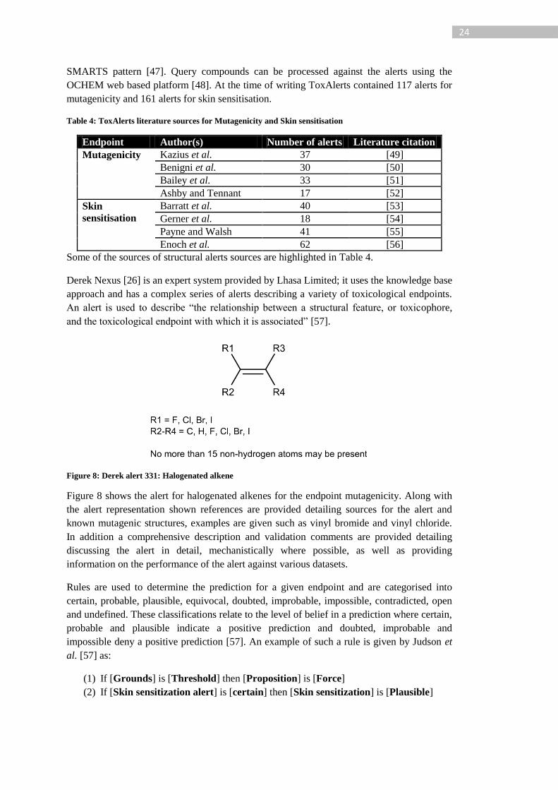
24
SMARTS pattern [47]. Query compounds can be processed against the alerts using the
OCHEM web based platform [48]. At the time of writing ToxAlerts contained 117 alerts for
mutagenicity and 161 alerts for skin sensitisation.
Table 4: ToxAlerts literature sources for Mutagenicity and Skin sensitisation
Endpoint Author(s) Number of alerts Literature citation
Mutagenicity Kazius et al. 37 [49]
Benigni et al. 30 [50]
Bailey et al. 33 [51]
Ashby and Tennant 17 [52]
Skin
sensitisation
Barratt et al. 40 [53]
Gerner et al. 18 [54]
Payne and Walsh 41 [55]
Enoch et al. 62 [56]
Some of the sources of structural alerts sources are highlighted in Table 4.
Derek Nexus [26] is an expert system provided by Lhasa Limited; it uses the knowledge base
approach and has a complex series of alerts describing a variety of toxicological endpoints.
An alert is used to describe “the relationship between a structural feature, or toxicophore,
and the toxicological endpoint with which it is associated” [57].
Figure 8: Derek alert 331: Halogenated alkene
Figure 8 shows the alert for halogenated alkenes for the endpoint mutagenicity. Along with
the alert representation shown references are provided detailing sources for the alert and
known mutagenic structures, examples are given such as vinyl bromide and vinyl chloride.
In addition a comprehensive description and validation comments are provided detailing
discussing the alert in detail, mechanistically where possible, as well as providing
information on the performance of the alert against various datasets.
Rules are used to determine the prediction for a given endpoint and are categorised into
certain, probable, plausible, equivocal, doubted, improbable, impossible, contradicted, open
and undefined. These classifications relate to the level of belief in a prediction where certain,
probable and plausible indicate a positive prediction and doubted, improbable and
impossible deny a positive prediction [57]. An example of such a rule is given by Judson et
al. [57] as:
(1) If [Grounds] is [Threshold] then [Proposition] is [Force]
(2) If [Skin sensitization alert] is [certain] then [Skin sensitization] is [Plausible]

25
Where the grounds relates to an alert such as that for skin sensitization or mutagenicity and
the threshold is the likelihood of an event from the categories certain, probable, plausible etc.
An alert match may be certain where the query is a known example. Derek Nexus will
reason between multiple alerts to produce a final prediction. Readers are referred to [57] for
a more in depth explanation of the Derek reasoning. Other expert-systems will use different
methodologies for predicting based on rules; essentially they can be represented as IF…
THEN… cases.
ToxTree [58] is an expert-system decision tree based approach containing rules involving
both structural features and physicochemical properties. As of version 2.6.6 Toxtree contains
17 software plugins covering: Cramer rules, Verhaar scheme, skin irritation prediction, eye
irritation prediction, Benigni / Bossa rulebase for mutagenicity and carcinogenicity, START
biodegradation and persistence, structure alerts for identification of Michael acceptors,
structure alerts for skin sensitisation, Kroes TTC decision tree, SMARTCyp, structure alerts
for in vivo micronucleus assay in rodents, structural alerts for functional group identification,
DNA binding alerts, protein binding alerts and in vitro mutagenicity alerts by Istituto
Superiore di Sanita.
In cases where the model requires physicochemical descriptors these may be calculated by
ToxTree. Additionally, QSAR models may be run to support prediction made using
structural alerts such as in the case of the Benigni-Bossa mutagenicity rulebase where QSAR
models are used for the prediction of carcinogenicity [59]. ToxTree does not provide a
mechanistic interpretation of the prediction like that given by Derek Nexus as the alert
matches are not supplemented with human expert discussion.
3.2.2 Purpose designed interpretable models
Sarah Nexus is another software application developed by Lhasa Limited. Unlike Derek
Nexus, Sarah Nexus utilises a statistical machine learning algorithm called Self Organising
Hypothesis Network (SOHN) [60]4 to organise (and mine) hypotheses describing
toxicophores (or deactivations of toxicophores). These hypotheses are then organised into a
hierarchical network based on subset-superset relationships of supporting examples. When
predicting, the most appropriate hypotheses for a query structure are identified and one of the
multiple reasoning algorithms is used to combine hypotheses into a single prediction. At the
time of writing Sarah Nexus has been released for the prediction of Ames mutagenicity. The
SOHN algorithm is a learning technique that provides interpretable hypotheses currently in
the form of structural fragments with associated activity. Sarah Nexus has been used for
comparison in chapters 6 and 7. Full details of the algorithm can be found in [60]; a brief
explanation of the algorithms for knowledge mining and prediction as applied to binary data
is included here.
The first step for SOHN models is the creation of hypotheses which will later be organised
into a hierarchical network. These hypotheses can be provided independently of the SOHN
methodology. In the case of the modelling carried out in chapters 6 and 7 a fragmentation
approach is used on the entire training set, recursive partitioning is then used to select the
most discriminating structural fragment hypotheses from the large dictionary, see Figure 9.
4 Author’s contribution to this article: Contributed to scientific elaboration of the SOHN
approach and performed machine learning experiments.
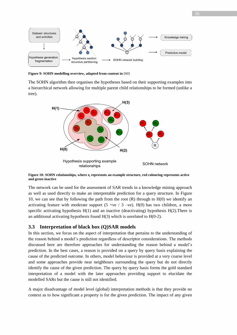
26
Figure 9: SOHN modelling overview, adapted from content in [60]
The SOHN algorithm then organises the hypotheses based on their supporting examples into
a hierarchical network allowing for multiple parent child relationships to be formed (unlike a
tree).
Figure 10: SOHN relationships, where ei represents an example structure, red colouring represents active
and green inactive
The network can be used for the assessment of SAR trends in a knowledge mining approach
as well as used directly to make an interpretable prediction for a query structure. In Figure
10, we can see that by following the path from the root (R) through to H(0) we identify an
activating feature with moderate support (5 +ve / 3 –ve). H(0) has two children, a more
specific activating hypothesis H(1) and an inactive (deactivating) hypothesis H(2).There is
an additional activating hypothesis found H(3) which is unrelated to H(0-2).
3.3 Interpretation of black box (Q)SAR models
In this section, we focus on the aspect of interpretation that pertains to the understanding of
the reason behind a model’s prediction regardless of descriptor considerations. The methods
discussed here are therefore approaches for understanding the reason behind a model’s
prediction. In the best cases, a reason is provided on a query by query basis explaining the
cause of the predicted outcome. In others, model behaviour is provided at a very coarse level
and some approaches provide near neighbours surrounding the query but do not directly
identify the cause of the given prediction. The query by query basis forms the gold standard
interpretation of a model with the later approaches providing support to elucidate the
modelled SARs but the cause is still not identified.
A major disadvantage of model level (global) interpretation methods is that they provide no
context as to how significant a property is for the given prediction. The impact of any given
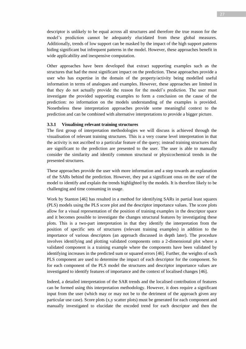
27
descriptor is unlikely to be equal across all structures and therefore the true reason for the
model’s prediction cannot be adequately elucidated from these global measures.
Additionally, trends of low support can be masked by the impact of the high support patterns
hiding significant but infrequent patterns in the model. However, these approaches benefit in
wide applicability and inexpensive computation.
Other approaches have been developed that extract supporting examples such as the
structures that had the most significant impact on the prediction. These approaches provide a
user who has expertise in the domain of the property/activity being modelled useful
information in terms of analogues and examples. However, these approaches are limited in
that they do not actually provide the reason for the model’s prediction. The user must
investigate the provided supporting examples to form a conclusion on the cause of the
prediction: no information on the models understanding of the examples is provided.
Nonetheless these interpretation approaches provide some meaningful context to the
prediction and can be combined with alternative interpretations to provide a bigger picture.
3.3.1 Visualising relevant training structures
The first group of interpretation methodologies we will discuss is achieved through the
visualisation of relevant training structures. This is a very coarse level interpretation in that
the activity is not ascribed to a particular feature of the query; instead training structures that
are significant to the prediction are presented to the user. The user is able to manually
consider the similarity and identify common structural or physicochemical trends in the
presented structures.
These approaches provide the user with more information and a step towards an explanation
of the SARs behind the prediction. However, they put a significant onus on the user of the
model to identify and explain the trends highlighted by the models. It is therefore likely to be
challenging and time consuming in usage.
Work by Stanton [46] has resulted in a method for identifying SARs in partial least squares
(PLS) models using the PLS score plot and the descriptor importance values. The score plots
allow for a visual representation of the position of training examples in the descriptor space
and it becomes possible to investigate the changes structural features by investigating these
plots. This is a two-part interpretation in that they identify the interpretation from the
position of specific sets of structures (relevant training examples) in addition to the
importance of various descriptors (an approach discussed in depth later). The procedure
involves identifying and plotting validated components onto a 2-dimensional plot where a
validated component is a training example where the components have been validated by
identifying increases in the predicted sum or squared errors [46]. Further, the weights of each
PLS component are used to determine the impact of each descriptor for the component. So
for each component of the PLS model the structures and descriptor importance values are
investigated to identify features of importance and the context of localised changes [46].
Indeed, a detailed interpretation of the SAR trends and the localised contribution of features
can be formed using this interpretation methodology. However, it does require a significant
input from the user (which may or may not be to the detriment of the approach given any
particular use case). Score plots (x,y scatter plots) must be generated for each component and
manually investigated to elucidate the encoded trend for each descriptor and then the

28
transition between the score plots must be investigated to understand the relationship
between the components used in the model. This approach is not model agnostic and has
been developed for the interpretation of PLS models.
Hansen et al. [61] have developed a method to allow for the interpretation of models built
using kernel based learning algorithms – methods that use a kernel function to operate in
higher dimensional space – such a support vector machines. The explanation of the model is
provided by returning the most relevant structures to the prediction of a Gaussian model
providing a similar interpretation to that of Stanton’s method in terms of presenting the
activity of similar structures.
Hansen et al. [61] present a method for quantifying the influence of a training compound on
a query by query basis. The interpretation is described in terms of providing the ‘molecular
evidence’ behind the prediction. This approach does not however provide the reasoning for
the placement of structures in the model space. The interpretation is achieved by the expert
visualising and inferring trends based on the structural features present in the selected similar
training structures.
If a model is being used by a human expert the presentation of similar structures, particularly
those with a great influence on the prediction, can provide valuable information. These
similar structures potentially present structural analogues and allow the user to investigate
local changes that may be beneficial or detrimental to the predicted property or activity. As
highlighted, these interpretations are not directly providing the model’s reason for the
prediction nor are they providing a mechanistic interpretation. Supporting evidence is
provided to the human expert.
3.3.2 Identifying the importance of features: globally and locally
Some learning algorithms are able to give a global ranking of descriptors such as the
Random Forest or partial least squares algorithms. These measures are just of global
importance across a dataset, but they may provide some insight into the model. However on
a query by query basis this is a very coarse level interpretation. This differs to approaches in
descriptor selection where a strategy for identifying the strongest correlated descriptors with
the target variable may be performed. Guha et al. [62] have shown that the Random Forest
approach to descriptor importance, by scrambling the descriptors and measuring the change
in model error, can also be used on artificial neural networks.
A significant limitation to such approaches is that they are independent of the prediction of a
specific query. For example a model may be built on the presence of features; feature 1 could
be the most significant feature in the model via approaches such as that described by Guha et
al. [62]. However, feature 1 may not even be present in a given query structure and these
approaches particularly suffer in identifying the importance of low frequency features. The
relationship between descriptors is also not inferred from such approaches.
However, some approaches investigate the importance of features for a given query. In these
cases the issues related to global trend identification are removed. Carlsson et al. [63] have
successfully used a decision gradient function from RF or SVM models to identify the most
significant descriptor for a prediction. The decision function is analysed to determine the
impact of each descriptor on the local neighbourhood and the descriptor with the largest
gradient (impact) is identified. When coupled with fragment based toxicophore descriptors
29
this has allowed for the identification of local significant toxicophore for a given prediction.
This methodology provides a significant improvement by providing insight into the
prediction produced by the two black box methodologies. However, accounting for the most
significant feature alone could be misleading where multiple causes of activity are present or
the activity is caused by a combination of features. For the mapping of the features to atoms
and bonds on the structure a feature must be identifiable and would thus not allow the use of
hashed fingerprint descriptors.
These methods go a step further than the visualisation methods discussed above and may
provide additional benefit from coupling the two techniques. They are, however, unable to
capture subtleties in the algorithm or capture the relationships between the descriptors.
Kuz’min et al. [64] have developed a methodology for determining atom contributions
towards a regression prediction of a Random Forest model. Models built from simplex
descriptors (atom environment type descriptors) were used for training. However the authors
state that other fragment approaches would also be appropriate. The methodology works by
assessing the change in mean activity between each parent and child couple along the tree
path per tree for the query, with the contributions from each tree being incorporated into a
forest level importance measure. This importance measure is then applied to individual
atoms allowing for an understanding of the contribution of the atoms to the predicted value.
This interpretation algorithm provides a very clear picture of the contribution of various
structural descriptors. The approach is limited by the requirement for defined structural
feature descriptors and the specificity of the approach to the Random Forest learning
algorithm.
In a similar approach to that of Kuz’min et al. [64] a method has been developed for the
interpretation of classification based Random Forests models by Palczewska et al. [65]. In
this approach the trees are traversed and the change in probability distribution at each split is
measured. This returns a feature importance for each tree and these values are aggregated
into a forest level importance for each feature on a query by query basis. This approach is
capable of generating feature importance for binary and multi class classifiers. Further
analysis via median, cluster-analysis and log-likelihood can be performed to identify patterns
in the random forests predictions.
These approaches to interpreting the Random Forest model provide clear explanations for
the importance of each feature (descriptor) to the outcome of the prediction. However, where
structural descriptors are used these must form pre-defined entities such as fragments or
Molecular Access System (MACCS) keys to understand the link to the structural graph. The
importance of a bit in a hashed fingerprint will not be meaningful in these interpretations.
Baskin et al. [66] have developed a methodology for producing an interpretation from
artificial neural networks using the same approach as methods such as linear regression. The
methodology determines the influence of the descriptors on the predicted variable and the
statistics are reported to be relatively stable to rebuilding the model (which can produce
different weights within the network). The analysis of the network reveals information about
how the model has incorporated the descriptors and can be used to get an understanding of
the learned (Q)SAR.
30
In these approaches we can see how the lack of an interpretable descriptor results in the
overall lack of an interpretation. Having a measure of the significance of a descriptor is
ultimately of little use where there is no understanding of the relevance of the descriptor on
the property of activity being modelled.
3.3.3 Identifying the behaviour of atoms and/or fragments
Another group of interpretation methods tackle the problem by identifying the contribution
of atoms, bonds and/or fragments. Two approaches have been taken:
1) Combine a learning algorithm that provides weights for the importance of a feature
with a descriptor that can be mapped to atoms, bonds and/or fragments.
2) Elucidate the importance of atoms, bonds and/or fragments by determining the
change in prediction when said component is removed.
These methods provide a wider variety of applicable descriptors. For approach 1 we see a
significant onus on the choice of descriptor as specific atoms and bonds must be associated.
The second approach has a smaller onus on descriptor choice; however, there is no
accounting for the impact of the combination of the components being removed. These
methods provide the most detailed explanation of the model’s behaviour and the reason for
the model’s prediction. Again we have no mechanistic interpretation; however, unlike with
the methods discussed above we are getting a clear picture of the model’s behaviour as
opposed to being presented with a series of structures in addition to global importance
measures of the most significant features.
Spowage et al. [67] have developed a set of interpretable descriptors that when combined
with a PLS model can be utilised for interpretation of the underlying SAR used for
prediction. This SAR is projected as a categorised contribution {Very Positive, Positive,
Neutral, Negative, Very Negative} onto the atoms in the query structure. The utilised
topological maximum cross correlation (TMACC) descriptors can be linked to specific
atoms. Contribution is assigned by identifying the regression coefficient for each descriptor
and assigning an equal share to the atoms contained within. Where an atom is present in
more than one descriptor the values are summed. This interpretation methodology highlights
the initial component of an interpretation: interpretable descriptors are required even when
utilising a white box model. The regression weights which reveal the underlying SAR are
utilised in combination with these interpretable descriptors to assign contribution to specific
atoms within the query structure. If the descriptor is not interpretable knowing the regression
weights does not result in a useful interpretation of the model.
Ajmani et al. [68] have developed a method for improving the interpretation of PLS. A
normal PLS model can be interpreted on a global scale by investigating which descriptors
were chosen, and the weight value and sign associated with each. This allows for a global
molecule context but is not necessarily interpretable on a local scale, i.e. identifying specific
impact such as a particular functional group or substitution pattern. Ajmani et al.’s G-QSAR
method approach improves the interpretation of the PLS models by using descriptors that are
localised to specific features in addition to providing the ability to account for
combinations/relationships between structural features. A fragmentation approach is devised
(specific to the model/dataset) based around defining substitution positions for congeneric
series or components for non-congeneric series. The structures are fragmented and
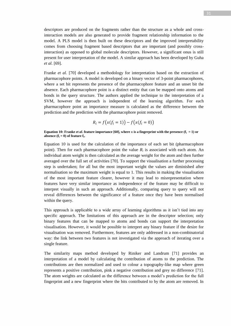
31
descriptors are produced on the fragments rather than the structure as a whole and cross-
interaction models are also generated to provide fragment relationship information to the
model. A PLS model is then built on these descriptors and the improved interpretability
comes from choosing fragment based descriptors that are important (and possibly cross-
interaction) as opposed to global molecule descriptors. However, a significant onus is still
present for user interpretation of the model. A similar approach has been developed by Guha
et al. [69].
Franke et al. [70] developed a methodology for interpretation based on the extraction of
pharmacophore points. A model is developed on a binary vector of 3-point pharmacophores,
where a set bit represents the presence of the pharmacophore feature and an unset bit the
absence. Each pharmacophore point is a distinct entity that can be mapped onto atoms and
bonds in the query structure. The authors applied the technique to the interpretation of a
SVM, however the approach is independent of the learning algorithm. For each
pharmacophore point an importance measure is calculated as the difference between the
prediction and the prediction with the pharmacophore point removed.
( ( )) ( ( ))
Equation 10: Franke et al. feature importance [60], where x is a fingerprint with the presence (fi = 1) or
absence (fi = 0) of feature fi.
Equation 10 is used for the calculation of the importance of each set bit (pharmacophore
point). Then for each pharmacophore point the value Ri is associated with each atom. An
individual atom weight is then calculated as the average weight for the atom and then further
averaged over the full set of activities [70]. To support the visualisation a further processing
step is undertaken; for all but the most important weight the values are diminished after
normalisation so the maximum weight is equal to 1. This results in making the visualisation
of the most important feature clearer, however it may lead to misrepresentation where
features have very similar importance as independence of the feature may be difficult to
interpret visually in such an approach. Additionally, comparing query to query will not
reveal differences between the significance of a feature once they have been normalised
within the query.
This approach is applicable to a wide array of learning algorithms as it isn’t tied into any
specific approach. The limitations of this approach are in the descriptor selection; only
binary features that can be mapped to atoms and bonds can support the interpretation
visualisation. However, it would be possible to interpret any binary feature if the desire for
visualisation was removed. Furthermore, features are only addressed in a non-combinatorial
way: the link between two features is not investigated via the approach of iterating over a
single feature.
The similarity maps method developed by Riniker and Landrum [71] provides an
interpretation of a model by calculating the contribution of atoms to the prediction. The
contributions are then normalized and used to colour a topography-like map where green
represents a positive contribution, pink a negative contribution and grey no difference [71].
The atom weights are calculated as the difference between a model’s prediction for the full
fingerprint and a new fingerprint where the bits contributed to by the atom are removed. In
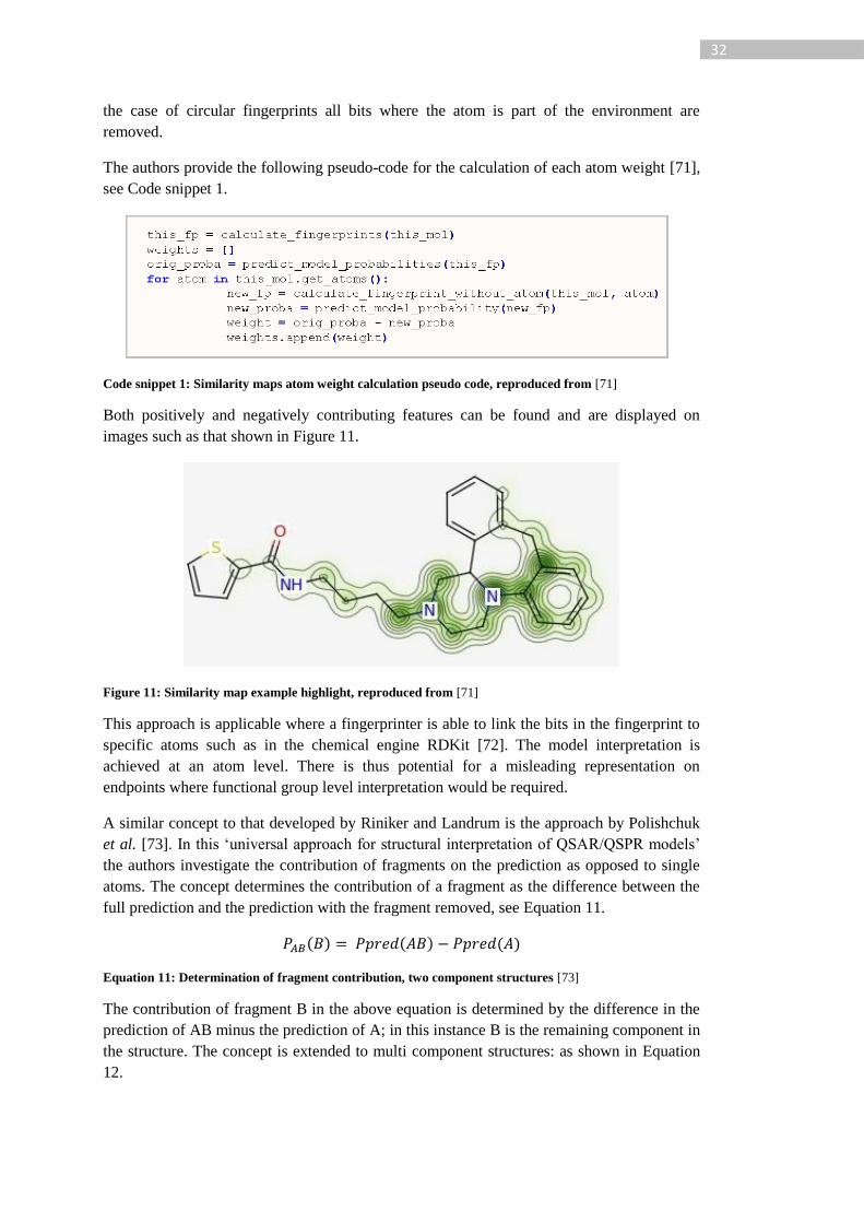
32
the case of circular fingerprints all bits where the atom is part of the environment are
removed.
The authors provide the following pseudo-code for the calculation of each atom weight [71],
see Code snippet 1.
Code snippet 1: Similarity maps atom weight calculation pseudo code, reproduced from [71]
Both positively and negatively contributing features can be found and are displayed on
images such as that shown in Figure 11.
Figure 11: Similarity map example highlight, reproduced from [71]
This approach is applicable where a fingerprinter is able to link the bits in the fingerprint to
specific atoms such as in the chemical engine RDKit [72]. The model interpretation is
achieved at an atom level. There is thus potential for a misleading representation on
endpoints where functional group level interpretation would be required.
A similar concept to that developed by Riniker and Landrum is the approach by Polishchuk
et al. [73]. In this ‘universal approach for structural interpretation of QSAR/QSPR models’
the authors investigate the contribution of fragments on the prediction as opposed to single
atoms. The concept determines the contribution of a fragment as the difference between the
full prediction and the prediction with the fragment removed, see Equation 11.
( ) ( ) ( )
Equation 11: Determination of fragment contribution, two component structures [73]
The contribution of fragment B in the above equation is determined by the difference in the
prediction of AB minus the prediction of A; in this instance B is the remaining component in
the structure. The concept is extended to multi component structures: as shown in Equation
12.

33
( ) ( ) ( )
Equation 12: Determination of fragment contribution in multi component structures [73], where ..
indicates a multi component fragment (A is not connected to C in the graph)
However, in this second approach an additional descriptor generation approach is imposed
due to the common inability to process mixtures (multi component structures) through
descriptor calculators [73].
The approach has been applied to classification and regression tasks of both an additive and
a non-additive nature. However, during the descriptor calculation step undertaken by the
authors, explicit hydrogens were added to cleaved sites resulting in a ‘closed’ structure; this
activity in addition to the generation of any descriptor type can result in the generation of
features (descriptors) not present in the original query structure and may result in a ‘false’
interpretation where impact is ascribed to a feature novel to the resultant generated fragment.
Where a model has multiple causes for activity this approach is insufficient to elucidate the
underlying SARs. Consider a classification task where the activity is 1 for active and 0 for
inactive. The model predicts 1 for the structure represented by A-B-C. Where A and C are
both causes for activation this interpretation approach will determine the activity of each
fragment to be 0 since the predictions of A-B, B-C and A..C are all 1:
( )
( )
( )
Equation 13: Interpretation of a three component structure with two activating causes (A,C)
In Equation 13 we can see that the assessment of all three fragments {A,B,C} returns 0
indicating that they are not activating features. After an exhaustive assessment of each
feature no activating cause has been found for this positive prediction. This limitation to the
approach has been acknowledged by the authors [73].
Polishchuk et al. have established a technique that is capable of interpreting on a query by
query (local) basis the impact of fragments in a query structure. They have also developed a
method for investigating a fragment across a dataset by obtaining fragment contributions
across the a full dataset as opposed to a single structure revealing potential local deviations
[73]. Additionally, the approach is able to work in both directions and identify activating and
deactivating fragments in a structure. However, as implemented in their work pre-existing
knowledge has been utilised to define the fragmentation in terms of matching SMARTS
patterns describing known toxicophores / SAR rules. This approach is able to investigate
known feature behaviour in a given dataset but will not support the identification of
previously unknown fragments. To do this, the approach must be combined with an known
knowledge agnostic fragmentation methodology. As implemented in their work and in their
implementation available at [74] (http://physchem.od.ua/compute) this was not available at
time of writing.
Optibrium Ltd. have developed an approach for the interpretation of black box models
named ‘Glowing Molecules’ [75]. However, little information is available about how the

34
importance of the atoms and bonds are calculated given the commercial nature of the
approach. The approach provides a colour map overlaid onto the chemical structure
indicating regions that contribute positively, negative or have no impact to the property or
activity being predicted [76].
The approaches in this category provide an interpretation that is meaningful in the context of
the modelling of chemical structures. Their main limitation is in the ability to link together
atoms of functional groups to elucidate the impact of combinations of patterns to the
outcome. For example where a negative contributing fragment is found what activating
component of the structure is it drawing activity away from? It is also common to see that
the functionality of the interpretation required that the descriptors can be mapped onto atoms
and bonds e.g. by using a fragment descriptor.
3.4 Knowledge mining
Knowledge mining approaches, used in the support of the developed SAR by human experts,
may facilitate descriptor selection or generation for models or support the automated
generation of interpretable rule bases for prediction. We discussed earlier that the
development of (Q)SAR models may not be to produce a model for prediction but rather to
investigate a dataset and support the knowledge acquisition of a domain expert. Here we
discuss in more detail approaches in the literature aimed at the knowledge acquisition side of
data mining.
Methods for knowledge mining include emerging pattern mining (EP mining) [77], [78],
fragmentation [79], tree building through maximum common substructure analysis [80], rule
extraction from models built from algorithms such as neural networks [81]–[83] and support
vector machines [84].
Two sub categories exist: the first method using a dataset directly to perform the knowledge
mining task and second using a machine learning algorithm to identify trends and then
pulling information out of the resultant model.
3.4.1 Mining from datasets
Rule mining algorithms are designed to learn from a dataset and produce the learnt
knowledge in the form of rules that will then be used to predict new data. Various rule
generation algorithms exist with the aim of generating rule sets which can be applied to new
data instead of a model such as a decision tree, neural network or support vector machine.
Figure 3 from section 2.2.1.1 represents a classification decision tree where attributes A, B
and C are used for splitting. Of the nodes shown the following rules can be extracted based
on the conjunctions between the nodes:
1) If attribute A does not equal 1 then inactive
2) If attribute A equals 1 and attribute B greater than 2.5 then active
3) If attribute A equals 1 and attribute B less than or equal to 2.5 and attribute C is false
then active
by traversing the decision tree and extracting the paths from the root to the leaves. These
rules can be verbose and without care in descriptor selection can be uninterpretable. Rule
extraction methods commonly use a decision tree algorithm and add additional processing to
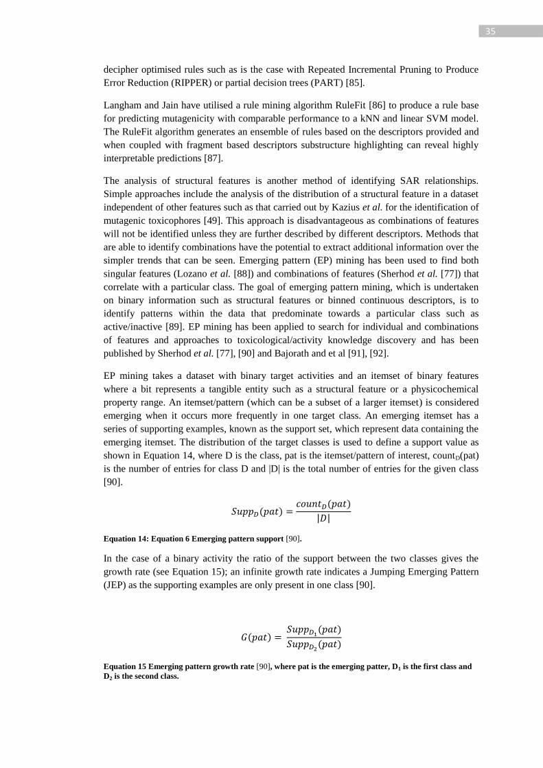
35
decipher optimised rules such as is the case with Repeated Incremental Pruning to Produce
Error Reduction (RIPPER) or partial decision trees (PART) [85].
Langham and Jain have utilised a rule mining algorithm RuleFit [86] to produce a rule base
for predicting mutagenicity with comparable performance to a kNN and linear SVM model.
The RuleFit algorithm generates an ensemble of rules based on the descriptors provided and
when coupled with fragment based descriptors substructure highlighting can reveal highly
interpretable predictions [87].
The analysis of structural features is another method of identifying SAR relationships.
Simple approaches include the analysis of the distribution of a structural feature in a dataset
independent of other features such as that carried out by Kazius et al. for the identification of
mutagenic toxicophores [49]. This approach is disadvantageous as combinations of features
will not be identified unless they are further described by different descriptors. Methods that
are able to identify combinations have the potential to extract additional information over the
simpler trends that can be seen. Emerging pattern (EP) mining has been used to find both
singular features (Lozano et al. [88]) and combinations of features (Sherhod et al. [77]) that
correlate with a particular class. The goal of emerging pattern mining, which is undertaken
on binary information such as structural features or binned continuous descriptors, is to
identify patterns within the data that predominate towards a particular class such as
active/inactive [89]. EP mining has been applied to search for individual and combinations
of features and approaches to toxicological/activity knowledge discovery and has been
published by Sherhod et al. [77], [90] and Bajorath and et al [91], [92].
EP mining takes a dataset with binary target activities and an itemset of binary features
where a bit represents a tangible entity such as a structural feature or a physicochemical
property range. An itemset/pattern (which can be a subset of a larger itemset) is considered
emerging when it occurs more frequently in one target class. An emerging itemset has a
series of supporting examples, known as the support set, which represent data containing the
emerging itemset. The distribution of the target classes is used to define a support value as
shown in Equation 14, where D is the class, pat is the itemset/pattern of interest, countD(pat)
is the number of entries for class D and |D| is the total number of entries for the given class
[90].
( ) ( )
Equation 14: Equation 6 Emerging pattern support [90].
In the case of a binary activity the ratio of the support between the two classes gives the
growth rate (see Equation 15); an infinite growth rate indicates a Jumping Emerging Pattern
(JEP) as the supporting examples are only present in one class [90].
( ) ( )
( )
Equation 15 Emerging pattern growth rate [90], where pat is the emerging patter, D1 is the first class and
D2 is the second class.
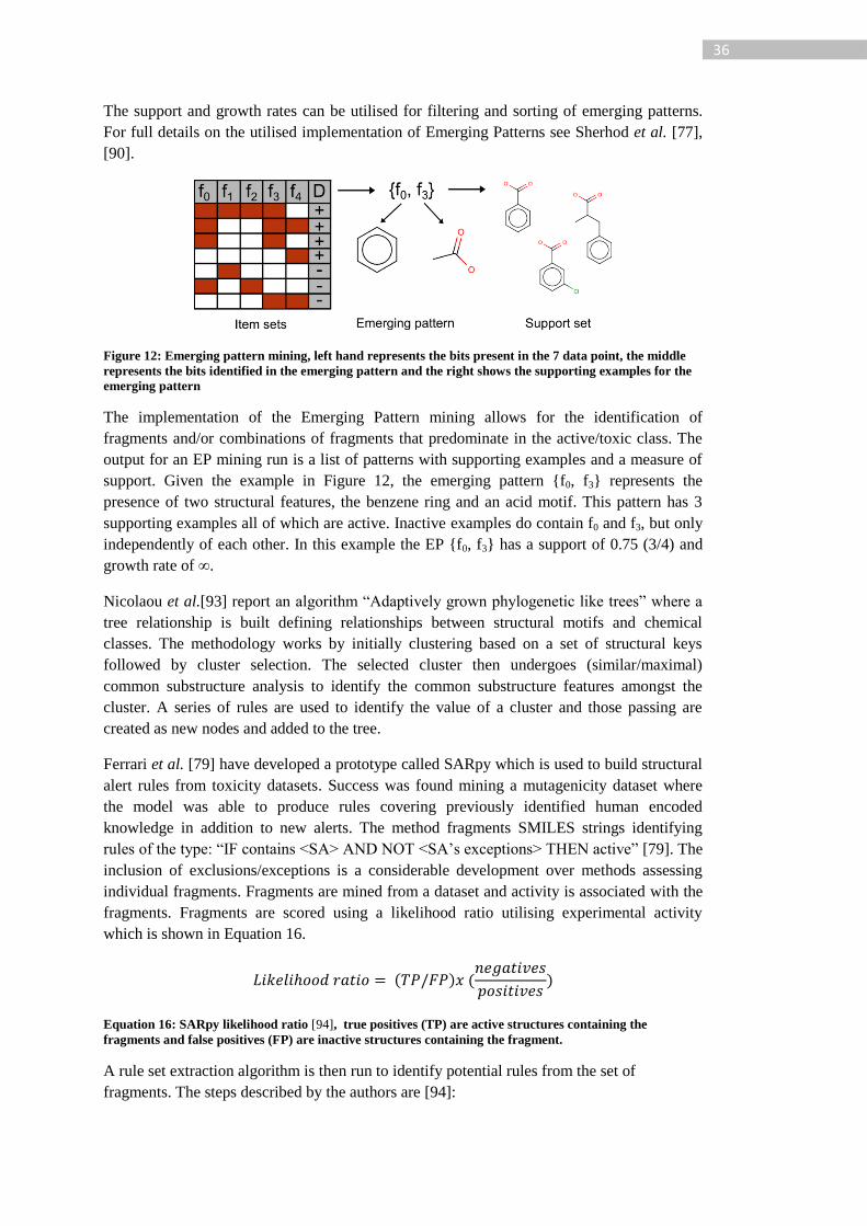
36
The support and growth rates can be utilised for filtering and sorting of emerging patterns.
For full details on the utilised implementation of Emerging Patterns see Sherhod et al. [77],
[90].
Figure 12: Emerging pattern mining, left hand represents the bits present in the 7 data point, the middle
represents the bits identified in the emerging pattern and the right shows the supporting examples for the
emerging pattern
The implementation of the Emerging Pattern mining allows for the identification of
fragments and/or combinations of fragments that predominate in the active/toxic class. The
output for an EP mining run is a list of patterns with supporting examples and a measure of
support. Given the example in Figure 12, the emerging pattern {f0, f3} represents the
presence of two structural features, the benzene ring and an acid motif. This pattern has 3
supporting examples all of which are active. Inactive examples do contain f0 and f3, but only
independently of each other. In this example the EP {f0, f3} has a support of 0.75 (3/4) and
growth rate of ∞.
Nicolaou et al.[93] report an algorithm “Adaptively grown phylogenetic like trees” where a
tree relationship is built defining relationships between structural motifs and chemical
classes. The methodology works by initially clustering based on a set of structural keys
followed by cluster selection. The selected cluster then undergoes (similar/maximal)
common substructure analysis to identify the common substructure features amongst the
cluster. A series of rules are used to identify the value of a cluster and those passing are
created as new nodes and added to the tree.
Ferrari et al. [79] have developed a prototype called SARpy which is used to build structural
alert rules from toxicity datasets. Success was found mining a mutagenicity dataset where
the model was able to produce rules covering previously identified human encoded
knowledge in addition to new alerts. The method fragments SMILES strings identifying
rules of the type: “IF contains <SA> AND NOT <SA’s exceptions> THEN active” [79]. The
inclusion of exclusions/exceptions is a considerable development over methods assessing
individual fragments. Fragments are mined from a dataset and activity is associated with the
fragments. Fragments are scored using a likelihood ratio utilising experimental activity
which is shown in Equation 16.
( ) (
)
Equation 16: SARpy likelihood ratio [94], true positives (TP) are active structures containing the
fragments and false positives (FP) are inactive structures containing the fragment.
A rule set extraction algorithm is then run to identify potential rules from the set of
fragments. The steps described by the authors are [94]:

37
1) Order the list of potential alerts by likelihood ratio
2) Select the top ranked one, add it to the rule set and remove it from the list of
potential alerts
3) Remove the TPs and Fps containing the alert just selected
4) Update TP and FP values of the remaining potential alerts
5) Update the likelihood ratios of potential alerts
6) Return to point 1
The output of the algorithm is a list of structural alerts generated from the entire list of
fragments. These alerts are then incorporated into a rule based system. A series of structural
alerts for mutagenicity can be found with the details of the algorithm in [94].
3.4.2 Mining from models
Another approach to the generation of predictive rules is to use a trained model for
knowledge gathering/building. Relationships learned by the model will be investigated to
generate a rule set. Of the wide range of learning algorithms artificial neural networks have
proven popular with a variety of approaches taken to rule extraction; a series of
classifications have been created to group and evaluate rule extraction methods for ANN and
have likewise been applied to SVM models: transparency, rule quality, expressive power,
portability and algorithmic complexity [20], [95].
Huber and Berthold [96] have developed a method of the generation of IF…THEN rules
from rectangular basis functional neural networks. The technique benefits from no
requirements for parameter optimisation a priori and allows for pruning of the developed
rule set with a smooth relationship between extent of pruning and misclassification rate.
Ryman-Tubb [82] has developed a rule extraction technique that extracts rules from an
artificial neural network in a human readable form. The approach was developed for the
financial fraud domain where a general overview of fundamental factors was desired
allowing for a reduced complexity as the number of rules extracted is minimal. The loss in
performance compared to the original this caused was acceptable and the overall
performance was still higher than a decision tree built on the data [82].
A review by Barakat and Bradley [20] groups support vector machine (SVM) extraction
methods into four categories depending on what aspects of the model are utilised: (1) closed
box, (2) support vector extraction, (3) support vector and decision function utilisation and
finally (4) the use of support vectors, the decision function and the training data. Barakat
and Bradley included a method by He et al. [97] where the authors used a procedure of
producing a more informative training subset using a support vector machine prior to
building a decision tree to produce a rule set for predicting protein secondary structure.
Methods of this type are not strictly rule extraction from a support vector machines as the
decision tree algorithm is used to generate the rules from the dataset directly. The method
has resulted in an improved accuracy of the decision trees, although the performance still
falls short of the SVM alone [97]. The other methods use the built classifier in various ways
to generate rules for example using the support vectors to assign fuzzy cluster membership
and then using these clusters to generate rules. Another method uses both the training data
and the support vectors to generate clusters with associated rules. High accuracy and
concordance with the support vector predictions are seen. Unfortunately the technique does
not scale well with increasing descriptors and/or training examples [20].
38
3.4.3 Impact of this work to knowledge mining
It is unlikely that a single knowledge or rule mining approach will be able to produce an
exhaustive coverage of the underlying structures/patterns in a dataset. The combination of
approaches is likely to provide the most benefit to modeller in investigating a dataset to
improve their knowledge or in the goal of developing alerts for prediction.
The developed interpretation algorithm discussed in chapter 6 provides the components
required for the purposes of knowledge mining. The knowledge mining algorithm developed
and utilised in chapter 6 implements the iterative steps required and supports the organisation
of the extracted interpretations.
3.5 Current need in model interpretation
The work discussed in this thesis proposes to address some of the current issues in the
interpretation of predictions made by statistical ML models; in particular focusing on the
practical application of the developed models from the software user point of view. The
developed algorithm thus aims to provide a meaningful context specific explanation for the
models prediction.
The interpretation methodology developed and discussed in chapter 6 is a combination of
assigning contribution to fragments (without requiring the structural features to be
identifiable to specific atoms and bonds) and providing the contribution of a
physicochemical property if used. The approach differs from those discussed above in that
the relationship between the features is investigated. The developed approach is also capable
of providing supporting examples which are labelled according to their reason for being
active, providing a more detailed picture than the support example approaches discussed
above. The interpretation methodology has been developed with the end user in mind by not
only providing the reason for the model’s prediction mapped to the chemical domain being
modelled (highlighting of structure motifs) but also providing relevant training examples that
have been predicted to the given class for the same reason(s) when utilising an external test
set or via a cross validation procedure. Not only does this support the user understanding of a
prediction but also supports the user’s judgement in the reliability of the prediction. The
algorithm has been developed for the application to toxicity hazard prediction and due to the
clear justification that it provides it can and has been utilised for knowledge mining
investigations which is discussed in chapter 7.
In chapter 4 background required for the appreciation of the later chapters is discussed
including details on the practical application of the machine learning algorithms.

39
4 Cheminformatics: Software, data, descriptors and fragmentation A variety of cheminformatic techniques will be used in the model building discussed in later
chapters. Fundamental concepts for appreciation of the work and the developed algorithm
are discussed in this chapter.
4.1 Software
A variety of software applications and libraries have been used in both the back and front
end development as well as for general data treatment. Eclipse RCP [98], the Zest eclipse
plugin [99], KNIME [100] and Weka [101] have been heavily used as standalone
applications and built upon for the software developed and described in chapters 6 and 7.
4.1.1 Chemical engines
A number of chemical engines have been used in this work. The chemical engines are relied
upon to provide a wide variety of cheminformatics functionality such as: structure
representation, fingerprinting, descriptor calculation, fragmentation and clustering.
Ceres [102], [103], Lhasa Limited’s in-house chemical engine, has been the most heavily
used as it provides a comprehensive and easily extensible Java based framework. Where
functionality was readily available in other packages and not available within Ceres these
have also been used. CDK [104] has been used for descriptor calculation, RDKit [72] for
SMARTS substructure searching and ChemAxon for structure standardization and curation
[105].
4.1.2 Coralie
Coralie is an in-house Eclipse RCP [98] application designed as a cheminformatics research
platform. The algorithms discussed in Chapter 5 have been integrated to provide
interpretation of models built using Weka [101]. Coralie provides access to Emerging Pattern
mining [77], Self-Organising Hypotheses Networks (SOHN) [60] as well as ENCORE
(feature networks, [106], elaborated in chapters 6 and 7) for both prediction and knowledge
mining.
4.1.3 KNIME
KNIME [100] is an open source workflow tool written as a JAVA eclipse RCP application.
KNIME provides a framework to support quick development of complex routines using the
large variety of in built nodes in addition to those provided by third parties (commercial and
open source). New nodes can be developed using KNIME’s node development framework
and extending core classes. Additions have been made to KNIME to provide extended
cheminformatic functionality using Ceres, ENCORE nodes as well as a variety of bespoke
nodes.
4.2 Data
There is a variety of sources for toxicity data: literature, in-house data repositories, pre-built
(Q)SAR datasets and global search engines [25]. Different sources come with different pros
and cons and the use of each should be guided by the purpose of the model building.
In-house datasets have a number of advantages over publicly available sources such as the
potential availability of the full test study and information on the protocol used [25].
Regardless of commercial advantage of building models based on private data, benefits may

40
be seen in the predictive performance against a particular area of chemical space. Models
perform best when the query is within the domain of the model (interpolation); if the purpose
of model building is to predict a specific chemical space of interest, in-house data may
provide a wealth of data not available externally. However, if the area of interest is a new
domain, data may not be available even in the in-house archives. If the built model is
intended to be provided externally, limitations may need to be imposed due to the
confidential nature of the data and significant human effort may be required to format the
data in a way appropriate for modelling [25].
There exists a wide variety of public data; some sources of data may be in the form of a pre-
built dataset for a specific endpoint such as mutagenicity [49], [107] or carcinogenicity [108]
while others may be repositories of data covering a variety of biological activity [109]. A
few examples of publicly available toxicity data are summarised in Table 5 which has been
adapted from reference [110].
Table 5: Examples of publicly available toxicity data partially reproduced from [110]
Database Description
AERS US FDA/CDER Adverse Effects Reporting system of post-market
safety surveillance for all approved drug and therapeutic biologic
products
CCRIS Chemical carcinogenesis research information system
CEBS US NIH/NIEHS Chemical Effects in Biological Systems
Knowledgebase; integrates genomic and biological data including dose–
response studies in toxicology and pathology
CPDB University of California, Berkeley, carcinogenic potency database
Danish (Q)SAR
database
Danish EPA repository of estimates from over 70 QSAR models and
health effects for 166,072 chemicals
DSSTox Distributed Structure-Searchable Toxicity Database Network of
downloadable, structure-searchable, standardized chemical structure
files associated with toxicity data
Gene-Tox US NLM Peer-reviewed genetic toxicology test data for over 3000
chemicals
NTP US NIH/NIEHS National Toxicology Program testing status and
information of agents registered in the US of public health interest
Toxnet US NLM Databases on toxicology, hazardous chemicals, environmental
health, and toxic releases For the full figure see Table 1 [110]
Pre-built datasets for specific endpoints have potential benefits over retrieving data from
publicly available data sources. The datasets are likely to have been used for model building
previously; as a result an assessment of data quality and curation efforts may have already
been undertaken making it easier to assign confidence to the data [25]. If the data quality has
been assessed, curated revisions of the datasets made available and the procedure for the
development of the dataset released, a number of hurdles for model building may have
already been passed. However, in both the publicly available data sources and modelling
datasets it is likely that the data will have been compiled from a variety of sources reducing
the overall quality of the data. It is often seen that a dataset is compiled from multiple
different sources each providing different levels of granularity with regards to the level of
detail in the experimental results recorded. The dataset with the poorest depth of information
often forms the maximum level of recorded information in the compiled dataset. Richer
41
information may therefore be found from smaller datasets. However, this has the cost of a
more limited coverage of chemical space.
4.2.1 Dataset size
Datasets should be sufficient in size to represent the domain that is being modelled. Some
models may be training on non-congeneric datasets with the intention of covering a wide
chemical space while others may be designed to look at a specific chemical series. In both
cases the data should represent as widely as possible the chemical space of the domain being
modelled (local or global).
While there are no defined guidelines or requirements on dataset size for (Q)SAR building
some studies have been undertaken to investigate the impact of the size of the training set on
model accuracy and building. Roy et al. [111] undertook a study to investigate the impact of
training set size on the quality of the predictions made for three datasets: anti-HIV
thiocarbonates (n = 62), HIV reverse transcriptase inhibition on a HEPT derivative dataset (n
= 107) and bioconcentration factor of diverse functional compounds (n = 122). The datasets
were divided into training and test sets of varying size ratios before model building.
Reducing the size of the training set for the thiocarbonate and HEPT datasets was found to
have a detrimental effect on the predictive performance on the models. However, the
bioconcentration models were largely unaffected by training set size. The recommendation
by Roy et al. is that the optimum size of the training set should be based on a particular data
set, the types of the descriptor and the learning algorithm used. Recommendations by
Tropsha [30] are formed based on computational limitations and model quality. Datasets that
are too large may result in practicality issues regarding model building and datasets that are
too small may suffer from chance correlation and over fitting [30]. The size of the dataset
has an impact on descriptor selection, reducing the number of data points while retaining the
number of descriptors increases the chance of over fitting the model to the training data
resulting in poor external predictivity. Care must be taken to address such issues and this can
be achieved through validation studies as discussed in section 2.5.
Where large data sources are available these results hint towards a benefit of producing local
models for specific features, for example based on individual mechanisms or chemical series
should this be relevant to the endpoint. Realistically there is unlikely to be a catch all set of
criteria for defining the requirements of a dataset.
The second consideration for the datasets is activity bias: the distribution of the data over the
various classes or activity ranges. For classification tasks a heuristic is that there should be
“at least 20 compounds for each class” [30] and for regression tasks the “total range of
activities should be at least five times higher than the experimental error” in addition to “no
large gaps (that exceed 10-15% of the entire range of activities) between two consecutive
values of activities ordered by value” [30].
4.2.2 Data quality and curation
In the modelling process the learning algorithm usually assumes that the given data is
correct, i.e. the activity, structure and descriptors are free of errors. The job of the modeller is
to identify issues in the data prior to model building and validation. All data sources are
going to contain errors and these errors can be present in both the activity and the structure.
42
Some approaches can account for an associated confidence with a data point and the
uncertainty in the data quality of specific training instances can be accounted for in this way.
A number of studies have been carried out assessing the quality of the data in public
databases [29], [112]–[114]. These findings highlight the need for modelling activities to
include a curation effort on any new data used. Structural issues may arise through the
conversion of chemical structures (systematic errors) or through human transcription
(random errors) [114]. The systematic issues arise where software is used to convert between
file formats in an erroneous method (although some failure may be attributed to user error)
and may be easier to identify than the random error caused by human drawing of structures.
In addition to erroneous structures issues may also arise due to duplication of structures,
mixtures and the presence of isomers [112].
Erroneous structures cause issues for learning for several reasons: different representations
of chemical motifs may not be seen as the same by structural descriptors, the calculation of
physicochemical descriptors will be affected by the representation of the structure, mixtures
and salts have their biological activity measured in the mixture form but are sometimes
represented by the largest component [112]. These issues in addition to the duplication of
structures – which can also occur through the result of curation activities such as salt
stripping – may all result in decreased performance of statistical models [114]. Differences
in the representation of a structure may not be due to an error. For example different
tautomeric forms may be present and the modeller must be aware of these situations and
decide how they should be handled.
Work has been carried out, most notably by Fourches et al. [112], into the assessment of
structural errors in public datasets and methods for addressing such issues. In addition to
chemical structure curation there are also issues related to the activity or property data.
Errors can be present with the activity or property provided with the structure and these
issues may result in erroneous learning of the underlying SAR trends. Where multiple
sources of data are present for the same compound automated strategies for identification of
such issues are possible; if the values are reported to be equal then the confidence in the
activity being correct may be higher. However, it is common for sources of data to acquire
results from another dataset and errors will be copied. Looking for outliers in the data may
also provide a semi-automated method for activity data curation; this identification will be
complicated where activity cliffs – significant changes in activity from small changes in
structure – are present. In addition care must be taken to ensure that reported activity is
normalised to the same units and that where multiple protocols have been used that they are
comparable.
4.3 Chemical structures, chemical space and similarity
Chemical structures are represented in a variety of formats, each with various benefits and
disadvantages. Common formats suitable for storage and transfer include: simplified
molecular-input line-entry system (SMILES) [115] and molfiles [11]. SMILES represents a
line notation format describing chemical structures with ASCII strings. SMILES provide a
human readable notation that can be converted by most chemical editors to internal and other
shared formats. SMILES stores only atom types, charges and bonds. A format such as an
MDL molfile stores the structural information (atoms and connectivity (bonds)) in a
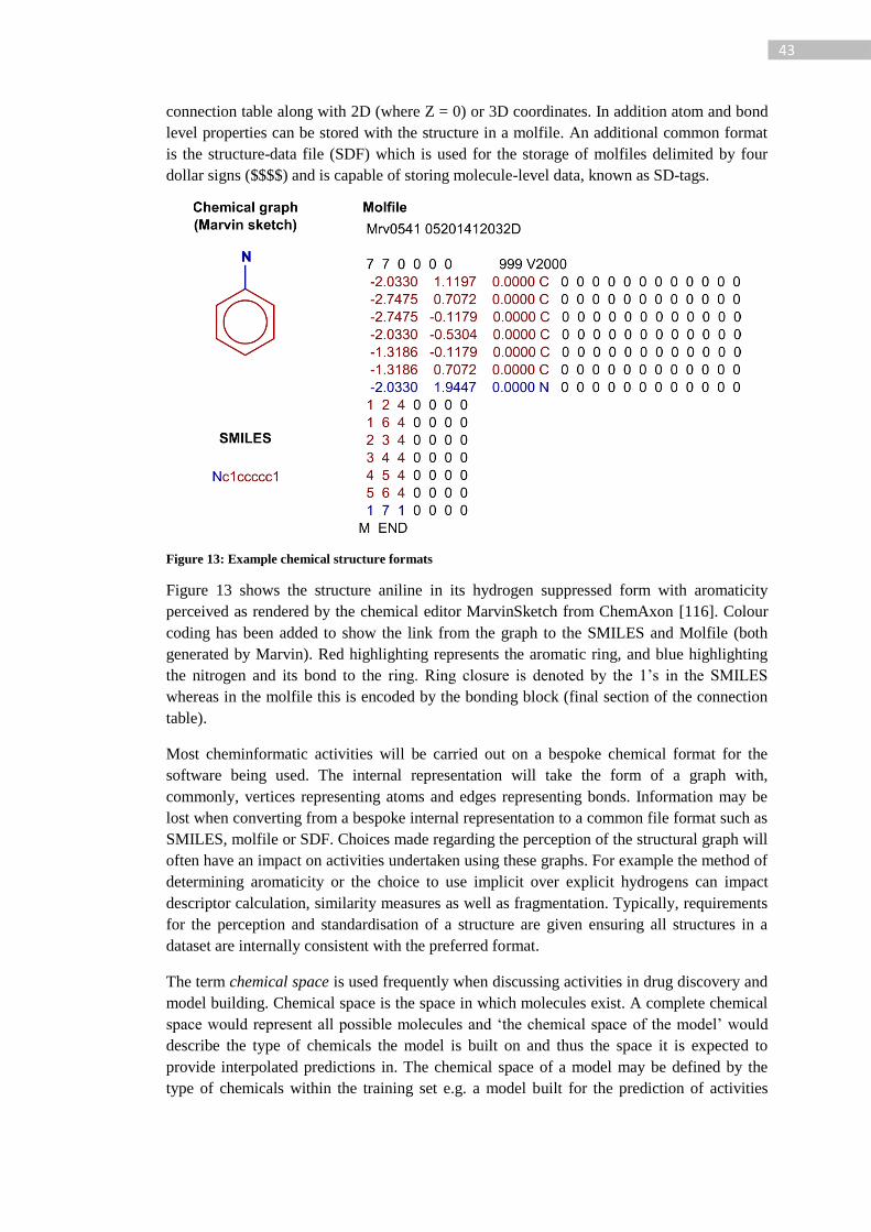
43
connection table along with 2D (where Z = 0) or 3D coordinates. In addition atom and bond
level properties can be stored with the structure in a molfile. An additional common format
is the structure-data file (SDF) which is used for the storage of molfiles delimited by four
dollar signs ($$$$) and is capable of storing molecule-level data, known as SD-tags.
Figure 13: Example chemical structure formats
Figure 13 shows the structure aniline in its hydrogen suppressed form with aromaticity
perceived as rendered by the chemical editor MarvinSketch from ChemAxon [116]. Colour
coding has been added to show the link from the graph to the SMILES and Molfile (both
generated by Marvin). Red highlighting represents the aromatic ring, and blue highlighting
the nitrogen and its bond to the ring. Ring closure is denoted by the 1’s in the SMILES
whereas in the molfile this is encoded by the bonding block (final section of the connection
table).
Most cheminformatic activities will be carried out on a bespoke chemical format for the
software being used. The internal representation will take the form of a graph with,
commonly, vertices representing atoms and edges representing bonds. Information may be
lost when converting from a bespoke internal representation to a common file format such as
SMILES, molfile or SDF. Choices made regarding the perception of the structural graph will
often have an impact on activities undertaken using these graphs. For example the method of
determining aromaticity or the choice to use implicit over explicit hydrogens can impact
descriptor calculation, similarity measures as well as fragmentation. Typically, requirements
for the perception and standardisation of a structure are given ensuring all structures in a
dataset are internally consistent with the preferred format.
The term chemical space is used frequently when discussing activities in drug discovery and
model building. Chemical space is the space in which molecules exist. A complete chemical
space would represent all possible molecules and ‘the chemical space of the model’ would
describe the type of chemicals the model is built on and thus the space it is expected to
provide interpolated predictions in. The chemical space of a model may be defined by the
type of chemicals within the training set e.g. a model built for the prediction of activities
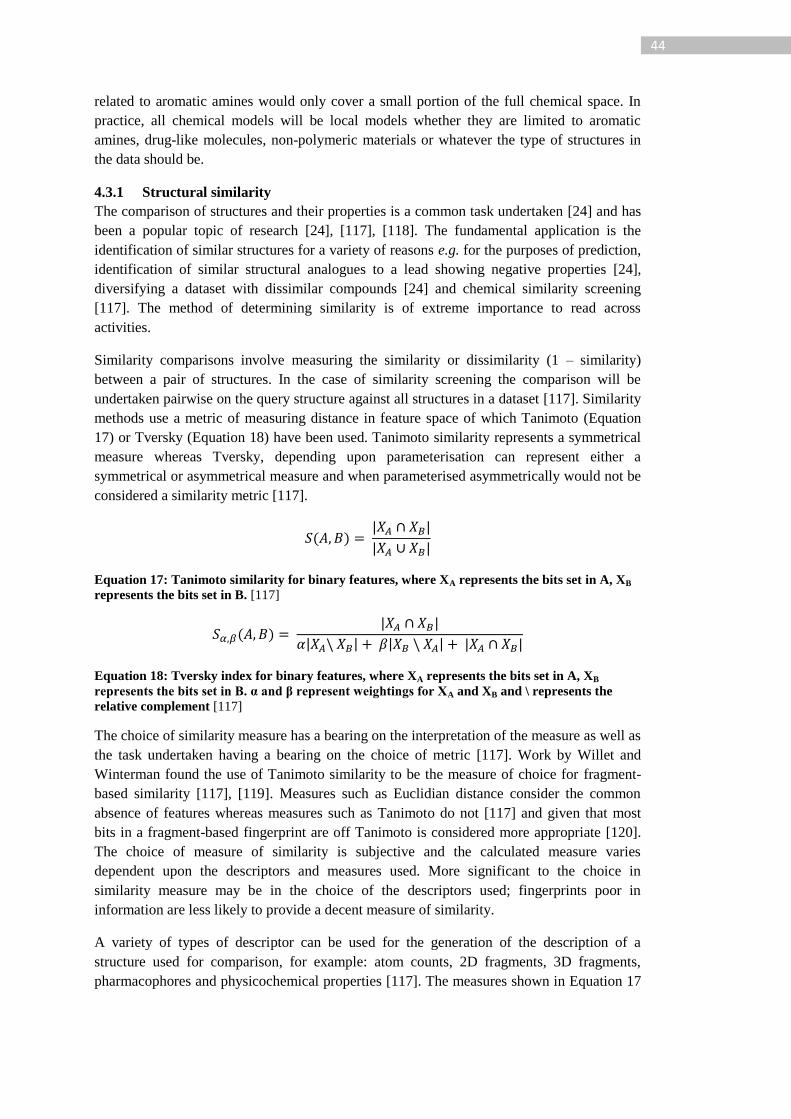
44
related to aromatic amines would only cover a small portion of the full chemical space. In
practice, all chemical models will be local models whether they are limited to aromatic
amines, drug-like molecules, non-polymeric materials or whatever the type of structures in
the data should be.
4.3.1 Structural similarity
The comparison of structures and their properties is a common task undertaken [24] and has
been a popular topic of research [24], [117], [118]. The fundamental application is the
identification of similar structures for a variety of reasons e.g. for the purposes of prediction,
identification of similar structural analogues to a lead showing negative properties [24],
diversifying a dataset with dissimilar compounds [24] and chemical similarity screening
[117]. The method of determining similarity is of extreme importance to read across
activities.
Similarity comparisons involve measuring the similarity or dissimilarity (1 – similarity)
between a pair of structures. In the case of similarity screening the comparison will be
undertaken pairwise on the query structure against all structures in a dataset [117]. Similarity
methods use a metric of measuring distance in feature space of which Tanimoto (Equation
17) or Tversky (Equation 18) have been used. Tanimoto similarity represents a symmetrical
measure whereas Tversky, depending upon parameterisation can represent either a
symmetrical or asymmetrical measure and when parameterised asymmetrically would not be
considered a similarity metric [117].
( )
Equation 17: Tanimoto similarity for binary features, where XA represents the bits set in A, XB
represents the bits set in B. [117]
( )
Equation 18: Tversky index for binary features, where XA represents the bits set in A, XB
represents the bits set in B. α and β represent weightings for XA and XB and \ represents the
relative complement [117]
The choice of similarity measure has a bearing on the interpretation of the measure as well as
the task undertaken having a bearing on the choice of metric [117]. Work by Willet and
Winterman found the use of Tanimoto similarity to be the measure of choice for fragment-
based similarity [117], [119]. Measures such as Euclidian distance consider the common
absence of features whereas measures such as Tanimoto do not [117] and given that most
bits in a fragment-based fingerprint are off Tanimoto is considered more appropriate [120].
The choice of measure of similarity is subjective and the calculated measure varies
dependent upon the descriptors and measures used. More significant to the choice in
similarity measure may be in the choice of the descriptors used; fingerprints poor in
information are less likely to provide a decent measure of similarity.
A variety of types of descriptor can be used for the generation of the description of a
structure used for comparison, for example: atom counts, 2D fragments, 3D fragments,
pharmacophores and physicochemical properties [117]. The measures shown in Equation 17
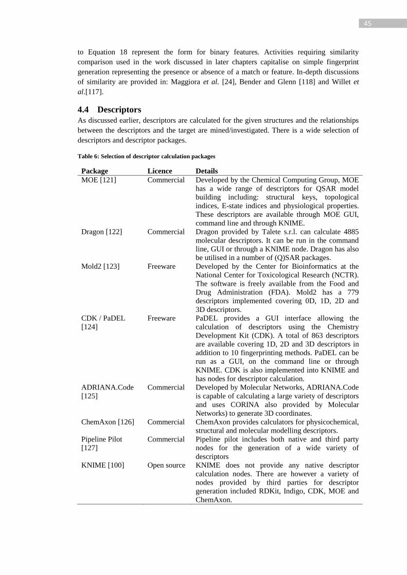
45
to Equation 18 represent the form for binary features. Activities requiring similarity
comparison used in the work discussed in later chapters capitalise on simple fingerprint
generation representing the presence or absence of a match or feature. In-depth discussions
of similarity are provided in: Maggiora et al. [24], Bender and Glenn [118] and Willet et
al.[117].
4.4 Descriptors
As discussed earlier, descriptors are calculated for the given structures and the relationships
between the descriptors and the target are mined/investigated. There is a wide selection of
descriptors and descriptor packages.
Table 6: Selection of descriptor calculation packages
Package Licence Details
MOE [121] Commercial Developed by the Chemical Computing Group, MOE
has a wide range of descriptors for QSAR model
building including: structural keys, topological
indices, E-state indices and physiological properties.
These descriptors are available through MOE GUI,
command line and through KNIME.
Dragon [122] Commercial Dragon provided by Talete s.r.l. can calculate 4885
molecular descriptors. It can be run in the command
line, GUI or through a KNIME node. Dragon has also
be utilised in a number of (Q)SAR packages.
Mold2 [123] Freeware Developed by the Center for Bioinformatics at the
National Center for Toxicological Research (NCTR).
The software is freely available from the Food and
Drug Administration (FDA). Mold2 has a 779
descriptors implemented covering 0D, 1D, 2D and
3D descriptors.
CDK / PaDEL
[124]
Freeware PaDEL provides a GUI interface allowing the
calculation of descriptors using the Chemistry
Development Kit (CDK). A total of 863 descriptors
are available covering 1D, 2D and 3D descriptors in
addition to 10 fingerprinting methods. PaDEL can be
run as a GUI, on the command line or through
KNIME. CDK is also implemented into KNIME and
has nodes for descriptor calculation.
ADRIANA.Code
[125]
Commercial Developed by Molecular Networks, ADRIANA.Code
is capable of calculating a large variety of descriptors
and uses CORINA also provided by Molecular
Networks) to generate 3D coordinates.
ChemAxon [126] Commercial ChemAxon provides calculators for physicochemical,
structural and molecular modelling descriptors.
Pipeline Pilot
[127]
Commercial Pipeline pilot includes both native and third party
nodes for the generation of a wide variety of
descriptors
KNIME [100] Open source KNIME does not provide any native descriptor
calculation nodes. There are however a variety of
nodes provided by third parties for descriptor
generation included RDKit, Indigo, CDK, MOE and
ChemAxon.

46
Descriptor choice should be guided by the mechanism behind activity and the descriptor
package used will be influenced by aspects such as budget and descriptor selection.
Descriptors could also be provided as experimentally measured values rather than calculated
values. Some packages for descriptor calculation are detailed in Table 6.
Structural descriptors can be represented under a dimensionality grouping. 0D descriptors
represents atom/bond counts, molecular weight, ring counts etc. 1D descriptors represent
fragment counts e.g. the number of primary C (sp3). 2D descriptors represent topological
descriptors like Balaban, Weiner or Zagreb indices. 3D descriptors represent geometrical
descriptors like 3D MoRSE descriptors or WHIM descriptors. 3D descriptors can also be
classified into surface or grid properties detailing properties such as hydrophobicity
potential. 4D descriptors use 3D coordinates and conformation sampling [11]. An extremely
comprehensive in depth guide to molecular descriptors has been created by R. Todeschini
and V. Consonni and published by Wiley-CVH as the Molecular Descriptors for
Cheminformatics book in the Methods and Principles of Medicinal Chemistry series [128].
Descriptors can be encoded in different formats such as: binary information representing this
feature is present/not present; integer values representing the count of a feature; or real
values representing a specific value. A common method for encoding the presence of
structural motifs is the generation of a fingerprint. Fingerprints are particularly important for
the models described in this thesis, and so are described below.
4.4.1 Fingerprints
Fingerprints aim to describe the presence or absence of features. They are however not
typically unique to a specific structure. A binary fingerprint can be represented as a sequence
of bits i.e. in a bitstring; where a value of 0 denotes an unset bit (false) and a set bit is
represented by a 1 (true).
Some fingerprints (structural keys) such as MACCS keys [129] have a known linking of a
specific bit to a structural key and can therefore be directly linked with a motif on the
structure. Another fingerprint method is to produce a hashed fingerprint where each bit is not
predefined. The hashing method allows for different fragments to encode bits at the same
index positions resulting in bit position overlap between elements. It is therefore not possible
to directly relate a bit to a structural motif as we could with a key based fingerprint [11].
Some hashed fingerprints do allow for the identification of a list of features present at a bit
position such as ChemAxon’s implementation of Extended Connectivity Fingerprint (ECFP)
[130] and RDKit Morgan fingerprints [72] provides a mapping of atoms with bits in the
fingerprints.
4.4.1.1 Structural keys
Using the dictionary of bits allows for the interpretation of a key based fingerprint for a
given structure; a benefit over hashed fingerprints. However, structural keys are limited in
scope to the defined bits and do not adapt to new use cases with ease. Information not
encoded in the fingerprint cannot be found without adding additional keys. Structural keys
are often also slower to calculate than hashed fingerprints due to the need for substructure
searching. The generalisation of structural keys can be limited and their use may be restricted
to their intended purpose / chemical space.
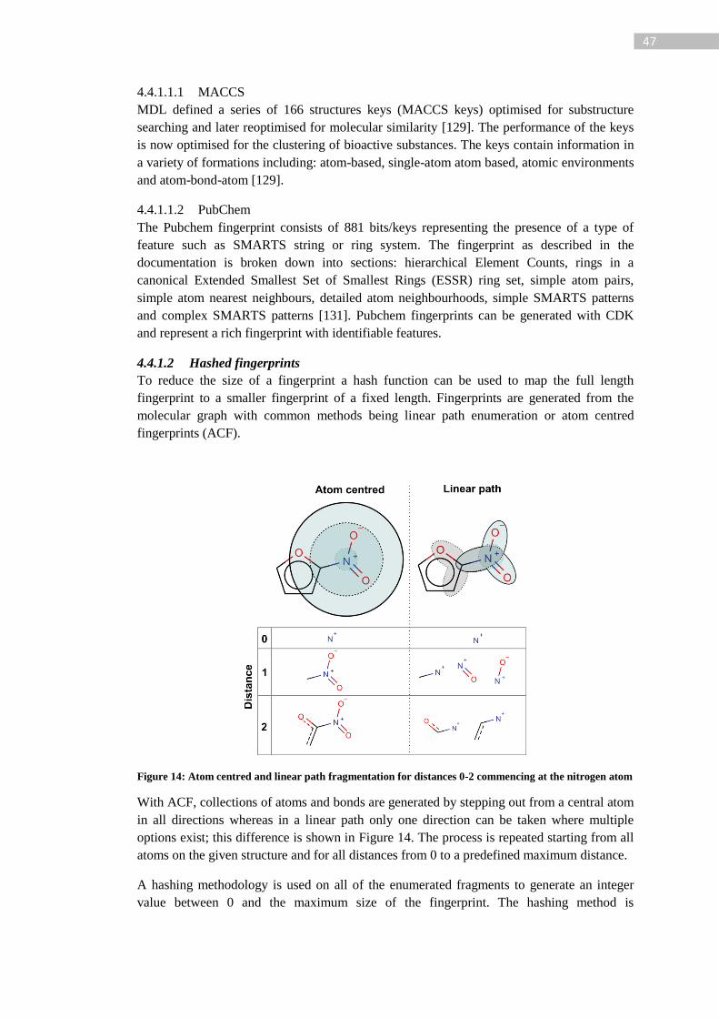
47
4.4.1.1.1 MACCS
MDL defined a series of 166 structures keys (MACCS keys) optimised for substructure
searching and later reoptimised for molecular similarity [129]. The performance of the keys
is now optimised for the clustering of bioactive substances. The keys contain information in
a variety of formations including: atom-based, single-atom atom based, atomic environments
and atom-bond-atom [129].
4.4.1.1.2 PubChem
The Pubchem fingerprint consists of 881 bits/keys representing the presence of a type of
feature such as SMARTS string or ring system. The fingerprint as described in the
documentation is broken down into sections: hierarchical Element Counts, rings in a
canonical Extended Smallest Set of Smallest Rings (ESSR) ring set, simple atom pairs,
simple atom nearest neighbours, detailed atom neighbourhoods, simple SMARTS patterns
and complex SMARTS patterns [131]. Pubchem fingerprints can be generated with CDK
and represent a rich fingerprint with identifiable features.
4.4.1.2 Hashed fingerprints
To reduce the size of a fingerprint a hash function can be used to map the full length
fingerprint to a smaller fingerprint of a fixed length. Fingerprints are generated from the
molecular graph with common methods being linear path enumeration or atom centred
fingerprints (ACF).
Figure 14: Atom centred and linear path fragmentation for distances 0-2 commencing at the nitrogen atom
With ACF, collections of atoms and bonds are generated by stepping out from a central atom
in all directions whereas in a linear path only one direction can be taken where multiple
options exist; this difference is shown in Figure 14. The process is repeated starting from all
atoms on the given structure and for all distances from 0 to a predefined maximum distance.
A hashing methodology is used on all of the enumerated fragments to generate an integer
value between 0 and the maximum size of the fingerprint. The hashing method is
48
implemented in various ways by different fingerprint providers. For example the Chemistry
Development Kit (CDK) implementation generates a fingerprint between bits 0 and 1023 as
follows [104]:
1) Breadth-first linear path search (see, Figure 14) commencing from each atom in
the molecule up to a length of 6:
a. For each generated linear path:
i. Generate hash code for SMILES-like strings using standard Java
string hashing
ii. Generate a random number with hash code as a seed between 0
and 1023
iii. Set bitstring position to generated random number
This reduces the theoretical size of the fingerprint from circa 4 billion to 1024 bits5. Benefits
include improved usability for modelling and a reduction in computational expense when
using the fingerprints. However, bit collision occurs where different components (paths in
CDK example) are hashed to the same position and as a result degrades the transparency of
the information.
Figure 15: Example hashed fingerprint process; red represents bit collisions and orange bits exceeding the
max fingerprint length (1023)
Figure 15 shows a visual overview of the procedure taken by CDK fingerprint generation.
The path enumeration provides a collection of elements which are then hashed to get an
integer. The integers are then mapped between 0 and 1023 to be stored in a bitstring format.
Values in orange represent numbers that could not be stored normally as they exceed the
max of 1023 and red mapped positions represent values where bit collision has occurred.
Bit collision results in 2 or more features being assigned to the same bit in the fingerprint.
This may have negative consequences in learning where information about a feature is based
upon 2 or more independent structural motifs resulting in the dilution or alternatively
misleading importance of a motif.
5 Min and max int values in JAVA are -2
31 and 2
31-1 respectively which define the max and min
possible values from the JAVA String hash method.
49
4.4.1.2.1 Ceres fingerprint
The Ceres fingerprint is a mixed atom centred and path fingerprint:
- Each atom has a fingerprint generated to the desired distance.
- The hashing algorithm generates a value.
- All atom fingerprints are combined with a logical OR (if a bit is set in any atom
fingerprint it is set in the full structure fingerprint).
- Ring systems are accounted for and bits representing branching are also present.
- The size (number of possible bits) and diameter (distance from atom) are
configurable.
- Where unspecified the defaults have been used of 1024 and 8 respectively.
4.4.1.2.2 CDK and CDK extended
The Chemistry Development Kit (CDK) produces Daylight type fingerprints (based on linear
path enumeration and a hashing function) using a breadth-first search from each atom to
generate linear paths up to a set length (default, n = 8). The extended CDK fingerprint adds
additional bits to describe ring systems [104]. The algorithm is shown in more detail in
Figure 15.
4.4.1.3 Fingerprint equivalence
Different structures can be represented by the same fingerprint, these structures are deemed
highly similar based on a fingerprint but can differ for example in features not captured by
the fingerprint or features present at a bit collision, see below.
1. check for equivalence of fingerprint
2. if fingerprints not equal exact match is false
3. if fingerprints equal check for exact match via alternative method (graph matching,
InChI matching...)
Code snippet 2: Identifying identical structures with fingerprints
For example the fingerprint {1,2,3,4} could be generate from two different structural graphs.
Checking for equivalence of the fingerprint would result in true. Further checks must be
undertaken to identify if the structures are truly the same. If the fingerprint equivalence
check results in false then the structures can be identified as different. Substructure matching
the molecular graphs to identify the equivalence of the structures can be achieved via but is
not limited to the use of molecular graphs. InChI string matching could also be used to
identify if structures are the same
4.4.2 Physicochemical descriptors
Various physicochemical descriptors are available, two of which have been used in later
chapters include logP and logKp which are described here.
The lipophilicity of a molecule is of interest in a number of biological and toxicological
models. LogP, the log of the octanol-water partition coefficient, is often used as a measure of
lipophilicity and estimated values are available using in silico tools such as ClogP from
Biobyte Inc [132], and logKp, the log of the skin permeability coefficient, can be calculated
with the Potts and Guy equation shown in Equation 19 [133].

50
Equation 19: Potts and Guy equation for logKp[133], MW = molecular weight
The calculated logP values provided by ClogP are generated via a fragment contribution
method. A fragment dictionary containing experimental values of fragments in various
bonding environments is searched and corrections made based on differences in the
environment. The reported value is derived from the sum of the fragment contributions
accounting for any environmental corrections [134].
4.4.3 Descriptor selection
Descriptor selection methods aim to reduce redundancy and collinearity in the descriptor set
[135] which can result in unrequired computation or a reduction in model performance. “A
good feature subset is one that contains features highly correlated with (predictive of) the
class, yet uncorrelated with (not predictive of) each other” [136]. As discussed earlier it is
also important to consider the number of descriptors used in model building relative to the
number of data points so as to prevent/reduce overtraining.
Descriptor selection6 is an important step in model building. However, some algorithms are
affected more than others by the choice of descriptor [136]. A study by Eklund et al. [137]
concluded that as with learning algorithms no one variable selection method will be
“universally better than any other”. Choosing an optimal set of descriptors may result in
increased performance, computational cost decrease and improve model transparency [137].
A wide variety of methods exist for variable selection and they can be broken down into two
groups: wrappers and filters. Wrappers use the learning algorithm whereas filters use
heuristics are based on the data independent of the learning algorithm [136], [138]. Filter
methodologies have the benefit of speed over wrappers. However, wrappers are found to
often provide better performance as the technique is optimised for the learning algorithm
used [136].
4.4.4 Descriptor discretisation
The learning algorithms used in the model building activities in chapters 6 and 7 can handle
binary, nominal and continuous variables. Due to a limitation imposed by the interpretation
algorithm discussed in chapter 6, discretisation of continuous variables must be undertaken.
Descriptor discretisation identifies range boundaries which are used to convert the
continuous variable into discrete ranges (bins). In the case of some learning algorithms an
improvement in the model can be seen [139], in the case of this modelling work it is
undertaken purely as a necessity due to the requirements of the ENCORE algorithm.
Supervised class discretisation (target activity class is used) is undertaken in a way to
generate boundaries that have good class coherence in addition to maximisation of the
interdependence between class labels and attribute values [139]. The discretised ranges are
used in the learning as nominal values for a variable, or in the case of the work described in
this thesis the nominal ranges are converted to individual variables and treated as a binary
variable. In depth discussions of discretisation approaches are provided in the reviews by
Kotsiantis and Kanellopoulos [139] and Liu et al. [140]. The general concept and undertaken
approach is discussed here.
6 Also known as variable or feature selection
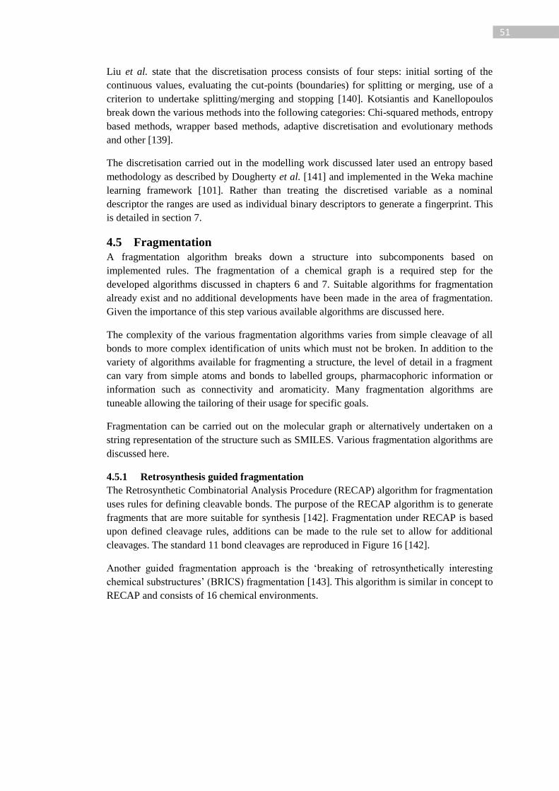
51
Liu et al. state that the discretisation process consists of four steps: initial sorting of the
continuous values, evaluating the cut-points (boundaries) for splitting or merging, use of a
criterion to undertake splitting/merging and stopping [140]. Kotsiantis and Kanellopoulos
break down the various methods into the following categories: Chi-squared methods, entropy
based methods, wrapper based methods, adaptive discretisation and evolutionary methods
and other [139].
The discretisation carried out in the modelling work discussed later used an entropy based
methodology as described by Dougherty et al. [141] and implemented in the Weka machine
learning framework [101]. Rather than treating the discretised variable as a nominal
descriptor the ranges are used as individual binary descriptors to generate a fingerprint. This
is detailed in section 7.
4.5 Fragmentation
A fragmentation algorithm breaks down a structure into subcomponents based on
implemented rules. The fragmentation of a chemical graph is a required step for the
developed algorithms discussed in chapters 6 and 7. Suitable algorithms for fragmentation
already exist and no additional developments have been made in the area of fragmentation.
Given the importance of this step various available algorithms are discussed here.
The complexity of the various fragmentation algorithms varies from simple cleavage of all
bonds to more complex identification of units which must not be broken. In addition to the
variety of algorithms available for fragmenting a structure, the level of detail in a fragment
can vary from simple atoms and bonds to labelled groups, pharmacophoric information or
information such as connectivity and aromaticity. Many fragmentation algorithms are
tuneable allowing the tailoring of their usage for specific goals.
Fragmentation can be carried out on the molecular graph or alternatively undertaken on a
string representation of the structure such as SMILES. Various fragmentation algorithms are
discussed here.
4.5.1 Retrosynthesis guided fragmentation
The Retrosynthetic Combinatorial Analysis Procedure (RECAP) algorithm for fragmentation
uses rules for defining cleavable bonds. The purpose of the RECAP algorithm is to generate
fragments that are more suitable for synthesis [142]. Fragmentation under RECAP is based
upon defined cleavage rules, additions can be made to the rule set to allow for additional
cleavages. The standard 11 bond cleavages are reproduced in Figure 16 [142].
Another guided fragmentation approach is the ‘breaking of retrosynthetically interesting
chemical substructures’ (BRICS) fragmentation [143]. This algorithm is similar in concept to
RECAP and consists of 16 chemical environments.
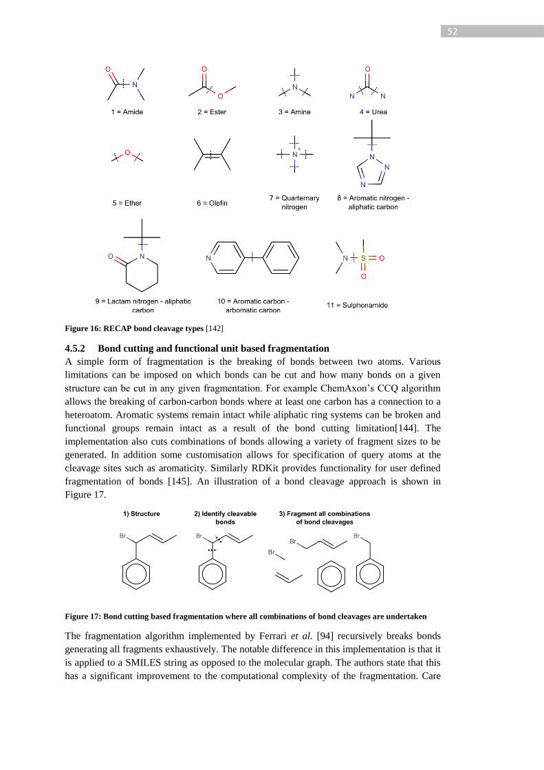
52
Figure 16: RECAP bond cleavage types [142]
4.5.2 Bond cutting and functional unit based fragmentation
A simple form of fragmentation is the breaking of bonds between two atoms. Various
limitations can be imposed on which bonds can be cut and how many bonds on a given
structure can be cut in any given fragmentation. For example ChemAxon’s CCQ algorithm
allows the breaking of carbon-carbon bonds where at least one carbon has a connection to a
heteroatom. Aromatic systems remain intact while aliphatic ring systems can be broken and
functional groups remain intact as a result of the bond cutting limitation[144]. The
implementation also cuts combinations of bonds allowing a variety of fragment sizes to be
generated. In addition some customisation allows for specification of query atoms at the
cleavage sites such as aromaticity. Similarly RDKit provides functionality for user defined
fragmentation of bonds [145]. An illustration of a bond cleavage approach is shown in
Figure 17.
Figure 17: Bond cutting based fragmentation where all combinations of bond cleavages are undertaken
The fragmentation algorithm implemented by Ferrari et al. [94] recursively breaks bonds
generating all fragments exhaustively. The notable difference in this implementation is that it
is applied to a SMILES string as opposed to the molecular graph. The authors state that this
has a significant improvement to the computational complexity of the fragmentation. Care
53
must be taken to ensure canonicalization of the SMILES prior to fragmentation to prevent
redundant but non equal fragments in terms of string matching.
4.5.3 Reduced graph fragmentation
An alternative approach to the fragmentation of the molecular graph is to fragment a reduced
graph - generated from the molecular graph - such as that proposed by Hanser et al. [60]
which is shown in Figure 18. In this context a reduced graph represents a graph with fewer
edges and vertices by combining the edges and vertices in the original graph using reducing
rules.
Figure 18: Reduced graph fragmentation. Step 1 involves identification of the reduced units using a
functional reducer (green units) and a ring reducer (orange units). The reduced graph represents the
reduced units with R6 being a six membered ring and F3 being a 3 membered functional group. In
step 3 the path is enumerated from depths 0 to 2 (representing the full reduced graph), as the
connections are kept the reduced graphs can be expanded back into fragments.
A rule for example may represent ring system reducing of a 6 membered ring (6 vertices and
6 edges) to a reduced single unit representing the ring in its entirety (see steps 1 and 2 in
Figure 18). Information on the origin of the reduced unit is kept so that is can be projected
back onto the original graph (step 4). A configuration could identify rings in a fused system
as individual units or alternatively reduce the entire fused system to a single unit. For
example the two R6 units represent benzene ring motifs in Figure 18 but could be reduced to
a single R10 representing a 10 atom fused ring system (naphthalene ring motif) instead of
two individual 6 membered rings.
The fragmentation is then carried out by breaking the connections between the reduced units
in much the same way as breaking bonds on a chemical graph. The rules defining the

54
reduced units control the type of fragments generated and the depth of searching controls the
size of the combinations of connected units in a fragment; a depth of 0 will only produce
single units, a depth or 1 will include single neighbours and so on. The fragments are then
expanded back out into a full molecular graph describing the fragment.
4.5.4 Usage
The fragmentation can be extended to provide hierarchies and meta information. The specific
use case of the fragmentation will guide the choice of approach, how the fragments are
stored, linked to each other and displayed.
Fragments can be used as descriptors either as counts or binary features. The full fragment
fingerprint can also be hashed to reduce the size. Fragmentation is used here for purposes of
interpretation and knowledge mining. In the interpretation it is used to identify atoms and
bonds to map activity. In the case of knowledge mining, activity is associated with a
fragment.
Fragmentation can result in the generation of a large dictionary of fragments. This dictionary
can be too large for use as a set of descriptors. A strategy for using large fragment
dictionaries as descriptors is to generate a hashed fingerprint as described in section 4.4.1.2.
To reduce the dictionary to a more manageable size without requiring a hashing algorithm
the techniques discussed in section 4.4.3 could be performed.
4.6 Summary
We can see from this and preceding chapters that there is much to be considered when
undertaking (Q)SAR model building. In this chapter a variety of cheminformatic techniques
were introduced covering specific software applications, data and related issues to
descriptors and fragmentation. The discussion has been limited for the most part to specific
techniques or issues relating to the application of cheminformatics in chapters 6 and 7 or in
the management of the data and descriptors for the modelling of the endpoints discussed in
chapter 5.
The potential descriptor pool from which to build models is vast; as discussed in chapter 3
descriptors should where possible be kept to those that can be linked with existing
mechanistic understanding. The descriptors discussed in detail in this chapter are relevant to
the endpoints discussed in chapter 5. In addition fragmentation was discussed to provide
context for the algorithms discussed in chapters 6 and 7; although only the reduced graph
fragmentation has been used in this work.
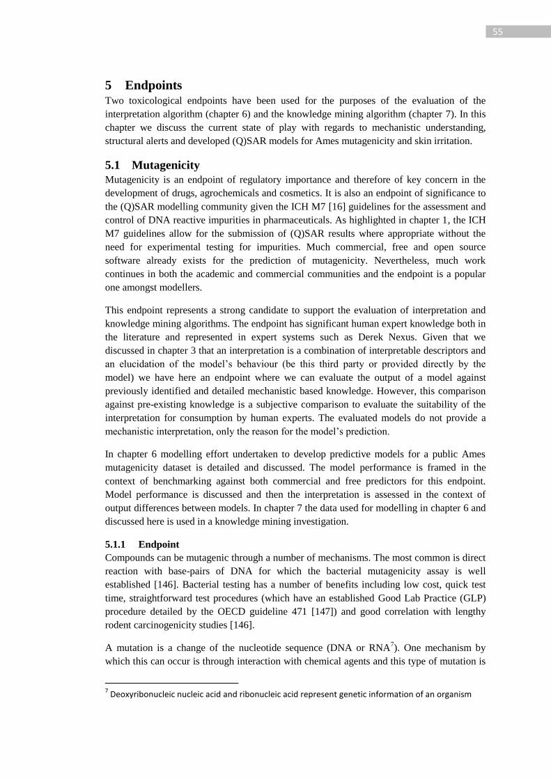
55
5 Endpoints Two toxicological endpoints have been used for the purposes of the evaluation of the
interpretation algorithm (chapter 6) and the knowledge mining algorithm (chapter 7). In this
chapter we discuss the current state of play with regards to mechanistic understanding,
structural alerts and developed (Q)SAR models for Ames mutagenicity and skin irritation.
5.1 Mutagenicity
Mutagenicity is an endpoint of regulatory importance and therefore of key concern in the
development of drugs, agrochemicals and cosmetics. It is also an endpoint of significance to
the (Q)SAR modelling community given the ICH M7 [16] guidelines for the assessment and
control of DNA reactive impurities in pharmaceuticals. As highlighted in chapter 1, the ICH
M7 guidelines allow for the submission of (Q)SAR results where appropriate without the
need for experimental testing for impurities. Much commercial, free and open source
software already exists for the prediction of mutagenicity. Nevertheless, much work
continues in both the academic and commercial communities and the endpoint is a popular
one amongst modellers.
This endpoint represents a strong candidate to support the evaluation of interpretation and
knowledge mining algorithms. The endpoint has significant human expert knowledge both in
the literature and represented in expert systems such as Derek Nexus. Given that we
discussed in chapter 3 that an interpretation is a combination of interpretable descriptors and
an elucidation of the model’s behaviour (be this third party or provided directly by the
model) we have here an endpoint where we can evaluate the output of a model against
previously identified and detailed mechanistic based knowledge. However, this comparison
against pre-existing knowledge is a subjective comparison to evaluate the suitability of the
interpretation for consumption by human experts. The evaluated models do not provide a
mechanistic interpretation, only the reason for the model’s prediction.
In chapter 6 modelling effort undertaken to develop predictive models for a public Ames
mutagenicity dataset is detailed and discussed. The model performance is framed in the
context of benchmarking against both commercial and free predictors for this endpoint.
Model performance is discussed and then the interpretation is assessed in the context of
output differences between models. In chapter 7 the data used for modelling in chapter 6 and
discussed here is used in a knowledge mining investigation.
5.1.1 Endpoint
Compounds can be mutagenic through a number of mechanisms. The most common is direct
reaction with base-pairs of DNA for which the bacterial mutagenicity assay is well
established [146]. Bacterial testing has a number of benefits including low cost, quick test
time, straightforward test procedures (which have an established Good Lab Practice (GLP)
procedure detailed by the OECD guideline 471 [147]) and good correlation with lengthy
rodent carcinogenicity studies [146].
A mutation is a change of the nucleotide sequence (DNA or RNA7). One mechanism by
which this can occur is through interaction with chemical agents and this type of mutation is
7 Deoxyribonucleic nucleic acid and ribonucleic acid represent genetic information of an organism
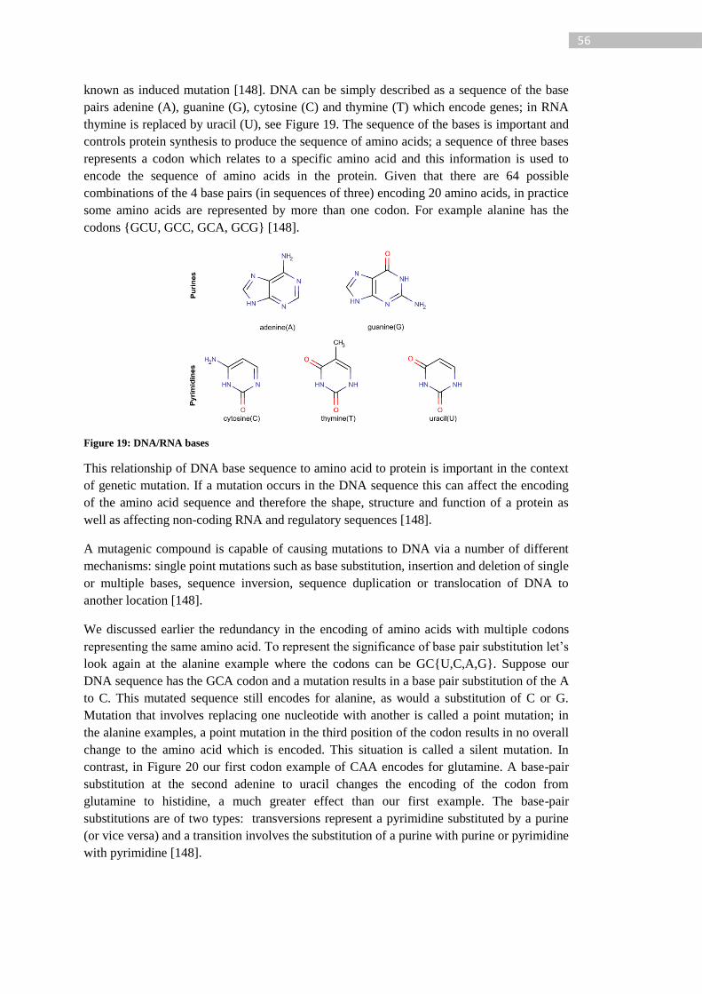
56
known as induced mutation [148]. DNA can be simply described as a sequence of the base
pairs adenine (A), guanine (G), cytosine (C) and thymine (T) which encode genes; in RNA
thymine is replaced by uracil (U), see Figure 19. The sequence of the bases is important and
controls protein synthesis to produce the sequence of amino acids; a sequence of three bases
represents a codon which relates to a specific amino acid and this information is used to
encode the sequence of amino acids in the protein. Given that there are 64 possible
combinations of the 4 base pairs (in sequences of three) encoding 20 amino acids, in practice
some amino acids are represented by more than one codon. For example alanine has the
codons {GCU, GCC, GCA, GCG} [148].
Figure 19: DNA/RNA bases
This relationship of DNA base sequence to amino acid to protein is important in the context
of genetic mutation. If a mutation occurs in the DNA sequence this can affect the encoding
of the amino acid sequence and therefore the shape, structure and function of a protein as
well as affecting non-coding RNA and regulatory sequences [148].
A mutagenic compound is capable of causing mutations to DNA via a number of different
mechanisms: single point mutations such as base substitution, insertion and deletion of single
or multiple bases, sequence inversion, sequence duplication or translocation of DNA to
another location [148].
We discussed earlier the redundancy in the encoding of amino acids with multiple codons
representing the same amino acid. To represent the significance of base pair substitution let’s
look again at the alanine example where the codons can be GC{U,C,A,G}. Suppose our
DNA sequence has the GCA codon and a mutation results in a base pair substitution of the A
to C. This mutated sequence still encodes for alanine, as would a substitution of C or G.
Mutation that involves replacing one nucleotide with another is called a point mutation; in
the alanine examples, a point mutation in the third position of the codon results in no overall
change to the amino acid which is encoded. This situation is called a silent mutation. In
contrast, in Figure 20 our first codon example of CAA encodes for glutamine. A base-pair
substitution at the second adenine to uracil changes the encoding of the codon from
glutamine to histidine, a much greater effect than our first example. The base-pair
substitutions are of two types: transversions represent a pyrimidine substituted by a purine
(or vice versa) and a transition involves the substitution of a purine with purine or pyrimidine
with pyrimidine [148].
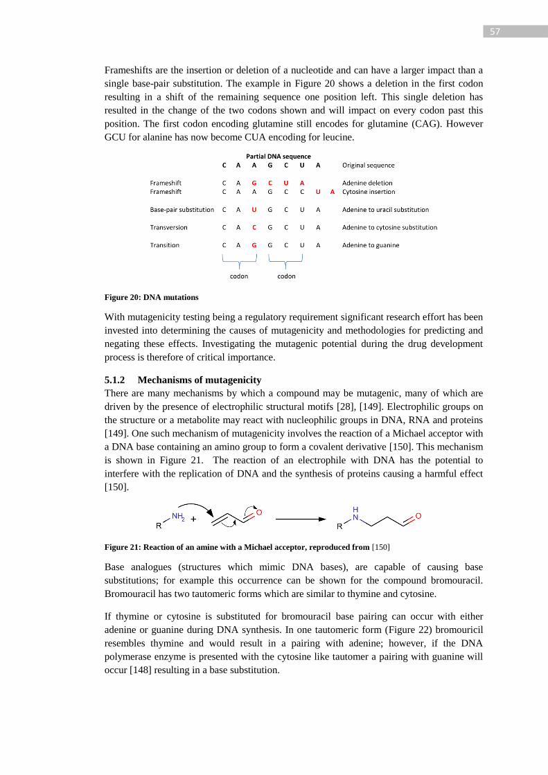
57
Frameshifts are the insertion or deletion of a nucleotide and can have a larger impact than a
single base-pair substitution. The example in Figure 20 shows a deletion in the first codon
resulting in a shift of the remaining sequence one position left. This single deletion has
resulted in the change of the two codons shown and will impact on every codon past this
position. The first codon encoding glutamine still encodes for glutamine (CAG). However
GCU for alanine has now become CUA encoding for leucine.
Figure 20: DNA mutations
With mutagenicity testing being a regulatory requirement significant research effort has been
invested into determining the causes of mutagenicity and methodologies for predicting and
negating these effects. Investigating the mutagenic potential during the drug development
process is therefore of critical importance.
5.1.2 Mechanisms of mutagenicity
There are many mechanisms by which a compound may be mutagenic, many of which are
driven by the presence of electrophilic structural motifs [28], [149]. Electrophilic groups on
the structure or a metabolite may react with nucleophilic groups in DNA, RNA and proteins
[149]. One such mechanism of mutagenicity involves the reaction of a Michael acceptor with
a DNA base containing an amino group to form a covalent derivative [150]. This mechanism
is shown in Figure 21. The reaction of an electrophile with DNA has the potential to
interfere with the replication of DNA and the synthesis of proteins causing a harmful effect
[150].
Figure 21: Reaction of an amine with a Michael acceptor, reproduced from [150]
Base analogues (structures which mimic DNA bases), are capable of causing base
substitutions; for example this occurrence can be shown for the compound bromouracil.
Bromouracil has two tautomeric forms which are similar to thymine and cytosine.
If thymine or cytosine is substituted for bromouracil base pairing can occur with either
adenine or guanine during DNA synthesis. In one tautomeric form (Figure 22) bromouricil
resembles thymine and would result in a pairing with adenine; however, if the DNA
polymerase enzyme is presented with the cytosine like tautomer a pairing with guanine will
occur [148] resulting in a base substitution.
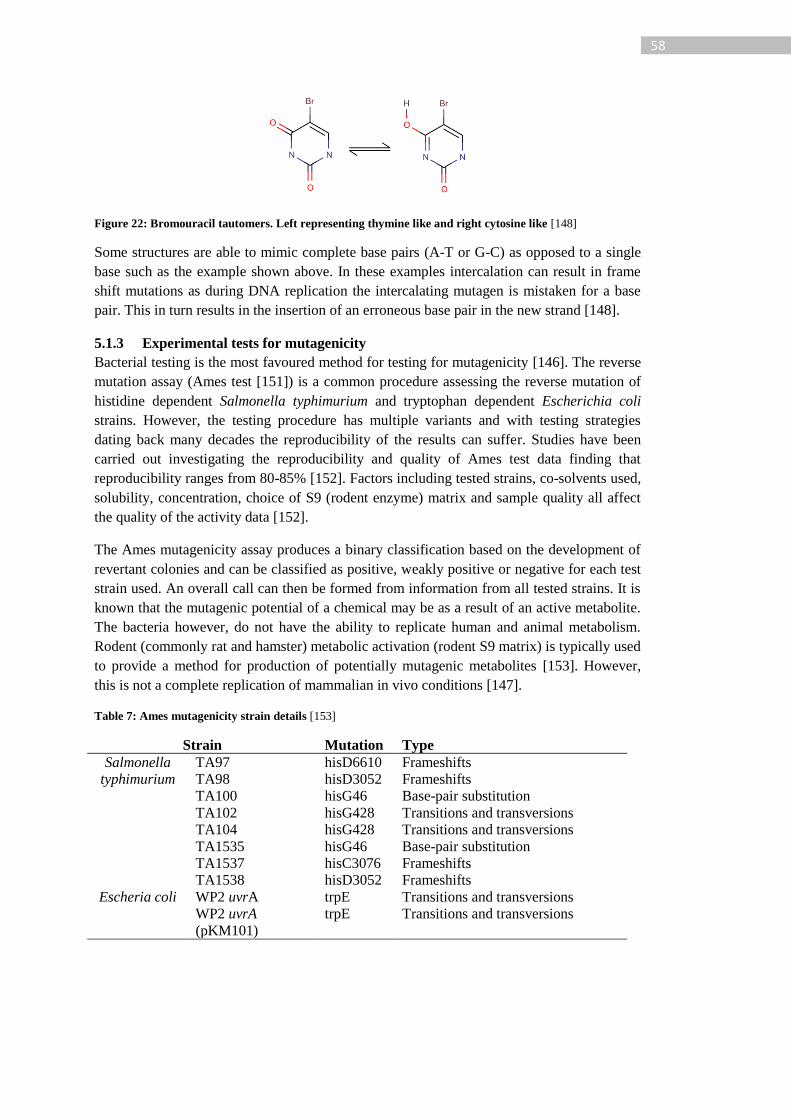
58
Figure 22: Bromouracil tautomers. Left representing thymine like and right cytosine like [148]
Some structures are able to mimic complete base pairs (A-T or G-C) as opposed to a single
base such as the example shown above. In these examples intercalation can result in frame
shift mutations as during DNA replication the intercalating mutagen is mistaken for a base
pair. This in turn results in the insertion of an erroneous base pair in the new strand [148].
5.1.3 Experimental tests for mutagenicity
Bacterial testing is the most favoured method for testing for mutagenicity [146]. The reverse
mutation assay (Ames test [151]) is a common procedure assessing the reverse mutation of
histidine dependent Salmonella typhimurium and tryptophan dependent Escherichia coli
strains. However, the testing procedure has multiple variants and with testing strategies
dating back many decades the reproducibility of the results can suffer. Studies have been
carried out investigating the reproducibility and quality of Ames test data finding that
reproducibility ranges from 80-85% [152]. Factors including tested strains, co-solvents used,
solubility, concentration, choice of S9 (rodent enzyme) matrix and sample quality all affect
the quality of the activity data [152].
The Ames mutagenicity assay produces a binary classification based on the development of
revertant colonies and can be classified as positive, weakly positive or negative for each test
strain used. An overall call can then be formed from information from all tested strains. It is
known that the mutagenic potential of a chemical may be as a result of an active metabolite.
The bacteria however, do not have the ability to replicate human and animal metabolism.
Rodent (commonly rat and hamster) metabolic activation (rodent S9 matrix) is typically used
to provide a method for production of potentially mutagenic metabolites [153]. However,
this is not a complete replication of mammalian in vivo conditions [147].
Table 7: Ames mutagenicity strain details [153]
Strain Mutation Type
Salmonella
typhimurium
TA97 hisD6610 Frameshifts
TA98 hisD3052 Frameshifts
TA100 hisG46 Base-pair substitution
TA102 hisG428 Transitions and transversions
TA104 hisG428 Transitions and transversions
TA1535 hisG46 Base-pair substitution
TA1537 hisC3076 Frameshifts
TA1538 hisD3052 Frameshifts
Escheria coli WP2 uvrA trpE Transitions and transversions
WP2 uvrA
(pKM101)
trpE Transitions and transversions
59
Table 7 shows the test strains commonly used each of which could be used with or without
the S9 matrix, the gene mutated and the type of mutation they are sensitive to. Each strain
has undergone mutation of the genes controlling the synthesis of the amino acid histidine (in
S. typhimurium) or tryptophan (in E. coli). Without an external source of histidine or
tryptophan these bacteria cannot grow and form colonies. Significant colony growth is seen
as a positive result for mutation as the bacteria has reverted to be non-histidine/tryptophan
dependent.
The bacteria are combined with the test compound and optionally with a S9 matrix. The
mixture is incubated on an agar plate for 48 hours at 37oC. The colony growth is measured
and compared with background control samples [153]. OECD guidelines recommend the
testing of at least 5 strains in the following way [147]:
1) “S. typhimurium TA1535; and
2) S. typhimurium TA1537 or TA97 or TA97a, and
3) S. typhimurium TA98, and
4) S. typhimurium TA100, and
5) E. coli WP2 uvrA, or E. coli WP2 uvrA (pKM1010), or S. typhimurium TA102”
However, it is common for compounds to be tested against fewer than five strains and results
may often be added to datasets with an overall call and the loss of the individual strain
details. It is also recommended to test each strain with and without S9 to determine
metabolic effects [147].
5.1.4 Structural alerts and models
Established mechanisms for mutagenicity discussed in the previous section allow for the
formulation of structural alerts (SA) which can be rationalised in terms of being
electrophiles, intercalators etc. Many sets of structural alerts for mutagenicity have been
devised and these are discussed in sections 5.1.4.2 to 5.1.4.6 along with (Q)SAR systems for
mutagenicity prediction.
An alert is a definable and matchable entity the presence of which indicates an outcome. For
example an alert could be: the presence of the SMARTS pattern [#8-]-[#7+]=O encoding for
a nitro group and may be used to indicate mutagenicity. The discussion in 5.1.4.2 to 5.1.4.6
will briefly review structural alerts.
5.1.4.1 Kazius toxicophores
A study by Kazius et al. [49] on the Bursi dataset (see section 5.1.5) of 4337 (2401 +ve/1936
-ve) compounds found that the majority of the mutagenic compounds in the dataset could be
detected by eight general toxicophores. Further analysis provided additional toxicophores
resulting in 27 approved structural alerts encoded as SMARTS.
The toxicophores derived by Kazius et al. were used to make predictions for an external
validation set of 342 mutagenic and 193 non mutagenic structures resulting in a predictive
accuracy of 85% [49]. This result along with the 82% accuracy on the original 4337
structures shows the strong capabilities of using structural alerts for the prediction of
mutagenicity. These results also support the choice of structural feature based descriptors for
machine learning approaches to mutagenicity prediction.

60
5.1.4.2 Ashby-Tennant alerts
Significant studies were carried out by Ashby and Tennant [52] into the mechanistic causes
behind the mutagenicity (or potential lack thereof) of a large number of chemicals resulting
in a number of structural alerts for mutagenicity and carcinogenicity which were then
incorporated into a single theoretical structure, which can be found in [52]. The structural
alert elements for the Ashby Tennant structure are listed in Table 8.
Table 8 Ashby and Tennant structural alerts [52]
Alert description
Alkyl esters of phosphonic or sulphonic acids
Aromatic nitro groups
Aromatic azo groups
Aromatic ring N-oxides
Aromatic mono- and dialkylamino groups
Alkyl hydrazines
Alkyl aldehydes
N-methylol deriatives
Monohaloalkenes
A large family of N and S mustards (β-haloethyl)
N-chloroamines
Propiolactones and propiosultones
Aziridinyl derivates
Substituted primary alkyl halides
Urethane derivatives (carbamates)
Alkyl N-nitroso amines
Aromatic amines, their derivatives and the derived esters
Aliphatic and aromatic epoxides
5.1.4.3 Benigni-Bossa alerts / ToxTree
Benigni and Bossa developed an expert system for the prediction of carcinogenicity and
mutagenicity for inclusion in the ToxTree predictive system [28]. The expert system consists
of 30 alerts for mutagenicity which have been sourced and selected from multiple sources:
Ashby and Tennant [52], Bailey et al. [51], Kazius et al. [49], [154] and from the oncologic
expert system provided by the US EPA [155], [156].
5.1.4.4 Derek Nexus
Derek Nexus (a commercial knowledge based expert system by Lhasa Limited) contains a
well-developed Ames and mammalian mutagenicity endpoint. The knowledge base is
developed by mining and refining literature sources of alerts in addition to the development
of new alerts based on SAR derivation using datasets. Recently automatic knowledge
extraction techniques have been used to support the identification of clusters of data for
prioritisation from large datasets [90].
Given the commercial nature of the software these alerts are not detailed here; they have
however been used in the comparison studies discussed in chapters 6 and 7. For more details
on Derek Nexus see chapters 2 and 3.
61
5.1.4.5 VEGA-QSAR
The VEGA-QSAR toolkit [157] is a free application for the prediction of a number of
toxicity endpoints including mutagenicity, carcinogenicity and skin sensitisation. The
CAESAR mutagenicity model is available along with a beta version of the SARpy rules as of
version 1.0.8 used in this study.
The CAESAR model is a two stage approach consisting of a statistical model based on a
SVM trained on a curated version of the Bursi dataset followed by two sets of structural
alerts [158]. A positive mutagenicity prediction can be made by the SVM or the structural
alerts. Given a negative prediction from the SVM a series of 12 structural alerts (SA)
selected from the Benigni-Bossa rule-base are then evaluated. If an alert is fired a positive
prediction for mutagenicity is provided. Finally a set of 4 SAs again taken from the Benigni-
Bossa rule-base are evaluated, a positive match here (preceded by negative evaluations from
the SVM and 12 SAs) results in a ‘Suspicious’ prediction for mutagenicity. A negative
prediction is made when neither the SVM nor any of the structural alerts sets are fired [158].
The SVM model is trained on 4204 curated structures using 25 descriptors: Gmin (minum E-
state value for all atoms), idw –bar (Bonchev-Trinajstic mean information content based on
graph distances), ALOGP (Ghose-Cripped octanol water coefficient), nrings (number of
rings in the molecular graph) and simple atom type counts denoting the presence or absence
of specific features in the molecular graph. The C-CVC SVM algorithm was used with the
Radial Basis Function (RBF) kernel. Optimisation was done via grid searching [158].
5.1.4.6 SARpy alerts
SARpy [79], [94] alerts are generated through the mining of toxicity datasets. SARpy rule
extraction was carried out on a curated form of the Bursi dataset published by Kazius et al.
[49] (see Kazius toxicophores); 117 structural alerts encoded as SMILES/SMARTS were
produced. The algorithm employed by SARpy is detailed in chapter 3 and the SA’s were
taken from [94] for use in the comparison in chapter 6.
5.1.5 Data
A variety of public mutagenicity data sources are available as well as precompiled modelling
datasets. Two commonly used datasets are the Bursi dataset consisting of 4337 structures
[49] which was provided by Kazius et al. with the results of their toxicophore mining effort
in 2005. Later, Hansen et al. produced a larger dataset of 7090 structures released in 2008
and then a curated version (version 2) in 2009 consisting of 6512 structures. Additional
sources of mutagenicity data include Vitic Nexus [109], a commercial database provided by
Lhasa Limited consisting of curated literature and collaborative data sharing initiatives and
ToxNet [159] a database of toxicology, hazardous chemicals, environmental health and toxic
provided by the United States National Institute of Health.
Many groups report the use of the Hansen [107] and Bursi [49] datasets in an internally
curated form. The data used in the Vega-QSAR mutagenicity models as well as for SARpy
are reported to be built from 4204 curated structures from the Bursi dataset [94], [158].
Fourches et al. undertook a curation effort on version 1 of the Hansen benchmark dataset
details of which are published in “Trust but verify” [112]. The use of various datasets, or
even revised editions of the same data in the literature and available predictive systems can
complicate comparisons. It is not always the case that a predictive system will report an

62
exact match of the query to a training example; performance can therefore be skewed by
comparison on a dataset where the models have had different levels of exposure to the
validation data in the training sets.
The main source of data for the modelling and mining effort discussed in chapters 6 and 7 is
based on version 2 of the Hansen benchmark mutagenicity dataset [107] acquired from the
website managed by Technische Universität Berlin [160]. A curation effort was undertaken
on this dataset to produce the final version used for the model building and knowledge
mining which has been published by Sherhod et al. [90]8 as a supplementary file with the
exception of structures with an equivocal prediction from Derek Nexus.
5.1.5.1 Curation
A curation effort was undertaken to improve the quality of the structural data and briefly
assess the potential reliability of the experimental results of a mutagenicity benchmark
dataset (Hansen) that had been constructed by combining data from multiple sources [107];
not all of these sources provide the data in a readily available format. CCRIS [161] and
GENETOX [159] data are provided in a web interface with structures being represented in a
picture format. Another limitation is caused by the lack of a unique identifier common
between the source and benchmark datasets. The combination of ChemAxon software and
various cheminformatic KNIME nodes allowed for an easy identification of issues and a
semi-automated curation procedure. Curation was only undertaken on structures; the activity
remains that of the initial dataset. However, a simple comparison of the Hansen dataset
where CAS numbers are known and comparable to the original dataset shows the
experimental activity to be the same as that reported at the data source. However, no
assessment of errors between dataset and published literature has been undertaken.
Data were acquired from the following data sources: Hansen [107], Bursi [49], NISS [162],
Helma [163], GENETOX [159], CCRIS [161], CPDB [108] and Vitic Nexus [109]. A
curation of the benchmark data was then undertaken using the following approach:
1) Where original source data were deemed of higher quality replace the benchmark
structure where the structures are readily available
2) Replace all known benchmark structures with Vitic structures (match by CAS)
3) Treat mixtures: remove salts, remove structures containing significant multiple
components (such as CAS 3546-41-6, Pyrvinium pamoate)
4) Remove structures containing X or R atoms
5) Identify and fix structural issues such as misrepresentation of nitro groups
6) Clean and redraw the structures including aromatisation and removal of explicit
hydrogens and stereochemistry
7) Check experimental activity is consistent between the various data sources
8) Remove duplicates, some of which may have been generated through steps 1-7
5.1.5.2 Data division
This curated dataset was then split into 70% training (2443 +ve / 2090 -ve), 15% testing (525
+ve / 447 -ve) and 15% validation (526 +ve / 446 -ve) using random sampling through the
KNIME partitioning node. The intra-set similarities are shown in Figure 23.
8 Authors contribution: curation of Hansen dataset
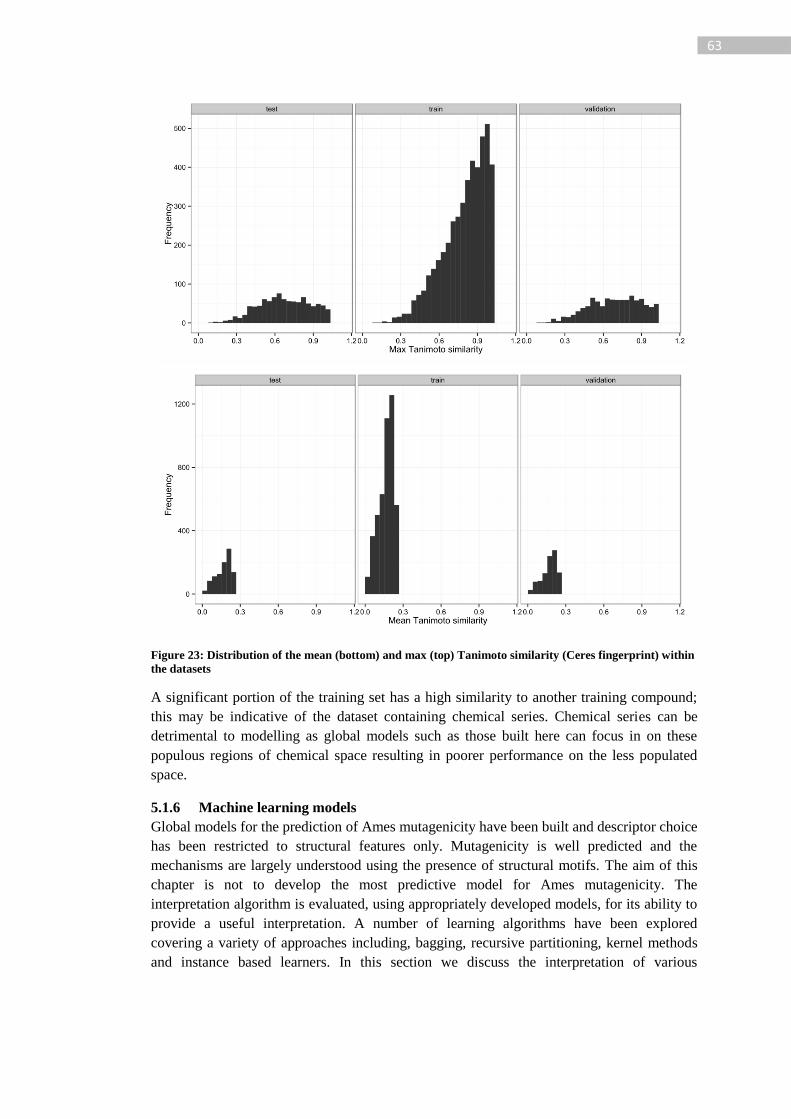
63
Figure 23: Distribution of the mean (bottom) and max (top) Tanimoto similarity (Ceres fingerprint) within
the datasets
A significant portion of the training set has a high similarity to another training compound;
this may be indicative of the dataset containing chemical series. Chemical series can be
detrimental to modelling as global models such as those built here can focus in on these
populous regions of chemical space resulting in poorer performance on the less populated
space.
5.1.6 Machine learning models
Global models for the prediction of Ames mutagenicity have been built and descriptor choice
has been restricted to structural features only. Mutagenicity is well predicted and the
mechanisms are largely understood using the presence of structural motifs. The aim of this
chapter is not to develop the most predictive model for Ames mutagenicity. The
interpretation algorithm is evaluated, using appropriately developed models, for its ability to
provide a useful interpretation. A number of learning algorithms have been explored
covering a variety of approaches including, bagging, recursive partitioning, kernel methods
and instance based learners. In this section we discuss the interpretation of various

64
combinations of descriptors and machine learning algorithms for the prediction of Ames
mutagenicity.
5.1.6.1 Descriptors
Five structural fingerprints have been employed: Ceres hashed fingerprint, CDK standard,
CDK extended, MACCS and Pubchem. The first three being of the hashed fingerprint type
and the remainder being structural keys, for more information see Chapter 4.
5.1.6.2 Domain calculation
The domain of the model is calculated according to the fragments present in the training
structures (see section 5.1.5). For a query to be deemed as in-domain all of its atoms must be
covered by fragments present in the training set.
Approach:
1) Fragment training set creating a dictionary of fragments.
2) For each query structure:
a. Create a list of atoms
b. Fragment the query creating a list of fragments
i. For each fragment, if the fragment is present in the dictionary ≥ cut-
off remove the atoms in the fragment from the list
c. If no atoms remain in the list of atoms then the structure is in the domain,
otherwise the structure is out of the domain due to the presence of a novel
motif
The cut-off value used for these models is 1 resulting in the in-domain definition being: the
atoms in the structure are represented by a least 1 fragment in the training fragment
dictionary.
5.1.6.3 Predictive model building and evaluation
To allow for an assessment of the interpretation a variety of learning algorithms have been
used in model building. Support Vector Machine and Random Forest algorithms have been
used as popular black box learning algorithms. A decision tree and k Nearest Neighbours
have been used from the more white box approach, however, in the case of the fingerprints
used here direct interpretation is unrealistic. These four algorithms give a spread of common
approaches used in the (Q)SAR literature and have been used successfully for the modelling
of the Ames mutagenicity endpoint [152], [158], [164], [165]. The predictions are expected
to differ not only in predicted class but also in cause, by comparing models an assessment of
the stability and clarity of the interpretation algorithm can be undertaken.
All data pre-processing (curation, dataset compilation) and predictive model building has
been carried out in KNIME 2.9.4. KNIME provides access to their own implementations of
Random Forest through use of the Tree Ensemble Learner; kNN is provided by the k Nearest
Neighbour node, C4.5 decision tree building in the Decision Tree learner and SVM models
are provided by the LIBSVM learner node implementing version 2.89 of the LIBSVM code.
Further details of the learning algorithm implementations are shown in Table 9.

65
Table 9: Learning algorithm details
Algorithm KNIME Node Parameters
Random Forest Tree Ensemble
Learner
Split criterion: information gain ratio
Limit number of levels: false
Minimum split node size: false
Number of models: 50, 100, 150 best
selected from cross validation balanced
accuracy
Data sampling: 0.7 without replacement
Descriptor sampling: sample (square root)
at each node
Decision tree Decision Tree
Learner
Quality measure: Gini index
Pruning method: MDL
Reduced error pruning: true
Min number of records per node: 2
Support Vector
Machine
LIBSVM Type: C-CSV
Kernel: RBF
Gamma and cost learned through grid
searching with LibSVM grid.py using
default configuration
K Nearest
Neighbour
K Nearest Neighbour Weighted = true
Value of k = models built from 5, 8 and 10.
Best selected from cross validation
performance.
Some parameter selection has been carried out using the performance of the models against
the test set (see section 5.1.5) to reduce over training. Grid.py, a python script provided with
LibSVM was used to determine the optimal settings for gamma and cost in the chosen RBF
kernel for the support vector machine. The Random Forest was manually optimised from 4
values of the number of trees: 50, 100, 150 and 200. The value of k in the k nearest
neighbour algorithm was selected from the best balanced accuracy from the cross validation
using values of 5, 8 and 10. Other values remain fixed and are recorded in Table 9.
In addition to the KNIME implementation the whole process can be carried out within
Coralie. Coralie provides a richer user interface, see Figure 40 in section Error! Reference
source not found., for interacting with the interpretation. However, it is limited in the ability
to automate the generation of large numbers of models and evaluation against multiple
datasets. For this purpose, the KNIME implementation has been used for the benchmarking
of the models against external predictive tools.
5.1.6.4 Model performance
The 5 fold cross validation performance for the selected models can be seen in Table 10 and
the test set performance of the final selected models in Table 11.
For each learning algorithm a model was built with each fingerprint type (MACCS, CDK,
CDK extended, Pubchem and Ceres) resulting in a total of 30 models (5 algorithms * 6
descriptor sets). For each learning algorithm the best performing model was selected based
on the performance against the test dataset. For the purposes of completeness the best
method from the Ceres hashed fingerprint has also been included (RF-Ceres). These final 5
models where then used for evaluation against the validation set and later for comparison of
interpretation.
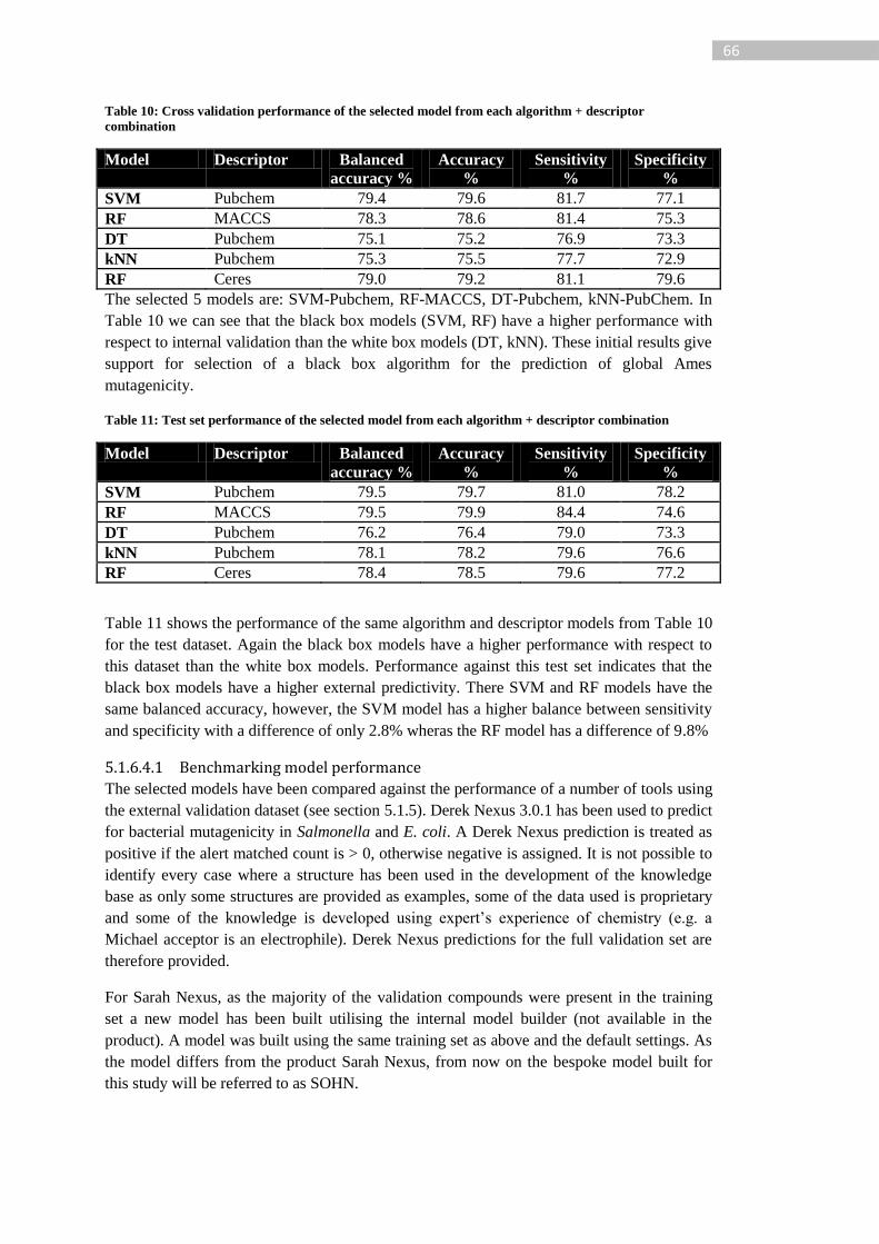
66
Table 10: Cross validation performance of the selected model from each algorithm + descriptor
combination
Model Descriptor Balanced
accuracy %
Accuracy
%
Sensitivity
%
Specificity
%
SVM Pubchem 79.4 79.6 81.7 77.1
RF MACCS 78.3 78.6 81.4 75.3
DT Pubchem 75.1 75.2 76.9 73.3
kNN Pubchem 75.3 75.5 77.7 72.9
RF Ceres 79.0 79.2 81.1 79.6
The selected 5 models are: SVM-Pubchem, RF-MACCS, DT-Pubchem, kNN-PubChem. In
Table 10 we can see that the black box models (SVM, RF) have a higher performance with
respect to internal validation than the white box models (DT, kNN). These initial results give
support for selection of a black box algorithm for the prediction of global Ames
mutagenicity.
Table 11: Test set performance of the selected model from each algorithm + descriptor combination
Model Descriptor Balanced
accuracy %
Accuracy
%
Sensitivity
%
Specificity
%
SVM Pubchem 79.5 79.7 81.0 78.2
RF MACCS 79.5 79.9 84.4 74.6
DT Pubchem 76.2 76.4 79.0 73.3
kNN Pubchem 78.1 78.2 79.6 76.6
RF Ceres 78.4 78.5 79.6 77.2
Table 11 shows the performance of the same algorithm and descriptor models from Table 10
for the test dataset. Again the black box models have a higher performance with respect to
this dataset than the white box models. Performance against this test set indicates that the
black box models have a higher external predictivity. There SVM and RF models have the
same balanced accuracy, however, the SVM model has a higher balance between sensitivity
and specificity with a difference of only 2.8% wheras the RF model has a difference of 9.8%
5.1.6.4.1 Benchmarking model performance
The selected models have been compared against the performance of a number of tools using
the external validation dataset (see section 5.1.5). Derek Nexus 3.0.1 has been used to predict
for bacterial mutagenicity in Salmonella and E. coli. A Derek Nexus prediction is treated as
positive if the alert matched count is > 0, otherwise negative is assigned. It is not possible to
identify every case where a structure has been used in the development of the knowledge
base as only some structures are provided as examples, some of the data used is proprietary
and some of the knowledge is developed using expert’s experience of chemistry (e.g. a
Michael acceptor is an electrophile). Derek Nexus predictions for the full validation set are
therefore provided.
For Sarah Nexus, as the majority of the validation compounds were present in the training
set a new model has been built utilising the internal model builder (not available in the
product). A model was built using the same training set as above and the default settings. As
the model differs from the product Sarah Nexus, from now on the bespoke model built for
this study will be referred to as SOHN.
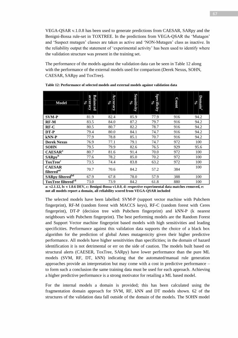
67
VEGA-QSAR v.1.0.8 has been used to generate predictions from CAESAR, SARpy and the
Benigni-Bossa rule-set in TOXTREE. In the predictions from VEGA-QSAR the ‘Mutagen’
and ‘Suspect mutagen’ classes are taken as active and ‘NON-Mutagen’ class as inactive. In
the reliability output the statement of ‘experimental activity’ has been used to identify where
the validation structure was present in the training set.
The performance of the models against the validation data can be seen in Table 12 along
with the performance of the external models used for comparison (Derek Nexus, SOHN,
CAESAR, SARpy and ToxTree).
Table 12: Performance of selected models and external models against validation data
Model
Ba
lan
ced
acc
ura
cy
%
Acc
ura
cy
%
Sen
sitivity
%
Sp
ecificity
%
Co
un
t
Do
ma
ine
%
SVM-P 81.9 82.4 85.9 77.9 916 94.2
RF-M 83.5 84.0 87.2 79.7 916 94.2
RF-C 80.5 80.7 82.2 78.7 916 94.2
DT-P 79.4 80.0 84.1 74.7 916 94.2
kNN-P 77.9 78.8 85.1 70.7 916 94.2
Derek Nexus 76.9 77.1 79.1 74.7 972 100
SOHN 79.5 79.9 82.6 76.5 929 95.6
CAESARa 80.7 81.6 91.4 70.0 972 100
SARpyb 77.6 78.2 85.0 70.2 972 100
ToxTreec 73.5 74.4 83.8 63.2 972 100
CAESAR
filteredad
70.7 70.6 84.2 57.2 384
100
SARpy filteredbd
67.9 67.8 78.0 57.9 388 100
ToxTree filteredcd
73.0 73.9 84.2 61.8 880 100
a: v2.1.12, b: v 1.0.6 DEV, c: Benigni-Bossa v1.0.0, d: respective experimental data matches removed, e:
not all models report a domain, all reliability scored from VEGA-QSAR included
The selected models have been labelled: SVM-P (support vector machine with Pubchem
fingerprint), RF-M (random forest with MACCS keys), RF-C (random forest with Ceres
fingerprint), DT-P (decision tree with Pubchem fingerprint) and kNN-P (k nearest
neighbours with Pubchem fingerprint). The best performing models are the Random Forest
and Support Vector machine fingerprint based models with high sensitivities and leading
specificities. Performance against this validation data supports the choice of a black box
algorithm for the prediction of global Ames mutagenicity given their higher predictive
performance. All models have higher sensitivities than specificities; in the domain of hazard
identification it is not detrimental or err on the side of caution. The models built based on
structural alerts (CAESER, ToxTree, SARpy) have lower performance than the pure ML
models (SVM, RF, DT, kNN) indicating that the automated/manual rule generation
approaches provide an interpretation but may come with a cost in predictive performance –
to form such a conclusion the same training data must be used for each approach. Achieving
a higher predictive performance is a strong motivator for retailing a ML based model.
For the internal models a domain is provided; this has been calculated using the
fragmentation domain approach for SVM, RF, kNN and DT models shown. 62 of the
structures of the validation data fall outside of the domain of the models. The SOHN model
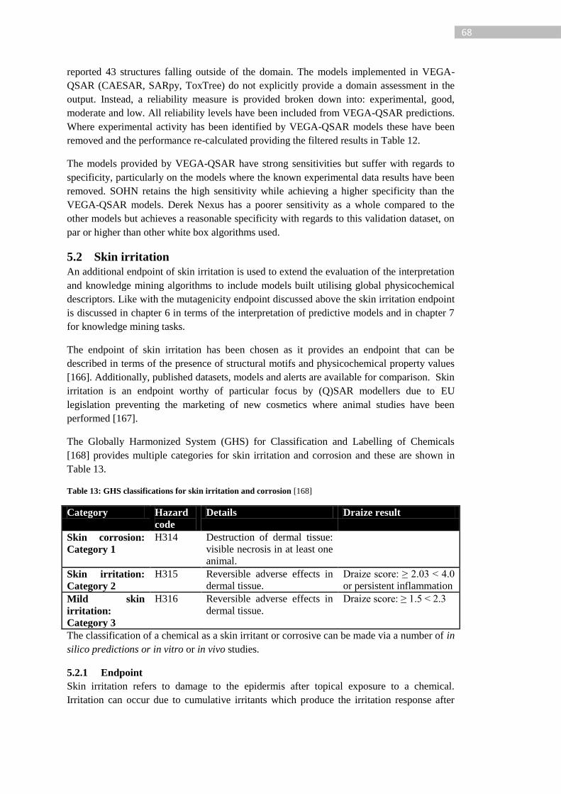
68
reported 43 structures falling outside of the domain. The models implemented in VEGA-
QSAR (CAESAR, SARpy, ToxTree) do not explicitly provide a domain assessment in the
output. Instead, a reliability measure is provided broken down into: experimental, good,
moderate and low. All reliability levels have been included from VEGA-QSAR predictions.
Where experimental activity has been identified by VEGA-QSAR models these have been
removed and the performance re-calculated providing the filtered results in Table 12.
The models provided by VEGA-QSAR have strong sensitivities but suffer with regards to
specificity, particularly on the models where the known experimental data results have been
removed. SOHN retains the high sensitivity while achieving a higher specificity than the
VEGA-QSAR models. Derek Nexus has a poorer sensitivity as a whole compared to the
other models but achieves a reasonable specificity with regards to this validation dataset, on
par or higher than other white box algorithms used.
5.2 Skin irritation
An additional endpoint of skin irritation is used to extend the evaluation of the interpretation
and knowledge mining algorithms to include models built utilising global physicochemical
descriptors. Like with the mutagenicity endpoint discussed above the skin irritation endpoint
is discussed in chapter 6 in terms of the interpretation of predictive models and in chapter 7
for knowledge mining tasks.
The endpoint of skin irritation has been chosen as it provides an endpoint that can be
described in terms of the presence of structural motifs and physicochemical property values
[166]. Additionally, published datasets, models and alerts are available for comparison. Skin
irritation is an endpoint worthy of particular focus by (Q)SAR modellers due to EU
legislation preventing the marketing of new cosmetics where animal studies have been
performed [167].
The Globally Harmonized System (GHS) for Classification and Labelling of Chemicals
[168] provides multiple categories for skin irritation and corrosion and these are shown in
Table 13.
Table 13: GHS classifications for skin irritation and corrosion [168]
Category Hazard
code
Details Draize result
Skin corrosion:
Category 1
H314 Destruction of dermal tissue:
visible necrosis in at least one
animal.
Skin irritation:
Category 2
H315 Reversible adverse effects in
dermal tissue.
Draize score: ≥ 2.03 < 4.0
or persistent inflammation
Mild skin
irritation:
Category 3
H316 Reversible adverse effects in
dermal tissue.
Draize score: ≥ 1.5 < 2.3
The classification of a chemical as a skin irritant or corrosive can be made via a number of in
silico predictions or in vitro or in vivo studies.
5.2.1 Endpoint
Skin irritation refers to damage to the epidermis after topical exposure to a chemical.
Irritation can occur due to cumulative irritants which produce the irritation response after
69
repeat exposure or by acute irritants which only require a single exposure. Skin irritation can
be broken down into skin irritation, which is described by reversible local inflammatory
reaction, and skin corrosion, which is classified as irreversible damage to the skin [169],
[170]. Skin irritation specifically is modelled in chapters 6 and 7. Corrosion data has not
been used.
5.2.2 Experimental tests
Both in vitro and in vivo tests are accepted for skin irritation testing. The in vitro tests are
based on reconstructed human epidermis (RHE) and validated by the European Centre for
the Validation of Alternative Methods (ECVAM) [169]. OECD guidelines are available for
both in vivo (Rabbit Draize) and in vitro testing and are detailed below.
5.2.2.1 Rabbit Draize (in vivo) for skin irritation
The OECD guidelines state that Rabbit Draize in vivo testing should not be undertaken until
all available data pertinent to dermal corrosivity and irritation has been obtained and
evaluated in a weight of evidence analysis.
Should a Rabbit Draize test be carried out OECD guidelines are set out in [171] and a
selection of the guidelines is reproduced here:
- Apply in a single dose to the skin of the experimental animal with untreated areas
providing the control
- Record the degree of irritation/corrosion at specified intervals
- Animals showing continuing signs of severe distress and/or pain at any stage of the
test should be killed humanely and the substance assessed accordingly
- The test substance should be applied to a small area approximately 6cm2 of skin and
covered with a gauze patch. If direct testing of the substance is not possible the test
substance should be applied to the gauze patch.
- The test patch should be held in place with a suitable semi-occlusive dressing for the
duration of the exposure period.
- Liquid test substances are generally used undiluted, solids may be pulverised when
necessary. If necessary water may be used to moisten the sample to ensure good skin
contact. If using an alternative vehicle the influence must be accounted for.
- At the end of the exposure period (normally 4 hours), residual test substances should
be removed without altering the existing response of integrity of the epidermis.
- The duration of the observation period should be sufficient to evaluate fully the
reversibility of the effects observed.
- All animals should be examined for signs of erythema and oedema
- The grading of skin response is subjective. To support the harmonisation of the skin
response adequate training of the examiner must be undertaken.
5.2.2.2 In Vitro tests for skin irritation
Guidelines for the use of in vitro tests for use in the hazard identification of irritant
chemicals conforms with the UN GHS and EU CLP Category 2 [172]. The guidelines are
designed to address the human health endpoint for skin irritation by the use of in vitro tests
that are derived from transformed epidermis keratinocytes and the use of a representative
tissue and cytoarchitecture [172]. At the time of writing the guidelines covers three validated
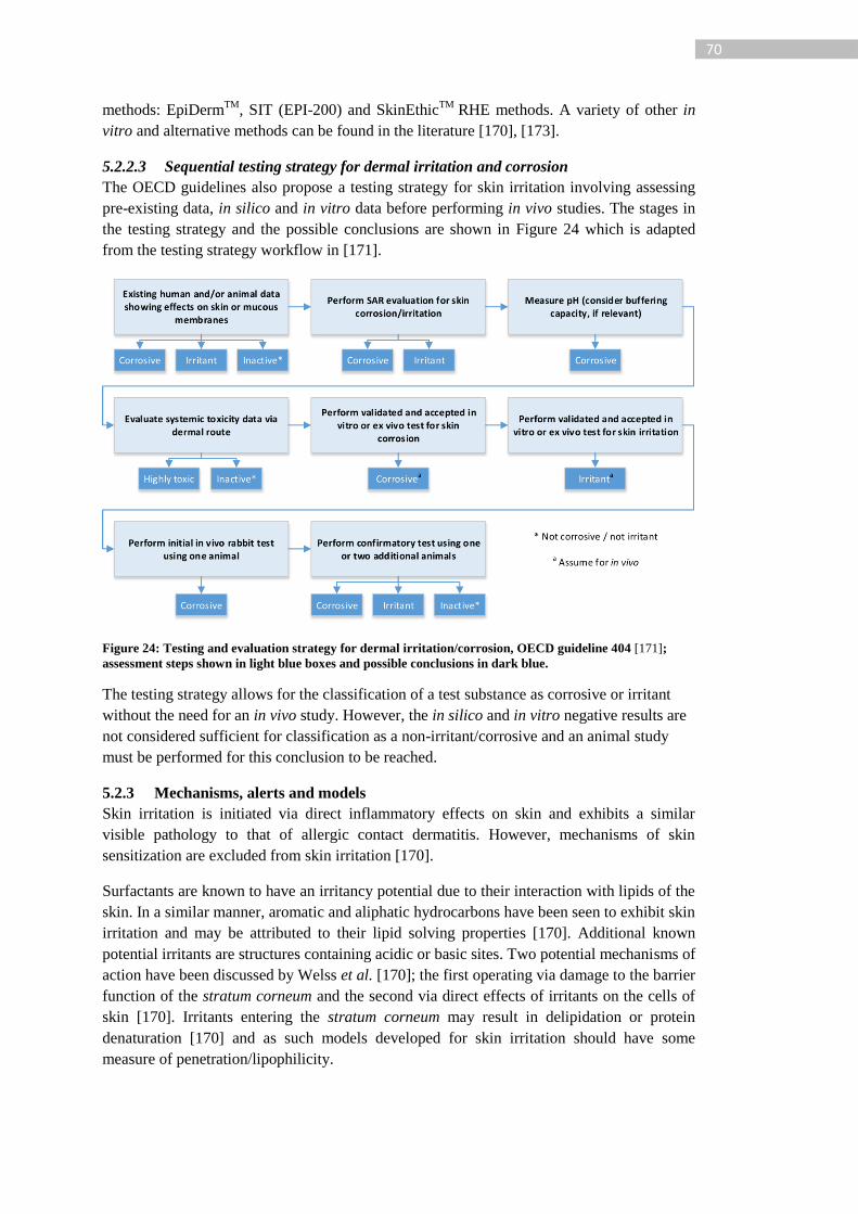
70
methods: EpiDermTM
, SIT (EPI-200) and SkinEthicTM
RHE methods. A variety of other in
vitro and alternative methods can be found in the literature [170], [173].
5.2.2.3 Sequential testing strategy for dermal irritation and corrosion
The OECD guidelines also propose a testing strategy for skin irritation involving assessing
pre-existing data, in silico and in vitro data before performing in vivo studies. The stages in
the testing strategy and the possible conclusions are shown in Figure 24 which is adapted
from the testing strategy workflow in [171].
Figure 24: Testing and evaluation strategy for dermal irritation/corrosion, OECD guideline 404 [171];
assessment steps shown in light blue boxes and possible conclusions in dark blue.
The testing strategy allows for the classification of a test substance as corrosive or irritant
without the need for an in vivo study. However, the in silico and in vitro negative results are
not considered sufficient for classification as a non-irritant/corrosive and an animal study
must be performed for this conclusion to be reached.
5.2.3 Mechanisms, alerts and models
Skin irritation is initiated via direct inflammatory effects on skin and exhibits a similar
visible pathology to that of allergic contact dermatitis. However, mechanisms of skin
sensitization are excluded from skin irritation [170].
Surfactants are known to have an irritancy potential due to their interaction with lipids of the
skin. In a similar manner, aromatic and aliphatic hydrocarbons have been seen to exhibit skin
irritation and may be attributed to their lipid solving properties [170]. Additional known
potential irritants are structures containing acidic or basic sites. Two potential mechanisms of
action have been discussed by Welss et al. [170]; the first operating via damage to the barrier
function of the stratum corneum and the second via direct effects of irritants on the cells of
skin [170]. Irritants entering the stratum corneum may result in delipidation or protein
denaturation [170] and as such models developed for skin irritation should have some
measure of penetration/lipophilicity.
71
Leist et al. have developed a mechanism of action (MoA) based model for skin irritancy
[174]. The global dataset for skin irritancy was divided into MoA based groups covering:
alcohols, alkenes, amines, carboxylic acids/esters, reactive groups and surfactants. Molecular
descriptors were used in combination with a PLS learner for each MoA dataset. The final
prediction is based on a weight of evidence (WoE) approach for the prediction of irritant vs
non-irritant. The authors report a sensitivity of 95% and a specificity of 84% but no details
on how these values were acquired is given.
Liew and Yap [175] have developed models for the predictions of skin and eye irritancy and
corrosions as independent models. A committee modelling approach has been performed
where models are produced, selected and then combined into a committee model. Support
vector machines were used as the learning algorithm and the model parameterisation,
training and descriptors were varied for each model in the committee [175]. The final model
external performance is reported to be 55.2% sensitivity and 82.9% specificity indicating
that the model’s external predictivity is poor relative to its internal performance measure
which had 94.3% sensitivity and 84.7% specificity.
Expert systems or rule-bases are available for the prediction of skin irritancy. Derek Nexus
contains 25 alerts for the prediction of skin irritation to mammals initially created in 1999.
This endpoint covers both irritation and corrosion and doesn’t distinguish between the two
categories. Walker et al. have developed the ‘Skin Irritation Corrosion Rules Estimation
Tool’ (SICRET) which is based upon a series of structural alerts and physicochemical
exclusions for example: IF logPow or logKow < -3.1 THEN NOT IRRITATING OR
CORROSIVE TO SKIN [166]. The physicochemical rules used for exclusions in SICRET
are: melting point, logPow or logKow, lipid solubility, molecular weight, melting point,
surface tension, aqueous solubility and vapour pressure [166]. 12 structural alerts for skin
corrosion and 28 further alerts for skin irritation and corrosion are provided in the
companion paper by Hulzebos et al. [176]. The SICRET rule base has been implemented in
ToxTree and the OECD toolbox [177].
5.2.4 Data and curation
A dataset for skin irritation has been compiled and published along with the modelling
studies by Liew and Yap [175] for skin irritation. The dataset is compiled from “Table 3.1 of
Part 3 of Annex VI to Regulation (EC) No 1272/ 2008 [listing] the harmonized classification
and labelling of hazardous substances set out in the regulation” [175]. The published data has
been acquired in the form of two SD files from the authors website [178].
The data was processed through a general structural curation process using Lhasa Limited’s
internal chemical engine for an initial check resulting in no errors. The next level was to
process through the ChemAxon Standardizer running the default normalisation
transformations and removal of explicit hydrogens and dearomatisation. Finally the
structures were checked for mixtures and aromaticity errors with the ChemAxon Structure
Checker, again resulting in no errors.
As can be seen from Table 14 this data has a significant negative bias (83%) which could
have a detrimental impact on the model learning process. Liew and Yap’s modelling efforts
resulted in a sensitivity of 55.2% and a specificity of 82.9% on external validation indicating

72
that this dataset may pose significant difficulties for modelling, as might be expected their
model has learnt more about the inactive compounds than the active.
Table 14: Skin irritation datasets
Counts
Division active inactive
Training 283 1424
Validation 67 334
5.2.5 Machine learning models
As with the study on mutagenicity a variety of models have been built with different
descriptor and learning algorithm combinations; the focus of this work is not to develop the
best predictive model for skin irritation. Rather, a model of sufficient performance using
appropriate descriptors is built. The interpretations generated by the ENCORE algorithm are
then investigated.
5.2.5.1 Descriptors
Given the modest differences between the performance of the various models when for
different fingerprints for mutagenicity only the Ceres fingerprint has been used in this study
on skin irritation.
In addition to the hashed structural fingerprint two physicochemical properties have been
investigated: calculated octanol-water partition coefficient (logP) and the Potts and Guy
equation for skin permeability (logKp). Both descriptors are calculated using BioByte
version 5.3. Skin irritation is affected by the absorption of the chemical through the skin and
as such models of lipophilicity and permeation should provide useful, and mechanistically
relevant, information to the learning algorithm.
Table 15: Descriptor details
Descriptors Details
Ceres fingerprint Only using the Ceres hashed structural
fingerprint. No logKp information provided
to the model.
Ceres fingerprint, continuous variable for
logKp
Using the Ceres hashed structural fingerprint
in addition to a continuous variable for
logKp
Ceres fingerprint, binned nominal
variable for logKp
Using the Ceres hashed structural fingerprint
in addition to a nominal variable for logKp
represented by the bin range identified from
the supervised discretisation.
Ceres fingerprint, fingerprint
representing identified bins for logKp
Using the Ceres hashed structural fingerprint
in addition to a generated fingerprint
representing the discretised ranges of logKp
identified from the supervised discretisation.
These physicochemical properties have been used for interpretation and knowledge mining
purposes as fingerprints with the method discussed in earlier in this chapter. For an
evaluation of the impact this has on performance they have also been used as continuous
descriptors, binned nominal descriptors and then converted to a fingerprint. Discretisation of

73
the logP and logKp values was performed using Weka 3.7 and the supervised Discretize
filter which employs Fayyad and Irani’s MDL method [179], [180]. The supervised
discretisation resulted in 2 bins for LogKp (-inf to -1.595 and -1.595 to +inf) which can be
described as less skin permeable and more skin permeable. A single bin for logP has been
identified; due to only a single bin being identified for logP this descriptor was not
investigated further.
5.2.5.2 Domain calculation
The domain calculation is performed in a similar way to the approach for mutagenicity.
Where a model contains a physicochemical property a simple range based method has been
employed. More sophisticated methods for domain calculation are available; the focus of this
work is on the interpretation of the model (which does not change relative to the domain
calculation) and therefore appropriate albeit simple methods for domain calculation have
been used.
A query structure is considered to be in the domain of the model if the following criteria are
met:
1) All the fragments contained in the structure are seen at least once in the training set.
2) The values for all physicochemical properties used in the model fall within the range
of the physicochemical property in the training set.
35 structures were deemed out of domain by step 1 followed by a further 2 structures in step
2.
5.2.5.3 Weighted learning
To address the issue of the data imbalance, which has a detrimental effect on the learning of
the model, a strategy with instance weights has been adopted. For a discussion on the impact
and alternative strategies see section 2.3.1.
Where a class weighting is equal (default = 1) the sum of the class weights is proportionate
to the bias in the classes. By providing a balanced class weight the sum of the class weights
should be approximately equal.
( )
Equation 20: Class weight for given class C
From Equation 20 the weight of the active class is 1.000 and the inactive (majority) class
0.199. The sum of the weights is 283 for both classes as opposed to the unweighted sum of
283 for the active class and 1424 for the inactive class.
Instance weights have been added to allow for class balanced learning in Weka. Weka
provides a variety of learning algorithms which can use instance weights including: Random
Forest, IBk (kNN) and J48 (decision tree). At a high level the class weighting impacts by
giving relative importance to instances based upon their weight. In the case of the random
forest, which is implemented in Weka as bagging of random trees, an instance with a higher
weight has a higher chance of being selected for a tree than an instance with a lower weight.
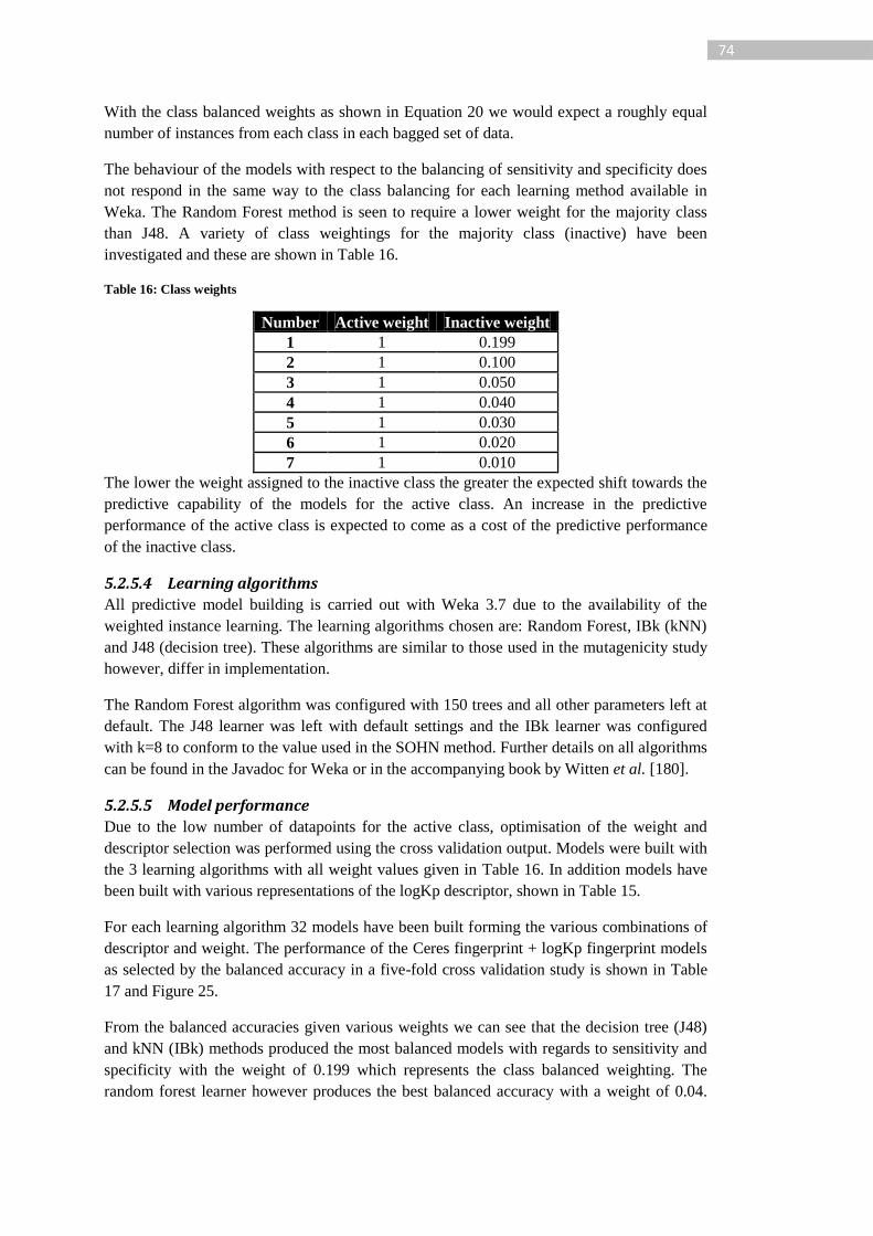
74
With the class balanced weights as shown in Equation 20 we would expect a roughly equal
number of instances from each class in each bagged set of data.
The behaviour of the models with respect to the balancing of sensitivity and specificity does
not respond in the same way to the class balancing for each learning method available in
Weka. The Random Forest method is seen to require a lower weight for the majority class
than J48. A variety of class weightings for the majority class (inactive) have been
investigated and these are shown in Table 16.
Table 16: Class weights
Number Active weight Inactive weight
1 1 0.199
2 1 0.100
3 1 0.050
4 1 0.040
5 1 0.030
6 1 0.020
7 1 0.010
The lower the weight assigned to the inactive class the greater the expected shift towards the
predictive capability of the models for the active class. An increase in the predictive
performance of the active class is expected to come as a cost of the predictive performance
of the inactive class.
5.2.5.4 Learning algorithms
All predictive model building is carried out with Weka 3.7 due to the availability of the
weighted instance learning. The learning algorithms chosen are: Random Forest, IBk (kNN)
and J48 (decision tree). These algorithms are similar to those used in the mutagenicity study
however, differ in implementation.
The Random Forest algorithm was configured with 150 trees and all other parameters left at
default. The J48 learner was left with default settings and the IBk learner was configured
with k=8 to conform to the value used in the SOHN method. Further details on all algorithms
can be found in the Javadoc for Weka or in the accompanying book by Witten et al. [180].
5.2.5.5 Model performance
Due to the low number of datapoints for the active class, optimisation of the weight and
descriptor selection was performed using the cross validation output. Models were built with
the 3 learning algorithms with all weight values given in Table 16. In addition models have
been built with various representations of the logKp descriptor, shown in Table 15.
For each learning algorithm 32 models have been built forming the various combinations of
descriptor and weight. The performance of the Ceres fingerprint + logKp fingerprint models
as selected by the balanced accuracy in a five-fold cross validation study is shown in Table
17 and Figure 25.
From the balanced accuracies given various weights we can see that the decision tree (J48)
and kNN (IBk) methods produced the most balanced models with regards to sensitivity and
specificity with the weight of 0.199 which represents the class balanced weighting. The
random forest learner however produces the best balanced accuracy with a weight of 0.04.
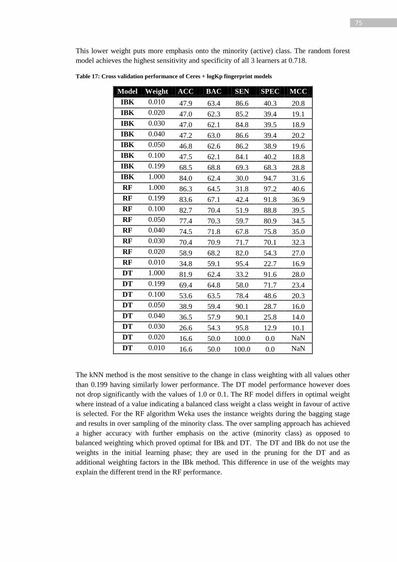
75
This lower weight puts more emphasis onto the minority (active) class. The random forest
model achieves the highest sensitivity and specificity of all 3 learners at 0.718.
Table 17: Cross validation performance of Ceres + logKp fingerprint models
Model Weight ACC BAC SEN SPEC MCC
IBK 0.010 47.9 63.4 86.6 40.3 20.8
IBK 0.020 47.0 62.3 85.2 39.4 19.1
IBK 0.030 47.0 62.1 84.8 39.5 18.9
IBK 0.040 47.2 63.0 86.6 39.4 20.2
IBK 0.050 46.8 62.6 86.2 38.9 19.6
IBK 0.100 47.5 62.1 84.1 40.2 18.8
IBK 0.199 68.5 68.8 69.3 68.3 28.8
IBK 1.000 84.0 62.4 30.0 94.7 31.6
RF 1.000 86.3 64.5 31.8 97.2 40.6
RF 0.199 83.6 67.1 42.4 91.8 36.9
RF 0.100 82.7 70.4 51.9 88.8 39.5
RF 0.050 77.4 70.3 59.7 80.9 34.5
RF 0.040 74.5 71.8 67.8 75.8 35.0
RF 0.030 70.4 70.9 71.7 70.1 32.3
RF 0.020 58.9 68.2 82.0 54.3 27.0
RF 0.010 34.8 59.1 95.4 22.7 16.9
DT 1.000 81.9 62.4 33.2 91.6 28.0
DT 0.199 69.4 64.8 58.0 71.7 23.4
DT 0.100 53.6 63.5 78.4 48.6 20.3
DT 0.050 38.9 59.4 90.1 28.7 16.0
DT 0.040 36.5 57.9 90.1 25.8 14.0
DT 0.030 26.6 54.3 95.8 12.9 10.1
DT 0.020 16.6 50.0 100.0 0.0 NaN
DT 0.010 16.6 50.0 100.0 0.0 NaN
The kNN method is the most sensitive to the change in class weighting with all values other
than 0.199 having similarly lower performance. The DT model performance however does
not drop significantly with the values of 1.0 or 0.1. The RF model differs in optimal weight
where instead of a value indicating a balanced class weight a class weight in favour of active
is selected. For the RF algorithm Weka uses the instance weights during the bagging stage
and results in over sampling of the minority class. The over sampling approach has achieved
a higher accuracy with further emphasis on the active (minority class) as opposed to
balanced weighting which proved optimal for IBk and DT. The DT and IBk do not use the
weights in the initial learning phase; they are used in the pruning for the DT and as
additional weighting factors in the IBk method. This difference in use of the weights may
explain the different trend in the RF performance.
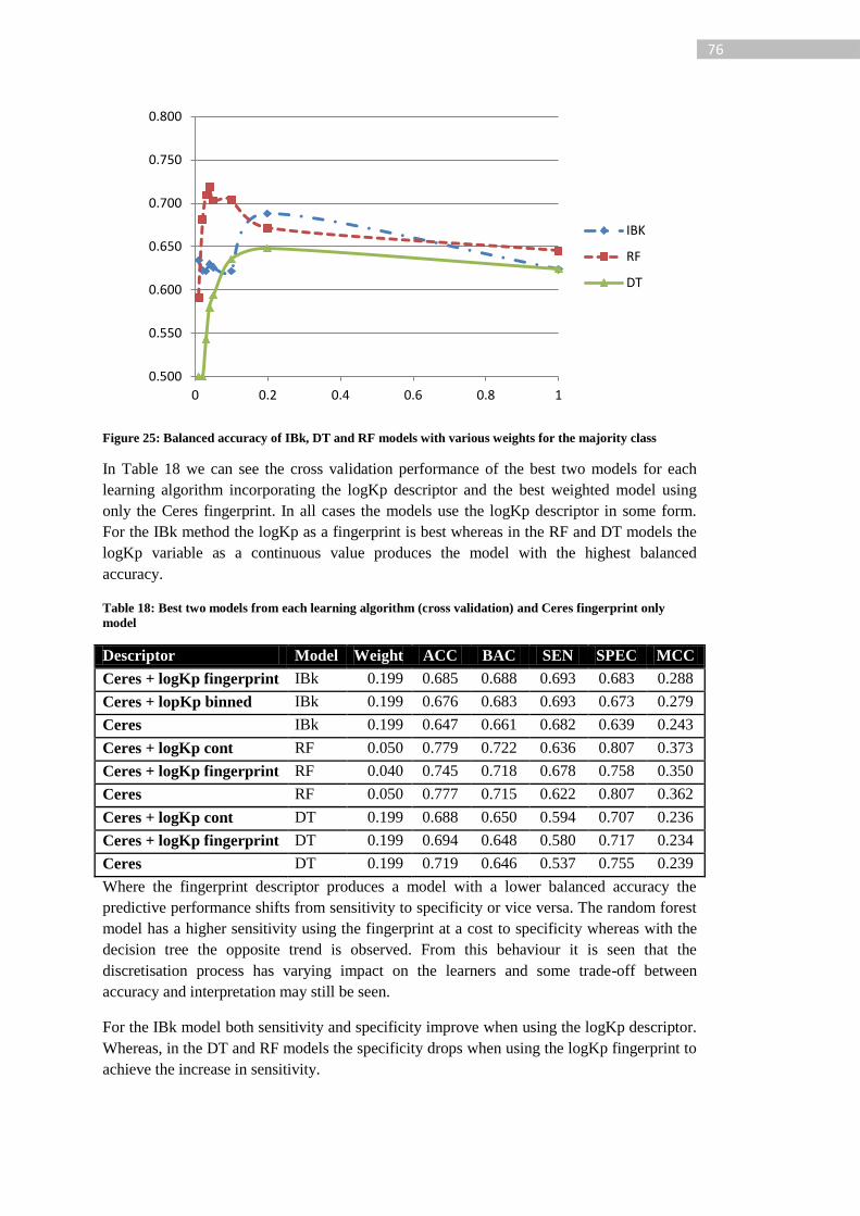
76
Figure 25: Balanced accuracy of IBk, DT and RF models with various weights for the majority class
In Table 18 we can see the cross validation performance of the best two models for each
learning algorithm incorporating the logKp descriptor and the best weighted model using
only the Ceres fingerprint. In all cases the models use the logKp descriptor in some form.
For the IBk method the logKp as a fingerprint is best whereas in the RF and DT models the
logKp variable as a continuous value produces the model with the highest balanced
accuracy.
Table 18: Best two models from each learning algorithm (cross validation) and Ceres fingerprint only
model
Descriptor Model Weight ACC BAC SEN SPEC MCC
Ceres + logKp fingerprint IBk 0.199 0.685 0.688 0.693 0.683 0.288
Ceres + lopKp binned IBk 0.199 0.676 0.683 0.693 0.673 0.279
Ceres IBk 0.199 0.647 0.661 0.682 0.639 0.243
Ceres + logKp cont RF 0.050 0.779 0.722 0.636 0.807 0.373
Ceres + logKp fingerprint RF 0.040 0.745 0.718 0.678 0.758 0.350
Ceres RF 0.050 0.777 0.715 0.622 0.807 0.362
Ceres + logKp cont DT 0.199 0.688 0.650 0.594 0.707 0.236
Ceres + logKp fingerprint DT 0.199 0.694 0.648 0.580 0.717 0.234
Ceres DT 0.199 0.719 0.646 0.537 0.755 0.239
Where the fingerprint descriptor produces a model with a lower balanced accuracy the
predictive performance shifts from sensitivity to specificity or vice versa. The random forest
model has a higher sensitivity using the fingerprint at a cost to specificity whereas with the
decision tree the opposite trend is observed. From this behaviour it is seen that the
discretisation process has varying impact on the learners and some trade-off between
accuracy and interpretation may still be seen.
For the IBk model both sensitivity and specificity improve when using the logKp descriptor.
Whereas, in the DT and RF models the specificity drops when using the logKp fingerprint to
achieve the increase in sensitivity.
0.500
0.550
0.600
0.650
0.700
0.750
0.800
0 0.2 0.4 0.6 0.8 1
IBK
RF
DT
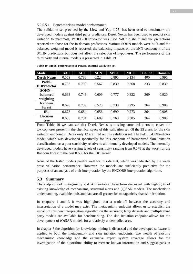
77
5.2.5.5.1 Benchmarking model performance
The validation set provided by the Liew and Yap [175] has been used to benchmark the
developed models against third party predictors. Derek Nexus has been used to predict skin
irritation to mammals, PaDEL-DDPredictor was used ‘off the shelf’ and the predictions
reported are those for the in-domain predictions. Various SOHN models were built and the
balanced weighted model is reported; the balancing impacts on the kNN component of the
SOHN predictions but does not affect the selection of hypotheses. The performance of the
third party and internal models is presented in Table 19.
Table 19: Model performance of PaDEL external validation set
Model BAC ACC SEN SPEC MCC Count Domain
Derek Nexus 0.559 0.783 0.224 0.895 0.134 400 0.996
Padel-
DDPredictor 0.703 0.790 0.567 0.839 0.368 333 0.830
SOHN –
balanced
weighting
0.693 0.748 0.609 0.777 0.322 369 0.920
Random
forest 0.676 0.739 0.578 0.730 0.295 364 0.908
IBk 0.673 0.684 0.656 0.690 0.273 364 0.908
Decision
tree 0.685 0.734 0.609 0.760 0.305 364 0.908
From Table 19 we can see that Derek Nexus is missing structural alerts to cover the
toxicophores present in the chemical space of this validation set. Of the 25 alerts for the skin
irritation endpoint in Derek only 12 are fired on this validation set. The PaDEL-DDPredictor
model which was developed specifically for this endpoint of harmonized skin irritation
classification has a poor sensitivity relative to all internally developed models. The internally
developed models have varying levels of sensitivity ranging from 0.578 at the worst for the
Random Forest to the best 0.656 for the IBk learner.
None of the tested models predict well for this dataset, which was indicated by the weak
cross validation performance. However, the models are sufficiently predictive for the
purposes of an analysis of their interpretation by the ENCORE interpretation algorithm.
5.3 Summary
The endpoints of mutagenicity and skin irritation have been discussed with highlights of
existing knowledge of mechanisms, structural alerts and (Q)SAR models. The mechanistic
understanding, available tools and data are all greater for mutagenicity than skin irritation.
In chapters 1 and 3 it was highlighted that a trade-off between the accuracy and
interpretation of a model may exist. The mutagenicity endpoint allows us to establish the
impact of this new interpretation algorithm on the accuracy; large datasets and multiple third
party models are available for benchmarking. The skin irritation endpoint allows for the
development of (Q)SAR models for a relatively understudied area.
In chapter 7 the algorithm for knowledge mining is discussed and the developed software is
applied to both the mutagenicity and skin irritation endpoints. The wealth of existing
mechanistic knowledge and the extensive expert system coverage allows for the
investigation of the algorithms ability to recreate known information and suggest gaps in

78
existing knowledge. For skin irritation the focus is more on the identification of novel
potential toxicophores for the purposes of suggesting new potential toxicophores.
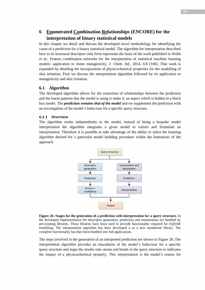
79
6 Enumerated Combination Relationships (ENCORE) for the
interpretation of binary statistical models In this chapter we detail and discuss the developed novel methodology for identifying the
cause of a prediction for a binary statistical model. The algorithm for interpretation described
here in its structural descriptor only form represents the basis of the work published in Webb
et al., Feature combination networks for the interpretation of statistical machine learning
models: application to Ames mutagenicity, J. Chem. Inf., 2014, 6:8 [106]. That work is
expanded by detailing the incorporation of physicochemical properties for the modelling of
skin irritation. First we discuss the interpretation algorithm followed by its application to
mutagenicity and skin irritation.
6.1 Algorithm
The developed algorithm allows for the extraction of relationships between the prediction
and the learnt patterns that the model is using to make it, an aspect which is hidden in a black
box model. The prediction remains that of the model and we supplement the prediction with
an investigation of the model’s behaviour for a specific query structure.
6.1.1 Overview
The algorithm works independently to the model, instead of being a bespoke model
interpretation the algorithm integrates a given model to extract and formulate an
interpretation. Therefore it is possible to take advantage of the ability to select the learning
algorithm desired for a particular model building procedure within the limitations of the
approach.
Figure 26: Stages for the generation of a prediction with interpretation for a query structure. In
the developed implementation the descriptor generation, prediction and enumeration are handled by
pre-existing libraries. These libraries have been used to provide functionality required for (Q)SAR
modelling. The interpretation algorithm has been developed a as a new standalone library. The
complete functionality has then been bundled into full applications.
The steps involved in the generation of an interpreted prediction are shown in Figure 26. The
interpretation algorithm provides an elucidation of the model’s behaviour for a specific
query structure and maps the results onto atoms and bonds in the query structure or indicates
the impact of a physicochemical property. This interpretation is the model’s reason for
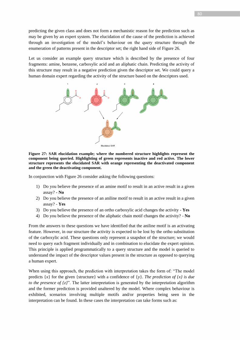
80
predicting the given class and does not form a mechanistic reason for the prediction such as
may be given by an expert system. The elucidation of the cause of the prediction is achieved
through an investigation of the model’s behaviour on the query structure through the
enumeration of patterns present in the descriptor set; the right hand side of Figure 26.
Let us consider an example query structure which is described by the presence of four
fragments: amine, benzene, carboxylic acid and an aliphatic chain. Predicting the activity of
this structure may result in a negative prediction given the descriptor set. We could query a
human domain expert regarding the activity of the structure based on the descriptors used.
Figure 27: SAR elucidation example; where the numbered structure highlights represent the
component being queried. Highlighting of green represents inactive and red active. The lower
structure represents the elucidated SAR with orange representing the deactivated component
and the green the deactivating component.
In conjunction with Figure 26 consider asking the following questions:
1) Do you believe the presence of an amine motif to result in an active result in a given
assay? - No
2) Do you believe the presence of an aniline motif to result in an active result in a given
assay? - Yes
3) Do you believe the presence of an ortho carboxylic acid changes the activity - Yes
4) Do you believe the presence of the aliphatic chain motif changes the activity? - No
From the answers to these questions we have identified that the aniline motif is an activating
feature. However, in our structure the activity is expected to be lost by the ortho substitution
of the carboxylic acid. These questions only represent a snapshot of the structure; we would
need to query each fragment individually and in combination to elucidate the expert opinion.
This principle is applied programmatically to a query structure and the model is queried to
understand the impact of the descriptor values present in the structure as opposed to querying
a human expert.
When using this approach, the prediction with interpretation takes the form of: “The model
predicts {x} for the given {structure} with a confidence of {y}. The prediction of {x} is due
to the presence of {z}”. The latter interpretation is generated by the interpretation algorithm
and the former prediction is provided unaltered by the model. Where complex behaviour is
exhibited, scenarios involving multiple motifs and/or properties being seen in the
interpretation can be found. In these cases the interpretation can take forms such as:
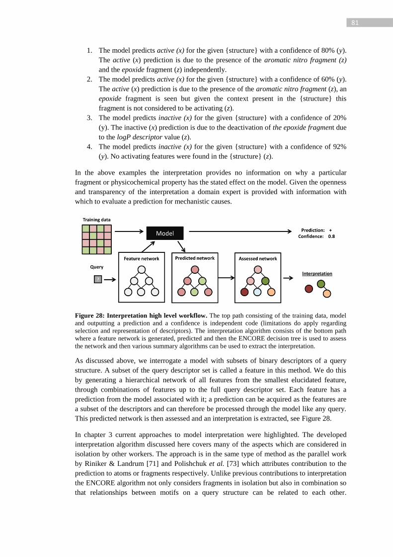
81
1. The model predicts active (x) for the given {structure} with a confidence of 80% (y).
The active (x) prediction is due to the presence of the aromatic nitro fragment (z)
and the epoxide fragment (z) independently.
2. The model predicts active (x) for the given {structure} with a confidence of 60% (y).
The active (x) prediction is due to the presence of the aromatic nitro fragment (z), an
epoxide fragment is seen but given the context present in the {structure} this
fragment is not considered to be activating (z).
3. The model predicts inactive (x) for the given {structure} with a confidence of 20%
(y). The inactive (x) prediction is due to the deactivation of the epoxide fragment due
to the logP descriptor value (z).
4. The model predicts inactive (x) for the given {structure} with a confidence of 92%
(y). No activating features were found in the {structure} (z).
In the above examples the interpretation provides no information on why a particular
fragment or physicochemical property has the stated effect on the model. Given the openness
and transparency of the interpretation a domain expert is provided with information with
which to evaluate a prediction for mechanistic causes.
Figure 28: Interpretation high level workflow. The top path consisting of the training data, model
and outputting a prediction and a confidence is independent code (limitations do apply regarding
selection and representation of descriptors). The interpretation algorithm consists of the bottom path
where a feature network is generated, predicted and then the ENCORE decision tree is used to assess
the network and then various summary algorithms can be used to extract the interpretation.
As discussed above, we interrogate a model with subsets of binary descriptors of a query
structure. A subset of the query descriptor set is called a feature in this method. We do this
by generating a hierarchical network of all features from the smallest elucidated feature,
through combinations of features up to the full query descriptor set. Each feature has a
prediction from the model associated with it; a prediction can be acquired as the features are
a subset of the descriptors and can therefore be processed through the model like any query.
This predicted network is then assessed and an interpretation is extracted, see Figure 28.
In chapter 3 current approaches to model interpretation were highlighted. The developed
interpretation algorithm discussed here covers many of the aspects which are considered in
isolation by other workers. The approach is in the same type of method as the parallel work
by Riniker & Landrum [71] and Polishchuk et al. [73] which attributes contribution to the
prediction to atoms or fragments respectively. Unlike previous contributions to interpretation
the ENCORE algorithm not only considers fragments in isolation but also in combination so
that relationships between motifs on a query structure can be related to each other.
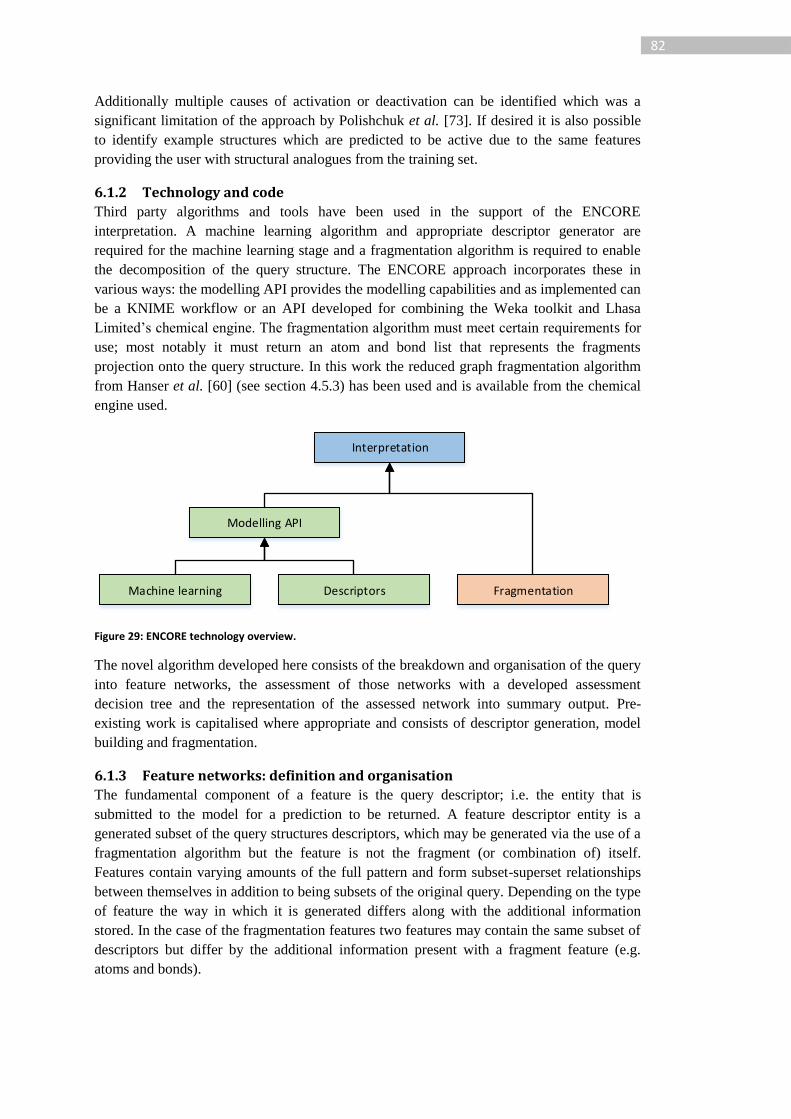
82
Additionally multiple causes of activation or deactivation can be identified which was a
significant limitation of the approach by Polishchuk et al. [73]. If desired it is also possible
to identify example structures which are predicted to be active due to the same features
providing the user with structural analogues from the training set.
6.1.2 Technology and code
Third party algorithms and tools have been used in the support of the ENCORE
interpretation. A machine learning algorithm and appropriate descriptor generator are
required for the machine learning stage and a fragmentation algorithm is required to enable
the decomposition of the query structure. The ENCORE approach incorporates these in
various ways: the modelling API provides the modelling capabilities and as implemented can
be a KNIME workflow or an API developed for combining the Weka toolkit and Lhasa
Limited’s chemical engine. The fragmentation algorithm must meet certain requirements for
use; most notably it must return an atom and bond list that represents the fragments
projection onto the query structure. In this work the reduced graph fragmentation algorithm
from Hanser et al. [60] (see section 4.5.3) has been used and is available from the chemical
engine used.
Interpretation
Machine learning Descriptors Fragmentation
Modelling API
Figure 29: ENCORE technology overview.
The novel algorithm developed here consists of the breakdown and organisation of the query
into feature networks, the assessment of those networks with a developed assessment
decision tree and the representation of the assessed network into summary output. Pre-
existing work is capitalised where appropriate and consists of descriptor generation, model
building and fragmentation.
6.1.3 Feature networks: definition and organisation
The fundamental component of a feature is the query descriptor; i.e. the entity that is
submitted to the model for a prediction to be returned. A feature descriptor entity is a
generated subset of the query structures descriptors, which may be generated via the use of a
fragmentation algorithm but the feature is not the fragment (or combination of) itself.
Features contain varying amounts of the full pattern and form subset-superset relationships
between themselves in addition to being subsets of the original query. Depending on the type
of feature the way in which it is generated differs along with the additional information
stored. In the case of the fragmentation features two features may contain the same subset of
descriptors but differ by the additional information present with a fragment feature (e.g.
atoms and bonds).

83
All features at the core contain:
1) Identifier: a unique identifier for the feature
2) Index position: the index position of the node in the network
3) Type: combination, physicochemical or fragment
4) Query descriptor: the descriptor vector in this implementation. This is a subset of
the query structures descriptors
5) Parent list: a list of the parent index positions
6) Child list: a list of the child index positions
7) Ascendant list: a list of the ascendant index positions
8) Descendant list: a list of the descendant index positions
9) Prediction: the prediction from the model
10) Confidence: the confidence from the model
11) Assessment: the assessment of the node
Additional information is contained within a feature depending on the method used for
generation. For example a feature generated through the use of a fragmentation method will
also contain a molecular graph and atom and bond lists which are used to match the
assessment with a structural motif. This information may be used for visualisation of the
assessment or in the organisation of the features into a hierarchical network.
The enumerated features are organised into hierarchical networks. The networks are
represented by a directed acyclic graph (DAG) where a vertex represents a feature and an
edge the relationship between two features.
0
1 2
3 4 5
Root node
Combination node
Leaf nodes
Vertex
Edge
Figure 30: Directed acyclic graph. Node 0 is a parent of nodes {1,2} and an ascendant of nodes {1,2,3,4,5}.
Node 1 is a parent and ascendant of nodes {3,4}. Node 2 is not a parent of node 3.
The root node represents the feature describing the full query structure descriptors. Nodes
with no children represent leaf nodes describing the smallest subsets of descriptors described
by a feature. The combination nodes (those with children) represent the union of features
and describe combinations of child nodes. The graphs are directed with traversing up the
network from a leaf node representing an increase in representation of the query structure’s
descriptors and a node can be described as a larger context than all of its descendants.
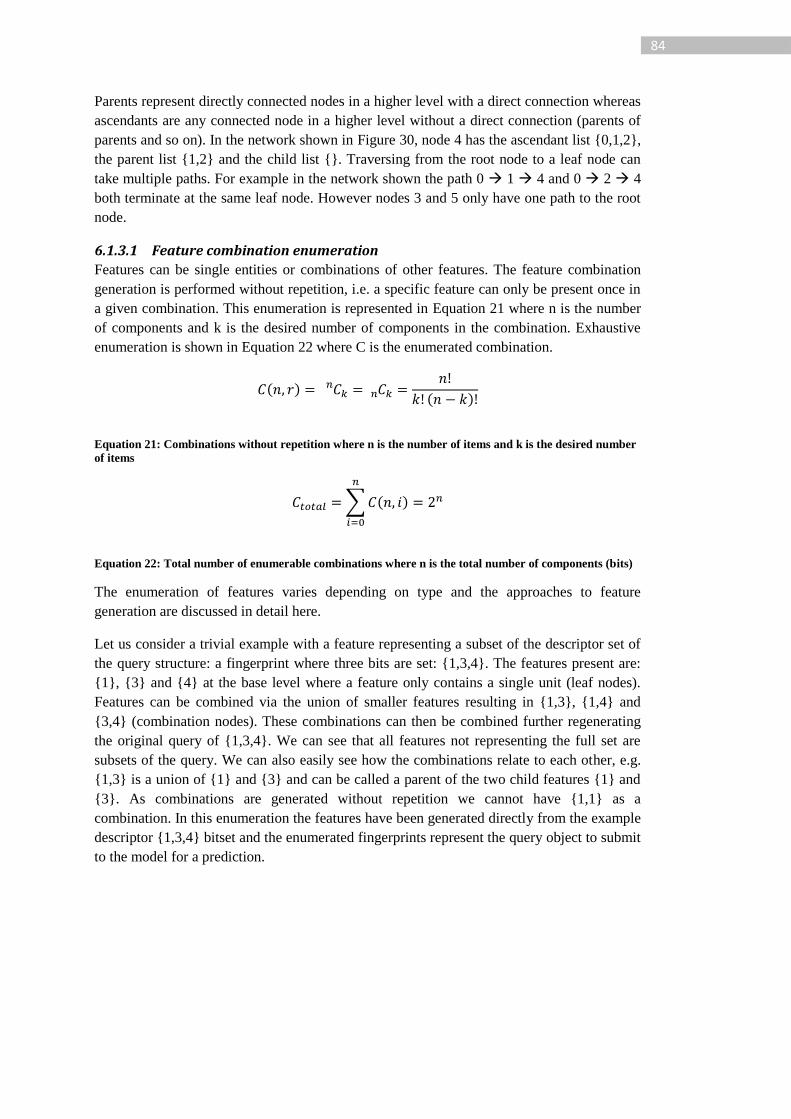
84
Parents represent directly connected nodes in a higher level with a direct connection whereas
ascendants are any connected node in a higher level without a direct connection (parents of
parents and so on). In the network shown in Figure 30, node 4 has the ascendant list {0,1,2},
the parent list {1,2} and the child list {}. Traversing from the root node to a leaf node can
take multiple paths. For example in the network shown the path 0 1 4 and 0 2 4
both terminate at the same leaf node. However nodes 3 and 5 only have one path to the root
node.
6.1.3.1 Feature combination enumeration
Features can be single entities or combinations of other features. The feature combination
generation is performed without repetition, i.e. a specific feature can only be present once in
a given combination. This enumeration is represented in Equation 21 where n is the number
of components and k is the desired number of components in the combination. Exhaustive
enumeration is shown in Equation 22 where C is the enumerated combination.
( )
( )
Equation 21: Combinations without repetition where n is the number of items and k is the desired number
of items
∑ ( )
Equation 22: Total number of enumerable combinations where n is the total number of components (bits)
The enumeration of features varies depending on type and the approaches to feature
generation are discussed in detail here.
Let us consider a trivial example with a feature representing a subset of the descriptor set of
the query structure: a fingerprint where three bits are set: {1,3,4}. The features present are:
{1}, {3} and {4} at the base level where a feature only contains a single unit (leaf nodes).
Features can be combined via the union of smaller features resulting in {1,3}, {1,4} and
{3,4} (combination nodes). These combinations can then be combined further regenerating
the original query of {1,3,4}. We can see that all features not representing the full set are
subsets of the query. We can also easily see how the combinations relate to each other, e.g.
{1,3} is a union of {1} and {3} and can be called a parent of the two child features {1} and
{3}. As combinations are generated without repetition we cannot have {1,1} as a
combination. In this enumeration the features have been generated directly from the example
descriptor {1,3,4} bitset and the enumerated fingerprints represent the query object to submit
to the model for a prediction.
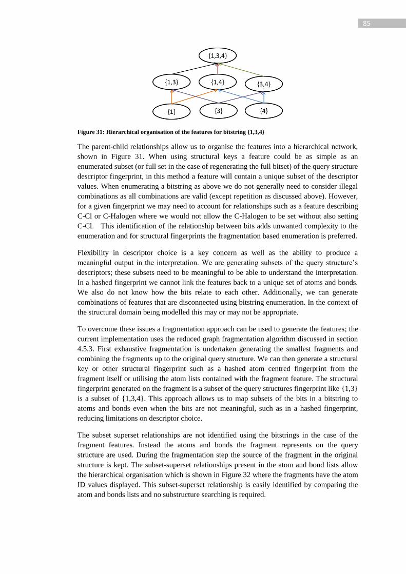
85
Figure 31: Hierarchical organisation of the features for bitstring {1,3,4}
The parent-child relationships allow us to organise the features into a hierarchical network,
shown in Figure 31. When using structural keys a feature could be as simple as an
enumerated subset (or full set in the case of regenerating the full bitset) of the query structure
descriptor fingerprint, in this method a feature will contain a unique subset of the descriptor
values. When enumerating a bitstring as above we do not generally need to consider illegal
combinations as all combinations are valid (except repetition as discussed above). However,
for a given fingerprint we may need to account for relationships such as a feature describing
C-Cl or C-Halogen where we would not allow the C-Halogen to be set without also setting
C-Cl. This identification of the relationship between bits adds unwanted complexity to the
enumeration and for structural fingerprints the fragmentation based enumeration is preferred.
Flexibility in descriptor choice is a key concern as well as the ability to produce a
meaningful output in the interpretation. We are generating subsets of the query structure’s
descriptors; these subsets need to be meaningful to be able to understand the interpretation.
In a hashed fingerprint we cannot link the features back to a unique set of atoms and bonds.
We also do not know how the bits relate to each other. Additionally, we can generate
combinations of features that are disconnected using bitstring enumeration. In the context of
the structural domain being modelled this may or may not be appropriate.
To overcome these issues a fragmentation approach can be used to generate the features; the
current implementation uses the reduced graph fragmentation algorithm discussed in section
4.5.3. First exhaustive fragmentation is undertaken generating the smallest fragments and
combining the fragments up to the original query structure. We can then generate a structural
key or other structural fingerprint such as a hashed atom centred fingerprint from the
fragment itself or utilising the atom lists contained with the fragment feature. The structural
fingerprint generated on the fragment is a subset of the query structures fingerprint like {1,3}
is a subset of {1,3,4}. This approach allows us to map subsets of the bits in a bitstring to
atoms and bonds even when the bits are not meaningful, such as in a hashed fingerprint,
reducing limitations on descriptor choice.
The subset superset relationships are not identified using the bitstrings in the case of the
fragment features. Instead the atoms and bonds the fragment represents on the query
structure are used. During the fragmentation step the source of the fragment in the original
structure is kept. The subset-superset relationships present in the atom and bond lists allow
the hierarchical organisation which is shown in Figure 32 where the fragments have the atom
ID values displayed. This subset-superset relationship is easily identified by comparing the
atom and bonds lists and no substructure searching is required.
86
By exhaustively generating the fragment hierarchy an independent assessment of structural
motifs that may occur multiple times in a given query structure can be performed. Nodes E
and F are independent features that contain the same descriptor subset, they differ in the
atom and bond lists which define the map between the descriptor subset and a motif on the
query structure. The prediction from the model will be the same given the equality of the
descriptor subset, however, the assessment given to these nodes may differ depending on the
prediction of their ascendants and/or descendants as appropriate.
Figure 32: Fragment feature hierarchy for 1-nitronapthalene. The smallest fragments are at the
bottom (D-F) which combine as the network is traversed upwards towards the original structure at
node A. The atoms are labelled with their original position on the structure showing how the hierarchy
can be generated from atom and bond numbers (not shown).
In Figure 33 we see the fragments from 1-nitronapthalene and the resulting structural
fingerprints generated from the fragments. Fragment 1 represents the original structure
which is regenerated and fragments 2-6 represent fragments present within this structure. We
can see from the fingerprints that the generated fragment fingerprints form subsets of the
original query structure’s fingerprint. These descriptor values are stored in the network,
when a prediction is made is this descriptor set that is predicted not the fragment.
This generation of the fingerprint from the fragment may result in undesirable behaviour for
certain fingerprinting methodologies. When generating the fingerprint the fingerprinter may
perceive the fragment as a closed structure in that a CH2 in the fragment at a cleavage site is
perceived as a terminal CH3 by the fingerprinter. This impact can be limited by removing
any bits novel to the fragment descriptor: any bits not set in the parent are fixed as false in
the fragment descriptor. However, if a bit is not associated with the fragment but is present
elsewhere in the structure this approach will not solve this problem. For the method to ensure
a fragment is perceived as an open structure a fingerprinter that can return the fingerprint
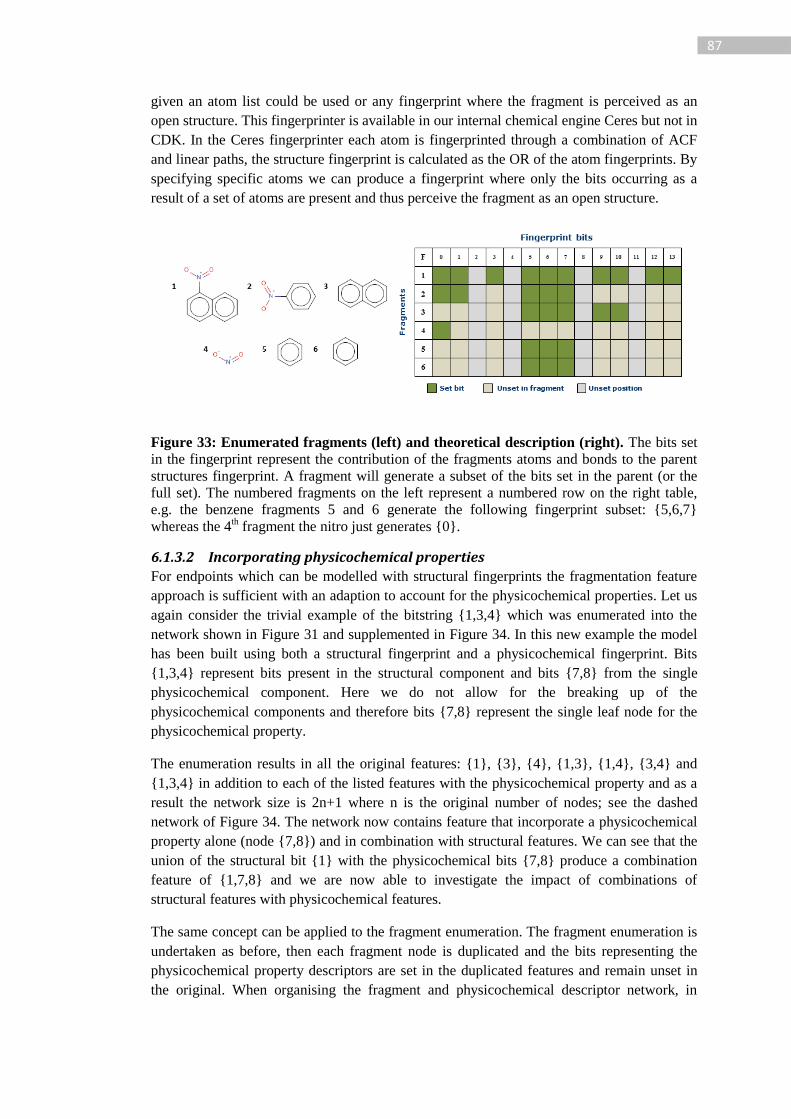
87
given an atom list could be used or any fingerprint where the fragment is perceived as an
open structure. This fingerprinter is available in our internal chemical engine Ceres but not in
CDK. In the Ceres fingerprinter each atom is fingerprinted through a combination of ACF
and linear paths, the structure fingerprint is calculated as the OR of the atom fingerprints. By
specifying specific atoms we can produce a fingerprint where only the bits occurring as a
result of a set of atoms are present and thus perceive the fragment as an open structure.
Figure 33: Enumerated fragments (left) and theoretical description (right). The bits set
in the fingerprint represent the contribution of the fragments atoms and bonds to the parent
structures fingerprint. A fragment will generate a subset of the bits set in the parent (or the
full set). The numbered fragments on the left represent a numbered row on the right table,
e.g. the benzene fragments 5 and 6 generate the following fingerprint subset: {5,6,7}
whereas the 4th fragment the nitro just generates {0}.
6.1.3.2 Incorporating physicochemical properties
For endpoints which can be modelled with structural fingerprints the fragmentation feature
approach is sufficient with an adaption to account for the physicochemical properties. Let us
again consider the trivial example of the bitstring {1,3,4} which was enumerated into the
network shown in Figure 31 and supplemented in Figure 34. In this new example the model
has been built using both a structural fingerprint and a physicochemical fingerprint. Bits
{1,3,4} represent bits present in the structural component and bits {7,8} from the single
physicochemical component. Here we do not allow for the breaking up of the
physicochemical components and therefore bits {7,8} represent the single leaf node for the
physicochemical property.
The enumeration results in all the original features: {1}, {3}, {4}, {1,3}, {1,4}, {3,4} and
{1,3,4} in addition to each of the listed features with the physicochemical property and as a
result the network size is 2n+1 where n is the original number of nodes; see the dashed
network of Figure 34. The network now contains feature that incorporate a physicochemical
property alone (node {7,8}) and in combination with structural features. We can see that the
union of the structural bit {1} with the physicochemical bits {7,8} produce a combination
feature of {1,7,8} and we are now able to investigate the impact of combinations of
structural features with physicochemical features.
The same concept can be applied to the fragment enumeration. The fragment enumeration is
undertaken as before, then each fragment node is duplicated and the bits representing the
physicochemical property descriptors are set in the duplicated features and remain unset in
the original. When organising the fragment and physicochemical descriptor network, in
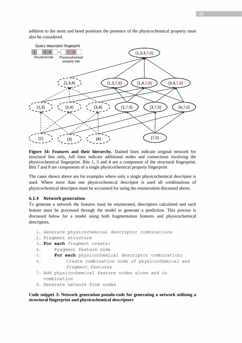
88
addition to the atom and bond positions the presence of the physicochemical property must
also be considered.
Figure 34: Features and their hierarchy. Dashed lines indicate original network for
structural bits only, full lines indicate additional nodes and connections involving the
physicochemical fingerprint. Bits 1, 3 and 4 are a component of the structural fingerprint.
Bits 7 and 8 are components of a single physicochemical property fingerprint
The cases shown above are for examples where only a single physicochemical descriptor is
used. Where more than one physicochemical descriptor is used all combinations of
physicochemical descriptor must be accounted for using the enumeration discussed above.
6.1.4 Network generation
To generate a network the features must be enumerated, descriptors calculated and each
feature must be processed through the model to generate a prediction. This process is
discussed below for a model using both fragmentation features and physicochemical
descriptors.
1. Generate physicochemical descriptor combinations
2. Fragment structure
3. For each fragment create:
4. Fragment feature node
5. For each physicochemical descriptor combination:
6. Create combination node of physicochemical and
fragment features
7. Add physicochemical feature nodes alone and in
combination
8. Generate network from nodes
Code snippet 3: Network generation pseudo-code for generating a network utilising a
structural fingerprint and physicochemical descriptors

89
In the pseudo-code shown in Code snippet 3 we generate the physicochemical descriptor
combinations. For example if using two physicochemical descriptors we would generate
{physchem1}, {phsychem2} and {physchem1, physchem2}; these combinations will be
combined with each fragment feature generated. We then fragment the query structure (line
2) and for each fragment we create a fragment node and a combination node adding them to
a list of nodes. If we had two fragments we would have a list of nodes containing: {frag1},
{frag1, physchem1}, {frag1, physchem2}, {frag1, physchem1, physchem2}, {frag2}, {frag2,
physchem1}, {frag2, physchem2} and {frag2, physchem1, physchem2} by the end of line 6.
Finally, we add nodes for just the physicochemical features; by the end of line 7 the list of
nodes also contains {physchem1}, {physchem2} and {physchem1, physchem2}.
A feature node is responsible for identifying whether it is an ascendant or descendant of a
comparison node. If a given node’s atoms, bonds and physicochemical descriptor inclusion
lists are a proper subset of another feature, that feature is deemed to be an ascendant. The
opposite comparison reveals descendants. Code snippet 4 shows pseudo-code to identify if
the current node is a descendant
1. int atoms = currentAtoms AND NOT compareAtoms
2. int bonds = currentBonds AND NOT compareBonds
3. int physchem = currentPhyschem AND NOT comparePhyschem
4. Boolean descendant = atoms == 0 & bonds == 0 & physchem == 0
Code snippet 4: Pseudo-code for identifying descendant relationship. Atoms, bonds and
physchem represent the number of each element in the current node after removing the
elements present in the compare node.
In Code snippet 4 a node is a descendant only if the atoms, bonds and physchem properties
are entirely contained within the compare nodes lists of said features. At this point we have
sufficient information in the nodes to generate the network, see Code snippet 5. Once the
ascendants and descendants have been identified (lines 1-4) it is trivial to calculate the parent
child relationships (lines 6-12) as the difference between the descendent list of the current
node and the descendant list of all its descendants.
1. For each node in list (node a):
2. For each node in list (node b):
3. If node a is descendant of node b add relationships
4. If node a is ascendant of node b add relationships
5.
6. For each node in list (node a):
7. Clone ascendant list to make parent list
8. Clone descendant list to make child list
9. For each ascendant node (node b):
10. Remove node b ascendants from node a parents
11. For each descendant node (node b):
12. Remove node b descendants from node a children
Code snippet 5: Hierarchy generation
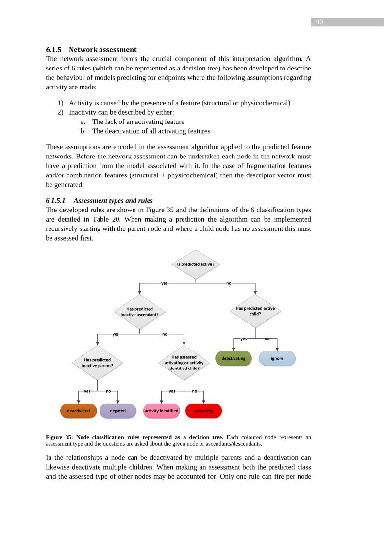
90
6.1.5 Network assessment
The network assessment forms the crucial component of this interpretation algorithm. A
series of 6 rules (which can be represented as a decision tree) has been developed to describe
the behaviour of models predicting for endpoints where the following assumptions regarding
activity are made:
1) Activity is caused by the presence of a feature (structural or physicochemical)
2) Inactivity can be described by either:
a. The lack of an activating feature
b. The deactivation of all activating features
These assumptions are encoded in the assessment algorithm applied to the predicted feature
networks. Before the network assessment can be undertaken each node in the network must
have a prediction from the model associated with it. In the case of fragmentation features
and/or combination features (structural + physicochemical) then the descriptor vector must
be generated.
6.1.5.1 Assessment types and rules
The developed rules are shown in Figure 35 and the definitions of the 6 classification types
are detailed in Table 20. When making a prediction the algorithm can be implemented
recursively starting with the parent node and where a child node has no assessment this must
be assessed first.
Figure 35: Node classification rules represented as a decision tree. Each coloured node represents an
assessment type and the questions are asked about the given node or ascendants/descendants.
In the relationships a node can be deactivated by multiple parents and a deactivation can
likewise deactivate multiple children. When making an assessment both the predicted class
and the assessed type of other nodes may be accounted for. Only one rule can fire per node
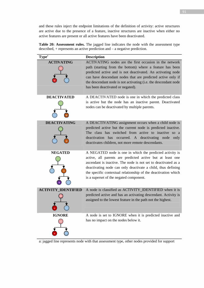
91
and these rules inject the endpoint limitations of the definition of activity: active structures
are active due to the presence of a feature, inactive structures are inactive when either no
active features are present or all active features have been deactivated.
Table 20: Assessment rules. The jagged line indicates the node with the assessment type
described, + represents an active prediction and – a negative prediction.
Typea Description
ACTIVATING
+
-+
ACTIVATING nodes are the first occasion in the network
path (starting from the bottom) where a feature has been
predicted active and is not deactivated. An activating node
can have descendant nodes that are predicted active only if
the descendant node is not activating (i.e. the descendant node
has been deactivated or negated).
DEACTIVATED
-
- +
A DEACTIVATED node is one in which the predicted class
is active but the node has an inactive parent. Deactivated
nodes can be deactivated by multiple parents.
DEACTIVATING
+-
-
A DEACTIVATING assignment occurs when a child node is
predicted active but the current node is predicted inactive.
The class has switched from active to inactive so a
deactivation has occurred. A deactivating node only
deactivates children, not more remote descendants.
NEGATED
-
+
-
-
+
A NEGATED node is one in which the predicted activity is
active, all parents are predicted active but at least one
ascendant is inactive. The node is not set to deactivated as a
deactivating node can only deactivate a child, thus defining
the specific contextual relationship of the deactivation which
is a superset of the negated component.
ACTIVITY_IDENTIFIED
+ -
+
A node is classified as ACTIVITY_IDENTIFIED when it is
predicted active and has an activating descendant. Activity is
assigned to the lowest feature in the path not the highest.
IGNORE
+
+ -
A node is set to IGNORE when it is predicted inactive and
has no impact on the nodes below it.
a: jagged line represents node with that assessment type, other nodes provided for support
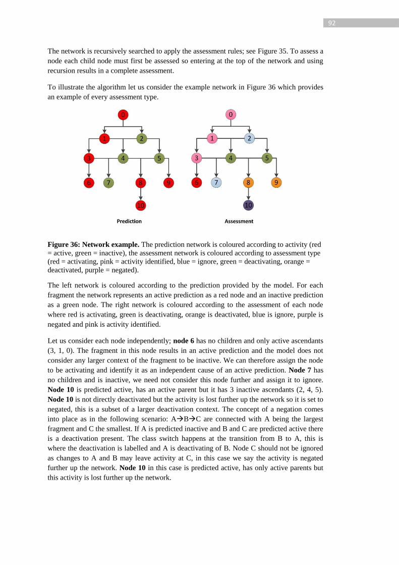
92
The network is recursively searched to apply the assessment rules; see Figure 35. To assess a
node each child node must first be assessed so entering at the top of the network and using
recursion results in a complete assessment.
To illustrate the algorithm let us consider the example network in Figure 36 which provides
an example of every assessment type.
Figure 36: Network example. The prediction network is coloured according to activity (red
= active, green = inactive), the assessment network is coloured according to assessment type
(red = activating, pink = activity identified, blue = ignore, green = deactivating, orange =
deactivated, purple = negated).
The left network is coloured according to the prediction provided by the model. For each
fragment the network represents an active prediction as a red node and an inactive prediction
as a green node. The right network is coloured according to the assessment of each node
where red is activating, green is deactivating, orange is deactivated, blue is ignore, purple is
negated and pink is activity identified.
Let us consider each node independently; node 6 has no children and only active ascendants
(3, 1, 0). The fragment in this node results in an active prediction and the model does not
consider any larger context of the fragment to be inactive. We can therefore assign the node
to be activating and identify it as an independent cause of an active prediction. Node 7 has
no children and is inactive, we need not consider this node further and assign it to ignore.
Node 10 is predicted active, has an active parent but it has 3 inactive ascendants (2, 4, 5).
Node 10 is not directly deactivated but the activity is lost further up the network so it is set to
negated, this is a subset of a larger deactivation context. The concept of a negation comes
into place as in the following scenario: ABC are connected with A being the largest
fragment and C the smallest. If A is predicted inactive and B and C are predicted active there
is a deactivation present. The class switch happens at the transition from B to A, this is
where the deactivation is labelled and A is deactivating of B. Node C should not be ignored
as changes to A and B may leave activity at C, in this case we say the activity is negated
further up the network. Node 10 in this case is predicted active, has only active parents but
this activity is lost further up the network.
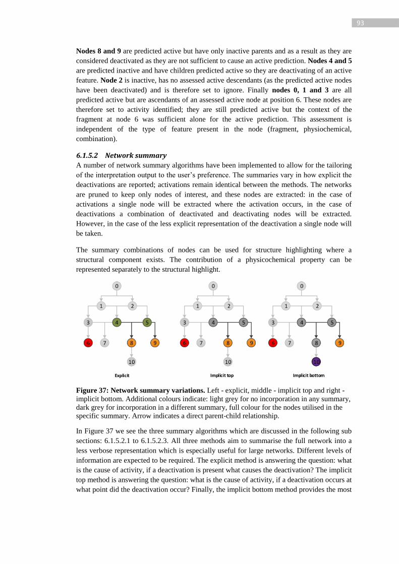
93
Nodes 8 and 9 are predicted active but have only inactive parents and as a result as they are
considered deactivated as they are not sufficient to cause an active prediction. Nodes 4 and 5
are predicted inactive and have children predicted active so they are deactivating of an active
feature. Node 2 is inactive, has no assessed active descendants (as the predicted active nodes
have been deactivated) and is therefore set to ignore. Finally nodes 0, 1 and 3 are all
predicted active but are ascendants of an assessed active node at position 6. These nodes are
therefore set to activity identified; they are still predicted active but the context of the
fragment at node 6 was sufficient alone for the active prediction. This assessment is
independent of the type of feature present in the node (fragment, physiochemical,
combination).
6.1.5.2 Network summary
A number of network summary algorithms have been implemented to allow for the tailoring
of the interpretation output to the user’s preference. The summaries vary in how explicit the
deactivations are reported; activations remain identical between the methods. The networks
are pruned to keep only nodes of interest, and these nodes are extracted: in the case of
activations a single node will be extracted where the activation occurs, in the case of
deactivations a combination of deactivated and deactivating nodes will be extracted.
However, in the case of the less explicit representation of the deactivation a single node will
be taken.
The summary combinations of nodes can be used for structure highlighting where a
structural component exists. The contribution of a physicochemical property can be
represented separately to the structural highlight.
Figure 37: Network summary variations. Left - explicit, middle - implicit top and right -
implicit bottom. Additional colours indicate: light grey for no incorporation in any summary,
dark grey for incorporation in a different summary, full colour for the nodes utilised in the
specific summary. Arrow indicates a direct parent-child relationship.
In Figure 37 we see the three summary algorithms which are discussed in the following sub
sections: 6.1.5.2.1 to 6.1.5.2.3. All three methods aim to summarise the full network into a
less verbose representation which is especially useful for large networks. Different levels of
information are expected to be required. The explicit method is answering the question: what
is the cause of activity, if a deactivation is present what causes the deactivation? The implicit
top method is answering the question: what is the cause of activity, if a deactivation occurs at
what point did the deactivation occur? Finally, the implicit bottom method provides the most

94
condensed information answering the question: what is the cause of activity, if a deactivation
occurs what is the first point the activity is seen but ultimately lost?
6.1.5.2.1 Explicit
In Figure 37 we see the reduction of the network to an activation represented by node 6 and
deactivations represented by the following combinations: 4-8, 5-8 and 5-9. This summary
represents an explicit representation of the deactivations.
1. For each node
2. If assessmentType == ACTIVATING
3. Create SummaryActivation from node
4. Add summary to list
5. Else if assessmentType == DEACTIVATED
6. Create SummaryDeactivation from node
7. Add summary to list
Code snippet 6: Pseudo-code for the extraction of explicit and implicit top interpretation summary
Code snippet 6 shows the extraction of assessment summaries from an assessed network.
This method is used for both the explicit and the implicit top summary methods.
6.1.5.2.2 Implicit top
This summary approach represented by the middle network in Figure 37 provides only
information on the feature that has been deactivated and does not explicitly detail the cause
of the deactivation. In the case of the implicit top the deactivating information in an
assessment summary is not used and the extraction code is that shown in Code snippet 6 with
the exception of node keeping the information on the parent of the DEACTIVATED node.
6.1.5.2.3 Implicit bottom
This summary approach represented by the right hand network in Figure 37 provides the
smallest context of a deactivation. Unlike the other approaches negated features are chosen
as the source and deactivated parents are ignored. See Code snippet 7 for pseudo-code
implementation.
1. For each node
2. If assessmentType == ACTIVATING
3. Create SummaryActivation from node
4. Add summary to list
5. Else if assessmentType == DEACTIVATED or NEGATED
6. If node hasNegatedChild == false
7. Create SummaryDeactivation from node
8. Add summary to list
Code snippet 7: Pseudo-code for explicit bottom summary interpretation extraction
In this summary method we only add a deactivation if it is not the parent of a negated node,
if a negation is present we only keep this node.
6.1.6 Limitations and practical implementations
The algorithm is able to generate, assess and then summarise a network to produce an
interpretation for a prediction. The results can be projected onto structural motifs on the
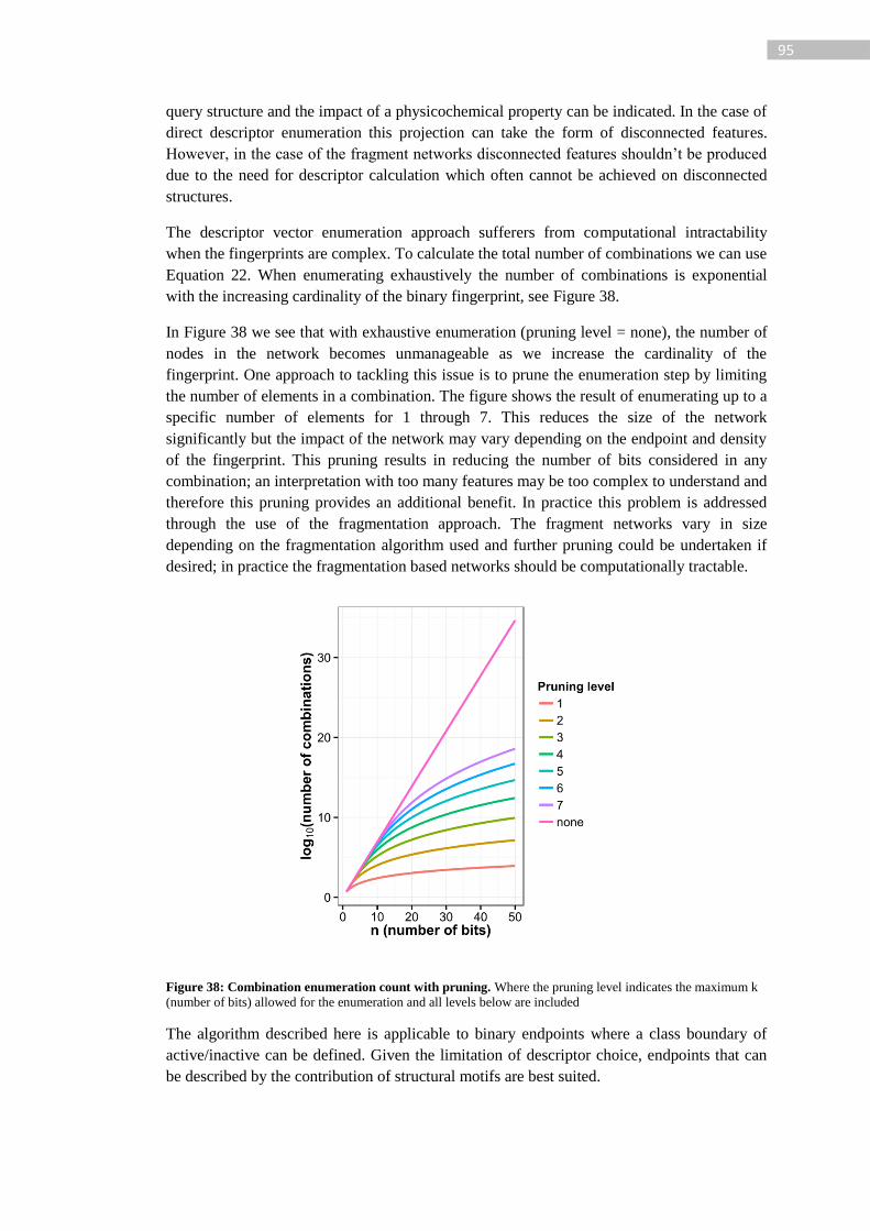
95
query structure and the impact of a physicochemical property can be indicated. In the case of
direct descriptor enumeration this projection can take the form of disconnected features.
However, in the case of the fragment networks disconnected features shouldn’t be produced
due to the need for descriptor calculation which often cannot be achieved on disconnected
structures.
The descriptor vector enumeration approach sufferers from computational intractability
when the fingerprints are complex. To calculate the total number of combinations we can use
Equation 22. When enumerating exhaustively the number of combinations is exponential
with the increasing cardinality of the binary fingerprint, see Figure 38.
In Figure 38 we see that with exhaustive enumeration (pruning level = none), the number of
nodes in the network becomes unmanageable as we increase the cardinality of the
fingerprint. One approach to tackling this issue is to prune the enumeration step by limiting
the number of elements in a combination. The figure shows the result of enumerating up to a
specific number of elements for 1 through 7. This reduces the size of the network
significantly but the impact of the network may vary depending on the endpoint and density
of the fingerprint. This pruning results in reducing the number of bits considered in any
combination; an interpretation with too many features may be too complex to understand and
therefore this pruning provides an additional benefit. In practice this problem is addressed
through the use of the fragmentation approach. The fragment networks vary in size
depending on the fragmentation algorithm used and further pruning could be undertaken if
desired; in practice the fragmentation based networks should be computationally tractable.
Figure 38: Combination enumeration count with pruning. Where the pruning level indicates the maximum k
(number of bits) allowed for the enumeration and all levels below are included
The algorithm described here is applicable to binary endpoints where a class boundary of
active/inactive can be defined. Given the limitation of descriptor choice, endpoints that can
be described by the contribution of structural motifs are best suited.
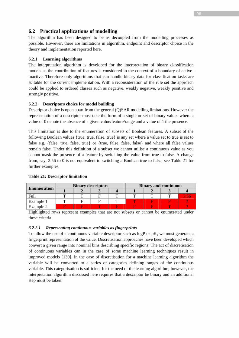
96
6.2 Practical applications of modelling
The algorithm has been designed to be as decoupled from the modelling processes as
possible. However, there are limitations in algorithm, endpoint and descriptor choice in the
theory and implementation reported here.
6.2.1 Learning algorithms
The interpretation algorithm is developed for the interpretation of binary classification
models as the contribution of features is considered in the context of a boundary of active-
inactive. Therefore only algorithms that can handle binary data for classification tasks are
suitable for the current implementation. With a reconsideration of the rule set the approach
could be applied to ordered classes such as negative, weakly negative, weakly positive and
strongly positive.
6.2.2 Descriptors choice for model building
Descriptor choice is open apart from the general (Q)SAR modelling limitations. However the
representation of a descriptor must take the form of a single or set of binary values where a
value of 0 denote the absence of a given value/feature/range and a value of 1 the presence.
This limitation is due to the enumeration of subsets of Boolean features. A subset of the
following Boolean values {true, true, false, true} is any set where a value set to true is set to
false e.g. {false, true, false, true} or {true, false, false, false} and where all false values
remain false. Under this definition of a subset we cannot utilise a continuous value as you
cannot mask the presence of a feature by switching the value from true to false. A change
from, say, 2.56 to 0 is not equivalent to switching a Boolean true to false, see Table 21 for
further examples.
Table 21: Descriptor limitation
Enumeration Binary descriptors Binary and continuous
1 2 3 4 1 2 3 4
Full T T F T T T T 2.56
Example 1 T F F T T F F ?
Example 2 F F T F F F T ?
Highlighted rows represent examples that are not subsets or cannot be enumerated under
these criteria.
6.2.2.1 Representing continuous variables as fingerprints
To allow the use of a continuous variable descriptor such as logP or pKa we must generate a
fingerprint representation of the value. Discretisation approaches have been developed which
convert a given range into nominal bins describing specific regions. The act of discretisation
of continuous variables can in the case of some machine learning techniques result in
improved models [139]. In the case of discretisation for a machine learning algorithm the
variable will be converted to a series of categories defining ranges of the continuous
variable. This categorisation is sufficient for the need of the learning algorithm; however, the
interpretation algorithm discussed here requires that a descriptor be binary and an additional
step must be taken.
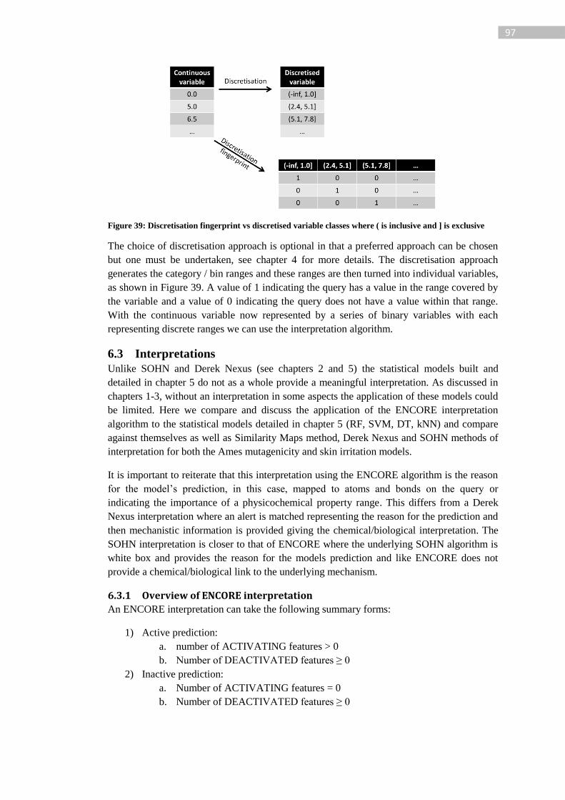
97
Figure 39: Discretisation fingerprint vs discretised variable classes where ( is inclusive and ] is exclusive
The choice of discretisation approach is optional in that a preferred approach can be chosen
but one must be undertaken, see chapter 4 for more details. The discretisation approach
generates the category / bin ranges and these ranges are then turned into individual variables,
as shown in Figure 39. A value of 1 indicating the query has a value in the range covered by
the variable and a value of 0 indicating the query does not have a value within that range.
With the continuous variable now represented by a series of binary variables with each
representing discrete ranges we can use the interpretation algorithm.
6.3 Interpretations
Unlike SOHN and Derek Nexus (see chapters 2 and 5) the statistical models built and
detailed in chapter 5 do not as a whole provide a meaningful interpretation. As discussed in
chapters 1-3, without an interpretation in some aspects the application of these models could
be limited. Here we compare and discuss the application of the ENCORE interpretation
algorithm to the statistical models detailed in chapter 5 (RF, SVM, DT, kNN) and compare
against themselves as well as Similarity Maps method, Derek Nexus and SOHN methods of
interpretation for both the Ames mutagenicity and skin irritation models.
It is important to reiterate that this interpretation using the ENCORE algorithm is the reason
for the model’s prediction, in this case, mapped to atoms and bonds on the query or
indicating the importance of a physicochemical property range. This differs from a Derek
Nexus interpretation where an alert is matched representing the reason for the prediction and
then mechanistic information is provided giving the chemical/biological interpretation. The
SOHN interpretation is closer to that of ENCORE where the underlying SOHN algorithm is
white box and provides the reason for the models prediction and like ENCORE does not
provide a chemical/biological link to the underlying mechanism.
6.3.1 Overview of ENCORE interpretation
An ENCORE interpretation can take the following summary forms:
1) Active prediction:
a. number of ACTIVATING features > 0
b. Number of DEACTIVATED features ≥ 0
2) Inactive prediction:
a. Number of ACTIVATING features = 0
b. Number of DEACTIVATED features ≥ 0
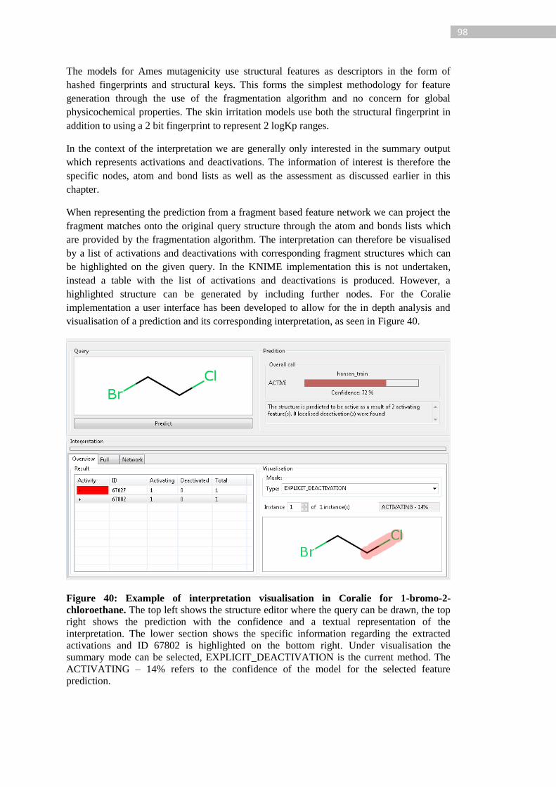
98
The models for Ames mutagenicity use structural features as descriptors in the form of
hashed fingerprints and structural keys. This forms the simplest methodology for feature
generation through the use of the fragmentation algorithm and no concern for global
physicochemical properties. The skin irritation models use both the structural fingerprint in
addition to using a 2 bit fingerprint to represent 2 logKp ranges.
In the context of the interpretation we are generally only interested in the summary output
which represents activations and deactivations. The information of interest is therefore the
specific nodes, atom and bond lists as well as the assessment as discussed earlier in this
chapter.
When representing the prediction from a fragment based feature network we can project the
fragment matches onto the original query structure through the atom and bonds lists which
are provided by the fragmentation algorithm. The interpretation can therefore be visualised
by a list of activations and deactivations with corresponding fragment structures which can
be highlighted on the given query. In the KNIME implementation this is not undertaken,
instead a table with the list of activations and deactivations is produced. However, a
highlighted structure can be generated by including further nodes. For the Coralie
implementation a user interface has been developed to allow for the in depth analysis and
visualisation of a prediction and its corresponding interpretation, as seen in Figure 40.
Figure 40: Example of interpretation visualisation in Coralie for 1-bromo-2-
chloroethane. The top left shows the structure editor where the query can be drawn, the top
right shows the prediction with the confidence and a textual representation of the
interpretation. The lower section shows the specific information regarding the extracted
activations and ID 67802 is highlighted on the bottom right. Under visualisation the
summary mode can be selected, EXPLICIT_DEACTIVATION is the current method. The
ACTIVATING – 14% refers to the confidence of the model for the selected feature
prediction.
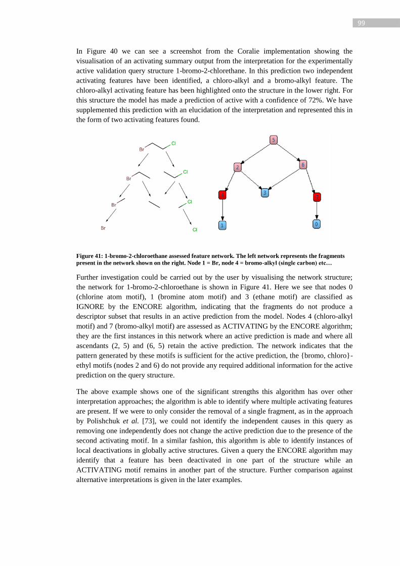
99
In Figure 40 we can see a screenshot from the Coralie implementation showing the
visualisation of an activating summary output from the interpretation for the experimentally
active validation query structure 1-bromo-2-chlorethane. In this prediction two independent
activating features have been identified, a chloro-alkyl and a bromo-alkyl feature. The
chloro-alkyl activating feature has been highlighted onto the structure in the lower right. For
this structure the model has made a prediction of active with a confidence of 72%. We have
supplemented this prediction with an elucidation of the interpretation and represented this in
the form of two activating features found.
Figure 41: 1-bromo-2-chloroethane assessed feature network. The left network represents the fragments
present in the network shown on the right. Node 1 = Br, node 4 = bromo-alkyl (single carbon) etc…
Further investigation could be carried out by the user by visualising the network structure;
the network for 1-bromo-2-chloroethane is shown in Figure 41. Here we see that nodes 0
(chlorine atom motif), 1 (bromine atom motif) and 3 (ethane motif) are classified as
IGNORE by the ENCORE algorithm, indicating that the fragments do not produce a
descriptor subset that results in an active prediction from the model. Nodes 4 (chloro-alkyl
motif) and 7 (bromo-alkyl motif) are assessed as ACTIVATING by the ENCORE algorithm;
they are the first instances in this network where an active prediction is made and where all
ascendants (2, 5) and (6, 5) retain the active prediction. The network indicates that the
pattern generated by these motifs is sufficient for the active prediction, the {bromo, chloro}-
ethyl motifs (nodes 2 and 6) do not provide any required additional information for the active
prediction on the query structure.
The above example shows one of the significant strengths this algorithm has over other
interpretation approaches; the algorithm is able to identify where multiple activating features
are present. If we were to only consider the removal of a single fragment, as in the approach
by Polishchuk et al. [73], we could not identify the independent causes in this query as
removing one independently does not change the active prediction due to the presence of the
second activating motif. In a similar fashion, this algorithm is able to identify instances of
local deactivations in globally active structures. Given a query the ENCORE algorithm may
identify that a feature has been deactivated in one part of the structure while an
ACTIVATING motif remains in another part of the structure. Further comparison against
alternative interpretations is given in the later examples.
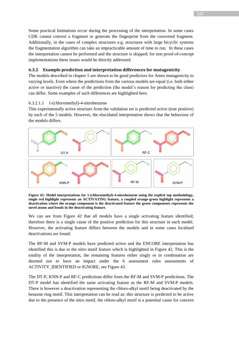
100
Some practical limitations occur during the processing of the interpretation. In some cases
CDK cannot convert a fragment or generate the fingerprint from the converted fragment.
Additionally, in the cases of complex structures e.g. structures with large bicyclic systems
the fragmentation algorithm can take an impracticable amount of time to run. In these cases
the interpretation cannot be performed and the structure is skipped; for non proof-of-concept
implementations these issues would be directly addressed.
6.3.2 Example prediction and interpretation differences for mutagenicity
The models described in chapter 5 are shown to be good predictors for Ames mutagenicity to
varying levels. Even where the predictions from the various models are equal (i.e. both either
active or inactive) the cause of the prediction (the model’s reason for predicting the class)
can differ. Some examples of such differences are highlighted here.
6.3.2.1.1 1-(chloromethyl)-4-nitrobenzene
This experimentally active structure from the validation set is predicted active (true positive)
by each of the 5 models. However, the elucidated interpretation shows that the behaviour of
the models differs.
Figure 42: Model interpretations for 1-(chloromethyl)-4-nitrobenzene using the explicit top methodology,
single red highlight represents an ACTIVATING feature, a coupled orange-green highlight represents a
deactivation where the orange component is the deactivated feature the green components represents the
novel atoms and bonds in the deactivating feature.
We can see from Figure 42 that all models have a single activating feature identified;
therefore there is a single cause of the positive prediction for this structure in each model.
However, the activating feature differs between the models and in some cases localised
deactivations are found.
The RF-M and SVM-P models have predicted active and the ENCORE interpretation has
identified this is due to the nitro motif feature which is highlighted in Figure 42. This is the
totality of the interpretation, the remaining features either singly or in combination are
deemed not to have an impact under the 6 assessment rules assessments of
ACTIVITY_IDENTIFIED or IGNORE, see Figure 43.
The DT-P, KNN-P and RF-C predictions differ from the RF-M and SVM-P predictions. The
DT-P model has identified the same activating feature as the RF-M and SVM-P models.
There is however a deactivation representing the chloro-alkyl motif being deactivated by the
benzene ring motif. This interpretation can be read as: this structure is predicted to be active
due to the presence of the nitro motif, the chloro-alkyl motif is a potential cause for concern

101
but in the context of the larger chloro-alkyl-benzene motif the positive activity is not seen in
this structure’s prediction, i.e. it has been deactivated.
Figure 43: Model assessed networks for 1-(chloromethyl)-4-nitrobenzene. The fragment
network is displayed on the left with the smallest fragments on the bottom and combined as
the network is traversed up to the full query. The various assessments are shown in the
coloured networks on the right where: red = ACTIVATING, pink =
ACTIVITY_IDENTIFIED, blue = IGNORE, green = DEACTIVATING and orange =
DEACTIVATED.
The RF-C and KNN-P predictions are more complex; activity is seen relating the nitro motif
in RF-C and the nitro-benzene motif in KNN-P; this activity is lost in the larger contexts.
Nevertheless, the models do consider the full substituted ring system to be activating. Here
we can read the interpretation as: although activity is seen relating to either the nitro motif or
nitro benzene motifs the full substituted ring system is required to maintain this activity.
Such interpretations occur where a path through the network follows: DEACTIVATED
DEACTIVATING ACTIVATING indicating that the specific context at the
DEACTIVATING node is predicted to be inactive but the larger context at the
ACTIVATING node is considered to be active. Such interpretations could be simplified by
considering such trends and keeping the deactivated feature. This has not been implemented
in the assessment rules as it would mask the impact of potential structural modifications that
could be gleaned from the full trends in the network. Such trends could warrant the
development of another summary assessment method.
6.3.2.1.2 1-bromo-3-chloropropane
This experimentally active structure from the validation set is predicted active by all models.
4 of the 5 models identify 2 causes of activity whereas the SVM-P model identifies only a
single cause.
In Figure 44 we see the highlighted output from the interpretation from each model. All
models consider the bromo-alkyl (single carbon) to be an ACTIVATING feature and this
feature forms the only component of the SVM-P interpretation. The other models consider in
some form the chloro-alkyl feature: DT-P with a single carbon, RF-C and RF-M with two
carbons and kNN-P with three carbons. With these features the carbon chain size will
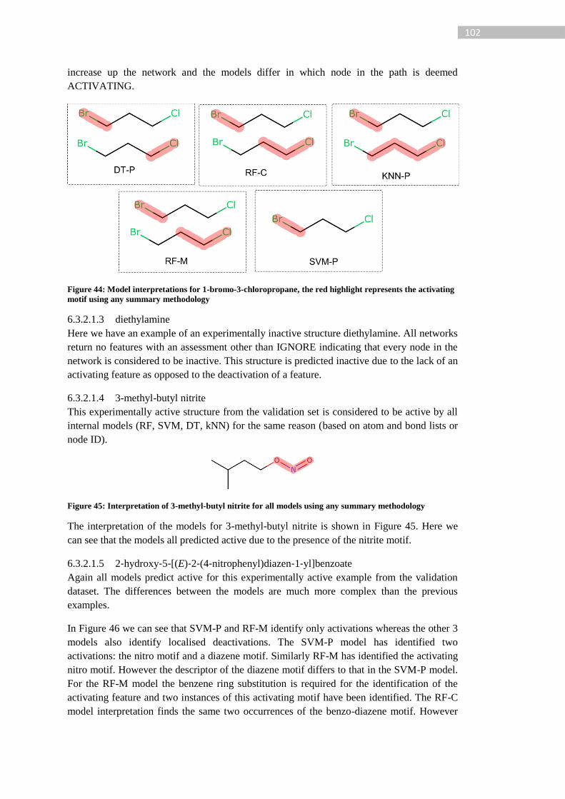
102
increase up the network and the models differ in which node in the path is deemed
ACTIVATING.
Figure 44: Model interpretations for 1-bromo-3-chloropropane, the red highlight represents the activating
motif using any summary methodology
6.3.2.1.3 diethylamine
Here we have an example of an experimentally inactive structure diethylamine. All networks
return no features with an assessment other than IGNORE indicating that every node in the
network is considered to be inactive. This structure is predicted inactive due to the lack of an
activating feature as opposed to the deactivation of a feature.
6.3.2.1.4 3-methyl-butyl nitrite
This experimentally active structure from the validation set is considered to be active by all
internal models (RF, SVM, DT, kNN) for the same reason (based on atom and bond lists or
node ID).
Figure 45: Interpretation of 3-methyl-butyl nitrite for all models using any summary methodology
The interpretation of the models for 3-methyl-butyl nitrite is shown in Figure 45. Here we
can see that the models all predicted active due to the presence of the nitrite motif.
6.3.2.1.5 2‐hydroxy‐5‐[(E)‐2‐(4‐nitrophenyl)diazen‐1‐yl]benzoate
Again all models predict active for this experimentally active example from the validation
dataset. The differences between the models are much more complex than the previous
examples.
In Figure 46 we can see that SVM-P and RF-M identify only activations whereas the other 3
models also identify localised deactivations. The SVM-P model has identified two
activations: the nitro motif and a diazene motif. Similarly RF-M has identified the activating
nitro motif. However the descriptor of the diazene motif differs to that in the SVM-P model.
For the RF-M model the benzene ring substitution is required for the identification of the
activating feature and two instances of this activating motif have been identified. The RF-C
model interpretation finds the same two occurrences of the benzo-diazene motif. However
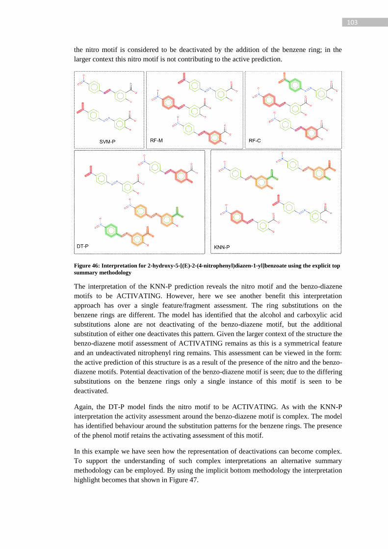
103
the nitro motif is considered to be deactivated by the addition of the benzene ring; in the
larger context this nitro motif is not contributing to the active prediction.
Figure 46: Interpretation for 2‐hydroxy‐5‐[(E)‐2‐(4‐nitrophenyl)diazen‐1‐yl]benzoate using the explicit top
summary methodology
The interpretation of the KNN-P prediction reveals the nitro motif and the benzo-diazene
motifs to be ACTIVATING. However, here we see another benefit this interpretation
approach has over a single feature/fragment assessment. The ring substitutions on the
benzene rings are different. The model has identified that the alcohol and carboxylic acid
substitutions alone are not deactivating of the benzo-diazene motif, but the additional
substitution of either one deactivates this pattern. Given the larger context of the structure the
benzo-diazene motif assessment of ACTIVATING remains as this is a symmetrical feature
and an undeactivated nitrophenyl ring remains. This assessment can be viewed in the form:
the active prediction of this structure is as a result of the presence of the nitro and the benzo-
diazene motifs. Potential deactivation of the benzo-diazene motif is seen; due to the differing
substitutions on the benzene rings only a single instance of this motif is seen to be
deactivated.
Again, the DT-P model finds the nitro motif to be ACTIVATING. As with the KNN-P
interpretation the activity assessment around the benzo-diazene motif is complex. The model
has identified behaviour around the substitution patterns for the benzene rings. The presence
of the phenol motif retains the activating assessment of this motif.
In this example we have seen how the representation of deactivations can become complex.
To support the understanding of such complex interpretations an alternative summary
methodology can be employed. By using the implicit bottom methodology the interpretation
highlight becomes that shown in Figure 47.
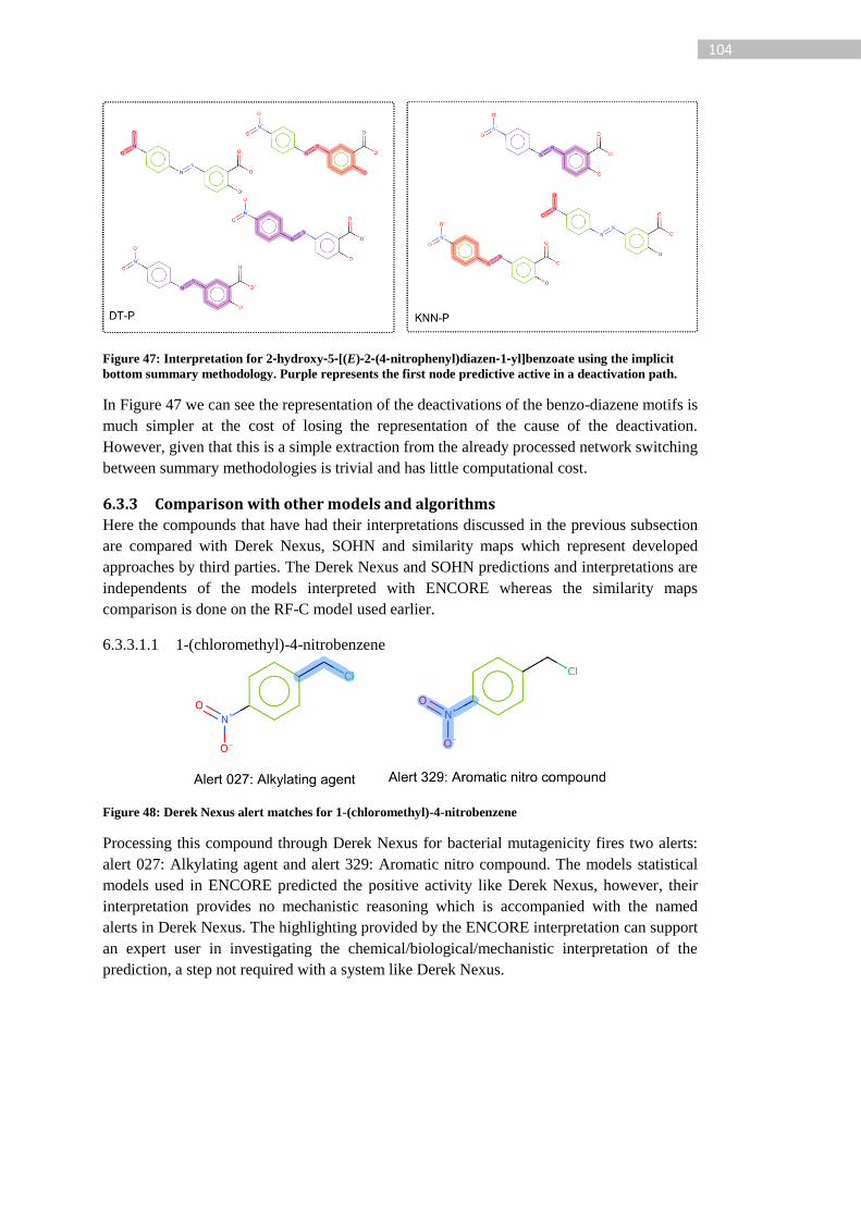
104
Figure 47: Interpretation for 2‐hydroxy‐5‐[(E)‐2‐(4‐nitrophenyl)diazen‐1‐yl]benzoate using the implicit
bottom summary methodology. Purple represents the first node predictive active in a deactivation path.
In Figure 47 we can see the representation of the deactivations of the benzo-diazene motifs is
much simpler at the cost of losing the representation of the cause of the deactivation.
However, given that this is a simple extraction from the already processed network switching
between summary methodologies is trivial and has little computational cost.
6.3.3 Comparison with other models and algorithms
Here the compounds that have had their interpretations discussed in the previous subsection
are compared with Derek Nexus, SOHN and similarity maps which represent developed
approaches by third parties. The Derek Nexus and SOHN predictions and interpretations are
independents of the models interpreted with ENCORE whereas the similarity maps
comparison is done on the RF-C model used earlier.
6.3.3.1.1 1-(chloromethyl)-4-nitrobenzene
Figure 48: Derek Nexus alert matches for 1-(chloromethyl)-4-nitrobenzene
Processing this compound through Derek Nexus for bacterial mutagenicity fires two alerts:
alert 027: Alkylating agent and alert 329: Aromatic nitro compound. The models statistical
models used in ENCORE predicted the positive activity like Derek Nexus, however, their
interpretation provides no mechanistic reasoning which is accompanied with the named
alerts in Derek Nexus. The highlighting provided by the ENCORE interpretation can support
an expert user in investigating the chemical/biological/mechanistic interpretation of the
prediction, a step not required with a system like Derek Nexus.
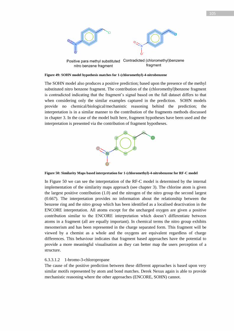
105
Figure 49: SOHN model hypothesis matches for 1-(chloromethyl)-4-nitrobenzene
The SOHN model also produces a positive prediction; based upon the presence of the methyl
substituted nitro benzene fragment. The contribution of the (chloromethyl)benzene fragment
is contradicted indicating that the fragment’s signal based on the full dataset differs to that
when considering only the similar examples captured in the prediction. SOHN models
provide no chemical/biological/mechanistic reasoning behind the prediction; the
interpretation is in a similar manner to the contribution of the fragments methods discussed
in chapter 3. In the case of the model built here, fragment hypotheses have been used and the
interpretation is presented via the contribution of fragment hypotheses.
Figure 50: Similarity Maps based interpretation for 1-(chloromethyl)-4-nitrobenzene for RF-C model
In Figure 50 we can see the interpretation of the RF-C model is determined by the internal
implementation of the similarity maps approach (see chapter 3). The chlorine atom is given
the largest positive contribution (1.0) and the nitrogen of the nitro group the second largest
(0.667). The interpretation provides no information about the relationship between the
benzene ring and the nitro group which has been identified as a localised deactivation in the
ENCORE interpretation. All atoms except for the uncharged oxygen are given a positive
contribution similar to the ENCORE interpretation which doesn’t differentiate between
atoms in a fragment (all are equally important). In chemical terms the nitro group exhibits
mesomerism and has been represented in the charge separated form. This fragment will be
viewed by a chemist as a whole and the oxygens are equivalent regardless of charge
differences. This behaviour indicates that fragment based approaches have the potential to
provide a more meaningful visualisation as they can better map the users perception of a
structure.
6.3.3.1.2 1-bromo-3-chloropropane
The cause of the positive prediction between these different approaches is based upon very
similar motifs represented by atom and bond matches. Derek Nexus again is able to provide
mechanistic reasoning where the other approaches (ENCORE, SOHN) cannot.
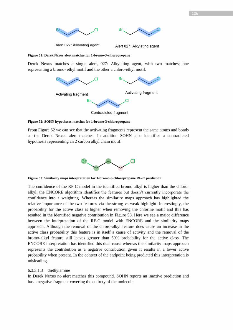
106
Figure 51: Derek Nexus alert matches for 1-bromo-3-chloropropane
Derek Nexus matches a single alert, 027: Alkylating agent, with two matches; one
representing a bromo- ethyl motif and the other a chloro-ethyl motif.
Figure 52: SOHN hypotheses matches for 1-bromo-3-chloropropane
From Figure 52 we can see that the activating fragments represent the same atoms and bonds
as the Derek Nexus alert matches. In addition SOHN also identifies a contradicted
hypothesis representing an 2 carbon alkyl chain motif.
Figure 53: Similarity maps interpretation for 1-bromo-3-chloropropane RF-C prediction
The confidence of the RF-C model in the identified bromo-alkyl is higher than the chloro-
alkyl; the ENCORE algorithm identifies the features but doesn’t currently incorporate the
confidence into a weighting. Whereas the similarity maps approach has highlighted the
relative importance of the two features via the strong vs weak highlight. Interestingly, the
probability for the active class is higher when removing the chlorine motif and this has
resulted in the identified negative contribution in Figure 53. Here we see a major difference
between the interpretation of the RF-C model with ENCORE and the similarity maps
approach. Although the removal of the chloro-alkyl feature does cause an increase in the
active class probability this feature is in itself a cause of activity and the removal of the
bromo-alkyl feature still leaves greater than 50% probability for the active class. The
ENCORE interpretation has identified this dual cause whereas the similarity maps approach
represents the contribution as a negative contribution given it results in a lower active
probability when present. In the context of the endpoint being predicted this interpretation is
misleading.
6.3.3.1.3 diethylamine
In Derek Nexus no alert matches this compound. SOHN reports an inactive prediction and
has a negative fragment covering the entirety of the molecule.
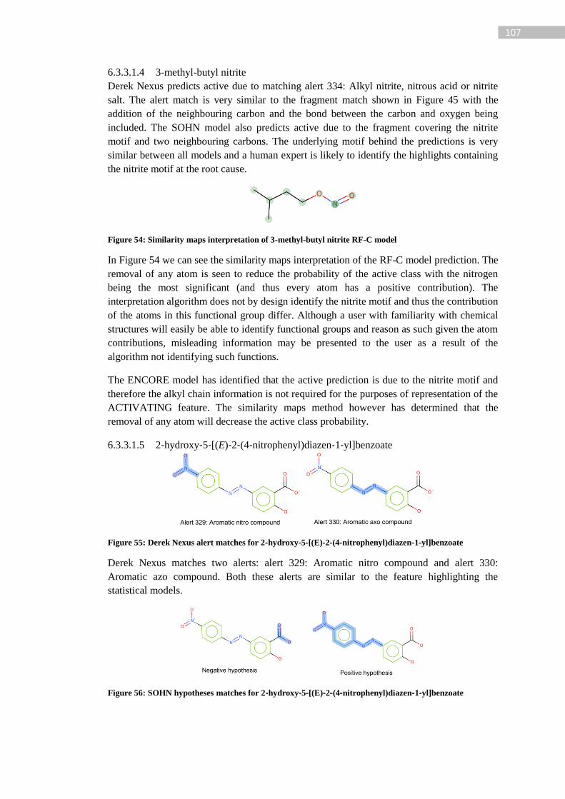
107
6.3.3.1.4 3-methyl-butyl nitrite
Derek Nexus predicts active due to matching alert 334: Alkyl nitrite, nitrous acid or nitrite
salt. The alert match is very similar to the fragment match shown in Figure 45 with the
addition of the neighbouring carbon and the bond between the carbon and oxygen being
included. The SOHN model also predicts active due to the fragment covering the nitrite
motif and two neighbouring carbons. The underlying motif behind the predictions is very
similar between all models and a human expert is likely to identify the highlights containing
the nitrite motif at the root cause.
Figure 54: Similarity maps interpretation of 3-methyl-butyl nitrite RF-C model
In Figure 54 we can see the similarity maps interpretation of the RF-C model prediction. The
removal of any atom is seen to reduce the probability of the active class with the nitrogen
being the most significant (and thus every atom has a positive contribution). The
interpretation algorithm does not by design identify the nitrite motif and thus the contribution
of the atoms in this functional group differ. Although a user with familiarity with chemical
structures will easily be able to identify functional groups and reason as such given the atom
contributions, misleading information may be presented to the user as a result of the
algorithm not identifying such functions.
The ENCORE model has identified that the active prediction is due to the nitrite motif and
therefore the alkyl chain information is not required for the purposes of representation of the
ACTIVATING feature. The similarity maps method however has determined that the
removal of any atom will decrease the active class probability.
6.3.3.1.5 2‐hydroxy‐5‐[(E)‐2‐(4‐nitrophenyl)diazen‐1‐yl]benzoate
Figure 55: Derek Nexus alert matches for 2‐hydroxy‐5‐[(E)‐2‐(4‐nitrophenyl)diazen‐1‐yl]benzoate
Derek Nexus matches two alerts: alert 329: Aromatic nitro compound and alert 330:
Aromatic azo compound. Both these alerts are similar to the feature highlighting the
statistical models.
Figure 56: SOHN hypotheses matches for 2‐hydroxy‐5‐[(E)‐2‐(4‐nitrophenyl)diazen‐1‐yl]benzoate
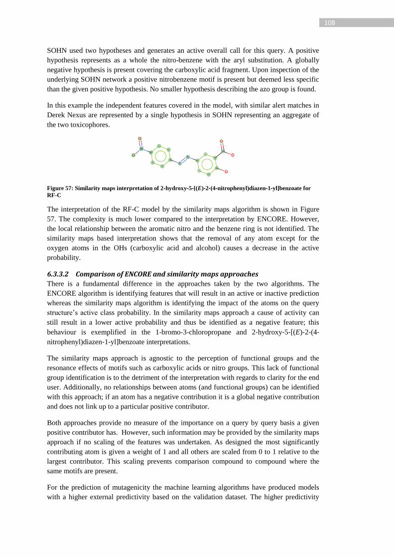
108
SOHN used two hypotheses and generates an active overall call for this query. A positive
hypothesis represents as a whole the nitro-benzene with the aryl substitution. A globally
negative hypothesis is present covering the carboxylic acid fragment. Upon inspection of the
underlying SOHN network a positive nitrobenzene motif is present but deemed less specific
than the given positive hypothesis. No smaller hypothesis describing the azo group is found.
In this example the independent features covered in the model, with similar alert matches in
Derek Nexus are represented by a single hypothesis in SOHN representing an aggregate of
the two toxicophores.
Figure 57: Similarity maps interpretation of 2‐hydroxy‐5‐[(E)‐2‐(4‐nitrophenyl)diazen‐1‐yl]benzoate for
RF-C
The interpretation of the RF-C model by the similarity maps algorithm is shown in Figure
57. The complexity is much lower compared to the interpretation by ENCORE. However,
the local relationship between the aromatic nitro and the benzene ring is not identified. The
similarity maps based interpretation shows that the removal of any atom except for the
oxygen atoms in the OHs (carboxylic acid and alcohol) causes a decrease in the active
probability.
6.3.3.2 Comparison of ENCORE and similarity maps approaches
There is a fundamental difference in the approaches taken by the two algorithms. The
ENCORE algorithm is identifying features that will result in an active or inactive prediction
whereas the similarity maps algorithm is identifying the impact of the atoms on the query
structure’s active class probability. In the similarity maps approach a cause of activity can
still result in a lower active probability and thus be identified as a negative feature; this
behaviour is exemplified in the 1-bromo-3-chloropropane and 2‐hydroxy‐5‐[(E)‐2‐(4‐
nitrophenyl)diazen‐1‐yl]benzoate interpretations.
The similarity maps approach is agnostic to the perception of functional groups and the
resonance effects of motifs such as carboxylic acids or nitro groups. This lack of functional
group identification is to the detriment of the interpretation with regards to clarity for the end
user. Additionally, no relationships between atoms (and functional groups) can be identified
with this approach; if an atom has a negative contribution it is a global negative contribution
and does not link up to a particular positive contributor.
Both approaches provide no measure of the importance on a query by query basis a given
positive contributor has. However, such information may be provided by the similarity maps
approach if no scaling of the features was undertaken. As designed the most significantly
contributing atom is given a weight of 1 and all others are scaled from 0 to 1 relative to the
largest contributor. This scaling prevents comparison compound to compound where the
same motifs are present.
For the prediction of mutagenicity the machine learning algorithms have produced models
with a higher external predictivity based on the validation dataset. The higher predictivity
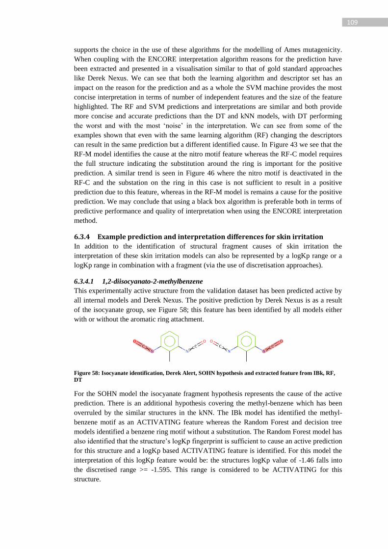
109
supports the choice in the use of these algorithms for the modelling of Ames mutagenicity.
When coupling with the ENCORE interpretation algorithm reasons for the prediction have
been extracted and presented in a visualisation similar to that of gold standard approaches
like Derek Nexus. We can see that both the learning algorithm and descriptor set has an
impact on the reason for the prediction and as a whole the SVM machine provides the most
concise interpretation in terms of number of independent features and the size of the feature
highlighted. The RF and SVM predictions and interpretations are similar and both provide
more concise and accurate predictions than the DT and kNN models, with DT performing
the worst and with the most ‘noise’ in the interpretation. We can see from some of the
examples shown that even with the same learning algorithm (RF) changing the descriptors
can result in the same prediction but a different identified cause. In Figure 43 we see that the
RF-M model identifies the cause at the nitro motif feature whereas the RF-C model requires
the full structure indicating the substitution around the ring is important for the positive
prediction. A similar trend is seen in Figure 46 where the nitro motif is deactivated in the
RF-C and the substation on the ring in this case is not sufficient to result in a positive
prediction due to this feature, whereas in the RF-M model is remains a cause for the positive
prediction. We may conclude that using a black box algorithm is preferable both in terms of
predictive performance and quality of interpretation when using the ENCORE interpretation
method.
6.3.4 Example prediction and interpretation differences for skin irritation
In addition to the identification of structural fragment causes of skin irritation the
interpretation of these skin irritation models can also be represented by a logKp range or a
logKp range in combination with a fragment (via the use of discretisation approaches).
6.3.4.1 1,2-diisocyanato-2-methylbenzene
This experimentally active structure from the validation dataset has been predicted active by
all internal models and Derek Nexus. The positive prediction by Derek Nexus is as a result
of the isocyanate group, see Figure 58; this feature has been identified by all models either
with or without the aromatic ring attachment.
Figure 58: Isocyanate identification, Derek Alert, SOHN hypothesis and extracted feature from IBk, RF,
DT
For the SOHN model the isocyanate fragment hypothesis represents the cause of the active
prediction. There is an additional hypothesis covering the methyl-benzene which has been
overruled by the similar structures in the kNN. The IBk model has identified the methyl-
benzene motif as an ACTIVATING feature whereas the Random Forest and decision tree
models identified a benzene ring motif without a substitution. The Random Forest model has
also identified that the structure’s logKp fingerprint is sufficient to cause an active prediction
for this structure and a logKp based ACTIVATING feature is identified. For this model the
interpretation of this logKp feature would be: the structures logKp value of -1.46 falls into
the discretised range >= -1.595. This range is considered to be ACTIVATING for this
structure.
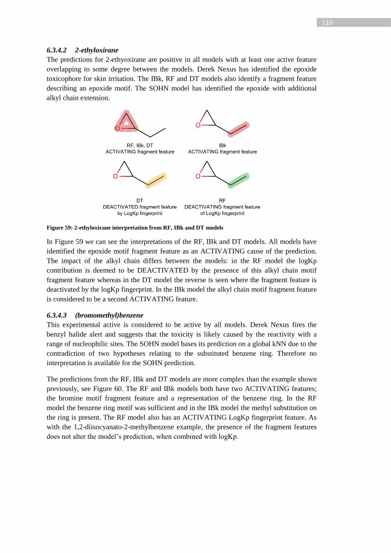
110
6.3.4.2 2-ethyloxirane
The predictions for 2-ethyoxirane are positive in all models with at least one active feature
overlapping to some degree between the models. Derek Nexus has identified the epoxide
toxicophore for skin irritation. The IBk, RF and DT models also identify a fragment feature
describing an epoxide motif. The SOHN model has identified the epoxide with additional
alkyl chain extension.
Figure 59: 2-ethyloxirane interpretation from RF, IBk and DT models
In Figure 59 we can see the interpretations of the RF, IBk and DT models. All models have
identified the epoxide motif fragment feature as an ACTIVATING cause of the prediction.
The impact of the alkyl chain differs between the models: in the RF model the logKp
contribution is deemed to be DEACTIVATED by the presence of this alkyl chain motif
fragment feature whereas in the DT model the reverse is seen where the fragment feature is
deactivated by the logKp fingerprint. In the IBk model the alkyl chain motif fragment feature
is considered to be a second ACTIVATING feature.
6.3.4.3 (bromomethyl)benzene
This experimental active is considered to be active by all models. Derek Nexus fires the
benzyl halide alert and suggests that the toxicity is likely caused by the reactivity with a
range of nucleophilic sites. The SOHN model bases its prediction on a global kNN due to the
contradiction of two hypotheses relating to the substituted benzene ring. Therefore no
interpretation is available for the SOHN prediction.
The predictions from the RF, IBk and DT models are more complex than the example shown
previously, see Figure 60. The RF and IBk models both have two ACTIVATING features;
the bromine motif fragment feature and a representation of the benzene ring. In the RF
model the benzene ring motif was sufficient and in the IBk model the methyl substitution on
the ring is present. The RF model also has an ACTIVATING LogKp fingerprint feature. As
with the 1,2-diisocyanato-2-methylbenzene example, the presence of the fragment features
does not alter the model’s prediction, when combined with logKp.
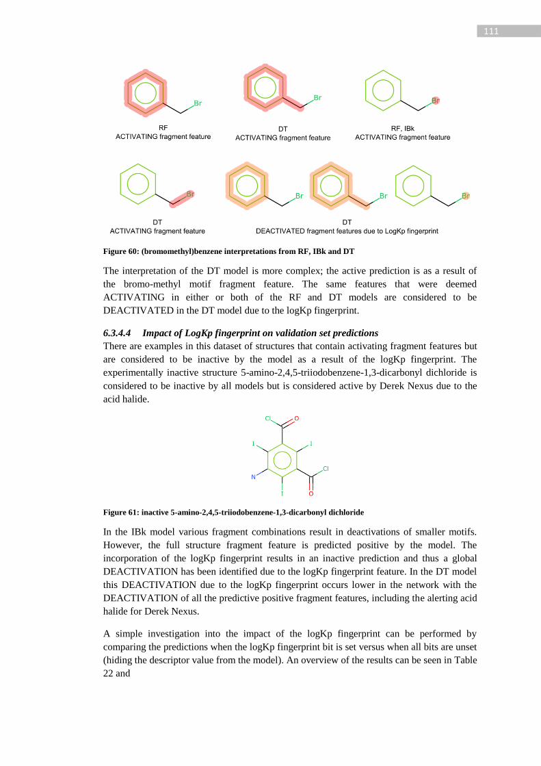
111
Figure 60: (bromomethyl)benzene interpretations from RF, IBk and DT
The interpretation of the DT model is more complex; the active prediction is as a result of
the bromo-methyl motif fragment feature. The same features that were deemed
ACTIVATING in either or both of the RF and DT models are considered to be
DEACTIVATED in the DT model due to the logKp fingerprint.
6.3.4.4 Impact of LogKp fingerprint on validation set predictions
There are examples in this dataset of structures that contain activating fragment features but
are considered to be inactive by the model as a result of the logKp fingerprint. The
experimentally inactive structure 5-amino-2,4,5-triiodobenzene-1,3-dicarbonyl dichloride is
considered to be inactive by all models but is considered active by Derek Nexus due to the
acid halide.
Figure 61: inactive 5-amino-2,4,5-triiodobenzene-1,3-dicarbonyl dichloride
In the IBk model various fragment combinations result in deactivations of smaller motifs.
However, the full structure fragment feature is predicted positive by the model. The
incorporation of the logKp fingerprint results in an inactive prediction and thus a global
DEACTIVATION has been identified due to the logKp fingerprint feature. In the DT model
this DEACTIVATION due to the logKp fingerprint occurs lower in the network with the
DEACTIVATION of all the predictive positive fragment features, including the alerting acid
halide for Derek Nexus.
A simple investigation into the impact of the logKp fingerprint can be performed by
comparing the predictions when the logKp fingerprint bit is set versus when all bits are unset
(hiding the descriptor value from the model). An overview of the results can be seen in Table
22 and
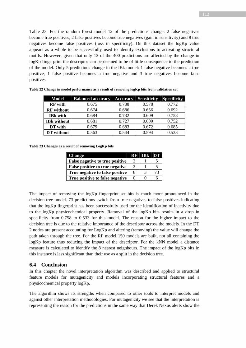
112
Table 23. For the random forest model 12 of the predictions change: 2 false negatives
become true positives, 2 false positives become true negatives (gain in sensitivity) and 8 true
negatives become false positives (loss in specificity). On this dataset the logKp value
appears as a whole to be successfully used to identify exclusions to activating structural
motifs. However, given that only 12 of the 400 predictions are affected by the change in
logKp fingerprint the descriptor can be deemed to be of little consequence to the prediction
of the model. Only 5 predictions change in the IBk model: 1 false negative becomes a true
positive, 1 false positive becomes a true negative and 3 true negatives become false
positives.
Table 22 Change in model performance as a result of removing logKp bits from validation set
Model Balanced accuracy Accuracy Sensitivity Specificity
RF with 0.675 0.738 0.578 0.772
RF without 0.674 0.686 0.656 0.692
IBk with 0.684 0.732 0.609 0.758
IBk without 0.681 0.727 0.609 0.752
DT with 0.679 0.683 0.672 0.685
DT without 0.563 0.544 0.594 0.533
Table 23 Changes as a result of removing LogKp bits
Change RF IBk DT
False negative to true positive 2 1 5
False positive to true negative 2 1 5
True negative to false positive 8 3 73
True positive to false negative 0 0 6
The impact of removing the logKp fingerprint set bits is much more pronounced in the
decision tree model. 73 predictions switch from true negatives to false positives indicating
that the logKp fingerprint has been successfully used for the identification of inactivity due
to the logKp physicochemical property. Removal of the logKp bits results in a drop in
specificity from 0.758 to 0.533 for this model. The reason for the higher impact to the
decision tree is due to the relative importance of the descriptor across the models. In the DT
2 nodes are present accounting for LogKp and altering (removing) the value will change the
path taken through the tree. For the RF model 150 models are built, not all containing the
logKp feature thus reducing the impact of the descriptor. For the kNN model a distance
measure is calculated to identify the 8 nearest neighbours. The impact of the logKp bits in
this instance is less significant than their use as a split in the decision tree.
6.4 Conclusion
In this chapter the novel interpretation algorithm was described and applied to structural
feature models for mutagenicity and models incorporating structural features and a
physicochemical property logKp.
The algorithm shows its strengths when compared to other tools to interpret models and
against other interpretation methodologies. For mutagenicity we see that the interpretation is
representing the reason for the predictions in the same way that Derek Nexus alerts show the
113
alert matches, although we do see differences between the cause in the prediction between
the machine learning models and the Derek Nexus expert system. The key point here is that
the ENCORE methodology is extracting the cause and representing this to the user in an
understandable way: the highlighting of atoms and bonds and attributing the impact on the
prediction.
When comparing the approach to the similarity maps interpretation, a fundamental
difference in the two approaches becomes clear even on trivial examples such as 1-bromo-3-
chloropropane. There are two causes of activity in this structure, both alkylating agents with
either bromine or chlorine. The ENCORE model identifies that there are two features
causing the active prediction from the model and highlights these features independently
(without mechanism). However, the similarity maps approach is concerned with identifying
the contribution of the atoms to the active probability and identifies that the chlorine based
alkylating agent decreases the active class probability. In terms of an understandable
interpretation in the context of what is being modelled (binary Ames mutagenicity) what we
want to know is what causes the model to predict positive. The similarity maps approach
does not provide this information; the negative contribution of the chlorine will be
misleading in this concept. The similarity maps approach does not say the removal of the
chlorine will cause a switch from an active to inactive prediction but it also does not identify
that the chlorine (and connecting carbon) will cause the active class probability to exceed
50%. The similarity maps interpretation approach therefore does not meet the goal of
identifying why the query structure is predicted to be active and is more suited to regression
models where a continuous value is being predicted rather than a prediction either side of a
class boundary. In regression based models a desired interpretation may be in assessing an
atoms contribution towards an increase or decrease in the value which can be achieved
through similarity maps (for example as applied to the comparison of structural similarity
comparisons [71]) and this does not need to account for class switching like in the models
discussed in this thesis.
We have also seen from these examples that there can be multiple causes of activity. The
ENCORE algorithm is able to extract these independent causes. The ‘universal’
interpretation algorithm developed by Polishchuk et al. [73] will not be able to produce an
interpretation in these terms as the removal of a single activating feature will not result in a
change in the class prediction.
When moving onto the interpretation of models involving a physicochemical descriptor the
similarity maps approach is not able to handle these descriptors and thus cannot be used. The
‘universal’ approach could but, as identified, the lack of accounting for combinations reveals
that where the cause of the active prediction is not simple the interpretation methodology is
not able to extract the underlying causes.
The interpretation algorithm has shown that we can capitalise on the performance of the
black box algorithms where the interpretation of the model is a requirement. These black box
models have been shown to be better predictors in both the Ames mutagenicity and skin
irritation datasets. Although the interpretation does not provide the mechanistic reasoning
available in expert systems like Derek Nexus, the development of the model requires a
fraction of the time over developing expert alerts and rules. This is not advocating for the
exclusive use of this approach over an expert system as the mechanistic information provides

114
invaluable information for some use cases. Indeed, in the following chapter we discuss how
to capitalise on this interpretation to support the development of expert systems.
The algorithm is providing an interpretation of a black box learning algorithm and a large
degree of flexibility is provided to the user in terms of algorithm and descriptor choice. We
do see that the different combinations of learning algorithm and descriptor result in changes
in predictions both in terms of the predicted class and the reason for the prediction as
elucidated by the ENCORE interpretation algorithm. The interpretations from the SVM and
RF models can be deemed more concise relative to the DT and kNN interpretations: smaller
functional groups are identified as the cause and these more closely resemble the human
identified toxicophores. It is also more frequent in the DT and kNN approaches for a feature
to be deactivated but contribute to a larger fragment that is deemed an activating feature;
whereas in the RF and SVM models the smaller feature is kept and thus the interpretation is
more concise. The RF and SVM models therefore perform better in terms of predictive
accuracy and legibility of the elucidated interpretation.
With regards to the choice in descriptor set the structural component should ideally be a
descriptor that does not form a pre-defined list (such as keys) so as to allow the model to
learn about the full relationships in a dataset and not limit the understanding to a pre-defined
set. This has the impact of generally increasing the size of an identified feature which can
add complexity but may reveal more information regarding the importance of the
connectivity of the features which is more explicit in the hashed fingerprints vs the keys.
Users may benefit from optimisation on model performance as opposed to interpretation as
the most accurate model has been seen to generally provide the most concise interpretation.
Some limitations still remain to be resolved; the interpretation algorithm shows weaknesses
in the description of complex deactivations and alternative summary approaches show how
to simplify the output. With the current design the method is only applicable to binary
predictions; this limitation is discussed further in chapter 8.
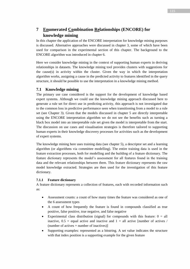
115
7 Enumerated Combination Relationships (ENCORE) for
knowledge mining In this chapter the application of the ENCORE interpretation for knowledge mining purposes
is discussed. Alternative approaches were discussed in chapter 3, some of which have been
used for comparison in the experimental section of this chapter. The background to the
ENCORE algorithm was introduced in chapter 6.
Here we consider knowledge mining in the context of supporting human experts in deriving
relationships in datasets. The knowledge mining tool provides clusters with suggestions for
the cause(s) in activity within the cluster. Given the way in which the interpretation
algorithm works, assigning a cause in the predicted activity to features identified in the query
structure, it should be possible to use the interpretation in a knowledge mining method.
7.1 Knowledge mining
The primary use case considered is the support for the development of knowledge based
expert systems. Although we could use the knowledge mining approach discussed here to
generate a rule set for direct use in predicting activity, this approach is not investigated due
to the common loss in predictive performance seen when transitioning from a model to a rule
set (see Chapter 3). Given that the models discussed in chapter 5 are directly interpretable
using the ENCORE interpretation algorithm we do not see the benefits such as turning a
black box model into an interpretable rule set given the model is interpretable from the start.
The discussion on use cases and visualisation strategies is therefore tailored to supporting
human experts in their knowledge discovery processes for activities such as the development
of expert systems.
The knowledge mining here uses training data (see chapter 5), a descriptor set and a learning
algorithm (or algorithms via committee modelling). The entire training data is used in the
feature extraction processes, both for modelling and the building of a feature dictionary. The
feature dictionary represents the model’s assessment for all features found in the training
data and the relevant relationships between them. This feature dictionary represents the raw
model knowledge extracted. Strategies are then used for the investigation of this feature
dictionary.
7.1.1 Feature dictionary
A feature dictionary represents a collection of features, each with recorded information such
as:
Assessment counts: a count of how many times the feature was considered as one of
the 6 assessment types
A count of how frequently the feature is found in compounds classified as true
positive, false positive, true negative, and false negative
Experimental class distribution (signal) for compounds with this feature: 0 = all
inactive, 0.5 = equal active and inactive and 1 = all active [number of actives /
(number of actives + number of inactives)]
Supporting examples: represented as a bitstring. A set value indicates the structure
with that index position is a supporting example for the given feature
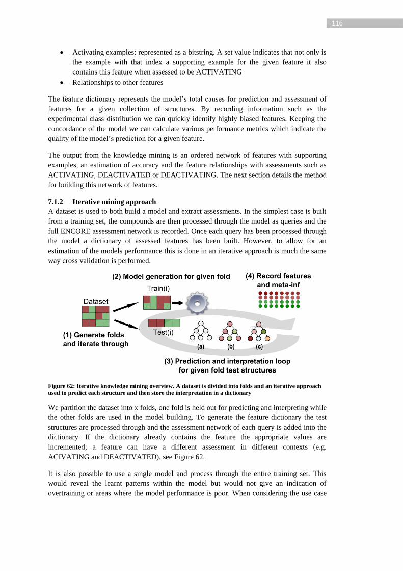
116
Activating examples: represented as a bitstring. A set value indicates that not only is
the example with that index a supporting example for the given feature it also
contains this feature when assessed to be ACTIVATING
Relationships to other features
The feature dictionary represents the model’s total causes for prediction and assessment of
features for a given collection of structures. By recording information such as the
experimental class distribution we can quickly identify highly biased features. Keeping the
concordance of the model we can calculate various performance metrics which indicate the
quality of the model’s prediction for a given feature.
The output from the knowledge mining is an ordered network of features with supporting
examples, an estimation of accuracy and the feature relationships with assessments such as
ACTIVATING, DEACTIVATED or DEACTIVATING. The next section details the method
for building this network of features.
7.1.2 Iterative mining approach
A dataset is used to both build a model and extract assessments. In the simplest case is built
from a training set, the compounds are then processed through the model as queries and the
full ENCORE assessment network is recorded. Once each query has been processed through
the model a dictionary of assessed features has been built. However, to allow for an
estimation of the models performance this is done in an iterative approach is much the same
way cross validation is performed.
Figure 62: Iterative knowledge mining overview. A dataset is divided into folds and an iterative approach
used to predict each structure and then store the interpretation in a dictionary
We partition the dataset into x folds, one fold is held out for predicting and interpreting while
the other folds are used in the model building. To generate the feature dictionary the test
structures are processed through and the assessment network of each query is added into the
dictionary. If the dictionary already contains the feature the appropriate values are
incremented; a feature can have a different assessment in different contexts (e.g.
ACIVATING and DEACTIVATED), see Figure 62.
It is also possible to use a single model and process through the entire training set. This
would reveal the learnt patterns within the model but would not give an indication of
overtraining or areas where the model performance is poor. When considering the use case
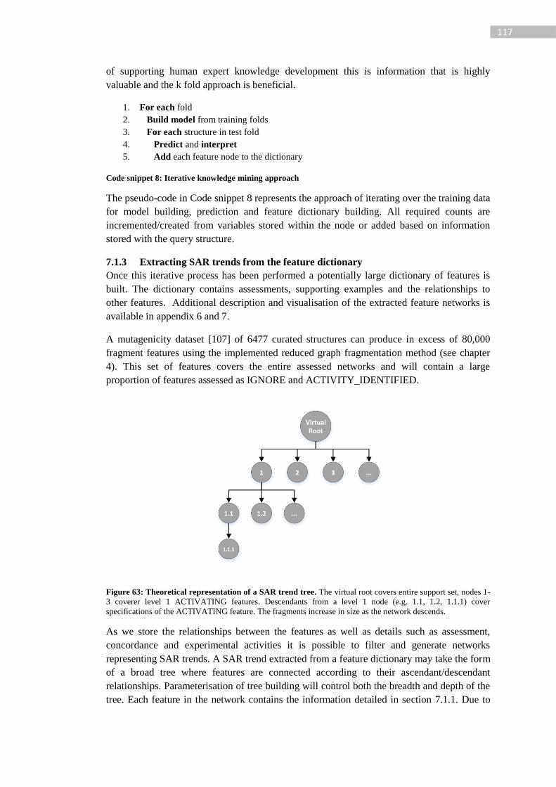
117
of supporting human expert knowledge development this is information that is highly
valuable and the k fold approach is beneficial.
1. For each fold
2. Build model from training folds
3. For each structure in test fold
4. Predict and interpret
5. Add each feature node to the dictionary
Code snippet 8: Iterative knowledge mining approach
The pseudo-code in Code snippet 8 represents the approach of iterating over the training data
for model building, prediction and feature dictionary building. All required counts are
incremented/created from variables stored within the node or added based on information
stored with the query structure.
7.1.3 Extracting SAR trends from the feature dictionary
Once this iterative process has been performed a potentially large dictionary of features is
built. The dictionary contains assessments, supporting examples and the relationships to
other features. Additional description and visualisation of the extracted feature networks is
available in appendix 6 and 7.
A mutagenicity dataset [107] of 6477 curated structures can produce in excess of 80,000
fragment features using the implemented reduced graph fragmentation method (see chapter
4). This set of features covers the entire assessed networks and will contain a large
proportion of features assessed as IGNORE and ACTIVITY_IDENTIFIED.
Figure 63: Theoretical representation of a SAR trend tree. The virtual root covers entire support set, nodes 1-
3 coverer level 1 ACTIVATING features. Descendants from a level 1 node (e.g. 1.1, 1.2, 1.1.1) cover
specifications of the ACTIVATING feature. The fragments increase in size as the network descends.
As we store the relationships between the features as well as details such as assessment,
concordance and experimental activities it is possible to filter and generate networks
representing SAR trends. A SAR trend extracted from a feature dictionary may take the form
of a broad tree where features are connected according to their ascendant/descendant
relationships. Parameterisation of tree building will control both the breadth and depth of the
tree. Each feature in the network contains the information detailed in section 7.1.1. Due to

118
variation in models (when performing folding) and local context a feature can have a non-
zero count for more than 1 assessment type. A feature may appear in multiple places in the
generated tree both as a result of relationships with other features and being assigned non
zero counts for multiple assessment types.
Figure 64: Example SAR trend representation, red indicates active and green inactive
The choice of filter to apply to this SAR trend network building affects which features in the
trend will be displayed. For example at the first level only nodes assessed to be activating X
times may be desired, indicating potential toxicophores. The first level in the tree (nodes 1-3
in Figure 63) represents the features that meet a minimum occurrence in both supporting
examples and an assessment of ACTIVATING. All descending nodes (1.1, 1.2, 1.1.1)
represent specifications of this feature (and are therefore larger fragments / combinations of
features) and again can have an occurrence of any assessment type > 0. In the example
shown in Figure 63 node 1.1 is a specification of the feature in node 1, for example node 1
may represent a benzene ring motif and feature 1.1 a nitrobenzene motif. We may then wish
to only show increased context of the feature if the parent nodes represent a deviation from
the ACTIVATING assessment. This could be done simply by specifying a change in
experimental bias (+ve, -ve) or by choosing specifically to only include DEACTIVATING
parents.
In Figure 64 we see an example SAR tree along with a representation of the chemical space
from which it was extracted. 11 supporting examples are present; a supporting example is a
structure containing the feature regardless of the assessment. A feature has been identified as
ACTIVATING that corresponds to these 11 supporting examples; note that not all 11 of the
supporting examples are classified as ACTIVATING. Two deactivations are seen: features 2
and 3. These deactivations represent a larger context where the ACTIVATING feature is not
considered to be active. The deactivation at feature 2 has a supporting example set of 3
structures and the deactivation at feature 3 has a supporting example set of 2 structures.
Based on the supporting examples we are able to calculate the performance of the model
when the feature is present indicating the quality of the model’s behaviour. We also have
access to the supporting example experimental activity.
Figure 65 shows an example child feature of a quinoline motif feature. The node details
shown represent a deactivation due to the peri-carboxy substitution. Green labels represent
119
experimentally inactive and red experimentally active. This feature has been seen in 11
structures and deemed DEACTIVATING in all occurrences. The structures where the
experimental activity is positive is likely due to a secondary toxicophore such as the
aromatic nitro shown in Figure 65 and the identification of the DEACTIVATION may be
appropriate for these true positives as a localised deactivation on a globally active structure.
Figure 65: Example deactivating child feature with supporting examples and assessment counts
7.2 Implementation
The ENCORE algorithm has been developed as a Java API providing network building,
network assessment and network summary. Through dependencies to core Lhasa libraries
such as the chemical engine a wrapper has been provided for various functionality
requirement by the interpretation workflow such as fragmentation. The model building and
predictions are provided by third party libraries and/or KNIME nodes.
7.2.1 Software implementations
Coralie provides a more efficient environment for the knowledge mining activities that can
be carried out through the use of ENCORE than KNIME. All knowledge mining jobs are run
in Coralie where SAR trends can then be visualised. For additional processing the features
and supporting examples are exported as SD files allowing for processing in other
applications. Machine learning models are built through the use of the Java Weka 3.7 library
which has been incorporated into a wrapper and provided as a plugin along with ENCORE.
A variety of extensions to the user interface have been created to provide a user friendly
representation of the knowledge mining and model output; examples can be seen in the
Appendix. The knowledge mining implementation relies on core Lhasa Limited libraries as
well as Weka to provide the required cheminformatic and machine learning algorithms.
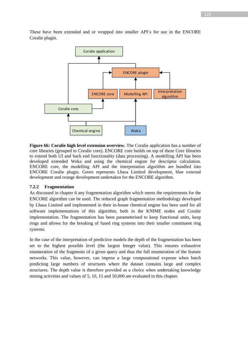
120
These have been extended and or wrapped into smaller API’s for use in the ENCORE
Coralie plugin.
Coralie core
ENCORE plugin
Coralie application
ENCORE core Modelling API
Chemical engine Weka
Interpretation algorithm
Figure 66: Coralie high level extension overview. The Coralie application has a number of
core libraries (grouped to Coralie core). ENCORE core builds on top of these Core libraries
to extend both UI and back end functionality (data processing). A modelling API has been
developed extended Weka and using the chemical engine for descriptor calculation.
ENCORE core, the modelling API and the interpretation algorithm are bundled into
ENCORE Coralie plugin. Green represents Lhasa Limited development, blue external
development and orange development undertaken for the ENCORE algorithm.
7.2.2 Fragmentation
As discussed in chapter 6 any fragmentation algorithm which meets the requirements for the
ENCORE algorithm can be used. The reduced graph fragmentation methodology developed
by Lhasa Limited and implemented in their in-house chemical engine has been used for all
software implementations of this algorithm, both in the KNIME nodes and Coralie
implementation. The fragmentation has been parameterised to keep functional units, keep
rings and allows for the breaking of fused ring systems into their smaller constituent ring
systems.
In the case of the interpretation of predictive models the depth of the fragmentation has been
set to the highest possible level (the largest Integer value). This ensures exhaustive
enumeration of the fragments of a given query and thus the full enumeration of the feature
networks. This value, however, can impose a large computational expense when batch
predicting large numbers of structures where the dataset contains large and complex
structures. The depth value is therefore provided as a choice when undertaking knowledge
mining activities and values of 5, 10, 15 and 50,000 are evaluated in this chapter.
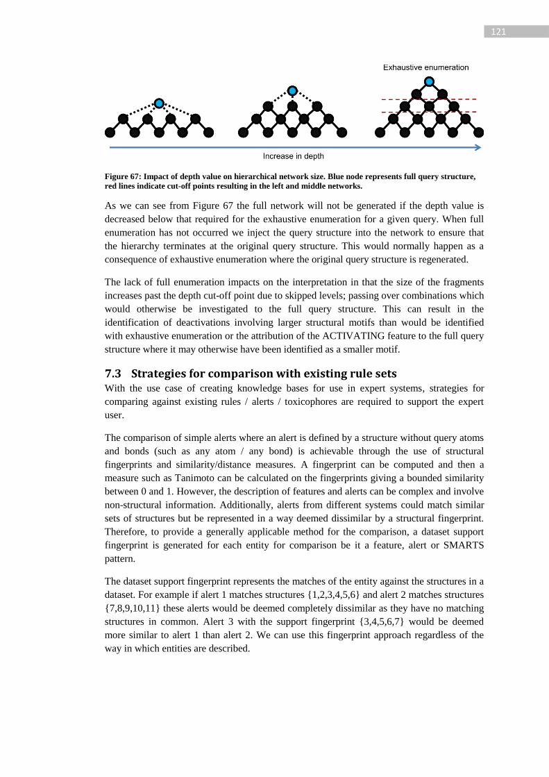
121
Figure 67: Impact of depth value on hierarchical network size. Blue node represents full query structure,
red lines indicate cut-off points resulting in the left and middle networks.
As we can see from Figure 67 the full network will not be generated if the depth value is
decreased below that required for the exhaustive enumeration for a given query. When full
enumeration has not occurred we inject the query structure into the network to ensure that
the hierarchy terminates at the original query structure. This would normally happen as a
consequence of exhaustive enumeration where the original query structure is regenerated.
The lack of full enumeration impacts on the interpretation in that the size of the fragments
increases past the depth cut-off point due to skipped levels; passing over combinations which
would otherwise be investigated to the full query structure. This can result in the
identification of deactivations involving larger structural motifs than would be identified
with exhaustive enumeration or the attribution of the ACTIVATING feature to the full query
structure where it may otherwise have been identified as a smaller motif.
7.3 Strategies for comparison with existing rule sets With the use case of creating knowledge bases for use in expert systems, strategies for
comparing against existing rules / alerts / toxicophores are required to support the expert
user.
The comparison of simple alerts where an alert is defined by a structure without query atoms
and bonds (such as any atom / any bond) is achievable through the use of structural
fingerprints and similarity/distance measures. A fingerprint can be computed and then a
measure such as Tanimoto can be calculated on the fingerprints giving a bounded similarity
between 0 and 1. However, the description of features and alerts can be complex and involve
non-structural information. Additionally, alerts from different systems could match similar
sets of structures but be represented in a way deemed dissimilar by a structural fingerprint.
Therefore, to provide a generally applicable method for the comparison, a dataset support
fingerprint is generated for each entity for comparison be it a feature, alert or SMARTS
pattern.
The dataset support fingerprint represents the matches of the entity against the structures in a
dataset. For example if alert 1 matches structures {1,2,3,4,5,6} and alert 2 matches structures
{7,8,9,10,11} these alerts would be deemed completely dissimilar as they have no matching
structures in common. Alert 3 with the support fingerprint {3,4,5,6,7} would be deemed
more similar to alert 1 than alert 2. We can use this fingerprint approach regardless of the
way in which entities are described.
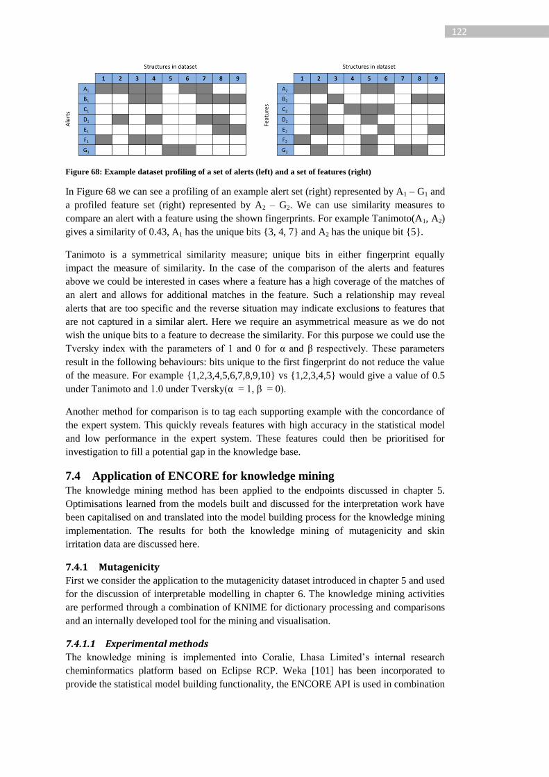
122
Figure 68: Example dataset profiling of a set of alerts (left) and a set of features (right)
In Figure 68 we can see a profiling of an example alert set (right) represented by A1 – G1 and
a profiled feature set (right) represented by A2 – G2. We can use similarity measures to
compare an alert with a feature using the shown fingerprints. For example Tanimoto(A1, A2)
gives a similarity of 0.43, A1 has the unique bits {3, 4, 7} and A2 has the unique bit {5}.
Tanimoto is a symmetrical similarity measure; unique bits in either fingerprint equally
impact the measure of similarity. In the case of the comparison of the alerts and features
above we could be interested in cases where a feature has a high coverage of the matches of
an alert and allows for additional matches in the feature. Such a relationship may reveal
alerts that are too specific and the reverse situation may indicate exclusions to features that
are not captured in a similar alert. Here we require an asymmetrical measure as we do not
wish the unique bits to a feature to decrease the similarity. For this purpose we could use the
Tversky index with the parameters of 1 and 0 for α and β respectively. These parameters
result in the following behaviours: bits unique to the first fingerprint do not reduce the value
of the measure. For example {1,2,3,4,5,6,7,8,9,10} vs {1,2,3,4,5} would give a value of 0.5
under Tanimoto and 1.0 under Tversky(α = 1, β = 0).
Another method for comparison is to tag each supporting example with the concordance of
the expert system. This quickly reveals features with high accuracy in the statistical model
and low performance in the expert system. These features could then be prioritised for
investigation to fill a potential gap in the knowledge base.
7.4 Application of ENCORE for knowledge mining
The knowledge mining method has been applied to the endpoints discussed in chapter 5.
Optimisations learned from the models built and discussed for the interpretation work have
been capitalised on and translated into the model building process for the knowledge mining
implementation. The results for both the knowledge mining of mutagenicity and skin
irritation data are discussed here.
7.4.1 Mutagenicity
First we consider the application to the mutagenicity dataset introduced in chapter 5 and used
for the discussion of interpretable modelling in chapter 6. The knowledge mining activities
are performed through a combination of KNIME for dictionary processing and comparisons
and an internally developed tool for the mining and visualisation.
7.4.1.1 Experimental methods
The knowledge mining is implemented into Coralie, Lhasa Limited’s internal research
cheminformatics platform based on Eclipse RCP. Weka [101] has been incorporated to
provide the statistical model building functionality, the ENCORE API is used in combination
123
with Weka to implement the knowledge mining procedure detailed later in this chapter. CDK
version 1.4.2 is used for the calculation of various additional fingerprints and knowledge
mining can be carried out with the following descriptor choices: Ceres fingerprint, CDK
standard, CDK extended, MACCS keys and Pubchem keys. Various visualisations of the
SAR trends are provided. However the dictionary and supporting examples are exported as
SD files for processing in KNIME.
Various parameters are available in the knowledge mining implementation relating to the
choice of descriptor, choice of fragmentation and the number of folds to use in the iterative
process.
Based on the parameter selection carried out for the predictive models built in chapter 5 with
the various combinations of descriptor and learning algorithm, two learning algorithms are
chosen and configured for the knowledge mining activity. Firstly the J48 decision tree
algorithm has been selected and configured with the default settings in Weka 3.7. Secondly
the random forest algorithm has been used with 100 trees. Two fingerprints have been
chosen for comparison: the Ceres hashed fingerprint provided by Lhasa Limited’s chemical
engine and the MACCS keys provided by CDK. The models are labelled DT-M for the
decision tree with MACCS keys, DT-C for the decision tree with the Ceres fingerprint, RF-
M for the random forest with MACCS keys and RF-C for the random forest with the Ceres
hashed fingerprint.
7.4.1.2 ENCORE mined models
Various model mining jobs have been run through the knowledge mining implementation of
ENCORE using a various depths and 0 or 10 folds. The depth parameter relates to the
fragmentation algorithm. The impact of this parameter is discussed in section 7.2.2. To
summarise, this value controls the combination of features and the network size. The folds
parameter controls the number of divisions and thus models built in a similar concept to
cross validation. Two values were used: 0 folds indicates that no folding was undertaken and
the training data was processed through the model and 10 folds indicates that 10 divisions of
the data were made resulting in 10 iterations of the procedure of the different dataset
divisions.
7.4.1.2.1 Impact of parameter choice
The choice of descriptor has a major effect on the time to process. Fingerprinting approaches
such as the hashed linear path fingerprints from CDK or the Ceres fingerprint have a quick
computation time. Structural keys such as MACCS and Pubchem fingerprints have a
significant slower computation time due to the need to substructure search. The following
timings were for an Intel® Core™ i7-4770 @ 3.40GHz with a Java heap space of 14GB
(exceeded memory requirements for the mining job) with a SDD hard drive. With a depth of
15 the knowledge mining on the dataset of ~4500 structures takes 40 minutes to run whereas
the same configuration with the MACCS keys provided by CDK takes ~6 hours of runtime.
The code has not been developed for computational efficiency and is single threaded so time
savings could be made. Nevertheless descriptors involving substructure searching will
always add significantly to the runtime of the mining job. Near exhaustive enumeration, 10
fold mining and a Random Forest with 100 trees required ~60 minutes to complete using the
Ceres fingerprint. The mining job is not taxing for the CPU and could therefore be
parallelised to take advantage multi core processors. However, even without optimisation the
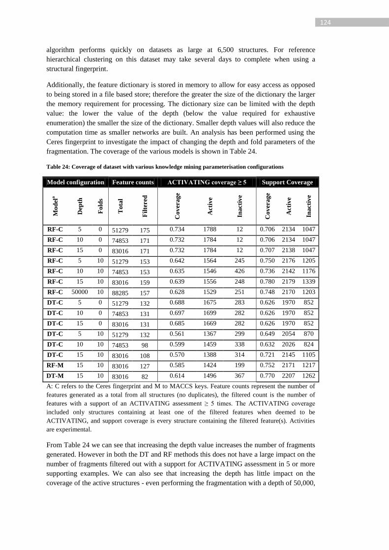
124
algorithm performs quickly on datasets as large at 6,500 structures. For reference
hierarchical clustering on this dataset may take several days to complete when using a
structural fingerprint.
Additionally, the feature dictionary is stored in memory to allow for easy access as opposed
to being stored in a file based store; therefore the greater the size of the dictionary the larger
the memory requirement for processing. The dictionary size can be limited with the depth
value: the lower the value of the depth (below the value required for exhaustive
enumeration) the smaller the size of the dictionary. Smaller depth values will also reduce the
computation time as smaller networks are built. An analysis has been performed using the
Ceres fingerprint to investigate the impact of changing the depth and fold parameters of the
fragmentation. The coverage of the various models is shown in Table 24.
Table 24: Coverage of dataset with various knowledge mining parameterisation configurations
Model configuration Feature counts ACTIVATING coverage ≥ 5 Support Coverage
Mo
del
a
Dep
th
Fo
lds
To
tal
Fil
tere
d
Co
ver
ag
e
Act
ive
Ina
ctiv
e
Co
ver
ag
e
Act
ive
Ina
ctiv
e
RF-C 5 0 51279 175 0.734 1788 12 0.706 2134 1047
RF-C 10 0 74853 171 0.732 1784 12 0.706 2134 1047
RF-C 15 0 83016 171 0.732 1784 12 0.707 2138 1047
RF-C 5 10 51279 153 0.642 1564 245 0.750 2176 1205
RF-C 10 10 74853 153 0.635 1546 426 0.736 2142 1176
RF-C 15 10 83016 159 0.639 1556 248 0.780 2179 1339
RF-C 50000 10 88285 157 0.628 1529 251 0.748 2170 1203
DT-C 5 0 51279 132 0.688 1675 283 0.626 1970 852
DT-C 10 0 74853 131 0.697 1699 282 0.626 1970 852
DT-C 15 0 83016 131 0.685 1669 282 0.626 1970 852
DT-C 5 10 51279 132 0.561 1367 299 0.649 2054 870
DT-C 10 10 74853 98 0.599 1459 338 0.632 2026 824
DT-C 15 10 83016 108 0.570 1388 314 0.721 2145 1105
RF-M 15 10 83016 127 0.585 1424 199 0.752 2171 1217
DT-M 15 10 83016 82 0.614 1496 367 0.770 2207 1262
A: C refers to the Ceres fingerprint and M to MACCS keys. Feature counts represent the number of
features generated as a total from all structures (no duplicates), the filtered count is the number of
features with a support of an ACTIVATING assessment ≥ 5 times. The ACTIVATING coverage
included only structures containing at least one of the filtered features when deemed to be
ACTIVATING, and support coverage is every structure containing the filtered feature(s). Activities
are experimental.
From Table 24 we can see that increasing the depth value increases the number of fragments
generated. However in both the DT and RF methods this does not have a large impact on the
number of fragments filtered out with a support for ACTIVATING assessment in 5 or more
supporting examples. We can also see that increasing the depth has little impact on the
coverage of the active structures - even performing the fragmentation with a depth of 50,000,

125
ensuring full enumeration for all but extremely complex structures, we do not have any gain
in the coverage of the active structures in the dataset; the more significant factor in
increasing the coverage is – as would be expected – not undertaking the folding approach.
When using the MACCS keys as descriptors, performing the run with a depth of 15 and 10
folds results in a runtime of ~6 hours indicating that the choice in descriptor plays the more
significant role in runtime. This runtime increase is due to the speed of descriptor
calculation. The Ceres fingerprint is generated with a much lower computation cost than the
MACCS key fingerprint. The MACCS keys gave a greater coverage than the Ceres
fingerprint in the decision trees but less coverage than the Ceres fingerprint in the random
forest.
When performing the folding approach we can see that the total number of features drops
along with coverage. The benefit to folding is that an estimation of the model’s accuracy can
be made when each feature is provided in the form of the performance on the out of training
fold predictions. This has resulted in a drop in the coverage of the ACTIVATING features
with a support ≥ 5. The drop in number of features when increasing the depth value can be
attributed to the impact discussed in 7.2.2 where by increasing the depth larger networks are
generated and the algorithm has the opportunity to assign activity to smaller features. In
some cases a lower depth will result in activity shifting to a larger fragment. The drop
associated with using 10 fold vs 0 fold will be twofold. Firstly, multiple models are
generated and they will not learn the underlying SARs in identical ways. Secondly, when
using folding we are not identifying the placement of a training instance and thus greater
variations between the placement of structures in the prediction space will be seen. To
increase the coverage while retaining the accuracy of the model an external test set (such as
with the model building in chapter 6) could be processed against the model to provide the
estimation of the predictivity of the extracted features. However, a complete coverage of the
fragment space would not be ensured by the random selection of the data from the total data
available.
The coverage, model accuracy and number of features extracted are greater in the random
forest models. Descriptors could not be calculated on some structures (either on the parent
structure or a fragment) due exceptions thrown in the CDK library. These structures will
have an impact on the coverage of the dataset for MACCS key models, which is reported for
the full training set and not the subset that could be processed. For the RF-M, 10 fold and
depth 15 model the coverage is 5.4% lower than the corresponding Ceres descriptor based
model; the Ceres based model may have learned more of the underlying patterns in the data.
The majority of the ACTIVATING features found in all models have a support of less than
50 examples. The distribution of ACTIVATING feature example support is shown in Figure
69. Outside the area of the plot in Figure 69 the number of distinct counts is: J48-M 7, J48-C
9, RF-M 5 and RF-C 10. These very highly supported features indicate regions of chemical
space in the dataset biased towards certain classes, for example aromatic nitro compounds.
All models also contain many features below the minimum support cut-off value of 5 used:
1211 for J48-M, 1555 for J48-C, 1629 for RF-C and 1498 for RF-M. Features with a support
this low have been considered too poor in support to contribute significantly to a knowledge
mining study. However, usage of the tool by a knowledge base developer at Lhasa Limited
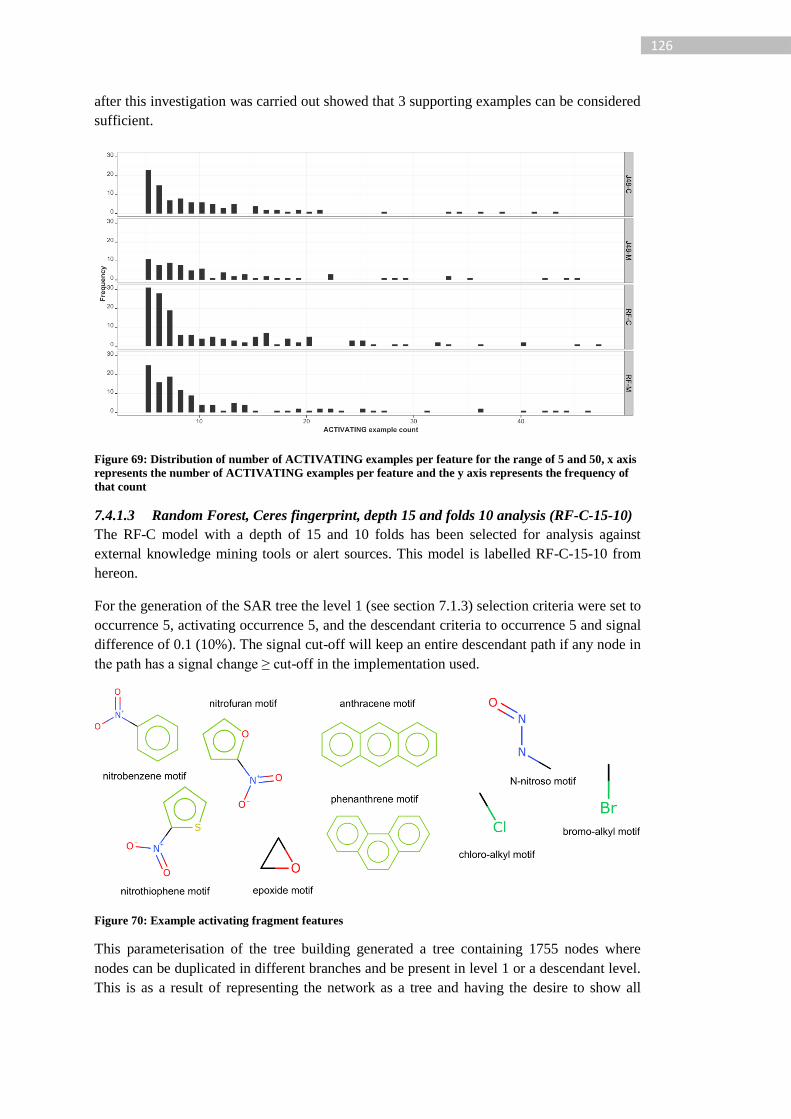
126
after this investigation was carried out showed that 3 supporting examples can be considered
sufficient.
Figure 69: Distribution of number of ACTIVATING examples per feature for the range of 5 and 50, x axis
represents the number of ACTIVATING examples per feature and the y axis represents the frequency of
that count
7.4.1.3 Random Forest, Ceres fingerprint, depth 15 and folds 10 analysis (RF-C-15-10)
The RF-C model with a depth of 15 and 10 folds has been selected for analysis against
external knowledge mining tools or alert sources. This model is labelled RF-C-15-10 from
hereon.
For the generation of the SAR tree the level 1 (see section 7.1.3) selection criteria were set to
occurrence 5, activating occurrence 5, and the descendant criteria to occurrence 5 and signal
difference of 0.1 (10%). The signal cut-off will keep an entire descendant path if any node in
the path has a signal change ≥ cut-off in the implementation used.
Figure 70: Example activating fragment features
This parameterisation of the tree building generated a tree containing 1755 nodes where
nodes can be duplicated in different branches and be present in level 1 or a descendant level.
This is as a result of representing the network as a tree and having the desire to show all

127
activations that meet the cut-off in level 1 regardless of their relationship to other activating
features resulting in 159 level 1 nodes. The filtered dictionary consists of: single ring
systems, fused ring systems, ring systems with functional substitutions and functional
groups.
We can see a limitation of the approach from the examples in Figure 70. Where a functional
group with an aromatic connection is required the specific ring is included in the feature. We
cannot describe the fragment aromatic carbon-NO2 in the fragmentation approach as we have
a requirement for descriptor generation; instead we have nitrobenzene, nitrofuran and
nitrothiophenes as independent features. A human expert may abstract these three features
into a single aromatic nitro toxicophore in a similar way to identifying a generic halo-alkyl
as opposed to chloro and bromo independently. An alternative fragmentation and descriptor
generation strategy is required to handle this behaviour. Strategies for addressing this
limitation are discussed in chapter 8.
In the above we discussed solely the filtered ACTIVATING features. A core functionality of
the knowledge mining application is the visualisation of the SAR trends extracted from the
model. The trends are visualised by the links between the features with the root node being a
feature considered ACTIVATING and descendant nodes are larger contexts of the feature
that may have alternative assessments such as ACTIVITY_IDENTIFIED or
DEACTIVATING. Although the ACTIVITY_IDENTIFIED nodes are not deemed the
causes of activity, they may nonetheless provide useful information for a human expert.
7.4.1.3.1 Overview of extracted activating features
The majority of the extracted features show a high accuracy against the cross validation
based predictions indicating that the external predictivity of the features is high. However in
some cases when considering the sensitivity and specificity of the model when the feature is
present the models appear to be ‘over-predicting’ the active class for each feature (where
inactives are present). The ability of the model to capture the subtleties of the deactivations
is not exhaustive and this can be seen in the performance of the model. See Figure 71, where
some features have a high sensitivity but a low specificity.
Figure 71: Top left: frequency of accuracy in ACTIVATING examples, top right: frequency of
accuracy in all supporting examples, bottom: supporting example sensitivity vs supporting
example specificity.
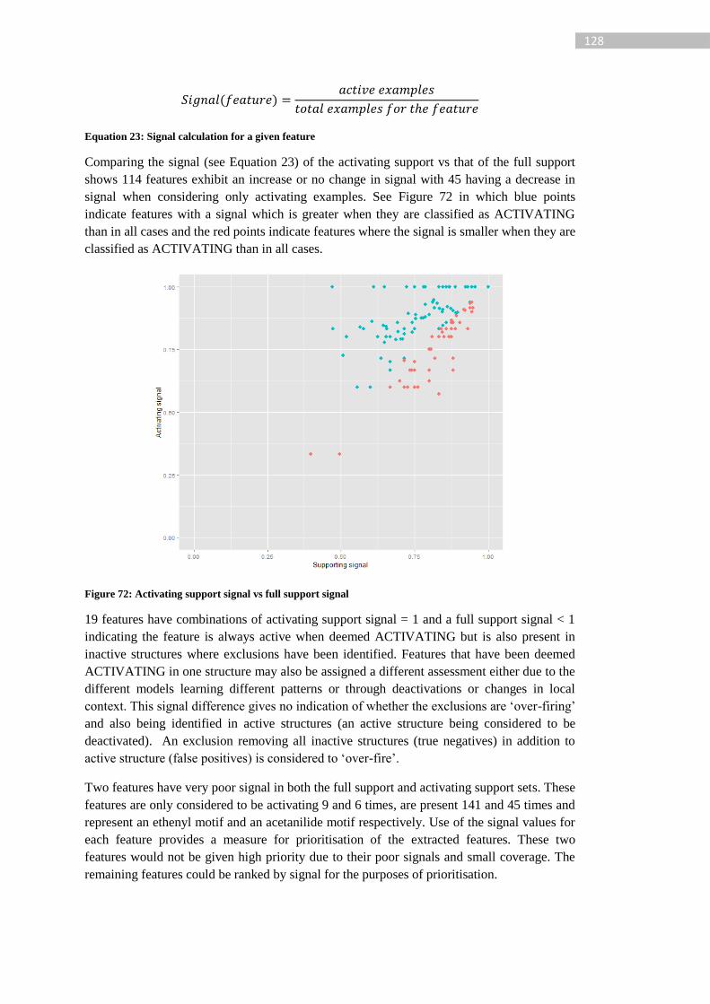
128
( )
Equation 23: Signal calculation for a given feature
Comparing the signal (see Equation 23) of the activating support vs that of the full support
shows 114 features exhibit an increase or no change in signal with 45 having a decrease in
signal when considering only activating examples. See Figure 72 in which blue points
indicate features with a signal which is greater when they are classified as ACTIVATING
than in all cases and the red points indicate features where the signal is smaller when they are
classified as ACTIVATING than in all cases.
Figure 72: Activating support signal vs full support signal
19 features have combinations of activating support signal = 1 and a full support signal < 1
indicating the feature is always active when deemed ACTIVATING but is also present in
inactive structures where exclusions have been identified. Features that have been deemed
ACTIVATING in one structure may also be assigned a different assessment either due to the
different models learning different patterns or through deactivations or changes in local
context. This signal difference gives no indication of whether the exclusions are ‘over-firing’
and also being identified in active structures (an active structure being considered to be
deactivated). An exclusion removing all inactive structures (true negatives) in addition to
active structure (false positives) is considered to ‘over-fire’.
Two features have very poor signal in both the full support and activating support sets. These
features are only considered to be activating 9 and 6 times, are present 141 and 45 times and
represent an ethenyl motif and an acetanilide motif respectively. Use of the signal values for
each feature provides a measure for prioritisation of the extracted features. These two
features would not be given high priority due to their poor signals and small coverage. The
remaining features could be ranked by signal for the purposes of prioritisation.

129
7.4.1.3.2 Example SAR trends extracted from the model
Let us now discuss some example investigation of SAR trends from the model focussing on
particular structural motifs. Two example SAR trends are discussed here: first the
deactivation of an epoxide motif given a sufficient alkyl chain length and secondly the
deactivation of a quinoline motif given specific substitutions to the ring system.
7.4.1.3.2.1 Epoxides
The epoxide motif feature has 13 level 2 nodes representing various specifications around
the epoxide motif with signals ranging from 1.000 (all active) to 0.167 (1:5). The details for
the supporting examples for some of the epoxide motif feature tree branch are shown in
Table 25 with the tree and fragments being shown in Figure 73.
Table 25: Node details for epoxide SAR tree subset
Tree Supporting examples
Node Level Actives Inactives Total Signal
1 1 163 61 224 0.728
2 2 6 0 6 1.000
3 2 77 22 99 0.778
4 3 8 0 8 1.000
5 3 6 0 6 1.000
6 3 12 8 20 0.600
7 4 1 5 6 0.167
8 4 5 0 5 1.000
From Table 25 we can see that the signal at the initial node representing the epoxide (node 1)
is already strongly biased to the active class (signal = 0.728) and already provides a useful
cluster of structures from which to derive knowledge. Further nodes specified in Figure 73
represent more specific contexts of the epoxide that have a majority assessment for the node
deemed to be ACTIVITY_IDENTIFIED due to the presence of the epoxide motif,
DEACTIVATED or DEACTIVATING.
Investigation of the tree allows for the further assessment of the initial cluster defined by the
support set of node 1. In the case of this epoxide subset we can see motifs representing a
more predominant active bias as well as a cluster representing the deactivation of the
epoxide motif when the aliphatic chain exceeds 2 carbons.
In Figure 73 we see a single ACTIVATING feature as level 1 in the tree. The full network
contains many more descendants but for clarity only a representative sample are selected for
display in this figure. Node 2 represents a feature that is deemed to be
ACTIVITY_IDENTFIED and represents a specification of the epoxide environment as a
fusion to an aromatic ring system. Features 3 and 6 represent epoxides substituted with
aliphatic chains that are considered to be either ACTIVITIY_IDENTIFIED or
DEACTIVATED. The deactivation of node 6 is shown in node 7 with the extension of the
aliphatic chain, the deactivation occurs at this level rather than node 1 (the negated epoxide
feature) to provide the complete context about the extracted SAR. From assessment of the
support sets and other nodes, such as node 8, it can be seen that the deactivation required an
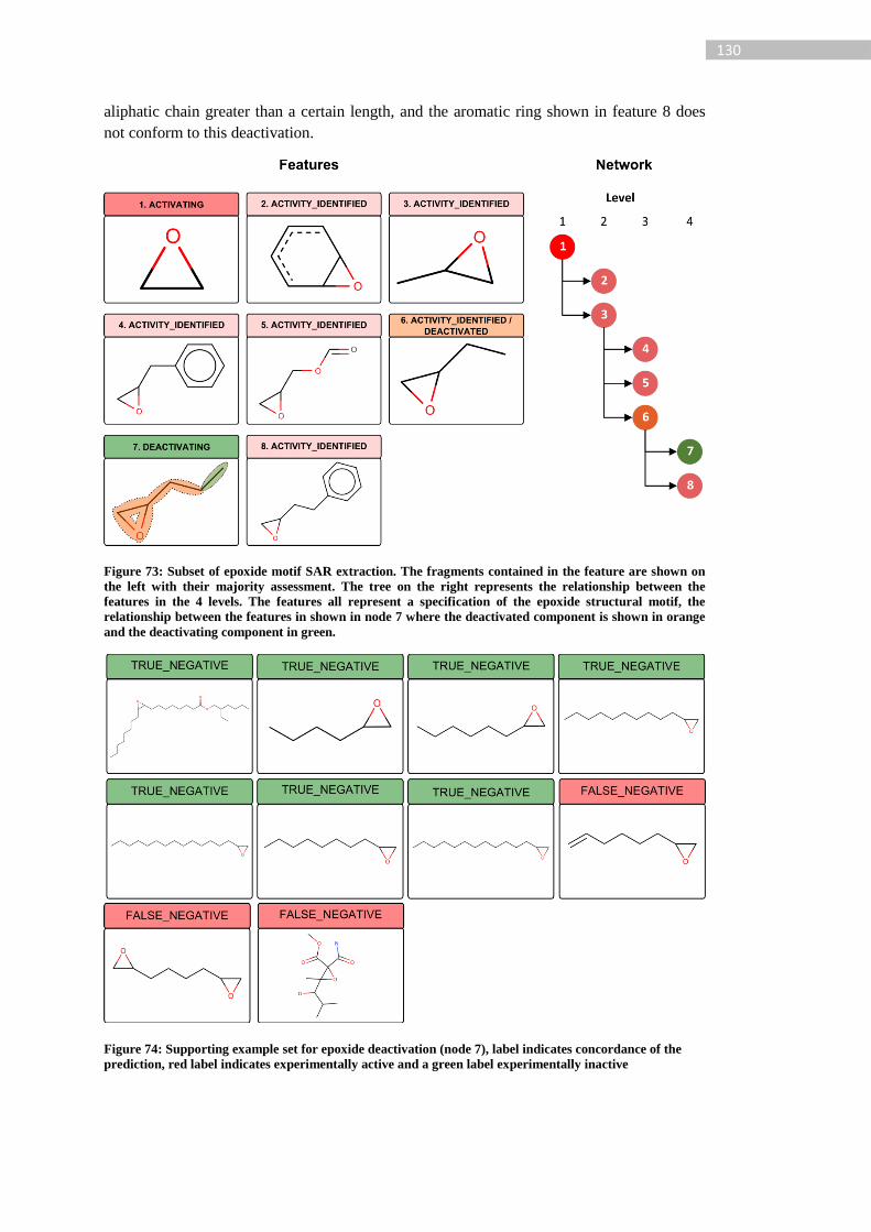
130
aliphatic chain greater than a certain length, and the aromatic ring shown in feature 8 does
not conform to this deactivation.
Figure 73: Subset of epoxide motif SAR extraction. The fragments contained in the feature are shown on
the left with their majority assessment. The tree on the right represents the relationship between the
features in the 4 levels. The features all represent a specification of the epoxide structural motif, the
relationship between the features in shown in node 7 where the deactivated component is shown in orange
and the deactivating component in green.
Figure 74: Supporting example set for epoxide deactivation (node 7), label indicates concordance of the
prediction, red label indicates experimentally active and a green label experimentally inactive

131
Figure 74 shows the supporting examples for node 7 in the epoxide SAR tree in Figure 73;
we can see in this set that the structures with an alkyl chain > 3 are inactive and that the three
FALSE_NEGATIVES have additional flavouring on the structure such an ethenyl, second
epoxide or carbonamide.
Given the supporting examples and cause of the activations and deactivations it is possible to
start investigating the mechanistic reasons that may exist supporting the cause identified by
the model (which is not the cause for the structure’s activity). Derek Nexus contains an alert
for epoxides (Alert 019). Relevant comment sections from the Derek Nexus Epoxide alert
state that:
1) “Epoxides are electrophilic compounds that readily bind to DNA …[and] may
exhibit mutagenicity in the Ames test, generally in strains TA100 and TA1535”
2) “Mono-alkyl substituted epoxides generally give a positive response in the Ames test
except where the alkyl substituent is long”
From the comments in Derek Nexus we can see that there is known mechanism of activity
relating to epoxides and that there are known effects of the substitution around the epoxide
ring on the mutagenicity expressed in the Ames test. One of the identified deactivations
found in this model relates to the known trend with alkyl chain length. Canter et al. [181]
report Ames mutagenicity negative results for unsubstituted aliphatic 1,2-epoxides for chain
lengths of 10, 12, 14, 16 and 18 carbon atoms.
7.4.1.3.2.2 Quinolines
The node that contains the fragment feature describing the quinoline motif has a signal of
0.710 and has 33 descendants at level 2 with signals varying from 1 to 0. The quinoiline
fragment can be generated from larger fused ring systems in addition to the quinoline ring
itself. Many of the level 2 nodes represent ACTIVITY_IDENTIFIED classifications on
larger ring systems with some representing functional substitutions around the quinoline
ring.
Three functional substitutions represent carbonamide, sulphonamide and ester/carboxylic
acid substitutions in the peri position; see Table 26 and Figure 75.
Table 26 Quinoline feature tree node details
Tree Supporting examples Details
Node Level Actives Inactives Total Signal
1 1 164 67 231 0.710 Quinoline
2 2 7 0 7 1.000 Peri-carbonamide
3 2 2 6 8 0.250 Peri-ester/carboxylic acid
4 2 0 8 8 0.000 Peri-sulphonamide
Of the three substitutions in the peri position the ester/carboxylic acid and sulphonamide are
considered to be deactivating of the quinoline motif whereas the carbonamide is considered
as ACTIVITY_IDENTIFIED with a signal showing a greater distribution ratio of actives to
inactives compared to the quinoline feature (1.000 vs 0.710). These trends indicate the nature
of the substitution in the peri position plays an important role in the mediation of the
mutagenic activity of quinolines.
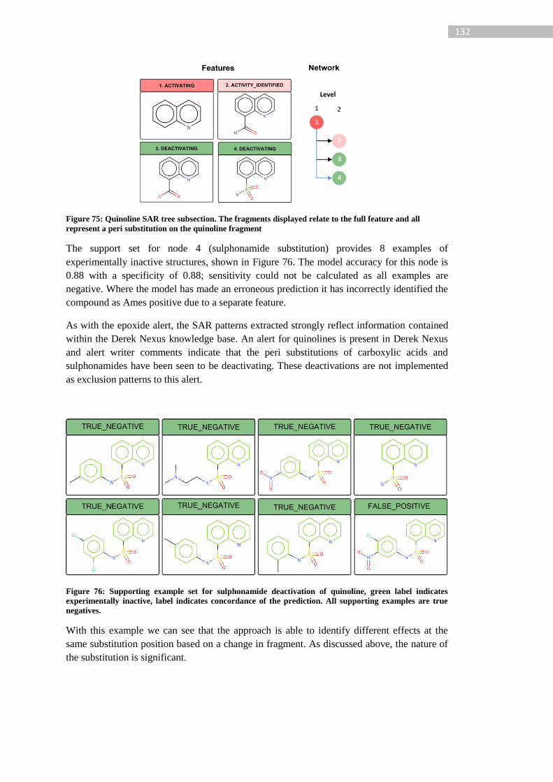
132
Figure 75: Quinoline SAR tree subsection. The fragments displayed relate to the full feature and all
represent a peri substitution on the quinoline fragment
The support set for node 4 (sulphonamide substitution) provides 8 examples of
experimentally inactive structures, shown in Figure 76. The model accuracy for this node is
0.88 with a specificity of 0.88; sensitivity could not be calculated as all examples are
negative. Where the model has made an erroneous prediction it has incorrectly identified the
compound as Ames positive due to a separate feature.
As with the epoxide alert, the SAR patterns extracted strongly reflect information contained
within the Derek Nexus knowledge base. An alert for quinolines is present in Derek Nexus
and alert writer comments indicate that the peri substitutions of carboxylic acids and
sulphonamides have been seen to be deactivating. These deactivations are not implemented
as exclusion patterns to this alert.
Figure 76: Supporting example set for sulphonamide deactivation of quinoline, green label indicates
experimentally inactive, label indicates concordance of the prediction. All supporting examples are true
negatives.
With this example we can see that the approach is able to identify different effects at the
same substitution position based on a change in fragment. As discussed above, the nature of
the substitution is significant.

133
7.4.1.4 Comparison of knowledge mining for mutagenicity
The output of the knowledge mining has been compared with a pre-existing Derek
knowledge base (section 7.4.1.4.1) as well as two published knowledge mining / rule
extraction algorithms (section 7.4.1.4.2). The comparison against the Derek knowledge base
allows for an assessment of this approaches capability for supporting the development of
human expert knowledge. The comparison with other algorithms allows for an assessment of
the benefits and disadvantages of various approaches including this one.
7.4.1.4.1 Comparison with Derek Nexus knowledge base
Derek Nexus contains an extensive knowledge base of bacterial mutagenicity prediction.
This knowledge base however is not exhaustive and there is scope for improvement with
regards to:
1) Identification of new alerts
2) Expanding current alerts
a. Additional inclusion patterns
b. Additional exclusion patterns
c. Adjustments to current patterns
This could be achieved with the support of a knowledge mining approach such as that
described here. Such knowledge mining applications have been successfully used internally
within Lhasa Limited, for example the application of emerging pattern mining [90].
To investigate the potential for further development of an established knowledge base the
output of the RF-C-15-10 model has been compared to the predictions made by Derek Nexus
for the supporting examples (training examples).
A strong candidate for a new alert would be a feature containing a high proportion of false
negatives as predicted by Derek Nexus. A strong candidate for an additional exclusion
pattern would be a deactivating feature that contains a high proportion of false positives as
predicted by Derek Nexus. The general identification of inclusion modifications to existing
alerts is trickier and can be achieved using the comparison strategy discussed in earlier.
Derek Nexus has fired 73 alerts for mutagenicity on the training data used in this study. As a
whole Derek Nexus fires at least one alert on 2409 structures (covering 53.4% of the active
structures), 1909 of which are active (78.4% coverage of actives). Derek Nexus has a ~6%
greater coverage of the active structures than models where the training set is processed.
Much of this training data will have been seen by knowledge base developers as well as
additional data outside of this training set.
7.4.1.4.1.1 Accuracy comparison
In Figure 77 we can see a scatter plot of the accuracy of the feature based on the predictions
for the activating supporting examples versus the accuracy of Derek Nexus. Points falling
above the 0,0 1,1 line represent higher accuracy in the ENCORE model and points below
represent higher accuracy in Derek Nexus. The points with a higher accuracy in the
ENCORE model represent features for prioritisation of human expert assessment.
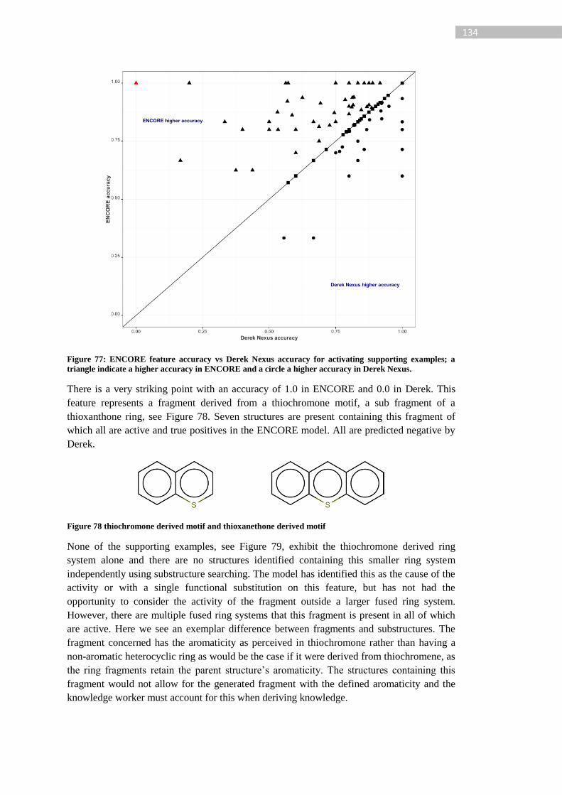
134
Figure 77: ENCORE feature accuracy vs Derek Nexus accuracy for activating supporting examples; a
triangle indicate a higher accuracy in ENCORE and a circle a higher accuracy in Derek Nexus.
There is a very striking point with an accuracy of 1.0 in ENCORE and 0.0 in Derek. This
feature represents a fragment derived from a thiochromone motif, a sub fragment of a
thioxanthone ring, see Figure 78. Seven structures are present containing this fragment of
which all are active and true positives in the ENCORE model. All are predicted negative by
Derek.
Figure 78 thiochromone derived motif and thioxanethone derived motif
None of the supporting examples, see Figure 79, exhibit the thiochromone derived ring
system alone and there are no structures identified containing this smaller ring system
independently using substructure searching. The model has identified this as the cause of the
activity or with a single functional substitution on this feature, but has not had the
opportunity to consider the activity of the fragment outside a larger fused ring system.
However, there are multiple fused ring systems that this fragment is present in all of which
are active. Here we see an exemplar difference between fragments and substructures. The
fragment concerned has the aromaticity as perceived in thiochromone rather than having a
non-aromatic heterocyclic ring as would be the case if it were derived from thiochromene, as
the ring fragments retain the parent structure’s aromaticity. The structures containing this
fragment would not allow for the generated fragment with the defined aromaticity and the
knowledge worker must account for this when deriving knowledge.
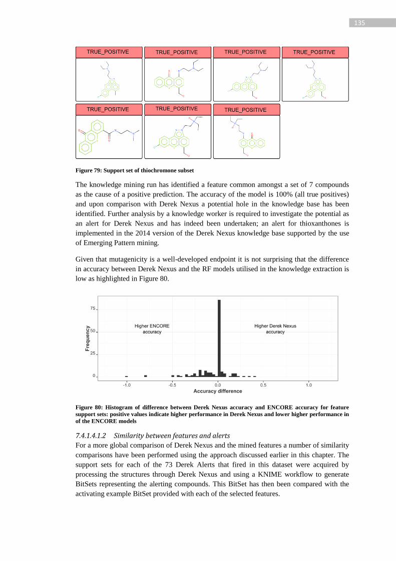
135
Figure 79: Support set of thiochromone subset
The knowledge mining run has identified a feature common amongst a set of 7 compounds
as the cause of a positive prediction. The accuracy of the model is 100% (all true positives)
and upon comparison with Derek Nexus a potential hole in the knowledge base has been
identified. Further analysis by a knowledge worker is required to investigate the potential as
an alert for Derek Nexus and has indeed been undertaken; an alert for thioxanthones is
implemented in the 2014 version of the Derek Nexus knowledge base supported by the use
of Emerging Pattern mining.
Given that mutagenicity is a well-developed endpoint it is not surprising that the difference
in accuracy between Derek Nexus and the RF models utilised in the knowledge extraction is
low as highlighted in Figure 80.
Figure 80: Histogram of difference between Derek Nexus accuracy and ENCORE accuracy for feature
support sets: positive values indicate higher performance in Derek Nexus and lower higher performance in
of the ENCORE models
7.4.1.4.1.2 Similarity between features and alerts
For a more global comparison of Derek Nexus and the mined features a number of similarity
comparisons have been performed using the approach discussed earlier in this chapter. The
support sets for each of the 73 Derek Alerts that fired in this dataset were acquired by
processing the structures through Derek Nexus and using a KNIME workflow to generate
BitSets representing the alerting compounds. This BitSet has then been compared with the
activating example BitSet provided with each of the selected features.
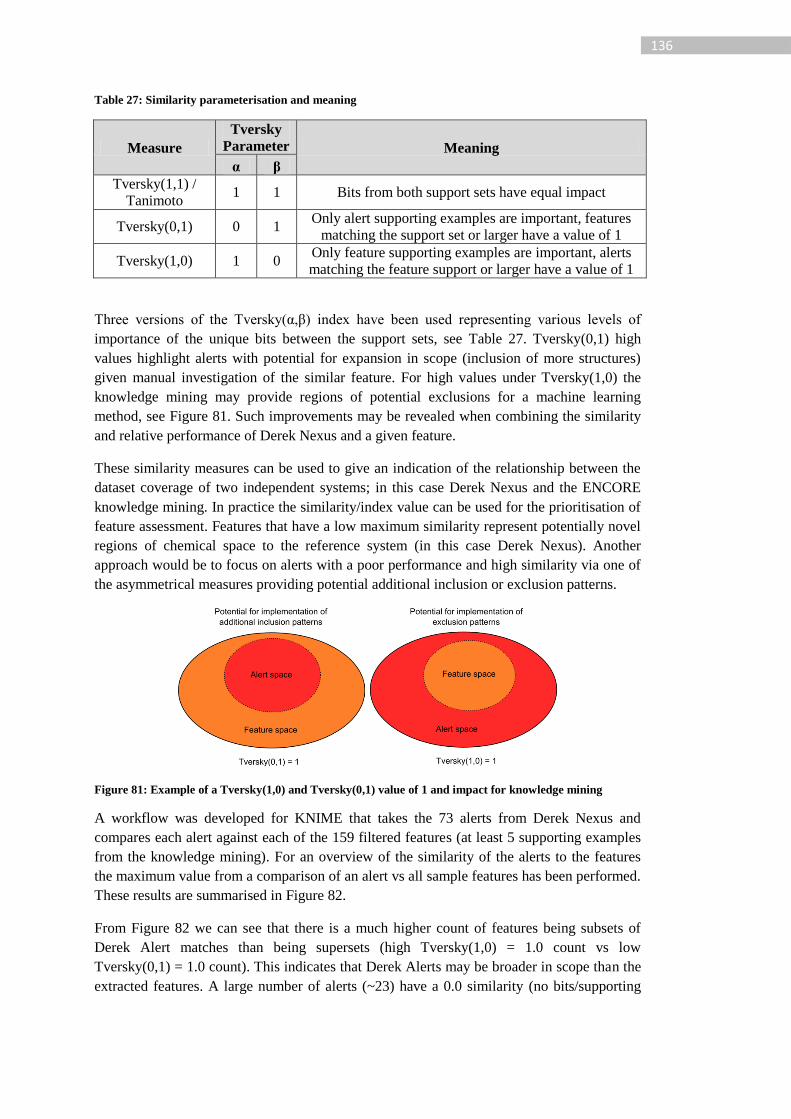
136
Table 27: Similarity parameterisation and meaning
Measure
Tversky
Parameter Meaning
α β
Tversky(1,1) /
Tanimoto 1 1 Bits from both support sets have equal impact
Tversky(0,1) 0 1 Only alert supporting examples are important, features
matching the support set or larger have a value of 1
Tversky(1,0) 1 0 Only feature supporting examples are important, alerts
matching the feature support or larger have a value of 1
Three versions of the Tversky(α,β) index have been used representing various levels of
importance of the unique bits between the support sets, see Table 27. Tversky(0,1) high
values highlight alerts with potential for expansion in scope (inclusion of more structures)
given manual investigation of the similar feature. For high values under Tversky(1,0) the
knowledge mining may provide regions of potential exclusions for a machine learning
method, see Figure 81. Such improvements may be revealed when combining the similarity
and relative performance of Derek Nexus and a given feature.
These similarity measures can be used to give an indication of the relationship between the
dataset coverage of two independent systems; in this case Derek Nexus and the ENCORE
knowledge mining. In practice the similarity/index value can be used for the prioritisation of
feature assessment. Features that have a low maximum similarity represent potentially novel
regions of chemical space to the reference system (in this case Derek Nexus). Another
approach would be to focus on alerts with a poor performance and high similarity via one of
the asymmetrical measures providing potential additional inclusion or exclusion patterns.
Figure 81: Example of a Tversky(1,0) and Tversky(0,1) value of 1 and impact for knowledge mining
A workflow was developed for KNIME that takes the 73 alerts from Derek Nexus and
compares each alert against each of the 159 filtered features (at least 5 supporting examples
from the knowledge mining). For an overview of the similarity of the alerts to the features
the maximum value from a comparison of an alert vs all sample features has been performed.
These results are summarised in Figure 82.
From Figure 82 we can see that there is a much higher count of features being subsets of
Derek Alert matches than being supersets (high Tversky(1,0) = 1.0 count vs low
Tversky(0,1) = 1.0 count). This indicates that Derek Alerts may be broader in scope than the
extracted features. A large number of alerts (~23) have a 0.0 similarity (no bits/supporting
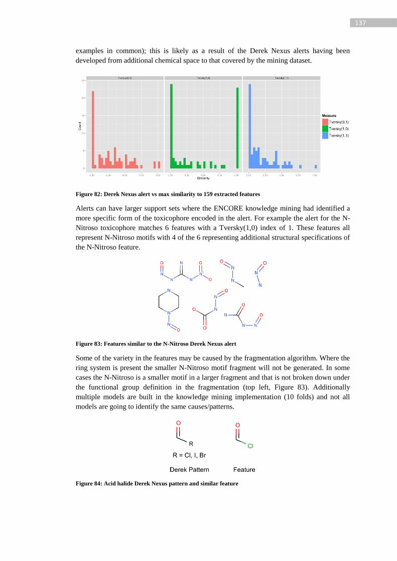
137
examples in common); this is likely as a result of the Derek Nexus alerts having been
developed from additional chemical space to that covered by the mining dataset.
Figure 82: Derek Nexus alert vs max similarity to 159 extracted features
Alerts can have larger support sets where the ENCORE knowledge mining had identified a
more specific form of the toxicophore encoded in the alert. For example the alert for the N-
Nitroso toxicophore matches 6 features with a Tversky(1,0) index of 1. These features all
represent N-Nitroso motifs with 4 of the 6 representing additional structural specifications of
the N-Nitroso feature.
Figure 83: Features similar to the N-Nitroso Derek Nexus alert
Some of the variety in the features may be caused by the fragmentation algorithm. Where the
ring system is present the smaller N-Nitroso motif fragment will not be generated. In some
cases the N-Nitroso is a smaller motif in a larger fragment and that is not broken down under
the functional group definition in the fragmentation (top left, Figure 83). Additionally
multiple models are built in the knowledge mining implementation (10 folds) and not all
models are going to identify the same causes/patterns.
Figure 84: Acid halide Derek Nexus pattern and similar feature

138
Derek Nexus alert 315, Acid Halide, contains a number of patterns relating to the acid halide
toxicophore. One of the patterns has been identified by a feature with a Tversky(1,0) index
of 1. This feature represents an acid chloride motif which has been identified in 15 structures
and deemed activating in 10. In the Derek Nexus pattern the pattern allows for Cl, I or Br
(Figure 84); should all of these substitutions be deemed activating in the model they would
be extracted as independent features identifying the acid chloride, acid iodide and acid
bromide separately.
We have seen from earlier comparisons that features have been identified that do not have a
corresponding alert. From these alert versus feature comparisons, where similar features to
Derek Nexus alerts are identified, we can see that the motifs described in the alerts are
structurally similar to those encoded by human knowledge base developers. It is therefore
likely that the encoding of the features is meaningful for both interpretation and knowledge
mining purposes.
7.4.1.4.1.3 Conclusions
Even with a well development toxicological endpoint such as mutagenicity this knowledge
mining algorithm has been able to identify additional toxicophores as well as specifications
to existing toxicophores that may result in improved performance. The algorithm shows a
weakness in its ability to abstract information such as grouping halogens instead of
identifying separate patters of the form A-Cl, A-F or A-I where A is a common motif.
Many similar features are found which indicates that the output of the model is in a suitable
form for use by human experts. The algorithm will likely be able to support the early stages
of toxicophore identification as well as in the specification of already identified
toxicophores.
7.4.1.4.2 Comparison with other knowledge mining approaches
The comparison of knowledge mining tools is largely a subjective activity. Unlike with the
automated generation of a rule base system where performance metrics can be compared,
knowledge mining tools provide output for a human expert to use in their knowledge
development work. The usefulness of the output and success at identifying meaningful trends
is therefore the core of the comparison. However, such comparisons require significant
involvement of said knowledge base developers. As this resource has not been available a
comparison has been performed in terms of coverage and similarity between the features. No
conclusion has been reached in terms of any particular tool’s suitability over another. It is
likely that a combination of tools is best suited for use in knowledge mining activities.
7.4.1.4.2.1 Emerging pattern mining
A manual comparison has been performed to identify how this knowledge mining approach
compares to the approach reported by Sherhod et al. [90] using emerging pattern mining. In
the work reported these authors used the emerging pattern mining method for alert
development in combination with Lhasa Limited’s knowledge base developers.
For an initial comparison a manual investigation was done to identify if the xanthene ring
system reported in the article was found in this mining work. Sherhod et al. report that the
xanthene ring motif emerging pattern has resulted in the development of two new alerts
filling a gap in the Derek Nexus knowledge base. This feature has not been identified in the
same way in this knowledge mining using the ENCORE algorithm, primarily due to a
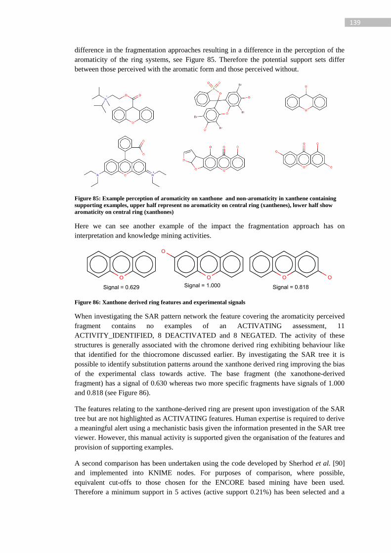
139
difference in the fragmentation approaches resulting in a difference in the perception of the
aromaticity of the ring systems, see Figure 85. Therefore the potential support sets differ
between those perceived with the aromatic form and those perceived without.
Figure 85: Example perception of aromaticity on xanthone and non-aromaticity in xanthene containing
supporting examples, upper half represent no aromaticity on central ring (xanthenes), lower half show
aromaticity on central ring (xanthones)
Here we can see another example of the impact the fragmentation approach has on
interpretation and knowledge mining activities.
Figure 86: Xanthone derived ring features and experimental signals
When investigating the SAR pattern network the feature covering the aromaticity perceived
fragment contains no examples of an ACTIVATING assessment, 11
ACTIVITY_IDENTIFIED, 8 DEACTIVATED and 8 NEGATED. The activity of these
structures is generally associated with the chromone derived ring exhibiting behaviour like
that identified for the thiocromone discussed earlier. By investigating the SAR tree it is
possible to identify substitution patterns around the xanthone derived ring improving the bias
of the experimental class towards active. The base fragment (the xanothone-derived
fragment) has a signal of 0.630 whereas two more specific fragments have signals of 1.000
and 0.818 (see Figure 86).
The features relating to the xanthone-derived ring are present upon investigation of the SAR
tree but are not highlighted as ACTIVATING features. Human expertise is required to derive
a meaningful alert using a mechanistic basis given the information presented in the SAR tree
viewer. However, this manual activity is supported given the organisation of the features and
provision of supporting examples.
A second comparison has been undertaken using the code developed by Sherhod et al. [90]
and implemented into KNIME nodes. For purposes of comparison, where possible,
equivalent cut-offs to those chosen for the ENCORE based mining have been used.
Therefore a minimum support in 5 actives (active support 0.21%) has been selected and a
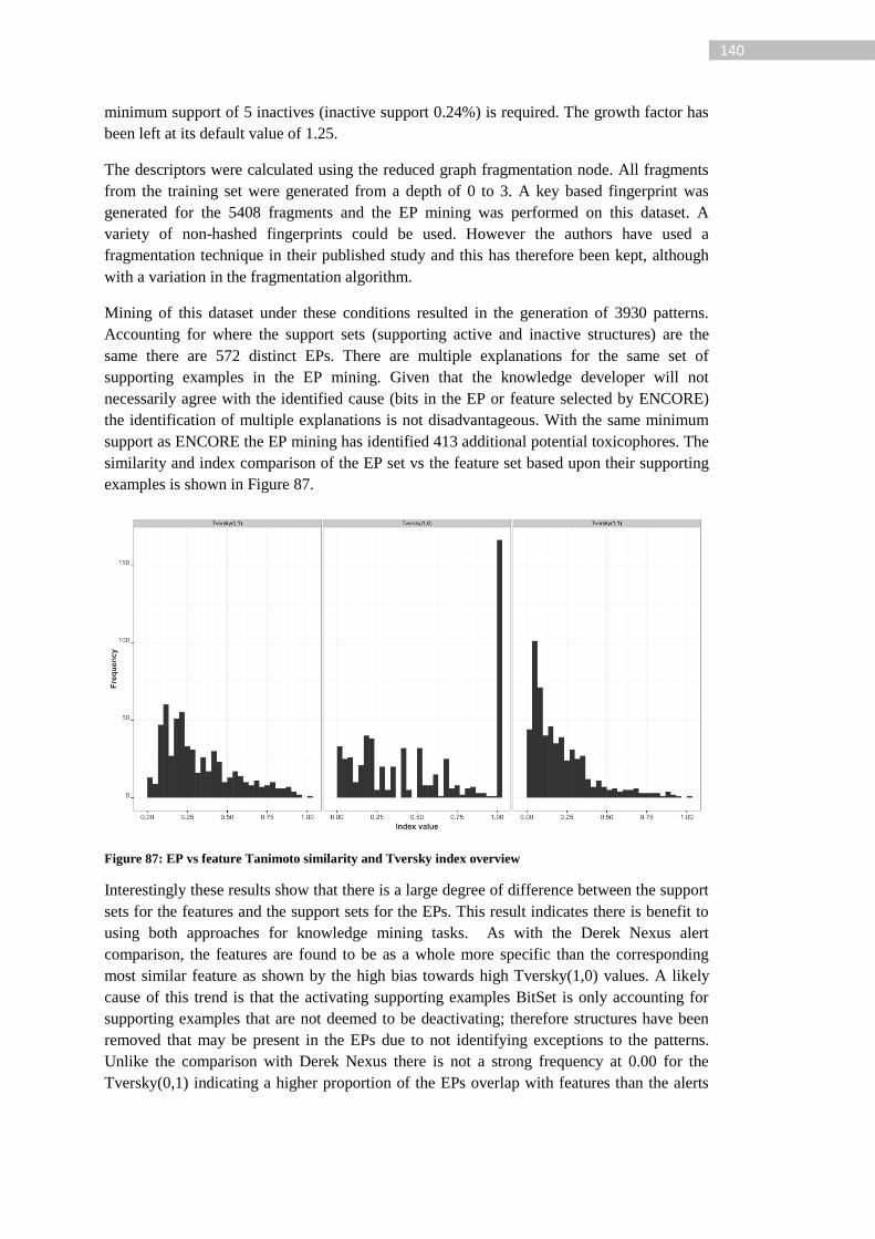
140
minimum support of 5 inactives (inactive support 0.24%) is required. The growth factor has
been left at its default value of 1.25.
The descriptors were calculated using the reduced graph fragmentation node. All fragments
from the training set were generated from a depth of 0 to 3. A key based fingerprint was
generated for the 5408 fragments and the EP mining was performed on this dataset. A
variety of non-hashed fingerprints could be used. However the authors have used a
fragmentation technique in their published study and this has therefore been kept, although
with a variation in the fragmentation algorithm.
Mining of this dataset under these conditions resulted in the generation of 3930 patterns.
Accounting for where the support sets (supporting active and inactive structures) are the
same there are 572 distinct EPs. There are multiple explanations for the same set of
supporting examples in the EP mining. Given that the knowledge developer will not
necessarily agree with the identified cause (bits in the EP or feature selected by ENCORE)
the identification of multiple explanations is not disadvantageous. With the same minimum
support as ENCORE the EP mining has identified 413 additional potential toxicophores. The
similarity and index comparison of the EP set vs the feature set based upon their supporting
examples is shown in Figure 87.
Figure 87: EP vs feature Tanimoto similarity and Tversky index overview
Interestingly these results show that there is a large degree of difference between the support
sets for the features and the support sets for the EPs. This result indicates there is benefit to
using both approaches for knowledge mining tasks. As with the Derek Nexus alert
comparison, the features are found to be as a whole more specific than the corresponding
most similar feature as shown by the high bias towards high Tversky(1,0) values. A likely
cause of this trend is that the activating supporting examples BitSet is only accounting for
supporting examples that are not deemed to be deactivating; therefore structures have been
removed that may be present in the EPs due to not identifying exceptions to the patterns.
Unlike the comparison with Derek Nexus there is not a strong frequency at 0.00 for the
Tversky(0,1) indicating a higher proportion of the EPs overlap with features than the alerts
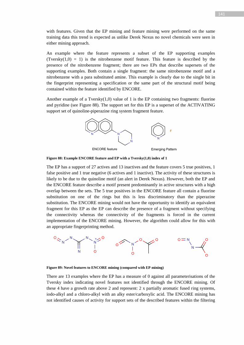
141
with features. Given that the EP mining and feature mining were performed on the same
training data this trend is expected as unlike Derek Nexus no novel chemicals were seen in
either mining approach.
An example where the feature represents a subset of the EP supporting examples
(Tversky(1,0) = 1) is the nitrobenzene motif feature. This feature is described by the
presence of the nitrobenzene fragment; there are two EPs that describe supersets of the
supporting examples. Both contain a single fragment: the same nitrobenzene motif and a
nitrobenzene with a para substituted amine. This example is clearly due to the single bit in
the fingerprint representing a specification or the same part of the structural motif being
contained within the feature identified by ENCORE.
Another example of a Tversky(1,0) value of 1 is the EP containing two fragments: fluorine
and pyridine (see Figure 88). The support set for this EP is a superset of the ACTIVATING
support set of quinoline-piperazine ring system fragment feature.
Figure 88: Example ENCORE feature and EP with a Tversky(1,0) index of 1
The EP has a support of 27 actives and 13 inactives and the feature covers 5 true positives, 1
false positive and 1 true negative (6 actives and 1 inactive). The activity of these structures is
likely to be due to the quinoline motif (an alert in Derek Nexus). However, both the EP and
the ENCORE feature describe a motif present predominantly in active structures with a high
overlap between the sets. The 5 true positives in the ENCORE feature all contain a fluorine
substitution on one of the rings but this is less discriminatory than the piperazine
substitution. The ENCORE mining would not have the opportunity to identify an equivalent
fragment for this EP as the EP can describe the presence of a fragment without specifying
the connectivity whereas the connectivity of the fragments is forced in the current
implementation of the ENCORE mining. However, the algorithm could allow for this with
an appropriate fingerprinting method.
Figure 89: Novel features to ENCORE mining (compared with EP mining)
There are 13 examples where the EP has a measure of 0 against all parameterisations of the
Tversky index indicating novel features not identified through the ENCORE mining. Of
these 4 have a growth rate above 2 and represent: 2 x partially aromatic fused ring systems,
iodo-alkyl and a chloro-alkyl with an alky ester/carboxylic acid. The ENCORE mining has
not identified causes of activity for support sets of the described features within the filtering
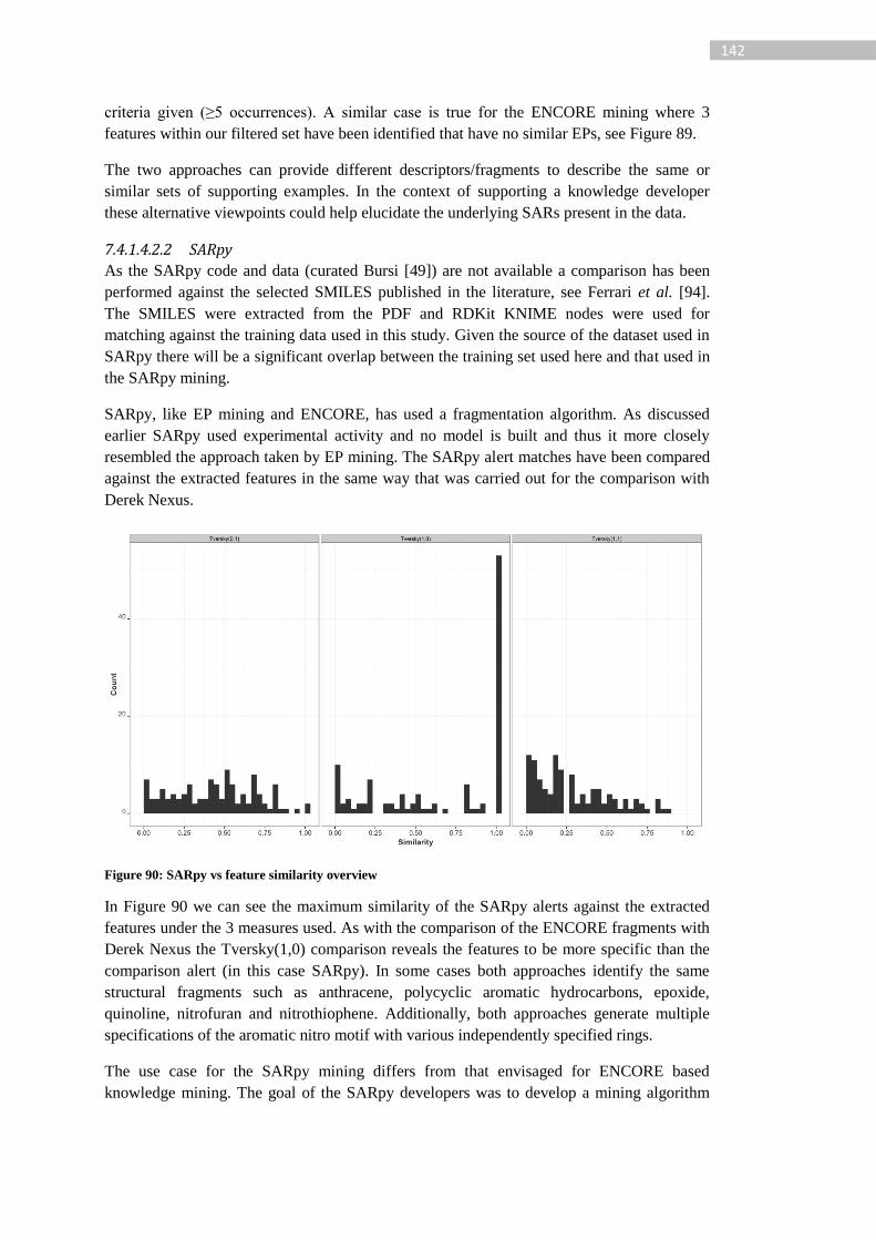
142
criteria given (≥5 occurrences). A similar case is true for the ENCORE mining where 3
features within our filtered set have been identified that have no similar EPs, see Figure 89.
The two approaches can provide different descriptors/fragments to describe the same or
similar sets of supporting examples. In the context of supporting a knowledge developer
these alternative viewpoints could help elucidate the underlying SARs present in the data.
7.4.1.4.2.2 SARpy
As the SARpy code and data (curated Bursi [49]) are not available a comparison has been
performed against the selected SMILES published in the literature, see Ferrari et al. [94].
The SMILES were extracted from the PDF and RDKit KNIME nodes were used for
matching against the training data used in this study. Given the source of the dataset used in
SARpy there will be a significant overlap between the training set used here and that used in
the SARpy mining.
SARpy, like EP mining and ENCORE, has used a fragmentation algorithm. As discussed
earlier SARpy used experimental activity and no model is built and thus it more closely
resembled the approach taken by EP mining. The SARpy alert matches have been compared
against the extracted features in the same way that was carried out for the comparison with
Derek Nexus.
Figure 90: SARpy vs feature similarity overview
In Figure 90 we can see the maximum similarity of the SARpy alerts against the extracted
features under the 3 measures used. As with the comparison of the ENCORE fragments with
Derek Nexus the Tversky(1,0) comparison reveals the features to be more specific than the
comparison alert (in this case SARpy). In some cases both approaches identify the same
structural fragments such as anthracene, polycyclic aromatic hydrocarbons, epoxide,
quinoline, nitrofuran and nitrothiophene. Additionally, both approaches generate multiple
specifications of the aromatic nitro motif with various independently specified rings.
The use case for the SARpy mining differs from that envisaged for ENCORE based
knowledge mining. The goal of the SARpy developers was to develop a mining algorithm
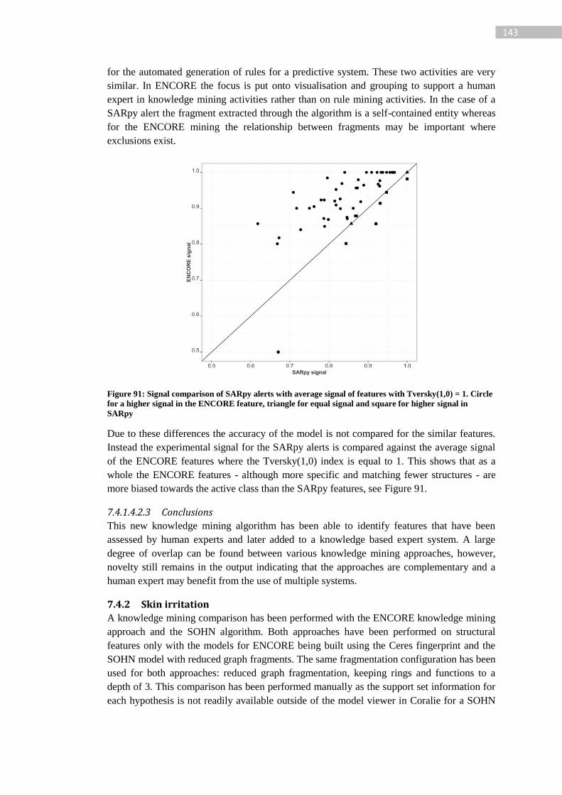
143
for the automated generation of rules for a predictive system. These two activities are very
similar. In ENCORE the focus is put onto visualisation and grouping to support a human
expert in knowledge mining activities rather than on rule mining activities. In the case of a
SARpy alert the fragment extracted through the algorithm is a self-contained entity whereas
for the ENCORE mining the relationship between fragments may be important where
exclusions exist.
Figure 91: Signal comparison of SARpy alerts with average signal of features with Tversky(1,0) = 1. Circle
for a higher signal in the ENCORE feature, triangle for equal signal and square for higher signal in
SARpy
Due to these differences the accuracy of the model is not compared for the similar features.
Instead the experimental signal for the SARpy alerts is compared against the average signal
of the ENCORE features where the Tversky(1,0) index is equal to 1. This shows that as a
whole the ENCORE features - although more specific and matching fewer structures - are
more biased towards the active class than the SARpy features, see Figure 91.
7.4.1.4.2.3 Conclusions
This new knowledge mining algorithm has been able to identify features that have been
assessed by human experts and later added to a knowledge based expert system. A large
degree of overlap can be found between various knowledge mining approaches, however,
novelty still remains in the output indicating that the approaches are complementary and a
human expert may benefit from the use of multiple systems.
7.4.2 Skin irritation
A knowledge mining comparison has been performed with the ENCORE knowledge mining
approach and the SOHN algorithm. Both approaches have been performed on structural
features only with the models for ENCORE being built using the Ceres fingerprint and the
SOHN model with reduced graph fragments. The same fragmentation configuration has been
used for both approaches: reduced graph fragmentation, keeping rings and functions to a
depth of 3. This comparison has been performed manually as the support set information for
each hypothesis is not readily available outside of the model viewer in Coralie for a SOHN
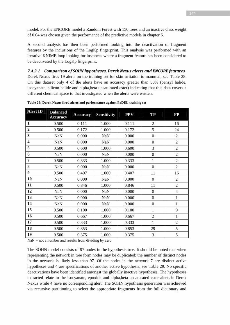
144
model. For the ENCORE model a Random Forest with 150 trees and an inactive class weight
of 0.04 was chosen given the performance of the predictive models in chapter 6.
A second analysis has then been performed looking into the deactivation of fragment
features by the inclusions of the LogKp fingerprint. This analysis was performed with an
iterative KNIME loop looking for instances where a fragment feature has been considered to
be deactivated by the LogKp fingerprint.
7.4.2.1 Comparison of SOHN hypotheses, Derek Nexus alerts and ENCORE features
Derek Nexus fires 19 alerts on the training set for skin irritation to mammal, see Table 28.
On this dataset only 4 of the alerts have an accuracy greater than 50% (benzyl halide,
isocyanate, silicon halide and alpha,beta-unsaturated ester) indicating that this data covers a
different chemical space to that investigated when the alerts were written.
Table 28: Derek Nexus fired alerts and performance against PaDEL training set
Alert ID Balanced
Accuracy Accuracy Sensitivity PPV TP FP
1 0.500 0.111 1.000 0.111 2 16
2 0.500 0.172 1.000 0.172 5 24
3 NaN 0.000 NaN 0.000 0 2
4 NaN 0.000 NaN 0.000 0 2
5 0.500 0.600 1.000 0.600 3 2
6 NaN 0.000 NaN 0.000 0 2
7 0.500 0.333 1.000 0.333 1 2
8 NaN 0.000 NaN 0.000 0 2
9 0.500 0.407 1.000 0.407 11 16
10 NaN 0.000 NaN 0.000 0 2
11 0.500 0.846 1.000 0.846 11 2
12 NaN 0.000 NaN 0.000 0 4
13 NaN 0.000 NaN 0.000 0 1
14 NaN 0.000 NaN 0.000 0 1
15 0.500 0.100 1.000 0.100 1 9
16 0.500 0.667 1.000 0.667 2 1
17 0.500 0.333 1.000 0.333 1 2
18 0.500 0.853 1.000 0.853 29 5
19 0.500 0.375 1.000 0.375 3 5
NaN = not a number and results from dividing by zero
The SOHN model consists of 97 nodes in the hypothesis tree. It should be noted that when
representing the network in tree form nodes may be duplicated; the number of distinct nodes
in the network is likely less than 97. Of the nodes in the network 7 are distinct active
hypotheses and 4 are specifications of another active hypothesis, see Table 29. No specific
deactivations have been identified amongst the globally inactive hypotheses. The hypotheses
extracted relate to the isocyanate, epoxide and alpha,beta-unsaturated ester alerts in Derek
Nexus while 4 have no corresponding alert. The SOHN hypothesis generation was achieved
via recursive partitioning to select the appropriate fragments from the full dictionary and

145
does not account for the class weightings (unlike at prediction time), therefore the
predominant representation of the network by inactive hypotheses is expected.
Table 29: SOHN extracted active hypotheses from PaDEL harmonised skin irritation hazard training set
Hypothesis details Supporting
examples
Description
ID Coverage Signal active inactive Structural motif described Corresponding
Derek alert ID
527 0.8 0.846 11 2 Isocyanate fragment motif 10
528 0.3 0.600 3 2 Additional specification of
H527
10
543 0.9 0.600 9 6 Epoxide fragment motif,
single carbon substition
8
544 0.6 0.700 7 3 Glycidol fragment motif (OH
or ester), specification of
H543
8
523 2.3 0.750 30 10 Unsaturated ester motif 17
524 0.8 0.857 12 2 Substitution pattern
specification of H523
17
526 1.1 0.778 14 4 Substitution pattern
specification of H523
17
555 1.8 0.581 18 13 Unsaturated alkyl chain,
branching specified
N/A
575 0.4 0.571 4 3 Pyridin ring with charged
nitrogen
N/A
551 0.4 0.667 4 2 Similar unsaturated alkyl
branched chain
N/A
542 0.3 1.000 5 0 Branched alkyl chain N/A
The ENCORE model using 10 fold cross validation generates 893 nodes in the SAR trend
tree, 38 of which are level 1 ACTIVATING features when selecting a minimum number of
supporting structures of 4. Many of the extracted features have a poor sensitivity and
specificity; given the overall low performance of the model this is expected. Given the cross
validation run it is possible to separate the features with a strong predictive performance
from those with a weak predictive performance with ease. For example we can use positive
predictivity (TP/TP+FP) to identify features that have a higher proportion of true positives
relative to false positives, see Figure 92.
The features with a support ≥4 in ACTIVATING assessment cover 136 active structures and
170 inactive structures; the coverage of the experimental actives is therefore only 48%. This
low coverage is likely caused by the poor performance of the model; the model misclassifies
a significant proportion of the experimental actives. Additionally many of the active
predictions are predicted active by a feature(s) that is used less than 4 times across the
dataset. The distribution of positive predictivity of the 30 features considered to be activating
with a supporting example count ≥4 is shown in Figure 92. Here we see many of the features
result in more false positives than true positives. Using the cross validation mining approach
we are easily able to spot and ignore (or look further down the SAR trend) these features.
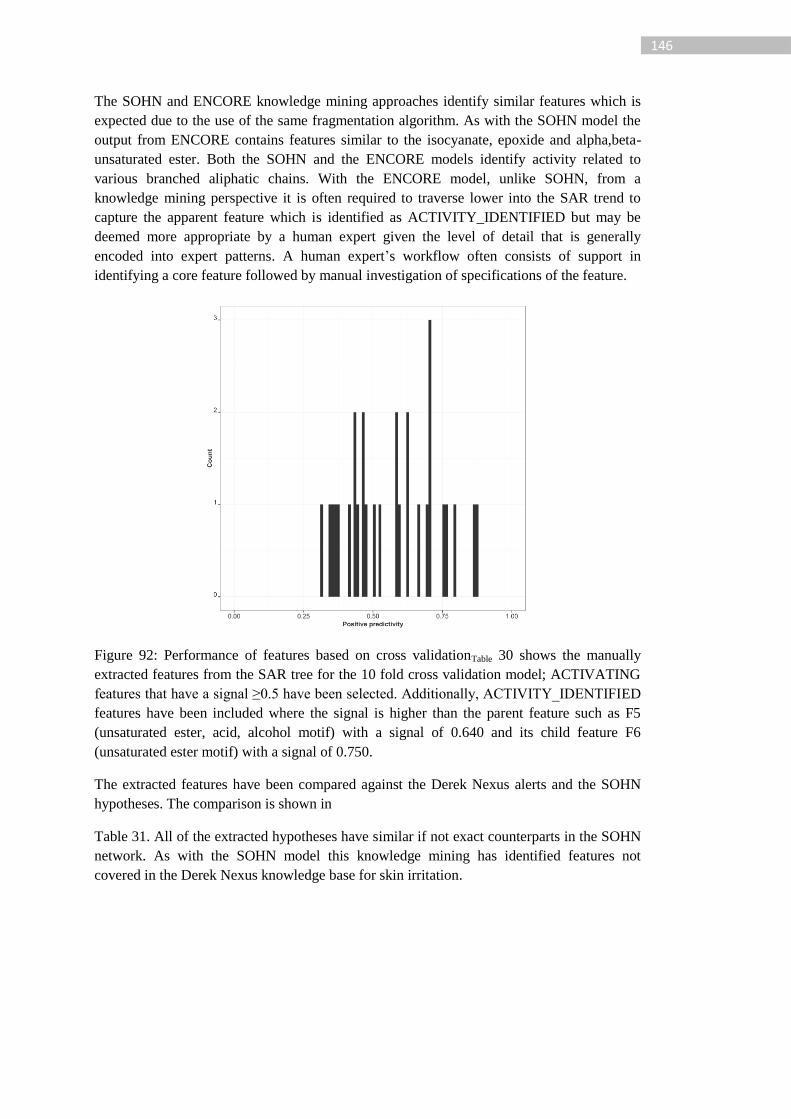
146
The SOHN and ENCORE knowledge mining approaches identify similar features which is
expected due to the use of the same fragmentation algorithm. As with the SOHN model the
output from ENCORE contains features similar to the isocyanate, epoxide and alpha,beta-
unsaturated ester. Both the SOHN and the ENCORE models identify activity related to
various branched aliphatic chains. With the ENCORE model, unlike SOHN, from a
knowledge mining perspective it is often required to traverse lower into the SAR trend to
capture the apparent feature which is identified as ACTIVITY_IDENTIFIED but may be
deemed more appropriate by a human expert given the level of detail that is generally
encoded into expert patterns. A human expert’s workflow often consists of support in
identifying a core feature followed by manual investigation of specifications of the feature.
Figure 92: Performance of features based on cross validationTable 30 shows the manually
extracted features from the SAR tree for the 10 fold cross validation model; ACTIVATING
features that have a signal ≥0.5 have been selected. Additionally, ACTIVITY_IDENTIFIED
features have been included where the signal is higher than the parent feature such as F5
(unsaturated ester, acid, alcohol motif) with a signal of 0.640 and its child feature F6
(unsaturated ester motif) with a signal of 0.750.
The extracted features have been compared against the Derek Nexus alerts and the SOHN
hypotheses. The comparison is shown in
Table 31. All of the extracted hypotheses have similar if not exact counterparts in the SOHN
network. As with the SOHN model this knowledge mining has identified features not
covered in the Derek Nexus knowledge base for skin irritation.
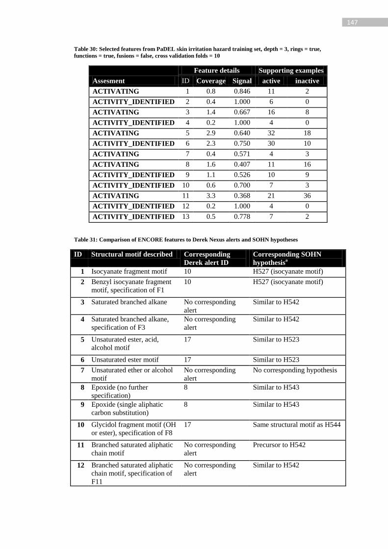
147
Table 30: Selected features from PaDEL skin irritation hazard training set, depth = 3, rings = true,
functions = true, fusions = false, cross validation folds = 10
Feature details Supporting examples
Assesment ID Coverage Signal active inactive
ACTIVATING 1 0.8 0.846 11 2
ACTIVITY_IDENTIFIED 2 0.4 1.000 6 0
ACTIVATING 3 1.4 0.667 16 8
ACTIVITY_IDENTIFIED 4 0.2 1.000 4 0
ACTIVATING 5 2.9 0.640 32 18
ACTIVITY_IDENTIFIED 6 2.3 0.750 30 10
ACTIVATING 7 0.4 0.571 4 3
ACTIVATING 8 1.6 0.407 11 16
ACTIVITY_IDENTIFIED 9 1.1 0.526 10 9
ACTIVITY_IDENTIFIED 10 0.6 0.700 7 3
ACTIVATING 11 3.3 0.368 21 36
ACTIVITY_IDENTIFIED 12 0.2 1.000 4 0
ACTIVITY_IDENTIFIED 13 0.5 0.778 7 2
Table 31: Comparison of ENCORE features to Derek Nexus alerts and SOHN hypotheses
ID Structural motif described Corresponding
Derek alert ID
Corresponding SOHN
hypothesisa
1 Isocyanate fragment motif 10 H527 (isocyanate motif)
2 Benzyl isocyanate fragment
motif, specification of F1
10 H527 (isocyanate motif)
3 Saturated branched alkane No corresponding
alert
Similar to H542
4 Saturated branched alkane,
specification of F3
No corresponding
alert
Similar to H542
5 Unsaturated ester, acid,
alcohol motif
17 Similar to H523
6 Unsaturated ester motif 17 Similar to H523
7 Unsaturated ether or alcohol
motif
No corresponding
alert
No corresponding hypothesis
8 Epoxide (no further
specification)
8 Similar to H543
9 Epoxide (single aliphatic
carbon substitution)
8 Similar to H543
10 Glycidol fragment motif (OH
or ester), specification of F8
17 Same structural motif as H544
11 Branched saturated aliphatic
chain motif
No corresponding
alert
Precursor to H542
12 Branched saturated aliphatic
chain motif, specification of
F11
No corresponding
alert
Similar to H542
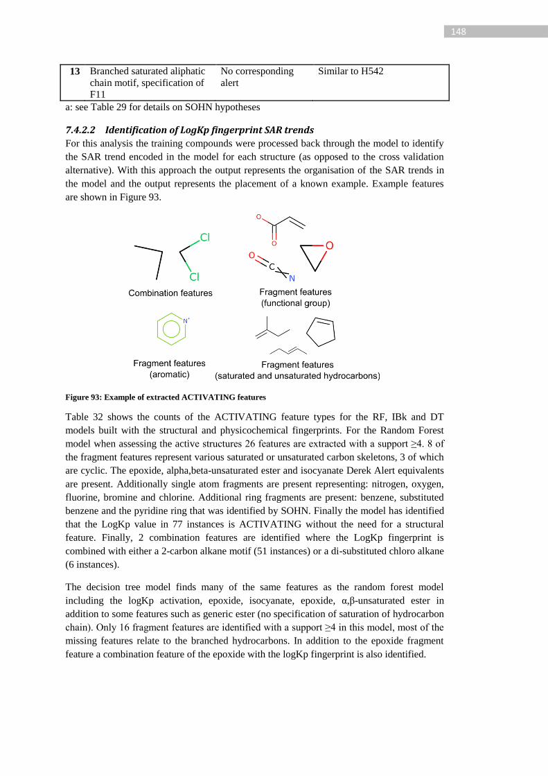
148
13 Branched saturated aliphatic
chain motif, specification of
F11
No corresponding
alert
Similar to H542
a: see Table 29 for details on SOHN hypotheses
7.4.2.2 Identification of LogKp fingerprint SAR trends
For this analysis the training compounds were processed back through the model to identify
the SAR trend encoded in the model for each structure (as opposed to the cross validation
alternative). With this approach the output represents the organisation of the SAR trends in
the model and the output represents the placement of a known example. Example features
are shown in Figure 93.
Figure 93: Example of extracted ACTIVATING features
Table 32 shows the counts of the ACTIVATING feature types for the RF, IBk and DT
models built with the structural and physicochemical fingerprints. For the Random Forest
model when assessing the active structures 26 features are extracted with a support ≥4. 8 of
the fragment features represent various saturated or unsaturated carbon skeletons, 3 of which
are cyclic. The epoxide, alpha,beta-unsaturated ester and isocyanate Derek Alert equivalents
are present. Additionally single atom fragments are present representing: nitrogen, oxygen,
fluorine, bromine and chlorine. Additional ring fragments are present: benzene, substituted
benzene and the pyridine ring that was identified by SOHN. Finally the model has identified
that the LogKp value in 77 instances is ACTIVATING without the need for a structural
feature. Finally, 2 combination features are identified where the LogKp fingerprint is
combined with either a 2-carbon alkane motif (51 instances) or a di-substituted chloro alkane
(6 instances).
The decision tree model finds many of the same features as the random forest model
including the logKp activation, epoxide, isocyanate, epoxide, α,β-unsaturated ester in
addition to some features such as generic ester (no specification of saturation of hydrocarbon
chain). Only 16 fragment features are identified with a support ≥4 in this model, most of the
missing features relate to the branched hydrocarbons. In addition to the epoxide fragment
feature a combination feature of the epoxide with the logKp fingerprint is also identified.

149
Table 32: ACTIVATING feature counts from the LogKP RF, IBk and DT mining
Model Physchem Fragment Combination
RF 1 23 2
DT 1 16 3
Ibk 0 18 1
The epoxide, isocyanate and alpha,beta-unsaturated ester features have also been identified
in the IBk model along with many of the hydrocarbon features. In this model the logKp
fingerprint alone was not considered to be an activating feature. Novel features have been
identified with respect to the RF and DT model covering halogenated benzene and phenol
motifs.
Relationships with logKp and deactivation are also seen: logKp has been seen to deactivate a
variety of fragment features as well as being deactivated itself by the presence of specific
fragment features. However, the clarity of such activations and deactivations related to
logKp is not as clear as with the fragment features. Here we only have an indication that the
query structures logKp value resulted in a fingerprint that when combined with the structural
fingerprint resulted in the detailed behaviours (activation/deactivation). The fingerprint can
be investigated to identify which bin was set, and in the case of this model this is trivial
given the binary (two-bin) split. For more complex physicochemical property fingerprints
such activities may not be feasible. Even with this limitation we are still provided with the
contribution of the global physicochemical property and given an appropriate choice in
descriptors a human expert forming mechanistic conclusions from the presented information
may be possible.
7.4.2.3 Comparison with emerging pattern mining
Emerging pattern mining has been carried out using a fingerprint generated from the
fragmentation algorithm (configured as per SOHN and ENCORE mining) with two
additional bits describing the logKp fingerprint like in the ENCORE mining. The EP mining
job was configured with an active percent threshold of 1.4% (4 structures), an inactive
percent threshold of 0.28% (4 structures) and a curve of 1.25.
The EP mining produced 1002 emerging patterns at these settings consisting of single
fragments, multiple fragments and fragment(s) with logKp_upper range (>= -1.595).
However, many of the emerging patterns have the same support sets (supporting example
structures). The 1002 EPs only consist of 87 distinct support sets; the full EP set has been
filtered to keep the smallest EP for each support set where multiple EPs exist. Of the 87 EPs
63 contain only fragments, 7 involve fragment(s) and logKp_lower and 17 fragment(s) and
logKp_upper.
The EP mining has identified the alpha,beta-unsaturated ester, epoxide, and isocyanate
motifs as seen in Derek Nexus alerts and identified by SOHN and ENCORE. The glycidol
motif identified by SOHN and ENCORE has also been found. The EP mining algorithm,
unlike SOHN and the implementation of ENCORE that was used is able to identify
disconnected fragments. These disconnected features form the majority of the novel EPs
with respect to SOHN hypotheses and ENCORE features. As with the SOHN and ENCORE
150
models, patterns describing various saturated, unsaturated and branched hydrocarbons have
been found.
7.5 Conclusion The initial goal was to develop an interpretation algorithm that provides meaningful
representation of the model’s underlying SARs and not the development of a knowledge
mining algorithm. It has been found that due to the way in which the interpretation algorithm
represents the underlying SARs to the user it is possible to integrate the interpretation into a
knowledge mining strategy. In this chapter the integration of the interpretation algorithm into
a knowledge mining strategy was detailed and its application to the mining of mutagenicity
and skin irritation data was discussed.
To recap, the knowledge mining use case is considered in the context of supporting human
domain experts in developing new knowledge or alerts to enter into expert systems such as
Derek Nexus. In this context strategies for comparing against existing knowledge bases were
also discussed. This comparison revealed that it is possible to recreate existing knowledge
contained within Derek Nexus. For mutagenicity a couple of examples were discussed: the
quinoline alert and deactivations as well as the epoxide alert and deactivations were
recreated in that both features have been identified by the model and through the linking of
features in the SAR tree the known deactivations mentioned in the Derek Nexus alert
comments were found. In the case of skin irritation three alerts were identified within the
dataset: isocyanate, epoxide and alpha,beta-unsaturated ester. Given the approach’s ability to
represent the SAR trends in similar ways to encoding in the expert system alerts we can have
high confidence when investigating the SAR tree that information will be useful and
pertinent to the user.
The knowledge mining studies for both mutagenicity and skin irritation revealed new
features not contained within the Derek Nexus knowledge base. Two such features have
been identified in a study carried out by Sherhod et al. [90] and have been implemented into
the 2014 version of the Derek Nexus knowledge base. We can see from the comparison with
Emerging Patterns, SOHN and SARpy that the approaches are complementary and find - to a
large extent - similar features with some novelty between each approach. The SOHN and
ENCORE approaches have used a machine learning algorithm to identify trends and extract
these whereas the SARpy and EP mining trends are extracted directly from the descriptors or
structures. The runtimes of all approaches are not prohibitive and are therefore not a limiting
factor to consider in the choice of any particular technique. It is likely that a combination of
these complementary approaches will be useful to a human expert.
151
8 Conclusions In this thesis the topic of interpretable machine learning applied to the modelling of (Q)SAR
was discussed. What constitutes interpretable is subjective with the details of the
interpretation required often differing between use cases.
The most detailed interpretations can be provided by expert systems where mechanistic and
human knowledge can be encoded into the prediction. However, expert systems have a
limitation in the time it takes to develop a comprehensive rule base. Highly predictive
models can often be built using machine learning algorithms of which there is a great
variety. A common limitation of such algorithms is in their explanatory power behind why a
prediction has been made. In some applications the lack of explanation and transparency
results in the model being disregarded regardless of its predictive performance [44].
Irrespective of the speed in which a highly accurate model can be built, in some instances the
model is considered useless due to the lack of explanatory power.
8.1.1 Advancement of the area
This thesis addresses the interpretability issue from two fronts: firstly a novel algorithm for
the interpretation of binary classification models has been developed; secondly this
algorithm has been implemented into a knowledge mining strategy to support development
of human knowledge and expert systems.
8.1.1.1 Interpretation
The ENCORE interpretation algorithm elucidates the model’s reason for prediction based on
the contribution of features: where a feature is a subset of the descriptors either singly or in
combination with another feature. For the structural based descriptors such as a hashed
fingerprint or structural key, mapping to atoms and bonds can be formed representing
activations and deactivations present in the model’s prediction. In the case of a
physicochemical property the impact of the property in combination with or independent of
the structural features is identified.
The main strengths of the algorithm compared to the approaches discussed in chapter 3 are:
1) Learning algorithm independent.
2) Does not require the descriptor set to be directly relatable to substructures on the
query. A separate atom and bond mapping is created for structural fingerprints such
as hashed atom centred fingerprints.
3) Accounts for contribution at the functional group level; atom based contributions can
be misleading especially where mesomeric effects are not accounted for. Where
mesomerism is present such as a charge separated nitro group or a carboxylic acid,
assigning different activities to the oxygens is not representing the functional group
in an appropriate chemical way.
4) Accounts for the combinations of features; approaches only considering the removal
of a single feature (such as a fragment) cannot generate an interpretation where more
than one cause is present.
5) Investigates at the class-based level, identifying the features that can cause a
prediction of active or a class switch to inactive. Methods investigating predictions
based on the change in probability of the active class are not able to identify features
152
that are activating in their own right but result in a lower probability than the full
structure such as in examples discussed in chapter 6.
6) Accounts for multiple features on a single query: a structure can contain multiple
activating or deactivating groups.
As highlighted earlier, assessing the value of an interpretation is subjective. However, the
interpretation algorithm developed incorporates a number of benefits from other approaches
such as being able to show relevant training structures. The way in which the contribution of
structural features is displayed is similar to the long-established display of a Derek Nexus
alert match, ensuring that the interpretation is meaningful to the user.
The incorporation of the interpretation has also been found to support the user confidence in
the model. Where predictions are deemed to be making the prediction ‘for the right reason’
the subjective confidence the user has in the model increases. This however is a double
edged sword; if a prediction disagrees with the human expert’s opinion the prediction can be
written off as incorrect; such trends have also been published in the literature [44]. The
interpretation is not providing a mechanistic reason for the model’s prediction and indeed a
prediction can be ‘right for the wrong reason’. However, the interpretation can reveal trends
that disagree with the expert’s opinion and by providing support examples, preferably with
labelled references, further investigation is possible.
8.1.1.2 Knowledge mining
The knowledge mining algorithm capitalises on the ENCORE interpretation’s clear and
relevant representation of the models underlying SARs. By storing the interpretation of each
node in a network it was possible to build up detailed SAR trends within a given dataset.
Through the utilisation of a folding procedure, value could be added in terms of the model’s
predictive performance when a given feature is present.
The knowledge mining algorithm itself can be viewed as the organisation of the
interpretation of multiple structures. Through the use of visualisation strategies it is possible
to represent SAR trends with supporting examples and external predictive performance to a
human domain expert. This visualisation allows the domain expert to tackle large and
diverse datasets and the measures stored in the dictionary support the prioritisation of the
features.
Some of the use cases of such knowledge mining activities were discussed and strategies for
automation and prioritisation were given. Such strategies were used to compare the output of
the ENCORE mining with SARpy, Emerging Patterns, Derek Nexus and SOHN.
8.2 Real world application
The developed algorithm has been implemented as a JAVA API that was implemented into
KNIME via a series of nodes and in an internal application to support the knowledge mining
functionality. Going from theory to practice is trivial in terms of the application of the
approach to endpoints meeting the stated criteria in chapter 6 and reiterated in section 8.3.
The code base is currently developed in a single threaded stepwise approach and significant
speed improvements could be achieved via the use of a multithreaded approach. The
interpretation is independent of the provider of the descriptors and prediction and could
therefore be utilised with any preferred package within the limitations of the approach.
153
The knowledge mining algorithm developed as a module for Coralie has been used within
Lhasa Limited by a knowledge developer for the investigation of a skin sensitisation dataset.
The outcome of the investigation reveals that the approach is providing information to the
knowledge developer in a meaningful way by providing both the supporting examples and
reason for the models behaviour. The approach was used side by side with emerging pattern
mining and a large degree of similarity was found between the suggested features and
emerging patterns; like in the study presented in chapter 7 there are differences between the
outputs of the two approaches.
This approach does not provide the user with a technique that beats all others. However, the
approach is able to provide the user with meaningful results in a form that is understandable
in the domain being modelled (chemical structures). The support of knowledge extraction
even when only resulting in marginal improvements in the performance of an expert-system
can be of a significant commercial benefit. Tools such as the ENCORE knowledge mining
and emerging pattern mining are able to identify missing features in a defined knowledge
base and provide significant gains in speed where large datasets are present; by eye analysis
on large sets is unfeasible and these tools excel at such activities.
Many models are available for the prediction of toxicological endpoints. Increasingly, the
use of model interpretation techniques – such as that used by Optibrium or Lhasa Limited’s
focus on interpretable predictions – are considered to be selling points for predictive models.
Having an interpretation algorithm which is superior to others in its ability to express why a
prediction has been made, and which can make the interpretation in a way that is
understandable by the user, is of benefit to the scientific community in the knock-on effect it
can have for the take-up of predictive models by experts, regulators and other decision
makers.
8.3 Future work
The algorithm as currently developed is applicable to binary endpoints where the endpoint
activity meets the following criteria:
1) Activity is caused by the presence of a structural feature
2) Inactivity can be described by either:
a. The lack of an activating feature
b. The deactivation of all activating features
These assumptions are encoded in the assessment algorithm applied to the predicted feature
networks. Not all endpoints will meet these criteria so further strategies are required for
handling:
1) Multi class classification
2) Endpoints where the activity does not meet the assumptions provided above
3) Regression models
The algorithm may be relatively adaptable to ordered multi class classification tasks where
the activity can be ranked e.g. negative, weak negative, equivocal, weak positive and
positive. The features could be assessed in terms of the direction in which they draw activity
as well as where the class boundary at equivocal has been passed. Where an endpoint does
not meet the activity criteria a new strategy for the assessment of the feature networks will

154
be required as the current assessment algorithm incorporates the described criteria into the
assessment of each node. For example a leaf node that is predicted inactive is labelled
IGNORE due to the definition of inactivity which will not hold up on all endpoints and a leaf
node predicted inactive could contain information relevant to the prediction of that class. It
may be seen that the definition of the activity is fundamental to the algorithm and other
approaches must be explored. With regards to regression models there is a significant
divergence from the underlying assumptions in the approach as there is no class switch to
categorise activations and deactivations. The utilisation of fragmentation to interpret
regression models was undertaken by Polishchuk et al. [73] and for additive models has
shown success. For non-additive approaches the lack of accounting for the interaction of the
fragments is a significant limitation. Other approaches will need to be explored to produce an
interpretation algorithm for regression models that isn’t tied to a specific learning algorithm.
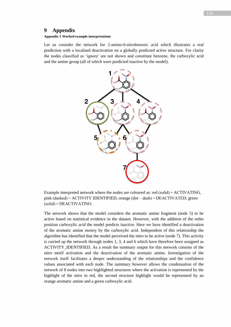
155
9 Appendix Appendix 1 Worked example interpretations
Let us consider the network for 2-amino-6-nitrobenzoic acid which illustrates a real
prediction with a localised deactivation on a globally predicted active structure. For clarity
the nodes classified as ‘ignore’ are not shown and constitute benzene, the carboxylic acid
and the amine group (all of which were predicted inactive by the model).
Example interpreted network where the nodes are coloured as: red (solid) = ACTIVATING,
pink (dashed) = ACTIVITY IDENTIFIED, orange (dot – dash) = DEACTIVATED, green
(solid) = DEACTIVATING.
The network shows that the model considers the aromatic amine fragment (node 5) to be
active based on statistical evidence in the dataset. However, with the addition of the ortho
position carboxylic acid the model predicts inactive. Here we have identified a deactivation
of the aromatic amine moiety by the carboxylic acid. Independent of this relationship the
algorithm has identified that the model perceived the nitro to be active (node 7). This activity
is carried up the network through nodes 1, 3, 4 and 6 which have therefore been assigned as
ACTIVITY_IDENTIFIED. As a result the summary output for this network consists of the
nitro motif activation and the deactivation of the aromatic amine. Investigation of the
network itself facilitates a deeper understanding of the relationships and the confidence
values associated with each node. The summary however allows the condensation of the
network of 8 nodes into two highlighted structures where the activation is represented by the
highlight of the nitro in red, the second structure highlight would be represented by an
orange aromatic amine and a green carboxylic acid.

156
Appendix 2 KNIME interpretation workflow
In the above workflow all a KNIME table containing the training data with descriptors is
read in, in the upper path a Random Forest is built using the Tree Ensemble Learner node.
In the lower path a structure can be drawn using the in-house structure editor or the
MarvinSketch node. This structure is standardised in the meta-node before the features are
generated along with their descriptors.
The Tree Ensemble Predictor predicts for the query and all of the features and these
predictions along with the details of the features are passed into the Hierarchical
Interpretation node.
The above screenshot shows the dialog for the Hierarchical Interpretation node. Various
column selections need to be performed for the first input table (parent) and the second input
table (Enumerations). The nodes are populated based on the information provided in this
dialog.
For the fragment implementation an example output from this node is shown below.

157
Here we see the output of the interpretation methodology listing the summary combinations.
In the above snapshot we can see an ACTIVATING feature consisting of a nitro motif and
the atoms and bonds are provided which can be used for highlighting of the query structure.
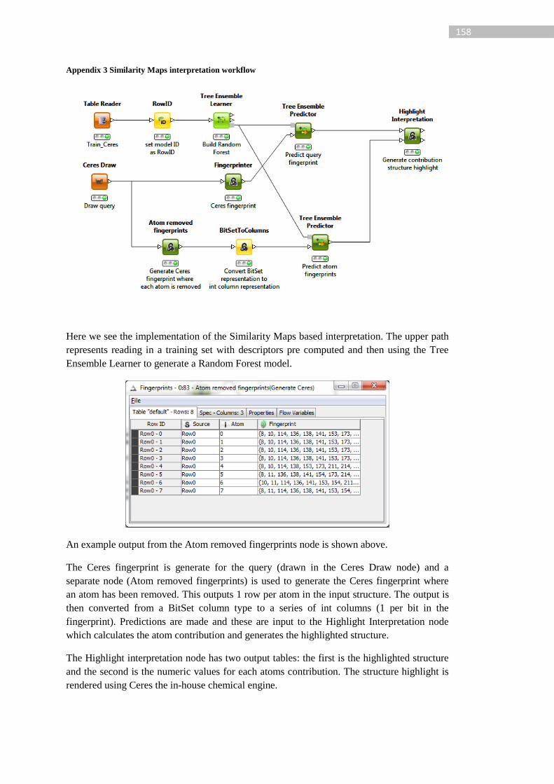
158
Appendix 3 Similarity Maps interpretation workflow
Here we see the implementation of the Similarity Maps based interpretation. The upper path
represents reading in a training set with descriptors pre computed and then using the Tree
Ensemble Learner to generate a Random Forest model.
An example output from the Atom removed fingerprints node is shown above.
The Ceres fingerprint is generate for the query (drawn in the Ceres Draw node) and a
separate node (Atom removed fingerprints) is used to generate the Ceres fingerprint where
an atom has been removed. This outputs 1 row per atom in the input structure. The output is
then converted from a BitSet column type to a series of int columns (1 per bit in the
fingerprint). Predictions are made and these are input to the Highlight Interpretation node
which calculates the atom contribution and generates the highlighted structure.
The Highlight interpretation node has two output tables: the first is the highlighted structure
and the second is the numeric values for each atoms contribution. The structure highlight is
rendered using Ceres the in-house chemical engine.
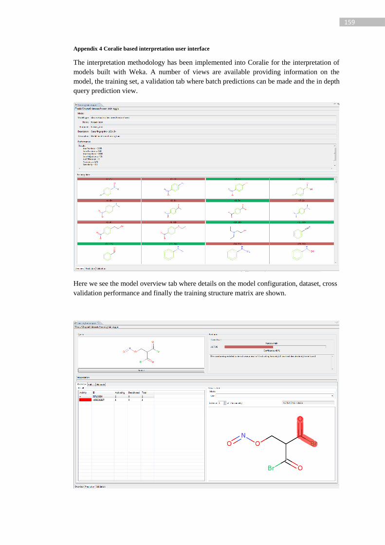
159
Appendix 4 Coralie based interpretation user interface
The interpretation methodology has been implemented into Coralie for the interpretation of
models built with Weka. A number of views are available providing information on the
model, the training set, a validation tab where batch predictions can be made and the in depth
query prediction view.
Here we see the model overview tab where details on the model configuration, dataset, cross
validation performance and finally the training structure matrix are shown.
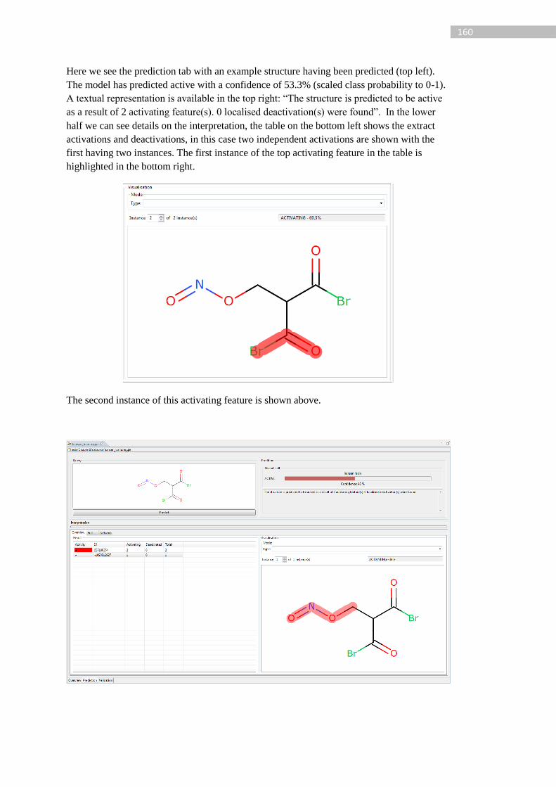
160
Here we see the prediction tab with an example structure having been predicted (top left).
The model has predicted active with a confidence of 53.3% (scaled class probability to 0-1).
A textual representation is available in the top right: “The structure is predicted to be active
as a result of 2 activating feature(s). 0 localised deactivation(s) were found”. In the lower
half we can see details on the interpretation, the table on the bottom left shows the extract
activations and deactivations, in this case two independent activations are shown with the
first having two instances. The first instance of the top activating feature in the table is
highlighted in the bottom right.
The second instance of this activating feature is shown above.
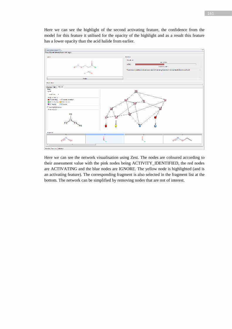
161
Here we can see the highlight of the second activating feature, the confidence from the
model for this feature it utilised for the opacity of the highlight and as a result this feature
has a lower opacity than the acid halide from earlier.
Here we can see the network visualisation using Zest. The nodes are coloured according to
their assessment value with the pink nodes being ACTIVITY_IDENTIFIED, the red nodes
are ACTIVATING and the blue nodes are IGNORE. The yellow node is highlighted (and is
an activating feature). The corresponding fragment is also selected in the fragment list at the
bottom. The network can be simplified by removing nodes that are not of interest.
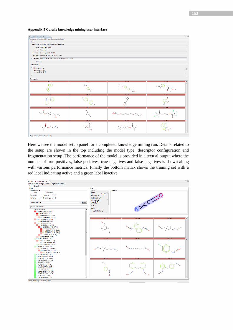
162
Appendix 5 Coralie knowledge mining user interface
Here we see the model setup panel for a completed knowledge mining run. Details related to
the setup are shown in the top including the model type, descriptor configuration and
fragmentation setup. The performance of the model is provided in a textual output where the
number of true positives, false positives, true negatives and false negatives is shown along
with various performance metrics. Finally the bottom matrix shows the training set with a
red label indicating active and a green label inactive.
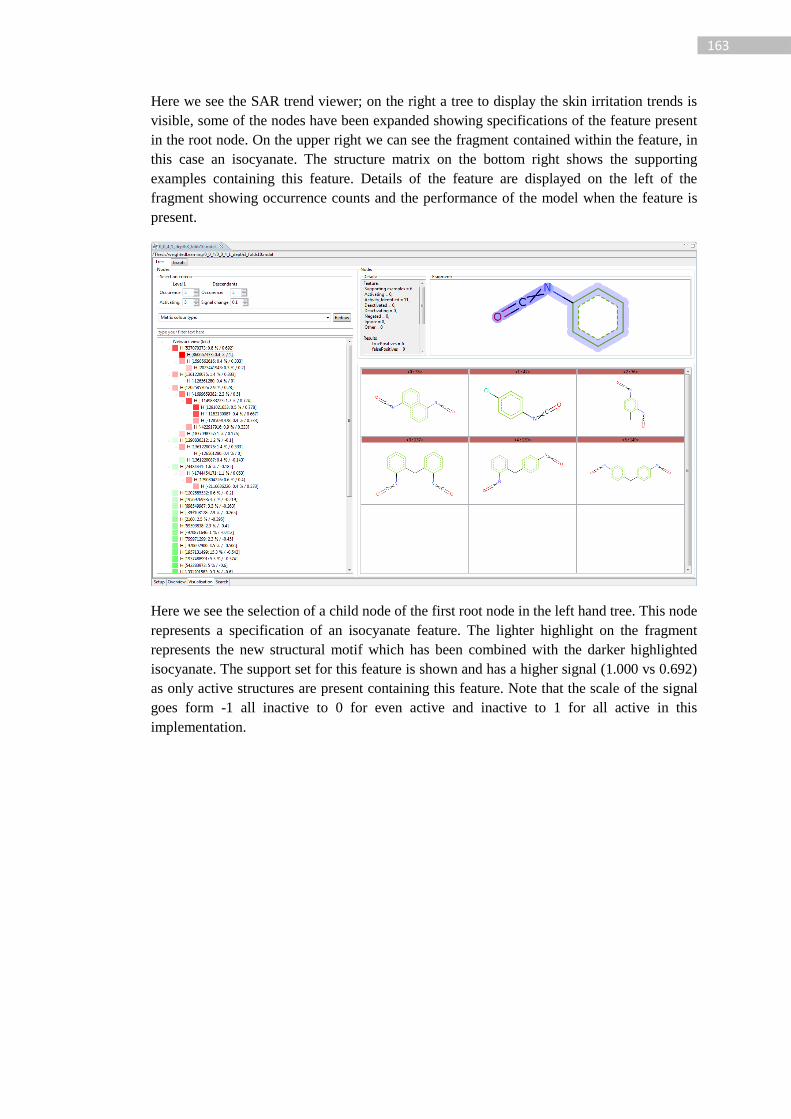
163
Here we see the SAR trend viewer; on the right a tree to display the skin irritation trends is
visible, some of the nodes have been expanded showing specifications of the feature present
in the root node. On the upper right we can see the fragment contained within the feature, in
this case an isocyanate. The structure matrix on the bottom right shows the supporting
examples containing this feature. Details of the feature are displayed on the left of the
fragment showing occurrence counts and the performance of the model when the feature is
present.
Here we see the selection of a child node of the first root node in the left hand tree. This node
represents a specification of an isocyanate feature. The lighter highlight on the fragment
represents the new structural motif which has been combined with the darker highlighted
isocyanate. The support set for this feature is shown and has a higher signal (1.000 vs 0.692)
as only active structures are present containing this feature. Note that the scale of the signal
goes form -1 all inactive to 0 for even active and inactive to 1 for all active in this
implementation.
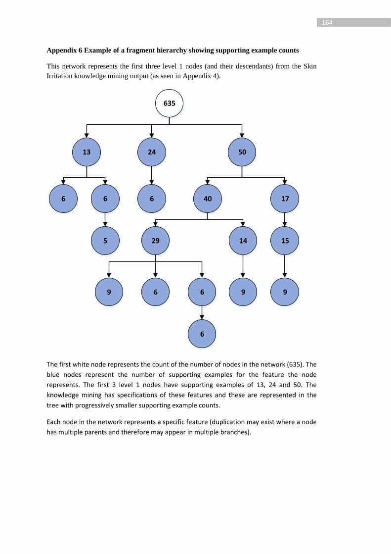
164
Appendix 6 Example of a fragment hierarchy showing supporting example counts
This network represents the first three level 1 nodes (and their descendants) from the Skin
Irritation knowledge mining output (as seen in Appendix 4).
635
13
6 6
24
6
50
40 17
15
9
29 14
99 6 6
6
5
The first white node represents the count of the number of nodes in the network (635). The
blue nodes represent the number of supporting examples for the feature the node
represents. The first 3 level 1 nodes have supporting examples of 13, 24 and 50. The
knowledge mining has specifications of these features and these are represented in the
tree with progressively smaller supporting example counts.
Each node in the network represents a specific feature (duplication may exist where a node
has multiple parents and therefore may appear in multiple branches).
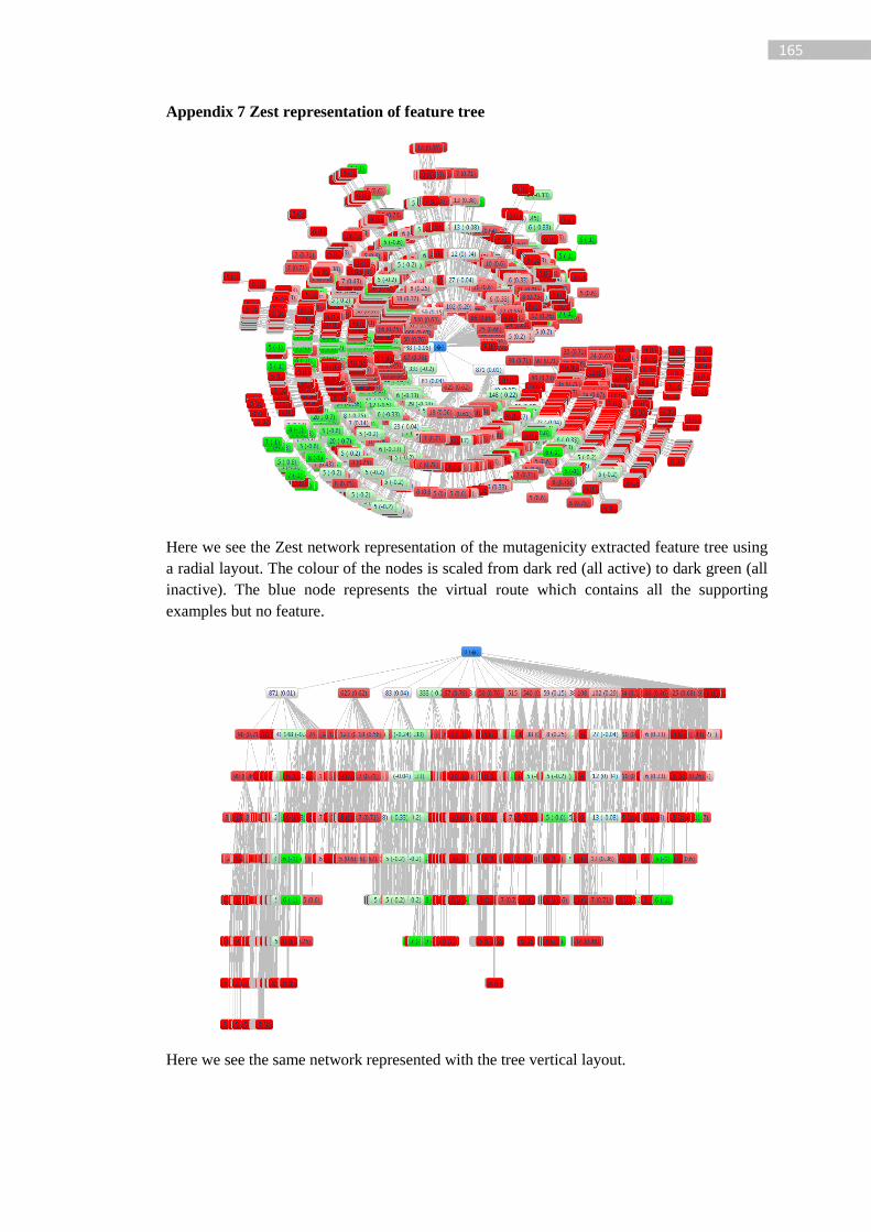
165
Appendix 7 Zest representation of feature tree
Here we see the Zest network representation of the mutagenicity extracted feature tree using
a radial layout. The colour of the nodes is scaled from dark red (all active) to dark green (all
inactive). The blue node represents the virtual route which contains all the supporting
examples but no feature.
Here we see the same network represented with the tree vertical layout.

166
10 Bibliography
[1] R. B. Silverman, The organic chemistry of drug design and drug action, 2nd ed.
Elsevier Academic Press, 2004.
[2] S. M. Paul, D. S. Mytelka, C. T. Dunwiddie, C. C. Persinger, B. H. Munos, S. R.
Lindborg, and A. L. Schacht, “How to improve R&D productivity: the
pharmaceutical industry’s grand challenge.,” Nat. Rev. Drug Discov., vol. 9, no. 3,
pp. 203–14, Mar. 2010.
[3] G. C. Terstappen and a Reggiani, “In silico research in drug discovery.,” Trends
Pharmacol. Sci., vol. 22, no. 1, pp. 23–6, Jan. 2001.
[4] M. Hay, D. W. Thomas, J. L. Craighead, C. Economides, and J. Rosenthal, “Clinical
development success rates for investigational drugs.,” Nat. Biotechnol., vol. 32, no. 1,
pp. 40–51, Jan. 2014.
[5] “Introduction to (Quantitative) Structure Activity Relationships.” [Online]. Available:
http://www.oecd.org/chemicalsafety/risk-
assessment/introductiontoquantitativestructureactivityrelationships.htm. [Accessed:
27-Jul-2014].
[6] R. Guha, “On the interpretation and interpretability of quantitative structure-activity
relationship models.,” J. Comput. Aided. Mol. Des., vol. 22, no. 12, pp. 857–71, Dec.
2008.
[7] A. Varnek and I. Baskin, “Machine learning methods for property prediction in
chemoinformatics: Quo Vadis?,” J. Chem. Inf. Model., vol. 52, no. 6, pp. 1413–37,
Jun. 2012.
[8] A. Cherkasov, E. N. Muratov, D. Fourches, A. Varnek, I. I. Baskin, M. Cronin, J.
Dearden, P. Gramatica, Y. C. Martin, R. Todeschini, V. Consonni, V. E. Kuz’min, R.
Cramer, R. Benigni, C. Yang, J. Rathman, L. Terfloth, J. Gasteiger, A. Richard, and
A. Tropsha, “QSAR modeling: Where have you been? Where are you going to?,” J.
Med. Chem., vol. 57, no. 12, pp. 4922–5010, Jan. 2014.
[9] J. C. Dearden, M. T. D. Cronin, and K. L. E. Kaiser, “How not to develop a
quantitative structure-activity or structure-property relationship (QSAR/QSPR).,”
SAR QSAR Environ. Res., vol. 20, no. 3–4, pp. 241–66, Jan. 2009.
[10] OECD, “OECD principels for the validation, for regulatory purposes, of
(Quantivative) structure-activity relationship models.” [Online]. Available:
http://www.oecd.org/dataoecd/33/37/37849783.pdf. [Accessed: 01-Sep-2014].
[11] J. Gasteiger and T. Engel, Eds., Chemoinformatics. Darmstadt: Wiley-VCH, 2003.
[12] A. R. Leach and V. J. Gillet, An introduction to chemoinformatics. Dorderecht:
Kluwer Academic Publishers, 2003.
[13] “What is REACH?,” 2014. [Online]. Available:
http://www.hse.gov.uk/reach/whatisreach.htm. [Accessed: 21-May-2014].
167
[14] “The REACH requirements for QSAR,” 2014. [Online]. Available:
http://www.orchestra-qsar.eu/regulatory-context/the-reach-requirements-for-qsar.
[Accessed: 21-May-2014].
[15] ECHA, “Grouping of substances and read-across approach. Part 1: Introductory
note,” 2013. [Online]. Available:
http://echa.europa.eu/documents/10162/13628/read_across_introductory_note_en.pdf
.
[16] ICH, “Assessment and control of DNA reactive (mutagenic) impurities in
pharmaceuticals to limit potential carciongenic risk - step 4,” 2014. [Online].
Available:
http://www.ich.org/fileadmin/Public_Web_Site/ICH_Products/Guidelines/Multidisci
plinary/M7/M7_Step_4.pdf.
[17] A. Sutter, A. Amberg, S. Boyer, A. Brigo, J. F. Contrera, L. L. Custer, K. L. Dobo, V.
Gervais, S. Glowienke, J. van Gompel, N. Greene, W. Muster, J. Nicolette, M. V.
Reddy, V. Thybaud, E. Vock, A. T. White, and L. Müller, “Use of in silico systems
and expert knowledge for structure-based assessment of potentially mutagenic
impurities.,” Regul. Toxicol. Pharmacol., vol. 67, no. 1, pp. 39–52, Oct. 2013.
[18] T. Hastie, R. Tibshirani, and J. Friedman, The elements of statistical learning: data
mining, inference, and prediction, 2nd ed. New York: Springer, 2011.
[19] C. M. Bishop, Pattern recognition and machine learning. New York: Springer, 2006.
[20] N. Barakat and A. P. Bradley, “Rule extraction from support vector machines: A
review,” Neurocomputing, vol. 74, no. 1–3, pp. 178–190, Dec. 2010.
[21] K. P. Bennett, “Support vector machines: hype or hallelujah?,” ACM SIGKDD
Explor. Newsl., vol. 2, no. 2, pp. 1–13, 2000.
[22] H. Brighton and C. Mellish, “Advances in instance selection for instance-based
learning algorithms,” Data Min. Knowl. Discov., vol. 6, pp. 153–172, 2002.
[23] G. Beliakov and G. Li, “Improving the speed and stability of the k-nearest neighbors
method,” Pattern Recognit. Lett., vol. 33, no. 10, pp. 1296–1301, Jul. 2012.
[24] G. Maggiora, M. Vogt, D. Stumpfe, and J. Bajorath, “Molecular similarity in
medicinal chemistry.,” J. Med. Chem., vol. 57, no. 8, pp. 3186–204, Apr. 2014.
[25] M. T. D. Cronin and J. C. Madden, Eds., In Silico Toxicology. Cambridge: RSC
Publishing, 2010.
[26] A. Long, K. Fielding, N. McSweeney, M. Payne, and E. Smoraczewska, “Expert
systems: the use of expert systems in drug design - toxicity and metabolism,” in Drug
Design Strategies: Quantitative Approaches, D. J. Livingstonew and A. M. Davis,
Eds. Cambridge: RSC Publishing, 2012.
[27] “Genetox expert alerts suite : Leadscope - chemoinformatics platform for drug
discovery.” [Online]. Available: http://www.leadscope.com/genetox_expert_alerts/.
[Accessed: 29-Jul-2014].
168
[28] R. Benigni, C. Bossa, N. Jeliazkova, T. Netzeva, and A. Worth, “The Benigni / Bossa
rulebase for mutagenicity and carcinogenicity – a module of Toxtree,” Luxembourg,
2008.
[29] M. T. D. Cronin and T. W. Schultz, “Pitfalls in QSAR,” J. Mol. Struct. THEOCHEM,
vol. 622, no. 1–2, pp. 39–51, Mar. 2003.
[30] A. Tropsha, “Best practices for QSAR model development, validation, and
exploitation,” Mol. Inform., vol. 29, no. 6–7, pp. 476–488, Jul. 2010.
[31] J. Van Hulse, T. M. Khoshgoftaar, and A. Napolitano, “Experimental perspectives on
learning from imbalanced data,” in ICML ’07 Proceedings of the 24th international
conference on Machine learning, 2007, pp. 935–942.
[32] F. Sahigara, K. Mansouri, D. Ballabio, A. Mauri, V. Consonni, and R. Todeschini,
“Comparison of different approaches to define the applicability domain of QSAR
models,” Molecules, vol. 17. pp. 4791–4810, 2012.
[33] M. Hewitt and C. M. Ellison, “Developing the applicability domain of in silico
models: releance, importance and methods,” in In Silico Toxicology, M. T. D. Cronin
and J. C. Madden, Eds. Cambridge: RSC Publishing, 2010, pp. 301 – 344.
[34] C. M. Ellison, S. J. Enoch, M. T. Cronin, J. C. Madden, and P. Judson, “Definition of
the applicability domains of knowledge-based predictive toxicology expert systems
by using a structural fragment-based approach.,” Altern. Lab. Anim., vol. 37, no. 5,
pp. 533–45, Nov. 2009.
[35] S. Weaver and M. P. Gleeson, “The importance of the domain of applicability in
QSAR modeling.,” J. Mol. Graph. Model., vol. 26, no. 8, pp. 1315–26, Jun. 2008.
[36] I. Sushko, S. Novotarskyi, R. Körner, A. K. Pandey, A. Cherkasov, J. Li, P.
Gramatica, K. Hansen, T. Schroeter, K.-R. Müller, L. Xi, H. Liu, X. Yao, T. Öberg,
F. Hormozdiari, P. Dao, C. Sahinalp, R. Todeschini, P. Polishchuk, A. Artemenko, V.
Kuz’min, T. M. Martin, D. M. Young, D. Fourches, E. Muratov, A. Tropsha, I.
Baskin, D. Horvath, G. Marcou, C. Muller, A. Varnek, V. V Prokopenko, and I. V
Tetko, “Applicability domains for classification problems: Benchmarking of distance
to models for Ames mutagenicity set.,” J. Chem. Inf. Model., vol. 50, no. 12, pp.
2094–111, Dec. 2010.
[37] C. M. Ellison, J. C. Madden, P. Judson, and M. T. D. Cronin, “Using in silico tools in
a weight of evidence approach to aid toxicological assessment,” Mol. Inform., vol. 29,
no. 1–2, pp. 97–110, Jan. 2010.
[38] I. V Tetko, I. Sushko, A. K. Pandey, H. Zhu, A. Tropsha, E. Papa, T. Oberg, R.
Todeschini, D. Fourches, and A. Varnek, “Critical assessment of QSAR models of
environmental toxicity against Tetrahymena pyriformis: focusing on applicability
domain and overfitting by variable selection.,” J. Chem. Inf. Model., vol. 48, no. 9,
pp. 1733–46, Sep. 2008.
[39] A. P. Bradley, “The use of the area under the ROC curve in the evaluation of machine
learning algorithms,” Pattern Recognit., vol. 30, no. 7, pp. 1145–1159, Jul. 1997.

169
[40] P. Gramatica, “Principles of QSAR models validation: internal and external,” QSAR
Comb. Sci., vol. 26, no. 5, pp. 694–701, May 2007.
[41] P. Gramatica, “External Evaluation of QSAR Models, in Addition to Cross-
Validation: Verification of Predictive Capability on Totally New Chemicals,” Mol.
Inform., vol. 33, no. 4, pp. 311–314, Apr. 2014.
[42] A. Tropsha, P. Gramatica, and V. Gombar, “The importance of neing earnest:
validation is the absolute essential for successful application and interpretation of
QSPR models,” QSAR Comb. Sci., vol. 22, no. 1, pp. 69–77, Apr. 2003.
[43] A. Vellido, J. D. Martin-Guerrero, and P. J. G. Lisboa, “Making machine learning
models interpretable,” in The 20th European Symposium on Artificial Neural
Networks, Computational Intelligence and Machine Learning, 2012, no. April, pp.
163–172.
[44] I. Bratko, “Machine Learning: Between accuracy and interpretability,” in Learning,
Networks and Statistics, G. Riccia, H.-J. Lenz, and R. Kruse, Eds. Vienna: Springer
Vienna, 1997.
[45] S. Rüping, “Learning interpretable models,” Universitat Dortmund, 2006.
[46] D. T. Stanton, “On the physical interpretation of QSAR models.,” J. Chem. Inf.
Comput. Sci., vol. 43, no. 5, pp. 1423–33, 2003.
[47] I. Sushko, E. Salmina, V. a Potemkin, G. Poda, and I. V Tetko, “ToxAlerts: a Web
server of structural alerts for toxic chemicals and compounds with potential adverse
reactions.,” J. Chem. Inf. Model., vol. 52, no. 8, pp. 2310–6, Aug. 2012.
[48] I. Sushko, S. Novotarskyi, R. Körner, A. K. Pandey, M. Rupp, W. Teetz, S.
Brandmaier, A. Abdelaziz, V. V Prokopenko, V. Y. Tanchuk, R. Todeschini, A.
Varnek, G. Marcou, P. Ertl, V. Potemkin, M. Grishina, J. Gasteiger, C. Schwab, I. I.
Baskin, V. a Palyulin, E. V Radchenko, W. J. Welsh, V. Kholodovych, D.
Chekmarev, A. Cherkasov, J. Aires-de-Sousa, Q.-Y. Zhang, A. Bender, F. Nigsch, L.
Patiny, A. Williams, V. Tkachenko, and I. V Tetko, “Online chemical modeling
environment (OCHEM): web platform for data storage, model development and
publishing of chemical information.,” J. Comput. Aided. Mol. Des., vol. 25, no. 6, pp.
533–54, Jun. 2011.
[49] J. Kazius, R. McGuire, and R. Bursi, “Derivation and validation of toxicophores for
mutagenicity prediction.,” J. Med. Chem., vol. 48, no. 1, pp. 312–20, Jan. 2005.
[50] R. Benigni and C. Bossa, “Structure alerts for carcinogenicity, and the Salmonella
assay system: a novel insight through the chemical relational databases technology.,”
Mutat. Res., vol. 659, no. 3, pp. 248–61, 2008.
[51] A. B. Bailey, R. Chanderbhan, N. Collazo-Braier, M. a Cheeseman, and M. L.
Twaroski, “The use of structure-activity relationship analysis in the food contact
notification program.,” Regul. Toxicol. Pharmacol., vol. 42, no. 2, pp. 225–35, Jul.
2005.
170
[52] J. Ashby and R. W. Tennant, “Chemical structure, Salmonella mutagenicity and
extent of carcinogenicity as indicators of genotoxic carcinogenesis among 222
chemicals tested in rodents by the U.S. NCI/NTP.,” Mutat. Res., vol. 204, no. 1, pp.
17–115, Jan. 1988.
[53] M. D. Barratt, D. A. Basketter, M. Chamberlain, M. P. Payne, G. D. Admans, and J.
J. Langowski, “Development of an expert system rulebase for identifying contact
allergens,” in Toxicology in Vitro, 1994, vol. 8, pp. 837–839.
[54] I. Gerner, M. D. Barratt, S. Zinke, K. Schlegel, and E. Schlede, “Development and
prevalidation of a list of structure-activity relationship rules to be used in expert
systems for prediction of the skin-sensitising properties of chemicals.,” Altern. Lab.
Anim., vol. 32, no. 5, pp. 487–509, Nov. 2004.
[55] M. P. Payne and P. T. Walsh, “Structure-activity relationships for skin sensitization
potential: development of structural alerts for use in knowledge-based toxicity
prediction systems.,” J. Chem. Inf. Comput. Sci., vol. 34, no. 1, pp. 154–61.
[56] S. J. Enoch, J. C. Madden, and M. T. D. Cronin, “Identification of mechanisms of
toxic action for skin sensitisation using a SMARTS pattern based approach.,” SAR
QSAR Environ. Res., vol. 19, no. 5–6, pp. 555–78, Jan. 2008.
[57] P. N. Judson, C. A. Marchant, and J. D. Vessey, “Using argumentation for absolute
reasoning about the potential toxicity of chemicals,” J. Chem. Inf. Model., vol. 43, no.
5, pp. 1364–1370, Sep. 2003.
[58] G. Patlewicz, N. Jeliazkova, R. J. Safford, a P. Worth, and B. Aleksiev, “An
evaluation of the implementation of the Cramer classification scheme in the Toxtree
software.,” SAR QSAR Environ. Res., vol. 19, no. 5–6, pp. 495–524, Jan. 2008.
[59] N. Jeliazkova, “Toxtree User Manual: version 10 July 2013,” Sofia, 2013.
[60] T. Hanser, C. Barber, E. Rosser, J. D. Vessey, S. J. Webb, and S. Werner, “Self
organising hypothesis networks: a new approach for representing and structuring
SAR knowledge,” J. Cheminform., vol. 6, no. 1, p. 21, 2014.
[61] K. Hansen, D. Baehrens, T. Schroeter, M. Rupp, and K.-R. Müller, “Visual
interpretation of kernel-nased prediction models,” Mol. Inform., vol. 30, no. 9, pp.
817–826, Sep. 2011.
[62] R. Guha and P. C. Jurs, “Interpreting computational neural network QSAR models: a
measure of descriptor importance.,” Journal of chemical information and modeling,
vol. 45, no. 3. pp. 800–6.
[63] L. Carlsson, E. A. Helgee, and S. Boyer, “Interpretation of nonlinear QSAR models
applied to Ames mutagenicity data.,” J. Chem. Inf. Model., vol. 49, no. 11, pp. 2551–
8, Nov. 2009.
[64] V. E. Kuz’min, a G. Artemenko, and E. N. Muratov, “Hierarchical QSAR technology
based on the Simplex representation of molecular structure.,” J. Comput. Aided. Mol.
Des., vol. 22, no. 6–7, pp. 403–21, 2008.
171
[65] A. Palczewska, J. Palczewski, R. Marchese Robinsion, and D. Neagu, “Interpreting
random forest classification models using a feature contribution method,” in
Integration of Reusable Systems, T. Bouabana-Tebibel and S. H. Rubin, Eds.
Switzerland: Springer International Publishing, 2014, pp. 193–218.
[66] I. I. Baskin, a O. Ait, N. M. Halberstam, V. a Palyulin, and N. S. Zefirov, “An
approach to the interpretation of backpropagation neural network models in QSAR
studies.,” SAR QSAR Environ. Res., vol. 13, no. 1, pp. 35–41, Mar. 2002.
[67] B. M. Spowage, C. L. Bruce, and J. D. Hirst, “Interpretable correlation descriptors for
quantitative structure-activity relationships.,” J. Cheminform., vol. 1, no. 1, p. 22, Jan.
2009.
[68] S. Ajmani, K. Jadhav, and S. A. Kulkarni, “Group-based QSAR (G-QSAR):
mitigating interpretation challenges in QSAR,” QSAR Comb. Sci., vol. 28, no. 1, pp.
36–51, Jan. 2009.
[69] R. Guha, D. T. Stanton, and P. C. Jurs, “Interpreting computational neural network
quantitative structure-activity relationship models: a detailed interpretation of the
weights and biases.,” J. Chem. Inf. Model., vol. 45, no. 4, pp. 1109–21.
[70] L. Franke, E. Byvatov, O. Werz, D. Steinhilber, P. Schneider, and G. Schneider,
“Extraction and visualization of potential pharmacophore points using support vector
machines: application to ligand-based virtual screening for COX-2 inhibitors.,” J.
Med. Chem., vol. 48, no. 22, pp. 6997–7004, Nov. 2005.
[71] S. Riniker and G. a Landrum, “Similarity maps - a visualization strategy for
molecular fingerprints and machine-learning methods.,” J. Cheminform., vol. 5, no. 1,
p. 43, Sep. 2013.
[72] G. Landrum, “RDKit: Open-source cheminformatics (http://www.rdkit.org).” .
[73] P. G. Polishchuk, V. E. Kuz’min, A. G. Artemenko, and E. N. Muratov, “Universal
approach for structural interpretation of QSAR/QSPR models,” Mol. Inform., vol. 32,
no. 9–10, pp. 843–853, Oct. 2013.
[74] “Online QSAR interpretation.” [Online]. Available: http://physchem.od.ua/compute.
[Accessed: 01-Sep-2014].
[75] “Glowing molecules.” [Online]. Available:
http://www.optibrium.com/stardrop/stardrop-glowing-molecule.php. [Accessed: 25-
Jul-2014].
[76] M. Segall and E. Champness, “Opening the ‘black box’: interpreting in silico models
to guide compound design,” in Medicinal Chemistry Europe, 2007.
[77] R. Sherhod, V. J. Gillet, P. N. Judson, and J. D. Vessey, “Automating knowledge
discovery for toxicity prediction using jumping emerging pattern mining.,” J. Chem.
Inf. Model., vol. 52, no. 11, pp. 3074–87, Nov. 2012.
[78] M. Garcia-Borroto, J. F. Martinez-Trinidad, and J. A. Carrasco-Ochoa, “A new
emerging pattern mining algorithm and its application in supervised classification,” in

172
Pacific-Asia Conference on Knowledge Discovery and Data Mining, 2010, pp. 150–
157.
[79] T. Ferrari, G. Gini, N. Golbamaki Bakhtyari, and E. Benfenati, “Mining toxicity
structural alerts from SMILES: A new way to derive Structure Activity
Relationships,” 2011 IEEE Symp. Comput. Intell. Data Min., pp. 120–127, Apr. 2011.
[80] P. A. Bacha, H. S. Gruver, B. K. Den Hartog, S. Y. Tamura, and R. F. Nutt, “Rule
extraction from a mutagenicity data set using adaptively grown phylogenetic-like
trees.,” J. Chem. Inf. Comput. Sci., vol. 42, no. 5, pp. 1104–11, 2002.
[81] N. F. Ryman-tubb and P. Krause, “Neural network rule extraction to detect credit
card fraud,” in Engineering Applications of Neural Networks, L. Iliadis and C. Jayne,
Eds. Berlin Heidelberg: Springer, 2011, pp. 101–110.
[82] N. F. Ryman-Tubb, “SOAR – Sparse Oracle-based Adaptive Rule Extraction:
Knowledge extraction from large-scale datasets to detect credit card fraud,” in The
2010 International Joint Conference on Neural Networks (IJCNN), 2010, no. July,
pp. 1–9.
[83] M. Craven and J. Shavlik, “Rule extraction : where do we go from here ?,”
Wisconsin, 1999.
[84] N. Barakat and J. Diederich, “Learning-based Rule-Extraction from Support Vector
Machines,” in The 14th International Conference on Computer Theory and
applications ICCTA’2004, 2004.
[85] E. Frank and I. H. Witten, “Generating accurate rule sets without global
optimization.” University of Waikato, Department of Computer Science, 01-Jan-
1998.
[86] J. Friedman and B. Popescu, “Predictive Learning via Rule Ensembles,” Ann. Appl.
Stat., vol. 2, no. 3, pp. 916–954, 2008.
[87] J. J. Langham and A. N. Jain, “Accurate and interpretable computational modeling of
chemical mutagenicity.,” J. Chem. Inf. Model., vol. 48, no. 9, pp. 1833–9, Sep. 2008.
[88] S. Lozano, G. Poezevara, M.-P. Halm-Lemeille, E. Lescot-Fontaine, A. Lepailleur, R.
Bissell-Siders, B. Crémilleux, S. Rault, B. Cuissart, and R. Bureau, “Introduction of
jumping fragments in combination with QSARs for the assessment of classification in
ecotoxicology.,” J. Chem. Inf. Model., vol. 50, no. 8, pp. 1330–9, Aug. 2010.
[89] G. Dong and J. Li, “Efficient Mining of Emerging Patterns : Discovering Trends and
Differences The University of Melbourne,” in KDD ’99 Proceedings of the fifth ACM
SIGKDD international conference on Knowledge discovery and data mining, 1999,
pp. 43–52.
[90] R. Sherhod, P. Judson, T. Hanser, J. Vessey, S. J. Webb, and V. Gillet, “Emerging
pattern mining to aid toxicological knowledge discovery.,” J. Chem. Inf. Model., May
2014.
173
[91] J. Auer and J. Bajorath, “Emerging chemical patterns: a new methodology for
molecular classification and compound selection.,” J. Chem. Inf. Model., vol. 46, no.
6, pp. 2502–14, Jan. 2006.
[92] V. Namasivayam, D. Gupta-Ostermann, J. Balfer, K. Heikamp, and J. Bajorath,
“Prediction of compounds in different local structure-activity relationship
environments using emerging chemical patterns.,” J. Chem. Inf. Model., vol. 54, no.
5, pp. 1301–10, May 2014.
[93] C. A. Nicolaou, S. Y. Tamura, B. P. Kelley, S. I. Bassett, and R. F. Nutt, “Analysis of
large screening data sets via adaptively grown phylogenetic-like trees.,” J. Chem. Inf.
Comput. Sci., vol. 42, no. 5, pp. 1069–79, 2002.
[94] T. Ferrari, D. Cattaneo, G. Gini, N. Golbamaki Bakhtyari, a Manganaro, and E.
Benfenati, “Automatic knowledge extraction from chemical structures: the case of
mutagenicity prediction.,” SAR QSAR Environ. Res., vol. 24, no. 5, pp. 631–49, Jan.
2013.
[95] R. Andrews, J. Diederich, and A. B. Tickle, “Survey and critique of techniques for
extracting rules from trained artificial neural networks,” Knowledge-Based Syst., vol.
8, no. 6, pp. 373–389, Dec. 1995.
[96] K.-P. Huber and M. R. Berthold, “Building precise classifiers with automatic rule
extraction,” Proc. ICNN’95 - Int. Conf. Neural Networks, vol. 3, pp. 1263–1268.
[97] J. He, H.-J. Hu, R. Harrison, P. C. Tai, and Y. Pan, “Rule generation for protein
secondary structure prediction with support vector machines and decision tree.,”
IEEE Trans. Nanobioscience, vol. 5, no. 1, pp. 46–53, Mar. 2006.
[98] “Eclipse.” [Online]. Available: https://www.eclipse.org/. [Accessed: 29-Jul-2014].
[99] “Zest Eclipe plugin.” [Online]. Available: http://www.eclipse.org/gef/zest/.
[Accessed: 29-Jul-2014].
[100] M. R. Berthold, N. Cebron, F. Dill, T. R. Gabriel, T. Kötter, T. Meinl, P. Ohl, C.
Sieb, K. Thiel, B. Wiswedel, C. Preisach, H. Burkhardt, L. Schmidt-Thieme, and R.
Decker, “KNIME: The Konstanz Information Miner,” in Data Analysis, Machine
Learning and Applications, C. Preisach, H. Burkhardt, L. Schmidt-Thieme, and R.
Decker, Eds. Berlin, Heidelberg: Springer Berlin Heidelberg, 2008, pp. 319–326.
[101] M. Hall, E. Frank, G. Holmes, B. Pfahringer, P. Reutemann, and I. H. Witten, “The
WEKA data mining software,” ACM SIGKDD Explor. Newsl., vol. 11, no. 1, p. 10,
Nov. 2009.
[102] T. Hanser, E. Rosser, M. Ulyatt, and S. Werner, “L_Patterns : a novel perspective on
structure class definition and search in chemical structural spaces,” in 5th Joint
Sheffield Conference on Chemoinformatics, 2010.
[103] T. Hanser, E. Rosser, S. Werner, and P. Górny, “Explora: A new language to define
powerful structural queries,” in 9th International Conference on Chemical Structures,
2011, p. P–8.
174
[104] C. Steinbeck, Y. Han, S. Kuhn, O. Horlacher, E. Luttmann, and E. Willighagen, “The
Chemistry Development Kit (CDK): an open-source Java library for Chemo- and
Bioinformatics.,” J. Chem. Inf. Comput. Sci., vol. 43, no. 2, pp. 493–500, Jan. 2003.
[105] ChemAxon, “Standardizer and structure checker, part of the ChemAxon JChem
package.” 2011.
[106] S. J. Webb, T. Hanser, B. Howlin, P. Krause, and J. D. Vessey, “Feature combination
networks for the interpretation of statistical machine learning models: application to
Ames mutagenicity.,” J. Cheminform., vol. 6, no. 1, p. 8, Jan. 2014.
[107] K. Hansen, S. Mika, T. Schroeter, A. Sutter, A. ter Laak, T. Steger-Hartmann, N.
Heinrich, and K.-R. Müller, “Benchmark data set for in silico prediction of Ames
mutagenicity.,” J. Chem. Inf. Model., vol. 49, no. 9, pp. 2077–81, Sep. 2009.
[108] L. S. Gold, T. H. Slone, B. N. Ames, N. B. Manley, G. B. Garfinkel, and L.
Rohrbach, “Carcinogenic Potency Database,” in Handbook of Carcinogenic Potency
and Genotoxicity Databases, L. Gold and E. Zeiger, Eds. Boca Raton: CRC Press,
1997, pp. 1–106.
[109] “Vitic Nexus,” 2011. [Online]. Available: https://www.lhasalimited.org/vitic_nexus/.
[110] L. G. Valerio, “In silico toxicology for the pharmaceutical sciences.,” Toxicol. Appl.
Pharmacol., vol. 241, no. 3, pp. 356–70, Dec. 2009.
[111] P. P. Roy, J. T. Leonard, and K. Roy, “Exploring the impact of size of training sets
for the development of predictive QSAR models,” Chemom. Intell. Lab. Syst., vol.
90, no. 1, pp. 31–42, Jan. 2008.
[112] D. Fourches, E. Muratov, and A. Tropsha, “Trust, but verify: on the importance of
chemical structure curation in cheminformatics and QSAR modeling research.,” J.
Chem. Inf. Model., vol. 50, no. 7, pp. 1189–204, Jul. 2010.
[113] A. J. Williams and S. Ekins, “A Quality Alert and Call for Improved Curation of
Public Chemistry Databases,” Drug Discov. Today, Jul. 2011.
[114] D. Young, T. Martin, R. Venkatapathy, and P. Harten, “Are the chemical structures in
your QSAR correct?,” QSAR Comb. Sci., vol. 27, no. 11–12, pp. 1337–1345, Dec.
2008.
[115] “Daylight Theory: SMILES.” [Online]. Available:
http://www.daylight.com/dayhtml/doc/theory/theory.smiles.html. [Accessed: 27-Jul-
2014].
[116] “Marvin.” ChemAxon, Budapest, Hungary.
[117] P. Willett, J. M. Barnard, and G. M. Downs, “Chemical similarity searching,” J.
Chem. Inf. Comput. Sci., pp. 983–996, 1998.
[118] A. Bender and R. C. Glen, “Molecular similarity: a key technique in molecular
informatics.,” Org. Biomol. Chem., vol. 2, pp. 3204–3218, 2004.
175
[119] P. Willett and V. Winterman, “A comparison of some measures for the determination
of inter-molecular structural similarity measures of inter-molecular structural
similarity,” Quant. Struct. Relationships, vol. 5, pp. 18–25, 1986.
[120] “Daylight manual: fingerprints,” 2014. [Online]. Available:
http://www.daylight.com/dayhtml/doc/theory/theory.finger.html.
[121] Chemical Computing Group Inc., “Molecular Operating Environment (MOE).”
Montreal, Canada.
[122] R. Todeschini, V. Consonni, A. Mauri, and M. Pavan, “DRAGON-Software for the
calculation of molecular descriptors.” Talete SRL, Milan, Italty.
[123] H. Hong, Q. Xie, W. Ge, F. Qian, H. Fang, L. Shi, Z. Su, R. Perkins, and W. Tong,
“Mold(2), molecular descriptors from 2D structures for chemoinformatics and
toxicoinformatics.,” J. Chem. Inf. Model., vol. 48, no. 7, pp. 1337–44, Jul. 2008.
[124] C. W. Yap, “PaDEL-descriptor: an open source software to calculate molecular
descriptors and fingerprints.,” J. Comput. Chem., vol. 32, no. 7, pp. 1466–74, May
2011.
[125] Molecular Networks, “ADRIANA.code.” Erlangen, Germany.
[126] ChemAxon, “ChemAxon Calculator Plugins.” Budapest, Hungary.
[127] Accelrys, “Pipeline Pilot.” San Diego, USA.
[128] R. Todeschini and V. Consonni, Handbook of Molecular Descriptors. Weinheim:
Wiley, 2008.
[129] J. L. Durant, B. A. Leland, D. R. Henry, and J. G. Nourse, “Reoptimization of MDL
Keys for Use in Drug Discovery,” J. Chem. Inf. Model., vol. 42, no. 6, pp. 1273–
1280, Nov. 2002.
[130] ChemAxon, “ChemAxon chemical engine.” Budapest, Hungary.
[131] “Pubchem fingerprint.” [Online]. Available:
ftp://ftp.ncbi.nlm.nih.gov/pubchem/specifications/pubchem_fingerprints.txt.
[132] “BioByte.” [Online]. Available: http://www.biobyte.com/. [Accessed: 29-Jul-2014].
[133] R. O. Potts and R. H. Guy, “Predicting skin permeability.,” Pharm. Res., vol. 9, no. 5,
pp. 663–9, May 1992.
[134] BioByte, “ClogP User Guide v 4.0.” [Online]. Available:
http://www.biobyte.com/bb/prod/40manual.pdf.
[135] D. Ballabio, V. Consonni, A. Mauri, M. Claeys-Bruno, M. Sergent, and R.
Todeschini, “A novel variable reduction method adapted from space-filling designs,”
Chemom. Intell. Lab. Syst., vol. 136, pp. 147–154, Aug. 2014.
176
[136] M. A. Hall, “Correlation-based feature selection for machine learning,” The
University of Waikato, 1999.
[137] M. Eklund, U. Norinder, S. Boyer, and L. Carlsson, “Benchmarking variable
selection in QSAR,” Mol. Inform., vol. 31, no. 2, pp. 173–179, Feb. 2012.
[138] R. Kohavi, “Wrappers for performance enhancement and oblivious decision graphs,”
Stanford University, 1995.
[139] S. Kotsiantis and D. Kanellopoulos, “Discretization techniques : a recent survey,”
GESTS Int. Trans. Comput. Sci. Eng., vol. 32, no. 1, pp. 47–58, 2006.
[140] H. Liu, H. Farhad, C. L. Tan, and D. Manoranjan, “Discretization : an enabling
technique,” Data Min. Knowl. Discov., vol. 6, pp. 393–423, 2002.
[141] J. Dougherty, R. Kohavi, and S. Mehran, “Supervised and unsupervised discretization
of continious features,” in Machine learning: proceedings of the twelth international
conference, 1995, vol. 0.
[142] X. Q. Lewell, D. B. Judd, S. P. Watson, and M. M. Hann, “RECAP--retrosynthetic
combinatorial analysis procedure: a powerful new technique for identifying
privileged molecular fragments with useful applications in combinatorial chemistry.,”
J. Chem. Inf. Comput. Sci., vol. 38, no. 3, pp. 511–22, 1998.
[143] J. Degen, C. Wegscheid-Gerlach, A. Zaliani, and M. Rarey, “On the art of compiling
and using ‘drug-like’ chemical fragment spaces.,” ChemMedChem, vol. 3, no. 10, pp.
1503–7, Oct. 2008.
[144] “Chemaxon: CCQ method - Fragmenter - ChemAxon .” [Online]. Available:
https://docs.chemaxon.com/display/fragmenter/CCQ+method. [Accessed: 29-Jul-
2014].
[145] “The RDKit Documentation — The RDKit 2014.03.1 documentation.” [Online].
Available: http://www.rdkit.org/new_docs/. [Accessed: 29-Jul-2014].
[146] K. Mortelmans and E. Zeiger, “The Ames Salmonella/microsome mutagenicity
assay,” Mutat. Res. Mol. Mech. Mutagen., vol. 455, no. 1–2, pp. 29–60, Nov. 2000.
[147] OECD, “OECD guideline for testing of chemicals, section 4. Test No. 471: bacterial
reverse mutation test,” 1997.
[148] D. P. Clark, Molecular biology: understanding the genetic revolution. Burlington,
MA, USA: Academic Press, 2005, pp. 333 – 366.
[149] E. C. Miller and J. a Miller, “Searches for ultimate chemical carcinogens and their
reactions with cellular macromolecules.,” Cancer, vol. 47, no. 10, pp. 2327–45, May
1981.
[150] P. Judson, “The application of structure – activity relationships to the prediction of
the mutagenic activity of chemicals,” in Genetic Toxicology: Principles and Methods,
vol. 817, J. M. Parry and E. M. Parry, Eds. 2012.
177
[151] B. N. Ames, “An Improved Bacterial Test System for the Detection and
Classification of Mutagens and Carcinogens,” Proc. Natl. Acad. Sci., vol. 70, no. 3,
pp. 782–786, Mar. 1973.
[152] P. McCarren, C. Springer, and L. Whitehead, “An investigation into pharmaceutically
relevant mutagenicity data and the influence on Ames predictive potential.,” J.
Cheminform., vol. 3, no. 1, p. 51, Nov. 2011.
[153] K. Mortelmans and E. Zeiger, “The Ames Salmonella/microsome mutagenicity
assay.,” Mutat. Res., vol. 455, no. 1–2, pp. 29–60, Nov. 2000.
[154] J. Kazius, S. Nijssen, J. Kok, T. Bäck, and A. P. Ijzerman, “Substructure mining
using elaborate chemical representation.,” J. Chem. Inf. Model., vol. 46, no. 2, pp.
597–605, 2006.
[155] “ONCOLOGIC.” [Online]. Available:
http://www.epa.gov/oppt/newchems/tools/oncologic.htm. [Accessed: 23-Jul-2014].
[156] Y. Woo, D. Y. Lai, M. F. Argus, and J. C. Arcos, “Development of structure-activity
relationship rules for predicting carcinogenic potential of chemicals,” Toxicol. Lett.,
vol. 79, no. 1–3, pp. 219–228, Sep. 1995.
[157] “VEGA-QSAR.” [Online]. Available: http://www.vega-qsar.eu/. [Accessed: 20-Jul-
2014].
[158] T. Ferrari and G. Gini, “An open source multistep model to predict mutagenicity from
statistical analysis and relevant structural alerts.,” Chem. Cent. J., vol. 4 Suppl 1, no.
Suppl 1, p. S2, Jan. 2010.
[159] Bethsesda: National Library of Medicine (US), “TOXNET,” 2001, 2011. [Online].
Available: http://toxnet.nlm.nih.gov/.
[160] “Benchmark mutagenicity dataset.” [Online]. Available: http://doc.ml.tu-
berlin.de/toxbenchmark/.
[161] “Chemical Carcinogenesis Research Information System (CCRIS),” 2011. [Online].
Available: http://toxnet.nlm.nih.gov/cgi-bin/sis/htmlgen?CCRIS. [Accessed: 19-Oct-
2011].
[162] J. Feng, L. Lurati, H. Ouyang, T. Robinson, Y. Wang, S. Yuan, and S. S. Young,
“Predictive toxicology: benchmarking molecular descriptors and statistical
methods.,” J. Chem. Inf. Comput. Sci., vol. 43, no. 5, pp. 1463–70, 2003.
[163] C. Helma, T. Cramer, S. Kramer, and L. De Raedt, “Data mining and machine
learning techniques for the identification of mutagenicity inducing substructures and
structure activity relationships of noncongeneric compounds.,” J. Chem. Inf. Comput.
Sci., vol. 44, no. 4, pp. 1402–11, Jan. 2004.
[164] Q.-Y. Zhang and J. Aires-de-Sousa, “Random forest prediction of mutagenicity from
empirical physicochemical descriptors.,” J. Chem. Inf. Model., vol. 47, no. 1, pp. 1–8,
2007.
178
[165] J. R. Votano, M. Parham, L. H. Hall, L. B. Kier, S. Oloff, A. Tropsha, Q. Xie, and W.
Tong, “Three new consensus QSAR models for the prediction of Ames
genotoxicity.,” Mutagenesis, vol. 19, no. 5, pp. 365–77, Sep. 2004.
[166] J. D. Walker, I. Gerner, E. Hulzebos, and K. Schlegel, “The skin irritation corrosion
rules estimation tool (SICRET),” QSAR Comb. Sci., vol. 24, no. 3, pp. 378–384, Apr.
2005.
[167] “Ban on animal testing - European Commission.” [Online]. Available:
http://ec.europa.eu/consumers/archive/sectors/cosmetics/animal-
testing/index_en.htm. [Accessed: 29-Jul-2014].
[168] “A guide to the Globally Harmonized System of classification and labelling of
chemicals (GHS).” [Online]. Available:
https://www.osha.gov/dsg/hazcom/ghs.html#3.2.
[169] “Skin Irritation — Institute for Health and Consumer Protection – (JRC-IHCP),
European Commission.” [Online]. Available:
http://ihcp.jrc.ec.europa.eu/our_labs/eurl-ecvam/validation-regulatory-
acceptance/topical-toxicity/skin-irritation. [Accessed: 29-Jul-2014].
[170] T. Welss, D. A. Basketter, and K. R. Schröder, “In vitro skin irritation: facts and
future. State of the art review of mechanisms and models.,” Toxicol. In Vitro, vol. 18,
no. 3, pp. 231–43, Jun. 2004.
[171] OECD, “OECD Guidelines for the testing of chemicals: Actute Dermal
Irritation/Corrosion.” [Online]. Available: http://ihcp.jrc.ec.europa.eu/our_labs/eurl-
ecvam/validation-regulatory-acceptance/docs-skin-irritation-1/DOC2_OECD-TG-
404.pdf.
[172] OECD, “OECD guidelines for the testing of chemicals: In Vitro skin irritation:
reconstructed human Epidermis test method.”
[173] M. Macfarlane, P. Jones, C. Goebel, E. Dufour, J. Rowland, D. Araki, M. Costabel-
Farkas, N. J. Hewitt, J. Hibatallah, A. Kirst, P. McNamee, F. Schellauf, and J. Scheel,
“A tiered approach to the use of alternatives to animal testing for the safety
assessment of cosmetics: skin irritation.,” Regul. Toxicol. Pharmacol., vol. 54, no. 2,
pp. 188–96, Jul. 2009.
[174] M. Leist, B. A. Lidbury, C. Yang, P. J. Hayden, J. M. Kelm, S. Ringeissen, A.
Detroyer, J. R. Meunier, J. F. Rathman, G. R. Jackson, G. Stolper, and N. Hasiwa,
“Novel technologies and an overall strategy to allow hazard assessment and risk
prediction of chemicals, cosmetics, and drugs with animal-free methods,” ALTEX,
vol. 29, no. 4, pp. 373–388, 2012.
[175] C. Y. Liew and C. W. Yap, “QSAR and predictors of eye and skin effects,” Mol.
Inform., vol. 32, no. 3, pp. 281–290, Mar. 2013.
[176] E. Hulzebos, J. D. Walker, I. Gerner, and K. Schlegel, “Use of structural alerts to
develop rules for identifying chemical substances with skin irritation or skin
corrosion potential,” QSAR Comb. Sci., vol. 24, no. 3, pp. 332–342, Apr. 2005.

179
[177] “OECD QSAR Toolbox for Grouping Chemicals into Categories.” [Online].
Available: http://www.qsartoolbox.org/home. [Accessed: 18-Aug-2014].
[178] C. Y. Liew and C. W. Yap, “Skin irritation dataset.” [Online]. Available:
http://padel.nus.edu.sg/software/padelddpredictor/models/toxicity/skinirritation/2011
0805/. [Accessed: 12-Jul-2014].
[179] U. M. Fayyad and K. B. Irani, “Multi-interval discretization of continuos-valued
attributes for classification learning,” Proc. Int. Jt. Conf. Uncertain. AI, pp. 1022–
1027, 1993.
[180] I. H. Witten, E. Frank, and M. A. Hall, Data mining: practical machine learning tools
and techniques, 3rd ed. Elsevier, 2011.
[181] D. A. Canter, E. Zeiger, S. Haworth, T. Lawlor, K. Mortelmans, and W. Speck,
“Comparative mutagenicity of aliphatic epoxides in Salmonella.,” Mutat. Res., vol.
172, pp. 105–138, 1986.
Related Documents


