INTERPLAN model validation and testing

INTERPLAN INTEgrated opeRation PLAnning tool towards

the Pan-European Network

Work Package 6

INTERPLAN model validation and testing

Deliverable 6.4

Report on the validation tests

Grant Agreement No: 773708

Funding Instrument: Research and Innovation Action (RIA)

Funded under: H2020 LCE-05-2017: Tools and technologies for coordination and integration of the European energy system

Starting date of project: 01.11.2017

Project Duration: 39 months Contractual delivery date: 31.01.2021

Actual delivery date: 1.02.2021

Lead beneficiary: 6 Instytut Energetyki (IEn)

Deliverable Type: Report (R)

Dissemination level: Public (PU)

Revision / Status: FINAL

This project has received funding from the European Union’s Horizon 2020 Research and Innovation Programme under Grant Agreement No. 773708

GA No: 773708

Deliverable: D6.4 Revision / Status: V1.1 2 of 111

Document Information Document Version: 1.1

Revision / Status: FINAL All Authors/Partners Jan Ringelstein / DERlab Yannic Harms / IEE Lothar Löwer / IEE Ata Khavari / DERlab Marialaura Di Somma / ENEA Roberto Ciavarella / ENEA Bogdan Sobczak / IEn Anna Wakszyńska / IEn Michał Kosmecki / IEn Michał Bajor / IEn Christina Papadimitriou / FOSS Venizelos Efthymiou / FOSS Minas Patsalides/ FOSS Distribution List INTERPLAN consortium Keywords: Validation, Evaluation, Simulation, Verification Document History Revision Content / Changes Resp. Partner Date

0.1 Document creation DERlab 25.05.2020

0.1 Structuring the document IEE 01.06.2020

0.1 Proposing a methodology for UC validation IEn 29.06.2020

0.1 Preparation of a template for UC validation IEn 14.08.2020

0.1 Providing model descriptions All partners 13.10.2020

0.1 Describing validation results of use cases All partners 25.11.2020

0.1 Describing test results of the INTERPLAN tool IEE / DERlab 27.11.2020

0.1 Concluding the document (introduction, exec. summary, summary, etc.)

IEn 15.12.2020

0.1 Internal review at task level IEn 17.12.2020

1.0 Corrections All partners 21.12.2020

1.1 Finalization IEn, DERlab 29.01.2020

Document Approval

Final Approval Name Resp. Partner Date

Review WP Level Jan Ringelstein DERlab 23.12.2020

Review Management Level Roberto Ciavarella Helfried Brunner

ENEA AIT

25.01.2020

GA No: 773708


Disclaimer This document contains material, which is copyrighted by certain INTERPLAN consortium parties and may not be reproduced or copied without permission. The information contained in this document is the proprietary confidential information of certain INTERPLAN consortium parties and may not be disclosed except in accordance with the consortium agreement. The commercial use of any information in this document may require a licence from the proprietor of that information. Neither the INTERPLAN consortium as a whole, nor any single party within the INTERPLAN consortium warrant that the information contained in this document is capable of use, nor that the use of such information is free from risk. Neither the INTERPLAN consortium as a whole, nor any single party within the INTERPLAN consortium accepts any liability for loss or damage suffered by any person using the information. This document does not represent the opinion of the European Community, and the European Community is not responsible for any use that might be made of its content. Copyright Notice © The INTERPLAN Consortium, 2017 - 2020

GA No: 773708


Table of contents

Abbreviations .............................................................................................................. 5 Executive Summary .................................................................................................... 7

1. Introduction ...................................................................................................... 8 1.1 Purpose and scope of the Document ............................................................ 8 1.2 Structure of the Document ............................................................................ 8

2. Items under test and means of validation ......................................................... 8 2.1 Methodology ................................................................................................ 8

3. Grid models used for validation ...................................................................... 13 3.1 Introduction ................................................................................................. 13 3.2 WP5 Simbench based model ...................................................................... 13 3.3 WP6 (extended) Simbench based model ................................................... 16 3.4 Simple Cyprus grid model .......................................................................... 19 3.5 Complex Cyprus grid model ....................................................................... 22 3.6 Danish grid model ....................................................................................... 24 3.7 AIT simplified grid model ............................................................................. 25 3.8 AIT synthetic grid model ............................................................................. 27 3.9 IEEE 14 Bus Power System ........................................................................ 28

4. Results and evaluation ................................................................................... 31 4.1 Introduction ................................................................................................. 31 4.2 UC1: Coordinated voltage/reactive power control ....................................... 31 4.3 UC2: Grid congestion management ............................................................ 38 4.4 UC3: Provision of tertiary control reserve based on coordinated TSO-DSO optimal power flow calculations ............................................................................. 45 4.5 UC4: Fast Frequency Restoration Control .................................................. 52 4.6 UC5: Power balancing at DSO level .......................................................... 62 4.7 UC6: Inertia management ........................................................................... 67 4.8 UC7: Optimal Energy Interruption Management .......................................... 79

5. Testing the INTERPLAN tool .......................................................................... 85 5.1 Summary of the INTERPLAN tool ............................................................... 85 5.2 Testing the INTERPLAN tool ..................................................................... 87 5.3 Test setup ................................................................................................... 91 5.4 Test results ................................................................................................ 96

6. Summary and conclusions............................................................................ 103 7. Outlook ........................................................................................................ 104 8. References ................................................................................................... 105 Annex ..................................................................................................................... 106

8.1 List of Figures ........................................................................................... 106 8.2 List of Tables ............................................................................................ 107 8.3 Glossary of terms and definitions .............................................................. 107

GA No: 773708


Abbreviations AMPL A Mathematical Programming Language AMQP Advanced Message Queuing Protocol BESS Battery Electric Storage System BSC Base Showcase CGMES Common Grid Model Exchange Standard CPFC Cell Power Frequency Characteristic CSV Comma Separated Values DBH DataBase Handler DER Distributed Energy Resource DG Distributed generation DR Demand response DRES Distributed renewable energy sources DPL DIgSILENT Programming Language DSL DIgSILENT Simulation Language DSO Distribution System Operator EAC Energy Authority of Cyprus EBGL Electricity Balancing Guideline EHV Extra High Voltage EMTP ElectroMagnetic Transient Program ENTSO-E European Network of Transmission System Operators for Electricity EU European Union EV Electric vehicle FACTS Flexible Alternate Current Transmission Systems fFRC fast Frequency Restoration Control GEq Grid Equivalent GHG GreenHouse Gas GIS Geographical Information System GUI Graphic User Interface HV High voltage HVDC High Voltage Direct Current IEEE Institute of Electrical and Electronics Engineers IP Internet Protocol IPOPT Interior Point OPTimizer IT Information Technology JSON Java Script Object Notation KPI Key Performance Indicator LV Low voltage MCP Master Control Process MQTT Message Queue Telemetry Transport MV Medium voltage NPC Neutral Point Clamped OLTC On-Load Tap Changer OPF Optimal Power Flow OPSD Open Power System Data PGM Power-Generating Machine

GA No: 773708


PLL Phase Locked Loop PV PhotoVoltaic RES Renewable Energy Sources RMS Root Mean Square RoCoF Rate of Change of Frequency RSCAD Real-time simulations software package RTDS Real Time Digital Simulator SGEN/SG Synchronous GENerator SI System Inertia SOGL System Operation Guideline SQL Structured Query Language TRL Technology readiness level TSO Transmission System Operator UC Use case WP Work Package XML eXtended Markup Language

GA No: 773708


Executive Summary Power system industry has been witnessing the ongoing process of change of paradigm of power system operation, from the one where centralised generation follows predictable load variations to the one in which system demand has to be balanced by distributed and intermittent power resources, much less controllable in terms of power production than the conventional generation. This shift calls for new solutions on all possible levels, including regulations, market models, new, yet fully functional and ready for massive deployment technologies, such as energy storage and demand response, and methodologies to harness the new potential and guarantee stability and security of supply. This project focuses on the latter, as it aims to develop a methodology for operation planning of a power system that undergoes this dramatic change in the way it works. Power system operation planning is a complex and multidimensional responsibility of the power system operators and as such has been treated in this project. The project focused on several challenging and novel planning problems identified in the planning practice of today or expected to emerge tomorrow, for which appropriate solutions have been proposed. Within INTERPLAN these solutions were developed in the framework of use cases, comprised of carefully selected models, system development scenarios, time series data and sets of planning criteria to be met. Subsequent showcases allowed to demonstrate not only accurate operation of developed controllers and algorithms, but also an ability to integrate use cases, so that several planning problems could be addressed simultaneously. The final development of this project is the INTERPLAN tool, which is a methodology for effective recognition of possible solutions applicable to identified problems in power system operation planning. Such kind of development projects require a thorough validation of the proposed concepts. Validation which proves that the devised controllers and methods are robust, meaning that they can effectively work in different operation environments than the one they were designed in. Equally important, validation needs to answer the question whether the devised solutions are indeed those that system operation planning is waiting for. The results of such a validation are the core content of this report. Validation showed that all use cases were prepared with due diligence. All use cases accurately address those operation planning criteria that have the highest relevance for them. However cases where less relevant criteria had only marginal improvement were also noted. This result confirms that it is very difficult to come up with one common solution to many distinct problems. The second phase of validation, which was partly performed using advanced techniques like real time simulation and co-simulation, confirmed transferability and applicability of proposed methods and controllers to other situations, for some use cases with preserving the high level of efficiency seamlessly, but for others with great deal of additional work. Where possible, indication of necessary developments needed to increase TRL of proposed solutions has been provided. The report is aimed to be self-contained, therefore apart from validation results for use cases (Chapter 4) and INTERPLAN tool (Chapter 5) it has all necessary introductory information regarding test models and scenarios used for validation (Chapter 3) as well as explanation of the validation methodology (Chapter 2). The report concludes with a summary of validation results (Chapter 6).

GA No: 773708


1. Introduction Purpose and scope of the Document This document, together with complementary reports D4.3, D5.3, D5.4 and D6.3 (see Table 1), contains and describes the final results of INTERPLAN project. The main role of this report is to present validation results of controllers, control functions and models developed within the project. As defined by commonly used industrial standards and norms such as ISO 9000 or IEEE standard 1012-2012 [1], validation refers to “the assurance that a product, service, or system meets the needs of the customer and other identified stakeholders”. In particular, validation should be distinguished from verification, which in the same standard is defined as “the evaluation of whether or not a product, service, or system complies with a regulation, requirement, specification, or imposed condition”. This clear distinction between the scope of the two processes is followed in INTERPLAN project structurally, i.e. the verification, being an internal process highly embedded in the controller design phase, is described and carried out in D5.3. The main tool for verification are the key performance indicators [15], which are used to quantitatively evaluate the progress measured from the base case to the case in which all designed functions and controllers work as intended. All relevant results are also comprehensively described in the mentioned deliverable. Consequently, the work described within this deliverable is intended to ensure that the controllers and functions devised in the project conform to the requirements and operational needs of the user. Thus, a more generic picture is presented here, in which the focus is put on explaining whether and how the controllers can be utilised for the identified problems.

Table 1 Complementary reports

Deliverable no. Deliverable title

4.3 Approach for generating grid equivalents for different use cases (final version)

5.3 Control system logics: cluster and interface controllers (first version) 5.4 Control system logics: cluster and interface controllers (final version)

6.3 Operating real-time co-simulation

Structure of the Document The document is structured as follows. Chapter 2 presents the methodology and assumptions for the validation. Chapter 3 describes the power system models developed and used in use cases. Next, in Chapter 4 the results of validation are presented. A separate section, namely Chapter 5, is dedicated to the evaluation of the INTERPLAN tool. The document is concluded with a summary in Chapter 6 and outlook in Chapter 7. 2. Items under test and means of validation Methodology Validation methodology applied in this project is based on the following three-level approach (see table below). Validation is performed on use case basis. Each INTEPLAN use case (UC) [15] is processed through validation level 1, 2 and 3.

GA No: 773708


Table 2 Validation levels

Validation level

Validation action

1 Assessment of compliance with user requirements and objectives 2 Performance evaluation 3 Identification of peculiarities of individual UCs

Validation level 1: Assessment of compliance with user requirements and objectives As explained in section 1.1, validation consists in assuring and evaluating how the functions and controllers fulfil user needs, requirements and objectives, which from perspective of power system operation planning can be associated with operation planning criteria. The project identified ten important planning criteria and used them in use cases formulation phase as well as for the purpose of showcases definition. These criteria are listed and grouped into categories in table 3.

Table 3 Operation planning criteria used in the project

No. Operation planning criterion (goal) Category

1 Assuring voltage stability Stability criteria

2 Assuring transient stability

3 Assuring frequency stability

4 Mitigating grid congestion Optimizing criteria

5 Minimizing losses

6 Minimizing cost

7 Minimizing energy interruptions

8 Optimize TSO/DSO interaction

9 Maximizing share of RES Criteria supporting RES integration

10 Maximize DG/DRES contribution to ancillary services

The use cases were characterised by how much they relate to particular planning criteria. Each criterion was assigned low (1), medium (2) or high (3) relevance for each use case. Figure 1 shows the results of this process in the form of dark blue polar plots, whereas the coloured dashed lines represent the areas of criteria categories. As depicted in figure 1 each use case is focused on different planning criteria. Thus level 1 validation concerns only those criteria that are relevant for use case being validated, e.g. in UC1 it should be confirmed that criteria 1, 8 and 10 are highly supported, whereas criteria 5, 6 and 9 are at least moderately influenced. Criteria 2, 3, 4 and 7 are of no importance to this use case.

UC1: Coordinated grid voltage/reactive power

UC2: Grid congestion management

UC3: Frequency tertiary control based on optimal

GA No: 773708


control power flow

UC4: Fast Frequency Restoration Control

UC5: Power balancing at DSO level

UC6: Inertia management

UC7: Energy interruption

management

Figure 1 Realisation of different planning criteria within the project use cases

The result of the above-mentioned assessment is provided in a descriptive and illustrative form covering: 1.1 Elaboration of how a use case addresses criteria that are relevant (medium or high ranking)

to this use case. • If a particular criterion is not met with adequate relevance in the use case, justification is

provided; this situation can appear when meeting one criterion is inherently linked with violating or deteriorating another.

1.2 Assessment of any legal or regulatory limitations and barriers that were identified. 1.3 Evaluation of possibility of practical deployment and/or identification of steps needed to bring the functionality technology readiness level (TRL) higher than 5 (TRL 5 is the target for INTERPLAN results). Validation level 2: Performance evaluation

GA No: 773708


Performance evaluation is the second step of use case validation. It consists of two different validation means, both aimed at assessing if a use case fulfils additional criteria that are related to practical applicability of developed functions to similar problems. These means are: 2.1 Evaluation of controller/function robustness: to prove that it works for different data than the

data used for controller/function development. Robustness validation can be realized in two different ways:

i. by using different power flow data for the same grid (e.g. different scenario, different time series),

ii. by using a model representing a power system of different structure (e.g. other power system, the same power system but different level of topology detail).

2.2 Assessment of implementation requirements: to prove that the whole process is manageable in a reasonable time frame as seen from the operation planning perspective. Important factors to mention here are algorithm complexity, number and type of programming/simulating tools needed to run the use case, automation/scripting possibilities, data bottlenecks, readability of results, necessity of operator intervention, etc.

The results of this validation step are also mostly in a form of explanatory text with focus on significant deviations from observations from step 1 and results presented in D5.4. It should be noted that the performance to be expected depends on the TRL of the use cases. In case of INTERPLAN the maximum development level is defined as TRL 5. Validation level 3: Identification of peculiarities of individual use cases Although all use cases allow realizing one or more operation planning goals within the given time frame, each use case is different and works in a different way. Thus, the purpose of validation level 3 is to identify and evaluate all special conditions, requirements and needs of the developed functions. These might include for instance: 3.1 special requirements concerning access to data and data exchange, e.g. for use cases

covering both transmission and distribution networks, 3.2 critical requirements determining feasibility of an use case, e.g. measurement delay and

accuracy in use cases dealing with dynamic simulation regime, 3.3 extraordinary system operation conditions in which an use case cannot work correctly or will

only work for these conditions, 3.4 other. Summary The three-step validation procedure is summarised on a diagram in figure 2. The results for each use case are available in Chapter 4.

GA No: 773708


Figure 2 Validation procedure applied in INTERPLAN

GA No: 773708


3. Grid models used for validation Introduction The following chapter describes grid models used for use cases validation in WP6. In total nine different models developed mainly in PowerFactory were used. The most utilized model was SimBench (developed in basic and extended versions), which was used for validation of use cases 1, 2, 3 and 5, as well as for testing the INTEPLAN tool. The Simbench model was developed based on Simbench project data sets and it represents all voltage levels. Additionally, this model was used in two variants: with radial and with meshed DSO network. The Cyprus model (both simple and complex version) was inspired by a part of the real electricity grid of Cyprus and was utilized for validation of use case 4 and 6, as these grid models enable performing dynamic simulations. Use case 6 was additionally validated using Danish grid model (based on ENTSO-E grid model) and IEEE 14 Bus Power System (which was adapted for validation purposes and implemented in RTDS). Moreover, AIT simplified and synthetic models were used for UC7 testing. Those models were based on DECAS project grid models and focus on MV and LV networks. In the following subchapters the details on each grid model are presented.

WP5 Simbench based model This model has been used by UC1, 2, 3 and 5.

Table 4 Simbench model description

Name North-Eastern Germany grid model Origin The origin is the SimBench benchmark network data set.

The extra high voltage (EHV) part of the model represents north-eastern Germany. A part of the lower voltage levels in that area is represented by high voltage (HV), medium volage (MV) and low voltage (LV) synthetic SimBench1 benchmark models, since there is no public data available for them.

Adaptation • Selection of according benchmark grid models from SimBench dataset, including time series.

• Scaling of generator time series and installed nominal powers according to INTERPLAN 2 - 2050 scenario (load powers are left unchanged because the scenario does not indicate significant changes)

• Selection of the timestep with least grid limit violations • Application of grid reinforcements to remove all limit violations and

get a valid starting point for time series generation, i.e.: o adaptation of voltage regulation of one EHV generator, o increasing reactive power infeed of 15 EHV static

generators o reduction of active power of 6 HV generators (wind, solar

and biomass) o introduction of one new HV line

• Generation of time series for all assets Class Static model (quasi-stationary simulation) Implementation PowerFactory, pandapower

1 SimBench is a German R&D project which provides benchmark data sets for electric network analysis, planning and operation, cp https://simbench.de.

GA No: 773708


environment Model characteristics

• 380 kV, 110 kV, 20 kV and 0.4 kV levels • Asset count:

Grid level

Load Generation

Gas& Other

WPP PV Biogas Hydro

EHV 12 4 16 15 3 0 HV 59 0 12 33 11 1 MV 113 0 0 115 4 1 LV 41 0 0 1 0 0

Note: most assets are concentrated / equivalent assets representing multiple units in the physical network.

• Installed generation:

Type P [MVA] Nuclear 0 Fossil 222 Solar 2098 Wind 2590 Hydro 25 Biomass 13 Total 4948

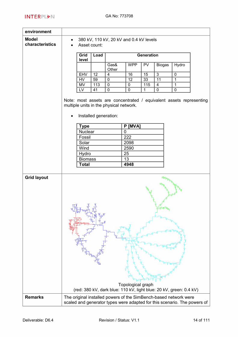
Grid layout

Topological graph

(red: 380 kV, dark blue: 110 kV, light blue: 20 kV, green: 0.4 kV) Remarks The original installed powers of the SimBench-based network were

scaled and generator types were adapted for this scenario. The powers of

GA No: 773708


fossil generators were also modified in such that all oil, coal and waste powered plants were set out of service. The installed nominal power of the remaining gas powered generators was scaled down in order to match the 2050 scenario target. Each non-fossil or distributed generator was assigned one of the types solar, wind, hydro, biomass, other, or mixed and powers were increased according to INTERPLAN-2 “Small and local”. This results are the installed powers as listed under “model characterictics” above. The load was left unchanged. The network model is primarily meant for development and testing purposes for several showcases. One of the most strict requirements was that the model must not be confidential to one INTERPLAN partner only; hence, only publicly available data were used. In effect, different simplifications were made and in particular, the model does not contain regionalized MV and LV networks or generator attributions. Hence, the model does not represent a validated predicted scenario for the Eastern German network in the year 2050. For UC5 purposes the distribution grid was changed to radial grid as shown on the picture below. Five storage units of total installed power equal to 76 MVA were added.

Topological graph of radial version

GA No: 773708


WP6 (extended) Simbench based model This model has been used by UC2 and 5.

Table 5 Extended Simbench model description

Name Eastern Germany benchmark grid model Origin The origin is the SimBench benchmark network data set.

The EHV part of the model represents the balancing zone of the German TSO 50Hertz, covering eastern Germany and the city of Hamburg. A part of the lower voltage levels in that area is represented by HV, MV and LV synthetic SimBench benchmark models, since there is no public data available for them. The model is described in detail in D6.3 chapter 3.2.1.

Adaptation In comparison to the North-Eastern Germany grid model, this model contains an extended TSO level and includes more assets. Grid reinforcements according to the German network development plan were included, and the model also uses different time series. Time series were adapted to INTERPLAN-2 2050 scenario. Adaptation process:

• Selection of according benchmark models from SimBench dataset, including time series and full EHV dataset of eastern Germany

• Application of grid reinforcements to represent future grid, i.e.: o Reinforcement of EHV topology according to the German

network development plan, including creation of 22 new lines, 8 new substations, and 4 new transformers

o Correction of generator placement and installed power according to generation data from Bundesnetzagentur, introducing equivalent generators to represent aggregated generation in HV, MV and LV areas that are not fully modelled. Placement of generators using dataset from Open Power System Data by means of a Voroni area decomposition of EHV grid node locations. According correction was not necessary for the loads since the SimBench data already contains equivalents.

• Adaptation of generation installed power, type and load to INTERPLAN-2 2050 scenario

• Selection of the timestep with least grid limit violations • Application of further grid reinforcements to remove all limit violations

and get a valid starting point for time series generation: o Reduction of EHV, HV and MV generator active power for the

timestep considered to remove voltage violations o Reduction of two concentrated EHV level load reactive

powers and adaptation of voltage regulation of 16 EHV generators in order to move reactive power outputs of generators into admittable limits

o Increasing reactive power outputs of 5 EHV static generators to move reactive power output of rotating generators into admittable limits

o Reduction of active power infeed of 5 HV and 2 MV generators to reduce line loading below 100%

o Reduction of active power infeed of two EHV generators to reduce nearby transformer loadings

o Reinforcement of one EHV line and 8 HV lines o Creation of 1 new transformer at EHV level and 2 new

GA No: 773708


transformers at HV level • Generation of time series for all assets

Class Static model (quasi-stationary simulation) Implementation environment

PowerFactory, pandapower

Model characteristics

• 380 kV, 110 kV, 20 kV and 0.4 kV levels • Asset count:

Grid level

Load Generation

Gas& Other

WPP PV Biogas Hydro

EHV 54 29 209 93 42 24 HV 59 0 47 9 0 1 MV 113 0 126 203 31 0 LV 41 0 114 114 112 113

Note: most assets are concentrated / equivalent assets representing multiple units in the physical network.

• Installed generation:

Type P [MVA] Nuclear 0 Gas&Other 2,557 Solar 22,393 Wind 27,736 Hydro 292 Biomass 2,593 Total 55,571

GA No: 773708


Grid layout

Geographic graph (red: 380 kV, dark blue: 110 kV, green: 20 kV and 0.4 kV)

Topological graph

(red: 380 kV, dark blue: 110 kV, light blue: 20 kV, green: 0.4 kV) Remarks Generally, the same remarks apply as for the north-eastern Germany

SimBench model. In particular, it should be noted that the various grid reinforcement measures to enable the high distributed renewable energy resources (DRES) infeed in the INTERPLAN-2 2050 scenario are not based on a thorough grid reinforcement planning; there was no cost assessment or worst-case analysis. Also, the placement of equivalent generators are not based on regionalization of the various generation types. For UC5 purposes the distribution grid was changed to radial grid as shown on the picture below. Five storage units of total installed power equal to 76 MVA were added.

GA No: 773708


Topological graph of radial version

Simple Cyprus grid model This model has been used by UC4 and 6.

Table 6 Simple Cyprus model description

Name Cyprus simplified model Origin Electricity Authority of Cyprus

The grid system under investigation is inspired by a part of the real physical grid area of Cyprus with a simplified version of distribution grid. Specifically, the model represents a synthetic benchmark grid which comprises transmission substations with terminals of 132 kV voltage level. Also, it comprises distribution substations operating at voltage levels of 11 kV and 400 V phase to phase.

Adaptation • The distribution substation model is composed of a distribution transformer and aggregated elements for load, electric vehicles, photovoltaic systems, distributed power generators and storage units.

• The main grid model also incorporates conventional power generation and wind power generation areas.

• The wind power generation area is composed of two transmission transformers and two aggregated areas of wind turbines.

• The conventional power generation area includes two transmission transformers and two synchronous machines.

Class Dynamic model (transient stability model) Implementation environment

PowerFactory


Transmission Substation 1, 2 and 3: with two feeders each where two HV to MV transformers of 100 MVA respectively serve the distribution side. Each of the substations serves load at the MV side (11kV). PV, BESS (storage), distributed power generators and EVs depend on the scenario. Generation Plant area: Two parallel slack node synchronous machines having a rated power of 50 MVA each. The power provided by the generators is produced at the voltage level of 11 kV and delivered into the

GA No: 773708


132 kV transmission network, through two 100 MVA transformers. Wind farm area: includes one 16 MVA transformer and two wind turbine generators (WTG). The following models are included:

• Static Generators-2 wind turbine generators (23.57 MVA each) • Load - 3 load areas with user defined models: 63.10 MW (area 1),

31.65 MW (area 2), and 25.2 MW (area 3) • PV systems - 1 aggregated PV system per load area (user defined

models) • Synchronous Generators - 2 x 50 MVA each (Automatic Voltage

Regulator Type: EXAC4, Speed Governor Type: TGOV1)

Grid layout

Remarks The Cyprus grid has been studied under two different projection scenarios.

This was of critical importance as Electricity Authority of Cyprus is willing to validate the INTERPLAN solutions and thus stress the system under the challenging RES integration rate of the future. This is also critical especially for the non-interconnected systems where the integration rate can be impactful especially in the future where low inertia systems are foreseen. In these selected scenarios, a European agreement for climate mitigation is achieved and fossil fuel consumption is expected to be low worldwide by the year 2030. Therefore, due to the low dependence on conventional fuels, fuel costs are relatively low. The CO2 costs are high due to the existence of a global carbon market. The EU's ambition for greenhouse gas (GHG) emission reductions of 80-95% by the year 2050 as compared to 1990 is achieved through this selected scenario. The strategy focuses on the deployment of large-scale RES technologies.2 Similarly, a high priority is given to the development of centralized storage solutions (pumped hydro storage, compressed air, etc.) which accompanies the large-scale RES deployment. Decentralized storage

2 ENTSO-E (The European Network for Transmission System Operators’ Electricity) Ten Year Development Plan

GA No: 773708


solutions are insufficient to support the large-scale RES deployment. Electrification of transport, heating and industry is considered to occur both at centralized (large-scale) and decentralized (domestic) level. However, the political focus is mainly on the supply side: large amounts of fossil-free generation will be complemented with investments in energy efficiency. Scenario 2030: Scenario - Nominal Capacity per power source type (MVA) Solar Wind Hydro Biomass Conventional Pump

Storage 42.3 42.3 48.9 9.2 22.5 —

It shall be noted that in the case of evaluating the stability behaviour of the Cyprus power grid, while investigating a realistic case scenario, it will be required to omit hydro power generation and reallocate its power potential to the rest of the generation technologies based on the roadmap of Cyprus power production energy mix3. Also, time series were created in collaboration with EAC engineers based on the projection and targets of 2030 and 2050 for Cyprus grid. Time series of the past years were used to extrapolate the projections. In this work, one power event was defined to enable the study of frequency stability within UC4 and UC6. The specific event simulates realistic conditions and challenges that the grid operator may confront. The stability analysis scenario adopted for 2030 simulates the loss of generation capacity of one power source as shown below. The bold characters in the tables show the affected types of generation due to the fault. The differences in the figures between the scenarios and the test cases result from the inertia that is reserved to maintain system stability

Stability Analysis Scenario for 2030 - Loss of generation capacity [MVA]

(affected source type marked with bold) - Fault in Power Station Area

Solar Wind Hydro Biomass Conventional Pump Storage

42.3 42.3 34.2 6.4 15.8 -- Scenario 2050:

Nominal Capacity per power source type (MVA) Solar Wind Hydro Biomass Conventional Pump

Storage 47.8 47.8 33.6 6.2 38.0 15.6

3 Cyprus’ Integrated National Energy and Climate Plan under the Regulation (EU) 2018/1999 of the European Parliament and of the Council of 11 December 2018 on the Governance of the Energy Union and Climate Action

GA No: 773708


In order to evaluate the frequency response for scope of both UC4 and UC6 two power events are defined. Those events simulate conditions and challenges that can occur in a realistic case.

Stability Analysis Scenarios for 2050 - Loss of generation capacity [MVA]

(affected source type marked with bold) - Fault in Power Station Area

Solar Wind Hydro Biomass Conventional Pump Storage

47.8 47.8 23.5 4.4 26.6 10.9

Complex Cyprus grid model

This model has been used by UC4 and UC6.

Table 7 Complex Cyprus model description

Name Cyprus extended model Origin Electricity Authority of Cyprus

The grid system under investigation models a part of the real physical grid area of Cyprus in 2019. Specifically, the model represents a synthetic benchmark grid which comprises transmission substations with terminals of 132 kV voltage level. Also, it comprises distribution substations operating at voltage levels of 11 kV and 400 V phase to phase. In more detail, the Complex Cyprus grid model, in addition to the structure of the Simple Cyprus grid model, includes the full 11kV distribution power network of three transmission substations of Cyprus: ALAMBRA-Area1, PROTARAS-Area 2 and DISTRICT OFFICE-Area 3

Adaptation • Each transmission substation constitutes a different control area with a significant number of distributed generation and storage units, electric vehicles, and loads according to scenario 2030 and 2050 projection.

• Each distribution substation model is composed of a distribution transformer and aggregated elements for load, EV, PV systems, and storage units at distribution substation level.

• The main grid model also incorporates a conventional power generation and a wind power generation area.

• The nominal capacity per power source type is shown for the two different projections in the table below.

• Storage units and dynamic models with synthetic inertia are added.

Scenario – Nominal capacity per power source type (MVA) Scenario Case

Solar Wind Hydro Bio-mass

Conven-tional

Pump Storage

2030 42.3 42.3 48.9 9.2 22.5 - 2050 47.8 47.8 33.6 6.2 38.0 15.6

Class Dynamic model (transient stability model) Implementation PowerFactory

GA No: 773708


environment Model characteristics

The model contains a total of 1721 lines, 3009 busbars (4891 terminals), 1006 transformers, 1925 loads (including 962 electric vehicle loads), and 1931 generators (962 PV systems, 2 synchronous machines, 962 BESS, 2 hydro systems, 2 wind farm systems and 1 biomass unit). In addition, it provides 2284 protection devices (993 fuses) and 1291 breakers/switches. • Dynamic models:

o synchronous generators: AVR: SEXS_standard GOV: TGOV1_standard

• Frequency Controllers

Grid layout

Remarks The same scenarios of study apply as in section 3.3.

GA No: 773708


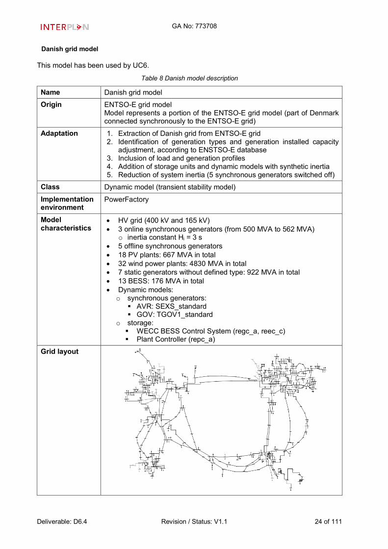
Danish grid model This model has been used by UC6.

Table 8 Danish model description

Name Danish grid model Origin ENTSO-E grid model

Model represents a portion of the ENTSO-E grid model (part of Denmark connected synchronously to the ENTSO-E grid)

Adaptation 1. Extraction of Danish grid from ENTSO-E grid 2. Identification of generation types and generation installed capacity

adjustment, according to ENSTSO-E database 3. Inclusion of load and generation profiles 4. Addition of storage units and dynamic models with synthetic inertia 5. Reduction of system inertia (5 synchronous generators switched off)

Class Dynamic model (transient stability model) Implementation environment

PowerFactory


• HV grid (400 kV and 165 kV) • 3 online synchronous generators (from 500 MVA to 562 MVA)

o inertia constant Hi = 3 s • 5 offline synchronous generators • 18 PV plants: 667 MVA in total • 32 wind power plants: 4830 MVA in total • 7 static generators without defined type: 922 MVA in total • 13 BESS: 176 MVA in total • Dynamic models:

o synchronous generators: AVR: SEXS_standard GOV: TGOV1_standard

o storage: WECC BESS Control System (regc_a, reec_c) Plant Controller (repc_a)

Grid layout

GA No: 773708


Remarks Time series were generated using methodology described in D6.1 (chapter 6).

AIT simplified grid model

This model has been used in UC7.

Table 9 AIT simplified model description

Name AIT synthetic simplified grid model Origin DECAS project grid model

Model represents a portion of an European country Electric grid model Adaptation 1. extension of the grid model with simplified LV feeders

2. identification of generation types and generation installed capacity, inclusion of load and generation profiles

3. definition of failure models of different grid components 4. definition of stochastic models of generation 5. definition of cost functions of different load types interruptions 6. definition of different load shedding scenarios 7. definition of generation operating costs


PowerFactory


The synthetic network used in this use case consists of 34 LV feeders connected to two MV feeders (rural and urban). Among them, 10 LV feeders are modelled in detail while the remaining LV networks are represented by the equivalent models.

Feeder name

No. of PVs

No. of gene-rators

No. of lines

No. of loads

No. of termi-nals

No. of trans-formers

MV Rural 0 4 39 6 61 22 MV Urban 0 4 15 0 25 10 LV urban 5 14 0 21 19 21 0 LV urban 1 20 0 28 25 28 0 LV urban 2 14 0 22 19 22 0 LV urban 3 20 0 30 26 30 0 LV urban 4 24 0 34 31 34 0 LV rural 1 12 0 26 16 26 0 LV rural 2 10 0 22 14 22 0 LV rural 3 12 0 30 17.0 30 0 LV rural 4 16 0 34 22 34 0 LV rural 5 0 0 2 1 2 0

Some of the LV grids are equivalented, following is the information about them:

Feeder name

Number of

GA No: 773708


PVs Gene-rators

Lines Loads Termi-nals

Trans-formers

Rural LV 14 1 0 105 103 105 0 Rural LV 15 2 0 108 110 108 0 Rural LV 4 2 0 137 139 137 0 Rural LV 20 1 0 114 114 113 0 Rural LV 21 2 0 110 116 108 0 Rural LV 10 1 0 77 104 77 0 Rural LV 11 0 0 96 103 95 0 Rural LV 12 0 0 88 103 86 0 Rural LV 3 1 0 152 144 151 0 Rural LV 5 1 0 137 123 135 0 Rural LV 6 1 0 114 111 112 0 Rural LV 8 0 0 109 103 109 0 Rural LV 9 6 0 79 100 79 0 Rural LV 1 1 0 169 144 164 0 Rural LV 16 4 0 83 109 83 0 Rural LV 17 3 0 118 113 118 0 Rural LV 18 2 0 121 117 121 0 Urban LV 3 4 0 683 213 676 0 Urban LV 5 2 0 390 193 388 0 Urban LV 7 4 0 457 200 451 0 Urban LV 9 0 0 438 173 437 0 Urban LV 1 1 0 98 113 96 0

Static generators connected to MV grid:

Name Nominal power (MW) Biomass 1 Biomass 2 DG1_Coal-fired combustion turbine DG2_Natural gas combustion turbine DG3_Coal gasification combined-cycle (IG DG4_Natural gas combined-cycle DG5_Hydroelectric DG6_Hydroelectric Wind Farm 1 Wind Farm 2

1.2 0.2 0.25 0.4 1.2 0.2 0.5 0.65 3.2 1.4

No. of Busbars 346 No. of Lines 311 No. of Loads 273 No. of 2-w Trfs. 34 No. of 3-w Trfs. 2

GA No: 773708


Grid layout

Remarks The time series were used for this grid model in the preparation phase for generating a credible contingency list These were created using Austrian standard load profiles.

AIT synthetic grid model

This model has been used in UC7.

Table 10 AIT synthetic model description

Name AIT synthetic extended grid model Origin DECAS project grid model.

The grid model under test has detailed urban and rural feeder models. Adaptation 1. extension of the grid model with detailed LV feeders

2. identification of generation types and generation installed capacity, inclusion of load and generation profiles

3. definition of failure models of different grid components 4. definition of stochastic models of generation 5. definition of cost functions of different load types interruptions 6. definition of different load shedding scenarios 7. definition of generation operating costs


PowerFactory


The synthetic network used in this use case consists of 34 LV feeders connected to two MV feeders (rural and urban). All LV feeders are modelled in details. 1. The same data are used as in the simplified grid 2. The same models and data are used for the extended LV grids 3. No equivalented LV grids are used

GA No: 773708


4. Reliability model parameters and load flexibilities are defined In addition,interruption costs tariffs for loads flexibility whether loads are industrial, residential or commercial are used. Scenario Households Commercial Industrial

Base 0 – 40 % 0 – 30 % 0 – 40 % 1 0 – 50 % 0 – 50 % 0 – 50 % 2 0 – 70 % 0 – 60 % 0 – 60 % 3 0 – 100 % 0 – 70 % 0 – 70 %

Load shedding flexibility scenarios Grid layout

Remarks The time series were used for this grid model in the preparation phase for

generating a credible contingency list These were created using Austrian standard load profiles.

IEEE 14 Bus Power System This model has been used by UC6.

Table 11 IEEE 14 Bus Power System model description

Name IEEE 14 Bus Power System Origin The model is based on Freris et al. [9] Adaptation 1. Base frequency of the model was changed from 60 Hz to 50 Hz.

2. Operating point of generators was changed to the following values:

Gen 1 Gen 2 Gen 3 Gen 6 Gen 8 Type Synch. Synch. Synch. Wind Wind

Rating MVA] 200 220 160 72 100 Active power [MW]

50 30 117 49 77

H [s] 3.2 4.0 2.0 0 0

GA No: 773708


3. A battery energy storage system (BESS) was added to the model and connected to bus 12

Class ElectroMagnetic Transient Program (EMTP) class model Implementation environment

Real-time digital simulator (RTDS)


The benchmark 14 bus power system is one of many widely used models for studying voltage stability, angle stability, FACTS (flexible alternate current transmission systems) applications, HVDC (high voltage direct current) transmissions, renewable sources integration and others. As explained under “Adaptation”, the model was changed to reflect a scenario in which synchronous generation is substituted with wind generation. Wind generation constitutes 23% of total generation in this model and the current operating point is selected such that 39% of load is supplied from wind generation. The added BESS model simulated in RSCAD (real-time simulations software package) consists of two 9.69 MWh Li-Ion batteries interfaced to the grid through an three-phase three-level Neutral Point Clamped (NPC) converter and a 10.39 V/15 kV transformer. The converter operates at a switching frequency of 1250 Hz. The BESS operates in a power range of -100 MW .. +100 MW. The BESS model is determined by the following main parameters:

• number of cells per stack: 10000 • number of stacks in parallel: 300 • capacity of a single cell: 0.85 Ah.

The RTDS lithium-ion battery system model enables the proper representation of the device in real time simulation. The battery model can be represented by one of two different ways of modeling the li-ion battery dynamics. The first one is referred to as ‘Min/Rincon-Mora’ model while the second one is referred to as ‘Huria/Ceraolo/Gazzarri/Jackey’ model. The ‘Min/RinconPower’ model [10] was extracted from a real commercial li-ion polymer battery, TCL-PL-383562 from TCL Hyperpower Batteries Inc. (China). The modelling method is focused on the electrical behaviour of the battery and voltage-current characteristics. Neither the battery lifetime modelling nor the thermal aspect of the battery such as the thermal dependency of the circuit parameters is considered in the model. The ‘Min/Rincon-Mora’ has been chosen as suitable for process simulation. Compared to this model the ‘Huria/Ceraolo/Gazzarri/Jackey’ model takes account of the temperature effect on the model dynamics. The equivalent electrical circuit of the battery model is presented below.

GA No: 773708


Grid layout

Remarks

GA No: 773708


4. Results and evaluation

Introduction Following the methodology described in chapter 2.1, the use cases are validated using the grid models described in the previous chapter. For validation purposes ten planning criteria were used:

1 Assuring voltage stability 2 Assuring transient stability 3 Assuring frequency stability 4 Mitigating grid congestion 5 Minimizing losses 6 Minimizing cost 7 Minimizing energy interruptions 8 Optimize TSO/DSO interaction 9 Maximizing share of RES 10 Maximize DG/DRES contribution to ancillary services

Additionally, the base showcases results (presented in D5.2) were used as benchmarks for the validation of WP6 results, since base use cases were cases in which no controllers were present in the analysed grid models. The results of use cases testing were described in the following subsections. UC1: Coordinated voltage/reactive power control UC description

The goal of this UC is application of reactive power control of DER at the TSO and DSO levels in order to ensure voltage stability in a coordinated manner. The presence of DER can significantly impact the power networks, exposing the system to much higher power fluctuations and potentially compromising the system power quality. Ensuring voltage stability is an even more important issue looking at the increasing penetration levels of DER. Therefore, innovative control schemes that include the DER voltage control capabilities have to be considered in the future power systems. Hence, the UC presents a control scheme to improve TSO-DSO coordination in managing the grid for voltage stability at all voltage levels by applying a coordinated TSO-DSO optimization methodology. This includes utilization of the DSO flexibilities to respect TSO optimization objectives that aim to prevent voltages violation problems in the system. The active resources used for this are synchronous generators and distributed generators using renewable energy sources. The operation principle of the control scheme consists of four steps. The first step is meant for preparation. It includes an initialisation consisting mainly of a power flow calculation, resulting in initial voltage levels and generator set points for powers. The second step assesses the reactive power flexibility at the TSO/DSO connection points, resulting in in minimum and maximum reactive powers that can be provided by the DSO at those points. The second step uses a DSO grid equivalent to simplify the calculation. The third step consists in an optimal power flow calculation at the TSO side, which results in an optimal selection of reactive power provided by TSO assets and reactive power to be provided by the DSO at each connection point. The latter power is chosen within the flexibility range obtained in step 2. Finally in step 4, a DSO optimal power flow (OPF) is carried out in order to fix the DSO generator set points that allow for optimal provision of the reactive power that was fixed in step 3. At the end of step 4, all reactive power set points for all generators in all regarded voltage levels are calculated.

GA No: 773708


High relevance planning criteria

1. Assuring voltage stability 5. Minimizing losses 8. Optimize TSO/DSO interaction

Planning criteria plot for UC1

Medium relevance planning criteria

10. Maximize DG / DRES contribution to ancillary services

Validation level 1: Assessment of compliance with user requirements and objectives 1.1 Elaboration on how a use case addresses planning criteria The following elaboration is based on the testing of the use case in the framework of showcases 2 and 4. The testing was done using the SimBench network provided for WP5. The use case was generally applied for generating a day-ahead reactive power operation plan for controllable generators. Nominal active and reactive power operation points for all generators were available for one day through the time series prepared for base showcases (BSC) 2 and 4, and the use case application resulted in modification of the reactive power operation points for all time steps. Criterion: Assuring voltage stability This criterion was assessed using the voltage magnitude of each of the 246 buses in the EHV, HV, MV and LV levels of the test network. This refers to KPI 10 “Voltage Quality”. The results from both SC2 and SC4 test cases with activated use case control indicate that, for the simulated day, all voltage levels stay within a range of 0.99 ... 1.015 p.u. for the transmission network, and 0.99 ... 1.05 p.u. for the total network including the distribution level. This is well within thresholds permitted by the relevant standards. A comparison with the base showcases (BSC2, BSC4) shows that the use case controller narrowed down the voltage band in the transmission level (BSC: 0.96 ... 1.04 p.u). This is attributable to the OPF calculation at both TSO and DSO levels, which is carried out for the SC2 and 4 but not for BSC2 and 4. Criterion: Minimizing losses This criterion was assessed using KPI 1 “Level of losses in transmission and distribution networks”. The losses are calculated as time-dependent active line-by-line power losses for the whole network set in relation to the total injected active power. The result shows that, depending on the time step of the simulated day, they vary between 1.2 % and 2.087 % for the whole network. The peak value for the transmission level is 1.84%. This indicates the amount of losses in the grid. A comparison with BSC2 shows that the transmission level losses are lower for all time steps if the SC2 controller is activated. The same result was generally obtained by comparing BSC4 and SC4. The result can be attributed to the OPF calculations at TSO and DSO levels, where loss minimization is the primary optimization goal. Criterion: Optimize TSO/DSO interaction This criterion was assessed using KPI 13 “Mean quadratic deviations from voltage and reactive power targets at each connection point between TSO and DSO grids”. This KPI is calculated as time-dependent mean quadratic deviation over all TSO/DSO connection points for voltage and reactive power targets individually. Said targets are a result of the third step of the use case. The results for SC2 show that the deviations can be kept lower than 0.05 Mvar (reactive power) and

GA No: 773708


0.002 p.u. (voltage) for most of the time steps. Peak values of around 1 Mvar and 0.0045 p.u. occur at three time steps only. For BSC2, the minimum KPI values were around 13 Mvar and 0.008 p.u. Hence, the use case controller has much improved the KPI. Taking a look at SC4, the reactive power deviation is around 1.1 Mvar at maximum and close to zero otherwise. The voltage deviation is at around 0.0012 at maximum. Again, this is a substantial improvement when compared to BSC4, where the maximum values were around 9 Mvar and 0.0135 p.u. This result can be attributed to the DSO OPF carried out in step four of the use case because minimizing the reactive power and voltage deviation is part of the objective function in this step, where the DSO tries to follow the TSO targets as close as possible. Criterion: Maximize DG / DRES contribution to ancillary services This criterion was assessed using KPI 14 “Level of DG / DRES utilization for ancillary services”. The ancillary service relevant for use case 1 is reactive power provision for means of voltage control. The KPI was calculated as time-dependent ratio between inductive, capacitive and absolute reactive power scheduled for DER and the total according reactive power delivered by all generation in the network. For SC2, it was found that in most of the time steps of the day simulated, DER inject reactive power (inductive) into the network with a maximum contribution of 66.02%. The maximum capacitive reactive power is 55.7 %. A comparison with BSC2 is not possible for this KPI, since there was no provision of reactive power used for voltage control in BSC2. In case of SC4, KPI 14 was not calculated, but instead KPI 24 “Reactive energy provided by RES and DG” can be used to assess the criterion. This KPI is calculated as sum of the reactive power absolute over all generators within a time interval t1..t2. The KPI was also calculated for BSC4, and the result shows that sum for SC4 exceeds the BSC4 values for some of the time steps. Even if the KPI cannot be used to quantify the DER contribution to voltage control directly, it indicates that the use case controller actively uses RES and DG reactive power generation for voltage control. 1.2 Assessment of legal and regulatory conditions The provision of reactive power for means of static voltage control is addressed by regulation in various European countries. The requirements are partly specific to voltage levels and generation technology. E.g. in Italy, DER generators connected to LV and MV levels have to participate in voltage control according to CEI 0-21 and CEI 0-16. In Germany, generation units in the EHV, HV and MV grids must contribute to reactive power provision for voltage control within certain limits depending on the type of the plant. If applicable due to the type, the grid operator may apply a reactive power set point which may also be transmitted remotely (VDE-AR-N 4130, VDE AR-N 4120, VDE-AR-N 4110) as one option of reactive power provision. The according regulation for the LV level does not list this option. This is also the case for storages and electric vehicle charging stations. The use case foresees a collaboration between TSO and DSO in terms of the DSO offering flexibility for reactive power provision, and the TSO requesting such reactive power provision per TSO/DSO connection point. In Germany, VDE-AR-N 4141 applies to this, but this option is not specifically described. The European network code NC DCC Art. 15 (3) allows the TSO to require active control of reactive power exchange by DSOs for benefit of the entire system. It states: “The relevant TSO and the transmission-connected distribution system operator shall agree on a method to carry out this control”. NC DCC Art. 15 (4) states that, vice-versa “The transmission-connected distribution system operator may require the relevant TSO to consider its transmission-connected distribution system for reactive power management”. All in all, regulation supports the reactive power / voltage control scheme proposed by the use case with the sole exception of the low voltage level, where DER are not generally required to be able to follow a reactive power set point from the grid operator. 1.3 Deployment possibilities

GA No: 773708


The original idea of the use case is to make use of distributed generation for optimal voltage control for the whole network, involving a coordination between TSO and DSO. This is an idea very close to application because, as can be seen from the regulation assessment above, it can be expected that many generators already allow for remote reactive power control. Also, TSO/DSO coordination is considered of growing importance as grid operation becomes more and more complex, and the DSO level can no longer be regarded as inactive consumer level. Hence the use case concept can be seen as an extension of state-of-the-art methods of voltage control. The main question in terms of applicability is if classic methods – the most important being TSO-level reactive power generation, reactive power compensation units and regulation transformers at TSO/DSO connection points – are sufficient for an optimal voltage control scheme. Also, the cost of classic methods versus the use case concept are of interest; if e.g. usage of DSO-level generators for reactive power provision has the same performance and security in terms of voltage control as the building of a new reactive power compensation unit, but at lower cost, it is obviously the preferable option. In reality, it might be the case that reactive power control schemes not requiring remote connections are preferred for reasons of simplicity and security, even at the cost of lower optimality of the overall grid operation. After all, it cannot be expected that TSO and DSO optimize their combined costs, but rather optimize costs individually as two independent utilities. It is obvious that a thorough study of this would be needed for reaching detailed conclusions; however, studying this has been out of scope of the use case development. There are various obstacles to use case implementation:

• The availability of DSO-level generators with the ability of remote reactive power control may be limited

• TSO and DSO control centers may be missing the IT infrastructures to (i) remotely connect to generators for means of reactive power control and (ii) targetfully use this means for grid planning in a way that is automated and integrated. This is a very wide and problematic area. It applies to hardware used for data transmission and processing, but also software for support of grid operation planning (this includes not only planning, but also simulation of expected system behaviour), and life on-line grid operation. Next to this, grid operation simulation tools are also needed to assess the potential benefit of applying reactive power control to new generators, and to find the optimal solution in terms of which controllable units to use (also in terms of cost, cp. above). Finally, practical application must also involve TSO and DSO control center operators who need to be trained on using the new systems. IT infrastructures furthermore have to be made robust against connection outages and cyber-attacks.

• The application of the use case requires TSO/DSO interaction which may be unusually close. According structures for such interaction may be missing. This especially applies for the exchange of potentially critical data (e.g. information about the peer network)

Considering the last point, grid models come into mind. The current implementation of the use case only adopts grid equivalents at one of the steps; hence, applicability is only given for TSO/DSO pairs that already collaborate very closely and are willing to at least exchange part of their grid data. A possibly realistic example for application is a network with limited area that contains all voltage levels, e.g. a larger island system like Cyprus. If the use case can be shown to yield cost benefits when compared to conventional methods, application in continental networks becomes an interesting option.

GA No: 773708


Validation level 2: Performance evaluation 2.1 Controller robustness Validation method: same grid, different time series Model used for controller design (use case): North-Eastern Germany grid model (cp. chapter 3.1). Model used for validation: North-Eastern Germany grid model Key differences between the models: time series used in the two cases of applications Validation results: UC1 is one out of two use cases that are included in two different showcases. The application of the use case in these two showcases is different. In the first one, SC2, the use case is applied after UC2, which fixes the active power set points of controllable network assets in order to avoid grid congestions. These set points are taken as input to UC1, which optimizes the reactive power set points of the same assets, keeping the active power set points unchanged. In the second showcase, SC4, UC1 is applied first, taking the active power operation points from the original baseline time series as input. The design and development of the use case control function was done mainly during the work for SC2, which was the first showcase that was completed. As mentioned under validation level 1, the results from the application of the control function to the different time series in showcase 4 confirms the previous results. The difference in the results can be attributed to the difference in the time series. Hence it is concluded that the use case, in its current implementation, performs adequately for two different time series. Since the algorithms used for implementation are generally independent from the specific time series, adequate performance can be expected for any time series which does not violate operational limits of the network. 2.2 Implementation procedure and requirements Use case workflow:

• Preparations: prepare grid models in right format. Prepare time series. Configure grid to target configuration (e.g. close/open switches, activate assets). Make sure power flow can converge. Used Tools: PowerFactory

• Network data (complete TSO/DSO and reduced TSO/DSO network) as well as time series information have to be prepared once in advance

• Step 1: Initialization o Fetch set points for asset active powers (if applicable, cp. SC2) from an Excel

file. o Accordingly set grid assets in PowerFactory. o Generate .dat file (automatic, by DPL script). o Reading .dat file, perform initial power flow for given time step in AMPL o use resulting grid state as initial state for Step 2. o Used tools: PowerFactory, AMPL o Used functions: AC Power flow in PowerFactory and AMPL

• Step 2: DSO reactive power flexibility assessment o calculate amount of reactive power that can be delivered to each DSO/TSO

connection point as input for Step 3. o Flexibilities calculated by two optimizations for Qmin as well as Qmax o Write flexibility values in .dat file to be used in step 3 o Used tools: AMPL o Used functions/method: AC Optimal Power Flow in AMPL

• Step 3: TSO OPF

GA No: 773708


o Generate a TSO network where the DSO is represented by equivalent generators at each DSO/TSO connection point.

o Generate .dat file from this network o Read network .dat file as well as .dat file from Step 2 into AMPL o Set reactive power flexibility of generators at DSO/TSO connection points as

operation range for TSO AC OPF. o Carry out AC OPF based on loss minimization. o Extract reactive power set points for TSO assets and DSO/TSO interconnections

and write into .dat file. o Used tools: PowerFactory, AMPL o Used functions/method: AC Optimal Power Flow in AMPL

• Step 4: DSO OPF o Read grid .dat file from step 1 and .dat file resulting from step 3 into AMPL o Set reactive power set points at TSO/DSO interconnections obtained from step

3 by implementation in objective function. o Fix set points for TSO assets. o Carry out AC Optimal Power Flow based on loss minimization considering

predefined set points from step 3. o Store reactive power set points for all assets as Excel file. o Used tools: AMPL o Used functions/method: AC Optimal Power Flow in AMPL

Figure 3 The procedure of use case 1 control algorithms

Additional factors:

• The runtime for step 1 to step 4 is within the range of 2-5 Minutes on a normal notebook (Intel Core i7-8550, 16 GB RAM, Windows 10) for 24 time steps (might vary)

• The process will not fail, if all data are provided correctly. If the initial power flow does not converge, it might be possible that the optimization provides infeasible solutions due to the not converging power flow. This can be seen by the output from the used solver in the AMPL interface.

GA No: 773708


Validation level 3: Identification of peculiarities of individual use cases The main drawback of the current implementation of the use case control function is that it causes comparatively high effort to apply it to a different network. This requires deep understanding of the control function code and proper modification, which was not possible within the project’s resources and taking into consideration targeting rather low TRL5. Nevertheless, there is no general technical hindrance to this, as the control function algorithm does not rely on assumptions valid for a specific network only.

GA No: 773708


UC2: Grid congestion management UC description

This use case is about TSO and DSO using control logics to mitigate grid congestion problems at both transmission and distribution levels. During the operation planning phase, the tool evaluates the suitable resources through their generation schedule in order to re-dispatch the related active power flows for mitigating grid congestion. This use case acts both on DSO and TSO levels by operating on the available controllable resources (e.g. storage, flexible loads, EVs, DG), and considering power flow re-dispatch. With the increasing share of distributed renewable energy, both transmission and distribution grids have to face new challenges. Generally, the places with significant availability of renewable energy are often not very densely populated areas, thus the local energy production may exceed the local demand. This situation may lead to network congestions such as network overloading. In this scenario, the power flow re-dispatch during the operation phase plays a key role. The main functions implemented in the congestion management control are:

• Congestion detection • Active power flexibility evaluation per each asset in the grid • Sensitivities analysis • Active power redispatching

When congestion problems are detected in the grid, the control is triggered and as first step, the active power flexibility available by each asset in the grid is evaluated. An internal table is created with the information about maximum/minimum active/reactive power per each asset, busbar linked with the asset, etc. With the sensitivities analysis the effects of Iactive/reactive power injection changes ΔP and ΔQ at busbar i are evaluated providing a sensitivities matrix varying the ΔP and ΔQ injection point (busbar). This information is used for the optimal solution calculation (active power variation at each busbar) to mitigate/solve the detected congestion problems. Once the optimal solution in terms of minimal active power variation at each busbar has been calculated, an active power redispatching function is triggered.


4. Mitigating grid congestion 10. Maximize DG / DRES contribution to ancillary services



GA No: 773708


Validation level 1: Assessment of compliance with user requirements and objectives 1.1 Elaboration on how a use case addresses planning criteria Criterion: Mitigating grid congestion problems The growing share of distributed generation and renewable energy sources in the electrical grids increases the reliability issues leading to congestion problems and possible disconnections of network parts. In this situation finding proper solutions for mitigating grid congestion problems is a crucial point and DG/DRES contribution can play a crucial role. The grid congestion mitigation assessment is done with the KPI 2 "Congestion detection" evaluating the grid congestion state before and after UC2 control action. The line loadings are continuously monitoring and in case of congestion detection, the active power is re-dispatched among the DG/DRES in the grid based on the optimal solution obtained. Criterion: Maximize DG / DRES contribution to ancillary services Related to this criterion, this also represents a new opportunity for the DG/RES to be involved in the ancillary services to solve the aforementioned issues. 1.2 Assessment of legal and regulatory conditions

Network codes and guidelines provide the first basis for congestion management and balancing (especially System Operation Guideline (SOGL) and Electricity Balancing Guideline (EBGL)). However, both SOGL and EBGL are focused on TSO level neglecting the DSO role. The DSO can only provide information for congestion solutions without clear provisions about the resources controllability and observability at DSO level. This means that the flexibility resources are provided only at TSO level. Indeed, due to unbundling, grid operators are basically forbidden to interfere with generator operation, but there are specific laws and regulations which make exceptions for ensuring stable grid operation. E.g. in Germany, there is the infeed management acc. to §13 EnWG / §§14, 15 EEG which is in effect when grid congestions occur; RES generation assets at the DSO level may be derated as a mitigation measure as well.

1.3 Deployment possibilities

The idea behind the UC2 control is using the rising DG/RES presence in the power grid to provide an ancillary service regarding grid congestion problems mitigation at all voltage levels. With an optimal active power re-dispatching it is possible to solve congestion problems avoiding/delaying an expensive grid reinforcement and maximizing the DG/DRES contribution to ancillary services. The applicability of the use case requires the controllability of the DG/RES and storages in the grid at all voltage levels as well as a close collaboration between TSO and DSO. Absence of regulations allowing the provision of services for balancing and congestion management from DER, storage, demand and EV represents a barrier for the applicability control. Moreover, since the information about the asset flexibility in the grid, at both TSO and DSO level, represent critical data for the proposed control, close collaboration between TSO and DSO is important to ensure an effective and reliable bidirectional exchanged data. Indeed, information about flexibility resources in grid, as well as detected congestions information, have to be continuously exchanged between TSO and DSO to allow a proper control activation.

Validation level 2: Performance evaluation 2.1 Controller robustness Validation method: different grid, different scenario, different detail representation

GA No: 773708


Model used for controller design (use case): North-Eastern Germany grid model (section 3.1) Model used for validation: Eastern Germany benchmark grid model (section 3.2) Key differences between the models: The model used for validation contains an extended TSO model. Moreover, it uses a new time series in compliance with INTERPLAN-2 2050 scenario.

Figure 4 Maximum line loading in the TSO grid

Any line with loading value greater than 95% are considered congested in this example. As shown in the figure above, no congestion problems are detected at the TSO level. At the DSO level time steps with congestion issues were determined according to the table below.

Time Steps Congested Lines 44 MV2101 Line 13 – 96.87%

MV2101 Line 86 – 95.4% 46 MV2101 Line 13 – 96.2%

MV2101 Line 86 – 96% 47 MV2101 Line 13 – 98.5%

MV2101 Line 49 – 97% MV2101 Line 74 – 97.6% MV2101 Line 86 – 96.2%

48 MV2101 Line 49 – 97.3% MV2101 Line 74 – 96.6% MV2101 Line 86 – 95.6%

49 MV2101 Line 74 – 96% All the lines listed in the table have a loading value greater than 95%. The congestion management algorithm is employed to mitigate the detected congestion problems by changing the active power set points of the DG/RES in the grid. The figure below shows the maximum line loading value before and after the control action.

GA No: 773708


Figure 5 Maximum loading lines value before and after the control action

After the control action (blue line) all lines in the grid have a loading value less the 95% per each time steps. The active power for the ancillary services provided by DG / DRES is calculated as minimal active power variation at bus bar i to solve the detected congestion problems in the grid (i.e. to provide the required ancillary services). Since the line loading value at congested time steps are close to the loading threshold (95%), the active power contribution required to DG/RES to solve the congestion problems is not significant (see table below).

Time Steps DG/RES

contribution [%] 44 0.02 46 0.03 47 0.03 48 0.027 49 0.02

As previously described, the used grid model is an Eastern Germany benchmark model with different time series compared with the one used for the base case simulation. The new time series have modified the congestion scenario compared to the base case, leading to congestion problems at DSO level and a TSO level without congestion events. The UC2 has been anyway capable to solve the detected problems showing an adaptability behaviour despite grid and time series modifications. 2.2 Implementation procedure and requirements Use case workflow: The steps below describe the main stages of the proposed use case:

1. Congestion Detection 2. Active power flexibility evaluation per each asset in the grid 3. Grid Sensitivities Assessment

GA No: 773708


4. Optimization Stage 5. Active power redispatching

Congestion Detection By means of a continuous grid monitoring, each line current is measured and compared with the line’s rated current. In the event that the measured current value is greater than the rated current, the congestion control is triggered. Flexibility Resources Assessment The active power flexibility available by each asset in the grid is evaluated. During this stage an internal table is created with the information about maximum/minimum active/reactive power per each asset, busbar linked with the asset, etc. Grid Sensitivities Assessment The effect on active/reactive power of the injection of ΔP and ΔQ at busbar i is evaluated during the sensitivities analysis stage providing a sensitivities matrix varying ΔP and ΔQ at the injection point (busbar). Optimization Stage The optimal solution in terms of minimal active power variation at each busbar to solve/mitigate the detected congestion problems in the grid is calculated. Active power redispatching Based on the optimal solution, new active power setpoints per each assets in the grid are calculated. The execution times for the described stages related to the detected time steps with congestion problems are shown below. The first step has been neglected, since it does not require significant computational effort. It is worth noticing that the execution times are pretty much equal per each detected congested time step. Stages 2 and 3 have the highest execution times. They depend on the grid complexity. The stage 2 execution time increases with DG/RES increasing in the grid, while the stage 3 execution time grows with the busbar number in the grid. Also, the stage 4 execution time depends on grid complexity but it requires a lower computation effort and thus has lower execution time compared with stages 2 and 3. The figure below shows the control execution time related to the time step 46. As can be seen in the congested lines table above, the congestion situation at time step 46 is pretty much equal to the congestion status at time step 44. Consequently, the execution time to solve the congestion problem related to these steps is the same. Thus, the execution time for the time step 44 has been neglected.

GA No: 773708


Figure 6 Control execution time related to time step 46

The figures below show the UC2 execution time to solve the congestion problems detected at time steps 47, 48 and 49. As can be seen, the execution time trend is the same and per each time step the higher execution times are attributable to stage 2 and 3.

GA No: 773708


Figure 7 Control execution time related to time steps 47,48 and 49

Validation level 3: Identification of peculiarities of individual use cases

No special issues

GA No: 773708


UC3: Provision of tertiary control reserve based on coordinated TSO-DSO optimal power flow calculations

UC description

With the rising amount of distributed renewable energy sources, which naturally have intermittent generation, the grid operation strategies have to be adapted and planned in an optimised fashion. It is expected that the future pan-European network will host a considerably high share of RES and storage in time horizon 2030 to 2050 in comparison to the current situation. To ensure stable and optimal operation of such a network, a more coordinated real time TSO-DSO network operation strategy should be taken into consideration. One of the important aspects in operation is frequency control, which is consisting of different levels with different timings. Tertiary control is the last control level which considers optimal dispatch of required reserve for restoring and maintaining the frequency at its nominal value. In a network with high share of RES, new control strategies for such optimal dispatch are required in order to plan the operation of the network more efficiently considering the challenge these technologies bring to the system. Use case 3 presents an optimization strategy for energy flow management between transmission and distribution grid ensuring power balancing on one hand, and on the other hand for participation of non-synchronous energy resources in the tertiary reserve market and supporting the TSO in keeping the whole network stable. The active resources used for this are synchronous generators and distributed generators using renewable energy sources. The operation principle of the control scheme consists of four steps as shown in figure 7. The steps are executed for each time step considered: Step 0: The time series data are introduced to the grid model and the initial conditions are defined by a load flow calculation. Step 1: The DSO, having an equivalent model for the transmission network, identifies the maximum and minimum available active power that it can provide to the TSO level through the available connection points between these two levels. Step 2: Considering the required tertiary reserve for the considered time and having an equivalent model for the distribution network, the TSO identifies the active power set points for the TSO/DSO interconnection points and the TSO generation units. Step 3: The DSO with regards to the identified set points from step 2, calculates the set points for the remaining controllable units, i.e. generators and controllable loads at DSO level, through solving a multi-objective optimisation problem (minimising the losses, maximising the share of RES, etc.).

GA No: 773708


Figure 8: The procedure of use case 3 control algorithms


3. Assuring frequency stability 5. Minimizing losses 8. Optimize TSO/DSO interaction 9. Maximizing share of RES 10. Maximize DG / DRES contribution to ancillary services



4. Mitigating grid congestion 6. Minimizing cost

Validation level 1: Assessment of compliance with user requirements and objectives 1.1 Elaboration on how a use case addresses planning criteria Criterion: Assuring frequency stability The control functions are meant to utilise the available flexibility at DSO level as much as possible for satisfying the need for tertiary reserve for frequency control. The need for tertiary reserve is identified by the TSO, and the DSO contributes to it based on its available resources. Criterion: Mitigating grid congestion The control function assesses the loading of all lines and transformers in each case of active power redistribution among controllable units. In case any of those are expected to be overloaded, the redistribution is modified. Therefore the optimized solution will be always without grid congestion issues. The maximum capacity for lines and transformers is considered as 100% in the corresponding test case. Nevertheless, this limit is modifiable in the use case control algorithms. Criterion: Minimizing losses The main objective of the optimisation problem integrated in the control function is to minimise the active power losses. In other words, the control algorithm finds the optimal active power redistribution among controllable units with respect to the lines and transformers power losses

GA No: 773708


and of course other restrictions such as availability of controllable units and congestion issues. As an example, the use case 3 control function was applied in showcase 4 for every 4th time step in the interval between time steps 28 to 88 (whenever there is an assumed tertiary reserve request). The figure below illustrates that, whenever the use case 3 control function is active, the level of losses is decreased by about 0.5%.

Figure 9 Level of losses in the network

Criteria: Minimizing cost, Maximizing share of RES, Maximize DG / DRES contribution to ancillary services Another optimisation objective of this use case is maximising the share of RES in both the total generation and in ancillary services, which is the provision of tertiary reserve, and consequently minimising the costs of generation. It is assumed that the generation costs for RES and DRES in the grid scenario are lower than the conventional/synchronous generators' costs. In order to realise this, the control algorithms give higher priority to the RES/DRES, whenever they are available and controllable. As shown in the figures below, the level of DG/DRES utilisation for ancillary services has been increased from 0 % up to maximum 3.0% and the share of RES in generation has been also increased from minimum 85% to 100% in the time steps that use case 3 is active in showcase 4 as compared to base showcase 4, where no control functions were applied. Considering the mentioned criteria and their importance in this use case, a multi-objective optimisation function was designed in order to address all these planning criteria. As there is more than one objective/criteria in the optimization function, they are weighted based on their priorities. Depending on the need of the system operator, these priorities can be changed and adapted.

GA No: 773708


Figure 10 Level of DG/RES utilization for ancillary services

Figure 11 Share of RES

Criterion: Optimize TSO/DSO interaction As shown by the previous figures, the control algorithms involve both TSO and DSO levels in the process of optimisation and this requires their close collaboration in order to utilise the flexibility available in both levels as much as possible, and to minimise the total grid power losses. 1.2 Assessment of legal and regulatory conditions

The latest European grid code in the context of this use case is provided at PART IV, “LOAD-FREQUENCY CONTROL AND RESERVES” in “Commission Regulation (EU) 2017/1485 of 2 August 2017 establishing a guideline on electricity transmission system operation” [12].

GA No: 773708


In this grid code, it is emphasized that the TSO and DSO should collaborate on providing the replacement reserve or tertiary reserve similarly as in the use case. Nevertheless, this mentioned collaboration seems to be of longer range of time and not specifically about planning the operation in short term, for instance for the next 24 hours, which is the considered time in the use case. Besides, according to the grid code, the replacement reserve units should be equal or bigger than 1.5 MW, but there is no specification on the technologies, such as renewable sources or storage. In the grid codes, it is mentioned that operational security limits should be taken into consideration when activating the reserve capacity, which is very important. Nevertheless, there is no specification on minimisation of power losses. 1.3 Deployment possibilities

Use case 3 suggests an optimisation strategy for a coordinated provision of tertiary reserve for a near future like the next 24 hours. At the moment this is not put into practice. Even though the regulation emphasises on TSO-DSO collaboration, this is not meant for a real time and planning collaboration of tertiary reserve / replacement reserve. In order to prepare for deploying such strategies, the following is suggested:

• Improve the regulation and grid codes from the perspective of TSO-DSO real-time interaction on network operation.

• The ICT infrastructure should be further developed, in order to respond to the need of TSO-DSO interaction as describe above.

• The market of provision of replacement reserve shall be reviewed and adapted to if such strategies are approved and need to be implemented.

Validation level 2: Performance evaluation 2.1 Controller robustness Validation method: The use case 3 control function was included in two different showcases, namely “SC3: TSO-DSO power flow optimisation” and “SC4: coordinated TSO-DSO active and reactive power optimisation for voltage control and provision of tertiary control”. This means the use case 3 control function was designed for the implementation in showcase 4 and then validated for the second time through its implementation in showcase 3. This is described below under part 1. Additionally, use case 3 was a part of the INTERPLAN tool demonstration and as such was validated for the third time, which is described under part 2. Part 1: Validation method: same grid, different detail representation Model used for controller design (use case): North-Eastern Germany grid model (section 3.1), meshed distribution network, usage of grid equivalents for both TSO and DSO levels Model used for validation: North-Eastern Germany grid model (section 3.1) with radial distribution network, usage of grid equivalents for both TSO and DSO levels Key differences between the models: In these validations, two versions of the North-Eastern Germany grid model (section 3.1) were used. The first one used in SC4 is the original one, where the distribution level topology is meshed and the other one used in SC3 is the adapted version, where the distribution level topology is radial. Validation results: Considering the results from the two aforementioned validations, it can be concluded that the control function is able to increase the share of RES in generation and ancillary services.

GA No: 773708


Additionally, It can decrease the power losses in both cases. The KPI calculations showed that the control function was more effective in a meshed distribution grid in comparison to the radial grid. This is due to the higher flexibility that the topology of meshed grids provide naturally. In the other words, the flexibility of controllable assets can be exploited better and with less overloading and congestion issues The detailed results are provided in D5.4. Part 2: Validation method: same grid, different detail representation Model used for controller design (use case): North-Eastern Germany grid model (section 3.1), radial distribution network, usage of grid equivalents for both TSO and DSO levels based on the described procedure before. Model used for validation: North-Eastern Germany grid model (section 3.1), radial distribution network, usage of full physical grid without any grid equivalents. Key differences between the models: In the control function design, grid equivalent models were used based on the presented procedure, whereas in the validation, the full physical grid was used. Validation results: The overall results from the third validation proved that the control function provides satisfactory and similar results in both use case control function design process and implementation in the full physical grid. The details of these results are presented in chapter 5.4. 2.2 Implementation procedure and requirements

The use case workflow as shown in Figure 1 is as following: • Preparations: prepare grid models in the right format. Prepare time series. Make sure

power flow can converge. Used Tools: PowerFactory • Network data (complete TSO/DSO and reduced TSO/DSO network) as well as time

series information have to be prepared once in advance • Step 0: Initialization

o Fetch set points for asset active powers from an Excel file o Accordingly set grid assets in PowerFactory o Use resulting grid state as initial state for Step 1 o Used tools: Python and PowerFactory o Used functions: AC Power flow in PowerFactory o Direct data exchange between Python and PowerFactory

• Step 1: DSO reactive power flexibility assessment o Calculate amount of active power that can be delivered to each DSO/TSO

connection point as input for Step 2 o Calculate flexibilities by two optimizations for Pmin as well as Pmax o Used tools: Python and PowerFactory o Used functions/method: AC power flow in PowerFactory and AC Optimal power

flow in Python and PowerFactory o Direct data exchange between Python and PowerFactory

• Step 2: TSO OPF o Generate a TSO network where the DSO is represented by equivalent generators

at each DSO/TSO connection point o Set active power flexibility of generators at DSO/TSO connection points as

operation range for TSO AC OPF o Identify the required tertiary reserve and apply to the grid model o Carry out AC Optimal Power Flow based on loss minimization

GA No: 773708


o Extract active power set points for TSO assets and DSO/TSO interconnections o Used tools: Python and PowerFactory o Used functions/method: AC power flow in PowerFactory and AC Optimal power


• Step 3: DSO OPF o Set active power set points at TSO/DSO interconnections obtained from step 2

by implementation in objective function o Fix set points for TSO assets o Carry out AC Optimal Power Flow based on loss minimization considering

predefined set points from step 2 o Store active power set points for all assets as xml file. o Used tools: Python and PowerFactory o Used functions/method: AC power flow in PowerFactory and AC Optimal power


Additional factors: The runtime for step 0 to step 3 is within 3 minutes for the simulation of the North-Eastern Germany grid model (section 3.1) on a normal notebook for each time step in SC4 and around 6 minutes for each time step in SC3.


No special issues

GA No: 773708


UC4: Fast Frequency Restoration Control UC description

Power systems with low share of synchronous generation, and consequently low total system inertia, are vulnerable to power imbalances. Such systems can experience frequency stability problems, such as high frequency excursions and higher rates of change of frequency. The main goal of this use case is to demonstrate how frequency stability in low inertia systems can be provided through capabilities of active assets such as RES, distributed generation (DG), controllable loads and storage systems by utilizing smart controllers. In order to secure stability of the system, capabilities of emerging technologies to support the frequency through advanced control capabilities of fast frequency control are employed as follows:

Figure 12: The procedure of use case 4 control algorithms

The UC4 control has been designed as new frequency regulation process without a primary control but with a fast secondary control. Moreover, the proposed control has been developed for a power grid made up of several control areas. The main local controller functions are:

• Event Location • fFRC - fast Frequency Restoration Control • Pre-defined Power-Frequency curve calculation • Local Resources Control

The "Event location" function locates the possible instability event. For this purpose, the frequency and total active power tie-lines variation signs among the near control areas are evaluated. The instability event is external to the area if the signs are concordant, internal to it in case of discordant signs. In case of internal instability, a trigger signal activates both the fFRC control and power-frequency predefined response of the resources at local resources level. The fFRC in particular deals with the total tie-lines active power variation with the aim to counteract it using the assets in the own control area while the power-frequency curve predefined is calculated per each resource at control area level considering the available active power flexibility [14]. In the figure below the control logical scheme is shown with highlighted main

GA No: 773708


functions.

Figure 13: UC4 control logical scheme


2. Assuring transient stability 3. Assuring frequency stability 10. Maximize DG / DRES contribution to ancillary services



n/a

Validation level 1: Assessment of compliance with user requirements and objectives 1.1 Elaboration on how a use case addresses planning criteria

GA No: 773708


Criterion: Assuring transient stability High RES penetration as foreseen in scenarios 2030 and 2050 (see sections 3.3 and 3.4) implies power grids with low inertia. Low inertia systems have in general low transient stability as the inherent quality of the system to return to its normal conditions is diminished. Such situation can occur e.g. for grids with low interconnectivity as the Cyprus grid where interconnection with other bulk systems is absent. For optimal handling of frequency stability and achieving the desirable match between consumption and power production at the very first moment after a disturbance, enhancing in that way the transient response of the system, the UC4 control employs the distributed resources present in the grid. For this purpose, several control areas, under a local controller responsibility, are defined in the grid with the aim to solve local problems locally. More detailed, if an instability event occurs in area 1, only generators, storage systems or loads in the control area 1 will be involved in the frequency stability process. The frequency error variation is contained under a predefined value ensuring the transient stability also considering the low inertia of the power grid. Criterion: Assuring frequency stability In a power system, the first few seconds after a disturbance event are crucial for maintaining the frequency within acceptable range and hence ensure that the power system will remain stable. The figure below shows the frequency regulation process and presents how traditional systems are expected to deal with under-frequency disturbance events within the depicted time-frame and moment [13].

Figure 14 The frequency regulation process steps and time-frame

Consequently, for optimal handling of frequency stability and achieving the desirable match between consumption and power production at the very first moment after a disturbance, it is mandatory to adopt intelligent and advanced frequency control schemes as the ones developed within UC4. With the UC4 control, a new frequency regulation process without a primary control and with a fast secondary control is proposed. Per each control area defined in the grid the Power-Frequency curve is calculated bases on the following steps per each asset:

1. Active power flexibility evaluation for each asset in the control area. The information is stored in a merit order collection table (MOC) containing the values about Pmax [W], Pmin [W], Pactual [W], Preserve [W] per each asset in the control area. The values in the table represent the maximum and minimum power limits of the asset respectively, the measured actual power and finally Preserve represent the available flexibility. The information is sorted in descending order based on preserve values

2. Calculation of control area’s contribution to Frequency containment CPFC(Cell Power

https://derlab-repo.net/ds-vpath/6.0.2-5/web-apps/apps/documenteditor/main/index.html?_dc=6.0.2-5&lang=en-GB&customer=ONLYOFFICE&headerlogo=https://derlab-repo.net/skins/default/images/onlyoffice_logo/editor_logo.png&frameEditorId=iframeEditor&parentOrigin=https://derlab-repo.net#_ftn1

GA No: 773708


Frequency Characteristic) [W/Hz] 3. Definition of frequency error threshold ferror [Hz] 4. Definition of frequency threshold steps nstep 5. Calculation of the ferror//nstep 6. Calculation of the total active power contribution per each step; 7. Calculation of active power contribution provided by assets for negative and positive

frequency slope The frequency deviation is contained in a fast way using the fast distributed resources in the grid. Criterion: Maximize DG / DRES contribution to ancillary services The used controller aims to solve the power grid frequency instability issues using the distributed resources present in the grid. For this purpose, each control area has a local controller, which is defined in the grid with the aim to solve local problems in a local way. More detailed, if an instability event occurs in area 1, only resources in the control area 1 will be involved in the frequency stability process. This way it is ensured that the contribution to ancillary services coming from local DERs is maximised. 1.2 Assessment of legal and regulatory conditions

• TSOs currently lack the operational capabilities to identify what the DERs within the distribution grid are and thus cannot support the urgency of developing solutions like the ones proposed by UC4. Hence, TSO-DSO cooperation is absolutely necessary for the employment of UC4 especially as UC4 control is based on distributed control areas. For each of them an operator should be defined that would also facilitate the seamless collaboration among areas.

• Operation codes should be technology neutral and serve the functionalities and operations of the grid. The codes should be seen as having two dimensions. The first dimension is how to include the capabilities of the new technologies to the traditional operation of the grid and thus to focus on the amendments that are needed in the existing codes. The second dimension is how to develop from scratch codes that support the new functionalities such as FFR and unlock the capabilities of the new technologies.

• Costs, grid rules and related authorization issues are not defined for storage. • Storage connection rules cover RES technologies (pump storage) and partly batteries

i.e. not all storage options are covered. • E-mobility as a source of flexibility is not addressed. • In the process of introducing new regulations a good practice is to make use of the

sandbox framework. Through this approach, operators can relax the regulation regime and thus different actors can apply different operations to reach optimal solutions. This can be a useful recommendation for the integration of RES/DG and the flexibility that can be provided by UC4.


Growing penetration of RES and DER impacts the operation of the power system, exposing it to instability issues that are related to i.a. the low inertia of the resulting system. In the future grid, these emerging technologies will be the building blocks and dominant technologies of the grid. UC4 introduces analytical capabilities for investigating the response of the system to disturbances and committing the respective system components that can offer the required support. It can be combined with the traditional analysis of optimal load flows, fault level calculations etc., and thus be applicable within the DSO/TSO operational framework.

GA No: 773708


Obstacles related to the application of the proposed solution can be: • Regulatory barriers linked to connection and operation as referred previously • Specificities of a power system. Central Europe systems do not face the problem of low

inertia due to extensive interconnections of surrounding systems. • Other system characteristics like voltage currently are of more importance especially

when hundreds of km of transmission grid are needed to reach consumers Having said that, power systems with low interconnectivity can benefit from the application of such a control approach. To this extent, Electricity Authority of Cyprus has shown interest in piloting this use case. For further deployment and higher TRL for broader use the following should be secured:

• The use case solutions should pass a rigorous proof of adequately representing the emerging technologies and reflect correctly the system that they represent under demanding operational regimes.

• User friendly interface and easy engineering capabilities

• Inclusion of financial dimensions

Validation level 2: Performance evaluation 2.1 Controller robustness

Validation method: different grid, different scenario on detailed grid Model used for controller design (use case): Cyprus simplified model (section 3.3) Model used for validation: Cyprus extended model. Two different versions of this model were used, referring to two future Cyprus scenarios for power generation (section 3.3). Key differences between the models:

• These two models represent the same power systems but they have different equivalent system inertia, different dynamics and generation portfolio. Thus, the operation conditions are completely changed in the validation model.

• The extended Cyprus grid model is the detailed version of the simple Cyprus grid model (section 3.3). Validation is undertaken by comparing the results of the different grid models and between two different future power production future for 2030 and 2050 (time series data and type/number of power resources are modified according to scenario particularities).

Validation results:

• Graphical representation of results are provided to enable the comparison of validation results.

• KPIs are calculated, compared and presented for each simulation case • Fault at the power generation area with controllers activated for a July day (summer

period) for both scenarios is calculated. Scenario 2030: In the following results, KPIs indicating the stability of the simple/reduced and extended grid in comparison are presented. First, the frequency Nadir is evaluated for the scenario 2030. It was found that the response of controllers for both the reduced and extended grid was similar (figure 13).

GA No: 773708


Figure 15 Frequency Nadir - Scenario 2030

Another important observation is made by inspecting figure 14, in which it can be clearly seen that the controllers in both cases manage to recover the frequency level within desirable limits close to nominal frequency, validating in this way their capability of restoring frequency during major power events.

Figure 16 Steady State value - Scenario 2030

Furthermore, in figure 15, it can be observed that the RoCoF variations for both maximum and minimum and for both grids lies are within the same range and scale.

GA No: 773708


Figure 17 RoCoF variation - Scenario 2030

In general, the indicative results presented validate the performance of the FFR controllers in both grids. In both cases, transient stability of the system is secured and frequency stability is achieved as the characteristics are within desirable and expected limits. Scenario 2050: As previously, KPIs indicating the stability of simple and extended grids are presented. From the results shown in figures 16 - 19, the same qualitative behaviour is observed if the specific results are compared with scenario 2030.

Figure 18. Frequency Nadir - Scenario 2050

GA No: 773708


Figure 19 Frequency Zenith - Scenario 2050

Figure 20 Steady State value - Scenario 2050

GA No: 773708


Figure 21 RoCoF variation - Scenario 2050

Therefore, by the results presented for UC4, it is justified that the FFR controllers prove robust for indicative use cases in both grids and in both scenarios and can be quite effective in restoring frequency close to nominal frequency. 2.2 Implementation procedure and requirements

Use case workflow: The use case workflow is shown below. Each time step takes minutes to complete and consist of a load flow, an RMS simulation and a statistical analysis process. The whole workflow is repeated per each time step in a daily profile. Specifically, the time step is set to the initial time stamp of the time series data related with the power production of system elements and then a load flow simulation is performed. After that, an RMS simulation is executed during which a power disturbance is imposed in one of the areas of the electricity network under investigation. The results are analysed and stored, and the time step is increased to repeat the load-flow and RMS simulations. The simulations are repeated until all scenarios under investigation are completed. It must be noted that the obtained results are statistically analyzed according to the defined KPIs.

GA No: 773708


Figure 22 UC4 algorithm

Additional factors: The following factors are affecting the range of variation of results: a) The adopted scenario values b) The time series data and the year collected c) The parametrization and fine tuning of the controllers d) The detailed grid representation could incorporate low voltage circuits if available (in rare cases) but this is not recommended as it can make the simulation case slow, reducing the capability of producing meaningful and useful results in time.

Validation level 3: Identification of peculiarities of individual use cases Attaching controllers to a huge number of power elements of a detailed grid can be a challenging procedure and requires developing automation methods. Finding the optimum values for the controller parametrization requires the utilization of optimization algorithms and can be a quite sophisticated and time consuming task when referring to a detailed grid representation with thousands of power elements.

GA No: 773708


UC5: Power balancing at DSO level UC description

The focus of this use case in on minimization of power flow between TSOs and DSOs networks, through optimal and local usage of energy at the DSO level. The intention is to prevent congestion issues that may appear with a growing number of generators in the DSO grid, as well as minimizing losses associated with power transmission. This use case employs storages and RES resources located within a chosen DSO sub-grid, and optimizes this sub-grid through changing operation points of given resources according to predefined weights for objective function components.


5. Minimizing losses



1. Assuring voltage stability 4. Mitigating grid congestion 8. Optimize TSO/DSO interaction

Validation level 1: Assessment of compliance with user requirements and objectives 1.1 Elaboration on how a use case addresses planning criteria Criterion: Assuring voltage stability The algorithm keeps track of voltage levels and makes sure that the minimum and maximum voltage thresholds are not violated. Acceptable voltage ranges can be set by the user or default values can be applied (±10% p.u.). Criterion: Mitigating grid congestion The algorithm keeps track of lines and transformers loading levels. Therefore, the optimized solution will be always without grid congestion issues. Moreover, the transformer loading is one of the optimization function components, consequently preventing congestion of the TSO/DSO interconnection. Criterion: Minimizing losses If a weight for minimizing losses criterion is set to a non-zero value then the algorithm will optimize the grid to reduce the losses (the level of this reduction will be dependent on weight set by the user). Criterion: Optimize TSO/DSO interaction The algorithm uses the whole (or equivalented) grid model and therefore includes the TSO grid and it’s conditions while calculating optimized solution. The TSO and DSO can work together to find the best solution for the whole grid by optimizing the DSO grid (or parts of it).

GA No: 773708


1.2 Assessment of legal and regulatory conditions

COMMISSION REGULATION (EU) 2017/1485 of 2 August 2017 establishing a guideline on electricity transmission system operation (TITLE II: Data exchange)

• Chapter 3: Data exchange between TSOs and DSOs within the TSO's control area • Chapter 5: Data exchange between TSOs, DSOs and distribution-connected power

generating modules

Above mentioned regulations give a framework for data exchange between TSOs, DSOs and power modules, which is relevant to this UC as it depends on close cooperation between those parties (and therefore data exchange).

The details of proposed service (UC) that could be offered by power-generating modules (PGMs) or agreggators to the DSOs (and/or TSOs) should be specified by the relevant party.


In today’s power system large conventional generation connected to EHV and HV grid is being replaced by distributed generation (mostly RES). Storage units are being connected mainly in the distribution grid, nearby the highly volatile resources like wind turbines. Not only the generation portfolio is changing but also new types of load has been emerging (EVs), which will have a significant impact on grid operation. Due to these factors this use case was proposed as a way of operation planning that includes DSO resources in system energy management, in order to ensure minimal losses while maintaining voltage stability and avoiding congestions.

An obstacle for implementing this use case could be the need for close cooperation between TSO and DSOs in terms of used models, the level of complexity of those models, creating accurate predictions for wind and PV (time-series data) as well as centralized management of many small resources connected to the DSO grid.

GA No: 773708


Validation level 2: Performance evaluation 2.1 Controller robustness Validation method: different grid, different operational conditions (time series) Model used for controller design (use case): North-Eastern Germany grid model (section 3.1) - radial version Model used for validation: Eastern Germany benchmark grid model (section 3.2) - radial version Key differences between the models: the key difference is the higher level of complexity of the grid which may affect the calculation time; the other key difference is the time series, which directly influence the initial load flow. Validation results:

Figure 23 Percentage of original (pre-optimization) power losses

Figure 24 RES curtailment after optimization

GA No: 773708


Figure 25 TSO/DSO transformer loading pre- and post - optimization

Figure 26 Objective function pre- and post- optimization

For validation purposes, simulation of 28 time steps (from midnight to 7 AM) has been performed using one of the radial distribution sub-grids. It can be seen in figures 23 and 24 that the UC5 algorithm has successfully optimized chosen sub-grid at all steps. Also, as depicted in figure 21, overall grid losses have been decreased to 24 to 29 percent of pre-controller values. As a result of the optimization process, RES generation has been reduced by 12 to 16 percent of their available power (figure 22). The weights used for individual criteria in the simulation are presented in the table below.

Criterion Weight (Transf. loading > 0,9 pu)

Weight (Transf. loading ≤ 0,9 pu)

TSO/DSO transformer loading 0,5 0,35 Active power losses 0,15 0,15 RES reduction 0,35 0,5

The above mentioned results, as well as results presented in D5.4, indicate that the use case has been developed properly and can be used with different grid models and different grid conditions.

GA No: 773708


2.2 Implementation procedure and requirements Use case workflow: The general workflow is presented in the figure below. The main loop consists of checking the marginal gain for every available resource to determine the most effective action (change of resource output) and implement it in the model. This loop is performed iteratively as long as there are any effective resources available (i.e. those with positive marginal gain).

Figure 27 UC5 algorithm

Additional factors: The temporal complexity of the algorithm is depending on two factors: 1) size of analysed network and, even more importantly, 2) the possibility to improve the situation in the grid (as measured by the objective function value) which translates to the number of iterations that are performed for individual time steps (no room for improvement = only one iteration performed). Therefore, the execution time of a single time step for the analysed case varied from ca. 3 minutes to over 15 minutes, while for a smaller network the execution time was not longer than 4 minutes and could be as short as 2 seconds. The results are saved in XML files, which can be then processed to be presented in graphs or tables.

GA No: 773708


UC6: Inertia management UC description

This use case is relevant for power systems with high penetration of renewable generation, where problems with too low inertia might occur, such as small island systems or systems weakly interconnected to larger systems. In favourable weather conditions, RES generation can become so high that conventional generation, having lower priority, might have to be disconnected in order to keep the power balance as scheduled. By switching off the synchronous generation (SG), the overall power system inertia will decrease. In order to assure safe operation, these situations need to be predicted and known before to the operators, and special measures need to be ready. UC6 addresses both of these problems, presenting a holistic approach for inertia management. Methods devised within UC6 include:

• synthetic inertia (SI) controller • operation planning methodology focused on assuring frequency stability

The synthetic inertia controller designed within this use case allows for simple tuning, universal application and straightforward utilisation when active. It can be used with BESSs and with renewable generators (e.g. wind, solar) operating in constrained mode, in which power is limited in order to allow for SI contribution. Here, an application with BESS is presented. Main components of the SI controller are presented below. Parameters can be selected in order to precisely set inertial contribution of a given resource to the overall power system inertial response. The main goal of the planning methodology is to evaluate the whole available forecast window and determine if there are any moments in which frequency stability is in peril. If so, the SI service can be requested by the operator in terms of so-called SI units. These units can be identified as energy expressed in kWs or MWs and have strictly defined time related characteristics corresponding to the required inertial response shape.


2. Assuring transient stability 3. Assuring frequency stability 10. Maximize DG / DRES contribution to ancillary services



9. Maximizing share of RES

GA No: 773708


Validation level 1: Assessment of compliance with user requirements and objectives 1.1 Elaboration of how a use case addresses planning criteria Criterion: Assuring transient stability In general, higher penetration of renewable generation providing no support for inertia tends to deteriorate transient stability. This is due to the fact that the more power from RES is available the less power from synchronous generation is needed to meet the demand. In order to decrease the amount of power from SG, the loading of these units can be decreased. However, this is not economically justified nor is possible below the technical minimum. Thus, usually the units are switched off and the remaining units can be loaded higher. Lower number of synchronous units and their higher loading are factors contributing to more difficult operation conditions as seen from transient stability perspective. On the other hand inertia support by means of SI should have positive influence on transient stability as compared to the case without SI support. Firstly, the equivalent system inertia constant is increased owing to SI, thus the rotors of the synchronous units will accelerate slower during severe faults. Secondly, having SI on board will allow for more sophisticated methods for transient stability improvement, such as the one described in [2]. Criterion: Assuring frequency stability Assuring frequency stability is the main focus of this use case. This UC allows for quick and automatic calculation of system inertia and RoCoF, the two very important indicators of the power system state. As far as low inertia is not a critical parameter by itself, usually high RoCoF is associated with it. High RoCoF, especially negative, might cause problems with proper operation of under frequency load shedding or generator protection. Whenever too high RoCoF is found, the algorithm calculates necessary amount of synthetic inertia that is needed to decrease RoCoF to a safe level. Then, depending on the approach to implementation, this value might be automatically redistributed to available resources or other mechanism can govern the distribution, e.g. merit order for ancillary services. Criterion: Maximize DG / DRES contribution to ancillary services A part of this use case is a new SI controller, which in principle could be implemented in any kind of energy resource, including DG / DRES, enabling them to contribute to system inertia. Of course there are types of DRES whose inherent features make them virtually useless for such applications. These are for instance wind turbines without embedded virtual inertia functionalities, with too slow dynamic response of active power change [7]. Other sources, such as PV require prior curtailment of active power in order to be operational in both directions. Nevertheless, the new SI concept could in principle be added to any resource which fulfils basic criteria in a form of a supplementary control function. Criterion: Maximizing share of RES Along with increasing penetration of RES in the power system, SI decreases as there is fewer conventional power resources in the system. Therefore, the level of inertia could become a limiting factor for the amount of RES that could be operational at any given time. The amount of RES could be increased without paying attention to the degradation of the inertia only if other means than conventional generation are used to support inertia. This use case is one of the ways to achieve it, as it facilitates deployment of virtual inertia to non-conventional generation and other power system resources. 1.2 Assessment of legal and regulatory conditions

• The concept of SI was introduced to the Grid Codes by:

GA No: 773708


o COMMISSION REGULATION (EU) 2016/631 of 14 April 2016 establishing a network code on requirements for grid connection of generators

o COMMISSION REGULATION (EU) 2016/1447 of 26 August 2016 establishing a network code on requirements for grid connection of high voltage direct current systems and direct current-connected power park modules

o COMMISSION REGULATION (EU) 2016/1388 of 17 August 2016 establishing a Network Code on Demand Connection

• Several Implementation Guidance Documents were released by ENTSO-E dealing with: o RoCoF withstand capability [4], o Inertia in the system [5], o High penetration of inertia-less devices [6].

Even though the concept of synthetic inertia was introduced in the Grid Codes, at the moment it is not mandatory for TSOs to require from PPMs inertia support. Additionally no details on operating principle and the associated performance parameters are given, as they should be specified by the relevant TSO. 1.3 Deployment possibilities

• Both resource-level SI controllers and operation planning methodology devised within this UC are highly relevant for the power system in the years to come. The concept is driven by the latest changes in the regulations (see section 1.2 of this UC) and practical demands from power systems already experiencing problems with low inertia. No standard solutions have existed until recently, due to the fact that the tackled problem is relatively new. Several TSOs, however, have had their own tools related to inertia assessment or inertia planning, and therefore this concept might be considered as further advancement of such in-house tools. Also market solutions have started to emerge. On the generation side there are e.g. new wind turbine models that allow for accurate representation of virtual inertia functionality offered by some manufacturers as an add-on feature. On the application side there are wide area monitoring system based inertia evaluation and prediction systems to be offered to TSOs [8].

• The target applicability is twofold, i.e. the SI controllers can be utilised predominantly in generation and DER domains, whereas the inertia planning methodology is mainly to be used in the operation zone (TSO responsibility).

• Steps needed to bring the UC to the level of applicability at TSO or DSO planning/dispatching centre are the following: o for the methodology part of the UC: the core of the main algorithm is ready, but it is

estimated that it is not more than 10% of the actual programming effort to convert this tool into a fully functional application operating in the dispatching centre environment (considering targeted project TRL5).

o for the synthetic inertia controller part: extensive testing is needed in more accurate and detailed setup, starting from electromagnetic transients program (EMTP) simulations, via hardware in the loop testing up to testing using physical models or real devices

• This UC is aimed to be applied at all systems where low inertia is an issue. Validation level 2: Performance evaluation 2.1 Controller robustness Validation method no. 1: different grid Model used for controller design (use case): Cyprus simplified model (section 3.3) Model used for validation: EMTP representation of the IEEE 14 Bus Power System (section 3.8)

GA No: 773708


Key differences between the models: • These two models represent two different power systems, with different equivalent

system inertia, different dynamics and generation portfolio. Thus the operation conditions are completely changed in the validation model.

• The model is implemented and run in a real time environment in EMTP representation (RTDS), which allows for a more detailed analysis of the controller operation.

• The controller has been implemented in BESS of 100 MVA rating. RTDS model of BESS comprises of detailed models of Li-Ion batteries and a 3-level NPC converter (depicted below).

Figure 28 Structure of BESS model in RTDS simulation software

Validation results: Because RTDS allows for very accurate representation of dynamics of the physical phenomena taking place both in the grid and in the devices, this validation is focused solely on the SI controller part of the use case. First results obtained from RTDS rapidly confirmed shortages in the controller structure. The figure below shows simulation results for a single disturbance - a sudden increase of load causing frequency decrease. The top plot shows frequency measurement performed by a PLL (phase-locked loop). The second plot shows RoCoF measured with a 100 ms long sliding window, next there is the filtered output from the main derivative block of the controller, the washout block and finally active power exchanged by BESS is presented (note the sign convention as for loads - negative value means power injection). Initial response of the controller is correct - it injects power almost instantly after the frequency drop starts and then slowly decays. Wrong behaviour can be noticed between 2.4 s and 6.4 s when the frequency is still below nominal and RoCoF is correctly negative, but RoCoF is rising. In this period the BESS changed its operation to power consumption, which in case of frequency drop should not happen, because it slows down the frequency stabilisation and restoration process.

GA No: 773708


Figure 29 Simulation results for a single disturbance showing unnecessary operation of SI after the

inertial response has finished (BESS active power from 2.4 s to 6.4 s) To correct this flaw additional control logic was added. This logic allows for SI blocking if certain conditions are met:

• if (f < fn) & (RoCoF < 0) & (Pref@SI < 0) then unblock SI • if (f > fn) & (RoCoF > 0) & (Pref@SI > 0) then unblock SI • otherwise block SI

The final block diagram of the controller is depicted below:

Figure 30: Block diagram of UC6 controller

Validation tests were repeated with the new logic block added. A comparison for similar disturbance for cases without and with SI is presented below. Here the last plot shows active power BESS in the generator sign convention together with primary frequency control response of the conventional generation running in this model. The most important observation and conclusion is that active power contribution from BESS associated with SI disappears after the initial inertial response is finished, which is an improvement in SI controller operation as compared to the case before validation. Overall, validation by means of RTDS simulation - much more complex and accurate than RMS simulation - confirmed that the SI controller proposed in this use case is a valid concept. The second part of the use case, i.e. the methodology how to use this controller has been validated

GA No: 773708


with different models and presented below in subsections Validation method no. 2 and Validation method no. 3.

Figure 31 Results comparison for case with and without SI with added blocking logic for SI

Validation method no. 2: different grid Model used for controller design (use case): Cyprus simplified model (section 3.3) Model used for validation: Danish grid (section 3.5) Key differences between the models:

• These two models represent two different power systems, with different equivalent system inertia, different dynamics and generation portfolio. Thus the operation conditions are completely changed in the validation model.

GA No: 773708


Validation results:

Figure 32 RoCoF values for base and test cases

The main goal of UC6 is to assure that the RoCoF will remain within a predefined range. In this example the maximum value of RoCoF was chosen to be 0.5 Hz/s (measured in 500 ms window), which is marked on the figure 29 with solid black line. As can be observed, in almost half of the cases RoCoF after generator trip (largest possible active power imbalance for a given time step) dropped below the maximum allowable value (green line). Through employment of UC6 control it was possible to reduce initial RoCoF (blue line) so that its value was within desired range. It can be also seen that, as expected, the synthetic inertia was disabled by the UC6 control in the time steps in which system had enough “traditional” inertia to address possible generator trip.

Figure 33 Frequency nadir and zenith for cases with and without SI

As there is not enough primary reserve in the system, the frequency stabilizes at the very low

GA No: 773708


values. Additionally, even though the frequency is supported by the synthetic inertia in the first few seconds, in the longer time frame it causes the frequency to settle at even lower values than in the base case (visible difference between green and blue line in the figure 30). This could be due to the lack of reverse signal blocking by the SI controller, which during underfrequency event causes storage units to switch to the power consumption after the initial inertial support (when the RoCoF changes its sign). The opposite will be observed during overfrequency event: after initial power consumption (desirable) the BESS unit will start discharging (therefore acting in the opposite direction to the desired). This behaviour could be mitigated by either blocking the reverse signal or by implementing primary response into the storage.

GA No: 773708


Validation method no. 3: same grid, different detail representation (full detail model) Model used for controller design (use case): Cyprus simplified model (section 3.3) Model used for validation: Cyprus extended model (section 3.4) Key differences between the models:

• These two models represent the same power systems but they have different equivalent system inertia, different dynamics and generation portfolio. Thus, the operation conditions are completely changed in the validation model.

• The Cyprus extended model is the detailed version of the simple Cyprus grid model (section 3.3). Validation will be undertaken by comparing the results of different grid models for 2030 (time series data and type/number of power resources if modified according to scenario particularities)

Validation results: Figures 27 and 28 present the frequency nadir in both cases (with and without SI enabled) and the frequency zenith for both cases respectively. In case when there is not enough primary reserve in the system, the frequency stabilizes at a lower or a larger value than the nominal (50 Hz), depending on the disturbance. In the test case that the frequency is supported by the synthetic inertia (UC6 controllers enabled), the frequency settles at values closer to the nominal frequency value, as expected keeping RoCoF within chosen range (above -0.1 Hz/s). In time horizons where the system has enough conventional inertial reserve, the frequency lies close to the nominal value and no need of employing SI is seen. In these cases the graphs with and without SI controllers coincides.

Figure 34 Frequency Nadir - Scenario 2030 (with and without SI enabled)

GA No: 773708


Figure 35 Frequency Zenith - Scenario 2030 (with and without SI enabled)

Figure 36 RoCoF variation - Scenario 2030 (with and without SI enabled)

As already mentioned, the RoCoF needs to remain within the predefined range with the support of the SI. In this validation case, the limit of RoCoF was chosen to be 0.1 Hz/s (measured over 500 ms window), which is marked on the figure 29 with magenta dashed line. As can be observed, RoCoF in the base case scenario (blue line), after generator trip drops below the minimum allowable value. Through employment of UC6 control the RoCoF absolute value is reduced and maintained within desired range at all times. As expected, the synthetic inertia was not employed in cases that the system had enough conventional inertia to address disturbances in the system and thus base case and use case RoCof coincides in the graph. 2.2 Implementation procedure and requirements

GA No: 773708


Use case workflow: • For each time step the algorithm starts with a static evaluation of the grid’s state. In this

stage equivalent system inertia is calculated and maximum RoCoF is assessed. • In the second step dynamic evaluation is performed with a purpose of accurately

determining RoCoF. • Step three is a simple check – if the resulting value of RoCoF is within the predefined

range, the algorithm moves to another time step, as the system is able to withstand the largest possible trip for the given grid operating conditions. Otherwise, step 4 is executed.

• Step four determines necessary additional inertia to keep RoCoF below the assumed limit. SI gains are calculated.

• In step five final dynamic simulation is performed to confirm the calculations. It has to be noted that more than one BESS or other device can take part in SI service.

The use case is run in PowerFactory software through python code and requires dynamic models equipped with SI modules. Additional factors: The algorithm performs several dynamic simulations which can be time consuming for more complex models. The results are automatically exported in csv format for each time step and can be then processed through a dedicated python code.


3.1 RoCoF measurement One of the core elements of this use case is RoCoF measurement. It is implemented within an averaging sliding window that slides through frequency signal and outputs a value according to the following formula:

𝑅𝑅𝑅𝑅𝑅𝑅𝑅𝑅𝑅𝑅 = 𝑓𝑓(𝑛𝑛)−𝑓𝑓(𝑚𝑚)𝛥𝛥𝛥𝛥𝑛𝑛−𝑚𝑚

where 𝛥𝛥𝛥𝛥𝑛𝑛−𝑚𝑚 is the width of the sliding window. The width of the sliding window has tremendous impact on the resulting values of RoCoF. Here is the example for several widths:

GA No: 773708


Figure 37 Dependence of RoCoF values on measuring window width

As expected, the highest values of RoCoF are associated with the narrowest measurement windows. These differences are also confirmed by the plot from the report [11], shown in fig. 35. From this plot is can be concluded that faster frequency variations, that might correspond to local or inter-area modes, should not be influencing the RoCoF measurement. In general, the size of the time window should be precisely and consciously selected based on the characteristics of the given power system.

Figure 38 Selection of the width for averaging window for RoCoF measurement

GA No: 773708


UC7: Optimal Energy Interruption Management UC description

The focus of this use case is on minimization the costs associated with generator redispatch and load interruption for satisfying operational constraints in the post-contingency operational state of the grid. This is done through solving an optimization problem in which the active and reactive power of participating generators is redispatched and a schedule for energy interruption for loads is obtained with the aim of minimizing the cost of energy interruption and generators redispatch. This use case employs the flexibilities of loads shedding and redispatchable generation units.


1. Assuring voltage stability 4. Mitigating grid congestion 5. Minimizing losses 7. Minimizing energy interruptions 9. Maximizing share of RES



6. Minimizing costs 10. Maximize DG/DRES contribution to ancillary services

Validation level 1: Assessment of compliance with user requirements and objectives 1.1 Elaboration on how a use case addresses planning criteria Criterion: Assuring voltage stability This criterion was achieved by tracking voltage levels at all terminals and makes sure that the minimum and maximum voltage thresholds are not violated. The acceptable voltage range can be set by the user at different voltage levels. Criterion: Mitigating grid congestion This criterion was achieved by tracking of lines and transformers loading levels. This criterion is related to power quality and an acceptable maximum loading level can be set by the user for different grids elements. Criterion: Minimizing losses This criterion was achieved using KPI 1 “Level of losses in transmission and distribution networks”. The losses are calculated before and after applying any control action during a contingency for the whole network. A comparison is done between before and after and the results show that during most of contingencies simulated the total grid losses are decreased. Criterion: Minimizing costs This criterion was achieved by defining the energy interruption costs of each load type. Through the minimization of the energy interrupted, the costs of the interruption will be decreased.

GA No: 773708


Criterion: Minimizing energy interruption This criterion was achieved by redispatching existing generation and applying load shedding with the objective of minimizing energy interrupted. Criterion: Maximizing share of RES This criterion was achieved by allowing partial active power curtailment of photovoltaic systems to assure voltage quality. Criterion: Maximize DG/DRES contribution to ancillary services This criterion was achieved by presenting to the DSO and TSO a schedule of active power needed to be curtailed if a contingency activated and the location of the PV system to be curtailed giving an insight to the hosting capacity and the RES distribution serving to minimize the energy interruption minimization. 1.2 Assessment of legal and regulatory conditions Network codes, standards and guidelines provide the basis for power and voltage quality and stability to fulfil grid operation conditions, to increase network stability and reliability and decrease service interruptions and the related costs. 1.3 Deployment possibilities The idea behind the UC7 control is resolving the network constraint violations (line congestion, voltage limits) after a contingency, maximizing DG/DRES contribution to ancillary services and providing optimal schedule for interruptible loads based on the energy tariffs. In fact, with an active and reactive power redispatching of participating generators and a schedule of interruption of loads, it is possible to reduce the energy interruption and its related costs. The applicability of the use case requires full controllability of the DG/RES in the grid at all voltage levels as well as full reliability data of different grid components. Absence of regulations allowing the provision of services for flexible or interruptible demand represents a barrier for the applicability control. Information about flexibility resources in grid, as well as detected violation information, have to be continuously exchanged between TSO and DSO to allow a proper control activation.

Validation level 2: Performance evaluation 2.1 Controller robustness Validation method: same grid, different detail representation Model used for controller design (use case): AIT simplified grid model (section 3.6) Model used for validation: AIT synthetic grid model (section 3.7) Key differences between the models: AIT synthetic grid model is extended with detailed LV feeders Validation results: Considering the results from the two grid models and three load shedding scenarios, it can be concluded that the control function is able to decrease the energy interrupted and the related costs. It was also able to increase the share of RES in generation and ancillary services. Additionally, the power losses were not decreased in all scenarios. The control function was effective in both meshed and radial grid. The comparison between full and simplified network control function results shows some deviations in the results but within the acceptable range.

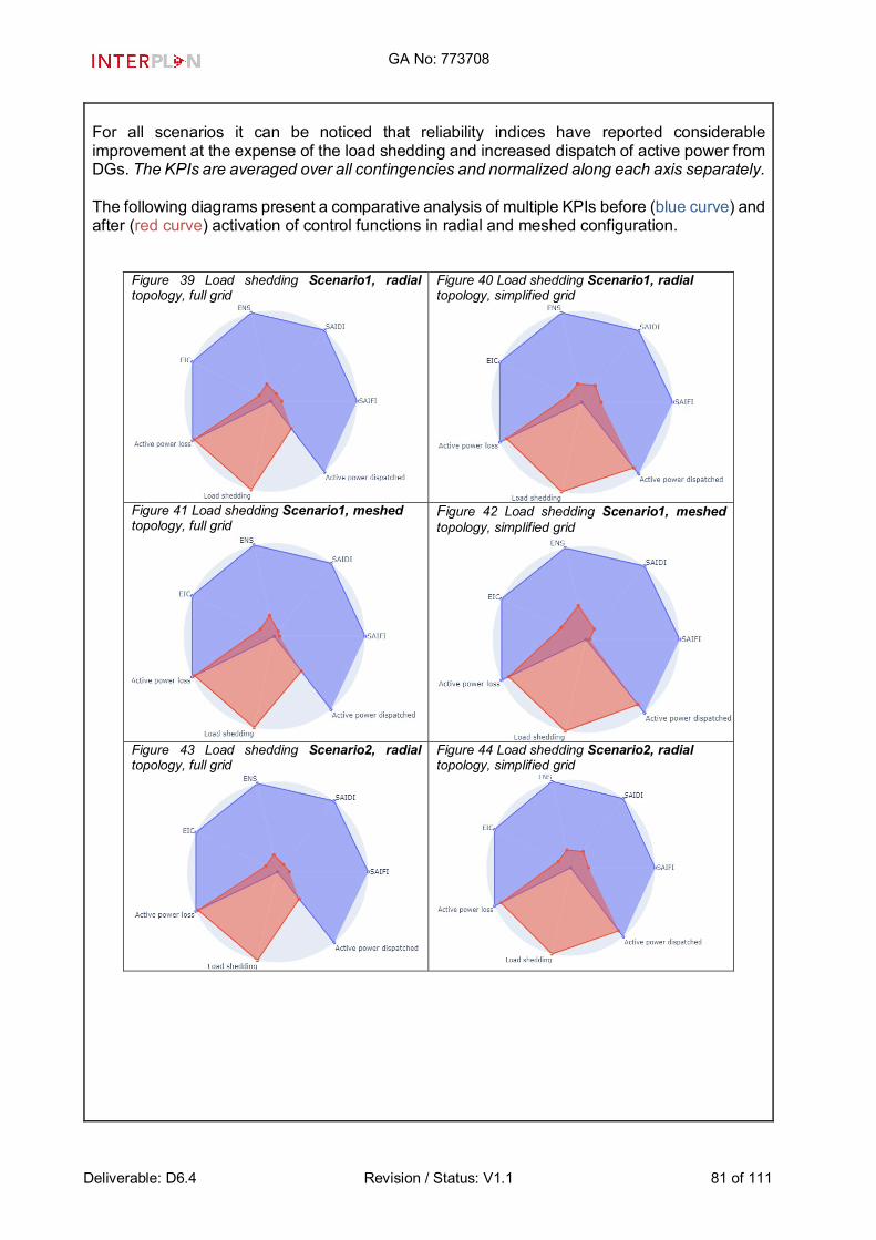
GA No: 773708


For all scenarios it can be noticed that reliability indices have reported considerable improvement at the expense of the load shedding and increased dispatch of active power from DGs. The KPIs are averaged over all contingencies and normalized along each axis separately. The following diagrams present a comparative analysis of multiple KPIs before (blue curve) and after (red curve) activation of control functions in radial and meshed configuration.

Figure 39 Load shedding Scenario1, radial topology, full grid

Figure 40 Load shedding Scenario1, radial topology, simplified grid

Figure 41 Load shedding Scenario1, meshed topology, full grid

Figure 42 Load shedding Scenario1, meshed topology, simplified grid

Figure 43 Load shedding Scenario2, radial topology, full grid

Figure 44 Load shedding Scenario2, radial topology, simplified grid

GA No: 773708


Figure 45 Load shedding Scenario2, meshed topology, full grid

Figure 46 Load shedding Scenario2, meshed topology, simplified grid

For load shedding Scenario3, similar results were obtained. The next figures show a detailed example for load shedding, power losses and energy not supplied respectively in MW for every contingency in scenario 1 using the simplified grid radial topology .

Figure 47 Load shedding in MW Scenario1 radial topology simplified grid

Figure 48 Power Loss in MW Scenario1 radial topology simplified grid

GA No: 773708


Figure 49 Energy not supplied in MW Scenario1 radial topology simplified grid

The last figure shows the improvement and the reduction in the energy not supplied values at each contingency after applying the optimization action which is the main objective of the controller. The validation process using the simplified grid showed similar results with small deviations in some contingencies, which do not have clear impact on the total result in comparison to the saved effort and time in modelling the full grid and the simulation time needed. These deviations are also due to not only using simplified LV grids but some parameters of the reliability models needed to be aggregated. 2.2 Implementation procedure and requirements Use case workflow: Load flow and contingency identification

The user can be a TSO or a DSO who provides the grid information (network model) and load & generation forecasts. This action performs the load flow to calculate the status of the grid. This information is used to identify the critical contingencies in the grid, the user (TSO/DSO) can also specify them. The resulting list of credible contingencies is sent to next stage.

Sensitivity analysis

Here, the sensitivity of the critical lines and buses is calculated with respect to the buses having dispatchable generators and interruptible loads for the selected contingency. The sensitivity information is used to define the penalty cost terms that assign less penalty costs to the terminals whose control action can influence more the grid constraint violation. This information is communicated to the next stage of constraint modelling.

Constraints modelling

This action prepares the matrices for the constraints for the optimization process. The mathematical model of the problem is sent to the optimizer.

Min f(x): objective function minimization

At this stage, the optimization problem is solved with constraints enabled in the network. The optimization results are load and generator setpoints. Fall back strategy

If the optimization process is either unable to meet the demand, due to lack of generation or there is a grid constraint violation, then the fall back or predefined backup strategy is selected. That could include allowing more load to be interrupted.

GA No: 773708


Output signal

In this step the control signals from the optimizer are received and send them to the respective generators and loads. The optimization problem is solved to yield generator & load setpoints. This schedule is evaluated for each contingency and can be used offline to prepare network resources. Additional factors: The run time of the simulations using the full grid model is huge in comparison to the simplified grid. The simulation time with full grid took several hours in comparison to simplified grid, which needs minimum one and half an hour for simulation depending on the scenario. This means also that the simulation time defers from scenario to scenario and depends on the complexity of the grid.

Validation level 3: Identification of peculiarities of individual use cases No special issues

GA No: 773708


5. Testing the INTERPLAN tool

Summary of the INTERPLAN tool As described in D5.2, the INTERPLAN tool is a methodology that consists of three stages according to Fig. 47. The tool user is typically a TSO or DSO having a specific grid operation challenge in mind. The stages guide the user towards selecting the most proper INTERPLAN solution addressing the operation challenge.

Figure 50: INTERPLAN tool flowchart [2]

5.1.1 Stage 1 As a prerequisite to step 1, the user selects one or more planning criteria from a predefined list. A planning criterion is associated to one or more of the INTERPLAN use cases. Likewise, there is an association between planning criteria and showcases. Hence, the user makes a selection of possible use cases and/or showcases by selecting a specific subset of planning criteria. On the other hand, a subset of showcases may also be proposed for the user who selected a sub-group of planning criteria. The next action is selection of one or more simulation functionalities from a predefined list, including e.g. “Basic Load Flow”, “OPF”, etc. (step 1.1). After this, the user selects one or more

GA No: 773708


KPIs from a list, where the possible options are determined by the selection of the planning criteria (step 1.2). Finally in step 1.3, the user selects one out of four INTERPLAN scenarios, and a target year. There is a suggested selection of the scenario depending on the planning criterion/criteria, simulation functionality and KPIs previously chosen. 5.1.2 Stage 2 Stage 2 is about selection and preparation of a grid model and grid equivalent. In effect it prepares all input data that is needed for the simulation in stage 3. In step 2.1 the user selects if a transmission, a distribution, or a combined transmission-distribution grid should be investigated. In step 2.2 the user needs to select an according grid model from a set of benchmark grid models, or insert an own grid model. It is also allowed to select both own grid model and benchmark model, where the latter e.g. represents a part of the grid the user does not have an own model for. In step 2.3 it is calculated if a grid equivalent (GEq) is needed according to the previous selections by the user. In case a GEq is needed, the user may either select one from the GEq library (containing basic, advanced, and dynamic GEq’s), or a GEq is generated. The first option is possible if the user selected a benchmark grid model in step 2.2, the latter option otherwise. The latter option is enabled by a GEq generation procedure provided by the tool, and takes the original grid and the KPIs the user selected as inputs. The requirements and types of the GEq depend on the use cases and showcases.In step 2.4, the GEq (if any) is applied to the network model, which results in a grid model for further use. Step 2.5 is about application of the chosen INTERPLAN scenario onto the grid model. This involves finding a stable operation point that matches the installed generation and load powers from the scenario for the given grid area, which might include applying a set of reinforcements to the grid, applying additional components (e.g. compensation units) or adjusting generator operation points (e.g. apparent power nominal setpoints). This process is nontrivial and needs manual work. In step 2.6 the user sets the “time-step” for the simulation phase in step 3. Step 2.7 is the final step of stage 2 and is about assignment of time series data adapted to chosen scenario and time step selection. This is done through a time series generation procedure that is designed for a grid model that fulfills a set of requirements. 5.1.3 Stage 3 Stage 3 is about simulation of the INTERPLAN control functions in the setting of the chosen scenario, grid model, grid equivalents, and use cases / showcase in order to calculate the selected KPIs. In step 3.0/3.1, the user selects one out of two mutually excluding options, i.e. (i) performing simulations directly without controllers or (ii) selecting an INTERPLAN solution for the simulation. Option (i) is meant to generate a reference case. Option (ii) allows to select an INTERPLAN solution that matches the inputs as previously selected in stage 1; one or more INTERPLAN solutions might thus be available. In step 3.2 the actual simulation is carried out. In step 3.3 the user calculates and evaluates the selected KPIs, which is apparently supposed to be done manually or using the tools preferred by the user. If the user is not satisfied with the KPIs, the whole methodology may be repeated starting

GA No: 773708


with stage 1 in order to investigate other INTERPLAN solutions. The step 3.2 simulation is apparently supposed to use the grid equivalent(s) as selected in step 2.3. Step 3 results in an operation planning for controllable grid assets which fulfill the user’s KPI targets, using selected INTERPLAN solution. It is important to note that such planning may have been calculated with usage of grid equivalents, if so selected in step 2.3.

Testing the INTERPLAN tool As seen from the summary above, the INTERPLAN tool provides a concise methodology for investigating one or more grid operation challenges that arise due to distributed and renewable electricity generation or distributed storages. In order to provide a proof-of-concept, the tool needs to be tested by a concrete showcase. The INTERPLAN showcase 3 was selected for this purpose, because it includes a high variety of solutions developed in the project, namely two control functions which consistently use grid equivalenting. Furthermore it considers the TSO/DSO interface which is of high practical relevance. Hence this showcase is set into a user story that includes TSO and DSO as the tool users. This is elaborated as follows. The assumed TSO’s goal is to acquire tertiary reserve, utilizing own resources but also flexible resources at the DSO level, in a way that results in stable grid operation and minimal grid losses. Likewise, the DSO is aiming for providing tertiary reserve for the TSO with minimal grid losses in its own network. For all times when the TSO does not require tertiary reserve power, the DSO aims to optimize the balance between maximal RES curtailment and minimal losses and transformer loading (cp. D5.4 sections 4.3.2.1 and 4.3.2.2). As described in deliverable D5.4, an application of the INTERPLAN tool to showcase 3 has already been demonstrated for the largest part, namely including all of the steps mentioned above. This was done mainly from the perspective of the DSO. The particular planning criteria are:

• Minimizing grid losses • Maximizing share of RES • Optimize TSO/DSO interaction and • Maximize DG/RES contribution to ancillary services

The relevant KPIs at the DSO side are:

• Level of DG/DRES utilization for ancillary services • Transformer loading • RES curtailment, and • Share of RES.

The relevant scenario is INTERPLAN scenario 2 “Small and Local” for the target year 2050, and the North-Eastern Germany grid model (cp. 0) is selected for the showcase. Grid equivalents are used at both DSO and TSO sides to mutually represent the peer network for the individual steps of the two use cases that provide control functions for satisfying the showcase’s planning criteria. The tool application as described in D5.4 finalizes with calculation of the following KPIs in stage 3:

• KPI 1 - Level of losses in the network • KPI 7 - Power losses

GA No: 773708


• KPI 10 - Voltage quality • KPI 14 - Level of DG/DRES utilization for ancillary services • KPI 16 - TSO/DSO Transformer loading • KPI 17 - RES curtailment • KPI 22 - Quadratic deviation from global active power production target • KPI 23 - Mean quadratic deviations from active power targets

The test described in the following complements and finalizes the INTERPLAN tool demonstration. It represents the final stage of the tool’s application, consisting in the application of the showcase to the full physical grid model (Figure 48).

Figure 51 Final step of the INTERPLAN tool proof-of-concept

Looking at practical implementation of the tool, the TSO is involved in some of the steps directly as they involve calculation that needs to be done using the full TSO network, which usually is not handed to the DSO due to confidentiality. The same is the case for handing the DSO full network model to the TSO. Hence, when still the DSO is considered as primary tool user, but also includes the TSO as a partner who adheres to the INTERPLAN tool methodology, a sequence of action as summarized in table 10 follows is needed. This can be considered a practical refinement of the process described in D5.4.

GA No: 773708


Table 12 Sequence of action for showcase 3 INTERPLAN tool application by DSO and TSO

Action Tool stage

Primary Actor

Result

Selection of planning criteria 0 DSO Planning criteria as listed above1 Selection of possible solution 1.1 DSO SC3 is selected Selection of KPIs 1.2 DSO KPIs as listed above Selection of scenario 1.3 DSO INTERPLAN-2 “Small and Local” 2050 Grid Type selection 2.1 DSO Transmission and distribution grids2 Grid Model selection 2.2 DSO North-Eastern Germany grid model3 Identifying the need for grid equivalents

2.3 DSO Transmission and distribution equivalents are needed4

Application of grid equivalents 2.4 DSO, TSO

Grid equivalents5

Adaptation of scenario 2.5 DSO, TSO

Transmission and distribution grid models adapted to INTERPLAN-26

Preparation of time series 2.6 DSO, TSO

Time series for adapted grid models7

Grid model preparation 2.7 DSO, TSO

Grid models ready for stage 3

Reference case simulation 3.0 DSO, TSO

Reference case simulation results

Solution selection 3.1 DSO Showcase 3 is selected as it is the only solution offered

Solution simulation 3.2 TSO, DSO

Solution simulation results, grid operation planning including control function8

KPI calculation 3.3 DSO KPIs Preparation of full physical grid model

4.1 DSO, TSO

Complete SimBench grid as full physical grid model in pandapower format9

Solution selection 4.2 DSO, TSO

Showcase 3 is selected as it is the only solution offered

Co-simulation 4.3 DSO, TSO

Co-simulation results

KPI re-evaluation 4.4 DSO, TSO

KPIs obtained from Co-simulation compared to KPIs from step 3.310

Referring to the numbers in the “Result” column of table 12, the following notes apply with respect to the aforementioned relation between DSO and TSO:

1. It is assumed that DSO and TSO mutually agree on the named planning criteria. 2. While the DSO selects that the showcase generally operates on the full grid model, it is

already clear that – because the peer grid models cannot be mutually exchanged – equivalents for transmission and distribution level are mutually needed. The DSO thus needs to ask the TSO for provision of a transmission grid equivalent, and vice-versa offer a distribution grid equivalent in order to meet the common planning criteria.

3. DSO and TSO need to agree on a grid area for investigation, where each of them has a model of their individual physical networks. The example implies that the North-Eastern Germany grid model is the result of that agreement, and is used as basis for further calculation. The model represents a fictional physical grid in that example. In practice the distribution and transmission level parts of that model would be available to DSO resp. TSO only.

4. This requirement directly follows from the consideration above

GA No: 773708


5. This step involves calculation of grid equivalents at both TSO and DSO side that are suitable for the showcase, cp. 5.3.3.

6. In our example, the North-Eastern Germany grid model used is already adapted accordingly. However, it is important that from this step until step 4.1, TSO and DSO are mutually using transmission and distribution parts of the model only, while replacing the peer part by equivalents prepared in step 2.4 respectively.

7. This step obviously includes an agreement on the considered time interval between DSO and TSO, as well as e.g. agreement on the needed data basis (e.g. weather forecast dataset)

8. The simulation in this step involves an own sequence of actions according to showcase workflow. In the case of showcase 3 this involves execution of the two use cases 5 and 3, which involves calculation sub-steps at DSO and TSO sides according to the following sequence (cp. D5.4 chapter 4.3). The calculation is basically done for each timestep in the planning period. In case of our example, this is 24 hours with duration of 15 minutes for each time step.

Table 13 Detailed sequence of action for step 3.2

Action Use Case

Actor

For all timesteps with tertiary reserve provision Initialization of DSO grid model 3 DSO Assessment of DSO active power flexibiltiy 3 DSO OPF calculation at TSO to obtain active power setpoints for TSO assets and for power flows at TSO/DSO connection points

3 TSO

OPF calculation at DSO to obtain active power setpoints for DSO assets for optimal provision of power flows at TSO/DSO connection points

3 DSO

For all timesteps without tertiary reserve provision Initialization of DSO grid model 5 DSO OPF calculation at DSO to obtain active power setpoints for DSO assets with optimal balance between RES curtailment, losses and transformer loading

5 DSO

9. From this step on, the full grid model is used. The practical relevance of this can be

interpreted in two ways: (i) steps 4.1 and following may represent application of the grid operation planning as obtained in step 3.2 to the physical network or (ii) DSO and TSO provide their full grid models to a trusted third party which carries out an additional simulation, in order to clarify if the grid operation planning obtained in step 3.2 may be successfully applied to the full grid model. The pandapower format is chosen for technical reasons, cp. chapter 5.3.

10. This step finally allows to judge if the KPIs obtained by co-simulation match the ones expected, i.e. as calculated by step 3.3. A close match indicates that the INTERPLAN solution works also in the full physical network.

The remainder of this chapter exclusively covers steps 2.4 as well as 4.1 - 4.4. The latter steps need collaborative action between TSO and DSO which is enabled by co-simulation. The according setup is explained in the next section.

GA No: 773708


Test setup

The test of the aforementioned steps 4.1 – 4.4 is based on the co-simulation platform OpSim that was previously developed by Fraunhofer IEE and University of Kassel and enhanced within INTERPLAN. A co-simulation bundles several sub-simulation components to execute a common simulation experiment. OpSim basically allows for a distributed, remote and modular co-simulation of smart grid operation and control concepts. 5.1.4 Basic setup Figure 49 shows a simple OpSim setup. Certain elements, e.g. client/proxy modules, are left out for reasons of comprehensiveness. The components are arranged around a message bus based on the AMQP (Advanced Message Queuing Protocol) technology. In each OpSim simulation, there is one component simulating the “real” physical network; in this case, it is “Component A”. The other components may represent control functions for network assets or even whole control centers. In the example, there is a “Component B” directly connected to the message bus. This is only possible for components running in the Fraunhofer network. “Component C” is running at a remote location. This component is connected over a secure internet link using a so-called WebProxy in the Fraunhofer network. WebProxys may also be used within the Fraunhofer network, e.g. if a component is prepared and tested for later remote deployment. At the upper left, a graphic user interface (GUI) component is shown with which the whole simulation can be configured and started. The actual management of dataflow and synchronization is handeled by a ”Core” component which is not shown in the figure. Components can come in different flavours. The physical grid component may e.g. use a software for grid simulation (e.g. PowerFactory or pandapower), or a hardware grid simulator (e.g. OpalRT). The control components (B, C), may use different simulation tools (e.g. Python, Java, but also PowerFactory or pandapower). For the master control GUI, there are two options: the first one is a stand-alone application, and the second one offers a web-based portal for controlling the simulation. The latter option has been developed with support of INTERPLAN and even offers the possibility to control the whole simulation from remote.

Figure 52 Basic OpSim co-simulation setup

In project INTERPLAN, various additions were made that mainly apply to the upper part of the

GA No: 773708


figure. They basically simplify the definition of a co-simulation scenario as typical for INTERPLAN, and provide a means for data storage. The major part of this data concerns the network assets (generators, loads, storages, transformers) with adjacent parameters, as well as input and output time series. The additions are shown in a simplified way in figure 50, highlighting parts in the Fraunhofer network only.

Figure 53 INTERPLAN specific additions to OpSim basic setup

Starting from above, all grid assets are defined in a “Devices” Excel file. The file contains unique asset names, control capabilities, and basic parameters as e.g. nominal installed power and device types (e.g. PV, wind). The Excel file is eventually broken down into multiple csv files that are read by a module named DataBase Handler (DBH). Also, time series data for the grid asset active powers are provided as csv file. The DBH module reads the information from the files and stores them into an SQL Database (SQL DB). The physical grid model, shown in the figure as green box, is provided in a format native to pandapower, an open grid calculation software by University of Kassel. The RealGrid co-simulation component uses that software. The SQL DB contains a link to the according grid model file. Also, a module named “ScenGen” is reading the device information from the SQL DB and generates a so-called “Scenario file”, which is fed into the Master Control GUI. It is there used to setup the co-simulation. 5.1.5 Validation of the basic setup The solution simulation according to stage 3.2 (cp. table 12) was carried out with PowerFactory as grid calculation software. In contrast, the co-simulation basic setup uses pandapower. Hence, it is crucial to validate if both grid calculation softwares deliver the same results if the same grid model data and asset operation setpoints are used. The following section summarizes how we carried out this validation. The starting point for the validation is the data available in PowerFactory. This data consists of the North-Eastern Germany grid model, and time series data for one day with a 15 minute resolution for most generators and loads (67 of the grid assets were equipped with a constant operating point instead of time series). Using a Python script starting PowerFactory in “Engine Mode”, a quasi-stationary load flow simulation of the time series can be carried out. This results in according time series of node voltages, active and reactive power flows, line and transformer loadings. The results can be exported from PowerFactory using a Python script. The goal of the

GA No: 773708


validation is to reproduce these results with the co-simulation basic setup, and to compare them with the PowerFactory results. This process is highlighted in figure 51. It includes a converter from PowerFactory to pandapower called “Pf2pp”. This converter is included in the pandapower-pro software which is an extension of pandapower. Also, the process includes an export function for PowerFactory time series which was implemented in Python. The results are exported as Python DataFrames. The results considered for the comparison were the node voltages.

Figure 54 Process for validation of basic setup

Through the validation it was found that the reactive power limitation of synchronous generators is important. In PowerFactory, there are significant limitations which are not respected by the Pf2pp conversion process. Hence, the limitations have to be manually added to the pandapower network, and such limitations need to be enforced during the pandapower time series simulation. If this is respected, the maximal deviation of the absolute node voltages is lower than 5 * 10-7 p.u. for each time step. This is shown in figure 52. This deviation is considered within the precision range of the calculation, thus the validation is successful.

GA No: 773708


Figure 55 Box-plot of maximal voltage deviations per time step

5.1.6 Grid equivalents Based on the requirements and control functions of showcase 3, basic grid equivalents are needed for both transmission and distribution networks in order to perform the validation study. The main requirement of these grid equivalents is to present the active power flow from the replaced network model (TSO/DSO level). The equivalents were modelled as external grid objects and were created at each TSO/DSO connection point. For each time step, active and reactive power as well as voltage at the given terminal were recorded and saved in form of time characteristics, so that the values can be later used by the created external grid objects. 5.1.7 Setup for the INTERPLAN tool test The INTERPLAN tool test has been set up as to represent steps 4.1 - 4.4 (cp. Table 12) as realistically as possible. This means that TSO- and DSO-related simulation components were distributed to different machines and networks. The remote simulation capability via WebProxies was used in order to demonstrate that a common co-simulation can be carried out for the showcase. The resulting co-simulation setup is shown in figure 53.

GA No: 773708


Figure 56 Co-simulation setup for INTERPLAN tool demonstration

The simulation was distributed to three computers PC1..PC3. PC1 was situated in a private network with internet connection and used to control the simulation using the web version of the Master Control GUI. PC2 was located in the Fraunhofer network and was used to run both the physical network model (RealGrid) and the TSO subsimulation, which was locally connected to OpSim by a WebProxy (WebProxy2). PC3 was located in the DERlab network and used to run the DSO component, connected to OpSim by WebProxy1 and a VPN tunnel. The OpSim core components and WebProxy1 were run at Fraunhofer Servers (applik-d16 and applik-d23). Notably, the same setup could be used for running the TSO component at a computer in a third network, in order to also physically separate it from the RealGrid component. As can be seen at the bottom of the graphics, the DSO and TSO components were both fed with the setpoints as calculated by step 3.2, obtaining setpoints for their individual grid assets. The file contains one day of setpoints in 15 min resolution, which is the result of a day-ahead grid operation planning as obtained by the solution simulation in step 3.2. The simulation was set up using the auxilliary functions as mentioned under 5.3.1. Namely, a device file representing all assets in the North-Eastern Germany network was used where DSO-level devices and TSO-level devices were attributed to the according operation centers, represented by the subsimulation components. The file was read into the SQL database and used together with the grid model converted to the pandapower format. Using this, the co-simulation could be prepared and executed through remote connection from three workstations: PC1 .. PC3. Figure 54 shows a screenshot of the Web GUI during simulation execution as displayed on PC1. The dashboard in the background is displayed in an internet browser and shows that all simulation components are running. The window in the front with the three bars is the stand-alone Master Control GUI application, which was started alongside. The bars show the simulation progress of the three subsimulation components (RealGrid, DSO and TSO from top to bottom).

GA No: 773708


Figure 57 Co-simulation GUI screenshot

The results of the simulation are stored in the SQL data base. This includes the node voltages, line and transformer loadings, and active and reactive powers for each grid asset and each time step. From this information, the KPIs relevant for the showcase can be calculated ex-post. Here for, Python routines were prepared and used for automatic KPI evaluation. 5.1.8 Limitations of the test The test documented herein completes the INTERPLAN tool demonstration. However, it has following limitations:

Although steps 4.1-4.4 were carried out with strict separation of TSO and DSO, the other steps were not – most notably, step 3.2 was carried out by a Python script which mutually used two PowerFactory networks: one representing the full DSO network with TSO equivalent, the other representing the full TSO network with DSO equivalent. Introducing strict separation would have been possible by creating individual scripts for TSO and DSO, and exchanging intermediate results, without changing the underlying algorithms and without changing the results. Other notable limitations regard the practical application of the scenario. First, it is noted that the day-ahead planning done in step 3.2 used an ideal forecast. There was no extra forecast dataset used, but the original time series including PV and wind infeed were used in the planning phase. This is obviously not possible in practice and unavoidable forecast errors will have an effect onto the KPIs. However, since the test is meant as a proof-of-concept, quantifying the effects of forecast errors is out of scope.

Test results The obtained results from the validation is presented and compared to the testing results in control function design (available in D5.4). As described above, the validation methodology is based on co-simulation of different network components (TSO, DSO and real grid components) using one single physical grid model. In contrary, the testing of control functions that was done previously is based on individual simulations at TSO and DSO using grid equivalents. The comparison is made based on the calculation results of INTERPLAN tool demo KPIs in the following.

GA No: 773708


KPI 1- Level of losses in transmission and distribution networks Description The transport of electrical energy through the distribution or transmission

network is associated with a certain amount of power losses. Therefore, the amount of power being produced has to be a few percentage points higher than consumption levels. This KPI is meant to present the active power losses in percentage.

Formula 𝑃𝑃losses =

amount of injected power − amount of power delivered to customers amount of injected power × 100 [%]

Comparison diagram

Figure 58: KPI 1 comparison for INTERPLAN tool test

Analysis The diagram illustrates that the amounts of power losses calculated based on

the output of co-simulation is very close to the control function testing results. The maximum deviation is 0.02%. This approves that the control algorithms function in the same way in both experiments.

KPI 14- Level of DG / DRES utilization for ancillary services Description The purpose of this KPI is to measure the utilization of DER for ancillary

services (UAS). It is expressed as a ratio between the energy used for ancillary services and the total energy produced.

Formula UAS% =

𝐸𝐸AS𝐸𝐸total

× 100 [%]

𝐸𝐸AS - the energy used for ancillary services [MWh] 𝐸𝐸total - the total energy produced [MWh]

GA No: 773708


Comparison diagram


Analysis Considering the comparison diagram, the co-simulation relevant output data leads to almost the same levels of DG/DRES utilisation for ancillary services, as in control function testing results. The maximum deviation is around 0.05% which is acceptable. This approves that the control algorithms function in the same way in both experiments.

KPI 17- RES curtailment Description The purpose of this KPI is to give an indication of the volume of RES-generated

available energy curtailed because of controller actions aiming to meet other goals of optimization. Minimizing RES curtailment is itself one of optimization objectives for UC5.

Formula Curtailment = 100 −

energy supplied by RES to the gridRES available energy

∗ 100 [%]

Comparison diagram

Analysis Considering the comparison diagram, the co-simulation relevant output data

leads to the same levels of RES curtailment, as in control function testing

GA No: 773708


results without any deviation. This approves that the control algorithms function in the same way in both experiments. The level of curtailment is negative in some time steps due to the increase in their generation output in comparison to the initial time series. These are the time steps, where the participation of RES is required in providing the requested tertiary reserve.

KPI 16- Transformer loading Description This KPI reflects the value of TSO/DSO transformer loading and is the primary

optimization objective of the UC5 controller function, as the main goal of UC5 is to optimize the local usage of energy through minimizing the power exchange between DSO and TSO networks.

Formula Loading =

power at transformer primary winding transformer nominal power

∗ 100 [%]

Comparison diagram


Analysis The diagram illustrates that the amounts of transformer (at the TSO-DSO connection point) loading calculated based on the output of co-simulation is very close to the control function testing results. The maximum deviation is less than 0.5%. This approves that the control algorithms function in the same way in both experiments.

KPI 22- Quadratic deviation from global active power exchange target KPI 23- Mean quadratic deviations from active power targets at TSO/DSO connection points Description KPI 22: This KPI calculates the quadratic deviation from global active power

production target, which is based on the needed tertiary reserve. Minimizing this KPI is an optimization objective. KPI 23: This KPI calculates the mean quadratic deviations from active power targets (based on the needed tertiary reserve for each connection point) at each connection point between TSO and DSO grids. Minimizing this KPI is an optimization objective.

GA No: 773708


Formula KPI 22: Let ptarget (t) be the global active power production target for tertiary reserve at time t. Let G be the set of generators producing active power, and pg(t) be the active power generated by generator g at a given time t. Then, the KPI at this time is:

�𝑝𝑝target(𝛥𝛥) −�𝑝𝑝𝑔𝑔(𝛥𝛥)𝑔𝑔∈G

�

2

KPI 23: Let C be the set of connection points between TSOs and DSOs. Let pc,target (t) [kW] be the target value for active power transmission from DSO to TSO at connection point c and time t, as e.g. calculated by grid operation planning. Let pc(t) be the active power actually provided from DSO to TSO at connection point c and time t. Then the KPI related to active power at time t is defined as:

1|C|��𝑝𝑝c,target(𝛥𝛥) − 𝑝𝑝𝑐𝑐(𝛥𝛥)�

2

𝑐𝑐∈C

Comparison diagram

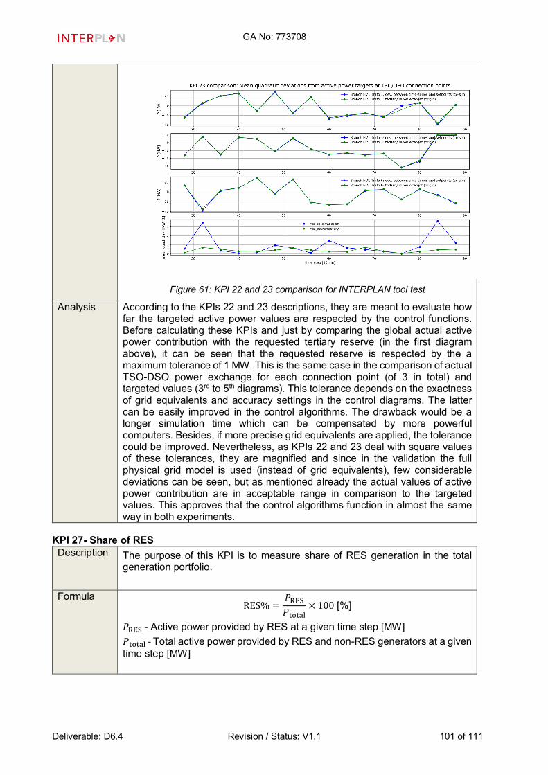
GA No: 773708


Figure 61: KPI 22 and 23 comparison for INTERPLAN tool test

Analysis According to the KPIs 22 and 23 descriptions, they are meant to evaluate how far the targeted active power values are respected by the control functions. Before calculating these KPIs and just by comparing the global actual active power contribution with the requested tertiary reserve (in the first diagram above), it can be seen that the requested reserve is respected by the a maximum tolerance of 1 MW. This is the same case in the comparison of actual TSO-DSO power exchange for each connection point (of 3 in total) and targeted values (3rd to 5th diagrams). This tolerance depends on the exactness of grid equivalents and accuracy settings in the control diagrams. The latter can be easily improved in the control algorithms. The drawback would be a longer simulation time which can be compensated by more powerful computers. Besides, if more precise grid equivalents are applied, the tolerance could be improved. Nevertheless, as KPIs 22 and 23 deal with square values of these tolerances, they are magnified and since in the validation the full physical grid model is used (instead of grid equivalents), few considerable deviations can be seen, but as mentioned already the actual values of active power contribution are in acceptable range in comparison to the targeted values. This approves that the control algorithms function in almost the same way in both experiments.

KPI 27- Share of RES Description The purpose of this KPI is to measure share of RES generation in the total

generation portfolio.

Formula RES% =

𝑃𝑃RES𝑃𝑃total

× 100 [%]

𝑃𝑃RES - Active power provided by RES at a given time step [MW] 𝑃𝑃total - Total active power provided by RES and non-RES generators at a given time step [MW]

GA No: 773708


Comparison diagram


Analysis The comparison diagram on share of RES in generation illustrates that these shares are in the same range and with maximum 2% of deviation based on the in the results of co-simulation and control function testing. This approves that the control algorithms function in the same way in both experiments. The minor deviation is most probably due to the application of simple grid equivalents in the testing. The more accurate the equivalent is, the more precise and closer results are expected.

GA No: 773708


6. Summary and conclusions The use case validation process presented in this report was the final step in the development procedure of the novel methods aimed at facilitation and improvement of different aspects of power system operation planning. Not only did it allow to identify shortcomings in the developed controllers, which manifested themselves only when subjected to different operation conditions, but more importantly it helped better understand how the controllers and methods can be applied to different problems and what needs to be done in order to increase usability of these products. Eight different power system models, ranging from a few to thousands of buses, were used throughout the design and validation phase. All use cases were validated using different model setups than those used for controller development. Modifications of models for validation consisted in changing time series, in the simplest case, to changing the whole model or even modelling environment, in the most extensive cases. In all cases but one similar quality of results was obtained, which means that even if the controllers are applied to completely different models, they still perform as expected, and that the design is robust. The case that needed a revision was the one which was further validated with use of real time simulation environment. The error in design manifested itself only when the controller was idling after the main control response was over. This set of circumstances is seldom met in transient stability simulation run offline but is unavoidable when running the model in real time. This example shows that changing the simulation environment can trigger faults in unexpected areas, which is very advantageous to the whole validation process. Apart from confirming the robustness of the design or detecting small flaws in it, validation allowed the authors to reassess the usability and applicability of the functions they designed and double check who the target receiver of each function could be. This confirmation process started already with the KPIs, which provide quantitative evaluation of the progress that given controller brings in each of the planning criteria. Here it is further extended with polar plots expressing applicability of each use case to different planning criteria and clear explanation how the most relevant criteria are addressed in each function. The test of the INTERPLAN tool as a methodology was completed by execution of a co-simulation using showcase 3 as an example. The showcase is set into a user story where a TSO and DSO are using the tool collaboratively. Their aim is to (i) acquire tertiary reserve utilizing resources at all voltage levels in a way that results in stable grid operation and minimal grid losses, and (ii) to optimize the balance between maximal RES curtailment and minimal losses and transformer loading at the DSO level for times in which no tertiary reserve provision is planned. The results show that the grid operation plans calculated by the showcase’s control functions using grid equivalents also work well when applied to the full physical network, as was evaluated in terms of KPIs. It was possible to physically separate the software representing the DSO and TSO control centers by means of co-simulation.

GA No: 773708


7. Outlook An important part of the validation process described in this report was the assessment of implementation requirements and possibilities. Many obstacles were reported in this phase of validation, among which the most significant are:

• lack or insufficient regulation supporting different mechanism that are necessary for use case operation,

• high risk of finding insufficient IT infrastructure or too high cost of such infrastructure, • unwillingness or lack of possibility for data exchange between involved stakeholders, • lack of market mechanisms, • infancy of some technologies (e.g. virtual inertia offered by RES), • a need to relay on forecasts and predictions, which might be unacceptable for some

TSOs/DSOs, • access to higher level of controllability of RES, which might never be the case unless

regulations change. Whilst executing this task the authors also performed an qualitative evaluation of the usability of each function. Some functions require high effort to be reuse for different networks, which is caused by the need of deep understanding of the function code and/or the power system model. Other functions require manageable time for implementation but might be too time consuming to be executed if applied to large models. Although the core parts of many of the main algorithms are ready, there is still very high programming effort needed to convert them into fully functional applications capable to operate in dispatching centre environments. These types of responses are considered acceptable at the low TRL5 target of this project. The external obstacles mentioned above practically prevent these use cases from being implemented in the planning or dispatching centres of the DSOs and TSOs in the very near future. However, considering the validation proved that all use cases work and can be applied to different problems, the internal obstacles can be eliminated in the process of further development of the concepts as they climb on the TRL ladder, until they reach the “industry ready” status. This process requires time, during which many of the external obstacles might disappear thank to the technology development or can be overcome by different means. For instance, the data exchange problem can be dealt with by using equivalent models of the network, an idea strongly supported in this project. Therefore, it is recommended that the development process of all use cases of this project be continued in such a way that the next milestone would be the field demonstration. In fact, this process has already started for several use cases still within this project, as they were either adapted to run in real time, or to run in distributed co-simulation environment. A very important lesson learned for the future is, however, that further development should not take place without the final users, which are the DSOs and TSOs, as they are those who could best validate the concepts. DSOs and TSOs, among others, are those who provided positive feedback during many occasions within the project lifetime by confirming that in medium to long term perspective all use cases are important, and that an integrated planning tool would be of high value.

GA No: 773708


8. References [1] IEEE Standard for System and Software Verification and Validation," in IEEE Std 1012-

2012 (Revision of IEEE Std 1012-2004) , vol., no., pp.1-223, 25 May 2012, doi: 10.1109/IEEESTD.2012.6204026.

[2] X. Zhang, Z. Zhu, Y. Fu, and W. Shen, ‘Multi-objective virtual inertia control of renewable power generator for transient stability improvement in interconnected power system’, International Journal of Electrical Power & Energy Systems, vol. 117, p. 105641, 2020, doi: https://doi.org/10.1016/j.ijepes.2019.105641.

[3] M. Chen and G. A. Rincon-Mora, ‘Accurate Electrical Battery Model Capable of Predicting Runtime and I–V Performance’, IEEE Trans. On Energy Conversion, vol. 21, no. 2, pp. 504–511, Jun. 2006, doi: 10.1109/TEC.2006.874229.

[4] ENTSO-E, Rate of Change of Frequency (RoCoF) withstand capability ENTSO-E guidance document for national implementation for network codes on grid connection, 31 January 2018

[5] ENTSO-E, “Need for synthetic inertia (SI) for frequency regulation: ENTSO-E guidance document for national implementation for network codes on grid connection”, 31 January 2018

[6] ENTSO-E, “High Penetration of Power Electronic Interfaced Power Sources (HPoPEIPS) ENTSO-E Guidance document for national implementation for network codes on grid connection”, 29 March 2017

[7] M. Singh and S. Santoso, ‘Dynamic Models for Wind Turbines and Wind Power Plants’, NREL/SR-5500-52780, 1028524, Oct. 2011. doi: 10.2172/1028524.

[8] General Electric Company, ‘Digital Energy, Effective Inertia’, [Online]. Available: https://www.ge.com/digital/sites/default/files/download_assets/effective-inertia-datasheet-ge-grid-analytics.pdf.

[9] Freris L. L., Sasson A. M., "Investigation of the load-flow problem", Proc. IEE, vol. 115, no. 10, pp. 1459-1470. 1968.

[10] Min C., Rincon-Mora G. A., "Accurate electrical battery model capable of predicting runtime and I-V performance," Energy Conversion, IEEE Transactions on, vol. 21, no. 2, pp. 504-511, 2006.

[11] EirGrid-SONI, report; “RoCoF Modification Proposal–TSOs Recommendation” [12] Official Journal of the European Union, “COMMISSION REGULATION (EU) 2017/1485 of

2 August 2017 establishing a guideline on electricity transmission system operation”, 25.08.2017, Available: https://eur-lex.europa.eu/legal-content/EN/TXT/HTML/?uri=CELEX:32017R1485&from=EN

[13] Ulbig A., Rinke T., Chatzivasileiadis S., Andersson G.: Predictive control for real-time frequency regulation and rotational inertia provision in power systems. 52ndIEEE Conference on Decision and Control, Firenze, 2013, p. 2946-2953.

[14] Patsalides, M.; Papadimitriou, C.N.; Efthymiou, V.; Ciavarella, R.; Di Somma, M.; Wakszyńska, A.; Kosmecki, M.; Graditi, G.; Valenti, M. Frequency Stability Evaluation in Low Inertia Systems Utilizing Smart Hierarchical Controllers. Energies 2020, 13, 3506

[15] INTERPLAN, Deliverable D3.2 INTERPLAN use cases, [online], Available : https://interplan-project.eu/resources/

Note: all online sources were accessed at Jan 26th 2021

https://doi.org/10.2172/1028524

GA No: 773708


Annex List of Figures

Figure 1 Realisation of different planning criteria within the project use cases ........................10 Figure 2 Validation procedure applied in INTERPLAN ............................................................12 Figure 3 The procedure of use case 1 control algorithms ........................................................36 Figure 4 Maximum line loading in the TSO grid .......................................................................40 Figure 5 Maximum loading lines value before and after the control action...............................41 Figure 6 Control execution time related to time step 46...........................................................43 Figure 7 Control execution time related to time steps 47,48 and 49 ........................................44 Figure 8: The procedure of use case 3 control algorithms .......................................................46 Figure 9 Level of losses in the network ...................................................................................47 Figure 10 Level of DG/RES utilization for ancillary services ....................................................48 Figure 11 Share of RES ..........................................................................................................48 Figure 12: The procedure of use case 4 control algorithms .....................................................52 Figure 13: UC4 control logical scheme ....................................................................................53 Figure 14 The frequency regulation process steps and time-frame .........................................54 Figure 15 Frequency Nadir - Scenario 2030 ............................................................................57 Figure 16 Steady State value - Scenario 2030 ........................................................................57 Figure 17 RoCoF variation - Scenario 2030 ............................................................................58 Figure 18. Frequency Nadir - Scenario 2050 ...........................................................................58 Figure 19 Frequency Zenith - Scenario 2050 ..........................................................................59 Figure 20 Steady State value - Scenario 2050 ........................................................................59 Figure 21 RoCoF variation - Scenario 2050 ............................................................................60 Figure 22 UC4 algorithm .........................................................................................................61 Figure 23 Percentage of original (pre-optimization) power losses ...........................................64 Figure 24 RES curtailment after optimization ..........................................................................64 Figure 25 TSO/DSO transformer loading pre- and post - optimization .....................................65 Figure 26 Objective function pre- and post- optimization .........................................................65 Figure 27 UC5 algorithm .........................................................................................................66 Figure 28 Structure of BESS model in RTDS simulation software ...........................................70 Figure 29 Simulation results for a single disturbance showing unnecessary operation of SI after

the inertial response has finished (BESS active power from 2.4 s to 6.4 s) ........................71 Figure 30: Block diagram of UC6 controller .............................................................................71 Figure 31 Results comparison for case with and without SI with added blocking logic for SI ...72 Figure 32 RoCoF values for base and test cases ....................................................................73 Figure 33 Frequency nadir and zenith for cases with and without SI .......................................73 Figure 34 Frequency Nadir - Scenario 2030 (with and without SI enabled) .............................75 Figure 35 Frequency Zenith - Scenario 2030 (with and without SI enabled) ............................76 Figure 36 RoCoF variation - Scenario 2030 (with and without SI enabled) ..............................76 Figure 37 Dependence of RoCoF values on measuring window width ....................................78 Figure 38 Selection of the width for averaging window for RoCoF measurement ....................78 Figure 39 Load shedding Scenario1, radial topology, full grid................................................81 Figure 40 Load shedding Scenario1, radial topology, simplified grid .....................................81 Figure 41 Load shedding Scenario1, meshed topology, full grid ............................................81 Figure 42 Load shedding Scenario1, meshed topology, simplified grid .................................81 Figure 43 Load shedding Scenario2, radial topology, full grid................................................81 Figure 44 Load shedding Scenario2, radial topology, simplified grid .....................................81 Figure 45 Load shedding Scenario2, meshed topology, full grid ............................................82 Figure 46 Load shedding Scenario2, meshed topology, simplified grid .................................82 Figure 47 Load shedding in MW Scenario1 radial topology simplified grid ............................82 Figure 48 Power Loss in MW Scenario1 radial topology simplified grid .................................82 Figure 49 Energy not supplied in MW Scenario1 radial topology simplified grid ....................83

GA No: 773708


Figure 50: INTERPLAN tool flowchart [2] ................................................................................85 Figure 51 Final step of the INTERPLAN tool proof-of-concept ................................................88 Figure 52 Basic OpSim co-simulation setup ............................................................................91 Figure 53 INTERPLAN specific additions to OpSim basic setup .............................................92 Figure 54 Process for validation of basic setup .......................................................................93 Figure 55 Box-plot of maximal voltage deviations per time step ..............................................94 Figure 56 Co-simulation setup for INTERPLAN tool demonstration.........................................95 Figure 57 Co-simulation GUI screenshot ................................................................................96 Figure 58: KPI 1 comparison for INTERPLAN tool test............................................................97 Figure 59: KPI 14 comparison for INTERPLAN tool test..........................................................98 Figure 60: KPI 16 comparison for INTERPLAN tool test..........................................................99 Figure 61: KPI 22 and 23 comparison for INTERPLAN tool test ............................................ 101 Figure 62: KPI 27 comparison for INTERPLAN tool test........................................................ 102

List of Tables

Table 1 Complementary reports ................................................................................................8 Table 2 Validation levels ...........................................................................................................9 Table 3 Operation planning criteria used in the project..............................................................9 Table 4 Simbench model description ......................................................................................13 Table 5 Extended Simbench model description ......................................................................16 Table 6 Simple Cyprus model description ...............................................................................19 Table 7 Complex Cyprus model description ............................................................................22 Table 8 Danish model description ...........................................................................................24 Table 9 AIT simplified model description .................................................................................25 Table 10 AIT synthetic model description ................................................................................27 Table 11 IEEE 14 Bus Power System model description ........................................................28 Table 12 Sequence of action for showcase 3 INTERPLAN tool application by DSO and TSO 89 Table 13 Detailed sequence of action for step 3.2...................................................................90

Glossary of terms and definitions 8.1.1 Definition of project general terms Term Definition

Use Case The specification of a set of actions performed by a system, which yields an observable result that is, typically, of value for one or more actors or other stakeholders of the system.

Sub Use Case

Description of a specific situation a use case is applied to. A Sub Use Case is always attributed to one (main) use case, but one use-case may have multiple sub use cases which detail the main use case in at least one aspect.

Base showcase

Presentation of base use case(s) with no planning criteria and no controllers for emerging technologies, such as RES, DG, demand response or storages in the frame of chosen scenario, simulation type, test model, and time-series data. The base showcase allows to analyze the operation challenges of the related use case(s) and improvements achieved through the application of planning criteria with related implementation of controllers in the associated showcase.

GA No: 773708


Showcase Presentation of use case(s) in the frame of chosen scenario, simulation type, test model, time-series data and planning criteria

Scenario

Definition of a future situation applying to a well-defined time (most often year). A scenario can be fictional or predicted from the present situation. In INTERPLAN, scenarios describe the future situation of the European electric network, typically including grid topology, generation mix, loads and diffusion of EV, RES and storages.

Dynamic Simulation

A simulation experiment which considers the time dependent behaviour of a physical system, looking at events occurring in real-time operation, with a frequency of occurrence of less than one second of real time. The simulation may run faster or slower than real time, and may, despite the fast event frequency, span a total time interval of several hours real-time.

Semi-Dynamic Simulation (also: Quasi-Dynamic Simulation)

A medium- to long-term simulation experiment based on steady-state analysis, considering the state of a physical system at discrete steps of real time through user-defined time step sizes. The real time between the steps is at least one minute.

Grid Cluster A group of grids and parts of grids with similar characteristics

Grid Equivalent

A simplified network model, which approximately behaves like an associated complex physical network or a group of physical networks. The grid equivalent thus is a representation of the physical network(s), which is typically used for a simulation experiment.

Control function

A set point definition, which is determined based on the goals of each use case. A control function defines the set points of specific elements (e.g. OLTC, DGs, RESs) or some programs (e.g. demand response) calculated by an operation objective in the network..

Interface

A means of transmitting information between two or more controllers or actors. It usually includes a specification about which information is to be transmitted, how this information is represented by data elements, and defines a physical means for transmission of those data elements.

Cluster Controller A controller having the aggregated behavior of individual controller characteristic in a larger grid.

Interface Controller

A controller, which is intended to be installed in a specific "home" cluster, and uses information received through an interface from at least one other cluster data source outside the home cluster. This data source could e.g. be another cluster, but also e.g. an external weather forecast provider using an interface

Local Controller

A controller which is associated with a single specific generator, load or grid asset and which operation does not rely on remotely received information originating from any remote source. i.e. the operation only relies on information available within the local area network of the local

GA No: 773708


controller’s installation site.

Co-simulation

A simulation which consists of different parts that form a coupled problem and are modelled and simulated in a distributed manner (cp. Wikipedia). The parts are called "Co-simulation subsystems" and are exchanging data during the simulation. Different models and simulation means can be used in different subsystems. The Co-simulation (in the ideal case) is carried out by running the subsystems, which were individually tested and validated beforehand, in a black-box manner. In INTERPLAN, the data exchange between subsystems is done by the OpSim platform.

Co-simulation subsystem / Co-simulation subcomponents

A part of a Co-simulation which is developed, modelled and validated individually, while at the same time able to be integrated into the Co-simulation platform. In INTERPLAN, a subsystem might represent e.g. a DSO or TSO operation centre, a controller, or even the real physical network model.

Data model

An abstract model that represents a real-world entity, and defines, organizes and standardizes the description of the data elements related with that entity. Since real-world entities are typically consisting of other entities (e.g. an electric grid consists of lines, transformers etc.), a data model typically is hierarchically structured and also allows to define interrelations between entities.

V2G and G2V

Vehicle-to-grid (V2G) describes a system in which plug-in electric vehicles communicate with the power grid to sell demand response services by either returning electricity to the grid or by throttling their charging rate. When an EV is being charged, it’s called G2V (Grid to Vehicle).

Allocation

With reference to the grid operation planning phase, it is the process deciding, which are the most suitable resources to commit and dispatch among n operating resources for a specific objective and under specific constraints.

Placement and sizing

With reference to the grid planning, it is the process deciding the most proper location (bus) and the size of a resource (active power) for a specific objective and under specific constraints.

Energy Not Supplied Energy Not Supplied is defined as the amount of energy that would have been supplied to the customer if there had been no interruption.

Energy spillage Energy spillage is the production (from Solar and Wind) that is unable to be accommodated due to demand being lower than production.

GA No: 773708


8.1.2 Definition of actors Term Definition

TSO - Transmission System Operator

Natural or legal person responsible for operating, ensuring the maintenance of the transmission system and, if necessary, developing the transmission system in a given area and, where applicable, its interconnections with other systems, and for ensuring the long-term ability of the system to meet reasonable demands for the transmission of electricity. The term ‘transmission’ means the transport of electricity on the extra high-voltage and high-voltage interconnected system with a view to its delivery to final customers or to distributors, but does not include supply.

DSO - Distribution System Operator

A natural or legal person responsible for operating, ensuring the maintenance of and, if necessary, developing the distribution system in a given area and, where applicable, its interconnections with other systems and for ensuring the long-term ability of the system to meet reasonable demands for the distribution of electricity. The term ‘distribution’ means the transport of electricity on high-voltage, medium-voltage and low-voltage distribution systems with a view to its delivery to customers, but does not include supply.

ESCO

Electricity supply company (sometimes also: Electricity service company). General term for a company which supplies end users with electric energy. An ESCO may offer additional services, e.g. electricity generation, metering or supply with non-electric energy.

Prosumer

Active energy consumer who consumes and produces electricity. Various types of prosumers exist: residential prosumers who produce electricity at home - mainly through rooftop PV, citizen-led energy cooperatives, commercial prosumers whose main business activity is not electricity production, and public institutions.

Generator A device which produces electricity.

Load A device which consumes electricity.

Producer A natural or legal person generating electricity.

Consumer A natural or legal person consuming electricity.

Distributed Energy Resource (DER)

A source or sink of electric power that is located on the distribution system, any subsystem thereof, or behind a customer meter. DER may include distributed generation, electric storage, electric vehicles and demand response.

Aggregator

Company who grouping distinct agents in a power system (i.e. consumers, producers, prosumers, or any mix thereof) to act as a single entity when engaging in power system markets (both wholesale and retail) or selling services to the system operator(s).

Distributed generation (DG) unit

Any source of electric power of limited capacity, directly connected to the power system distribution network. DG can be powered by photovoltaic system, micro-turbines, combustion engines, fuel cells, wind turbines,

GA No: 773708


geothermal, etc.

Flexible Loads

A load which consumption can be influenced in terms of power, time, or total energy consumed while still serving its intended purpose. The influence may be exerted by manual means (e.g. switching the load on or off at arbitrary times) or automatic means (e.g. external control signal).