Internship Report

Effect of Multiple Length Scales on

Turbulent Mixing in High Intensity

Flows

ABSTRACT

The experimental research at Wind Tunnel Facility at University of California, Irvine aims to

find the behavior of passive scalar when mixed with a turbulent flow of air. An electrically

heated wire grid heats up the turbulent air, which acts as a passive scalar. A region of

homogenous and isotropic turbulence was established and decay power law validity was

confirmed. An understanding is developed on how the velocity field evolves downstream of a

turbulence generating active grid by looking at the homogeneity data. The power decay law was

found to be valid with a decay exponent of n= 1.504 for Taylor Reynolds number 200-275 and

n=1.389 for Taylor Reynolds number is 375-500. A 4m/s flow becomes isotropic at x/Mu=120

and an 8m/s flow is not isotropic until x/Mu=142 which is the farthest point in our test section.

INTRODUCTION

The mixing of passive scalar in a turbulent flow has long been a topic of interest for engineers.

The study is important for understanding how turbulence helps in mixing of fuel and air in a

simple Gas Turbine pre-mixer. The current experimental research at University of California,

Irvine is motivated by the observation that complete pre-mixing of fuel and air leads to a more

efficient chemical reaction in the combustion chamber. The proper mixing of fuel and air is

proportional to the mixing time and the challenge is to minimize that mixing time. Since the flow

inside the pre-mixer is turbulent, basic understanding of turbulence is necessary. A number of

experiments have been conducted to get an insight into how the turbulent velocity field decays

and how the approach to isotropy can be controlled. By using a hot-wire sensor, readings were

taken across the test section (at a constant downstream position) inside the wind tunnel. The

region of homogenous isotropic turbulence was established inside the test section and validity of

power decay law was investigated.

Homogeneity

Homogenous turbulence refers to a flow whose average properties are independent of the

transverse position in the fluid. The kind of turbulence encountered in nature is more

complicated and is almost always not homogeneous, but our experiment will focus on a

simplified fluid flow to aid in understanding the more complex, natural flows.

Isotropy

Isotropic turbulence is a flow in which the velocity fluctuations are independent of the direction,

another way of saying this is that root mean square (RMS) velocity in all three principle axes is

equal. Isotropic turbulence by its nature is always homogenous. There are different ways of

determining whether the flow is isotropic; the most direct is by using x-hotwire sensor, which

can measure u and v RMS simultaneously. Indirect measures can be used if a single, u-

component hotwire sensor is used. The flow is said to be isotropic in the large scales if skewness

of velocity, S(u)=0, and in the small scales if skewness of derivative of velocity, S(𝜕𝑢

𝜕𝑡) =-0.5.

The most stringent criteria for a turbulent flow to be isotropic is that ε/ε*=1, where ε* is measure

of energy dissipation with the assumption that the flow is isotropic in the large scales and using

Taylor’s hypothesis, the expression is given by:

𝜀 ∗= −3

2𝑈(𝜕𝑢2

𝜕𝑥)

And 𝜀 is measure of energy dissipation based on local isotropy-

𝜀 = (15𝑢/𝑈2) (𝜕𝑢

𝜕𝑡)2

Power decay law

Power decay law is a measure of determining rate of decay of turbulence from a point where the

turbulence is generated downstream of the tunnel. A simplified power decay law equation is

given as below

𝑢2

𝑈2= 𝐴(

𝑥

𝑀𝑢)−𝑛

u=Vrms; A= Decay law constant; x= Distance of sensor from origin relative to active grid

U= Vmean; n= Decay Exponent; Mu= Mesh length (2 inches)

Passive Scalar

A passive scalar is a “diffusive contaminant in a fluid flow that is present in such low

concentration that it has no dynamical effect (such as buoyancy) on fluid motion itself”

(Warhaft, 2000). There are numerous examples of passive scalars- both natural and artificial.

Natural passive scalars include pollutants in air and industrial waste in water bodies. Artificial

Scalars include mixing of fuel and air in combustion chamber of IC Engines or Gas turbine pre-

mixer. Moisture mixing in air and dye in water are the other examples.

When two chemicals are independently introduced into a fluid, turbulence provides an efficient

means of mixing that enables combustion to occur. An understanding of passive scalar behavior

is important in understanding turbulence. Theoretically, heated air is also a passive scalar as long

as the temperature rise in the air is small enough to ignore buoyancy effects. In past passive

scalars have also been introduced by means of heating the cylinders of turbulence generating grid

as in Mills et al (1958), Sreenivasan et al (1980), Warhaft and Lumley (1958).

Velocity wake

When a laminar fluid at a high enough speed flows over a cylinder, a turbulent velocity wake is

formed behind the cylinder. The wake is a result of vortices shedding off at different frequencies

and merging downstream. The diameter of the cylinder is proportional to the size of a largest

eddy, also known as the integral eddy.

When there are a number of horizontal cylinders (e.g. stationary grid), the size of the largest

eddy is equal to the spacing between the cylinders. The energy cascades through inertial means

from the largest eddy (integral scale) to the smallest eddy (Kolmogorov scale). At the

Kolmogorov scale, the turbulent kinetic energy gets dissipated into heat through viscosity.

Pre-mixer

A gas turbine pre-mixer is a section inside a gas turbine engine where air and fuel are mixed

before entering the combustion chamber. A complete premixing of fuel and air inside the pre-

mixer increases the efficiency of turbine. The test section at Wind Tunnel Facility at University

of California, Irvine resembles the simplest form of a pre-mixer. A region of homogenous and

isotropic turbulence is established in this study by taking data at several station going

downstream of a turbulence generating active grid.

In the next section I will explain the experimental setup and discuss the results. Based on my

findings the future scope and extension of the experiments will also be discussed.

EXPERIMENTAL SETUP

The coordinate system used in the experiment is as illustrated in Figure 1.

Figure 1 Coordinate system used in our experiment (Courtesy- Alejandro Puga, 2013)

x/Mu= 0 is the position of turbulence generating active grid; x/Mu=35 is the starting point for the

downstream decay study. x/Mu= 142 is farthest data point. The point is about 215 inches from

x/Mu= 0

Wind Tunnel: The large, closed return wind tunnel at the University of California, Irvine used in

this study has a test section that is 6.71m long, 0.61m wide and 0.91m high. The test section is

preceded by a contraction section with a contraction ratio of 9.36 (from 5.15 to 0.552m ). The fan

of the tunnel is controlled by an electronic speed control system that can maintain the mean wind

velocity in the tunnel to within ±0.05𝑚/𝑠. The upper and lower walls of the test section are

slightly divergent with downstream distance in order to minimize the effect of the boundary layer

growth on the mean velocity in the middle of the section. The wind tunnel is fitted with cooling

pipes to absorb the heat generated from the friction of the flow and the electrical heating of the

wires. The test section is marked with a measuring tape downstream of the tunnel, which tells us

what position the sensor is at relative to active grid.

Figure 2 an outline of wind tunnel, (Courtesy- Goushcha, 2010 #142)

The test section is equipped with a motorized traverse that can move vertically in the y-direction

and horizontally in the x-direction. During the current study, the traverse has been fitted with a

linear magnetic encoder to measure the vertical position with a resolution of 5µm. (The

transducer is a Renishaw model LM10 and is connected to a P201 USB Encoder Interface that

connects it to a software position reader on a personal computer.)

Hot Wire Sensor: A hot wire sensor gives us the time-resolved velocity measurements. This is

achieved by heating a wire with an electric current. The wire's electrical resistance increases as

the wire’s temperature increases, which limits electrical current flowing through the circuit.

When air flows past the wire, the wire cools, decreasing its resistance, which in turn allows more

current to flow through the circuit. As more current flows, the wire’s temperature increases until

the resistance reaches equilibrium again. The amount of current required to maintain the wire’s

temperature is proportional to the velocity of air flowing past the wire. The integrated electronic

circuit converts the measurement of current into a voltage signal. All the hotwire measurements

at wind tunnel facility are taken at constant temperature mode.

The sensing filament of the hotwire is a very thin platinum wire, soldered onto nickel-plated

stainless steel prong ends. The wire is about 1mm long and 5μm in diameter with l/d (length to

diameter)=200. Platinum was used because of its excellent resistance to oxidation and it can be

soldered, but is very fragile to work with. Tungsten is another typical material used for hotwires.

It has the benefits of being much stronger than platinum, but has an oxidation temperature close

to its operational temperature.

Figure 3 Size of a hotwire sensor compared to a coin, (courtesy GNU Free Documentation License)

The hotwire is run in constant temperature mode with an AA Labs Systems model AN-1005

constant temperature anemometer (CTA).

The hotwire is calibrated against a Pitot tube in order to convert its voltage signal to a velocity

signal. The calibration constants for the hot wire are determined generally by varying the speed

in the wind tunnel and comparing the CTA voltage output with velocity computed from the Pitot

tube then computing the calibration constants The procedure is described in {Goushcha, 2010

#142;Selzer, 2001 #794}.Velocity calibration is obtained just before the start of a data collection

period and right after the data collection period.

SIGNAL CONDITIONING: The voltage output from the CTA is passed through a low pass

filter. The corner frequency of the low pass filters is set, according to the Nyquist criterion, to

half the sampling frequency in order to minimize aliasing. The signal is split into two, and then

sent to a low noise, high gain amplifier. One of the signals is passed through a custom made

analog differentiator to produce the time derivative of the signal. The output from the Baratron

pressure transducer and the two PRT channels are also passed through an amplifier. The offset

and gain of each amplifier channel is then set to allow the amplified signal of each channel to

occupy as much as possible of the dynamic range of analog to digital converter, which is

described in the following section.

DATA ACQUISITION: The filtered and amplified output of each of the signals is connected to a

Measurement Computing model USB-1616FS data acquisition board (DAQ). The DAQ has a

16-bit Analog to Digital converter and is operated at an input voltage range of ±10V. The DAQ

is connected via a USB port to a Personal Computer that is running Windows 7 operating

system. The DAQ is driven by a custom-built software application written on National

Instrument’s LabView 8.6 development environment. The raw data along with log files

documenting the various parameters for each point in a profile and for a whole profile are

recorded in easily accessible text files on the data logging PC. Parameters for each session

include, sampling speed, sample length, first and last logged channels, total number of points to

be logged, file names for the data at each point plus some other technical details. Parameters for

each point include the station number corresponding to spatial position, as well as offsets and

gains for each of the input channels.

ACTIVE GRID: The Active grid is based on Makita’s (1991) design (shown in fig.4). It consists

of 12 vertical and 18 horizontal rods with center-mounted diamond flaps. These rods are

connected to individual stepper motors. The stepper motors are controlled by 2 Parallax

microcontrollers that govern the rotational speed of rods. The stepper motor has a resolution of

200 steps per revolution and for this experiment have a mean revolution speed of 2 revolutions

per second with a 25% speed variation. The time elapsed in a new speed or direction selection is

250 ms with a time variation of 50%.

Figure 4 Active grid

Fig.5 shows the coupling between the motor and rods. The motors are connected to two propeller

boards, which in turn are connected to a personal computer. The software interface allows the

user to input a set of instructions such as motor mean speed and its variance, and the time

elapsed in making a new selection in the speed and direction of spin.

Figure 5 Stepper motors connected to the rods

EXPERIMENTAL PROCEDURE

Downstream Decay:

First, the tunnel is turned on in the morning and allowed to warm up for 2-3 hours. The active

grid is prepared for calibration by aligning the rods in such a way that no flaps on the grid

obstruct the incoming laminar flow of air. The calibration procedure is very similar to the one

described in {Selzer, 2001 #794}. After the calibration, the active grid is turned on by passing a

set of instructions to software, which then commands the propeller boards to run the stepper

motor. The Speed of tunnel is set to 4m/s. The data points are taken from station number x=0 to

x= 216 inches every 4 inches. The x=0 is about 72 inches downstream of Active grid; this is to

allow turbulence some time to become more homogenous and isotropic. After taking data points,

a post calibration is done to ensure the consistency of the hotwire sensor.

Homogeneity:

For homogeneity test, readings are taken at three different stations- x/Mu=35, x/Mu=85 and

x/Mu=142. At each station, the sensor is kept in the middle of the tunnel; data is taken vertically

every 25mm from top of test section to bottom. y=0 and y=500mm correspond to vertically

highest and the lowest point respectively.

RESULTS

Homogeneity

x/Mu= 85; Wind speed is 4m/s.

Figure 6 Comparison of Percentage variation for Mean and RMS velocity.

From figure 6, we see the mean velocity is homogenous to within ±0.70%. The maximum

deviation occurs at y/Mu=4.428. There is a trend of increase in mean velocity with increase in

y/Mu. Looking at homogeneity with respect to RMS Velocity, we see more scatter as compared

to the mean velocity homogeneity. The maximum variation is 3% from the mean of RMS

velocity. The increased scatter of the homogeneity of the RMS velocity is in agreement with

what other researchers find.

-3.2

-2.8

-2.4

-2

-1.6

-1.2

-0.8

-0.4

0

0.4

0.8

1.2

1.6

2

2.4

2.8

3.2

3.6

-6 -4 -2 0 2 4 6

RMS Velocity

Mean Velocity

x/Mu=142, 4m/s vs 8m/s;

The homogeneity test runs for both 4m/s and 8m/s wind speeds were conducted at station

x/Mu= 142. The following figures give the comparison of 4m/s vs. 8m/s in terms of

percentage variation from the mean value.

Figure 7 Percentage variation in Mean velocities for 4m/s and 8m/s

From the figure 7, the flow at 4m/s is homogenous to within 0.91% while the 8m/s run is

homogeneity to within 1.2% from mean value. Both values are within the traditional

acceptable level.

-1.4

-1.2

-1

-0.8

-0.6

-0.4

-0.2

0

0.2

0.4

0.6

0.8

1

1.2

1.4

-6 -4 -2 0 2 4 6

4m/s

8m/s

Figure 8 Percentage variation in RMS velocity for 4m/s and 8m/s

Looking at homogeneity with respect to RMS velocity, the RMS velocity fluctuations for 4m/s

run is small with maximum deviation of 4.4% from mean value as compared to maximum

deviation of 7.4% for 8m/s case. The truncated data (shown in fig. 9) gives us improved

homogeneity statistics but the window of the experiment is smaller. The maximum deviation for

4m/s run is now reduced to 1.3% and 1.67% for 8m/s run. The y/Mu for truncated data is from -

3.94 to +3.94.

-9

-8

-7

-6

-5

-4

-3

-2

-1

0

1

2

3

4

5

6

-6 -4 -2 0 2 4 64m/s

8m/s

Figure 9 The truncated homogeneity data at x/Mu=142

-2.000

-1.000

0.000

1.000

2.000

-5 -4 -3 -2 -1 0 1 2 3 4 5

8m/s

4m/s

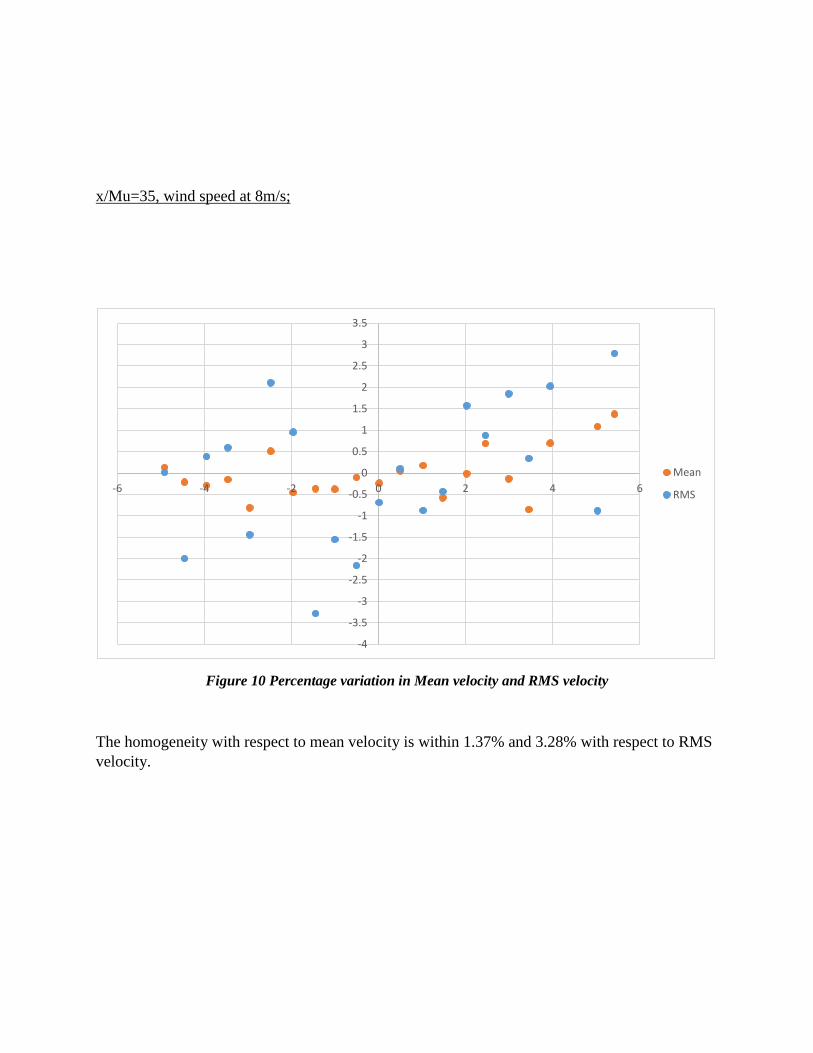
x/Mu=35, wind speed at 8m/s;

Figure 10 Percentage variation in Mean velocity and RMS velocity

The homogeneity with respect to mean velocity is within 1.37% and 3.28% with respect to RMS

velocity.

-4

-3.5

-3

-2.5

-2

-1.5

-1

-0.5

0

0.5

1

1.5

2

2.5

3

3.5

-6 -4 -2 0 2 4 6

Mean

RMS

Isotropy:

Wind speed at 4m/s.

Figure 11 Skewness of velocity

-0.100

-0.050

0.000

0.050

0.100

0.150

0.200

0.250

0.0000 20.0000 40.0000 60.0000 80.0000 100.0000 120.0000 140.0000 160.0000

x/Mu

The trend in the above plot shows that Skewness is decreasing and starts approaching zero at

around x/Mu=116. A similar observation can be made by looking at the Skewness of derivative

plot. The trend plot is approaching 0.5 at about x/Mu=115.

Figure 12 Skewness of derivative of velocity

Figure 13 ε/ε*plot

Looking at ε/ε*, the plot approaches unity at about x/Mu=96. Based on this plot, the flow appears

to become isotropic at x/Mu=96 and eventually overshoots. The possible explanation could be

that the data points chosen were too close to the grid and the points did not fit in the power decay

law.

0.450

0.470

0.490

0.510

0.530

0.550

0.570

0.590

0.610

0.630

0.650

0.0000 20.0000 40.0000 60.0000 80.0000 100.0000 120.0000 140.0000 160.0000

x/Mu

0.0000

0.2000

0.4000

0.6000

0.8000

1.0000

1.2000

1.4000

0.0000 20.0000 40.0000 60.0000 80.0000 100.0000 120.0000 140.0000 160.0000

Wind speed at 8m/s.

Figure 14 Skewness of velocity

For 8m/s the skewness of velocity is not zero until x/Mu=140. Also, the skewness of derivative

is above 0.5 at x/Mu=142.

0.000

0.050

0.100

0.150

0.200

0.250

0.300

0.350

0.0000 20.0000 40.0000 60.0000 80.0000 100.0000 120.0000 140.0000 160.0000

x/Mu

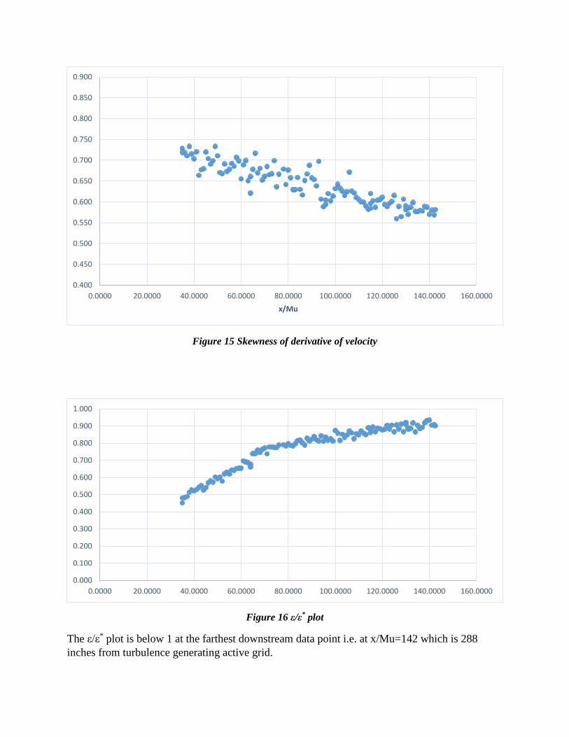
Figure 15 Skewness of derivative of velocity

Figure 16 ε/ε* plot

The ε/ε* plot is below 1 at the farthest downstream data point i.e. at x/Mu=142 which is 288

inches from turbulence generating active grid.

0.400

0.450

0.500

0.550

0.600

0.650

0.700

0.750

0.800

0.850

0.900

0.0000 20.0000 40.0000 60.0000 80.0000 100.0000 120.0000 140.0000 160.0000

x/Mu

0.000

0.100

0.200

0.300

0.400

0.500

0.600

0.700

0.800

0.900

1.000

0.0000 20.0000 40.0000 60.0000 80.0000 100.0000 120.0000 140.0000 160.0000

Decay Power Law:

Wind speed at 4m/s

By performing downstream decay experiment we were able to confirm the validity of power

decay law, which is shown in fig. 18 below.

Figure 17 Decay Power Law plot

The power decay law is governed by equation-

𝑢2

𝑈2= 𝐴(

𝑥

𝑀𝑢)−𝑛

The axes are converted on a Logarithmic scale to obtain linear relationship.

The curve fit equation from the plot matches with the above equation. Comparing the curve fit

and original equation we can find the values of A and n. i.e. A=5.6336and n=1.504.

y = 5.6336x-1.504

R² = 0.9982

0.0010

0.0100

0.1000

10.0000 100.0000 1000.0000

x/Mu

Wind speed at 8m/s

The decay power law plot for 8m/s is shown below. Similarly, the values of A and n are 5.3742

and 1.4 respectively.

Figure 18 Decay power law plot for 8m/s

CONCLUSION

From homogeneity data, we can conclude that at x/Mu=142, the flow at 4m/s is more

homogenous than the flow at 8m/s. Though the further improvement in homogeneity for both

cases can be expected further downstream of flow.

The flow at 4m/s starts showing isotropy after x/Mu=96 with ε/ε* approaching unity. The

skewness approaches 0 at x/Mu=115 and at same position, the skewness of derivative is nearly

0.5. But the 8m/s flow does not approach any of the benchmarks until x/Mu=142. The plot

appears to be flattening as it approaches ε/ε*=1. Though looking at the trend in all three plots, it

can be inferred that a larger test section may accommodate a nearly isotropic data point. But for

4m/s case, the choice of bad data points for power decay law explains why the level of flat

region was off.

The decay exponent is greater than 1 in the 4m/s and 8m/s case. For a linear downstream

variation of 𝑢2

𝑈2 as a function of 𝑥

𝑀𝑢 , the power decay law has exponent in the form of – (n+1)

(Mohamed and LaRue, 1990) i.e. the exponent is always greater than 1 with a negative sign. The

y = 5.3742x-1.4

R² = 0.9972

0.0010

0.0100

0.1000

10.0000 100.0000 1000.0000

x/Mu

decay exponents for both 4m/s and 8m/s are -1.504 and -1.4 respectively. Thus the validity of

Decay power law is established.

FUTURE WORK

The experiment will be extended to study the isotropic behavior of turbulence by using a cross-

wire, which registers velocity in two perpendicular directions. After an understanding of velocity

field is developed, the temperature field will be studied by using a scalar grid in between active

grid and sensor. Heated air from scalar grid will act as a surrogate to fuel in a premixer.

ACKNOWLEDGEMENTS

I would like to acknowledge the help that I gathered from Prof. John C. LaRue with his broad

experience and deep insight in the field of turbulence. I would also like to acknowledge the

efforts made by Alejandro Puga and Tim Koster in helping me understand the most difficult of

the concepts of turbulence. They have been my guides throughout the internship. Four undergrad

students- Kyle Johnson, Thomas Sayles, Baolong Nguyen and Christine lao helped me run the

experiments. My parents have been the constant source of motivation throughout.

References

Pijush K. Kundu/Ira M. cohen (2006), Fluid Mechanics, Academic Press Elsevier.

Batchelor, GK (1953), The Theory of Homogeneous Turbulence. Cambridge University Press.

Mohsen S. Mohamed and John C. LaRue, J. Fluid Mech.(1990). vol. 219, pp. 195-214 Printed in

Great Britain

Z. Warhaft (2000), Passive Scalars in Turbulent Flows, Annual Review of Fluid Mechanics,Vol.

32: 203-240

Ory D. Selzer (2001), The effect of initial scalar size on the mixing of a passive scalar in grid-

generated turbulence, Thesis, University of California, Irvine.

Abdullah MohammadFarid N Alkudsi (2011), Effect of Length Scales on the Mixing of Passive

Scalars in Grid Turbulence, Dissertation, University of California, Irvine.