INTERNATIONAL TRADE AND THE ENVIRONMENT: THEORETICAL AND POLICY LINKAGES* J. Peter Neary University College Dublin and CEPR June 1999 This revision 23 June 2005 Abstract I review and extend three approaches to trade and environmental policies: competitive general equilibrium, oligopoly and monopolistic competition. The first two have surprisingly similar implications: deviations from first-best rules are justified only by constraints on policy choice (which motivates what I call a "single dividend" approach to environmental policy), and taxes and emissions standards differ in ways which reflect the Le Chatelier principle. I also show how environmental taxes may lead to a catastrophic relocation of industry in the presence of agglomeration effects, although not necessarily if there is a continuum of industries which differ in pollution intensity. JEL: O13, L13, F12. Keywords: Environmental policy; international trade policy; location and economic geography; pollution abatement; strategic trade policy. * An earlier version was presented as an invited plenary lecture to the European Association for Environmental and Resource Economics Conference, Oslo, 1999. I am very grateful to an anonymous referee, to Peter Clinch, Gernot Klepper, Danny McCoy, Michael Rauscher and Daniel Sturm, and to participants at Oslo and at the Irish Economic Association Annual Conference, for helpful comments. This research forms part of the International Trade and Investment programme of the Geary Institute at UCD.

Welcome message from author
This document is posted to help you gain knowledge. Please leave a comment to let me know what you think about it! Share it to your friends and learn new things together.
Transcript
INTERNATIONAL TRADE AND THE ENVIRONMENT:
THEORETICAL AND POLICY LINKAGES*
J. Peter NearyUniversity College Dublin and CEPR
June 1999This revision 23 June 2005
Abstract
I review and extend three approaches to trade and environmental policies: competitivegeneral equilibrium, oligopoly and monopolistic competition. The first two have surprisinglysimilar implications: deviations from first-best rules are justified only by constraints on policychoice (which motivates what I call a "single dividend" approach to environmental policy),and taxes and emissions standards differ in ways which reflect the Le Chatelier principle. Ialso show how environmental taxes may lead to a catastrophic relocation of industry in thepresence of agglomeration effects, although not necessarily if there is a continuum ofindustries which differ in pollution intensity.
JEL: O13, L13, F12.
Keywords: Environmental policy; international trade policy; location and economicgeography; pollution abatement; strategic trade policy.
* An earlier version was presented as an invited plenary lecture to the European Associationfor Environmental and Resource Economics Conference, Oslo, 1999. I am very grateful toan anonymous referee, to Peter Clinch, Gernot Klepper, Danny McCoy, Michael Rauscher andDaniel Sturm, and to participants at Oslo and at the Irish Economic Association AnnualConference, for helpful comments. This research forms part of the International Trade andInvestment programme of the Geary Institute at UCD.
My objective in this paper is to review and extend some points of intersection between
international trade theory and environmental economics. These two sub-fields of economics
have much in common. At the theoretical level, both are branches of applied
microeconomics, focusing on the implications of a set of important real-world phenomena:
differential international mobility (of goods, factors or ideas) in the case of trade theory,
specific externalities in the case of environmental economics. At the policy level, the
interaction of trade and environmental policies is increasingly recognised by both analysts and
policy-makers as central to the successful operation of both.
Two key areas of policy concern have motivated recent studies of the trade-
environment nexus. One is the fear that trade liberalisation will increase pollution emissions,
which raises the issue of whether environmental policy should be tightened to compensate for
changes in trade policy. A second major focus of linkages between the two areas is the
debate over environmental regulation and international competitiveness. Ongoing debates
about increased environmental regulation in the EU have renewed fears that such measures
could reduce on competitiveness, leading to both deindustrialisation and "carbon leakage" as
polluting industries relocate to other countries. The net effect would be to shift the costs of
environmental degradation but also the benefits of industrial agglomeration towards foreign
and away from domestic locations.
To explore these issues, I consider three alternative approaches to modelling the
interaction between trade and environmental policies. First, I consider the benchmark case
of a competitive small open economy and review the familiar but important second-best
considerations, which can make lax environmental policies desirable if trade policy is
constrained, or tariffs welfare-improving when environmental policy is constrained to be sub-
optimal.
Next, I consider models of technical choice by polluting oligopolists. Once again, it
turns out that second-best considerations complicate the ranking of alternative interventions.
Strategic considerations may mandate an investment subsidy to shift rents towards home
firms, whereas environmental concerns may require a tax.
Finally, I turn to the less well-explored area of locational choice by firms which,
because of increasing returns in differentiated product industries, confer pecuniary externalities
on each other. Such externalities have been shown to introduce the possibility of
agglomeration in equilibrium, with firms locating close together to avail of lower costs of
serving the larger market. However, such an equilibrium is not a deeply-rooted one, in the
sense that a change in circumstances, such as the introduction of an environmentally
motivated tax, may lead to a catastrophic relocation of industrial activity. I explore the extent
to which these tendencies can be offset if there is a continuum of industries, which differ in
their pollution intensity, and so in their vulnerability to environmental policies.
1. Second-Best Intervention in Competitive Open Economies
The first setting in which I illustrate the interaction of trade and environmental policies
is a competitive general equilibrium model of a small open economy.1 The economy
produces and consumes n+1 goods and h "bads" or pollution emissions. I take an arbitrary
good as numeraire, so its home and foreign price are set equal to unity and kept in the
background throughout. The prices of the n non-numeraire goods equal p at home and p*
abroad, with the difference attributable to a vector of trade taxes r=p−p*. The emissions are
1 The extensive literature on trade policy reform in this framework, stemming from Hatta(1977), has been extended to environmental policies by Copeland (1994), Beghin et al. (1997)and Ulph (1997), among others. I draw extensively on these papers in what follows, and usesome techniques from my own work (especially Neary and Schweinberger (1986) and Neary(1994) which introduced the trade expenditure function and the potato diagram respectively),to simplify and generalise the analysis.
2
generated in the production sector and can be controlled either by binding standards z or by
emission taxes t, while they cause environmental damage only to consumers. I begin with
the case of emissions standards, which is probably less realistic than taxes but is simpler and
introduces some important concepts which will prove useful throughout.
It has become standard to characterise the behaviour of individual agents in such an
economy using the dual techniques popularised by Dixit and Norman (1980). Thus the
production side of the economy can be represented by a GDP function: g(p,z) ≡ Max {x} {p′x:
F(x,z)<_0}. Here x and z represent the net outputs of goods and emissions respectively, which
must be consistent with the economy’s production possibilities, summarised by the aggregate
production constraint F(x,z)<_0. (This constraint in turn depends on factor endowments, the
state of technology and so on, but since I will not consider changes in these underlying
variables I do not need to make their levels explicit.) From Hotelling’s Lemma, the price
derivatives of the GDP function give the equilibrium outputs of goods: gp=x; while the
derivatives with respect to emissions gz give the marginal costs of reducing emissions or the
marginal abatement costs. (Subscripts denote partial derivatives.)
As for consumers, I ignore distributional considerations and assume a single aggregate
household whose behaviour can be represented by an expenditure function: e(p,z,u) ≡ Min q
{p′q: u(q,z)>_u}, where utility depends positively on consumption of goods and negatively on
emissions: uq>0 and uz<0. From Shephard’s Lemma, the price derivatives of the function
equal the Hicksian demands: ep=q; while from Neary and Roberts (1980) the derivatives with
respect to z are the virtual prices of the pollution levels, and so measure the marginal
willingness to pay for reductions in emissions.
It turns out to be very convenient to combine the consumption and production sides
of the economy into a single function. I call this the trade expenditure function, which is
3
simply the difference between the expenditure and GDP functions:
Two useful properties follow immediately. First, the derivative of E with respect to goods
(1)
prices is the vector of net imports m, Ep=ep−gp=q−x, and its second derivative matrix Epp is
negative definite, so, heuristically, compensated net import demand functions slope
downwards.2 Second, the derivative of E with respect to emissions z measures the
environmental distortions in the economy, the difference between consumers’ marginal
willingness to pay for a reduction in emissions and the marginal abatement costs: Ez=ez−gz.
Armed with these properties, the general equilibrium of the economy is easily
expressed. I ignore intertemporal considerations, so all factor income is spent on current
consumption. In addition, I assume the government redistributes all tax revenue to consumers
in a lump-sum fashion. Hence the aggregate household’s budget constraint, which is also the
balance of payments equilibrium condition, requires that expenditure minus GDP (i.e., the
value of the trade expenditure function) must equal tariff revenue:3
The elements of the vector of net imports, m, can be either positive or negative. However,
(2)
to avoid tedious repetition I will describe the results on the assumption that all exports are
untaxed and subsumed into the numeraire good, so m is strictly positive. (The equations
obviously apply more generally.)
Totally differentiating (2) (and using Ep=m and dp=dr to simplify) leads immediately
2 Technical details are in appendices, available on my home page.
3 I assume throughout that all government revenue is returned costlessly to the private sector.Alternative assumptions about the disposition of government revenue from quotas or emissionlicences complicate the analysis in significant ways: see Anderson and Neary (1992).
4
to the conditions for a first-best optimum:
The left-hand side is the change in utility expressed in numeraire units: call this the change
(3)
in real income. For this to be maximised requires from the right-hand side that both tariffs
r and environmental distortions Ez be eliminated.
These first-best rules are a crucial benchmark. But, of course, the interesting policy
questions are those which arise when the economy is not already at the first best. To evaluate
these, we eliminate dm from (3) to obtain:4
where:
(4)
The left-hand side of (4) is just the change in real income deflated by the "tariff multiplier"
(5)
or "shadow price of foreign exchange" (1−r′xI)−1: a scalar correction factor which must be
positive if the equilibrium is stable and which can otherwise be ignored henceforward. As
for the right-hand side, it depends on changes in the two instruments, tariffs and emissions
standards, which I consider in turn.
The tariff reform term in (4) has a simple form, since the matrix Epp is negative
definite. This gives the well-known result that a proportionate reduction in tariffs (dr=−rdα,
where dα is a positive scalar) must raise welfare. This result continues to hold irrespective
of the levels of emissions, reflecting the principle that quantitative restrictions neutralise the
4 Recall that m=Ep. Hence dm = Eppdr+Epzdz+xIeudu, where xI=epu/eu is the vector ofMarshallian income derivatives. See Neary (1995) for discussion and further references.
5
by-product distortions of sub-optimal taxes and so avoid second-best complications.5
As for the emissions term in (4), this is more complex because their optimal values
are non-zero and because consumers are directly affected by the level of pollution. The h-by-
1 vector δ measures the marginal welfare effect of an increase in emissions, and must be zero
at the second-best optimum. It equals the difference between marginal abatement costs gz and
the full social costs of emissions: both the direct cost ez and the indirect cost through any
induced reduction in tariff revenue, −r′Epz.6 Because of the latter term, second-best
considerations cannot be avoided when considering reforms of emissions policy in the
presence of irremovable tariffs. Setting δ equal to zero implies that marginal abatement costs
should exceed marginal damage costs to the extent that higher pollution leads to increased
imports and so (from (3)), raises welfare.
I turn next to the case where emissions are controlled by taxes. This has many
similarities with the standards case just considered. However, we need to specify the
production side of the model somewhat differently. Where before the level of emissions was
a constraint on producers’ behaviour, now they respond to prices for both goods and bads.
To model this, I use the flex-price GDP function from Neary (1985): g(p,t) ≡ Max {x,z}
{p′x−t′z: F(x,z)<_0}. Now, Hotelling’s Lemma implies that the price derivatives of the GDP
function give the equilibrium outputs of both goods and emissions: gp=x and gt=−z. In
addition, the properties of the flex-price and emissions-constrained GDP functions can be
5 See Corden and Falvey (1985), Copeland (1994) and Neary (1995).
6 This has to be interpreted with care. Take, for example, a case considered by Ulph (1997),where extra pollution causes domestic residents to take more foreign holidays, which aresubject to domestic taxes (so Epz>0). The trade taxes lead to sub-optimal levels of tourismimports and so, from (3), any measure which increases these imports (even an increase inpollution) is to that extent welfare-improving. Hence, in this case trade taxes reduce ratherthan increase the social cost of pollution.
6
directly linked by noting that the functions are related as follows:
This implies a number of useful properties. In particular, the supply responses of the flex-
(6)
price economy are greater than those of the emissions-constrained one, a result known as the
Le Chatelier principle.7 Finally, the equilibrium can now be specified in terms of the flex-
price trade expenditure function (which depends on both t and z):
Here I have introduced a new (n+h)-by-1 vector π for the prices of both goods and bads, and
(7)
a corresponding vector τ for tariffs and taxes; while the derivative of E with respect to the
full price vector π is the vector of net imports and emissions:
Note that the matrix of second derivatives Eππ is negative definite.
(8)
Inspection of (6) and (7) shows that the equilibrium condition for this model is
formally identical to (2): net spending by the private sector must equal redistributed tax and
tariff revenue. This can be written in compact form as follows:
Totally differentiating gives:
(9)
7 Differentiating (6) twice gives: gpp−gpp=−gpzgzz−1gzp. Thus, since gzz is negative definite, the
difference between the two positive definite matrices of price-output responses, gpp and gpp,is itself positive definite.
7
This is identical to (3) once we make allowance for the switch in policy instrument from
(10)
standards to taxes, so that t=gz. Hence the first-best policy prescription is essentially the
same: free trade (r=0) combined with pollution taxes which equal the consumers’ marginal
willingness to pay for abatement (t=ez).
Eliminating the endogenous terms from the left-hand side of (10) (details are in
Appendix 1), gives:
where:
(11)
The right-hand side of (11) is more complicated than that of equation (4) in the standards
(12)
case, since it contains four terms rather than two. But, as before, it depends on the "excess
taxes", or the deviations of taxes from their optimal values, denoted by the new vector τ. In
the case of trade taxes, these are just the tariff levels themselves (since their optimal values
are zero); while in the case of emissions, the excess taxes on pollution take account of the
indirect cost of emissions through any induced reduction in tariff revenue.
Notwithstanding the complexity of the model, the right-hand side of (11) has a very
convenient and simple form, since the matrix Eππ is negative definite.8 This gives a direct
8 Equation (11) is essentially equation (7) in Copeland (1994), rewritten in more compactform. Very similar expressions are found in many policy reform contexts, including tariffreform in large open economies (Neary (1995)), simultaneous reform of taxes on trade andinternational factor movements (Neary (1993)), and multilateral trade policy reform by themembers of a customs union (Neary (1998)).
8
proof of a result due to Copeland (1994): welfare must rise following a uniform reduction in
all distortions in proportion to their deviations from optimal. An across-the-board policy
reform of this kind implies that dτ=−τdα (where dα is a positive scalar), and so the right-
hand side of (11) must be positive (since τ′Eππτ is a quadratic form in a negative definite
matrix and so is unambiguously negative).
Consider next the case where only one set of policy instruments can be varied. If only
tariffs are available (dt=0), equation (11) can be solved for their optimal second-best values:
Symmetrically, if tariffs cannot be altered (dr=0), equation (11) can be solved for the optimal
(13)
second-best values of the "excess" pollution taxes:
These equations have a standard second-best interpretation: if one set of policy instruments
(14)
is fixed at non-optimal levels, then the other set should deviate systematically from their first-
best levels. More specifically, note that both equations (13) and (14) have in common a
matrix which cannot be signed a priori: gtp, which equals −zp (minus the responsiveness of
emissions to tariffs) is the transpose of gpt, which equals xt (the responsiveness of importables
to pollution taxes). I will describe importables as "pollution-intensive" if the elements of this
matrix are negative on average. In that case, equation (13) shows that, when environmental
policy is constrained to be lax (δ<0), then imports should be subsidised to compensate; while
equation (14) shows that, when tariffs cannot be cut (r>0), then environmental policy should
be tightened to compensate. The key to this example is that, with gtp negative, outputs and
emissions are complements in production and hence tariffs and pollution taxes are alternatives
from a policy perspective: if one cannot be lowered towards its optimal level then the other
9
should be raised above its optimal level instead (and conversely).
A final result is that equation (14) is identical to the second-best optimal rule, δ=0,
which we found for the case of emission standards. To see this, use the derivatives of (6) to
simplify the right-hand side of (14).9 The second-best optimal value of emissions taxes then
becomes:
This is identical to setting (5) equal to zero. Hence, whether environmental policy is
(15)
implemented by standards or taxes, marginal abatement costs should equal marginal damage
costs less the change in tariff revenue induced by an increase in emissions.
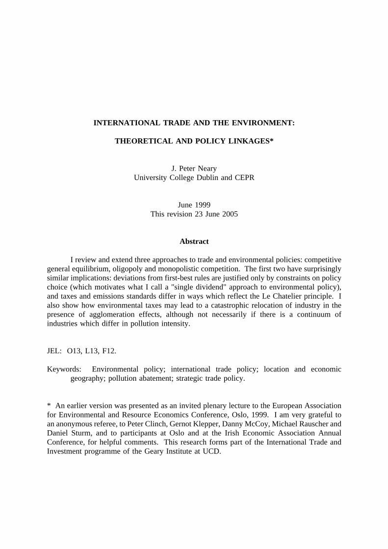
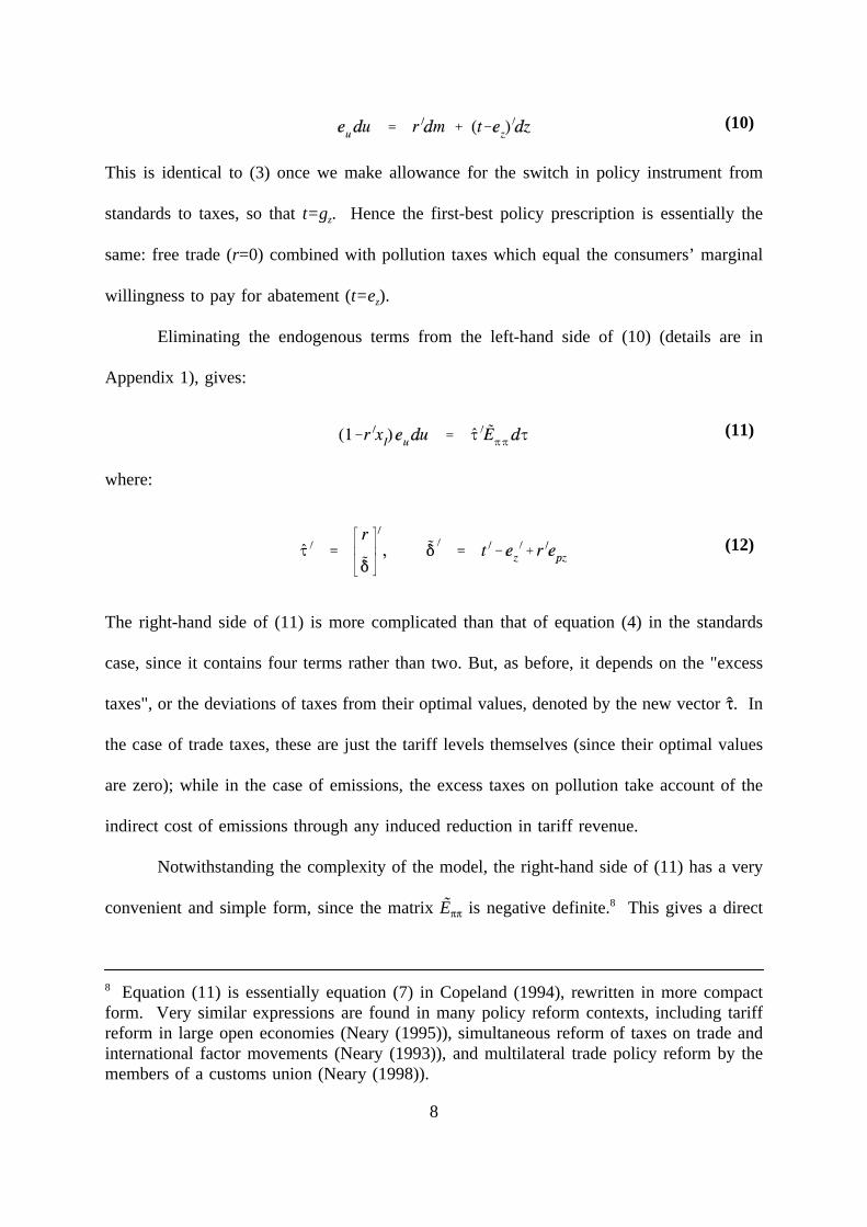
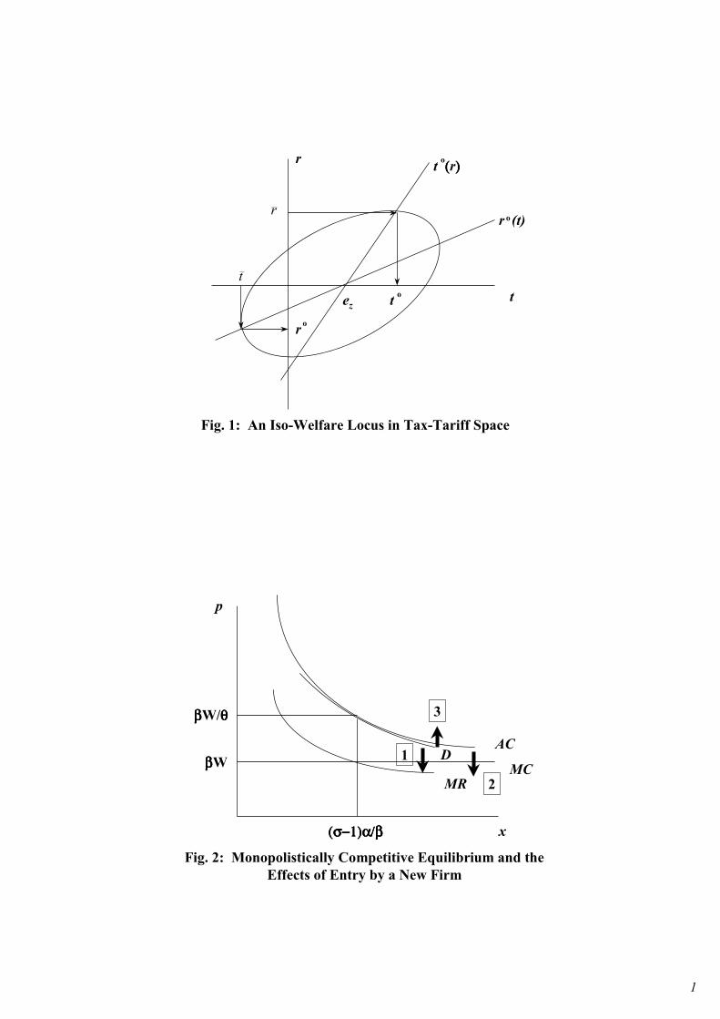
Fig. 1 illustrates some of these results in the case of a single tariff and a single
pollution tax, with the additional simplification that goods demands are unaffected by
emissions (epz=0). The two second-best loci must intersect at the first-best optimal point of
free trade and t=ez. Assuming for concreteness that the importable is pollution-intensive and
so the two instruments are alternatives implies, from (13) and (14), that the loci are upward-
sloping as shown. Every iso-welfare locus must therefore have the upward-tilted potato shape
shown (since it must be horizontal where it crosses a to locus and vertical where it crosses
a ro locus). The implications for each instrument of fixing the other one at an arbitrary level
can then be read off the figure as shown. For example, if the tariff r is fixed at r, then the
optimal second-best pollution tax to exceeds the first-best tax ez.
Two extensions may be mentioned briefly. International factor mobility does not
affect the formal analysis to any great extent, and the policy prescriptions are unaffected as
long as factor movements are untaxed. From Neary (1985), the main difference is that supply
9 By relating the second derivatives of the g and g functions, it can be checked that gpt(gtt)−1
equals −gpz.
10
responses to price are now more elastic and so specialisation in production is more likely:
another reflection of the Le Chatelier principle. As noted by Copeland (1994), this implies
that increased globalisation in the sense of greater openness of domestic markets to
competition tends to exacerbate the costs of sub-optimal environmental policy. By contrast,
extending the model to a large open economy requires some extra notation, mainly to keep
track of the complications arising from income effects between countries. However, the
policy prescriptions are largely unchanged with one key amendment: the benchmark for trade
policy is no longer free trade but rather the "optimal tariff". (See Neary (1995).)
2. Strategic Trade and Environmental Policies
The general equilibrium framework of the last section provides an essential reference
for the discussion of trade and environmental policies. However, it gives only a shadowy role
to individual firms and so cannot throw light on issues such as how strategic considerations
affect emissions policy or how firms respond to incentives to invest in pollution abatement.
In recent years, an extensive literature has developed which addresses these issues using the
theory of strategic trade policy pioneered by Brander and Spencer (1985).10 In this section
I again try to synthesise this literature within a common framework.
As in Brander and Spencer (1985), it is very convenient to consider a model with no
domestic consumption, with two firms, one home and one foreign, competing in a third
market. The firms engage in a non-cooperative Nash game but, as in Brander (1995) and
Neary and Leahy (2000), I leave open the nature of the competition between them. Thus, I
assume only that each firm chooses the value of some "action", a for the home firm and a*
10 Applications of strategic trade policy to environmental issues include Barrett (1994),Conrad (1993), Kennedy (1994), Rauscher (1994), Ulph (1996, 1997) and Ulph and Ulph(1996).
11
for the foreign firm. This allows me to develop a common set of results which apply both
to Cournot competition (when the actions are quantities x and x*) and to Bertrand competition
(when the actions are prices p and p*). The home firm also generates a level of pollution
denoted by z. Finally, the home government may offer a subsidy to exports at a rate s and
may also implement an environmental policy: to begin with, I assume that this takes the form
of direct controls on the emissions level z.
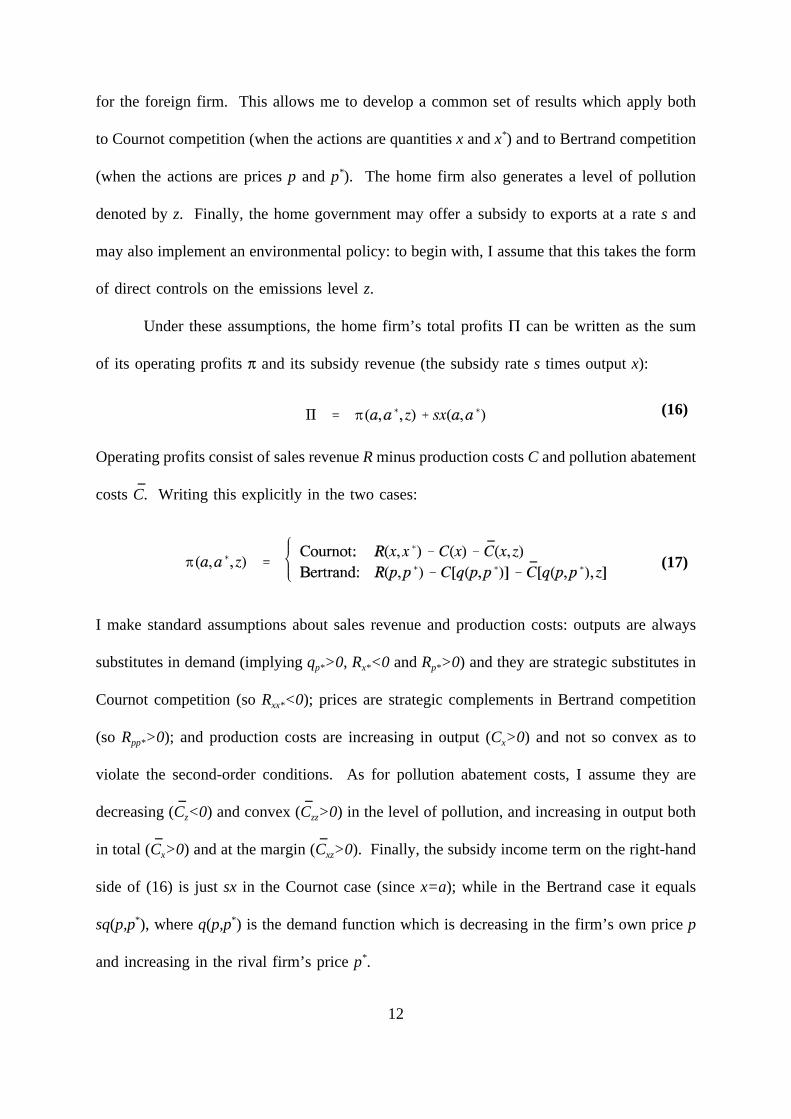
Under these assumptions, the home firm’s total profits Π can be written as the sum
of its operating profits π and its subsidy revenue (the subsidy rate s times output x):
Operating profits consist of sales revenue R minus production costs C and pollution abatement
(16)
costs C. Writing this explicitly in the two cases:
I make standard assumptions about sales revenue and production costs: outputs are always
(17)
substitutes in demand (implying qp*>0, Rx*<0 and Rp*>0) and they are strategic substitutes in
Cournot competition (so Rxx*<0); prices are strategic complements in Bertrand competition
(so Rpp*>0); and production costs are increasing in output (Cx>0) and not so convex as to
violate the second-order conditions. As for pollution abatement costs, I assume they are
decreasing (Cz<0) and convex (Czz>0) in the level of pollution, and increasing in output both
in total (Cx>0) and at the margin (Cxz>0). Finally, the subsidy income term on the right-hand
side of (16) is just sx in the Cournot case (since x=a); while in the Bertrand case it equals
sq(p,p*), where q(p,p*) is the demand function which is decreasing in the firm’s own price p
and increasing in the rival firm’s price p*.
12
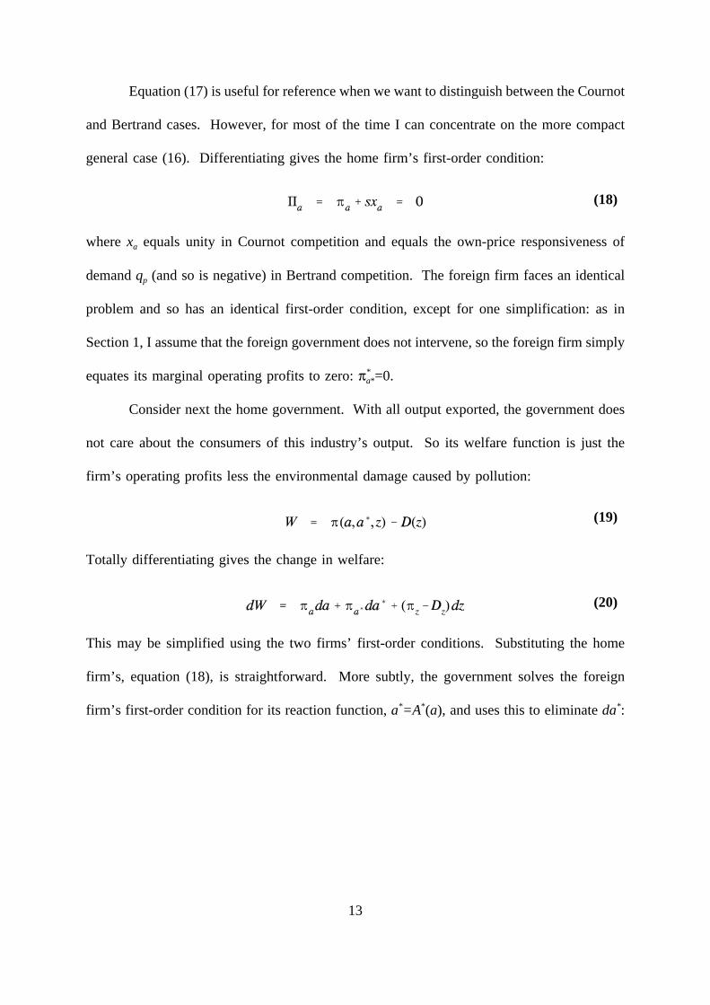
Equation (17) is useful for reference when we want to distinguish between the Cournot
and Bertrand cases. However, for most of the time I can concentrate on the more compact
general case (16). Differentiating gives the home firm’s first-order condition:
where xa equals unity in Cournot competition and equals the own-price responsiveness of
(18)
demand qp (and so is negative) in Bertrand competition. The foreign firm faces an identical
problem and so has an identical first-order condition, except for one simplification: as in
Section 1, I assume that the foreign government does not intervene, so the foreign firm simply
equates its marginal operating profits to zero: π*a*=0.
Consider next the home government. With all output exported, the government does
not care about the consumers of this industry’s output. So its welfare function is just the
firm’s operating profits less the environmental damage caused by pollution:
Totally differentiating gives the change in welfare:
(19)
This may be simplified using the two firms’ first-order conditions. Substituting the home
(20)
firm’s, equation (18), is straightforward. More subtly, the government solves the foreign
firm’s first-order condition for its reaction function, a*=A*(a), and uses this to eliminate da*:
13
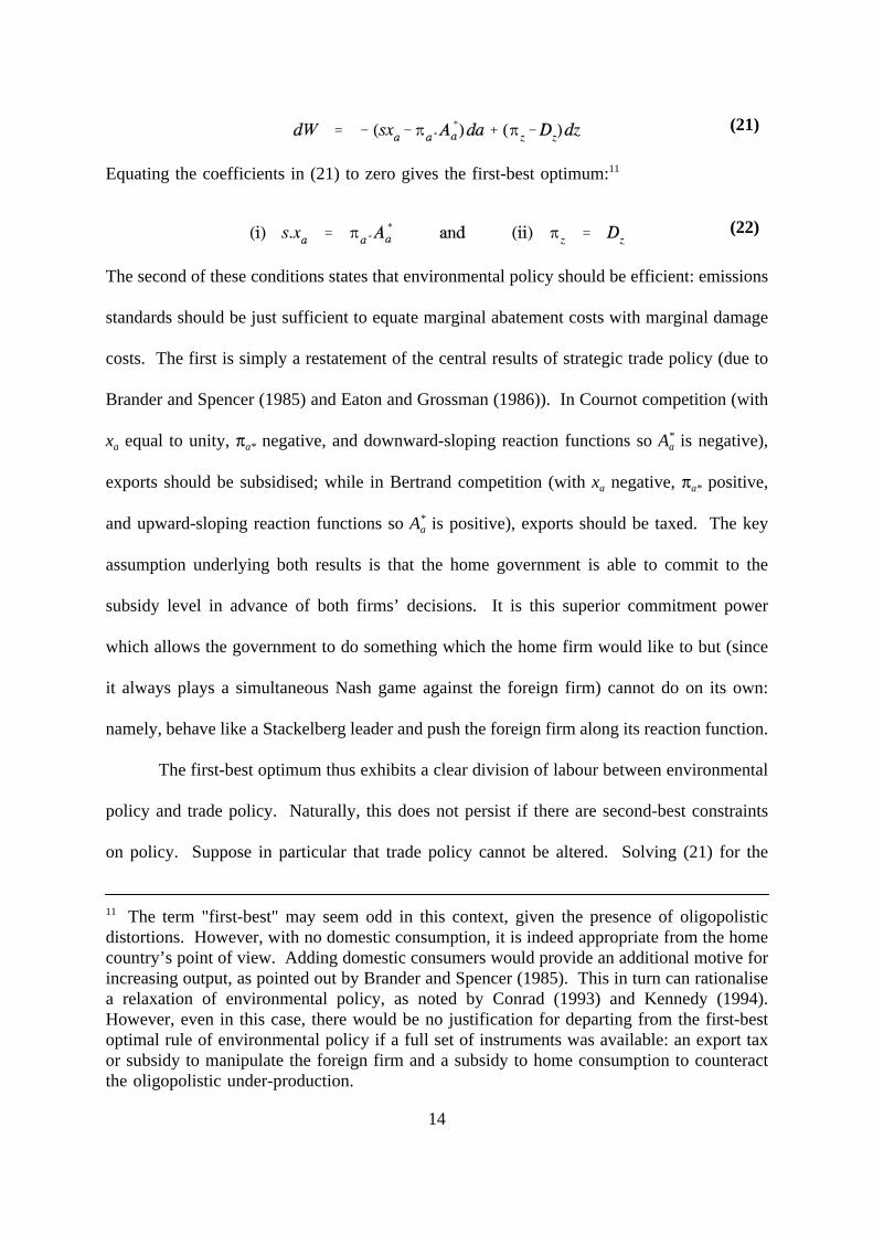
Equating the coefficients in (21) to zero gives the first-best optimum:11
(21)
The second of these conditions states that environmental policy should be efficient: emissions
(22)
standards should be just sufficient to equate marginal abatement costs with marginal damage
costs. The first is simply a restatement of the central results of strategic trade policy (due to
Brander and Spencer (1985) and Eaton and Grossman (1986)). In Cournot competition (with
xa equal to unity, πa* negative, and downward-sloping reaction functions so A*a is negative),
exports should be subsidised; while in Bertrand competition (with xa negative, πa* positive,
and upward-sloping reaction functions so A*a is positive), exports should be taxed. The key
assumption underlying both results is that the home government is able to commit to the
subsidy level in advance of both firms’ decisions. It is this superior commitment power
which allows the government to do something which the home firm would like to but (since
it always plays a simultaneous Nash game against the foreign firm) cannot do on its own:
namely, behave like a Stackelberg leader and push the foreign firm along its reaction function.
The first-best optimum thus exhibits a clear division of labour between environmental
policy and trade policy. Naturally, this does not persist if there are second-best constraints
on policy. Suppose in particular that trade policy cannot be altered. Solving (21) for the
11 The term "first-best" may seem odd in this context, given the presence of oligopolisticdistortions. However, with no domestic consumption, it is indeed appropriate from the homecountry’s point of view. Adding domestic consumers would provide an additional motive forincreasing output, as pointed out by Brander and Spencer (1985). This in turn can rationalisea relaxation of environmental policy, as noted by Conrad (1993) and Kennedy (1994).However, even in this case, there would be no justification for departing from the first-bestoptimal rule of environmental policy if a full set of instruments was available: an export taxor subsidy to manipulate the foreign firm and a subsidy to home consumption to counteractthe oligopolistic under-production.
14
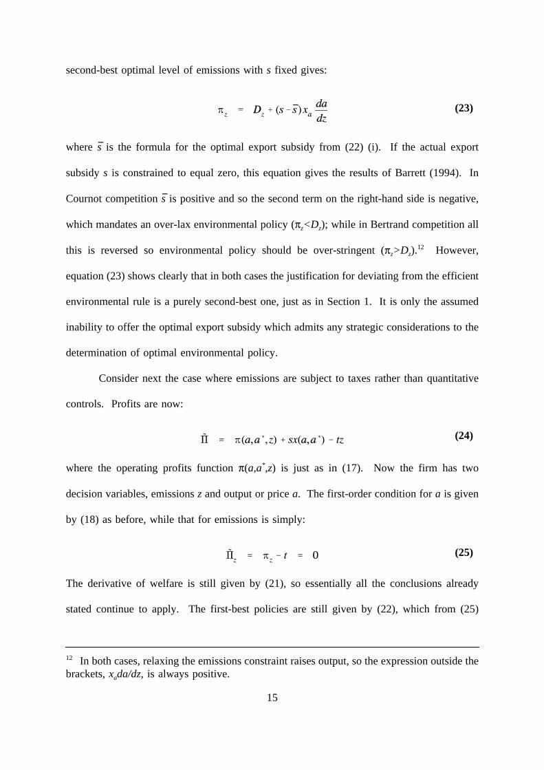
second-best optimal level of emissions with s fixed gives:
where s is the formula for the optimal export subsidy from (22) (i). If the actual export
(23)
subsidy s is constrained to equal zero, this equation gives the results of Barrett (1994). In
Cournot competition s is positive and so the second term on the right-hand side is negative,
which mandates an over-lax environmental policy (πz<Dz); while in Bertrand competition all
this is reversed so environmental policy should be over-stringent (πz>Dz).12 However,
equation (23) shows clearly that in both cases the justification for deviating from the efficient
environmental rule is a purely second-best one, just as in Section 1. It is only the assumed
inability to offer the optimal export subsidy which admits any strategic considerations to the
determination of optimal environmental policy.
Consider next the case where emissions are subject to taxes rather than quantitative
controls. Profits are now:
where the operating profits function π(a,a*,z) is just as in (17). Now the firm has two
(24)
decision variables, emissions z and output or price a. The first-order condition for a is given
by (18) as before, while that for emissions is simply:
The derivative of welfare is still given by (21), so essentially all the conclusions already
(25)
stated continue to apply. The first-best policies are still given by (22), which from (25)
12 In both cases, relaxing the emissions constraint raises output, so the expression outside thebrackets, xada/dz, is always positive.
15
implies that t=Dz: the emissions tax should be set equal to the marginal damage cost. As for
the second-best case, equation (23) still applies, which gives the results of Conrad (1993) and
Kennedy (1994): the emissions tax should deviate from the marginal damage cost to an extent
which compensates for the inability to impose the optimal export subsidy or tax.
There is one interesting difference between the tax and standards cases, and it concerns
the slope of the foreign reaction function A*a. Under Cournot competition this is now greater
in absolute value (i.e., more negative) than when emissions are controlled by standards; while
under Bertrand competition it is presumptively less positive. So, other things equal, the
optimal subsidy is algebraically greater when emissions are controlled by taxes than by
standards. These differences are yet another reflection of the Le Chatelier principle: removing
a quantity constraint on an economy or firm typically increases its responsiveness to shocks,
whether of outputs to prices as in Section 1 or of own to rival’s actions as here. (Proofs are
given in Appendix 3.)
The final case to be considered is where each firm can make a prior investment in
R&D in order to reduce emissions.13 The main lessons can be illustrated easily in a special
case, where the level of emissions is uniquely determined (inversely of course) by the level
of investment in abatement technology. (Appendix 4 considers the general case where the
link between investment and emissions depends on the level of output.) Formally, this special
case does not alter the specification of the model given in equations (17) and (24). In
particular, we can continue to treat the level of pollution z as one of the firm’s choice
variables, with the additional interpretation that it is also an inverse measure of the level of
investment in pollution abatement. However, the change in interpretation invites a change
13 Ulph and Ulph (1996) show that the model can be extended to allow for investment inprocess R&D as well without affecting the results.
16
in the assumptions about the timing of moves in the model: it now makes more sense to
assume that each firm chooses its level of investment z before the actions a and a* are chosen.
This introduces a new strategic motive for choosing the level of emissions and hence a new
reason for the home government to diverge from the first-best rule for emissions.14
If emissions are chosen before actions, each firm has an incentive to use its choice of
z to influence its rival’s choice of action in a way which will raise its profits. The first-order
condition for a is given by (18) as before, but that for emissions is now:
Compared with (25), the new strategic term reflects incentives which have been summarised
(26)
in the "animal spirits" taxonomy of Fudenberg and Tirole (1984). If the second-stage game
is Cournot, the strategic effect is positive (higher emissions lower foreign output a*, which
raises home profits) and the firm has an incentive to behave like a "top dog": over-investing
in emissions and so under-investing in pollution abatement relative to the efficient benchmark
given by (25). Conversely, if the second-stage game is Bertrand, the strategic effect is
negative (higher emissions lower the foreign price a*, which lowers home profits) and the
firm has an incentive to behave like a "puppy dog": under-investing in emissions and so over-
investing in pollution abatement.
In a policy context, following Neary and Leahy (2000), this animal spirits taxonomy
implies a corresponding "animal training" taxonomy of policy responses. To see this,
substitute from (26) into (20) and set the coefficients to zero to solve for the first-best
14 I assume that the equilibrium is sub-game perfect: each firm rationally anticipates theeffect its choice of emissions will have on the actions chosen in the second stage. I alsoassume that the government can commit to its export subsidy before decisions on emissionsare made; otherwise firms would have an incentive to vary their level of emissions in orderto manipulate the export subsidy. (See Leahy and Neary (1999).)
17
instruments as before:
The condition for the optimal export subsidy is unchanged from (22), but that for the optimal
(27)
emissions tax has an added term which exactly offsets the strategic effect. In the Cournot
case, this means "restraining" the top dog by a higher tax on emissions; while in the Bertrand
case it means "encouraging" the puppy dog by a lower tax on emissions. In both cases, the
optimal emissions tax diverges from the first-best optimal rule. However, (as in Spencer and
Brander (1983)) optimal intervention has the effect of restoring the first-best optimal
condition: substituting from (27) (ii) into (26) yields exactly the same first-best optimal
condition as (22) (ii). So, even strategic investment behaviour by firms does not provide a
first-best justification for diverging from optimal environmental policy. Of course, once again
a constraint on the use of trade policy provides a second-best justification for "strategic"
environmental policy. However, it can be checked that the divergence from the first-best is
again given by equation (23): strategic investment in pollution abatement introduces no new
qualitative argument for deviating from the optimal rule for environmental policy.15
The results of this section can be used to throw some light on the so-called "Porter
hypothesis" (see Porter (1991) and Porter and van der Linde (1995)), which asserts that strict
environmental policy would enhance rather than reduce competitiveness. This hypothesis can
be formalised in different ways. For example, it can be interpreted to mean that tight
regulation will raise profits. In the absence of strategic behaviour, as Palmer et al. (1995)
15 The term "qualitative" in this sentence should be stressed. Because the foreign firm is alsobehaving strategically, the equilibrium attained in this case will be quantitatively differentfrom that in the absence of strategic behaviour, even though the home first-order conditionsare identical.
18
argue, this requires that the firm is not maximising to begin with, and begs the question of
why environmental regulation should be the trigger for greater efficiency. Alternatively, it
can be interpreted as implying that tight regulation will raise total investment (including
investment in pollution abatement). The results of Simpson and Bradford (1996) and Ulph
(1996) show that this is sensitive to the functional forms assumed.16 Finally, the Porter
hypothesis can be interpreted simply as a call for tighter environmental policy on the grounds
that this will raise welfare. The results of this section show that, on this interpretation, the
validity of the Porter hypothesis, like so much else, hinges on the assumptions made about
firm behaviour. Specifically, when trade policy cannot be used (so s is constrained to equal
zero), the Porter hypothesis is valid (in the sense that πz should exceed Dz), if firms are
Bertrand competitors but not if they are Cournot competitors.
3. Environmental Regulation and Production Relocation
The final case I want to consider throws light on the issue of whether environmental
policy can lead to relocation of industry. In this section, I want to consider the approach
which draws on the recent work in economic geography by Krugman (1991) and Krugman
and Venables (1995).17 Venables (1999) has applied this approach to environmental taxation
and the first part of this section presents a simple version of his model.
The model is one of Chamberlinian monopolistic competition. As in much recent
work in a variety of fields, it is very convenient to parameterise this in terms of the
symmetric constant-elasticity-of-substitution utility function pioneered by Dixit and Stiglitz
16 Yet another implication, explored by Rauscher (1997, Section 6.5), is that national welfarewill rise if governments impose higher product quality standards.
17 For alternative approaches, see Markusen, Morey and Olewiler (1993), Motta and Thisse(1994) and Hoel (1997).
19
(1977). Here, following Neary (1999) and (2001) respectively, I first present the basic ideas
in a simple diagram and then sketch the consequences of environmental taxation using general
functional forms.
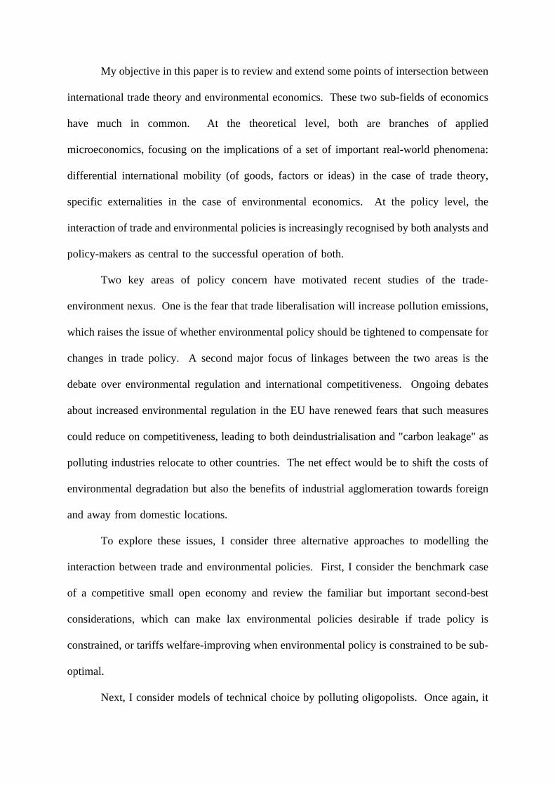
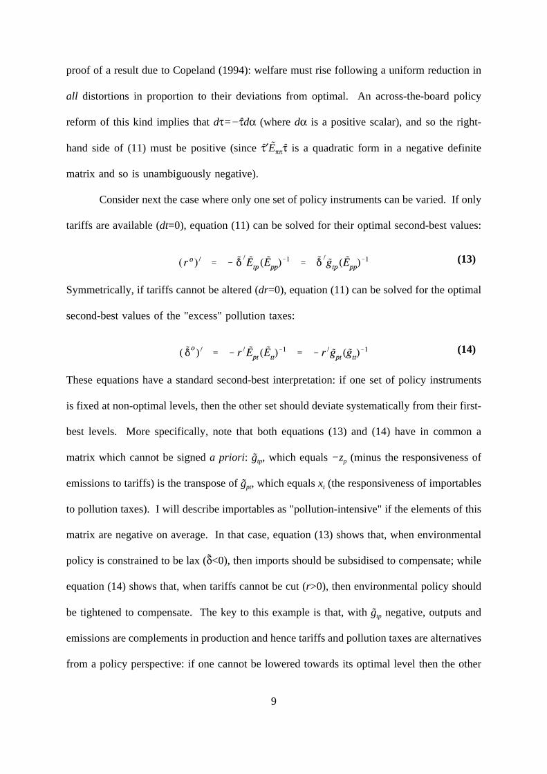
The cost structure of a typical firm is extremely simple. A composite input is
purchased at given price W, fixed costs are αW and production of x units incurs marginal
costs of βW. Hence the total production cost function is:
This implies a marginal cost curve at the level βW, and an average cost curve which is a
(28)
rectangular hyperbola with respect to the vertical axis and the horizontal marginal cost curve.
Fig. 2 illustrates.
Turning to demand, the utility function is:
where qi is the amount of each variety demanded. Because this utility function embodies a
(29)
preference for diversity, and (from (28)) there are increasing returns to scale, each firm
produces a distinct variety. Hence the number of firms in the world (both at home and
abroad), n, is also the number of varieties consumed in both countries. This number is
assumed to be relatively large, which allows us to assume that each firm ignores the actions
of other firms in choosing its output (so the strategic considerations highlighted in the last
section are assumed away). The typical firm then faces a simple constant-elasticity demand
function which can be written (in inverse form) as:
20
Here σ, which equals 1/(1−θ), is the elasticity of substitution between varieties, while A is
(30)
an intercept term, depending on income and the prices of other goods, and assumed to be
taken as given by the firm. Marginal revenue is then easily shown to be:
These two constant-elasticity curves are also shown in Fig. 2. For the model to make sense
(31)
we clearly require that 0<θ<1, or, equivalently, 1<σ<∞.
Equilibrium for the firm now reflects the famous Chamberlinian tangency condition.
Profit maximisation implies that marginal revenue equals marginal cost:
while free entry implies that profits must be zero:
(32)
This simplifies, using (32), to give a remarkably simple result:
(33)
This says that the output of each firm depends only on the cost parameters α and β and on
(34)
the elasticity of substitution σ. Changes in any other parameters or variables (including the
demand intercept A and the cost of the composite input W) lead to adjustments in industry
output via changes in the number of firms only.
So far, this is just an illustration of an equilibrium, with much of the action taking
place in the background: the values of the industry-wide parameters A and W, taken as given
by firms, must be compatible with as yet unspecified constraints on aggregate demand and
21
factor supply. When these are taken into account, the equilibrium level of profits can be
written as the sum of revenues from home and foreign sales, R and R*, respectively, less total
production costs C and environmental taxation, tz:
Consider each of the terms on the right-hand side in turn. Revenue in each market depends
(35)
positively on the industry price index (P and P*) and on the level of expenditure (e and e*)
there, while revenue in the foreign market also depends negatively on the level of trade costs
r. Since every firm sells in both markets and consumers prefer greater variety, each price
index depends negatively on the number of firms (n and n*) producing in both markets and
depends positively on trade costs:
The distinctive features of the Venables variant of economic geography enter through
(36)
the expenditure and cost functions. I will only consider a partial equilibrium version of the
model, so consumer demand and factor prices are given. However, each firm uses some of
the output of every other firm as an input, which complicates the model in two significant
ways. First, local demand in each country depends positively on the number of firms located
there and on the local price index:
Second, the composite input is an aggregate of labour (supplied at an exogenous wage w) and
(37)
the output of all the firms in the industry, whose price is just P. Assuming a Cobb-Douglas
specification for simplicity, where µ is the cost share of intermediate inputs, we have:
22
Hence, as the penultimate term in (35) indicates, production costs depend positively on the
(38)
local price index P. Finally, I assume for simplicity that emissions are proportional to output
(z=γx), so from the last term in (35) environmental taxes are also proportional to output.
What are the implications of these assumptions for the existence of an agglomerated
equilibrium, even though the two countries are ex ante identical? To answer this, consider
the following thought experiment. Assume the economy is initially in a diversified long-run
equilibrium, and consider how the entry of one extra home firm affects the profits of existing
firms (which are initially zero because of free entry). If they fall, then the diversified
equilibrium is stable: losses force at least one firm to exit and the initial equilibrium is
restored. However, if profits rise, the initial equilibrium is unstable and more firms are
encouraged to enter. As a result, the world economy moves towards an equilibrium with
agglomeration: the whole industry locates in the home country.
From the above equations, the effects of entry are easily deduced:
The first effect, represented by the bracketed terms on the right-hand side, is that an extra
(39)
firm reduces the industry price index both at home and abroad which reduces revenue and
hence profits. In Fig. 2, the demand and marginal revenue curves tend to shift downwards.
This effect is standard and encourages stability of the diversified equilibrium. By contrast,
the two other effects tend to encourage instability and so lead to agglomeration. The
reduction in price has a cost or forward linkage (represented by the middle term on the right-
hand side of (39)), as the cost of the composite intermediate input is reduced for all firms,
23
so raising profitability. In Fig. 2, this shifts the cost curves downwards. Finally, the last term
in (39) reflects a demand or backward linkage. An extra firm raises demand for the output
of every other firm and so also raises profitability. This effect tends to shift the demand and
marginal revenue curves upwards in Fig. 2.
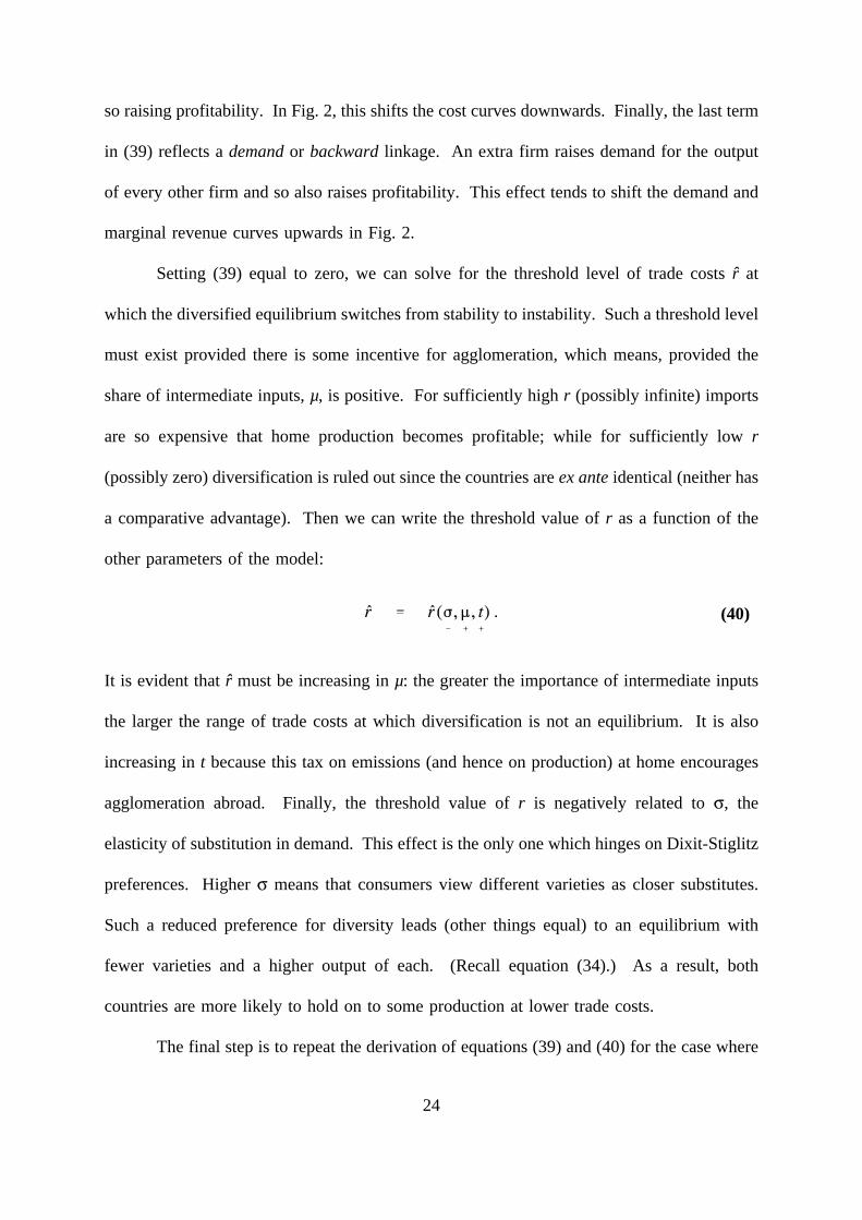
Setting (39) equal to zero, we can solve for the threshold level of trade costs r at
which the diversified equilibrium switches from stability to instability. Such a threshold level
must exist provided there is some incentive for agglomeration, which means, provided the
share of intermediate inputs, µ, is positive. For sufficiently high r (possibly infinite) imports
are so expensive that home production becomes profitable; while for sufficiently low r
(possibly zero) diversification is ruled out since the countries are ex ante identical (neither has
a comparative advantage). Then we can write the threshold value of r as a function of the
other parameters of the model:
It is evident that r must be increasing in µ: the greater the importance of intermediate inputs
(40)
the larger the range of trade costs at which diversification is not an equilibrium. It is also
increasing in t because this tax on emissions (and hence on production) at home encourages
agglomeration abroad. Finally, the threshold value of r is negatively related to σ, the
elasticity of substitution in demand. This effect is the only one which hinges on Dixit-Stiglitz
preferences. Higher σ means that consumers view different varieties as closer substitutes.
Such a reduced preference for diversity leads (other things equal) to an equilibrium with
fewer varieties and a higher output of each. (Recall equation (34).) As a result, both
countries are more likely to hold on to some production at lower trade costs.
The final step is to repeat the derivation of equations (39) and (40) for the case where
24
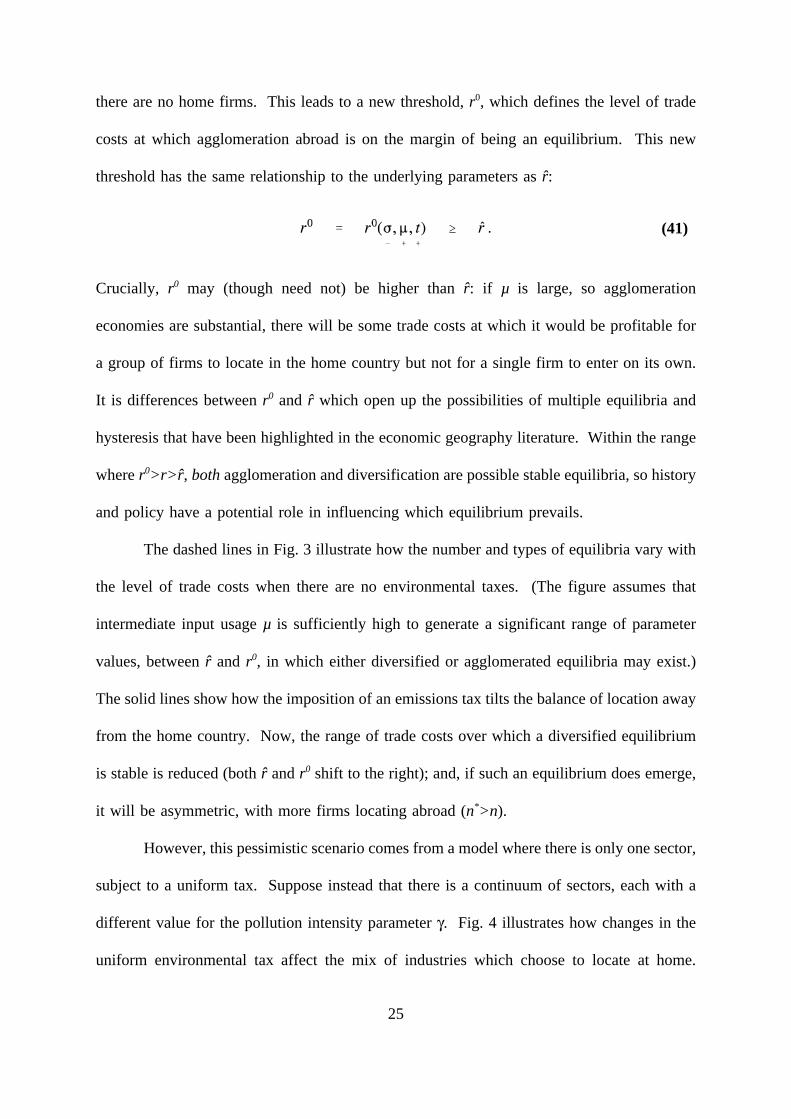
there are no home firms. This leads to a new threshold, r0, which defines the level of trade
costs at which agglomeration abroad is on the margin of being an equilibrium. This new
threshold has the same relationship to the underlying parameters as r:
Crucially, r0 may (though need not) be higher than r: if µ is large, so agglomeration
(41)
economies are substantial, there will be some trade costs at which it would be profitable for
a group of firms to locate in the home country but not for a single firm to enter on its own.
It is differences between r0 and r which open up the possibilities of multiple equilibria and
hysteresis that have been highlighted in the economic geography literature. Within the range
where r0>r>r, both agglomeration and diversification are possible stable equilibria, so history
and policy have a potential role in influencing which equilibrium prevails.
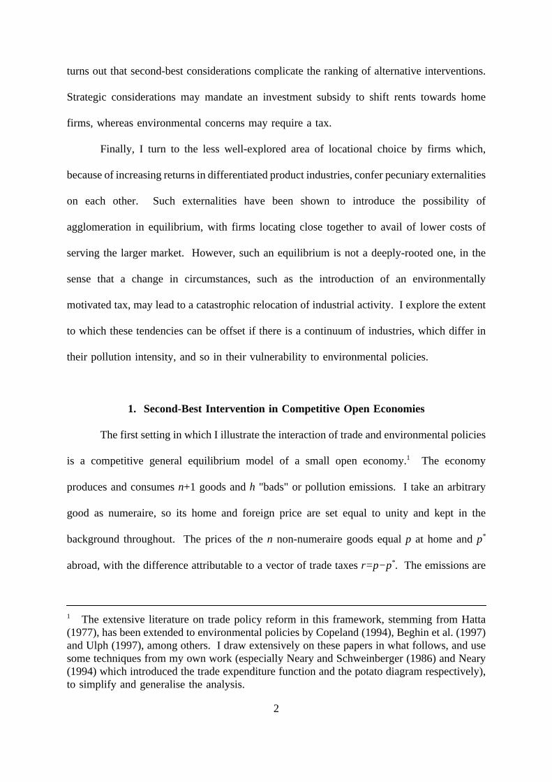
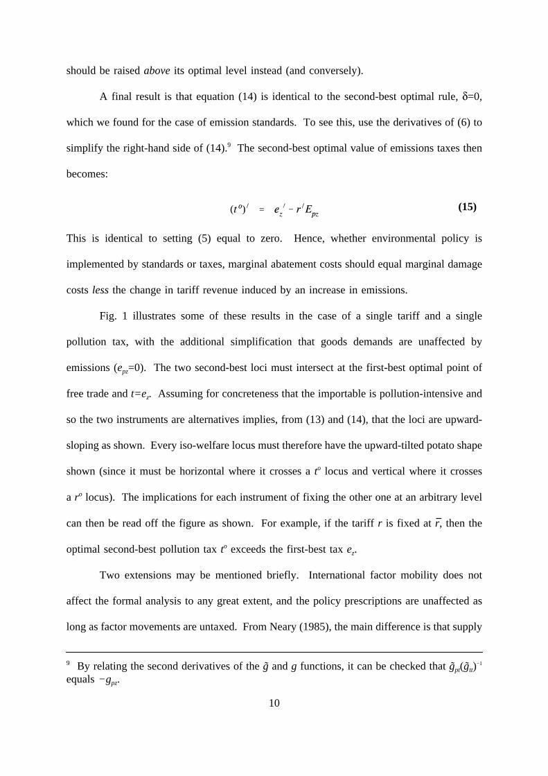
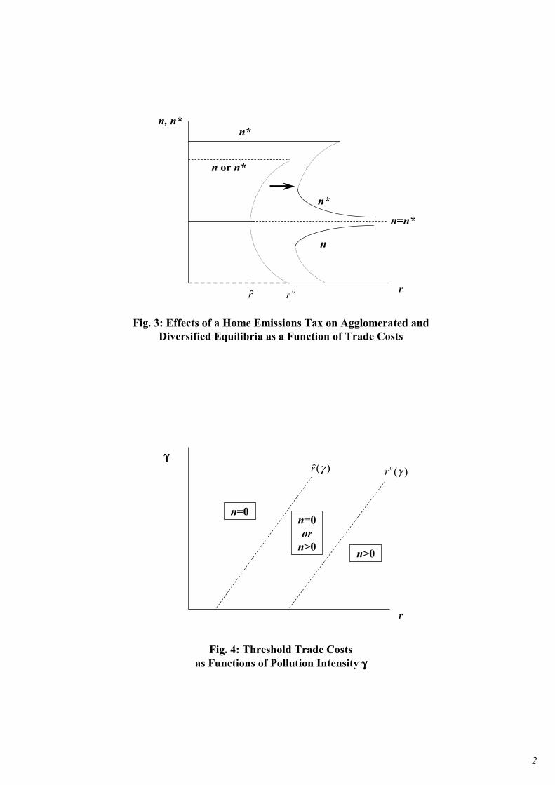
The dashed lines in Fig. 3 illustrate how the number and types of equilibria vary with
the level of trade costs when there are no environmental taxes. (The figure assumes that
intermediate input usage µ is sufficiently high to generate a significant range of parameter
values, between r and r0, in which either diversified or agglomerated equilibria may exist.)
The solid lines show how the imposition of an emissions tax tilts the balance of location away
from the home country. Now, the range of trade costs over which a diversified equilibrium
is stable is reduced (both r and r0 shift to the right); and, if such an equilibrium does emerge,
it will be asymmetric, with more firms locating abroad (n*>n).
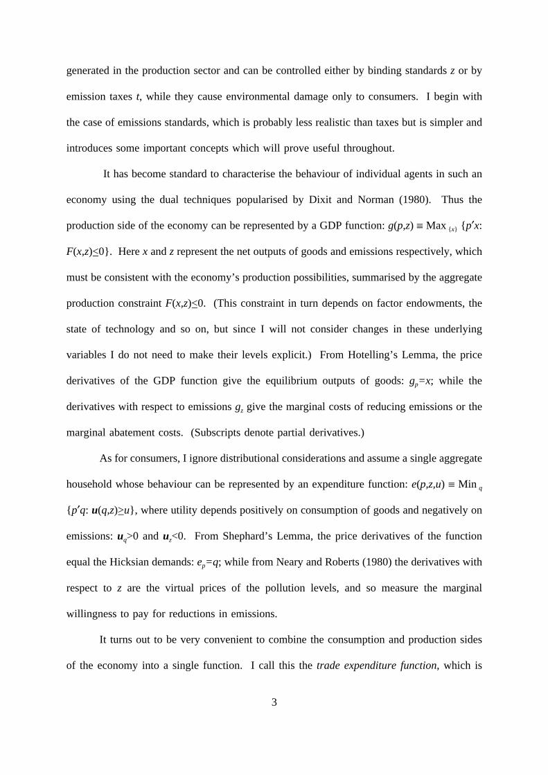
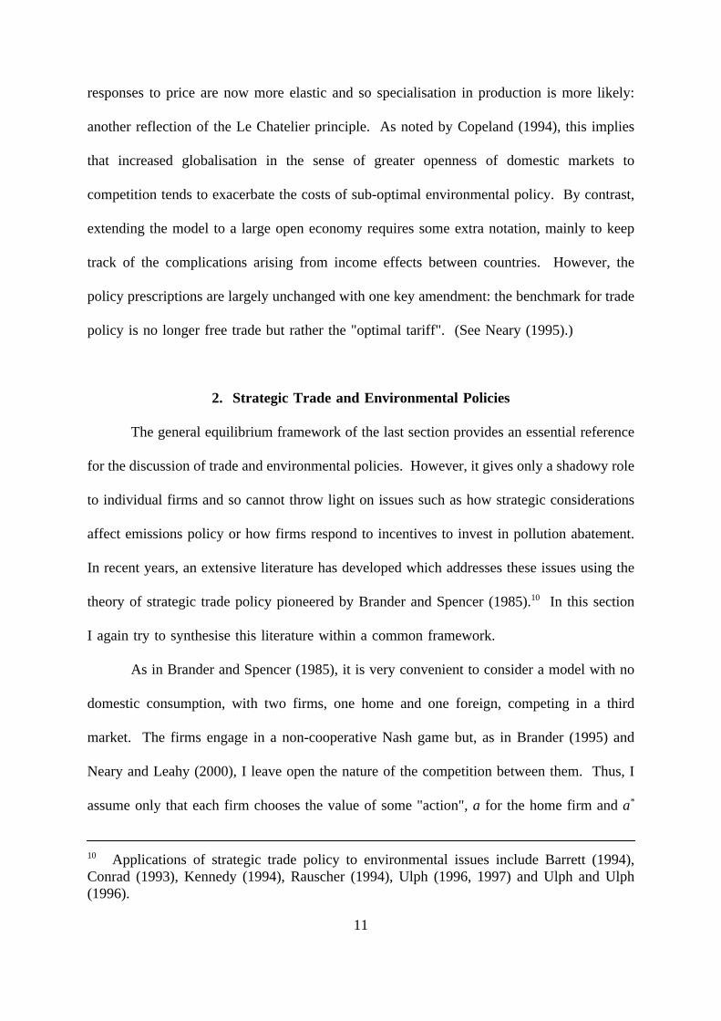
However, this pessimistic scenario comes from a model where there is only one sector,
subject to a uniform tax. Suppose instead that there is a continuum of sectors, each with a
different value for the pollution intensity parameter γ. Fig. 4 illustrates how changes in the
uniform environmental tax affect the mix of industries which choose to locate at home.
25
Equilibrium is now a continuous function of parameters, without the cataclysmic effects of
the one-sector case.
4. Conclusions
In this paper I have reviewed three types of models which have been applied to the
study of environmental policy in open economies, and have tried to highlight their most
interesting results in a compact and consistent manner.
A key finding from Sections 1 and 2 is that departing from the standard first-best rule
of environmental policy is never justified in itself: whether taxes or emission standards are
used, they should be set at a level which equates marginal abatement costs to marginal
damage costs. "Inefficient" environmental policy can only be defended as a surrogate for
some other policy assumed to be unavailable: free trade in Section 1, export subsidies or taxes
in Section 2. The benchmark optimal trade policy differs depending on whether firms’
behaviour is competitive or oligopolistic. But in most other respects the policy conclusions
are surprisingly similar.
As for the fear that environmental policy may lead to catastrophic relocation of
economic activity, the economic geography model of Section 3 illustrated how this can indeed
occur in certain circumstances. However, allowing realistically for a multiplicity of industries,
with varying degrees of pollution intensity, suggests that fears of a dramatic loss of industrial
competitiveness are probably misplaced.18
Naturally, even in a long paper I have had to ignore many important issues. I have
assumed that economies are linked by trade alone and have not considered international
spillovers of R&D or pollution. I have ignored actions by foreign governments, so ruling out
18 The empirical evidence summarised by Jaffe et al. (1995) is consistent with this.
26
consideration of international policy games, international environmental agreements and issue
linkage. Finally, while I have looked at the potentially catastrophic effects of environmental
policy on industrial agglomeration, I have not considered the effects of lax policy on the
environment itself, as in Brander and Taylor (1998)’s model of ecological collapse.
Let me take up that point to end on a more speculative note. It should be recalled that
the theories of trade with imperfect competition reviewed in Sections 2 and 3 had their origin
in a general feeling of unease with the traditional competitive paradigm. In the same way,
non-economists and even some economists may feel uneasy at the generally benign
implications of the literature I have reviewed. Our models, even with stochastic elements
added, do not seem capable of dealing with small but finite probabilities of cataclysmic events
such as habitat destruction, environmental degradation and reduced species diversity: concerns
not just of extreme environmentalists but of distinguished biologists such as Wilson (1984).
All this suggests to me that the most important direction in which our models need to be
extended is to take account of uncertainty about the long-term environmental effects of
consumption, production and trade.
That said, while future work may lead to less optimism about the environmental and
ecological consequences of free trade, it is unlikely to affect the main message of this paper,
which can be summarised as advocating a "single dividend" approach to policy choice.
Policy makers and analysts are best advised to concentrate on targeting trade and
environmental policies towards their primary objectives. There are many reasons for
departing from first-best rules, but second-best considerations depend on a host of factors
which are not easily quantifiable. Foregoing the benefits of free trade is too high a price to
pay for failing to develop and implement appropriate environmental policies.
27
References
Anderson, J.E. and J.P. Neary (1992): "Trade reform with quotas, partial rent retention, and
tariffs," Econometrica, 60, 57-76.
Barrett, S. (1994): "Strategic environmental policy and international trade," Journal of Public
Economics, 54, 325-338.
Beghin, J., Roland Holst, D., and D. van der Mensbrugghe (1997): "Trade and pollution
linkages: Piecemeal reform and optimal intervention," Canadian Journal of
Economics, 30, 442-455.
Brander, J.A.(1995): "Strategic trade policy," in G. Grossman and K. Rogoff (eds.): Handbook
of International Economics, Volume 3, Amsterdam: North-Holland, 1395-455.
Brander, J.A. and B.J. Spencer (1985): "Export subsidies and international market share
rivalry," Journal of International Economics, 18, 83-100.
Brander, J.A. and M.S. Taylor (1998): "The simple economics of Easter Island: A Ricardo-
Malthus model of resource use," American Economic Review, 88, 119-138.
Conrad, K. (1993): "Taxes and subsidies for pollution-intensive industries as trade policy,"
Journal of Environmental Economics and Management, 25, 121-135.
Copeland, B.R.(1994): "International trade and the environment: Policy reform in a polluted
small open economy,"Journal of Environmental Economics and Management,26,44-65.
Corden, W.M. and R.E. Falvey (1985): "Quotas and the second best," Economics Letters, 18,
67-70.
Dixit, A.K. and V. Norman (1980): Theory of International Trade: A Dual, General
Equilibrium Approach, London: Cambridge University Press.
Dixit, A.K. and J.E. Stiglitz (1977): "Monopolistic competition and optimum product
diversity," American Economic Review, 67, 297-308.
28
Eaton, J. and G.M. Grossman (1986): "Optimal trade and industrial policy under oligopoly,"
Quarterly Journal of Economics, 101, 383-406.
Fudenberg, D. and J. Tirole (1984): "The fat-cat effect, the puppy-dog ploy, and the lean and
hungry look," American Economic Review, Papers and Proceedings, 74, 361-366.
Hatta, T. (1977): "A theory of piecemeal policy recommendations," Review of Economic
Studies, 44, 1-21.
Hoel, M. (1997): "Environmental policy with endogenous plant locations", Scandinavian
Journal of Economics, 99, 241-259.
Jaffe, A.B. et al. (1995): "Environmental regulation and the competitiveness of U.S.
manufacturing: What does the evidence tell us?", Journal of Economic Literature, 33,
132-163.
Kennedy, P.W. (1994): "Equilibrium pollution taxes in open economies with imperfect
competition," Journal of Environmental Economics and Management, 27, 49-63.
Krugman, P.R. (1991): "Increasing returns and economic geography," Journal of Political
Economy, 99, 483-499.
Krugman, P.R. and A.J. Venables (1995): "Globalization and the inequality of nations,"
Quarterly Journal of Economics, 110, 857-880.
Leahy, D. and J.P. Neary (1999): "Learning by doing, precommitment and infant-industry
promotion," Review of Economic Studies 66, 447-474.
Markusen, J.R., E.R. Morey and N.D. Olewiler (1993): "Environmental policy when market
structure and plant locations are endogenous," Journal of Environmental Economics
and Management, 24, 68-86.
Motta, M. and J.F. Thisse (1994): "Does environmental dumping lead to delocation?",
European Economic Review, 38, 563-576.
29
Neary, J.P. (1985): "International factor mobility, minimum wage rates and factor-price
equalization: A synthesis," Quarterly Journal of Economics, 100, 551-570.
Neary, J.P. (1993): "Welfare effects of tariffs and investment taxes," in W.J. Ethier, E.
Helpman and J.P. Neary (eds.): Theory, Policy and Dynamics in International Trade:
Essays in Honor of R.W. Jones, Cambridge: Cambridge University Press, 131-156.
Neary, J.P. (1994): "Cost asymmetries in international subsidy games: Should governments
help winners or losers?", Journal of International Economics, 37, 197-218.
Neary, J.P. (1995): "Trade liberalisation and shadow prices in the presence of tariffs and
quotas," International Economic Review, 36, 531-554.
Neary, J.P. (1998): "Pitfalls in the theory of international trade policy: Concertina reforms of
tariffs, and subsidies to high-technology industries," Scandinavian Journal of
Economics, 100, 187-206.
Neary, J.P. (1999): "Comment" on Venables (1999), in R.E. Baldwin and J.F. Francois (eds.):
Dynamic Issues in Commercial Policy Analysis, Cambridge: Cambridge University
Press, 196-200.
Neary, J.P. (2001): "Of hype and hyperbolas: Introducing the new economic geography,"
Journal of Economic Literature, 39,536-561.
Neary, J.P. and D. Leahy (2000): "Strategic trade and industrial policy towards dynamic
oligopolies," Economic Journal, 110, 484-508.
Neary, J.P. and K.W.S. Roberts (1980): "The theory of consumer behaviour under rationing,"
European Economic Review, 13, 25-42.
Neary, J.P. and A.G. Schweinberger (1986): "Factor content functions and the theory of
international trade," Review of Economic Studies, 53, 421-432.
Palmer, K., W.E. Oates and P.R. Portney (1995): "Tightening environmental standards: The
30
benefit-cost or the no-cost paradigm?", Journal of Economic Perspectives, 9, 119-132.
Porter, M.E. (1991): "America’s green strategy," Scientific American, 264, 168.
Porter, M.E. and C. van der Linde (1995): "Toward a new conception of the environment-
competitiveness relationship," Journal of Economic Perspectives, 9, 97-118.
Rauscher, M. (1994): "On ecological dumping," Oxford Economic Papers, 46, 822-840.
Rauscher, M. (1997): International Trade, Factor Movements, and the Environment, Oxford:
Clarendon Press.
Simpson, R.D. and R.L. Bradford (1996): "Taxing variable cost: Environmental regulation as
industrial policy," Journal of Environmental Economics and Management, 30,282-300.
Spencer, B.J. and J.A. Brander (1983): "International R&D rivalry and industrial strategy,"
Review of Economic Studies, 50, 707-722.
Ulph, A. (1996): "Environmental policy and international trade when governments and
producers act strategically," Journal of Environmental Economics and Management,
30, 265-281.
Ulph, A. (1997): "Environmental policy and international trade," in C. Carraro and D.
Siniscalco (eds.): New Directions in the Economic Theory of the Environment,
Cambridge: Cambridge University Press, 147-192.
Ulph, A. and D. Ulph (1996): "Trade, strategic innovation and strategic environmental policy:
A general analysis," in C. Carraro, Y. Katsoulacos and A. Xepapadeas (eds.):
Environmental Policy and Market Structure, Dordrecht: Kluwer Academic, 181-208.
Venables, A.J. (1999): "Economic policy and the manufacturing base: Hysteresis in location,"
in R.E. Baldwin and J.F. Francois (eds.): Dynamic Issues in Commercial Policy
Analysis, Cambridge: Cambridge University Press, 177-195.
Wilson, E.O. (1984): Biophilia, Cambridge, Mass.: Harvard University Press.
31
1
t
r (t)
t ((((r))))
o
or
Fig. 1: An Iso-Welfare Locus in Tax-Tariff Space
r ot o
r
t
ez
MR
p
x
MC
ACD
3
2
1
(σ(σ(σ(σ−−−−1)α/β1)α/β1)α/β1)α/β
ββββW
ββββW/θθθθ
Fig. 2: Monopolistically Competitive Equilibrium and the Effects of Entry by a New Firm
2
n, n*
r
n*
Fig. 3: Effects of a Home Emissions Tax on Agglomerated and Diversified Equilibria as a Function of Trade Costs
<r
n
n*
ro
n=n*
n or n*
γγγγ
r
n=0
Fig. 4: Threshold Trade Costsas Functions of Pollution Intensity γγγγ
>( )r γ
n>0
n=0or
n>0
r 0 ( )γ
Related Documents