International Supply Chains and the Volatility of Trade Benjamin Bridgman ∗ Bureau of Economic Analysis August 2010 Abstract The world trade collapsed in the most recent recession. Some analysts have sug- gested the increasing offshoring of the supply chain, or vertical specialization (VS) trade, can explain the apparent increase in volatility of trade over the business cy- cle. This paper develops a model of VS trade to examine its impact on the volatility of trade. The model features increased trade volatility as VS trade increases when goods production is more volatile than services production. While the simulated model generates the observed increase in relative volatility of trade to GDP from 1967 to 2002, most of the increase is due to GDP’s shift to less volatile services production. VS trade only accounts for a third of the increase. Counterintuitively, VS trade can moderate trade volatility. JEL classification : E3, F1. Keywords : Business cycles; Vertical specialization; Manufacturing trade. ∗ I thank George Alessandria and seminar participants at the 2010 Midwest Macro Meetings and International Industrial Organization Conference for comments. The views expressed in this paper are solely those of the author and not necessarily those of the U.S. Bureau of Economic Analysis or the U.S. Department of Commerce. Address: U.S. Department of Commerce, Bureau of Economic Analysis, Washington, DC 20230. email: [email protected]. Tel. (202) 606-9991. Fax (202) 606-5366. 1

Welcome message from author
This document is posted to help you gain knowledge. Please leave a comment to let me know what you think about it! Share it to your friends and learn new things together.
Transcript
International Supply Chains and the Volatility of
Trade
Benjamin Bridgman∗
Bureau of Economic Analysis
August 2010
Abstract
The world trade collapsed in the most recent recession. Some analysts have sug-gested the increasing offshoring of the supply chain, or vertical specialization (VS)trade, can explain the apparent increase in volatility of trade over the business cy-cle. This paper develops a model of VS trade to examine its impact on the volatilityof trade. The model features increased trade volatility as VS trade increases whengoods production is more volatile than services production. While the simulatedmodel generates the observed increase in relative volatility of trade to GDP from1967 to 2002, most of the increase is due to GDP’s shift to less volatile servicesproduction. VS trade only accounts for a third of the increase. Counterintuitively,VS trade can moderate trade volatility.
JEL classification: E3, F1.Keywords: Business cycles; Vertical specialization; Manufacturing trade.
∗I thank George Alessandria and seminar participants at the 2010 Midwest Macro Meetings andInternational Industrial Organization Conference for comments. The views expressed in this paper aresolely those of the author and not necessarily those of the U.S. Bureau of Economic Analysis or the U.S.Department of Commerce. Address: U.S. Department of Commerce, Bureau of Economic Analysis,Washington, DC 20230. email: [email protected]. Tel. (202) 606-9991. Fax (202) 606-5366.
1
1 Introduction
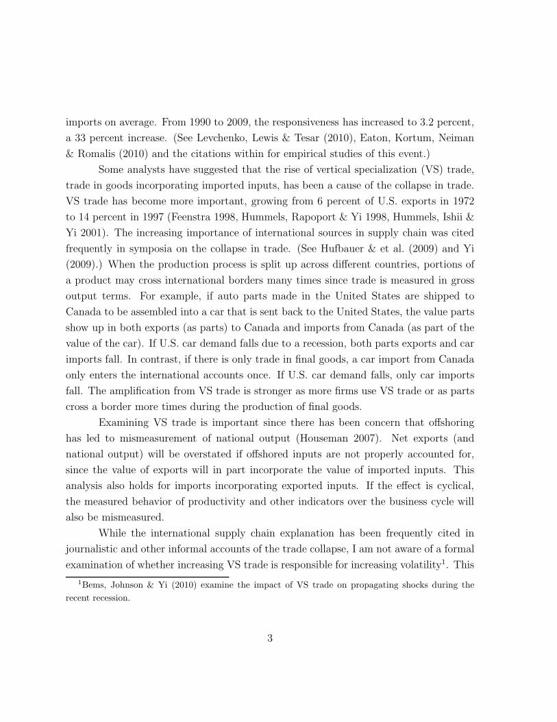
While the recession beginning in 2007 was quite acute, the collapse in trade that accom-
panied it was staggering. Since its peak in the third quarter of 2007 to the trough in the
second quarter of 2009, the volume of U.S. goods imports fell 24 percent. Exports show
a similar decline in an even shorter period. In terms of goods trade share of GDP, this
decline undid the trade expansion of the 2000s in less than two years. (See Figure 1.)
World trade recorded a similar decline.
Figure 1: U.S. Goods Trade Share of GDP, 1947:Q1-2010:Q2
0
0.02
0.04
0.06
0.08
0.1
0.12
0.14
0.16
0.18
1947-I
1950-I
1953-I
1956-I
1959-I
1962-I
1965-I
1968-I
1971-I
1974-I
1977-I
1980-I
1983-I
1986-I
1989-I
1992-I
1995-I
1998-I
2001-I
2004-I
2007-I
2010-I
Goods Exports
Goods Imports
The recent decline is part of a wider increase in the relative volatility of trade over
the business cycle. Real output fell 3.24 percent in the 1973-75 recession, similar to the
3.8 output drop in the 2007 recession (to 2009Q2, the point of trade’s largest decline).
However, real imports only fell 15.2 percent in the mid-1970s recession. This anecdotal
evidence holds up in a more formal examination of the data. As documented in detail
below, a shock to GDP - as defined by deviation from a Hodrick-Prescott (H-P) trend
- has stronger impact on trade now than it did in the past. Over the last 40 years, the
responsiveness of imports to GDP shocks has increased in the United States. From 1967
to 1989, a 1 percent GDP deviation from HP trend led to a 2.4 percent deviation in
2
imports on average. From 1990 to 2009, the responsiveness has increased to 3.2 percent,
a 33 percent increase. (See Levchenko, Lewis & Tesar (2010), Eaton, Kortum, Neiman
& Romalis (2010) and the citations within for empirical studies of this event.)
Some analysts have suggested that the rise of vertical specialization (VS) trade,
trade in goods incorporating imported inputs, has been a cause of the collapse in trade.
VS trade has become more important, growing from 6 percent of U.S. exports in 1972
to 14 percent in 1997 (Feenstra 1998, Hummels, Rapoport & Yi 1998, Hummels, Ishii &
Yi 2001). The increasing importance of international sources in supply chain was cited
frequently in symposia on the collapse in trade. (See Hufbauer & et al. (2009) and Yi
(2009).) When the production process is split up across different countries, portions of
a product may cross international borders many times since trade is measured in gross
output terms. For example, if auto parts made in the United States are shipped to
Canada to be assembled into a car that is sent back to the United States, the value parts
show up in both exports (as parts) to Canada and imports from Canada (as part of the
value of the car). If U.S. car demand falls due to a recession, both parts exports and car
imports fall. In contrast, if there is only trade in final goods, a car import from Canada
only enters the international accounts once. If U.S. car demand falls, only car imports
fall. The amplification from VS trade is stronger as more firms use VS trade or as parts
cross a border more times during the production of final goods.
Examining VS trade is important since there has been concern that offshoring
has led to mismeasurement of national output (Houseman 2007). Net exports (and
national output) will be overstated if offshored inputs are not properly accounted for,
since the value of exports will in part incorporate the value of imported inputs. This
analysis also holds for imports incorporating exported inputs. If the effect is cyclical,
the measured behavior of productivity and other indicators over the business cycle will
also be mismeasured.
While the international supply chain explanation has been frequently cited in
journalistic and other informal accounts of the trade collapse, I am not aware of a formal
examination of whether increasing VS trade is responsible for increasing volatility1. This
1Bems, Johnson & Yi (2010) examine the impact of VS trade on propagating shocks during therecent recession.
3
paper seeks to fill this gap by examining whether the unraveling of international supply
chains is a quantitatively important source of this increased responsiveness. It presents a
tractable general equilibrium model with Ricardian trade in intermediate goods. There
are two countries with two layers of goods production: Intermediate goods are inputs
to final consumption goods. Both types of goods may be traded, but incur an iceberg
transportation cost and may face tariffs. There is a service sector that is not traded. I
calibrate the model to match the U.S. economy in 1967 and 2002 using tariff and freight
cost data. I then simulate the effect of productivity shocks on trade.
Model simulations generate significant increased volatility. The relative volatility
of trade to GDP increases 33 percent from 1967 to 2002 in the baseline simulation, the
same increase as in the data. Two thirds of the increase is due to the shift to less volatile
services production while imports continue to be dominated by goods trade.
About a third of the volatility increase is attributable to VS trade. However, the
mechanism is different than the one in popular accounts. In the model, parts trade is
more volatile than final goods trade. Increasing VS trade means that more trade is in
volatile parts.
The unwinding of the supply chain does not increase trade volatility. Since nomi-
nal trade is proportional to nominal goods production, trade falls by the same percentage
as goods production regardless of trade share. While the rising importance of VS trade
explains the rapid increase in trade levels, the higher trade share does not directly affect
volatility. The higher level does explain the high absolute decline in trade volumes.
Increasing VS trade may even reduce trade volatility. The impact of VS trade is
reversed if parts production is less volatile than that of final goods. In an alternative
calibration, the model can generate the observed increase in volatility even though in-
creasing parts trade is a moderating influence. While careful data work will be required
to determine the exact impact of VS trade, the results indicate that structural change
has been a more significant source of increased import volatility relative to GDP.
Alternative theories have been put forth to explain the recent fall in trade. Amiti
& Weinstein (2009) and Chor & Manova (2009) suggest the loss of trade credit due to
stress on banking system. Alessandria, Kaboski & Midrigan (2010) examine adjustments
to inventories. Gamberoni & Newfarmer (2009) cite increasing protectionism. This paper
4

only examines the ability of VS trade and GDP composition changes to explain the trade
collapse rather than run a horse race between all of the popular explanations.
Modeling the volatility of trade over the business cycle has received interest re-
cently. Standard international real business cycle (IRBC) models fail to deliver the
relative volatility of trade to output. Boileau (1999) and Ercega, Guerrieria & Gust
(2008) show that trade will be more volatile when trade is dominated by capital goods.
Engel & Wang (2008) augment the standard IRBC model with trade in durable goods.
This paper takes a similar approach to these papers: The traded sector is more volatile
than overall production. It differs in that it simplifies the shocks and does not contain
durable goods to concentrate on VS trade.
A portion of the IRBC literature examines the impact of higher trade share on the
co-movement of business cycles, including Backus & Crucini (2000), Bems et al. (2010),
Kose & Yi (2001), Kose & Yi (2006) and Burstein, Kurz & Tesar (2008). This paper
concentrates on the effects of shocks on trade rather than the degree to which trade
transmits shocks to other countries.
A number of papers have examined the importance of intermediates trade for
a number of issues including development (Jones 2008, Goldberg, Khandelwal, Pavc-
nik & Topalova 2008), firm productivity (Amiti & Konings 2007), trade elasticities
(Ramanaryanan 2006) and the border effect in gravity equations (Yi 2010). Grossman
& Rossi-Hansberg (2008) examine the growth of trade in intermediate services. Theoret-
ical models of vertical specialization trade include Dixit & Grossman (1982) and Sanyal
(1983). Unlike these papers, I examine the volatility of trade over the business cycle.
2 Evidence on Trade and the Business Cycle
This section examines the evidence on U.S. trade over the business cycle in greater detail.
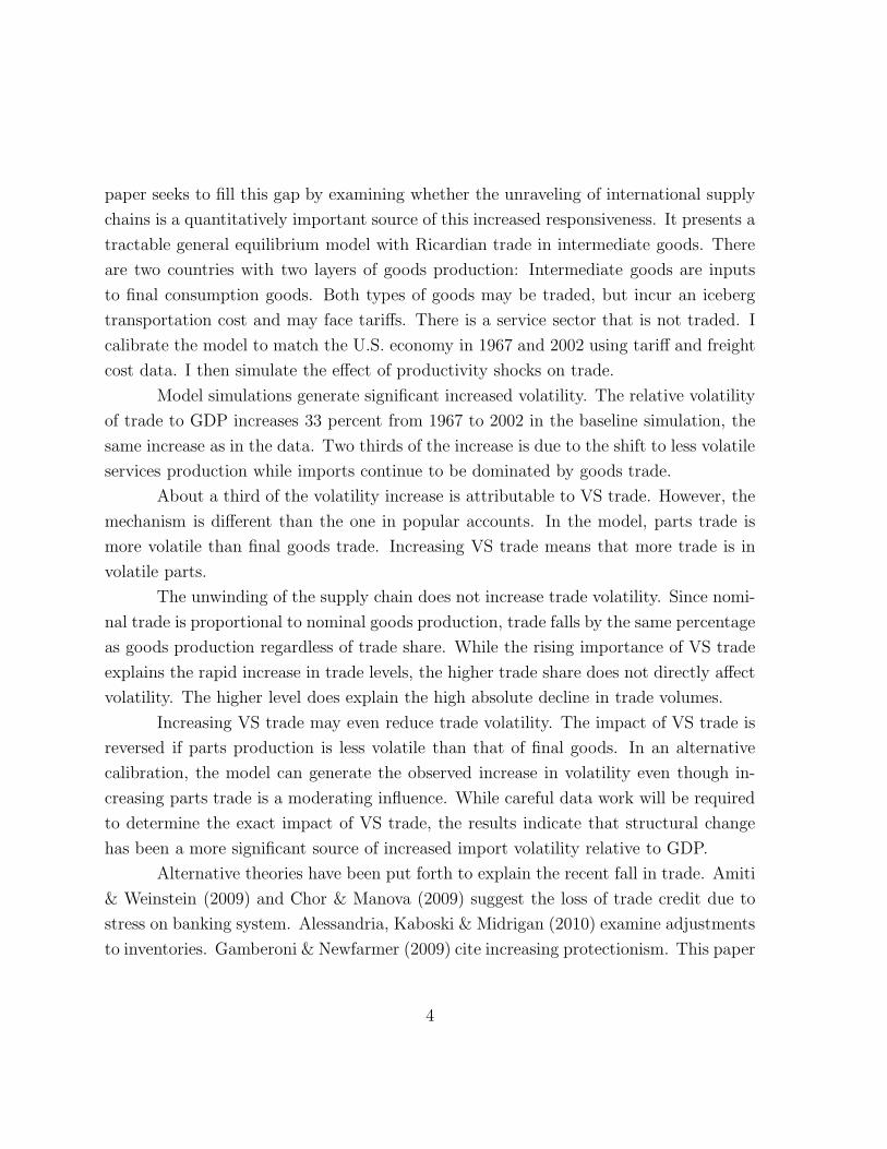
The volatility of trade relative to that of GDP has increased. Figure 2 shows
the relative volatility of U.S. trade and output. Volatility is measured as the standard
deviation of the percentage deviation from a H-P trend in a seven year moving window
ending in the year reported. The ratio of volatilities has increased to its highest sustained
levels in the last 20 to 25 years. Prior to the mid to late 1980s, both GDP and trade
5
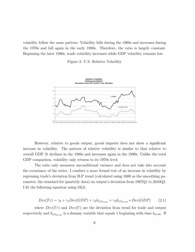
volatility follow the same pattern: Volatility falls during the 1960s and increases during
the 1970s and fall again in the early 1980s. Therefore, the ratio is largely constant.
Beginning the later 1980s, trade volatility increases while GDP volatility remains low.
Figure 2: U.S. Relative Volatility
Relative VolatilitySD(Imports)/SD(Y)
Deviation from HP trend/7 Year Window
0.5
1
1.5
2
2.5
3
3.5
4
4.5
5
Q1-1967 Q1-1970 Q1-1973 Q1-1976 Q1-1979 Q1-1982 Q1-1985 Q1-1988 Q1-1991 Q1-1994 Q1-1997 Q1-2000 Q1-2003 Q1-2006 Q1-2009
Y=Goods GDP
Y =GDP
However, relative to goods output, goods imports does not show a significant
increase in volatility. The pattern of relative volatility is similar to that relative to
overall GDP. It declines in the 1980s and increases again in the 1990s. Unlike the total
GDP comparison, volatility only returns to its 1970s level.
The ratio only measures unconditional variance and does not take into account
the covariance of the series. I conduct a more formal test of an increase in volatility by
regressing trade’s deviation from H-P trend (calculated using 1600 as the smoothing pa-
rameter, the standard for quarterly data) on output’s deviation from 1967Q1 to 2010Q2.
I fit the following equation using OLS,
Dev(Tr) = γ0 + γ1Dev(GDP ) + γ2δt≥tbreak + γ3δt≥tbreak ∗Dev(GDP ) (2.1)
where Dev(Tr) and Dev(Y ) are the deviation from trend for trade and output
respectively and δt≥tbreak is a dummy variable that equals 1 beginning with time tbreak. If
6
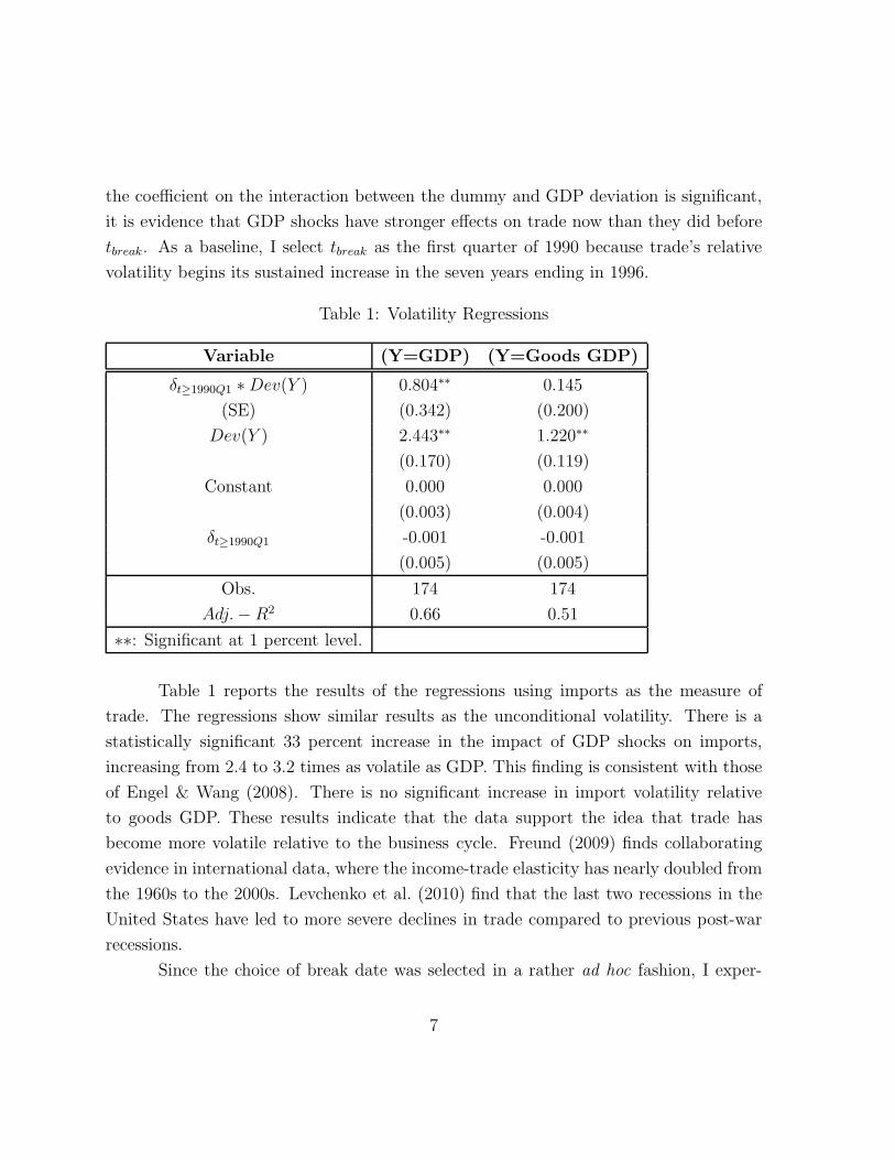
the coefficient on the interaction between the dummy and GDP deviation is significant,
it is evidence that GDP shocks have stronger effects on trade now than they did before
tbreak. As a baseline, I select tbreak as the first quarter of 1990 because trade’s relative
volatility begins its sustained increase in the seven years ending in 1996.
Table 1: Volatility Regressions
Variable (Y=GDP) (Y=Goods GDP)
δt≥1990Q1 ∗Dev(Y ) 0.804∗∗ 0.145
(SE) (0.342) (0.200)
Dev(Y ) 2.443∗∗ 1.220∗∗
(0.170) (0.119)
Constant 0.000 0.000
(0.003) (0.004)
δt≥1990Q1 -0.001 -0.001
(0.005) (0.005)
Obs. 174 174
Adj.− R2 0.66 0.51
∗∗: Significant at 1 percent level.
Table 1 reports the results of the regressions using imports as the measure of
trade. The regressions show similar results as the unconditional volatility. There is a
statistically significant 33 percent increase in the impact of GDP shocks on imports,
increasing from 2.4 to 3.2 times as volatile as GDP. This finding is consistent with those
of Engel & Wang (2008). There is no significant increase in import volatility relative
to goods GDP. These results indicate that the data support the idea that trade has
become more volatile relative to the business cycle. Freund (2009) finds collaborating
evidence in international data, where the income-trade elasticity has nearly doubled from
the 1960s to the 2000s. Levchenko et al. (2010) find that the last two recessions in the
United States have led to more severe declines in trade compared to previous post-war
recessions.
Since the choice of break date was selected in a rather ad hoc fashion, I exper-
7
imented with changing the break date, moving it both forward and backward. The
results show a robust increase in relative volatility beginning some time in the early
1990s. Relative trade volatility has increased between 1960s and the 2000s in a statis-
tically meaningful way, even if the current analysis does not isolate when that increase
occurred.
3 Model
3.1 Households
There are two countries each with a representative household. Households have prefer-
ences over a final consumption good Cif and a service good Ci
s represented by:
U = [γ(Cif)ψ + (1 − γ)(Ci
s)ψ]
1ψ (3.1)
The associated prices are P if and P i
s . Each country is endowed with labor N i. The wage
is W i.
3.2 Intermediate Goods Sector
There is a continuum of intermediate goods xi(z) with a price P ix,j(z) for z ∈ [0, 1]. Each
country is endowed with technologies that use labor N ix(z) to produce intermediates.
Total output of intermediate z is given by:
Y ix(z) = Aix(z)N
ix(z). (3.2)
The productivity parameters are given by A1(z) = 1(1+z)θ
and A2(z) = 1(2−z)θ , a variant of
the mirror image technology in Bridgman (2008) which is based on Dornbusch, Fischer
& Samuelson (1977) and Eaton & Kortum (2002).
3.3 Consumption Goods Sector
Intermediate goods can be assembled into consumption goods using labor N ic . Each
country can only produce the good with its name: j = i. The total output is given by
8
the technology:
Y ic,j = Aic(N
ic)α(
∫(xi(z))σ)dz)
1−ασ (3.3)
for i = 1, 2 and j = i. The associated price is P ic,j.
3.4 Goods Assembly Sector
The consumption goods from each country are assembled into the final consumption
good with the technology:
Cif = [
∑j=1,2
φij(Cic,j)
ρ]1ρ (3.4)
where φij = φ if j = i and φij = 1 − φ and if j �= i. The associated price is P if . The final
consumption good cannot be traded. This sector is a dummy industry to stand in for
household’s preferences over the consumption goods to simplify the presentation of the
model.
3.5 Service Sector
Each country is endowed with a technology that uses labor N is to produce services Ci
s =
AisNis. Services cannot be traded.
3.6 Transportation Sector
The countries may trade the goods they produce with each other by incurring an iceberg
transportation cost specific to that good: fk for k ∈ {x, c}.
3.7 Government
The countries each have a government that can impose an ad valorem (net of trans-
port fees) tariff τ ik on traded goods k ∈ {x, c}. The government gives the domestic
representative household transfers T i and maintains budget balance.
9
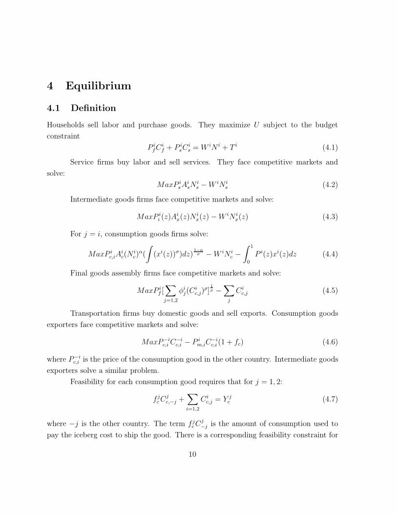
4 Equilibrium
4.1 Definition
Households sell labor and purchase goods. They maximize U subject to the budget
constraint
P ifC
if + P i
sCis = W iN i + T i (4.1)
Service firms buy labor and sell services. They face competitive markets and
solve:
MaxP isA
isN
is −W iN i
s (4.2)
Intermediate goods firms face competitive markets and solve:
MaxP ii (z)A
ix(z)N
ix(z) −W iN i
x(z) (4.3)
For j = i, consumption goods firms solve:
MaxP ic,iA
ic(N
ic)α(
∫(xi(z))σ)dz)
1−ασ −W iN i
c −∫ 1
0
P i(z)xi(z)dz (4.4)
Final goods assembly firms face competitive markets and solve:
MaxP if [
∑j=1,2
φij(Cic,j)
ρ]1ρ −
∑j
Cic,j (4.5)
Transportation firms buy domestic goods and sell exports. Consumption goods
exporters face competitive markets and solve:
MaxP−ic,i C
−ic,i − P i
m,iC−ic,i (1 + fc) (4.6)
where P−ic,i is the price of the consumption good in the other country. Intermediate goods
exporters solve a similar problem.
Feasibility for each consumption good requires that for j = 1, 2:
f jcCjc,−j +
∑i=1,2
Cic,j = Y j
c (4.7)
where −j is the other country. The term f jcCj−j is the amount of consumption used to
pay the iceberg cost to ship the good. There is a corresponding feasibility constraint for
10
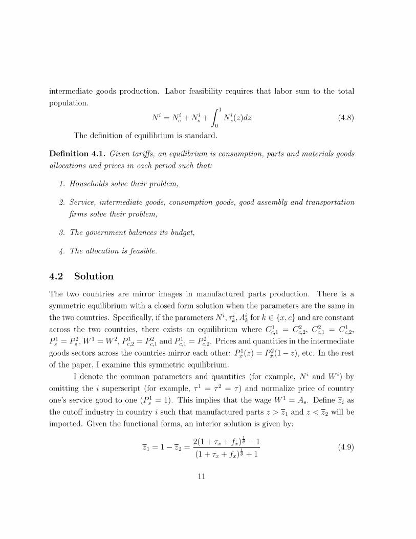
intermediate goods production. Labor feasibility requires that labor sum to the total
population.
N i = N ic +N i
s +
∫ 1
0
N ix(z)dz (4.8)
The definition of equilibrium is standard.
Definition 4.1. Given tariffs, an equilibrium is consumption, parts and materials goods
allocations and prices in each period such that:
1. Households solve their problem,
2. Service, intermediate goods, consumption goods, good assembly and transportation
firms solve their problem,
3. The government balances its budget,
4. The allocation is feasible.
4.2 Solution
The two countries are mirror images in manufactured parts production. There is a
symmetric equilibrium with a closed form solution when the parameters are the same in
the two countries. Specifically, if the parameters N i, τ ik, Aik for k ∈ {x, c} and are constant
across the two countries, there exists an equilibrium where C1c,1 = C2
c,2, C2c,1 = C1
c,2,
P 1s = P 2
s , W 1 = W 2, P 1c,2 = P 2
c,1 and P 1c,1 = P 2
c,2. Prices and quantities in the intermediate
goods sectors across the countries mirror each other: P 1x (z) = P 2
x (1− z), etc. In the rest
of the paper, I examine this symmetric equilibrium.
I denote the common parameters and quantities (for example, N i and W i) by
omitting the i superscript (for example, τ 1 = τ 2 = τ) and normalize price of country
one’s service good to one (P 1s = 1). This implies that the wage W 1 = As. Define zi as
the cutoff industry in country i such that manufactured parts z > z1 and z < z2 will be
imported. Given the functional forms, an interior solution is given by:
z1 = 1 − z2 =2(1 + τx + fx)
1θ − 1
(1 + τx + fx)1θ + 1
(4.9)
11
5 Results
In this section, I use the model to measure the effects of increasing vertical specialization
trade on the volatility of trade over the business cycle. I calibrate the model to match
moments of the data in 1967 and 2002 and examine the impact of productivity shocks
on international trade.
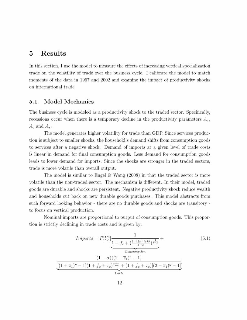
5.1 Model Mechanics
The business cycle is modeled as a productivity shock to the traded sector. Specifically,
recessions occur when there is a temporary decline in the productivity parameters Ax,
Ac and As.
The model generates higher volatility for trade than GDP. Since services produc-
tion is subject to smaller shocks, the household’s demand shifts from consumption goods
to services after a negative shock. Demand of imports at a given level of trade costs
is linear in demand for final consumption goods. Less demand for consumption goods
leads to lower demand for imports. Since the shocks are stronger in the traded sectors,
trade is more volatile than overall output.
The model is similar to Engel & Wang (2008) in that the traded sector is more
volatile than the non-traded sector. The mechanism is different. In their model, traded
goods are durable and shocks are persistent. Negative productivity shock reduce wealth
and households cut back on new durable goods purchases. This model abstracts from
such forward looking behavior - there are no durable goods and shocks are transitory -
to focus on vertical production.
Nominal imports are proportional to output of consumption goods. This propor-
tion is strictly declining in trade costs and is given by:
Imports = P icY
ic [
1
1 + fc + ( (1+fc+τc)φ1−φ )
11−ρ︸ ︷︷ ︸
Consumption
+ (5.1)
(1 − α)((2 − z1)η − 1)
[(1 + z1)η − 1](1 + fx + τx)1
1−σ + (1 + fx + τx)[(2 − z1)η − 1]︸ ︷︷ ︸Parts
]
12
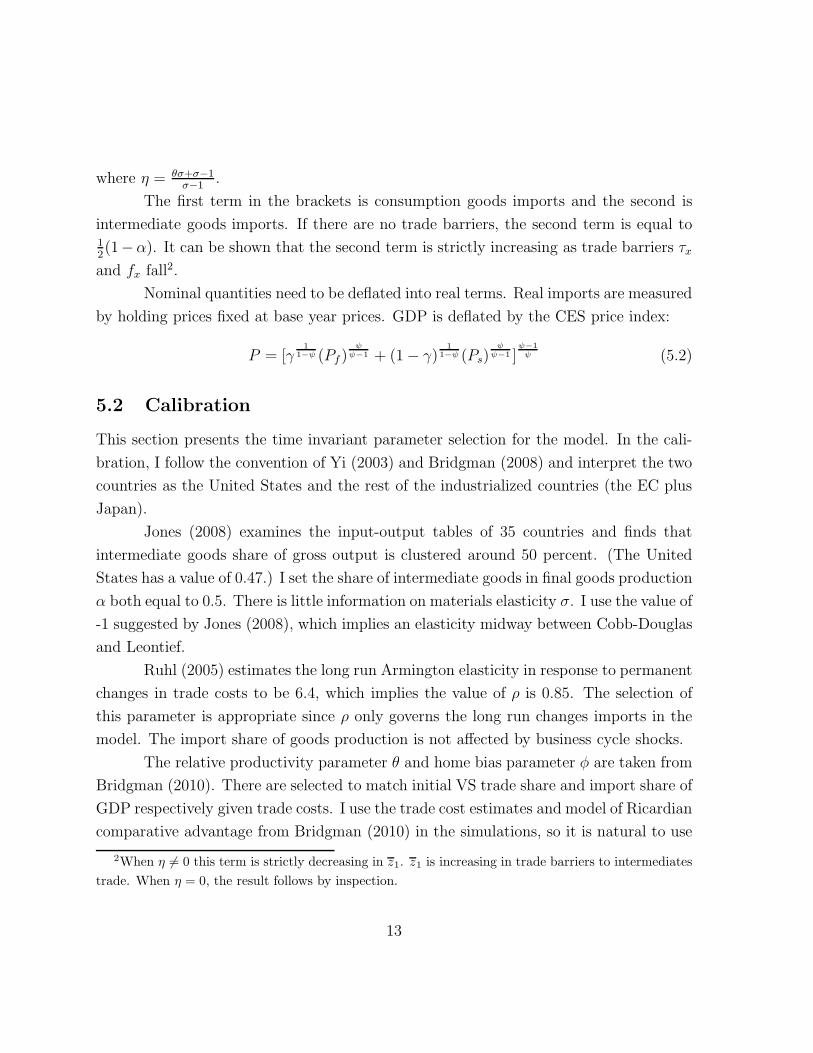
where η = θσ+σ−1σ−1
.
The first term in the brackets is consumption goods imports and the second is
intermediate goods imports. If there are no trade barriers, the second term is equal to12(1−α). It can be shown that the second term is strictly increasing as trade barriers τx
and fx fall2.
Nominal quantities need to be deflated into real terms. Real imports are measured
by holding prices fixed at base year prices. GDP is deflated by the CES price index:
P = [γ1
1−ψ (Pf )ψψ−1 + (1 − γ)
11−ψ (Ps)
ψψ−1 ]
ψ−1ψ (5.2)
5.2 Calibration
This section presents the time invariant parameter selection for the model. In the cali-
bration, I follow the convention of Yi (2003) and Bridgman (2008) and interpret the two
countries as the United States and the rest of the industrialized countries (the EC plus
Japan).
Jones (2008) examines the input-output tables of 35 countries and finds that
intermediate goods share of gross output is clustered around 50 percent. (The United
States has a value of 0.47.) I set the share of intermediate goods in final goods production
α both equal to 0.5. There is little information on materials elasticity σ. I use the value of
-1 suggested by Jones (2008), which implies an elasticity midway between Cobb-Douglas
and Leontief.
Ruhl (2005) estimates the long run Armington elasticity in response to permanent
changes in trade costs to be 6.4, which implies the value of ρ is 0.85. The selection of
this parameter is appropriate since ρ only governs the long run changes imports in the
model. The import share of goods production is not affected by business cycle shocks.
The relative productivity parameter θ and home bias parameter φ are taken from
Bridgman (2010). There are selected to match initial VS trade share and import share of
GDP respectively given trade costs. I use the trade cost estimates and model of Ricardian
comparative advantage from Bridgman (2010) in the simulations, so it is natural to use
2When η �= 0 this term is strictly decreasing in z1. z1 is increasing in trade barriers to intermediatestrade. When η = 0, the result follows by inspection.
13
the same parameter estimates.
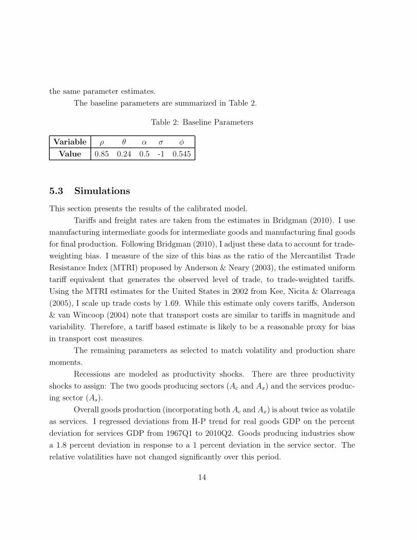
The baseline parameters are summarized in Table 2.
Table 2: Baseline Parameters
Variable ρ θ α σ φ
Value 0.85 0.24 0.5 -1 0.545
5.3 Simulations
This section presents the results of the calibrated model.
Tariffs and freight rates are taken from the estimates in Bridgman (2010). I use
manufacturing intermediate goods for intermediate goods and manufacturing final goods
for final production. Following Bridgman (2010), I adjust these data to account for trade-
weighting bias. I measure of the size of this bias as the ratio of the Mercantilist Trade
Resistance Index (MTRI) proposed by Anderson & Neary (2003), the estimated uniform
tariff equivalent that generates the observed level of trade, to trade-weighted tariffs.
Using the MTRI estimates for the United States in 2002 from Kee, Nicita & Olarreaga
(2005), I scale up trade costs by 1.69. While this estimate only covers tariffs, Anderson
& van Wincoop (2004) note that transport costs are similar to tariffs in magnitude and
variability. Therefore, a tariff based estimate is likely to be a reasonable proxy for bias
in transport cost measures.
The remaining parameters as selected to match volatility and production share
moments.
Recessions are modeled as productivity shocks. There are three productivity
shocks to assign: The two goods producing sectors (Ac and Ax) and the services produc-
ing sector (As).
Overall goods production (incorporating bothAc andAx) is about twice as volatile
as services. I regressed deviations from H-P trend for real goods GDP on the percent
deviation for services GDP from 1967Q1 to 2010Q2. Goods producing industries show
a 1.8 percent deviation in response to a 1 percent deviation in the service sector. The
relative volatilities have not changed significantly over this period.
14
The relative shocks to the two goods producing industries are are difficult to
recover directly. The data do not separate out final goods and intermediate goods pro-
ducing industries. The tools used to estimate the split between the two do not work
well at business cycle frequencies, since they use very low frequency input-output tables
and real trade data are not reported using the I-O classifications. To get some sense
of the relative volatilities, I examined U.S. imports by use category. “Non-petroleum
industrial supplies” is a classification that is likely to only include intermediate goods
while “Consumer goods” is likely to only include final goods. These categories do not
show a strong difference in relative volatility. The standard deviation from H-P trend
for non-petroleum industrial supplies over the period 1967Q1 to 2010Q2 is 0.070, slightly
higher than the 0.069 for consumer goods.
Since the data are imprecise, I set a baseline recession to be when the productivity
parameters fall from Ax = Ac = As = 1 to Ax = 0.965, Ac = 0.99, As = 0.99. These
shocks generate reasonable volatilities given the above facts. In the baseline case, goods
production matches the relative volatility of goods to services production (1.8 times in
1967). These shocks imply that intermediate imports are somewhat more volatile than
final goods imports: A recession leads to a 4.3 percent decline in intermediates trade and
a 3.6 percent decline in final goods in 2002. I discuss alternative shock parameterizations
below.
Given these shocks, the household’s share parameters on service and final goods
γ is set in each period to match the share of GDP that is manufacturing value added.
The service sector has become more important as manufacturing industries have fallen
from 26 percent of GDP in 1967 to 13 percent in 2002.
Finally, the elasticity between service and final goods ψ is chosen to match the
relative volatility of imports to GDP in 1967, as measured by the coefficient on GDP
from the regression in Table 1: Imports are 2.4 times as volatile as GDP. The value of
ψ is 0.361. This value implies the elasticity between the traded and non-trade sectors
is 1.565. This value is somewhat close to that used in Engel & Wang (2008) (1.1) and
well within the range reasonable values they cite from Baxter (1996): 0.5 to 2.5. The
robustness of the results to this parameter choice is discussed below.
Table 3 shows that the model generates the empirical increase in trade volatility
15
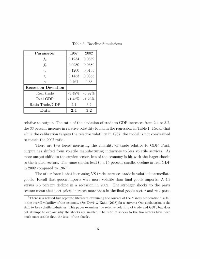
Table 3: Baseline Simulations
Parameter 1967 2002
fx 0.1234 0.0659
fc 0.0980 0.0389
τx 0.1200 0.0135
τc 0.1453 0.0355
γ 0.461 0.33
Recession Deviation
Real trade -3.48% -3.92%
Real GDP -1.45% -1.23%
Ratio Trade/GDP 2.4 3.2
Data 2.4 3.2
relative to output. The ratio of the deviation of trade to GDP increases from 2.4 to 3.2,
the 33 percent increase in relative volatility found in the regression in Table 1. Recall that
while the calibration targets the relative volatility in 1967, the model is not constrained
to match the 2002 ratio.
There are two forces increasing the volatility of trade relative to GDP. First,
output has shifted from volatile manufacturing industries to less volatile services. As
more output shifts to the service sector, less of the economy is hit with the larger shocks
to the traded sectors. The same shocks lead to a 15 percent smaller decline in real GDP
in 2002 compared to 19673.
The other force is that increasing VS trade increases trade in volatile intermediate
goods. Recall that goods imports were more volatile than final goods imports: A 4.3
versus 3.6 percent decline in a recession in 2002. The stronger shocks to the parts
sectors mean that part prices increase more than in the final goods sector and real parts
3There is a related but separate literature examining the sources of the “Great Moderation,” a fallin the overall volatility of the economy. (See Davis & Kahn (2008) for a survey.) One explanation is theshift to less volatile industries. This paper examines the relative volatility of trade and GDP, but doesnot attempt to explain why the shocks are smaller. The ratio of shocks to the two sectors have beenmuch more stable than the level of the shocks.
16
imports fall more. Since a greater share of imports in 2002 is parts trade, trade volatility
increases.
Note that VS trade does not increase volatility by unwinding supply chains, the
explanation that figures into popular accounts of the its importance. Nominal trade is
proportional to nominal goods output, a proportion that increases as trade costs fall.
While a recession reduces trade since there is less goods output, it does not change the
share of nominal goods output traded. To see this, note from equation 5.1 imports M
are constant share s of nominal consumption goods output: M = sPcYc. In a recession,
the deviation of imports is given by: M ′M
= sP ′cY
′c
sPcYc= P ′
cY′c
PcYc. Therefore, the volatility of
trade does not increase as a result of rising trade share.
We can decompose the impact of the two effects. If we impose 1967 parts tariffs
on the 2002 economy, there is no trade in parts. The relative volatility ratio without VS
trade falls to 2.9. Therefore, about two thirds of the increase in the volatility ratio is
due to structural change and one third is due to VS trade.
These findings are consistent with the decomposition of the trade decline in
Levchenko et al. (2010). They find that assuming that trade in each sector fell by
the same amount as industrial production would explain 83 percent of the real decline
in imports. Eaton et al. (2010) also find that falling demand for manufactures explain
the bulk of declining trade. In their regression of different candidate sources, Levchenko
et al. (2010) find that a 13 percent share of the decline in imports that are attributable
to downstream production linkages. These results are consistent with the model’s pre-
diction that the majority of the decline in imports is due to volatility in the traded sector
with a smaller role for VS trade.
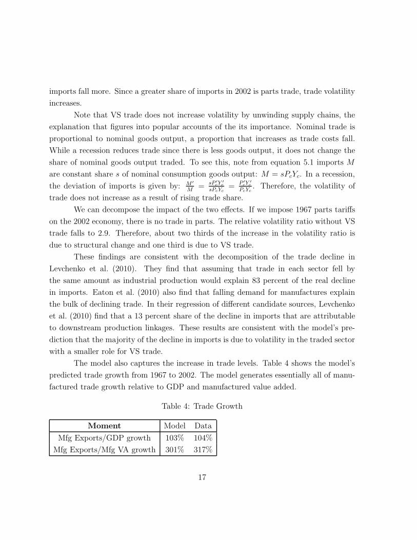
The model also captures the increase in trade levels. Table 4 shows the model’s
predicted trade growth from 1967 to 2002. The model generates essentially all of manu-
factured trade growth relative to GDP and manufactured value added.
Table 4: Trade Growth
Moment Model Data
Mfg Exports/GDP growth 103% 104%
Mfg Exports/Mfg VA growth 301% 317%
17
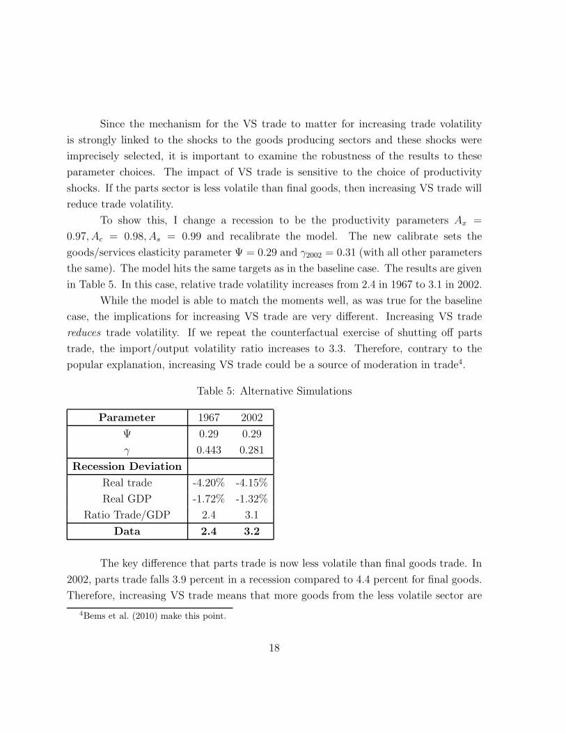
Since the mechanism for the VS trade to matter for increasing trade volatility
is strongly linked to the shocks to the goods producing sectors and these shocks were
imprecisely selected, it is important to examine the robustness of the results to these
parameter choices. The impact of VS trade is sensitive to the choice of productivity
shocks. If the parts sector is less volatile than final goods, then increasing VS trade will
reduce trade volatility.
To show this, I change a recession to be the productivity parameters Ax =
0.97, Ac = 0.98, As = 0.99 and recalibrate the model. The new calibrate sets the
goods/services elasticity parameter Ψ = 0.29 and γ2002 = 0.31 (with all other parameters
the same). The model hits the same targets as in the baseline case. The results are given
in Table 5. In this case, relative trade volatility increases from 2.4 in 1967 to 3.1 in 2002.
While the model is able to match the moments well, as was true for the baseline
case, the implications for increasing VS trade are very different. Increasing VS trade
reduces trade volatility. If we repeat the counterfactual exercise of shutting off parts
trade, the import/output volatility ratio increases to 3.3. Therefore, contrary to the
popular explanation, increasing VS trade could be a source of moderation in trade4.
Table 5: Alternative Simulations
Parameter 1967 2002
Ψ 0.29 0.29
γ 0.443 0.281
Recession Deviation
Real trade -4.20% -4.15%
Real GDP -1.72% -1.32%
Ratio Trade/GDP 2.4 3.1
Data 2.4 3.2
The key difference that parts trade is now less volatile than final goods trade. In
2002, parts trade falls 3.9 percent in a recession compared to 4.4 percent for final goods.
Therefore, increasing VS trade means that more goods from the less volatile sector are
4Bems et al. (2010) make this point.
18
traded.
Other models of the business cycle with intermediate goods, such as Hornstein
& Praschnik (1997), have the feature that intermediate goods are less volatile than
final goods. However, these studies have identified final output as durable goods and
intermediates as nondurables. U.S. trade data by use show that this breakdown does not
reflect trade data. About a third of the nominal value of industrial supplies are durable
goods. Likewise, a third of consumer goods are non-durable. Disentangling the two uses
will require careful data work.
Intersectoral linkages tend to make final goods more volatile than parts, since
shocks in the parts sector feed into the final goods sector. Lower parts productivity
increases their prices, which tends to reduce parts demand. Higher parts prices raise the
cost of producing final goods. Therefore, the cost of final goods is pushed up by both
parts and final goods shocks5. Parts trade can be less volatile even if it is hit with a
bigger productivity shock than final goods.
The findings indicate the rising VS trade is not likely to be a first order cause of
increasing trade volatility. Even when parts production is more volatile than final goods,
structural change is a much more important factor.
Why is VS trade a relatively unimportant source of trade volatility? Perhaps
the result is not surprising. Other examinations of the impact of VS trade on business
cycle phenomena, such as Kose & Yi (2001) and Kose & Yi (2006), have not given
it a large role. Arkolakis & Ramanaryanan (2009) argue that perfect competition in
trade eliminates the impact of productivity shocks in amplifying productivity shocks in
international business cycles. They suggest that imperfect competition may increase the
impact of productivity shocks.
Since the relative volatility of imports to goods output has not increased by much,
the empirical impact of VS trade is limited. Therefore, the data do not support modeling
changes that would significantly increase the impact of shocks on the volatility of goods
imports relative to good output. While VS trade has expanded, other forces tend to
reduce volatility. The rise of Just-in-Time inventories reduce the stock of parts that
5The importance of intersectoral linkages has been long known in the real business cycle literature.For example, see Long & Plosser (1983).
19
firms hold (Dalton 2009). Fewer inventories mean that negative shocks lead to smaller
inventory adjustments of the type identified in Alessandria, Kaboski & Midrigan (2008),
even if more inputs are imported.
5.4 Robustness
The values of some of the parameters are not assigned with precision. The main finding,
that structural change rather than VS trade is more important for increasing trade
volatility, is robust to changes in these parameters.
Changing the elasticity between goods and services ψ affects the relative volatility
of trade to output. As this elasticity increases, trade becomes more volatile relative to
output. As long as the elasticity is greater than one (ψ > 0), the relative volatility of
trade increases from 1967 to 2002. Changing ψ does not change the relative importance
of VS trade. VS trade scales up total trade by the same amount as in the baseline case.
Therefore, the contribution of VS trade to increasing volatility is unaffected.
The parts elasticity σ was taken from Jones (2008) who assigned it as a midpoint
between Leontief and Cobb-Douglas. The results are nearly unchanged by changing σ.
As can be seen in Equation 4.9, the extensive margin for parts trade is not affected this
elasticity. It only affects the intensive margin, leading to quantitatively minor changes
in parts and total trade.
6 Conclusion
While the internationalization of the manufacturing supply chain has been an important
source of increased volume of trade over the last 40 years, it does not appear to be a first
order source of the increase in the relative volatility of trade over the business cycle. In
fact, it is possible that it reduced trade volatility. The decline of the relatively volatile
goods producing sector in GDP has been much more important. The interpretation of
the trade collapse beginning in 2007 that the model supports is that the shocks to the
economy were unusually strong for the post Great Moderation period. Similar shocks in
an economy with a 1960s industrial composition would have led to a very severe recession.
20
Data Sources
Figure 1 Current dollar GDP, goods exports and goods imports, BEA NIPA Table
1.1.5, lines 1, 16 and 19. Accessed August 18, 2010.
Figure 2 GDP, imports volume index, expenditure approach, OECD.Stat table VIXOBSA,
lines B1 GE, P6 and P7. Goods GDP quantity index, BEA NIPA Table 1.2.3, line
4. Accessed April 2nd, 2010.
References
Alessandria, George, Joseph Kaboski & Virgiliu Midrigan (2008), Inventories, lumpy
trade and large devaluations, Working Paper 13790, NBER.
Alessandria, George, Joseph P. Kaboski & Virgiliu Midrigan (2010), The great trade
collapse of 2008-09: An inventory adjustment?, Working Paper 16059, NBER.
Amiti, Mary & David E. Weinstein (2009), Exports and financial shocks, Working Paper
15556, NBER.
Amiti, Mary & Jozef Konings (2007), ‘Trade liberalization, intermediate inputs, and
productivity: Evidence from Indonesia’, American Economic Review 97(5), 1611–
1638.
Anderson, James E. & Eric van Wincoop (2004), ‘Trade costs’, Journal of Economic
Literature 42(3), 691–751.
Anderson, James E. & Peter Neary (2003), ‘The mercantalist index of trade policy’,
International Economic Review 44(2), 627–649.
Arkolakis, Costas & Anath Ramanaryanan (2009), ‘Vertical specialization and in-
ternational business cycle synchronization’, Scandanavian Journal of Economics
111(4), 655 – 680.
Backus, David K. & Mario J. Crucini (2000), ‘Oil prices and the terms of trade’, Journal
of International Economics 50(1), 185–213.
21
Baxter, Marianne (1996), ‘Are consumer durables important for business cycles?’, Review
of Economic Studies 78(1), 147–155.
Bems, Rudolfs, Robert C. Johnson & Kei-Mu Yi (2010), Demand spillovers and the
collapse of trade in the global recession, Working Paper 10/142, IMF.
Boileau, Martin (1999), ‘Trade in capital goods and the volatility of net exports and the
terms of trade’, Journal of International Economics 48, 347365.
Bridgman, Benjamin (2008), ‘Energy prices and the expansion of world trade’, Review
of Economic Dynamics 11(4), 904–916.
Bridgman, Benjamin (2010), The rise of vertical specialization trade, Working Paper
2010-01, Bureau of Economic Analysis.
Burstein, Ariel, Christopher Kurz & Linda Tesar (2008), ‘Trade, production sharing, and
the international transmission of business cycles’, Journal of Monetary Economics
55(4), 775–795.
Chor, Davin & Kalina Manova (2009), Off the cliff and back?: Credit conditions and
international trade during the global financial crisis, mimeo, Stanford University.
Dalton, John T. (2009), Explaining the growth in manufacturing trade, mimeo, Univer-
sity of Minnesota.
Davis, Steven J. & James A. Kahn (2008), ‘Interpreting the great moderation: Changes
in the volatility of economic activity at the micro and macro levels’, Journal of
Economic Perspectives 22(4), 155–180.
Dixit, Avinash & Gene Grossman (1982), ‘Trade and protection with multistage produc-
tion’, Review of Economic Studies 49, 583–594.
Dornbusch, Rudiger, Stanley Fischer & Paul Samuelson (1977), ‘Comparative advantage,
trade, and payments in a Ricardian model with a continuum of goods’, American
Economic Review 67(5), 823–839.
22
Eaton, Jonathan & Samuel Kortum (2002), ‘Technology, geography, and trade’, Econo-
metrica 70(5), 1741–1779.
Eaton, Jonathan, Samuel Kortum, Brent Neiman & John Romalis (2010), Trade and the
global recession, mimeo, University of Chicago.
Engel, Charles & Jian Wang (2008), International trade in durable goods: Understanding
volatility, cyclicality, and elasticities, Working Paper 13814, NBER.
Ercega, Christopher J., Luca Guerrieria & Christopher Gust (2008), ‘Trade adjust-
ment and the composition of trade’, Journal of Economic Dynamics and Control
32(8), 2622–2650.
Feenstra, Robert (1998), ‘Integration of trade and disintegration of production in the
global economy’, Journal of Economic Perspectives 12(4), 31–50.
Freund, Caroline (2009), The trade response to global downturns: Historical evidence,
Policy Research Working Paper 5015, World Bank.
Gamberoni, Elisa & Richard Newfarmer (2009), Trade protection: Incipient but worri-
some trends, in R.Baldwin & S.Evenett, eds, ‘The collapse of global trade, murky
protectionism, and the crisis: Recommendations for the G20’, Centre for Economic
Policy Research, London, pp. 49–53.
Goldberg, Pinelopi K., Amit Khandelwal, Nina Pavcnik & Petia Topalova (2008), Im-
ported intermediate inputs and domestic product growth: Evidence from India,
Working Paper 14416, NBER.
Grossman, Gene & Esteban Rossi-Hansberg (2008), Task trade between similar countries,
Working Paper 14554, NBER.
Hornstein, Andreas & Jack Praschnik (1997), ‘Intermediate inputs and sectoral comove-
ment in the business cycle’, Journal of Monetary Economics 40, 573–595.
Houseman, Susan (2007), ‘Outsourcing, offshoring, and productivity measurement in
U.S. manufacturing’, International Labour Review 146(1-2), 61–80.
23
Hufbauer, Gary C. & et al. (2009), ‘Collapse in world trade: A symposium’, The Inter-
national Economy pp. 28–38.
Hummels, David, Dana Rapoport & Kei-Mu Yi (1998), ‘Vertical specialization and the
changing nature of world trade’, FRBNY Economic Policy Review 4(2), 79–99.
Hummels, David, Jun Ishii & Kei-Mu Yi (2001), ‘The nature and growth of vertical
specialization in world trade’, Journal of International Economics 54(1), 75–96.
Jones, Charles I. (2008), Intermediate goods and weak links: A theory of economic
development, Working paper, U.C. Berkeley.
Kee, Hiau Looi, Alessandro Nicita & Marcelo Olarreaga (2005), Estimating trade re-
strictiveness indices, mimeo, World Bank.
Kose, M. Ayhan & Kei-Mu Yi (2001), ‘International trade and business cycles: Is vertical
specialization the missing link?’, American Economic Review Papers and Proceed-
ings 91, 371–375.
Kose, M. Ayhan & Kei-Mu Yi (2006), ‘Can the standard international business cycle
model explain the relation between trade and comovement’, Journal of International
Economics 68, 267–295.
Levchenko, Andrei A., Logan T. Lewis & Linda L. Tesar (2010), The collapse of inter-
national trade during the 2008-2009 crisis: In search of the smoking gun, Working
Paper 16006, NBER.
Long, John B. & Charles I. Plosser (1983), ‘Real business cycles’, Journal of Political
Economy 91(1), 39–69.
Ramanaryanan, Anath (2006), International trade dynamics with intermediate inputs,
mimeo, University of Minnesota.
Ruhl, Kim J. (2005), Solving the elasticity puzzle in international economics, mimeo,
University of Texas.
24
Sanyal, Kalyan (1983), ‘Vertical specialization in a Ricardian model with a continuum
of stages of production’, Economica 50(197), 71–78.
Yi, Kei-Mu (2003), ‘Can vertical specialization explain the growth of world trade?’,
Journal of Political Economy 111(1), 52–102.
Yi, Kei-Mu (2009), The collapse of global trade: The role of vertical specialisation, in
R.Baldwin & S.Evenett, eds, ‘The collapse of global trade, murky protectionism, and
the crisis: Recommendations for the G20’, Centre for Economic Policy Research,
London, pp. 45–48.
Yi, Kei-Mu (2010), ‘Can multi-stage production explain the home bias in trade?’, Amer-
ican Economic Review 100(1), 364–93.
25
Related Documents