Welcome message from author
This document is posted to help you gain knowledge. Please leave a comment to let me know what you think about it! Share it to your friends and learn new things together.
Transcript


International Series in OperationsResearch & Management Science
Volume 148
Series Editor:Frederick S. HillierStanford University, CA, USA
Special Editorial Consultant:Camille C. PriceStephen F. Austin, State University, TX, USA
For further volumes:http://www.springer.com/series/6161


ManMohan S. Sodhi · Christopher S. TangEditors
A Long View of Researchand Practice in OperationsResearch and ManagementScience
The Past and the Future
123

EditorsManMohan S. SodhiCity UniversityCass Business SchoolBunhill Row 106EC1Y 8TZ LondonUnited [email protected]
Christopher S. TangUniversity of CaliforniaLos AngelesAnderson School of ManagementWestwood Plaza 11090095 Los Angeles CaliforniaBox [email protected]
ISSN 0884-8289ISBN 978-1-4419-6809-8 e-ISBN 978-1-4419-6810-4DOI 10.1007/978-1-4419-6810-4Springer New York Dordrecht Heidelberg London
Library of Congress Control Number: 2010934120
c© Springer Science+Business Media, LLC 2010All rights reserved. This work may not be translated or copied in whole or in part without the writtenpermission of the publisher (Springer Science+Business Media, LLC, 233 Spring Street, New York,NY 10013, USA), except for brief excerpts in connection with reviews or scholarly analysis. Use inconnection with any form of information storage and retrieval, electronic adaptation, computersoftware, or by similar or dissimilar methodology now known or hereafter developed is forbidden.The use in this publication of trade names, trademarks, service marks, and similar terms, even ifthey are not identified as such, is not to be taken as an expression of opinion as to whether or notthey are subject to proprietary rights.
Printed on acid-free paper
Springer is part of Springer Science+Business Media (www.springer.com)

Foreword
As generation of academics and practitioners follows generation, it is worthwhileto compile long views of the research and practice in the past to shed light onresearch and practice going forward. This collection of peer-reviewed chapters isintended to provide such a long view. The effort is motivated by the views ofProfessor Arthur M. Geoffrion, who we seek to honor for not only his consider-able contribution to OR/MS research in the past decades but also his continuingchampionship and involvement in matters pertaining to the education and practice ofOR/MS.
Professor Geoffrion’s contributions are well highlighted in “About ProfessorArthur M. Geoffrion,” but I would like to add a personal note. When I was an un-known first year assistant professor and Art was an established superstar, he took thetrouble to obtain a copy of my thesis, read it, and call me to offer advice and encour-agement. His advice covered both high-level direction and important details and wasdelivered with a charm and humor that made it easy to accept. For example, I waspretty green then as a mathematician and had used the term “cycle-less graph” in mythesis. Art’s wry remark was “‘Cycle-less graph,’ that must be an east coast term.Here in California, and I think most of the world, that’s called an ‘acyclic graph’.”My thesis concerned using Lagrange multipliers to solve job shop scheduling prob-lems. Art subsequently described in the article Geoffrion, AM. (1974) Lagrangeanrelaxation for integer programming. Math Program Stud 2:82–114 how this workand several other problem-specific uses of Lagrange multipliers could be embracedwithin a powerful concept he called “Lagrangian Relation.”
The target audience of this book is young researchers, graduate/advanced under-graduate students from OR/MS and related fields like computer science, engineer-ing, and management as well as practitioners who want to understand how OR/MSmodeling came about over the past few decades and what research topics or model-ing approaches they could pursue in research or application.
This book contains a collection of chapters written by leading scholars/practitioners who have continued their efforts in developing and/or implementinginnovative OR/MS tools for solving real-world problems. In this book, the contribu-tors share their perspectives about the past, present, and future of OR/MS theoreticaldevelopment, solution tools, modeling approaches, and applications. Specifically,this book collects chapters that offer insights about the following topics:
v

vi Foreword
• Survey articles taking a long view over the past two or more decades to arriveat the present state of the art while outlining ideas for future research. Surveysfocus on use of a particular OR/MS approach, e.g., mathematical programming(LP, MILP, etc.), and solution methods for particular family of application, e.g.,distribution system design, distribution planning system, health care.
• Autobiographical or biographical accounts of how particular inventions (e.g.,structured modeling) were made. These could include personal experiences inearly development of OR/MS and an overview of what has happened since.
• Development of OR/MS mathematical tools (e.g., stochastic programming, opti-mization theory).
• Development of OR/MS in a particular industry sector such as global supplychain management.
• Modeling systems for OR/MS and their development over time as well as specu-lation on future development (e.g., LINDO, LINGO, and What’s Best!).
• New applications of OR/MS models (e.g., happiness).
I believe this book will stimulate others to follow Professor Geoffrion’s footstepsin making OR/MS a vibrant community.
The Wharton School, Marshall FisherUniversity of Pennsylvania,Philadelphia, PA, USAFebruary 2010

Acknowledgments
We would like to thank Professor Fred Hillier (Stanford University), the editor ofSpringer’s International Series in Operations Research and Management Science,who strongly encouraged us to work on this book from the very beginning. The bookreceived strong support from colleagues from many universities and companies,many of them committing to contribute to this collection. We would like to expressour sincere appreciation to them for providing their leading edge research for thisbook.
Name (in alphabeticalorder) Affiliation Chapter
Mustafa Atlihan,Kevin Cunningham,Gautier Laude,Linus Schrage
LINDO Systems,University of Chicago
Challenges in adding a stochasticprogramming/scenario planningcapability to a general purposeoptimization modeling system
Manel Baucells,Rakesh Sarin
IESE BusinessSchool, University ofCalifornia,Los Angeles
Optimizing happiness
Dirk Beyer,Scott Clearwater,Kay-Yut Chen,Qi Feng,Bernardo A. Huberman,Shailendra Jain,Alper Sen,Hsiu-Khuern Tang,Zainab Jamal,Bob Tarjan,Krishna VenkatramanJulie Ward,Alex Zhang,Bin Zhang
M-Factor, Inc.,Hewlett-PackardLabs, University ofTexas at Austin,Bilkent University,Intuit
Advances in business analytics at HPLaboratories
vii

viii Acknowledgments
John Birge University of Chicago The persistence and effectiveness oflarge-scale mathematicalprogramming strategies: Projection,outer linearization, and innerlinearization
Gerald G. Brown (andRichard E. Rosenthal,deceased)
Naval PostgraduateSchool
Optimization tradecraft: Hard-woninsights from real-world decisionsupport (reprinted with permissionfrom INFORMS)
Daniel Dolk Naval PostgraduateSchool
Structured modeling and modelmanagement
Donald Erlenkotter University ofCalifornia,Los Angeles
Economic planning models for Indiain the 1960s
Robert Fourer NorthwesternUniversity
Cyber-infrastructure andoptimization
Arthur M. Geoffrion,Glenn Graves
University ofCalifornia,Los Angeles
Multi-commodity distribution systemdesign by Bender’s decomposition(reprinted with permission fromINFORMS)
Hau L. Lee Stanford University Global trade process and supplychain management
Grace Lin,Ko-Yang Wang
World ResourceOptimization Inc.,IBM Global BusinessServices
Sustainable globally integratedenterprise
Richard Powers Formerly atINSIGHT Inc.
Retrospective: 25 years applyingmanagement science to logistics
ManMohan S. Sodhi,Christopher S. Tang
City UniversityLondon, University ofCalifornia,Los Angeles
Capitalizing on our strengths to availopportunities in the face of weaknessand threats
Mark S. Daskin,Sanjay Mehrotra,Jonathan Turner
NorthwesternUniversity, Universityof Michigan
Perspectives on healthcare resourcemanagement problems
Last, but not least, we are grateful to Mirko Janc for typesetting each chapterbeautifully and expeditiously. Of course, we are responsible for any errors that mayoccur in this book as a result of our editing or our own writing.
ManMohan S. Sodhi, LondonChristopher S. Tang, Los Angeles

Contents
1 Introduction: A Long View of Research and Practice in OperationsResearch and Management Science . . . . . . . . . . . . . . . . . . . . . . . . . . . . 1ManMohan S. Sodhi, Christopher S. Tang1.1 The Roots of Operations Research . . . . . . . . . . . . . . . . . . . . . . . . . . . 11.2 About This Compilation . . . . . . . . . . . . . . . . . . . . . . . . . . . . . . . . . . . . 21.3 Part I—A Long View of the Past . . . . . . . . . . . . . . . . . . . . . . . . . . . . . 2
1.3.1 Use of OR for Economic Development . . . . . . . . . . . . . . . 21.3.2 The Principal Approaches for Solving Large-Scale
Mathematical Programs . . . . . . . . . . . . . . . . . . . . . . . . . . . . 31.3.3 Efficient Distribution System Designs . . . . . . . . . . . . . . . . 31.3.4 Modeling and Modeling Frameworks . . . . . . . . . . . . . . . . . 31.3.5 Distribution and Supply Chain Planning from 1985 to
2010 . . . . . . . . . . . . . . . . . . . . . . . . . . . . . . . . . . . . . . . . . . . . 41.3.6 Insight from Application . . . . . . . . . . . . . . . . . . . . . . . . . . . 4
1.4 Part II—A Long View of the Future . . . . . . . . . . . . . . . . . . . . . . . . . . 41.4.1 Extending Modeling Interfaces to Deal with Uncertainty . 41.4.2 Extending Applications in the Supply Chain . . . . . . . . . . . 51.4.3 Global Trade . . . . . . . . . . . . . . . . . . . . . . . . . . . . . . . . . . . . . 51.4.4 Globally Integrated Enterprises . . . . . . . . . . . . . . . . . . . . . . 51.4.5 The Internet . . . . . . . . . . . . . . . . . . . . . . . . . . . . . . . . . . . . . . 61.4.6 Health Care . . . . . . . . . . . . . . . . . . . . . . . . . . . . . . . . . . . . . . 61.4.7 Happiness . . . . . . . . . . . . . . . . . . . . . . . . . . . . . . . . . . . . . . . . 61.4.8 The OR/MS Ecosystem as the Context for the Future . . . . 7
References . . . . . . . . . . . . . . . . . . . . . . . . . . . . . . . . . . . . . . . . . . . . . . . . . . . . . 7
Part I A Long View of the Past
2 Economic Planning Models for India in the 1960s . . . . . . . . . . . . . . . . 11Donald Erlenkotter2.1 Preface . . . . . . . . . . . . . . . . . . . . . . . . . . . . . . . . . . . . . . . . . . . . . . . . . . 112.2 Introduction . . . . . . . . . . . . . . . . . . . . . . . . . . . . . . . . . . . . . . . . . . . . . . 12
ix

x Contents
2.3 The MIT Model for India . . . . . . . . . . . . . . . . . . . . . . . . . . . . . . . . . . . 122.4 The Manne–Weisskopf Model for India . . . . . . . . . . . . . . . . . . . . . . . 142.5 Epilogue . . . . . . . . . . . . . . . . . . . . . . . . . . . . . . . . . . . . . . . . . . . . . . . . . 172.6 Concluding Reflections . . . . . . . . . . . . . . . . . . . . . . . . . . . . . . . . . . . . 182.7 Notes . . . . . . . . . . . . . . . . . . . . . . . . . . . . . . . . . . . . . . . . . . . . . . . . . . . 19
3 The Persistence and Effectiveness of Large-Scale MathematicalProgramming Strategies: Projection, Outer Linearization, andInner Linearization . . . . . . . . . . . . . . . . . . . . . . . . . . . . . . . . . . . . . . . . . . 23John R. Birge3.1 Introduction . . . . . . . . . . . . . . . . . . . . . . . . . . . . . . . . . . . . . . . . . . . . . . 233.2 Projection . . . . . . . . . . . . . . . . . . . . . . . . . . . . . . . . . . . . . . . . . . . . . . . . 24
3.2.1 Projection in Interior Point Methods . . . . . . . . . . . . . . . . . . 243.2.2 Projection in Discrete Optimization . . . . . . . . . . . . . . . . . . 25
3.3 Outer Linearization . . . . . . . . . . . . . . . . . . . . . . . . . . . . . . . . . . . . . . . . 263.3.1 Nonlinear Mixed-Integer Programming Methods . . . . . . . 273.3.2 Outer Approximation for Convex, Dynamic
Optimization . . . . . . . . . . . . . . . . . . . . . . . . . . . . . . . . . . . . . 283.4 Inner Linearization . . . . . . . . . . . . . . . . . . . . . . . . . . . . . . . . . . . . . . . . 29
3.4.1 Inner and Outer Approximations for ConvexOptimization . . . . . . . . . . . . . . . . . . . . . . . . . . . . . . . . . . . . . 30
3.4.2 Linearization in Approximate Dynamic Programming . . . 313.5 Conclusions . . . . . . . . . . . . . . . . . . . . . . . . . . . . . . . . . . . . . . . . . . . . . . 32References . . . . . . . . . . . . . . . . . . . . . . . . . . . . . . . . . . . . . . . . . . . . . . . . . . . . . 32
4 Multicommodity Distribution System Design by BendersDecomposition . . . . . . . . . . . . . . . . . . . . . . . . . . . . . . . . . . . . . . . . . . . . . . 35A. M. Geoffrion, G. W. Graves4.1 Introduction . . . . . . . . . . . . . . . . . . . . . . . . . . . . . . . . . . . . . . . . . . . . . . 36
4.1.1 The Model . . . . . . . . . . . . . . . . . . . . . . . . . . . . . . . . . . . . . . . 364.1.2 Discussion of the Model . . . . . . . . . . . . . . . . . . . . . . . . . . . . 374.1.3 Plan of the Paper . . . . . . . . . . . . . . . . . . . . . . . . . . . . . . . . . . 40
4.2 Application of Benders Decomposition . . . . . . . . . . . . . . . . . . . . . . . 414.2.1 Specialization of Benders Decomposition . . . . . . . . . . . . . 424.2.2 Details on Step 2b . . . . . . . . . . . . . . . . . . . . . . . . . . . . . . . . 434.2.3 The Variant Actually Used . . . . . . . . . . . . . . . . . . . . . . . . . . 454.2.4 Re-Optimization . . . . . . . . . . . . . . . . . . . . . . . . . . . . . . . . . . 46
4.3 Computer Implementation . . . . . . . . . . . . . . . . . . . . . . . . . . . . . . . . . . 474.3.1 Master Problem . . . . . . . . . . . . . . . . . . . . . . . . . . . . . . . . . . . 474.3.2 Subproblem . . . . . . . . . . . . . . . . . . . . . . . . . . . . . . . . . . . . . . 484.3.3 Data Input and Storage . . . . . . . . . . . . . . . . . . . . . . . . . . . . . 48
4.4 Solution of a Large Practical Problem . . . . . . . . . . . . . . . . . . . . . . . . 494.4.1 Overview . . . . . . . . . . . . . . . . . . . . . . . . . . . . . . . . . . . . . . . . 494.4.2 Eight Types of Computer Runs . . . . . . . . . . . . . . . . . . . . . . 49

Contents xi
4.4.3 Computational Performance . . . . . . . . . . . . . . . . . . . . . . . . . 534.5 A Lesson on Model Representation . . . . . . . . . . . . . . . . . . . . . . . . . . 554.6 Conclusion . . . . . . . . . . . . . . . . . . . . . . . . . . . . . . . . . . . . . . . . . . . . . . . 59References . . . . . . . . . . . . . . . . . . . . . . . . . . . . . . . . . . . . . . . . . . . . . . . . . . . . . 60
5 Structured Modeling and Model Management . . . . . . . . . . . . . . . . . . . 63Daniel Dolk5.1 Introduction . . . . . . . . . . . . . . . . . . . . . . . . . . . . . . . . . . . . . . . . . . . . . . 635.2 A Brief History of Model Management . . . . . . . . . . . . . . . . . . . . . . . 645.3 Structured Modeling . . . . . . . . . . . . . . . . . . . . . . . . . . . . . . . . . . . . . . . 68
5.3.1 Structured Model Schema . . . . . . . . . . . . . . . . . . . . . . . . . . 695.3.2 Genus Graph . . . . . . . . . . . . . . . . . . . . . . . . . . . . . . . . . . . . . 715.3.3 Elemental Detail . . . . . . . . . . . . . . . . . . . . . . . . . . . . . . . . . . 725.3.4 Modules . . . . . . . . . . . . . . . . . . . . . . . . . . . . . . . . . . . . . . . . . 735.3.5 Structured Modeling Language (SML) . . . . . . . . . . . . . . . . 735.3.6 Structured Modeling Environments . . . . . . . . . . . . . . . . . . . 74
5.4 Structured Modeling Contributions to Model Management . . . . . . . 765.5 Limitations of Structured Modeling . . . . . . . . . . . . . . . . . . . . . . . . . . 775.6 Limitations of Model Management . . . . . . . . . . . . . . . . . . . . . . . . . . . 785.7 Trajectory of Model Management in the Internet Era . . . . . . . . . . . . 805.8 Next Generation Model Management . . . . . . . . . . . . . . . . . . . . . . . . . 80
5.8.1 Enterprise Model Management . . . . . . . . . . . . . . . . . . . . . . 815.8.2 Service-Based Model Management . . . . . . . . . . . . . . . . . . . 815.8.3 Leveraging XML and Data Warehouse/OLAP
Technology . . . . . . . . . . . . . . . . . . . . . . . . . . . . . . . . . . . . . . . 825.8.4 Model Management as Knowledge Management . . . . . . . 825.8.5 Search-Based Model Management . . . . . . . . . . . . . . . . . . . 845.8.6 Computational Model Management . . . . . . . . . . . . . . . . . . 845.8.7 Model Management: Dinosaur or Leading Edge? . . . . . . . 85
5.9 Summary . . . . . . . . . . . . . . . . . . . . . . . . . . . . . . . . . . . . . . . . . . . . . . . . 85References . . . . . . . . . . . . . . . . . . . . . . . . . . . . . . . . . . . . . . . . . . . . . . . . . . . . . 86
6 Retrospective: 25 Years Applying Management Science to Logistics . 89Richard Powers6.1 Where It All Began . . . . . . . . . . . . . . . . . . . . . . . . . . . . . . . . . . . . . . . . 896.2 The Rise of Logistics . . . . . . . . . . . . . . . . . . . . . . . . . . . . . . . . . . . . . . 926.3 The Rise of Finance . . . . . . . . . . . . . . . . . . . . . . . . . . . . . . . . . . . . . . . 926.4 Globalization . . . . . . . . . . . . . . . . . . . . . . . . . . . . . . . . . . . . . . . . . . . . . 936.5 Computer Technology . . . . . . . . . . . . . . . . . . . . . . . . . . . . . . . . . . . . . 936.6 Optimizing Solver Technology . . . . . . . . . . . . . . . . . . . . . . . . . . . . . . 936.7 Insight Takes Off . . . . . . . . . . . . . . . . . . . . . . . . . . . . . . . . . . . . . . . . . . 946.8 Bumps in the Road . . . . . . . . . . . . . . . . . . . . . . . . . . . . . . . . . . . . . . . . 966.9 The View Ahead . . . . . . . . . . . . . . . . . . . . . . . . . . . . . . . . . . . . . . . . . . 976.10 In Sum . . . . . . . . . . . . . . . . . . . . . . . . . . . . . . . . . . . . . . . . . . . . . . . . . . 98

xii Contents
7 Optimization Tradecraft: Hard-Won Insights from Real-WorldDecision Support . . . . . . . . . . . . . . . . . . . . . . . . . . . . . . . . . . . . . . . . . . . . 99Gerald G. Brown, Richard E. Rosenthal7.1 Design Before You Build . . . . . . . . . . . . . . . . . . . . . . . . . . . . . . . . . . . 1007.2 Bound All Decisions . . . . . . . . . . . . . . . . . . . . . . . . . . . . . . . . . . . . . . 1017.3 Expect Any Constraint to Become an Objective, and Vice Versa . . 1027.4 Classical Sensitivity Analysis Is Bunk—Parametric Analysis
Is Not . . . . . . . . . . . . . . . . . . . . . . . . . . . . . . . . . . . . . . . . . . . . . . . . . . . 1037.5 Model and Plan Robustly . . . . . . . . . . . . . . . . . . . . . . . . . . . . . . . . . . . 1047.6 Model Persistence . . . . . . . . . . . . . . . . . . . . . . . . . . . . . . . . . . . . . . . . . 1047.7 Pay Attention to Your Dual . . . . . . . . . . . . . . . . . . . . . . . . . . . . . . . . . 1067.8 Spreadsheets (and Algebraic Modeling Languages) Are Easy,
Addictive, and Limiting . . . . . . . . . . . . . . . . . . . . . . . . . . . . . . . . . . . . 1077.9 Heuristics Can Be Hazardous . . . . . . . . . . . . . . . . . . . . . . . . . . . . . . . 1087.10 Modeling Components . . . . . . . . . . . . . . . . . . . . . . . . . . . . . . . . . . . . . 1107.11 Designing Model Reports . . . . . . . . . . . . . . . . . . . . . . . . . . . . . . . . . . 1117.12 Conclusion . . . . . . . . . . . . . . . . . . . . . . . . . . . . . . . . . . . . . . . . . . . . . . . 112References . . . . . . . . . . . . . . . . . . . . . . . . . . . . . . . . . . . . . . . . . . . . . . . . . . . . . 113
Part II A Long View of the Future
8 Challenges in Adding a Stochastic Programming/Scenario PlanningCapability to a General Purpose Optimization Modeling System . . . . 117Mustafa Atlihan, Kevin Cunningham, Gautier Laude,and Linus Schrage8.1 Introduction . . . . . . . . . . . . . . . . . . . . . . . . . . . . . . . . . . . . . . . . . . . . . . 117
8.1.1 Tribute . . . . . . . . . . . . . . . . . . . . . . . . . . . . . . . . . . . . . . . . . . 1188.2 Statement of the SP Problem . . . . . . . . . . . . . . . . . . . . . . . . . . . . . . . . 118
8.2.1 Applications . . . . . . . . . . . . . . . . . . . . . . . . . . . . . . . . . . . . . . 1198.2.2 Background and Related Work . . . . . . . . . . . . . . . . . . . . . . 120
8.3 Steps in Building an SP Model . . . . . . . . . . . . . . . . . . . . . . . . . . . . . . 1208.3.1 Statement/Formulation of an SP Model in LINGO . . . . . . 1218.3.2 Statement/Formulation of an SP Model in the
What’sBest! Spreadsheet System . . . . . . . . . . . . . . . . . . . . . 1228.3.3 Multi-stage Models . . . . . . . . . . . . . . . . . . . . . . . . . . . . . . . . 124
8.4 Scenario Generation . . . . . . . . . . . . . . . . . . . . . . . . . . . . . . . . . . . . . . . 1278.4.1 Uniform Random Number Generation . . . . . . . . . . . . . . . . 1278.4.2 Random Numbers from Arbitrary Distributions . . . . . . . . 1278.4.3 Quasi-random Numbers and Latin Hypercube Sampling . 1288.4.4 Generating Correlated Random Variables . . . . . . . . . . . . . . 129
8.5 Solution Output for an SP Model . . . . . . . . . . . . . . . . . . . . . . . . . . . . 1318.5.1 Histograms . . . . . . . . . . . . . . . . . . . . . . . . . . . . . . . . . . . . . . . 1318.5.2 Expected Value of Perfect Information and Modeling
Uncertainty . . . . . . . . . . . . . . . . . . . . . . . . . . . . . . . . . . . . . . . 132

Contents xiii
8.6 Conclusions . . . . . . . . . . . . . . . . . . . . . . . . . . . . . . . . . . . . . . . . . . . . . . 134References . . . . . . . . . . . . . . . . . . . . . . . . . . . . . . . . . . . . . . . . . . . . . . . . . . . . . 134
9 Advances in Business Analytics at HP Laboratories . . . . . . . . . . . . . . . 137Business Optimization Lab, HP Labs, Hewlett-Packard9.1 Introduction . . . . . . . . . . . . . . . . . . . . . . . . . . . . . . . . . . . . . . . . . . . . . . 137
9.1.1 Diverse Applied Research Areas with High BusinessImpact . . . . . . . . . . . . . . . . . . . . . . . . . . . . . . . . . . . . . . . . . . . 139
9.2 Revenue Coverage Optimization: A New Approachfor Product Variety Management . . . . . . . . . . . . . . . . . . . . . . . . . . . . 1409.2.1 Solution . . . . . . . . . . . . . . . . . . . . . . . . . . . . . . . . . . . . . . . . . 1419.2.2 Results . . . . . . . . . . . . . . . . . . . . . . . . . . . . . . . . . . . . . . . . . . 1499.2.3 Summary . . . . . . . . . . . . . . . . . . . . . . . . . . . . . . . . . . . . . . . . 150
9.3 Wisdom Without the Crowd . . . . . . . . . . . . . . . . . . . . . . . . . . . . . . . . 1509.3.1 Mechanism Design . . . . . . . . . . . . . . . . . . . . . . . . . . . . . . . . 151
9.4 Experimental Verification . . . . . . . . . . . . . . . . . . . . . . . . . . . . . . . . . . 1539.5 Applications and Results . . . . . . . . . . . . . . . . . . . . . . . . . . . . . . . . . . . 1549.6 Modeling Rare Events in Marketing: Not a Rare Event . . . . . . . . . . 155
9.6.1 Methodology . . . . . . . . . . . . . . . . . . . . . . . . . . . . . . . . . . . . . 1579.6.2 Empirical Application and Results . . . . . . . . . . . . . . . . . . . 160
9.7 Distribution Network Design . . . . . . . . . . . . . . . . . . . . . . . . . . . . . . . . 1649.7.1 Outbound Network Design . . . . . . . . . . . . . . . . . . . . . . . . . . 1649.7.2 A Formal Model . . . . . . . . . . . . . . . . . . . . . . . . . . . . . . . . . . 1669.7.3 Implementation . . . . . . . . . . . . . . . . . . . . . . . . . . . . . . . . . . . 1689.7.4 Regarding Data . . . . . . . . . . . . . . . . . . . . . . . . . . . . . . . . . . . 1699.7.5 Exemplary Analyses . . . . . . . . . . . . . . . . . . . . . . . . . . . . . . . 169
9.8 Collaborations and Conclusion . . . . . . . . . . . . . . . . . . . . . . . . . . . . . . 172References . . . . . . . . . . . . . . . . . . . . . . . . . . . . . . . . . . . . . . . . . . . . . . . . . . . . . 172
10 Global Trade Process and Supply Chain Management . . . . . . . . . . . . 175Hau L. Lee10.1 Introduction . . . . . . . . . . . . . . . . . . . . . . . . . . . . . . . . . . . . . . . . . . . . . . 17610.2 Supply Chain Design and Trade Processes . . . . . . . . . . . . . . . . . . . . 178
10.2.1 Supply Chain Design . . . . . . . . . . . . . . . . . . . . . . . . . . . . . . 17810.2.2 Trade Process Uncertainties and Risks . . . . . . . . . . . . . . . . 18110.2.3 Postponement Design . . . . . . . . . . . . . . . . . . . . . . . . . . . . . . 181
10.3 Improving Global Trade Processes in Supply Chains . . . . . . . . . . . . 18310.3.1 Logistics Efficiency and Bilateral Trade . . . . . . . . . . . . . . . 18310.3.2 Cross-Border Processes for Supply Chain Security . . . . . . 18510.3.3 IT-Enabled Global Trade Management for Efficient
Trade Process . . . . . . . . . . . . . . . . . . . . . . . . . . . . . . . . . . . . . 18710.3.4 Empirical Analysis of Trade Processes . . . . . . . . . . . . . . . . 190
10.4 Concluding Remarks . . . . . . . . . . . . . . . . . . . . . . . . . . . . . . . . . . . . . . 192References . . . . . . . . . . . . . . . . . . . . . . . . . . . . . . . . . . . . . . . . . . . . . . . . . . . . . 192

xiv Contents
11 Sustainable Globally Integrated Enterprise (GIE) . . . . . . . . . . . . . . . . 195Grace Lin, Ko-Yang Wang11.1 Introduction . . . . . . . . . . . . . . . . . . . . . . . . . . . . . . . . . . . . . . . . . . . . . . 19511.2 An Overview of GIEs and the Challenges they Face . . . . . . . . . . . . 19711.3 The Evolution of Supply Chains and the Sense-and-Respond
Value Net . . . . . . . . . . . . . . . . . . . . . . . . . . . . . . . . . . . . . . . . . . . . . . . . 19911.4 A Case Study . . . . . . . . . . . . . . . . . . . . . . . . . . . . . . . . . . . . . . . . . . . . . 204
11.4.1 Extended Enterprise Supply-Chain Management . . . . . . . 20611.4.2 Innovative Business Models and Business Optimization . 20711.4.3 Adaptive Sense-and-Respond Value Net . . . . . . . . . . . . . . . 20811.4.4 Sense-and-Respond Demand Conditioning . . . . . . . . . . . . 20811.4.5 Value-Driven Services and Delivery . . . . . . . . . . . . . . . . . . 210
11.5 Sustainability of the Globally Integrated Enterprise . . . . . . . . . . . . . 21111.6 Conclusion . . . . . . . . . . . . . . . . . . . . . . . . . . . . . . . . . . . . . . . . . . . . . . . 215References . . . . . . . . . . . . . . . . . . . . . . . . . . . . . . . . . . . . . . . . . . . . . . . . . . . . . 215
12 Cyberinfrastructure and Optimization . . . . . . . . . . . . . . . . . . . . . . . . . 219Robert Fourer12.1 Cyberinfrastructure and Optimization . . . . . . . . . . . . . . . . . . . . . . . . 22012.2 COIN-OR . . . . . . . . . . . . . . . . . . . . . . . . . . . . . . . . . . . . . . . . . . . . . . . 22212.3 The NEOS Server . . . . . . . . . . . . . . . . . . . . . . . . . . . . . . . . . . . . . . . . . 22212.4 Optimization Services . . . . . . . . . . . . . . . . . . . . . . . . . . . . . . . . . . . . . 22312.5 Intelligent Optimization Systems . . . . . . . . . . . . . . . . . . . . . . . . . . . . 22512.6 Advanced Computing . . . . . . . . . . . . . . . . . . . . . . . . . . . . . . . . . . . . . . 22612.7 Prospects for Cyberinfrastructure in Optimization . . . . . . . . . . . . . . 227References . . . . . . . . . . . . . . . . . . . . . . . . . . . . . . . . . . . . . . . . . . . . . . . . . . . . . 228
13 Perspectives on Health-Care Resource Management Problems . . . . . . 231Jonathan Turner, Sanjay Mehrotra, Mark S. Daskin13.1 Introduction . . . . . . . . . . . . . . . . . . . . . . . . . . . . . . . . . . . . . . . . . . . . . . 23113.2 A Multi-dimensional Taxonomy of Health-Care
Resource Management . . . . . . . . . . . . . . . . . . . . . . . . . . . . . . . . . . . . . 23313.2.1 Who and What of Health-Care Resource Management . . . 23313.2.2 Decision Horizon . . . . . . . . . . . . . . . . . . . . . . . . . . . . . . . . . . 23413.2.3 Level of Uncertainty . . . . . . . . . . . . . . . . . . . . . . . . . . . . . . . 23613.2.4 Decision Criteria . . . . . . . . . . . . . . . . . . . . . . . . . . . . . . . . . . 236
13.3 Operations Research Literature on ResourceManagement Decisions in Healthcare . . . . . . . . . . . . . . . . . . . . . . . . 23713.3.1 Nurse Scheduling . . . . . . . . . . . . . . . . . . . . . . . . . . . . . . . . . 23813.3.2 Scheduling of Other Health-Care Professionals . . . . . . . . . 24013.3.3 Patient Scheduling . . . . . . . . . . . . . . . . . . . . . . . . . . . . . . . . . 24013.3.4 Facility Scheduling . . . . . . . . . . . . . . . . . . . . . . . . . . . . . . . . 24113.3.5 Longer Term Planning . . . . . . . . . . . . . . . . . . . . . . . . . . . . . 242
13.4 Summary, Conclusions, and Directions for Future Work . . . . . . . . . 243References . . . . . . . . . . . . . . . . . . . . . . . . . . . . . . . . . . . . . . . . . . . . . . . . . . . . . 244

Contents xv
14 Optimizing Happiness . . . . . . . . . . . . . . . . . . . . . . . . . . . . . . . . . . . . . . . 249Manel Baucells, Rakesh K. Sarin14.1 Introduction . . . . . . . . . . . . . . . . . . . . . . . . . . . . . . . . . . . . . . . . . . . . . . 24914.2 Time Allocation Model . . . . . . . . . . . . . . . . . . . . . . . . . . . . . . . . . . . . 252
14.2.1 Optimal Allocation . . . . . . . . . . . . . . . . . . . . . . . . . . . . . . . . 25514.3 Income–Happiness Relationship . . . . . . . . . . . . . . . . . . . . . . . . . . . . . 25814.4 Predicted Versus Actual Happiness . . . . . . . . . . . . . . . . . . . . . . . . . . . 26014.5 Higher Pay—Less Satisfaction . . . . . . . . . . . . . . . . . . . . . . . . . . . . . . 26414.6 Social Comparison . . . . . . . . . . . . . . . . . . . . . . . . . . . . . . . . . . . . . . . . 26714.7 Reframing . . . . . . . . . . . . . . . . . . . . . . . . . . . . . . . . . . . . . . . . . . . . . . . 26814.8 Conclusions . . . . . . . . . . . . . . . . . . . . . . . . . . . . . . . . . . . . . . . . . . . . . . 270References . . . . . . . . . . . . . . . . . . . . . . . . . . . . . . . . . . . . . . . . . . . . . . . . . . . . . 271
15 Conclusion: A Long View of Research and Practice in OperationsResearch and Management Science . . . . . . . . . . . . . . . . . . . . . . . . . . . . 275ManMohan S. Sodhi, Christopher S. Tang15.1 Introduction . . . . . . . . . . . . . . . . . . . . . . . . . . . . . . . . . . . . . . . . . . . . . . 27515.2 The OR/MS Ecosystem . . . . . . . . . . . . . . . . . . . . . . . . . . . . . . . . . . . . 27615.3 Strengths . . . . . . . . . . . . . . . . . . . . . . . . . . . . . . . . . . . . . . . . . . . . . . . . 278
15.3.1 Problem Orientation . . . . . . . . . . . . . . . . . . . . . . . . . . . . . . . 27815.3.2 Generality or Non-domain Specificity . . . . . . . . . . . . . . . . 27915.3.3 Multidisciplinary Nature . . . . . . . . . . . . . . . . . . . . . . . . . . . . 27915.3.4 Grounding in Mathematical Theory . . . . . . . . . . . . . . . . . . 27915.3.5 Ability to Add Value to Information Technology . . . . . . . 280
15.4 Weaknesses . . . . . . . . . . . . . . . . . . . . . . . . . . . . . . . . . . . . . . . . . . . . . . 28015.4.1 The Imbalance in OR/MS Journals . . . . . . . . . . . . . . . . . . . 28015.4.2 Unclear Identity . . . . . . . . . . . . . . . . . . . . . . . . . . . . . . . . . . . 28115.4.3 Excessive Tools Orientation . . . . . . . . . . . . . . . . . . . . . . . . . 28215.4.4 The Makeup of Professional Societies . . . . . . . . . . . . . . . . 282
15.5 Opportunities . . . . . . . . . . . . . . . . . . . . . . . . . . . . . . . . . . . . . . . . . . . . . 28315.5.1 Improving Enterprise IT Applications . . . . . . . . . . . . . . . . 28315.5.2 Extending Applications from One Industry to Another . . . 28315.5.3 New Sectors . . . . . . . . . . . . . . . . . . . . . . . . . . . . . . . . . . . . . . 28415.5.4 New Computing Platforms . . . . . . . . . . . . . . . . . . . . . . . . . . 28515.5.5 Globalization . . . . . . . . . . . . . . . . . . . . . . . . . . . . . . . . . . . . . 28515.5.6 The Environment . . . . . . . . . . . . . . . . . . . . . . . . . . . . . . . . . . 28515.5.7 AACSB’s Reversal Regarding the MBA Curriculum . . . . 286
15.6 Threats . . . . . . . . . . . . . . . . . . . . . . . . . . . . . . . . . . . . . . . . . . . . . . . . . . 28615.6.1 Rapidly Disseminating OR/MS Tools . . . . . . . . . . . . . . . . . 28615.6.2 Decreasing Native-Born Student Population in OR/MS . . 28615.6.3 Dispersion of OR/MS Practitioners . . . . . . . . . . . . . . . . . . . 28715.6.4 Shaky Position in Business Schools . . . . . . . . . . . . . . . . . . 28715.6.5 Slow Growth in Visible Employment . . . . . . . . . . . . . . . . . 288
15.7 What Academics, Practitioners, Universities, and FundingAgencies Should Do . . . . . . . . . . . . . . . . . . . . . . . . . . . . . . . . . . . . . . . 288

xvi Contents
15.7.1 Increase Opportunities for Practice . . . . . . . . . . . . . . . . . . . 28915.7.2 Improve Research . . . . . . . . . . . . . . . . . . . . . . . . . . . . . . . . . 29115.7.3 Improve Education . . . . . . . . . . . . . . . . . . . . . . . . . . . . . . . . 292
15.8 What Next? . . . . . . . . . . . . . . . . . . . . . . . . . . . . . . . . . . . . . . . . . . . . . . 294References . . . . . . . . . . . . . . . . . . . . . . . . . . . . . . . . . . . . . . . . . . . . . . . . . . . . . 294

About Professor Arthur M. Geoffrion
Arthur Geoffrion is the James A. Collins Professor of Management Emeritus (re-called) at the UCLA Anderson School of Management. He received his Ph.D. inoperations research from Stanford University in 1965, following B.M.E. and M.I.E.degrees from Cornell University. He has been on the UCLA faculty since that time.
As OR/MS has evolved over time, so has Professor Geoffrion’s research. In thelate 1960s and early 1970s, he focused on mathematical programming techniquesfor solving large-scale problems efficiently. These included linearization (cf., [2]),duality (cf., [3]), integer programming (cf., [16]), Lagrangian relaxation (cf., [4]),multi-criterion optimization and decomposition techniques for special structures(cf., [12]). Computational cost at the time was high and computational capabilitywas quite limited relative to what we are used to now and researchers needed tofocus on computational efficiency. Geoffrion and Graves [12] presented an efficientsolution using Bender’s decomposition for solving practical, and therefore large-scale, multi-commodity distribution problems while Geoffrion and Marsten [16]provided a systematic framework for dealing with integer programming problems.Using the newly developed ideas, he helped develop and implement distribution de-sign systems based on mathematical programming at many companies [17] throughINSIGHT, Inc., a management consulting firm he co-founded in 1978 that special-izes in optimization-based applications in supply-chain management and produc-tion planning. He was also consultant to government agencies on applications ofoptimization to problems of distribution, production, and capital budgeting.
During the 1980s, his interests turned to modeling formalisms and computer-based modeling environments as an approach to improving the quality, productivity,and acceptability of OR/MS in practice. From his experience with companies andgovernment agencies, he realized that there was a need to develop a formalized wayto manage models and related data. Managers wanted interface facilities that would“make it easy to build and solve complex models” [18]. In the early 1980s, databasemanagement systems were well developed, but there were no unified model man-agement systems to enable users to retrieve or modify models. Without a unifiedmodel management system, companies found it difficult to re-use existing mod-els by expanding or otherwise modifying them to meet changing needs. There wasthus need for a model management system (MMS) that would (a) have a uniformcomputer-executable model representation that supports multiple views of a model
xvii

xviii About Professor Arthur M. Geoffrion
as in relational model for database management; (b) support modeling languages;(c) support multiple OR/MS tools (simulations, regressions, queueing, optimiza-tion, etc.); and (d) allow separation of models, data, and solvers. Geoffrion offeredstructured modeling [6–10] with these properties and consequently received muchattention by researchers [1].
Since the mid-1990s, his interests have centered on the implications of the Inter-net and digital economy for management and for management science. By viewingthat the “network is the computer,” Geoffrion changed his focus to the digital econ-omy. OR/MS can play an important role in the digital economy because OR/MS isequipped to copy large scales of data and complex problems [13]. At the same time,the digital economy can influence the development and deployment of OR/MS.Geoffrion and Krishnan [14, 15] highlight this “mutual impact” in a two-part specialissue of Management Science.
With over 60 highly cited papers, Professor Geoffrion’s research is well recog-nized (cf., [5, 11]). His research has been supported by about 45 grants and con-tracts, including many from the National Science Foundation and the Office of NavalResearch. His work in the area of distribution planning was awarded a NATO Sys-tem Science Prize.
His service to the OR/MS community goes well beyond his research. His edito-rial service includes 8 years as department editor (mathematical programming andnetworks) of Management Science, posts at Mathematical Programming and Jour-nal of the Association of Computing Machinery, several editorial advisory boards,and reviewing for about 40 journals. Through his public lectures, he has often ex-horted the OR/MS community to understand and adapt to changes (cf., [11]). Hisprofessional society service includes the presidency of The Institute of ManagementSciences (TIMS) in 1981–1982 and of INFORMS in 1997. In 1982 he foundedthe Management Science Roundtable, an organization composed of the leaders ofOR/MS activity in about 50 companies, and he remains actively involved.
Not surprisingly, Professor Geoffrion’s research and service has earned himmany accolades. He is an honorary member of Omega Rho, a Fellow of the In-ternational Academy of Management, a Fellow of INFORMS, and a member of theNational Academy of Engineering. In 1992 he was awarded the Distinguished Ser-vice Medal from TIMS, in 2000 the George E. Kimball Medal from INFORMS,in 2002 the Harold Larnder Memorial Prize from the Canadian Operational Re-search Society, and in 2005 an honorary doctorate from RWTH Aachen University(Germany).
References
1. Dolk D (2010) Structured modeling and model management. In Sodhi M, Tang CS (eds) Along view of OR/MS research and practice. Springer, New York
2. Geoffrion AM (1970) Elements of large-scale mathematical programming. Part I: Concepts.Management Science 16(11):652–675

About Professor Arthur M. Geoffrion xix
3. Geoffrion AM (1971) Duality in nonlinear programming: A simplified applications-orienteddevelopment. SIAM Review 13(1):1–37
4. Geoffrion AM (1974) Lagrangian relaxation for Integer programming. Mathematical Pro-gramming Study 2:82–114
5. Geoffrion AM (1976) The purpose of mathematical programming is insights, not numbers.Interfaces 7(1):81–92
6. Geoffrion AM (1987) An introduction to structured modeling. Management Science33(5):547–588
7. Geoffrion AM (1989) The formal aspects of structured modeling. Operations Research37(1):30–51
8. Geoffrion AM (1991) FW/SM: A prototype structured modeling environment. ManagementScience 37(12):1513–1538
9. Geoffrion AM (1992a) The SML language for structured modeling: Levels 1 and 2. Opera-tions Research 40(1):38–57
10. Geoffrion AM (1992b) The SML language for structured modeling: Levels 3 and 4. Opera-tions Research 40(1):58–75
11. Geoffrion AM (1992c) Forces, trends, and opportunities in MS/OR. Operations Research40(3):423–445
12. Geoffrion AM, Graves G (1974) Multicommodity distribution system design by Benders de-composition. Management Science 20(5):822–844
13. Geoffrion AM, Krishnan R (2001) Prospects for operations research in the e-business era.Interfaces 31(2):6–36
14. Geoffrion AM, Krishnan R (2003a) E-business and management science: Mutual impacts(part 1 of 2). Special issue on e-business and management science. Management Science49(10):1275–1286
15. Geoffrion AM, Krishnan R (2003b) E-business and management science: Mutual impacts(part 2 of 2). Special issue on e-business and management science. Management Science49(11):1445–1456
16. Geoffrion AM, Marsten R (1972) Integer programming algorithm: A framework and state-of-the-art survey. Management Science 18(9):465–491
17. Geoffrion AM, Powers R (1995) Twenty years of strategic distribution system design: Anevolutionary perspective. Interfaces 25(5):105–127
18. Powers RF, Karrenbauer JJ, Doolittle G (1983) The myth of the simple model. CPMS/TIMSPrize Papers. Interfaces 13(6):84–91


Contributors
Mustafa AtlihanLINDO Systems, 1415 N. Dayton Street, Chicago, IL 60622, USA
Manel BaucellsDepartment of Managerial Decision Sciences, IESE Business School, Barcelona,Spain
Dirk BeyerM-Factor, Inc., San Mateo, CA 94404, USA
John R. BirgeBooth School of Business, University of Chicago, Chicago, IL, USA
Gerald G. BrownDepartment of Operations Research, Naval Postgraduate School, Monterey,CA 93943, USA
Kay-Yut ChenHP Labs, Palo Alto, CA, USA
Scott ClearwaterHP Labs, Palo Alto, CA, USA
Kevin CunninghamLINDO Systems, 1415 N. Dayton Street, Chicago, IL 60622, USA
Mark S. DaskinUniversity of Michigan, USA
Daniel DolkDepartment of Information Sciences, Naval Postgraduate School, Monterey,CA 93943, USA
Donald ErlenkotterAnderson Graduate School of Management, University of California, Los Angeles,CA, USA
xxi

xxii Contributors
Qi FengMcCombs School of Business, University of Texas at Austin, Austin, TX, USA
Robert FourerNorthwestern University, Evanston, IL, USA
A. M. GeoffrionUniversity of California, Los Angeles, CA, USA
G. W. GravesUniversity of California, Los Angeles, CA, USA
Bernardo A. HubermanHP Labs, Palo Alto, CA, USA
Shailendra JainHP Labs, Palo Alto, CA, USA
Zainab JamalHP Labs, Palo Alto, CA, USA
Gautier LaudeLINDO Systems, 1415 N. Dayton Street, Chicago, IL 60622, USA
Hau L. LeeGraduate School of Business, Stanford University, Stanford, CA 94305, USA
Grace LinWorld Resource Optimization Inc., Chappaqua, NY, USA; IBM Global BusinessServices, Armonk, NY, USA
Sanjay MehrotraDepartment of Industrial Engineering and Management Sciences, NorthwesternUniversity, Evanston, IL 60208, USA
Richard PowersFormerly at Insights, Inc., Stuart, FL, USA
Richard E. RosenthalDepartment of Operations Research, Naval Postgraduate School, Monterey,CA 93943, USA
Rakesh K. SarinDecisions, Operations & Technology Management Area, UCLA Anderson Schoolof Management, University of California, Los Angeles, Los Angeles, CA, USA
Linus SchrageUniversity of Chicago, Chicago, IL, USA
Alper SenDepartment of Industrial Engineering, Bilkent University, Ankara, Turkey

Contributors xxiii
ManMohan S. SodhiCass Business School, City University of London, 106 Bunhill Row, London EC1Y8TZ, UK
Christopher S. TangUCLA Anderson School, UCLA, 110 Westwood Plaza, Los Angeles, CA 90095,USA
Hsiu-Khuern TangIntuit, Moutain View, CA, USA
Bob TarjanHP Labs, Palo Alto, CA, USA
Jonathan TurnerDepartment of Industrial Engineering and Management Sciences, NorthwesternUniversity, Evanston, IL 60208, USA
Krishna VenkatramanIntuit, Moutain View, CA, USA
Ko-Yang WangWorld Resource Optimization Inc., Chappaqua, NY, USA; IBM Global BusinessServices, Armonk, NY, USA
Julie WardHP Labs, Palo Alto, CA, USA
Alex ZhangHP Labs, Palo Alto, CA, USA
Bin ZhangHP Labs, Palo Alto, CA, USA


Chapter 1Introduction: A Long View of Researchand Practice in Operations Researchand Management Science
ManMohan S. Sodhi, Christopher S. Tang
1.1 The Roots of Operations Research
Operations Research (O.R.) is rooted in three fields: military operations, economics,and computer science. Operations Research (O.R.)—or, Operational Research—asa field was formally created by scientists in the UK, in particular by researchersworking for the Royal Air Force. At the same time, there were parallel efforts inthe US to examine ways of making better decisions in the different areas of militaryoperations during WWII [15]. Still, research in operations already had a long his-tory in England rooted in economics, going back to Charles Babbage’s study of thepin industry (that following Adam Smith’s “division of labor” study of the sameindustry) and of the postal system resulting in “penny post” that continues to bethe model in most countries, thus justifiably earning Babbage the “father of opera-tional research” [23]. It is interesting that Babbage also designed the analytic engine,essentially a programmable computer, because modern O.R.’s insistence on mathe-matical theory lie in the work of von Neumann and Alan Turing among others wholaid down the foundations of the modern computer and of computer science. Thisbook, with a long view of research and practice in O.R., reflects these three roots ofoperations research.
We can view O.R. as a kind of “management engineering”; in fact the name“management science” co-evolved and the field is sometimes called “operationsresearch/management science” (OR/MS). In this, it follows the path of manyengineering fields having originated as military engineering over the past two cen-turies. The success of OR/MS military applications motivated others to develop andapply OR/MS tools to solve similar problems arising in industry starting in thelate 1940s. Many companies created OR/MS departments for internal consulting.Gradually, many engineering and business schools created new groups and
ManMohan S. SodhiCass Business School, City University of London, 106 Bunhill Row, London, EC1Y 8TZ, UK
Christopher S. TangUCLA Anderson School, UCLA, 110 Westwood Plaza, Los Angeles, CA 90095, USA
M.S. Sodhi, C.S. Tang (eds.), A Long View of Research and Practice in Operations Research 1and Management Science, International Series in Operations Research & Management Science 148,DOI 10.1007/978-1-4419-6810-4 1, c© Springer Science+Business Media, LLC 2010
2 ManMohan S. Sodhi, Christopher S. Tang
programs—OR, MS, Operations Management, Decision Sciences, System Engi-neering, etc.—to meet the need for OR-trained graduates and better OR methods.OR/MS continued to flourish during 1970s and 1980s in universities and in indus-try despite questions about the directions of development within the community[16, 17].
Since the 1950s, OR/MS has expanded rapidly both in terms of the applicationdomains and in terms of modeling and solution approaches, drawing strengths fromits three roots. Growing from a group of researchers solving military problems, thefield now has a well-developed community comprising of practitioners and aca-demics developing modeling approaches and tools for solving problems arising indifferent functional areas, e.g., finance, marketing, and operations, and in differentsectors, e.g., manufacturing, telecommunications, and government. The domainsof OR/MS applications rooted in military logistics alone expanded to productionplanning, distribution planning, and eventually to global supply chain planning.Likewise, the focus on manufacturing or transportation operations broadened to in-clude health care, finance, and many other fields. At the same time, the underlyingmodeling and solution approaches have evolved from deterministic to stochas-tic models [5]. The computing platforms also diversified, starting from the main-frame to minicomputers, personal computers, or even mobile computing platform[13]. Finally, on the economics front, the objectives for improvement have evolvedfrom simple single-firm-single-objective to multi-firm-multi-objective models and atypical journal article will encompass the divergent objectives of multiple players.
1.2 About This Compilation
This book is divided into two sections, the first section with chapters taking a longview of the past few decades and the second section with chapters taking a longview of the future. The first section sheds light on where we are and how we gothere and the second section provides opportunities for application and researchfor the coming decades. Our concluding chapter attempts to span both, viewingthe community of OR professionals—practitioners, researchers and teachers—as anecosystem in which the evolution of OR has taken place and can continue to thriveto take advantage of these opportunities.
1.3 Part I—A Long View of the Past
The chapters in Part I take a retrospective look spanning decades.
1.3.1 Use of OR for Economic Development
Use of OR for economic development goes back quite far although Leontief [19, 20]devised “input–output” modeling. As a result many countries adopted input–output

1 Research and Practice in Operations Research and Management Science 3
modeling. Over time, this also gave impetus to application of a broader base ofOR tools for economic development. Consider, for example, India. Erlenkotter [8]provides an account of modeling applications from the 1960s, considered “large-scale” in those times, to explore options for the economic development of India.Erlenkotter’s account includes institutional environment, application and evolutionof the models, and political and economic ramifications thus capturing a reality ofOR/MS that is rare in the professional literature describing such models and theirapplication.
1.3.2 The Principal Approaches for Solving Large-ScaleMathematical Programs
As computers become more powerful and efficient, OR professionals (practitionersand researchers) are aspired to solve real-world problems that can involve millionsof decision variables. Consequently, there is a constant need to develop moreefficient approaches for solving large-scale mathematical programming problems.Birge [4] provides a thoughtful review of fundamental methods for solving large-scale problems that are based on three principal approaches described in Geoffrion[10], namely, projection, outer linearization, and inner linearization. In addition,Birge establishes a link between these three approaches and recent advances inmathematical programming and how they form a basis for solving a variety of real-world problems.
1.3.3 Efficient Distribution System Designs
Distribution system design typically involves the optimal location of intermediatedistribution facilities between plants and customers. Geoffrion and Graves [12],whose paper is reprinted here, presented a multi-commodity capacitated single-period version of this problem as a mixed integer linear program. They developed asolution technique based on Benders Decomposition and describe its implemen-tation and application for a major food manufacturing company and obtained aprovably optimal solution with a surprisingly small number of Benders cuts. Theirmethod provided a computationally efficient technique that became the basis ofapplication of math programming models to large-scale problems in industry andgovernment; see for instance, Geoffrion and Powers [14] who described the sub-sequent evolution of distribution design system over the period between 1976 and1995.
1.3.4 Modeling and Modeling Frameworks
Dolk [7] offers a historical perspective on modeling and model management sys-tems. He uses Geoffrion’s Structured Modeling [11], developed in the 1980s, to

4 ManMohan S. Sodhi, Christopher S. Tang
address such questions as, Is model management relevant? Can we reframe the basicobjectives of such research in today’s network-driven, simulation-centric technolo-gies? Answers to these questions remain relevant today in guiding further develop-ment of modeling systems.
1.3.5 Distribution and Supply Chain Planning from 1985 to 2010
Next, Powers [22] shares his perspectives regarding the evolution OR/MS applica-tions to logistics planning systems from 1985 to 2010, 25 years of applying OR/MSto corporations and governments all over the world. He argues that the impact of thiswork resulted in top companies recognizing the value of OR/MS in making resourceallocation decisions.
1.3.6 Insight from Application
Providing decision support in the real world is difficult because it necessarily re-quires dealing with enterprise data systems, legacy procedures, and people withagendas different from the one you are charged with. Brown and Rosenthal [6]provide key insights obtained from his field experience of completing hundreds ofoptimization-based decision-support engagements over several decades.
1.4 Part II—A Long View of the Future
The other contributing authors present emerging trends for future development ofOR/MS tools and applications.
1.4.1 Extending Modeling Interfaces to Deal with Uncertainty
Increasing perception of risk and improved computation technology have resultedin extension of mathematical programming models to stochastic programming.However, tools for modeling practical situations using stochastic programming andthereby creating a broad base of experience are still in short supply. Atlihan et al.[1] describe the stochastic programming (SP) capabilities added to LINDO API(Application Programming Interface) optimization library, as well as how these SPcapabilities are presented to users in the modeling systems What’sBest! and LINGO.They discuss the features needed to make SP both easy to use and yet powerful. Forinstance, they discuss generality in terms of number of stages of the stochastic pro-gramming model and allowing integer variables in any stage. Constraints may belinear or nonlinear. Achieving such goals is a challenge because of adding stochas-tic features to already difficult deterministic optimization problems. They discuss

1 Research and Practice in Operations Research and Management Science 5
how developers of such systems need to decide where a particular computationalcapability should reside: in the frontend that is seen by the user or in the computa-tional engine that does the “heavy computational lifting.”
1.4.2 Extending Applications in the Supply Chain
This chapter presents four applied research projects that extend supply chain ap-plications [3]. These projects are being undertaken by the Business OptimizationLab of Hewlett-Packard (HP) Labs to address HP’s business needs in diverse ar-eas. The first project describes HP Labs’ work in product variety management,which is at the interface of marketing and supply chain management decisions. HPLabs introduced a new metric, coverage, for evaluating product portfolios in con-figurable product businesses and an accompanying Revenue Coverage Optimizationtool (RCO). The project focuses on developing prediction markets for forecastingbusiness events, involving a handful of busy experts, who do not constitute an ef-ficient market. The work entails harnessing the distributed knowledge of these ex-perts using a two-stage mechanism. The third project encompasses modeling of rareevents for the purpose of marketing, for instance, to estimate the response proba-bilities at the customer level to a direct mail campaign when the campaign sizesare very large (in millions) and the response rates are extremely low. The fourthproject involves a mathematical programming model that is the core of a numberof decision-support applications that range from design of manufacturing and dis-tribution networks to evaluation of complex supplier offers in logistics procurementprocesses.
1.4.3 Global Trade
To sustain profitable growth, many multinational firms focused on two basicstrategies. To reduce cost, many firms source from developing countries. To increaserevenue, these firms are also selling in various development countries because oftheir market potentials. To operate these global supply chains effectively, one needsto align the operations of these supply chains with the global trade process. Lee [18]describes how trade agreements, regulations, and local requirements can affect sup-ply chain efficiency. Also, he explains how process re-engineering and informationtechnologies can be helpful in reducing the logistics frictions involved in the globaltrade processes.
1.4.4 Globally Integrated Enterprises
As more multinational firms launch their global initiatives, many firms find it dif-ficult to obtain competitive advantages mainly due to “the world is flat” syndrome.

6 ManMohan S. Sodhi, Christopher S. Tang
To compete successfully in the global marketplace, firms need to differentiatethemselves by creating unique value. To do so, Lin and Wang [21] argue that multi-national firms must make structural, operational, and cultural changes. Using IBMas a case in point, they show how IBM has transformed itself from a high-tech firmto a “globally integrated enterprise” that utilizes global resources to compete glob-ally without losing sight on its social and environmental responsibilities.
1.4.5 The Internet
Fourer [9] describes three types of projects that fall into the intersection of cyber-infrastructure and large-scale optimization. First, there are the frameworks formaking optimization software more readily available. Second, there are projectsrelated by the goal of helping people make better use of available optimization soft-ware. Finally, there are projects that apply diverse high-performance computing fa-cilities to problems of optimization. He presents these as having an encouragingfuture, especially in the context of emerging business models.
1.4.6 Health Care
With ageing population in the developed countries and “western-style” diseases onthe rise in emerging economies, health care is an area of national importance incountries around the globe. Turner et al. [26] review resource management as animportant area within health care because of the system’s unique objectives andchallenges. They review recent papers in planning and scheduling along four dimen-sions: (a) who or what is being scheduled, (b) the planning or scheduling horizon,(c) the level of uncertainty inherent in the planning, and (d) the decision criteria.They point out that the problems at the extreme ends of the planning/schedulinghorizon deserve more attention: long-term planning/staffing and real-time task as-signment.
1.4.7 Happiness
As societies around the world are getting more affluent, questions are increasinglyarising about the pursuit of happiness. Studies have suggested that happiness oreven “satisfaction” remained flat over the past few decades (reference? Economist?)even as personal wealth or income has risen, thus raising questions about “utility”as a monotonically increasing function of wealth. Baucells and Sarin [2] seek to ex-plain this anomaly and key empirical findings in the happiness literature. They con-sider a resource allocation problem in which time is the principal resource. Utilityis derived from time-consuming leisure activities, as well as from consumption thatcomes from time-consuming income-generating activities. They examine the impact
1 Research and Practice in Operations Research and Management Science 7
of projection bias on time allocation between work and leisure and show how thisbias can cause an individual to overrate the utility derived from income, causing himto allocate more than the optimal time to work and producing a scenario in which ahigher wage rate results in a lower total utility.
1.4.8 The OR/MS Ecosystem as the Context for the Future
Based on the collected thoughts of many researchers, we wrap up this book with ourperspectives about the future of OR/MS as an ecosystem [25] based on an earlierpaper [24]. While research and practice in OR/MS is flourishing, we believe that asa whole the area is at threat in that research, teaching, and practice are becomingincreasingly disengaged from each other in the OR/MS ecosystem. This ecosys-tem comprises researchers, educators, and practitioners in its core along with endusers, universities, and funding agencies. It is possible that OR/MS in the futurewill occupy only niche areas but disappear as a distinct field even though its toolswould live on. We present the ecosystem’s strengths, weaknesses, opportunities, andthreats before discussing the activities the community needs to undertake to mitigatethreats and overcome weaknesses so as to use our strengths to exploit the opportu-nities that lie ahead. These activities can strengthen the interactions among differentinterest groups of our OR/MS ecosystem, creating a virtuous cycle associated withhealthy flows between the various communities in the OR/MS ecosystem.
References
1. Atlihan M, Cunningham K, Laude G, Schrage L (2010) Challenges in adding a stochastic pro-gramming/scenario planning capability to a general purpose optimization modeling system.In: Sodhi MS, Tang CS (eds) A long view of research and practice in operations research andmanagement science: The past and the future. Springer, New York, NY, pp. 117–135
2. Baucells M, Sarin R (2010) Optimizing happiness. In: Sodhi MS, Tang CS (eds) A long viewof research and practice in operations research and management science: The past and thefuture. Springer, New York, NY, pp. 249–273
3. Beyer D, Clearwater S, Chen KY, Feng Q, Huberman BA, Jain S, Jamal A, Sen A, TangHK, Tarjan B, Venkatraman K, Ward J, Zhang A, Zhang B (2010) Advances in businessanalytics at HP laboratories. In: Sodhi MS, Tang CS (eds) A long view of research andpractice in operations research and management science: The past and the future. Springer,New York, NY, pp. 137–173
4. Birge J (2010) The persistence and effectiveness of large-scale mathematical programmingstrategies: Projection, outer linearization, and inner linearization. In: Sodhi MS, Tang CS (eds)A long view of research and practice in operations research and management science: The pastand the future. Springer, New York, NY, pp. 23–33
5. Birge J, Louveaux F (1997) Introduction to stochastic programming. Springer, New York, NY6. Brown G, Rosenthal RE (2008) Optimization tradecraft: Hard-won insights from real-world
decision support. In: Sodhi MS, Tang CS (eds) A long view of research and practice in op-erations research and management science: The past and the future. Springer New York, NY,pp. 99–114. (Reprinted with permission from INFORMS)

8 ManMohan S. Sodhi, Christopher S. Tang
7. Dolk D (2010) Structured modeling and model management. In: Sodhi MS, Tang CS (eds) Along view of research and practice in operations research and management science: The pastand the future. Springer, New York, NY, pp. 63–88
8. Erlenkotter D (2010) Economic planning models for India in the 1960s. In: Sodhi MS, TangCS (eds) A long view of research and practice in operations research and management science:The past and the future. Springer, New York, NY, pp. 11–22
9. Fourer R (2010) Cyberinfrastructure and optimization. In: Sodhi MS, Tang CS (eds) A longview of research and practice in operations research and management science: The past andthe future. Springer, New York, NY, pp. 219–229
10. Geoffrion AM (1970) Elements of large-scale mathematical programming, Part I: Concepts.Management Science 16(11):652–675
11. Geoffrion AM (1987) An introduction to structured modeling. Management Science33(5):547–588
12. Geoffrion AM, Graves G (1974) Multi-commodity distribution system design by Bender’sdecomposition. In: Sodhi MS, Tang CS (eds) A long view of research and practice in oper-ations research and management science: The past and the future. Springer, New York, NY.(Reprinted with permission from INFORMS)
13. Geoffrion AM, Krishnan R (2003) E-business and management science: Mutual impacts(Part 1 of 2). Special issue on e-business and management science. Management Science49(10):1275–1286
14. Geoffrion AM, Powers R (1995) Twenty years of strategic distribution system design: Anevolutionary perspective. Interfaces 25(5):105–127
15. Kirby MW (2000) Operations research trajectories: The Anglo-American experience from the1940s to the 1990s. Operations Research 48(5):661–670
16. Kirby MW, Capey R (1998) The origins and diffusion of operational research in the UK.Journal Operational Research Society 49(4):307–326
17. Kirkwood CW (1990) Does operations research address strategy? Operations Research38(5):747–751
18. Lee HL (2010) Global trade process and supply chain management. In: Sodhi MS, Tang CS(eds) A long view of research and practice in operations research and management science:The past and the future. Springer, New York, NY, pp. 175–193
19. Leontief W (1936) Quantitative input and output relations in the economic system of theUnited States. Rev Economics Statistics 18(3):105–125
20. Leontief W (1966) Input-output economics. Oxford University Press, New York, NY21. Lin G, Wang KY (2010) Sustainable globally integrated enterprises. In: Sodhi MS, Tang CS
(eds) A long view of research and practice in operations research and management science:The past and the future. Springer, New York, NY, pp. 195–217
22. Powers R (2010) Retrospective: 25 years of applying management science to logistics. In:Sodhi MS, Tang CS (eds) A long view of research and practice in operations research andmanagement science: The past and the future. Springer, New York, NY, pp. 89–98
23. Sodhi M (2007) What about the “O” in O.R.? OR/MS Today (December). Retrieved fromhttp://www.lionhrtpub.com/orms/orms-12-07/frqed.html on 8th Feb 2010
24. Sodhi M, Tang CS (2008) The OR ecosystem: Strengths, weaknesses, opportunities andthreats. Operations Research 56(2):267–277
25. Sodhi M, Tang CS (2010) Capitalizing on our strengths to avail opportunities in the faceof weakness and threats. In: Sodhi MS, Tang CS (eds) A long view of research and prac-tice in operations research and management science: The past and the future. Springer,New York, NY, pp. 275–297
26. Turner J, Mehrotra S, Daskin MS (2010) Perspectives on healthcare resource managementproblems. In: Sodhi MS, Tang CS (eds) A long view of research and practice in opera-tions research and management science: The past and the future. Springer, New York, NY,pp. 231–247

Part IA Long View of the Past


Chapter 2Economic Planning Models for Indiain the 1960s
Donald Erlenkotter
Abstract In the 1960s two major linear programming models were constructed toprovide guidance for planning the economic development of India. These multi-sectoral, multiperiod models, although modest in size compared to present linearprogramming applications, were regarded as large according to the standards andcomputing capabilities of that time. We review the experiences with these two ap-plications and discuss how they demonstrate the need for Geoffrion’s subsequentresearch in large-scale mathematical programming, data aggregation in models, andstructured modeling.
2.1 Preface
The early and seminal work in mathematical programming by Art Geoffrion in-cluded major contributions in three important areas: large-scale programming, dataaggregation in models, and structured modeling. Through large-scale programmingapproaches, specific model structures are exploited to enable solution of much largerproblems than would be possible with standard methods. Data aggregation seeks toreduce model size by justifiable combination of activities and their data into aggre-gate activities. Structured modeling stresses the separation of the actual mathemati-cal model from its specific realization in data.
Here we provide an account of some modeling applications from the 1960sthat were considered as large scale by the standards of the time. This experi-ence provides insight into the need for innovations of the sort subsequently de-veloped by Geoffrion. These models were designed to explore options for theeconomic development of India, a country then with some 500 million people. Ouraccount covers the total modeling experience as it evolved, including institutionalenvironment, application and evolution of the models, and political and economicramifications. Real applications of models invariably are linked to such broader
Donald ErlenkotterAnderson Graduate School of Management, University of California, Los Angeles, CA, USA
M.S. Sodhi, C.S. Tang (eds.), A Long View of Research and Practice in Operations Research 11and Management Science, International Series in Operations Research & Management Science 148,DOI 10.1007/978-1-4419-6810-4 2, c© Springer Science+Business Media, LLC 2010

12 Donald Erlenkotter
contexts, even though this is often excluded from the professional literature describ-ing the models.
2.2 Introduction
In 1966 I went to India to work on sectoral and industrial planning studies forthe US Agency for International Development (USAID) Mission in New Delhi.This work was in support of projects that USAID had under consideration forfinancing. During my 3-year assignment in India, I became involved in the na-tional economic modeling effort that was conducted to explore the potential impactof different levels of economic assistance on India’s development. Here I discussthe use and evolution of these national economic models in India from the per-spective of my experiences. Most of what I say about modeling efforts there priorto 1966 is based on recollections of contemporary conversations and experienceswith those who were close to these efforts and who had no reason to give biasedviews. These recollections correspond reasonably well with published accounts ofthis work.1
The use of national planning models in India for exploring growth options hadits heritage in the simple growth models developed by Frank Ramsey in the 1920s.2
This type of model is solved by the calculus of variations. While such models pro-vide some insight into the relationship between savings and growth, they are farfrom adequate as guides to economic policy. Growth models are heavily depen-dent on one magical parameter, the capital–output ratio. In reality, there are dis-tinct capital–output ratios for each economic sector and the allocation of investmentamong these sectors influences the overall capital–output ratio. Allocation of invest-ment among sectors also implies decisions about imports and exports and so one isled to expand models to include international trade possibilities.
Multisectoral economic growth models became feasible with the development ofcomputer codes for solving mathematical programming problems. The first modelsof this sort were devised by Ragnar Frisch of Norway and Jan Tinbergen of TheNetherlands in the 1950s, and in 1969 these two men shared the first Nobel Memo-rial Prize in Economic Sciences for their work. The underlying structure of thesemodels was based on the interindustry input–output framework devised at Harvardby Wassily Leontief, for which he received the Nobel Memorial Prize in EconomicSciences in 1973.
2.3 The MIT Model for India
In the early 1960s, a project was launched to develop and apply such models inIndia. At the time, India had carried out, more or less, a series of 5-year plansbeginning from 1951 and was the largest experiment in economic planning in thenon-totalitarian world. In reality, these plans were far removed from the rigid formatof their counterparts in the Soviet Union, and I don’t believe that anyone expected an

2 Economic Planning Models for India in the 1960s 13
economic planning model to provide an exact prescription for action. These modelswere intended more as information systems that would provide guidance as to thepotential impact of various policy options.3
The initial modeling effort in India was launched by the Massachusetts In-stitute of Technology’s Center for International Studies, which was located inCambridge, Massachusetts, with a branch office in New Delhi. The project teamwas international, with leadership provided by Sukhamoy Chakravarty, RichardEckaus, Louis Lefeber, and Kirit Parikh.4 For short, their model was known as theCELP model. India then had little in the way of resources for high-speed comput-ing and so the project team was divided into two groups. Chakravarty and Lefeberwere mainly in India and they had the primary responsibility for data acquisition.Eckaus and Parikh were in Cambridge and they were in charge of carrying outthe computations. International communications were not easy at this time, sincemail was slow and telephone service was erratic and very expensive. Communi-cations difficulties were to play a critical role in the outcome of this modelingexercise.
In any modeling effort, the model is regarded as “on probation” until its structureand data have been thoroughly checked and the model’s results are understood andregarded as reliable. As data were acquired for the CELP model, preliminary runswere being made at MIT. In October 1964, during these runs of the model and whilethe data were still being checked, the MIT Center in Cambridge was visited byIndia’s Ambassador to the United States, B. K. Nehru.5 The ambassador was veryinterested in the model and its results, and when he returned to Washington, he senta cable back to New Delhi reporting his findings. Then the fun began.
At that time, India was in the process of formulating its Fourth 5-Year Plan,which was intended to span the period from 1966 to 1971. There were two majorfactions involved in the preparations for this plan. The Planning Commission wasresponsible for the final dimensions of the plan. In particular, the detailed parametersunderlying the plan were overseen by the Perspective Planning Division, headed byPitambar Pant. The Planning Commission generally favored an “ambitious” planwith high-growth targets, since the need for rapid development in India was obvious.The other major faction was represented by the Ministry of Finance (MoF), whichhad the responsibility for raising the resources necessary to carry out the plan. Notsurprisingly, the MoF tended to favor a less ambitious plan than did the PlanningCommission.
The Indian Ambassador in Washington was aligned with the MoF faction. He hadreported back to New Delhi that the MIT experts’ calculations showed the PlanningCommission’s announced targets for the Fourth Plan could not be attained. This, ofcourse, provided major support for the MoF’s campaign for a less ambitious plan.And, not surprisingly, these latest developments in the ongoing controversy over theplan soon appeared in the press.
On the other hand, Chakravarty and Lefeber, in New Delhi, had been workingclosely with the Planning Commission and they immediately lined up on that sideof the dispute. The computer runs at MIT, they said, were preliminary and hadn’tused the most recent data available in India. In particular, there was one crucial

14 Donald Erlenkotter
and difficult-to-estimate parameter that made a significant difference in the model’sresults. This was the capital–output ratio for the housing sector, which is a substan-tial portion of the Indian economy. Output for housing typically is an imputed figure,and a number of assumptions must be made to arrive at an imputation. Once the datawere adjusted, the Planning Commission’s targets actually were reasonable, in theopinion of Chakravarty and Lefeber.
The impact of press involvement on the modeling process was devastating. Ina reaction typical for India, the next charge was that the MIT Center was a frontfor CIA espionage in the country and that a large safe in the Center’s New Delhioffice was used to store clandestine intelligence materials. As this political stormgrew, the New Delhi office was closed and the Center’s operations in India ceased.The project team split, with Eckaus and Parikh publishing a book on their modelingefforts6 while Chakravarty and Lefeber published separately in India on their work.7
According to Rosen, the alleged CIA involvement here “helped to start a processleading to a more or less steady decline of opportunities for academic social science(and economic) research by American scholars in India.”8
2.4 The Manne–Weisskopf Model for India
I arrived in New Delhi in August 1966 from Stanford University, where I had beenworking on my Ph.D. dissertation. Already there was Alan Manne, my dissertationadvisor at Stanford, who had come on a 1-year assignment with USAID as the eco-nomic adviser to the Mission Director, John P. Lewis. Alan had been in India 2years before with the MIT Center, working on sectoral planning studies involvingthe sizes, locations, and time phasing of plants in various industries. He and I wouldcontinue that line of work. In addition, following another research track initiatedduring his earlier stay in India, he would establish a multiperiod, multisectoralnational planning model that could be used to explore the impact of differenteconomic assistance strategies.9
Scheduled to join us was Thomas E. Weisskopf, who had been finishing his dis-sertation at MIT on a programming model for import substitution for India.10 How-ever, by the time I had reported to Washington for my USAID orientation, Tom hadresigned his position in protest over the US bombing of Hanoi and Haiphong. Undera last-minute arrangement, he came over to join the Planning Unit of the IndianStatistical Institute in New Delhi. There he would carry out economic modelingwork as one of his assignments.
Alan and Tom began work on the dynamic multisectoral (DMS) model forIndia in close association with Pitambar Pant and the Perspective Planning Division,which was a primary source of data. India’s Fourth 5-Year Plan had been delayedfor several years due to the 1965 war with Pakistan and two successive years of dis-astrous droughts. The model would span the time interval from 1967 through 1975,which included the revised Plan period. It differed from previous efforts both in itsscope and in the incorporation of new theoretical ideas that Manne had developed toenable a model with just a few periods to approximate reasonably well the reality of

2 Economic Planning Models for India in the 1960s 15
an unlimited horizon.11 It also employed the objective of maximizing a “gradualist”consumption path, which increased at an increasing rate over time. Although I wasinvolved mainly with industry studies at the time, I kept abreast of the work on theDMS model.
The DMS model was not large by present-day standards, but in 1966 it requiredwhat was considered a very large computer.12 There was no such computer in NewDelhi at the time. The Ford Foundation had brought in several IBM 1620s, but thesewere much too small for our purposes. The Indian Institute of Technology at Kanpurhad an IBM 7044, but this was an inconvenient site and the availability of softwarewas problematical. Our choice for a computational facility was the Tata Institute forFundamental Research (TIFR) on Colaba Point in Bombay (now Mumbai). TIFRhad a Control Data Corporation (CDC) 3600 with a linear programming packageknown as CDM4.
The initial trial runs with the DMS model began in August 1967 and continuedinto the following month.13 On our trips to Bombay, we had to use the 3600 lateat night and in the wee hours of the morning since the Institute’s physicists hadpriority. The first runs there were an education for all. In India there was quite a rigiddivision of tasks among project personnel. The scientists would design the programand hand it to the programmers for coding. The programmers would then give thecode to clerical staff for keypunching and if corrections had to be made these wouldgo back to the keypunching staff.14 This time-consuming process would not workwith the limited time we had on our trips to Bombay, especially since there was noclerical staff available at night. The breakthrough came when Alan Manne sat downat the keypunch and banged out cards with the corrections he needed. Our assistantsquickly got the message that the work was to be done expeditiously, regardless ofwho had to do it.
As we began our computer work, I was able to learn some useful informationabout the CDM4 linear programming code. “CD” was short for “Control Data,”obviously. The actual name of the code was “M4.” In the summer of 1964 I hadworked in the Mathematical Modeling Group at Standard Oil of California (SOCal)in San Francisco. They had a linear programming code named “M3,” which wasthe third generation of codes originally developed jointly by SOCal and the RANDCorporation in Santa Monica. At that time, development of a fairly reliable linearprogramming code had been at least a million dollar undertaking. The names ofvarious subroutines in the CDM4 code verified its pedigree to me and provided agreat deal of information about how the code operated. This turned out to be quiteuseful later on.
TIFR provided a very pleasant working environment, even late at night. Onecould look out over the Arabian Sea or watch the rain squalls sweep in. The institutewas in a striking modern building, with walls well decorated with contemporaryIndian paintings. These were much appreciated as we waited for the whirring tapedrives to complete our runs with the model. Even on this large and high-speedcomputer, and under the best of circumstances, each run could easily take 45 min.
We were able to complete our runs and the results were recorded in a prelimi-nary paper.15 Manne returned to Stanford shortly after these preliminary runs weremade, taking a copy of the model to run there. A paper describing a revised version
16 Donald Erlenkotter
of the DMS model with new computational results was presented by Manne andWeisskopf in January 1968 at the Fourth International Conference on Input–OutputTechniques held in Geneva. The final version of this paper was published in theproceedings volume for that conference.16
In mid-1968 we ran the DMS model again to obtain updated calculations forthe impact of various aid levels on the Indian economy. These results were used inthe Country Field Submission forwarded by USAID-New Delhi to Washington tosupport the annual aid request.17 Later that summer Weisskopf left India to join theeconomics faculty at Harvard University. I continued to maintain and use the modelat USAID through mid-1969.
Early in 1969 we had the opportunity to prepare a report for the World Bank(Pearson) Commission on International Development using the DMS model. Thisreport assessed the impact of one billion dollars in additional foreign aid providedover a 10-year period and coupled with a set of socially oriented government expen-diture programs intended to attack the “low end” poverty problem in India.18 Forthis exercise, the model was modified slightly to incorporate a constant per capitamarginal savings rate and a maximand of terminal year net national product.19 Wealso extended the model’s time frame to include a fifth time period. Although thishad seemed to be a relatively straightforward undertaking, the first time we triedto find a solution with the expanded model the computer run exceeded the timeavailable and we had to stop prematurely. This was very puzzling and a postmortemexamination revealed that the program had essentially reached a final solution buthad failed to terminate normally because of difficulties with minor numerical errorsin the computations.
Solving models of this size at TIFR was never a straightforward undertaking,not so much because of inadequacies of the software but more because of hardwarebreakdowns. Replacement parts often were impossible to obtain because of India’sstrict controls over imports. Normally we could stop and restart a computational runby saving an intermediate solution. However, this required a free tape drive. Usuallythere was one free drive in addition to the one needed for saving the intermediatesolution, but at the time this spare drive was out of order and would be so until aCDC technician was able to come to India and smuggle in the needed parts. Thenight we made our run, the operator had sheared off the mounting spindle on oneof the other drives while mounting a tape. Without this drive, we could not stop arun and restart—any stop meant starting again from scratch. This is why we hadwatched the tape drives whir back and forth for several hours without stopping tocheck the intermediate results.
Analyzing the run log revealed that the program had continued for well over anhour to exchange one variable for another and then to reverse this exchange overand over. This is called “cycling,” and any mathematician will provide proof that itis impossible. But mathematicians do not consider numerical error in their analysis,and with a large model there can be enough numerical errors to cause such cycling.Meanwhile, our team at USAID was waiting for our results so the report could becompleted in time for the Pearson Commission’s deadline.
This is where my knowledge of the CDM4 code saved us. I knew that the codeused what is called the “product form of the inverse” to calculate successive trial

2 Economic Planning Models for India in the 1960s 17
solutions for the model. And, the earlier versions of the code I had used at SOCalhad naively introduced each variable into the calculations in the order provided inthe input. We had placed all the data for the investment variables at the beginningof the input card deck, followed by sets of variables that appeared only in each indi-vidual time period. The investment variables linked all the periods together and byincluding these linking variables first we were causing the variables for the differ-ent time periods to be linked together as they were brought in. By simply movingthe cards for the investment variables to the end of the deck, we kept the individualperiod variables disconnected until all the periods had been processed. It turned outthat this not only eliminated the problem caused by numerical error, it also substan-tially reduced the time for each run.20
By the time all this was figured out, I had to return to Delhi to wrap up thereport. I left my assistant, S. M. Luthra, to complete the runs, keeping my fingerscrossed, and flew back. Luthra worked through several nights and returned with allthe results and we were able to complete the report on time. For his efforts, he wasgiven an award by USAID. By this time our enchantment with TIFR and Colaba haddiminished considerably, especially when we found that taxis couldn’t be obtainedout there in the very wee hours of the morning and the trek of several miles back toBombay on foot in the dark was something less than enjoyable.
One of the features of our Pearson Commission report was an exploration ofthe consequences of imperfect forecasting of aid amounts. In particular, the reportdemonstrated the value of reduction in uncertainty through long-term commitmentof aid levels.21 As events turned out, uncertainty rather than long-term commitmentwas to rule the future of the USA’s aid to India.
The new variant of the DMS model was used once more in mid-1969 tosupport the aid requests in that year’s Country Field Submission. For these calcu-lations, further revisions were made in the model to incorporate information aboutIndia’s economic performance in 1969/1970 and to introduce recent estimates ofunderutilized capacity in several industries. Including this underutilized capacity,which was a consequence of the recession induced by the drought years, led to in-creased short-term productivity for aid.
2.5 Epilogue
Use of the DMS model at USAID did not survive very long after my departure fromIndia in July 1969 and the changes brought by the Nixon administration. Follow-ing Nixon’s “tilt” to Pakistan in 1971 during the turmoil that led to the creation ofBangladesh, American aid to India was suspended. The American staff at USAIDin New Delhi was cut from 260 in 1968 to just 8 at the beginning of 1974.22
In the various computational runs with the DMS model, the long-run targetfor economic growth typically had been set at 8% per year. Short-term growthrates varied with the level of economic assistance, but were substantially lower.India’s actual economic performance during the 1970s and 1980s exhibited growthrates more in the range of 4–5% per year. But from 1990 on, economic growth

18 Donald Erlenkotter
accelerated, and over the past 3 years India’s annual growth in gross domestic prod-uct (GDP) has averaged 8.1%—virtually the same as the long-run target used in themodel.23 This accelerated growth is widely attributed to the removal in 1991 of crip-pling restrictions on trade and investment that had been imposed for many years bythe Government of India through its licensing procedures. Such a “liberalization,”or decontrol had been encouraged for many years by USAID, the World Bank, andother international and domestic institutions.
Among those involved in the modeling efforts discussed here, Sukhamoy Chak-ravarty continued his career as a leading economist in India and internationally. Hewas a member of India’s Planning Commission from 1971 to 1977 and served asChairman of the Economic Advisory Council of the Prime Minister from 1983 untilhis death in 1990.24 Richard Eckaus remained at MIT for many years and continuedto work on problems of economic development. He was made Ford InternationalProfessor there in 1977 and served as head of the Department of Economics in thelate 1980s. Louis Lefeber was denied promotion to full professor by the administra-tion at MIT in 1965, reportedly because he had objected to the MIT Center’s use ofresearch on Indian planning for political purposes. He moved to Brandeis Universityand eventually to York University, where he was the founding director of the Centerfor Economic Research in Latin America and the Caribbean. Kirit Parikh returnedto India, where he continued fundamental work in economic modeling, particularlyin agriculture and energy. From 1980 to 1986 he was Program Leader of the Foodand Agricultural Program at the International Institute for Applied Systems Analy-sis (IIASA) in Austria. In 1986 he became Founder-Director of the Indira GandhiInstitute of Development Research in Mumbai and was appointed as a member ofIndia’s Planning Commission in 2004. Alan Manne returned to Stanford, where hecarried out modeling studies on the Mexican economy and then in the 1970s turnedto large-scale energy and environmental modeling research. He continued work inthis area up to his death in 2005. Tom Weisskopf went on to become a founder andleader of the Radical Political Economics movement, moving from Harvard to theUniversity of Michigan in 1972.
As part of the evaluation of these past modeling efforts, the data for a versionof the DMS model were exhumed and incorporated into a program written in theGAMS modeling language.25 The effects of the advances in modeling and compu-tation over the intervening years were dramatic. Even on a relatively slow desktopcomputer, compilation and solution of the “large” model by 1960s standards tookno more than a couple of seconds, less than the preparation time for just one of themore than 2000 punched data cards required for the original model.
2.6 Concluding Reflections
As we have seen here, advances in modeling and computation over the past half-century have had an enormous impact on the concept of model size. Much of this,of course, is due to dramatic increases in computational speed and memory capacity.

2 Economic Planning Models for India in the 1960s 19
But what of more model-specific innovations? The recent DMS computations wereperformed by the CPLEX linear programming system, as integrated with the GAMSmodeling language. Although this system does not directly include approachesusually classified under the heading of “large-scale mathematical programming,” itdoes exploit model structure and data sparsity through basis inversion techniquesthat use LU decomposition. This approach is especially well suited to dynamicplanning models, which primarily have a “staircase” data structure.
As for advances in modeling, the algebraic statement of the DMS model remainsvalid and now can be implemented directly and conveniently through modeling lan-guages such as GAMS. But the original structure of the model was reduced in sizefor computational purposes by using rather ad hoc aggregation procedures. Theseaggregations were based on preliminary inspections of the structure of the data.Does this violate the principle of separation of model and data or can it be viewedas an example of skillful modeling practice? We leave it to the reader to ponder thisissue.
A major innovation brought by modeling languages is the capability for spec-ifying each data element uniquely and then using the language to perform all therequired data calculations. This also provides documentation and transparency thatwere lacking in modeling efforts of the 1960s, where each data coefficient was cal-culated separately and punched into an 80-column card. The advantages here foravoiding computational errors and the improved capability for performing revisionsto the model are evident.
2.7 Notes
1. In particular, see Rosen, G (1985) Western economists and eastern societies:Agents of change in South Asia, 1950–1970. The Johns Hopkins UniversityPress, Baltimore, MD, pp. 101–146; also Blackmer DLM, (2002) The MIT cen-ter for international studies: The Founding Years, 1951–1969. MIT Center forInternational Studies, Cambridge, MA, pp. 175–201.
2. Ramsey, FP (December 1928) A mathematical theory of saving. EconomicJournal 38 (152): 543–559.
3. For an excellent overview of economic analysis and modeling in India’s plan-ning efforts, see Bhagwati, JN Chakravarty, S (September 1969) Contributionsto Indian economic analysis: A Survey. American Economic Review 59 (4):1–73, Part 2, Supplement.
4. Chakravarty had received his Ph.D. degree from the Netherlands School of Eco-nomics under the supervision of Tinbergen. The conceptual foundations of themodeling effort for India are given in chapters by Chakravarty S, Eckaus S,Lefeber L (1964) In: Rosenstein-Rodan PN (ed) Capital formation and eco-nomic development. MIT Press, Cambridge, MA.
5. Rosen, op. cit., pp. 133–134. In the following month, Eckaus presented themodel at a National Bureau of Economic Research conference on economic

20 Donald Erlenkotter
planning and some of the discussants’ comments about the model’s policy ap-plicability were quite critical. See Eckaus, RS (1967) Planning in India. In. Mil-likan MF (ed) National economic planning. Columbia University Press, NewYork, NY, pp. 305–369. On p. 326 of this paper Eckaus states that
“The numerical solutions remain hypothetical exercises. . . . In particular, Ishould like to emphasize that I do not presume to be laying down guidelines forIndian policymakers. The empirical results are intended to be illustrative ratherthan definitive.”
6. Eckaus, RS Parikh, KS (1968) Planning for growth: Multisectoral intertempo-ral models applied to India. MIT Press, Cambridge, MA. Over a 3-year period,the modeling effort had required 150 h of computer time on an IBM 7094,the largest commercially available computer at the time (p. 15, note 12). Thebook’s dust jacket states that “It is of considerable interest to note that the ap-plication of the models to Indian planning produces results strongly suggestingthat the Third Five Year Plan and a proposed Fourth Five Year plan were notfeasible . . . ”
7. See Chakravarty, S Lefeber, L (February 1965) An optimizing planning model.The Economic Weekly (Bombay) 17 (5–7): 237–252; Srinivasan, TN (Febru-ary 1965) A critique of the optimising planning model. The Economic Weekly(Bombay) 17 (5–7): 255–264. These papers issue several cautions about theinadequacies of the particular model and its results for policy comparisons. No-ticeably absent is any mention of the MIT Center, but on p. 237 Chakravartyand Lefeber comment that “. . . several misunderstandings about the policy im-plications of the approach have recently arisen.”
8. Rosen, op. cit., p. 143.9. See Manne, AS Rudra, (February 1965) A consistency model of India’s fourth
plan. Sankhya: The Indian Journal of Statistics Series B 27: 57–144 Parts 1 & 2for an earlier planning model done at the MIT Center in New Delhi; also Bergs-man, J Manne, AS (November 20, 1965) An almost consistent intertemporalmodel for India’s fourth and fifth plans. The Economic Weekly, (Bombay) 17(47): 1733–1741, and in Adelman, I Thorbecke E (eds) (1966) The Theory andDesign of Economic Development. Johns Hopkins Press, Baltimore, MD, pp.239–261.
10. Weisskopf, TE (December 1967) A programming model for import substitu-tion in India. Sankhya: The Indian Journal of Statistics Series B 29: 257–306Parts 3 & 4; “Alternative Patterns of Import Substitution in India,” in Chenery,H B et al. (eds) (1971) Studies in development planning. Harvard UniversityPress, Cambridge, MA, pp. 95–121. Weisskopf had begun work on this projectin 1964–1965 while on a doctoral research fellowship at the New Delhi branchof the Indian Statistical Institute.
11. See Manne, AS (January 1970) Sufficient conditions for optimality in an infinitehorizon development plan. Econometrica 38 (1): 18–38.
12. The DMS model divided the Indian economy into 37 sectors and contained four2-year time periods. This required 228 constraints and 236 variables in the lin-ear programming formulation. Explicit interindustry detail was included only

2 Economic Planning Models for India in the 1960s 21
for 17 endogenous production-oriented sectors. The remaining 20 sectors wereconsumption oriented or exogenous and had negligible interindustry deliver-ies. They were aggregated, with their outputs and inputs related to aggregateconsumption, investment, and value added. Applying an analogy from the cardgame of bridge to this aggregation procedure, Manne commented that “Onepeek is worth two finesses.”
13. The team for the second round of DMS computations in September 1967 con-sisted of myself and S.M. Luthra from USAID, T. Weisskopf from the ISI Plan-ning Unit, and P.N. Radhakrishnan and H.K. Raina from the Perspective Plan-ning Division.
14. In those days, all input was submitted on 80 column punched computer cards,each of which contained a single coefficient with its row and column identifi-cation. The modeling languages of today were not even a distant dream backthen.
15. See Manne, AS Weisskopf, TE (December 1967) A dynamic multisectoral plan-ning model for India. Discussion Paper No. 34, Indian Statistical Institute Plan-ning Unit, New Delhi, India.
16. Manne, AS Weisskopf, TE (1970) A dynamic multisectoral model for India,1967–1975. In: Carter, AP Brody A (eds) Applications of input-output analysis,Vol. 2. North-Holland, Amsterdam, pp. 70–102. The computations reported inthe paper were done at Stanford in May 1968 with DMS5, the fifth version ofthe DMS model. The paper includes the following caveat:
“Before applying any of our numerical results to check the internal consis-tency of India’s forthcoming official plan documents, it is essential to isolatethose discrepancies that arise from differences in technological norms fromthose that arise from differences in macroeconomic policy viewpoints. The nu-merical results from DMS are sensitive, not only to assumptions regarding aidinflows and domestic austerity, but also to estimates of the likely improvementsin efficiency of resource use. Regrettably, on this subject of efficiency in imple-mentation, there is only a thin line that separates prudent planning from wishfulthinking.”
17. Annex C of USAID’s FY 1970 Program Memorandum—India, titled “Develop-ment Planning,” makes the following comment on p. C-8:
“DMS does not purport to quantify two considerations—factors that are par-tially offsetting, and that would become operative at low levels of aid: First,India’s import liberalization program might be substantially curtailed or aban-doned. Without this program, a substantial element of allocative efficiencywould be lost—a factor over and above the loss of comparative advantage in-cluded directly within DMS. Second, without the ‘soft option’ of aid available,the Government of India might take more vigorous actions to solve the coun-try’s development problems. We leave it to the reader to allow for these factors.”
18. The attraction of such programs to reduce rural poverty in India continues—recently it has been proposed that up to 25 million people be employed in de-velopment projects such as building roads, planting trees, and digging irrigation

22 Donald Erlenkotter
canals. See Watson, P (August 25, 2005) India moves toward guaranteed jobsprogram for rural poor. Los Angeles Times p. A3.
19. In the terminology of planning models, this change converted the DMS modelinto a “closed loop” format from an “open loop” one. See Manne, AS (1974)Multi-sector models for development planning. Journal of Development Eco-nomics 1 (1): 43–69.
20. Subsequent generations of linear programming codes incorporated more sophis-ticated routines that essentially carried out this reordering of variables automat-ically.
21. Erlenkotter, D Lubell, H (April 1969) Additional foreign aid for socially ori-ented government programs. Economic Affairs Division, US Agency for Inter-national Development, New Delhi, India.
22. Lelyveld, J (June 25, 1974) A case study in disillusion: U.S. aid effort in India.New York Times p. 6.
23. See “Can India Fly?” The Economist, June 3, 2006, p. 13.24. Sen, A (1993) Sukhamoy Chakravarty: An appreciation. In: Basu K, Majumdar
M, Mitra T (eds) Capital, investment and development: Essays in memory ofSukhamoy Chakravarty. Basil Blackwell Ltd., Oxford, UK, pp. xi–xx.
25. Brooke A, Kendrick D, Meeraus A (1992) GAMS: A user’s Guide, release 2.25.The Scientific Press, South San Francisco, CA.

Chapter 3The Persistence and Effectiveness of Large-ScaleMathematical Programming Strategies:Projection, Outer Linearization, and InnerLinearization
John R. Birge
Abstract Geoffrion [19] gave a framework for efficient solution of large-scalemathematical programming problems based on three principal approaches thathe described as problem manipulations: projection, outer linearization, and innerlinearization. These fundamental methods persist in optimization methodology andunderlie many of the innovations and advances since Geoffrion’s articulation of theirfundamental nature. This chapter reviews the basic principles in these approachesto optimization, their expression in a variety of methods, and the range of theirapplicability.
3.1 Introduction
Optimization methodology development has been characterized by regular and rapiddecreases in solution times. At the same time, problem sizes have also increased dra-matically. These efficiency gains derive not just from hardware advances but equallyfrom improvements in the underlying methodology (see, e.g., [10]). While such ad-vances continue to expand the reach and effectiveness of optimization methodologyin addressing practical decision problems, much of the fundamental properties inthese innovations relate to a set of approaches described in Geoffrion [19].
Geoffrion [19] describes three principal problem manipulations: projection, outerlinearization, and inner linearization. This chapter describes how these approachesrelate to many of the more recent advances in mathematical programming and howthey form a basis for the consideration of a variety of problems associated withdecision modeling in general. In the following sections, I describe each of the
John R. BirgeBooth School of Business, University of Chicago, Chicago, IL, USA
This chapter is dedicated to Arthur M. Geoffrion for his many contributions to operations research,management science, and mathematical programming. The work was supported by The Universityof Chicago Booth School of Business.
M.S. Sodhi, C.S. Tang (eds.), A Long View of Research and Practice in Operations Research 23and Management Science, International Series in Operations Research & Management Science 148,DOI 10.1007/978-1-4419-6810-4 3, c© Springer Science+Business Media, LLC 2010

24 John R. Birge
basic manipulations and relate them to more recent uses, their applicability, andeffectiveness.
3.2 Projection
The fundamental approach in projection is to manipulate the domain of an opti-mization problem, generally from a higher to a lower dimension, but also fromunbounded to bounded domains. As described in Geoffrion [19], a fundamentalproblem might be described in two sets of variables x and y 1 as
minx∈X ,y∈Y
f (x,y) s. t. g(x,y)≤ 0, (3.1)
where X ⊂ℜn, Y ⊂ℜp, f : ℜn×ℜp→ℜ, and g : ℜn×ℜp→ℜm. Geoffrion [19]defines a projection of X ×Y to X ∩V where V = {x | g(x,y)≤ 0 for some y ∈ Y},with objective v(x) such that
v(x) = infy∈Y,g(x,y)≤0
f (x,y), (3.2)
creating the equivalent problem to (3.1) in x alone as
minx∈X∩V
v(x). (3.3)
As Geoffrion [19] notes, this manipulation forms the basis of several classicalmethods in mathematical programming, such as Benders’ [5] decomposition andRosen’s [26] partitioning method. He also observes that the fundamental basis ofdynamic programming, as in Bellman [4] and Dantzig [11], is to use this formof projection with decisions sequentially determined at each stage. Projection alsoforms the core of more recent methods that are now the most efficient algorithmsfor various problem structures. Interior point methods, for example, which startedfrom early descriptions by Fiacco and McCormick [17], and which spread broadlyin applications following Karmarkar’s [20] discovery of their efficient applicationfor linear programs, can be viewed as applications of projection.
3.2.1 Projection in Interior Point Methods
To see how interior point methods fit the general projection in (3.3), consider, as anexample, the linear program with g(x,y) = (Ax+ Iy−b,−Ax− Iy+b,−Iy), so thatg(x,y) = {x,y | Ax+ Iy = b,y≥ 0} and f (x,y) = cT x. Directly using the projectionsteps above would, of course, yield
mincT x s. t. Ax≤ b. (3.4)
1 The roles of x and y are reversed from Geoffrion [19] to be consistent with later descriptions.

3 Large-Scale Mathematical Programming Strategies 25
Instead of directly reducing (3.2) to (3.4), interior point methods with projectionuse two additional projection steps to produce a different iteration. They start with acurrent iterate (xk,yk) and search for (x,y) = (xk +s,yk +t) for some search direction(s, t). Relative to the current iterate, problem (3.4) is equivalent to
mincT (xk + s) s. t. As≤ yk, (3.5)
or, for Y k = diag(yk),
mincT s(+cT xk) s. t. (Y k)−1As≤ 1, (3.6)
where 1 is a vector of ones. The first application of projection is to make the regionin (3.6) compact by projecting the region in (3.6) into a simplex using the pro-jective transformation, z = s/
(1− 1
m+1 eT (Y k)−1As), which also yields an inverse,
s = z/(1+ 1
m+1 1T (Y k)−1Az), when the denominator is positive. Now, substituting
for s and imposing the feasible constraint yields an equivalent feasible region in z as
Lk = {z | Akz≤ 1}, (3.7)
where
Ak =
((Y k)−1A−1 1
m+1 1T (Y k)−1A
− 1m+1 1T (Y k)−1A
)
.
The algorithm then make an appropriate approximation of cT s (through some formof linearization, the theme discussed in the next section) as (dk)T z to yield a surro-gate problem
min(dk)T z s. t. Akz≤ 1, (3.8)
which with w = Akz can in turn be written as
min(λ k)T w s. t. w≤ 1,w−ΠAk w = 0, (3.9)
where dk = (Ak)T λ k and ΠAk corresponds to projection onto the column space of Ak.The representation in (3.9)shows how the algorithm can be interpreted as optimizinga linear function over a simplicial region. The algorithm then solves for a searchdirection over a restriction on (3.9) that can be given as the inner sphere, W ={w |wT w≤m+1}, intersected with the projection constraint. Since a magnificationby m of this inner sphere circumscribes the region in (3.9), with a consistent defi-nition of the objective approximation, each step can then be shown to attain a fixedrate of convergence that yields a computationally efficient method overall.
3.2.2 Projection in Discrete Optimization
Another significant application area for projection has been in discrete optimization.In this case, the basic problem in (3.1) is assumed to correspond to Y = {y j | y j ∈

26 John R. Birge
{0,1}, j = 1, . . . , p}. The methods first raise the dimension of the problem and thenproject back into the original dimension to obtain stronger linear approximations ofthe original feasible region than would be obtained with a direct continuous relax-ation of the original problem. The lift-and-project method by Balas et al. [2] andsimilar approaches from Lovasz and Schrijver [23] and Sherali and Adams [28] allhave this feature.
The lift-and-project method proceeds again with a set of linear constraintsg(x,y) = Ax +Cy− b, which here includes restrictions implying that x ≥ 0, y ≥ 0,and y ≤ 1. Let K = {(x,y) | g(x,y) ≤ 0} and K0 = {(x,y) | (x,y) ∈ K,y ∈ Y}, i.e.,such that y j ∈ {0,1}, for j = 1, . . . , p. The method constructs a sequence of approx-imations Pj(K) through the following procedure:
1. Let K′ = {(x,y) | (1− y j)(Ax+Cy−b)≤ 0,y j(Ax+Cy−b)≤ 0}.2. Replace all xiy j terms in the constraints of K′ by a new variable ui, all yiy j,
i = j terms by a new variable vi, and y2j by y j. Let the resulting feasible region
(a polyhedron) in (x,y,u,v) be Mj(K).3. Project Mj(K) onto (x,y)-space as Pj(K)= {(x,y) | ∃u,v s. t. (x,y,u,v)∈Mj(K)}.
By defining these projections iteratively as P1,...,p(K) = P1(P2(· · ·(Pp(K)) · · ·)), itcan be shown (Corollary 2.3 in Balas et al. [2]) that P1,...,p(K) = co(K0), the convexhull of K0. By iteratively generating facets of Pj(K), a finite algorithm can then beobtained that follows the basic procedure below (Theorem 3.1 in Balas et al. [2]).
Lift-and-Project Cutting Plane Algorithm
1. Let K1 = K. k = 1.2. Solve for (xk,yk) = argmin{cT x+dTY | (x,y) ∈ Kk}. If yk ∈ Y , stop.3. Let j be the largest index when 0 < yk
j < 1. For αk(x,y) ≤ bk, a facet identified
on Pj(K), let Kk+1 = Kk ∩{(x,y) | αk(x,y)≤ bk}.4. Set k = k +1 and go to Step 2.
3.3 Outer Linearization
The lift-and-project cutting plane algorithm in the previous section involves bothprojection in the construction of the Pj(K) relaxations and also outer linearizationthrough the progressive identification of facets and their inclusion into the kth iter-ate feasible-region relaxation, Kk. As Geoffrion [19] observes, projection is oftencombined with outer linearization in the form of the cutting planes as, for example,used in the lift-and-project method.
Broadly, for a problem defined as
minx∈X
f (x) s. t. g(x)≤ 0, (3.10)

3 Large-Scale Mathematical Programming Strategies 27
outer linearization can apply either to the objective (or some part of the objective)or to the constraints. In this way, f (x) is replaced by f q(x) = maxi=1,...,q(αT
i x+βi),where f (xi) = αT
i xi + βi, and g(x) ≤ 0 is replaced by gr(x) ≤ 0, where gri (x) =
ETi x− ei ≤ 0 for i = 1, . . . ,r. For these linearizations to be outer, f q(x)≤ f (x) and{x | gr(x)≤ 0} ⊃ {x | g(x)≤ 0}.
Outer linearization is motivated by convexity. For any point xi, if f is convex,
f (x)≥ f (xi)+∇ f (xi)T (x− xi); (3.11)
so that αi = ∇ f (xi)T and βi = f (xi)−∇ f (xi)T xi can yield the form of f q for outerlinearization applied at successive iterates, x1, . . . ,xq. Similarly, this approach canbe used to approximate each constraint gi(x) ≤ 0 or other relaxations as in the lift-and-project method.
The value of outer linearization in convex optimization extends from the ability tocapture global properties of the objective and constraints using only local informa-tion. Complex nonlinear structures can often be rendered with a parsimonious useof linearizations at a relatively small number of points. New methods built on thisapproach continue to be developed to take advantage of this property. The followingtwo approaches from nonlinear, discrete optimization and from dynamic optimiza-tion, respectively, provide examples.
3.3.1 Nonlinear Mixed-Integer Programming Methods
Outer linearization is the basis for the nonlinear approaches described by Duranand Grossmann [16], Fletcher and Leyffer [18], and the extension in Quesada andGrossmann [24] that is implemented in the solver, FilMINT, by Abhishek et al. [1].The method applies to the general formulation in (3.1) where Y includes integerrestrictions (i.e., Y ⊂ ZZp). The method solves a relaxation on a branch of a branch-and-bound tree defined by bounds l ≤ y≤ u, as (NLPR(l,u)) given by
minx∈X
f (x,y) s. t. g(x,y)≤ 0, l ≤ y≤ u. (3.12)
This solution provides a lower bound on the given branch(or overall on (3.1) if
Y ⊂ [l,u]).
The method then applies outer linearization again using a form of projection byconsidering sub-problems, (NLP(k)), given by
minx∈X
f (x,yk) s. t. g(x,yk)≤ 0. (3.13)
Solving (NLP(k)) for xk (or solving a corresponding feasibility problem) yields thelinearization from the gradient information at xk as in (3.11) for both the objec-tive and constraints. The outer linearization problem, (MP(k)), at iteration k is thendefined by

28 John R. Birge
minx∈X ,y∈Y
f k(x,y) s. t. gk(x,y)≤ 0, (3.14)
and its continuous relaxation on a branch with restriction [l,u] is (CMP(k)) givenby
minx∈X ,y∈[l,u]
f k(x,y) s. t. gk(x,y)≤ 0. (3.15)
The algorithm proceeds by solving (CMP(k)) at a given node of the branch-and-bound tree to obtain (xk,yk). If yk ∈ Y , then (NLP(k)) is solved, the current upperbound is updated if (NLP(k)) is feasible, and additional cuts are added to CMP(k),which is then solved again. If yk ∈ Y , then either additional cuts are generated or anew branch is formed.
3.3.2 Outer Approximation for Convex, Dynamic Optimization
The general form of outer linearization for convex optimization extends at leastback to Kelley [21]. The methodology also has appeared frequently in the contextof dynamic optimization, particularly for stochastic programs with two and morestages (in, e.g., Dantzig and Madansky [13], Van Slyke and Wets [29], and Birge[7]). This principle can also apply to infinite-horizon dynamic programs as describedin Birge and Zhao [9] and summarized here.
The goal is not just to find a single optimum but to find an entire value functionV ∗ of the infinite-horizon problem
V ∗(x) = miny1,y2,...
∞
∑t=0
δ t ct(xt ,yt) (3.16)
s.t. xt+1 = Atxt +Btyt +bt , for t = 0,1,2, . . . , (3.17)
x0 = x, (3.18)
where 0 < δ t < 1 is a discount factor, and the equation, xt+1 = Atxt + Btyt + bt ,characterizes the dynamics of the state transition from stage t to t +1. The problemmay also include random parameters in ct and the dynamics (in which case, theobjective is an expectation functional).
The above problem can be represented as
miny0{c0(x0,y0)+δ min
y1{c1(x1,y1)+δ min
y2{c2(x2,y2)+ . . .}}}
s.t. xt+1 = Atxt +Btyt +bt , for t = 0,1,2, . . . ,
x0 = x.
The value function V ∗ defined by (3.16) is a solution of V = M(V ), where themapping M is defined by
M(V )(x) = miny{c(x,y)+δV (Ax+By+b)}. (3.19)

3 Large-Scale Mathematical Programming Strategies 29
For the algorithm to find V ∗, suppose that the domain (feasible set) is D∗ =dom(V ∗), which is compact and polyhedral. The outer linearization for this methodprogressively refines an approximation V k of V ∗. Unlike the standard outer lin-earization, however, each new approximation is only based on an approximationM(V k) and is not necessarily a support of V ∗. The algorithm also must samplethroughout D∗ to converge to V ∗. We let
V k(x) = max{Qix+qi : i = 1, . . . ,uk},
for a set of cuts defined by Qi and qi as in the definition of f k and gk above. Wemaintain that V k ≤V ∗ and continue to iterate as long as there exists x∈D∗ such thatM(V k)(x) > V k(x).
Outer Approximation for Infinite-Horizon Dynamic Programs
1. Initialization: Find a piecewise linear convex function V 0 satisfying V 0 ≤V ∗. Setk← 0.
2. If V k ≥ M(V k), stop, V k is the solution. Otherwise, find a point xk ∈ D∗ withV k(xk) < M(V k)(xk).
3. Find a supporting hyperplane of M(V k) at xk, e.g., Qk+1x+qk+1.Define V k+1(x) = max{V k(x),Qk+1x+qk+1}.k← k +1. Go to Step 2.
3.4 Inner Linearization
Outer linearization relies on forming an outer approximation of a convex func-tion or convex constraint, while inner linearization, as the name suggests, buildsthe approximation from within the epigraph of the function or within the feasibleregion defined by the constraints. In this way, inner linearization implies a restrictedversion of the original problem while outer linearization implies a relaxation.
The basic approach in inner linearization to a problem of the form (3.10) is tosearch for a solution in the convex hull of a set of candidate points, x1, . . . ,xk, withvariables corresponding to weights λ1, . . . ,λk on those points. Problem (3.10) thenbecomes
minλ≥0,1T λ=1
k
∑i=1
λi f (xi). (3.20)
Assuming that g(xi) ≤ 0 for each i = 1, . . . ,k ensures that g(x) ≤ 0 for any x =∑k
i=1 λi f (xi). To define the inner linearization for a given point x, let
Fk(x) = minλ≥0, 1T λ=1, x=∑k
i=1 λixi
k
∑i=1
λi f (xi). (3.21)

30 John R. Birge
In general, inner linearization methods, such as Dantzig–Wolfe decomposition(Dantzig and Wolfe [14]), solve the restricted problem in (3.20) and then searchfor a new solution xk+1 that optimizes an auxiliary objective to improve the currentapproximation. This method is also known as column generation, which allows thesolution of problems with large numbers of variables without explicitly represent-ing all of them, a particularly valuable strategy in integer programming (see, e.g.,Barnhart et al. [3] and Wilhelm [30]). The approach also forms the basis of general-ized linear programming (Dantzig ([12], chapter 24)) to solve convex programs. Inaddition, inner linearization forms the foundation for more recent methods as well.As examples, I will describe a recent convex optimization method by Bertsekas andYu [6] and the linear programming approach to approximate dynamic programming,as described by Van Roy and de Farias [15].
3.4.1 Inner and Outer Approximations for Convex Optimization
The generalized polyhedral approximation algorithm in Bertsekas and Yu [6]assumes that (3.10) can be written as
min(x0,...,xm)∈S
m
∑i=0
fi(xi), (3.22)
where S is a sub-space and xi ∈ℜni , i = 1, . . . ,m. A problem of the form (3.10) mightbe represented in this way by re-writing all of the constraints gi(x)≤ 0 as fi(x) usingthe corresponding indicator function that vanishes ( fi(x) = 0) when gi(x) ≤ 0 andhas infinite value ( fi(x) = +∞) when gi(x) > 0. The constraints then follow fromS = {xi | xi− x j = 0,∀i, j}.
This method uses a duality result that the convex conjugate (see Rockafellar [25])( f k)∗ of an outer linearization f k of a function f is an inner linearization of theconvex conjugate f ∗ of f . With this observation, each iteration of the algorithmidentifies a set of primal solutions xk and a corresponding set of dual solutionsλ k that correspond to sub-gradients of the relevant approximation of each fi or,equivalently, are points in the approximation of f ∗i . The algorithm partitions I0 ={0, . . . ,m} as I0 = I ∪ Iinner ∪ Iouter, where Iinner will correspond to fi that are innerlinearized and Iouter corresponds to fi that are outer linearized. The iteration is thento solve
min(x0,...,xm)∈S
∑i∈I
fi(xi)+ ∑i∈Iinner
f ki (xi)+ ∑
i∈Iouter
Fki (xi), (3.23)
where the approximations in f k and Fk are updated on each iteration. The methodeither obtains a strictly improving inner or outer linearization in Iinner and Iouter,respectively, or obtains an optimal solution to (3.22).

3 Large-Scale Mathematical Programming Strategies 31
3.4.2 Linearization in Approximate Dynamic Programming
The goal of this method is to solve for a value function V ∗ as in (3.16) with a generalset of dynamic equations. In this approach, inner approximation is used instead ofouter approximation. An approximation in this case can be written as
V k(x) = min
{ nk
∑i=0
λiVki
∣∣∣∣
nk
∑i=0
λixi = x,
nk
∑i=1
λi = 1,λ ≥ 0
}, (3.24)
where V ki = V k(xi) represents an approximation value at xi that may be generalized.
To achieve efficiencies in this approach, the points can be chosen so that x0 is acentering point and x = x0 +∑nk
i=1 λ i(xi−x0), where each λ i can be found quickly as,for example, when xi−x0 corresponds to positive and negative coordinate directionsor when co{xi, i = 1, . . . ,nk} is a simplex containing x0 and x and the λ i valuescorrespond to the unique barycentric coordinates around x0. If each V k is conical inthe sense that the epigraph of V k is a cone centered at x0, then V k
i can be extendedto obtain approximations throughout the space spanned by {xi− x0} by centeringat x0 and noting that V k(xi)−V k(x0) is such that V k(x0 + ρ(xi− x0)) = V k(x0)+ρ(V k(xi)−V k(x0)) for any ρ ≥ 0. Conditions for this conical property arise in linearoptimal control problems (see Birge and Takriti [8]), allowing efficient solutions forthat structure.
If each xi = x0 + 1i (i.e., a unit increase in the ith coordinate), the valuesφi(x) = (xi−x0
i )(Vk(xi)−V k(x0))+V k(x0) can be used as a general approximation
of V ∗(x) in the ith coordination direction. The principle in approximate dynamicprogramming, as, for example, given in Schweitzer and Seidmann [27], is that thisform of linearization can be applied by defining each φi as a basis function witha linear or affine form as here or with more general characteristics. The solutionprocedure then searches for consistent λi values to solve the equation V k = M(V k),where V k(x,λ ) is now given as
V k(x,λ ) =nk
∑i=0
λiφi(x). (3.25)
As discussed by de Farias and Van Roy [15], this problem can be solved by the(possibly infinite) linear program
min∫
x∈XV k(x,λ )μ(dx) s. t. M(V k)≥V k, (3.26)
where μ is a weighting measure that assigns positive weight on all possible statesx ∈ domV ∗. When X is finite, de Farias and Van Roy show that the error in usingthis approximation can be bounded by a multiple (that depends on the discountfactor and weighting measure) of the error in the best approximation V k to V ∗ forany λ . The approximations can also be improved to obtain convergence by suitablychoosing the set of φi functions (see Adelman and Klabjan [22]).

32 John R. Birge
3.5 Conclusions
Geoffrion’s [19] description of fundamental problem manipulations for solvinglarge-scale mathematical programs gave a framework for ongoing research to developincreasingly efficient methods to apply to ever wider domains of application.Geoffrion’s clear description and unifying treatment of those ideas has providedmany subsequent researchers with the insight to make improvements to previousapproaches and to uncover new possibilities. The themes of projection, outerlinearization, and inner linearization in that paper are indeed the basis for many ofthe optimization methods that have been proposed since Geoffrion [19] appeared. Inthis chapter, I have attempted to describe a few of the more recent developments thathave built on those fundamental themes. Those fundamental ideas and Geoffrion’sclear articulation of them will without a doubt continue to provide researchers withinspiration and guidance for many years to come.
References
1. Abhishek K, Leyffer S, Linderoth JT (2008) FilMINT: An outer-approximation-based solverfor nonlinear mixed integer programs. Argonne National Laboratory, Mathematics and Com-puter Science Division Preprint ANL/MCS-P1374-0906, March 28
2. Balas E, Ceria S, Cornuejols G (1993) A lift-and-project cutting plane algorithm for mixed0–1 programs. Mathematical Programming 58:295–324
3. Barnhart C, Johnson EL, Nemhauser GL, Savelsbergh MWP, Vance PH (1998) Branch andprice: Column generation for solving huge integer programs. Operations Research 46:316–329
4. Bellman R (1957) Dynamic programming. Princeton University Press, Princeton, NJ5. Benders JF (1962) Partitioning procedures for solving mixed-variables programming prob-
lems. Numerische Mathematik 4:238–2526. Bertsekas DP, Yu H (2009) A unifying polyhedral approximation framework for convex opti-
mization. MIT Working Paper: Report LIDS–2820, September7. Birge JR (1985) Decomposition and partitioning methods for multi-stage stochastic linear
programs. Operations Research 33:989–10078. Birge JR, Takriti S (1998) Successive approximations of linear control models. SIAM Journal
of Control Optimization 37:165–1769. Birge JR, Zhao G (2007) Successive linear approximation solution of infinite-horizon dynamic
stochastic programs. SIAM Journal of Optimization 18:1165–118610. Bixby RE (2002) Solving real-world linear programs: A decade and more of progress. Oper-
ations Research 50:3–1511. Dantzig GB (1959) On the status of multistage linear programming problems. Management
Science 6:53–7212. Dantzig GB (1963) Linear programming and extensions. Princeton University Press, Prince-
ton, NJ13. Dantzig GB, Madansky A (1961) On the solution of two–stage linear programs under uncer-
tainty. Proceedings of the Fourth Berkeley Symposium on Mathematical Statistics and Proba-bility, University of California Press, Berkeley, CA
14. Dantzig GB, Wolfe P (1960) The decomposition principle for linear programs. OperationsResearch 8:101–111
15. de Farias DP, Van Roy B (2003) The linear programming approach to approximate dynamicprogramming. Operations Research 51:850–865

3 Large-Scale Mathematical Programming Strategies 33
16. Duran MA, Grossmann I (1986) An outer-approximation algorithm for a class of mixed inte-ger nonlinear programs. Mathematical Programming 36:307–339
17. Fiacco Av, McCormick GP (1964) The sequential unconstrained minimization technique fornonlinear programing, a primal-dual method. Management Science 10:360–366
18. Fletcher R, Leyffer S (1994) Solving mixed integer nonlinear programs by outer approxima-tion. Mathematical Programming 66:327–349
19. Geoffrion AM (1970) Elements of large-scale mathematical programming. ManagementScience 16:652–675
20. Karmarkar N (1984) A new polynomial-time algorithm for linear programming.Combinatorica 4:373–395
21. Kelley JE (1960) The cutting plane method for solving convex programs. Journal of SIAM8:703–712
22. Klabjan D, Adelman D (2007) An infinite dimensional linear programming algorithm fordeterministic semi-Markov decision processes on Borel spaces. Mathematics of OperationsResearch 32:528–550
23. Lovasz L, Schrijver A (1991) Cones of matrices and set-functions and 0-1 optimization. SIAMJournal of Optimization 1:166–190
24. Quesada I, Grossmann IE (1992) An LP/NLP based branch-and-bound algorithm for convexMINLP optimization problems. Computers and Chemical Engineering 16:937–947
25. Rockafellar RT (1970) Convex analysis. Princeton University Press, Princeton, NJ26. Rosen JB (1963) Convex partition programming. In: Graves RL, Wolfe P (eds) Recent
advances in mathematical programming. McGraw-Hill, New York, NY27. Schweitzer P, Seidmann A (1985) Generalized polynomial approximations in Markovian
decision processes. Journal of Mathematical Analysis Applications 110:568–58228. Sherali H, Adams W (1990) A hierarchy of relaxations between the continuous and convex
hull representations for zero-one programming problems. SIAM Journal of Discrete Mathe-matics 3:411–430
29. Van Slyke R, Wets RJ-B (1969) L-shaped linear programs with application to optimal controland stochastic programming. SIAM Journal of Applied Mathematics 17:638–663
30. Wilhelm WE (2001) A technical review of column generation in integer programming. Opti-mization and Engineering 2:1573–2924


Chapter 4Multicommodity Distribution System Designby Benders Decomposition∗ † ‡
A. M. Geoffrion, G. W. Graves§
Abstract A commonly occurring problem in distribution system design is theoptimal location of intermediate distribution facilities between plants and cus-tomers. A multicommodity capacitated single-period version of this problem is for-mulated as a mixed integer linear program. A solution technique based on Ben-ders Decomposition is developed, implemented, and successfully applied to a realproblem for a major food firm with 17 commodity classes, 14 plants, 45 possibledistribution center sites, and 121 customer zones. An essentially optimal solutionwas found and proven with a surprisingly small number of Benders cuts. Some dis-cussion is given concerning why this problem class appears to be so amenable tosolution by Benders’ method, and also concerning what we feel to be the properprofessional use of the present computational technique.
A. M. Geoffrion, G. W. GravesUniversity of California, Los Angeles, CA, USA
∗ Reprinted by permission, A. M. Geoffrion, G. W. Graves: Multicommodity Distribution SystemDesign by Benders Decomposition, Management Science 20(5), 822–844, 1974. Copyright 1974,the Institute for Operations Research and the Management Sciences, 7240 Parkway Drive, Suite310, Hanover, MD 21076 USA.
† Received August 15, 1973.
‡ An earlier version of this paper was presented at the NATO Conference on Applications ofOptimization Methods for Large-Scale Resource Allocation Problems, Elsinore, Denmark, July 5–9, 1971. This research was partially supported by the National Science Foundation under Grant GP-36090X and the Office of Naval Research under Contract N00014-69-A-0200-4042. Reproductionin whole or in part is permitted for any purpose of the United States Government.
§ We wish to express our gratitude to Mr. Steven M. Niino, Manager of Operations Research atHunt-Wesson Foods, Inc., for his outstanding contribution to the success of the practical applicationreported in this paper. We also want to thank Mr. Shao-Ju Lee of California State University atNorthridge for his invaluable assistance in carrying out a difficult computer implementation.
M.S. Sodhi, C.S. Tang (eds.), A Long View of Research and Practice in Operations Research 35and Management Science, International Series in Operations Research & Management Science 148,DOI 10.1007/978-1-4419-6810-4 4, c© Springer Science+Business Media, LLC 2010

36 A. M. Geoffrion, G. W. Graves
4.1 Introduction
4.1.1 The Model
The simplest version of the problem to be modeled is this. There are several com-modities produced at several plants with known production capacities. There is aknown demand for each commodity at each of a number of customer zones. Thisdemand is satisfied by shipping via regional distribution centers (abbreviated DC),with each customer zone being assigned exclusively to a single DC. There are loweras well as upper bounds on the allowable total annual throughput of each DC. Thepossible locations for the DC’s are given, but the particular sites to be used are to beselected so as to result in the least total distribution cost. The DC costs are expressedas fixed charges (imposed for the sites actually used) plus a linear variable charge.Transportation costs are taken to be linear.
Thus the problem is to determine which DC sites to use, what size DC to have ateach selected site, what customer zones should be served by each DC, and what thepattern of transportation flows should be for all commodities. This is to be done soas to meet the given demands at minimum total distribution cost subject to the plantcapacity and DC throughput constraints. There may also be additional constraintson the logical configuration of the distribution system.
The mathematical formulation of the problem uses the following notation.
i index for commodities,j index for plants,k index for possible distribution center (DC) sites,l index for customer demand zones,
Si j supply (production capacity) for commodity i at plant j,Dil demand for commodity i in customer zone l,
V k,Vk minimum, maximum allowed total annual throughput for a DC at site k,fk fixed portion of the annual possession and operating costs for a DC at site k,vk variable unit cost of throughput for a DC at site k,
ci jkl average unit cost of producing and shipping commodity i from plant jthrough DC k to customer zone l,
xi jkl a variable denoting the amount of commodity i shipped from plant j throughDC k to customer zone l,
ykl a 0–1 variable that will be 1 if DC k serves customer zone l, and 0 otherwisezk a 0–1 variable that will be 1 if a DC is acquired at site k, and 0 otherwise.
The problem can be written as the following mixed integer linear program.
Minimizex�0;y,z=0,1
∑i jkl
ci jklxi jkl +∑k
[fkzk + vk ∑
il
Dilykl
](1)
subject to

4 Multicommodity Distribution System Design by Benders Decomposition 37
∑kl
xi jkl ≤ Si j, all i j (2)
∑j
xi jkl = Dilykl , all ikl (3)
∑k
ykl = 1, all l (4)
V kzk ≤∑il
Dilykl ≤ Vkzk, all k (5)
Linear configuration constraints on y and/or z. (6)
The notation y,z = 0,1 means that every component ykl and zk must be zero orone. It is understood that all summations run over the allowable combinations ofthe indices, since many combinations are either physically impossible (such as ani j combination which signifies a commodity that cannot be made at plant j) orso obviously uneconomical as not to merit inclusion in the model (such as a klcombination that would serve customers in Miami from a DC in Seattle).
The correspondence between this model and the verbal problem statement shouldbe apparent. The quantity ∑il Dilykl is interpreted as the total annual throughput ofthe kth DC. Constraints (2) are the supply constraints, and (3) stipulates both thatlegitimate demand must be met (when ykl = 1) and that xi jkl must be 0 for all i jwhen ykl = 0. Constraints (4) specify that each customer zone must be served bya single DC. Besides keeping the total annual throughput between V k and Vk or at0 according to whether or not a DC is open, (5) also enforces the correct logicalrelationship between y and z (i.e., zk = 1⇐⇒ ykl = 1 for some l). Constraints (6)are deliberately not spelled out in detail for the sake of notational simplicity. Theonly requirement is that they be linear and do not involve any x-variables.
4.1.2 Discussion of the Model
There are several features of the model which warrant some discussion either topoint out the flexibility they afford or to indicate the manner in which they differfrom related models to be found in the literature.
The reader may have noticed that the transportation variables are quadruply sub-scripted, whereas previous intermediate location models (Bartakke et al. [2]; Ell-wein and Gray [8, p. 296]; Elson [9]; Marks, Liebman and Bellmore [19]) employseparate transportation variables for plant-to-DC and DC-to-customer shipments.That is, we might have used two sets of triply subscripted variables (xi jk and xikl ,say) linked by a flow conservation constraint for each commodity-DC combination.This alternative suffers from a lack of flexibility for some applications because it“forgets” the origin of a commodity once it arrives at a DC. In the real applicationwhich sired the work reported in this paper, for instance, the so-called “storage-in-transit” privilege was a very important determinant of rail transportation costs forseveral of the commodities. A transit rate is figured as the direct plant-customer rate

38 A. M. Geoffrion, G. W. Graves
plus a nominal charge for stopping over at the DC which serves the customer, solong as this DC is not too far off the direct line. The transit rate is usually smallerthan the simple sum of the plant-DC rate and the DC-customer rate. Obviously thexi jk and xikl formulation cannot cope with the transit feature. Another advantageof the xi jkl formulation over the xi jk & xikl formulation arises when some com-modities are perishable; it may be necessary to disallow the possibility of shippingsuch commodities over jkl routes for which the total journey times are likely to beexcessive.
The quadruply subscripted transportation variables also make it easy to accom-modate direct plant-customer zone shipments so long as a customer zone does nottry to receive a given commodity both from a DC and a plant. For instance, supposethat a certain subset of customer zones is to obtain all commodities directly from theplants instead of via DC’s. Then one simply adds a fictitious DC site k0, say, withthe associated zk0 and yk0l’s fixed at unity, and specifies the rates ci jk0l appropriatelyfor each associated i jl (there is no need for (5) to include a constraint for k0). Onemay also accommodate the situation in which a customer zone obtains some com-modities directly from the plants and the others through its DC. Just make the ci jkl’scorresponding to the direct commodities independent of the possible DC’s for sucha customer zone, and omit the il combinations corresponding to the directly shippedcommodities from both ∑il Dilykl terms in the model.
Another unique feature of the model is that no customer zone is allowed to dealwith more than one DC, since the ykl’s must be 0 or 1 and not fractional. Thus eachcustomer’s demands must be satisfied by a single DC or directly from a producingplant (as described above). This assumption, which is required by the decomposi-tion technique developed below, is frequently justified in practice. Our first-handexperience with three firms, each in a different industry, is that their accountingsystems and marketing structures are geared to serving each customer zone froma single DC. Any change in this convention would be expensive both in terms ofadded administrative costs and in terms of less convenient service as perceived bycustomers. There would also be economic disadvantages due to reduced economiesof scale in DC-to-customer shipments. Evidently a similar situation exists for otherfirms, as the desirability of this feature is frequently mentioned by other authorswith practical experience [2], [6], [9], [10].
Notice that lower bounds as well as the customary upper bounds may be stip-ulated on warehouse throughput. This is useful for its own sake when there arereasons why each DC must be larger than a certain minimum size, and also to facil-itate using a simple trick to permit a piecewise-linear representation of economiesof scale and other nonlinearities (or even discontinuities) in DC costs as a functionof throughput: simply introduce alternative DC’s at a given site with different sizeranges controlled by V k and Vk, with fk and vk specialized accordingly. For instance,a piecewise-linear DC cost function with three pieces would require three alternativeDC’s (small, medium and large) each with fk and vk dictated by the correspondingpiece of the DC cost function. A simple configuration constraint can be includedamong (6) to ensure that at most one of the alternative DC’s is opened at each siteif this is not an automatic economic consequence of the model. The same trick also

4 Multicommodity Distribution System Design by Benders Decomposition 39
allows some economies-of-scale in transportation costs to be incorporated. This isespecially useful for the in-bound (plant-to-DC) component of transportation costsfor nontransit commodities. The larger the size range of an alternative DC, the lowershould be the unit in-bound rates. The annual throughput of a DC has a much smallerinfluence on economies-of-scale for the out-bound rates, because the mode of trans-portation and delivery requirements are largely determined by the customers. Thisis especially true in view of the model assumption that each customer zone mustbe supplied by a single DC (the degree of consolidation of out-bound shipments istherefore relatively predictable for a given DC-customer zone pair).
The arbitrary configuration constraints (6) give the model quite a lot of flexibil-ity to incorporate many of the complexities and idiosyncrasies found in most realapplications. For instance, (6) permits:
• upper and/or lower bounds on the total number of open DC’s allowed;• specification of subsets of DC’s among which at most one, at least one, exactly
two, etc., are required to be open;• precedence relations pertaining to the open DC’s (not A unless B, etc.);• mandatory service area constraints (if DC A is open, it must serve customer
zone B);• more detailed capacity constraints on the size of a DC than (5) permits, as by
weighting the capacity consumption characteristics of each commodity differ-ently or by writing separate constraints for individual or subsets of commodities;
• constraints on the joint capacity of several DC’s if they share common resourcesor facilities;
• customer service constraints like(
∑kl
tiklDilykl
)/
∑l
Dil ≤ Ti,
where tikl is the average time to make a delivery of commodity i to customer zone lafter receiving an order at DC k, and Ti is a desired bound on the average deliverydelay for commodity i.
A few additional remarks are in order concerning how the present model fitsinto the existing literature. Its chief ancestors are, of course, the well-known andmuch simpler “plant location” models (see Balinski and Spielberg [1, p. 268ff.];Gray [16]; Ellwein [7] for surveys). These are basically single commodity trans-portation problems with fixed charges for the use of a source. Often the sources areassumed to have unlimited capacity. Recent work on capacitated problems of thistype includes Davis and Ray [5], Ellwein and Gray [8], Fieldhouse [10], Geoffrionand McBride [13], Khumawala and Akinc [17], and Soland [21]. These authors alluse branch-and-bound, which has emerged clearly as the most practical optimizingapproach.
A natural extension of the capacitated plant location problem to the optimal loca-tion of intermediate facilities in multi-echelon systems has been studied by Marks,Liebman and Bellmore [19]. They report reasonably good computational experi-ence with a conventional branch-and-bound algorithm in which the linear programs,

40 A. M. Geoffrion, G. W. Graves
which specialize to capacitated trans-shipment problems, are solved by an out-of-kilter routine. The same model is considered very briefly by Ellwein and Gray [8],who indicate that their capacitated plant location algorithm can be generalized tothis case but give no computational experience.
If we now add the multicommodity feature, there appears to be no existing litera-ture on special purpose optimizing algorithms. The only studies of multicommodityintermediate facilities location problems of which we are aware have used generalpurpose mixed integer linear programming systems. Bartakke et al. [2] describean application of Bonner and Moore’s Functional Mathematical Programming Sys-tem for the Univac 1108 to an industrial problem with 4 plants, 4 commodities, 10intermediate distribution sites with 3 possible sizes for each, and 39 customer points.It reportedly required 45 minutes of CPU time to optimize the resulting model with210 rows, 30 binary variables and 1600 continuous variables. Elson [9] describes aspecialized matrix generator and report writer for use in conjunction with the OPHE-LIE MIXED system for multicommodity intermediate location problems. Compu-tational experience is given for one relatively small problem. The author refers toother computational experience with problems of similar size, from which he esti-mates that problems with 15 plants, 3 commodities, 45 DC sites, and 50 customerzones can be solved in about 8 1
2 system minutes on the CDC 6600 (assuming a 3:1conversion ratio of billable system time to central processor time).
The reader who wishes to delve into the literature more deeply is encouraged toconsult the excellent and massive (273 page) annotated bibliography on location-allocation systems prepared recently by Lea [18].
4.1.3 Plan of the Paper
§2 specializes Benders’ well-known partitioning procedure to our problem in such away that the multicommodity LP subproblem decomposes into as manyindependent classical transportation problems as there are commodities. Thisdecomposition makes it possible to solve problems with virtually any number ofcommodities. Possible points of interest in this section include the technique used torecover the optimal multipliers for each LP subproblem from its analytically reducedand separated components, a variation of Benders’ original procedure which hasproven effective in this context, and some remarks on the reoptimization capabilityof this approach via the use of previously generated Benders constraints for revisedproblems.§3 briefly describes a full-scale computational implementation which we have
used to redesign the national distribution system of a major food firm. Thisapplication is discussed at some length in §4, with considerable stress placed on theimportance of certain types of pre- and postoptimality runs to the professional suc-cess of this study. Actual computational experience is quoted in detail. The readerwill be surprised, as we were, that in every run just a few iterations of Benders’

4 Multicommodity Distribution System Design by Benders Decomposition 41
procedure sufficed to find and verify a solution optimal to within a few tenths ofone percent. Since this was also true for another large (unrelated) practical problem,it would seem that the class of problems studied herein is unusually amenable tosolution by Benders’ method.§5 passes along a lesson learned from early computational experience concerning
alternative logically equivalent model representations which are really not equiva-lent at all when solved by Benders Decomposition. We found that the representationused here is far superior to the natural more compact one we had tried earlier. Thisphenomenon is examined and implications emerge which may well be useful inother applications of Benders’ method.
Some conclusions from our experience to date are offered in §6.
4.2 Application of Benders Decomposition
Most real-life applications of problem (1)–(6) are too large to be solved economi-cally by existing general mixed integer linear programming codes [12]. The applica-tion addressed below had 11,854 rows, 727 binary variables and 23,513 continuousvariables. The model does, however, have a conspicuous special property that en-ables it to be decomposed in such a way that the multicommodity aspect becomesmuch less burdensome: when the binary variables are temporarily held fixed so asto satisfy (4)–(6), the remaining optimization in x separates into as many indepen-dent classical transportation problems as there are commodities. This can be seeneither from the physical interpretation of the problem or directly from (1)–(3). Thetransportation problem for the ith commodity is of the form
Minimize∑jl
ci jk(l)lxi jk(l)l
subject to
∑l
xi jk(l)l ≤ Si j, all j
∑j
xi jk(l)l = Dil , all l
xi jk(l)l ≥ 0, all jl,
(7i)
where k(l) is defined, for each l, as the k-index for which ykl = 1 in the temporarilyfixed y-array (by (4), k(l) is unique for each l).
The simplicity of the problem for fixed (y,z) suggests the application of Ben-ders Decomposition [4]. A conventional specialization of this approach is givenin §2.1, and the following section explains how the necessary multipliers of the fullsubproblem may be analytically synthesized from the multipliers of the reduced andseparated subproblems (7i). §2.3 describes a variant of Benders’ approach which wehave found to be more suitable for computational purposes. Finally, the cost-savingreoptimization capability inherent in this approach is pointed out in §2.4.

42 A. M. Geoffrion, G. W. Graves
4.2.1 Specialization of Benders Decomposition
Application of Benders Decomposition to (1)–(6) in the standard fashion leads tothe following algorithm.
Step 0. Select a convergence tolerance parameter ε ≥ 0. Initialize UB = ∞, LB =−∞, H = 0. If a binary airay (y1,z1) satisfying (4), (5) and (6) is given, go toStep 2; otherwise, go to Step 1.
Step 1. Solve the current master problem
Minimizey,z=0,1;y0
∑k
[fkzk + vk ∑
il
Dilykl
]+ y0 (8)
subject to (4), (5), (6) and
yo +∑ikl
πhiklDilykl ≥−∑
i juh
i jSi j, h = 1, . . . ,H (9)
by any applicable algorithm. Let (yH+1,zH+1,yH+1) be any optimal solution. PutLB equal to the optimal value of (8), which is a lower bound on the optimal valueof (1)–(6). Terminate if UB≤ LB+ ε .
Step 2.
(a) Solve the linear programming subproblem
Minimizex�0
∑i jkl
ci jklxi jkl (10)
subject to (2) and (3)with y = yH+1 by any applicable algorithm. Denote the optimal value byT (yH+1) and the optimal solution by xH+1. Then the quantity
∑k
[fkzH+1
k + vk ∑il
DilyH+1kl
]+T (yH+1) (11)
is an upper bound on the optimal value of (1)–(6). If (11) is less than UB,replace UB by this quantity, store (yH+1,zH+1,xH+1) as the Incumbent, andterminate if UB≤ LB+ ε .
(b) Determine an optimal dual solution for (10) with y = yH+1: denote it by uH+1
(corresponding to (2)) and πH+1 (corresponding to (3)). Increase H by 1 andreturn to Step 1.
A few remarks on this procedure are in order. First, note that an ε-optimal termi-nation criterion has been used. The available upper and lower bounds on the optimalvalue of (1)–(6) coincide to within ε upon termination, at which time the Incumbenthas been demonstrated to be ε-optimal in (1)–(6). Prior to termination it is knownonly that the Incumbent is within (UB− LB) of the optimal value. Finite conver-gence is assured for any ε ≥ 0.

4 Multicommodity Distribution System Design by Benders Decomposition 43
Second, note that no provision is made at Step 2 for the possibility that (10) maybe infeasible for some choices of y. This possibility can be handled easily within thestandard framework of Benders Decomposition by slightly complicating the abovealgorithm, but we elect to preclude it here by assuming without loss of generalitythat ∑ j Si j ≥ ∑l Dil for all i (otherwise (1)–(6) is infeasible) and that all possiblejk combinations are technically allowed (if j0k0 corresponds to an uneconomicalroute, take ci j0k0l equal to any comparatively large number). It is not difficult toverify that these innocuous assumptions imply that (10) is feasible and has a finiteoptimal solution for every binary y satisfying (4).
Third, as indicated previously, the LP subproblem (10) is most easily solved bysolving an equivalent collection of independent classical transportation problems—one for each commodity. This can be demonstrated by observing that since yH+1
satisfies (4), (3) implies
xH+1i jkl = 0 for all i jkl with k = k(l)
where k(l) is the k-index for which yH+1kl = 1. Thus (10) simplifies to
Minimize ∑i
(
∑jl
ci jk(l)lxi jk(l)l
)
subject to
∑l
xi jk(l)l ≤ Si j, all i j
∑j
xi jk(l)l = Dil , all il
xi jk(l)l ≥ 0, all i jl.
This problem obviously separates on i into independent transportation problems ofthe form (7i). If the optimal value of (7i) is denoted by Ti(yH+1), then T (yH+1) =∑i Ti(yH+1).
The reduction of (10) to independent problems of the form (7i) greatly simplifiesStep 2a, but Step 2b then becomes less straightforward. The required optimal dualsolution for (10) must be synthesized from the optimal dual solutions of (7i). Therelationship between the optimal primal solutions of (10) and (7i) is obvious, butthe relationship between the optimal dual solutions requires some analysis. Thisanalysis is as follows.
4.2.2 Details on Step 2b
Step 2b requires an optimal dual solution (uH+1,πH+1) to (10) with y fixed at yH+1.Since (10) is solved via (7i) rather than directly, the required dual solution must besynthesized from the available dual optimal solutions to (7i).

44 A. M. Geoffrion, G. W. Graves
For notational simplicity, the superscript H + 1 will be replaced by an overbar(e.g., yH+1 becomes y). Denote the available optimal dual variables of (7i) by ui j
(corresponding to the supply constraints) and vil (corresponding to the demand con-straints). It will be shown that the appropriate formulae to be used at Step 2b are:
ui j = μi j, all i j (12a)
πikl = Maxj{−μi j− ci jkl}, all ikl. (12b)
To derive (12), one must compare the duals of (10) with those of (7i), where y isfixed at y. The dual of (10) is
Maximizeu�0;π
∑ikl
πikl(−Dil ykl)+∑i j
ui j(−Si j)
subject to (13)
−ui j−πikl ≤ ci jkl , all i jkl.
Notice that for any fixed u, the optimal choice of π is obvious since there are nojoint constraints on π and each πikl is constrained only from below by the bound
bikl(u) � Maxj{−ui j− ci jkl}.
If (−Dil ykl) < 0 then the best choice of πikl is bikl(u), while if (−Dil ykl) = 0 thenthe optimal choice is any number greater than or equal to bikl(u).
Notice also that when (−Dil ykl) = 0, as when k = k(l), the corresponding con-straints may simply be dropped from (13) since they may always be satisfied withoutany effect on the value of the objective function. Thus (13) is equivalent to
Maximizeu�o;πik(l)l ,∀ il
∑il
πik(l)l(−Dil yk(l)l)+∑i j
ui j(−Si j)
subject to (14)
−ui j−πik(l)l ≤ ci jk(l)l , all i jl,
with the understanding that for ikl with k = k(l), πikl is any number greater than orequal to bikl(u).
Now consider the duals of (7i) for each i, which may be combined into a singlelinear program since there are no variables in common. That is, (μ, v) is an optimalsolution of
Maximizeμ�0;v
∑i
[
∑j
μi j(−Si j)+∑l
vil(−Dil)]
subject to (15)
−μi j− vi j ≤ ci jk(l)l , all i jl.
Comparison of (14) and (15) reveals that these are identical optimization problems(remember that yk(l)l = 1), and hence the choice

4 Multicommodity Distribution System Design by Benders Decomposition 45
ui j = ui j, all i j (16a)
πik(l)l = vil , all il (16b)
is optimal in (14). In view of the previous discussion, we also have the followingnecessary (given (16a)) and sufficient condition on the remaining πikl’s:
πikl ≥Maxj{−μi j− ci jkl}, for all ikl with k = k(l). (16c)
Relations (16a)–(16c) give the desired complete optimal solution to (13). Since(16a) is identical to (12a), it remains but to reduce (16b) and (16c) to the form (12b).
Relation (16c) is easily converted to the form of (12b) by selecting πikl in (16c)to be as small as possible, that is, so that equality holds—for, by the nonnegativityof Dilykl in (9), this gives the best approximation to the optimal transportation costfunction T . Second, by inspection of (15) we see that
vil = Maxj{−μi j− ci jk(l)l}, all il: −Dil < 0 (17a)
vil ≥Maxj{−μi j− ci jk(l)l}, all il: −Dil = 0. (17b)
We may assume without loss of generality that equality holds in (17b), for if notthen one may simply redefine vil so that it does hold without upsetting the optimalityof (μ, v) in (15). Hence
vil = Maxj{−μi j− ci jk(l)l}, all il,
which shows that (16b) reduces to (12b) and concludes the proof of (12).
4.2.3 The Variant Actually Used
There are numerous variants of the pure Benders Decomposition algorithmdescribed in §2.1. One variant of particular interest is not to solve the current masterproblem at Step 1 to optimality, but rather to stop as soon as a feasible solution to itis produced which has value below UB− ε . This implies, of course, that the masterproblem no longer produces a lower bound on the optimal value of (1)–(6) and soLB must be inactivated. The termination criterion of Step 2a must be deleted andthat of Step 1 must be replaced by: “terminate if the current master problem has nofeasible solution with value below UB− ε; the current Incumbent is an ε-optimalsolution of (1)–(6).”
It is not difficult to see that this variant must converge to an ε-optimal solutionwithin a finite number of iterations. This follows from the finiteness of the numberof dual solutions of (10) and from the easily verified fact that if any dual solu-tion should be produced more than once at Step 2b, then the Incumbent must be
46 A. M. Geoffrion, G. W. Graves
improved by at least ε at each such repetition. There can be no more than a finitenumber of repetitions because the optimal value of (1)–(6) is bounded below.
The principal motivation behind this variant is that the early master problemshave too little information about transportation costs to be worth optimizing verystrictly. It takes several “Benders cuts” of the form (9) in order to give accurateinformation concerning these costs. This suggests that the master problems shouldbe suboptimized, particularly when H is small. The degree of optimality achievedby this variant increases with H for two reasons: the minimal value of the masterproblem increases as H increases due to the accumulation of cuts, and the thresholdUB− ε decreases each time an improved Incumbent is found.
A second motivation is that the variant’s master problems are feasibility-seekingonly:
Find y,z = 0,1 and y0 to satisfy (4),(5),(6),(9) and
∑k
[fkzk + vk ∑
il
Dilykl
]+ y0 ≤UB− ε
or, equivalently upon elimination of y0,
Find y,z = 0,1 to satisfy (4),(5),(6) and
∑k
[fkzk + vk ∑
il
Dilykl
]−∑
i juh
i jSi j−∑ikl
πhiklDilykl ≤UB− ε,
h = 1, . . . ,H.
(9a)
Thus we may literally introduce any appealing (linear) objective function, sayφ(y,z), and take the master problem to be:
Minimizey,z=0,1
φ(y,z) subject to (4), (5), (6) and (9a). (8a)
It is not necessary to optimize (8a), of course, but merely to produce a feasiblesolution if one exists. The choice of φ should be so as to encourage the productionof useful feasible solutions. We have found the last (Hth) function appearing on theleft-hand side of (9a) to be a good choice in practice.
We remark that (8a) is a pure 0–1 integer program, whereas (8) is a mixed integerprogram due to the appearance of y0. This gives (8a) the added advantage of beingsomewhat more convenient to work with.
4.2.4 Re-Optimization
One of the advantages of the Benders Decomposition approach is that it offers thepossibility of making sequences of related runs in considerably reduced comput-ing times as compared with doing each run independently. The need for multipleruns is particularly acute in distribution system design studies because of the greateconomic consequences of the final solution, the difficulties of ascertaining

4 Multicommodity Distribution System Design by Benders Decomposition 47
future demands and costs with precision, and other reasons discussed at some lengthin §4.2.
The reoptimization capability of Benders’ approach is due to the fact that the cuts(9a) generated to solve one problem can often be revised with little or no work soas to be valid in a modified version of the same problem. Assume for a moment thatthis is so. Then the modified problem can be started with these old (possibly revised)cuts included in the initial master problem and each master thereafter. If the optimal(y,z) solution of the modified problem is not too far from the optimal (y,z) solutionof the original problem, then one would expect termination of the procedure in fewermajor iterations than would be the case if it were begun from scratch.
The revision of cuts so as to be valid in a modified version of the problem is aneasy matter so long as the ci jkl coefficients do not decrease. This limitation is due tothe requirement that (uh,πh) in (9) and (9a) must be feasible in the dual subproblem(13) corresponding to the modified version. Thus, increasing some ci jkl’s and mak-ing arbitrary changes in the V k’s and Vk’s and in the configuration constraints (6)require no revisions at all in (9a); except, of course, that appropriate values of UBand ε must be used. Changing an fk or vk is easily accomplished by a simple revi-sion formula. Changing an Si j or Dil , on the other hand, requires forethought in thatthe ui j’s and πikl’s themselves enter into the revision formulae; normally these dualswill not be saved since there is no need for them once a cut is calculated. Saving theui j’s poses no particular problem because the number of allowable i j combinationsis relatively small in most applications. This would permit arbitrary changes in theSi j’s. Saving all of the πikl’s would be burdensome storage-wise, so it is best to re-construct them from the ui j’s via (12). Thus arbitrary changes in the Dil’s are onlyslightly more difficult to accommodate than changes in the Si j’s.
The usefulness of this reoptimization capability is indicated by the computationalexperience presented in §4.3.
4.3 Computer Implementation
An elaborate all-FORTRAN implementation has been carried out for the variant ofBenders Decomposition described in §2. The objective of solving large problems inmoderate computing times required the use of efficient algorithms for solving themaster problems and subproblems, and careful data management techniques. Thesematters are discussed briefly in this section.
4.3.1 Master Problem
The master problems, of the form (8a), are pure 0–1 integer linear programs witha variable for every allowable DC-customer zone combination (ykl) and for everypossible DC site (zk). Typically this leads to at least several hundred binary

48 A. M. Geoffrion, G. W. Graves
variables. Thus it was necessary to devise a specialized method which exploitsthe special structure of (8a). The method we employ is a hybrid branch-and-bound/cutting-plane approach with numerous special features.
The cuts employed are the original mixed integer cuts proposed by Gomory in1960, and are applied to each node problem in order to strengthen the LP bounds andto drive variables toward integer values in preparation for the choice of a branchingvariable. Absolute priority is given to z-variables over y-variables in branching. Re-versal bounds are calculated for variables which are branched upon using relaxedversions of (8a) which drop the integrality requirements on y (while keeping the inte-grality requirements on z) and transfer a linear combination of all constraints except(5) and individual variable bounds up into the objective function [11]. The multipli-ers which determine the linear combination are the appropriate dual variables of anode problem solved as a linear program (ignoring the integrality requirements onboth y and z).
The linear programming subroutine takes full advantage of the generalized up-per bounding constraints (4), and also exploits certain other aspects of the problemstructure. It economizes on the use of core storage by generating columns as neededfrom compactified data arrays.
Finally, it should be mentioned that a number of logical relationships betweenthe variables are built in at various points of the master problem algorithm so as todetect several kinds of infeasibility and “fix” the free variables when this is justified.
4.3.2 Subproblem
The transportation subproblems (7i) are solved using a new primal simplex-basedalgorithm with factorization (Graves and McBride [15]). Contrary to the conven-tional wisdom, such methods are superior to out-of-kilter type algorithms for mostnetwork flow applications [14], [15]. This is certainly true for the present applica-tion, where only the costs of the transportation subproblems change between suc-cessive solutions. An earlier implementation using an out-of-kilter algorithm was anorder of magnitude slower on the average.
4.3.3 Data Input and Storage
Core storage requirements are economized by extensive use of overlay, cumulativeindexing, and the creation of compact data sets from which model coefficients canbe generated conveniently as needed. Most of the larger of these data sets are kepton disk. Raw problem data pertaining to permissible i jkl combinations, transporta-tion costs, and customer demands are input from tape to a preprocessor programwhich creates the appropriate data sets on disk. These are then accessed directlyby the main program, which receives the rest of the problem data (Si j, V k, Vk, fk,

4 Multicommodity Distribution System Design by Benders Decomposition 49
vk and configuration data for (6)) from direct keyboard input using the URSA con-versational CRT-display remote job entry system at UCLA. The editing and scopedisplay facilities of URSA make this an ideal means of entering and revising all butbulk data. Matrix generation and similar chores are accomplished entirely by thepreprocessor and main programs.
The specific types of configuration constraints (6) accommodated in the currentprogram include: fixing selected ykl and zk variables at specific values to set upregional or otherwise reduced versions of the full problem; mutual exclusivity con-straints on DC sites; mandatory service area constraints for each DC; and a limit onthe maximum number of DC’s that may be open.
Newly generated cuts are stored on disk for use in the reoptimization modedescribed in §2.4. The last primal transportation solution is also stored on disk toserve as an advanced start in subsequent runs for which it is still feasible.
4.4 Solution of a Large Practical Problem
4.4.1 Overview
Hunt-Wesson Foods, Inc., produces several hundred distinguishable commoditiesat 14 locations (Wesson refineries, Hunt canneries, and co-packers) and distributesnationally through a dozen distribution centers. The firm decided in 1970 to under-take a thorough study of its distribution system design with particular emphasis onthe question of distribution center locations. The study was prompted both by theneed to resolve several expansion and relocation issues that had arisen, and by therecognition that a systematic global study of the entire distribution system wouldbe likely to disclose opportunities for improvement that could not be identified byconventional analyses of individual cases and geographic regions.
The primary outcome of the study was that five changes were recommendedin the firm’s configuration of distribution centers (the movement of existing DC’sto different cities and the opening of new DC’s). The three most urgent of thesechanges have been carried out as of this writing and the other two are in process.The realizable annual cost savings produced by the study are estimated to be in thelow seven figures.§4.2 describes the various types of computer runs needed to carry out the study.
Actual computational experience is summarized in §4.3.
4.4.2 Eight Types of Computer Runs
It is obvious that most distribution system design problems are of sufficiently majoreconomic consequence to warrant the most careful computational treatment. Yetwe were surprised by the large number of runs needed to deal properly with thevarious aspects of a real application. No less than 8 different types of runs can

50 A. M. Geoffrion, G. W. Graves
be distinguished, each of which may require several—sometimes many—distinctsubmissions:
• probationary exercises• regional optimization• global optimization• “what if . . .?”• sensitivity analysis• continuity analysis• tradeoff analysis• priority analysis.
For obvious reasons we cannot go into detail on all of these phases of the study, butwe would like to make some general remarks on each in the light of our experience.
The purpose of the probationary exercises is to expose any possible shortcomingsof the model, data, or computer code that may compromise their managerial useful-ness. They must be regarded as “on probation” until proven otherwise, no matterhow meticulous have been the data verification and program debugging efforts. Aseries of exercises is required in which the computer competes with management incarefully designed decision situations. Each situation must be limited in scope, asby restricting the number of free optimization variables, so that its complexity doesnot overwhelm the managers’ ability to apply experience and familiar analyticaltechniques—yet it should be broad enough to exercise a significant portion of themodel. The computer’s solution and the managers’ solution must be compared andany significant discrepancies must be reconciled, by hand calculation if necessary.For instance, it is useful to run the problem locked in to the current configuration ofdistribution centers so that the only optimization required is service area design andtransportation flows. The series of exercises should involve each part of the modelat least once. In this fashion the model, data and computer code truly earn theircredibility.
Regional optimizations focusing on natural geographical regions are bridgesbetween probationary exercises and global optimizations runs, to help tune internalalgorithmic parameters and tactics while producing useful results. Four such regionswere sufficient in our application.
Far from being the climax of a study, a global optimization run with all decisionvariables free requires considerable further study to confirm its validity and enhanceits usefulness. It spawns additional runs to answer management’s many inevitable“what if . . .?” questions (what if a certain DC were kept open, or a certain customerzone were serviced by another DC, or a better rail rate negotiated here or DC leasethere, etc.). It also raises questions concerning the sensitivity of the optimal solutionto variation of the data. The need to address such questions is taken for granted inapplications of linear programming but they are often slighted in large-scale integerprogramming applications—presumably on the grounds of their excessive computa-tional cost. Our experience, however, is that such runs are indispensable as a sourceof useful insight into the behavior of the model and its tolerance for estimation

4 Multicommodity Distribution System Design by Benders Decomposition 51
errors. For instance, they revealed a serious error made during the initial formula-tion of the model concerning the specification of the lower limits V k on distributioncenter throughput. Runs done using demand projected for several years beyond theprimary target period of the study gave reassurance that dynamic factors were notunduly difficult to cope with via the static model used here.
Continuity analysis is similar to sensitivity analysis except that the purpose is todiscover a possible pathology which cannot arise for ordinary linear programmingmodels. We are referring to the possibility that a small change in the data may in-duce a sudden incommensurately large decrease in the optimal value of (1)–(6), asituation to which a modeler is likely to be quite averse since almost any datum canbe changed by a small amount for a commensurately small cost (see Williams [23]).This situation can occur when the data changes lead to a discontinuous change in thefeasible region. Changes in data appearing only in the objective function (1) [i.e., inthe ci jkl , vk and fk coefficients] cannot lead to such behavior. The other data shouldbe checked by doing a run which relaxes each such coefficient somewhat; that is,each V k should be decreased and each Vk and Si j should be increased (it can beshown that relaxation of the V k’s and Vk’s precludes the need to perturb the Dil’s). Ifthe decrease in the optimal value of (1)–(6) is excessively large by comparison withthe estimated economic cost of changing these coefficients,1 then additional morespecific runs must be undertaken to localize the source of difficulty. A managerialdecision would then have to be made concerning possible revisions of the problemdata or even of the model itself. No serious discontinuities were detected for thisapplication.
Tradeoff analysis runs are appropriate when there are other major quantifiablecriteria besides cost in evaluating the desirability of a given distribution system de-sign. Perhaps the most important secondary criterion is the quality of customer ser-vice as it depends upon the distance between a DC and the customer zones it serves.One possibility is to adopt the average delivery delay criterion suggested in §1.2 andto solve the problem with successively tighter Ti’s. In this manner one may generatethe tradeoff curve between total distribution cost and the average delivery delay forany given product or weighted combination of products.
The last type of run on the list is priority analysis. When a study reaches the pointwhere management is ready to consider practical implementation of the results, itis useful to distinguish the aspects of the solution yielding the largest savings fromthose of relatively marginal significance. Runs done to help refine this distinctionsuggest which aspects of the solution most urgently call for implementation andwhich should be postponed or even dropped as too marginal to be worth the orga-nizational upset. In the present application this mainly involved trying to assess therelative economic value of each of the major changes recommended for the distribu-tion center configuration then extant. The actual process is summarized in Table 1,which focuses on the distribution center locations because these are the decisionsof primary managerial concern. As the first row indicates, the optimal DC config-uration can be viewed as requiring 6 changes to the current (1970) configuration.
1 Only the coefficient changes actually required for feasibility of the new solution would, of course,enter into this estimation.

52 A. M. Geoffrion, G. W. Graves
Table 1 Priority analysis results
Service Areas TotalDC Locations and Transport Cost Differences
OPT Optimum (6 changes) Optimum 100.00A Current Current 103.15B CurrentB.1B.2B.3 Current & OneB.4 Change:B.5B.6B.7 Current & BestB.8 Subset of ChangesB.9 Omitting:
⎧⎪⎪⎪⎪⎪⎪⎨⎪⎪⎪⎪⎪⎪⎩
123456⎧⎨
⎩124
Optimum
“““
“““
““““““
101.43101.45101.34101.14101.42101.37100.71100.01100.12100.13
1.72 save over A−0.02
0.090.290.010.060.72
⎫⎪⎪⎪⎪⎪⎪⎬⎪⎪⎪⎪⎪⎪⎭
0.010.120.13
⎫⎬⎭
saveoverB
lossoverOPT
C Current & Changes 3,5,6C.1 Current & ChangesC.2 3, 5, 6 and Also:C.3 4
⎧⎨⎩
124
Optimum 100.30100.29100.17100.13
1.13 save over B0.010.130.17
⎫⎬⎭
saveoverC
D Current & Optimum 100.01 0.29 save over CChanges 2, 3, 4, 5, 6
Some of the changes require relocating an existing DC to a different city and theothers require opening a new DC. The total distribution costs corresponding to theoptimal configuration are normalized to 100. Row A gives the relative total costcorresponding to the current DC configuration and also the current service areasand transportation flows. Row B retains the current DC configuration but optimizesthe service areas and transportation flows. Notice that slightly more than half ofthe total possible savings could be achieved by service area and transportation flowrealignments alone.
Now comes the analysis of the relative value of each of the 6 changes, fromwhich some subset is to be selected for implementation. Runs B.1–B.6 indicatethe savings of each change if done individually. Changes 3 and 6 appear to be veryattractive, changes 2 and 5 only moderately attractive, and changes 1 and 4 unattrac-tive. Change 5, however, was quite appealing to management on the grounds that itwould give additional warehousing space in a region of the country where spacewas in particularly short supply. Management therefore was inclined to give topimplementation priority to changes 3, 5 and 6. This inclination was supported bythe results of runs B.7–B.9, which examine the effect of omittinig one of the otherchanges and selecting the best subset of the remainder. It turned out that changes 3,5 and 6 were among those selected in every case. Top priority was therefore givento changes 3, 5 and 6 which, row C reveals, jointly save a little more than one wouldexpect from simply adding their individual savings (1.13 versus 1.07). Changes 1, 2and 4 were examined again individually given the acceptance of 3, 5 and 6. Changes2 and 4 now look quite attractive, while 1 continues to be borderline. This conclusionis supported by runs B.7–B.9 because the same results would have been obtained ifchanges 3, 5 and 6 had been mandatory in these runs. In light of this analysis and of

4 Multicommodity Distribution System Design by Benders Decomposition 53
factors outside the scope of the model, management gave second priority to changes2 and 4. Change 1 was considered too marginal for implementation. Row D showsthat changes 2 through 6 are only 1/100 of 1% away from the system optimum.
4.4.3 Computational Performance
This section summarizes the code’s computational performance on the Hunt-Wessonproblem. All computing times refer to UCLA’s IBM 360/91.
Table 2 presents ten representative runs without use of the reoptimization tech-nique discussed in §2.4, and three with it (labeled R). None of these runs incorpo-rated any type (6) configuration constraints beyond the locking open or closed ofcertain distribution center sites, so that the reader would be assured that the problemwas not so severely constrained as to greatly facilitate optimization (our experiencehas been that while configuration constraints do tend to make the problem easier,the influence on computing times is rarely dramatic). Runs 6 and 7 are identicalexcept for the specification of ε . Runs 8 and 9 are identical except that the V k’swere all 10% higher in run 8. Runs 2R, 3R and 6R are identical to runs 2, 3 and 6respectively, except that each was initiated using all of the cuts generated by runs1, 5 and 4, respectively. The largest number of free DC sites in any of these runsis 30 because the remaining sites were determined to be dominated as obviouslyuneconomical during the probationary exercises and regional optimizations.
The most striking conclusion to be drawn from Table 2, and indeed from ourentire computational experience, is the surprisingly small number of iterations
Table 2 Representative runs
DC’sLocked Free 0–1 Major Execution
Run No. Free Open Variables(a) Rows (%)b Iter. Time (Sec.)(c)
1 0 16 249 4,403 0.06 3 16.72 0 16 254 4,488 0.03 4 23.82R 0 16 254 4,488 0.03 4 16.63 7 11 287 4,944 0.03 5 25.53R 7 11 287 4,944 0.03 4 17.54 15 4 336 5,657 0.06 4 23.25 20 1 349 5,783 0.15 4 24.96 20 5 411 6,857 0.06 7 50.56R 20 5 411 6,857 0.06 5 38.17 20 5 411 6,837 0.15 4 29.48 25 1 427 7,054 0.15 5 43.89 25 1 427 7,054 0.15 5 37.710 30 1 513 8,441 0.15 5 191.0
(Notes: (a) zk’s corresponding to the free DC’s plus ykl’s corresponding to DC’s either free orlocked open; (b) percentage of the optimal total cost; (c) in addition to execution time, each runrequired about one second of link editing time.)

54 A. M. Geoffrion, G. W. Graves
required for convergence even with very small values of the optimality tolerance ε .The number of iterations increases only slowly with the size of the problem. Somepartial explanations for this fortunate state of affairs are offered in the next section.
Table 3 gives further details on the runs listed in Table 2. For convenience, theoptimal value of each run is normalized to 100. The difference between the “total”and “master” columns is the time at each major iteration spent extracting and solvingthe 17 transportation problems plus cut generation time. About half of this time,which runs quite consistently around 5 seconds, is spent performing the extractionfrom the data sets on disk.
Table 3 Detailed results for the runs of Table 2
Execution Time (Sec.)Major Value of Design fromRun No. Iteration Current Master (11) Master Total1 1 103.51 5.8 11.5
2 100.00 0.2 5.13 Termination 0.1 0.1
2 1 102.78 7.5 13.12 100.00 0.2 5.33 100.01 0.6 5.14 Termination 0.3 0.3
2R 1 100.02 0.9 6.92 100.04 0.2 4.53 100.00 0.3 5.04 Termination 0.2 0.2
3 1 102.96 3.7 9.42 100.04 0.2 5.33 100.01 0.4 5.44 100.00 0.3 5.35 Termination 0.1 0.1
3R 1 100.04 0.9 6.92 100.02 0.4 5.13 100.00 0.5 5.34 Termination 0.2 0.2
4 1 102.00 1.3 6.92 100.01 0.5 5.33 100.00 3.7 8.64 Termination 2.4 2.4
5 1 101.94 1.3 6.82 100.30 0.5 5.53 100.00 5.4 10.44 Termination 2.2 2.2
6 1 102.95 1.4 7.22 100.40 0.6 5.73 100.35 2.5 7.54 100.29 2.6 7.55 100.19 1.1 6.16 100.00 0.3 5.37 Termination 11.2 11.2
6R 1 100.39 0.8 7.32 100.34 0.2 5.03 100.30 5.9 10.84 100.00 0.9 6.05 Termination 9.0 9.0

4 Multicommodity Distribution System Design by Benders Decomposition 55
Table 3 (Continued)
Execution Time (Sec.)Major Value of Design fromRun No. Iteration Current Master (11) Master Total7 1 102.90 1.5 7.1
2 100.36 0.5 5.43 100.00 3.3 8.84 Termination 8.1 8.1
8 1 103.86 0.7 7.32 100.37 0.7 5.73 100.15 4.6 9.84 100.00 0.5 5.45 Termination 15.6 15.6
9 1 104.09 1.5 7.02 100.37 0.6 5.63 100.20 2.7 7.84 100.00 0.5 5.55 Termination 11.8 11.8
10 1 105.51 1.6 6.92 100.38 0.5 5.33 100.19 2.7 7.64 100.00 0.3 5.15 Termination 166.1 166.1
From Table 3 it can be seen that suboptimizing the master problem as describedin §2.3 is generally successful in helping to keep the time spent on it quite small.As one might expect, the final master problem tends to be relatively difficult forthe larger problems. Notice also that the actual cost of the designs produced by thesuccessive master problems usually (but not always) improves monotonely. Finally,we can observe that reoptimization saves computing time but not necessarily majoriterations, and that it tends to yield a good first design.
It should be emphasized that the same standard internal and external parametersettings have been used in all of the runs. This was done in the interest of compa-rability. But, obviously, many useful alternatives exist which may lead to improvedperformance in specific cases. For instance, gradually reducing ε at each major it-eration is a more effective way to achieve a desired low final ε at termination thankeeping it constant. Initializing UB at a good known upper bound less than +∞ isalso possible and beneficial in most runs. And selectivity in choosing which priorcuts to use for reoptimization is helpful. All such ad hoc adjustments have beenavoided here.
4.5 A Lesson on Model Representation
Anyone accustomed to working with linear programming applications is inclined toeconomize on the number of constraints he uses in a large-scale model. The model(1)–(6) presents an obvious opportunity to economize on the number of type (3)

56 A. M. Geoffrion, G. W. Graves
constraints without changing the logical content of the model in any way: replace(3) by
∑jk
xi jkl = Dil all il (3a)
∑i j
xi jkl =(
∑i
Dil
)ykl , all kl. (3b)
This formulation performs the two functions of (3) separately, namely ensuring thatall demands are met and enforcing the appropriate logical relationship between thex’s and the y’s. The resulting representation of the problem is equivalent (has thesame set of feasible solutions), and usually has fewer constraints. For the Hunt-Wesson application, the representation using (3a) and (3b) in place of (3) has 8,855fewer constraints!
It turns out, however, that it would be a serious mistake to use this representationwith any type of Benders Decomposition approach. The reason is that it leads tomuch weaker cuts. To see this, recall that all variants of Benders Decompositionwork by accumulating linear supports to T (y), which is defined in Sec. 2.1 as theoptimal total transportation cost as a function of the configuration design y. For agiven binary y satisfying (4),
−∑i j
ui jSi j +∑kl
(−∑
iDil πikl
)ykl (18)
is such a support, where u and π are defined as in (12). This support is derived fromthe original formulation of the problem using (3) and is implicit in (9) and (9a). Thecorresponding support for the revised formulation using (3a) and (3b) in place of (3)can be written as:
−∑i j
ui jSi j +∑kl
[−∑
iDil
(πik(l)l +Max
i′{πi′kl− πi′k(l)l}
)]ykl . (18a)
It is evident by inspection (subtract πik(l)l from both sides) that
πikl ≤ πik(l)l +Maxi′{πi′kl− πi′k(l)l} for all ikl,
with the magnitude of the difference increasing with the number of commodityclasses. Hence every ykl-coefficient of (18) must be at least as large as the cor-responding coefficient of (18a). That is, (18) uniformly dominates (18a) over theregion of interest (y � 0); it is a “tighter” support for the function T (·). Themore commodity classes there are the greater will be the improvement of (18)over (18a).
The result that (18) dominates (18a) implies that the representation using (3)is to be preferred over the “equivalent” more compact representation using (3a)and (3b). Any variant of Benders Decomposition should converge in fewer major

4 Multicommodity Distribution System Design by Benders Decomposition 57
Table 4 First comparisonl of Benders decomposition for two alternativemodel representations
Representation(3a) and (3b) Representation (3)Major Iteration
Number LB UB LB UB1 — 5.410 — 5.0532 4.150 5.023
““““““““““““““““
5.000 5.0283 4.349 ≥5.008 (Convergence)4 4.4155 4.5346 4.6017 4.6318 4.6619 4.714
10 4.71611 4.75012 4.75013 4.77414 4.77415 4.80816 4.81717 4.81718 4.839
(No convergence)
iterations for the first formulation than for the second. We have direct computa-tional confirmation of this fact as a result of having turned to the first representationonly after experiencing disappointing results with the second. Tables 4–6 show threeapproximately comparable disjoint regional optimizations using the original Ben-ders Decomposition approach for both representations. We say “approximately”comparable because some internal parameters of the master problem algorithm werechanged slightly during the time lapse between the runs, but we are confident thatthis does not alter the comparison significantly. The convergence parameter ε wasset at 0.02 in all runs.
These comparative results indicate that the more compact representation con-sistently requires many more iterations for convergence, due principally to poorerlower bounds from the master problem. The time per iteration is approximately thesame for both representations because the size and structure of the master prob-lem and the individual transportation subproblems is exactly the same in both cases.Thus the representation using (3) is far superior. The other representation was all butunuseable in our application, considering the many validation and post-optimizationruns required.
A closely analogous observation concerning the crucial importance of model rep-resentation has been reported recently by Beale and Tomlin [3]. They undertook tosolve a practical problem concerning the optimal decentralization of office facili-ties using a direct branch-and-bound approach with a problem formulation whichturns out to be very close to the one considered here. Their experience was that

58 A. M. Geoffrion, G. W. Graves
Table 5 Second comparison of Benders decomposition for two alternativemodel representations
Representation(3a) and (3b) Representation (3)Major Iteration
Number LB UB LB UB1 — 5.134
““
— 5.0832 3.892 4.937 4.9603 4.245 ≥4.940 (Convergence)4 4.453 5.046
““
5 4.5346 4.5447 4.574 5.043
“““““
8 4.6809 4.680
10 4.73511 4.73512 4.74913 4.749 5.027
““““
14 4.74915 4.75916 4.76817 4.76818 4.785 5.010
““
19 4.78520 4.785
(No convergence)
Table 6 Third comparison of Benders decomposition for two alternativemodel representations
Representation(3a) and (3b) Representation (3)Major Iteration
Number LB UB LB UB1 — 5.158 — 5.1582 4.425 5.036
““
4.925 4.9573 4.431 ≥4.937 (Convergence)4 4.4365 4.438 4.967
“““““““
6 4.4617 4.4948 4.4949 4.496
10 4.50511 4.50812 4.512
(No convergence)
the problem proved to be much more tractable computationally when some of theirconstraints like (3a) and (3b) were replaced by constraints like (3).2
2 The authors are grateful to K. Spielberg for pointing out the following early reference containingrelated ideas: Guignard, M. and Spielberg, K. “Search Techniques with Adaptive Features forCertain Mixed Integer Programming Problems,” Proceedings IFIPS Congress, Edinburgh, 1968.

4 Multicommodity Distribution System Design by Benders Decomposition 59
In this connection, we would like to point out an interesting relation betweenthe two representations which becomes pertinent when problems of this sort are ad-dressed by LP-based branch-and-bound. It can be shown that the convex hull of thefeasible solutions to (3a), (3b), (4), x � 0 and y = 0, 1 is given by the constraints (3),(4), x � 0 and y � 0. Thus the common practice of dropping integrality requirementsin order to produce an LP relaxation at each node yields a tighter relaxation when(3) is used than when (3a) and (3b) are used. The price of this tighter bound and thereduction in branching which it affords is, of course, the additional time requiredto solve a larger LP at each node. It seems probable that some mixture of the tworepresentations will be superior to either one alone in terms of total computing time(e.g., the separability of (3), (3a) and (3b) with respect to l suggests that (3) mightbe used just for the l’s corresponding to the largest total demand). This appeared tobe the case in Beale and Tomlin’s study. It should be emphasized that the extra sizeof (3) by comparison with (3a) and (3b) does not offer any difficulty whatever whenBenders’ approach is used, thanks to the analytic reduction which takes place priorto setting up the continuous subproblems to be solved at each major iteration. Theease with which Benders Decomposition can use such superior model representa-tions is a comparative advantage over direct branch-and-bound which does not seemto be generally appreciated.
The theoretical result stated above also suggests a general methodology for dis-covering improved model representations: for various subsets of constraints involv-ing some of the integer variables, try to explicitly derive the convex hull of theinteger feasible points. Another related instance where this can be done is given inGeoffrion and McBride [13].
4.6 Conclusion
The major conclusion arising from this study is the remarkable effectiveness of Ben-ders Decomposition as a computational strategy for static multicommodity interme-diate location problems. The numerical experience quoted in §4.3 shows that onlya few cuts are needed to find and verify a solution within one or two tenths of onepercent of the global optimum. The same type of behavior was observed in anotherfull-scale application carried out recently for a major manufacturer of hospital sup-plies with 5 commodity classes, 3 plants, 67 possible DC’s and 127 customer zones.This behavior, together with the advantages of being able to decouple the multi-commodity capacitated multiechelon transportation portion of the problem into aseparate classical transportation problem for each commodity, yields an extraordi-narily powerful computational approach.
The reasons why Benders’ approach requires so few cuts for this problem classare not yet clearly understood. The discussion of §5 shows that one essential ingre-dient is making an appropriate choice among alternative mathematical representa-tions of the same physical problem. We were able to employ a representation whichincorporates the many constraints describing the convex hull of a portion of the

60 A. M. Geoffrion, G. W. Graves
problem’s integer feasible solutions. This was workable because of special oppor-tunities for analytic simplification inherent in Benders’ approach (it would not havebeen computationally feasible to use the same representation with a branch-and-bound approach to the problem). We hope that others will be motivated to studythe questions raised by our observations with the objective of understanding moreclearly the convergence behavior of Benders Decomposition and how to enhance itthrough appropriate choice of model representation.
Another conclusion we have reached on the basis of our experience is that everyeffort must be made to make it easy and economical to carry out the numerous pre-and postoptimality runs required to properly execute a practical application. Thispoint, discussed in §4.2 and so well appreciated in the domain of linear program-ming, is rarely addressed in the existing integer programming literature. The burdenof this requirement is exacerbated by the fact that many of the required runs mustachieve very nearly optimal solutions if they are to be useful. This is certainly trueof the probationary exercises, where significant suboptimality could shake manage-ment’s confidence in the entire project, and is also true for “what if . . .?,” sensitivity,continuity, tradeoff and priority analysis runs as well because their very usefulnessdepends on the ability to measure differences between the solutions of different runsin a series. Obviously the tolerance on optimality must be quite tight if one is toavoid reaching spurious conclusions when making such comparisons. The resultsof §4.3 show that the approach developed here meets this requirement at reasonablecomputational cost.
The success with the present model suggests the desirability of expanding itsscope. We shall mention here but two of the more appealing and easily accom-plished possibilities. One is to include selection among alternative plant sites andplant capacity expansion projects via some additional 0–1 variables. Another is totake account of the service elasticity of demand, that is, of the fact that a customerzone’s demand for various commodities tends to increase with the proximity of itsassigned distribution center due to the advantages of decreased delivery delay [20],[22]. One way to incorporate this effect is to replace Dil in the model by Dikl , thedemand for product i by customer l if assigned to distribution center k. A (negative)net revenue term would also have to be appended to the objective function sincetotal revenues to the firm would no longer be constant. Both of these extensionsrequire but simple modifications to the algorithmic approach and do not upset themajor factors controlling its efficiency (the use of a model representation yieldingpowerful Benders cuts and the separability of the multicommodity transshipmentsubproblem into an independent transportation problem for each commodity). Wehope to be able to report on these and other extensions in a future paper.
References
1. Balinski ML, Spielberg K (1969) Methods for integer programming: Algebraic, combinato-rial and enumerative. In: Aronofsky JS (ed) Progress in operations research, Vol. III, Wiley,New York

4 Multicommodity Distribution System Design by Benders Decomposition 61
2. Bartakke MN, Bloomquist JV, Korah JK, Popino JP (1971) Optimization of a multi-nationalphysical distribution system, Sperry Rand Corporation, Blue Bell, Pa. Presented at the 40thNational ORSA Meeting, Anaheim, California, October
3. Beale EML, Tomlin JA (1972) An integer programming approach to a class of combinatorialproblems. Math Programming 3(3)(December):339–344
4. Benders JF (1962) Partitioning procedures for solving mixed-variables programming prob-lems. Numerische Mathematik 4:238–252
5. Davis PS, Ray TL (1969) A branch-bound algorithm for the capacitated facilities locationproblem. Naval Research Logistics Quarterly 16(3)(September):331–344
6. De Maio A, Roveda C (1971) An all zero-one algorithm for a certain class of transportationproblems. Operations Research 19(6):(October):1406–1418
7. Ellwein LB (1970) Fixed charge location-allocation problems with capacity and configurationconstraints. Ph.D. Dissertation, Dept. of Industrial Engineering, Stanford University, August
8. Ellwein LB, Gray P (1971) Solving fixed charge location-allocation problems with capacityand configuration constraints. AIIE Transactions III(4)(December):290–298
9. Elson DG (1972) Site location via mixed-integer programming. Operational Research Quar-terly 23(1)(March):31–43
10. Fieldhouse M (1970) The depot location problem. University Computing Company, Ltd., Lon-don. Presented at the 17th International Conference of TIMS, London, July
11. Geoffrion AM (1973) Lagrangean relaxation and its uses in integer programming. Work-ing Paper No. 195, Western Management Science Institute, UCLA, December 1972 (revisedSeptember 1973)
12. Geoffrion AM, Marsten RE (1972) Integer programming algorithms: A framework and state-of-the-art survey. Management Science 18(9)(May):465–491
13. Geoffrion AM, McBride RD (1973) The capacitated facility location problem with additionalconstraints. Working Paper, Western Management Science Institute, UCLA, December
14. Glover F, Karney D, Klingman D, Napier A (1974) A computational study on start procedures,basis change criteria, and solution algorithms for transportation problems. Management Sci-ence 20(5)
15. Graves GW, McBride RD (1973) The factorization approach to large-scale linear program-ming. Working Paper No. 208, Western Management Science Institute, UCLA, August
16. Gray P (1967) Mixed integer programming algorithms for site selection and other fixed chargeproblems having capacity constraints. Ph.D. Dissertation, Dept. of Operations Research, Stan-ford University, November 30
17. Khumawala B, Akinc V (1973) An efficient branch and bound algorithm for the capacitatedwarehouse location problem. Presented at the 43rd National ORSA Meeting, Milwaukee, May
18. Lea AC (1973) Location-allocation systems: An annotated bibliography. Discussion PaperNo. 13, Dept. of Geography, University of Toronto, May
19. Marks DH, Liebman JC, Bellmore M (1970) Optimal location of intermediate facilities in atrans-shipment network. paper R-TP3.5 presented at the 37th National ORSA Meeting, Wash-ington, DC, April
20. Mossman FH, Morton N (1965) Logistics of distribution systems. Allyn and Bacon, 245–25621. Soland R (1973) Optimal facility location with concave costs. Research Report CS 126, Center
for Cybernetic Studies, University of Texas at Austin, February22. Willett RP, Stephenson PR (1969) Determinants of buyer response to physical distribution
service. J Marketing Research VI(August):279–28323. Williams AC (1973) Sensitivity to data in LP and MIP. Presented at VIII International Sym-
posium on Mathematical Programming, Stanford, California, August


Chapter 5Structured Modeling and Model Management
Daniel Dolk
Abstract We discuss Geoffrion’s contribution to model management and thepractice of modeling through his structured modeling formalism. We review thetrajectory of structured model management research, enumerating the contributionsand limitations of both structured modeling and model management in general. Wesummarize by suggesting how Geoffrion’s work could be leveraged to contribute toa next generation of model management.
5.1 Introduction
It is a distinct pleasure and privilege to contribute to book honoring Art Geoffrion.My chapter discusses just one facet of the many areas where Art has made pro-lific research contributions, namely the foundations of modeling as embodied in hisdevelopment of structured modeling. Structured modeling is essentially a formal-ism for meta-modeling which relies heavily upon the conceptual modeling practicesused in information system design, especially those relevant to database design.I will provide a retrospective of structured modeling in the overall context of modelmanagement, which hopefully will serve as a comprehensible introduction to thisresearch for those unfamiliar with it, highlight the substantial contributions Art hasmade in this field, and suggest ways in which structured modeling and model man-agement may still be relevant today.
Modeling plays a central role not only in the disciplines of operations researchand management science (OR/MS) but also in the process of information systemsanalysis and design. Indeed, modeling and simulation have become the third pillarof scientific inquiry in addition to theory and experimentation. Yet, though modelsare apparently sacrosanct in so many areas of intellectual endeavor, there appearsto be no sense of urgency to cataloguing and managing the processes, contents,assumptions, results, and impacts of these artifacts we call models. This, despite the
Daniel DolkDepartment of Information Sciences, Naval Postgraduate School, Monterey, CA 93943, USA
M.S. Sodhi, C.S. Tang (eds.), A Long View of Research and Practice in Operations Research 63and Management Science, International Series in Operations Research & Management Science 148,DOI 10.1007/978-1-4419-6810-4 5, c© Springer Science+Business Media, LLC 2010

64 Daniel Dolk
significant body of work done in the area called model management in the last twodecades of the 20th century.
The inability of model management to catch the attention of a broadercommunity, particularly the organizations and associated decision makers who standto benefit the most from it, and suffer the most from lack of it, is a curious pheno-menon. One wonders whether the times have not yet caught up with this oppor-tunity or whether there is a deeper cultural rift that leaves the art and practice ofmodeling beyond the pale of ordinary organizational concerns. Perhaps it is apropitious time to launch a modest retrospective of model management to ascer-tain what lessons may be learned and what promise, if any, the discipline may stillhold. Specifically, I address the following questions: “Is model management stillrelevant?” “Can we reframe the basic objectives of this research to be relevant tocontemporary network-driven, simulation-centric technologies?” “If so, what wouldit look like in today’s landscape?”
In order to address these questions succinctly, Geoffrion’s structured modeling[25] will serve as the operative lens. Although structured modeling is only one ofmany knowledge representation schemes for models, it is the most fully developedtheoretically and practically, so it will serve by authorial fiat as the exemplar formodel representation in this discussion. As a result, I will address the same questionsspecifically to structured modeling as to model management in the large.
5.2 A Brief History of Model Management
Around 1980, the research climate in the field of management information systems(MIS) was rife with opportunities. MIS itself was a brand new discipline, and therewere cross-currents from many exciting developments taking place in other areas.Database theory as embodied in the relational data model [13] was still a veryactive arena (recall that the first commercial relational system did not appearuntil 1982). Artificial intelligence was experiencing a renaissance buoyed by a surgeof optimism in the possibility of generating in silico human-like behavior. Decisionsupport systems were also just emerging as a special class of information systemtranscending mere operational systems to provide more complex information to aidhuman decision making. The confluence of these streams of research in concertwith the rapid development of computing languages and object-oriented methodol-ogy in computer science provided a wide open playing field for those who saw anopportunity for integrating information technology with existing OR/MS modelingtechniques.
Model management was born from this landscape of developments in computerscience and database management and was initially conceived as a modelingcounterpart to data management [53]. The main tenet followed accordingly, namelythat models, like data, should be treated as a shared corporate resource requiringsystematic management and control. This would be aided and abetted by the func-tionality of a model management system (MMS) which would be the model coun-terpart of a database management system (DBMS). Implicit in this vision was the
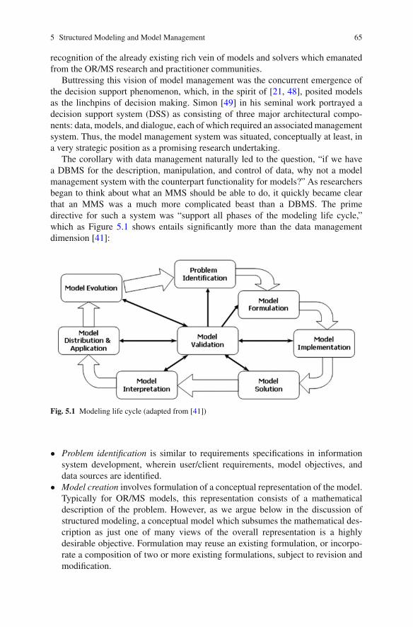
5 Structured Modeling and Model Management 65
recognition of the already existing rich vein of models and solvers which emanatedfrom the OR/MS research and practitioner communities.
Buttressing this vision of model management was the concurrent emergence ofthe decision support phenomenon, which, in the spirit of [21, 48], posited modelsas the linchpins of decision making. Simon [49] in his seminal work portrayed adecision support system (DSS) as consisting of three major architectural compo-nents: data, models, and dialogue, each of which required an associated managementsystem. Thus, the model management system was situated, conceptually at least, ina very strategic position as a promising research undertaking.
The corollary with data management naturally led to the question, “if we havea DBMS for the description, manipulation, and control of data, why not a modelmanagement system with the counterpart functionality for models?” As researchersbegan to think about what an MMS should be able to do, it quickly became clearthat an MMS was a much more complicated beast than a DBMS. The primedirective for such a system was “support all phases of the modeling life cycle,”which as Figure 5.1 shows entails significantly more than the data managementdimension [41]:
Fig. 5.1 Modeling life cycle (adapted from [41])
• Problem identification is similar to requirements specifications in informationsystem development, wherein user/client requirements, model objectives, anddata sources are identified.
• Model creation involves formulation of a conceptual representation of the model.Typically for OR/MS models, this representation consists of a mathematicaldescription of the problem. However, as we argue below in the discussion ofstructured modeling, a conceptual model which subsumes the mathematical des-cription as just one of many views of the overall representation is a highlydesirable objective. Formulation may reuse an existing formulation, or incorpo-rate a composition of two or more existing formulations, subject to revision andmodification.

66 Daniel Dolk
• Model implementation is the development of a computer executable represen-tation of the model either through ad hoc program development or preferablyusing existing modeling languages and environments. Also, critically, this stageencompasses the identification, collection, and quality control of the associateddata that will instantiate the model.
• Model solution requires identification of an appropriate solution algorithm, datapreprocessing for providing input to the solver and delivering results to thedatabase, and solver sequencing and execution.
• Model interpretation involves analyzing the results, understanding and debug-ging the model, and performing sensitivity analysis.
• Model distribution and application refers to the process of making a model op-erational and accessible to the user community on a need to know basis. Modeland data security are mission-critical functions in the Internet age of informationassurance.
• Model evolution. Model versions reflecting different sets of assumptions, data,and/or insights can proliferate rapidly and must be managed carefully. This maywell result in a reformulation of the model, occasioning additional iterationsthrough the life cycle process.
• Model validation is a persistent process occurring throughout the life cycle. Thismay range from dimensional and unit consistency analysis at the Formulationstage to the traditional internal and external validation processes at the Solutionand Interpretation stages that the model solution is consistent with the initialassumptions and with the “real world.”
In addition to the rather high-level life cycle requirements, more detailed func-tionality and design guidelines began to emerge as researchers delved more deeplyinto the architecture of an MMS. A majority of the work at this stage of research wasfocused upon environments for optimization models since they are generally wellstructured and there exists a large universe of models and solvers available for de-ployment. Some of the major requirements and associated guiding design principlesemerged from the limitations of second-generation optimization software:
• An MMS should have a uniform computer executable model representation. Thedesideratum would be a representation formalism equal in power to the relationaldata model which underlies the database management environment. Addition-ally, the model representation should support multiple views of a model as therelational model does for data.
• An MMS should support modeling languages. The ability to describe models in asufficiently general and abstract form, especially in a pseudo-mathematical rep-resentation, streamlines the ability to formulate models and widens the audiencefor model builders [22]. Earlier generations of software for optimization models,for example, required a matrix representation of models which one could corre-late to programming assembly language in the software development arena. Thisrestricted model formulation to a relatively small cadre of dedicated analysts.
• An MMS should support cross-paradigm models. The OR/MS world is an archi-pelago of modeling silos. A powerful alternative is a single environment which

5 Structured Modeling and Model Management 67
simultaneously supports optimization, regressions, simulations, queuing,dynamic programming, etc., and reduces the need to learn a new software sys-tem for each different modeling paradigm. The potential of such a system tofacilitate model integration is large. The OR/MS community has developed, andcontinues to develop, a broad portfolio of single paradigm models, access to anycombination of which in a single environment would be a powerful tool in modelintegration (see below).
• An MMS should have access to a library of solvers. The OR/MS communityhas developed a multitude of solution algorithms and meta-heuristics for specificclasses of models. As above, access to these solvers widens the range of modelswhich can be usefully solved in this environment.
• Models and model data should be separate in an MMS. Early modeling sys-tems required data to be in a very application-specific format which reduced orobviated the ability to reuse the data. Data should be independent of model rep-resentations until such time as a model instance is required. An MMS shouldleverage relational technology for managing the data. Data can be bound to amodel representation using the powerful capabilities of relational databases. Thisunderscores the separation of models and data mentioned above.
• Models and solvers should be separate in an MMS. Many models can be solvedin different ways, for example, an LP model may be solved using simplex orbranch-and-bound if an integer solution is desired. A model should not be boundto a particular solver until model solution time. The MMS should then be ableto convert the data of the model instance to the appropriate format for the solver,and back again for the solution vector(s).
• An MMS should support the reuse and integration of models. Models are typi-cally built for a single application and rarely ever reused beyond that application.The ability to reuse models not only has the potential for reducing model formu-lation costs but can significantly increase ROI from model development as well.Further, the ability to link existing models into composite models facilitates thedevelopment of more complex models.
The central theme which emerged from the list of requirements above was theneed for a powerful model representation which is simultaneously comprehensibleto a variety of different users (clients, analysts, mathematicians) and computerexecutable. The theoretical driver behind this quest started naturally enough witha database analogy: Is there a way to represent models that is comparable in powerto the relational theory representation of data?
The first attempts at model representation leveraged artificial intelligencetechniques for representing knowledge: semantic networks of nodes and edges forrepresenting knowledge about models [19], first order predicate calculus to repre-sent mathematical programming models in a way that allows useful inferences tobe made [6] and frames for representing mathematical programming and economet-ric forecasting models [15]. Frames provided a basis for thinking about models interms of object-oriented representations; many authors subsequently proposed vari-ous object-oriented representations for model management (see e.g., [24, 42]).

68 Daniel Dolk
Early attempts to apply relational theory directly to model representation foundthat the transitive closure property which unifies relational theory does not carryover to its modeling counterpart [4, 5]. Thus, two or more models that are somehowjoined with one another do not necessarily yield another model. The lack of a directrelational corollary led researchers to consider different alternatives.
Geoffrion developed a full model representation formalism called structuredmodeling based roughly on the entity-relationship data model, but which includedsignificant extensions accommodating the ability to represent OR/MS models,particularly mathematical programming models [27]. Details of structured model-ing will be discussed below, but it is interesting to note that structured modelingwas the first contribution with respect to model representation which came from theOR/MS, rather than the information systems, research community. Other powerfulrepresentation techniques were developed as well including a relational version ofstructured modeling [16], logic modeling [2], graph grammars [37, 38], systemstheory [45], and metagraphs [1].
5.3 Structured Modeling
Of the model representation approaches summarized above, Geoffrion’s structuredmodeling has received the most attention by researchers. We provide a generalrecapitulation of this model representation formalism and show its vital role inthe model management movement. This will by no means constitute a full andthorough review; readers are directed to [25, 27] for such a treatment.
Structured modeling (SM) is a semantic framework for representing wide classesof models, primarily from the domain of operations research and managementscience. Although many of the applications that structured modeling addresses inthe research literature tend to be optimization models, Geoffrion went to great painsto show that models from a broad array of domains, some outside OR/MS altogether,could be represented using structured modeling.
SM has roots in the entity-relationship data model [12] but goes well beyondthat in terms of formalism and extensions which accommodate modelinglanguages and indexing semantics. Every structured model is a collection of dis-tinct elements, namely the primitive entity (/pe/), the compound entity (/ce/), andattributes. Attributes can be of four types: a regular attribute (/a/), a variableattribute (/va/) to designate decision variables in a model, a function element (/f/)based on the mathematical idea of a function, and a test element (/t/) which isa special Boolean case of a function, used, e.g., to represent constraints withinoptimization models.
Elements are grouped into classes called genera; a single such class is calleda genus. A genus is in an “IS A” relationship with the elements comprising it. Forexample a supply constraint test genus may consist of an indexed set of supply cons-traint test elements, one for each supplier. Genera may be organized hierarchicallyto reflect high-level structures and to manage model complexity. This is done using

5 Structured Modeling and Model Management 69
modules which are collections of genera constituting a subgraph of the overall genusgraph (see below).
5.3.1 Structured Model Schema
Structured models are represented in three basic modalities: the schema, the genusgraph, and the elemental detail (data) tables. The schema shown in Figure 5.2 is afull structured model schema representation of a simplified blending problem calledFeedMix which determines amounts of materials to be used in animal feed thatmust satisfy certain nutritional requirements. The mathematical description of themodel is
min ∑m
Cm∗Qm (5.1)
s.t. ∑m
Aim∗Qm≥MRi ∀i (5.2)
Qm≥ 0 ∀m (5.3)
Fig. 5.2 Structured modeling schema for FeedMix model

70 Daniel Dolk
where m = material, i = nutrient, Cm = unit cost of material m, MRi = minimumrequirement of nutrient i, Qm = quantity of material m, Aim = amount of nutrient iin material m.
The schema contains a full description of each of the genera and modulesaccording to a pre-specified format. Genus information in a schema includes thegenus name, associated index(es), any other genera it depends upon, genus type(/pe/, /ce/, /a/, etc.), domain (Real, Integer, etc.), and computable function (for testand function genera). Module information includes name and description. By con-vention modules are designated by a leading “&.” Underlined and capitalized wordsin the descriptions are intended to be the main identifiers for the associated genus ormodule.
Structured models are built from the primitive entities outward. Primitiveentities do not depend on any other genera so they form the foundation of themodel. A typical building sequence is to identify each primitive entity and itsassociated attributes (NUTR/MIN and MATERIAL/{UCOST, Q}, for example),any compound entities and their associated attributes (NUTR MATERIAL andANALYSIS in this example), test genera (T:NLEVEL), function genera (TOTCOSTand NLEVEL), and modules (&NUTR and &MATERIALS). Note that NLEVEL isused to compute the test genus T:NLEVEL and is more of an intermediary compu-tation whereas TOTCOST is a terminal computation (leaf node) which may likelyserve as an objective function for the model. Typically model building is moreeasily accomplished using the genus graph than working directly with the schemarepresentation.
The schema is a textual description represented as a hierarchical structure in out-line form. Each entry in a schema line is either a genus or a module (prefaced by“&”) name. Modules are aggregations of genera and/or modules which allow sub-sets of a model to be collected into a higher order structure. &NUTR DATA, forexample, captures the part of the model that deals solely with nutrients, specificallythe genera NUTR and MIN. The genus is the basic component and may be of severaldifferent types as designated within the “//” separators: primitive entity (/pe/), com-pound entity (/ce/), attribute (/a/), function (/f/), and test (/t/). Primitive entities willusually have an associated index which is specified as part of the name, e.g.,MATERIALm. For mathematical programming models, primitive entities corre-spond to index sets.
Each genus has a calling sequence, which may be null, specifying all genera thecurrent genus may reference. The genus MIN, for example, references the primi-tive entity NUTR since it is an attribute of NUTR; therefore, NUTRi is containedwithin its calling sequence. Note the indexes are carried forward into the callingsequences; the indexing specification can become quite convoluted ([32] for moredetails). Primitive entities have no calling sequences; they are in effect a root of thegenus graph tree (see below).
Attributes are equivalent to parameters in math programming models and thushave a data type; in our example, all attributes are in the set of positive real num-bers. Test and function elements such as T:NLEVEL and TOTCOST, respectively,are typically described by equations represented in a modeling language (SML:Structured Modeling Language in this case).

5 Structured Modeling and Model Management 71
Finally, each entry has a documentation segment with the potential for hyperlink-ing among them (words in all caps above). The documentation provides a mediumfor descriptions of the entry as well as any attendant model assumptions.
The schema is flexible in that different subsets, or views, can be displayed toappeal to different audiences. For example, one could provide an outline containingonly the names and descriptions for end users and decision makers. Alternatively,one could suppress the documentation and only display the more analytical aspectsof the model (material in bold face) for analysts and modelers.
5.3.2 Genus Graph
The genus graph shown in Figure 5.3 is an acyclic directed graph which showsthe relationships among the various model genera as specified in the schema. Itresembles an entity-relationship diagram in many respects. Entities come in twoforms: primitive entities and compound entities. Note that the root nodes of the treeare the primitive entities which in the case of optimization models typically corre-spond to the indexes of the mathematical model. Compound entities represent theequivalent of relationships between two or more primitive and/or compound entities.In Figure 5.3, for example, the compound entity NUTR MATERIAL represents tworelationships between the primitive entities NUTR and MATERIAL, namely “eachMATERIAL contains one or more NUTRIENTs” and “each NUTRIENT may bepresent in one or more MATERIALS.” Genera which depend on other genera suchas NUTR MATERIAL are connected by a directed arc to the antecedent genera.Structured modeling does not provide an explicit way to designate the cardinality of
Fig. 5.3 Structured modeling genus graph for FeedMix model

72 Daniel Dolk
a relationship between two entities as is the case with entity-relationship diagramswhere each arc is labeled with the cardinality.
The parameters of the mathematical model are attributes of primitive or com-pound entities such as Q, the quantity of MATERIAL. Other dependencies cascadedown the graph to the leaf nodes, which typically correspond to the constraints andobjective function of the corresponding optimization model. We must emphasize,however, that the structured model does not specify the decision variables or ob-jective functions explicitly. This binding takes place only at solution time when theuser identifies the objective function(s), the constraint(s), the decision variable(s),and the solver, perhaps using a notional modeling language statement similar to
SOLVE FEEDMIXMIN TOTCOSTSUBJ TO T:NLEVELVARYING QUSING CPLEX
5.3.3 Elemental Detail
The elemental detail aspect of a structured model is the relational table equivalent ofthe genus graph. Like entity-relationship diagrams and unified modeling language(UML) diagrams, a relational database schema of tables can be automatically cre-ated from a well-formed genus graph. The associated set of tables for the FeedMixgenus graph is shown in Figure 5.4. These tables can be populated manually orby using more sophisticated SQL and XML commands to import data from externalsource databases. Note that this enforces the independence between model represen-tations and data in the sense that we can add nutrients and/or materials by simplymaking additional entries in the data tables without changing the model representa-tion at all.
A model that has its elemental detail tables populated is called a model instance.A model instance will be solved as indicated above, which in turn requires the abilityto convert the elemental detail tables into the format required by the solver and then
Fig. 5.4 Elemental detail (data) tables for the FeedMix model

5 Structured Modeling and Model Management 73
conversely to translate the solution from the solver back into the elemental detailtables. In our example the column Q in table Q and the singleton table TOTCOSTwould both receive values from the solver indicating the optimum levels of Q andresultant TOTCOST, respectively.
5.3.4 Modules
Structured modeling also supports the hierarchical decomposition of models and thenotion of multiple views via Modules which allow users to group related genera intoa compressed subgraph for subsequent drill-down. Figure 5.5 shows the modular-ization of the Nutrient and Materials components of the FeedMix model.
Fig. 5.5 The use of modules to compress the FeedMix model
5.3.5 Structured Modeling Language (SML)
Structured modeling strongly supports the technology of modeling languagesthrough its Structured Modeling Language (SML) [30, 31]. The objective ofalgebraic modeling languages is to formulate models in relatively abstract,

74 Daniel Dolk
quasi-mathematical form which allows a parsimonious, computer executabledescription of a model. The effect of such modeling languages is to place a higherlevel of the processing costs on the modeling software rather than the user. SMLdiffers from two of the most popular algebraic languages, GAMS and AMPL, inthat it includes four different semantic levels, of which only one is algebraic. Level1 is for simple, definitional systems and directed graph models. Level 2 includesLevel 1 plus the ability to express numeric formulae and propositional calculusexpressions. Level 3 encompasses Level 2 with simple indexing capabilities as wellas predicate calculus expressions. Level 4 subsumes Level 3 plus the ability to han-dle more complex indexing expressions as well as relational and semantic databasemodels. SML levels are upward compatible in that a model expression at any levelis valid at any higher level. The FeedMix schema shown above is an example ofLevel 3 SML.
5.3.6 Structured Modeling Environments
As research in structured modeling evolved, the concept of a model managementsystem also evolved into a more general version called a modeling environmentor integrated modeling environment [28]. A modeling environment is based lessupon the notion of a single, stand-alone RDBMS-like counterpart and more uponthe premise of a resource-rich infrastructure for supporting most, if not all, of themodeling life cycle as shown in Figure 5.1. Modeling environments may even berelatively application specific (e.g., [43]), but nevertheless transcend the narrow,single-platform focus of existing decision support and modeling software.
Many prototypes of structured modeling environments have been developed withvarying degrees of success; we will mention only a few here (see [33] for referencesto some of the earlier versions). Geoffrion’s own FW/SM [29] was built using theFramework system, a personal productivity tool from the late 1980s. Frameworkwas an unfortunate choice for such a prototype because it lacked scalability andalso had a short shelf-life in the software marketplace. Nevertheless, the platformwas coaxed into supporting a robust version of structured modeling which did allthe complex parsing of schemas and was able to generate database schemas au-tomatically from the structured modeling descriptions. This proof of concept en-forced many of the design principles mentioned in Section 5.2 such as model–dataindependence, model–solver independence, leveraging relational databases for datamanagement, and linking with actual solvers in real time. There was not, however,a graphical user interface to ease model formulation, a serious shortcoming whichwe address in more detail later.
An ambitious implementation of structured modeling in the form of VMS/SM(Visual Modeling System for Structured Modeling) did include a GUI and imple-mented a substantial subset of structured modeling principles [55]. The GBMS/SMprototype also featured a genus graph GUI for the specification of structuredmodels [11]. Later, a spreadsheet-based version of structured modeling was

5 Structured Modeling and Model Management 75
developed as part of providing service-oriented, Web-based model management[36]. Their prototype GUI, although a simplification of the genus graph, isnotable for using spreadsheets as the underlying platform for model managementand structured modeling implementation. It would have been most interesting to seewhether a GUI-driven FW/SM using a spreadsheet rather than Framework wouldhave gained more traction for structured modeling and model management in gen-eral. Several other prototypes emerged based on object-oriented methodologies,including the ASUMMS/DAMS project [47] and BLOOMS [24]. All of theseimplementations represented valiant attempts at producing a generalized modelingenvironment for widespread usage; however, none of them survived with onenotable exception.
The most enduring implementation of structured modeling is the StructuredModeling Technology (SMT) project at IIASA [43]. SMT supports a very large andcomplex optimization model called RAINS which is used to support internationalnegotiations over European air quality. RAINS consists of several sub-models con-taining over 30,000 variables and 30,000 constraints in aggregate. Updated versionsof the model will be even larger. Some of the interesting aspects of this implemen-tation are as follows:
• No genus graph GUI has been implemented. The rationale for this design deci-sion was that the complexity of the model in terms of the number of variablesand their attendant interactions prevents a concise graphical representation. Evenwith larger contemporary monitors, one could see only an insignificantly smallsubset of the model at any one time.
• The centrality of data management. SMT leverages relational DBMS technologyheavily to integrate and manage not only data sets but also model versions, modelresults, and model documentation.
• Multiple views of models and data. SMT supports a large community of userswith diverse requirements. This results in the need for viewing models froma number of different perspectives. The structured modeling representation isleveraged to provide these model views.
• Open source. SMT subscribes to the open source philosophy to make the plat-forms as universally accessible as possible.
• No dimensional or unit specifications. An attempt at implementing units for eachof the parameters led to the proliferation of such complex, non-intuitive unit spec-ifications in the composite variables that this effort was eventually abandoned.
• Enforced documentation. SMT generates automatically human-readable docu-mentation at each step of the model life cycle process.
• No model integration. The SMT philosophy is that it is easier to construct modelsfrom “scratch” than attempt to reuse already built models.
SMT remains heavily used to this day. It demonstrates the utility and scalabil-ity of the generalized structured modeling approach for large, complex optimiza-tion models with a diverse community of users. As a case study, it is invaluable inhighlighting which of the tenets of model management and structured modeling arecritical and which are optional or even dispensable.

76 Daniel Dolk
5.4 Structured Modeling Contributions to Model Management
The contributions of structured modeling to model management are numerous. Firstand foremost, it provides a formal semantic ontology for models within a rigorouslydeveloped framework based on graph theory. In this formalism, mathematical mod-els can be represented as conceptual models, thus unifying mathematical modelingas practiced in the OR/MS fields with the disciplines of information and data model-ing. This cross-fertilization, it should be noted, was unusual in that it emanated froma research luminary in operations research adopting IS approaches rather than themore common situation at the time of IS researchers trying to extend data and infor-mation modeling concepts to operations research. Geoffrion’s high standing in hisfield lent tangible momentum to the model management movement and generated aflurry of research on this topic from both communities.
Another advantage of structured modeling, as with most forms of conceptualmodeling, is that it provides a bridge that allows analysts to communicate moreeffectively with decision makers. The ability to view the model structure as an in-fluence diagram separate from the mathematical description provides, in principle,less analytically gifted players the ability to question assumptions and better com-prehend the relevance of the model to the business environment. The commercialAnalyticaTM system relies heavily upon this model representation which offers theadvantage of a more “user friendly” view of mathematical models while simultane-ously providing computer executability.
Another major contribution of structured modeling was the furthering of alge-braic modeling languages as an accepted way of formulating computer executablemathematical models. The powerful modeling language, SML, with sophisticatedindexing capabilities augmented the seminal work done in the development of theGAMS [9] and AMPL [23] languages. Although we take such modeling languagesfor granted today, the path from “horseblanket” matrix generators to algebraic rep-resentations was a rather slow and arduous process that spanned quite a few comput-ing generations. The emphasis on model representation which structured modelingembodied served as an important catalyst for this transition.
Structured modeling also contributes to the goal of model reuse and integration.The lack of reuse is frequently cited as one of the factors in the relatively high costof model development. In the same way that relational databases free data from be-ing too tightly tied to specific applications, it is also desirable for models to escapethe “one time only” application label. As shown in [26], genus graphs can be savedin model libraries and ultimately reused either by revising existing templates forapplications with similar assumptions and structures or by composing more elab-orate models from the linkage of two or more templates. Although genus graphsprovide a fruitful medium for identifying potential sources of this latter form ofmodel integration, it is by no means an easy task to carry out the integration itself.Not surprisingly, it appears this process cannot usually be done completely automat-ically but requires manual intervention to resolve semantic incongruencies betweengenus graphs, for example, in the resolution of naming differences and dimensionalinconsistencies [7, 3].

5 Structured Modeling and Model Management 77
There is a very large body of research dealing with structured modeling andrelated model management issues, much of it chronicled by Geoffrion [33]. I be-lieve it is safe to say that this research has demonstrated structured modeling tobe a powerful representational basis for comprehensive modeling environments thatsupport OR/MS models. However, it is also safe to say that, with a few exceptions,structured modeling is not widely used today and never gained wide acceptance evenamong practitioners in the OR/MS community. The following section will attemptto address why this is the case.
5.5 Limitations of Structured Modeling
The limitations of structured modeling and the obstacles toward adopting it asa standard model representation form can be attributed to both endogenous andexogenous factors. Among the inherent limitations of structured modeling whichhave impeded its use by a wider audience is the high degree of complexity ofthe schema representation itself, particularly with respect to indexing semantics.Even seasoned modelers have been known to struggle when working at the struc-tured modeling schema level. Generating a formal, correct schema even for a simplemodel such as that shown in Figure 5.2 is challenging in that each segment of theschema has its own precise syntax which leads to a steep learning curve.
One obvious way to mitigate this problem would have been to create a graph-ical user interface (GUI) for constructing genus graphs which could automaticallygenerate most of the needed syntax. Although several graphical prototypes of struc-tured modeling were implemented, e.g., [11, 36], none reached effective operationalstatus. Surprisingly, Geoffrion’s own FW/SM prototype did not include a GUI butrather required users to input the schema textually. As a result, there was never a full“cradle-to-grave” structured modeling implementation with a “user friendly frontend.” Without a GUI feature, structured modeling was regrettably confined to a rel-atively small cadre of experienced modelers and acolytes. It should be mentionedthat at the height of the research into model management, graphics software wasstill a relatively immature technology. Graphics libraries were relatively expensive,typically not widely available or particularly easy to use, and tended to be confinedto high end, programming intensive applications. There was no VisioTM equivalentat that time which could have solved this problem handily.
Another major shortcoming of structured modeling is that its strength lies in therepresentation of static models vis-a-vis dynamic models. It is not by chance thatoptimization models were the most successfully rendered examples in structuredmodeling. Their high degree of structure is well suited to the structured modelingformalism. However, when we consider the class of discrete event simulation mod-els, for example, representation becomes inexorably more complex. Now we mustdeal not only with structures but also with events and processes that are time drivenas well. There are no available means within structured modeling for representingevent-driven processes in an elegant or concise fashion. Nor are there ways to in-corporate the stochastic nature of such models. Although some suggestions were

78 Daniel Dolk
made to address this shortcoming such as extending structured modeling to includea new random-valued attribute genus type [46], this avenue of research never gaineda foothold.
In this vein, technology to some extent overcame structured modeling as well.During the past decade, the object-oriented Unified Modeling Language (UML) hasbecome the prevalent data modeling methodology, overtaking the entity-relationshipapproach in system development. Although UML is anything but a polished modelrepresentation system, it does provide capabilities for representing both the staticand dynamic dimensions of a model. Nevertheless, UML still does not offer a naturalway to represent decision models in its environment [17].
There were also significant exogenous factors affecting the acceptance of struc-tured modeling. Perhaps of primary importance from an organizational perspec-tive is that most organizations do not support a modeling culture in which modelsare viewed as a sustainable asset. Models are too often consigned to spreadsheetexercises or ad hoc, application-specific projects. Thus, it is difficult in this settingto see any payoff for a general methodology such as structured modeling.
In the academic world, a cultural factor weighing against the adoption of struc-tured modeling is that OR analysts, who would comprise the most likely user com-munity, tend to be primarily mathematically trained and solver oriented. In that usergroup, mathematics is the lingua franca of model representation, and reframing theformulation of models into a conceptual modeling context is likely to be seen as anextra, undesirable layer in model development. Structured modeling forces generalmodel structure to be specified before any model instance can be specified, and thisis resisted for all the same reasons that documentation of models (and software)is always resisted. Even in the field of database design, the birthplace of concep-tual modeling, database analysts often circumvent this phase and jump directly tobuilding tables. Perhaps then, structured modeling might best be used in the class-room as a way of developing sound modeling practices that transcend simply themathematical dimension.
5.6 Limitations of Model Management
One cannot easily view structured modeling outside the context of model manage-ment, and “model management” is a term that is rarely used today. It is neithercommercially nor academically viable. Both model management and structuredmodeling faded away with the advent of the Internet and distributed computing.Some of the reasons for this are conjectured below.
• No demand for MMS. To the chagrin of those involved in this research over theyears, it is not clear that there is, or ever was, a market demand for a modelmanagement system [54]. Although researchers heroically assumed that such anartifact would be valuable, no business value proposition was ever formulated ortested to verify this hypothesis. Few organizations support a modeling culture tothe extent that development or purchase of a model management system could be

5 Structured Modeling and Model Management 79
easily justified. Further, for many organizations, modeling begins and ends withthe spreadsheet, so it would not be an exaggeration to say that, in the commercialworld, “the spreadsheet is the MMS.” Unfortunately, the spreadsheet is a fairlyprimitive modeling platform, which suffers from a spate of problems not theleast of which is the widespread abuse of modeling practices by vast hordes ofamateur modelers. Nevertheless, I believe the model management communitycould have benefitted, and could still benefit, from more research into the useof the spreadsheet as a model management generator. The spreadsheet-drivenstructured modeling prototype described in [36] not only showed the promise ofthis approach for smaller applications but also demonstrated that a conceptualmodeling interface could serve as an effective vehicle for enforcing improvedintegrity in model formulation. With the advent of more scalable spreadsheets incontemporary software suites, much larger models would lend themselves to thisapproach as well.
• Modeling too infrequently used in decision making. This is the eternal complaintof the OR/MS community so shall not be dwelt upon further here. Despite thebest efforts of our MBA and masters programs in management, end users ofmodels, namely decision makers in organizations, are all too often either “modeladverse,” or less charitably, “model challenged.”
• Cross-paradigm myopia. Selling model management in the academic communitywas not much more successful than in the commercial marketplace. Even in theanalyst world where one might expect a more cordial reception to the concept ofan MMS, cross-paradigm myopia tends to be prevalent, and this undermines theobjectives of a generalized system. People tend to see the world in terms of themodeling paradigm in which they specialize, whether it be optimization, multi-criteria decision analysis, simulation, statistics, etc., and subsequently becomefamiliar with one or two “stand-alone” software systems which solve only thosekinds of models. The benefits of a generalized system which could handle modelsacross multiple paradigms as is required for integrated supply chain management,for example, are thus not highly valued, and the stovepipe mentality persists.
• Data but not models. Models in general do not command the same respect as datain organizations. Everyone in this age is familiar with the need for data manage-ment, the value of institutional data for data mining purposes, and the challengeof and necessity for data security. A similar awareness about models is simply notprevalent; the fact is that the basic assumptions about model management articu-lated 30 years ago simply do not hold up in practice. Perhaps this will change asinformation technology evolves, but it is difficult to be confident about this con-jecture. Underscoring this pessimism is the current landscape where enterpriseresource planning (ERP) vendors are now including basic optimization modelsas part of their integrated architectures, particularly with respect to supply chainmanagement. However, these models are essentially “black boxes” to the userswho generally have little or no idea about the structure or details of the modelsbeing implemented and presumably used in decision making. In fact, this “stealthmodeling” contravenes every principle of model management, obscuring ratherthan revealing the true purpose and value of modeling in an organization.

80 Daniel Dolk
5.7 Trajectory of Model Management in the Internet Era
The concept of model management changed dramatically with the advent of theInternet. The emergence of the Internet shifted attention away from the generalized,monolithic system concept to a distributed resources perspective as we discussbelow. Some of the well-known transitions which the Internet effected are shifts inperspective from stand-alone machine centric systems to network-centric systems,from top down to bottom up, from MMS as a single monolithic system to MMS asdynamic, configurable software components, from software as a product to softwareas a service, and from individual problem solving to collaborative problem solving.
In the model management domain this manifested in projects such as Decision-Net [3] which effectively decomposed model management systems into distributedresources managed by a centralized registry and directory. In this highly distributedenvironment, model representations, solvers, data, and sensitivity analysis softwareare all presumed to reside at distributed locations rather than in a centralized sys-tem. The environment is responsible for registering various resources, ensuring theavailability of appropriate interfaces, and facilitating the necessary integration ofresources for modelers to accomplish specific tasks in the life cycle. This network-centric version of model management views software as a service rather than a prod-uct, to be priced on a “per-use” basis as opposed to a one time purchase. In fact muchof the work done in DecisionNet prefigured the more recent trends toward Web ser-vices and cloud computing.
The Internet also changed the kinds of models that organizations cared about.The flattening of organizational hierarchies manifested in Internet-based businessled directly to a much higher requirement for, and interest in, collaboration, which,in turn, put a very strong emphasis upon business process and workflow models.These models are much more dynamic and therefore, akin to simulations than thosewith which structured modeling dealt.
The service-oriented Internet paradigm effectively eliminated most of the interestin the concept of a unified model management system. In principle, the ability toaccess modeling resources on demand, and only those resources which are requiredfor any particular application at hand, is a much cleaner business model than the“all singing, all dancing” MMS. By the turn of the century, model management andstructured modeling were no longer seen as central to the paradigm of dynamic,distributed computing. As a result, research interest in these areas per se began tofade and fragment into other related channels of inquiry. Nevertheless, pockets ofresearch in model management persist to this day, and perhaps it is possible to buildupon them and retrench as we discuss in the next section.
5.8 Next Generation Model Management
We now address the central question posed at the beginning, “Is model manage-ment relevant today?” Certainly research that incorporates this term has diminished

5 Structured Modeling and Model Management 81
in recent years; however, we note that modeling itself is still a vibrant activity andcontinues unabated in organizations in the areas of information system develop-ment (e.g., business process modeling and enterprise integration architectures) aswell as OR/MS-based decision models (e.g., supply chain management). The ag-gregate levels of modeling activity remain high, but the recognition of the need tomanage these models still goes unheeded. We assume that model management isstill a vital requirement but that we need to look at it in new ways that are consis-tent with advances in technology. We begin with the work that is still ongoing inmodel management augmented by suggestions which might be considered a partialblueprint for a “next generation model management”.
5.8.1 Enterprise Model Management
The benefits of bringing model management to the field of enterprise and businessprocess modeling are described in [34]. A unified enterprise modeling language(UEML, not to be confused with UML) is specified in [51] as a vehicle for bringingcoherence to this endeavor in much the same way Geoffrion envisioned structuredmodeling serving the needs of the OR/MS modeling community. The UEML isintended to represent business logic in a platform-independent manner which nev-ertheless can be mapped to specific enterprise modeling toolkits and “that can, intheory, be merged, integrated, composed or otherwise operated upon to provide alarger subset of an enterprise model, thereby providing . . . a composed EM viewof the enterprise” [34, p. 919]. This sounds very much like model–solver indepen-dence in the structured modeling world, model integration in the model managementworld, and service composition in the SOA world (see below). The UEML is itself astatic conceptual model which could be rendered as a structured model schema thuspossibly integrating decision models as an ingredient in the overall enterprise ar-chitecture. Regardless of the model representation employed, it is heartening to seethat there is a realization of the need for model management in this arena. Hopefully,we can avoid reinventing the wheel and leverage the substantial model managementresearch to move this agenda forward.
5.8.2 Service-Based Model Management
Another closely related opportunity for model management is the emergence of theservice science, management and engineering (SSME) movement, which empha-sizes service-dominant logic over the historically prevalent product-dominant logic[50]. This change in perspective from production to services changes the Producer–Customer relationship to a Provider–Consumer relationship in which both partiesstrive to “co-create value.” This again will put emphasis on business process mod-els, particularly collaborative models, but it will also require, in turn, a rethinking

82 Daniel Dolk
of the more traditional quantitative modeling approaches which tend to optimizemanufacturing efficiency over customer satisfaction.
On the information technology side of SSME, contemporary service-oriented ar-chitectures for delivering modeling and decision support will be required as well.Many of the problems faced by model management researchers in addressing the is-sue of model integration have resurfaced recently in the context of service-orientedarchitectures (SOAs). Specifically, an SOA must meet the challenge of composingservices “on the fly” in order to satisfy a user’s “on demand,” and often ad hoc, re-quest. This issue of service composition is very similar to that of model compositionwhen trying to link existing models and data to satisfy a particular application (e.g.,[10, 40, 45]). Interestingly, the SOA literature seems to show little, if any, awarenessof the model management work already done in this area (e.g., [3, 35, 36]).However, research is beginning to resurface on service-oriented architectures formodel management which redresses this situation [8, 14].
5.8.3 Leveraging XML and Data Warehouse/OLAP Technology
Even today, neither the entity-relationship model nor the UML model support therepresentation of decision models, so almost by definition there is room for a con-ceptual modeling approach which does. Because structured modeling has such astrong definitional character, it would also seem logical as a medium for some kindof ontological XML model interchange standard. This is consistent at a low level ofimplementation with the notion of model management as knowledge managementproffered above. See [36] for an example of an XML representation of structuredmodels.
Another immediate application for structured modeling would be to link SMLrepresentations with data warehouses and their associated online analytical process-ing (OLAP) environments. This provides an opportunity for accessing multidimen-sional data that align rather naturally with the mathematical index representationof OR/MS models [18]. Thus, it should be significantly easier to overlay a model-ing system on a data warehouse than on a traditional relational database. The SMTsystem mentioned earlier adopts this approach, using a data warehouse as its dataengine. In general, however, it seems that the modeling community has been slowto adopt this technology, and it is certainly the case that the data warehouse/OLAPvendors have been very slow to add significant modeling capabilities to their OLAPtools.
5.8.4 Model Management as Knowledge Management
As mentioned at the beginning of this retrospective, model management grew as acorollary to data management. Given the contemporary focus on knowledge flow,

5 Structured Modeling and Model Management 83
the learning organization, and the knowledge society, a more robust metaphor maybe model management as knowledge management. And even the term “manage-ment” has perhaps historically been used in too limited a scope, often implying aconcern more with the management control issues of data, models, and knowledgethan with their uses in conducting business more effectively.
When one looks at the modeling life cycle, it is difficult to escape the conclusionthat modeling deals with anything less than the flow of knowledge. The purposeof building and solving models is to illuminate decision landscapes by identifyingviable choices and evaluating trade-offs among the choice set. As such, models,properly fashioned, are knowledge creators. The stages of problem identificationand model interpretation, for example, require extensive knowledge about thedomain(s) for which the model is being developed. Model creation and solution, onthe other hand, require specialized knowledge about mathematics and algorithms.Every aspect of the life cycle can be characterized in a similar knowledge-basedidiom. I believe it is necessary to position modeling within the larger context ofknowledge and to establish the “management” designation as the entire spectrum ofmanagement rather than focusing solely upon the control aspects. This perspectiveis examined in more detail in [44, 52].
Models from the decision support perspective are primarily used to guide andenlighten decision making. Too much of decision support, however, has dealtwith isolated decision situations, for example, budget planning or optimal resourceallocation. Experience with information system development over the past 15 yearshas shown us the primacy of business processes in the systems analysis process.Decisions need to be similarly cast not just as point events but as processes withoverarching organizational objectives. Supply chain management is an excellentexample often requiring multiple decisions which are highly interconnected anddependent on each other. The models which support these decisions must capturethese interconnections and interdependencies. This puts a high premium upon modelintegration.
Simon’s science of design philosophy has had a major impact on research inthe areas of information system development, decision support, and operations re-search/management science. Too often, however, the focus from his approach hasbeen on individual decision making in relatively narrow contexts. The Internet withits flattening of hierarchies increases the criticality of collaborative decision making,and the “new” model management must be able to marshal the flow and synthesisof modeling knowledge within collaborative environments.
At a higher level of knowledge sharing, one might imagine a Wikipedia counter-part for models, a knowledge-based equivalent of an open source operating systemperhaps, where a community of committed scholars and practitioners creates andsustains an encyclopedia of information about a particular domain of applicationsand their attendant models. Consider supply chain management as an example. Aknowledge environment for the supply chain world might contain a high level con-cept map, a semantic network of sorts, containing among other things, a taxonomyof supply chain functions. The concept map would contain for each function linksto case studies, scholarly articles, and models suitably represented in structured

84 Daniel Dolk
modeling or an equivalent robust representation. These models could serve peda-gogical purposes as well as be computer executable in the distributed computingsense of DecisionNet.
5.8.5 Search-Based Model Management
Although decision support speaks of semi-structured and unstructured decisionmaking, the majority of applications developed deal with quite structured data. Theemergence of search engine technology provides a powerful capability to manipu-late semi-structured data, especially documents. Thus we need to reconsider whatmodels might look like that use these semi-structured data rather than, or in addi-tion to, the typical data stored in relational databases. Can this kind of knowledgebe used to refine model assumptions, amplify model interpretation, guide us to newsolution heuristics, or build model taxonomies for model formulation? The “new”model management must leverage search engine technology to access and manip-ulate a wider range of knowledge. One interesting avenue of attack in this regardis the use of “mash ups” for identifying domain-specific indicators which could bemarshaled toward a preliminary stage of model formulation; [39] gives an exampleof this in the area of clean energy.
5.8.6 Computational Model Management
For structured modeling to be truly relevant, I believe it is necessary to revisit thedynamic model representation issue to examine whether structured modeling can beextended elegantly and naturally to accommodate dynamic models such as discreteevent and agent-based simulation models. The prevalence of computational model-ing, particularly in the biological sciences, with its emphasis on bottom up complex-ity, cellular automata, agents, and emergent behavior, presents a distinct challenge tothe relatively static forms of structured modeling. Yet this form of modeling seemsto be gaining ascendancy and may lead us into another complete iteration of howwe view models, what model management entails, and what modeling environmentswill look like.
In the new perspective on complexity that has resulted from research in the evolu-tionary and biological sciences, systems are simulated as “bottom up” phenomena,often represented as cellular automata, exhibiting emergent macro behavior from therepeated interaction of localized agents following (usually) relatively simple rules[20]. Interestingly, however, the software platforms which support these classes ofagent-based simulations (ABS) seem hauntingly reminiscent of optimization soft-ware as it existed before modeling languages or representational formalisms suchas structured modeling were developed. Other than the use of object-oriented archi-tectures, there do not seem to be any uniform model representations for agent-based

5 Structured Modeling and Model Management 85
models and simulations, and each model is built in an ad hoc, stand-alone mode.Each platform has its own protocol for representing and constructing simulations,and oftentimes its own community of practice for sharing knowledge. Given the ex-tensive interest that currently exists about ABS, perhaps there is an opportunity forapplying model management design principles that can accelerate the evolution ofthis modeling paradigm.
Agent-based simulations have evolved from cellular automata into elaborate vir-tual environments which pose different challenges for model management, espe-cially around the issue of external model validation. This proliferation of what issometimes termed computational modeling quickly outstrips the older, rather static,notions of model management and requires a more fluid, knowledge-based approachfor the related processes of computational experimentation and computationalexplanation. The “new” model management must be able to handle a much moredynamic kind of model and oftentimes a fuzzier notion of validation, while perhapssimultaneously relying upon the more conventional OR/MS models as validationand calibration vehicles.
5.8.7 Model Management: Dinosaur or Leading Edge?
It is difficult to know, even in retrospect, whether model management has been over-come by events or whether it perhaps may still be ahead of its time. One can see inthe agent-based simulation environment and the enterprise modeling endeavors thesame phenomenon which occurred in the evolution of OR/MS modeling languages.The unregulated proliferation of different low level languages and methodologies,each with its relative strengths and weaknesses, leads to a recognition of the need forsome uniform, integrative, higher level modeling methodology (“meta-models” intoday’s terminology) which allows a wide range of models to be described in “busi-ness friendly” or “decision friendly” terms while simultaneously being computerexecutable. Structured modeling, among other methodologies, played this evolu-tionary role in the world of OR/MS models, and it will be interesting to see whetherit, or derivatives thereof, may eventually find purchase in other environments.
5.9 Summary
Geoffrion’s foray into meta-modeling via structured modeling represented a signi-ficant intellectual departure for the majority of the operations research communitywhich, at least in the mathematical programming arena, typically focused princi-pally upon generating and demonstrating the relative efficiency of newsolution algorithms and meta-heuristics. This shift of attention from model solu-tion to the overall modeling life cycle and subsequently to the conceptualization ofmodels and modeling languages was strongly cross-fertilized by the disciplines of

86 Daniel Dolk
computer science and information systems. Structured modeling is an admirableblend of operations research, management science, programming languages,database management systems, software engineering, and information systems mod-eling. This union, it seems to me, has been underutilized by all the communitiesinvolved. The processes of building models and building information systems are re-markably similar as are, in a more focused context, the processes of building solversand writing application programs. Yet, too often the software engineering world allbut ignores model-based decision making, and too often the OR/MS world ignoresproven system and software development methodologies in the course of modelbuilding. Geoffrion’s signature contribution in the creation of structured modelingwas to illuminate both these landscapes and show where and how they could befruitfully combined.
I would like to conclude on a personal note of deep gratitude. My own careerwould not have been nearly as enjoyable or as fruitful without Art Geoffrion’sfriendship; working with Art and the structured modeling community he generatedhas been the most rewarding part of my academic life. It has been a distinct honorto see a Master Scholar at work and to be invited to participate in some of thatwork. I celebrate Art for his mentorship and support, for his boundless intellectualenergy, his ability to see beyond boundaries and across the horizon, and for being agenerous, wise, congenial, and committed colleague.
References
1. Basu A, Blanning R (1994) Model integration using metagraphs. Information SystemsResearch 5(3):195–218
2. Bhargava H, Kimbrough S (1993) Model management: An embedded languages approach.Decision Support Systems 10:277–299
3. Bhargava H, Krishnan R, Muller R (1997) Decision support on demand: Emerging electronicmarkets for decision technologies. Decision Support Systems 19:193–214
4. Blanning R (1982) A relational framework for model management. DSS-82 Transactions:1:16–28
5. Blanning R (1985) A relational framework for join implementation in model managementsystems. Decision Support Systems 1:69–81
6. Bonczek R, Holsapple C, Whinston A (1978) Mathematical programming within thecontext of a generalized data base management system. R.A.I.R.O. Recherche Opera-tionelle/Operations Research 12(2)(May):117–139
7. Bradley G, Clemence R (1987) A type calculus for executable modeling languages. IMAJournal of Mathematics in Management 1(4):277–291
8. Brodsky A, Al-Nory M, Nash H (2008) Service composition language to unify simulation andoptimization of supply chains. Proceedings of the 41st Annual Hawaii International Confer-ence on System Sciences, Hawaii, January 2008
9. Brooke A, Kendrick D, Meeraus A (1992) GAMS: A user’s guide. Release 2.25. The ScientificPress, San Francisco, CA
10. Chari K (2003) Model composition in a distributed environment. Decision Support Systems35:399–413
11. Chari K, Sen T (1998) An implementation of a graph-based modeling system for structuredmodeling (GBMS/SM). Decision Support Systems 22(2):103–120

5 Structured Modeling and Model Management 87
12. Chen P (1976) The entity relationship model: Toward a unified view of data. ACM Transac-tions Database Systems 1(1):9–36
13. Codd E (1970) A relational model of data for large shared data banks. Communications ACM13(6)(June):377–387
14. Deokar A, El-Gayar O (2008) A semantic web services-based architecture for model man-agement systems. Proceedings of the 41st Annual Hawaii International Conference on SystemSciences, Hawaii January, 95
15. Dolk D, Konsynski B (1984) Knowledge representation for model management systems. IEEETransactions on Software Engineering SE-10(6):619–628
16. Dolk D (1988) Model management and structured modeling: The role of an informationresource dictionary system. Communications ACM 31(6):704–718
17. Dolk D, Ackroyd M (1995) Enterprise modeling and object technology. Proceedings of the3rd International Conference on Decision Support Systems, Vol. 1, Jun 22–23. Elsevier, HongKong, pp. 235–246
18. Dolk D (2000) Model integration in the data warehouse era. European Journal of OperationalResearch 122(April):199–218
19. Elam J (1980) Model management systems: A framework for development. Proceedings of1980 Southwest AIDS Conference, Atlanta, GA
20. Epstein J (2007) Generative social science: Studies in agent-based computational modeling.Princeton University Press, Princeton, NJ
21. Forrester J (1958) Industrial dynamics: A major breakthrough for decision makers. HarvardBusiness Review 36(4):37–66
22. Fourer R (1983) Modeling languages versus matrix generators for linear programming. ACMTransactions on Mathematical Software 143–183
23. Fourer R, Gay D, Kernighan B (1993) AMPL, A modeling language for mathematical pro-gramming. The Scientific Press, San Francisco, CA
24. Gagliardi M, Spera C (1997) BLOOMS: A prototype modeling language with object orientedfeatures. Decision Support Systems 19(1):1–21
25. Geoffrion A (1987) An introduction to structured modeling. Management Science33(5)(May):547–588
26. Geoffrion A (1989) Reusing structured models via model integration. Proceedings of the 22Annual Hawaii International Conference on System Sciences. IEEE Computer Society Press,Los Alamitos, CA, pp. 601–611
27. Geoffrion A (1989) The formal aspects of structured modeling. Operations Research37(1)(January–February):30–51
28. Geoffrion A (1989) Computer-based modeling environments. European Journal of Opera-tional Research 41(1)(July):33–43
29. Geoffrion A (1991) FW/SM: A prototype structured modeling environment. Management Sci-ence 37(12)(December):1513–1538
30. Geoffrion A (1992) The SML language for structured modeling: Levels 1 and 2. OperationsResearch 40(1)(January–February):38–57
31. Geoffrion A (1992) The SML language for structured modeling: Levels 3 and 4. OperationsResearch 40(1)(January–February):58–75
32. Geoffrion A (1992) Indexing in modeling languages for mathematical programming. Manage-ment Science 38(3)(March):325–344
33. Geoffrion A (1999) Structured modeling: Survey and future directions. INFORMS Interac-tive Transactions of ORMS. http://www.anderson.ucla.edu/faculty/art.geoffrion/home/biblio/text.htm, June
34. Goul M, Corral K (2007) Enterprise model management and next generation decision support.Decision Support Systems 43:915–932
35. Guntzer U, Muller R, Muller S, Schimkat R-D (2007) Retrieval for decision support resourcesby structured models. Decision Support Systems 43:1117–1132
36. Iyer B, Shankaranarayanan G, Lenard M (2005). Model management decision environment:A Web service prototype for spreadsheet models. Decision Support Systems 40:283–304

88 Daniel Dolk
37. Jones CV (1990) An introduction to graph based modeling systems, Part I: Overview. ORSAJournal of Computing 2(2):136–151
38. Jones CV (1991) An introduction to graph based modeling systems, Part II: Graph grammarsand the implementation. ORSA Journal of Computing 3(3):180–206
39. Kimbrough S, Lee T, Oktem U (2008) On deriving indicators from text. Wharton workingpaper, University of Pennsylvania, Philadelphia, PA, June 2008
40. Kottemann J, Dolk D (1992) Model integration and modeling languages: A process perspec-tive. Information Systems Research 3(1)(March):1–16
41. Krishnan R, Chari K (2000) Model management: Survey, future directions and a bibliography.Interactive Transactions of ORMS 3(1):1–19
42. Lenard M (1993) An object-oriented approach to model management. Decision SupportSystems 9(1)(January):67–73
43. Makowski M (2005) A structured modeling technology. European Journal of OperationalResearch 166(3)(2005):615–648
44. Makowski M, Wierzbicki A (2003) Modeling knowledge: Model-based decision support andsoft computations. In: Yu X, Kacprzyk J (eds) Applied decision support with soft comput-ing, vol. 124 of Series: Studies in Fuzziness and Soft Computing. Springer, New York, NY,pp. 3–60
45. Muhanna W, Pick R (1994) Meta-modeling concepts and tools for model management: Asystems approach. Management Science 40(9):1093–1123
46. Pollatschek M (1995) SML for simulation. Faculty of Industrial Engineering and Manage-ment, Technion, Haifa, Israel, 27 p
47. Ramirez R (1995) A management system for MS/OR models. Journal of MicrocomputerApplications 14(2):53–60
48. Sprague R, Carlson E (1982) Building effective decision support systems. Prentice-Hall,Englewood Cliffs, NJ
49. Simon H (1969) The sciences of the artificial. MIT Press, Cambridge, MA50. Vargo S, Lusch R (2004) Evolving to a new dominant logic for Marketing. Journal of
Marketing 68:1–1751. Vernadat F (2002) UEML: Towards a unified enterprise modeling language. International
Journal of Production Research 40(17):4309–432152. Wierzbicki A, Makowski M (2000) Modeling for knowledge exchange: Global aspects of
software for science and mathematics. In: Wouters P, Schroder P (eds) Access to publiclyfinanced research. NIWI, Amsterdam, The Netherlands, pp. 123–140
53. Will H (1975) Model management systems. In: Grochia E, Szyperski N (eds) Informationsystems and organization structure. Walter de Gruyter, Berlin, pp. 468–482
54. Wright G, Chaturvedi AR, Mookerjee R, Garrod S (1998) Integrated modeling environmentsin organizations: An empirical study. Information Systems Research 9(1):64–85
55. Yeo G, Jian H (1997) Visual modeling with VMS/SM. Proceedings of the IASTEDInternational Conference on Simulation and Modelling, Pittsburgh, PA, pp. 202–205

Chapter 6Retrospective: 25 Years Applying ManagementScience to Logistics
Richard Powers
Abstract A management science practitioner recounts his 25 years of providingthe corporate world with logistics optimization software and consulting. Clientsincluded a substantial portion of the world’s largest businesses as well as the USDepartment of Defense and General Services Administration. Significant contribu-tions were made to the profitability and return on assets of these client organizations.At the same time the members of the author’s company contributed to the ongoingdevelopment of optimization technology and large-scale data management to sup-port logistics modeling. These efforts led to the publication of dozens of articles infirst-rate logistics and management science journals as well as the election of twoof the company’s principals to the National Academy of Engineering.
6.1 Where It All Began
In the spring of 1975 I was working in the Office of the Secretary of Defense (OSD)when I received orders from the Chief of Naval Personnel to “report immediately”to a special study group that was being formed to revamp the logistics infrastructureof the Department of Defense (DOD). For the previous few years I had been work-ing on the realignment of force structures of the military services as we departedfrom Vietnam and on the introduction of the All Volunteer Force (AVF). This newassignment would in a way be an extension of that work because the logistics infras-tructure which was in place to support the war in Southeast Asia was still in placein 1975 although the force levels had been reduced significantly.
When I reported to the Department of Defense Material Distribution System(DODMDS) study, a group made up of about 50 military and civilian personnelfrom all of the military services and the Defense Logistics Agency (DLA), I was as-signed the tasks of developing and applying analytical tools, defining and acquiringthe data necessary to do the analysis, and managing the contracts that we would letwith the private sector to assist our efforts.
Richard PowersFormer CEO and President, Insights, Inc., Redwood City, CA, USA
M.S. Sodhi, C.S. Tang (eds.), A Long View of Research and Practice in Operations Research 89and Management Science, International Series in Operations Research & Management Science 148,DOI 10.1007/978-1-4419-6810-4 6, c© Springer Science+Business Media, LLC 2010

90 Richard Powers
This admittedly seemed an overwhelming task to me at first blush. I had beendoing manpower and cost modeling in OSD, but I had no relevant experience in thesort of resource allocation optimization implied by a “restructuring” of the DODlogistics system. In 1975 there were 34 wholesale distribution facilities across thefour military services and DLA. Those facilities were scattered across the continen-tal United States (CONUS) and Hawaii, with major concentrations along the coastalareas of the country. In 1975 there were 50,000 separate customers of the wholesalelogistics system who received 27.4 million shipments worth almost $100 billion in2008 dollars. Material moved into the DODMDS from 19,000 separate procurementsources. There were 3.7 million stock keeping units (SKUs) stored in 866 separatebuildings within the 34 facilities. Just the base year warehousing and transportationcosts, excluding inventory holding costs, were $4.6 billion in 2008 dollars.
As usual in Washington when the word gets around that a major effort like theDODMDS study is cranking up, numerous government contractors start pleadingtheir cases about how they are the right ones to undertake this massive effort. Wetalked with all of those who claimed they knew just what to do, given that theyreceived seven or eight figure contracts, but I was not convinced any of those con-tractors truly understood the magnitude of the task or had the tools and expertise todo it right. From day one we knew that it was highly likely that we had excess ca-pacity in the DODMDS and that the results of our study would be the recommendedclosure of some of those DODMDS facilities, thus a political hot potato. This expec-tation pretty well guaranteed that our conclusions and recommendations would beseverely scrutinized, challenged, and opposed as our report worked its way throughDOD, OMB, and the Congress. For that reason I believed we should first exploreconducting the data development and modeling work ourselves rather than just turnit over to a third party.
Fortunately there was a young Air Force officer, Lt. Jeffrey Karrenbauer, serv-ing at the Air Force Logistics Command (AFLC) in Dayton, OH, who had recentlycompleted his course work for a doctorate in logistics at Ohio State University, atthat time arguably the best logistics academic program in the country. I requestedthat Karrenbauer be transferred to the DODMDS study group as he seemed to knowa good deal about logistics modeling and the sorts of tools that were available to doit. Karrenbauer educated me about both goal-seeking and simulation models for lo-gistics analysis and was aware of a recent article published in Management Scienceby Arthur Geoffrion and Glenn Graves at UCLA that appeared to hold some poten-tial for our modeling requirements. We contacted Geoffrion and asked him to visitus in Washington to see if the approach he and Graves had developed could work forus. We concluded that adopting a location optimization model of the sort Geoffriondescribed was the way to go and set on that course and contracted with Geoffrionand Graves to work with us to do that. Looking inside the DOD for some furtheroptimization expertise, we solicited the assistance of a relatively new member of thefaculty of the Naval Postgraduate School in Monterey, Jerry Brown. Brown was arecent graduate of the doctoral program at UCLA and had worked with Graves andGeoffrion during his time there.

6 Retrospective: 25 Years Applying Management Science to Logistics 91
At the same time, we knew that to withstand the scrutiny and challenges thatwould inevitably come with results based solely on least cost we would have to beable to show that the structure we would recommend could support mobilizationrequirements in the time specified by the Joint Chiefs of Staff (JCS). To satisfy thequestions about mobilization and operational requirements of our least cost structurewe adopted a dynamic simulation model, LREPS, which had been developed atMichigan State University and was offered commercially by Systems Research inEast Lansing. Meantime we had initiated a data call to all of the military servicesand DLA to provide to us all of the logistics transaction data for a year.
The DODMDS study group concluded its analytical work in the spring of 1978.We had processed over 3000 magnetic tapes of logistics data and consumed thou-sands of hours of large-scale computer resources at two DOD computer facilities.The two models we used served us well and gave us great confidence that we haddone it right. Although our recommendations took several months to work theirway through the various echelons of DOD, OMB, and Congress, the results werenever successfully challenged on technical grounds. However, the political processin Washington has a way of altering and delaying the actions that appear to bewarranted from a study as thorough and comprehensive as the DODMDS study.Nonetheless, over the roughly 20 years following the completion of the DODMDSstudy in 1978, virtually all of our recommendations were implemented in one formor another. I have no way of knowing the actual savings that did accrue for DOD andthe American taxpayers over those 20 some years, but in 1975 we estimated that an-nual savings of 10% could be achieved by implementing our recommendations. Thenumber of distribution facilities could be reduced by one-third and annual savingswould be $500 million in 2008 dollars.
In the summer of 1978 I had 20 years service in the Navy. Those 20 years hadbeen most rewarding and enjoyable, but as I thought about what we had accom-plished with the DODMDS project I believed we should take the technology wehad developed and the experience we had and take it to corporate America. Lookingdown the road it was clear that global competition was going to play a larger andlarger role in the affairs of American companies. It seemed to me that if we couldincrease the productivity of American businesses, they could compete more effec-tively in this emerging global economy. So I decided to exchange my Navy blueuniform for pin stripes. Brown, Geoffrion, Graves, and Karrenbauer joined with mein 1978 to form INSIGHT, Inc., a company to be devoted to providing the bestpossible optimization-based management support systems to corporate America.
Within a couple of years we added several notable management scientists to IN-SIGHT’S professional stable of optimization expertise: Gordon Bradley and RickRosenthal from the Naval Postgraduate School, David Ronen from the Universityof Missouri, St. Louis, Richard McBride from USC, Shao Ju Lee from Cal StateNorthridge, John Mamer from UCLA, and Terry Harrison from Penn State.
Although we perceived some of them, but not all, a fortuitous confluence of fac-tors was coming together in the late 1970s and early 1980s as we were gettingstarted: a recognition of logistics as a crucial corporate function; the rise of financeas a driving force in corporate America; the emerging globalization of markets and

92 Richard Powers
manufacturing; the spectacular increases in computing power; and the developmentof powerful new mathematical techniques for solving large, complex optimizationproblems of the sort encountered in logistics.
Before delving a bit into each of those converging forces let me explain my pref-erence for the term “logistics network” rather than the frequently used term “supplychain.” To me supply chain implies a hierarchical singularity that is seldom foundin the business world, whereas a logistics network conveys the correct image of ahighly complex, inter-related set of relationships within and between echelons of asourcing, manufacturing, and distributing network.
6.2 The Rise of Logistics
Perhaps Peter Drucker was the first to see it in 1962 when he wrote about physicaldistribution as the “dark continent” of the US economy. The traditionalbusiness functions of warehousing and transportation were relegated to the bottomof the organizational hierarchy in most businesses. However, by the late 1970s andinto the 1980s old hierarchical organization models for control and communica-tions were proving to be inadequate in the rapidly changing global market place.Speed and flexibility became the name of the game, and the technologies of com-munications and computers were the enablers of that speed and flexibility. The oldorganizational structure of the pyramid, which had served well for decades, was tooslow and cumbersome. Information systems replaced the middle echelons of theold pyramid structure, and the old ways of ordering business and making decisionsabout sourcing, manufacturing, and distribution were giving way to a need for in-tegrating a diversity of players in a logistics network. Outsourcing many activitiesbecame an effective strategy and that required information and coordination. Thelogistics organization became that coordinating center for sourcing, manufacturing,and distribution. Wal-Mart recognized that before most other organizations. Wal-Mart recognized early-on the name of the game was logistics. Worth noting, LeeScott, the third CEO of Wal-Mart following Sam Walton and David Glass, beganwith the company in the transportation department and moved up in the companythrough logistics.
6.3 The Rise of Finance
The early part of the twentieth century saw manufacturing people rising to the topof the corporate hierarchy—that was where the problems and leverage were as webecame a mass-producing economy. After WWII manufacturing gave way to therise of marketers to the top who could promote and sell the mass-produced goods.By the 1980s those with finance backgrounds were emerging to the top of manycompanies. With the emphasis on profitability and return on investment that camewith greater numbers of powerful institutional investors, companies that wanted to

6 Retrospective: 25 Years Applying Management Science to Logistics 93
grow had to show returns on assets that would attract the capital they needed. Asthe well-known DuPont model made quite clear in simple terms, return on assets(ROA) is the product of capital turnover X profit margin. By finding effective waysto reduce capital committed to the business (close unneeded facilities, contract outwarehousing, vehicle fleets, etc.) and to increase profit margins by decreasing all theoperating costs associated with sourcing, manufacturing, and distributing products,ROA could be improved.
6.4 Globalization
The globalization of capital flows, manufacturing, and markets has had a profoundeffect on business organizations throughout the world. As Asian, Latin American,and European countries took on more and more of the manufacturing of productsand components sold in the United States, the complexities of effectivelymanaging these world-wide logistics networks became highly challenging. Theamount of information required to envision the entire logistics network of a size-able business was not only difficult to collect, it was equally difficult to assimilatein a meaningful way to support resource allocation decisions.
6.5 Computer Technology
Little needs to be said here other than that the incredible advances in computationalcapability over the past 30 years have been an absolutely critical enabler of the ap-plication of management science methods to complex logistics network issues. I donot think many people in 1978 really grasped the profound implications of “Moore’sLaw” for the kinds of complex logistics analyses that would be possible within a fewshort years. Today a reasonably well-configured laptop has more computing powerthan a roomful of mainframe computers in 1980.
6.6 Optimizing Solver Technology
Great strides were made in the late 1970s and early 1980s in creating optimizingsolver technologies that enabled the solution of the huge and extremely complexresource allocation problems inherent in logistics networks. Mention was made ear-lier of the work of Geoffrion and Graves that was applied in the DODMDS projectand that was followed quickly by network optimization codes developed by Brown,Bradley, and McBride. Of course, the rapidly evolving computer power was a potentenabler of these new optimizing solvers, which have continued a steady evolutionever since.

94 Richard Powers
6.7 Insight Takes Off
With our objective of applying the best optimization technology available to theresource allocation problems of corporate America we launched in the summer of1978. We were convinced that logistics management and management science weremade for each other. INSIGHT’s vision was from the beginning to marry researchin large-scale optimization with application to real-world business problems. Themanifestation of that vision and the delivery of INSIGHT’s technology and exper-tise have changed with the times over the past 30 years, but the vision has beenconstant. INSIGHT has always had close ties to academia to assure the continuingfocus on research. Although INSIGHT grew and added marketing, administrativeand support staff, the heavy emphasis on research in large-scale optimization wasmaintained.
In the first few years, INSIGHT performed consulting engagements for corporateclients using our proprietary network optimization and data management software.Our earliest clients were Becton-Dickinson, Maryland Cup, and Glidden. The onlycomputers capable of handling the huge databases and optimization programs werelarge mainframes. Our early computation work was done at UCLA and Geico In-surance where we bought computer time. When a logistics network optimizationproject started we would meet with the client management to get a clear under-standing of their objectives and then work with them to build the model of theirproduction–distribution system. We would then tell the clients what data they wouldneed to provide us and set up a task plan to get the project done. After all the requireddata were collected and validated we would make a baseline model run, followedby optimization scenarios at our contract computer center. With printed outputs inhand we would then sit down again with client management to analyze modelingresults and work through the “why” of those results. If more optimization modelruns were necessary at this point we would do those and wrap up the project with awritten report describing what had been done, the results, and recommended coursesof action.
In 1980 Baxter Healthcare came to INSIGHT with a request to license our pro-prietary logistics network optimization software, ODS, and the data managementsoftware that built the databases and input files for ODS, DATA-1. (In 1984 ODSand DATA-1 were incorporated with a transportation simulator, SHIPCONS, intoa fully integrated logistics network optimization and data management package,SAILS.) After creating some documentation and “hardening” the software, a licenseagreement was set up and Baxter became INSIGHT’s first software licensee. Thisstarted a trend, and over the next several years more large companies wanted to in-stall our software in-house. These companies included Abbott Laboratories, Nestle,Mars, Pet, Sun Oil, Bristol-Myers, and Clorox. We continued to do logistics opti-mization projects in the early 1980s for Basic American Foods and R&G SloaneManufacturing, but the trend was clearly shifting toward in-house licensing of IN-SIGHT software. This trend reflected the existence of competent corporate plan-ning staffs and management science professionals who wanted to acquire powerful

6 Retrospective: 25 Years Applying Management Science to Logistics 95
optimization software to use themselves to support their organizations’ strategic andtactical planning activities.
In addition to SAILS consulting and licensing, INSIGHT had an increasing flowof custom optimization work through the 1980s. Indeed, by the mid-1980s roughly70% of our revenues were from custom optimization work with 30% coming fromlicensing and consulting with SAILS. This custom modeling work came mainlyfrom large companies with management science staffs who were trying to solvelarge and complex resource allocation problems. We often joked that INSIGHT wasthe stop of last resort when in-house modeling groups had tried everything else tosolve their models and failed. These corporate management science professionalswere familiar with the management science literature and found INSIGHT to be acompany with outstanding representation in relevant research published in the toprefereed journals. The results we were delivering to our clients and that were pub-lished in Interfaces, Management Science, and The Journal of Business Logistics,among other top-rated journals, were evidence that if you had been struggling witha tough resource allocation optimization problem without success, it was worth acall to INSIGHT.
Although we developed and implemented powerful optimization systems forcapital budgeting and portfolio selection (GTE, Mobil Oil), petroleum dispatch-ing (Chevron, Mobil Oil, Getty Oil), and airline crew scheduling (United Airlines),the greatest amount of our custom optimization work involved various aspects ofproduction planning and scheduling (Basic American Foods, Clorox, M&M/Mars,Nabisco, Eli Lilly, Kellogg’s, Iowa Beef Processors, Anheuser-Busch).
During the last half of the 1980s the licensing of SAILS for in-house companyuse increased steadily. The gap between license revenue and custom softwaredevelopment was narrowing. Then, in 1989, two large custom projects werelaunched which came to play a significant role in INSIGHT’s already shiftingemphasis toward licensing packaged products. These projects were the GlobalSupply Chain Model (GSCM) for Digital Equipment Corporation and the HeavyProducts Computer Assisted Dispatch (HPCAD) system for Mobil Oil. Both ofthese projects were completed with great success and reported in Interfaces.A decision was made to put these two modeling systems into packaged form forstand-alone use on the increasingly powerful PCs of the mid-1990s.
In this same period, 1991–1992, we moved SAILS to the PC from the mainframe.PCs had finally become serious computing platforms where large optimization pro-grams could be executed in reasonable times. Many clients continued to use SAILSon their mainframes, but there was rapidly increasing demand for “easier-to-use”and graphically appealing software which could be used independent of the cor-porate information system bureaucracy. The logistics analysts wanted to have theirown models on their own machines on their desks. Our first PC-based SAILS clientwas GE Appliances in 1992. Many other PC implementations of SAILS quickly fol-lowed, and by the mid-1990s our revenue pattern had flip-flopped in that 70% wasnow from licenses for SAILS and our “new” packages, GSCM and SHIPCONS II,while 30% was from custom optimization work.

96 Richard Powers
A significant phenomenon was becoming apparent by the mid-1990s which con-tinued up until the time I retired as CEO of INSIGHT in 2003. As corporate America“re-engineered” to be more competitive in a global economy many large businesses,including our client base, reduced or eliminated their corporate management scienceand planning staffs. Those groups of management science and logistics planningprofessionals which had been our key contacts and users of our software in clientorganizations started disappearing. As a consequence more businesses started look-ing to buy turn-key solutions from outside sources. This was reflected in the moveto buy enterprise resource planning (ERP) and supply chain management (SCM)suites. It was also reflected in more companies asking for consulting support todo logistics optimization projects, even when they had already licensed the SAILSsoftware for in-house use. Ironically, this change in the environment for our servicestook us full circle back to where we began in 1978, using our proprietary softwareto conduct analyses for our clients. That pattern continued until my retirement in2003.
6.8 Bumps in the Road
Every business has the same set of obstacles to overcome to achieve success:financial, technical, organizational, and market presence. We had all of those to besure, but they were always met and overcome. However, we did have a consistentset of issues that caused frustration. The first source of frustration was the orga-nizational inertia of some of our clients and potential clients. Notwithstanding thefrequent admonishments in the management literature of the dysfunctional effectsof organizational silos, we found that for most organizations those silos were wellentrenched. The traditional functional divisions of manufacturing, finance,marketing and logistics viewed the world and their businesses from the narrowperspectives of their own divisions’ best interests. This view of the world wasreinforced, and indeed caused, by the compensation systems that existed in mostclient companies. As a consequence, when a cross functional analysis was done thatlooked at the business as a whole one or more of the functional divisions would viewthe results as detrimental to its own division’s interests. The response, not surpris-ingly, would be to try to torpedo or discredit the analytical results and thus preventthe implementation of what we proposed as a way to increase the overall return onassets for the business.
A second source of frustration was the frequent inclination of client organiza-tions to seek “simple solutions.” We published an article on this very subject inINTERFACES in 1983, The Myth of the Simple Model. Although analyzing theentire logistics system of a major business organization was an inherently data-intense and complex undertaking, many potential clients wanted a methodologylike spreadsheets that they understood. We often commented that an organizationwould rather accept an inferior or wrong solution than accept one they did not fullyunderstand. Many potential client organizations did not have trained management

6 Retrospective: 25 Years Applying Management Science to Logistics 97
scientists who were comfortable with mathematical optimization technology. Logis-tics planners were uneasy trusting the results of a process they did not fully grasp.Consequently we sometimes lost assignments to competitors who offered simpleheuristic or simulation approaches. The fact that we could demonstrate with exam-ples that such “simple” approaches not only did not guarantee the best result butsometimes the wrong result, did not carry the day.
A third source of frustration was the emergence of Enterprise Resource Plan-ning (ERP) systems. Those who adopted such systems became captives of whatdata were readily available in the ERP databases as well as warnings by the vendorsof those systems that any analytical programs other than what they provided wereincompatible with the ERP package. As the ERP systems were usually committedat very high levels in client organization, and for a different set of reasons than thesupport of logistics network analysis, we sometimes found ourselves excluded forfallacious reasons. We even had existing clients who had been using our software foryears who had to spend large amounts of time and money to simply extract the datafrom ERP systems that had always been available in legacy systems that weredisplaced.
6.9 The View Ahead
As was noted earlier, the loss of management science professionals in many clientand potential client organizations has continued. It seems the currency has been de-based in far too many instances to the point that client organizations want grandconsulting solutions using simple tools inadequate to the task of modeling highlycomplex logistics networks. Without the management science expertise in-house toadequately evaluate options offered, low-technology solutions are quite often pre-ferred because they seem easy to understand.
On the other hand, for those organizations that do have the expertise to grasp thevalue of truly globally optimal solutions more complexity and richness are being in-corporated into logistics network models, thus placing ever greater demands on thesolution technology. Forward-looking companies want to consider “green supplychains” where energy consumption is a component of the optimal solution. Ratherthan the classic logistics network of producer–distribution center–customer, muchmore comprehensive logistics network models are sought: incorporation of raw ma-terial sources, marketing impacts of various configurations, seasonality of demandor materials, and multiple stages of production and conversion. Postponement strate-gies and inventory stratification and staging are increasingly looked at with compre-hensive network design models. So we have two almost opposite effects occurringat the same time: organizations that will settle for “simple” methodology in a largerconsulting context, and organizations with management science professionals whoare demanding ever more capable solution technologies to handle far more complexmodel features than in the past.

98 Richard Powers
6.10 In Sum
My 25 years applying management science not only to corporate America, as westarted out to do, but to corporations and governments all over the world, has beenstimulating, challenging, and I believe for our clients, quite profitable. We executedscores of client engagements and license support assignments for the top companiesin the world. At one point in 2001 I counted 40% of the Fortune 50 as our clientsand, excluding purely financial firms like banks and insurance companies, 45% ofthe top 50 companies in the Business Week Global 1000 were our clients. We hadlong observed that our clients were consistently among the most profitable firms intheir industries. We believe we contributed to that, but more importantly it reflectedthat the top companies recognized the value of management science and modeling inmaking resource allocation decisions. Although many of our clients did not divulgeto INSIGHT the magnitude of their ROA that resulted from using our software orfrom our consulting engagements, I am confident the savings in operating costsand asset reductions ran to the tens of billions of dollars. One client alone, DigitalEquipment, reported savings in operating costs over 4 years of $1 billion and assetreductions of $400 million from decisions made based on the use of GSCM.
On the professional side, INSIGHT’s staff has had a tremendous record ofarticles published in the top refereed journals in management science and logis-tics. Many of the scores of articles published by INSIGHT’s staff members havedescribed modeling work done with our clients. In addition to a prodigious volumeof seminal articles in the professional literature there has been recognition of othersorts. INSIGHT clients were runners-up for the Edelman Prize on three occasions.INSIGHT staff members were frequent speakers at national conferences for man-agement science and logistics as well as invited guest faculty for several universityexecutive management programs. Several INSIGHT members have played promi-nent leadership roles in the top professional organizations for management scienceand logistics. Finally, and most significant, Geoffrion and Brown, two of the originalmembers of INSIGHT, were elected to the National Academy of Engineering.
It was a wonderful 25 years spent with top-notch associates and loyal clients,many of whom became and remain good friends.

Chapter 7Optimization Tradecraft: Hard-Won Insightsfrom Real-World Decision Support∗
Gerald G. Brown, Richard E. Rosenthal
“Thou shalt never get such a secret from me but by a parable.”Shakespeare, The Two Gentlemen of Verona
This paper honors the memory of deceased coauthor Richard E. Rosenthal
Abstract Practitioners of optimization-based decision support advise commerceand government on how to coordinate the activities of millions of people whoemploy assets worth trillions of dollars. The contributions of these practitionerssubstantially improve planning methods that benefit our security and welfare. Thesuccess of real-world optimization applications depends on a few trade secrets thatare essential, but that rarely, if at all, appear in textbooks. This paper summarizes aset of these secrets and uses examples to discuss each.
Clients consult specialists because they have real-world problems to be solved. Clar-ifying a problem statement by talking with a client or, better, getting first-handexperience with the client organization is very different from reading a textbookcase study. (However, some clients might feel that your success would threaten theirjobs.) In this paper, we offer advice that we learned from completing hundreds ofoptimization-based decision-support engagements over several decades. These arehard-won lessons based on field experience. As a practitioner of our optimizationart, you must obtain some experience beyond textbook coursework before thesesuggestions will make complete sense to you. Thus, you will not find this materialhighlighted in any textbook. Providing decision support in the real world is difficultbecause it requires that you deal with enterprise data systems, legacy procedures,and human beings who might not share your passion for making things better.
Gerald G. BrownDepartment of Operations Research, Naval Postgraduate School, Monterey, California 93943, USA
∗ Reprinted by permission, Gerald G. Brown, Richard E. Rosenthal: Optimization Tradecraft:Hard-Won Insights from Real-World Decision Support, Interfaces 38(5), 356–366, 2008. Copy-right 2008, the Institute for Operations Research and the Management Sciences, 7240 ParkwayDrive, Suite 310, Hanover, MD 21076 USA.
M.S. Sodhi, C.S. Tang (eds.), A Long View of Research and Practice in Operations Research 99and Management Science, International Series in Operations Research & Management Science 148,DOI 10.1007/978-1-4419-6810-4 7, c© Springer Science+Business Media, LLC 2010

100 Gerald G. Brown, Richard E. Rosenthal
We receive many phone calls from colleagues and ex-students who are workingwith optimization. Sadly, too many of these callers do not extol the wonders ofoptimization; rather, they lament practitioner problems in getting things to workright. Unfortunately, this may have given us a distorted view of the issues we addresshere.
In this paper, we present our tradecraft in the topical categories that we have usedto collect our lessons learned. Even if you are not a practicing optimizer, we suspectyou will find insights here.
7.1 Design Before You Build
We have had an astonishing number of opportunities to address problems with op-timization models that have been implemented, but are behaving badly (e.g., theyare very hard to solve, too large to solve, or produce strange results) and are notdocumented. They have been built without a design!
Documentation must—not should, must—include these three critical compo-nents:
• A nonmathematical executive summary,• A mathematical formulation, and• A verbal description of the formulation (Figure 1).
A nonmathematical executive summary must answer the following five ques-tions, preferably in this order (Brown 2004a):
• What is the problem?• Why is this problem important?• How would the problem be solved if you were not involved?• What are you doing to solve this problem?• How will we know when you have succeeded?
Express your executive summary in your executive sponsor’s language, ratherthan in technical jargon. If you have trouble writing such a summary in less thanfive pages, you are not ready to proceed. The following tricks will make writingyour summary easier and more effective:
• Have a nonanalyst read your executive summary to you, out loud,• Ask this reader to explain your executive summary to you,• Listen well, and• Revise and repeat.
A mathematical formulation should include the following in this order (Brownand Dell 2007):
• Index use (define problem dimensions),• Given data (and units),• Decision variables (and units),

7 Optimization Tradecraft: Hard-Won Insights from Real-World Decision Support 101
• Objectives and constraints, and• (perhaps) a dual formulation.
Remember to define terms before using them. The earliest definition of such astandard formulation format appears in Beale et al. (1974). To distinguish inputsfrom outputs, adopt a convention such as using lowercase for indexes and data, anduppercase for decision variables.
A verbal description of the formulation (Figure 7.1) explains, in plain Englishand in your executive sponsor’s language, what each decision variable, objective,and constraint adds to the mathematical model. It gives you the opportunity to definewhat the mathematics means and why each feature appears in your model. Avoid lit-erally translating mathematics into English. For example, avoid saying “the sum ofX over item subscripts i must be no more than m for each time subscript t.” Instead,say “the total production of all items must not consume more raw material than willbe available in any year.” Do state and justify any simplifying assumptions (someexamples include “our planning time fidelity is monthly, with a 10-year planninghorizon,” and “we allow fractional production quantities of these large volumes”).
Nonmathematicalexecutive problem
summary
Verbal descriptionof problem
Modelimplementation
Mathematicalformulation
SPONSOR
Fig. 7.1 The model sponsor will only likely see the nonmathematical executive problem summaryand the verbal problem description. The actual model implementation must be embedded withthese two essential documents and with a mathematical formulation. In our experience, there is nosubstitute for any of these components.
7.2 Bound All Decisions
Bounds restrict the domain of every decision. An unbounded variable does not existin our real, OR analyst’s world. Establishing bounds for each decision variable is atrivial concept that is often ignored. While any reasonable optimization solver will

102 Gerald G. Brown, Richard E. Rosenthal
do this automatically, the solver cannot tell you that its analysis is based on bogusdata or missing features in your model. If you manually apply simple ratio tests(e.g., “If I had all the steel the world produced this year, how many automobilescould I build?”) and get ridiculous answers (e.g., “2.1 autos,” or “10 trillion autos”),you have discovered an error either in the data or in the description of the mannerin which automobile production consumes steel. These conversions reveal an erro-neous steel consumption rate per auto or a constraint that has no influence on yourmodel; thus, you can jettison them.
Do you remember all the formal “neighborhood” assumptions that underlie youroptimization method? Taylor’s theorem makes any continuous function appear lin-ear if you bound your decision neighborhood tightly enough. All your costs andtechnology likely exhibit nonlinear effects across widely varying magnitudes; how-ever, they might not exhibit the same effects over a small neighborhood—the do-main for which you are planning.
It is easier to branch-and-bound enumerate models with integer variables if thebounds on the integer variables are as tight as possible. This is worth addressingbefore you try to solve large models. If the tightest bounds that you can state permita “large” integer domain, relax the integrality requirement and round the continuousresult to the nearest integer. The inaccuracy that rounding inflicts will be no worsethan one divided by the final value of the variable.
Bounding all your decision variables pays an unexpected bonus. Pull out yourfavorite optimization textbook and look at the basic theorems that might haveseemed so hard in class. Notice how much mathematical lawyering becomessuperfluous when you rule out the unbounded case. Voila!
7.3 Expect Any Constraint to Become an Objective, and ViceVersa
Important planning models almost always exhibit multiple, conflicting objectives.Get familiar with a “weighted average objective,” and what it really means. Learnabout “hierarchical (i.e., lexicographic) objectives,” and how to coerce off-the-shelfoptimization software into following your hierarchy. For example, you might max-imize the highest-priority objective, and then add a constraint on this objective tomaintain this performance in all subsequent solutions. Repeat this process with eachlower-priority objective until these successive restrictions have addressed your en-tire hierarchy, or your model is so overconstrained that further restriction would bepointless. Using some algebraic modeling languages, you can automate all of thisas a single model excursion.
You can see that there is a continuum (sic) between weighted objectives in asingle monolithic model, and strictly hierarchical ones in a sequence of succes-sive restrictions. It is possible to force hierarchical results by using wide-rangingvalues for weights; however, you might regret the attempt. Take care to use yourmodel-generation logic to control a hierarchal-solution sequence, rather than try to

7 Optimization Tradecraft: Hard-Won Insights from Real-World Decision Support 103
force your optimization model to make this asymptotic transition from finite weightsto the infinite weights required to render absolutely lexicographic results. Floating-point numerical errors increase in direct proportion to the relative magnitude ofthe terms in your additive weighted objective. You might be able to express suchan objective; however, your solver will not see what you intend to be lower in theobjective hierarchy.
In one of our engagements, we dealt with an extreme case with 14 objectives,each weighted at least an order of magnitude more than its predecessor in theweighted hierarchy. This was not a pretty numerical experience for the solver.
Expert guidance from senior executives frequently filters down to modelers asconstraints (i.e., orders). In our experience, constraints deriving from literal inter-pretation of such guidance inevitably lead to an infeasible planning model. Dis-covering what can be done changes your concept of what should be done. Thisleads you to “aspiration constraints,” a situation in which you determine how muchof something you can maximize in isolation; you can then write a constraint say-ing, for example, “I’ll settle for 90 percent of this isolated maximum.” If you workwith your senior sponsors using these simple methods, you will be able to guidethem to give you better advice. As OR analysts, we may think that our job is togive advice; however, our real objective is to help our sponsors to make the rightdecisions.
Much of the relevant literature advises us on how to deal with multiple objectives.It does a nice job of defining and explaining concepts, such as pareto-optimality.However, simple ideas usually work best.
7.4 Classical Sensitivity Analysis Is Bunk—Parametric AnalysisIs Not
Blind application of dual values, right-side ranging, and other textbook tricks offerlittle useful advice on how the solution will respond as the inputs all change. Evenfor the few models that are continuously linear, classical textbook sensitivity analy-sis is rarely useful. Some of the best off-the-shelf mathematical modeling languagesand solvers do not support such analysis. We professors love to teach this “stuff.”We will continue to teach it because it conveys lessons on the foundations of ouroptimization methods, and on how to interpret the quantitative (how much to do)and qualitative (what to do) influence of restrictions and relaxations.
However, in the real world, plan on solving many model excursions; do not hes-itate to try this approach because “it may take weeks to complete.” In the past15 years, improvements in linear program (LP) solvers and, in particular, in inte-ger linear program (ILP, aka MIP) solvers and their controls have improved perfor-mance by a factor of at least 10,000 independent of the much faster speeds of newercomputers. Some in our profession, especially the senior, experienced professorsand textbook authors, still recall overnight batch processing of mathematical pro-gramming system (MPS) tapes. This is not a fond memory; therefore, our adviceis simple—“get over it.” All you need today is a reasonably endowed desktop or

104 Gerald G. Brown, Richard E. Rosenthal
laptop computer. For almost any modeling engagement, we can expect to set up anoptimization model that allows us to express a question and get an answer while oursponsor still remembers the question.
7.5 Model and Plan Robustly
Ensure that your model considers alternative future scenarios and renders a robustsolution. There are many ways to capture this in your model; all boil down to arriv-ing at a single plan that, if applied to any of your scenarios, solves that scenario withacceptable quality, and which you can express as some combination of feasibilityand optimality.
In the military, we plan for what is possible, not what is likely; therefore, we sel-dom employ random variables to represent the likelihood of each alternative future.We use simulation to make quantitative (perhaps random) changes to data elements;however, we rarely randomly sample qualitative future changes. Senior plannersuse judgment to arrive at what they think is a fully representative set of determinis-tic scenarios. While there could be many theater-war plans, we normally only haveone chance per year to request what we need to prepare for all of them.
We pay attention to the current defense-planning guidance. As we develop ourmodel, we try to address the sponsor requirements. For example, suppose that ourguidance is to fight and win one engagement while suppressing another, and then tofight the other and win it. If we do not have the option of selecting our favorites of20 available war plans for such potential engagements, we might have to plan for20-times-19 permutations of engagement pairs.
You might not be able to develop a plan that addresses all scenarios; thus, youcould be motivated to search for a worst-case plan, which will distort your results.It is better to convey truthful insights to your sponsor than to delude yourself withbaseless optimism. From the full scenario set, we can devolve to, for example, meet-ing a maximum subset of scenario requirements, or maximizing some gauge of sce-nario fulfillment. Whatever plan you select, do your best to document with exquisiteclarity your assumptions and compromises that differ from the overarching defense-planning guidance. Despite apocryphal tales of the demise of analysts bearing badnews, an OR analyst who uses diplomatic, unambiguous language and careful anal-ysis to deliver bad news will be a hero.
We seek the worst case among a reasonable set of outcomes that we controlbecause that is what we are obligated to worry about and defend against. There aremany commercial analogs to this advice. We find little to distinguish private-sectorcompetition from military planning.
7.6 Model Persistence
Optimization has a well-earned reputation for amplifying small changes in inputsinto breathtaking changes in advice.

7 Optimization Tradecraft: Hard-Won Insights from Real-World Decision Support 105
Decision-support engagements typically require many model excursions, fol-lowed by analysis, followed by revisions and more model runs. When we haveinvested heavily in analyzing a legacy scenario, and must make some trivial ad-justment to attend to some minor planning flaw, the last thing we want is a revisionthat advises major changes. This is always an issue with rolling-horizon models; italso arises when you make iterative refinements to a static model.
If your model is unaware of its own prior advice, it is ignorant. You can expectannoying turbulence and disruption when solving any revision of a legacy model.Any prescriptive model that suggests a plan, and, if used again, is ignorant of itsown prior advice, is free to advise something completely, needlessly different. Thiswill surely cost you the faith of your sponsor. Sometimes, there are many nearlyoptimal policies; however, if you have already promulgated one of these, it is now alegacy-planning standard that is worth trying to preserve.
Persistence means “continuing steadily in some course of action.” This is exactlywhat we do with long-term optimization-based decision-support engagements. Wemust successively meld our sponsor’s expert judgment with our model’s optimaladvice.
It is easy to add model features that limit needless revisions. To do this, you needto make a published legacy solution a required input, and then add model features toretain attractive features or limit needless revisions of this legacy. These persistentfeatures might include the following (Brown et al. 1997):
• Do not change this legacy resource consumption by more than 2 percent,• Between this legacy solution and any revision, add (or delete or change) no more
than three of the binary options in this set,• Do not change X unless you also change Y.
We give our students a handout showing them how to state integer linear con-straints that express the ubiquitous logical relationships required in decision support(for example, for binary options A and B, “A only if B,” “A and B, or neither,” “Aor B, but not both,” or “A or B, or both”). We also show them how to state persis-tent guidance for revisions (because this information rarely appears in textbooks).For example, the Hamming distance between a legacy vector of binary decisionsand a revision counts only the bit-wise number of changes. To solve a sequence ofrevisions, you can use constraints either to limit the number of revisions; in casesin which you are looking for a set of alternative courses of action to present to yoursponsor for subjective evaluation, you can force diversity of each revision from anylegacy solution (Brown and Dell 2007).
The literature suggests widely that in a facility location, for example, one shoulduse a binary variable to represent each close-open decision with a fixed cost inflictedwhen we choose open. We rarely get to apply this in the real world because eachfacility might be in one of several states (e.g., open, open but idle, mothballed,closed, or disposed); the real problem is to decide which state transitions are best forthe client. In even the simplest case, we have preexisting legacy facilities and theirstates and we choose revisions of those states; in these revisions, each before-afterstate pair has its own distinct, fixed transition cost. Multiperiod planning requires a

106 Gerald G. Brown, Richard E. Rosenthal
binary variable for each state transition and a constraint to force choice of only onetransition per decision.
Solution cascades (Brown et al. 1987, p. 341) solve a window of active con-straints and variables moved over, e.g., time, fixing the values of each variable asthe value determined when it was last in a window, for several reasons. For example,omniscient long-term optimization models sometimes are too clever about anticipat-ing the distant future; we prefer more realistic time-myopic planning. We can alsouse persistent cascades to incrementally revise a plan locally while preserving itsoverall scheme. Sometimes, the cascade subproblems are much easier and faster tosolve in large numbers than the seminal, monolithic model.
We also wonder why our literature pays scant attention to end effects. When weplan on using periodic state reviews over a finite number of planning periods, howdo we plan to leave our system at the end of this planning horizon? There may beindustry rules of thumb or policies on the admissible state of your enterprise (e.g.,always have sufficient supply on hand to satisfy the next 90 days of demand). Lack-ing such guidance, we often plan further into the future than the planning horizonrequires because we want to get some realistic representation of the actions up toexactly the end of the planning horizon (and discarding the further future results)(Brown et al. 2004).
7.7 Pay Attention to Your Dual
A conventional linear program equality constraint has an unrestricted dual variablethat we can interpret as “this is how much it would be worth to relax this constraintby one unit.”
An elastic linear program equality constraint uses a linear penalty per unit ofviolation below (or above) its minimal (or maximal) range. Allowing this constraintto be violated below (or above) either range at some finite penalty cost-per-unitviolation bounds its dual variable (i.e., “this is the most it is worth to me to satisfythis constraint; otherwise I’ll violate it, pay this penalty, and deal with the con-sequences”). There is no such thing as an infinitely valuable constraint. Decisionmakers get paid to deal with infeasibilities and cannot rule them out in the realworld.
When you convince your sponsor to work with you to state each constraint with awell-planned penalty for its violation, you have enormously enhanced your controland understanding of your decision-support model. Remember that a phone callbeats a clever planning method every time. That phone call could be between youand your sponsor, or between the sponsor and a supplier, superior, or even the IRS.A written problem description or model statement could never have the level ofimpact that relaxing exasperating restrictions does. Managers are paid to make thesecalls and deal with infeasibilities.
Elastic constraints provide another surprise bonus: integer linear programmingis much easier to deal with when you know a priori that every candidate integer

7 Optimization Tradecraft: Hard-Won Insights from Real-World Decision Support 107
solution in an enumeration is, by definition, admissible (i.e., satisfies the constraints,albeit perhaps with some penalties). In addition, if you set your elastic penaltiescarefully, you will be rewarded with remarkable improvements in linear-integer so-lution quality and solver responsiveness.
If you have a linear program, or can relax to one, state its dual. If you cannotwrite an abstract of the meaning of this dual, if you cannot interpret your dual at all,or if your dual is nonsense (e.g., unbounded or infeasible), your primal problem isridiculous. OK, this is strong language. Amend this to read “your primal problemneeds more attention before you are ready to use it.”
Consider this example of a simple maximum-flow model that we have used formilitary planning and, since 9/11, for planning homeland defense. It includes asource node, a destination node, and a capacitated, directed network through whichwe wish to push the maximum-flow volume from source to destination. Write thisprimal linear program and solve it. Now, recover the dual solution. Admire thesedual values and note that each arc on a minimum cut is distinguished by two inci-dent dual values that differ. If you want to attack this maximum-flow network andcan cut these arcs, you have decapitated it.
Interpreting linear programming duals is the foundation of decomposition (Brownet al. 1987) and the bilevel defender-attacker or attacker-defender models (Brownet al. 2006).
7.8 Spreadsheets (and Algebraic Modeling Languages) Are Easy,Addictive, and Limiting
OK, we have a new problem; we need a quick answer; we need database support formodel development and cataloging solutions; and we need a graphical user interfacethat supports ad-hoc analysis and graphical output. Thus, we must either spend along time and a small fortune developing a purpose-built graphical user interface oruse our off-the-shelf office software suite.
Spreadsheets with embedded optimization solvers are inviting. Even executivesponsors likely know how to bring up a spreadsheet; therefore, you will gain imme-diate acceptance by adopting this familiar “look and feel” standard. In addition, youwill be able to catalog and display a spreadsheet solution immediately by using thetools you use in your integrated office software suite daily.
However, spreadsheets support only two-dimensional views (and pivot tables) ofmany-dimensional models; they exhibit “dimensional arthritis”—they can support amany-dimensional model; however, they do not do it easily or naturally (Geoffrion1997).
We get many calls from spreadsheet users who wonder why their optimizationresults either take forever or generate incorrect results. One of the first questions thatwe ask is, “how much did you pay for the solver you used?” Consider spending afew thousand dollars per seat on a well-known, off-the-shelf, supported, and docu-mented, commercial-quality optimization package. In addition, before you commit

108 Gerald G. Brown, Richard E. Rosenthal
to using any solver, check the credentials of the optimization software provider andverify how you will get help if you have problems.
Modeling languages are crafted to accommodate multidimensional models; theyfeature interface links to all contemporary database, spreadsheet, and presentationmanagers, and make great prototypes. However, even if a prototype works and gainsacceptance, the modeling language used for prototypic implementation might notmake a good decision-support tool. Some modeling languages isolate models fromoff-the-shelf commercial solvers. They do not provide good support for large-scale,indirect-solution methods (for example, column generation or decomposition). Ifyou are working on an important problem, why would you jettison 40 years of expe-rience in solving it well, and, instead, simplify and aggregate away essential detailsmerely to be able to mechanically generate and solve problem instances?
The transition from hasty prototype to production-model generator and interfaceis not easy. However, in our experience, the results always justify the investment.The use of a commercial-quality optimization package could reduce your model-generation and solution times from hours to just seconds (Brown and Washburn2007).
7.9 Heuristics Can Be Hazardous
A heuristic—whether a simple rule of thumb or a well-known local search method—is so easy to explain and implement that we are often tempted to use one in lieu ofmore formal methods. Heuristics might not require optimization software and mightoffer a tantalizing first choice to quickly assess a “common sense” solution. How-ever, heuristics should rarely be your first (or only) choice. Geoffrion and Van Roy(1979) offer some simple, exquisite examples that they have used with executives toshow how blind adoption of common-sense heuristics can bring you grief.
We can also develop bounds on the best solution possible, although this is not asmuch fun to do as building a solution-seeking method. Without some similar bound,our advice is of unknown quality. This quality certification is important: a bound onthe value of the best possible solution is just as important as the best solution youhave.
A mathematical optimization model takes longer than a heuristic to develop, andperhaps to solve; however, it can provide a bound. We develop models of relaxationsof very hard problems merely to recover the bounds that they provide. Lacking atrustworthy assessment of the quality of your advice, you are betting your reputationthat nobody else is more scrupulous or just plain luckier than you are.
While publishing a bound with your solution is the right thing to do, there is arisk. We have been told: “Hey, you’re leaving money on the table!” Well, maybe weare and maybe we are not. At least, we are honest about the possibility.
The interval of uncertainty is what we call the interval between the value of asolution and a bound on the value of the best-possible solution (various sources ex-ist, including integrality gap, decomposition gap, Lagrangean gap, and duality gap).

7 Optimization Tradecraft: Hard-Won Insights from Real-World Decision Support 109
When you compare two alternative scenarios, you can be absolutely sure about thewinner if the two intervals of uncertainty are disjoint, no matter how large each ofthese intervals is. Realizing this, you can work only hard enough to find a distin-guishing difference—and no harder.
We have also been in a private-sector competition in which our heuristic competi-tors wrote the sponsor and said, “these guys admit their solutions may not be right.”Boy, they thought they got us there, didn’t they? To this, they responded “but, ourmethod gets better solutions the longer you run it.” This reminds us of the differencebetween “known unknowns” and “unknown unknowns.” We can work with the for-mer; we get nightmares from the latter. While a heuristic might suggest a provablybetter plan than the plan the enterprise is using currently, you will never know howmuch more you might have discovered. Would we implement a solution with noquality assessment? No, thanks.
We have also been told (sigh, and have read in the literature) that “this ILP isNP-hard, so we use a heuristic.” Please. Even if (ahem) you prove that your ILP isNP-hard (an essential reduction proof that is still absent from our literature too fre-quently), this only means it is as hard as many other problems that are routinely andreliably solved to good tolerance. How much better is a heuristic with polynomialrun time than a bounded ILP enumeration, which benefits from hundreds of yearsof research and experience by our optimizers? In addition, is the heuristic really anyfaster?
The simplex method has been criticized for its exponential worst-case run timeon polynomially complex linear programs. Given its excellent average performanceon an immense diversity of real-world linear programs, the worst-case run time limitis a poor excuse to adopt an alternative solution method. We have a good idea of theclasses of problems for which the simplex method works well.
We prefer to solve any model that we can, even approximately, using conven-tional mathematical optimization and the best software we have. If we convince ourclient that our suggested planning tool is worthy, software that costs a few thousanddollars per seat should not be a problem.
In cases in which the cost per seat would be too high to distribute the best soft-ware we have, or the number of seats required is necessarily high, and the modeladmits a heuristic solution, we try to develop a heuristic. Using our best software,we test empirically to assess performance. If we distribute the heuristic, we main-tain a backup with our more-expensive software to objectively assess any curiousperformance in the field. At the Naval Postgraduate School, this means that wemust maintain computers and software at various classification levels in appropri-ately secured facilities. While this requires a significant investment in hardware andsoftware, it is essential to providing a safety net for fielded heuristic solvers.
We have encountered other obstacles both in the government and in the pri-vate sector with “enterprise standard” computers that are not allowed to run “for-eign” executables and “exotic” applications, such as our optimization models. Forexample, Navy Marine Corps Intranet (NMCI), which governs 351,000 comput-ers, is the largest standardized internal computer network worldwide (ElectronicData Systems 2006). Presumably this standardization has had benefits for “one size

110 Gerald G. Brown, Richard E. Rosenthal
fits all” IT support. However, it has been a continuing headache to us. We cannotafford to have each of our models “vetted” and “approved” (a process that takesmany months and many thousands of dollars) for NMCI. Accordingly, we have de-veloped heuristics that can run, for example, with Visual Basic within MicrosoftExcel on a standard NMCI computer. We have also developed applications that runexclusively on a universal serial bus (USB) drive that can be connected to a NMCIcomputer.
We have also had to purchase computers, install our applications, and ship theseto our clients. We refuse to confirm or deny where these clients serve, or if they alsohave their own private computers to do mission-essential work outside of NMCI.We do whatever is necessary to complete our missions.
Perversely, one of the most influential arguments for heuristics, and against excel-lent, off-the-shelf commercial optimization solvers, is the Draconian license man-agers of these solvers, which treat paying clients like criminals. We have seen manycases, in academe and in industry, where a good solver would have helped; how-ever, it was rejected because of the sheer IT burden it would cause—that of strug-gling with optimization-provider sales persons, computer-specific, immobile licensekeys, and license-manager hassles.
7.10 Modeling Components
Models usually exhibit a variety of functional components that express different as-pects of the modeled enterprise. Observe how this enterprise is organized and mimicthis with your model. For example, when production plans influence financial plans,link these components with “passenger variables” (a passenger variable does notchange the degrees of freedom in your model because it is defined by an equation)that isolate and highlight this communication between components. Choosing pas-senger variables deserves some care; you are trying to capture how the connectedenterprise components communicate with each other.
You might think that cluttering your model with superfluous passenger variablesand defining equations makes the resulting, larger model harder to solve. Fortu-nately, solvers employ “presolve” features that quickly identify “rank-one” alge-braic redundancies (e.g., those that are identifiable without substituting more thanone variable for its defining equation); remove them from the model before yousolve it; then substitute them back in when you have completed the solution.
Incremental development of components offers an added benefit. During thisphase of development, you need only work with representatives of the enterprisecomponent that you are currently modeling; thus, you can focus without dis-traction on the lexicon, operation, fidelity, and key issues to capture. Better yet,you can arrange each component to be optimized in isolation during developmentand testing. Fix or constrain the passenger variables linking to other components,run the component alone, and unwind any mischief that appears in this localizedexercise.

7 Optimization Tradecraft: Hard-Won Insights from Real-World Decision Support 111
7.11 Designing Model Reports
Design model reports to match those that planners are already using.It is not unusual to spend as much time in reporting as in modeling. For example,
if you find that a Gantt chart is a key display that manual planners use, mimic it. Ifyour model has significance for the enterprise, i.e., if your optimized plans can ma-terially change profitability, plan on producing a set of operating statements. Suchstatements might contain a cash flow report, income statement, and balance sheet,including the most important gauge—return on owners’ equity. This is difficult workbecause preparing such statements requires much enterprise operating data that youwould not otherwise need. The payback for doing this foundation work is two-fold:you gain a deeper appreciation for where and how your model can influence theenterprise, and these synthetic reports will get the attention of your sponsor.
For example, if your advice might require raising significant amounts of funding(e.g., by borrowing, selling stock, issuing bonds, or diverting funds from other uses),the sources, methods, and forecast consequences of such fundraising are essentialfeatures of your model. If your objective is earnings per share, and both earningsand number of shares are discretionary, you have a ratio of decision variables thatyou might (or might not) be able to back out algebraically into a linear (sic) inte-ger program. While this greatly complicates your modeling, it is essential to yourreporting.
To our knowledge, the earliest example of such operating-statement reportingappears in paired papers by Bradley (1986) and Geoffrion (1986), who advised theboard of directors of General Telephone and Electric (GTE) Corporation how tocommit huge capital improvements with substantial impact on corporate results.Contributions by their GTE cohorts in this modeling project accompanied thesepapers. These authors generously provided us with all their historical client notesand model source code; we have dissected these and reapplied their methods.
We have had the distinct pleasure of working with both closely held compa-nies and sole proprietorships. These owners quickly grasped optimization and itsnuances, including integrality gaps, duality gaps, model fidelity, and uncertainty.Because their own money is at stake, they really engaged with the details and val-ued these operating statements. We have also had experience with scrupulously run,publicly held corporations; they also valued operating-statement outputs, but withnot with the level of intensity of private entrepreneurs.
An added advantage accrues from reporting in terms of operating statements.The managers of various “stovepipes” (i.e., enterprise components that are stronglyintraconnected, but weakly interconnected) in the enterprise can see their businesscomponent and its interaction with others. This provides a level playing field amongthese managers, and encourages them to plan, negotiate, and speak in a commonlanguage. We have seen cases where, for example, marketing wants to make itsquarterly “numbers” for incentive bonuses, finance seeks goals that are stated interms of float, accounts receivable currency, and cash-versus-debt positions, andmanufacturing strives to meet production-standard goals. This is akin to the fable ofblind men each touching one part of an elephant’s anatomy, and guessing what the

112 Gerald G. Brown, Richard E. Rosenthal
animal looks like. If you gather these managers in the same room and ask them tolook at the same integrated operating reports, wondrous insights will follow.
Optimization also enables the generation of reports that management might nothave known were possible. For example, it is easy to embellish a customary demand-fill rate report with an estimate of the total landed profit (or loss) accruing from thosesales. Wow, this gets attention!
Design model outputs that are directly useable as model inputs. In practice,we frequently repeat model applications to iteratively revise our advice with smallchanges.
7.12 Conclusion
You may ask “why aren’t these simple topics part of basic optimization coursework?” We have been asked this before, and respond: “where were you when thesepages were blank?” These ideas may be simple; however, we know of no othersource of instructional materials that addresses these real-world concerns.
While many analysts have successfully applied optimization to real-world prob-lems, few will admit the failures and false starts that too frequently delay a planningproject. For example, INFORMS Edelman presentations include some very impres-sive results; understandably, however, they rarely discuss the failures that occur onthe path to completion. You might seek out these authors to learn, as we have, thatthe topics we report here are ubiquitous.
We have invested heavily to incorporate these principles into our graduatecourses. In our program, each student is part of a group; the students attend a tightlycoordinated, lengthy sequence of optimization core classes as a cohort. Thus, wehave the luxury of getting to know and teach them individually and as a group overan extended period. While we have had some success in helping them to understandthe material, it is not at a sufficiently high level. We have concluded that the onlyway students will appreciate the value of some of our advice, which might admit-tedly be tedious to implement, is through experience.
Accordingly, we try to convey these ideas to our military-officer students usingboth humorous, self-deprecating case studies of our past peccadilloes and homeworkexercises. However, we also realize that this will not make much of an impressionuntil the student has had some seasoning. We include a continuing, evolving copyof this document in our course materials; we also give each graduate a “lifetimemoney-back guarantee” to call us later, admonishing them to have this document inhand when they do (Rosenthal 2007).
Suffice to say we have seen the same problems arise scores of times, even for veryexperienced operations researchers; we have cataloged some in this paper, alongwith our prescriptive cures.
We wish you the best of luck in helping us to extend our reach with prescriptiveoptimization-based decision support to make our world better and more secure.

7 Optimization Tradecraft: Hard-Won Insights from Real-World Decision Support 113
Acknowledgments
This paper derives from decades of modeling engagements, many of which were exi-gent exercises assisting colleagues and past students. Successful rescue drills earnedus a reputation, which led to an invited plenary tutorial at a Military Operations Re-search Society meeting (Brown 2002) and another at an INFORMS practice meeting(Brown and Rosenthal 2005). Along the way, we were asked to publish a “how to”guide for documenting optimization (Brown 2004a). Kirk Yost encouraged an inter-mediate “secrets to success” publication (Brown 2004b). In this paper, we focus onimproving models that are correctly formulated. By collecting a rogues’ gallery ofexamples that frequently lead to confusion (Brown and Dell 2007), Rob Dell helpedus hone these topics and isolate the most common mistakes leading to incorrectformulations. We are aware that the references we cite here are insular. This is notan oversight. Our advice is so opinionated, we hesitate to implicate others. We alsowant to present a self-consistent, unified view of our complicated topic. These ref-erences are postcards home from a life journey in optimization. We credit our closecolleague, Art Geoffrion, for his many insightful observations about the conduct ofdecision-support engagements (Geoffrion 1976a, b; Geoffrion and Van Roy 1979;Geoffrion and Powers 1980; and Geoffrion 1986, 1997). Most of all, we are gratefulto so many students who have confronted real-world problems using the optimiza-tion tools we teach, and have claimed the “lifetime money-back guarantee” that wegrant each of them to come back at us and complain that “neither my textbooks normy notes from our courses explain this.” You students were right. We fixed this witheach of you and learned a lot along the way. We thank each of you. (And, every oneof Distinguished Professor Rosenthal’s many such warranties, public and personal,will be honored by me, and by my colleagues. Just get in touch with us.)
References
1. Beale EML, Breare GC, Tatham PB (1974) The DOAE reinforcement and redeploymentstudy: A case study in mathematical programming. In: Hammer PI, Zoutendijk G (eds) Math-ematical programming in theory and practice. Elsevier, New York, 417–442
2. Bradley GH (1986) Optimization of capital portfolios. Proc. National Comm. Forum 86:11–173. Brown GG (2002) Top ten secrets for successful application of optimization. Military Oper.
Res. Soc. Annual Meeting, Ft. Leavenworth, KS, June 194. Brown GG (2004a) How to write about operations research. PHALANX 37(3):7ff5. Brown GG (2004b) Top ten secrets to success with optimization. PHALANX 37(4):12ff6. Brown GG, R. F. Dell. 2007. Formulating linear and integer linear programs: A rogues’
gallery. INFORMS Trans. Ed. 7(2, January)7. Brown GG, Rosenthal RE (2005) Secrets of success with optimization. INFORMS Practice
Meeting, Palm Springs, CA, April 188. Brown GG, Washburn AR (2007) The fast theater model (FATHM). Military Oper. Res.
12(4):33–459. Brown GG, Dell RF, Newman AM (2004) Optimizing military capital planning. Interfaces
34:415–425

114 Gerald G. Brown, Richard E. Rosenthal
10. Brown GG, Dell RF, Wood RK (1997) Optimization and persistence. Interfaces 27:15–3712. Brown GG, Graves GW, Honczarenko MD (1987) Design and operation of a multicommodity
production distribution system using primal goal decomposition. Management Sci. 33:1469–1480
12. Brown GG, Graves GW, Ronen D (1987) Scheduling ocean transportation of crude oil. Man-agement Sci. 33:335–346
13. Brown GG, Carlyle M, Salmeron J, Wood K (2006) Defending critical infrastructure. Inter-faces 36:530–544
14. Electronic Data Systems (2006) EDS signs NMCI contract extension to 2010. Retrieved April24, 2008, http://www.eds.com/news/news.aspx?news id=2905
15. Geoffrion AM (1976a) The purpose of mathematical programming is insight, not numbers.Interfaces 7(1, November):81–92
16. Geoffrion AM (1976b) Better distribution planning with computer models. Harvard Bus. Rev.54(4, July–August):92–99
17. Geoffrion AM (1986) Capital portfolio optimization: A managerial overview. Proc. NationalComm. Forum 40(1):6–10
18. Geoffrion AM (1997) Maxims for modelers. Retrieved April 18, 2008, http://www.anderson.ucla.edu/faculty/art.geoffrion/home/docs/Gudmdlg2.htm
19. Geoffrion AM, Powers RF (1980) Facility location analysis is just the beginning. Interfaces10(2, April):22–30
20. Geoffrion AM, Van Roy TJ (1979) Caution: Common sense planning methods can be haz-ardous to your corporate health. Sloan Management Rev. 20(4, summer):31–42
21. Rosenthal RE (2007) It’s more than a job or an adventure. OR/MS Today (August):22–28

Part IIA Long View of the Future


Chapter 8Challenges in Adding a StochasticProgramming/Scenario Planning Capabilityto a General Purpose Optimization ModelingSystem
Mustafa Atlihan, Kevin Cunningham, Gautier Laude, and Linus Schrage
Abstract We describe the stochastic programming capabilities that have recentlybeen added to LINDO application programming interface optimization library, aswell as how these stochastic programming capabilities are presented to users in themodeling systems: What’sBest! and LINGO. Stochastic programming, which mightalso be suggestively called Scenario Planning, is an approach for solving problemsof multi-stage decision making under uncertainty. In simplest form stochastic pro-gramming problems are of the form: we make a decision, then “nature” makes arandom decision, then we make a decision, etc. A notable feature of the implemen-tation is the generality. A model may have integer variables in any stage; constraintsmay be linear or nonlinear. Achieving these goals is a challenge because addingthe probabilistic feature makes already complex deterministic optimization prob-lems even more complex, and stochastic programming problems can be difficult tosolve, with a computational effort that may increase exponentially with the numberof stages in the “we, nature” sequence of events. An interesting design decision forour particular case is where a particular computational capability should reside, inthe front end that is seen by the user or in the computational engine that does the“heavy computational lifting.”
8.1 Introduction
We describe the stochastic programming (SP) capabilities that have recently beenadded to LINDO API (Application Programming Interface) optimization library, aswell as how these SP capabilities are presented to users in the modeling systems:What’sBest! and LINGO. SP, which might also be suggestively called ScenarioPlanning, is an approach for solving problems of multi-stage decision making un-der uncertainty. In simplest form SP problems are of the form: we make a decision,
Mustafa Atlihan, Kevin Cunningham, Gautier LaudeLINDO Systems Inc., Chicago, IL, USA
Linus SchrageUniversity of Chicago, Chicago, IL, USA
M.S. Sodhi, C.S. Tang (eds.), A Long View of Research and Practice in Operations Research 117and Management Science, International Series in Operations Research & Management Science 148,DOI 10.1007/978-1-4419-6810-4 8, c© Springer Science+Business Media, LLC 2010
118 Mustafa Atlihan, Kevin Cunningham, Gautier Laude, and Linus Schrage
then “nature” makes a random decision, then we make a decision, etc. An underly-ing theme of our design of SP capabilities is, what are the features that are neededto make SP both (a) easy to use for relatively unsophisticated decision makers, butnevertheless (b) a powerful and useful tool. A notable feature of the implementationis the generality. A model may have integer variables in any stage. Constraints maybe linear or nonlinear. Achieving these goals is a challenge because (a) adding theprobabilistic feature makes already complex deterministic optimization problemseven more complex and (b) SP problems can be difficult to solve, with a computa-tional effort that may increase exponentially with the number of stages in the “we,nature” sequence of events. An interesting design decision for our particular caseis where a particular computational capability should reside, in the front end that isseen by the user or in the computational engine that does the “heavy computationallifting.”
8.1.1 Tribute
When we were designing the LINGO and What’sBest! modeling systems in the1980s, we benefited substantially from interactions with and from reading thepapers of Art Geoffrion. In particular, as Art was writing the paper on indexingin modeling languages (Geoffrion [14]), we had regular interactions with him. Theset handling capabilities of LINGO were much improved as a result. Art provideda general philosophy of modeling as outlined in his papers such as his “Insight,not Numbers” paper (Geoffrion [12]), and his “structured modeling” papers, seeGeoffrion [13]. We found these papers very useful in providing general direction indesigning a modeling system. Internally, we succinctly referred to these papers andtheir author as “The Art of Modeling.” At one point in our discussions, Art madethe comment that “One man’s parameter is another man’s variable.” This particularcomment affected the design of LINGO in two ways. In the declarations section ofLINGO, a numeric attribute of a set element does not receive a type declaration suchas parameter, variable, or integer. So, (a) an attribute becomes a variable only as aresult of not being set to a value as part of data input and (b) a variable is declaredinteger or not as part of the model statements. Thus, in a multi-stage planning modelwe may want Produce(1) and Produce(2) to be restricted to integer values, whereasit may be convenient to allow the later Produce(3), Produce(4), etc. to be allowedcontinuous. In our design of SP capabilities for a modeling system, we have tried toremain true to what Art taught us.
8.2 Statement of the SP Problem
SP is concerned with solving multi-stage problems of decision making under un-certainty. An important concept in these problems is that of a “stage.” Various

8 Adding Stochastic Programming to an Optimization Modeling System 119
researchers have used various definitions of a stage. We have found the followingdescription of SP and the role of a stage useful:
(0) In stage 0 we make a decision, e.g., how much to order, taking into account thatlater,
(1) At the beginning of stage 1, “Nature” makes a random decision, e.g., demand,
1.a) At the end of stage 1, having seen Nature’s decision, as well as our pre-vious decision, we make a decision, e.g., order some more, taking intoaccount that . . .
(2) Later, at the beginning in stage 2, “Nature” makes a random decision, etc.. . .
n) At the beginning of stage n, “Nature” makes a random decision, and
n.a) At the end of stage n, having seen all of Nature’s n previous decisions, aswell as all our previous decisions, we make a decision.
Thus, a stage is defined as an ordered pair (random event, decision). Stage 0 isspecial in that there is no random event. The last stage may be special in that theremay be no terminating decision. In some settings, e.g., Markov decision processes,one may be interested in problems with an infinite number of stages. We are hereinterested only in problems with a finite number of stages. We also assume that weare dealing with an indifferent nature, i.e., Nature’s random decisions do not dependon our decisions, although Nature’s decision in stage n, may depend on Nature’sdecisions in earlier stages. If there are only a finite number of outcomes (which istrue computationally) for nature at each stage, then it may be helpful to visualizethe process by a tree, as in Figure 8.1.
8.2.1 Applications
SP has been applied, or proposed, for a wide range of problems. A collection ofexamples appear in the book edited by Wallace and Ziemba [25]. Specific examplestherein are fleet management, production planning, metal blending, mortgage refi-nancing, electricity generator unit commitment in the face of uncertain demand, andtelecommunications planning over unreliable networks. Additional examples else-where are financial portfolio planning over multiple periods for insurance and otherfinancial companies, in the face of uncertain prices, interest rates, exchange rates,and bankruptcies, see Carino and Ziemba [5]; capacity and production planning inthe face of uncertain future demands and prices, Eppen, Martin, and Schrage [8];fuel purchasing when facing uncertain future fuel demand and prices, Knowles andWirick [18]; metal blending in the face of uncertain input scrap qualities, Gaustadet al. [11]; fleet assignment: vehicle type to route assignment in the face of uncertainroute demand, Dantzig [6]; and hydroelectricity generation in the face of uncertainrainfall, Pereira and Pinto [22];

120 Mustafa Atlihan, Kevin Cunningham, Gautier Laude, and Linus Schrage
Fig. 8.1 A scenario tree for a stochastic program
8.2.2 Background and Related Work
There has been substantial effort in adding explicit SP capabilities to modelinglanguages. Some examples are Bisschop [2], Brooke et al. [3], Buchanan et al.[4], Entriken [7], Fourer and Lopes [9], Gassman and Ireland [10], Infanger [15],Kall and Mayer [16, 17], Kristjansson [19], Messina and Mitra [21], and Valenteet al. [24].
With regard to the general theory of SP, there is an extensive literature. Birgeand Louveaux [1] give a good introduction to all aspects of SP. Ruszczynski andShapiro [23] contain a collection of 10 chapters by various SP experts on theoreticalunderpinnings of SP.
8.3 Steps in Building an SP Model
The approach we have taken in both LINGO and What’sBest! for constructing anSP model is based on the following steps.
(1) Write a standard deterministic model (the core model) as if the random variableswere constants.

8 Adding Stochastic Programming to an Optimization Modeling System 121
(2) Identify the random variables, and decision variables, and their staging, i.e., thesequence in which random events occur and decisions are made.
(3) Specify the distributions describing the random variables,(4) Specify manner of sampling from the distributions (mainly the sample size) and
by implication the scenario tree,(5) Optionally, list the variables for which we want a scenario-by-scenario report
and the variables for which we want a histogram.
We illustrate above steps in both the LINGO modeling language and in theWhat’sBest! spreadsheet modeling system. Our first example will be perhaps thesimplest SP model possible, the newsvendor model for deciding how much to stockin advance of uncertain demand.
8.3.1 Statement/Formulation of an SP Model in LINGO
We illustrate first in LINGO.
! LINGO model of Newsvendor as a stochastic program.DATA:C = 30; ! Purchase cost/unit;H = 5; ! Holding cost/unit on surplus;P = 20; ! Penalty cost/unit unmet demand;R = 65; ! Revenue/unit sold;MU = 80; ! Mean demand;SD = 20; ! Standard deviation in demand;
ENDDATA
! Step 1: Core model ------------------------------------+;MAX = PROFIT;PROFIT = R * SALES - C * Q - DISPOSAL COSTS - SHORTAGE COSTS;SALES + SHORT = DEMAND;SALES + SURPLUS = Q;DISPOSAL COSTS = H * SURPLUS;SHORTAGE COSTS = P * SHORT;@FREE(PROFIT); @FREE(SALES);
! SP related declarations -------------------------------+;! Step 2: Stage information;! Q = stage 0 decision of how much to stock;@SPSTGVAR( 0, Q);
! Demand is a random variable observed (at beginning) in stage 1;
@SPSTGRNDV(1, DEMAND);! 3) Distribution information;@SPDISTNORM(MU, SD, DEMAND);
! 4) Sample size information;@SPSAMPSIZE( 1, 1000);
Giving a guided tour of the model, the DATA section, as advised by Geoffrion invarious papers, separates the data for a specific application instance from the generalmodel equations. The Core model set of statements describe the objective and give

122 Mustafa Atlihan, Kevin Cunningham, Gautier Laude, and Linus Schrage
two equations that relate lost sales (SHORT) and left-over inventory (SURPLUS) tothe amount stocked (Q) and the actual demand (DEMAND).
In step 2 we use the two qualifier functions, @SPSTGVAR(stage, decision vari-able) and @SPSTRNDV(stage, random variable) to tell LINGO that the decisionvariable Q must be chosen in stage 0 before the demand random variable is observedat the beginning of stage 1. An interesting feature of LINGO is that the user doesnot have to specify the stage of every variable. LINGO automatically infers theappropriate stage for variables for which a stage is not specified.
In step 3 the qualifier function @SPDISTNORM(MU, SD, DEMAND) tellsLINGO that the random variable DEMAND has a normal distribution with meanMU and standard deviation SD. Step 4 tells LINGO to use 1000 scenarios or sam-ples in stage 1.
Later we will describe and discuss the solution results for this model. For nowwe simply mention that the solution recommends setting Q = 85.6466 and to expecta profit of 2109.68. This newsvendor model is simple enough to be solved ana-lytically. The analytical or “true” solution says that Q should be 85.6443 and theexpected profit is 2109.94. Later we will discuss why the results based on optimiz-ing over a sample of size 1000 are so close to the analytical solution.
8.3.2 Statement/Formulation of an SP Model in the What’sBest!Spreadsheet System
We next illustrate the same model in What’sBest! The model specification is verysimilar to that in LINGO in that “qualifier” functions are used in steps 2, 3, and4 to provide the SP-specific information. All information about the SP features isstored explicitly/openly on the spreadsheet, so that using standard Excel navigationor viewing of cells allows one to observe the SP features of the model. Figure 8.2illustrates.
Providing a guided tour of the model, in (1) the core model is a regular, validdeterministic What’sBest! model. You may plug in real numbers in a random cell tocheck results. (2) Staging information is stored about decisions in cells with qualifierfunctions of the form WBSP VAR(stage, cell list). A cell is identified as a randomcell of a specified stage with a qualifier function of the form: WBSP RAND(stage,cell list). (3) Distribution specification is stored in a cell with the qualifier func-tion like WBSP DIST NORMAL(mean, standard deviation). (4) Sample size ornumber of scenarios for each stage is stored in a qualifier function of the form:WBSP STSC(table). (5) Cells to be reported are listed in a qualifier function of theform WBSP REP(cell list). A cell for which we want a histogram is specified in afunction of the form: WBSP HIST(number bins, cell);
It is possible to produce a large amount of information from an SP solution.Information on the cells listed in the WBSP REP(cell list) specification is sent to aseparate tab of the worksheet as shown in Figure 8.3.
At the top of Figure 8.2 we see some summary information. In particular, theexpected value for the profit is estimated to be 2109.68. We willpostpone until

8 Adding Stochastic Programming to an Optimization Modeling System 123
Fig. 8.2 A newsvendor model specified in What’sBest!
Fig. 8.3 Solution information generated from the Newsvendor model
later a discussion of the other “Expected Value” lines. One line is generated for eachscenario. In Figure 8.2 we see that scenario 1 had a probability of 0.001, the amountstocked was about 85.65 (which must be the same in all scenarios), the Demand Dwas 104.552. This resulted in a lost sales of 18.905 and a total profit of 2619.52.Any kind of statistical analysis, such as computing standard deviations or highermoments, can be performed on the scenario data using standard Excel tools.

124 Mustafa Atlihan, Kevin Cunningham, Gautier Laude, and Linus Schrage
8.3.3 Multi-stage Models
The previous example was a model with two stages. Multiple stage models withmore than two stages can be formulated and solved in the similar fashion. Belowwe show the formulation in LINGO of the well-known three-stage college plan-ning model of Birge and Louveaux [1]. Some of the key things to note are the useof SPSTGVAR and SPSTGRNDV qualifier functions to specify the stages of theinvestment decisions and the random return outcomes.
! Three stage financial portfolio model. Ref. Birge & Louveaux;! Step 1: Core Model in LINGO-------------------------------+;SETS:
TIME; ! Set of time periods/stages;ASSETS; ! Assets to invest in;TXA( TIME, ASSETS): RETURN, INVEST;
SCENARIO; ! Set of possible outcomes each period;! Combinations of outcomes & assets;
SXA( SCENARIO, ASSETS): S RETURN;ENDSETS! Decision variables...
INVEST(t,a) = amount to invest in asset a, at end of period t.Random variables...RETURN(t,a) = growth factor for asset a, observed beginningperiod t;
DATA:INITIAL = 55; ! Start with $55K;GOAL = 80; ! Want to get at least $80K after 3 period;PENALTY = 4; ! Penalty for falling short of goal;TIME = T0..T3;ASSETS = BONDS, STOCKS; ! Investments available;
SCENARIO = BONDSHI, STOCKSHI; ! Two scenarios;! Outcomes for BONDS & STOCKS in each scenario;
S RETURN = 1.14 1.251.12 1.06 ;
ENDDATA
! The core model;! Maximize overage minus penalty for under target;MAX = OVER - PENALTY * UNDER;
! Initial allocation;[R INIT] @SUM( ASSETS( A): INVEST( 1, A)) = INITIAL;
! Portfolio value in period t;@FOR( TIME( T) | T #GT# 1:@SUM( ASSETS( A): INVEST( T, A)) =@SUM( ASSETS( A): RETURN( T, A) * INVEST( T - 1, A));
);FINAL = @SUM( ASSETS( A): INVEST( @SIZE( TIME), A));OVER - UNDER = FINAL - GOAL ;
! SP Related Declarations -----------------------------+;! Step 2) Stage information;! Declare the stage of each decision variable;

8 Adding Stochastic Programming to an Optimization Modeling System 125
@FOR( TXA( T, A):@SPSTGVAR( T-1, INVEST( T, A)););
! The stages of the return random variables;@FOR( TXA( T, A) | T #GT# 1:
@SPSTGRNDV( T-1, RETURN( T, A)););
! Step 3, the distributions;! Construct a discrete distribution table, D1;! Declare a discrete distribution table D1;@SPTABLESHAPE( ’D1’, @SIZE( SCENARIO), @SIZE( ASSETS));! Fill the distribution D1,...;@FOR( SCENARIO( s):@SPTABLEOUTC( ’D1’, 1/@SIZE( SCENARIO)); ! Probabilities 1st;! and then the actual outcomes;@FOR( ASSETS( A): @SPTABLEOUTC( ’D1’, S RETURN( s, A)));
);! Now specify that each stage has the same distribution D1;
@FOR( TIME( T) | T #GT# 1:! Declare an instance of our parent distribution;@SPTABLEINST( ’D1’, TIME( T));! Bind the random variables to the instance;@FOR( ASSETS( A):
@SPTABLERNDV( TIME( T), RETURN( T, A)));
);
The same three-stage model in What’sBest! is shown in Figure 8.4.
Fig. 8.4 Optimal portfolio reinvestment over three periods

126 Mustafa Atlihan, Kevin Cunningham, Gautier Laude, and Linus Schrage
The essential formulae of the core model are in column D where the begin-ning wealth in stage t is set equal to the amount invested in each of stocks andbonds, columns G and H in the preceding stage, times the (random) growth fac-tors in columns B and C, e.g., D12 = SUMPRODUCT(G10:H10,B12:C12). Theover- or underachievement of goal is computed with D17 = D14 − D3 + D16. CellE17 constrains D17 >= 0. Columns K and M specify the stages for the decisionvariables, columns G and H, and the random cells, columns B and C. The distribu-tion of two possible outcomes each period is specified in the cell range O10:T14.Thus, there are two possible stage scenarios in each stage, see cells K16:O20.Cell K21 asks for a scenario-by-scenario report of certain cells with the qualifier:WBSP REP(F9,G9,H9,D10,G10,H10,D12,G12,H12,D14,D16,D17,D18).
Two possible outcomes in each of three periods mean 23 = 8 full scenariosin total. This scenario-by-scenario report appears in the Excel tab displayed inFigure 8.5. Notice the interesting behavior of the optimal policy in stage 2. We wantto maximize the wealth at the end of stage 3; however, there is a heavy penalty (of 4)for falling short of the target of 80. Notice that if the beginning wealth is either verylow (64) or very high (83.8399), we invest everything in STOCK, the investmentwith the higher expected return, even though it is the riskier one. The reasoning is ifwe are at 64, we know we will fall short of the goal, so we might as well minimizethe expected amount short. If we are at 83.8399, we know we will achieve our goal,so we might as well maximize the expected amount by which we exceed our goal.
If we are at an intermediate level (71.428571), we invest everything in bondsbecause it will safely guarantee that we will just achieve our goal, regardless ofwhich two scenarios next occur.
Fig. 8.5 Optimal policy for portfolio reinvestment over three periods

8 Adding Stochastic Programming to an Optimization Modeling System 127
8.4 Scenario Generation
A crucial capability of an SP modeling system is that of populating the scenario treewith appropriate random values. We break this down into three steps: (1) generatinguniform random numbers, (2) converting uniform random numbers into randomnumbers of a specified general distribution, and (3) inducing correlation betweentwo or more random variables, or more generally, generating a vector of randomvariables with an appropriate joint distribution. In terms of design, all aspects ofscenario generation are contained in random variable generation component of theLINDO API. The user front end, LINGO or What’sBest! in our case, need not beconcerned with scenario generation other than getting from the user the stage infor-mation, the distribution information, and the sampling choices.
8.4.1 Uniform Random Number Generation
An important component of any Monte Carlo package is a pseudo-uniform ran-dom number generator. The LINDO API has three options for generating uniforms:(1) the classic 31 bit linear congruential generator, (2) a composite linear congruen-tial generator, and (3) a Mersenne twister generator. The default generator is (2), thecomposite generator, see L’Ecuyer et al. [20]. The stream of uniforms in (0,1), u[n]is generated by the recursion:
x[n] = (1403580 · x[n−2]−810728 · x[n−3]) mod 4294967087;
y[n] = (527612 · y[n−1]−1370589 · y[n−3]) mod 4294944443;
z[n] = (x[n]− y[n]) mod 4294967087;
u[n] = z[n]/4294967088 if z[n] > 0;
= 4294967087/4294967088 if z[n] = 0.
This generator has cycle length of about 2191 = 3.14 ·1057. This is a considerableimprovement over 231 = 2.15 · 109 cycle length for tradition single stream 31-bitgenerators. It has good multidimensional uniformity up to about 45-dimensionalhypercubes.
8.4.2 Random Numbers from Arbitrary Distributions
The LINDO API is able to generate random variables from about two dozenstandard distributions, including Beta, Binomial, Cauchy, Chisquare, Exponential,F, Gamma, Geometric, Gumbel, Hypergeometric, Laplace, Logarithmic, Logistic,

128 Mustafa Atlihan, Kevin Cunningham, Gautier Laude, and Linus Schrage
Lognormal, Negative binomial, Normal, Pareto, Poisson, Student t, Triangular, Uni-form,Weibull. In addition jointly distributed random variables can be generated froma user specified Discrete/Empirical/Joint table of outcomes.
All general random variables are generated by the inverse transform method.Suppose a random variable has a cumulative distribution function (cdf), F(x) =Prob{the random variable ≤ x}. The basic steps are as follows:
(1) Generate a uniform random number, u, in (0,1).(2) Convert the uniform to the desired distribution by inverting the cdf, that is, invert
the function u = F(x) to solve for x in terms of u: x = F−1(u). A graph, seeFigure 8.6, perhaps explains it best.
Fig. 8.6 Inverse transform method, graphically
8.4.3 Quasi-random Numbers and Latin Hypercube Sampling
The default sampling method in LINDO API is Latin hypercube sampling. If youask it to generate 100 random numbers uniformly distributed in (0,1), it will (1) di-vide the interval (0,1) into 100 equal subintervals and (2) generate one randomnumber uniformly distributed over each subinterval. This method has an importantqualitative feature and an important theoretical feature, namely (a) the distributionappears more uniform than if one had taken a purely random sample and (b) nev-ertheless, it is unbiased in that every point in (0,1) has equal probability of beingchosen. The inverse transform method works nicely with Latin hypercube sampling.If we generate a sample of 100 normal random variables using this combination ofmethods, the sample has the nice feature that each percentile of the normal distribu-tion will have one sample drawn from it. Figures 8.7 and 8.8 illustrate this feature.We took a sample of 100 from a normal distribution with mean 100 and standard de-viation 10. Notice that the Latin hypercube sample not only looks more normal, butthe sample mean and standard deviation more closely approximate the populationmean.

8 Adding Stochastic Programming to an Optimization Modeling System 129
Fig. 8.7 Sample of 100 normal deviates using pure random sampling; mean = 100.31, sd = 10.14
Fig. 8.8 Sample of 100 normal deviates using Latin hypercube sampling; mean = 99.98, sd = 9.98
8.4.4 Generating Correlated Random Variables
There are three traditional ways of measuring correlation between two random vari-ables x and y, the traditional Pearson “linear” correlation taught in Stat 101 and tworank correlation methods, Spearman rank and Kendall tau rank. The LINDO APIallows the user to choose which of the three is to be used in generating correlatedrandom variables. Pearson correlation makes sense for normal random variables. Forarbitrary distributions, the two rank correlation measures may be more convenient.All three are summarized below.

130 Mustafa Atlihan, Kevin Cunningham, Gautier Laude, and Linus Schrage
Pearson
Define
x =n
∑i=1
xi/n; sx =
√n
∑i=1
(xi− x)2/(n−1),
then the Pearson correlation is defined as
ρs =n
∑i=1
(xi− x)(yi− y)/(nsxsy).
Spearman Rank
Same as Pearson, except xi and yi are replaced by their ranks, with minor adjust-ments if there are ties, e.g., if xi = xi+1.
Kendall Tau Rank
Here
ρτ =n
∑i=1
n
∑k=i+1
2sign[(xi− xk)(yi− yk)]/[n(n−1)],
where sign(x) =−1, 0, or +1 depending on whether x < 0, x = 0, or x > 0.The Kendall correlation has a simple probabilistic interpretation. If (x1,y1) and
(x2,y2) are two observations on two random variables that have a Kendall corre-lation of ρk, then the probability that the two random variables move in the samedirection is (1+ ρk)/2. That is,
Prob{(x2− x1)(y2− y1) > 0}= (1+ρk)/2.
For example, if the weekly change in the DJI and the SP500 has a Kendall corre-lation of 0.8, then the probability that these two indices will change in the samedirection next week is (1+0.8)/2 = 0.9. Although the Kendall rank correlation hasthis simple interpretation, the Spearman correlation contains more information. Forexample, if you have a sample of size four for two random variables, there are onlyseven possible values, −1, −2/3, −1/3, 0, 1/3, 2/3, 1, for the Kendall correlation,whereas there are 11 possible values for the Spearman correlation.
A useful feature of rank correlation is that it is unchanged by a monotonic in-creasing transformation, such as the inverse transform method. Thus, if we can gen-erate two uniform random variables u and v with a certain rank correlation and wegenerate two random variables x and y from arbitrary distributions by the inversetransform method, i.e., x = F−1
x (u) and y = F−1y (v), then x and y will have the same
rank correlation as u and v.

8 Adding Stochastic Programming to an Optimization Modeling System 131
8.5 Solution Output for an SP Model
In the process of solving an SP model, a lot of information is generated. How is thisinformation best summarized and presented to the user?
8.5.1 Histograms
One advantage of SP, as well as simulation, relative to an analytic solution of amodel is that a good portrayal of the distribution of various outcomes such as profitis available. Sometimes the distribution of an outcome random variable may be sur-prising. In What’sBest!, one can request a histogram with 15 bins of cell TOT PROFby inserting the qualifier = WBSP HIST(15,TOT PROF) somewhere in the sheet.As an example, consider the standard newsboy problem with normal distributed de-mand. One might expect that if demand is normal distributed, then profit might alsobe approximately normal distributed. The histogram in Figure 8.9, based on ourearlier newsboy example, shows that such is definitely not the case.
Fig. 8.9 Empirical distribution of profit from newsvendor optimal policy
Another example is a put option, i.e., the ability to sell a share of a specific stockat a specified strike price at some point in the future. You do not want to exercisethe option in the current period if the current price is above the strike price. If thecurrent price is below the strike price, you may want to exercise, but you may alsowant to consider waiting in case later the price drops even lower. SP can be used tofind an optimal exercise policy. An important question is the expected value of suchan option, assuming an optimal exercise policy is followed. For a certain such optionthe optimal policy was found by SP and its expected present value was determined

132 Mustafa Atlihan, Kevin Cunningham, Gautier Laude, and Linus Schrage
Fig. 8.10 Empirical distribution of present value of a put option under optimal policy
to be $3.845. One might expect that the typical value of the option would be about$3.85. The graph in Figure 8.10 shows that, in fact, outcomes near $3.85 are ratherunlikely. About 60% of the time the option expires, unused, and is worthless. About20% of the time the option is worth around $12.
Making histograms available to the user presents an interesting design question:where should histogram construction be implemented, in the front end or in thesolver engine? We have implemented histogram construction in the solver engine,LINDO API, but leave display of the histogram to the front end. The user has theoption of specifying the number of bins in advance. If the number of bins is notspecified, then the API chooses the number of bins based on aesthetic considerationsand the number of scenarios. If a histogram has too few bins, then the histogram willlook “saw-toothed” or lumpy. If the histogram has too many bins, then the histogrammay look ragged or erratic because of randomness in the number of scenarios thatfall in a given bin. A heuristic is used to strike a compromise between these twoconsiderations.
8.5.2 Expected Value of Perfect Information and ModelingUncertainty
A current user of SP is interested in two things, what is the expected profit of anoptimal policy and what are the actions or decisions to be taken now in stage 0 inorder achieve this profit in expectation? Both LINGO and What’sBest! report theexpected profit in solution summary information and directly display the optimalstage 0 decisions.
Before even using SP, a thoughtful user might ask the following two questions:(1) How much can I improve my expected profits by using SP and (2) How much isuncertainty costing me, e.g., if I had perfect forecasts, how much could I improve

8 Adding Stochastic Programming to an Optimization Modeling System 133
profits? The answers to these two questions can be any one of the four combinationsof “a lot” and/or “not much.” For example, in a newsvendor-like inventory problem,if the cost/unit of carrying too much is about equal to the cost/unit of carrying toolittle, then the value of using SP is not much relative to just stocking as if demandwill always be equal to the mean. On the other hand, if the variance in demand ishigh, then the value of having better forecasts may be a lot. There are other situationswhere just the reverse is true, i.e., the value of using SP is a lot, even though thevalue of better forecasts is not much. LINGO and What’sBest! supply two statistics,EVMU (Expected Value of Modeling Uncertainty) and EVPI (Expected Value ofPerfect Information). Slightly more explicitly
EVPI = Expected increase in profit if we know the future in advance.EVMU = Expected decrease in profit if we replaced each random variable by a
single estimate and act as if this value is certain.
In the SP literature, EVMU is sometimes called VSS (Value of Stochastic Solu-tion). Let us look at how EVMU and EVPI are provided in LINGO for the Newsven-dor model considered previously. The solution summary section is as follows:
Objective (EV): 2109.684Wait-and-see model’s objective (WS): 2799.685Perfect information (EVPI = |EV - WS|): 690.0007Policy based on mean outcome (EM): 2081.542Modeling uncertainty (EVMU = |EM - EV|): 28.14211
The first line says that, given the problem as stated, the estimate of expectedprofit is 2109.684. The second, “Wait-and-see,” line says that if we could postponeour inventory stocking decision until we saw demand (alternatively, we have perfectforecasts), then our expected profit is estimated to be 2799.685. The third line, EVPI,is the estimated amount of additional profit from having this information.
The fourth line, EM, reports our estimated expected profit if we acted as if thedemand would always be the mean. In this case we would stock the mean, 80, ratherthan the SP recommended level of 85.647. Thus, we would incur higher shortagecosts than under the optimal policy.
Figure 8.11 lays out graphically the relationship between doing the best job pos-sible with the available information (EVMU) and the benefit of getting perfect in-formation (EVPI).
Profit →
EVMU EVPI
Disregarduncertainty
Use SP Have perfectforecast
[2081.542] [2109.684] [2799.685]
Fig. 8.11 Relationship between good decision making plus good information
134 Mustafa Atlihan, Kevin Cunningham, Gautier Laude, and Linus Schrage
The above is for a two-stage SP. EVPI generalizes easily to more than two stages;however, it is not so straightforward to generalize EVMU to more than two stages.
8.6 Conclusions
We have shown two approaches, in a modeling language and in a spreadsheet, tomaking SP available to typical modeling analysts. There are two challenges in mak-ing SP available to wider audience: computability and usability. Users expect to beable to solve nontrivial problems with an SP modeling capability. In this sense, SPis similar to integer programming. Unsophisticated users can easily formulate rel-atively simple looking models that take very long to solve. Much good effort bytalented researchers has been devoted to methods for solving SP problems. Less ef-fort has been devoted to usability, although our experience is that the challenge thereis almost as great. We hope that this chapter illustrates that many of the traditionaltheories of good modeling and good model system design apply to SP just as wellto more traditional types of operations research models.
References
1. Birge J, Louveaux F (1987) Introduction to stochastic programming. Springer, New York, NY2. Bisschop J (2006) AIMMS-optimization modeling. Lulu Press, Haarlem, The Netherlands3. Brooke A, Kendrick D, Meeraus A (1992) GAMS, a user’s guide. The Scientific Press, Red-
wood City, CA4. Buchanan C, McKinnon K, Skondras G (2001) The recursive definition of stochastic lin-
ear programming problems within an algebraic modeling language. Annals of OperationsResearch 104(1):15–32
5. Carino D, Ziemba W (1998) Formulation of the Russell–Yasuda Kasai financial planningmodel. Operations Research 46:433–449
6. Dantzig G (1963) Linear programming and extensions. Princeton University Press,Princeton, NJ
7. Entriken R (2001) Language constructs for modeling stochastic linear programs. Annals ofOperations Research 104(1):49–66
8. Eppen G, Martin R, Schrage L (1989) A scenario approach to capacity planning. OperationsResearch 37(4):517–527
9. Fourer R, Lopes L (2009) StAMPL: A filtration-oriented modeling tool for multistage stochas-tic recourse problems. INFORMS Journal of Computing 21(2):242–256
10. Gassmann HI, Ireland AM (1996) On the formulation of stochastic linear programs usingalgebraic modeling languages. Annals of Operations Research 64:83–112
11. Gaustad G, Li P, Kirchain R (2007) Modeling methods for managing raw material composi-tional uncertainty in alloy production. Resources Conservation & Recycling 52:180–207
12. Geoffrion AM (1976) The purpose of mathematical programming is insight, not numbers.Interfaces 7(1):81–92
13. Geoffrion AM (1989) The formal aspects of structured modeling. Operations Research37(1):30–51
14. Geoffrion AM (1992) Indexing in modeling languages for mathematical programming. Man-agement Science 38(3):325–344

8 Adding Stochastic Programming to an Optimization Modeling System 135
15. Infanger G (1999) GAMS/DECIS user’s guide. http://www.gams.com/dd/docs/solvers/decis.pdf
16. Kall P, Mayer J (1996) An interactive model management system for stochastic linear pro-grams. Mathematical Programming 75:221–240
17. Kall P, Mayer J (2005) Stochastic linear programming: Models, theory, and computation.Springer
18. Knowles T, Wirick J (1988) Peoples gas light and coke company plans gas supply. Interfaces28(5):1–12
19. Kristjansson B (2005) MPL user manual. Maximal Software, Arlington, VA20. L’Ecuyer P, Simard R, Chen E, Kelton W (2002) An object-oriented random-number package
with many long streams and substreams. Operations Research 50(6):1073–107521. Messina E, Mitra G (1997) Modelling and analysis of multistage stochastic programming
problems: A software environment. European Journal of Operations Research 101:343–35922. Pereira M, Pinto L (1991) Multi-stage stochastic optimization applied to energy planning.
Mathematical Programming 52(2):359–37523. Ruszczynski A, Shapiro A (2003) Stochastic programming. Handbooks in operations research
and management science, vol 10. Elsevier, Amsterdam24. Valente C, Mitra G, Sadki M, Fourer R (2009) Extending algebraic modeling languages for
stochastic programming. INFORMS Journal of Computing 21(1):107–12225. Wallace SW, Ziemba WT (2005) Applications of stochastic programming. MPS-SIAM Series
on Optimization, Philadelphia, PA


Chapter 9Advances in Business Analytics at HPLaboratories
Business Optimization Lab, HP Labs, Hewlett-Packard
Abstract HP Labs’ Business Optimization Lab is a group of researchers focusedon developing innovations in business analytics that deliver value to HP. This chap-ter describes several activities of the Business Optimization Lab, including workin product portfolio management, prediction markets, modeling of rare events inmarketing, and supply chain network design.
9.1 Introduction
Hewlett-Packard is a technology company that operates in more than 170 countriesaround the world. HP explores how technology and services can help people andcompanies address their problems and challenges and realize their possibilities, as-pirations, and dreams.
HP provides infrastructure and business offerings ranging from handheld devicesto some of the world’s most powerful supercomputer installations. HP offers con-sumers a wide range of products and services from digital photography to digitalentertainment and from computing to home printing. HP was founded in 1939. Itscorporate headquarters are in Palo Alto, CA. HP is among the world’s largest ITcompanies, with revenue totaling $118.36 billion for the fiscal year that ended Oct31, 2008.
HP’s three business groups drive industry leadership in core technology areas:
• Personal Systems Group: business and consumer PCs, mobile computing devicesand workstations.
Dirk Beyer, M-Factor, Inc. • Scott Clearwater • Kay-Yut Chen, HP Labs • Qi Feng, McCombsSchool of Business, University of Texas at Austin • Bernardo A. Huberman, HP Labs • Shailen-dra Jain, HP Labs • Zainab Jamal, HP Labs • Alper Sen, Department of Industrial Engineering,Bilkent University • Hsiu-Khuern Tang, Intuit • Bob Tarjan, HP Labs • Krishna Venkatraman,Intuit • Julie Ward, HP Labs • Alex Zhang, HP Labs • Bin Zhang, HP Labs
M.S. Sodhi, C.S. Tang (eds.), A Long View of Research and Practice in Operations Research 137and Management Science, International Series in Operations Research & Management Science 148,DOI 10.1007/978-1-4419-6810-4 9, c© Springer Science+Business Media, LLC 2010

138 Business Optimization Lab, HP Labs, Hewlett-Packard
• Imaging and Printing Group: Inkjet, LaserJet and commercial printing, printingsupplies, digital photography and entertainment.
• Enterprise Business Group: enterprise services, business products including stor-age and servers, software and technology services for customer support.
At its heart, HP is a technology company, fueled by progress and innovation. Themajority of HP’s research is conducted in our business groups, which develop theproducts and services we offer to customers. As Hewlett-Packard’s central researchorganization, HP Labs’ role is to invent for the company’s future.
HP Labs’ function is to deliver breakthrough technologies and technologyadvancements that provide a competitive advantage for HP and to create businessopportunities that go beyond HP’s current strategies. The lab also helps shape HPstrategy, and it invests in fundamental science and technology in areas of interestto HP.
For more than 40 years, HP Labs has been advancing technology and improv-ing the way our customers live and work. From the invention of the desktop sci-entific calculator and the HP LaserJet printer to blade technology innovations andpower-efficiency improvements for data centers, HP Labs is continuously pushingthe boundaries of research to deliver more valuable technology experiences.
With 600 researchers across 23 labs in seven worldwide locations, HP Labsbrings together some of the most distinguished researchers across a diverse setof scientific and technical disciplines—including experts in economics, science,physics, computer science, sociology, psychology, mathematics, and engineering.
These dedicated researchers are tackling some of the most important challengesof the next decade through a focus on high-impact research, a commitment to openinnovation, and a drive to transfer technology to the marketplace. HP Labs’ goal is tocreate breakthrough technology experiences for individuals and businesses aroundthe world.
HP’s deep roots in technologies and very competitive business environment pro-vide a very rich set of opportunities for applied research in advanced analytics. Someof this applied research thrust in analytics is directed toward new product or servicecreations, though the major share of activities is geared toward operational pro-cesses innovation. This chapter describes selected activities of HP Labs’ BusinessOptimization Lab, a group focused on advancing technologies and building high-impact innovative applications for operations and personalization, both driven byadvanced analytics.
The researchers in the Business Optimization Lab exploit opportunities to buildupon existing methodologies and create advanced analytics models and solutionsfor a comprehensive array of business contexts. The applications of this work spana wide range of areas including marketing, supply chain management, enterprise-wide risk management, service operations, and new service creation. Methodolo-gies driving this applied research at HP Labs include operations research, industrialengineering, economics, statistics, marketing science, and computer science. For asummary of these activities see Jain [15].

9 Advances in Business Analytics at HP Laboratories 139
9.1.1 Diverse Applied Research Areas with High Business Impact
This chapter presents four applied research projects conducted in the BusinessOptimization Lab that address HP’s business needs in diverse areas.
The first study describes HP Labs’ work in product variety management, whichis at the interface of marketing and supply chain management decisions. Conven-tional wisdom suggests that a manufacturer should offer a broad variety of productsin order to meet the needs of a diverse set of customers. While this is true to an ex-tent, product variety comes with significant operational costs, which in excess maybe counter-productive to profitability. Since the 1990s HP has faced many of thesechallenges due to its vast product portfolio. Business units sought methods to under-stand the costs of complexity and to identify which products were truly important totheir business, so that they could refine their product offering without compromisingrevenue. To address these challenges, HP Labs introduced a new metric, coverage,for evaluating product portfolios in configurable product businesses. Coverage looksbeyond the individual performance of products and considers their interdependencethrough orders. This metric, and HP Labs’ accompanying Revenue Coverage Opti-mization tool (RCO), enables HP to identify products most critical to its offering, aswell as candidates for discontinuance. As a result, HP has improved its operationalfocus on key products while also reducing the complexity of its product offering,leading to significant business benefits.
The second section describes the methodology and application of predictionmarket for forecasting business events, when markets are not efficient. Forecast-ing has been important since the dawn of business. There are two approaches in thecontext of using information for forecasting. The popular approach, backed up bydecades of development of computing technologies, is the use of statistical analysison historical data. This approach can be very successful when the relevant infor-mation is captured in historical data. In many situations, however, there is eitherno historical data or the data contain no patterns useful for forecasting. A goodexample is forecasting the demand of a new product. Thus, a second approach is totap into tacit and subjective information in the minds of individuals. This so-calledwisdom of crowds phenomenon has been documented over the centuries. The pre-diction markets, where people are allowed to interact in organized markets governedby well-defined interaction rules, have been shown to be an effective way to tap intothe collective intelligence of crowds. If these markets are large enough and properlydesigned, they can be more accurate than other techniques for extracting diffuse in-formation, such as surveys and opinions polls. Forecasting business events, on theother hand, may involve only a handful of busy experts, and they do not constitutean efficient market. We describe an alternate method of harnessing the distributedknowledge of a small group of individuals by using a two-stage mechanism. Thismechanism is designed to work on small groups, or even an individual. This tech-nique has been applied to several real-world demand forecasting problems. We willpresent a case study of its use in demand forecasting a technology hardware productand also discuss issues about real-world implementation.

140 Business Optimization Lab, HP Labs, Hewlett-Packard
In the third area, we describe modeling of rare events in marketing. A rare eventis an event with a very small probability of occurrence. Typical examples of suchevents from social sciences that readily come to mind are wars, outbreak of in-fections, and breakdown of a city’s transport system or levies. Examples of suchevents from marketing are in the area of database marketing (e.g., catalogs, news-paper inserts, direct mailers sent to a large population of prospective customers)where only a small fraction (less than 1%) responded resulting in a very small prob-ability of a response (event). More recent examples of rare events have emerged inmarketing with the advent of the Internet and digital age and the use of new types ofmarketing instruments. A firm can reach a large population of potential customersthrough its web site, display ads, e-mails, and search marketing. But only a verysmall proportion of those exposed to these instruments respond. To make businessand policy planning more effective it is important to be able to analyze and pre-dict these events accurately. Rare event variables have been shown to be difficultto predict and analyze. There are two sources of the problem. The first source isthat standard statistical procedures, such as logistic regression, can sharply under-estimate the probability of rare events. The second source of the problem is thatcommonly used data collection strategies are grossly inefficient for rare eventsdata. In this study we share a choice-based sampling approach to discrete-choicemodels and decision-tree algorithms to estimate the response probabilities atthe customer level to a direct mail campaign when the campaign sizes are very large(in millions) and the response rates are extremely low. We use the predicted responseprobabilities to rank the customers which will allow the business to run targetedcampaigns.
In our fourth and last study, we describe a mathematical programming modelthat constitutes the core of a number of analytical decision support applications fordecision problems ranging from design of manufacturing and distribution networksto evaluation of complex supplier offers in logistics procurement processes. We pro-vide some details on two applications of the model to evaluate various distributionstrategy alternatives. In these applications, the model helps answer questions suchas whether it is efficient to add more distribution centers to the existing network andwhich distribution centers and transport modes are to be used to supply each cus-tomer location and segment, by quantifying the trade-off between the supply chaincosts and order cycle times.
9.2 Revenue Coverage Optimization: A New Approachfor Product Variety Management
HP’s Personal Systems Group (PSG) is a $40B business that sells workstations,desktops, notebooks, and handheld devices to consumers and businesses. InOctober 2004, PSG offered tens of thousands of distinct products in its productlines. PSG’s Global Business Unit Team knew their large and complex productoffering led to confusion among sales people and customers, high administrativecosts for forecasting and managing inventory of each product, and, most seriously,
9 Advances in Business Analytics at HP Laboratories 141
poor order cycle time (OCT). A typical PSG order consists of many products, andan order does not ship until each of its products is available, so a stock-out of a sin-gle product delays the entire order. Because PSG’s product line was so large, it wasdifficult and costly to maintain adequate availability for all products. Consequently,PSG’s average OCT ranged from 11 to 14 days in North America (depending onthe product line) compared to 5–7 days for the leading competitor. This differenceadversely affected HP’s customer satisfaction and market share.
The PSG team sought to identify a “Core Portfolio” of products that were mostimportant to achieve their business goals. Once these Core products were identified,PSG could reduce the wait time for these products by renegotiating supply contractsand increasing inventory as needed. PSG also hoped to identify lower-priority prod-ucts and either eliminate them from the product offering or offer them with longerlead times than Core Portfolio products. Prior to 2004, PSG used revenue thresholdsas the measure for product importance. However, revenue is an insufficient criterionbecause it fails to recognize that some low-revenue products, such as power sup-plies, are critical to fulfilling many orders. PSG needed a more effective way tomeasure each product’s importance.
Similar product proliferation issues affected other parts of HP, including Busi-ness Critical Systems (BCS). Business leaders sought the help of OR researchersand practitioners in the company to manage HP’s product portfolio in a disciplinedmanner. As a result, HP created two powerful OR-based solutions for managingproduct variety (see Ward et al. [29].) The first solution, developed by HP’s StrategicPlanning and Modeling (SPaM) group, is a framework for screening new productsprior to introduction. It uses custom-built return-on-investment (ROI) calculators toevaluate each proposed new product; those that do not meet a threshold ROI levelare targeted for exclusion from the proposed lineup. The second, HP Labs’ RevenueCoverage Optimization (RCO) tool, is used to manage product variety after intro-duction. RCO enables HP businesses to increase operational focus on their mostcritical products. Together, these tools have enabled HP to streamline its productofferings, improve execution, achieve faster delivery, lower overhead, and increasecustomer satisfaction and market share.
This chapter focuses on the second solution. It describes the RCO technologyfor managing product variety after it has been introduced into the portfolio and itsimplementation in HP. The next section introduces the metric of coverage for evalu-ating a product portfolio and describes the evolution of approaches that led to a fastnew maximum flow algorithm for revenue coverage optimization. The subsequentsections present the results achieved through the use of RCO in HP, followed byconcluding remarks.
9.2.1 Solution
9.2.1.1 Coverage: A New Metric for Product Portfolios
The joint business unit and HP Labs team knew that when determining the impor-tance of products in an existing product portfolio, it would not suffice to examine

142 Business Optimization Lab, HP Labs, Hewlett-Packard
each product in isolation in order history, particularly in a business where ordersconsist of many interdependent items. As mentioned previously, a product that gen-erated relatively little revenue of its own could, in fact, be a critical componentto some large-revenue orders, and therefore be essential to order fulfillment. Toaddress this, HP Labs developed a new metric of a product portfolio that capturesthe interrelationship among products and orders. This metric, called order coverage,represents the percentage of past orders that could be completely fulfilled from theportfolio. Similarly, revenue coverage of a portfolio is the revenue of its coveredorders as a percentage of the total revenue of orders in the data set. The conceptof coverage provides a meaningful way of measuring the overall impact of eachproduct on a business. The tool we developed, called the Revenue Coverage Opti-mization (RCO) Tool, finds the smallest portfolio of products that covers any givenpercentage of historical order revenue.1 More generally, given a set of historical or-ders, RCO computes a nested series of product portfolios along the efficient frontierof order revenue coverage and portfolio size.
The black curve in Figure 9.1 illustrates this efficient frontier. In this exam-ple, 80% of order revenue can be covered with less than 27% of the total prod-uct portfolio, if those products are selected according to RCO’s recommendations.One can use this tool to select the portfolio along the efficient frontier that offersthe best trade-off—relative to their business objectives—between revenue coverageand portfolio size. The strong Pareto effect in the RCO curve presents an important
Fig. 9.1 This chart shows revenue coverage vs. portfolio size achieved by RCO (black) and fourother product ranking methods, applied to the same historical data. The four other curves, in de-creasingly saturated grays, are based on ranking by the following product metrics: revenue impact(the total revenue of orders containing the product); maximum revenue of orders containing theproduct; number of units shipped; and finally, individual product revenue
1In a nutshell, the RCO tool answers questions like “If I can pick only 100 products, which onesshould I choose so I can maximize the revenue from orders that only have these products in it?” Weargue, this is a better question to ask than “Which 100 products sold the most units?” or “Which100 products show the highest line-item revenue?”

9 Advances in Business Analytics at HP Laboratories 143
opportunity to improve on-time delivery performance. A small investment in im-proved availability of the top few products will significantly reduce average OCT.
In the remainder of this section, we describe the evolution of the RCO tool.
9.2.1.2 Math Programming Approaches to Optimize Coverage
The HP Labs team started by formulating the problem of finding the portfolio ofsize at most n that maximizes the revenue of covered orders as an integer program,IP(n):
IP(n): Maximize ∑o royo subject to:
(1) yo ≤ xp for each product-order combination (o, p)(2) ∑p xp ≤ n
(3) xp ∈ {0,1}, yo ∈ {0,1},
where ro is the revenue of order o, and binary decision variables xp and yo representwhether product p is included in the portfolio and whether order o is covered by theportfolio, respectively.
Solving this integer program can be difficult in practice. Typical data sets havehundreds of thousands of product–order combinations, leading to hundreds of thou-sands of constraints of type (1). The integer program can take many hours to solve,and in some very large cases cannot be solved at all due to computer memory limi-tations.
However, it does have the nice property that constraints (1) are totally unimodu-lar. This observation led to the following Lagrangian relaxation, denoted by LR(λ ),in which we replace constraint (2) with a term in the objective penalizing the numberof products used in the solution by a nonnegative scalar λ :
LR(λ ): Maximize ∑o royo−λ ∑p xp subject to:
yo ≤ xp for each product–order combination (o, p)xp ∈ [0,1], yo ∈ [0,1].
The Lagrangian relaxation offers several advantages over the integer program. Asmentioned previously, the remaining constraints are totally unimodular and so itsoptimal solution to a linear program is integer. Moreover, if a set of orders andproducts (O, P) is the optimal solution to LR(λ ), then it will be an optimal solutionto the original integer program IP(|P|).
One very nice property of the series of solutions generated by this method isthat they are nested, as is shown in the proof of the following theorem. This nestedproperty is essential to application of the approach in business decisions, where arange of alternative portfolio choices are desired. Let O(λ ) denote the set of orderscovered in the optimal solution to LR(λ ), and let P(O) denote the set of all productsappearing in at least one order in O.

144 Business Optimization Lab, HP Labs, Hewlett-Packard
Theorem 1 If λ1 < λ2, then O(λ2)⊆ O(λ1).
Proof Suppose Oλ2 ⊆ O(λ1). Then let O′ = O(λ2)\O(λ1) = /0. Then
0≥|O′|−λ1|P(O′)\P(O(λ1))|>|O′|−λ2|P(O′)\P(O(λ1))|≥|O′|−λ2|P(O′)\P(O(λ1))|.
The first inequality holds by the optimality of O(λ1) for λ1; if this inequality werenot true, then one could increase the objective function of LR(λ1) by adding theorders in O′ to O(λ1). The second inequality follows from the fact that λ1 < λ2.The third inequality is true because, by the definition of O′, the set of ordersO(λ2)\O′ is contained in O(λ1) and so P(O(λ2)\O′) ⊆ P(O(λ1)). However, if|O′|−λ2|P(O′)\P(O(λ2)\O′)| ≤ 0, then one could improve the objective of LR(λ2)by removing O′ from O(λ2), which contradicts the optimality of O(λ2) for LR(λ2).Thus O(λ2)⊆ O(λ1). ��
Solving LR(λ ) for a series of values of λ generates a series of solutions to IP(n)for several values of n. These solutions lie along the efficient frontier of revenuecoverage vs. portfolio size. This series does not provide an integer solution for everypossible value of n; solutions below the concave envelope of the efficient frontier areskipped. However, a wise selection of values of λ produces quite a dense curve ofsolutions for typical HP data sets; the number of distinct solutions is typically atleast 85% of the total product count. To obtain a complete product ranking, we mustbreak ties among products that are added between consecutive solutions to LR(λ ).We employ a product’s revenue impact, the total revenue or orders containing theproduct, as a tie-breaking metric. This metric proved to be the best approximationto RCO among the heuristics we tried (see Figure 9.1).
Our original implementation of RCO used a linear programming solver (CPLEX)to solve the series of problems LR(λ ). However, for very large problems containingmillions of order line items, each such problem can take several minutes to solve.To solve it for many values of λ in order to create a dense efficient frontier can takemany hours. Large problems called for a more efficient approach to solve the seriesof problems LR(λ ).
9.2.1.3 Relationship to Maximum Flow Problem
We learned that the problem LR(λ ) for fixed λ is an example of a selection problemintroduced independently in Balinski [4] and Rhys [25]. The former paper showedthat a selection problem is equivalent to the problem of finding a minimum cut ina particular bipartite network. To see how LR(λ ) can be viewed as a minimum cutproblem, consider the network in Figure 9.2. Adjacent to the source node s is a setof nodes, each corresponding to one product. Adjacent to the sink node t is a setof nodes, each corresponding to one order. The capacity of the links adjacent to s

9 Advances in Business Analytics at HP Laboratories 145
Fig. 9.2 A bipartite minimum cut/maximum flow problem corresponding to the Lagrangianrelaxation LR(λ ).
is λ . The capacity of the link from the node for order i is the revenue of order i. Thecapacity of links between product nodes and order node is infinite.
For the network shown in Figure 9.2, the set T in a minimum cut correspondsto the products selected and orders covered by an optimal solution to LR(λ ). Tosee why, first observe that since the links from product nodes to order nodes haveinfinite capacity, they will not be included in a finite capacity cut. Therefore, for anyorder nodes in the T set of a finite capacity cut, each product that is in the order mustalso have its node in T . So a finite capacity cut corresponds to a feasible solution toLR(λ ). Moreover, the value of an s–t cut is ∑o ro(1− yo)+λ ∑p xp; in other words,the revenue of the orders not covered by the portfolio, plus λ times the numberof products in the portfolio. Minimizing this quantity is equivalent to maximizing∑o royo−λ ∑p xp; therefore a minimum cut is an optimal solution to LR(λ ).
It is a well-known result of Ford and Fulkerson [11] that the value of a maximalflow equals the value of a minimum cut. Moreover, the minimum cut can be obtainedby finding a maximal flow.
If λ is allowed to vary, the problem LR(λ ) becomes a parametric maximumflow problem, since the arc capacities depend on the parameter λ . There areseveral known algorithms for parametric maximum flow, such as those in Galloet al. [12] for general networks and Ahuja et al. [1] for bipartite networks. In mostprior algorithms for parametric maximum flow, a series of maximum flow problemsis solved, and previous problem’s solution is used to speed up the solution to the nextone. By comparison, the HP Labs team developed a new parametric maximum flowalgorithm for bipartite networks that finds the maximum flow for all breakpoints ofthe parameter values simultaneously (Zhang et al. [28], Tarjan et al. [30–32]). If welook at the maximum flow from the source s to the target t as a scalar function ofthe parameter λ , this maximum flow is a piecewise linear function of λ . A break-point of the parameter value is where the derivative of the piecewise linear functionchanges.

146 Business Optimization Lab, HP Labs, Hewlett-Packard
9.2.1.4 Parametric Bipartite Maximum Flow Algorithm
As mentioned above, the problem LR(λ ) is equivalent to finding a feasible assign-ment of flows in the graph that maximizes the total flow from s to t. The SPMFalgorithm takes advantage of the special structure of the capacity constraints.
The intuition behind the algorithm is as follows. First assume that λ=∞. Then theonly constraints on flows result from the capacity limitations on arcs incident to t.It is easy to find flow assignments that saturate all capacitated links, resulting in amaximum total flow.
The next step is to find such a maximum flow assignment that distributes flowsas evenly as possible across all arcs leaving s. The property “evenly as possible”means that it is impossible to rebalance flows between any pair of arcs in such away that the absolute difference between these two flows decreases. Note that evenin this most even maximum flow assignment, not all flows will be the same.
Now, with the most even assignment discussed above, impose capacity con-straints of λ < ∞ on the arcs leaving s. If the flow assignment for one of these givenarcs exceeds λ , reduce the flow on this arc to λ and propagate the flow reductionappropriately through the rest of the graph.
Since the original flow assignment was most evenly balanced, the total flow lostto the capacity constraint is minimal and the total flow remaining is maximal for thegiven parameter λ .
More formally, the algorithm works as follows:
Step 1. For a graph as in Figure 9.2 with λ = ∞, select an initial flow assignmentthat saturates the arcs incident to t. This is most easily done backward, startingfrom t and choosing an arbitrary path for a flow of size ri from t through oi to s.
Step 2. Rebalance the flow assignment iteratively to obtain a “most evenly bal-anced” flow assignment. Let f (a→ b) denote the flow along the link from nodea to node b. The rule for redistributing the flows is as follows. Pick i and jfor which there exists an order node ok as well as arcs pi → ok and p j → ok
such that f (s→ pi) < f (s→ p j) and f (p j → ok) > 0. Then, reduce f (s→ p j)and f (p j → ok) by min{( f (s→ p j)− f (s→ pi))/2, f (p j → ok)} and increasef (s→ pi) and f (pi → ok) by the same amount. Repeat Step 2 until no suchrebalancing can be found.
The procedure in Step 2 converges, as proven in Zhang et al. [30, 31]. The limitis a flow assignment that is “most evenly balanced.” In addition, since total flow isnever reduced, the resulting flow assignment is a maximum flow for the graph withλ = ∞.
Step 3. To find a maximum flow assignment for a given value of λ , replace flowsexceeding λ on arcs leaving the source s by λ and reduce subsequent flowsappropriately to reconcile flow conservation. The resulting flow assignmentis a maximum flow for λ .
For more details and a rigorous mathematical treatment of the problem, seeZhang et al. [31]. In Zhang et al. [30] it is shown that the algorithm generalizesto the case where arc capacities are a more general function of a single parameter.

9 Advances in Business Analytics at HP Laboratories 147
In addition, since our application requires only knowledge of the minimum cut,one only needs to identify those arcs that exceed the capacity limit of λ after Step 2.Those arcs will be part of the minimum cut, and the ones leaving s with flows lessthan λ will not. To find the remaining arcs that are part of the minimum cut, oneonly has to identify which order nodes connect to s through one of the arcs withflows less than λ and cut through those nodes’ arcs to t.
As discussed earlier, a bipartite minimum cut/maximum flow problem corre-sponds to the Lagrangian relaxation problem LR(λ ). It can be shown that the t-partition of the minimum cut with respect to λ contains products whose flows fromthe source equals λ and the orders containing only those products. These productsconstitute the optimal portfolio for parameter λ .
Note that Steps 1 and 2 are independent of λ . The result of Step 2 allows usimmediately to determine the optimal portfolio for any value of λ .
Since the flows are balanced between two arcs s→ pi and s→ p j, in the algorithmdescribed above, we call it arc-balancing method. Arc-balancing SPMF reduced thetime for finding the entire efficient frontier from hours to a couple of minutes.
Another version of SPMF algorithm was developed based on the idea of redis-tributing the flows going into a node o in a single step so that for all pairs pi → oand p j → o, flows f (s→ p j) and f (p j → ok) are “most evenly balanced.” Thismethod of redistributing flows around a vertex o is named vertex-balancing method[32]. Vertex-balancing SPMF further reduces the time for finding the entire efficientfrontier to seconds.
9.2.1.5 Comparison to Other Approaches
Because the Lagrangian relaxation skips some portfolio sizes in its series of solu-tions, the worst-case difference between the RCO coverage and the optimal integerprogram’s coverage can be significant. This can be illustrated through a simple ex-ample with four products and three orders shown in Table 9.1. The solutions tothe integer program, Lagrangian relaxation, and RCO for this example are shownin Table 9.2. In this example, solving the Lagrangian relaxation LR(λ ) for anyλ ∈[0,21/4] generates the portfolio {1, 2, 3, 4}; any larger value of λ yields theempty portfolio. Portfolio sizes 1, 2, and 3 are skipped and the corresponding rev-enue covered is zero. RCO invokes the revenue-impact heuristic to break ties amongproducts, thereby achieving better coverage than the Lagrangian relaxation alone.
Table 9.1 A simple example of order data
Order Products Order Revenue
A {1,2,3} $12B {3,4} $6C {1} $3

148 Business Optimization Lab, HP Labs, Hewlett-Packard
Table 9.2 Solutions to example problem for several approaches
Integer LagrangianProgram Relaxation RCO
Portfolio Revenue Revenue RevenueSize Solution Covered Solution Covered Solution Covered
1 {1} $3 skipped $0 {3} $02 {3,4} $6 skipped $0 {1,3} $33 {1,2,3} $12 skipped $0 {1,2,3} $124 {1,2,3,4} $21 {1,2,3,4} $21 {1,2,3,4} $21
While this example illustrates worst-case behavior, in practice, RCO typicallyperforms very close to optimal because the Lagrangian relaxation skips few solu-tions when applied to large order data sets from HP’s business. RCO also has theadded benefit of producing a nested subset of solutions, which is not true in generalof the series of solutions to the integer program. Moreover, RCO compares favor-ably to other heuristics for ranking products (Figure 9.1). The gray curves show thecumulative revenue coverage achieved by four heuristic product rankings, in com-parison to the coverage achieved by RCO. The best alternative to RCO for typicaldata sets is one that ranks each product according to its revenue impact, a metric ourteam devised to represent the total revenue of orders in which the product appears.The revenue-impact heuristic comes closest to RCO’s coverage curve, because it isbest among the heuristics at capturing product interdependencies. Still, in our empir-ical tests, we found that the revenue-impact ranking provides notably less revenuecoverage than RCO’s ranking. Given that RCO runs in less than 2 min for typicaldata sets and requires no more data than the heuristics, HP had no reason to settlefor inferior coverage.
Another advantage of the RCO model is in its data requirements. Unlike metricsbased on individual product performance, RCO does not require the metric associ-ated with orders to be broken down to individual products in the order. This is anadvantage in applying RCO to real-world data, where it is often difficult to breakdown an order-level metric to the product level.
9.2.1.6 Generalizations
While the discussion thus far has emphasized the application of maximizing histor-ical revenue coverage subject to a constraint on portfolio size, this approach is flex-ible enough to accommodate a much wider range of objectives, such as coverage oforder margin, number of orders, or any other metric associated with individual or-ders. It can easily accommodate up-front strategic constraints on product inclusionor exclusion. RCO can also be applied at any level of the product hierarchy, fromSKUs down to components. Moreover, our algorithm has broader applications, suchas in the selection of parts and tools for repair kits, terminal selection in transporta-tion networks, and database record segmentation. Each of these problems can benaturally formulated as a parametric maximum flow problem in a bipartite network.

9 Advances in Business Analytics at HP Laboratories 149
The SPMF algorithm has applications well beyond product portfolio manage-ment, such as in the selection of parts and tools for repair kits, terminal selectionin transportation networks, and database record segmentation. The team’s extensionof SPMF to non-parametric max flows in general networks (Tarjan et al [28]) hasan even broader range of applications in areas such as airline scheduling, open pitmining, graph partitioning in social networks, baseball elimination, staff scheduling,and homeland security.
9.2.1.7 Implementation
HP businesses typically use the previous 3 months of orders as input data to RCO,because this duration provides a representative set of orders. Significantly longerhorizons might place too much weight on products that are obsolete or nearing endof life. When analysis on longer horizons is desired, RCO allows weighting of ordersin the objective, thus placing more emphasis on covering the most recent orders ina given time window.
The RCO tool was not meant to replace human judgment in the design of theproduct portfolio. Portfolio design depends critically on knowledge of strategic newproduct introductions and planned obsolescence, which historical order data do notreveal. Instead, RCO is used to enhance and facilitate interactive human processesthat include such strategic considerations.
9.2.2 Results
Various HP businesses have used RCO in different ways to manage their productportfolios more effectively. This section describes benefits obtained in several busi-nesses across HP.
PSG Recommended Offering Program. PSG has used RCO to improve competi-tiveness by significantly reducing order cycle time. PSG used RCO to analyze orderhistory for the USA, Europe, Middle East and Africa (EMEA), and Asia/Pacific(APJ). RCO revealed that roughly 20% of products, if optimally selected, wouldcompletely fulfill 80–85% of all customer orders. When these 20% of items arestocked to be ready-to-ship, they help significantly decrease order cycle time for amajority of orders. Using this insight, PSG established Recommended Offering foreach region.
Today, the Notebook Recommended Offering ships 4 days faster than the overallNotebook offering. In EMEA, the Desktop Recommended Offering ships on aver-age 2 days faster than the rest of the offering. The savings are impressive. Lowerorder cycle time improves competitiveness, each day of OCT improvement acrossPSG saves roughly $50M annually. PSG management estimates they have realizedsavings of $130M per year in EMEA and the USA. APJ is also anticipating strongbenefits as they roll out the program there.

150 Business Optimization Lab, HP Labs, Hewlett-Packard
PSG Global Series Offering Program. RCO is used on an ongoing basis by thePSG Global Business Team to define the Global Series Offering for commercialnotebooks. The Global Series Offering is the set of products available to HP’s largestglobal customers. As a result of RCO, global customers are now ordering over 80%of their notebook needs from the global series portfolio, compared to 15% prior tothe use of RCO. The total notebook business for global customers is $2.6B. PSG es-timates the benefits of this 18% increased utilization of the recommended portfolioto be $130M in revenue.
BCS Portfolio Simplification. BCS runs RCO quarterly to evaluate its productportfolio. In the last 2 years, RCO has been used to eliminate 3,300 productsfrom the portfolio of over 10,000 products. BCS Supply Chain Managers estimatethat this reduction has resulted in $11M cost savings due to reduced inventoryand planning costs. Moreover, BCS has used RCO to design options for newproduct platforms based on order history for previous generation platforms.
9.2.3 Summary
The coverage metric provides a new way to evaluate product portfolios. Coveragelooks beyond the individual performance of products and considers their interde-pendence through orders, which is particularly important in configurable productbusinesses. This metric, and HP Labs’ accompanying optimization tool, RCO, en-ables HP to identify products most critical to its offering, as well as candidates fordiscontinuance. As a result, HP has improved its operational focus on key prod-ucts while also reducing the complexity of its product offering, leading to improvedexecution, significant cost savings, and increased customer satisfaction.
9.3 Wisdom Without the Crowd
Forecasting has been important since the dawn of business. Fundamentally, it isan exercise of using today’s information to predict tomorrow’s events. The popularapproach, backed up by decades of development of computing technologies, is theuse of statistical analysis on historical data. This approach can be very successfulwhen the relevant information is captured in historical data.
In many situations, there is either no historical data or the data contain no usefulpattern for forecasting. A good example is the forecast of the demand of a newproduct. A new approach is to tap into tacit and subjective information in the mindsof individuals. Groups consistently perform better than individuals in forecastingfuture events. This so-called wisdom of crowds phenomenon has been documentedover the centuries. The prediction market, where people are allowed to interact inorganized markets governed by well-defined interaction rules, was shown to be aneffective way to tap into the collective intelligence of crowds. Real-world examplesinclude the Hollywood Stock Exchange and the Iowa Electronic Markets. There
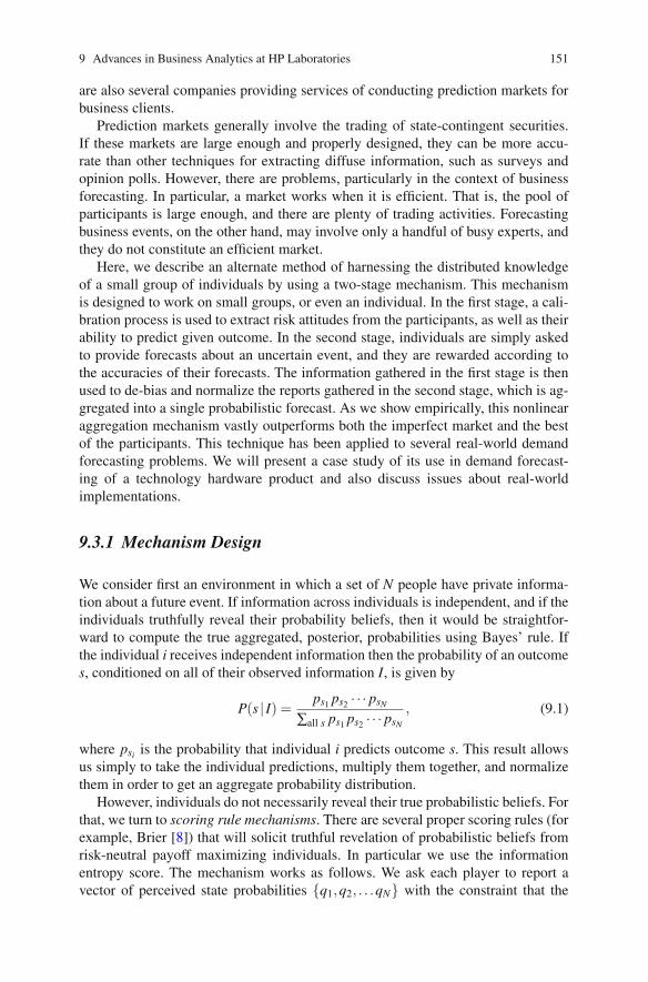
9 Advances in Business Analytics at HP Laboratories 151
are also several companies providing services of conducting prediction markets forbusiness clients.
Prediction markets generally involve the trading of state-contingent securities.If these markets are large enough and properly designed, they can be more accu-rate than other techniques for extracting diffuse information, such as surveys andopinion polls. However, there are problems, particularly in the context of businessforecasting. In particular, a market works when it is efficient. That is, the pool ofparticipants is large enough, and there are plenty of trading activities. Forecastingbusiness events, on the other hand, may involve only a handful of busy experts, andthey do not constitute an efficient market.
Here, we describe an alternate method of harnessing the distributed knowledgeof a small group of individuals by using a two-stage mechanism. This mechanismis designed to work on small groups, or even an individual. In the first stage, a cali-bration process is used to extract risk attitudes from the participants, as well as theirability to predict given outcome. In the second stage, individuals are simply askedto provide forecasts about an uncertain event, and they are rewarded according tothe accuracies of their forecasts. The information gathered in the first stage is thenused to de-bias and normalize the reports gathered in the second stage, which is ag-gregated into a single probabilistic forecast. As we show empirically, this nonlinearaggregation mechanism vastly outperforms both the imperfect market and the bestof the participants. This technique has been applied to several real-world demandforecasting problems. We will present a case study of its use in demand forecast-ing of a technology hardware product and also discuss issues about real-worldimplementations.
9.3.1 Mechanism Design
We consider first an environment in which a set of N people have private informa-tion about a future event. If information across individuals is independent, and if theindividuals truthfully reveal their probability beliefs, then it would be straightfor-ward to compute the true aggregated, posterior, probabilities using Bayes’ rule. Ifthe individual i receives independent information then the probability of an outcomes, conditioned on all of their observed information I, is given by
P(s | I) =ps1 ps2 · · · psN
∑all s ps1 ps2 · · · psN
, (9.1)
where psi is the probability that individual i predicts outcome s. This result allowsus simply to take the individual predictions, multiply them together, and normalizethem in order to get an aggregate probability distribution.
However, individuals do not necessarily reveal their true probabilistic beliefs. Forthat, we turn to scoring rule mechanisms. There are several proper scoring rules (forexample, Brier [8]) that will solicit truthful revelation of probabilistic beliefs fromrisk-neutral payoff maximizing individuals. In particular we use the informationentropy score. The mechanism works as follows. We ask each player to report avector of perceived state probabilities {q1,q2, . . .qN} with the constraint that the

152 Business Optimization Lab, HP Labs, Hewlett-Packard
vector sums to one. Then the true state x is revealed and each player paid c1 +c2 log(qx), where c1 and c2 are positive numbers. It is straightforward to verify that ifan individual believes the probability to be {p1, p2, . . . , pN} and he or she maximizesthe expected payoff, he or she will report {q1 = p1, q2 = p2, . . ., qN = pN}.
Furthermore, there is ample evidence in the literature that individuals are notrisk-neutral payoff maximizers. In most realistic situations, a risk-averse person willreport a probability distribution that is flatter than their true beliefs as they tend tospread their bets among all possible outcomes. In the extreme case of risk aver-sion, an individual will report a uniform probability distribution regardless of theirinformation. In this case, no predictive information is revealed by the report. Con-versely, a risk-loving individual will tend to report a probability distribution thatis more sharply peaked around a particular prediction, and in the extreme case ofrisk-loving behavior a subject’s optimal response will be to put all the weight onthe most probable state according to their observations. In this case, their report willcontain some, but not all the information contained in their observations.
In order to account for both the diverse levels of risk aversion and informationstrengths, we add a first stage to the mechanism. Before each individual is asked toreport their beliefs, their risk behavior is measured and captured by a single param-eter. In the original research, and subsequent experiments that validated the effec-tiveness of the mechanism, we use a market mechanism, designed to elicit their riskattitudes and other relevant behavioral information. We use the portfolio held by in-dividuals to calculate their correction factor. The formula to calculate this factor isdetermined empirically and has little theoretical basis.2
The aggregation function, after behavioral corrections, is
P(s | I) =pβ1
s1 pβ2s2 · · · pβN
sN
∑all s pβ1s1 pβ2
s2 · · · pβNsN
, (9.2)
where βi is the exponent assigned to individual i. The role of βi is to help recoverthe true posterior probabilities from individual i’s report. The value of βi for a risk-neutral individual is one, as this individual should report the true probabilities com-ing out of their information. For a risk-averse individual, βi is greater than one so asto compensate for the flatter distribution that such individuals report. The reverse,namely βi smaller than one, applies to risk-loving individuals. The technique of so-liciting this behavior adjustment parameter βi has evolved over time. In some of thelater applications, surveys were used for initial estimations and the estimates wereupdated using historical performance measures. Finally, a learning mechanism wasused to only aggregate the best performing individuals on a moving average basis.
2 In terms of both the market performance and the individual holdings and risk behavior, a simplefunctional form for βi is given by βi = r(Vi/σi)c, where r is a parameter that captures the riskattitude of the whole market and is reflected in the market prices of the assets, Vi is the utility ofindividual i, and σi is the variance of their holdings over time. We use c as a normalization factor sothat if r = 1, βi equals the number of individuals. Thus the problem lies in the actual determinationof the risk attitudes both of the market as a whole and of the individual players.
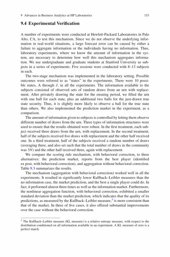
9 Advances in Business Analytics at HP Laboratories 153
9.4 Experimental Verification
A number of experiments were conducted at Hewlett-Packard Laboratories in PaloAlto, CA, to test this mechanism. Since we do not observe the underlying infor-mation in real-world situations, a large forecast error can be caused by either afailure to aggregate information or the individuals having no information. Thus,laboratory experiments, where we know the amount of information in the sys-tem, are necessary to determine how well this mechanism aggregates informa-tion. We use undergraduate and graduate students at Stanford University as sub-jects in a series of experiments. Five sessions were conducted with 8–13 subjectsin each.
The two-stage mechanism was implemented in the laboratory setting. Possibleoutcomes were referred to as “states” in the experiments. There were 10 possi-ble states, A through J, in all the experiments. The information available to thesubjects consisted of observed sets of random draws from an urn with replace-ment. After privately drawing the state for the ensuing period, we filled the urnwith one ball for each state, plus an additional two balls for the just-drawn truestate security. Thus, it is slightly more likely to observe a ball for the true statethan others. We also implemented the prediction market in the experiment, as acomparison.
The amount of information given to subjects is controlled by letting them observedifferent number of draws from the urn. Three types of information structures wereused to ensure that the results obtained were robust. In the first treatment, each sub-ject received three draws from the urn, with replacement. In the second treatment,half of the subjects received five draws with replacement and the other half receivedone. In a third treatment, half of the subjects received a random number of draws(averaging three, and also set such that the total number of draws in the communitywas 3N) and the other half received three, again with replacement.
We compare the scoring rule mechanism, with behavioral correction, to threealternatives: the prediction market, reports from the best player (identifiedex post, with behavioral correction), and aggregation without behavioral correction.Table 9.3 summarizes the results.
The mechanism (aggregation with behavioral correction) worked well in all theexperiments. It resulted in significantly lower Kullback–Leibler measures than theno information case, the market prediction, and the best a single player could do. Infact, it performed almost three times as well as the information market. Furthermore,the nonlinear aggregation function, with behavioral correction, exhibited a smallerstandard deviation than the market prediction, which indicates that the quality of itspredictions, as measured by the Kullback–Leibler measure,3 is more consistent thanthat of the market. In three of five cases, it also offered substantial improvementsover the case without the behavioral correction.
3 The Kullback–Leibler measure (KL measure) is a relative entropy measure, with respect to thedistribution conditioned on all information available in an experiment. A KL measure of zero is aperfect match.

154 Business Optimization Lab, HP Labs, Hewlett-Packard
Table 9.3 Kullback–Leibler measure (smaller = better), by experiment
No InformationPredictionMarket Best Player
AggregationWithoutBehavioralCorrection
Aggregation WithBehavioralCorrection
1.977 (0.312) 1.222 (0.650) 0.844 (0.599) 1.105 (2.331) 0.553 (1.057)1.501 (0.618) 1.112 (0.594) 1.128 (0.389) 0.207 (0.215) 0.214 (0.195)1.689 (0.576) 1.053 (1.083) 0.876 (0.646) 0.489 (0.754) 0.414 (0.404)1.635 (0.570) 1.136 (0.193) 1.074 (0.462) 0.253 (0.325) 0.413 (0.260)1.640 (0.598) 1.371 (0.661) 1.164 (0.944) 0.478 (0.568) 0.395 (0.407)
9.5 Applications and Results
This mechanism was implemented into a web application called BRAIN (Behav-iorally Robust Aggregation of Information in Networks). The process is used forforecasting tasks in several companies including a major European telecommunica-tion company and several divisions of the largest technology company in the USA.Participants enter their reports through a web site. The behavioral corrections arecarried out automatically and management can access the results directly from theweb site.
A project was started in spring 2009 to make use of this process to forecast salesof a technology product. Two business events are to be forecasted. The first is theworldwide monthly shipment units of this product. This product sells into two dif-ferent customer segments (designated A and B). The second is the percentage of theworldwide shipment going into customer segment A for a particular month.
For each event (for example, worldwide shipment in September 2009), there aresix forecasts, two in each month for the 3 months leading up to the event. Theforecasts are typically conducted in the first and third week of the month. For theSeptember 2009 shipment, the forecasting process is conducted in late June, twicein July, twice in August and in early September. Note that partial information aboutshipment of September is available when the forecasting process is conducted. Thedesign allows the forecasts to be updated if new information is available to the in-dividuals. For each event, the real line is divided into distinct intervals and eachinterval is considered a possible outcome. Individuals are asked to “bet” (report)on each of the possible interval. Twenty-five individuals from different parts of thebusiness organization, including marketing, finance, and supply chain managementfunctions, were recruited for this process. The first forecast was conducted in lateMay 2009. Participation fluctuated. In the forecasts conducted in early August 2009,16 out of the 25 recruits (64%) submitted their reports. A small budget was autho-rized as incentive to pay the participants.
The following figure shows the predictions and the actual events for July 2009.The predictions for Shipments and Customer Segment A have varied over the courseof the predictions. The ranges are the bin widths. Prediction starts with the EarlyJune forecasts, beginning about 7 weeks prior to the actual event.

9 Advances in Business Analytics at HP Laboratories 155
Fig. 9.3 Shipment forecast (units not available). Note: Rectangles: most likely interval; thick line:actual outcome
Fig. 9.4 Customer Segment A % forecast. Note: Rectangles: most likely interval; thick line: actualoutcome
As one can see, the BRAIN process has provided accurate forecast at least 1month in advance for the shipment prediction and 3 months in advance for Julyconsumer percentage. BRAIN is also more accurate in comparison to other internalbusiness forecasts. In particular, the shipment forecasts made 1 month prior for eachmonth from May through July had an absolute error of 2.5% using BRAIN vs. anabsolute error of 6.0% for the current forecasting method.
9.6 Modeling Rare Events in Marketing: Not a Rare Event
A rare event is an event with a very small probability of occurrence. Rare eventdata could be of the form where the binary dependent variable has dozens to thou-sands of times fewer ones (“events”) than zeros (“nonevents”). Typical examples

156 Business Optimization Lab, HP Labs, Hewlett-Packard
of such events from social sciences that readily come to mind are wars, outbreakof infections, breakdown of a city’s transport system, or levies. Past examples ofsuch events from marketing are in the area of database marketing (e.g., catalogs,newspaper inserts, direct mailers sent to a large population of prospective cus-tomers) where only a small fraction (less than 1%) responded resulting in a verysmall probability of a response (event) [6, 18]. The examples of rare events wherethey occur infrequently over a period of time can be thought of as longitudinal rareevents, while the examples where a small subset of the population responds can bethought of as cross-sectional rare events.
More recent examples of rare events have emerged in marketing with the adventof the Internet and digital age and the use of new types of marketing instruments.A firm can reach a large population of potential customers through its web site,display ads, e-mails, and search marketing. But only a very small proportion ofthose exposed to these instruments respond. For example, of the millions of visitorsto a firm’s web site only a handful of them click on a link or make a purchase.To make business and policy planning more effective it is important to be able toanalyze and predict these events accurately.
Rare event variables have been shown to be difficult to predict and analyze. Thereare two sources to the problem. The first source is that standard statistical proce-dures, such as logistic regression, can sharply underestimate the probability of rareevents. The intuition is that there are very few values available for the independentvariables to understand the circumstances that cause an event and these few valuesdo not fully cover the tail of the logistic regression. The model infers that there arefewer circumstances under which the event will occur resulting in an underestimate.Additionally, parametric link functions such as those used for probit or logit assumespecific shapes for the underlying link functions implying a given tail probabilityexpression that remains invariant to observed data characteristics. As a result thesemodels cannot adjust for the case when there are not enough observations to fullyspan the range needed for estimating these link functions. The second source of theproblem is that commonly used data collection strategies are grossly inefficient forrare events data. For example, the fear of collecting data with too few events leadsto data collections with huge numbers of observations but relatively few, and poorlymeasured, explanatory variables, such as in international conflict data with morethan a quarter-million dyads, only a few of which are at war [6, 16, 18].
Researchers have tried to tackle the problem of using logistic regression (orprobit) to analyze rare events data in three ways [6]. First approach is to adjustthe coefficients and predictions of the estimated logistic regression model. King andZeng [18] describe how to adjust the maximum likelihood estimates of the logisticregression parameters to calculate approximately unbiased coefficients and predic-tions. Second approach is to use choice-based sampling where the sample is con-structed based on the value of the dependent variable. This can cause biased results(sample selection bias) and corrections must be undertaken. Manski and Lerman[21] developed the weighted exogenous maximum likelihood (WESML) estimatorfor dealing with the bias. Third approach is to relax the logit or probit parametriclink assumptions which can be too restrictive for rare events data. Naik and Tsai

9 Advances in Business Analytics at HP Laboratories 157
[24] developed an isotonic single-index model and developed an efficient algorithmfor its estimation.
In this study we apply the second approach of choice-based sampling to discrete-choice models and decision-tree algorithms to estimate the response probabilitiesat the customer level to a direct mail campaign when the campaign sizes are verylarge (in millions) and the response rates are extremely low. We use the predictedresponse probabilities to rank the customers which will allow the business to runtargeted campaigns, identify best and at-risk customers, reduce their cost of runningthe campaign, and increase response rate.
9.6.1 Methodology
9.6.1.1 Choice-Based Sampling
In a discrete-choice modeling framework sometimes one outcome can strongly out-number the other such as when many households do not respond (e.g., to a di-rect mailing). Alternative sampling designs have been proposed. A case–controlor choice-based sample design is one in which the sampling is stratified on thevalues of the response variable itself and disproportionately more observations aresampled from the smaller group. This ensures that the variation in the dependentvariable is maximized with subsequent statistical analysis accounting for this sam-pling strategy to ensure the estimates are asymptotically unbiased and efficient[10, 21, 22].
In the biostatistical literature, case–control studies were prompted by studies inepidemiology on the effect of exposure to possible hazards such as smoking on therisks of contracting a disease condition. In a prospective study design, a sample ofindividuals is followed and their responses recorded. However, many disease condi-tions are rare and even large studies may produce few diseased individuals (cases)and little information about the hazard. In a case–control study separate samples aretaken of cases and controls—individuals without the disease [27].
In the economics literature, estimation of models to understand choices for travelmodes or recreation sites has used different sampling designs to collect data onconsumer choices. For example, studies of participation levels and destinations foreconomic activities such as recreation have traditionally been analyzed using ran-dom samples of households, with either cross-section observations or panel data onrepeat choices obtained from diaries. In travel demand analysis, an alternative sam-pling design is to conduct intercept surveys at sites. This can result in substantialreductions in survey costs and guarantee adequate sample sizes for sites of interest,but the statistical analysis must take into account the “choice-based” sample frame[23].
There is a well-developed theory for this analysis in the case of cross-sectionobservations, where data are collected only on the intercept trip. In site choice mod-els when subjects are intercepted at various sites, a relevant statistical analysis is

158 Business Optimization Lab, HP Labs, Hewlett-Packard
the theory of estimation from choice-based samples due to Manski and Lerman[21] and Manski and McFadden [22]. This theory was developed for situationswhere the behavior of a subject was observed only on the intercept choice occa-sion and provided convenient estimators when all sites were sampled at a positiverate. One of these estimators, called weighted exogenous sample maximum likeli-hood (WESML), reweights the observations so that the weighted sample choicefrequencies coincide with population frequencies. A second, called conditionalmaximum likelihood (CML), weights the likelihood function so that the weightedsample choice probabilities average to the sample choice frequencies. The WESMLsetup carries out maximum pseudolikelihood estimation with a weighted log like-lihood function where in conventional choice-based sampling the weights are thesampling rates for the alternatives, given by the sample frequency divided by thepopulation frequency for each alternative. The CML setup carries out maximumconditional likelihood estimation with a log likelihood function.
However, recently sampling schemes have emerged in the literature on recre-ational site choice that combine interception at sites with diaries that provide paneldata on intercept respondents on subsequent choice occasions. McFadden’s [23]paper provides a statistical theory for these “Intercept and Follow” surveys, and in-dicates where analysis based on random sampling or simple choice-based samplingrequires correction.
9.6.1.2 Modeling Approach
We developed a discrete-choice (logit) model and a classification-tree algorithm(aucCART) for predicting a user’s probability of responding to an e-mail. Thediscrete-choice model is statistical based while the classification-tree algorithm ismachine-learning oriented. Both response modeling methods use as input dozensof columns (or attributes) from the data sample and identify the most important(relevant) columns that are predictive of the response. By employing different typesof response models for predicting the same response behavior, we were able tocross-check the models and discover predictors and attribute transformations thatwould be overlooked and missed in a single model. We then performed hold-out (or out-of-sample) tests on the accuracy of both methods and select the bestmodel.
The output of each model consists of the probability that each customer will re-spond to a campaign and the strength of each attribute that influences this probabil-ity. We extracted about 80 explanatory attributes from the transaction and campaigndatabases. These may be broadly classified as (1) customer static (nontime-varying)attributes such as gender and acquisition code; (2) customer dynamic attributes justprior to the campaign, which include the recency, frequency, and monetary (RFM)attributes for customer actions, responses to previous campaigns, etc.; and (3) cam-paign attributes such as the campaign format and the offer type (e.g., fixed price andpercentage discounts, free shipping, and freebies).
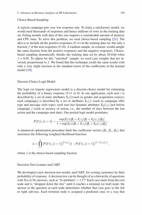
9 Advances in Business Analytics at HP Laboratories 159
Choice-Based Sampling
A typical campaign gets very low response rate. To learn a satisfactory model, wewould need thousands of responses and hence millions of rows in the training dataset. Fitting models with data of this size requires a considerable amount of memoryand CPU time. To solve this problem, we used choice-based sampling [21]. Theidea is to include all the positive responses (Y =1) in the training data set, but only afraction f of the non-responses (Y =0). A random sample, in contrast, would samplethe same fraction from the positive responses and the negative responses. Choice-based sampling dramatically shrinks the training data set by about 20-fold whenf = 0.05. To adjust for this “enriched” sample, we used case weights that are in-versely proportional to f . We found that this technique yields the same results withonly a very slight increase in the standard errors of the coefficients in the learnedmodel [10].
Discrete-Choice Logit Model
The logit (or logistic regression) model is a discrete-choice model for estimatingthe probability of a binary response (Y =1 or 0). In our application, each user i isdescribed by a set of static attributes Xs(i)(such as gender and acquisition source);each campaign j is described by a set of attributes Xc( j) (such as campaign offertype and message style type); each user has dynamic attributes Xd(i, j) just beforecampaign j (such as recency of action, i.e., the number of days between the lastaction and the campaign start date). Our pooled logit model postulates
P{Y (i, j) = 1}=exp[Xs(i)βs +Xc( j)βc +Xd(i, j)βd ]
1+ exp[Xs(i)βs +Xc( j)βc +Xd(i, j)βd ].
A numerical optimization procedure finds the coefficient vectors (β s, β c, β d) thatmaximize the following weighted likelihood function:
L =N
∏i=1
[P{Y (i, j) = 1}]Y (i, j) [1−P{Y (i, j) = 1}][1−Y (i, j)]/ f ,
where f is the choice-based sampling fraction.
Decision-Tree Learner aucCART
We developed a new decision-tree model, aucCART, for scoring customers by theirprobability of response. A decision tree can be thought of as a hierarchy of questionswith Yes or No answers, such as “Is attribute1 > 1.5?” Each case starts from the rootnode and is “dropped down the tree” until it reaches a terminal (or leaf) node; theanswer to the question at each node determines whether that case goes to the leftor right sub-tree. Each terminal node is assigned a predicted class in a way that

160 Business Optimization Lab, HP Labs, Hewlett-Packard
minimizes the misclassification cost (penalty). The task of a decision-tree model isto fit a decision tree to training data, i.e., to determine the set of suitable questionsor splits.
Like traditional tree models such as CART (Classification and Regression Trees)[7], aucCART is a non-parametric, algorithmic model with built-in variable selec-tion and cross-validation. However, traditional classification trees have somedeficiencies for scoring:
They are designed to minimize the misclassification risk and typically do not per-form well in scoring. This is because there is a global misclassification cost function,which makes it undesirable to split a node whose class distribution is relatively faraway from that of the whole population, even though there may be sufficient in-formation to distinguish between the high- and low-scoring cases in that node. Forexample, assume that the two classes, say 0 and 1, occur in equal proportions in thetraining data and the costs of misclassifying 0 as 1 and 1 as 0 are equal. Supposethat, while fitting the tree, one finds a node with 80% 1s (and 20% 0s) which canbe split into two equally sized children nodes, one with 90% 1s and the other with70% 1s. All these nodes have a majority of 1s and will be assigned a predicted classof 1; any reasonable decision tree will not proceed with this split since it does notimprove the misclassification rate. However, when scoring is the objective, this splitis potentially attractive since it separates the cases at that node into a high-scoringgroup (90% 1s) and a lower-scoring group (70% 1s).
A related problem is the need to specify a global misclassification cost. This isnot a meaningful input when the objective is to score cases.
The aucCART method is based on CART and is designed to avoid these prob-lems. It combines a new tree-growing method that uses a local loss function togrow deeper trees and a new tree-pruning method that uses the penalized AUC riskRα(T ) = R(T ) + α|T |. Here, the AUC risk R(T ) is the probability that a randomlyselected response scores lower than a randomly selected non-response, |T | is thesize of the tree, and α is the regularization parameter, which is selected by cross-validation. This method is (even) more computationally intensive than CART, inpart because it runs CART repeatedly on subsets of the data and in part becauseminimizing the penalized AUC risk requires an exhaustive search over a very largeset of sub-trees; in practice, we avoid the exhaustive search by limiting the searchdepth. Our numerical experiments on specific data sets have shown that aucCARTperforms better than CART for scoring.
9.6.2 Empirical Application and Results
9.6.2.1 Background
Customers continue to use e-mails as one of their main channels for communicatingand interacting online. According to Forrester Research (2007) 94% of online cus-tomers in the USA use e-mails at least once a month. Customers also ranked opt-in

9 Advances in Business Analytics at HP Laboratories 161
e-mails among their top five sources of advertisements they trust for product infor-mation (Forrester Research 2009). E-mail marketing has become an important partof any online marketing program. In fact, according to the 2007 Forrester Researchreport, 60% of marketers said that they believe marketing effectiveness of e-mail asa channel of communication will increase in the next 3 years.
An HP online service with millions of users uses e-mail marketing as one oftheir marketing vehicles for reaching out to its customers with new product an-nouncements and offers. In general, each e-mail campaign is sent to all users andon a regular basis with millions of customers contacted during any specific cam-paign. One drawback of this “spray-and-pray” approach is the increased risk ofbeing blacklisted by Internet Service Providers (ISPs) when they receive too manycomplaints. In addition to direct loss of revenue when an e-mail program is stoppedearly, it increases the risks of using e-mail as a regular channel for communicationin the future. So the marketing team was interested in methods that would help themto identify who their best customers and “at-risk” customers were and understandwhat key factors are that drive customer response. This would enable them to sendmore targeted e-mail campaigns with relevant messages and offers.
9.6.2.2 Data Set and Variables
We selected a subset of past e-mail campaigns from the marketing campaignsdatabase that were representative of (and similar to) the planned future campaigns.We, then, selected a subset of customers from the sent list of these past campaigns.Each campaign had a date–time and a number of attributes associated with it. Thecampaign date allowed us to “go back in time” and derive the user’s behavioral at-tributes just before each of the past campaigns. We, a priori, split the customers intotwo customer segments based on whether they did a specific action in the past (inline with the business practice). Table 9.4 gives some descriptive statistics of thetwo samples.
The outcome variable, response to a campaign, indicates whether or not (1 or 0)the user responded to each of the selected campaigns. For each campaign we usedthe campaign database to create the campaign-specific attributes. Some examples ofthese attributes are the e-mail message’s subject line, the format of the e-mail, thevalue offered in the e-mail (percentage discounts, dollar amount of free products, the
Table 9.4 Descriptive statistics of the data samples
CustomerSegment
Number ofCampaigns
Number ofObservations(Customercampaign)
Number ofObservationsChoice-basedSample
Number ofCustomersChoice-basedSample
Action-Active 32 4.2 X 0.21 X 0.16 XAction-Inactive 25 7.8 X 0. 39 X 0.33 X
Note: We depict the sample sizes as multiples of X to anonymize the data

162 Business Optimization Lab, HP Labs, Hewlett-Packard
type of product featured), the time-of-the-year occasion of the e-mail timing (suchas Christmas shopping season).
For each customer we used the full history of their transactions since registration,available in the transaction database, to create customer-specific attributes just priorto the beginning of each campaign. These attributes included recency (how manydays prior to the campaign did the user take an action), frequency (how many timesin the month, quarter, or year prior to the campaign did the user undertake an action),and monetary (how much in dollars did the user spend in the month, quarter, or yearprior to the campaign and in which product categories). In addition, we used datasources like the US Census Bureau and other sources of first names and gender tocreate a first-name-to-gender translator which predicted the probability of a personbeing male or female given the person’s first name.
We tried all reasonable transformations of the attributes and selected the onesthat yielded the best model. We determined the best transformation by investigat-ing the residual plots for the logit model. Furthermore, the output produced fromour classification tree-based aucCART algorithm (which automatically transformssome attributes) also gave us some suggestions for the most appropriate transfor-mations. In the logit model, we selected the final set of attributes by using bothforward and backward step-wise selection. In forward selection, we started with asingle predictor variable (attribute) and added variables (with appropriate variabletransformations) one by one, until no statistically significant variable can be added,or AIC (Akaike Information Criterion) value can be improved. In backward selec-tion, we started with all attributes (properly transformed) included in the model anddelete statistically insignificant variables one at a time, until all remaining variablesare statistically significant. For the classification tree-based aucCART algorithm,variable selection was automatically performed (a built-in feature of classificationtree-based algorithms).
The final data sample had several hundred thousands of data rows (each rowrepresents a user) and approximately 80 columns (each column is an attribute de-scribing the user at various points of time). We randomly selected 50% of the rowsin the data sample as training data and the rest as testing data to evaluate the twoapproaches and select the best one.
9.6.2.3 Validation, Model Selection, and Results
We validated our models on holdout data sets with different customers and cam-paigns than the training data. Our holdout tests were designed to simulate anin-the-field application of our models to existing and new customers and newcampaigns.
In addition to the two approaches outlined, various heuristics or scoring ruleshave been commonly used by marketing professionals to predict responses andselecting target recipients. One such heuristic for selecting recipients is by actionrecency, which ranks recipients by the most recent to least recent in their last action;
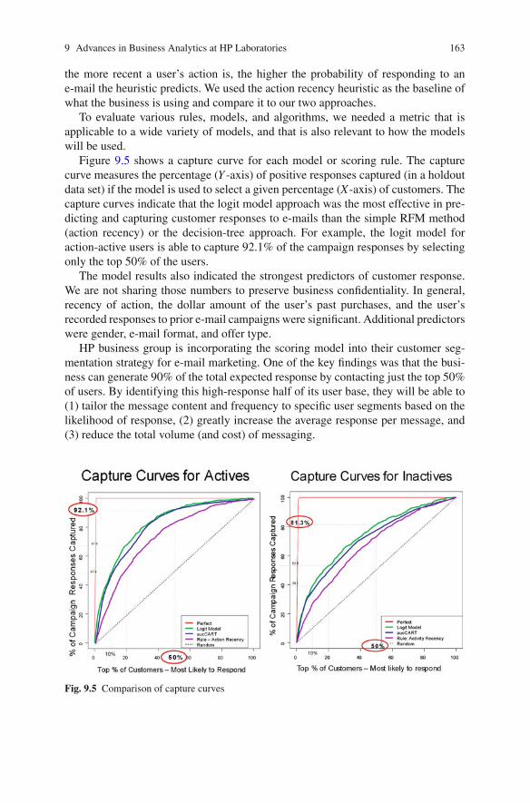
9 Advances in Business Analytics at HP Laboratories 163
the more recent a user’s action is, the higher the probability of responding to ane-mail the heuristic predicts. We used the action recency heuristic as the baseline ofwhat the business is using and compare it to our two approaches.
To evaluate various rules, models, and algorithms, we needed a metric that isapplicable to a wide variety of models, and that is also relevant to how the modelswill be used.
Figure 9.5 shows a capture curve for each model or scoring rule. The capturecurve measures the percentage (Y -axis) of positive responses captured (in a holdoutdata set) if the model is used to select a given percentage (X-axis) of customers. Thecapture curves indicate that the logit model approach was the most effective in pre-dicting and capturing customer responses to e-mails than the simple RFM method(action recency) or the decision-tree approach. For example, the logit model foraction-active users is able to capture 92.1% of the campaign responses by selectingonly the top 50% of the users.
The model results also indicated the strongest predictors of customer response.We are not sharing those numbers to preserve business confidentiality. In general,recency of action, the dollar amount of the user’s past purchases, and the user’srecorded responses to prior e-mail campaigns were significant. Additional predictorswere gender, e-mail format, and offer type.
HP business group is incorporating the scoring model into their customer seg-mentation strategy for e-mail marketing. One of the key findings was that the busi-ness can generate 90% of the total expected response by contacting just the top 50%of users. By identifying this high-response half of its user base, they will be able to(1) tailor the message content and frequency to specific user segments based on thelikelihood of response, (2) greatly increase the average response per message, and(3) reduce the total volume (and cost) of messaging.
Fig. 9.5 Comparison of capture curves

164 Business Optimization Lab, HP Labs, Hewlett-Packard
In future studies we want to see if our conclusions hold for direct mail. Furtherwe want to examine if the customers with low ranks based on the model are also theones most likely to unsubscribe, complain, and create negative word-of-mouth.
9.7 Distribution Network Design
Hewlett-Packard provides a wide range of products and services for a diverse setof customers located across the globe leveraging a worldwide network of suppliers,partners, and facilities. As the operator of the largest supply chain in the IT industryHP relies on analytical modeling to support many strategic and operational deci-sions with detailed optimization models enabling evaluation of alternative supplychain strategies—procurement, location, inventory—to investigate opportunities todecrease supply chain-related costs and improve order cycle times. HP has a longtradition of employing operations research for its supply chain problems [20]. Somerecent examples include reverse supply chain redesign for Personal Systems Group(PSG) in Europe [14], network design for Imaging and Printing Group (IPG) in Eu-rope [19], production line design for IPG in the USA [9], and inventory managementfor former network server division [5].
In this section we describe a mathematical programming model that constitutesthe core of a number of analytical decision support applications for decision prob-lems ranging from design of manufacturing and distribution networks to evaluationof complex supplier offers in logistics procurement processes. We provide somedetails on two applications of the model to evaluate various distribution strategyalternatives—to answer questions such as whether it is efficient to add more distri-bution centers to the existing network and which distribution centers and transportmodes are to be used to supply each customer location and segment—by quantifyingthe trade-off between the supply chain costs and order cycle times.
9.7.1 Outbound Network Design
HP provides personal computers, workstations, handheld computing devices, dig-ital entertainment systems, calculators and other related accessories, software andservices for commercial and consumer markets. The customers in the commercialsegment include direct customers such as big corporations, small and medium sizebusinesses (SMB), government agencies and indirect channel partners. Supply chainconfigurations vary by product as well as by customer segments. HP utilizes a num-ber of contract manufacturers (CMs) and original design manufacturers (ODMs) tomanufacture certain HP-designed products to generate cost efficiencies and reducetime to market. There are three types of nodes in a typical supply chain: inboundhubs, manufacturing sites, and outbound hubs. The inbound hubs store componentsand are usually situated close to the manufacturing sites. The inventory at these

9 Advances in Business Analytics at HP Laboratories 165
locations is owned by the suppliers and is pulled by the manufacturing sites per cus-tomer order. For some critical parts, the inventory may also be owned by HP. Oncethe products are manufactured, they are shipped to outbound hubs (or distributioncenters) for further shipment to customer locations. Certain products may also beshipped directly to customers from the manufacturing sites.
The outbound hubs play a number of critical roles in a typical supply chain.First, outbound hubs are used to consolidate shipments from manufacturing sites tocustomer locations for a portion of the trip. Finished goods are first shipped to anoutbound hub in a bulk mode. Individual customer shipments are then scheduled fora shorter distance. Thus outbound hubs are used to leverage from volume of ship-ments for a particular region. Second, outbound hubs are used to merge shipmentsfrom different manufacturing sites into a single shipment to customer locations.Finally, outbound hubs are used to carry finished goods inventory for certain cus-tomers with short order cycle time requirements and for certain stable SKUs (e.g.,certain standard configurations).
Given the existing and potential outbound hubs, the model is used to seek an-swers to the following questions: Which of the existing and potential outbound hubsshould HP use in its operations? Which customer locations and segments should beassigned to each outbound hub? Which product groups should be assigned to eachoutbound hub? What should be the mode of transportation in meeting customer de-mands for each customer location and segment?
The answers to these questions hinge on various aspects of the fundamental trade-offs between customer service levels and supply chain-related costs. The former ismeasured by Order to Delivery Time (ODT), the time between customer order andorder delivery to customer. The latter, supply chain costs, fall in four broad cate-gories: First, Inventory-Driven Costs (IDC) include all of the costs that derive fromthe level of inventory in the regions, such as obsolescence and component devalua-tions. Second, Trading Expenses (TE) include freight, duties, taxes, allocations, andwarehousing. Third, Manufacturing Expenses (MOH) include the cost of manufac-turing products, as well as any costs related to the support of that manufacturingactivity including customization and rework. Finally, Cash to Cash (C2C) takes intoaccount how long inventory is held in the region and how long it takes to pay thesuppliers and to receive payment from customers.
ODT is an important metric for a product division’s supply chain. Service levelagreements with customers usually involve explicit ODT requirements. ODT iscomposed of several components such as order entry time, material wait time, fac-tory cycle time, and delivery time. Of these components, material wait time and thedelivery time are likely to get impacted by the supply chain configuration. Further-more, for a given supply chain configuration, the three components of ODT—orderentry, factory cycle time, and the delivery time—are not likely to change from oneorder to another (for the same customer location and product group), while the mate-rial wait time can be considerably variable depending on the immediate availabilityof the components at the designated inbound hub. Also note that from the abovefour components, delivery time is the only component that will be impacted bythe outbound strategy. Different customer groups—corporate, small and medium

166 Business Optimization Lab, HP Labs, Hewlett-Packard
businesses, public sector, indirect channel partners—may have distinct ODT re-quirements. Any outbound strategy should ensure that the ODT requirements aresatisfied for each customer segment.
Trading expenses and inventory-driven costs are likely to be impacted most bythe outbound strategy. Major components of Trading Expenses are transportationcosts from manufacturing sites into the outbound hubs and from outbound hubs tothe customer locations, material handling costs, and facility costs. Main elements ofInventory-Driven Costs are costs due to inventory in transit from manufacturing sitesto the outbound hubs, and from outbound hubs to customer locations, and inventoryin the outbound hubs.
The decision problem is to minimize trading expenses and inventory-driven costswhile satisfying order to delivery time targets set by management. Various businessconstraints such as limiting the total number of outbound hubs that will be used,forcing a particular outbound hub to stay open or closed will also need to be incor-porated as constraints in the model.
Products can be modeled at the SKU level or at the product category level af-ter aggregation. Customer segments are modeled separately as shipment volumesand ODT requirements vary by segment. For customer locations various levels ofaggregation—by state, zip code, etc.—are possible. HP works with many differenttransportation service providers including parcel carriers, airfreight companies, less-than-truckload (LTL) and full truckload (FTL) carriers. Transportation mode can bemodeled using the physical mode of transportation (type of vehicle or type of com-pany) or using delivery times to code transportation modes—e.g., 1-day service,2-day service, 3-day service.
In order to capture the variability in ODT targets, two modes of delivery aredefined. For a fraction θ r
js of orders originating from customer segment s for productj, the order needs to be shipped from the factory with regular delivery within wr
js.Likewise, for a fraction θ e
js = 1−θ rjs of orders originating from customer segment
s for product j, the order needs to be shipped from the factory with emergencydelivery within we
js.
9.7.2 A Formal Model
We next introduce the notation needed for a formal presentation of the mathematicalmodel. Let M denote the set of manufacturing sites, I denote the set of potentialoutbound hub sites, K denote the set of customer locations, S denote the set ofcustomer segments, J denote the set of product groups, and T denote the set oftransportation modes available.
The following variables define the parameters of the model:
dks j : demand in location k for customer segment s for product jcmitks j : cost to satisfy demand in location k for customer segment s for product j
by manufacturing in site m through outbound hub i with transport mode t

9 Advances in Business Analytics at HP Laboratories 167
�mitks j : delivery time to satisfy demand in location k for customer segment s forproduct j by manufacturing in site m through outbound hub i with transportmode t
fi : fixed operating cost of outbound hub site iCi : capacity of outbound hub site i
wrjs : time window specified for product j for customer segment s for regular
deliverywe
js : time window specified for product j for customer segment s for emergencydelivery
θ rjs : fraction of orders in segment s for product j requiring regular delivery
θ ejs : fraction of orders in segment s for product j requiring emergency delivery
We also define the following variables to be used in the mathematical program:
δ rmitks j =
{1 if �mitks j ≤ wr
s j0 otherwise
δ emitks j =
{1 if �mitks j ≤ we
s j0 otherwise
The following parameters are used to enforce a specific scenario for the networkdesign:
αi ={
1 if outbound hub i needs to be open in a scenario0 otherwise
βi ={
1 if outbound hub i needs to be closed in a scenario0 otherwise
γi ={
1 if outbound hub i’s capacity needs to be enforced in a scenario0 otherwise
The following variables are the decision variables of the problem:
xrmitks j =
⎧⎪⎪⎨
⎪⎪⎩
1 if segment s’s regular demand in location k for product j issatisfied by manufacturing site m through outbound hub iwith mode t
0 otherwise
xemitks j =
⎧⎪⎪⎨
⎪⎪⎩
1 if segment s’s emergency demand in location k for product j issatisfied by manufacturing site m through outbound hub iwith mode t
0 otherwise
yi ={
1 if outbound site i is used0 otherwise
With the notation introduced the mathematical program is written as
min ∑m∈M
∑i∈I
∑t∈T
∑k∈K
∑s∈S
∑j∈J
dks jcmitks j[θ rs jx
rmitks j+θ e
s jxemitks j]+∑
i∈Ifiyi, (9.3)

168 Business Optimization Lab, HP Labs, Hewlett-Packard
∑m∈M
∑i∈I
∑t∈T
δ rmitks jx
rmitks j = 1 for all k ∈ K,s ∈ S, j ∈ J, (9.4)
∑m∈M
∑i∈I
∑t∈T
δ emitks jx
emitks j = 1 for all k ∈ K,s ∈ S, j ∈ J, (9.5)
xrmitks j− yi ≤ 0 for all m ∈M, i ∈ I, t ∈ T,k ∈ K,s ∈ S, j ∈ J, (9.6)
xemitks j− yi ≤ 0 for all m ∈M, i ∈ I, t ∈ T,k ∈ K,s ∈ S, j ∈ J, (9.7)
yi ≥ αi for all i ∈ I, (9.8)
yi ≤ (1−βi) for all i ∈ I, (9.9)
γi
(
∑m∈M
∑t∈T
∑k∈K
∑s∈S
∑j∈J
dks j[θ rs jx
rmitks j +θ e
s jxemitks j]
)≤Ci for all i ∈ I, (9.10)
xrmitks j ∈ {0,1} for all m ∈M, i ∈ I, t ∈ T,k ∈ K,s ∈ S, j ∈ J, (9.11)
xemitks j ∈ {0,1} for all m ∈M, i ∈ I, t ∈ T,k ∈ K,s ∈ S, j ∈ J, (9.12)
yi ∈ {0,1} for all i ∈ I. (9.13)
The objective in (9.3) minimizes all incoming and outgoing transportation costs, ma-terial handling, inventory, and the facility costs. The constraints in (9.4) and (9.5)ensure that each customer segment in each location is assigned to one outboundsite, manufacturing site, and one transportation mode for each product group thatare within delivery time requirements for regular and emergency demands, respec-tively. Note that the product groups from a single customer location and segmentcan be assigned to different manufacturing sites, outbound hubs, and transportationmodes. The constraints in (9.6) and (9.7) ensure that service from an outboundhub is available only if the facility is open. The constraints in (9.8) and (9.9) en-sure that the outbound hubs are forced to be open or closed based on the scenariospecification.
The constraints in (9.10) ensure that the capacity of the outbound hub is enforcedif specified in the scenario. The constraints in (9.11), (9.12), and (9.13) ensure thatall decision variables are binary. Note that the formulation in (9.3)–(9.13) assumesthat the model is full, e.g., every customer location has demand from all |S| segmentsand for all |J| product groups. This is only to make the exposition simple. The actualmodel used in implementation takes advantage of the link sparsity.
9.7.3 Implementation
The model in the previous section was implemented using ILOG’s OPL Studio andsolved using CPLEX. The raw data are stored in several tables in a database and canbe imported from a spreadsheet or a flat file. A typical implementation may involveup to 1,000 customer locations (actual customer locations aggregated at the 3 digitzip code), 5–10 customer segments, 5–10 transport modes, up to 10 product groups,and up to 100 potential outbound hub sites. Standardized forms are used to allowthe user to specify the parameters for what–if scenarios in order to see the impact

9 Advances in Business Analytics at HP Laboratories 169
of several critical variables. Through various forms the user can change the deliv-ery time targets, enforce a particular outbound hub to stay open or closed, activateor deactivate the capacity constraint on a particular hub, and limit the number ofoutbound hubs. The user sees the results of the model via several reports. LocationSummary report shows which outbound hubs are open and what costs are incurredin doing so. Location Usage report shows the total number of units in each productcategory that flows through each outbound hub. Delivery Performance report showsthe resulting average delivery times for each customer segment and product group.Location Customer Assignment report shows the detailed assignment of customerlocations/customer segments to manufacturing sites/outbound hubs/transportationmodes.
9.7.4 Regarding Data
The data requirements can be categorized into four groups: logistics, financial, de-mand, and customer service requirements. Some critical data elements need to beestimated from various data sources. Transportation costs and times between manu-facturing sites and outbound hubs are estimated assuming that a bulk mode is usedand scale economies are fully utilized, considering the typically large volume ofshipments. Based on the manufacturing scenario, the shipments can be originatingfrom various locations worldwide. Depending on the origin, the shipments may bemade over the ocean by major carriers or by FTL carriers. Cost and time estimatesare created using data on rate tables and maps from major carriers. Estimation oftransportation costs and times between outbound hubs and customer locations isbased on data on shipment histories and representative carrier cost and time informa-tion for various weight categories. Annual demands at the product group, customersegment, and customer locations were estimated from data on shipment history. Inaddition to these three items, data such as material handling and facility setup costsfor outbound hubs, unit manufacturing costs (estimates) at different manufacturingsites, inventory holding cost rates and customer service level requirements are ob-tained from various sources in finance, logistics, and procurement operations.
9.7.5 Exemplary Analyses
The outbound model proved to be very useful for internal consulting teams for eval-uating alternative distribution strategies for various product groups. The outboundmodel was also used as a primary input to the assessment of end-to-end manufac-turing scenarios for a product group.
The model described above provides the core for analysis of a number of broadersupply chain strategy decisions including the selection for manufacturing sites.The analysis for the outbound strategy clearly depends on the locations of the

170 Business Optimization Lab, HP Labs, Hewlett-Packard
manufacturing facilities. For this purpose, viable scenarios included the baselinescenario describing the manufacturing locations at the time of implementation.These manufacturing scenarios specify manufacturing location(s) for each productcategory.
For each manufacturing scenario, various analyses can be carried out. The firstcategory of analysis takes the current level of OTD targets as input and developsan outbound strategy for each manufacturing scenario. The analysis in this categorywas used to determine the optimal outbound hub locations and to assess the valueof additional outbound hubs for each manufacturing scenario. The analysis provedvery useful in understanding the marginal value of each additional outbound hub.An example of this analysis (with fictitious data) is provided in Figure 9.6.
Fig. 9.6 Impact of number of hubs
In the example, we consider a manufacturing scenario with a single manufac-turing location co-located with one of the outbound hubs. Since each additionalhub provides the flexibility to consolidate a portion of the trip for shipments tocustomer locations, the total costs decline. However, as expected, there aredecreasing marginal returns. Understanding the exact value of each additional out-bound hub, together with an evaluation of operational complexity, provides valu-able guidance for the management decisions on the number and locations of eachoutbound hub. In Figure 9.6, we also show the percentage of products shipped di-rectly from the outbound hub co-located with the single manufacturing site for twoproduct groups: bulky products (product group 1) and small/light products (prod-uct group 2). Clearly, shipment consolidation is more beneficial for bulkier items(product group 1), and we see that more of this group of products are shippedvia additional hubs than the second group. The analysis is also useful in esti-mating the transportation cost component of different manufacturing scenarios.In addition to the strategic insights, the analysis can also be used to support de-tailed operational decisions such as which manufacturing sites, outbound hubs, and

9 Advances in Business Analytics at HP Laboratories 171
Fig. 9.7 Impact of delivery time targets
transportation modes should be used to deliver orders of a particular region and acustomer segment.
The model can also be used to study the trade-off between the supply chain costsand OTD targets. Naturally, this trade-off varies with manufacturing scenarios. InFigure 9.7 we present an example of such analysis (with fictitious, but representa-tive data). In this example, we consider three manufacturing scenarios. In the firstscenario, the products can be manufactured in an offshore location as well as locallyin the USA. Modifying the per unit costs cmitks j in the mathematical model to in-clude manufacturing costs, the model is used to select a manufacturing site amongthe set of possible sites for satisfying demand in a particular customer location. Inthe second scenario, all manufacturing is done at an overseas site. Finally in thethird scenario, all manufacturing is done locally in the USA. Each manufacturingscenario is combined with various target delivery time levels starting from a casewhere there is no time constraint on shipping a customer order.
The analysis reveals that, for all three manufacturing scenarios, the total costsincrease as the delivery time targets are more aggressive. The mixed scenario out-performs the other two scenarios for all target levels, since it has the flexibility ofemploying offshore as well as local manufacturing. For this scenario, as the de-livery time targets get more aggressive, more manufacturing is moved to domesticsites. Note also that while the total cost for the offshore-only scenario is quite sen-sitive to the delivery time targets, the total cost for the US-only scenario is ratherinsensitive.

172 Business Optimization Lab, HP Labs, Hewlett-Packard
9.8 Collaborations and Conclusion
For development and deployment of decision sciences solutions, the HP Labs teamworks very closely with business units. In addition, in most cases HP’s InformationTechnology (HP IT) group has a significant role in the success of the projects. TheHP Labs team takes the ownership of development of underlying algorithms andcore algorithmic software engine. HP IT is generally responsible for integration ofthe core analytical engine with back-end IT systems, database design and develop-ment, system architecture, deployment, and support of the complete system.
Over the years, HP Labs’ Business Optimization Lab has built strong researchcollaborations with leading faculty members in several areas of interests to HP andthe academic community. The university collaboration for the work presented in thischapter is reflected in the author list.
This chapter covers a very narrow slice of advanced analytics project at HP Labsand at HP. It is safe to say that the creation and application of rigorous mathemat-ical models is well established throughout the company. Applied researchers andpractitioners are making contributions that directly impact the top and bottom line.
Acknowledgments
In this chapter, we have summarized the work of several members of the HP Labsand business units of HP. In particular, we are very thankful to Kemal Guler fororganizing the content of distribution network design portion of this chapter.
References
1. Ahuja RK, Orlin RB, Stein C, Tarjan RE (1994) Improved algorithms for bipartite networkflow. SIAM Journal of Computing 23:903–933
2. Ansari A, Mela CF (2003) E-customization. Journal of Marketing Research XL:131–1453. Babenko M, Derryberry J, Goldberg A, Tarjan R, Zhou Y (2007) Experimental evaluation of
parametric max-flow algorithms. Proceedings of WEA. Lecture Notes in Computer Science4525. Springer, Berlin–Heidelberg, Germany, pp. 612–623
4. Balinski ML (1970) On a selection problem. Management Science 17(3):230–2315. Beyer D, Ward J (2002) Network server supply chain at HP: A case study. In: Song J, Yao
D (eds) Supply chain structures: Coordination, information and optimization. InternationalSeries in Operations Research and Management Science, Kluwer, Norwell, MA
6. Blattberg RC, Kim P, Neslin S (2008) Database marketing: Analyzing and managing cus-tomers. Springer, New York
7. Breiman L, Friedman J, Olshen R, Stone C (1984) Classification and regression trees. Chap-man and Hall, New York
8. Brier, GW (1950) Verification of forecasts expressed in terms of probability. Mon. Wea. Rev.,78:1–3
9. Burman M, Gershwin SB, Suyematsu C (1998) Hewlett-Packard uses operations research toimprove the design of a printer production line. Interfaces 28:24–36

9 Advances in Business Analytics at HP Laboratories 173
10. Donkers B, Franses PH, Verhoef PC (2003) Selective sampling for binary choice models.Journal of Marketing Research XL:492–497
11. Ford LR, Fulkerson DR (1956) Maximum flow through a network. Canadian Journal of Math-ematics 8:339–404
12. Gallo G, Grigoriadis MD, Tarjan RE (1989) A fast parametric maximum flow algorithm andapplications. SIAM Journal of Computing 18:30–55
13. Goldberg AV, Tarjan RE (1986) A new approach to the maximum flow problem. Proceed-ings of the 18th Annual ACM Sympos Theory Computation (Berkeley, CA), May 28–30,pp. 136–146
14. Guide Jr VDR, Mulydermans L, Van Wassenhove LN (2005) Hewlett-Packard company un-locks the value potential from time-sensitive returns. Interfaces 35:281–293
15. Jain S (2008) Decision sciences—A story of excellence at Hewlett-Packard. OR/MS Today,April
16. Kamakura WA, Mela CF, Ansari A, Bodapati A, Fader P, Iyengar R, Naik P, Neslin S, Sun B,Verhoef P, Wedel M, Wilcox R (2005) Choice models and customer relationship management.Marketing Letters 16(3/4):279–291
17. Kamakura WA, Russell GJ (1989) A probabilistic choice model for market segmentation andelasticity structure. Journal of Marketing Research 26(4):379–390
18. King G, Zeng L (2001) Logistic regression in rare events data. Political Analysis 9(2):137–16319. Laval C, Feyhl M, Kakouros S (2005) Hewlett-Packard combined or and expert knowledge to
design its supply chains. Interfaces 35:238–24720. Lee HL, Billington C (1995) The evolution of supply chain management models and practice
at Hewlett-Packard company. Interfaces 25:42–4621. Manski CF, Lerman SR (1977) The estimation of choice probabilities from choice based sam-
ples. Econometrica 45(8)(November):1977–198822. Manski CF, McFadden D (1981) Structural analysis of discrete data with econometric appli-
cations. MIT, Cambridge, MA23. McFadden D (1996) On the analysis of “Intercept and Follow” surveys. Working Paper. Uni-
versity of California, Berkeley, CA24. Naik PA, Tsai CL (2004) Isotonic single-index model for high-dimensional database market-
ing. Computational Statistics & Data Analysis 47(4):775–79025. Rhys JMW (1970) A selection problem of shared fixed costs and network flows. Management
Science 17(3):200–20726. Rossi PE, McCulloch RE, Allenby GM (1996) The value of purchase history data in target
marketing. Marketing Science 15(4):321–340.27. Scott AJ, Wild CJ (1986) Fitting logistic models under case-control or choice based sampling.
Journal of the Royal Statistical Society 48(2):170–18228. Tarjan R, Ward J, Zhang B, Zhou Y, Mao J (2006) Balancing applied to maximum net-
work flow problems. Proceedings of the ESA, Lecture Notes in Computer Science 4168,pp. 612–623
29. Ward J, Zhang B, Jain S, Fry C, Olavson T, Mishal H, Amaral J, Beyer D, Brecht A, CargilleB, Chadinha R, Chou K, DeNyse G, Feng Q, Padovani C, Raj S, Sunderbruch K, Tarjan R,Venkatraman K, Woods J, Zhou J (2010) HP transforms product portfolio management withoperations research. Interfaces 40(1):17–32
30. Zhang B, Ward J, Feng Q (2004) A simultaneous parametric maximum flow algorithm forfinding the complete chain of solutions. HP Technical Report: HPL-2004-189, Palo Alto, CA
31. Zhang B, Ward J, Feng Q (2005a) Simultaneous parametric maximum flow algorithm for theselection model. HP Technical Report HPL-2005-91, Palo Alto, CA
32. Zhang B, Ward J, Feng Q (2005b) Simultaneous parametric maximum flow algorithm withvertex balancing, HP Technical Report HPL-2005-121, Palo Alto, CA


Chapter 10Global Trade Process and Supply ChainManagement
Hau L. Lee
Abstract As a result of increased globalization of industrial supply chains, effectivesupply chain management requires sound alignment with the global trade processes.The design of the global supply chain and the determination of the right level ofpostponement are both tied intimately to the prevailing network of trade agreements,regulations, and local requirements of the countries in which the company is oper-ating in. Moreover, the dynamic changes and uncertainties of these agreements andrequirements must be anticipated. In addition, the complexity of the cross-bordertrade processes results in uncertainties in the lead time and costs involved in globaltrade, which naturally forms part of the consideration of global sourcing, and the re-sulting safety stocks or other hedging decisions. Governments, exporters, importers,carriers, and other service providers have to work together to reduce the logisticsfrictions involved in the global trade processes. The benefits accrue not only to theexporters, importers, and the intermediaries but ultimately they could foster bilateraltrade. The only way to reduce the frictions is to gain a deep understanding of the de-tailed process steps involved to improve upon it by using information technologiesand potentially re-engineer the processes. But the payoffs to such investments can behuge. This chapter provides some preliminary discussion of the inter-relationshipsbetween global trade processes and supply chain management, with the objective tostimulate research in this area.
Prelude
Supply chain management has been my research focus for most of my professionalcareer. I started research in this area in the last year of my PhD program at Wharton.My advisor, Professor Morris Cohen, and I were looking at how companies shouldstructure their supply chain network, i.e., where to locate their manufacturing anddistribution centers and how customers were to be served by this network. We laterextended considerations of this problem when the network was global. The very first
Hau L. LeeGraduate School of Business, Stanford University, Stanford, CA 94305, USA
M.S. Sodhi, C.S. Tang (eds.), A Long View of Research and Practice in Operations Research 175and Management Science, International Series in Operations Research & Management Science 148,DOI 10.1007/978-1-4419-6810-4 10, c© Springer Science+Business Media, LLC 2010

176 Hau L. Lee
step of our research involved a thorough literature review, and at that time, the mostimportant and relevant paper that impacted the way we thought of our research ap-proach was the paper by Geoffrion and Graves [5], as well as some follow-on papersby the same authors. In a way, Geoffrion and Graves [5] was the starting point of mysupply chain research. It was a great pleasure to me that I eventually came to knowProfessor Geoffrion, the person behind the very paper that was the anchor point ofmy early supply chain research. I also learnt about the many contributions that hehas made to the OR/MS field. It was therefore a great honor for me to contributeto this book to show our respect, admiration, and recognition of Professor Art Ge-offrion. It is also very fitting that I use this opportunity to write about supply chaindesign and global trade, a topic that is quite linked to the Geoffrion and Graves [5]article.
10.1 Introduction
For most industries, supply chains today are increasingly global, with suppliers,manufacturers, distributers, and retail markets located globally. Companies are look-ing for new and perhaps lower cost sources of supply and production, new part-ners to innovate and develop new products, and expanding the markets to new andemerging economies. Outsourcing and offshoring have become key focal pointsfor management. Indeed, as a recent study by Accenture showed that companieswere increasingly sourcing from and selling to markets outside of where the core ofthe companies resided (see Figure 10.1). The globalization of supply chains conse-quently led to an explosion of world trade, since raw materials, components, semi-finished products, and finished products flowing through the global supply chainwould need to cross country borders many times. Indeed, in the last 10 years, the
Selling to and Outsourcing from Outside of Home Market
FY0838%
42%
FY0531%
35%
FY0222%
27%
Sourcing
Revenue Generated
Source: Accenture Global Operations Survey, 2005
Fig. 10.1 Global sourcing and selling
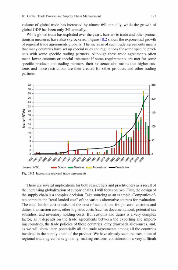
10 Global Trade Process and Supply Chain Management 177
volume of global trade has increased by almost 6% annually, while the growth ofglobal GDP has been only 3% annually.
While global trade has exploded over the years, barriers to trade and other protec-tionism measures have also skyrocketed. Figure 10.2 shows the exponential growthof regional trade agreements globally. The increase of such trade agreements meansthat many countries have set up special rules and regulations for some specific prod-ucts with some specific trading partners. Although these trade agreements oftenmean lower customs or special treatment if some requirements are met for somespecific products and trading partners, their existence also means that higher cus-toms and more restrictions are then created for other products and other tradingpartners.
Fig. 10.2 Increasing regional trade agreements
There are several implications for both researchers and practitioners as a result ofthe increasing globalization of supply chains. I will focus on two. First, the design ofthe supply chain is a complex decision. Take sourcing as an example. Companies of-ten compute the “total landed cost” of the various alternative sources for evaluation.The total landed cost consists of the cost of acquisition, freight cost, customs andduties, transaction costs, other logistics costs (such as documentation), potential taxsubsidies, and inventory holding costs. But customs and duties is a very complexfactor, as it depends on the trade agreements between the exporting and import-ing countries, the trade policies of these countries, duty drawback allowances, and,as we will show later, potentially all the trade agreements among all the countriesinvolved in the supply chain of the product. We have already seen the escalation ofregional trade agreements globally, making customs consideration a very difficult

178 Hau L. Lee
and complex one. The additional challenge is that there are still a lot of uncertain-ties involved—the trade agreements, regulations, and requirements may change overtime.
Moreover, given the trade agreements and the customs duties in place, companiesshould design the right postponement strategies so that the right level of customiza-tion of the product can occur in the market regions instead of centrally at the factory.The key question often is what should be the portion of the product to be built at thefactory and what should be the portion to be built at the (multiple and distributed)distribution centers that are in the market regions. There are certainly economies ofscale and easier production and quality control to build products at the factory; butthe increasing protectionism and resulted tariffs for products can motivate havingsome portion of the product, i.e., some of the customization steps to be carried outin distribution. The right level of postponement must take account of the associatedcustoms and duties implications.
Second, cross-border trade processes are non-trivial. From the initiation of ex-port/import, to the physical movement of goods across the borders, and then thearrival at the final destination, the trade process can be complex, time-consuming,and costly. This process can also become even more complex when some nations,such as the United States, are concerned with the threat of security when containershipments can be used by terrorists as a weapon of mass destruction. The result isadded documentation requirements, inspection, and delays. In the total landed costanalysis, the logistics and transaction costs, and the inventory holding costs, can begreatly affected by the cross-border trade processes. For example, if such processesare long and unreliable, then the inventory in transit will be high, and the safetystocks that the importing company need to carry would have to be increased.
In this chapter, I do not attempt to give a complete treatment of these two impli-cations. Instead, I like to highlight some important considerations that practitionersshould pay attention to, and some possible research that can be carried out.
10.2 Supply Chain Design and Trade Processes
10.2.1 Supply Chain Design
In classic supply chain design problems, the key factors for considerations includefixed and variable costs of the sites for manufacturing and distribution, the trans-portation costs, and inventory costs (see the classic work of Geoffrion and Graves[5]). There is a rich literature on this topic, ranging from deterministic applications(e.g., [1]) and stochastic demand versions (e.g., [2]). Extending this to global sup-ply chain design often requires modeling additional factors such as local contentrequirements, customs and duties rates, differential tax rates in different countries,transfer pricing schemes, and in some cases, exchange rate fluctuations (e.g., [3]).
The proliferation of trade agreements has added a new dimension of complex-ity to the supply chain design problem. Prior to the Agreement on Trade-Related

10 Global Trade Process and Supply Chain Management 179
Investment Measures (TRIMS Agreement), in an effort to increase labor participa-tion in their country and attract investment, some developing countries had includedparticular rules that provide incentives for companies in a particular industry to en-ter the respective countries. These incentives often included duty-free rates or areduction in duties paid on imports; the result was that companies increased theiruse of local contents in the final exported product or so-called local contents andtrade balancing requirements. Under these regimes, companies could only achievereduced duties on their imports used to serve the domestic market, by increasingthe country’s exports. Otherwise, companies were forced to use local contents toserve the domestic market and, in some cases, it was not possible and too costlyto source the parts that the company needed. The use of the previously mentionedincentive schemas was prohibited when the TRIMS Agreement of the MultilateralAgreements on Trade in Goods was negotiated during the Uruguay Round of WTOnegotiations and came into force in 1995. This agreement applied to trade in goodsand generally prohibited trade-related investment measures.
Such agreements can complicate the supply chain design problem. At the sametime, clever exploitation of such agreements can lead to significant savings to thefirm! It was due to such duty savings that Crocs used to manufacture its plastic shoesin Canada to serve the demands in Israel, since the special trade agreement betweenCanada and Israel resulted in zero duty for shoes made in Canada, versus 40% other-wise [8]. Consider the Logan car of Renault (see [12]). The Logan was designed as acar for new markets with high potential growth. Renault initially targeted customersin Colombia, Iran, Romania, Russia, and the Maghreb region. However, the Loganwas also designed to be sold in markets throughout Africa, Asia, Eastern Europe,and South America.
Automobiles sold in a given country could be built with a range of local con-tents. At one extreme, a company could export a car to its customers abroad as acompletely built-up vehicle (CBU), where the importing country received a fullyassembled vehicle ready for sale in the local market. CBU were advantageous inthat all vehicle production and assembly could be centralized. Only the logisticswould thus be required to transport the vehicle from its origin to its destination.However, duties on vehicles imported as CBUs were traditionally exorbitant, rang-ing from 35% in South America to 90% in Iran and 100% in India. An alternativeapproach was to export vehicles as completely knocked down units (CKDs). Whilethe definition could vary by importing country where the final assembly took place,CKDs described the entire kit of parts that would be required to assemble the finalvehicle.
Consider the Pitesti plant in Romania as a production site of the Logan. ThePitesti factory could be used to support Logan assembly plants in Russia, Morocco,Colombia, Brazil, India, and Iran by providing them with CKD parts.Romania could also produce Logan as CBUs for export to European countries,Croatia, and Turkey, where customs unions or free trade agreements allowed forduty-free import of CBUs, by following the rules of origin. When Romania joinedthe European Union (EU) in 2007, a whole new set of trade agreements becameeffective, and the customs and duties implications to the supply chain turned out tobe huge.

180 Hau L. Lee
The immediate consequence of Romania entering the EU was that Renault couldnow import parts from several countries using the free trade agreements availableas a member of the EU. This was also the case for mechanical parts supplied fromBrazil, which were subject to an MFN duty rate of 30% prior to 2007. Accord-ingly, Romanian vehicles would be considered as European vehicles. For example,the duty rate on the import of vehicles into Mexico was 50% (before Romania’saccession) and 0%, with a certificate of origin (after accession).
Another outcome of Romania’s membership in the EU was that, under rules oforigin requirements for CBU imports into the EU, Romanian parts would be countedas local contents. Prior to its EU membership, Morocco had been importing partsfrom Romania, using these parts to assemble CBUs in Morocco, and attempting toexport these CBUs to Europe. Since these Romanian parts did not qualify as localcontents of the EU, the Logan did not have enough European parts to satisfy therules of origin requirements for CBUs imported into the EU and was subject to the10% duty rate on imported CBUs. However, with Romania’s accession into the EU,the Romanian parts could qualify as European parts, and the Logan could satisfy therules of origin to achieve a duty-free rate on CBU imports from Morocco to Europe.While Logan was introduced as a product for developing countries, the car wasunexpectedly successful in Europe. Making use of the network of trade agreements,Renault was able to make use of the Morocco plant to fill European demands withouthaving to pay hefty duties.
Figure 10.3 illustrates the supply network of the Logan car and the resultingduty-free flows as a result of Romania’s accession into the EU.
This case example shows that, to fully capture the impact of regional trade agree-ments on customs and duties, it is not sufficient for us to simply look at the customduty rate of a particular product from one country to another. In fact, we need to firstexamine the complete bill of materials of the product, and then the trade agreements
Romania
Turkey
E. Europe
EU
Russia
Brazil
Columbia
India
Morocco
Russia,Ukraine
Columbia,Ecuador,
Venezuela
Maghrebregion,Egypt,
Tunisia,Jordan
CKD
CBU
Suppliers
Parts Red color denotes duty-free flows.
Fig. 10.3 Supply network of Logan car

10 Global Trade Process and Supply Chain Management 181
of the components and the product among all the trading countries. For example, ifCountry A supplies CKD parts to Country B, which then supplies CBU to CountryC, the trade agreements between Country A and B, Country B and C, and CountryA and C must all be considered. Just as we need to consider the supply network, wenow have to consider the network of trade agreements.
10.2.2 Trade Process Uncertainties and Risks
The complex trade agreements, regulations, and requirements set up by countries fortrade could give rise to one big challenge to companies involved in trade. Even ifone was able to figure out how to design the supply chain network to take advantageof the existing trade agreements and regulations, there is still a very high degree ofrisk that these agreements and regulations would change over time.
To illustrate, we return to the Logan car example of Renault. To reach the Egyp-tian market, Renault relied on the opportunities available by using Morocco as atrading center. As it was possible to import CKD parts into Morocco at a duty-freerate, Renault could import European parts into Morocco at a 0% duty and assem-ble the vehicles in that country. Renault could then export CBUs to Egypt fromMorocco and obtain a 0% duty rate on these imports, a benefit of the free tradeagreement between Morocco and Egypt. It was not possible, however, to exportCBUs from Europe to Morocco and then export these to Egypt, as the CBU importrate into Morocco from the EU was 25% by the end of 2006. So using Morocco asthe place to assemble the CKUs into CBUs for the Egyptian market seemed to be asmart move. However, such a design may not be optimal in 2009 as the duty rates onCBUs between Europe and Egypt were expected to decrease according to the PanEuro Med protocol of origin. By 2019, a 0% duty rate for exports of CBUs fromEurope to Egypt could be possible. Morocco may not be the optimal final assemblysite then.
Apparel manufacturers have learnt first hand the uncertainties in trade agree-ments. When China entered WTO, the apparel quota for Chinese apparel productsentering the United States was supposed to be phased out. Some manufacturers haveclosed down factories in other parts of the world, since these factories were not asefficient as the ones in China, in anticipation of the phasing out of quota from China.Of course, we soon learnt that the quota was not to be lifted totally. Some of thesemanufacturers were caught off guard.
10.2.3 Postponement Design
High technology products with a modular product structure can postpone some ofthe assembly processes to multiple global distribution points instead of integrat-ing the complete product at the factory. Distribution points are much closer to the

182 Hau L. Lee
customers, and so by allowing them to perform some of the final assembly pro-cesses, the point of differentiation of the product into multiple end-products can bedeferred. Defining what is to be assembled in the factory, and what is to be assem-bled in distribution, is termed the postponement boundary problem. The labor costrates, productivity, and customs and duty rates in the countries in which the DCsreside can be very different from those of the factory. These differences can have asignificant impact on determining the best postponement boundary of a product.
Consider Hewlett Packard’s (HP) workstation businesses in the late 1990s (see[10]). At the time, HP manufactured the workstation in two factories: one in theUnited States and the other in Germany. The factories distributed partially com-pleted products to distribution centers in Europe and Asia as well as to a resellernetwork. This particular business also worked with six major resellers in the NorthAmerican market and five major European resellers. The US and German facto-ries also built fully configured systems for direct shipments to customers in NorthAmerica and Europe, respectively, effectively serving as integrated factories anddistribution centers.
When HP planned to introduce a new line of product with a modular design,it considered postponing some of the computer configuration processes to its DCsand even to its resellers. The two HP factories would continue to serve as their owndistribution centers for their regions, which accounted for about 60% of all orders.For the rest of the orders, the postponement boundary problem would amount todefining the steps that were to be performed at the factories and those which wereto be performed at the DCs.
The workstation product was sold in developed countries with high labor costsand moderate or high customs and duties levied on the product, such as Japan andparts of Europe that are outside of the EU; and in developing countries with lowerlabor costs but very high customs and duties levied on the product, such as Koreaand Eastern Europe.
Figure 10.4 displays the total annual costs and the cost components for differ-ent postponement boundaries—the factory could build the complete product; orthe product without storage and memory; or without storage, memory, and graphicboards; or without storage, memory, graphic boards, and processor; or without allthe above plus the backplane; or delegate all key modules to be assembled at theDC. The bulk of the total costs were materials, and to highlight the cost differen-tials, we have chosen to show only the differential material and processing costs foreach alternative relative to the least cost alternative for those particular costs.
The analysis showed that the best alternative was to assemble the chassis, powersupply, and backplane assembly in the factory; this meant postponing the remainingsteps, starting with the processor board, to the distribution centers and resellers. TheU-shape result for the costs of the various options clearly indicated that the extremeoptions, building to order at the postponement sites and stocking fully configuredunits at the factories, were not cost effective.
As expected, inventory was the primary driver of the product configuration point;its effect followed the trade-off between the parts inventory created by postponingthe activities and the stock of configured product. As the product content at the

10 Global Trade Process and Supply Chain Management 183
Fig. 10.4 Postponement boundary analysis
factories increased, the cost due to customs and duties also increased, since theconfigured product shipped from the factory to the DCs increased in its dutiablevalue. In addition, the duty rate applied to a product can also change dependingon whether the product contained no processor, a processor, or a processor plusmemory. This application case shows that, in a global supply chain, customs andduties can constitute a major cost driver in evaluating the postponement boundaries.Freight and processing costs did not factor as heavily in this particular example. Thechassis accounted for the majority of the weight of the product, so there was littledifference in freight expense between the different alternatives (we assumed highpercentages of inbound surface transportation and outbound air transportation). Thefixed costs of adding postponement capabilities to the distribution network wererelatively insignificant. Because these other factors had so little effect, inventoryand customs and duties made the difference in every scenario.
Hence, trade agreements and the resulting customs and duties affect the designof the supply chain, as well as the design of the postponement boundary.
10.3 Improving Global Trade Processes in Supply Chains
10.3.1 Logistics Efficiency and Bilateral Trade
As noted, the times and costs in global cross-border trade processes affect the totallanded costs, which affect companies’ sourcing decisions. Consequently, the effi-ciency of global trade processes could impact trade flows between two countries.The significance of this effect has been established by Hausman et al. [6].

184 Hau L. Lee
Economists have long attempted to explain the variations of bilateral tradesamong nations by examining measures such as distances, the GDPs, and institu-tional quality factors (such as corruption and infrastructures). The gravity model hasbeen a common means to perform statistical studies to examine the contributions ofthese factors toward explaining bilateral trade (see the review in [6]). Distance asa measure could certainly serve as a surrogate for the friction between two tradingpartners, negatively impacting trade. But in practice, this is only one of many factorsthat serve as frictions of cross-border trade flows. There are many process steps in-volved in cross-border trade, e.g., the times and costs required to make declaration,waiting for containers to be loaded on ships, customs clearance at both the export-ing and the importing countries, the transportation time, inspection times at ports,and the times waiting for local transportation companies to bring goods to the finaldestination. There are also variances of these times that could also result in addedfrictions.
The Hausman et al. [6] study collected logistics performance metrics on somekey cross-border trade flows across 80 countries, based on container flows of threekey types of products: textile yarn, fabrics, made-up articles; apparel and clothingaccessories; and coffee, tea, cocoa, spices, and manufactures thereof. These metricswere used in statistical analysis of an augmented gravity model, and the result wasthat cross-border global trade efficiencies (or the lack of) significantly impactedbilateral trade. While the best gravity model was able to explain about 66% of theadjusted R2 of bilateral trade variation, the addition of cross-border logistics metricsimproved the R2 to 72%. As expected, the average process time to cross borderswould negatively impact trade, but the variation of process times (the study usedthe difference between the maximum time and the average time as a surrogate forvariation) also negatively impact trade. Hence, it is important for governments andcompanies to work on reducing both the mean and variance of times and costs ofcross-border trade processes. Figure 10.5 shows the results of the augmented modelin Hausman et al. (2009)
Hausman et al. [6] described some implications from the results of Figure 10.5.For example, the results can be used to see the benefits from reducing total processtimes through deregulating transportation, expanding ports to increase capacity, andpromoting the growth of the third-party logistics industry to allow more consolida-tion of cargo flows. Trade-related processing time and cost can also be improved byre-engineering processes to eliminate unnecessary steps and streamline others (suchas by introducing more parallel processing rather than sequential processing), in-troducing advanced information technologies (such as electronic customs clearanceand documentation flows), using data mining and screening methods to identifyonly high-risk containers for security inspections, and adopting advanced scanningtechnologies to shorten cargo inspection times.
The model result can also be used to calculate the elasticity of the key logisticsmetrics to bilateral trade [6]. Let
S(i, j) = value of bilateral trade from country i to country j;d(i, j) = distance from country i to country j;T (i, j) = average total time (transport and trade-related processing) from i to j;

10 Global Trade Process and Supply Chain Management 185
Independent variable Coefficient T-statistic
Log of exporter’s GDP 1.265 72.57
Log of importer’s GDP 0.956 54.17
Log of distance –1.390 –39.02
Exporter’s Corruption Perception Index 0.188 10.82
Importer’s Corruption Perception Index 0.134 6.27
Regional trade agreement dummy variable 0.343 4.73
Log of average time for all procedures –0.373 –5.24
Log of total cost of procedures –0.492 –10.68
Log of Maximum time-Average time –0.236 –4.28
Adjusted R-squared: 0.716; Observations: 5149: F-statistic: 1287Dependent variable is total bilateral exports (in logs) in 2003 or latest year available. Corruption Perception Index is for 2004, from Transparency International. OLS estimates; constant term not shown
Fig. 10.5 Augmented gravity model
C(i, j) = total processing cost from country i to country j;σ(i, j) = maximum time minus average time from country i to country j.
Here, the (i, j) term in the variables can be suppressed without loss of generality.Figure 10.5 shows that
logS = K′ −1.390logd−0.373logT −0.492logC−0.236logσ ,
where K′ is a constant representing the non-logistic independent variables. It is easyto see that −1.390, −0.373, −0.492, and −0.236 represent the elasticities of thelogistics metrics in bilateral trade. Thus a 1% reduction in the “distance” measurewould be associated with an increase of 1.39% in bilateral trade. Regarding pro-cessing time, a 1% reduction would be associated with a 0.37% increase in bilateraltrade. Similarly, a 1% reduction in the total trade-related processing cost would beassociated with a 0.49% increase in bilateral trade, while a 1% reduction in the vari-ability measure (maximum time−average time) would be associated with a 0.24%increase in bilateral trade.
10.3.2 Cross-Border Processes for Supply Chain Security
After September 11, 2001, the security of a supply chain has become a major con-cern to the public and the private sector. In particular, the ocean segment of asupply chain is most vulnerable to security threats, as more than 90% of worldtrade involves containers aboard ships [4]. The US government, in particular, has

186 Hau L. Lee
been concerned with the threat of terrorism and the potential of having weaponsof mass destruction (WMD) in materials flowing through a supply chain. WMDcan result in significant loss in human lives, destruction of infrastructure, and ero-sion of public and business confidence. Ultimately, global trade and prosperity arethreatened.
On the other hand, the private sector is concerned about the costs of assuringsecurity and the potential disruptions associated with real or potential terrorist acts.Governments and industry have responded with proposals, such as increased infor-mation exchange among trading partners, ports, shipping companies, and the gov-ernments; and heightened inspection and scrutiny of the goods flowing through asupply chain. Increased inspection at the destination ports as a way to assure secu-rity can add tremendous cost, delays, and uncertainties in the supply chain.
US Customs has also launched the Container Security Initiative (CSI) and theCustoms-Trade Partnership Against Terrorism (C-TPAT) in January and April of2002, respectively. The C-TPAT program involves multiple countries and promotesthe use of best security practices. Shippers and carriers that certify the use of bestsecurity practices are given expedited processing at US ports of entry. Manufactur-ers, importers, carriers, and third-party logistics service providers can all participateby completing detailed questionnaires and self-appraisals of their supply chain se-curity practices, while Customs would perform periodic audits and verifications ofsuch practices.
Another proposal was the Smart and Secure Tradelane (SST) initiative. This ini-tiative has some similarities to total quality control (see [14]), which calls for havingquality inputs and tight process control to assure quality, instead of relying on finalinspection. Hence, rather than relying on inspecting containers arriving at the des-tination ports, we would focus on having containers inspected at the source andusing technologies to monitor the transportation process to assure the integrity ofthe containers. Any tampering of the containers during the journey would have tobe detected. To do this effectively, we do need to use modern technologies. Onepromising technology is the use of electronic cargo seals and sensors (smart con-tainers). Such an initiative is not free, and so proper quantification of its benefits iscrucial for general adoption.
The SST process starts with the identification of personnel, cargo, and transporta-tion information about the container and its contents at the point of origin. This isfollowed by providing real-time supply chain security and management informa-tion to partners involved in the end-to-end shipment, through integrating data fromActive-RFID (radio frequency identification) tags and intrusion-detection sensorsattached to the containers. The RFID tags are read by stationary and mobile readersat key nodes.
Simple models can be developed to assess the benefits of SST (see [13]). Let
p = the inspection rate of containers arriving at a destination port;x = transit lead time in days, a random variable;y = inspection dwell time in days, a random variable;T = total lead time in days.

10 Global Trade Process and Supply Chain Management 187
Note that
E(T ) = E(x)+ pE(y) and Var(T ) = Var(x)+ pVar(y)+ p(1− p)[E(y)]2.
μ = mean daily demand of a product;σ = standard deviation of the daily demand of the product;R = inter-replenishment time in days for the DC;k = safety stock factor;p′ = new inspection rate under SST;1−θ = percentage reduction of the transit time variance as a result of SST.
Hence, the new transit time variance under SST is given by θ Var(x).Without SST, i.e., in the current process, the safety stock is given by (see, for
example, [15]):
S0 = k√
μ2 Var(T )+σ2E(T +R).
With SST, we have advanced information about the lead time statistics and so couldadjust the safety stock based on the knowledge of whether inspection is needed ornot. The resulting expected safety stock is
S1=k{
p′√
μ2 [θ Var(x)+Var(y)]+σ2 [E(x)+E(y)+R]
+ (1− p′)√
μ2θ Var(x)+σ2 [E(x)+R]}
.
Lee and Whang [13] showed that S1 ≤ S0, providing one benefit of SST.
10.3.3 IT-Enabled Global Trade Management for Efficient TradeProcess
Using advanced information technologies (IT) on some process steps in cross-border processes to assure supply chain security is one way in which we can im-prove the trade process and gain some benefits. But there are many other processsteps that could also benefit from process improvements through the use of IT. ITcan of course potentially reduce the mean and variance of the lead time in a processstep (through direct work savings and reduction in errors and reworks). But it canalso enable, in some cases, parallel processing of some process steps instead of se-quential. It can allow for some re-sequencing of the process steps that could lead tooverall savings. Finally, it is also possible that some process steps can be eliminated(e.g., if IT results in a process with zero defects, then another subsequent step forthe purpose of checking and verification can be eliminated). Hence, investment inIT can be a powerful way to improve cross-border trade processes, which wouldthen lead to supply chain performance improvements.
To do a complete analysis of the potential process improvements, we need to (1)characterize all the process steps involved in trade flow, as well as their precedence

188 Hau L. Lee
relationships; (2) estimate the current duration and cost for each of the process step;(3) estimate new process flow with IT fully implemented, and the resulting durationand cost for each of the process step; and (4) given these changes, quantify the bene-fits to the exporters, importers, and other intermediaries involved in trade processes.Teamed with TradeBeam, a leading IT provider of trade processes, Stanford Univer-sity has developed the Stanford Trade Process Model for the purpose of performingsuch an analysis (see [7]).
The trade process is extremely complex. This is partly due to the proliferationof regional trade agreements described earlier. Compliance to these agreements re-quires extensive documentation, tracking, and verification, all of which become partof the cross-border processes. The term Global Trade Management (GTM) refersto the processes required to support cross-border transactions between importers,exporters, their trading partners, and governments. GTM encompasses networkplanning, sourcing, order collaboration, compliance with government regulations,transportation, inventory, and warehousing management, as well as financial settle-ment. GTM can be performed manually, or in a highly automated fashion, and withpoor or efficient processes. Information Technology-Enabled Global Trade Man-agement (IT-GTM) is the set of information technologies and software solutionsthat can be used by companies to streamline and perform their global trading pro-cesses. They can include automation of export and import management and compli-ance, electronic integration with trading partners, trade financing, and trade contentmanagement.
The Stanford Trade Process Model is focused on apparel trade from China tothe United States and is based on extensive interviews and data collection with tradeexperts and companies involved in such trades [7]. It involves over 100 process stepsthat cover broadly the following processes (Figure 10.6):
Fig. 10.6 Stanford trade process model

10 Global Trade Process and Supply Chain Management 189
Pre-export: initiation of the global trade process, e.g., import screening, price ne-gotiation price, contract and payment terms, creation of purchase/sales orders,and export screening;
Transport arrangement and export declaration: preparation for exportation, in-cluding arrangement of transportation carriers, obtaining approval from inspec-tion agencies, export declaration, and preparation and transmission of securityfilings to US Customs and Border Protection;
Transport and import declaration: ocean or air transport of the goods, generationand submission of import documents, and import customs clearance;
Post-import customs clearance and payment: inland delivery from the border tothe importer’s site, receipt of goods, review of landed cost, settling payment withthe forwarder, broker and exporter, and filing for foreign exchange verificationand tax refund if applicable.
IT-Enabled GTM could result in direct process improvements or process re-engineering which have tremendous benefits (Figure 10.7).
ProcessExcellence
ProcessRedesign
Focus
• Faster
• More accurate
• More reliable
• Re-sequencing
• Parallel processing
• Elimination
Values
• Shorter cycle time
• Less delays & reworks
• Lower capital tied up
• Faster cash cycle
• Less penalties from errors
• Accurate duty payment and refunds
Fig. 10.7 Values of IT-enabled innovations
To quantify the benefits of such improvements, one needs to develop modelsto capture the benefits in the form of inventory savings, savings in financing costs,speeding up tax rebates, reduction in expedite costs, reduction in fines, logistics costsavings, labor cost savings, potential reduction in procurement, markdown and lostrevenues for importers, and customs savings due to accurate classification of prod-ucts. Intermediaries (such as banks, freight forwarders, and other service providers)can also benefit through workload reduction and reduced cost of receivables financ-ing. The benefits to exporters, importers, and intermediaries have to be modeledseparately. The analysis of the apparel trade from China to United States shows thatthe value of IT-Enabled GTM can be significant (see Figure 10.8).
To illustrate, Hausman et al. [7] show that, for exporters, the order to receipt cy-cle could reduce from 104 to 68 days; the number of days outstanding could dropfrom 42 to 30; and the manufacture to invoice cycle could be shortened from 45 to
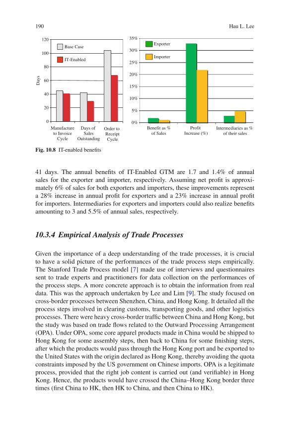
190 Hau L. Lee
0
20
40
60
80
100
120
Manufactureto Invoice
Cycle
Day
s
Days of Sales
Outstanding
Order to ReceiptCycle
0%
5%
10%
15%
20%
25%
30%
35%
Benefit as %of Sales
Profit Increase (%)
Intermediaries as % of their sales
Base Case
IT-Enabled
Exporter
Importer
Fig. 10.8 IT-enabled benefits
41 days. The annual benefits of IT-Enabled GTM are 1.7 and 1.4% of annualsales for the exporter and importer, respectively. Assuming net profit is approxi-mately 6% of sales for both exporters and importers, these improvements representa 28% increase in annual profit for exporters and a 23% increase in annual profitfor importers. Intermediaries for exporters and importers could also realize benefitsamounting to 3 and 5.5% of annual sales, respectively.
10.3.4 Empirical Analysis of Trade Processes
Given the importance of a deep understanding of the trade processes, it is crucialto have a solid picture of the performances of the trade process steps empirically.The Stanford Trade Process model [7] made use of interviews and questionnairessent to trade experts and practitioners for data collection on the performances ofthe process steps. A more concrete approach is to obtain the information from realdata. This was the approach undertaken by Lee and Lim [9]. The study focused oncross-border processes between Shenzhen, China, and Hong Kong. It detailed all theprocess steps involved in clearing customs, transporting goods, and other logisticsprocesses. There were heavy cross-border traffic between China and Hong Kong, butthe study was based on trade flows related to the Outward Processing Arrangement(OPA). Under OPA, some core apparel products made in China would be shipped toHong Kong for some assembly steps, then back to China for some finishing steps,after which the products would pass through the Hong Kong port and be exported tothe United States with the origin declared as Hong Kong, thereby avoiding the quotaconstraints imposed by the US government on Chinese imports. OPA is a legitimateprocess, provided that the right job content is carried out (and verifiable) in HongKong. Hence, the products would have crossed the China–Hong Kong border threetimes (first China to HK, then HK to China, and then China to HK).

10 Global Trade Process and Supply Chain Management 191
To collect real data, the researchers installed GPS and RFIDs on a sample oftrucks and had readers mounted at some key choke points along the China–HongKong border. Figure 10.9 shows the points in which readers were installed so thatthe movements of the trucks were tracked. Consequently, the actual times requiredto go through all the cross-border process steps could be recorded, leading to somevery concrete estimates.
• Total: 17 points along the cross-border route between China and Hong Kong
• Lok Ma Chau yellow bus stop: A1-A4
• Lok Ma Chau Hong Kong Customs: B1-B5
• Huanggang customs: C1
• Pedestrian bridge at Huanggang customs: D1
• Pedestrian bridge besides Guangyin building: E1
• Riverside besides Guangyin building: F1
• Southern point of crossroad outside Huangyuyuan north gate: G1
• Customs truck north exit: H1
• Truck park north entrance: H1
• Huanggang Customs truck entrance: J1
Fig. 10.9 Data collection for sample points
HK SZ
Queue Process Inspection Queue Process Inspection
HK to SZ (5,258 trips)
Rate 17% 14%
Mean 3.00 1.25 6.54 18.93 3.03 20.81
Std Dev 5.17 2.38 14.36 39.46 7.51 30.48
SZ to HK (4,662 trips)
Rate 8% 19%
Mean 1.03 1.01 9.44 3.17 3.08 58.62
Std Dev 2.15 2.00 23.57 5.74 5.32 70.61
Fig. 10.10 Cross-border cycle times (hours)

192 Hau L. Lee
After extensive data collection, the study was able to have very accurate esti-mate of the inspection rate performed by customs office, the means and standarddeviations of the queueing and process times in crossing the border on the HongKong (HK) side as well as the Shenzhen (SZ), China, side. Figure 10.10 shows thestatistics.
Hence, using GPS and RFID can be one way to get real-life data on the tradeprocesses.
10.4 Concluding Remarks
As a result of increased globalization of industrial supply chains, effective sup-ply chain management requires sound alignment with the global trade processes.I have discussed how the design of the global supply chain and the determinationof right level of postponement are both tied intimately to the prevailing network oftrade agreements, regulations, and local requirements of the countries in which thecompany is operating in. Moreover, the dynamic changes and uncertainties of theseagreements and requirements must be anticipated.
In addition, the complexity of the cross-border trade processes results in uncer-tainties in the lead time and costs involved in global trade, which naturally formspart of the consideration of global sourcing, and the resulting safety stocks or otherhedging decisions. Governments, exporters, importers, carriers, and other serviceproviders have to work together to reduce the logistics frictions involved in theglobal trade processes. The benefits accrue not only to the exporters, importers, andthe intermediaries, but ultimately, they could foster bilateral trade. The only wayto reduce the frictions is to gain a deep understanding of the detailed process stepsinvolved, to improve upon it by IT, and potentially re-engineer the processes. Butthe payoffs to such investments can be huge.
The inter-relationships between global trade processes and supply chain man-agement form a fertile ground of research. I hope that the above discussion canstimulate ideas for this purpose.
Acknowledgment
This chapter draws upon past and ongoing research that I have done with colleagueslike Professors Chung-Yee Lee, Warren Hausman, Lingxiu Dong, Seungjin Whang,and Morris Cohen.
References
1. Arntzen BC, Brown GG, Harrison TP, Trafton LL (1995) Global supply chain management atdigital equipment corporation. Interfaces 25(1):69–93.

10 Global Trade Process and Supply Chain Management 193
2. Cohen MA, Lee HL (1988) Strategic analysis of integrated production-distribution systems:Models and methods. Operations Research 36(2):216–228.
3. Cohen MA, Lee HL (1989) Resource deployment analysis of global manufacturing and dis-tribution networks, J Manufacturing and Operation Management 2(2):81–104.
4. Cuneo EC (2003) Safe at sea. Information Week (April 7)5. Geoffrion AM, Graves GW (1974) Multicommodity distribution system design by benders
decomposition, Management Science 20(5): 822–844 (also reprinted in this volume)6. Hausman WH, Lee HL, Subramanian U (2009) The impact of logistics performance on trade.
Production and Operations Management (under review)7. Hausman WH, Lee HL, Napier G, Thompson A, Zhang K (2010) A process analysis of global
trade management: An inductive approach. Journal of Supply Chain Management (to appear)8. Hoyt D (2007) Crocs: Revolutionizing an industry supply chain model for competitive advan-
tage. Stanford Graduate School of Business case GS-57, May 99. Lee CY, Lim A (2008) RFID cross-border project: Process enhancement feasibility study.
Hong Kong University of Science and Technology10. Lee HL, Dong L (2009) Postponement boundary for global supply chain efficiency. Working
paper11. Lee HL, Shao M (2009) European recycling platform: Promoting competition in e-waste re-
cycling. Stanford Graduate School of Business case GS-67, August 1812. Lee HL, Silverman A (2008) Renault’s Logan car: Managing customs duties for a global
product. Stanford Graduate School of Business case GS-62, April 2913. Lee HL, Whang S (2005) Higher supply chain security at lower cost: Lessons from total
quality management, International Journal Production Economics 96:289–300.14. Lee HL, Wolfe M (2003) Supply chain security without tears. Supply Chain Management
Review 7(1)(Jan/Feb):12–2015. Silver E, Pyke D, Peterson R (1998) Inventory management and production planning &
scheduling. 3rd ed. Wiley, New York, NY


Chapter 11Sustainable Globally Integrated Enterprise(GIE)
Grace Lin, Ko-Yang Wang
Abstract In this chapter, we present the globally integrated enterprise (GIE) asan emerging business model with strong implications for how companies run andoperate their global supply-and-demand chains. The GIE shifts the focus from anefficiency-driven model to a value-driven one which leverages and integrates globalcapabilities to deliver value speedily, seamlessly, and in a flexible way, while max-imizing profits. A GIE is a complex organization that faces many challenges. Theevolution of the supply chain in the last 20 years has paved the way for the Oper-ation Research (OR)-enabled Sense-and-Respond Value Net that supports today’sGIE needs. We present a GIE case study of a business transformation journey. Wethen describe the next steps for GIEs to become more socially, economically, andenvironmentally responsible through the use of OR, business analytics, and IT.
11.1 Introduction
A Globally Integrated Enterprise (GIE) is an open, modular organization that is integratedinto the fabric of the networked economy and operates under a business model that makeseconomic sense in the new global landscape [14].
Several fundamental changes in the last 20 years have caused multinational compa-nies to rethink their approach:
1. The breakdown of economic nationalism caused trade/investment barriers to re-cede, accelerating the globalization trend.
2. Advances in technology and open standards have significantly improved thespeed and reduced the cost of global communication.
3. Geopolitical changes opened up new markets and skill pools which had beenunexplored by multinational corporations.
Grace Lin, Ko-Yang WangWorld Resource Optimization Inc., Chappaqua, NY, USA; Global Business Services, IBM,Armonk, NY, USA
M.S. Sodhi, C.S. Tang (eds.), A Long View of Research and Practice in Operations Research 195and Management Science, International Series in Operations Research & Management Science 148,DOI 10.1007/978-1-4419-6810-4 11, c© Springer Science+Business Media, LLC 2010

196 Grace Lin, Ko-Yang Wang
These changes have caused companies to re-evaluate how they manage their busi-ness since where and how business value is created in this new environment is evolv-ing. For example, sharing work across country or continent borders becomes pos-sible, and outsourcing and global operations seem much more appealing. Many USand European companies have moved or outsourced some or all of their manufactur-ing or services to Asia, South America, and East Europe, with increasing speed. Themultinational companies’ traditional approach of replicating themselves and build-ing plants locally while maintaining some key corporate functions such as R&D andproduct design in their home countries is no longer sustainable. They need to createflatter, more efficient operating models while building new innovative capabilitiesglobally to drive profitable growth. This new model has implications for how com-panies run and operate themselves and their global supply chains. Fundamentally,the focus has shifted from simply managing the supply chain for greater efficiencyto leveraging it to drive revenue, profit, and customer satisfaction. In the 2008 IBMGlobal CEO study, CEOs indicated that they were embracing the global integrationand unpredictability as the new routine [22]. They were also anticipating the needfor their business to respond seamlessly and globally with unprecedented speed andflexibility. In his 2006 article in “Foreign Affairs,” Sam Palmisano, IBM’s CEO,coined the term “Globally Integrated Enterprise” (GIE) for this emerging businessmodel [45].
In his article, Mr. Palmisano pointed out four major challenges for a GIE: (1) se-curing a supply of high-value skills; (2) creating sensible worldwide regulation ofintellectual property; (3) determining how to maintain trust in enterprises based onincreasingly distributed business models; and (4) managing requirements for long-term vision and continuous investment from business leaders. Recognizing the scaleof these challenges, Mr. Palmisano called for the leaders in business, government,education, and civil society to learn the emerging dynamics of GIEs and to helpGIEs mature in ways that would contribute to social, economic, and environmentalprogress around the planet. Two years later, in his 2008 speech to the Council onForeign Relations, Mr. Palmisano discussed “A Smarter Planet: The Next Leader-ship Agenda” [46]. He described the IBM vision for a Smarter Planet and the way inwhich the world is becoming instrumented, interconnected, and intelligent. He laidout visionary scenarios that lead the way to transforming companies into GIEs andalso pointed out a new direction toward sustainability, asking IBM, business, andcivil leaders to jointly work on specific solutions.
The key motivations for the multinational companies to go global have remainedthe same: to improve revenue and profits by entering new markets, reducing pro-duction costs, and seeking skilled workers at low costs [24]. However, in the faceof accelerating change brought about by globalization, technology advances, stan-dardization, competition, and geopolitical evolution, as well as the skills evolutionof both developing and developed countries, the operational model of the multina-tional companies is undergoing fundamental changes structurally, operationally, andculturally and at an unprecedented pace. The benefits of a well-run GIE are obvious:With the support of global skills and communication, the GIEs are able to strategi-cally place their operations anywhere in the world that offers the lowest cost or the

11 Sustainable Globally Integrated Enterprise (GIE) 197
best strategic value. However, transforming companies into well-run GIEs is notan easy task. They require fundamentally different approaches to production, dis-tribution, workforce management, product design, and risk management, etc. Anymisstep or miscalculation can cause significant cost and damage to the company.
In the last few years, more and more companies have started to examine theirsustainability. For example, IBM and its clients’ Smarter Planet efforts [SmarterPlanet, Web], Dubai’s SmartCity [SmartCity, Web], US government and utility com-panies’ Smart Meters, and Intelligent Grids initiates [48]. Thus, we define the sus-tainability of GIEs: The ability to improve business performance while reconcilingthe company’s needs with those of its supporting ecosystems from an environmen-tal, social, and economic perspective. We believe that (1) the emerging GIE trend isaccelerating and it is important for enterprises and society to embrace it and focuson maximizing the positive impact of GIEs on business performance while mini-mizing the negative impact of GIEs on the economy, society, and the environmentand (2) sustainability is a critical success factor for the GIEs. This means thatenterprises have a social responsibility to ensure that their pursuit of maximizingprofits and minimizing costs has a positive impact on the sustainability of the econ-omy, society, and environment. Also, the transformation of GIEs should improvetheir own sustainability, i.e., their ability to manage, survive, and even prosper whilefacing unexpected environmental changes, disasters, or disruptive events.
In this chapter, we focus on the supply-chain and value-net aspects of the GIEsand their sustainability. We will examine the recent advances in supply-chain man-agement (SCM) and information technology and their critical role in GIEs. InSection 11.2, we briefly touch on the key challenges that today’s GIEs face. InSection 11.3, we discuss the evolution of SCM and how it has driven the majorchanges seen in today’s GIEs. We will also discuss using the OR-based adaptiveSense-and-Respond Value Net to better enable GIE. In Section 11.4, we review acase study and examine some best practices in improving business performance andthe process of transforming a company into a GIE. Finally, in Section 11.5, wediscuss the characteristics of effective GIEs and how these companies can becomemore sustainable and socially responsible by leveraging advanced SCM solutions.
11.2 An Overview of GIEs and the Challenges they Face
“The crisis in our financial markets has jolted us awake to the realities and dangers of highlycomplex global systems. But in truth, the first decade of the 21st century has been a seriesof wake-up calls with a single subject: The reality of global integration.” Sam Palmisano[45]
Companies started to move or outsource their operations abroad in the late 1980sbut the trend toward GIEs has accelerated in the last 10 years. With the advancesin technology, we see communication and collaboration becoming easier and lesscostly and location, distances, and geographic borders becoming less relevant. Thedecisions about where, whom, and how products and services are made or provided

198 Grace Lin, Ko-Yang Wang
are driven less by the “where” and more by cost, skills/knowledge, and even eco-political considerations. We are not only seeing companies moving labor-intensivemanufacturing to lower cost countries such as China, India, or Brazil but also wit-nessing components of skill-intensive products/parts/services being moved in thesame manner and integrated back into the corporate processes on a global scale. Tounderstand these changes and how to transform enterprises into successful GIEs, wewill first examine the key challenges that GIEs face today.
The financial meltdown of October 2008 and the subsequent collapse or near col-lapse of the financial, housing, construction, automotive, and many other industriesdid not happen overnight. The problems were years in the making. However, formost enterprises, the sudden realization of the realities and the dangers of venerablebusiness models and financial stability had executives scrambling to rethink theirstrategy and operational models and to seek new solutions. The scale and reach ofthe crisis and the speed with which some seemingly infallible companies crumbled,as well as the vulnerability of companies in general, surprised virtually everyone.
The crisis highlighted several key realities of today’s business environment:
1. We are all connected. This close interdependence exposes enterprises to risksthat they cannot totally control. Today’s enterprises operate in a complex webof business relationships so that interdependence is deeply rooted in the fabricof the business model. Close collaboration with business partners is essential forperformance improvement.
2. It’s a small world. The financial crisis triggered by the US mortgage industrywould have brought down almost all major financial institutions in the majorfinancial markets had central governments not intervened and saved them. Thiscrisis revealed the fragility of the business models of many enterprises (e.g. theauto industry’s crisis triggered by consumers tightening up during the financialcrisis). Sustainability should be a key focus of any enterprise.
3. When the market changes faster than a company’s ability to react to it, the com-pany is in trouble. Unfortunately, not every company can keep pace with the ac-celeration of market changes. For example, the major American auto companiesthat relied heavily on SUV and truck sales for profit found that consumers hadchanged their buying habits in the face of the great financial crisis in 2008. As thecrisis deepened, auto sales slowed to half their size from the previous year. Al-though some companies recognized the peril of the market earlier (with the automarket slowdown beginning in early 2008), they were unable to adjust quicklyenough which resulted in the auto industry bailout in 2009. This highlights theimportance of agility and flexibility.
Another incident in the auto industry, the Toyota “sticky gas paddle and suddenacceleration” issue which continues to involve millions of car recalls in 2010 alsodemonstrates that a company is only as strong as the weakest link in its supplychain. Toyota, with its stellar reputation of reliability, stopped selling half of its carsovernight because of a faulty part from a weak link in its supply chain causing therecall. The problem was compounded by Toyota’s initial slow response to a keycrisis. The long-term damage to this widely admired company is immeasurable.

11 Sustainable Globally Integrated Enterprise (GIE) 199
Today, enterprises face the following key challenges:
1. Labor is only one of the many costs of global operation. Relocating operationsto low-cost areas also increases the risks of disruptive missteps due to increasedcomplexity, communication, and logistics issues. Simply replicating existing op-erating models will not work well.
2. The rapid pace of market changes often renders business models obsolete beforetransformation is complete or becomes effective.
3. Technology advances are accelerating process automation and enterprise collab-oration but many companies are confused by different incompatible technologystandards in business modeling and process automation.
4. Information integration is a critical step in enabling intelligence business analysisbut to integrate monolithic applications and clean up data is expensive and timeconsuming. Intelligence and business analysis too have to be explored.
5. Agility and flexibility are a reflection of the business model and operational pro-cess model. IT technologies are critical enablers but resistance to change oftenreduces or prevents a company’s form being agile or flexible.
6. The social and economic impact of GIEs’ “cherry picking” can have a profoundimpact on the communities/countries they abandon; and the backlash can impactthe customer relationship/markets as well.
Enterprises can leverage experience, R&D, technology, and natural evolution in aholistic approach that will allow them to transform into GIEs, enhance their agilityand flexibility to improve business performance, and, more importantly, becomemore sustainable.
11.3 The Evolution of Supply Chains and theSense-and-Respond Value Net
Business and information technology advances in the last decade, particularly in businessanalytics, process modeling and automation, information integration, and business perfor-mance management, present new opportunities for enterprises to enhance their ability tocompete. At the same time, converging social and technological trends are changing the na-ture of decision-making to create a more collaborative approach [37]. The evolution of thesupply chain in the last 20 years has paved the way for the OR-enabled Sense-and-RespondValue Net to leverage these technologies to support today’s GIE needs.
Over the last two decades, companies have evolved from the internal functional andprocess efficiency transformation toward collaborative and adaptive GIEs. SCM hasbeen vital in many companies’ transformation success such as Toyota [31], Nokia[16], Dell [17], Amazon, and IBM . In this section, we will discuss the supply-chain evolution and lessons learned. We will also describe the adaptive Sense-and-Respond (S&R) Value-Net model and its applicability for GIEs.
In the early 1990s, Enterprise Resources Planning (ERP) was adopted by manycompanies as a means for automation and improving transactional efficiency.

200 Grace Lin, Ko-Yang Wang
However, we have seen the top-down, ERP-based processes being stressed past theirintended capabilities for transitional efficiency. A major issue with the ERP systemsis their lack of flexibility and speed to support decision making throughout the inter-nal and extended supply chain to meet changing business needs. By the mid-1990s,various Advanced Planning and Scheduling (APS) tools implemented with legacyand ERP systems were developed to support the optimization of supply chains dur-ing planning and execution cycles. Business Process Reengineering, Just-in-Time,and Lean Supply-Chain process implementation were also becoming major trends.In the late 1990s and early 2000s, the development of e-commerce and e-businesstools offered Internet connectivity and some limited capability for supply-chain col-laboration and near real-time information sharing (see Figure 11.1).
SustainableGIT
„Those companies with high performance supply chains carry less inventory, have shorter, cash-to-cash cycle times and are more profitable.“
– Source: “The AMR Research Supply Chain Top 25 and the New Trillion-Dollar Opportunity” - AMR Research.
StaticSupply Chain
FunctionalExcellence
HorizontalIntegration
ExternalCollaboration
On DemandSupply Chain
ERP
APS
B2B
Visibility
Sense & Respond
Extended Enterprise Supply Chain Management
Business Models Innovations and Business
Optimization
Adaptive Sense-and-Respond Value Net
Value-Driven Services and Delivery
Sustainability
Fig. 11.1 The evolution of the enterprise—Enterprises have been evolving from functional andprocess efficiency to a collaborative and adaptive globally integrated enterprise (Source: IBMSense-and-Respond Presentation, 2004)
However, despite the implementation of supply-chain management tools and In-ternet connectivity, the ROI of supply-chain management package implementationhas constantly come under question. Based on interviews with senior executivesfrom 25 firms, Forrester reported that companies overspent on supply-chain opti-mization packages and received diminished returns: 80% of the companies spentmore time than expected and, on average, companies spent 74% over budget toimplement supply-chain optimization tools [49]. It was also reported that productmarkdowns due to excess inventory jumped from 10% to 30% of total units soldwhile customer satisfaction with product availability plummeted [30].
Why did efficiency gains and automation fail to delivery business value? In thechanging business environment, disruptive business and technical events can occur

11 Sustainable Globally Integrated Enterprise (GIE) 201
any time and at every level. Major business disruptions and inefficiencies can bethe result of the inability to handle these events quickly and intelligently due to(1) a lack of information visibility across internal and external supply chains; (2) in-sufficient partner collaboration; (3) a lack of customer intimacy; (4) an inability toleverage knowledge and manage uncertainty; and (5) a lack of flexibility in businessprocesses, applications, and infrastructure. The just-in-time supply-chain model per-formed well in improving supply-chain efficiency and minimizing product defects.However, the model depends on the ability of its supply network to control theirinventory and deliver parts “in time.” If not, the process breaks down. Furthermore,local supply-chain optimization based on incomplete or disjointed information un-der rigid top-down planning models can not only result in sub-optimization but alsocause significant adverse effects. Therefore, since early 2000, many supply-chainexperts have vigorously started to explore new models that expand the supply-chainscope and allow more agility and flexibility. Studies of some of the more successfulsupply chains of the early 2000s revealed that supply-chain optimization depends ontheir ability to streamline operations while processing information intelligently andholistically, allowing quick, proactive, and effective responses to frequent changesin the market place. This includes understanding the needs of customers and theneeds and capabilities of business partners and employees, as well as gathering rel-evant information to analyze risks and opportunities and gain situational awarenessin changing environments [2, 21, 27–29, 35, 39, 51].
These studies concluded that the key to successful, adaptive organizations is toensure continued focus on responsiveness and agility. This, however, cannot beachieved through technology implementation alone but by transformation into abusiness model supported by real-time business processes and performance manage-ment that will allow to quickly evaluate situations and determine how best to adjustbusiness models, processes, applications, or partnerships to key issues and events.This is what we called the “Sense-and-Respond Value-Net Model” [39], what HauLee called the “Triple A Model,” [29, 36] and what AMR called “Demand-DrivenSupply Chain” [10].
AMR in particular defined the “demand-driven supply network” (DDSN) modelthat transforms a factory-oriented “push” set of activities to an innovation and sup-ply capability driven by the demands of customers. AMR research has benchmarkedbusiness processes in detail [e.g., 16] and found a clear correlation between lead-ership in the use of demand-driven principles and tools and higher level financialmetrics. Professor Hau Lee identified the three characteristics of successful supplychains based on supply-chain success stories including Wal-Mart, Dell, and Ama-zon: Agility, Adaptability, and Alignment. Lee concluded that to achieve a sustain-able competitive advantage, a supply chain needs all three of these qualities simul-taneously.
The Sense-and-Respond Value-Net model was introduced by Lin et al. at IBMin 2000. The objective was to build an open and adaptive framework to enablevalue-driven business optimization. A Sense-and-Respond Value Net was then anew paradigm that integrates real-time decision support, risk and resource man-agement, supply-chain optimization, business processes automation, and partner

202 Grace Lin, Ko-Yang Wang
alliances in an integrated management system. Through its sensing, responding, andanalyzing capabilities, a Sense-and-Respond enterprise monitors and evaluates real-time business performance and market conditions, aligns operations with strategyand customer requirements, proactively detects events, and engages value-net part-ners in collaborative decision making (see Figure 11.2). It could be viewed as adigital brain with sensors reaching all the way from a company’s global value chainto the Internet world, blending business and IT to support value-net optimization inuncertain and dynamic environments [39].
In 2004 Lin et al. [36] presented a framework for S&R value-net transforma-tion as well as a maturity model for identifying gaps and defining roadmaps. Theydefined the five areas needed to support the development and adoption of the Sense-and-Respond model: (1) Adopting Sense-and-Respond Managerial and TechnologyTransformation with a focus on culture, (2) Support for Integration, Collaboration,and Security, (3) Information Intelligence, Analysis and Trustability of Data andTheir Aggregated Impacts, (4) Modeling Uncertainty and Managing Performance,and (5) Support for Agent Systems and Distributed Decision Support. In 2006, theyfurther identified and studied the S&R technology enablers and concluded that mostenabling technologies are actually available today (see Figure 11.3).
Within the last 10 years, the Sense-and-Respond model has been adopted bymany companies and software vendors, as well as by United States and internationaldefense agencies [9]. We will discuss IBM’s success story in Section 11.4.
Respond& Execute
Response
Respond – execute decisions to negotiate joint actions orrespond to events. Adaptcapabilities as needed.
Decide
Decide what response is best through collaboration
Analyze
Analyze alternativeresponses, their impactsand provide advanceddecision support todetected situations
Detect &Interpret
Interpret the information and recognize events and changing conditions
Monitor &Sense
Monitor the environment, collect & share critical data
Control
Control – manage the Sense and Respondcycle as rapidly andeffectively as required
Partners & Competitors / Allies
& Enemies
Events
Fig. 11.2 The Sense-and-Respond operational model (Source: [36])

11 Sustainable Globally Integrated Enterprise (GIE) 203
Collaboration and decision support technologyAnalysis and analytics
Real-time logistics and effect analyticsSimulation and what-if analysisAnalytic optimization modulesRisk and impact analysisSemantic webRule-based systems
Collaborative decisionShared sense makingPolicy-driven decision-making systemSecured collaboration supportImpact and value analysisDistributed decision-making protocolsCollaborative decision support
Control & learnBusiness performance monitoringEffect measurement and monitoringFeedback and learning technologyRapid process transformation supportModel-based business transformation
Changemanagement
Change management process
Business models and rapid transformation support
Sensing and information analysis technologies Dashboard
Monitor & senseSensors and sensor networks (sensors and actuators, RFIDs, TREC, etc)Data integration technologySecured communication networks
Information integrationSituational filter based on rolesVisualization technologiesPortal and info push-and-pull technology
Detect & interpretData cleansing & filteringPattern & event recognitionText/Knowledge miningReal time stream mining
Powerful computing/infrastructure
Secured networkCommunication protocolSecurity and entitlement
InfrastructureSOA-based enterprise services busRapid integration supportWorkflow enablementRuntime configurationSelf- healing, self configuration
Rapid operation supportRespond & execute
Real-time infrastructureReal-time process execution supportAgent frameworkAutonomic decision supportRapid application integration
• Cultural Issues
Compressed
Operations
• Physical Advantages
• Cognitive Advantages
• Information Advantages
SharedAwareness
PrecisionForce
Adapt
Sense Respond
Collaborative Decision Making
Fig. 11.3 Most key technologies needed for enabling Sense-and-Respond value nets are availabletoday (Source: [7])
To summarize, we have seen the supply-chain transformation focus changefrom efficiency-driven automation, cost reduction, and streamlining of the supply-chain processes to information- and collaboration-driven extended supply-chainintegration to value-driven adaptive Sense-and-Respond value net, which combine
Fig. 11.4 VCC provides end-to-end visibility to enable value-net partners to collaboratively sup-port chain performance (Source: IBM VCC Presentation, 2008)

204 Grace Lin, Ko-Yang Wang
information integration, adaptive process enablement, and business analytics to im-prove collaboration and the quality of decisions.
The next logical step for GIEs is to fully utilize S&R to integrate supply, demand,logistics, and other key business functions globally and to perform S&R culturetransformation to become a true GIE.
IBM’s recent 2008 CEO study of more than 1,000 C level executives found thatthe vast majority of companies are becoming globally integrated, with 75% activelyentering new markets [22]. Of those, 84% plan to partner with local companies tobecome truly globally integrated. Companies that can master the enabling technolo-gies shown in Figure 11.4 and integrate them into the fabric of their business totransform their business model to become more instrumented, connected, and intel-ligent will have significant competitive advantages.
Some success stories in GIE are already being reported, such as already men-tioned Wal-Mart, Nokia, and IBM. In Section 11.4, we will discuss howanalytics/OR was used in combination with business process modeling and inno-vative business models to support IBM’s GIE Transformation.
11.4 A Case Study
IBM has one of the largest and most complex supply chains in the world. Being a technol-ogy leader in the Industry, IBM needs pragmatic and powerful supply-chain technology toaddress its business challenges driven by rapidly changing business environments. Over thelast 20 years, it has demonstrated a compelling story in business transformation and globalintegration.
IBM’s transformation in the last 20 years makes a great case study for the GlobalIntegrated Enterprise. The company’s reengineering effort of the 1990s began outof necessity. From the late 1980s to the early 1990s, only several years after record-ing its record-high revenue, IBM suffered a remarkably rapid fall from grace dueto its slow reaction to a market transformation from mainframe computing to a dis-tributed computing model. Both its technology and its relationship with customerswere viewed as antiquated. In 1993, a victim of its size, bureaucracy, insular culture,and the workstations and PCs that it had helped invent, the company lost a record$8.1 billion. At that time, IBM’s cost structure was too high; the company was toodecentralized; it stayed with an old strategy too long; and it had lost touch with bothindustry changes and its customers. IBM and its mainframe were dubbed dinosaursand their imminent extinction was predicted [43]. With a pending plan to break upthe company, IBM hired Lou Gerstner as CEO in 1993. Realizing that the real valueIBM offered its customers was its ability to provide end-to-end solutions to busi-ness problems, Gerstner [18] reversed course and set a strategy to create a unified,integrated company. As part of this effort, IBM brought together its operations intoa globally integrated supply-chain organization. It changed its manufacturing frombuild-to-plan to build-to-order. It started its services business and aligned its prod-ucts and solutions to provide end-to-end solutions to their clients. The strategy paid

11 Sustainable Globally Integrated Enterprise (GIE) 205
off. By the year 2000, IBM’s net income had grown to $8 billion—a $16 billionturnaround from the dark days of 1993.
Beginning in 2002, IBM embarked on the second phase of its transformationjourney. Its strategy was to become the showcase example of an on-demand busi-ness and innovation company. This transformation was no longer made critical by aburning platform and a struggle for survival but rather driven by a collective aspira-tion to turn a good company into a great company again. IBM continued to changeits business model, its operations, its processes, and its culture to respond to thechanging demands of globalization in the 2000s. In 2008, IBM posted excellent re-sults despite an ailing global economy: the company had record revenue of $103billion, a profit of $16 billion, earnings per share of $8.93, and a record cash flow of$15 billion, up almost $2 billion year to year.
IBM’s Integrated Supply-Chain transformation is a cornerstone of IBM’s trans-formation success over the past decade, coupled with the applications of advancedOR and BPM technology. The company has turned the management of its nearly$40 billion in annual spend into a disciplined application of services science, onethat has produced billions of dollars in cost savings and contributed in a major wayto IBM’s steady improvement in earnings per share over the past several years.
A decade ago, IBM’s supply chain was fragmented throughout the company invarious business units and operating structures. Bringing together these organiza-tions into a globally integrated supply chain can be complex and risky. The Inte-grated Supply-Chain (ISC) organization was created in 2002 as a single businessunit, charged with making the company’s supply chain a competitive advantage,i.e., an operational difference-maker to help IBM become adaptive and responsive,gain market share, reduce costs, grow revenue and profit, improve cash flow, andenhance client satisfaction.
Today, IBM’s supply chain is managed on a global basis, leveraging coststhrough an integrated network of global suppliers and partners. The ISC encom-passes manufacturing, procurement, customer fulfillment, and global logistics andincludes nearly 20,000 employees spread across 56 countries. In 2006, the head ofprocurement, a major element within ISC, was relocated to Shenzhen, China, fromthe corporate headquarters in Armonk, New York.
Within ISC, the customer fulfillment process offers a good example of the bene-fits of global integration. Its transformation began in the early 1990s, just as the In-ternet was transforming the way individuals and organizations work. IBM began toextend electronic links for collaboration to suppliers, partners, and clients to stream-line its process, improve its visibility into the supply chains, reduce inventory, andenhance its collaboration with their partners. The new single globally integrated op-eration immediately started realizing savings of 10–15% year after year. ISC elim-inated steps in some fulfillment processes and automated others: For example, theorder process was streamlined, eliminating the redundancy of having clients orderfrom business partners and then business partners order from IBM. Today, clientsorder directly from business partners’ Web sites using B2B systems with ordersautomatically feeding into the IBM order system. In fact, 95% of orders throughbusiness partners in the United States are automated. Client support processes have

206 Grace Lin, Ko-Yang Wang
been automated through a variety of Web tools, telewebs, and self-service applica-tions that enhance client satisfaction, reduce support cost, and improve productivity.For example, the combined effort cut the average processing time for a purchase or-der from a month to a few hours, driving substantial savings in the form of paperlessprocesses and automation.
Through this transformation and the use of business analytics, IBM componen-tized the customer fulfillment processes, deciding which process steps were bestdone close to the client and which ones could be handled globally. This assess-ment led IBM to extract transaction processing and data entry work and consolidateit in global delivery centers in Malaysia, Slovakia, Spain, and Brazil. As a result,roughly 20% of customer fulfillment resources are in low-cost countries. For theother 80%, these resources have been redirected toward higher value work, closerto client teams. For example, in Europe, customer fulfillment resources are workingon high-value tasks and new roles such as customer relationship and proposal teamcoordinator. This has helped reduced the time that sales teams spend on fulfillmentactivities by 25%, allowing them to spend nearly 40% more time with clients.
As the globally integrated supply chain became a model of integration for IBM,the company began applying the experience to all its operations. For example,supply-chain principles and tools are being adapted to apply to managing hardwareand software assets to increase competitiveness in the services business. In addition,IBM also takes its ISC know-how to help its clients manage and improve their ownsupply chains.
One of the key areas in which IBM differentiates itself and takes the lead in the in-dustry is its use of Operations Research/Business Analytics (OR/BA) and informa-tion technology coupled with innovative business models and disciplined businessprocess reengineering to transform its supply chain into a “smarter supply chain”to achieve a competitive advantage. The innovative use of OR along with processand information technology in the following four interrelated areas have supportedIBM’s supply-chain transformation in the last 15 years:
• Extended Enterprise Supply-Chain Management• Innovative Business Models and Business Optimization• Adaptive Sense-and-Respond Value Net• Value-Driven Sales and Delivery
11.4.1 Extended Enterprise Supply-Chain Management
In 1993, IBM launched an internal reengineering effort to streamline business pro-cesses. The reengineering effort focused on improving customer satisfaction andmarket competitiveness by increasing the speed, reliability, and efficiency withwhich IBM delivers products to the marketplace. In 1994, the company added anasset management reengineering initiative to the effort.
A cross-functional team identified five areas that needed modeling support:(1) design of methods for reducing inventory within each business unit;

11 Sustainable Globally Integrated Enterprise (GIE) 207
(2) development of alternatives for achieving inventory objectives for senior man-agement consideration; (3) development and implementation of a consistent processfor managing inventory and customer-service targets—including tool deployment—within each business unit; (4) complete evaluation of such assets as service parts,production materials, and finished goods in the global supply network; and (5) eval-uation of cross-brand product and unit synergy to improve the management of inven-tory and risk. The Asset Management Tool (AMT), an OR-based strategic decision-support tool, was developed to address these issues. AMT integrates graphical pro-cess modeling, analytical performance optimization, simulation, activity-based cost-ing, and enterprise database connectivity into a system that allows quantitative anal-ysis of extended supply chains. The central function of the optimization engineis a constrained multi-echelon inventory optimization model for large-scale sup-ply networks which couple nonlinear programming with gradient search, heuristicclustering, and queuing analysis [15]. IBM has used AMT to study such issues asinventory budgets, turnover objectives, customer-service targets, product simplifica-tion, and new-product introductions.
This work became the backbone of the successful reengineering of many IBMbusiness units in North America and Europe, as well as for customers such as GECapital, Best Buy, and Xilinx [38]. Financial savings through the AMT implemen-tations amounted to more than $750 million at IBM Personal System Group in 1998alone. Furthermore, AMT has helped IBM’s business partners to meet their cus-tomers’ requirements with much lower inventory and has led to a co-location policywith many business partners. In 1999, The IBM AMT team received the 1999 IN-FORMS Franz Edelman Award as well as IBM’s Outstanding Technical Achieve-ment Award.
11.4.2 Innovative Business Models and Business Optimization
In early 2000, a major IBM effort was to transition from an indirect build-to-plan business model to a flexible build-to-order and configure-to-order (CTO) busi-ness model to support a hybrid indirect and direct (Web-based) business [11]. Aconfigure-to-order (CTO) system is a hybrid of build-to-plan and build-to-order op-erations. In a traditional build-to-plan or build-to-order environment, there usuallyis a pre-fixed set of end-product types from which customers must choose, as wellas a pre-specified notion of demand types. In contrast, a CTO system allows eachcustomer to configure his/her own product in terms of selecting a personalized setof components that go into the product. Therefore, the CTO system appears to bean ideal business process model that provides both mass customization and a quickresponse time to order fulfillment.
To support this transition, a set of OR-based initiatives were formed to performsupply-chain assessment, examine and enhance business processes, and optimizesupply-chain policies and control parameters in the CTO environment [4]. Manyinteresting and new OR problems such as building-block-based forecasting [20],
208 Grace Lin, Ko-Yang Wang
[19], pricing, [1], [8] inventory optimization for CTO products [5], flexible supplycontract, and reverse logistics [39] were discovered and analyzed. One example wasabout exploring flexible supply contracts as a means to facilitate coordination amongsupply partners [12]. Properly designed supply contracts allow value-net partners toshare demand-and-supply risks and enable better coordination between decentral-ized supply chains while lowering costs. Quantity flexibility can be specified in asupply contract to allow a buyer to adjust its order quantities after the initial order isplaced. Such flexibility enables buyers to reduce its risk of overstock or understock,which naturally comes at an extra cost to buyers. The extra cost gives the supplierincentive to offer flexibility while undertaking more risk. The model also generatesqualitative insights to support channel coordination through a profit-sharing mech-anism. This kind of analysis can be leveraged to evaluate the shared risks and faircompensations in a globally integrated supply network for GIEs.
Recognizing the value of OR/Business Analytics to business, the Value Chain In-novation Center (VCIC) was formed in 2002 with support from both IBM ISC andIBM Research. The mission of this center has been to create a cross-business andcross-functional “incubator” to develop advanced technologies and thought leader-ship for value-net collaboration and optimization, to create a value-net community,and to build a knowledge repository for assets. This center became the key technol-ogy center for delivering advanced technologies for ISC value-net transformationand is still actively supporting ISC technology needs today.
11.4.3 Adaptive Sense-and-Respond Value Net
Following the transition from Build-to-Plan to a hybrid of Build-to-Order andConfigure-to-Order business model, it was time to explore more flexible and re-sponsive models to help IBM leapfrog the competition. As discussed in Section 11.3above, the Sense-and-Respond Value-Net effort was first initiated in 2000 to buildan open and adaptive framework, using intelligent decision making and IT tech-nology for business optimization. There have been several successful S&R pilots/implementations since then. Sense-and-Respond Value Net was adopted by IBMas a key supply-chain strategy in 2003. We will discuss two S&R implementationsbelow: Sense-and-Respond Demand Conditioning and Virtual Command Center.
11.4.4 Sense-and-Respond Demand Conditioning
Sense-and-Respond Demand/Supply Conditioning Solution enables the supply chainto sense fluctuations in demand early on, intelligently analyze the signals, and seam-lessly adjust itself in real time [6]. It allows a better understanding oftransactional data representing customer needs, provides visibility of real-timesupply-and-demand conditions, identifies supply–demand imbalances, and indicatesout-of-threshold situations on an enterprise dashboard to allow proactive decision

11 Sustainable Globally Integrated Enterprise (GIE) 209
making and needed adjustments. The system analyzes the order loads, shipments,supply commits, and demand forecasts data from enterprise-planning systems, cor-relates and analyzes the information, identifies imbalance events, alerts the appro-priate business users, and recommends corrective actions. A key analytics system isthe Order-Trend Analysis. “Order Analyzer” uses both historical demand and partialdemand signals that are visible in a current time period, as well as other demand-related signals that can serve as headlights for future demand.
The implementation of S&R Demand Conditioning at IBM Personal ComputingDivision (PCD) in 2004 has produced great business benefits and improvements, in-cluding better data integration and visibility for earlier, more efficient responsesand fast resolution. The order-trend analysis gives PCD earlier headlights intocustomer needs and supply constraints and excesses. Before the new process wasimplemented, demand-and-supply imbalance would need to contact each functionseparately, identify solutions to imbalances, and reach consensus on the best solu-tion. The resolution of an imbalance issue that could take as long as 2 months wasdramatically reduced. Sales also became more efficient and overall sales volume hasincreased through improved product availability or substitution. In the last quarterof 2004, time spent on administrative activities declined by 20% and sales increasedby 5%. In addition, there was a 40% reduction in unfilled orders worldwide with$200 million in additional revenue.
Virtual Command Center
The Virtual Command Center (VCC) is a multi-enterprise, supply–demand balanc-ing and collaboration solution based on the S&R model. It is composed of threemajor hubs which manage and synchronize demand, supply, and logistics (seeFigure 11.4). It offers visibility, real-time performance management, event man-agement, collaboration enablement, analytical platform, and intelligence. IBM iscurrently using the VCC Demand Hub in its own supply chains so as to collaboratewith channel partners in order to support smart alignment of demand and inventorysupply decisions and execution for selected products in North America and Europe[26].
Three key analytical capabilities were developed and incorporated. The ChannelSales Forecasting function predicts demand at business partners, analyzes entiresales out profile, incorporates headlights such as future marketing campaign dataand promotion, detects abnormal events that deviate significantly from historicalprofile, and captures order skew by placing larger weights on historical sales inthe same week within a quarter. The Optimized Buy Recommendations functioncaptures price protection expenses, inventory carrying costs, and customer service;analyzes “lumpiness” of historical sales out; and minimizes costs while achievinga target service level (98% product availability at distributor). Finally, the DemandShaping function identifies viable product alternatives if preferred product choicesare unavailable to support “sell-what-you-have.”

210 Grace Lin, Ko-Yang Wang
The business benefits of VCC have been significant. Within 1 year of VCCimplementation along with related business process transformation initiatives, thetotal inventory is now down by 50% for the selected products in the United States.Promotion payments and price protection payouts were also reduced. The VCC hasbeen deployed in more than 20 countries with more than 40 distributors in NorthAmerica and Europe with more and more business partners increasingly acceptingthe VCC’s purchase recommendations.
11.4.5 Value-Driven Services and Delivery
In recent years, IBM has undergone a transformation from a hardware companyinto a major services and software business. The company’s revenue from Serviceshas increased from $11B in 1993 to $59B in 2008. In 2005, a key effort, Value-Driven Sales and Delivery (VDSD)—later renamed the “Financial TransformationWorkbench” (FTW)—was initiated to support Service Sales and Delivery [32]. Themotivation was that enterprises increasingly focus on delivered values rather thanon product, function, or initiatives. When buying an external service, enterprisesexpect the service provider to demonstrate the value of its services throughout thesale and delivery phases. If it is an internal initiative, they expect to see value be-fore, during, and after implementation. Figure 11.5 shows the VDSD model. It pro-vides an environment for enterprise-wide capability assessment and a comprehen-sive framework for design, development, deployment, and operation of services/initiatives.
Givenbusiness
pain points
Buildsemantic
business map
Identify“hot”
businesscomponents
IdentifyIT shortfalls
Identify orcompose
IT solutions
Measurebiz value ofIT solutions
Prioritizeproposed
IT solutions
Monitorvalue of
IT solutions
Capture relations:value drivers,biz processes,IT solutions w/biz components
Metrics-baseddependencyanalysis,heat map analysis
Overlayanalysis
Solution map w/biz components
Advancedvaluemodeling
BCD analysisriskassessment
Biz-level BPMw/ CBM
Value-Driven Sales and Delivery (VDSD)
CBM Analysis Value Modeling Analysis
Fig. 11.5 Value-driven services and delivery model (Source: [32])
This model combines OR quantitative modeling with component-based qualita-tive modeling to help enhance sales and services based on business value. Morespecifically, VDSD leverages advanced business modeling techniques includingComponent Business Modeling (CBM) and semantic modeling and value modelingto assist customers in identifying areas for business transformation and operationalimprovement, recognizing and categorizing deficiencies in existing IT systems, cal-culating business values of transformational and IT initiatives, and prioritizing ITinitiatives based on business values.

11 Sustainable Globally Integrated Enterprise (GIE) 211
At the forefront of the industry trend of focusing on value in sales and services[25], VDSD is a pioneering effort of integrating business, IT and delivery, risk anal-ysis and management, and of creating tools that link, calculate, monitor, and demon-strate value delivered. An IBM research and service team filed five VDSD patents[32]. CNN reported that “This Finance Transformation Workbench tool underscoresthe future of IBM’s services business. The services’ model of the future includesanalytical software coupled with high-value consulting services and world-class re-search underpinning it” [CNN News, July 2008].
IBM has demonstrated a core competence in business transformation. It has cre-ated a new business model—the GIE—and delivered significant financial perfor-mance. State-of-the-art business analytics and information technology have beenused through the transformation journey to help enable growth and productivity. Theresulting transformation showcases how science was brought to the art of decisionmaking to help optimize business performance. However, culture change alwaysplays a key role in any business transformation.
11.5 Sustainability of the Globally Integrated Enterprise
Sustainable GIEs are enterprises that participate in global commerce and leverageglobal resources and capabilities to improve their business performance smartlywhile reconciling their needs with those of their supporting ecosystems from an en-vironmental, social, and economic perspective. They are often Globally Distributedand Economy Driven; Integrated; Agile; Performance Driven and Technology En-abled; Skills, Innovation, and People Focused; and Environmentally, Socially, andEconomically Responsible.
1. Globally Distributed and Economy Driven Competition has forced companiesto seek global markets and operations but globalization has also greatly increasedcomplexity and risks. With ever-increasing competition and narrowing operatingmargins, it has become more important than ever for companies to understandend-to-end performance, to make intelligent use of available resources, and toinvest in moving their operations to where they will be most cost effective. Itmay also require decomposing the company into modular functions according toneeds. These modular functions can be either supported within the organizationor outsourced to different areas.
A GIE therefore needs to strategically distribute its operations globally and thedistributed entities need to perform their operations efficiently as an integratedenterprise. This requires the GIE to know its own capabilities and those of itspartners as well as the values and costs/risks of each potential participant or solu-tion component. It needs to evaluate the merits/impacts of the operational designand the adjustments needed to improve business performance. The Value-DrivenSales and Services-Delivery model (VDSD) that we describe in Section 11.4 canbe used to model the values and costs of value-net participants and help an enter-prise design its GIE operational model.
212 Grace Lin, Ko-Yang Wang
2. Integrated A key challenge that GIEs face is to integrate distributed opera-tions and get partners across the globe to work in tandem despite the difficultiesintroduced by time, distance, communication, and culture barriers. To operateefficiently, participants in the value net need to share critical information toimprove the situational awareness of the entire value net as well as that of theenvironment in which they operate. They also need to coordinate and synchronizetheir operations and collaboratively make decisions to address unexpected events.In the event of a supply-chain disruption, real-time assessment of the impactacross the value chain is crucial for corrective actions. The IBM Virtual Com-mand Center is a supply-chain/value-net solution that not only visualizes but alsomanages supply-chain visibility and real-time events based on integrated infor-mation. It was designed for collecting and integrating information from a het-erogeneous global environment of business units and value-net partners. Its threemajor hubs manage and synchronize demand, supply, and logistics needs andprovide analytics that greatly enhance related real-time decision making for har-monizing these needs.
3. Agile In the new global, continuously changing environment, events such as fi-nancial market disruptions, customer buying behavior changes, pandemic threats,terrorist attacks, and natural disasters, once considered rare, are becoming morecommonplace. Disruptive technologies are also increasingly affecting business.Companies can no longer ignore the threats of a changing environment and needto prepare themselves to effectively adopt new technology for evolving situa-tions. In this fast-changing environment, agility is a critical capability for anenterprise to remain sustainable. The faster a company can change its opera-tional model to adjust to environmental changes, the more competitive it be-comes. However, enabling a large enterprise to become agile is no simple task.The business processes need to be streamlined and, more importantly, the oper-ational model needs to be flexible for quick reconfiguration. The changes needto be automated with application support such as the performance-, model-, andvalue-driven VDSD described in detail in Section 11.4.
4. Performance Driven and Technology Enabled A GIE employs Communica-tion, Operation Research, Business Analytics, and Information Technologies toimprove its business performance and to react to environmental changes. In addi-tion, business leaders are looking for technology that will help them analyze largeamounts of data collected from different sources so that they can, proactivelyand, if possible, in real time, detect exceptions and conduct root-cause analysisquickly and effectively and make an optimal use of resources. They seek technol-ogy that will generate alerts and quickly communicate those alerts to concernedparties [32]. GIEs need technology support for accurate and timely performancereports, disruptive events recognition, and role-based event notification with in-tegrated information that can be presented to executives, managers, and opera-tors ensuring their timely and fast communication and action [33]. The VDSDmodel-driven framework enables rapid process and application integration atbuild time and performance monitoring and quick operation reconfiguration atruntime.

11 Sustainable Globally Integrated Enterprise (GIE) 213
• Continuous Innovation - proactively infuse innovations into business to insure vitality
Invention CommercializationInnovation +=
Product Paradigm
• Technology• Productivity
• Price + Features• Product niches• Choices
• Go to Market– E.g., Xerox Vs. Microsoft– # of patents Vs. # of Product
• Market leadership
+ =
BusinessValue
Paradigm
• Intellectual Property(operational models, insights, assets, etc)
• Value capture & delivery
• Solutions + Services, Bus. Transformation & Process Out-sourcing
• Flexibility and Values
• Value net ecosystemTransform innovations into delivered values
• Value net leadership• Continual Innovation
+ =
DifferentiatorsFocuses
Innovation = the act of successfully commercializing or applying new ideas, models, technologies, products or solutions to create tangible value for our clients, business or society
Through
Fig. 11.6 Continual innovation is a fundamental source of competitive advantage (Source: [52])
5. Skills, Innovation, and People Focused An efficient GIE will continue to trainits workforce and develop a culture of continuous innovation so it can remain theleader in its field (see Figure 11.6). It also has to pay attention to how global-ization and the e-commerce transformation of the last 20 years have changed theenterprise landscape. Companies are increasingly forming value nets to collab-orate with partners and clients, gaining shared situation awareness, and makingquick decisions. This has created a need for state-of-the-art negotiation modelsand frameworks that can facilitate collaboration among partners.
A company’s most important resources are its people, skills, and assets. His-tory shows that a market leader can fail quickly if it stops innovating or failsto sense and respond to market changes. IBM, Xerox, Kodak, Polaroid, Sears,Timex, US Steel, etc., are just a few of many great companies which once dom-inated their industries but then fell from grace because they stayed with theirsuccessful model for too long and failed to change with the environment. Someof them became great again by reinventing themselves but others faded intohistory. For an enterprise to be sustainable, it needs to reinvent itself continu-ously. In [17], the authors pointed out that the reason Dell’s supply-chain successwas difficult to replicate elsewhere was the company’s culture and people. A cul-ture of innovation can only take root when the company focuses on its people andencourages employees and partners to take risks to explore business innovationand sustainability. An innovative culture encourages taking calculated risks—even when these may result in occasional failure. Furthermore, the corporationrelies on its people in all countries to self-regulate its operations, to be sociallyresponsible, and to have a positive impact on the environment, communities, con-sumers, stakeholders, and employees.

214 Grace Lin, Ko-Yang Wang
6. Environmentally, Socially, and Economically Responsible For a company totransform to a GIE is a complex issue. Cost and skills are not necessarily theonly considerations; environmental, social, and economic impacts are also crit-ical success factors. Shifting operations can be costly and time consuming andissues and concerns need to be thoroughly analyzed and confronted. These issuesrange from transportation and distribution costs of physical goods and parts andthe potentially positive or negative productivity impact of reduced collaborationcaused by time-zone differences and distances to the much larger and sensitivegeo-social-political issues of outsourcing jobs.
The benefits of the GIE transformation are not always obvious and can benegated by the adverse impact of the transformation—particularly as relatedto economic, societal, and environmental factors. For example, shifting jobs tolower cost countries often reduces domestic jobs opportunities and brings aboutsocial/political issues which may affect domestic buying power orcustomer relationships, thereby lowering the demand for goods. On the otherhand, the exploitation of low-cost skill pools often improves the local economythereby increasing local buying power but, at the same time, increasing labor andother costs. The six characteristics of a well-run GIE that we have just discussedalso apply to the sustainability of the GIE.
Corporate social responsibility is not a new concept but in the past compa-nies have tended to focus on financial performance and only recently realized thatshort-term financial gain at the expense of product safety, social, and environmentalresponsibilities can have a long-term negative impact on their brand and business.The 2010 Toyota gas pedals and brakes issues, the 2007 Mattel toxic toys incident,the industrial accident of Union Carbide at the Bhopal, India plant, and the Exxon’sValdez oil spill in Alaska in 1989 all caused significant damage to these companies’business and brand equity.
More and more, companies are realizing that they can earn a profit while be-ing socially and environmentally responsible. For example, British retailer Marks &Spencer (M&S) has embarked on a £200-million, 5-year plan that impacts almostevery aspect of its operations. One initiative is to simultaneously improve efficiencyand sustainability through its online supplier exchange. For instance, farmers whocreate biogases from farm waste are now selling green electricity to M&S—alongwith their beef. M&S has proven that it is possible to do well while doing good: thecompany’s operating profit has increased at a compound annual growth rate of morethan 14% for 5 consecutive years [42]. Starbucks and many other corporations’ sup-port of fair-trade coffee and tea have helped both the farmers and the company’sbusiness. Carbon trading is another example. A recent study found that there is acorrelation between social/environmental performance and financial performance[44]. IBM’s Smarter Planet initiatives have identified many areas where the compa-nies can reap financial gains while being socially and environmentally responsible[Smarter Planet, Web]. Smarter city, Smarter Grid/Meters, Smarter Supply Chains,Smart Water Management, Smart Health Care, Green Data Centers, etc., are just afew of the promising examples.

11 Sustainable Globally Integrated Enterprise (GIE) 215
11.6 Conclusion
We live in a hugely complex and interconnected world where the old criteria formaintaining a thriving and profitable business no longer apply. Taking the roadto transformation creates immeasurable challenges, with great creativity and inno-vation as a result. Adapting to evolving technology and to different environmentshas created highly efficient new models. The new emerging model is the GloballyIntegrated Enterprise (GIE) that shows the way for companies to run and operatetheir global supply-and-demand chains. Our own research and the IBM experiencein becoming a Sense-and-Respond GIE demonstrate how a deep awareness on thepart of businesses to go beyond the bottom line and become responsible players onthe global scene is helping companies take the road to transformation. Challengesremain but opportunities abound. Using the available and continuously refinedOperations Research, business analytics, value-driven methods and tools, and in-formation technologies, GIEs can become more socially, economically, and envi-ronmentally responsible and achieve sustainable success.
References
1. Bichler M, Kalagnanam J, Katircioglu K, King A, Lawrence R, Lee HS, Lin G, Lu Y (2002)Application of flexible pricing in B-to-B electronic commerce. IBM System Journal 41(2)
2. Bittner E (2000) E-business requires supply chain event management. AMR Research Report3. Bradley S, Richard P, Nolan L (eds) (1998) Sense and respond: Capturing value in the network
era. HBS Press Book, Massachusetts4. Breitwieser R, Cheng F, Eagen J, Ettl M, Lin G (2000) Product hardware complexity and its
impact on inventory and customer on-time delivery. International Journal of Flexible Manu-facturing Systems 12(2–3):145–163
5. Brown A, Ettl M, Lin G, Petrakian R, Yao D (2001) Inventory allocation at a semiconductorcompany: modeling and optimization. In: Song JS, Yao DD (eds) Supply chain structures:Coordination, information, and optimization. Kluwer, Massachusetts
6. Buckley S, Ettl M, Lin G, Wang K (2005) Intelligent business performance management—sense and respond value net optimization. In: Fromm H, An C (eds) Supply chain manage-ment on demand. pp. 309–337, Springer, Massachusetts
7. Buckley S, Ettl M, Lin G, Wang KY (2005) Sense and respond business performance man-agement. In: An C, Fromm H (eds) Supply chain management on demand, pp. 287–311,Springer
8. Cao H, Gung R, Lin G, Jang Y, Lawrence R (2006) Method and structure for bid winningprobability estimation and pricing model. US patent 7139733. Issued December 2006
9. Castano-Pardo A, Lin G, Williams T (2006) On the move—Advancing military logistics to-ward sense-and-respond. IBM Industry Business Value Whitepaper
10. Cecere L, Hofman D, Martin R, Preslan L (2005) The handbook for becoming demand driven.AMR Research
11. Cheng F, Ettl M, Lin G, Yao D (2002) Inventory-service optimization in configure-to-ordersystems. Journal of Manufacturing Service Operations Management
12. Cheng F, Ettl M, Lin G, Schwarz M, Yao D (2009) Flexible supply contracts via options. In:Uzsoy R et al (eds) Handbook of production planning. Springer, Massachusetts
13. Correia J, Schroder N, Bam N (2002) A composite market view. Gartner report

216 Grace Lin, Ko-Yang Wang
14. Donofrio N (2009) Creating real value through innovation, transformation and continuouschange. Asean CIO leadership exchange. July 2009. http://ftp.software.ibm.com/software/sg/cioleadershipexchange/0910hrs NDD ASEAN CIO Presentation Final.pdf
15. Ettl M, Feigin G, Lin G, Yao D (2000) A supply network model with base-stock control andservice requirements. Operations Research 48(2):216–232
16. Friscia T, O’Marah K, Hofman D (2007) The AMR research supply chain top 25 for 2007.AMR Research, May 31, 2007
17. Fugate B, Metzer J (2004) Dell’s supply chain DNA. Supply Chain Management Review,October 1, 2004
18. Gerstner L (2002) Who says elephants can’t dance? Inside IBM’s historic turnaround. Collins,ISBN-10: 0060523794
19. Gung R, Hosking J, Lin G, Tajima A (2004) Demand planning for configure-to-order andbuilding blocks-based market environment. US patent 6816839. Issued November 11, 2004
20. Gung R, Leung Y, Lin G, Tsai R (2002) Demand forecasting today. ORMS Today21. Haeckel S (1999) Adaptive enterprise: Creating and leading sense-and-respond organizations.
Harvard Business School Press, Cambridge22. IBM CEO Study (2008) 2008 CEO study report—Enterprise of the future. May 25, 2008.
http://www.ibm.com/ibm/ideasfromibm/us/ceo/20080505/23. IBM Smarter Planet (20090 Smarter planet. Nov. 1, 2009.
http://www.ibm.com/smarterplanet/24. IBM (2005) Business impact of outsourcing—a fact based analysis. IBM Research, Research
report. www.ibm.com/services/in/igs/pdf/ibm biz impact of outsourcing.pdf.25. Kaplan R, Norton D (1992) The balanced scorecard—measures that drive performance. Har-
vard Business Review, Cambridge26. Kapoor S, Binney B, Buckley S, Chang H, Chao T, Ettl M, Luddy EN, Ravi RK, Yang J (2007)
Sense-and-respond supply chain using model-driven techniques. IBM Systems Journal 46(4)27. Kumaran S (2004) Model driven enterprise. Global EAI summit, Banff, Canada28. Lawrie G (2003) Preparing for adaptive supply networks. Forrester Report29. Lee H (2004) The triple—A supply chain. Harvard Business Review 82(10):102–11230. Lee H, Continuous A (2002) Sustainable improvement through supply chain performance
management. Stanford global supply chain forum, Stanford university31. Lee H, Peleg B, Whang S (2005) Toyota: Demand chain management. Mar 18, 2005. GS42-
PDF-ENG, Stanford supply chain forum, Stanford university32. Lee J, Lin G, Wang K, Woody C (2005) Value-driven sales and delivery. IBM white paper33. Lee J, Lin G, Jang Y, Yao D (2005) System and method for value evaluation of business and
it capabilities. Disclosure number: END820050173, Docket number: END920050106US1.Filed: August 2005
34. Lee J, Lin G, Wang K, Woody C (2005) System and methods for value-driven sales anddelivery. Doc number: END9-2005-0068. Filed: August 2005
35. Lehmann C (2003) The rapid sense-and-respond enterprise: Part 1 & part 2. Meta groupreports
36. Lin G, Luby B, Wang K (2004) New model for military transformation. OR/MS Today 31(6)37. Lin G, Jeng JJ, Wang K (2004) Enabling value net collaborations. In: Chang YS et al. (eds)
Evaluation of supply chain management. Kluwer, pp. 417–43038. Lin G, Ettl M, Buckley S, Bagchi S, Yao D, Naccarato BL, Allan R, Kim K, Koenig L (2000)
Extended-enterprise supply-chain management at ibm personal systems group and other di-visions. Interfaces 30(1):7–21
39. Lin G, Buckley S, Cao H, Caswell N, Ettl M, Kapoor S, Koenig L, Katircioglu K, Nigam A,Ramachandran B, Wang K (2002) The sense and respond enterprise. OR/MS Today 29(2):34–39
40. Lin G, Lu Y, Yao D (2008) The stochastic knapsack revisited: Switch over policies and dy-namic pricing. Operations Research 56(4):945–957
41. Lin G, Wang K (2008) Presentation to the IBM Automotive Industry Architect Community.July 27

11 Sustainable Globally Integrated Enterprise (GIE) 217
42. Marks & Spencer (2006 and 2007) Annual reports43. Neubarth M (2009) The mainframe: The dinosaur that wouldn’t die. Sept. 24, 2009. http://
www.ciozone.com/index.php/Server-Technology-Zone/The-Mainframe-The-Dinosaur-That-Wouldn-t-Die/1.html
44. Orlitzky M, Schmidt FL, Rynes SL (2003) Corporate social and financial performance: ameta-analysis. Organization Studies 24(3):403–441
45. Palmisano S (2006) The globally integrated enterprise. Foreign Affairs Magazine 85(3)(May/June):127–136
46. Palmisano S (2008) A smarter planet—the next leadership agenda. Speech at the Councilon Foreign Relations, New York. Nov 06, 2008.http://www.ibm.com/ibm/ideasfromibm/us/smartplanet/20081106/sjp speech.shtml
47. Plambeck E, Denend L (2007) Wal-Mart’s sustainability strategy. Case no. OIT71, Stanfordsupply chain forum, Stanford university.
48. Richards C (2008) The “Smarts” of an Intelligent grid: Analytics for intelligent grid initia-tives. IDC Report #EQ12029, ISBN-10B001BXWEHM
49. Roehrig P (2007) Outsourcing clients can expect 12 to 17% savings. Forrester Research, Inc.,August 30, 2007
50. SmartCity (2009) SmartCity. Dec. 10, 2009. http://www.smartcity.ae/51. Suleski J, Quirk C (2001) Supply chain event management: The antidote for next year’s sup-
ply chain pain. AMR Research Report52. Wang K (2004) Creating a Sense and Respond Enterprise of the Future, Today. IBM 2004
Professional Technical Leadership Exchange


Chapter 12Cyberinfrastructure and Optimization
Robert Fourer
Abstract In 2002 the U.S. National Science Foundation created a Blue-RibbonAdvisory Panel on Cyberinfrastructure, which submitted in January of 2003 a re-port entitled “Revolutionizing Science and Engineering Through Cyberinfrastruc-ture.” Subsequently, the NSF created an Office of Cyberinfrastructure (OCI) inde-pendent of its directorates in such traditional areas as biology, computer science,geosciences, physical science, and engineering. In the following 3 years the NSFsponsored workshops leading to nearly 30 reports (www.nsf.gov/od/oci/reports.jsp)on the role of cyberinfrastructure in specific areas of research. This chapter de-scribes a variety of projects that fall into the intersection of cyberinfrastructure withthe study and practice of large-scale optimization. In general, these projects involvelarge-scale optimization problems in system design, production planning, and lo-gistics. However, the notion of large-scale optimization occurs in other disciplinesincluding physical and biological sciences, engineering, economics. As such, thereis a benefit to establish a community whose members use the same modeling andalgorithmic techniques and who can benefit from the same software and services.
In 2002 the U.S. National Science Foundation created a Blue-Ribbon AdvisoryPanel on Cyberinfrastructure, which submitted in January of 2003 a report entitled“Revolutionizing Science and Engineering Through Cyberinfrastructure” [2]. Sub-sequently, the NSF created an Office of Cyberinfrastructure (OCI) independent ofits directorates in such traditional areas as biology, computer science, geosciences,physical science, and engineering. In the following 3 years the NSF sponsored work-shops leading to nearly 30 reports (www.nsf.gov/od/oci/reports.jsp) on the role ofcyberinfrastructure in specific areas of research.
OCI’s statements of its mission (www.nsf.gov/od/oci/about.jsp) provide a tasteof what the term cyberinfrastructure is intended to encompass:
Robert FourerNorthwestern University, Evanston, IL 60208, USA
M.S. Sodhi, C.S. Tang (eds.), A Long View of Research and Practice in Operations Research 219and Management Science, International Series in Operations Research & Management Science 148,DOI 10.1007/978-1-4419-6810-4 12, c© Springer Science+Business Media, LLC 2010

220 Robert Fourer
The Office of Cyberinfrastructure coordinates and supports the acquisition, developmentand provision of state-of-the-art cyberinfrastructure resources, tools and services essentialto the conduct of 21st century science and engineering research and education.
OCI supports cyberinfrastructure resources, tools and related services such as super-computers, high-capacity mass-storage systems, system software suites and programmingenvironments, scalable interactive visualization tools, productivity software libraries andtools, large-scale data repositories and digitized scientific data management systems, net-works of various reach and granularity and an array of software tools and services that hidethe complexities and heterogeneity of contemporary cyberinfrastructure while seeking toprovide ubiquitous access and enhanced usability.
OCI supports the preparation and training of current and future generations of re-searchers and educators to use cyberinfrastructure to further their research and educationgoals, while also supporting the scientific and engineering professionals who create andmaintain these IT-based resources and systems and who provide essential customer servicesto the national science and engineering user community.
The purpose of this chapter is to describe a variety of projects that fall into theintersection of cyberinfrastructure with the study and practice of large-scale opti-mization, as explained further in Section 12.1.
Of particular interest in this context are frameworks for making optimization soft-ware more readily available; Sections 12.2, 12.3, and 12.4 present distinct projectsfor this purpose. Several other projects, considered in Section 12.5, are related bythe goal of helping people make better use of available optimization software.Finally, Section 12.6 describes efforts to apply diverse high-performance comput-ing facilities to problems of optimization. Concluding remarks in Section 12.7 seethese activities as having an encouraging future, though perhaps less as the sort ofcyberinfrastructure projects that appeal to research sponsors (such as NSF’s OCI)and more in the context of emerging business models that are beginning to showpromise.
Naturally many of these projects have to do with minimizing costs or maximiz-ing profits in operations research applications. A great variety of activities in design,manufacturing, distribution, and scheduling seek to minimize costs or maximizeprofits (or surrogates for these). But optimization is also an established paradigmfor problems in the physical and biological sciences, numerous engineering disci-plines, economics, and business, ranging as broadly as the minimization of energyin a protein structure, the cost of a circuit configuration, and the total bid priceof a combinatorial auction. Problems of these and many other kinds are addressedby a large optimization community whose members use the same modeling andalgorithmic techniques and who can benefit from the same software and services.
12.1 Cyberinfrastructure and Optimization
Everyone is familiar with infrastructures: road systems, rail networks, power grids.An infrastructure does not produce goods or services itself; rather, it makes a widerange of productive activities possible. The interstate highway infrastructure does

12 Cyberinfrastructure and Optimization 221
not itself carry out supply-chain management, for example, but it permits the de-velopment of supply-chain management systems that would not be possible other-wise. Indeed, it paves the way for phenomena that were not foreseen when it wasbuilt, such as crossdocks and suburban sprawl. The effectiveness of infrastructuresdepends critically on standards (track gauges and time zones for railroads, bridgeheights for highways, voltages for power grids) and on accessibility to a broad baseof users.
Among the major infrastructures of modern life, cyberinfrastructures constructedfrom computers, data networks, software, and communication standards are amongthe newest and most elaborate instances. The Internet and the Web are the bestknown examples. Like other infrastructures, they facilitate myriad applications—theWeb’s use for unexpected purposes is already legendary—and they depend criticallyon software standards such as IP, HTTP, and HTML.
Optimization as currently practiced is inherently computational. Of greatest rel-evance to cyberinfrastructure are optimization software packages that address prob-lem classes defined by mathematical properties of the objective and constraints, suchas linearity or discreteness of the variables. Hundreds of these solvers are in regularuse, based on a broad variety of optimizing algorithms and combinations of algo-rithms, many of them quite complex; each offers some trade-off between breadthof problem, efficiency of solution, convenience of implementation, and cost. At thesame time a variety of modeling languages and support systems have been devel-oped to translate between the problem representations familiar and convenient tohuman modelers and the data structures required for efficiency of the algorithms.The independent profusion of solvers and of modeling systems is characteristic ofoptimization and provides much of the impetus for the creation of independent op-timization infrastructures.
Indeed, solvers resemble infrastructure tools in several respects. They do not di-rectly address people’s concerns in science, engineering, or commerce, but ratherserve as tools for bringing optimization models to bear within application areas andsystems. As a result the concept of optimization has been applied to many problemsthat were unknown to the creators of the relevant solvers. At the same time optimiza-tion software has become more accessible through the adoption of interfaces that,although serving as standards only for certain problem types or product groups,are at least widely known and readily grasped by individuals who have technicaltraining in many different fields. These characteristics, together with distributionthrough the Internet, underlie the possibilities for optimization cyberinfrastructuresof diverse kinds.
Application-specific optimization software targets models and methods in partic-ular areas of endeavor such as vehicle routing, pattern cutting, workforce schedul-ing, circuit design, or portfolio management (to name just a few). These kinds of op-timization packages are used in relatively predictable ways and tend to be designedas self-contained “solutions” that have less need for standard interfaces. Neverthe-less, these packages often use general-purpose solvers as components and in doingso can also make good use of optimization cyberinfrastructures.

222 Robert Fourer
12.2 COIN-OR
The COIN-OR Foundation (www.coin-or.org) manages an initiative to supportthe development of open-source software for the operations research community.Founded in 2000 as the Common Optimization Interface for Operations Research,its scope has broadened [14] and its name has been changed to the ComputationalInfrastructure for Operations Research. Nevertheless after 9 years its 35 projectsare still predominantly in the optimization field.
COIN-OR acts as a cyberinfrastructure in several ways. It is an Internet reposi-tory for freely available, general-purpose solvers that can serve as foundations foroptimization applications as previously described. It makes available uniform toolsfor developing, managing, and documenting open-source optimization projects. In-deed it provides tools at a number of levels, in a way that encourages building newsolvers upon routines already available, both for specialized functions (automaticdifferentiation, cut generation) and for easier problems (linear programming). Thisfocus distinguishes COIN-OR from larger, more general open-source repositoriessuch as SourceForge or the GNU Free Software Directory.
As presented on the COIN-OR home page, open source has a number of attractivefeatures as a paradigm for software development:
When people can read, redistribute, and modify the source code, software evolves.People improve it, people adapt it, people fix bugs. The results of open-source devel-opment have been remarkable. Community-based efforts to develop software underopen-source licenses have produced high-quality, high-performance code—code onwhich much of the Internet is run.
This is an appealing context for the development of optimization software. ManyCOIN-OR solvers were initially developed in the context of research and then grad-ually improved through the addition or combination of algorithmic ideas. Addi-tionally the IBM Corporation contributed many of the initial projects, which wereconsidered worth the effort of development but perhaps too specialized to justifycommercialization.
By requiring its projects to select from licenses approved by the Open Source Ini-tiative (www.opensource.org), COIN-OR adopts an expansive view of open sourcethat does not allow, for example, software that is only free for academic use.Open-source licenses do differ in the requirements that they impose on reuse andredistribution, and here COIN-OR has encouraged (though not required) the use oflicenses that permit incorporation of its software into proprietary, non-open projects.This reflects COIN-OR’s IBM origins as well as a general desire in the OR commu-nity to promote optimization methods as relevant to operational problems faced byindustry.
12.3 The NEOS Server
Since 1996 a large group of collaborators have developed NEOS, a Network-Enabled Optimization System, with the goal of making optimization an Internetresource [4]. The NEOS Server (neos.mcs.anl.gov) in particular has become a key

12 Cyberinfrastructure and Optimization 223
online resource in the optimization field, not by providing solvers for download likeCOIN-OR, but rather by offering a software service that accepts descriptions of opti-mization problem instances and sends back solutions. A central server, established atArgonne National Laboratory, manages solver requests generated through special-ized Web forms and submission tools; it maintains “job” queues, monitors progress,and returns results, while hosting guides to solver features and submission proce-dures. The work of running solvers is farmed out to other computers contributed ata variety of locations, so that the service is readily scaled up.
The NEOS Server has had a continuing impact on optimization research, teach-ing, and applications, by providing immediate access to over 60 solvers—far morethan optimization users could hope to install locally. Many are open source (fromCOIN-OR and elsewhere), with a strong representation of algorithms based onrecent research in such areas as global optimization, semidefinite programming,and nonlinear optimization over integer variables. But even commercial solverdevelopers have made their products available free through NEOS to encouragepotential customers to try them out. In 2009 submissions were averaging about20,000 a month, predominantly using commercial modeling languages alsoprovided free by their developers.
For the optimization community, the NEOS Server provides the characteristicsgenerally associated with a cyberinfrastructure: facilitating applications rather thandirectly performing them; enabling more applications than were originally imag-ined; providing open access to Internet-based resources; and supporting whateverstandards solvers have adopted for the expression of problems. Originally a stand-alone tool, the Server has adopted the eXtensible Markup Language (XML) standardfor data transfer and XML/RPC [5] for remote procedure calls, so that its facilitiescan be invoked from programs running anywhere on the Internet.
The NEOS Server’s success has largely been as a tool for learning, experimenta-tion, and benchmarking. While there are no rules against its ongoing use in supportof a project or business, it does not provide the guarantees of reliability or confiden-tiality that would encourage such applications. Its emphasis has reflected in part itsorigins, as in the case of COIN-OR, but those origins have been quite different: ateam drawn from the numerical analysis community more than operations researchand a focus at a government laboratory rather than a corporation (though academicswere involved in both cases).
12.4 Optimization Services
Looking forward to a “next generation” of the NEOS Server, a newer project hasbeen undertaken to design a distributed optimization environment in which model-ing languages, servers, registries, agents, interfaces, analyzers, solvers, and simula-tion engines can be implemented as services and utilities under a unified framework.This work, called Optimization Services or OS (www.optimizationservices.org), de-fines standards for all activities necessary to support decentralized optimization onthe Internet. A reference implementation [6] is freely available as an open-sourceproject under COIN-OR.

224 Robert Fourer
The OS framework conceives of optimization as a modern software service,based on Internet-wide standards such as Web Services, Service-Oriented Archi-tecture, and XML. Thus it is a specialized cyberinfrastructure, but unlike more tra-ditional optimization systems it is designed explicitly to integrate optimization intobroader distributed computing environments, using technologies that are already fa-miliar to the Information Technology community.
Making optimization into the kind of service envisioned by the OS project iseasier said than done. For one thing, optimization currently relies on a hodgepodgeof not-quite-standard formats for problem description, some tracing their origins asfar back as punch card technology. These formats are moreover entirely inadequateto the needs of powerful modeling languages and analysis tools; as a result eachoptimization modeling product has adopted its own proprietary scheme for repre-senting problems and results. Whereas the NEOS Server leaves it to each solverhost to decide what input formats to accept, the OS project incorporates an initiativeto create a comprehensive standard, the OS instance language or OSiL, for repre-senting linear, nonlinear, stochastic, and other broadly applicable problem instancesin a consistent way. To meet the needs of varied optimization environments, OSiLspecifies an XML-based file format, a corresponding in-memory data structure, anda common interface to these forms for data transfer and function evaluation.
The requirements of a comprehensive optimization service demand a variety ofother standards and protocols, moreover, which scarcely exist at present. These servepurposes such as
• representation of solver algorithms’ options and results;• communication between clients and solvers;• registration and discovery of solvers and related software using the concept of
Web Services.
Designing such standards is particularly challenging because optimization ser-vices exhibit a greater variety and complexity of information to be moved aroundthan do typical business applications. To further complicate matters, the mathemat-ical problem types that categorize solvers do not readily correspond to the modeltypes familiar to human users. Overall, building an OS framework is much more ofa challenge than simply copying XML, SOA, and Web Services ideas from existingsoftware over to optimization packages.
The OS project’s ultimate goal is to “make optimization as easy as hooking upto the network.” The vision is for all optimization system components to be imple-mented as services under the OS framework and for customers to use these com-putational services much like utilities, with specialized knowledge of optimizationalgorithms, problem types, and solver options being potentially valuable but not re-quired. The OS framework will in turn be built upon standards that are independentof programming language, operating system, and hardware and that are open andreadily available for use by the optimization community.
The OS project’s success will necessarily depend on developers’ acceptance of itsproposed standards. COIN-OR’s OSI project has shown one way of facilitating thisstandardization on the solver side, by creating a more uniform interface to linear

12 Cyberinfrastructure and Optimization 225
and mixed-integer solvers. But it will be a greater challenge to get products onthe modeling language side to forego their proprietary interfaces, which have beentuned and specialized over the years, in favor of a standard representation of solverinputs and outputs. Initially such a change will only mean more work, but overthe longer term it promises to streamline the creation and maintenance of solverinterfaces.
12.5 Intelligent Optimization Systems
Optimization services have largely been conceived as providing solver access topeople who seek optimal (or at least very good) solutions to optimization prob-lem instances. Underlying this view has been a confidence that owners of problemsare knowledgeable as to which solvers are appropriate. Yet as previously noted,solvers are applicable to specific mathematical problem types distinguished by tech-nical characteristics such as linearity, smoothness, and various discrete and logicalstructures. These do not readily correspond to the concerns of modelers who arethinking in terms of production, distribution, scheduling, design, and other modeltypes applied in particular areas of science, engineering, and commerce.
It is thus worth considering what might be gained by taking a broader view.One can imagine an optimization cyberinfrastructure that incorporates software toaid in the selection of solvers. Features might include converting common nondif-ferentiable and discontinuous functions to forms that diverse solvers can handle;identifying convexity, both generally in objective functions and constraint regionsand specifically in the case of constraints that can be viewed as quadratic cones; andmaking natural combinatorial and logical operators accessible to both numericaland logic-based solvers. The DrAMPL project [9] has taken some steps along theselines, including the matching of deduced problem characteristics against a databaseof solver features.
Going further, one can envision a optimization services framework that incorpo-rates “intelligent” assistance for modeling, tuning of solver options, and analysis ofresults. Software embodying aids for these purposes were in existence as far backas the late 1970s, when ANALYZE [12] was developed at the U.S. Federal EnergyAdministration. Greenberg [11] provides an overview and bibliography of develop-ments through the mid-1990s.
Work in this area has continued, as evidenced by MProbe [3] which offers anextensive suite of analysis tools and graphics for examining the shape of the ob-jective function, the effectiveness of constraints, and the characteristics of the fea-sible region. Other mechanisms for problem analysis and transformation are foundincreasingly in implementations of modeling languages and solvers. There remainmany ways in which the power of such systems could be further expanded, however,and it will be a significant challenge even to adapt existing systems like MProbe tofunction as independent services that can be treated as part of the infrastructure ofoptimization.

226 Robert Fourer
12.6 Advanced Computing
Software as a service implies the existence of hardware platforms to act as servers.Current optimization service frameworks, like NEOS and OS, rely on ordinary com-puters, mainly PCs running Windows or Linux. But there also exists the potential toenhance the practice of optimization by bringing advanced computing—a conceptwidely associated with cyberinfrastructure—to the optimization community.
In the context of optimization, “advanced” may refer to any of several approachesthat employ multiple processors to accomplish what cannot be done effectively byindividual computers, including
• high-performance computing, exploiting large numbers of processors throughspecialized, high-speed interconnections;
• distributed computing, using conventional computers working together throughstandard networks;
• high-throughput computing, marshalling the computational resources of other-wise idle networked computers.
A great variety of optimization problems have features that permit advancedcomputing to be used to advantage. For example, the metaNEOS project of 1997–2001 applied advanced computing approaches in solving all of the following:
• the 1010-variable deterministic equivalent of a 107-scenario stochastic programon a computational grid of about 800 workstations, in about 32 h of wall-clocktime [13];
• a previously intractable quadratic assignment problem using an average of650 worker machines over a 1-week period, providing the equivalent of almost7 years of computation on a single workstation [1];
• a mixed-integer nonlinear programming problem with parallel efficiency ap-proaching 80% on 600 million search-tree nodes [10].
Yet despite the impressive technical achievements of these and similar projects,they have had a disappointingly limited impact on optimization in practice. Indeed,experience in the use of advanced computing platforms remains rare among peopletrained in large-scale optimization. For most members of the optimization commu-nity, whose focus is modeling and solving rather than computing, it is a dauntingchallenge to arrange for the hardware and software resources necessary to apply oreven experiment with such advanced computational approaches.
The software services concept offers a clear possibility for a remedy to this sit-uation. An advanced computing platform and the software tailored to it could beset up to act as an optimization server. Users anywhere on the Internet could sendtheir problems to be solved, in much the same forms as are sent to ordinary solversthrough NEOS today, and requiring at most a limited knowledge of advanced com-puting technology. The developers and maintainers of the optimization methods im-plemented on such servers would need to understand the technology in detail, butthey would see their efforts benefit a great many more applications than at present.

12 Cyberinfrastructure and Optimization 227
High-performance computers are already accessed by their users via the Inter-net, to be sure. But for reasons of scarcity, security, or simply custom, specializedmultiprocessor computers and large multiprocessor networks have been availableonly by prearrangement of availability of the software and, in many cases, avail-ability of hardware time. In contrast, optimization users expect to be able to requestthe use of algorithms when they are needed and for unpredictable amounts of time;that is the level of service available from NEOS, after all. Such needs are inher-ent in the nature of large-scale optimization, which involves the use of algorithmsthat work well in practice but have no theoretical performance guarantees and infact exhibit performance that is highly variable (though quite good on average). Forthe hardest problems, variability is made even greater by the use of complex itera-tive schemes that repeatedly apply assorted algorithms to a range of automaticallygenerated problems.
In sum, an infrastructure for large-scale optimization on advanced computingplatforms will require a sort of supercomputing on demand that does not seem tohave been so necessary for other applications. This is an area where the optimizationand computing communities could benefit from collaboration on substantive andoriginal cyberinfrastructure research.
12.7 Prospects for Cyberinfrastructure in Optimization
This chapter began by introducing its topic through a description of the NationalScience Foundation’s Office of Cyberinfrastructure, whose mandate is to fund basicresearch. Do innovations in cyberinfrastructure for optimization have a potential tobe treated as research contributions? Some of the work described herein has beenfunded by NSF and other agencies, though not directly by OCI. Yet grant panelistsand journal referees have at times viewed these projects as straightforward applica-tions of ideas already pioneered more broadly in the context of Information Technol-ogy. To advance cyberinfrastructure as a research topic in optimization, proponentsof this area of investigation will have to better educate the IT and OR communi-ties in the aspects of optimization that truly pose challenges for cyberinfrastructureprojects. Some of these aspects have been noted in this chapter.
Perhaps the creation of cyberinfrastructures for optimization will evolve to be asmuch a commercial as a scientific activity, however. The last decade has seen anincreasing number of companies that provide or embed optimization in their prod-ucts and that could benefit from some of the ideas I have described. Bigger playerssuch as SAS, Microsoft, and IBM are greatly expanding the role of optimizationin their offerings and have the resources to establish the ideas and standards of theOptimization Services project among a broad range of clients.
Indeed many of the concepts described in this chapter have lately been broughttogether under the umbrella of “cloud computing,” which is a predominantly com-mercial phenomenon. At least one large-scale solver is already being made availablefor a fee through Amazon’s Elastic Compute Cloud facility (aws.amazon.com/ec2),

228 Robert Fourer
and this sort of development may further encourage efforts to bring solvers andmodeling languages together as optimization services. Overall, the intersection ofcyberinfrastructure and optimization would seem to have considerable potential foran exciting and influential future.
Acknowledgments
Several of the analyses herein have been adapted from earlier collaborative workon cyberinfrastructure [7, 8] and optimization services [6]. An earlier version ofthis chapter appeared in the Fall 2008 newsletter of the INFORMS ComputingSociety.
References
1. Anstreicher K, Brixius N, Goux J-P, Linderoth J (2002) Solving large quadratic assignmentproblems on computational grids. Mathematical Programming 91(3):563–588
2. Atkins DE, Droegemeier KK, Feldman SI, Garcia-Molina H, Klein ML, MesserschmittDG, Messina P, Ostriker JP, Wright MH (2004) Revolutionizing science and engineeringthrough cyberinfrastructure: Report of the National Science Foundation Blue-Ribbon Advi-sory Panel on Cyber-infrastructure. Report cise051203. National Science Foundation. Avail-able at www.nsf.gov/od/oci/reports/toc.jsp
3. Chinneck JW (2001) Analyzing mathematical programs using MProbe. Annals of OperationsResearch 104:33–48
4. Dolan ED, Fourer R, More JJ, Munson TS (2002) Optimization on the NEOS server. SIAMNews 35(6):4, 8–9
5. Dolan ED, Fourer R, Goux J-P, Munson TS, Sarich J (2008) Kestrel: An interface from op-timization modeling systems to the NEOS server. INFORMS Journal on Computing 20(4):525–538
6. Fourer R, Ma J, Martin K (2008) Optimization services: A framework for distributedoptimization. Technical report, Optimization Services Project. Available at www.er.org/CI/Optimization-Services.pdf; forthcoming in Operations Research
7. Fourer R, More JJ, Munson T, Leyffer S (2006) Extending a cyberinfrastructure to bring high-performance computing and advanced web services to the optimization community. Proposalto the National Science Foundation. Available at www.4er.org/CI/NSF-Proposal-2006.pdf
8. Fourer R, More JJ, Ramani K, Wright SJ (2004) An operations cyberinfrastructure: Using cy-berinfrastructure and operations research to improve productivity in the enterprise. Report ona workshop sponsored by the National Science Foundation. Available at www.optimization-online.org/OCI/OCI.pdf
9. Fourer R, Orban D (2009) DrAmpl: A meta solver for optimization problem analysis. Compu-tational Management Science, published online first, dx.doi.org/10.1007/s10287-009-0101-z
10. Goux J-P, Leyffer S (2002) Solving large MINLPs on computational grids. Optimization andEngineering 3(3):327–346
11. Greenberg HJ (1996) A bibliography for the development of an intelligent mathematical pro-gramming system. Annals of Operations Research 65:55–90

12 Cyberinfrastructure and Optimization 229
12. Greenberg HJ (1993) A computer-assisted analysis system for mathematical programmingmodels and solutions: A user’s guide for ANALYZE. Operations Research/Computer ScienceInterfaces Series, vol 1. Kluwer, Boston, MA
13. Linderoth JT, Wright SJ (2003) Implementing a decomposition algorithm for stochas-tic programming on a computational grid. Computational Optimization and Applications24(2–3):207–250
14. Lougee-Heimer R (2008) COIN-OR in 2008. OR/MS Today 35(5):46. Available at www.lionhrtpub.com/orms/orms-10-08/frcoin-or.html


Chapter 13Perspectives on Health-Care ResourceManagement Problems
Jonathan Turner, Sanjay Mehrotra, Mark S. Daskin
Abstract Research devoted to health-care applications has grown increasinglywithin operations research over the past 30 years, with over 200 presentations atthe 2008 INFORMS conference. Resource management is of particular importancewithin healthcare because of the system’s unique objectives and challenges. We pro-vide a perspective of the current health-care literature, focusing on recent papers inplanning and scheduling and reviewing them along four dimensions: (1) who orwhat is being scheduled, (2) the time horizon of the scheduling or planning, (3) thelevel of uncertainty inherent in the planning, and (4) the decision criteria. With thisperspective on the literature we observe that the problems at the extreme ends of thetime dimension deserve more attention: long-term planning/staffing and real-timetask assignment.
13.1 Introduction
The USA spends a larger proportion of its gross domestic product on health-careexpenditures than does any other country in the world. Approximately one in ev-ery six dollars of GDP is spent on healthcare in the USA [34]. In addition, theUSA spends more per capita on healthcare than any other country in the world [38].Despite these vast expenditures, the USA ranks 47th in terms of life expectancy atbirth behind virtually all western European countries [36]. Life expectancy at birthin the USA (78.14 years) is nearly 4 years less than that in Japan (82.07 years) and3 years less than Canada and Australia (81.16 and 81.53 years, respectively). In theUSA, 6.3 infants die per 1000 live births putting the it behind 41 other countriesincluding Canada (5.08 deaths), South Korea (4.29 deaths), France (3.36 deaths),and Singapore (2.3 deaths per 1000 live births), which leads the 226 listed countries[39]. Of 28 countries for which data are available, the USA is first in the percent
Jonathan Turner, Sanjay MehrotraDepartment of Industrial Engineering and Management Sciences, Northwestern University,Evanston, IL 60208, USA
Mark S. DaskinUniversity of Michigan, USA
M.S. Sodhi, C.S. Tang (eds.), A Long View of Research and Practice in Operations Research 231and Management Science, International Series in Operations Research & Management Science 148,DOI 10.1007/978-1-4419-6810-4 13, c© Springer Science+Business Media, LLC 2010

232 Jonathan Turner, Sanjay Mehrotra, Mark S. Daskin
of the population that is obese (30.6%), with most western countries between 8 and15% [40]. In Japan and South Korea, the obesity rate is roughly one-tenth that ofthe USA.
The availability of health-care services in the USA also lags that of many othercountries. Recent statistics indicate that there are 8.1 nurses per 1000 people in theUSA, compared to over 10 per 1000 people in such countries as Norway (10.3), Aus-tralia (10.7), Switzerland (10.7), the Netherlands (13.4), Ireland (14), and Finland(14.7) [37]. If availability is measured in terms of hospital beds per 1000 people,the USA (at 3.3 beds per 1000 people) lags behind much of the world, ranking 81stout of 191 countries in a recent data set [35] behind such countries as Japan (14.3),Germany (8.9), France (7.7), and Israel (6.1).
Thus, in spite of massive spending, the USA trails many countries in terms ofhealth-care outcomes and in terms of available resources per capita. Hence, us-ing the limited resources more effectively becomes even more important in UShealthcare to improve the less-than-excellent health outcomes. Planning, schedul-ing, and assignment of the available resources become critical. The need for usingoperations research tools to address such issues has been well recognized. Friespresented a comprehensive bibliography of 188 papers that had been published inhealthcare over 30 years ago [22]. He noted the then dramatic increase in papers inthe field observing that “more articles were published in the first four years of thisdecade [the 1970s] than in the two decades preceding it.” The growth has contin-ued nearly unabated. The 2008 INFORMS (Institute for Operations Research andthe Management Sciences) annual conference included 57 sessions and over 200presentations devoted to health-care issues. Two sessions and 26 presentations fo-cused on scheduling within healthcare. A recent issue of the European Journal ofOperational Research includes nearly a dozen health-care-related papers, at leastfour of which relate in some way to planning, scheduling, and allocation issues(185(3)). Since Fries’ paper, many new journals devoted to health-care managementhave been initiated, the most prominent of which may be Healthcare ManagementScience. Traditional operations research journals have recently devoted entire issuesto healthcare (e.g., IIE Transactions 40(9), 2008). The literature in this field is trulyvast and it is not possible to capture all that has been done in the available space.This chapter focuses on planning and scheduling issues in healthcare.
Even though operations research has much to contribute to planning, scheduling,and assignment problems in healthcare, its attention to date has focused excessivelyon a relatively narrow class of problems. While these problems are important fromthe operational perspective of a health-care provider, the literature generally fails toaddress some of the more critical problems faced by health-care institutions and bythe nation. Our hope is that this chapter will stimulate additional research in thesecritical areas.
The remainder of the chapter is organized as follows. In Section 13.2, we out-line a multi-dimensional framework for planning, scheduling, and allocation prob-lems in healthcare. The two primary dimensions are (1) who or what is beingplanned for and (2) time. In addition, we discuss the impact of (3) uncertainty and(4) decision criteria on the problems being modeled. Section 13.3 provides a brief,

13 Perspectives on Health-Care Resource Management Problems 233
and necessarily incomplete, overview of the available literature on health-careplanning, scheduling, and allocation problems. In Section 13.4, we present con-clusions and suggestions for future work.
13.2 A Multi-dimensional Taxonomy of Health-CareResource Management
Major dimensions of a health-care resource management problem are (1) who andwhat; (2) the time horizon over which the resources are being managed; (3) the levelof uncertainty inherent in the planning; and (4) the decision criteria. As discussedbelow, these dimensions distinguish resource management problems in healthcarefrom those arising in manufacturing, transportation, and logistics industries.
13.2.1 Who and What of Health-Care Resource Management
At least three different entities are simultaneously being managed in health-caresystems:
• Physical resources such as surgical theaters, emergency rooms, sterilization labs,and hospital beds
• Health-care personnel including emergency physicians; residents and interns;nurses; pharmacological support and technicians
• Patients themselves
The problem complexity will vary with constrained availability of one or more ofthese entities, assuming that the rest are unlimited. Consider an example of thesethree entities associated with scheduling a vascular surgical procedure. For thesurgery to take place, a surgical suite must be available. Thus, there is a need toschedule the operating rooms and to assign them to different surgery practices (e.g.,vascular surgery). Second, a group of physicians, not just the surgeons, must beavailable at the same time. For the surgery to occur, surgical nurses, anesthesiolo-gists, and perhaps other specialists (for example, radiologists) must also be availableat the same time, thus creating the need for more coordinated personnel scheduling.Physicians have specialty areas and it is often objectionable, if not impossible, tosubstitute one surgeon or physician for another. This is in sharp contrast to manymanufacturing operations in which, for example, one lathe operator can readily besubstituted for another. Thus, there is a need to simultaneously schedule surgeonsas well as operating rooms. The necessary surgical equipments (e.g., scalpels, su-tures, anesthetics, and medicines) must be in place in the surgical suite, creatingscheduling demands for the sterilization lab and pharmacy. A particular patient isthen assigned a time in the operating room, and space must be available for thepatient in an appropriate recovery room.

234 Jonathan Turner, Sanjay Mehrotra, Mark S. Daskin
Thus health-care scheduling must be done accounting for (1) the other demandsplaced on the time of the personnel (e.g., surgeon’s clinical schedule), (2) the otherdemands placed on the physical resources (e.g., the operating theater), (3) demandplaced by the schedule on other personnel and resources affected from the schedule,and (4) the highly uncertain nature of the processes involved as discussed later inSection 13.2.3.
13.2.2 Decision Horizon
The second dimension along which it is useful to stratify the literature is the tempo-ral scale or planning horizon affected by the managerial decisions. These decisionstake place at five strategic stages as shown in Fig. 13.1.
PLANNINGMany years to a decade
STAFFING6 months to a
year
SCHEDULING4 to 6 weeks
ALLOCATIONA single shift
ASSIGNMENTPatient level
Fig. 13.1 Temporal dimension of decisions in healthcare
Warner [64] identifies the latter four levels (yearly to patient assignment) of tem-poral decision making for nurse planning and scheduling and to the best of ourknowledge the operations research literature has focused on these levels only.
Long-term planning should also address questions of national policy in addi-tion to questions about the sizing of a particular operating facility. At the nationallevel, how many new physicians should we be training to prepare for future needsanticipating the aging of the baby boomers with the attendant increase in demandfor healthcare? Who is responsible for making these decisions and are their objec-tives consistent with those of good public policy? Given that approximately one insix Americans lack health-care coverage today, what would be the impact on thedemand for medical services in general and physicians and nurses in particular ofmandated health-care coverage? How would the need for physicians break downby specialty and by region under such a plan? Are there medical needs that arelargely addressed for all patients today independent of whether or not the patientscurrently have medical insurance while other needs may dramatically increase indemand with mandated coverage? Are there some specialties that might experiencea decrease in demand if national health insurance is mandated? What will happento the demand for expensive testing equipment if another 15–20% of the populationsuddenly has insurance benefits? Will we experience a 15–20% increase in demandfor MRI testing or is there a significant marginal usage of MRI testing (testing that

13 Perspectives on Health-Care Resource Management Problems 235
may be prescribed now simply to ensure full utilization of the facility) that wouldsimply be driven out of the market by the more critical (and perhaps legitimate)usage demands of the newly insured?
While these issues have been largely absent from the operations research litera-ture, others have recognized the need for national projections of supply and demandfor medical personnel. The Bureau of Labor Statistics [62] projects nursing employ-ment and the Department of Health and Human Services [63] projects physiciansupply and demand by specialty. The latter report also examines usage by patientage and by the type of medical coverage the individual has. Neither report examinesthe impact of possible changes in health-care coverage. Also, these reports providepoint estimates only of supply and demand in the case of physicians. As noted in USDepartment of Health and Human Services [63] “projecting demand for physicianservices [is difficult], where much uncertainty exists regarding the characteristics ofthe future healthcare system” (p. 31). Thus, there is a need for improved stochasticmodeling of future supply and demand in healthcare.
Staffing refers to decisions, typically made annually, dealing with the number ofpersonnel of each type to employ at a health-care institution. For example, a hospi-tal must decide how many LPNs and RNs to employ, how many hospitalists to haveon staff, and how many internists should be granted admitting privileges. Schedul-ing decisions, the focus of Warner’s paper and of much of the operations researchliterature as indicated below, are made every 4–6 weeks. The key issue is to assignindividual health-care workers (e.g., nurses, emergency room physicians) to shiftsover the time frame in question. As discussed below, there are a myriad of hard re-quirements which must be satisfied and soft requirements which should be satisfiedif possible. The objective function typically includes penalties for violations of thesoft requirements.
The fourth stage deals with allocation decisions. Allocation refers to the need toemploy temporary or traveling nurses or to use float nurses to handle unexpectedlylarge patient demands during particular shifts and to assign individual nurses toparticular units. This allocation phase is done at the shift level, with shifts typicallylasting between 8 and 12 h. Clearly, longer term staffing and scheduling decisionsimpact the extent to which temporary or traveling nurses need to be employed [15].
The fifth and final stage of planning deals with assignment of personnel to in-dividual tasks. For example, in an intensive care unit, as patients arrive from theemergency room or from an operating room and as other patients leave for less criti-cal medical-surgical beds over the course of a shift, how should patients be assignedand re-assigned to the nursing staff that is on duty? How many patients should beassigned to a nurse? How should new patients be assigned to rooms?
While we have discussed the temporal dimension of planning in terms of nursepersonnel, several of these stages also apply to physicians, attending residents, tech-nicians, and other medical staff, as well as the physical resources used in healthcare.For example, a hospital typically decides annually the number of hours per week toallocate to each surgical specialty. On a weekly or monthly basis, blocks of timeare then assigned to the surgical practices in accordance with these overall hourlyquotas. Each specialty area is then tasked with allocating time within its assigned

236 Jonathan Turner, Sanjay Mehrotra, Mark S. Daskin
block to individual surgeons who then schedule particular patients for the surgerythat is needed.
13.2.3 Level of Uncertainty
Demand uncertainty is significantly higher in health-care situations that in manufac-turing. The stochasticity arises not only from the uncertainty regarding the need forany particular procedure but also from the duration of the procedure. To understandthis issue, let us return to our vascular surgery example. Unlike many manufactur-ing contexts where demand forecasts with reasonable accuracy are available far inadvance, demand for elective surgery is often unknown until a few weeks beforesurgery begins while demand for emergent surgery is often unknown until a fewdays or hours before surgery begins. In dealing with uncertain demand in manufac-turing, we can produce goods in advance of the demand and hold them in inventory.We cannot maintain an inventory of unused time in a surgical suite. Like manyother services, unused capacity is lost and cannot be inventoried in healthcare. Also,manufacturers are sometimes willing to incur lost sales if inventory costs are high,whereas to a physician, rejecting a patient’s need for surgery is inconceivable.
A second source of uncertainty in healthcare arises from the actual surgicaltask itself. Differing patient characteristics contribute significantly to this. Wrightet al. highlight the difficulties associated with predicting surgical times [67]. Notwo patients are identical, and sometimes it is only after the surgery has begun thata surgeon knows all that may be required. For example, one coronary artery by-pass graft (CABG) surgical patient may require only one vascular graft, while adifferent patient may require five. One patient may experience a sudden drop inblood pressure during surgery, requiring additional interventions, while a differentpatient surgery may proceed normally. There are also pre- and post-surgical require-ments that depend on patient characteristics. For example, one CABG patient mayexperience a quick recovery requiring limited post-surgical monitoring, while an-other patient may require dedicated post-surgical support for several hours from thesurgeon.
13.2.4 Decision Criteria
Planning and scheduling decisions in healthcare are fundamentally multi-objective.While decisions in manufacturing and other service industries are driven primarilyby cost minimization or profit maximization, such is not the case for the health-careproblems. Whereas delays and defects in manufacturing may result in lost revenue,delays or lack of proper service in healthcare may result in loss of life. Hence, costminimization and resource utilization decisions must consider the patient safety con-sequences of such decisions. While the resources and personnel being scheduled are

13 Perspectives on Health-Care Resource Management Problems 237
very expensive, and administrators and physicians naturally want to maximize theutilization of these scarce resources, slack must be incorporated in the schedules in astrategic manner to accommodate unexpected emergency demands. Other examplesof multiple, often competing, objectives are patient and staff satisfaction, patientcontinuity of care, and educational goals in case of residents.
Warner’s [64] paper is seminal for nurse scheduling. It not only outlined thetemporal dimensions along which decisions are made, as discussed above, but alsoidentified six attributes that a good (nurse) schedule should possess. These include
• Coverage or the ability of a schedule to provide the adequate number of nursesneeded in each shift;
• Quality of the schedule as judged by the nursing staff working the schedule;• Stability of the schedule or the degree to which the schedule is predictable and
seems to follow prescribed guidelines;• Flexibility of the scheduling system to handle different schedule requirements;• Fairness of the schedule across all staff; and the• Cost of the schedule to the hospital.
Quality, stability, and fairness issues are central to achieving better staff satisfac-tion. Incorporation of such requirements makes the modeling of health-care resourcemanagement problems more difficult and the models become increasingly difficultto solve.
In short, resource management in healthcare has multiple temporal stages thatrequire coordination of multiple personnel and physical resources in a highly un-certain environment, with multiple competing objectives and requirements that areoften difficult to model.
13.3 Operations Research Literature on ResourceManagement Decisions in Healthcare
As indicated above, the operations research literature on resource management prob-lems in healthcare is vast. Most of it focuses on intermediate-term (4–6 weeks)scheduling problems. We do not pretend to be able to review all or even a signifi-cant portion of the literature in a short chapter. Instead, we begin by referring thereader to a number of recent review papers. Cardoen, Demeulemeester, and Belienprovide a recent review of roughly 125 papers on operating room scheduling prob-lems and models [10, 11]. Burke summarizes the state of the art in nurse scheduling[9] as do Cheang et al. [13]. Ernst et al. review staff scheduling in general, but in-clude a section on health-care applications [19]. The reader is encouraged to consultthese overview papers for a more comprehensive summary of the state of the art inscheduling.
The rest of this section is organized as follows. In Sections 13.3.1, 13.3.2, 13.3.3,and 13.3.4, we focus on scheduling problems from the perspective of who or what isbeing scheduled. Section 13.3.1 deals with nurse scheduling, Section 13.3.2 focuses

238 Jonathan Turner, Sanjay Mehrotra, Mark S. Daskin
on scheduling other medical personnel, Section 13.3.3 summarizes patient schedul-ing, while Section 13.3.4 turns to facility scheduling. In Section 13.3.5, we shift ourfocus to examine longer term planning issues.
13.3.1 Nurse Scheduling
Nurse scheduling, or alternatively nurse rostering, is the problem of assigning nursesto shifts over a 4-to 6-week period of time. Nurse scheduling is difficult becausehospitals must be staffed by nurses (and others) 24 h a day. This gives rise to satis-faction and fairness issues. Even simple scheduling problems that can be formulatedas network flow problems when the planning day ends at some point in time (e.g.,the store closes at 8 p.m.) become NP-hard when 24-h staffing is required. Fromthe perspective of the nurses, poor schedules lead to numerous problems. There isevidence that increasing the patient-to-nurse ratio correlates with in-patient mor-tality rates and increased medication errors [20, 24, 29, 47, 52, 53, 56]. Nursesthemselves may suffer adverse health impacts from poor shift schedules includingpeptic ulcers, coronary heart disease, and compromised pregnancy outcomes [30],colorectal cancer [50], and breast cancer [51].
Nurse schedules typically take one of three forms. A cyclic schedule develops aset of different cycles of work (e.g., schedule 1 might be Monday, Wednesday, andFriday 8 a.m. to 8 p.m.; schedule 2 might be Tuesday, Wednesday, Thursday, andFriday 4 p.m. to midnight plus Sunday 8 p.m. to 8 a.m.). Nurses rotate through aseries of schedules in such a way that the staffing needs of all shifts are satisfiedthroughout the planning horizon and work rules for the nursing staff are obeyed.As an example of a violation of a typical work rule, schedule 2 could not precedeschedule 1 since the nurse would then effectively have to work from Sunday at 8p.m. through Monday at 8 p.m., a 24-h period. Note also that the two schedulesabove account for 36 and 40 h of work, respectively, again reflecting the fact thatdifferent nurses may be contracted for different numbers of hours of work each weekand/or the nursing staff may not always work the same number of hours each week.Cyclic schedules tend to be very inflexible. Some amount of flexibility is necessaryin personnel scheduling so that staff can attend to emergencies or other personalneeds. With the current shortage of nursing staff across the country—a shortage thatmost predict will get worse before it gets better—flexible schedules are increasinglyimportant as hospitals attempt to retain their best staff. Bard and Purnomo appliedLagrangian relaxation [6] to the cyclic scheduling problem as well as branch andprice techniques [46].
At the other extreme is self-scheduling in which nurses sign up for individualshifts with limits on the total number permitted per shift by the hospital adminis-tration. Again, fairness can be an issue in that those who sign up early often getthe preferred schedules while those who sign up late (either due to their own ten-dency to procrastinate or due to a monthly rotating order of signups) often get theless desirable ones. Bailyn et al. [7] describe a recent effort in implementing suchapproaches at a unit consisting of 70 RNs.

13 Perspectives on Health-Care Resource Management Problems 239
Preference scheduling allows the medical staff (e.g., the nurses) to express pref-erences for specific shifts during the planning horizon. Preferences may be eitherpositive, indicating that the individual wants to work at that time, or negative, indi-cating that they do not want to be on duty then. The objective is then to maximize thetotal staff preferences, perhaps in combination with penalties for violating some ofthe soft constraints. Recent efforts to automate generation of nurse schedules basedon mathematical modeling approaches while incorporating nurse preference are de-scribed in Ronnberg and Larsson [48]. The responses from the nurses in their pilotstudy were both expected and skeptical; expected because of the time-consumingwork and difficulties associated with the manual process and skeptical mainly be-cause of the nurses’ loss of influence on the outcome of the scheduling. These au-thors conclude, “Because of the nurses’ scepticism it is important to emphasizethat the optimization tool only provides a qualified suggestion for a schedule, andencourage the nurses to make minor adjustments themselves if beneficial.” An al-ternative to mathematical programming approach as a means of dealing with nursepreferences is the use of auctions [17].
Bard and Purnomo identify 13 different categories of constraints that typicallyappear in nurse scheduling problems and classify them as either hard constraints—those that must be satisfied in any schedule—or soft constraints—those that shouldideally be satisfied but whose violation is penalized in the objective function [3].Most other authors (e.g., Burke et al. [8, 9], Wright et al. [68], Parr and Thompson[43]) also make such distinctions. A hard constraint might stipulate that there mustbe an 8-h break between every shift. Another might stipulate that each nurse mustwork at least a given number of hours each week, with the number of hours varyingby nurse according to the type of contract they have with the hospital. Anotherhard constraint might be that a nurse cannot work more than six consecutive days.A related soft constraint might penalize the objective function if a nurse works sixconsecutive days in a row as the goal might be to work no more than five consecutivedays.
Bard and Purnomo address the shorter term allocation problem or reactivescheduling problem as they term it [4]. The problem is formulated as a mixed integerprogramming model and is solved with up to 200 nurses. Bard and Purnomo exam-ine the problem using column generation [3–5]. The models in Burke et al. [8, 9]were solved using an evolutionary and a neighborhood search heuristic. Wright et al.[68] develop a bi-criteria scheduling model and perform computational experimentsto evaluate how mandatory nurse-to-patient ratios and other policies impact a sched-ule’s cost and desirability (from the nurses’ perspective). Their findings suggestthat (i) the nurse wage costs can be highly nonlinear with respect to changes inmandatory nurse-to-patient ratios of the type being considered by legislators; (ii)the number of undesirable shifts can be substantially reduced without incurring ad-ditional wage costs; (iii) more desirable scheduling policies, such as assigning fewerweekends to each nurse, have only a small impact on wage costs; and (iv) complexpolicy statements involving both single-period and multi-period service levels cansometimes be relaxed while still obtaining good schedules that satisfy the nurse-to-patient ratio requirements. Thompson and Parr [59] consider a multi-objective

240 Jonathan Turner, Sanjay Mehrotra, Mark S. Daskin
nurse scheduling problem using a weighted sum cost function and use a simulatedannealing-based heuristic.
Mullinax and Lawley [32] develop an integer linear programming model thatassigns patients to nurses in a neonatal intensive care unit. The nurseries are di-vided into a number of physical zones. The authors used a zone-based heuristicthat assigns nurses to zones and computes patient assignments within each zone.Earlier approaches and patient classification systems ignore uncertainty. Punnaki-tikashem et al. [45] present a stochastic integer programming model for the nurseassignment problem. This model is further integrated into the staffing problem inPunnakitikashem [44]. The objective is to minimize excess workload for nurses.By considering randomness in the models, Punnakitikashem [44] shows that betterstaffing and assignments decisions are possible.
13.3.2 Scheduling of Other Health-Care Professionals
The literature on scheduling problems for other health-care professionals is limited.Scheduling of emergency room physicians was considered in Carter and Lapierre[12] and subsequently discussed in Gendreau et al. [23]. The types of constraintused in these papers are similar to those considered in the nurse scheduling/rosteringproblem. The latter paper discusses the use of column generation, tabu search, andconstraint logic programming as possible methods for solving this problem. Con-straint logic programming was also used recently in Edqvist [18] for physicianscheduling in a clinical setting.
The resident scheduling problem is considered in Ozkarahan [42], Sherali et al.[54], White and White [66], Day et al. [16], and Topaloglu [60, 61]. The educationalbenefit of the activities in which residents and interns are engaged [1, 2] is a criticalfactor in resident and intern scheduling that is absent from nurse scheduling. Onlyone of these papers [16] deals with the educational facets of these problems.
13.3.3 Patient Scheduling
Patient scheduling, in contrast to nurse and resident scheduling, typically operatesat the daily time frame. The key issues in patient scheduling revolve around the needto minimize (1) the physician’s idle time, (2) the time at which the physician seesthe last patient of the day, and (3) the total patient waiting time. Thus, this problemis also multi-objective. These times are impacted not only by the scheduled appoint-ment times—the key decision variables in most of the literature—but also by thevariability in arrival times about the scheduled time, the mean and variability of theservice time(s), and the patient no-show rates. Many of the commonly used schedul-ing rules, including the well-known Bailey–Welch rule [65], seem to give priority tothe physician-related times as opposed to the patient waiting time. This rule suggestsscheduling two patients at the beginning of the day and scheduling successive pa-tients at intervals of one mean service time following the initial appointment time.

13 Perspectives on Health-Care Resource Management Problems 241
Clearly, by ignoring variability in the service times and by initializing the systemwith one waiting patient, this model prioritizes physician idle times more highlythan patient delays.
Murthuraman and Lawley consider the problem of dynamically assigning pa-tients to appointment slots at an outpatient clinic during a day accounting for noshow rates [33]. Liu, et al. also studied the impact of patient no-shows and can-cellations on outpatient scheduling [31]. They determine optimal scheduling poli-cies using Markov decision processes comparing them to an open access (OA) pol-icy. OA policies do not schedule patients very far in advance and are favored bypatients who walk in. Ho and Lau analyzed a variety of factors impacting outpa-tient scheduling and found that the Bailey–Welch rule is remarkably robust withrespect to a range of input conditions and assumptions [27]. Kaandorp and Koole[28] also validate the Bailey–Welch rule by formulating a discrete time queueingmodel to minimize a weighted sum of patient waiting time, physician idle time, andtardiness.
13.3.4 Facility Scheduling
Facility scheduling is intimately linked to patient scheduling in many cases, as it isthe patients who are being scheduled for services at a facility. One additional facetof facility scheduling that is typically not present in scheduling physicians at a clinicis the need to balance scheduled patient needs with those of unscheduled emergencypatients. Green et al. analyze scheduling problems for a facility that handles inpa-tients, outpatients, and emergency cases, each with different arrival characteristics,service needs, and delay costs [25]. Swisher et al. adopt a long-term perspective anduse simulation coupled with experimental design to analyze the impact of facilitydesign on patient delays and facility costs [57]. Factors considered in the design ofthe facility include the number of physician assistants, nurses, and medical assis-tants, as well as the number of check-in rooms, examination rooms, and specialtyrooms.
Of all the facilities in a health-care institution, operating rooms have attracted themost attention within the scheduling literature. Cardoen et al. [11] provide an up-dated review of operating room scheduling literature focusing on manuscripts pub-lished in or after 2000, which make up around half of the manuscripts they found.They label each of these papers according to nine different fields, some of whichare methodology, whether the models include stochasticity, and the level of thedecision (date, time, room, or capacity). The vast majority of the papers reviewedby Cardoen et al. focus on patient level decision making, discipline level (as invascular surgery, cardiology, etc.), or other levels. Most also focus on date, time,or room decisions rather than budgeting capacity. One of these is by Denton andGupta [26] and slots patients for operating room times using a stochastic program.Not all operating room scheduling literature is focused on the short- to medium-term problem, however. O’Neill and Dexter [41] show how a hospital can analyzepopulation data and federal surgical rates to plan for operating room capacity needsby surgical specialty. Others, like Testi et al. [58], bridge decision making across

242 Jonathan Turner, Sanjay Mehrotra, Mark S. Daskin
short- and long-term planning horizons. They use optimization and simulation mod-els to budget operating room capacity on a weekly basis, allocate operating roomtime to surgical units, and assign patients to time slots.
13.3.5 Longer Term Planning
Longer term personnel planning issues have also been considered. Sinreich andJabali [55] focus on the task of determining patient demand and finding work shiftschemes for meeting this demand. They propose a staggered work shift sched-ule, each starting on the hour, to better match the demand on different emer-gency room resources. Using a simulation–optimization framework and an iteratedapproach to schedule physicians and nurses they show a significant reduction inthe required physician (8–18%), nurse (13–47%), and technician (3–33%) hourlycapacity, while maintaining the current patient length of stay operationalmeasures.
Franz and Miller [14, 21] formulate an integer programming problem for as-signing residents to rotations over the course of a year recognizing many of thecritical constraints that limit the possible assignments. Interestingly, although the[21] project was successful in terms of the ability of the model to solve the prob-lem at hand, overall it was deemed unsuccessful. The authors state (p. 277), “theimplementation effort must be regarded as a failure at this time.” They cite six pri-mary causes for the failure, including
1. the senior management who could direct the implementation of the model werenot directly involved in the scheduling task and as such had no vested interest inaltering the status quo;
2. the residents tasked with scheduling are physicians and scheduling is not theirprimary concern;
3. the group doing scheduling in a year changes to a different group in the followingyear resulting in a lack of continuity;
4. the person who championed the original effort had left the hospital;5. the confidence of the residents in the automated process inhibits their willingness
to forgo the more transparent manual assignment process, and6. the residents believe, despite the available evidence, that they can do better than
a computer.
We emphasize that the problems listed above are likely to plague any schedulingor planning effort if they are not continuously addressed throughout the modeling,analysis, and implementation processes. It is therefore important to share and benefitfrom lessons such as those reported by Cohn et al. [14], who report a more positiveexperience with their effort to schedule psychiatric medical residents for the BostonUniversity School of Medicine. They attribute their success to (1) on-going commu-nication between their team and the application expert which corrected their earliermistakes in problem formulations, (2) not striving for “optimality” as the objective

13 Perspectives on Health-Care Resource Management Problems 243
but presenting “acceptable” solution choices to the application expert, (3) modify-ing smaller models rather than focusing on solving one single larger model, (4) thespeed for providing solutions, instead of getting bogged down into technical re-search questions.
Long-term facility planning has received some, though relatively little, attentionin the operations research literature. Santibanez et al. [46] report on the use of aninteger programming model to plan for future clinical practices across a 12 hospitalsystem in Canada. The model assumes that patients can be assigned to hospitals,whereas many patient/hospital assignments are the result of patient choices and notsystem-wide allocation rules. While no final decisions have been made based on themodel, the authors report that they were “successful in that the configurations we an-alyzed in this planning initiative were useful and relevant to executive managementin developing a hospital configuration plan” (p. 206).
13.4 Summary, Conclusions, and Directions for Future Work
In Section 13.2, we outlined a multi-dimensional framework for examining plan-ning, staffing, scheduling, allocation, and assignment problems in healthcare. Thefirst dimension dealt with who or what was being scheduled: (a) healthcare providersincluding nurses, residents, and physicians; (b) medical facilities; and (c) patients.The second dimension dealt with the planning horizon over which the schedulingdecisions were relevant: (a) long-term planning, (b) annual staffing, (c) intermediate-term or monthly scheduling problems, (d) short-term allocation problems, and(e) real-time task allocation issues. Uncertainty and the decision criteria were identi-fied as two additional facets of health-care planning and scheduling that complicatethe problems at hand. In Section 13.3, we provided a sampling of the available lit-erature, recognizing that a complete analysis is beyond the scope of this (or any)chapter.
The vast majority of the operations research literature seems to focus onintermediate-term provider scheduling problems and short-term patient and facil-ity scheduling. Provider scheduling problems focus on ensuring adequate coverageof each shift during a month accounting for work rule restrictions (hard constraints)and employee preferences (often modeled as soft constraints). Short-term and facil-ity scheduling models try to balance the costs of physician idle time and daily taskcompletion times with the costs of patient waiting time.
Two directions for research seem to emerge from this review. First, many of themost critical health-care problems facing the country today are not related to short-term or intermediate-term scheduling. Instead, they deal with long-term planningdecisions. As indicated above, if mandatory health insurance is adopted nationally,there are likely to be significant but differential impacts on provider institutions andthe demands placed on health-care facilities. Also, as the population continues toage, additional demands will be placed on limited facilities and already overworkedpersonnel. The resolution of these problems is not likely to lie in (marginally)

244 Jonathan Turner, Sanjay Mehrotra, Mark S. Daskin
improved schedules for outpatients or diagnostic facilities. Thus, some research at-tention should be devoted directly to these issues.
At the same time, relatively little research seems to have focused on real-time taskassignment problems. These problems are ripe for stochastic optimization in whicha decision must be made, for example, about which nurse to assign to a new patiententering an intensive care unit, accounting for unknown departure times of currentpatients and the arrivals of additional patients. Similarly, real-time rescheduling ofoperating rooms in response to unexpected delays, or early terminations of proce-dures, is also an area for potential research.
Finally, there seems to have been relatively little work that cuts across the twoprimary dimensions of planning and scheduling. In particular, long-term planningshould be influenced by the best practices in intermediate-term (monthly) schedul-ing. Inefficient monthly schedules are likely to result in long-term facility sizingand employee hiring decisions that incur excess cost. The best models for long-termannual planning, however, are not likely to include an embedded shift-schedulingmodel as this will represent excessive detail. Instead, some good method of approx-imating the monthly scheduling costs should be developed for long-term schedulingproblems.
References
1. ACGME (2007) Duty hours language. http://www.acgme.org/acWebsite/dutyhours/dhindex.asp
2. ACGME (2008) The ACGME’s approach to limit resident duty hours 2007-2008: A sum-mary of achievements for the fifth year under the common requirements. www.acgme.org/acWebsite/dutyhours/dh achievesum0708.pdf
3. Bard JF, Purnomo HW (2005) Hospital-wide reactive scheduling of nurses with preferenceconsiderations. IIE Transactions 37(7):589–608
4. Bard JF, Purnomo HW (2005) Preference scheduling for nurses using column generation.European Journal of Operational Research 164(2):510–534
5. Bard JF, Purnomo HW (2005) A column generation-based approach to solve the prefer-ence scheduling problem for nurses with downgrading. Socio-Economic Planning Sciences39(3):193–213
6. Bard JF, Purnomo HW (2007) Cyclic preference scheduling of nurses using a Lagrangian-based heuristic. Journal of Scheduling 10(1):5–23
7. Bailyn L, Collins R, et al (2007) Self-scheduling for hospital nurses: An attempt and itsdifficulties. Journal of Nursing Management 15:72–77
8. Burke EK, Causmaecker PD, et al (2002) A multi criteria meta-heuristic approach to nurserostering. Proceedings of the Evolutionary Computation Congress, IEEE Press, Honolulu, HI
9. Burke EK, Causmaecker PD, et al (2004) The state of the art of nurse rostering. Journal ofScheduling 7:441–499
10. Cardoen B, Demeulemeester E, et al (2007) Operating room planning and scheduling: Aliterature review. Department of Decision Sciences and Information Management, Faculty ofBusiness and Economics, Catholic University, Leuven
11. Cardoen B, Demeulemeester E, et al (2009) Operating room planning and scheduling: Aliterature review. European Journal of Operational Research, 201(3):921–932

13 Perspectives on Health-Care Resource Management Problems 245
12. Carter MW, Lapierre SD (2001) Scheduling emergency room physicians. Healthcare Man-agement Science 4:347–360
13. Cheang B, Li H, et al (2003) Nurse rostering problems—A bibliographic survey. EuropeanJournal of Operational Research 151:447–460
14. Cohn A, Root S, et al (2006) Using mathematical programming to schedule medical residents.Industrial and Operations Engineering, University of Michigan, Ann Arbor, Michigan 48109
15. Davis A (2009) The nurse shortage crisis. IE 490, Operations Research in Healthcare, TermProject, Evanston, IL. Department of Industrial Engineering, Northwestern University
16. Day TE, Napoli JT, et al (2006) Scheduling the resident 80-hour work week: An operationsresearch algorithm. Current Surgery 63(2):136–142
17. De Grano ML, Medeiros DJ, et al (2008) Accommodating individual preferences in nursescheduling via auctions and optimization. Healthcare Management Science forthcoming
18. Edqvist S (2008) Scheduling physicians using constraint programming. Master Thesis in En-gineering Physics, Report UPTEC F08 064, Faculty of Science and Technology, UppsalaUniversity, Sweden
19. Ernst AT, Jiang H, Krishnamoorty M, Sier D (2004) Staff scheduling and rostering: A reviewof applications, methods and models. European Journal of Operational Research 153:3–27
20. Fitzpatrick JM, While AE, et al (1999) Shift work and its impact upon nurse performance:Current knowledge and research issues. Journal of Advanced Nursing 29(1):18–27
21. Franz LS, Miller JL (1993) Scheduling medical residents to rotations—Solving the large-scale multiperiod staff assignment problem. Operations Research 41(2):269–279
22. Fries BE (1976) Bibliography of operations research in healthcare systems. Operations Re-search 24(5):801–814
23. Gendreau M, Ferland J, et al (2006) Physician scheduling in emergency rooms. Proceedingsof the 6th international conference on Practice and theory of automated timetabling VI, Brno,Czech Republic, pp. 53–66
24. Gold DR, Rogacz S, et al (1992) Rotating shift work, sleep, and accidents related to sleepinessin hospital nurses. American Journal of Public Health 32(7):1011–1015
25. Green LV, Savin S, et al (2006) Managing patient service in a diagnostic medical facility.Operations Research 54(1):11–25
26. Gupta D, Denton B (2008) Appointment scheduling in health care: Challenges andopportunities. IIE Transactions http://www.informaworld.com/smpp/title∼db=all∼content=t713772245∼tab=issueslist∼branches=40 - v40 40(9):800–819
27. Ho CJ, Lau HS (1992) Minimizing total-cost in scheduling outpatient appointments. Man-agement Science 38(12):1750–1764
28. Kaandorp GC, Koole G (2007) Optimal outpatient appointment scheduling. Healthcare Man-agement Science 10:217–229
29. Kane RL, Shamliyan T, et al (2007) Nurse staffing and quality of patient care. EvidenceReport/Technology Assessment, Number 151, Minnesota Evidence-based Practice Center,Minneapolis, MN
30. Knutsson A (2003) Health disorders of shift workers. Occupational Medicine 53:103–108
31. Liu N, Ziya S, et al (2008) Dynamic scheduling of outpatient appointments under patient no-shows and cancellation. Chapel Hill, NC, Department of Statistics and Operations Research,University of North Carolina
32. Mullinax C, Lawley M (2002) Assigning patients to nurses in neonatal intensive care. Journalof Operational Research Society 53(1):25–35
33. Muthuraman K, Lawley M (2008) A stochastic overbooking model for outpatient clinicalscheduling with no-shows. IIE Transactions 40(9):820–837
34. Nationmaster.com (2009a) Health statistics—Expenditures per capita—Current US$ (mostrecent) by country
35. Nationmaster.com (2009b) Health statistics—Hospital beds—per 1,000 people (most re-cent) by country. Retrieved June 11, 2009, from http://www.nationmaster.com/graph/hea hos bed per 1000 peo-beds-per-1-000-people

246 Jonathan Turner, Sanjay Mehrotra, Mark S. Daskin
36. Nationmaster.com (2009c) Health statistics—Life expectancy at birth—Total population(most recent) by country. Retrieved June 11, 2009, from http://www.nationmaster.com/graph/hea lif exp at bir tot pop-life-expectancy-birth-total-population
37. Nationmaster.com (2009d). Health statistics—Nurses (most recent) by country. RetrievedJune 11, 2009, from http://www.nationmaster.com/graph/hea nur-health-nurses
38. Nationmaster.com (2009e) Health statistics—Expenditures, total—% of GDP (most re-cent) by country. Retrieved June 11, 2009, from http://www.nationmaster.com/graph/hea exp tot of gdp-health-expenditure-total-of-gdp
39. Nationmaster.com (2009f) Heath statistics—Infant mortality rate—Total (most re-cent) by country. Retrieved June 11, 2009, from http://www.nationmaster.com/graph/hea inf mor rat tot-health-infant-mortality-rate-total
40. Nationmaster.com (2009g) Heath statistics—Obesity (most recent) by country. RetrievedJune 11, 2009, from http://www.nationmaster.com/graph/hea obe-health-obesity
41. O’Neill L, Dexter F (2007) Tactical increases in operating room block time based on financialdata and market growth estimates from data envelopment analysis. Anesthesia and Analgesia104(2):355–368
42. Ozkarahan I (1994) A scheduling model for hospital residents. Journal of Medical Systems18(5):251–265
43. Parr D, Thompson JM (2007) Solving the multi-objective nurse scheduling problem with aweighted cost function. Annals of Operations Research 155(1):279–288
44. Punnakitikashem P (2007) Integrated nurse staffing and assignment under uncertainty, Ph.D.Thesis, University of Texas at Arlington, Arlington, TX
45. Punnakitikashem P, Rosenberger JM, et al (2008) Stochastic programming for nurse assign-ment. Computational Optimization and Applications 40(3):321–349
46. Purnomo HW, Bard JF (2007) Cyclic preference scheduling for nurses using branch and price.Naval Research Logistics 54(2):200–220
47. Rogers AE, Hwang WT, et al (2004) The working hours of hospital staff nurses and patientsafety. Health Affairs 23(4):202–212
48. Ronnberg E, Larsson T (2010) Automating the self-scheduling process of nurses in Swedishhealthcare: a pilot study. Health Care Management Science 13(1):35–53
49. Santibanez P, Bekiou G, Yip K (2009) Fraser Health uses mathematical programming to planits inpatient hospital network. Interfaces 39(3):196–208
50. Schernhammer ES, Laden F, et al (2003) Night-shift work and risk of colorectal cancer in thenurses’ health study. Journal of National Cancer Institute 95(11):825–828
51. Schernhammer ES, Laden F, et al (2001) Rotating night shifts and risk of breast cancerin women participating in the nurses’ health study. Journal of National Cancer Institute93(20):1563–1568
52. Seago JA (2008) Nurse staffing, models of care delivery, and interventions. http://www.ahrq.gov/clinic/ptsafety/chap39.htm
53. Seago JA, Williamson A, et al (2006) Longitudinal analyses of nurse staffing and patientoutcomes: More about failure to rescue. JONA The Journal of Nursing Administration36(1):13–21
54. Sherali H, Ramahi M, et al (2002) Hospital resident scheduling problem. Production Planningand Control 13(2):220–233
55. Sinreich D, Jabali O (2007) Staggered work shifts: A way to downsize and restructure anemergency department workforce yet maintain current operational performance. Health CareManagement Science 10:293–308
56. Stanton MW, Rutherford M (2004) Hospital nurse staffing and quality of care. Agency forHealthcare Research and Quality, Rockville, MD
57. Swisher JR, Jacobson SH, et al (2001) Modeling and analyzing a physician clinic environmentusing discrete-event (visual) simulation. Computers & Operations Research 28(2):105–125
58. Testi A, Tanfani E, et al (2007) A three-phase approach for operating theatre schedules.Healthcare Management Science 10:163–172

13 Perspectives on Health-Care Resource Management Problems 247
59. Thompson JM, Parr D (2007) Solving the multi-objective nurse scheduling problem with aweighted cost function. Annals Operations Research 155(1):279–288
60. Topaloglu S (2006) A multi-objective programming model for scheduling emergencymedicine residents. Computers and Industrial Engineering 51(3):375–388
61. Topaloglu S (2008) A shift scheduling model for employees with different seniority levelsand an application in healthcare. European Journal of Operation Research, 198(3):943–957
62. US Bureau of Labor Statistics (2009) Occupational outlook handbook, 2008-2009 edition,http://www.bls.gov/oco/pdf/ocos083.pdf
63. US Department of Health and Human Services (2006) Physician supply and demand: Projec-tions to 2020. HRSA, Bureau of Health Professionals http://bhpr.hrsa.gov/healthworkforce/reports/physiciansupplydemand/default.htm
64. Warner DM (1976) Scheduling nursing personnel according to nursing preference: A mathe-matical programming approach. Operations Research 24(5):842–856
65. Welch J, Bailey N (1952) Appointment systems in hospital outpatient departments. TheLancet 1:1105–1108
66. White CA, White GM (2003) Scheduling doctors for clinical training unit rounds usingtabu optimization. LNCS: Practice and theory of automated timetabling IV, Springer, Berlin,pp. 120–128
67. Wright IH, Kooperberg C, et al (1996) Statistical modeling to predict elective surgery time:Comparison with a computer scheduling system and surgeon-provided estimates. Anesthesi-ology 85(6):1235–1245
68. Wright PD, Bretthauer KM, et al (2006) Reexamining the nurse scheduling problem: Staffingratios and nursing shortages. Decision Sciences 37(1):39–70


Chapter 14Optimizing Happiness
Manel Baucells, Rakesh K. Sarin
Abstract We consider a resource allocation problem in which time is the principalresource. Utility is derived from time-consuming leisure activities, as well as fromconsumption. To acquire consumption, time needs to be allocated to income generat-ing activities (i.e., work). Leisure (e.g., social relationships, family, and rest) is con-sidered a basic good, and its utility is evaluated using the Discounted Utility Model.Consumption is adaptive and its utility is evaluated using a reference-dependentmodel. Key empirical findings in the happiness literature can be explained by ourtime allocation model. Further, we examine the impact of projection bias on timeallocation between work and leisure. Projection bias causes individuals to overratethe utility derived from income; consequently, individuals may allocate more thanthe optimal time to work. This misallocation may produce a scenario in which ahigher wage rate results in a lower total utility.
14.1 Introduction
“The constitution only gives you the right to pursue happiness. You have to catch ityourself.”
— Benjamin Franklin
The Ancient Greeks believed that happiness was controlled by luck, fate, or the godsand was beyond human control [38]. Socrates and Aristotle regarded the humandesire to be happy as self-evident and focused instead on how to become happy.In recent years, the science of happiness has emerged as a new area of researchthat attempts to determine what makes us happy. This area of research has at itsfoundation the measurement of happiness or well-being by means of self-reports.
Manel BaucellsDepartment of Managerial Decision Sciences, IESE Business School, Barcelona, Spain
Rakesh K. SarinDecisions, Operations & Technology Management Area, UCLA Anderson School of Management,University of California, Los Angeles. CA, USA
M.S. Sodhi, C.S. Tang (eds.), A Long View of Research and Practice in Operations Research 249and Management Science, International Series in Operations Research & Management Science 148,DOI 10.1007/978-1-4419-6810-4 14, c© Springer Science+Business Media, LLC 2010

250 Manel Baucells, Rakesh K. Sarin
In line with Easterlin [16] and Frey and Stutzer [21], we use the terms happiness,well-being and life satisfaction interchangeably and assume that these measures area satisfactory empirical approximation of individual utility.
In developed countries, particularly in the United States, economic progress isa key factor in improving individuals’ well-being. Tocqueville [55] observed, “Thelure of wealth is therefore to be traced, as either a principle or an accessory mo-tive at the bottom of all that the Americans do, this gives to all their passions asort of family likeness.” Survey results show, however, that happiness scores haveremained flat in developed countries despite considerable increases in average in-come. In Japan, for example, a fivefold increase in real per capita income has ledto virtually no increase in average life satisfaction (Figure 14.1). A similar patternholds for the United States and Britain. In spite of these survey results, we contendthat most people believe that more money will buy them more happiness.
Fig. 14.1 Satisfaction with life and income per capita in Japan between 1958 and 1991. Source:[21, figure 2]
The purpose of this chapter is twofold. The first is to show that an adaptationand social comparison model of time allocation is consistent with key empiricalfindings on the relationship between money and happiness. The second is to showthat under the plausible psychological assumption of projection bias there could bea misallocation of time resulting in some paradoxical predictions. It is because ofprojection bias that individuals believe that more money will buy them a lot morehappiness than it actually does, and this may even lead to a scenario in which ahigher wage rate results in a lower total utility.

14 Optimizing Happiness 251
We present our adaptation and social comparison model of time allocation inSection 14.2. An individual allocates a fixed amount of time between work andleisure in each period. The total utility is the discounted sum of utility derived fromconsumption and leisure. Leisure (e.g., time spent with friends and family) providesdirect utility and is not adaptive. In contrast, there is evidence in the literature thatbeyond a set level of income at which basic needs are met, consumption is adaptive.The carrier of per-period utility of consumption is therefore the relative consump-tion with respect to a reference level. In general, the reference level of consumptiondepends on past consumption and social comparison. A rational individual will al-locate the same fixed proportion of time to work and leisure in each period (say 40%to work and 60% to leisure) and choose an increasing consumption path over time.
In Section 14.3, we summarize some key empirical findings from the “happiness”literature. Our model, under the assumption of optimizing individual utility, is con-sistent with some of the findings in the literature. Our model can explain (1) whyhappiness scores in developed countries are flat in spite of considerable increasesin average income and (2) why there is a positive relationship between individualincome and happiness within a society at any given point in time. However, thisoptimization model cannot explain, without some further assumptions, the puzzle:Why do we believe that more money will buy us lot more happiness than it actuallydoes?
In Section 14.4, we introduce projection bias into our model. Projection biascauses people to underestimate the effects of adaptation, which in turn causes themto overestimate the utility derived from adaptive goods. This is akin to buying morefood at the grocery store when hungry or ruling out the possibility of a large turkeydinner for Christmas after finishing a hearty meal at Thanksgiving. Similarly, an in-dividual who moves to a more prosperous neighborhood may insufficiently accountfor the increased desire for fancy cars and a higher standard of living that will occuronce he begins to compare himself to and identify with his new neighbors. A perni-cious effect of projection bias may be that an individual continues to allocate moreand more time to work at the expense of leisure.
In Section 14.5, we examine the impact of wage rate on total utility. Under pro-jection bias, an individual may allocate a greater amount of time to work than whatis optimal. The resulting misallocation of time between work and leisure could ac-tually lower total utility at higher wage rates.
Social comparison has been found to be a determinant of behavior in both humanand animal studies. In Section 14.6, we examine the implications of our model whenreference levels are influenced by social comparison.
An underlying tenet of our human condition is that to gain happiness, youmust either earn more or desire less. Indeed, in our model, initial adaptationlevel and social comparison act to reduce the available budget. Reference levelscan be moderated through reframing or perspective seeking activities. Such ac-tivities, however, require an investment of time. In Section 14.7, we extend thetime allocation model to include the possibility that reference levels can be influ-enced by investing time in reframing activities such as meditation or other spiritualpractices.

252 Manel Baucells, Rakesh K. Sarin
Finally, we conclude our chapter in Section 14.8 and discuss some implicationsof our model to improve individual and societal well-being.
14.2 Time Allocation Model
We consider a simple model of work–leisure decisions. In each period t, t = 1 toT , an individual divides one unit of time between work, wt , and leisure, �t . Workproduces income at a rate of μ units of money per unit of time spent at work.For simplicity, this wage rate is constant over the T periods. The individual an-ticipates the total amount of income generated by work during the entire planninghorizon (μ ∑T
t=1 wt) and plans consumption, ct , t = 1 to T , so that total consump-tion (∑T
t=1 ct) does not exceed total income. For simplicity, we assume that theindividual borrows and saves at an interest rate of zero percent. We also set theprice of the consumption good to a constant over time that is equal to one unit.
The individual derives utility from both consumption (i.e., necessities and con-veniences of life) and leisure (e.g., time spent with friends and family, active andpassive sports, rest). We assume that the per-period utility derived from consump-tion and leisure is separable and that the total utility is simply the discounted sumof per-period utilities.
We posit that leisure provides direct utility and is not reference dependent. Onealways enjoys time spent with friends and family. Sapolsky et al. [47] observed thatamongst the baboons of the Serengeti, those who had more friends suffered fromless stress (measured by levels of stress hormones including cortisol). Cicero said,“If you take friendship out of life, you take the sun out of the world.” Similarly,family warmth, sleep, sex, and exercise improve life satisfaction. Some aspects ofleisure could indeed be adaptive, but Frank [19] argues that conspicuous consump-tion is much more adaptive than leisure. Leisure is often consumed more privatelyand is valued for itself and not often sought for the purpose of achieving prestigeor status. Solnick and Hemenway [53] found that vacation days are not referencedependent. Similarly, consumption of basic goods (food and shelter) is not adaptive.Since a large part of consumption in affluent societies is adaptive, we assume forsimplicity that consumption is reference dependent, but that leisure is not. Our re-sults should hold with the weaker assumption that consumption is more referencedependent than leisure.
There is considerable evidence that the utility derived from consumption dependsprimarily on two factors: (1) adaptation or habituation to previous consumption lev-els and (2) social comparison to a reference or peer group [6, 8, 16–20, 32].
A woman who drives a rusty old compact car as a student may find temporaryjoy upon acquiring a new sedan when she lands her first job, but she soon adapts todriving the new car and assimilates it as a part of her lifestyle. Brickman et al. [6]find that lottery winners report only slightly higher levels of life satisfaction than thecontrol group just a year after their win (4.0 versus 3.8 on a 5-point scale). Clark [8]

14 Optimizing Happiness 253
finds evidence that job satisfaction—a component of well-being—is strongly relatedto changes in pay, but not levels of pay. Klein [30] reports that when monkeys wereoffered raisins and not the customary apple, their neurons fired strongly in responseto the welcome change. After a few repetitions, this euphoria stopped as the animalshad adapted to the better food. People also adapt to country clubs and dining in finerestaurants. A crucial implication of adaptation is that the utility derived from thesame $3,000 per month worth of consumption is quite different for someone whois used to consuming that amount of goods and services than for someone who isused to consuming only $2,000 per month. Several authors have proposed modelsthat account for adaptation in the determination of the total utility of a consumptionstream [42, 45, 59, 60].
In addition to adaptation, the utility derived from consumption also depends onthe consumption of others in an individual’s peer group. Driving a new Toyota sedanwhen everyone else in the peer group drives a new Lexus sedan seems quite differ-ent than if others in the peer group drive economy cars. Frank [18, 19] providesevidence from the psychological and behavioral economics literature that well-being or satisfaction depends heavily on social comparison. Solnick and Hemenway[53, table 2] asked students in the School of Public Health at Harvard to choose be-tween living in one of two imaginary worlds in which prices are the same. In the firstworld, you get $50,000 a year, while other people get $25,000 a year (on average).In the second world, you get $100,000 a year, while other people get $250,000 ayear (on average). A majority of students chose the first world.
People are likely to compare themselves to those who are similar in income andstatus. A university professor is unlikely to compare herself to a movie star or ahomeless person. She will most likely compare her lifestyle to those of other pro-fessors at her university and similarly situated colleagues at other, comparable uni-versities. Medvec et al. [39] find that Olympic bronze medalists are happier thanOlympic silver medalists, as the former compare themselves to the athletes who gotno medal at all, whereas the latter have regrets of missing the gold.
Relative social position influences biochemical markers such as serotonin invervet monkeys [37]. When a dominant monkey is placed in an isolation cage, anew monkey rises to the dominant position. The serotonin level increases in thenewly dominant monkey and decreases in the formerly dominant monkey. Elevatedlevels of serotonin are found in the leaders of college fraternities and athletic teams.Higher concentrations of serotonin are associated with better mood and enhancedfeelings of well-being.
We now state our adaptation and social comparison model of time alloca-tion. We assume the discount factor to be 1. The set of decision variables inour model comprises three vectors, each with T components. The first vector isleisure, l = (�1, �2, . . . , �T ), measured in time units. The second vector is work,w = (w1,w2, . . . ,wT ), also measured in time units. The third vector is consump-tion, c = (c1,c2, . . . ,cT ), measured in dollars. All three vectors take non-negativevalues. The individual’s total utility, interpreted as happiness or life satisfaction, isgiven by

254 Manel Baucells, Rakesh K. Sarin
V (l,c) =T
∑t=1
u(�t)+T
∑t=1
v(ct − rt), (14.1)
rt = σst +(1−σ)at , t = 1, . . . ,T, (14.2)
at = αct−1 +(1−α)at−1, t = 2, . . . ,T, (14.3)
where a1 and st , t = 1, . . . ,T, are given.In the above model, rt is the reference level in period t. The reference level is
a convex combination of social comparison level, st , and adaptation level, at . Theadaptation level is the exponentially weighted sum of past consumptions in whichrecent consumption levels are given greater weight than more distant past consump-tion levels.
For the remainder of the chapter, the initial adaptation level, a1, will be set tozero by default. Both u and v are normalized to take a value of zero if evalu-ated at zero. The first component, u, is the contribution of leisure to happiness;the second component, v, is the contribution of consumption to happiness. Both uand v are concave and twice differentiable. To capture the phenomenon of loss aver-sion [28, 56], we allow v to be non-differentiable at zero, with v′(0−) ≥ v′(0+).1
Loss aversion is an important feature of adaptation models, as it imparts the be-havioral property that the individual will be reluctant to choose negative values forthe argument of v—that is, to choose consumption below the adaptation level (seeFigure 14.2).
Fig. 14.2 Exemplary per-period utility for leisure and consumption
That leisure is considered a basic good implies that the per-period utility ofleisure depends solely on the leisure time experienced during that period. For basicgoods, the Discounted Utility Model is appropriate [4]. In contrast to leisure, con-sumption is considered an adaptive good. It contributes positively to happiness dur-ing a given period only if consumption is above some reference point; consumption
1 It is appropriate to think of v as the value function of prospect theory. This function is usuallytaken to be concave for gains and convex for losses. As our focus is on the positive region of v, weassume for mathematical tractability that v is concave throughout. Empirical evidence shows thatv is close to linear in the negative domain [1], so that the assumption of concavity for gains andlinearity for losses is not farfetched.

14 Optimizing Happiness 255
below the reference point yields unhappiness. The dynamics of the adaptation level,at , are endogenously determined by the individual’s own behavior. Specifically, theadaptation level is a convex combination of past consumption and past adaptationlevel [3, 59]. The parameter α measures the speed of adaptation. If α = 0, then thereference level does not change and consumption is a basic good (for example, foodand shelter in poor countries). If α = 1, then the reference level is always equal tothe previous period’s consumption (e.g., buying a car in the next period that is worsethan the current car would feel like a loss). For mathematical tractability and insight,we will often set α = 1 in our examples.
Work does not contribute to utility, but does provide the budget to purchaseconsumption. An individual can plan consumption based on their total lifetime in-come. As there is just one unit of time available per period, time spent at workreduces the available time for leisure. Work yields μ monetary units per unit oftime. With this in mind, the individual faces the following obvious time and moneyconstraints:
�t +wt ≤ 1, t = 1, . . . ,T, and (14.4)T
∑t=1
ct ≤ μT
∑t=1
wt . (14.5)
14.2.1 Optimal Allocation
The goal is to choose (l,w,c) so as to maximize V (l,c). To explicitly solve for theoptimal time and consumption allocation problem, it is convenient to define effectiveconsumption as zt = ct − rt . We redefine the problem as one of finding the optimalvalues of �t and zt in the usual form of a discounted utility model. The next step is toexpress the budget constraint, (14.5), in terms of zt . To do so, we use the definitionof effective consumption and the dynamics of (14.2) and (14.3) to write
ct = zt +σst +(1−σ)at , t = 1, . . . ,T, and (14.6)
at = αct−1 +(1−α)at−1
= αzt−1 +ασst−1 +(1−ασ)at−1, t = 2, . . . ,T +1. (14.7)
One can then recursively calculate the overall lifetime consumption. In the generalcase where both α and σ are strictly positive, we have
T
∑t=1
ct =T
∑t=1
κt(zt +σst)+(κ0−1)
αa1, where (14.8)
κt =1− (1−σ)(1−ασ)T−t
σ, t = 0, . . . ,T. (14.9)
To see this, let C, Z, S, and A denote the summation from t = 1 to T of ct ,zt ,st ,and at , respectively. Adding expression (14.6) from 1 to T and expression (14.7)

256 Manel Baucells, Rakesh K. Sarin
from 2 to T +1 (defining aT+1 in the obvious way) yields
C = Z +σS +(1−σ)A, and
A+aT+1−a1 = αZ +ασS +(1−ασ)A.
From the second equation, we have that A = Z/σ +S+(a1−aT+1)/ασ , which weplug into the first equation to obtain
C =1σ
(Z +σS)+1−σασ
(a1−aT+1). (14.10)
Using (14.7), one can verify that
aT+1 = αT
∑t=1
(1−ασ)T−t(zt +σst)+(1−ασ)T a1.
Replacing aT+1 in (14.10) produces (14.8) and (14.9).If σ = 0, then we notice that ct = zt + at and that at = αzt−1 + at−1. Using
induction it follows that
T
∑t=1
ct =T
∑t=1
(1+(T − t)α)zt +Ta1. (14.11)
Finally, if α = 0, adding expression (14.6) from 1 to T produces
T
∑t=1
ct =T
∑t=1
(zt +σst)+(1−σ)Ta1. (14.12)
We assume the general case in which α,σ > 0. Replacing (14.8) in the left-hand side of (14.5), using ∑T
t=1 wt = T −∑Tt=1 �t in the right-hand side of (14.5) and
rearranging terms produces
max(l,z)
V (l,z) =T
∑t=1
u(�t)+T
∑t=1
v(zt), (14.13)
s.t. μT
∑t=1
�t +T
∑t=1
κt zt ≤ μT −T
∑t=1
σκt st − κ0−1α
a1. (14.14)
The first order conditions are
u′(�t) = μλ , t = 1, . . . ,T, and (14.15)
v′(zt) = κtλ , t = 1, . . . ,T. (14.16)
It is interesting to examine expression (14.14). The left-hand side contains thedrivers of utility: leisure time and effective consumption. The wage rate increasesnot only the price of leisure (in reality, it makes consumption more affordable)but also the maximum budget, μT . Effective consumption is multiplied by the

14 Optimizing Happiness 257
coefficient, κt , which is easy to see from (14.9) that it is decreasing in t. If weinterpret this coefficient as a price, we observe that effective consumption is moreexpensive to purchase at the beginning of the planning horizon than at the end. Thereason for this, of course, is that early consumption above the adaptation level in-creases future adaptation levels.
The right-hand side of (14.14) contains the constraints of the drivers of utility.The main constraint is the total money that could be earned if all available time wereto be spent working, μT . This maximum budget is reduced by (a weighted sum of)the social comparison level and the initial adaptation level. Subsequent adaptationlevels are not included, as they follow endogenously from the optimization pro-gram. In summary, social comparison and current adaptation reduce the availablebudget.
We assume that the right-hand side of the modified budget constraint (14.14) isnon-negative. It follows from (14.15) that the optimal time allocated to leisure, �t ,is the same in every period. Let � denote this constant value. The remaining time isdevoted to work, w = 1− �, which is also constant.
We now examine (14.16). Knowing that κt is decreasing and that v′ is strictly de-creasing implies that the optimal effective consumption, zt , is necessarily increasingover time. To ensure that z1 ≥ 0, it is sufficient to have v′(0−) ≥ κ1u′(0)/μ . Thateffective consumption is increasing is intuitive. Recall that consumption above theadaptation level yields positive utility during the current period, but lowers utilityduring the subsequent periods as it increases the adaptation levels. This negativeeffect fades the closer one gets to the final period. Hence, optimal planning inducesincreasing values of zt . Of course, increases in zt produce increases in ct , as is ev-ident from expression (14.8). This expression shows that an increase in zt directlytranslates to an increase in ct and an additional increase in ct+1, . . . ,cT . Hence, con-sumption increases more than effective consumption.
In the optimal plan, a decision maker follows a regular schedule of w hours ofwork and � hours of leisure. Both consumption and effective consumption are in-creasing, which means saving in early periods, followed by borrowing later in life.If the consumption good is not adaptive, α = 0, and there is no social comparison,σ = 0, then it follows from (14.6) that consumption and effective consumption areconstant, as ct = zt +a1.
It is possible to find a closed form solution if both u and v take a power form withthe same exponent β , that is, u(�) = �β and v(z) = zβ , �,z≥ 0. In this case,
� =μT −∑T
t=1 σκt st − ((κ0−1)/α)a1
μT + μ1/(1−β ) ∑Tt=1(1/κt)β/(1−β )
and (14.17)
zt =μT −∑T
t=1 σκt st − ((κ0−1)/α)a1
κ1/(1−β )t (1/μ)β/(1−β )T +κ1/(1−β )
t ∑Tt=1(1/κt)β/(1−β )
. (14.18)
Assuming β > 0, we verify that time spent on leisure decreases with social compar-ison level, initial adaptation, and wage. In contrast, effective consumption increaseswith wage. Actual consumption can be derived from effective consumption using(14.6) and (14.7).

258 Manel Baucells, Rakesh K. Sarin
14.3 Income–Happiness Relationship
Total utility in our model is regarded as an empirical approximation of happiness.Aristotle believed that happiness must be judged over a lifetime and that its con-stituent parts included wealth, relationships, and bodily excellences (e.g., health andbeauty). To Bentham [5], happiness was attained by maximizing the positive balanceof pleasure over pain as measured by experienced utility [29]. He argued that humanaffairs should be arranged to attain the greatest happiness for the greatest number ofpeople.
In recent years, researchers have been able to measure happiness and have col-lected a great deal of empirical data that relates income, as well as other social andbiological factors, to happiness. Happiness in these surveys is measured by askingpeople how satisfied they are with their lives. A typical example is the GeneralSocial Survey [12], which asks “Taken all together, how would you say things arethese days—Would you say that you are very happy, pretty happy, or not too happy?”In the World Values Survey, Inglehart and colleagues [24] use a 10-point scale with 1representing dissatisfied and 10 representing satisfied to measure well-being. Pavotand Diener [41] use five questions each rated on a scale from one to seven to mea-sure life satisfaction.
Davidson et al. [9, 11] have found that when people are cheerful and experiencepositive feelings (e.g., funny film clips), there is more activity in the front left sec-tion of their brains. The difference in activity between the left and right sides ofthe prefrontal cortex seems to be a good measure of happiness. Self-reported mea-surements of happiness correlate with this measure of brain activity, as well as withratings of one’s happiness made by friends and family members [33]. Diener andTov [13] report that subjective measures of well-being correlate with other typesof measurements of happiness, such as biological measurements, informant reports,reaction times, open-ended interviews, smiling behavior, and online sampling. Kah-neman et al. [26] discuss biases in measuring well-being that are induced by usinga focusing illusion in which the importance of a specific factor (e.g., income, mar-riage, health) is exaggerated by drawing attention to it. Nevertheless, Kahnemanand Krueger [25] argue that self-reported measures of well-being may be relevantto future decisions, as idiosyncratic effects are likely to average out in representa-tive population samples. Frey and Stutzer [21] conclude as follows: “The existingresearch suggests that, for many purposes, happiness or reported subjective well-being is a satisfactory empirical approximation to individual utility.”
If people pursue the goal of maximization of happiness and have reported theirhappiness levels truthfully in the variety of surveys discussed above, then how dowe explain that happiness scores have remained flat in spite of significant increasesin real income over time (Figure 14.1)? Of course, happiness depends on factorsother than income such as the genetic makeup of a person, family relationships,community and friends, health, work environment (unemployed, job security), ex-ternal environment (freedom, wars or turmoil in society, crime), and personal values(perspective on life, religion, spirituality). Income, however, does influence an indi-vidual’s happiness up to a point and has a moderating effect on the adverse effects of

14 Optimizing Happiness 259
Fig. 14.3 Mean happiness and real household income for a cross-section of Americans in 1994.Source: diTella and MacCulloch [14]
some life events [52]. As shown in Figure 14.3, mean happiness for a cross-sectionof Americans does increase with income, though at a diminishing rate. In fact, richerpeople are substantially happier relative to poorer people in any given society.
Our time allocation model is consistent with the joint empirical finding that hap-piness over time does not increase appreciably in spite of large increases in realincome, but happiness in a cross-section of data does depend on relative levels ofincome. That rich people are happier than poor people at a given time and place iseasy to justify even by the Discounted Utility Model. Income effects are magnifiedif the reference level depends on social comparison as, by and large, richer peoplehave a favorable evaluation of their own situation compared to others. Over time,though, both rich and poor people have significantly improved their living stan-dards, but neither group has become happier. Adaptation explains this paradoxicalfinding.
Consider Mr. Yoshi, a young professional living in Japan in the 1950s. He wascontent to live in his parents’ house, drive a used motorcycle for transportation,wash his clothes in a sink and listen to the radio for entertainment. Also considerMs. Yuki, a young professional living in Japan in the 1990s. She earns five timesthe income of Mr. Yoshi in real terms. She wants her own house, automobile, wash-ing machine, refrigerator, and television. She travels abroad for vacation and enjoysexpensive international restaurants. Because Mr. Yoshi and Ms. Yuki are in simi-lar social positions for their times, then both will have the same level of happiness.Happiness does not depend on the absolute level of consumption, which is substan-tially higher for Ms. Yuki. Instead, happiness depends on the level of consumptionrelative to the adaptation level. Ms. Yuki has become adapted to a much higher levelof consumption and therefore finds that she is no happier than Mr. Yoshi. In ourtime allocation model, as the wage rate (μ) increases, total utility stands still if the

260 Manel Baucells, Rakesh K. Sarin
initial reference point (r1) also increases in the same manner calculated by themodel. Thus, the “Easterlin Paradox”—that happiness scores have remained flat indeveloped countries despite considerable increases in average income—can be ex-plained by the total utility maximization, provided the initial reference level, whichmeasures expectations, increases with prosperity. Happiness scores for poorer coun-tries have in fact increased over time as the increased income has provided for addi-tional basic goods such as adequate food, shelter, clean water, and health care.
Many authors have given a qualitative argument that the reference point is higherfor a person living in 1990s Japan than in 1950s Japan. Actually, we now show thatas μ increases, total utility stands still if a1 increases. In the following numericalexample, we set α = 1 and σ = 0. An individual with a1 = 0 and μ = 1 would obtaina total optimal utility of 11.4. This is obtained by solving the leisure–consumptionproblem (14.1) assuming the power form for u and v with exponent 0.5. This sameoptimal total utility is obtained by setting μ = 5 and a1 = 3.4. Thus, a substantialincrease in wage does not lead to an increase in total utility if the initial referencelevel has also increased.
So far, we have seen that our time allocation model is consistent with empiricalfindings that within a country richer people are happier than poorer people, but, forprosperous countries, well-being does not increase over time in spite of permanentincreases in income for all. In a survey in the United States, when asked to specify asingle factor that would most improve their quality of life, the most frequent answerwas “more money.” Thus, the puzzle remains: why do people believe more moneywill buy them more happiness when in fact it may not. There is also some evidencethat people are working harder at the expense of leisure; sleep time has gone downfrom 9.1 h per night to 6.9 h per night during the 20th century. The misallocationof time between work and leisure is difficult to prove, but we will show that underthe plausible psychological assumption of projection bias such a misallocation isindeed possible.
14.4 Predicted Versus Actual Happiness
The great source of both the misery and disorders of human life, seems to arise from over-rating the difference between one permanent situation and another.
— Adam Smith (1759, Part III, Chapter III]
If people plan optimally, then they will maximize happiness by appropriately bal-ancing time devoted to work and to leisure and by choosing an increasing consump-tion path. Optimal planning, however, requires that one correctly predict the impactof current consumption on future utility. An increase in consumption has two per-ilous effects on future utility. First, the adaptation level goes up and therefore futureexperienced utility declines (e.g., people get used to a fancier car, a bigger house,or vacation abroad). Second, the social comparison level may go up, which againreduces experienced utility. When one joins a country club or moves to a moreprosperous neighborhood, the peer group with which social comparisons are made

14 Optimizing Happiness 261
changes. The individual now compares himself with more prosperous “Joneses”and comparisons to his previous peer group of less prosperous “Smiths” fades. Ifthe individual foresees all this, then he can appropriately plan consumption overtime and realize higher total utility in spite of a higher level of adaptation and anupward movement in peer group. The rub is that people underestimate adaptationand changes in peer group. Loewenstein et al. [35] have documented and analyzedunderestimation of adaptation and have called it projection bias.
Because of projection bias, an individual will realize less happiness than pre-dicted. The gap between predicted and actual levels of happiness (total utility)further increases if one plans myopically rather than optimally. An example of amyopic plan is to allocate a budget or income equally in each period (constant con-sumption), as opposed to an increasing plan. A worse form of myopic planningwould be to maximize immediate happiness through splurging (large consumptionearly on) which is what some lottery winners presumably end up doing.
We buy too much when hungry [40], forget to carry warm clothing during hotdays for cooler evenings, predict that living in California will make us happy [48],and generally project too much of our current state into the future and underestimateadaptation [22, 34, 36]. vanPraag and Frijters [57] estimate a rise of between 35 and60 cents in what one considers required income for every dollar increase in actualincome. Stutzer [54] also estimates an increase in adaptation level of at least 40 centsfor each dollar increase in income. After the very first year, the joy of a one-dollarincrease in income is reduced by 40%, but people are unlikely to foresee this reducedcontribution to happiness. People do qualitatively understand that some adaptationto the change in lifestyle that comes with higher income will take place; they simplyunderestimate the magnitude of the changes.
In our model, the chosen consumption plan determines the actual reference level,rt , by means of (14.2) and (14.3). In every period, an individual observes the currentreference level, but may fail to correctly predict the value of this state variable infuture periods. According to projection bias, the predicted reference level is some-where between the current reference level and the actual reference level. The rela-tionship between the actual and predicted reference levels can be modeled using asingle parameter, π , as follows:
Predicted reference level = π(current reference level)+(1−π)(actual reference level).
Thus, when π = 0, there is no projection bias, and the predicted reference levelcoincides with the actual reference level. If π = 1, then the individual adopts thecurrent reference level as the future reference level. An intermediate value of π = 0.5implies that the individual’s predicted reference level is halfway between the currentand actual reference levels. This projection bias model can be extended to any statevariables that influence preferences, such as satiation level [3]. If consumption staysabove the actual reference level over time, then an individual with projection biasmay be surprised that the actual, realized utility in a future period is lower than whatwas predicted. The reason, of course, is that the actual reference level is higher than

262 Manel Baucells, Rakesh K. Sarin
anticipated. Actual happiness associated with higher levels of consumption may bemuch lower than what was hoped for. This gap may motivate an individual to workeven harder to increase income in the hopes of improving happiness. But this chasefor happiness through higher and higher consumption is futile if the reference levelkeeps increasing.
To formalize these ideas, let τ be the current period. The actual and predictedreference levels for a subsequent period t are rt and rτ ,t , respectively. Now,
rτ ,t = πrτ +(1−π)rt ,
for which rt follows the dynamics governed by (14.2) and (14.3). The actual utilityis given by the chosen consumption plan according to the time allocation model;however, the chosen consumption plan might not be the optimal one. The reason forthis is that during period τ , the individual will maximize the predicted utility givenby
Vτ(�τ , �τ+1, . . . , �T ;cτ ,cτ+1, . . . ,cT |rτ ,π) =T
∑t=τ
u(�t)+T
∑t=τ
v(ct − rτ ,t). (14.19)
The difference between the actual and the predicted utility can be demonstratedby a simple example. Figure 14.4 compares the optimal plan to the plan imple-mented by an individual experiencing the most extreme form of projection bias,namely, π = 1 and α = 1. In this example, wage is set to one, and both u(x) andv(x) are set to
√x.
The optimal consumption plan exhibits an accelerating, increasing pattern, as ar-gued in Section 14.2. This is indeed rational for an individual who is fully awareof two facts: (1) increments and not absolute levels are the drivers of utility of con-sumption and (2) high consumption at the beginning of the time horizon heavilytaxes utility in later periods, as it raises the adaptation level in a permanent way.Hence, it is no surprise that consumption is low in the beginning and high towardthe end of the planning horizon. As expected, the optimal time for work and leisureis constant over time.
A rational individual would allocate approximately 80% of his time to leisure and20% to work. Now, consider the projection bias plan; the consumption plan underprojection bias begins in period 1 with a plan to consume 0.5 units. The amount oftime devoted to work and leisure is the same, i.e., 50% to work and 50% to leisure.This is not a coincidence. If π = 1, then the individual predicts that the referencepoint for consumption will remain constant; therefore, this individual treats bothleisure and consumption as basic goods. As u and v are identical, an equal allocationof time to work and leisure is optimal. Moreover, the individual plans to maintainthe constant level of consumption of five units per period.
In period 2, the individual realizes that the reference level, r2, is higher thanr1; in fact, r2 = c1 = 0.5. This is a cause of concern, as the original plan of flatconsumption of 0.5 units will yield zero utility, v(0.5−0.5) = 0 for the consumptioncomponent. Here, projection bias enters again. The individual again predicts that the

14 Optimizing Happiness 263
Fig. 14.4 Impact of projection bias on time allocation [α = 1,π = 1,μ = 1]
future reference level will be the same as the current reference level of 0.5 units. Theindividual, therefore, hopes that by increasing consumption above 0.5 units, he canobtain higher utility. But to do so, he needs to expand the budget, which is not aproblem because he can work for 0.75 units, instead of 0.5. The additional units oftime are taken from leisure time, which now decreases to 0.25 units. In period 3, thesame process repeats itself. The gap between the actual and the predicted referencelevel may motivate the person to work even harder to increase income in the hopesof improving happiness. But this chase for happiness through higher and higherconsumption is futile as the reference level keeps on increasing. Actual happinessassociated with higher levels of consumption may be much lower than what washoped for.
The degree of misallocation of time between work and leisure depends on boththe adaptation factor, α , and the projection bias parameter, π . In our example, per-centage time allocations to work for various combinations of α and π are shown

264 Manel Baucells, Rakesh K. Sarin
Table 14.1 Percent of time allocated to work [μ = 1]
Optimal Projection Bias
Adaptation Factor π = 0 π = 0.1 π = 0.5 π = 1.0
α = 0.1 42 43 50 60α = 0.5 28 32 54 81α = 1.0 23 28 64 90
in Table 14.1. For the optimal plan, as the adaptation rate increases, the percent-age of time allocated to work decreases. Similarly, for a given α , as projection biasincreases, the individual works harder. In all cases, the actual total utility underprojection bias will be lower than that given by the optimal plan because of themisallocation of time and the excessive consumption in early periods.
14.5 Higher Pay—Less Satisfaction
So far we have demonstrated that projection bias could induce people to work harderand therefore be left with less leisure time compared to the rational plan. We nowexamine the effects of increases in wage rate on total utility. A rational individualwill always experience a higher total utility with a higher wage rate by judiciouslyallocating time between work and leisure. Individuals, however, do not always makesensible tradeoffs between work and leisure. Average sleep hours in the UnitedStates fell from 9 h per night in 1910 to 7.5 h per night in 1975 with a furtherdecline to 6.9 h per night between 1975 and 2002. A USA Today report on May4, 2007 titled “U.S. Workers Feel Burn of Long Hours, Less Leisure” reports thatUS workers put in an average of 1,815 h in 2002 compared to European workerswho ranged from 1,300 to 1,800 h (see also [32, p. 50]). Schor [49] argues thatAmericans are overworked. In some professions in which the relationship betweenincome and hours worked is transparent (e.g., billable hours for lawyers and con-sultant), there is a tendency to allocate relatively more time to work due to peerpressure.
A theory in anthropology holds that the rise of civilization is the consequenceof the increased availability of leisure time [23]; Sahlins [46, pp. 85–89] arguesthat the quantity of leisure time proxies for well-being. Putnam [43] observed inhis book, Bowling Alone, that people who engage in leisurely activities with otherswere, on average, happier than those who spent their leisure time alone. Aguiarand Hurst [2], who document an increase in leisure time for less educated people,observe that there has been a substantial increase in time spent watching television(passive leisure) and a significant decline in socializing (active leisure) for peopleof all education levels from 1965 to 2003.
It is possible that experienced utility in a given period ut +vt may be lower if onedisproportionately allocates more time to work at the expense of leisure. Buddingentrepreneurs, investment bankers, and executives of technology companies maycomplain about their “all work and no play” lifestyle, but many of them do retire

14 Optimizing Happiness 265
early or change careers and it is hard to argue that their excessive work in the earlypart of their careers was not rational. All work and no play may make Jack a dullboy, but if that is what Jack desires then there can be no disputing his taste. Weshow that in the presence of projection bias, an individual may reduce his actualtotal utility by choosing a higher wage option. A simple, two-period example willsuffice to illustrate this paradoxical result.
Consider a two-period example with α = 1 and π = 1. In period 1, an individualmaximizes predicted utility over the two periods by planning to work w1,1 in period1 and w1,2 in period 2. Because leisure is a basic good, the individual plans an equalamount of leisure in each period. Consequently, the amount of work in each periodis also equal, i.e., w1,1 = w1,2. Under extreme projection bias, π = 1, the individualconsiders that consumption also behaves as a basic good. Hence, the per-periodconsumption corresponds to the budget generated for that period, namely, μw1,1.Finally, w1,1 is found by optimizing the predicted total utility given by
V (�,w) = 2[u(1−w1,1)+ v(μw1,1)]. (14.20)
The first-order condition is given by
u′(1−w1,1) = μv′(μw1,1). (14.21)
The individual solves this problem and decides on his allocation of budget to leisureand consumption.2 During the second period, the adaptation level takes the valuer2 = μw1,1.3 The individual then realizes that the utility of consumption in period2 will be zero if he stays with the original plan. He therefore revises the plan bymaximizing the utility in period 2:
V (w, �) = u(1−w2,2)+ v(μ(w2,2−w1,1)). (14.22)
The optimal time spent working in period 2, w2,2, is the solution to the first-ordercondition:
u′(1−w2,2) = μv′(μ(w2,2−w1,1)). (14.23)
Inspecting (14.21) and (14.23), we observe that if v′(0+) > u′(1), then w1,1 isstrictly positive and w2,2 is strictly larger than w1,1. Therefore, the individual alwaysrevises the plan in favor of increasing work and reducing leisure for the secondperiod. The increase in work in the second period is bounded, as w2,2−w1,1 ≤ w1,1,with strict inequality if u is strictly concave.4 Thus, the utility from consumption
2 Applying the implicit function theorem to the first-order condition (14.21), it follows that w1,1increases with μ if and only if the Arrow–Pratt measure of relative risk aversion of v is less than1. This same condition also applies to w2,2, the time that the individual decides to work in period 2after re-optimizing the predicted utility.3 The conclusions and insights are the same if we use the full model and let r2 = σs2 +(1−σ)αμw1,1.4 If w2,2 > w1,1, then using (14.21) and (14.23) yields μv′(μw1,1) = u′(1−w2,2) ≥ u′(w1,1) =μv′(μ(w2,2−w1,1)). As v′ is non-increasing, it follows that w2,2−w1,1 ≤ w1,1.

266 Manel Baucells, Rakesh K. Sarin
obtained in period 2, in spite of revising the plan, is less than or equal to the predictedutility v(μw1,1).
The actual total utility is given by
u(1−w1,1)+ v(μw1,1)+u(1−w2,2)+ v(μ(w2,2−w1,1)). (14.24)
It is clear that the actual total utility (14.24) is lower than the predicted total utility(14.20). In period 1, actual and predicted utilities coincide. However, in period 2,the actual utility of leisure is lower than the predicted utility of leisure (w2,2 > w1,1).Similarly, in period 2, the actual utility of consumption is lower than the predictedutility of consumption (w2,2−w1,1 < w1,1). We now show that the misallocation oftime between work and leisure could lower actual total utility when the wage rateincreases.
In the particular case that u is linear and v(x) = xβ , x ≥ 0, the actual utility isincreasing in μ if β < 2/3 and is decreasing in μ if β > 2/3. That actual utilitymay be decreasing with wage rate is puzzling. To see this, notice that planned workis given by
w1,1 = μβ/(1−β )β 1/(1−β ) and w2,2 = 2w1,1,
Fig. 14.5 Impact of wage rate on total utility under projection bias [T = 10, u(�) = �0.8, v(z) = z0.5,σ = 0]

14 Optimizing Happiness 267
which, when plugged into the equation for actual utility, yields
2+(2−3β )(μβ )β/(1−β ). (14.25)
The puzzling result that total utility can be decreasing with wage rate holds moregenerally. Figure 14.5 shows the relationship between total utility and wage rate fora 10-period case (T = 10) in which both u and v are strictly concave (taking powerforms with exponents 0.8 and 0.5, respectively). Optimal total utility is, of course,always increasing with wage rate, but projection bias may decrease the actual totalutility as shown in the upper left panel of Figure 14.5.
One must therefore be deliberate in choosing a high wage career (e.g., consultingor investment banking) and be mindful of Veblen’s [58] observation: “But as fast asa person makes new acquisitions, and becomes accustomed to the resulting newstandard of wealth, the new standard forthwith ceases to afford appreciably greatersatisfaction than the earlier standard did.”
14.6 Social Comparison
Adam Smith [50] stated “With the greater part of rich people, the chief enjoymentof riches consists in the parade of riches.” Veblen [58] echoes a similar sentiment:“The tendency in any case is constantly to make the present pecuniary standard thepoint of departure for a fresh increase of wealth; and this in turn gives rise to a newstandard of sufficiency and a new pecuniary classification of one’s self as comparedwith one’s neighbors.” Meaning, because most rich people pursue comparative ends,they will ultimately fail to become happier.
An immediate question arises whether one can improve one’s happiness sim-ply by imagining less fortunate people. However, Kahneman and Miller [27] as-sert that to influence our hedonic state, counterfactuals must be plausible, not justpossible, alternatives to reality. The all too common tactic of a parent coaxing achild to appreciate food by reminding them of starving children in third worldcountries does not work. There seems to be a tendency to want conspicuous suc-cess. In many professions, income has become that measure of success; there-fore, people pursue higher income not just for consumption, but as a scorecardof their progress. Conspicuous success also seems to have no end. Russell [44]wrote, “If you desire glory, you may envy Napoleon. But Napoleon envied Caesar,Caesar envied Alexander, and Alexander, I dare say, envied Hercules, who neverexisted.”
Social comparison levels in our model are exogenous, though a theory in whichthe appropriate peer group and social comparison level is endogenous would beuseful. Nevertheless, we can provide some insight into the influence of social com-parison on happiness. Consider, for example, three groups of people: those in thehighest quintile, in the lowest quintile, and at the median level of income ($83,500,$17,970, and $42,228, respectively, for the United States in 2001). By and large,

268 Manel Baucells, Rakesh K. Sarin
richer people have a favorable evaluation of their own situation compared to oth-ers. In contrast, the economically disadvantaged will have an unfavorable evalua-tion of their relative position in society. Assume that the social comparison level,S, is equal to the median income. For simplicity, we assume constant consump-tion around the annual income for each group. If we focus only on the utility ofconsumption, then without social comparison (σ = 0) each of the three groups willconverge to the neutral level of happiness as each becomes adapted to their own pastconsumption levels. By including social comparison, the happiness levels are pulledtoward, but do not converge on, the neutral level. The long run experienced util-ity is given by v(σ(x−m)), which is the median income. This heuristic argumentis consistent with the empirical finding that richer people are happier than poorerpeople.
Now consider two individuals: Average Joe and Fantastic Sam. Average Joe is ahighly paid stockbroker (μ = 10), but his peer group also has high incomes (S = 8).Assume that u(x) = v(x) =
√x, α = 1, σ = 0.5, and a1 = 0. In an optimal plan,
Average Joe would devote 96% of his available time to work and 4% to leisure. Histotal consumption would be 96 units and his total utility would be 13.8. In contrast,Fantastic Sam is an above average journalist who earns half as much as Joe (μ = 5),but compares favorably with his peer group (S = 1). Planning optimally, Sam woulddevote 80% of his time to work and 20% to leisure. His total consumption wouldbe 40 units and his total utility would be 17.89. Sam would be happier than Joe inspite of his lower income and lower consumption because his position relative to hispeers is superior to that of Joe’s.
Projection bias could induce Sam to chase the prosperous life of a stockbrokerif offered the opportunity. In this case, projection bias would affect him throughhis underestimation of the upcoming change in social comparison level. Sam couldindeed be happier as a stockbroker, but he should put some thought into forecastinghis relative position amongst stockbrokers and how that would impact his futureutility. If he concludes that he would be an average stockbroker, then journalismmight indeed be the right pond for Fantastic Sam [17].
14.7 Reframing
One does not become happy overnight, but with patient labor day after day. Happiness isconstructed, and that requires effort and time. In order to become happy, we have to learnhow to change ourselves.
— Luca and Francesco Cavalli-Sforza (1998)
In our model, the dynamics of adaptation and social comparison are not part of anindividual’s choices. This implies that an individual does not have control over adap-tation to consumption or over one’s own expectations determined by his peer group.It is possible to have heterogeneous individuals with different speeds of adaptationand weights given to social comparison. However, for a given individual, both α and

14 Optimizing Happiness 269
σ are fixed, and there is nothing this individual can do to change his speed of adap-tation or intensity of social comparison. The same can be said about π , the inabilityto accurately predict future reference levels.
While adaptation and social comparison are unavoidable to a certain extent, webelieve that individuals do have some tools available to moderate these factors. It ispossible that through reframing activities such as spiritual practices, meditation, orprayer, one might gain a better perspective on life and reduce the harmful effects ofcomparison. Such practices, however, require considerable time, effort, and disci-pline. An admiring fan congratulated a violinist for playing so beautifully and said“I would love to play like you.” The violinist answered: “Yes, but would you love iteven if you had to practice 10,000 h?”
We now attempt to introduce the impact of reframing and perspective seekinginto our model. We assume that a new decision variable is available to the individual,namely the time that he sets aside in each period for “reframing activities.” To keepthings simple, we assume that this time is constant throughout the planning horizon,which we denote by q.
The choice of q is made in period 1, and after this choice is made the time avail-able for work and leisure is reduced to 1− q in all periods. In other words, anindividual commits in period 1 to set aside a fixed amount of time to such prac-tices. Reframing activities contribute to gaining perspective on life, appreciating allreceived goods as if had been received for the first time, encountering ways to sup-press or avoid (unfavorable) social comparison and finding inner happiness. Lamaand Cutler [31] explain “The actual secrets of the path to happiness are determi-nation, effort, and time.” Neuroscience confirms that repetition is essential for thebrain to be retrained. Cellists have more developed brain areas for the fingers oftheir left hand, mechanics for their sense of touch, and monks for the activity in theleft prefrontal cortex, which is associated with cheerfulness.
Devoting time to reframing activities has an opportunity cost (less time availablefor work or leisure). We assume that the benefit of reframing activities is in loweringthe reference level. Specifically, we modify the time allocation model by replacingand updating (14.2) with
rt = e−ρq[σst +(1−σ)at ], t = 1, . . . ,T,
where ρ measures the effectiveness of reframing activities (e.g., competent teacher,seriousness of commitment) and q is the time devoted to such activities. The mod-ification simply multiplies the previous reference level by a reduction factor, e−ρq.This reduction factor is 1 if the time spent in reframing activities is 0; however, ifq > 0, then the factor is strictly less than 1. The value of q is now part of the set ofdecision variables.
It is possible that unless ρ is larger than a certain threshold value, the individ-ual may find that it is not worth spending any time in reframing activities. This isillustrated in Figure 14.6. Note that the optimal time spent in reframing activities isnon-monotonic with ρ . This is to be expected. If ρ is sufficiently high, then a littletime devoted to reframing can do a lot to reduce reference levels. Of course, total

270 Manel Baucells, Rakesh K. Sarin
Fig. 14.6 Total optimal time spent on spiritual practices and total utility as a function of the effec-tiveness of these practices [S = 5, σ = 0.5, α = 1]
utility is monotonic with ρ , as the per-period utility of consumption increases asreference levels decrease.
14.8 Conclusions
No society can surely be flourishing and happy, of which the far greater part of the membersare poor and miserable.
— Adam Smith (1776)
A rational individual chooses an appropriate trade-off between work and leisure,thereby maximizing happiness. In this chapter, we have proposed a simple adap-tation and social comparison model of time allocation, which predicts that happi-ness increases with income at a diminishing rate. Furthermore, the optimal con-sumption path is increasing over time, as is relative consumption over the referencelevel.
Our model is consistent with the empirical findings that richer people are happierthan poorer people, but that happiness scores have remained flat over time in spiteof astonishing increases in real income. Perhaps, the most interesting implicationsof our model are obtained under the assumption that people underestimate the risein their reference level (due to projection bias) and thus overestimate the utility ofconsumption. Projection bias may lead an individual to devote too much time towork at the expense of leisure. Their predicted utility under projection bias is higherthan the actual realized utility. This is why we believe that more money will buyus more happiness when in fact it may not. Because of their misallocation of time

14 Optimizing Happiness 271
between work and leisure, the actual realized utility may even decline at higher wagerates.
In a preliminary attempt, we show that reframing activities, such as meditation orother spiritual practices, may improve happiness, but these activities require a com-mitment of time. Davidson and Harrington [10] find that the happiness level of Bud-dhist monks is higher than the average population in spite of their frugal lifestyle.Additional empirical and theoretical work is needed to understand the influence ofreframing activities on moderation of reference levels.
Projection bias diverts resources from leisure toward adaptive consumption.Great discipline is therefore required to give adequate attention to the importanceof leisure (e.g., time spent with family and friends, sleep, and exercise). We arereluctant to venture into policy prescriptions without a thorough analysis. How-ever, if there is no awareness of projection bias, then a judicious application ofpolicies like mandatory leave (2 weeks in the United States versus 6 weeks inFrance), restrictions on work hours within limits (recent reforms for medical res-idents), having higher sales taxes for adaptive goods than for basic goods, and fam-ily friendly practices, such as flexible hours, could improve happiness. Time is theultimate finite resource; therefore, its allocation between work and leisure toimprove happiness needs further empirical and theoretical inquiry. Restoring a har-monious balance between work and leisure is a precondition to “catching” theelusive goal of happiness.
References
1. Abdellaoui M, Bleichrodt H, Paraschiv C (2007) Loss aversion under prospect theory: Aparameter-free measurement. Management Science 53:1659–1674
2. Aguiar M, Hurst E (2006) Measuring trends in leisure: The allocation of time over fivedecades. NBER Working paper n.12082
3. Baucells M, Sarin R (2006) Predicting utility under satiation and habituation. IESE BusinessSchool. http://webprofesores.iese.edu/mbaucells/
4. Baucells M, Sarin R (2007) Satiation in discounted utility. Operations Research 55(1):170–181
5. Bentham J (1789) Principles of morals and legislation. Clarendon Press, Oxford6. Brickman P, Coates D, Janoff-Bullman R (1978) Lottery winners and accident victims: Is
happiness relative? Journal of Personality and Social Psychology 36:917–9277. Cavalli-Sforza L, Cavalli-Sforza F (1998) La science du bonheur. Odile Jacob, Paris8. Clark AE (1996) Job satisfaction in Britain. British Journal of Industrial Relations 34:
189–2179. Davidson R, Jackson D, Kalin N (2000) Emotion, plasticity, context, and regulation: Perspec-
tives from affective neuroscience. Psychological Bulletin 126:890–90610. Davidson RJ, Harrington A (2001) Visions of compassion: Western scientists and Tibetan
Buddhists examine human nature. Oxford University Press, Oxford11. Davidson RJ, Kabat-Zinn J, Schumacher J, Rosenkranz M, Muller D, Santorelli SF, Ur-
banowski F, Harrington A, Bonus K, Sheridan JF (2003) Alterations in brain and immunefunction produced by mindfulness meditation. Psychosomatic Medicine 65:564–570

272 Manel Baucells, Rakesh K. Sarin
12. Davis JA, Smith TW, Marsden PV (2001) General social surveys, 1972–2000, Cumulativecodebook. Roper Center for Public Opinion Research, Storrs, CT
13. Diener E, Tov W (2005) National subjective well-being indices: An assessment. In: Land KC(ed) Encyclopedia of social indicators and quality-of-life studies. Springer, New York
14. diTella R, MacCulloch R (2006) Some uses of happiness data in economics. Journal of Eco-nomic Perspective 20(1):25–46
15. Easterlin RA (2003) Explaining happiness. Proceedings National Academy Sciences100(19):11176–11186
16. Easterlin RA (1995) Will raising the incomes of all increase the happiness of all? Journal ofEconomic Behavior Organization 27:35–48
17. Frank RH (1985) Choosing the right pond. Oxford University Press, New York18. Frank RH (1997) The frame of reference as a public good. The Economic Journal
107(445):1832–184719. Frank (1999) Luxury fever. Princeton University Press, Princeton20. Frederick S, Loewenstein G (1999) Hedonic adaptation. In; Kahneman D, Diener E, Schwarz
N (eds) Well being: The foundation of hedonic psychology. Russell Sage, New York, 302–32921. Frey BS, Stutzer A (2002) What can economists learn from happiness research. Journal of
Economic Literature 40(2):402–43522. Gilbert D (2006) Stumbling on happiness. Alfred A. Knopf, New York23. Gross DR (1984) Time allocation: A tool for the study of cultural behavior. Annual Review
of Anthropology 13:519–55924. Inglehart R, et al (2000) World values surveys and European values surveys, 1981–84, 1990–
93, 1995–97. Institute for Social Research, Ann Arbor, MI25. Kahneman D, Krueger AB (2006) Developments in the measurement of subjective well-
being. Journal of Economic Perspectives 20(1):3–2426. Kahneman D, Krueger AB, Schkade DA, Schwarz N, Stone AA (2006) Would you be happier
if you were richer? A focusing illusion. Science 312(30):1776–178027. Kahneman D, Miller DT (1986) Norm theory: Comparing reality to its alternatives. Psycho-
logical Review 93(2):136–15328. Kahneman D, Tversky A (1979) Prospect theory: An analysis of decision under risk. Econo-
metrica 47(2):263–29229. Kahneman D, Wakker PP, Sarin RK (1997) Back to Bentham? Explorations of experienced
utility. Quarterly Journal of Economics 112(2):375–40530. Klein S (2006) The science of happiness: How our brains make us happy and what we can do
to get happier. Da Capo Press, Tra edition, New York31. Lama Dalai, Cutler HC (1998) The art of happiness. Riverhead Hardcover, New York32. Layard R (2005) Happiness: Lessons from a new science. The Penguin Press, London33. Lepper HS (1998) Use of other-reports to validate subjective well-being measures. Social
Indicators Research 44:367–37934. Loewenstein G, Schkade DA (1999) Wouldn’t it be nice: Predicting future feelings. In: Kah-
neman D, Diener E, Schwarz N (eds) Well being: The foundation of hedonic psychology.Russell Sage, New York, 85–108
35. Loewenstein G, O’Donoghue T, Rabin M (2003a) Projection bias in predicting future utility.Quarterly Journal of Economics 118(3):1209–1248
36. Loewenstein G, Read D, Baumeister R (2003b) Decision and time. Russell Sage Foundation,New York
37. McGuire M, Raleigh M, Brammer G (1982) Sociopharmacology. Annual Review of Pharma-cological Toxicology 22:643–661
38. McMahon DM (2006) Happiness: A history. Grove Press, New York39. Medvec V, Madey S, Gilovich T (1995) When less is more: Counterfactual thinking and
satisfaction among Olympic medalists. Journal of Personality and Social Psychology 69:603–610
40. Nisbett RE, Kanouse DE (1968) Obesity, hunger, and supermarket shopping behavior. ProcAnnual Convention American Psychological Association 3:683–684

14 Optimizing Happiness 273
41. Pavot W, Diener E (1993) The affective and cognitive cortex of self-reported measures ofsubjective well-being. Social Indicators Research 28(1):1–20
42. Pollak R (1970) Habit formation and dynamic demand functions. Journal of Political Econ-omy 78:745–763
43. Putnam RD (2000) Bowling alone: The collapse and revival of American community. Simonand Schuster, New York
44. Russell B (1930) The conquest of happiness. Liveright, New York45. Ryder HE, Heal GM (1973) Optimal growth with intertemporally dependent preferences. The
Review of Economic Studies 40:1–3346. Sahlins M (1968) Notes on the original affluent society. In: Lee R, Devore I (eds) Man the
hunter. Aldine, Chicago, IL47. Sapolsky RM, Alberts SC, Altmann J (1997) Hyper cortisolism associated with social isola-
tion among wild baboons. Archives of General Psychiatry 54:1137–114348. Schkade DA, Kahneman D (1998) Does living in California make people happy? A focusing
illusion in judgments of life satisfaction. Psychological Science 9(5):340–34649. Schor J (1992) The overworked American: The unexpected decline of leisure. Basic Books,
New York50. Smith A (1759) The theory of moral sentiments. Oxford University Press, Oxford, UK51. Smith A (1776) The wealth of nations. Reprinted by The University of Chicago Press, 1981,
Chicago52. Smith DM, Langa KM, Kabeto MV, Ubel PA (2005) Health, wealth, and happiness. Psycho-
logical Science 16(9):663–66653. Solnick SJ, Hemenway D (1998) Is more always better? A survey on positional concerns.
Journal of Economic Behavior & Organization 37:373–38354. Stutzer A (2003) The role of income aspirations in individual happiness. Journal of Economic
Behavior & Organization 54:89–10955. Tocqueville A (1998) Democracy in America. Harper Perennial, New York56. Tversky A, Kaneman D (1991) Loss aversion in riskless choice: A reference-dependent
model. Quarterly Journal of Economics 106(4):1039–106157. van Praag, BMS, Frijters P (1999) The measurement of welfare and well-being: The Leyden
approach. In: Kahneman D, Diener E, Schwarz N (eds) Well being: The foundation of hedonicpsychology. Russell Sage, New York, 413–433
58. Veblen T (1899) The theory of the leisure class; an economic study in the evolution of insti-tutions. Reprint by The Macmillan Company, New York
59. Wathieu L (1997) Habits and the anomalies in intertemporal choice. Management Science43(11):1552–1563
60. Wathieu L (2004) Consumer habituation. Management Science 50(5):587–596
Related Documents