International Macroeconomics Sessions 7-8 Nicolas Coeurdacier - [email protected] Master EPP - Fall 2014

Welcome message from author
This document is posted to help you gain knowledge. Please leave a comment to let me know what you think about it! Share it to your friends and learn new things together.
Transcript

International Macroeconomics Sessions 7-8
Nicolas Coeurdacier - [email protected]
Master EPP - Fall 2014

Practical Information
• email : [email protected]
• References: reading list for articles. Obstfeld and Rogoff "Foundations
of International Macroeconomics". Compulsory readings marked with an
* on the website.
• Course website: Link Master EPP on my webpage
http://econ.sciences-po.fr/staff/nicolas-coeurdacier

Practical Information
Grading
• Second mid-term homework: Given at lecture 8. To be handed back at
lecture 10
• Final Exam: One (or two) non-technical question(s) related to the course.
One (or two) problem set(s).

Road-map for the course
• Lectures 7-8: Financial integration, globalization and world income
• Lectures 9-10: International capital flows and current account dynamics
• Lectures 11-12: Risk-Sharing and International Real Business Cycles

Financial integration, globalization and world income
• Stylized facts on financial globalization: past and present
• Gains from international financial integration: theory and empirics

Stylized facts on financial globalization: past and present
Financial globalization �= Trade globalization
Measures of trade openness : What are the restrictions (tariffs and regulations)
to free trade?
(Exports + Imports)/GDP
Measures of financial globalization: extent of the openness in cross-border
financial transactions

Measures of financial globalization
De Jure and de Facto financial openness measures
De Jure: What are the restrictions to international capital movements based on the infor-
mation from the IMF’s Annual Report on Exchange Arrangements and Exchange Restrictions
(AREAER); example: In October 09, Brazil decided to tax capital inflows to discourage short-
term hot money from flowing in.
De Facto: how much international trade in financial assets ?

Which financial assets?
Characteristics of financial assets: mean to transfer some purchasing power
over periods (and states)
- Portfolio investment: equity or debt
- Foreign direct investment: > 10% ownership
- Other investments: loans, trade credit
- Derivatives (futures, options)
- Reserves (central banks)

Financial openness (De Jure)
Chinn-Ito index based on IMF information on restrictions to capital movements
Source: Chinn and Ito, 2008
Note: Index between -2.5 and 2.5. -2.5=Closed capi tal market; 2.5=Fully opened
-0,5
0
0,5
1
1,5
2
2,5
197
0
197
2
19
74
197
6
19
78
198
0
1982
19
84
198
6
19
88
199
0
1992
199
4
199
6
199
8
200
0
200
2
200
4
20
06
200
8
-0,8
-0,6
-0,4
-0,2
0
0,2
0,4
0,6
Developed Count ries (l eft -axis) Emerging Count ries (excluding Cent ral and Eastern Europe) (right-axis)

The world map of financial openness (De Jure) : index based on IMF information on restrictions to capital movements
Source: Chinn and Ito, 2008

De facto measure of financial globlization: flows and stocks
Flows: the value of assets traded for a given year : at
Stocks: the value of assets held in a given year:
At = At−1 + at = At−2 + at−1 + at = . . . Stocks are the cumulative flows
Several measures of financial globalization:
Stocks: IFI (International Financial Integration) measure
= (Domestic assets held by foreigners + Foreign assets held by domestic agents)/GDP
Issue of valuation (the value of assets can change over time, see later)

Several measures of financial globalization:
Flows:
inflows/GDP and outflows/GDP
Inflows: capital inflows/GDP: net purchases of domestic assets by foreign in-
vestors (for example, a loan by a foreign bank to a domestic firm). Inflows can
be negative if a foreign resident sells a domestic asset to a domestic resident
Outflows: net purchases of foreign assets by domestic investors (for example,
a domestic household buying a bond issued by a foreign government)

Strong increase in international assets held in both groups
More so in industrialized countries (x7!) than in emerging and dev. countries (x3)
International financial openness, 1970–2004(Domestic assets held by foreigners + Fore ign assets held by domestic agents)/ GDPsource Lane and Milesi-Ferreti (2007)

Financial Globalisation
Flows are more volatile than stocks: in the 2008 crisis, collapse of international flows
Two forms of globalization
• « Real »: trade flows
• Financial: financial flows
Compare the two forms of globalization:
= Ratio of financial openness (financial assets) to real openess (goods)
=(Domestic assets held by foreigners + Foreign assets held by domestic agents)/(Exports +
Imports)

Trade and financial integration, 1970–2004source Lane and Milesi-Ferreti (2007)
Domestic assets held by foreigners + Foreign assets held by domestic agents______________________________________________________________
Exports + Imports

Comparison of industrialized countries share in goods trade and financial trade

The first financial globalization
World capital markets very integrated at the end of the 19th century: Share of
British wealth invested overseas: 17% in 1870 and 33% in 1913 (larger than
any country today). Similar in France, Germany
Capital outflows from UK (purchase of foreign assets): mostly to the « New
World » with natural resources: Canada + Australia (28%), US (15%), Latin
America (24%)
source Taylor and Williamson (1994)
What form? Portfolio investment (equity and bonds to invest in railroads,
harbors)

Capital mobility: Obstfeld and Taylor, 2002 (a narrative based measure)

The first and second globalization: the financial side
Causes and consequences of the 19th century financial globalization
Causes:
- Transportation and communication (telegraph): information!
- High investment/growth in New World
Consequence:
- Fosters catch-up of the New World
- European capital chased European labor: both migrated to New World
A Remark: Capital Flows and the Lucas Puzzle
Neoclassical growth model predicts:
- Capital flows to capital scarce countries (higher marginal productivity of cap-
ital)
- Capital flows towards fast growing countries
Lucas Puzzle: Capital does not flow towards poorer countries. Less of a puzzle
during first globalization wave than now (see Lectures 8-9, Part I ‘Assessing
long-run international efficiency’)

Foreign capital used to flow to poor and rich countries , but now flows mostly to rich countries (The Lucas Puzzle)
The case for Financial Globalisation?
Washington Consensus: collection of loosely articulated ideas in the begin-
ning of the 1990s aimed at modernizing, reforming, deregulating and opening
economies
Mostly came from Latin American governments (IMF, WB, US Treasury came
later)
Consequence: many emerging markets opened up their capital markets in the
90s (while most developed markets were already opened, thus since the 80s).
Important to note restrictions on capital mobility are still more stringent for
developing countries (see previous graphs). Less of a consensus now.
Why did governments promote financial integration so actively?

Expected gains from financial integration
1) Intertemporal gains: consumption smoothing in response to shocks or inresponse to capital scarcity - small (Gourinchas and Jeanne (2006))
2) Intratemporal gains = international risk-sharing - still quite a debate on theirmagnitude (large if look at asset prices/small if look at real consumption)
3) Growth effects: risk-taking and specialization - scarce empirical evidence
4) The benefits in terms of domestic allocative efficiency: superior foreigntechnology (FDI), market discipline on domestic policies, social infrastructure,etc...
“[The] main potential positive role of international capital markets is to disci-pline policymakers who might be tempted to exploit a captive domestic capitalmarket” (Obstfeld 1998).
Expected gains from financial integration
- Intertemporal gains from financial integration
Gourinchas and Jeanne (2006)
- Intratemporal gains = international risk sharing
Basic two country (static) extension of Lucas (1978)
- Risk diversification and risk-taking
Saint Paul (1993) and empirical evidence

Gains from financial integration? Empirics
- Cross country regressions using IMF-based measures look at the impact of
financial integration on growth.
- Results range from no effect (Rodrik (1998)), to (small) significant effects
(Quinn(1997,2008), Edwards (2001), Bekaert et al (2005)...).
- Stock market liberalization increases equity prices (Henry (2003)) and to a
lesser extent investment and growth (Henry (2003), Bekaert et al (2005))
- Not obvious how to translate a given increase in growth in terms of welfare:
how permanent is the effect on growth? Does it change output levels in steady
state? What share goes to foreigners?

- Modern empirical growth literature emphasizes conditional convergence (Mankiw
Romer and Weil (1992), Barro, Mankiw and Sala-i-Martin (1995)).
- Early papers stressed factor accumulation, but recent literature emphasizes
total factor productivity (TFP) or social infrastructure (Hall and Jones (1999),
Parente and Prescott (2001)) as main drivers of cross-country income differ-
ences.
- Large welfare gains difficult to reconcile with portfolio home-bias

Empirical evidence of financial liberalization on growth
- Evidence based on event study in Henry (2003) for a sample of emerging
markets
- Tests predictions of standard neoclassical model:
(i) financial integration boosts growth and investment.
(ii) reduces the cost of capital (or increases asset prices).


Empirical evidence of financial liberalization on growth
Bekaert et al. (2003) investigates the opening of stock markets to foreign
investors in a sample of 95 emerging markets. Pick up equity market liberal-
ization dates (�= capital account liberalization where effects are found to be
smaller/less robust)
Find roughly 1% increase in real GDP growth after stock market liberalization.
Mostly through capital accumulation but also TFP growth.
-Temporary effect?
- Is the date exogenous? Is it financial integration of stock markets or just
financial development?
- Upper bound of the effect?

Financial integration and real GDP growth
Source: Bek aert et al. ( 2003)

Classic Growth Regression and the Impact of Liberalization
Sample I II III IV
Constant -0.2281 -0.2374 -0.1493 -0.2018 Std. error 0.0179 0.0214 0.0286 0.0658
Log(GDP) -0.0094 -0.0088 -0.0115 -0.0158 Std. error 0.0007 0.0007 0.0008 0.0011
Govt/GDP -0.0039 -0.0178 -0.0187 -0.0301 Std. error 0.0087 0.0098 0.0105 0.0165Enrollment 0.0305 0.0112 0.0243 0.0566 Std. error 0.0077 0.0097 0.0116 0.0171Population Growth -0.5594 -0.5731 -0.8159 -1.1013 Std. error 0.0621 0.0691 0.0835 0.1151
Log(Life Expectancy) 0.0755 0.0781 0.0627 0.0838 Std. error 0.0049 0.0056 0.0076 0.0167
Official Liberalization Indicator 0.0095 0.0083 0.0113 0.0130 Std. error 0.0016 0.0017 0.0020 0.0036
Source: Bekaert et al. (2003)

Financial integration boosts investment
Source: Bek aert et al. ( 2003)
Impact F inanci al Liberalizat ion on GDP components
-0,025
-0,02
-0,015
-0,01
-0,005
0
0,005
0,01
0,015
0,02
Investment/GDP Consumpt ion/GDP Governm ent Spendings/GDP Net Exports /GDP
The elusive gains for international financial integration
Gourinchas and Jeanne (2006) proposes a new piece of empirical evidence basedon calibration of a standard neoclassical growth model
Main findings: first class of benefits is small
why?
- Countries needs to be very capital-scarce or abundant to experience largegains from financial integration.
- The ‘convergence-gap’ accounts for little of the world income inequality. Mostinequality explained by long-run cross country differences in productivity orsocial infrastructure (Hall and Jones (1999)).
- Important implications for the research agenda on capital account liberaliza-tion.

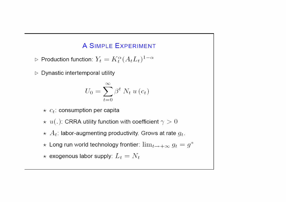
Gourinchas and Jeanne (2006)
- Look at the implications for capital account liberalization.
Focus on welfare benefits in response to capital scarcity.
- Calibrate variants of the standard (Ramsey-Koopman-Cass) model and com-
pare transition paths towards steady state under two scenarios:
- financial autarky;
- perfect financial integration with the rest of the world (small open economy).


Dynamic of consumption: autarky

With financial integration: If this is a poor country and ROW in SS:
Euler equation becomes: ct = ct+1(βR∗)−1/γ
so consumption grows at g∗ when country is financially integrated.
Capital stock jumps to its steady state level. Why?

Dynamic of consumption: autarky versus integration

How much gain?
Calculate equivalent variation µ defined as the % (permanent) increase in con-
sumption that brings domestic welfare under autarky up to its level under inte-
gration.
Calibration:
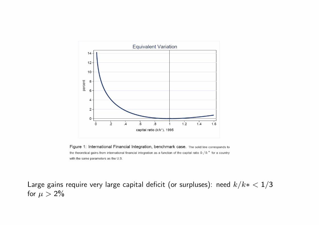
Large gains require very large capital deficit (or surpluses): need k/k∗ < 1/3for µ > 2%

This despite (temporary) gains in growth (consistent with literature: after eq-
uity market liberalization, GDP growth increases by 1% over the next 5 years)
Basic intuition: the distorsion from financial autarky is transitory in nature (the
distorsion disappears anyway)
- either speed of convergence is fast (Ramsey) and not much gain from going
fast to SS
- or the problem is not convergence but the level of the SS level of capital,
consumption...

Limits and potential extensions to the neoclassical model
Deterministic view: risk affects the steady state level of capital stock (precau-
tionary savings). Hence, financial integration by providing risk sharing oppor-
tunities modifies the steady state. Can go either way in terms of welfare (see
Coeurdacier, Rey and Winant (2011) for a concept of ’risky steady-state’ and
Coeurdacier, Rey and Winant (2013) for the welfare gains of integration with
production & risk).
Absence of financial frictions: capital scarcity can be due to credit constraints.
If financial integration alleviates credit constraints, can generate permanent
welfare gains.
Possibility of non-convexities (poverty traps).
Financial integration and international risk-sharing: an introduction
- Other gains from financial integration: allow countries to diversify risks and
stabilize consumption.
- Empirical evidence: hard to reconcile with the data though.
1) some (but scarce) evidence financial integration reduces volatility of con-
sumption (small impact and financial integration increases the probability of
crisis)
2) risk-sharing predicts high consumption correlation across countries. But
smaller in the data than the correlation of output. "The quantity puzzle".
(much more on this in lectures 7-9).

A basic model of international risk-sharing
Set-up
Two symmetric countries (H) and (F ). One good (numeraire)
2 periods: t = 0 et t = 1
2 states of the world in each country (s = {rain, sun}) with equal probabilities
= 12;
p = probability that the weather is the same in both countries (rain or sun);
0 ≤ p ≤ 1.

A basic model of international risk-sharing
Set-up
Representative agent in country (i = H,F ) owns a project at t = 0.
At t = 1 project delivers yrain = (1 + ε) if s = {rain} and ysun = (1− ε)
if s = {sun}.
At t = 1, uncertainty is realized and agents consume according to a standard
CRRA utility:
u(c) =c1−σ
1− σ
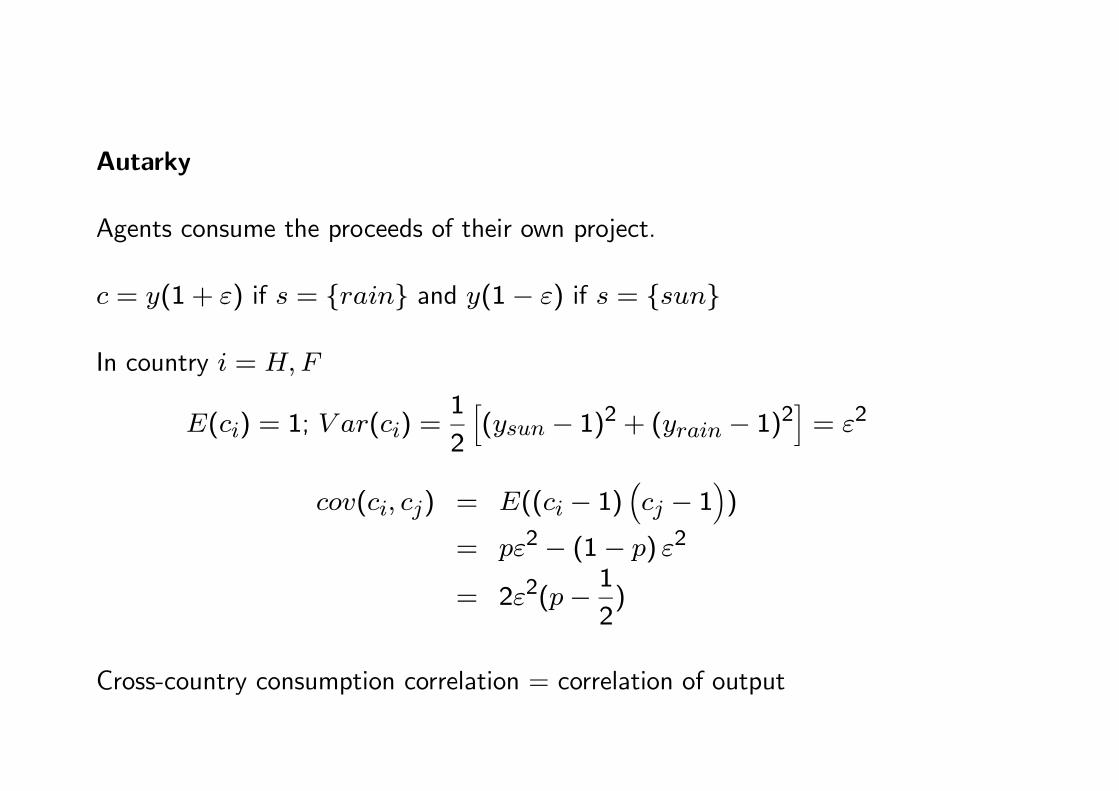
Autarky
Agents consume the proceeds of their own project.
c = y(1 + ε) if s = {rain} and y(1− ε) if s = {sun}
In country i = H,F
E(ci) = 1; V ar(ci) =1
2
�(ysun − 1)
2 + (yrain − 1)2�= ε2
cov(ci, cj) = E((ci − 1)�cj − 1
�)
= pε2 − (1− p) ε2
= 2ε2(p−1
2)
Cross-country consumption correlation = correlation of output
Financial integration
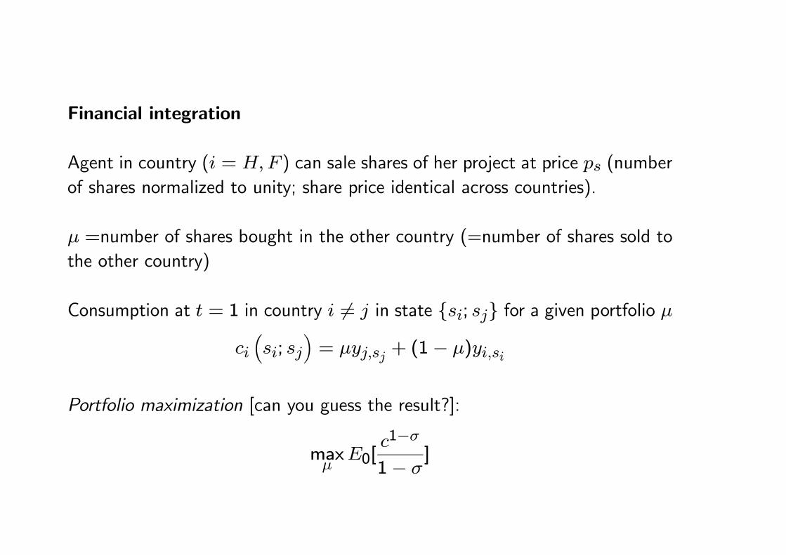
Agent in country (i = H,F ) can sale shares of her project at price ps (number
of shares normalized to unity; share price identical across countries).
µ =number of shares bought in the other country (=number of shares sold to
the other country)
Consumption at t = 1 in country i �= j in state {si; sj} for a given portfolio µ
ci�si; sj
�= µyj,sj + (1− µ)yi,si
Portfolio maximization [can you guess the result?]:
maxµ
E0[c1−σ
1− σ]

[Technical steps towards the solution]
E0[c1−σ
1−σ ] =p2
�(1+ε)1−σ
1−σ+(1−ε)1−σ
1−σ�
+1−p2
�(µ(1+ε)+(1−µ)(1−ε))
1−σ
1−σ+(µ(1−ε)+(1−µ)(1+ε))
1−σ
1−σ�
E0[c1−σ
1−σ ] =p2
�(1+ε)1−σ
1−σ+(1−ε)1−σ
1−σ�
+1−p2
�(1−ε+2µε)
1−σ
1−σ+(1+ε−2µε)
1−σ
1−σ�
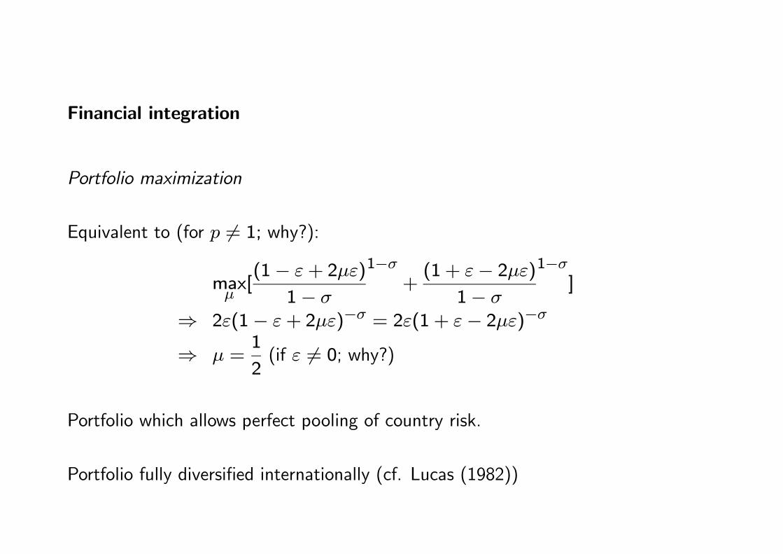
Financial integration
Portfolio maximization
Equivalent to (for p �= 1; why?):
maxµ[(1− ε+ 2µε)
1− σ
1−σ
+(1 + ε− 2µε)
1− σ
1−σ
]
⇒ 2ε(1− ε+ 2µε)−σ = 2ε(1 + ε− 2µε)−σ
⇒ µ =1
2(if ε �= 0; why?)
Portfolio which allows perfect pooling of country risk.
Portfolio fully diversified internationally (cf. Lucas (1982))

Financial integration
In country i = H,F
E(ci) = 1; V ar(ci) =p
2
�(ysun − 1)
2 + (yrain − 1)2�= pε2
As long as p < 1, volatility of consumption falls with respect ot autarky: welfaregains from risk sharing due to risk diversification (gains are higher when p islow).
Note that consumption is not constant (there is still world aggregate risk unlessp = 0).
cH = cF in all states
Perfect correlation of consumption across countries. In particular higher thanoutput correlation.

Welfare implications
Income smoothing across states provide positive welfare gains. Financial inte-
gration complete financial markets. How big are these gains?
Small if one looks at consumption and standard CRRA preferences (unless very
large coefficient of risk aversion). Similar to Lucas calculations about the gains
from removing business cycles.
But asset prices extremely volatile: welfare gains implied by asset prices usually
larger.
Still hard to reconcile both views (see Lewis (2000)).

Implications of financial integration and discussion of the evidence
1) Risk diversification lowers consumption volatility. Scarce evidence and small
effects but yes (see Bekaert et al. (2006)). Issue: also seems to increase the
probability of crisis.
2) Raises consumption correlation (and in particular above output correlation).
Consumption far to be perfectly correlated across countries in the data. Points
the lack of risk sharing but at least countries which exhibit higher degree of
integration have higher correlation of consumption (see Imbs (2006)).
3) Risk diversification implies full international portfolio diversification. Not true
in the data although international portfolio diversification has been increasing
over the last two decades. Investors still holds a disproportionate share of local
assets: Home bias in equities (French and Poterba (1991)).

The limits of financial integration
- Consumption correlation across countries quite low and lower than output for
most countries ("Quantity Puzzle"; see lectures 11-12)
- Home bias in equity puzzle
Investors tend to hold a disproportionate share of their local assets. Goes
against the view of a large decrease in barriers to international investments;
unless it is actually optimal to hold undiversified portfolios.
Note: Useful measure of Home Bias:
HB = 1− Share of Foreign of Equity HoldingsShare of Foreign Stocks in World Market Capitalisation . Why?


0.5
0.6
0.7
0.8
0.9
1
1988 1989 1990 1991 1992 1993 1994 1995 1996 1997 1998 1999 2000 2001 2002 2003 2004 2005
Europe
North America
Oceania
Japan
Home Bias (HB) across time for selected regions

Financial markets, risk diversification and growth
- International financial markets provide risk diversification (risk sharing).
- Saint Paul (1993) and Obstfeld (1994) go one step further: risk diversification
allows more risk taking towards more productive activities (specialization).
(see also Acemoglu and Fabrizio Zilibotti (1997))
- Financial integration improves the risk/return of savers
=⇒ risk taking/specialization
=⇒ growth effect of integration beyond standard neoclassical and risk-sharing
effects

Risk-taking and financial integration
adapted from Saint Paul (1993)
Set-up
One country (H) and 2 technologies of production (1 and 2)
2 states of the world (s = 1 or 2) with equal probabilities
2 periods: t = 0 et t = 1
Entrepreneurs have one unit of capital at t = 0
Production technologies are risky with constant return to scale

- technology 1 pays at t = 1 in state s = 1 (proba = 12) and gives R per unit
of capital invested at t = 0 (and gives 0 is state s = 2))
- technology 2 pays at t = 1 in state s = 2 (proba = 12) and gives r per unit
of capital invested at t = 0 (and gives 0 is state s = 1))
We assume r < R (H is more efficient in technology 1)
At t = 0, entrepreneurs invest their inital dotation in each technology (tech-
nological choice)
θ (resp. (1− θ)) = capital invested in technology 1 (resp. 2).

At t = 1, uncertainty is realized and entrepreneurs consume according to astandard CRRA utility:
u(c) =c1−σ
1− σ
1) Autarky
Technological choice
maxθ
E0[c1−σ
1− σ] = max
θ(1
2
(Rθ)
1− σ
1−σ
+1
2
(r(1− θ))
1− σ
1−σ
)
Optimal technological choice satisfies θ∗
θ∗
1− θ∗= (
r
R)1−
1σ ⇒ θ∗ =
( rR)1−1σ
1 + ( rR)1−1σ
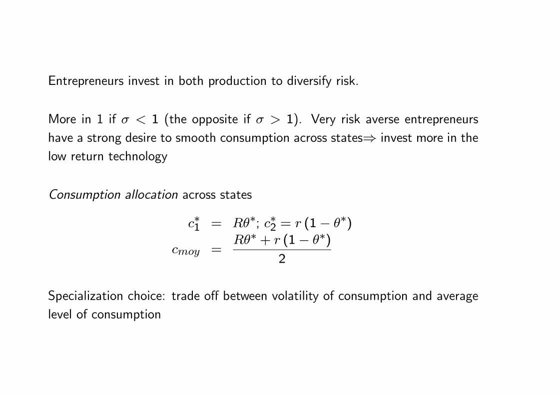
Entrepreneurs invest in both production to diversify risk.
More in 1 if σ < 1 (the opposite if σ > 1). Very risk averse entrepreneurs
have a strong desire to smooth consumption across states⇒ invest more in the
low return technology
Consumption allocation across states
c∗1 = Rθ∗; c∗2 = r (1− θ∗)
cmoy =Rθ∗ + r (1− θ∗)
2
Specialization choice: trade off between volatility of consumption and average
level of consumption
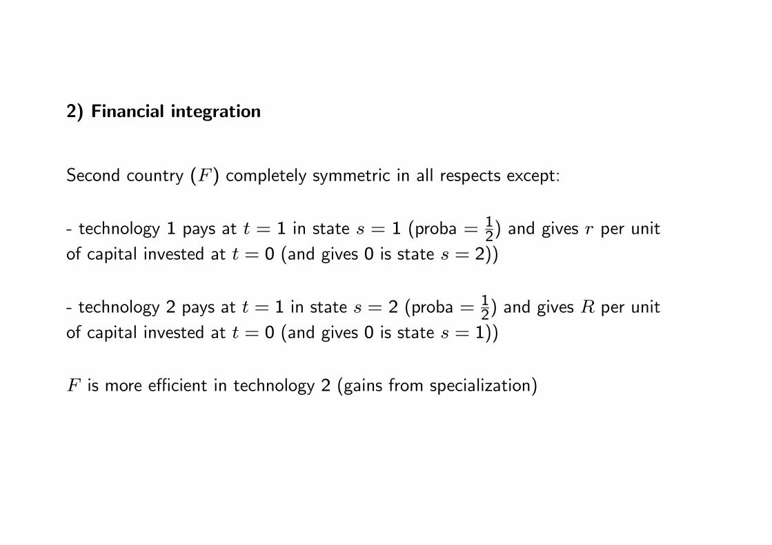
2) Financial integration
Second country (F ) completely symmetric in all respects except:
- technology 1 pays at t = 1 in state s = 1 (proba = 12) and gives r per unit
of capital invested at t = 0 (and gives 0 is state s = 2))
- technology 2 pays at t = 1 in state s = 2 (proba = 12) and gives R per unit
of capital invested at t = 0 (and gives 0 is state s = 1))
F is more efficient in technology 2 (gains from specialization)

Entrepreneurs can buy and sell claims on future output (portfolio choice made
at t = 0) in international financial markets. Buying µ shares of firms in country
H gives right to a share µ of country H production at t = 1 (number of shares
normalized to unity). Idem for country F . Before trading claims, entrepreneurs
hold all the shares of the country.
Same technological choice as earlier. Once technological choice has been made,
entrepreneurs trade shares of their firms with foreigners.
We denote by µ the number of shares of country H held by entrepreneurs in
countryH (and (1−µ) the number of shares held in country F by entrepreneurs
in country H).

Portfolio choice for a given θ
Due to symmetry if country H chooses to invest θ in technology 1, country F
chooses to invest θ in technology 2
Portfolio choice maximization:
maxµ
E0[c1−σ
1− σ]
maxµ(1
2
(µRθ + (1− µ)r(1− θ))
1− σ
1−σ
+1
2
(µr(1− θ) + (1− µ)Rθ)
1− σ
1−σ
)

Portfolio choice for a given θ
FOC:
(Rθ − r(1− θ))�u′(c1)− u′(c2)
�= 0⇒ c1 = c2
Then:
µRθ + (1− µ)r(1− θ) = µr(1− θ) + (1− µ)Rθ ⇒ µ =1
2
Perfect pooling of risk.
Such a portfolio allows optimal risk diversification for any value of θ
Technological choice
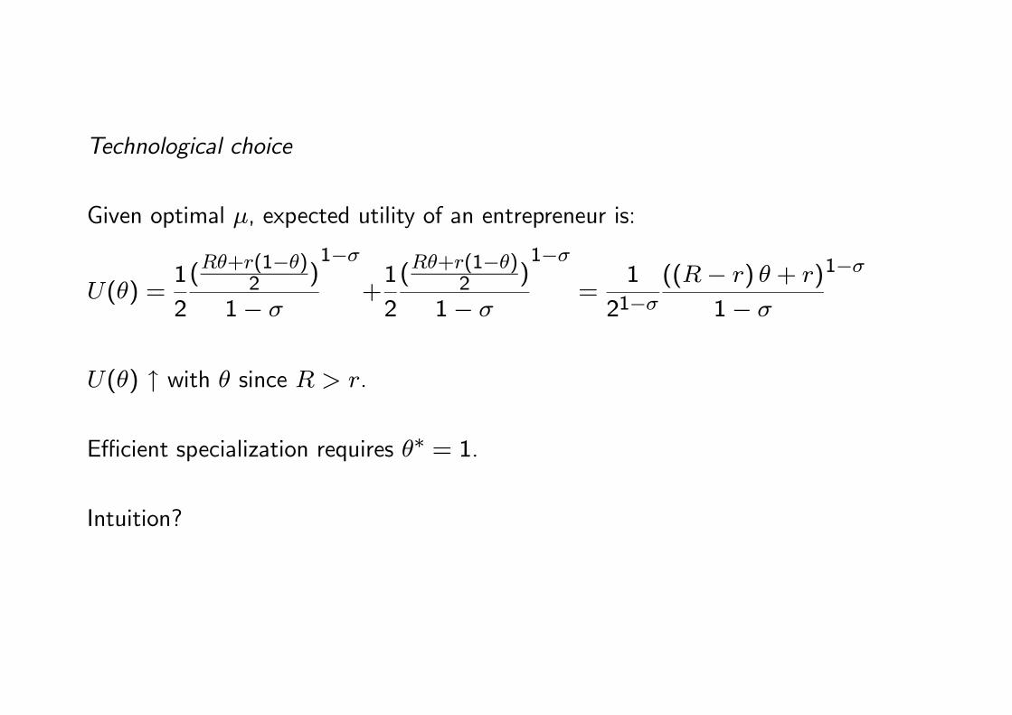
Given optimal µ, expected utility of an entrepreneur is:
U(θ) =1
2
(Rθ+r(1−θ)
2 )
1− σ
1−σ
+1
2
(Rθ+r(1−θ)
2 )
1− σ
1−σ
=1
21−σ
((R− r) θ + r)
1− σ
1−σ
U(θ) ↑ with θ since R > r.
Efficient specialization requires θ∗ = 1.
Intuition?
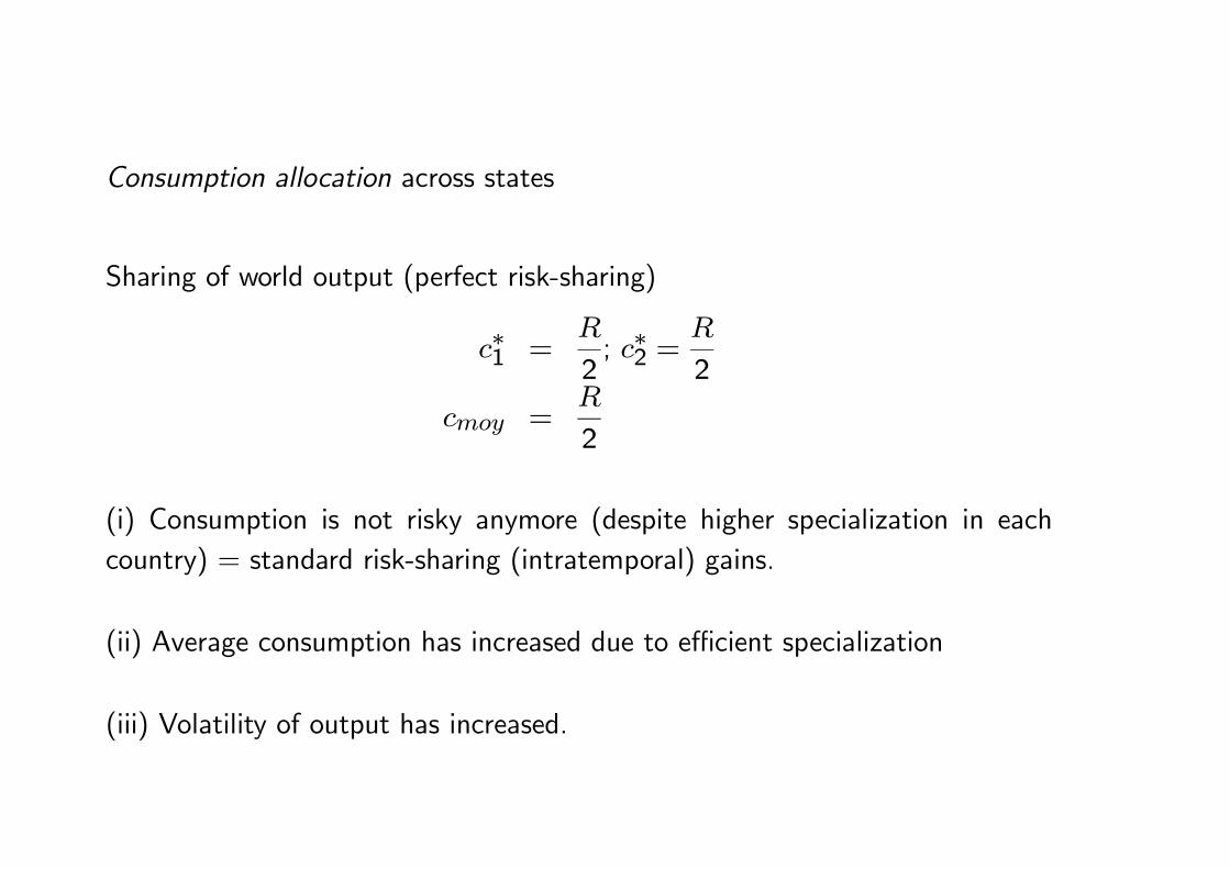
Consumption allocation across states
Sharing of world output (perfect risk-sharing)
c∗1 =R
2; c∗2 =
R
2
cmoy =R
2
(i) Consumption is not risky anymore (despite higher specialization in each
country) = standard risk-sharing (intratemporal) gains.
(ii) Average consumption has increased due to efficient specialization
(iii) Volatility of output has increased.
Risk diversification, risk taking and growth: empirical evidence?
Very scarce, only indirect evidence but...
Kalemli-Ozcan„ Sorensen and Yosha (2003)
Hypothesis tested:
Two regions better integrated financially are more specialized as they can share
risks better.
Sample of non-EU OECD countries and regions within countries for EU, Canada,
US.

Two stages:
1) measure the degree of "lack of risk-sharing" (=sensitivity of incomes to local
output =β1) in a given region (i):
∆logPINCit� � incomes
= αt + β1ilogGDPit� � output
+ ǫit
Risk-sharing is measured by βKi = 1− β1i
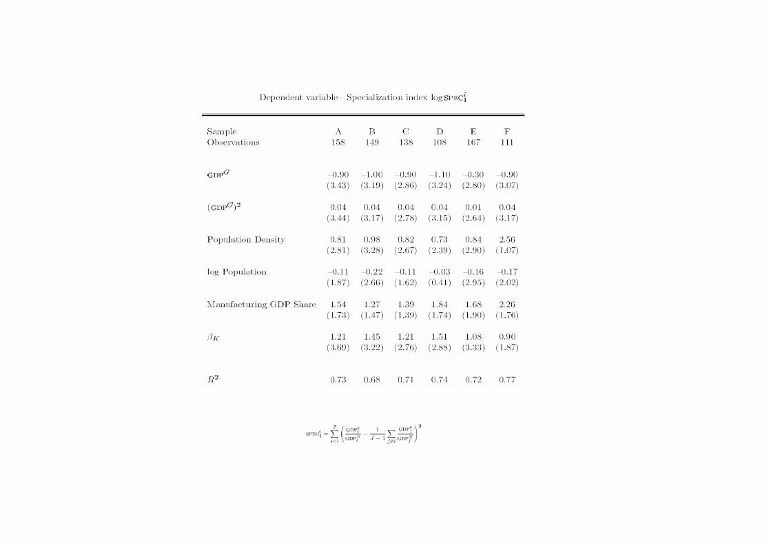
2) investigates the impact of (βKi = 1− β1i) on regions specialization (under
the assumption that countries devote more ressources to sectors where they are
the most productive). Specialization Herfindahl Index at 2-digits ISIC category.

Empirical issues
Endogeneity: more specialization of countries can increase the need for financial
integration and risk sharing (reverse causality).
Use variables related to financial development (such as shareholder rights, the
size of the financial sector (relative to GDP), legal systems) as instruments for
the amount of risk sharing βKi.
Similar findings.
Risk diversification, risk taking and growth: empirical evidence?
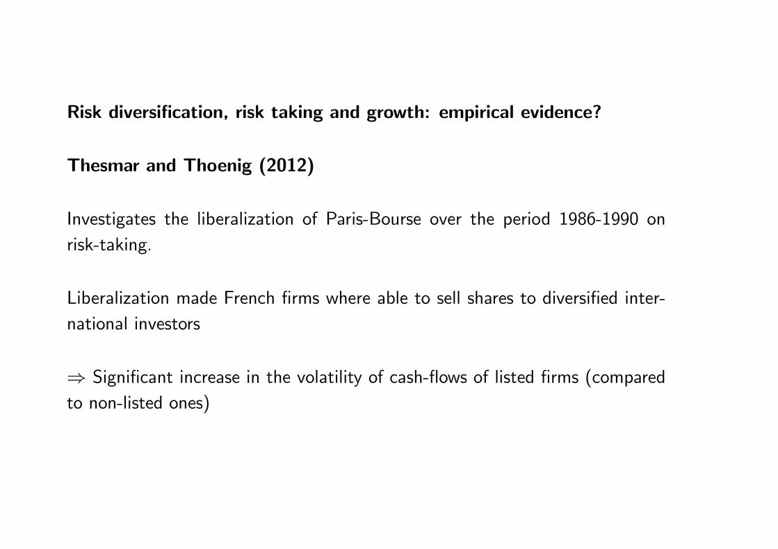
Thesmar and Thoenig (2012)
Investigates the liberalization of Paris-Bourse over the period 1986-1990 on
risk-taking.
Liberalization made French firms where able to sell shares to diversified inter-
national investors
⇒ Significant increase in the volatility of cash-flows of listed firms (compared
to non-listed ones)


Risk diversification, risk taking and growth: empirical evidence?
Kalemli-Ozcan, Sorensen. and Volosovych (2010)
Similar evidence: Firms with more diversified (international ownership) are more
volatile sales growth and operating revenues.
Large sample of firms in Europe (AMADEUS) over 1996-2006. 16 countries
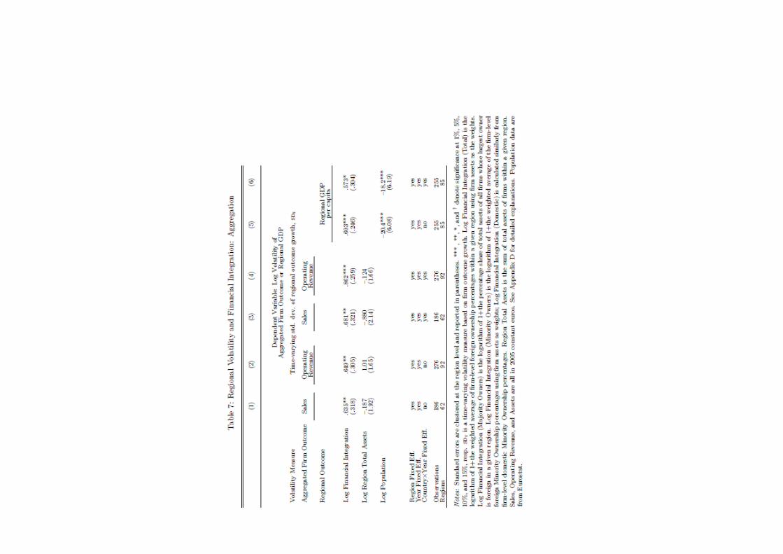
Important additional finding: result survives when ’aggregating up’ at the
macro-level (regional level). Not obvious à priori, why?
Control as much as possible for reverse causality by controlling for firm FE and
also using IV (’exogenous’ harmonization of financial regulation between EU
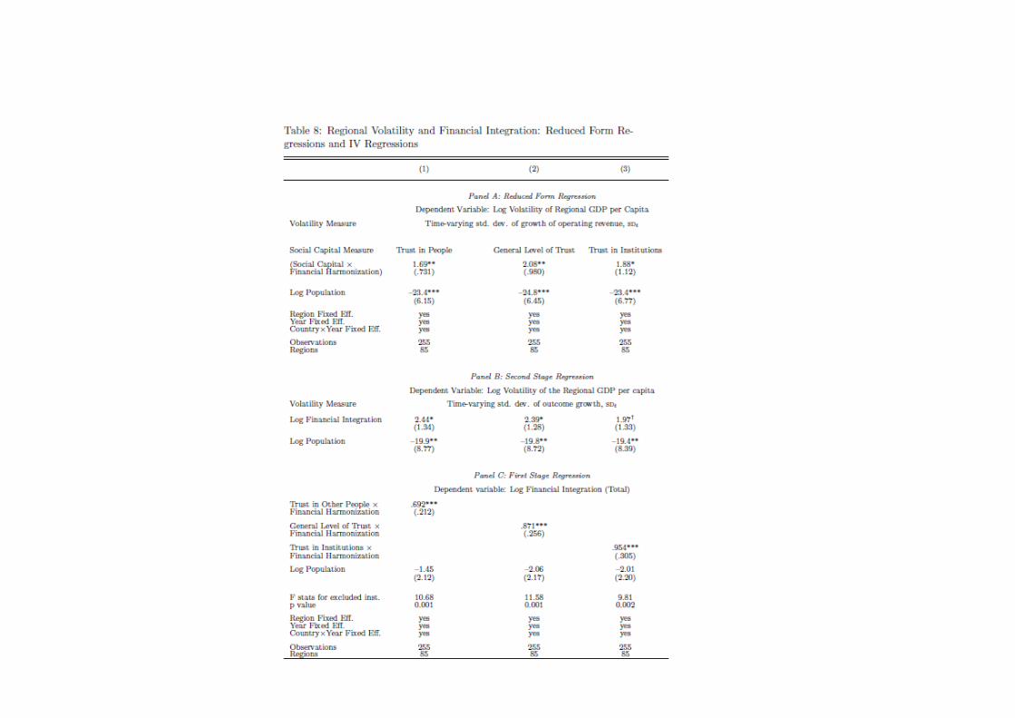
countries and ’trust’).

Cross-sectional regressions
Firm i in region j in country c and sector s
log(V OLijc) = µc + µs + α log(1 + FOijc) + δXijc + εijc
V OLijc = average measure of firm-level volatility
FOijc = % of foreign ownership (also use dummies when largest shareholder
is foreign)
µc, µs country and sector dummies, Xijc set of control variables


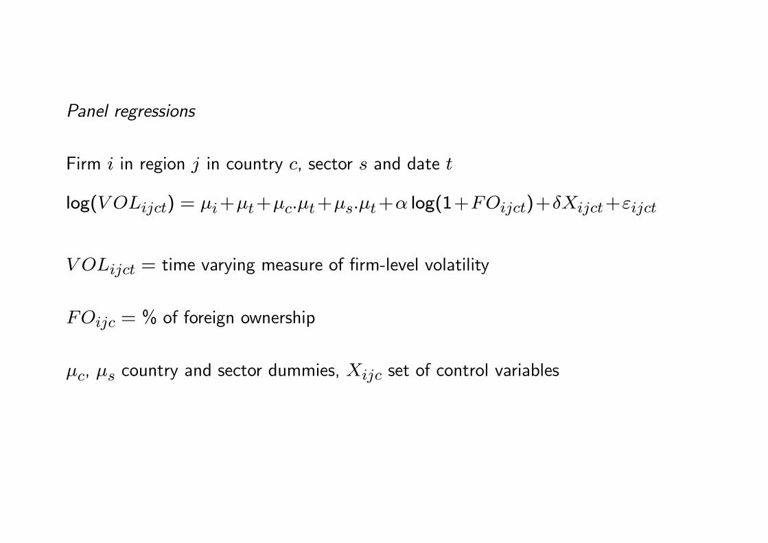
Panel regressions
Firm i in region j in country c, sector s and date t
log(V OLijct) = µi+µt+µc.µt+µs.µt+α log(1+FOijct)+δXijct+εijct
V OLijct = time varying measure of firm-level volatility
FOijc = % of foreign ownership
µc, µs country and sector dummies, Xijc set of control variables

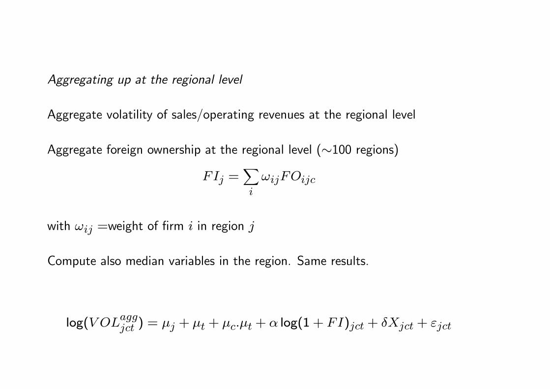
Aggregating up at the regional level
Aggregate volatility of sales/operating revenues at the regional level
Aggregate foreign ownership at the regional level (∼100 regions)
FIj =�
i
ωijFOijc
with ωij =weight of firm i in region j
Compute also median variables in the region. Same results.
log(V OLaggjct ) = µj + µt + µc.µt + α log(1 + FI)jct + δXjct + εjct

Related Documents