International Journal of Fracture Fatigue & Wear Volume 4, 2016 ISSN 2294-7868 Editor in chief: Professor Magd Abdel Wahab © Labo Soete, Universiteit Gent

Welcome message from author
This document is posted to help you gain knowledge. Please leave a comment to let me know what you think about it! Share it to your friends and learn new things together.
Transcript

International Journal of
Fracture Fatigue & Wear
Volume 4, 2016
ISSN 2294-7868
Editor in chief: Professor Magd Abdel Wahab
© Labo Soete, Universiteit Gent

International Journal of Fracture Fatigue and Wear: Conference Series proceedings Volume 4, 2016
Published by
Laboratory Soete – Ghent University
Technologiepark Zwijnaarde 903
B-9052 Zwijnaarde, Belgium
http://www.soetelaboratory.ugent.be/
Edited by: Professor Magd Abdel Wahab
ISSN: 2294-7868
Proceedings of 5th International Conference on
Fracture Fatigue and Wear, FFW 2016, Kitakyushu,
Japan, 24-26 August 2016
International Journal of Fracture Fatigue and Wear, Volume 4
ii
5th International Conference on Fracture Fatigue and Wear, FFW
2016, Kitakyushu, Japan, 24-26 August 2016
Chairman
Professor Magd Abdel Wahab Laboratory Soete, Ghent University
Belgium
Co-chairman Professor Nao-Aki Noda
Kyushu Institute of Technology Japan
Local Organizing Committee
Prof. N-A Noda, Kyushu Institute of Technology, Japan Prof. H Sakamoto, Kumamoto University, Japan
Prof. M Endo, Fukuoka University, Japan Prof. M Goto, Oita University, Japan
Prof. C Makabe, University of Ryukyu, Japan Prof. A Saimoto, Nagasaki University, Japan
Prof. K Oda, Oita University, Japan Prof. G Hotta, National Institute of Technology, Ariake College, Japan
Prof. T Miyazaki, University of Ryukyu, Japan Prof. K Ushijima, Tokyo University of Science, Japan Dr. Y Sano, Kyushu Institute of Technology, Japan
Prof. S Nishida, Saga University, Japan Dr. K Masuda, University of Toyama, Japan
Dr. Y Takase, Kyushu Institute of Technology, Japan
International Scientific Committee Prof. S Abdullah, Universiti Kebangsaan Malaysia, Malaysia
Dr. J Abenojar, Universidad Carlos III de Madrid, Spain Prof. D Bigoni, University of Trento, Italy
Dr. H Boffy, University of Twente, Netherlands Prof. S Bordas, University of Luxembourg, Luxembourg
Dr. R Das, University of Auckland, New Zealand Dr. A Ertas, Karabuk University, Turkey
Dr. S Fouvry, Ecole Centrale de Lyon, France Prof. T Hattori, Shizuoka Institute of Science and Technology, Japan
Dr. K Masuda, University of Toyama, Japan Prof. T Miyazaki, University of Ryukyu, Japan
Prof. K Oda, Oita University, Japan Prof. RV Prakash, Indian Institute of Technology, India
Prof. T Qin, China Agricultural University, China Prof. F Rezai-Aria, Ecole des Mines d'Albi, France
Dr. A Rudawska, Lublin University of Technology, Poland Dr. Y Sano, Kyushu Institute of Technology, Japan Prof. J Song, Ostwestfalen-Lippe University, Germany
Prof. J Toribio, University of Salamanca, Spain Prof. C Xu, China Agricultural University, China
Prof C Zhou, Nanjing University of Aeronautics and Astronautics, China
International Journal of Fracture Fatigue and Wear, Volume 4
iii
Editorial
The fourth volume of the International Journal of Fracture Fatigue and Wear contains the proceedings of the fifth International Conference of Fracture Fatigue and Wear (FFW) held in Kitakyushu, Japan, 24-26 August 2016.
The organising committee is grateful to Professor Toshio Hattori, Department of Mechanical Engineering, Faculty of Science and Technology, Shizuoka Institute of Science and Technology, Japan, for agreeing to deliver the keynote lecture, entitled ‘Fatigue process, stress analysis and strength evaluation’, at the opening of the conference.
The sponsorship of Soete laboratory, Ghent University (Belgium), Kyushu Institute of Technology (Japan) and several Japanese companies is highly appreciated.
Most of the papers published in this volume have been sent to reviewers, who are members of Scientific Committee of FFW 2016, to judge their scientific merits. Based on the recommendation of reviewers and the scientific quality of the research work, the papers were accepted for publication in the conference proceedings and for presentation at the conference venue. The organizing committee would like to thank all members of Scientific Committee for their valuable contribution in evaluating the papers.
The efforts of the local organizers of FFW 2016 at Kyushu Institute of Technology, Japan, the team of Professor Nao-Aki Noda, are highly acknowledged.
Finally, the editor would like to thank to all authors, who have contributed to this volume and presented their research work at FFW 2016.
The Editor Professor Magd Abdel Wahab
International Journal of Fracture Fatigue and Wear, Volume 4
iv
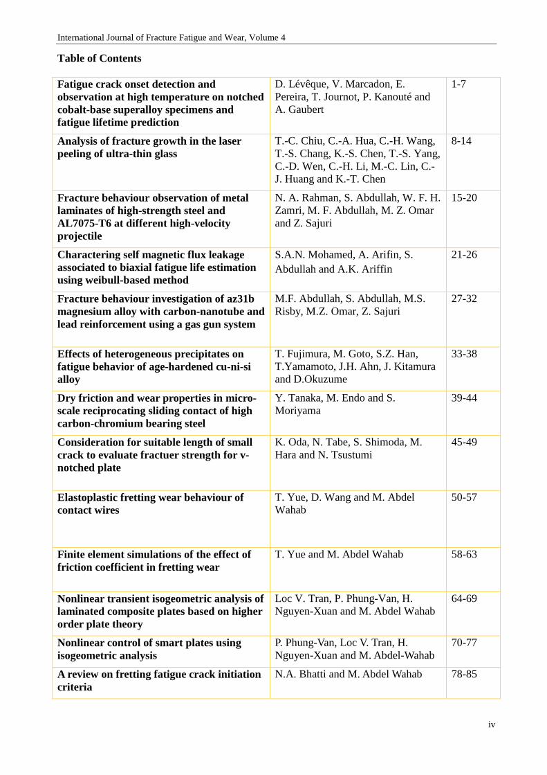
Table of Contents Fatigue crack onset detection and observation at high temperature on notched cobalt-base superalloy specimens and fatigue lifetime prediction
D. Lévêque, V. Marcadon, E. Pereira, T. Journot, P. Kanouté and A. Gaubert
1-7
Analysis of fracture growth in the laser peeling of ultra-thin glass
T.-C. Chiu, C.-A. Hua, C.-H. Wang, T.-S. Chang, K.-S. Chen, T.-S. Yang, C.-D. Wen, C.-H. Li, M.-C. Lin, C.-J. Huang and K.-T. Chen
8-14
Fracture behaviour observation of metal laminates of high-strength steel and AL7075-T6 at different high-velocity projectile
N. A. Rahman, S. Abdullah, W. F. H. Zamri, M. F. Abdullah, M. Z. Omar and Z. Sajuri
15-20
Charactering self magnetic flux leakage associated to biaxial fatigue life estimation using weibull-based method
S.A.N. Mohamed, A. Arifin, S. Abdullah and A.K. Ariffin
21-26
Fracture behaviour investigation of az31b magnesium alloy with carbon-nanotube and lead reinforcement using a gas gun system
M.F. Abdullah, S. Abdullah, M.S. Risby, M.Z. Omar, Z. Sajuri
27-32
Effects of heterogeneous precipitates on fatigue behavior of age-hardened cu-ni-si alloy
T. Fujimura, M. Goto, S.Z. Han, T.Yamamoto, J.H. Ahn, J. Kitamura and D.Okuzume
33-38
Dry friction and wear properties in micro-scale reciprocating sliding contact of high carbon-chromium bearing steel
Y. Tanaka, M. Endo and S. Moriyama
39-44
Consideration for suitable length of small crack to evaluate fractuer strength for v-notched plate
K. Oda, N. Tabe, S. Shimoda, M. Hara and N. Tsustumi
45-49
Elastoplastic fretting wear behaviour of contact wires
T. Yue, D. Wang and M. Abdel Wahab
50-57
Finite element simulations of the effect of friction coefficient in fretting wear
T. Yue and M. Abdel Wahab
58-63
Nonlinear transient isogeometric analysis of laminated composite plates based on higher order plate theory
Loc V. Tran, P. Phung-Van, H. Nguyen-Xuan and M. Abdel Wahab
64-69
Nonlinear control of smart plates using isogeometric analysis
P. Phung-Van, Loc V. Tran, H. Nguyen-Xuan and M. Abdel-Wahab
70-77
A review on fretting fatigue crack initiation criteria
N.A. Bhatti and M. Abdel Wahab 78-85
International Journal of Fracture Fatigue and Wear, Volume 4
v
Predicting residual stress in welds using empirical and reconstructive methods
J. Ni and M. Abdel Wahab
86-92
Effects of graphite and artificial defects on the fatigue strength of ferritic-pearlitic ductile cast iron
T. Deguchi, T. Matsuo, S. Takemoto, T. Ikeda and M. Endo
93-98
Evaluation of adhesive strength based on the intensity of singular stress field of single lap joint
R. Li, N.A. Noda, Y. Sano, T. Miyazaki, K. Iida and Y. Takase
99-103
T convenient debonding strength evaluation for spray coating based on intensity of singular stress
Z. Wang, N.A. Noda, Y. Sano, Y. Takase and K. Iida
104-108
Design and performance of honeycomb structure for nanobubbles generating apparatus
Nao-Aki Noda, Fei Ren, Wataru Yamamoto, Yoshikazu Sano, Dai-Hen Chen and Yuuji Yonezawa
109-113
Influence of strain rate for notch- bend strength on ductile cast iron
T. Ikeda, T. Umetani, N. Kai, N-A. Noda and Y. Sano
114-119
Effect of low-pressure plasma treatment on surface modification and friction coefficient of poly-(methyl-methacrylate)
J. Abenojar, P. Gálvez and M.A. Martínez
120-125
Contact area actual self-friction in polyolefins
M.A. Martinez and J. Abenojar 126-132
Study on test of fatigue crack growth rate along the weld line
Z. Qian and R. Zhang 133-138
Fatigue analysis of an aluminium Alloy Wheel in the Dynamic Radial fatigue test by using Finite Element Analysis
W. Phusakulkajorn, R. Naewngerndee, S. Sucharitpwatskul, A. Malatip and S. Otarawanna
139-145
Bending fatigue strength of annealed 0.45% carbon steel specimens finished by cutting and rubbing techinque utilizing cemented carbide tip
T. Yakushiji, F. Nakagawa and M. Goto
146-152
Loading frequencies effects on the oxide-induced crack closure in extremely low stress intensity factor range
K. Tazoe, M. Oka and G. Yagawa 153-157
Fretting wear and fretting corrosion of electrical contacts
Haomiao Yuan, Jian Song and Vitali Schinow
158-165
Analysis of intensity of singular stress field for bonded cylinder under bending load
T. Miyazaki and N. -A. Noda
166-171
Fatigue behavior of flexurally strengthened FRP concrete structures
H. A. Toutanji, R. Vuddandam, D. Wang, M. Hussak
172-177
Fatigue crack growth behavior of specimen with grooves cut along loading direction
C. Makabe 178-183

International Journal of Fracture Fatigue and Wear, Volume 4
vi
Non-ductile failure analysis of steam generator tube sheet based on different standards and codes
Chang Liu, Hao Qian, Xingyun Liang and Yongcheng Xie
184-193
Estimation of the maximum bending moment of U-section beams
K. Masuda
194-199
Structural health monitoring via using transmissibility coherence
Yun-Lai Zhou, Xiaobo Yang and Magd Abdel Wahab
200-203
Parallelization approaches for fretting fatigue simulation
R. Trobec, M. Depolli, G. Kosec, S. Bordas, S. Tomar, K. Pereira and M. Abdel Wahab
204-208
Desired fatigue design code for railroad truck frame
Haruo Sakamoto 209-215
Mechanical properties of steel fibre reinforced polymer composites
W. N. M. Jamil, Z. Sajuri, M. A. Aripin, S. Abdullah, M. Z. Omar, M.F. Abdullah and W. F. H. Zamri
216-222
International Journal of Fracture Fatigue and Wear, Volume 4
1
Proceedings of the 5th International Conference on Fracture Fatigue and Wear, pp. 1-7, 2016
FATIGUE CRACK ONSET DETECTION AND OBSERVATION AT HIGH
TEMPERATURE ON NOTCHED COBALT-BASE SUPERALLOY
SPECIMENS AND FATIGUE LIFETIME PREDICTION
D. Lévêque1, V. Marcadon1, E. Pereira1, T. Journot1, P. Kanouté1 and A. Gaubert2
1 ONERA, 29 Avenue de la Division Leclerc, BP72, 92322 Châtillon Cedex, France 2 SNECMA (SAFRAN GROUP), 77550 Moissy-Cramayel, France
Abstract: The cobalt-base superalloy Haynes 188 is currently used in military and commercial aircraft turbine engines for combustor liners. In such applications, the components are subjected to repeated thermal stresses as a result of temperature gradients but also to local stress gradient effects due to the presence of cooling and dilution holes. Fatigue cracking is a major mode of failure in such parts. This work deals with gradient effects on fatigue lifetime prediction under isothermal low-cycle fatigue (LCF) condition. A fatigue test campaign was designed on different notched specimens to identify the onset and growth of cracks during cycling loads for two different temperatures (600°C and 900°C). A Potential Drop Technique (PDT) was used to measure continuously the crack length. Crack initiation detection and crack growth were also monitored optically. The use of a Digital Image Correlation (DIC) technique was found to be accurate enough to detect the crack tip and the crack length estimate was consistent with the PDT values. By the use of previously identified behaviour and damage fatigue models on this material, a finite element analysis (FEA) and a post-processing method, fatigue lifetimes on single-hole specimens were rather well predicted. A special care was taken to analyse the multi-axiality state of stresses around the holes.
Keywords: Low-cycle fatigue; Crack detection; Combustion chamber; Co-base superalloy; Lifetime
1 INTRODUCTION
Cobalt-base superalloys are widely used for aircraft engine combustion chamber applications. Such components are subjected to very high cyclic thermal gradients, which results from start-up and shut-down procedures. Moreover local mechanical stress gradients are superimposed due to the presence of cooling and dilution holes. A complex series of processes, involving crack propagation not only induced by fatigue, but also by creep and creep-fatigue interaction could cause the final failure of these high temperature components. This work deals with gradient effects on fatigue lifetime prediction under isothermal conditions with creep interaction. The co-base superalloy studied here, Haynes 188, is currently used in military and commercial aircraft turbine engines for combustor liners application. Such a material exhibits a complex viscoplastic behaviour including cyclic hardening and dynamic strain aging effects. A complete model was previously developed and identified for a large temperature range [1].
In this work, a fatigue test campaign has been designed on different notched plate specimens to identify the onset and growth of cracks during cycling loadings under isothermal LCF condition. To be representative of the combustion chamber issue, three different hole diameters were investigated. All the tests were performed under a 5 Hz repeated cycle with imposed stress levels calculated in order to obtain representative lifetimes. By the use of the previously identified model, finite element analyses with Z-set software [2] are performed in order to obtain the evolution of the mechanical stress and strain fields during cycling loadings. On the stabilised cycle a creep-fatigue damage model is applied as a post-processing to estimate the fatigue lifetimes on single-hole specimens. The results are compared to the experimental ones and discussed in terms of multi-axial and mean stress effects.
2 MATERIAL, SPECIMEN AND EXPERIMENTAL PROCEDURE
Haynes 188 (HA188) is a cobalt-base superalloy (39Co–22Ni–22Cr–14W, in weight percent) which possesses excellent high-temperature strength with very good oxidation resistance [3]. This alloy combines properties which make it suitable for a variety of gas turbine engines parts such as combustion cans,

International Journal of Fracture Fatigue and Wear, Volume 4
2
transition ducts and after-burner components. In our study, this material was provided by Snecma in the form of rolled plates (about 1.6 mm thick).
A fatigue test campaign was conducted on different notched rectangular specimens. To be representative of the combustion liner machining, three different hole diameters (from 0.4 to 4.0 mm) were realized on plate specimens (38 mm in width) by a laser drilling process (trepan mode for the larger holes and percussion mode for the smaller ones, both modes for the intermediate 1 mm hole diameter). As can be seen in Fig. 1, the laser drilling process implies a conical form of the hole through the thickness of the plates, less marked in the trepan mode (the diameter variation is then two times less between upper and lower specimen faces).
Percussion mode Trepan mode
Fig. 1 Face views and fractographic observations of a 1 mm diameter hole for both laser drilling modes
The isothermal low-cycle fatigue tests were conducted using a servo-hydraulic machine under a stress-controlled condition. All tests were performed under a 5 Hz repeated cycle with high and low imposed stress levels calculated in order to obtain representative lifetimes (Rσ = 0+). Specimens were heated up to 600°C or 900°C using a middle frequency induction system. The temperature was controlled by four thermocouples welded around the hole (Fig. 2) coupled with an IR pyrometer scanning the surface just above the hole free-edge.
A Potential Drop Technique (PDT) was used to measure continuously the crack length, the electric potential monitoring being synchronized with the maximum load of the cycle. Crack initiation detection and crack growth was also monitored optically. A CCD camera coupled with a long working distance microscope or a macro objective (for larger holes, see Fig. 2) was used to take high-resolved pictures of the close area to the hole.
Fig. 2 Experimental setup for crack detection during isothermal LCF testing
3 EXPERIMENTAL RESULTS
Fig. 3 compares the three methods used for the crack length assessment (here in the case of a LCF test on a specimen with a 4 mm hole diameter at T = 900°C): the direct optical observation, the Digital Image Correlation (DIC) technique and the Potential Drop Technique (PDT). In this last technique, Johnson [4] has proposed an analytical expression of the crack length estimate depending on both the measured potential

International Journal of Fracture Fatigue and Wear, Volume 4
3
variation and the geometrical parameters for a penny shape initial crack. We have used the same expression in our case taking care of calibrating this method by FE computation, being necessary for larger holes [5]. Concerning the direct observation, it may not be enough precise. Indeed, due to the elevated temperature, the image contrast remains low and a simple grey-scale threshold may not be sufficient to correctly assess the crack length. On the contrary the use of a Digital Image Correlation (DIC) technique was found to be more precise to detect the crack tip, using an in-house fast correlation code [6] and a discontinuity criterion to localize the crack path [7]. The crack length estimate was then more consistent with the PDT values (Fig. 3). Nevertheless, a gap persists between these methods and is due to the curvature of the crack front (see Fig. 4 for instance) that implies the mean crack length is always greater than the one measured on the surface of the specimens, whatever the method applied. The interest of the PDT method is that it catches the volumic response of the specimen, not only the surfacic one. Moreover, it seems more sensible to the smallest crack length. In that sense, this method can be considered as the reference method in particular to define a crack onset criterion, fixed at 300 µm in length in our case.
Fig. 4 shows at left the crack extension assessment by the PDT technique in the case of a LCF test conducted at 600°C on a 0.4 mm hole diameter plate. After the complete rupture, the through-the-thickness optical observation of the two parts (Fig. 4 at right) shows: (i) the curvature of the crack front as already discussed; (ii) the crack initiation site near the free edge of the hole particularly visible considering this is the most oxidised area; (iii) serrations appearing during the LCF test and (iv) some curved marks well identified on this fractography, each mark being relative to a sudden progress in the crack length. This kind of instability is well known as the Portevin and Le Châtelier (PLC) effect, many metallic materials experiencing such dynamic strain ageing (DSA) effects in some temperature and strain rate domains, around 600°C concerning the HA 188 material [1]. All the fractographic observations show the same serrations for the tests conducted at this temperature, whereas the fractographies are flat in the case of 900°C tests.
Fig. 3 Comparison of three methods to follow crack extension around a 4 mm hole diameter (T = 900°C)
Fig. 4 Crack extension and fractographic observation after LCF testing at 600°C (0.4 mm hole diameter)

International Journal of Fracture Fatigue and Wear, Volume 4
4
We have represented in Fig. 5 all the LCF test results in term of normalised nominal imposed stress as a function of the lifetime at the crack onset, i.e. when the mean crack length determined by the PDT estimate is over 300 µm in length. As usual, for greater cycle number, the final rupture is shortly consecutive to this initiation phase, the crack propagating rapidly through the specimen width. The first observation is that the laser drilling mode has few or no influence in the lifetime results (comparison for the 1 mm hole diameters). Moreover there is no apparent evidence of some gradient effect at 900°C (Fig. 5 at left) for this material: the lifetimes follow the same tendency whatever the hole diameter, although the stress gradients are different near the hole. In a previous study, such gradient effects were emphasised for a single crystal superalloy [8]. On the contrary a difference is appearing for the 600°C LCF tests (Fig. 5 at right) where the results on the larger hole diameter are slightly different from the others. It seems that the behaviour for this material at 900°C depends strongly on creep mechanisms, whereas there is more a competition between fatigue and creep mechanisms at 600°C.
Fig. 5 Normalised nominal stress vs. lifetimes (at 300 µm crack onset) at 900°C (left) and 600°C (right)
4 SIMULATION OF THE TESTS
The fatigue tests aforementioned have been simulated by using Z-set FE software [2]. It is usually observed for metallic materials a nonlinear damage evolution in fatigue and creep. The long lifetimes considered here allow then to assume that the behaviour of the material is not affected by damage mechanisms. The modelling approach has consisted in simulating 100 cycles of loading first (Fig. 6 at left). Then a post-processing has been used to estimate the lifetime from the characteristics of this hundredth cycle considered such as stabilised. This post-processing is based on the model FatFlu, proposed at Onera [9], which requires for multi-axial application the octahedric stress amplitude and the mean hydrostatic stress over the cycle as input data. Different expressions for the dependence on these quantities exist. In the present work the model parameters were identified in the case of both the Sines and Variant formulations [10,11].
Fig. 6 Evolution of the mechanical load at the critical point, where damage starts, when simulating
100 cycles on a 1 mm diameter single-hole specimen (left) and the corresponding FE mesh (at right).
International Journal of Fracture Fatigue and Wear, Volume 4
5
The definition of the stabilised cycle is very critical since the precision of the model predictions depends on it. This issue has been investigated by plotting the evolutions of the stress amplitude, the mean stress and there derivatives towards the number of cycles, according to the number of cycles. Here, because of the conic shape of the holes (Fig. 6 at right), the samples must have been simulated in 3D, inducing problems with about 200,000 degrees of freedom by using quadratic tetrahedrons. For each hole geometry we have considered a unique mesh by defining an average hole geometry for all the samples drilled in the same manner. However, the main computation costs came from the complexity of the elasto-viscoplastic behaviour law used for Haynes 188. Even by using multi-threading computations on four processors the modelling of the first hundred cycles took about five days at 900°C where the behaviour is the simplest. Consequently the number of 100 cycles was a good compromise in terms of computation times and accuracy of the lifetimes predicted numerically. At 600°C we did not succeed in making the computation converged and some works are in progress to solve this problem.
The results have shown that the lifetimes predicted at 900°C are rather close to those measured experimentally, especially when using the Variant formulation. In that case, the ratio between the numerical and experimental lifetime values remained lower than 7. And except for one test, in all other cases the modelling estimates were conservative which is crucial regarding the application.
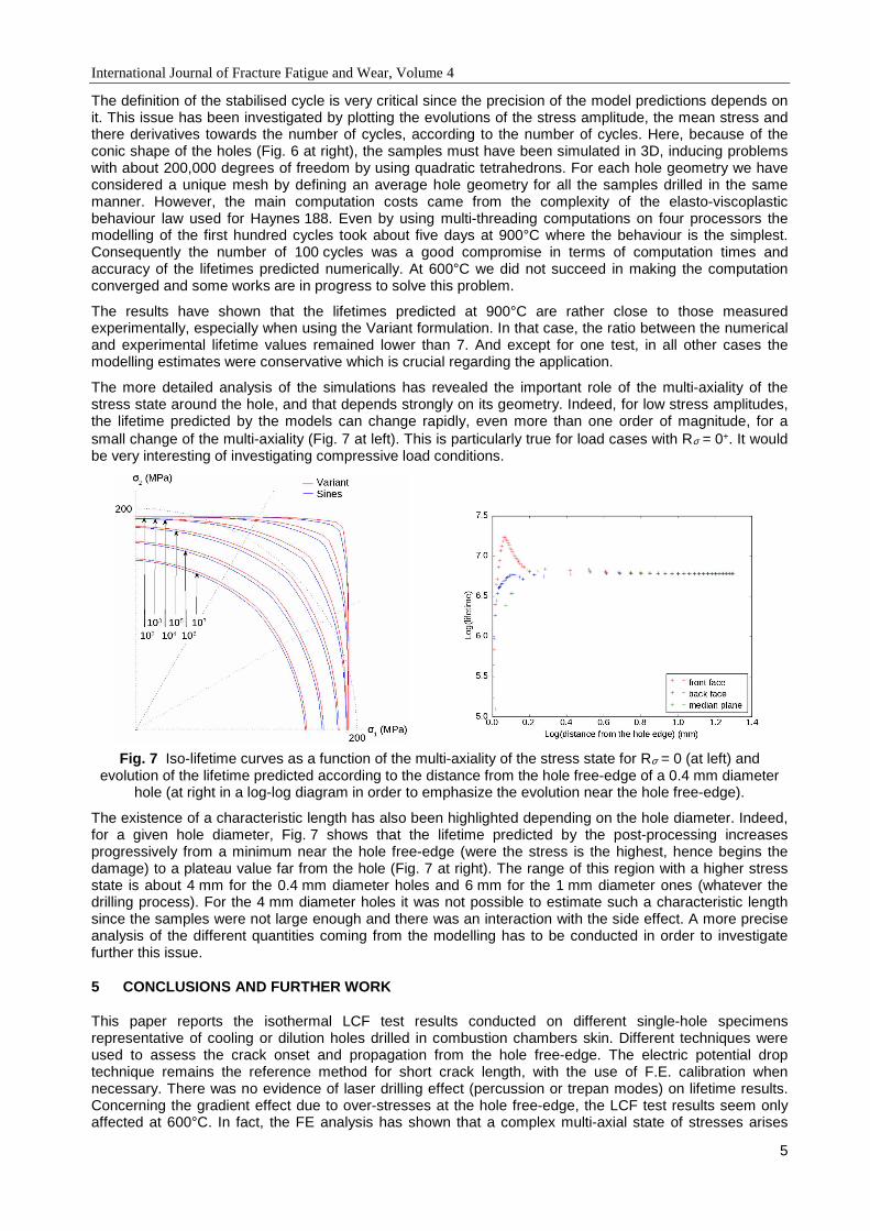
The more detailed analysis of the simulations has revealed the important role of the multi-axiality of the stress state around the hole, and that depends strongly on its geometry. Indeed, for low stress amplitudes, the lifetime predicted by the models can change rapidly, even more than one order of magnitude, for a small change of the multi-axiality (Fig. 7 at left). This is particularly true for load cases with Rσ = 0+. It would be very interesting of investigating compressive load conditions.
Fig. 7 Iso-lifetime curves as a function of the multi-axiality of the stress state for Rσ = 0 (at left) and evolution of the lifetime predicted according to the distance from the hole free-edge of a 0.4 mm diameter
hole (at right in a log-log diagram in order to emphasize the evolution near the hole free-edge).
The existence of a characteristic length has also been highlighted depending on the hole diameter. Indeed, for a given hole diameter, Fig. 7 shows that the lifetime predicted by the post-processing increases progressively from a minimum near the hole free-edge (were the stress is the highest, hence begins the damage) to a plateau value far from the hole (Fig. 7 at right). The range of this region with a higher stress state is about 4 mm for the 0.4 mm diameter holes and 6 mm for the 1 mm diameter ones (whatever the drilling process). For the 4 mm diameter holes it was not possible to estimate such a characteristic length since the samples were not large enough and there was an interaction with the side effect. A more precise analysis of the different quantities coming from the modelling has to be conducted in order to investigate further this issue.
5 CONCLUSIONS AND FURTHER WORK
This paper reports the isothermal LCF test results conducted on different single-hole specimens representative of cooling or dilution holes drilled in combustion chambers skin. Different techniques were used to assess the crack onset and propagation from the hole free-edge. The electric potential drop technique remains the reference method for short crack length, with the use of F.E. calibration when necessary. There was no evidence of laser drilling effect (percussion or trepan modes) on lifetime results. Concerning the gradient effect due to over-stresses at the hole free-edge, the LCF test results seem only affected at 600°C. In fact, the FE analysis has shown that a complex multi-axial state of stresses arises
International Journal of Fracture Fatigue and Wear, Volume 4
6
around the hole that has a significant influence on the lifetime prediction. However, even if comparison between the lifetimes predicted and those measured experimentally has not been performed yet at 600°C because of numerical problems, at 900°C it has shown rather good results.
In a further work, multiple-hole configurations will be investigated to be more representative of the combustion chamber configuration with the possible interaction between the different dilution and cooling holes, including anisothermal situations. Moreover a new lifetime prediction scheme will be proposed in order to take into account thermal gradients and multi-axial loading with a modelling of the holes network by a homogenised law.
6 ACKNOWLEDGEMENTS
DGAC is acknowledged for the funding of the French National Research Program “Hot Metallic Structures” involving Onera, Snecma & Turbomeca (SAFRAN Group) and several academic research teams.
S. Quilici, from Mines Paris-Tech, is gratefully acknowledged for his heavy work on numerical implementation of the Haynes 188 behaviour law in Z-set FE software.
7 REFERENCES
[1] J.-L. Chaboche, A. Gaubert, P. Kanouté, A. Longuet, F. Azzouz, M. Mazière, Viscoplastic
constitutive equations of combustion chamber materials including cyclic hardening and dynamic
strain aging, International Journal of Plasticity 46 (2013) 1-22.
[2] Z-set/Zebulon, Material and structure analysis suite, http://www.zset-software.com.
[3] HAYNES 188, datasheet on http://www.haynesintl.com/pdf/h3001.pdf.
[4] H. Johnson, Calibration method for the electric potential drop method for crack growth, Materials
Research and Standards, vol. 5, pp. 442-445, 1965.
[5] D. Lévêque, V. Bonnand, D. Pacou, “Gradient effects on elevated-temperature fatigue crack onset
and growth on notched cobalt-base superalloy specimens”, Int. Conf. on Fatigue Damage of
Structural Materials IX, September 16-21, 2012, Hyannis, MA, USA.
[6] F Champagnat, A Plyer, G Le Besnerais, B Leclaire, S Davoust, Y Le Sant, Fast and accurate PIV
computation using highly parallel iterative correlation maximization, Experiments in fluids 50 (4),
1169-1182, 2011.
[7] D. Grégoire, H. Maigre, F. Morestin, New experimental techniques for dynamic crack localization,
European Journal of Computational Mechanics, 18(3), 255-283, 2009.
[8] R. Degeilh, V. Bonnand, D. Pacou, Study and 3D analysis of the drilling process influence on
notched single crystal superalloy specimens, ICMFF9, Parma (IT) 2010, 665-672.
[9] S. Kruch, P. Kanouté, V. Bonnand, ONERA's multiaxial and anisothermal lifetime assessment for
engine components, Aerospace Lab Journal 9 (2015) DOI: 10.12762/2015.AL09.08.
[10] M. Chaudonneret, A simple and efficient multiaxial fatigue damage model for engineering
applications of macro-crack initiation, Journal of Engineering Materials and Technology 115 (1993)
373-379.
[11] M. Chaudonneret, M. Robert, Fatigue lifetime prediction methods: an analysis of the different
approximations involved in local approaches, International Journal of Pressure Vessels and Piping
66 (1996) 113-123.
International Journal of Fracture Fatigue and Wear, Volume 4
8
Proceedings of the 5th International Conference on Fracture Fatigue and Wear, pp. 8-14, 2016
ANALYSIS OF FRACTURE GROWTH IN THE LASER PEELING
OF ULTRA-THIN GLASS
T.-C. Chiu1, C.-A. Hua1, C.-H. Wang1, T.-S. Chang1, K.-S. Chen1, T.-S. Yang1, C.-D. Wen1, C.-H. Li2, M.-C. Lin2, C.-J. Huang2 and K.-T. Chen2
1 National Cheng Kung University, Tainan, Taiwan 2 Industrial Technology Research Institute, Tainan, Taiwan
Abstract: Laser peeling is a surface defect removal process involving irradiating laser pulses on edges of ultra-thin glasses. Mechanical- or laser-glass cutting induced edge defects are removed by peeling off a thin glass layer containing the cutting defects. The new surfaces of the ultra-thin glasses are defect-free and much less prone to cracking failure. In this study, the mechanism of this material removal process is investigated by using experimental and numerical approaches. From the analysis it is shown that the laser peeling is a controlled brittle fracture process driven by laser irradiation induced glass residual stress. A numerical fracture mechanics model is also developed to simulate the laser induced glass peeling.
Keywords: phase change; fracture mechanics; crack growth; residual strain
1 INTRODUCTION
Ultra-thin flexible glasses of thicknesses lower than 200 μm have been used extensively as the cover material for flat panel displays used from smartphones to televisions. The scratch resistances of these glasses are typically enhanced chemically by doping large-volume ions to introduce residual compressive stresses around glass surfaces and accompanying residual tensile stress in the interior of the glass. These strengthened glasses, while are much improved against mechanical loading applied on their surfaces, are still prone to shattering when loadings are exerted on the periphery of the glasses because cracks propagating from, for example, glassing cutting induced edge and corner defects. A direct and effective approach for mitigating the periphery cracking induced glass failure is to remove the pre-existing defects by mechanically polishing the periphery of the ultra-thin glass. Implementation of the periphery polishing process for small glass components used in hand-held electronics is relatively straightforward, but would be very complicated for large panels and glass rolls used in roll-to-roll (R2R) processing [1] because of the glass support issues. As an alternative solution to the mechanical polishing process, a novel technique for removing the micro-defects on the periphery of ultra-thin glasses is recently proposed [2]. In this approach, a CO2 laser with a suitable power is irradiated on the side-surface of the ultra-thin glass, which leads to a spontaneous peeling of a thin glass layer from the edge of the glass. As a result, the preexisting micro-defects are removed from the edge, the new edge of the glass becomes crack-free, and the strength of the ultra-thin glass is substantially enhanced. An example of the edge-surface quality improvement of a 100 μm-thick borosilicate glass resulting from the laser peeling process is shown in Fig. 1. From Fig. 1a it can be seen that the edge surface of a typically CO2-laser-cutted ultra-thin glass contains many microscopic defects. After the laser peeling process, a pristine edge-surface as shown in Fig. 1b is obtained. In addition, it can be seen from Fig. 1c that, the cutting induced rough edge becomes very smooth after the exposure to laser irradiation, which is an indication of glass melting and solidification.
Aside from improving edge quality of ultra-thin glasses, laser peeling of glass strips had been implemented for creating microchannels on glass substrates [3,4]. From experimental evaluation on the laser-peeling of ultra-thin glass edge and literature information on microchannel formation process, it was shown that the CO2 laser irradiation may lead to isolated or continuous cracking regions, melted region with surrounded cracking, or a continuous strip peeling off, depending on the laser power and scan speed. In order to optimize the laser parameters for specific materials and dimensions, it is important to comprehend the underlying physics of the peel-off process and develop a mathematical model for describing the process.
A comprehensive model of the laser peeling problem would involve two main components: the laser irradiation induced transient heat transfer and material phase change phenomena, and the thermal and residual stresses induced fracture process. The heat transfer problem of the laser-peeling process have

International Journal of Fracture Fatigue and Wear, Volume 4
9
been considered in another paper by using an analytical formulation [2]. This paper deals with the fracture aspect of the laser peeling process. A set of CO2 laser irradiation experiments was first conducted to evaluate the effects of laser parameters and glass surface conditions on the strip peeling process for identifying the underlying mechanism. Because of the complications related to the phase change phenomenon and uncertainties in thermophysical properties of the glass, the fracture driving force was not calculated directly based on the thermal solutions in [2]. Instead, an indirect experimental approach was applied to estimate the laser irradiation induced residual strain. A numerical finite element model based on the experimentally measured strain was then developed for simulating the brittle fracture process and compared to experimental results for validation.
2 EXPERIMENTAL ANALYSIS
A schematic of the laser irradiation path used in the laser peeling process is shown in Fig. 2. In this process, the CO2 laser is set to move along a pattern consisted of repeated straight-line legs above the edge of the glass slide, and it irradiates intermittently at a prescribed frequency f. Given that the average emitting power of the laser is W, the emitted energy per laser shot can be calculated as W/f. In this study, laser peeling experiments were conducted on 100 µm-thick glass slides. The laser was set to emit with f = 10000 Hz, and it moved a stepping distance of 50 µm between two consecutive shots. The spot size of the laser shot was 150 µm. Length of each of the legs perpendicular and parallel to the edge of the glass slide were set as 1 mm and 50 µm, respectively. It thus can be calculated that the laser periodically returned to the top of the glass at a time interval of 2 ms. In addition, because the laser spot size used in this study is greater than the glass thickness and the laser stepping distance, there were 5 shots partially irradiated on the glass during each pass of the laser across the glass edge, and the total energy imparted upon the glass during each pass is equivalent to the energy delivered by 2 complete shots. With properly tuned laser power, the energy absorbed by the glass would cause a thin layer on the laser-heated glass edge to peel off.
(a) (b)
(c)
Fig. 1 Scanning electron micrographs of the edge of ultra-thin glass, (a) the edge before laser peeling, (b) the laser-peeled surface, (c) starting point of the laser scanning path after peeling process
Fig. 2 Schematic of the laser scanning path

International Journal of Fracture Fatigue and Wear, Volume 4
10
ac d
b
Fig. 3 A partially peeled glass slide
(a) (b)
(c) (d)
Fig. 4 Micrographs of the partially peeled glass shown in Fig. 3, (a) starting point of the laser scanning path, (b) tip of the peeled glass strip, (c) end point of the laser scanning path, (d) new edge surface of the
glass after laser peeling
Table 1 Effect of laser power on peeled strip characteristics
Laser power (W)
Peeled strip thickness (µm)
Surface layer depth (µm)
30 165 62 34 171 64 38 206 67
For investigating the peeling mechanism, glass slides prepared by a typical CO2-laser cutting procedure were subjected to the peeling process under a constant laser power of 34 W. Shown in Fig. 3 is a partially peeled glass slide, for which optical micrographs as shown in Fig. 4 were taken at locations indicated with arrows. By examining the micrographs at the starting location of the laser peeling path (Fig. 4a) and the tip of the peeled glass strip (Fig. 4b), it can be seen that the laser peeling process induced a smooth cracking path starting from the surface of the glass, and then grew to and propagated at a constant depth around 160 µm underneath the surface. In addition, the surface topology of the glass edge changed from a rough appearance for the part without been subjected to laser peeling irradiation (Fig. 4a) to a smooth appearance for the part under the laser peeling irradiation (Fig. 4b). Upon further examination of Fig. 4b, it can be seen in the peeled strip that the surface layer of around 60 µm in thickness has a distinct appearance compared to the underneath glass. It can also be seen that the surface layer in Fig. 4b contains small bubbles, which implies glass melting and re-solidification due to laser irradiation. The micrograph of the glass at the laser scanning end point is shown in Fig. 4c, from which the end point can be identified by the change from a smooth edge to a rough one. It can be seen from Fig. 4c that the crack growth corresponding to the peeling process stopped at around 300 µm behind the laser scanning end point. In addition, the glass contains a second edge crack that started on the leading side and propagated to beneath the laser scanning end point. Shown in Fig. 4d is the new edge surface of the glass slide after the top layer was peeled-off. It can be seen from Fig. 4d that the new surface contains striation marks, but is much more pristine than the original edge surface.
To investigate the effect of laser power on the crack growth, laser-peeling experiments were performed on 10 ultra-thin glass specimens under power settings of 30 W, 34 W, and 38 W, respectively. Shown in Table 1 are the measurement results of the peeled glass thickness and laser-affected surface layer depth.

International Journal of Fracture Fatigue and Wear, Volume 4
11
From Table 1 it can be seen that both peeled glass thickness and laser-affected surface layer depth increases as the laser power increases. Experiments were also conducted under laser powers outside of the 30-to-38 W range. It was found that the lower laser power did not induce continuous peeling, while higher laser power results in excessive cracking locally at laser irradiation site, and consequently, were inadequate for the laser peeling process. The effect of laser scan length on the peeling crack growth was also studied experimentally. For the cases of extremely short scan lengths (below 100 µm), crack growth was observed in some specimens but not in the others. As laser scan length increases, the maximum crack depth increases rapidly and reaches a stable depth as the scan length on glass edge reaches beyond 1000 µm.
3 LASER INDUCED RESIDUAL STRESS
From the experimental analyses it is concluded that the laser peeling process is essentially a brittle crack growth process. The driving force for the crack growth is quantified indirectly by experimentally measuring the residual deformation of the peeled glass strip. By assuming that the residual deformation in the glass is mostly due to the shrinkage of surface layer glass during its liquid-to-solid phase change, the residual stress state of the peeled glass strip as shown in Fig. 5 is modeled by using the Euler-Bernoulli beam theory. In this model, it is assumed that the laser-affected glass surface layer is subjected to a uniform phase change-induced residual strain ε T . The strain distribution in the peeled glass strip can be written as
ε ρ= − − < < −( ) , y y y y h y (1)
where ρ is the radius of curvature of the peeled glass strip. The corresponding stress distribution in the peeled glass strip can be expressed as
ρσ
ερ
− − < < − −=
− + − − < < −
T
, ,
( )
, ,
yE y y h t y
yy
E h t y y h y (2)
where E is the Young’s modulus of the glass, ρ is the radius of curvature of the peeled glass strip, y , h, and t are the neutral axis height, thickness of peeled glass strip, and thickness of the laser-affected surface layer, respectively. By substituting Eq. 2 into and solving the force and moment equilibriums of the peeled glass strip given by
σ σ− −
− −= =∫ ∫d 0, d 0,
h y h y
y yy y y (3)
y
y
t
hN. A.
laser affected layer
Fig. 5 Beam model for the laser peeled glass strip
The residual strain and neutral axis height can be expressed as
ερ
−= − =− −
3T (2 3 )
, 6 ( ) 6( )
h h t hy
t h t h t (4)
It can be seen from Eq. 4 that the residual strain associated with the glass re-solidification can be estimated from the experimentally measured peeled strip thickness and radius of curvature, and the laser-affected surface layer thickness.

International Journal of Fracture Fatigue and Wear, Volume 4
12
0
10
20
30
40
50
60
-0.5
-0.4
-0.3
-0.2
-0.1
0
0.1
30
W-1
30
W-2
30
W-3
30
W-4
30
W-5
30
W-6
30
W-7
30
W-8
30
W-9
30
W-1
0
34
W-1
34
W-2
34
W-3
34
W-4
34
W-5
34
W-6
34
W-7
34
W-8
34
W-9
34
W-1
0
38
W-1
38
W-2
38
W-3
38
W-4
38
W-5
38
W-6
38
W-7
38
W-8
38
W-9
ρ (m
m)
εT (
%)
specimen
residual strain
radius of curvature
Fig. 6 Effect of laser power on the peeled strip characteristics
10
11
12
13
14
15
0
10
20
30
40
50
0 10 20 30 40
y(m
m)
G(J
/m2)
x (mm)
strain energy release rate
crack path
Fig. 7 Strain energy release rate evolution as the crack tip advances
10
11
12
13
14
15
-20
-10
0
10
20
30
0 10 20 30 40
y(m
m)
ph
ase
an
gle
(°)
x (mm)
phase angle
crack path
Fig. 8 Phase angle change as the crack tip advances
Shown in Fig. 6 are the radii of curvature and residual strains obtained from the peeled glass strips by using 30 W, 34 W and 38 W laser settings. It can be seen that, while the radius of curvature of the peeled strip increases as laser power increases, the residual strain remains relative unchanged at around -0.32%. The observation of constant residual strain over different power settings implies that the same thermophysical changes are experienced in the whole laser-affected zone, and the size of the laser-affected zone is related to the laser power setting. Consequently, it is feasible to model the laser peeling by considering the glass fracture under the driving force of a constant residual strain in the laser-affected surface layer.
4 GLASS PEELING SIMULATION
To validate the proposed mechanism and model the peeling process, numerical finite element procedure is applied to simulate the brittle fracture phenomenon. Because the laser affected region is limited to the edge surface of the glass and the residual stress can be approximated as in-plane loading, the ultra-thin glass is assumed to be in a plane stress state during the laser peeling process. In the numerical simulation, an ultra-thin glass of length 37.5 mm and width 15 mm is modeled by using two-dimensional quadratic finite elements. The Young’s modulus and Poisson’s ratio of the glass are 71.5 GPa and 0.21, respectively. The laser-affected path considered is along the top edge, starting at 7.5 mm from one corner and finishing at the other corner (total scanning length is 30 mm). Glass peeling driving force is considered by a uniform residual strain of -0.32% in the 60 μm-thick surface layer along the laser scanning path. It is assumed that the glass contains a pre-existing edge crack of length 15 μm at 30 μm away from the starting point and outside of the scan path. From experimental observations, it was shown that the initial edge defect does not
International Journal of Fracture Fatigue and Wear, Volume 4
13
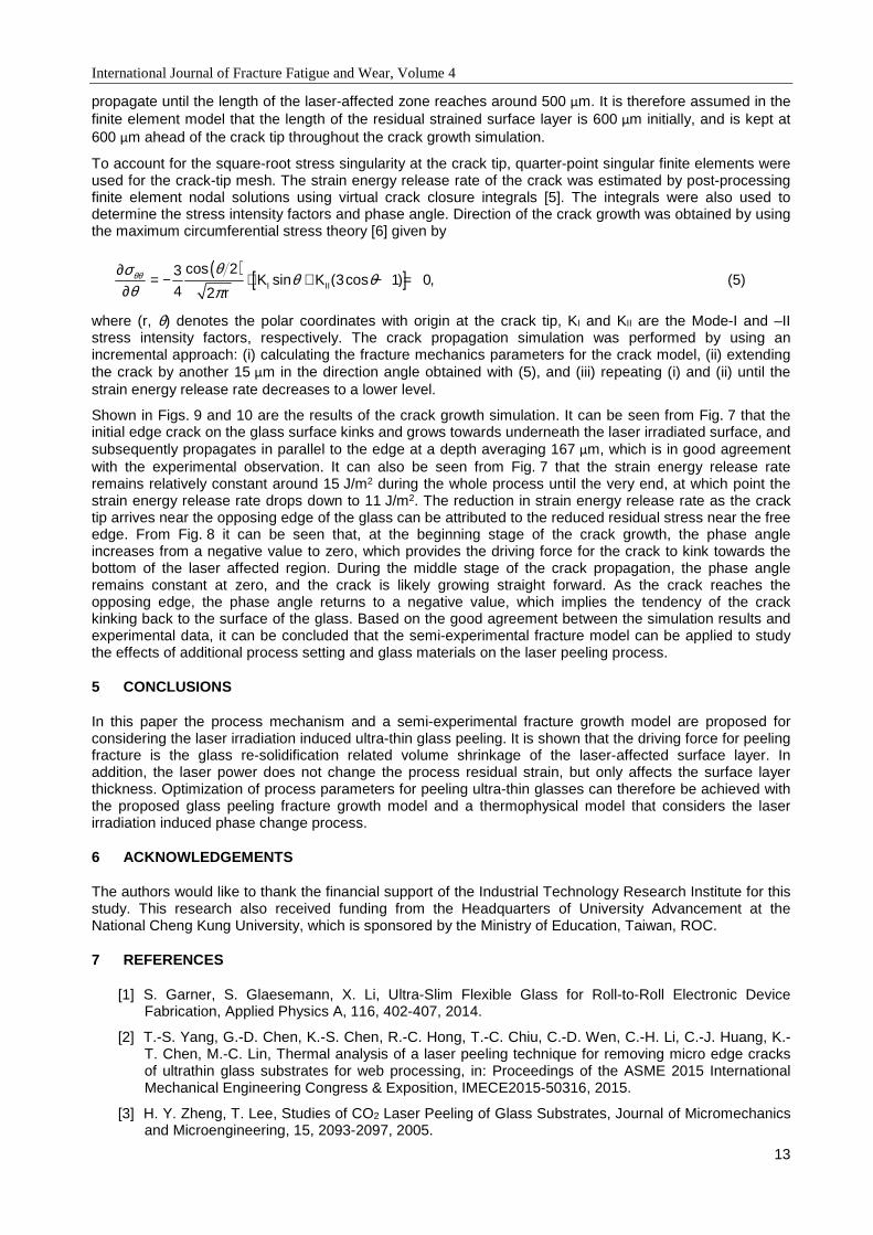
propagate until the length of the laser-affected zone reaches around 500 μm. It is therefore assumed in the finite element model that the length of the residual strained surface layer is 600 μm initially, and is kept at 600 μm ahead of the crack tip throughout the crack growth simulation.
To account for the square-root stress singularity at the crack tip, quarter-point singular finite elements were used for the crack-tip mesh. The strain energy release rate of the crack was estimated by post-processing finite element nodal solutions using virtual crack closure integrals [5]. The integrals were also used to determine the stress intensity factors and phase angle. Direction of the crack growth was obtained by using the maximum circumferential stress theory [6] given by
( ) [ ]θθ θσ θ θθ π
∂= − ⋅ + − =
∂ I II
cos 23sin (3cos 1) 0,
4 2K K
r (5)
where (r, θ) denotes the polar coordinates with origin at the crack tip, KI and KII are the Mode-I and –II stress intensity factors, respectively. The crack propagation simulation was performed by using an incremental approach: (i) calculating the fracture mechanics parameters for the crack model, (ii) extending the crack by another 15 μm in the direction angle obtained with (5), and (iii) repeating (i) and (ii) until the strain energy release rate decreases to a lower level.
Shown in Figs. 9 and 10 are the results of the crack growth simulation. It can be seen from Fig. 7 that the initial edge crack on the glass surface kinks and grows towards underneath the laser irradiated surface, and subsequently propagates in parallel to the edge at a depth averaging 167 μm, which is in good agreement with the experimental observation. It can also be seen from Fig. 7 that the strain energy release rate remains relatively constant around 15 J/m2 during the whole process until the very end, at which point the strain energy release rate drops down to 11 J/m2. The reduction in strain energy release rate as the crack tip arrives near the opposing edge of the glass can be attributed to the reduced residual stress near the free edge. From Fig. 8 it can be seen that, at the beginning stage of the crack growth, the phase angle increases from a negative value to zero, which provides the driving force for the crack to kink towards the bottom of the laser affected region. During the middle stage of the crack propagation, the phase angle remains constant at zero, and the crack is likely growing straight forward. As the crack reaches the opposing edge, the phase angle returns to a negative value, which implies the tendency of the crack kinking back to the surface of the glass. Based on the good agreement between the simulation results and experimental data, it can be concluded that the semi-experimental fracture model can be applied to study the effects of additional process setting and glass materials on the laser peeling process.
5 CONCLUSIONS
In this paper the process mechanism and a semi-experimental fracture growth model are proposed for considering the laser irradiation induced ultra-thin glass peeling. It is shown that the driving force for peeling fracture is the glass re-solidification related volume shrinkage of the laser-affected surface layer. In addition, the laser power does not change the process residual strain, but only affects the surface layer thickness. Optimization of process parameters for peeling ultra-thin glasses can therefore be achieved with the proposed glass peeling fracture growth model and a thermophysical model that considers the laser irradiation induced phase change process.
6 ACKNOWLEDGEMENTS
The authors would like to thank the financial support of the Industrial Technology Research Institute for this study. This research also received funding from the Headquarters of University Advancement at the National Cheng Kung University, which is sponsored by the Ministry of Education, Taiwan, ROC.
7 REFERENCES
[1] S. Garner, S. Glaesemann, X. Li, Ultra-Slim Flexible Glass for Roll-to-Roll Electronic Device Fabrication, Applied Physics A, 116, 402-407, 2014.
[2] T.-S. Yang, G.-D. Chen, K.-S. Chen, R.-C. Hong, T.-C. Chiu, C.-D. Wen, C.-H. Li, C.-J. Huang, K.-T. Chen, M.-C. Lin, Thermal analysis of a laser peeling technique for removing micro edge cracks of ultrathin glass substrates for web processing, in: Proceedings of the ASME 2015 International Mechanical Engineering Congress & Exposition, IMECE2015-50316, 2015.
[3] H. Y. Zheng, T. Lee, Studies of CO2 Laser Peeling of Glass Substrates, Journal of Micromechanics and Microengineering, 15, 2093-2097, 2005.
International Journal of Fracture Fatigue and Wear, Volume 4
14
[4] Z. K. Wang, H. Y. Zheng, Investigation on CO2 Laser Irradiation Inducing Glass Strip Peeling for Microchannel Formation, Biomicrofluidics, 6, 012820-1-012820-12, 2012.
[5] F. Erdogan, G. C. Sih, On the Crack Extension in Plates Under Plane Loading and Transverse Shear, Journal of Basic Engineering-Transactions of ASME, 85, 519-527, 1963.
[6] T.-C. Chiu, H.-C. Lin, On the Homogenization of Multilayered Interconnect for Interfacial Fracture Analysis, IEEE Transactions on Components and Packaging Technology, 31, 388-398, 2008.

International Journal of Fracture Fatigue and Wear, Volume 4
15
Proceedings of the 5th International Conference on Fracture Fatigue and Wear, pp. 15-20, 2016
FRACTURE BEHAVIOUR OBSERVATION OF METAL LAMINATES OF
HIGH-STRENGTH STEEL AND AL7075-T6 AT DIFFERENT
HIGH-VELOCITY PROJECTILE
N. A. Rahman, S. Abdullah, W. F. H. Zamri, M. F. Abdullah, M. Z. Omar and Z. Sajuri
Department Mechanical and Materials Engineering, Faculty of Engineering and Built Environment, Universiti Kebangsaan Malaysia, 43600 UKM Bangi, Selangor, Malaysia.
Abstract: This paper presents the behaviour of mixed triple-layered panels under ballistic impact at different initial projectile velocity. The fracture and damage behaviour has been investigated in terms of depth of penetration and energy absorption capability for different metal thickness combinations. The depth of penetration and energy absorption are closely related, and they are vital to be evaluated for the purpose of the ballistic performance. A numerical model of triple-layered panels mixed of high-strength steel and Al7075-T6 and a 7.62 mm armour piercing projectile were computationally modelled. The layer thickness combinations were constructed to achieve a range of 20% to 30% weight reduction from the existing ballistic resistant panel. The panels were subjected to an initial velocity of 400 m/s to 900 m/s. The depth of penetration and energy absorption were assessed. It is observed that at 400 m/s, maximum stress occurred at the end of penetration while at 900 m/s, maximum stress occurred at the start of penetration. It is found that panel with 25% weight reduction obtained the smallest depth of penetration and highest energy absorption capability. Based on the results, a better metal-laminate for ballistic resistant panel was then suggested for a specific use.
Keywords: Ballistic impact; depth of penetration; energy absorption; metal-laminates.
1 INTRODUCTION
Military industry nowadays is focusing on integrating the lightweight materials into the armoured vehicle designs to reduce the vehicle weight in order to improve the fuel consumption efficiency and vehicle maneuverability, without sacrificing the performance and safety [1]. Layering aluminium plate with high strength steel has become an interest in reducing the overall density of the armour vehicle body while improving the ballistic perforation resistance [2]. Impact performance of target panel mostly evaluated through the ballistic limit velocity, the fracture shape, the residual velocity and the loss of kinetic energy by the projectile [3-4]. Computational method has decreased the needs of expensive and time consuming experimental work on ballistic impact and it can access the parameter such as stress distribution on the target panel which cannot be extracted through experiment [5]. The effect of the layer thickness on the ballistic impact performance becomes an important consideration for further investigation. The application involving the survivability of passengers against the penetration by high velocity projectiles is important and demands complete understanding of the penetration process of the multi-layered plates subjected to ballistic impact.
Considering the importance, significant amount of work has been performed on the multi-layered panels subjected to projectile impact at high velocities. Previous studies have explored the behaviour of different combinations of layered composites armour [3-5] and most of the work has focused on the ceramic front layer and metallic composite back layer. Studies have also been done on the behaviour of different configuration layers comprised of mixed high strength steel such as Weldox 700E or Rolled-homogeneous armour (RHA) steel with aluminium alloys such as Al7075-T651 or Al5083-H116 against the ballistic impact [6-7]. The previous works concentrated on evaluation of ballistic limit velocity as a function of target thickness and also energy absorbed by various mechanism at different initial impact velocity. The penetration process occurs in two separate phases. These phases include firstly the initial penetration into the plate target and secondly the following perforation of the target as the projectile exits the target rear surface. The penetration phase involves a simultaneous process of projectile deceleration and erosion which causes the reduction in original length, and target plate plastic flow which causes the reduction in plate thickness [8].
International Journal of Fracture Fatigue and Wear, Volume 4
16
The results from research work done by Forrestal et al. [6] and Übeyli et al. [7] emphasized that aluminium ductility can play a major role in resistance to impacts. An effective layering configuration and thickness of aluminium in a multi-layered ballistic resistant panel can improve its ballistic performance. To complete this assumption, this study is performed to investigate the behaviour of triple-layered configuration ballistic resistant panel mixed of high strength steel and aluminium alloy under ballistic impact using an explicit non-linear finite element program. Computational ballistic simulation was performed to analyse the effect of initial impact velocity on different triple-layered plates with different areal density, leading to the assessment of the depth of penetration, the energy absorption capability and the maximum stress.
2 FINITE ELEMENT METHOD
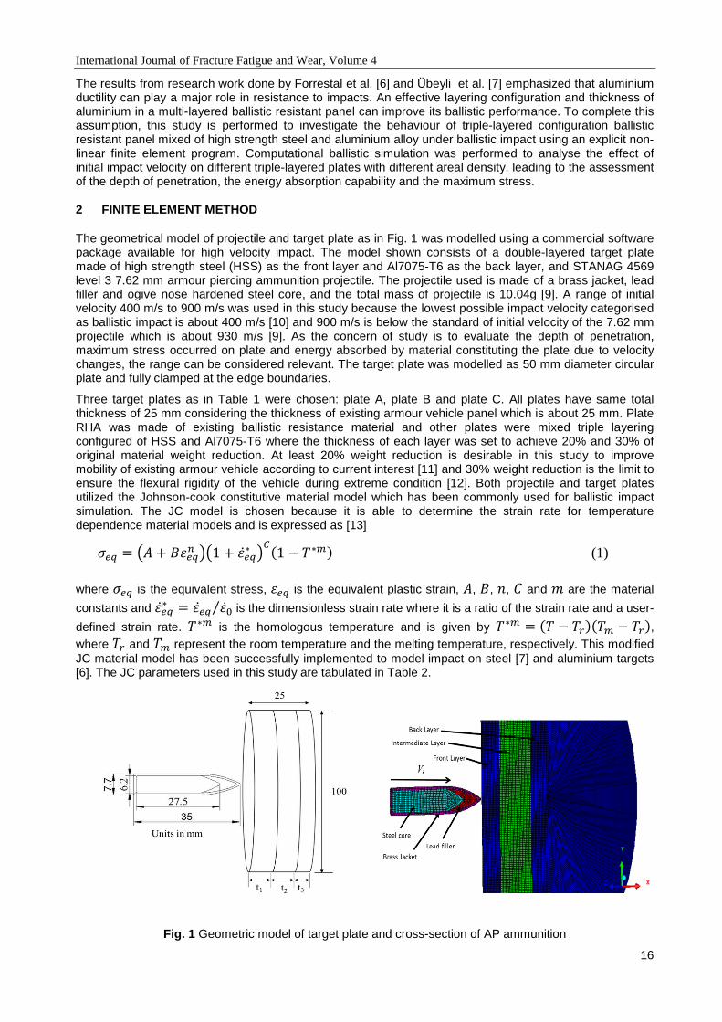
The geometrical model of projectile and target plate as in Fig. 1 was modelled using a commercial software package available for high velocity impact. The model shown consists of a double-layered target plate made of high strength steel (HSS) as the front layer and Al7075-T6 as the back layer, and STANAG 4569 level 3 7.62 mm armour piercing ammunition projectile. The projectile used is made of a brass jacket, lead filler and ogive nose hardened steel core, and the total mass of projectile is 10.04g [9]. A range of initial velocity 400 m/s to 900 m/s was used in this study because the lowest possible impact velocity categorised as ballistic impact is about 400 m/s [10] and 900 m/s is below the standard of initial velocity of the 7.62 mm projectile which is about 930 m/s [9]. As the concern of study is to evaluate the depth of penetration, maximum stress occurred on plate and energy absorbed by material constituting the plate due to velocity changes, the range can be considered relevant. The target plate was modelled as 50 mm diameter circular plate and fully clamped at the edge boundaries.
Three target plates as in Table 1 were chosen: plate A, plate B and plate C. All plates have same total thickness of 25 mm considering the thickness of existing armour vehicle panel which is about 25 mm. Plate RHA was made of existing ballistic resistance material and other plates were mixed triple layering configured of HSS and Al7075-T6 where the thickness of each layer was set to achieve 20% and 30% of original material weight reduction. At least 20% weight reduction is desirable in this study to improve mobility of existing armour vehicle according to current interest [11] and 30% weight reduction is the limit to ensure the flexural rigidity of the vehicle during extreme condition [12]. Both projectile and target plates utilized the Johnson-cook constitutive material model which has been commonly used for ballistic impact simulation. The JC model is chosen because it is able to determine the strain rate for temperature dependence material models and is expressed as [13]
1 ∗ 1 ∗ (1)
where is the equivalent stress, is the equivalent plastic strain, , , , and are the material
constants and ∗ ⁄ is the dimensionless strain rate where it is a ratio of the strain rate and a user-
defined strain rate. ∗ is the homologous temperature and is given by ∗ , where and represent the room temperature and the melting temperature, respectively. This modified JC material model has been successfully implemented to model impact on steel [7] and aluminium targets [6]. The JC parameters used in this study are tabulated in Table 2.
Fig. 1 Geometric model of target plate and cross-section of AP ammunition
International Journal of Fracture Fatigue and Wear, Volume 4
17
Table 1 Target plate configuration
Target Plate Name Material
Mass Reduction
(%)
Front Layer (mm)
Intermediate layer (mm)
Back layer (mm)
Initial velocity, Vi (m/s)
Plate A HSS + Al7075-T6 +
HSS
20 9 8 8
400-900 Plate B 25 8 10 7
Plate C 30 7 12 6
Table 2 Material Properties and Modified Johnson-Cook model parameters [7, 6]
Material Properties RHA HSS AA7075-T6
Steel core Lead cap
Brass jacket
Density, ρ (kg/m3) 7830 7860 2804 7850 10600 8520
Young's Modulus E, (Gpa) 7.83 7.69 70 210 1 115
Poisson's ratio, ν 0.33 0.33 0.3 0.33 0.42 0.31
Yield Strength, A (MPa) 780 1250 480 1200 24 206
Strain Hardening, B (MPa) 362 362 477 50000 300 505
Strain Hardening exponent, n 0.106 1 0.52 1 1 0.42
Strain rate constant, c 0.004 0.0108 0.001 0 0.1 0.1
Thermal softening constant, m 1 1 1 1 1 1.68
Melting temperature, Tm (K) 1800 1800 893 1811 760 1189
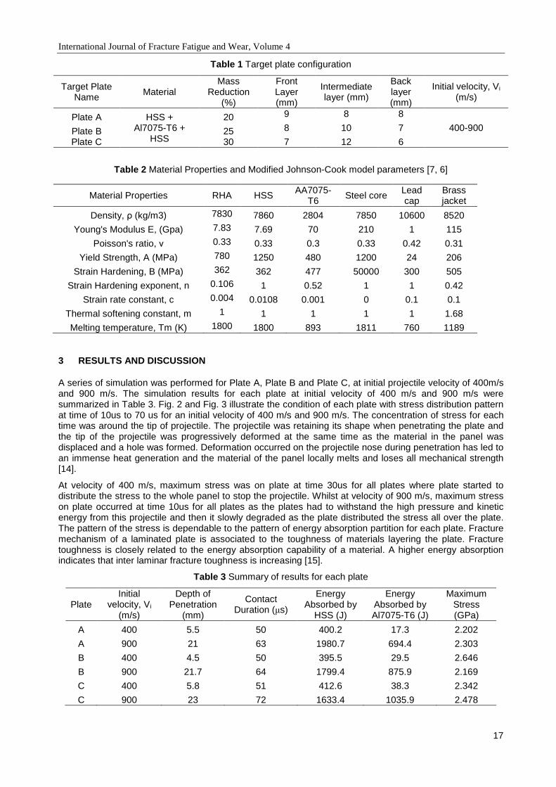
3 RESULTS AND DISCUSSION
A series of simulation was performed for Plate A, Plate B and Plate C, at initial projectile velocity of 400m/s and 900 m/s. The simulation results for each plate at initial velocity of 400 m/s and 900 m/s were summarized in Table 3. Fig. 2 and Fig. 3 illustrate the condition of each plate with stress distribution pattern at time of 10us to 70 us for an initial velocity of 400 m/s and 900 m/s. The concentration of stress for each time was around the tip of projectile. The projectile was retaining its shape when penetrating the plate and the tip of the projectile was progressively deformed at the same time as the material in the panel was displaced and a hole was formed. Deformation occurred on the projectile nose during penetration has led to an immense heat generation and the material of the panel locally melts and loses all mechanical strength [14].
At velocity of 400 m/s, maximum stress was on plate at time 30us for all plates where plate started to distribute the stress to the whole panel to stop the projectile. Whilst at velocity of 900 m/s, maximum stress on plate occurred at time 10us for all plates as the plates had to withstand the high pressure and kinetic energy from this projectile and then it slowly degraded as the plate distributed the stress all over the plate. The pattern of the stress is dependable to the pattern of energy absorption partition for each plate. Fracture mechanism of a laminated plate is associated to the toughness of materials layering the plate. Fracture toughness is closely related to the energy absorption capability of a material. A higher energy absorption indicates that inter laminar fracture toughness is increasing [15].
Table 3 Summary of results for each plate
Plate Initial
velocity, Vi (m/s)
Depth of Penetration
(mm)
Contact Duration (µs)
Energy Absorbed by
HSS (J)
Energy Absorbed by Al7075-T6 (J)
Maximum Stress (GPa)
A 400 5.5 50 400.2 17.3 2.202
A 900 21 63 1980.7 694.4 2.303
B 400 4.5 50 395.5 29.5 2.646
B 900 21.7 64 1799.4 875.9 2.169
C 400 5.8 51 412.6 38.3 2.342
C 900 23 72 1633.4 1035.9 2.478

International Journal of Fracture Fatigue and Wear, Volume 4
18
Plate Plate Condition
A
t=10µs
σ=1.474 GPa
t=20µs
σ=1.657 GPa
t=30µs
σ=2.032 GPa
t=50µs
σ=1.978 GPa
t=70µs
σ=1.647 GPa
B
t=10µs
σ=1.469 GPa
t=20µs
σ=1.646 GPa
t=30µs
σ=2.236 GPa
t=50µs
σ=2.002 GPa
t=70µs
σ=1.635 GPa
C
t=10µs
σ=1.470 GPa
t=20µs
σ=1.656 GPa
t=30µs
σ=2.183 GPa
t=50µs
σ=2.288 GPa
t=70µs
σ=1.643 GPa
Fig. 2 Stress distribution patterns of each plate at time between 10µs to 70µs at initial projectile velocity of 400 m/s
Plate Plate Condition
A
t=10µs,
σ=2.173 GPa
t=20µs
σ=2.141 GPa
t=30µs
σ=2.303 GPa
t=50µs
σ=1.988 GPa
t=70µs
σ=1.981 GPa
B
t=10µs
σ=2.147 GPa
t=20µs
σ=2.169 GPa
t=30µs
σ=2.040 GPa
t=50µs
σ=2.101 GPa
t=70µs
σ=1.973 GPa
C
t=10µs
σ=2.478 GPa
t=20µs
σ=2.056 GPa
t=30µs
σ=2.076 GPa
t=50µs
σ=2.065 GPa
t=70µs
σ=1.938 GPa
Fig. 3 Stress distribution patterns of each plate at time between 10µs to 70µs at initial projectile velocity of 900 m/s
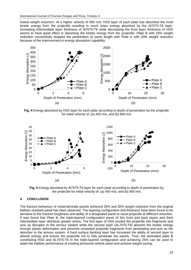
Fig. 4a-b show the energy absorbed by HSS for each plate at velocity of 400 m/s and 900 m/s. At a lower velocity of 400 m/s, the maximum energy absorption for each plate was comparable about 420 J. However, Plate B with 25% weight reduction achieved maximum energy absorption at 40 µs whereas Plate A and Plate C attained maximum energy absorption at 55 µs. Similar energy absorption pattern for Al7075-T6 can be seen in Fig. 5a. The ability of Plate C which possesses the maximum weight reduction to absorb energy better than others has allowed the plate to stop the projectile at same length with Plate A which takes the
International Journal of Fracture Fatigue and Wear, Volume 4
19
lowest weight reduction. At a higher velocity of 900 m/s, HSS layer of each plate has absorbed the most kinetic energy from the projectile resulting in much lower energy absorbed by the Al7075-T6 layer. Increasing intermediate layer thickness of Al7075-T6 while decreasing the front layer thickness of HSS seems to have good effect in absorbing the kinetic energy from the projectile. Plate B with 25% weight reduction successfully stopped the penetration at same length with Plate A with 20% weight reduction because of the improvement in energy absorption capability.
(a)
(b)
Fig. 4 Energy absorbed by HSS layer for each plate according to depth of penetration by the projectile for initial velocity of: (a) 400 m/s, and (b) 900 m/s
(a)
(b)
Fig. 5 Energy absorbed by Al7075-T6 layer for each plate according to depth of penetration by the projectile for initial velocity of: (a) 400 m/s, and (b) 900 m/s
4 CONCLUSION
The fracture behaviour of metal-laminate panels achieved 20% and 30% weight reduction from the original ballistic resistant panel has been observed. The layering configuration and thickness have been found to be sensitive to the fracture toughness and ability of a designated panel to resist projectile at different velocities. It was found that Plate B, the triple-layered configuration panel of thin front and back layers and thick intermediate layer distribute greater stress. The first layer of HSS eroded the projectile into fragments and acts as disruptor to the armour system while the second layer (AL7075-T6) absorbs the kinetic energy through plastic deformation and prevents unwanted projectile fragments from penetrating and acts as the absorber to the armour system. A hard surface backing layer has increased the ability of second layer to absorb energy and ensure the projectile not to fully penetrate the panels. Thus, the laminated plate B constituting HSS and AL7075-T6 in the triple-layered configuration and achieving 25% can be used to attain the ballistic performance of existing armoured vehicle panel and achieve weight-saving.
0
50
100
150
200
250
300
350
400
450
0 2 4 6
Ene
rgy
Abs
orpt
ion
(J)
Depth of Penetration (mm)
Plate APlate BPlate C 0
500
1000
1500
2000
2500
0 10 20 30
Ene
rgy
Abs
optio
n (J
)Depth of Penetration (mm)
Plate APlate BPlate C
0
5
10
1520
25
30
35
4045
0 2 4 6
Ene
rgy
Abs
orpt
ion
(J)
Depth of Penetration (mm)
Plate APlate BPlate C
-200
0
200
400
600
800
1000
1200
0 10 20 30
Ene
rgy
Abs
orpt
ion
(J)
Depth of Penetration (mm)
Plate APlate BPlate C
International Journal of Fracture Fatigue and Wear, Volume 4
20
5 ACKNOWLEDGEMENT
The authors wish to express their gratitude to Ministry of Higher Education Malaysia via Universiti Kebangsaan Malaysia and Universiti Pertahanan Nasional Malaysia under research funding LRGS/2013/UPNM-UKM/DS/04 for supporting this research project.
6 REFERENCES
[1] T. Demir, M. Übeyli, R. O. Yildirim, Investigation on the ballistic impact behaviour of various alloys against 7.62 mm armor piercing projectile, Material and Design, 29(10), 2009–2016, 2008.
[2] M. Übeyli, H. Deniz, T. Demir, B. Ögel, B. Gürel, Ö. Keleş, Ballistic impact performance of an armor material consisting of alumina and dual phase steel layers, Material and Design, 32(3), 1565–1570, 2011.
[3] H. Abdulhamid, A. Kolopp, C. Bouvet, S. Rivallant, Experimental and numerical study of AA5086-H111 aluminium plates subjected to impact, Journal of Impact Engineering, 51, 1-12, 2013.
[4] R. Nasirzadeh, A. R. Sabet, Study of foam density variations in composite sandwich panels under high velocity impact loading, International Journal of Impact Engineering, 63, 129–139, 2014.
[5] T. Børvik, M. J. Forrestal, O. S. Hopperstad, T. L. Warren, M. Langseth, Perforation of AA5083-H116 aluminium plates with conical-nose steel projectiles - Calculations, International Journal of Impact Engineering, 36(3), 426–437, 2009.
[6] M. J. Forrestal, T. Børvik, T. L. Warren, Perforation of 7075-T651 Aluminum Armor Plates with 7.62 mm APM2 Bullets, Experiment Mechanics, 50(8), 1245–1251, 2010.
[7] M. Übeyli, R. O. Yildirim, B. Ögel, On the comparison of the ballistic performance of steel and laminated composite armors, Material and Design, 28(4), 1257–1262, 2007.
[8] R. Zaera, V. Sanchez-Galvez, Modelling of fracture processes in the ballistic impact on ceramic armours, Journal De Physique, 687-692, 1997.
[9] N. Kiliç, B. Ekici, Ballistic resistance of high hardness armor steels against 7.62 mm armor piercing ammunition, Material and Design, 44, 35–48, 2013.
[10] M. A. Iqbal, A. Chakrabarti, S. Beniwal, N. K. Gupta, 3D numerical simulations of sharp nosed projectile impact on ductile targets, International Journal of Impact Engineering, 37(2), 185–195, 2010.
[11] J. Zhou, Z. W. Guan, W. J. Cantwell, The impact response of graded foam sandwich structures, Composite Structure, 97, 370–377, 2013
[12] E. Medvedovski, Ballistic performance of armour ceramics: Influence of design and structure. Part 1, Ceramic International, 36(7), 2103–2115, 2010.
[13] E. A. Flores-Johnson, M. Saleh, L. Edwards, Ballistic performance of multi-layered metallic plates impacted by a 7.62-mm APM2 projectile, International Journal of Impact Engineering, 38(12), 1022–1032, 2011.
[14] D.R. Lesuer, C.K. Syn, O.D. Sherby, J. Wadsworth, Laminated metals composites-fracture and ballistic impact behaviour, Third Pacific Rim Conference on Advanced Materials and Processing, 1998.
[15] J. Dean, C.S. Dunleavy, P.M. Brown, T.W. Clyne, Energy absorption during projectile perforation of thin steel plates and the kinetic energy of ejected fragments, International Journal of Impact Engineering, 36(10-11), 1250-1260, 2009.
International Journal of Fracture Fatigue and Wear, Volume 4
21
Proceedings of the 5th International Conference on Fracture Fatigue and Wear, pp. 21-26, 2016
CHARACTERING SELF MAGNETIC FLUX LEAKAGE ASSOCIATED TO
BIAXIAL FATIGUE LIFE ESTIMATION USING WEIBULL-BASED
METHOD
S.A.N. Mohamed, A. Arifin, S. Abdullah and A.K. Ariffin
Department of Mechanical and Materials, Faculty of Engineering and Built Environment, Universiti Kebangsaan Malaysia, 43600 Bangi, Selangor, Malaysia
Abstract: This study discusses the biaxial fatigue life prediction method using magnetic flux leakage signal parameters. Biaxial fatigue failure in engineering components cannot be detected during the early stages of the existence of micro cracks. Therefore, ferromagnetic components experience fatigue failure, as a result development on the stress concentration zone, under the influence of acting stress until completely fracture. The experiment is conducted using a combination of stress biaxial tensile stresses and torsional stress according to ASTM E2207 standards. Torsional stress is set to 15º normal to tensile stress. The magnetic flux signals are observed when the machine is stopped at a pre-determined interval cycle. From the results it is found that the biaxial fatigue defects can be detected, in which the magnetic flux signal indicate a significant change in the magnetogram graph. The correlation between fatigue life and signal biaxial magnetic flux is formed using the Basquin equation approach. Therefore, monitoring failure, using the metal magnetic memory method, can be used to predict the biaxial fatigue life. Keywords: biaxial fatigue, ferromagnetic, magnetic flux leakage, non-destructive test, stress concentration zone
1 INTRODUCTION
Most engineering components are subject to more complex stresses, which are normal stress and shear stress. Every material undergoes a deformation process when subjected to stress. The deformation process that occurs through the severance and restructuring of the atomic bonds in the material can lead to cracking and fracture of the material when subjected to stress beyond the limits of the material strength or when subjected to constant stress, which causes fatigue failure in the material [1]. Fatigue failure occurs progressively as a result of repetitive stress cycles. This situation is largely determined by the maximum shear stress and the maximum normal stress in the structure of the material [2]. Therefore, a basic understanding of the combination of external loads, i.e. the normal stress and the shear stress, for components in the production of stress at a critical location is very important. A multi-axial analytical approach can be divided into three categories, namely stress-based, strain-based and energy-based [3].
The existence of micro-defects and local stress concentrations in metal structures are factors that cause failure and accidents in mechanical structures. The distributions of internal stresses in metals affect the service performance, where the internal stresses and defects in components are interdependent [4]. Non-destructive testing using the MMM method is based on a standalone analysis of the magnetic flux leakage (MFL) on the surface of the component to determine the stress concentration zones and defects in the metal structure [5]. Unlike most other non-destructive testing methods, this method can be employed for the early detection of defects [6].
Most ferromagnetic components operate in conditions where a multi-axial load is present, that is, from the complex geometry of the components or the external load that is applied. Normally the stress concentration due to the existence of micro cracks in the action of stress unable to be detected clearly in the early stages using macroscopic assessment. Fractures due to fatigue usually occur in areas of stress concentration, where there are microscopic defect zones, which are the main sources for the development of defects. Therefore, the MMM method is an alternative method for predicting the fatigue life of ferromagnetic components via a single correlation between the fatigue life and the magnetic flux leakage parameter. The MMM method provides a quick inspection and spontaneous monitoring of the surface of the component that is generating a self-magnetic flux leakage (SMFL) and detects the location of the stress concentration from
International Journal of Fracture Fatigue and Wear, Volume 4
22
the magnetic signal. The non-destructive testing method is adopted for the prediction of fatigue life as an alternative to the existing conventional methods as it is only based on the value of the magnetic flux leakage signal of the material.
2 METHODOLOGY
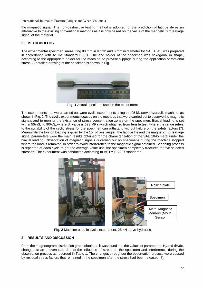
The experimental specimen, measuring 80 mm in length and 6 mm in diameter for SAE 1045, was prepared in accordance with ASTM Standard E8-01. The end holder of the specimen was hexagonal in shape, according to the appropriate holder for the machine, to prevent slippage during the application of torsional stress. A detailed drawing of the specimen is shown in Fig. 1.
Fig. 1 Actual specimen used in the experiment
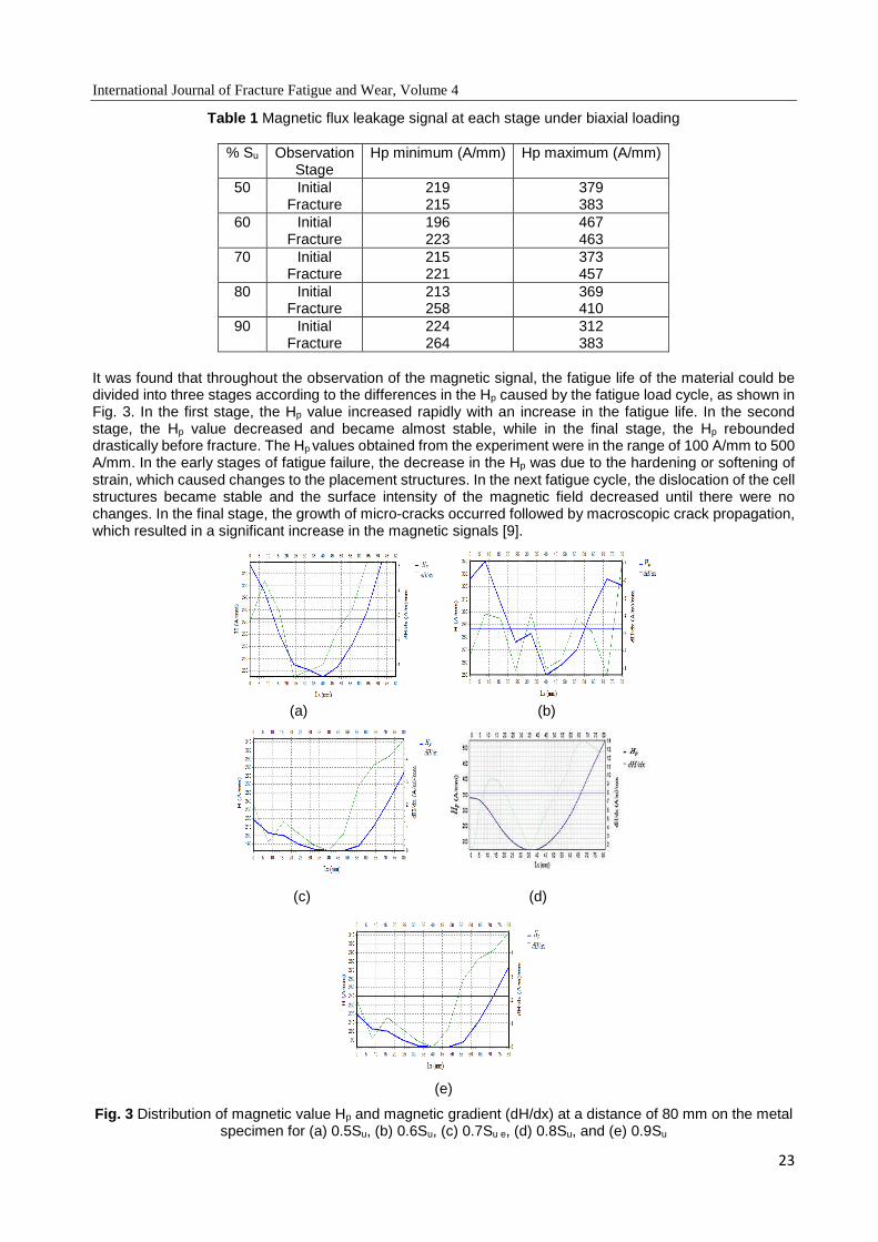
The experiments that were carried out were cyclic experiments using the 25 kN servo-hydraulic machine, as shown in Fig. 2. The cyclic experiments focused on the methods that were carried out to observe the magnetic signals and to monitor the existence of stress concentration zones on the specimen. Biaxial loading is set within 50%Su to 90%Su where Su value is 623 MPa which obtained from tensile test, where the range refers to the suitability of the cyclic stress for the specimen can withstand without failure on the safety factors [7]. Meanwhile the torsion loading is given by the 15° of twist angle. The fatigue life and the magnetic flux leakage signal parameters were the main results obtained for the characterization of the SAE 1045 metal under the biaxial loading. Observation of magnetic signals is carried out on specimens during the machine stopped where the load is removed, in order to avoid interference to the magnetic signal obtained. Scanning process is repeated at each cycle to get the average value until the specimen completely fractures for five selected stresses. The experiment was conducted according to ASTM E-2207 standards.
Fig. 2 Machine used in cyclic experiment, 25 kN servo-hydraulic
3 RESULTS AND DISCUSSION
From the magnetogram distribution graph obtained, it was found that the values of parameters, Hp and dH/dx, changed at an uneven rate due to the influence of stress on the specimen and interference during the observation process as recorded in Table 1. The changes throughout the observation process were caused by residual stress factors that remained in the specimen after the stress had been released [8].
Specimen
Metal Magnetic Memory (MMM)
Sensor
Rolling plate
International Journal of Fracture Fatigue and Wear, Volume 4
23
Table 1 Magnetic flux leakage signal at each stage under biaxial loading
% Su Observation Stage
Hp minimum (A/mm) Hp maximum (A/mm)
50 Initial Fracture
219 215
379 383
60 Initial Fracture
196 223
467 463
70 Initial Fracture
215 221
373 457
80 Initial Fracture
213 258
369 410
90 Initial Fracture
224 264
312 383
It was found that throughout the observation of the magnetic signal, the fatigue life of the material could be divided into three stages according to the differences in the Hp caused by the fatigue load cycle, as shown in Fig. 3. In the first stage, the Hp value increased rapidly with an increase in the fatigue life. In the second stage, the Hp value decreased and became almost stable, while in the final stage, the Hp rebounded drastically before fracture. The Hp values obtained from the experiment were in the range of 100 A/mm to 500 A/mm. In the early stages of fatigue failure, the decrease in the Hp was due to the hardening or softening of strain, which caused changes to the placement structures. In the next fatigue cycle, the dislocation of the cell structures became stable and the surface intensity of the magnetic field decreased until there were no changes. In the final stage, the growth of micro-cracks occurred followed by macroscopic crack propagation, which resulted in a significant increase in the magnetic signals [9].
(a) (b)
(c) (d)
(e)
Fig. 3 Distribution of magnetic value Hp and magnetic gradient (dH/dx) at a distance of 80 mm on the metal specimen for (a) 0.5Su, (b) 0.6Su, (c) 0.7Su e, (d) 0.8Su, and (e) 0.9Su
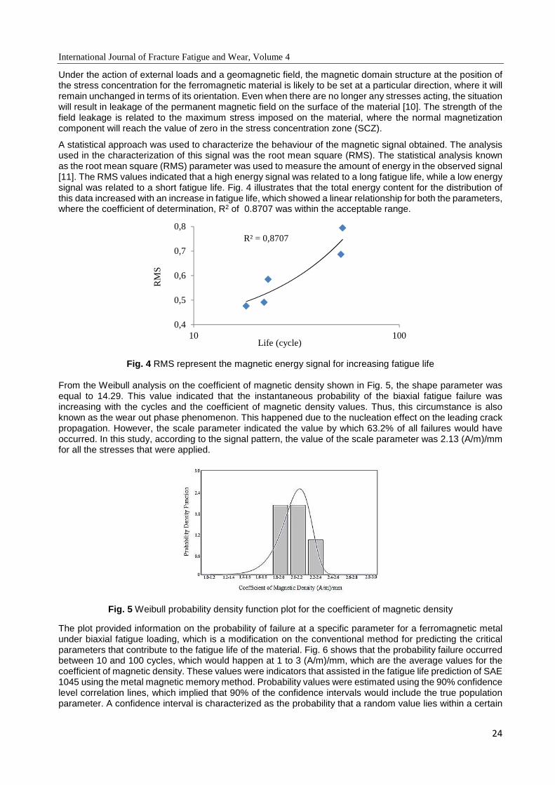
International Journal of Fracture Fatigue and Wear, Volume 4
24
Under the action of external loads and a geomagnetic field, the magnetic domain structure at the position of the stress concentration for the ferromagnetic material is likely to be set at a particular direction, where it will remain unchanged in terms of its orientation. Even when there are no longer any stresses acting, the situation will result in leakage of the permanent magnetic field on the surface of the material [10]. The strength of the field leakage is related to the maximum stress imposed on the material, where the normal magnetization component will reach the value of zero in the stress concentration zone (SCZ).
A statistical approach was used to characterize the behaviour of the magnetic signal obtained. The analysis used in the characterization of this signal was the root mean square (RMS). The statistical analysis known as the root mean square (RMS) parameter was used to measure the amount of energy in the observed signal [11]. The RMS values indicated that a high energy signal was related to a long fatigue life, while a low energy signal was related to a short fatigue life. Fig. 4 illustrates that the total energy content for the distribution of this data increased with an increase in fatigue life, which showed a linear relationship for both the parameters, where the coefficient of determination, R2 of 0.8707 was within the acceptable range.
Fig. 4 RMS represent the magnetic energy signal for increasing fatigue life
From the Weibull analysis on the coefficient of magnetic density shown in Fig. 5, the shape parameter was equal to 14.29. This value indicated that the instantaneous probability of the biaxial fatigue failure was increasing with the cycles and the coefficient of magnetic density values. Thus, this circumstance is also known as the wear out phase phenomenon. This happened due to the nucleation effect on the leading crack propagation. However, the scale parameter indicated the value by which 63.2% of all failures would have occurred. In this study, according to the signal pattern, the value of the scale parameter was 2.13 (A/m)/mm for all the stresses that were applied.
Fig. 5 Weibull probability density function plot for the coefficient of magnetic density
The plot provided information on the probability of failure at a specific parameter for a ferromagnetic metal under biaxial fatigue loading, which is a modification on the conventional method for predicting the critical parameters that contribute to the fatigue life of the material. Fig. 6 shows that the probability failure occurred between 10 and 100 cycles, which would happen at 1 to 3 (A/m)/mm, which are the average values for the coefficient of magnetic density. These values were indicators that assisted in the fatigue life prediction of SAE 1045 using the metal magnetic memory method. Probability values were estimated using the 90% confidence level correlation lines, which implied that 90% of the confidence intervals would include the true population parameter. A confidence interval is characterized as the probability that a random value lies within a certain
R² = 0,8707
0,4
0,5
0,6
0,7
0,8
10 100
RM
S
Life (cycle)
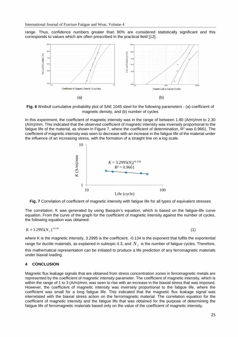
International Journal of Fracture Fatigue and Wear, Volume 4
25
range. Thus, confidence numbers greater than 90% are considered statistically significant and this corresponds to values which are often prescribed in the practical field [12].
(a) (b)
Fig. 6 Weibull cumulative probability plot of SAE 1045 steel for the following parameters - (a) coefficient of magnetic density, and (b) number of cycles
In this experiment, the coefficient of magnetic intensity was in the range of between 1.80 (A/m)/mm to 2.30 (A/m)/mm. This indicated that the observed coefficient of magnetic intensity was inversely proportional to the fatigue life of the material, as shown in Figure 7, where the coefficient of determination, R2 was 0.9661. The coefficient of magnetic intensity was seen to decrease with an increase in the fatigue life of the material under the influence of an increasing stress, with the formation of a straight line on a log scale.
Fig. 7 Correlation of coefficient of magnetic intensity with fatigue life for all types of equivalent stresses
The correlation, K was generated by using Basquin’s equation, which is based on the fatigue-life curve equation. From the curve of the graph for the coefficient of magnetic intensity against the number of cycles, the following equation was obtained:
0.1343.2995( )fK N −= (1)
where K is the magnetic intensity, 3.2995 is the coefficient, -0.134 is the exponent that fulfils the exponential range for ductile materials, as explained in subtopic 4.3, and fN is the number of fatigue cycles. Therefore,
this mathematical representation can be initiated to produce a life prediction of any ferromagnetic materials under biaxial loading.
4 CONCLUSION
Magnetic flux leakage signals that are obtained from stress concentration zones in ferromagnetic metals are represented by the coefficient of magnetic intensity parameter. The coefficient of magnetic intensity, which is within the range of 1 to 3 (A/m)/mm, was seen to rise with an increase in the biaxial stress that was imposed. However, the coefficient of magnetic intensity was inversely proportional to the fatigue life, where the coefficient was small for a long fatigue life. This indicated that the magnetic flux leakage signal was interrelated with the biaxial stress action on the ferromagnetic material. The correlation equation for the coefficient of magnetic intensity and the fatigue life that was obtained for the purpose of determining the fatigue life of ferromagnetic materials based only on the value of the coefficient of magnetic intensity.
K = 3.2995(Nf)-0.134
R²= 0.9661
1
10
10 100
K(A
/m)/
mm
Life (cycle)
International Journal of Fracture Fatigue and Wear, Volume 4
26
5 ACKNOWLEDGEMENTS
The authors would like to express their gratitude to National University of Malaysia through the fund of LRGS/2013/UPNM-UKM/DS/04 for supporting this project research.
6 REFERENCES
[1] P. P. Milella, Fatigue and Corrosion in Metals, Springer-Verlag Italia, 2013.
[2] V. Anes, L. Reis, M. Freitas, Asynchronous multiaxial fatigue damage evaluation, Procedia
Engineering, 101, 421-429, 2015.
[3] K.Z. Golos, D.K. Debski, M.A. Debski, A stress-based fatigue criterion to assess high cycle fatigue
under in-phase multiaxial loading condition, Theoretical and Applied Fracture Mechanics, 73, 3-8,
2014.
[4] Q. Xin, D. Shu, L. Hui, W. Wei, J. Chen, Magnetic Barkhausen noise, metal magnetic memory testing
and estimation of the ship plate welded structure stress, Journal of Non-destructive Evaluation, 31(1),
80-89, 2012.
[5] Z.D. Wang, B. Deng, K. Yao, Physical model of plastic deformation on magnetization in ferromagnetic
materials, Journal of Applied Physics, 109(8), 83-28, 2011.
[6] L.J. Yang, B. Liu, L.J. Chen, S.W. Gao, The quantitative interpretation by measurement using the
magnetic memory method (MMM)-based on density functional theory. NDT & E International, 55, 15-
20, 2013.
[7] U. Krupp, Fatigue crack propagation in metals and alloys: microstructural aspects and modelling
concepts, New York, 2007.
[8] M. Roskosz, A. Rusin, M. Bieniek, K. Fryczowski, Identification of the stress-strain state of
ferromagnetic steels based on the measurement of magnetic parameters, 11th European
Conference on Non-Destructive Testing ECNDT, pp. 1-8, 2014.
[9] J. Leng, M. Xu, S. Zhao, J. Zhang, Fatigue damage evaluation on ferromagnetic-- materials using
magnetic memory method, Proceedings of 2009 International Conference on Measuring Technology
and Mechatronics Automation, pp. 784-786, 2009.
[10] J. Yuan, W. Zhang, Detection of stress concentration and early plastic deformation by monitoring
surface weak magnetic field change, Proceedings of 2010 International Conference on Mechatronics
and Automation, pp. 395-400, 2010.
[11] T.P. Ryan, Modern Engineering in Statistics, New York, 2007.
[12] B. Bertsche, Reliability in automotive and mechanical engineering: determination of component and
system reliability, Springer Science & Business Media, Italia, 2008.

International Journal of Fracture Fatigue and Wear, Volume 4
27
Proceedings of the 5th International Conference on Fracture Fatigue and Wear, pp. 27-32, 2016
FRACTURE BEHAVIOUR INVESTIGATION OF AZ31B MAGNESIUM
ALLOY WITH CARBON-NANOTUBE AND LEAD REINFORCEMENT
USING A GAS GUN SYSTEM
M.F. Abdullah2, S. Abdullah1, M.S. Risby2, M.Z. Omar1, Z. Sajuri1
1 Department of Mechanical and Materials Engineering, Faculty of Engineering & Built Environment,
Universiti Kebangsaan Malaysia. 43600 UKM Bangi, Selangor, Malaysia
2Department of Mechanical Engineering, Faculty of Engineering, Universiti Pertahanan Nasional Malaysia,
Kem Sg. Besi 57000 Kuala Lumpur, Malaysia
Abstract: This paper presents the fracture behaviour of AZ31B materials with reinforcement of Carbon-Nanotube (CNT) and Lead subjected to gas gun testing through simulation and experiment. The study is divided into two parts, i.e. numerical simulation for gas gun and microstructure observation. Simulation accommodated Cowper-Symonds material constitutive model to observe the penetration effect and material fracture behaviour. The projectile used was a cone-nose type with diameter of 11 mm and made up of steel series of 1006. Initial velocity of the projectile was set at 600 m/s, and the sample thickness was set at 25 mm. The second part is an experimental observation the microstructure and CNT Constance on AZ31B. From the simulation results, it was found that the depth of penetration for the Magnesium alloy AZ31B reinforced with the CNT and lead shows a good agreement findings. The depth penetrations onto the simulation were obtained between 15 to 25 mm. The added reinforcement materials provide a reduction in the depth penetration of 39% compared to the original Magnesium alloy AZ31B. Thus, this type of magnesium alloy reinforced with the CNT and lead was found to be a suitable candidate material for ballistic resistant panel with weight saving determination.
Keywords: ballistic, CNT, depth of penetration, Lead, Magnesium alloy AZ31B
1 INTRODUCTION
Recent technology development in automotive field requires lightweight material which has high strength. Exploration of new materials has high impact in the study of changing in strain, especially when subjected to high velocity impact [1,2]. Changing strain at high velocity impact affects the material energy absorption and prevents the occurrence of fracture failure [3,4]. The magnesium alloy is characterized as lightweight materials and has high energy absorption capability. Magnesium alloys can naturally withstand impacts effectively because of their unique combination of high tensile strength, low density, and superior shock absorbency which are 100 times greater than that of ordinary aluminum alloys [4].
Magnesium has a hexagonal close-packed structure (HCP). This structure affects the strength and ductility of materials because there are voids between the molecules [5]. Therefore, it is necessary to have a material that is able to fill these voids in order to prevent the structural collapse of the material. The most suitable materials to fill those voids are carbon nanotubes (CNTs). CNTs have unique characteristics that can generate strong materials with enhanced energy absorption properties [6-8], and many researchers have acknowledged that CNTs can improve the strength of materials. CNT materials are produced from nano-technology for the purpose of filling the voids in structures and producing van der Waals bonds within them [9-11]. In addition, lead (Pb) materials are also being used extensively to increase the absorption of energy as well as to enhance the ductility of materials. Since an increase in the ductility of a material is directly proportional to the elasticity of the material, an increase in the lead content can have an effect on the enhancement of the ductility of AZ31B [12].
Magnesium alloy, AZ31B has high energy absorption capability. However, it has disadvantage of low ductility. The addition of reinforce material can affect changing in strain and material properties. The strength of the material was closely effect to the changing in strain, especially that material can

International Journal of Fracture Fatigue and Wear, Volume 4
28
accommodate the high velocity impact. This study to observe the effects of changing strain on the material AZ31B with reinforcement Lead and CNT under high velocity impact. These additions affect the structure of magnesium alloy, AZ31B on the strain rate which result in improved energy absorption of materials.
2 METHODOLOGY
2.1 Sample preparation
Mixture of magnesium alloy, AZ31B with CNT and Pb were prepared using induction furnace. Ingot type for magnesium alloy, AZ31B were used. The reinforcement of materials into AZ31B was based on the weight percentage of Pb and CNT materials. The CNT has outer diameter of 10-30 nm, the density is 2.1 g/cm3 and it contains more than 90% purity. The Lead powder added contains 99.9% purity with density of 11.34 g/cm3. The process of reinforcement materials into the AZ31B utilized the Disintegrated Melt Deposition (DMD) method by which the ingot AZ31B were heated to the melting temperature. Heating process was done in the chamber with partly vacuum and Argon gas were induced into the combustion chamber at 25 mm/min. The function of Argon gas is to avoid the oxidization process of magnesium when it was melting. After the ingot was completely melted, the composition of CNT and Lead were added into the chamber through pipeline chamber. Specimen of AZ31B was reinforced with 0.5% of Pb and 0.1% CNT. Fig. 1 shows the induction furnace machine has been used for reinforcement process.
Fig. 1 (a) Induction furnace for melting magnesium, (b) AZ31B ingot on a crucible, (c) Size of the CNT, (d) Lead powder.
2.2 Microstructure observation
After CNT and Pb compositions had been added to the AZ31B, the uniformity of the mix had to be observed in the microstructure of the alloy. Fig. 2 shows the Scanning Electron Microscope (SEM) to observe the nano size of CNT on AZ31B. From the view of the grain boundary, a comparison could be made of the roughness of the material because the grain boundary plays a role in determining the relationship between the roughness and the strength of a material. This compound involved a mixture of nano-sized materials, with a size of between 10 nm, which required a SEM with a high magnification.
Fig. 2 The Scanning Electron Microscope (SEM) was used to observed the nano size particle
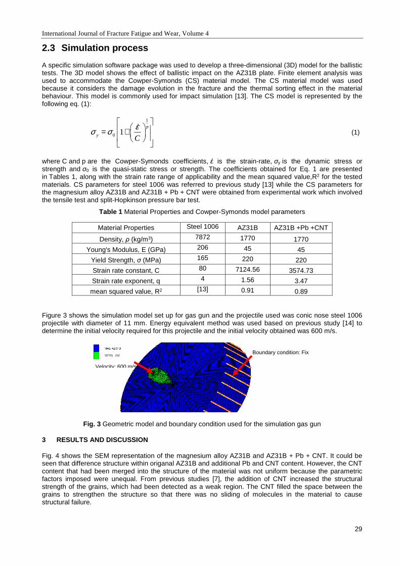
International Journal of Fracture Fatigue and Wear, Volume 4
29
2.3 Simulation process
A specific simulation software package was used to develop a three-dimensional (3D) model for the ballistic tests. The 3D model shows the effect of ballistic impact on the AZ31B plate. Finite element analysis was used to accommodate the Cowper-Symonds (CS) material model. The CS material model was used because it considers the damage evolution in the fracture and the thermal sorting effect in the material behaviour. This model is commonly used for impact simulation [13]. The CS model is represented by the following eq. (1):
1
0 1p
y C
εσ σ
= +
ɺ (1)
where C and p are the Cowper-Symonds coefficients, έ is the strain-rate, σy is the dynamic stress or strength and σ0 is the quasi-static stress or strength. The coefficients obtained for Eq. 1 are presented in Tables 1, along with the strain rate range of applicability and the mean squared value,R2 for the tested materials. CS parameters for steel 1006 was referred to previous study [13] while the CS parameters for the magnesium alloy AZ31B and AZ31B + Pb + CNT were obtained from experimental work which involved the tensile test and split-Hopkinson pressure bar test.
Table 1 Material Properties and Cowper-Symonds model parameters
Material Properties Steel 1006 AZ31B AZ31B +Pb +CNT
Density, ρ (kg/m3) 7872 1770 1770
Young's Modulus, E (GPa) 206 45 45
Yield Strength, σ (MPa) 165 220 220
Strain rate constant, C 80 7124.56 3574.73
Strain rate exponent, q 4 1.56 3.47
mean squared value, R2 [13] 0.91 0.89
Figure 3 shows the simulation model set up for gas gun and the projectile used was conic nose steel 1006 projectile with diameter of 11 mm. Energy equivalent method was used based on previous study [14] to determine the initial velocity required for this projectile and the initial velocity obtained was 600 m/s.
Fig. 3 Geometric model and boundary condition used for the simulation gas gun
3 RESULTS AND DISCUSSION
Fig. 4 shows the SEM representation of the magnesium alloy AZ31B and AZ31B + Pb + CNT. It could be seen that difference structure within origanal AZ31B and additional Pb and CNT content. However, the CNT content that had been merged into the structure of the material was not uniform because the parametric factors imposed were unequal. From previous studies [7], the addition of CNT increased the structural strength of the grains, which had been detected as a weak region. The CNT filled the space between the grains to strengthen the structure so that there was no sliding of molecules in the material to cause structural failure.
Velocity: 600 m/s
Boundary condition: Fix

International Journal of Fracture Fatigue and Wear, Volume 4
30
AZ31B
AZ31B + Pb
+ CNT
Fig. 4 SEM representation of AZ31B and AZ31B +Pb + CNT at (a) magnification of 10kx, and (b)
magnification 50kx.
Figure 5 shows the materials deformation patterns of each plate at time between 6 µs to 115 µs at initial projectile velocity of 600 m/s. Fig. 6 shows stress distribution patterns of each plate at time between 6 µs to 115 µs at initial projectile velocity of 600 m/s. Based on the simulation observation, the concentration of stress for each time was around the tip of projectile. The projectile was retaining its shape when penetrating the plate and the tip of the projectile was progressively deformed at the same time as the material in the panel was displaced and a hole was formed. Deformation occurred on the projectile nose during penetration has led to an immense heat generation and the material of the panel locally melts and loses all mechanical strength [15].
Figure 7 (a) shows the energy (J) was absorb through on magnesium alloys AZ31B and AZ31B +Pb +CNT. It can be seen that the resulting graph of response shows the energy absorption of the magnesium alloys is uniform at 50 µs for AZ31B +Pb +CNT and at 80 µs for AZ31B. Fig 7 (b) shows the velocity (m/s) decrease through the plates. Fig. 8 shows the energy absorbtion responde through depth of penetration of each plate. From the analysis, the AZ31B plate was totally paneterate but the bahaviour of material it self still can be support the energy from projectile to stoped it. The AZ31B +Pb +CNT can support the projectile with 15.06 mm penetration. It seam the reinforcement of CNT and Pb onto AZ31B will decearese about 39.76 % of depth penetertion.
AZ31B
6 µs
12 µs 25 µs 115 µs
AZ31B + Pb + CNT
6 µs 12 µs 25 µs 115 µs
Fig. 5 Materials deformation patterns of each plate at time between 6 µs to 115 µs at initial projectile velocity of 600 m/s
(b)
(a) (b)
(a) (b)
(b) CNT

International Journal of Fracture Fatigue and Wear, Volume 4
31
AZ31B
6 µs
12 µs 25 µs 115 µs
AZ31B + Pb + CNT
6 µs 12 µs 25 µs 115 µs
Fig. 6 Stress distribution patterns of each plate at time between 6 µs to 115 µs at initial projectile velocity of 600 m/s
(a) (b)
Fig. 7 (a) Trend of energy absorption increase through plates, (b) Trend of velocity decrease through plates.
Fig. 8 Energy absorbtion responde through depth of penetration
4 CONCLUSION
The fracture behaviour of magnesium alloy with reinforcement Pb and CNT was reduce the depth of panetration up to 39% compare to original material. Reinforcement material such as Pb and CNT will be Increasing capability of energy absorption of materials. Energy absorption was important factors in controlling the depth of penetration. However, fracture failure occurred because the energy applied was beyond the energy absorption. Thus, the use of magnesium alloy in ballistic applications is feasible, but several of its properties need to be improved. Furthermore, addition of an element in the original alloy composition enhances the durability characteristics and results in a difference in energy absorption.

International Journal of Fracture Fatigue and Wear, Volume 4
32
5 ACKNOWLEDGMENTS
The authors would like to express their gratitude to Ministry of Higher Education Malaysia via Universiti Kebangsaan Malaysia and Universiti Pertahanan National Malaysia (Research funding: FRGS/1/2012/TK04/UPNM/0304 and LRGS/2013/UPNM-UKM/DS/04) for supporting this research.
6 REFERENCES
[1] N.K. Naik, C.H. Veerraju, V.R. Kavala, Hybrid composites under high strain rate compressive
loading, Mater Sci Eng A 2008;498(1–2):87–99.
[2] Z. Li, J. Lambros, Determination of the dynamic response of brittle composites by the use of the
split Hopkinson pressure bar, Composites Science and Technology 59 (1999) 1097-1107.
[3] R. Chen, K. Xia, F. Dai, F. Lu, S.N. Luo, Determination of dynamic fracture parameters using a
semi-circular bend technique in split Hopkinson pressure bar testing, Engineering Fracture
Mechanics 76 (2009) 1268–1276.
[4] T.L. Jones, D.D. Richard, S.B. Matthew, A.G. William, Ballistic performance of magnesium alloy
AZ31B. 23rd Int. Sym. on Ballistics. Tarragona, Spain. 2007; 989-995.
[5] Jena, P.K. K. S. Kumar, V. R. Krishna, A.K. Singh and T. B. Bhat. Studies on the role of
microstructure on performance of a high strength armour steel. Engineering Failure Analysis 15
(2008) 1088–1096
[6] Qianqian Li, Christian A. Rottmair, Robert F. Singer. CNT Reinforced Light Metal Composites
Produced by Melt Stirring and by High Pressure Die Casting. Composites Science and Technology
2012. Pp 1-17.
[7] Muhammad Rahman, Mahesh Hosur, Shaik Zainuddin, Uday Vaidya, Arefin Tauhid, Ashok Kumar,
Jonathan Trovillion, Shaik Jeelani. Effects of amino-functionalized MWCNTs on ballistic impact
performance of E-glass/epoxy composites using a spherical projectile. International Journal of
Impact Engineering 57 (2013) 108-118.
[8] Eslam M. Soliman, Michael P. Sheyka, Mahmoud Reda Taha. Low-velocity impact of thin woven
carbon fabric composites incorporating multi-walled carbon nanotubes. International Journal of
Impact Engineering 47 (2012) pp39-47.
[9] Avila AF, Soares MI, Neto AS. A study on nanostructured laminated plates behaviour under low-
velocity impact loadings. Int J Impact Eng 2007;34: 28-41
[10] Patent N0.2 US 7,921,899 B2. Method for marking magnesium-based carbon nanotube composite
material. United States Patent 2011. Pp 1-6.
[11] Tan V, Ching T. Computational simulation of fabric armour subjected to ballistic impacts. Int J
Impact Eng 2006;32:1737-51.
[12] Srinivasan A, Pillai U.T.S and Pai B.C. Effect of Pb addition on ageing behavior of AZ91
Magnesium alloy. Material Science and Engineering A. 2007; (452-453): 87-92.
[13] C. Hernandez, A. Maranon, I. A. Ashcroft, and J. P. Casas-Rodriguez, "A computational
determination of the Cowper–Symonds parameters from a single Taylor test," Applied Mathematical
Modelling, vol. 37, pp. 4698-4708, 2013.
[14] M.F. Abdullah, S. Abdullah, M.Z. Omar, Z. Sajuri, M.S. Risby, Failure observation of the AZ31B
Magnesium Alloy and the Effect of Lead Addition Content under ballistic impact. Advances in
Mechanical Engineering 7 (5), pp. 1-13, 2015.
[15] D.R. Lesuer, C.K. Syn, O.D. Sherby, J. Wadsworth, Laminated metals composites-fracture and
ballistic impact behaviour, Third Pacific Rim Conference on Advanced Materials and Processing,
1998.
International Journal of Fracture Fatigue and Wear, Volume 4
33
Proceedings of the 5th International Conference on Fracture Fatigue and Wear, pp. 33-38, 2016
EFFECTS OF HETEROGENEOUS PRECIPITATES ON FATIGUE
BEHAVIOR OF AGE-HARDENED CU-NI-SI ALLOY
T. Fujimura1, M. Goto 1, S.Z. Han2, T.Yamamoto1, J.H. Ahn2, J. Kitamura1 and D.Okuzume1
1 Oita University, Oita, 870-1147, Japan 2 Korea Institute of Materials Science, Changwon, Republic of Korea
Abstract: The strengthening of age-hardened Cu-Ni-Si alloys are attributed to the precipitation of a nano-size δ-Ni2Si phase in the copper matrix. In aging process, large heterogeneous precipitates are formed, followed by the generation of discontinuous precipitates which bring a detrimental effect on mechanical properties. However, there are few studies on the effect of heterogeneous precipitates and discontinuous precipitates on fatigue behaviour. The present study was performed in an attempt to obtain a better understanding on the effect of the precipitates on fatigue behaviour of Cu-Ni-Si alloy.
Keywords: fatigue crack; age-hardened Cu-Ni-Si alloy; grain boundaries; precipitates
1 INTRODUCTION
Precipitate strengthened Cu-Ni-Si alloys [1] have been widely used in electrical/electronic components. In spite of the comparatively early discovery of the age hardening effect in this alloy system, relatively little work has been published on mechanical properties of the alloys [2-4], in general, and its fatigue characteristics, in particular. For the actual structural applications, the fatigue characteristics should been clarified for safe design and maintenance of components. To develop Cu-Ni-Si system alloy for improving the fatigue resistance, a fatigue mechanism, such as crack initiation and propagation, should be clarified. The fracture surfaces of Cu-Ni-Si alloys analysed by a scanning electron microscope (SEM) have showed intergranular facets, leading to a hypothesis that grain boundaries (GBs) were an origin of fatigue crack [2,3]. Up to now, however, there was no clear evidence for crack nucleation at the GBs.
The strengthening of Cu-Ni-Si alloys are attributed to nano-size δ-Ni2Si intermetallic compounds precipitated in the copper matrix due to aging. During subsequent aging, however, large heterogeneous precipitates are formed, in addition, some parts of matrix are transformed into discontinuous precipitate (DP) phases. At a later stage of aging, the matrix is fully transformed into DP phases which bring a detrimental effect on mechanical properties. However, there are few studies on the effect of large heterogeneous large precipitates and scattered DP phases on fatigue behaviour.
The present work was performed in an attempt to obtain a better understanding on fatigue damage of precipitate strengthened Cu-Ni-Si alloy. In this regard, clear evidence of the crack initiation from GBs and the effect of DP phase on the behaviour of fatigue cracks was shown.
2 EXPERIMENTAL PROCEDURES
Cu and Si 99.99% pure, and 99.9% pure Ni were used as alloying elements for the fabrication of the Cu–6wt%Ni–1.5wt%Si alloy ingots by induction melting. The ingots were cold-rolled with 80% reduction in thickness, and were subsequently solution heat-treated at 980 °C for 1 h and aged at 500 °C. Large amounts of Ni and a Si content of about 7.5 wt% increased the precipitation driving force because of the large difference between the supersaturated alloy matrix composition and the equilibrium solution limit [5], reducing the aging time. Fig.1 shows an optical micrograph of the Cu–6Ni–1.5Si alloy, showing the change in microstructure with an increase in aging time. After 30 min aging, bright and dark/tarnished grains were formed. The dark grains were DP phase. In this study, the solution heat-treated alloy was aged at 500 °C for 30 min. The microstructure was observed using an optical microscope (OM, GX51. Olympus) and a SEM (JSM-6610LV, JEOL). The characterization of precipitates was carried out using a 200 kV field-emission transmission electron microscope (TEM, JEOL-2100F. JEOL) equipped with an energy-dispersive X-ray spectroscopy (EDS) detector along with a scanning TEM. The 3-mm-diameter, 100-µm-thick disk was

International Journal of Fracture Fatigue and Wear, Volume 4
34
prepared for TEM observation by mechanical polishing with a digitally enhanced precision specimen grinder (DEPS-101, Total Solution) and dimpling by a dimple grinder (656 dimple grinder, Gatan).
Fig. 1 The change in an optical micrograph of the Cu–6Ni–1.5Si alloy during an increase in aging time
The microhardness was measured using a Vickers hardness tester (MXT70, Matsuzawa) with an applied load of 1 N and tensile tests (4 mm diameter specimen) were performed on a tensile testing machine (4206, Instron) with a loading speed of 10 mm/s at room temperature. Round bar fatigue specimens with 5 mm diameter (Fig. 2a) were machined from the aged samples. Although the specimens had a shallow partial notch (Fig. 2b; 2.5 mm radius and 0.1 mm depth), the fatigue strength reduction factor for this geometry was close to 1, meaning that they could be considered plain. To remove any surface layer affected by the preparation, a layer of approximately ≈25 µm was electrolytically polished from the surface of the specimen prior to fatigue testing. All fatigue tests were carried out at room temperature using a rotating bending fatigue machine (constant bending-moment type) operating at 50 Hz. The fatigue damage on the specimen surface and on the fracture surface was observed by using OM and SEM. The crack length, l, was measured along the circumferential direction of the surface using a plastic replication technique. The stress value referred to is that of the nominal stress amplitude, σa, at the minimum cross-section (5 mm diameter).
Fig. 2 The fatigue specimen: (a) shape and dimensions and (b) the details of a partial notch (in mm)
3 EXPERIMENTAL RESULTS AND DISCUSSION
3.1 Microstructure
Fig. 3a shows an optical micrograph of the Cu–6Ni–1.5Si alloy with bright and dark/tarnished grains. Fig. 3b shows high-resolution TEM (HRTEM) images of the matrix (bright grains). Disc-shaped precipitates from aging were observed, which were identified as δ-Ni2Si intermetallic compounds by an optical diffractogram (Fig. 3c). SEM observation of the dark grains at high magnification showed that the cellular structure consisted of Ni2Si precipitates with an extremely high aspect ratio (Fig. 3d). The Ni2Si intermetallic compounds were found to precipitate as spherical particles, and DPs formed simultaneously in a small fractioned area in the matrix. This is because a difference in precipitation kinetics was present in the matrix, in particular near the GBs, under the same aging conditions. The DPs are generally formed by the growth
Fig. 3 Microstructure by aging at 500oC for 30 min after solution treatment at 980oC for 1 hr: (a) microstructure by OM; (b) HRTEM images of continuous precipitated structure; (c) SADP of continuous precipitated structure; (d) microstructure of discontinuous precipitated structure by SEM

International Journal of Fracture Fatigue and Wear, Volume 4
35
of newly generated moving GBs that act as a solute diffusion path. The precipitates grow perpendicular to their moving direction along the lower interface energy between the precipitates and the alloy matrix [6], forming a cellular structure with fibre-like precipitates.
The SEM bright-field TEM, and HRTEM micrographs in Fig. 4a–c present the microstructure around GB areas; large δ-Ni2Si particles heterogeneously precipitated along the GBs can be observed (Fig. 4b). An enlarged image of the large δ-Ni2Si particle region was shown in Fig. 4c. The fast diffusion along the GBs appeared to lead the formation of precipitates at GBs and subsequent rapid growth (heterogeneous precipitates shown in Fig. 4b and c). In addition, very large particles, larger than several micrometres, were observed on GB areas (shown in Fig. 4a). These large particles might be classified as inclusions that had already existed before aging or as large heterogeneous precipitates. Further evidence and discussion are needed to elucidate the formation mechanism of these very large particles. In the bright-field TEM image of GB areas (Fig. 4b), a band-like bright zone along the GBs indicated the precipitate-free zone (PFZ) that was formed as the result of solute atoms’ absorption near the heterogeneous precipitates.
Fig. 4 Microstructure around GB areas: (a) SEM micrograph; (b) bright-field TEM image; (c) HRTEM image of heterogeneous δ-Ni2Si precipitate
3.2 Tensile properties and fatigue behaviour
Fig. 5 shows the stress-strain curve of the Cu–6Ni–1.5Si alloy, showing a tensile strength of 820 MPa, a yield strength (0.2 %) of 634 MPa and a tensile elongation of 14.3% (average of 3 specimens). The value of Vickers hardness was 259.
Fig. 5 The stress-strain curve of Cu-6Ni-1.5Si alloy
To clarify the positional relationship between the crack initiation sites and the microstructure, the specimen surface was etched prior to the fatigue tests to reveal the microstructure. After the optical micrographs of the etched surface were taken, a layer of a few micrometres was polished off the surface by buffing to remove the etching-induced damaged areas that would affect crack initiation behaviour during stressing; this was followed by fatigue tests. After initiation of fatigue cracks with grain-size length, the fatigue test was interrupted for etching to reveal the microstructure, and the test was resumed with the etched specimen. During the fatigue test, the specimen surface was monitored at regular intervals by means of both direct OM observation and observation using a plastic replication technique. Figure 6a shows the change in surface states around a crack initiated within the partial notched surface during cyclic stressing at σa = 240 MPa. At an extremely early fatigue stage (N/Nf = 0.077), a crack was formed on the buffed surface (Nf = 5.19×10⁵, σa = 240 MPa). On the same surface treated by etching, GBs and DP structures were recognized along the cracks. A comparison between prefatigued and fatigued surfaces suggested that the starting point of cracks was GBs, as shown by white arrows. After the initiation, the cracks grew with shear mode along the slip orientation of adjacent grains (Fig. 6b) and GBs. Fig.6c shows the change in surface states
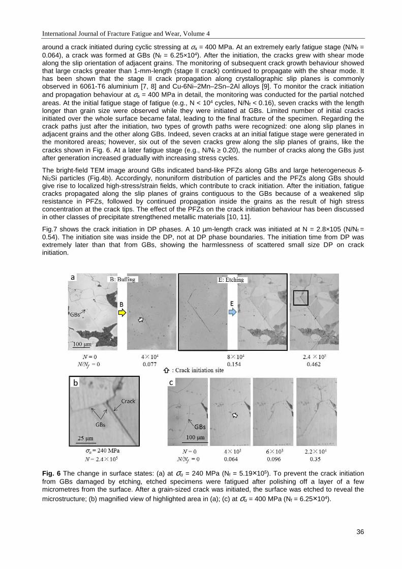
International Journal of Fracture Fatigue and Wear, Volume 4
36
around a crack initiated during cyclic stressing at σa = 400 MPa. At an extremely early fatigue stage (N/Nf = 0.064), a crack was formed at GBs (Nf = 6.25×10⁴). After the initiation, the cracks grew with shear mode along the slip orientation of adjacent grains. The monitoring of subsequent crack growth behaviour showed that large cracks greater than 1-mm-length (stage II crack) continued to propagate with the shear mode. It has been shown that the stage II crack propagation along crystallographic slip planes is commonly observed in 6061-T6 aluminium [7, 8] and Cu-6Ni–2Mn–2Sn–2Al alloys [9]. To monitor the crack initiation and propagation behaviour at σa = 400 MPa in detail, the monitoring was conducted for the partial notched areas. At the initial fatigue stage of fatigue (e.g., N < 104 cycles, N/Nf < 0.16), seven cracks with the length longer than grain size were observed while they were initiated at GBs. Limited number of initial cracks initiated over the whole surface became fatal, leading to the final fracture of the specimen. Regarding the crack paths just after the initiation, two types of growth paths were recognized: one along slip planes in adjacent grains and the other along GBs. Indeed, seven cracks at an initial fatigue stage were generated in the monitored areas; however, six out of the seven cracks grew along the slip planes of grains, like the cracks shown in Fig. 6. At a later fatigue stage (e.g., N/Nf ≥ 0.20), the number of cracks along the GBs just after generation increased gradually with increasing stress cycles.
The bright-field TEM image around GBs indicated band-like PFZs along GBs and large heterogeneous δ-Ni2Si particles (Fig.4b). Accordingly, nonuniform distribution of particles and the PFZs along GBs should give rise to localized high-stress/strain fields, which contribute to crack initiation. After the initiation, fatigue cracks propagated along the slip planes of grains contiguous to the GBs because of a weakened slip resistance in PFZs, followed by continued propagation inside the grains as the result of high stress concentration at the crack tips. The effect of the PFZs on the crack initiation behaviour has been discussed in other classes of precipitate strengthened metallic materials [10, 11].
Fig.7 shows the crack initiation in DP phases. A 10 µm-length crack was initiated at N = 2.8×10⁵ (N/Nf = 0.54). The initiation site was inside the DP, not at DP phase boundaries. The initiation time from DP was extremely later than that from GBs, showing the harmlessness of scattered small size DP on crack initiation.
Fig. 6 The change in surface states: (a) at σa = 240 MPa (Nf = 5.19×10⁵). To prevent the crack initiation from GBs damaged by etching, etched specimens were fatigued after polishing off a layer of a few micrometres from the surface. After a grain-sized crack was initiated, the surface was etched to reveal the microstructure; (b) magnified view of highlighted area in (a); (c) at σa = 400 MPa (Nf = 6.25×10⁴).
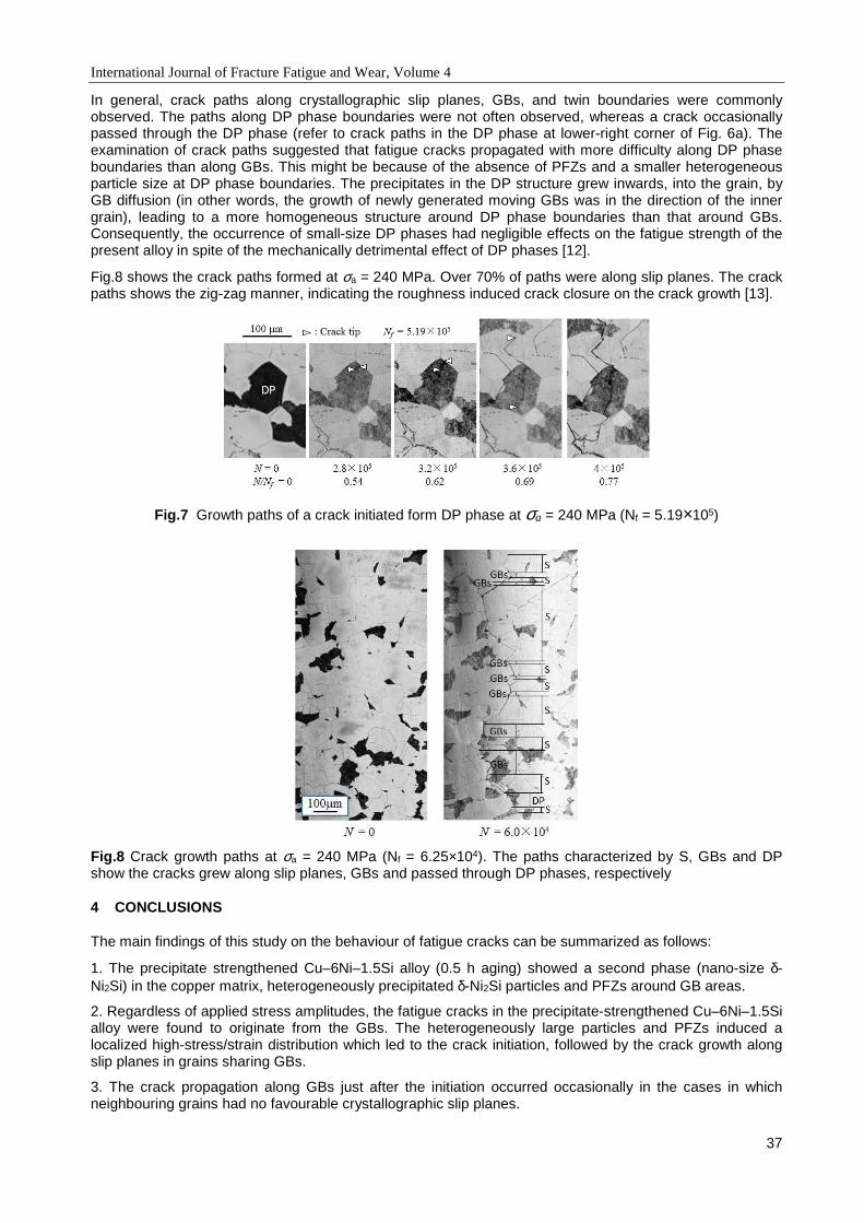
International Journal of Fracture Fatigue and Wear, Volume 4
37
In general, crack paths along crystallographic slip planes, GBs, and twin boundaries were commonly observed. The paths along DP phase boundaries were not often observed, whereas a crack occasionally passed through the DP phase (refer to crack paths in the DP phase at lower-right corner of Fig. 6a). The examination of crack paths suggested that fatigue cracks propagated with more difficulty along DP phase boundaries than along GBs. This might be because of the absence of PFZs and a smaller heterogeneous particle size at DP phase boundaries. The precipitates in the DP structure grew inwards, into the grain, by GB diffusion (in other words, the growth of newly generated moving GBs was in the direction of the inner grain), leading to a more homogeneous structure around DP phase boundaries than that around GBs. Consequently, the occurrence of small-size DP phases had negligible effects on the fatigue strength of the present alloy in spite of the mechanically detrimental effect of DP phases [12].
Fig.8 shows the crack paths formed at σa = 240 MPa. Over 70% of paths were along slip planes. The crack paths shows the zig-zag manner, indicating the roughness induced crack closure on the crack growth [13].
Fig.7 Growth paths of a crack initiated form DP phase at σa = 240 MPa (Nf = 5.19×10⁵)
Fig.8 Crack growth paths at σa = 240 MPa (Nf = 6.25×10⁴). The paths characterized by S, GBs and DP show the cracks grew along slip planes, GBs and passed through DP phases, respectively
4 CONCLUSIONS
The main findings of this study on the behaviour of fatigue cracks can be summarized as follows:
1. The precipitate strengthened Cu–6Ni–1.5Si alloy (0.5 h aging) showed a second phase (nano-size δ-Ni2Si) in the copper matrix, heterogeneously precipitated δ-Ni2Si particles and PFZs around GB areas.
2. Regardless of applied stress amplitudes, the fatigue cracks in the precipitate-strengthened Cu–6Ni–1.5Si alloy were found to originate from the GBs. The heterogeneously large particles and PFZs induced a localized high-stress/strain distribution which led to the crack initiation, followed by the crack growth along slip planes in grains sharing GBs.
3. The crack propagation along GBs just after the initiation occurred occasionally in the cases in which neighbouring grains had no favourable crystallographic slip planes.

International Journal of Fracture Fatigue and Wear, Volume 4
38
4. A small number of scattered discontinuous precipitation phases were observed in the matrix, but the effect of such phases on the fatigue strength was negligible in spite of the mechanically detrimental effect of DP phases.
5 ACKNOWLEDGEMENTS
This study was supported by a Grant-in-Aid for Scientific Research (C) (KAKENHI: No. 26420021) from the Japan Society for the Promotion of Science-Japan, as well as a National Research Foundation of Korea (NRF) grant funded by the Global Frontier R&D Program (2013M3A6B1078874) at the Global Frontier Hybrid Interface Materials R&D Centre funded by the Ministry of Science, ICT, and a Future Planning and National Research Foundation of Korea (NRF) grant funded by the Korea government (MSIP) (no. 2011-0030058). The authors are very grateful to the members of the Strength of Materials Laboratory of Oita University for their excellent experimental assistance. Thanks are also extended to the members of the Korea Institute of Materials Science, for the fabrication of the Cu–Ni–Si system alloys.
6 REFERENCES
[1] M.G. Corson MG. Electrical conductor alloys, Electr. World, 89, 137-139, 1927.
[2] S.A. Lockyer, F.W. Noble, Fatigue of precipitate strengthened Cu-Ni-Si alloy. Mater. Sci. Technol., 15, 1147–1153, 1999.
[3] Z. Sun, C. Laitem, A. Vincent, Dynamic embrittlement during fatigue of a Cu-Ni-Si alloy. Mater. Sci. Eng. A, 528, 6334–6337, 2011.
[4] T. Fujii, H. Kamio, Y. Sugisawa, S. Onaka, M. Kato, Cyclic softening of Cu-Ni-Si alloy single crystals under low-cycle fatigue, Mater. Sci. Forum, 654–656:1287–1290, 2010.
[5] H.G. Kim, T.W. Lee, S.M. Kim, S.Z. Han, K. Euh, Y.W. Kim, S.H. Lim, Effects of Ti addition and heat treatments on mechanical and electrical properties of Cu-Ni-Si alloys. Met. Mater. Inter., 19, 61–65, 2013.
[6] F. Findik, Discontinuous (cellular) precipitation, J. Mater. Sci. Lett., 17, 79–83, 1998.
[7] H. Nisitani H, K. Takao, Significance of initiation, propagation and closure of microcracks in high
cycle fatigue of ductile metals, Eng. Fract. Mech., 15, 445-456, 1981.
[8] M. Goto, D.L. DuQuesnay, Fatigue behavior of 6061-T6 aluminum alloy plain specimens, SAE
Tech. Paper Ser., No.970703, 1-7, 1997.
[9] M. Goto, S.Z. Han, K. Euh, N. Kawagoishi, S. Kim, K. Kamil, Statistical description of the effect of
Zr addition on the behavior of microcracks in Cu–6Ni–2Mn–2Sn–2Al Alloy, J. Mater. Sci., 47:1497-
1503, 2012.
[10] K.T. Venkateswara, K.T. Rao, R.O. Ritchie, Fatigue of aluminium-lithium alloys, Inter. Mater.
Reviews, 37, 153-185, 1992.
[11] J. Zhong, S. Zhong, Z.Q. Zheng, H.F. Zhang, X.F. Luo, Fatigue crack initiation and early
propagation behavior of 2A97 Al−Li alloy. Trans. Nonferrous Metals Soc. China, 24, 303-309, 2014.
[12] E. Lee, K. Euh, S.Z. Han, S.H. Lim, J. Lee, S. Kim, Tensile and electrical properties of direct aged
Cu-Ni-Si-x%Ti alloys, Met. Mater. Inter., 19, 183–188, 2013.
[13] M. Goto, S.Z. Han, S.H. Lim, J. Kitamura, T. Fujimura, J-H. Ahn, T. Yamamoto, S. Kim, J. Lee,
Role of microstructure on initiation and propagation of fatigue cracks in precipitate strengthened
Cu-Ni-Si alloy, Inter. J. Fatigue, 87, 15-21, 2016.
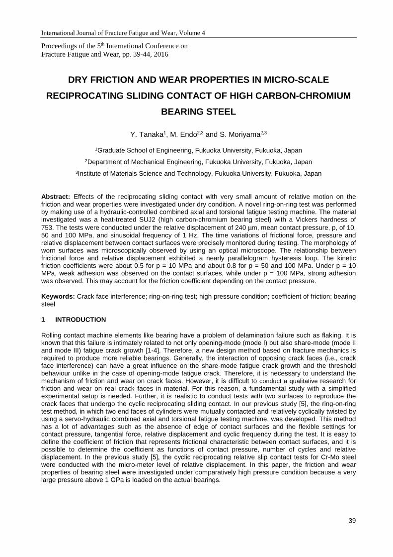
International Journal of Fracture Fatigue and Wear, Volume 4
39
Proceedings of the 5th International Conference on Fracture Fatigue and Wear, pp. 39-44, 2016
DRY FRICTION AND WEAR PROPERTIES IN MICRO-SCALE
RECIPROCATING SLIDING CONTACT OF HIGH CARBON-CHROMIUM
BEARING STEEL
Y. Tanaka1, M. Endo2,3 and S. Moriyama2,3
1Graduate School of Engineering, Fukuoka University, Fukuoka, Japan
2Department of Mechanical Engineering, Fukuoka University, Fukuoka, Japan
3Institute of Materials Science and Technology, Fukuoka University, Fukuoka, Japan
Abstract: Effects of the reciprocating sliding contact with very small amount of relative motion on the friction and wear properties were investigated under dry condition. A novel ring-on-ring test was performed by making use of a hydraulic-controlled combined axial and torsional fatigue testing machine. The material investigated was a heat-treated SUJ2 (high carbon-chromium bearing steel) with a Vickers hardness of 753. The tests were conducted under the relative displacement of 240 µm, mean contact pressure, p, of 10, 50 and 100 MPa, and sinusoidal frequency of 1 Hz. The time variations of frictional force, pressure and relative displacement between contact surfaces were precisely monitored during testing. The morphology of worn surfaces was microscopically observed by using an optical microscope. The relationship between frictional force and relative displacement exhibited a nearly parallelogram hysteresis loop. The kinetic friction coefficients were about 0.5 for p = 10 MPa and about 0.8 for p = 50 and 100 MPa. Under p = 10 MPa, weak adhesion was observed on the contact surfaces, while under p = 100 MPa, strong adhesion was observed. This may account for the friction coefficient depending on the contact pressure.
Keywords: Crack face interference; ring-on-ring test; high pressure condition; coefficient of friction; bearing steel
1 INTRODUCTION
Rolling contact machine elements like bearing have a problem of delamination failure such as flaking. It is known that this failure is intimately related to not only opening-mode (mode I) but also share-mode (mode II and mode III) fatigue crack growth [1-4]. Therefore, a new design method based on fracture mechanics is required to produce more reliable bearings. Generally, the interaction of opposing crack faces (i.e., crack face interference) can have a great influence on the share-mode fatigue crack growth and the threshold behaviour unlike in the case of opening-mode fatigue crack. Therefore, it is necessary to understand the mechanism of friction and wear on crack faces. However, it is difficult to conduct a qualitative research for friction and wear on real crack faces in material. For this reason, a fundamental study with a simplified experimental setup is needed. Further, it is realistic to conduct tests with two surfaces to reproduce the crack faces that undergo the cyclic reciprocating sliding contact. In our previous study [5], the ring-on-ring test method, in which two end faces of cylinders were mutually contacted and relatively cyclically twisted by using a servo-hydraulic combined axial and torsional fatigue testing machine, was developed. This method has a lot of advantages such as the absence of edge of contact surfaces and the flexible settings for contact pressure, tangential force, relative displacement and cyclic frequency during the test. It is easy to define the coefficient of friction that represents frictional characteristic between contact surfaces, and it is possible to determine the coefficient as functions of contact pressure, number of cycles and relative displacement. In the previous study [5], the cyclic reciprocating relative slip contact tests for Cr-Mo steel were conducted with the micro-meter level of relative displacement. In this paper, the friction and wear properties of bearing steel were investigated under comparatively high pressure condition because a very large pressure above 1 GPa is loaded on the actual bearings.
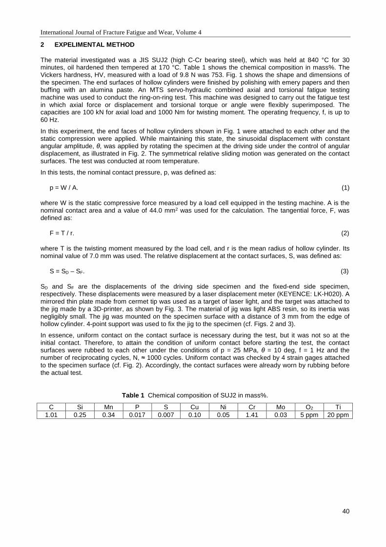
International Journal of Fracture Fatigue and Wear, Volume 4
40
2 EXPELIMENTAL METHOD
The material investigated was a JIS SUJ2 (high C-Cr bearing steel), which was held at 840 °C for 30 minutes, oil hardened then tempered at 170 °C. Table 1 shows the chemical composition in mass%. The Vickers hardness, HV, measured with a load of 9.8 N was 753. Fig. 1 shows the shape and dimensions of the specimen. The end surfaces of hollow cylinders were finished by polishing with emery papers and then buffing with an alumina paste. An MTS servo-hydraulic combined axial and torsional fatigue testing machine was used to conduct the ring-on-ring test. This machine was designed to carry out the fatigue test in which axial force or displacement and torsional torque or angle were flexibly superimposed. The capacities are 100 kN for axial load and 1000 Nm for twisting moment. The operating frequency, f, is up to 60 Hz.
In this experiment, the end faces of hollow cylinders shown in Fig. 1 were attached to each other and the static compression were applied. While maintaining this state, the sinusoidal displacement with constant angular amplitude, θ, was applied by rotating the specimen at the driving side under the control of angular displacement, as illustrated in Fig. 2. The symmetrical relative sliding motion was generated on the contact surfaces. The test was conducted at room temperature.
In this tests, the nominal contact pressure, p, was defined as:
p = W / A. (1)
where W is the static compressive force measured by a load cell equipped in the testing machine. A is the nominal contact area and a value of 44.0 mm2 was used for the calculation. The tangential force, F, was defined as:
F = T / r. (2)
where T is the twisting moment measured by the load cell, and r is the mean radius of hollow cylinder. Its nominal value of 7.0 mm was used. The relative displacement at the contact surfaces, S, was defined as:
S = SD – SF. (3)
SD and SF are the displacements of the driving side specimen and the fixed-end side specimen, respectively. These displacements were measured by a laser displacement meter (KEYENCE: LK-H020). A mirrored thin plate made from cermet tip was used as a target of laser light, and the target was attached to the jig made by a 3D-printer, as shown by Fig. 3. The material of jig was light ABS resin, so its inertia was negligibly small. The jig was mounted on the specimen surface with a distance of 3 mm from the edge of hollow cylinder. 4-point support was used to fix the jig to the specimen (cf. Figs. 2 and 3).
In essence, uniform contact on the contact surface is necessary during the test, but it was not so at the initial contact. Therefore, to attain the condition of uniform contact before starting the test, the contact surfaces were rubbed to each other under the conditions of p = 25 MPa, θ = 10 deg, f = 1 Hz and the number of reciprocating cycles, N, ≈ 1000 cycles. Uniform contact was checked by 4 strain gages attached to the specimen surface (cf. Fig. 2). Accordingly, the contact surfaces were already worn by rubbing before the actual test.
Table 1 Chemical composition of SUJ2 in mass%.
C Si Mn P S Cu Ni Cr Mo O2 Ti 1.01 0.25 0.34 0.017 0.007 0.10 0.05 1.41 0.03 5 ppm 20 ppm
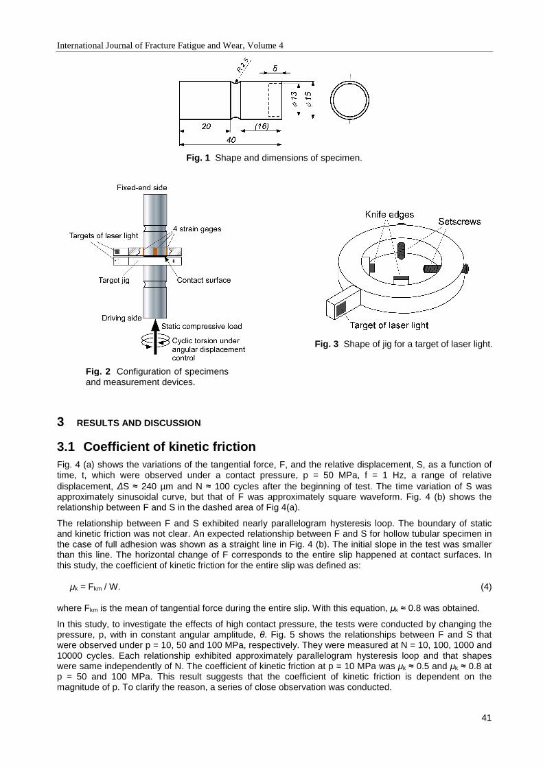
International Journal of Fracture Fatigue and Wear, Volume 4
41
3 RESULTS AND DISCUSSION
3.1 Coefficient of kinetic friction Fig. 4 (a) shows the variations of the tangential force, F, and the relative displacement, S, as a function of time, t, which were observed under a contact pressure, p = 50 MPa, f = 1 Hz, a range of relative displacement, ∆S ≈ 240 µm and N ≈ 100 cycles after the beginning of test. The time variation of S was approximately sinusoidal curve, but that of F was approximately square waveform. Fig. 4 (b) shows the relationship between F and S in the dashed area of Fig 4(a).
The relationship between F and S exhibited nearly parallelogram hysteresis loop. The boundary of static and kinetic friction was not clear. An expected relationship between F and S for hollow tubular specimen in the case of full adhesion was shown as a straight line in Fig. 4 (b). The initial slope in the test was smaller than this line. The horizontal change of F corresponds to the entire slip happened at contact surfaces. In this study, the coefficient of kinetic friction for the entire slip was defined as:
µk = Fkm / W. (4)
where Fkm is the mean of tangential force during the entire slip. With this equation, µk ≈ 0.8 was obtained.
In this study, to investigate the effects of high contact pressure, the tests were conducted by changing the pressure, p, with in constant angular amplitude, θ. Fig. 5 shows the relationships between F and S that were observed under p = 10, 50 and 100 MPa, respectively. They were measured at N = 10, 100, 1000 and 10000 cycles. Each relationship exhibited approximately parallelogram hysteresis loop and that shapes were same independently of N. The coefficient of kinetic friction at p = 10 MPa was µk ≈ 0.5 and µk ≈ 0.8 at p = 50 and 100 MPa. This result suggests that the coefficient of kinetic friction is dependent on the magnitude of p. To clarify the reason, a series of close observation was conducted.
Fig. 1 Shape and dimensions of specimen.
Fig. 2 Configuration of specimens and measurement devices.
Fig. 3 Shape of jig for a target of laser light.
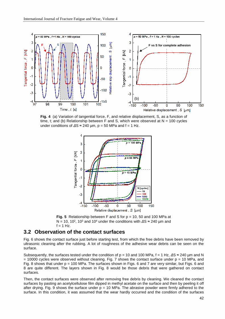
International Journal of Fracture Fatigue and Wear, Volume 4
42
3.2 Observation of the contact surfaces Fig. 6 shows the contact surface just before starting test, from which the free debris have been removed by ultrasonic cleaning after the rubbing. A lot of roughness of the adhesive wear debris can be seen on the surface.
Subsequently, the surfaces tested under the condition of p = 10 and 100 MPa, f = 1 Hz, ∆S ≈ 240 µm and N = 10000 cycles were observed without cleaning. Fig. 7 shows the contact surface under p = 10 MPa, and Fig. 8 shows that under p = 100 MPa. The surfaces shown in Figs. 6 and 7 are very similar, but Figs. 6 and 8 are quite different. The layers shown in Fig. 8 would be those debris that were gathered on contact surfaces.
Then, the contact surfaces were observed after removing free debris by cleaning. We cleaned the contact surfaces by pasting an acetylcellulose film dipped in methyl acetate on the surface and then by peeling it off after drying. Fig. 9 shows the surface under p = 10 MPa. The abrasive powder were firmly adhered to the surface. In this condition, it was assumed that the wear hardly occurred and the condition of the surfaces
Fig. 4 (a) Variation of tangential force, F, and relative displacement, S, as a function of time, t; and (b) Relationship between F and S, which were observed at N = 100 cycles under conditions of ∆S ≈ 240 µm, p = 50 MPa and f = 1 Hz.
Fig. 5 Relationship between F and S for p = 10, 50 and 100 MPa at N = 10, 102, 103 and 104 under the conditions with ∆S ≈ 240 µm and f = 1 Hz.
F S
(b)
F vs S for complete adhesion
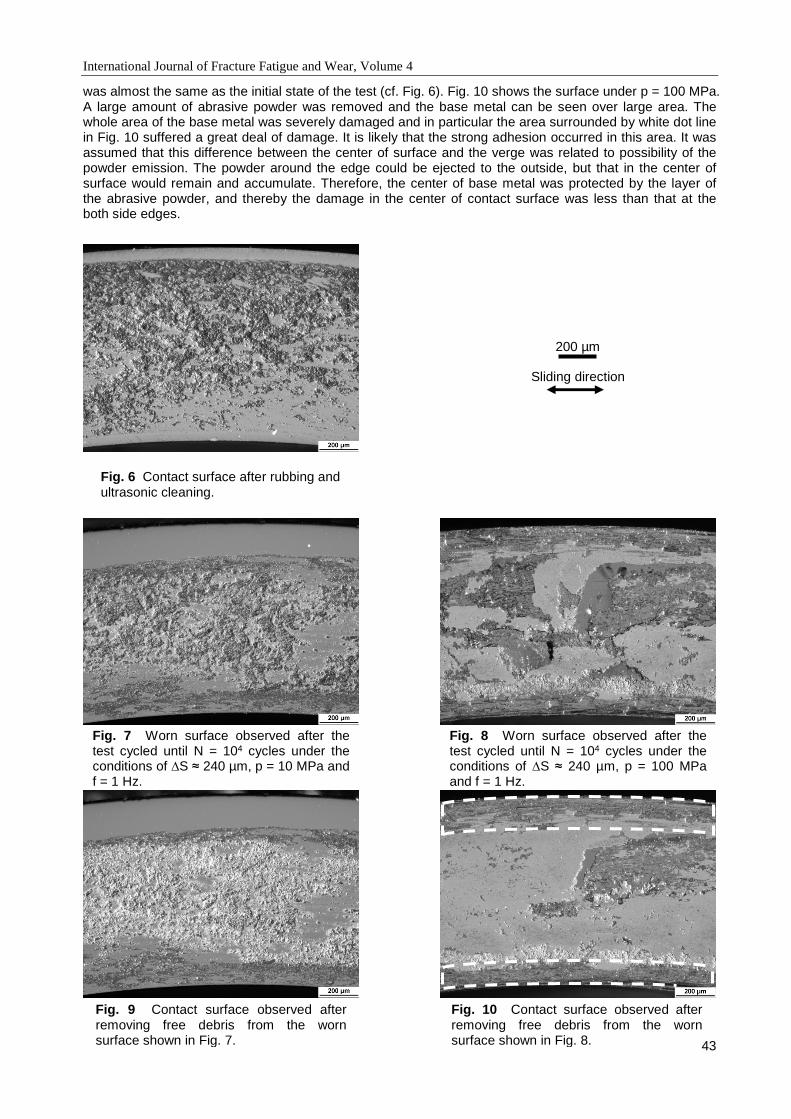
International Journal of Fracture Fatigue and Wear, Volume 4
43
was almost the same as the initial state of the test (cf. Fig. 6). Fig. 10 shows the surface under p = 100 MPa. A large amount of abrasive powder was removed and the base metal can be seen over large area. The whole area of the base metal was severely damaged and in particular the area surrounded by white dot line in Fig. 10 suffered a great deal of damage. It is likely that the strong adhesion occurred in this area. It was assumed that this difference between the center of surface and the verge was related to possibility of the powder emission. The powder around the edge could be ejected to the outside, but that in the center of surface would remain and accumulate. Therefore, the center of base metal was protected by the layer of the abrasive powder, and thereby the damage in the center of contact surface was less than that at the both side edges.
Fig. 6 Contact surface after rubbing and ultrasonic cleaning.
Fig. 7 Worn surface observed after the test cycled until N = 104 cycles under the conditions of ∆S ≈ 240 µm, p = 10 MPa and f = 1 Hz.
Fig. 8 Worn surface observed after the test cycled until N = 104 cycles under the conditions of ∆S ≈ 240 µm, p = 100 MPa and f = 1 Hz.
Fig. 10 Contact surface observed after removing free debris from the worn surface shown in Fig. 8.
Fig. 9 Contact surface observed after removing free debris from the worn surface shown in Fig. 7.
Sliding direction
200 µm
International Journal of Fracture Fatigue and Wear, Volume 4
44
Furthermore, after the end of the test, we noticed small breaking sound when the specimens were separated. This may be an evidence that a strong adhesion occurred at the verge of contact surfaces. The extent of adhesion on the contact surfaces was very limited when p = 10 MPa, and the coefficient of kinetic friction was µk ≈ 0.5. On the other hand, it is considered that when p = 100 MPa, the friction force increased with the occurrence of strong adhesion, and the coefficient became as large as µk ≈ 0.8.
4 CONCLUSIONS
The cyclic reciprocating sliding contact experiment for JIS SUJ2 (high carbon-chromium bearing steel) was conducted to investigate the characteristics of friction and wear and the effects of static load and the number of reciprocating cycles. The obtained results are summarized as follows:
The relationship between friction force, F, and relative displacement, S, exhibited nearly parallelogram hysteresis loop.
Under high pressure condition, the friction and wear on contact surfaces was strongly affected by the adhesion.
When the effect of adhesion was dominant, the coefficient of kinetic friction was µk ≈ 0.8.
When the effect of adhesion was small, the coefficient of kinetic friction was µk ≈ 0.5.
The coefficient of kinetic friction was approximately constant independently of the number of reciprocating cycles, N.
5 FUTURE WORKS
In this paper, the tests were conducted under the limited conditions. Therefore, the wide range of experimental conditions will be considered in and the following investigation will be conducted:
Conduct tests under low pressure conditions.
Investigate the effects of test frequency, f, on the characteristics of friction and wear.
Study the effects of relative displacement, S.
6 REFERENCES
[1] A. Otsuka, Y. Fujii and K. Maeda, A new Testing Method to Obtain Mode II Fatigue Crack Growth Characteristics of Hard Materials, Fatigue & Fracture of Engineering Materials & Structures, 27, 203-212, 2004
[2] S. Beretta, M. Boniardi, M. Carboni and H. Desimone, Mode II Fatigue Failures at Rail Butt-welds, Engineering Failure Analysis, 12, 157-165, 2005.
[3] M. W. J. Lewis and B. Tomkins, A Fracture Mechanics Interpretation of Rolling Bearing Fatigue, J. Engineering Tribology, 226, 389-405, 2012.
[4] H. Matsunaga, N. Shomura, S. Muramoto and M. Endo, Shear Mode Threshold for a Small Fatigue Crack in a Bearing Steel, Fatigue & Fracture of Engineering Materials & Structures, 34, 72-82, 2010.
[5] M. Endo, T. Saito, S. Moriyama, S. Okazaki, H. Matsunaga, Friction and Wear Properties of Heat-treated Cr-Mo Steel during Reciprocating Sliding Contact with Small Relative Motion, Int. J. Fracture Fatigue and Wear, 3, 215-220, 2015.
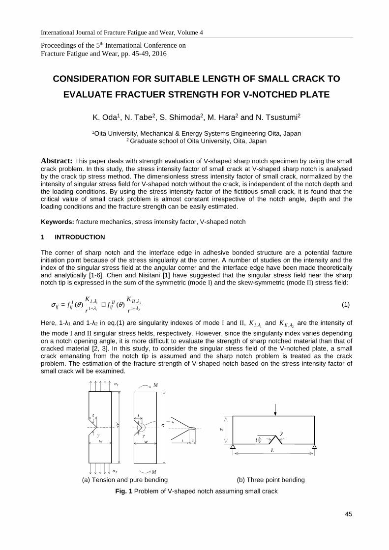
International Journal of Fracture Fatigue and Wear, Volume 4
45
Proceedings of the 5th International Conference on Fracture Fatigue and Wear, pp. 45-49, 2016
CONSIDERATION FOR SUITABLE LENGTH OF SMALL CRACK TO
EVALUATE FRACTUER STRENGTH FOR V-NOTCHED PLATE
K. Oda1, N. Tabe2, S. Shimoda2, M. Hara2 and N. Tsustumi2
1Oita University, Mechanical & Energy Systems Engineering Oita, Japan 2 Graduate school of Oita University, Oita, Japan
Abstract: This paper deals with strength evaluation of V-shaped sharp notch specimen by using the small crack problem. In this study, the stress intensity factor of small crack at V-shaped sharp notch is analysed by the crack tip stress method. The dimensionless stress intensity factor of small crack, normalized by the intensity of singular stress field for V-shaped notch without the crack, is independent of the notch depth and the loading conditions. By using the stress intensity factor of the fictitious small crack, it is found that the critical value of small crack problem is almost constant irrespective of the notch angle, depth and the loading conditions and the fracture strength can be easily estimated.
Keywords: fracture mechanics, stress intensity factor, V-shaped notch
1 INTRODUCTION
The corner of sharp notch and the interface edge in adhesive bonded structure are a potential facture initiation point because of the stress singularity at the corner. A number of studies on the intensity and the index of the singular stress field at the angular corner and the interface edge have been made theoretically and analytically [1-6]. Chen and Nisitani [1] have suggested that the singular stress field near the sharp notch tip is expressed in the sum of the symmetric (mode Ι) and the skew-symmetric (mode ΙΙ) stress field:
2
2
1
1
1
,
1
,)()( λ
λλλ θθσ
−−+=
r
Kf
r
Kf
IIIIij
IIijij (1)
Here, 1-λ1 and 1-λ2 in eq.(1) are singularity indexes of mode Ι and ΙΙ, 1,λIK and
2,λIIK are the intensity of
the mode Ι and ΙΙ singular stress fields, respectively. However, since the singularity index varies depending on a notch opening angle, it is more difficult to evaluate the strength of sharp notched material than that of cracked material [2, 3]. In this study, to consider the singular stress field of the V-notched plate, a small crack emanating from the notch tip is assumed and the sharp notch problem is treated as the crack problem. The estimation of the fracture strength of V-shaped notch based on the stress intensity factor of small crack will be examined.
σT
σT
t
wγ
M
M
t
wγ
at
(a) Tension and pure bending (b) Three point bending
Fig. 1 Problem of V-shaped notch assuming small crack
γt
L
w
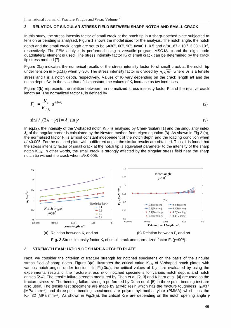
International Journal of Fracture Fatigue and Wear, Volume 4
46
2 RELATION OF SINGULAR STRESS FIELD BETWEEN SHARP NOTCH AND SMALL CRACK
In this study, the stress intensity factor of small crack at the notch tip in a sharp-notched plate subjected to tension or bending is analysed. Figure 1 shows the model used for the analysis. The notch angle, the notch depth and the small crack length are set to be γ=30º, 60º, 90º, t/w=0.1~0.5 and a/t=1.67×10-5~3.33×10-2, respectively. The FEM analysis is performed using a versatile program MSC.Marc and the eight node quadrilateral element is used. The stress intensity factor KI of small crack can be determined by the crack tip stress method [7].
Figure 2(a) indicates the numerical results of the stress intensity factor KI of small crack at the notch tip under tension in Fig.1(a) when γ=90º. The stress intensity factor is divided by tT πσ , where σT is a tensile
stress and t is a notch depth, respectively. Values of KI vary depending on the crack length a/t and the notch depth t/w. In the case that a/t is constant, the values of KI increase as t/w increases.
Figure 2(b) represents the relation between the normalized stress intensity factor FΙ and the relative crack length a/t. The normalized factor FΙ is defined by
1
1
5.0
,
λ
λ
−= aK
KF
I
II (2)
γλγπλ sin)2(sin 11 =− (3)
In eq.(2), the intensity of the V-shaped notch KI,λ1 is analysed by Chen-Nisitani [1] and the singularity index λ1 of the angular corner is calculated by the Newton method from eigen equation (3). As shown in Fig.2 (b), the normalized factor FΙ is almost constant independent of the notch depth and the loading condition when a/t<0.005. For the notched plate with a different angle, the similar results are obtained. Thus, it is found that the stress intensity factor of small crack at the notch tip is equivalent parameter to the intensity of the sharp notch KI,λ1. In other words, the small crack is strongly affected by the singular stress field near the sharp notch tip without the crack when a/t<0.005.
0
0.5
1
1.5
2
2.5
0.00001 0.0001 0.001 0.01 0.1
KΙ/σ
T√π
t
crack length a/t
0.10.20.30.4
Notch depth t/w
Notch angleγ=90°
0.8
0.85
0.9
0.95
1
1.05
1.1
0.00001 0.0001 0.001 0.01 0.1
FⅠ
=KIa
0.5-λ/K
I,λ I
Relation crack length a/t
0.1(Tension) 0.2(Tension)
0.3(Tension) 0.4(Tension)
0.1(Bending) 0.2(Bending)
0.3(Bending) 0.4(Bending)
t/w
Notch angleγ=90°
(a) Relation between KI and a/t. (b) Relation between FI and a/t.
Fig. 2 Stress intensity factor KI of small crack and normalized factor FI (γ=90º).
3 STRENGTH EVALUATION OF SHARP-NOTCHED PLATE
Next, we consider the criterion of fracture strength for notched specimens on the basis of the singular stress filed of sharp notch. Figure 3(a) illustrates the critical value KI,λ1 of V-shaped notch plates with various notch angles under tension. In Fig.3(a), the critical values of KI,λ1 are evaluated by using the experimental results of the fracture stress σf of notched specimens for various notch depths and notch angles [2-4]. The tensile failure strength measured by Chen et al. [2, 3] and Kihara et al. [4] are used as the fracture stress σf. The bending failure strength performed by Dunn et al. [5] in three-point-bending test are also used. The tensile test specimens are made by acrylic resin which has the fracture toughness KIC=37 [MPa mm0.5] and three-point bending specimens are polymethyl methacrylate (PMMA) which has the KIC=32 [MPa mm0.5]. As shown in Fig.3(a), the critical KI,λ1 are depending on the notch opening angle γ
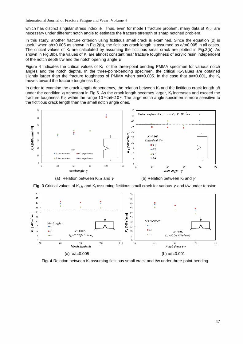
International Journal of Fracture Fatigue and Wear, Volume 4
47
which has distinct singular stress index λ1. Thus, even for mode I fracture problem, many data of KI,λ1 are necessary under different notch angle to estimate the fracture strength of sharp notched problem.
In this study, another fracture criterion using fictitious small crack is examined. Since the equation (2) is useful when a/t<0.005 as shown in Fig.2(b), the fictitious crack length is assumed as a/t=0.005 in all cases. The critical values of KI are calculated by assuming the fictitious small crack are plotted in Fig.3(b). As shown in Fig.3(b), the values of KI are almost constant near fracture toughness of acrylic resin independent of the notch depth t/w and the notch opening angle γ.
Figure 4 indicates the critical values of KI of the three-point bending PMMA specimen for various notch angles and the notch depths. In the three-point-bending specimen, the critical KI-values are obtained slightly larger than the fracture toughness of PMMA when a/t=0.005. In the case that a/t=0.001, the KI moves toward the fracture toughness KIC.
In order to examine the crack length dependency, the relation between KI and the fictitious crack length a/t under the condition σf =constant in Fig.5. As the crack length becomes larger, KI increases and exceed the fracture toughness KIC within the range 10-3<a/t<10-2. The large notch angle specimen is more sensitive to the fictitious crack length than the small notch angle ones.
0
10
20
30
40
50
60
70
0 30 60 90 120 150
KI,λ 1
[MP
amm
(1-λ
1)]
Notch angle γ
0.1 experiment 0.2 experiment
0.3 experiment 0.4 experiment
t/w
(a) Relation between KI,λ1 and γ (b) Relation between KI and γ
Fig. 3 Critical values of KI,λ1 and KI assuming fictitious small crack for various γ and t/w under tension
(a) a/t=0.005 (b) a/t=0.001
Fig. 4 Relation between KI assuming fictitious small crack and t/w under three-point-bending
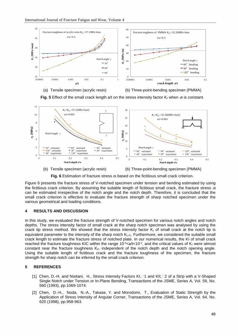
International Journal of Fracture Fatigue and Wear, Volume 4
48
25
30
35
40
45
50
0.00001 0.0001 0.001 0.01 0.1 1
KⅠ
[MP
a√m
m]
a/t
t/w=0.3
30°
60°
90°
Fracture toughness of acrylic resin KΙC=37.1MPa√mm
Notch angle γ
0
10
20
30
40
50
60
0.00001 0.0001 0.001 0.01 0.1
KⅠ
[MP
a√m
]
crack length a/t
t/w=0.3
60°bending
90°bending
120°bending
Fracture toughness of PMMA KΙC=32.26MPa√mm
Notch angle γ
(a) Tensile specimen (acrylic resin) (b) Three-point-bending specimen (PMMA)
Fig. 5 Effect of the small crack length a/t on the stress intensity factor KI when σf is constant.
0
2
4
6
8
10
12
0 0.1 0.2 0.3 0.4 0.5
σ f[M
Pa]
Notch depth t/w
30°estimated 60°estimated 90°estimated120°estimated 30°experiment 60°experiment90°experiment 120°experiment
Notch angle γ
KI=KIC=37.1[MPa√mm]
a/t=0.005
0
5
10
15
20
25
30
0 0.1 0.2 0.3 0.4 0.5
σ f[M
Pa]
Notch depth t/w
60°estimated 90°estimated 120°estimated60°experiment 90°experiment 120°experiment
KI=KIC=32.26[MPa√mm]
a/t=0.001
Notch angle γ
(b) Tensile specimen (acrylic resin) (b) Three-point-bending specimen (PMMA)
Fig. 6 Estimation of fracture stress σf based on the fictitious small crack criterion.
Figure 6 presents the fracture stress of V-notched specimen under tension and bending estimated by using the fictitious crack criterion. By assuming the suitable length of fictitious small crack, the fracture stress σf can be estimated irrespective of the notch angle and the notch depth. Therefore, it is concluded that the small crack criterion is effective to evaluate the fracture strength of sharp notched specimen under the various geometrical and loading conditions.
4 RESULTS AND DISCUSSION
In this study, we evaluated the fracture strength of V-notched specimen for various notch angles and notch depths. The stress intensity factor of small crack at the sharp notch specimen was analysed by using the crack tip stress method. We showed that the stress intensity factor KI of small crack at the notch tip is equivalent parameter to the intensity of the sharp notch KI,λ1. Furthermore, we considered the suitable small crack length to estimate the fracture stress of notched plate. In our numerical results, the KI of small crack reached the fracture toughness KIC within the range 10-3<a/t<10-2, and the critical values of KI were almost constant near the fracture toughness KIC independent of the notch depth and the notch opening angle. Using the suitable length of fictitious crack and the fracture toughness of the specimen, the fracture strength for sharp notch can be inferred by the small crack criterion.
5 REFERENCES
[1] Chen, D.-H. and Nisitani, H., Stress Intensity Factors KI,1 and KΙΙ,2 of a Strip with a V-Shaped Single Notch under Tension or In-Plane Bending, Transactions of the JSME, Series A, Vol. 59, No. 560 (1993), pp.1069-1074.
[2] Chen, D.-H., Noda, N.-A., Takase, Y. and Morodomi, T., Evaluation of Static Strength by the Application of Stress Intensity of Angular Corner, Transactions of the JSME, Series A, Vol. 64, No. 620 (1998), pp.958-963.

International Journal of Fracture Fatigue and Wear, Volume 4
49
[3] Chen, D.-H. and Noda, N.-A., A Comparison on the Fracture Criterion for a Sharp Notch, Transactions of the JSME, Series A, Vol. 64, No. 626 (1998), pp.2574-2582.
[4] Kihara, S. and Yoshii, A., Evaluation of the Effect of a Sharp Notch on the Fatigue and Static Strength by the Application of an Equivalent Stress-Intensity Factor, Transactions of the JSME, Series A, Vol. 56, No. 524 (1990), pp.903-910.
[5] Dunn, M.L., Suwito, W. and Cunningham, S., Fracture initiation at sharp notches: Correlation using critical stress intensities, International Journal of Solids and Structures, Vol.34, No.29 (1997), pp.3873-3883.
[6] Noda, N.-A., Miyazaki, T., Li, R., Uchikoba, T., Sano, Y. and Takase, Y., Debonding Strength Evaluation in terms of the Intensity of Singular Stress at the Interface Corner with and without Fictitious Crack, International Journal of Adhesion & Adhesives, Vol.61 (2015), pp.46-64.
[7] Teranishi, T. and Nisitani, H., Determination of Highly Accurate Values of Stress Intensity Factor in a Plate of Arbitrary Form by FEM, Transactions of the JSME, Series A, Vol. 65, No. 638(1999), pp2032-2037.
International Journal of Fracture Fatigue and Wear, Volume 4
50
Proceedings of the 5th International Conference on Fracture Fatigue and Wear, pp. 50-57, 2016
ELASTOPLASTIC FRETTING WEAR BEHAVIOUR OF CONTACT WIRES
T. Yue1, D. Wang2 and M. Abdel Wahab1 1Soete Laboratory, Faculty of Engineering and Architecture, Ghent University, Belgium
2School of Mechatronic Engineering, China University of Mining and Technology, Xuzhou 221116 China
Abstract: Fretting wear is damage caused by small movement between contact surfaces and imposed normal load. It occurs more seriously in gross sliding condition. Wire ropes in mine hoisting are typical examples where fretting wear occurs. This fretting damage causes stress concentration and accelerates the failure of ropes by decreasing cross section area. Considering the difficulties in monitoring stresses in experiments, finite element method (FEM) is a suitable numerical method to study the detail of this process. However, there is scarce information on the effect of material property on fretting wear of wire ropes in FEM. In this study, based on the FE model of wires, the FE results are validated with analytical solution and experiments. Then, the fretting loops and wear depth after 1000 cycles from different material behaviours are analysed. The results show that under elastic material behaviour, FEM has a good agreement with Hertzian solution. In addition, the wear depth obtained by FEM is close to experimental one. However, the fretting loop is a typical gross sliding shape in contrast to the experimental findings. For elastic perfectly plastic condition, the shape of fretting loop after 1000 cycles is same as that for elastic one, but the dissipated energy is higher. Moreover, the wear depth and wear scar calculated by plasticity is different from the elastic condition.
Keywords: Fretting wear, FEM, Material behaviour
1 INTRODUCTION
Fretting is small movement between contact surfaces. Depending on different loading conditions, namely combinations of normal load and oscillation, it could result in fretting fatigue in partial slip condition or fretting wear in gross sliding condition. The wire rope in mine hoisting is a typical example, in which fretting damage occurs due to the micro displacement of individual wires against their adjacent wires when the ropes are under axial cyclic stretching load and cyclic bending load. This causes stress concentration and accelerates the failure of ropes by decreasing of cross section area [1-3]. Previously, Wang et al. studied the influence of kinematic parameters of mine hoist on fretting parameters of the hoisting rope model [4], effects of displacement on fretting damage of wires in low cycle fatigue condition [5] and the influence of pH value in the corrosive media on fretting wear and fatigue life of wires [6]. This global hoisting rope model shows hoisting is a complex process, and experiments present complicated interaction of fretting wear and fretting fatigue. However, due to its micro displacement and micro size of debris, it is difficult to investigate the evolution of contact surfaces in the process of fretting wear by experiments. Therefore, researchers turn to numerical modelling, e.g. finite element method (FEM), to study the detail of this process. Cruzado et al. [7] firstly simulated the process of fretting wear in wires in a 90° crossed elastic cylinders configuration, then studied the influence of fretting wear on fatigue life of wires [8]. In their recent research[9], crossed-cylinder models of different angles under fretting condition were simulated, of which results showed good agreement with experimental data. Besides fretting model of wires, Wang [10] firstly studied stress distribution and fretting fatigue parameters of two upscale structures, i.e. 6 × 19 + IWS rope and (1 + 6 + 12) strand with three layered strands to investigate the global response of rope in axially load condition and the influence of fretting wear on fretting scar. However, the process of fretting wear was calculated by the analytical solution instead of instantaneous contact pressure and relative slip of each increment, which are of importance in fretting wear simulations.
Though FEM could give a good agreement with experiments, the effect of material property on fretting wear has not been considered. However, assuming that the material is elastically deformed, which is usually defined in fretting wear simulations, underestimates the displacement for gross sliding in theoretical values [11]. Also, of a high friction coefficient fretting couple with typical tangential displacement, this high coefficient of friction is sufficient to cause plastic deformation in the contact surface [12].
In this paper, we investigated the influence of material property on fretting wear of wire ropes. The remainder of this paper is organized as follows. In section 2, the FE model used for the fretted wire is described, including geometry information and wears coefficient calculation. After that, the FE results are validated with analytical
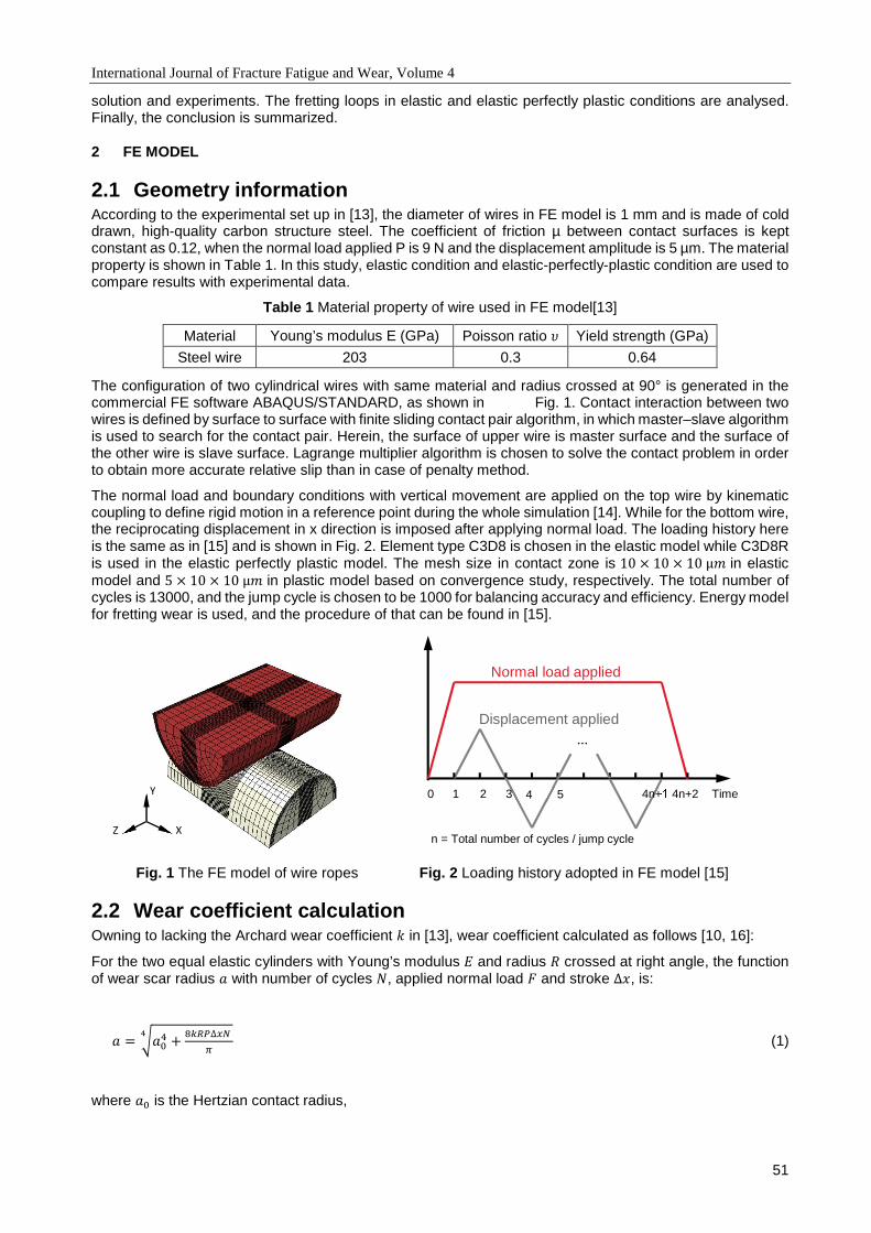
International Journal of Fracture Fatigue and Wear, Volume 4
51
solution and experiments. The fretting loops in elastic and elastic perfectly plastic conditions are analysed. Finally, the conclusion is summarized.
2 FE MODEL
2.1 Geometry information According to the experimental set up in [13], the diameter of wires in FE model is 1 mm and is made of cold drawn, high-quality carbon structure steel. The coefficient of friction µ between contact surfaces is kept constant as 0.12, when the normal load applied P is 9 N and the displacement amplitude is 5 µm. The material property is shown in Table 1. In this study, elastic condition and elastic-perfectly-plastic condition are used to compare results with experimental data.
Table 1 Material property of wire used in FE model[13]
Material Young’s modulus E (GPa) Poisson ratio Yield strength (GPa)
Steel wire 203 0.3 0.64
The configuration of two cylindrical wires with same material and radius crossed at 90° is generated in the commercial FE software ABAQUS/STANDARD, as shown in Fig. 1. Contact interaction between two wires is defined by surface to surface with finite sliding contact pair algorithm, in which master–slave algorithm is used to search for the contact pair. Herein, the surface of upper wire is master surface and the surface of the other wire is slave surface. Lagrange multiplier algorithm is chosen to solve the contact problem in order to obtain more accurate relative slip than in case of penalty method.
The normal load and boundary conditions with vertical movement are applied on the top wire by kinematic coupling to define rigid motion in a reference point during the whole simulation [14]. While for the bottom wire, the reciprocating displacement in x direction is imposed after applying normal load. The loading history here is the same as in [15] and is shown in Fig. 2. Element type C3D8 is chosen in the elastic model while C3D8R is used in the elastic perfectly plastic model. The mesh size in contact zone is 10 × 10 × 10μ in elastic model and 5 × 10 × 10μ in plastic model based on convergence study, respectively. The total number of cycles is 13000, and the jump cycle is chosen to be 1000 for balancing accuracy and efficiency. Energy model for fretting wear is used, and the procedure of that can be found in [15].
Fig. 1 The FE model of wire ropes Fig. 2 Loading history adopted in FE model [15]
2.2 Wear coefficient calculation Owning to lacking the Archard wear coefficient in [13], wear coefficient calculated as follows [10, 16]:
For the two equal elastic cylinders with Young’s modulus and radius crossed at right angle, the function of wear scar radius with number of cycles , applied normal load and stroke ∆, is:
+ ∆ !
" (1)
where is the Hertzian contact radius,
0 4n+1 4n+2 5 4 3 2 1 Time
Normal load applied
Displacement applied ...
n = Total number of cycles / jump cycle
Y
X Z

International Journal of Fracture Fatigue and Wear, Volume 4
52
0.909$%
(2)
And the relation between fretting wear depth ℎ' and is given by:
ℎ' ()*(+), (3)
Therefore the Archard wear coefficient could be obtained as:
[.,/01(+)2)*(+"]!4∆ (4)
Thus, energy wear coefficient $, based on Coulomb's friction law is obtained as:
$ [.,/01(+)2)*(+"]!4∆ 5 (5)
Therefore, $ could be calculated based on ℎ' measured. When 9N, ∆ 10μm, ℎ' 1.89μm from [13]. It should be mentioned that plastic deformation occurs in this loading condition based on FE result and material property. Fig. 3 shows that the maximum indentation displacement is 0.7μ due to plastic deformation. However, by experiments, it is difficult to separate plastic deformation from wear depth measurement. Therefore, in experiments, ℎ' measured is the wear depth plus plastic deformation, where the depth due to plastic deformation is 37.6% of ℎ' in this loading condition. Thus $ calculated by ℎ' is larger than the real situation. Considering this point, four conditions are simulated listed in Table 2. $ 4.04 ×10*<=*', is calculated by ℎ', while $ 2.09 × 10*<=*' is obtained by the subtraction of the plastic displacement from ℎ'. Due to the convergence problem in plastic deformation of the whole period of fretting wear, the first 1000 cycles is studied here.
Fig. 3 The indentation depth of specimen surface in vertical direction from FEM,> ?@, A B. CDD
Table 2 key parameters on elastoplastic behaviour studying
No. of simulation Number of cycles $ Material behaviour
1 13000 4.04 × 10* elastic
2 13000 2.09 × 10* elastic
3 1000 4.04 × 10* Elastic-perfectly-plastic
4 1000 2.09 × 10* Elastic-perfectly-plastic
-8,0E-04
-6,0E-04
-4,0E-04
-2,0E-04
0,0E+00
2,0E-04
-0,1 -0,05 0 0,05 0,1
ind
en
tati
on
de
pth
(mm
)
contact width(mm)
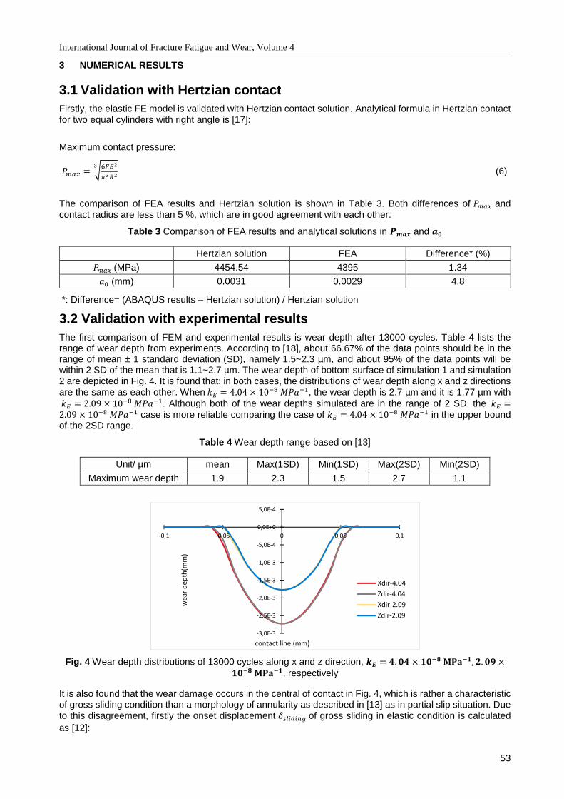
International Journal of Fracture Fatigue and Wear, Volume 4
53
3 NUMERICAL RESULTS
3.1 Validation with Hertzian contact Firstly, the elastic FE model is validated with Hertzian contact solution. Analytical formula in Hertzian contact for two equal cylinders with right angle is [17]:
Maximum contact pressure:
=E( F4$)!%)%
(6)
The comparison of FEA results and Hertzian solution is shown in Table 3. Both differences of =E( and contact radius are less than 5 %, which are in good agreement with each other.
Table 3 Comparison of FEA results and analytical solutions in GHIJ and IB Hertzian solution FEA Difference* (%)
=E( (MPa) 4454.54 4395 1.34
(mm) 0.0031 0.0029 4.8
*: Difference= (ABAQUS results – Hertzian solution) / Hertzian solution
3.2 Validation with experimental results The first comparison of FEM and experimental results is wear depth after 13000 cycles. Table 4 lists the range of wear depth from experiments. According to [18], about 66.67% of the data points should be in the range of mean ± 1 standard deviation (SD), namely 1.5~2.3 µm, and about 95% of the data points will be within 2 SD of the mean that is 1.1~2.7 µm. The wear depth of bottom surface of simulation 1 and simulation 2 are depicted in Fig. 4. It is found that: in both cases, the distributions of wear depth along x and z directions are the same as each other. When$ 4.04 × 10*<=*', the wear depth is 2.7 µm and it is 1.77 µm with $ 2.09 × 10*<=*'. Although both of the wear depths simulated are in the range of 2 SD, the $ 2.09 × 10*<=*' case is more reliable comparing the case of $ 4.04 × 10*<=*' in the upper bound of the 2SD range.
Table 4 Wear depth range based on [13]
Unit/ µm mean Max(1SD) Min(1SD) Max(2SD) Min(2SD)
Maximum wear depth 1.9 2.3 1.5 2.7 1.1
Fig. 4 Wear depth distributions of 13000 cycles along x and z direction, KL M. BM × NB*OPQR*N, S. B? ×NB*OPQR*N, respectively
It is also found that the wear damage occurs in the central of contact in Fig. 4, which is rather a characteristic of gross sliding condition than a morphology of annularity as described in [13] as in partial slip situation. Due to this disagreement, firstly the onset displacement TUVWXWYZ of gross sliding in elastic condition is calculated as [12]:
-3,0E-3
-2,5E-3
-2,0E-3
-1,5E-3
-1,0E-3
-5,0E-4
0,0E+0
5,0E-4
-0,1 -0,05 0 0,05 0,1
we
ar
de
pth
(mm
)
contact line (mm)
Xdir-4.04
Zdir-4.04
Xdir-2.09
Zdir-2.09

International Journal of Fracture Fatigue and Wear, Volume 4
54
TUVWXWYZ [\(,*])'F(+^ (7)
Where _ $
,('1`). Thus, the threshold of displacement in the case is 0.294 µm. It means that in the elastic condition, gross sliding occurs when the applied displacement is greater than 0.294 µm. The applied displacement here is 5 µm that is 17 times larger than this threshold and gross sliding occurs. This is the case of the FE results.
Next, fretting loops are compared. In Fig. 5 (a) from [13], the fretting loop displays a typical quasi-closed line, which means only the adhesive occurs in the centre of contact surface. This micro displacement only leads to elastic deformation of the contact surface. However, the fretting loops of Fig. 5 (b) based on the FEM results after both 1000 and 13000 cycles, show quasi-rectangular shapes revealing that the entire bulks is sliding with each other, i.e. gross sliding condition. Meanwhile, with increasing number of cycles, the dissipated energy increases. This tendency was also found in aluminium alloy [19].
The possible reasons causing the difference between experiment and FE model in fretting loops maybe explained from two points as follows: a) the material property used is elastic with both wear coefficient while plastic deformation occurs according to the material property. Therefore fretting wear in plastic deformation is studied in the next section. b) in this paper, Coulomb law is used for contact problem. However, some researchers [20] found that this friction law is not suitable for describing the transition from ‘static’ to ‘dynamic’ friction. Ciavarella [20] proposed an ‘adhesive model’ that the Griffith condition is employed in the inception of slip and the Coulomb law is used in slip condition. The stick region is about 10-20% larger than the prediction based on Coulomb law. In the experiment, it was adhesive condition while the FE result showed slip condition. Based on the study of Ciavarella, using Griffith model may improve FE model. Further study should be done in the future.
(a) (b)
Fig. 5 Fretting loops: (a) experimental results [13], (b) fretting loops after 1000 cycles and 13000 cycles in elastic condition based on FEA, $ 4.04 × 10*<=*'
3.3 Comparison between elastic model and elastic-perfectly-plastic model The comparison of fretting loops after 1000 cycles in plastic model and elastic model is plotted in Fig. 6. All these loops presented the quasi-rectangular shape. In both $ cases, the friction force of plastic condition is increasing comparing to elastic condition, with little changes in the displacement. Thus the dissipated energy, the area of the fretting loop, in plastic condition is 16.54 × 10*Fa and the elastic case is 11.07 × 10*Fa . Meanwhile, the friction force and the dissipated energy are independent of the wear coefficient.
Since part of dissipated energy is consumed for wear, the wear depths of FE model with different material behaviours are compared in Fig. 7. In the plastic deformation condition, the wear depth is obtained by subtraction of plastic deformation (shown in Fig. 3) from the displacement of bottom surface along y direction after unloading. It is found that:
1) In the same material behaviour condition, the wear depth increases with rising wear coefficient, while the wear width has little changes.
2) When the material behaviour changes from elastic to plastic and keeps the same wear coefficient, the wear width increases.
-15
-10
-5
0
5
10
15
-5 -4 -3 -2 -1 0 1 2 3 4 5
fric
tio
n f
orc
e (
N)
displacement (mm)
13000EL+4.04 1000EL+4.04

International Journal of Fracture Fatigue and Wear, Volume 4
55
3) The wear depth in elastic case is more sensitive to the wear coefficient: wear depth of central point is growing by 66.5% while it is only 15.1% in plastic case, in which situation that the wear coefficient rises from 2.09 × 10*<=*' to 4.04 × 10*<=*'. Meanwhile, in the lower wear coefficient case, the maximum wear depth of plastic case is larger than the elastic one. However, when the wear coefficient increases, the wear of elastic case gets more serious than the plastic one, especially at the centre of contact.
4) The profiles of wear scars are different in these two material behaviour conditions. The maximum wear depth in elastic model is in the centre of contact surface and decreased gradually to the contact edge, as ‘U’ shape. In plastic condition, however, the maximum depth is distributed at the contact edge and flattens in the centre of the contact surface, as ‘W’. This wear profile is similar as the wear scar shape of partial slip condition. In this condition, maximum wear damage is in the edge of contact and little damage happens at the contact centre. The ploughing effect presents in the edge of wear scar due to the plastic deformation, which was also reported in [21, 22].
In the end, the wear scar including plastic deformation is displayed in Fig. 8. The shapes of wear scars in both material cases are same as ‘U’, but plastic deformation brings more scar depth and width. Again, the wear coefficient in elastic condition plays more important role on the wear depth than in the plastic case. It should be mentioned that the wear scar displayed in the plastic case is much larger than the elastic case which without plastic deformation. In this condition, the wear coefficient calculated by plastic deformed wear volume would be much higher than the real case.
Fig. 8 wear scars after 1000 cycles in elastic and elastic perfectly plastic conditions, along x direction
4 CONCLUSION
To validate the fretting wear model and investigate the influence of material behaviour on fretting wear, the fretting wear model of wires crossed in right angle is generated in elastic behaviour with 13000 cycles and elastic perfectly plastic condition with 1000 cycles. For fretting wear model with elastic behaviour, the contact pressure and contact radius are in good agreement with the Hertzian analytical solution. The wear depth of 13000 cycles simulated is in the range of experimental results. However, the shape of fretting loop is a quasi-
-1
-0,75
-0,5
-0,25
0
0,25
0,5
0,75
1
-5 -2,5 0 2,5 5
Fri
ctio
n F
orc
e (
N)
displacement (µm)
1000EL+4.04 1000PL+4.04
1000EL+2.09 1000PL+2.09
-5E-4
-4E-4
-3E-4
-2E-4
-1E-4
0E+0
1E-4
2E-4
-0,08 -0,04 0,00 0,04 0,08
we
ar
de
pth
(mm
)
contact width(mm)
RealDepthPL+2.09 RealDepthPL+4.04
Elastic+4.04 Elastic+2.09
-1E-3
-1E-3
-8E-4
-6E-4
-4E-4
-2E-4
0E+0
2E-4
-0,08 -0,04 0,00 0,04 0,08
sca
r d
ep
th (
mm
)
contact width(mm)
Plastic+2.09 Plastic+4.04 Elastic+4.04 Elastic+2.09
Fig. 6 Fretting loops of 1000 cycles in elastic and elastic perfectly plastic
conditions
Fig. 7 Wear depth of 1000 cycles in elastic and elastic perfectly plastic
conditions, along x direction
International Journal of Fracture Fatigue and Wear, Volume 4
56
rectangular shape, which means that the gross sliding happens rather than the partial slip reported in the experiments, though these FEA results are in accordance with analytical solution. For the plastic model, the fretting loop also shows gross sliding characteristic, but with higher dissipated energy. Meanwhile, the maximum wear depth distribution is a circle in the plastic model instead of one point in the elastic one. In this paper, only 1000 cycles’ wear scar is simulated and the future work will be the FE modelling of the whole period of fretting wear in plastic condition.
ACKNOWLEDGEMENTS
The first author would like to acknowledge the research funding from China Scholarship Council and CWO - Mobility fund of Ghent University. The third author would like to acknowledge the research funding from National Nature Science Foundation of China, China (Grant no. 51405489) and Tribology Science Fund of State Key Laboratory of Tribology (SKLTKF13A04).
5 REFERENCES
[1] Zhang DK, Ge SR, Qiang YH. Research on the fatigue and fracture behavior due to the fretting wear of steel wire in hoisting rope. Wear. 2003;255:1233-7.
[2] Cruzado A, Hartelt M, Wäsche R, Urchegui MA, Gómez X. Fretting wear of thin steel wires. Part 1: Influence of contact pressure. Wear. 2010;268:1409-16.
[3] Wang D, Zhang D, Ge S. Finite element analysis of fretting fatigue behavior of steel wires and crack initiation characteristics. Engineering Failure Analysis. 2013;28:47-62.
[4] Wang D, Zhang D, Zhang Z, Ge S. Effect of various kinematic parameters of mine hoist on fretting parameters of hoisting rope and a new fretting fatigue test apparatus of steel wires. Engineering Failure Analysis. 2012;22:92-112.
[5] Wang D, Zhang D, Ge S. Effect of displacement amplitude on fretting fatigue behavior of hoisting rope wires in low cycle fatigue. Tribology International. 2012;52:178-89.
[6] Wang D, Zhang D, Zhao W, Ge S. Quantitative analyses of fretting fatigue damages of mine rope wires in different corrosive media. Materials Science and Engineering: A. 2014;596:80-8.
[7] Cruzado A, Urchegui MA, Gómez X. Finite element modeling and experimental validation of fretting wear scars in thin steel wires. Wear. 2012;289:26-38.
[8] Cruzado A, Leen SB, Urchegui MA, Gómez X. Finite element simulation of fretting wear and fatigue in thin steel wires. International Journal of Fatigue. 2013;55:7-21.
[9] Cruzado A, Urchegui MA, Gómez X. Finite element modeling of fretting wear scars in the thin steel wires: Application in crossed cylinder arrangements. Wear. 2014;318:98-105.
[10] Wang D, Zhang D, Wang S, Ge S. Finite element analysis of hoisting rope and fretting wear evolution and fatigue life estimation of steel wires. Engineering Failure Analysis. 2013;27:173-93.
[11] Vingsbo O, Söderberg S. On fretting maps. Wear. 1988;126:131-47.
[12] Giannakopoulos AE, Suresh S. A three-dimensional analysis of fretting fatigue. Acta Materialia. 1998;46:177-92.
[13] Shen Y, Zhang D, Ge S. Effect of fretting amplitudes on fretting wear behavior of steel wires in coal mines. Mining Science and Technology (China). 2010;20:803-8.
[14] Wang D, Magd Abdel Wahab, LL Wang, XW Li, ZC Zhu, DK Zhang, and XB Mao. Finite element analysis of fretting fatigue of fretted wires. In: Wahab MA, editor. 4th International Conference on Fracture Fatigue and Wear. Ghent2015. p. 135-42.
[15] Yue T, Abdel Wahab M. Finite element analysis of stress singularity in partial slip and gross sliding regimes in fretting wear. Wear. 2014;321:53-63.
[16] Argatov II, Gómez X, Tato W, Urchegui MA. Wear evolution in a stranded rope under cyclic bending: Implications to fatigue life estimation. Wear. 2011;271:2857-67.
[17] Popov VL. CONTACT MECHANICS AND FRICTION: Springer-Verlag Berlin Heidelberg; 2010.
[18] Cumming G, Fidler F, Vaux DL. Error bars in experimental biology. The Journal of Cell Biology. 2007;177:7-11.
International Journal of Fracture Fatigue and Wear, Volume 4
57
[19] Zhou Z, Fayeulle S, Vincent L. Cracking behaviour of various aluminium alloys during fretting wear. Wear. 1992;155:317-30.
[20] Ciavarella M. Transition from stick to slip in Hertzian contact with “Griffith” friction: The Cattaneo–Mindlin problem revisited. Journal of the Mechanics and Physics of Solids. 2015;84:313-24.
[21] Mohd Tobi AL, Ding J, Bandak G, Leen SB, Shipway PH. A study on the interaction between fretting wear and cyclic plasticity for Ti–6Al–4V. Wear. 2009;267:270-82.
[22] Li J, Lu YH. Effects of displacement amplitude on fretting wear behaviors and mechanism of Inconel 600 alloy. Wear. 2013;304:223-30.

International Journal of Fracture Fatigue and Wear, Volume 4
58
Proceedings of the 5th International Conference on Fracture Fatigue and Wear, pp. 58-63, 2016
FINITE ELEMENT SIMULATIONS OF THE EFFECT OF FRICTION
COEFFICIENT IN FRETTING WEAR
T. Yue and M. Abdel Wahab
Soete Laboratory, Faculty of Engineering and Architecture, Ghent University, Belgium
Abstract: Assuming a constant coefficient of friction (CoF) is a simplification in the finite element (FE) modelling of fretting wear. CoF is an essential factor of energy model for predicting fretting wear. Therefore, taking the variation of CoF into account during fretting wear cycles is necessary. In this research, based on the cylinder/flat fretting wear model, the effects of CoF are studied. At the end of fretting wear cycles, only slightly lower wear depth and wear width for the case of variable CoF model compared to the case of constant CoF model is observed. At the end of the initial running-in stage, the wear depth obtained from the variable CoF model is significantly different from that obtained from the constant CoF model.
Keywords: Fretting wear, FEM, Friction coefficient
1 INTRODUCTION
Finite element method (FEM) is widely used in the simulation of fretting wear. However, to balance efficiency and accuracy, FE model of fretting wear is usually simplified in some aspects, such as assuming constant coefficient of friction (CoF) during the wear process.
CoF is a system-dependent parameter rather than an intrinsic property of a material or combination of materials. It is sensitive to the sliding distance and environment parameters, such as contact pressure and surface quality [1]. Blau [2] grouped the factor impacting the friction behavior as: contact geometry, fluid properties and flow, lubricant chemistry, relative motion, applied forces, third-bodies, temperature and stiffness, and vibrations.
During fretting wear, both applied normal load and displacement have significant influence on CoF. Zhang et al. [3] shows that the CoF of the steady stage decreases with increasing the normal load for a given displacement condition. Similar tendency could also be found in the fretting coupling of high strength alloy steel [4] and steel wire [5]. This tendency may be explained as when the normal load is small, elastic deformation causes asperities of contact surfaces interlock with each other, inducing high CoF. When increasing normal load to activate plastic deformation of asperities, the CoF becomes lower due to less interlocking [3]. In addition, the displacement does affect the CoF under both dry and lubricated contact in a given normal load condition. Besides the continuous changing of contact pressure induced by evolution of contact geometry, debris also plays a significant role. Due to composition of the debris, a critical contact pressure exists at which a transition to a higher CoF occurs [6].
For a given fretting couple, evolution of CoF with number of fretting wear cycles usually could be divided into 3 stages. In the initial running-in stage, CoF is low since the contact surfaces are covered by the oxide and ‘nature pollution’ film weakening the adhesion between contact surfaces. Later on in the second stage, CoF increases gradually because of the removing of this film, and due to the increase of adhesion and abrasion in the substrate interfaces. Then, the balance between generation and ejection of debris are reached. Therefore, CoF keeps stable at this last stage [3].
The motivation of this work is to improve FE modelling of fretting wear in order to increase the accuracy compared to the experimental results. In this study, the effects of variation of CoF during the first few thousands cycles on fretting wear are studied. This paper is divided into 4 parts. After the introduction section, the FE model is described. Then, the effect of CoF are presented. Finally, a conclusion is presented.
2 FE MODEL
2.1 Geometry information Fig. 1 shows the geometry of the FE model. The dimensions are the same as used in the literature [4], since the simulation results could be validated by the experimental results. The 4-node plane strain element (CPE4)
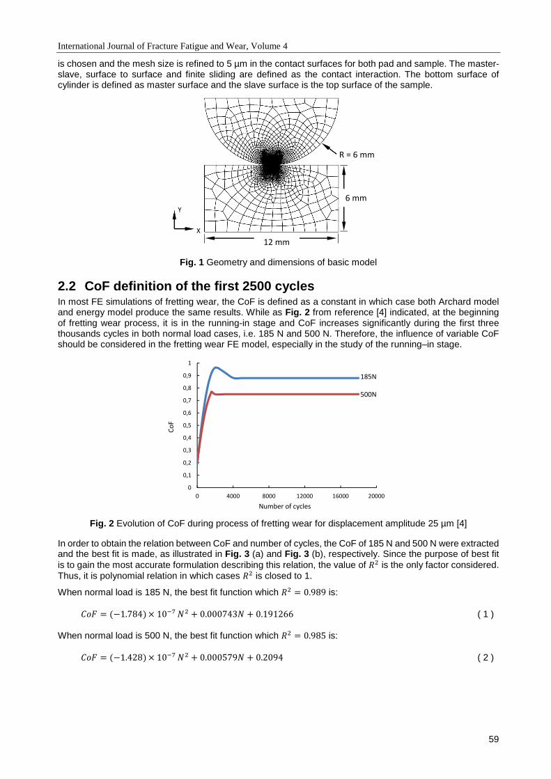
International Journal of Fracture Fatigue and Wear, Volume 4
59
is chosen and the mesh size is refined to 5 µm in the contact surfaces for both pad and sample. The master-slave, surface to surface and finite sliding are defined as the contact interaction. The bottom surface of cylinder is defined as master surface and the slave surface is the top surface of the sample.
Fig. 1 Geometry and dimensions of basic model
2.2 CoF definition of the first 2500 cycles In most FE simulations of fretting wear, the CoF is defined as a constant in which case both Archard model and energy model produce the same results. While as Fig. 2 from reference [4] indicated, at the beginning of fretting wear process, it is in the running-in stage and CoF increases significantly during the first three thousands cycles in both normal load cases, i.e. 185 N and 500 N. Therefore, the influence of variable CoF should be considered in the fretting wear FE model, especially in the study of the running–in stage.
Fig. 2 Evolution of CoF during process of fretting wear for displacement amplitude 25 µm [4]
In order to obtain the relation between CoF and number of cycles, the CoF of 185 N and 500 N were extracted and the best fit is made, as illustrated in Fig. 3 (a) and Fig. 3 (b), respectively. Since the purpose of best fit is to gain the most accurate formulation describing this relation, the value of is the only factor considered. Thus, it is polynomial relation in which cases is closed to 1.
When normal load is 185 N, the best fit function which 0.989 is:
1.784 10 0.000743 0.191266 ( 1 ) When normal load is 500 N, the best fit function which 0.985 is:
1.428 10 0.000579 0.2094 ( 2 )
0
0,1
0,2
0,3
0,4
0,5
0,6
0,7
0,8
0,9
1
0 4000 8000 12000 16000 20000
Co
F
Number of cycles
185N
500N
12 mm
6 mm
R = 6 mm
Y
X
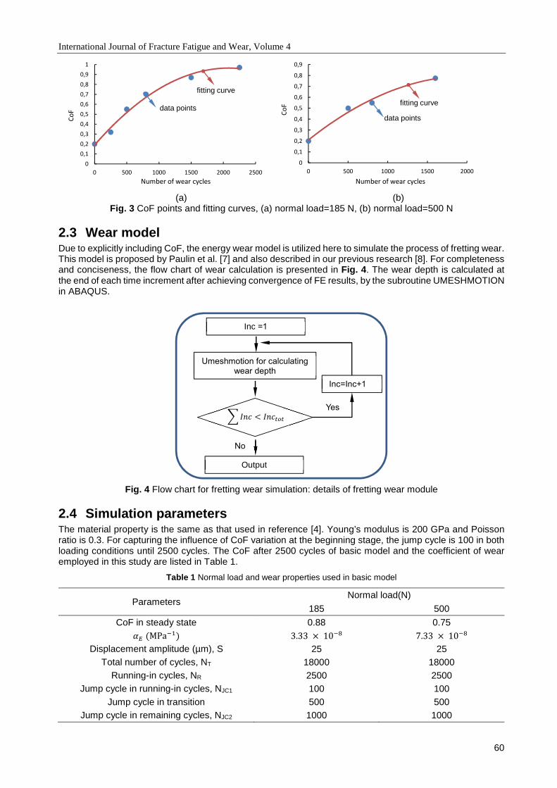
International Journal of Fracture Fatigue and Wear, Volume 4
60
(a) (b)
Fig. 3 CoF points and fitting curves, (a) normal load=185 N, (b) normal load=500 N
2.3 Wear model Due to explicitly including CoF, the energy wear model is utilized here to simulate the process of fretting wear. This model is proposed by Paulin et al. [7] and also described in our previous research [8]. For completeness and conciseness, the flow chart of wear calculation is presented in Fig. 4. The wear depth is calculated at the end of each time increment after achieving convergence of FE results, by the subroutine UMESHMOTION in ABAQUS.
Fig. 4 Flow chart for fretting wear simulation: details of fretting wear module
2.4 Simulation parameters The material property is the same as that used in reference [4]. Young’s modulus is 200 GPa and Poisson ratio is 0.3. For capturing the influence of CoF variation at the beginning stage, the jump cycle is 100 in both loading conditions until 2500 cycles. The CoF after 2500 cycles of basic model and the coefficient of wear employed in this study are listed in Table 1.
Table 1 Normal load and wear properties used in basic model
Parameters Normal load(N)
185 500
CoF in steady state 0.88 0.75 MPa 3.33 10! 7.33 10!
Displacement amplitude (µm), S 25 25 Total number of cycles, NT 18000 18000
Running-in cycles, NR 2500 2500 Jump cycle in running-in cycles, NJC1 100 100
Jump cycle in transition 500 500 Jump cycle in remaining cycles, NJC2 1000 1000
0
0,1
0,2
0,3
0,4
0,5
0,6
0,7
0,8
0,9
1
0 500 1000 1500 2000 2500
Co
F
Number of wear cycles
fitting curve
data points
0
0,1
0,2
0,3
0,4
0,5
0,6
0,7
0,8
0,9
0 500 1000 1500 2000
Co
F
Number of wear cycles
fitting curve
data points
Inc =1
Umeshmotion for calculating wear depth
"#$% & #$%'(' Yes
Inc=Inc+1
Output
No
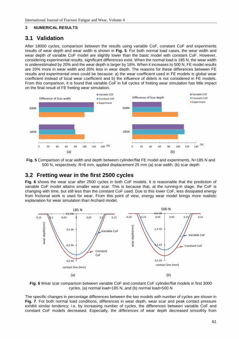
International Journal of Fracture Fatigue and Wear, Volume 4
61
3 NUMERICAL RESULTS
3.1 Validation After 18000 cycles, comparison between the results using variable CoF, constant CoF and experiments results of wear depth and wear width is shown in Fig. 5. For both normal load cases, the wear width and wear depth of variable CoF model are slightly lower than the basic model with constant CoF. However, considering experimental results, significant differences exist. When the normal load is 185 N, the wear width is underestimated by 20% and the wear depth is larger by 16%. When it increases to 500 N, FE model results are 20% more in wear width and 35% less in wear depth. The reasons for these differences between FE results and experimental ones could be because: a) the wear coefficient used in FE models is global wear coefficient instead of local wear coefficient and b) the influence of debris is not considered in FE models. From this comparison, it is found that variable CoF in full cycles of fretting wear simulation has little impact on the final result of FE fretting wear simulation.
(a) (b)
Fig. 5 Comparison of scar width and depth between cylinder/flat FE model and experiments, N=185 N and 500 N, respectively. R=6 mm, applied displacement 25 mm (a) scar width, (b) scar depth
3.2 Fretting wear in the first 2500 cycles Fig. 6 shows the wear scar after 2500 cycles in both CoF models. It is reasonable that the prediction of variable CoF model attains smaller wear scar. This is because that, at the running-in stage, the CoF is changing with time, but still less than the constant CoF used. Due to this lower CoF, less dissipated energy from frictional work is used for wear. From this point of view, energy wear model brings more realistic explanation for wear simulation than Archard model.
(a) (b)
Fig. 6 Wear scar comparison between variable CoF and constant CoF cylinder/flat models in first 3000 cycles, (a) normal load=185 N, and (b) normal load=500 N
The specific changes in percentage differences between the two models with number of cycles are shown in Fig. 7. For both normal load conditions, differences in wear depth, wear scar and peak contact pressure exhibit similar tendency; i.e. by increasing number of cycles, the differences between variable CoF and constant CoF models decreased. Especially, the differences of wear depth decreased smoothly from
0 20 40 60 80 100 120 140
Variable COF
Constant COF
Experiment
185N
500N
Difference of Scar width
(%) 0 20 40 60 80 100 120 140
Variable COF
Constant COF
Experiment
185N
500N
Difference of Scar depth
(%)
-3,E-03
-2,E-03
-1,E-03
0,E+00
-0,25 -0,15 -0,05 0,05 0,15 0,25
we
ar
de
pth
(mm
)
contact line (mm)
500 N
Variable CoF
Constant CoF
-9,E-04
-6,E-04
-3,E-04
0,E+00
-0,15 -0,1 -0,05 0 0,05 0,1 0,15
we
ar
de
pth
(mm
)
contact line (mm)
185 N
Constant
CoF
Variable CoF

International Journal of Fracture Fatigue and Wear, Volume 4
62
approximately 55% after 200 cycles to approximately 10% after 2500 cycles. These changes could be described by a polynomial formula as:
when normal load is 185 N,
)*++,-,$%, 8 10. 0.0421 64.391, 0.9993 ( 3 ) When it is 500 N,
)*++,-,$%, 8 10. 0.0384 60.886, 0.9978 ( 4 ) Thus, the wear depth after 2500 cycles could be calculated by the best fitting curve instead of fretting wear simulation. However, the other three variables are oscillated with number of cycles. The reasons for this oscillation would be further studied in future work.
(a) (b)
Fig. 7 Influence of variable CoF in wear depth, peak contact pressure and wear width in the first 2500 cycles. (a) normal load=185 N, and (b) normal load=500 N
4 CONCLUSIONS
Two FE models are generated to study the fretting wear process. The effect of variable CoF on fretting wear are analysed based on a basic model having a constant CoF. After 18000 cycles, there are very limited differences in wear width and wear depth between constant CoF and variable CoF fretting wear models. However, after the first 2500 cycles, where CoF increases significantly, the differences in wear width, wear depth and peak contact pressure are clear. All the differences of these variables decreased with time. Particularly, the differences of wear depth reduced smoothly from 55% to 10%.
5 ACKNOWLEDGEMENTS
The first author would like to acknowledge the research funding from China Scholarship Council and CWO - Mobility fund of Ghent University.
6 REFERENCES
[1] N. P. Suh and H.-C. Sin, The genesis of friction, Wear, 69 (1), 91-114, 1981.
[2] P. J. Blau, The significance and use of the friction coefficient, Tribology International, 34 (9), 585-591, 2001.
[3] D. K. Zhang, S. R. Ge and Y. H. Qiang, Research on the fatigue and fracture behavior due to the fretting wear of steel wire in hoisting rope, Wear, 255 (7–12), 1233-1237, 2003.
[4] I. R. McColl, J. Ding and S. B. Leen, Finite element simulation and experimental validation of fretting wear, Wear, 256 (11-12), 1114-1127, 2004.
[5] Y. Shen, D. Zhang, J. Duan and D. Wang, Fretting wear behaviors of steel wires under friction-increasing grease conditions, Tribology International, 44 (11), 1511-1517, 2011.
0
10
20
30
40
50
60
0 500 1000 1500 2000 2500
dif
fere
nce
(%)
Number of cycles
185 N
Wear depth
Peak contact pressure
Wear width
Fitting curve
0
10
20
30
40
50
60
0 500 1000 1500 2000 2500
dif
fere
nce
(%)
Number of cycles
500 N
Wear depth
Peak contact pressure
Wear width
Fitting curve

International Journal of Fracture Fatigue and Wear, Volume 4
63
[6] N. Diomidis and S. Mischler, Third body effects on friction and wear during fretting of steel contacts, Tribology International, 44 (11), 1452-1460, 2011.
[7] C. Paulin, S. Fouvry and C. Meunier, Finite element modelling of fretting wear surface evolution: Application to a Ti–6A1–4V contact, Wear, 264 (1-2), 26-36, 2008.
[8] T. Yue and M. Abdel Wahab, Finite element analysis of stress singularity in partial slip and gross sliding regimes in fretting wear, Wear, 321 (0), 53-63, 2014.

International Journal of Fracture Fatigue and Wear, Volume 4
64
Proceedings of the 5th International Conference on Fracture Fatigue and Wear, pp. 64-69, 2016
NONLINEAR TRANSIENT ISOGEOMETRIC ANALYSIS OF LAMINATED
COMPOSITE PLATES BASED ON HIGHER ORDER PLATE THEORY
Loc V. Tran1,2, P. Phung-Van1,2, H. Nguyen-Xuan3 and M. Abdel Wahab1,2 1Division of Computational Mechanics, Ton Duc Thang University, Vietnam
2Faculty of Engineering and Architecture, Ghent University, Belgium 3Center for Interdisciplinary Research in Technology, HUTECH University, Vietnam
Abstract: Geometrically nonlinear transient analysis of laminated composite plates is studied using isogeometric analysis (IGA). Herein, higher-order shear deformation theory (HSDT) is applied in displacement field to ensure by itself the realistic shear strain energy part without shear correction factors. IGA utilizing higher-order B-splines basis functions enables to satisfy easily the stringent continuity requirement of the HSDT model without any additional variables. The nonlinearity of the plates based on the von-Karman strain assumptions is solved by the Newmark time integration associated with the Picard method. Two numerical examples of square composite plates are provided to demonstrate the effectiveness of the proposed method.
Keywords: Laminated composite plate, Isogeometric analysis, Higher-order Shear Deformation Theory, Nonlinear analysis, Newmark integration.
1. INTRODUCTION
Laminated composite plates were widely studied by various scientists with a numerous models including 3D elasticity model [1], layer-wise model [2] or equivalent single layer (ESL) theory. The 3D elasticity solution and layer-wise (LW) model can be recommended to improve the accuracy of transverse shear stresses. However, they have a numerous unknown variables producing much computational cost. Thus, reduction a 3D problem to a 2D problem based on the equivalent single layer theory is considered.
Among the ESL plate theories, classical laminate plate theory (CLPT) relied on the Kirchoff-Love assumptions just provides acceptable results for thin plate. First order shear deformation theory (FSDT) based on Reissner-Mindlin hypothesis, which considers the shear deformation effects, was therefore developed for thin and thick plates. Furthermore, higher order shear deformable theories (HSDT), which include higher-order terms in the approximation of the displacement field has then been devised. It is worth mentioning that the HSDT models ensure non-linear distributions of the shear strains/stresses with traction-free boundary condition at the plate surfaces and provide better results and yield more accurate and stable solutions than the FSDT ones. However, the HSDT requires the C1-continuity of generalized displacement field which is easily satisfied by the approximated functions from isogeometric analysis (IGA).
IGA [3] firstly proposed by Thomas Hughes fulfils a seamless bridge link between computer aided design (CAD) and finite element analysis (FEA). The basis idea of this approach is using the same B-Spline functions in describing the exact geometry of problem and constructing finite approximation for analysis. Being thankful to higher order continuity of B-Spline functions, IGA naturally verifies the C1-continuity of plates based on the HSDT assumptions. IGA has been widely applied to the plate structures with various plate models such as CLPT [4], FSDT[5], HSDT[6], four unknown variables refined plate theory (RPT) [7], layerwise [8], etc. The literatures mentioned above, however, did not take into account geometric nonlinearity, except two recent papers [9, 10] based on the FSDT. Therefore, our goal in this paper is firstly extended the HSDT model in study transient analysis of the laminated composite plates. Based on the von-Karman strain which considers small strain and moderate rotation assumptions, the nonlinearity of the plates is formulated using total Lagrange approach and solved by the Newmark time integration associated with the Picard methods. Two numerical examples are given to show the effectiveness of the present formulation.
2. ISOGEOMETRIC COMPOSITE PLATE FORMULATION FOR NONLINEAR ANALYSIS
2.1. The higher-order shear deformation plate theory The displacement of an arbitrary point in plate can be expressed as:
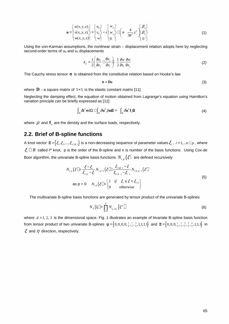
65
,0
30 , 2
( , , )4
( , , )3
( , , ) 0 0
x x
y y
wuu x y z
v x y z v z w z zh
w x y z w
ββ
= = − + −
u (1)
Using the von-Karman assumptions, the nonlinear strain – displacement relation adopts here by neglecting second-order terms of u0 and v0 displacements
1 1
2 2ji
ijj i i j
uu w w
x x x xε
∂∂ ∂ ∂= + + ∂ ∂ ∂ ∂ (2)
The Cauchy stress tensor σ is obtained from the constitutive relation based on Hooke’s law
=σ Dε (3)
where D - a square matrix of 5 5× is the elastic constant matrix [11].
Neglecting the damping effect, the equation of motion obtained from Lagrange’s equation using Hamilton’s variation principle can be briefly expressed as [12]
d d dT T Tsδ δ ρ δ
Ω Ω ΩΩ + Ω = Ω∫ ∫ ∫σ u u u fɺɺε (4)
where ρ and sf are the density and the surface loads, respectively.
2.2. Brief of B-spline functions
A knot vector 1 2 1, ,..., n pξ ξ ξ + +=Ξ is a non-decreasing sequence of parameter values iξ , 1,...i n p= + , where
i Rξ ∈ called ith knot, p is the order of the B-spline and n is number of the basis functions. Using Cox-de
Boor algorithm, the univariate B-spline basis functions ( ),i pN ξ are defined recursively
( ) ( ) ( )1, , 1 1, 1
1 1
i pii p i p i p
i p i i p i
N N Nξ ξξ ξξ ξ ξ
ξ ξ ξ ξ+ +
− + −+ + + +
−−= +
− −
as p = 0 ( ) 1,0
1
0 otherwisei i
i
ifN
ξ ξ ξξ +≤ <
=
(5)
The multivariate B-spline basis functions are generated by tensor product of the univariate B-splines
( ) ( ),1
d
A i pN Nα α
α
α =
= ∏ξ ξ (6)
where 1, 2, 3d = is the dimensional space. Fig. 1 illustrates an example of bivariate B-spline basis function
from tensor product of two univariate B-splines 1 1 3
4 2 40,0,0,0, , , ,1,1,1,1=ψ and 1 2 3 3 4
5 5 5 5 50,0,0, , , , , ,1,1,1=Ξ in
ξ and η direction, respectively.
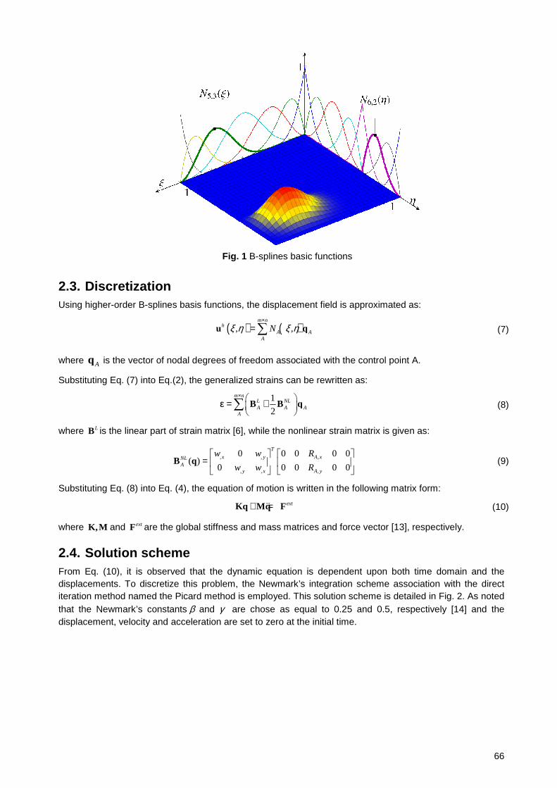
66
Fig. 1 B-splines basic functions
2.3. Discretization Using higher-order B-splines basis functions, the displacement field is approximated as:
( ) ( ), ,m n
hA A
A
Nξ η ξ η×
=∑u q (7)
where Aq is the vector of nodal degrees of freedom associated with the control point A.
Substituting Eq. (7) into Eq.(2), the generalized strains can be rewritten as:
1
2
m nL NLA A A
A
× = +
∑ B B qε (8)
where LB is the linear part of strain matrix [6], while the nonlinear strain matrix is given as:
, , ,
, , ,
0 0 0 0 0( )
0 0 0 0 0
T
x y A xNLA
y x A y
w w R
w w R
=
B q (9)
Substituting Eq. (8) into Eq. (4), the equation of motion is written in the following matrix form:
ext+ =Kq Mq Fɺɺ (10)
where K,M and extF are the global stiffness and mass matrices and force vector [13], respectively.
2.4. Solution scheme From Eq. (10), it is observed that the dynamic equation is dependent upon both time domain and the displacements. To discretize this problem, the Newmark’s integration scheme association with the direct iteration method named the Picard method is employed. This solution scheme is detailed in Fig. 2. As noted that the Newmark’s constants β and γ are chose as equal to 0.25 and 0.5, respectively [14] and the displacement, velocity and acceleration are set to zero at the initial time.

67
Fig. 2 Flow chart of Picard method.
3. NUMERICAL RESULTS
Firstly, an orthotropic plate [15] with dimensions as; length L = 250 mm, thickness h = 5 mm is studied for validation. For this problem, the fully simply supported plate is subjected to a uniform step loading of 1 MPa. Its time history of transverse displacement /w w h= under both linear and nonlinear analysis is shown in Fig. 3. It is observed that present method predicts the very close deflection response as compared with finite strip method (FSM) [15]. It also clearly exhibits that the magnitude and wavelength of the non-linear response are lower than that of linear behaviour with the same loading intensity.
0 0.4 0.8 1.2 1.6 2
x 10−3
−0.5
0
0.5
1
1.5
2
2.5
3
3.5
4
4.5
Time
Cen
tral
def
lect
ion
IGA: Nonlinear
: Linear
FSM: Nonlinear
: Linear
Fig. 3 Time history of the transverse displacement of an orthotropic plate.
Next, the dynamic response of three layer [0/90/0] thick plate [16] is investigated. The plate is square in dimension of h = 0.1526m, L/h = 5. The transverse load is sinusoidally distributed in spatial domain and is assumed to vary with time as follows
0 0 0( , , ) sin( )sin( ) ( )x y
f x y t q F ta b
π π= (11)
in which 0 0.689 GPaq = and value of force 0 ( )F t depicted in Fig. 4 depends on loading types: step,
triangular, sinusoidal and explosive blast, respectively. Once again the observation in Fig. 5 is that nonlinear analysis takes the lower central deflection and higher frequency than that of the linear one.
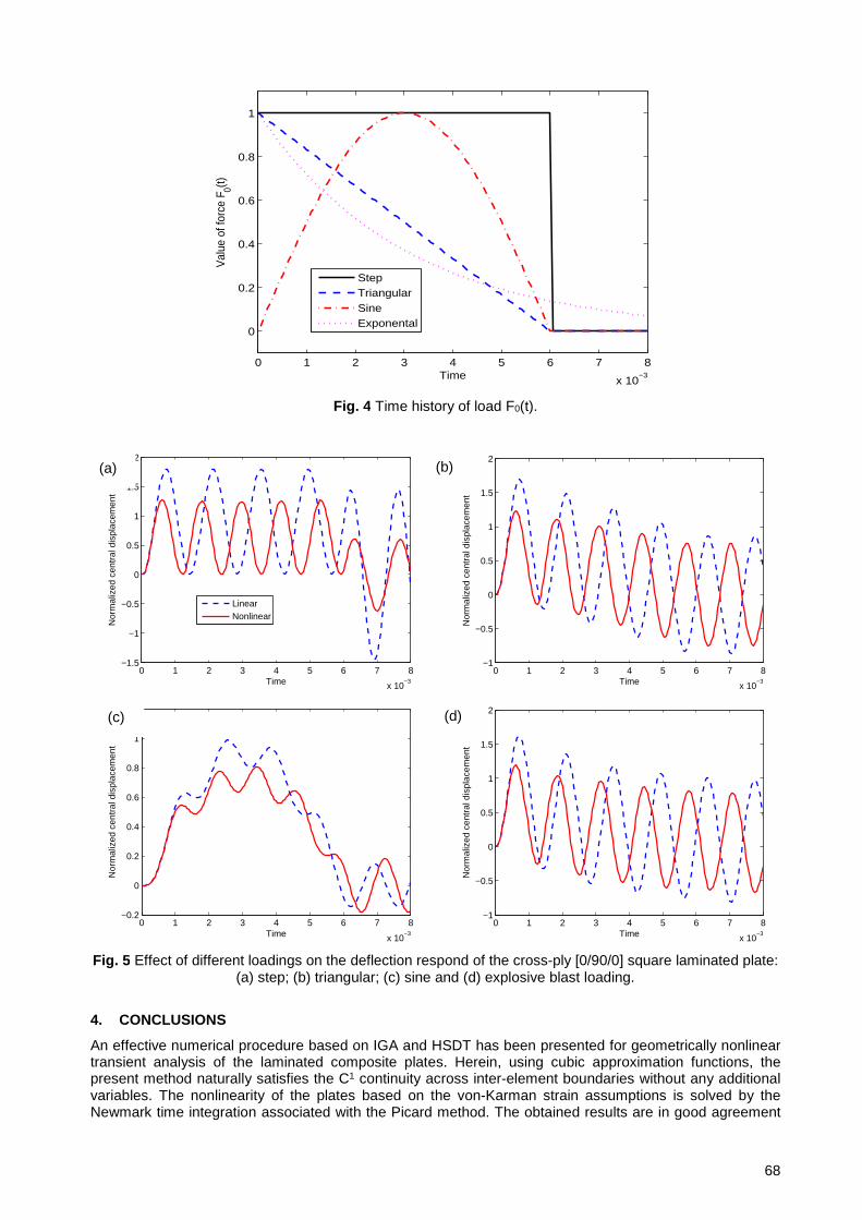
68
0 1 2 3 4 5 6 7 8
x 10−3
0
0.2
0.4
0.6
0.8
1
Time
Val
ue o
f for
ce F
0(t)
StepTriangularSineExponental
Fig. 4 Time history of load F0(t).
0 1 2 3 4 5 6 7 8
x 10−3
−1.5
−1
−0.5
0
0.5
1
1.5
2
Time
Nor
mal
ized
cen
tral
dis
plac
emen
t
LinearNonlinear
0 1 2 3 4 5 6 7 8
x 10−3
−1
−0.5
0
0.5
1
1.5
2
Time
Nor
mal
ized
cen
tral
dis
plac
emen
t
0 1 2 3 4 5 6 7 8
x 10−3
−0.2
0
0.2
0.4
0.6
0.8
1
Time
Nor
mal
ized
cen
tral
dis
plac
emen
t
0 1 2 3 4 5 6 7 8
x 10−3
−1
−0.5
0
0.5
1
1.5
2
Time
Nor
mal
ized
cen
tral
dis
plac
emen
t
Fig. 5 Effect of different loadings on the deflection respond of the cross-ply [0/90/0] square laminated plate:
(a) step; (b) triangular; (c) sine and (d) explosive blast loading.
4. CONCLUSIONS
An effective numerical procedure based on IGA and HSDT has been presented for geometrically nonlinear transient analysis of the laminated composite plates. Herein, using cubic approximation functions, the present method naturally satisfies the C1 continuity across inter-element boundaries without any additional variables. The nonlinearity of the plates based on the von-Karman strain assumptions is solved by the Newmark time integration associated with the Picard method. The obtained results are in good agreement
(b) (a)
(d) (c)

69
with available solutions in the literature. It is also concluded that the nonlinear analysis produces lower magnitude and wavelength of the transverse displacement as compare with linear one.
ACKNOWLEDGMENTS
The first author would like to acknowledge the support from Erasmus Mundus Action 2, Lotus Unlimited Project.
5. REFERENCES
[1] Pagano, N., Exact solutions for rectangular bidirectional composites and sandwich plates. Journal of composite materials, 1970. 4(1): p. 20-34.
[2] Ferreira, A., Analysis of composite plates using a layerwise theory and multiquadrics discretization. Mechanics of Advanced Materials and Structures, 2005. 12(2): p. 99-112.
[3] Hughes, T.J.R., J.A. Cottrell, and Y. Bazilevs, Isogeometric analysis: CAD, finite elements, NURBS, exact geometry and mesh refinement. Computer Methods in Applied Mechanics and Engineering, 2005. 194(39–41): p. 4135-4195.
[4] Shojaee, S., et al., Free vibration analysis of thin plates by using a NURBS-based isogeometric approach. Finite Elements in Analysis and Design, 2012. 61(0): p. 23-34.
[5] Beirão da Veiga, L., et al., An isogeometric method for the Reissner–Mindlin plate bending problem. Computer Methods in Applied Mechanics and Engineering, 2012. 209: p. 45-53.
[6] Tran, L.V., A.J.M. Ferreira, and H. Nguyen-Xuan, Isogeometric analysis of functionally graded plates using higher-order shear deformation theory. Composites Part B: Engineering, 2013. 51(0): p. 368-383.
[7] Tran, L.V., et al., Isogeometric analysis of laminated composite plates based on a four-variable refined plate theory. Engineering Analysis with Boundary Elements, 2014. 47(0): p. 68-81.
[8] Thai, C.H., et al., Isogeometric analysis of laminated composite and sandwich plates using a layerwise deformation theory. Composite Structures, 2013. 104(0): p. 196-214.
[9] Kapoor, H. and R. Kapania, Geometrically nonlinear NURBS isogeometric finite element analysis of laminated composite plates. Composite Structures, 2012. 94(12): p. 3434-3447.
[10] Le-Manh, T. and J. Lee, Postbuckling of laminated composite plates using NURBS-based isogeometric analysis. Composite Structures, 2014. 109(0): p. 286-293.
[11] Reddy, J.N., Mechanics of laminated composite plates-theory and analysis. 2004, New York: CRC Press 2nd Edit.
[12] Chen, J. and D.J. Dawe, Linear transient analysis of rectangular laminated plates by a finite strip-mode superposition method. Composite Structures, 1996. 35(2): p. 213-228.
[13] Thai, C.H., et al., Generalized shear deformation theory for functionally graded isotropic and sandwich plates based on isogeometric approach. Computers & Structures, 2014. 141(0): p. 94-112.
[14] Reddy, J.N., Geometrically nonlinear transient analysis of laminated composite plates. AIAA Journal, 1983. 21(4): p. 621-629.
[15] Chen, J., D.J. Dawe, and S. Wang, Nonlinear transient analysis of rectangular composite laminated plates. Composite Structures, 2000. 49(2): p. 129-139.
[16] Khdeir, A.A. and J.N. Reddy, Exact solutions for the transient response of symmetric cross-ply laminates using a higher-order plate theory. Composites Science and Technology, 1989. 34(3): p. 205-224.

International Journal of Fracture Fatigue and Wear, Volume 4
70
Proceedings of the 5th International Conference on
Fracture Fatigue and Wear, pp. 70-77, 2016
NONLINEAR CONTROL OF SMART PLATES USING ISOGEOMETRIC
ANALYSIS
P. Phung-Van1,2, Loc V. Tran1,2, H. Nguyen-Xuan3 and M. Abdel-Wahab1,2
1Division of Computational Mechanics, Ton Duc Thang University, Vietnam
2Faculty of Engineering and Architecture, Ghent University, Belgium
3Center for Interdisciplinary Research in Technology, HUTECH University, Vietnam
Abstract: In this paper, isogeometric analysis (IGA) based on a generalized unconstrained approach for
nonlinear analysis of smart composite plates is investigated. In composite plates, the mechanical
displacement field is approximated according to the proposal model and the nonlinear formulation for plates
is based on the von Kármán strains. Through the thickness of each piezoelectric layer, the electric potential
is assumed linearly. For active control of the piezoelectric composite plates, a close-loop system is used.
Various numerical examples are investigated to show high accuracy and reliability of the proposed method.
Keywords: Nonlinear control, isogeometric analysis (IGA), smart materials, piezoelectric plates.
1. INTRODUCTION
Piezoelectric materials belong to a smart material class that expresses electromechanical coupling. The main
feature of smart materials is transformation between mechanical energy and electric energy. When the
application of electric field to piezoelectric structures is considered, the mechanical deformation is generated.
With the advantages of piezoelectric materials, various numerical methods have been devised. Mitchell and
Reddy [1] presented the classical plate theory (CPT) using the third order shear deformation theory (TSDT)
to obtain the Navier solution for composite laminates with piezoelectric lamina. The radial point interpolation
method (RPIM) combined with the first order shear deformation theory (FSDT) and the CPT with rectangular
plate bending element were investigated by Liu et al. [2] to compute and simulate the static deformation and
responses of smart plates. A HSDT-layerwise generalized finite element formulation [3] and the layerwise
based on analytical formulation [4] were investigated to study piezoelectric composite plates. For vibration
control, Bailey et al [5] and Shen et al. [6] investigated smart beams integrated with layers using analytical
solutions. Wang et al. [7] used FEM to investigate dynamic stability of piezoelectric composite plates, where
the governing equations of motion using Lyapunov’s energy with active damping was used. Recently,
isogeometric analysis (IGA) has been developed to investigate the piezoelectric composite plates [8] and
plates/shells [9-13]. However, nonlinear transient analysis has not considered in their previous work. Hence,
this paper tries to fill this gap by using IGA based on the general unconstrained third order shear deformation

International Journal of Fracture Fatigue and Wear, Volume 4
71
theory (UTSDT). For reference, it is termed as IGA-UHSDT. The method will be applied for nonlinear analysis
of piezoelectric composite plates. The IGA-UHSDT is used to approximate the displacement field of smart
plates. Through the thickness of each piezoelectric layer, the electric potential is assumed linearly. The
nonlinear formulation for plates is formed in the total Lagrange approach based on the von Kármán strains.
The reliability and accuracy of the method are confirmed by numerical examples.
2. FORMULATION OF PIEZOELECTRICITY
Consider a piezoelectric composite plate as shown in Figure 1, the lower and upper layers of the composite
plate are piezoelectric layers. The UHSDT is used to approximate the variable displacements for the
composite plate, while the electrical displacements are assumed to be independent.
Fig. 1 Configuration of a piezoelectric laminated composite plate.
2.1. UHSDT
The unconstrained theory based on HSDT can be rewritten
0 1 2
0 1 2
( , , , ) ( , , ) ( , , ) ( , , )
( , , , ) ( , , ) ( , , ) ( , , )
( , , , ) ( , , )
u x y z t u x y t zu x y t f z u x y t
v x y z t v x y t zv x y t f z v x y t
w x y z t w x y t
(1)
where u0, u1, u2, v0, v1, v2 and w are displacement variables. For UTSDT in [14], the function f(z) = z3 is used.
In what follows, we introduce a new function ( )f(z)= arctan z that ensures that its first derivative is nonlinear
through the plate thickness and solutions are more accurate than for the case of f(z) = z3.
For a plate bending, the strain vector is represented by:
1 1
2 2
ji k kij
j i i j
uu u u
x x x x
(2)
The material behavior of smart composite plates is expressed as follows [15]:

International Journal of Fracture Fatigue and Wear, Volume 4
72
T
σ c e
D Ee g
(3)
where and σ are the strain vector and the stress vector, respectively; g denotes the dielectric constant
matrix and D is the dielectric displacement; e is the piezoelectric constant; E, the electric field vector, can be
defined as:
gradE (4)
in which is the electric potential field; and c, the elasticity matrix, is defined as:
15 11
15 22
31 32 33 33
0 0 0 0 0 0 0
; 0 0 0 0 0 ; 0 0
0 0 0 0 0
k k
k k
s s
s s
d p
d p
d d d p
A B L 0 0
B G F 0 0
c L F H 0 0 e g
0 0 0 A B
0 0 0 B D
(5)
in which:
/22 2
/2
/2 2
/2
, , , , , 1, , , ( ), ( ), ( ) d , 1,2,6
, , 1, ( ), ( ) d , 4,5
h
ijh
h
s s s ijh
z z f z zf z f z Q z i j
f z f z Q z i j
A B G L F H
A B D
(6)
where 𝑖𝑗 is calculated as in [1].
2.2. The piezoelectric plate formulation based on NURBS basic
functions
2.2.1. Mechanical displacement
Using NURBS basic function, the field u of the composite plate is approximated as:
1
, ,m n
h
I I
I
N
u d (7)
where 0 0 1 1 2 2
T
I I I I I I I Iu v u v u v wd , and NI is the shape function as defined in [16].
The strains can be rewritten as:
1
1[ ]
2
m nT L NL
p s I I I
I
ε ε B B d (8)
where 0 1 2 0 1
TL s s
I I I I I I B B B B B B , in which

International Journal of Fracture Fatigue and Wear, Volume 4
73
,0 1
,
0 0 0 0 0 0 0 00 0 0,
0 0 0 0 0 0 0 00 0 0
I xI Is s
I I
I yI I
NN N
NN N
B B
, ,
,2
, ,
,
, , , ,
0 0 0 0 0 0 00 0 0 0 0 0
0 0 0 0 0 0 , ( ) 00 0 0 0 0 0
0 0 0 0 0
I x I x
I xNL g
I I y I I y I
I x
I y I x I y I x
N wN
N wN
N N w w
B B d A B
, ,
0 1
, ,
, , , ,
0 0 0 0 0 0 0 0 0 0 0 0
0 0 0 0 0 0 , 0 0 0 0 0 0 ,
0 0 0 0 0 0 0 0 0 0
I x I x
I I y I I y
I y I x I y I x
N N
N N
N N N N
B B
(9)
2.2.2. Electric potential field
The electric potential field is approximated as follows [15]:
( )i i iz N (10)
where i
N is the shape functions
The electric field E in Eq. (4) can be rewritten:
i i i
E R B (11)
2.2.3. Governing equations
The equations for the smart plate are written as:
0
0 0
uu uuu
u
K KM d fdMq Kq f
K K Q (12)
and for dynamic control
* Md K d F (13)
where * 1
uu d u us s sG
K K K K K in which where Gd is the constant gains of the
displacement feedback control, and
12
0
( ) ( )d ; ( ) d
d ; d ; d
L NL T L NL L T T
uu u
T T
uu q
K B +B c B + B K B e B
K B pB M N mN f N (14)

International Journal of Fracture Fatigue and Wear, Volume 4
74
in which q0 is a uniform load; 0 0 0 0 0 0 ;IN N m is defined by:
1 2 4
/22 2
2 3 5 1 2 3 4 5 7/2
4 5 7
, , , , , , 1, , , ( ), ( ), ( ) dh
h
I I I
I I I I I I I I I z z f z zf z f z z
I I I
m (15)
and
1
2 1 2 3
3
0 0000 0 00 0 000 00000 0
, 0 0000 0 , 00 0 000 , 00000 0
0 0 0000 0 0 0 000 00000 0 0
I I I
I I I
I
N N N
N N N
N
N
N N N N N
N
(16)
3. NUMERICAL RESULTS
3.1. Static analysis
A square smart plate with length 20 cm under a uniform load q = 100 N/m2 is considered. The plate has six
layers: two outer piezo layers represented by pie and four composite layers. Each layer thickness of the non-
piezoelectric composite plate is 0.25 mm and the thickness of the piezo layer is 0.1 mm. The composite layers
are made of T300/976 graphite/epoxy and the piezo-ceramic layers are PZTG1195N. First, the effect of input
voltages on deflection of the CFFF plate [pie/-45/45]as is shown in Figure 2a. It can be seen, the present
results agree well with those of Liu et al. (2004). Furthermore, the deflection of the plate using only mesh of
9×9 elements with different boundary conditions (CFFF, SSFF, SSSS) is shown in Figure 2b. Again, it can be
seen that the present method agrees very well with those of RPIM [2].
(a) (b)
Fig. 2 (a) Effect of input voltages on deflection of the piezoelectric composite plate; (b) The deflection of
the piezoelectric composite plates with various boundary conditions
0 20 40 60
-3
-2
-1
0
x 10-3
Actuator Voltage (V)
Deflection (
m)
RPIM (SSFF)
RPIM (CFFF)
IGA (CFFF)
IGA (SSSS)RPIM (SSSS)
IGA (SSFF)
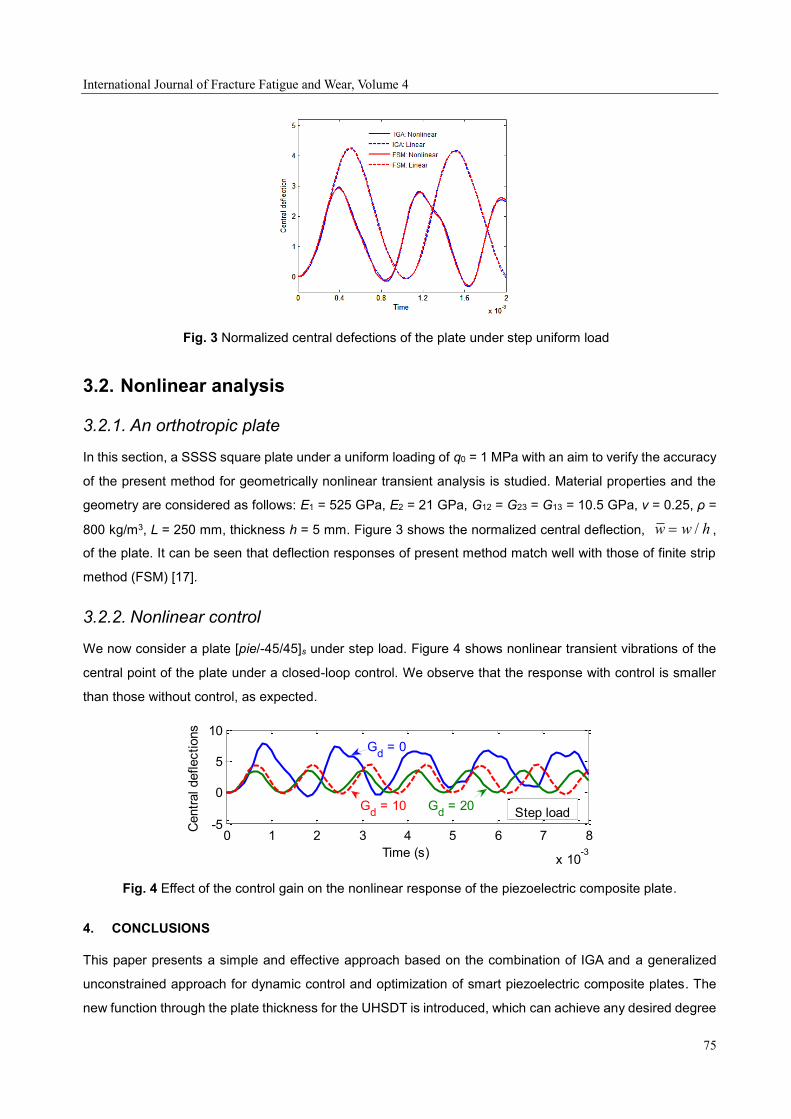
International Journal of Fracture Fatigue and Wear, Volume 4
75
Fig. 3 Normalized central defections of the plate under step uniform load
3.2. Nonlinear analysis
3.2.1. An orthotropic plate
In this section, a SSSS square plate under a uniform loading of q0 = 1 MPa with an aim to verify the accuracy
of the present method for geometrically nonlinear transient analysis is studied. Material properties and the
geometry are considered as follows: E1 = 525 GPa, E2 = 21 GPa, G12 = G23 = G13 = 10.5 GPa, ν = 0.25, ρ =
800 kg/m3, L = 250 mm, thickness h = 5 mm. Figure 3 shows the normalized central deflection, /w w h ,
of the plate. It can be seen that deflection responses of present method match well with those of finite strip
method (FSM) [17].
3.2.2. Nonlinear control
We now consider a plate [pie/-45/45]s under step load. Figure 4 shows nonlinear transient vibrations of the
central point of the plate under a closed-loop control. We observe that the response with control is smaller
than those without control, as expected.
Fig. 4 Effect of the control gain on the nonlinear response of the piezoelectric composite plate.
4. CONCLUSIONS
This paper presents a simple and effective approach based on the combination of IGA and a generalized
unconstrained approach for dynamic control and optimization of smart piezoelectric composite plates. The
new function through the plate thickness for the UHSDT is introduced, which can achieve any desired degree
0 1 2 3 4 5 6 7 8
x 10-3
-5
0
5
10
Time (s)
Centr
al deflections
Gd = 0
Gd = 10 G
d = 20
Step load

International Journal of Fracture Fatigue and Wear, Volume 4
76
of smoothness through the choice of the interpolation order and easily fulfills the C1-continuity requirements
for plate elements stemming from the HSDT. In analyses, the present approach would provide a reliable
source of reference when calculating laminated composite plates with other methods.
ACKNOWLEDGMENTS
The first author would like to acknowledge the support from Erasmus Mundus Action 2, Lotus Unlimited
Project.
5. REFERENCES
[1] Reddy JN (1997). Mechanics of laminated composite plates – Theory and Analysis, New York, CRC
Press.
[2] Liu GR, Dai KY, Lim KM (2004). Static and vibration control of composite laminates integrated with
piezoelectric sensors and actuators using the radial point interpolation method. Smart Materials and
Structures, 13, 1438-1447.
[3] Torres DAF, Mendonca PdTR, Barcellos CSD (2011). Evaluation and verification of an HSDT-
layerwise generalized finite element formulation for adaptive piezoelectric laminated plates.
Computer Methods in Applied Mechanics and Engineering, 200, 675-691.
[4] Saravanos DA, Heyliger PR, Hopkins DA (1997). Layerwise mechanics and finite element for the
dynamic analysis of piezoelectric composite plates. International Journal of Solids and Structures,
34, 359-378.
[5] Bailey T, Hubbard JE (1985). Distributed piezoelectric-polymer active control of a cantilever beam.
Journal of Guidance Control and Dynamic, 8, 605–611.
[6] Shen IS (1995). Bending and torsional vibration control of composite beams through intelligent
constrained-layer damping treatments. Smart Materials and Structures, 4, 340–355.
[7] Wang SY, Quek ST, Ang KK (2004). Dynamic stability analysis of finite element modeling of
piezoelectric composite plates. International Journal of Solids and Structures, 41, 745-764.
[8] Phung-Van P, De Lorenzis L, Thai Chien H, Abdel-Wahab M, Nguyen-Xuan H (2015). Analysis of
laminated composite plates integrated with piezoelectric sensors and actuators using higher-order
shear deformation theory and isogeometric finite elements. Computational Materials Science, 96,
496-505.
[9] Phung-Van P, Nguyen-Thoi T, Luong-Van H, Lieu-Xuan Q (2014). Geometrically nonlinear analysis
of functionally graded plates using a cell-based smoothed three-node plate element (CS-MIN3)
based on the C 0-HSDT. Computer Methods in Applied Mechanics and Engineering 270, 15-36
[10] Phung-Van P, Abdel-Wahab M, Liew KM, Bordas SPA, Nguyen-Xuan H (2015). Isogeometric analysis
of functionally graded carbon nanotube-reinforced composite plates using higher-order shear
deformation theory. Composite Structures 123, 137-149.
[11] Phung-Van P, Nguyen-Thoi T, Luong-Van H, Thai-Hoang C, Nguyen-Xuan H (2014). A cell-based
International Journal of Fracture Fatigue and Wear, Volume 4
77
smoothed discrete shear gap method (CS-FEM-DSG3) using layerwise deformation theory for
dynamic response of composite plates resting on viscoelastic foundation. Computer Methods in
Applied Mechanics and Engineering 272, 138-159.
[12] Phung-Van P, Thai-Hoang C, Nguyen-Thoi T, Nguyen-Xuan H (2014). Static and free vibration
analyses of composite and sandwich plates by an edge-based smoothed discrete shear gap method
(ES-DSG3) using triangular elements based on layerwise theory. Composites Part B: Engineering
60, 227-238.
[13] Phung-Van P, Lieu B Nguyen, Loc V Tran, Dinh TD, Chien H Thai, Bordas SPA, Abdel-Wahab M,
Nguyen-Xuan H (2015). An efficient computational approach for control of nonlinear transient
responses of smart piezoelectric composite plates. International Journal of Non-Linear Mechanics
76, 190-202.
[14] Leung AYT (1991). An unconstrained third-order plate theory. Composite Structures, 40(4), 871–875.
[15] Phung-Van P, Nguyen-Thoi T, Le-Dinh T, Nguyen-Xuan H (2013). Static and free vibration analyses
and dynamic control of composite plates integrated with piezoelectric sensors and actuators by the
cell-based smoothed discrete shear gap method (CS-FEM-DSG3). Smart Materials and Structures,
22, 095026.
[16] Cottrell JA, Hughes TJR, Bazilevs Y (2009). Isogeometric Analysis, Towards Integration of CAD and
FEA, Wiley.
[17] Chen J, Dawe DJ, Wang S (2000). Nonlinear transient analysis of rectangular composite laminated
plates. Composite Structures, 49, 129-139.
International Journal of Fracture Fatigue and Wear, Volume 4
78
Proceedings of the 5th International Conference on
Fracture Fatigue and Wear, pp. 78-85, 2016
A REVIEW ON FRETTING FATIGUE CRACK INITIATION CRITERIA
N.A. Bhatti and M. Abdel Wahab
Ghent University, Laboratory Soete, Ghent, Belgium
Abstract: This paper aims to provide an overview of experimental and numerical work related to fretting
fatigue crack initiation criteria. The complexity of modelling fretting fatigue arises due to the presence of multi axial stress state and wear, hence, it is imperative to define the crack initiation criteria. Among many available criteria, some of the most widely used have been summarized here, to provide an insight of the topic and to demonstrate the applicability of these criteria. For convenience, different criteria have been grouped together based on the approaches used to define failure parameters. The generalize classification includes, critical plane approach, stress-invariant approach and continuum damage mechanics approach. Besides experimental work, quantum of work has been done to implement these models using finite element methods (FEM). The strength of finite element methods is demonstrated as it provides minute information about crack initiation phase, contact stresses and estimated life. At the end, conclusions are drawn to advocate the proximity and efficacy of numerical methods in comparison to experimental work.
Keywords: Fretting fatigue; crack initiation criteria; FEM.
1 INTRODUCTION
Fretting can be referred as a material damage caused by small oscillatory movements between the contacting bodies. This may lead to a deterioration of surfaces and dimensional changes. Also a remarkable decrease in service life can be observed in the presence of bulk stress [1]. The surface degradation is defined as fretting wear, whereas the development of crack can be termed as fretting fatigue [2]. For estimation of life in fretting fatigue problems the complete process is usually divided in two phases, namely, crack initiation and crack propagation. While there is still a debate on the proportion of life time taken by these two phases, most of the authors have considered both the phases for total life estimation [3,4]. Therefore, the search for selection of most suitable criteria still continues. Each criterion is suitable in certain combination of selected material, geometry, type of contact and loading conditions [5]. This article, however, presents a review on the crack initiation criteria and its applications using finite element analysis.
Fretting fatigue is a type of multi-axial fatigue having non-proportional loading [6], thus introduces multiaxial stress fields and severe stress gradients [7]. Therefore, multiaxial criteria are used to define the failure [8,9]. Different multi-axial criteria have been developed in the past that use critical damage parameters, along with various methods to define estimated life. In general, the stress or strain components combining with material constants are equated to fatigue strength limit in fully reversed tension/torsion or by Manson-Coffin and Basquin relation [10]. Hence, allowing to compute the estimated life under fretting fatigue scenario. Some researchers have used continuum damage mechanics (CDM) approach which is based on thermodynamic potential function and initiation life can be estimated using bulk material properties. Based on the approach used to model fretting fatigue crack initiation, different criteria can be classified as; critical plane approach, stress invariant approach and CDM approach.
2 CRITICAL PLANE APPROACH
According to this approach the crack initiate on specific planes known as critical planes. Therefore, the damage parameters are evaluated on these planes. Depending on the material and loading conditions, these planes are either maximum shear planes or maximum tensile stress planes. The most frequently used criteria based on this approach are presented below.
2.1 Smith-Watson-Topper (SWT) parameter
SWT parameter can be used to predict fretting fatigue crack initiation life. The parameter proposed by Smith et al. [11] can be expressed as a function of number of cycles to initiation (Ni) as:
International Journal of Fracture Fatigue and Wear, Volume 4
79
σnmax ∆ϵ1
2=
σf′2
E(2Ni)
2b′ (1)
Where, σn
max is the maximum normal stress in the plane of principal strain range and ∆ϵ1 is the maximum principal strain range. σf
′ is fatigue strength coefficient and b′is fatigue strength exponent. This criteria is also
applied to non-proportional loading by Socie [12] to predict crack initiation under multiaxial loading. The initiation is assumed to occur on the plane where, combination of range of strain normal to the plane (∆ϵ/2) and maximum stress normal to the plane (σmax), is most damaging. Lykins et al. [13] have used finite element analysis to successfully implement SWT model, where different fretting fatigue parameters have been computed to estimate the initiation life.
2.2 Fatemi-Socie (FS) parameter
Fatemi and Socie proposed a modification to Brown and Miller’s critical plane formulation to predict multi axial fatigue life and to account for an additional cyclic hardening during non-proportional loading condition [14]. Furthermore, variable amplitude loading and effect of mean stress is accounted for with the proposed model. This model is applicable to the material and loading condition, where failure is produced by shear mode, thus the plane, where the shear strain range is maximum, is the critical plane. For fully reverse uniaxial strain condition the FS parameter can be defined as [14]:
∆γmax
2(1 + k
σnmax
σy)= [(1 + νe)
σf′
E(2Ni)
b′ + (1 + νp)ϵf′(2Ni)
c′] [1 + kσf′
2σy(2Ni)
b′] (2)
Where, ∆γmax is the maximum shear strain range, σn
max is the maximum normal stress perpendicular to the
critical plane, σy is the yield strength and k is a constant that is fitted from the uniaxial to torsion fatigue test
data. b′ and c′ are fatigue strength exponent and fatigue ductility exponent respectively. ϵf′ is fatigue ductility
coefficient, νe and νp are elastic and plastic Poisson’s ratio respectively. Sabsabi et al. [15] have applied FS
criterion to fretting fatigue problem for comparison of experimental lives and estimated lives using extended finite element methods (X-FEM). The results showed that combining FS parameter with X-FEM provides good estimation of experimental total lives.
2.3 McDiarmid parameter
The criterion proposed by McDiarmid is a high cycle fatigue multi axial criteria. The fatigue strength is defined in terms of shear stress amplitude and maximum normal stress on critical plane of maximum shear stress amplitude [16]. The critical plane is the one where shear stress range is maximum for one cycle. The number of cycles to initiation can be related to McDiarmid parameter for the plain fatigue case as [5]:
∆τmax
2+ (
τ′f−1
2σu) σn
max =1
2(1 +
τ′f−1
2σu)σf
′(2Ni)b′ (3)
Where, ∆τmax is the maximum increment of shear stress, σn
max is the maximum normal stress in the direction
perpendicular to maximum shear stress range. τ′f−1 is the shear fatigue limit and σu is the ultimate tensile
stress. McDiarmid used two shear fatigue limits, one for the case where crack grows parallel to the surface and one across the surface. This criterion has been successfully implemented by Sabsabi et al. [15] and Navarro et al. [17] to estimate fretting fatigue crack initiation. Li et al. [18] has shown good agreement between experimental and estimated lives and also location and orientation of crack initiation using finite element methods.
2.4 Dang Van criterion
Dang Van proposed critical plane based initiation criteria, where the fatigue failure is dependent on shear stress and hydrostatic stress [19]. The maximum of the linear combination of both the parameters should be less than fatigue strength limit. Mathematically this criterion can be expressed as:
[κ(τ) + 3 − 1.5κ(σH)]max ≤ σf−1
′ (4)
Where, τ is shear stress amplitude on the examined plane, σH is the hydrostatic stress and σf−1
′ is fatigue limit
in fully reversed axial loading. κ is the fatigue limit ratio between fully reversed axial to torsion loading. Later, Dang Van et al. [20] proposed a three dimension criterion for fatigue limit where the results show a good agreement for industrial application. Alfredson and Cadario [6] and Nesládek et al. [10] have implemented

International Journal of Fracture Fatigue and Wear, Volume 4
80
Dang Van criterion for evaluation of fretting fatigue crack initiation. Moreover, Nesládek et al. [10] found fatigue index error to be 0.6 and 15.3 for 5 kN and 15 kN, respectively, using finite element methods.
2.5 Papadopoulos criterion
This is a high cycle fatigue criteria which accounts for out of phase bending and torsion loading. The criteria presented by Papadopoulos et al. [21] is valid for hard metals with ratio of fatigue limit in torsion to bending in a range of 0.577 – 0.8. In this criterion a parameter called resolved shear stress is introduced for each plane. Introducing an average formula, which represents the mean average value of shear stress this criterion can be defined as:
√5.√1
8π2∫ ∫ ∫ (τ(φ, θ, χ))2dχ. sinθ. dθ. dφ
2π
χ=0
π
θ=0
2π
φ=0+
τ′f−1−σf−1′ /√3
σf−1′ /3
(σH)max ≤ τ′f−1
(5)
Where, τ′f−1 is the fatigue limit under torsion and σf−1
′ under axial load. (σH)max is the maximum hydrostatic
stress. Ferré et al. [22] have applied this criterion to predict crack nucleation under fretting fatigue condition, using local and non-local approaches. The error computed is found to be less than 5%. According to their research the non local approaches are more suitable to be used with finite element methods.
2.6 Findley parameter (FP)
Findley proposed the criterion as a function of maximum normal stress and amplitude of shear stress [23]. The critical plane can be referred to as a plane with maximum value of the parameter. Mathematically this criterion in expressed as
FP = τ + k(σn
max) (6) Where, τ is the shear stress amplitude, σn
max is the maximum normal stress and k is the material coefficient. While applying this parameter for fretting fatigue crack initiation of spherical contact Alfredson and Cadario [6] suggested that this criteria has given better results than the others. However, the endurance limit of the criteria was higher than the experimental endurance limit. Concerning the applicability of the said criterion using finite element methods Li et al. [18] have predicted the fretting fatigue life in a scatter band of ±3N.
2.7 Shear Stress Range (SSR) parameter
This parameter is developed to predict crack location, orientation and number of cycles to fretting fatigue crack initiation and applied to Titanium alloy using different pad geometries. The parameter introduced by Lykins et al. [24] is based on shear stress range, where maximum and minimum shear stress is evaluated to find the critical plane from -90° to 90° with an increment of 0.1°. Mathematical expression is as follows
∆τcrit = (τmax − τmin) (7)
To account for the effect of different stress ratios the formula takes the following form modified using the Walker’s method.
SSR = ∆τcrit = τmax(1 − Rτ)
m (8) Where, τmax is the maximum shear stress, Rτ is the shear stress ratio and m is the fitting parameter. Apart from establishing the prediction of crack initiation and orientation, the initiation life is observed to fall in the band of ±3N from plane fatigue data. However, with different pad geometries significant variation in slip amplitude at the contact interface is observed [24].
2.8 Rolović and Tipton criteria
Rolović and Tipton presented the multi axial criteria based on combination of stresses and strains [25]. This criterion also consider damage on the critical plane with a length of 1mm crack size. The criteria has been tested against proportional and non-proportional loading conditions. The results are compared for both in phase and out-of-phase test data. Based on this criteria life estimation can be predicted with the following equation:
γ(τ + 0.3σnmax) + σn
max(ϵn) =σf′2
E(2Ni)
2b′ + σf′ϵf′(2Ni)
b′+c′ (9)
International Journal of Fracture Fatigue and Wear, Volume 4
81
Where,τ and γ are the shear stress and shear strain amplitude respectively on critical plane, σnmax is the
maximum normal stress on the critical plane, ϵn is the normal strain amplitude, σf′ and ϵf
′ is the fatigue strength
and fatigue ductility coefficient respectively, b′ and c′ are fatigue strength exponent and fatigue ductility exponent respectively. This criterion is also used for evaluation of fretting fatigue problems. Li et al. [18] implemented this criterion for calculation of fatigue damage parameter and also for estimation of life. The life prediction results computed with this criterion are shown to fall in a scatter band of ±3N . Moreover, they have implemented finite element methods for calculation of normal, shear and tangential stresses at the contact interface.
3 STRESS INVAIRANT APPROACH
This approach uses stress invariants or tensor approach to define failure. Several multi axial criteria based on this approach are available in the literature, however only Crossland model in used frequently for application to fretting fatigue problems.
3.1 Crossland parameter
Crossland introduced a parameter which is based on the maximum amplitude of the second invariant of
deviatoric stress tensor √J2 and maximum hydrostatic pressure (σH)max [26]. Mathematically this criterion can
be expressed as
CP = √J2 +τ′f−1−σf−1
′ /√3
σf−1′ /3
(σH)max ≤ τ′f−1 (10)
Where, τ′f−1 is the fatigue limit under torsion and σf−1
′ fatigue limit under axial load. (σH)max is the maximum
hydrostatic stress. This method intuitively has an advantage of shorter computation time over the critical plane approach models. This criterion has been used by many researches for computation of initiation life in fretting fatigue. Navarro et al. [5] have shown that Crossland parameter gives better standard deviation than other criteria for the case of spherical contact, however larger scatter band is observed for cylindrical contact. Nesládek et al. [10] has shown the drop of fatigue limits from plain fatigue and CP has performed well in fatigue prediction. Furthermore, finite element analysis is used to calibrate the coefficient of friction.
4 CONTINUUM DAMAGE MECHANICS APPROACH
This approach defines the failure in terms of damage, which constitutes on a damage variable. The evolution of this damage variable is calculated and failure is concluded when it reaches a critical value. This approach was first introduced by Kachanov [27], and is based on thermodynamic principle. Based on this concept, several theories have been developed and applied to predict crack nucleation in fretting fatigue problems.
4.1 Bhattacharya- Ellingwood damage model
The model presented by Bhattacharya and Ellingwood [28] is based on Continuum Damage Mechanics (CDM), which calculate cumulative fatigue damage. This model can predict crack initiation with the assumption that fatigue damage occurs before localization. The mean stress effects, loading sequence effects, stress controlled and strain controlled loading cycle effects are also accounted for. The equation for isotropic fatigue damage under uniaxial loading as function of loading cycle is given by:
Dn = 1 − (1 − D0)∏
1
1 +1h′
∆ϵ0i
1+1h′ − ∆ϵp1i
1h′ ∆ϵ0i + Ai
1
1 +1h′
∆ϵpmi
1+1h′ − ∆ϵp1i
1h′ ∆ϵpmi
+ Ai
; σmaxi > σe
1 ; otherwise
n
i=1
(11)
Ai =3σf
4(21−1/h′ H)
−∆ϵp0i
1+1h′
1 +1h′
+ ∆ϵp1i
1h′ ∆ϵp0i
(12)
International Journal of Fracture Fatigue and Wear, Volume 4
82
In the above set of equations (11) and (12), Dn is the damage after n cycles, D0 is the initiation damage at
fatigue cycle (for undamaged material D0 = 0), H and h′ are the cyclic hardening modulus and cyclic
hardening exponent respectively. σf, σmaxi, σe ,are the true failure stress, maximum stress for cycle i and
endurance limit respectively. ∆ϵ0i, ∆ϵp1i, ∆ϵpmi, ∆ϵp0i are the threshold strain of damage increment, initial
plastic strain, final plastic strain and threshold plastic strain of damage increment for cycle i respectively.
When the damage value reaches the critical value DNI ≥ DC, the crack is initiated.
Using the same model Quraishi et al. [29] have adopted it for fretting fatigue problems. Due to fretting loading conditions, shear stresses are calculated. These shear stresses are resolved into components alternating tensile and compressive stresses. By applying CDM approach fretting fatigue initiation life is predicted by combining the damage caused by stresses in two directions. The expression relating critical damage Dc and number of cycles to initiation Ni is given by:
Dc = 1 −
[ 1
1 +1h′
∆ϵ0i
1+1h′ − ∆ϵp1i
1h′ ∆ϵ0i + Ai
1
1 +1h′
∆ϵpmi
1+1h′ − ∆ϵp1i
1h′ ∆ϵpmi
+ Ai] 2Ni
(13)
The results shows good agreement for predicting number of cycles to failure for given maximum normal stress[29]. The S-N curves for Al 2024 and S45C are comparable with the experimental results.
4.2 Lemaitre damage model
Lemaitre introduced damage models based on CDM approach for ductile damage, creep damage and fatigue damage [30]. The damage is considered to be isotropic for predicting number of cycles to failure. Later in his work [31,32] the dissipation potential function φ was presented for the case of elastic and plastic conditions as expressed in equation (14) and (15) respectively.
φ =C
(β
2)+1
(−Y
C)(β
2)+1
Y (14)
φ =C
(β
2)+1
(−Y
C)(β
2)+1
(p + π) (15)
Where, C and β are material dependent damage parameters, Y is elastic strain energy p + π are plastic strain rate and accumulated micro-plastic strain respectively. Based on the theory of Lemaitre [31], a promising work is contributed by Hojjati-Talemi and Wahab [33] by deriving the equations for elastic and elasto-plastic condition and developed an uncoupled damage model for application to fretting fatigue problems. They developed a predictor tool to calculate fretting fatigue crack initiation life time and initiation location by combining CDM approach with FEM. Moreover, the effect of contact geometry, axial stress, normal load and tangential load is presented. Using the dissipation potential function φ for elastic condition, the damage D and number of cycles to initiation are given by equation (16) and (17) respectively.
D = 1 − [1 − A(β + 3)(σeq,maxβ+2
− σeq,minβ+2
) 2
3(1 + ν) + 3(1 − 2ν) (
σH
σeq)2
(β
2)+1
N]
1/(β+3)
(16)
Ni =1
A(β+3)(σeq,max
β+2− σeq,min
β+2)−1
Rv−(
β
2)−1
(17)
Where A and β are material dependent damage parameters and are obtained by fitting equation (17) in the experimental data. σeq,max and σeq,min are the maximum and minimum equivalent Von Mises stress
respectively. The estimated results for initiation life time with this model are found in close approximation with the experimental data and fall in a scatter band of ±2N.
International Journal of Fracture Fatigue and Wear, Volume 4
83
Using the function φ defined in equation (15), Hojjati-Talemi et al. [34] have derived the damage equation as a function of number of cycles. In this study CDM approach is used along with FEM to compute initiation life and XFEM is used to compute the propagation life.
D = 1 − [1 − A(m + 2β + 2)(σeq,maxm+2β
− σeq,minm+2β
)RvβN]
1
(m+2β+2) (18)
Ni =(σeq,max−m−2β
−σeq,min−m−2β
)Rv−β
A(m+2β+2) (19)
Where, m is the power constant in Ramberg-Osgood equation. The results have shown good agreement between numerical data and experimental data, also total estimated life fall in a scatter band of ±2N [34].
5 CONCLUSIONS
In this paper different approaches regarding fretting fatigue crack initiation criteria have been reviewed and the following important points can be concluded.
1. The criteria using critical plane approaches are suitable to model crack initiation and orientation. These
criteria predict fretting fatigue behavior as they can also be used with non- proportional loading. Initiation life mostly fall in a scatter band of ±3N.
2. Stress invariant based approach can also be used for modeling fretting fatigue problems. This approach is intuitively more efficient than critical plane models as the parameter does not have to be computed on different planes, yet it loses the physical meaning of the problem.
3. CDM approach is recently employed to predict crack initiation/ nucleation for fretting fatigue problems. Various authors have predicted initiation life within a scatter band of ±2N using this approach. This approach can be used with coupled and uncoupled damage models for initiation and propagation phase.
4. Finite element methods can be used with various criteria for prediction of crack initiation/ nucleation location and estimated life. Almost all of the criteria can be modeled with FEM with good accuracy, also the effects of various fretting fatigue parameters can be studied. Furthermore, XFEM can be used for modeling of crack propagation and can be combined with various approaches to predict total life.
5. Studies have shown that there is no universal criteria, which gives best results for all type of materials, contact type and loading conditions. The results of the multi axial criteria also depends on the definition of crack initiation or nucleation, as crack initiation has been defined from micro level upto a length of millimeter. Various local and non-local approaches have been developed to evaluate failure parameters over specified length or volume. Therefore selection for the most suitable approach and criteria depends on various factors and vary from case to case.
6 REFERENCES
[1] D. Nowell, D.A. Hills, Crack initiation criteria in fretting fatigue, Wear, 136, 329-343, 1990.
[2] D.A. Hills, D. Nowell, Mechanics of fretting fatigue, Dordrecht, Kluwer Academic Publishers, 1994.
[3] J.A. Araújo , D. Nowell, The effect of rapidly varying contact stress fields on fretting fatigue, International Journal of Fatigue, 24, 763-775, 2002.
[4] M.P. Szolwinski, T.N. Farris, Observation, analysis and prediction of fretting fatigue in 2024-T351 aluminum alloy, Wear, 221, 24-36, 1998.
[5] C. Navarro, S. Muñoz, J. Domínguez, On the use of multiaxial fatigue criteria for fretting fatigue life assessment, International Journal of Fatigue, 30, 32-44, 2008.
[6] B. Alfredson, A. Cadario, A study on fretting friction evolution and fretting fatigue crack initiation for a spherical contact, International Journal of Fatigue, 26, 1037-1052, 2004.
[7] D. Nowell, D. Dini, D.A. Hills, Recent developments in the understanding of fretting fatigue, Engineering Fracture Mechanics, 73, 207-222, 2006.
[8] I.V. Papadopoulos, A high-cycle fatigue criterion applied in biaxial and triaxial out-of-phase stress conditions, Fatigue & Fracture of Engineering Materials & Structures,18, 79-91, 1995.
[9] M.P. Szolwinski, T.N. Farris, Mechanics of fretting fatigue crack formation, Wear,198, 93-107, 1996.
International Journal of Fracture Fatigue and Wear, Volume 4
84
[10] M. Nesládek, M. Španiel, J. Jurenka, J. Růžička, J. Kuželka, Fretting fatigue experimental and numerical approaches, International Journal of Fatigue, 44, 61-73, 2012.
[11] K.N. Smith, P. Watson, T.H. Topper, A stress-strain function for fatigue of metals, Journal of Materials, 5, 767-778, 1970.
[12] D. Socie, Multiaxial fatigue damage models, Journal of Engineering Materials and Technology, 109, 292-298, 1987.
[13] C.D. Lykins, S. Mall, V. Jain, An evaluation of parameters for predicting fretting fatigue crack initiation. International Journal of Fatigue, 22, 703-716, 2000.
[14] A. Fatemi, D. Socie, A critical plane approach to multiaxial fatigue damage including out-of-phase loading, Fatigue & Fracture of Engineering Materials & Structures, 11, 149-165, 1988.
[15] M. Sabsabi, E. Giner, F.J. Fuenmayor, Experimental fatigue testing of a fretting complete contact and numerical life correlation using X-FEM, International Journal of Fatigue, 33, 811-822, 2011.
[16] D.L. McDiarmid, A general criterion for high cycle multiaxial fatigue failure, Fatigue & Fracture of Engineering Materials & Structures, 14, 429-453, 1991.
[17] C. Navarro, M. García, J. Domínguez, A procedure for estimating the total life in fretting fatigue, Fatigue & Fracture of Engineering Materials & Structures, 26, 459-468, 2003.
[18] X. Li, Z. Zuo, W. Qin, A fretting related damage parameter for fretting fatigue life prediction, International Journal of Fatigue, 73, 110-118, 2015.
[19] K. Dang Van, Sur la résistance à la fatigue des métaux, Thèse de Doctorat ès Sciences, Sci. Techniq. l’Armement, vol. 47, p.647, 1973.
[20] K. Dang Van, G. Cailletaud, J.F. Flavenot, A. Le Douaron , H.P. Lieurade, Criterion for high cycle fatigue failure under multiaxial loading, In: Brown MW, Miller KJ, editors, Biaxial and multiaxial fatigue, EGF3, London, Mech Eng Publications, p. 459-478, 1989.
[21] I.V. Papadopoulos , P. Davoli, M. Filippini, A. Bernasconi, A comparative study of multiaxial high-
cycle fatigue criteria for metals, International Journal of Fatigue, 19(3), 219–235, 1997.
[22] R. Ferré , S. Fouvry , B. Berthel , J.A. Ruiz-Sabariego, Stress gradient effect on the crack nucleation process of a Ti-6Al-4V titanium alloy under fretting loading: Comparison between non-local fatigue approaches, International Journal of Fatigue, 54, 56-67, 2013.
[23] W.N. Findley, Fatigue of metals under combinations of stresses, Division of Engineering, Brown University, 1956.
[24] C.D. Lykins, S. Mall, V. Jain, A shear stress-based parameter for fretting fatigue crack initiation, Fatigue & Fracture of Engineering Materials & Structures, 24, 461-476, 2001.
[25] R. Rolović, S.M. Tipton, An energy based critical plane approach to multiaxial fatigue analysis, In: T.L. Panontin, S.D. Shepard, editors, Fatigue and fracture mechanics ASTM STP, 1332, Philadelphia, American Society for Testing and Materials, p. 599–613, 1999.
[26] B. Crossland, Effect of large hydrostatic pressures on the torsional fatigue strength of an alloy steel, Proceedings of the international conference on fatigue of metals, p. 138-49, 1956.
[27] L. Kachanov, Time of the rupture process under creep conditions. Isv. Akad. Nauk. SR. Otd Tekh. Nauk., 8, 26-31, 1958.
[28] B. Bhattacharya, B. Ellingwood, Continuum damage mechanics analysis of fatigue crack initiation, International Journal of Fatigue, 20(9), 631-639, 1998.
[29] S.M. Quraishi, M.M. Khonsari, D.K. Baek, A thermodynamic approach for predicting fretting fatigue life, Tribology Letters, 19(3), 169-175, 2005.
[30] J. Lemaitre, How to use damage mechanics. Nuclear Engineering and design, 80, 233-245, 1984.
[31] J. Lemaitre, Formulation and identification of damage kinetic constitutive equations, Continuum Damage Mechanics, Theory and Application, edited by Krajcinovic et al., International Centre for Mechanical Sciences, CISM Courses and Lectures, 295, 1987.
[32] J. Lemaitre, R. Desmorat, Engineering damage mechanics: ductile, creep, fatigue and brittle failures, Springer, 2005.

International Journal of Fracture Fatigue and Wear, Volume 4
85
[33] R. Hojjati-Talemi, M.A. Wahab, Fretting fatigue crack initiation lifetime predictor tool: Using damage mechanics approach, Tribology International, 60,176–186, 2013.
[34] R. Hojjati-Talemi, M.A. Wahab, E. Giner, M. Sabsabi, Numerical estimation of fretting fatigue lifetime using damage and fracture mechanics, Tribology Letters, 52(1), 11-25, 2013.
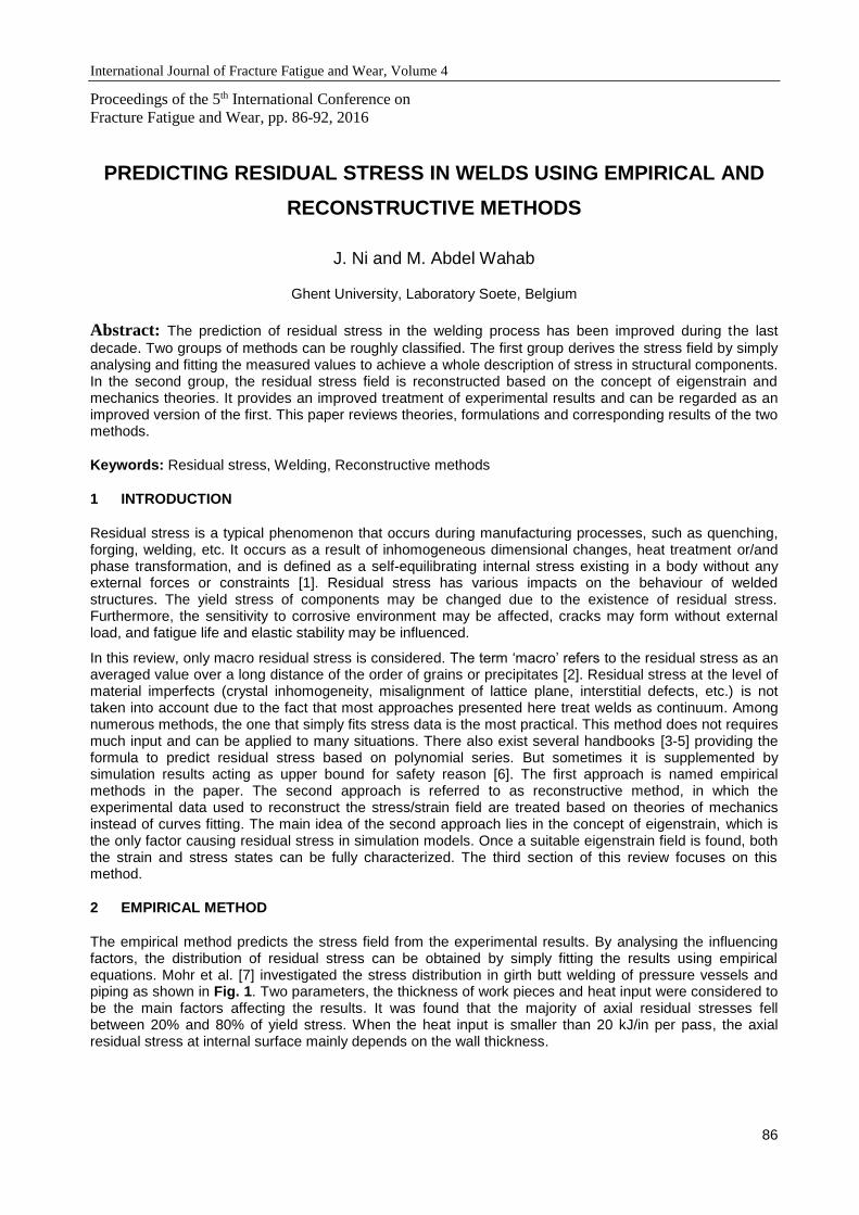
International Journal of Fracture Fatigue and Wear, Volume 4
86
Proceedings of the 5th International Conference on
Fracture Fatigue and Wear, pp. 86-92, 2016
PREDICTING RESIDUAL STRESS IN WELDS USING EMPIRICAL AND
RECONSTRUCTIVE METHODS
J. Ni and M. Abdel Wahab
Ghent University, Laboratory Soete, Belgium
Abstract: The prediction of residual stress in the welding process has been improved during the last
decade. Two groups of methods can be roughly classified. The first group derives the stress field by simply analysing and fitting the measured values to achieve a whole description of stress in structural components. In the second group, the residual stress field is reconstructed based on the concept of eigenstrain and mechanics theories. It provides an improved treatment of experimental results and can be regarded as an improved version of the first. This paper reviews theories, formulations and corresponding results of the two methods.
Keywords: Residual stress, Welding, Reconstructive methods
1 INTRODUCTION
Residual stress is a typical phenomenon that occurs during manufacturing processes, such as quenching, forging, welding, etc. It occurs as a result of inhomogeneous dimensional changes, heat treatment or/and phase transformation, and is defined as a self-equilibrating internal stress existing in a body without any external forces or constraints [1]. Residual stress has various impacts on the behaviour of welded structures. The yield stress of components may be changed due to the existence of residual stress. Furthermore, the sensitivity to corrosive environment may be affected, cracks may form without external load, and fatigue life and elastic stability may be influenced.
In this review, only macro residual stress is considered. The term ‘macro’ refers to the residual stress as an averaged value over a long distance of the order of grains or precipitates [2]. Residual stress at the level of material imperfects (crystal inhomogeneity, misalignment of lattice plane, interstitial defects, etc.) is not taken into account due to the fact that most approaches presented here treat welds as continuum. Among numerous methods, the one that simply fits stress data is the most practical. This method does not requires much input and can be applied to many situations. There also exist several handbooks [3-5] providing the formula to predict residual stress based on polynomial series. But sometimes it is supplemented by simulation results acting as upper bound for safety reason [6]. The first approach is named empirical methods in the paper. The second approach is referred to as reconstructive method, in which the experimental data used to reconstruct the stress/strain field are treated based on theories of mechanics instead of curves fitting. The main idea of the second approach lies in the concept of eigenstrain, which is the only factor causing residual stress in simulation models. Once a suitable eigenstrain field is found, both the strain and stress states can be fully characterized. The third section of this review focuses on this method.
2 EMPIRICAL METHOD
The empirical method predicts the stress field from the experimental results. By analysing the influencing factors, the distribution of residual stress can be obtained by simply fitting the results using empirical equations. Mohr et al. [7] investigated the stress distribution in girth butt welding of pressure vessels and piping as shown in Fig. 1. Two parameters, the thickness of work pieces and heat input were considered to be the main factors affecting the results. It was found that the majority of axial residual stresses fell between 20% and 80% of yield stress. When the heat input is smaller than 20 kJ/in per pass, the axial residual stress at internal surface mainly depends on the wall thickness.
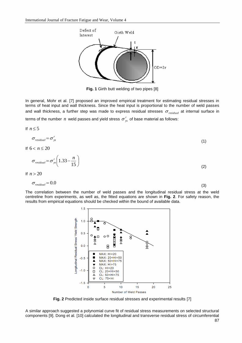
International Journal of Fracture Fatigue and Wear, Volume 4
87
Fig. 1 Girth butt welding of two pipes [8]
In general, Mohr et al. [7] proposed an improved empirical treatment for estimating residual stresses in terms of heat input and wall thickness. Since the heat input is proportional to the number of weld passes
and wall thickness, a further step was made to express residual stresses residual at internal surface in
terms of the number n weld passes and yield stress r
ys of base material as follows:
If 5n
r
ysresidual (1)
If 6 20n
1533.1
nr
ysresidual (2)
If 20n
0.0residual (3)
The correlation between the number of weld passes and the longitudinal residual stress at the weld centreline from experiments, as well as, the fitted equations are shown in Fig. 2. For safety reason, the results from empirical equations should be checked within the bound of available data.
Fig. 2 Predicted inside surface residual stresses and experimental results [7]
A similar approach suggested a polynomial curve fit of residual stress measurements on selected structural components [9]. Dong et al. [10] calculated the longitudinal and transverse residual stress of circumferential
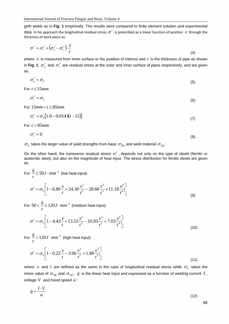
International Journal of Fracture Fatigue and Wear, Volume 4
88
girth welds as in Fig. 1 empirically. The results were compared to finite element solution and experimental
data. In his approach the longitudinal residual stress r is prescribed as a linear function of position x through the
thickness of work piece as:
t
xr
i
r
o
r
i
r (4)
where x is measured from inner surface to the position of interest and t is the thickness of pipe as shown
in Fig. 1. r
o and r
i are residual stress at the outer and inner surface of pipes respectively, and are given
as:
Y
r
o (5)
For mmt 15
Y
r
i (6)
For mmtmm 8515
150143.00.1 tY
r
i (7)
For mmt 85
0r
i (8)
Y takes the larger value of yield strengths from base YB and weld material YW .
On the other hand, the transverse residual stress t , depends not only on the type of steels (ferritic or
austenitic steel), but also on the magnitude of heat input. The stress distribution for ferritic steels are given as:
For 250 mmJ
t
q (low heat input)
4
4
3
3
2
2
18.1168.2830.2480.61t
x
t
x
t
x
t
xY
t
(9)
For 212050 mmJ
t
q (medium heat input)
4
4
3
3
2
2
03.793.1653.1343.41t
x
t
x
t
x
t
xY
t
(10)
For 2120 mmJ
t
q (high heat input)
3
3
2
2
88.106.322.01t
x
t
x
t
xY
t
(11)
where x and t are defined as the same in the case of longitudinal residual stress while Y takes the
minor value of YB and YW . q is the linear heat input and expressed as a function of welding current I ,
voltage V and travel speed u :
u
VIq
(12)

International Journal of Fracture Fatigue and Wear, Volume 4
89
The stress distribution at high heat input for autenitic steels holds the same as ferritic steels. The stresses in medium and low heat input have the same expression as Equation (9). Comparison with experimental data showed that the results from empirical equations were relatively conservative. Improvement can be done in several aspects. For example, the heat input can be treated as continuous rather than discretely as low, medium and high. Important geometrical parameters, such as pipe radius can be considered in expressions as well.
3 RECONSTRUCTIVE METHOD
An improvement is made with respect to the treatment of measured and simulated results using a reconstructive method. Unlike the empirical method, this method solves residual stress field based on mechanics theories. By implementing theories of shells or micromechanics, the problem is simply reduced to figuring out a stress field inherited with non-elastic strains. The non-elastic strain refers to the total plastic strain due to phase transformation, thermal expansion, geometrical mismatch, etc. In many researches, non-elastic strain is also named eigenstrain [11] or inherent strain [12]. It should be noted that the eigenstrain accounts for all permanent strains that give rise to residual stresses, but not a simply addition of
the various non-linear strains. A general decomposition of the total strain total can be decomposed as:
e
total (13)
where e is elastic strain and
is eigenstrain.
Masubuchi [13] considered four steps in this method, namely a) heat flow analysis, b) transient thermal stresses analysis, c) determination of non-elastic strain and total strain, and finally d) residual stresses analysis. Among those steps the third is the most important for the analysis of the distribution and magnitude of residual stress. Mura [11] developed a mathematical framework determining residual stresses considered in an infinite 3-D body. In his approach, the phases were supposed to transform within a domain of sphere or ellipsoid, and the resultant volume change was assumed to be uniform within that domain. Then, corresponding eigenstrain was uniformly distributed as well and constant throughout the domain according to Eshelby [14]. At a long distance outside the domain it decreased to zero.
With the knowledge of eigenstrain, the corresponding elastic and total strain can be determined. If the whole eigenstrain field is known, the residual stress and strain field can be deduced directly, which is known as the direct problem of eigenstrain theory [15]. The fundamental equations in the case of infinitely extended material are given as [11]:
jklijklljkijkl CuC ,, (14)
xξξx iijij exp (15)
where ijklC is elastic moduli and u the displacement. The eigenstrain is supposed to be in the form of
a single wave of amplitude and ξ is the wave vector corresponding to the given period of distribution
(15). However, the direct solution of eigenstrain theory is not practical when applied to other geometries like plane-bounded semi-infinite space or when the information of eigenstrain is incomplete.
To avoid the limitation of direction solution, an inverse method was developed. The basis of this method lies in the quantitative comparison between experimental data and predicted values of reconstructed strain field at the same location, which is called the inverse problem of eigenstrain theory [16]. In the inverse method, the unknown eigenstrain distribution is expressed as a summation of series of basic functions with coefficients to be determined. Those unknown coefficients are deduced by the least square method. Ueda
et al [17] proposed the relations between residual residual , elastic strains e and eigenstrain
as:
H (16)
Dresidual (17)
where H is elastic response matrix and D the stress-strain matrix.
The choice of basic function for eigenstrain varies for different researchers. Cao et al. [18] and Qian et al. [19] adopted a series of smooth functions, such as two-term or trigonometric polynomials. Kartal et al. [20]

International Journal of Fracture Fatigue and Wear, Volume 4
90
used the polynomials of Legendre and Korsunsky et al. [21] and the Chebyshev polynomials to present the nature of eigenstrain distribution. A general expression of eigenstrain is:
M
m
m
m
ijij N1
* (18)
where m
ij is the unknown coefficients, M the number of terms of polynomial and mN the chosen basic
functions.
Jun et al. [16] summarized the framework of reconstructing eigenstrain field and solving the inverse problem by finite element method (FEM). First, the FE model is set up according to the sample geometry, in which only the elastic material properties, such as Young’s modulus and Poisson’s ratio are needed. For regions where eigenstrains are possibly localized, fine mesh is recommended. Then, arbitrary eigenstrains are introduced in FE model by arbitrarily prescribing coefficients of thermal expansion. The eigenstrain is treated comparable to thermal strain since the modelling does not require explicit knowledge about its origin. After the completion of simulation, the elastic strains of the same experimental area are extracted for optimizing the coefficients. The simulations and optimizations are conducted until a good agreement is achieved. The final FE model provides extensive information such as residual stresses, strains, displacement, etc. Fig. 3 shows the residual strains predicted by this procedure [16].
Fig. 3 Contour plots of (left) localised eigenstrain input at different positions and (right) the corresponding residual strain distributions [16]
Besides FEM, boundary element method (BEM) can be used to calculate residual stresses as well. Qian et al. [22] approximated the eigenstrain field as a series of two-term polynomials. Based on the work by Cheng et al. [23], the corresponding domain integral is then transformed into boundary integral. Two examples are presented to demonstrate the effectiveness of this approach.
Instead of measuring and comparing strains directly, the deformation after welding can also be used to determine residual stresses. Wang et al. [24] estimated eigenstrains by analysing the deformation and the tendon force and applied them in an elastic FE analysis.
Similarly, a shell theory based scheme is developed by Song et al. [25, 26] to estimate the residual stress distribution. After analysing the distribution features of numerous residual stress solutions, Dong et al. [8] identified that the residual stress at weld toe can be decomposed into three parts, through-thickness
membrane m , bending b and self-equilibrating ..es stresses:
..esbm
yS
(19)
5432
.. hgfees (20)
mmm bt
ra
ln
(21)
bbb bt
ra
ln
(22)

International Journal of Fracture Fatigue and Wear, Volume 4
91
where 12 t
x with x , t and r identically defined in Chapter 2 and yS is the material yield strength of
base material. Coefficients ma , ba , mb , bb , e , f , g and h are determined using empirical equations of
heat input and specimen geometry. With the knowledge of stresses at weld toe, the distribution of residual stresses in other area can be calculated analytically through classical shell theory. Yang et al. [27] adopted shell theory as well but considered the material as ideal plastic.
4 CONCLUSION
As far as concerned, the empirical method adopts a set of easy and practical equations to predict the residual stress profiles in welds. However, the case study [10] shows that it provides relatively conservative results in engineering applications. The treatment of heat input and component geometries can be improved to have a more realistic results. The reconstructive method is developed to treat the measurements in a more decent way. The framework mentioned in section 3 can be flexibly applied to any other complex structures. To achieve a stable solution of the stress/strain field, the choice of basic functions of eigenstrain and measurement points are of considerable importance.
5 ACKNOWLEDGEMENTS
The authors would like to acknowledge the financial support of DeMopreCI-MDT SBO project.
6 REFERENCES
[1] Totten, G.E., Handbook of Residual Stress and Deformation of Steel. 2002: ASM International.
[2] Radaj, D., Heat Effects of Welding: Temperature Field, Residual Stress, Distortion. 2012: Springer Berlin Heidelberg.
[3] API, R., 579-1/ASME FFS-1. Houston, TX:, American Petroleum Institute, 2007.
[4] Koçak, M., et al., FITNET Fitness-for-Service (FFS) Annex-Volume 2, Revision MK8. Joint Research Centre, GKSS Research Centre Geesthacht, 2008.
[5] BSi, B., 7910: Guide on methods for assessing the acceptability of flaws in metallic structures. British Standards Institute, 2005.
[6] Bouchard, P.J., Code characterisation of weld residual stress levels and the problem of innate scatter. International Journal of Pressure Vessels and Piping, 2008. 85(3): p. 152-165.
[7] Mohr, W.C., P. Michaleris, and M.T. Kirk, Improved treatment of residual stresses in flaw assessment of pipes and pressure vessels fabricated from ferritic steels. American Society of Mechanical Engineers, Pressure Vessels and Piping Division(Publication) PVP., 1997. 359: p. 37-47.
[8] Dong, P., On the mechanics of residual stresses in girth welds. Journal of Pressure Vessel Technology-Transactions of the Asme, 2007. 129(3): p. 345-354.
[9] Bjorhovde, R., et al., Residual Stresses in Thick Welded Plates. 1971: Fritz Engineering Laboratory, Lehigh University.
[10] Dong, P.S., et al., On residual stress prescriptions for fitness for service assessment of pipe girth welds. International Journal of Pressure Vessels and Piping, 2014. 123: p. 19-29.
[11] Mura, T., Micromechanics of defects in solids. Vol. 3. 2012: Springer Science & Business Media.
[12] Ueda, Y., et al., A New Measuring Method of Residual Stresses with the Aid of Finite Element Method and Reliability of Estimated Values. Transactions of JWRI, 1975. 4(2): p. 123-131.
[13] Masubuchi, K., Analysis of welded structures: residual stresses, distortion, and their consequences. 1980: Pergamon Press.
[14] Eshelby, J.D., The Determination of the Elastic Field of an Ellipsoidal Inclusion, and Related Problems. Proceedings of the Royal Society of London Series a-Mathematical and Physical Sciences, 1957. 241(1226): p. 376-396.
[15] Korsunsky, A.M., Residual elastic strain due to laser shock peening: modelling by eigenstrain distribution. Journal of Strain Analysis for Engineering Design, 2006. 41(3): p. 195-204.
International Journal of Fracture Fatigue and Wear, Volume 4
92
[16] Jun, T.S. and A.M. Korsunsky, Evaluation of residual stresses and strains using the Eigenstrain Reconstruction Method. International Journal of Solids and Structures, 2010. 47(13): p. 1678-1686.
[17] Ueda, Y., Y.C. Kim, and M.G. Yuan, A Predicting Method of Welding Residual Stress Using Source of Residual Stress (Report I) : Characteristics of Inherent Strain (Source of Residual Stress)(Mechanics, Strength & Structural Design). Transactions of JWRI, 1989. 18(1): p. 135-141.
[18] Cao, Y.P., et al., An inverse approach for constructing the residual stress field induced by welding. Journal of Strain Analysis for Engineering Design, 2002. 37(4): p. 345-359.
[19] Qian, X.Q., et al., An inverse approach for constructing residual stress using BEM. Engineering Analysis with Boundary Elements, 2004. 28(3): p. 205-211.
[20] Kartal, M.E., et al., Determination of the profile of the complete residual stress tensor in a VPPA weld using the multi-axial contour method. Acta Materialia, 2008. 56(16): p. 4417-4428.
[21] Korsunsky, A.M., G.M. Regino, and D. Nowell, Variational eigenstrain analysis of residual stresses in a welded plate. International Journal of Solids and Structures, 2007. 44(13): p. 4574-4591.
[22] Qian, X.Q., et al., An inverse approach to construct residual stresses existing in axisymmetric structures using BEM. Engineering Analysis with Boundary Elements, 2005. 29(11): p. 986-999.
[23] Cheng, A.H.D., et al., BEM for theomoelasticity and elasticity with body force - a revisit. Engineering Analysis with Boundary Elements, 2001. 25(4-5): p. 377-387.
[24] Wang, J., S. Rashed, and H. Murakawa, Mechanism investigation of welding induced buckling using inherent deformation method. Thin-Walled Structures, 2014. 80: p. 103-119.
[25] Song, S.P., P.S. Dong, and X.J. Pei, A full-field residual stress estimation scheme for fitness-for-service assessment of pipe girth welds: Part I - Identification of key parameters. International Journal of Pressure Vessels and Piping, 2015. 126: p. 58-70.
[26] Song, S.P., P.S. Dong, and X.J. Pei, A full-field residual stress estimation scheme for fitness-for-service assessment of pipe girth welds: Part II - A shell theory based implementation. International Journal of Pressure Vessels and Piping, 2015. 128: p. 8-17.
[27] Yang, L.J. and Z.M. Ziao, Elastic-Plastic Modeling of the Residual-Stress Caused by Welding. Journal of Materials Processing Technology, 1995. 48(1-4): p. 589-601.
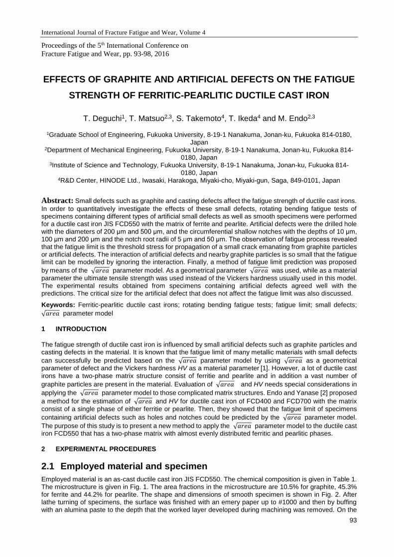
International Journal of Fracture Fatigue and Wear, Volume 4
93
Proceedings of the 5th International Conference on
Fracture Fatigue and Wear, pp. 93-98, 2016
EFFECTS OF GRAPHITE AND ARTIFICIAL DEFECTS ON THE FATIGUE
STRENGTH OF FERRITIC-PEARLITIC DUCTILE CAST IRON
T. Deguchi1, T. Matsuo2,3, S. Takemoto4, T. Ikeda4 and M. Endo2,3
1Graduate School of Engineering, Fukuoka University, 8-19-1 Nanakuma, Jonan-ku, Fukuoka 814-0180, Japan
2Department of Mechanical Engineering, Fukuoka University, 8-19-1 Nanakuma, Jonan-ku, Fukuoka 814-0180, Japan
3Institute of Science and Technology, Fukuoka University, 8-19-1 Nanakuma, Jonan-ku, Fukuoka 814-0180, Japan
4R&D Center, HINODE Ltd., Iwasaki, Harakoga, Miyaki-cho, Miyaki-gun, Saga, 849-0101, Japan
Abstract: Small defects such as graphite and casting defects affect the fatigue strength of ductile cast irons.
In order to quantitatively investigate the effects of these small defects, rotating bending fatigue tests of specimens containing different types of artificial small defects as well as smooth specimens were performed for a ductile cast iron JIS FCD550 with the matrix of ferrite and pearlite. Artificial defects were the drilled hole with the diameters of 200 μm and 500 μm, and the circumferential shallow notches with the depths of 10 μm, 100 μm and 200 μm and the notch root radii of 5 μm and 50 μm. The observation of fatigue process revealed that the fatigue limit is the threshold stress for propagation of a small crack emanating from graphite particles or artificial defects. The interaction of artificial defects and nearby graphite particles is so small that the fatigue limit can be modelled by ignoring the interaction. Finally, a method of fatigue limit prediction was proposed
by means of the √𝑎𝑟𝑒𝑎 parameter model. As a geometrical parameter √𝑎𝑟𝑒𝑎 was used, while as a material parameter the ultimate tensile strength was used instead of the Vickers hardness usually used in this model. The experimental results obtained from specimens containing artificial defects agreed well with the predictions. The critical size for the artificial defect that does not affect the fatigue limit was also discussed.
Keywords: Ferritic-pearlitic ductile cast irons; rotating bending fatigue tests; fatigue limit; small defects;
√𝑎𝑟𝑒𝑎 parameter model
1 INTRODUCTION
The fatigue strength of ductile cast iron is influenced by small artificial defects such as graphite particles and casting defects in the material. It is known that the fatigue limit of many metallic materials with small defects
can successfully be predicted based on the √𝑎𝑟𝑒𝑎 parameter model by using √𝑎𝑟𝑒𝑎 as a geometrical parameter of defect and the Vickers hardness HV as a material parameter [1]. However, a lot of ductile cast irons have a two-phase matrix structure consist of ferritie and pearlite and in addition a vast number of
graphite particles are present in the material. Evaluation of √𝑎𝑟𝑒𝑎 and HV needs special considerations in
applying the √𝑎𝑟𝑒𝑎 parameter model to those complicated matrix structures. Endo and Yanase [2] proposed
a method for the estimation of √𝑎𝑟𝑒𝑎 and HV for ductile cast iron of FCD400 and FCD700 with the matrix consist of a single phase of either ferritie or pearlite. Then, they showed that the fatigue limit of specimens
containing artificial defects such as holes and notches could be predicted by the √𝑎𝑟𝑒𝑎 parameter model.
The purpose of this study is to present a new method to apply the √𝑎𝑟𝑒𝑎 parameter model to the ductile cast iron FCD550 that has a two-phase matrix with almost evenly distributed ferritic and pearlitic phases.
2 EXPERIMENTAL PROCEDURES
2.1 Employed material and specimen
Employed material is an as-cast ductile cast iron JIS FCD550. The chemical composition is given in Table 1. The microstructure is given in Fig. 1. The area fractions in the microstructure are 10.5% for graphite, 45.3% for ferrite and 44.2% for pearlite. The shape and dimensions of smooth specimen is shown in Fig. 2. After lathe turning of specimens, the surface was finished with an emery paper up to #1000 and then by buffing with an alumina paste to the depth that the worked layer developed during machining was removed. On the

International Journal of Fracture Fatigue and Wear, Volume 4
94
surface of specimens, then, a small hole was introduced by a micro-drilling machine or a circumferential shallow notch was introduced by a lathe into the shapes shown in Fig. 3. The diameters of holes were d = 200 μm and 500 μm. The depth h was equal to its diameter d (i.e. d = h). The depth of circumferential notches
were t = 10μm, 100 μm and 200 μm. The notch tip radii were = 5 μm and 50 μm. Before the fatigue testing, the surface layer of about 10 μm in thickness was removed from the specimens by electro-polishing.
.
2.2 Fatigue testing machine and definition of fatigue limit
A rotating bending fatigue testing machine of uniform moment type with the operating speed of 67 Hz and the capacity of 100 Nm was used. Fatigue limit was defined as the maximum nominal bending stress under which a specimen endured 107 cycles. The minimum step of stress level for determining the fatigue limit was 5 MPa.
3 RESULTS AND DISCUSSION
The results of fatigue test are given in Table 2 and Fig. 4. It is seen that fatigue limit decreases with increase
in √𝑎𝑟𝑒𝑎 of artificial defects independently of types of artificial defects. However, the fatigue limit for the circumferential notch with the depth t = 10 μm was equal to that of smooth specimen. Therefore, this circumferential notch is a harmless defect that does not influence the fatigue limit.
Fig. 5 shows the non-propagating cracks observed at hole edge (left) and notch root (right) at the fatigue limit. Smooth specimens also had numerous non-propagating cracks emanating from graphite particles at the
C Si Mn P S Cu Mg
3.84 2.5 0.66 0.017 0.009 0.21 0.043
t
t = 10, 100 and 200μm
ρ = 5 and 50μm, √𝑎𝑟𝑒𝑎 = √10・t
Fig. 3 Geometries of circumferential notch and drilled hole.
h
d
d=h = 200 and 500μm, √𝑎𝑟𝑒𝑎 = ට𝑑 ቀℎ −𝑑
4√3ቁ
ρ
Fig. 1 Microstructure in FCD550
6 80 50 80
210
13
10
15
Fig. 2 Geometry of smooth specimen.
(18.8)
100μm
Fig. 1 Microstructure of FCD550.
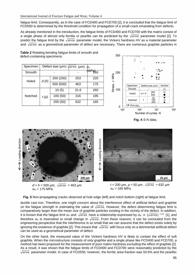
International Journal of Fracture Fatigue and Wear, Volume 4
95
fatigue limit. Consequently, as in the case of FCD400 and FCD700 [2], it is concluded that the fatigue limit of FCD550 is determined by the threshold condition for propagation of a small crack emanating from defects.
As already mentioned in the introduction, the fatigue limits of FCD400 and FCD700 with the matrix consist of
a single phase of almost only ferritie or pearlite can be predicted by the √𝑎𝑟𝑒𝑎 parameter model [2]. To
predict the fatigue limit by the √𝑎𝑟𝑒𝑎 parameter model, the Vickers hardness HV as a material parameter
and √𝑎𝑟𝑒𝑎 as a geometrical parameter of defect are necessary. There are numerous graphite particles in
ductile cast iron. Therefore, one might concern about the interference effect of artificial defect and graphite
on the fatigue strength in estimating the value of √𝑎𝑟𝑒𝑎. However, the defect determining fatigue limit is comparatively larger than the mean size of graphite particles existing in the vicinity of the defect. In addition,
it is known that the fatigue limit σw and √𝑎𝑟𝑒𝑎 have a relationship expressed by σw ∝ (√𝑎𝑟𝑒𝑎)−1/6 [1], and
therefore σw is insensitive to small change in √𝑎𝑟𝑒𝑎. From these reasons, it can be concluded from the engineering perspective that the interference is so small that we can assume that the defect exists solely by
ignoring the existence of graphite [2]. This means that √𝑎𝑟𝑒𝑎 with focus only on a detrimental artificial defect can be used as a geometrical parameter of defect.
On the other hand, the measured value of the Vickers hardness HV is likely to contain the effect of soft graphite. When the microstructure consists of only graphite and a single phase like FCD400 and FCD700, a method has been proposed for the measurement of pure matrix hardness excluding the effect of graphite [2]. As a result, it was shown that the fatigue limits of FCD400 and FCD700 were reasonably predicted by the
√𝑎𝑟𝑒𝑎 parameter model. In case of FCD550, however, the ferritic area fraction was 50.6% and the pearlitic
d = h = 500 μm, √𝑎𝑟𝑒𝑎 = 463 μm σw = 175 MPa
t = 200 μm, ρ = 50 μm, √𝑎𝑟𝑒𝑎 = 632 μm σw = 165 MPa
Table 2 Rotating bending fatigue limits of smooth and defect-containing specimens.
Specimen Defect size (μm)
Smooth - - 260
Holed d (h) 200 (200) 253 220
500 (500) 463 175
Notched t (ρ)
10 (5) 31.6 260
100 (50) 316 195
200 (50) 632 165
√𝑎𝑟𝑒𝑎 (μm) σw (MPa)
Fig. 4 S-N data.
Run-out
Fig. 5 Non-propagating cracks observed at hole edge (left) and notch bottom (right) at fatigue limit.
Lo
ad
ing
dir
ection
Lo
ad
ing
dir
ection
200 μm
25 μm
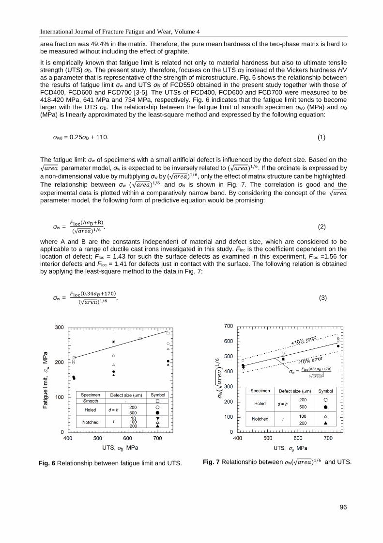
International Journal of Fracture Fatigue and Wear, Volume 4
96
area fraction was 49.4% in the matrix. Therefore, the pure mean hardness of the two-phase matrix is hard to be measured without including the effect of graphite.
It is empirically known that fatigue limit is related not only to material hardness but also to ultimate tensile strength (UTS) σB. The present study, therefore, focuses on the UTS σB instead of the Vickers hardness HV as a parameter that is representative of the strength of microstructure. Fig. 6 shows the relationship between the results of fatigue limit σw and UTS σB of FCD550 obtained in the present study together with those of FCD400, FCD600 and FCD700 [3-5]. The UTSs of FCD400, FCD600 and FCD700 were measured to be 418-420 MPa, 641 MPa and 734 MPa, respectively. Fig. 6 indicates that the fatigue limit tends to become larger with the UTS σB. The relationship between the fatigue limit of smooth specimen σw0 (MPa) and σB (MPa) is linearly approximated by the least-square method and expressed by the following equation:
σw0 = 0.25σB + 110. (1)
The fatigue limit σw of specimens with a small artificial defect is influenced by the defect size. Based on the
√𝑎𝑟𝑒𝑎 parameter model, σw is expected to be inversely related to (√𝑎𝑟𝑒𝑎)1/6. If the ordinate is expressed by
a non-dimensional value by multiplying σw by (√𝑎𝑟𝑒𝑎)1/6, only the effect of matrix structure can be highlighted.
The relationship between σw ( √𝑎𝑟𝑒𝑎)1/6 and σB is shown in Fig. 7. The correlation is good and the
experimental data is plotted within a comparatively narrow band. By considering the concept of the √𝑎𝑟𝑒𝑎 parameter model, the following form of predictive equation would be promising:
σw = 𝐹loc(A𝜎B+B)
(√𝑎𝑟𝑒𝑎)1/6 . (2)
where A and B are the constants independent of material and defect size, which are considered to be applicable to a range of ductile cast irons investigated in this study. Floc is the coefficient dependent on the location of defect; Floc = 1.43 for such the surface defects as examined in this experiment, Floc =1.56 for interior defects and Floc = 1.41 for defects just in contact with the surface. The following relation is obtained by applying the least-square method to the data in Fig. 7:
σw = 𝐹loc(0.34𝜎𝐵+170)
(√𝑎𝑟𝑒𝑎)1/6 . (3)
σw( √
𝑎𝑟𝑒
𝑎)1
/6
σw = 𝐹loc(0.34𝜎𝐵+170)
(√𝑎𝑟𝑒𝑎)16
Fig. 6 Relationship between fatigue limit and UTS. Fig. 7 Relationship between σw(√𝑎𝑟𝑒𝑎)1/6 and UTS.

International Journal of Fracture Fatigue and Wear, Volume 4
97
where σw is in MPa and √𝑎𝑟𝑒𝑎 is in μm. Although Eq. 3 was obtained from the data for surface defects, it is also applicable to other locations of defect by changing the value of Floc. The prediction line drawn by Eq. 3 is shown in Fig. 7. All experimental results are predicted within the error of ±10%. Fig. 8 shows the modified S-N data. In this relationship, the ordinate is the dimensionless relative fatigue strength, which is obtained by normalising the applied stress amplitude σ by the fatigue limit σwp predicted using Eqs. 1 and 3. The S-N data for smooth specimens and specimens containing various types and sizes of artificial defects is well characterized by this expression.
Eq. 3 indicates that σw → ∞ when √𝑎𝑟𝑒𝑎 → 0. However, this never happens actually and σw will never significantly exceed the upper bound of fatigue limit determined by Eq. 1. This is because the determination of fatigue limit of smooth specimens without artificial defects is controlled by graphite particles and other casting defects inherently existing in the material. The critical size of artificial defect that does not decrease the fatigue limit of smooth specimen is given from σw0 = σw with Eqs. 1 and 3 as
√𝑎𝑟𝑒𝑎c = 𝐹loc(0.34𝜎B+170)
0.25𝜎B + 110
6 (4)
where 𝜎B is in MPa and √𝑎𝑟𝑒𝑎c is in μm. Eq. 4 gives √𝑎𝑟𝑒𝑎c = 77 μm by putting 𝜎B = 552 MPa for FCD550
and by choosing 𝐹loc = 1.43 for surface defect. The circumferential notch of t = 10 μm gives √𝑎𝑟𝑒𝑎 = √10・
t = √10・10 μm = 32 μm (cf. Fig. 3), which is smaller than √𝑎𝑟𝑒𝑎c = 77 μm. Thus, it is reasonably understood
that this circumferential notch was a harmless defect that did not decrease the fatigue limit.
The value of σB is obtained by the tensile test, and it contains the effect of graphite in addition to the effect of matrix. The volume fraction of graphite is usually in the range of about 10-15% and the size distribution of graphite particles is not so much different among regular ductile cast irons. Therefore, it may be reasonable to assume the tensile strength σB as a parameter representative of the effect of matrix. However, Eqs. 1 and 3 require cautious use of σB when the target ductile cast iron is an irregular material that has quite different volume fraction or size distribution of graphite. Further, one must keep in mind that Eq. 1 is derived based on the experimental results obtained by using small number of specimens. The faigue limit of smooth specimen is influenced by the statistical factor accociated with the control volume being subjected to high stress. For a larger number of smecimens or massive products, the possibility of occurance for larger size of the graphite particles or casting defects that determine fatigue strength will increase and as a result, the fatigue limit precicted by Eq. 1 could unexpectedly be non-conservative.
4 CONCULUSIONS
The rotating bending fatigue strength of smooth and specimens containing artificial small defects of drilled hole and circumferential shallow notch was experimentally investigated for a ferritic-pearlitic ductile cast iron
FCD550 and the applicability of the √𝑎𝑟𝑒𝑎 parameter model was discussed. The obtained results are summarized as follows:
Fatigue limit was determined by the limiting condition for non-propagation of a crack emanating from graphite particles or artificial defects.
Fig. 8 S-N data normalized by the predictive values of fatigue limit σwp.
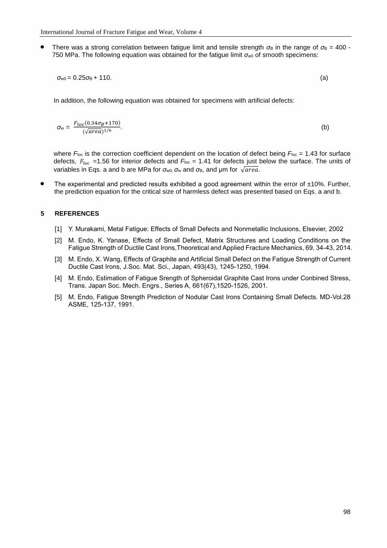
International Journal of Fracture Fatigue and Wear, Volume 4
98
There was a strong correlation between fatigue limit and tensile strength σB in the range of σB = 400 - 750 MPa. The following equation was obtained for the fatigue limit σw0 of smooth specimens:
σw0 = 0.25σB + 110. (a)
In addition, the following equation was obtained for specimens with artificial defects:
σw = 𝐹loc(0.34𝜎𝐵+170)
(√𝑎𝑟𝑒𝑎)1/6 . (b)
where Floc is the correction coefficient dependent on the location of defect being Floc = 1.43 for surface defects, 𝐹loc =1.56 for interior defects and Floc = 1.41 for defects just below the surface. The units of
variables in Eqs. a and b are MPa for σw0, σw and σB, and μm for √𝑎𝑟𝑒𝑎.
The experimental and predicted results exhibited a good agreement within the error of ±10%. Further, the prediction equation for the critical size of harmless defect was presented based on Eqs. a and b.
5 REFERENCES
[1] Y. Murakami, Metal Fatigue: Effects of Small Defects and Nonmetallic Inclusions, Elsevier, 2002
[2] M. Endo, K. Yanase, Effects of Small Defect, Matrix Structures and Loading Conditions on the Fatigue Strength of Ductile Cast Irons,Theoretical and Applied Fracture Mechanics, 69, 34-43, 2014.
[3] M. Endo, X. Wang, Effects of Graphite and Artificial Small Defect on the Fatigue Strength of Current Ductile Cast Irons, J.Soc. Mat. Sci., Japan, 493(43), 1245-1250, 1994.
[4] M. Endo, Estimation of Fatigue Srength of Spheroidal Graphite Cast Irons under Conbined Stress, Trans. Japan Soc. Mech. Engrs., Series A, 661(67),1520-1526, 2001.
[5] M. Endo, Fatigue Strength Prediction of Nodular Cast Irons Containing Small Defects. MD-Vol.28 ASME, 125-137, 1991.

International Journal of Fracture Fatigue and Wear, Volume 4
99
Proceedings of the 5th International Conference on
Fracture Fatigue and Wear, pp. 99-103, 2016
EVALUATION OF ADHESIVE STRENGTH BASED ON THE INTENSITY
OF SINGULAR STRESS FIELD OF SINGLE LAP JOINT
R. Li, N.A. Noda, Y. Sano, T. Miyazaki, K. Iida and Y. Takase
Department of Mechanical Engineering, Kyushu Institute of Technology, 1-1 Sensui-cho Tobata-ku, Kitakyushu-shi 804-8550, Japan
Abstract: In this study, the adhesive strength for single lap joint is investigated based on the intensity of
singular stress field. First, the critical intensity of singular stress at the adhesive dissimilar joint is calculated by using finite element method (FEM) based on the experimental result. It is found that the adhesive strength can be expressed as the critical intensity of singular stress field. Then, a suitable evaluation method of adhesive strength is investigated focusing on the intensity of singular stress field. The effect of specimen geometry on the intensity of singular stress is considered. The results show that the intensity of singular stress field decreases with increasing the adherend thickness, the minimum intensity of singular stress can be obtained when the adherend thickness is large enough. The results of the deformation angle at the interface corner edge show a similar trend as in intensity of singular stress field, and the minimum deformation angle can be obtained when the adherend thickness is large enough. The usefulness of the method is investigated focusing on the deformation angle at the interface corner edge.
Keywords: Stress intensity factor; Interfaces; Deformation angle; Single lap joint
1 INTRODUCTION
Since adhesively joints are economical, practical and easy to be used; thus they have been widely used in a variety of industries. A number of studies of adhesive joints have been made so far [1-4]. The authors investigated the adhesive butt joint strength in Fig. 1 by changing the adhesive thickness and material combination [5,6]. It is found that the adhesive strength can be expressed as the critical intensity of singular
stress field as cK =const based on the experimental results. The adhesive strengths of the single lap joint
(see Fig. 2(a)) and double lap joint (see Fig.2(b)) were also investigated previouly [7]. In this result, the adhesive strength of double lap joint is not equal to the one of single lap joint as expected and is almost twice larger than the one of single lap joint. Compared with double lap joint, single lap joint testing is more stable and used conveniently. The testing method and experimental adhesive strength are prescribed by Japanese Industrial Standards (JIS) [8]. However, since the debonding strength is defined as the magnitude of the load, the strength is affected by the specimen dimension and difficult to be applied to other geometries. Therefore, it is necessary to find a suitable method to evaluation the debonding strength of single lap joint testing. In this paper, first, the debonding strength of single lap joint will be investigated based on the experimental results [9] by using the evaluation method shown in [6]. Then, a suitable evaluation method of adhesive strength will be evaluated focusing on the intensity of singular stress field and the deformation angle appearing at the end of interface.
(a) Single lap joint
(b) Double lap joint
Fig.1 Adhesive strength expressed as cK =const
for butt joint.
Fig.2 Single and double lap joints.
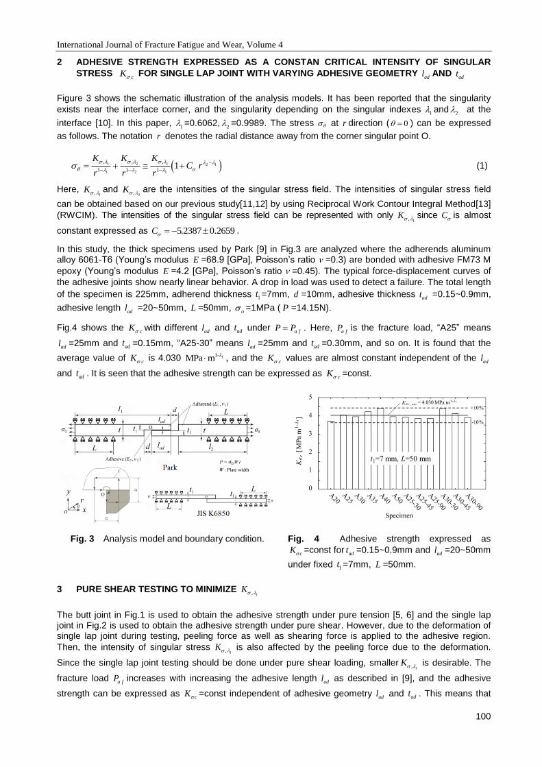
International Journal of Fracture Fatigue and Wear, Volume 4
100
2 ADHESIVE STRENGTH EXPRESSED AS A CONSTAN CRITICAL INTENSITY OF SINGULAR
STRESS cK FOR SINGLE LAP JOINT WITH VARYING ADHESIVE GEOMETRY
adl AND adt
Figure 3 shows the schematic illustration of the analysis models. It has been reported that the singularity
exists near the interface corner, and the singularity depending on the singular indexes 1 and
2 at the
interface [10]. In this paper, 1 =0.6062,
2 =0.9989. The stress at r direction ( 0 ) can be expressed
as follows. The notation r denotes the radial distance away from the corner singular point O.
1 2 1 2 1
1 2 1
, , ,
1 1 11
K K KC r
r r r
(1)
Here, 1,K and
2,K are the intensities of the singular stress field. The intensities of singular stress field
can be obtained based on our previous study[11,12] by using Reciprocal Work Contour Integral Method[13]
(RWCIM). The intensities of the singular stress field can be represented with only 1,K since C is almost
constant expressed as 5.2387 0.2659C .
In this study, the thick specimens used by Park [9] in Fig.3 are analyzed where the adherends aluminum alloy 6061-T6 (Young’s modulus E =68.9 [GPa], Poisson’s ratio =0.3) are bonded with adhesive FM73 M
epoxy (Young’s modulus E =4.2 [GPa], Poisson’s ratio =0.45). The typical force-displacement curves of
the adhesive joints show nearly linear behavior. A drop in load was used to detect a failure. The total length
of the specimen is 225mm, adherend thickness 1t =7mm, d =10mm, adhesive thickness adt =0.15~0.9mm,
adhesive length adl =20~50mm, L =50mm,
o =1MPa ( P =14.15N).
Fig.4 shows the cK with different adl and adt under a fP P . Here,
a fP is the fracture load, “A25” means
adl =25mm and adt =0.15mm, “A25-30” means adl =25mm and adt =0.30mm, and so on. It is found that the
average value of cK is 4.030 11-
MPa m
, and the cK values are almost constant independent of the
adl
and adt . It is seen that the adhesive strength can be expressed as cK =const.
Fig. 3 Analysis model and boundary condition. Fig. 4 Adhesive strength expressed as
cK =const for adt =0.15~0.9mm and adl =20~50mm
under fixed 1t =7mm, L =50mm.
3 PURE SHEAR TESTING TO MINIMIZE 1,K
The butt joint in Fig.1 is used to obtain the adhesive strength under pure tension [5, 6] and the single lap joint in Fig.2 is used to obtain the adhesive strength under pure shear. However, due to the deformation of single lap joint during testing, peeling force as well as shearing force is applied to the adhesive region.
Then, the intensity of singular stress 1,K is also affected by the peeling force due to the deformation.
Since the single lap joint testing should be done under pure shear loading, smaller1,K is desirable. The
fracture load a fP increases with increasing the adhesive length adl as described in [9], and the adhesive
strength can be expressed as cK =const independent of adhesive geometry adl and adt . This means that

International Journal of Fracture Fatigue and Wear, Volume 4
101
when 1,K is small, the fracture load
afP is large. Therefore, in order to minimize1,K , the effect of
specimen geometry is considered under the same adhesive geometry and load P . In this section, we
assume P =14.15N, the adhesive length adl =25mm, and adhesive thickness
adt =0.15mm. Then, the
effects of specimen geometries 1t (adherend thickness) and L (fixed boundary length) on the intensity of
singular stress field 1,K are discussed.
Figure 5 shows the relationship between the intensity of singular stress field 1,K and adherend thickness
1t under different fixed length L . The dashed line shows the minimum value of1,K . Here, JIS* means only
the adherend thickness 1t =1.5mm and fixed boundary length L =50mm in JIS K6850 are used as shown in
Fig.3. As can be seen from Fig.5, the 1,K decreases with increasing
1t and L . The 1,K value becomes
constant if 1t is large enough. The
1 1, 1.5mm|tK (JIS K6850) is 5 times larger than the one of ,minK , and the
1 1, 7mm|tK [9] is more than twice than that of ,minK . It is seen that the specimen in [9] is better than the JIS,
but it is more desirable to use larger adherend thickness.
Fig. 5. Effect of L and 1t on
1,K under fixed adl and
adt (JIS*: Only 1t =1.5mm and L =50mm in JIS K6850 are
used as shown in Fig.3).
Fig.6. Definition of deformation angle.
4 DEFORMATION ANGLE AT THE INTERFACE CORNER
As shown in section 3, the intensity of singular stress1,K decreases with increasing the adherend
thickness1t . It is found that the minimum
1,K can be obtained when 1t is large enough. In this section, the
deformation angle at interface corner is considered by changing the distance l .
Fig. 6 shows the deformation example near the interface corners. In order to obtain the deformation angle,
two target points are considered. For the deformation angleol at interface corner O, two target points are
points O and A with the distance l . For the deformation angleor at interface corner O, two target points are
points O and B with the distance l . Fig. 7 shows the deformation angles ol and
or vs. l under 1t =7mm.
It is found that the values of ol and
or both increase with increasing l , and the difference between ol
and or increases with decreasing l . Therefore, we cannot obtain the maximum deformation angle at
corner O. Fig. 8 shows the deformation angle C vs. l under
1t =7mm. It is seen that the value of C
increases initially with increasing l and then decreases. Then, the maximum C can be obtained when
l =1/33mm. Thus, in this study, the deformation angle will be considered by using the maximum
deformation angle at corner C rather than at corner O.

International Journal of Fracture Fatigue and Wear, Volume 4
102
Fig. 7 Deformation angle at corner edge O. Fig. 8 Deformation angle at corner edge C.
As can be seen from Fig. 5, the minimum 1,K can be obtained when
1t is large enough. Similar to the
variation trend of 1,K , the minimum
C can be obtained when the adherend thickness 1t is large enough.
5 CONCLUSION
In this study, the adhesive strength for single lap joint is investigated based on the intensity of singular stress field. Since the experiments are often time-consuming and costly, the analysis method shown in this paper can help to predict the strength of adhesive joint accurately and conveniently. The conclusions can be summarized in the following way.
(1) In this paper, the critical intensity of singular stress field cK is investigated by using the analysis
method presented. It is seen that the adhesive strength can be expressed as cK =const.
(2) The effects of specimen geometries 1t (adherend thickness) and L (fixed boundary length) on the
intensity of singular stress field1,K are discussed. The results show that the
1,K at the interface corner
decreases with increasing the 1t , and the minimum intensity of singular stress field ,minK can be
obtained when 1t is large enough.
(3) The deformation angle at the interface corner is investigated by using the maximum deformation angle
at interface corner C. It is found that the minimum deformation angle C can be obtained when the
adherend thickness 1t is large enough.
6 REFERENCES
[1] Y. M. Jen, C. W. Ko, Evaluation of fatigue life of adhesively bonded aluminum single-lap joints using interfacial parameters, International Journal of Fatigue, 32(2): 330-340, 2010.
[2] M. Y. Tsai, J. Morton, An investigation into the stresses in double-lap adhesive joints with laminated composite adherends, International Journal of Solids and Structures, 47(24): 3317-3325, 2010.
[3] Li. G, P. Lee-Sullivan, R. W. Thring, Nonlinear finite element analysis of stress and strain distributions across the adhesive thickness in composite single-lap joints, Composite Structures, 46(4): 395-403, 1999.
[4] M. Imanaka., K. Ishii., H. Nakayama, Evaluation of fatigue strength of adhesively bonded single and single step double lap Joints based on stress singularity parameters, Engineering Fractures Mechanics, 62(4-5): 409-424, 1999.
[5] Y. Zhang, N.A. Noda, K. T. Takaishi, X. Lan, Effect of adhesive thickness on the interface of singular stress at the adhesive dissimilar joint, Journal of Solid Mechanics and Materials Engineering, 4(10), 2010.
[6] N. A. Noda, T. Miyazaki, R. Li, T. Uchikoba, Y. Sano, Dedbonding strength evaluation in terms of the intensity of singular stress at the interface corner with and without fictitious crack, International Journal of Adhesion and Adhesives, 61: 46-64, 2015.
International Journal of Fracture Fatigue and Wear, Volume 4
103
[7] K. Ikegami, H. Kyogoku, H. Kawagoe, T. Sugibayashi, K. Nohno, T. Fujii, K. Motoie, F. Yoshida, Benchmark tests for synthetic evaluation of adhesive-joint strength (1st Report, Experimental results of butt, single-lap, double-lap joints and DCB test).Japan Society of Mechanical Engineers, 63(608): 174-181,1997-4. (in Japanese)
[8] JIS K6850:1999, Adhesives-Determination of tensile lap-shear strength of rigid-to-rigid bonded assemblies. (in Japanese)
[9] J. H. Park, J. H. Choi, J. H. Kweon. Evaluating the strengths of thick aluminum -to-aluminum joints with different adhesive lengths and thicknesses, Composite Structures, 92, 2226-2235, 2010.
[10] R. Yuuki. Mechanics of interface. Baifuukann, Tokyo, 283p, 1993. (in Japanese)
[11] T. Miyazaki, N.A. Noda, R. Li, T. Uchikoba, Y. Sano. Debonding criterion for single lap joints from the intensity of singular stress field. Journal of Japan Institute of Electronics Packaging.16(2): 143-151, 2013. (in Japanese)
[12] T. Miyazaki, N. A. Noda, R. Li, T. Uchikoba, Y. Sano. Examination on a criterion for a debonding fracture of single lap joints from the intensity of singular stress field, Proceeding of 13th International Conference on Fracture: S11-029, 2013.
[13] Carpenter, W. C. Byers C. A path independent integral for computing stress intensities for V-notched cracks in a bi-material, International Journal of Fracture, 35: 245-268, 1987.

International Journal of Fracture Fatigue and Wear, Volume 4
104
Proceedings of the 5th International Conference on
Fracture Fatigue and Wear, pp. 104-108, 2016
T CONVENIENT DEBONDING STRENGTH EVALUATION FOR SPRAY
COATING BASED ON INTENSITY OF SINGULAR STRESS
Z. Wang1, N.A. Noda2, Y. Sano2, Y. Takase2 and K. Iida2
1Department of Mechanical Engineering, Kyushu Institute of Technology, 1-1 Sensui-cho, Tobata-ku,
Kitakyushu-shi, Fukuoka, 804-8550 2Department of Mechanical Engineering, Kyushu Institute of Technology, 1-1 Sensui-cho, Tobata-ku,
Kitakyushu-shi, Fukuoka, 804-8550
Abstract: Hearth rolls are used in continuous annealing furnace to produce thin steel sheet. The roll surface
is usually coated by using thermal spraying, which has high adhesive strength and wears resistance. However, in the ceramics coating, thermal stress caused during heating and cooling process in the furnace may lead to debonding due to the low toughness of ceramics. In order to improve the heat resistance of the thermally sprayed coating, it is essential to evaluate the debonding strength. Generally, heat resistance of thermal spray coating is evaluated by thermal shock test prescribed by JIS H8304 and it has been discussed in terms of singular stress at the end of the interface for JIS specimen under thermal shock. However there is no research considering the real axial-symmetric geometry condition of the multilayer structure. Thus this paper will focus on the intensity of the singular stress at the end of interface for a 2D axial-symmetric model. Then, the most suitable conditions are discussed with varying the coating thickness and compared with our previous study.
Keywords: ceramics, interface, strength, thermal spraying, thermal shock, Intensity of singular stress
1. INTRODUCTION
In continuous annealing furnace for producing steel sheet, it’s common to apply spraying coating on the hearth rolls (Fig. 1 (a)) to improve its adhesive strength and wear resistance. Especially for the ceramic spraying coating rolls, due to its excellent chemical stability and high hardness at high temperatures, it is expected to have expansion of application coverage. However, the peeling of the ceramic coating layer due to prolonged use under heating and cooling process in the furnace should be considered. Therefore, the ceramic coating is not usually sprayed alone, while multi-layer coating with adhesive layer is usually employed.
In order to improve the thermal shock resistance of the ceramic coating, it is necessary to accurately evaluate the peel strength of the sprayed coating. The thermal shock resistance of ceramic coating is usually evaluated by the thermal shock test (Fig. 1 (b),(c)) specified by JIS8304 (2007) [1]. Mutoh et al have reported the thermal shock damage characteristics based on experimental results and finite element analysis [2]. However in order to more accurately assess the interfacial strength of dissimilar materials adhesive structures, it is necessary to consider the singularity of thermal stress near the corner of the interface. So far, few studies have been
(a) Roll used in annealing furnace
(b) JIS 8304 specimen for thermal shock test 50×50×(H+h+l)
(c) Thermal cycle of thermal shock testing
Fig.1 Specimen for thermal shock test and the test conditions
H
h=0.1
l=10
W=50
W=10 Unit: mm
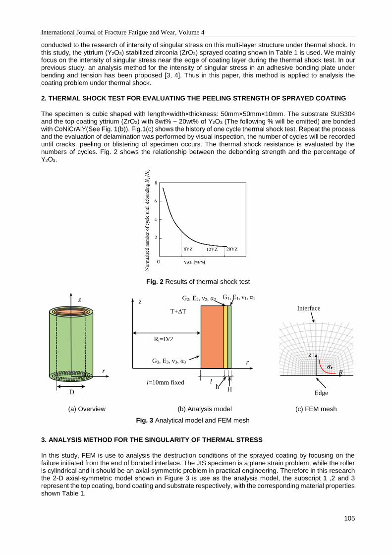
International Journal of Fracture Fatigue and Wear, Volume 4
105
conducted to the research of intensity of singular stress on this multi-layer structure under thermal shock. In this study, the yttrium (Y2O3) stabilized zirconia (ZrO2) sprayed coating shown in Table 1 is used. We mainly focus on the intensity of singular stress near the edge of coating layer during the thermal shock test. In our previous study, an analysis method for the intensity of singular stress in an adhesive bonding plate under bending and tension has been proposed [3, 4]. Thus in this paper, this method is applied to analysis the coating problem under thermal shock.
2. THERMAL SHOCK TEST FOR EVALUATING THE PEELING STRENGTH OF SPRAYED COATING
The specimen is cubic shaped with length×width×thickness: 50mm×50mm×10mm. The substrate SUS304 and the top coating yttrium (ZrO2) with 8wt% ~ 20wt% of Y2O3 (The following % will be omitted) are bonded with CoNiCrAlY(See Fig. 1(b)). Fig.1(c) shows the history of one cycle thermal shock test. Repeat the process and the evaluation of delamination was performed by visual inspection, the number of cycles will be recorded until cracks, peeling or blistering of specimen occurs. The thermal shock resistance is evaluated by the numbers of cycles. Fig. 2 shows the relationship between the debonding strength and the percentage of Y2O3.
Fig. 2 Results of thermal shock test
3. ANALYSIS METHOD FOR THE SINGULARITY OF THERMAL STRESS
In this study, FEM is use to analysis the destruction conditions of the sprayed coating by focusing on the failure initiated from the end of bonded interface. The JIS specimen is a plane strain problem, while the roller is cylindrical and it should be an axial-symmetric problem in practical engineering. Therefore in this research the 2-D axial-symmetric model shown in Figure 3 is use as the analysis model, the subscript 1 ,2 and 3 represent the top coating, bond coating and substrate respectively, with the corresponding material properties shown Table 1.
(a) Overview (b) Analysis model (c) FEM mesh
Fig. 3 Analytical model and FEM mesh
h l
H
G1, E1, ν1, α1 z
r
Ri=D/2
l=10mm fixed
T+ΔT
G2, E2, ν2, α2
G3, E3, ν3, α3
z
r
D
Interface
Edge
R
z
σr
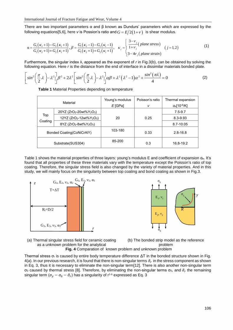
International Journal of Fracture Fatigue and Wear, Volume 4
106
There are two important parameters α and β known as Dundurs’ parameters which are expressed by the
following equations[5,6], here v is Possion’s ratio and 2 1G E is shear modulus.
1 2 2 1 1 2 2 1
1 2 2 1 1 2 2 1
31 1 1 1
1α , , 1,21 1 1 1
3 4
j
jj
j
plane stressG G G Gj
G G G Gplane strain
(1)
Furthermore, the singular index λ, appeared as the exponent of r in Fig.3(b), can be obtained by solving the following equation. Here r is the distance from the end of interface in a dissimilar materials bonded plate.
2
2 2 2 2 2 2 2 2 22 1 02 2 4
sinsin sin
(2)
Table 1 Material Properties depending on temperature
Table 1 shows the material properties of three layers: young’s modulus E and coefficient of expansion αe. It’s found that all properties of these three materials vary with the temperature except the Poisson’s ratio of top coating. Therefore, the singular stress field is also changed by the variety of material properties. And in this study, we will mainly focus on the singularity between top coating and bond coating as shown in Fig.3.
Thermal stress σr is caused by entire body temperature difference ΔT in the bonded structure shown in Fig.
4(a). In our previous research, it is found that there is non-singular terms 𝑟 in the stress component as shown
in Eq. 3, thus it is necessary to eliminate the non-singular term[12]. There is also another non-singular term
σ0 caused by thermal stress [8]. Therefore, by eliminating the non-singular terms σ0, and 𝑟 the remaining
singular term (𝜎𝑦 − 𝜎0 − 𝑟) has a singularity of r1-λ expressed as Eq. 3
Material Young’s modulus
E [GPa]
Poisson’s ratio
ν
Thermal expansion
αe[10-6/K]
Top
Coating
20YZ (ZrO2-20wt%Y2O3)
20 0.25
7.5-9.7
12YZ (ZrO2-12wt%Y2O3) 8.3-9.93
8YZ (ZrO2-8wt%Y2O3) 8.7-10.05
Bonded Coating(CoNiCrAlY) 103-180
0.33 2.8-16.8
Substrate(SUS304) 85-200
0.3 16.8-19.2
(a) Thermal singular stress field for ceramic coating as a unknown problem for the analytical
(b) The bonded strip model as the reference problem
Fig. 4 Comparation of known problem and unknown problem
G1, E1, ν1, α1 z
r
Ri=D/2
T+ΔT
G2, E2, ν2, α2
G3, E3, ν3, α3
E1, ν
1
σ0
E2, ν
2
σ0
σy
R
y
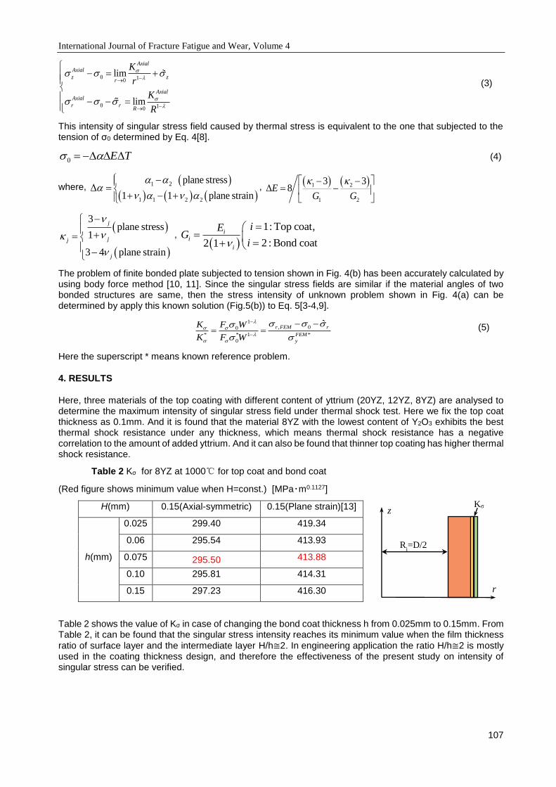
International Journal of Fracture Fatigue and Wear, Volume 4
107
0 10
0 10
lim
lim
AxialAxial
z zr
AxialAxial
r rR
K
r
K
R
(3)
This intensity of singular stress field caused by thermal stress is equivalent to the one that subjected to the tension of σ0 determined by Eq. 4[8].
0 E T (4)
where,
1 2
1 1 2 2
plane stressΔ
1 1 plane strain
, 1 2
1 2
3 3Δ 8E
G G
3plane stress
1
3 4 plane strain
j
jj
j
,
1: Top coat,
2 : Bond coat2 1
ii
i
iEG
i
The problem of finite bonded plate subjected to tension shown in Fig. 4(b) has been accurately calculated by using body force method [10, 11]. Since the singular stress fields are similar if the material angles of two bonded structures are same, then the stress intensity of unknown problem shown in Fig. 4(a) can be determined by apply this known solution (Fig.5(b)) to Eq. 5[3-4,9].
1
0
* * 1 *
0
, 0r FEM
FEM
y
rK F W
K F W
(5)
Here the superscript * means known reference problem.
4. RESULTS
Here, three materials of the top coating with different content of yttrium (20YZ, 12YZ, 8YZ) are analysed to determine the maximum intensity of singular stress field under thermal shock test. Here we fix the top coat thickness as 0.1mm. And it is found that the material 8YZ with the lowest content of Y2O3 exhibits the best thermal shock resistance under any thickness, which means thermal shock resistance has a negative correlation to the amount of added yttrium. And it can also be found that thinner top coating has higher thermal shock resistance.
Table 2 Kσ for 8YZ at 1000 for top coat and bond coat
(Red figure shows minimum value when H=const.) [MPa・m0.1127]
H(mm) 0.15(Axial-symmetric) 0.15(Plane strain)[13]
h(mm)
0.025 299.40 419.34
0.06 295.54 413.93
0.075 295.50 413.88
0.10 295.81 414.31
0.15 297.23 416.30
Table 2 shows the value of Kσ in case of changing the bond coat thickness h from 0.025mm to 0.15mm. From Table 2, it can be found that the singular stress intensity reaches its minimum value when the film thickness
ratio of surface layer and the intermediate layer H/h≅2. In engineering application the ratio H/h≅2 is mostly used in the coating thickness design, and therefore the effectiveness of the present study on intensity of singular stress can be verified.
z
r
Ri=D/2
Kσ
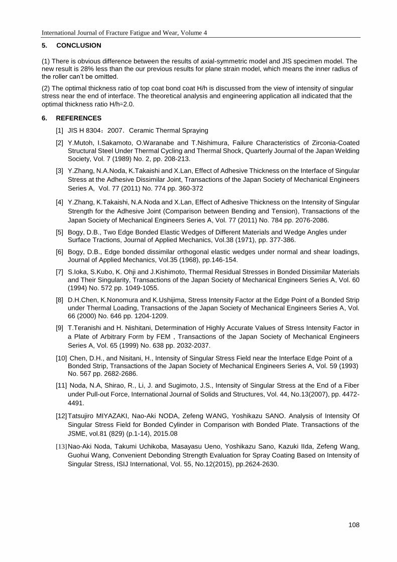
International Journal of Fracture Fatigue and Wear, Volume 4
108
5. CONCLUSION
(1) There is obvious difference between the results of axial-symmetric model and JIS specimen model. The new result is 28% less than the our previous results for plane strain model, which means the inner radius of the roller can’t be omitted.
(2) The optimal thickness ratio of top coat bond coat H/h is discussed from the view of intensity of singular stress near the end of interface. The theoretical analysis and engineering application all indicated that the
optimal thickness ratio H/h≅2.0.
6. REFERENCES
[1] JIS H 8304:2007.Ceramic Thermal Spraying
[2] Y.Mutoh, I.Sakamoto, O.Waranabe and T.Nishimura, Failure Characteristics of Zirconia-Coated
Structural Steel Under Thermal Cycling and Thermal Shock, Quarterly Journal of the Japan Welding
Society, Vol. 7 (1989) No. 2, pp. 208-213.
[3] Y.Zhang, N.A.Noda, K.Takaishi and X.Lan, Effect of Adhesive Thickness on the Interface of Singular
Stress at the Adhesive Dissimilar Joint, Transactions of the Japan Society of Mechanical Engineers
Series A, Vol. 77 (2011) No. 774 pp. 360-372
[4] Y.Zhang, K.Takaishi, N.A.Noda and X.Lan, Effect of Adhesive Thickness on the Intensity of Singular
Strength for the Adhesive Joint (Comparison between Bending and Tension), Transactions of the
Japan Society of Mechanical Engineers Series A, Vol. 77 (2011) No. 784 pp. 2076-2086.
[5] Bogy, D.B., Two Edge Bonded Elastic Wedges of Different Materials and Wedge Angles under Surface Tractions, Journal of Applied Mechanics, Vol.38 (1971), pp. 377-386.
[6] Bogy, D.B., Edge bonded dissimilar orthogonal elastic wedges under normal and shear loadings,
Journal of Applied Mechanics, Vol.35 (1968), pp.146-154.
[7] S.Ioka, S.Kubo, K. Ohji and J.Kishimoto, Thermal Residual Stresses in Bonded Dissimilar Materials
and Their Singularity, Transactions of the Japan Society of Mechanical Engineers Series A, Vol. 60
(1994) No. 572 pp. 1049-1055.
[8] D.H.Chen, K.Nonomura and K.Ushijima, Stress Intensity Factor at the Edge Point of a Bonded Strip
under Thermal Loading, Transactions of the Japan Society of Mechanical Engineers Series A, Vol.
66 (2000) No. 646 pp. 1204-1209.
[9] T.Teranishi and H. Nishitani, Determination of Highly Accurate Values of Stress Intensity Factor in
a Plate of Arbitrary Form by FEM , Transactions of the Japan Society of Mechanical Engineers
Series A, Vol. 65 (1999) No. 638 pp. 2032-2037.
[10] Chen, D.H., and Nisitani, H., Intensity of Singular Stress Field near the Interface Edge Point of a Bonded Strip, Transactions of the Japan Society of Mechanical Engineers Series A, Vol. 59 (1993) No. 567 pp. 2682-2686.
[11] Noda, N.A, Shirao, R., Li, J. and Sugimoto, J.S., Intensity of Singular Stress at the End of a Fiber
under Pull-out Force, International Journal of Solids and Structures, Vol. 44, No.13(2007), pp. 4472-
4491.
[12] Tatsujiro MIYAZAKI, Nao-Aki NODA, Zefeng WANG, Yoshikazu SANO. Analysis of Intensity Of
Singular Stress Field for Bonded Cylinder in Comparison with Bonded Plate. Transactions of the
JSME, vol.81 (829) (p.1-14), 2015.08
[13] Nao-Aki Noda, Takumi Uchikoba, Masayasu Ueno, Yoshikazu Sano, Kazuki IIda, Zefeng Wang,
Guohui Wang, Convenient Debonding Strength Evaluation for Spray Coating Based on Intensity of
Singular Stress, ISIJ International, Vol. 55, No.12(2015), pp.2624-2630.
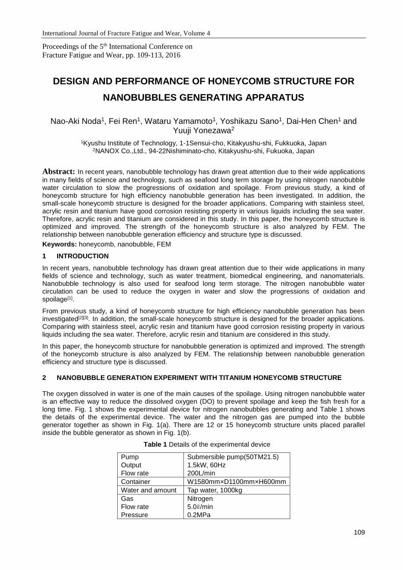
International Journal of Fracture Fatigue and Wear, Volume 4
109
Proceedings of the 5th International Conference on
Fracture Fatigue and Wear, pp. 109-113, 2016
DESIGN AND PERFORMANCE OF HONEYCOMB STRUCTURE FOR
NANOBUBBLES GENERATING APPARATUS
Nao-Aki Noda1, Fei Ren1, Wataru Yamamoto1, Yoshikazu Sano1, Dai-Hen Chen1 and Yuuji Yonezawa2
1Kyushu Institute of Technology, 1-1Sensui-cho, Kitakyushu-shi, Fukkuoka, Japan 2NANOX Co.,Ltd., 94-22Nishiminato-cho, Kitakyushu-shi, Fukuoka, Japan
Abstract: In recent years, nanobubble technology has drawn great attention due to their wide applications
in many fields of science and technology, such as seafood long term storage by using nitrogen nanobubble water circulation to slow the progressions of oxidation and spoilage. From previous study, a kind of honeycomb structure for high efficiency nanobubble generation has been investigated. In addition, the small-scale honeycomb structure is designed for the broader applications. Comparing with stainless steel, acrylic resin and titanium have good corrosion resisting property in various liquids including the sea water. Therefore, acrylic resin and titanium are considered in this study. In this paper, the honeycomb structure is optimized and improved. The strength of the honeycomb structure is also analyzed by FEM. The relationship between nanobubble generation efficiency and structure type is discussed.
Keywords: honeycomb, nanobubble, FEM
1 INTRODUCTION
In recent years, nanobubble technology has drawn great attention due to their wide applications in many fields of science and technology, such as water treatment, biomedical engineering, and nanomaterials. Nanobubble technology is also used for seafood long term storage. The nitrogen nanobubble water circulation can be used to reduce the oxygen in water and slow the progressions of oxidation and spoilage[1].
From previous study, a kind of honeycomb structure for high efficiency nanobubble generation has been investigated[2][3]. In addition, the small-scale honeycomb structure is designed for the broader applications. Comparing with stainless steel, acrylic resin and titanium have good corrosion resisting property in various liquids including the sea water. Therefore, acrylic resin and titanium are considered in this study.
In this paper, the honeycomb structure for nanobubble generation is optimized and improved. The strength of the honeycomb structure is also analyzed by FEM. The relationship between nanobubble generation efficiency and structure type is discussed.
2 NANOBUBBLE GENERATION EXPERIMENT WITH TITANIUM HONEYCOMB STRUCTURE
The oxygen dissolved in water is one of the main causes of the spoilage. Using nitrogen nanobubble water is an effective way to reduce the dissolved oxygen (DO) to prevent spoilage and keep the fish fresh for a long time. Fig. 1 shows the experimental device for nitrogen nanobubbles generating and Table 1 shows the details of the experimental device. The water and the nitrogen gas are pumped into the bubble generator together as shown in Fig. 1(a). There are 12 or 15 honeycomb structure units placed parallel inside the bubble generator as shown in Fig. 1(b).
Table 1 Details of the experimental device
Pump Submersible pump(50TM21.5)
Output 1.5kW, 60Hz
Flow rate 200L/min
Container W1580mm×D1100mm×H600mm
Water and amount Tap water, 1000kg
Gas Nitrogen
Flow rate 5.0ℓ/min
Pressure 0.2MPa
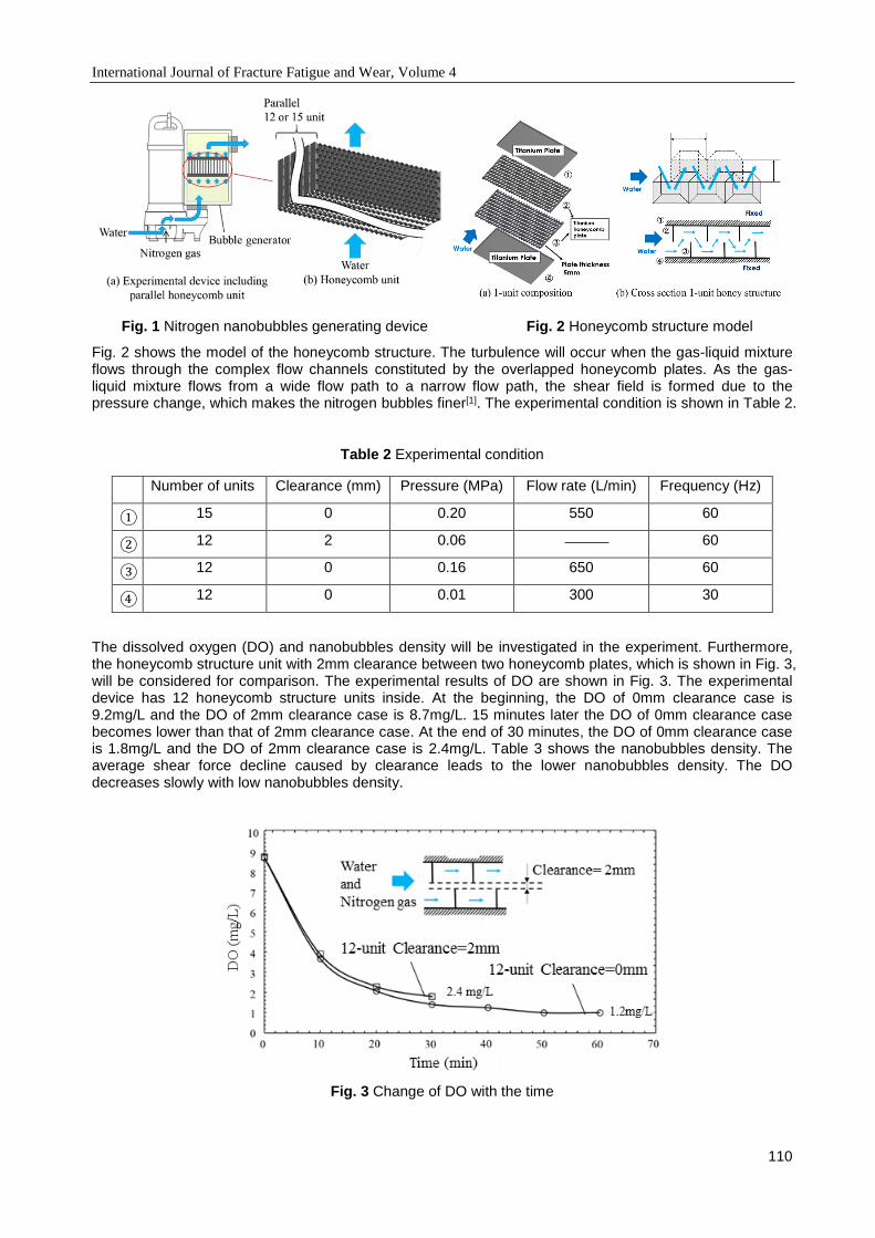
International Journal of Fracture Fatigue and Wear, Volume 4
110
Fig. 1 Nitrogen nanobubbles generating device Fig. 2 Honeycomb structure model
Fig. 2 shows the model of the honeycomb structure. The turbulence will occur when the gas-liquid mixture flows through the complex flow channels constituted by the overlapped honeycomb plates. As the gas-liquid mixture flows from a wide flow path to a narrow flow path, the shear field is formed due to the pressure change, which makes the nitrogen bubbles finer[1]. The experimental condition is shown in Table 2.
Table 2 Experimental condition
The dissolved oxygen (DO) and nanobubbles density will be investigated in the experiment. Furthermore, the honeycomb structure unit with 2mm clearance between two honeycomb plates, which is shown in Fig. 3, will be considered for comparison. The experimental results of DO are shown in Fig. 3. The experimental device has 12 honeycomb structure units inside. At the beginning, the DO of 0mm clearance case is 9.2mg/L and the DO of 2mm clearance case is 8.7mg/L. 15 minutes later the DO of 0mm clearance case becomes lower than that of 2mm clearance case. At the end of 30 minutes, the DO of 0mm clearance case is 1.8mg/L and the DO of 2mm clearance case is 2.4mg/L. Table 3 shows the nanobubbles density. The average shear force decline caused by clearance leads to the lower nanobubbles density. The DO decreases slowly with low nanobubbles density.
Fig. 3 Change of DO with the time
Number of units Clearance (mm) Pressure (MPa) Flow rate (L/min) Frequency (Hz)
① 15 0 0.20 550 60
② 12 2 0.06 60
③ 12 0 0.16 650 60
④ 12 0 0.01 300 30

International Journal of Fracture Fatigue and Wear, Volume 4
111
Table 3 Change of nanobubbles density with the time
3 FEM ANALYSIS OF THE FLUID AND THE HONEYCOMB STRUCTURE STRENGTH
3.1 FEM ANALYSIS OF THE FLUID
In order to simplify, only part of the honeycomb structure will be modeled for FEM analysis. Fig. 4(a) shows three types of fluid model with different size. It should be noted that the symmetry boundary conditions are applied in the symmetrical model to simulate the situation of more rows. In each case, the inlet pressure is 0.35MPa. The pressure and shear force distributions in the same position of each model are investigated and the results are shown in Fig. 4(b). The results of 1-row model are quite different with the results of two other models. That is because the investigated position in 1-row model is too close to the walls and the walls have effects on the fluid. The 1-row model cannot simulate the fluid in the honeycomb structure accurately. In order to avoid the influence of the walls, at least 5 rows should be modeled for analysis. From Fig. 5, it can be found that the average shear force of the honeycomb structure with clearance is lower.
(a) Three types of fluid model
(b) Pressure and shear force distributions of three models
Fig. 4 Fluid models
Time
(min)
Nanobubbles density (/mL)
Clearance=0mm Clearance=2mm
15-unit 12-unit 12-unit
0 0.43× 0.19× 0.10×
30 1.78 1.74 0.56
60 2.66 2.41
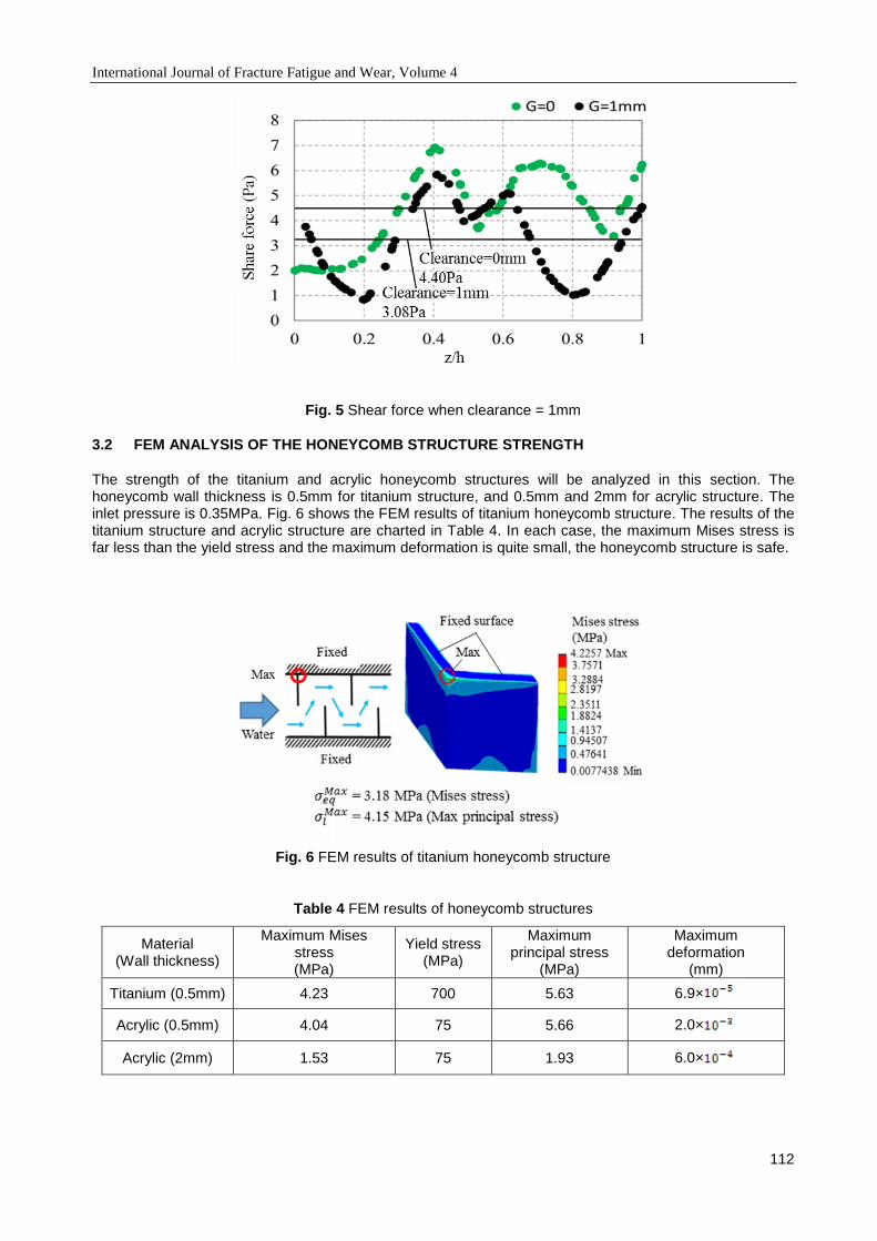
International Journal of Fracture Fatigue and Wear, Volume 4
112
Fig. 5 Shear force when clearance = 1mm
3.2 FEM ANALYSIS OF THE HONEYCOMB STRUCTURE STRENGTH
The strength of the titanium and acrylic honeycomb structures will be analyzed in this section. The honeycomb wall thickness is 0.5mm for titanium structure, and 0.5mm and 2mm for acrylic structure. The inlet pressure is 0.35MPa. Fig. 6 shows the FEM results of titanium honeycomb structure. The results of the titanium structure and acrylic structure are charted in Table 4. In each case, the maximum Mises stress is far less than the yield stress and the maximum deformation is quite small, the honeycomb structure is safe.
Fig. 6 FEM results of titanium honeycomb structure
Table 4 FEM results of honeycomb structures
Material (Wall thickness)
Maximum Mises stress (MPa)
Yield stress (MPa)
Maximum principal stress
(MPa)
Maximum deformation
(mm)
Titanium (0.5mm) 4.23 700 5.63 6.9×
Acrylic (0.5mm) 4.04 75 5.66 2.0×
Acrylic (2mm) 1.53 75 1.93 6.0×

International Journal of Fracture Fatigue and Wear, Volume 4
113
4 CONCLUSIONS
The device with honeycomb structure can make nitrogen nanobubbles to reduce the DO in water efficiently. The clearance between two honeycomb plates in each honeycomb structure unit will weaken the shear field of the fluid, which leads to weak ability of nanobubbles producing for DO decreasing.
The fluid model is investigated. The walls have effects on the fluid, so that 1-row model cannot simulate the fluid in the honeycomb structure accurately. In order to avoid the influence of the walls, at least 5 rows should be modeled for analysis. Similar to the experimental results, from FEM analysis it can be found that the clearance causes lower shear force.
The strength of the honeycomb structure is also analyzed by FEM. In each case, the maximum Mises stress is far less than the yield stress and the maximum deformation is quite small, the honeycomb structure is safe.
The honeycomb structure has the advantages of light weight, small size and high efficiency. This paper provides some references for the further research on nanobubble technology.
5 REFERENCES
[1] Koju HIRAKI, Efficient Long Term Storage Technology of Seafood Using Nitrogen Nanobubbles, The Latest Technology on Microbubbles and Nanobubbles, 2, 177-183, 2014.
[2] Yoshiaki KUDO, Koju HIRAKI, Visualization of Mixing Process in a Conduit with Honeycomb
Structure, Proceedings of Symposium on Micro-Nano Science and Technology, 2, 95-96, 2010.
[3] Hideki TSUGE, Fundamentals of Microbubbles and Nanobubbles, Bulletin of the Society of Sea
Water Science, Japan, 64, 4-10, 2010.
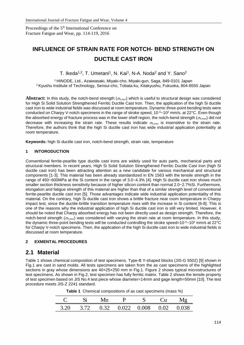
International Journal of Fracture Fatigue and Wear, Volume 4
114
C Si Mn P S Cu Mg
3.20 3.72 0.32 0.022 0.008 0.02 0.038
Proceedings of the 5th International Conference on
Fracture Fatigue and Wear, pp. 114-119, 2016
INFLUENCE OF STRAIN RATE FOR NOTCH- BEND STRENGTH ON
DUCTILE CAST IRON
T. Ikeda1,2, T. Umetani1, N. Kai1, N-A. Noda2 and Y. Sano2
1 HINODE, Ltd., Azaiwasaki, Miyaki-cho, Miyaki-gun, Saga, 849-0101 Japan 2 Kyushu Institute of Technology, Sensui-cho, Tobata-ku, Kitakyushu, Fukuoka, 804-8550 Japan
Abstract: In this study, the notch-bend strength (b,max) which is useful to structural design was considered
for High Si Solid Solution Strengthened Ferritic Ductile Cast Iron. Then, the application of the high Si ductile cast iron to wide industrial fields was discussed at room temperature. Dynamic three-point bending tests were conducted on Charpy V-notch specimens in the range of stroke speed, 10-3~102 mm/s, at 22°C. Even though
the absorbed energy of fracture process was in the lower shelf region, the notch-bend strength (b,max) did not
decrease with increasing the strain rate. These results indicate b,max is insensitive to the strain rate. Therefore, the authors think that the high Si ductile cast iron has wide industrial application potentiality at room temperature.
Keywords: high Si ductile cast iron, notch-bend strength, strain rate, temperature
1 INTORODUCTION
Conventional ferrite-pearlite type ductile cast irons are widely used for auto parts, mechanical parts and structural members. In recent years, High Si Solid Solution Strengthened Ferritic Ductile Cast Iron (high Si ductile cast iron) has been attracting attention as a new candidate for various mechanical and structural components [1-3]. This material has been already standardized in EN 1563 with the tensile strength in the range of 450~600MPa at the Si content in the range of 3.0~4.3% [4]. High Si ductile cast iron shows much smaller section thickness sensitivity because of higher silicon content than normal 2.0~2.7%Si. Furthermore, elongation and fatigue strength of this material are higher than that of a similar strength level of conventional ferrite-pearlite ductile cast iron [5]. Those advantages indicate wide industrial application potentiality of this material. On the contrary, high Si ductile cast iron shows a brittle fracture near room temperature in Charpy impact test, since the ductile-brittle transition temperature rises with the increase in Si content [6-8]. This is one of the reasons why the industrial application of high Si ductile cast iron is still very limited. However, it should be noted that Charpy absorbed energy has not been directly used as design strength. Therefore, the
notch-bend strength (b,max) was considered with varying the strain rate at room temperature. In this study, the dynamic three-point bending tests will be conducted controlling the stroke speed=10-3~102 mm/s at 22°C for Charpy V-notch specimens. Then, the application of the high Si ductile cast iron to wide industrial fields is discussed at room temperature.
2 EXMENTAL PROCEDURES
2.1 Material
Table 1 shows chemical composition of test specimens. Type-B Y-shaped blocks (JIS-G 5502) [9] shown in Fig.1 are cast in sand molds. All tests specimens are taken from the as cast specimens of the highlighted sections in gray whose dimensions are 40×25×250 mm in Fig.1. Figure 2 shows typical microstructures of test specimens. As shown in Fig.2, test specimen has fully ferritic matrix. Table 2 shows the tensile property of test specimen based on JIS No.4 test piece whose diameter=14mm and gage length=50mm [10]. The test procedure meets JIS-Z 2241 standard.
Table 1 Chemical compositions of as cast specimens (mass %)
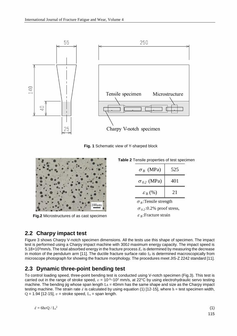
International Journal of Fracture Fatigue and Wear, Volume 4
115
B (MPa) 525
0.2 (MPa) 401
e B (%) 21
B :Tensile strength
0.2 :0.2% proof stress,
e B :Fracture strain
Fig. 1 Schematic view of Y-sharped block
Table 2 Tensile properties of test specimen
Fig.2 Microstructures of as cast specimen
2.2 Charpy impact test Figure 3 shows Charpy V-notch specimen dimensions. All the tests use this shape of specimen. The impact test is performed using a Charpy impact machine with 300J maximum energy capacity. The impact speed is 5.18×103mm/s. The total absorbed energy in the fracture process Ec is determined by measuring the decrease in motion of the pendulum arm [11]. The ductile fracture surface ratio fD is determined macroscopically from microscope photograph for showing the fracture morphology. The procedures meet JIS-Z 2242 standard [11].
2.3 Dynamic three-point bending test To control loading speed, three-point bending test is conducted using V-notch specimen (Fig.3). This test is carried out in the range of stroke speed, ʋ = 10-3~102 mm/s, at 22°C by using electrohydraulic servo testing machine. The bending jig whose span length Ls = 40mm has the same shape and size as the Charpy impact testing machine. The strain rate 𝜀 is calculated by using equation (1) [12-15], where h = test specimen width, Q = 1.94 [12-15], ʋ = stroke speed, Ls = span length.
𝜀 = 6hʋQ / Ls2 (1)

International Journal of Fracture Fatigue and Wear, Volume 4
116
0
5
10
15
20
-100 -50 0 50 100 150
Char
py a
bso
rbed
en
ergy E
c(J)
Temperature T ()
Critical temperature
of upper shelf = 80 Transition regionCritical temperature
of lower shelf = 20
Critical temperature
of upper shelf =
0
20
40
60
80
100
-100 -50 0 50 100 150
Duct
ile
frac
ture
rat
io f
D (
%)
Temperature T ()
80 20 Critical temperature
of lower shelf =
Transition region
The total absorbed energy Et in the fracture process is also obtained from area under the load-deflection curve of the three-point bending test. The fractographic analysis is performed by optical observations and scanning electron microscopy (SEM). The ductile fracture surface ratio fD is determined macroscopically from microscope photograph.
Fig. 3 V-notch specimen dimensions (JIS-Z 2242)
3 RESULTS AND DISCUSSION
3.1 Charpy transition curve
Figure 4 shows the results of V-notch Charpy impact test. In Fig.4(a), the absorbed energy Ec starts dropping at the critical temperature for upper shelf region of 80°C as indicated by the black arrow. In Fig.4(b), fD starts dropping at the same critical temperature of Ec. Brittle fracture surface appears below this critical temperature. In Fig.4 (a), (b), a good coincidence can be seen for the transition of Ec and fD. This means that the reduction of Ec is caused by ductile-brittle fracture surface transition. In Fig.4(a), lower shelf region is recognized and ductile fracture surface completely disappears below 20°C, Fig.4(b).
(a) Transition curves of absorbed energy (b) Transition curve of ductile fracture ratio
Fig. 4 Result of Charpy impact test
3.2 Absorbed energy depending on strain rate
Figure 5 shows the effects of the strain rate 𝜀 on (a) the absorbed energy Et and (b) the fD of the three-point bending test at 22°C. In Fig. 5(a), the upper shelf region is being recognized even at 22°C, room temperature. In Fig.5, the upper shelf energy is obtained because these 𝜀 are more than 103 times lower than 𝜀 of Charpy
impact test. In Fig.5(a), the absorbed energy starts dropping at 𝜀 of 2.5×10⁻¹s-1 as indicated by the black
arrow. Brittle fracture surface appears above this critical 𝜀. Similar to the results of Charpy impact test a good coincidence can be seen for the transition of Et and fD. It may be concluded that the reduction of Et is caused
by ductile-brittle fracture surface transition by increasing 𝜀.

International Journal of Fracture Fatigue and Wear, Volume 4
117
0
20
40
60
80
100
10-4
10-3
10-2
10-1
100
101
Duct
ile
frac
ture
rat
io f
D(%
)
2.5×10⁻¹ s-1
Strain rate ε(s-1)・
T = 22
Critical strain rate
of upper shelf =
2.5×10⁻¹ s-1
0
5
10
15
10-4
10-3
10-2
10-1
100
101
Abso
rbed
ener
gy E
t(J)
Strain rate ε(s-1)・
T = 22
・at e = 3.0×10
2s
-1
Ec = 5J for Charpy impact test
Critical strain rate
of upper shelf =
ε = 0.11×10⁻² s-1
(max=2.59mm, Pmax=9.0kN)
0
1
2
3
4
5
6
7
8
9
10
11
0 1 2 3 4
Lo
ad P
(kN
)
Displacement (mm)
×:Fracture (max)
××
×
×
・
Pmax
T = 22
ε = 3.64×10⁻² s-1
(max=2.43mm, Pmax=9.6kN)
・
ε = 72.3×10⁻² s-1
(max=0.63mm, Pmax=10.2kN)
・
ε = 227×10-2 s-1
(max=0.55mm, Pmax=10.4kN)
・
(a) Effect of strain rate on absorbed energy (b) Effect of strain rate on ductile fracture ratio
Fig. 5 Result of the three-point bending test at 22°C
3.3 Notch-bend strength insensitive to strain rate
Absorbed energy has not been directly used as design strength. Therefore, the strength was considered with varying the strain rate at 22°C, room temperature. Figure 6 shows a load-displacement curve on the three-
point bending test under different 𝜀 at 22°C. From Fig.6, it is seen that the maximum displacement max
decreases with increasing 𝜀. This is why Et decreases with increasing 𝜀 in Fig.5(a). On the contrary, in Fig.6, it should be noted that the maximum load Pmax slightly increases with increasing 𝜀. Figure 7 shows the
relationship between the notch-bend strength b,max and 𝜀 for the three-point bending test at 22°C. The notch-
bend strength b,max was calculated by equation (2) [16,17], where Pmax = maximum load, Ls = span length, b = test specimen thickness, h = test specimen width.
b,max = 3PmaxLs / 2bh2 (2)
For comparison, the relationship between Et and 𝜀 shown in Fig.5(a) is also put in Fig.7. In Fig.7, it should be
noted that even though Et is in the lower shelf region, the notch-bend strength, that is b,max, does not decrease
insensitive to 𝜀. The authors think that high Si ductile cast iron has a wide industrial application potentiality
because the notch-bend strength insensitiveness to 𝜀 although the absorbed energy is sensitive.
Fig. 6 Variation of load-displacement curves of the three-point bending test with strain rate at 22°C

International Journal of Fracture Fatigue and Wear, Volume 4
118
0
500
1000
1500
0
5
10
15
10-4
10-3
10-2
10-1
100
101
T = 22
2.5×10⁻¹ s-1
Strain rate ε(s-1)・
Notc
h-b
end s
tren
gth
b
,max
(MP
a)
Abso
rbed
ener
gy E
t(J)Et
b,max
Critical strain rate
of upper shelf =
Fig. 7 Effect of strain rate on the notch-bend strength of the three-point bending test at 22°C
4 CONCLUDION
In this study, the notch-bend strength was considered for high Si ductile cast iron. This material has attracted a lot of attention recently because of smaller section thickness sensitivity and higher fatigue strength. Dynamic three-point bending test were conducted in the range of stroke speed, 10-3~102 mm/s, at 22°C. The conclusions can be made the following way.
(1) The absorbed energy Et decrease with increasing 𝜀. The reduction of Et is caused by ductile-brittle fracture
surface transition by increasing 𝜀.
(2) Even though the absorbed energy Et is in the lower shelf region, b,max does not decrease with increasing
𝜀 in the range of 𝜀, 1.1×10⁻³~2.3×100s-1, at 22°C. Notch-bend strength b,max is insensitive to strain rate 𝜀 at
22°C, room temperature.
Therefore, the authors think that b,max is more useful than absorbed energy for structural design. The high Si ductile cast iron has wide industrial application potentiality at room temperature.
5 REFERENCES
[1] R.Larker, Solution strengthened ferritic ductile iron ISO 1083/JS/500-10 provides superior consistent properties in hydraulic rotators, China Foundry, 6, 343-351, 2009.
[2] R.Larker, Paradigm shift in revised 1563(GJS) enables improved properties and production economy in both as-cast and austempered (ADI) states, Proc. NEWCAST Forum, Bundesverband der Deutschen Gießerei Industrie, Düsseldorf, 29-34, 2011.
[3] H.Löblich, W.Stets, Die Einführung von mischkristallverfestigtem Gusseisen mit Kugei-graphit in die Industrie-eine Erfolgsstory, Proc. Deutscher Gießereitag 2013 und 5. NEWCAST Forum, Verein Deutscher Giessereifachleute, Fellbach, 14-17, 2013.
[4] EN 1563, Founding-Spheroidal graphite cast irons, 2011.
[5] T.Umetani, T.Ikeda, N.Sura, K.Ashizuka, T.Nemoto, H.Takada, K.Ogi: Tensile Strength, Fatigue Strength, and Impact Strength of Solution Strengthened High Silicon Ferritic Ductile Cast Iron, J.JFS., 86, 36-42, 2014.
[6] T.Okumoto, T.Aizawa, Effect of Silicon Phosphorus and Pearlite on the Impact Transition Curves of Spheroidal Graphite Cast Irons, Imono, 35, 670-677, 1963.
[7] K.Nagai, K.Kishitake, T.Owadano, The Effect of Silicon Content on the Impact Fracture Characteristics of Ferritic Spheroidal Graphite Cast Irons, Imono, 58, 350-355, 1986.
[8] H.Nagayoshi, H.Yasuda, K.Imanishi, Effects of Silicon Content on Impact Properties of Spheroidal Graphite Cast Iron, J.JFS., 68, 506-511, 1996.

International Journal of Fracture Fatigue and Wear, Volume 4
119
[9] JIS-G5502, Spheroidal graphite iron castings, 2001.
[10] JIS-Z2241, Metallic materials-Tensile test-ing-Method of test at room temperature, 2011.
[11] JIS-Z2242, Method for Charpy pendulum impact test of metallic materials, 2005.
[12] R.Sandstrom, Y.Bergstrom, Rerationship between Charpy V transition temperature in mild steel and various material parameters, Met. Sci., 18, 177-186, 1984.
[13] H.Yamamoto, T.Kobayashi, H.Fujita, Strain Rate Dependency of Ductile-Brittle Transition Behavior in Ductile Cast Iron, J.JFS, 72, 107-112, 2000.
[14] N.Sugiura, T.Kobayashi, I.Yamamoto, S.Nishido, K.Hayashi, Comparision of tensile and 3-point bend properties under impact loading in an AC4CH-T6 aluminum casting alloy, J. Jpn. Inst. Light Met.,45, 638-642 1995.
[15] K.Matsugi, G.Bando, G.Sasaki,O. Yanagisawa, Fracture Propaties at Elevated Temperatures of Ferritic Ductile Cast Irons, J.JFS., 79, 229-234, 2007.
[16] T. Kobayashi, H.Matsubara, Y.Ueda, Fracture Characteristics Obtained from Instrumented Impact Test of A533B Steel for Reactor Pressure Vessel, Tetsu-to-Hagané, 69, 1183-1189, 1983.
[17] S. Nunomura, M. Nakashiro, Fracture Characteristics Evaluation by Charpy Impact Bending Test, Tetsu-to-Hagané, 64, 860-868,1978.

International Journal of Fracture Fatigue and Wear, Volume 4
120
Proceedings of the 5th International Conference on
Fracture Fatigue and Wear, pp. 120-125, 2016
EFFECT OF LOW-PRESSURE PLASMA TREATMENT ON SURFACE
MODIFICATION AND FRICTION COEFFICIENT OF POLY-(METHYL-
METHACRYLATE)
J. Abenojar, P. Gálvez and M.A. Martínez
University Carlos III of Madrid, Materials Performance Research Group, Leganes, Spain
Abstract: Plasma treatments modify the surface properties of materials, especially polymeric materials.
Among these surface properties, the surface energy and the wettability increase are the most important ones. The procedures carried out after the plasma treatment (such as printing, adhesion, coating application. etc., for which the wettability is a fundamental factor) benefit from an improved effectiveness thanks to this surface treatment. The latter also changes the roughness of the material at micro- or nanometer scale, even though this depends on the treatment. Overall, the work of adhesion of the surface of the material is changed. As the plasma treatment is a surface phenomenon, the main objective of this project was to study the effect produced by this treatment on the friction coefficient of polymers, in particular on a commercial poly-(methyl-methacrylate) (PMMA). To this end, plasma treatment, using different gases (Argon, Nitrogen and Air) under vacuum, were performed. The surface was characterized by contact angle, surface energy, roughness, infrared spectroscopy (FTIR) and X-ray photoelectron spectroscopy. These characterizations were conducted on all the surfaces and on untreated PMMA. The contact angles allow to know the work of adhesion and these values can be associated with roughness and wear. The wear tests were pin-on-disk test and they were performed at low rate (60 and 120 rpm) and low load (2 N), over a 10 m distance with an alumina pin with a 6 mm radius. In these tests, friction coefficients were only evaluated and compared. The results obtained in this work show an increment in the friction coefficient with surface energy increases, especially when the polar component of surface energy is incremented.
Keywords: PMMA; Plasma treatments; Energy surface; Work of Adhesion; Friction coefficient.
1 INTRODUCTION
Poly-(methyl-methacrylate) (PMMA) is considered to be a biomaterial, since it is biocompatible [1] for many applications. Some of these applications are: rartificial kidneys, bone cement dental fillings, intraocular lenses and hard contact lenses. It is a hard, clear and crystalline material, besides it preserves its properties in the presence of water. Although there has been extensive discussion about what bonds are within its molecules, three types of bond have been accepted. They depend on the environment and are in the relation 1:1:3 (bonds a, b and c in Fig. 1). These bonds coincide with the groups O-C=O, C-O and C-C respectively [1].
Fig.1 Chemical structure of the methacrylate.
In spite of their excellent intrinsic properties, the integration of polymer pieces inside other structures is often restricted by its low polarity and chemistry surface, which leads to a low surface energy [2-5]. This causes the incompatibility of using most adhesives [6] (especially those water-based or of polar nature [7,8]). Therefore, surface preparation becomes a key factor for painting or adhesion processes, as well as for durability of the adhesive bond.

International Journal of Fracture Fatigue and Wear, Volume 4
121
The surface treatments that allow to change the surface properties are mechanical, cleaning, chemical, and physical treatments. This work focuses on physical treatments. The latter are performed by applying plasma generated by gas ionization. They can be hot plasmas (which are flamed) or cold plasmas (such as corona treatment, treatment with atmospheric plasma torch, and low pressure plasmas). The treatments chosen in
this study are low pressure plasmas. The available literature on the topic [9,10] indicates that cold plasma
treatment on polymers drastically changes their surface characteristics.
The surface changes are usually characterized chemically by X-ray spectroscopy, infrared spectroscopy, or surface energy. The only mechanical characterization used is the measurement of the surface roughness. Atomic force microscopy is used for studying the surface topography changes. These changes are typically at nanometric scale, even though sometimes micrometric changes can be found. Therefore, the main objective of this work is to investigate the effect different surface treatments with low pressure plasma produce on the PMMA. In this research, different gases were used and the surface characterization was performed both chemically and mechanically. An additional novelty of this study is to conduct wear tests to explore the effect of plasma on the friction coefficient and its correlation with the surface energy and adhesion work.
2. EXPERIMENTAL PROCEDURE
The material used in this work was Poly-(methyl-methacrylate) (PMMA). It was supplied by Henkel Ibérica S.A. (Barcelona, Spain). The 3 mm thick sheets were cut into test pieces of 80 mm long by 25 mm wide.
The surface treatment of the specimens was performed in a cold plasma chamber, which operates under vacuum (300 mbar). Its supplier was Plasma Cleaner PDC-002 model (Harrick Plasma, Ithaca, USA). Three gases were used: N2, air and Argon. The plasma application parameters were optimized by contact angles measurements with deionized water. Table 1 summarises how the parameters were changed for each gas. In the case of argon and air the treatment was better for a duration of 5 min and power of 20 W (medium power) than other treatment. For nitrogen, 7 min and 30 W (high power) were determined to be better. Furthermore, the treatments were tested after 5 and 10 days to study their durability. The durability is no more than 5 days.
Table 1 Application parameters of different treatments
The selection of the liquids for the contact angle measurements was done considering a wide range of polarities, including deionized water, diiodomethane, and 1,5-pentanediol. Measurements were performed with an OCA 15 plus device from Data Physics (Neurtek Instruments, Eibar, Guipúzcoa, Spain), using the sessile drop method and following the UNE EN 828:2010 standard. Surface energy was obtained by the Owens–Wendt–Rable–Kaelble (OWRK) calculation method, which enables the determination of the contributions to the total surface energy and its dispersive and polar components. From the contact angles and the surface tensions of the liquids, it was possible to calculate the adhesion work.
Chemical composition analysis was performed by an infrared spectrum (ATR-FTIR) and X-ray photoelectron spectroscopy (XPS). A Brucker Tensor 27 (Brucker Optik GmbH, Madrid, Spain) spectrometer was used to obtain the infrared spectra of both untreated and plasma treated samples. The attenuated total multiple reflection technique (ATR) was used to analyse the surface chemical modifications produced up to about 5–10 μm deep into the pieces. A diamond prism was used and the incident angle of the IR radiation was 45º. Thirty-two scans with a resolution of 4 cm−1 were obtained and averaged. Spectra were recorded from 600 to 4000 cm−1.
The XPS technique allows to observe chemical modifications on the outermost surface layer (about 5 nm) in the treated samples, and they were performed with a VG Scientific Microtech Multilab (VG Scientia, Hastings, United Kingdom) spectrometer using a Mg-Kα X-ray source (1253.6 eV) operating at 15 keV and 300 W. A survey scan encompassing the 0–1200 eV region was obtained for each sample. All binding energies were referred to the C 1s core level spectrum position for C–C and C–H (hydrocarbons) species at 285.0 eV. Atomic concentrations were calculated using a VGX900-W system.
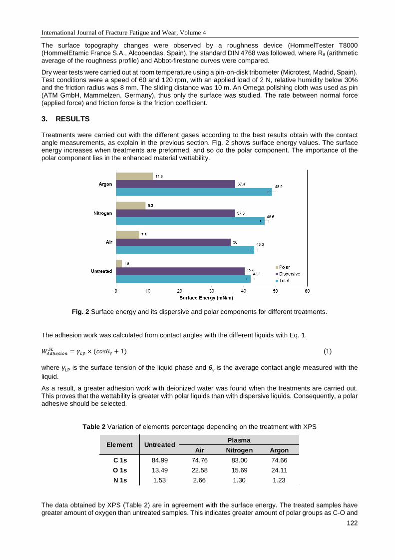
International Journal of Fracture Fatigue and Wear, Volume 4
122
The surface topography changes were observed by a roughness device (HommelTester T8000 (HommelEtamic France S.A., Alcobendas, Spain), the standard DIN 4768 was followed, where Ra (arithmetic average of the roughness profile) and Abbot-firestone curves were compared.
Dry wear tests were carried out at room temperature using a pin-on-disk tribometer (Microtest, Madrid, Spain). Test conditions were a speed of 60 and 120 rpm, with an applied load of 2 N, relative humidity below 30% and the friction radius was 8 mm. The sliding distance was 10 m. An Omega polishing cloth was used as pin (ATM GmbH, Mammelzen, Germany), thus only the surface was studied. The rate between normal force (applied force) and friction force is the friction coefficient.
3. RESULTS
Treatments were carried out with the different gases according to the best results obtain with the contact angle measurements, as explain in the previous section. Fig. 2 shows surface energy values. The surface energy increases when treatments are preformed, and so do the polar component. The importance of the polar component lies in the enhanced material wettability.
Fig. 2 Surface energy and its dispersive and polar components for different treatments.
The adhesion work was calculated from contact angles with the different liquids with Eq. 1.
𝑊𝐴𝑑ℎ𝑒𝑠𝑖𝑜𝑛𝑆𝐿 = 𝛾𝐿𝑝 × (𝑐𝑜𝑠𝜃𝛾 + 1) (1)
where γLP is the surface tension of the liquid phase and θγ is the average contact angle measured with the
liquid.
As a result, a greater adhesion work with deionized water was found when the treatments are carried out. This proves that the wettability is greater with polar liquids than with dispersive liquids. Consequently, a polar adhesive should be selected.
Table 2 Variation of elements percentage depending on the treatment with XPS
The data obtained by XPS (Table 2) are in agreement with the surface energy. The treated samples have greater amount of oxygen than untreated samples. This indicates greater amount of polar groups as C-O and
Air Nitrogen Argon
C 1s 84.99 74.76 83.00 74.66
O 1s 13.49 22.58 15.69 24.11
N 1s 1.53 2.66 1.30 1.23
PlasmaUntreatedElement
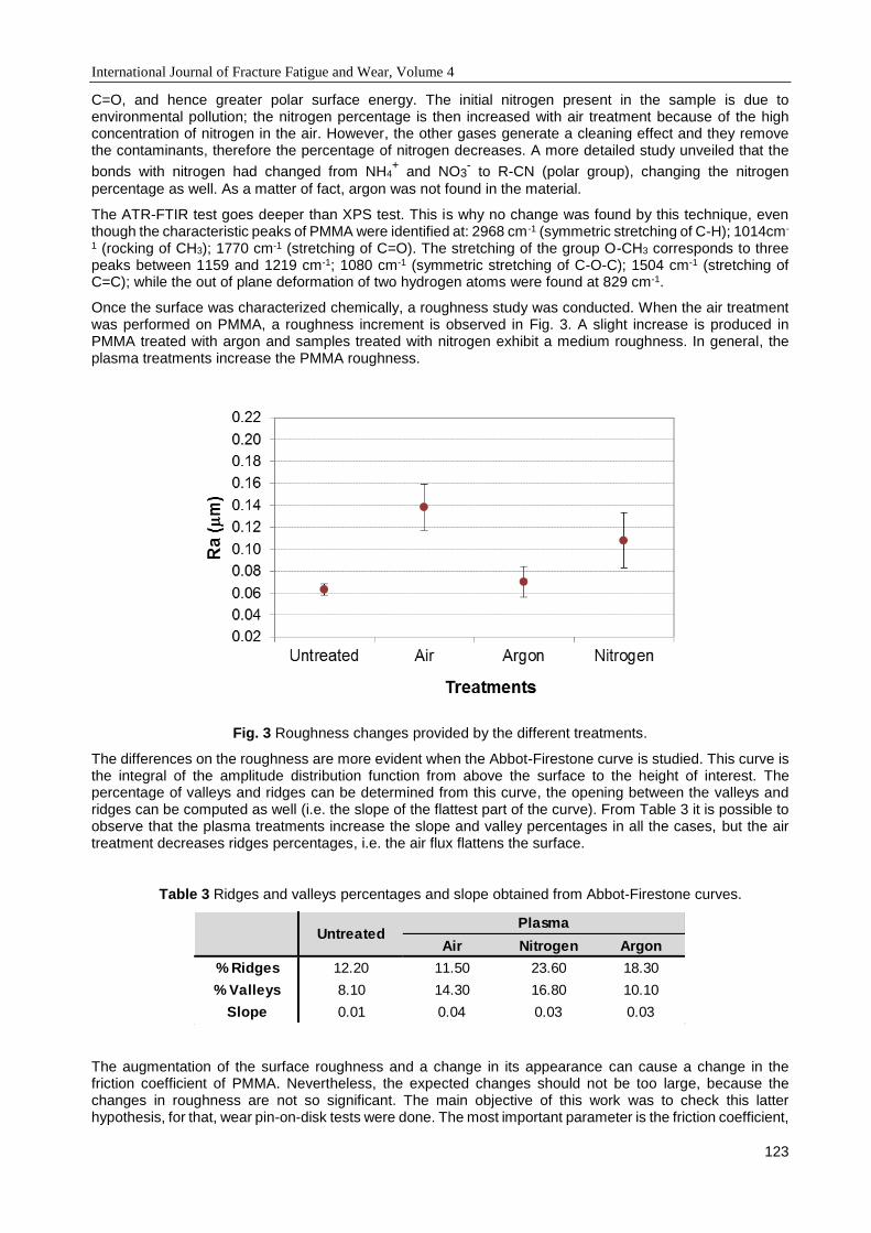
International Journal of Fracture Fatigue and Wear, Volume 4
123
C=O, and hence greater polar surface energy. The initial nitrogen present in the sample is due to environmental pollution; the nitrogen percentage is then increased with air treatment because of the high concentration of nitrogen in the air. However, the other gases generate a cleaning effect and they remove the contaminants, therefore the percentage of nitrogen decreases. A more detailed study unveiled that the
bonds with nitrogen had changed from NH4+ and NO3
- to R-CN (polar group), changing the nitrogen
percentage as well. As a matter of fact, argon was not found in the material.
The ATR-FTIR test goes deeper than XPS test. This is why no change was found by this technique, even though the characteristic peaks of PMMA were identified at: 2968 cm-1 (symmetric stretching of C-H); 1014cm-
1 (rocking of CH3); 1770 cm-1 (stretching of C=O). The stretching of the group O-CH3 corresponds to three peaks between 1159 and 1219 cm-1; 1080 cm-1 (symmetric stretching of C-O-C); 1504 cm-1 (stretching of C=C); while the out of plane deformation of two hydrogen atoms were found at 829 cm-1.
Once the surface was characterized chemically, a roughness study was conducted. When the air treatment was performed on PMMA, a roughness increment is observed in Fig. 3. A slight increase is produced in PMMA treated with argon and samples treated with nitrogen exhibit a medium roughness. In general, the plasma treatments increase the PMMA roughness.
Fig. 3 Roughness changes provided by the different treatments.
The differences on the roughness are more evident when the Abbot-Firestone curve is studied. This curve is the integral of the amplitude distribution function from above the surface to the height of interest. The percentage of valleys and ridges can be determined from this curve, the opening between the valleys and ridges can be computed as well (i.e. the slope of the flattest part of the curve). From Table 3 it is possible to observe that the plasma treatments increase the slope and valley percentages in all the cases, but the air treatment decreases ridges percentages, i.e. the air flux flattens the surface.
Table 3 Ridges and valleys percentages and slope obtained from Abbot-Firestone curves.
The augmentation of the surface roughness and a change in its appearance can cause a change in the friction coefficient of PMMA. Nevertheless, the expected changes should not be too large, because the changes in roughness are not so significant. The main objective of this work was to check this latter hypothesis, for that, wear pin-on-disk tests were done. The most important parameter is the friction coefficient,
Air Nitrogen Argon
% Ridges 12.20 11.50 23.60 18.30
% Valleys 8.10 14.30 16.80 10.10
Slope 0.01 0.04 0.03 0.03
UntreatedPlasma

International Journal of Fracture Fatigue and Wear, Volume 4
124
and the wear is not taken into account, because the test was only 10 m. After distance, the superficial effect is not appreciated, because treatments only affect the first atom layers.
Figs. 4 and 5 correspond to the change in the friction coefficient with the distance for all the plasma treatments, tested at two rotational speeds. The most interesting area of the graph is the initial one. This is why the alterations produced by the plasma are only located on the surface of the treated material.
PMMA plasma-treated samples have higher values of initial friction. This is consistent with the higher surface energy associated with the polar component. It is also in agreement with the higher work of adhesion values as well as with the greater roughness caused by the treatment. Due to the higher impact force of the ionized argon and nitrogen gas on the surface, the samples treated with these gases have bigger friction coefficients than the samples treated with air. As seen in Fig. 2 and Table 3, these gases produce a higher polar component and larger ridges percentage than the air does.
Once the wear track is formed, the friction coefficient tends to stabilise and its value is similar for all the treatments, except when argon is used. The value of the stabilised friction coefficient is higher when the rotational speed is lower (60 rpm), with its value being between 0.7 and 0.8, whereas its value is between 0.45 and 0.65 when the rotational speed is 120 rpm. In the case of argon treatment, the stabilised friction coefficient has value close to 1. It seems that the treatment goes deeper than with the other gases, therefore the friction coefficient remains still high after 10 m.
Fig. 4 Friction coefficient versus distance covered at 120 rpm for the different treatments.
Fig. 5 Friction coefficient versus distance covered at 60 rpm for the different treatments.
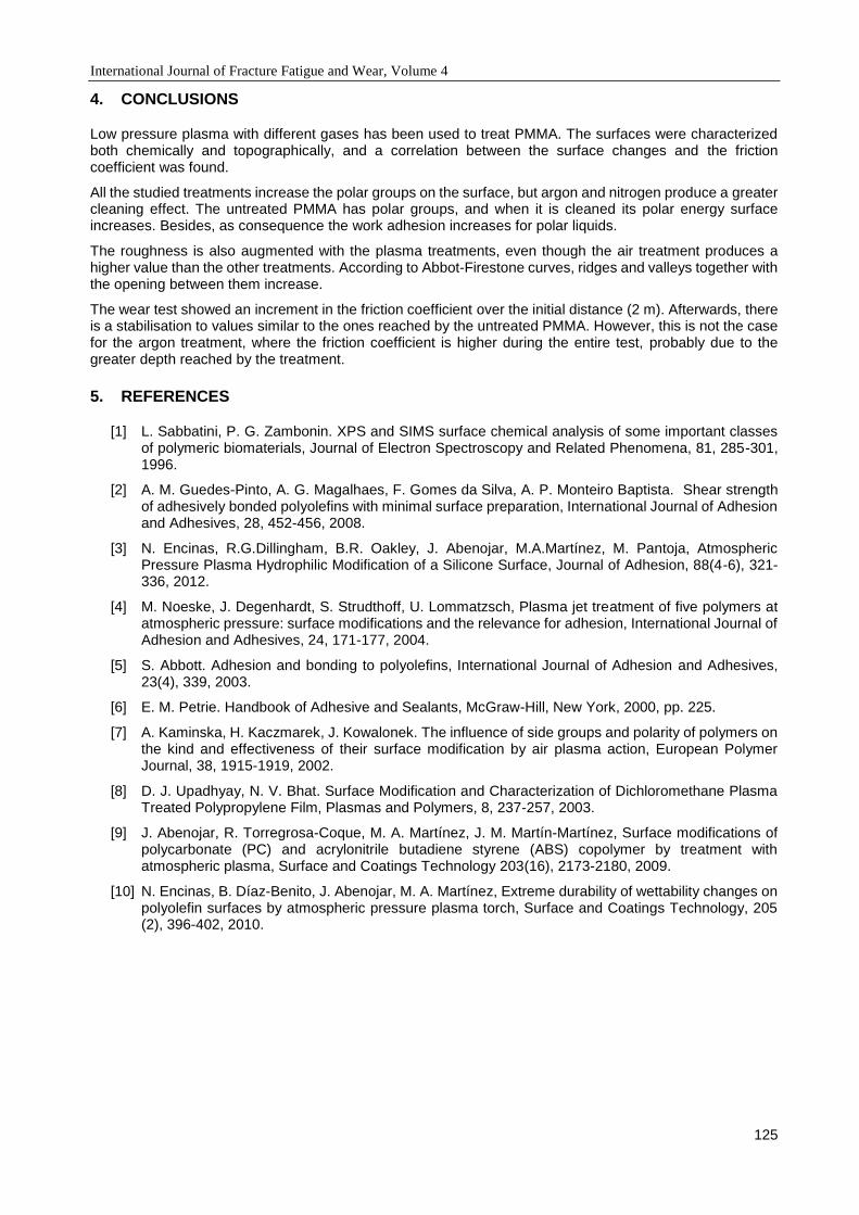
International Journal of Fracture Fatigue and Wear, Volume 4
125
4. CONCLUSIONS
Low pressure plasma with different gases has been used to treat PMMA. The surfaces were characterized both chemically and topographically, and a correlation between the surface changes and the friction coefficient was found.
All the studied treatments increase the polar groups on the surface, but argon and nitrogen produce a greater cleaning effect. The untreated PMMA has polar groups, and when it is cleaned its polar energy surface increases. Besides, as consequence the work adhesion increases for polar liquids.
The roughness is also augmented with the plasma treatments, even though the air treatment produces a higher value than the other treatments. According to Abbot-Firestone curves, ridges and valleys together with the opening between them increase.
The wear test showed an increment in the friction coefficient over the initial distance (2 m). Afterwards, there is a stabilisation to values similar to the ones reached by the untreated PMMA. However, this is not the case for the argon treatment, where the friction coefficient is higher during the entire test, probably due to the greater depth reached by the treatment.
5. REFERENCES
[1] L. Sabbatini, P. G. Zambonin. XPS and SIMS surface chemical analysis of some important classes of polymeric biomaterials, Journal of Electron Spectroscopy and Related Phenomena, 81, 285-301, 1996.
[2] A. M. Guedes-Pinto, A. G. Magalhaes, F. Gomes da Silva, A. P. Monteiro Baptista. Shear strength of adhesively bonded polyolefins with minimal surface preparation, International Journal of Adhesion and Adhesives, 28, 452-456, 2008.
[3] N. Encinas, R.G.Dillingham, B.R. Oakley, J. Abenojar, M.A.Martínez, M. Pantoja, Atmospheric Pressure Plasma Hydrophilic Modification of a Silicone Surface, Journal of Adhesion, 88(4-6), 321-336, 2012.
[4] M. Noeske, J. Degenhardt, S. Strudthoff, U. Lommatzsch, Plasma jet treatment of five polymers at atmospheric pressure: surface modifications and the relevance for adhesion, International Journal of Adhesion and Adhesives, 24, 171-177, 2004.
[5] S. Abbott. Adhesion and bonding to polyolefins, International Journal of Adhesion and Adhesives, 23(4), 339, 2003.
[6] E. M. Petrie. Handbook of Adhesive and Sealants, McGraw-Hill, New York, 2000, pp. 225.
[7] A. Kaminska, H. Kaczmarek, J. Kowalonek. The influence of side groups and polarity of polymers on the kind and effectiveness of their surface modification by air plasma action, European Polymer Journal, 38, 1915-1919, 2002.
[8] D. J. Upadhyay, N. V. Bhat. Surface Modification and Characterization of Dichloromethane Plasma Treated Polypropylene Film, Plasmas and Polymers, 8, 237-257, 2003.
[9] J. Abenojar, R. Torregrosa-Coque, M. A. Martínez, J. M. Martín-Martínez, Surface modifications of polycarbonate (PC) and acrylonitrile butadiene styrene (ABS) copolymer by treatment with atmospheric plasma, Surface and Coatings Technology 203(16), 2173-2180, 2009.
[10] N. Encinas, B. Díaz-Benito, J. Abenojar, M. A. Martínez, Extreme durability of wettability changes on polyolefin surfaces by atmospheric pressure plasma torch, Surface and Coatings Technology, 205 (2), 396-402, 2010.

International Journal of Fracture Fatigue and Wear, Volume 4
126
Proceedings of the 5th International Conference on
Fracture Fatigue and Wear, pp. 126-132, 2016
CONTACT AREA ACTUAL SELF-FRICTION IN POLYOLEFINS
M.A. Martinez and J. Abenojar
University Carlos III of Madrid. Materials Performance Research Group. Leganes (Spain)
Abstract: During friction processes, two bodies are generally in contact only over very small discrete areas. Some tribological properties occurring at the micro-scale level are strongly controlled by the actual contact area, which is a small fraction of the nominal or apparent contact area. This work studies the relationship between normal load, actual contact area and static self-friction coefficient in different polymeric materials (low density polyethylene, high density polyethylene, polypropylene and silicone). To this end, friction tests were carried out to measure the force of static friction. Moreover, hardness and roughness test were performed, which allow to calculate the actual contact area and to formulate hypotheses on this phenomenon. In this study, the normal tensile stress and the shear resistance necessary to start the displacement between two surfaces in contact with one another are consistent with theoretical expectations. The ratio between their values and the apparent tensions are indeed close to one. This is found when the normal force begins to be relatively high.
Keywords: Polymer Surface; Actual Contact Area; Static Self-friction Coefficient.
1. INTRODUCTION
The knowledge of the actual contact area between two surfaces is the main current problem that tribology is facing [1,2]. For metals, the lineal proportionality between the actual contact area and the normal applied load is known, when the loads are low enough [2]. At higher loads, the relationship becomes asymptotic when approaching the apparent area [3,4,5], and the proposed equations are semi-empirical for the relationship between normal force and actual contact area. For this reason, the elastic-plastic and plastic contacts theory have to be used.
Previous works on tribology of polymeric materials were primarily focused on the study of the sliding or rolling effects for polymer-polymer or polymer-metal systems [6,7,8]. Conversely this work investigates the effect of the normal force on and stresses generated on the static self-friction coefficient. In general, there is missing information about the polymeric materials behaviour, which is important for adhesion study. For these materials, the mechanical anchoring plays a fundamental role in the behaviour of adhesives. The latter is indeed the main operating principle behind the pressure-sensitive adhesives and the hot-melt adhesives.
At the micrometric scale, the solid surfaces present asperities and valleys, which could be evaluated through the measurement of the roughness. Due to the roughness, when two surfaces are in contact, they do not touch each other over the entire apparent contact area (AT), but the contact occurs only over some parts of the roughness [4,9].
Fig. 1 Initial no contact (left) and contact (right) between two surfaces under a certain pressure
The actual contact area (Ar) is the sum of all the points where the contact takes place. This area is independent of the apparent contact area. These contact points are responsible for resisting to the normal force and for generating the friction force. Ar depends on the material hardness and the normal force applied on the surfaces, as described by the Amontons equation (Eq.1) [10].
𝐴𝑟 =𝐹𝑁
𝐻 (1)
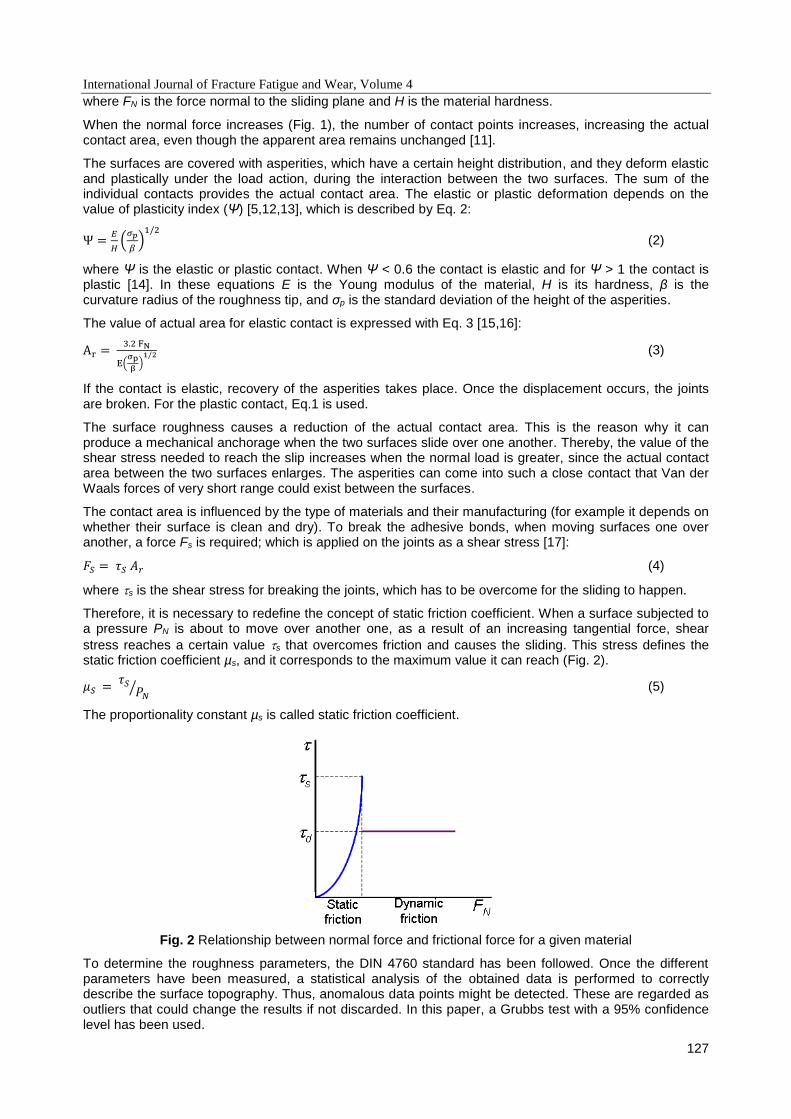
International Journal of Fracture Fatigue and Wear, Volume 4
127
where FN is the force normal to the sliding plane and H is the material hardness.
When the normal force increases (Fig. 1), the number of contact points increases, increasing the actual contact area, even though the apparent area remains unchanged [11].
The surfaces are covered with asperities, which have a certain height distribution, and they deform elastic and plastically under the load action, during the interaction between the two surfaces. The sum of the individual contacts provides the actual contact area. The elastic or plastic deformation depends on the value of plasticity index (Ψ) [5,12,13], which is described by Eq. 2:
Ψ =𝐸
𝐻(
𝜎𝑝
𝛽)
1/2
(2)
where Ψ is the elastic or plastic contact. When Ψ < 0.6 the contact is elastic and for Ψ > 1 the contact is plastic [14]. In these equations E is the Young modulus of the material, H is its hardness, β is the curvature radius of the roughness tip, and σp is the standard deviation of the height of the asperities.
The value of actual area for elastic contact is expressed with Eq. 3 [15,16]:
Ar = 3.2 FN
E(σp
β)
1/2 (3)
If the contact is elastic, recovery of the asperities takes place. Once the displacement occurs, the joints are broken. For the plastic contact, Eq.1 is used.
The surface roughness causes a reduction of the actual contact area. This is the reason why it can produce a mechanical anchorage when the two surfaces slide over one another. Thereby, the value of the shear stress needed to reach the slip increases when the normal load is greater, since the actual contact area between the two surfaces enlarges. The asperities can come into such a close contact that Van der Waals forces of very short range could exist between the surfaces.
The contact area is influenced by the type of materials and their manufacturing (for example it depends on whether their surface is clean and dry). To break the adhesive bonds, when moving surfaces one over another, a force Fs is required; which is applied on the joints as a shear stress [17]:
𝐹𝑆 = 𝜏𝑆 𝐴𝑟 (4)
where s is the shear stress for breaking the joints, which has to be overcome for the sliding to happen.
Therefore, it is necessary to redefine the concept of static friction coefficient. When a surface subjected to a pressure PN is about to move over another one, as a result of an increasing tangential force, shear
stress reaches a certain value s that overcomes friction and causes the sliding. This stress defines the static friction coefficient µs, and it corresponds to the maximum value it can reach (Fig. 2).
𝜇𝑆 = 𝜏𝑆
𝑃𝑁⁄ (5)
The proportionality constant µs is called static friction coefficient.
Fig. 2 Relationship between normal force and frictional force for a given material
To determine the roughness parameters, the DIN 4760 standard has been followed. Once the different parameters have been measured, a statistical analysis of the obtained data is performed to correctly describe the surface topography. Thus, anomalous data points might be detected. These are regarded as outliers that could change the results if not discarded. In this paper, a Grubbs test with a 95% confidence level has been used.

International Journal of Fracture Fatigue and Wear, Volume 4
128
2. EXPERIMENTAL PROCEDURE
2.1 Materials
Table 1 summarises the materials used in this study along with their elastic modulus and apparent area.
Table 1 Materials used in this work [18]
Material Elastic modulus (MPa)
Apparent area (mm2)
LDPE 150 1853.7
HDPE 700 1427.5
PP 1400 1858.7
Silicone 10 2400.0
2.2 Determination of actual contact area
In order to compute the actual contact area, the roughness parameters have to be determined [19].The points of the surface were measured on each of the materials 10 times in random directions with a contact roughness device (Hommel Tester T500). Thereafter, a statistical study was carried out. The device filters the signal obtained and displays three graphs: profile, waviness and roughness.
It was considered that the contact between the two surfaces occurs through the touching of the asperities. It is over these waviness that the ridges height is determined (Fig. 3) as well as the curvature radius of the tips of the asperities are computed (Fig. 4).
Fig. 3 Determination of the height of the asperities
Fig. 4 Determining the radius of curvature of the asperities
2.3 Determination of Hardness
The hardness test was performed by Brinell test [20]. An indenter with a steel ball at the tip was used. The steel ball has a diameter (D) of 5 mm. The applied load (P) was 612.5 N for a duration of 30 seconds. The depth of the resulting deformation was measured and the surface area of the impression was calculated. The hardness is then expressed in MPa. In Fig. 5, traces of hardness test can be seen.
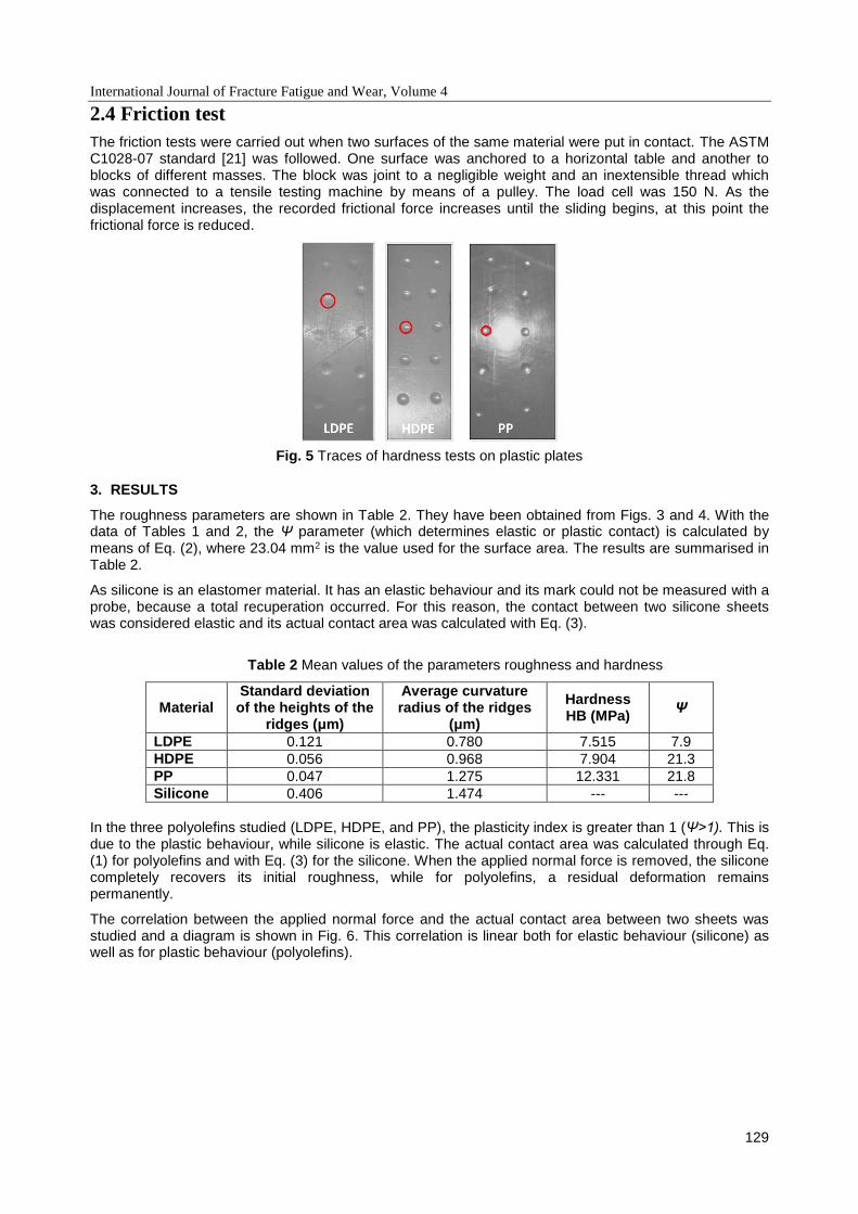
International Journal of Fracture Fatigue and Wear, Volume 4
129
2.4 Friction test
The friction tests were carried out when two surfaces of the same material were put in contact. The ASTM C1028-07 standard [21] was followed. One surface was anchored to a horizontal table and another to blocks of different masses. The block was joint to a negligible weight and an inextensible thread which was connected to a tensile testing machine by means of a pulley. The load cell was 150 N. As the displacement increases, the recorded frictional force increases until the sliding begins, at this point the frictional force is reduced.
Fig. 5 Traces of hardness tests on plastic plates
3. RESULTS
The roughness parameters are shown in Table 2. They have been obtained from Figs. 3 and 4. With the data of Tables 1 and 2, the Ψ parameter (which determines elastic or plastic contact) is calculated by means of Eq. (2), where 23.04 mm2 is the value used for the surface area. The results are summarised in Table 2.
As silicone is an elastomer material. It has an elastic behaviour and its mark could not be measured with a probe, because a total recuperation occurred. For this reason, the contact between two silicone sheets was considered elastic and its actual contact area was calculated with Eq. (3).
Table 2 Mean values of the parameters roughness and hardness
Material Standard deviation of the heights of the
ridges (μm)
Average curvature radius of the ridges
(μm)
Hardness HB (MPa)
Ψ
LDPE 0.121 0.780 7.515 7.9
HDPE 0.056 0.968 7.904 21.3
PP 0.047 1.275 12.331 21.8
Silicone 0.406 1.474 --- ---
In the three polyolefins studied (LDPE, HDPE, and PP), the plasticity index is greater than 1 (Ψ>1). This is due to the plastic behaviour, while silicone is elastic. The actual contact area was calculated through Eq. (1) for polyolefins and with Eq. (3) for the silicone. When the applied normal force is removed, the silicone completely recovers its initial roughness, while for polyolefins, a residual deformation remains permanently.
The correlation between the applied normal force and the actual contact area between two sheets was studied and a diagram is shown in Fig. 6. This correlation is linear both for elastic behaviour (silicone) as well as for plastic behaviour (polyolefins).
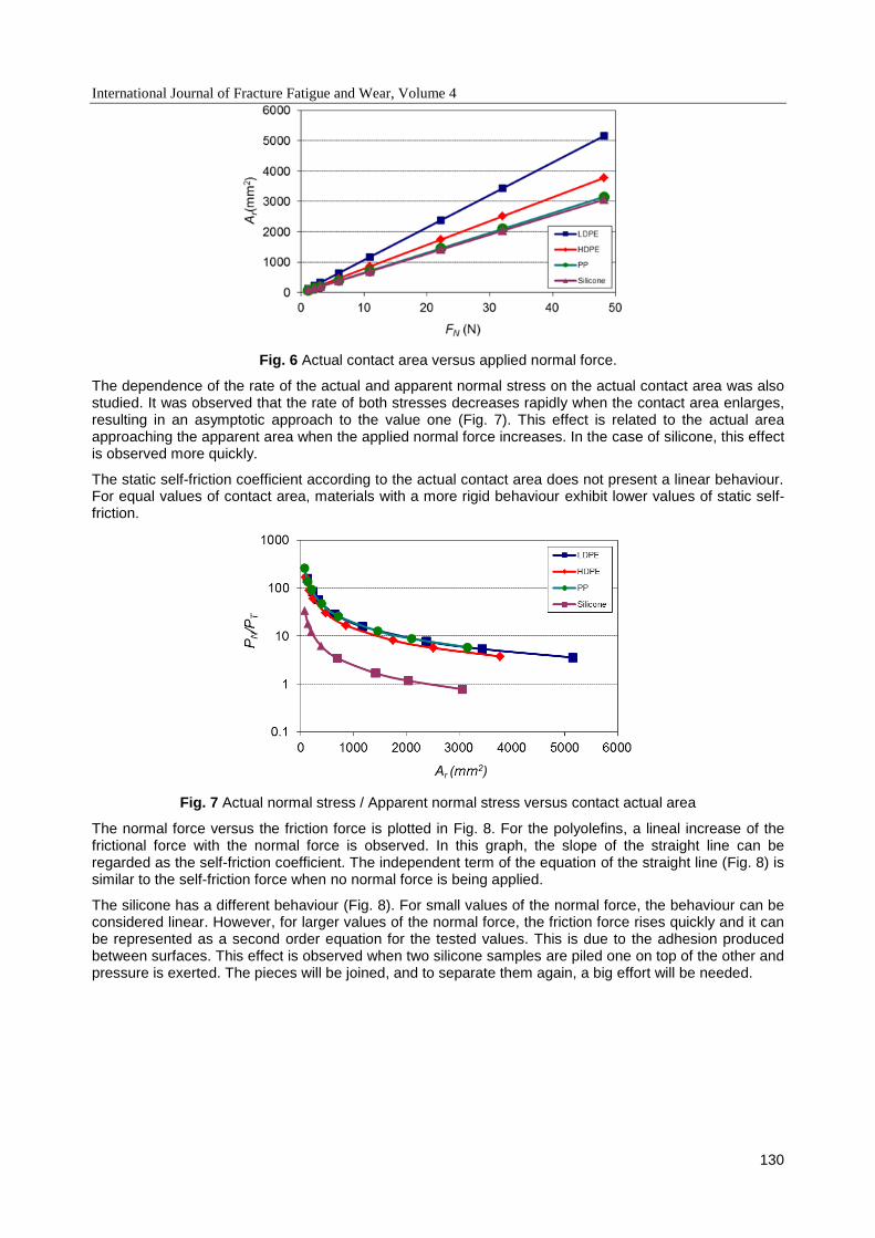
International Journal of Fracture Fatigue and Wear, Volume 4
130
Fig. 6 Actual contact area versus applied normal force.
The dependence of the rate of the actual and apparent normal stress on the actual contact area was also studied. It was observed that the rate of both stresses decreases rapidly when the contact area enlarges, resulting in an asymptotic approach to the value one (Fig. 7). This effect is related to the actual area approaching the apparent area when the applied normal force increases. In the case of silicone, this effect is observed more quickly.
The static self-friction coefficient according to the actual contact area does not present a linear behaviour. For equal values of contact area, materials with a more rigid behaviour exhibit lower values of static self-friction.
Fig. 7 Actual normal stress / Apparent normal stress versus contact actual area
The normal force versus the friction force is plotted in Fig. 8. For the polyolefins, a lineal increase of the frictional force with the normal force is observed. In this graph, the slope of the straight line can be regarded as the self-friction coefficient. The independent term of the equation of the straight line (Fig. 8) is similar to the self-friction force when no normal force is being applied.
The silicone has a different behaviour (Fig. 8). For small values of the normal force, the behaviour can be considered linear. However, for larger values of the normal force, the friction force rises quickly and it can be represented as a second order equation for the tested values. This is due to the adhesion produced between surfaces. This effect is observed when two silicone samples are piled one on top of the other and pressure is exerted. The pieces will be joined, and to separate them again, a big effort will be needed.
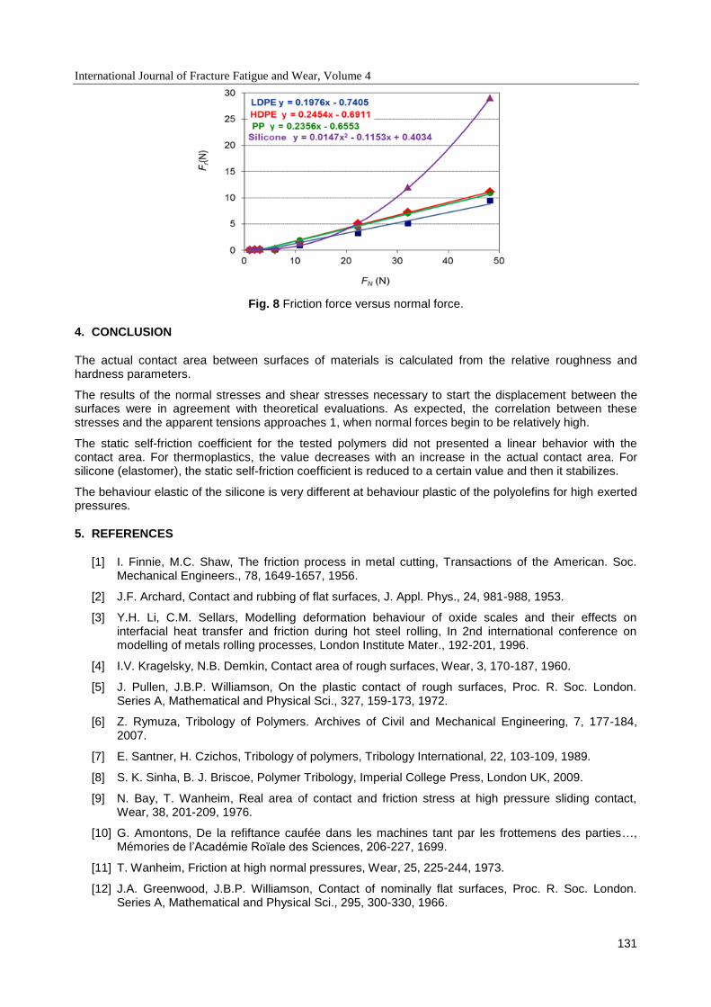
International Journal of Fracture Fatigue and Wear, Volume 4
131
Fig. 8 Friction force versus normal force.
4. CONCLUSION
The actual contact area between surfaces of materials is calculated from the relative roughness and hardness parameters.
The results of the normal stresses and shear stresses necessary to start the displacement between the surfaces were in agreement with theoretical evaluations. As expected, the correlation between these stresses and the apparent tensions approaches 1, when normal forces begin to be relatively high.
The static self-friction coefficient for the tested polymers did not presented a linear behavior with the contact area. For thermoplastics, the value decreases with an increase in the actual contact area. For silicone (elastomer), the static self-friction coefficient is reduced to a certain value and then it stabilizes.
The behaviour elastic of the silicone is very different at behaviour plastic of the polyolefins for high exerted pressures.
5. REFERENCES
[1] I. Finnie, M.C. Shaw, The friction process in metal cutting, Transactions of the American. Soc. Mechanical Engineers., 78, 1649-1657, 1956.
[2] J.F. Archard, Contact and rubbing of flat surfaces, J. Appl. Phys., 24, 981-988, 1953.
[3] Y.H. Li, C.M. Sellars, Modelling deformation behaviour of oxide scales and their effects on interfacial heat transfer and friction during hot steel rolling, In 2nd international conference on modelling of metals rolling processes, London Institute Mater., 192-201, 1996.
[4] I.V. Kragelsky, N.B. Demkin, Contact area of rough surfaces, Wear, 3, 170-187, 1960.
[5] J. Pullen, J.B.P. Williamson, On the plastic contact of rough surfaces, Proc. R. Soc. London. Series A, Mathematical and Physical Sci., 327, 159-173, 1972.
[6] Z. Rymuza, Tribology of Polymers. Archives of Civil and Mechanical Engineering, 7, 177-184, 2007.
[7] E. Santner, H. Czichos, Tribology of polymers, Tribology International, 22, 103-109, 1989.
[8] S. K. Sinha, B. J. Briscoe, Polymer Tribology, Imperial College Press, London UK, 2009.
[9] N. Bay, T. Wanheim, Real area of contact and friction stress at high pressure sliding contact, Wear, 38, 201-209, 1976.
[10] G. Amontons, De la refiftance caufée dans les machines tant par les frottemens des parties…, Mémories de l’Académie Roïale des Sciences, 206-227, 1699.
[11] T. Wanheim, Friction at high normal pressures, Wear, 25, 225-244, 1973.
[12] J.A. Greenwood, J.B.P. Williamson, Contact of nominally flat surfaces, Proc. R. Soc. London. Series A, Mathematical and Physical Sci., 295, 300-330, 1966.
International Journal of Fracture Fatigue and Wear, Volume 4
132
[13] J.A. Greenwood, The real area of contact between rough surfaces and flats, J. Lub. Technol. (ASME) 1, 81-91, 1967.
[14] J.A. Willians, R.S. Dwyer-Joyce, Contact between solid surfaces, Moden Tribology Handbook. B. Bhushan editor, CRC Press, New York USA, 1, 121-162, 2001.
[15] N.P. Shu, Tribophysics, Prentice-Hall Inc., New York USA, 498-499, 1986.
[16] B. Bhushan, B. K. Gupta, Handbook of Tribology: Materials, Coatings and Surface Treatments. Krieger Publishing Co., Melbourne USA 1997.
[17] F.P. Bowden, D. Tabor, The Friction and Lubrication of Solids, Part I J. Appl. Phys., 6, 79-81, 1950.
[18] M.P. Groover, Fundamentals of Modern Manufacturing, Prentice-Hall Inc., New York USA, 1997.
[19] EN-ISO 4287. Geometrical Product Specifications (GPS) - Surface texture: Profile method - Terms, definitions and surface texture parameters.
[20] ISO 2039-1:2001 Plastics - Determination of hardness - Part 1: Ball indentation method.
[21] ASTM C1028 - 07 (EN ISO 10545 - Part 17): Standard Test Method for Determining the Static Coefficient of Friction of Ceramic Tile and Other Like Surfaces by the Horizontal Dynamometer Pull-Meter Method.

International Journal of Fracture Fatigue and Wear, Volume 4
133
Proceedings of the 5th International Conference
Fracture Fatigue and Wear, pp. 133-138, 2016
STUDY ON TEST OF FATIGUE CRACK GROWTH RATE ALONG THE
WELD LINE
Z. Qian and R. Zhang
Northeastern University, School of Mechanical Engineering and Automation, China
Abstract: As plate welded aluminium alloy structure are widely used in the field of aviation and rail transit,
the fatigue crack along the weld line due to inevitable welding defect is one kind of failure type in the engineering. However, the current national test standards of crack growth rate are all based on the homogeneous specimens. Few experimental researches could be found on fracture mechanics analysis of the fatigue crack along weld line. In this paper, the experimental method of fatigue crack growth rate along the weld line was studied by taking account of the inhomogeneous mechanical properties of weld joint. At first, a three regional model was used to study the effect of different mechanical properties at weld joint on SIF (Stress Intensity Factor). Then, the specimen of fatigue crack growth rate along the weld line was designed, and a modified functional relationship between the SIF of the weld line and crack length could be got by using FEM simulation method. Further, the constants C and m values of Paris equation and the formula of fatigue crack growth rate along weld line were obtained based on experimental and simulation results.
Keywords: fatigue crack; growth rate; weld line; finite element analysis; SIF
1 INTRODUCTION
Because of low density, good mechanical properties and processing performance of aluminium, plate welded aluminum alloy structures are widely used in the field of aviation and rail transit [1]. Due to local re-melting, the size of the grains in the weld zone can be different from those of the base metal. The disparity between grain sizes results in different yield stresses and, thus, reduced strength (Hall-Petch relationship). For steel alloys, the weld strength is higher or, at least, equal to the base metal strength. It is not the case for aluminium alloys [2-3]. However, the failure of the weld structure in engineering is mainly caused by fatigue under cyclic loading. It could be attributed to the residual stress and the inevitable defects due to welding processing [4-9].
Many researches are available on fatigue of the welded structures and the welding line. P. Dong [10-11] carried out the fatigue analysis of the weld components based on the structural strain method and the master S-N curve method. It is formulated by taking advantage of elastically calculated mesh-insensitive structural stresses based on nodal forces available from finite element solutions, and is shown effective in correlating low-cycle fatigue test data of various sources documented in the literature. X. Wu [12] studied the SIF at crack tip based on the finite element method. It turned out that there is a close relationship between the yield strength and the SIF at the tip of crack. The SIF was the lowest one in the welding zone, then it followed in the base metal, and the highest one was in the HAZ (Heat Affected Zone). However, for the fatigue crack propagating along weld line, few literatures can be found on the experimental method to research fracture properties of the weld structure, as the current test standards of crack growth rate are always based on the homogeneous specimens.
The crack growth rate, denoted da/dN is an important material property to characterize fatigue crack propagation under constant amplitude loading, which is one of necessary preconditions to assess fatigue crack propagation life . In this paper, the experimental method of fatigue crack growth rate along the weld line was studied by taking account of the different mechanical properties at weld joint. The fracture mechanics simulation was carried out to obtain the new relationship function between the correctional SIF K and the crack length a based on FEM. Finally, the fatigue crack growth rate model along the weld was obtained based on experimental results.

International Journal of Fracture Fatigue and Wear, Volume 4
134
2 CRACK GROWTH EXPERIMENT ALONG THE WELD LINE
Three single edge crack bending specimens SE(B) were cut from a 7N01 aluminium alloy weld structure. The weld line was located at the centre of specimen, and a notch was fabricated by wire-electrode cutting on weld line at one edge of the specimen. The shape and the details of specimen are given in Fig. 1, which dimensions are in millimetres and similar as standard test specimen refer to “GB/T6398-2000 Metal materials fatigue crack growth rate test method”. The specimen was subjected to three-point bend loading (as shown in Fig. 2). The loads were applied at two end of upper edge of specimen, and the support was at the centre point of bottom edge.
Fig. 1 Crack growth rate SE(B) test specimen
The experiments were carried out by using an Instron 8872 electro-hydraulic servo material fatigue test machine with 25 kN load capacity. The specimens were tested with a stress ratio of R = 0.1, the load frequency of 10 Hz, and the constant load amplitude ΔP of 2.4kN in the steady crack propagation region. The crack length a were measured using COD gauge based on compliance method, the number of loading cycle N and the loads P were automatically collected by the software of fatigue test machine. Thus the crack growth rate da/dN was calculated based on the crack length a and the cycle number N by using seven points incremental polynomial method.
3 FRACTURE MECHANICS SIMULATION ALONG THE WELD CRACK
3.1 Finite element model
In the national standard “GB/T6398-2000 Metal materials fatigue crack growth rate test method”, the SIF K for a homogeneous metallic SE(B) specimen could be calculated using a formula in national standard. In fact, the specimen in this paper had different mechanical properties in three regions including weld line, HAZ, and base metal, so influent of inhomogeneous mechanical property on the SIF along weld line should be studies by using FEM simulation method.
A finite element model including three regions was established according to SE(B) specimen as shown
in Fig.3. As the high stress gradients exist around the crack tip in the weld region, a special singular element type with the midside nodes placed at the quarter points was used around the crack tip. As same as the experimental condition, the load was applied on the centre of upper side of the model, and the constrains were applied on the two ends of bottom side of the model.
Fig. 2 Three-point bend loading apparatus Fig. 3 Finite element model of SE(B) specimen
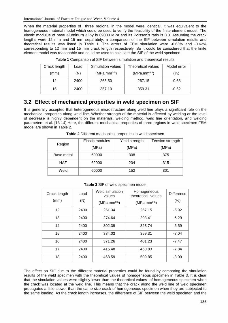
International Journal of Fracture Fatigue and Wear, Volume 4
135
When the material properties of three regional in the model were identical, it was equivalent to the homogeneous material model which could be used to verify the feasibility of the finite element model. The
elastic modulus of base aluminum alloy is 69000 MPa and its Poisson’s ratio is 0.3. Assuming the crack
lengths were 12 mm and 15 mm separately, a comparison of the SIF between simulation results and theoretical results was listed in Table 1. The errors of FEM simulation were -0.63% and -0.62% corresponding to 12 mm and 15 mm crack length respectively. So it could be considered that the finite element model was reasonable and could be used to calculate the SIF of the weld specimen.
Table 1 Comparison of SIF between simulation and theoretical results
Crack length
(mm)
Load
(N)
Simulation values
(MPa.mm0.5)
Theoretical values
(MPa.mm0.5)
Model error
(%)
12 2400 265.50 267.15 -0.63
15 2400 357.10 359.31 -0.62
3.2 Effect of mechanical properties in weld specimen on SIF
It is generally accepted that heterogeneous microstructure along weld line plays a significant role on the mechanical properties along weld line. Whether strength of the material is affected by welding or the level of decrease is highly dependent on the materials, welding method, weld line orientation, and welding parameters et al. [13-14] Here, the different mechanical properties of three regions in weld specimen FEM model are shown in Table 2.
Table 2 Different mechanical properties in weld specimen
Region Elastic modules
(MPa)
Yield strength
(MPa)
Tension strength
(MPa)
Base metal 69000 308 375
HAZ 62000 204 315
Weld 60000 152 301
Table 3 SIF of weld specimen model
Crack length
(mm)
Load
(N)
Weld simulation values
(MPa.mm0.5)
Homogeneous theoretical values
(MPa.mm0.5)
Difference
(%)
12 2400 251.34 267.15 -5.92
13 2400 274.64 293.41 -6.29
14 2400 302.39 323.74 -6.59
15 2400 334.03 359.31 -7.04
16 2400 371.26 401.23 -7.47
17 2400 415.48 450.83 -7.84
18 2400 468.59 509.85 -8.09
The effect on SIF due to the different material properties could be found by comparing the simulation results of the weld specimen with the theoretical values of homogeneous specimen in Table 3. It is clear that the simulation values were slightly lower than the theoretical values of homogeneous specimen when the crack was located at the weld line. This means that the crack along the weld line of weld specimen propagates a little slower than the same size crack of homogeneous specimen when they are subjected to the same loading. As the crack length increases, the difference of SIF between the weld specimen and the

International Journal of Fracture Fatigue and Wear, Volume 4
136
homogeneous metal specimen increases from -5.92% of crack with length 12 mm to -8.09% of crack with length 18 mm. Therefore, the influence of the weld material differences on the SIF could not be ignored, and the relationship between the SIF K and the crack length a should be modified.
3.3 Modified formula of the weld SIF
According to the relevant national standards, the theoretical formula of SIF at the crack tip of standard SE(B) specimen is:
aFBw
aPK I
4 (1)
Here, P is the load (N), a is the crack length (mm), B is the specimen thickness (mm), w is the specimen width (mm), and F(a) is the geometry corrected factor.
For the weld specimen, both the geometry dimension and the difference of mechanical material should be considered in the formula. So the factor F(a) should be modified in terms of the crack length a based on the simulation results of the weld specimen. According to Eq.(1), the factor F(a) could be calculated by
aP
BwKaF I
4)( (2)
Table 4 Relationship between a and F
Crack length
(mm) 12 13 14 15 16 17 18
F 2.948 3.094 3.283 3.504 3.771 4.094 4.487
Then, a series of SIF KI could be obtained dependant on the crack length a by using simulation method. The modified corrected factor F(a) values in relation to the crack length a were shown in Table 4. The formula of F(a) of the weld specimen could be obtained by polynomial fitting the simulation data, as shown in Fig.4 and Eq. (3).
F(a)=12.7-2.9a+0.03a2-0.01a3+2.5e-4a4 (3)
Fig. 4 Curve fitting of F-a
It should be noted that the modified corrected factor F(a) is obtained based on the FEM simulation values, which are dependent on a proper FEM model and accurate material properties of weld structure. These include the base metal material, welding methods, welding parameters, the thickness ratio, welding quality et al.
4 FATIGUE CRACK GROWTH RATE MODEL OF WELD STRUCTURE
Fatigue crack growth rate expressed as a function of crack-tip SIF range, da/dN versus ΔK, characterizes a material's resistance to stable crack extension under cyclic loading. Based on the experimental results,
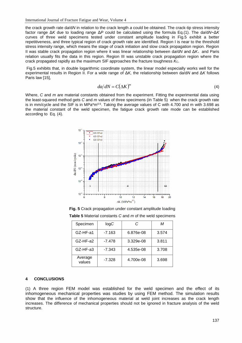
International Journal of Fracture Fatigue and Wear, Volume 4
137
the crack growth rate da/dN in relation to the crack length a could be obtained. The crack-tip stress intensity factor range ΔK due to loading range ΔP could be calculated using the formula Eq.(1). The da/dN~ΔK curves of three weld specimens tested under constant amplitude loading in Fig.5 exhibit a better repetitiveness, and three typical region of crack growth rate are identified. Region I is near to the threshold stress intensity range, which means the stage of crack initiation and slow crack propagation region. Region
II was stable crack propagation region where it was linear relationship between da/dN and ΔK,and Paris
relation usually fits the data in this region. Region III was unstable crack propagation region where the crack propagated rapidly as the maximum SIF approaches the fracture toughness KC.
Fig.5 exhibits that, in double logarithmic coordinate system, the linear model especially works well for the experimental results in Region II. For a wide range of ΔK, the relationship between da/dN and ΔK follows Paris law [15],
mKCdNda (4)
Where, C and m are material constants obtained from the experiment. Fitting the experimental data using
the least-squared method gets C and m values of three specimens (in Table 5) when the crack growth rate
is in mm/cycle and the SIF is in MPa*m0.5. Taking the average values of C with 4.700 and m with 3.698 as the material constant of the weld specimen, the fatigue crack growth rate mode can be established according to Eq. (4).
Fig. 5 Crack propagation under constant amplitude loading
Table 5 Material constants C and m of the weld specimens
Specimen logC C M
GZ-HF-a1 -7.163 6.876e-08 3.574
GZ-HF-a2 -7.478 3.329e-08 3.811
GZ-HF-a3 -7.343 4.535e-08 3.708
Average values
-7.328 4.700e-08 3.698
4 CONCLUSIONS
(1) A three region FEM model was established for the weld specimen and the effect of its inhomogeneous mechanical properties was studies by using FEM method. The simulation results show that the influence of the inhomogeneous material at weld joint increases as the crack length increases. The difference of mechanical properties should not be ignored in fracture analysis of the weld structure.
International Journal of Fracture Fatigue and Wear, Volume 4
138
(2) According to the national test standard of homogeneous metallic specimen, the weld specimen of fatigue crack growth rate along the weld line was designed, and a new test method of weld structure was given by combining experimental method with FEM simulation.
(3) Using 7N01 aluminium alloy weld specimens, the fatigue crack growth rate test was completed, and a modified relationship between the SIF and crack length was obtained by using simulation method. Then, the model of fatigue crack growth rate along the weld was established.
5 ACKNOWLEDGEMENTS
This research is subsidized by the Natural Science Foundation of China “Study on reliability modeling and
simulation of mechanical structure of aero engine” (Grant No.51335003)
6 REFERENCES
[1] T. HATAYAMA, Research and development of aluminum extrusion alloy products for shinkansen
train coach, Kobe Steel Engineering Reports, 58(3), 55-61, 2008
[2] P.A. Friedman, G.T. Kridli, Microstructural and mechanical investigation of aluminum tailor-welded
blanks, Journal of Materials Engineering and Performance, 9(5), 541-551, 2000
[3] A.A. Zadpoor, J. Sinke, R. Benedictus, Mechanics of Tailor Welded Blanks: An Overview, Key
Engineering Materials, vol. 344, 373-382, 2007
[4] W. Fricke, Fatigue analysis of welded joints: state of development, Marine Structures, 16(3), 185-
200, 2003.
[5] TR. Gumey, SJ. Maddox, A re-analysis of fatigue data for welded joints in steel, Welding Research
Int, 3(4), 1-54, 1973.
[6] T. Nykänen, G. Marquis, T. Björk, Fatigue analysis of non-load-carrying fillet welded cruciform
joints, Engineering Fracture Mechanics, 74(3), 399-415, 2007.
[7] S. Kainuma, Y. Kusumoto, N. Hosomi, I. Kim, Fatigue behaviour of load-carrying, fillet-welded,
cruciform joints with plates of different thickness, Welding International, 19(8), 608-616, 2005.
[8] JH. Devletian, Failure Analysis of Steel Welds, Failure Analysis of Heat Treated Steel Components,
L.C.F. Canale, R.A. Mesquita, and G.E. Totten, editors, pp. 503-519, ASM international, 2008
[9] D.A. Lados, D. Apelian, The Effect of Residual Stress on the Fatigue Crack Growth Behavior of Al-
Si-Mg Cast Alloys -Mechanisms and Corrective Mathematical Models. Metallurgical and Materials
Transactions A-Physical Metallurgy and Materials Science, 37A, 133-145, 2006.
[10] P. Dong, J.K. Hong, D.A. Osage, M. Prager, Master S-N curve method for fatigue evaluation of
welded components, Welding Research Council Bulletin, vol.474, 1-44, 2002
[11] P. Dong, X. Pei, S. Xing, MH. Kim, A structural strain method for fatigue evaluation of welded
components, International Journal of Pressure Vessels & Piping, 119(4), 39-51, 2014
[12] X. Wu, L. Hui, S. Zhou, The Study in Stress Intensity Factor of Crack Tip Based on ANSYS.
Mechanical Engineer, 2011(1): 42-43.
[13] R.W. Davies, M.T. Smith, H.E. Oliver, M.A. Khaleel, S.G. Pitman, Weld metal ductility in aluminum
tailor welded blanks, Metallurgical and Materials Transactions A: Physical Metallurgy and Materials
Science, 31(11), 2755-2763, 2000
[14] C.H. Cheng, L.C. Chan, C.L. Chow, T.C. Lee, Experimental investigation on the weldability and
forming behavior of aluminum alloy tailor-welded blanks, Journal of Laser Applications, 17(2), 81-
88, 2005
[15] P.C. Paris, F. Erdogan, A critical analysis of crack propagation laws. Journal of Basic Engineering,
85, 528-534, 1963.
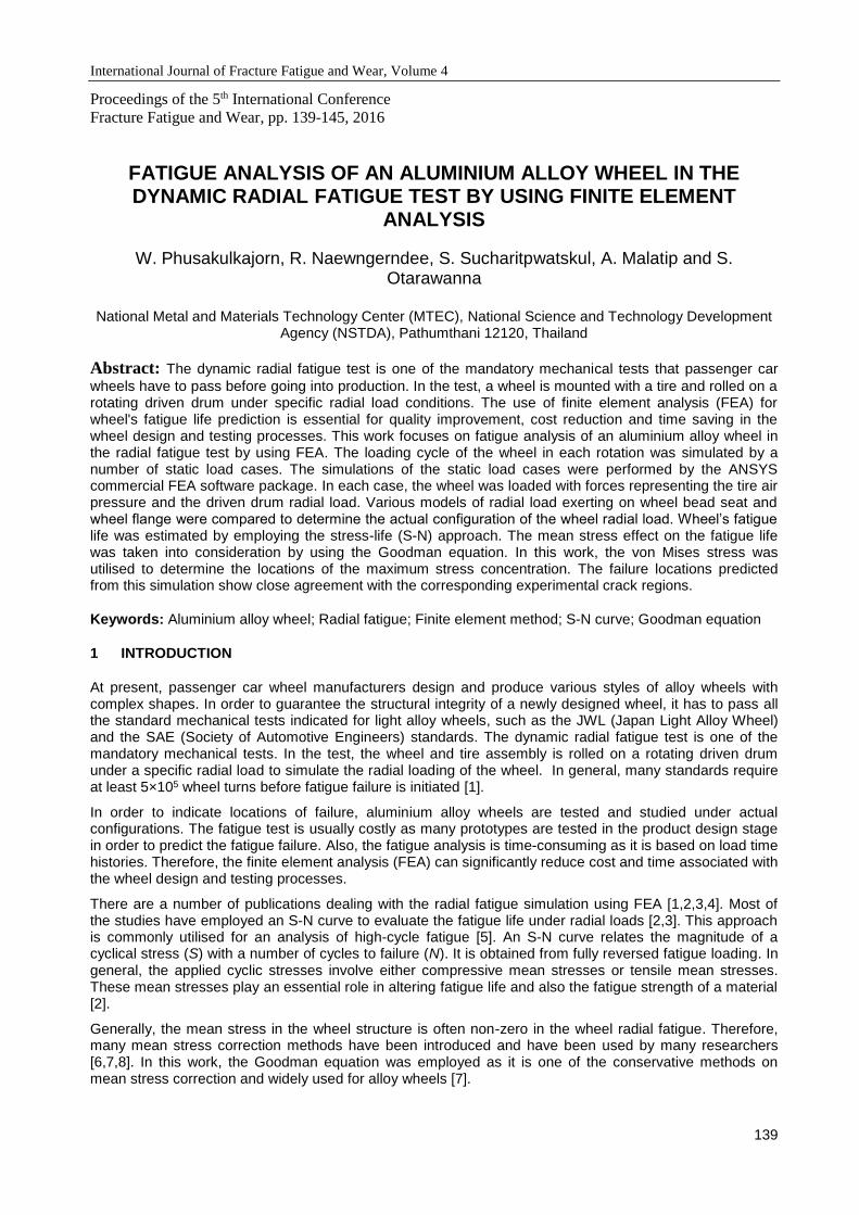
International Journal of Fracture Fatigue and Wear, Volume 4
139
Proceedings of the 5th International Conference
Fracture Fatigue and Wear, pp. 139-145, 2016
FATIGUE ANALYSIS OF AN ALUMINIUM ALLOY WHEEL IN THE DYNAMIC RADIAL FATIGUE TEST BY USING FINITE ELEMENT
ANALYSIS
W. Phusakulkajorn, R. Naewngerndee, S. Sucharitpwatskul, A. Malatip and S. Otarawanna
National Metal and Materials Technology Center (MTEC), National Science and Technology Development
Agency (NSTDA), Pathumthani 12120, Thailand
Abstract: The dynamic radial fatigue test is one of the mandatory mechanical tests that passenger car
wheels have to pass before going into production. In the test, a wheel is mounted with a tire and rolled on a rotating driven drum under specific radial load conditions. The use of finite element analysis (FEA) for wheel's fatigue life prediction is essential for quality improvement, cost reduction and time saving in the wheel design and testing processes. This work focuses on fatigue analysis of an aluminium alloy wheel in the radial fatigue test by using FEA. The loading cycle of the wheel in each rotation was simulated by a number of static load cases. The simulations of the static load cases were performed by the ANSYS commercial FEA software package. In each case, the wheel was loaded with forces representing the tire air pressure and the driven drum radial load. Various models of radial load exerting on wheel bead seat and wheel flange were compared to determine the actual configuration of the wheel radial load. Wheel’s fatigue life was estimated by employing the stress-life (S-N) approach. The mean stress effect on the fatigue life was taken into consideration by using the Goodman equation. In this work, the von Mises stress was utilised to determine the locations of the maximum stress concentration. The failure locations predicted from this simulation show close agreement with the corresponding experimental crack regions.
Keywords: Aluminium alloy wheel; Radial fatigue; Finite element method; S-N curve; Goodman equation
1 INTRODUCTION
At present, passenger car wheel manufacturers design and produce various styles of alloy wheels with complex shapes. In order to guarantee the structural integrity of a newly designed wheel, it has to pass all the standard mechanical tests indicated for light alloy wheels, such as the JWL (Japan Light Alloy Wheel) and the SAE (Society of Automotive Engineers) standards. The dynamic radial fatigue test is one of the mandatory mechanical tests. In the test, the wheel and tire assembly is rolled on a rotating driven drum under a specific radial load to simulate the radial loading of the wheel. In general, many standards require at least 5×10⁵ wheel turns before fatigue failure is initiated [1].
In order to indicate locations of failure, aluminium alloy wheels are tested and studied under actual configurations. The fatigue test is usually costly as many prototypes are tested in the product design stage in order to predict the fatigue failure. Also, the fatigue analysis is time-consuming as it is based on load time histories. Therefore, the finite element analysis (FEA) can significantly reduce cost and time associated with the wheel design and testing processes.
There are a number of publications dealing with the radial fatigue simulation using FEA [1,2,3,4]. Most of the studies have employed an S-N curve to evaluate the fatigue life under radial loads [2,3]. This approach is commonly utilised for an analysis of high-cycle fatigue [5]. An S-N curve relates the magnitude of a cyclical stress (S) with a number of cycles to failure (N). It is obtained from fully reversed fatigue loading. In general, the applied cyclic stresses involve either compressive mean stresses or tensile mean stresses. These mean stresses play an essential role in altering fatigue life and also the fatigue strength of a material [2].
Generally, the mean stress in the wheel structure is often non-zero in the wheel radial fatigue. Therefore, many mean stress correction methods have been introduced and have been used by many researchers [6,7,8]. In this work, the Goodman equation was employed as it is one of the conservative methods on mean stress correction and widely used for alloy wheels [7].

International Journal of Fracture Fatigue and Wear, Volume 4
140
The goal of this paper is to present and discuss the loads and boundary conditions applied on the aluminium alloy wheel presented in Fig. 2. Finite element analysis was carried out in the ANSYS commercial software package to analyse failure of an aluminium alloy wheel in the radial fatigue test. The obtained stress distribution and the failure initiation area were compared with the corresponding experimental observations.
2 THE WHEEL RADIAL FATIGUE ANALYSIS
2.1 The dynamic radial fatigue test
In the radial fatigue test, the wheel was mounted with a tire and rolled on a rotating driven drum under specific radial load conditions as shown in Fig. 1. For the wheel of our consideration, shown in Fig. 2, it is considered to pass the JWL standard test if no cracks are observed after 5×10⁵ wheel turns for the load of 2,621.5 kg.
In this test, the wheel failed after 5×10⁵ wheel turns. Cracks were observed at the contact between the rim and the spoke located on the outboard side of the wheel as depicted in Fig. 2.
Fig. 1 Wheel radial fatigue test setup
Fig. 2 The location of cracks obtained from the wheel radial fatigue test
2.2 Material properties
The wheel was low pressure die cast from A356.2 aluminium alloy and heat treated to the T6 condition. In order to find the mechanical properties of this wheel, tensile test was carried out from specimens taken from different locations of the wheel. Table 1 shows the mechanical properties of the wheel after the test was conducted.

International Journal of Fracture Fatigue and Wear, Volume 4
141
In order to approximate the fatigue properties of the wheel in this work, the S-N curve of a similar material was employed from the work of Raju et al. [2]. The graph in Fig. 3 shows that the stress must be less than 130 MPa in order for the wheel to tolerate 5×10⁵ cycles. It is noted that the S-N curve in Fig. 3 was from the wheel specimens having the tensile strength of 250 MPa [2]. Assuming that fatigue strength is proportional to the tensile strength, the fatigue strength at 5×10⁵ cycles of our wheel is, approximately, 122 MPa.
Generally, there should be a difference between the result obtained from the experiment and the simulation. Raju et al. [2] showed in their work that some safety factors were introduced to correlate the experimental results with the finite element analysis. This is consistent with the work of Topaҫ et al. [1] that employed the Marin factors to correct the effects of manufacturing parameters. By using the endurance limit modifying factor introduced in Marin equation described in [1], the true fatigue strength of our material is, approximately, 103 MPa for 5×10⁵ wheel turns.
Table 1 Material properties of the aluminium alloy wheel
Material Young’s modulus
(GPa)
Yield strength
(MPa)
Tensile strength
(MPa)
A365.2-T6 72 145 235
Fig. 3 The S-N curve of the aluminium alloy wheels (modified from [2])
2.3 Finite element model
The ANSYS commercial FEA software package was employed to analyse failure of aluminium alloy wheels in the radial fatigue test. The wheel was modelled by tetrahedral elements. An element size of 5 mm was used to mesh the model with 378,759 elements and 642,380 nodes.
2.3.1 Loads and Boundary conditions
The loads and boundary conditions on the aluminium alloy wheel considered throughout this work were elaborated. According to the JWL standard test, the load of 2,621.5 kg (25,691 N) was applied on the wheel. The wheel was loaded with forces representing the tire air pressure and the driven drum radial loads. These represented both static and fatigue loads on the wheel.
For the static load, the tire air pressure was taken into account by applying a uniform pressure of 0.46 MPa on the rim area located between the inboard and the outboard bead seats. In order to indicate the fatigue load from the driven drum, the radial load was exerted on the tire bead seat for both inner and outer circumferences in which its distributed profile was represented by the cosine function. The central angle of the load distribution was 80° as suggested in the work of Raju et al. [2]. With respect to the wheel offset, the driven drum load of 25,691 N was generated on the inboard and outboard sides of the wheel with radial loads of 10,204 and 15,487 N, respectively. The contact surfaces between the nut-wheel disc and the wheel disc-brake drum were fixed, as suggested in Ref. [4]. These boundary conditions are illustrated in Fig. 4.
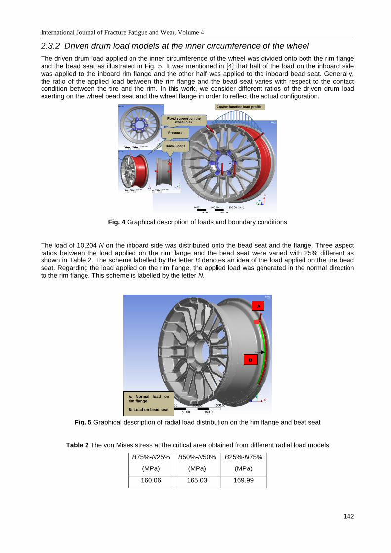
International Journal of Fracture Fatigue and Wear, Volume 4
142
2.3.2 Driven drum load models at the inner circumference of the wheel
The driven drum load applied on the inner circumference of the wheel was divided onto both the rim flange and the bead seat as illustrated in Fig. 5. It was mentioned in [4] that half of the load on the inboard side was applied to the inboard rim flange and the other half was applied to the inboard bead seat. Generally, the ratio of the applied load between the rim flange and the bead seat varies with respect to the contact condition between the tire and the rim. In this work, we consider different ratios of the driven drum load exerting on the wheel bead seat and the wheel flange in order to reflect the actual configuration.
Fig. 4 Graphical description of loads and boundary conditions
The load of 10,204 N on the inboard side was distributed onto the bead seat and the flange. Three aspect ratios between the load applied on the rim flange and the bead seat were varied with 25% different as shown in Table 2. The scheme labelled by the letter B denotes an idea of the load applied on the tire bead seat. Regarding the load applied on the rim flange, the applied load was generated in the normal direction to the rim flange. This scheme is labelled by the letter N.
Fig. 5 Graphical description of radial load distribution on the rim flange and beat seat
Table 2 The von Mises stress at the critical area obtained from different radial load models
B75%-N25%
(MPa)
B50%-N50%
(MPa)
B25%-N75%
(MPa)
160.06 165.03 169.99
A: Normal load on rim flange
B: Load on bead seat
A
B
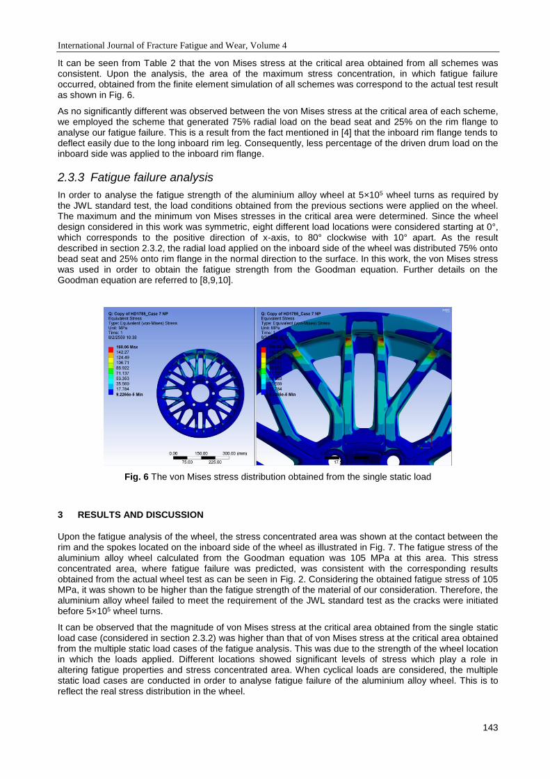
International Journal of Fracture Fatigue and Wear, Volume 4
143
It can be seen from Table 2 that the von Mises stress at the critical area obtained from all schemes was consistent. Upon the analysis, the area of the maximum stress concentration, in which fatigue failure occurred, obtained from the finite element simulation of all schemes was correspond to the actual test result as shown in Fig. 6.
As no significantly different was observed between the von Mises stress at the critical area of each scheme, we employed the scheme that generated 75% radial load on the bead seat and 25% on the rim flange to analyse our fatigue failure. This is a result from the fact mentioned in [4] that the inboard rim flange tends to deflect easily due to the long inboard rim leg. Consequently, less percentage of the driven drum load on the inboard side was applied to the inboard rim flange.
2.3.3 Fatigue failure analysis
In order to analyse the fatigue strength of the aluminium alloy wheel at 5×10⁵ wheel turns as required by the JWL standard test, the load conditions obtained from the previous sections were applied on the wheel. The maximum and the minimum von Mises stresses in the critical area were determined. Since the wheel design considered in this work was symmetric, eight different load locations were considered starting at 0°, which corresponds to the positive direction of x-axis, to 80° clockwise with 10° apart. As the result described in section 2.3.2, the radial load applied on the inboard side of the wheel was distributed 75% onto bead seat and 25% onto rim flange in the normal direction to the surface. In this work, the von Mises stress was used in order to obtain the fatigue strength from the Goodman equation. Further details on the Goodman equation are referred to [8,9,10].
Fig. 6 The von Mises stress distribution obtained from the single static load
3 RESULTS AND DISCUSSION
Upon the fatigue analysis of the wheel, the stress concentrated area was shown at the contact between the rim and the spokes located on the inboard side of the wheel as illustrated in Fig. 7. The fatigue stress of the aluminium alloy wheel calculated from the Goodman equation was 105 MPa at this area. This stress concentrated area, where fatigue failure was predicted, was consistent with the corresponding results obtained from the actual wheel test as can be seen in Fig. 2. Considering the obtained fatigue stress of 105 MPa, it was shown to be higher than the fatigue strength of the material of our consideration. Therefore, the aluminium alloy wheel failed to meet the requirement of the JWL standard test as the cracks were initiated before 5×10⁵ wheel turns.
It can be observed that the magnitude of von Mises stress at the critical area obtained from the single static load case (considered in section 2.3.2) was higher than that of von Mises stress at the critical area obtained from the multiple static load cases of the fatigue analysis. This was due to the strength of the wheel location in which the loads applied. Different locations showed significant levels of stress which play a role in altering fatigue properties and stress concentrated area. When cyclical loads are considered, the multiple static load cases are conducted in order to analyse fatigue failure of the aluminium alloy wheel. This is to reflect the real stress distribution in the wheel.
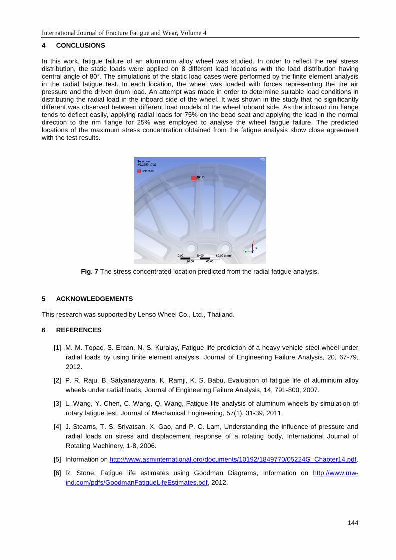
International Journal of Fracture Fatigue and Wear, Volume 4
144
4 CONCLUSIONS
In this work, fatigue failure of an aluminium alloy wheel was studied. In order to reflect the real stress distribution, the static loads were applied on 8 different load locations with the load distribution having central angle of 80°. The simulations of the static load cases were performed by the finite element analysis in the radial fatigue test. In each location, the wheel was loaded with forces representing the tire air pressure and the driven drum load. An attempt was made in order to determine suitable load conditions in distributing the radial load in the inboard side of the wheel. It was shown in the study that no significantly different was observed between different load models of the wheel inboard side. As the inboard rim flange tends to deflect easily, applying radial loads for 75% on the bead seat and applying the load in the normal direction to the rim flange for 25% was employed to analyse the wheel fatigue failure. The predicted locations of the maximum stress concentration obtained from the fatigue analysis show close agreement with the test results.
Fig. 7 The stress concentrated location predicted from the radial fatigue analysis.
5 ACKNOWLEDGEMENTS
This research was supported by Lenso Wheel Co., Ltd., Thailand.
6 REFERENCES
[1] M. M. Topaҫ, S. Ercan, N. S. Kuralay, Fatigue life prediction of a heavy vehicle steel wheel under
radial loads by using finite element analysis, Journal of Engineering Failure Analysis, 20, 67-79,
2012.
[2] P. R. Raju, B. Satyanarayana, K. Ramji, K. S. Babu, Evaluation of fatigue life of aluminium alloy
wheels under radial loads, Journal of Engineering Failure Analysis, 14, 791-800, 2007.
[3] L. Wang, Y. Chen, C. Wang, Q. Wang, Fatigue life analysis of aluminum wheels by simulation of
rotary fatigue test, Journal of Mechanical Engineering, 57(1), 31-39, 2011.
[4] J. Stearns, T. S. Srivatsan, X. Gao, and P. C. Lam, Understanding the influence of pressure and
radial loads on stress and displacement response of a rotating body, International Journal of
Rotating Machinery, 1-8, 2006.
[5] Information on http://www.asminternational.org/documents/10192/1849770/05224G_Chapter14.pdf.
[6] R. Stone, Fatigue life estimates using Goodman Diagrams, Information on http://www.mw-
ind.com/pdfs/GoodmanFatigueLifeEstimates.pdf, 2012.

International Journal of Fracture Fatigue and Wear, Volume 4
145
[7] Q. Bader, E. Kadum, Mean Stress Correction Effects On the Fatigue Life Behavior of Steel Alloys
by Using Stress Life Approach Theories, International Journal of Engineering & Technology IJET-
IJENS, 14(4), 50-58, 2014.
[8] J. Goodman, Mechanics Applied to Engineering, Longmans, Green and Co., London, pp. 631- 636,
1919.
[9] R. I. Stephens, A. Fatemi, R. R. Stephens, H. O. Fuchs, Metal fatigue in engineering, second ed.,
John Wiley & Sons, New York, 2001.
[10] N. E. Frost, K. J. Marsh, L. P. Pook, Metal fatigue, Dover, New York, 1999.

International Journal of Fracture Fatigue and Wear, Volume 4
146
Proceedings of the 5th International Conference
Fracture Fatigue and Wear, pp. 146-152, 2016
BENDING FATIGUE STRENGTH OF ANNEALED 0.45% CARBON STEEL
SPECIMENS FINISHED BY CUTTING AND RUBBING TECHINQUE
UTILIZING CEMENTED CARBIDE TIP
T. Yakushiji1, F. Nakagawa2 and M. Goto3
1 National Institute of Technology, Oita College, Oita, Japan 2 TOTO LTD, Kitakyushu, Japan
3 Oita University, Oita, Japan
Abstract: Aiming at an enhanced fatigue strength of annealed 0.45% carbon steel, a cutting tip with
unique shape, which gave the severe plastic deformation on the surface at the final stage of lathe turning, was developed. The developed processing produced the hard surface-layer with a fine microstructure composed of grains down to the sub-micron level (~100 nm). The layer had about 4 μm thickness and Vickers hardness value of 760 (4.5 times of non-processed surface). Fatigue limit stress of the processed specimens was enhanced to 1.5 times of smooth specimen finished with #1000 emery paper. The specimen endured the 108 repetitions of fatigue limit stress was fractured at subsequent overstress. Fish-eye pattern generated at the fatigue-limit stressing was formed on the fracture surface, indicating an enhanced fatigue resistance in the surface layer produced by the processing.
Keywords: Surface Treatment,Affected Layer,Work Hardening,Nanocrystal grain,Fatigue
1 INTRODUCTION
Since fatigue cracks usually are initiated at a free surface of machines and components, the surface treatments which produce a hard surface layer and compressive residual stress have been conducted through heat-treatment and thermomechanical processes. However, such processing leads to a degraded cost-performance of processed products. For improving fatigue resistance, the surface treatments with severe plastic deformation such as shot peening [1], ultrasonic impact peening [2], drilling [3], surface grinding [4] and friction sliding [5], which induce a grain refinement and an inclined distribution of grain size in sub-surface layer, have been developed. Recently, a new surface-treatment technique which consists of cutting and rubbing processes utilizing a cemented carbide tip was developed by Yakushiji et al. [6]; the technique are hereafter referred to as CR-Tech. The CR-Tech is a consecutive process with a product turning and a surface rubbing treatment. It yields a short processing time, as well as a low cost, that resulted from no exchange of instruments at the finishing stage because of the use of the same NC-lathe for cutting and rubbing. It has been shown that the fatigue strength of high strength materials, Ti-6Al-4V alloy [6] and quenched and tempered 0.45% carbon steel [7], was significantly enhanced by the CR-Tech. The action of the CR-Tech on the fatigue strength for soft steels appears to change from that for hard steels, because that the degree of an expansion of plastically deformed surface layer in soft steels should differ from that in hard steels. In the present study, the effect of the CR-Tech on the fatigue strength of soft-steel (annealed 0.45% carbon steel) was studied in terms of surface roughness, sub-surface microstructure and fracture surface analysis.
2 EXPERIMENTAL PROCEDURE
1.1 Specimen and cutting and rubbing processing Material used was an annealed 0.45% carbon steel. The heat treatment condition and mechanical properties are tabulated in Table 1. Fig. 1 shows the shape and dimensions of fatigue specimens. The fatigue strength reduction factor for this geometry was close to 1, meaning that they could be considered plain. After machining the fatigue specimens, the middle surface of the specimens were finished by the CR-Tech. Fig. 2 shows the schematics of rub-processing and press-load controlling system during the CR-Tech processing. The CR-Tech was achieved by pressing a flank of cemented carbide tip to the surface of
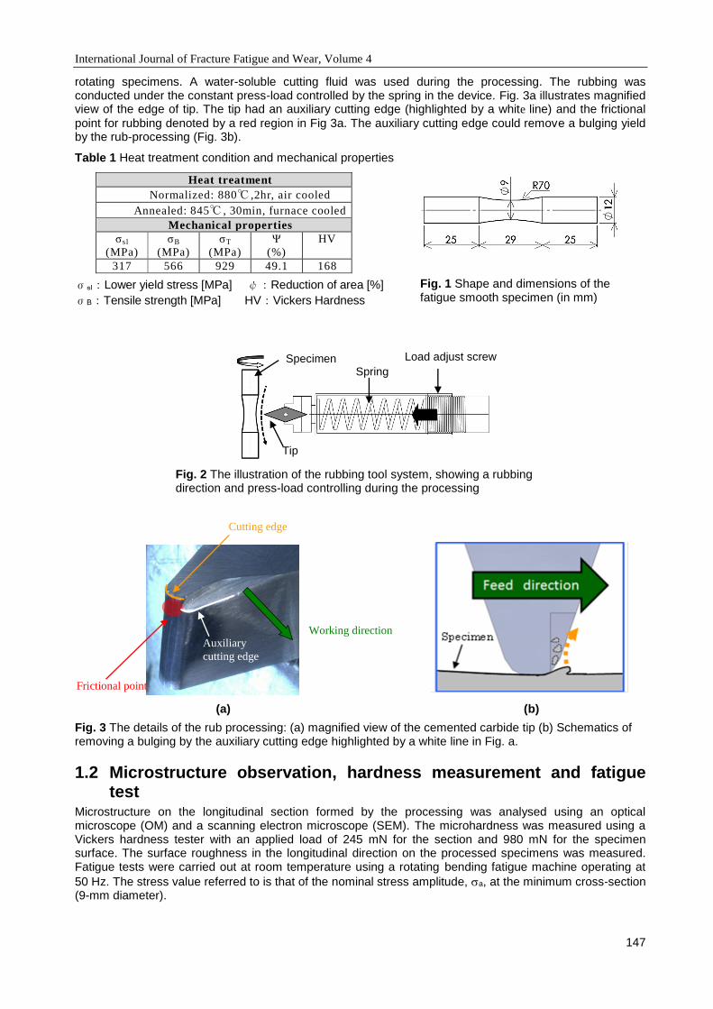
International Journal of Fracture Fatigue and Wear, Volume 4
147
rotating specimens. A water-soluble cutting fluid was used during the processing. The rubbing was conducted under the constant press-load controlled by the spring in the device. Fig. 3a illustrates magnified view of the edge of tip. The tip had an auxiliary cutting edge (highlighted by a white line) and the frictional
point for rubbing denoted by a red region in Fig 3a. The auxiliary cutting edge could remove a bulging yield by the rub-processing (Fig. 3b).
Table 1 Heat treatment condition and mechanical properties
σsl:Lower yield stress [MPa] ψ:Reduction of area [%]
σB:Tensile strength [MPa] HV:Vickers Hardness
(a) (b)
Fig. 3 The details of the rub processing: (a) magnified view of the cemented carbide tip (b) Schematics of removing a bulging by the auxiliary cutting edge highlighted by a white line in Fig. a.
1.2 Microstructure observation, hardness measurement and fatigue test
Microstructure on the longitudinal section formed by the processing was analysed using an optical microscope (OM) and a scanning electron microscope (SEM). The microhardness was measured using a Vickers hardness tester with an applied load of 245 mN for the section and 980 mN for the specimen surface. The surface roughness in the longitudinal direction on the processed specimens was measured. Fatigue tests were carried out at room temperature using a rotating bending fatigue machine operating at
50 Hz. The stress value referred to is that of the nominal stress amplitude, a, at the minimum cross-section (9-mm diameter).
Heat treatment
Normalized: 880 ,2hr, air cooled
Annealed: 845 , 30min, furnace cooled
Mechanical properties
σsl
(MPa)
σB
(MPa)
σT
(MPa)
Ψ
(%)
HV
317 566 929 49.1 168
Specimen
Tip
Spring
Load adjust screw
Fig. 1 Shape and dimensions of the fatigue smooth specimen (in mm)
Auxiliary
cutting edge
Cutting edge
Frictional point
Working direction
Fig. 2 The illustration of the rubbing tool system, showing a rubbing direction and press-load controlling during the processing

International Journal of Fracture Fatigue and Wear, Volume 4
148
3 EXPERIMENTAL RESULTS AND DISCUSSION
Fig.4 shows the relationship between the press-load during the processing and Vickers hardness measured at the processed surface (rubbing speed 80 m/min, feeding rate 0.05 mm/rev). The hardness of processed surface showed a drastic increase with an increase in the press-load, followed by a saturation trend after press-load of 600 N. Fig. 5 shows OM micrographs of sub-surface layer (press-loads: 220 and 1130 N) observed along the longitudinal direction. A lamella structure was formed at sub-surface layer of the specimen processed under press-load of 220 N. The closer the specimen surface, the finer the lamella
thickness. A surface layer with 6-m-thickness which has corrosion resistance was formed in the specimen processed by the press-load of 1130 N, showing a different microstructure from the lamella. Fig. 6 shows SEM micrographs of sub-surface layer corresponding to OM micrographs in Fig. 5. Ultrafine grained (UFG) microstructure with nano- to submicron-order sizes was formed at the sub-surface layer. The thickness of UFG layer tended to increase with an increase in the press-load. Fig. 7 shows the value of Vickers hardness as a function of distance from the specimen surface at the press-loads of 220 and 1130 N. The surface hardness for 1130 N reached HV = 800 which was nearly equivalent to the hardness of a quenched 0.45% carbon steel. The hardness value showed a sharp drop with increasing depth from the surface up to
50 m, followed by a gradual decreasing trend. The hardness for 1130 N was larger than that for 220 MPa
at the same distance from the surface below 250 m. In addition, the hardness at 350 m from the surface was HV = 200 which was close to the HV-value of annealed matrix (HV = 168).
Fig.8 shows the surface roughness, arithmetic mean of vertical deviation from mean line (Ra) and average maximum peak-to-valley height (Rz), for the specimens finished by various processes. In the figure, a mark (a), (b), (c) and (d) corresponds to the surface finished by lathe machining, CR-Tech, CR-Tech with two-step press-load (600 to 150 N) and emery paper with #1000, respectively. The Rz value for the surface
Fig. 5 OM micrographs of sub-surface layer (longitudinal section) for the specimen processed by CR-Tech
(a): Press load 220N (b): Press load 1130N
Fig. 7 Vickers hardness value, HV, as a function O distance from the specimen surface
surface surface
Fig. 6 SEM micrographs of sub-surface layer (longitudinal section) for the specimen processed by CR-Tech.
(a): Press load 220N (b): Press load 1130N
Fig. 4 The relationship between Vickers hardness value of processed surface and the press-load
surface surface
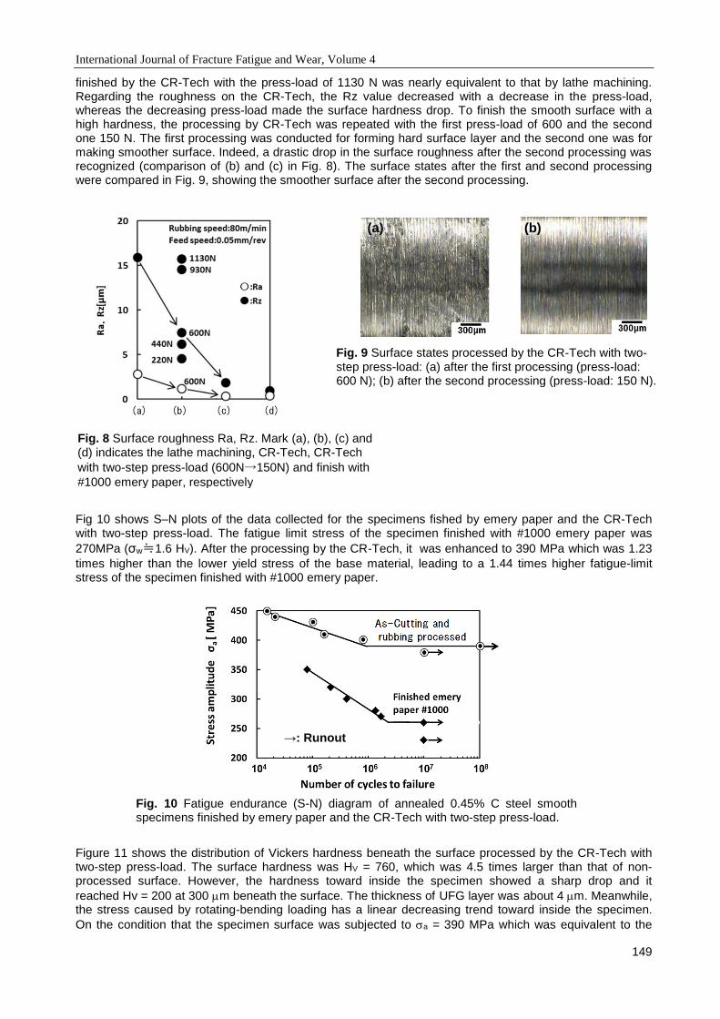
International Journal of Fracture Fatigue and Wear, Volume 4
149
finished by the CR-Tech with the press-load of 1130 N was nearly equivalent to that by lathe machining. Regarding the roughness on the CR-Tech, the Rz value decreased with a decrease in the press-load, whereas the decreasing press-load made the surface hardness drop. To finish the smooth surface with a high hardness, the processing by CR-Tech was repeated with the first press-load of 600 and the second one 150 N. The first processing was conducted for forming hard surface layer and the second one was for making smoother surface. Indeed, a drastic drop in the surface roughness after the second processing was recognized (comparison of (b) and (c) in Fig. 8). The surface states after the first and second processing were compared in Fig. 9, showing the smoother surface after the second processing.
Fig 10 shows S–N plots of the data collected for the specimens fished by emery paper and the CR-Tech with two-step press-load. The fatigue limit stress of the specimen finished with #1000 emery paper was
270MPa (σw≒1.6 HV). After the processing by the CR-Tech, it was enhanced to 390 MPa which was 1.23
times higher than the lower yield stress of the base material, leading to a 1.44 times higher fatigue-limit stress of the specimen finished with #1000 emery paper.
Figure 11 shows the distribution of Vickers hardness beneath the surface processed by the CR-Tech with two-step press-load. The surface hardness was HV = 760, which was 4.5 times larger than that of non-processed surface. However, the hardness toward inside the specimen showed a sharp drop and it
reached Hv = 200 at 300 m beneath the surface. The thickness of UFG layer was about 4 m. Meanwhile, the stress caused by rotating-bending loading has a linear decreasing trend toward inside the specimen.
On the condition that the specimen surface was subjected to a = 390 MPa which was equivalent to the
Fig. 9 Surface states processed by the CR-Tech with two-step press-load: (a) after the first processing (press-load: 600 N); (b) after the second processing (press-load: 150 N).
Fig. 8 Surface roughness Ra, Rz. Mark (a), (b), (c) and (d) indicates the lathe machining, CR-Tech, CR-Tech
with two-step press-load (600N→150N) and finish with
#1000 emery paper, respectively
(a) (b)
Fig. 10 Fatigue endurance (S-N) diagram of annealed 0.45% C steel smooth specimens finished by emery paper and the CR-Tech with two-step press-load.
→: Runout
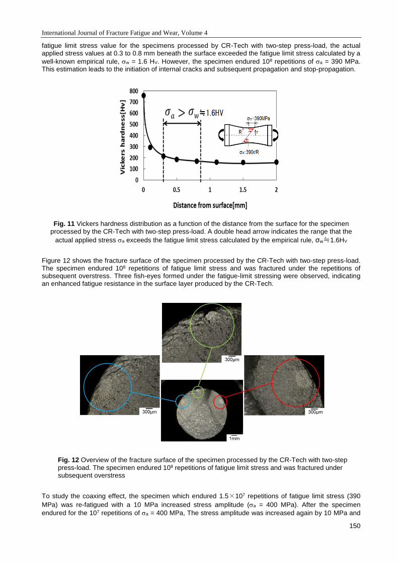
International Journal of Fracture Fatigue and Wear, Volume 4
150
fatigue limit stress value for the specimens processed by CR-Tech with two-step press-load, the actual applied stress values at 0.3 to 0.8 mm beneath the surface exceeded the fatigue limit stress calculated by a
well-known empirical rule, w = 1.6 HV. However, the specimen endured 108 repetitions of a = 390 MPa. This estimation leads to the initiation of internal cracks and subsequent propagation and stop-propagation.
Figure 12 shows the fracture surface of the specimen processed by the CR-Tech with two-step press-load. The specimen endured 108 repetitions of fatigue limit stress and was fractured under the repetitions of subsequent overstress. Three fish-eyes formed under the fatigue-limit stressing were observed, indicating an enhanced fatigue resistance in the surface layer produced by the CR-Tech.
To study the coaxing effect, the specimen which endured 1.5×10⁷ repetitions of fatigue limit stress (390
MPa) was re-fatigued with a 10 MPa increased stress amplitude (a = 400 MPa). After the specimen
endured for the 107 repetitions of a = 400 MPa, The stress amplitude was increased again by 10 MPa and
Fig. 11 Vickers hardness distribution as a function of the distance from the surface for the specimen processed by the CR-Tech with two-step press-load. A double head arrow indicates the range that the
actual applied stress a exceeds the fatigue limit stress calculated by the empirical rule, σw≒1.6HV
Fig. 12 Overview of the fracture surface of the specimen processed by the CR-Tech with two-step press-load. The specimen endured 108 repetitions of fatigue limit stress and was fractured under subsequent overstress
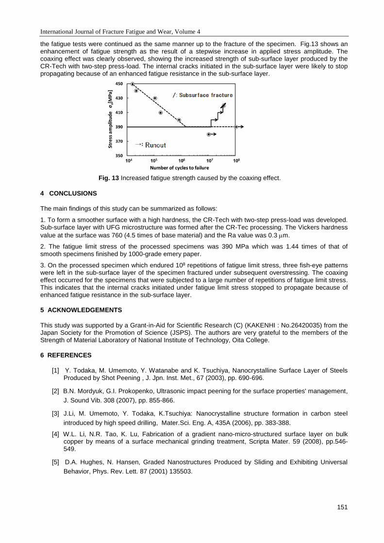
International Journal of Fracture Fatigue and Wear, Volume 4
151
the fatigue tests were continued as the same manner up to the fracture of the specimen. Fig.13 shows an enhancement of fatigue strength as the result of a stepwise increase in applied stress amplitude. The coaxing effect was clearly observed, showing the increased strength of sub-surface layer produced by the CR-Tech with two-step press-load. The internal cracks initiated in the sub-surface layer were likely to stop propagating because of an enhanced fatigue resistance in the sub-surface layer.
4 CONCLUSIONS
The main findings of this study can be summarized as follows:
1. To form a smoother surface with a high hardness, the CR-Tech with two-step press-load was developed. Sub-surface layer with UFG microstructure was formed after the CR-Tec processing. The Vickers hardness
value at the surface was 760 (4.5 times of base material) and the Ra value was 0.3 m.
2. The fatigue limit stress of the processed specimens was 390 MPa which was 1.44 times of that of smooth specimens finished by 1000-grade emery paper.
3. On the processed specimen which endured 108 repetitions of fatigue limit stress, three fish-eye patterns were left in the sub-surface layer of the specimen fractured under subsequent overstressing. The coaxing effect occurred for the specimens that were subjected to a large number of repetitions of fatigue limit stress. This indicates that the internal cracks initiated under fatigue limit stress stopped to propagate because of enhanced fatigue resistance in the sub-surface layer.
5 ACKNOWLEDGEMENTS
This study was supported by a Grant-in-Aid for Scientific Research (C) (KAKENHI : No.26420035) from the Japan Society for the Promotion of Science (JSPS). The authors are very grateful to the members of the Strength of Material Laboratory of National Institute of Technology, Oita College.
6 REFERENCES
[1] Y. Todaka, M. Umemoto, Y. Watanabe and K. Tsuchiya, Nanocrystalline Surface Layer of Steels Produced by Shot Peening , J. Jpn. Inst. Met., 67 (2003), pp. 690-696.
[2] B.N. Mordyuk, G.I. Prokopenko, Ultrasonic impact peening for the surface properties' management,
J. Sound Vib. 308 (2007), pp. 855-866.
[3] J.Li, M. Umemoto, Y. Todaka, K.Tsuchiya: Nanocrystalline structure formation in carbon steel
introduced by high speed drilling, Mater.Sci. Eng. A, 435A (2006), pp. 383-388.
[4] W.L. Li, N.R. Tao, K. Lu, Fabrication of a gradient nano-micro-structured surface layer on bulk copper by means of a surface mechanical grinding treatment, Scripta Mater. 59 (2008), pp.546-549.
[5] D.A. Hughes, N. Hansen, Graded Nanostructures Produced by Sliding and Exhibiting Universal
Behavior, Phys. Rev. Lett. 87 (2001) 135503.
Fig. 13 Increased fatigue strength caused by the coaxing effect.

International Journal of Fracture Fatigue and Wear, Volume 4
152
[6] T. Yakushiji, K. Watarikawa, M. Goto and Y. Todaka, Cutting and rubbing process for a Ti–6Al–4V
alloys, and its effects, Transactions of the Japan Society of Mechanical Engineers, Vol.80, No.818
(2014), pSMM0296
[7] K. Koujina, Y. Todaka, T. Yakushiji, H. Nagai, Y. Iguchi, M. Umemoto, Formation of Ultrafine-
grained Structure at Worn Surface in Carbon Steel by Wearing Process, Proceedings of Processing
and Fabrication of Advanced Materials XVIII, (2009),pp.1925-1932
[8] M.F. Garwood, H.H Zurburg and M.A. Erickson, Corriation of Laboratry Tests and Survice Performance, Interpretation of Tests and Correlation with Service, ASM, PA,(1951), pp.1-77

International Journal of Fracture Fatigue and Wear, Volume 4
153
Proceedings of the 5th International Conference
Fracture Fatigue and Wear, pp. 153-157, 2016
LOADING FREQUENCIES EFFECTS ON THE OXIDE-INDUCED CRACK
CLOSURE IN EXTREMELY LOW STRESS INTENSITY FACTOR RANGE
K. Tazoe1, M. Oka1 and G. Yagawa2
1 Reliability Group, Research & Development Center, YANMAR CO., LTD, Japan 2 Emeritus Professor, University of Tokyo and Toyo University, Japan
Abstract: In order to investigate the effect of loading frequency on oxide-induced crack closure in an
extremely low stress intensity factor range, ΔK decreasing tests under a stress ratio of 0.1 and loading frequencies of 20 Hz, 10 Hz, 5 Hz and 3 Hz were carried out, respectively. The following results were obtained: a) In case of Cr-Mo steel, oxide films were observed at the near threshold macroscopic fracture surface at 20 Hz and 10 Hz, but not observed at 5 Hz and 3 Hz. b) The EDX analysis on the microscopic fracture surface at both 5 Hz and 3 Hz showed that no oxide was detected in the threshold area. c) It is noted that the ΔKth values were 7.1 MPa √m at 20 Hz, 5.0 MPa√m at 10 Hz and 4.6 MPa√m at 5 Hz and 3 Hz, respectively. In the range of 20 Hz to 5 Hz, the threshold showed a tendency to decrease with the loading frequency due to the decrease of oxide-induced crack closure. On the other hand, the values became constant with frequencies smaller than 5 Hz, because there were no oxides in this range. d) In the case of low carbon steel and cast iron, similarly to Cr-Mo steel, no clear oxides were observed in the macroscopic fracture surface tested under 5 Hz. e) It is concluded from the above results that the oxide-induced crack closure would disappear under a low frequency condition.
Keywords: Fatigue, Near-Threshold Crack Growth Characteristics, Oxide-induced Crack Closure, Load Frequency, Steel,
1 INTRODUCTION
Ensuring the safety of mechanical structures is one of the most important engineering themes in the world. Almost all structures exposed to long-term fluctuating loads are known to become damaged due to fatigue. Therefore, it is essential to study the phenomena and take measures against fatigue fracture. Although there are many ways to study fatigue phenomena, it is essential to investigate the fatigue crack growth characteristics, especially those near threshold characteristics from the view point of the life of the structures.
In the case of low stress ratio (R = Kmin/Kmax), it is well known that some crack closures, such as plasticity-induced crack closure [1,2], roughness-induced crack closure [3] and oxide-induced crack closure [2,4,5], affect fatigue crack growth characteristics and thresholds, because, in an extremely low stress intensity factor range (ΔK), minimum load becomes lower than the crack opening load. In most instances of steels, the effect of oxide-induced crack closure is dominant due to fretting oxide films [2,4,5]. Past research has shown that the effect of the closure depends on the humidity of the environment [2], specimen width [6], and loading frequency (f) [7].
Though almost all past research stood on the hypothesis that fretting oxide films appear in all cases with low R in the air, there is doubt as to whether or not the appearance of oxide films is inevitable in all cases. For example, in the result, one of the authors carried out a test with a Cr-Mo Steel 12.7 mm CT specimen under R = 0.1 and f = 5 Hz, and no oxide films were observed in the near threshold macroscopic fracture surface [8]. In the result of the same specimen tested under R = 0.05 and f = 50 Hz, Ritchie et al reported that clear oxide films were observed in the fracture surface [4]. So, these results suggest there is a possibility of fretting oxide-less conditions with a low loading frequency, if fracture surfaces smash each other under low loading ratio.
However, the studies were only fragmentary. Therefore, it is meaningful to reveal the oxide-less load frequencies of steels and cast irons systematically to devise a new testing method or verify the hypothesis of past research. Then, in this study, ΔK-decreasing tests of low alloy steel, low carbon steel and cast iron were carried under 4 different load frequency conditions, and the oxide-less load frequencies of these were investigated systematically.
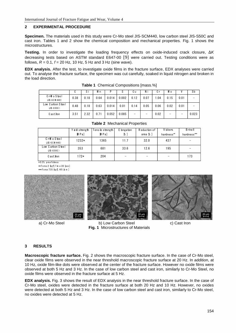
International Journal of Fracture Fatigue and Wear, Volume 4
154
2 EXPERIMENTAL PROCEDURE
Specimen. The materials used in this study were Cr-Mo steel JIS-SCM440, low carbon steel JIS-S50C and cast iron. Tables 1 and 2 show the chemical composition and mechanical properties. Fig. 1 shows the microstructures.
Testing. In order to investigate the loading frequency effects on oxide-induced crack closure, ΔK
decreasing tests based on ASTM standard E647-00 [9] were carried out. Testing conditions were as
follows, R = 0.1, f = 20 Hz, 10 Hz, 5 Hz and 3 Hz (sine wave).
EDX analysis. After the test, to investigate oxide films in the fracture surface, EDX analyses were carried out. To analyse the fracture surface, the specimen was cut carefully, soaked in liquid nitrogen and broken in the load direction.
Table 1 Chemical Compositions [mass.%]
C S i M n P S C u N i C r M o V S b
C r-M o S teel
(JIS -S C M 440)0.38 0.18 0.64 0.014 0.002 0.12 0.07 1.04 0.15 0.01 -
Low C arbon S teel
(JIS -S 50C )0.48 0.18 0.63 0.014 0.01 0.14 0.05 0.06 0.02 0.01 -
C ast Iron 3.51 2.32 0.71 0.052 0.085 - - 0.02 - - 0.023
Table 2 Mechanical Properties
Y ield strength
[M P a]
Tensile strength
[M P a]
E longation
[% ]
R eduction of
area [% ]
V ickers
hardness**
B rinell
hardness***
C r-M o S teel
(JIS -S C M 440)1232* 1365 11.7 32.0 437 -
Low C arbon S teel
(JIS -S 50C )353 681 33.6 12.6 195 -
C ast Iron 172* 204 - - - 173
* 0.2% proof stress
** Force:2 [kgf], Tim e:30 [sec]
*** Force:735 [kgf], Φ:5 [m m ]
a) Cr-Mo Steel b) Low Carbon Steel c) Cast Iron
Fig. 1 Microstructures of Materials
3 RESULTS
Macroscopic fracture surface. Fig. 2 shows the macroscopic fracture surface. In the case of Cr-Mo steel, clear oxide films were observed in the near threshold macroscopic fracture surface at 20 Hz. In addition, at 10 Hz, oxide film-like dots were observed at the center of the fracture surface. However no oxide films were observed at both 5 Hz and 3 Hz. In the case of low carbon steel and cast iron, similarly to Cr-Mo Steel, no oxide films were observed in the fracture surface at 5 Hz.
EDX analysis. Fig. 3 shows the result of EDX analysis in the near threshold fracture surface. In the case of Cr-Mo steel, oxides were detected in the fracture surface at both 20 Hz and 10 Hz. However, no oxides were detected at both 5 Hz and 3 Hz. In the case of low carbon steel and cast iron, similarly to Cr-Mo steel, no oxides were detected at 5 Hz.
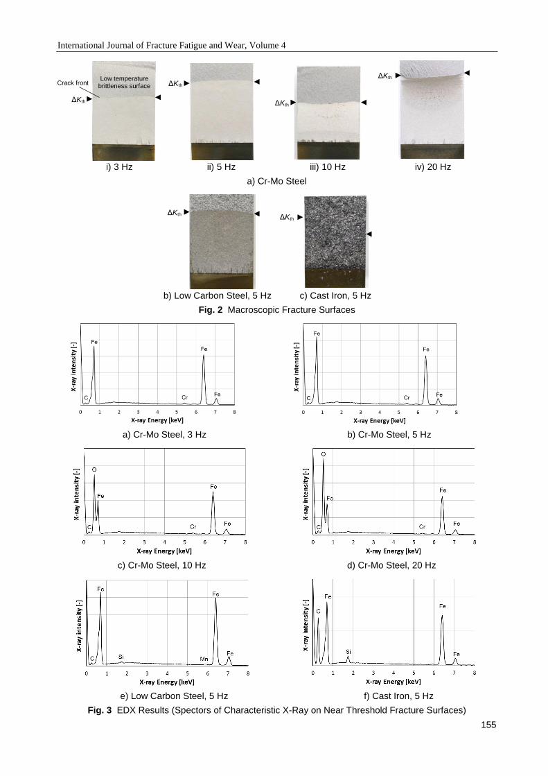
International Journal of Fracture Fatigue and Wear, Volume 4
155
i) 3 Hz ii) 5 Hz iii) 10 Hz iv) 20 Hz
a) Cr-Mo Steel
b) Low Carbon Steel, 5 Hz c) Cast Iron, 5 Hz
Fig. 2 Macroscopic Fracture Surfaces
a) Cr-Mo Steel, 3 Hz b) Cr-Mo Steel, 5 Hz
c) Cr-Mo Steel, 10 Hz d) Cr-Mo Steel, 20 Hz
e) Low Carbon Steel, 5 Hz f) Cast Iron, 5 Hz
Fig. 3 EDX Results (Spectors of Characteristic X-Ray on Near Threshold Fracture Surfaces)
ΔKth
ΔKth
Low temperature brittleness surface
Crack front
ΔKth ΔKth
ΔKth
ΔKth
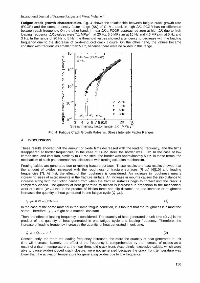
International Journal of Fracture Fatigue and Wear, Volume 4
156
Fatigue crack growth characteristics. Fig. 4 shows the relationship between fatigue crack growth rate (FCGR) and the stress intensity factor range (ΔK) of Cr-Mo steel. In high ΔK, FCGR has no difference between each frequency. On the other hand, in near ΔKth, FCGR approached zero at high ΔK due to high loading frequency. ΔKth values were 7.1 MPa√m at 20 Hz, 5.0 MPa√m at 10 Hz and 4.6 MPa√m at 5 Hz and 3 Hz. In the range of 20 Hz to 5 Hz, the threshold values showed a tendency to decrease with the loading frequency due to the decrease of oxide-induced crack closure. On the other hand, the values became constant with frequencies smaller than 5 Hz, because there were no oxides in this range.
Fig. 4 Fatigue Crack Growth Rates vs. Stress Intensity Factor Ranges
4 DISCUSSIONS
These results showed that the amount of oxide films decreased with the loading frequency, and the films disappeared at border frequencies. In the case of Cr-Mo steel, the border was 5 Hz. In the case of low carbon steel and cast iron, similarly to Cr-Mo steel, the border was approximately 5 Hz. In these terms, the mechanism of such phenomenon was discussed with fretting oxidation mechanism.
Fretting oxides are generated due to rubbing fracture surfaces. These results and past results showed that the amount of oxides increased with the roughness of fracture surfaces (R frac) [6][10] and loading frequencies [7]. At first, the effect of the roughness is considered. An increase in roughness means increasing sizes of micro mounts in the fracture surface. An increase in mounts causes the slip distance to increase along with the friction caused from when the fracture surfaces begin to contact until the crack is completely closed. The quantity of heat generated by friction is increased in proportion to the mechanical work of friction (W fric) that is the product of friction force and slip distance, so, the increase of roughness increases the quantity of heat generated in one fatigue cycle (Q cycle).
Q cycle = W fric (∝R frac) (1)
In the case of the same material in the same fatigue condition, it is thought that the roughness is almost the same. Therefore, Q cycle might be a material constant.
Then, the effect of loading frequency is considered. The quantity of heat generated in unit time (Q unit) is the product of the quantity of heat generated in one fatigue cycle and loading frequency. Therefore, the increase of loading frequency increases the quantity of heat generated in unit time.
Q unit = Q cycle × f (2)
Consequently, the more the loading frequency increases, the more the quantity of heat generated in unit time will increase. Namely, the effect of the frequency is comprehended by the increase of oxides as a result of a rise in temperature at the near threshold crack front. Accordingly, excessive oxides, which were able to cause oxide-induced crack closure, were not generated because the crack front temperature was lower than the activation temperature for generating oxides due to low frequency.
1010
-11
1x10⁻¹⁰
1x10⁻⁹
1x10⁻⁸
1x10⁻⁷
Kth
Kth
Kth
Cr-Mo Steel (JIS-SCM440)
√76 943 30205 8
20Hz
10Hz
5Hz
3Hz
Stress intensity factor range, K [MPa m]
R = 0.1
Fa
tig
ue
cra
ck g
row
th r
ate
, da/d
N
[ m
/cycle
]
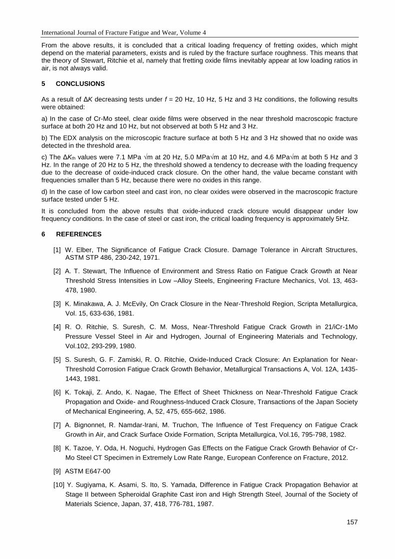
International Journal of Fracture Fatigue and Wear, Volume 4
157
From the above results, it is concluded that a critical loading frequency of fretting oxides, which might depend on the material parameters, exists and is ruled by the fracture surface roughness. This means that the theory of Stewart, Ritchie et al, namely that fretting oxide films inevitably appear at low loading ratios in air, is not always valid.
5 CONCLUSIONS
As a result of ΔK decreasing tests under f = 20 Hz, 10 Hz, 5 Hz and 3 Hz conditions, the following results were obtained:
a) In the case of Cr-Mo steel, clear oxide films were observed in the near threshold macroscopic fracture surface at both 20 Hz and 10 Hz, but not observed at both 5 Hz and 3 Hz.
b) The EDX analysis on the microscopic fracture surface at both 5 Hz and 3 Hz showed that no oxide was detected in the threshold area.
c) The ΔKth values were 7.1 MPa √m at 20 Hz, 5.0 MPa√m at 10 Hz, and 4.6 MPa√m at both 5 Hz and 3 Hz. In the range of 20 Hz to 5 Hz, the threshold showed a tendency to decrease with the loading frequency due to the decrease of oxide-induced crack closure. On the other hand, the value became constant with frequencies smaller than 5 Hz, because there were no oxides in this range.
d) In the case of low carbon steel and cast iron, no clear oxides were observed in the macroscopic fracture surface tested under 5 Hz.
It is concluded from the above results that oxide-induced crack closure would disappear under low frequency conditions. In the case of steel or cast iron, the critical loading frequency is approximately 5Hz.
6 REFERENCES
[1] W. Elber, The Significance of Fatigue Crack Closure. Damage Tolerance in Aircraft Structures, ASTM STP 486, 230-242, 1971.
[2] A. T. Stewart, The Influence of Environment and Stress Ratio on Fatigue Crack Growth at Near
Threshold Stress Intensities in Low –Alloy Steels, Engineering Fracture Mechanics, Vol. 13, 463-
478, 1980.
[3] K. Minakawa, A. J. McEvily, On Crack Closure in the Near-Threshold Region, Scripta Metallurgica,
Vol. 15, 633-636, 1981.
[4] R. O. Ritchie, S. Suresh, C. M. Moss, Near-Threshold Fatigue Crack Growth in 21/iCr-1Mo
Pressure Vessel Steel in Air and Hydrogen, Journal of Engineering Materials and Technology,
Vol.102, 293-299, 1980.
[5] S. Suresh, G. F. Zamiski, R. O. Ritchie, Oxide-Induced Crack Closure: An Explanation for Near-
Threshold Corrosion Fatigue Crack Growth Behavior, Metallurgical Transactions A, Vol. 12A, 1435-
1443, 1981.
[6] K. Tokaji, Z. Ando, K. Nagae, The Effect of Sheet Thickness on Near-Threshold Fatigue Crack
Propagation and Oxide- and Roughness-Induced Crack Closure, Transactions of the Japan Society
of Mechanical Engineering, A, 52, 475, 655-662, 1986.
[7] A. Bignonnet, R. Namdar-Irani, M. Truchon, The Influence of Test Frequency on Fatigue Crack
Growth in Air, and Crack Surface Oxide Formation, Scripta Metallurgica, Vol.16, 795-798, 1982.
[8] K. Tazoe, Y. Oda, H. Noguchi, Hydrogen Gas Effects on the Fatigue Crack Growth Behavior of Cr-
Mo Steel CT Specimen in Extremely Low Rate Range, European Conference on Fracture, 2012.
[9] ASTM E647-00
[10] Y. Sugiyama, K. Asami, S. Ito, S. Yamada, Difference in Fatigue Crack Propagation Behavior at
Stage II between Spheroidal Graphite Cast iron and High Strength Steel, Journal of the Society of
Materials Science, Japan, 37, 418, 776-781, 1987.
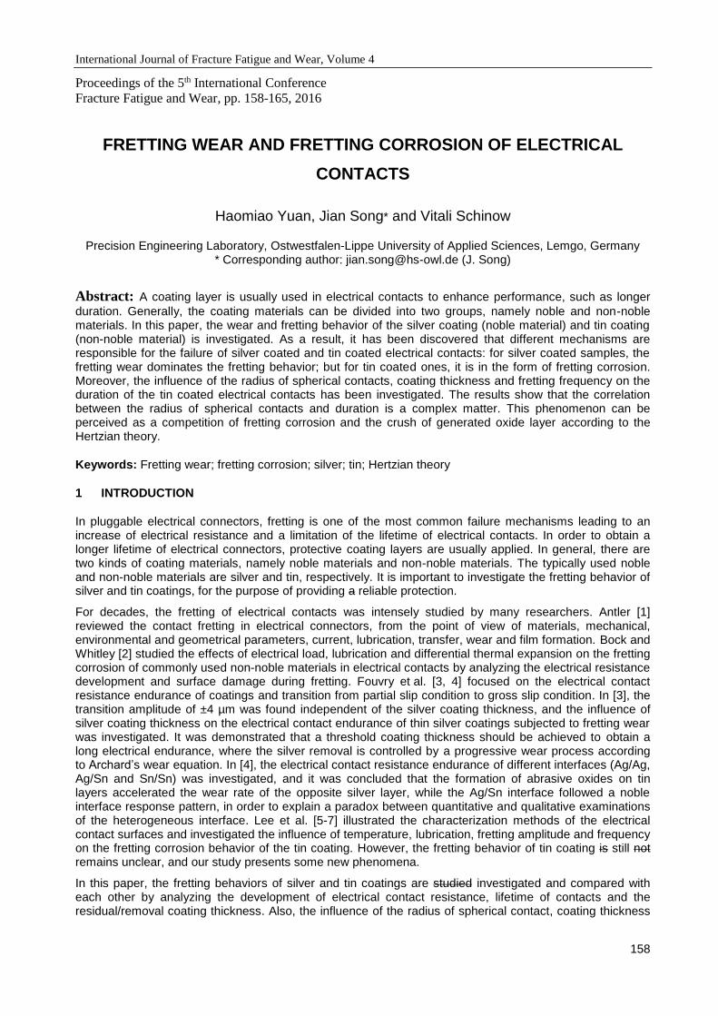
International Journal of Fracture Fatigue and Wear, Volume 4
158
Proceedings of the 5th International Conference
Fracture Fatigue and Wear, pp. 158-165, 2016
FRETTING WEAR AND FRETTING CORROSION OF ELECTRICAL
CONTACTS
Haomiao Yuan, Jian Song* and Vitali Schinow
Precision Engineering Laboratory, Ostwestfalen-Lippe University of Applied Sciences, Lemgo, Germany * Corresponding author: [email protected] (J. Song)
Abstract: A coating layer is usually used in electrical contacts to enhance performance, such as longer
duration. Generally, the coating materials can be divided into two groups, namely noble and non-noble materials. In this paper, the wear and fretting behavior of the silver coating (noble material) and tin coating (non-noble material) is investigated. As a result, it has been discovered that different mechanisms are responsible for the failure of silver coated and tin coated electrical contacts: for silver coated samples, the fretting wear dominates the fretting behavior; but for tin coated ones, it is in the form of fretting corrosion. Moreover, the influence of the radius of spherical contacts, coating thickness and fretting frequency on the duration of the tin coated electrical contacts has been investigated. The results show that the correlation between the radius of spherical contacts and duration is a complex matter. This phenomenon can be perceived as a competition of fretting corrosion and the crush of generated oxide layer according to the Hertzian theory.
Keywords: Fretting wear; fretting corrosion; silver; tin; Hertzian theory
1 INTRODUCTION
In pluggable electrical connectors, fretting is one of the most common failure mechanisms leading to an increase of electrical resistance and a limitation of the lifetime of electrical contacts. In order to obtain a longer lifetime of electrical connectors, protective coating layers are usually applied. In general, there are two kinds of coating materials, namely noble materials and non-noble materials. The typically used noble and non-noble materials are silver and tin, respectively. It is important to investigate the fretting behavior of silver and tin coatings, for the purpose of providing a reliable protection.
For decades, the fretting of electrical contacts was intensely studied by many researchers. Antler [1] reviewed the contact fretting in electrical connectors, from the point of view of materials, mechanical, environmental and geometrical parameters, current, lubrication, transfer, wear and film formation. Bock and Whitley [2] studied the effects of electrical load, lubrication and differential thermal expansion on the fretting corrosion of commonly used non-noble materials in electrical contacts by analyzing the electrical resistance development and surface damage during fretting. Fouvry et al. [3, 4] focused on the electrical contact resistance endurance of coatings and transition from partial slip condition to gross slip condition. In [3], the transition amplitude of ±4 µm was found independent of the silver coating thickness, and the influence of silver coating thickness on the electrical contact endurance of thin silver coatings subjected to fretting wear was investigated. It was demonstrated that a threshold coating thickness should be achieved to obtain a long electrical endurance, where the silver removal is controlled by a progressive wear process according to Archard’s wear equation. In [4], the electrical contact resistance endurance of different interfaces (Ag/Ag, Ag/Sn and Sn/Sn) was investigated, and it was concluded that the formation of abrasive oxides on tin layers accelerated the wear rate of the opposite silver layer, while the Ag/Sn interface followed a noble interface response pattern, in order to explain a paradox between quantitative and qualitative examinations of the heterogeneous interface. Lee et al. [5-7] illustrated the characterization methods of the electrical contact surfaces and investigated the influence of temperature, lubrication, fretting amplitude and frequency on the fretting corrosion behavior of the tin coating. However, the fretting behavior of tin coating is still not remains unclear, and our study presents some new phenomena.
In this paper, the fretting behaviors of silver and tin coatings are studied investigated and compared with each other by analyzing the development of electrical contact resistance, lifetime of contacts and the residual/removal coating thickness. Also, the influence of the radius of spherical contact, coating thickness

International Journal of Fracture Fatigue and Wear, Volume 4
159
and fretting frequency on the lifetime of the tin coated electrical contacts is examined. Some new results have been found compared to previous studies and investigations.
2 MATERIALS AND EXPERIMENTAL SETUP
The sphere-plane configuration of the samples is shown in Fig. 1. Different radii of spherical contact can be set. The base material is bronze (CuSn4). The coating materials in this paper are silver and tin, and they are galvanically coated on the base material. The coating thickness is analyzed by XRF spectroscopy (X-ray fluorescence spectroscopy) from HELMUT FISCHER GmbH&Co.KG. The fretting behaviour of the samples was tested by wear and fretting corrosion measurements. The apparatus is shown in Fig. 2. The tests parameters of the measurements can range as follows [8]: amplitude from ±0.5 µm to ±150 µm, normal contact force from 1 N to 6 N, frequency between 0.1 and 10 Hz, and the test temperature from ambient temperature to 80 °C. During the measurements, the samples were slid against each other without lubrication. The tests can run until either a pre-set number of cycles or the electrical failure of the contacts (electrical contact resistance>300 mΩ). After the tests, the residual coating thickness is determined by XRF spectroscopy, and consequently the thickness of the removed coating can be calculated. The tests parameters and the information of the used samples are listed in Table 1.
Fig. 1 Configuration of the samples
Fig. 2 Apparatus of wear and fretting corrosion measurement [9]
Table 1 Test parameters of different samples
Coating material Silver Tin
Radius of spherical contact (mm) 1.5, 4.5 1.5, 4.5
Coating thickness (µm) 3, 6 1, 3
Frequency (Hz) 1 0.1, 1
Normal contact force (N) 2
Amplitude (µm) ±25
Temperature (°C) 20-22

International Journal of Fracture Fatigue and Wear, Volume 4
160
3 RESULTS AND DISCUSSION
3.1 Fretting behavior of silver coated electrical contacts
3.1.1 Mechanism responsible for electrical failure of silver coated electrical contacts
In this section, the development of electrical contact resistant at silver coated contacts, the lifetime of the electrical contacts and the removed coating thickness during measurements are investigated, in order to characterize the fretting behavior of silver coated electrical contacts.
The contact resistance development of two silver contact pairs is illustrated in Fig. 3. The contact resistance can remain stable for a relatively large number of cycles, namely ca. 10,000 cycles. Since silver exhibits good resistance to oxidation, the electrical contact resistance should remain low before the wear through of silver coatings. After this, the fretting occurs at the base material, i.e. bronze. The base material is then oxidized, and the formation of an oxidation layer leads to the dramatic increase of electrical contact resistance, which results in electrical failure at around 20,000 cycles. This result corresponds to [10], where the wear curve and development of electrical contact resistance at silver coated contacts were shown: the electrical failure (ca. 75,000) takes place considerably later than the wear through of the silver coating (ca. 25,000).
In addition the residual/removed coating thickness (listed in Table 2) reflects the same fretting behavior. It is noticeable that the spherical part experiences more severe wear, which determines the wear through of silver coating. Thus, the study is focused on the spherical parts. The residual coating thickness of these parts is less than 0.2 µm. Considering the XRF spectroscopy measuring an average thickness value in an area and silver having an adhesion effect, the small amount of silver can be the wear debris in the contact zone. The removed silver coating thickness is ca. 3 µm. The wear through of the silver coating can be expected, since the nominal coating thickness is 3 µm.
Based on the aforementioned, the fretting behaviour of silver coating is mainly in the form of fretting wear. The electrical contact resistance can remain stable and low, when the silver coating provides a full protection before wear-through. After this, the base material participates in the wear process, and the oxides will be generated and accumulated, which leads to the electrical failure.
Fig. 3 Development of electrical contact resistance at silver coated samples
Table 2 Removed thickness of silver coatings and lifetime of contacts
Contact 1 Contact 2
Sphere Plane Sphere Plane
Coating material Ag Ag Ag Ag
Initial coating thickness (µm) 3.12 3.06 3.19 3.10
Residual coating thickness (µm) 0.11 1.47 0.18 1.85
Removed thickness (µm) 3.01 1.59 3.01 1.25
Lifetime of contacts (number of cycles) 19252 22429
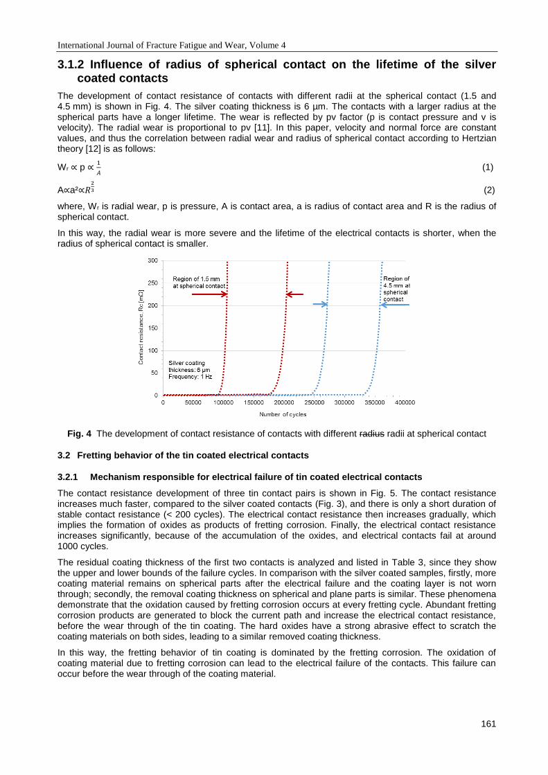
International Journal of Fracture Fatigue and Wear, Volume 4
161
3.1.2 Influence of radius of spherical contact on the lifetime of the silver coated contacts
The development of contact resistance of contacts with different radii at the spherical contact (1.5 and 4.5 mm) is shown in Fig. 4. The silver coating thickness is 6 µm. The contacts with a larger radius at the spherical parts have a longer lifetime. The wear is reflected by pv factor (p is contact pressure and v is velocity). The radial wear is proportional to pv [11]. In this paper, velocity and normal force are constant values, and thus the correlation between radial wear and radius of spherical contact according to Hertzian theory [12] is as follows:
Wr ∝ p ∝ 1
𝐴 (1)
A∝a²∝𝑅2
3 (2)
where, Wr is radial wear, p is pressure, A is contact area, a is radius of contact area and R is the radius of spherical contact.
In this way, the radial wear is more severe and the lifetime of the electrical contacts is shorter, when the radius of spherical contact is smaller.
Fig. 4 The development of contact resistance of contacts with different radius radii at spherical contact
3.2 Fretting behavior of the tin coated electrical contacts
3.2.1 Mechanism responsible for electrical failure of tin coated electrical contacts
The contact resistance development of three tin contact pairs is shown in Fig. 5. The contact resistance increases much faster, compared to the silver coated contacts (Fig. 3), and there is only a short duration of stable contact resistance (< 200 cycles). The electrical contact resistance then increases gradually, which implies the formation of oxides as products of fretting corrosion. Finally, the electrical contact resistance increases significantly, because of the accumulation of the oxides, and electrical contacts fail at around 1000 cycles.
The residual coating thickness of the first two contacts is analyzed and listed in Table 3, since they show the upper and lower bounds of the failure cycles. In comparison with the silver coated samples, firstly, more coating material remains on spherical parts after the electrical failure and the coating layer is not worn through; secondly, the removal coating thickness on spherical and plane parts is similar. These phenomena demonstrate that the oxidation caused by fretting corrosion occurs at every fretting cycle. Abundant fretting corrosion products are generated to block the current path and increase the electrical contact resistance, before the wear through of the tin coating. The hard oxides have a strong abrasive effect to scratch the coating materials on both sides, leading to a similar removed coating thickness.
In this way, the fretting behavior of tin coating is dominated by the fretting corrosion. The oxidation of coating material due to fretting corrosion can lead to the electrical failure of the contacts. This failure can occur before the wear through of the coating material.
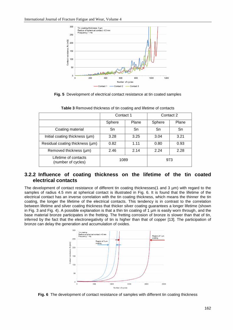
International Journal of Fracture Fatigue and Wear, Volume 4
162
Fig. 5 Development of electrical contact resistance at tin coated samples
Table 3 Removed thickness of tin coating and lifetime of contacts
Contact 1 Contact 2
Sphere Plane Sphere Plane
Coating material Sn Sn Sn Sn
Initial coating thickness (µm) 3.28 3.25 3.04 3.21
Residual coating thickness (µm) 0.82 1.11 0.80 0.93
Removed thickness (µm) 2.46 2.14 2.24 2.28
Lifetime of contacts (number of cycles)
1089 973
3.2.2 Influence of coating thickness on the lifetime of the tin coated electrical contacts
The development of contact resistance of different tin coating thicknesses(1 and 3 µm) with regard to the samples of radius 4.5 mm at spherical contact is illustrated in Fig. 6. It is found that the lifetime of the electrical contact has an inverse correlation with the tin coating thickness, which means the thinner the tin coating, the longer the lifetime of the electrical contacts. This tendency is in contrast to the correlation between lifetime and silver coating thickness that thicker silver coating guarantees a longer lifetime (shown in Fig. 3 and Fig. 4). A possible explanation is that a thin tin coating of 1 µm is easily worn through, and the base material bronze participates in the fretting. The fretting corrosion of bronze is slower than that of tin, inferred by the fact that the electronegativity of tin is higher than that of copper [13]. The participation of bronze can delay the generation and accumulation of oxides.
Fig. 6 The development of contact resistance of samples with different tin coating thickness
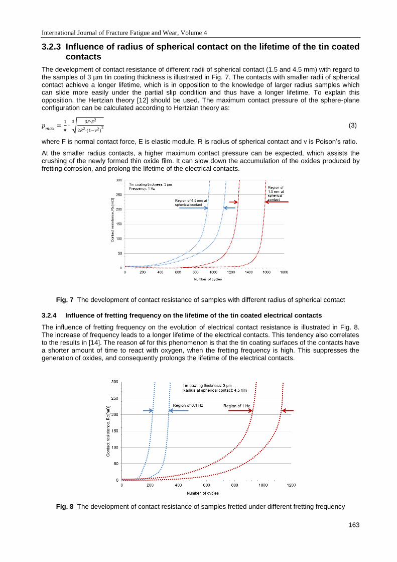
International Journal of Fracture Fatigue and Wear, Volume 4
163
3.2.3 Influence of radius of spherical contact on the lifetime of the tin coated contacts
The development of contact resistance of different radii of spherical contact (1.5 and 4.5 mm) with regard to the samples of 3 µm tin coating thickness is illustrated in Fig. 7. The contacts with smaller radii of spherical contact achieve a longer lifetime, which is in opposition to the knowledge of larger radius samples which can slide more easily under the partial slip condition and thus have a longer lifetime. To explain this opposition, the Hertzian theory [12] should be used. The maximum contact pressure of the sphere-plane configuration can be calculated according to Hertzian theory as:
𝑝𝑚𝑎𝑥
=1
𝜋∙ √
3𝐹∙𝐸2
2𝑅2∙(1−𝜈2)2
3 (3)
where F is normal contact force, E is elastic module, R is radius of spherical contact and ν is Poison’s ratio.
At the smaller radius contacts, a higher maximum contact pressure can be expected, which assists the crushing of the newly formed thin oxide film. It can slow down the accumulation of the oxides produced by fretting corrosion, and prolong the lifetime of the electrical contacts.
Fig. 7 The development of contact resistance of samples with different radius of spherical contact
3.2.4 Influence of fretting frequency on the lifetime of the tin coated electrical contacts
The influence of fretting frequency on the evolution of electrical contact resistance is illustrated in Fig. 8. The increase of frequency leads to a longer lifetime of the electrical contacts. This tendency also correlates to the results in [14]. The reason of for this phenomenon is that the tin coating surfaces of the contacts have a shorter amount of time to react with oxygen, when the fretting frequency is high. This suppresses the generation of oxides, and consequently prolongs the lifetime of the electrical contacts.
Fig. 8 The development of contact resistance of samples fretted under different fretting frequency

International Journal of Fracture Fatigue and Wear, Volume 4
164
4 CONCLUSIONS
In this paper, various fretting behaviors of silver and tin coated electrical contacts are investigated and compared by analyzing the development of electrical contact resistance, lifetime of the electrical contacts and the residual/removed coating thickness with the assistance of the wear and fretting corrosion measurements. Moreover, a close study of the influence of radii of spherical contact, coating thickness and fretting frequency on the duration of the tin coated electrical contacts is conducted. The main conclusions are as follows:
The dominating fretting mechanism of silver coated contacts is fretting wear of the silver coating. The spherical parts experience a more severe fretting wear compared to the plane parts. The oxides are initially generated after the wear through of the silver coating on the spherical parts by fretting corrosion of the base material bronze.
The dominating fretting mechanism of the tin coated contacts is fretting corrosion. The oxides are generated at the beginning of the sliding phase. The fretting corrosion of tin coating materials can lead to electrical failure, before the wear through of the coating. The removed coating thickness of spherical and plane parts, according to the measurements, is similar.
With a thicker silver coating, a longer lifetime of electrical contacts can be guaranteed. However, with a thinner tin coating, it is possible to obtain a longer lifetime of electrical contacts. The reason may be the participation of the base material bronze in the fretting process at of tin coating.
The silver coated contacts underpin the traditional knowledge that the samples with larger radii at the spherical contact have electrical contacts with a longer lifetime, because the wear is proportional to pressure and thus inversely proportional to the radius of spherical contact. In contrast, an opposite tendency is found with regard to tin coated contacts that samples with smaller radius at the spherical contact can achieve electrical contacts with a longer lifetime of the. This phenomenon can be recognized as a competition of fretting corrosion and the crush of generated oxide layer according to the Hertzian theory.
The increase of fretting frequency assists in prolonging the lifetime of the electrical contacts. This correlates with the results of in previous work and results from the short reaction time with oxygen at the tin coating surface, when the fretting frequency is high.
5 FUTURE WORK
It is intended to carry out a more systematic investigation, by examining the phenomena presented in this paper under various normal force conditions and comparing them in detail to previous research. Based on the understanding of fretting phenomena, models for the forecasting of fretting behavior can be developed. The wear process of silver coating contacts can be interpreted by the correlation of wear depth and sliding distance according to Archard’s equation.
6 ACKNOWLEDGEMENT
The authors would like to acknowledge the financial support of German Federal Ministry for Education and Research (BMBF, 1758X07), the European Union and the German State Northrhine-Westfalia (w0804nm001).
7 REFERENCES
[1] M. Antler, Survey of Contact Fretting in Electrical Connectors, IEEE Transactions on Components, Hybrids, and Manufacturing Technology, 8(1), 87-104, 1985.
[2] E. M. Bock, J. H. Whitley, Fretting Corrosion in Electric Contacts, The Twentieth Annual Holm Seminar on Electrical Contacts 1974, 128-138, 1974.
[3] P. Jedrzejczyk, S. Fouvry, O. Alquier, Quantification of the Electrical Contact Endurance of Thin Platted Silver Coatings Subjected to Fretting Wear: Influence of Coating Thickness, Proceedings of the 26th International Conference on Electrical Contacts (ICEC) Beijing, 205-212, 2012.
[4] O. Perrinet, J. Laporte, S. Fouvry, O. Alquier, The Electrical Contact Resistance Endurance of Heterogeneous Ag/Sn Interfaces Subjected to Fretting Wear, Proceedings of the 27th International Conference on Electrical Contacts (ICEC) Dresden, 114-119, 2014.

International Journal of Fracture Fatigue and Wear, Volume 4
165
[5] Y. W. Park, T.S.N. S. Narayanan, K. Y. Lee, Fretting Corrosion of Tin-Plated Contacts: Evaluation of Surface Characteristics, Tribology International, 40, 548-559, 2007.
[6] T.S.N. S. Narayanan, Y. W. Park, K. Y. Lee, Fretting Corrosion of Lubricated Tin Plated Copper Alloy Contacts: Effect of Temperature, Tribology International, 41, 87-102, 2008.
[7] Y. W. Park, T.S.N. S. Narayanan, K. Y. Lee, Effect of Fretting Amplitude and Frequency on the Fretting Corrosion Behaviour of Tin Plated Contacts, Surface and Coatings Technology, 201, 2181-2192, 2006.
[8] F. Sawitzki, Einflussparameter von Reibkorrosionsuntersuchungen [Master thesis], Ostwestfalen-Lippe University of Applied Sciences, Germany, 2009.
[9] D. Luther, Entwicklung, Bau und Erprobung eines Tribo- und Reibkorrosionsprüfstandes für elektrische Kontakte [Bachelor thesis], Ostwestfalen-Lippe University of Applied Sciences, Germany, 2012.
[10] J. Song, V. Schinow, H. Yuan, The Influence of Coating Thickness on Linear Wear Rate in Silver Coated Contacts, Proceedings of the 4th International Conference on Fracture, Fatigue and Wear (FFW) Ghent, 200-207, 2015.
[11] C. Cusano, Porous Metal Bearings, in: E. R. Booser (Ed.), CRC Handbook of Lubrication and Tribology, Volume III: Monitoring, Materials, Synthetic Lubricants, and Applications, Volume III, CRC Press, Boca Raton, 1994, pp. 491-514.
[12] Information on https://en.wikipedia.org/wiki/Contact_mechanics, checked on March 3rd 2016.
[13] W. M. Haynes, D. R. Lide, T. J. Bruno, Electronegativity, in: CRC Handbook of Chemistry and Physics, 94th ed., CRC Press, Boca Raton, 2013, pp. 9-97.
[14] J. Song, F. Sawitzki, Einflussparameter von Reibkorrosionsuntersuchungen, Elektronische und optische Verbindungstechnik 2009 Lemgo, 74-79, 2009.
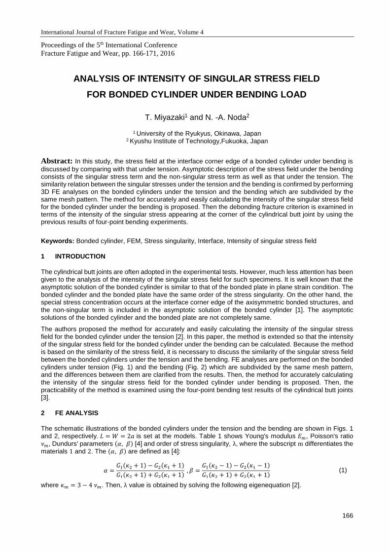
International Journal of Fracture Fatigue and Wear, Volume 4
166
Proceedings of the 5th International Conference
Fracture Fatigue and Wear, pp. 166-171, 2016
ANALYSIS OF INTENSITY OF SINGULAR STRESS FIELD
FOR BONDED CYLINDER UNDER BENDING LOAD
T. Miyazaki1 and N. -A. Noda2
1 University of the Ryukyus, Okinawa, Japan 2 Kyushu Institute of Technology,Fukuoka, Japan
Abstract: In this study, the stress field at the interface corner edge of a bonded cylinder under bending is
discussed by comparing with that under tension. Asymptotic description of the stress field under the bending consists of the singular stress term and the non-singular stress term as well as that under the tension. The similarity relation between the singular stresses under the tension and the bending is confirmed by performing 3D FE analyses on the bonded cylinders under the tension and the bending which are subdivided by the same mesh pattern. The method for accurately and easily calculating the intensity of the singular stress field for the bonded cylinder under the bending is proposed. Then the debonding fracture criterion is examined in terms of the intensity of the singular stress appearing at the corner of the cylindrical butt joint by using the previous results of four-point bending experiments.
Keywords: Bonded cylinder, FEM, Stress singularity, Interface, Intensity of singular stress field
1 INTRODUCTION
The cylindrical butt joints are often adopted in the experimental tests. However, much less attention has been given to the analysis of the intensity of the singular stress field for such specimens. It is well known that the asymptotic solution of the bonded cylinder is similar to that of the bonded plate in plane strain condition. The bonded cylinder and the bonded plate have the same order of the stress singularity. On the other hand, the special stress concentration occurs at the interface corner edge of the axisymmetric bonded structures, and the non-singular term is included in the asymptotic solution of the bonded cylinder [1]. The asymptotic solutions of the bonded cylinder and the bonded plate are not completely same.
The authors proposed the method for accurately and easily calculating the intensity of the singular stress field for the bonded cylinder under the tension [2]. In this paper, the method is extended so that the intensity of the singular stress field for the bonded cylinder under the bending can be calculated. Because the method is based on the similarity of the stress field, it is necessary to discuss the similarity of the singular stress field between the bonded cylinders under the tension and the bending. FE analyses are performed on the bonded cylinders under tension (Fig. 1) and the bending (Fig. 2) which are subdivided by the same mesh pattern, and the differences between them are clarified from the results. Then, the method for accurately calculating the intensity of the singular stress field for the bonded cylinder under bending is proposed. Then, the practicability of the method is examined using the four-point bending test results of the cylindrical butt joints [3].
2 FE ANALYSIS
The schematic illustrations of the bonded cylinders under the tension and the bending are shown in Figs. 1 and 2, respectively. 𝐿 = 𝑊 = 2𝑎 is set at the models. Table 1 shows Young's modulus 𝐸𝑚, Poisson's ratio 𝜈𝑚, Dundurs' parameters (𝛼, 𝛽) [4] and order of stress singularity, λ, where the subscript m differentiates the materials 1 and 2. The (𝛼, 𝛽) are defined as [4]:
𝛼 =𝐺1(𝜅2 + 1) − 𝐺2(𝜅1 + 1)
𝐺1(𝜅2 + 1) + 𝐺2(𝜅1 + 1) , 𝛽 =
𝐺1(𝜅2 − 1) − 𝐺2(𝜅1 − 1)
𝐺1(𝜅2 + 1) + 𝐺2(𝜅1 + 1) (1)
where 𝜅𝑚 = 3 − 4 𝜈𝑚. Then, λ value is obtained by solving the following eigenequation [2].
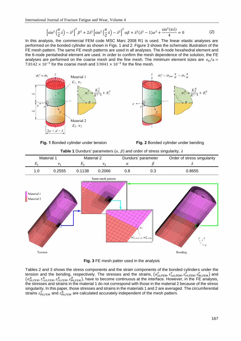
International Journal of Fracture Fatigue and Wear, Volume 4
167
[sin2 (𝜋
2𝜆) − 𝜆2]
2
𝛽2 + 2𝜆2 [sin2 (𝜋
2𝜆) − 𝜆2]
2
𝛼𝛽 + 𝜆2(𝜆2 − 1)𝛼2 +sin2(𝜋𝜆)
4= 0 (2)
In this analysis, the commercial FEM code MSC Marc 2008 R1 is used. The linear elastic analyses are performed on the bonded cylinder as shown in Figs. 1 and 2. Figure 3 shows the schematic illustration of the FE mesh pattern. The same FE mesh patterns are used in all analyses. The 8-node hexahedral element and the 6-node pentahedral element are used. In order to confirm the mesh dependence of the solution, the FE analyses are performed on the coarse mesh and the fine mesh. The minimum element sizes are e0 a⁄ =7.8142 × 10⁻⁵ for the coarse mesh and 3.9041 × 10⁻⁵ for the fine mesh.
Fig. 1 Bonded cylinder under tension Fig. 2 Bonded cylinder under bending
Table 1 Dundurs' parameters (𝛼, 𝛽) and order of stress singularity, 𝜆
Material 1 Material 2 Dundurs’ parameter Order of stress singularity
𝐸1 𝜈1 𝐸2 𝜈2 𝛼 𝛽 𝜆
1.0 0.2555 0.1138 0.2066 0.8 0.3 0.8655
Fig. 3 FE mesh patter used in the analysis
Tables 2 and 3 shows the stress components and the strain components of the bonded cylinders under the tension and the bending, respectively. The stresses and the strains, (σz0,FEM
𝑇 , τrz0,FEM𝑇 , εr0,FEM
𝑇 , εθ0,FEM𝑇 ) and
(𝜎𝑧0,𝐹𝐸𝑀𝐵 , 𝜏𝑟𝑧0,𝐹𝐸𝑀
𝐵 , 𝜀𝑟0,𝐹𝐸𝑀𝐵 , 𝜀𝜃0,𝐹𝐸𝑀
𝐵 ), have to become continuous at the interface. However, in the FE analysis, the stresses and strains in the material 1 do not correspond with those in the material 2 because of the stress singularity. In this paper, those stresses and strains in the materials 1 and 2 are averaged. The circumferential strains 𝜀𝜃0,𝐹𝐸𝑀
𝑇 and 𝜀𝜃0,𝐹𝐸𝑀𝐵 are calculated accurately independent of the mesh pattern.
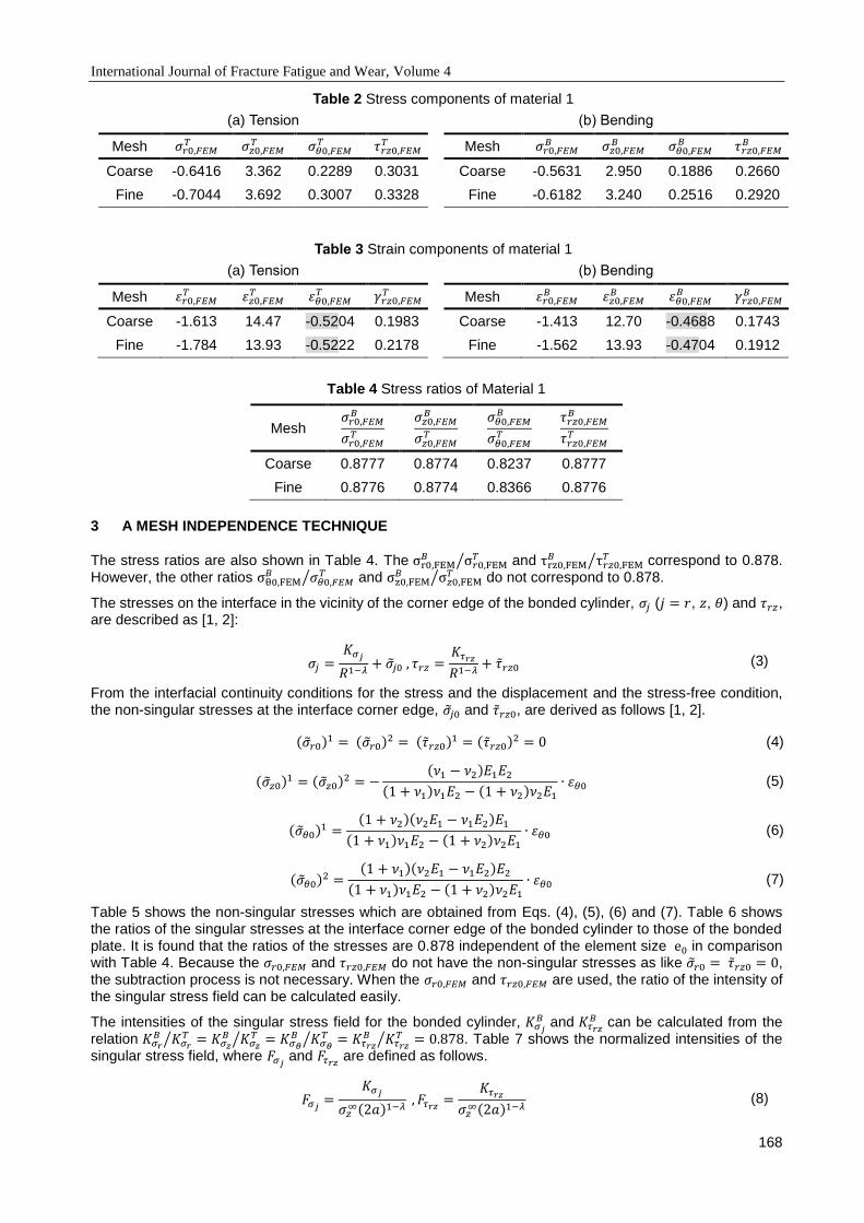
International Journal of Fracture Fatigue and Wear, Volume 4
168
Table 2 Stress components of material 1
(a) Tension (b) Bending
Mesh 𝜎𝑟0,𝐹𝐸𝑀𝑇 𝜎𝑧0,𝐹𝐸𝑀
𝑇 𝜎𝜃0,𝐹𝐸𝑀𝑇 𝜏𝑟𝑧0,𝐹𝐸𝑀
𝑇 Mesh 𝜎𝑟0,𝐹𝐸𝑀𝐵 𝜎𝑧0,𝐹𝐸𝑀
𝐵 𝜎𝜃0,𝐹𝐸𝑀𝐵 𝜏𝑟𝑧0,𝐹𝐸𝑀
𝐵
Coarse -0.6416 3.362 0.2289 0.3031 Coarse -0.5631 2.950 0.1886 0.2660
Fine -0.7044 3.692 0.3007 0.3328 Fine -0.6182 3.240 0.2516 0.2920
Table 3 Strain components of material 1
(a) Tension (b) Bending
Mesh 𝜀𝑟0,𝐹𝐸𝑀𝑇 𝜀𝑧0,𝐹𝐸𝑀
𝑇 𝜀𝜃0,𝐹𝐸𝑀𝑇 𝛾𝑟𝑧0,𝐹𝐸𝑀
𝑇 Mesh 𝜀𝑟0,𝐹𝐸𝑀𝐵 𝜀𝑧0,𝐹𝐸𝑀
𝐵 𝜀𝜃0,𝐹𝐸𝑀𝐵 𝛾𝑟𝑧0,𝐹𝐸𝑀
𝐵
Coarse -1.613 14.47 -0.5204 0.1983 Coarse -1.413 12.70 -0.4688 0.1743
Fine -1.784 13.93 -0.5222 0.2178 Fine -1.562 13.93 -0.4704 0.1912
Table 4 Stress ratios of Material 1
Mesh 𝜎𝑟0,𝐹𝐸𝑀
𝐵
𝜎𝑟0,𝐹𝐸𝑀𝑇
𝜎𝑧0,𝐹𝐸𝑀𝐵
𝜎𝑧0,𝐹𝐸𝑀𝑇
𝜎𝜃0,𝐹𝐸𝑀𝐵
𝜎𝜃0,𝐹𝐸𝑀𝑇
𝜏𝑟𝑧0,𝐹𝐸𝑀𝐵
𝜏𝑟𝑧0,𝐹𝐸𝑀𝑇
Coarse 0.8777 0.8774 0.8237 0.8777
Fine 0.8776 0.8774 0.8366 0.8776
3 A MESH INDEPENDENCE TECHNIQUE
The stress ratios are also shown in Table 4. The σr0,FEM𝐵 σ𝑟0,FEM
𝑇⁄ and τrz0,FEM𝐵 τ𝑟𝑧0,FEM
𝑇⁄ correspond to 0.878. However, the other ratios σθ0,FEM
𝐵 𝜎𝜃0,𝐹𝐸𝑀𝑇⁄ and σz0,FEM
𝐵 σ𝑧0,FEM𝑇⁄ do not correspond to 0.878.
The stresses on the interface in the vicinity of the corner edge of the bonded cylinder, 𝜎𝑗 (𝑗 = 𝑟, 𝑧, 𝜃) and 𝜏𝑟𝑧, are described as [1, 2]:
𝜎𝑗 =𝐾𝜎𝑗
𝑅1−𝜆+ 𝑗0 , 𝜏𝑟𝑧 =
𝐾𝜏𝑟𝑧
𝑅1−𝜆+ 𝑟𝑧0 (3)
From the interfacial continuity conditions for the stress and the displacement and the stress-free condition, the non-singular stresses at the interface corner edge, 𝑗0 and 𝑟𝑧0, are derived as follows [1, 2].
(𝑟0)1 = (𝑟0)2 = (𝑟𝑧0)1 = (𝑟𝑧0)2 = 0 (4)
(𝑧0)1 = (𝑧0)2 = −(𝜈1 − 𝜈2)𝐸1𝐸2
(1 + 𝜈1)𝜈1𝐸2 − (1 + 𝜈2)𝜈2𝐸1
∙ 𝜀𝜃0 (5)
(𝜃0)1 =(1 + 𝜈2)(𝜈2𝐸1 − 𝜈1𝐸2)𝐸1
(1 + 𝜈1)𝜈1𝐸2 − (1 + 𝜈2)𝜈2𝐸1
∙ 𝜀𝜃0 (6)
(𝜃0)2 =(1 + 𝜈1)(𝜈2𝐸1 − 𝜈1𝐸2)𝐸2
(1 + 𝜈1)𝜈1𝐸2 − (1 + 𝜈2)𝜈2𝐸1
∙ 𝜀𝜃0 (7)
Table 5 shows the non-singular stresses which are obtained from Eqs. (4), (5), (6) and (7). Table 6 shows the ratios of the singular stresses at the interface corner edge of the bonded cylinder to those of the bonded plate. It is found that the ratios of the stresses are 0.878 independent of the element size e0 in comparison with Table 4. Because the 𝜎𝑟0,𝐹𝐸𝑀 and 𝜏𝑟𝑧0,𝐹𝐸𝑀 do not have the non-singular stresses as like 𝑟0 = 𝑟𝑧0 = 0, the subtraction process is not necessary. When the 𝜎𝑟0,𝐹𝐸𝑀 and 𝜏𝑟𝑧0,𝐹𝐸𝑀 are used, the ratio of the intensity of the singular stress field can be calculated easily.
The intensities of the singular stress field for the bonded cylinder, 𝐾𝜎𝑗𝐵 and 𝐾𝜏𝑟𝑧
𝐵 can be calculated from the relation 𝐾𝜎𝑟
𝐵 𝐾𝜎𝑟𝑇⁄ = 𝐾𝜎𝑧
𝐵 𝐾𝜎𝑧𝑇⁄ = 𝐾𝜎𝜃
𝐵 𝐾𝜎𝜃𝑇⁄ = 𝐾𝜏𝑟𝑧
𝐵 𝐾𝜏𝑟𝑧𝑇⁄ = 0.878. Table 7 shows the normalized intensities of the
singular stress field, where 𝐹𝜎𝑗 and 𝐹𝜏𝑟𝑧
are defined as follows.
𝐹𝜎𝑗=
𝐾𝜎𝑗
𝜎𝑧∞(2𝑎)1−𝜆
, 𝐹𝜏𝑟𝑧=
𝐾𝜏𝑟𝑧
𝜎𝑧∞(2𝑎)1−𝜆
(8)
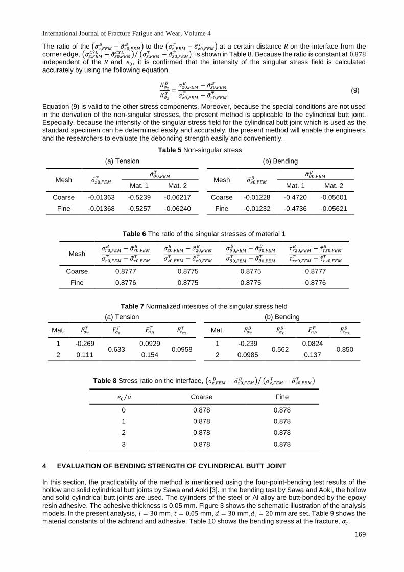
International Journal of Fracture Fatigue and Wear, Volume 4
169
The ratio of the (𝜎𝑧,𝐹𝐸𝑀𝐵 − 𝑧0,𝐹𝐸𝑀
𝐵 ) to the (𝜎𝑧,𝐹𝐸𝑀𝑇 − 𝑧0,𝐹𝐸𝑀
𝑇 ) at a certain distance 𝑅 on the interface from the corner edge, (𝜎𝑧,𝐹𝐸𝑀
𝐶𝑌𝐿 − 𝑧0,𝐹𝐸𝑀𝐶𝑌𝐿 ) (𝜎𝑧,𝐹𝐸𝑀
𝑇 − 𝑧0,𝐹𝐸𝑀𝑇 )⁄ , is shown in Table 8. Because the ratio is constant at 0.878
independent of the 𝑅 and 𝑒0 , it is confirmed that the intensity of the singular stress field is calculated accurately by using the following equation.
𝐾𝜎𝑧𝐵
𝐾𝜎𝑧𝑇
=𝜎𝑧0,𝐹𝐸𝑀
𝐵 − 𝑧0,𝐹𝐸𝑀𝐵
𝜎𝑧0,𝐹𝐸𝑀𝑇 − 𝑧0,𝐹𝐸𝑀
𝑇 (9)
Equation (9) is valid to the other stress components. Moreover, because the special conditions are not used in the derivation of the non-singular stresses, the present method is applicable to the cylindrical butt joint. Especially, because the intensity of the singular stress field for the cylindrical butt joint which is used as the standard specimen can be determined easily and accurately, the present method will enable the engineers and the researchers to evaluate the debonding strength easily and conveniently.
Table 5 Non-singular stress
(a) Tension
(b) Bending
Mesh 𝑧0,𝐹𝐸𝑀𝑇
𝜃0,𝐹𝐸𝑀𝑇
Mesh 𝑧0,𝐹𝐸𝑀𝐵
𝜃0,𝐹𝐸𝑀𝐵
Mat. 1 Mat. 2 Mat. 1 Mat. 2
Coarse -0.01363 -0.5239 -0.06217 Coarse -0.01228 -0.4720 -0.05601
Fine -0.01368 -0.5257 -0.06240 Fine -0.01232 -0.4736 -0.05621
Table 6 The ratio of the singular stresses of material 1
Mesh 𝜎𝑟0,𝐹𝐸𝑀
𝐵 − 𝑟0,𝐹𝐸𝑀𝐵
𝜎𝑟0,𝐹𝐸𝑀𝑇 − 𝑟0,𝐹𝐸𝑀
𝑇 𝜎𝑧0,𝐹𝐸𝑀
𝐵 − 𝑧0,𝐹𝐸𝑀𝐵
𝜎𝑧0,𝐹𝐸𝑀𝑇 − 𝑧0,𝐹𝐸𝑀
𝑇 𝜎𝜃0,𝐹𝐸𝑀
𝐵 − 𝜃0,𝐹𝐸𝑀𝐵
𝜎𝜃0,𝐹𝐸𝑀𝑇 − 𝜃0,𝐹𝐸𝑀
𝑇 𝜏𝑟𝑧0,𝐹𝐸𝑀
𝐵 − 𝑟𝑧0,𝐹𝐸𝑀𝐵
𝜏𝑟𝑧0,𝐹𝐸𝑀𝑇 − 𝑟𝑧0,𝐹𝐸𝑀
𝑇
Coarse 0.8777 0.8775 0.8775 0.8777
Fine 0.8776 0.8775 0.8775 0.8776
Table 7 Normalized intesities of the singular stress field
(a) Tension
(b) Bending
Mat. 𝐹𝜎𝑟𝑇 𝐹𝜎z
𝑇 𝐹𝜎𝜃𝑇 𝐹𝜏𝑟z
𝑇 Mat. 𝐹𝜎𝑟𝐵 𝐹𝜎z
𝐵 𝐹𝜎𝜃𝐵 𝐹𝜏𝑟z
𝐵
1 -0.269 0.633
0.0929 0.0958
1 -0.239 0.562
0.0824 0.850
2 0.111 0.154 2 0.0985 0.137
Table 8 Stress ratio on the interface, (𝜎𝑧,𝐹𝐸𝑀𝐵 − 𝑧0,𝐹𝐸𝑀
𝐵 ) (𝜎𝑧,𝐹𝐸𝑀𝑇 − 𝑧0,𝐹𝐸𝑀
𝑇 )⁄
𝑒0 𝑎⁄ Coarse Fine
0 0.878 0.878
1 0.878 0.878
2 0.878 0.878
3 0.878 0.878
4 EVALUATION OF BENDING STRENGTH OF CYLINDRICAL BUTT JOINT
In this section, the practicability of the method is mentioned using the four-point-bending test results of the hollow and solid cylindrical butt joints by Sawa and Aoki [3]. In the bending test by Sawa and Aoki, the hollow and solid cylindrical butt joints are used. The cylinders of the steel or Al alloy are butt-bonded by the epoxy resin adhesive. The adhesive thickness is 0.05 mm. Figure 3 shows the schematic illustration of the analysis models. In the present analysis, 𝑙 = 30 mm, 𝑡 = 0.05 mm, 𝑑 = 30 mm,𝑑𝑖 = 20 mm are set. Table 9 shows the
material constants of the adhrend and adhesive. Table 10 shows the bending stress at the fracture, 𝜎𝑐.
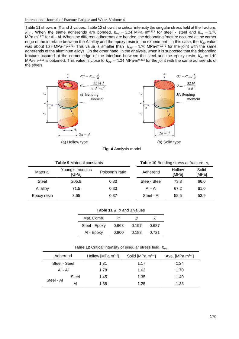
International Journal of Fracture Fatigue and Wear, Volume 4
170
Table 11 shows 𝛼, 𝛽 and 𝜆 values. Table 12 shows the critical intensity the singular stress field at the fracture, 𝐾𝜎𝑐 . When the same adherends are bonded, 𝐾𝜎𝑐 = 1.24 MPa ∙ m0.313 for steel - steel and 𝐾𝜎𝑐 = 1.70
MPa∙m0.279 for Al - Al. When the different adherends are bonded, the debonding fracture occured at the corner
edge of the interface between the Al alloy and the epoxy resin in the experiment ; in this case, the 𝐾𝜎𝑐 value
was about 1.33 MPa∙m0.279. This value is smaller than 𝐾𝜎𝑐 = 1.70 MPa∙m0.279 for the joint with the same adherends of the aluminum alloys. On the other hand, in the analysis, when it is supposed that the debonding fracture occured at the corner edge of the interface between the steel and the epoxy resin, 𝐾𝜎𝑐 = 1.40
MPa∙m0.313 is obtained. This value is close to 𝐾𝜎𝑐 = 1.24 MPa∙m0.313 for the joint with the same adherends of the steels.
(a) Hollow type (b) Solid type
Fig. 4 Analysis model
Table 9 Material constants Table 10 Bending stress at fracture, σc
Material Young’s modulus
[GPa] Poisson’s ratio
Adherend
Hollow [MPa]
Solid [MPa]
Steel 205.8 0.30 Stee - Steel 73.3 66.0
Al alloy 71.5 0.33 Al - Al 67.2 61.0
Epoxy resin 3.65 0.37 Steel - Al 58.5 53.9
Table 11 𝛼, 𝛽 and 𝜆 values
Mat. Comb. 𝛼 𝛽 𝜆
Steel - Epoxy 0.963 0.197 0.687
Al - Epoxy 0.900 0.183 0.721
Table 12 Critical intensity of singular stress field, 𝐾𝜎𝑐
Adherend Hollow [MPa m1- Solid [MPa m1- Ave. [MPa m1-
Steel - Steel 1.31 1.17 1.24
Al - Al 1.78 1.62 1.70
Steel - Al Steel 1.45 1.35 1.40
Al 1.38 1.25 1.33

International Journal of Fracture Fatigue and Wear, Volume 4
171
5 CONCLUSIONS
In this paper, the method for accurately calculating the intensity of the singular stress field for the bonded cylinder under bending was proposed. The following conclusion can be drawn.
1. The circumferential strain at the interface corner edge, 𝜀𝜃0, is not influenced by the stress singularity and can be calculated accurately by FEM.
2. The mesh-independence technique is applicable to the bonded cylinder and the cylindrical butt joints through the subtraction process of the non-singular stress. The stress-free boundary condition causes the non-singular stresses 𝑟0,𝐹𝐸𝑀 = 𝑟𝑧0,𝐹𝐸𝑀 = 0 . hhen the radial stress 𝜎𝑟0,𝐹𝐸𝑀 or the shear stress
𝜏𝑟𝑧0,𝐹𝐸𝑀 are used, the intensity of the singular stress field can be calculated easily without the subtraction
process. 3. The practicability of the method was examined using the four-point bending test results of the hollow and
solid cylindrical butt joints.
REFERENCES
[1] Li, Y. L., Hu, S. Y., Munz, D., Yang, Y. Y., Asymptotic description of the stress field around the bond edge of a cylindrical joint, Archive of Applied Mechanics, Vol. 68,No. 7 - 8(1998),pp. 552 - 565.
[2] Miyazaki, T., Noda, N. -A., Wang, Z., Sano, Y., Analysis of Intensity of Singular Stress Field for Bonded Cylinder in Comparison with Bonded Plate, Trans. Jpn. Soc. Mech. Eng., Vol. 81, No. 829 (2015), DOI:10.1299/transjsme.15-00210 (in Japanese).
[3] Sawa, T., Aoki, M., Elastoplastic FEM Stress Analysis and Strength of Adhesive Butt Joints of Dissimilar Hollow Shafts Subjected to External Bending Moments, Trans. Jpn. Soc. Mech. Eng., Ser. A, 62 - 593 (1996), 168 - 174 (in Japanese).
[4] Dundurs, J., Discussion of edge-bonded dissimilar orthotropic elastic wedges under normal and shear loading, Trans. ASME, J. Appl. Mech., Vol. 36 (1969), pp. 650-652.

International Journal of Fracture Fatigue and Wear, Volume 4
172
Proceedings of the 5th International Conference on
Fracture Fatigue and Wear, pp. 172-177, 2016
FATIGUE BEHAVIOR OF FLEXURALLY STRENGTHENED FRP
CONCRETE STRUCTURES
H. A. Toutanji1, R. Vuddandam2, D. Wang3, M. Hussak4
1Western Michigan University, Kalamazoo, MI, USA 2Tarleton State University, Stephenville, TX, USA
3TRC companies, Inc., Baton Rouge, LA, USA 4Crown Castle Inc., Pennsylvania, PA, USA
Abstract: Flexural strengthening of Reinforced Concrete (RC) beams with externally bonded Fiber
Reinforced Polymers (FRP) under monotonic loading has been documented in numerous studies. However, this strengthening system behavior under cyclic loading still needs more investigation. The current study aims at developing an analytical model to determine the life of RC beams strengthened with FRP in flexure under fatigue loading in terms of the number of cycles to failure. A cyclic dependent modulus of rupture is proposed to address the degradation of flexural stiffness at fatigue load cycles by determining the corresponding neutral axis location and moment of inertia. A fatigue life prediction model (S-N curve relationship) is proposed to predict the fatigue behavior, based on steel stress levels of RC beams strengthened with FRP. The proposed model shows good agreement with data from literature and in-house tested beams under four point bending setup subjected to fatigue loading.
Keywords: Fatigue test; CFRP; Externally bonded reinforcement (EBR); Four-point bending test (FPBT); Fatigue life prediction model.
1 INTRODUCTION
For the past two decades, fiber reinforced polymers (FRP) materials have been accepted as a commonly used method for strengthening conventional materials such as reinforced concrete (RC) structures. Although studies on RC beams strengthened with FRP subjected to monotonic loading [1] are abundant and well documented in current design guidelines [2, 3], studies related to beams subjected to fatigue loading is limited.
Primarily, Meier et al [4] conducted fatigue tests on reinforced concrete beams strengthened with glass/carbon-hybrid sheet. Later accompanied fatigue tests from different researchers [5], noticed no significant change in fatigue behavior for strengthened and non-strengthened beams. However, some studies [6-9] showed an enhanced serviceability. The FRP-strengthened beams showed improved deflections avoiding the gradual flexural stiffness degradation, as compared to conventional RC beams. For FRP-strengthened beams, significant fatigue damage is recognized within first few cycles and the rate of change in flexural stiffness is considerably lower at later cycles [10, 11]. The same trend was observed by the authors through in-house experiments. The significance of this paper is to develop an analytical model, and create a fatigue life prediction model. The proposed analytical model predicts the cycle dependent deflections considering the gradual degradation of beams flexural stiffness, while the proposed fatigue life prediction model predicts the fatigue life of a FRP strengthened beam based on steel stress.
2 ANALYTICAL MODEL
Within literature, most of the researchers investigated fatigue performance considering load range (or stress range) in three different ways: (1) the load range as percentage of ultimate capacity; (2) the load range as percentage of yield capacity; and (3) the stress range as percentage of the yield strength of steel. Steel yielding followed by FRP failure (rupture or delamination) is the most commonly observed fatigue failure mode for FRP-strengthened beams at high stress range [9, 11, 12]. In literature, low load range refers to as the applied maximum fatigue load is within the service load (50-60% of yield capacity of the monotonically loaded beam) [13]. The maximum fatigue load chosen beyond the service load is considered to be under high load range.
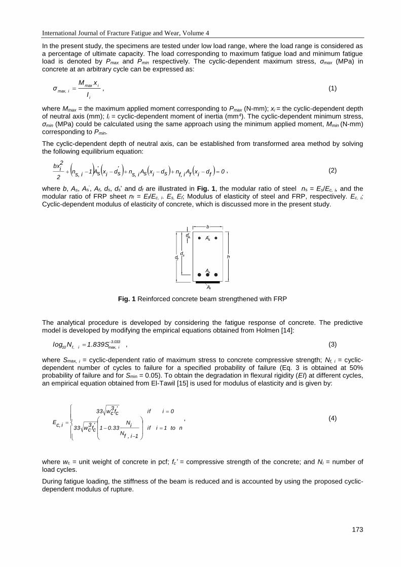
International Journal of Fracture Fatigue and Wear, Volume 4
173
In the present study, the specimens are tested under low load range, where the load range is considered as a percentage of ultimate capacity. The load corresponding to maximum fatigue load and minimum fatigue load is denoted by Pmax and Pmin respectively. The cyclic-dependent maximum stress, σmax (MPa) in concrete at an arbitrary cycle can be expressed as:
i
imax
imax,I
xMσ , (1)
where Mmax = the maximum applied moment corresponding to Pmax (N-mm); xi = the cyclic-dependent depth of neutral axis (mm); Ii = cyclic-dependent moment of inertia (mm4). The cyclic-dependent minimum stress, σmin (MPa) could be calculated using the same approach using the minimum applied moment, Mmin (N-mm) corresponding to Pmin.
The cyclic-dependent depth of neutral axis, can be established from transformed area method by solving the following equilibrium equation:
0f
di
xf
Aif,
nsdi
xsAis,
n'sd
ix
'sA1
is,n
2
2i
bx , (2)
where b, As, As’, Af, ds, ds’ and df are illustrated in Fig. 1, the modular ratio of steel ns = Es/Ec, i, and the
modular ratio of FRP sheet nf = Ef/Ec, i. Es, Ef; Modulus of elasticity of steel and FRP, respectively. Ec, i; Cyclic-dependent modulus of elasticity of concrete, which is discussed more in the present study.
Fig. 1 Reinforced concrete beam strengthened with FRP
The analytical procedure is developed by considering the fatigue response of concrete. The predictive model is developed by modifying the empirical equations obtained from Holmen [14]:
3.033
imax,if,101.839SNlog
, (3)
where Smax, i = cyclic-dependent ratio of maximum stress to concrete compressive strength; Nf, i = cyclic-dependent number of cycles to failure for a specified probability of failure (Eq. 3 is obtained at 50% probability of failure and for Smin = 0.05). To obtain the degradation in flexural rigidity (EI) at different cycles, an empirical equation obtained from El-Tawil [15] is used for modulus of elasticity and is given by:
nto1iif
1i, fN
iN
0.331'cf
3cw33
0iif'cf
3cw33
i c,E
, (4)
where wc = unit weight of concrete in pcf; fc’ = compressive strength of the concrete; and Ni = number of load cycles.
During fatigue loading, the stiffness of the beam is reduced and is accounted by using the proposed cyclic-dependent modulus of rupture.

International Journal of Fracture Fatigue and Wear, Volume 4
174
nto1iif
1i,fN
10log
iN
10log
1'cfcwrg
0iif'cfcwrg
ir,f
, (5)
where gr = 0.6 to 1.0, 0.6 is a conservative value [16]. From the proposed modulus of rupture, corresponding cracking moment is obtained and consequently the deflection at arbitrary number of cycles can be determined as shown in Fig. 2.
Fig. 2 Schematic illustration of the proposed analytical model
3 EXPERIMENTAL INVESTIGATION
Seven beams were fabricated and tested in four-point bending test setup. Fig. 3Error! Reference source not found. shows the loading configuration, notch details and reinforcement details of the test specimen. Maximum and minimum loads applied for fatigue cycle and failure modes of the tested specimens are shown in Table 1.

International Journal of Fracture Fatigue and Wear, Volume 4
175
Fig. 3 Loading configuration and reinforcement details of the concrete beam (dimension: mm).
Table 1 Fatigue Test Data
Specimen
Minimum and maximum load applied (kN)
No. of cycles to failure
Failure mode
CF 4.27-21.35a >2 x 10⁶ No failure
NCF 4.27-21.35a >2 x 10⁶ No failure
FT1 10.01 – 50.04b 3.15 x 10⁵ S→D
FT2 8.01-40.03a >2 x 10⁶ No failure
FT3 8.01-40.03a >2 x 10⁶ No failure
FT4 8.01-40.03a >2 x 10⁶ No failure
NFT1 8.01-40.03a 8 x 10⁵ S→D
C = Control beam; N = Notched beam; F = Fatigue loading; T = two layers of FRP; S = Steel yielding; D =
Delamination of the FRP.
aLoad range corresponds to 12%-60% of ultimate capacity with load ratio of R = 0.2, amplitude ratio of A =
0.67 and loading frequency of 2 Hz.
bLoad range corresponds to 15%-75% of ultimate capacity with load ratio of R = 0.2, amplitude ratio of A =
0.67 and loading frequency of 2 Hz.
4 VERIFICATION OF ANALYTICAL MODEL
As verification to the present analytical solution, a comparison of the deflections from the present analytical study with experimental data is made in Table 2.
Table 2 Predicted Deflection vs Experimental Deflection
Number of the load cycle
Number of cycles to failure Nf, i
Flexural Rigidity
Ec, i IΔ, i (N-mm2)
Predicted Def-lection Δi, pred (mm)
Experimental Def-lection Δi, exp(mm)
0th cycle (monotonic) 2,054,276,591 4.427E+11 6.02 8.17
50,000th cycle 2,054,719,496 4.217E+11 6.32 8.69
100,000th cycle 2,055,162,313 4.212E+11 6.32 8.77
500,000th cycle 2,058,701,702 4.202E+11 6.34 8.71
1,000,000th cycle 2,063,118,116 4.198E+11 6.34 8.78
1,500,000th cycle 2,067,525,906 4.197E+11 6.35 8.85
2,000,000th cycle 2,071,925,139 4.196E+11 6.35 8.88
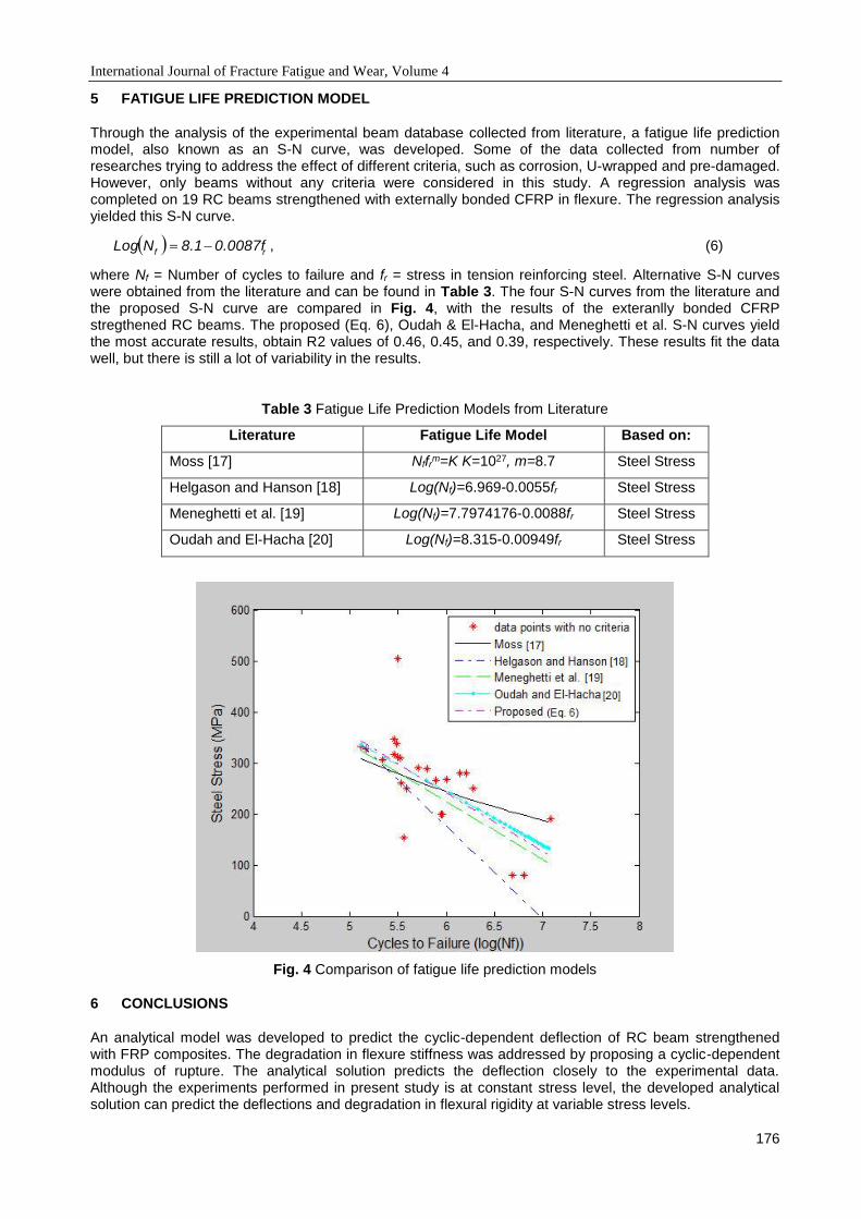
International Journal of Fracture Fatigue and Wear, Volume 4
176
5 FATIGUE LIFE PREDICTION MODEL
Through the analysis of the experimental beam database collected from literature, a fatigue life prediction model, also known as an S-N curve, was developed. Some of the data collected from number of researches trying to address the effect of different criteria, such as corrosion, U-wrapped and pre-damaged. However, only beams without any criteria were considered in this study. A regression analysis was completed on 19 RC beams strengthened with externally bonded CFRP in flexure. The regression analysis yielded this S-N curve.
rf
0.0087f8.1NLog , (6)
where Nf = Number of cycles to failure and fr = stress in tension reinforcing steel. Alternative S-N curves were obtained from the literature and can be found in Table 3. The four S-N curves from the literature and the proposed S-N curve are compared in Fig. 4, with the results of the exteranlly bonded CFRP stregthened RC beams. The proposed (Eq. 6), Oudah & El-Hacha, and Meneghetti et al. S-N curves yield the most accurate results, obtain R2 values of 0.46, 0.45, and 0.39, respectively. These results fit the data well, but there is still a lot of variability in the results.
Table 3 Fatigue Life Prediction Models from Literature
Literature Fatigue Life Model Based on:
Moss [17] Nffrm=K K=1027, m=8.7 Steel Stress
Helgason and Hanson [18] Log(Nf)=6.969-0.0055fr Steel Stress
Meneghetti et al. [19] Log(Nf)=7.7974176-0.0088fr Steel Stress
Oudah and El-Hacha [20] Log(Nf)=8.315-0.00949fr Steel Stress
Fig. 4 Comparison of fatigue life prediction models
6 CONCLUSIONS
An analytical model was developed to predict the cyclic-dependent deflection of RC beam strengthened with FRP composites. The degradation in flexure stiffness was addressed by proposing a cyclic-dependent modulus of rupture. The analytical solution predicts the deflection closely to the experimental data. Although the experiments performed in present study is at constant stress level, the developed analytical solution can predict the deflections and degradation in flexural rigidity at variable stress levels.
International Journal of Fracture Fatigue and Wear, Volume 4
177
7 REFERENCES
[1] H. Saadatmanesh, A. M. Malek, Design guidelines for flexural strengthening of RC beams with FRP plates, Journal of Composites for Construction, 2(4), 158–164, 1998.
[2] American Concrete Institute (ACI) Committee 440, Guide for the Design and Construction of Externally bonded FRP Systems for Strengthening Concrete Structures, ACI, MI, USA, 2008.
[3] National Cooperative Highway Research Program (NCHRP), Report 655: Recommended Guide Specification for the Design of Externally bonded FRP Systems for Repair and Strengthening of Concrete Bridge Elements, 2010.
[4] U. Meier, M. Deuring, H. Meier, G. Schwegler, Strengthening of structures with CFRP laminates: Research and applications in Switzerland, Advanced Composite Materials in Bridges and Structures, K. W. Neale and P. Labossiere (eds), 1992.
[5] R. A. Barnes, G. C. Mays, Fatigue performance of concrete beams strengthened with CFRP plates, ASCE Journal of Composites for Construction, 3(2), 63-72, 1999.
[6] M. Shahawy, T. E. Beitelman, Static and fatigue performance of RC beams strengthened with CFRP laminates, ASCE Journal of Structural Engineering, 125(6), 613-621, 1999.
[7] C. G. Papakonstantinou, Fatigue Performance of Reinforced Concrete Beams Strengthened with Glass Fiber Reinforced Polymer Composite Sheets, M.S. Thesis, University of South Carolina, Columbia, SC, 29-64, 2000.
[8] C. G. Papakonstantinou, P. N. Balaguru, M. Petrou, Analysis of reinforced concrete beams streng-thened with composites subjected to fatigue loading, ACI Special Publication, 206, 41-60, 2002.
[9] J. Aidoo, K. A. Harries, M. F. Petrou, Fatigue behavior of carbon fiber reinforced polymer strengthened reinforced concrete bridge girders, Journal of Composites for Construction, 8(6), 501–509, 2004.
[10] P. J. Heffernan, M. Erki, Fatigue behavior of reinforced concrete beams strengthened with carbon fiber reinforced plastic laminates, Journal of Composites for Construction, 8(2), 132–140, 2004.
[11] R. Gussenhoven, S. F. Brena, Fatigue behavior of reinforced concrete beams strengthened with different FRP laminate configurations, Fiber-Reinforced Polymer (FRP) Reinforcement for Concrete Structures (SP-230), 613–630, 2005.
[12] H. Toutanji, L. Zhao, Y. Deng, Y. Zhang, P. Balaguru, Cyclic behavior of RC beams strengthened with carbon fiber sheets bonded by inorganic matrix, Journal of Material and Civil Engineering, 18(1), 28–35, 2006.
[13] Y. J. Kim, J. P. Heffernan, Fatigue behavior of externally strengthened concrete beams with fiber-reinforce polymers: state of art, Journal of Composites for Construction, 12(3) 246–256, 2008.
[14] J. O. Holmen, Fatigue of concrete by constant and variable amplitude loading, Fatigue of Concrete Structures, American Concrete Institute, Detroit, 71–110, 1982.
[15] S. El-Tawil, C. Ogunc, A. Okeil, M. Shahawy, Static and fatigue analysis of RC beams strengthened with CFRP laminates, Journal of Composites for Construction, 5(4) 258–267, 2001.
[16] American Concrete Institute (ACI) Committee 209, Prediction of Creep, Shrinkage, and Temparature Effects in Concrete Structures. ACI, MI, USA, 1992.
[17] D.S. Moss, Bending Fatigue of High-yield Reinforcing Bars in Concrete, TRRL Supplementary Rep. 748, Transport and Road Research Laboratory, Crowthome, U.K, 1982.
[18] T. Helgason, J. M. Hanson, Investigation of Design Factors Affecting Fatigue Strength of Reinforcing Bars – Statistical Analysis, Abeles Symposium on Fatigue of Concrete, American Concrete Institute SP 41, 107-138, 1974.
[19] L. C. Meneghetti, M. R. Garcez, Silva, L. C. Filho, F. P. Gastal, Fatigue life regression model of reinforced concrete beams strengthened with FRP, Magazine of Concrete Research, 63-539, 2011.
[20] F. Oudah, R. El-Hacha, Research progress on the fatigue performance of RC beams strengthened in flexure using Fiber Reinforced Polymers, Composites: Part B, 82–95, 2013.
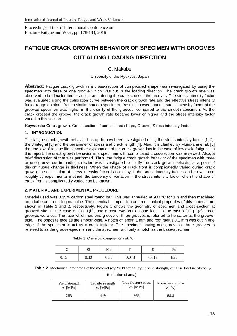
International Journal of Fracture Fatigue and Wear, Volume 4
178
Proceedings of the 5th International Conference on
Fracture Fatigue and Wear, pp. 178-183, 2016
FATIGUE CRACK GROWTH BEHAVIOR OF SPECIMEN WITH GROOVES
CUT ALONG LOADING DIRECTION
C. Makabe
University of the Ryukyus, Japan
Abstract: Fatigue crack growth in a cross-section of complicated shape was investigated by using the
specimen with three or one groove which was cut in the loading direction. The crack growth rate was observed to be decelerated or accelerated during the crack crossed the grooves. The stress intensity factor was evaluated using the calibration curve between the crack growth rate and the effective stress intensity factor range obtained from a similar smooth specimen. Results showed that the stress intensity factor of the grooved specimen was higher in the vicinity of the grooves, compared to the smooth specimen. As the crack crossed the groove, the crack growth rate became lower or higher and the stress intensity factor varied in this section.
Keywords: Crack growth, Cross-section of complicated shape, Groove, Stress intensity factor
1. INTRODUCTION
The fatigue crack growth behavior has up to now been investigated using the stress intensity factor [1, 2], the J integral [3] and the parameter of stress and crack length [4]. Also, it is clarified by Murakami et al. [5] that the law of fatigue life is another explanation of the crack growth law in the case of low cycle fatigue. In this report, the crack growth behavior in a specimen with complicated cross-section was reviewed. Also, a brief discussion of that was performed. Thus, the fatigue crack growth behavior of the specimen with three or one groove cut in loading direction was investigated to clarify the crack growth behavior at a point of discontinuous change in thickness. When the shape of crack front is complicatedly varied during crack growth, the calculation of stress intensity factor is not easy. If the stress intensity factor can be evaluated roughly by experimental method, the tendency of variation in the stress intensity factor when the shape of crack front is complicatedly varied can be known. 2. MATERIAL AND EXPERIMENTAL PROCEDURE
Material used was 0.15% carbon steel round bar. This was annealed at 900 °C for 1 h and then machined on a lathe and a milling machine. The chemical composition and mechanical properties of this material are shown in Table 1 and 2, respectively. Figure 1 shows the geometry of specimen and cross-section at grooved site. In the case of Fig. 1(b), one groove was cut on one face. In the case of Fig1 (c), three grooves were cut. The face which has one groove or three grooves is referred to hereafter as the groove-side. The opposite face as the smooth-side. A notch of length 1 mm and root radius 0.1 mm was cut in one edge of the specimen to act as a crack initiator. The specimen having one groove or three grooves is referred to as the groove-specimen and the specimen with only a notch as the base-specimen. Table 1 Chemical composition (wt, %)
Table 2 Mechanical properties of the material (σS: Yield stress, σB: Tensile strength, σT: True fracture stress, :
Reduction of area)
C Si Mn P S Fe
0.15 0.30 0.50 0.013 0.013 Bal.
Yield strength
σS [MPa]
Tensile strength
σB [MPa]
True fracture stress
σT [MPa] Reduction of area
[%]
283 449 956 68.8

International Journal of Fracture Fatigue and Wear, Volume 4
179
(a) (b) (c)
Fig. 1 Geometry of specimen; (a) Specimen, (b) Case of one groove, (c) Case of three grooves.
Fatigue tests under constant stress amplitude were carried out. The stress ratio R is chosen -1 and
maximum cyclic stress max is fixed 85.84 MPa. Crack length a, which included the notch length was measured with two sets of traveling microscope and dial-gauge at the mean load. In order to examine the
relationship between crack growth rate and crack closure, the crack opening stress op was measured by using the strain gages. The features of the crack front in the case of groove-specimen were observed by means of the beach mark.
3. EXPERIMENTAL RESULTS AND DISCUSSION
3.1 Crack growth behavior
3.1.1 In the case of one groove
The data of crack growth curves of the specimen with one groove is plotted in Fig. 2. The solid line with Base is the data of base-specimen. The effect of groove in the case of b/t (groove depth/ specimen thickness) = 0.125 on crack growth behavior was very small, in comparison to the base specimen. However, the retardation of crack growth was observed in the case of b/t = 0.65. The acceleration of crack growth was happen in the case of b/t = 0.45. Figure 3 shows the relationship between crack length a and crack growth rate da/dN at the groove-side and smooth-side. In the case of smooth-side, it is find that the crack growth rate was decreased after crack crossed over the groove. Also, the groove depth was the deeper, the crack growth rate was the lower. The tendency of crack growth rate of groove-side is different in each specimen. Especially, the crack growth rate was clearly accelerated in the case of b/t = 0.45. This behavior is related to the shortening of fatigue life in the case of b/t = 0.45. Therefore, the difference of fatigue life depending on the groove depth is related to the difference of crack growth behavior between the groove-side and smooth-side.
Fig. 2 Crack growth curves (In the case of one groove) .
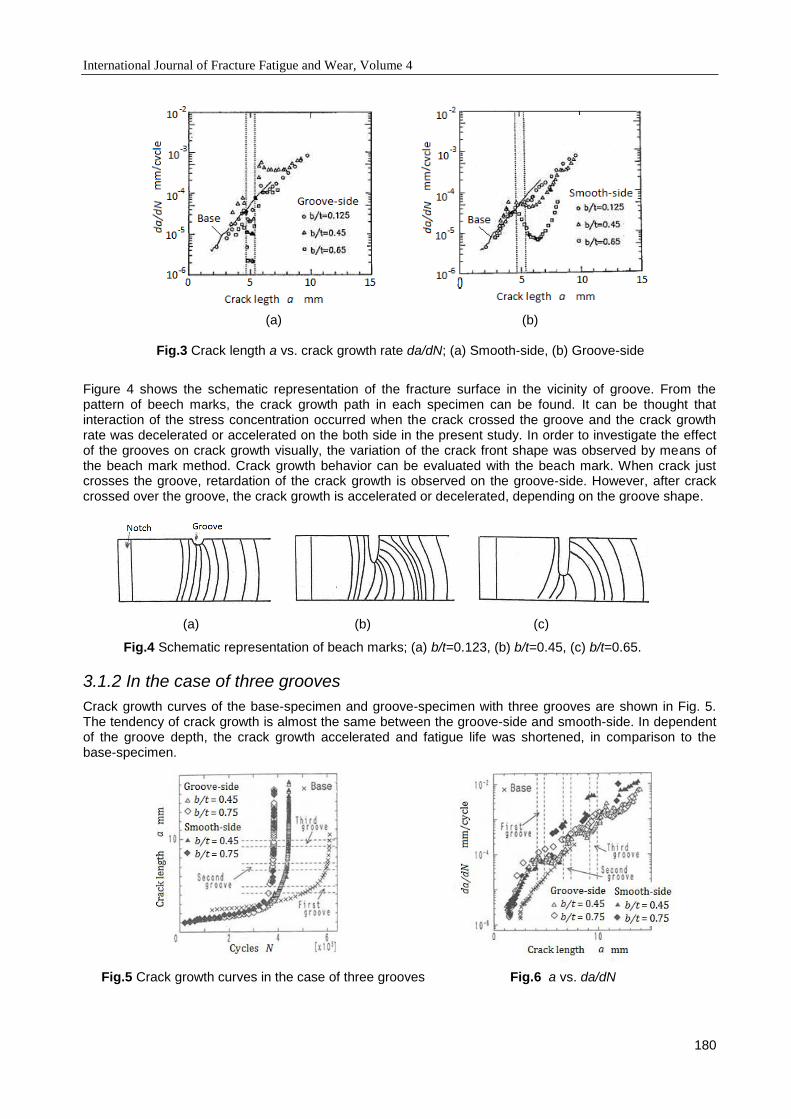
International Journal of Fracture Fatigue and Wear, Volume 4
180
(a) (b)
Fig.3 Crack length a vs. crack growth rate da/dN; (a) Smooth-side, (b) Groove-side
Figure 4 shows the schematic representation of the fracture surface in the vicinity of groove. From the pattern of beech marks, the crack growth path in each specimen can be found. It can be thought that interaction of the stress concentration occurred when the crack crossed the groove and the crack growth rate was decelerated or accelerated on the both side in the present study. In order to investigate the effect of the grooves on crack growth visually, the variation of the crack front shape was observed by means of the beach mark method. Crack growth behavior can be evaluated with the beach mark. When crack just crosses the groove, retardation of the crack growth is observed on the groove-side. However, after crack crossed over the groove, the crack growth is accelerated or decelerated, depending on the groove shape.
(a) (b) (c)
Fig.4 Schematic representation of beach marks; (a) b/t=0.123, (b) b/t=0.45, (c) b/t=0.65.
3.1.2 In the case of three grooves
Crack growth curves of the base-specimen and groove-specimen with three grooves are shown in Fig. 5. The tendency of crack growth is almost the same between the groove-side and smooth-side. In dependent of the groove depth, the crack growth accelerated and fatigue life was shortened, in comparison to the base-specimen.
Fig.5 Crack growth curves in the case of three grooves Fig.6 a vs. da/dN
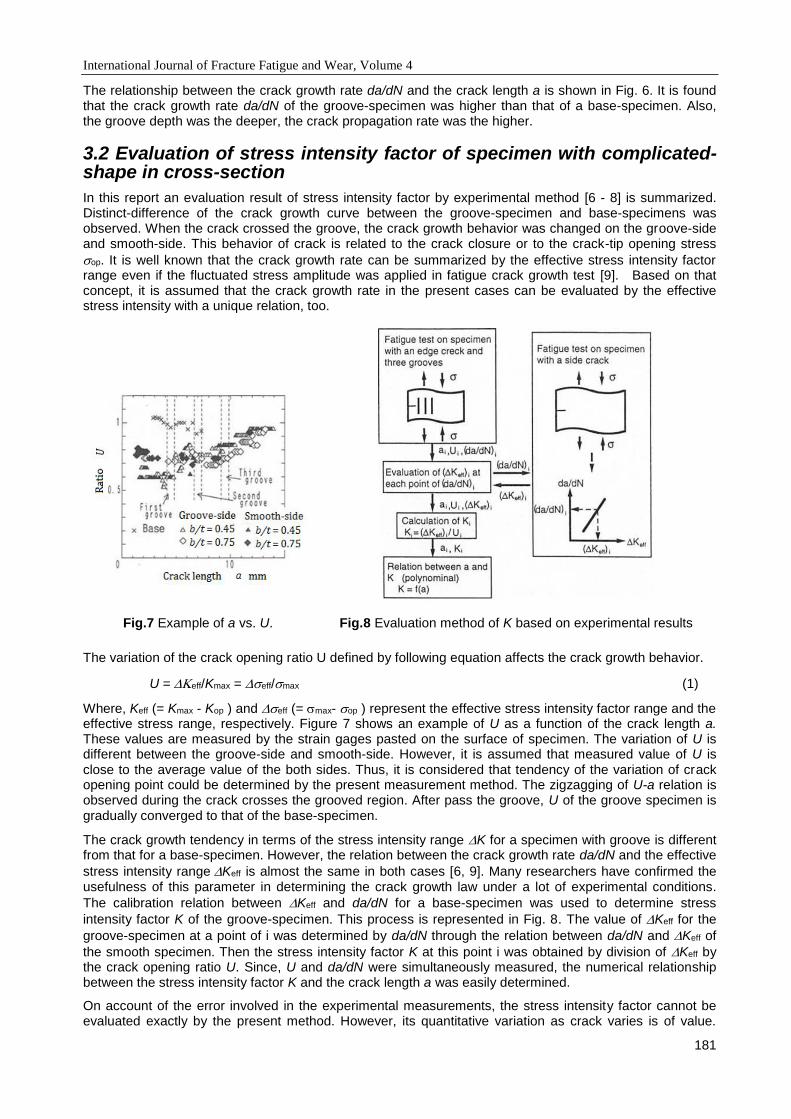
International Journal of Fracture Fatigue and Wear, Volume 4
181
The relationship between the crack growth rate da/dN and the crack length a is shown in Fig. 6. It is found that the crack growth rate da/dN of the groove-specimen was higher than that of a base-specimen. Also, the groove depth was the deeper, the crack propagation rate was the higher.
3.2 Evaluation of stress intensity factor of specimen with complicated-shape in cross-section
In this report an evaluation result of stress intensity factor by experimental method [6 - 8] is summarized. Distinct-difference of the crack growth curve between the groove-specimen and base-specimens was observed. When the crack crossed the groove, the crack growth behavior was changed on the groove-side and smooth-side. This behavior of crack is related to the crack closure or to the crack-tip opening stress
op. It is well known that the crack growth rate can be summarized by the effective stress intensity factor range even if the fluctuated stress amplitude was applied in fatigue crack growth test [9]. Based on that concept, it is assumed that the crack growth rate in the present cases can be evaluated by the effective stress intensity with a unique relation, too.
Fig.7 Example of a vs. U. Fig.8 Evaluation method of K based on experimental results
The variation of the crack opening ratio U defined by following equation affects the crack growth behavior.
U =eff/Kmax = eff/max (1)
Where, Keff (= Kmax - Kop ) and eff (= max- op ) represent the effective stress intensity factor range and the effective stress range, respectively. Figure 7 shows an example of U as a function of the crack length a. These values are measured by the strain gages pasted on the surface of specimen. The variation of U is different between the groove-side and smooth-side. However, it is assumed that measured value of U is close to the average value of the both sides. Thus, it is considered that tendency of the variation of crack opening point could be determined by the present measurement method. The zigzagging of U-a relation is observed during the crack crosses the grooved region. After pass the groove, U of the groove specimen is gradually converged to that of the base-specimen.
The crack growth tendency in terms of the stress intensity range K for a specimen with groove is different from that for a base-specimen. However, the relation between the crack growth rate da/dN and the effective
stress intensity rangeKeff is almost the same in both cases [6, 9]. Many researchers have confirmed the usefulness of this parameter in determining the crack growth law under a lot of experimental conditions.
The calibration relation between Keff and da/dN for a base-specimen was used to determine stress
intensity factor K of the groove-specimen. This process is represented in Fig. 8. The value of Keff for the
groove-specimen at a point of i was determined by da/dN through the relation between da/dN and Keff of
the smooth specimen. Then the stress intensity factor K at this point i was obtained by division of Keff by the crack opening ratio U. Since, U and da/dN were simultaneously measured, the numerical relationship between the stress intensity factor K and the crack length a was easily determined.
On account of the error involved in the experimental measurements, the stress intensity factor cannot be evaluated exactly by the present method. However, its quantitative variation as crack varies is of value.
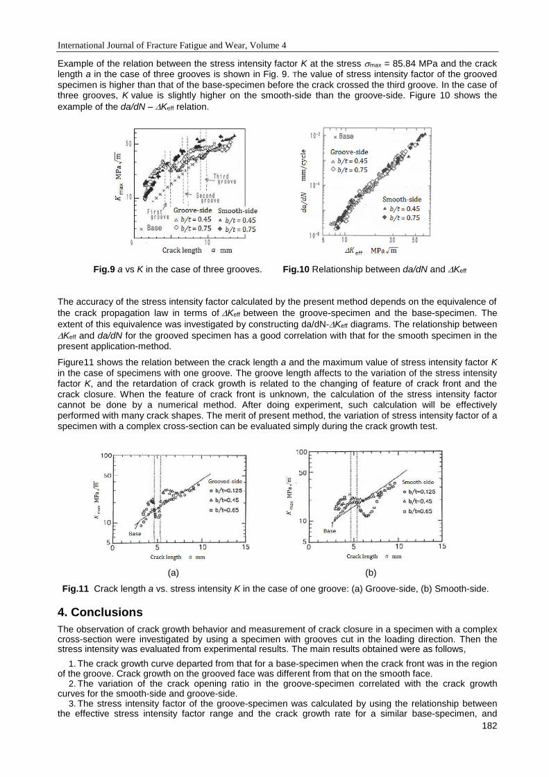
International Journal of Fracture Fatigue and Wear, Volume 4
182
Example of the relation between the stress intensity factor K at the stress max = 85.84 MPa and the crack length a in the case of three grooves is shown in Fig. 9. The value of stress intensity factor of the grooved specimen is higher than that of the base-specimen before the crack crossed the third groove. In the case of three grooves, K value is slightly higher on the smooth-side than the groove-side. Figure 10 shows the
example of the da/dN –Keff relation.
Fig.9 a vs K in the case of three grooves. Fig.10 Relationship between da/dN and Keff
The accuracy of the stress intensity factor calculated by the present method depends on the equivalence of
the crack propagation law in terms ofKeff between the groove-specimen and the base-specimen. The
extent of this equivalence was investigated by constructing da/dN-Keff diagrams. The relationship between
Keff and da/dN for the grooved specimen has a good correlation with that for the smooth specimen in the present application-method.
Figure11 shows the relation between the crack length a and the maximum value of stress intensity factor K in the case of specimens with one groove. The groove length affects to the variation of the stress intensity factor K, and the retardation of crack growth is related to the changing of feature of crack front and the crack closure. When the feature of crack front is unknown, the calculation of the stress intensity factor cannot be done by a numerical method. After doing experiment, such calculation will be effectively performed with many crack shapes. The merit of present method, the variation of stress intensity factor of a specimen with a complex cross-section can be evaluated simply during the crack growth test.
(a) (b)
Fig.11 Crack length a vs. stress intensity K in the case of one groove: (a) Groove-side, (b) Smooth-side.
4. Conclusions
The observation of crack growth behavior and measurement of crack closure in a specimen with a complex cross-section were investigated by using a specimen with grooves cut in the loading direction. Then the stress intensity was evaluated from experimental results. The main results obtained were as follows,
1. The crack growth curve departed from that for a base-specimen when the crack front was in the region of the groove. Crack growth on the grooved face was different from that on the smooth face.
2. The variation of the crack opening ratio in the groove-specimen correlated with the crack growth curves for the smooth-side and groove-side.
3. The stress intensity factor of the groove-specimen was calculated by using the relationship between the effective stress intensity factor range and the crack growth rate for a similar base-specimen, and

International Journal of Fracture Fatigue and Wear, Volume 4
183
represented as a polynomial in the crack length. 4. The stress intensity factor of the groove-specimen exhibited a complicated variation when the crack
front crossed the groove, as did the crack growth law in terms of the maximum value of stress intensity factor.
References
[1] P. C. Paris and F. A. Erdogan, Critical Analysis of Crack Propagation Law, Transaction of ASME, Ser.
D, 85, 528-533, 1963.
[2] W. Elber, The Significance of Fatigue Crack Closure, Damage Tolerance in Aircraft Structures, ASTM STP 486, American Society for Testing and Materials, Philadelphia, 230-242. 1971.
[3] N. E. Dowling and J. A. Begley, Fatigue Crack Growth During Gross Plasticity and the J-Integral, Mechanics of Crack Growth, ASTM STP 590, American Society for Testing and Materials, Phil-adelphia, 82-103, 1976.
[4] H. Nisitani, M. Goto and N. Kawagoishi, A Small-crack Growth Law and Its Related Phenomena, Engineering Fracture Mechanics, 41, 499-513, 1992.
[5] Y. Murakami, S. Harada, T. Endo, H. Tani-ishi, H. and Y. Fukushima, Correlations among Growth Law of Small Cracks, Low-Cycle Fatigue Law and Applicability of Miner’s Rule, Engineering Fracture Mechanics,18, 909-924, 1983.
[6] C. Makabe, H. Kaneshiro and H. Yara, Fatigue Crack Propagation in a Specimen with Complicated Cross-Section; Characterization of the Stress Intensity Factor, J. Testing and Evaluation, 22, 91-97, 1992.
[7] Y. Hagiwara and T. Shimada, Through Fatigue Crack Propagation Behavior In and Around the Heavily Changed Cross- Sectioned Area, Transactions of Japan Society of Mechanical Engineers, 56A, 552-558, 1990.
[8] C. S. Shin, The Stress Intensity of Corner Cracks Emanating from Holes, Engineering Fracture Mechanics, 37, 423-436, 1990.
[9] H. Bao and A. J. McEvily, The Effect of Overload on the Rate of Crack Propagation Under Plane Stress Conditions, Metallurgical Transaction A, 21 A, 1725-1733, 1995.
International Journal of Fracture Fatigue and Wear, Volume 4
184
Proceedings of the 5th International Conference on
Fracture Fatigue and Wear, pp. 184-193, 2016
NON-DUCTILE FAILURE ANALYSIS OF STEAM GENERATOR TUBE
SHEET BASED ON DIFFERENT STANDARDS AND CODES
Chang Liu, Hao Qian, Xingyun Liang and Yongcheng Xie
Department of Component Research and Design, Shanghai Nuclear Engineering Research and Design Institute, Shanghai, China
Abstract: The Steam Generators (SG) are used in Pressurized Water Reactors (PWR) between the
primary and the secondary loops in order to convert hot water into saturated steam. The tube sheet locates in the lower part of the SG, supporting large amounts of tubes, which is one of the most crucial components in the SG. Therefore, the non-ductile failure computation and evaluation on the tube sheet is essential to ensure the 60-year lifetime of the SG. This paper dedicates on the investigation of the non-ductile failure computation and evaluation of the SG tube sheet, based on different standards and codes, which include R6 Code, RCC-M Code and ASME B&PVC. Because of the different experimental material data, different safety factors and different methods in these codes, even for the same case, different results can be obtained. The non-ductile failure computation and evaluation of the SG tube sheet is intensively conducted quantitatively and qualitatively in order to address the safety margin and the advantages among each code.
Keywords: non-ductile failure; steam generator; tube sheet; codes
0 INTRODUCTION
Since the 1940s, low stress brittle fracture accidents occurred in succession, which promoted the establishment of the Fracture Mechanics. Low stress brittle fracture implies that the nominal stress is significantly less than the yield stress with no obvious deformation [1]. Fracture Mechanics is an important branch of modern mechanics, under this approach, the postulated flaws of the vessel’s weak part or actual flaws by non-destructive testing (NDT) can be calculated and assessed in order to prevent the brittle fracture accidents which may be disastrous.
Although high strength materials has been wildly used, some fracture accidents still occurs even for the products which are designed and manufactured by traditional strength theory transcend the quite strict inspection. For example, in July 1978, a Spanish liquid propylene tank explosion killed 260 people [2]. For another example, in the famous American “260SL-1” rocket, brittle fractures occurred during the hydraulic test for the engine vessel and the 657 MPa failure stress was far less tan the yield stress of 1716.2 MPa [2]. It can be concluded from these catastrophic accidents that even the high-strength structures deserve a close attention in case of brittle fracture.
For SG, which plays the lead role in heat transfer by converting hot water into saturated steam in PWR. fracture mechanics analysis must be conducted for the key component by corresponding Code on the request of safety review of NNSA (National Nuclear Safety Administration),
This paper dedicates on the investigation of the non-ductile failure computation and assessment of the SG tube sheet, based on different standards and codes, including R6 Code [3], RCC-M Code [4] and ASME B&PVC [5]. Because of the different experimental material data, safety factors and methods in these codes, even for the same case, different results can be obtained. The non-ductile failure computation and evaluation of the SG tube sheet is intensively conducted quantitatively and qualitatively in order to address the safety margin and the advantages among each code. The result maybe a practical conclusion when solving the engineering problem whether during the SG design stage or in the inspection stage when the SG has already been in operation.
International Journal of Fracture Fatigue and Wear, Volume 4
185
1 FRACTURE MECHANICS ANALYSIS METHOD
1.1 Linear-elastic Fracture Mechanics
The object of linear-elastic fracture mechanics analysis is a cracked structure, which has a linear stress-strain curve around the crack (obey hooke`s law). For common metallic materials, the plastic deformation may always occurs when the crack grows, so the hooke`s law can not be kept very strictly. Despite all this, as long as the plastic area is far less than the size of the crack, it does not produce large errors after appropriate amendments. A method of stress intensity factor (KI) is usually used to solve the linear-elastic fracture mechanics problem. KI is an important indicator to judge whether the crack is unstable or not, who is always used to characterize the stress intensity of the crack tip.
The ASME (The American Society of Mechanical Engineers) Boiler & Pressure Vessel Code is the very first Code, in which fracture mechanics is applied for pressure vessel design and the crack assessment. The corresponding sections in ASME provide the don-ductile failure analysis method base on linear-elastic
fracture mechanics. The safety criterion is CII KK in ASME 2007 edition [5], herein IK stands for the
stress intensity factor, CIK stands for the fracture toughness. The method is widely used in SG design
phase for non-ductile failure analysis, which is simple and easy to operate and can guarantee a certain safety margin.
1.2 Elastic-plastic Fracture Mechanics
Linear-elastic fracture mechanics is suitable for the situation when a small scale yielding arises in the crack tip, as for the high toughness steel SA508 Gr.3 Cl.2, the cracked structure is likely to be ductile who has a quite a long stable propagation stage after the crack initiation. Therefore during the in-service inspection stage, linear-elastic fracture mechanics analysis seems too conservation for a cracked structure that we may not make full use of the material’s carrying capacity. As a result, elastic-plastic fracture mechanics analysis can be applied for SG component when a crack is detected during non-destructive evaluation, maximize the economic efficiency on the premise of ensure SG safety.
In elastic-plastic fracture mechanics analysis, the safety criterion is based on the crack tip opening displacement (CTOD) and J-integral. The core of the CTOD theory is the curve of the non-dimensional
displacement parameter as
2 and the non-dimensional stress parameter
s
. Herein the stands
for the crack opening displacement, the a stands for half length of the original crack, the s stands for the
yield strain and the stands for the actual stain. The COTD curve played a major role in the fracture
mechanics analysis of the pressured vessel because of the intuitional and easy to operate of the curve.
In 1968, an American named Rice proposed the J-integral theory [6], in which the J-integral is path-independent linear energy integral shows the stress-strain field of the crack tip. The corresponding safety
criterion is CI JJ , herein the IJ stands for the actual J-integral of the crack tip and the CJ the threshold
value of IJ . This theory gets a wide application because it avoids the complex filed of the crack tip properly
and solves the disagreements in the COTD theory.
In 1978, CEGB(Central Electricity Generating Board) first put forward the two-criteria approach and applied it in the R6 code (R6)(first edition), since then, the pressure vessel integrity assessment technology step into the Failure Assessment Diagram(FAD) times. Then EPRI(Electric Power Research Institute) has carefully studied R6 FAD method, used J-integral in place of narrow-strip –yield model(D-M) and provides a
new failure assessment curve: 2
1
12
1
n
rnre
rrr
LHLH
LJK , herein eH 、 nH are related to the
material hardening parameter n. The curve is more reasonable and advanced than the FAD in the first edition of R6 because more parameters has been considered. Soon afterwards, R6 make a radical change of the FAD and provide three assessment curves which has different difficulty levels, so the status of the new R6 FAD has been further improved in the filed of pressure vessel integrity assessment.
The following section will describe the internationally accepted Codes and their calculation method briefly including R6, RCC-MR and ASME. More importantly, we will provide the result of the contrast calculation trough the specific example, the result include the different sensitive parameters dominating the calculation, the different degrees of the conservative, the different application difficulty and the different applicable

International Journal of Fracture Fatigue and Wear, Volume 4
186
conditions, the result maybe a very practice conclusion when solving the engineering problem whether during the SG design stage or in the inspection stage when the SG has already been in operation.
2 FRACTURE MECHANICS ANALYSIS REQUIREMENTS IN DIFFERENT CODES
2.1 Requirement in R6 Code
R6 is the Assessment of the Integrity of Structures containing Defects by the British Energy which is suitable for elastic-plastic fracture mechanics assessment. The R6-Revision 4:2001 is maintained by the R6 Panel under a Structural Integrity Assessment Procedures collaboration involving British Energy, BNFL Magnox Generation and Serco Assurance.
2.1.1 Two-criteria approach
The FAD is used for structure integrity analysis and assessment in R6, which is a failure assessment diagram proposed and developed by Bowling and Townley with the original name two-criteria approach [7].The two-criteria is built on the linear-elastic fracture mechanics, in this theory it is believed that the structure may cause damage when the external load reached the lower one between the brittle failure load value in linear-elastic fracture mechanics theory and the limit load value in limit analysis. In 2006, the fourth edition R6 proposed three available FAD curves, if the result unable to meet the first curve, the second curve can be used for the assessment. If he results also unable to meet the second curve, the third curve can be used for the assessment conditionally, the conservation of the three curves decreases progressively.
2.1.2 Definition of key parameters in two-criteria approach
In R6 section IV.3, the algorithm of stress intensity factor is defined, there are four methods according to the position the crack. The KI of the circumferential crack not penetrate who occurred frequently is defined as follows:
dua
utrtafu
aK
i
ii
i
i
a
I
23
1/,/2
1 3
10
(2.1.2-1)
Herein,
t
uu bm
21 , tu 0 , stands for the stress towards the wall that the crack
is not contained, m stands for the membrane stress and b stands for the bending stress, a stands for
the crack length, t stands for the thickness of the vessel shell, ir stands for the inner diameter of the
vessel shell.
In R6 section I.9, the rK is defined as a measure of proximity to LEFM (Linear Elastic Fracture Mechanics)
failure, it means the fracture behaviour obeys the plastic fracture mechanics theory when the value of rK
is very low. The rK is defined as follows:
IC
s
IIC
p
I
s
r
p
rr KKKKKKK // (2.1.2-2)
Herein, the p
IK is the linear elastic stress intensity factor for the flow size a for the loads giving rise to p
and the s
IK is the linear elastic stress intensity factor for the flow size a for the loads giving rise to s ,
p
is stress arising from loads which contribute to plastic collapse and the p is stress arising from loads
which do not contribute to plastic collapse, ICK is the fracture toughness of materials.
In R6 section I.8, plasticity effects are included in the failure assessment procedure by means of the
parameter rL which is a measure of how close the cracked structure is to plastic collapse. rL is defined as
the ratio of the loading condition being assessed to the plastic limit load of the structure:
structure flawed theof loadlimit plastic
stresses togiving load apllied total prL (2.1.2-3)
Herein, the p is stress arising from loads which do not contribute to plastic collapse
International Journal of Fracture Fatigue and Wear, Volume 4
187
2.1.3 Three types of failure assessment diagram
In R6 section I.6, three types of failure assessment diagram is defined used for two-criterion assessment. The option 1 curve of the first FAD is described as follow:
62/12
1 6.0exp7.03.05.01 rrr LLLf (2.1.3-1)
y
uy
rr LL
2
max
(2.1.3-2)
The y stands for 0.2% proof stress, u stands for ultimate tensile strength and the other parameters are
already described above. Any cases who meet the limit of option 1 curve do not need the option 2 and 3 curve assessment.
There are three cases in the option 2 curve. In the case that the material stress-strain relationship is known, the option 2 curve is defined as follows:
max
max
2/13
2
0
2
rr
rr
ref
yr
yr
ref
rr
LL
LLE
L
L
E
KLf
(2.1.3-3)
Where the ref is the true strain obtained from the uniaxial mean tensile stress-strain curve at true
stress yrL , E is Young’s modulus and y is the 0.2% proof stress, the other cases can be found in R6
section I.6.
When the fracture mechanics assessment can not meet the limit of option 2 curves, a curve specific to a particular material and geometry may be obtained from a detailed analysis of the defective structure as a
function of the loads given rise to p stress. The option 3 curve is defined as follows:
2/1
3 )(
J
JKLf e
rr (2.1.3-4)
Where eJ and J are values of the J-integral from elastic and elastic-plastic analyse, respectively, at a load
corresponding to the value rL , option 3 curve may be useful in specific cases as an alternative approach
to Options 1 and 2.
2.2 Requirement in RCC-M Code
The RCC-M, short for the Design and Construction Rules for Mechanical Components of PWR Nuclear Islands, published in Code form by AFCEN (French Association for Design, Construction and In-service Inspection Rules for Nuclear Island components) mainly apply to safety related components.
In RCC-M section I sub-section ZG, the acceptable provisions for fast fracture prevention is presented for safety level 1 pressure vessel and its components.
2.2.1 Fast fracture analysis steps in RCC-M
1) The component size, material properties and loadings should be evaluated according to the appendix ZG2000, and then make a decision whether the screening criteria are met no analysis requirements. If not, proceed to the following steps.
2) According to the appendix ZG3000, a conventional fast fracture analysis is proposed intending to obtain a design tolerance towards potential defects. To aim this, conventional defects are postulated with no direct link to potential manufacturing defects or in-service degradation. Specified data are taken into account and conventional safety margins are verified. This analysis method is also dedicated to : -establishing P-T curves giving allowable operation pressure as a function of temperature -determining minimum temperatures for hydrostatic tests.
3) A detailed fast fracture analysis approach according to ZG4000 is proposed, which consists in
International Journal of Fracture Fatigue and Wear, Volume 4
188
determining the maximum defect size for which the prescribed safety margins are just meant.
2.2.2 Definition of key parameters in RCC-M Code
The stress perpendicular to the defect plane can be expressed by polynomial fitting as following when the stress distribution near the defect is gained. Herein, x stands for the distance of defect in the thickness
direction, L stands for the defect depth.
4
4
3
3
2
210
L
x
L
x
L
x
L
xx (2.2.2-1)
The stress intensity factor KI can be computed by the following equation, herein the a stands for the defect,
the 0 、1 、
2 、 3 can be fitted by the equation 2.2.2-1 and the 3210 iiii 、、、 can be obtained from
the table ZG 5121 and ZG 5122.
])/()/()/([ 3
3
32
2
21100 iLaiLaiLaiaK I
(2.2.2-2)
Moreover, plastic zone correction must be applied to the stress intensity factor according to the following procedure:
a) determine the radius yr of the plastic zone at the defect tip, as follows:
p
Iy
R
K
6
1r (2.2.2-3)
Where pR is the yield strength value for the material at the crack tip, this value is given in the RCC-M
Appendix Z I, and KI is the stress intensity factor at the crack tip, regardless of the end of the defect being corrected.
b) determine the corrected value of the intensity factor KCP as follows:
a
raKK
y
I
CP (2.2.2-4)
Where KI is the stress intensity factor determined at the end of the defect considered, and where the value is determined as follows:
-if 0.05( )yr t a 1
-if y0.05( ) r 0.12( )t a t a
20.05( )
1 0.050.035( )
yr t a
t a
-if 0.12( )yr t a 1.6
For the materials covered by procurement specifications in M2110 and M2120, critical stress intensity factor
IcK may be determined from the curve with analytic expression as following, in the range
60 NDTRTT
NDTRTT
NDTIc eRTTK
038.0
2009.040 (2.2.2-5)
Where KIC is expressed in mMPa , and T and NDTRT are expressed in 。

International Journal of Fracture Fatigue and Wear, Volume 4
189
2.3 Requirement in ASME B&PVC
2.3.1 Calculation of Stress intensity factor
For shells and heads that remote from discontinuities, the stress intensity factor KI can be calculated according to the following equations by the ASME Codes Section III Appendix G:
1 1 2 2I Im Ib Im Ib IRK SF K SF K K K K
(2.3.1-1)
1 1Im m mK M
(2.3.1-2)
1 1Ib b bK M
(2.3.1-3)
2 2Im m mK M
(2.3.1-4)
2 2Ib b bK M
(2.3.1-5)
Where, SF stands for the safety factor related with the service level, m1 stands for the primary membrane
stress, b1 stands for the primary bending stress, m2 stands for the secondary membrane stress, b2
stands for the secondary bending stress, mM are experiential parameters which can be looked up in Fig.
G2214-1 of ASME Codes Section III Appendix G, and bM is defined as two-thirds of the mM .
For nozzles, flanges and shell region near geometric discontinuities, the method is also available by enlarge the safety factor or another method provided in WRCB 175.
2.3.2 Reference critical stress intensity factor
KIC is regarded as the reference critical stress intensity factor which has a relation with the working
temperature T and reference nil-ductility transition temperature NDTRT . The equation is available for the
ferritic steels which have specified minimum yield strength at room temperature of 50 ksi or less. For materials which have specified minimum yield strengths at at room temperature greater than 50 ksi but not exceeding 90 ksi, the equation may be used provided fracture mechanics data are obtained at least three heats of the material on a sufficient number of specimens to cover the temperature range of interest, and provide that the data are equal or above the curve of KIC.
36.5 22.783exp 0.036IC NDTK T RT (2.3.2-1)
3 NUMERICAL EXAMPLE BASED ON DIFFERENT CODES
3.1 Object selection
The SG is used in Pressurized Water Reactors (PWR) between the primary and the secondary loops in order to convert hot water into saturated steam. The tube sheet (TS) locates in the lower part of the SG, supporting large amounts of tubes, which is one of the most crucial components in the SG. Therefore, the non-ductile failure computation and evaluation on the tube sheet is essential to ensure the 60-year lifetime of the SG. Therefore, in this paper TS of s SG is chosen as the object for non-ductile failure analysis, the specific interesting analysis section is illustrated in Fig.3.1-1.
3.2 Computational Input
Typical reactor coolant system (RCS) transient is chosen as the computational input load, including its pressure, temperature and heat transfer coefficient. Detailed transient parameters are illustrated in Fig.3.2-1, Fig.3.2-2 and Fig.3.2-3.

International Journal of Fracture Fatigue and Wear, Volume 4
190
Fig. 3.1-1 Analysis Model of TS Fig. 3.2-1 Temperature curves of the transient
Fig. 3.2-2 Pressure curves of the transient Fig. 3.2-3 Heat transfer coefficient curves of the transient
3.3 Results and parameter sensitivity analysis
3.3.1 Results by R6 Code
The postulated flaw feature is defined as a/c=1/3,a/t=1/4,r/t=7.824, according to these dimensional
characteristics and the method discussed in section 2.1, key parameters can be obtained as follows, herein a stands for the depth of the flaw, 2c stands for the length of the flaw and r stands for the inner-radius.
Table 3.3.1-1 fiA parameters
a/t=0.25,2c/a=6.67,R/t=7.824
f0A f1
A f2A f3
A
1.086 0.600 0.453 0.369
Furthermore, on the basis of the stress distribution and the method already discussed, IK and rL are
calculated, which are listed in table xx along with the corresponding stress .
Analysis section
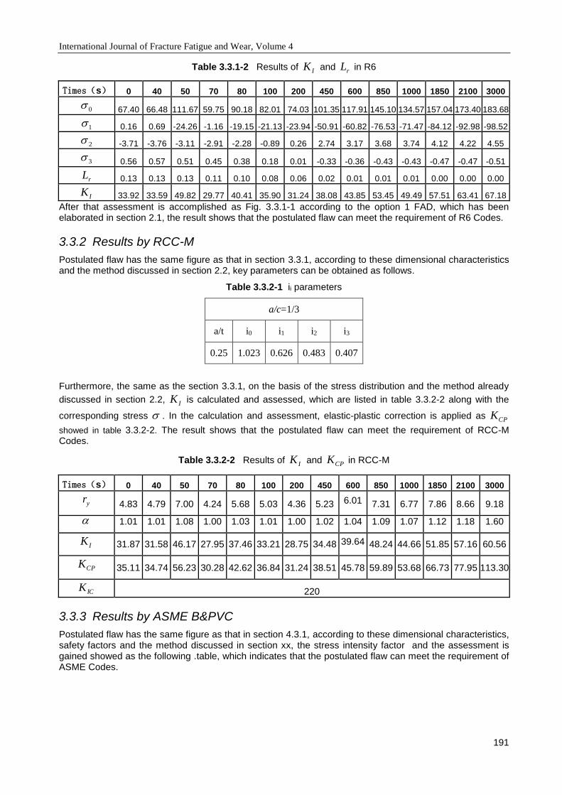
International Journal of Fracture Fatigue and Wear, Volume 4
191
Table 3.3.1-2 Results of IK and rL in R6
Times(s) 0 40 50 70 80 100 200 450 600 850 1000 1850 2100 3000
0 67.40 66.48 111.67 59.75 90.18 82.01 74.03 101.35 117.91 145.10 134.57 157.04 173.40 183.68
1 0.16 0.69 -24.26 -1.16 -19.15 -21.13 -23.94 -50.91 -60.82 -76.53 -71.47 -84.12 -92.98 -98.52
2 -3.71 -3.76 -3.11 -2.91 -2.28 -0.89 0.26 2.74 3.17 3.68 3.74 4.12 4.22 4.55
3 0.56 0.57 0.51 0.45 0.38 0.18 0.01 -0.33 -0.36 -0.43 -0.43 -0.47 -0.47 -0.51
rL 0.13 0.13 0.13 0.11 0.10 0.08 0.06 0.02 0.01 0.01 0.01 0.00 0.00 0.00
IK 33.92 33.59 49.82 29.77 40.41 35.90 31.24 38.08 43.85 53.45 49.49 57.51 63.41 67.18
After that assessment is accomplished as Fig. 3.3.1-1 according to the option 1 FAD, which has been elaborated in section 2.1, the result shows that the postulated flaw can meet the requirement of R6 Codes.
3.3.2 Results by RCC-M
Postulated flaw has the same figure as that in section 3.3.1, according to these dimensional characteristics and the method discussed in section 2.2, key parameters can be obtained as follows.
Table 3.3.2-1 ii parameters
a/c=1/3
a/t i0 i1 i2 i3
0.25 1.023 0.626 0.483 0.407
Furthermore, the same as the section 3.3.1, on the basis of the stress distribution and the method already
discussed in section 2.2, IK is calculated and assessed, which are listed in table 3.3.2-2 along with the
corresponding stress . In the calculation and assessment, elastic-plastic correction is applied as CPK
showed in table 3.3.2-2. The result shows that the postulated flaw can meet the requirement of RCC-M Codes.
Table 3.3.2-2 Results of IK and CPK in RCC-M
Times(s) 0 40 50 70 80 100 200 450 600 850 1000 1850 2100 3000
yr 4.83 4.79 7.00 4.24 5.68 5.03 4.36 5.23 6.01 7.31 6.77 7.86 8.66 9.18
1.01 1.01 1.08 1.00 1.03 1.01 1.00 1.02 1.04 1.09 1.07 1.12 1.18 1.60
IK 31.87 31.58 46.17 27.95 37.46 33.21 28.75 34.48 39.64 48.24 44.66 51.85 57.16 60.56
CPK 35.11 34.74 56.23 30.28 42.62 36.84 31.24 38.51 45.78 59.89 53.68 66.73 77.95 113.30
ICK 220
3.3.3 Results by ASME B&PVC
Postulated flaw has the same figure as that in section 4.3.1, according to these dimensional characteristics, safety factors and the method discussed in section xx, the stress intensity factor and the assessment is gained showed as the following .table, which indicates that the postulated flaw can meet the requirement of ASME Codes.

International Journal of Fracture Fatigue and Wear, Volume 4
192
Table 3.3.3-1 Results of IK in ASME B&PVC
Times(s) 0 40 50 70 80 100 200 450 600 850 1000 1850 2100 3000
ImK 54.15 54.15 54.15 46.63 42.87 35.31 6.71 4.95 2.04 2.04 2.14 0.00 0.00 0.00
IbK 5.43 5.70 3.06 3.74 2.80 0.00 7.20 9.57 12.89 15.02 15.13 18.05 18.26 19.10
ItK 0.00 0.00 0.00 0.00 0.52 7.74 14.24 41.71 48.92 50.22 57.29 66.71 67.80 76.63
IK 59.58 59.85 57.21 50.36 46.18 43.05 28.15 56.23 63.85 67.28 74.57 84.76 86.07 95.73
ICK 220
3.3.4 Parameter sensitivity analysis
The result according with different Codes are gathered in the following figure comparatively, the points represent the KI values, plotted by transient time on the horizontal axis and KI values on the vertical. From Fig.3.3.4-1, though the KI values by different Codes are variable, the variation tendency is consistent. The results of ASME Codes have the maximum safety margin, the results of RCC-M code after plastic correction have the second safety margin and the ones of R6 has the least. In addition to this, other parameters sensitivity is obtained as table 3.3.4-1, the symbol “+” stands for comparative degrees for the corresponding key factors, “+++” means the large extent , “+”means the little extent and “++” means the medium extent.
Fig. 3.3.1-1 Assessment of the postulated flaw by R6 Code
Fig. 3.3.4-1 The comparative KI of different Codes
Table 3.3.4-1 Key parameters sensitivity Results
Degree of Conservative
Handle ability Elastic-plastic
sensitivity Safety margin
sensitivity Dependency of
feature
R6 + + +++ + +
RCC-M ++ ++ ++ ++ ++
ASME +++ +++ + +++ +++
4 CONCLUSION
By means of fracture mechanics analysis in accordance with different Codes for the same object and the same load, three types of methods are summarized comparatively and the conclusions are acquired as following, which is conductive to address the safety margin and the other parameter sensitivity among each code.
International Journal of Fracture Fatigue and Wear, Volume 4
193
1) In consideration of the theory basis, the method provided by ASME B&PVC is base on the elastic fracture mechanics, and the other two are on account of elastic-plastic fracture mechanics, among them the R6 considers the most plastic factor.
2) The ASME B&PVC, RCC-M Codes and R6 Codes are all appropriate for the fracture mechanics analysis of engineering application, among each code, the ASME B&PVC have the maximum safety margin, the R6 Codes has the least and the RCC-M after plastic correction is medium.
3) For practical application, the method by ASME B&PVC is easy to use, which has the highest handle ability, the RCC-M takes the second place and the R6 Codes is the most complicated to handle.
4) The stress distribution of the defect and its close-by region are all indispensable for the three methods, but the ASME B&PVC is most affected by the object feature, R6 has the least dependency of feature, and the RCC-M Codes is medium.
5 REFERENCES
[1] Zhang Xiaomin, Fracture Mechanics, Tsinghua University Press, Beijing, 2012.
[2] Wu Qingke, Fracture Prevention Design, China Machine Press, 1991.
[3] R6 Assessment of the Integrity of Structures containing Defects, Revision 4, British Energy, November 2000.
[4] RCC-M Design and Construction Rules for Mechanical Components of PWR Nuclear Islands, June 2000 Edition, AFCEN.
[5] ASME Boiler and Pressure Vessel Code, Section III, “Rules for Construction of Nuclear Power Plant Components,” 1998 Edition with Addenda through 2007, The American Society of Mechanical Engineers, New York, 2007.
[6] Ren Xiaobo, Analysis and assessment of RPV in PWR, Tianjin University.
[7] Cai Yebin, Assessment Techniques for Pressure Vessels Containing Defects Based on Two-Criteria Approach, Journal of Fushun Petroleum Institute, 19(1), 1999.
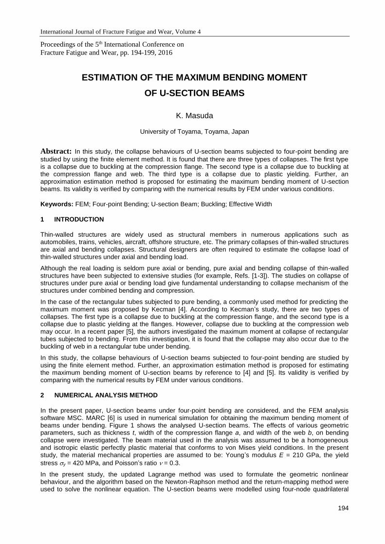
International Journal of Fracture Fatigue and Wear, Volume 4
194
Proceedings of the 5th International Conference on
Fracture Fatigue and Wear, pp. 194-199, 2016
ESTIMATION OF THE MAXIMUM BENDING MOMENT
OF U-SECTION BEAMS
K. Masuda
University of Toyama, Toyama, Japan
Abstract: In this study, the collapse behaviours of U-section beams subjected to four-point bending are
studied by using the finite element method. It is found that there are three types of collapses. The first type is a collapse due to buckling at the compression flange. The second type is a collapse due to buckling at the compression flange and web. The third type is a collapse due to plastic yielding. Further, an approximation estimation method is proposed for estimating the maximum bending moment of U-section beams. Its validity is verified by comparing with the numerical results by FEM under various conditions.
Keywords: FEM; Four-point Bending; U-section Beam; Buckling; Effective Width
1 INTRODUCTION
Thin-walled structures are widely used as structural members in numerous applications such as automobiles, trains, vehicles, aircraft, offshore structure, etc. The primary collapses of thin-walled structures are axial and bending collapses. Structural designers are often required to estimate the collapse load of thin-walled structures under axial and bending load.
Although the real loading is seldom pure axial or bending, pure axial and bending collapse of thin-walled structures have been subjected to extensive studies (for example, Refs. [1-3]). The studies on collapse of structures under pure axial or bending load give fundamental understanding to collapse mechanism of the structures under combined bending and compression.
In the case of the rectangular tubes subjected to pure bending, a commonly used method for predicting the maximum moment was proposed by Kecman [4]. According to Kecman’s study, there are two types of collapses. The first type is a collapse due to buckling at the compression flange, and the second type is a collapse due to plastic yielding at the flanges. However, collapse due to buckling at the compression web may occur. In a recent paper [5], the authors investigated the maximum moment at collapse of rectangular tubes subjected to bending. From this investigation, it is found that the collapse may also occur due to the buckling of web in a rectangular tube under bending.
In this study, the collapse behaviours of U-section beams subjected to four-point bending are studied by using the finite element method. Further, an approximation estimation method is proposed for estimating the maximum bending moment of U-section beams by reference to [4] and [5]. Its validity is verified by comparing with the numerical results by FEM under various conditions.
2 NUMERICAL ANALYSIS METHOD
In the present paper, U-section beams under four-point bending are considered, and the FEM analysis software MSC. MARC [6] is used in numerical simulation for obtaining the maximum bending moment of beams under bending. Figure 1 shows the analysed U-section beams. The effects of various geometric parameters, such as thickness t, width of the compression flange a, and width of the web b, on bending collapse were investigated. The beam material used in the analysis was assumed to be a homogeneous and isotropic elastic perfectly plastic material that conforms to von Mises yield conditions. In the present study, the material mechanical properties are assumed to be: Young’s modulus E = 210 GPa, the yield
stress y = 420 MPa, and Poisson’s ratio = 0.3.
In the present study, the updated Lagrange method was used to formulate the geometric nonlinear behaviour, and the algorithm based on the Newton-Raphson method and the return-mapping method were used to solve the nonlinear equation. The U-section beams were modelled using four-node quadrilateral

International Journal of Fracture Fatigue and Wear, Volume 4
195
thickness shell element (Element type 75). The elements divided the wall width into at least 20 sub lengths and divided the axial length such that the elements become almost square.
In addition, the length of beams used in the analysis was assumed to be large enough to neglect the influence of the boundary conditions. The ratio of the length and web width L/b was set to L/b > 6.
Enforced displacement : Uy
L
A
A
A-A
tt
t b
aL L
Enforced displacement : Uy
x
y
z
Fig. 1 U-section beam to which a four-point bending is applied
3 INVESTIGATION AND DISCUSSION
3.1 Proposal of extended Kecman’s method [4] for U-section beams
An extended Kecman’s method for predicting the maximum bending moment of U-section beams is as
follow. Depending on the value of buckling stress buc of the compression flange
(1)
Three cases are distinguished, as shown in Fig. 2.
Case 1: buc < y
In this case, the buckling at the compression flange occurs. The value of buckling stress buc is equation (1). After the buckling, the axial stress near the corner reaches to the yield stress. In order to consider this phenomenon, the effective width ae is introduced to the following simplified equation
(2)
(a) (b) (c)
Fig. 2 Schematic representation of axial stress distribution used in extended Kecman’s method: (a) Case 1:
buc < y; (b) Case 2: y < buc < 2y; (c) Case 3: buc > 2y
22
25.23 0.16
12 1buc
E a t
b a
0.7 0.3 .buce
y
a a

International Journal of Fracture Fatigue and Wear, Volume 4
196
The schematic representation of axial stress distribution is shown in Fig. 2(a). A distance from the bottom of the web to the neutral axis is shown as y1. Therefore, y1 is given as follows
(3)
A distance from the top of the web to the center of inertia is shown as s1. Therefore, s1 is given as follows
(4)
Therefore, the moment of each part at the maximum moment is as follows.
The elastic moment of the compression web 1 1 1 1
1: .
3yM b s y y t
The elastic moment of the tension web 2 1 1 1
5: .
3yM s b y y t
The plastic moment of the tension web 3 1 1 1: 2 2 .2
y
bM s y b y t
The moment of the compression flange due to effective width 4 1: .y eM b s a t
Therefore, in this case (buc < y), the maximum moment is derived as follows
(5)
Case 3: buc < 2y
In this case, the stress distribution in the maximum moment is shown in Fig. 2(c). Namely, it is assumed that the maximum moment is equal to a fully plastic moment Mp. The maximum bending moment can be derived as follows
(6)
Case 2: y < buc < 2y
First, if the buckling stress buc is equal to the yield stress y, it is assumed that the axial stress distribution is shown in Fig. 2(b). In this axial stress distribution, the moment Me can be derived by plugging ae = a into
the equation (5). Finally, in this case (y < buc < 2y), the maximum bending moment can be derived by linear interpolation
(7)
Figure 3 shows the distributions of axial stress x on cross section at the maximum moment obtained from FEM numerical analysis by black lines for three U-section beams. In Fig. 3, the distributions of axial stress obtained from Fig. 2 are also shown by red lines, which correspond to Case 1, Case 2 and Case 3 for Fig. 3(a), 3(b) and 3(c), respectively. As shown in these figures, proposed stress distributions are in good agreement with the FEM results.
1
1 1.
2 4ey b a
1 .
2
b a bs
b a
max 1 2 3 4.M M M M M
2 2
max
1 1.
2 4p yM M t b ab a
max .buc y
e p e
y
M M M M
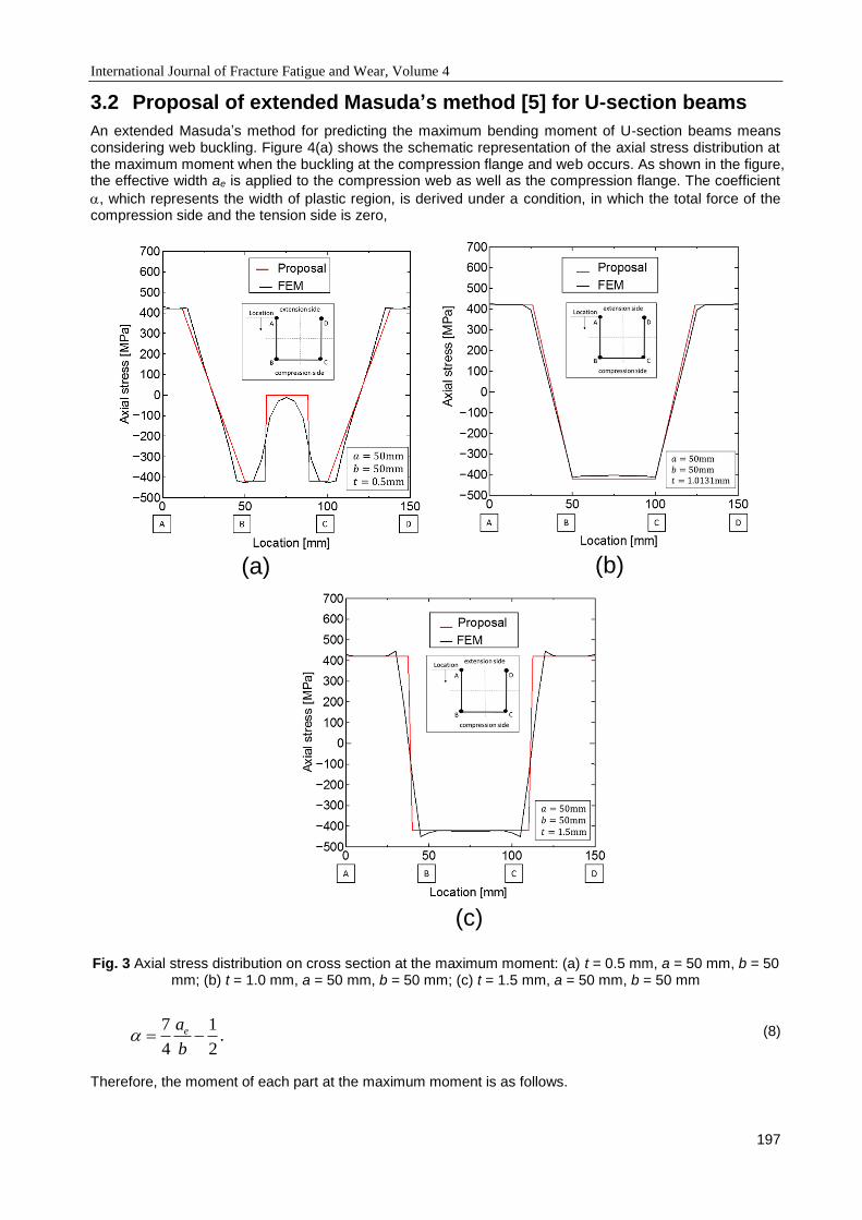
International Journal of Fracture Fatigue and Wear, Volume 4
197
3.2 Proposal of extended Masuda’s method [5] for U-section beams
An extended Masuda’s method for predicting the maximum bending moment of U-section beams means considering web buckling. Figure 4(a) shows the schematic representation of the axial stress distribution at the maximum moment when the buckling at the compression flange and web occurs. As shown in the figure, the effective width ae is applied to the compression web as well as the compression flange. The coefficient
, which represents the width of plastic region, is derived under a condition, in which the total force of the compression side and the tension side is zero,
(a) (b)
(c)
Fig. 3 Axial stress distribution on cross section at the maximum moment: (a) t = 0.5 mm, a = 50 mm, b = 50 mm; (b) t = 1.0 mm, a = 50 mm, b = 50 mm; (c) t = 1.5 mm, a = 50 mm, b = 50 mm
(8)
Therefore, the moment of each part at the maximum moment is as follows.
7 1.
4 2
ea
b

International Journal of Fracture Fatigue and Wear, Volume 4
198
The moment of the compression web due to effective width 1 1
1: .
4e y eM b s a a t
'
The elastic moment of the tension web '
2 1 1 1
1 1 2: .
3 3 3yM y b s b b y b t
The plastic moment of the tension web '
3 1
1: 2 .
2yM s b bt
The moment of the compression flange due to effective width 4 1: .y eM b s a t
Therefore, when the web buckling occurs, the maximum moment is derived as follows
(9)
Therefore, in this case (buc < y), the maximum moment is derived as follows
(10)
Figure 4(b) compares the FEM results and the results obtained by present method at the maximum moment for a = 50 mm and b = 50 mm. As shown in the figure, the results obtained by present method are in good agreement with the FEM results.
(a) (b)
b
Fig. 4 (a) Schematic representation of axial stress distribution used in extended Masuda’s method;
(b) Comparison of present method and the FEM results
4 CONCLUSIONS
In this study, bending collapse of U-section beams was investigated using the finite element method. The following results were obtained.
' ' ' '
max 1 2 3 4.M M M M M
max .(5), .(9) .M Min eq eq

International Journal of Fracture Fatigue and Wear, Volume 4
199
(1) The maximum moment of a U-section beam subjected to pure bending is associated with buckling at the compression flange, plastic yielding at the flange, and buckling at the compression web.
(2) By using the proposed method, which applies an effective width to the web, it is possible to obtain the axial stress distribution for buckling at the compression web.
(3) It is possible to predict the maximum moment for U-section beams by using the present method.
5 REFERENCES
[1] M. M. Pastor and F. Roure, Open cross-section beams under pure bending I. Experimental investigations, Thin-Walled Struct., Vol. 46, 476-483, 2008.
[2] M. M. Pastor and F. Roure, Open cross-section beams under pure bending II. Finite element simulation, Thin-Walled Struct., Vol. 47, 514-521, 2009.
[3] M. S. Park and B. C. Lee, Prediction of bending collapse behaviours of thin-walled open section beams, Thin-Walled Struct., Vol. 25, 185-206, 1996.
[4] D. Kecman, Bending Collapse of Rectangular and Square Section Tubes, Int. J. Mech. Sci., Vol. 25,
623-636, 1983.
[5] K. Masuda and D. H. Chen, Prediction of Maximum Moment of Rectangular Tubes Subjected to
Pure Bending, J. Environ. Eng., Vol. 6, 554-566, 2011.
[6] MSC, 2013, Marc 2013 User’s Guide, MSC Software, Newport Beach, CA.

International Journal of Fracture Fatigue and Wear, Volume 4
200
Proceedings of the 5th International Conference on
Fracture Fatigue and Wear, pp. 200-203, 2016
STRUCTURAL HEALTH MONITORING VIA USING TRANSMISSIBILITY
COHERENCE
Yun-Lai Zhou1, Xiaobo Yang2 and Magd Abdel Wahab3
1 National University of Singapore, Center for Offshore Research Engineering, Singapore 2 Xi'an institute of aerospace composites, Xi'an, China
3 Ghent University, Laboratory Soete, Belgium
Abstract: Transmissibility has been commonly used in structural health monitoring, during the last
decades; transmissibility has been both put forward in theory and applications. However, the use of transmissibility is still a profound and uncompleted work. In this study, a general summary of transmissibility is given, and in addition, transmissibility coherence is put forward to system identification for extracting natural frequencies in theory with recalling the transmissibility for system identification.
Keywords: Transmissibility; Structural health monitoring; Transmissibility coherence; system identification
1 INTRODUCTION
In the past decades, structural health monitoring (SHM) has become a multidisciplinary research focus to the scientific communities that attracts a lot of attention, due to the fact that the engineering structures are commonly designed with more complexity and more sophisticated newly invented material productions, and within daily use the structures are usually and generally applied with higher operational loads and unexpected loadings, and are demanding for longer lifecycle periods. Hence, numerous mechanical, civil and aerospace engineering researchers extensively developed vast of approaches for analysing the structural states that means to evaluate whether the structure is damaged or not, in order to prevent the anticipated damage, which might cause a vast loss in human daily lives in an inevitable way. Various categories of SHM procedures have been developed for analyzing the structural states. Vibration-based, strain-based, Electrical Impedance-based, probability-based, statistical based methods and so on have been studied and published a quantity of papers, reports and books. Literature review about the SHM can be found in [1].
For SHM, methodologies can be divided into two categories: physical model and data model/statistical model. For physical model, normally finite element analysis (FEA) is undertaken and different levels and patterns, such as fatigue in adhesively bonded joints [2-3]; crack initiation [4]; fretting wear [5], are numerically analyzed in order to provide a pre-design assessment as a reference for further analysis, especially in fatigue life-cycle prediction [4]. Generally, FEA analysis is validated with experimental results. And model updating intends to minimize the differences between FEA and experimental responses [6-8] by optimizing the FEA model. In this direction, due to the low cost and good performance in analyzing real engineering problems, other numerical techniques have been developed, e.g. boundary element methods (BEM), mesh free approaches, extended finite element methods (XFEM), isogeometric analysis (IGA).
On the other hand, for data model, the traditional modal testing is quite commonly used in structural dynamic analysis [9], like experimental modal analysis (EMA). In modal analysis, the mode shape derivatives, for instance, first derivative (rotations), second derivative (curvatures) and third and higher derivatives were utilized for damage localization. Frequency response function (FRF) is another parameter commonly used in EMA. In addition, the strain before and after damage in the structure is also a direction in SHM. However, EMA requires the measurement of excitation while this is arduous in real engineering as normally the engineering structures are commonly subjected to complex loading and environmental uncertainties. Then, new methodology is pursued due to the demanding from engineering application.
In SHM, transmissibility has been widely studied in the past decades, and it has been used for damage detection, localization, quantification and so on [10-17]. On the other hand, it has also been used for FRF estimation [18], force reconstruction [19], system identification [20-21] and so on.
This study tries to extend the transmissibility coherence (TC) for natural frequency extraction, and henceforth, to give a general summary in transmissibility estimation.

International Journal of Fracture Fatigue and Wear, Volume 4
201
2 THRETICAL DERIVATION
In structural dynamics, for a linear multiple-degree-of-freedom (MDOF) system shown in Figure 1, the dynamic equilibrium equation can be written by the well-known second order differential equation,
(1)
where M, C and K are the mass, damping, and stiffness matrices of the system, respectively, f(t) is the input force vector and x(t) contains the responses of each degree-of-freedom (DOF) of the system.
Figure 1. A linear multiple-degree-of-freedom system.
Herein, for a harmonic applied force at a given coordinate, the transmissibility between point i and a reference point j can be defined as
T( i , j )
(w ) =X
i(w )
Xj(w )
(2)
where Xi and Xj are the complex amplitudes of the system responses, xi(t) and xj(t), respectively, and is
the frequency.
In order to calculate the transmissibility, no matter in real engineering or experiment analysis, apart from its direct extracting from the two responses, it can be derived in several ways, for instance:
T( i , j )
(w ) =X
i(w )
Xj(w )
=X
i(w ) ´ X
i(w )
Xj(w ) ´ X
i(w )
=G
( i ,i )(w )
X( j ,i )
(w ) (3)
T( i , j )
(w ) =X
i(w )
Xj(w )
=X
i(w ) ´ X
j(w )
Xj(w ) ´ X
j(w )
=G
( i , j )(w )
X( j , j )
(w ) (4)
where G means the auto- or cross- spectrum. Herein, Equation (3) and (4) can be compared with the FRF estimation for avoiding noise influence, then transmissibility coherence can be drawn out. Detailed analysis about it will be given in next section.
Besides, for a chosen reference P, when the variable approaches system’s th pole, denoted by v, the following equation is verified with Laplace transform [21] and Fourier transform [20] as
lims®l
v
T( i , j )
P (w ) =f
( i ,v)
f( j ,v)
(5)
And its inverse [20, 21], also called inverse transmissibility subtraction function (ITSF) [21] is as
D-1T( i , j )
P1P
2 =1
DT( i , j )
P1P
2
=1
T( i , j )
P1 -T
( i , j )
P2
=G
( j ,P1)G
( j ,P2
)
G( i ,P
1)G
( j ,P2
)- G
( i ,P2
)G
( j ,P1)
(6)
Herein, through the equation above one can identify the natural frequencies via peak picking method. Note that the denominator of the equation above is result of a subtraction, which might cause singularity if the reference is not well chosen or the transform is not well chosen and made. Meanwhile, it can yield more roots than the system real roots, which requires further work in validating the corresponding frequencies.
International Journal of Fracture Fatigue and Wear, Volume 4
202
Thirdly, all the references like j and P (P1, P2, …) should be paid more attention, otherwise it would be possible to miss some system roots. One possible solution is to use average normalization ITSF [21], or to take all the ITSFs into consideration directly.
On the other hand, if transmissibility is directly estimated using two outputs, i.e. not taking the FRFs into account, referring to the conception of coherence, TC can be also derived solely by using the auto- and cross- spectrum of the two responses signals [12, 15]. And TC will be expressed as
gTC
2 =T
1( i , j )(w )
T2( i , j )
(w )=
G( i , j )
(w )
G( j , j )
(w )/
G( i ,i )
(w )
G( j ,i )
(w )=
G( i , j )
(w )G( j ,i )
(w )
G( j , j )
(w )G( i ,i )
(w )=
G( i , j )
(w )2
G( j , j )
(w )G( i ,i )
(w ) (7)
As the coherence is a squared magnitude, TC is higher than zero. And basically, TC reveals the coherence of two outputs, i.e. it indicates the interrelation of the dynamic characteristics of two outputs.
Herein, note that the TC might be used for system identification, i.e. to identify the resonant frequencies. Recalling the Equation (6), and by introducing TC into it, one can get
D-1T( i , j )
i , j =1
T( i , j )
i -T( i , j )
j=
1
T2( i , j )
- T1( i , j )
=1
T2( i , j )
´1
1-T
1( i , j )
T2( i , j )
=1
T2( i , j )
´1
1-gTC
2 (8)
Herein, one might use TC in the resonant frequencies estimation; however, further investigation should be conducted for a better understanding.
3 CONCLUSIONS
In this paper, transmissibility estimation flowchart is given, and transmissibility is put forward to system identification in theory. We presented a general summary of transmissibility, and transmissibility coherence and their applications to system identification for extracting natural frequencies. However, further investigation is needed to have a better analyzing of their performance.
ACKNOWLEDGEMENTS
The first author thanks CWO (Commissie Wetenschappelijk Onderzoek), Faculty of Engineering and Architecture, Ghent University for providing financial support for a research stay at Soete Laboratory.
REFERENCES
[1] Hoon Sohn, C. R. Farrar, F. M. Hemez, D. D. Shunk, D. W. Stinemates, B. R. Nadler, J. J. Czarnecki (2004). A Review of Structural Health Monitoring Literature: 1996-2001. Los Alamos National Laboratory Report, LA-13976-MS, 2004.
[2] MMA Wahab, IA Ashcroft, AD Crocombe, SJ Shaw (2001). Prediction of fatigue thresholds in adhesively bonded joints using damage mechanics and fracture mechanics. Journal of adhesion science and technology; 15 (7), 763-781.
[3] MMA Wahab, I Hilmy, IA Ashcroft, AD Crocombe (2011). Damage Parameters of Adhesive Joints with General Triaxiality Part I: Finite Element Analysis. Journal of Adhesion Science and Technology; 25 (9), 903-923.
[4] R Hojjati-Talemi, MA Wahab, J De Pauw, P De Baets (2014). Prediction of fretting fatigue crack initiation and propagation lifetime for cylindrical contact configuration. Tribology International; 76, 73-91.
[5] A Ferjaoui, T Yue, MA Wahab, R Hojjati-Talemi (2015). Prediction of fretting fatigue crack initiation in double lap bolted joint using Continuum Damage Mechanics. International Journal of Fatigue; 73, 66-76.
[6] MMA Wahab, G De Roeck, B Peeters (1999). Parameterization of damage in reinforced concrete structures using model updating. Journal of Sound and Vibration; 228 (4), 717-730.
[7] MMA Wahab (2001). Effect of modal curvatures on damage detection using model updating. Mechanical Systems and Signal Processing; 15 (2), 439 - 445.
International Journal of Fracture Fatigue and Wear, Volume 4
203
[8] OA Adediran, MMA Wahab, W Xu, AD Crocombe (2012). Application of FE model updating for damage assessment of FRP composite beam structure. Topics in Modal Analysis II, Volume 6, 385-398.
[9] Yun-Lai Zhou, M. Abdel Wahab, R. Perera, N. Maia, R. Sampaio, E. Figueiredo (2015). Single side damage simulations and detection in beam-like structures. Proceedings of 11th International Conference on Damage Assessment of Structures (DAMAS 2015); August 2015, Gent, Belgium.
[10] Zhou Yun Lai, Ricardo Perera (2014). Transmissibility based damage assessment by intelligent algorithm. Proceedings of the 9th International Conference on Structural Dynamics, EURODYN 2014, Porto, Portugal, July 2014.
[11] Yun-Lai Zhou, Magd Abdel Wahab, and Ricardo Perera (2015). Damage detection by transmissibility conception in beamlike structures. International Journal of Fracture Fatigue and Wear, Volume 3, 254-259.
[12] Yun-Lai Zhou, E. Figueiredo, Nuno M. Maia, R. Perera (2015). Damage detection and quantification using transmissibility coherence analysis, Shock and Vibration, (2015), ID 290714.
[13] Yun-Lai Zhou, E. Figueiredo, N. Maia, R. Sampaio, R. Perera (2015). Damage detection in structures using a transmissibility-based Mahalanobis distance. Structural Control and Health Monitoring; 22: 1209-1222.
[14] Yun Lai Zhou, Ricardo Perera, Enrique Sevillano (2012). Damage identification from power spectrum density transmissibility. Proceedings of the 6th European Workshop on Structural Health Monitoring; July 2012, Dresden, Germany.
[15] Yun Lai Zhou (2015). Structural health monitoring by using transmissibility. PhD thesis, 2015.
[16] Yun Lai Zhou, Ricardo Perera (2013). Damage Localization via Transmissibility Power Mode Shape. Proceedings of the 5th European-American Workshop on Reliability of NDE; October 2013, Berlin, Germany.
[17] Y.L. Zhou, E. Figueiredo, N. Maia, R. Sampaio, R. Perera (2014). Transmissibility-based damage detection using linear discriminant analysis. Proceedings of the 2014 Leuven Conference on Noise and Vibration Engineering (ISMA 2014); September 2014, Leuven, Belgium.
[18] APV Urgueira, RAB Almeida, NMM Maia (2011). On the use of the transmissibility concept for the evaluation of frequency response functions. Mechanical Systems and Signal Processing; 25 (2011) 940-951.
[19] YE Lage, NMM Maia, MM Neves (2014). Force Magnitude Reconstruction Using the Force Transmissibility Concept. Shock and Vibration; Volume 2014, Article ID 905912, 9 pages.
[20] C Devriendt, P Guillaume (2008). Identification of modal parameters from transmissibility measurements. Journal of Sound and Vibration; (314): 343-356.
[21] WJ Yang, WX Ren (2012). Operational Modal Parameter Identification from Power Spectrum Density Transmissibility. Computer-Aided Civil and Infrastructure Engineering; 27(3): 202-217.

International Journal of Fracture Fatigue and Wear, Volume 4
204
Proceedings of the 5th International Conference on
Fracture Fatigue and Wear, pp. 204-208, 2016
PARALLELIZATION APPROACHES FOR FRETTING FATIGUE
SIMULATION
R. Trobec1, M. Depolli1, G. Kosec1, S. Bordas2, S. Tomar2, K. Pereira3 and M. Abdel Wahab3
1Department of Communication Systems, Jožef Stefan Institute, Slovenia 2Faculté des Sciences, de la Technologie et de la Communication, Université du Luxembourg, Luxembourg
3Department of Electrical energy, systems and automation, Ghent University, Belgium
Abstract: This paper is an initial investigation of parallelization approaches for the numerical simulation of fretting fatigue under realistic conditions, e.g. cyclic non-proportional loading. The major difficulty in parallelising such simulations is the severe non-linearity of involved mechanical processes, which spans over multiple spatial and temporal scales. Generally, the problem comprises modelling of the contact, friction, stick and slip conditions that result in non-linearities localised upon the interfaces between components, the crack initiation phase that can be simulated using damage accumulation, and crack propagation, where the regions surrounding the tips of the cracks typically require a much more precise treatment and therefore present much higher computational burden than the rest of the domain. In general, such highly non-linear problems are difficult to implement in parallel, primarily due to the load-balancing issues.
Keywords: parallel simulation, speed-up, scalability, computational complexity, fretting fatigue, crack initiation and propagation
1 INTRODUCTION
Failure in mechanical components due to fretting fatigue is popular research topic due to its immediate practical application, e.g. aerospace riveted joints [1] and many other industrial applications in mechanical and civil engineering. The crack initiation, propagation and lifetime of the fretting fatigue have been studied both experimentally [2] and numerically, within a finite element framework [3]. Most of the numerical studies simulate fretting fatigue by Continuum Damage Mechanics (CDM) for the analysis of crack initiation and Linear Elastic Fracture Mechanics (LEFM) for the analysis of crack propagation. Assuming proportional loading conditions and therefore constant ratio between mode I and mode II Stress Intensity Factors (SIFs) enables fast simulation on a single lumped cycle only [4]. The drawback of such simplified approach is that it might lead to incorrect crack paths and fatigue lives as reported in [5]. The cycle-by-cycle simulations, e.g. using Cohesive Zone Models (CZM) [6], admit the non-proportionality, however require significantly higher computational power. Additionally, a significant amount of time is needed for the calculation of reliable stresses and for the adaptive re-meshing. For this reason, FEM could be ineffective for simulating high-cycle fatigue, e.g. 107 fatigue cycles [7]. A possible alternative is an explicit Meshless Local Strong Form Method (MLSM) that has been proven as effective in several application fields [8-10], in particular, if implemented on parallel computers [11, 12]. The downside of the MLSM approach is that it does not guarantee that the equilibrium equations are strictly satisfied at each time step, and must satisfy stability conditions which might induce additional complications due to the existence of cracks in the domain.
The computational time of simulations grows rapidly with higher required accuracy, typically ensured with denser spatial discretization, i.e. more elements or computational nodes, and number of loading cycles. An important part of the numerical approach is thus the effective implementation of the solution procedure on modern computer architectures. The developments in the technology of the computer architectures are nowadays extremely vivid. The processing power can be increased either by increasing the processor’s clock frequency or by increasing the number of processing units. The clock frequencies are approaching their physical limits; therefore the second option - increased number of processing units - is becoming more attractive. Parallel computers, available today in most desktop computers or computer servers, can compensate for the lack of performance of a single computer, but only in cases where an efficient parallelization of the computational method is known. Various application programming interfaces (APIs) for parallel programming are used to maximize the performance of parallel systems. Nowadays, the most widely used APIs for parallel programming are MPI for distributed-memory systems, and Ptreads and OpenMP for shared-memory systems [13]. Moreover, using graphical processing units (GPUs) for solving parallel problems is widely spreading. APIs that support parallel programming on GPUs are becoming more and more

International Journal of Fracture Fatigue and Wear, Volume 4
205
popular, like CUDA and OpenCL [14, 15]. Solving crack problems in parallel is intrinsically difficult, and rarely attempted in practice due to the implementation complexity and the learning curve involved. Besides the parallelization techniques for FEM that are mature [16], considerable effort has been recently invested in the parallelization of adaptive eXtended FEM (XFEM) [17] for simulations of composites fracture.
This paper describes an initial investigation of the parallelization approaches and opportunities for the numerical simulation of fretting fatigue cracks under real conditions, e.g. high resolution cyclic non-proportional loading, with high computational requirements that exceed the computational capabilities of a single computer. In Section 2, the crack simulation method is functionally decomposed. In Section 3, opportunities for the parallel speed-up of the crack simulations are analysed together with an approximate estimation of most promising numerical techniques.
2 FRETTING FATIGUE SIMULATION
The fretting fatigue solution methodology can be decomposed into independent functional blocks that can be executed on different computers. Note that the sub-functions cannot be always executed in parallel because of the data dependencies, i.e. results of a block are inputs of another block. Some functional blocks can be further decomposed by domain decomposition and implemented again in parallel on several computing cores.
Let us consider a generic simulation of a high number of cycles in fretting fatigue crack life. A birds view on such a functional decomposition results in (i) modelling of domain geometry, crack initiation, crack propagation and loading cycle, which mostly needs human resources, (ii) discretization, numerical solution, and parameter sweep, which require computational resources. Each block can be further decomposed. For example, the crack initiation phase is usually composed of (i) determination of geometry, (ii) modelling and simulation of contact's dynamic, (iii) testing of initiation criteria. The crack propagation phase is usually composed of the following steps: (i) computation of the stress intensity factors, (ii) verification of the crack stability, and (iii) computation of the direction of crack propagation. A principal functional decomposition of a fretting fatigue crack simulation is shown in Fig. 1. The blocks that can run in parallel are shown on a symbolic time axis.
Domain modelling
Crack modeling
Cycle modeling
Human resources
Domain discretization
Computational resources
Numerical solution of a crack cycle
Stopping criteria
Numerical solution of a crack cycle
Stopping criteria
…
Parameters' sweep
Fig. 1 Main functional blocks of the simulation of crack propagation under high-cycle fretting fatigue conditions
3 PARALLELIZATION AND COMPLEXITY ESTIMATION
In order to simulate millions of nodes and millions of fretting cycles, the parallelization of the fretting fatigue cracks simulation programs is required. Thousands of computing cores are available today in distributed-memory computing clusters with interconnected processing nodes that incorporate a multiple shared-memory processors and optionally also many-core accelerators, such as GPUs, for number crunching. Such hybrid architectures requires also hybrid parallelization strategy that incorporates thread-level parallelization, e.g. OpenMP in each computing node, combined with a node-level parallelization, e.g. problem decomposition and message passing communication (MPI). There exist some successful attempts to address the non-linear mechanics problems with the hybrid parallelization approach [18], with the aim to preserve acceptable computational scalability with high number of computational nodes in a wide area of applications. It seems that adaptivity [19] and XFEM [20] are appropriate solution methodologies for the parallel simulation of the fretting fatigue crack propagation. However, alternative algorithms can be used that are less optimal on a
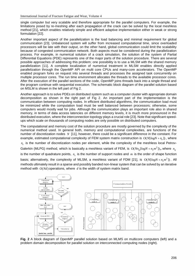
International Journal of Fracture Fatigue and Wear, Volume 4
206
single computer but very scalable and therefore appropriate for the parallel computers. For example, the limitations posed by re-meshing after each propagation of the crack can be solved by the local meshless method [21], which enables relatively simple and efficient adaptive implementation either in weak or strong formulation [22].
Another important aspect of the parallelization is the load balancing and minimal requirement for global communication [23]. Unbalanced system will suffer from increased computational time, since overloaded processors will be late with their output, on the other hand, global communication could limit the scalability because of congested communication network. Both aspects must be considered during the parallelization process. For example, in numerical solution of a crack simulation, the solution of the system of Partial Differential Equations (PDE) represents one of the major parts of the solution procedure. There are several possible approaches of addressing this problem; one possibility is to use a MLSM with the shared memory parallelization [11]. A complete localization of numerical treatment in MLSM enables directly applied parallelization through the OpenMP API on multi core CPUs and many-core accelerators. The OpenMP enabled program forks on request into several threads and processes the assigned task concurrently on multiple processor cores. The run time environment allocates the threads to the available processor cores. After the execution of the parallel sections of the code, OpenMP joins threads back into a single thread and the program continue with sequential execution. The schematic block diagram of the parallel solution based on MSLM is shown in the left part of Fig 2.
Another approach is to solve PDEs on distributed system such as a computer cluster with appropriate domain decomposition as shown in the right part of Fig 2. An important part of the implementation is the communication between computing nodes. In efficient distributed algorithms, the communication load must be minimized while the computation load must be well balanced between processors; otherwise, some computers would mostly wait for jobs. Although the communication plays an important role also in shared memory, in terms of data access latencies on different memory levels, it is much more pronounced in the distributed execution, where the interconnection topology plays a crucial role [23]. Note that significant speed-ups which scale on thousands of computing nodes are only possible on distributed computers.
The computational and memory cost of the solution procedure are mostly governed by the complexity of the numerical method used. In general both, memory and computational complexities, are functions of the number of discretization nodes N [11], however, there could be a significant difference in the constant. For
example, estimated computational complexity of FEM system matrix construction is ( [ ])eO N logN n , where
en is the number of discretization nodes per element, while the complexity of the meshless local Petrov-
Galerkin (MLPG) method, which is basically a meshless variant of FEM, is 2( [ ])q sO Nn logN n m , where qn
is the number of quadrature points, sn is the number of support nodes and m is the order of shape function
basis; alternatively, the complexity of MLSM, a meshless variant of FDM [21], is 2( [ ])sO N logN n m . All
methods ultimately result in a sparse and possibly banded non-linear system that can be solved by an iterative
method with ( )O Nd operations, where d is the width of system matrix band.
Fig. 2 A block diagram of OpenMP parallel solution based on MLMS on multicore computers (left) and a problem domain decomposition for parallel solution on interconnected computing nodes (right).

International Journal of Fracture Fatigue and Wear, Volume 4
207
4 CONCLUSIONS
This paper is a short review of possibilities for speeding up the fretting fatigue simulations in order to approach the real situations with millions of fatigue cycles. The functional decomposition followed by the parallelization of numerical solution of each cycle, on a heterogeneous computer with hundreds of interconnected nodes, each with several cores, seems to be a viable approach. Near ideal speed-ups, as reported for other solid mechanics simulations, can be expected for the simulation of a single fatigue cycle, if using methodologies with local approach that reduce the frequency or complexity of re-meshing. The problem of inherently sequential nature of the fatigue simulation seems to remain a serious bottleneck, unless the crack history could be modelled differently, for example by a simulation of only few consecutive cycles and extrapolation of the results. On the other hand, multiple simulations with different parameters, which are often used in the real problem, are trivial for parallelization.
5 ACKNOWLEDGEMENTS
The authors would like to acknowledge the financial support of the Research Foundation - Flanders - (FWO), The Luxembourg National Research Fund (FNR) and Slovenian Research Agency (ARRS) in the framework of the FWO Lead Agency project: G018916N ‘Multi-analysis of fretting fatigue using physical and virtual experiments’.
6 REFERENCES
[1] Hojjati-Talemi R, M. AW. Finite element analysis of localized plasticity in Al 2024-T3 subjected to fretting fatigue. Tribol Int. 2012;55:805-14.
[2] Hojjati-Talemi R, Abdel Wahab M, De Pauw J, De Baets P. Prediction of fretting fatigue crack initiation and propagation lifetime in cylindrical contact configuration. Tribology Int. 2014;76:73-91.
[3] Proudhon H, Basseville S. Finite element analysis of fretting crack propagation. Eng Fract Mech. 2011;78:685-94.
[4] Abdel Wahab M. Simulating mode I fatigue crack propagation in adhesively-bonded composite joints. Fatigue and fracture of adhesively-bonded composite joints: Elsevier; 2015. p. 323 - 44.
[5] Giner E, Sukumar N, Denia FD, Fuenmayor FJ. Direction of crack propagation in a complete contact fretting fatigue problem. Int J Fatigue. 2014;58:172-80
[6] Hillerborg A, Modeer M, Petersson PE. nalysis of crack formation and crack growth in concrete by means of fracture mechanics and finite elements. Cem Concr Res. 1976;6:773-81.
[7] Kim K, Yoon MJ. Fretting fatigue simulation for aluminum alloy using cohesive zone law approach. Int J Mech Sci. 2014;85:30-7.
[8] Kosec G, Trobec R. Simulation of semiconductor devices with a local numerical approach. Eng Anal Bound Elem. 2015;50:69-75.
[9] Kosec G, Šarler B. Simulation of macrosegregation with mesosegregates in binary metallic casts by a meshless method. Eng Anal Bound Elem. 2014;45:36-44.
[10] Kosec G. A local numerical solution of a fluid-flow problem on an irregular domain. Adv Eng Softw. 2016 10.1016/j.advengsoft.2016.05.010.
[11] Kosec G, Depolli M, Rashkovska A, Trobec R. Super linear speedup in a local parallel meshless solution of thermo-fluid problems. Comput Struct. 2014;133:30-8. 10.1016/j.compstruc.2013.11.016.
[12] Kosec G, Zinterhof P. Local strong form meshless method on multiple Graphics Processing Units. CMES-Comp Model Eng. 2013;91:377-96.
[13] Pacheco PS. An Introduction to Parallel Programming. Burlington: Morgan Kaufmann Publishers; 2011.
[14] Kirk DB, Hwu WW. Programming Massively Parallel Processors. Burlington: Morgan Kaufmann Publishers; 2010.
[15] Domínguez JM, Crespo AJC, Valdez-Balderas D, Rogers BD, Gómez-Gesteira M. New multi-GPU implementation for smoothed particle hydrodynamics on heterogeneous clusters. Comput Phys Commun. 2013
International Journal of Fracture Fatigue and Wear, Volume 4
208
[16] Babuska I. Some aspects of parallel implementation of the finite-element method on message. Parallel Algorithms for Numerical Linear Algebra. 2014;1:157.
[17] Vigueras G, Sket F, Samaniego C, Wu L, Noels L, Tjahjanto D, et al. An XFEM/CZM implementation for massively parallel simulations of composites fracture. Compos Struct. 2015;125:542-57. 10.1016/j.compstruct.2015.01.053.
[18] Casoni E, Jérusalem A, Samaniego C, Eguzkitza B, Lafortune P, Tjahjanto DD, et al. Alya: Computational Solid Mechanics for Supercomputers. Arch Comput Method E. 2015;22:557-76. 10.1007/s11831-014-9126-8.
[19] Waisman H, Berger-Vergiat L. An adaptive domain decomposition preconditioner for crack propagation problems modeled by XFEM. 2013;11:633-54. 10.1615/IntJMultCompEng.2013006012.
[20] Vigueras G, Sket F, Samaniego C, Wu L, Noels L, Tjahjanto D, et al. An XFEM/CZM implementation for massively parallel simulations of composites fracture. Compos Struct. 2015;125:542-57. http://dx.doi.org/10.1016/j.compstruct.2015.01.053.
[21] Trobec R, Kosec G. Parallel scientific computing : theory, algorithms, and applications of mesh based and meshless methods: Springer; 2015.
[22] Kosec G, Šarler B. H-adaptive local radial basis function collocation meshless method. CMC-Comput Mater Con. 2011;26:227-53.
[23] Trobec R, Šterk M, Robič B. Computational complexity and parallelization of the meshless local Petrov-Galerkin method. Comput Struct. 2009;87:81-90.
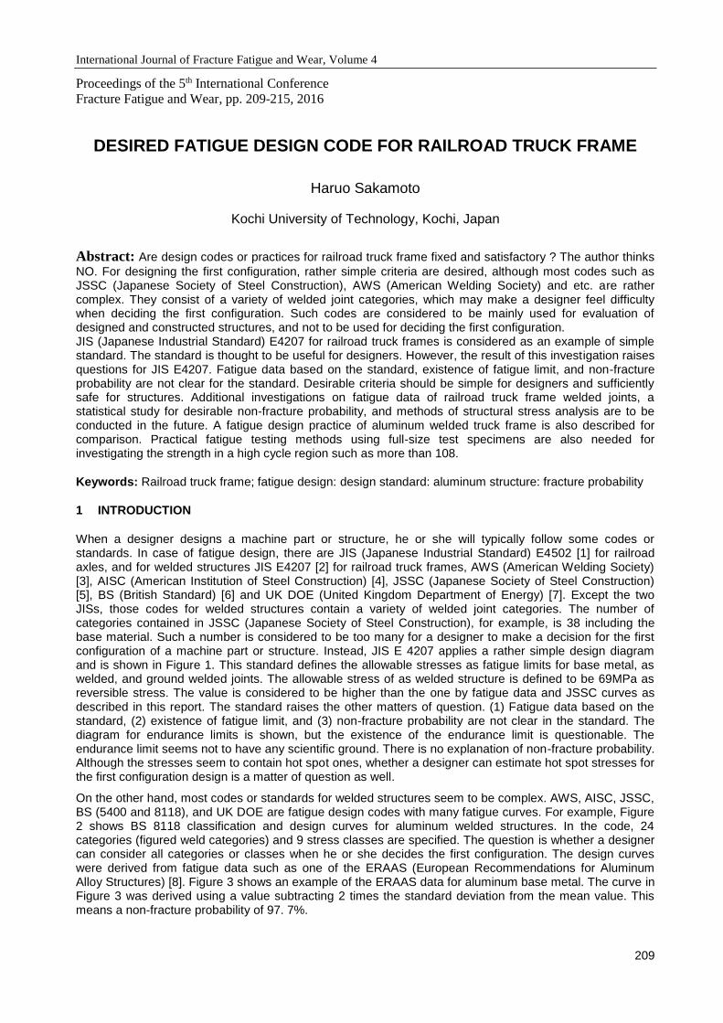
International Journal of Fracture Fatigue and Wear, Volume 4
209
Proceedings of the 5th International Conference
Fracture Fatigue and Wear, pp. 209-215, 2016
DESIRED FATIGUE DESIGN CODE FOR RAILROAD TRUCK FRAME
Haruo Sakamoto
Kochi University of Technology, Kochi, Japan
Abstract: Are design codes or practices for railroad truck frame fixed and satisfactory ? The author thinks
NO. For designing the first configuration, rather simple criteria are desired, although most codes such as JSSC (Japanese Society of Steel Construction), AWS (American Welding Society) and etc. are rather complex. They consist of a variety of welded joint categories, which may make a designer feel difficulty when deciding the first configuration. Such codes are considered to be mainly used for evaluation of designed and constructed structures, and not to be used for deciding the first configuration. JIS (Japanese Industrial Standard) E4207 for railroad truck frames is considered as an example of simple standard. The standard is thought to be useful for designers. However, the result of this investigation raises questions for JIS E4207. Fatigue data based on the standard, existence of fatigue limit, and non-fracture probability are not clear for the standard. Desirable criteria should be simple for designers and sufficiently safe for structures. Additional investigations on fatigue data of railroad truck frame welded joints, a statistical study for desirable non-fracture probability, and methods of structural stress analysis are to be conducted in the future. A fatigue design practice of aluminum welded truck frame is also described for comparison. Practical fatigue testing methods using full-size test specimens are also needed for investigating the strength in a high cycle region such as more than 108.
Keywords: Railroad truck frame; fatigue design: design standard: aluminum structure: fracture probability
1 INTRODUCTION
When a designer designs a machine part or structure, he or she will typically follow some codes or standards. In case of fatigue design, there are JIS (Japanese Industrial Standard) E4502 [1] for railroad axles, and for welded structures JIS E4207 [2] for railroad truck frames, AWS (American Welding Society) [3], AISC (American Institution of Steel Construction) [4], JSSC (Japanese Society of Steel Construction) [5], BS (British Standard) [6] and UK DOE (United Kingdom Department of Energy) [7]. Except the two JISs, those codes for welded structures contain a variety of welded joint categories. The number of categories contained in JSSC (Japanese Society of Steel Construction), for example, is 38 including the base material. Such a number is considered to be too many for a designer to make a decision for the first configuration of a machine part or structure. Instead, JIS E 4207 applies a rather simple design diagram and is shown in Figure 1. This standard defines the allowable stresses as fatigue limits for base metal, as welded, and ground welded joints. The allowable stress of as welded structure is defined to be 69MPa as reversible stress. The value is considered to be higher than the one by fatigue data and JSSC curves as described in this report. The standard raises the other matters of question. (1) Fatigue data based on the standard, (2) existence of fatigue limit, and (3) non-fracture probability are not clear in the standard. The diagram for endurance limits is shown, but the existence of the endurance limit is questionable. The endurance limit seems not to have any scientific ground. There is no explanation of non-fracture probability. Although the stresses seem to contain hot spot ones, whether a designer can estimate hot spot stresses for the first configuration design is a matter of question as well.
On the other hand, most codes or standards for welded structures seem to be complex. AWS, AISC, JSSC, BS (5400 and 8118), and UK DOE are fatigue design codes with many fatigue curves. For example, Figure 2 shows BS 8118 classification and design curves for aluminum welded structures. In the code, 24 categories (figured weld categories) and 9 stress classes are specified. The question is whether a designer can consider all categories or classes when he or she decides the first configuration. The design curves were derived from fatigue data such as one of the ERAAS (European Recommendations for Aluminum Alloy Structures) [8]. Figure 3 shows an example of the ERAAS data for aluminum base metal. The curve in Figure 3 was derived using a value subtracting 2 times the standard deviation from the mean value. This means a non-fracture probability of 97. 7%.
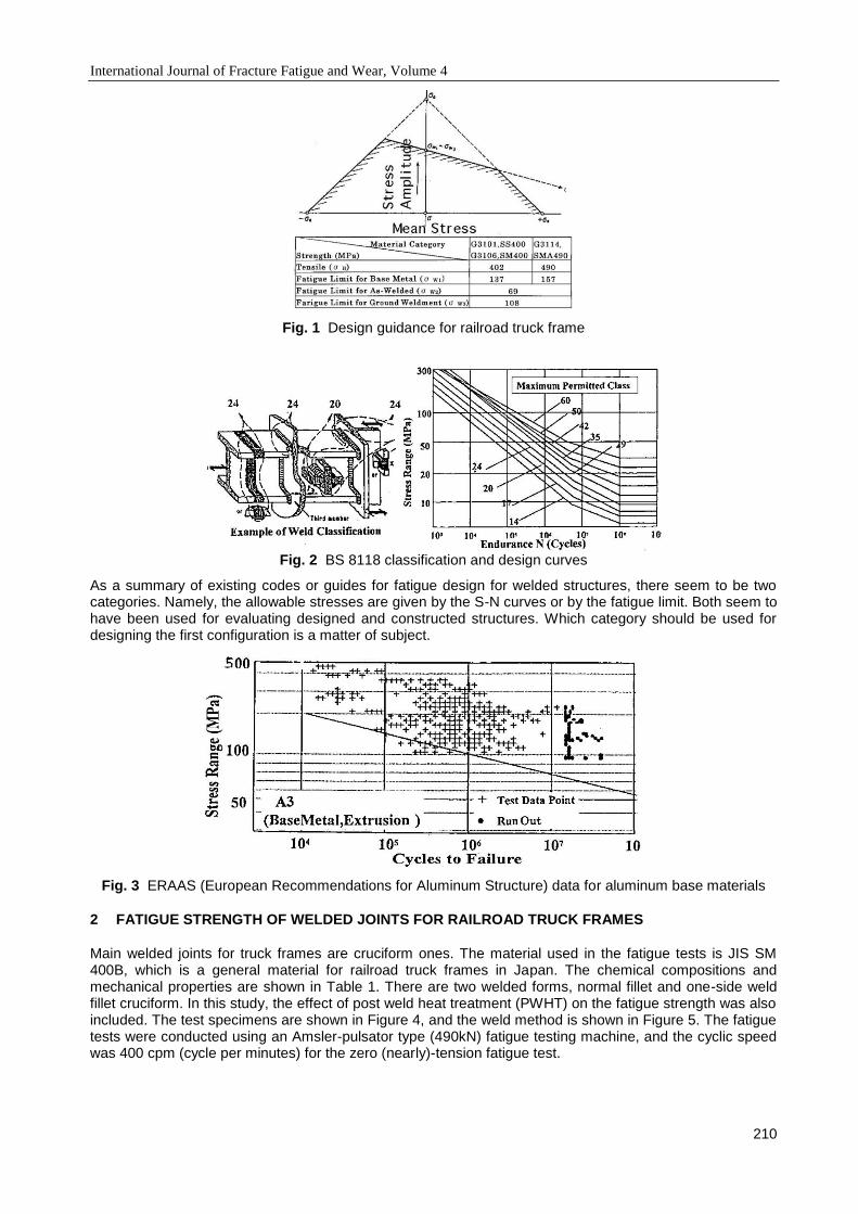
International Journal of Fracture Fatigue and Wear, Volume 4
210
Fig. 1 Design guidance for railroad truck frame
Fig. 2 BS 8118 classification and design curves
As a summary of existing codes or guides for fatigue design for welded structures, there seem to be two categories. Namely, the allowable stresses are given by the S-N curves or by the fatigue limit. Both seem to have been used for evaluating designed and constructed structures. Which category should be used for designing the first configuration is a matter of subject.
Fig. 3 ERAAS (European Recommendations for Aluminum Structure) data for aluminum base materials
2 FATIGUE STRENGTH OF WELDED JOINTS FOR RAILROAD TRUCK FRAMES
Main welded joints for truck frames are cruciform ones. The material used in the fatigue tests is JIS SM 400B, which is a general material for railroad truck frames in Japan. The chemical compositions and mechanical properties are shown in Table 1. There are two welded forms, normal fillet and one-side weld fillet cruciform. In this study, the effect of post weld heat treatment (PWHT) on the fatigue strength was also included. The test specimens are shown in Figure 4, and the weld method is shown in Figure 5. The fatigue tests were conducted using an Amsler-pulsator type (490kN) fatigue testing machine, and the cyclic speed was 400 cpm (cycle per minutes) for the zero (nearly)-tension fatigue test.
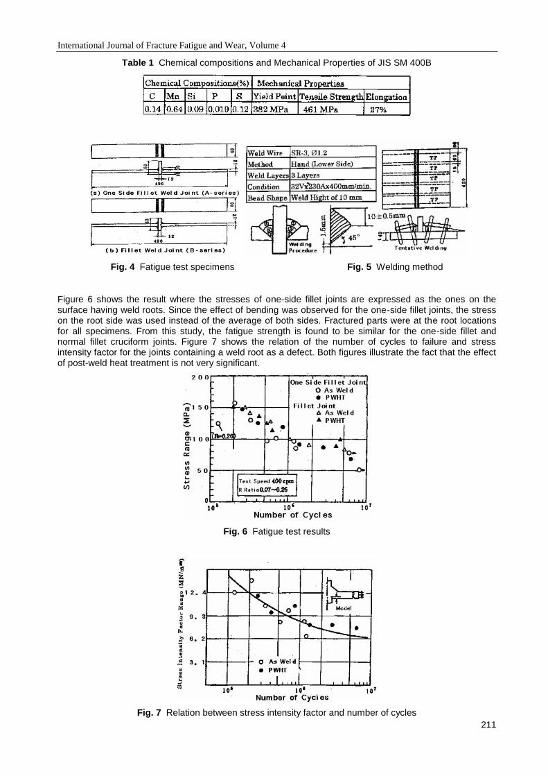
International Journal of Fracture Fatigue and Wear, Volume 4
211
Table 1 Chemical compositions and Mechanical Properties of JIS SM 400B
Fig. 4 Fatigue test specimens Fig. 5 Welding method
Figure 6 shows the result where the stresses of one-side fillet joints are expressed as the ones on the surface having weld roots. Since the effect of bending was observed for the one-side fillet joints, the stress on the root side was used instead of the average of both sides. Fractured parts were at the root locations for all specimens. From this study, the fatigue strength is found to be similar for the one-side fillet and normal fillet cruciform joints. Figure 7 shows the relation of the number of cycles to failure and stress intensity factor for the joints containing a weld root as a defect. Both figures illustrate the fact that the effect of post-weld heat treatment is not very significant.
Fig. 6 Fatigue test results
Fig. 7 Relation between stress intensity factor and number of cycles
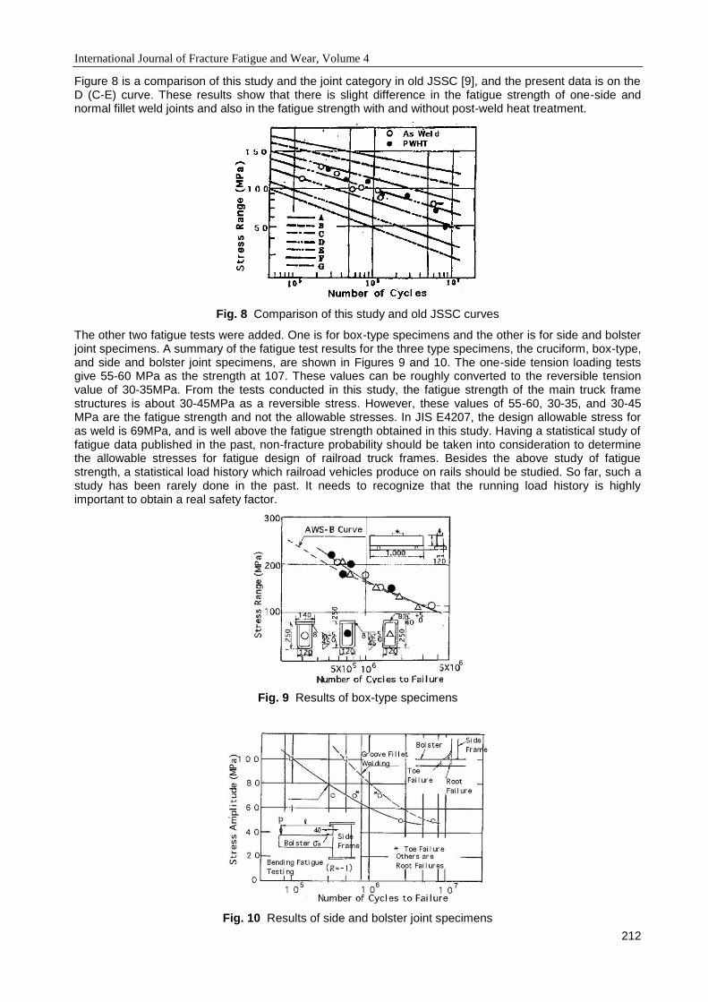
International Journal of Fracture Fatigue and Wear, Volume 4
212
Figure 8 is a comparison of this study and the joint category in old JSSC [9], and the present data is on the D (C-E) curve. These results show that there is slight difference in the fatigue strength of one-side and normal fillet weld joints and also in the fatigue strength with and without post-weld heat treatment.
Fig. 8 Comparison of this study and old JSSC curves
The other two fatigue tests were added. One is for box-type specimens and the other is for side and bolster joint specimens. A summary of the fatigue test results for the three type specimens, the cruciform, box-type, and side and bolster joint specimens, are shown in Figures 9 and 10. The one-side tension loading tests give 55-60 MPa as the strength at 107. These values can be roughly converted to the reversible tension value of 30-35MPa. From the tests conducted in this study, the fatigue strength of the main truck frame structures is about 30-45MPa as a reversible stress. However, these values of 55-60, 30-35, and 30-45 MPa are the fatigue strength and not the allowable stresses. In JIS E4207, the design allowable stress for as weld is 69MPa, and is well above the fatigue strength obtained in this study. Having a statistical study of fatigue data published in the past, non-fracture probability should be taken into consideration to determine the allowable stresses for fatigue design of railroad truck frames. Besides the above study of fatigue strength, a statistical load history which railroad vehicles produce on rails should be studied. So far, such a study has been rarely done in the past. It needs to recognize that the running load history is highly important to obtain a real safety factor.
Fig. 9 Results of box-type specimens
Fig. 10 Results of side and bolster joint specimens

International Journal of Fracture Fatigue and Wear, Volume 4
213
3 DESIGN OF ALUMINUM TRUCK FRAME
3.1 DESIGN CURVES FOR ALUMINUM WELDED STRUCTURES Fatigue tests were performed using plate-type specimens, whose thickness is 4mm, since the designed thickness is planned to be as small as possible such as 4.0 or 3.5mm. Data from the present study and those from the manufacturer were combined to obtain the design curves. The design stress or allowable stress was determined based on the following results,
(1) The curve for allowable stresses is set to be the value subtracting three times the standard deviation (s.d.) from the mean value to obtain a fracture probability of 1.3x10⁻³, which is one-order less than the one of BS8118. This was decided in order to obtain lower design stresses in a higher stress amplitude range, which makes the fatigue propagation less than 2xs.d.such as BS8118.
(2) Allowable stress between 107 and 108 was maintained to be the same. The reason is that the data beyond 107 were almost all unfailed ‘run-out’ results in the present data and that in the data from the material manufacturer.
The obtained example of the allowable stress curve is shown in Figure 11, which is the case for ground weld joints. The comparison between the present curve and the one from BS8118 is shown in Figure 12. It is noted that the present curve is in a more conservative area than the curve for BS8118.
Fig. 11 Example of design curve for ground weld joints
Fig. 12 Design curve for fatigue damage estimation of ground weld joints
3.2 DESIGN OF ALUMINUM WELDED STRUCTURE From the design curves obtained in this study, an aluminum welded structure was designed [10]. The material is 7N01, and the main plate thickness is 4 mm. The load conditions were given at 13 locations in three-dimensional directions from a user. To determine a configuration, structural stress analyses were conducted using software by Applied Structure in the United States. The criteria for the fatigue design are curves for the parent material and welded joints of butt and fillet welds. In designing, the fatigue strength of ground weld joints not considered at first was taken into consideration after manufacturing and static tests. Figure 13 shows the analytical results for an assembly model and part of the structure. In order to reduce the weight, windows in the structure were considered. However, stress concentration factors at such
locations were ignored, since the estimation of the stress concentration factor in the analysis is not practical. Stress at every position was judged as normal stress from the viewpoint of safety.

International Journal of Fracture Fatigue and Wear, Volume 4
214
However, after manufacturing the structure, stress measurement under static load sometimes shows a higher stress origination than expected by the analytical study. If the point of higher stress is in the weldment, grinding can be applied. If the point of higher stress is in the parent material, then the configuration needs to be modified. In this case, the higher stress part was in the window, and fatigue damage at the ground weld part and the window was estimated. Since the allowable fatigue damage is not specified in BS8118, this study followed the guidance of offshore structures. For such guidance, the fatigue damage is specified to be below 1.0 by calculation using the mean value minus 2xs.d. In this case, the fatigue damage was calculated using the mean value minus 3xs.d. with modified Miners’ rule. It was found that the damage in the concerned area is well below 1.0.
Fig. 13 Analytical stress distribution by a structural software
4 CONSIDERATION ON DESIRABLE FATIGUE DESIGN FOR WELDED STRUCUTURES
Specific concerns to be considered and solved in fatigue design for welded structures are,
(1) Fatigue limit design or fatigue damage design?
(2) Allowable stress with reasonable non-fracture probability?
(3) Design stress of normal or local hot spot?
(4) Evaluation of stress calculated by FEM. Normal or local?
(5) Load history data?
The above subjects for designing welded structures should be clarified for obtaining more conservative and safer designs for welded structures. More structural examples designed by codes or guidance are desired to be available to the public. Codes or guidance used in the design examples in the past seem to have been used for the evaluation of existing or constructed structures. More information concerning how to design welded structures for the first decision of a structure is needed for further study.
As for the evaluation of designed and constructed structures, static stress measurements and fatigue tests using a real structure are needed. BS8118 requires the fatigue testing, which is consistent with the service conditions. In the case of railroad truck frames, it requires around 108 cycles. The fastest test speed is about at 1.5Hz for a real structure, and this speed needs 2.2 years for 108 cycles, which is not realistic. A normal fatigue test machine is made of several cylinders. An accelerated test of around 2-3x10⁶ cycles is a way to get a result that should project the strength at 108 cycles. The question is how an accelerated test can be done and how the test result can indicate real life for a long life region.
5 CONCLUDING REMARKS
5.1 Codes and practice for designing railroad truck frame welded structures are discussed in this study. The existing codes for welded structures are mostly given by S-N curves, and there are many weld categories. For example, JSSC includes 38 weld categories and 8 S-N curves. For determining the first configuration, too many categories are thought to be too complex for a designer. Instead, such a fatigue design guidance as JIS E 4207 for a railroad truck frame is considered to be simple and useful for the first design.
5.2 However, the guidance is needed for modification to obtain more safety considerations. Fatigue data based on the standard, existence of fatigue limit, and non-fracture probability are not clear in the standard. There are no fatigue data based on the standard. The diagram for endurance limits is shown, but the existence of the endurance limit is questionable. There is no explanation of non-fracture probability.
International Journal of Fracture Fatigue and Wear, Volume 4
215
Although the stresses seem to contain the hot spot ones, whether a designer can consider hot spot stresses for the first configuration design is a matter of question as well.
6 ACKNOWLEDGEMENT
The author greatly acknowledges the work conducted by people in Sumitomo Metal Industries (Presently Shinnitetsu-Sumikin Co. ).
REFERENCES
[1] JIS (Japanese Industrial Standard) E 4502-1993, General Rule for Design of Railway Axle (In Japanese)
[2] JIS E 4207-1992, General Rule for Design of Truck Frame for Railway Rolling Stock (In Japanese)
[3] American Welding Society, AWS Structural Welding Code Steel, AWS D1.1-83, 1983
[4] American Institute of Steel Construction, Specification for the Design, Fabrication, and Erection of Structural Steel for Building, 1969
[5] Japanese Society of Steel Construction, Fatigue Design Guidance for Steel Structures, 1993 (In Japanese)
[6] British Standard, BS5400, Steel, Concrete and Composite Bridges, Part 10 Code of Practice for Fatigue. BS8118 Structural Use of Aluminium, Part 1, Code of Practice for Design, 1991.
[7] UK (United Kingdom) Department of Energy, Offshore Installation Guidance on Design and Construction, New Fatigue Design Guidance for Steel Welded Joints in Offshore Structures, 1981
[8] R. Jaccard, et al., Elements, Background and Evaluation on Fatigue and Fracture Behavior of Aluminium Components, 6th. Int. Conf. On Aluminium Weldments, 1995, Ohio, USA
[9] Japanese Society of Steel Construction, Fatigue Design Guidance for Steel Structures, 1974 (In Japanese)
[10] H. Sakamoto, Fatigue Design Code and Practice for Aluminium Welded Structure, Engineering Structural Integrity Assessment, 1998, England.

International Journal of Fracture Fatigue and Wear, Volume 4
216
Proceedings of the 5th International Conference
Fracture Fatigue and Wear, pp. 216-222, 2016
MECHANICAL PROPERTIES OF STEEL FIBRE REINFORCED POLYMER
COMPOSITES
W. N. M. Jamil1, Z. Sajuri1, M. A. Aripin1, S. Abdullah1,2, M. Z. Omar1, M.F. Abdullah1 and W. F. H. Zamri1
1Department of Mechanical and Materials Engineering, Faculty of Engineering and Build Environment, Universiti Kebangsaan Malaysia, 43600 UKM Bangi, Selangor, Malaysia.
2Centre for Automotive Research, Faculty of Engineering and Build Environment, Universiti Kebangsaan Malaysia, 43600 UKM Bangi, Selangor, Malaysia.
Abstract: This paper presents the effectiveness of steel fibres as a reinforcing material to increase the flexural
strength of polymer composites. Composite materials are commonly applied as a ballistic resistance material for their superior performance in energy absorption as well as being lightweight. Nowadays, various materials have been used as reinforcement in polymer materials. Steel fibres are usually used in concrete reinforcement in order to increase the crack and impact resistance in protective areas and are ideal candidates to reinforce polymer materials in order to increase energy absorption for ballistic resistance applications. Two different lengths of steel fibres were used. The effects of fibre length and density were investigated through bending tests. The results showed that for steel fibres of similar densities, polymers reinforced with long fibres exhibited higher bending strengths than that of short fibres and matrices with no fibres. Steel fibres would improve the strength and crack resistance by acting as a barrier and restrict the development of cracks by transferring the matrix’s low impact resistance into a superior composite. Other than that, higher deformations of long fibre-reinforced polymers were obtained due to ductile fractures during bending tests. Lower deformations were present in short fibres which fractured in a brittle manner. The results presented here may facilitate improvements in the mechanical performance of polymer composites for the configuration of new composite panels for ballistic resistance applications. Keywords: steel fibres, reinforcement, mechanical properties, polymer composite
1 INTRODUCTION
The mixture of two or more materials will cause the formation of a composite material. The main benefit of composite materials is the high strength as compared to individual materials. Composite materials have also become an essential component in the shielding of structures. Reinforcement and the matrix are the two factors in composites. Reinforcing a material has the added advantage of superior flexural strength, energy absorption, crack arrest and ductility [1-4]. These materials have been applied in different fields like construction and architecture. Reinforcement materials generally include a fibre or particulate. This material is commonly used in concrete to increase the strength of the matrix. Nowadays, steel fibres reinforced with polymer composites have also been extensively used in ballistic applications due to the high capacity and performance in energy absorption. Higher impact resistance can be achieved by adding these steel fibres with polymer composites [5]. Impact tests have shown that the load is distributed because of the arrangement of the steel fibres. The ability of steel fibres to split up energy increases the ballistic performance.
Steel fibres in a matrix increase the mechanical properties like ductility, energy absorption capacity and impact strength [6]. Study by Zhou [7] on the ballistic resistance of steel fibres reinforced by two layers of plates found that the steel fibres fractured from bending and tensile failure. Steel fibres can absorb the fragments’ kinetic energy during impact. The performance of steel fibre-reinforced polymer composites is influenced by the fibre’s length and diameter (aspect ratio), type, direction of the fibres and percentage of fibre to volume fraction. The greater dosage of steel fibres and aspect ratio increases the toughness, strength and impact resistance [3, 8].
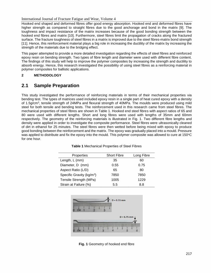
International Journal of Fracture Fatigue and Wear, Volume 4
217
Hooked end shaped and deformed fibres offer good energy absorption. Hooked end and deformed fibres have higher strength as compared to straight fibres due to the good anchorage and bond in the matrix [9]. The toughness and impact resistance of the matrix increases because of the good bonding strength between the hooked end fibres and matrix [10]. Furthermore, steel fibres limit the propagation of cracks along the fractured surface. The fracture toughness of steel fibres in a matrix is improved due to the steel fibres-matrix bond strength [11]. Hence, this reinforcement material plays a big role in increasing the ductility of the matrix by increasing the strength of the materials due to the bridging effect.
This paper attempted to provide a more detailed investigation regarding the effects of steel fibres and reinforced epoxy resin on bending strength. Two types of fibre length and diameter were used with different fibre content. The findings of this study will help to improve the polymer composites by increasing the strength and ductility to absorb energy. Hence, this research investigated the possibility of using steel fibres as a reinforcing material in polymer composites for ballistic applications.
2 METHODOLOGY
2.1 Sample Preparation
This study investigated the performance of reinforcing materials in terms of their mechanical properties via bending test. The types of matrices used included epoxy resin in a single part of heat cured epoxy with a density of 1.5g/cm3, tensile strength of 24MPa and flexural strength of 40MPa. The moulds were produced using mild steel for both tensile and bending tests. The reinforcement used in this research came from steel fibres. The mechanical properties of steel fibres are shown in Table 1. Hooked end steel fibres with aspect ratios of 65 and 80 were used with different lengths. Short and long fibres were used with lengths of 35mm and 60mm respectively. The geometry of the reinforcing materials is illustrated in Fig. 1. Two different fibre lengths and density were applied in order to investigate the composite performance. Steel fibres were ultrasonically cleaned of dirt in ethanol for 25 minutes. The steel fibres were then wetted before being mixed with epoxy to produce good bonding between the reinforcement and the matrix. The epoxy was gradually placed into a mould. Pressure was applied to distribute and fix the epoxy into the mould. This polymer composite was allowed to cure at 150oC for one hour.
Table 1 Mechanical Properties of Steel Fibres
Fig. 1 Geometry of hooked end fibre
Properties Short Fibre Long Fibre
Length, L (mm) 35 60
Diameter, D (mm) 0.55 0.75
Aspect Ratio (L/D) 65 80
Specific Gravity (kg/m3) 7850 7850
Tensile Strength (MPa) 1005 1229
Strain at Failure (%) 5.5 8.8
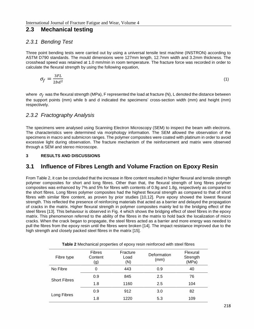
International Journal of Fracture Fatigue and Wear, Volume 4
218
2.3 Mechanical testing
2.3.1 Bending Test
Three point bending tests were carried out by using a universal tensile test machine (INSTRON) according to ASTM D790 standards. The mould dimensions were 127mm length, 12.7mm width and 3.2mm thickness. The crosshead speed was retained at 1.0 mm/min in room temperature. The fracture force was recorded in order to calculate the flexural strength by using the following equation,
𝜎𝑓 =3𝐹𝐿
2𝑏𝑑2 (1)
where 𝜎𝑓 was the flexural strength (MPa), F represented the load at fracture (N), L denoted the distance between
the support points (mm) while b and d indicated the specimens’ cross-section width (mm) and height (mm) respectively.
2.3.2 Fractography Analysis
The specimens were analysed using Scanning Electron Microscopy (SEM) to inspect the beam with electrons. The characteristics were determined via morphology information. The SEM allowed the observation of the specimens in macro and submicron ranges. The polymer composites were coated with platinum in order to avoid excessive light during observation. The fracture mechanism of the reinforcement and matrix were observed through a SEM and stereo microscope.
3 RESULTS AND DISCUSSIONS
3.1 Influence of Fibres Length and Volume Fraction on Epoxy Resin
From Table 2, it can be concluded that the increase in fibre content resulted in higher flexural and tensile strength polymer composites for short and long fibres. Other than that, the flexural strength of long fibres polymer composites was enhanced by 7% and 5% for fibres with contents of 0.9g and 1.8g, respectively as compared to the short fibres. Long fibres polymer composites had the highest flexural strength as compared to that of short fibres with similar fibre content, as proven by prior studies [10,12]. Pure epoxy showed the lowest flexural strength. This reflected the presence of reinforcing materials that acted as a barrier and delayed the propagation of cracks in the matrix. Higher flexural strength in polymer composites mainly led to the bridging effect of the steel fibres [13]. This behaviour is observed in Fig. 4 which shows the bridging effect of steel fibres in the epoxy matrix. This phenomenon referred to the ability of the fibres in the matrix to hold back the localization of micro cracks. When the crack began to propagate, the steel fibres acted as a barrier and more energy was needed to pull the fibres from the epoxy resin until the fibres were broken [14]. The impact resistance improved due to the high strength and closely packed steel fibres in the matrix [15].
Table 2 Mechanical properties of epoxy resin reinforced with steel fibres
Fibre type Fibres
Content (g)
Fracture Load (N)
Deformation (mm)
Flexural Strength (MPa)
No Fibre 0 443 0.9 40
Short Fibres 0.9 845 2.5 76
1.8 1160 2.5 104
Long Fibres 0.9 912 3.0 82
1.8 1220 5.3 109
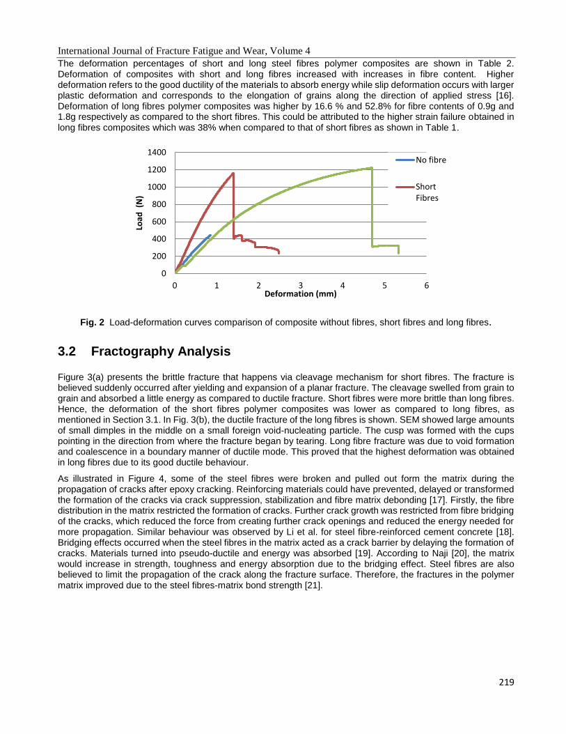
International Journal of Fracture Fatigue and Wear, Volume 4
219
The deformation percentages of short and long steel fibres polymer composites are shown in Table 2. Deformation of composites with short and long fibres increased with increases in fibre content. Higher deformation refers to the good ductility of the materials to absorb energy while slip deformation occurs with larger plastic deformation and corresponds to the elongation of grains along the direction of applied stress [16]. Deformation of long fibres polymer composites was higher by 16.6 % and 52.8% for fibre contents of 0.9g and 1.8g respectively as compared to the short fibres. This could be attributed to the higher strain failure obtained in long fibres composites which was 38% when compared to that of short fibres as shown in Table 1.
Fig. 2 Load-deformation curves comparison of composite without fibres, short fibres and long fibres.
3.2 Fractography Analysis
Figure 3(a) presents the brittle fracture that happens via cleavage mechanism for short fibres. The fracture is believed suddenly occurred after yielding and expansion of a planar fracture. The cleavage swelled from grain to grain and absorbed a little energy as compared to ductile fracture. Short fibres were more brittle than long fibres. Hence, the deformation of the short fibres polymer composites was lower as compared to long fibres, as mentioned in Section 3.1. In Fig. 3(b), the ductile fracture of the long fibres is shown. SEM showed large amounts of small dimples in the middle on a small foreign void-nucleating particle. The cusp was formed with the cups pointing in the direction from where the fracture began by tearing. Long fibre fracture was due to void formation and coalescence in a boundary manner of ductile mode. This proved that the highest deformation was obtained in long fibres due to its good ductile behaviour.
As illustrated in Figure 4, some of the steel fibres were broken and pulled out form the matrix during the propagation of cracks after epoxy cracking. Reinforcing materials could have prevented, delayed or transformed the formation of the cracks via crack suppression, stabilization and fibre matrix debonding [17]. Firstly, the fibre distribution in the matrix restricted the formation of cracks. Further crack growth was restricted from fibre bridging of the cracks, which reduced the force from creating further crack openings and reduced the energy needed for more propagation. Similar behaviour was observed by Li et al. for steel fibre-reinforced cement concrete [18]. Bridging effects occurred when the steel fibres in the matrix acted as a crack barrier by delaying the formation of cracks. Materials turned into pseudo-ductile and energy was absorbed [19]. According to Naji [20], the matrix would increase in strength, toughness and energy absorption due to the bridging effect. Steel fibres are also believed to limit the propagation of the crack along the fracture surface. Therefore, the fractures in the polymer matrix improved due to the steel fibres-matrix bond strength [21].
0
200
400
600
800
1000
1200
1400
0 1 2 3 4 5 6
Load
(N
)
Deformation (mm)
No fibre
ShortFibres

International Journal of Fracture Fatigue and Wear, Volume 4
220
(a)
(b)
Fig. 3 Fractography surface analysis using Scanning Electron Microscopy (SEM) (a) short fibres (b) long fibres
(a) (b)
Fig. 4 Fracture behaviour of steel fibre (a) bridging (b) debonding and pullout effects
4 CONCLUSION
Reinforcement by steel fibres resulted in better bending properties as compared to pure epoxy resin. The addition of steel fibres in polymer composites increased the flexural strength as compared to only pure epoxy matrix. Other than that, long fibres polymer composites exhibited better performance in flexural strength as compared to short fibres with the same density. Steel fibres polymer composites exhibited better mechanical properties due to their capability to control the propagation of cracks inside the matrix. Crack bridging effects of steel fibres improved the matrix in polymer composites. Cracks were delayed by these reinforcing materials. Long fibres
Steel Pullout
P
Steel Debonding
International Journal of Fracture Fatigue and Wear, Volume 4
221
showed a higher percentage of deformation as compared to short fibres due to their good ductility in absorbing energy and fractures. Short fibres that fractured in a brittle manner represented lower percentage of deformation.
5 ACKNOWLEDGEMENTS
The authors would like to express their gratitude to Universiti Kebangsaan Malaysia (UKM) and Universiti Pertahanan National Malaysia (UPNM) for their research facilities and support and the Ministry of Higher Education Malaysia for their research funding (LRGS/2013/UPNM-UKM/04). REFERENCES
[1] K. S. Kene, Experimental Study on Behavior of Steel and Glass Fiber Reinforced Concrete Composites, International Journal of Industrial Engineering and Management Science, 2(4), 125–130, 2012
[2] Y. Şahin, F. Köksal, The influences of Matrix and Steel Fibre Tensile Strengths on the Fracture Energy of High-Strength Concrete, Construction and Building Materials, 25(4), 1801–1806. 2011.
[3] J. N. Karadelis, Y. Lin, Flexural strengths and Fibre Efficiency of Steel-Fibre-Reinforced, Roller-Compacted, Polymer Modified Concrete, Construction and Building Materials, 498–505, 2015.
[4] I. F. Kara, A. F. Ashour, M. A. Köroğlu, Flexural Behavior of Hybrid FRP/Steel Reinforced Concrete Beams, Composite Structures, 111–121, 2015.
[5] A. Khanlou, A. Scott, M. Holden, T. Yeow, M. Saleh, A. G. Macrae, Performance of Concrete Slabs with Different Reinforcing, Proceedings of the Ninth Pacific Conference on Earthquake Engineering, 1–8,1998.
[6] K. R. Venkatesan, P. N. Raghunath, K. Suguna, Flexural Behavior of High Strength Steel Fibre Reinforced Concrete Beams, International Journal of Engineering Science and Innovative Technology (IJESIT), 135–140, 2015.
[7] N. Zhou, J. Wang, C. Peng, Z. Tong, Experimental and Numerical Study on the Ballistic Resistance of Steel–Fibre Reinforced Two-Layer Explosively Welded Plates, Materials and Design, 104–111, 2014.
[8] S. P. Yap, K. R. Khaw, U. J. Alengaram, M. Z. Jumaat, Effect of Fibre Aspect Ratio on the Torsional Behaviour of Steel Fibre-Reinforced Normal Weight Concrete and Lightweight Concrete, Engineering Structures, 24–33, 2015.
[9] E. Baran, T. Akis, S. Yesilmen, Pull-Out Behavior of Prestressing Strands in Steel Fiber Reinforced Concrete, Construction and Building Materials, 28(1), 362–371, 2012.
[10] K. S. Sable, M. K. Rathi, Effect of Different Type of Steel Fibre and Aspect Ratio on Mechanical Properties of Self Compacted Concrete, International Journal of Engineering and Innovative Technology (IJEIT), 184–188, 2012.
[11] F. Köksal, Y. Şahin, O. Gencel, İ. Yiğit, Fracture Energy-Based Optimisation of Steel Fibre Reinforced Concretes, Engineering Fracture Mechanics, 29–37, 2013.
[12] A. A. Aliabdo, A. E. M. Elmoaty, M. Hamdy, Effect of Internal Short Fibers, Steel Reinforcement, and Surface Layer On Impact And Penetration Resistance Of Concrete, Alexandria Engineering Journal, 52(3), 407–417, 2013.
[13] A. Krasnikovs, O. Kononova, A. Pupurs, Crack Propagation in Short Steel Fiber Reinforced Concrete . Modeling and Experimental, Scientific Proceedings of 13th European Conference on Composite Material, 2632-2642, 2008.
[14] M. A. Yusof, N. M. Nor, M. Fauzi, M. Zain, N. C. Peng, A. Ismail, R. M. Sohaimi, Mechanical Properties of Hybrid Steel Fibre Reinforced Concrete with Different Aspect Ratio, Australian Journal of Basic and Applied Sciences, 5(7), 159-166, 2011.
[15] R. Ahmadi, P. Ghoddousi, M. Sharifi, A simple solution for prediction of steel fiber reinforcd concrete behavior under flexure, International Journal of Civil Engineering, IJCE, 10(4), 274-279, 2012.
[16] N. P. Cheremisinoff, Materials Selection Deskbook. William Andrew, 1996.
International Journal of Fracture Fatigue and Wear, Volume 4
222
[17] M. Nili, V. Afroughsabet, Combined effect of Silica Fume and Steel Fibers on the Impact Resistance and Mechanical Properties of Concret, International Journal of Impact Engineering, 37(8), 879–886, 2010.
[18] G. Li, X. Zhao, C. Rong, Z. Wang, Properties of Polymer Modified Steel Fiber-Reinforced Cement Concretes, Construction and Building Materials, 24(7), 1201–1206, 2010.
[19] L. G. Sorelli, A. Meda, G. A. Plizzari, Bending and Uniaxial Tensile Tests on Concrete Reinforced with Hybrid Steel Fibers, Journal of Materials in Civil Engineering, 519–527, 2005.
[20] H. Z. Naji, Mechanical Properties of Composite Materials Based on Epoxy Resin Reinforced Low Carbon Steel, The Iraqi Journal For Mechanical And Material Engineering, 11(4), 663-671, 2011.
[21] M. G. Callens, L. Gorbatikh, E. Bertels, B. Goderis, M. Smet, I. Verpoest, Tensile Behaviour of Stainless Steel Fibre/Epoxy Composites with Modified Adhesion, Composites Part A: Applied Science and Manufacturing, 208–218, 2015.
Related Documents