International Journal of Engineering Issues - Vol 2015 - No 1 - Paper2

International Journal of Engineering Issues Vol. 2015, no. 1, pp. 17-32 ISSN: 2458-651X Copyright © Infinity Sciences

The Comparison of Back-Propagation (BPNN) and General Regression (GRNN) Neural Network

Architectures used for SPT Based Liquefaction Analysis

Zeynel Abidin DERELI1, Mert TOLON2

1Ministry of National Defense, Ankara, Turkey 2Department of Civil Engineering, Nisantası University, Istanbul, Turkey

Email: [email protected], [email protected]

Abstract- State of 'soil liquefaction' occurs when the effective stress of soil is reduced to essentially zero, which corresponds to a complete loss of shear strength. The effects of liquefaction have long been understood, it was more thoroughly brought to the attention of engineers after the 1964 Niigata earthquake and 1964 Alaska earthquake. It was also a major factor in the destruction in San Francisco's Marina District during the 1989 Loma Prieta earthquake, and in Port of Kobe during the 1995 Great Hanshin earthquake.

Due to damage risks, many types of analyses have been developed by researchers. The most used ones are the simplified methods with simple equations. Nowadays, Artificial Neural Network (ANN) algorithm is used to analyze liquefaction occurrence probabilities by the researchers.

Liquefaction triggering database taken from the report of Cetin et al. (2004) is arranged for 157 liquefaction cases and given in to the program. 107 of the cases are for the training and the testing phases, while the last 50 of them for the forecasting studies.

We try to do the analysis by using different ANN architecture types to evaluate which of the architecture type (BPNN or GRNN) is more suitable for liquefaction analysis. As a result of the current study, we determined that cyclic resistance ratio, cyclic stress ratio, corrected SPN-N number and the magnitude parameters are the most effective parameters for liquefaction occurrence. Also, the simplified method of Tokimatsu and Yoshimi (1983)’s results are approximately equal to the developed GRNN model results. Thus, we recommend using the developed GRNN model to evaluate liquefaction occurrence of a site more easily, fast and approximately. Finally, we argue that ANN methods are suitable and suggested methodologies in liquefaction analysis for geotechnical researchers in future studies.

Keywords: Liquefaction; Neural network; SPT.

I. INTRODUCTION

Liquefaction is one of the most common failure reasons for structures. Generally, there is no structural damage on structural element of buildings due to liquefaction. However, much displacement due to liquefaction, prevent buildings from service. Liquefaction is usually observed in loose, saturated cohesionless soil, sensitive clays and during dynamic loading like earthquakes. Therefore, evaluating the liquefaction potential of soil especially in urbanized areas is necessary because of the devastating result of liquefaction as in Niigata Earthquake (1964), Alaska

Z. A. DERELI et al. / International Journal of Engineering Issues

18

Earthquake (1964) and Izmit earthquake (1999). There are laboratory and in situ tests and many other procedures to evaluate the liquefaction potential. In situ tests are more common than laboratory tests due to the disturbing problem of cohesionless soil. Standard penetration test (SPT), which is the mostly-used one, cone penetration test (CPT) and shear wave velocity measurements are in-situ test methods to evaluate the liquefaction assessment. For each test, there are analytical evaluation techniques. Simplified procedure depends on SPT. Liquefaction evaluating procedures have been developed by scientists since the 1970s. There are many research studies and suggestions about stress reduction coefficient. Additionally there are many other studies about magnitude correction factor, stress correction factor and other correction factors to reach real situations.

Developing computer technologies provides good solutions especially for complex problems. Artificial intelligence is one of these new technologies. It works like a nerve cell in the brain. For this reason, it is also named neural networks. Neural network is used in variety of areas to solve medical, scientific and engineering problems. It can be used in geotechnical engineering as well. The application of neural networks in geotechnical engineering problem is a new area. Neural Network Algorithms give better result for evaluating liquefaction assessments.

The aim of the current study is to investigate the evaluation of liquefaction assessment with neural network algorithm and indicate the effect of parameter for liquefaction occurrence.

A. Liquefaction Analysis with SPT

Liquefaction is defined as the transformation of a granular material from a solid to a liquefied state as a consequence of increased pore water pressure and reduced effective stress (Marcuson, 1978). Liquefaction analysis may be necessary if a facility has liquefaction potential. Especially, in heavily urbanized areas which also have high seismic risk, the assessment of the liquefaction potential of surface soil needs an exhaustive geotechnical investigation and calculation.

According to Seed and Idriss (1982); Marcuson, (1990); and Youd et al. (2001), fine soils can liquefy. Nevertheless, initially liquefaction is relevant only to sand. It was well recognized for a long time that clean sands with few fines are susceptible to liquefaction. However, in the past two to three decades and following the observations during strong earthquakes in China, Turkey and Taiwan, it is concluded that non-plastic to low plasticity fine grained materials - as well as granular material - may also be subjected to classical liquefaction. Boulanger and Idriss (2004) review the mechanisms of liquefaction of no to low plasticity fine grain materials subjected to cyclic loading. Taking into account recent advances on this subject, the latter reference uses the term “liquefaction” to describe the onset of high excess pore water pressures and large shear strains during undrained cyclic loading of sand-like soils, while term “cyclic failure” is used to describe the corresponding behavior of clay-like soils.

Laboratory tests are not very well accepted for liquefaction analysis due to difficulties to obtain undisturbed and representative samples from non-cohesive soils. In order to evaluate the liquefaction assessment, there are commonly used four in-situ test methods which are standard penetration test (SPT), cone penetration test (CPT), shear wave velocity measurements, and Becker penetration test (BPT). For each test, there are analytical evaluation techniques.

SPT is relatively simple and very well developed. Seed et al. (2003) claim that the oldest and most widely-used in-situ testing method for liquefaction assessment is the SPT method. Furthermore, SPT-based correlations for liquefaction assessments have been in use for relatively long time and are validated by numerous case histories. Various evaluation methods have been proposed for liquefaction assessment using SPT method such as Seed and Idriss Simplified method (Seed et al. 1984), Youd and Idriss (2001), and Cetin et al. (2004). Most of the available liquefaction analysis procedures follow the formats initially used in Seed and Idriss simplified method.

The assessment of liquefaction potential includes two main stages which are evaluating the effect of earthquake loading on soil, and evaluating soil strength against earthquake loading. The earthquake loading on soil is expressed using the term Cyclic Stress Ratio (CSR), and the soil strength (capacity of soil) to resist liquefaction is expressed using Cyclic Resistance Ratio. The capacity of the soil to resist liquefaction was denoted using different symbols. Seed and Harder (1990) used the symbol CSRl; Youd (1993) used the symbol CSRL; and Kramer (1996) used the symbol CSRL to denote this. Yet, the NCEER workshop (Youd et al., 2001) recommends the use of CRR to denote the soil resistance against liquefaction, and this notation is followed in this study.

Z. A. DERELI et al. / International Journal of Engineering Issues

19

Seed and Idriss (1971) formulated the equation for calculation of the cyclic stress ratio:

CSR = 0.65σv

σv′

amax

grd (1)

Where,

σv : Total vertical overburden stress

σv′ : Effective vertical overburden stress

amax : Peak horizontal ground surface acceleration

g : The acceleration of gravity

rd : Stress reduction factor

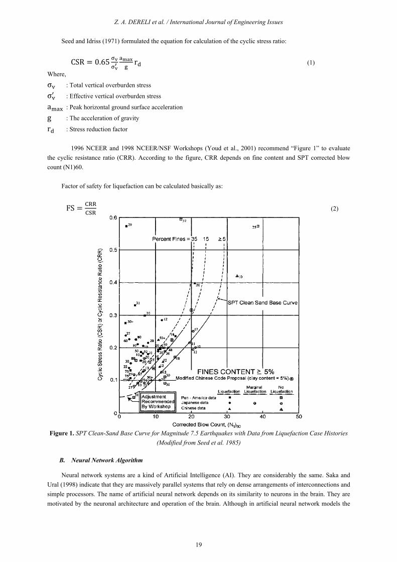
1996 NCEER and 1998 NCEER/NSF Workshops (Youd et al., 2001) recommend “Figure 1” to evaluate the cyclic resistance ratio (CRR). According to the figure, CRR depends on fine content and SPT corrected blow count (N1)60.

Factor of safety for liquefaction can be calculated basically as:

FS =CRR

CSR (2)

Figure 1. SPT Clean-Sand Base Curve for Magnitude 7.5 Earthquakes with Data from Liquefaction Case Histories

(Modified from Seed et al. 1985)

B. Neural Network Algorithm

Neural network systems are a kind of Artificial Intelligence (AI). They are considerably the same. Saka and Ural (1998) indicate that they are massively parallel systems that rely on dense arrangements of interconnections and simple processors. The name of artificial neural network depends on its similarity to neurons in the brain. They are motivated by the neuronal architecture and operation of the brain. Although in artificial neural network models the

Z. A. DERELI et al. / International Journal of Engineering Issues

20

majority of biological details are eliminated, they contain enough structure observed in the brain to provide insight into how biological neural processing occurs. Neural network algorithms use a processing structure that has numerous processing units and many interconnections between them. Each unit is connected to many of its neighbors; therefore, there are huge numbers of connections. Thus, these connections provide power of neural network (Ural, 1998)

Neural Network Systems are used in a great variety of application areas that include medical, scientific and engineering problems. Ordinary equation and model can be replaced with neural networks to analyze problems. Analyses that involve many variables become more convenient in neural network. The application of neural networks in geotechnical engineering problem is a new area.

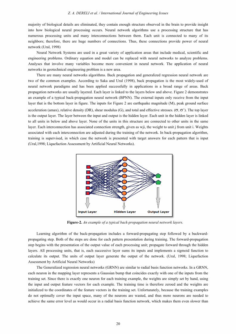
There are many neural networks algorithms. Back propagation and generalized regression neural network are two of the common examples. According to Saka and Ural (1998), back propagation is the most widely-used of neural network paradigms and has been applied successfully in applications in a broad range of areas. Back propagation networks are usually layered. Each layer is linked to the layers below and above. Figure 2 demonstrates an example of a typical back-propagation neural network (BPNN). The external inputs only receive from the input layer that is the bottom layer in figure. The inputs for Figure 2 are earthquake magnitude (M), peak ground surface

acceleration (amax), relative density (DR), shear modulus (G), and total and effective stresses. (, ’). The top layer is the output layer. The layer between the input and output is the hidden layer. Each unit in the hidden layer is linked to all units in below and above layer. None of the units in this structure are connected to other units in the same layer. Each interconnection has associated connection strength, given as wji, the weight to unit j from unit i. Weights associated with each interconnection are adjusted during the training of the network. In back-propagation algorithm, training is supervised, in which case the network is presented with target answers for each pattern that is input (Ural,1998; Liquefaction Assessment by Artificial Neural Networks).

Figure-2. An example of a typical back-propagation neural network layers.

Learning algorithm of the back-propagation includes a forward-propagating step followed by a backward-

propagating step. Both of the steps are done for each pattern presentation during training. The forward-propagation step begins with the presentation of the output value of each processing unit; propagate forward through the hidden layers. All processing units, that is, each successive layer sums its inputs and implements a sigmoid function to calculate its output. The units of output layer generate the output of the network. (Ural, 1998; Liquefaction Assessment by Artificial Neural Networks)

The Generalized regression neural networks (GRNN) are similar to radial basis function networks. In a GRNN, each neuron in the mapping layer represents a Gaussian bump that coincides exactly with one of the inputs from the training set. Since there is exactly one neuron for each training example, the weights are simply set by hand, using the input and output feature vectors for each example. The training time is therefore zeroed and the weights are initialized to the coordinates of the feature vectors in the training set. Unfortunately, because the training examples do not optimally cover the input space, many of the neurons are wasted, and thus more neurons are needed to achieve the same error level as would occur in a radial basis function network, which makes them even slower than

Z. A. DERELI et al. / International Journal of Engineering Issues

21

RBF networks at producing an output (Use of Artificial Neural Networks in Geomechanical and Pavement Systems, Transportation Research, 1999).

Neural network analysis involves two main stages: training and testing. In the training stage, neural networks learn the relationship between input and output from an educational group. Then, in the testing stage, in order to measure the generalization ability of the network, it is tested against educational group. Education should be repeated until logical output is produced by convenient inputs.

In order to develop neural network, selecting data is one of the most significant stages for training the neural networks due to the fact that neural networks are powerful in interpolation compared to extrapolation. For this reason, training data should cover all aspects of the problem. Moreover, neural network may not learn the data due to specific sort of data. This leads network to lose its learning power.

Artificial Neural Networks were applied to evaluate the assessment of soil liquefaction potential. The goal of networks is to forecast whether soil layers liquefy or not. Input parameters of neural network are obtained from the standard penetration test. The occurrence of liquefaction is the output parameter. Ten input variables including depth (z), ground water table (m), total vertical stress σv (kPa) effective vertical stress σv’ (kPa), fines content (%), corrected SPN-N number, N1(60), maximum surface acceleration, magnitude (M), cyclic resistance ratio (CRR), cyclic stress ratio (CSR) were used for ANN model development.

II. CASE STUDY

A report called “SPT-Based Liquefaction Triggering Procedures” by I. M. Idriss and Ross W. Boulanger was published in December, 2010 which presents an updated examination of SPT-based liquefaction triggering procedures for cohesionless soils, with the specific purpose of updating and documenting the case history database, providing more detailed illustrations of the database distributions relative to liquefaction triggering correlation by Idriss and Boulanger (2004, 2008), re-examining the database of cyclic test results for frozen sand samples, presenting a probabilistic version of the Idriss-Boulanger (2004, 2008) liquefaction triggering correlation using the updated case history database, presenting a number of new findings regarding components of the liquefaction analysis framework used to interpret and extend the case history experiences, and presenting an examination of the reasons for the differences between some current liquefaction triggering correlations.

This report describes the updated database of SPT-based liquefaction/no liquefaction case histories (Cetin et al. (2004) liquefaction triggering database). The selection of earthquake magnitudes, peak accelerations, and representative (N1)60cs values are described, and the classification of site performance is discussed as well.

The SPT-based case history database used to develop the Idriss and Boulanger (2004, 2008) liquefaction correlation for cohesionless soils is updated in this report, with the following specific goals of incorporating additional data from Japan; incorporating updated estimates of earthquake magnitudes, peak ground accelerations, and other details where improved estimates are available; illustrating details of the selection and computation of SPT (N1)60cs for a number of representative case histories; and presenting the distributions of the database relative to the various major parameters used in the liquefaction triggering correlation. The updated database described in this report incorporates the 44 Kobe proprietary cases which were provided by Professor Kohji Tokimatsu (2010, personal communication), an additional 26 case histories summarized in Iai et al. (1989), and a small number of other additions.

The total number of case histories in the updated database is 230, among which 115 cases had surface evidence of liquefaction, 112 cases had no surface evidence of liquefaction, and 3 cases were at the margin between liquefaction and no liquefaction.

Our database is created by filtering the extreme values of liquefaction possibilities and omitting 73 case histories from the list. 56 case histories for non-liquefaction and 101 case histories for the evidence of liquefaction are taken into consideration. Thus, the total number of case histories used in our models is 157. The case histories database is given in the appendices.

Z. A. DERELI et al. / International Journal of Engineering Issues

22

III. ANALYSIS

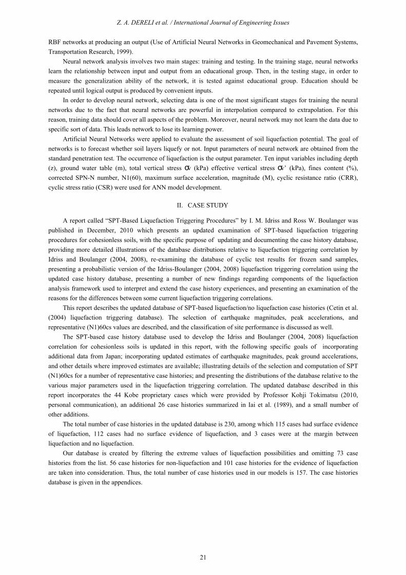
As mentioned before, the datasets are arranged for 157 liquefaction cases and given in to the program. 107 of them are for the training and the testing phases, and the last 50 are for the forecasting studies. 45 of 107 data in the testing and the training phases exhibit non-liquefaction, while 52 of them are simulating the liquefaction occurrences. Figure 3 represents an example dataset for the developed BPNN model.

Figure-3. An Example Input of dataset for the developed BPNN model.

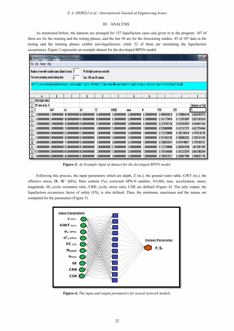
Following this process, the input parameters which are depth, Z (m.); the ground water table, GWT (m.); the

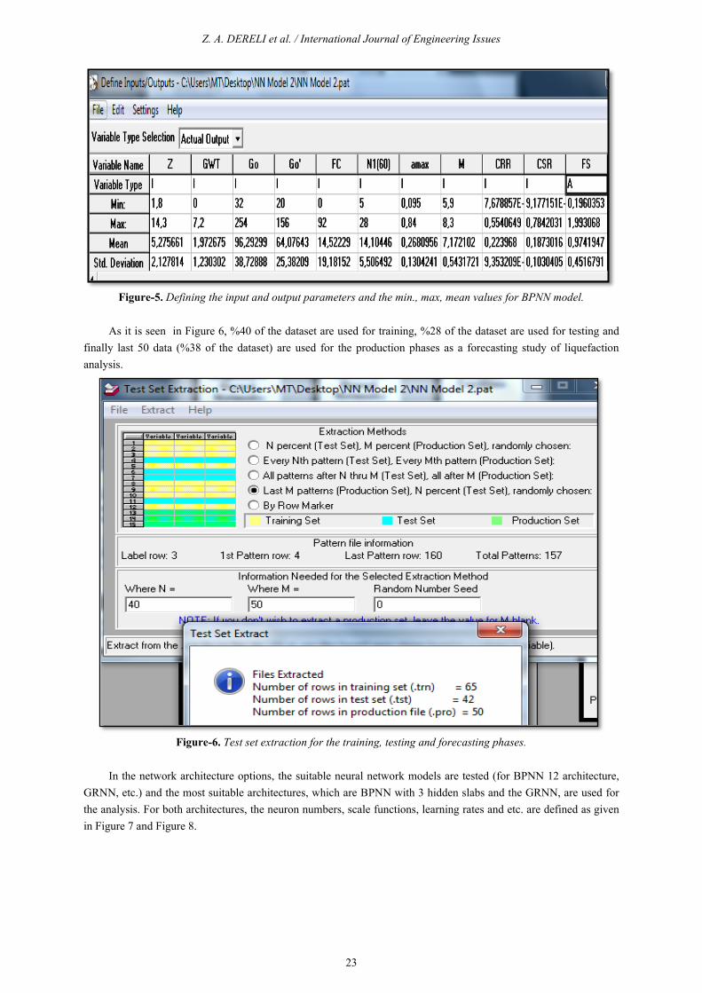
effective stress, σv, σv’ (kPa); fines content (%); corrected SPN-N number, N1(60); max. acceleration, amax; magnitude, M; cyclic resistance ratio, CRR; cyclic stress ratio, CSR are defined (Figure 4). The only output, the liquefaction occurrence factor of safety (FS), is also defined. Then, the minimum, maximum and the means are computed for the parameters (Figure 5).

Figure-4. The input and output parameters for neural network models.

Z. A. DERELI et al. / International Journal of Engineering Issues

23

Figure-5. Defining the input and output parameters and the min., max, mean values for BPNN model.

As it is seen in Figure 6, %40 of the dataset are used for training, %28 of the dataset are used for testing and finally last 50 data (%38 of the dataset) are used for the production phases as a forecasting study of liquefaction analysis.

Figure-6. Test set extraction for the training, testing and forecasting phases.

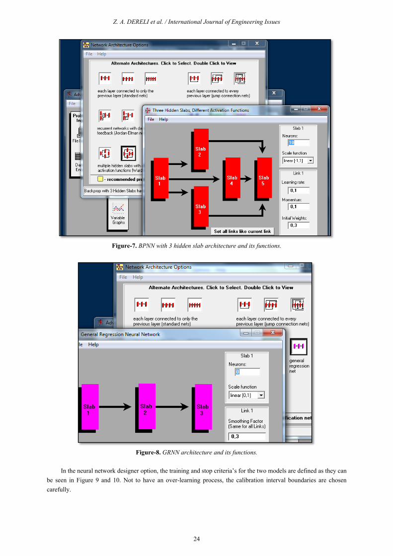
In the network architecture options, the suitable neural network models are tested (for BPNN 12 architecture,

GRNN, etc.) and the most suitable architectures, which are BPNN with 3 hidden slabs and the GRNN, are used for the analysis. For both architectures, the neuron numbers, scale functions, learning rates and etc. are defined as given in Figure 7 and Figure 8.

Z. A. DERELI et al. / International Journal of Engineering Issues

24

Figure-7. BPNN with 3 hidden slab architecture and its functions.

Figure-8. GRNN architecture and its functions.

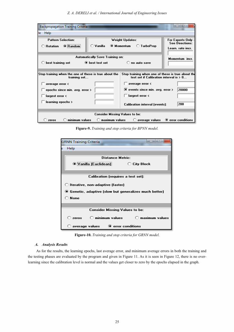
In the neural network designer option, the training and stop criteria’s for the two models are defined as they can

be seen in Figure 9 and 10. Not to have an over-learning process, the calibration interval boundaries are chosen carefully.

Z. A. DERELI et al. / International Journal of Engineering Issues

25

Figure-9. Training and stop criteria for BPNN model.

Figure-10. Training and stop criteria for GRNN model.

A. Analysis Results

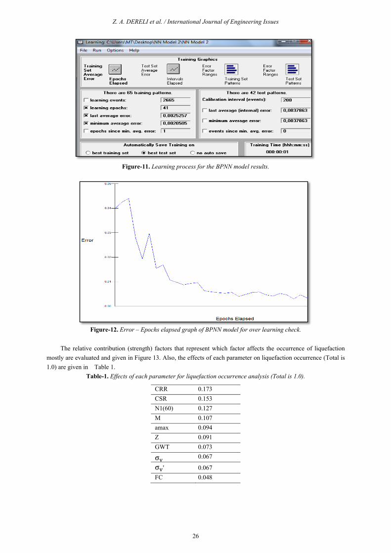
As for the results, the learning epochs, last average error, and minimum average errors in both the training and the testing phases are evaluated by the program and given in Figure 11. As it is seen in Figure 12, there is no over-learning since the calibration level is normal and the values get closer to zero by the epochs elapsed in the graph.

Z. A. DERELI et al. / International Journal of Engineering Issues

26

Figure-11. Learning process for the BPNN model results.

Figure-12. Error – Epochs elapsed graph of BPNN model for over learning check.

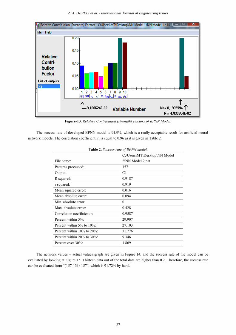
The relative contribution (strength) factors that represent which factor affects the occurrence of liquefaction

mostly are evaluated and given in Figure 13. Also, the effects of each parameter on liquefaction occurrence (Total is 1.0) are given in Table 1.

Table-1. Effects of each parameter for liquefaction occurrence analysis (Total is 1.0).

CRR 0.173

CSR 0.153

N1(60) 0.127

M 0.107

amax 0.094

Z 0.091

GWT 0.073

σv 0.067

σv' 0.067

FC 0.048

Z. A. DERELI et al. / International Journal of Engineering Issues

27

Figure-13. Relative Contribution (strength) Factors of BPNN Model.

The success rate of developed BPNN model is 91.9%, which is a really acceptable result for artificial neural network models. The correlation coefficient, r, is equal to 0.96 as it is given in Table 2.

Table 2. Success rate of BPNN model.

File name: C:\Users\MT\Desktop\NN Model 2\NN Model 2.pat

Patterns processed: 157

Output: C1

R squared: 0.9187

r squared: 0.919

Mean squared error: 0.016

Mean absolute error: 0.094

Min. absolute error: 0

Max. absolute error: 0.428

Correlation coefficient r: 0.9587

Percent within 5%: 29.907

Percent within 5% to 10%: 27.103

Percent within 10% to 20%: 31.776

Percent within 20% to 30%: 9.346

Percent over 30%: 1.869

The network values – actual values graph are given in Figure 14, and the success rate of the model can be

evaluated by looking at Figure 15. Thirteen data out of the total data are higher than 0.2. Therefore, the success rate can be evaluated from “(157-13) / 157”, which is 91.72% by hand.

Z. A. DERELI et al. / International Journal of Engineering Issues

28

Figure-14: The network values – actual values graph of BPNN model.

Figure-15: The actual network– actual graph of BPNN model for evaluating success rate.

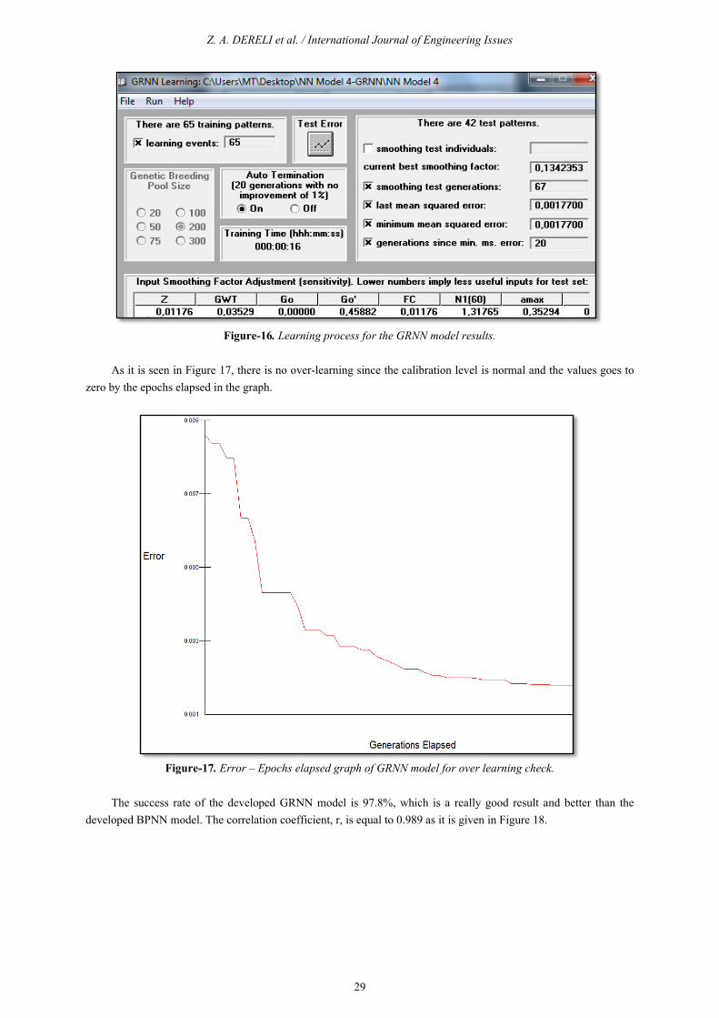
As the results of GRNN model demonstrate, smoothing test generation value, last mean error, and minimum

mean errors in testing phase values are evaluated by the program and given in Figure 16.

Z. A. DERELI et al. / International Journal of Engineering Issues

29

Figure-16. Learning process for the GRNN model results.

As it is seen in Figure 17, there is no over-learning since the calibration level is normal and the values goes to

zero by the epochs elapsed in the graph.

Figure-17. Error – Epochs elapsed graph of GRNN model for over learning check.

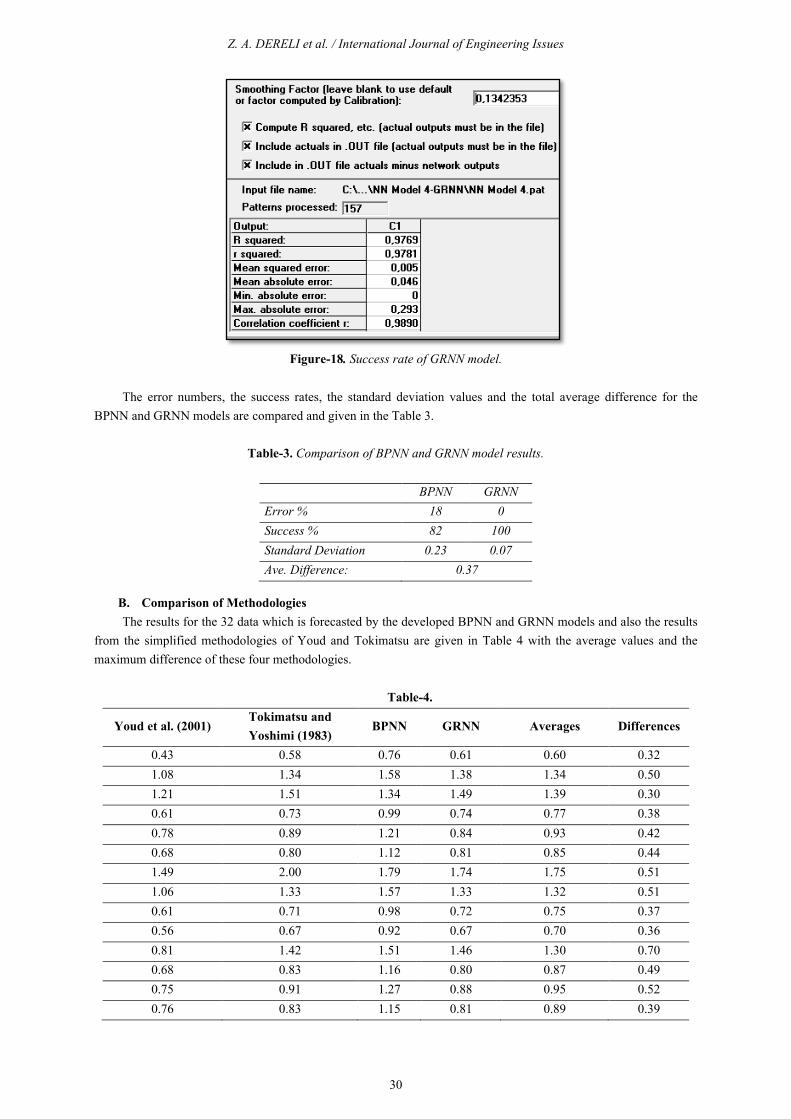
The success rate of the developed GRNN model is 97.8%, which is a really good result and better than the

developed BPNN model. The correlation coefficient, r, is equal to 0.989 as it is given in Figure 18.

Z. A. DERELI et al. / International Journal of Engineering Issues

30

Figure-18. Success rate of GRNN model.

The error numbers, the success rates, the standard deviation values and the total average difference for the

BPNN and GRNN models are compared and given in the Table 3.

Table-3. Comparison of BPNN and GRNN model results.

BPNN GRNN

Error % 18 0

Success % 82 100

Standard Deviation 0.23 0.07

Ave. Difference: 0.37

B. Comparison of Methodologies The results for the 32 data which is forecasted by the developed BPNN and GRNN models and also the results

from the simplified methodologies of Youd and Tokimatsu are given in Table 4 with the average values and the maximum difference of these four methodologies.

Table-4.

Youd et al. (2001) Tokimatsu and Yoshimi (1983)

BPNN GRNN Averages Differences

0.43 0.58 0.76 0.61 0.60 0.32

1.08 1.34 1.58 1.38 1.34 0.50

1.21 1.51 1.34 1.49 1.39 0.30

0.61 0.73 0.99 0.74 0.77 0.38

0.78 0.89 1.21 0.84 0.93 0.42

0.68 0.80 1.12 0.81 0.85 0.44

1.49 2.00 1.79 1.74 1.75 0.51

1.06 1.33 1.57 1.33 1.32 0.51

0.61 0.71 0.98 0.72 0.75 0.37

0.56 0.67 0.92 0.67 0.70 0.36

0.81 1.42 1.51 1.46 1.30 0.70

0.68 0.83 1.16 0.80 0.87 0.49

0.75 0.91 1.27 0.88 0.95 0.52

0.76 0.83 1.15 0.81 0.89 0.39

Z. A. DERELI et al. / International Journal of Engineering Issues

31

0.45 0.62 0.76 0.63 0.61 0.32

0.51 0.63 0.80 0.65 0.65 0.29

0.84 1.00 1.38 1.03 1.06 0.54

0.68 0.91 1.03 0.95 0.90 0.35

0.78 0.79 0.98 0.79 0.83 0.20

0.76 0.82 0.96 0.83 0.84 0.20

0.48 0.50 0.53 0.51 0.50 0.05

0.38 0.46 0.50 0.51 0.46 0.13

0.38 0.46 0.46 0.52 0.46 0.14

0.49 0.58 0.77 0.70 0.64 0.27

0.24 0.38 0.43 0.48 0.38 0.23

0.46 0.59 0.75 0.62 0.60 0.29

0.35 0.43 0.45 0.46 0.42 0.11

0.78 1.95 1.73 1.72 1.55 1.17

0.18 0.25 0.20 0.30 0.23 0.12

0.35 0.42 0.44 0.51 0.43 0.16

0.78 1.25 1.43 1.18 1.16 0.65

0.53 0.66 0.91 0.69 0.70 0.39

0.61 1.05 1.24 1.18 1.02 0.63

0.42 0.52 0.54 0.56 0.51 0.15

0.64 1.12 1.30 1.18 1.06 0.66

0.70 0.88 1.18 0.79 0.89 0.48

0.58 0.65 0.92 0.74 0.72 0.35

0.47 0.54 0.66 0.51 0.55 0.20

0.43 0.55 0.71 0.51 0.55 0.28

0.47 0.53 0.69 0.56 0.56 0.23

0.32 0.38 0.38 0.45 0.39 0.13

0.70 0.82 1.13 0.79 0.86 0.43

0.26 0.34 0.32 0.30 0.30 0.09

1.02 1.81 1.71 1.78 1.58 0.79

0.37 0.50 0.64 0.55 0.52 0.27

0.37 0.51 0.59 0.52 0.50 0.22

0.83 1.45 1.58 1.56 1.36 0.75

0.49 0.63 0.86 0.61 0.65 0.37

0.58 0.74 1.05 0.69 0.77 0.48

0.67 0.75 0.99 0.78 0.80 0.32

Ave. Difference: 0.37

IV. CONCLUSION

An overview of the different methods of evaluating soil liquefaction occurrence problem during earthquakes is presented in this paper. Based on the Youd et al. (2001) equation and Tokimatsu and Yoshimi (1983) equations, the evaluation is done by using simplified methods. The results are meaningful; they are approximately in the same ranges.

As a result of the need for using more reliable and fast analysis in civil engineering, artificial neural network algorithm is used nowadays especially in geotechnical engineering problems. However, the results are discussed by researchers and is connected to the result that NN analyses are suitable in this area.

Z. A. DERELI et al. / International Journal of Engineering Issues

32

Due to this situation, a comparison of different kinds of methodologies for liquefaction analysis is done in this study. Different kinds of NN algorithms, which are GRNN, BPNN, Kohonen, Probabilistic and GMDH are tested, and two of them are discussed in this paper due to the better success rates.

In conclusion, it is shown that GRNN is better than BPNN algorithm for these problems. Furthermore, GRNN gives approximately the same results with Tokimatsu and Yoshimi (1983) simplified method. Moreover, it can be said that using neural network algorithms for liquefaction analysis saves our time by giving accurate and reliable results in an easiest way.

For future studies, collecting more datasets from different cases and increasing the distribution of soil and earthquake property types may help us conduct more successful liquefaction analysis. Thus, we recommended a web-based soil dataset portal in a suitable format for researchers who use neural network algorithms.

REFERENCES

[1] BOULANGER, Ross W. et IDRISS, Izzat M. Evaluating the potential for liquefaction or cyclic failure of silts and clays. Center for Geotechnical Modeling, 2004. [2] CETIN, K. Onder, SEED, Raymond B., DER KIUREGHIAN, Armen, et al.Standard penetration test-based probabilistic and deterministic assessment of seismic soil liquefaction potential. Journal of Geotechnical and Geoenvironmental Engineering, 2004, vol. 130, no 12, p. 1314-1340. [3] CIRCULAR, T. R. B. Use of artificial neural networks in geomechanical and pavement systems. Transportation Research Board, National Research Council, Washington, DC Report No. E-C012, 1999.

[4] KRAMER, Steven Lawrence. Geotechnical earthquake engineering. Upper Saddle River, NJ : Prentice Hall, 1996. [5] MARCUSON, William F. Definition of terms related to liquefaction. Journal of the Geotechnical Engineering Division, 1978, vol. 104, no 9, p. 1197-1200. [6] MARCUSON, W. F., HYNES, M. E., et FRANKLIN, A. G. Evaluation and use of residual strength in seismic safety analysis of embankments. Earthquake Spectra, 1990, vol. 6, no 3, p. 529-572. [7] NASSERI-MOGHADDAM, Ali et BENNETT, Joseph. Assessment of liquefaction potential at a site in Ottawa using SPT and shear wave velocities. In : Proceedings of Pan-Am CGS Geotechnical Conferences, October. 2011. p. 2-6. [8] SEED, Harry Bolton et IDRISS, Izzat M. Ground motions and soil liquefaction during earthquakes. Earthquake Engineering Research Institute, 1982. [9] SEED, Harry Bolton et IDRISS, Izzat M. Simplified procedure for evaluating soil liquefaction potential. Journal of Soil Mechanics & Foundations Div, 1971.

[10] SEED, H. B., TOKIMATSU, Kohji, HARDER, L. F., et al. The influence of SPT procedures in soil liquefaction resistance evaluations: Berkeley, University of California. Earthquake Engineering Research Center Report UBC/EERC-84/15, 1984. [11] SEED, Raymond B. et HARDER, Leslie F. SPT-based analysis of cyclic pore pressure generation and undrained residual strength. In : H. Bolton Seed Memorial Symposium Proceedings. 1990. p. 351-376. [12] SEED, Raymond B., CETIN, K. Onder, MOSS, Robb ES, et al. Recent advances in soil liquefaction engineering: a unified and consistent framework. In : Proceedings of the 26th Annual ASCE Los Angeles Geotechnical Spring Seminar: Long Beach, CA. 2003. [13] SITHARAM, T. G. et VIPIN, K. S. Seismic Soil Liquefaction Based on In situ Test Data. [14] URAL, Derin N. et SAKA, Hasan. Liquefaction assessment by artificial neural networks. EJGE, 1998, vol. 3. [15] YOUD, T. L., IDRISS, I. M., ANDRUS, Ronald D., et al. Liquefaction resistance of soils: summary report from the 1996 NCEER and 1998 NCEER/NSF workshops on evaluation of liquefaction resistance of soils.Journal of geotechnical and geoenvironmental engineering, 2001 [16] YOUD, T.L. Liquefaction-Induced Lateral Spread Displacement, US Navy, NCEL Technical Note N-1862, p. 44, 1993.