International Fiscal Spillovers - QMRO Home

International Fiscal Spillovers∗

Renato Faccini† Haroon Mumtaz‡ Paolo Surico§

November 2015

Abstract

A two-country business cycle model featuring nominal rigidities, countercyclicalmark-ups, rule of thumb consumers and government spending reversals is used to iden-tify inequality predictions that are robust across a range of empirically plausible pa-rameterizations. These robust inequality restrictions are imposed onto a regime-changefactor model for the United States and its main trade partners to estimate the in-ternational fiscal spillovers. The effects of U.S. government spending on foreign realactivity are found to be sizable and significant, operating mainly by lowering real in-terest rates rather than boosting trade balances. In contrast, there seems to be onlylimited evidence of state dependence in the international transmission of fiscal policy.

JEL classification: E3, E6, F4

Key words: regime-change factor model, fiscal spillovers, international transmission.

∗We are grateful to Giancarlo Corsetti and two anonymous referees for very useful comments and sugges-tions. Surico gratefully acknowledges financial support from the European Research Council (Starting Grant263429 and Consolidator Grant 647049). The graphs in this paper are best viewed in color.

†Queen Mary University and Centre for Macroeconomics (LSE). Email: [email protected].‡Queen Mary University. Email: [email protected].§London Business School and CEPR. Email: [email protected].

1 Introduction

The great recession of 2007-09 has reignited the discussion in policy and academic circles

about the economic circumstances under which fiscal policy (and government spending in

particular) can stimulate the economy, both domestically and internationally. On the theo-

retical side, recent contributions have shown that accommodative monetary policy has the

potential to alter the transmission of fiscal policy in closed economy models (Hall, 2009,

Woodford, 2011, and Christiano, Eichenbaum and Rebelo, 2011) as well as in multi-country

models (Cook and Devereux, 2011 and Coenen et al. 2011).

On the empirical side, Canova and Pappa (2011) report that whenever a fiscal expansion

is associated with negative real short-term interest rates, the domestic fiscal multipliers in

the United States, United Kingdom and the Euro area tend to be somewhat larger than the

estimates based on various identification schemes reported in Blanchard and Perotti (2002),

Mountford and Uhlig (2009) and Barro and Redlick (2011). Auerbach and Gorodnichenko

(2012) show that the fiscal multipliers are typically larger during recessions whereas, using a

longer sample, Ramey and Zubairy (2014) find little evidence for state-dependent government

spending multipliers in the United States.

While the dynamic response of the real exchange rate to a U.S. fiscal shock has been the

subject of a rapidly growing empirical literature (Monacelli and Perotti, 2011, Ravn, Schmitt-

Grohe and Uribe, 2012, and Enders, Muller and Scholl, 2011), little is known on whether

international fiscal spillovers –defined as the response of foreign output to a domestic fiscal

shock conditional on fiscal policy abroad– are (i) positive, (ii) heterogeneous across trade

partners and (iii) varying over time.

In this paper, we address this important gap in the literature by identifying international

fiscal spillovers. Our reference framework is a two-country real business cycle model featur-

ing countercyclical markups (in the spirit of Ravn, Schimtt-Grohe and Uribe, 2012), sticky

prices and wages, rule of thumb consumers (a la Galı, Lopez-Salido and Valles, 2007), and

government spending reversals (following Corsetti, Meier and Muller, 2010 and 2012). The

contributions above have shown that each of these channels has the potential to alter the

effects of government spending.

The theoretical framework is used to derive a set of sign restrictions in the dynamic

2

responses to a government spending shock that are robust across a range of empirically

plausible parameterizations of these theoretical mechanisms. The robust sign restrictions are

then imposed onto a change point factor model for the U.S. economy and its main trade

partners over the post-Bretton Woods period. Following Kilian and Murphy (2012), we

impose the additional restriction that the size of the domestic fiscal multiplier cannot be

implausibly higher than the point estimates available in the literature for the U.S.. Finally,

while the empirical model allows fiscal policy in the foreign economy to adjust following a

U.S. government spending shock, the analysis in Section 4 reveals that the response of foreign

government spending is often insignificant across countries and regimes, implying that our

estimates can be interpreted as the international fiscal spillovers holding foreign government

spending constant.

The choice of a factor model fulfills our desire to identify government spending shocks

using large information, which Forni and Gambetti (2010) and Gambetti (2010) have shown

to ameliorate the non-fundamentalness problem raising from fiscal foresight in small-scale

VARs. More specifically, as shown conceptually by Leeper, Walker and Yang (2013), whenever

government policies are anticipated by the public and the variables used by the econometrician

span a smaller information set than available to the agents, identification strategies based

on combinations of VAR residuals fail to recover the structural shocks. The reason is that

the VAR residuals are still contaminated by the component of government spending that the

agents could have predicted using the variables omitted by the econometrician. In contrast,

a large information approach, as taken in this paper, is more likely to avoid the distorted

inference associated with fiscal foresight.

Time-variation is introduced because our sample is characterized by significant changes

in (i) the conduct of fiscal policy (Davig and Leeper, 2006, and Bianchi and Ilut, 2011)

and monetary policy (Cogley and Sargent, 2005), (ii) business cycle conditions and (iii) the

volatility of structural shocks (Primiceri, 2005, and Sims and Zha, 2006), ranging from the

1970s great inflation to the great moderation and finally the great recession. To avoid taking

a stand a-priori on the most relevant source of changes (and its precise timing), our statistical

model identifies in the data the most likely break points.

Our main results can be summarized as follows. First, the probability of a positive re-

3

sponse of foreign output to an unanticipated increase of government spending in the United

States is typically larger than fifty percent over the post-Bretton Woods period (especially

after 1984), with the largest effects recorded for Canada and the United Kingdom. Second,

an expansionary U.S. government spending shock leads to a significant decrease in real rates,

both domestically and internationally, but small and insignificant changes in the trade bal-

ances. We interpret this as suggestive that the international transmission of fiscal policy

might operate through a financial channel rather than a trade channel. Third, we find little

support for regime dependence: both the spending multipliers and the international trans-

mission of government spending shocks seem remarkably stable over the statistical different

regimes identified by our factor model, and neither the adoption of the Euro nor the state

of the business cycle (either internationally or domestically) seem to have led to a significant

change in the international transmission of U.S. fiscal policy.

In the rest of the paper, Section 2 introduces the theoretical framework and illustrates

the way we nest a number of hypotheses for the international transmission of fiscal policy.

It also reports the inequality predictions (for the dynamic effects of a government spending

shock on the endogenous variables) that are robust to a wide perturbation of the parameter

space. These theory-robust sign restrictions are imposed in Section 3 onto a factor model for

the U.S. economy and some of its main trade partners. Results are presented in Section 4

before conclusions. The appendices provide details of the theoretical model, the estimation

of the empirical model, data and variance decomposition. We also relegate to the Appendices

a discussion of the propagation of the various theoretical transmission channels, and further

details on the identification of the sign restrictions.

2 Theoretical framework and sign restrictions

The reference framework is a two-country New-Keynesian model augmented with counter-

cyclical markups, rule of thumb consumers and government spending reversals. Each of these

ingredients is meant to exemplify a specific channel within a broad class of competing models

for the international transmission of fiscal policy.

There are two symmetric countries, and in each country two types of firms: final good and

intermediate good firms. Final good firms combine home and foreign intermediate products

4

into a homogeneous consumption good. We assume home bias in the production of the con-

sumption good as a reduced-form device to modeling trade openness. While final good firms

operate under perfect competition, intermediate producers set their price under monopolistic

competition and Calvo price stickiness, using differentiated labor services as the only factor

of production.

On the household side we introduce both asset holders and rule of thumb consumers.

These two types of agents differ in that only asset holders can access international capital

markets and transfer wealth into the future. We assume that the elasticity of substitution

varies procyclically with aggregate output, so as to give rise to countercyclical markups. As

for policy, the monetary institution is captured by a Taylor rule, while the government takes

the shape of a fiscal rule that allows for spending and taxes to respond to the real level of

debt, so as to produce spending reversals.

In the special case where prices and wages are fully flexible, the mark-up is constant, the

budget is balanced at all times and there are no rule-of-thumb consumers, the model boils

down to the standard neo-classical model. Introducing procyclical elasticity of substitution

over this benchmark gives us the counter-cyclical markup model; introducing both price and

wage rigidity coupled with either limited asset market participation or fiscal feedback rules will

provide a benchmark for the rule of thumb model and spending reversal model, respectively.

Because the different specifications allowing for rule of thumb consumers, spending reversals

and countercyclical markups are relatively standard in the literature, details of the model

and derivation of the log-linearized system of equation is relegated to the web Appendix

C. We refer to the web Appendix D for an illustration of differences and similarities in the

propagation of the various theoretical channels.

Using the nested framework where rule of thumb consumers, countercyclical markups,

government spending reversals as well as stickiness in wages and prices are allowed to interact

with each other, we are able to identify sign restrictions for government spending shocks that

are common across empirically plausible perturbations of the parameter space. We find that

following a positive government spending shock, (i) government spending, (ii) taxes, and

(iii) domestic output, increase on impact, while the response of (iv) the government budget

surplus, is non-positive. Furthermore, the nesting model generates a positive comovement

5

(v) between short-term nominal interest rate and inflation, and (vi) between consumption

and real exchange rate.1

It is worth noting that our sign restrictions on the joint response of output, budget surplus

and taxes uniquely identify the government spending shock. Any other shock that is included

in the nesting model would generate opposite comovements between primary budget surplus

and taxes. For instance, expansionary TFP, monetary, preference, labor supply, and markup

shocks would increase surplus and decrease taxes. For more details on the computation and

the robustness of these sign restrictions we refer to the web Appendix in Section D.3.

On the basis of this finding, our theory-based strategy to identify a government spending

shock in the data is to impose the common sign restrictions (i) to (vi), which are reported in

Table 1, onto the factor model of Section 3. The ultimate goal is to let the data inform us

about the sign and size of the international fiscal spillovers, namely the dynamic response of

foreign output to unanticipated government purchases in the United States.

3 The empirical framework

In this section, we present the dynamic factor model with independent break points in the

factor loadings and idiosyncratic variances, which will be used to investigate any possible

time-variation in the international transmission of government spending shocks. We lay out

here the estimation and identification procedures while providing a more detailed description

in Appendix B.

The reasoning behind the choice of a model with time-varying parameters is twofold.

First, a large empirical literature has documented significant variation in the evolution of

the volatility of real activity, inflation and interest rates in a number of advanced economies

over the post-WWII period. Second, our sample has been arguably characterized by several

monetary and fiscal regimes, both in the U.S. and its main trade partners, featuring different

degrees of commitment (and success) to fight inflation and stabilize debt.

As discussed in the introduction, the identification of a structural shock requires that no

variable available to the agents (but omitted by the econometrician) could predict the shock.

1The parameter values used in the simulations are drawn from uniform distributions over 10,000 repeti-tions. Our results indicate that the inequality predictions (i) to (iv) are satisfied in every single draw. Therestrictions (v) and (vi) are instead satisfied in 97.7% and 99.4% of the draws, respectively.

6

To confront this problem, which is referred to in the literature as ‘non-fundamentalness’, we

follow Gambetti (2010) and Forni and Gambetti (2010) and use a dynamic factor model as

an efficient way to summarize the information in a large dataset of variables for the U.S. and

its main trade partners.

3.1 A change point factor model

In the empirical model, we assume that a few factors summarize the comovements among a

large cross-section of observables Xit according to the following specification:

Xit = βi,SFt + σi,Qeit (1)

Ft = c +

L∑

j=1

λjFt−j + Σ1/2vt (2)

where the factors Ft = f1t, ..fK,t and L = 2. We allow for independent structural breaks in

the factor loadings βi and the variances σi. As shown below, this specification is preferred to

an alternative with fixed coefficients and to another that allows for breaks in the parameters of

the transition equation. Following Chib (1998), M structural breaks are introduced through

the unobserved discrete state variable S. This state variable is assumed to follow a M + 1

state Markov chain process with a restricted transition probability matrix P .2 The transition

probabilities pij = p (St = j|St−1 = i) are given by

pij > 0 if i = j , pij > 0 if j = i+ 1 (3)

pM+1M+1 = 1 , pij = 0 otherwise.

Analogously, the state variable Q follows an M + 1 Markov chain process with a similarly

restricted transition probability matrix Q, which is independent of P .

The process described in (3) is a Markov switching model where transitions are allowed

in a sequential manner. For example, to move from regime 1 to regime 3, the process has

to visit regime 2. Similarly, and without loss of generality, transitions to past regimes are

not allowed. Note, however, that this is not restrictive as two (non-consecutive) regimes that

were similar or identical to one another would simply be given two labels.3

2Kim and Nelson (1999, Chapter 10) provide further examples of factor models with switching parameters.Del Negro and Otrok (2005) were the first to consider a factor model with time-varying factor loadings.

3The proposed model has computational advantages over a more ‘conventional’ Markov switching specifi-

7

3.2 Estimation

The model is estimated using a Gibbs sampling algorithm. Details of the priors and condi-

tional posteriors are given in the appendix. Here we sketch the main steps:

1. Given a value for the factors, draw the VAR parameters.

• The VAR coefficients c, λj have a normal conditional posterior, while the condi-

tional posterior of the covariance matrix Σ is Inverse Wishart.

2. Given a value for the factors, draw the factor loadings (βi,S), the variance of the id-

iosyncratic components σi,Q and the state variable St and Qt.

• Given data on Xi,t and Ft, equation (1) is a system of equations with indepen-

dently switching coefficients and variances. Following Kim and Nelson (1999,

Chapter 9), we use the Multi-Move Gibbs sampling to draw St from the joint con-

ditional density f(St|βi,S, σi,Q, P , Qt

)and Qt from the joint conditional density

f(Qt|βi,S, σi,Q, Q, Qt

).

• Conditional on St and Qt, standard results for regression models can be used and

the coefficients and the variances are simulated from a normal and inverse gamma

distribution.

3. Conditional on St and Qt, elements of P and Q are drawn from the Dirichlet distribu-

tion.

4. Simulate the factors conditional on all the other parameters.

• This is done by employing the methods described in Carter and Kohn (1994).

5. Go to step 1.

The autocorrelations of the retained draws (see Appendix B) show little variation which

provides some evidence of convergence of the algorithm.

cation. In the latter, the labels of the regimes are not identified and researchers typically refer to the propertiesof a particular time series so that, for instance, a high regime corresponds to a higher unconditional meanfor a specific endogenous variable. Given the factor structure as well as the large panel dimension, however,this strategy is not feasible in our context and the choice of a specific variable for labeling the regimes maynot be innocuous. Hence, we adopt the simpler structure for regime transitions described in equation (20).

8

3.3 Model comparison

We carry out a model comparison exercise to determine the number and location of breaks

and the number of factors. In particular, we estimate three versions of the factor model: (i)

a model with fixed parameters, (ii) a model with M breaks in the vectors β ′is and parameters

σ′is of the observation equation 1 and (iii) a model with M breaks in the vectors

∑Lj=1 λ

′js

and the matrix Σ1/2 of the transition equation 2. Note that in (ii) and (iii) we allow for

independent breaks in the coefficients and variances as described above.

We assume M = 1, 2, 3 and in each case allow for the possibility of up to eight factors.

The model comparison is carried out via the Bayesian Deviance Information Criterion (DIC).

Introduced in Spiegelhalter et al. (2002), the DIC is a generalisation of the Akaike informa-

tion criterion – it penalises model complexity while rewarding fit to the data. The DIC is

defined as

DIC = D + pD.

The first term D = E (−2 lnL (Ξi)) =1M

∑i (−2 lnL (Ξi)) where L (Ξi) is the likelihood eval-

uated at the draws of all of the parameters Ξi in the MCMC chain. This term measures good-

ness of fit. The second term pD is defined as a measure of the number of effective parameters in

the model (or model complexity). This is defined as pD = E (−2 lnL (Ξi))−(−2 lnL (E(Ξi)))

and can be approximated as pD = 1M

∑i (−2 lnL (Ξi)) −

(−2 lnL

(1M

∑i

Ξi

)).4 Prior dis-

tributions on the parameters in our model and the presence of latent variables implies that

the number of parameters (as used in the calculation of the Akaike and Schwarz informa-

tion criterion) do not necessarily represent model complexity. The definition of the effective

number of parameters used in the computation of the DIC avoids this problem. Note that

the model with the lowest estimated DIC is preferred. Calculation of the DIC requires the

calculation of the likelihood of the change point factor model. In our application this is done

via the approximate filter discussed in Kim and Nelson (1999).5

4The first term in this expression is an average of −2 times the likelihood function evaluated at eachMCMC iteration. The second term is (−2 times) the likelihood function evaluated at the posterior mean.

5For an accurate approximation of the likelihood function, Kim and Nelson (Chapter 5, 1999) recommendto keep track of the regimes in three periods: t, t-1 and t-2. As our empirical model involves (M+1)2 regimes(in a combination of factor loading and volatility breaks), their recommendation amounts to keep track of[(M+1)2]3 possible trajectories for the evolution of the parameters. To keep the estimation computationallytractable, we therefore consider up to four possible regimes (i.e. M=3). This leads to more than four

9

Table 2 reports the DIC statistics for each estimated model. The fixed parameter speci-

fications is not favoured by the DIC criterion, which in fact provides support for the model

with 3 (independent) breaks in the factor loadings and the idiosyncratic variances of the

observation equation and seven factors. Note that this model also has a lower DIC than

models (not shown in the table) with drifting factor loadings (DIC= 8275) or parameter drift

and stochastic volatility in the VAR transition equation (DIC=17042). In other words, for

our dataset a model with structural breaks appears favored relative to one that allows for

smooth time-variation. In addition, the model with 3 independent breaks in the parameters

of the observation equation and seven factors is also preferred to restricted specifications

(not reported in Table 2) that only allow for 3 breaks in the factor loadings (DIC=2952)

or 3 breaks in idiosyncratic variances (DIC=-1873.64). Finally, our preferred change point

factor specification compares favorably with a model in which recessions feature as a possible

separate regime as the latter is associated with a DIC statistics of 1837.03.

3.4 Computation of the impulse response functions

We calculate the impulse responses ∆t of Ft to a government spending shock. With these

in hand, the regime-specific impulse responses of each underlying variables can be easily

obtained using the observation equation of the model. The impulse response ∆t is estimated

using a contemporaneous impact matrix A0 which is calculated to satisfy the sign restrictions

in Table 1, which are based on the theoretical framework of Section 2.

In addition to these sign restrictions, we impose ‘plausibility’ restrictions on the short-run

response of domestic and foreign real per-capita GDP growth requiring the contemporaneous

impact of the government spending shock to be less than 0.6%. Coupled with a government

spending-GDP ratio of about 20%, these restrictions map into fiscal multipliers smaller than

three, consistently with both the top end of the structural VAR confidence bands and the

quantitative analysis in Cook and Deveraux (2001) for the home-bias case when the nominal

interest rate responds neither in the domestic nor in the foreign country. As emphasized

by Kilian and Murphy (2012), impulse response functions based on sign restrictions only,

implicitly assume that all admissible models, including those with economically implausible

thousands possible regime permutations.

10

fiscal multipliers, are equally likely. Finally, to explore the possibility that the zero lower

bound on the domestic short-term nominal interest rate may have amplified the effects of

fiscal policy during the most recent period, in the fourth regime only we add the additional

restrictions that the short-term rate does not move by more than ten basis points either way

on impact.6

The sign restrictions are implemented as follows: let Σ =PP ′ be the Cholesky decompo-

sition of the transition equation covariance matrix Σ. We draw a 4 × 4 matrix, J , from the

N(0, 1) distribution. We take the QR decomposition of J , which gives us a candidate struc-

tural impact matrix as A0 = PQ. Then, we compute the impulse response of X1,t, ...XN,t.

We check if these impulse responses satisfy our sign and plausibility restrictions. If this is

the case, we store A0,t and move to the next Gibbs iteration.

3.5 Data

We fit the change point factor model described above to an international panel of 143 quarterly

series over the post-Bretton woods sample 1975Q1-2010Q4. The United States is treated as

the domestic economy while the foreign block is made up of Canada, France, Germany, Japan

and the United Kingdom. These countries account for the lion share of trade volumes with

the United States.7 As for the domestic variables, we include –among others– real government

spending, real net taxes, real GDP, CPI, 3-month Treasury bills rate, 10 year government

bond yields, real private consumption expenditure, real wage, investment, terms of trade

and CPI real effective exchange rate. The foreign block includes government spending, real

GDP, personal consumption expenditures, investment, the trade balance, CPI and the 3-

month Treasury bills rate for each country. The inclusion of foreign government spending

fulfills our desire to control for fiscal interventions abroad which, if omitted, may distort the

inference drawn upon the estimated effects of U.S. government spending on its main trade

partners GDP. As shown in Section 4, however, the response of government spending abroad

is typically insignificant.

6While results are not sensitive to the specific cut off of ten basis points, they are meant to exemplify ascenario in which the short-term nominal rate is forced to remain close to its sub-sample average, which inthe fourth regime is 0.4% on an annual basis.

7China is excluded because of the possible currency manipulation over part of our sample period.

11

All real variables are expressed in per capita terms. All variables but interest rates and

terms of trade are in log-difference. A full description of the individual time series and

their sources is provided in Appendix C where we also report the forecast error variance

decomposition and the contribution of the factors to the total variance of the main variables

in our panel (Table 4).

4 Results

In this section, we present the main results of the paper, namely the dynamic responses of

U.S. and some of its main trade partner variables to a U.S. government spending shock. The

impulse responses are obtained using the estimates from the change point factor model of

Section 3. We begin by discussing the statistical regimes identified by the empirical model

and then, we move to the impulse response function analysis. We start with the reaction

of domestic variables before looking at the magnitude of the fiscal spillovers on foreign real

activity. Finally, we explore the international transmission mechanism of the U.S. government

spending shock as well as assess the role of the business cycle abroad and the introduction of

a single currency in the Euro area in confounding our results.

4.1 Regimes

Modeling time-variation in both variances and parameters of a large fiscal panel is attractive

because both the structure of the economy, the volatility of the shocks and the stance of

economic policy may have changed over the post-Bretton Woods period.

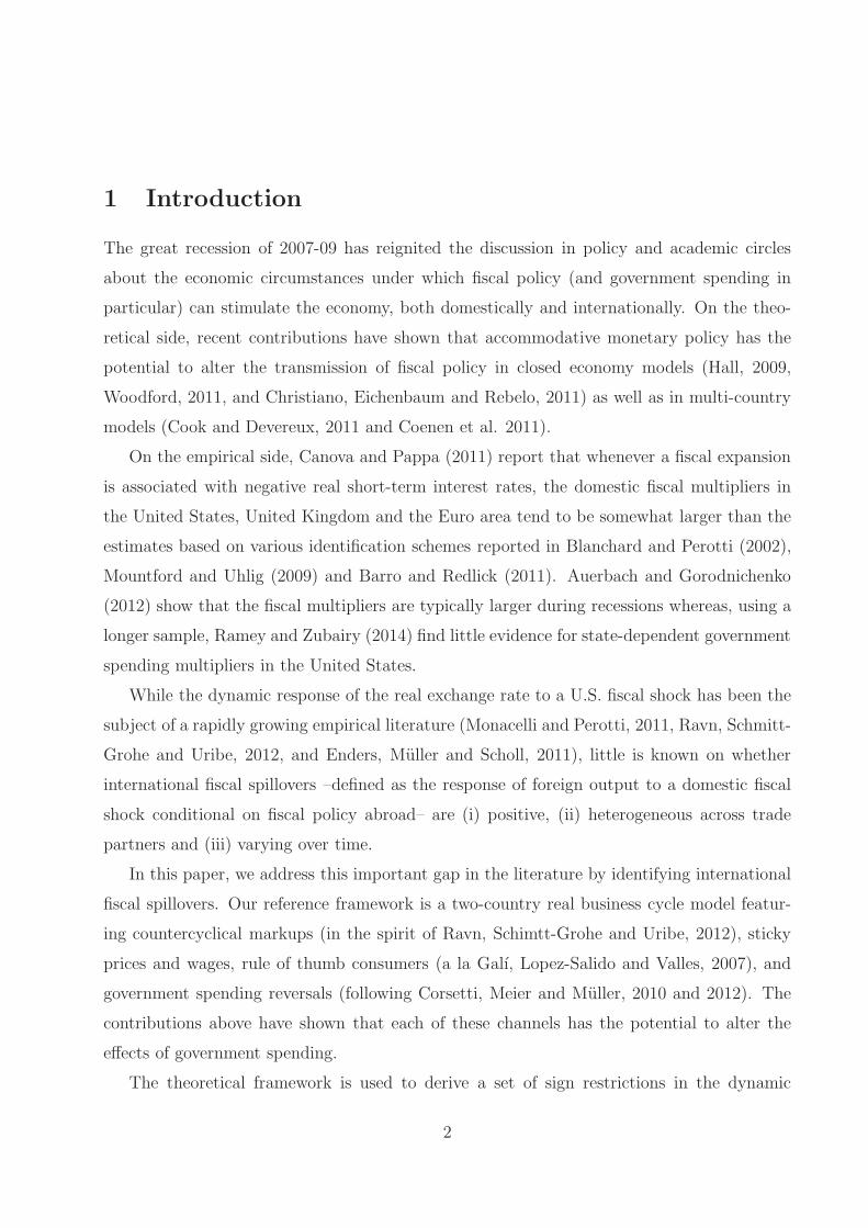
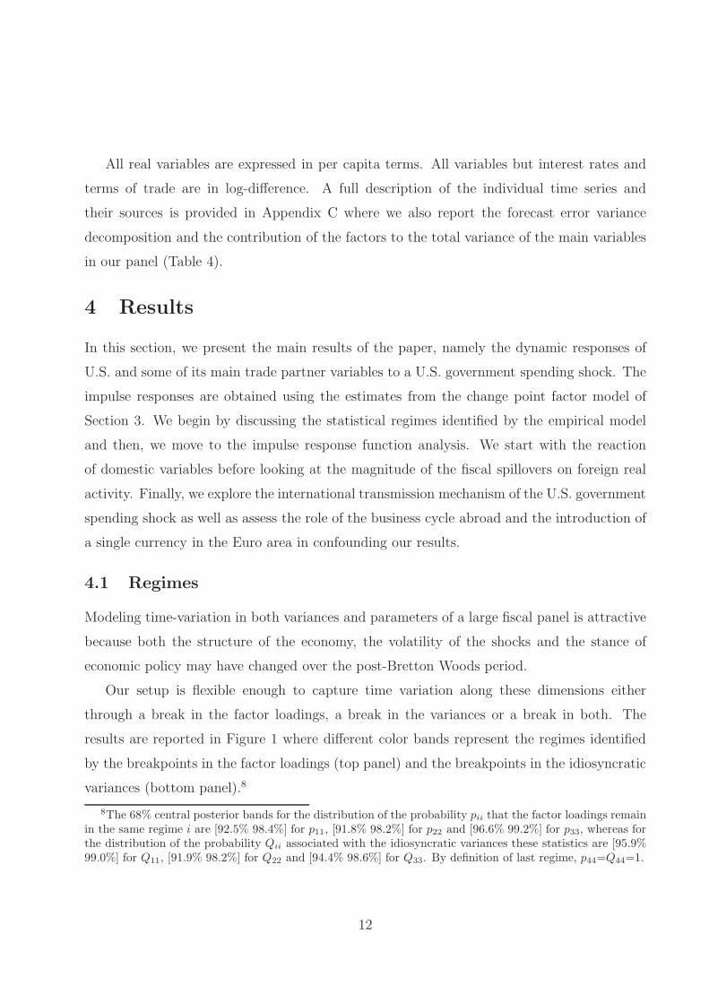
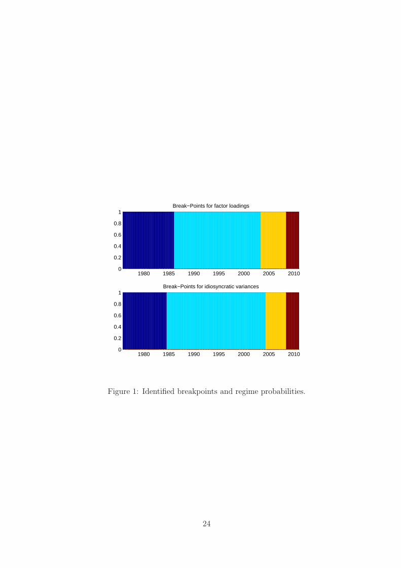
Our setup is flexible enough to capture time variation along these dimensions either

through a break in the factor loadings, a break in the variances or a break in both. The

results are reported in Figure 1 where different color bands represent the regimes identified

by the breakpoints in the factor loadings (top panel) and the breakpoints in the idiosyncratic

variances (bottom panel).8

8The 68% central posterior bands for the distribution of the probability pii that the factor loadings remainin the same regime i are [92.5% 98.4%] for p11, [91.8% 98.2%] for p22 and [96.6% 99.2%] for p33, whereas forthe distribution of the probability Qii associated with the idiosyncratic variances these statistics are [95.9%99.0%] for Q11, [91.9% 98.2%] for Q22 and [94.4% 98.6%] for Q33. By definition of last regime, p44=Q44=1.

12

While the empirical model allows for the break points in the two panels to be unsyn-

chronized, the results in Figure 1 suggests that the last regime has been characterized by a

virtually simultaneous shift in factor loadings and variances. On the other hand, the break

in the variances during the first half of the 1980s seems to have preceded the break in the

factor loadings by a couple of years whereas the beginning of the third regime preceded the

break in variances by one year. The top panel reveals that the second regime lasted longer

than any other regime and largely overlapped with the period of Great moderation in the

idiosyncratic variances recorded in the bottom panel. Finally, the third period appears to

mark the run-up to the fourth regime, which coincides with the global crisis triggered by the

great recession.

4.2 The response of domestic variables and fiscal spillovers

This section reports impulse responses for domestic variables and fiscal spillovers in each of

the regimes estimated on the basis of the factor loading breakpoints identified in the previous

section. In the next section, we will look at the international transmission mechanism and

the role played by the foreign business cycle.

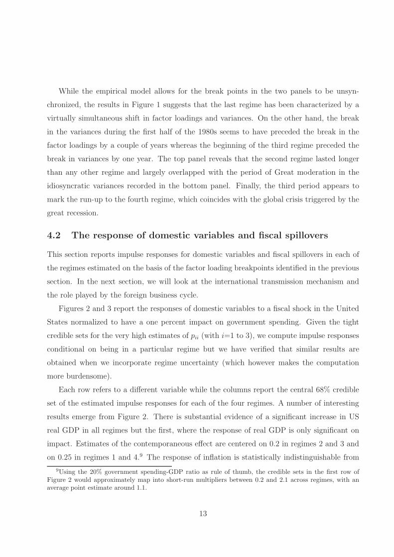
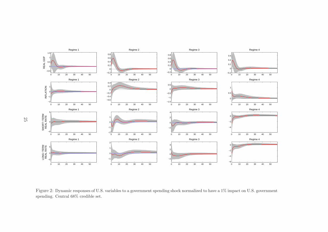
Figures 2 and 3 report the responses of domestic variables to a fiscal shock in the United

States normalized to have a one percent impact on government spending. Given the tight

credible sets for the very high estimates of pii (with i=1 to 3), we compute impulse responses

conditional on being in a particular regime but we have verified that similar results are

obtained when we incorporate regime uncertainty (which however makes the computation

more burdensome).

Each row refers to a different variable while the columns report the central 68% credible

set of the estimated impulse responses for each of the four regimes. A number of interesting

results emerge from Figure 2. There is substantial evidence of a significant increase in US

real GDP in all regimes but the first, where the response of real GDP is only significant on

impact. Estimates of the contemporaneous effect are centered on 0.2 in regimes 2 and 3 and

on 0.25 in regimes 1 and 4.9 The response of inflation is statistically indistinguishable from

9Using the 20% government spending-GDP ratio as rule of thumb, the credible sets in the first row ofFigure 2 would approximately map into short-run multipliers between 0.2 and 2.1 across regimes, with anaverage point estimate around 1.1.

13

zero at all horizons in regimes 1 and 3, while in regimes 2 and 4 it is positive and significant.

The response of the short-term real rate is flat and insignificant at all horizons in regime

1, while in the other regimes the median responses are strongly negative in the short-term,

albeit still insignificant.10 The median responses of the long-term real rate always lies in

positive territory in regime one. In any other regime, the probability of the long-term rate

being negative in the short-term is larger than 50 percent.

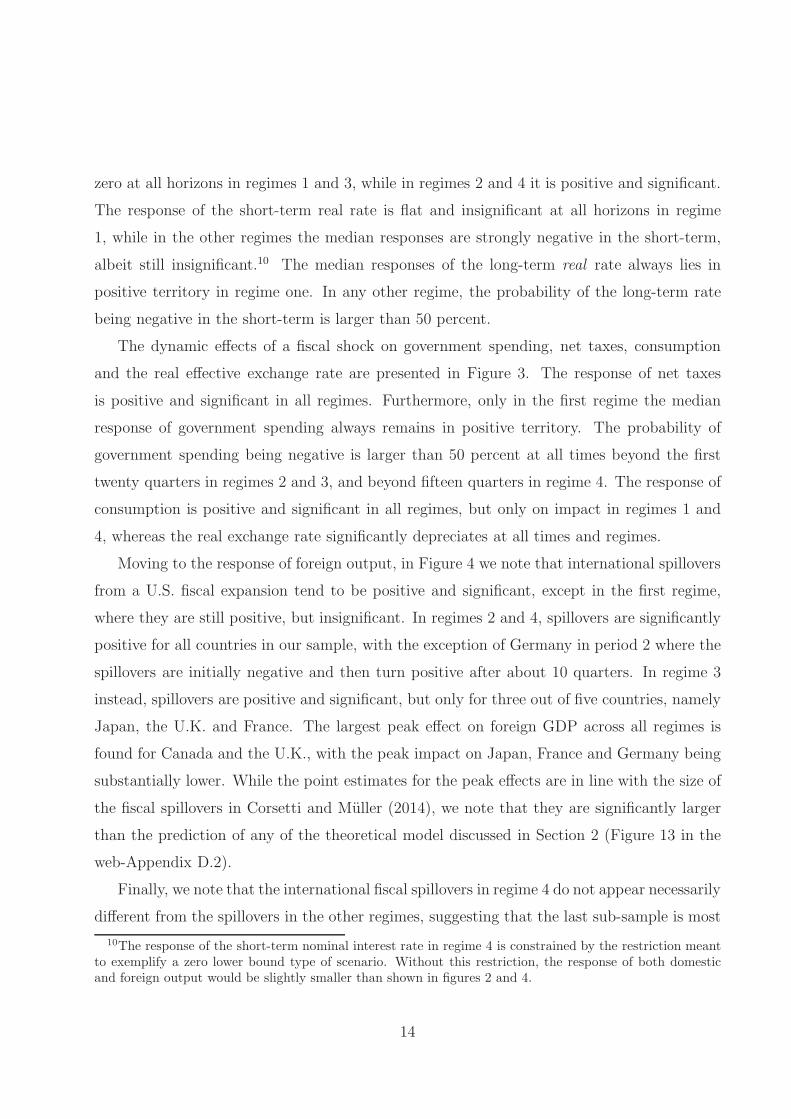
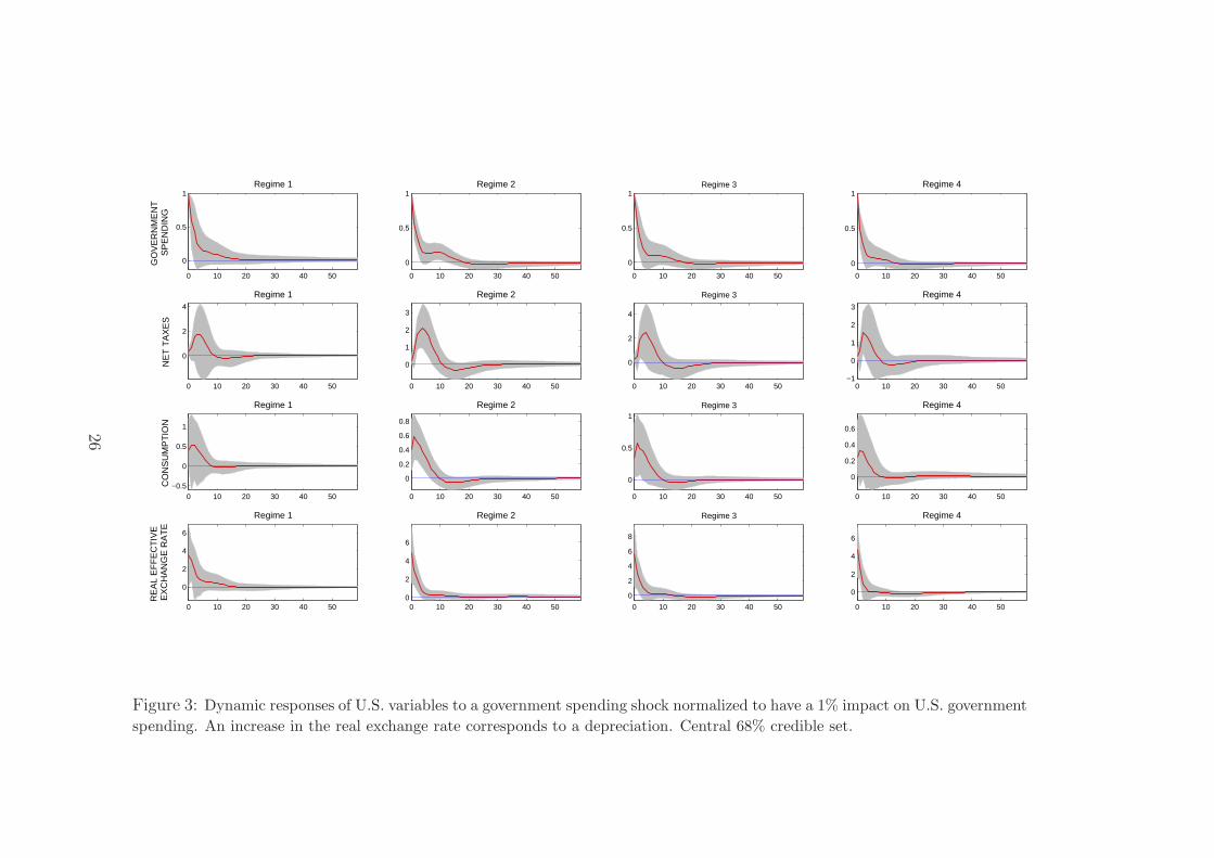
The dynamic effects of a fiscal shock on government spending, net taxes, consumption

and the real effective exchange rate are presented in Figure 3. The response of net taxes

is positive and significant in all regimes. Furthermore, only in the first regime the median

response of government spending always remains in positive territory. The probability of

government spending being negative is larger than 50 percent at all times beyond the first

twenty quarters in regimes 2 and 3, and beyond fifteen quarters in regime 4. The response of

consumption is positive and significant in all regimes, but only on impact in regimes 1 and

4, whereas the real exchange rate significantly depreciates at all times and regimes.

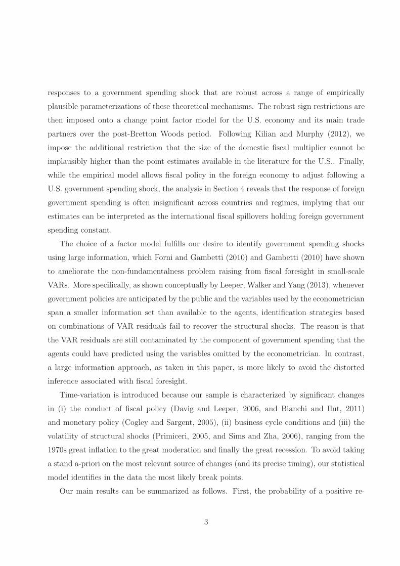
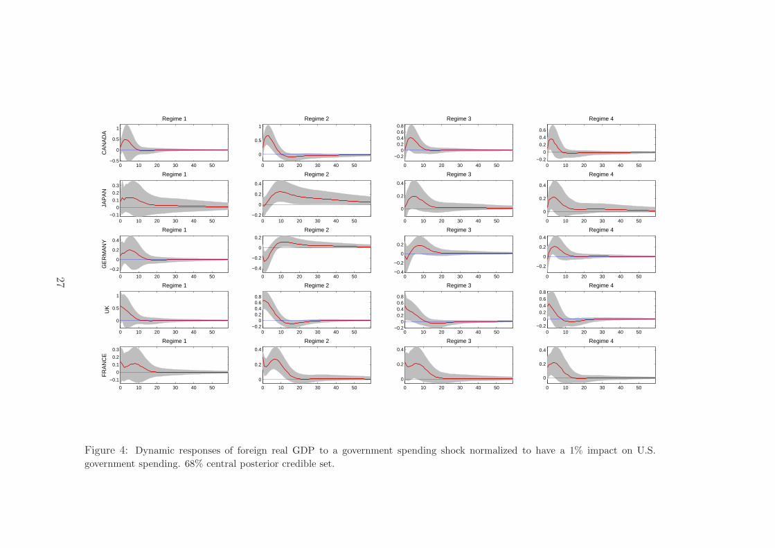
Moving to the response of foreign output, in Figure 4 we note that international spillovers

from a U.S. fiscal expansion tend to be positive and significant, except in the first regime,

where they are still positive, but insignificant. In regimes 2 and 4, spillovers are significantly

positive for all countries in our sample, with the exception of Germany in period 2 where the

spillovers are initially negative and then turn positive after about 10 quarters. In regime 3

instead, spillovers are positive and significant, but only for three out of five countries, namely

Japan, the U.K. and France. The largest peak effect on foreign GDP across all regimes is

found for Canada and the U.K., with the peak impact on Japan, France and Germany being

substantially lower. While the point estimates for the peak effects are in line with the size of

the fiscal spillovers in Corsetti and Muller (2014), we note that they are significantly larger

than the prediction of any of the theoretical model discussed in Section 2 (Figure 13 in the

web-Appendix D.2).

Finally, we note that the international fiscal spillovers in regime 4 do not appear necessarily

different from the spillovers in the other regimes, suggesting that the last sub-sample is most

10The response of the short-term nominal interest rate in regime 4 is constrained by the restriction meantto exemplify a zero lower bound type of scenario. Without this restriction, the response of both domesticand foreign output would be slightly smaller than shown in figures 2 and 4.

14

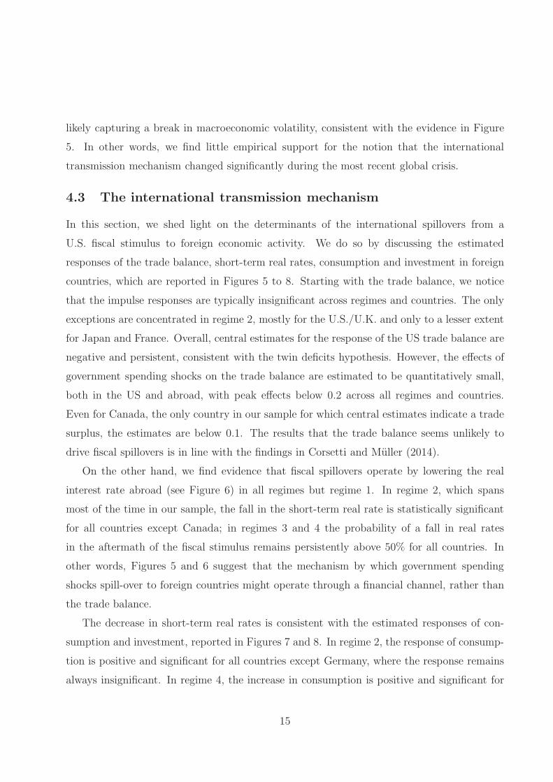
likely capturing a break in macroeconomic volatility, consistent with the evidence in Figure

5. In other words, we find little empirical support for the notion that the international

transmission mechanism changed significantly during the most recent global crisis.

4.3 The international transmission mechanism

In this section, we shed light on the determinants of the international spillovers from a

U.S. fiscal stimulus to foreign economic activity. We do so by discussing the estimated

responses of the trade balance, short-term real rates, consumption and investment in foreign

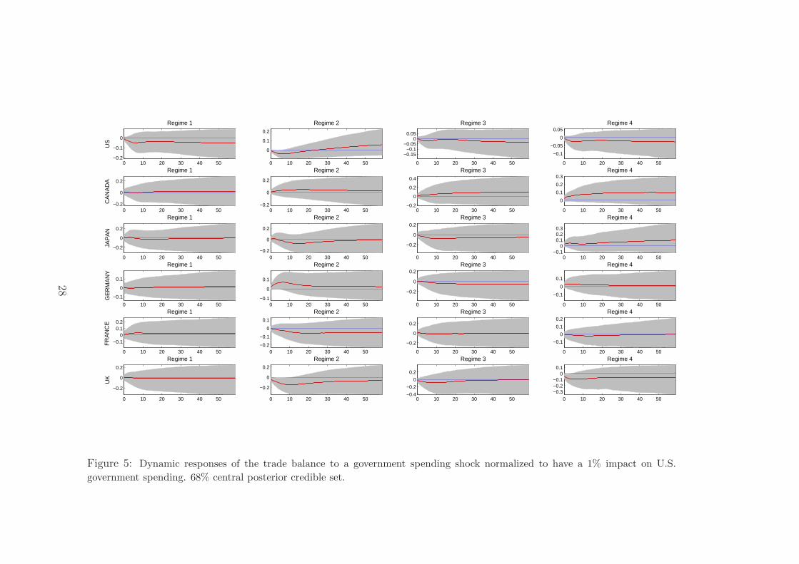
countries, which are reported in Figures 5 to 8. Starting with the trade balance, we notice

that the impulse responses are typically insignificant across regimes and countries. The only

exceptions are concentrated in regime 2, mostly for the U.S./U.K. and only to a lesser extent

for Japan and France. Overall, central estimates for the response of the US trade balance are

negative and persistent, consistent with the twin deficits hypothesis. However, the effects of

government spending shocks on the trade balance are estimated to be quantitatively small,

both in the US and abroad, with peak effects below 0.2 across all regimes and countries.

Even for Canada, the only country in our sample for which central estimates indicate a trade

surplus, the estimates are below 0.1. The results that the trade balance seems unlikely to

drive fiscal spillovers is in line with the findings in Corsetti and Muller (2014).

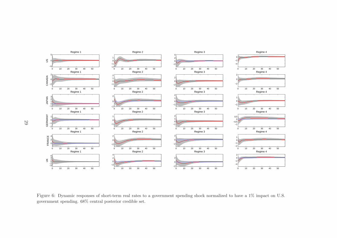
On the other hand, we find evidence that fiscal spillovers operate by lowering the real

interest rate abroad (see Figure 6) in all regimes but regime 1. In regime 2, which spans

most of the time in our sample, the fall in the short-term real rate is statistically significant

for all countries except Canada; in regimes 3 and 4 the probability of a fall in real rates

in the aftermath of the fiscal stimulus remains persistently above 50% for all countries. In

other words, Figures 5 and 6 suggest that the mechanism by which government spending

shocks spill-over to foreign countries might operate through a financial channel, rather than

the trade balance.

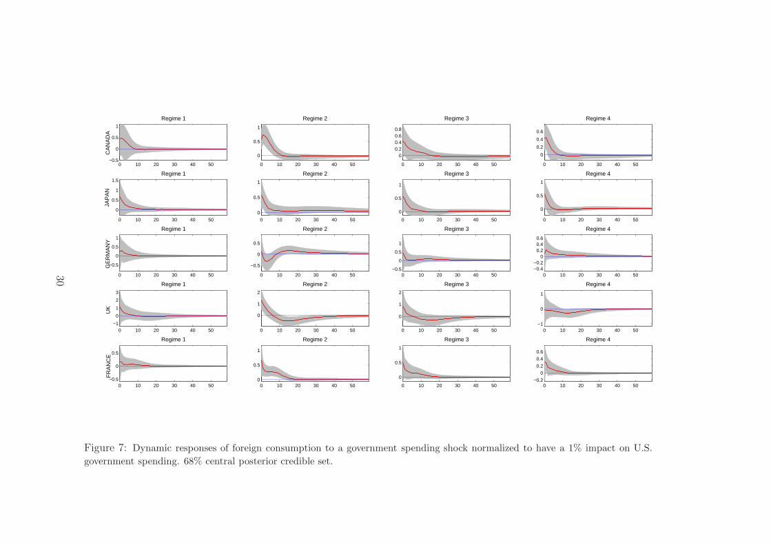
The decrease in short-term real rates is consistent with the estimated responses of con-

sumption and investment, reported in Figures 7 and 8. In regime 2, the response of consump-

tion is positive and significant for all countries except Germany, where the response remains

always insignificant. In regime 4, the increase in consumption is positive and significant for

15

Canada, Japan and France, but insignificant for Germany. The response of consumption in

the U.K. is instead significantly negative after about 10 quarters. In regimes 1 and 3 instead,

the point estimate for the response of consumption is always positive, but never significant,

with the exception of Japan in regime 3.

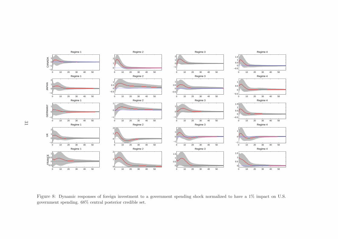
The adjustment in investment broadly mimics the adjustment in consumption across

countries and regimes, with central estimates of the impulse responses being positive for all

countries and regimes a few quarters after the shock, but attaining statistical significance only

over a subset of country-regime pairs. In regimes 2 and 4, investment increases significantly in

all countries, with the exception of the U.K. in regime 4. In regime 1 instead, the increase in

investment is always statistically indistinguishable from zero, while in regime 3 the response

is significant only in Canada and France.

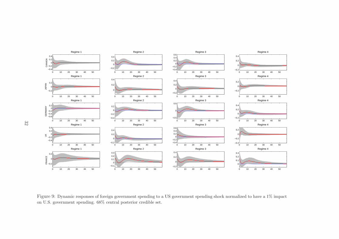
Finally, in Figure 9 we report impulse responses for foreign government spending. In

almost all countries and regimes we find little evidence of significant responses in foreign

spending, with error bands generally being very wide around central estimates (France and

Canada represent sporadic exceptions). Arguably, lower real interest rates induced by the

US fiscal stimulus could improve fiscal sustainability abroad and induce a delayed increase in

spending in foreign countries. But we find little evidence in support of this hypothesis.

In summary, we find little evidence of structural breaks in the transmission of fiscal

spillovers after 1985, when U.S. fiscal policy begins to produce significant domestic and cross-

border effects. The international transmission of government spending shocks does not appear

to operate through the trade balance (with the only possible exception of regime 2) but most

likely through a financial channel in the form of a decrease in real rates abroad, which in turn

stimulates consumption and investment.

4.4 State-dependence

The regimes in our factor model are identified statistically. But a possible economic interpre-

tation is that they reflect different states of the domestic or the international business cycle.

Indeed, a prominent literature for the U.S., exemplified by the contributions of Auerbach

and Gorodichenko (2012) and Ramey and Zubairy (2014), has studied (reaching opposite

conclusions) whether the government spending multiplier is larger during periods of slack in

16

economy activity. In analogy to these studies, we ask whether the international transmission

of fiscal policy depends on the presence of a recession abroad or on the introduction of a

single currency among some of the U.S. main trade partners.

More specifically, we estimate two Factor Augmented VAR models where the stochastic

regime shifts are replaced with a dummy variable. In the first model, the dummy takes the

value of one during periods in which at least one of the countries in the panel is in recession

and takes the value of zero otherwise.11 The second model sets the value of the dummy to one

after the first quarter of 1999 to account for any possible break associated with the adoption

of the Euro.

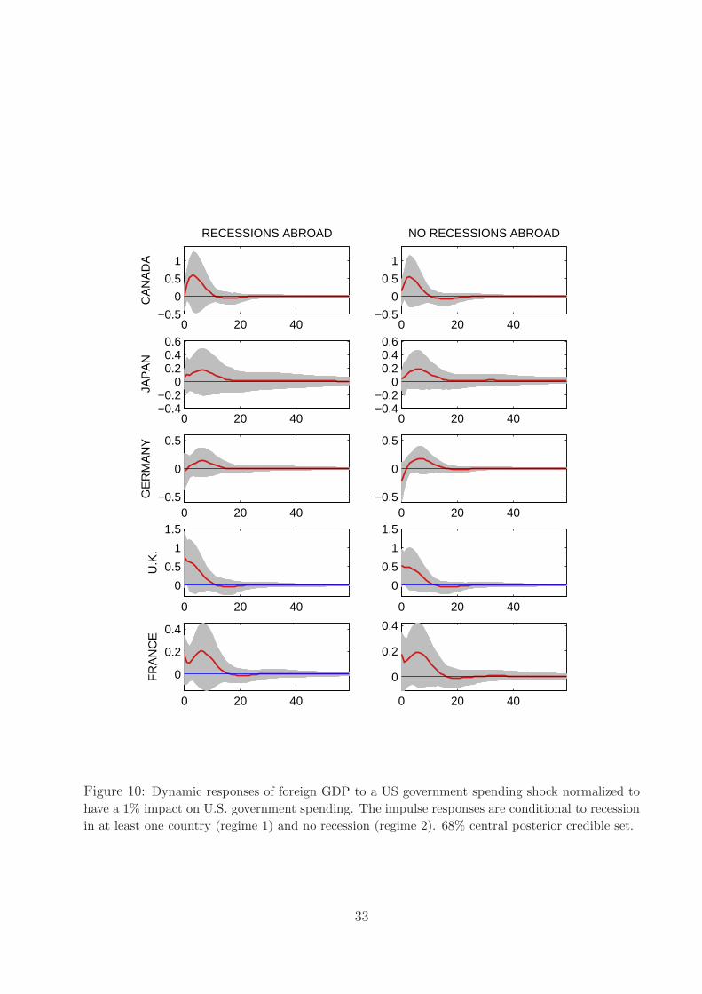
Figure 10 records the response of foreign output to a U.S. government spending shock

conditioned on the two regimes, with the left (right) column corresponding to periods of

recessions (no recessions) abroad. The median responses appear remarkably similar across the

two regimes, suggesting that international fiscal spillovers tend to vary neither with the state

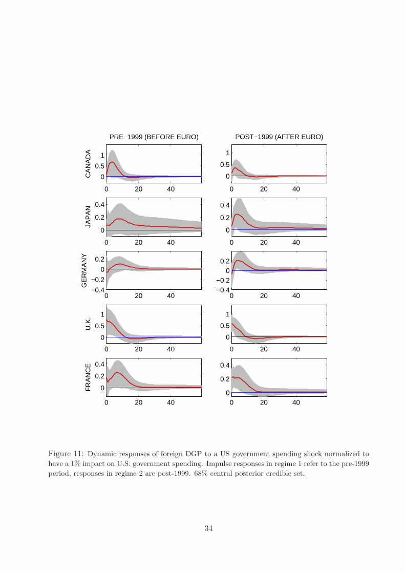
of the foreign economy nor with the state of the domestic economy. The results are similar

when the impulse responses are conditioned to the sub-samples before and after adoption of

the Euro, thereby providing little evidence in favour of the hypothesis that the transmission

of U.S. fiscal policy (in Europe) changed systematically after this date (see Figure 11).

5 Conclusions

What are the effects of a fiscal expansion in the United States on foreign real activity? This

paper has searched for international fiscal spillovers using theory-robust sign restrictions and

a factor model. Our evidence suggests that an increase in U.S. government spending tends

to have a positive influence on its main trade partners. The transmission mechanism appears

to operate through a financial channel (as exemplified by negative real rates abroad) rather

than a trade channel and appears to have been remarkably stable over time.

The ongoing period of policy retrenchment is likely to offer new challenges for modelling

the interaction between fiscal and monetary policies. Furthermore, the current reversal of

government spending and other policy interventions is suggestive of the possible start of a

new regime. Whether the international fiscal spillovers associated with a newly identified

11We use NBER (OECD) recession dates (recession indicators) for the U.S. (for the remaining countries).

17

fiscal consolidation era may be significantly different from the past is of course an empirical

question. But the strategy outlined in this paper appears well placed to evaluate in future

research any possible change in the international transmission of fiscal policy.

18

References

Auerbach, Alan and Yuriy Gorodnichenko, 2012, Fiscal Multipliers in Recession and Ex-

pansion, in Fiscal Policy after the Financial Crisis, Alberto Alesina and FrancescoGiavazzi, eds., University of Chicago Press.

Barattieri, Alessandro, Basu Susanto and Peter Gottschalk, 2014, Some Evidence on theImportance of Sticky Wages, American Economic Journal: Macroeconomics 6, pp. 70-

101.

Barro, Robert and Charles Redlick, 2011, Macroeconomic Effects from Government Pur-chases and Taxes, The Quarterly Journal of Economics 126, pp. 51-102.

Bianchi, Francesco and Cosmin Ilut, 2011, Monetary/Fiscal Policy Mix and Agents’ Beliefs,mimeo, Duke University.

Blanchard, Olivier and Roberto Perotti, 2002, An Empirical Characterization of the Dy-namic Effect of Changes in Government Spending and Taxes on Output, The Quarterly

Journal of Economics 117, pp. 1329-1368.

Campbell, John and Gregory Mankiw, 1989, Consumption, Income, and Interest Rates:

Reinterpreting the Time Series Evidence, in NBER Macroeconomics Annual, eds. O.Blanchard and S. Fischer, pp. 185–216.

Canova, Fabio and Evi Pappa, 2011, Fiscal Policy, Pricing Frictions and Monetary Accom-modation, Economic Policy 56, pp. 555-598.

Carter, Christopher and Robert Kohn, 1994, On Gibbs Sampling for State Space Models,

Biometrika 81, pp. 541-553.

Christiano, Lawrence, Martin Eichenbaum and Charles L. Evans, 2005, Nominal Rigidities

and the Dynamic Effects of a Shock to Monetary Policy, Journal of Political Economy,University of Chicago Press, 113(1), pp. 1-45.

Christiano, Lawrence, Martin Eichenbaum and Sergio Rebelo, 2011, When Is the Govern-ment Spending Multiplier Large?, Journal of Political Economy 119, pp. 78-121.

Coenen, Gunter, Christopher J. Erceg, Charles Freedman, Davide Furceri, Michael Kumhof,Rene Lalonde, Douglas Laxton, Jesper Linde, Annabelle Mourougane, Dirk Muir, Su-

sanna Mursula, Carlos de Resende, John Roberts, Werner Roeger, Stephen Snudden,Mathias Trabandt, and Jan in’t Veld. 2012, Effects of Fiscal Stimulus in Structural

Models, American Economic Journal: Macroeconomics 4, pp. 22–68.

Cogley, Timothy and Thomas Sargent, 2005, Drift and Volatilities: Monetary Policies andOutcomes in the Post WWII US, Review of Economic Dynamics 8, pp. 262-302.

19

Cook, David and Michael Devereux, 2011, Optimal Fiscal Policy in a World Liquidity Trap,

European Economic Review 55, pp. 443-462.

Corsetti, Giancarlo, Luca Dedola and Sylvain Leduc, 2008, International Risk Sharing and

the International Transmission of Productivity Shocks, Review of Economic Studies 75,pp. 443-473.

Corsetti, Giancarlo, Andre Meier and Gernot Muller, 2010, Cross-Borders Spillovers fromFiscal Stimulus, International Journal of Central Banking 6, pp. 5-37.

Corsetti, Giancarlo, Andre Meier and Gernot Muller, 2012, Fiscal Stimulus with SpendingReversals, Review of Economics and Statistics, 94(4), 878-895, November.

Corsetti, Giancarlo, Keith Kuester, Andre Meier and Gernot Muller, 2010, Debt Consoli-

dation and Fiscal Stabilization of Deep Recessions, American Economic Review P&P,100(2), pp.41-45.

Corsetti, Giancarlo and Gernot Muller, 2014, Multilateral economic cooperation and theinternational transmission of fiscal policy, in Globalization in an Age of Crisis: Multi-

lateral Economic Cooperation in the Twenty-First Century, Feenstra and Taylor.

Davig, Troy and Eric Leeper, 2006, Fluctuating macro policies and the fiscal theory, NBER

Macroeconomics Annual 21, pp. 247-298.

Del Negro, Marco and Christopher Otrok, 2005, Dynamic Factor Models with Time-Varying

Parameters, mimeo, Federal Reserve Bank of Atlanta and University of Virginia.

Erceg, Christopher J., Dale W. Henderson and Andrew T. Levin, 2000, Optimal monetary

policy with staggered wage and price contracts, Journal of Monetary Economics, 46(2),pp. 281-313.

Enders, Zeno, Gernot Muller and Almuth Scholl, 2011, How do fiscal and technology shocks

affect real exchange rates? New evidence for the U.S., Journal of International Eco-nomics 83, pp. 53–69.

Forni, Mario and Luca Gambetti, 2010, Fiscal Foresight and the Effects of GovernmentSpending, mimeo, Universita’ di Modena e Reggio Emilia and Universitat Autonoma

de Barcelona.

Galı, Jordi, 2011, The Return of the Wage Phillips Curve, Journal of the European Economic

Association, 9, ppp. 436-461.

Galı, Jordi, David Lopez-Salido, and Javier Valles, 2007, Understanding the Effects of Gov-

ernment Spending on Consumption, Journal of the European Economic Association 5,pp. 227-270.

20

Galı, Jordi and Roberto Perotti, 2003, Fiscal Policy and Monetary Integration in Europe,

Economic Policy 37, pp. 534–572.

Gambetti Luca, 2010, Fiscal Policy, Foresight and the Trade Balance in the US, mimeo,

Universitat Autonoma de Barcelona.

Gertler, Mark, Luca Sala and Antonella Trigari, 2008, An Estimated Monetary DSGEModel

with Unemployment and Staggered Nominal Wage Bargaining, Journal of Money,Credit and Banking, 40(8), pp. 1713-1764.

Hall, Robert, 2009, By how much does GDP Rise if the Government Buys more Output?,Brookings Papers on Economic Activity 2, pp. 183-231.

Leeper, Eric M., Todd B. Walker and Shu-Chun Susan Yang, 2013, Foresight and Informa-

tion Flows, Econometrica 81(3), pp. 1115-1145.

Kilian, Lutz and Daniel Murphy, 2012, Why Agnostic Sign Restrictions Are Not Enough:

Understanding the Dynamics of Oil Market VAR Models, Journal of the EuropeanEconomic Association, 10(5), pages 1166-1188.

Kim, Chang and Charles Nelson, 1999, State-Space Models with Regime Switching, MitPress.

Misra, Kanishka and Paolo Surico, 2014, Consumption, Income Changes and Heterogene-ity: Evidence from Two Fiscal Stimulus Programmes, American Economic Journal:

Macroeconomics 6, pp. 84-106.

Monacelli, Tommaso and Roberto Perotti, 2011, Fiscal Policy, the Real Exchange Rate, and

Traded Goods, Economic Journal 120, pp. 437-461.

Mountford, Andrew and Harald Uhlig, 2009, What are the effects of fiscal policy shocks?,

Journal of Applied Econometrics 24, pp. 960–992.

Primiceri, Giorgio, 2005, Time-Varying Vector Autoregressions and Monetary Policy, TheReview of Economic Studies 72, pp. 821-852.

Ramey, Valery and Sarah Zubairy, 2014, Government Spending Multipliers in Good Timesand in Bad: Evidence from U.S. Historical Data, mimeo, University of California at

San Diego.

Ravn, Morten, Stephanie Schmitt-Grohe and Martin Uribe, 2012, Consumption, Govern-

ment Spending, and the Real Exchange Rate, Journal of Monetary Economics, 59(3),pp.215-34.

Ravn, Morten, Stephanie Schmitt-Grohe and Martin Uribe, 2007, Pricing to Habits and theLaw of One Price, American Economic Review 97, pp. 232-238.

21

Sims, Chris and Tao Zha, 2006, Were There Regime Switches in U.S. Monetary Policy?,

American Economic Review 96, pp. 54–81.

Spiegelhalter, D., N. Best, B. Carlin, and A. Linde, 2002, Bayesian Measures of Model Com-

plexity and fit, Journal of the Royal Statistical Society, Series B (Statistical Methodol-ogy) 64, pp. 583.639.

Taylor, John, 1993, Discretion versus policy rules in practice, Carnegie-Rochester ConferenceSeries on Public Policy 39, pp. 195-214.

Woodford, Michael, 2011, Simple Analytics of the Government Expenditure Multiplier,American Economic Journal: Macroeconomics 3, pp. 1-35.

22

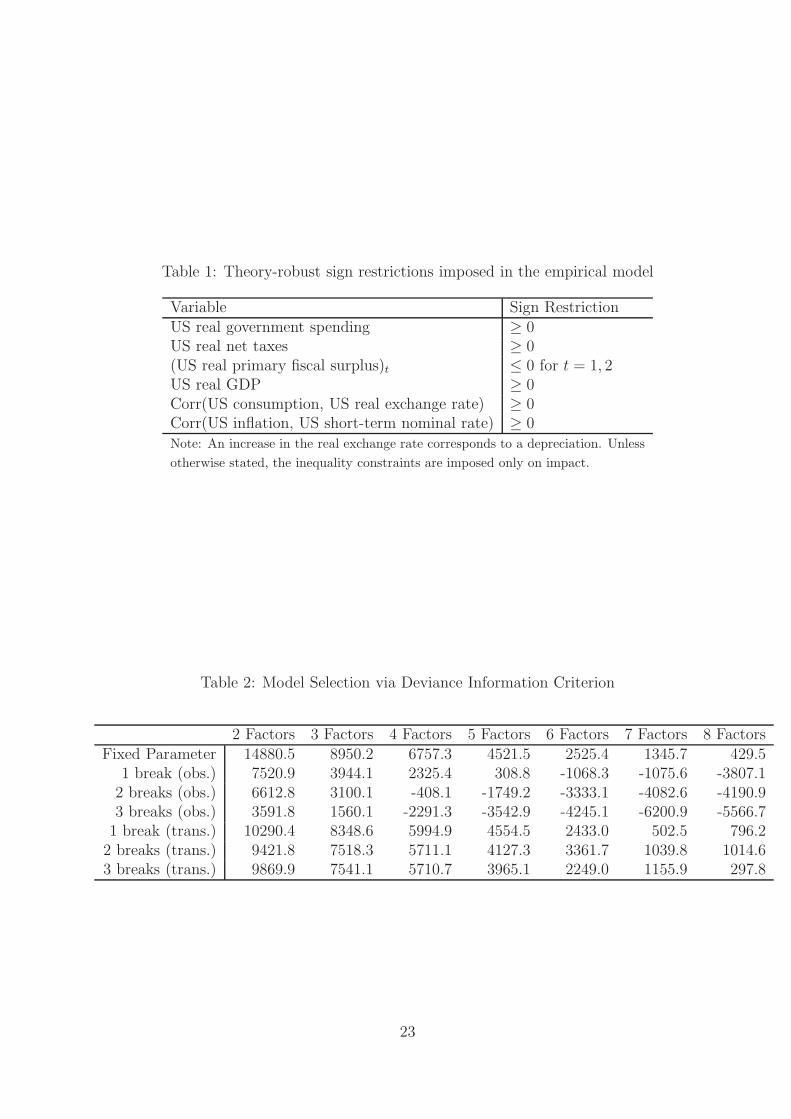
Table 1: Theory-robust sign restrictions imposed in the empirical model

Variable Sign RestrictionUS real government spending ≥ 0US real net taxes ≥ 0(US real primary fiscal surplus)t ≤ 0 for t = 1, 2US real GDP ≥ 0Corr(US consumption, US real exchange rate) ≥ 0Corr(US inflation, US short-term nominal rate) ≥ 0Note: An increase in the real exchange rate corresponds to a depreciation. Unless

otherwise stated, the inequality constraints are imposed only on impact.

Table 2: Model Selection via Deviance Information Criterion

2 Factors 3 Factors 4 Factors 5 Factors 6 Factors 7 Factors 8 FactorsFixed Parameter 14880.5 8950.2 6757.3 4521.5 2525.4 1345.7 429.5

1 break (obs.) 7520.9 3944.1 2325.4 308.8 -1068.3 -1075.6 -3807.12 breaks (obs.) 6612.8 3100.1 -408.1 -1749.2 -3333.1 -4082.6 -4190.93 breaks (obs.) 3591.8 1560.1 -2291.3 -3542.9 -4245.1 -6200.9 -5566.71 break (trans.) 10290.4 8348.6 5994.9 4554.5 2433.0 502.5 796.22 breaks (trans.) 9421.8 7518.3 5711.1 4127.3 3361.7 1039.8 1014.63 breaks (trans.) 9869.9 7541.1 5710.7 3965.1 2249.0 1155.9 297.8

23

1980 1985 1990 1995 2000 2005 20100

0.2

0.4

0.6

0.8

1Break−Points for factor loadings

1980 1985 1990 1995 2000 2005 20100

0.2

0.4

0.6

0.8

1Break−Points for idiosyncratic variances

Figure 1: Identified breakpoints and regime probabilities.

24

0 10 20 30 40 50

−0.5

0

0.5

1

1.5

Regime 1

RE

AL

GD

P

0 10 20 30 40 50−0.2

0

0.2

0.4

0.6

0.8

Regime 2

0 10 20 30 40 50−0.2

0

0.2

0.4

0.6

0.8

Regime 3

0 10 20 30 40 50−0.2

0

0.2

0.4

0.6

Regime 4

0 10 20 30 40 50−2

−1

0

1

Regime 1

INF

LAT

ION

0 10 20 30 40 50

−0.6

−0.4

−0.2

0

0.2

0.4

Regime 2

0 10 20 30 40 50−1.5

−1

−0.5

0

0.5

Regime 3

0 10 20 30 40 50

0

0.5

1

Regime 4

0 10 20 30 40 50−5

0

5Regime 1

SH

OR

T−

TE

RM

RE

AL

RA

TE

0 10 20 30 40 50−2

−1

0

1

Regime 2

0 10 20 30 40 50

−2

0

2

4Regime 3

0 10 20 30 40 50

−4

−2

0

Regime 4

0 10 20 30 40 50

−5

0

5

Regime 1

LON

G−

TE

RM

R

EA

L R

AT

E

0 10 20 30 40 50

−1

0

1

2

Regime 2

0 10 20 30 40 50

−2

0

2

4

Regime 3

0 10 20 30 40 50−6

−4

−2

0

Regime 4

Figure 2: Dynamic responses of U.S. variables to a government spending shock normalized to have a 1% impact on U.S. government

spending. Central 68% credible set.

25

0 10 20 30 40 50

0

0.5

1Regime 1

GO

VE

RN

ME

NT

S

PE

ND

ING

0 10 20 30 40 50

0

0.5

1Regime 2

0 10 20 30 40 50

0

0.5

1Regime 3

0 10 20 30 40 50

0

0.5

1Regime 4

0 10 20 30 40 50

0

2

4

Regime 1

NE

T T

AX

ES

0 10 20 30 40 50

0

1

2

3

Regime 2

0 10 20 30 40 50

0

2

4

Regime 3

0 10 20 30 40 50−1

0

1

2

3

Regime 4

0 10 20 30 40 50−0.5

0

0.5

1

Regime 1

CO

NS

UM

PT

ION

0 10 20 30 40 50

0

0.2

0.4

0.6

0.8

Regime 2

0 10 20 30 40 50

0

0.5

1Regime 3

0 10 20 30 40 50

0

0.2

0.4

0.6

Regime 4

0 10 20 30 40 50

0

2

4

6

Regime 1

RE

AL

EF

FE

CT

IVE

E

XC

HA

NG

E R

AT

E

0 10 20 30 40 500

2

4

6

Regime 2

0 10 20 30 40 50

0

2

4

6

8

Regime 3

0 10 20 30 40 50

0

2

4

6

Regime 4

Figure 3: Dynamic responses of U.S. variables to a government spending shock normalized to have a 1% impact on U.S. government

spending. An increase in the real exchange rate corresponds to a depreciation. Central 68% credible set.

26

0 10 20 30 40 50−0.5

0

0.5

1

Regime 1

CA

NA

DA

0 10 20 30 40 50

0

0.5

1

Regime 2

0 10 20 30 40 50

−0.20

0.20.40.60.8

Regime 3

0 10 20 30 40 50−0.2

0

0.2

0.4

0.6

Regime 4

0 10 20 30 40 50−0.1

0

0.1

0.2

0.3

Regime 1

JAP

AN

0 10 20 30 40 50−0.2

0

0.2

0.4

Regime 2

0 10 20 30 40 50

0

0.2

0.4

Regime 3

0 10 20 30 40 50

0

0.2

0.4

Regime 4

0 10 20 30 40 50

−0.2

0

0.2

0.4

Regime 1

GE

RM

AN

Y

0 10 20 30 40 50

−0.4

−0.2

0

0.2

Regime 2

0 10 20 30 40 50−0.4

−0.2

0

0.2

Regime 3

0 10 20 30 40 50

−0.2

0

0.2

0.4

Regime 4

0 10 20 30 40 50

0

0.5

1

Regime 1

UK

0 10 20 30 40 50−0.2

00.20.40.60.8

Regime 2

0 10 20 30 40 50−0.2

00.20.40.60.8

Regime 3

0 10 20 30 40 50−0.2

00.20.40.60.8

Regime 4

0 10 20 30 40 50

−0.1

0

0.1

0.2

0.3

Regime 1

FR

AN

CE

0 10 20 30 40 50

0

0.2

0.4

Regime 2

0 10 20 30 40 50

0

0.2

0.4

Regime 3

0 10 20 30 40 50

0

0.2

0.4

Regime 4

Figure 4: Dynamic responses of foreign real GDP to a government spending shock normalized to have a 1% impact on U.S.

government spending. 68% central posterior credible set.

27

0 10 20 30 40 50−0.2

−0.1

0

Regime 1

US

0 10 20 30 40 50

0

0.1

0.2

Regime 2

0 10 20 30 40 50

−0.15−0.1

−0.050

0.05

Regime 3

0 10 20 30 40 50

−0.1

−0.05

0

0.05Regime 4

0 10 20 30 40 50−0.2

0

0.2

Regime 1

CA

NA

DA

0 10 20 30 40 50−0.2

0

0.2

Regime 2

0 10 20 30 40 50−0.2

0

0.2

0.4

Regime 3

0 10 20 30 40 50

0

0.1

0.2

0.3Regime 4

0 10 20 30 40 50

−0.2

0

0.2

Regime 1

JAP

AN

0 10 20 30 40 50−0.2

0

0.2

Regime 2

0 10 20 30 40 50

−0.2

0

0.2

Regime 3

0 10 20 30 40 50−0.1

00.10.20.3

Regime 4

0 10 20 30 40 50

−0.1

0

0.1

Regime 1

GE

RM

AN

Y

0 10 20 30 40 50−0.1

0

0.1

Regime 2

0 10 20 30 40 50

−0.2

0

0.2Regime 3

0 10 20 30 40 50

−0.1

0

0.1

Regime 4

0 10 20 30 40 50

−0.10

0.10.2

Regime 1

FR

AN

CE

0 10 20 30 40 50−0.2

−0.1

0

0.1

Regime 2

0 10 20 30 40 50

−0.2

0

0.2

Regime 3

0 10 20 30 40 50

−0.1

0

0.1

0.2Regime 4

0 10 20 30 40 50

−0.2

0

0.2

Regime 1

UK

0 10 20 30 40 50

−0.2

0

0.2

Regime 2

0 10 20 30 40 50−0.4

−0.2

0

0.2

Regime 3

0 10 20 30 40 50−0.3−0.2−0.1

00.1

Regime 4

Figure 5: Dynamic responses of the trade balance to a government spending shock normalized to have a 1% impact on U.S.


28

0 10 20 30 40 50−5

0

5Regime 1

US

0 10 20 30 40 50−2

−1

0

1

Regime 2

0 10 20 30 40 50

−2

0

2

4Regime 3

0 10 20 30 40 50

−4

−2

0

Regime 4

0 10 20 30 40 50

−2

0

2Regime 1

CA

NA

DA

0 10 20 30 40 50

−1012

Regime 2

0 10 20 30 40 50

−2

0

2

Regime 3

0 10 20 30 40 50

−2

0

2Regime 4

0 10 20 30 40 50−1

0123

Regime 1

JAP

AN

0 10 20 30 40 50−2

0

2

Regime 2

0 10 20 30 40 50

−1

0

1

2

Regime 3

0 10 20 30 40 50

−1

0

1

Regime 4

0 10 20 30 40 50−2

−1

0

1

Regime 1

GE

RM

AN

Y

0 10 20 30 40 50

−1

0

1

Regime 2

0 10 20 30 40 50

−1012

Regime 3

0 10 20 30 40 50

−1−0.5

00.5

Regime 4

0 10 20 30 40 50

0

2

4

Regime 1

FR

AN

CE

0 10 20 30 40 50

−2

0

2

Regime 2

0 10 20 30 40 50

−2

0

2

Regime 3

0 10 20 30 40 50−2−1

01

Regime 4

0 10 20 30 40 50−4−2

0246

Regime 1

UK

0 10 20 30 40 50

−2

0

2

4

Regime 2

0 10 20 30 40 50−2

0

2

Regime 3

0 10 20 30 40 50

−4

−2

0

2

Regime 4

Figure 6: Dynamic responses of short-term real rates to a government spending shock normalized to have a 1% impact on U.S.


29

0 10 20 30 40 50−0.5

0

0.5

1

Regime 1

CA

NA

DA

0 10 20 30 40 50

0

0.5

1

Regime 2

0 10 20 30 40 50

00.20.40.60.8

Regime 3

0 10 20 30 40 50

0

0.2

0.4

0.6

Regime 4

0 10 20 30 40 50

0

0.5

1

1.5Regime 1

JAP

AN

0 10 20 30 40 50

0

0.5

1

Regime 2

0 10 20 30 40 50

0

0.5

1

Regime 3

0 10 20 30 40 50

0

0.5

1

Regime 4

0 10 20 30 40 50

−0.5

0

0.5

1

Regime 1

GE

RM

AN

Y

0 10 20 30 40 50

−0.5

0

0.5

Regime 2

0 10 20 30 40 50−0.5

0

0.5

1

Regime 3

0 10 20 30 40 50−0.4−0.2

00.20.40.6

Regime 4

0 10 20 30 40 50−1

0

1

2

3

Regime 1

UK

0 10 20 30 40 50

0

1

2

Regime 2

0 10 20 30 40 50

0

1

2

Regime 3

0 10 20 30 40 50−1

0

1

Regime 4

0 10 20 30 40 50−0.5

0

0.5

Regime 1

FR

AN

CE

0 10 20 30 40 500

0.5

1

Regime 2

0 10 20 30 40 50

0

0.5

1

Regime 3

0 10 20 30 40 50−0.2

0

0.2

0.4

0.6

Regime 4

Figure 7: Dynamic responses of foreign consumption to a government spending shock normalized to have a 1% impact on U.S.


30

0 10 20 30 40 50−2

−1

0

1

Regime 1

CA

NA

DA

0 10 20 30 40 50

0

1

2

Regime 2

0 10 20 30 40 50

−1

0

1

2

Regime 3

0 10 20 30 40 50

−0.50

0.51

1.5

Regime 4

0 10 20 30 40 50

−1

0

1

2

Regime 1

JAP

AN

0 10 20 30 40 50

−0.5

0

0.5

1

Regime 2

0 10 20 30 40 50

−0.5

0

0.5

1

Regime 3

0 10 20 30 40 50−0.5

0

0.5

1

Regime 4

0 10 20 30 40 50

−1

0

1

Regime 1

GE

RM

AN

Y

0 10 20 30 40 50

−1

0

1Regime 2

0 10 20 30 40 50

−1

0

1

Regime 3

0 10 20 30 40 50

−0.5

0

0.5

1

1.5

Regime 4

0 10 20 30 40 50−1

0

1

2

Regime 1

UK

0 10 20 30 40 50

0

1

2

Regime 2

0 10 20 30 40 50

−1

0

1

Regime 3

0 10 20 30 40 50−1

0

1

Regime 4

0 10 20 30 40 50

−0.5

0

0.5

1

Regime 1

FR

AN

CE

0 10 20 30 40 500

1

2Regime 2

0 10 20 30 40 50

0

0.5

1

1.5

Regime 3

0 10 20 30 40 50

0

0.5

1

1.5

Regime 4

Figure 8: Dynamic responses of foreign investment to a government spending shock normalized to have a 1% impact on U.S.


31

0 10 20 30 40 50−0.4

−0.2

0

0.2

0.4

Regime 1

CA

NA

DA

0 10 20 30 40 50

−0.2

0

0.2

0.4

Regime 2

0 10 20 30 40 50−0.4−0.2

00.20.40.6

Regime 3

0 10 20 30 40 50−0.2

0

0.2

0.4

Regime 4

0 10 20 30 40 50

−0.2

0

0.2

Regime 1

JAP

AN

0 10 20 30 40 50

0

0.2

0.4

Regime 2

0 10 20 30 40 50

−0.2

0

0.2

0.4

Regime 3

0 10 20 30 40 50

−0.2

0

0.2

Regime 4

0 10 20 30 40 50

−0.6−0.4−0.2

00.2

Regime 1

GE

RM

AN

Y

0 10 20 30 40 50−0.4

−0.2

0

0.2

Regime 2

0 10 20 30 40 50−0.5

0

0.5Regime 3

0 10 20 30 40 50−0.2

0

0.2

0.4

Regime 4

0 10 20 30 40 50

−0.4

−0.2

0

0.2

0.4Regime 1

UK

0 10 20 30 40 50−0.2

0

0.2

0.4

Regime 2

0 10 20 30 40 50−0.4−0.2

00.20.40.6

Regime 3

0 10 20 30 40 50−0.4

−0.2

0

0.2

Regime 4

0 10 20 30 40 50

−0.2

0

0.2

Regime 1

FR

AN

CE

0 10 20 30 40 50

−0.1

0

0.1

0.2

0.3

Regime 2

0 10 20 30 40 50−0.2

0

0.2

0.4

Regime 3

0 10 20 30 40 50

0

0.1

0.2

0.3

Regime 4

Figure 9: Dynamic responses of foreign government spending to a US government spending shock normalized to have a 1% impact

on U.S. government spending. 68% central posterior credible set.

32

0 20 40−0.5

0

0.5

1

RECESSIONS ABROAD

CA

NA

DA

0 20 40−0.5

0

0.5

1

NO RECESSIONS ABROAD

0 20 40−0.4−0.2

00.20.40.6

JAP

AN

0 20 40−0.4−0.2

00.20.40.6

0 20 40−0.5

0

0.5

GE

RM

AN

Y

0 20 40−0.5

0

0.5

0 20 40

0

0.5

1

1.5

U.K

.

0 20 40

0

0.5

1

1.5

0 20 40

0

0.2

0.4

FR

AN

CE

0 20 40

0

0.2

0.4

Figure 10: Dynamic responses of foreign GDP to a US government spending shock normalized to

have a 1% impact on U.S. government spending. The impulse responses are conditional to recession

in at least one country (regime 1) and no recession (regime 2). 68% central posterior credible set.

33

0 20 40

0

0.5

1

PRE−1999 (BEFORE EURO)

CA

NA

DA

0 20 40

0

0.5

1

POST−1999 (AFTER EURO)

0 20 40

0

0.2

0.4

JAP

AN

0 20 40

0

0.2

0.4

0 20 40−0.4

−0.2

0

0.2

GE

RM

AN

Y

0 20 40−0.4−0.2

00.2

0 20 40

0

0.5

1

U.K

.

0 20 40

0

0.5

1

0 20 40

0

0.2

0.4

FR

AN

CE

0 20 400

0.2

0.4

Figure 11: Dynamic responses of foreign DGP to a US government spending shock normalized to

have a 1% impact on U.S. government spending. Impulse responses in regime 1 refer to the pre-1999

period, responses in regime 2 are post-1999. 68% central posterior credible set.

34

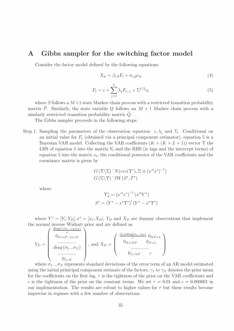
A Gibbs sampler for the switching factor model

Consider the factor model defined by the following equations:

Xit = βi,SFt + σi,Qeit (4)

Ft = c +

L∑

j=1

λjFt−j + Σ1/2vt (5)

where S follows aM+1 state Markov chain process with a restricted transition probability

matrix P . Similarly, the state variable Q follows an M + 1 Markov chain process with a

similarly restricted transition probability matrix Q.The Gibbs sampler proceeds in the following steps:

Step 1. Sampling the parameters of the observation equation: c, λj and Σ. Conditional onan initial value for Ft (obtained via a principal component estimator), equation 5 is a

Bayesian VAR model. Collecting the VAR coefficients (K × (K × L+ 1)) vector Υ theLHS of equation 5 into the matrix Yt and the RHS (ie lags and the intercept terms) of

equation 5 into the matrix xt, the conditional posterior of the VAR coefficients and thecovariance matrix is given by

G (Υ\Σ) ˜N(vec(Υ∗),Σ⊗ (x∗′x∗)−1)

G (Σ\Υ) ˜IW (S∗, T ∗)

where

Υ∗S = (x∗′x∗)

−1(x∗′Y ∗)

S∗ = (Y ∗ − x∗Υ∗)′ (Y ∗ − x∗Υ∗)

where Y ∗ = [Yt; YD], x∗ = [xt;XD]. YD and XD are dummy observations that implement

the normal inverse Wishart prior and are defined as

YD =

diag(γ1σ1...γNσN )τ

0N×(P−1)×N

..............diag (σ1...σN )..............01×N

, and XD =

JP⊗diag(σ1...σN )τ

0NP×1

0N×NP 0N×1

..............01×NP c

where σ1....σN represents standard deviations of the error term of an AR model estimatedusing the initial prinicipal component estimate of the factors, γ1 to γN denotes the prior mean

for the coefficients on the first lag, τ is the tightness of the prior on the VAR coefficients andc is the tightness of the prior on the constant terms. We set τ = 0.01 and c = 0.000001 in

our implementation. The results are robust to higher values for τ but these results becomeimprecise in regimes with a few number of observations.

35

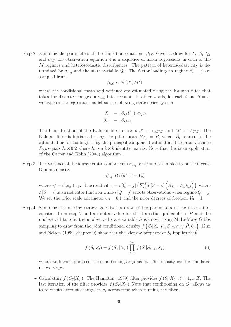
Step 2. Sampling the parameters of the transition equation: βi,S. Given a draw for Ft, St, Qt

and σi,Q the observation equation 4 is a sequence of linear regressions in each of theM regimes and heteroscedastic disturbances. The pattern of heteroscedasticity is de-

termined by σi,Q and the state variable Qt. The factor loadings in regime St = j aresampled from

βi,S ∼ N (β∗,M∗)

where the conditional mean and variance are estimated using the Kalman filter that

takes the discrete changes in σi,Q into account. In other words, for each i and S = s,we express the regression model as the following state space system

Xt = βs,tFt + σQet

βs,t = βs,t−1

The final iteration of the Kalman filter delivers β∗ = βs,T\T and M∗ = PT\T . The

Kalman filter is initialised using the prior mean B0\0 = Bi where Bi represents theestimated factor loadings using the principal component estimator. The prior variance

P0\0 equals Ik×0.2 where Ik is a k×k identity matrix. Note that this is an applicationof the Carter and Kohn (2004) algorithm.

Step 3. The variance of the idiosyncratic components σi,Q for Q = j is sampled from the inverse

Gamma density:σ2i,Q˜IG (σ∗

i , T + V0)

where σ∗i = e′iteit+σ0. The residual et = ι [Q = j]

(∑Ss I [S = s]

(Xit − Ftβi,S

))where

I [S = s] is an indicator function while ι [Q = j] selects observations when regime Q = j.

We set the prior scale parameter σ0 = 0.1 and the prior degrees of freedom V0 = 1.

Step 4. Sampling the markov states: S. Given a draw of the parameters of the observation

equation from step 2 and an initial value for the transition probabilities P and theunobserved factors, the unobserved state variable S is drawn using Multi-Move Gibbs

sampling to draw from the joint conditional density f(St|Xt, Ft, βi,S, σi,Q, P , Qt

). Kim

and Nelson (1999, chapter 9) show that the Markov property of St implies that

f (St|Zt) = f (ST |XT )T−1∏

t=1

f (St|St+1, Xt) (6)

where we have suppressed the conditioning arguments. This density can be simulatedin two steps:

• Calculating f (ST |XT ): The Hamilton (1989) filter provides f (St|Xt) , t = 1, ....T. Thelast iteration of the filter provides f (ST |XT ) .Note that conditioning on Qt allows us

to take into account changes in σi across time when running the filter.

36

• Calculating f (St|St+1, Xt): Kim and Nelson (1999) show that

f (St|St+1, Xt) ∝ f (St+1|St) f (St|Xt) (7)

where f (St+1|St) is the transition probability matrix and f (St|Xt) is obtained via

Hamilton (1989) filter in step a. Kim and Nelson (1999) (pp. 214) show how to sampleSt from (7).

Step 5. Sampling the Markov states: Qt. Given the parameters of the observation equation,a draw for the transition probabilities Q, the Markov states St and the factors, the

algorithm in Step 4 above is used to simulate Qt.

Step 6. Sampling the transition probabilities: P . The prior for the non zero elements of thetransition probability matrix pij is of the following form

p0ij = D (uij)

where D(.) denotes the Dirichlet distribution and uij = 15 if i = j and uij = 1 if

i 6= j. This choice of uij implies that the regimes are fairly persistent. The posteriordistribution is:

pij = D (uij + ηij)

where ηij denotes the number of times regime i is followed by regime j.

Step 7. Sampling the transition probabilities Q : The priors and conditional posteriors are in

step 5.

Step 8. Sampling the factors: Ft Given a draw for the parameters of the observation and

transition equation and the state variable St the Carter and Kohn (1994) algorithm isused to draw from the conditional posterior of Ft.

To compute the impulse responses, we use 500,000 replications of the Gibbs sampler,discarding the first 10,000 replications as burn-in and retaining those draws which satisfy the

sign restrictions set out above. In Figure 12 below we plot the recursive means of a sampleof 1000 retained draws. The stability of these provides evidence for convergence.

37

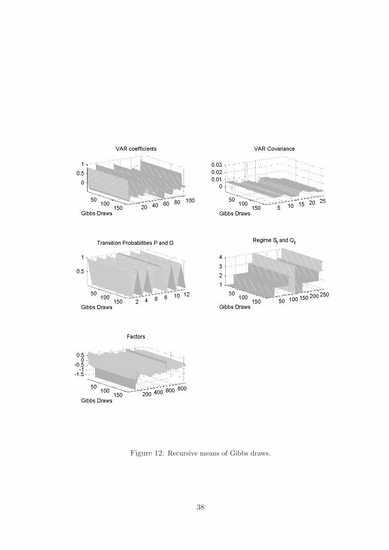
Figure 12: Recursive means of Gibbs draws.

38

B Data description and variance decomposition

The variables in the dataset used for the estimation of the factor model are listed in ta-

ble 3 below. The table also reports the data source and the transformation applied to thevariable. BEA refers to Bureau of Economic Analysis (http://www.bea.gov/), FRED is

Federal Reserve Economic Data (http://research.stlouisfed.org/fred2/), IFS is the IMF’s In-ternational Financial Statistics (www.imfstatistics.org/) and GFD is the Global Financial

Database (www.globalfinancialdata.com). LD refers to the log difference transformation.US fiscal variables are constructed as follows:

• Government spending: government consumption expenditures and gross investment(BEA Table 1.15 Line 21) deflated by GDP deflator (FRED series id GDPDEF) and

divided by population ( FRED series id POP).

• Net Taxes: current receipts (BEA Table 3.1 Line 1) minus current transfer payments(BEA Table 3.1 Line 17) and interest payments (BEA Table 3.1 Line 22) deflated by

GDP deflator and divided by population

39

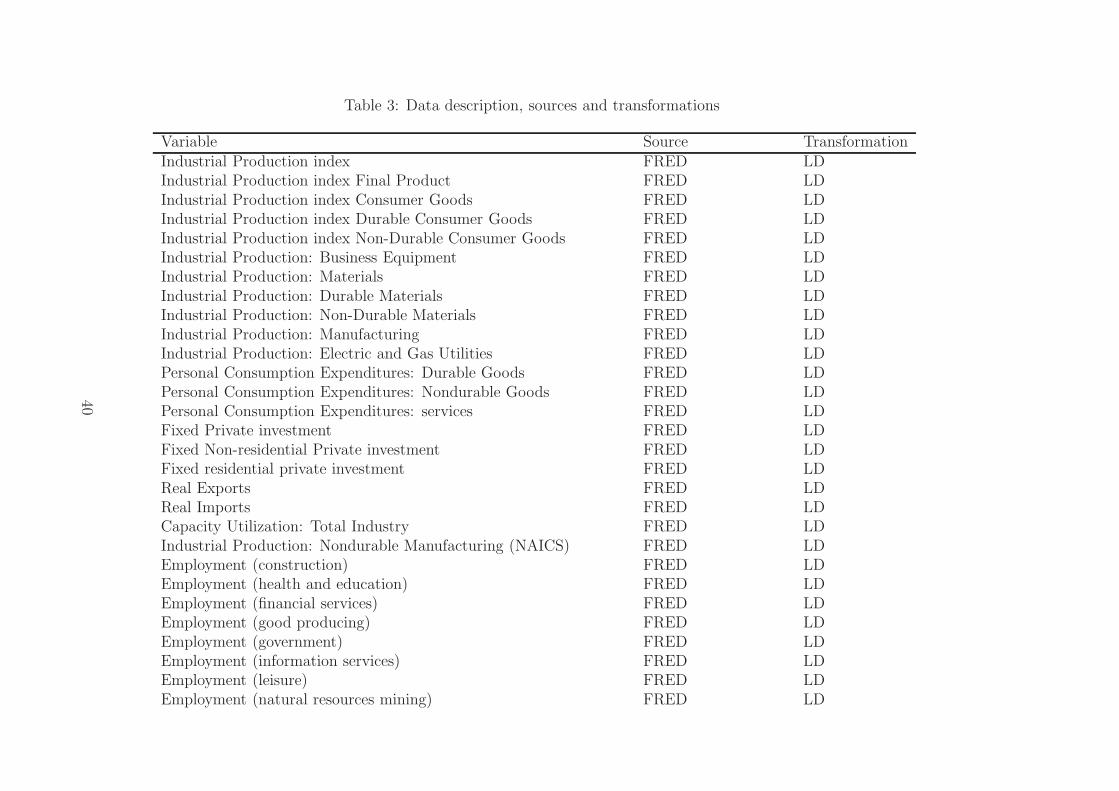
Table 3: Data description, sources and transformations

Variable Source TransformationIndustrial Production index FRED LDIndustrial Production index Final Product FRED LDIndustrial Production index Consumer Goods FRED LDIndustrial Production index Durable Consumer Goods FRED LDIndustrial Production index Non-Durable Consumer Goods FRED LDIndustrial Production: Business Equipment FRED LDIndustrial Production: Materials FRED LDIndustrial Production: Durable Materials FRED LDIndustrial Production: Non-Durable Materials FRED LDIndustrial Production: Manufacturing FRED LDIndustrial Production: Electric and Gas Utilities FRED LDPersonal Consumption Expenditures: Durable Goods FRED LDPersonal Consumption Expenditures: Nondurable Goods FRED LDPersonal Consumption Expenditures: services FRED LDFixed Private investment FRED LDFixed Non-residential Private investment FRED LDFixed residential private investment FRED LDReal Exports FRED LDReal Imports FRED LDCapacity Utilization: Total Industry FRED LDIndustrial Production: Nondurable Manufacturing (NAICS) FRED LDEmployment (construction) FRED LDEmployment (health and education) FRED LDEmployment (financial services) FRED LDEmployment (good producing) FRED LDEmployment (government) FRED LDEmployment (information services) FRED LDEmployment (leisure) FRED LDEmployment (natural resources mining) FRED LD

40

Employment (other services) FRED LDEmployment (professional and business services) FRED LDEmployment (retail trade) FRED LDEmployment (service providing ind) FRED LDEmployment (trade transportation utilities) FRED LDEmployment (wholesale trade) FRED LDCivilian employment FRED LDCivilian labor force FRED LDCivilian participation rate FRED LDNonfarm Business Sector: Average Weekly Hours FRED LDAverage Weekly Overtime Hours of Production and Nonsupervisory FRED LDEmployees: ManufacturingUnemployment Rate FRED noneAverage (Mean) Duration of Unemployment FRED LDCivilians Unemployed for 5-14 Weeks FRED LDCivilians Unemployed for 15-26 Weeks FRED LDCivilians Unemployed - Less Than 5 Weeks FRED LDCivilians Unemployed - 15 Weeks & Over FRED LDCivilians Unemployed for 27 Weeks and Over FRED LDHousing Starts: Total: New Privately Owned Housing Units Started FRED LDHousing Starts in Northeast Census Region FRED LDHousing Starts in Midwest Census Region FRED LDHousing Starts in South Census Region FRED LDHousing Starts in West Census Region FRED LDISM Manufacturing: New Orders Index FRED noneISM Manufacturing: Inventories Index FRED noneISM Manufacturing: Supplier Deliveries Index FRED noneGDP deflator FRED LDPersonal Consumption Expenditures: Chain-type Price Index FRED LDPersonal Consumption Expenditures: Chain-type Price Index Less FRED LDFood and EnergyConsumer Price Index for All Urban Consumers: All Items Less FRED LD

41

Food & EnergyGross Private Domestic Investment: Chain-type Price Index FRED LDConsumer Price Index for All Urban Consumers: Energy FRED LDConsumer Price Index for All Urban Consumers: Food FRED LDConsumer Price Index for All Urban Consumers: Housing FRED LDConsumer Price Index for All Urban Consumers: Apparel FRED LDConsumer Price Index for All Urban Consumers: Transportation FRED LDConsumer Price Index for All Urban Consumers: Medical Care FRED LDConsumer Price Index for All Urban Consumers: Other G. and S. FRED LDExport Price IFS LDImport Price IFS LDDescription: Economist All-Commodity Dollar Index GFD LDWest Texas Intermediate Oil Price (US$/Barrel) GFD LDNonfarm Business Sector: Output Per Hour of All Persons FRED LDNonfarm Business Sector: Real Compensation Per Hour FRED LDNonfarm Business Sector: Unit Labor Cost FRED LDFederal Funds Rate FRED none6-Month Treasury Bill: Secondary Market Rate GFD noneUSA 1-year Constant Maturity Note Yield GFD noneUSA 5-year Note Constant Maturity Yield GFD none6mth-3mth GFD none12mth-3mth GFD none10yr-3mth GFD noneAAA-10yr GFD noneAAB-10yr GFD noneM1 Money Stock GFD LDMZM Money Stock GFD LDM2 Money Stock GFD LDMonetary Base GFD LDNon Borrowed Reserves GFD LDTotal Reserves GFD LDCommercial and Industrial Loans at All Commercial Banks GFD LD

42

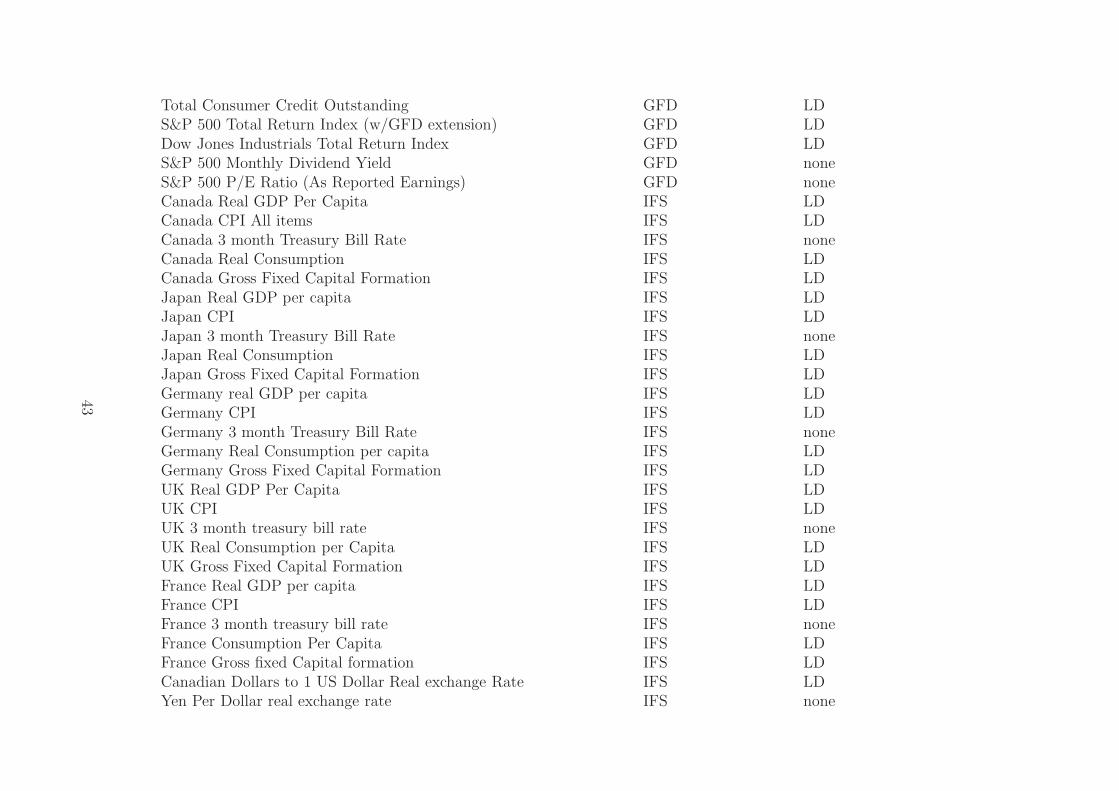
Total Consumer Credit Outstanding GFD LDS&P 500 Total Return Index (w/GFD extension) GFD LDDow Jones Industrials Total Return Index GFD LDS&P 500 Monthly Dividend Yield GFD noneS&P 500 P/E Ratio (As Reported Earnings) GFD noneCanada Real GDP Per Capita IFS LDCanada CPI All items IFS LDCanada 3 month Treasury Bill Rate IFS noneCanada Real Consumption IFS LDCanada Gross Fixed Capital Formation IFS LDJapan Real GDP per capita IFS LDJapan CPI IFS LDJapan 3 month Treasury Bill Rate IFS noneJapan Real Consumption IFS LDJapan Gross Fixed Capital Formation IFS LDGermany real GDP per capita IFS LDGermany CPI IFS LDGermany 3 month Treasury Bill Rate IFS noneGermany Real Consumption per capita IFS LDGermany Gross Fixed Capital Formation IFS LDUK Real GDP Per Capita IFS LDUK CPI IFS LDUK 3 month treasury bill rate IFS noneUK Real Consumption per Capita IFS LDUK Gross Fixed Capital Formation IFS LDFrance Real GDP per capita IFS LDFrance CPI IFS LDFrance 3 month treasury bill rate IFS noneFrance Consumption Per Capita IFS LDFrance Gross fixed Capital formation IFS LDCanadian Dollars to 1 US Dollar Real exchange Rate IFS LDYen Per Dollar real exchange rate IFS none

43

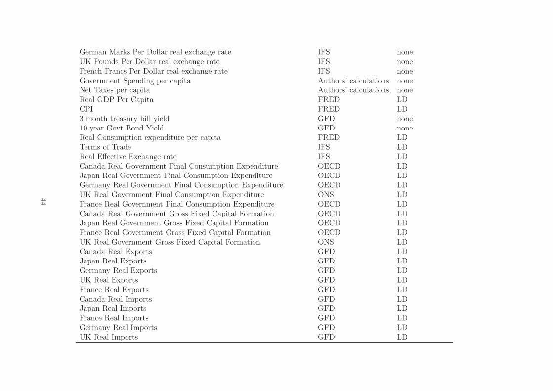
German Marks Per Dollar real exchange rate IFS noneUK Pounds Per Dollar real exchange rate IFS noneFrench Francs Per Dollar real exchange rate IFS noneGovernment Spending per capita Authors’ calculations noneNet Taxes per capita Authors’ calculations noneReal GDP Per Capita FRED LDCPI FRED LD3 month treasury bill yield GFD none10 year Govt Bond Yield GFD noneReal Consumption expenditure per capita FRED LDTerms of Trade IFS LDReal Effective Exchange rate IFS LDCanada Real Government Final Consumption Expenditure OECD LDJapan Real Government Final Consumption Expenditure OECD LDGermany Real Government Final Consumption Expenditure OECD LDUK Real Government Final Consumption Expenditure ONS LDFrance Real Government Final Consumption Expenditure OECD LDCanada Real Government Gross Fixed Capital Formation OECD LDJapan Real Government Gross Fixed Capital Formation OECD LDFrance Real Government Gross Fixed Capital Formation OECD LDUK Real Government Gross Fixed Capital Formation ONS LDCanada Real Exports GFD LDJapan Real Exports GFD LDGermany Real Exports GFD LDUK Real Exports GFD LDFrance Real Exports GFD LDCanada Real Imports GFD LDJapan Real Imports GFD LDFrance Real Imports GFD LDGermany Real Imports GFD LDUK Real Imports GFD LD

44

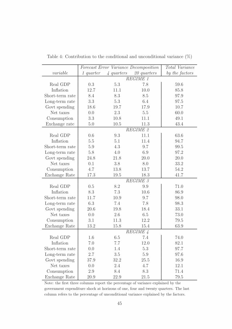
Table 4: Contribution to the conditional and unconditional variance (%)

Forecast Error Variance Decomposition Total Variancevariable 1 quarter 4 quarters 20 quarters by the factors

REGIME 1Real GDP 0.3 5.3 7.8 59.6Inflation 12.7 11.1 10.0 85.8

Short-term rate 8.4 8.3 8.5 97.9Long-term rate 3.3 5.3 6.4 97.5Govt spending 18.6 19.7 17.9 10.7

Net taxes 0.0 2.3 5.5 60.0Consumption 3.3 10.8 11.1 49.1Exchange rate 5.0 10.5 11.3 43.4



Net taxes 0.1 3.8 8.0 33.2Consumption 4.7 13.8 13.7 54.2Exchange Rate 17.3 19.5 18.3 41.7



Net taxes 0.0 2.6 6.5 73.0Consumption 3.1 11.3 12.2 79.5Exchange Rate 13.2 15.8 15.4 63.9



Net taxes 0.0 2.4 4.7 12.1Consumption 2.9 8.4 8.3 71.4Exchange Rate 20.9 22.9 21.5 79.5Note: the first three columns report the percentage of variance explained by the

government expenditure shock at horizons of one, four and twenty quarters. The last

column refers to the percentage of unconditional variance explained by the factors.

45

C The model -Web-Appendix-

C.1 Firms

Final good firms. The consumption good is produced by final good firms as a bundle of

home and foreign intermediate goods, and it is sold to consumers in perfect competition. Inturn intermediate goods are produced by a continuum of monopolistically competitive firms

at home and abroad under imperfect competition. The subscript i ∈ [0, 1] is used to indexintermediate good firms together with their products and prices. We denote intermediate

home goods by YH,t(i) and imported goods by YF,t(i). Final good firms minimize expendituresubject to the aggregation constraint:

Ct = ΦYv/2H,t Y

1−v/2F,t , 1 ≤ v ≤ 2,

where Φ = (v/2)v/2(1− (v/2))v/2, Ct denotes the aggregate consumption good, and YHt and

YFt are the bundles of goods produced in the home and foreign country, respectively. Theparameter v captures home bias in the production of the consumption good: the higher is v,

the more closed is the economy. In the special case where v = 1 there is no home-bias whilefor v = 2 the economy is autarkic. Final good firms in the foreign country are symmetric, with

the aggregation technology having weight v/2 on the foreign good as in Cook and Deveraux(2011). YHt and YFt are CES aggregates over a continuum of goods:

YHt =

1∫

0

YH,t(i)1−1/εY,tdi

1(1−1/εY,t)

, YFt =

1∫

0

YF,t(i)1−1/ε∗Y,tdi

1(1−1/ε∗

Y,t)

,

where εY,t > 1 and ε∗Y,t > 1 are the time varying elasticities of substitution for the home

and foreign goods, respectively. We assume that the elasticity of substitution is procyclicaland follows the process εY,t = ηyH,tξt for the home country good, and ε∗Y,t = ηyF,t for the

foreign country good, where εY,t and yH,t are used to denote percentage deviations of thehome elasticity of substitution and intermediate output from their steady-state values and ξtcaptures a mark-up shock, which follows a log-linear AR(1) stochastic process. The parameterη > 0 governs the procyclical behavior of the elasticity of demand: the higher is η, the more

countercyclical is the mark-up.12

Expenditure minimization implies the following price indices associated with the home

and foreign intermediate good bundles:

PH,t =

1∫

0

PH,t(i)1−εY,tdi

11−εY,t

, PF,t =

1∫

0

PF,t(i)1−ε∗Y,tdi

11−ε∗

Y,t

,

12This reduced form process for the elasticity of substitution is intended to capture the dynamics of themark-up as described by Ravn, Schmitt-Grohe and Uribe (2007).

46

and the aggregate CPI is Pt = Pv/2H,t P

1−v/2F,t . Minimization of expenditure by the domestic final

good producers yields the following demand functions for the home and foreign intermediategood bundles:

Y DH,t =

v

2

PtPH,t

Ct,

Y DF,t =

(1−

v

2

) PtPF,t

Ct.

The demand for a generic variety YH,t(i) and YF,t(i) is given by:

Y DH,t(i) =

[PH,t(i)

PH,t

]−εY,t

Y DH,t,

Y DF,t(i) =

[PF,t(i)

PF,t

]−ε∗Y,t

Y DF,t.

Symmetric demand functions can be derived for the foreign final good producer.

Intermediate good firms. Home intermediate firms employ labor to produce a differen-

tiated good according to the production function:

YH,t(i) = ΨtLt(i),

where Ψt is a standard TFP shock that follows an AR(1) log-linear stochastic process andLt(i) is an aggregator of differentiated labor services supplied by the households, which we

define below. The unit cost of labor services is denoted byWt and is interpreted as the aggre-

gate nominal wage index. Firm imaximizes profits defined as Πt(i) = PH,t(i)YH,t(i)−WtLt(i),and resets the price according to Calvo pricing, where the probability of readjusting prices

in each period is 1 − δp. The home firm faces the elasticity of substitution εY,t when sellingto home and foreign customers, as well as to the domestic government. Profit maximization

leads to the following optimal price setting condition:

PH,t(i) =

Et∞∑s=0

εY,t+sΛt,t+sδspWt+s

At+sYt+s(i)

Et∞∑s=0

(εY,t+s − 1)Λt,t+sδspYt+s(i), (8)

where Et denotes the expectation operator, PH,t(i) is the new price set by the firms that areallowed to readjust their prices and Λt,t+j = βj(Pt/ϑtC

−σA,t)(ϑt+sC

−σA,t+j/Pt+j) is the stochastic

nominal discount factor of the households, which we derive in the following section. In theaggregate, the price index for the home good follows the process given by:

PH,t =[(1− δp) P

1−εY,t

H,t + δpP1−εY,t

H,t−1

]1/(1−εY,t). (9)

The behavior of foreign firms and the foreign good price index can be described analogously.

47

C.2 Households

The world is populated by a unit measure of monopolistically competitive households indexed

by h ∈ [0, 1] (Erceg et al., 2000). Each household supplies differentiated labor services Lt(h)to the production sector and receives a wage payment Wt(h). These different types of labor

are combined into the following Dixit-Stiglitz aggregator, which is used as an input in theintermediate sector:

Lt =

1∫

0

Lt(h)1−1/εLdh

1(1−1/εL)

,

where εL denotes the elasticity of substitution between different types of labor services. Theunit cost associated with the labor index is:

Wt =

1∫

0

Wt(h)1−εLdh

11−εL

,

and the aggregate demand for labor services of type h is:

Lt(h) =

[Wt(h)

Wt

]−εLLt. (10)

A fraction 1−λ of households are asset holders and they are indexed by subscript A. These

households are the owners of firms and have access to the financial market. The remainingfraction of households λ do not participate to the asset market and are indexed by N .

Asset holders. In each period, the asset holding household derives utility from consump-

tion and disutility from work. This household maximizes lifetime utility defined as:

UA,t(h) = Et

∞∑

s=0

βsϑt+s

[1

1− σC1−σA,t+s(h)−

χt+s1 + ϕ

L1+ϕA,t+s(h)

], (11)

where β is the discount factor, σ governs the degree of risk aversion, ϕ is the inverse Frischelasticity of labor supply, ϑt is a preference shock and χt is a labor supply shock, both

following a standard AR(1) log-linear process.Households supply labor services to a continuum of firms in their own country and receive

in return the nominal average wageWt(h). Each period households receive profits Υt and paylump sum taxes TA,t. Letting Ωt+1 denote the payoff in units of domestic currency in period

t + 1 of the portfolio held at the end of period t, the budget constraint of the household isgiven by:

PtCA,t(h) + EtΛt,t+1Ωt+1(h) =Wt(h)LA,t(h) + Υt(h)− TA,t(h) + Ωt(h),

48

where Λt,t+1 is the stochastic discount factor for the one-period ahead nominal payoffs relevant

to the domestic household. Foreign asset holder households have analogous preferences andface an analogous budget constraint.

Combining the first order conditions with respect to CA,t(h) and Ωt+1(h) yields (afterinvoking symmetry and thus dropping the household-specific index h):

Etβ

(CA,t+1

CA,t

)−σϑt+1

ϑt

PtPt+1

= EtΛt,t+1. (12)

If EtΛt,t+1 is the price of a riskless one-period discount bond paying one unit of domesticcurrency in t + 1, and Rt = 1/ (EtΛt,t+1) is its gross return, the equation above can be

rearranged to obtain the standard Euler condition:

βRtEt

(CA,t+1

CA,t

)−σϑt+1

ϑt

PtPt+1

= 1. (13)

Under the assumption of complete asset markets, a first order condition analogous to (12)must hold for the foreign country:

Etβ

(C∗A,t+1

C∗A,t

)−σ (StP

∗t

St+1P∗t+1

)= EtΛt,t+1,

where St denotes the nominal exchange rate (home price of the foreign currency), and P ∗t =

P∗v/2F,t P

∗1−v/2H,t is the foreign CPI. The real exchange rate is defined as Qt = StP

∗t /Pt and home

terms of trade as Tt = StP∗F,t/PH,t. Combining the domestic and the foreign Euler conditions

to eliminate Λt,t+1 and assuming that the law of one price holds in individual goods and bothhome and foreign composite consumption goods (i.e., so that PF,t = SP ∗

F,t), it is possible to

obtain:

ϑtCσA,t = C∗σ

A,tQt = C∗σA,tT

v−1t , (14)

which implies that state contingent marginal utilities are equalized across countries.

Forward looking households set wages in staggered contracts. Each period, householdsreset their wage with probability 1 − δw. In any period in which the household is allowed

to renegotiate the wage, the household maximizes the utility function in (11) subject to asequence of demand schedules for their labor type (10). The first order condition reads:

∞∑

s=0

(βδw)sEt

LA,t+s|tχt+sCσ

A,t+s

Wt

Pt+s−

εLεL − 1

MRSA,t+s|t

= 0, (15)

where LA,t+s|t denotes the quantity demanded at time t + s of a labor type whose wagewas renegotiated at time t, and MRSA,t+s|t ≡ χt+sC

σA,t+sL

ϕA,t+s|t is the marginal rate of

substitution between consumption and labor at time t + s conditional on the wage being

renegotiated at time t.

49

Non asset holders. Non asset holders, also known as rule of thumb consumers (ROT)

choose consumption CN,t and supply labor LN,t to maximize the flow of utility UN,t on aperiod-by-period basis:

UN,t(h) =1

1− σC1−σN,t (h)−

χt1 + ϕ

L1+ϕN,t (h),

subject to the constraint that consumption expenditure equals net income:

PtCN,t(h) = WtLN,t(h)− TN,t(h). (16)

The above budget constraint assumes that non asset holders set their wage to be the average

wage of the optimizing households. Since ROT consumers face the same labor demandschedule as the forward looking households, each ROT household works the same number of

hours as the average for asset holding households.

C.3 Monetary and fiscal policy

We assume that the monetary authority sets the gross nominal interest rate Rt according tothe following Taylor rule:

Rt

R=

[(πtπ

)φπ (YtY

)φy](1−ρR)(Rt−1

R

)ρRςt, (17)

where variables without time subscript indicate steady-state values and πt = Pt/Pt−1 denotes

the rate of inflation of the consumption bundle. The parameters φπ and φy measure thestrength of the response of the short-term nominal interest rate to deviations of the home

CPI inflation rate and domestic output from their respective steady-state values. Interestrate smoothing is captured by the parameter ρR, and ςt denotes a standard monetary shock,

which follows an AR(1) log-linear stochastic process.

Since the expectation hypothesis holds in this framework, nominal and real long termrates are related to the expected path of short term rates. For example, the real yield on a

n-period bond at time t, Rrt,t+n, is related to the sequence of one-period real rates as follows:

Rrt,t+n = Et

n−1∏

j=0

(Rt+j

πt+j+1

), (18)

For future reference we define the long term real interest rate as the real yield of a bond of

infinite duration, that is, limn→∞

Rrt,t+n.

Following Corsetti, Meier and Muller (2010), we assume that the government can finance

its spending either through lump-sum taxes, Tt, or through issuance of one-period nominal

bonds, Dt. The budget constraint of the government is:

R−1t Dt+1 = Dt + PH,tGt − Tt, (19)

50

where Tt = λTN,t + (1− λ) TA,t, and Gt denotes government spending, which is assumed to

be directed exclusively on domestic goods. Denoting real debt by Drt = Dt/Pt−1 and real

taxes as T rt = Tt/Pt, we let fiscal policy be described by the following feedback rule:

Gt = (1− ρ)G+ ρGt−1 + ψGDDrt + θt, (20)

T rt = G

(PH,tGt

PtG

)ψTG

+ ψTDDrt , (21)

where θt denote exogenous i.i.d. shocks to government spending. The response of governmentspending to government debt is captured by the parameter ψGD, while the parameters ψTGand ψTD capture the responsiveness of taxes to government spending and debt, respectively.

Taxes for asset holders and ROT consumers are assumed to follow the same aggregate ruledefined in equation (21).

C.4 Equilibrium

Market clearing requires that the supply of intermediate goods equals government spendingplus total demand from home and foreign final good firms. The demand for a particular

variety of the home good is therefore defined by:

YH,t(i) =

[PH,t(i)

PH,t

]−εY,t[v

2

PtPH,t

Ct +(1−

v

2

) StP ∗t

PF,tC∗t +Gt

].

Since all firms are identical at equilibrium, aggregating across firms yields the market clearing

condition for the home good:

YH,t =v

2

PtPH,t

Ct +(1−

v

2

) StP ∗t

PH,tC∗t +Gt. (22)

By symmetry, the aggregate market clearing condition for foreign output can be written:

YF,t =v

2

P ∗t

P ∗F,t

C∗t +

(1−

v

2

) PtStP ∗

F,t

Ct + G∗t . (23)

In addition, total consumption in the home country is given by:

Ct = λCN,t + (1− λ)CA,t. (24)

An analogous condition holds for the foreign country.

D The international transmission of fiscal policy -Web-

Appendix-

In this section we illustrate the transmission mechanism of government spending shocks bycomparing impulse responses that are produced under different restrictions of the parameter

51

space. We begin by illustrating impulse responses in the neo-classical benchmark. Then, we

distinguish between three competing (but not necessarily mutually exclusive) specifications,which differ by the nature of the restrictions they impose on either the structure of the econ-

omy or the stance of fiscal policy: (i) countercyclical mark-up, (ii) rule of thumb consumersand (iii) spending reversals. In the last part of this section, we show that despite the differ-

ent set of assumptions, it is possible to identify a number of inequality constraints that arenot overturned by empirically plausible perturbations of the parameter space spanning all

theoretical specifications.

D.1 Parameterization

In Table 5, we report the values taken by the parameters of the model under three spec-ifications, in each of which only one of the mechanisms for the transmission of fiscal policy

described above is at play. For illustrative purposes, we also report a further restrictive pa-rameterization, which corresponds to the neo-classical benchmark. The top panel reports

the set of common values, which are relatively standard. The discount factor is set to 0.99,and government spending is assumed to be 20% of output in steady state, which implies a

private consumption-output ratio of 0.8. Following Cook and Devereux (2011), we set theelasticity of intertemporal substitution to 2 and the inverse of the Frisch elasticity to 1. The

home bias in consumption is 1.7, which implies an import-output ratio of 0.12 as in Corsetti,Meier and Muller (2010), whereas the elasticity of substitution across labor services is set to

4.5 (Galı, 2011). To develop intuition for the logic behind each mechanism, in the illustra-tive calculations of this section we restrict monetary policy to react only to inflation, with a

parameter of 1.5 as suggested by Taylor (1993). In the nested model used below to derivethe theory-robust sign restrictions, we verify robustness to a range of values for the interest

rate response to output and the smoothing parameter. Finally, the persistence of government

spending is 0.9, consistent with Galı and Perotti (2003).The neo-classical benchmark in the first column is characterized by monopolistically com-

petitive households and firms, flexible prices (δp = 0), flexible wages, (δw = 0), and balancedgovernment budget (ψTG = 1). The parameterization in the second column differs from the

neoclassical benchmark only insofar as the mark-up is assumed to be countercyclical. Theremaining two columns belong to the family of new-keynesian models. Beyond the assump-

tions of sticky prices and wages, the model in column three (four) differs from the benchmarkneoclassical model for the introduction of rule of thumb consumers (policy reversals).

In the second column, we select a value for the parameter governing the countercyclicalityof the price markup lying at the lowest range of values that are sufficient to generate an

increase in consumption and a real exchange depreciation in response to an unanticipatedincrease in government spending. For higher values of η, the transmission of fiscal policy

would remain qualitatively unchanged. For the new-Keynesian models, we calibrate thedegree of price rigidity so that the probability of keeping prices fixed at any given point in

time is 50% as in Christiano Eichenbaum and Evans (2005), implying an average frequency of

52

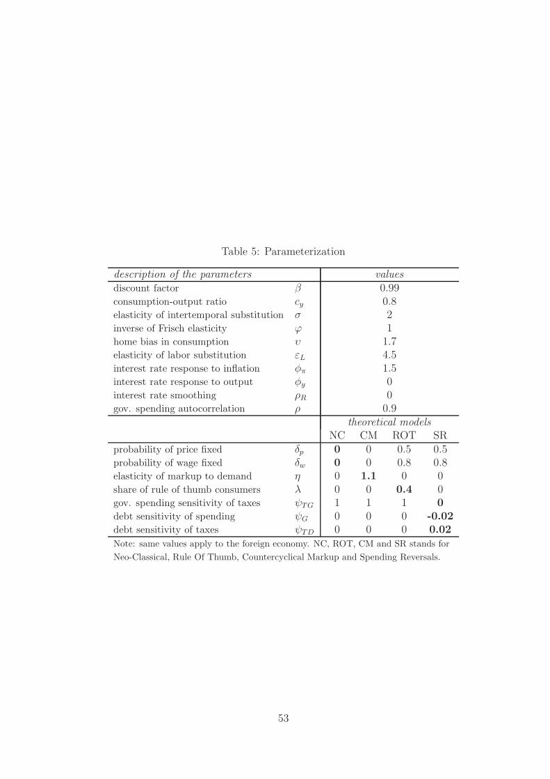
Table 5: Parameterization

description of the parameters valuesdiscount factor β 0.99consumption-output ratio cy 0.8elasticity of intertemporal substitution σ 2inverse of Frisch elasticity ϕ 1home bias in consumption υ 1.7elasticity of labor substitution εL 4.5interest rate response to inflation φπ 1.5interest rate response to output φy 0interest rate smoothing ρR 0gov. spending autocorrelation ρ 0.9

theoretical modelsNC CM ROT SR

probability of price fixed δp 0 0 0.5 0.5probability of wage fixed δw 0 0 0.8 0.8elasticity of markup to demand η 0 1.1 0 0share of rule of thumb consumers λ 0 0 0.4 0gov. spending sensitivity of taxes ψTG 1 1 1 0

debt sensitivity of spending ψG 0 0 0 -0.02

debt sensitivity of taxes ψTD 0 0 0 0.02

Note: same values apply to the foreign economy. NC, ROT, CM and SR stands for

Neo-Classical, Rule Of Thumb, Countercyclical Markup and Spending Reversals.

53

price adjustment of two quarters. In addition, we assume that in each quarter, the probability

that a household experiences a nominal wage change is 20%, implying a coefficient of δw = 0.8.This number lies within the range of values consistent with estimates by Barattieri, Basu and

Gottshalk (2014) and Gertler, Sala and Trigari (2008). The share of rule of thumb consumersin the third model is equal to 0.4, consistent with evidence in Campbell and Mankiw (1989),

and Misra and Surico (2014). The last column refers to the spending reversals model, whichrelaxes the assumption of a balanced government budget at each point in time by allowing

spending and taxes to depend on the level of real debt in a way that is consistent with theevidence in Galı and Perotti (2003). The parameters governing the evolution of government

spending and taxation are calibrated along the lines of Corsetti, Meier and Muller (2010).13

To illustrate differences and similarities across the three specifications and the neo-classical

benchmark, Table 5 makes clear that in each column there is only one specific mechanismat play for the transmission of fiscal policy, as the relevant parameters associated with the

identifying features of the other models are set so as to shut down those alternative channels.

D.2 Dynamic responses to a government spending shock

In Figure 13, we present the dynamic responses of domestic and foreign variables to adomestic government spending shock in the neo-classical benchmark and the three specifi-

cations augmented according to the parameter values in the last three columns of Table ??.The blue solid line refers to the neo-classical transmission mechanism and the red dots to the

model with countercyclical mark-up. As for the new-Keynesian models, the purple circlesand green squares denote the impulse responses associated with the existence of rule of thumb

consumers and spending reversals, respectively.

13As discussed in Corsetti, Meier and Mueller (2010), a coefficient of ψTD = 0.02 ensures the stationarityof debt even in the absence of spending reversals, i.e., it ensures that the condition (1 − ψTD)/β < 1 holdsat the calibrated equilibrium.

54

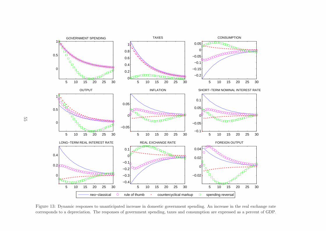
5 10 15 20 25 30

0

0.5

1GOVERNMENT SPENDING

5 10 15 20 25 300

0.2

0.4

0.6

0.8

1

TAXES

5 10 15 20 25 30

−0.2

−0.15

−0.1

−0.05

0

0.05

CONSUMPTION

5 10 15 20 25 30

0

0.5

1

OUTPUT

5 10 15 20 25 30

−0.05

0

0.05

INFLATION

5 10 15 20 25 30−0.1

−0.05

0

0.05

0.1

SHORT−TERM NOMINAL INTEREST RATE

5 10 15 20 25 30

0

0.2

0.4

LONG−TERM REAL INTEREST RATE

5 10 15 20 25 30−0.4

−0.3

−0.2

−0.1

0

0.1

REAL EXCHANGE RATE

5 10 15 20 25 30

−0.02

0

0.02

0.04

FOREIGN OUTPUT

neo−classical rule of thumb countercyclical markup spending reversal

Figure 13: Dynamic responses to unanticipated increase in domestic government spending. An increase in the real exchange rate

corresponds to a depreciation. The responses of government spending, taxes and consumption are expressed as a percent of GDP.

55

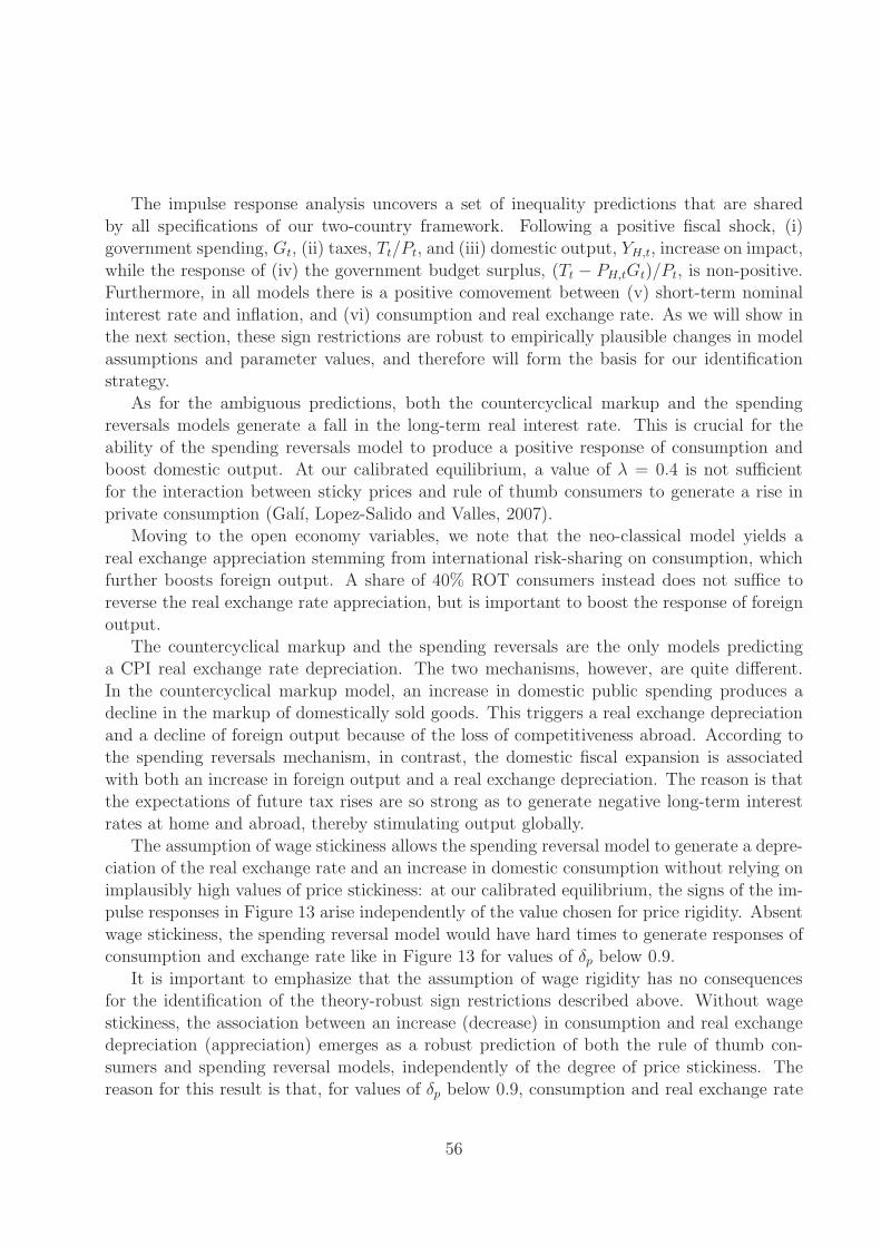
The impulse response analysis uncovers a set of inequality predictions that are shared

by all specifications of our two-country framework. Following a positive fiscal shock, (i)government spending, Gt, (ii) taxes, Tt/Pt, and (iii) domestic output, YH,t, increase on impact,

while the response of (iv) the government budget surplus, (Tt − PH,tGt)/Pt, is non-positive.Furthermore, in all models there is a positive comovement between (v) short-term nominal

interest rate and inflation, and (vi) consumption and real exchange rate. As we will show inthe next section, these sign restrictions are robust to empirically plausible changes in model

assumptions and parameter values, and therefore will form the basis for our identificationstrategy.

As for the ambiguous predictions, both the countercyclical markup and the spendingreversals models generate a fall in the long-term real interest rate. This is crucial for the

ability of the spending reversals model to produce a positive response of consumption andboost domestic output. At our calibrated equilibrium, a value of λ = 0.4 is not sufficient

for the interaction between sticky prices and rule of thumb consumers to generate a rise in

private consumption (Galı, Lopez-Salido and Valles, 2007).Moving to the open economy variables, we note that the neo-classical model yields a

real exchange appreciation stemming from international risk-sharing on consumption, whichfurther boosts foreign output. A share of 40% ROT consumers instead does not suffice to

reverse the real exchange rate appreciation, but is important to boost the response of foreignoutput.

The countercyclical markup and the spending reversals are the only models predictinga CPI real exchange rate depreciation. The two mechanisms, however, are quite different.

In the countercyclical markup model, an increase in domestic public spending produces adecline in the markup of domestically sold goods. This triggers a real exchange depreciation

and a decline of foreign output because of the loss of competitiveness abroad. According tothe spending reversals mechanism, in contrast, the domestic fiscal expansion is associated

with both an increase in foreign output and a real exchange depreciation. The reason is thatthe expectations of future tax rises are so strong as to generate negative long-term interest

rates at home and abroad, thereby stimulating output globally.

The assumption of wage stickiness allows the spending reversal model to generate a depre-ciation of the real exchange rate and an increase in domestic consumption without relying on

implausibly high values of price stickiness: at our calibrated equilibrium, the signs of the im-pulse responses in Figure 13 arise independently of the value chosen for price rigidity. Absent

wage stickiness, the spending reversal model would have hard times to generate responses ofconsumption and exchange rate like in Figure 13 for values of δp below 0.9.

It is important to emphasize that the assumption of wage rigidity has no consequencesfor the identification of the theory-robust sign restrictions described above. Without wage

stickiness, the association between an increase (decrease) in consumption and real exchangedepreciation (appreciation) emerges as a robust prediction of both the rule of thumb con-

sumers and spending reversal models, independently of the degree of price stickiness. Thereason for this result is that, for values of δp below 0.9, consumption and real exchange rate

56

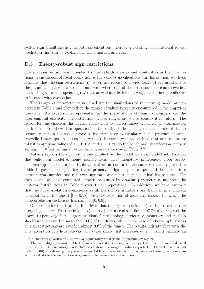
switch sign simultaneously in both specifications, thereby generating an additional robust

prediction that can be exploited in the empirical analysis.

D.3 Theory-robust sign restrictions

The previous section was intended to illustrate differences and similarities in the interna-

tional transmission of fiscal policy across the various specifications. In this section, we checkformally that the sign-restrictions (i) to (vi) are robust to a wide range of perturbations of

the parameter space in a nested framework where rule of thumb consumers, countercyclicalmarkups, government spending reversals as well as stickiness in wages and prices are allowed

to interact with each other.

The ranges of parameter values used for the simulations of the nesting model are re-ported in Table 2 and they reflect the ranges of values typically encountered in the empirical

literature. An exception is represented by the share of rule of thumb consumers and theintertemporal elasticity of substitution, whose ranges are set to conservative values. The

reason for this choice is that higher values lead to indeterminacy whenever all transmissionmechanisms are allowed to operate simultaneously. Indeed, a high share of rule of thumb

consumers makes the model prone to indeterminacy, particularly in the presence of coun-tercyclical markups. As a sensitivity check, however, we have verified that our results are

robust to applying values of λ ∈ [0, 0.3] and σ ∈ [1, 20] to the benchmark specification, namelysetting η = 0 but letting all other parameters to vary as in Table 2.14

Table 7 reports the sign restrictions implied by the model for an extended set of shocksthat buffet our model economy, namely fiscal, TFP, monetary, preferences, labor supply

and markup shocks. In this table we restrict attention to the same variables reported inTable 1: government spending, taxes, primary budget surplus, output and the correlations

between consumption and real exchange rate, and inflation and nominal interest rate. For

each shock, we have computed impulse responses by drawing parameter values from theuniform distributions in Table 2 over 10,000 repetitions. In addition, we have assumed

that the autocorrelation coefficients for all the shocks in Table 7 are drawn from a uniformdistribution with support [0.7, 0.98], with the exception of monetary shocks, for which the

autocorrelation coefficient has support [0, 0.9] .Our results for the fiscal shock indicate that the sign restrictions (i) to (iv) are satisfied in

every single draw. The restrictions (v) and (vi) are instead satisfied in 97.7% and 99.4% of thedraws, respectively.15 All sign restrictions for technology, preference, monetary and markup

shocks were satisfied in more than 99% of the draws, while in the case of labor supply shocksall sign restrictions are satisfied almost 99% of the times. The results indicate that with the

only exception of a fiscal shocks, any other shock that increases output would generate an

14In this setting values of λ above 0.3 significantly enlarge the indeterminacy region.15The inequality constraints (i) to (vi) are also robust to two significant departures from the model derived

in Section 2: (i) non-unitary trade elasticities along the range of values reported by Corsetti, Dedola andLeduc (2008), (ii) drawing the parameters in Table 2 independently for the home and foreign economies soas to break down the assumption of symmetry between the two countries.

57

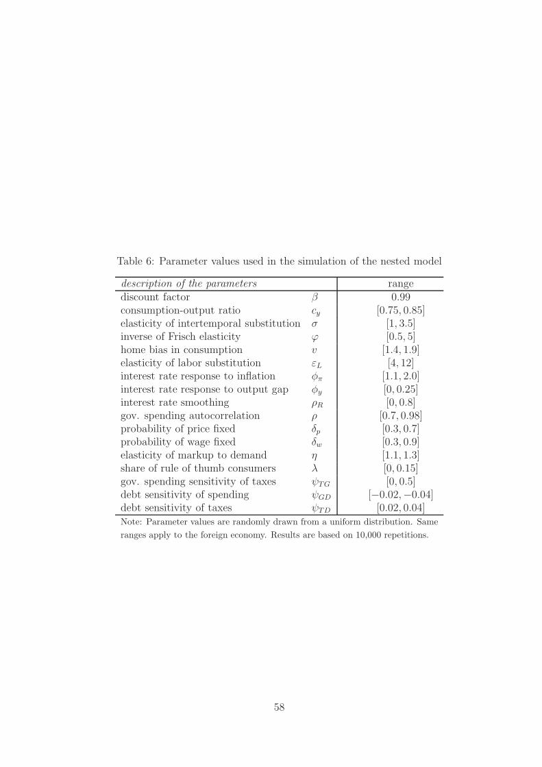
Table 6: Parameter values used in the simulation of the nested model

description of the parameters rangediscount factor β 0.99consumption-output ratio cy [0.75, 0.85]elasticity of intertemporal substitution σ [1, 3.5]inverse of Frisch elasticity ϕ [0.5, 5]home bias in consumption v [1.4, 1.9]elasticity of labor substitution εL [4, 12]interest rate response to inflation φπ [1.1, 2.0]interest rate response to output gap φy [0, 0.25]interest rate smoothing ρR [0, 0.8]gov. spending autocorrelation ρ [0.7, 0.98]probability of price fixed δp [0.3, 0.7]probability of wage fixed δw [0.3, 0.9]elasticity of markup to demand η [1.1, 1.3]share of rule of thumb consumers λ [0, 0.15]gov. spending sensitivity of taxes ψTG [0, 0.5]debt sensitivity of spending ψGD [−0.02,−0.04]debt sensitivity of taxes ψTD [0.02, 0.04]Note: Parameter values are randomly drawn from a uniform distribution. Same

ranges apply to the foreign economy. Results are based on 10,000 repetitions.

58

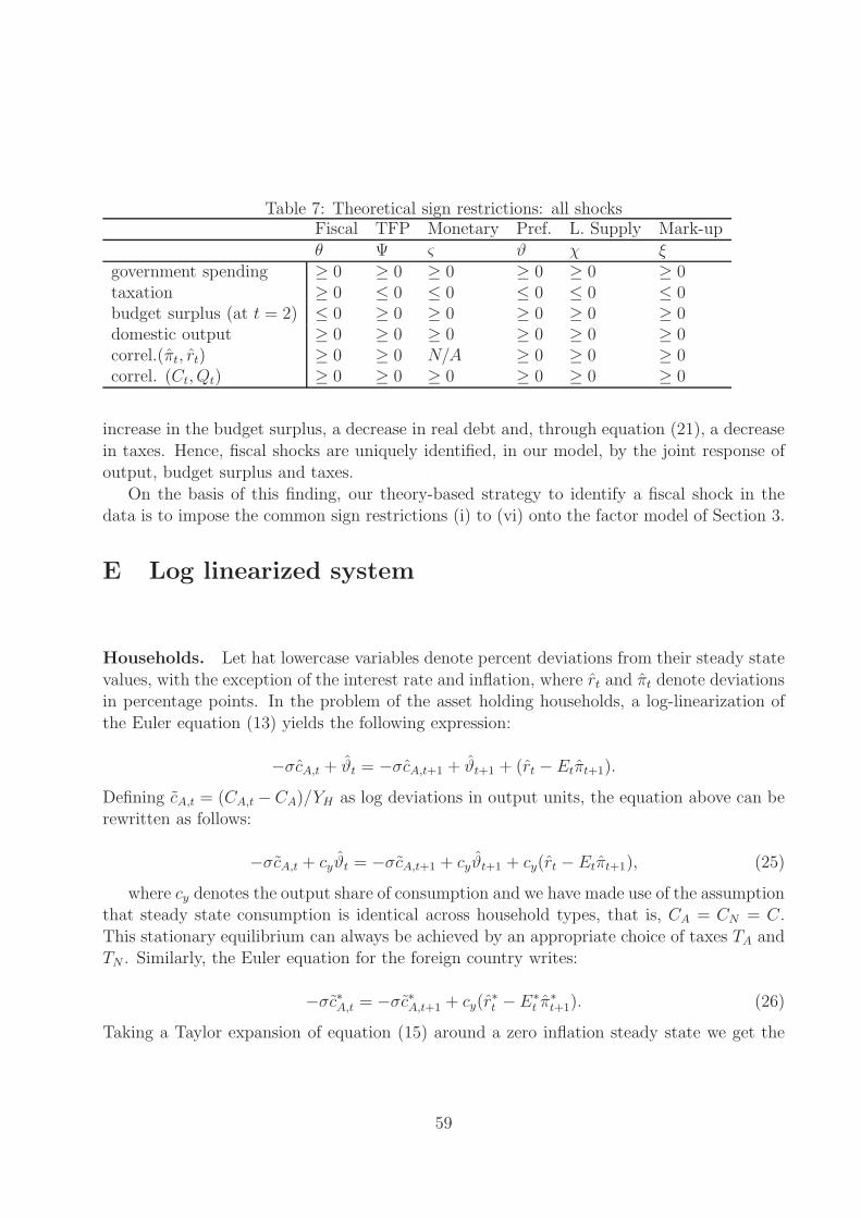
Table 7: Theoretical sign restrictions: all shocksFiscal TFP Monetary Pref. L. Supply Mark-upθ Ψ ς ϑ χ ξ

government spending ≥ 0 ≥ 0 ≥ 0 ≥ 0 ≥ 0 ≥ 0taxation ≥ 0 ≤ 0 ≤ 0 ≤ 0 ≤ 0 ≤ 0budget surplus (at t = 2) ≤ 0 ≥ 0 ≥ 0 ≥ 0 ≥ 0 ≥ 0domestic output ≥ 0 ≥ 0 ≥ 0 ≥ 0 ≥ 0 ≥ 0correl.(πt, rt) ≥ 0 ≥ 0 N/A ≥ 0 ≥ 0 ≥ 0correl. (Ct, Qt) ≥ 0 ≥ 0 ≥ 0 ≥ 0 ≥ 0 ≥ 0

increase in the budget surplus, a decrease in real debt and, through equation (21), a decrease

in taxes. Hence, fiscal shocks are uniquely identified, in our model, by the joint response ofoutput, budget surplus and taxes.

On the basis of this finding, our theory-based strategy to identify a fiscal shock in thedata is to impose the common sign restrictions (i) to (vi) onto the factor model of Section 3.

E Log linearized system

Households. Let hat lowercase variables denote percent deviations from their steady state

values, with the exception of the interest rate and inflation, where rt and πt denote deviationsin percentage points. In the problem of the asset holding households, a log-linearization of

the Euler equation (13) yields the following expression:

−σcA,t + ϑt = −σcA,t+1 + ϑt+1 + (rt − Etπt+1).

Defining cA,t = (CA,t − CA)/YH as log deviations in output units, the equation above can berewritten as follows:

−σcA,t + cyϑt = −σcA,t+1 + cyϑt+1 + cy(rt − Etπt+1), (25)

where cy denotes the output share of consumption and we have made use of the assumptionthat steady state consumption is identical across household types, that is, CA = CN = C.

This stationary equilibrium can always be achieved by an appropriate choice of taxes TA andTN . Similarly, the Euler equation for the foreign country writes:

−σc∗A,t = −σc∗A,t+1 + cy(r∗t −E∗

t π∗t+1). (26)

Taking a Taylor expansion of equation (15) around a zero inflation steady state we get the

59

following wage setting rule:

w∗t = (1− βδ)

∞∑

s=0

(βδ)sEtmrsA,t+s|t + pt+s

,

where µw = ln εLεL−1

. Using mrsA,t = χt + σcA,t + ϕlA,t and a log-linear approximation of thelabor demand equation (10) we can write:

mrsA,t+s|t = mrsA,t+s + ϕ(lA,t+s|t − lA,t+s

)= mrsA,t+s − εLϕ (w∗

t − wt+s) .

Combining the two equations above and rearranging we get:

w∗t =

1− βδ

1 + εϕ(mrsA,t + pt + εϕwt) + βδEtw

∗t+1

A log linear approximation of the wage index reads as follows:

wt = δwwt−1 + (1− δw)w∗t .

These last two equations can be combined to get the wage Phillips Curve:

πwt = κw(σcA,t + cyχt + cyϕlA,t − cyw

rt

)+ βEtπ

wt+1, (27)

where κw = (1−βδ)(1−δ)δ[1+εLϕ]

and wrt denotes deviations of the real wage from its steady-state value.

The wage inflation equation for the foreign country reads:

πw∗t = κw(σc∗A,t + cyϕl

∗A,t − cyw

r∗t

)+ βEtπ

w∗t+1. (28)

In addition, the change in the real wage can be expressed as the difference between nominal

wage inflation and CPI inflation:

wrt = wrt−1 + πwt − πt, (29)

In the foreign country, the following symmetric equation holds:

wr∗t = wr∗t−1 + πw∗t − π∗t . (30)

The budget constraint for the ROT consumers in equation (16) can be linearized as follows:

YH cN,t =WLNP

(wrt + lN,t

)− YH tax

r

t ,

where taxr

t =(TN,t/Pt−TN/P)

YH. Since LA = LN = L, the above equation can be rewritten as:

cN,t = wrt + lN,t − taxr

t . (31)

60

An analogous equation will determine consumption for the ROT households in the foreign

country:c∗N,t = wr∗t + l∗N,t − tax

r∗

t . (32)

Since forward-looking and ROT consumers are paid the same wage and face the same labor

demand schedule, their labor supply will be identical, both in the home and in the foreigncountry:

lN,t = lA,t, (33)

l∗N,t = l∗A,t. (34)

From the problem of the asset holding households, the interest rate parity condition in equa-

tion (14) can be linearized and written:

σct − cyϑt = σc∗t + cy(v − 1)τt. (35)

Firms. The linearized production function for the home and the foreign countries can be

written as follows:

yt = Ψt + lt, (36)

y∗t = l∗t . (37)

Using the first order condition in equation (8) and the law of motion for the price index in

equation (9) we can derive the Phillips curve for the home and the foreign economy:

πH,t =(1− βδp) (1− δp)

δp

[wrt − ηyt +

(1−

v

2

)τt

]+ EtβπHt+1, (38)

πF,t =(1− βδp) (1− δp)

δp

[wr∗t − ηy∗t −

(1−

v

2

)τt

]+ EtβπF,t+1. (39)

Term structure. A log-linearization of equation (18) around the stationary equilibriumcan be used to express the real yield on a bond of infinite duration expressed in deviations

from the steady state and denoted by rrt , as the infinite sum of expected short-term real rates:

rrt = Et

∞∑

j=0

(rrt+j − πt+1

).

Iterating forward on equation (25), and using the assumption that the model is stationaryand therefore consumption reverts to its steady state value (i.e., lims→∞ ct+s = 0), rrt can be

rewritten as a function of consumption in log deviations from output:

rrt =−σcA,tcy

. (40)

A similar relationship holds for the foreign country:

rr∗t =−σc∗A,tcy

. (41)

61

Price indices, terms of trade and real exchange rate. Having defined the real ex-

change rate as Qt = StP∗t /Pt and home terms of trade as Tt = StP

∗F,t/PH,t, substituting the

price indices into Qt it is possible to derive the following linearized relationship:

qt = (v − 1) τt (42)

Using the definition of the price indices it is possible to derive the following expressions for

domestic and foreign CPI inflation:

πt = πH,t +(1−

v

2

)(τt − τt−1) , (43)

π∗t = πF,t −

(1−

v

2

)(τt − τt−1) . (44)

Monetary and fiscal policies. Linearizing the Taylor rule in equation (17) yields the two

following expressions for the home and the foreign country:

rt = ρRrt−1 + (1− ρR)[φππt + φyyy

]+ ςt, (45)

r∗t = ρRr∗t−1 + (1− ρR)

[φππ

∗t + φyy

∗y

]. (46)

Denoting gt = (Gt −G) /YH and drt = Dt/ (Pt−1YH), the government spending feedback rulein (20) becomes for the home and the foreign country:

gt = ρGgt−1 + ψGDdrt + et, (47)

g∗t = ρGg∗t−1 + ψGDd

r∗t . (48)

Linearizing the tax feedback rule in equation (21) yields the following expressions for thehome and the foreign country:

taxr

t = ψTG

[gt − (1− cy)

(1−

v

2

)τt

]+ ψTDd

rt , (49)

taxr∗

t = ψTG

[g∗t + (1− cy)

(1−

v

2

)τt

]+ ψTDd

r∗t . (50)

The log-linearized conditions for the domestic government budget constraint in equation (19)can be written as follows:

βdrt = drt−1 − (1− cy)(1−

v

2

)τt−1 + gt−1 − tax

r

t−1. (51)

A similar condition holds for the foreign country:

βdr∗t = dr∗t−1 + (1− cy)(1−

v

2

)τt−1 + g∗t−1 − tax

r∗

t−1. (52)

62

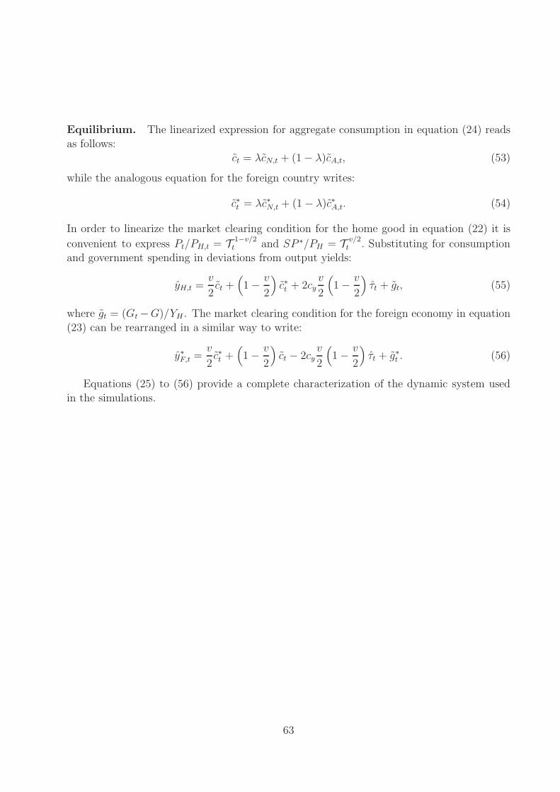
Equilibrium. The linearized expression for aggregate consumption in equation (24) reads

as follows:ct = λcN,t + (1− λ)cA,t, (53)

while the analogous equation for the foreign country writes:

c∗t = λc∗N,t + (1− λ)c∗A,t. (54)

In order to linearize the market clearing condition for the home good in equation (22) it is

convenient to express Pt/PH,t = T1−v/2t and SP ∗/PH = T

v/2t . Substituting for consumption

and government spending in deviations from output yields:

yH,t =v

2ct +

(1−

v

2

)c∗t + 2cy

v

2

(1−

v

2

)τt + gt, (55)

where gt = (Gt−G)/YH . The market clearing condition for the foreign economy in equation

(23) can be rearranged in a similar way to write:

y∗F,t =v

2c∗t +

(1−

v

2

)ct − 2cy

v

2

(1−

v

2

)τt + g∗t . (56)

Equations (25) to (56) provide a complete characterization of the dynamic system used

in the simulations.

63

International Fiscal Spillovers - QMRO Home

Documents