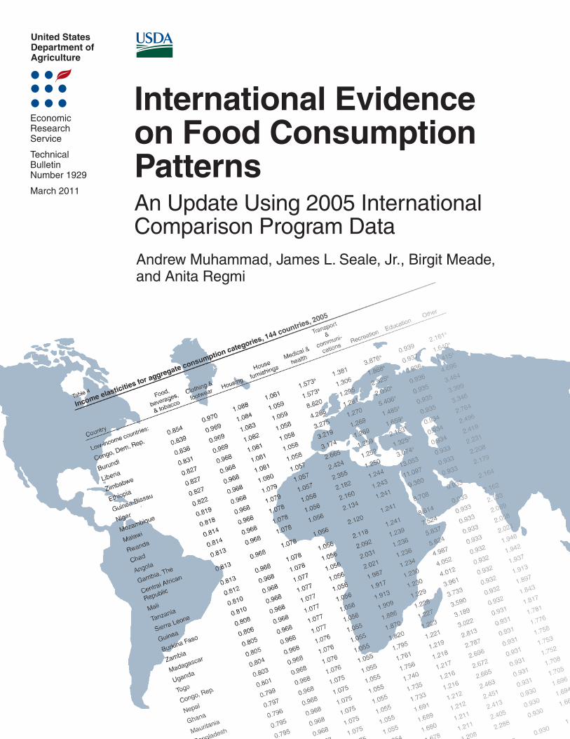
United States Department of Agriculture Economic Research Service Technical Bulletin Number 1929 March 2011 Andrew Muhammad, James L. Seale, Jr., Birgit Meade, and Anita Regmi International Evidence on Food Consumption Patterns An Update Using 2005 International Comparison Program Data

Welcome message from author
This document is posted to help you gain knowledge. Please leave a comment to let me know what you think about it! Share it to your friends and learn new things together.
Transcript
United StatesDepartment ofAgriculture
EconomicResearchService
TechnicalBulletinNumber 1929
March 2011
Andrew Muhammad, James L. Seale, Jr., Birgit Meade, and Anita Regmi
International Evidence on Food Consumption PatternsAn Update Using 2005 International Comparison Program Data
The U.S. Department of Agriculture (USDA) prohibits discrimination in all its programs and activities on the basis of race, color, national origin, age, disability, and, where applicable, sex, marital status, familial status, parental status, religion, sexual orientation, genetic information, political beliefs, reprisal, or because all or a part of an individual's income is derived from any public assistance program. (Not all prohibited bases apply to all programs.) Persons with disabilities who require alternative means for communication of program information (Braille, large print, audiotape, etc.) should contact USDA's TARGET Center at (202) 720-2600 (voice and TDD).
To file a complaint of discrimination write to USDA, Director, Office of Civil Rights, 1400 Independence Avenue, S.W., Washington, D.C. 20250-9410 or call (800) 795-3272 (voice) or (202) 720-6382 (TDD). USDA is an equal opportunity provider and employer.
ww
ww
w.wwer
sr .usda.govoo
Visit Our Website To Learn More!
www.ers.usda.gov/
Recommended citation format for this publication:
Muhammad, Andrew, James L. Seale, Jr., Birgit Meade,and Anita Regmi. International Evidence on Food Consumption Patterns: An Update Using 2005 International Comparison Program Data. TB-1929. U.S. Dept. of Agriculture, Econ. Res. Serv. March 2011.
i International Evidence on Food Consumption Patterns: An Update Using 2005 International Comparison Program Data / TB-1929
Economic Research Service / USDA
United States Department of Agriculture
www.ers.usda.gov
A Report from the Economic Research Service
Technical BulletinNumber 1929
March 2011
International Evidence on Food Consumption PatternsAn Update Using 2005 International Comparison Program Data
Abstract
In a 2003 report, International Evidence on Food Consumption Patterns, ERS econo-mists estimated income and price elasticities of demand for broad consumption catego-ries and food categories across 114 countries using 1996 International Comparison Program (ICP) data. This report updates that analysis with an estimated two-stage demand system across 144 countries using 2005 ICP data. Advances in ICP data collec-tion since 1996 led to better results and more accurate income and price elasticity esti-mates. Low-income countries spend a greater portion of their budget on necessities, such as food, while richer countries spend a greater proportion of their income on luxuries, such as recreation. Low-value staples, such as cereals, account for a larger share of the food budget in poorer countries, while high-value food items are a larger share of the food budget in richer countries. Overall, low-income countries are more responsive to changes in income and food prices and, therefore, make larger adjustments to their food consumption pattern when incomes and prices change. However, adjustments to price and income changes are not uniform across all food categories. Staple food consumption changes the least, while consumption of higher-value food items changes the most.
Andrew Muhammad, [email protected] James L. Seale, Jr. Birgit Meade, [email protected] Regmi
iiInternational Evidence on Food Consumption Patterns: An Update Using 2005 International Comparison Program Data / TB-1929
Economic Research Service / USDA
Contents
Summary . . . . . . . . . . . . . . . . . . . . . . . . . . . . . . . . . . . . . . . . . . . . . . . . . . . iii
Introduction . . . . . . . . . . . . . . . . . . . . . . . . . . . . . . . . . . . . . . . . . . . . . . . . . . 1
International Comparison Program Data . . . . . . . . . . . . . . . . . . . . . . . . . . . . 2
Two-Stage Cross-Country Demand Model . . . . . . . . . . . . . . . . . . . . . . . . . . 6
Estimation Procedure and Results . . . . . . . . . . . . . . . . . . . . . . . . . . . . . . . . 11
Conclusion . . . . . . . . . . . . . . . . . . . . . . . . . . . . . . . . . . . . . . . . . . . . . . . . . . 19
References . . . . . . . . . . . . . . . . . . . . . . . . . . . . . . . . . . . . . . . . . . . . . . . . . . 20
iii International Evidence on Food Consumption Patterns: An Update Using 2005 International Comparison Program Data / TB-1929
Economic Research Service / USDA
Summary
In a 2003 report, International Evidence on Food Consumption Patterns, ERS and collaborating economists estimated income and price elasticities of demand for broad consumption categories—such as food, clothing, educa-tion, and other goods—and for food categories such as cereals, meats, and dairy across 114 countries using 1996 International Comparison Program (ICP) data. These elasticities measure the degree to which consumption changes when prices or incomes change. The estimates have been widely used in economic models such as the USDA’s Baseline model, the Global Trade Analysis Project (GTAP) model, and the International Food Policy Research Institute’s IMPACT model. This report updates that analysis with a similar two-stage demand system using 2005 ICP data.
What Is the Issue?
An understanding of food demand and food trends across countries, and the ability to predict potential shifts in demand for different food products, are invaluable tools. The most prominent measures of food consumption behavior are income and price elasticities. A number of studies have esti-mated income and price elasticities using 1996 ICP data and data from years prior. However, advances in ICP data collection since 1996 should lead to better results and more accurate income and price elasticity estimates. Furthermore, the most recent ICP data round (2005) includes a greater number of countries, like developing countries in Sub-Saharan Africa, as well as China and India.
What Did the Study Find?
•Low-income countries allocate a greater portion of additional income to food. As countries become more affluent, more is allocated to luxury categories like recreation. For instance, a dollar increase in income would cause food expenditures in the Democratic Republic of Congo to increase by 63 cents, but only by 6 cents in the United States. In contrast, recreation expenditures in the Democratic Republic of Congo would not increase at all, while in the United States recreation expenditures would increase by 13 cents.
•The share of total budget allocated to housing is lowest in low-income countries and fairly similar in middle- and high-income countries, while the budget share on house furnishings is fairly similar across all income groups. Spending on health clearly rises with income, from 4.5 percent of the average household budget in low-income countries to 8.9 percent in high-income countries.
•The income elasticity of demand for food varies greatly among countries and is highest among low-income countries, where it varies from 0.85 for the Democratic Republic of Congo to 0.71 for Tunisia. It ranges between 0.71 and 0.57 for middle-income countries, and from 0.56 to 0.35 for high-income countries. The average income elasticity for low-income countries is 0.78, over 1.5 times the average for high-income countries.
ivInternational Evidence on Food Consumption Patterns: An Update Using 2005 International Comparison Program Data / TB-1929
Economic Research Service / USDA
•With affluence, the portion of additional food expenditures allocated to cereals and other staples decreases. For instance, a dollar increase in food expenditures results in cereal expenditures in the Democratic Republic of Congo increasing by 31 cents. By contrast, cereal expenditures in the United States would actually decrease by 2 cents, indicating the lower status afforded this food category by most consumers in rich countries.
•The own-price elasticities (holding marginal utility of income constant) for the food subcategories vary by affluence according to economic theory; low-income countries are more responsive to price changes compared with higher-income countries. For instance, the own-price elasticity value for breads and cereals ranges from -0.50 for the Democratic Republic of Congo to near zero for the United States.
•Overall, low-income countries are more responsive to changes in income and food prices and, therefore, make larger adjustments to their food consumption pattern when incomes and prices change.
•Unlike previous ICP data, restaurant and catering expenditures are included among food in the 2005 data. Consequently, our estimates of the income elasticity of demand for food in high-income countries are larger than the estimates in Seale et al. (2003, derived using 1996 ICP data). We find that the average income elasticity for high-income countries is 0.50, while Seale et al. found it to be 0.34.
How Was the Study Conducted?
We estimate a two-stage demand system using 2005 ICP data. We analyze demand across 144 countries. The first stage involves estimating an aggre-gate demand system using the Florida-Preference Independence model across nine broad consumption categories: food—which includes food prepared and consumed at home, food away from home, and beverages and tobacco—clothing and footwear, education, housing, house furnishings and operations, medical care, transportation and communications, recreation, and other expenditures. The second stage of the analysis involves a second demand system using the Florida-Slutsky model to estimate demand across eight food subcategories: bread and cereals, meat, fish, dairy products, fruits and vegetables, oils and fats, beverages and tobacco, and other food prod-ucts. Estimates are used to derive income and price elasticities of demand for broad consumption categories and food categories by country.
1 International Evidence on Food Consumption Patterns: An Update Using 2005 International Comparison Program Data / TB-1929
Economic Research Service / USDA
Introduction
An understanding of food demand and food trends across countries and the ability to predict potential shifts in demand for different food products is an invaluable tool for all individuals involved in the agricultural sector. In an earlier ERS report, International Evidence on Food Consumption Patterns, Seale, Regmi, and Bernstein (2003) fit a two-stage demand system to 1996 International Comparison Program (ICP) data across 114 countries. In that report, Seale and his colleagues estimated income and own-price elasticities of demand for broad consumption categories—such as food, clothing, educa-tion, and other goods—and for food categories such as cereals, meats, dairy, and other food groups.
This report updates that analysis with a similar two-stage demand system using 2005 ICP data. In this study, we analyze demand across 144 countries and present income and price elasticities that can be used as inputs in future work to forecast food demand, as well as the need for housing, clothing, transportation, medical care, and other broad consumption categories. Consumers make food purchase decisions based on a budget that must also cover expenses for other goods and services. The budget available for food is dependent on the amount of income spent on these other goods and services. Therefore, an indepth study of food demand requires an understanding of the complete demand patterns of consumers. In this study, we present such a complete demand analysis where household decisionmaking is examined in two stages. In the first stage, a consumer is assumed to make budgetary deci-sions across broad consumption categories (food, housing, clothing, educa-tion, and other goods). In the second stage, the total food budget is further allocated to different food items. In conducting such a complete analysis, we provide demand estimates and income and own-price elasticities for nine broad consumption categories and eight food subcategories. These estimates are provided for countries ranging from low-income and developing, such as Zimbabwe, to high-income developed countries like Canada and the United States.
Advances in ICP data collection since the 1996 round should lead to better results and more accurate income and price elasticity estimates. The Inter- national Comparison Project started as a joint venture between the United Nations and the University of Pennsylvania, with the overall purpose of providing comparable Gross Domestic Product (GDP) data for a large number of consumption items across countries (World Bank, 2008; Kravis et al., 1975). The latest ICP round (2005) covers 146 countries; corrects for the scaling problem common to past ICP data as reported by Seale et al. (2003); and employs a new methodology to ensure data accuracy and consistency across the selected countries (Diewert, 2010). The elasticity esti-mates derived by Seale, Regmi, and Bernstein (2003) using 1996 ICP data have been widely used as input in economic models such as the USDA’s Baseline model, the Global Trade Analysis Project (GTAP) model (Reimer and Hertel (2003, 2004), the International Food Policy Research Institute’s IMPACT model, and others (see, for example, studies by Winters (2005), von Braun (2007), Hertel and Winters (2006), and Valenzuela et al. (2007)). Additionally, Cox and Alm (2007) used the parameter estimates from Seale et al. (2003) to derive elasticities based on 2006 expenditure data. The updated results in this report should prove equally valuable.
2International Evidence on Food Consumption Patterns: An Update Using 2005 International Comparison Program Data / TB-1929
Economic Research Service / USDA
International Comparison Program Data
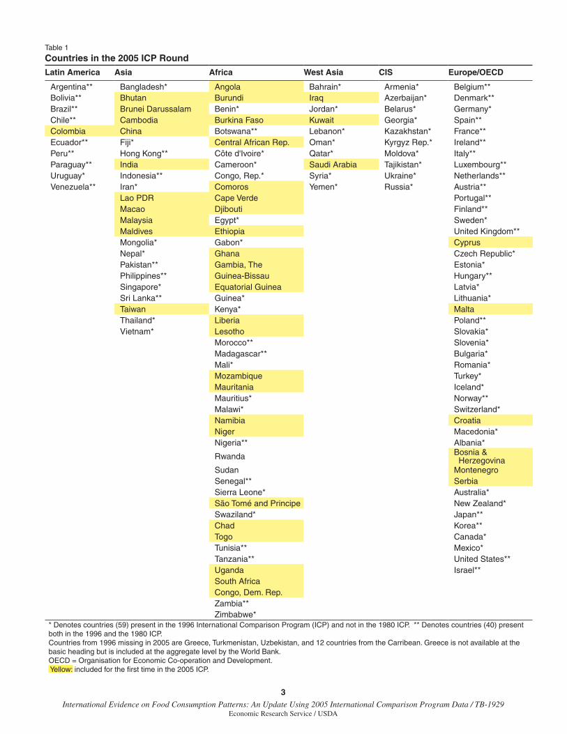
Expenditure and price data for the two-stage cross-country demand model were again obtained from the International Comparison Project, initiated in 1975 by researchers at the University of Pennsylvania (Kravis et al., 1978) and maintained by the ICP Development Data Group of the World Bank. Over the years, data collected by the ICP have increased from 10 countries in Phase I (1970) to 146 countries in 2005 (table 1). The elasticities presented in this report are based on modeling work that began with Theil, Chung, and Seale (1989) using the data from the first four phases, covering a total of 60 countries. Seale, Regmi, and Bernstein (2003) provided updates for existing countries and additional coverage based on 1996 data that included 65 more countries. However, 10 countries included in the earlier 3 phases were excluded in the 1996 data, resulting in a total of 115 countries, 114 of which were covered by Seale et al. (2003).
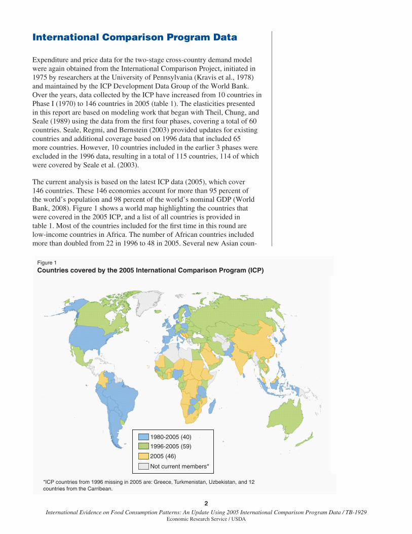
The current analysis is based on the latest ICP data (2005), which cover 146 countries. These 146 economies account for more than 95 percent of the world’s population and 98 percent of the world’s nominal GDP (World Bank, 2008). Figure 1 shows a world map highlighting the countries that were covered in the 2005 ICP, and a list of all countries is provided in table 1. Most of the countries included for the first time in this round are low-income countries in Africa. The number of African countries included more than doubled from 22 in 1996 to 48 in 2005. Several new Asian coun-
*ICP countries from 1996 missing in 2005 are: Greece, Turkmenistan, Uzbekistan, and 12 countries from the Carribean.
1980-2005 (40)
1996-2005 (59)
2005 (46)
Not current members*
Figure 1
Countries covered by the 2005 International Comparison Program (ICP)
3 International Evidence on Food Consumption Patterns: An Update Using 2005 International Comparison Program Data / TB-1929
Economic Research Service / USDA
Table 1
Countries in the 2005 ICP Round
Latin America Asia Africa West Asia CIS Europe/OECD
Argentina** Bangladesh* Angola Bahrain* Armenia* Belgium**Bolivia** Bhutan Burundi Iraq Azerbaijan* Denmark**Brazil** Brunei Darussalam Benin* Jordan* Belarus* Germany*Chile** Cambodia Burkina Faso Kuwait Georgia* Spain**Colombia China Botswana** Lebanon* Kazakhstan* France**Ecuador** Fiji* Central African Rep. Oman* Kyrgyz Rep.* Ireland**Peru** Hong Kong** Côte d'Ivoire* Qatar* Moldova* Italy**Paraguay** India Cameroon* Saudi Arabia Tajikistan* Luxembourg**Uruguay* Indonesia** Congo, Rep.* Syria* Ukraine* Netherlands**Venezuela** Iran* Comoros Yemen* Russia* Austria**
Lao PDR Cape Verde Portugal**Macao Djibouti Finland**Malaysia Egypt* Sweden*Maldives Ethiopia United Kingdom**Mongolia* Gabon* CyprusNepal* Ghana Czech Republic*Pakistan** Gambia, The Estonia*Philippines** Guinea-Bissau Hungary**Singapore* Equatorial Guinea Latvia*Sri Lanka** Guinea* Lithuania*Taiwan Kenya* MaltaThailand* Liberia Poland**Vietnam* Lesotho Slovakia*
Morocco** Slovenia*Madagascar** Bulgaria*Mali* Romania*Mozambique Turkey*Mauritania Iceland*Mauritius* Norway**Malawi* Switzerland*Namibia CroatiaNiger Macedonia*Nigeria** Albania*
Rwanda Bosnia & Herzegovina
Sudan MontenegroSenegal** SerbiaSierra Leone* Australia*São Tomé and Principe New Zealand*Swaziland* Japan**Chad Korea**Togo Canada*Tunisia** Mexico*Tanzania** United States**Uganda Israel**South AfricaCongo, Dem. Rep.Zambia**
Zimbabwe* * Denotes countries (59) present in the 1996 International Comparison Program (ICP) and not in the 1980 ICP. ** Denotes countries (40) present both in the 1996 and the 1980 ICP.Countries from 1996 missing in 2005 are Greece, Turkmenistan, Uzbekistan, and 12 countries from the Carribean. Greece is not available at the basic heading but is included at the aggregate level by the World Bank.OECD = Organisation for Economic Co-operation and Development. Yellow: included for the first time in the 2005 ICP.
4International Evidence on Food Consumption Patterns: An Update Using 2005 International Comparison Program Data / TB-1929
Economic Research Service / USDA
tries have been included, most notably China and India. In Latin America, Colombia has been added, while 12 Caribbean countries were excluded. The Commonwealth of Independent States no longer covers Turkmenistan and Uzbekistan. In West Asia, Iraq and Kuwait were added, while the countries added to the Eurostat/Organisation for Economic Co-operation and Development (OECD) group include Cyprus and Malta in addition to Croatia, Bosnia and Herzegovina, Montenegro, and Serbia.1
Problems in comparing expenditures across countries occur due to differ-ences in currency. Using exchange rates to convert expenditures to a single currency may not always be desirable since exchange rates fail to account for the fact that services are cheaper in developing countries. The 2005 ICP uses a new methodology to compare relative price levels and GDP levels across the 146 countries included in this round.2 This time, the world was divided into 6 regions: 5 geographic regions—Africa (48 countries included), Asia Pacific (23 countries), West Asia (11 countries), South America (10 countries), and the Commonwealth of Independent States (CIS) (10 coun-tries)—and the OECD and other European countries, plus Israel and Russia (46 countries). In earlier rounds, one product list was used for all countries covered, and prices for these products needed to be collected. However, consumption varies sufficiently across regions, making such a common product list impractical. For the 2005 round, each of the regions was able to develop its own product lists and determine its purchasing power parity (PPP) and volume shares independently. Later, the regional results were linked into a global world comparison model, which left the regional relative parities intact. The linking was accomplished by a methodology using 19 ring countries, thus providing representatives from each region.3
To facilitate the analysis, the 144 countries covered by the 2005 ICP are divided into low-, middle-, and high-income countries, based on their income relative to that of the United States.4 Low-income countries represent those with real per capita income less than 15 percent of the U.S. level, middle-income countries are those with income between 15 and 45 percent of the U.S. level, and high-income countries have per capita income equal to or greater than 45 percent of the U.S. level. This criterion for grouping indicates that the majority of Sub-Saharan African countries, poor transition econo-mies such as Mongolia and Turkmenistan, and low-income Middle Eastern and Asian countries such as Yemen and Nepal fall within the first group. High-income countries include most Western European countries, Australia, New Zealand, Canada, and the United States; while the middle-income countries include better-off transition economies such as Estonia, Hungary, Slovenia, North African countries, and many Latin American countries.
Budget Shares and Volume of Consumption5
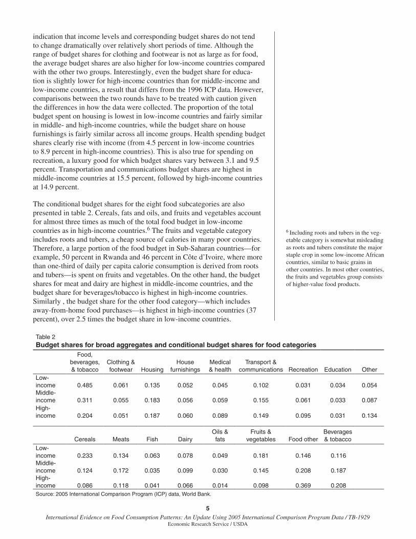
The average budget shares for the aggregate consumption categories and each of the three country groups are presented in table 2. In the past, the food grouping included food prepared and consumed at home, plus bever-ages and tobacco. In the 2005 ICP round, food for the first time includes food consumed away from home, captured under the “other food” category. As expected, the budget shares for food tend to decrease as incomes rise, ranging from over 73 percent of the total budget in Tanzania to about 14 percent in the United States. These shares are very close to those of the 1996 round, an
1India and Colombia were in ICP Phases I, II, III, and IV. They were not included in the 1996 ICP data.
2Regional total sums to 148 countries, but Egypt appears in both the African and West Asia regions and Russia appears in both the OECD and CIS regions. This discussion draws heav-ily on Diewert (2010), who provides detailed methodological information on the 2005 ICP.
3Ring countries serve as a small sample of countries stratified by regions that are both representative of their region and have available a wide range of goods and services found in countries outside of their region.4This classification facilitates analysis in this publication and is not based on any generally accepted criteria for classification. Since the classification is based on the ICP data used in this analysis, some countries may be in a group with which they normally would not be associated. Although the 2005 ICP covers 146 countries, Greece is not available at the basic heading level and Comoros was excluded from the analysis.
5For detailed data on volume of con-sumption, nominal expenditures, and budget shares for each country, see World Bank (2008).
5 International Evidence on Food Consumption Patterns: An Update Using 2005 International Comparison Program Data / TB-1929
Economic Research Service / USDA
indication that income levels and corresponding budget shares do not tend to change dramatically over relatively short periods of time. Although the range of budget shares for clothing and footwear is not as large as for food, the average budget shares are also higher for low-income countries compared with the other two groups. Interestingly, even the budget share for educa-tion is slightly lower for high-income countries than for middle-income and low-income countries, a result that differs from the 1996 ICP data. However, comparisons between the two rounds have to be treated with caution given the differences in how the data were collected. The proportion of the total budget spent on housing is lowest in low-income countries and fairly similar in middle- and high-income countries, while the budget share on house furnishings is fairly similar across all income groups. Health spending budget shares clearly rise with income (from 4.5 percent in low-income countries to 8.9 percent in high-income countries). This is also true for spending on recreation, a luxury good for which budget shares vary between 3.1 and 9.5 percent. Transportation and communications budget shares are highest in middle-income countries at 15.5 percent, followed by high-income countries at 14.9 percent.
The conditional budget shares for the eight food subcategories are also presented in table 2. Cereals, fats and oils, and fruits and vegetables account for almost three times as much of the total food budget in low-income countries as in high-income countries.6 The fruits and vegetable category includes roots and tubers, a cheap source of calories in many poor countries.
Therefore, a large portion of the food budget in Sub-Saharan countries—for example, 50 percent in Rwanda and 46 percent in Côte d’Ivoire, where more than one-third of daily per capita calorie consumption is derived from roots and tubers—is spent on fruits and vegetables. On the other hand, the budget shares for meat and dairy are highest in middle-income countries, and the budget share for beverages/tobacco is highest in high-income countries. Similarly , the budget share for the other food category—which includes away-from-home food purchases—is highest in high-income countries (37 percent), over 2.5 times the budget share in low-income countries.
6 Including roots and tubers in the veg-etable category is somewhat misleading as roots and tubers constitute the major staple crop in some low-income African countries, similar to basic grains in other countries. In most other countries, the fruits and vegetables group consists of higher-value food products.
Table 2Budget shares for broad aggregates and conditional budget shares for food categories
Food, beverages, & tobacco
Clothing & footwear Housing
House furnishings
Medical & health
Transport & communications Recreation Education Other
Low-income 0.485 0.061 0.135 0.052 0.045 0.102 0.031 0.034 0.054Middle-income 0.311 0.055 0.183 0.056 0.059 0.155 0.061 0.033 0.087High-income 0.204 0.051 0.187 0.060 0.089 0.149 0.095 0.031 0.134
Cereals Meats Fish DairyOils & fats
Fruits & vegetables Food other
Beverages & tobacco
Low-income 0.233 0.134 0.063 0.078 0.049 0.181 0.146 0.116Middle-income 0.124 0.172 0.035 0.099 0.030 0.145 0.208 0.187High-income 0.086 0.118 0.041 0.066 0.014 0.098 0.369 0.208Source: 2005 International Comparison Program (ICP) data, World Bank.
6International Evidence on Food Consumption Patterns: An Update Using 2005 International Comparison Program Data / TB-1929
Economic Research Service / USDA
Two-Stage Cross-Country Demand Model
Our analysis of international food consumption patterns is conducted in two steps. The first step involves estimating an aggregate demand system using the Florida-Preference Independence (PI) model across nine broad consump-tion categories: food—which includes food prepared and consumed at home, food away from home, and beverages and tobacco—clothing and footwear, education, housing, house furnishings and operations, medical care, transport and communications, recreation, and other expenditures. The second step of the analysis involves a second demand system using the Florida-Slutsky model across eight food subcategories: bread and cereals, meat, fish, dairy products, fruits and vegetables, oils and fats, beverages and tobacco, and other food products. Both the Florida-PI model and the Florida-Slutsky model are discussed in more detail later in this section.
Stepwise demand analysis, which assumes that consumers spend their income in stages, requires assumptions about the separability of consumer preferences. Consumer preferences are independent or strongly separable if the preference ordering among goods is not dependent on the quantities consumed of any other goods. This concept can be applied to broad product groups or categories and is referred to as block independence. Block inde-pendence or strong group separability implies that the preference ordering among items within one broad consumption group is not dependent on the quantities of items consumed in other groups. This assumption enables stepwise demand analysis, where in the first stage consumers allocate their incomes across broad categories of goods, like food, shelter, and entertain-ment. In the second stage, consumers spend the amount budgeted to a partic-ular product group on goods within the group.
While it is reasonable to assume that expenditures among broad consumption categories in the first stage of the budgeting process might be independent, demand for goods within the food product group may not be independent. For example, many food products are substitutes or complements and have cross-price effects. Therefore, when estimating the second stage of the model, preference independence is generally replaced by weak separability, which suggests that food categories are groupwise-dependent. In our analysis of the food categories, the Florida-Slutsky model assuming weak separability is used instead of the Florida-PI model.
Florida-Preference Independence (PI) Model
The Florida-PI model—also known as the Working-Preference Independence model—is an extension of the model developed by Working (1943). In its general form, Working’s model expresses budget shares as a linear function of real aggregate expenditures and is specified as follows:
. (1)
ii
Ew
E= is the budget share for good i, Ei represents the expenditure on good
i, and 1
ni
iE E
==∑ is real aggregate expenditures. iε is a residual term and
αi and βi are parameters to be estimated. Since the budget shares across
logi
i i i iE
w EE
α β ε= = + +
7 International Evidence on Food Consumption Patterns: An Update Using 2005 International Comparison Program Data / TB-1929
Economic Research Service / USDA
all consumption categories sum to 1, α and β are subject to the following adding-up conditions:
. (2)
From equation 1 we can derive the marginal share (θi), which is a measure of how an additional unit of expenditure is allocated to the ith good:
. (3)
Note that the marginal share is not constant but varies with affluence, and it exceeds the budget share (wi) by βi . Accordingly, when income changes, wi changes as does the marginal share.
Using the differential approach to consumer demand, Theil, Chung, and Seale (1989) incorporated prices into Working’s model to derive the Florida-PI model. The resulting specification can be divided into linear, quadratic, and cubic components, as indicated below:
wic = LINEAR + QUADRATIC + CUBIC + eic . (4a)
LINEAR = Real-income term
. (4b)
QUADRATIC = Pure-price term
= . (4c)
CUBIC = Substitution term
= . (4d)
The c subscript denotes the country. qc is the natural logarithm of Qc, which is a measure of real per capita income, and qc* = (1+qc).
1
1log log
N
i iccp p
N == ∑ , which is the geometric mean of the price of i (pi)
over all countries, and φ is the income flexibility coefficient—the inverse of
the income elasticity of the marginal utility of income—which is assumed constant in the model.
The linear term in the model represents the effect of a change in real income—that is, the volume of total expenditures—on the budget share. Since the quadratic and cubic terms vanish at geometric mean prices, the linear term is also the budget share at geometric mean prices. The quadratic term—quadratic because it contains products of α and β—is the pure-price term, showing how an increase in price results in a higher budget share on good i, even if the volume of expenditures goes down or stays the same. The cubic term—cubic because it involves φ—is a substitution term reflecting how higher prices cause a lower budget share for good i due to the substitu-tion of good i for other goods.
1 11; 0
n n
i ii iα β
= == =∑ ∑
(1 log )ii i i i i
dEE w
dEθ α β β= = + + = +
i i cqα β= +
( ) ( )1
log logn
jcici i c j j c
i jj
ppq q
p pα β α β
=
+ − +
∑
( ) ( )* *
1
log logn
jcici i c j j c
i jj
ppq q
p pφ α β α β
=
+ − +
∑
8International Evidence on Food Consumption Patterns: An Update Using 2005 International Comparison Program Data / TB-1929
Economic Research Service / USDA
The expenditure elasticity for the Florida-PI model is calculated by the ratio of the marginal share to the budget share as follows (see Theil et al., 1989, pp. 110-111 for derivation):
, (5)
where, in this case, icw represents the budget share of good i at geometric mean prices, c represents the country, θic is the marginal share of good i in country c, and βi is the estimated coefficient on qc in the ith good equation.7
Three types of own-price elasticities of demand can be calculated from the parameter estimates in the Florida-PI model. The first of these, the Frisch-deflated own-price elasticity of good i, is the own-price elasticity when price changes and income is compensated to keep the marginal utility of income constant. It is given by:
. (6)
The Slutsky (compensated) own-price elasticity measures the change in demand for good i when the price of i changes, while real income remains unchanged. It is calculated as follows:
. (7)
The Cournot (uncompensated) own-price elasticity refers to the situation when own-price changes while nominal income remains constant but real income changes, and is given by:
. (8)
How each elasticity measure is applied depends on the needs of the researcher. For instance, the Slutsky elasticity is more suitable if the concern is the substitution effect of a change in price, while the Cournot elasticity encompasses both the substitution and real income effect. Consequently, the Slutsky elasticity will be smaller than the Cournot elasticity (in absolute value) for a normal good because the real income effect reinforces the substi-tution effect. However, the difference between these two measures declines with affluence since the real income effect decreases with rising income. The (absolute) value of the Frisch elasticity is between the Slutsky and Cournot elasticity. The three elasticities can be significantly different for low-income countries, but are relatively close for high-income countries.
log1
logic ic i
icc ic ic
d Ed E w w
θ βη = = = +
7Because expenditures in this instance are spending on all product categories, equation (5) is also referred to as the income elasticity.
ic i
ic
wF
wβ
φ+
=
( )( )( )
11ic i ic i
ic iic
w wS F w
wβ β
φ β+ − −
= = − −
( )( )( ) ( )
1ic i ic iic i ic i
ic
w wC w S w
wβ β
φ β β+ − −
= − + = − +
9 International Evidence on Food Consumption Patterns: An Update Using 2005 International Comparison Program Data / TB-1929
Economic Research Service / USDA
Florida-Slutsky Model
The Florida-Slutsky model is used to estimate the second stage of the model, the food subcategories. Like the Florida-PI model, the Florida-Slutsky model has three components: a linear real-income term, a quadratic pure-price term, and a linear substitution term replacing the cubic term in the former model, that is:
(9)
.
The πij’s represent the Slutsky price coefficients, a matrix of compensated price responses. The compensated (Slutsky) price elasticities may be esti-mated by the ratio ij icwπ , while the uncompensated (Cournot) own-price elasticity is given by the difference between the compensated elasticity and the income effect, that is ( )ij ic ic iw wπ β− + . Similar to the Florida-PI model, the expenditure elasticity for the Florida-Slutsky model can be calcu-lated at geometric mean prices using the formula given by equation 5.
Conditional Florida-Slutsky Model
The Florida Slutsky model can be written in terms of a conditional demand system—that is, the demand for good i contained in group Sg conditional on group expenditures. The conditional Florida-Slutsky model is:
(10)
,
where * /ic ic gcw w W= , the conditional budget share of good gi S∈ , wic is the unconditional budget share of good gi S∈ , Wgc is the budget share of group Sg in country c, ip is the geometric mean price of good gi S∈ , qgc is the log of real expenditures on group Sg, and * *,i iα β and *
ijπ are conditional parameters to be estimated where *
ijπ is the conditional Slutsky (compen-sated) price parameter.
Expenditure and price elasticities estimated from the conditional Florida-Slutsky model are conditional on total food expenditures. The unconditional demand elasticities can be obtained using the parameters estimated in the first step of the analysis. For example, the unconditional expenditure elasticity ( U
icη ) is simply the conditional expenditure elasticity * * *( 1 )ic i icwη β= + multi-plied by the income elasticity of demand for food as a group ( Fcη ) obtained from the Florida-PI model (equation 5):8
. (11)
( )ic i i cw qα β= +
( ) ( )1
log logn
jcici i c j j c
i jj
ppq q
p pα β α β
=
+ + − +
∑
1
logn
jcij
jj
pp
π=
+
∑
* * *ic i i gcw qα β= +
,* * * *( ) log ( ) logg
gg
i S c jci i gc j j gcj S
i S j
p pq q
p pα β α β
∈
∈∈
+ + − +
∑
* logg
jcijj S
j
pp
π∈
+∑
*Uic Fc ic gi Sη η η= ∀ ∈
8 The subscript Fc is used instead of ic since we are referring to the food group.
10International Evidence on Food Consumption Patterns: An Update Using 2005 International Comparison Program Data / TB-1929
Economic Research Service / USDA
The unconditional Frisch own-price elasticity is given by:
(12)
where Θgc is the marginal share for group Sg in country c, * /ic ic gcθ θ= Θ is the conditional marginal share of good gi S∈ , θic is the unconditional marginal share of good i, and φ is the income flexibility parameter estimated in stage one using the Florida-PI model.9
The unconditional Slutsky price elasticity is given by:
, (13)
where * * */ijc ij icwε π= is the conditional Slutsky price elasticity for good i in country c with respect to changes in the price of good j. / gcgc gc WφΦ = Θ ;
*icη and *
jcη are the conditional expenditure elasticities for i and j, respec-tively, in country c; and gcη is the unconditional expenditure elasticity for the group (food, in our case) in country c.
The unconditional Cournot price elasticity can be estimated using the uncon-ditional Slutsky elasticity, as given by equation 13:
. (14)
**
*gcu ic
i gc icgc ic
FW w
φ θφη η
Θ= =
9 The unconditional and conditional Frisch own-price elasticities of good
gi S∈ are equal.
( )* * * * 1 gcijc ijc gc ic jc ic gcw Wε ε η η η= +Φ −
* *ijc ijc ic jc gc gcC w Wε η η= −
11 International Evidence on Food Consumption Patterns: An Update Using 2005 International Comparison Program Data / TB-1929
Economic Research Service / USDA
Estimation Procedure and Results
The parameters in the Florida-PI and the Florida-Slutsky model were esti-mated by maximum likelihood (ML) using the scoring method (Harvey, 1990, pp. 133-135) and the GAUSS software. Similar to Seale et al. (2003), groups of countries had variances of differing magnitudes resulting in hetero-skedasticity that was country/group-specific. Consequently, the ML esti-mator used in this analysis explicitly takes heteroskedasticity into account. According to Theil et al. (1989), the covariance matrix for the group of countries in the original ICP data rounds differs from that of the newly added countries in latter data phases. Following Seale et al. (2003, p. 23), three country groups are considered: group 1 is all countries included in the first three phases of ICP data collection, group 2 includes the countries added in phase 4, and group 3 includes all newly added countries since the 1996 data round. For more details on the ML procedure when the covariance matrix is heteroskedastic by country groups, see Seale et al. (2003, pp. 20-23).
Seale and Regmi (2006) note that poor quality data for some countries, particularly low-income countries and newly added countries, are a continuing problem with ICP data. While the possibility of data outliers could be ignored, this could lead to model estimates being unreliable.
To identify the outliers, we follow Theil et al. (1989) and calculate the infor-mation inaccuracy measure from statistical information theory. The model estimates reported here account for the identified outlier countries. The details of this procedure are in Seale et al. (2003, pp. 50-51).
Aggregate Model Estimates
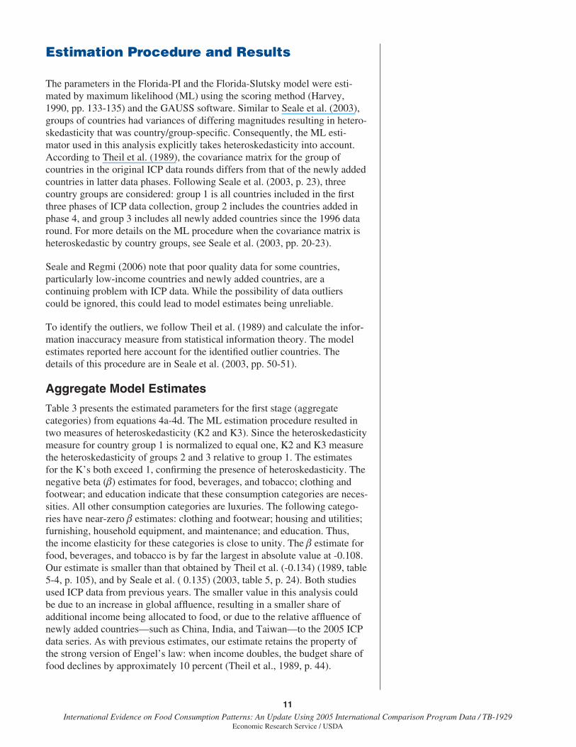
Table 3 presents the estimated parameters for the first stage (aggregate categories) from equations 4a-4d. The ML estimation procedure resulted in two measures of heteroskedasticity (K2 and K3). Since the heteroskedasticity measure for country group 1 is normalized to equal one, K2 and K3 measure the heteroskedasticity of groups 2 and 3 relative to group 1. The estimates for the K’s both exceed 1, confirming the presence of heteroskedasticity. The negative beta (β) estimates for food, beverages, and tobacco; clothing and footwear; and education indicate that these consumption categories are neces-sities. All other consumption categories are luxuries. The following catego-ries have near-zero β estimates: clothing and footwear; housing and utilities; furnishing, household equipment, and maintenance; and education. Thus, the income elasticity for these categories is close to unity. The β estimate for food, beverages, and tobacco is by far the largest in absolute value at -0.108. Our estimate is smaller than that obtained by Theil et al. (-0.134) (1989, table 5-4, p. 105), and by Seale et al. ( 0.135) (2003, table 5, p. 24). Both studies used ICP data from previous years. The smaller value in this analysis could be due to an increase in global affluence, resulting in a smaller share of additional income being allocated to food, or due to the relative affluence of newly added countries—such as China, India, and Taiwan—to the 2005 ICP data series. As with previous estimates, our estimate retains the property of the strong version of Engel’s law: when income doubles, the budget share of food declines by approximately 10 percent (Theil et al., 1989, p. 44).
12International Evidence on Food Consumption Patterns: An Update Using 2005 International Comparison Program Data / TB-1929
Economic Research Service / USDA
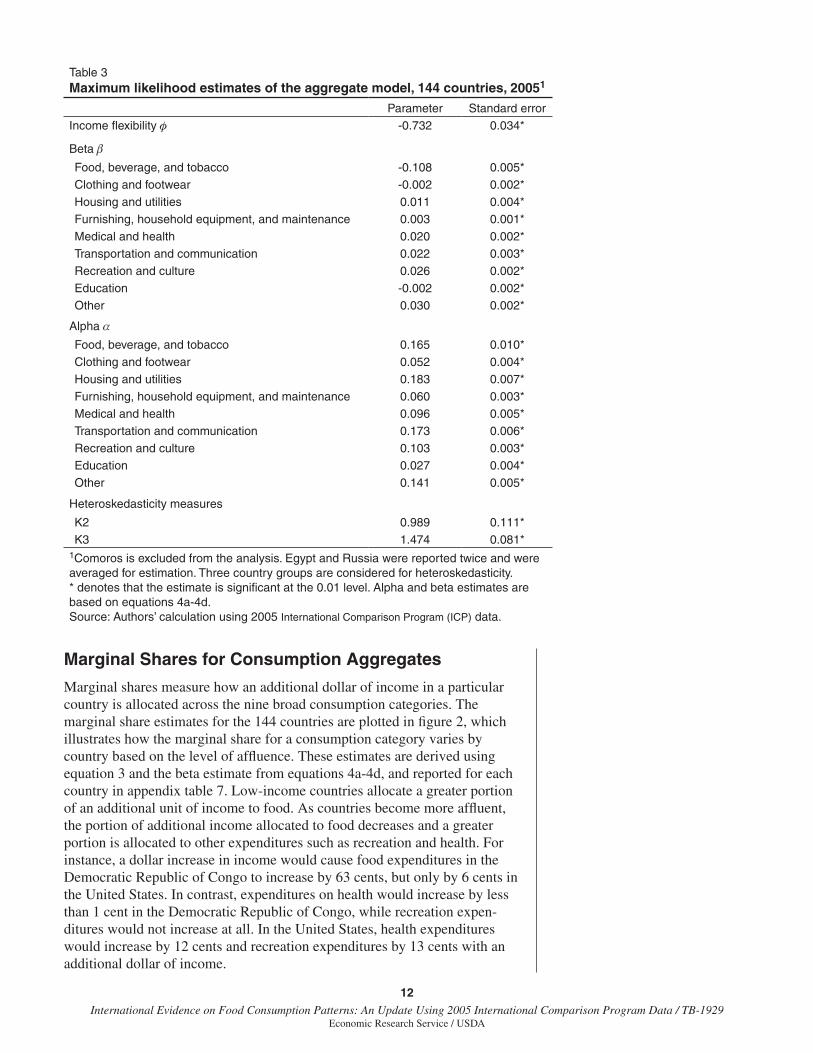
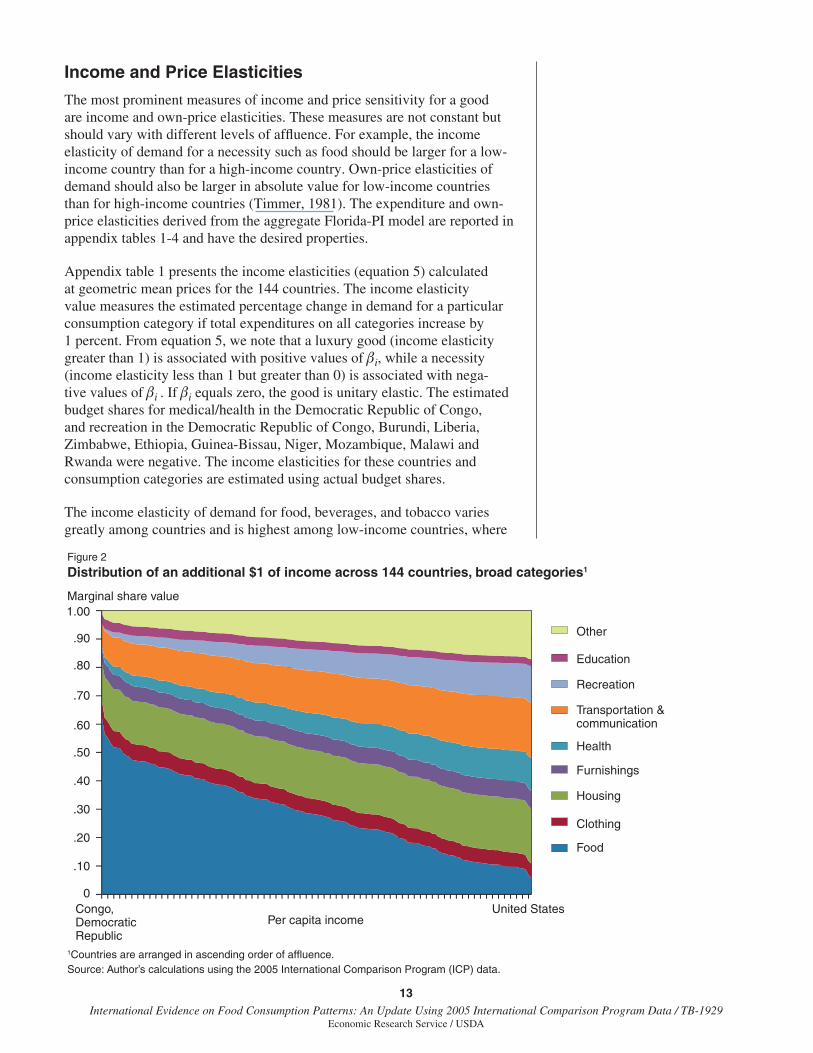
Marginal Shares for Consumption Aggregates
Marginal shares measure how an additional dollar of income in a particular country is allocated across the nine broad consumption categories. The marginal share estimates for the 144 countries are plotted in figure 2, which illustrates how the marginal share for a consumption category varies by country based on the level of affluence. These estimates are derived using equation 3 and the beta estimate from equations 4a-4d, and reported for each country in appendix table 7. Low-income countries allocate a greater portion of an additional unit of income to food. As countries become more affluent, the portion of additional income allocated to food decreases and a greater portion is allocated to other expenditures such as recreation and health. For instance, a dollar increase in income would cause food expenditures in the Democratic Republic of Congo to increase by 63 cents, but only by 6 cents in the United States. In contrast, expenditures on health would increase by less than 1 cent in the Democratic Republic of Congo, while recreation expen-ditures would not increase at all. In the United States, health expenditures would increase by 12 cents and recreation expenditures by 13 cents with an additional dollar of income.
Table 3 Maximum likelihood estimates of the aggregate model, 144 countries, 20051
Parameter Standard errorIncome flexibility φ -0.732 0.034*
Beta β
Food, beverage, and tobacco -0.108 0.005*Clothing and footwear -0.002 0.002*Housing and utilities 0.011 0.004*Furnishing, household equipment, and maintenance 0.003 0.001*Medical and health 0.020 0.002*Transportation and communication 0.022 0.003*Recreation and culture 0.026 0.002*Education -0.002 0.002*Other 0.030 0.002*
Alpha α
Food, beverage, and tobacco 0.165 0.010*Clothing and footwear 0.052 0.004*Housing and utilities 0.183 0.007*Furnishing, household equipment, and maintenance 0.060 0.003*Medical and health 0.096 0.005*Transportation and communication 0.173 0.006*Recreation and culture 0.103 0.003*Education 0.027 0.004*Other 0.141 0.005*
Heteroskedasticity measures
K2 0.989 0.111*K3 1.474 0.081*
1Comoros is excluded from the analysis. Egypt and Russia were reported twice and were averaged for estimation. Three country groups are considered for heteroskedasticity.* denotes that the estimate is significant at the 0.01 level. Alpha and beta estimates are based on equations 4a-4d.Source: Authors’ calculation using 2005 International Comparison Program (ICP) data.
13 International Evidence on Food Consumption Patterns: An Update Using 2005 International Comparison Program Data / TB-1929
Economic Research Service / USDA
Income and Price Elasticities
The most prominent measures of income and price sensitivity for a good are income and own-price elasticities. These measures are not constant but should vary with different levels of affluence. For example, the income elasticity of demand for a necessity such as food should be larger for a low-income country than for a high-income country. Own-price elasticities of demand should also be larger in absolute value for low-income countries than for high-income countries (Timmer, 1981). The expenditure and own-price elasticities derived from the aggregate Florida-PI model are reported in appendix tables 1-4 and have the desired properties.
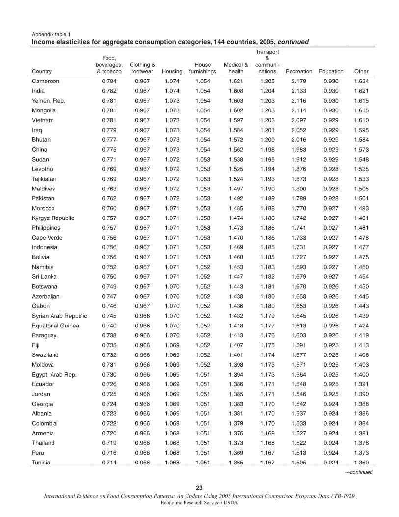
Appendix table 1 presents the income elasticities (equation 5) calculated at geometric mean prices for the 144 countries. The income elasticity value measures the estimated percentage change in demand for a particular consumption category if total expenditures on all categories increase by 1 percent. From equation 5, we note that a luxury good (income elasticity greater than 1) is associated with positive values of βi, while a necessity (income elasticity less than 1 but greater than 0) is associated with nega-tive values of βi . If βi equals zero, the good is unitary elastic. The estimated budget shares for medical/health in the Democratic Republic of Congo, and recreation in the Democratic Republic of Congo, Burundi, Liberia, Zimbabwe, Ethiopia, Guinea-Bissau, Niger, Mozambique, Malawi and Rwanda were negative. The income elasticities for these countries and consumption categories are estimated using actual budget shares.
The income elasticity of demand for food, beverages, and tobacco varies greatly among countries and is highest among low-income countries, where
United StatesPer capita income
Congo, DemocraticRepublic
Other
Education
Recreation
Transportation &communication
Health
Furnishings
Housing
Clothing
Food
1.00Marginal share value
.90
.80
.70
.60
.50
.40
.30
.20
.10
0
Figure 2
Distribution of an additional $1 of income across 144 countries, broad categories1
1Countries are arranged in ascending order of affluence.Source: Author’s calculations using the 2005 International Comparison Program (ICP) data.
14International Evidence on Food Consumption Patterns: An Update Using 2005 International Comparison Program Data / TB-1929
Economic Research Service / USDA
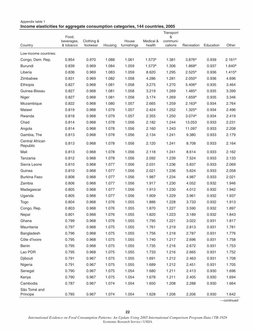
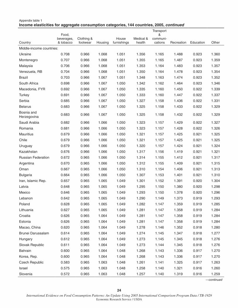
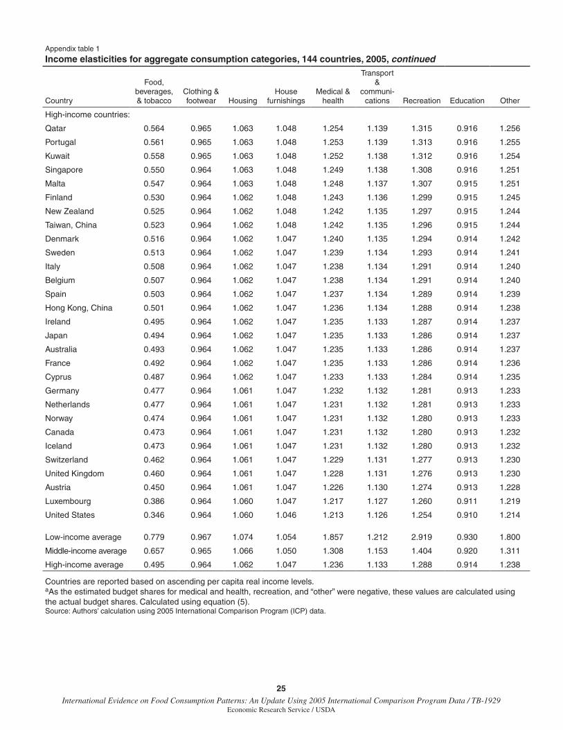
it varies from 0.85 for the Democratic Republic of Congo to 0.71 for Tunisia. It ranges between 0.71 and 0.57 for middle-income countries, and from 0.56 to 0.35 for high-income countries. The average income elasticity for low-income countries is 0.78, over 1.5 times the average for high-income coun-tries (0.50). The average food-income elasticity for high-income countries derived using 1996 ICP data (Seale et al., 2003, table 7, pp. 26-28) is smaller (0.34) than our estimate. Unlike the prior analysis, restaurant and catering expenditures are included among food in the 2005 ICP data, raising the income elasticity for food in high-income countries.
The income elasticity for clothing and footwear, another necessity, also decreases in value with income. However, given that the estimated value of βi is close to zero, the income elasticity values are close to unity for all coun-tries. Like clothing and footwear, education is also a necessity, and given the small value of βi, the income elasticity for education is also close to unity for all countries. The average value ranges from 0.93 for low-income countries to 0.91 for high-income countries. Using 1996 ICP data, Seale, Regmi and Bernstein (2003, table 7, pp. 26-28) found that education was a luxury cate-gory with an income elasticity ranging from 1.08 for low-income countries to 1.07 for high-income countries. Although the two estimates are close and are likely not statistically different, the fact that the more current estimate is smaller may indicate growing global affluence.
All other consumption categories are luxuries, with income elasticities greater than 1. The elasticity values are higher for less affluent countries and span a wide range. Recreation is by far the most luxurious good, with an income elasticity of demand ranging from 13.1 for Chad to 1.25 for the United States. The categories medical/health and “other” are the next most luxurious goods, followed by transportation/communication, housing, and house furnishings. The income elasticity for medical and health also spans a wide range, from 8.6 for Liberia to 1.21 for the United States.
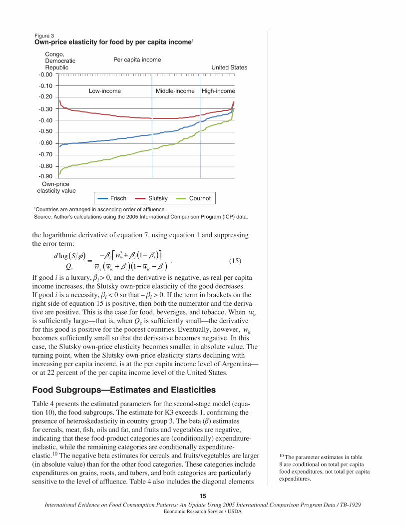
Using equations 6-8, three types of own-price elasticities of demand for a good can be calculated from the parameter estimates of the Florida-PI model. Appendix tables 2-4 present the estimated Frisch, Slutsky, and Cournot own-price elasticities for the 9 aggregate commodity groups, across 144 coun-tries. In the tables, the countries are listed in ascending order of affluence. The elasticity measures perform in accordance with Timmer’s proposition: own-price elasticities of demand are larger in absolute value for low-income countries than for high-income countries. The Cournot and Frisch own-price elasticities decline monotonically in absolute value from poor to rich coun-tries. The Cournot and Frisch own-price elasticities for food are all larger than the corresponding Slutsky elasticity. However, with rising affluence the real income effect of a food-price change becomes increasingly smaller and the three elasticities converge (fig. 3). The discussion that follows is limited to the Slutsky own-price elasticity for food since it is the only measure that did not fully perform in accordance with Timmer’s proposition.
In appendix table 3, the Slutsky own-price elasticity (equation 7) of demand for food, beverages, and tobacco begins at -0.23 for the Congo, increases (in absolute value) to -0.384 (Malaysia to Argentina), and declines thereafter (absolutely) to -0.24 for the United States. To clarify the reason for this, take
15 International Evidence on Food Consumption Patterns: An Update Using 2005 International Comparison Program Data / TB-1929
Economic Research Service / USDA
the logarithmic derivative of equation 7, using equation 1 and suppressing the error term:
. (15)
If good i is a luxury, βi > 0, and the derivative is negative, as real per capita income increases, the Slutsky own-price elasticity of the good decreases. If good i is a necessity, βi < 0 so that – βi > 0. If the term in brackets on the right side of equation 15 is positive, then both the numerator and the deriva-tive are positive. This is the case for food, beverages, and tobacco. When icw is sufficiently large—that is, when Qc is sufficiently small—the derivative for this good is positive for the poorest countries. Eventually, however, icw becomes sufficiently small so that the derivative becomes negative. In this case, the Slutsky own-price elasticity becomes smaller in absolute value. The turning point, when the Slutsky own-price elasticity starts declining with increasing per capita income, is at the per capita income level of Argentina—or at 22 percent of the per capita income level of the United States.
Food Subgroups—Estimates and Elasticities
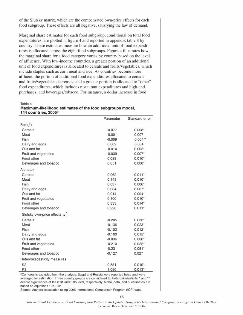
Table 4 presents the estimated parameters for the second-stage model (equa-tion 10), the food subgroups. The estimate for K3 exceeds 1, confirming the presence of heteroskedasticity in country group 3. The beta (β) estimates for cereals, meat, fish, oils and fat, and fruits and vegetables are negative, indicating that these food-product categories are (conditionally) expenditure-inelastic, while the remaining categories are conditionally expenditure-elastic.10 The negative beta estimates for cereals and fruits/vegetables are larger (in absolute value) than for the other food categories. These categories include expenditures on grains, roots, and tubers, and both categories are particularly sensitive to the level of affluence. Table 4 also includes the diagonal elements
( ) ( )( )( )
2 1log1
i ic i i
c ic ic i ic i
wd SQ w w w
β β βφ
β β
− + − =
+ − −
10 The parameter estimates in table 8 are conditional on total per capita food expenditures, not total per capita expenditures.
Figure 3Own-price elasticity for food by per capita income1
United StatesPer capita income
Low-income Middle-income High-income
Congo, DemocraticRepublic
1Countries are arranged in ascending order of affluence.Source: Author’s calculations using the 2005 International Comparison Program (ICP) data.
-0.90
-0.80
-0.70
-0.60
-0.50
-0.40
-0.30
-0.20
-0.10
-0.00
Own-price elasticity value
Frisch Slutsky Cournot
16International Evidence on Food Consumption Patterns: An Update Using 2005 International Comparison Program Data / TB-1929
Economic Research Service / USDA
of the Slutsky matrix, which are the compensated own-price effects for each food subgroup. These effects are all negative, satisfying the law of demand.
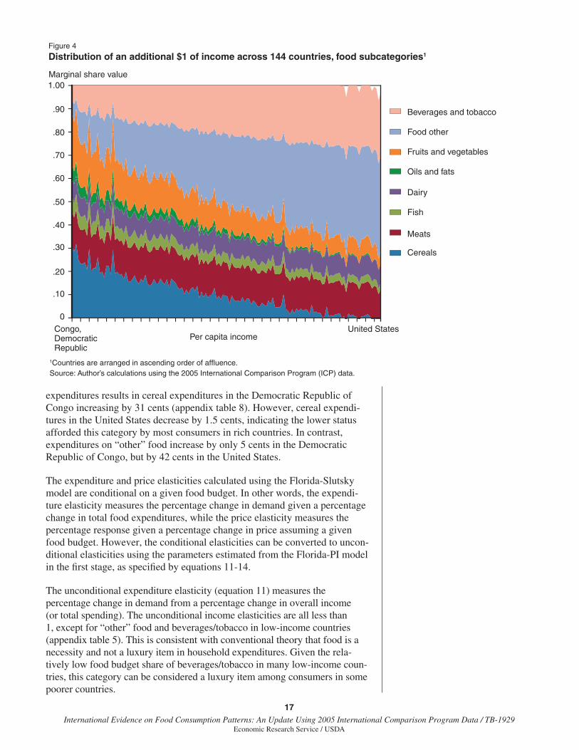
Marginal share estimates for each food subgroup, conditional on total food expenditures, are plotted in figure 4 and reported in appendix table 8 by country. These estimates measure how an additional unit of food expendi-tures is allocated across the eight food subgroups. Figure 4 illustrates how the marginal share for a food category varies by country based on the level of affluence. With low-income countries, a greater portion of an additional unit of food expenditures is allocated to cereals and fruits/vegetables, which include staples such as corn meal and rice. As countries become more affluent, the portion of additional food expenditures allocated to cereals and fruits/vegetables decreases, and a greater portion is allocated to “other” food expenditures, which includes restaurant expenditures and high-end purchases, and beverages/tobacco. For instance, a dollar increase in food
Table 4 Maximum-likelihood estimates of the food subgroups model, 144 countries, 2005a
Parameter Standard error
Beta β*
Cereals -0.077 0.008*Meat -0.001 0.007Fish -0.009 0.004**Dairy and eggs 0.002 0.004Oils and fat -0.014 0.003*Fruit and vegetables -0.039 0.007*Food other 0.088 0.010*Beverages and tobacco 0.051 0.008*
Alpha α*
Cereals 0.062 0.011*Meat 0.143 0.010*Fish 0.037 0.006*Dairy and eggs 0.084 0.007*Oils and fat 0.014 0.004*Fruit and vegetables 0.100 0.010*Food other 0.333 0.014*Beverages and tobacco 0.228 0.011*
Slutsky own-price effects *iiπ
Cereals -0.205 0.033*Meat -0.136 0.023*Fish -0.102 0.012*Dairy and eggs -0.100 0.015*Oils and fat -0.036 0.006*Fruit and vegetables -0.210 0.022*Food other -0.231 0.051*Beverages and tobacco -0.127 0.027
Heteroskedasticity measures
K2 0.851 0.019*K3 1.090 0.013*
aComoros is excluded from the analysis. Egypt and Russia were reported twice and were averaged for estimation. Three country groups are considered for heteroskedasticity. * and ** denote significance at the 0.01 and 0.05 level, respectively. Alpha, beta, and pi estimates are based on equations 10a−10c. Source: Authors’ calculation using 2005 International Comparison Program (ICP) data.
17 International Evidence on Food Consumption Patterns: An Update Using 2005 International Comparison Program Data / TB-1929
Economic Research Service / USDA
Figure 4
Distribution of an additional $1 of income across 144 countries, food subcategories1
United StatesPer capita income
Congo, DemocraticRepublic
1.00Marginal share value
.90
.80
.70
.60
.50
.40
.30
.20
.10
0
Beverages and tobacco
Food other
Fruits and vegetables
Oils and fats
Dairy
Fish
Meats
Cereals
1Countries are arranged in ascending order of affluence.Source: Author’s calculations using the 2005 International Comparison Program (ICP) data.
expenditures results in cereal expenditures in the Democratic Republic of Congo increasing by 31 cents (appendix table 8). However, cereal expendi-tures in the United States decrease by 1.5 cents, indicating the lower status afforded this category by most consumers in rich countries. In contrast, expenditures on “other” food increase by only 5 cents in the Democratic Republic of Congo, but by 42 cents in the United States.
The expenditure and price elasticities calculated using the Florida-Slutsky model are conditional on a given food budget. In other words, the expendi-ture elasticity measures the percentage change in demand given a percentage change in total food expenditures, while the price elasticity measures the percentage response given a percentage change in price assuming a given food budget. However, the conditional elasticities can be converted to uncon-ditional elasticities using the parameters estimated from the Florida-PI model in the first stage, as specified by equations 11-14.
The unconditional expenditure elasticity (equation 11) measures the percentage change in demand from a percentage change in overall income (or total spending). The unconditional income elasticities are all less than 1, except for “other” food and beverages/tobacco in low-income countries (appendix table 5). This is consistent with conventional theory that food is a necessity and not a luxury item in household expenditures. Given the rela-tively low food budget share of beverages/tobacco in many low-income coun-tries, this category can be considered a luxury item among consumers in some poorer countries.
18International Evidence on Food Consumption Patterns: An Update Using 2005 International Comparison Program Data / TB-1929
Economic Research Service / USDA
Similar to the estimated income elasticity for aggregate consumption catego-ries, the income elasticity for the food subcategories is largest in the poorer countries and declines in magnitude with affluence. Across each country, staple food items (with negative *
iβ ) have smaller elasticities than the more conditionally elastic food items such as beverages/tobacco, meat, and dairy. For example, the income elasticity for cereals ranges from 0.69 in the Democratic Republic of Congo to -0.09 in the United States. In contrast, the elasticity for beverages and tobacco is higher across all countries, ranging from 7.1 in Liberia to 0.42 in the United States.
The conditional Slutsky elasticity is given by * * */ijc ij icwε π= , where *ijπ is
the conditional Slutsky price parameter in country c for good i with respect to good j, and *
icw is the conditional fitted budget share (at geometric mean prices) of food group gi S∈ in country c. Since for a given food subgroup i, *
ijπ is invariant across countries, the conditional Slutsky elas-ticity for food subgroup i will be greater for smaller budget shares. Poorer countries typically have larger budget shares for staple items such as breads and cereals, which form a smaller share of food budget among wealthier countries. Therefore, contrary to theory, the estimated conditional Slutsky own-price elasticities for cereals may be larger for wealthier countries. This problem of a constant *
ijπ continues if one calculates unconditional Slutsky price elasticities from the conditional one using equation 13.
The unconditional Frisch own-price elasticities are not a function of *ijπ
and do not suffer the problem encountered in calculating the unconditional Slutsky elasticities. Using the estimated parameters from stage one and two and using equation 12, Frisch own-price elasticities are calculated. These unconditional own-price elasticities (appendix table 6) represent elasticities estimated at a point when the marginal utility of income is held constant. The values of the Frisch own-price elasticities lie between the values of the Slutsky own-price elasticities—when real income is held constant—and the Cournot own-price elasticities—when nominal income is held constant—and can be considered a reasonable estimate of the average own-price elastici-ties for the food subcategories. The Slutsky and Cournot elasticities are not estimated for these products, as their calculation using equations 13 and 14 requires the assumption of preference independence.
The Frisch own-price elasticities for the food subcategories vary by affluence according to economic theory; consumers in low-income countries are more responsive to price changes than are those in higher-income countries. For instance, the value for breads and cereals ranges from 0.50 in the Democratic Republic of Congo to 0.06 in the United States. The absolute values of the own-price elasticities are smaller for food groups such as breads/cereals, oils/fats, and fruits/vegetables, and particularly large for “other” foods and beverages/tobacco. Also, low-income countries are particularly sensitive to changes in the price of “other” food and beverages/tobacco, relative to middle- and high-income countries. Given a 1-percent increase in the price of “other” food, consumption in this category declines on average by more than 1 percent in low-income countries but by less than 0.5 percent in high-income countries.
19 International Evidence on Food Consumption Patterns: An Update Using 2005 International Comparison Program Data / TB-1929
Economic Research Service / USDA
Conclusion
This report provides income and price elasticities across 144 countries for 9 aggregate consumption categories and 8 food subcategories. No empirical work to date has been conducted across as many countries and consumption categories. The results of this research confirm many of the results obtained and established by earlier studies. Low-income countries spend a greater portion of their budget on necessities, such as food, while richer countries spend a greater proportion of their income on luxuries, such as recreation. Low-value staples, such as cereals, account for a larger share of the food budget in poorer countries, while high-value food items are a larger share of the food budget in richer countries. Low-income countries are also more responsive to changes in income and food prices and, therefore, make larger adjustments to their food consumption patterns when incomes and prices change. However, our study illustrates that adjustments to price and income changes are not made uniformly across all food categories. Staple food consumption changes the least, while consumption of higher-value food items changes the most.
The income and price elasticities estimated here can be used as inputs in future work designed to forecast future food demand and supply, and in proj-ects designed to simulate the effects of different government policy options. In addition to the actual elasticity estimates, parameters estimated from our models can be used (with more recent expenditure data) to estimate new elasticities for more recent years for the countries included in our analysis, as well as for other countries (Cox and Alm, 2007).
20International Evidence on Food Consumption Patterns: An Update Using 2005 International Comparison Program Data / TB-1929
Economic Research Service / USDA
References
Cox, W.M., and R. Alm. 2007. “Opportunity Knocks: Selling Our Services to the World,” Federal Reserve Bank of Dallas 2007 Annual Report. Dallas, TX.
Diewert, Erwin, 2010. “New Methodological Developments for the Inter-national Comparison Program,” The Review of Income and Wealth. June.
Harvey, A. 1990. The Econometric Analysis of Time Series. 2nd edition, MIT Press, Cambridge, MA.
Hertel, T.W., and L.A. Winters, 2006. Poverty and the WTO: Impacts of the Doha Development Agenda. Washington, DC: World Bank Publications.
Kravis, I.B., F. Kennessey, A.W. Heston, and R. Summers. 1975. A System of International Comparisons of Gross Product and Purchasing Power. Johns Hopkins University Press, Baltimore, MD.
Kravis, I.B., A.W. Heston, and R. Summers. 1978. International Comparisons of Real Product and Purchasing Power, Johns Hopkins University Press (for the World Bank), , Baltimore, MD.
Reimer, J.J., and T.W. Hertel, 2003. “International Cross Section Estimates of Demand for Use in the GTAP Model,” GTAP Working Paper No. 22, Center for Global Trade Analysis, Department of Agricultural Economics, Purdue University, West Lafayette, IN.
Reimer, J.J., and T.W. Hertel. 2004. “Estimation of International Demand Behavior for Use with Input-Output Based Data,” Economic Systems Research, Vol. 16(4), pp. 347-66.
Seale, James L., and Anita Regmi. 2006. “Modeling International Consumption Patterns,” Review of Income and Wealth, Vol. 52(4), pp. 603-24.
Seale, J.L., A. Regmi, and J. Bernstein. 2003. International Evidence on Food Consumption Patterns, Technical Bulletin No. 1904, Economic Research Service, U.S. Department of Agriculture.
Timmer, C.P. 1981. “Is There Curvature in the Slutsky Matrix?” Review of Economics and Statistics, Vol. 63, pp. 395-402.
Theil, H., C.F. Chung, and J.L. Seale, Jr. 1989. International Evidence on Consumption Patterns. Greenwich, CT: JAI Press, Inc.
Valenzuela, Ernesto, Kym Anderson, and Thomas Hertel. 2007. “Impacts of Trade Reform: Sensitivity of Model Results to Key Assumptions,” International Economics and Economic Policy, Vol. 4, pp. 395-420.
von Braun, J. 2007. The World Food Situation: New Driving Forces and Required Actions, Food Policy Report No. 18, IFPRI, Washington, DC.
21 International Evidence on Food Consumption Patterns: An Update Using 2005 International Comparison Program Data / TB-1929
Economic Research Service / USDA
Winters, L.A. 2005. “The European Agricultural Trade Policies and Poverty,” European Review of Agricultural Economics, Vol. 32(3), pp. 319–46.
Working, H. 1943. “Statistical Laws of Family Expenditure,” Journal of the American Statistical Association, Vol. 38, pp. 43-56.
World Bank, 2008. “Global Purchasing Power Parities and Real Expen-ditures, 2005 International Comparison Program.” Washington, DC.
22International Evidence on Food Consumption Patterns: An Update Using 2005 International Comparison Program Data / TB-1929
Economic Research Service / USDA
Appendix table 1
Income elasticities for aggregate consumption categories, 144 countries, 2005, continued
Country
Food, beverages, & tobacco
Clothing & footwear Housing
House furnishings
Medical & health
Transport &
communi- cations Recreation Education Other
Low-income countries:
Congo, Dem. Rep. 0.854 0.970 1.088 1.061 1.573a 1.381 3.876a 0.939 2.161a
Burundi 0.839 0.969 1.084 1.059 1.573a 1.306 1.868a 0.937 1.640a
Liberia 0.836 0.969 1.083 1.059 8.620 1.295 2.525a 0.936 1.415a
Zimbabwe 0.831 0.969 1.082 1.058 4.286 1.281 2.050a 0.936 4.696
Ethiopia 0.827 0.968 1.081 1.058 3.275 1.270 5.406a 0.935 3.464
Guinea-Bissau 0.827 0.968 1.081 1.058 3.219 1.269 1.485a 0.935 3.399
Niger 0.827 0.968 1.081 1.058 3.174 1.269 1.659a 0.935 3.346
Mozambique 0.822 0.968 1.080 1.057 2.665 1.259 2.163a 0.934 2.764
Malawi 0.819 0.968 1.079 1.057 2.424 1.252 1.325a 0.934 2.496
Rwanda 0.818 0.968 1.079 1.057 2.355 1.250 3.074a 0.934 2.419
Chad 0.814 0.968 1.078 1.056 2.182 1.244 13.053 0.933 2.231
Angola 0.814 0.968 1.078 1.056 2.160 1.243 11.097 0.933 2.208
Gambia, The 0.813 0.968 1.078 1.056 2.134 1.241 9.380 0.933 2.179
Central African Republic
0.813 0.968 1.078 1.056 2.120 1.241 8.708 0.933 2.164
Mali 0.813 0.968 1.078 1.056 2.118 1.241 8.614 0.933 2.162
Tanzania 0.812 0.968 1.078 1.056 2.092 1.239 7.524 0.933 2.133
Sierra Leone 0.810 0.968 1.077 1.056 2.031 1.236 5.837 0.933 2.069
Guinea 0.810 0.968 1.077 1.056 2.021 1.236 5.624 0.933 2.058
Burkina Faso 0.808 0.968 1.077 1.056 1.987 1.234 4.987 0.933 2.021
Zambia 0.806 0.968 1.077 1.056 1.917 1.230 4.052 0.932 1.946
Madagascar 0.805 0.968 1.077 1.056 1.913 1.230 4.012 0.932 1.942
Uganda 0.805 0.968 1.077 1.056 1.909 1.229 3.961 0.932 1.937
Togo 0.804 0.968 1.076 1.055 1.886 1.228 3.733 0.932 1.913
Congo, Rep. 0.803 0.968 1.076 1.055 1.870 1.227 3.590 0.932 1.897
Nepal 0.801 0.968 1.076 1.055 1.820 1.223 3.189 0.932 1.843
Ghana 0.799 0.968 1.076 1.055 1.795 1.221 3.022 0.931 1.817
Mauritania 0.797 0.968 1.075 1.055 1.761 1.219 2.813 0.931 1.781
Bangladesh 0.796 0.968 1.075 1.055 1.756 1.218 2.787 0.931 1.776
Côte d’Ivoire 0.795 0.968 1.075 1.055 1.740 1.217 2.696 0.931 1.758
Benin 0.795 0.968 1.075 1.055 1.735 1.216 2.672 0.931 1.753
Lao PDR 0.795 0.968 1.075 1.055 1.733 1.216 2.665 0.931 1.752
Djibouti 0.791 0.967 1.075 1.055 1.691 1.212 2.463 0.931 1.708
Nigeria 0.791 0.967 1.075 1.055 1.689 1.212 2.451 0.931 1.705
Senegal 0.790 0.967 1.075 1.054 1.680 1.211 2.413 0.930 1.696
Kenya 0.790 0.967 1.075 1.054 1.678 1.211 2.405 0.930 1.694
Cambodia 0.787 0.967 1.074 1.054 1.650 1.208 2.288 0.930 1.664
São Tomé and Principe 0.785 0.967 1.074 1.054 1.628 1.206 2.206 0.930 1.642
---continued
23 International Evidence on Food Consumption Patterns: An Update Using 2005 International Comparison Program Data / TB-1929
Economic Research Service / USDA
Appendix table 1
Income elasticities for aggregate consumption categories, 144 countries, 2005, continued
Country
Food, beverages, & tobacco
Clothing & footwear Housing
House furnishings
Medical & health
Transport &
communi- cations Recreation Education Other
Cameroon 0.784 0.967 1.074 1.054 1.621 1.205 2.179 0.930 1.634
India 0.782 0.967 1.074 1.054 1.608 1.204 2.133 0.930 1.621
Yemen, Rep. 0.781 0.967 1.073 1.054 1.603 1.203 2.116 0.930 1.615
Mongolia 0.781 0.967 1.073 1.054 1.602 1.203 2.114 0.930 1.615
Vietnam 0.781 0.967 1.073 1.054 1.597 1.203 2.097 0.929 1.610
Iraq 0.779 0.967 1.073 1.054 1.584 1.201 2.052 0.929 1.595
Bhutan 0.777 0.967 1.073 1.054 1.572 1.200 2.016 0.929 1.584
China 0.775 0.967 1.073 1.054 1.562 1.198 1.983 0.929 1.573
Sudan 0.771 0.967 1.072 1.053 1.538 1.195 1.912 0.929 1.548
Lesotho 0.769 0.967 1.072 1.053 1.525 1.194 1.876 0.928 1.535
Tajikistan 0.769 0.967 1.072 1.053 1.524 1.193 1.873 0.928 1.533
Maldives 0.763 0.967 1.072 1.053 1.497 1.190 1.800 0.928 1.505
Pakistan 0.762 0.967 1.072 1.053 1.492 1.189 1.789 0.928 1.501
Morocco 0.760 0.967 1.071 1.053 1.485 1.188 1.770 0.927 1.493
Kyrgyz Republic 0.757 0.967 1.071 1.053 1.474 1.186 1.742 0.927 1.481
Philippines 0.757 0.967 1.071 1.053 1.473 1.186 1.741 0.927 1.481
Cape Verde 0.756 0.967 1.071 1.053 1.470 1.186 1.733 0.927 1.478
Indonesia 0.756 0.967 1.071 1.053 1.469 1.185 1.731 0.927 1.477
Bolivia 0.756 0.967 1.071 1.053 1.468 1.185 1.727 0.927 1.475
Namibia 0.752 0.967 1.071 1.052 1.453 1.183 1.693 0.927 1.460
Sri Lanka 0.750 0.967 1.071 1.052 1.447 1.182 1.679 0.927 1.454
Botswana 0.749 0.967 1.070 1.052 1.443 1.181 1.670 0.926 1.450
Azerbaijan 0.747 0.967 1.070 1.052 1.438 1.180 1.658 0.926 1.445
Gabon 0.746 0.967 1.070 1.052 1.436 1.180 1.653 0.926 1.443
Syrian Arab Republic 0.745 0.966 1.070 1.052 1.432 1.179 1.645 0.926 1.439
Equatorial Guinea 0.740 0.966 1.070 1.052 1.418 1.177 1.613 0.926 1.424
Paraguay 0.738 0.966 1.070 1.052 1.413 1.176 1.603 0.926 1.419
Fiji 0.735 0.966 1.069 1.052 1.407 1.175 1.591 0.925 1.413
Swaziland 0.732 0.966 1.069 1.052 1.401 1.174 1.577 0.925 1.406
Moldova 0.731 0.966 1.069 1.052 1.398 1.173 1.571 0.925 1.403
Egypt, Arab Rep. 0.730 0.966 1.069 1.051 1.394 1.173 1.564 0.925 1.400
Ecuador 0.726 0.966 1.069 1.051 1.386 1.171 1.548 0.925 1.391
Jordan 0.725 0.966 1.069 1.051 1.385 1.171 1.546 0.925 1.390
Georgia 0.724 0.966 1.069 1.051 1.383 1.170 1.542 0.924 1.388
Albania 0.723 0.966 1.069 1.051 1.381 1.170 1.537 0.924 1.386
Colombia 0.722 0.966 1.069 1.051 1.379 1.170 1.533 0.924 1.384
Armenia 0.720 0.966 1.068 1.051 1.376 1.169 1.527 0.924 1.381
Thailand 0.719 0.966 1.068 1.051 1.373 1.168 1.522 0.924 1.378
Peru 0.716 0.966 1.068 1.051 1.369 1.167 1.513 0.924 1.373
Tunisia 0.714 0.966 1.068 1.051 1.365 1.167 1.505 0.924 1.369
---continued
24International Evidence on Food Consumption Patterns: An Update Using 2005 International Comparison Program Data / TB-1929
Economic Research Service / USDA
Appendix table 1
Income elasticities for aggregate consumption categories, 144 countries, 2005, continued
Country
Food, beverages, & tobacco
Clothing & footwear Housing
House furnishings
Medical & health
Transport &
communi- cations Recreation Education Other
Middle-income countries:
Ukraine 0.708 0.966 1.068 1.051 1.356 1.165 1.488 0.923 1.360
Montenegro 0.707 0.966 1.068 1.051 1.355 1.165 1.487 0.923 1.359
Malaysia 0.706 0.966 1.068 1.051 1.353 1.164 1.483 0.923 1.357
Venezuela, RB 0.704 0.966 1.068 1.051 1.350 1.164 1.478 0.923 1.354
Brazil 0.703 0.966 1.067 1.051 1.348 1.163 1.474 0.923 1.352
South Africa 0.698 0.966 1.067 1.050 1.342 1.162 1.464 0.923 1.346
Macedonia, FYR 0.692 0.966 1.067 1.050 1.335 1.160 1.450 0.922 1.339
Turkey 0.691 0.966 1.067 1.050 1.333 1.160 1.447 0.922 1.337
Serbia 0.685 0.966 1.067 1.050 1.327 1.158 1.436 0.922 1.331
Belarus 0.683 0.966 1.067 1.050 1.325 1.158 1.433 0.922 1.329
Bosnia and Herzegovina
0.683 0.966 1.067 1.050 1.325 1.158 1.432 0.922 1.329
Saudi Arabia 0.682 0.966 1.066 1.050 1.323 1.157 1.429 0.922 1.327
Romania 0.681 0.966 1.066 1.050 1.323 1.157 1.428 0.922 1.326
Mauritius 0.679 0.966 1.066 1.050 1.321 1.157 1.425 0.921 1.325
Chile 0.679 0.966 1.066 1.050 1.321 1.157 1.425 0.921 1.325
Uruguay 0.679 0.966 1.066 1.050 1.320 1.157 1.424 0.921 1.324
Kazakhstan 0.676 0.966 1.066 1.050 1.317 1.156 1.419 0.921 1.321
Russian Federation 0.672 0.965 1.066 1.050 1.314 1.155 1.412 0.921 1.317
Argentina 0.670 0.965 1.066 1.050 1.312 1.155 1.409 0.921 1.315
Oman 0.667 0.965 1.066 1.050 1.310 1.154 1.406 0.921 1.313
Bulgaria 0.664 0.965 1.066 1.050 1.307 1.153 1.401 0.921 1.310
Iran, Islamic Rep. 0.657 0.965 1.065 1.049 1.301 1.152 1.391 0.920 1.304
Latvia 0.648 0.965 1.065 1.049 1.295 1.150 1.380 0.920 1.298
Mexico 0.646 0.965 1.065 1.049 1.293 1.150 1.378 0.920 1.296
Lebanon 0.642 0.965 1.065 1.049 1.290 1.149 1.373 0.919 1.293
Poland 0.628 0.965 1.065 1.049 1.282 1.147 1.359 0.919 1.285
Lithuania 0.627 0.965 1.065 1.049 1.281 1.147 1.358 0.919 1.284
Croatia 0.626 0.965 1.064 1.049 1.281 1.147 1.358 0.919 1.284
Estonia 0.626 0.965 1.064 1.049 1.281 1.147 1.358 0.919 1.284
Macao, China 0.620 0.965 1.064 1.049 1.278 1.146 1.352 0.918 1.280
Brunei Darussalam 0.614 0.965 1.064 1.049 1.274 1.145 1.347 0.918 1.277
Hungary 0.612 0.965 1.064 1.049 1.273 1.145 1.345 0.918 1.276
Slovak Republic 0.611 0.965 1.064 1.049 1.273 1.144 1.345 0.918 1.276
Bahrain 0.600 0.965 1.064 1.048 1.268 1.143 1.336 0.917 1.270
Korea, Rep. 0.600 0.965 1.064 1.048 1.268 1.143 1.336 0.917 1.270
Czech Republic 0.583 0.965 1.063 1.048 1.261 1.141 1.325 0.917 1.263
Israel 0.575 0.965 1.063 1.048 1.258 1.140 1.321 0.916 1.260
Slovenia 0.572 0.965 1.063 1.048 1.257 1.140 1.319 0.916 1.259
---continued
25 International Evidence on Food Consumption Patterns: An Update Using 2005 International Comparison Program Data / TB-1929
Economic Research Service / USDA
Appendix table 1
Income elasticities for aggregate consumption categories, 144 countries, 2005, continued
Country
Food, beverages, & tobacco
Clothing & footwear Housing
House furnishings
Medical & health
Transport &
communi- cations Recreation Education Other
High-income countries:
Qatar 0.564 0.965 1.063 1.048 1.254 1.139 1.315 0.916 1.256
Portugal 0.561 0.965 1.063 1.048 1.253 1.139 1.313 0.916 1.255
Kuwait 0.558 0.965 1.063 1.048 1.252 1.138 1.312 0.916 1.254
Singapore 0.550 0.964 1.063 1.048 1.249 1.138 1.308 0.916 1.251
Malta 0.547 0.964 1.063 1.048 1.248 1.137 1.307 0.915 1.251
Finland 0.530 0.964 1.062 1.048 1.243 1.136 1.299 0.915 1.245
New Zealand 0.525 0.964 1.062 1.048 1.242 1.135 1.297 0.915 1.244
Taiwan, China 0.523 0.964 1.062 1.048 1.242 1.135 1.296 0.915 1.244
Denmark 0.516 0.964 1.062 1.047 1.240 1.135 1.294 0.914 1.242
Sweden 0.513 0.964 1.062 1.047 1.239 1.134 1.293 0.914 1.241
Italy 0.508 0.964 1.062 1.047 1.238 1.134 1.291 0.914 1.240
Belgium 0.507 0.964 1.062 1.047 1.238 1.134 1.291 0.914 1.240
Spain 0.503 0.964 1.062 1.047 1.237 1.134 1.289 0.914 1.239
Hong Kong, China 0.501 0.964 1.062 1.047 1.236 1.134 1.288 0.914 1.238
Ireland 0.495 0.964 1.062 1.047 1.235 1.133 1.287 0.914 1.237
Japan 0.494 0.964 1.062 1.047 1.235 1.133 1.286 0.914 1.237
Australia 0.493 0.964 1.062 1.047 1.235 1.133 1.286 0.914 1.237
France 0.492 0.964 1.062 1.047 1.235 1.133 1.286 0.914 1.236
Cyprus 0.487 0.964 1.062 1.047 1.233 1.133 1.284 0.914 1.235
Germany 0.477 0.964 1.061 1.047 1.232 1.132 1.281 0.913 1.233
Netherlands 0.477 0.964 1.061 1.047 1.231 1.132 1.281 0.913 1.233
Norway 0.474 0.964 1.061 1.047 1.231 1.132 1.280 0.913 1.233
Canada 0.473 0.964 1.061 1.047 1.231 1.132 1.280 0.913 1.232
Iceland 0.473 0.964 1.061 1.047 1.231 1.132 1.280 0.913 1.232
Switzerland 0.462 0.964 1.061 1.047 1.229 1.131 1.277 0.913 1.230
United Kingdom 0.460 0.964 1.061 1.047 1.228 1.131 1.276 0.913 1.230
Austria 0.450 0.964 1.061 1.047 1.226 1.130 1.274 0.913 1.228
Luxembourg 0.386 0.964 1.060 1.047 1.217 1.127 1.260 0.911 1.219
United States 0.346 0.964 1.060 1.046 1.213 1.126 1.254 0.910 1.214
Low-income average 0.779 0.967 1.074 1.054 1.857 1.212 2.919 0.930 1.800
Middle-income average 0.657 0.965 1.066 1.050 1.308 1.153 1.404 0.920 1.311
High-income average 0.495 0.964 1.062 1.047 1.236 1.133 1.288 0.914 1.238
Countries are reported based on ascending per capita real income levels.aAs the estimated budget shares for medical and health, recreation, and “other” were negative, these values are calculated using the actual budget shares. Calculated using equation (5). Source: Authors’ calculation using 2005 International Comparison Program (ICP) data.
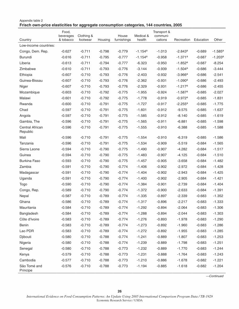
26International Evidence on Food Consumption Patterns: An Update Using 2005 International Comparison Program Data / TB-1929
Economic Research Service / USDA
Appendix table 2
Frisch own-price elasticities for aggregate consumption categories, 144 countries, 2005, continued
Country
Food, beverages & tobacco
Clothing & footwear Housing
House furnishings
Medical & health
Transport & communi-
cations Recreation Education Other
Low-income countries:
Congo, Dem. Rep. -0.627 -0.711 -0.798 -0.779 -1.154a -1.013 -2.843a -0.689 -1.585a
Burundi -0.616 -0.711 -0.795 -0.777 -1.154a -0.958 -1.371a -0.687 -1.203a
Liberia -0.613 -0.711 -0.794 -0.777 -6.323 -0.950 -1.852a -0.687 -8.254
Zimbabwe -0.610 -0.711 -0.793 -0.776 -3.144 -0.939 -1.504a -0.686 -3.444
Ethiopia -0.607 -0.710 -0.793 -0.776 -2.403 -0.932 -3.966a -0.686 -2.541
Guinea-Bissau -0.607 -0.710 -0.793 -0.776 -2.362 -0.931 -1.090a -0.686 -2.493
Niger -0.607 -0.710 -0.793 -0.776 -2.329 -0.931 -1.217a -0.686 -2.455
Mozambique -0.603 -0.710 -0.792 -0.775 -1.955 -0.924 -1.587a -0.685 -2.027
Malawi -0.601 -0.710 -0.792 -0.775 -1.778 -0.919 -0.972a -0.685 -1.831
Rwanda -0.600 -0.710 -0.791 -0.775 -1.727 -0.917 -2.255a -0.685 -1.775
Chad -0.597 -0.710 -0.791 -0.775 -1.601 -0.912 -9.575 -0.685 -1.637
Angola -0.597 -0.710 -0.791 -0.775 -1.585 -0.912 -8.140 -0.685 -1.619
Gambia, The -0.596 -0.710 -0.791 -0.775 -1.565 -0.911 -6.881 -0.685 -1.598
Central African Republic
-0.596 -0.710 -0.791 -0.775 -1.555 -0.910 -6.388 -0.685 -1.588
Mali -0.596 -0.710 -0.791 -0.775 -1.554 -0.910 -6.319 -0.685 -1.586
Tanzania -0.596 -0.710 -0.791 -0.775 -1.534 -0.909 -5.519 -0.684 -1.565
Sierra Leone -0.594 -0.710 -0.790 -0.775 -1.490 -0.907 -4.282 -0.684 -1.517
Guinea -0.594 -0.710 -0.790 -0.775 -1.483 -0.907 -4.125 -0.684 -1.510
Burkina Faso -0.593 -0.710 -0.790 -0.775 -1.457 -0.905 -3.658 -0.684 -1.482
Zambia -0.591 -0.710 -0.790 -0.774 -1.406 -0.902 -2.972 -0.684 -1.428
Madagascar -0.591 -0.710 -0.790 -0.774 -1.404 -0.902 -2.943 -0.684 -1.425
Uganda -0.591 -0.710 -0.790 -0.774 -1.400 -0.902 -2.905 -0.684 -1.421
Togo -0.590 -0.710 -0.790 -0.774 -1.384 -0.901 -2.739 -0.684 -1.404
Congo, Rep. -0.589 -0.710 -0.790 -0.774 -1.372 -0.900 -2.633 -0.684 -1.391
Nepal -0.587 -0.710 -0.789 -0.774 -1.335 -0.897 -2.339 -0.683 -1.352
Ghana -0.586 -0.710 -0.789 -0.774 -1.317 -0.896 -2.217 -0.683 -1.333
Mauritania -0.584 -0.710 -0.789 -0.774 -1.292 -0.894 -2.064 -0.683 -1.306
Bangladesh -0.584 -0.710 -0.789 -0.774 -1.288 -0.894 -2.044 -0.683 -1.303
Côte d'Ivoire -0.583 -0.710 -0.789 -0.774 -1.276 -0.893 -1.978 -0.683 -1.290
Benin -0.583 -0.710 -0.789 -0.774 -1.273 -0.892 -1.960 -0.683 -1.286
Lao PDR -0.583 -0.710 -0.789 -0.774 -1.272 -0.892 -1.955 -0.683 -1.285
Djibouti -0.580 -0.710 -0.788 -0.774 -1.241 -0.889 -1.807 -0.683 -1.253
Nigeria -0.580 -0.710 -0.788 -0.774 -1.239 -0.889 -1.798 -0.683 -1.251
Senegal -0.580 -0.710 -0.788 -0.773 -1.232 -0.889 -1.770 -0.683 -1.244
Kenya -0.579 -0.710 -0.788 -0.773 -1.231 -0.888 -1.764 -0.683 -1.243
Cambodia -0.577 -0.710 -0.788 -0.773 -1.210 -0.886 -1.678 -0.682 -1.221
São Tomé and Principe
-0.576 -0.710 -0.788 -0.773 -1.194 -0.885 -1.618 -0.682 -1.204
---Continued
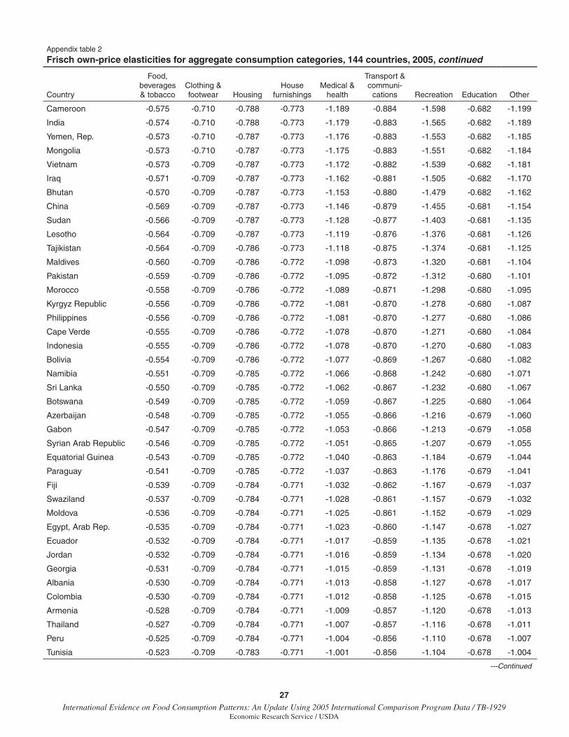
27 International Evidence on Food Consumption Patterns: An Update Using 2005 International Comparison Program Data / TB-1929
Economic Research Service / USDA
Appendix table 2
Frisch own-price elasticities for aggregate consumption categories, 144 countries, 2005, continued
Country
Food, beverages & tobacco
Clothing & footwear Housing
House furnishings
Medical & health
Transport & communi-
cations Recreation Education Other
Cameroon -0.575 -0.710 -0.788 -0.773 -1.189 -0.884 -1.598 -0.682 -1.199
India -0.574 -0.710 -0.788 -0.773 -1.179 -0.883 -1.565 -0.682 -1.189
Yemen, Rep. -0.573 -0.710 -0.787 -0.773 -1.176 -0.883 -1.553 -0.682 -1.185
Mongolia -0.573 -0.710 -0.787 -0.773 -1.175 -0.883 -1.551 -0.682 -1.184
Vietnam -0.573 -0.709 -0.787 -0.773 -1.172 -0.882 -1.539 -0.682 -1.181
Iraq -0.571 -0.709 -0.787 -0.773 -1.162 -0.881 -1.505 -0.682 -1.170
Bhutan -0.570 -0.709 -0.787 -0.773 -1.153 -0.880 -1.479 -0.682 -1.162
China -0.569 -0.709 -0.787 -0.773 -1.146 -0.879 -1.455 -0.681 -1.154
Sudan -0.566 -0.709 -0.787 -0.773 -1.128 -0.877 -1.403 -0.681 -1.135
Lesotho -0.564 -0.709 -0.787 -0.773 -1.119 -0.876 -1.376 -0.681 -1.126
Tajikistan -0.564 -0.709 -0.786 -0.773 -1.118 -0.875 -1.374 -0.681 -1.125
Maldives -0.560 -0.709 -0.786 -0.772 -1.098 -0.873 -1.320 -0.681 -1.104
Pakistan -0.559 -0.709 -0.786 -0.772 -1.095 -0.872 -1.312 -0.680 -1.101
Morocco -0.558 -0.709 -0.786 -0.772 -1.089 -0.871 -1.298 -0.680 -1.095
Kyrgyz Republic -0.556 -0.709 -0.786 -0.772 -1.081 -0.870 -1.278 -0.680 -1.087
Philippines -0.556 -0.709 -0.786 -0.772 -1.081 -0.870 -1.277 -0.680 -1.086
Cape Verde -0.555 -0.709 -0.786 -0.772 -1.078 -0.870 -1.271 -0.680 -1.084
Indonesia -0.555 -0.709 -0.786 -0.772 -1.078 -0.870 -1.270 -0.680 -1.083
Bolivia -0.554 -0.709 -0.786 -0.772 -1.077 -0.869 -1.267 -0.680 -1.082
Namibia -0.551 -0.709 -0.785 -0.772 -1.066 -0.868 -1.242 -0.680 -1.071
Sri Lanka -0.550 -0.709 -0.785 -0.772 -1.062 -0.867 -1.232 -0.680 -1.067
Botswana -0.549 -0.709 -0.785 -0.772 -1.059 -0.867 -1.225 -0.680 -1.064
Azerbaijan -0.548 -0.709 -0.785 -0.772 -1.055 -0.866 -1.216 -0.679 -1.060
Gabon -0.547 -0.709 -0.785 -0.772 -1.053 -0.866 -1.213 -0.679 -1.058
Syrian Arab Republic -0.546 -0.709 -0.785 -0.772 -1.051 -0.865 -1.207 -0.679 -1.055
Equatorial Guinea -0.543 -0.709 -0.785 -0.772 -1.040 -0.863 -1.184 -0.679 -1.044
Paraguay -0.541 -0.709 -0.785 -0.772 -1.037 -0.863 -1.176 -0.679 -1.041
Fiji -0.539 -0.709 -0.784 -0.771 -1.032 -0.862 -1.167 -0.679 -1.037
Swaziland -0.537 -0.709 -0.784 -0.771 -1.028 -0.861 -1.157 -0.679 -1.032
Moldova -0.536 -0.709 -0.784 -0.771 -1.025 -0.861 -1.152 -0.679 -1.029
Egypt, Arab Rep. -0.535 -0.709 -0.784 -0.771 -1.023 -0.860 -1.147 -0.678 -1.027
Ecuador -0.532 -0.709 -0.784 -0.771 -1.017 -0.859 -1.135 -0.678 -1.021
Jordan -0.532 -0.709 -0.784 -0.771 -1.016 -0.859 -1.134 -0.678 -1.020
Georgia -0.531 -0.709 -0.784 -0.771 -1.015 -0.859 -1.131 -0.678 -1.019
Albania -0.530 -0.709 -0.784 -0.771 -1.013 -0.858 -1.127 -0.678 -1.017
Colombia -0.530 -0.709 -0.784 -0.771 -1.012 -0.858 -1.125 -0.678 -1.015
Armenia -0.528 -0.709 -0.784 -0.771 -1.009 -0.857 -1.120 -0.678 -1.013
Thailand -0.527 -0.709 -0.784 -0.771 -1.007 -0.857 -1.116 -0.678 -1.011
Peru -0.525 -0.709 -0.784 -0.771 -1.004 -0.856 -1.110 -0.678 -1.007
Tunisia -0.523 -0.709 -0.783 -0.771 -1.001 -0.856 -1.104 -0.678 -1.004
---Continued
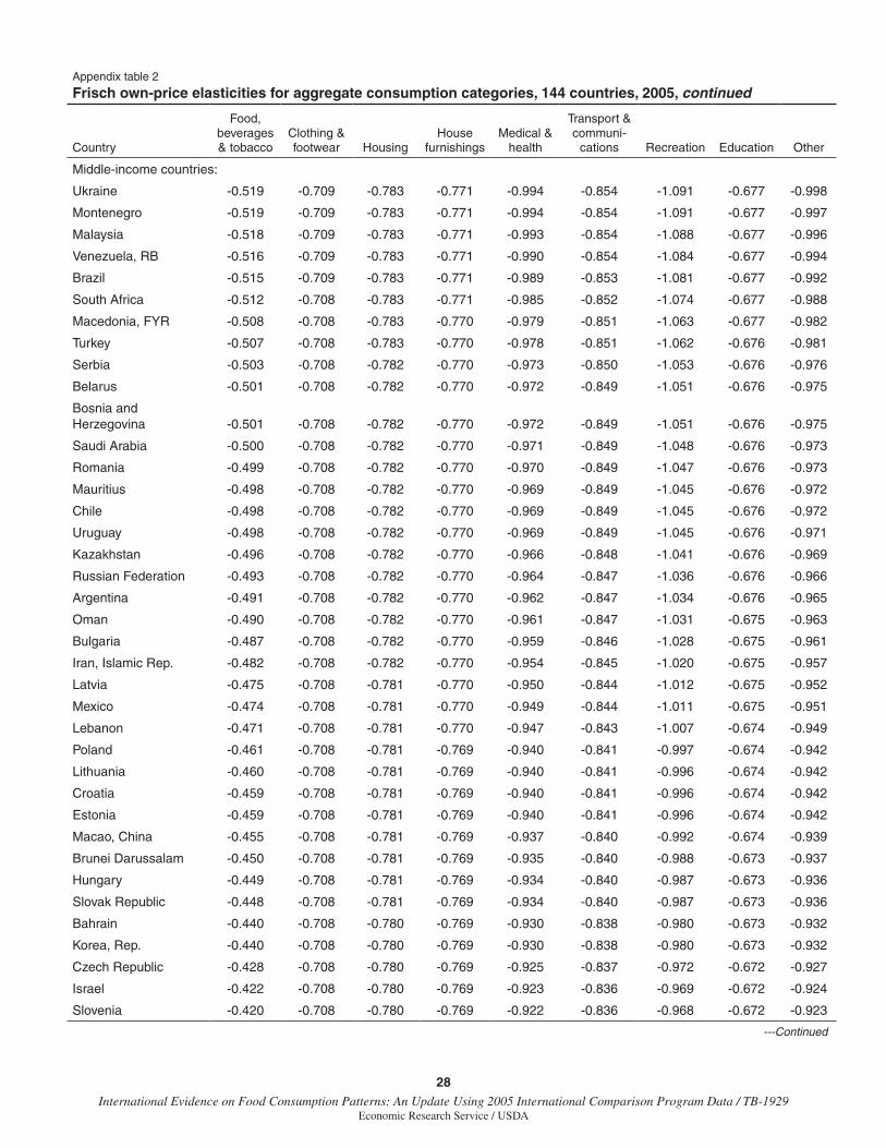
28International Evidence on Food Consumption Patterns: An Update Using 2005 International Comparison Program Data / TB-1929
Economic Research Service / USDA
Appendix table 2
Frisch own-price elasticities for aggregate consumption categories, 144 countries, 2005, continued
Country
Food, beverages & tobacco
Clothing & footwear Housing
House furnishings
Medical & health
Transport & communi-
cations Recreation Education Other
Middle-income countries:
Ukraine -0.519 -0.709 -0.783 -0.771 -0.994 -0.854 -1.091 -0.677 -0.998
Montenegro -0.519 -0.709 -0.783 -0.771 -0.994 -0.854 -1.091 -0.677 -0.997
Malaysia -0.518 -0.709 -0.783 -0.771 -0.993 -0.854 -1.088 -0.677 -0.996
Venezuela, RB -0.516 -0.709 -0.783 -0.771 -0.990 -0.854 -1.084 -0.677 -0.994
Brazil -0.515 -0.709 -0.783 -0.771 -0.989 -0.853 -1.081 -0.677 -0.992
South Africa -0.512 -0.708 -0.783 -0.771 -0.985 -0.852 -1.074 -0.677 -0.988
Macedonia, FYR -0.508 -0.708 -0.783 -0.770 -0.979 -0.851 -1.063 -0.677 -0.982
Turkey -0.507 -0.708 -0.783 -0.770 -0.978 -0.851 -1.062 -0.676 -0.981
Serbia -0.503 -0.708 -0.782 -0.770 -0.973 -0.850 -1.053 -0.676 -0.976
Belarus -0.501 -0.708 -0.782 -0.770 -0.972 -0.849 -1.051 -0.676 -0.975
Bosnia and Herzegovina -0.501 -0.708 -0.782 -0.770 -0.972 -0.849 -1.051 -0.676 -0.975
Saudi Arabia -0.500 -0.708 -0.782 -0.770 -0.971 -0.849 -1.048 -0.676 -0.973
Romania -0.499 -0.708 -0.782 -0.770 -0.970 -0.849 -1.047 -0.676 -0.973
Mauritius -0.498 -0.708 -0.782 -0.770 -0.969 -0.849 -1.045 -0.676 -0.972
Chile -0.498 -0.708 -0.782 -0.770 -0.969 -0.849 -1.045 -0.676 -0.972
Uruguay -0.498 -0.708 -0.782 -0.770 -0.969 -0.849 -1.045 -0.676 -0.971
Kazakhstan -0.496 -0.708 -0.782 -0.770 -0.966 -0.848 -1.041 -0.676 -0.969
Russian Federation -0.493 -0.708 -0.782 -0.770 -0.964 -0.847 -1.036 -0.676 -0.966
Argentina -0.491 -0.708 -0.782 -0.770 -0.962 -0.847 -1.034 -0.676 -0.965
Oman -0.490 -0.708 -0.782 -0.770 -0.961 -0.847 -1.031 -0.675 -0.963
Bulgaria -0.487 -0.708 -0.782 -0.770 -0.959 -0.846 -1.028 -0.675 -0.961
Iran, Islamic Rep. -0.482 -0.708 -0.782 -0.770 -0.954 -0.845 -1.020 -0.675 -0.957
Latvia -0.475 -0.708 -0.781 -0.770 -0.950 -0.844 -1.012 -0.675 -0.952
Mexico -0.474 -0.708 -0.781 -0.770 -0.949 -0.844 -1.011 -0.675 -0.951
Lebanon -0.471 -0.708 -0.781 -0.770 -0.947 -0.843 -1.007 -0.674 -0.949
Poland -0.461 -0.708 -0.781 -0.769 -0.940 -0.841 -0.997 -0.674 -0.942
Lithuania -0.460 -0.708 -0.781 -0.769 -0.940 -0.841 -0.996 -0.674 -0.942
Croatia -0.459 -0.708 -0.781 -0.769 -0.940 -0.841 -0.996 -0.674 -0.942
Estonia -0.459 -0.708 -0.781 -0.769 -0.940 -0.841 -0.996 -0.674 -0.942
Macao, China -0.455 -0.708 -0.781 -0.769 -0.937 -0.840 -0.992 -0.674 -0.939
Brunei Darussalam -0.450 -0.708 -0.781 -0.769 -0.935 -0.840 -0.988 -0.673 -0.937
Hungary -0.449 -0.708 -0.781 -0.769 -0.934 -0.840 -0.987 -0.673 -0.936
Slovak Republic -0.448 -0.708 -0.781 -0.769 -0.934 -0.840 -0.987 -0.673 -0.936
Bahrain -0.440 -0.708 -0.780 -0.769 -0.930 -0.838 -0.980 -0.673 -0.932
Korea, Rep. -0.440 -0.708 -0.780 -0.769 -0.930 -0.838 -0.980 -0.673 -0.932
Czech Republic -0.428 -0.708 -0.780 -0.769 -0.925 -0.837 -0.972 -0.672 -0.927
Israel -0.422 -0.708 -0.780 -0.769 -0.923 -0.836 -0.969 -0.672 -0.924
Slovenia -0.420 -0.708 -0.780 -0.769 -0.922 -0.836 -0.968 -0.672 -0.923
---Continued
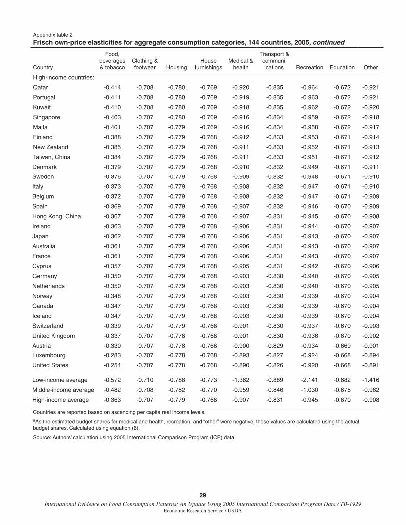
29 International Evidence on Food Consumption Patterns: An Update Using 2005 International Comparison Program Data / TB-1929
Economic Research Service / USDA
Appendix table 2
Frisch own-price elasticities for aggregate consumption categories, 144 countries, 2005, continued
Country
Food, beverages & tobacco
Clothing & footwear Housing
House furnishings
Medical & health
Transport & communi-
cations Recreation Education Other
High-income countries:
Qatar -0.414 -0.708 -0.780 -0.769 -0.920 -0.835 -0.964 -0.672 -0.921
Portugal -0.411 -0.708 -0.780 -0.769 -0.919 -0.835 -0.963 -0.672 -0.921
Kuwait -0.410 -0.708 -0.780 -0.769 -0.918 -0.835 -0.962 -0.672 -0.920
Singapore -0.403 -0.707 -0.780 -0.769 -0.916 -0.834 -0.959 -0.672 -0.918
Malta -0.401 -0.707 -0.779 -0.769 -0.916 -0.834 -0.958 -0.672 -0.917
Finland -0.388 -0.707 -0.779 -0.768 -0.912 -0.833 -0.953 -0.671 -0.914
New Zealand -0.385 -0.707 -0.779 -0.768 -0.911 -0.833 -0.952 -0.671 -0.913
Taiwan, China -0.384 -0.707 -0.779 -0.768 -0.911 -0.833 -0.951 -0.671 -0.912
Denmark -0.379 -0.707 -0.779 -0.768 -0.910 -0.832 -0.949 -0.671 -0.911
Sweden -0.376 -0.707 -0.779 -0.768 -0.909 -0.832 -0.948 -0.671 -0.910
Italy -0.373 -0.707 -0.779 -0.768 -0.908 -0.832 -0.947 -0.671 -0.910
Belgium -0.372 -0.707 -0.779 -0.768 -0.908 -0.832 -0.947 -0.671 -0.909
Spain -0.369 -0.707 -0.779 -0.768 -0.907 -0.832 -0.946 -0.670 -0.909
Hong Kong, China -0.367 -0.707 -0.779 -0.768 -0.907 -0.831 -0.945 -0.670 -0.908
Ireland -0.363 -0.707 -0.779 -0.768 -0.906 -0.831 -0.944 -0.670 -0.907
Japan -0.362 -0.707 -0.779 -0.768 -0.906 -0.831 -0.943 -0.670 -0.907
Australia -0.361 -0.707 -0.779 -0.768 -0.906 -0.831 -0.943 -0.670 -0.907
France -0.361 -0.707 -0.779 -0.768 -0.906 -0.831 -0.943 -0.670 -0.907
Cyprus -0.357 -0.707 -0.779 -0.768 -0.905 -0.831 -0.942 -0.670 -0.906
Germany -0.350 -0.707 -0.779 -0.768 -0.903 -0.830 -0.940 -0.670 -0.905
Netherlands -0.350 -0.707 -0.779 -0.768 -0.903 -0.830 -0.940 -0.670 -0.905
Norway -0.348 -0.707 -0.779 -0.768 -0.903 -0.830 -0.939 -0.670 -0.904
Canada -0.347 -0.707 -0.779 -0.768 -0.903 -0.830 -0.939 -0.670 -0.904
Iceland -0.347 -0.707 -0.779 -0.768 -0.903 -0.830 -0.939 -0.670 -0.904
Switzerland -0.339 -0.707 -0.779 -0.768 -0.901 -0.830 -0.937 -0.670 -0.903
United Kingdom -0.337 -0.707 -0.778 -0.768 -0.901 -0.830 -0.936 -0.670 -0.902
Austria -0.330 -0.707 -0.778 -0.768 -0.900 -0.829 -0.934 -0.669 -0.901
Luxembourg -0.283 -0.707 -0.778 -0.768 -0.893 -0.827 -0.924 -0.668 -0.894
United States -0.254 -0.707 -0.778 -0.768 -0.890 -0.826 -0.920 -0.668 -0.891
Low-income average -0.572 -0.710 -0.788 -0.773 -1.362 -0.889 -2.141 -0.682 -1.416
Middle-income average -0.482 -0.708 -0.782 -0.770 -0.959 -0.846 -1.030 -0.675 -0.962
High-income average -0.363 -0.707 -0.779 -0.768 -0.907 -0.831 -0.945 -0.670 -0.908
Countries are reported based on ascending per capita real income levels.aAs the estimated budget shares for medical and health, recreation, and “other” were negative, these values are calculated using the actual budget shares. Calculated using equation (6).
Source: Authors’ calculation using 2005 International Comparison Program (ICP) data.
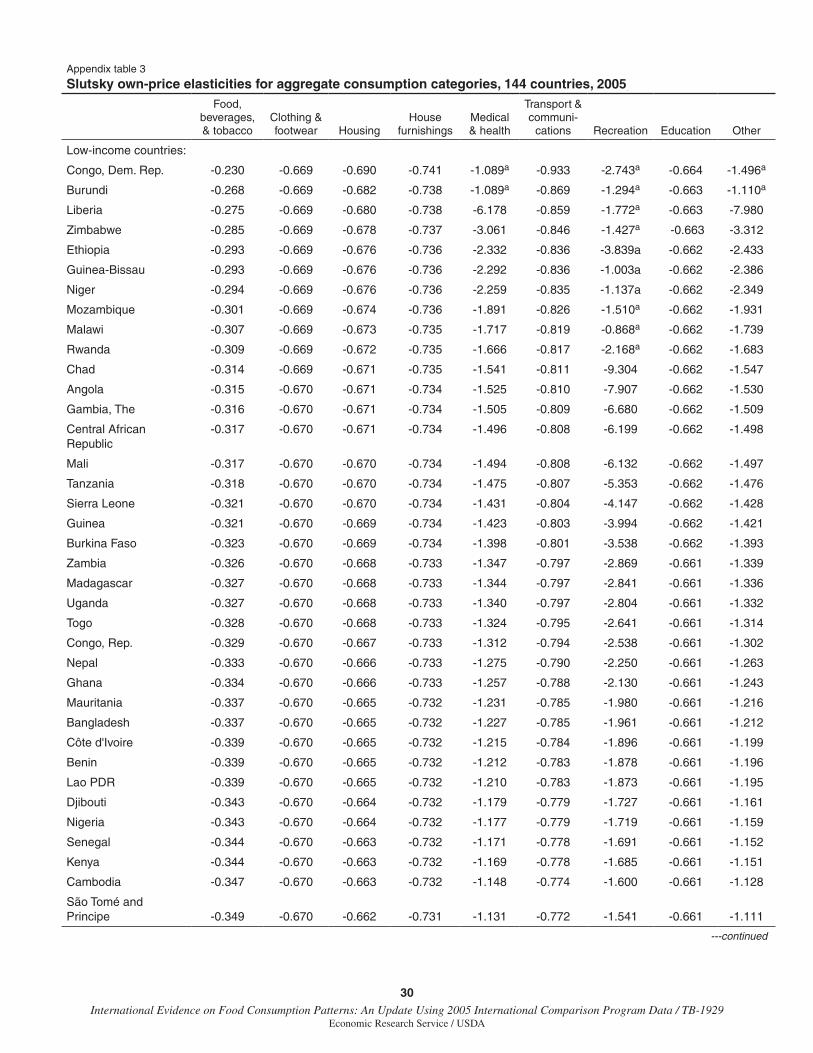
30International Evidence on Food Consumption Patterns: An Update Using 2005 International Comparison Program Data / TB-1929
Economic Research Service / USDA
Appendix table 3
Slutsky own-price elasticities for aggregate consumption categories, 144 countries, 2005, continuedFood,
beverages, & tobacco
Clothing & footwear Housing
House furnishings
Medical & health
Transport & communi-
cations Recreation Education Other
Low-income countries:
Congo, Dem. Rep. -0.230 -0.669 -0.690 -0.741 -1.089a -0.933 -2.743a -0.664 -1.496a
Burundi -0.268 -0.669 -0.682 -0.738 -1.089a -0.869 -1.294a -0.663 -1.110a
Liberia -0.275 -0.669 -0.680 -0.738 -6.178 -0.859 -1.772a -0.663 -7.980
Zimbabwe -0.285 -0.669 -0.678 -0.737 -3.061 -0.846 -1.427a -0.663 -3.312
Ethiopia -0.293 -0.669 -0.676 -0.736 -2.332 -0.836 -3.839a -0.662 -2.433
Guinea-Bissau -0.293 -0.669 -0.676 -0.736 -2.292 -0.836 -1.003a -0.662 -2.386
Niger -0.294 -0.669 -0.676 -0.736 -2.259 -0.835 -1.137a -0.662 -2.349
Mozambique -0.301 -0.669 -0.674 -0.736 -1.891 -0.826 -1.510a -0.662 -1.931
Malawi -0.307 -0.669 -0.673 -0.735 -1.717 -0.819 -0.868a -0.662 -1.739
Rwanda -0.309 -0.669 -0.672 -0.735 -1.666 -0.817 -2.168a -0.662 -1.683
Chad -0.314 -0.669 -0.671 -0.735 -1.541 -0.811 -9.304 -0.662 -1.547
Angola -0.315 -0.670 -0.671 -0.734 -1.525 -0.810 -7.907 -0.662 -1.530
Gambia, The -0.316 -0.670 -0.671 -0.734 -1.505 -0.809 -6.680 -0.662 -1.509
Central African Republic
-0.317 -0.670 -0.671 -0.734 -1.496 -0.808 -6.199 -0.662 -1.498
Mali -0.317 -0.670 -0.670 -0.734 -1.494 -0.808 -6.132 -0.662 -1.497
Tanzania -0.318 -0.670 -0.670 -0.734 -1.475 -0.807 -5.353 -0.662 -1.476
Sierra Leone -0.321 -0.670 -0.670 -0.734 -1.431 -0.804 -4.147 -0.662 -1.428
Guinea -0.321 -0.670 -0.669 -0.734 -1.423 -0.803 -3.994 -0.662 -1.421
Burkina Faso -0.323 -0.670 -0.669 -0.734 -1.398 -0.801 -3.538 -0.662 -1.393
Zambia -0.326 -0.670 -0.668 -0.733 -1.347 -0.797 -2.869 -0.661 -1.339
Madagascar -0.327 -0.670 -0.668 -0.733 -1.344 -0.797 -2.841 -0.661 -1.336
Uganda -0.327 -0.670 -0.668 -0.733 -1.340 -0.797 -2.804 -0.661 -1.332
Togo -0.328 -0.670 -0.668 -0.733 -1.324 -0.795 -2.641 -0.661 -1.314
Congo, Rep. -0.329 -0.670 -0.667 -0.733 -1.312 -0.794 -2.538 -0.661 -1.302
Nepal -0.333 -0.670 -0.666 -0.733 -1.275 -0.790 -2.250 -0.661 -1.263
Ghana -0.334 -0.670 -0.666 -0.733 -1.257 -0.788 -2.130 -0.661 -1.243
Mauritania -0.337 -0.670 -0.665 -0.732 -1.231 -0.785 -1.980 -0.661 -1.216
Bangladesh -0.337 -0.670 -0.665 -0.732 -1.227 -0.785 -1.961 -0.661 -1.212
Côte d'Ivoire -0.339 -0.670 -0.665 -0.732 -1.215 -0.784 -1.896 -0.661 -1.199
Benin -0.339 -0.670 -0.665 -0.732 -1.212 -0.783 -1.878 -0.661 -1.196
Lao PDR -0.339 -0.670 -0.665 -0.732 -1.210 -0.783 -1.873 -0.661 -1.195
Djibouti -0.343 -0.670 -0.664 -0.732 -1.179 -0.779 -1.727 -0.661 -1.161
Nigeria -0.343 -0.670 -0.664 -0.732 -1.177 -0.779 -1.719 -0.661 -1.159
Senegal -0.344 -0.670 -0.663 -0.732 -1.171 -0.778 -1.691 -0.661 -1.152
Kenya -0.344 -0.670 -0.663 -0.732 -1.169 -0.778 -1.685 -0.661 -1.151
Cambodia -0.347 -0.670 -0.663 -0.732 -1.148 -0.774 -1.600 -0.661 -1.128
São Tomé and Principe -0.349 -0.670 -0.662 -0.731 -1.131 -0.772 -1.541 -0.661 -1.111
---continued
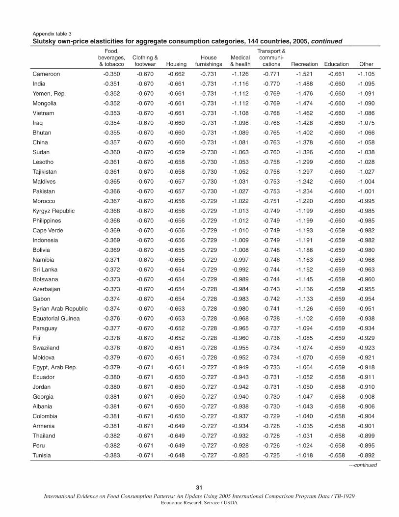
31 International Evidence on Food Consumption Patterns: An Update Using 2005 International Comparison Program Data / TB-1929
Economic Research Service / USDA
Appendix table 3
Slutsky own-price elasticities for aggregate consumption categories, 144 countries, 2005, continuedFood,
beverages, & tobacco
Clothing & footwear Housing
House furnishings
Medical & health
Transport & communi-
cations Recreation Education Other
Cameroon -0.350 -0.670 -0.662 -0.731 -1.126 -0.771 -1.521 -0.661 -1.105
India -0.351 -0.670 -0.661 -0.731 -1.116 -0.770 -1.488 -0.660 -1.095
Yemen, Rep. -0.352 -0.670 -0.661 -0.731 -1.112 -0.769 -1.476 -0.660 -1.091
Mongolia -0.352 -0.670 -0.661 -0.731 -1.112 -0.769 -1.474 -0.660 -1.090
Vietnam -0.353 -0.670 -0.661 -0.731 -1.108 -0.768 -1.462 -0.660 -1.086
Iraq -0.354 -0.670 -0.660 -0.731 -1.098 -0.766 -1.428 -0.660 -1.075
Bhutan -0.355 -0.670 -0.660 -0.731 -1.089 -0.765 -1.402 -0.660 -1.066
China -0.357 -0.670 -0.660 -0.731 -1.081 -0.763 -1.378 -0.660 -1.058
Sudan -0.360 -0.670 -0.659 -0.730 -1.063 -0.760 -1.326 -0.660 -1.038
Lesotho -0.361 -0.670 -0.658 -0.730 -1.053 -0.758 -1.299 -0.660 -1.028
Tajikistan -0.361 -0.670 -0.658 -0.730 -1.052 -0.758 -1.297 -0.660 -1.027
Maldives -0.365 -0.670 -0.657 -0.730 -1.031 -0.753 -1.242 -0.660 -1.004
Pakistan -0.366 -0.670 -0.657 -0.730 -1.027 -0.753 -1.234 -0.660 -1.001
Morocco -0.367 -0.670 -0.656 -0.729 -1.022 -0.751 -1.220 -0.660 -0.995
Kyrgyz Republic -0.368 -0.670 -0.656 -0.729 -1.013 -0.749 -1.199 -0.660 -0.985
Philippines -0.368 -0.670 -0.656 -0.729 -1.012 -0.749 -1.199 -0.660 -0.985
Cape Verde -0.369 -0.670 -0.656 -0.729 -1.010 -0.749 -1.193 -0.659 -0.982
Indonesia -0.369 -0.670 -0.656 -0.729 -1.009 -0.749 -1.191 -0.659 -0.982
Bolivia -0.369 -0.670 -0.655 -0.729 -1.008 -0.748 -1.188 -0.659 -0.980
Namibia -0.371 -0.670 -0.655 -0.729 -0.997 -0.746 -1.163 -0.659 -0.968
Sri Lanka -0.372 -0.670 -0.654 -0.729 -0.992 -0.744 -1.152 -0.659 -0.963
Botswana -0.373 -0.670 -0.654 -0.729 -0.989 -0.744 -1.145 -0.659 -0.960
Azerbaijan -0.373 -0.670 -0.654 -0.728 -0.984 -0.743 -1.136 -0.659 -0.955
Gabon -0.374 -0.670 -0.654 -0.728 -0.983 -0.742 -1.133 -0.659 -0.954
Syrian Arab Republic -0.374 -0.670 -0.653 -0.728 -0.980 -0.741 -1.126 -0.659 -0.951
Equatorial Guinea -0.376 -0.670 -0.653 -0.728 -0.968 -0.738 -1.102 -0.659 -0.938
Paraguay -0.377 -0.670 -0.652 -0.728 -0.965 -0.737 -1.094 -0.659 -0.934
Fiji -0.378 -0.670 -0.652 -0.728 -0.960 -0.736 -1.085 -0.659 -0.929
Swaziland -0.378 -0.670 -0.651 -0.728 -0.955 -0.734 -1.074 -0.659 -0.923
Moldova -0.379 -0.670 -0.651 -0.728 -0.952 -0.734 -1.070 -0.659 -0.921
Egypt, Arab Rep. -0.379 -0.671 -0.651 -0.727 -0.949 -0.733 -1.064 -0.659 -0.918
Ecuador -0.380 -0.671 -0.650 -0.727 -0.943 -0.731 -1.052 -0.658 -0.911
Jordan -0.380 -0.671 -0.650 -0.727 -0.942 -0.731 -1.050 -0.658 -0.910
Georgia -0.381 -0.671 -0.650 -0.727 -0.940 -0.730 -1.047 -0.658 -0.908
Albania -0.381 -0.671 -0.650 -0.727 -0.938 -0.730 -1.043 -0.658 -0.906
Colombia -0.381 -0.671 -0.650 -0.727 -0.937 -0.729 -1.040 -0.658 -0.904
Armenia -0.381 -0.671 -0.649 -0.727 -0.934 -0.728 -1.035 -0.658 -0.901
Thailand -0.382 -0.671 -0.649 -0.727 -0.932 -0.728 -1.031 -0.658 -0.899
Peru -0.382 -0.671 -0.649 -0.727 -0.928 -0.726 -1.024 -0.658 -0.895
Tunisia -0.383 -0.671 -0.648 -0.727 -0.925 -0.725 -1.018 -0.658 -0.892
---continued
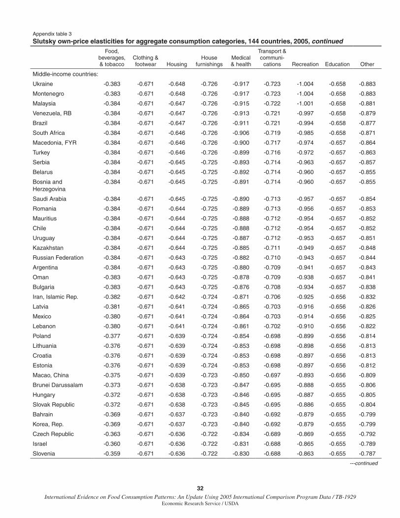
32International Evidence on Food Consumption Patterns: An Update Using 2005 International Comparison Program Data / TB-1929
Economic Research Service / USDA
Appendix table 3
Slutsky own-price elasticities for aggregate consumption categories, 144 countries, 2005, continuedFood,
beverages, & tobacco
Clothing & footwear Housing
House furnishings
Medical & health
Transport & communi-
cations Recreation Education Other
Middle-income countries:
Ukraine -0.383 -0.671 -0.648 -0.726 -0.917 -0.723 -1.004 -0.658 -0.883
Montenegro -0.383 -0.671 -0.648 -0.726 -0.917 -0.723 -1.004 -0.658 -0.883
Malaysia -0.384 -0.671 -0.647 -0.726 -0.915 -0.722 -1.001 -0.658 -0.881
Venezuela, RB -0.384 -0.671 -0.647 -0.726 -0.913 -0.721 -0.997 -0.658 -0.879
Brazil -0.384 -0.671 -0.647 -0.726 -0.911 -0.721 -0.994 -0.658 -0.877
South Africa -0.384 -0.671 -0.646 -0.726 -0.906 -0.719 -0.985 -0.658 -0.871
Macedonia, FYR -0.384 -0.671 -0.646 -0.726 -0.900 -0.717 -0.974 -0.657 -0.864
Turkey -0.384 -0.671 -0.646 -0.726 -0.899 -0.716 -0.972 -0.657 -0.863
Serbia -0.384 -0.671 -0.645 -0.725 -0.893 -0.714 -0.963 -0.657 -0.857
Belarus -0.384 -0.671 -0.645 -0.725 -0.892 -0.714 -0.960 -0.657 -0.855
Bosnia and Herzegovina
-0.384 -0.671 -0.645 -0.725 -0.891 -0.714 -0.960 -0.657 -0.855
Saudi Arabia -0.384 -0.671 -0.645 -0.725 -0.890 -0.713 -0.957 -0.657 -0.854
Romania -0.384 -0.671 -0.644 -0.725 -0.889 -0.713 -0.956 -0.657 -0.853
Mauritius -0.384 -0.671 -0.644 -0.725 -0.888 -0.712 -0.954 -0.657 -0.852
Chile -0.384 -0.671 -0.644 -0.725 -0.888 -0.712 -0.954 -0.657 -0.852
Uruguay -0.384 -0.671 -0.644 -0.725 -0.887 -0.712 -0.953 -0.657 -0.851
Kazakhstan -0.384 -0.671 -0.644 -0.725 -0.885 -0.711 -0.949 -0.657 -0.848
Russian Federation -0.384 -0.671 -0.643 -0.725 -0.882 -0.710 -0.943 -0.657 -0.844
Argentina -0.384 -0.671 -0.643 -0.725 -0.880 -0.709 -0.941 -0.657 -0.843
Oman -0.383 -0.671 -0.643 -0.725 -0.878 -0.709 -0.938 -0.657 -0.841
Bulgaria -0.383 -0.671 -0.643 -0.725 -0.876 -0.708 -0.934 -0.657 -0.838
Iran, Islamic Rep. -0.382 -0.671 -0.642 -0.724 -0.871 -0.706 -0.925 -0.656 -0.832
Latvia -0.381 -0.671 -0.641 -0.724 -0.865 -0.703 -0.916 -0.656 -0.826
Mexico -0.380 -0.671 -0.641 -0.724 -0.864 -0.703 -0.914 -0.656 -0.825
Lebanon -0.380 -0.671 -0.641 -0.724 -0.861 -0.702 -0.910 -0.656 -0.822
Poland -0.377 -0.671 -0.639 -0.724 -0.854 -0.698 -0.899 -0.656 -0.814
Lithuania -0.376 -0.671 -0.639 -0.724 -0.853 -0.698 -0.898 -0.656 -0.813
Croatia -0.376 -0.671 -0.639 -0.724 -0.853 -0.698 -0.897 -0.656 -0.813
Estonia -0.376 -0.671 -0.639 -0.724 -0.853 -0.698 -0.897 -0.656 -0.812
Macao, China -0.375 -0.671 -0.639 -0.723 -0.850 -0.697 -0.893 -0.656 -0.809
Brunei Darussalam -0.373 -0.671 -0.638 -0.723 -0.847 -0.695 -0.888 -0.655 -0.806
Hungary -0.372 -0.671 -0.638 -0.723 -0.846 -0.695 -0.887 -0.655 -0.805
Slovak Republic -0.372 -0.671 -0.638 -0.723 -0.845 -0.695 -0.886 -0.655 -0.804
Bahrain -0.369 -0.671 -0.637 -0.723 -0.840 -0.692 -0.879 -0.655 -0.799
Korea, Rep. -0.369 -0.671 -0.637 -0.723 -0.840 -0.692 -0.879 -0.655 -0.799
Czech Republic -0.363 -0.671 -0.636 -0.722 -0.834 -0.689 -0.869 -0.655 -0.792
Israel -0.360 -0.671 -0.636 -0.722 -0.831 -0.688 -0.865 -0.655 -0.789
Slovenia -0.359 -0.671 -0.636 -0.722 -0.830 -0.688 -0.863 -0.655 -0.787
---continued
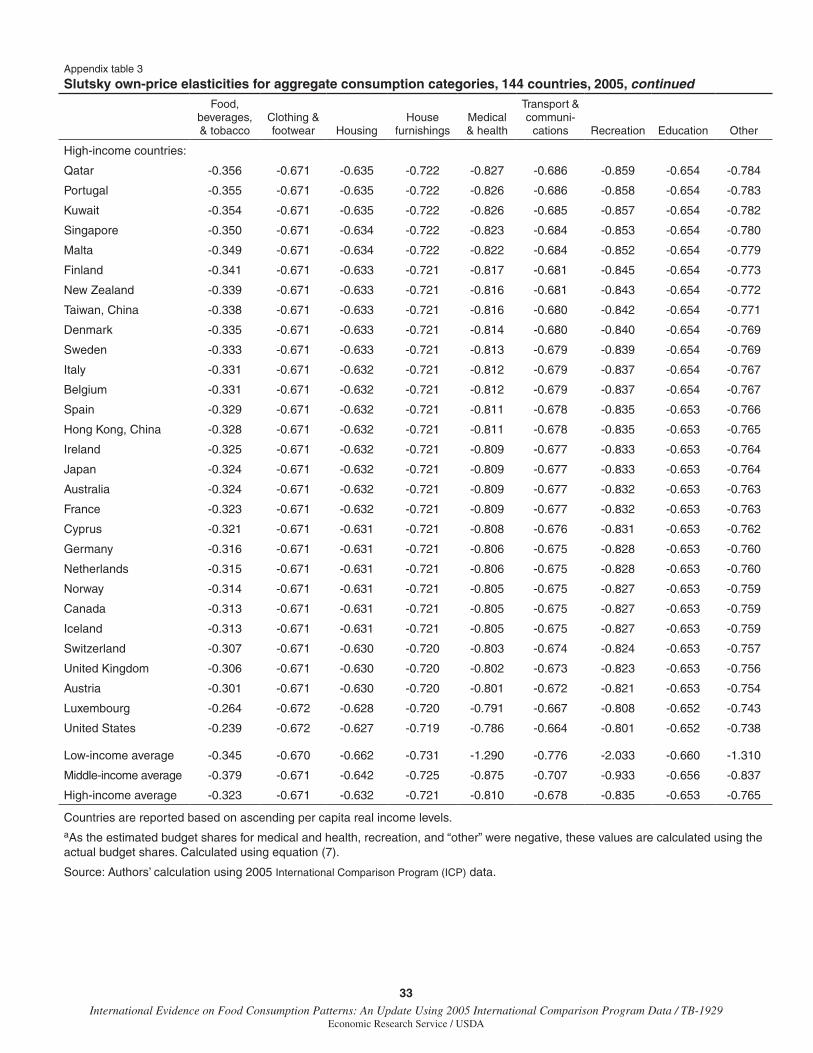
33 International Evidence on Food Consumption Patterns: An Update Using 2005 International Comparison Program Data / TB-1929
Economic Research Service / USDA
Appendix table 3
Slutsky own-price elasticities for aggregate consumption categories, 144 countries, 2005, continuedFood,
beverages, & tobacco
Clothing & footwear Housing
House furnishings
Medical & health
Transport & communi-
cations Recreation Education Other
High-income countries:
Qatar -0.356 -0.671 -0.635 -0.722 -0.827 -0.686 -0.859 -0.654 -0.784
Portugal -0.355 -0.671 -0.635 -0.722 -0.826 -0.686 -0.858 -0.654 -0.783
Kuwait -0.354 -0.671 -0.635 -0.722 -0.826 -0.685 -0.857 -0.654 -0.782
Singapore -0.350 -0.671 -0.634 -0.722 -0.823 -0.684 -0.853 -0.654 -0.780
Malta -0.349 -0.671 -0.634 -0.722 -0.822 -0.684 -0.852 -0.654 -0.779
Finland -0.341 -0.671 -0.633 -0.721 -0.817 -0.681 -0.845 -0.654 -0.773
New Zealand -0.339 -0.671 -0.633 -0.721 -0.816 -0.681 -0.843 -0.654 -0.772
Taiwan, China -0.338 -0.671 -0.633 -0.721 -0.816 -0.680 -0.842 -0.654 -0.771
Denmark -0.335 -0.671 -0.633 -0.721 -0.814 -0.680 -0.840 -0.654 -0.769
Sweden -0.333 -0.671 -0.633 -0.721 -0.813 -0.679 -0.839 -0.654 -0.769
Italy -0.331 -0.671 -0.632 -0.721 -0.812 -0.679 -0.837 -0.654 -0.767
Belgium -0.331 -0.671 -0.632 -0.721 -0.812 -0.679 -0.837 -0.654 -0.767
Spain -0.329 -0.671 -0.632 -0.721 -0.811 -0.678 -0.835 -0.653 -0.766
Hong Kong, China -0.328 -0.671 -0.632 -0.721 -0.811 -0.678 -0.835 -0.653 -0.765
Ireland -0.325 -0.671 -0.632 -0.721 -0.809 -0.677 -0.833 -0.653 -0.764
Japan -0.324 -0.671 -0.632 -0.721 -0.809 -0.677 -0.833 -0.653 -0.764
Australia -0.324 -0.671 -0.632 -0.721 -0.809 -0.677 -0.832 -0.653 -0.763
France -0.323 -0.671 -0.632 -0.721 -0.809 -0.677 -0.832 -0.653 -0.763
Cyprus -0.321 -0.671 -0.631 -0.721 -0.808 -0.676 -0.831 -0.653 -0.762
Germany -0.316 -0.671 -0.631 -0.721 -0.806 -0.675 -0.828 -0.653 -0.760
Netherlands -0.315 -0.671 -0.631 -0.721 -0.806 -0.675 -0.828 -0.653 -0.760
Norway -0.314 -0.671 -0.631 -0.721 -0.805 -0.675 -0.827 -0.653 -0.759
Canada -0.313 -0.671 -0.631 -0.721 -0.805 -0.675 -0.827 -0.653 -0.759
Iceland -0.313 -0.671 -0.631 -0.721 -0.805 -0.675 -0.827 -0.653 -0.759
Switzerland -0.307 -0.671 -0.630 -0.720 -0.803 -0.674 -0.824 -0.653 -0.757
United Kingdom -0.306 -0.671 -0.630 -0.720 -0.802 -0.673 -0.823 -0.653 -0.756
Austria -0.301 -0.671 -0.630 -0.720 -0.801 -0.672 -0.821 -0.653 -0.754
Luxembourg -0.264 -0.672 -0.628 -0.720 -0.791 -0.667 -0.808 -0.652 -0.743
United States -0.239 -0.672 -0.627 -0.719 -0.786 -0.664 -0.801 -0.652 -0.738
Low-income average -0.345 -0.670 -0.662 -0.731 -1.290 -0.776 -2.033 -0.660 -1.310
Middle-income average -0.379 -0.671 -0.642 -0.725 -0.875 -0.707 -0.933 -0.656 -0.837
High-income average -0.323 -0.671 -0.632 -0.721 -0.810 -0.678 -0.835 -0.653 -0.765
Countries are reported based on ascending per capita real income levels.aAs the estimated budget shares for medical and health, recreation, and “other” were negative, these values are calculated using the actual budget shares. Calculated using equation (7).
Source: Authors’ calculation using 2005 International Comparison Program (ICP) data.
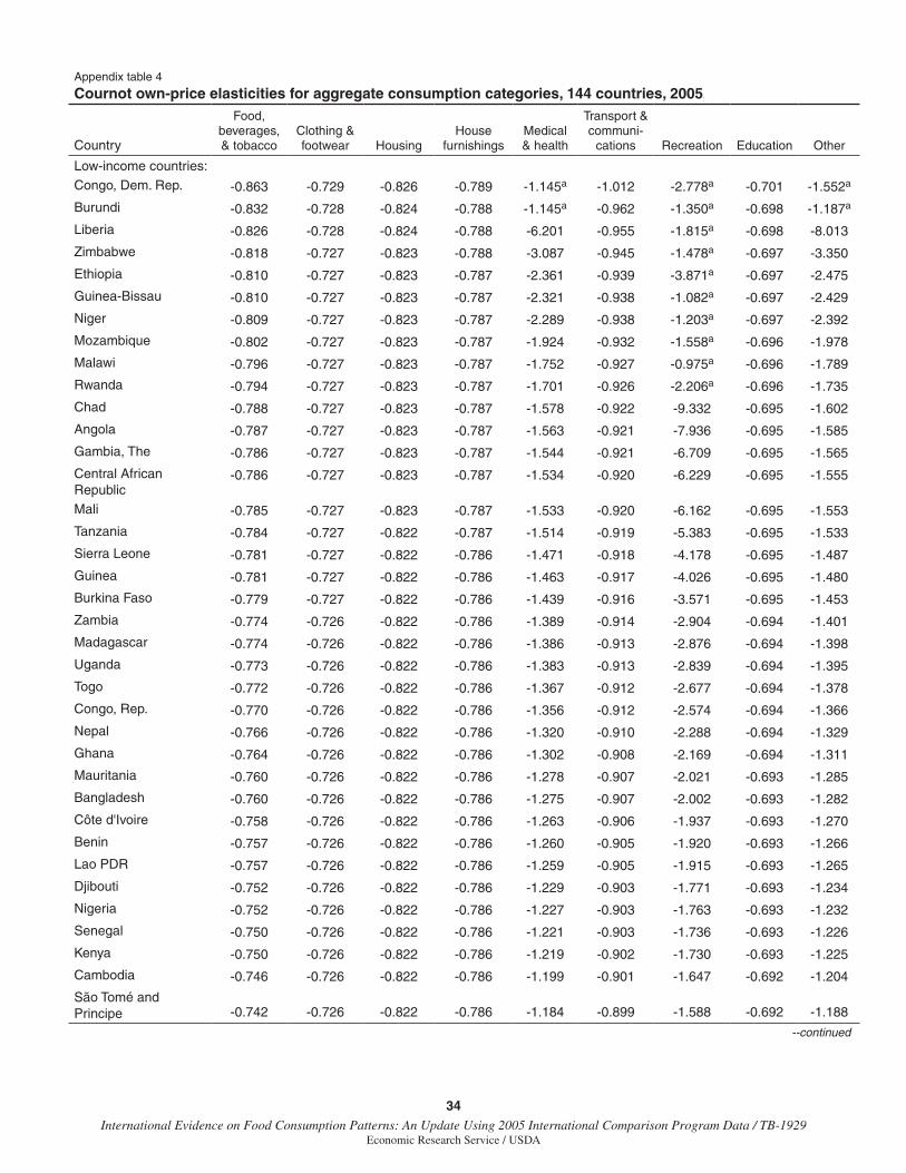
34International Evidence on Food Consumption Patterns: An Update Using 2005 International Comparison Program Data / TB-1929
Economic Research Service / USDA
Appendix table 4
Cournot own-price elasticities for aggregate consumption categories, 144 countries, 2005, continued
Country
Food, beverages, & tobacco
Clothing & footwear Housing
House furnishings
Medical & health
Transport & communi-
cations Recreation Education Other
Low-income countries:Congo, Dem. Rep. -0.863 -0.729 -0.826 -0.789 -1.145a -1.012 -2.778a -0.701 -1.552a
Burundi -0.832 -0.728 -0.824 -0.788 -1.145a -0.962 -1.350a -0.698 -1.187a
Liberia -0.826 -0.728 -0.824 -0.788 -6.201 -0.955 -1.815a -0.698 -8.013
Zimbabwe -0.818 -0.727 -0.823 -0.788 -3.087 -0.945 -1.478a -0.697 -3.350
Ethiopia -0.810 -0.727 -0.823 -0.787 -2.361 -0.939 -3.871a -0.697 -2.475
Guinea-Bissau -0.810 -0.727 -0.823 -0.787 -2.321 -0.938 -1.082a -0.697 -2.429
Niger -0.809 -0.727 -0.823 -0.787 -2.289 -0.938 -1.203a -0.697 -2.392
Mozambique -0.802 -0.727 -0.823 -0.787 -1.924 -0.932 -1.558a -0.696 -1.978
Malawi -0.796 -0.727 -0.823 -0.787 -1.752 -0.927 -0.975a -0.696 -1.789
Rwanda -0.794 -0.727 -0.823 -0.787 -1.701 -0.926 -2.206a -0.696 -1.735
Chad -0.788 -0.727 -0.823 -0.787 -1.578 -0.922 -9.332 -0.695 -1.602
Angola -0.787 -0.727 -0.823 -0.787 -1.563 -0.921 -7.936 -0.695 -1.585
Gambia, The -0.786 -0.727 -0.823 -0.787 -1.544 -0.921 -6.709 -0.695 -1.565
Central African Republic
-0.786 -0.727 -0.823 -0.787 -1.534 -0.920 -6.229 -0.695 -1.555
Mali -0.785 -0.727 -0.823 -0.787 -1.533 -0.920 -6.162 -0.695 -1.553
Tanzania -0.784 -0.727 -0.822 -0.787 -1.514 -0.919 -5.383 -0.695 -1.533
Sierra Leone -0.781 -0.727 -0.822 -0.786 -1.471 -0.918 -4.178 -0.695 -1.487
Guinea -0.781 -0.727 -0.822 -0.786 -1.463 -0.917 -4.026 -0.695 -1.480
Burkina Faso -0.779 -0.727 -0.822 -0.786 -1.439 -0.916 -3.571 -0.695 -1.453
Zambia -0.774 -0.726 -0.822 -0.786 -1.389 -0.914 -2.904 -0.694 -1.401
Madagascar -0.774 -0.726 -0.822 -0.786 -1.386 -0.913 -2.876 -0.694 -1.398
Uganda -0.773 -0.726 -0.822 -0.786 -1.383 -0.913 -2.839 -0.694 -1.395
Togo -0.772 -0.726 -0.822 -0.786 -1.367 -0.912 -2.677 -0.694 -1.378
Congo, Rep. -0.770 -0.726 -0.822 -0.786 -1.356 -0.912 -2.574 -0.694 -1.366
Nepal -0.766 -0.726 -0.822 -0.786 -1.320 -0.910 -2.288 -0.694 -1.329
Ghana -0.764 -0.726 -0.822 -0.786 -1.302 -0.908 -2.169 -0.694 -1.311
Mauritania -0.760 -0.726 -0.822 -0.786 -1.278 -0.907 -2.021 -0.693 -1.285
Bangladesh -0.760 -0.726 -0.822 -0.786 -1.275 -0.907 -2.002 -0.693 -1.282
Côte d'Ivoire -0.758 -0.726 -0.822 -0.786 -1.263 -0.906 -1.937 -0.693 -1.270
Benin -0.757 -0.726 -0.822 -0.786 -1.260 -0.905 -1.920 -0.693 -1.266
Lao PDR -0.757 -0.726 -0.822 -0.786 -1.259 -0.905 -1.915 -0.693 -1.265
Djibouti -0.752 -0.726 -0.822 -0.786 -1.229 -0.903 -1.771 -0.693 -1.234
Nigeria -0.752 -0.726 -0.822 -0.786 -1.227 -0.903 -1.763 -0.693 -1.232
Senegal -0.750 -0.726 -0.822 -0.786 -1.221 -0.903 -1.736 -0.693 -1.226
Kenya -0.750 -0.726 -0.822 -0.786 -1.219 -0.902 -1.730 -0.693 -1.225
Cambodia -0.746 -0.726 -0.822 -0.786 -1.199 -0.901 -1.647 -0.692 -1.204
São Tomé and Principe -0.742 -0.726 -0.822 -0.786 -1.184 -0.899 -1.588 -0.692 -1.188
--continued
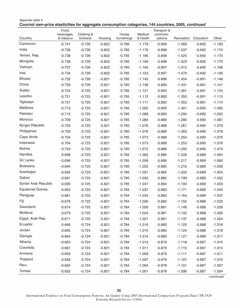
35 International Evidence on Food Consumption Patterns: An Update Using 2005 International Comparison Program Data / TB-1929
Economic Research Service / USDA
Appendix table 4
Cournot own-price elasticities for aggregate consumption categories, 144 countries, 2005, continued
Country
Food, beverages, & tobacco
Clothing & footwear Housing
House furnishings
Medical & health
Transport & communi-
cations Recreation Education Other
Cameroon -0.741 -0.726 -0.822 -0.786 -1.179 -0.899 -1.569 -0.692 -1.183
India -0.739 -0.726 -0.822 -0.785 -1.170 -0.898 -1.537 -0.692 -1.174
Yemen, Rep. -0.738 -0.726 -0.822 -0.785 -1.166 -0.898 -1.525 -0.692 -1.170
Mongolia -0.738 -0.726 -0.822 -0.785 -1.166 -0.898 -1.523 -0.692 -1.170
Vietnam -0.737 -0.726 -0.822 -0.785 -1.162 -0.897 -1.512 -0.692 -1.166
Iraq -0.734 -0.726 -0.822 -0.785 -1.153 -0.897 -1.479 -0.692 -1.156
Bhutan -0.732 -0.726 -0.821 -0.785 -1.145 -0.896 -1.454 -0.691 -1.148
China -0.730 -0.726 -0.821 -0.785 -1.138 -0.895 -1.431 -0.691 -1.141
Sudan -0.724 -0.725 -0.821 -0.785 -1.121 -0.893 -1.381 -0.691 -1.124
Lesotho -0.721 -0.725 -0.821 -0.785 -1.112 -0.892 -1.355 -0.691 -1.115
Tajikistan -0.721 -0.725 -0.821 -0.785 -1.111 -0.892 -1.353 -0.691 -1.114
Maldives -0.713 -0.725 -0.821 -0.785 -1.092 -0.890 -1.301 -0.690 -1.095
Pakistan -0.712 -0.725 -0.821 -0.785 -1.089 -0.890 -1.293 -0.690 -1.092
Morocco -0.709 -0.725 -0.821 -0.785 -1.084 -0.889 -1.280 -0.690 -1.087
Kyrgyz Republic -0.705 -0.725 -0.821 -0.785 -1.076 -0.888 -1.261 -0.690 -1.079
Philippines -0.705 -0.725 -0.821 -0.785 -1.076 -0.888 -1.260 -0.690 -1.078
Cape Verde -0.704 -0.725 -0.821 -0.785 -1.073 -0.888 -1.254 -0.690 -1.076
Indonesia -0.704 -0.725 -0.821 -0.785 -1.073 -0.888 -1.253 -0.690 -1.076
Bolivia -0.703 -0.725 -0.821 -0.785 -1.072 -0.888 -1.250 -0.690 -1.074
Namibia -0.698 -0.725 -0.821 -0.785 -1.062 -0.886 -1.226 -0.689 -1.064
Sri Lanka -0.696 -0.725 -0.821 -0.785 -1.058 -0.886 -1.217 -0.689 -1.060
Botswana -0.694 -0.725 -0.821 -0.785 -1.055 -0.885 -1.210 -0.689 -1.058
Azerbaijan -0.692 -0.725 -0.821 -0.785 -1.051 -0.885 -1.202 -0.689 -1.054
Gabon -0.691 -0.725 -0.821 -0.785 -1.050 -0.885 -1.199 -0.689 -1.052
Syrian Arab Republic -0.690 -0.725 -0.821 -0.785 -1.047 -0.884 -1.193 -0.689 -1.050
Equatorial Guinea -0.683 -0.725 -0.821 -0.784 -1.037 -0.883 -1.171 -0.689 -1.040
Paraguay -0.681 -0.725 -0.821 -0.784 -1.034 -0.883 -1.164 -0.688 -1.037
Fiji -0.678 -0.725 -0.821 -0.784 -1.030 -0.882 -1.155 -0.688 -1.033
Swaziland -0.674 -0.725 -0.821 -0.784 -1.026 -0.881 -1.146 -0.688 -1.028
Moldova -0.673 -0.725 -0.821 -0.784 -1.024 -0.881 -1.142 -0.688 -1.026
Egypt, Arab Rep. -0.671 -0.725 -0.821 -0.784 -1.021 -0.881 -1.137 -0.688 -1.024
Ecuador -0.666 -0.724 -0.821 -0.784 -1.016 -0.880 -1.125 -0.688 -1.018
Jordan -0.665 -0.724 -0.821 -0.784 -1.015 -0.880 -1.124 -0.688 -1.018
Georgia -0.664 -0.724 -0.821 -0.784 -1.014 -0.880 -1.121 -0.688 -1.017
Albania -0.663 -0.724 -0.821 -0.784 -1.012 -0.879 -1.118 -0.687 -1.015
Colombia -0.661 -0.724 -0.821 -0.784 -1.011 -0.879 -1.115 -0.687 -1.014
Armenia -0.659 -0.724 -0.821 -0.784 -1.009 -0.879 -1.111 -0.687 -1.011
Thailand -0.658 -0.724 -0.821 -0.784 -1.007 -0.879 -1.107 -0.687 -1.010
Peru -0.655 -0.724 -0.821 -0.784 -1.004 -0.878 -1.101 -0.687 -1.007
Tunisia -0.652 -0.724 -0.821 -0.784 -1.001 -0.878 -1.096 -0.687 -1.004
--continued
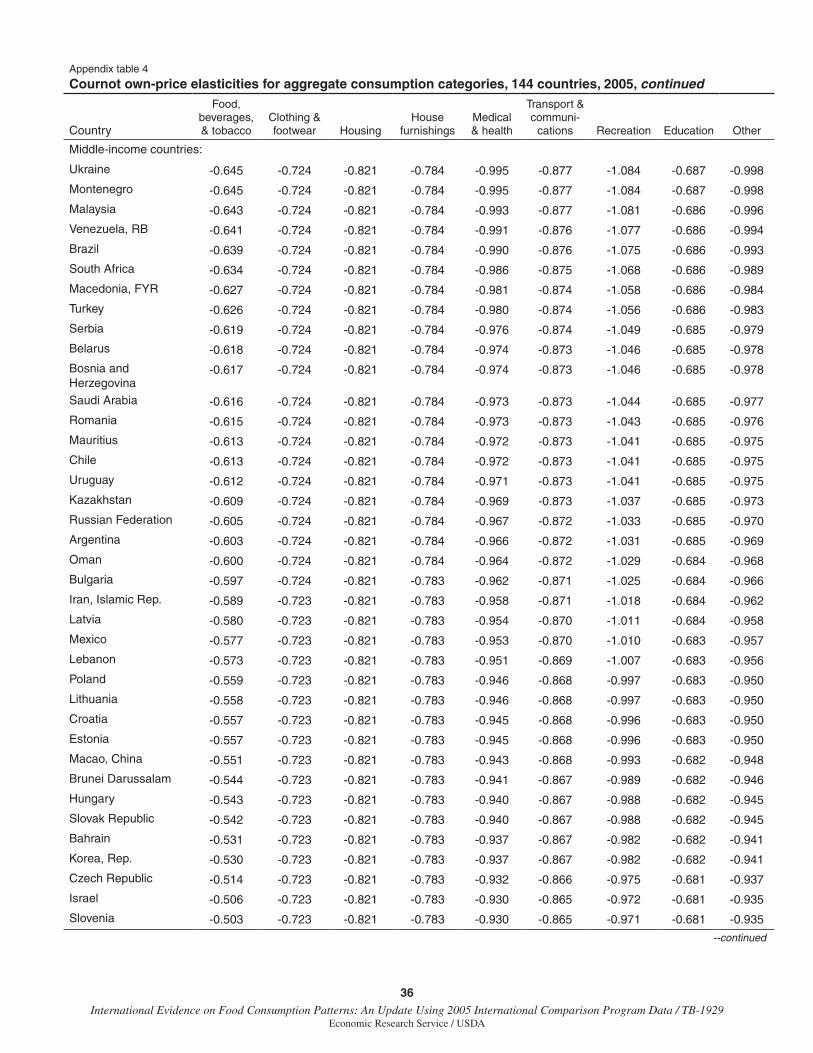
36International Evidence on Food Consumption Patterns: An Update Using 2005 International Comparison Program Data / TB-1929
Economic Research Service / USDA
Appendix table 4
Cournot own-price elasticities for aggregate consumption categories, 144 countries, 2005, continued
Country
Food, beverages, & tobacco
Clothing & footwear Housing
House furnishings
Medical & health
Transport & communi-
cations Recreation Education Other
Middle-income countries:
Ukraine -0.645 -0.724 -0.821 -0.784 -0.995 -0.877 -1.084 -0.687 -0.998
Montenegro -0.645 -0.724 -0.821 -0.784 -0.995 -0.877 -1.084 -0.687 -0.998
Malaysia -0.643 -0.724 -0.821 -0.784 -0.993 -0.877 -1.081 -0.686 -0.996
Venezuela, RB -0.641 -0.724 -0.821 -0.784 -0.991 -0.876 -1.077 -0.686 -0.994
Brazil -0.639 -0.724 -0.821 -0.784 -0.990 -0.876 -1.075 -0.686 -0.993
South Africa -0.634 -0.724 -0.821 -0.784 -0.986 -0.875 -1.068 -0.686 -0.989
Macedonia, FYR -0.627 -0.724 -0.821 -0.784 -0.981 -0.874 -1.058 -0.686 -0.984
Turkey -0.626 -0.724 -0.821 -0.784 -0.980 -0.874 -1.056 -0.686 -0.983
Serbia -0.619 -0.724 -0.821 -0.784 -0.976 -0.874 -1.049 -0.685 -0.979
Belarus -0.618 -0.724 -0.821 -0.784 -0.974 -0.873 -1.046 -0.685 -0.978
Bosnia and Herzegovina
-0.617 -0.724 -0.821 -0.784 -0.974 -0.873 -1.046 -0.685 -0.978
Saudi Arabia -0.616 -0.724 -0.821 -0.784 -0.973 -0.873 -1.044 -0.685 -0.977
Romania -0.615 -0.724 -0.821 -0.784 -0.973 -0.873 -1.043 -0.685 -0.976
Mauritius -0.613 -0.724 -0.821 -0.784 -0.972 -0.873 -1.041 -0.685 -0.975
Chile -0.613 -0.724 -0.821 -0.784 -0.972 -0.873 -1.041 -0.685 -0.975
Uruguay -0.612 -0.724 -0.821 -0.784 -0.971 -0.873 -1.041 -0.685 -0.975
Kazakhstan -0.609 -0.724 -0.821 -0.784 -0.969 -0.873 -1.037 -0.685 -0.973
Russian Federation -0.605 -0.724 -0.821 -0.784 -0.967 -0.872 -1.033 -0.685 -0.970
Argentina -0.603 -0.724 -0.821 -0.784 -0.966 -0.872 -1.031 -0.685 -0.969
Oman -0.600 -0.724 -0.821 -0.784 -0.964 -0.872 -1.029 -0.684 -0.968
Bulgaria -0.597 -0.724 -0.821 -0.783 -0.962 -0.871 -1.025 -0.684 -0.966
Iran, Islamic Rep. -0.589 -0.723 -0.821 -0.783 -0.958 -0.871 -1.018 -0.684 -0.962
Latvia -0.580 -0.723 -0.821 -0.783 -0.954 -0.870 -1.011 -0.684 -0.958
Mexico -0.577 -0.723 -0.821 -0.783 -0.953 -0.870 -1.010 -0.683 -0.957
Lebanon -0.573 -0.723 -0.821 -0.783 -0.951 -0.869 -1.007 -0.683 -0.956
Poland -0.559 -0.723 -0.821 -0.783 -0.946 -0.868 -0.997 -0.683 -0.950
Lithuania -0.558 -0.723 -0.821 -0.783 -0.946 -0.868 -0.997 -0.683 -0.950
Croatia -0.557 -0.723 -0.821 -0.783 -0.945 -0.868 -0.996 -0.683 -0.950
Estonia -0.557 -0.723 -0.821 -0.783 -0.945 -0.868 -0.996 -0.683 -0.950
Macao, China -0.551 -0.723 -0.821 -0.783 -0.943 -0.868 -0.993 -0.682 -0.948
Brunei Darussalam -0.544 -0.723 -0.821 -0.783 -0.941 -0.867 -0.989 -0.682 -0.946
Hungary -0.543 -0.723 -0.821 -0.783 -0.940 -0.867 -0.988 -0.682 -0.945
Slovak Republic -0.542 -0.723 -0.821 -0.783 -0.940 -0.867 -0.988 -0.682 -0.945
Bahrain -0.531 -0.723 -0.821 -0.783 -0.937 -0.867 -0.982 -0.682 -0.941
Korea, Rep. -0.530 -0.723 -0.821 -0.783 -0.937 -0.867 -0.982 -0.682 -0.941
Czech Republic -0.514 -0.723 -0.821 -0.783 -0.932 -0.866 -0.975 -0.681 -0.937
Israel -0.506 -0.723 -0.821 -0.783 -0.930 -0.865 -0.972 -0.681 -0.935
Slovenia -0.503 -0.723 -0.821 -0.783 -0.930 -0.865 -0.971 -0.681 -0.935
--continued
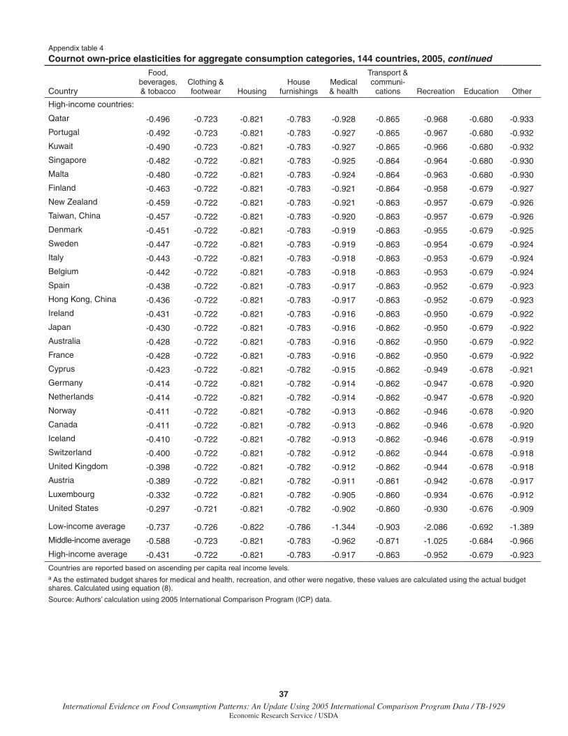
37 International Evidence on Food Consumption Patterns: An Update Using 2005 International Comparison Program Data / TB-1929
Economic Research Service / USDA
Appendix table 4
Cournot own-price elasticities for aggregate consumption categories, 144 countries, 2005, continued
Country
Food, beverages, & tobacco
Clothing & footwear Housing
House furnishings
Medical & health
Transport & communi-
cations Recreation Education Other
High-income countries:
Qatar -0.496 -0.723 -0.821 -0.783 -0.928 -0.865 -0.968 -0.680 -0.933
Portugal -0.492 -0.723 -0.821 -0.783 -0.927 -0.865 -0.967 -0.680 -0.932
Kuwait -0.490 -0.723 -0.821 -0.783 -0.927 -0.865 -0.966 -0.680 -0.932
Singapore -0.482 -0.722 -0.821 -0.783 -0.925 -0.864 -0.964 -0.680 -0.930
Malta -0.480 -0.722 -0.821 -0.783 -0.924 -0.864 -0.963 -0.680 -0.930
Finland -0.463 -0.722 -0.821 -0.783 -0.921 -0.864 -0.958 -0.679 -0.927
New Zealand -0.459 -0.722 -0.821 -0.783 -0.921 -0.863 -0.957 -0.679 -0.926
Taiwan, China -0.457 -0.722 -0.821 -0.783 -0.920 -0.863 -0.957 -0.679 -0.926
Denmark -0.451 -0.722 -0.821 -0.783 -0.919 -0.863 -0.955 -0.679 -0.925
Sweden -0.447 -0.722 -0.821 -0.783 -0.919 -0.863 -0.954 -0.679 -0.924
Italy -0.443 -0.722 -0.821 -0.783 -0.918 -0.863 -0.953 -0.679 -0.924
Belgium -0.442 -0.722 -0.821 -0.783 -0.918 -0.863 -0.953 -0.679 -0.924
Spain -0.438 -0.722 -0.821 -0.783 -0.917 -0.863 -0.952 -0.679 -0.923
Hong Kong, China -0.436 -0.722 -0.821 -0.783 -0.917 -0.863 -0.952 -0.679 -0.923
Ireland -0.431 -0.722 -0.821 -0.783 -0.916 -0.863 -0.950 -0.679 -0.922
Japan -0.430 -0.722 -0.821 -0.783 -0.916 -0.862 -0.950 -0.679 -0.922
Australia -0.428 -0.722 -0.821 -0.783 -0.916 -0.862 -0.950 -0.679 -0.922
France -0.428 -0.722 -0.821 -0.783 -0.916 -0.862 -0.950 -0.679 -0.922
Cyprus -0.423 -0.722 -0.821 -0.782 -0.915 -0.862 -0.949 -0.678 -0.921
Germany -0.414 -0.722 -0.821 -0.782 -0.914 -0.862 -0.947 -0.678 -0.920
Netherlands -0.414 -0.722 -0.821 -0.782 -0.914 -0.862 -0.947 -0.678 -0.920
Norway -0.411 -0.722 -0.821 -0.782 -0.913 -0.862 -0.946 -0.678 -0.920
Canada -0.411 -0.722 -0.821 -0.782 -0.913 -0.862 -0.946 -0.678 -0.920
Iceland -0.410 -0.722 -0.821 -0.782 -0.913 -0.862 -0.946 -0.678 -0.919
Switzerland -0.400 -0.722 -0.821 -0.782 -0.912 -0.862 -0.944 -0.678 -0.918
United Kingdom -0.398 -0.722 -0.821 -0.782 -0.912 -0.862 -0.944 -0.678 -0.918
Austria -0.389 -0.722 -0.821 -0.782 -0.911 -0.861 -0.942 -0.678 -0.917
Luxembourg -0.332 -0.722 -0.821 -0.782 -0.905 -0.860 -0.934 -0.676 -0.912
United States -0.297 -0.721 -0.821 -0.782 -0.902 -0.860 -0.930 -0.676 -0.909
Low-income average -0.737 -0.726 -0.822 -0.786 -1.344 -0.903 -2.086 -0.692 -1.389
Middle-income average -0.588 -0.723 -0.821 -0.783 -0.962 -0.871 -1.025 -0.684 -0.966
High-income average -0.431 -0.722 -0.821 -0.783 -0.917 -0.863 -0.952 -0.679 -0.923
Countries are reported based on ascending per capita real income levels.a As the estimated budget shares for medical and health, recreation, and other were negative, these values are calculated using the actual budget shares. Calculated using equation (8).
Source: Authors’ calculation using 2005 International Comparison Program (ICP) data.
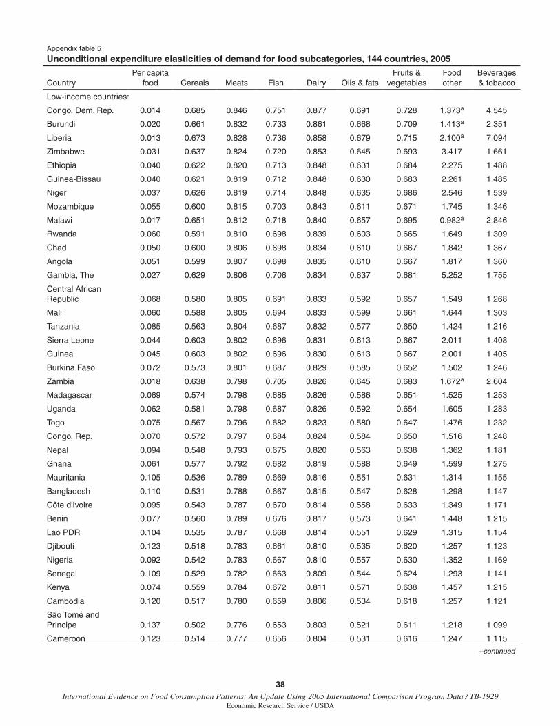
38International Evidence on Food Consumption Patterns: An Update Using 2005 International Comparison Program Data / TB-1929
Economic Research Service / USDA
Appendix table 5 Unconditional expenditure elasticities of demand for food subcategories, 144 countries, 2005, continued
CountryPer capita
food Cereals Meats Fish Dairy Oils & fatsFruits &
vegetablesFood other
Beverages & tobacco
Low-income countries:
Congo, Dem. Rep. 0.014 0.685 0.846 0.751 0.877 0.691 0.728 1.373a 4.545
Burundi 0.020 0.661 0.832 0.733 0.861 0.668 0.709 1.413a 2.351
Liberia 0.013 0.673 0.828 0.736 0.858 0.679 0.715 2.100a 7.094
Zimbabwe 0.031 0.637 0.824 0.720 0.853 0.645 0.693 3.417 1.661
Ethiopia 0.040 0.622 0.820 0.713 0.848 0.631 0.684 2.275 1.488
Guinea-Bissau 0.040 0.621 0.819 0.712 0.848 0.630 0.683 2.261 1.485
Niger 0.037 0.626 0.819 0.714 0.848 0.635 0.686 2.546 1.539
Mozambique 0.055 0.600 0.815 0.703 0.843 0.611 0.671 1.745 1.346
Malawi 0.017 0.651 0.812 0.718 0.840 0.657 0.695 0.982a 2.846
Rwanda 0.060 0.591 0.810 0.698 0.839 0.603 0.665 1.649 1.309
Chad 0.050 0.600 0.806 0.698 0.834 0.610 0.667 1.842 1.367
Angola 0.051 0.599 0.807 0.698 0.835 0.610 0.667 1.817 1.360
Gambia, The 0.027 0.629 0.806 0.706 0.834 0.637 0.681 5.252 1.755
Central African Republic 0.068 0.580 0.805 0.691 0.833 0.592 0.657 1.549 1.268
Mali 0.060 0.588 0.805 0.694 0.833 0.599 0.661 1.644 1.303
Tanzania 0.085 0.563 0.804 0.687 0.832 0.577 0.650 1.424 1.216
Sierra Leone 0.044 0.603 0.802 0.696 0.831 0.613 0.667 2.011 1.408
Guinea 0.045 0.603 0.802 0.696 0.830 0.613 0.667 2.001 1.405
Burkina Faso 0.072 0.573 0.801 0.687 0.829 0.585 0.652 1.502 1.246
Zambia 0.018 0.638 0.798 0.705 0.826 0.645 0.683 1.672a 2.604
Madagascar 0.069 0.574 0.798 0.685 0.826 0.586 0.651 1.525 1.253
Uganda 0.062 0.581 0.798 0.687 0.826 0.592 0.654 1.605 1.283
Togo 0.075 0.567 0.796 0.682 0.823 0.580 0.647 1.476 1.232
Congo, Rep. 0.070 0.572 0.797 0.684 0.824 0.584 0.650 1.516 1.248
Nepal 0.094 0.548 0.793 0.675 0.820 0.563 0.638 1.362 1.181
Ghana 0.061 0.577 0.792 0.682 0.819 0.588 0.649 1.599 1.275
Mauritania 0.105 0.536 0.789 0.669 0.816 0.551 0.631 1.314 1.155
Bangladesh 0.110 0.531 0.788 0.667 0.815 0.547 0.628 1.298 1.147
Côte d'Ivoire 0.095 0.543 0.787 0.670 0.814 0.558 0.633 1.349 1.171
Benin 0.077 0.560 0.789 0.676 0.817 0.573 0.641 1.448 1.215
Lao PDR 0.104 0.535 0.787 0.668 0.814 0.551 0.629 1.315 1.154
Djibouti 0.123 0.518 0.783 0.661 0.810 0.535 0.620 1.257 1.123
Nigeria 0.092 0.542 0.783 0.667 0.810 0.557 0.630 1.352 1.169
Senegal 0.109 0.529 0.782 0.663 0.809 0.544 0.624 1.293 1.141
Kenya 0.074 0.559 0.784 0.672 0.811 0.571 0.638 1.457 1.215
Cambodia 0.120 0.517 0.780 0.659 0.806 0.534 0.618 1.257 1.121
São Tomé and Principe 0.137 0.502 0.776 0.653 0.803 0.521 0.611 1.218 1.099
Cameroon 0.123 0.514 0.777 0.656 0.804 0.531 0.616 1.247 1.115
--continued
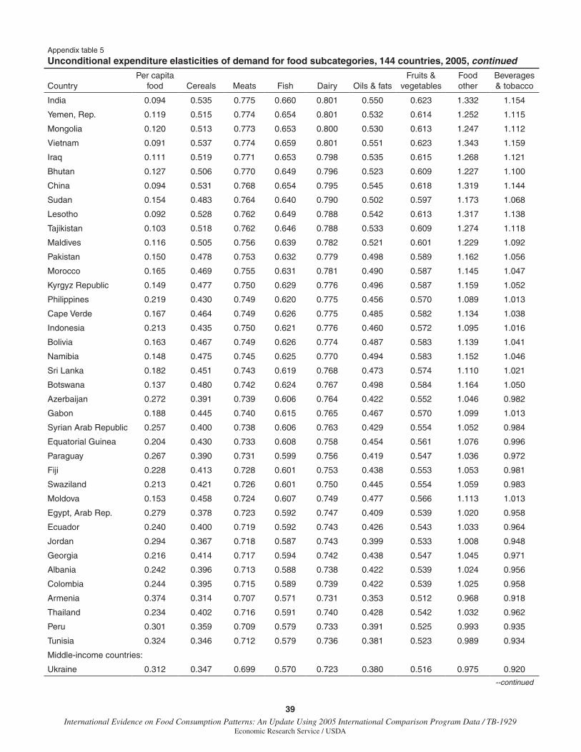
39 International Evidence on Food Consumption Patterns: An Update Using 2005 International Comparison Program Data / TB-1929
Economic Research Service / USDA
Appendix table 5 Unconditional expenditure elasticities of demand for food subcategories, 144 countries, 2005, continued
CountryPer capita
food Cereals Meats Fish Dairy Oils & fatsFruits &
vegetablesFood other
Beverages & tobacco
India 0.094 0.535 0.775 0.660 0.801 0.550 0.623 1.332 1.154
Yemen, Rep. 0.119 0.515 0.774 0.654 0.801 0.532 0.614 1.252 1.115
Mongolia 0.120 0.513 0.773 0.653 0.800 0.530 0.613 1.247 1.112
Vietnam 0.091 0.537 0.774 0.659 0.801 0.551 0.623 1.343 1.159
Iraq 0.111 0.519 0.771 0.653 0.798 0.535 0.615 1.268 1.121
Bhutan 0.127 0.506 0.770 0.649 0.796 0.523 0.609 1.227 1.100
China 0.094 0.531 0.768 0.654 0.795 0.545 0.618 1.319 1.144
Sudan 0.154 0.483 0.764 0.640 0.790 0.502 0.597 1.173 1.068
Lesotho 0.092 0.528 0.762 0.649 0.788 0.542 0.613 1.317 1.138
Tajikistan 0.103 0.518 0.762 0.646 0.788 0.533 0.609 1.274 1.118
Maldives 0.116 0.505 0.756 0.639 0.782 0.521 0.601 1.229 1.092
Pakistan 0.150 0.478 0.753 0.632 0.779 0.498 0.589 1.162 1.056
Morocco 0.165 0.469 0.755 0.631 0.781 0.490 0.587 1.145 1.047
Kyrgyz Republic 0.149 0.477 0.750 0.629 0.776 0.496 0.587 1.159 1.052
Philippines 0.219 0.430 0.749 0.620 0.775 0.456 0.570 1.089 1.013
Cape Verde 0.167 0.464 0.749 0.626 0.775 0.485 0.582 1.134 1.038
Indonesia 0.213 0.435 0.750 0.621 0.776 0.460 0.572 1.095 1.016
Bolivia 0.163 0.467 0.749 0.626 0.774 0.487 0.583 1.139 1.041
Namibia 0.148 0.475 0.745 0.625 0.770 0.494 0.583 1.152 1.046
Sri Lanka 0.182 0.451 0.743 0.619 0.768 0.473 0.574 1.110 1.021
Botswana 0.137 0.480 0.742 0.624 0.767 0.498 0.584 1.164 1.050
Azerbaijan 0.272 0.391 0.739 0.606 0.764 0.422 0.552 1.046 0.982
Gabon 0.188 0.445 0.740 0.615 0.765 0.467 0.570 1.099 1.013
Syrian Arab Republic 0.257 0.400 0.738 0.606 0.763 0.429 0.554 1.052 0.984
Equatorial Guinea 0.204 0.430 0.733 0.608 0.758 0.454 0.561 1.076 0.996
Paraguay 0.267 0.390 0.731 0.599 0.756 0.419 0.547 1.036 0.972
Fiji 0.228 0.413 0.728 0.601 0.753 0.438 0.553 1.053 0.981
Swaziland 0.213 0.421 0.726 0.601 0.750 0.445 0.554 1.059 0.983
Moldova 0.153 0.458 0.724 0.607 0.749 0.477 0.566 1.113 1.013
Egypt, Arab Rep. 0.279 0.378 0.723 0.592 0.747 0.409 0.539 1.020 0.958
Ecuador 0.240 0.400 0.719 0.592 0.743 0.426 0.543 1.033 0.964
Jordan 0.294 0.367 0.718 0.587 0.743 0.399 0.533 1.008 0.948
Georgia 0.216 0.414 0.717 0.594 0.742 0.438 0.547 1.045 0.971
Albania 0.242 0.396 0.713 0.588 0.738 0.422 0.539 1.024 0.956
Colombia 0.244 0.395 0.715 0.589 0.739 0.422 0.539 1.025 0.958
Armenia 0.374 0.314 0.707 0.571 0.731 0.353 0.512 0.968 0.918
Thailand 0.234 0.402 0.716 0.591 0.740 0.428 0.542 1.032 0.962
Peru 0.301 0.359 0.709 0.579 0.733 0.391 0.525 0.993 0.935
Tunisia 0.324 0.346 0.712 0.579 0.736 0.381 0.523 0.989 0.934
Middle-income countries:
Ukraine 0.312 0.347 0.699 0.570 0.723 0.380 0.516 0.975 0.920
--continued
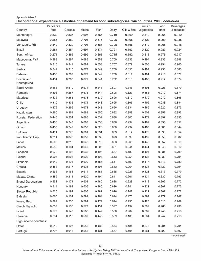
40International Evidence on Food Consumption Patterns: An Update Using 2005 International Comparison Program Data / TB-1929
Economic Research Service / USDA
Appendix table 5 Unconditional expenditure elasticities of demand for food subcategories, 144 countries, 2005, continued
CountryPer capita
food Cereals Meats Fish Dairy Oils & fatsFruits &
vegetablesFood other
Beverages & tobacco
Montenegro 0.330 0.335 0.696 0.565 0.719 0.369 0.510 0.965 0.912
Malaysia 0.256 0.380 0.701 0.576 0.725 0.408 0.527 0.999 0.935
Venezuela, RB 0.342 0.330 0.701 0.568 0.725 0.366 0.512 0.968 0.916
Brazil 0.281 0.364 0.697 0.571 0.721 0.393 0.520 0.983 0.924
South Africa 0.278 0.363 0.692 0.566 0.715 0.392 0.516 0.976 0.917
Macedonia, FYR 0.388 0.297 0.685 0.552 0.709 0.336 0.494 0.935 0.888
Turkey 0.310 0.341 0.684 0.558 0.707 0.372 0.505 0.954 0.900
Serbia 0.349 0.315 0.677 0.549 0.700 0.350 0.494 0.933 0.883
Belarus 0.433 0.267 0.677 0.542 0.700 0.311 0.481 0.915 0.871
Bosnia and Herzegovina
0.431 0.268 0.679 0.544 0.702 0.313 0.483 0.917 0.874
Saudi Arabia 0.356 0.310 0.674 0.546 0.697 0.346 0.491 0.928 0.879
Romania 0.396 0.287 0.675 0.544 0.698 0.327 0.485 0.919 0.874
Mauritius 0.432 0.265 0.673 0.539 0.696 0.310 0.479 0.910 0.866
Chile 0.310 0.335 0.672 0.548 0.695 0.366 0.496 0.938 0.884
Uruguay 0.379 0.296 0.673 0.543 0.696 0.334 0.486 0.920 0.873
Kazakhstan 0.260 0.361 0.669 0.550 0.692 0.388 0.502 0.952 0.892
Russian Federation 0.446 0.254 0.665 0.532 0.688 0.300 0.472 0.897 0.855
Argentina 0.456 0.248 0.663 0.530 0.686 0.294 0.469 0.893 0.851
Oman 0.455 0.247 0.658 0.526 0.680 0.292 0.465 0.885 0.844
Bulgaria 0.411 0.273 0.661 0.531 0.683 0.314 0.473 0.898 0.854
Iran, Islamic Rep. 0.211 0.378 0.650 0.539 0.673 0.399 0.497 0.950 0.882
Latvia 0.500 0.215 0.642 0.510 0.663 0.265 0.448 0.857 0.819
Mexico 0.550 0.184 0.640 0.506 0.661 0.241 0.441 0.848 0.812
Lebanon 0.673 0.106 0.635 0.496 0.657 0.182 0.424 0.831 0.799
Poland 0.505 0.205 0.622 0.494 0.643 0.255 0.434 0.830 0.794
Lithuania 0.640 0.125 0.620 0.486 0.641 0.193 0.417 0.813 0.782
Croatia 0.483 0.217 0.621 0.495 0.642 0.264 0.436 0.832 0.794
Estonia 0.566 0.168 0.614 0.485 0.635 0.225 0.421 0.813 0.779
Macao, China 0.489 0.214 0.620 0.494 0.641 0.261 0.434 0.830 0.793
Brunei Darussalam 0.552 0.174 0.608 0.480 0.628 0.228 0.418 0.806 0.772
Hungary 0.514 0.194 0.605 0.480 0.626 0.244 0.421 0.807 0.772
Slovak Republic 0.520 0.192 0.606 0.481 0.626 0.242 0.421 0.807 0.772
Bahrain 0.666 0.104 0.594 0.464 0.614 0.173 0.397 0.777 0.747
Korea, Rep. 0.392 0.255 0.594 0.479 0.614 0.290 0.428 0.810 0.769
Czech Republic 0.607 0.135 0.577 0.454 0.597 0.194 0.392 0.760 0.730
Israel 0.577 0.149 0.566 0.447 0.586 0.202 0.387 0.748 0.718
Slovenia 0.634 0.118 0.569 0.446 0.589 0.180 0.384 0.747 0.718
High-income countries:
Qatar 0.613 0.127 0.555 0.436 0.574 0.184 0.376 0.731 0.701
Portugal 0.797 0.016 0.558 0.431 0.577 0.104 0.361 0.722 0.697
--continued
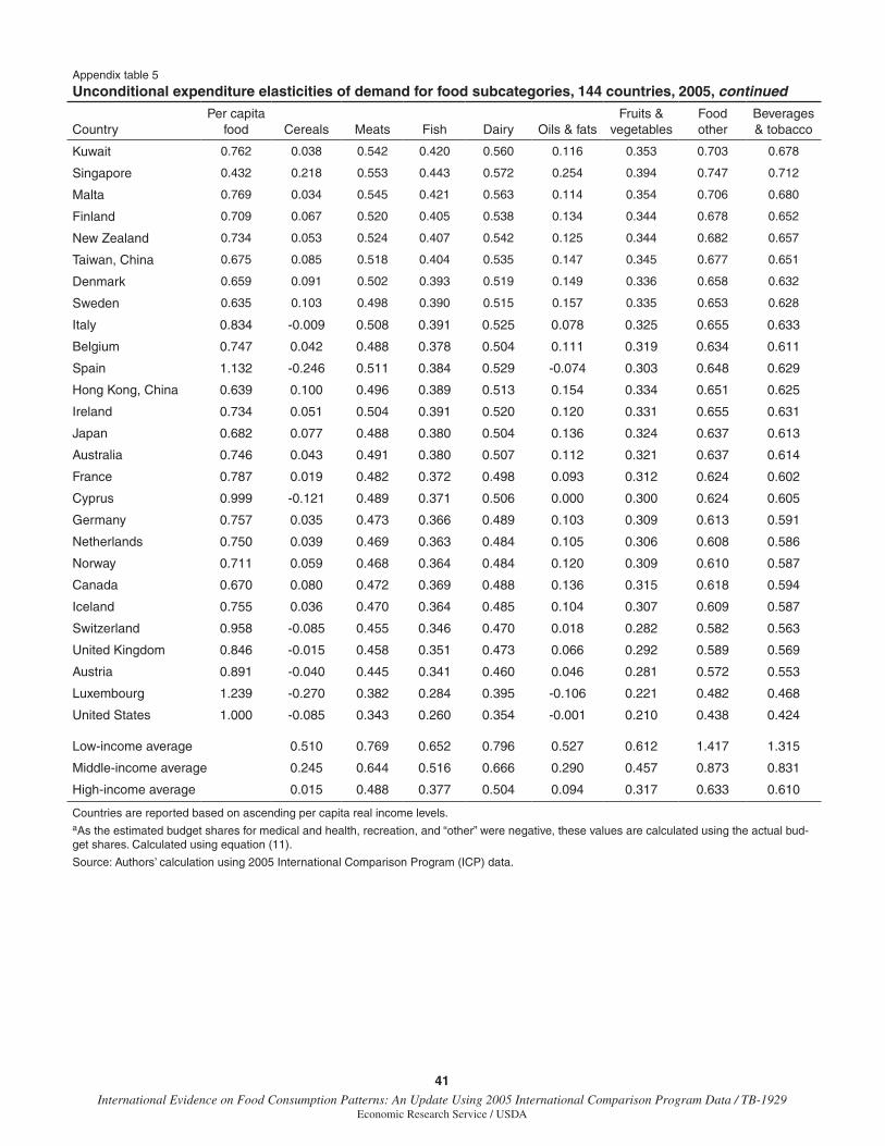
41 International Evidence on Food Consumption Patterns: An Update Using 2005 International Comparison Program Data / TB-1929
Economic Research Service / USDA
Appendix table 5 Unconditional expenditure elasticities of demand for food subcategories, 144 countries, 2005, continued
CountryPer capita
food Cereals Meats Fish Dairy Oils & fatsFruits &
vegetablesFood other
Beverages & tobacco
Kuwait 0.762 0.038 0.542 0.420 0.560 0.116 0.353 0.703 0.678
Singapore 0.432 0.218 0.553 0.443 0.572 0.254 0.394 0.747 0.712
Malta 0.769 0.034 0.545 0.421 0.563 0.114 0.354 0.706 0.680
Finland 0.709 0.067 0.520 0.405 0.538 0.134 0.344 0.678 0.652
New Zealand 0.734 0.053 0.524 0.407 0.542 0.125 0.344 0.682 0.657
Taiwan, China 0.675 0.085 0.518 0.404 0.535 0.147 0.345 0.677 0.651
Denmark 0.659 0.091 0.502 0.393 0.519 0.149 0.336 0.658 0.632
Sweden 0.635 0.103 0.498 0.390 0.515 0.157 0.335 0.653 0.628
Italy 0.834 -0.009 0.508 0.391 0.525 0.078 0.325 0.655 0.633
Belgium 0.747 0.042 0.488 0.378 0.504 0.111 0.319 0.634 0.611
Spain 1.132 -0.246 0.511 0.384 0.529 -0.074 0.303 0.648 0.629
Hong Kong, China 0.639 0.100 0.496 0.389 0.513 0.154 0.334 0.651 0.625
Ireland 0.734 0.051 0.504 0.391 0.520 0.120 0.331 0.655 0.631
Japan 0.682 0.077 0.488 0.380 0.504 0.136 0.324 0.637 0.613
Australia 0.746 0.043 0.491 0.380 0.507 0.112 0.321 0.637 0.614
France 0.787 0.019 0.482 0.372 0.498 0.093 0.312 0.624 0.602
Cyprus 0.999 -0.121 0.489 0.371 0.506 0.000 0.300 0.624 0.605
Germany 0.757 0.035 0.473 0.366 0.489 0.103 0.309 0.613 0.591
Netherlands 0.750 0.039 0.469 0.363 0.484 0.105 0.306 0.608 0.586
Norway 0.711 0.059 0.468 0.364 0.484 0.120 0.309 0.610 0.587
Canada 0.670 0.080 0.472 0.369 0.488 0.136 0.315 0.618 0.594
Iceland 0.755 0.036 0.470 0.364 0.485 0.104 0.307 0.609 0.587
Switzerland 0.958 -0.085 0.455 0.346 0.470 0.018 0.282 0.582 0.563
United Kingdom 0.846 -0.015 0.458 0.351 0.473 0.066 0.292 0.589 0.569
Austria 0.891 -0.040 0.445 0.341 0.460 0.046 0.281 0.572 0.553
Luxembourg 1.239 -0.270 0.382 0.284 0.395 -0.106 0.221 0.482 0.468
United States 1.000 -0.085 0.343 0.260 0.354 -0.001 0.210 0.438 0.424
Low-income average 0.510 0.769 0.652 0.796 0.527 0.612 1.417 1.315
Middle-income average 0.245 0.644 0.516 0.666 0.290 0.457 0.873 0.831
High-income average 0.015 0.488 0.377 0.504 0.094 0.317 0.633 0.610
Countries are reported based on ascending per capita real income levels.aAs the estimated budget shares for medical and health, recreation, and “other” were negative, these values are calculated using the actual bud-get shares. Calculated using equation (11).
Source: Authors’ calculation using 2005 International Comparison Program (ICP) data.
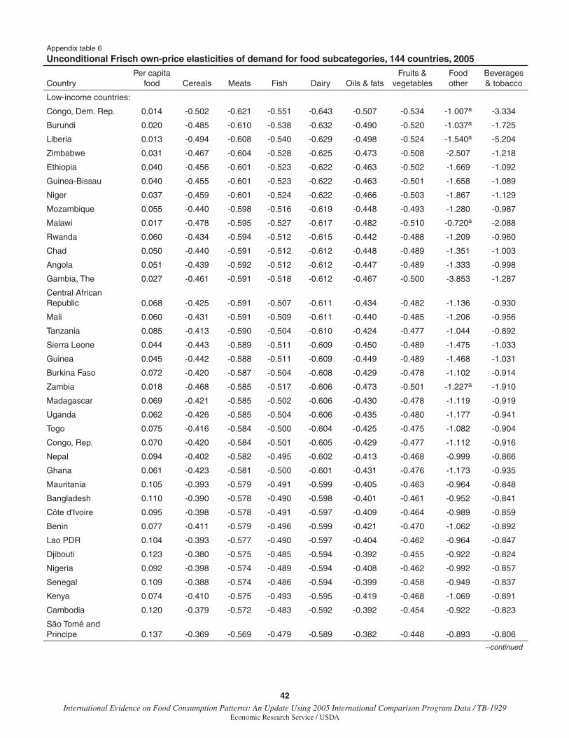
42International Evidence on Food Consumption Patterns: An Update Using 2005 International Comparison Program Data / TB-1929
Economic Research Service / USDA
Appendix table 6 Unconditional Frisch own-price elasticities of demand for food subcategories, 144 countries, 2005, continued
CountryPer capita
food Cereals Meats Fish Dairy Oils & fatsFruits &
vegetablesFood other
Beverages & tobacco
Low-income countries:
Congo, Dem. Rep. 0.014 -0.502 -0.621 -0.551 -0.643 -0.507 -0.534 -1.007a -3.334
Burundi 0.020 -0.485 -0.610 -0.538 -0.632 -0.490 -0.520 -1.037a -1.725
Liberia 0.013 -0.494 -0.608 -0.540 -0.629 -0.498 -0.524 -1.540a -5.204
Zimbabwe 0.031 -0.467 -0.604 -0.528 -0.625 -0.473 -0.508 -2.507 -1.218
Ethiopia 0.040 -0.456 -0.601 -0.523 -0.622 -0.463 -0.502 -1.669 -1.092
Guinea-Bissau 0.040 -0.455 -0.601 -0.523 -0.622 -0.463 -0.501 -1.658 -1.089
Niger 0.037 -0.459 -0.601 -0.524 -0.622 -0.466 -0.503 -1.867 -1.129
Mozambique 0.055 -0.440 -0.598 -0.516 -0.619 -0.448 -0.493 -1.280 -0.987
Malawi 0.017 -0.478 -0.595 -0.527 -0.617 -0.482 -0.510 -0.720a -2.088
Rwanda 0.060 -0.434 -0.594 -0.512 -0.615 -0.442 -0.488 -1.209 -0.960
Chad 0.050 -0.440 -0.591 -0.512 -0.612 -0.448 -0.489 -1.351 -1.003
Angola 0.051 -0.439 -0.592 -0.512 -0.612 -0.447 -0.489 -1.333 -0.998
Gambia, The 0.027 -0.461 -0.591 -0.518 -0.612 -0.467 -0.500 -3.853 -1.287
Central African Republic 0.068 -0.425 -0.591 -0.507 -0.611 -0.434 -0.482 -1.136 -0.930
Mali 0.060 -0.431 -0.591 -0.509 -0.611 -0.440 -0.485 -1.206 -0.956
Tanzania 0.085 -0.413 -0.590 -0.504 -0.610 -0.424 -0.477 -1.044 -0.892
Sierra Leone 0.044 -0.443 -0.589 -0.511 -0.609 -0.450 -0.489 -1.475 -1.033
Guinea 0.045 -0.442 -0.588 -0.511 -0.609 -0.449 -0.489 -1.468 -1.031
Burkina Faso 0.072 -0.420 -0.587 -0.504 -0.608 -0.429 -0.478 -1.102 -0.914
Zambia 0.018 -0.468 -0.585 -0.517 -0.606 -0.473 -0.501 -1.227a -1.910
Madagascar 0.069 -0.421 -0.585 -0.502 -0.606 -0.430 -0.478 -1.119 -0.919
Uganda 0.062 -0.426 -0.585 -0.504 -0.606 -0.435 -0.480 -1.177 -0.941
Togo 0.075 -0.416 -0.584 -0.500 -0.604 -0.425 -0.475 -1.082 -0.904
Congo, Rep. 0.070 -0.420 -0.584 -0.501 -0.605 -0.429 -0.477 -1.112 -0.916
Nepal 0.094 -0.402 -0.582 -0.495 -0.602 -0.413 -0.468 -0.999 -0.866
Ghana 0.061 -0.423 -0.581 -0.500 -0.601 -0.431 -0.476 -1.173 -0.935
Mauritania 0.105 -0.393 -0.579 -0.491 -0.599 -0.405 -0.463 -0.964 -0.848
Bangladesh 0.110 -0.390 -0.578 -0.490 -0.598 -0.401 -0.461 -0.952 -0.841
Côte d'Ivoire 0.095 -0.398 -0.578 -0.491 -0.597 -0.409 -0.464 -0.989 -0.859
Benin 0.077 -0.411 -0.579 -0.496 -0.599 -0.421 -0.470 -1.062 -0.892
Lao PDR 0.104 -0.393 -0.577 -0.490 -0.597 -0.404 -0.462 -0.964 -0.847
Djibouti 0.123 -0.380 -0.575 -0.485 -0.594 -0.392 -0.455 -0.922 -0.824
Nigeria 0.092 -0.398 -0.574 -0.489 -0.594 -0.408 -0.462 -0.992 -0.857
Senegal 0.109 -0.388 -0.574 -0.486 -0.594 -0.399 -0.458 -0.949 -0.837
Kenya 0.074 -0.410 -0.575 -0.493 -0.595 -0.419 -0.468 -1.069 -0.891
Cambodia 0.120 -0.379 -0.572 -0.483 -0.592 -0.392 -0.454 -0.922 -0.823
São Tomé and Principe 0.137 -0.369 -0.569 -0.479 -0.589 -0.382 -0.448 -0.893 -0.806
--continued
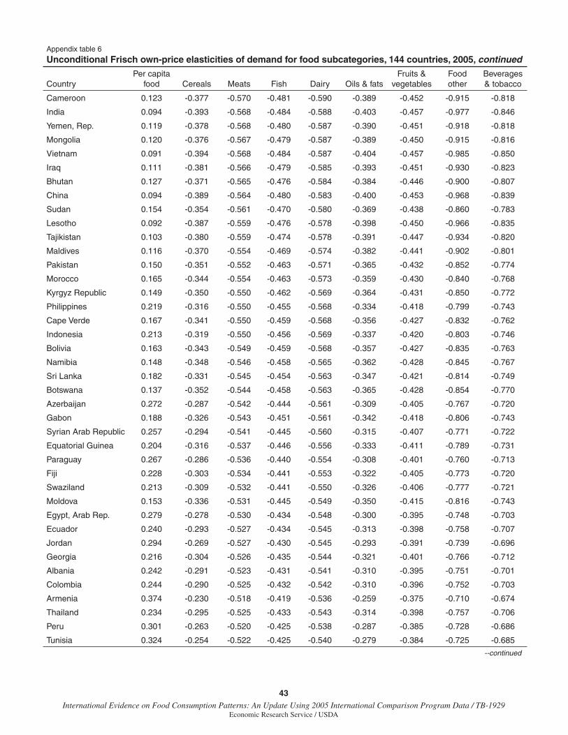
43International Evidence on Food Consumption Patterns: An Update Using 2005 International Comparison Program Data / TB-1929
Economic Research Service / USDA
Appendix table 6 Unconditional Frisch own-price elasticities of demand for food subcategories, 144 countries, 2005, continued
CountryPer capita
food Cereals Meats Fish Dairy Oils & fatsFruits &
vegetablesFood other
Beverages & tobacco
Cameroon 0.123 -0.377 -0.570 -0.481 -0.590 -0.389 -0.452 -0.915 -0.818
India 0.094 -0.393 -0.568 -0.484 -0.588 -0.403 -0.457 -0.977 -0.846
Yemen, Rep. 0.119 -0.378 -0.568 -0.480 -0.587 -0.390 -0.451 -0.918 -0.818
Mongolia 0.120 -0.376 -0.567 -0.479 -0.587 -0.389 -0.450 -0.915 -0.816
Vietnam 0.091 -0.394 -0.568 -0.484 -0.587 -0.404 -0.457 -0.985 -0.850
Iraq 0.111 -0.381 -0.566 -0.479 -0.585 -0.393 -0.451 -0.930 -0.823
Bhutan 0.127 -0.371 -0.565 -0.476 -0.584 -0.384 -0.446 -0.900 -0.807
China 0.094 -0.389 -0.564 -0.480 -0.583 -0.400 -0.453 -0.968 -0.839
Sudan 0.154 -0.354 -0.561 -0.470 -0.580 -0.369 -0.438 -0.860 -0.783
Lesotho 0.092 -0.387 -0.559 -0.476 -0.578 -0.398 -0.450 -0.966 -0.835
Tajikistan 0.103 -0.380 -0.559 -0.474 -0.578 -0.391 -0.447 -0.934 -0.820
Maldives 0.116 -0.370 -0.554 -0.469 -0.574 -0.382 -0.441 -0.902 -0.801
Pakistan 0.150 -0.351 -0.552 -0.463 -0.571 -0.365 -0.432 -0.852 -0.774
Morocco 0.165 -0.344 -0.554 -0.463 -0.573 -0.359 -0.430 -0.840 -0.768
Kyrgyz Republic 0.149 -0.350 -0.550 -0.462 -0.569 -0.364 -0.431 -0.850 -0.772
Philippines 0.219 -0.316 -0.550 -0.455 -0.568 -0.334 -0.418 -0.799 -0.743
Cape Verde 0.167 -0.341 -0.550 -0.459 -0.568 -0.356 -0.427 -0.832 -0.762
Indonesia 0.213 -0.319 -0.550 -0.456 -0.569 -0.337 -0.420 -0.803 -0.746
Bolivia 0.163 -0.343 -0.549 -0.459 -0.568 -0.357 -0.427 -0.835 -0.763
Namibia 0.148 -0.348 -0.546 -0.458 -0.565 -0.362 -0.428 -0.845 -0.767
Sri Lanka 0.182 -0.331 -0.545 -0.454 -0.563 -0.347 -0.421 -0.814 -0.749
Botswana 0.137 -0.352 -0.544 -0.458 -0.563 -0.365 -0.428 -0.854 -0.770
Azerbaijan 0.272 -0.287 -0.542 -0.444 -0.561 -0.309 -0.405 -0.767 -0.720
Gabon 0.188 -0.326 -0.543 -0.451 -0.561 -0.342 -0.418 -0.806 -0.743
Syrian Arab Republic 0.257 -0.294 -0.541 -0.445 -0.560 -0.315 -0.407 -0.771 -0.722
Equatorial Guinea 0.204 -0.316 -0.537 -0.446 -0.556 -0.333 -0.411 -0.789 -0.731
Paraguay 0.267 -0.286 -0.536 -0.440 -0.554 -0.308 -0.401 -0.760 -0.713
Fiji 0.228 -0.303 -0.534 -0.441 -0.553 -0.322 -0.405 -0.773 -0.720
Swaziland 0.213 -0.309 -0.532 -0.441 -0.550 -0.326 -0.406 -0.777 -0.721
Moldova 0.153 -0.336 -0.531 -0.445 -0.549 -0.350 -0.415 -0.816 -0.743
Egypt, Arab Rep. 0.279 -0.278 -0.530 -0.434 -0.548 -0.300 -0.395 -0.748 -0.703
Ecuador 0.240 -0.293 -0.527 -0.434 -0.545 -0.313 -0.398 -0.758 -0.707
Jordan 0.294 -0.269 -0.527 -0.430 -0.545 -0.293 -0.391 -0.739 -0.696
Georgia 0.216 -0.304 -0.526 -0.435 -0.544 -0.321 -0.401 -0.766 -0.712
Albania 0.242 -0.291 -0.523 -0.431 -0.541 -0.310 -0.395 -0.751 -0.701
Colombia 0.244 -0.290 -0.525 -0.432 -0.542 -0.310 -0.396 -0.752 -0.703
Armenia 0.374 -0.230 -0.518 -0.419 -0.536 -0.259 -0.375 -0.710 -0.674
Thailand 0.234 -0.295 -0.525 -0.433 -0.543 -0.314 -0.398 -0.757 -0.706
Peru 0.301 -0.263 -0.520 -0.425 -0.538 -0.287 -0.385 -0.728 -0.686
Tunisia 0.324 -0.254 -0.522 -0.425 -0.540 -0.279 -0.384 -0.725 -0.685
--continued
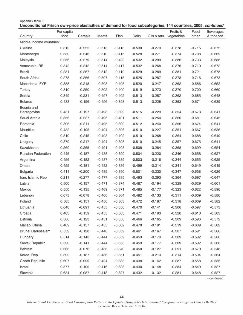
44International Evidence on Food Consumption Patterns: An Update Using 2005 International Comparison Program Data / TB-1929
Economic Research Service / USDA
Appendix table 6 Unconditional Frisch own-price elasticities of demand for food subcategories, 144 countries, 2005, continued
CountryPer capita
food Cereals Meats Fish Dairy Oils & fatsFruits &
vegetablesFood other
Beverages & tobacco
Middle-income countries:
Ukraine 0.312 -0.255 -0.513 -0.418 -0.530 -0.279 -0.378 -0.715 -0.675
Montenegro 0.330 -0.246 -0.510 -0.415 -0.528 -0.271 -0.374 -0.708 -0.669
Malaysia 0.256 -0.279 -0.514 -0.422 -0.532 -0.299 -0.386 -0.733 -0.686
Venezuela, RB 0.342 -0.242 -0.514 -0.417 -0.532 -0.268 -0.376 -0.710 -0.672
Brazil 0.281 -0.267 -0.512 -0.419 -0.529 -0.289 -0.381 -0.721 -0.678
South Africa 0.278 -0.266 -0.507 -0.415 -0.525 -0.287 -0.378 -0.716 -0.673
Macedonia, FYR 0.388 -0.218 -0.503 -0.405 -0.520 -0.247 -0.362 -0.686 -0.652
Turkey 0.310 -0.250 -0.502 -0.409 -0.519 -0.273 -0.370 -0.700 -0.660
Serbia 0.349 -0.231 -0.497 -0.402 -0.513 -0.257 -0.362 -0.685 -0.648
Belarus 0.433 -0.196 -0.496 -0.398 -0.513 -0.228 -0.353 -0.671 -0.639
Bosnia and Herzegovina 0.431 -0.197 -0.498 -0.399 -0.515 -0.229 -0.354 -0.673 -0.641
Saudi Arabia 0.356 -0.227 -0.495 -0.401 -0.511 -0.254 -0.360 -0.681 -0.645
Romania 0.396 -0.211 -0.495 -0.399 -0.512 -0.240 -0.356 -0.674 -0.641
Mauritius 0.432 -0.195 -0.494 -0.396 -0.510 -0.227 -0.351 -0.667 -0.636
Chile 0.310 -0.245 -0.493 -0.402 -0.510 -0.268 -0.364 -0.688 -0.649
Uruguay 0.379 -0.217 -0.494 -0.398 -0.510 -0.245 -0.357 -0.675 -0.641
Kazakhstan 0.260 -0.265 -0.491 -0.403 -0.508 -0.284 -0.368 -0.699 -0.654
Russian Federation 0.446 -0.187 -0.488 -0.390 -0.504 -0.220 -0.346 -0.658 -0.627
Argentina 0.456 -0.182 -0.487 -0.389 -0.503 -0.216 -0.344 -0.655 -0.625
Oman 0.455 -0.181 -0.482 -0.386 -0.499 -0.214 -0.341 -0.649 -0.619
Bulgaria 0.411 -0.200 -0.485 -0.390 -0.501 -0.230 -0.347 -0.658 -0.626
Iran, Islamic Rep. 0.211 -0.277 -0.477 -0.395 -0.493 -0.293 -0.364 -0.697 -0.647
Latvia 0.500 -0.157 -0.471 -0.374 -0.487 -0.194 -0.329 -0.629 -0.601
Mexico 0.550 -0.135 -0.469 -0.371 -0.485 -0.177 -0.323 -0.622 -0.596
Lebanon 0.673 -0.078 -0.466 -0.364 -0.482 -0.133 -0.311 -0.609 -0.586
Poland 0.505 -0.151 -0.456 -0.363 -0.472 -0.187 -0.318 -0.609 -0.582
Lithuania 0.640 -0.091 -0.455 -0.356 -0.470 -0.141 -0.306 -0.597 -0.573
Croatia 0.483 -0.159 -0.455 -0.363 -0.471 -0.193 -0.320 -0.610 -0.583
Estonia 0.566 -0.123 -0.451 -0.356 -0.466 -0.165 -0.309 -0.596 -0.572
Macao, China 0.489 -0.157 -0.455 -0.362 -0.470 -0.191 -0.319 -0.609 -0.582
Brunei Darussalam 0.552 -0.128 -0.446 -0.352 -0.461 -0.167 -0.307 -0.591 -0.566
Hungary 0.514 -0.143 -0.444 -0.352 -0.459 -0.179 -0.309 -0.592 -0.566
Slovak Republic 0.520 -0.141 -0.444 -0.353 -0.459 -0.177 -0.309 -0.592 -0.566
Bahrain 0.666 -0.076 -0.436 -0.340 -0.450 -0.127 -0.291 -0.570 -0.548
Korea, Rep. 0.392 -0.187 -0.436 -0.351 -0.451 -0.213 -0.314 -0.594 -0.564
Czech Republic 0.607 -0.099 -0.424 -0.333 -0.438 -0.142 -0.287 -0.558 -0.535
Israel 0.577 -0.109 -0.416 -0.328 -0.430 -0.148 -0.284 -0.549 -0.527
Slovenia 0.634 -0.087 -0.418 -0.327 -0.432 -0.132 -0.281 -0.548 -0.527
--continued
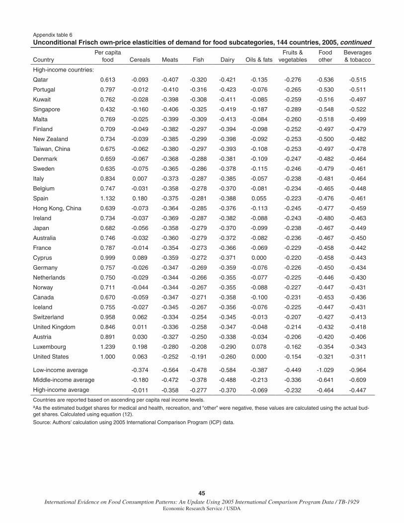
45 International Evidence on Food Consumption Patterns: An Update Using 2005 International Comparison Program Data / TB-1929
Economic Research Service / USDA
Appendix table 6 Unconditional Frisch own-price elasticities of demand for food subcategories, 144 countries, 2005, continued
CountryPer capita
food Cereals Meats Fish Dairy Oils & fatsFruits &
vegetablesFood other
Beverages & tobacco
High-income countries:
Qatar 0.613 -0.093 -0.407 -0.320 -0.421 -0.135 -0.276 -0.536 -0.515
Portugal 0.797 -0.012 -0.410 -0.316 -0.423 -0.076 -0.265 -0.530 -0.511
Kuwait 0.762 -0.028 -0.398 -0.308 -0.411 -0.085 -0.259 -0.516 -0.497
Singapore 0.432 -0.160 -0.406 -0.325 -0.419 -0.187 -0.289 -0.548 -0.522
Malta 0.769 -0.025 -0.399 -0.309 -0.413 -0.084 -0.260 -0.518 -0.499
Finland 0.709 -0.049 -0.382 -0.297 -0.394 -0.098 -0.252 -0.497 -0.479
New Zealand 0.734 -0.039 -0.385 -0.299 -0.398 -0.092 -0.253 -0.500 -0.482
Taiwan, China 0.675 -0.062 -0.380 -0.297 -0.393 -0.108 -0.253 -0.497 -0.478
Denmark 0.659 -0.067 -0.368 -0.288 -0.381 -0.109 -0.247 -0.482 -0.464
Sweden 0.635 -0.075 -0.365 -0.286 -0.378 -0.115 -0.246 -0.479 -0.461
Italy 0.834 0.007 -0.373 -0.287 -0.385 -0.057 -0.238 -0.481 -0.464
Belgium 0.747 -0.031 -0.358 -0.278 -0.370 -0.081 -0.234 -0.465 -0.448
Spain 1.132 0.180 -0.375 -0.281 -0.388 0.055 -0.223 -0.476 -0.461
Hong Kong, China 0.639 -0.073 -0.364 -0.285 -0.376 -0.113 -0.245 -0.477 -0.459
Ireland 0.734 -0.037 -0.369 -0.287 -0.382 -0.088 -0.243 -0.480 -0.463
Japan 0.682 -0.056 -0.358 -0.279 -0.370 -0.099 -0.238 -0.467 -0.449
Australia 0.746 -0.032 -0.360 -0.279 -0.372 -0.082 -0.236 -0.467 -0.450
France 0.787 -0.014 -0.354 -0.273 -0.366 -0.069 -0.229 -0.458 -0.442
Cyprus 0.999 0.089 -0.359 -0.272 -0.371 0.000 -0.220 -0.458 -0.443
Germany 0.757 -0.026 -0.347 -0.269 -0.359 -0.076 -0.226 -0.450 -0.434
Netherlands 0.750 -0.029 -0.344 -0.266 -0.355 -0.077 -0.225 -0.446 -0.430
Norway 0.711 -0.044 -0.344 -0.267 -0.355 -0.088 -0.227 -0.447 -0.431
Canada 0.670 -0.059 -0.347 -0.271 -0.358 -0.100 -0.231 -0.453 -0.436
Iceland 0.755 -0.027 -0.345 -0.267 -0.356 -0.076 -0.225 -0.447 -0.431
Switzerland 0.958 0.062 -0.334 -0.254 -0.345 -0.013 -0.207 -0.427 -0.413
United Kingdom 0.846 0.011 -0.336 -0.258 -0.347 -0.048 -0.214 -0.432 -0.418
Austria 0.891 0.030 -0.327 -0.250 -0.338 -0.034 -0.206 -0.420 -0.406
Luxembourg 1.239 0.198 -0.280 -0.208 -0.290 0.078 -0.162 -0.354 -0.343
United States 1.000 0.063 -0.252 -0.191 -0.260 0.000 -0.154 -0.321 -0.311
Low-income average -0.374 -0.564 -0.478 -0.584 -0.387 -0.449 -1.029 -0.964
Middle-income average -0.180 -0.472 -0.378 -0.488 -0.213 -0.336 -0.641 -0.609
High-income average -0.011 -0.358 -0.277 -0.370 -0.069 -0.232 -0.464 -0.447
Countries are reported based on ascending per capita real income levels.aAs the estimated budget shares for medical and health, recreation, and “other” were negative, these values are calculated using the actual bud-get shares. Calculated using equation (12).
Source: Authors’ calculation using 2005 International Comparison Program (ICP) data.
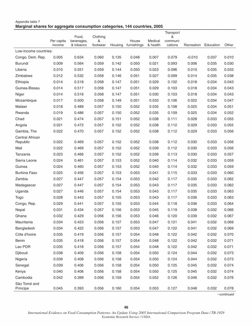
46International Evidence on Food Consumption Patterns: An Update Using 2005 International Comparison Program Data / TB-1929
Economic Research Service / USDA
Appendix table 7
Marginal shares for aggregate consumption categories, 144 countries, 2005, continued
Per capita income
Food, beverages, & tobacco
Clothing &
footwear HousingHouse
furnishingsMedical & health
Transport &
communi- cations Recreation Education Other
Low-income countries:
Congo, Dem. Rep. 0.005 0.634 0.060 0.135 0.048 0.007 0.079 -0.010 0.037 0.010
Burundi 0.009 0.564 0.059 0.142 0.050 0.021 0.093 0.006 0.035 0.030
Liberia 0.010 0.551 0.059 0.144 0.050 0.023 0.096 0.010 0.035 0.033
Zimbabwe 0.012 0.532 0.058 0.146 0.051 0.027 0.099 0.014 0.035 0.038
Ethiopia 0.014 0.518 0.058 0.147 0.051 0.029 0.102 0.018 0.034 0.043
Guinea-Bissau 0.014 0.517 0.058 0.147 0.051 0.029 0.103 0.018 0.034 0.043
Niger 0.014 0.516 0.058 0.147 0.051 0.030 0.103 0.018 0.034 0.043
Mozambique 0.017 0.500 0.058 0.149 0.051 0.033 0.106 0.022 0.034 0.047
Malawi 0.018 0.489 0.057 0.150 0.052 0.035 0.108 0.025 0.034 0.051
Rwanda 0.019 0.486 0.057 0.150 0.052 0.035 0.109 0.025 0.034 0.052
Chad 0.021 0.474 0.057 0.151 0.052 0.038 0.111 0.028 0.033 0.055
Angola 0.021 0.472 0.057 0.152 0.052 0.038 0.112 0.029 0.033 0.055
Gambia, The 0.022 0.470 0.057 0.152 0.052 0.038 0.112 0.029 0.033 0.056
Central African Republic 0.022 0.469 0.057 0.152 0.052 0.038 0.112 0.030 0.033 0.056
Mali 0.022 0.469 0.057 0.152 0.052 0.039 0.112 0.030 0.033 0.056
Tanzania 0.023 0.466 0.057 0.152 0.052 0.039 0.113 0.030 0.033 0.057
Sierra Leone 0.024 0.461 0.057 0.153 0.052 0.040 0.114 0.032 0.033 0.059
Guinea 0.024 0.460 0.057 0.153 0.052 0.040 0.114 0.032 0.033 0.059
Burkina Faso 0.025 0.456 0.057 0.153 0.053 0.041 0.115 0.033 0.033 0.060
Zambia 0.027 0.447 0.057 0.154 0.053 0.042 0.117 0.035 0.033 0.062
Madagascar 0.027 0.447 0.057 0.154 0.053 0.043 0.117 0.035 0.033 0.062
Uganda 0.027 0.446 0.057 0.154 0.053 0.043 0.117 0.035 0.033 0.063
Togo 0.028 0.443 0.057 0.155 0.053 0.043 0.117 0.036 0.033 0.063
Congo, Rep. 0.029 0.441 0.057 0.155 0.053 0.044 0.118 0.036 0.033 0.064
Nepal 0.031 0.434 0.057 0.156 0.053 0.045 0.119 0.038 0.032 0.066
Ghana 0.032 0.429 0.056 0.156 0.053 0.046 0.120 0.039 0.032 0.067
Mauritania 0.034 0.423 0.056 0.157 0.053 0.047 0.121 0.041 0.032 0.069
Bangladesh 0.034 0.422 0.056 0.157 0.053 0.047 0.122 0.041 0.032 0.069
Côte d'Ivoire 0.035 0.419 0.056 0.157 0.054 0.048 0.122 0.042 0.032 0.070
Benin 0.035 0.418 0.056 0.157 0.054 0.048 0.122 0.042 0.032 0.071
Lao PDR 0.035 0.418 0.056 0.157 0.054 0.048 0.122 0.042 0.032 0.071
Djibouti 0.038 0.409 0.056 0.158 0.054 0.050 0.124 0.044 0.032 0.073
Nigeria 0.039 0.408 0.056 0.158 0.054 0.050 0.124 0.044 0.032 0.073
Senegal 0.039 0.406 0.056 0.158 0.054 0.050 0.125 0.045 0.032 0.074
Kenya 0.040 0.406 0.056 0.158 0.054 0.050 0.125 0.045 0.032 0.074
Cambodia 0.042 0.399 0.056 0.159 0.054 0.052 0.126 0.046 0.032 0.076
São Tomé and Principe 0.045 0.393 0.056 0.160 0.054 0.053 0.127 0.048 0.032 0.078
--continued
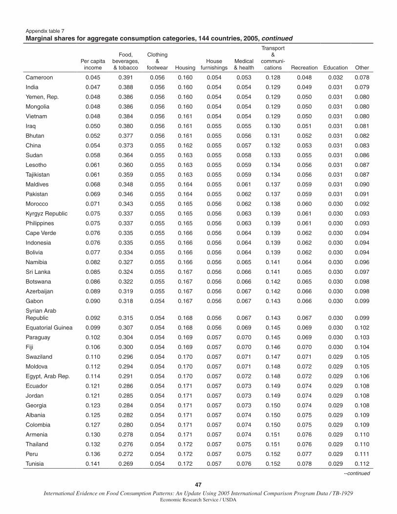
47 International Evidence on Food Consumption Patterns: An Update Using 2005 International Comparison Program Data / TB-1929
Economic Research Service / USDA
Appendix table 7
Marginal shares for aggregate consumption categories, 144 countries, 2005, continued
Per capita income
Food, beverages, & tobacco
Clothing &
footwear HousingHouse
furnishingsMedical & health
Transport &
communi- cations Recreation Education Other
Cameroon 0.045 0.391 0.056 0.160 0.054 0.053 0.128 0.048 0.032 0.078
India 0.047 0.388 0.056 0.160 0.054 0.054 0.129 0.049 0.031 0.079
Yemen, Rep. 0.048 0.386 0.056 0.160 0.054 0.054 0.129 0.050 0.031 0.080
Mongolia 0.048 0.386 0.056 0.160 0.054 0.054 0.129 0.050 0.031 0.080
Vietnam 0.048 0.384 0.056 0.161 0.054 0.054 0.129 0.050 0.031 0.080
Iraq 0.050 0.380 0.056 0.161 0.055 0.055 0.130 0.051 0.031 0.081
Bhutan 0.052 0.377 0.056 0.161 0.055 0.056 0.131 0.052 0.031 0.082
China 0.054 0.373 0.055 0.162 0.055 0.057 0.132 0.053 0.031 0.083
Sudan 0.058 0.364 0.055 0.163 0.055 0.058 0.133 0.055 0.031 0.086
Lesotho 0.061 0.360 0.055 0.163 0.055 0.059 0.134 0.056 0.031 0.087
Tajikistan 0.061 0.359 0.055 0.163 0.055 0.059 0.134 0.056 0.031 0.087
Maldives 0.068 0.348 0.055 0.164 0.055 0.061 0.137 0.059 0.031 0.090
Pakistan 0.069 0.346 0.055 0.164 0.055 0.062 0.137 0.059 0.031 0.091
Morocco 0.071 0.343 0.055 0.165 0.056 0.062 0.138 0.060 0.030 0.092
Kyrgyz Republic 0.075 0.337 0.055 0.165 0.056 0.063 0.139 0.061 0.030 0.093
Philippines 0.075 0.337 0.055 0.165 0.056 0.063 0.139 0.061 0.030 0.093
Cape Verde 0.076 0.335 0.055 0.166 0.056 0.064 0.139 0.062 0.030 0.094
Indonesia 0.076 0.335 0.055 0.166 0.056 0.064 0.139 0.062 0.030 0.094
Bolivia 0.077 0.334 0.055 0.166 0.056 0.064 0.139 0.062 0.030 0.094
Namibia 0.082 0.327 0.055 0.166 0.056 0.065 0.141 0.064 0.030 0.096
Sri Lanka 0.085 0.324 0.055 0.167 0.056 0.066 0.141 0.065 0.030 0.097
Botswana 0.086 0.322 0.055 0.167 0.056 0.066 0.142 0.065 0.030 0.098
Azerbaijan 0.089 0.319 0.055 0.167 0.056 0.067 0.142 0.066 0.030 0.098
Gabon 0.090 0.318 0.054 0.167 0.056 0.067 0.143 0.066 0.030 0.099
Syrian Arab Republic 0.092 0.315 0.054 0.168 0.056 0.067 0.143 0.067 0.030 0.099
Equatorial Guinea 0.099 0.307 0.054 0.168 0.056 0.069 0.145 0.069 0.030 0.102
Paraguay 0.102 0.304 0.054 0.169 0.057 0.070 0.145 0.069 0.030 0.103
Fiji 0.106 0.300 0.054 0.169 0.057 0.070 0.146 0.070 0.030 0.104
Swaziland 0.110 0.296 0.054 0.170 0.057 0.071 0.147 0.071 0.029 0.105
Moldova 0.112 0.294 0.054 0.170 0.057 0.071 0.148 0.072 0.029 0.105
Egypt, Arab Rep. 0.114 0.291 0.054 0.170 0.057 0.072 0.148 0.072 0.029 0.106
Ecuador 0.121 0.286 0.054 0.171 0.057 0.073 0.149 0.074 0.029 0.108
Jordan 0.121 0.285 0.054 0.171 0.057 0.073 0.149 0.074 0.029 0.108
Georgia 0.123 0.284 0.054 0.171 0.057 0.073 0.150 0.074 0.029 0.108
Albania 0.125 0.282 0.054 0.171 0.057 0.074 0.150 0.075 0.029 0.109
Colombia 0.127 0.280 0.054 0.171 0.057 0.074 0.150 0.075 0.029 0.109
Armenia 0.130 0.278 0.054 0.171 0.057 0.074 0.151 0.076 0.029 0.110
Thailand 0.132 0.276 0.054 0.172 0.057 0.075 0.151 0.076 0.029 0.110
Peru 0.136 0.272 0.054 0.172 0.057 0.075 0.152 0.077 0.029 0.111
Tunisia 0.141 0.269 0.054 0.172 0.057 0.076 0.152 0.078 0.029 0.112
--continued
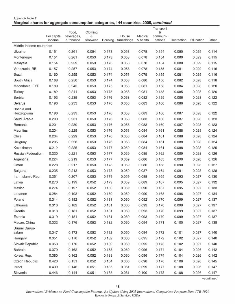
48International Evidence on Food Consumption Patterns: An Update Using 2005 International Comparison Program Data / TB-1929
Economic Research Service / USDA
Appendix table 7
Marginal shares for aggregate consumption categories, 144 countries, 2005, continued
Per capita income
Food, beverages, & tobacco
Clothing &
footwear HousingHouse
furnishingsMedical & health
Transport &
communi- cations Recreation Education Other
Middle-income countries:
Ukraine 0.151 0.261 0.054 0.173 0.058 0.078 0.154 0.080 0.029 0.114
Montenegro 0.151 0.261 0.053 0.173 0.058 0.078 0.154 0.080 0.029 0.115
Malaysia 0.154 0.259 0.053 0.173 0.058 0.078 0.154 0.080 0.029 0.115
Venezuela, RB 0.157 0.257 0.053 0.174 0.058 0.078 0.155 0.081 0.029 0.116
Brazil 0.160 0.255 0.053 0.174 0.058 0.079 0.155 0.081 0.029 0.116
South Africa 0.168 0.250 0.053 0.174 0.058 0.080 0.156 0.082 0.028 0.118
Macedonia, FYR 0.180 0.243 0.053 0.175 0.058 0.081 0.158 0.084 0.028 0.120
Turkey 0.182 0.241 0.053 0.175 0.058 0.081 0.158 0.085 0.028 0.120
Serbia 0.193 0.235 0.053 0.176 0.058 0.082 0.159 0.086 0.028 0.122
Belarus 0.196 0.233 0.053 0.176 0.058 0.083 0.160 0.086 0.028 0.122
Bosnia and Herzegovina 0.196 0.233 0.053 0.176 0.058 0.083 0.160 0.087 0.028 0.122
Saudi Arabia 0.200 0.231 0.053 0.176 0.058 0.083 0.160 0.087 0.028 0.123
Romania 0.201 0.230 0.053 0.176 0.058 0.083 0.160 0.087 0.028 0.123
Mauritius 0.204 0.229 0.053 0.176 0.058 0.084 0.161 0.088 0.028 0.124
Chile 0.204 0.229 0.053 0.176 0.058 0.084 0.161 0.088 0.028 0.124
Uruguay 0.205 0.228 0.053 0.176 0.058 0.084 0.161 0.088 0.028 0.124
Kazakhstan 0.212 0.225 0.053 0.177 0.059 0.084 0.161 0.088 0.028 0.125
Russian Federation 0.220 0.221 0.053 0.177 0.059 0.085 0.162 0.089 0.028 0.126
Argentina 0.224 0.219 0.053 0.177 0.059 0.086 0.163 0.090 0.028 0.126
Oman 0.228 0.217 0.053 0.178 0.059 0.086 0.163 0.090 0.028 0.127
Bulgaria 0.235 0.213 0.053 0.178 0.059 0.087 0.164 0.091 0.028 0.128
Iran, Islamic Rep. 0.251 0.207 0.053 0.179 0.059 0.088 0.165 0.093 0.027 0.130
Latvia 0.270 0.199 0.052 0.179 0.059 0.089 0.167 0.095 0.027 0.132
Mexico 0.274 0.197 0.052 0.180 0.059 0.090 0.167 0.095 0.027 0.133
Lebanon 0.284 0.193 0.052 0.180 0.059 0.090 0.168 0.096 0.027 0.134
Poland 0.314 0.182 0.052 0.181 0.060 0.092 0.170 0.099 0.027 0.137
Lithuania 0.316 0.182 0.052 0.181 0.060 0.093 0.170 0.099 0.027 0.137
Croatia 0.318 0.181 0.052 0.181 0.060 0.093 0.170 0.099 0.027 0.137
Estonia 0.319 0.181 0.052 0.181 0.060 0.093 0.170 0.099 0.027 0.137
Macao, China 0.332 0.176 0.052 0.182 0.060 0.094 0.171 0.100 0.027 0.138
Brunei Darus-salam 0.347 0.172 0.052 0.182 0.060 0.094 0.172 0.101 0.027 0.140
Hungary 0.351 0.170 0.052 0.182 0.060 0.095 0.172 0.102 0.027 0.140
Slovak Republic 0.353 0.170 0.052 0.182 0.060 0.095 0.173 0.102 0.027 0.140
Bahrain 0.379 0.162 0.052 0.183 0.060 0.096 0.174 0.104 0.026 0.142
Korea, Rep. 0.380 0.162 0.052 0.183 0.060 0.096 0.174 0.104 0.026 0.142
Czech Republic 0.420 0.151 0.052 0.184 0.060 0.098 0.176 0.106 0.026 0.145
Israel 0.439 0.146 0.051 0.185 0.061 0.099 0.177 0.108 0.026 0.147
Slovenia 0.446 0.144 0.051 0.185 0.061 0.100 0.178 0.108 0.026 0.147
--continued
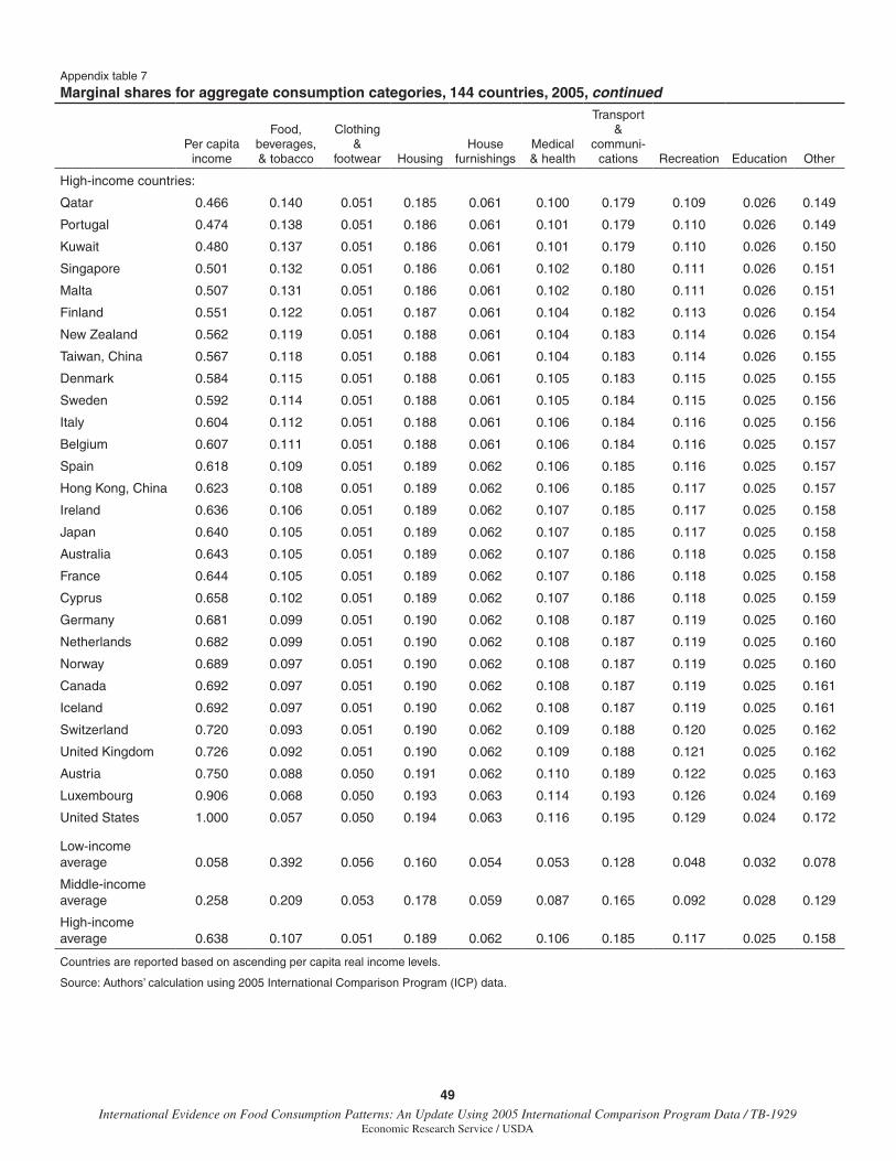
49 International Evidence on Food Consumption Patterns: An Update Using 2005 International Comparison Program Data / TB-1929
Economic Research Service / USDA
Appendix table 7
Marginal shares for aggregate consumption categories, 144 countries, 2005, continued
Per capita income
Food, beverages, & tobacco
Clothing &
footwear HousingHouse
furnishingsMedical & health
Transport &
communi- cations Recreation Education Other
High-income countries:
Qatar 0.466 0.140 0.051 0.185 0.061 0.100 0.179 0.109 0.026 0.149
Portugal 0.474 0.138 0.051 0.186 0.061 0.101 0.179 0.110 0.026 0.149
Kuwait 0.480 0.137 0.051 0.186 0.061 0.101 0.179 0.110 0.026 0.150
Singapore 0.501 0.132 0.051 0.186 0.061 0.102 0.180 0.111 0.026 0.151
Malta 0.507 0.131 0.051 0.186 0.061 0.102 0.180 0.111 0.026 0.151
Finland 0.551 0.122 0.051 0.187 0.061 0.104 0.182 0.113 0.026 0.154
New Zealand 0.562 0.119 0.051 0.188 0.061 0.104 0.183 0.114 0.026 0.154
Taiwan, China 0.567 0.118 0.051 0.188 0.061 0.104 0.183 0.114 0.026 0.155
Denmark 0.584 0.115 0.051 0.188 0.061 0.105 0.183 0.115 0.025 0.155
Sweden 0.592 0.114 0.051 0.188 0.061 0.105 0.184 0.115 0.025 0.156
Italy 0.604 0.112 0.051 0.188 0.061 0.106 0.184 0.116 0.025 0.156
Belgium 0.607 0.111 0.051 0.188 0.061 0.106 0.184 0.116 0.025 0.157
Spain 0.618 0.109 0.051 0.189 0.062 0.106 0.185 0.116 0.025 0.157
Hong Kong, China 0.623 0.108 0.051 0.189 0.062 0.106 0.185 0.117 0.025 0.157
Ireland 0.636 0.106 0.051 0.189 0.062 0.107 0.185 0.117 0.025 0.158
Japan 0.640 0.105 0.051 0.189 0.062 0.107 0.185 0.117 0.025 0.158
Australia 0.643 0.105 0.051 0.189 0.062 0.107 0.186 0.118 0.025 0.158
France 0.644 0.105 0.051 0.189 0.062 0.107 0.186 0.118 0.025 0.158
Cyprus 0.658 0.102 0.051 0.189 0.062 0.107 0.186 0.118 0.025 0.159
Germany 0.681 0.099 0.051 0.190 0.062 0.108 0.187 0.119 0.025 0.160
Netherlands 0.682 0.099 0.051 0.190 0.062 0.108 0.187 0.119 0.025 0.160
Norway 0.689 0.097 0.051 0.190 0.062 0.108 0.187 0.119 0.025 0.160
Canada 0.692 0.097 0.051 0.190 0.062 0.108 0.187 0.119 0.025 0.161
Iceland 0.692 0.097 0.051 0.190 0.062 0.108 0.187 0.119 0.025 0.161
Switzerland 0.720 0.093 0.051 0.190 0.062 0.109 0.188 0.120 0.025 0.162
United Kingdom 0.726 0.092 0.051 0.190 0.062 0.109 0.188 0.121 0.025 0.162
Austria 0.750 0.088 0.050 0.191 0.062 0.110 0.189 0.122 0.025 0.163
Luxembourg 0.906 0.068 0.050 0.193 0.063 0.114 0.193 0.126 0.024 0.169
United States 1.000 0.057 0.050 0.194 0.063 0.116 0.195 0.129 0.024 0.172
Low-income average 0.058 0.392 0.056 0.160 0.054 0.053 0.128 0.048 0.032 0.078
Middle-income average 0.258 0.209 0.053 0.178 0.059 0.087 0.165 0.092 0.028 0.129
High-income average 0.638 0.107 0.051 0.189 0.062 0.106 0.185 0.117 0.025 0.158
Countries are reported based on ascending per capita real income levels.
Source: Authors’ calculation using 2005 International Comparison Program (ICP) data.
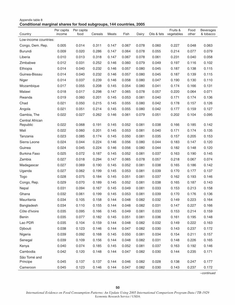
50International Evidence on Food Consumption Patterns: An Update Using 2005 International Comparison Program Data / TB-1929
Economic Research Service / USDA
Appendix table 8
Conditional marginal shares for food subgroups, 144 countries, 2005, continued
CountryPer capita
incomePer capita
food Cereals Meats Fish Dairy Oils & fatsFruits &
vegetablesFood other
Beverages & tobacco
Low-income countries:
Congo, Dem. Rep. 0.005 0.014 0.311 0.147 0.067 0.078 0.060 0.227 0.048 0.063
Burundi 0.009 0.020 0.286 0.147 0.064 0.078 0.055 0.214 0.077 0.079
Liberia 0.010 0.013 0.318 0.147 0.067 0.078 0.061 0.231 0.040 0.058
Zimbabwe 0.012 0.031 0.252 0.146 0.060 0.079 0.049 0.197 0.116 0.102
Ethiopia 0.014 0.040 0.232 0.146 0.057 0.080 0.045 0.187 0.138 0.115
Guinea-Bissau 0.014 0.040 0.232 0.146 0.057 0.080 0.045 0.187 0.139 0.115
Niger 0.014 0.037 0.239 0.146 0.058 0.080 0.047 0.190 0.130 0.110
Mozambique 0.017 0.055 0.208 0.145 0.054 0.080 0.041 0.174 0.166 0.131
Malawi 0.018 0.017 0.298 0.147 0.065 0.078 0.057 0.220 0.064 0.071
Rwanda 0.019 0.060 0.201 0.145 0.053 0.081 0.040 0.171 0.174 0.136
Chad 0.021 0.050 0.215 0.145 0.055 0.080 0.042 0.178 0.157 0.126
Angola 0.021 0.051 0.214 0.145 0.055 0.080 0.042 0.177 0.159 0.127
Gambia, The 0.022 0.027 0.262 0.146 0.061 0.079 0.051 0.202 0.104 0.095
Central African Republic 0.022 0.068 0.191 0.145 0.052 0.081 0.038 0.166 0.185 0.142
Mali 0.022 0.060 0.201 0.145 0.053 0.081 0.040 0.171 0.174 0.135
Tanzania 0.023 0.085 0.174 0.145 0.050 0.081 0.035 0.157 0.205 0.153
Sierra Leone 0.024 0.044 0.224 0.146 0.056 0.080 0.044 0.183 0.147 0.120
Guinea 0.024 0.045 0.224 0.146 0.056 0.080 0.044 0.182 0.148 0.120
Burkina Faso 0.025 0.072 0.187 0.145 0.052 0.081 0.037 0.163 0.190 0.145
Zambia 0.027 0.018 0.294 0.147 0.065 0.078 0.057 0.218 0.067 0.074
Madagascar 0.027 0.069 0.190 0.145 0.052 0.081 0.038 0.165 0.186 0.142
Uganda 0.027 0.062 0.199 0.145 0.053 0.081 0.039 0.170 0.177 0.137
Togo 0.028 0.075 0.184 0.145 0.051 0.081 0.037 0.162 0.193 0.146
Congo, Rep. 0.029 0.070 0.189 0.145 0.052 0.081 0.038 0.165 0.187 0.143
Nepal 0.031 0.094 0.167 0.145 0.049 0.081 0.033 0.153 0.213 0.158
Ghana 0.032 0.061 0.199 0.145 0.053 0.081 0.039 0.170 0.176 0.136
Mauritania 0.034 0.105 0.158 0.144 0.048 0.082 0.032 0.149 0.223 0.164
Bangladesh 0.034 0.110 0.155 0.144 0.048 0.082 0.031 0.147 0.227 0.166
Côte d'Ivoire 0.035 0.095 0.166 0.145 0.049 0.081 0.033 0.153 0.214 0.159
Benin 0.035 0.077 0.182 0.145 0.051 0.081 0.036 0.161 0.195 0.148
Lao PDR 0.035 0.104 0.159 0.144 0.048 0.082 0.032 0.149 0.222 0.163
Djibouti 0.038 0.123 0.146 0.144 0.047 0.082 0.030 0.143 0.237 0.172
Nigeria 0.039 0.092 0.168 0.145 0.050 0.081 0.034 0.154 0.211 0.157
Senegal 0.039 0.109 0.156 0.144 0.048 0.082 0.031 0.148 0.226 0.165
Kenya 0.040 0.074 0.185 0.145 0.052 0.081 0.037 0.163 0.192 0.146
Cambodia 0.042 0.120 0.148 0.144 0.047 0.082 0.030 0.144 0.235 0.171
São Tomé and Principe 0.045 0.137 0.137 0.144 0.046 0.082 0.028 0.138 0.247 0.177
Cameroon 0.045 0.123 0.146 0.144 0.047 0.082 0.030 0.143 0.237 0.172
--continued
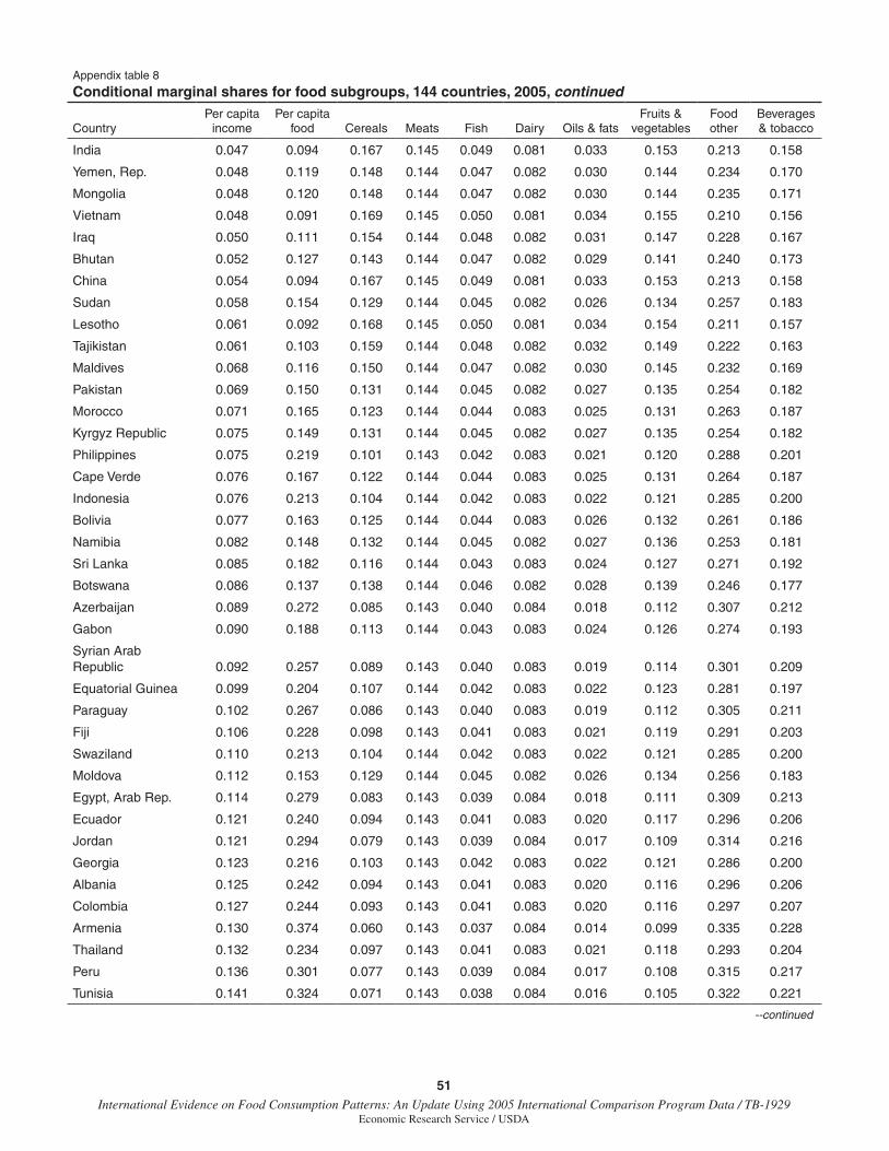
51 International Evidence on Food Consumption Patterns: An Update Using 2005 International Comparison Program Data / TB-1929
Economic Research Service / USDA
Appendix table 8
Conditional marginal shares for food subgroups, 144 countries, 2005, continued
CountryPer capita
incomePer capita
food Cereals Meats Fish Dairy Oils & fatsFruits &
vegetablesFood other
Beverages & tobacco
India 0.047 0.094 0.167 0.145 0.049 0.081 0.033 0.153 0.213 0.158
Yemen, Rep. 0.048 0.119 0.148 0.144 0.047 0.082 0.030 0.144 0.234 0.170
Mongolia 0.048 0.120 0.148 0.144 0.047 0.082 0.030 0.144 0.235 0.171
Vietnam 0.048 0.091 0.169 0.145 0.050 0.081 0.034 0.155 0.210 0.156
Iraq 0.050 0.111 0.154 0.144 0.048 0.082 0.031 0.147 0.228 0.167
Bhutan 0.052 0.127 0.143 0.144 0.047 0.082 0.029 0.141 0.240 0.173
China 0.054 0.094 0.167 0.145 0.049 0.081 0.033 0.153 0.213 0.158
Sudan 0.058 0.154 0.129 0.144 0.045 0.082 0.026 0.134 0.257 0.183
Lesotho 0.061 0.092 0.168 0.145 0.050 0.081 0.034 0.154 0.211 0.157
Tajikistan 0.061 0.103 0.159 0.144 0.048 0.082 0.032 0.149 0.222 0.163
Maldives 0.068 0.116 0.150 0.144 0.047 0.082 0.030 0.145 0.232 0.169
Pakistan 0.069 0.150 0.131 0.144 0.045 0.082 0.027 0.135 0.254 0.182
Morocco 0.071 0.165 0.123 0.144 0.044 0.083 0.025 0.131 0.263 0.187
Kyrgyz Republic 0.075 0.149 0.131 0.144 0.045 0.082 0.027 0.135 0.254 0.182
Philippines 0.075 0.219 0.101 0.143 0.042 0.083 0.021 0.120 0.288 0.201
Cape Verde 0.076 0.167 0.122 0.144 0.044 0.083 0.025 0.131 0.264 0.187
Indonesia 0.076 0.213 0.104 0.144 0.042 0.083 0.022 0.121 0.285 0.200
Bolivia 0.077 0.163 0.125 0.144 0.044 0.083 0.026 0.132 0.261 0.186
Namibia 0.082 0.148 0.132 0.144 0.045 0.082 0.027 0.136 0.253 0.181
Sri Lanka 0.085 0.182 0.116 0.144 0.043 0.083 0.024 0.127 0.271 0.192
Botswana 0.086 0.137 0.138 0.144 0.046 0.082 0.028 0.139 0.246 0.177
Azerbaijan 0.089 0.272 0.085 0.143 0.040 0.084 0.018 0.112 0.307 0.212
Gabon 0.090 0.188 0.113 0.144 0.043 0.083 0.024 0.126 0.274 0.193
Syrian Arab Republic 0.092 0.257 0.089 0.143 0.040 0.083 0.019 0.114 0.301 0.209
Equatorial Guinea 0.099 0.204 0.107 0.144 0.042 0.083 0.022 0.123 0.281 0.197
Paraguay 0.102 0.267 0.086 0.143 0.040 0.083 0.019 0.112 0.305 0.211
Fiji 0.106 0.228 0.098 0.143 0.041 0.083 0.021 0.119 0.291 0.203
Swaziland 0.110 0.213 0.104 0.144 0.042 0.083 0.022 0.121 0.285 0.200
Moldova 0.112 0.153 0.129 0.144 0.045 0.082 0.026 0.134 0.256 0.183
Egypt, Arab Rep. 0.114 0.279 0.083 0.143 0.039 0.084 0.018 0.111 0.309 0.213
Ecuador 0.121 0.240 0.094 0.143 0.041 0.083 0.020 0.117 0.296 0.206
Jordan 0.121 0.294 0.079 0.143 0.039 0.084 0.017 0.109 0.314 0.216
Georgia 0.123 0.216 0.103 0.143 0.042 0.083 0.022 0.121 0.286 0.200
Albania 0.125 0.242 0.094 0.143 0.041 0.083 0.020 0.116 0.296 0.206
Colombia 0.127 0.244 0.093 0.143 0.041 0.083 0.020 0.116 0.297 0.207
Armenia 0.130 0.374 0.060 0.143 0.037 0.084 0.014 0.099 0.335 0.228
Thailand 0.132 0.234 0.097 0.143 0.041 0.083 0.021 0.118 0.293 0.204
Peru 0.136 0.301 0.077 0.143 0.039 0.084 0.017 0.108 0.315 0.217
Tunisia 0.141 0.324 0.071 0.143 0.038 0.084 0.016 0.105 0.322 0.221
--continued
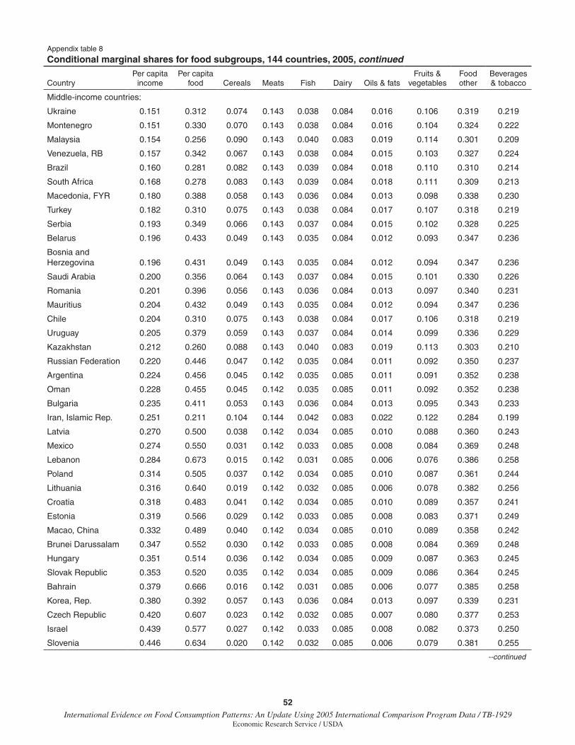
52International Evidence on Food Consumption Patterns: An Update Using 2005 International Comparison Program Data / TB-1929
Economic Research Service / USDA
Appendix table 8
Conditional marginal shares for food subgroups, 144 countries, 2005, continued
CountryPer capita
incomePer capita
food Cereals Meats Fish Dairy Oils & fatsFruits &
vegetablesFood other
Beverages & tobacco
Middle-income countries:
Ukraine 0.151 0.312 0.074 0.143 0.038 0.084 0.016 0.106 0.319 0.219
Montenegro 0.151 0.330 0.070 0.143 0.038 0.084 0.016 0.104 0.324 0.222
Malaysia 0.154 0.256 0.090 0.143 0.040 0.083 0.019 0.114 0.301 0.209
Venezuela, RB 0.157 0.342 0.067 0.143 0.038 0.084 0.015 0.103 0.327 0.224
Brazil 0.160 0.281 0.082 0.143 0.039 0.084 0.018 0.110 0.310 0.214
South Africa 0.168 0.278 0.083 0.143 0.039 0.084 0.018 0.111 0.309 0.213
Macedonia, FYR 0.180 0.388 0.058 0.143 0.036 0.084 0.013 0.098 0.338 0.230
Turkey 0.182 0.310 0.075 0.143 0.038 0.084 0.017 0.107 0.318 0.219
Serbia 0.193 0.349 0.066 0.143 0.037 0.084 0.015 0.102 0.328 0.225
Belarus 0.196 0.433 0.049 0.143 0.035 0.084 0.012 0.093 0.347 0.236
Bosnia and Herzegovina 0.196 0.431 0.049 0.143 0.035 0.084 0.012 0.094 0.347 0.236
Saudi Arabia 0.200 0.356 0.064 0.143 0.037 0.084 0.015 0.101 0.330 0.226
Romania 0.201 0.396 0.056 0.143 0.036 0.084 0.013 0.097 0.340 0.231
Mauritius 0.204 0.432 0.049 0.143 0.035 0.084 0.012 0.094 0.347 0.236
Chile 0.204 0.310 0.075 0.143 0.038 0.084 0.017 0.106 0.318 0.219
Uruguay 0.205 0.379 0.059 0.143 0.037 0.084 0.014 0.099 0.336 0.229
Kazakhstan 0.212 0.260 0.088 0.143 0.040 0.083 0.019 0.113 0.303 0.210
Russian Federation 0.220 0.446 0.047 0.142 0.035 0.084 0.011 0.092 0.350 0.237
Argentina 0.224 0.456 0.045 0.142 0.035 0.085 0.011 0.091 0.352 0.238
Oman 0.228 0.455 0.045 0.142 0.035 0.085 0.011 0.092 0.352 0.238
Bulgaria 0.235 0.411 0.053 0.143 0.036 0.084 0.013 0.095 0.343 0.233
Iran, Islamic Rep. 0.251 0.211 0.104 0.144 0.042 0.083 0.022 0.122 0.284 0.199
Latvia 0.270 0.500 0.038 0.142 0.034 0.085 0.010 0.088 0.360 0.243
Mexico 0.274 0.550 0.031 0.142 0.033 0.085 0.008 0.084 0.369 0.248
Lebanon 0.284 0.673 0.015 0.142 0.031 0.085 0.006 0.076 0.386 0.258
Poland 0.314 0.505 0.037 0.142 0.034 0.085 0.010 0.087 0.361 0.244
Lithuania 0.316 0.640 0.019 0.142 0.032 0.085 0.006 0.078 0.382 0.256
Croatia 0.318 0.483 0.041 0.142 0.034 0.085 0.010 0.089 0.357 0.241
Estonia 0.319 0.566 0.029 0.142 0.033 0.085 0.008 0.083 0.371 0.249
Macao, China 0.332 0.489 0.040 0.142 0.034 0.085 0.010 0.089 0.358 0.242
Brunei Darussalam 0.347 0.552 0.030 0.142 0.033 0.085 0.008 0.084 0.369 0.248
Hungary 0.351 0.514 0.036 0.142 0.034 0.085 0.009 0.087 0.363 0.245
Slovak Republic 0.353 0.520 0.035 0.142 0.034 0.085 0.009 0.086 0.364 0.245
Bahrain 0.379 0.666 0.016 0.142 0.031 0.085 0.006 0.077 0.385 0.258
Korea, Rep. 0.380 0.392 0.057 0.143 0.036 0.084 0.013 0.097 0.339 0.231
Czech Republic 0.420 0.607 0.023 0.142 0.032 0.085 0.007 0.080 0.377 0.253
Israel 0.439 0.577 0.027 0.142 0.033 0.085 0.008 0.082 0.373 0.250
Slovenia 0.446 0.634 0.020 0.142 0.032 0.085 0.006 0.079 0.381 0.255
--continued
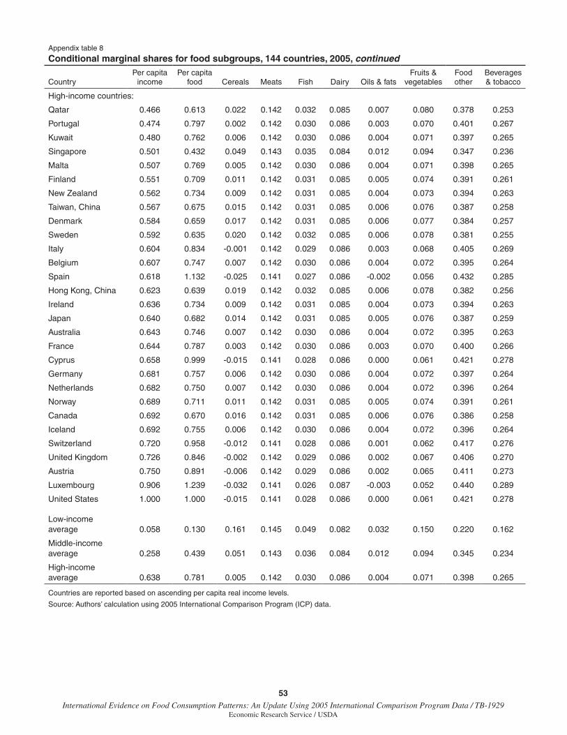
53 International Evidence on Food Consumption Patterns: An Update Using 2005 International Comparison Program Data / TB-1929
Economic Research Service / USDA
Appendix table 8
Conditional marginal shares for food subgroups, 144 countries, 2005, continued
CountryPer capita
incomePer capita
food Cereals Meats Fish Dairy Oils & fatsFruits &
vegetablesFood other
Beverages & tobacco
High-income countries:
Qatar 0.466 0.613 0.022 0.142 0.032 0.085 0.007 0.080 0.378 0.253
Portugal 0.474 0.797 0.002 0.142 0.030 0.086 0.003 0.070 0.401 0.267
Kuwait 0.480 0.762 0.006 0.142 0.030 0.086 0.004 0.071 0.397 0.265
Singapore 0.501 0.432 0.049 0.143 0.035 0.084 0.012 0.094 0.347 0.236
Malta 0.507 0.769 0.005 0.142 0.030 0.086 0.004 0.071 0.398 0.265
Finland 0.551 0.709 0.011 0.142 0.031 0.085 0.005 0.074 0.391 0.261
New Zealand 0.562 0.734 0.009 0.142 0.031 0.085 0.004 0.073 0.394 0.263
Taiwan, China 0.567 0.675 0.015 0.142 0.031 0.085 0.006 0.076 0.387 0.258
Denmark 0.584 0.659 0.017 0.142 0.031 0.085 0.006 0.077 0.384 0.257
Sweden 0.592 0.635 0.020 0.142 0.032 0.085 0.006 0.078 0.381 0.255
Italy 0.604 0.834 -0.001 0.142 0.029 0.086 0.003 0.068 0.405 0.269
Belgium 0.607 0.747 0.007 0.142 0.030 0.086 0.004 0.072 0.395 0.264
Spain 0.618 1.132 -0.025 0.141 0.027 0.086 -0.002 0.056 0.432 0.285
Hong Kong, China 0.623 0.639 0.019 0.142 0.032 0.085 0.006 0.078 0.382 0.256
Ireland 0.636 0.734 0.009 0.142 0.031 0.085 0.004 0.073 0.394 0.263
Japan 0.640 0.682 0.014 0.142 0.031 0.085 0.005 0.076 0.387 0.259
Australia 0.643 0.746 0.007 0.142 0.030 0.086 0.004 0.072 0.395 0.263
France 0.644 0.787 0.003 0.142 0.030 0.086 0.003 0.070 0.400 0.266
Cyprus 0.658 0.999 -0.015 0.141 0.028 0.086 0.000 0.061 0.421 0.278
Germany 0.681 0.757 0.006 0.142 0.030 0.086 0.004 0.072 0.397 0.264
Netherlands 0.682 0.750 0.007 0.142 0.030 0.086 0.004 0.072 0.396 0.264
Norway 0.689 0.711 0.011 0.142 0.031 0.085 0.005 0.074 0.391 0.261
Canada 0.692 0.670 0.016 0.142 0.031 0.085 0.006 0.076 0.386 0.258
Iceland 0.692 0.755 0.006 0.142 0.030 0.086 0.004 0.072 0.396 0.264
Switzerland 0.720 0.958 -0.012 0.141 0.028 0.086 0.001 0.062 0.417 0.276
United Kingdom 0.726 0.846 -0.002 0.142 0.029 0.086 0.002 0.067 0.406 0.270
Austria 0.750 0.891 -0.006 0.142 0.029 0.086 0.002 0.065 0.411 0.273
Luxembourg 0.906 1.239 -0.032 0.141 0.026 0.087 -0.003 0.052 0.440 0.289
United States 1.000 1.000 -0.015 0.141 0.028 0.086 0.000 0.061 0.421 0.278
Low-income average 0.058 0.130 0.161 0.145 0.049 0.082 0.032 0.150 0.220 0.162
Middle-income average 0.258 0.439 0.051 0.143 0.036 0.084 0.012 0.094 0.345 0.234
High-income average 0.638 0.781 0.005 0.142 0.030 0.086 0.004 0.071 0.398 0.265
Countries are reported based on ascending per capita real income levels.
Source: Authors’ calculation using 2005 International Comparison Program (ICP) data.
Related Documents


