Interleaved Q-Learning with Partially Coupled Training Process

Interleaved Q-Learning with Partially Coupled Training Process∗Main Track

Min He

University of Electronic Science and

Technology of China

Chengdu, China

[email protected]

Hongliang Guo

University of Electronic Science and

Technology of China

Chengdu, China

[email protected]

ABSTRACTThis paper studies estimating themaximum expected value (MEV) of

several independent random variables (RVs). No unbiased estimator

exists without knowing the distributions of those RVs a priori. Two

of the most famous estimators, maximum estimator (ME) and dou-

ble estimator (DE), yield positive bias and negative bias respectively.

We propose a coupled estimator (CE) which subsumes ME and DE

as special cases and yields a bias between that of ME and DE, while

maintaining the same variance bound. Furthermore, a simple yet

effective variance reduction technique is proposed and verified in

the experiments. The instantiated algorithm in the Markov decision

process (MDP) setting, called interleaved Q-learning, outperforms

Q-learning and double Q-learning in some highly stochastic envi-

ronments. Insights on how to adapt the coupling ratio in CE and

hence make interleaved Q-learning automatically shift between

Q-learning and double Q-learning are provided and verified in the

experimental section.

KEYWORDSMaximum Estimator; Double Estimator; Coupled Estimator; Estima-

tion Bias; Q-Learning; Double Q-Learning; Interleaved Q-learning

ACM Reference Format:Min He and Hongliang Guo. 2019. Interleaved Q-Learning with Partially

Coupled Training Process. In Proc. of the 18th International Conference on Au-tonomous Agents and Multiagent Systems (AAMAS 2019), Montreal, Canada,May 13–17, 2019, IFAAMAS, 9 pages.

1 INTRODUCTIONMany stochastic sequential decision making problems require esti-

mating the maximum expected value of several RVs1, given samples

collected from each variable [22]. Two of the most famous estima-

tors areME andDE respectively, and both of them have been applied

to various problem settings. For instance, in reinforcement learning

(RL), Q-learning employs ME to estimate the optimal value of an

action in a state; while double Q-learning uses DE for action-value

estimation [8]. It is widely accepted that in some highly stochas-

tic environments, Q-learning may perform poorly largely due to

the overestimation of action values from ME. On the other hand,

∗Titlenote — equal contribution by the first two authors.

1Without loss of generality, we assume that the target is to find themaximum expected

value over several RVs, the negative case applies in the same way.

Proc. of the 18th International Conference on Autonomous Agents and Multiagent Systems(AAMAS 2019), N. Agmon, M. E. Taylor, E. Elkind, M. Veloso (eds.), May 13–17, 2019,Montreal, Canada. © 2019 International Foundation for Autonomous Agents and

Multiagent Systems (www.ifaamas.org). All rights reserved.

double Q-learning steadily underestimates the action values be-

cause of using DE, and performs better than Q-learning in some

environmental settings [22].

This paper takes a fresh perspective to investigate the overesti-

mation/underestimation problem of ME/DE, and thereby delivers

an in-depth insight on which type of stochastic scenarios favours

ME and which type favours DE respectively. Inspired from the in-

sight, we propose a unifying estimator, namely coupled estimator(CE) which takes advantage of bothME and DE, and subsumes them

as special cases for MEV estimation. Instead of having a single set

for MEV estimation in ME or two completely disjoint sets in DE,

CE partitions the samples of RVs into two partially coupled sets

(Set A and Set B), in which the DE logic (using one set to evaluate

another one) is used to estimate MEV.

We further propose a coupling ratio adaptation algorithm, which

makes CE’s estimation bias find a balance between ME’s overesti-

mation and DE’s underestimation as verified through simulation

results. Moreover, we further show that through interleaving the

two evaluation terms from µ j (S1) and µ j (S2), CE’s estimation vari-

ance is greatly decreased (up to a factor of 1/2) as validated in the

experiments.

The CE-instantiated RL algorithm, namely interleaved Q-learning,absorbs the merits of both Q-learning and double Q-learning, and

subsumes them as special cases in two extreme conditions as what

CE does for ME and DE. Interleaved Q-learning embraces (1) a

partially coupled training process to mimic the partially overlapped

set partition process in CE, and (2) an interleaved evaluation process

similar to CE’s variance reduction technique.

The original contributions of the paper include: (1) a unifying

estimator (CE) which subsumes ME and DE as special cases and

a self-adaptive strategy for the coupling ratio adjustment; (2) a

simple yet effective interleaving approach decreasing the estima-

tor’s variance up to a factor of 1/2; (3) a CE-instantiated off-policy

reinforcement learning algorithm, namely interleaved Q-learning,

which steadily outperforms Q-learning and double Q-learning in

various stochastic environment and also subsumes Q-learning and

double Q-learning as special cases.

2 MAXIMUM EXPECTED VALUEESTIMATION

In this section, we first present the problem formulation of MEV

estimation for several independent RVs, i.e. maxi E(Xi ), then in-

troduce two of the most famous estimators (ME and DE) in the

literature and end the section with a brief literature review on

miscellaneous MEV estimators.

Session 2C: Knowledge Representation and Reasoning AAMAS 2019, May 13-17, 2019, Montréal, Canada

449

2.1 Notations and Problem FormulationThe problem is to estimate the maximum expected value over a

finite set of N ≥ 2 random variables X = X1,X2, · · · ,XN . The

probability density function (PDF) and cumulative density function

(CDF) of Xi are denoted as fi (x) and Fi (x), respectively, with µiand σ 2

i denoting the mean and variance of Xi . The true maximum

expected value µ∗(X ) is defined as:

µ∗(X ) = max

iµi = max

i

∫ +∞−∞

x fi (x)dx . (1)

In most application scenarios, the PDFs (fi ) are unknown before-

hand and therefore µ∗ = maxi µi cannot be found analytically. Inthis paper, we use S = S1, S2, · · · , SN to denote the samples of X ,

and denote µi (S) as an estimator for µi based on the sampled set S .Similarly, µ∗(S) is used as an estimator for µ∗

2.

We define Aj (S) as the event that the RV X j ’s sample average,

out of the given sample set S , is the largest out of all the sample

averages. In this case, P(Aj ) refers to the probability that event Ajhappens over the sampling space Ω. The term P(Aj ) is of great

importance when analysing the overestimation/underestimation of

ME/DE in later subsections.

Definition 2.1. The bias of an estimator (µ(S)) to the true value

(µ∗) is defined as Bias(µ) = E(µ) − µ∗.

It has been proved in [22] that no general unbiased estimator

exists even if all µi are unbiased. Two of the most famous estima-

tors, ME and DE, are described and analysed in the following two

subsections, respectively.

2.2 The Maximum EstimatorThe maximum estimator for µ∗(S) is

µME

∗ (S) ≡ max

iµi (S), (2)

where µi (S) is an estimator of µi , which can be unbiased. ME is

widely used in practice because it is conceptually simple and easy

to implement. There have been many works proving ME’s over-

estimation of true MEV, i.e. [17] and [22]. However, most of the

existing proofs rely on some logical explanation to justify ME’s

overestimation, this paper presents a concise mathematical deriva-

tion process for proving ME’s overestimation and the derivation

process inspires the bias reduction technique used in CE.

Before laying down the overestimation fact of ME and its corre-

sponding proof, we first present the following two lemmas.

Lemma 2.2. Let φ be a convex function, and X be an integrablereal-valued random variable, we have:

φ(E(X )

)≤ E

(φ(X )

)(3)

Lemma 2.3. The max operator is a convex function.

Both of the two lemmas are well known results. Lemma 2.2 is a

direct application of Jensen’s inequality, and the proof can be found

in [14]. The proof of Lemma 2.3 is in [4].

Theorem 2.4. For any given sampled set S out of the samplingspace Ω and unbiased estimators µi (S), i.e., E

(µi (S)

)= µi , we have

E(µME∗ (S)

)≥ µ∗.

2Note that we write µi and µ∗ when X and/or S is clear within the context.

Proof.

E(µME

∗ (S))= E

(max

iµi (S)

)≥ max

iE(µi (S)

)= max

iµi

= µ∗

The inequality is from Jensen’s inequality in Lemma 2.2 and the fact

that the max operator is a convex function as stated in Remark 2.3.

We have assumed that µi (S) is an unbiased estimator of µi , thus

E(µi (S)

)= µi .

Insights on ME’s bias: from Theorem 2.4’s proving process, we

can see that the inequality comes into play when we are exchanging

the max operator with the expectation operator. It means that, if

the arg max operator returns a constant RV index recommendation

which makes max operate on a single fixed RV, the inequality will

become equality, and ME will be unbiased. In MEV use cases, it

means that out of the set of RVs, there is one RV dominating others

(meaning that the RV’s expected value is much larger than the rest

of the RVs), ME tends to be unbiased.

Theorem 2.4 states that ME is always having a positive bias

and thus provides a lower bound of ME as zero. The following

two theorems provide upper bounds of ME’s bias and variance,

respectively.

Theorem 2.5. The upper bound of ME’s bias is expressed as:

Bias

(µME∗ (S)

)= E

(µME∗ (S)

)− µ∗ ≤

√√√N − 1

N

N∑i=1

Var(µi ). (4)

Theorem 2.6. The upper bound of ME’s variance is provided inEq. 5.

Var

(µME∗ (S)

)≤

N∑i=1

Var(µi ) (5)

The proofs of Theorem 2.5 and Theorem 2.6 are provided in [2]

and [22] respectively.

2.3 The Double EstimatorThe double estimator µDE∗ (S) first partitions the sampling set S into

two disjoint sets, namely S1 and S2. DE uses one of the sets, say

Set S1 to determine which RV to choose, and then uses Set S2 to

determine the value of the estimation. The calculation process is:

µDE∗ (S) = µ j (S2), (6)

where j = arg maxj µ j (S1). Note that the RV index selection process

and the value estimation process are separated and functioning

over two disjoint and independent sets of samples. In this way, the

overestimation bias is eliminated, however, the underestimation

bias is introduced as stated in the following theorem.

Theorem 2.7. For any given sampled set S out of the samplingspace Ω and unbiased estimators µi (S), we have E

(µDE∗ (S)

)≤ µ∗.

Proof.

E(µDE∗ (S)

)= E

(µ j (S2)

)

Session 2C: Knowledge Representation and Reasoning AAMAS 2019, May 13-17, 2019, Montréal, Canada

450

= E(∑

jP(Aj )µ j (S2)

)=∑jP(Aj )E

(µ j (S2)

)=∑jP(Aj )µ j

≤∑jP(Aj )max

jµ j

= µ∗.

The key derivation point is that index j is also a random variable,

andwhen calculating the expected value of DE, we need to represent

the probability of selecting each index explicitly. In our deduction

process, the probability of selecting index j as the largest RV’s indexis equal to the probability that eventAj happens out of the sampling

space Ω, which is denoted as P(Aj )3.

Insights onDE’s bias: fromTheorem 2.7’s proving process, we can

see that the inequality comes into play due to the fact that µ j ≤ µ∗.It means that, if the arg max operator only returns the set of RVs

with the expectation value of µ∗, the inequality become equality

and DE is unbiased. In real MEV use cases, it means that when

there is a subset of RVs having the same (or similar) expectation

values, and all the other RVs’ expectation values are dominated by

the subset, DE tends to be unbiased.

The following two theorems give the lower bound (upper bound

is zero) and variance of DE respectively and the corresponding

proofs are provided in [22].

Theorem 2.8. The lower bound of DE’s bias is expressed as:

Bias

(µDE∗ (S)

)= E

(µDE∗ (S)

)− µ∗ ≥ −

1

2

√√√ N∑i=1

Var(µi (S2)). (7)

Theorem 2.9. The upper bound of DE’s variance is

Var

(µDE∗ (S)

)≤

N∑i=1

Var(µi (S2)). (8)

2.4 Miscellaneous MEV EstimatorsSeveral other estimators targeting at alleviating the overestimation

of ME and/or underestimation of DE exist. Zhang et.al. propose

a weighted double estimator (WDE) for MEV estimation, and the

weight is decided by the difference between the largest estimated

value over the set of RVs and the smallest one [26]. A Gaussian esti-

mator (GE) is proposed by [6], and the authors assume a Gaussian

distribution of the sample averages, with this assumption, GE is

able to reach an estimation with the bias bound smaller than that

of both DE and ME. The extension of GE to an infinite number of

RVs is reported in [5].

3 COUPLED ESTIMATORIn the previous section, we have introducedME and DE respectively.

On the one hand, ME does not partition the sample set, and uses

the same one (S) for both index selection and value estimation; in

this case, the strong correlation (between index selection and value

3Note that

∑j P(Aj ) = 1

S1

S2

For estimator

A

For estimator

B

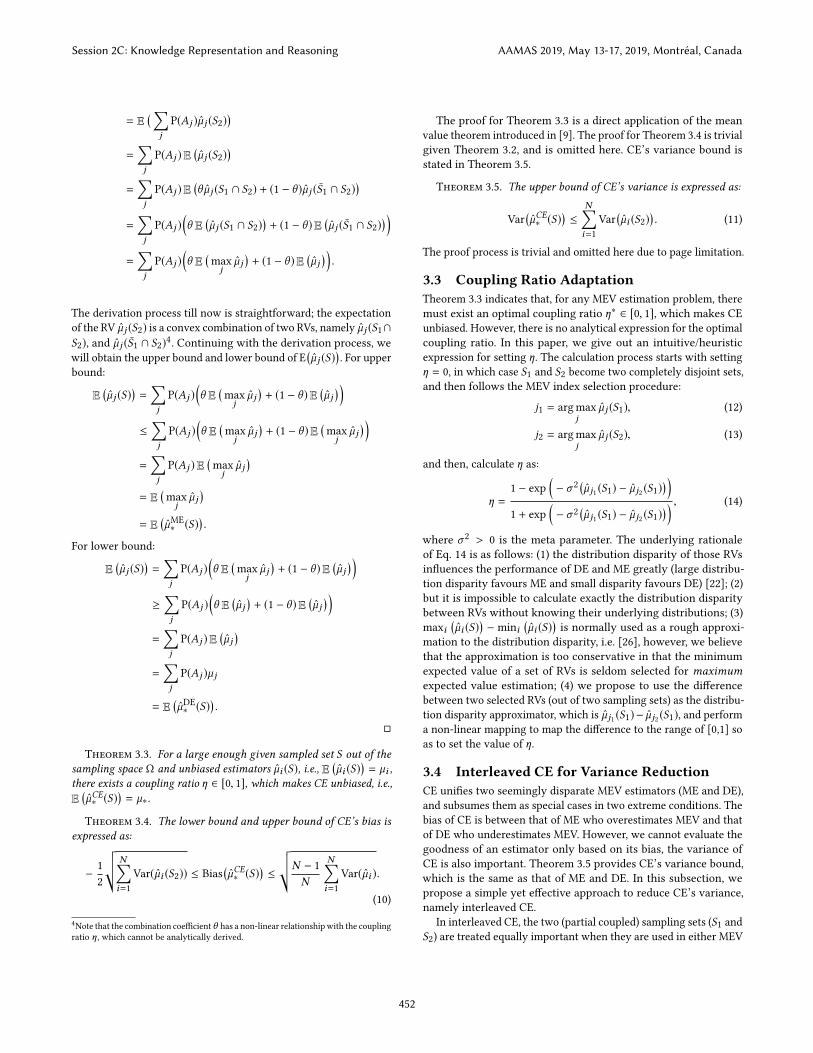
For estimator A and B

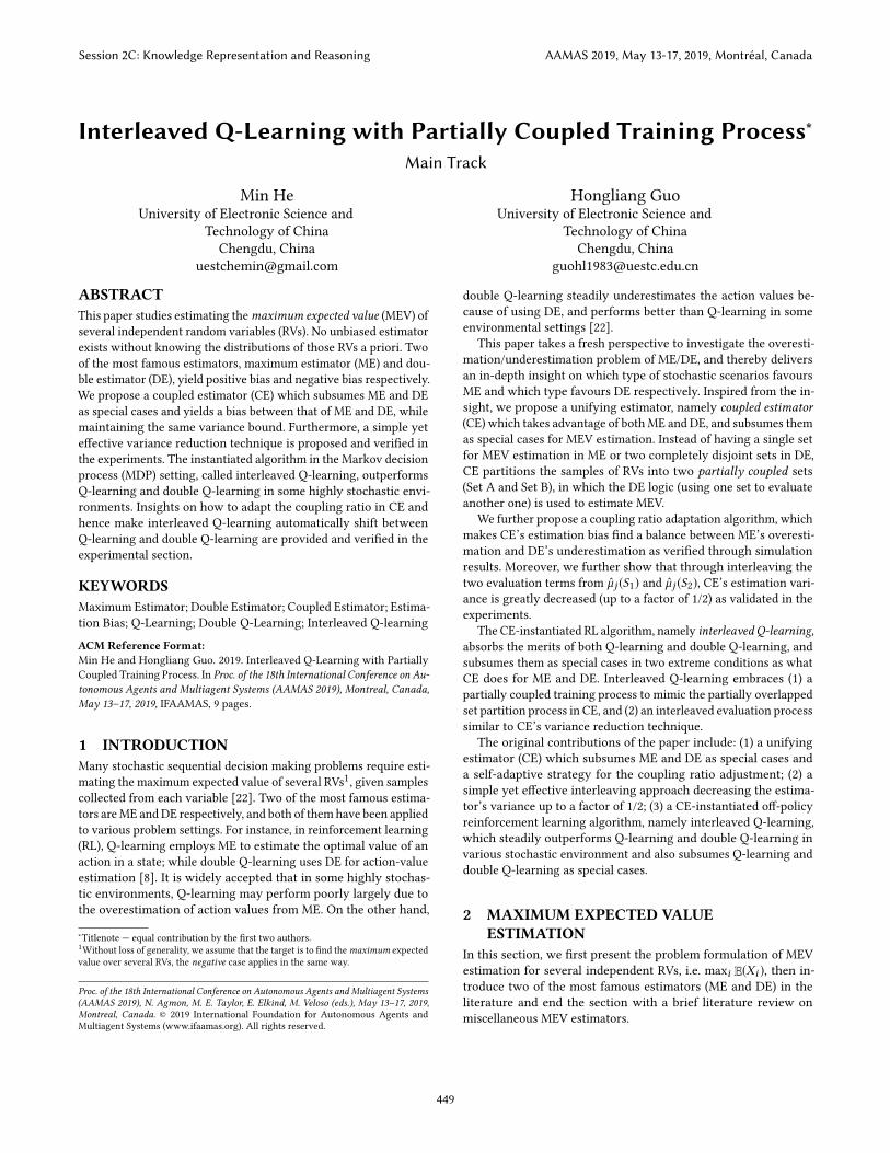
Figure 1: Illustration of the partially coupled parti-tion(estimators A and B can be any kind of estimators)

estimation) makes ME overestimate the MEV. On the other hand,

DE partitions the sample set S into two completely disjoint sets, S1

and S2; in this case, S1 and S2 are independent with each other, and

as a consequence, DE underestimates the MEV. We conjecture that

if we partition the sample set S into two partially coupled sets, say

S1 and S2, and tune the coupling ratio from 0 to 1, the corresponding

estimator, namely coupled estimator (CE), will shift continuously

from underestimation of DE to overestimation of ME. In the fol-

lowing subsections, we will formally present the coupled estimator,

analyse its bias bound, and corresponding variance bound.

3.1 The Coupled EstimatorBefore introducing the coupled estimator, we lay down the defini-

tion of coupling ratio and illustrate its influence in the sampling

set partition process.

Definition 3.1. The coupling ratio η ∈ [0, 1] of a sampling set Sis defined as the percentage of the shared data between the two

partitioned sets, S1 and S2, over the total data set.

Fig. 1 illustrates the meaning of coupling ratio of the sampling

set. Consider the sampling set S with only one variable for ease of

understanding, and there are N samples. After the partially cou-

pled/overlapped partition into S1 and S2, with N1 and N2 samples

for S1 and S2 respectively. The coupling ratio η is calculated as

η = (N1 +N2 −N )/N . The coupled estimator µCE∗ (S) first partitionsS into two partially coupled sets, namely S1 and S2. CE uses one of

the sets, say Set S1 to determine which index to choose, and then

uses the other set to determine the value of the estimation. The

calculation process is depicted as:

µCE∗ (S) = µ j (S1), (9)

where j = arg maxj µ j (S2). Note that CE’s calculation process is

similar to that of DE; the key difference lies in the partition process.

In CE, the partition process is partially coupled by the coupling

ratio (η), which is essential for the estimator’s bias reduction.

3.2 CE’s Bias, Bound and VarianceTheorem 3.2. For any given sampling set S out of the sampling

space Ω and unbiased estimators µi (S), i.e., E(µi (S)

)= µi , we have

E(µDE∗ (S)

)≤ E

(µCE∗ (S)

)≤ E

(µME∗ (S)

).

Proof.

E(µCE∗ (S)

)= E

(µ j (S2)

)

Session 2C: Knowledge Representation and Reasoning AAMAS 2019, May 13-17, 2019, Montréal, Canada

451

= E(∑

jP(Aj )µ j (S2)

)=∑jP(Aj )E

(µ j (S2)

)=∑jP(Aj )E

(θ µ j (S1 ∩ S2) + (1 − θ )µ j (S1 ∩ S2)

)=∑jP(Aj )

(θ E

(µ j (S1 ∩ S2)

)+ (1 − θ )E

(µ j (S1 ∩ S2)

) )=∑jP(Aj )

(θ E

(max

jµ j)+ (1 − θ )E

(µ j) ).

The derivation process till now is straightforward; the expectation

of the RV µ j (S2) is a convex combination of two RVs, namely µ j (S1∩

S2), and µ j (S1 ∩ S2)4. Continuing with the derivation process, we

will obtain the upper bound and lower bound of E

(µ j (S)

). For upper

bound:

E(µ j (S)

)=∑jP(Aj )

(θ E

(max

jµ j)+ (1 − θ )E

(µ j) )

≤∑jP(Aj )

(θ E

(max

jµ j)+ (1 − θ )E

(max

jµ j) )

=∑jP(Aj )E

(max

jµ j)

= E(max

jµ j)

= E(µME

∗ (S)).

For lower bound:

E(µ j (S)

)=∑jP(Aj )

(θ E

(max

jµ j)+ (1 − θ )E

(µ j) )

≥∑jP(Aj )

(θ E

(µ j)+ (1 − θ )E

(µ j) )

=∑jP(Aj )E

(µ j)

=∑jP(Aj )µ j

= E(µDE∗ (S)

).

Theorem 3.3. For a large enough given sampled set S out of thesampling space Ω and unbiased estimators µi (S), i.e., E

(µi (S)

)= µi ,

there exists a coupling ratio η ∈ [0, 1], which makes CE unbiased, i.e.,E(µCE∗ (S)

)= µ∗.

Theorem 3.4. The lower bound and upper bound of CE’s bias isexpressed as:

−1

2

√√√ N∑i=1

Var(µi (S2)) ≤ Bias

(µCE∗ (S)

)≤

√√√N − 1

N

N∑i=1

Var(µi ).

(10)

4Note that the combination coefficient θ has a non-linear relationshipwith the coupling

ratio η, which cannot be analytically derived.

The proof for Theorem 3.3 is a direct application of the mean

value theorem introduced in [9]. The proof for Theorem 3.4 is trivial

given Theorem 3.2, and is omitted here. CE’s variance bound is

stated in Theorem 3.5.

Theorem 3.5. The upper bound of CE’s variance is expressed as:

Var

(µCE∗ (S)

)≤

N∑i=1

Var

(µi (S2)

). (11)

The proof process is trivial and omitted here due to page limitation.

3.3 Coupling Ratio AdaptationTheorem 3.3 indicates that, for any MEV estimation problem, there

must exist an optimal coupling ratio η∗ ∈ [0, 1], which makes CE

unbiased. However, there is no analytical expression for the optimal

coupling ratio. In this paper, we give out an intuitive/heuristic

expression for setting η. The calculation process starts with setting

η = 0, in which case S1 and S2 become two completely disjoint sets,

and then follows the MEV index selection procedure:

j1 = arg max

jµ j (S1), (12)

j2 = arg max

jµ j (S2), (13)

and then, calculate η as:

η =1 − exp

(− σ 2

(µ j1 (S1) − µ j2 (S1)

) )1 + exp

(− σ 2

(µ j1 (S1) − µ j2 (S1)

) ) , (14)

where σ 2 > 0 is the meta parameter. The underlying rationale

of Eq. 14 is as follows: (1) the distribution disparity of those RVs

influences the performance of DE and ME greatly (large distribu-

tion disparity favours ME and small disparity favours DE) [22]; (2)

but it is impossible to calculate exactly the distribution disparity

between RVs without knowing their underlying distributions; (3)

maxi(µi (S)

)− mini

(µi (S)

)is normally used as a rough approxi-

mation to the distribution disparity, i.e. [26], however, we believe

that the approximation is too conservative in that the minimum

expected value of a set of RVs is seldom selected for maximumexpected value estimation; (4) we propose to use the difference

between two selected RVs (out of two sampling sets) as the distribu-

tion disparity approximator, which is µ j1 (S1)− µ j2 (S1), and perform

a non-linear mapping to map the difference to the range of [0,1] so

as to set the value of η.

3.4 Interleaved CE for Variance ReductionCE unifies two seemingly disparate MEV estimators (ME and DE),

and subsumes them as special cases in two extreme conditions. The

bias of CE is between that of ME who overestimates MEV and that

of DE who underestimates MEV. However, we cannot evaluate the

goodness of an estimator only based on its bias, the variance of

CE is also important. Theorem 3.5 provides CE’s variance bound,

which is the same as that of ME and DE. In this subsection, we

propose a simple yet effective approach to reduce CE’s variance,

namely interleaved CE.

In interleaved CE, the two (partial coupled) sampling sets (S1 and

S2) are treated equally important when they are used in either MEV

Session 2C: Knowledge Representation and Reasoning AAMAS 2019, May 13-17, 2019, Montréal, Canada

452

index selection or value estimation, and the final estimated value

is calculated as the average of the estimation from both sampling

sets. Specifically, we use Set S1 to select the MEV index, and use

Set S2 to estimate the value, and we perform the procedure with

swapped order (S2 for index selection and S1 for value estimation),

then the final estimation is the average of the two estimated value.

The calculation process for interleaved CE is:

µCE∗ (S) =1

2

(µ j1 (S2) + µ j2 (S1)

), (15)

where j1 = arg maxj µ j (S1) and j2 = arg maxj µ j (S2).

In this way,the variance of the interleaved CE in Eq. 15 is no

lager than that of normal CE in Eq. 9. The equality is strict when

η = 1, and the smaller the η is, the smaller the variance of the

interleaved CE than that of normal CE.(roughly by a factor of 1/2

in the expectation when η is small enough). The proof process is

straightforward and hence omitted here.

4 INTERLEAVED Q-LEARNINGWITHPARTIALLY COUPLED TRAINING PROCESS

In this section, we introduce one of CE’s most popular instantiated

algorithms in Markov decision process (MDP) settings, namely in-

terleaved Q-learning with partially coupled training process5. In

this section, we will lay down the backgrounds of interleaved Q-

learning, followed by the algorithm introduction with the pseudo

code depicting its flow process, inter-Q-learning algorithm’s con-

vergence proof, and the variance reduction technique.

4.1 BackgroundsAMarkov decision process (MDP) consists of a tuple of five elements

(S,A, Ps′

sa,γ ,R), where S is a set of state space, A is the action and

Ps′

sa is the state transition probabilities, R is the mean expected

reward after executing action a in state s and γ ∈ (0, 1) is thediscount factor [15]. The reinforcement learning problem is to find

a policy maximizing the expected discounted cumulative reward,

i.e. E(∑∞t=0

γ tRt+1) [19]. For any policy π , the state value functionis defined as:

V π (s) = E( ∞∑t=0

γ tRt+1

), (16)

An optimal policy π∗ maximizes the return for each state.

Q-learning is a popular reinforcement learning algorithm that

was proposed by Watkins and can be used to optimally solve MDP

problems [24, 25]. It is an instantiation of the maximum estimator to

estimate the maximum expected values of subsequent state values.

The update of Q-learning is:

Qt+1(st ,at ) = Qt (st ,at )+α(rt+1 +γ max

aQt (st+1,a) −Qt (st ,at )

),

(17)

where st is the current state, at is the action chosen at st , rt+1

is the reward and st+1 is the next state. Many research works

have proven the overestimation of the Q-learning algorithm in

stochastic environment [8], and the original Q-learning algorithm

inspires several improvements, such as delayed Q-learning [18],

5In the following part of the paper, we name the algorithm as ‘inter-Q-learning’ or

interleaved Q-learning for short.

phased Q-learning [10], fitted Q-iteration [7], bias-corrected Q-

learning [12] and deep Q-networks (DQN) [13]. It has been proven

that Q-learning reaches the optimal value function Q∗ with proba-

bility one in the limit under some mild conditions on the learning

rates and an exploration policy [21].

Double Q-learning [8] is an instantiation of DE for MEV estima-

tion. It stores two independent state-action value tables/functions

(QAand QB

), and each action value is updated with a value from

the other action value table/function for the next state. The origi-

nal double Q-learning also inspires several improvements, such as

deep double DQN [23], double delayed Q-learning [1] and weighted

multi-agent deep double Q-learning [27].

4.2 Interleaved Q-learning with PartiallyCoupled Training Process

It is not straightforward to instantiate CE for MEV estimation in

MDP settings, as one does not have the sampled data set at hand

to perform the partially coupled partition. In the reinforcement

learning context, data streams are provided on-line as the reinforce-

ment learning agent interacts with the environment. Therefore, one

needs an on-line data partition process to mimic the MEV estima-

tion in CE. Before introducing the inter-Q-learning algorithm, we

first define a crucial concept within the algorithm.

Definition 4.1. The coupled co-training rate(η) is defined as the

probability that a new data tuple is used in the training process of

both two action value estimators.

The coupled co-training rate (η) in inter-Q-learning, functions

similarly to the overlapping ratio (η) in the coupled estimator. Inter-

Q-learning initializes two independent action value estimators,

namelyQAandQB

respectively, similar to what double Q-learning

does. When a new data tuple ⟨st ,at , rt+1, st+1⟩ arrives, one can

(a) update QAwith QB

’s estimated value according to Eq. 18 with

probability (1 − η)/2, or (b) update QBwith QA

’s estimated value

according to Eq. 19 with probability (1 − η)/2 or (c) perform both

(a) and (b) with probability η.

QA(st ,at ) =QA(st ,at ) + α

(rt+1 (18)

+ γ (QB (st+1, arg max

aQA(st+1,a))) −Q

A(st ,at )),

QB (st ,at ) =QB (st ,at ) + α

(rt+1 (19)

+ γ (QA(st+1, arg max

aQB (st+1,a))) −Q

B (st ,at )),

Note that on one extreme condition, if the inter-Q-learning algo-

rithm only perform (a) and (b) alternatively or probabilistically, it is

equivalent to double Q-learning. On the other extreme condition, if

the inter-Q-learning algorithm always performs (c), it is equivalent

to Q-learning. Therefore, inter-Q-learning is a generalization of Q-

learning and double Q-learning, and subsumes them as special cases.

Performing (a),(b) and (c) in a probabilistic way enables a partial co-

training process of QAand QB

, therefore, inter-Q-learning mimics

the partially coupled partition process in CE and can be deemed

as a CE-instantiated reinforcement learning algorithm. Compared

to double Q-learning, inter-Q-learning increases its estimate by

Session 2C: Knowledge Representation and Reasoning AAMAS 2019, May 13-17, 2019, Montréal, Canada

453

performing the (partially) co-training process; on the other hand,

inter-Q-learning decreases its estimate by performing independent

updates in (a) or (b) when compared to Q-learning. We can instan-

tiate interleaved CE in the RL context through ‘interleaving’ QA’s

evaluation over QB’s action selection and vice versa, in this case,

the update of QAand QB

become:

QA(st ,at ) =QA(st ,at ) + α

(rt+1 + γ

(QB (st+1, arg max

aQA(st+1,a))

(20)

+QA(st+1, arg max

aQB (st+1,a))

)/2 −QA(st ,at )

),

QB (st ,at ) =QB (st ,at ) + α

(rt+1 + γ

(QA(st+1, arg max

aQB (st+1,a))

(21)

+QB (st+1, arg max

aQA(st+1,a))

)/2 −QB (st ,at )

).

The algorithm flow process of inter-Q-learning is depicted in Algo-

rithm 1.

Algorithm 1 Interleaved Q-learning

1: Initialize QA,QB , s,α,γ ,η2: Define a∗

1= arg maxa Q

A(s ′,a)

3: Define a∗2= arg maxa Q

B (s ′,a)4: repeat5: Choose a for s according to ϵ-greedy policy based on the

value of (QA +QB )/2

6: Execute action a, obtain r , s ′

7: Sample p from (0, 0.5) according to uniform distribution

8: if p < (1 − η)/2 then9: Choose to update QA

10: ∆QA(s,a) ← α(r+γ 1

2

(QB (s ′,a∗

1)+QA(s ′,a∗

2))−QA(s,a)

)11: else if p > (1 + η)/2 then12: Choose to update QB

13: ∆QB (s,a) ← α(r +γ 1

2

(QA(s ′,a∗

2)+QB (s ′,a∗

1))−QB (s,a)

)14: else15: Choose to update both QA

and QB

16: ∆QA(s,a) ← α(r +γ 1

2

(QB (s ′,a∗

1)+QA(s ′,a∗

2))−QA(s,a)

)17: ∆QB (s,a) ← α

(r +γ 1

2

(QA(s ′,a∗

2)+QB (s ′,a∗

1))−QB (s,a)

)18: end if19: s ← s ′

20: until END

4.3 Convergence ProofIn this subsection, we show that inter-Q-learning converges asymp-

totically to the optimal action values. Before the theorem prov-

ing process, we first give out an intuitive explanation. As inter-

Q-learning is a generalization of both Q-learning and double Q-

learning and subsumes them as special cases, in the meanwhile,

both Q-learning and double Q-learning converge in the limit, inter-

Q-learning also converges in the limit to the optimal action values.

Before posing the theorem and its proof, we first lay down the

following lemma, whose proof is provided in [16].

Lemma 4.2. Consider a stochastic process (αt ,∆t ,Ft ), t ≥ 0, whereαt ,∆t ,Ft : X → R satisfy the equations:

∆t+1(x) =(1 − αt (x)

)∆t (x) + αt (x)Ft (x), x ∈ X , t = 0, 1, 2, . . .

(22)

Let Pt be a sequence of increasing σ−fields such that α0 and ∆0

are P0−measurable, and αt , ∆t and Ft−1 are Pt−measurable, t =1, 2, . . .. Assume that the following conditions hold:(1) the set X isfinite; (2) 0 ≤ αt (x) ≤ 1,

∑t αt (x) = ∞,

∑t α

2

t (x) < ∞ w.p.1; (3)∥ E

(Ft (·)|Pt

)∥ ≤ κ∥∆t ∥ + ct , where κ ∈ [0, 1) and ct converges

to zero w.p.1;(4) Var

(Ft (x)|Pt

)≤ K

(1 + ∥∆t ∥

)2, where K is some

constant. Then ∆t converges to zero with probability one (w.p.1).

Theorem 4.3. BothQA andQB as updated by inter-Q-learning inAlgorithm 1 will converge to the optimal value Q∗ w.p.1 if an infinitenumber of experiences for each state action pair are presented to thelearning algorithm. The additional conditions are: 1) The MDP is finite,i.e. |S × A| < ∞; 2) γ ∈ [0, 1); 3) QA and QB are stored in lookuptables; 4) both QA and QB are updated an infinite number of times;5) αt (s,a) ∈ [0, 1],

∑t αt (s,a) = ∞,

∑t(αt (s,a)

)2

< ∞ w.p.1; 6)Var(R(s,a)) < ∞.

In the proving process, we apply Lemma 4.2 with Pt = QA0,QB

0,

s0,a0,α0, r1, s1, . . . , st ,at , X = S × A, ∆t = QAt − Q

∗,ζ = α and

Ft (st ,at ) = rt + γQBt (st+1,a

∗) − Q∗(st ,at ) to prove Theorem 4.3.

Requirements (1),(2) and (4) in Lemma 4.2 are straightforward to

verify, and omitted here.

Proof.

Ft (st ,at ) = rt + γQBt (st+1,a

∗) −Q∗t (st ,at )

= rt + γQAt (st+1,a

∗) −Q∗t (st ,at )

+ γ(QBt (st+1,a

∗) −QAt (st+1,a

∗)).

It has been proved in [25] that E(rt +γQ

At (st+1,a

∗)−Q∗t (st ,at ))≤

γ ∥∆t ∥. Therefore, we need to verify that ct = γ(QBt (st+1,a

∗) −

QAt (st+1,a

∗))converges to zero w.p.1. Let ∆BAt = QB

t − QAt , it

suffices to prove that ∆BAt converges to zero. Defining the following

two terms,

FBt (st ,at ) ≡(rt + γQ

At (st+1,b

∗) −QBt (st ,at )

), (23)

FAt (st ,at ) ≡(rt + γQ

Bt (st+1,a

∗) −QAt (st ,at )

), (24)

and depending on whether QBor QA

or both QBand QA

are up-

dated, the update of ∆BAt at time t + 1 is represented as:

∆BAt+1= ∆BAt + αFBt w .p.(1 − η)/2, (25)

∆BAt+1= ∆BAt − αFAt w .p.(1 − η)/2, (26)

∆BAt+1= ∆BAt + α(FBt − F

At ) w .p.η. (27)

Reapply Lemma 4.2 to analyse the stochastic process for ∆BAt ,

and perform corresponding expectation operations6, we conclude

that ∆BAt converges to zero w.p.1. With E(rt + γQ

At (st+1,a

∗) −

Q∗t (st ,at ))≤ γ ∥∆t ∥ and ct = γ

(QBt (st+1,a

∗) − QAt (st+1,a

∗))con-

verges to zero w.p.1, we conclude that condition (3) in Lemma 4.2

is satisfied, hence completes the proof for Theorem 4.3.

6Detailed derivation process proving ∆BAt ’s convergence to zero is sketched in [8]

Session 2C: Knowledge Representation and Reasoning AAMAS 2019, May 13-17, 2019, Montréal, Canada

454

0 200 400 600 800 1000Number of actions

0.04

0.02

0.00

0.02

0.04

0.06

0.08

0.10

Est

imat

ion

(a) Results on G1 (true value: 0.0)

0 200 400 600 800 1000Number of actions

0.97

0.98

0.99

1.00

1.01

1.02

1.03

Est

imat

ion

(b) Results on G2 (true value: 1.0)

0 200 400 600 800 1000Number of actions

0.98

0.99

1.00

1.01

1.02

1.03

1.04

1.05

1.06

Est

imat

ion

(c) Results on G3 (true value: 1.0) (d) Legend

0 200 400 600 800 1000Number of actions

0.0000

0.0005

0.0010

0.0015

0.0020

Var

iance

(e) Results on G1

0 200 400 600 800 1000Number of actions

0.0000

0.0005

0.0010

0.0015

0.0020

0.0025V

aria

nce

(f) Results on G2

0 200 400 600 800 1000Number of actions

0.0000

0.0005

0.0010

0.0015

0.0020

0.0025

0.0030

Var

iance

(g) Results on G3 (h) Legend

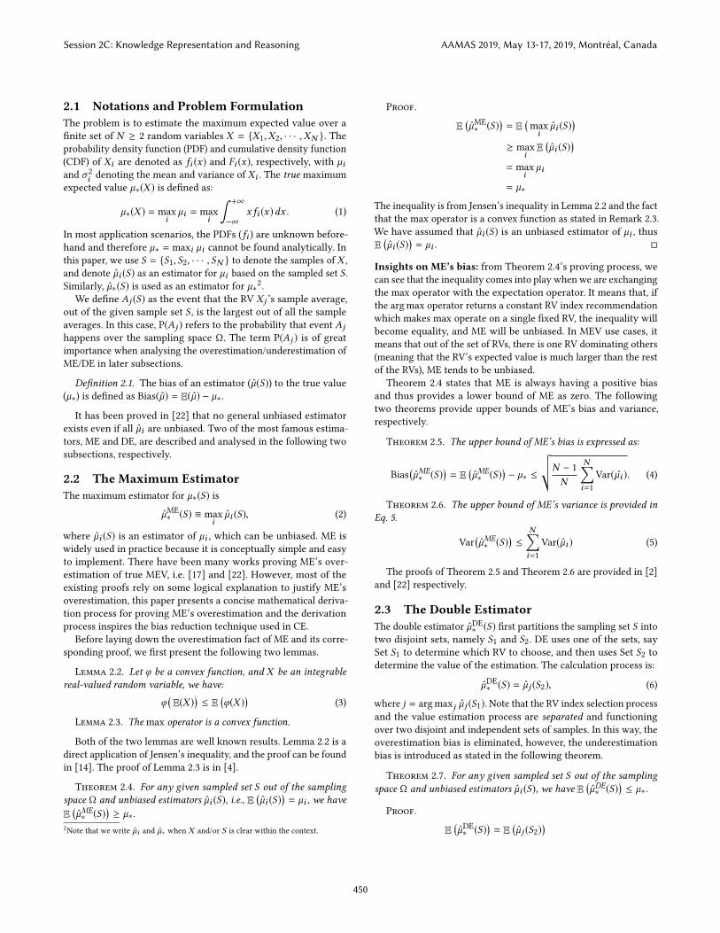
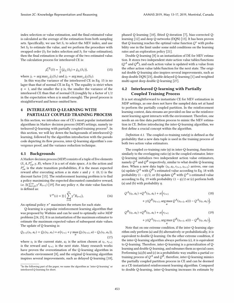
Figure 2: (a-d) Estimated values and true values and (e-h) Variance comparison for different MEV estimators on three groupsof multi-arm bandit problems, G1, G2, and G3. All the figures are best viewed in color.

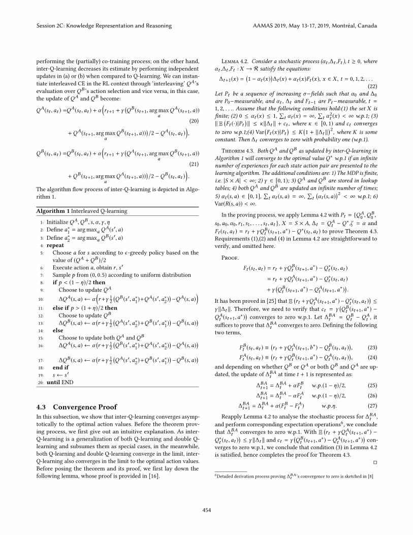
0

0

Figure 3: Comparison of Q-learning (Q), Double Q-learning(DQ) and interleaved Q-learning (inter-Q) on a simpleepisodic MDP (shown inset). The parameters are set as α =0.1, ϵ = 0.1 and γ = 1.

5 AN ILLUSTRATIVE EXAMPLEThe small MDP (twisted from Fig. 6.7 in [20]) shown inset in Fig. 3

provides a simple example of how CE’s low estimation bias benefits

TD control algorithms compared to ME and DE. The MDP has three

non-terminal states A, B and C. Episodes always start in A with a

choice among three actions, left, right and down. The down action

transitions immediately to the terminal state with a reward of zero.

The right action transitions deterministically to C with a reward

of zero, from which there are many possible actions all of which

cause immediate termination with a reward drawn from a normal

distribution withmean 0.1 and variance 1. Thus, the expected return

for any trajectory starting with C is 0.1. The left action transitions

deterministically to B with a reward of zero, from which there are

many possible actions all of which cause immediate termination

with a reward drawn from a normal distribution with mean -0.1 and

variance 2. Thus, the expected return for any trajectory starting

with B is -0.1. In this case, the optimal action from A is to go right

as the expected return is 0.1 which is the largest. However, since

ME overestimates the return and the larger the variance is, the

larger the overestimation is, it has some probability of take left as

the optimal action from A. Similarly, DE underestimates the return,

and it has some probability of choosing the down action as the

optimum. The simulation results are shown in Fig. 3.

6 SIMULATION RESULTS AND ANALYSISIn this section, we mainly perform experiments over two types

of scenarios, namely multi-armed bandits and grid world7. For

multi-armed bandits, we compare the proposed MEV estimator

(CE and interleaved CE) with state of the arts including ME [22],

DE [22], WDE [26], and interleaved DE8. For grid world, we com-

pare the instantiated interleaved Q-learning (inter-Q) with canoni-

cal Q-learning (Q) [25], double Q-learning (DQ) [8] and weighted

double Q-learning (WDQ) [26].

6.1 Multi-Armed BanditsMulti-armed bandit problem is a classical scenario for MEV estima-

tion [19]. Our experiments are conducted on three groups of multi-

armed bandit problems9: (G1) EXi = 0, for i ∈ 1, 2, · · · ,N ;

(G2) EX1 = 1 and EXi = 0 for i ∈ 2, 3, · · · ,N ; and (G3)

EXi = i/N , for i ∈ 1, 2, · · · ,N . Here N refers to the number

of actions in the multi-armed bandit context. In the scenario set

up, maxi EXi = 0 in G1, and maxi EXi = 1 in G2 and G3. In

7It is worth noting that these two types of scenarios are also selected as benchmark sce-

narios for the evaluation of double Q-learning [8], and weighted double Q-learning [26].

Maintaining the same benchmark scenarios ensures clear algorithm comparison.

8Note that the interleaving procedure can also be applied to DE for variance reduction

9Note that the scenario setup is the same as what is described in Section 5.1 in [26].

Session 2C: Knowledge Representation and Reasoning AAMAS 2019, May 13-17, 2019, Montréal, Canada

455

0 2000 4000 6000 8000 10000steps

10

5

0

5

10

15

max aQ

(s0,a

)

(a) 3 × 3 Grid World

0 2000 4000 6000 8000 10000steps

8

6

4

2

0

2

4

6

max aQ

(s0,a

)

(b) 4 × 4 Grid World

0 2000 4000 6000 8000 10000steps

10

8

6

4

2

0

2

4

max aQ

(s0,a

)

(c) 5 × 5 Grid World (d) Legend

0 2000 4000 6000 8000 10000steps

1.0

0.8

0.6

0.4

0.2

0.0

0.2

Mean r

ew

ard

per

step

(e) 3 × 3 Grid World

0 2000 4000 6000 8000 10000steps

1.4

1.2

1.0

0.8

0.6

0.4

0.2

0.0M

ean r

ew

ard

per

step

(f) 4 × 4 Grid World

0 2000 4000 6000 8000 10000steps

1.4

1.2

1.0

0.8

0.6

0.4

0.2

Mean r

ew

ard

per

step

(g) 5 × 5 Grid World (h) Legend

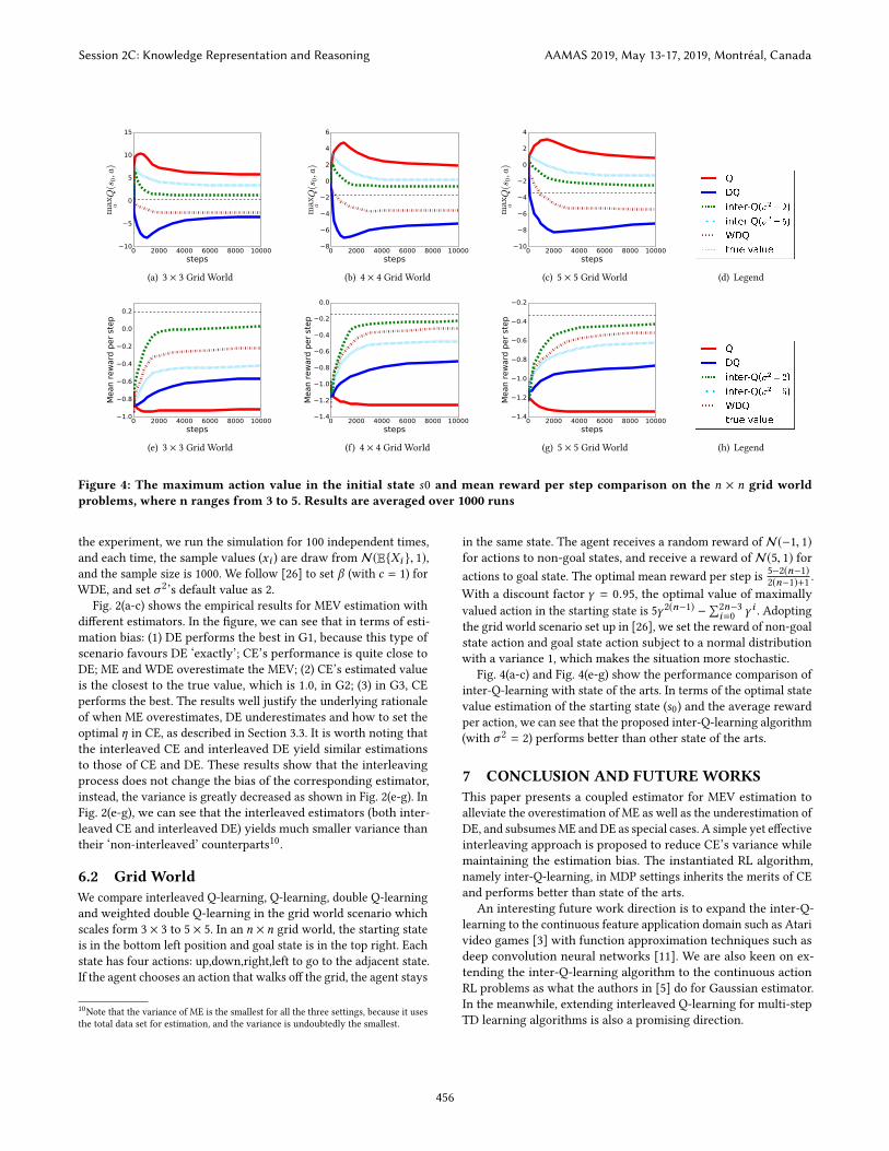
Figure 4: The maximum action value in the initial state s0 and mean reward per step comparison on the n × n grid worldproblems, where n ranges from 3 to 5. Results are averaged over 1000 runs

the experiment, we run the simulation for 100 independent times,

and each time, the sample values (xi ) are draw from N(EXi , 1),and the sample size is 1000. We follow [26] to set β (with c = 1) for

WDE, and set σ 2’s default value as 2.

Fig. 2(a-c) shows the empirical results for MEV estimation with

different estimators. In the figure, we can see that in terms of esti-

mation bias: (1) DE performs the best in G1, because this type of

scenario favours DE ‘exactly’; CE’s performance is quite close to

DE; ME and WDE overestimate the MEV; (2) CE’s estimated value

is the closest to the true value, which is 1.0, in G2; (3) in G3, CE

performs the best. The results well justify the underlying rationale

of when ME overestimates, DE underestimates and how to set the

optimal η in CE, as described in Section 3.3. It is worth noting that

the interleaved CE and interleaved DE yield similar estimations

to those of CE and DE. These results show that the interleaving

process does not change the bias of the corresponding estimator,

instead, the variance is greatly decreased as shown in Fig. 2(e-g). In

Fig. 2(e-g), we can see that the interleaved estimators (both inter-

leaved CE and interleaved DE) yields much smaller variance than

their ‘non-interleaved’ counterparts10.

6.2 Grid WorldWe compare interleaved Q-learning, Q-learning, double Q-learning

and weighted double Q-learning in the grid world scenario which

scales form 3 × 3 to 5 × 5. In an n × n grid world, the starting state

is in the bottom left position and goal state is in the top right. Each

state has four actions: up,down,right,left to go to the adjacent state.

If the agent chooses an action that walks off the grid, the agent stays

10Note that the variance of ME is the smallest for all the three settings, because it uses

the total data set for estimation, and the variance is undoubtedly the smallest.

in the same state. The agent receives a random reward of N(−1, 1)

for actions to non-goal states, and receive a reward of N(5, 1) for

actions to goal state. The optimal mean reward per step is5−2(n−1)

2(n−1)+1.

With a discount factor γ = 0.95, the optimal value of maximally

valued action in the starting state is 5γ 2(n−1) −∑

2n−3

i=0γ i . Adopting

the grid world scenario set up in [26], we set the reward of non-goal

state action and goal state action subject to a normal distribution

with a variance 1, which makes the situation more stochastic.

Fig. 4(a-c) and Fig. 4(e-g) show the performance comparison of

inter-Q-learning with state of the arts. In terms of the optimal state

value estimation of the starting state (s0) and the average reward

per action, we can see that the proposed inter-Q-learning algorithm

(with σ 2 = 2) performs better than other state of the arts.

7 CONCLUSION AND FUTUREWORKSThis paper presents a coupled estimator for MEV estimation to

alleviate the overestimation of ME as well as the underestimation of

DE, and subsumesME andDE as special cases. A simple yet effective

interleaving approach is proposed to reduce CE’s variance while

maintaining the estimation bias. The instantiated RL algorithm,

namely inter-Q-learning, in MDP settings inherits the merits of CE

and performs better than state of the arts.

An interesting future work direction is to expand the inter-Q-

learning to the continuous feature application domain such as Atari

video games [3] with function approximation techniques such as

deep convolution neural networks [11]. We are also keen on ex-

tending the inter-Q-learning algorithm to the continuous action

RL problems as what the authors in [5] do for Gaussian estimator.

In the meanwhile, extending interleaved Q-learning for multi-step

TD learning algorithms is also a promising direction.

Session 2C: Knowledge Representation and Reasoning AAMAS 2019, May 13-17, 2019, Montréal, Canada

456

REFERENCES[1] Bilal H Abed-alguni and Mohammad Ashraf Ottom. 2018. Double Delayed Q-

learning. International Journal of Artificial Intelligence 16, 2 (2018), 41–59.[2] Terje Aven. 1985. Upper (Lower) Bounds on theMean of theMaximum (Minimum)

of a Number of Random Variables. Journal of Applied Probability 22, 3 (1985),

723–728. http://www.jstor.org/stable/3213876

[3] Marc G. Bellemare, Yavar Naddaf, Joel Veness, and Michael Bowling. 2012. The

Arcade Learning Environment: An Evaluation Platform for General Agents. CoRRabs/1207.4708 (2012).

[4] Stephen Boyd and Lieven Vandenberghe. 2004. Convex Optimization. Cambridge

University Press.

[5] Carlo D’Eramo, Alessandro Nuara, Matteo Pirotta, and Marcello Restelli. 2017.

Estimating the Maximum Expected Value in Continuous Reinforcement Learning

Problems. In AAAI. AAAI Press, 1840–1846.[6] Carlo D’Eramo, Marcello Restelli, and Alessandro Nuara. 2016. Estimating Maxi-

mum Expected Value through Gaussian Approximation. In Proceedings of The 33rdInternational Conference on Machine Learning (Proceedings of Machine LearningResearch), Maria Florina Balcan and Kilian Q. Weinberger (Eds.), Vol. 48. PMLR,

New York, New York, USA, 1032–1040.

[7] Damien Ernst, Pierre Geurts, and Louis Wehenkel. 2005. Tree-Based Batch

Mode Reinforcement Learning. J. Mach. Learn. Res. 6 (Dec. 2005), 503–556.

http://dl.acm.org/citation.cfm?id=1046920.1088690

[8] Hado V. Hasselt. 2010. Double Q-learning. In Advances in Neural InformationProcessing Systems 23, J. D. Lafferty, C. K. I. Williams, J. Shawe-Taylor, R. S. Zemel,

and A. Culotta (Eds.). Curran Associates, Inc., 2613–2621.

[9] Harold Jeffreys and Bertha Jeffreys. 1999. Methods of Mathematical Physics (3ed.). Cambridge University Press.

[10] Michael Kearns and Satinder Singh. 1999. Finite-sample Convergence Rates for

Q-learning and Indirect Algorithms. In Proceedings of the 1998 Conference onAdvances in Neural Information Processing Systems II. MIT Press, Cambridge, MA,

USA, 996–1002. http://dl.acm.org/citation.cfm?id=340534.340896

[11] Alex Krizhevsky, Ilya Sutskever, and Geoffrey E Hinton. 2012. Imagenet classifica-

tion with deep convolutional neural networks. In Advances in neural informationprocessing systems. 1097–1105.

[12] Donghun Lee, Boris Defourny, and Warren B. Powell. 2013. Bias-corrected

Q-learning to control max-operator bias in Q-learning. In IEEE Symposium onAdaptive Dynamic Programming and Reinforcement Learning, ADPRL. 93–99.

[13] Volodymyr Mnih, Koray Kavukcuoglu, David Silver, Andrei A. Rusu, Joel Veness,

Marc G. Bellemare, Alex Graves, Martin Riedmiller, Andreas K. Fidjeland, Georg

Ostrovski, Stig Petersen, Charles Beattie, Amir Sadik, Ioannis Antonoglou, Helen

King, Dharshan Kumaran, Daan Wierstra, Shane Legg, and Demis Hassabis. 2015.

Human-level control through deep reinforcement learning. Nature 518, 7540(Feb. 2015), 529–533.

[14] Michael D. Perlman. 1974. Jensen’s inequality for a convex vector-valued function

on an infinite-dimensional space. Journal of Multivariate Analysis 4, 1 (1974), 52– 65. https://doi.org/10.1016/0047-259X(74)90005-0

[15] Martin L. Puterman. 1994. Markov Decision Processes: Discrete Stochastic DynamicProgramming (1st ed.). John Wiley & Sons, Inc., New York, NY, USA.

[16] Satinder Singh, Tommi Jaakkola, Michael L. Littman, and Csaba Szepesvári.

2000. Convergence Results for Single-Step On-Policy Reinforcement-Learning

Algorithms. Machine Learning 38, 3 (01 Mar 2000), 287–308.

[17] James E Smith and Robert L Winkler. 2006. The optimizerâĂŹs curse: Skepticism

and postdecision surprise in decision analysis. Management Science 52, 3 (2006),311–322.

[18] Alexander L. Strehl, Lihong Li, Eric Wiewiora, John Langford, and Michael L.

Littman. 2006. PAC Model-free Reinforcement Learning. In Proceedings of the23rd International Conference on Machine Learning (ICML ’06). ACM, New York,

NY, USA, 881–888. https://doi.org/10.1145/1143844.1143955

[19] Richard S. Sutton and Andrew G. Barto. 1998. Introduction to ReinforcementLearning (1st ed.). MIT Press, Cambridge, MA, USA.

[20] Richard S Sutton and Andrew G Barto. 2018. Reinforcement learning: An intro-duction (2nd ed.). MIT press.

[21] John N. Tsitsiklis. 1994. Asynchronous Stochastic Approximation and Q-Learning.

Machine Learning 16, 3 (Sept. 1994), 185–202.

[22] H. van Hasselt. 2013. Estimating the Maximum Expected Value: An Analysis

of (Nested) Cross Validation and the Maximum Sample Average. ArXiv e-prints(Feb. 2013). arXiv:stat.ML/1302.7175

[23] Hado Van Hasselt, Arthur Guez, and David Silver. 2016. Deep Reinforcement

Learning with Double Q-Learning.. In AAAI, Vol. 2. Phoenix, AZ, 5.[24] Christopher John Cornish HellabyWatkins. 1989. Learning from Delayed Rewards.

Ph.D. Dissertation. King’s College, Cambridge, UK.

[25] Christopher J. C. H. Watkins and Peter Dayan. 1992. Q-learning. In MachineLearning. 279–292.

[26] Zongzhang Zhang, Zhiyuan Pan, andMykel J. Kochenderfer. 2017. Weighted Dou-

ble Q-learning. In Proceedings of the Twenty-Sixth International Joint Conference onArtificial Intelligence, IJCAI-17. 3455–3461. https://doi.org/10.24963/ijcai.2017/483

[27] Yan Zheng, Zhaopeng Meng, Jianye Hao, and Zongzhang Zhang. 2018. Weighted

Double Deep Multiagent Reinforcement Learning in Stochastic Cooperative

Environments. In Pacific Rim International Conference on Artificial Intelligence.Springer, 421–429.

Session 2C: Knowledge Representation and Reasoning AAMAS 2019, May 13-17, 2019, Montréal, Canada

457