OECD Journal: Economic Studies Volume 2010 © OECD 2010 1 Intergenerational Social Mobility in OECD Countries* by Orsetta Causa and Åsa Johansson * Causa (e-mail: [email protected]) and Johansson (e-mail: [email protected]), OECD Economics Department. The authors would like to thank Anna d’Addio, Sveinbjörn Blöndal, Jørgen Elmeskov, Bo Hansson, Stephen Machin, Marc Pearson, Giuseppe Nicoletti, Jean-Luc Schneider and Rolph van der Hoeven for their valuable comments and Chatherine Chapuis for excellent statistical work, as well as Irene Sinha for excellent editorial support. The views expressed in this paper are those of the authors and do not necessarily reflect those of the OECD or its member countries. This paper assesses recent patterns of intergenerational social mobility across OECD countries and examines the role that public policies can play. It shows that the relationship between parental or socio-economic background and offspring educational and wage outcomes is positive and significant in practically all countries for which evidence is available. Intergenerational social mobility is measured by several different indicators, since no single indicator provides a complete picture. However, one pattern that emerges is of a group of countries, southern European countries and Luxembourg, which appears to rank as relatively immobile on most indicators, while another group, the Nordic countries, is found to be more mobile. Furthermore, public policies such as education and early childcare play a role in explaining observed differences in intergenerational social mobility across countries. JEL classification: J60, J62, I20, H23, C20, C21 Keywords: intergenerational wage mobility, intergenerational education mobility, education, public policies

Welcome message from author
This document is posted to help you gain knowledge. Please leave a comment to let me know what you think about it! Share it to your friends and learn new things together.
Transcript

OECD Journal: Economic Studies
Volume 2010
© OECD 2010
Intergenerational Social Mobility in OECD Countries*
byOrsetta Causa and Åsa Johansson
* Causa (e-mail: [email protected]) and Johansson (e-mail: [email protected]), OECDEconomics Department. The authors would like to thank Anna d’Addio, Sveinbjörn Blöndal,Jørgen Elmeskov, Bo Hansson, Stephen Machin, Marc Pearson, Giuseppe Nicoletti, Jean-LucSchneider and Rolph van der Hoeven for their valuable comments and Chatherine Chapuis forexcellent statistical work, as well as Irene Sinha for excellent editorial support. The views expressedin this paper are those of the authors and do not necessarily reflect those of the OECD or its membercountries.
This paper assesses recent patterns of intergenerational social mobility acrossOECD countries and examines the role that public policies can play. It shows thatthe relationship between parental or socio-economic background and offspringeducational and wage outcomes is positive and significant in practically allcountries for which evidence is available. Intergenerational social mobility ismeasured by several different indicators, since no single indicator provides acomplete picture. However, one pattern that emerges is of a group of countries,southern European countries and Luxembourg, which appears to rank as relativelyimmobile on most indicators, while another group, the Nordic countries, is found tobe more mobile. Furthermore, public policies such as education and early childcareplay a role in explaining observed differences in intergenerational social mobilityacross countries.
JEL classification: J60, J62, I20, H23, C20, C21
Keywords: intergenerational wage mobility, intergenerational education mobility,education, public policies
1

INTERGENERATIONAL SOCIAL MOBILITY IN OECD COUNTRIES
This paper assesses recent patterns in intergenerational social mobility across OECD
countries, examining the role that policies can play in affecting such mobility.
Intergenerational social mobility refers to the relationship between the socio-economic
status of parents and the status their children will attain as adults. A society can be more
or less mobile depending on whether this relationship is, on average, looser or tighter: in a
relatively immobile society an individual’s wage, education or occupation will tend to be
strongly related to those of his/her parents. Intergenerational mobility reflects a host of
factors, including inherited traits, social norms and public policies that may influence the
individual’s willingness and ability to seize economic opportunities. These factors are
difficult to unbundle precisely and, as regards norms and policies, to some extent reflect
societal choices over institutional settings as well as differences in choices over
redistribution and equity, which are likely to be valued differently across countries.
Therefore, no “benchmark” mobility level can be identified in cross-country comparisons.
Nonetheless, removing policy-related obstacles to social mobility can be advocated on
equity and efficiency grounds because it can improve equality of economic opportunities
and the way a society allocates human resources. Promoting intergenerational social
mobility means providing individuals with the same opportunities ex ante, even though it
does not imply that all individuals should achieve the same outcomes ex post. Furthermore,
policies that affect social mobility are closely related to growth. The ability of an economy to
allocate human resources to their best use can have important effects on economic
performance. However, trade-offs can exist between policies that remove obstacles to social
mobility and those that strengthen other drivers of growth. Therefore, understanding the
role played by public policies vis-à-vis social mobility can help design policies that enhance
equality of opportunity without adversely effecting economic growth. This could even
enhance growth and equality of economic opportunities across generations.
The socio-economic status of parents can influence that of their children in two main
ways: directly by affecting their labour productivity and labour market attachment and
indirectly by facilitating their success on the labour market by other means (e.g. by the
transmission of social norms such as work ethic or social networks). In turn, labour
productivity of children is, to a large extent, determined by parents’ investment in their
human capital and children’s ability to seize educational opportunities. One empirical
challenge is to separate the direct productivity channel from indirect ones. Arguably, both
can be influenced by public policies, e.g. education, redistributive and labour, or product
market policies.
Intergenerational transmission of social status is usually measured as “wage or income
persistence”, i.e. the fraction of parental income or wages reflected in their offspring’s
income or wages. Measuring and comparing wage or income persistence across countries is
made difficult by the lack of comparable cross-country data, especially of parents. Against
this background, and given that education is a key transmission mechanism in
intergenerational social mobility and matching skills with societal needs, this paper focuses
OECD JOURNAL: ECONOMIC STUDIES – VOLUME 2010 © OECD 20102
INTERGENERATIONAL SOCIAL MOBILITY IN OECD COUNTRIES
primarily on the role of education as a driver of mobility across generations. Its main
contribution is to provide comparable estimates of intergenerational wage and educational
mobility across OECD countries, focusing on the following concepts of mobility:
● The influence of parental background, as measured by educational achievement of
parents, on wages and educational attainment of various cohorts of adults for
14 European OECD countries.
● The influence of parental background, as measured by a composite index of their socio-
economic status, on cognitive achievements of 15-year-old students in 30 OECD
countries.
The analysis draws on existing and new evidence from two main sources of individual-
level information: wage and education mobility, using the 2005 Survey of Income and
Living Conditions (SILC) poverty module of Eurostat survey data; and the influence of
parental background on a teenager’s cognitive achievement, using the 2006 OECD
Programme for International Student Assessment (PISA) survey data. Though none of
these concepts of mobility refers to intergenerational transmission of wages proper, the
estimated persistence/mobility measures will be called “wage persistence/mobility” and
“education persistence/mobility”, respectively.
The paper is organised as follows. Section 1 outlines main findings. Section 2
describes the linkages between family background and wage and education outcomes of
individuals, explaining the role of education in determining wage mobility. Section 3
analyses the extent of intergenerational wage and educational mobility across those OECD
countries for which data are available. Finally, in light of these mobility patterns, Section 4
uses the same data sources to investigate the cross-country association between a range of
public policies (including education, redistributive and labour, and product market) and
social mobility and equality of opportunity across generations. Suggestive evidence is
provided that the main channel through which policies may influence social mobility is via
the link between cross-sectional inequality and intergenerational wage mobility.
1. Main findings
1.1. Mobility patterns
In this study intergenerational social mobility is measured by several different
indicators (e.g. wage persistence, secondary and post-secondary education persistence).
However, given the complex nature of social mobility, these indicators do not necessarily
provide the same cross-country ranking, suggesting that no single indicator provides a
complete picture.
● The influence of parental background on individual earnings varies widely across OECD
countries for which estimates are available. Low mobility across generations, as
measured by a close link between parents’ and children’s earnings, is particularly
pronounced in the United Kingdom, Italy, the United States and France, while mobility is
higher in the Nordic countries, Australia and Canada.
● Across European OECD countries covered by the analysis, there is a substantial wage
premium associated with growing up in a higher-educated family and a penalty with
growing up in a less-educated family, even after controlling for a number of individual
characteristics. The premium and penalty are particularly large in southern European
countries, the United Kingdom, Luxembourg and Ireland (a premium of 20% and penalty of
OECD JOURNAL: ECONOMIC STUDIES – VOLUME 2010 © OECD 2010 3

INTERGENERATIONAL SOCIAL MOBILITY IN OECD COUNTRIES
16% or more). In general, wage persistence across generations, measured as the difference
between the wage premium and penalty, is slightly stronger for sons than for daughters.
● The influence of parental socio-economic status on student achievement in secondary
education also differs across OECD countries. It is particularly strong in the United
States, France and Belgium, while weaker in some Nordic countries, Korea and Canada.
In over half of the OECD countries, including all the large continental European ones,
student cognitive skills are more strongly influenced by the average socio-economic
status of parents of other students in the same school, i.e. the schools’ average socio-
economic environment, than by their own parents’ socio-economic status.
● Inequalities in secondary cognitive skills are likely to translate into inequalities in post-
secondary educational achievement and subsequent wage inequality in the labour
market. Indeed, in European OECD countries, students from a higher-educated family
are more likely to achieve tertiary education, while there is a probability penalty
associated with growing up in a less-educated family. The increase in the probability of
achieving tertiary education is particularly strong in Luxembourg, Italy, Finland and
Denmark, where it is 30 percentage points higher for a son whose father had tertiary
education than for a son whose father had only upper-secondary education.
Furthermore, transmitted inequalities in education are positively associated across
countries with inequalities in wages.
● In all European OECD countries covered by the analysis, the probability of achieving below
secondary education is on average 18 percentage points higher for children whose father
had below upper-secondary education compared with those whose father had upper-
secondary education. Conversely, the probability of achieving below upper-secondary
education decreases on average by 10 percentage points for offspring of tertiary educated
fathers compared with children whose father had upper-secondary education.
1.2. Intergenerational mobility and inequality
● Intergenerational social persistence, as measured by a close link between parental
education achievement and children’s wages, is correlated across countries with cross-
sectional inequality and poverty. The association between parental socio-economic
status and teenager cognitive achievement is stronger in countries with a greater share
of children living under the poverty line or lacking basic material resources.
1.3. Policies and mobility
● Higher enrolment in child care and early childhood education correlates with a lower
influence of parental socio-economic background on teenager cognitive skills,
suggesting a positive effect on social mobility. These policies are likely to be most
efficient when targeted at children from low-income and/or second-language families.
● Practices that group students into different programmes or curricula according to
proficiency level, for instance, early tracking and ability grouping within classes,
correlate with a stronger influence of parental socio-economic background on teenager
cognitive skills. This reflects a stronger influence of the school socio-economic
environment on a student’s performance in the case of early tracking practices.
● By contrast, a better matching of school resources with needs, as well as a steeper
progression in teachers’ wages over their career, are associated with a lower influence of
parental background on student achievement, possibly by attracting experienced
OECD JOURNAL: ECONOMIC STUDIES – VOLUME 2010 © OECD 20104

INTERGENERATIONAL SOCIAL MOBILITY IN OECD COUNTRIES
teachers to disadvantaged areas. Likewise, a larger share of qualified teachers correlates
with lower inequalities transmitted by family background.
● Evidence suggests that increasing the social mix within schools increases performance
of disadvantaged students with neutral or in some cases positive effects on overall
performance. Thus, policies aimed at encouraging such a mix in neighbourhoods may
mitigate inequalities.
● There is suggestive evidence that universal government-supported loan systems for
tertiary education are associated with higher social mobility, as measured by the
probability of the offspring of disadvantaged families completing tertiary education. In
countries lacking such systems, financial constraints could be an obstacle to achieving
tertiary education for students from disadvantaged backgrounds.
● More progressive income taxation and higher short-term unemployment benefits are
associated with a looser link between parental background and teenager cognitive skills
and wages. This may indicate that well-targeted redistributive and income support
policies lower cross-sectional income inequality and poverty rates.
2. Determinants of intergenerational social mobility
2.1. The linkages between parental background and offspring outcomes
Intergenerational social mobility can be measured by income, education, occupation or
social class. Economic research has traditionally focused on some measure of income or
wages.1 Studies assessing the association between parent and offspring income focus on
pairs of fathers and sons. Ideally, income should be measured by a household’s disposable
income, as this most directly influences the standard of living of individuals (e.g. Chadwick
and Solon, 2002; Solon, 2004; Lee and Solon, 2006). In practice, accurate measurement is
difficult, as it should take into account the structure of the household, the extent of female
participation in the labour market and the different sources of income (e.g. earnings, assets,
welfare). Therefore, most studies use some measure of wages (Box 1). The extent to which
the offspring’s wage levels reflect those of the parents (the so-called “intergenerational wage
elasticity”) is taken as a measure of wage persistence across generations, or lack of
intergenerational wage mobility. The higher this elasticity, the lower is intergenerational
wage mobility. However, one difficulty in adopting this approach in a cross-country context
is that comparable information on wages of parents is seldom available.
Parental background can influence offspring wages (Figure 1) in very general terms, by
boosting both offspring labour productivity and successful insertion in the labour market.
One way children’s productivity, and hence future income, can be enhanced is through the
ability of parents to invest in their offspring’s human capital. However, wealth and assets
passed on from one generation to another, the inheritance of traits that are important for
economic success, such as propensities to undertake education, work ethics and risk-
related behaviours, as well as local conditions such as growing up in advantaged
neighbourhoods, are other important factors (for an overview see d’Addio, 2007).
One empirical challenge is to separate the direct productivity channel from indirect
labour market ones. Another more fundamental challenge is to empirically isolate the
effect of parental background (“nurture”) from that of genetic inheritance of abilities
(“nature”) on individuals’ wages and educational achievement. In general, as in this study,
estimates of the impact of parental background on individuals’ wages and educational
achievement combine these two effects. The relative importance of nature versus nurture
OECD JOURNAL: ECONOMIC STUDIES – VOLUME 2010 © OECD 2010 5

INTERGENERATIONAL SOCIAL MOBILITY IN OECD COUNTRIES
in explaining intergenerational social mobility is far from established (e.g. Sacerdote, 2002;
Bowles et al., 2002; Plug and Vijverberg, 2005). However, to the extent that genetic
inheritability of ability does not vary systematically across countries, such heritability
should not influence cross-country variation in wage or educational mobility.
An important part of wage persistence across generations is driven by the effect of
parental background on cognitive skills acquired by their children in formal (and informal)
education (which influences the offspring’s productivity). This includes secondary
education and post-secondary education (Figure 1 and Box 2). Indeed, recent studies show
that there is a clear connection between intergenerational wage mobility and
intergenerational educational mobility, although educational mobility cannot account for
all the estimated persistence in incomes (Blanden, 2008a; Blanden et al., 2005; Solon, 2004).
Educational differences tend to persist across generations, and differences in such persistence
explain a large share of the cross-country variation of intergenerational wage correlations
(e.g. Solon, 2004; Blanden et al., 2006; Blanden et al., 2005; d’Addio, 2007). The extent to which
education is responsible for intergenerational persistence in wages depends on how strongly
Box 1. Concepts in intergenerational social mobility
Measures of intergenerational income mobility are often based on empirical estimationof the intergenerational income elasticity, , which measures the extent to which offspringincome levels, Yi, reflect those of their parents, Yi
P, that is:
.
This estimated elasticity is a measure of average intergenerational income persistence.A low value implies that the link between parent and offspring incomes is relatively weak,while a high value implies a relatively strong link. An alternative measure is the partialcorrelation between parent and offspring incomes, which adjusts for potential differencesin the variance of income between the two generations.
Theoretical studies of intergenerational mobility regard long-run permanent disposableincome as the most appropriate income concept (e.g. Goldberger, 1989; Chadwick and Solon,2002; Solon, 2004; Lee and Solon, 2006; Haider and Solon, 2006). But basing estimates ofpersistence across generations on current wages raises some key issues (Solon, 2002). First,measuring permanent income/wages of parents with error leads to inconsistent estimates,causing an underestimation of the true intergenerational elasticity. Second, using currentwages of offspring as a proxy for lifetime income can also cause a bias, in particular whenlooking at individuals at the beginning of their careers (Haider and Solon, 2006). Studiesbased on such measures of offspring wages tend to find lower elasticity estimates thanstudies measuring wages further along their careers or life cycles. To overcome theseproblems, many studies average both parental and offspring wages over several years ormeasure offspring wages after a few years’ experience in the labour market.
Educational persistence is often measured by the correlation between years of schooling oreducational achievement of parents and their offspring. However, basing educationalpersistence on years of schooling assumes that the impact on human capital of an additionalyear of schooling is the same across generations, and that years of schooling affect humancapital in the same way across countries. These problems are overcome by studies that assesseducational mobility in terms of qualification or literacy levels achieved, as measured, forinstance, by the harmonised cross-country ISCED classification (e.g. Chevalier et al., 2007) or bytest scores of cognitive skills (OECD, 2007a; Hertz et al., 2007).
i
Pii YY lnln
OECD JOURNAL: ECONOMIC STUDIES – VOLUME 2010 © OECD 20106

INTERGENERATIONAL SOCIAL MOBILITY IN OECD COUNTRIES
educational achievement is tied to family background, that is, the degree of persistence in
education. Of course, the intergenerational wage link is also affected by the returns to
education in the labour market (e.g. Solon, 2004; d’Addio, 2007).2 It is likely that inequalities in
cognitive skills acquired in secondary education translate into inequalities in achieving post-
secondary education and into wages via the returns to education in the labour market.
Figure 1. Some links between parental background and their offspring’s outcomesSocial mobility – The explored links
Inequality Inequality
Inequality
Labour and product marketpolicies/institutions
Redistribution/transfer policies
Policies and factors interacting with parental background
Education policies
Hypothesis
Parental background
Parents’ socio-economic status
Parents’education
Education mobilityIncome mobility
Offspring's outcomes
Hypothesis Cognitive skills(secondaryeducation)
WagesPost-secondary
educationattainment
Returnsto
education
OECD JOURNAL: ECONOMIC STUDIES – VOLUME 2010 © OECD 2010 7

INTERGENERATIONAL SOCIAL MOBILITY IN OECD COUNTRIES
Persistence in wages across generations also appears to be positively associated across
countries with measures of inequality, i.e. of the dispersion of parental backgrounds (see
below and d’Addio, 2007, for an overview). Although causality between intra- and
intergenerational persistence of inequality is far from established, it is possible that
redistributive policies and institutions that narrow the gap between current incomes and/
or wages of parents could also mitigate the influence of parental background on wages and
educational outcomes of their offspring.
The empirical approach developed in the remainder of this paper has been partly
shaped by the considerations above. The analysis of wage mobility measures parental
background by fathers’ education and their offspring’s incomes as gross hourly wages.3
Basing the estimation of persistence on gross hourly wages implies that the persistence
measure reflect the impact of parental education on productivity. While, basing
persistence estimates on monthly or annual wages would, in addition to the productivity
effect, capture the labour supply decision, i.e. the decisions on working hours.
The study of wage mobility is supplemented by the analysis of educational mobility
for teenagers (with parental background measured by a broad index of the family’s socio-
economic status and educational outcomes measured by PISA test scores) and adults (with
parental background measured by father’s education and offspring educational outcome
measured by educational attainment). Finally, the analysis of policy influences on wage
and educational mobility focuses on both education and other policies that are likely to
affect cross-sectional inequality.
Box 2. Education as a determinant of intergenerational social mobility
Several recent studies analyse the link between intergenerational persistence ineducation and income (e.g. Solon, 2004). In these studies the offspring’s investment ineducation, which drives intergenerational income mobility, depends on family income.
Educational attainment varies with parental income due to both differing endowments(propensity to undertake education and possession of a work ethic) and differing privateinvestment in education across families. If all families had full access to perfect capitalmarkets, only inheritable traits would influence mobility (Becker and Tomes, 1979). But ifparents cannot borrow against their children’s future earnings to finance their education,liquidity-constrained parents will invest sub-optimally in their children’s education(Becker and Tomes, 1986; Grawe and Mulligan, 2002). Additionally, parental investment ineducation increases in the return to human capital investment, since parents are moreinclined to invest in their children’s education when the payoff is higher. Thus, in thepresence of financial constraints, wealthier families tend to invest more in their children’shuman capital, and such investment is increasing in labour market returns (Solon, 2004).
Some of these studies suggest that government spending on education can increaseintergenerational mobility (Solon, 2004; Mayer and Lopoo, 2008). Progressive publicinvestment in education can offset sub-optimal parental investment in education, to theextent that the offspring of liquidity-constrained parents benefit relatively more fromthese public programmes. A recent study for the United States shows that intergenerationalmobility is greater in high-spending states compared with low-spending states (Mayer andLopoo, 2008).
OECD JOURNAL: ECONOMIC STUDIES – VOLUME 2010 © OECD 20108

INTERGENERATIONAL SOCIAL MOBILITY IN OECD COUNTRIES
3. Intergenerational social mobility patterns
3.1. Cross-country patterns in intergenerational income mobility
3.1.1. Intergenerational income persistence is significant in all OECD countries
The relationship between socio-economic status of parents and their offspring is positive
and significant in practically all countries for which evidence is available, and for many
different aspects of social status (e.g. Hertz et al., 2007; Corak, 2004). International comparisons
of intergenerational income persistence are relatively common (e.g. Solon, 2002; Corak, 2006;
d’Addio, 2007). However, these comparisons can be invalid because different studies use
different variable definitions, samples, estimation methods and time periods.
Taking the available estimates at face value, cross-country comparison of
intergenerational income elasticities based on (various measures of) earnings for pairs of
fathers and sons suggests that persistence is higher in the United Kingdom, Italy, the
United States and France among the OECD countries for which comparable estimates are
available (e.g. Corak, 2006; Blanden, 2008b).4 In these countries at least, 40% of the
economic advantage high-earning parents have over low-earning parents is passed on to
the next generation (Figure 2). By contrast, intergenerational persistence is comparatively
low in the Nordic countries, Australia and Canada, with less than 20% of the earnings
advantage passed from parent to offspring.
These patterns of intergenerational persistence are partly confirmed by descriptive
evidence based on new comparable data for European OECD countries, which allow
systematic comparison of sons’ wages to the educational attainment of fathers (see Causa
et al., 2009, and Box 3). In all the countries covered, a son is much more likely to be in the
top wage quartile if his father had achieved tertiary education compared with a son whose
father had only basic (below upper-secondary) education, particularly in Portugal,
Luxembourg and the United Kingdom (Figure 3).5
Figure 2. Intergenerational earnings elasticity,1 estimates from various studies: selected OECD countries
1. The height of each bar measures the extent to which son’s earnings levels reflect those of their fathers. Theestimates are the best point estimate of the intergenerational earnings elasticity resulting from an extensivemeta-analysis carried out by Corak (2006) and supplemented with additional countries from d’Addio (2007). Thechoice of empirical estimates in this meta-analysis is motivated by the fact that they are based on studies that aresimilar in their estimation technique, sample and variable definitions. The higher the value, the greater is thepersistence of earnings across generations, thus the lower is the intergenerational earnings mobility.
Source: D’Addio (2007).
0.6
0.5
0.4
0.3
0.2
0.1
0ITAAUS NOR FIN CAN SWE DEU ESP FRA USA GBR
OECD JOURNAL: ECONOMIC STUDIES – VOLUME 2010 © OECD 2010 9

INTERGENERATIONAL SOCIAL MOBILITY IN OECD COUNTRIES
Figure 3. Ratio of the chance of being in the top wage quartile for sons of higher-educated vs. lower-educated fathers:1 Selected European
OECD countries
Note: Germany is not included in this figure as there is a problem with the representativeness of the German samplealong the education dimension.1. This figure shows the ratio of two conditional probabilities. It measures the ratio between the probability to end
up in the top wage quartile given that the son’s father had achieved tertiary education and the probability to endup in the top wage quartile given that the son’s father had achieved less than upper-secondary education.Probabilities are defined as simple frequency measures. Fathers’ educational achievement is a proxy for parentalbackground or wages.
2. 25-34 years old for Portugal.
Source: OECD calculations based on the 2005 EU-SILC Database.
Box 3. Measuring the link between parental educational background and offspring wages
The analysis in Causa et al. (2009) is based on the 2005 module on the intergenerationaltransmission of poverty of the EU-SILC Household Database. This poverty module containsretrospective information on parental background when the respondent was a teenager.This information is comparable across European OECD countries and includes familycomposition, age, educational qualification level, activity status and occupation of motherand father, as well as an indicator of financial distress conditions. However, informationon parents’ wages is lacking.
The approach taken in this study is to proxy parental background by the highesteducational qualification level achieved by the father according to the InternationalStandard Classification of Education (ISCED). One advantage of using father’s education asa proxy for his income is that education is likely to be a more permanent feature thancurrent wages, while being highly correlated with wages in most countries. The offspring’sincome concept refers to gross hourly wages and salaries paid in cash for time worked orfor time not worked, such as holidays, as well as additional payments (e.g. overtimepayments, bonuses). Henceforth, this will be referred to as wages. The results focus on twocohorts of offspring (35-44 and 45-54) and their parents. The youngest cohort (25-34 yearsold) is excluded because of the potential difficulties associated with measuring permanentwages/incomes at young ages, as discussed in Box 1, as well as with ensuring that theindividuals under consideration have reached their desired educational level.
3.5
2.5
2.0
3.0
1.5
1.0
0.5
0GBRGRC IRL AUT FRA SWE DNK BELNLD FIN ITAESP PRT2LUX
Equal chance
Men, 35-44 years old
OECD JOURNAL: ECONOMIC STUDIES – VOLUME 2010 © OECD 201010

INTERGENERATIONAL SOCIAL MOBILITY IN OECD COUNTRIES
To explore more fully this descriptive evidence through regression analysis, it was
assumed that individual wage prospects depend on fathers’ educational attainment in two
ways: through the direct transmission of factors that affect the economic success of
offspring; and through influencing their offspring’s educational attainment (see Causa
et al., 2009, and Box 4). The first channel, that is, estimates of parameter a in equation [1],
Box 4, captures the transmission of wealth, work ethic and social norms or networks that
Figure 4. Wage premium and penalty due to paternal education levels:1 Selected European OECD countries
Notes: * denotes statistically significant at 10% at least.** denotes statistically significant at 5% at least.Germany is not included in this figure, as there is a problem with the representativeness of the German sample alongthe education dimension.1. The figure shows the estimated percentage change in wages of the offspring depending on their parental
background measured by father’s highest education level. The wage premium is the increase in the offspring’swage of having a father with tertiary education relative to an offspring whose father had upper-secondaryeducation. The wage penalty is the decrease in the offspring’s wage of having a father with less than upper-secondary education relative to an offspring whose father had upper-secondary education. Fathers’ educationalachievement is a proxy for parental background or wage.
2. Based on OLS wage regression model.3. Based on wage regression model with selection into paid employment (Heckman full maximum likelihood
estimation).
Source: OECD calculations based on the 2005 EU-SILC Database.
80
60
40
20
0
-20
-40
-60
-80PRT GBR ITA ESP FIN SWE NLD BEL LUX FRA DNK AUT GRC IRL
80
60
40
20
0
-20
-40
-60
-80ITA ESP FIN GBR LUX NLD BEL PRT AUT GRC FRA IRL SWE DNK
**
**** ** *
*
**
** ** ** ** **
**
* *
**
*** ** ** ** **
**
**
*
**
**
**
****
**
Percentage change in wage A. Men, 35-44 years old2
Percentage change in wage B. Women, 35-44 years old3
Wage premium Wage penalty
OECD JOURNAL: ECONOMIC STUDIES – VOLUME 2010 © OECD 2010 11

INTERGENERATIONAL SOCIAL MOBILITY IN OECD COUNTRIES
eshe
[1]
eshent.
alg’snal
[2]
[3]
his inal
, isallts[1]
areToen or
aneirhe
tly inng isalnt
notion
as theit isinghat
Box 4. The influence of parental background on offspring wages
The empirical strategy for assessing the influence of parental background on offspring wages assumthat gross hourly wages (Wi) depend on both the offspring’s effort or educational attainment (ECi) and tinfluence of father’s educational attainment (Ei) (for details, see Causa et al., 2009):
,
where a measures the strength of the direct influence of the father’s educational attainment on wag(e.g. through the transmission of social norms, work ethic, social networks and other factors facilitating teconomic success of children) and b the offspring’s labour market returns to their educational attainme
In turn, the offspring’s educational attainment is assumed to depend on their fathers’ educationattainment, reflecting, for instance, the ability and willingness of fathers to invest in their offsprinhuman capital as well as other inheritable factors affecting the ability of their children to seize educatioopportunities, such that:
.
Combining these two equations yields,
,
where f = (a + bd) captures the total effect of a father’s educational attainment on individual wages. Teffect is decomposed in a direct effect on wages (a) and an indirect effect through education (bd), whichturn consists of the returns to offspring’s own education (b) and the influence of father’s educationattainment on their offspring’s educational attainment (d).
In the first stage, the total effect of a fathers educational attainment on individual wages, equation [3]estimated for various cohorts of men and women. The estimation controls for “Mincerian” individucharacteristics such as living in an urban/rural area and migrant and marital/cohabitant status. The resuare robust to inclusion of age and experience.1 Ordinary least squares (OLS) estimates of equationsand [3] may be biased due to non-random selection into employment, since it is likely that those who not working constitute a self-selected sample, particularly women who would earn low wages. overcome this selection problem, this study uses the Heckman sample selection bias estimator for womand OLS for men (e.g. Heckman, 1976). However, results for women remain broadly the same under OLSHeckman estimation techniques.
In the second stage, estimation of equation [1], offspring educational attainment is introduced as explanatory variable in order to find out whether fathers’ educational attainment mainly influences thoffspring’s wages through influence on education or if it has a direct effect on wages, over and above teffect on education.2
In the third stage, the influence of fathers’ educational attainment on that of their offspring is expliciestimated (equation [2]). The empirical results are obtained by estimating an Ordered Probit model,which observed educational outcomes of individuals (ECi) are assumed to be driven by an underlyicontinuous variable measuring their “propensity to achieve education”. This underlying variableassumed to be determined by their father’s educational attainment (Ei) and a number of individucharacteristics. The results suggest that in all European OECD countries fathers’ educational attainmeinfluences that of their offspring (Causa et al., 2009).
1. In “Mincerian” wage equations, age, experience and experience squared are standard controls. Life-cycle effects are considered in the final estimates because they are not statistically significant in the current setting, due to weak identificatwithin narrowly defined age groups (or cohorts).
2. It is possible that there is a potential endogeneity of own education in this specification due to unobserved variables suchability and/or motivation, which may be correlated with both education and wages. This would result in an upward bias ofinfluence of own education on wages. Usually, instrumental variable (IV) estimation is used to address this problem, but often difficult to find appropriate instruments, and weak instruments may bias the results further. Indeed, studies us(IV) estimations often find even higher estimates of the influence of education on wages than OLS, which suggests tmeasurement error in the education variable might be a more serious problem than endogeneity (e.g. Card, 2001).
1ln iiii ECbEakW
iii EdjEC 2
3ln iii EfeW
OECD JOURNAL: ECONOMIC STUDIES – VOLUME 2010 © OECD 201012

INTERGENERATIONAL SOCIAL MOBILITY IN OECD COUNTRIES
facilitate successful labour market insertion. The second channel, i.e. estimates of
parameter b in equation [1], Box 4, captures access to education, as well as the individual
propensity to acquire education and genetically transmitted ability to learn, which affect
an individual’s productivity (e.g. Bourguignon et al., 2003). As a first step in the analysis,
Figure 4 reports estimates of the overall effect of a father’s educational attainment on
offspring wages (estimates of parameter f in equation [3], Box 4), with no distinction
between these channels.
3.1.2. Wage premium or penalty depending on father’s educational attainment
In all European OECD countries covered by the analysis, there is a positive wage
premium (measured as the increase in gross hourly wages) for offspring of higher-educated
fathers, while there is a penalty (measured as the decrease in gross hourly wages) for
offspring of lower-educated fathers (Figure 4). The wage premium is particularly large in
southern European OECD countries, the United Kingdom and Finland. In these countries,
having a father with tertiary education raises sons’ wages by some 20% or more compared
with a son whose father had upper-secondary education. At the same time, the wage
penalty of having a father with only basic education compared with a father with upper-
secondary education appears to be high in the same countries, as well as in Luxembourg
and Ireland. In these countries, the wage of a son whose father had below upper-secondary
education falls short by more than 16% of the wage of a son whose father had upper-
secondary education.6 The influence of paternal background on daughters’ wage premia is,
in general, slightly lower than that of sons, yet still substantial. Moreover, for women, the
average wage penalty of coming from a disadvantaged background is sometimes much
higher than the premium of coming from an advantaged background.7
3.1.3. Summary measure of persistence in wages
One way of summarising the extent of wage persistence across generations is to
measure the gap between the estimated wage premium and the penalty of having a
tertiary-educated or below upper-secondary educated father, respectively. A greater gap
would imply stronger persistence in wages over generations. According to this measure,
intergenerational wage persistence for sons is particularly strong in some southern
European countries and in the United Kingdom, while it is lower in some Nordic countries,
Austria and Greece (Figure 5). The cross-country ranking of persistence in wages for
women is similar to that of men. However, these patterns could be influenced by
distributional differences in fathers’ educational attainment and individuals’ wages, since
wider distributions of individual wages (relative to parental background) could
mechanically translate into higher persistence estimates. One way of accounting for this is
to adjust the estimated wage persistence for cross-country differences in the dispersion of
father’s education and offspring’s wages. The cross-country ranking presented in Figure 5
remains fairly unchanged to this adjustment (the rank correlation between non-
standardised and standardised persistence measures is 0.96). The remainder of the
discussion in this study refers to the standardised measure of wage persistence.
It is difficult to compare this measure of persistence in wages over generations with
existing estimates of the “intergenerational elasticity of income” reported in Figure 1
because the proxy used for parental background in this study is different from what is
commonly used (some measure of fathers’ wage or income). Even so, the findings in this
study are qualitatively in line with existing evidence for pairs of fathers and sons.8 The
OECD JOURNAL: ECONOMIC STUDIES – VOLUME 2010 © OECD 2010 13

INTERGENERATIONAL SOCIAL MOBILITY IN OECD COUNTRIES
Figure 5. Summary measure of wage persistence levels:1 Selected European OECD countries
Notes: * denotes statistically significant at 10% at least.** denotes statistically significant at 5% at least.Germany is not included in this figure, as there is a problem with the representativeness of the German sample alongthe education dimension.1. Wage persistence is measured as the distance or gap between the estimated wage premium and penalty. Thus, it
measures the percentage increase in wages of an offspring having a father with tertiary education relative to anoffspring having a father with below-upper secondary education. A larger number implies a larger gap, thusstronger persistence in wages or a higher degree of immobility over generations. Fathers’ educationalachievement is a proxy for parental background or wage.
2. Based on OLS wage regression model.3. The summary measure of wage persistence, corrected for distributional differences, corresponds to the summary
measure of wage persistence, multiplied by the ratio of the standard deviation of fathers’ education to thestandard deviation of sons’ or daughters’ gross hourly wage.
4. Based on wage regression model with selection into paid employment (Heckman full maximum likelihoodestimation).
Source: OECD calculations based on the 2005 EU-SILC Database.
130
70
90
110
50
30
10
-10
70
90
110
50
30
10
-10
-30PRT GBR ITA ESP FINSWENLD BEL LUX FRA DNK AUTGRCIRL
130
-30ITAESP FINGBRLUX NLDBELPRT AUTGRC FRAIRL SWE DNK
**
****
****
**
**
*** *
*
**
*
**** ** **
* * * * ***
Difference between the wage premium and the wage penalty, percentage points
A. Men, 35-44 years old2
Difference between the wage premium and the wage penalty, percentage points
B. Women, 35-44 years old4
Summary measure of wage persistence
Summary measure of wage persistence, corrected for distributional differences3
OECD JOURNAL: ECONOMIC STUDIES – VOLUME 2010 © OECD 201014

INTERGENERATIONAL SOCIAL MOBILITY IN OECD COUNTRIES
United Kingdom is estimated to have relatively low wage mobility, while some Nordic
countries appear to be more mobile, as frequently found in previous empirical studies
(e.g. d’Addio, 2007; Corak, 2006). However, there are some differences. For instance, France
appears to be much less mobile in terms of the “intergenerational income elasticity” than
on the basis of the influence of fathers’ education on sons’ wages, perhaps reflecting that
fathers’ education is not a good proxy for parental income in this country.
3.1.4. The role of education as a driver of persistence
As a further step in the analysis of wage persistence, an attempt was made to separate
the direct influence of a father’s educational attainment on their offspring’s wages from
the indirect effect going through their offspring’s own educational attainment
(i.e. estimation of the relative magnitudes of coefficients a and b in equation [1], Box 4). The
resulting estimates suggest that parental background mainly influences offspring wages
through their own educational attainment (i.e. by indirectly influencing offspring
productivity) except in a few countries (the United Kingdom, Spain, Italy, Netherlands,
Luxembourg and Ireland) where direct linkages appear to be more important than the
indirect ones through education. More specifically, in most countries fathers’ educational
attainment (estimates of coefficient a in equation [1], Box 4) is no longer important
(i.e. significant) in determining sons’ wages once the sons’ educational attainment is taken
into account. This result is even more pronounced in the case of women (Causa et al., 2009,
for details). Thus, education is a key factor explaining persistence in wages across
generations in many countries and policies providing equal opportunities in access to
education are essential in enhancing social mobility.
3.2. Cross-country patterns in intergenerational education mobility
Given that individuals’ educational attainment appears to be a key driver of wages in
European OECD countries, it is important to understand to what extent skills acquired in
formal education, including secondary and post-secondary, are influenced by parental
background. Moreover, differences in secondary educational achievement due to parental
background may contribute to differences in post-secondary achievement which, in turn,
can lead to persistence in wages. To this end, this section analyses cross-country patterns
of intergenerational education persistence in secondary education for teenagers, followed
by persistence patterns in post-secondary education for adults.
3.2.1. Parental background influences student achievement in secondary school
The extent to which parental background, measured by a broad index of socio-
economic status of a student’s family, influences student cognitive performance at the
level of secondary education differs substantially across OECD countries (Figure 6).
Henceforth, when discussing persistence in secondary educational achievement, this
refers to the estimated influence of this index on a student’s performance on the PISA test
score (see Causa and Chapuis, 2009, and Box 5 for details). As in the case of wage
persistence, the estimates cannot distinguish between effects of parental background and
genetically inheritable factors. France, New Zealand, the Czech Republic, United States and
United Kingdom are among the countries where persistence is highest according to this
metric, while persistence is relatively low in Iceland, Finland, Southern European
countries, Mexico and Turkey.9
OECD JOURNAL: ECONOMIC STUDIES – VOLUME 2010 © OECD 2010 15

INTERGENERATIONAL SOCIAL MOBILITY IN OECD COUNTRIES
The variation within a country in the distribution of student socio-economic status
(parental background) may matter for the overall impact of background on student
achievement (OECD, 2007a; OECD, 2004). The cross-country patterns of intergenerational
educational persistence change considerably after taking country differences in the
distribution of socio-economic status into account (Figure 6).10 In countries like Mexico,
Portugal, Luxembourg, Spain and Turkey, where the dispersion in student socio-economic
background is wide, even a relatively mild influence of parental background on their
achievement can lead to a large overall difference. After adjusting for the country-specific
distribution of socio-economic status, the United States, France and Belgium are countries
where parental background has the greatest influence on student achievement. The
remainder of the discussion of persistence in secondary education takes these
distributional differences across countries into account.
3.2.2. In many countries the school environment has a large influence on student achievement
Using a similar approach to PISA 2007 (OECD, 2007a), Figure 7 decomposes the overall
influence of parental background on student achievement into an individual background
effect (“within-school” effect) and a school environment effect (“between-school” effect).
Figure 6. The influence of parental background on secondary students’ achievement1
Notes: Socio-economic gradient: change in PISA science score due to an improvement of one international standarddeviation in the PISA index of student socio-economic background. Socio-economic gradient taking cross-countrydistributional differences into account: change in PISA science score due to an improvement of one country-specific,inter-quartile change in the PISA index of student socio-economic background.Data in brackets are values of the difference between the highest and the lowest quartiles of the country-specificdistribution of the PISA index of economic, social and cultural status, calculated at the student-level.1. Regression of students’ PISA science performance scores on their PISA economic, social and cultural status
(ESCS), a broad indicator of family’s socio-economic background. Country-by-country least-squares regressionsweighted by students’ sampling probability. Robust standard errors adjusted for clustering at the school level.Regressions for Italy include regional fixed effects.
Source: OECD calculations based on the 2006 OECD PISA Database.
80
70
60
50
40
30
20
USA [1
.30]
FRA [1
.16]
BEL
[1.31
]
LUX [1
.46]
NZL
[1.15
]
DEU
[1.26
]
HUN [1
.29]
NLD [1
.28]
GBR [1
.12]
GRC [1
.45]
CZE [
1.06]
PRT [
1.89]
SVK [1
.18]
CHE [
1.20]
MEX [2
.07]
AUT [
1.09]
ESP [1
.58]
DNK [1
.28]
TUR [1.56]
AUS [1
.12]
IRL [
1.20]
SWE [
1.11]
POL [
1.06]
JPN [1
.05]
ITA [1
.35]
CAN [1
.13]
KOR [1
.14]
NOR [1
.05]
FIN [1
.13]
ISL [
1.26]
Influence of parental background (socio-economic gradient taking cross-country distributionaldifferences into account)
Influence of parental background (socio-economic gradient)
PISA score point difference
OECD JOURNAL: ECONOMIC STUDIES – VOLUME 2010 © OECD 201016

INTERGENERATIONAL SOCIAL MOBILITY IN OECD COUNTRIES
Box 5. The influence of parental background on student achievement in secondary education
The empirical analysis in Causa and Chapuis (2009) is based on the 2006 PISA Surveywhich collects a cross-country, comparable microeconomic dataset on studentachievement (for details see OECD, 2007a; OECD, 2005a, b). PISA assesses the skills ofstudents approaching the end of compulsory education in 67 countries, including all OECDcountries. PISA 2006 measures mathematical, scientific and reading literacy, as well asproblem-solving skills of students in each participating country. The target population is15-year-old students in each country, regardless of the grade they currently achieve andindependent of how many years of schooling are foreseen for 15-year-olds by the nationalschool systems. The main focus of the PISA 2006 Study is on science literacy, with about70% of the testing time devoted to this. Given the very high correlation among science,mathematics and reading scores, the analysis in this study focuses on those for science.OECD (2007a) points to the robustness of country-specific and cross-country empiricalassessments to the use of either score. PISA scores have an OECD mean of 500 points anda standard deviation of 100 points.
Equity in student achievement is defined by the concept of equality of opportunity(Roemer, 1998, 2004), according to which educational achievement should not reflectcircumstances that are beyond a person’s control, such as family socio-economicbackground. The empirical counterpart to this concept is to estimate the so-called “socio-economic gradient”, which measures how strongly student educational achievement,measured by PISA test scores, depends on the socio-economic background of the students’families. Specifically, the analysis uses the Index of Economic, Social, and Cultural Status(ESCS) provided by PISA as the measure of parental background.
The PISA ESCS index is intended to capture a range of aspects of a student’s family andhome background. It is explicitly created in a comparative perspective and with the goal ofminimising potential biases arising as a result of cross-country heterogeneity. The studentscores on the index are factor scores derived from a Principal Component Analysis whichare standardised to have an OECD mean of zero and a standard deviation of one. Thus, thesize of the achievement difference between students with high and low values on the ESCSindex provides a measure of how fair and inclusive each school system is: the smaller thedifference, the more equal are educational opportunities.
In the baseline empirical model the student-level score is regressed upon his or herfamily socio-economic background:
, [1]
where index i refers to individual, s to school and c to country; Yisc denotes the studentscience test score, Fisc denotes parental background as measured by the ESCS index; isc anerror term; and refers to the influence of parental background on student achievement(i.e. the socio-economic gradient). Baseline estimations can be enriched to control for anumber of individual factors (such as gender, migration and language spoken at home)and school factors (location, resources, size, ownership and funding), allowing comparisonof the “gross” and “net” impact of family background on student performance. Theestimates take into account the hierarchical and sampling structure of the PISA dataset;specifically, they are based on a clustering-robust linear regression technique, which doesnot require that individual observations be independent within schools, but only that theybe independent across schools (see Causa and Chapuis, 2009, for details). In addition,probability weighting is used to reflect differing sampling probabilities across studentswithin countries.
isciscccisc FY 11
OECD JOURNAL: ECONOMIC STUDIES – VOLUME 2010 © OECD 2010 17

INTERGENERATIONAL SOCIAL MOBILITY IN OECD COUNTRIES
The individual background effect measures the relationship between student socio-
economic background and student performance within a given school, while the school
environment effect measures the relationship between the average socio-economic status
of families of students in a given school and individual student performance, controlling
for his/her parental background (Box 5).11 The school environment effect can be considered
as a proxy for the contextual effect arising in the school, reflecting the extent to which
student achievement depends on the socio-economic composition of their peer group (see
Causa and Chapuis, 2009, for a detailed discussion). Not all of the contextual effect is
attributable to peer-group effects; it may also reflect educational school resources and the
way students are allocated within a district or region or to classes and programmes within
schools (OECD, 2007a).
The numbers presented in Figure 7 represent, respectively: i) the increase in a
student’s PISA score obtained from moving the student from a school where the average
socio-economic intake is relatively low to one where the average is relatively high; and
ii) the increase in a student’s PISA score obtained from moving the student from a relatively
low socio-economic status family to one that has a relatively high socio-economic status,
while he/she stays in the same school. Comparisons incorporate the impact of the country-
specific distribution of socio-economic status (both within and across schools) in the
analysis.12
In all OECD countries, there is a clear advantage in attending a school whose students are,
on average, from more advantaged socio-economic backgrounds, as indicated by the school
environmental effect. In over half of the OECD countries, the school environmental effect is
substantially higher than that of the individual background. However, cross-country
differences are striking. Some countries show substantial inequalities associated with
attending different schools: this is, for instance, the case in Germany or the Netherlands,
where moving a student from a below-average school environment to an above-average one
raises test scores by, respectively, 77 and 76 points, while the same move in Finland and
Norway raises test scores by 4 and 10 points, respectively. These cross-country patterns are in
line with existing evidence, in particular when comparing comprehensive school systems
(e.g. Nordic countries) and non-comprehensive systems (e.g. Austria and Germany) (OECD,
2007a; Fuchs and Wossmann, 2004; Entorf and Lauk, 2006).13
Box 5. The influence of parental background on student achievement in secondary education (cont.)
The influence of parental background on student performance in secondary educationcan be divided into two parts, the “individual background” effect (Fisc) and the “schoolenvironment” effect ( ), defined as the weighted average of students’ socio-economicbackground weighed by students’ individual weights in the school attended by individual i(which is computed excluding the student himself). The empirical approach for estimatingthe influence of individual background and school environment on student test scores isan extension of equation [1]:
. [2]
Hence, while parameter wc refers to the individual’s background effect, theparameter bc refers to the school environment effect. As in equation [1], equation [2] canalso be extended to control for student and school-level characteristics.
scF
iscscbciscwccisc FFY 1
OECD JOURNAL: ECONOMIC STUDIES – VOLUME 2010 © OECD 201018

INTERGENERATIONAL SOCIAL MOBILITY IN OECD COUNTRIES
3.2.3. Intergenerational persistence in post-secondary education achievement
Parental background can also influence post-secondary educational achievement of
their offspring, although cross-country comparable evidence is rather sparse (Box 6). Here,
this issue has been investigated empirically by estimating the percentage increase
(decrease) in the probability of achieving a certain level of education given parents’
education based on comparable data for European OECD countries (Box 4 and Causa et al.,
2009, for details). This gives an indication of the extent to which the offspring’s education
level reflects that of their parents, and can be taken as a measure of intergenerational
persistence in education.
Across all European OECD countries covered by the analysis, there is a positive
estimated probability premium of achieving tertiary education associated with coming
from a higher-educated family, while there is a probability penalty associated with growing
up in a less-educated family (Figure 9). For pairs of fathers and sons, the estimated
premium is particularly large in Luxembourg and Italy, and also in Finland and Denmark,
where the probability of achieving tertiary education is almost 30 percentage points higher
Figure 7. Effects of individual background and school socio-economic environment on students’ secondary achievement1
Socio-economic gradient taking cross-country distributional differences into accountDifferences in performance on the PISA science scale associated with the difference between the highest and the lowest
quartiles of the country-specific distribution of the PISA index of economic, social and cultural status
Notes: The individual background effect is defined as the difference in performance on the PISA science scale associatedwith the difference between the highest and the lowest quartiles of the average individual background effects distributionof the PISA index of economic, social and cultural status, calculated at the student-level. The school environment effect isdefined as the difference in performance on the PISA science scale associated with the difference between the highest andthe lowest quartiles of the country-specific school-level average distribution of the PISA index of economic, social andcultural status, calculated at the student-level.Data in brackets are values of the difference between the highest and the lowest quartiles of the country-specific school-level average distribution of the PISA index of economic, social and cultural status, calculated at the student-level.The negative school environment effect for Iceland is not statistically significant. 1. Regression of students’ science performance on students’ family socio-economic background (as measured by
PISA ESCS), and school-level socio-economic background (average PISA ESCS across students in the same school,excluding the individual student for whom the regression is run). Country-by-country least-squares regressionsweighted by students’ sampling probability. Robust standard errors adjusted for clustering at the school level.Regressions for Italy include regional fixed effects.
Source: OECD calculations based on the 2006 OECD PISA Database.
90
80
70
60
50
40
30
20
10
0
-10
DEU [0
.72]
NLD
[0.64]
BEL [0
.72]
HUN [0.83]
AUT [0.6
3]
FRA [0
.66]
JPN [0
.52]
LUX [0
.85]
ITA [0
.74]
TUR [0.78
]
CZE [0.4
3]
KOR [0.58]
MEX [1.25
]
GRC [0.67
]
SVK [0.62
]
CHE [0.5
7]
GBR [0.52
]
PRT [1.0
7]
USA [0.61
]
AUS [0.56]
NZL [0
.54]
CAN [0.53]
IRL [
0.47]
ESP [0
.73]
DNK [0.43]
SWE [0.4
5]
NOR [0.33]
POL [0.6
0]
FIN [0
.37]
ISL [0.5
3]
PISA score point difference
Individual background effect School environment effect
OECD JOURNAL: ECONOMIC STUDIES – VOLUME 2010 © OECD 2010 19

INTERGENERATIONAL SOCIAL MOBILITY IN OECD COUNTRIES
Box 6. Post-secondary education mobility in selected OECD countries
For the adult population, the internationally comparable evidence of educationalpersistence across generations is sparser than that of income persistence and the evidenceof educational persistence for teenagers. Intergenerational educational persistence can beestimated either based on the number of years of formal education, or on qualification orliteracy levels achieved.
Using data for a large number of countries, Chevalier et al. (2007) measure educationalpersistence based on adult literacy levels according to the International Adult LiteracySurvey (IALS). They find persistence in education over generations across a wide set ofdeveloping and developed countries. The ranking of countries varies depending on themobility measure employed. Overall, persistence is found to be high in Germany, Poland,Switzerland and the United Kingdom and lower in the Nordic countries, Belgium and theUnited States.* Furthermore, the intergenerational link in education is estimated to bemarginally weaker for women than for men. In general, educational mobility is estimated tohave increased over time.
A recent empirical study by Hertz et al. (2007) estimates educational mobility acrossgenerations using years of schooling for a number of countries. Again, there is persistencein education across generations for all countries (Figure 8). The correlation between parents’and their offspring’s years of schooling is particularly high in Italy, Slovenia, Hungary, theUnited States, Switzerland and Ireland, while it is much lower in most Nordic countries(except Sweden) and the Netherlands. On average, the correlation between years ofschooling for parents and their offspring is 0.39 for the countries surveyed, rangingfrom 0.54 in Italy to 0.30 in Denmark.
* This ranking is based on the eigen value mobility measure reported in Hertz et al. (2007).
Figure 8. Intergenerational persistence in years of schooling1
1. Correlation between parents and children’s years of schooling. The correlation is the intergenerationaleducation elasticity adjusted for the ratio of the standard deviations in years of schooling of parents andchildren. Data refers to men and women, aged 20-69.
2. Ages 20 to 64 or 65 only; nine cohorts.3. Northern Ireland.4. Belgium (Flanders).
Source: Hertz et al. (2007).
0.6
0.5
0.4
0.3
0.2
0.1
0
DNK
2
GBR
IRL2,
3
FIN2
NZL N
OR2
NLD
SVK
BEL
2, 4
SWE
POL
2
CHE
IRL2
USA
HUN
2
ITA2
Ave
rage
OECD JOURNAL: ECONOMIC STUDIES – VOLUME 2010 © OECD 201020

INTERGENERATIONAL SOCIAL MOBILITY IN OECD COUNTRIES
Figure 9. Probability premium and penalty of achieving tertiary education due to father’s education levels:1 Selected European OECD countries
Notes: * denotes statistically significant at 10% at least.** denotes statistically significant at 5% at least.Based on ordered probit estimation of individuals’ educational attainment, conditional on urbanisation of the livingarea, migration status, marital status, number of siblings and family status when the individual was a teenager.Marginal fixed effects reported.Germany is not included in this figure, as there is a problem with the representativeness of the German sample alongthe education dimension.1. The figure shows the estimated percentage point change in the probability of an offspring to achieve tertiary
education depending on the offspring’s parental background. The probability premium is the increase in theprobability of an offspring to achieve tertiary education given that his/her father had achieved tertiary educationrelative to an offspring whose father had upper-secondary education. The probability penalty is the decrease inthe probability of an offspring to achieve tertiary education given that his/her father had achieved below upper-secondary education relative to an offspring whose father had upper-secondary education.
Source: OECD calculations based on the 2005 EU-SILC Database.
60
40
20
0
-40
-20
0
20
40
-20
-40
-60LUX ITA DNK FIN FRAESPGBR PRT IRL BEL SWE AUTGRCNLD
60
-60NLDLUX GRCAUTFIN ESPBELIRL FRAITA PRTGBR DNK SWE
**
** ** ** ** ** **** * ** **
****
**
**** **
**
**
**
**
** **
**
** ** **** * ** ** **
* ** *
** **
** ***
**
**
****
** ****
*
Percentage point change in probability of achieving tertiary education
A. Men, 35-44 years old
Percentage point change in probability of achieving tertiary education
B. Women, 35-44 years old
Probability premium of having a father with high vs. medium education
Probability penalty of having a father with low vs. medium education
OECD JOURNAL: ECONOMIC STUDIES – VOLUME 2010 © OECD 2010 21

INTERGENERATIONAL SOCIAL MOBILITY IN OECD COUNTRIES
for a son whose father had tertiary education, compared with a son whose father had only
upper-secondary education. The estimated penalty of coming from a low-educated family
is sizeable in Ireland and Greece.14 The ranking of the probability premium for pairs of
fathers and daughters is relatively similar to that of sons. However, there are some
differences. Daughters’ probability premium is significantly lower than that of sons in
Denmark, while it is much higher in the Netherlands, Ireland, Belgium and Austria. The
probability penalty for daughters associated with growing up in a low-educated family is
higher than that for men in several countries, particular in Portugal and Sweden.
3.2.4. Summary measure of persistence in tertiary education
In the same way as with intergenerational wage persistence, the persistence in
tertiary education can be summarised by measuring the gap between the probability
premium and penalty to achieve tertiary education, as reported above. A larger gap implies
that a father’s education more strongly influences individuals’ education and, therefore,
indicates stronger persistence in tertiary education across generations. According to this
measure, persistence is relatively high in Luxembourg, Ireland and in most southern
European countries, while it is relatively low in Austria and Denmark (Figure 10), in line
with previous comparative studies (e.g. Hertz et al., 2007, and Box 6).
Figure 10. Summary measure of persistence in tertiary education:1 Selected European OECD countries
Notes: * denotes statistically significant at 10% at least.** denotes statistically significant at 5% at least.Germany is not included in this figure, as there is a problem with the representativeness of the German sample alongthe education dimension.1. Persistence in tertiary education is measured as the distance between the estimated probability premium and
penalty. Thus, it measures the percentage point increase in the probability of an offspring having a father withtertiary education to achieve tertiary education relative to an offspring having a father with below-uppersecondary education. A larger number implies a larger gap, thus stronger persistence in tertiary education or ahigher degree of educational immobility across generations. Based on ordered probit estimation of individuals’educational attainment. Marginal fixed effects reported.
Source: OECD calculations based on the 2005 EU-SILC Database.
80
70
60
50
40
30
20
10
0LUX IRL ITA ESP GRC BEL SWE GBR PRT NLD FIN DNKFRA AUT
** **
**
** ** **** ** * ** ** ** **
*
**
** ** **
**
**
**
**
**
****
**
**
**
Difference between the probability premium and penalty, percentage points
Men, 35-44 years old Women, 35-44 years old
OECD JOURNAL: ECONOMIC STUDIES – VOLUME 2010 © OECD 201022

INTERGENERATIONAL SOCIAL MOBILITY IN OECD COUNTRIES
3.2.5. Intergenerational persistence in below upper-secondary education achievement
In all European OECD countries covered by the analysis, there is an estimated increase
in the probability of achieving below upper-secondary education (“a probability penalty”)
for a son or daughter whose father had achieved below upper-secondary education
compared with one whose father had achieved upper-secondary education (see Causa
et al., 2009, for details). This probability penalty amounts on average to 18 percentage
points. Likewise, in most countries there is an estimated decrease in the probability
(“a probability premium”), on average 10 percentage points, for an offspring to achieve
below upper-secondary education if their father had achieved tertiary education compared
with one whose father had achieved upper-secondary education. Persistence in below-
upper secondary education is summarised by the difference in the probability of achieving
below-upper secondary education, depending on paternal education attainment, where a
larger difference implies stronger persistence (Figure 11). According to this metric,
persistence in below-upper secondary education is relatively strong in certain southern
European countries, Ireland and Luxembourg, while it is lower in Austria, some Nordic
countries, France and the United Kingdom.
Figure 11. Summary measure of persistence in below-upper secondary education:1 Selected European OECD countries
Notes: * denotes statistically significant at 10% at least.** denotes statistically significant at 5% at least.Germany is not included in this figure as there is a problem with the representativeness of the German sample alongthe education dimension.1. Persistence in below upper-secondary education is measured as the distance between the estimated probability
penalty and premium. Thus, it measures the percentage increase in the probability of an offspring having a fatherwith below upper-secondary education to achieve below upper-secondary education relative to an offspringhaving a father with tertiary education. A larger number implies a larger gap, thus stronger persistence in belowupper-secondary education or a higher degree of immobility across generations. Based on ordered probitestimation of individuals’ educational attainment. Marginal fixed effects reported.
Source: OECD calculations based on the 2005 EU-SILC Database.
70
60
50
40
30
20
10
0PRT ITA ESP IRL LUX GRC BEL DNK NLD GBR FIN SWEFRA AUT
*
**** **
****
** ****
** ** ** ***
**
** **
**
**
****
**
**
****
****
**
Difference between the probability penalty and premium, percentage points
Men, 35-44 years old Women, 35-44 years old
OECD JOURNAL: ECONOMIC STUDIES – VOLUME 2010 © OECD 2010 23

INTERGENERATIONAL SOCIAL MOBILITY IN OECD COUNTRIES
3.3. Intergenerational social mobility in OECD countries: some concluding remarks
In this study, intergenerational social mobility is measured by several different
indicators, since no single indicator provides a complete picture of social mobility. One
pattern that emerges is a group of countries that appears relatively immobile on most
indicators (e.g. southern European countries and Luxembourg) and another group that
tends to be relatively mobile (e.g. Nordic countries). However, these indicators do not
necessarily provide the same picture of persistence across countries. For instance, the
United Kingdom seems to be less mobile in terms of wage persistence (measured by the
summary indicator of wage persistence) than in terms of education persistence (measured
by the summary indicators of tertiary and below upper-secondary education persistence),
while the reverse is the case in Ireland. In some other cases there appears to be a relatively
large premium in achieving tertiary education associated with growing up in a well-
educated family at the same time as the penalty of growing up in a less-advantaged family
is fairly low (e.g. Denmark and Finland), whilst the reverse is true in some other countries
(e.g. Sweden and Greece). Differences in cross-country rankings of persistence also emerge
when comparing the measure of secondary education persistence (i.e. the influence of
socio-economic background on students’ PISA score) with education persistence
measures. For example, in France persistence appears to be much stronger on the former
than on the latter measures.15
3.3.1. Performance and equity in education
Even though family background influences offspring secondary and post-secondary
educational achievement in all OECD countries, albeit to a varying degree, some countries
have relatively low persistence in education and relatively high average schooling
performance (OECD, 2007a). In Finland, Canada, Korea and Japan, students attending
secondary education perform above OECD average on PISA scores, while the influence of
socio-economic background is below OECD average (Figure 12, panel A). Likewise, in
Finland, Sweden and Denmark, persistence in tertiary education over generations is
relatively low, whereas attainment levels are fairly high (Figure 12, panel B). This may
reflect cross-country differences in public policies, suggesting policies partly offset the
effect of family background on educational outcomes.
3.3.2. Low mobility in education could translate into inequalities in wages
Obstacles to social mobility may accumulate, making the achievement of upward
wage mobility particularly hard for the offspring of disadvantaged families. Inequalities at
one stage of life translate into inequalities at later stages. Since learning is an ongoing
process and skills acquired at one stage raise productivity and cognitive development in
the next stage (e.g. Cuhna et al., 2006), inequalities that arise in secondary education are
likely to translate into inequalities in higher education. For instance, a recent OECD study
showed that in Canada top performing students according to PISA scores were much more
likely to attend university than their lower performing peers (OECD, 2010). In turn, such
advantages could translate into inequalities in wages via returns to education in the labour
market, or possibly through employability.
OECD JOURNAL: ECONOMIC STUDIES – VOLUME 2010 © OECD 201024

INTERGENERATIONAL SOCIAL MOBILITY IN OECD COUNTRIES
Figure 12. Performance and equity in education
1. Regression of students’ science performance on students’ PISA index of economic, social and cultural status(ESCS). Country-by-country least-squares regressions weighted by students’ sampling probability. Robuststandard errors adjusted for clustering at the school level.
2. Socio-economic gradient, taking cross-country distributional differences into account: effect of students’ socio-economic background on student performance in science, defined as the difference in performance on the PISAscience scale associated with the difference between the 75th and the 25th quartiles of the country-specificdistribution of the student PISA index of economic, social and cultural status.
3. Persistence in tertiary education is measured as the distance between the estimated probability premium andpenalty in achieving tertiary education. It measures the percentage point increase in achieving tertiary educationof a child whose father had achieved tertiary education relative to a child whose father had below upper-secondary education. A larger number imply a larger gap, thus stronger persistence in education.
4. The attainment rate is defined as the percentage of 35-45 year old men in the population that has attained tertiaryeducation according to OECD Education at a Glance Database.
5. 25-34 years old for persistence in tertiary education in Portugal.
Sources: OECD calculations based on the 2006 OECD PISA Database and on the 2005 EU-SILC Database, OECD Educationat a Glance Database.
600
580
560
540
520
500
480
460
440
420
40035 40 45 50 55 60 65
35
30
25
20
15
1010 20 30 40 50 60 70
AUS
AUT BEL
CANCZE
DNKFRA
DEU
GRC
HUNISL
IRL
ITA
JPNKOR
FIN
LUX
MEX
NLD NZL
NORPOL
PRTSVKESP
SWE
CHE
TUR
GBR
USA
AUT
BELDNK
FIN
FRA
GRC
IRL
ITA
LUX
NLD
PRT5
ESP
SWE
GBR
A. Secondary education1, 2
PISA score in science
OEC
D m
ean
OECD mean
Above-average level of studentperformance in science andbelow-average impact ofsocio-economic background
B. Tertiary education
Men, 35-44 years old3Attainment rate4
Euro
pean
OEC
D m
ean
European OECD mean
Above-average attainmentin tertiary education andbelow-average persistencein tertiary education
Influence of parental background (taking cross-country distributional differences into account)
Persistence in tertiary education
OECD JOURNAL: ECONOMIC STUDIES – VOLUME 2010 © OECD 2010 25

INTERGENERATIONAL SOCIAL MOBILITY IN OECD COUNTRIES
4. Inequality, intergenerational social mobility and growth: the role of policies
4.1. Mobility and growth
Intergenerational social mobility may have positive effects on economic growth
through the allocation of talents and abilities in the economy. Lacking such mobility,
potential misallocation of talents and skills may lead to inefficiencies, with negative
consequences for growth (e.g. Galor and Tsiddon, 1997; Murphy et al., 1991, and Box 7).
Thus, public policies aimed at removing obstacles to intergenerational social mobility may
improve the allocation of resources, thereby increasing growth. The reverse is also possible,
Box 7. The potential effect of social mobility on growth
A simple numerical example can illustrate the potential impact of increasing social mobility ongrowth. Given the simplifying assumptions underlying the calculation, this example should beseen as purely speculative. Consider intergenerational education persistence and assume that theaverage relation between parent and offspring years of schooling in OECD countries (expressed indifferences from average years of schooling among OECD countries) is:
Offspring years of schooling = * Parent years of schooling.
The average years of schooling are 12.2 years and the average relationship between offspring andparent years of schooling, , is 0.39 (Hertz et al., 2007). Now, consider a country in which years ofschooling fall short of the OECD average, at the same time as persistence in years of schooling is aboveOECD average (Figure 13). For example, consider Italy with average years of schooling of 10.1 years andaverage persistence in years of schooling of 0.54. In this country, 1.16 years [i.e. 0.54*(10.1 – 12.2)] of theshortfall could potentially be passed on to offspring from parents. Reducing persistence in schooling tothe OECD average of 0.39 would reduce this shortfall that could be passed on to the next generationto 0.85 [0.39*(10.1 – 12.2)]. Thus, reducing intergenerational persistence in schooling to the OECDaverage would reduce from 1.16 to 0.85 the shortfall in years of schooling (relative to the OECD average)that could potentially be passed on from one generation to another.
Figure 13. Intergenerational persistence and average number of years of schooling1
1. Persistence refers to the correlation between parents and children’s years of schooling. The correlation is theintergenerational education elasticity adjusted for the ratio of the standard deviations in years of schooling ofparents and children. Data refers to men and women, aged 20-69.
Sources: Hertz et al. (2001) and Education at a Glance, 2006.
16
15
14
13
12
11
10
90.2 0.3 0.4 0.5 0.6
BEL
DNK
ITA
HUN
IRLGBR
FIN
NZL
NOR
POL
SVK SWECHE
NLD
USA
Aver
age
Average
Below average persistence andabove average years of schooling
Above average persistence andbelow average years of schooling
Years of schooling
Persistence in years of schooling
OECD JOURNAL: ECONOMIC STUDIES – VOLUME 2010 © OECD 201026

INTERGENERATIONAL SOCIAL MOBILITY IN OECD COUNTRIES
with faster economic growth generating more opportunities and enhancing intergenerational
social mobility if these opportunities disproportionately benefit the disadvantaged. For
instance, in periods of major technological progress, the relative importance of individual
ability relative to parental background to understand and take advantage of available
economic opportunities may increase. This enhances mobility and generates a higher
concentration of high-ability, better-educated individuals in technologically advanced sectors,
which in turn stimulates growth (Galor and Tsiddon, 1997).16
4.2. Mobility and inequality
An important channel through which public policies could influence intergenerational
social mobility is by affecting intra-generational inequality. The distribution of cross-
sectional household income is strongly influenced by the distribution of wages
(e.g. Galbraith and Kum, 2005; Gottshalk and Danziger, 2005), which in turn reflects
differences in returns to education. Differences in wage distribution across countries also
reflect labour supply and demand factors, as well as the institutional environment
(e.g. Blau and Kahn, 1996, 2003; Acemoglu, 2003; OECD, 2002). Across OECD countries, wage
dispersion is lower in countries where institutions compress the distribution of wages
(e.g. the Nordic countries). However, recent OECD evidence shows that such institutions
Box 7. The potential effect of social mobility on growth (cont.)
The effect on long-run GDP per capita of a decrease in educational persistence, resulting in anincrease in average years of schooling, depends on the influence of additional years of schooling onGDP as well as on how much of the original shortfall in schooling is explained by the offspringsbeing constrained by their background. Recent OECD estimates suggest that one additional year ofschooling would increase the long-run level of GDP per capita by between 4 to 7% (OECD, 2003). Tothe extent that the short-fall is entirely due to the fact that in Italy the offspring are constrained bytheir background, the potential increase in years of schooling from reducing persistence wouldtranslate into a 1.3 to 2.2% (i.e. 0.31*4 and 0.31*7) increase in long-run GDP per capita (see Table 1below). However, if the shortfall is only partly explained by parental background, then the range ofGDP per capita gains from decreasing persistence would be smaller. The numbers obtained in thisexample need to be interpreted with caution as a number of caveats apply to this exercise. It islikely that the misallocation of human resources is not fully captured by the link between parentsand their offspring education. Further, persistence in education may not be measured properly bythe relation between parents and offspring years of schooling.
Table 1. The effect of increased mobility on long-run growthPer cent
Short-fall in schooling explained fully by background
Short-fall in schooling explained half by background
Short-fall in schooling explained one-fifth by background
High influence of education on long-run GDP (7%) 2.2 1.1 0.4
Moderate influence of education on long-run GDP (5.5%) 1.7 0.9 0.3
Low influence of education on long-run GDP (4%) 1.3 0.6 0.2
Source: OECD calculations.
OECD JOURNAL: ECONOMIC STUDIES – VOLUME 2010 © OECD 2010 27

INTERGENERATIONAL SOCIAL MOBILITY IN OECD COUNTRIES
also tend to reduce employment among older workers (e.g. Bassanini and Duval, 2006) and
thus reduce the overall share of wage-earners in the economy. In turn, this increases cross-
sectional income inequality across the entire population.17
However, the relationship between cross-country income and/or wage inequality and
intergenerational income persistence is not straightforward, as various factors are at work,
sometimes in opposite directions. On the one hand, countries with a wide distribution of
income are also likely to be those where the returns to education are relatively high. As
discussed above, if parental background or income affects access to and/or investment in
education through credit or other constraints, then the ability to take advantage of the high
returns from education is limited to the offspring of relatively advantaged parents (Corak, 2006;
Solon, 2004, d’Addio, 2007). Therefore, when inequalities between parents increase,
intergenerational mobility falls because it is easier for advantaged parents to buy their children
educational advantages that disadvantaged parents cannot afford (Burtless and Jencks,
2003).18 On the other hand, inequality could increase intergenerational mobility by enhancing
incentives to undertake effort (e.g. Lazear and Rosen, 1981) by working longer hours or by
strengthening incentives to undertake education, which could result in more investment in
education if financial markets are sufficiently developed.19 With returns to education likely to
be higher in more unequal societies, and with incentives to acquire additional education
stronger in countries where the “pay-off” from doing so is relatively larger, social mobility
could be higher in countries where income or wage dispersion is higher.
4.2.1. Positive association between intergenerational income persistence and inequality
While theory and evidence are mixed, some studies suggest that higher cross-
sectional inequality tends to be associated with lower mobility (Björklund and Jäntti, 1997;
Solon, 2004; Andrews and Leigh, 2009; Corak, 2006; d’Addio, 2007). Indeed, the association
between cross-sectional inequality (measured by the Gini coefficient of household
disposable income) and the persistence in wages across generations measured by the
estimated wage gap between individuals coming from different family backgrounds is
positive in European OECD countries covered by the analysis (Figure 14). OECD estimates
also show that a higher degree of inequality is associated with a greater influence of
individual socio-economic background on student cognitive achievement in secondary
education in a larger set of OECD countries (Causa and Chapuis, 2009).
Similarly, there is a positive association across European OECD countries between
intergenerational persistence in wages and poverty rates (based on a measure of
household disposable income), although weaker than the association between persistence
and inequality (see Causa et al., 2009). Again, this link is recorded for OECD countries at the
level of teenagers’ cognitive skills. More specifically, higher levels of child poverty
(measured after taxes and transfers) and a greater lack of basic resources are associated
with a stronger influence of parents’ socio-economic background on their offspring’s
cognitive achievement.
4.3. Mobility and policies
Insofar as faster economic growth enhances social mobility, policies that have a
positive effect on the drivers of growth (e.g. tax or labour-market reforms) could also
increase social mobility across generations. Moreover, the direct effect of these policies on
growth is likely to materialise quicker than any indirect effect through social mobility,
since mobility largely influences growth by improving the allocation of human resources
OECD JOURNAL: ECONOMIC STUDIES – VOLUME 2010 © OECD 201028

INTERGENERATIONAL SOCIAL MOBILITY IN OECD COUNTRIES
over generations, which takes a long time to materialise. Thus, it is likely that any direct
effect of a policy on drivers of growth outweighs the indirect effect via social mobility, at
least in the short to medium term.
At the same time, some of the policies that are thought to positively affect social
mobility by reducing inequality may also have adverse effects on drivers of growth
(i.e. labour utilisation or productivity). Conversely, some policies that are thought to
enhance the drivers of growth may have adverse effects on social mobility. In this situation,
a prudent approach could be to implement policies that remove obstacles to
intergenerational social mobility without any adverse side effects on economic growth.
Furthermore, it may be desirable to accompany growth-oriented policies with measures to
lower their potentially negative effect on social mobility (especially through inequality),
both because it may be desirable in itself and because it may reduce potentially harmful
side effects on growth.
Ultimately, both the effects on growth of policies encouraging social mobility and
those on mobility of policies encouraging growth are an empirical issue. While assessing
the former effects is beyond the scope of this study, the remainder of this section explores
the role played by a range of public policies vis-à-vis social mobility, especially regarding
inequality. The empirical strategy for analysing such role of policies in a cross-country
context is described in Box 8 (with more details to be found in Causa and Chapuis, 2009,
and Causa et al., 2009).
Figure 14. Correlation between inequality and intergenerational wage persistence (corrected for distributional differences):1 Selected European OECD countries
Notes: ** denotes significant at 5%.Germany is not included in this figure, as there is a problem with the representativeness of the German sample alongthe education dimension.1. Persistence in wages is measured as the distance between the estimated wage premium and penalty. Thus, it
measures the percentage increase in wages of an offspring having a father with tertiary education relative to anoffspring having a father with below upper-secondary education. A larger number implies a larger gap, thusstronger persistence in wages or a higher degree of immobility across generations. The wage premium (penalty),corrected for distributional differences, corresponds to the wage premium (penalty), multiplied by the ratio of thestandard deviation of fathers’ education to the standard deviation of sons’ or daughters’ gross hourly wage.Inequality is measured by the Gini coefficient of disposable household income adjusted for household size.
Sources: OECD calculations based on the 2005 EU-SILC Database and OECD 2008, Growing unequal?
80
70
60
50
40
30
20
10
00.22 0.24 0.26 0.28 0.30 0.32 0.34 0.36 0.38 0.40
AUT
BEL
DNK
FIN FRA
GRC
IRL
ITALUX
NLD ESP
SWE
GBRPRT
Men, 35-44 years old
Correlation coefficient: 0.56**
Wage persistence, corrected for distributional differences (percentage point change in wages)
Gini coefficient
OECD JOURNAL: ECONOMIC STUDIES – VOLUME 2010 © OECD 2010 29

INTERGENERATIONAL SOCIAL MOBILITY IN OECD COUNTRIES
Box 8. The influence of policies on intergenerational social mobility
This box provides a simplified and stylised description of the common empirical approachunderlying the cross-country analyses of the role of policies for intergenerational socialmobility, based on PISA data for teenagers’ cognitive skills and EU-SILC data for wages. Theapproach is based on two cross-country variants of the country-level analyses described inBoxes 3 and 4 (for details see Causa and Chapuis, 2009 and Causa et al., 2009):
, [1a]
, [1b]
where Oic denotes outcomes (gross hourly wages and test score in PISA) of individual i incountry c, Fic denotes parental/family background (father’s education or family socio-economic status), Xic denotes individual characteristics, Zc denotes country-level variable(s),Pc denotes country-level policy variables and Cc denotes country fixed effects. In theseequations, individual characteristics display country-specific coefficients. Equations [1a]and [1b] describe country-specific models, in which only the impact of the variables Fic isrestricted to be equal across countries.
Equation [1a] allows estimating the direct impact of policies on individual’s outcome,while equation [1b] includes country-fixed effects and thus cannot identify the directinfluence of a policy on the dependent variable as policies do not vary within a country oracross cohorts. In order to assess the impact of policies on persistence, the analysis focuseson the signs and the magnitude of the interaction coefficient . Indeed, the familybackground effect varies across policy settings as follows:
, [1c]
where hats indicate estimated coefficients. A positive means that the influence of familybackground on outcomes increases ( and a negative means that it decreases( ) with the policy indicator Pc.
Equation [1c] can also be used to calculate the family background effect associated withdifferent levels of the policy indicator across OECD countries (e.g. minimum, mean ormaximum), providing a tentative way to quantify the relative impact of policies on equalityof opportunity.
Following this approach, Figures 15, Figure 16 and 17 provide illustrative examples of thequantitative impact of policies on persistence in secondary education and wages, bysimulating family background effects under different policy settings corresponding to theobserved variation of policies across the countries covered by estimations. Figure 15 showsthat increasing enrolment in childcare from the lowest level in the OECD (2%) to the highest(62%) would bring down the influence of the school environment effect on studentperformance from 61 to 13 test points in the PISA score. Similarly, Figure 17 shows thatraising the average unemployment benefits from the lowest to the highest level in the OECDwould reduce the wage gap associated with different family backgrounds from 15 to0.7 percentage points.
icccicciccicic ZPFPXFO 1
iccicciccicic CFPXFO 1
c
ic
ic PFO
ˆˆ
OECD JOURNAL: ECONOMIC STUDIES – VOLUME 2010 © OECD 201030

INTERGENERATIONAL SOCIAL MOBILITY IN OECD COUNTRIES
Box 8. The influence of policies on intergenerational social mobility (cont.)
Figure 15. Effect of the school socio-economic environment on secondary education achievement under different policy settings:1, 2 OECD countries
Note: Based on cross-country regressions presented in OECD Economics Department Working Paper No. 708,“Equity in Student Achievement across OECD Countries: An Investigation of the Role of Policies” by OrsettaCausa and Catherine Chapuis.1. Each bar represents the change in the school environment effect associated with a change from the least
to the most mobility-friendly level of the policy (based on OECD countries’ policies distribution, excludingMexico and Turkey).
2. Regression of students’ science performance on student socio-economic background, individual controlvariables (gender, migration status and language spoken at home), school-level socio-economic background(average across students in the same school, excluding the individual student for whom the regression is run),school location (small town or village, city), school size and school size squared, school resources (index ofquality of educational resources, index of teacher shortage, proportion of certified teachers, ratio of computersfor instruction to school size), average class size, average student learning time at school and school type(private independent, private government dependent, public). Student ESCS and school-level ESCS areinteracted with policy variables, entered one at a time. The regression includes country fixed effects. Country-specific parameters are used for all variables except student socio-economic background, school socio-economic background, and policy interactions. Cross-country least-squares regressions weighted by students’sampling probability, rescaled so that each country receives an equal weight, while taking country–specificsample representativeness into account.
Sources: OECD calculations based on PISA 2006 Database, various OECD and non-OECD sources.
100
90
80
70
60
50
40
30
20
10
0
PISA score point difference due to school’s environment
Enrolment rate in daycareand pre-school
Age of first tracking Enrolment ratein vocational education
Minimum rate:2.0 (POL)
Maximum age:10 (DEU)
Minimum rate:54.7 (NLD)
Minimum rate:61.7 (DNK)
Maximum age:16 (USA)
Minimum rate:0.0 (USA)
Effect at policy average
OECD JOURNAL: ECONOMIC STUDIES – VOLUME 2010 © OECD 2010 31

INTERGENERATIONAL SOCIAL MOBILITY IN OECD COUNTRIES
Box 8. The influence of policies on intergenerational social mobility (cont.)
Figure 16. Effect of individual parental background on secondary education achievement under different policy settings:1, 2 OECD countries
Note: Based on cross-country regressions presented in OECD Economics Department Working Paper No. 708“Equity in Student Achievement across OECD Countries: An Investigation of the Role of Policies” by OrsettaCausa and Catherine Chapuis.1. Each bar represents the change in the individual background effect associated with a change from the least
to the most mobility-friendly level of the policy (based on OECD countries’ policies distribution, excludingMexico and Turkey).
2. Regression of students’ science performance on student socio-economic background, individual controlvariables (gender, migration status and language spoken at home), school-level socio-economic background(average across students in the same school, excluding the individual student for whom the regression isrun), school location (small town or village, city), school size and school size squared, school resources(index of quality of educational resources, index of teacher shortage, proportion of certified teachers, ratioof computers for instruction to school size), average class size, average student learning time at school andschool type (private independent, private government dependent, public). The regression includes countryfixed effects. Student socio-economic background (and school socio-economic background in the case ofthe Ratio of teachers’s salary at top of scale to starting salary) are interacted with policy variables, enteredone at a time. Country-specific parameters are used for all variables except student socio-economicbackground, school socio-economic background (in the case of the ratio of teachers’s salary at top of scaleto starting salary) and policy interactions.Cross-country least-squares regressions weighted by students’sampling probability, rescaled so that each country receives an equal weight, while taking country–specificsample representativeness into account.
Sources: OECD calculations based on PISA 2006 Database, various OECD and non-OECD sources.
28
26
24
22
20
18
16
14
12
10
8
PISA score point difference due to individual background
Ratio of teacher’s salary at topof scale to starting salary
Short term net unemploymentreplacement rate
Effect at policy average
Tax progressivity rate
Minimum ratio:1.1 (DNK)
Minimum rate:47.5 (GRC)
Minimum rate:0.04 (USA)
Maximum ratio:2.8 (KOR)
Maximum rate:87.0 (LUX)
Minimum rate:0.4 (NLD)
OECD JOURNAL: ECONOMIC STUDIES – VOLUME 2010 © OECD 201032
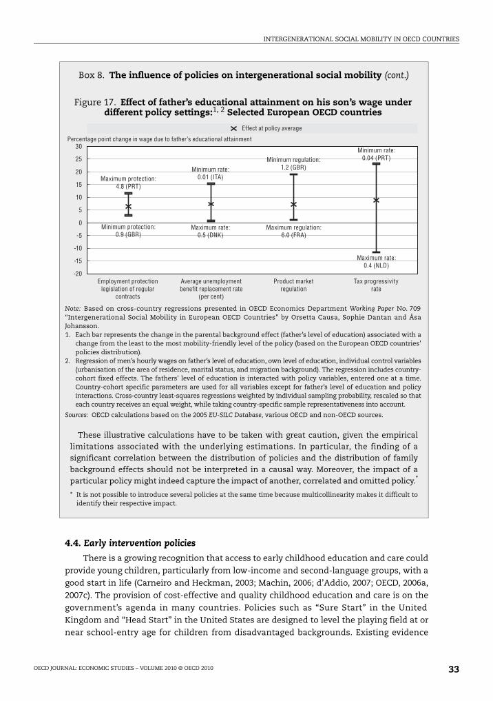
INTERGENERATIONAL SOCIAL MOBILITY IN OECD COUNTRIES
4.4. Early intervention policies
There is a growing recognition that access to early childhood education and care could
provide young children, particularly from low-income and second-language groups, with a
good start in life (Carneiro and Heckman, 2003; Machin, 2006; d’Addio, 2007; OECD, 2006a,
2007c). The provision of cost-effective and quality childhood education and care is on the
government’s agenda in many countries. Policies such as “Sure Start” in the United
Kingdom and “Head Start” in the United States are designed to level the playing field at or
near school-entry age for children from disadvantaged backgrounds. Existing evidence
Box 8. The influence of policies on intergenerational social mobility (cont.)
These illustrative calculations have to be taken with great caution, given the empiricallimitations associated with the underlying estimations. In particular, the finding of asignificant correlation between the distribution of policies and the distribution of familybackground effects should not be interpreted in a causal way. Moreover, the impact of aparticular policy might indeed capture the impact of another, correlated and omitted policy.*
* It is not possible to introduce several policies at the same time because multicollinearity makes it difficult toidentify their respective impact.
Figure 17. Effect of father’s educational attainment on his son’s wage under different policy settings:1, 2 Selected European OECD countries
Note: Based on cross-country regressions presented in OECD Economics Department Working Paper No. 709“Intergenerational Social Mobility in European OECD Countries” by Orsetta Causa, Sophie Dantan and ÅsaJohansson. 1. Each bar represents the change in the parental background effect (father’s level of education) associated with a
change from the least to the most mobility-friendly level of the policy (based on the European OECD countries’policies distribution).
2. Regression of men’s hourly wages on father’s level of education, own level of education, individual control variables(urbanisation of the area of residence, marital status, and migration background). The regression includes country-cohort fixed effects. The fathers’ level of education is interacted with policy variables, entered one at a time.Country-cohort specific parameters are used for all variables except for father’s level of education and policyinteractions. Cross-country least-squares regressions weighted by individual sampling probability, rescaled so thateach country receives an equal weight, while taking country-specific sample representativeness into account.
Sources: OECD calculations based on the 2005 EU-SILC Database, various OECD and non-OECD sources.
30
25
20
15
10
5
0
-5
-10
-15
-20
Percentage point change in wage due to father’s educational attainment
Employment protectionlegislation of regular
contracts
Average unemploymentbenefit replacement rate
(per cent)
Effect at policy average
Product marketregulation
Tax progressivityrate
Maximum protection:4.8 (PRT)
Minimum rate:0.01 (ITA)
Minimum rate:0.04 (PRT)Minimum regulation:
1.2 (GBR)
Maximum rate:0.5 (DNK)
Maximum regulation:6.0 (FRA)
Maximum rate:0.4 (NLD)
Minimum protection:0.9 (GBR)
OECD JOURNAL: ECONOMIC STUDIES – VOLUME 2010 © OECD 2010 33

INTERGENERATIONAL SOCIAL MOBILITY IN OECD COUNTRIES
concerning the impact of such programmes suggests that they have been successful in
alleviating some of the initial gaps of children born in adverse family environments
(e.g. Heckman, 2005; Currie and Blau, 2005; Brooks-Gunn, 2003; Sylva et al., 2004; OECD,
2004). Cross-country regression results obtained in the context of this study suggest that
enrolment in early childcare and education (day-care and pre-school) as well as spending on
childcare and early education, are inversely related to the influence of family background on
cognitive skills of teenagers (Figure 15 in Box 8 and Causa and Chapuis, 2009).
4.5. Educational policies and intergenerational social mobility
4.5.1. Education policies and school practices
Several empirical studies have documented a negative influence of early tracking
policies on equality in educational achievement.20 Systems that start grouping students
early in their educational curricula tend to be associated with larger socio-economic
inequalities, with no associated gains in average performance (OECD, 2007a). Results from
cross-country regressions confirm these findings, suggesting that the influence of parental
background on offspring performance at secondary school tends to be lower in countries
where tracking takes place at a later stage and/or where ability grouping within schools
occurs to a lesser extent (so called “comprehensive” systems), as compared with countries in
which tracking and ability grouping occurs earlier (so called “non-comprehensive” systems).
Regression estimates suggest that moving from a system that separates students into
different schools at age ten (as is done in Germany and Austria) to a system that separates
students at age sixteen (as is done in half of OECD countries) would reduce the effect of the
school’s socio-economic environment from 77 to 27 PISA score-points (Figure 15 in Box 8).21
Vocational education varies substantially across OECD countries in its design and
implementation, as well as in its degree of success in equipping individuals with the skills
needed in the labour market (e.g. Machin and Vignoles, 2005; Büchel, 2002). In many OECD
countries, upper-secondary students can enrol in vocational programmes, while some
countries delay vocational education (e.g. Canada and the United States).22 Moreover, in
some countries vocational training takes place mainly in schools and colleges (e.g. Nordic
and Eastern European countries), while in other countries such training takes place mainly
in the workplace through apprenticeships (e.g. Germany and Austria) or through a
combination of school and workplace. These differences need to be kept in mind when
evoking the concern that vocational education within secondary education ends up
grouping “weak/disadvantaged” students into programmes that limit their future learning
possibilities in a way similar to early tracking. Cross-country estimates suggest that there
is a positive association between enrolment in vocational education and the influence of
parental background on offspring secondary achievement (as measured by PISA scores).
Vocational education at the secondary education level appears to exacerbate achievement
differences associated with the school socio-economic environment without increasing
overall performance.
4.5.2. Education policies and resources
The link between human capital and growth has been emphasized in the policy
debate, and in many countries spending on education has increased since the mid-1990s.
However, research on the relationship between educational spending and student
performance is less encouraging. Most reviews reach the same conclusion: some
measurable school inputs do matter for performance but the magnitude of their effects is
OECD JOURNAL: ECONOMIC STUDIES – VOLUME 2010 © OECD 201034

INTERGENERATIONAL SOCIAL MOBILITY IN OECD COUNTRIES
relatively small (Hanushek, 2003, for a review; Schütz et al., 2005; OECD, 2007a). Cross-
country regression estimates performed in the context of this study also suggest that
increasing educational resources – either through raising spending or reducing class size-
might not be the most effective tool for promoting equity in secondary education (see
Causa and Chapuis, 2009).23 By contrast, the ability to prioritise and allocate resources
efficiently, measured by recently constructed OECD indicators capturing the “degree of
decentralisation” and “degree of mechanisms matching resources to specific needs”,
seems to be negatively associated with the influence of parental background on offspring
achievement in secondary education (see Sutherland and Price, 2007, for details of these
indicators). This effect mainly derives from a weaker association between the school socio-
economic environment and individual student performance.
The importance of teacher quality is rather well established (e.g. Hanushek, 2005, for
an overview). New estimates undertaken for this study show a negative association
between the proportion of qualified teachers and the influence of parental background on
offspring achievement at secondary school. While raising teacher quality/skills might
promote educational equity, little is known on how to translate this into effective policy.
One frequent suggestion is to raise their salary levels, increase salaries in the most
disadvantaged schools or areas, or introduce performance-based pay. Indeed, cross-
country estimates suggest that the influence of family background on student
achievement at secondary school is lower in countries where teacher wage profiles are
steeper over their career. However, it should be recognised that such wage profiles may not
capture performance-based pay systems, but rather constitute a proxy for cross-country
differences in “seniority wage profiles”.
4.5.3. Loan systems and persistence in post-secondary education
Evidence of credit constraints in undertaking tertiary education is rather limited and
mostly concerns the United States. A few studies tend to suggest that credit constraints
may not be the greatest obstacle to accessing higher education for disadvantaged students
(Carneiro and Heckman, 2003; Dreaden et al., 2004; Freynette, 2007; Wossman, 2008); rather
it is the lack of adequate qualifications to be accepted into higher education, which points
to the need for policies to intervene earlier (see above). By contrast, a recent study found
evidence of the presence of credit constraints in post-secondary education in some
European countries (Vandenberghe, 2007) and recent OECD work also found that lower
financial constraints are associated with higher tertiary graduation rates (Oliveira Martins
et al., 2007). If financial constraints are present they are likely to be more important for able
offspring from low-income backgrounds. In fact, cross-country empirical evidence shows
that in a few European OECD countries (e.g. Belgium, France, Italy, Luxembourg, the
Netherlands and the United Kingdom), financial constraints may hold back highly able
individuals from disadvantaged backgrounds (see Causa et al., 2009, for details).24
The design of tertiary educational loan systems and student support differs across
OECD countries. Some countries apply universal/individual-based systems which consider
higher education students as financially independent from their parents, whereas others
use systems in which students are considered members of their families for the purpose of
both financing and taxation. In general, in countries using other types of funding systems
than the universal/individual systems, the penalty of having a lower-educated father for
OECD JOURNAL: ECONOMIC STUDIES – VOLUME 2010 © OECD 2010 35

INTERGENERATIONAL SOCIAL MOBILITY IN OECD COUNTRIES
achieving tertiary education is larger (Figure 18). There is suggestive evidence that
universal government-supported loan systems can reduce liquidity constraints, thereby
enhancing equality of access while maintaining incentives for swift and successful study
completion (Oliveira Martins et al., 2007).
4.6. Redistributive and income support policies
Redistributive policies can alleviate financial constraints on disadvantaged families
and allow them to invest in their children’s human capital. Furthermore, social policies and
redistributive taxes may narrow the gap between current incomes of parents, so that the
incomes of their offspring could regress to the mean more quickly (Corak, 2006).25 In this
way, well-targeted redistributive policies could reduce not only current but also future
inequalities. However, such policies may also lower incentives to undertake effort and
invest in human capital as the net returns from these investments are reduced.
4.6.1. Taxation
One common measure of the redistributive nature of the tax system is the
progressivity in the personal income tax schedule, which differs significantly across OECD
countries and varies over time (Johansson et al., 2007). This may reflect differences in social
preferences, with strong progressivity in countries where emphasis is placed on a more
even distribution of post-tax income and consumption. Cross-country estimates suggest
that higher tax progressivity correlates across countries with a lower influence of parental
background on their offspring’s cognitive achievement in secondary education, as well as
on their wages (Figures 16 and 17 in Box 8 of Causa and Chapuis, 2009; Causa et al., 2009).
To capture the possible effect of taxation on parents’ ability to invest in their children’s
education, progressivity is measured at the time when the individual is a teenager. Thus,
Figure 18. Funding system and access to tertiary education:1 Selected European OECD countries
Note: Germany is not included in this figure as there is a problem with the representativeness of the German samplealong the education dimension.1. The figure shows the estimated percentage point decrease in the probability of a son to achieve tertiary education
given that the son’s father had achieved below upper-secondary education relative to a son whose father hadupper-secondary education.
Sources: OECD calculations based on the 2005 EU-SILC Database, Oliveira et al., 2007.
0
-10
-15
-5
-20
-25
-30
-35
-40
-45FRASWE LUX NLD GBR FIN DNK GRCIRL BEL ITAESP AUTPRT
Universal/individual system Other funding system
Men, 35-44 years old
Penalty from a disavantaged background (percentage point loss in probability of access)
OECD JOURNAL: ECONOMIC STUDIES – VOLUME 2010 © OECD 201036

INTERGENERATIONAL SOCIAL MOBILITY IN OECD COUNTRIES
one interpretation of the positive link with student performance and wages could be that
redistributive policies allow less-advantaged parents to provide their children with a better
environment, as well as with more time and resources for their education and upbringing
(see below). This may facilitate learning at later stages in life, which could reduce
inequality of opportunity in both higher education and wages. It is also possible that this
finding reflects targeted tax cuts or tax credits (e.g. in-work benefits) to low-income
households which, in turn, lowers the after-tax wage differential between low-income and
higher-income households (i.e. reduces inequality).
4.6.2. Unemployment benefits
Short-term net unemployment benefits are found to be negatively associated with the
influence of parental background on offspring achievement in secondary education
(Figure 16 in Box 8 and Causa and Chapuis, 2009). The average unemployment benefit
replacement ratio is also found to be negatively associated with intergenerational wage
persistence across the European OECD countries (Figure 17 in Box 8 and Causa et al., 2009).
As above, unemployment benefits are measured at the time when the individual is a
teenager. The policy implications of these findings are not clear, because existing empirical
evidence also suggests that the presence of transfer income among parents is associated
with lower wage prospects for their offspring (Corak, 2006). Moreover, some studies have
found a considerable degree of intergenerational persistence in reliance on welfare, which
could imply sustained cycles of welfare dependency (Page, 2004).26 Therefore, income-
support programmes are more likely to remove obstacles to intergenerational mobility if
they are designed to encourage labour market participation and self-sufficiency across
generations, while at the same time providing adequate income support during job search.
4.7. Housing policy
In some OECD countries housing-market outcomes encourage urban fragmentation
along socio-economic lines, with a concentration of disadvantaged households in
particular housing estates (OECD, 1998). Residential socio-economic segregation is often
matched by schooling socio-economic segregation, primarily because a large share of
students tends to go to schools in their own neighbourhood either for convenience or for
regulatory reasons. As discussed above, the school environmental effect is sizeable in a
number of OECD countries and tends to be larger in cities (see Causa and Chapuis, 2009).
This leads to higher education and wage persistence across generations.27 Thus, the design
of housing and urban planning policies may play a role in removing obstacles to
intergenerational social mobility. For example, in countries where there is a large contrast
between private and social rental housing (so called “dualist rental system”), and the latter
has a certain stigma, low-income households tend to cluster geographically (e.g. in the
United Kingdom, Belgium, Japan, Australia and New Zealand), while in countries where
private and social rental housing are integrated in one market (so called “unitary rental
system”), segregation tends to be less pronounced (e.g. Sweden, Denmark and Austria;
OECD, 2006b). Thus, policies aimed at increasing the social mix in neighbourhoods (for
instance, by improving housing quality in deprived areas in order to attract middle-class
families, OECD, 2006b) could be instrumental in improving social mobility, especially in
countries where the influence of the school socio-economic environment on student
performance is relatively large.
OECD JOURNAL: ECONOMIC STUDIES – VOLUME 2010 © OECD 2010 37

INTERGENERATIONAL SOCIAL MOBILITY IN OECD COUNTRIES
Cross-country regression results suggest that there could be potential equity and
efficiency gains from increasing social mix in schools for a number of OECD countries (see
Causa and Chapuis, 2009, for details). In countries suffering from high levels of school
socio-economic differences, low-skilled or disadvantaged students would benefit more
from interacting with more able or advantaged students, than the latter would lose from
interacting with less able students. Estimates also show that in most OECD countries there
is no adverse influence, and in some cases favourable effects, of the social mix on average
student performance. These results are only suggestive, but they would indicate that there
is no trade-off between social mix and overall performance. Hence, implementing
measures aimed at reducing school socio-economic segregation through educational
policies,28 and also through housing policies, could help to promote social mobility without
hampering, and perhaps even improving, educational efficiency.
Notes
1. Economists typically analyse income or wage/earnings mobility, while sociologists focus onmobility across social class and occupations (e.g. Erikson and Goldthorpe, 1992, for an overview ofsocial class mobility). One advantage of measuring intergenerational mobility by class oroccupation is that data restrictions are much less stringent, retrospective information of parent’soccupation being more widely available than information about their incomes, wages or earnings.A disadvantage is that it is difficult to make international comparisons of social class andoccupation since they may have very different meanings across countries.
2. There is ample evidence of sizeable returns to education, both to years of schooling and cognitiveachievement (e.g. Card, 1999; Oliveira et al., 2007). Furthermore, the returns to changes inqualitative measures of education, for example test scores on cognitive achievement, seem to behigher than those from additional years of schooling (Bishop, 1992; Riviera-Batiz, 1992).
3. The wage concept in this study refers to gross hourly wages and is based on new comparable microdata across European OECD countries, the EU-SILC database. Gross hourly wages are based onwages and salaries paid in cash for time worked in main and secondary jobs including holiday payand additional payments during the year preceding the interview. Given the strong persistence inwages, this is a good proxy for current wages. An hourly rate is calculated by using the currentnumber of hours the person works in his/her main job, including overtime. Admittedly, usinghours worked in the main job may lead to an over-estimation of hourly wages for persons with twoor more jobs. Moreover, only wage earners are covered. This may exaggerate the degree ofintergenerational wage mobility to the extent that the offspring of higher-educated families areless likely to be inactive than the offspring of low-educated families.
4. There is very little evidence concerning the intergenerational income persistence for womenacross OECD countries. This neglect partly reflects that in economies where women’s labour-forceparticipation rates are lower than men’s, their wages may be an unreliable indicator of theireconomic status. In the United States, income persistence for daughters is found to be somewhatweaker than for sons, but it is still rather substantial (Chadwick and Solon, 2002).
5. Across all European OECD countries covered by the analysis, there is substantial persistence inwages of pairs of fathers and daughters. This finding is robust to the use of mother’s educationinstead of father’s education.
6. Several studies have documented the existence of non-linearities in persistence; that is, the degreeof persistence in wages across generations differs along the wage distribution (e.g. Jäntti et al.,2006; Bratberg et al., 2007; Corak and Heisz, 1999; Grawe, 2004). Such non-linearities are oftenexplained by the fact that low-income parents face credit constraints in financing their children’seducation, and consequently such children’s wages fall below that of non-constrained childrenwith the same ability (e.g. Becker and Tomes, 1986; Becker, 1989). There seems to be somesuggestive evidence of the existence of non-linearities in wage persistence across a number ofEuropean countries (see Causa et al., 2009, for details).
7. Differences in immigration patterns across European OECD countries could influence the patterns inwage persistence. However, in most countries covered in this study the estimates of persistence
OECD JOURNAL: ECONOMIC STUDIES – VOLUME 2010 © OECD 201038

INTERGENERATIONAL SOCIAL MOBILITY IN OECD COUNTRIES
coefficients obtained, controlling for individual migration status, differ very little from those thatomit this control, and the differences are statistically insignificant (see Causa et al., 2009, for details).
8. There are much less comparable estimates of intergenerational persistence in wages or incomesfor daughters.
9. On average across OECD countries, for each improvement of one international standard deviation inthe family’s socio-economic background, the student performance on the OECD PISA science scaleimproves by 40 points, ranging from 25 (Mexico) to 54 (France). This corresponds to a performanceincrease of 5% and 10%, respectively (based on an OECD average PISA performance of 500 points).
10. In Figure 7, for each country, the influence of parental background (the so-called “socio-economicgradient”) is presented along with a “corrected” influence of parental background, defined as theincrease in student performance associated with the move from the first to the last quartile of thecountry-specific distribution of student background.
11. More precisely, the school environment effect is defined as the difference in predicted PISA scoresof two students with identical socio-economic backgrounds attending different schools (where theaverage background of students is separated by an amount equal to the inter quartile range of thecountry-specific school socio-economic distribution); the individual background effect is definedas the difference in predicted PISA scores of two students within a school (separated by the interquartile range of the country-specific average within school socio-economic distribution).
12. This necessitates taking into account differences in the between and within school distribution ofstudent socio-economic status. Hence, the comparison is made along two dimensions: both withinand across countries. The approach differs from OECD (2007a) in that it is chosen to take cross-country differences in the distribution of socio-economic background into account, hence usingcountry-specific distribution in the computations (Causa and Chapuis, 2009, for details).
13. Comprehensive school systems refer to those that do not systemically separate students accordingto ability or proficiency level; students follow a general unified curriculum across secondaryschools.
14. For pairs of fathers and daughters, there is also a sizeable probability premium and penalty inachieving tertiary education. The cross-country pattern in the estimated probability premium for35-44 year-old women is similar to that of men (see Causa et al., 2009, for details).
15. Education persistence may be understated in France because the group of tertiary educationfathers does not distinguish between having a father with a university degree and a father with adegree from a “Grande École”. It is possible that the premium of having a father with a Grande Écoledegree is higher than the premium of having a university-educated father.
16. But once existing technologies become more accessible, the importance of ability may decline andmobility may fall back to previous levels.
17. It is possible that institutions that impose wage floors (e.g. minimum wages or collectiveagreements) and compress wage distributions can in the long run force business to restructuretheir production, which may not necessarily lead to lower overall employment.
18. However, this effect will be mitigated to the extent that children from less-advantagedbackgrounds disproportionately benefit from public spending on education (Solon, 2004).
19. In addition, higher wage differentials can also be productivity-enhancing. If wages are based onrelative productivity, then workers with higher productivity (effort) will be rewarded with higherwages. This will increase equilibrium effort and lead to a positive relationship between wagedispersion and productivity. However, individual effort is reduced if wage differences are regardedas unfair (Akerlof and Yellen, 1990).
20. Both cross-country and country-specific studies have highlighted the negative impact of abilitytracking on mobility (for cross-country evidence, see OECD, 2004, 2007a; Schütz et al., 2005;Hanushek and Woessmann, 2005; Sutherland and Price, 2007; Duru-Bellat and Suchaut, 2005;Amermuller, 2005; for country-specific evidence, see e.g. Bauer and Riphahn, 2006; Pekkarinenet al., 2006; Holmlund, 2006; and Bratberg et al., 2005).
21. A similar result is found for the number of school programmes available to 15-year-olds, which isanother measure of early differentiation in secondary education (see Causa and Chapuis, 2009, fordetails).
22. On average, in the OECD, around 46% of upper-secondary students are enrolled in pre-vocationalor vocational programmes (OECD, 2009).
OECD JOURNAL: ECONOMIC STUDIES – VOLUME 2010 © OECD 2010 39

INTERGENERATIONAL SOCIAL MOBILITY IN OECD COUNTRIES
23. This summary presentation of the results does not distinguish between heterogeneous tools(spending increases, class-size reductions) that are tested in the cross-country regressions (seeCausa and Chapuis, 2009, for details). In particular, while spending is clearly a poor driver ofeducational equity, cross-country analysis shows that reductions in class size mitigate inequalitiesassociated with schools’ socio-economic differences (i.e. they reduce the school environmenteffect). However, the education literature emphasises the difficulty of properly identifyingchannels through which changes in class size have an impact on schools’ contextual effects andthe corresponding student outcomes, casting doubts on the effectiveness of reducing class sizesfor equity purposes.
24. This finding is obtained by assessing the influence of parental background on their children’searnings at different quantiles of children’s earnings distribution (so-called quantile regressions)(for details see Causa et al., 2009). If financial constraints are present, the influence of parentalbackground should be stronger in the upper quartile, since it is the more competent children fromlow-income families that are most likely to be financially constrained (Grawe, 2004).
25. This relies on two assumptions. First, an increase in income for parents has the same influence ontheir offspring regardless of its source, and second, the relationship between parent and offspringwages is linear and stable across the wage distribution.
26. A possible explanation of this phenomenon is that growing up in families that depend on welfaresupport reduces the stigma perceived by the offspring in getting his/her income from this source.Another possibility is that an individual living in a family receiving welfare support acquiresinformation about the programme and its rules, thereby making it easier for her/him to collect it(Corak, 2006).
27. School environmental effects, and the so-called “neighbourhood effects”, are interrelated socialphenomena. In particular, school environmental effects may be one of the channels throughwhich neighbourhood composition impacts individuals’ behaviour and outcomes (e.g. Goux andMaurin, 2007).
28. School policies, such as school choice, can also be used as a tool to reduce residential and schoolsegregation (see Causa and Chapuis, 2009). Cross-country research on this topic is scarce, mostlydue to measurement issues. School competition may induce cream skimming, increasesegregation and lead to adverse effects on disadvantaged students. However, specific experiencessuggest that properly designed and equitable voucher systems can yield positive outcomes (e.g. theWest and Peterson, 2006, study on voucher systems in Florida). Hoxby (2003) also suggests similarequity-enhancing effects of voucher and charter school programmes.
References
Acemoglu, D. (2003), “Cross-Country Inequality Trends”, Economic Journal, Vol. 113.
Akerlof, G.A. and J.L. Yellen (1990), “The Fair-Wage Hypothesis and Unemployment”, Quarterly Journalof Economics, Vol. 105.
Amermuller, A. (2005), “Educational Opportunities and the Role of Institutions”, ROA-RM-2005E,Research Centre for Education and the Labour market, Maastricht University.
Andrews, D. and A. Leigh (2009), “More Inequality, Less Social Mobility”, Applied Economics Letters,Vol. 16.
Bassanini, A. and R. Duval (2006), “Employment Patterns in OECD Countries: Reassessing the Role ofPolicies and Institutions”, OECD Economics Department Working Papers, No. 486, Paris.
Bauer, P. and R. Riphahn (2006), “Timing of School Tracking as a Determinant of IntergenerationalTransmission of Education”, Economics Letters, 91(1), pp. 90-97.
Becker, G. (1989), “On the Economics of the Family: Reply to a Skeptic”, American Economic Review,American Economic Association, Vol. 79.
Becker, G.S. and N. Tomes (1979), “An Equilibrium Theory of the Distribution of Income andIntergenerational Mobility”, Journal of Political Economy, Vol. 87, pp. 1153-89.
Becker, G.S. and N. Tomes (1986), “Human Capital and the Rise and Fall of Families”, Journal of LabourEconomics, Vol. 4, pp. S1-S39.
Bishop, J.H. (1992), “The Impact of Academic Competencies on Wages, Unemployment, and JobPerformance”, Carnegie-Rochester Conference Series on Public Policy, Vol. 37, pp. 127-194.
OECD JOURNAL: ECONOMIC STUDIES – VOLUME 2010 © OECD 201040

INTERGENERATIONAL SOCIAL MOBILITY IN OECD COUNTRIES
Björklund, A. and M. Jäntti (1997), “Intergenerational Income Mobility in Sweden Compared with theUnited States”, American Economic Review, 87(5), pp. 1009-1018.
Blanden, J. (2008a), “How Much Can We Learn from International Comparisons of Social Mobility?”,mimeo.
Blanden, J. (2008b), “Intergenerational Income Mobility in a Comparative Perspective” in P. Dolton,R. Apslund and E. Barth (eds.), Education and Inequality Across Europe, Edward Edgar, forthcoming.
Blanden, J., P. Gregg and S. Machin (2005), “Intergenerational Mobility in Europe and North America”,A report supported by the Sutton Trust.
Blanden, J., P. Gregg and L. Macmillan (2006), “Accounting for Intergenerational Income Persistence:Non-Cognitive Skills, Ability and Education” CEE Working Paper.
Blau, F. and L. Kahn (1996), “International Differences in Male Wage Inequality: Institutions VersusMarket Forces”, Journal of Political Economy, Vol. 104.
Blau, F. and L. Kahn (2003), “Understanding International Differences in the Gender Pay Gap”, Journal ofLabor Economics, Vol. 21.
Bowles, S., H. Gintis and M. Osborne (2002), “The Determinants of Individual Earnings: Skills,Preferences, and Schooling”, Journal of Economic Literature Vol. 39.
Bourguignon, F., F. Ferreira and M. Menendez (2003), “Inequality of Outcomes and Inequality ofOpportunities in Brazil”, Delta, Working Papers No. 2003-24.
Bratberg, E., Ø.A. Nilsen, and K. Vaage (2005), “Intergenerational Earnings Mobility in Norway: Levelsand Trends”, The Scandinavian Journal of Economics, Vol. 107.
Bratberg, E., Ø.A. Nilsen and K. Vaage (2007), “Trends in Intergenerational Mobility across Offspring’sEarnings Distribution in Norway”, Industrial Relations, Vol. 46.
Brooks-Gunn, J. (2003), “Do You Believe In Magic?: What We Can Expect From Early ChildhoodIntervention Programs”, Social Policy Report, Vol. XVII, No. 1.
Burtless, G and C. Jencks (2003), “American Inequality and its Consequences” in H. Aaron, J.M. Lindsayand P.S. Nivola (eds.), Agenda for the Nation, Washington DC.
Büchel, F. (2002), “Successful Apprenticeship-to-Work Transitions: on the Long-Term Change inSignificance of the German School-Leaving Certificate”, International Journal of Manpower, Vol. 23.
Card, D. (2001), “Estimating the Returns to Schooling: Progress on Some Persistent EconometricProblems” Econometrica, Vol. 69.
Card, D. (1999), “The Causal Effect of Education on Earnings”, in O. Ashenfelter and D. Card (eds.),Handbook of Labor Economics, Vol. 3, Amsterdam, Elsevier.
Causa, O. and C. Chapuis (2009), “Equity in Student Achievement across OECD Countries: AnInvestigation of the Role of Policies”, OECD Economics Department Working Papers, No. 708.
Causa, O, S. Dantan and Å. Johansson (2009), “Intergenerational Social Mobility in European OECDCountries”, OECD Economics Department Working Papers, No. 709.
Chadwick, L. and G. Solon (2002), “Intergenerational Income Mobility among Daughters”, AmericanEconomic Review, Vol. 92.
Chevalier, A, K. Denny and D. McMahon (2007), “A Multi-Country Study of Inter-GenerationalEducational Mobility” UCD Geary Institute Working Paper No. 25.
Carneiro, P. and J.J. Heckman (2003), “Human Capital Policy”, NBER Working Paper, No. 9495, NationalBureau of Economic Research, Cambridge MA.
Corak, M. (2004), Generational Income Mobility in North America and Europe, Cambridge University Press,Cambridge, England.
Corak, M. (2006), “Do Poor Children Become Poor Adults? Lessons from a Cross Country Comparison ofGenerational Earnings Mobility”, IZA Discussion Paper No. 1993.
Corak, M. and A. Heisz (1999), “The Intergenerational Income Mobility of Canadian Men”, Journal ofHuman Resources, Vol. 34.
Cunha, F., J.J. Heckman, L.J. Lochner and D.V. Masterov (2006), “Interpreting the Evidence on Life CycleSkill Formation”, in E.A. Hanushek and F. Welch (eds.), Handbook of the Economics of Education,Amsterdam, North-Holland.
OECD JOURNAL: ECONOMIC STUDIES – VOLUME 2010 © OECD 2010 41

INTERGENERATIONAL SOCIAL MOBILITY IN OECD COUNTRIES
Currie, J. and D. Blau (2005), “Who’s Minding the Kids?”, Handbook of Education Economics.
D’Addio, A. (2007), “Intergenerational Transmission of Disadvantage: Mobility or Immobility AcrossGenerations? A Review of the Evidence for OECD countries”, OECD Social, Employment and MigrationWorking Papers, No. 52.
Dearden, L., L. McGranahan and B. Sianesi (2004), “The Role of Credit Constraints in EducationalChoices: Evidence from the NCDS and BCS70”, CEE Working Paper, LSE, London.
Duru-Bellat, M. and B. Suchaut (2005), “Organisation and Context, Efficiency and equity of EducationalSystems: What PISA tells Us”, European Educational Research Journal, Vol. 4.
Entorf, H. and M. Lauk (2006), Peer Effects, Social Multipliers and Migrants at School: An InternationalComparison, IZA Discussion Papers 2182, Institute for the Study of Labor (IZA).
Erikson, R. and J.H. Goldthorpe (1992), The Constant Flux: A Study of Class Mobility in Industrial Societies,Clarendon, Oxford.
Feenstra, R.C. (2000), The Impact of International Trade on Wages, The University of Chicago Press.
Feenstra, R.C. and G. Hansen (1999), “The Impact of Outsourcing and High-Technology Capital onWages: Estimates for the United States”, Quarterly Journal of Economics, Vol. 114.
Freynette, M. (2007), “Why Are Youth from Lower-income Families Less Likely to Attend University?Evidence from Academic Abilities, Parental Influences, and Financial Constraints”, AnalyticalStudies Branch Research Paper Series, No. 295, Statistics Canada.
Fuchs, T. and L. Woessmann (2004), “What Accounts for International Differences in StudentPerformance? A Re-Examination using PISA Data”, mimeo.
Galbraith, J.K. and H. Kum (2005), “Estimating the Inequality of Household Incomes: A StatisticalApproach to the Creation of a Dense and Consistent Global Data Set”, Review of Income and Wealth,No. 51.
Galor, O. and D. Tsiddon (1997), “Technological Progress, Mobility, and Economic Growth”, AmericanEconomic Review, Vol. 87.
Garibaldi, P. and G. Violante (2005), “The Employment Effects of Severance Payments with WageRigidities”, The Economic Journal, Vol. 115.
Goldberger, A. (1989), “Economic and Mechanical models of Intergenerational Transmission”, AmericanEconomic Review, Vol. 79.
Gottschalk, P. and S. Danziger (2005), “Inequality of Wage Rates, Earnings and Family Income in theUnited States, 1975-2002”, Review of Income and Wealth, No. 51.
Goux, D. and E. Maurin (2007), “Close Neighbours Matter: Neighbourhood Effects on Early Performanceat School”, Economic Journal, Vol. 117.
Grawe, N.D. and C. Mulligan (2002), “Economic Interpretations of Intergenerational Correlations”, NBERWorking Paper No. 8948.
Grawe, N.D. (2004), “Reconsidering the Use of Nonlinearities in Intergenerational Earnings Mobility asa Test of Credit Constraints”, Journal of Human Resources, Vol. 34.
Haider, S. and G. Solon (2006), “Lifecycle Variation in the Association between Current and LifetimeEarnings”, American Economic Review, Vol. 96.
Hanushek, E.A. (2003), “The Failure of Input Based Schooling Policies”, The Economic Journal, Vol. 113.
Hanushek, E.A. and L. Woessmann (2005), “Does Educational Tracking Affect Performance andInequality? Differences-in-Differences Evidence across Countries”, NBER Working Paper, No. 11124.
Hanushek, E.A (2005), The Single Salary Schedule and Other Issues of Teacher Pay.
Heckman, J.J. (2005), “Invited Comments” in L.J. Schweinhart, J. Montie, Z. Xiang, W.S. Barnett,C.R. Beleld and M. Nores (eds.), Lifetime Effects: The High/Scope Perry Preschool Study Through Age 40,pp. 229-233. Ypsilanti, MI: High/Scope Press, Monographs of the High/Scope Educational ResearchFoundation, 14.
Heckman, J.J. (1976), “The Common Structure of Statistical Models of Truncation, Sample Selection andLimited Dependent Variables and a Simple Estimator for Such Models”, Annals of Economic and SocialMeasurement, Vol. 5.
OECD JOURNAL: ECONOMIC STUDIES – VOLUME 2010 © OECD 201042

INTERGENERATIONAL SOCIAL MOBILITY IN OECD COUNTRIES
Hertz, T., T. Jayasundera, P. Piraino, S. Selcuk, N. Smith and A. Verashchagina (2007), “The Inheritanceof Educational Inequality: International Comparisons and Fifty-Year Trends”, The B.E. Journal ofEconomic Analysis and Policy, Vol. 7.
Holmlund, H. (2006), “Intergenerational Mobility and Assortative Mating Effects of an EducationalReform”, Swedish Institute for Social Research Working Paper, No. 4/2006, Stockholm University.
Hoxby, C.M. (2003), “School Choice and School Competition: Evidence from the United States”, SwedishEconomic Policy Review, Vol. 10.
Jäntti, M., B. Bratsberg, K. Roed, O. Raaum, R. Naylor, E. Österbacka, A. Björklund and T. Eriksson(2006), “American Exceptionalism in a New Light: A Comparison of Intergenerational EarningsMobility in the Nordic Countries, the United Kingdom and the United States”, IZA Discussion PaperNo. 1938.
Johansson, Å., C. Heady, J. Arnold, B. Brys and L. Vartia (2008), “Tax and Economic Growth” , OECDEconomics Department Working Papers, No. 620.
Lazear, E. and S. Rosen (1981), “Rank-Order Tournaments as Optimum Labor Contracts”, Journal ofPolitical Economy, Vol. 89.
Lee, C.I. and G. Solon (2006), “Trends in Intergenerational Income Mobility”, NBER Working Paper,No. 12007.
Lindbeck, A. and D.J. Snower (1988), The Insider-Outsider Theory of Employment and Unemployment, MITPress, Cambridge, MA.
Machin, S.J. (2006), “Social Disadvantage and Education Experiences”, OECD Social, Employment andMigration Working Papers, No. 32, OECD, Paris.
Machin, S.J. and A. Vignoles (eds.) (2005), What’s the Good of Education? The Economics of Education in theUK, Princeton: Princeton University Press.
Mayer, S.E and L.M. Lopoo (2008), “Government Spending and Intergenerational Mobility”, Journal ofPublic Economics, Vol. 92.
Murphy, K, A. Shleifer and R. Vishny (1991), “The Allocation of Talent: Implications for Growth”,Quarterly Journal of Economics, Vol. 106.
OECD (1998), Integrating Distressed Urban Areas, OECD, Paris.
OECD (2002), Employment Outlook, Chapter 5, “And the Twain Shall Meet: Cross-Market Effects of Labourand Product Market Policies”, OECD, Paris.
OECD (2003), The Sources of Economic Growth in OECD Countries, OECD, Paris.
OECD (2004), Learning for Tomorrow’s World: First Results from PISA 2003, OECD, Paris.
OECD (2005a), PISA 2003 Technical Report, OECD, Paris.
OECD (2005b), PISA 2003 Data Analysis Manual, OECD, Paris.
OECD (2006a), Starting Strong II: Early Childhood Education and Care, OECD, Paris.
OECD (2006b), Interim Report on Socially Sustainable Housing, GOV/TDPC/URB(2006)3.
OECD (2006c), OECD Employment Outlook: Boosting Jobs and Incomes, OECD, Paris.
OECD (2007a), PISA 2006 Science Competencies for Tomorrow’s World, OECD, Paris.
OECD (2007b), Going for Growth, OECD, Paris.
OECD (2007c), Babies and Bosses – Reconciling Work and Family Life: A Synthesis of Findings for OECDCountries, OECD, Paris.
OECD (2009), Highlights from Education at a Glance 2008, OECD, Paris.
OECD (2010), Pathways to Success – How Knowledge and Skills at Age 15 Shape Future Lives in Canada, OECD,Paris.
Oliveira Martins, J., R. Boarini, H. Strauss, C. de la Maisonneuve and C. Saadi (2007), “The PolicyDeterminants of Investment in Tertiary Education”, OECD Economics Department Working Papers,No. 576.
Page, M. (2004), “New Evidence on the Intergenerational Correlation in Welfare Participation”, inM. Corak (ed.), Generational Income Mobility in North America and Europe, Cambridge University Press,Cambridge, England.
OECD JOURNAL: ECONOMIC STUDIES – VOLUME 2010 © OECD 2010 43

INTERGENERATIONAL SOCIAL MOBILITY IN OECD COUNTRIES
Pekkarinen, T., R. Uusitalo and S. Pekkala (2006), “Education Policy and Intergenerational IncomeMobility: Evidence from the Finnish Comprehensive School Reform”, IZA Discussion Paper, No. 2204.
Plug. E. and W. Vijverberg (2005), “Does Family Income Matter for Schooling Outcomes? UsingAdoptees as a Natural Experiment”, The Economic Journal, Vol. 115.
Rivera-Batiz, F.L. (1992), “Quantitative Literacy and the Likelihood of Employment Among YoungAdults in the United States”, Journal of Human Resources, Vol. 27.
Roemer, J.E. (1998), Equality of Opportunity, Cambridge, MA: Harvard University Press.
Roemer, J.E. (2004), “Equal Opportunity and Intergenerational Mobility: Going BeyondIntergenerational Income Transition matrices”, in Generational Income Mobility in North America andEurope, M. Corak (ed.), Cambridge University Press, Cambridge, England.
Sacerdote, B. (2002), “The Nature and Nurture of Economic Outcomes”, American Economic Review,Vol. 92.
Schütz, G., H.W. Ursprung and L. Woessmann (2005), “Education Policy and Equality of Opportunity”,IZA Discussion Paper, No. 1906, Institute for the Study of Labour, Bonn.
Solon, G. (2002), “Cross-Country Differences in Intergenerational Income Mobility”, Journal of EconomicPerspectives, Vol. 16.
Solon, G. (2004), “A Model of Intergenerational Mobility Variation over Time and Place”, in GenerationalIncome Mobility in North America and Europe, M. Corak (ed.), pp. 38-47, Cambridge University Press,Cambridge, England.
Shonkoff, J.P. and D.A. Phillips (eds.) (2000), From Neurons to Neighbourhoods: The Science of Early ChildhoodDevelopment, National Academy Press, Washington DC.
Sylva, K., E. Melhuish, P. Sammons, I. Siraj-Blatchford, B. Taggart and K. Elliot (2004), “The EffectiveProvision of Pre-School Education (EPPE) Project: Findings from the Pre-school Project”, Institute ofEducation.
Sutherland, D. and R. Price (2007), “Linkages Between Performance and Institutions in the Primary andSecondary Education Sector, Performance Indicators”, OECD Economics Department Working Papers,No. 558, Paris.
Vandenberghe, V. (2007), “Family Income and Tertiary Education Attendance across the EU: AnEmpirical Assessment Using Sibling Data”, Centre for Analysis of Social Exclusion, CASE/123.
West, M.R. and P.E. Peterson (2006), “The Efficacy of Choice Threats within School AccountabilitySystems: Results from Legislatively-Induced Experiments”, Economic Journal, Vol. 116.
Woessman, L. (2008), “Efficiency and Equity of European Education and Training Policies”, InternationalTax and Public Finance, Vol. 15.
OECD JOURNAL: ECONOMIC STUDIES – VOLUME 2010 © OECD 201044
Related Documents