HAL Id: tel-03117139 https://tel.archives-ouvertes.fr/tel-03117139 Submitted on 20 Jan 2021 HAL is a multi-disciplinary open access archive for the deposit and dissemination of sci- entific research documents, whether they are pub- lished or not. The documents may come from teaching and research institutions in France or abroad, or from public or private research centers. L’archive ouverte pluridisciplinaire HAL, est destinée au dépôt et à la diffusion de documents scientifiques de niveau recherche, publiés ou non, émanant des établissements d’enseignement et de recherche français ou étrangers, des laboratoires publics ou privés. Interference cancellation in MIMO and massive MIMO systems Abdelhamid Ladaycia To cite this version: Abdelhamid Ladaycia. Interference cancellation in MIMO and massive MIMO systems. Networking and Internet Architecture [cs.NI]. Université Sorbonne Paris Cité, 2019. English. NNT : 2019US- PCD037. tel-03117139

Welcome message from author
This document is posted to help you gain knowledge. Please leave a comment to let me know what you think about it! Share it to your friends and learn new things together.
Transcript
HAL Id: tel-03117139https://tel.archives-ouvertes.fr/tel-03117139
Submitted on 20 Jan 2021
HAL is a multi-disciplinary open accessarchive for the deposit and dissemination of sci-entific research documents, whether they are pub-lished or not. The documents may come fromteaching and research institutions in France orabroad, or from public or private research centers.
L’archive ouverte pluridisciplinaire HAL, estdestinée au dépôt et à la diffusion de documentsscientifiques de niveau recherche, publiés ou non,émanant des établissements d’enseignement et derecherche français ou étrangers, des laboratoirespublics ou privés.
Interference cancellation in MIMO and massive MIMOsystems
Abdelhamid Ladaycia
To cite this version:Abdelhamid Ladaycia. Interference cancellation in MIMO and massive MIMO systems. Networkingand Internet Architecture [cs.NI]. Université Sorbonne Paris Cité, 2019. English. �NNT : 2019US-PCD037�. �tel-03117139�

THÈSEpour obtenir le grade de
Docteur de l’université Paris 13, Sorbonne Paris CitéDiscipline : "Doctorat de sciences pour l’ingénieur"
présentée et soutenue publiquement par
Abdelhamid LADAYCIA
le 01 Juillet 2019
Annulation d’interférences dans les systèmes MIMO etMIMO massifs (Massive MIMO)
Directeur de thèse : Prof. Anissa Mokraoui
Co-directeur de thèse : Prof. Karim Abed-Meraim
Co-directeur de thèse : Prof. Adel Belouchrani
JURY
Pierre Duhamel, Directeur de recherches CNRS, Ecole Centrale Supélec Président
Philippe Ciblat, Professeur, Telecom Paristech Examinateur
Jean Pierre Delmas, Professeur, Telecom SudParis Rapporteur
Mohammed Nabil El Korso, Maître de conférences HDR, Université Paris Naterre Rapporteur
Gabriel Dauphin, maître de conférences, Université Paris 13 Examinateur
Anissa Mokraoui, Professeur, Université Paris 13 Examinateur
Karim Abed-Meraim, Professeur, Université d’Orléans Examinateur
Adel Belouchrani, Professeur, ENP d’Alger Examinateur


It is with my deepest gratitude and ap-
preciation that I dedicate this thesis
To my parents;
To my wife.
To my son Mouetez Billah;
To my daughters Alaa and Acile;
To brothers and sisters.
for their constant source of love,
support and encouragement.

iv

Acknowledgments
“ None of us got to where we are alone. Whether the as-
sistance we received was obvious or subtle, acknowledging
someone’s help is a big part of understanding the impor-
tance of saying thank you. ”Harvey Mackay.
Time goes by so fast and it has been already four years since the first time I came to
France for a huge turning point in my life. Doing a PhD thesis in France in general
and at University Sorbone, Paris 13 in particular has been one of the most enjoyable time in
my life. Without the guidance of the committee members, the help from my friends and the
encouragement of my family, my thesis would not have been possible. Therefore, I would like to
thank all people who have contributed in a variety of ways to this dissertation.
First of all, I would like to thank almighty Allah (SWT) for his countless blessing on me at
every sphere of life. May he help us to follow Islam in its true spirit according to the teachings
of his prophet Muhammed (PBUH).
Secondly, I would like to thank my country, Algeria, that gave me the opportunity to continue
my study and offer me PhD scholarship. Especially the RD department (DRD) of CFDAT/MDN,
I am greatly thankful to Mr. REMILI Kamel and Mr GUEROUI Fawzi.
I would like to express my deepest gratitude to my doctoral supervisors: Professor Anissa
MOKRAOUI, Professor Karim ABED-MERAIM and Professor Adel BELOUCHRANI for their
guidance and support in several years. It has been a great pleasure for me to work on an
interesting PhD project and from which I have a great chance to improve my mathematical skills
and work with various researchers from different institutions. I am thankful to them for listening
patiently all my questions, sharing their knowledge to me and giving me a lot of outstanding
advice to overcome numerous obstacles.

vi
Beside my supervisors, I am deeply thankful to Professors Jean Pierre DELMAS and Mo-
hammed Nabil EL KORSO, the two reviewers of my dissertation. It is a great honor for me
to have my PhD thesis evaluated by these experts. I also want to express my gratitude to the
president of my thesis committee Professor Pierre DUHAMEL and the two examinators Philippe
CIBLAT and Gabriel DAUPHIN, for their insightful comments and encouragements.
Moreover, without hesitation, I would like to thank all my friends in L2TI laboratory
(University Sorbonne, Paris 13) for their encouragement and support. They make my stay and
study in this place more enjoyable. I am happy to share a lot of memorable moments with them.
Finally, I would also express my appreciation to my wife who provide unending inspiration.
She is always supporting and encouraging me with their best effort.
Thank you very much, everyone !
RésuméLes systèmes de communications MIMO (Multiple Input Multiple Output) utilisent des réseaux
de capteurs qui peuvent s’étendre à de grandes dimensions (MIMO massifs) et qui sont pressentis
comme solution potentielle pour les futurs standards de communications à très hauts débits.
Un des problèmes majeur de ces systèmes est le fort niveau d’interférences dû au grand
nombre d’émetteurs simultanés. Dans un tel contexte, les solutions ’classiques’ de conception de
pilotes ’orthogonaux’ sont extrêmement coûteuses en débit utile permettant ainsi aux solutions
d’identification de canal dites ’aveugles’ ou ’semi-aveugles’ (abandonnées pour un temps dans
les systèmes de communications civiles) de revenir au-devant de la scène comme solutions
intéressantes d’identification ou de déconvolution de ces canaux MIMO.
Dans cette thèse, nous avons commencé par une analyse comparative des performances, en se
basant sur les bornes de Cramèr-Rao (CRB), afin de mesurer la réduction potentielle de la taille
des séquences pilotes et ce en employant les méthodes dites semi-aveugles basées sur l’exploitation
conjointe des pilotes et des données. Les résultats d’analyse montrent que nous pouvons réduire
jusqu’à 95% des pilotes sans affecter les performances d’estimation du canal.
Nous avons par la suite proposé de nouvelles méthodes d’estimation semi-aveugle du canal,
éventuellement de faible coût, permettant d’approcher les performances limites (CRB). Nous
avons proposé un estimateur semi-aveugle, LS-DF (Least Squares-Decision Feedback), basé
sur une estimation des moindres carrés avec retour de décision qui permet un bon compromis
performance / complexité numérique. Un autre estimateur semi-aveugle de type sous-espace a
aussi été proposé ainsi qu’un algorithme basé sur l’approche EM (Expectation Maximization)
pour lequel trois versions à coût réduit ont été étudiées. Dans le cas d’un canal spéculaire, nous
avons proposé un algorithme d’estimation paramétrique se basant sur l’estimation des temps
d’arrivés combinée avec la technique DF.
Mots Clés— MIMO/ massive MIMO, OFDM, CRB, semi-aveugle, méthode sous-espace,
algorithme EM, LS-DF, canal spéculaire.

viii
AbstractMultiple Input Multiple Output (MIMO) systems use sensor arrays that can be of large-scale
(we will then refer to them as massive MIMO systems) and are seen as a potential candidate for
future digital communications standards at very high throughput.
A major problem of these systems is the high level of interference due to the large number of
simultaneous transmitters. In such a context, ’conventional’ orthogonal pilot design solutions are
expensive in terms of throughput, thus allowing for the so-called ’blind’ or ’semi-blind’ channel
identification solutions (forsaken for a while in the civil communications systems) to come back
to the forefront as interesting solutions for identifying or deconvolving these MIMO channels.
In this thesis, we started with a comparative performance analysis, based on Cramèr-Rao
Bounds (CRB), to quantify the potential size reduction of the pilot sequences when using semi-
blind methods that jointly exploit the pilots and data. Our analysis shows that, up to 95% of
the pilot samples can be suppressed without affecting the channel estimation performance when
such semi-blind solutions are considered.
After that, we proposed new methods for semi-blind channel estimation, that allow to approach
the CRB with relatively low or moderate cost. At first, we have proposed a semi-blind estimator,
LS-DF (Least Squares-Decision Feedback), based on the decision feedback technique which allows
a good compromise between performance and numerical complexity. Other semi-blind estimators
have also been introduced based on the subspace technique and on the maximum likelihood
approach, respectively. The latter is optimized via an EM (Expectation Maximization) algorithm
for which three reduced cost versions are proposed. In the case of a specular channel model, we
considered a parametric estimation method based on times of arrival estimation combined with
the DF technique.
Keywords— MIMO/ massive MIMO, OFDM, CRB, semi-blind, subspace method, EM
algorithm, LS-DF, specular channel.

x
Contents
Acknowledgments v
Résumé vii
Abstract ix
Contents x
List of Tables xix
List of Figures xxi
Introduction 1
0.1 Overview . . . . . . . . . . . . . . . . . . . . . . . . . . . . . . . . . . . . . . . . 1
0.2 Channel estimation . . . . . . . . . . . . . . . . . . . . . . . . . . . . . . . . . . . 3
0.2.1 Pilot-based channel estimation . . . . . . . . . . . . . . . . . . . . . . . . 4
0.2.2 Blind channel estimation . . . . . . . . . . . . . . . . . . . . . . . . . . . 4
0.2.3 Semi-blind channel estimation . . . . . . . . . . . . . . . . . . . . . . . . . 4
0.3 Thesis purpose and manuscript organization . . . . . . . . . . . . . . . . . . . . . 4
0.3.1 Part I - Channel estimation limit Performance analysis . . . . . . . . . . . 5
0.3.2 Part II - Semi-blind channel estimation approaches . . . . . . . . . . . . . 7
0.4 List of publications . . . . . . . . . . . . . . . . . . . . . . . . . . . . . . . . . . . 8
I Performance bounds analysis for channel estimation using CRB 11
1 Performances analysis (CRB) for MIMO-OFDM systems 13
1.1 Introduction . . . . . . . . . . . . . . . . . . . . . . . . . . . . . . . . . . . . . . . 15
1.2 Mutli-carrier communications systems: main concepts . . . . . . . . . . . . . . . 16
xii Contents
1.2.1 MIMO-OFDM system model . . . . . . . . . . . . . . . . . . . . . . . . . 16
1.2.2 Main pilot arrangement patterns . . . . . . . . . . . . . . . . . . . . . . . 17
1.3 CRB for block-type pilot-based channel estimation . . . . . . . . . . . . . . . . . 18
1.4 CRB for semi-blind channel estimation with block-type pilot arrangement . . . . 20
1.4.1 Circular Gaussian data model . . . . . . . . . . . . . . . . . . . . . . . . . 21
1.4.2 Non-Circular Gaussian data model . . . . . . . . . . . . . . . . . . . . . . 23
1.4.3 BPSK and QPSK data model . . . . . . . . . . . . . . . . . . . . . . . . . 24
1.4.3.1 SIMO-OFDM system . . . . . . . . . . . . . . . . . . . . . . . . 24
1.4.3.2 MIMO-OFDM system . . . . . . . . . . . . . . . . . . . . . . . . 27
1.5 CRB for semi-blind channel estimation with comb-type and lattice-type pilot
arrangements . . . . . . . . . . . . . . . . . . . . . . . . . . . . . . . . . . . . . . 28
1.5.1 Circular Gaussian data model . . . . . . . . . . . . . . . . . . . . . . . . . 28
1.5.2 Non-Circular Gaussian data model . . . . . . . . . . . . . . . . . . . . . . 29
1.5.3 BPSK and QPSK data model . . . . . . . . . . . . . . . . . . . . . . . . . 29
1.6 Computational issue in large MIMO-OFDM communications systems . . . . . . . 29
1.6.1 Vector representation of a block diagonal matrix . . . . . . . . . . . . . . 30
1.6.2 Fast computational matrix product . . . . . . . . . . . . . . . . . . . . . . 30
1.6.3 Iterative matrix inversion algorithm . . . . . . . . . . . . . . . . . . . . . 31
1.7 Semi-blind channel estimation performance bounds analysis . . . . . . . . . . . . 32
1.7.1 (4× 4) MIMO-OFDM system . . . . . . . . . . . . . . . . . . . . . . . . . 32
1.7.1.1 Block-type pilot arrangement . . . . . . . . . . . . . . . . . . . . 34
1.7.1.2 Comb-type and lattice pilot arrangement . . . . . . . . . . . . . 35
1.7.2 Large MIMO-OFDM system . . . . . . . . . . . . . . . . . . . . . . . . . 36
1.8 Discussions and concluding remarks . . . . . . . . . . . . . . . . . . . . . . . . . 38
2 Performances analysis (CRB) for massive MIMO-OFDM systems 45
2.1 Introduction . . . . . . . . . . . . . . . . . . . . . . . . . . . . . . . . . . . . . . . 47
2.2 Massive MIMO-OFDM system model . . . . . . . . . . . . . . . . . . . . . . . . 48
2.3 Pilot contamination effect . . . . . . . . . . . . . . . . . . . . . . . . . . . . . . . 50
2.4 Cramér Rao Bound derivation . . . . . . . . . . . . . . . . . . . . . . . . . . . . . 51
2.4.1 CRB for pilot-based channel estimation . . . . . . . . . . . . . . . . . . . 51
2.4.2 CRB for semi-blind channel estimation . . . . . . . . . . . . . . . . . . . . 52
2.4.2.1 Gaussian source signal . . . . . . . . . . . . . . . . . . . . . . . . 52
Contents xiii
2.4.2.2 Finite alphabet source signal . . . . . . . . . . . . . . . . . . . . 53
2.5 Performance analysis and discussions . . . . . . . . . . . . . . . . . . . . . . . . . 54
2.6 Conclusion . . . . . . . . . . . . . . . . . . . . . . . . . . . . . . . . . . . . . . . 58
Appendix 2.A Proof of proposition 2.1 . . . . . . . . . . . . . . . . . . . . . . . . . . 59
Appendix 2.B Proof of proposition 2.2 . . . . . . . . . . . . . . . . . . . . . . . . . . 59
Appendix 2.C Proof of proposition 2.3 . . . . . . . . . . . . . . . . . . . . . . . . . . 60
3 SIMO-OFDM system CRB derivation and application 61
3.1 Introduction . . . . . . . . . . . . . . . . . . . . . . . . . . . . . . . . . . . . . . . 63
3.2 SIMO-OFDM wireless communications system . . . . . . . . . . . . . . . . . . . 63
3.3 CRB for SIMO-OFDM pilot-based channel estimation . . . . . . . . . . . . . . . 65
3.4 CRB for SIMO-OFDM semi-blind channel estimation . . . . . . . . . . . . . . . 65
3.4.1 Deterministic Gaussian data model . . . . . . . . . . . . . . . . . . . . . . 66
3.4.1.1 Special-case: Hybrid pilot in semi-blind channel estimation with
deterministic Gaussian data model . . . . . . . . . . . . . . . . . 67
3.4.2 Stochastic Gaussian data model (CRBStochSB ) . . . . . . . . . . . . . . . . 67
3.4.2.1 Special-case: Hybrid pilot in semi-blind channel estimation with
stochastic Gaussian model . . . . . . . . . . . . . . . . . . . . . 68
3.4.2.2 Reduction of the FIM computational complexity . . . . . . . . . 69
3.5 CRB analysis for defeating blind interception . . . . . . . . . . . . . . . . . . . . 70
3.6 Simulation results and discussions . . . . . . . . . . . . . . . . . . . . . . . . . . 71
3.6.1 Throughput gain analysis of SIMO-OFDM semi-blind channel estimation 71
3.6.2 Blind interception analysis . . . . . . . . . . . . . . . . . . . . . . . . . . 76
3.7 Conclusion . . . . . . . . . . . . . . . . . . . . . . . . . . . . . . . . . . . . . . . 77
4 Analysis of CFO and frequency domain channel estimation effects 81
4.1 Introduction . . . . . . . . . . . . . . . . . . . . . . . . . . . . . . . . . . . . . . . 83
4.2 MIMO-OFDM communications system model in the presence of MCFO . . . . . 84
4.3 CRB for channel coefficients estimation in presence of MCFO . . . . . . . . . . . 85
4.3.1 FIM for known pilot OFDM symbols . . . . . . . . . . . . . . . . . . . . . 85
4.3.2 FIM for unknown data OFDM symbols . . . . . . . . . . . . . . . . . . . 86
4.4 CRB for subcarrier channel coefficient estimation . . . . . . . . . . . . . . . . . . 88
4.5 Simulation results . . . . . . . . . . . . . . . . . . . . . . . . . . . . . . . . . . . 89
4.5.1 Experimental settings . . . . . . . . . . . . . . . . . . . . . . . . . . . . . 89
xiv Contents
4.5.2 Channel estimation performance analysis . . . . . . . . . . . . . . . . . . 89
4.6 Conclusion . . . . . . . . . . . . . . . . . . . . . . . . . . . . . . . . . . . . . . . 92
II Proposed semi-blind channel estimation approaches 95
5 Least Squares Decision Feedback Semi-blind channel estimator for MIMO-OFDM com-
munications system 97
5.1 Introduction . . . . . . . . . . . . . . . . . . . . . . . . . . . . . . . . . . . . . . . 99
5.2 LS-DF semi-blind channel estimation algorithm . . . . . . . . . . . . . . . . . . . 99
5.2.1 Main steps of the LS-DF algorithm . . . . . . . . . . . . . . . . . . . . . . 100
5.2.2 Computational cost comparison of LS and LS-DF algorithms . . . . . . . 101
5.3 Performance analysis and discussions . . . . . . . . . . . . . . . . . . . . . . . . . 102
5.3.1 Theoretical limit pilot’s power reduction . . . . . . . . . . . . . . . . . . . 103
5.3.2 LS-DF performance in terms of power consumption . . . . . . . . . . . . 105
5.4 conclusion . . . . . . . . . . . . . . . . . . . . . . . . . . . . . . . . . . . . . . . . 108
6 EM-based blind and semi-blind channel estimation 109
6.1 Introduction . . . . . . . . . . . . . . . . . . . . . . . . . . . . . . . . . . . . . . . 111
6.2 System model . . . . . . . . . . . . . . . . . . . . . . . . . . . . . . . . . . . . . . 112
6.3 ML-based channel estimation . . . . . . . . . . . . . . . . . . . . . . . . . . . . . 113
6.3.1 EM algorithm . . . . . . . . . . . . . . . . . . . . . . . . . . . . . . . . . . 113
6.3.2 MIMO-OFDM semi-blind channel estimation for comb-type pilot arrangement114
6.3.2.1 E-step . . . . . . . . . . . . . . . . . . . . . . . . . . . . . . . . . 114
6.3.2.2 M-step . . . . . . . . . . . . . . . . . . . . . . . . . . . . . . . . 115
6.3.3 MIMO-OFDM semi-blind channel estimation for block-type pilot arrangement115
6.4 Approximate ML-estimation . . . . . . . . . . . . . . . . . . . . . . . . . . . . . . 117
6.4.1 MISO-OFDM SB channel estimation . . . . . . . . . . . . . . . . . . . . . 117
6.4.2 Simplified EM algorithm (S-EM) . . . . . . . . . . . . . . . . . . . . . . . 118
6.4.3 MIMO-OFDM SB-EM channel estimation algorithm based on Nt EM-SIMO118
6.4.3.1 E-step . . . . . . . . . . . . . . . . . . . . . . . . . . . . . . . . . 119
6.4.3.2 M-step . . . . . . . . . . . . . . . . . . . . . . . . . . . . . . . . 120
6.5 Discussions . . . . . . . . . . . . . . . . . . . . . . . . . . . . . . . . . . . . . . . 120
6.6 Simulation results . . . . . . . . . . . . . . . . . . . . . . . . . . . . . . . . . . . 122
6.6.1 EM-MIMO performance analysis . . . . . . . . . . . . . . . . . . . . . . . 123
Contents xv
6.6.2 EM-MIMO versus EM-MISO . . . . . . . . . . . . . . . . . . . . . . . . . 127
6.6.3 EM-MIMO versus EM-SIMO . . . . . . . . . . . . . . . . . . . . . . . . . 129
6.7 Conclusion . . . . . . . . . . . . . . . . . . . . . . . . . . . . . . . . . . . . . . . 130
Appendix 6.A Derivation of the EM algorithm for comb-type scheme . . . . . . . . . 131
Appendix 6.B Derivation of the EM algorithm for block-type scheme . . . . . . . . . 132
7 Subspace blind and semi-blind channel estimation 135
7.1 Introduction . . . . . . . . . . . . . . . . . . . . . . . . . . . . . . . . . . . . . . . 137
7.2 System model . . . . . . . . . . . . . . . . . . . . . . . . . . . . . . . . . . . . . . 137
7.3 MIMO channel estimation . . . . . . . . . . . . . . . . . . . . . . . . . . . . . . . 138
7.3.1 Pilot-based channel estimation . . . . . . . . . . . . . . . . . . . . . . . . 138
7.3.2 Subspace based SB channel estimation . . . . . . . . . . . . . . . . . . . . 139
7.3.3 Fast semi-blind channel estimation . . . . . . . . . . . . . . . . . . . . . . 141
7.4 Performance analysis and discussions . . . . . . . . . . . . . . . . . . . . . . . . . 142
7.5 Conclusion . . . . . . . . . . . . . . . . . . . . . . . . . . . . . . . . . . . . . . . 145
8 Semi-blind estimation for specular channel model 147
8.1 Introduction . . . . . . . . . . . . . . . . . . . . . . . . . . . . . . . . . . . . . . . 149
8.2 SISO-OFDM system communications model . . . . . . . . . . . . . . . . . . . . . 149
8.3 Proposed channel estimation . . . . . . . . . . . . . . . . . . . . . . . . . . . . . 150
8.3.1 First stage: pilot-based TOA estimation . . . . . . . . . . . . . . . . . . . 151
8.3.2 Second stage: DF semi-blind channel estimation . . . . . . . . . . . . . . 153
8.4 Simulation results . . . . . . . . . . . . . . . . . . . . . . . . . . . . . . . . . . . 153
8.5 Conclusion . . . . . . . . . . . . . . . . . . . . . . . . . . . . . . . . . . . . . . . 157
Conclusion and future work 159
9 Conclusion and future work 161
9.1 Achieved work . . . . . . . . . . . . . . . . . . . . . . . . . . . . . . . . . . . . . 162
9.2 Thesis contributions . . . . . . . . . . . . . . . . . . . . . . . . . . . . . . . . . . 164
9.3 Future work . . . . . . . . . . . . . . . . . . . . . . . . . . . . . . . . . . . . . . . 165
xvi Contents
Appendices 167
A CFO and channel estimation 169
A.1 Introduction . . . . . . . . . . . . . . . . . . . . . . . . . . . . . . . . . . . . . . . 171
A.2 MISO-OFDM communications system model . . . . . . . . . . . . . . . . . . . . 171
A.3 Non-Parametric Channel Estimation . . . . . . . . . . . . . . . . . . . . . . . . . 173
A.4 Parametric Channel Estimation . . . . . . . . . . . . . . . . . . . . . . . . . . . . 174
A.5 Simulations results . . . . . . . . . . . . . . . . . . . . . . . . . . . . . . . . . . . 176
A.6 Conclusion . . . . . . . . . . . . . . . . . . . . . . . . . . . . . . . . . . . . . . . 181
B French summary 183
B.1 Introduction . . . . . . . . . . . . . . . . . . . . . . . . . . . . . . . . . . . . . . . 185
B.1.1 Motivations . . . . . . . . . . . . . . . . . . . . . . . . . . . . . . . . . . . 185
B.1.2 Estimation du canal de transmission . . . . . . . . . . . . . . . . . . . . . 186
B.1.2.1 Estimation de canal basée sur les séquences pilotes . . . . . . . . 186
B.1.2.2 Estimation aveugle du canal . . . . . . . . . . . . . . . . . . . . 187
B.1.2.3 Estimation semi-aveugle du canal . . . . . . . . . . . . . . . . . 187
B.1.3 Objectifs de la thèse . . . . . . . . . . . . . . . . . . . . . . . . . . . . . . 187
B.1.4 Liste des publications . . . . . . . . . . . . . . . . . . . . . . . . . . . . . 188
B.2 Analyse de performances limites d’estimation de canal des systèmes de communi-
cations MIMO-OFDM . . . . . . . . . . . . . . . . . . . . . . . . . . . . . . . . . 190
B.2.1 Systèmes de communications à porteuses multiples : concepts principaux 191
B.2.1.1 Modèle du système MIMO-OFDM . . . . . . . . . . . . . . . . . 191
B.2.1.2 Principaux modèles d’arrangement des pilotes . . . . . . . . . . 191
B.3 CRB pour une estimation de canal basée sur les pilotes arrangés selon le type bloc192
B.3.1 CRB pour une estimation semi-aveugle de canal dans le cas des pilotes
arrangés selon le type bloc . . . . . . . . . . . . . . . . . . . . . . . . . . . 192
B.3.1.1 Modèle de données gaussien circulaire . . . . . . . . . . . . . . . 193
B.3.1.2 Modèle de données gaussien non circulaire . . . . . . . . . . . . 194
B.3.1.3 Modèle de données BPSK et QPSK . . . . . . . . . . . . . . . . 194
B.3.2 Résultats de simulations . . . . . . . . . . . . . . . . . . . . . . . . . . . . 195
B.4 Algorithme EM efficace pour l’estimation semi-aveugle de canal MIMO-OFDM . 196
B.4.1 Système de communications MIMO-OFDM . . . . . . . . . . . . . . . . . 197
B.4.2 Estimation semi-aveugle de canal MIMO . . . . . . . . . . . . . . . . . . . 199

Contents xvii
B.4.2.1 Algorithme EM pour l’estimation semi-aveugle de canal MIMO . 200
B.4.2.2 Algorithme EM pour l’estimation semi-aveugle de canal des sous-
systèmes . . . . . . . . . . . . . . . . . . . . . . . . . . . . . . . 201
B.4.3 Analyse des performances . . . . . . . . . . . . . . . . . . . . . . . . . . . 204
B.5 Conclusion . . . . . . . . . . . . . . . . . . . . . . . . . . . . . . . . . . . . . . . 206
Bibliography 222

xviii Contents
List of Tables
1.1 MIMO-OFDM simulation parameters. . . . . . . . . . . . . . . . . . . . . . . . . 33
1.2 Block-type and Comb-type comparisons. . . . . . . . . . . . . . . . . . . . . . . . 37
2.1 Massive MIMO-OFDM simulation parameters. . . . . . . . . . . . . . . . . . . . 55
3.1 SIMO-OFDM simulation parameters. . . . . . . . . . . . . . . . . . . . . . . . . . 72
5.1 Flops number. . . . . . . . . . . . . . . . . . . . . . . . . . . . . . . . . . . . . . . 102
5.2 Simulation parameters. . . . . . . . . . . . . . . . . . . . . . . . . . . . . . . . . . 103
6.1 Simulation parameters. . . . . . . . . . . . . . . . . . . . . . . . . . . . . . . . . . 123
8.1 Specular channel model simulation parameters. . . . . . . . . . . . . . . . . . . . 154
A.1 MISO system simulation parameters. . . . . . . . . . . . . . . . . . . . . . . . . . 177

xx List of Tables
List of Figures
1.1 MIMO-OFDM communications system . . . . . . . . . . . . . . . . . . . . . . . . 18
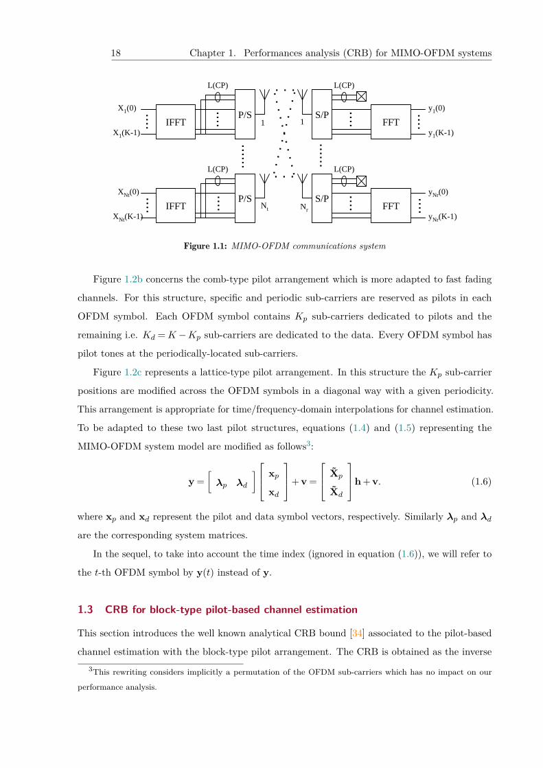
1.2 Pilot arrangements: (a) Block-type with Np pilot OFDM symbols and Nd data
OFDM symbols; (b) Comb-type with Kp pilot sub-carriers and Kd data sub-
carriers; and (c) Lattice-type with Kp pilot sub-carriers and Kd data sub-carriers
with time varying positions. . . . . . . . . . . . . . . . . . . . . . . . . . . . . . . 19
1.3 (a) Representation of function f w.r.t. the SNR, (b) BPSK Probability density
function . . . . . . . . . . . . . . . . . . . . . . . . . . . . . . . . . . . . . . . . . 26
1.4 Vector representation of the block diagonal matrix R with Ml = 3 and Mc = 2. . 30
1.5 Physical frame HT-mixed format in the IEEE 802.11n standard for 20 MHz
bandwith. . . . . . . . . . . . . . . . . . . . . . . . . . . . . . . . . . . . . . . . . 33
1.6 Pilot samples reduction scheme for block-type pilot arrangement. . . . . . . . . . 35
1.7 Normalized CRB for the block-type pilot arrangement versus SNRp(dB) . . . . 36
1.8 Normalized CRB for the block-type pilot arrangement versus Nd . . . . . . . . . 37
1.9 Normalized CRB versus the number of deleted pilot samples for the block-type
pilot arrangement . . . . . . . . . . . . . . . . . . . . . . . . . . . . . . . . . . . . 38
1.10 Number of deleted pilot samples versus Nd for the block-type pilot arrangement. 39
1.11 Pilot samples reduction scheme for comb-type and lattice-type pilot arrangements. 39
1.12 Normalized CRB versus SNRp for the comb-type pilot arrangement . . . . . . . 40
1.13 Normalized CRB versus the number of deleted pilot samples for the comb-type
pilot arrangement (serial reduction) . . . . . . . . . . . . . . . . . . . . . . . . . 41
1.14 Normalized CRB versus the number of deleted pilot samples for the comb-type
pilot arrangement (parallel reduction) . . . . . . . . . . . . . . . . . . . . . . . . 42
1.15 Normalized CRB in 10× 100 large MIMO-OFDM system versus SNRp (dB) . . 43
1.16 Normalized CRB in 10× 100 large MIMO-OFDM system versus the number of
deleted pilot samples . . . . . . . . . . . . . . . . . . . . . . . . . . . . . . . . . 43
xxii List of Figures
2.1 Illustration of pilot contamination in massive MIMO-OFDM systems where user1,2and user2,2 (resp. user1,1 and user2,1) share the same training sequence. . . . . . 47
2.2 Normalized CRB versus SNR. . . . . . . . . . . . . . . . . . . . . . . . . . . . . . 55
2.3 Gaussian CRB versus SNR with different orthogonality levels. . . . . . . . . . . . 56
2.4 Normalized CRB versus number of OFDM data symbols Nd. . . . . . . . . . . . 57
2.5 Normalized CRB versus number of BS antennas Nr. . . . . . . . . . . . . . . . . 58
2.6 Normalized CRB versus SNR with channel order overestimation . . . . . . . . . 59
3.1 SIMO-OFDM wireless communications system. . . . . . . . . . . . . . . . . . . . 64
3.2 Interception of signals. . . . . . . . . . . . . . . . . . . . . . . . . . . . . . . . . . 70
3.3 Received OFDM symbols as considered by the stations and the interceptor. . . . 71
3.4 Normalized CRB versus SNRp. . . . . . . . . . . . . . . . . . . . . . . . . . . . . 73
3.5 Normalized CRB versus Nd (SNRp = 6 dB). . . . . . . . . . . . . . . . . . . . . 73
3.6 Normalized CRB versus the number of deleted pilot samples (SNRp = 6 dB). . . 74
3.7 Number of deleted pilot samples versus Nd (SNRp = 6 dB; and CRBStochSB =
2.652× 10⁻³). . . . . . . . . . . . . . . . . . . . . . . . . . . . . . . . . . . . . . . 75
3.8 Number of deleted pilot samples versus the number Nr of receive antennas
(SNRp = 6 dB). . . . . . . . . . . . . . . . . . . . . . . . . . . . . . . . . . . . . . 75
3.9 Normalized CRB versus SNRp. . . . . . . . . . . . . . . . . . . . . . . . . . . . . 76
3.10 Normalized CRB versus Nr (SNR= 0 dB). . . . . . . . . . . . . . . . . . . . . . 77
3.11 Normalized CRB versus Nr (SNR= 5 dB). . . . . . . . . . . . . . . . . . . . . . 78
3.12 Normalized CRB versus Nr (SNR=−5 dB). . . . . . . . . . . . . . . . . . . . . 78
4.1 Normalized CRB versus SNR (with and without MCFO). . . . . . . . . . . . . . 90
4.2 Normalized CRB versus SNR (with (4× 4) MIMO-OFDM). . . . . . . . . . . . . 90
4.3 Normalized CRB versus SNR with circular Gaussian and non-circular Gaussian
signals (with (4× 4) MIMO-OFDM). . . . . . . . . . . . . . . . . . . . . . . . . . 91
4.4 Normalized CRB versus Nd (with SNR= 6 dB). . . . . . . . . . . . . . . . . . . 92
4.5 Normalized CRB for the subcarrier channel coefficients estimation. . . . . . . . . 93
4.6 Normalized CRB for the subcarriers channel coefficients estimation ((4×4) MIMO-
OFDM). . . . . . . . . . . . . . . . . . . . . . . . . . . . . . . . . . . . . . . . . . 93
5.1 LS-DF semi-blind channel estimation approach. . . . . . . . . . . . . . . . . . . . 100
5.2 Normalized CRB versus the reduced power (SNRp = 12 dB). . . . . . . . . . . . 104
List of Figures xxiii
5.3 Percentage of the transmitted pilot’s power versus the number of data OFDM
symbols Nd (SNRp = 12 dB). . . . . . . . . . . . . . . . . . . . . . . . . . . . . . 104
5.4 NRMSE of LS and LS-DF estimators versus SNRp. . . . . . . . . . . . . . . . . 105
5.5 Transmitted pilot’s power versus SNRp. . . . . . . . . . . . . . . . . . . . . . . . 106
5.6 Reduced pilot’s power versus SNRp. . . . . . . . . . . . . . . . . . . . . . . . . . 106
5.7 NRMSE of the LS-DF channel estimator versus the percentage of the reduced
pilot’s power (SNRp = 12 dB). . . . . . . . . . . . . . . . . . . . . . . . . . . . . 107
6.1 MIMO-OFDM system model using Nr parallel MISO-OFDM systems. . . . . . . 117
6.2 Simplified EM algorithm. . . . . . . . . . . . . . . . . . . . . . . . . . . . . . . . 118
6.3 Nt EM-SIMO SB channel estimation algorithm. . . . . . . . . . . . . . . . . . . . 121
6.4 EM-MIMO algorithm’s convergence: Convergence at SNR= 10dB. . . . . . . . . 124
6.5 SB EM-MIMO algorithm’s convergence: Number of iterations to converge versus
SNR. . . . . . . . . . . . . . . . . . . . . . . . . . . . . . . . . . . . . . . . . . . . 124
6.6 Performance of the proposed EM algorithm versus the number of deleted pilot
samples. . . . . . . . . . . . . . . . . . . . . . . . . . . . . . . . . . . . . . . . . . 125
6.7 EM-MIMO and S-EM algorithm’s performance versus G-EM: (a) 2× 2 MIMO-
OFDM; (b) 4× 4 MIMO-OFDM. . . . . . . . . . . . . . . . . . . . . . . . . . . . 126
6.8 NRMSE of the EM algorithms versus SNR: 2× 2 MIMO. . . . . . . . . . . . . . 127
6.9 NRMSE of the EM algorithms versus SNR: 4× 4 MIMO. . . . . . . . . . . . . . 128
6.10 NRMSE of the EM algorithms versus SNR in the underdetermined case (Nt >Nr).128
6.11 NRMSE versus the number of OFDM symbols (Nd). . . . . . . . . . . . . . . . . 129
6.12 Performance of EM-SIMO algorithm versus SNR: 2× 2 MIMO. . . . . . . . . . . 130
6.13 Performance of EM-SIMO algorithm versus SNR: 4× 4 MIMO. . . . . . . . . . . 131
7.1 NRMSE versus SNR. . . . . . . . . . . . . . . . . . . . . . . . . . . . . . . . . . 144
7.2 NRMSE versus the number of data OFDM symbols Nd (SNR= 10 dB). . . . . . 144
7.3 NRMSE versus the Size of the partitioned symbol G. . . . . . . . . . . . . . . . . 145
8.1 SISO-OFDM communications system . . . . . . . . . . . . . . . . . . . . . . . . . 150
8.2 DF semi-blind TOA estimation approach. . . . . . . . . . . . . . . . . . . . . . . 153
8.3 TOA (τ ) estimation performances versus SNR when Np=1 and Nd=8. . . . . . 154
8.4 Global channel estimation (h) performances versus SNR when Np=1 and Nd=8. 155
8.5 SER versus SNR when Np=1 and Nd=8. . . . . . . . . . . . . . . . . . . . . . . 156
xxiv List of Figures
8.6 TOA estimation performance versus the number of pilot OFDM symbols Np for
SNR=−5dB. . . . . . . . . . . . . . . . . . . . . . . . . . . . . . . . . . . . . . 156
8.7 TOA estimation performance versus the number data OFDM symbols Nd when
Np=1 and SNR=-5 dB. . . . . . . . . . . . . . . . . . . . . . . . . . . . . . . . . 157
A.1 MISO-OFDM model. . . . . . . . . . . . . . . . . . . . . . . . . . . . . . . . . . . 173
A.2 NMSE of the data versus SNRd (with and without CFO) at low CFO . . . . . . 178
A.3 Symbol error rate versus SNRd (with and without CFO) at low CFO . . . . . . 178
A.4 NMSE of the data versus SNRd (with and without CFO) at high CFO . . . . . 179
A.5 Symbol error rate versus SNRd (with and without CFO) at high CFO . . . . . . 179
A.6 NRMSE of the channel estimation versus SNR (with and without CFO). . . . . . 180
A.7 NRMSE of the channel estimate versus Np at low CFO. . . . . . . . . . . . . . . 180
A.8 NRMSE of the channel estimate versus Np at high CFO. . . . . . . . . . . . . . . 181
B.1 Modèle du système MIMO-OFDM . . . . . . . . . . . . . . . . . . . . . . . . . . 192
B.2 Organisation des séquences pilotes: (a) organisation en bloc; (b) en peigne; (c) en
réseau. . . . . . . . . . . . . . . . . . . . . . . . . . . . . . . . . . . . . . . . . . . 193
B.3 Trame physique du standard IEEE 802.11n. . . . . . . . . . . . . . . . . . . . . . 195
B.4 Réduction des pilotes . . . . . . . . . . . . . . . . . . . . . . . . . . . . . . . . . . 196
B.5 CRB normalisée en fonction du SNRp(dB) . . . . . . . . . . . . . . . . . . . . . 197
B.6 CRB normalisé en fonction du nombre des symboles OFDM donnés Nd . . . . . 198
B.7 CRB normalisée en fonction du nombre des pilotes supprimes . . . . . . . . . . . 199
B.8 Estimation semi-aveugle basée sur NCPU sous-systèmes. . . . . . . . . . . . . . . 203
B.9 Comparaison des performances d’estimation. . . . . . . . . . . . . . . . . . . . . 205
B.10 Performances en fonction de Nd. . . . . . . . . . . . . . . . . . . . . . . . . . . . 205

Abbreviations
BPSK Binary Phase Shift Keying signals
BS Base Station
CCG Circular Complex Gaussian
CFO Carrier Frequency Offset
CG Circular Gaussian
CP Cyclic Prefix
CRB Cramér-Rao Bound
CSI Channel State Information
DA Data-Aided
DFE Decision Feedback Equalizer
DFT Discrete Fourier Transform
DoA Direction-of-Arrival
EM Expectation Maximization
ESPRIT Estimation of Signal Parameters via Rotational Invariance Technique
EVD Eigenvalue Decomposition
FDD Frequency Division Duplexing
FFT Fast Fourier Transform
FIM Fisher Information Matrix
HT-LTF High Throughput Long Training Field
i.i.d. independent and identically distributed
LS Least-Squares
LS-DF Least-Squares Decision Feedback
LTE Long Term Evolution
MCFO Multiple Carrier Frequency Offset
MIMO Multiple-Input-Multiple-Output
MISO Multiple-Input-Single-Output

xxvi List of Figures
ML Maximum Likelihood
MSE Mean Squared Error
MUSIC MUltiple SIgnal Classification
NCG Non Circular Gaussian
NCRB Normalized Cramér-Rao Bound
NDA Non Data-Aided
NO Non Orthogonal
NRMSE Normalized Root Mean Square Error
OFDM Orthogonal Frequency Division Multiplexing
OMR OFDM-based Multi-hop Relaying
OP Only Pilots
PDF Probability Density Function
PR Partial Relaxation
QPSK Quadrature Phase Shift Keying signals
SB Semi-Blind
S-EM Simplified Expectation Maximization
SER Symbol Error Rate
SNR Signal-to-Noise Ratio
SIMO Single-Input-Multiple-Output
SISO Single-Input-Single-Output
SOS Second Order Statistics
SS Subspace
SVD Singular Value Decomposition
TDD Time Division Duplexing
ToA Time-of-Arrival
UAV Unmanned Aerial Vehicle
VC Virtual Carriers
w.r.t with respect to
ZC Zadoff-Chu
ZF Zero-Forcing

Notations
A, a non-bold letters are used to denote scalars
a boldface lower case letters are used for vectors
A boldface upper case letters are used for matrices
A, a a hat is used to denote an estimate
(.)T transpose
(.)∗ complex conjugate
(.)H conjugate transpose
<(.), =(.) real and imaginary parts
tr{.} trace
vec(A) operator stacking the columns of a matrix into a vector
diag(a) diagonal matrix constructed from a
diag(A) operator stacking the diagonal of a matrix into a vector
NC (µ,C) Complex Gaussian distribution with mean µ and covariance C
E [.] the expectation of [.]
Im m × m identity matrix
‖.‖2 L2 norm
⊗ Kronecker product
� Element-wise product
� Element-wise division

xxviii List of Figures
Introduction
“Creativity requires the courage to let go of certainties. ”Erich Fromm
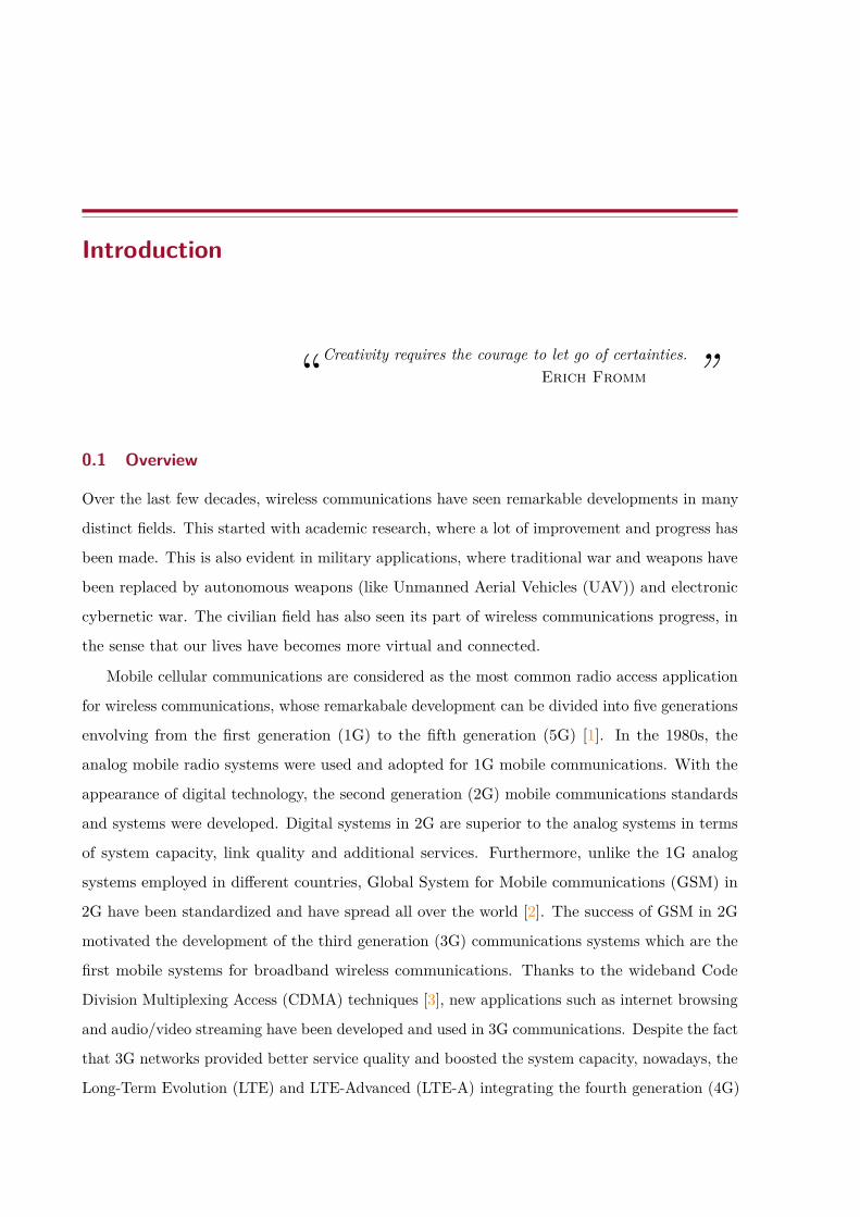
0.1 Overview
Over the last few decades, wireless communications have seen remarkable developments in many
distinct fields. This started with academic research, where a lot of improvement and progress has
been made. This is also evident in military applications, where traditional war and weapons have
been replaced by autonomous weapons (like Unmanned Aerial Vehicles (UAV)) and electronic
cybernetic war. The civilian field has also seen its part of wireless communications progress, in
the sense that our lives have becomes more virtual and connected.
Mobile cellular communications are considered as the most common radio access application
for wireless communications, whose remarkabale development can be divided into five generations
envolving from the first generation (1G) to the fifth generation (5G) [1]. In the 1980s, the
analog mobile radio systems were used and adopted for 1G mobile communications. With the
appearance of digital technology, the second generation (2G) mobile communications standards
and systems were developed. Digital systems in 2G are superior to the analog systems in terms
of system capacity, link quality and additional services. Furthermore, unlike the 1G analog
systems employed in different countries, Global System for Mobile communications (GSM) in
2G have been standardized and have spread all over the world [2]. The success of GSM in 2G
motivated the development of the third generation (3G) communications systems which are the
first mobile systems for broadband wireless communications. Thanks to the wideband Code
Division Multiplexing Access (CDMA) techniques [3], new applications such as internet browsing
and audio/video streaming have been developed and used in 3G communications. Despite the fact
that 3G networks provided better service quality and boosted the system capacity, nowadays, the
Long-Term Evolution (LTE) and LTE-Advanced (LTE-A) integrating the fourth generation (4G)
2 Chapter 0. Introduction
are deployed [4]. The flagship technologies of 4G systems are Multiple-Input Multiple-Output
(MIMO) and Orthogonal Frequency Division Multiplexing (OFDM) [4].
The use of multiple antennas at the transmitter or at the receiver or at both (MIMO), can
substantially increase data throughput and the reliability of radio communications [5, 6]. MIMO
communications systems offer additional degrees of freedom provided by the spatial dimension,
which can be exploited to either simultaneously transmit independent data-streams (spatial
multiplexing) thereby increasing the data-rate, or multiplicative transmission of single data
stream (spatial diversity) to increase the system reliability [5, 7].
On the other hand, multicarrier modulation techniques (OFDM) make the system robust
against frequency-selective fading channels by converting the overall channel into a number of
parallel flat fading channels, which helps to achieve high data rate transmission [8, 9]. Besides,
the OFDM eliminates the inter-symbol interference and inter-carrier interference thanks to
the use of a cyclic prefix and an orthogonal transform. Moreover, the combination of MIMO
technology with OFDM called MIMO-OFDM systems, has enabled high speed data transmission
and broadband multimedia services over wireless links [8, 10].
Another important development in wireless communications, apart from mobile cellular
networks, is the Wireless Local Area Network (WLAN) [11]. The Institute of Electrical and
Electronics Engineers (IEEE) 802.11 based WLAN is the most broadly deployed WLAN tech-
nology. Nowadays, WLAN services are widely used not only at homes and offices but also at
restaurants, libraries and many other public services and locations. The standardization process
of IEEE 802.11 based WLAN originated in the 1990s, and since it has evolved several times
in order to increase its throughput, enhance its security and compatibility leading to several
versions 802.11 b/a/g/n/ac [12, 13]. In 2009, the IEEE 802.11n standardization process was
completed and adopted in Wi-Fi (WIreless FIdelity) transmissions offering high data rate, which
primarily results from the use of multi-antennas (MIMO) and multi-subcarriers modulation
(OFDM) techniques (MIMO-OFDM systems) [10].
The unprecedented usage of smart phone, tablets, super-phones etc., equipped with data-
intensive applications like video streaming, graphics heavy social media interfaces and real time
navigation services, has called for revolutionary changes the current 4G to the next generation
wireless systems. Although 4G systems could be loaded with much more services, real time
functionality and data than previous systems, there is still a dramatic gap between the people’s
practical requirements and what can be offered by the 4G technologies. To meet the strong
demands from the explosive growth of cellular users and the associated potential services, currently
0.2. Channel estimation 3
the fifth generation (5G) standard is under extensive investigation and discussion. With speeds
of up to 10 gigabits per second, 5G is set to be as much as 100 times faster than 4G [14]. The
two prime technologies for sustaining the requirements of 5G are the use of millimeter wave
(mmWave) and massive MIMO systems [15].
With a higher number of Base Station (BS) antennas, around few hundreds, compared to the
classical MIMO systems (8 antennas for the LTE), massive MIMO or large-scale MIMO systems
can achieve huge gains in spectral and energy efficiencies [14, 16, 17]. Massive MIMO systems
overcome several limitations of the traditional MIMO systems such as security, robustness and
throughput rate [18, 15]. It has been demonstrated that massive MIMO systems hold greater
promises of boosting system throughput by 10 times or more by simultaneously serving tens of
users in the same time-frequency resource [18]. So that, both throughput and system capacity
will be highly enhanced in order to satisfy the increasing amount of data exchange and demand
for quality of service for the future cellular networks.
To fully realize the potentials of the aforementioned technologies, the knowledge of Channel
State Information (CSI) is indispensable. To improve the system performance, it is essential that
CSI is available at both transmitter and the receiver. The knowledge of CSI is used for coherent
detection of the transmitted signals at the receiver side. On transmitter side, CSI, is crucial to
design effective precoding schemes for inter-user interference cancellation. However, the perfect
knowledge of CSI is not available in practice, therefore it has to be estimated. This thesis is
concerned with efficient and low complexity channel estimation algorithms for MIMO-OFDM
and massive MIMO-OFDM systems.
0.2 Channel estimation
The well conduct of wireless communications system’s objective depends largely upon the
availability of the knowledge of its environment. The propagation environment refers to the
communications channel which provides the connection between the transmitter and the receiver.
Thus, channel estimation is of paramount importance to equalization and symbol detection.
Several channel models and channel estimation approaches have been developed in literature
depending on their applications and on the selected standard. The estimation approaches can be
divided into three main classes as follows:
4 Chapter 0. Introduction
0.2.1 Pilot-based channel estimation
Typically, channel estimation is performed by inserting, in the transmitted frame, a training
sequences (called pilots) known a priori at the receiver, according to a known arrangement
pattern in the frame (block, comb or lattice) [19, 20, 21]. At the receiver side then, by observing
the output in correspondence of the pilot symbols, it is possible to estimate the channel. This
knowledge is then fed into the detection process, to allow optimal estimation of the data. This
approach (pilot-based channel estimation), is the most commonly used in communications
standards [22, 13], for its low computational complexity and robustness. Its drawback consists
of the fact that the pilot symbols do not carry useful information, therefore they represent a
bandwidth waste. Moreover, most of the observations (those related to the unknown symbols)
are discarded in the estimation process, thus representing a missed opportunity to enhance the
accuracy of the channel estimate.
0.2.2 Blind channel estimation
Unlike pilot-based channel estimation, blind channel estimation methods are fully based on
the statistical properties of the unknown transmitted symbols (i.e. no pilots are transmitted)
[23, 24, 25]. This approach reduces the overhead but needs a large number of data symbols for
statistical properties and powerful algorithms. Moreover, pilot-based approaches give better
performance at low computational complexity than the blind ones.
0.2.3 Semi-blind channel estimation
Each channel estimation class has its own benefits and drawbacks. Generally, the first class
(i.e. pilot-based channel estimator) provides a more accurate channel estimation than the blind
estimation class. However, the second class, in most cases, increases the spectral efficiency
compared to the first one. Therefore, it would be advantageous to retain the benefits of the two
techniques through the use of Semi-Blind (SB) estimation methods [26, 27, 28, 29] which exploit
both data and pilots to achieve the desired channel identification.
0.3 Thesis purpose and manuscript organization
The number of channel parameters to be estimated in MIMO and massive MIMO systems
increases with the system dimension (i.e. number of transmitters and receivers). Hence, the
pilot-based channel estimation techniques have a severe limitation due to the required longer size
of the pilot sequences. However, the transmission of a longer pilot sequence is not desirable in a
0.3. Thesis purpose and manuscript organization 5
communications system, since they do not carry useful information and represent a bandwidth
waste. Furthermore, the wireless spectral resource is becoming more and more scarce and precious
due to the limitation, by nature, of the spectrum allocated to wireless communications services.
In this context, this thesis proposes to use semi-blind channel estimation approach, which
exploits all the transmitted signal’s information (i.e. pilots and unknown data), to overcome
the above-mentioned resource problems. Instead of using semi-blind estimation to improve
the channel estimation performances, herein, we propose to keep the same performances of
pilot-based estimation but reducing the pilot sequences. However, due to the complexity of
the blind estimation part, semi-blind estimation increases the receiver complexity compared to
pilot-based methods.
Thanks to the channel reciprocity property and according to the widely accepted Time
Division Duplexing (TDD) protocol used in MIMO-OFDM and massive MIMO-OFDM systems
[30, 31], CSI is estimated only during the uplink transmission (at the Base Station (BS)) then
transmitted to the different users for channel equalization in the downlink. Hence, the ’semi-blind’
complex channel estimation task could be easily achieved by the powerful calculator at the BS.
The study of the semi-blind solution, proposed in this thesis, is divided into two principal
parts. The first part concerns the performance analysis of semi-blind channel estimation methods.
The second part is dedicated to the derivation of semi-blind channel estimation algorithms.
0.3.1 Part I - Channel estimation limit Performance analysis
The first part of thesis focuses on the performance bounds analysis of the semi-blind and
pilot-based channel estimation methods in the context of MIMO-OFDM and massive MIMO-
OFDM systems. To obtain general comparative results independent from specific algorithms or
estimation methods, this analysis is carried out using the estimation performance limits given by
the Cramér-Roa-Bound (CRB).
The first contribution of this thesis is to quantify the rate of reduction of the transmitted
pilots using semi-blind channel estimation while ensuring the same pilot-based channel estimation
performance. Chapter 1 introduces the CRB derivations for semi-blind and pilot-based channel
estimation approaches [32]. This performance analysis is performed for different data models
(Circular Gaussian (CG), Non Circular Gaussian (NCG), Binary/Quadratic Phase Shift Keying
(BPSK/QPSK)) and different pilot design schemes such as: block-pilot type arrangement,
comb-type pilot arrangement and lattice-type arrangement. For the BPSK/QPSK case, a new
approximation of the CRB is proposed to avoid heavy numerical integral calculations. Moreover,
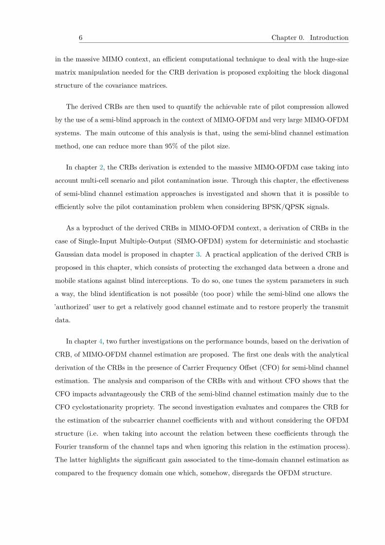
6 Chapter 0. Introduction
in the massive MIMO context, an efficient computational technique to deal with the huge-size
matrix manipulation needed for the CRB derivation is proposed exploiting the block diagonal
structure of the covariance matrices.
The derived CRBs are then used to quantify the achievable rate of pilot compression allowed
by the use of a semi-blind approach in the context of MIMO-OFDM and very large MIMO-OFDM
systems. The main outcome of this analysis is that, using the semi-blind channel estimation
method, one can reduce more than 95% of the pilot size.
In chapter 2, the CRBs derivation is extended to the massive MIMO-OFDM case taking into
account multi-cell scenario and pilot contamination issue. Through this chapter, the effectiveness
of semi-blind channel estimation approaches is investigated and shown that it is possible to
efficiently solve the pilot contamination problem when considering BPSK/QPSK signals.
As a byproduct of the derived CRBs in MIMO-OFDM context, a derivation of CRBs in the
case of Single-Input Multiple-Output (SIMO-OFDM) system for deterministic and stochastic
Gaussian data model is proposed in chapter 3. A practical application of the derived CRB is
proposed in this chapter, which consists of protecting the exchanged data between a drone and
mobile stations against blind interceptions. To do so, one tunes the system parameters in such
a way, the blind identification is not possible (too poor) while the semi-blind one allows the
’authorized’ user to get a relatively good channel estimate and to restore properly the transmit
data.
In chapter 4, two further investigations on the performance bounds, based on the derivation of
CRB, of MIMO-OFDM channel estimation are proposed. The first one deals with the analytical
derivation of the CRBs in the presence of Carrier Frequency Offset (CFO) for semi-blind channel
estimation. The analysis and comparison of the CRBs with and without CFO shows that the
CFO impacts advantageously the CRB of the semi-blind channel estimation mainly due to the
CFO cyclostationarity propriety. The second investigation evaluates and compares the CRB for
the estimation of the subcarrier channel coefficients with and without considering the OFDM
structure (i.e. when taking into account the relation between these coefficients through the
Fourier transform of the channel taps and when ignoring this relation in the estimation process).
The latter highlights the significant gain associated to the time-domain channel estimation as
compared to the frequency domain one which, somehow, disregards the OFDM structure.
0.3. Thesis purpose and manuscript organization 7
0.3.2 Part II - Semi-blind channel estimation approaches
The second part of the thesis, once the theoretical limit semi-blind channel estimation performance
based on the CRB is performed, proposes four semi-blind channel estimation algorithms. The
major requirements of the proposed algorithms are: (i) low complexity, (ii) good performance to
reach the CRB at moderate or high SNR.
The first considered estimator (LS-DF) is quite cheap as it uses a simple least squares (LS)
estimation together with a decision feedback (DF) where the estimated data is re-injected to the
channel estimation stage to enhance the estimation performance. In particular, we have taken
advantage of this estimator to quantify the overall power consumption gain (about 66%) due to
the pilot-size reduction associated to this semi-blind approach.
The second semi-blind channel estimator, proposed in this thesis, is based on the Maximum
Likelihood (ML) technique. The latter is known to be powerful but also too expensive. Hence,
for the ML cost optimization, new Expectation Maximization (EM) algorithms for the channel
taps estimation are introduced in chapter 6. A main focus of chapter 6 is the reduction of the
numerical complexity while preserving at best the channel estimation quality. To do so, three
approximation/simplification approaches are proposed after introducing the exact version of the
EM-MIMO algorithm, where the MIMO-OFDM system is treated as one block to estimate the
overall channel vector through an iterative process.
The first approach consists of decomposing the MIMO-OFDM system into parallel MISO-
OFDM systems. The EM algorithm is then applied in order to estimate the MIMO channel in
a parallel way. The second approach takes advantage of the semi-blind context to reduce the
EM cost from exponential to linear complexity by reducing the size of the search space. Finally,
the last proposed approach uses a parallel interference cancellation technique to decompose the
MIMO-OFDM system into several SIMO-OFDM systems. The latter are identified in a parallel
scheme and with a reduced complexity.
In between the cheap LS-DF and the relatively expensive EM method, we have considered
some intermediate solutions. Hence, in chapter 7, an efficient semi-blind subspace channel
estimation, in the case of MIMO-OFDM system, is proposed for which an identifiability result is
first established for the subspace based criterion. The proposed algorithm adopts the MIMO-
OFDM system model without cyclic prefix and takes advantage of the circulant property of the
channel matrix to achieve lower computational complexity and to accelerate the algorithm’s
convergence by generating a group of sub-vectors from each received OFDM symbol.
For the practical case of specular channel model, chapter 8 proposes a parametric approach
8 Chapter 0. Introduction
based on the Time-Of-Arrival (TOA) estimation using subspace methods for SISO-OFDM
systems. At first the TOA estimation is achieved using only one OFDM pilot. The latter is
used to generate a group of sub-vectors, with an appropriate windowing, to which one can apply
subspace methods to estimate the TOA. Then a refining step based on the incorporation of the
unknown data on the channel estimation process is considered. The semi-blind TOA estimation
is done using a Decision Feedback process (as detailed in chapter 5), where a first estimate of the
transmitted data is used with the existing pilot to enhance the TOA estimation performance.
At the end, in appendix A, we present joint channel and CFO estimation in a Multiple Input
Single Output (MISO) communications system. This problem arises in OFDM based multi-relay
transmission protocols such as the geo-routing one proposed by A. Bader et al. in 2012. Indeed,
the outstanding performance of this multi-hop relaying scheme relies heavily on the channel
and CFO estimation quality at the physical layer. In this work, two approaches are considered:
The first is based on estimating the overall channel (including the CFO) as a time-varying one
using an adaptive scheme under the assumption of small or moderate CFOs while the second
one performs separately, the channel and CFO parameters estimation based on the considered
data model.
0.4 List of publications
Based on the research work presented in this thesis, some papers have been published or submitted
for publication to journals and conferences as following:
Journal papers:
1) Ladaycia, A. Mokraoui, K. Abed-Meraim, and A. Belouchrani, "Performance bounds
analysis for semi-blind channel estimation in MIMO-OFDM communications systems,"
IEEE Transactions on Wireless Communications, vol. 16, no. 9, pp. 5925-5938, Sep. 2017.
2) A. Ladaycia, A. Belouchrani, K. Abed-Meraim and A. Mokraoui, "Semi-Blind MIMO-
OFDM Channel Estimation using EM-like Techniques," IEEE Transactions on Wireless
Communications, May. 2019. (submitted).
3) O. Rekik, A. Ladaycia, K. Abed-Meraim, and A. Mokraoui, "Performance Bounds Analysis
for Semi-Blind Channel Estimation with Pilot Contamination in Massive MIMO-OFDM
Systems," IET Communications, May. 2019. (submitted).
0.4. List of publications 9
Conference Papers:
1) A. Ladaycia, A. Mokraoui, K. Abed-Meraim, and A. Belouchrani, "What semi-blind channel
estimation brings in terms of throughput gain?" in 2016 10th ICSPCS, Dec. 2016, pp. 1-6,
Gold Coast, Australia.
2) A. Ladaycia, A. Belouchrani, K. Abed-Meraim, and A. Mokraoui, "Parameter optimization
for defeating blind interception in drone protection," in 2017 Seminar on Detection Systems
Architectures and Technologies (DAT), Feb. 2017, pp. 1-6, Alger, Algeria.
3) A. Ladaycia, A. Mokraoui, K. Abed-Meraim, and A. Belouchrani, "Further investigations on
the performance bounds of MIMO-OFDM channel estimation," in The 13th International
Wireless Communications and Mobile Computing Conference (IWCMC 2017), June 2017,
pp. 223-228, Valance, Spain.
4) A. Ladaycia, A. Mokraoui, K. Abed-Meraim, and A. Belouchrani, "Toward green commu-
nications using semi-blind channel estimation," in 2017 25th European Signal Processing
Conference (EUSIPCO), Aug. 2017, pp. 2254-2258, Kos, Greece.
5) A. Ladaycia, K. Abed-Meraim, A. Bader, and M.S. Alouini, "CFO and channel estimation for
MISO-OFDM systems," in 2017 25th European Signal Processing Conference (EUSIPCO),
Aug. 2017, pp. 2264-2268, Kos, Greece.
6) A. Ladaycia, A. Mokraoui, K. Abed-Meraim, and A. Belouchrani, "Contributions à
l’estimation semi-aveugle des canaux MIMO-OFDM," in GRETSI 2017, Sep. 2017, Nice,
France.
7) A. Ladaycia, A. Belouchrani, K. Abed-Meraim, and A. Mokraoui, "EM-based semi-blind
MIMO-OFDM channel estimation," in 2018 IEEE International Conference on Acoustics,
Speech and Signal Processing (ICASSP2018), Apr. 2018, Alberta, Canada.
8) A. Ladaycia, K. Abed-Meraim, A. Mokraoui, and A. Belouchrani, "Efficient Semi-Blind
Subspace Channel Estimation for MIMO-OFDM System," in 2018 26th European Signal
Processing Conference (EUSIPCO), Sep. 2018, Rome, Italy.
9) O. Rekik, A. Ladaycia, K. Abed-Meraim, and A. Mokraoui, "Performance Bounds Analysis
for Semi-Blind Channel Estimation with Pilot Contamination in Massive MIMO-OFDM
Systems," in 2018 26th European Signal Processing Conference (EUSIPCO), Sep. 2018,
Rome, Italy.
10 Chapter 0. Introduction
10) A. Ladaycia, M.Pesavento, A. Mokraoui, K. Abed-Meraim, and A. Belouchrani, "Decision
feedback semi-blind estimation algorithm for specular OFDM channels," in 2019 IEEE
International Conference on Acoustics, Speech and Signal Processing (ICASSP2019).
11) A. Ladaycia, A. Belouchrani, K. Abed-Meraim, and A. Mokraoui, "Efficient EM-algorithm
for MIMO-OFDM semi blind channel estimation," in 2019 Conference on Electrical Engi-
neering (CEE2019).
12) O. Rekik, A. Ladaycia, K. Abed-Meraim, and A. Mokraoui, "Semi-Blind Source Separation
based on Multi-Modulus Criterion: Application for Pilot Contamination Mitigation in
Massive MIMO Systems," in The 19th ISCIT, Ho Chi Minh City, Vietnam.
13) A. Ladaycia, A. Belouchrani, K. Abed-Meraim, and A. Mokraoui, "Algorithme EM efficace
pour l’estimation semi-aveugle de canal MIMO-OFDM," in GRETSI 2019.
Part IPerformance bounds analysis for channel estimation using
CRB
11


1
Ch
ap
te
r
Analysis of channel estimation performances limits of MIMO-
OFDM communications systems
Knowledge is the conformity
of the object and the intellect.
Averroes (Ibn Rochd)
The main objective of this chapter is to quantify the rate of reduction of the overhead due
to the use of a semi-blind channel estimation. Different data models and different pilot design
schemes have been considered in this study. By using the Cramér Rao Bound (CRB) tool, the
estimation error variance bounds of the pilot-based and semi-blind based channel estimators for a
MIMO-OFDM system are compared. In particular, for large MIMO-OFDM systems, a direct
computation of the CRB is prohibitive and hence a dedicated numerical technique for its fast
computation has been developed. The most important result is that, thanks to the semi-blind
approach, one can skip about 95% of the pilot samples without affecting the channel estimation
quality as shown in1[32].
Abstract
1 [32] Ladaycia, A. Mokraoui, K. Abed-Meraim, and A. Belouchrani, "Performance bounds analysis for semi-blind
channel estimation in MIMO-OFDM communications systems," IEEE Transactions on Wireless Communications,
vol. 16, no. 9, pp. 5925-5938, Sep. 2017.
14 Chapter 1. Performances analysis (CRB) for MIMO-OFDM systems
Chapter content1.1 Introduction . . . . . . . . . . . . . . . . . . . . . . . . . . . . . . . . . . . . . 15
1.2 Mutli-carrier communications systems: main concepts . . . . . . . . . . . . . . 16
1.2.1 MIMO-OFDM system model . . . . . . . . . . . . . . . . . . . . . . . . 16
1.2.2 Main pilot arrangement patterns . . . . . . . . . . . . . . . . . . . . . . 17
1.3 CRB for block-type pilot-based channel estimation . . . . . . . . . . . . . . . . 18
1.4 CRB for semi-blind channel estimation with block-type pilot arrangement . . . 20
1.4.1 Circular Gaussian data model . . . . . . . . . . . . . . . . . . . . . . . . 21
1.4.2 Non-Circular Gaussian data model . . . . . . . . . . . . . . . . . . . . . 23
1.4.3 BPSK and QPSK data model . . . . . . . . . . . . . . . . . . . . . . . . 24
1.4.3.1 SIMO-OFDM system . . . . . . . . . . . . . . . . . . . . . . . 24
1.4.3.2 MIMO-OFDM system . . . . . . . . . . . . . . . . . . . . . . . 27
1.5 CRB for semi-blind channel estimation with comb-type and lattice-type pilot
arrangements . . . . . . . . . . . . . . . . . . . . . . . . . . . . . . . . . . . . . 28
1.5.1 Circular Gaussian data model . . . . . . . . . . . . . . . . . . . . . . . . 28
1.5.2 Non-Circular Gaussian data model . . . . . . . . . . . . . . . . . . . . . 29
1.5.3 BPSK and QPSK data model . . . . . . . . . . . . . . . . . . . . . . . . 29
1.6 Computational issue in large MIMO-OFDM communications systems . . . . . 29
1.6.1 Vector representation of a block diagonal matrix . . . . . . . . . . . . . 30
1.6.2 Fast computational matrix product . . . . . . . . . . . . . . . . . . . . . 30
1.6.3 Iterative matrix inversion algorithm . . . . . . . . . . . . . . . . . . . . 31
1.7 Semi-blind channel estimation performance bounds analysis . . . . . . . . . . . 32
1.7.1 (4× 4) MIMO-OFDM system . . . . . . . . . . . . . . . . . . . . . . . . 32
1.7.1.1 Block-type pilot arrangement . . . . . . . . . . . . . . . . . . . 34
1.7.1.2 Comb-type and lattice pilot arrangement . . . . . . . . . . . . 35
1.7.2 Large MIMO-OFDM system . . . . . . . . . . . . . . . . . . . . . . . . 36
1.8 Discussions and concluding remarks . . . . . . . . . . . . . . . . . . . . . . . . 38
1.1. Introduction 15
1.1 Introduction
The combining of the Multiple-Input Multiple-Output (MIMO) technology with the Orthogonal
Frequency Division Multiplexing (OFDM) (i.e. MIMO-OFDM) is widely deployed in wireless
communications systems as in 802.11n wireless network [22], LTE and LTE-A [4]. Indeed, the use
of MIMO-OFDM enhances the channel capacity and improves the communications reliability. In
particular, it has been demonstrated in [14, 16], that thanks to the deployment of a large number
of antennas in the base stations, the system can achieve high data throughput and provide very
high spectral efficiency.
Using multicarrier modulation techniques (OFDM in this chapter) makes the system robust
against frequency-selective fading channels by converting the overall channel into a number of
parallel flat fading channels, which helps to achieve high data rate transmission [9]. Moreover,
the OFDM eliminates the inter-symbol interference and inter-carrier interference thanks to the
use of a cyclic prefix and an orthogonal transform. In such a system, channel estimation remains
a current concern since the overall performance depends strongly on it, particularly for large
MIMO systems where the channel state information becomes more challenging.
This chapter is dedicated to the comparative performance bounds analysis of the semi-blind
channel estimation and the data-aided approaches in the context of MIMO-OFDM systems. To
obtain general comparative results independent from specific algorithms or estimation methods,
this analysis is conducted using the estimation performance limits given by the CRB2. Therefore,
we begin by providing several CRB derivations for the different data models (Circular Gaussian
(CG), Non Circular Gaussian (NCG), Binary/Quadratic Phase Shift Keying (BPSK/QPSK))
and different pilot design schemes (block, comb and lattice). For the particular case of large
dimensional MIMO systems, we exploited the block diagonal structure of the covariance matrices
to develop a fast numerical technique that avoids the prohibitive cost and the out of memory
problems (due to the large matrix sizes) of the CRB computation. Moreover, for the BPSK/QPSK
case, a realistic approximation of the CRB is introduced to avoid heavy numerical integral
calculations. After computing all the needed CRBs, we use them to compare the performance of
the semi-blind and pilot based approaches. It is well known that semi-blind techniques can help
reduce the pilot size or improve the estimation quality [35]. However, to the best of our knowledge,
this is the first study that thoroughly quantifies the achievable rate of pilot compression allowed
by the use of a semi-blind approach in the context of MIMO-OFDM. A main outcome of this
2Note that the considered performance bounds are tight (i.e. they are reachable), as shown in [33, 34], and
hence their use for the considered communications system analysis and design is effective.
16 Chapter 1. Performances analysis (CRB) for MIMO-OFDM systems
analysis is that it highlights the fact that, by resorting to the semi-blind estimation, one can
get rid of most of the pilot samples without affecting the channel identification quality. Also
an important by-product of this study is the possibility to easily design semi-orthogonal pilot
sequences in the large dimensional MIMO case thanks to their significant shortening.
This chapter is organized as follows. Section 1.2 introduces the basic concepts and data
models of the MIMO-OFDM system. Section 1.3 briefly introduces the well known pilot-based
channel estimation CRB while section 1.4 derives the analytical expressions of the semi-blind
CRBs when block-type pilot arrangement is considered. Section 1.5 investigates the CRB for
semi-blind channel estimation for comb-type and lattice-type pilots arrangement. The large
MIMO computational issue is considered in section 1.6, where a new vector representation and
treatment for the fast manipulation of block diagonal matrices are proposed. Section 1.7 analyzes
the throughput gain of the semi-blind channel estimation as compared to pilot-based channel
estimation. Finally, discussions and concluding remarks are drawn in section 1.8.
1.2 Mutli-carrier communications systems: main concepts
This section first introduces the MIMO-OFDM wireless communications scheme represented by
its mathematical model. Given the context of this chapter related to channel estimation, this
section also provides the commonly used pilot arrangement patterns available in the literature or
already specified by communications standards.
1.2.1 MIMO-OFDM system model
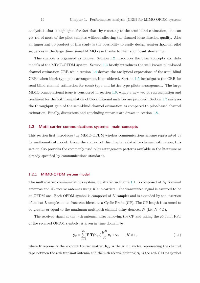
The multi-carrier communications system, illustrated in Figure 1.1, is composed of Nt transmit
antennas and Nr receive antennas using K sub-carriers. The transmitted signal is assumed to be
an OFDM one. Each OFDM symbol is composed of K samples and is extended by the insertion
of its last L samples in its front considered as a Cyclic Prefix (CP). The CP length is assumed to
be greater or equal to the maximum multipath channel delay denoted N (i.e. N ≤ L).
The received signal at the r-th antenna, after removing the CP and taking the K-point FFT
of the received OFDM symbols, is given in time domain by:
yr =Nt∑i=1
F T(hi,r)FH
Kxi + vr K × 1, (1.1)
where F represents the K-point Fourier matrix; hi,r is the N × 1 vector representing the channel
taps between the i-th transmit antenna and the r-th receive antenna; xi is the i-th OFDM symbol
1.2. Mutli-carrier communications systems: main concepts 17
of length K; and T(hi,r) is a circulant matrix. vr is assumed to be an additive white Circular
Gaussian (CG) noise satisfying E[vr(k)vr(i)H
]= σ2
vIKδki; (.)H being the Hermitian operator;
σ2v the noise variance; IK the identity matrix of size K ×K and δki the Dirac operator.
The eigenvalue decomposition of the circulant matrix T(hi,r) leads to:
T(hi,r) = FH
Kdiag{Whi,r}F, (1.2)
where W is a matrix containing the N first columns of F and diag is the diagonal matrix
composed by its vector argument. Finally equation (1.1) becomes:
yr =Nt∑i=1
diag{Whi,r}xi + vr. (1.3)
This equation can be extended to the Nr receive antennas as follows:
y = λx + v, (1.4)
where y =[yT1 · · ·yTNr
]T; x =
[xT1 · · ·xTNt
]T; v =
[vT1 · · ·vTNr
]Twithv ∼ NC
(0,σ2
vINrK); and
λ= [λ1 · · ·λNt ] with λi =[λi,1 · · ·λi,Nr
]T where λi,r = diag{Whi,r} .
Next sections address the analytical CRB derivations. In order to facilitate their calculations,
equation (1.4) is rewritten in a most appropriate form and some notations are introduced:
h =[hT1 · · ·hTNr
]Tis a vector of size NrNtN × 1 (where hr =
[hT1,r · · ·hTNt,r
]T); XDi = diag{xi}
is a diagonal matrix of size K×K; X =[XD1W · · ·XDNt
W]of size K×NNt; and X = INr ⊗X
a matrix of size NrK ×NNtNr and ⊗ refers to the Kronecker product. According to these
notations, equation (1.4) is rewritten as follows:
y = Xh + v. (1.5)
1.2.2 Main pilot arrangement patterns
Most wireless communications standards specify the insertion of training sequences (i.e. preamble)
in the physical frame. These sequences are considered as OFDM pilot symbols and are known
both by the transmitter and receiver (see e.g. [22]). Therefore the receiver exploits these pilots to
estimate the propagation channel. These pilots can be arranged in different ways in the physical
frame. This chapter focuses on three pilot patterns mainly adopted in communications systems.
They are described in what follows.
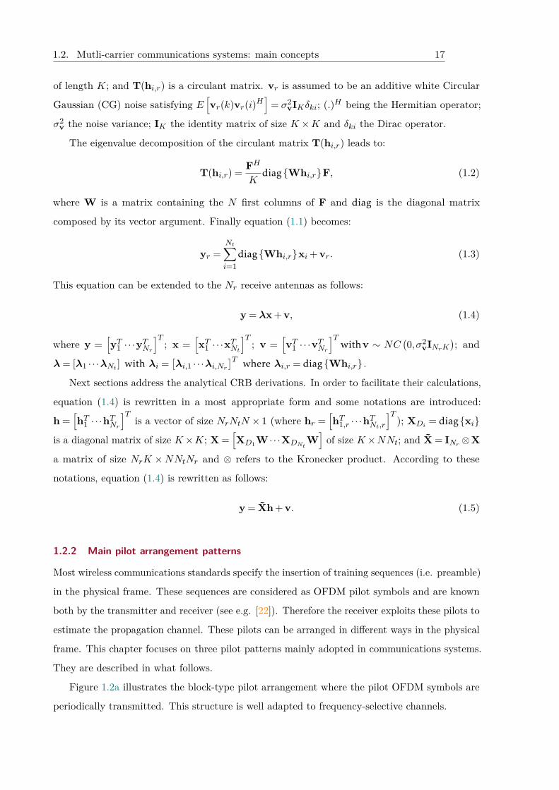
Figure 1.2a illustrates the block-type pilot arrangement where the pilot OFDM symbols are
periodically transmitted. This structure is well adapted to frequency-selective channels.
18 Chapter 1. Performances analysis (CRB) for MIMO-OFDM systems
P/SIFFT
L(CP)
S/PFFT
L(CP)
P/SIFFT
L(CP)
S/PFFT
L(CP)
Nt Nr
1 1
X1 (0)
X1 (K-1)
XNt (0)
XNt (K-1)
y1 (0)
y1 (K-1)
yNr (0)
yNr (K-1)
........
....
.... ........
....
......
......
....
. . .
. . .
. . . . . . . . . . .. . . . . . . . . . .
Figure 1.1: MIMO-OFDM communications system
Figure 1.2b concerns the comb-type pilot arrangement which is more adapted to fast fading
channels. For this structure, specific and periodic sub-carriers are reserved as pilots in each
OFDM symbol. Each OFDM symbol contains Kp sub-carriers dedicated to pilots and the
remaining i.e. Kd =K −Kp sub-carriers are dedicated to the data. Every OFDM symbol has
pilot tones at the periodically-located sub-carriers.
Figure 1.2c represents a lattice-type pilot arrangement. In this structure the Kp sub-carrier
positions are modified across the OFDM symbols in a diagonal way with a given periodicity.
This arrangement is appropriate for time/frequency-domain interpolations for channel estimation.
To be adapted to these two last pilot structures, equations (1.4) and (1.5) representing the
MIMO-OFDM system model are modified as follows3:
y =[λp λd
] xpxd
+ v =
Xp
Xd
h + v. (1.6)
where xp and xd represent the pilot and data symbol vectors, respectively. Similarly λp and λdare the corresponding system matrices.
In the sequel, to take into account the time index (ignored in equation (1.6)), we will refer to
the t-th OFDM symbol by y(t) instead of y.
1.3 CRB for block-type pilot-based channel estimation
This section introduces the well known analytical CRB bound [34] associated to the pilot-based
channel estimation with the block-type pilot arrangement. The CRB is obtained as the inverse3This rewriting considers implicitly a permutation of the OFDM sub-carriers which has no impact on our
performance analysis.
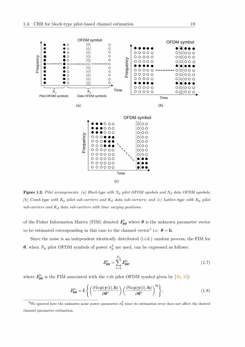
1.3. CRB for block-type pilot-based channel estimation 19
Pilot OFDM symbols Data OFDM symbols
Freq
uenc
y
Time
…....... …........ …........
OFDM symbol
pN dN
(a)
Time
Freq
uenc
y
…........
OFDM symbol
(b)
Time
Freq
uenc
y
OFDM symbol
(c)
Figure 1.2: Pilot arrangements: (a) Block-type with Np pilot OFDM symbols and Nd data OFDM symbols;
(b) Comb-type with Kp pilot sub-carriers and Kd data sub-carriers; and (c) Lattice-type with Kp pilot
sub-carriers and Kd data sub-carriers with time varying positions.
of the Fisher Information Matrix (FIM) denoted Jpθθ where θ is the unknown parameter vector
to be estimated corresponding in this case to the channel vector4 i.e. θ = h.
Since the noise is an independent identically distributed (i.i.d.) random process, the FIM for
θ, when Np pilot OFDM symbols of power σ2p are used, can be expressed as follows:
Jpθθ =Np∑i=1
Jpiθθ, (1.7)
where Jpiθθ is the FIM associated with the i-th pilot OFDM symbol given by [36, 35]:
Jpiθθ = E
{(∂ lnp(y(i),h)
∂θ∗
)(∂ lnp(y(i),h)
∂θ∗
)H}, (1.8)
4We ignored here the unknown noise power parameter σ2v since its estimation error does not affect the desired
channel parameter estimation.
20 Chapter 1. Performances analysis (CRB) for MIMO-OFDM systems
where E(.) is the expectation operator; and p(y(i),h) is the probability density function of the
received signal given h.
According to the complex derivation ∂∂θ∗ = 1
2
(∂∂α + j ∂
∂β
)for θ = α+ jβ, the derivation of
equation (1.8) is then expressed by:
Jpiθθ = X(i)HX(i)σ2
v. (1.9)
Therefore the lower bound, denoted CRBOP (OP stands for ’Only Pilot’), of the unbiased MSE
(Mean Square Error) channel estimation when only pilots are exploited to estimate the channel
is given by(
Xp =[X(1)T · · ·X(Np)
T]T)
:
CRBOP = σ2vtr
{(XHp Xp
)−1}. (1.10)
The best performance is reached when the pilot sequences are orthogonal, as designed in
[22, 37], in which case, XHp Xp is simplified as follows XH
p Xp =Npσ2pINtNrN .
1.4 CRB for semi-blind channel estimation with block-type pilot arrangement
This section addresses the derivation of the CRB analytical expression for semi-blind channel
estimation when the pilot arrangement pattern is assumed to be a block-type one. In this
context the CRB computation relies not only on the known transmitted pilot OFDM symbols
(i.e. training sequences) but also on the unknown transmitted OFDM symbols.
To derive the CRB expression, three cases have been considered depending on whether the
transmitted data is stochastic Circular Gaussian (CG)5, stochastic Non-Circular Gaussian (NCG)
or i.i.d. BPSK/QPSK signals. Data symbols and noise are assumed to be both i.i.d. and
independent. Therefore the FIM, denoted Jθθ, is divided into two parts:
Jθθ = Jpθθ + Jdθθ, (1.11)
where Jpθθ is related to the FIM associated with known pilots (given by (1.7) and (1.9)), and Jdθθconcerns the FIM dedicated to the unknown data. Depending on the data model, the vector of
unknown parameters θ is composed of complex and real parameters (i.e θc and θr) as follows:
θ =[θTc (θ∗c)
T θTr
]T, (1.12)
5We adopt here the Gaussian CRB as it is the most tractable one as well as the least favorable distribution
case [38].
1.4. CRB for semi-blind channel estimation with block-type pilot arrangement 21
where θc represents the complex-valued6 channel taps while θr concerns the unknown data and
noise parameters. The FIM for a complex parameter θ is derived in [40, 39]. With respect to
this new parameter vector, the previous pilot-based FIM matrix is expressed as:
Jpθθ =
XHp Xp
σ2v
0 0
0 XHp Xp
σ2v
0
0 0 Jpθrθr
, (1.13)
where Jpθrθr will be specified later for each considered data model.
Before proceeding further, let us introduce the following notation: Denote x the signal
composed of known pilots xp and unknown transmitted data xd: x = [xTp xTd ]T . The unknown
transmitted data xd is composed of Nd OFDM symbols, i.e xd = [xTs1 xTs2 · · · xTsNd
]T .
1.4.1 Circular Gaussian data model
In this section, the Nd unknown data OFDM symbols are assumed to be stochastic CG and
i.i.d. with zero mean and a covariance matrix Cx = diag(σ2
x)with σ2
xdef=[σ2
x1 · · ·σ2xNt
]Twhere
σ2xi denotes the transmit power of the i-th user. The data FIM is equal to the FIM of the first
data OFDM symbol multiplied by the number of symbols Nd. The observed OFDM symbol is
CG, i.e y∼NC (0,Cy), where the output auto-covariance matrix is given by:
Cy =Nt∑i=1
σ2xiλiλ
Hi +σ2
vIKNr . (1.14)
The unknown parameters θc and θr of the vector θ in equation (1.12) are given by:
θc = h ; θr =[σ2
xTσ2
v
]T. (1.15)
For the pilot-based FIM, the sub-matrix Jpθrθr is provided by:
Jpθrθr =
0Nt×Nt 0Nt×1
01×NtNrK2σ4
v
(1.16)
The data-based FIM of this model is given by [36]:
Jdθθ = tr
{C−1
y∂Cy∂θ∗
C−1y
(∂Cy∂θ∗
)H}. (1.17)
6A complex parameter represents two real valued parameters. So, one can use either the real and imaginary
parts or equivalently, the complex parameter and its conjugate (see [39] for more details).
22 Chapter 1. Performances analysis (CRB) for MIMO-OFDM systems
The derivation of the FIM is related to the following equations: ∂Cy∂σ2
xi= 1
2λiλHi ; ∂Cy
∂σ2v
= 12IKNr ;
and ∂Cy∂h∗i
= λCx∂λH
∂h∗i. To simplify the latter, for each i = 1, · · · , NNrNt, the corresponding
indices iNt = 1, · · · , Nt; iNr = 1, · · · , Nr; and iN = 1, · · · , N are calculated. Therefore after some
simplifications, we obtain ∂Cy∂h∗i
= σ2xiNt
λiNt
∂λHiNt∂h∗i
. The FIM Jdθθ has the following form:
Jdθθ =Nd
Jhh Jhh∗ Jhσ2x
Jhσ2v
Jh∗h Jh∗h∗ Jh∗σ2x
Jh∗σ2v
Jσ2xh Jσ2
xh∗ Jσ2xσ
2x
Jσ2xσ
2v
Jσ2vh Jσ2
vh∗ Jσ2vσ
2x
Jσ2vσ
2v
, (1.18)
where
[Jhh]i,j = [Jh∗h∗ ]Hi,j = tr
C−1y σ2
xiNtλiNt
∂λHiNt∂h∗i
C−1y σ2
xjNt
∂λjNt∂hj
λHjNt
,1≤ i, j ≤NtNrN (1.19)
[Jhh∗ ]i,j = [Jh∗h]Hi,j = tr
C−1y σ2
xiNtλiNt
∂λHiNt∂h∗i
C−1y σ2
xjNtλjNt
∂λHjNt∂h∗j
, (1.20)
[Jσ2
xσ2x
]i,j
= 14 tr
{C−1
y λiλHi C−1
y λjλHj
},1≤ i, j ≤Nt (1.21)
Jσ2vσ
2v
= 14 tr
{C−1
y C−1y
}, (1.22)
[Jhσ2
x
]i,j
=[Jh∗σ2
x
]Hi,j
= 12 tr
C−1y σ2
xiNtλiNt
∂λHiNt∂h∗i
C−1y λjλ
Hj
, 1≤ i≤NtNrN
1≤ j ≤Nt(1.23)
[Jhσ2
v
]i=[Jhh∗σ2
v
]Hi
= 12 tr
C−1y σ2
xiNtλiNt
∂λHiNt∂h∗i
C−1y
,1≤ i≤NtNrN (1.24)
[Jσ2
xσ2v
]i= 1
4 tr{C−1
y λiλHi C−1
y
},1≤ i≤Nt. (1.25)
Once the total FIM Jθθ is obtained by the summation of the two FIMs given by equations (1.13)
and (1.18) it is inverted to obtain the CRB matrix. Then, the top-left NNtNr×NNtNr subblock
of the CRB matrix (referred to as h-block) is extracted to deduce the CRB, denoted CRBCGSB ,
for the channel parameter vector.
1.4. CRB for semi-blind channel estimation with block-type pilot arrangement 23
1.4.2 Non-Circular Gaussian data model
In this section, the unknown data OFDM symbols are assumed to be NCG with:
Cx = E[xxH
]= diag
{σ2
x},
C′x = E[xxT
]= ρcdiag
{ejφ1 · · ·ejφNt
}Cx,
(1.26)
where 0< ρc ≤ 1 is the non-circularity rate (for simplicity, we consider here a common non-
circularity coefficient for all users); and φ= [φ1 · · ·φNt ]T the non-circularity phases.
The vectors θc and θr are given by :
θc = h ; θr =[σ2
xTφT ρc σ
2v
]T. (1.27)
For the pilot based FIM, Jpθrθr is still equal to zero except for its lower-right entry corre-
sponding to Jpσ2vσ
2vwhich is equal to NrK
2σ4v. The data-based FIM of this model is given by the
following expression [39, 41]:
[Jdθθ
]i,j
= 12 tr
C−1y∂Cy∂θ∗
C−1y
(∂Cy∂θ∗
)H , (1.28)
where
Cy =
Cy C′yC′∗y C∗y
, (1.29)
C′y = E[yyT
]=
Nt∑i=1
ρcejφiσ2
xiλiλiT . (1.30)
The FIM Jdθθ has the following form:
Jdθθ =Nd
Jhh Jhh∗ Jhσ2x
Jhφ Jhρc Jhσ2v
Jh∗h Jh∗h∗ Jh∗σ2x
Jh∗φ Jh∗ρc Jh∗σ2v
Jσ2xh Jσ2
xh∗ Jσ2xσ
2x
Jσ2xφ
Jσ2xρc
Jσ2xσ
2v
Jφh Jφh∗ Jφσ2x
Jφφ Jφρc Jφσ2v
Jρch Jρch∗ Jρcσ2x
Jρcφ Jρcρc Jρcσ2v
Jσ2vh Jσ2
vh∗ Jσ2vσ
2x
Jσ2vφ
Jσ2vρc
Jσ2vσ
2v
, (1.31)
To derive the FIMs[Jdθθ
]i,j, the following computational details are required:
∂Cy∂σ2
xi= 1
2
λiλiH ρce
jφiλiλiT
ρce−jφiλi
∗λiH λi
∗λiT
, 1≤ i≤Nt, (1.32)
∂Cy∂φi
= 12σ
2xiρc
0 jejφiλiλiT
−je−jφiλi∗λiH 0
, 1≤ i≤Nt, (1.33)
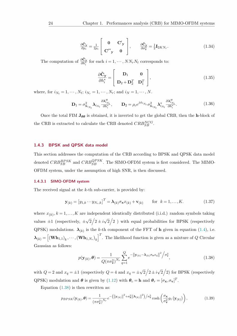
24 Chapter 1. Performances analysis (CRB) for MIMO-OFDM systems
∂Cy∂ρc
= 12ρc
0 C′yC′∗y 0
, ∂Cy∂σ2
v= 1
2I2KNr . (1.34)
The computation of ∂Cy∂h∗i
for each i= 1, · · · , NNrNt corresponds to:
∂Cy∂h∗i
=
D1 0
D2 + DT2 DT
1
, (1.35)
where, for iNt = 1, · · · , Nt; iNr = 1, · · · , Nr; and iN = 1, · · · , N .
D1 = σ2xiNt
λiNt
∂λHiNt∂h∗i
, D2 = ρcejφiNt σ2
xiNtλ∗iNt
∂λHiNt∂h∗i
. (1.36)
Once the total FIM Jθθ is obtained, it is inverted to get the global CRB, then the h-block of
the CRB is extracted to calculate the CRB denoted CRBNCGSB .
1.4.3 BPSK and QPSK data model
This section addresses the computation of the CRB according to BPSK and QPSK data model
denoted CRBBPSKSB and CRBQPSKSB . The SIMO-OFDM system is first considered. The MIMO-
OFDM system, under the assumption of high SNR, is then discussed.
1.4.3.1 SIMO-OFDM system
The received signal at the k-th sub-carrier, is provided by:
y(k) =[y1,k · · ·yNr,k
]T = λ(k)σxx(k) + v(k) for k = 1, . . . ,K. (1.37)
where x(k), k = 1, . . . ,K are independent identically distributed (i.i.d.) random symbols taking
values ±1 (respectively, ±√
2/
2± i√
2/
2 ) with equal probabilities for BPSK (respectively
QPSK) modulations. λ(k) is the k-th component of the FFT of h given in equation (1.4), i.e.
λ(k) =[(Wh1,1)k , · · · ,
(Wh1,Nr
)k
]T. The likelihood function is given as a mixture of Q Circular
Gaussian as follows:
p(y(k),θ) = 1Q(πσ2
v)NrQ∑q=1
e−‖y(k)−λ(k)σxxq‖2
/σ2
v, (1.38)
with Q= 2 and xq =±1 (respectively Q= 4 and xq =±√
2/
2± i√
2/
2) for BPSK (respectively
QPSK) modulation and θ is given by (1.12) with θc = h and θr = [σx,σv]T .Equation (1.38) is then rewritten as:
pBPSK(y(k),θ) = 1(πσ2
v)Nre−(‖y(k)‖2+σ2
x‖λ(k)‖2)/σ2
v cosh(σxσ2
vg1(y(k)
)), (1.39)
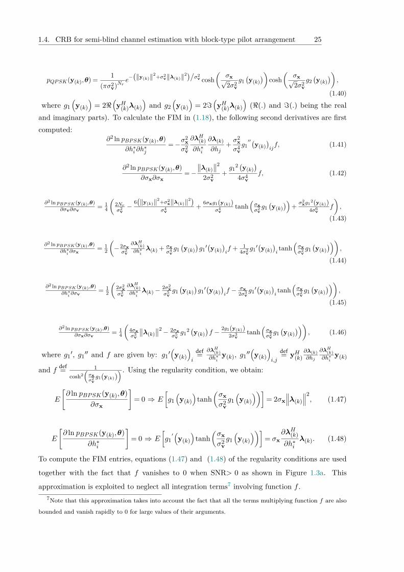
1.4. CRB for semi-blind channel estimation with block-type pilot arrangement 25
pQPSK(y(k),θ) = 1(πσ2
v)Nre−(‖y(k)‖2+σ2
v‖λ(k)‖2)/σ2
v cosh(
σx√2σ2
vg1(y(k)
))cosh
(σx√2σ2
vg2(y(k)
)),
(1.40)
where g1(y(k)
)= 2<
(yH(k)λ(k)
)and g2
(y(k)
)= 2=
(yH(k)λ(k)
)(<(.) and =(.) being the real
and imaginary parts). To calculate the FIM in (1.18), the following second derivatives are firstcomputed:
∂2 ln pBPSK(y(k),θ)∂h∗i ∂h
∗j
=−σ2xσ2
v
∂λH(k)∂h∗i
∂λ(k)∂hj
+ σ2xσ4
vg1′′(y(k)
)ijf, (1.41)
∂2 ln pBPSK(y(k),θ)∂σx∂σx
=−∥∥λ(k)
∥∥2
2σ2v
+g12 (y(k)
)4σ4
vf, (1.42)
∂2 ln pBPSK(y(k),θ)∂σv∂σv
= 14
(2Nrσ2
v−
6(‖y(k)‖2+σ2
x‖λ(k)‖2)σ4
v+ 6σxg1(y(k))
σ4v
tanh(σxσ2
vg1(y(k)
))+ σ2
xg12(y(k))4σ6
vf
),
(1.43)
∂2 ln pBPSK(y(k),θ)∂h∗i ∂σx
= 12
(−2σx
σ2v
∂λH(k)∂h∗i
λ(k) + σxσ4
vg1(y(k)
)g1′(y(k)
)if + 1
4σ2vg1′(y(k)
)itanh
(σxσ2
vg1(y(k)
))),
(1.44)
∂2 ln pBPSK(y(k),θ)∂h∗i ∂σv
= 12
(2σ2
xσ3
v
∂λH(k)∂h∗i
λ(k)−2σ2
xσ5
vg1(y(k)
)g1′(y(k)
)if − σx
2σ3vg1′(y(k)
)itanh
(σxσ2
vg1(y(k)
))),
(1.45)
∂2 ln pBPSK(y(k),θ)∂σx∂σv
= 14
(4σxσ3
v
∥∥λ(k)∥∥2− 2σx
σ5vg12 (y(k)
)f − 2g1(y(k))
2σ3v
tanh(σxσ2
vg1(y(k)
))), (1.46)
where g1′, g1′′ and f are given by: g1′(y(k)
)i
def= ∂λH(k)∂h∗i
y(k), g1′′(y(k)
)i,j
def= yH(k)∂λ(k)∂hj
∂λH(k)∂h∗i
y(k)
and f def= 1cosh2
(σxσ2
vg1(y(k))
) . Using the regularity condition, we obtain:
E
[∂ ln pBPSK(y(k),θ)
∂σx
]= 0 ⇒ E
[g1(y(k)
)tanh
(σxσ2
vg1(y(k)
))]= 2σx
∥∥∥λ(k)∥∥∥2, (1.47)
E
[∂ ln pBPSK(y(k),θ)
∂h∗i
]= 0 ⇒ E
[g1′(y(k)
)tanh
(σxσ2
vg1(y(k)
))]= σx
∂λH(k)∂h∗i
λ(k). (1.48)
To compute the FIM entries, equations (1.47) and (1.48) of the regularity conditions are used
together with the fact that f vanishes to 0 when SNR> 0 as shown in Figure 1.3a. This
approximation is exploited to neglect all integration terms7 involving function f .7Note that this approximation takes into account the fact that all the terms multiplying function f are also
bounded and vanish rapidly to 0 for large values of their arguments.
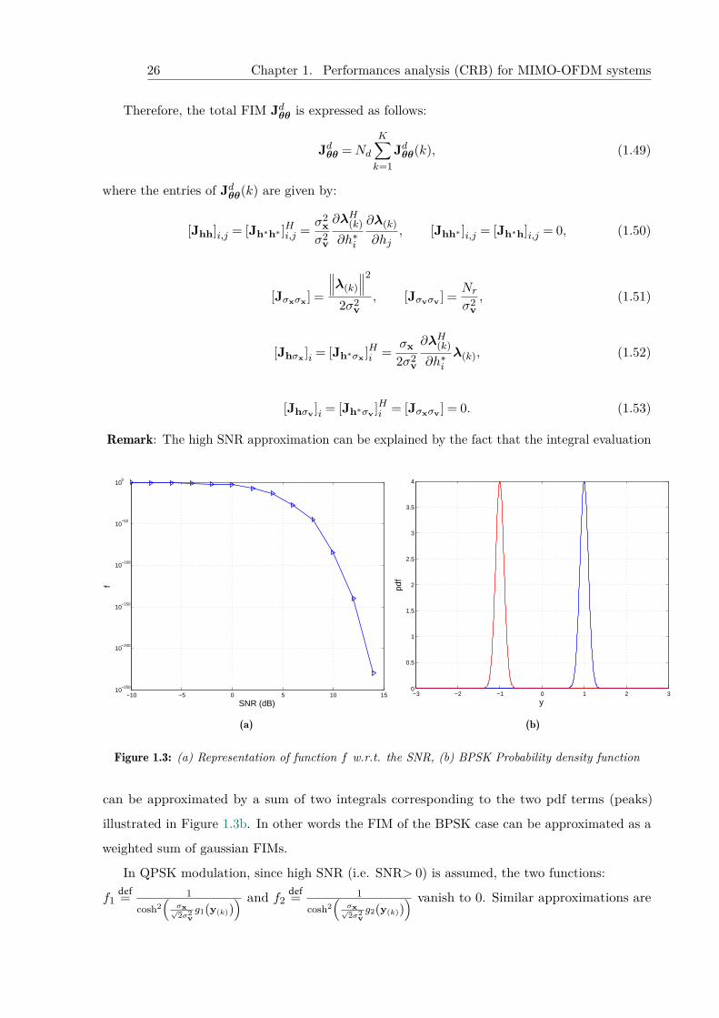
26 Chapter 1. Performances analysis (CRB) for MIMO-OFDM systems
Therefore, the total FIM Jdθθ is expressed as follows:
Jdθθ =Nd
K∑k=1
Jdθθ(k), (1.49)
where the entries of Jdθθ(k) are given by:
[Jhh]i,j = [Jh∗h∗ ]Hi,j = σ2xσ2
v
∂λH(k)∂h∗i
∂λ(k)∂hj
, [Jhh∗ ]i,j = [Jh∗h]i,j = 0, (1.50)
[Jσxσx ] =
∥∥∥λ(k)∥∥∥2
2σ2v
, [Jσvσv ] = Nrσ2
v, (1.51)
[Jhσx ]i = [Jh∗σx ]Hi = σx2σ2
v
∂λH(k)∂h∗i
λ(k), (1.52)
[Jhσv ]i = [Jh∗σv ]Hi = [Jσxσv ] = 0. (1.53)
Remark: The high SNR approximation can be explained by the fact that the integral evaluation
−10 −5 0 5 10 1510
−250
10−200
10−150
10−100
10−50
100
f
SNR (dB)
(a)
−3 −2 −1 0 1 2 30
0.5
1
1.5
2
2.5
3
3.5
4
y
(b)
Figure 1.3: (a) Representation of function f w.r.t. the SNR, (b) BPSK Probability density function
can be approximated by a sum of two integrals corresponding to the two pdf terms (peaks)
illustrated in Figure 1.3b. In other words the FIM of the BPSK case can be approximated as a
weighted sum of gaussian FIMs.
In QPSK modulation, since high SNR (i.e. SNR> 0) is assumed, the two functions:
f1def= 1
cosh2(
σx√2σ2
vg1(y(k))
) and f2def= 1
cosh2(
σx√2σ2
vg2(y(k))
) vanish to 0. Similar approximations are
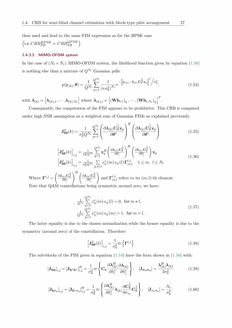
1.4. CRB for semi-blind channel estimation with block-type pilot arrangement 27
then used and lead to the same FIM expression as for the BPSK case(i.e.CRBBPSKSB = CRBQPSKSB
).
1.4.3.2 MIMO-OFDM system
In the case of (Nt×Nr) MIMO-OFDM system, the likelihood function given by equation (1.38)
is nothing else than a mixture of QNt Gaussian pdfs:
p(y(k),θ) = 1QNt
QNt∑q=1
1(πσ2
v)Nre−∥∥∥y(k)−λ(k)C
12x xq
∥∥∥2/σ2
v, (1.54)
with λ(k) =[λ(k),1, · · · ,λ(k),Nt
]where λ(k),i =
[(Whi,1)k , · · · ,
(Whi,Nr
)k
]T.
Consequently, the computation of the FIM appears to be prohibitive. This CRB is computed
under high SNR assumption as a weighted sum of Gaussian FIMs as explained previously.
Jdθθ(k) = 1σ2
vQNt
QNt∑q=1
∂λ(k)C12xxq
∂θ∗
H∂λ(k)C
12xxq
∂θ∗
(1.55)
[Jdθθ(k)
]i,j
= 1σ2
vQNt
QNt∑q=1
xHq
(∂λ(k)C
12x
∂θ∗i
)H(∂λ(k)C
12x
∂θ∗j
)xq[
Jdθθ(k)]i,j
= 1σ2
vQNt
∑q,m,l
x∗q (m)xq (l)Γi,jm,l 1≤m, l ≤Nt(1.56)
Where Γi,j =(∂λ(k)C
12x
∂θ∗i
)H(∂λ(k)C
12x
∂θ∗j
)and Γi,jm,l refers to its (m,l)-th element.
Note that QAM constellations being symmetric around zero, we have:
1QNt
QNt∑q=1
x∗q (m)xq (l) = 0, form , l,
1QNt
QNt∑q=1
x∗q (m)xq (m) = 1, form= l,
(1.57)
The latter equality is due to the chosen normalization while the former equality is due to the
symmetry (around zero) of the constellation. Therefore:[Jdθθ(k)
]i,j
= 1σ2
vtr{Γi,j
}(1.58)
The sub-blocks of the FIM given in equation (1.18) have the form shown in (1.58) with:
[Jhh]i,j = [Jh∗h∗ ]Hi,j = 1σ2
vtr
Cx∂λH(k)∂h∗i
∂λ(k)∂h∗j
; [Jσxσx ] =λH(k)λ(k)
2σ2v
(1.59)
[Jhσx ]i,j = [Jh∗σx ]Hi,j = 1σ2
vtr
∂λH(k)
∂h∗iλ(k)
∂C12x
∂σxjC
12x
; [Jσvσv ] = Nrσ2
v. (1.60)
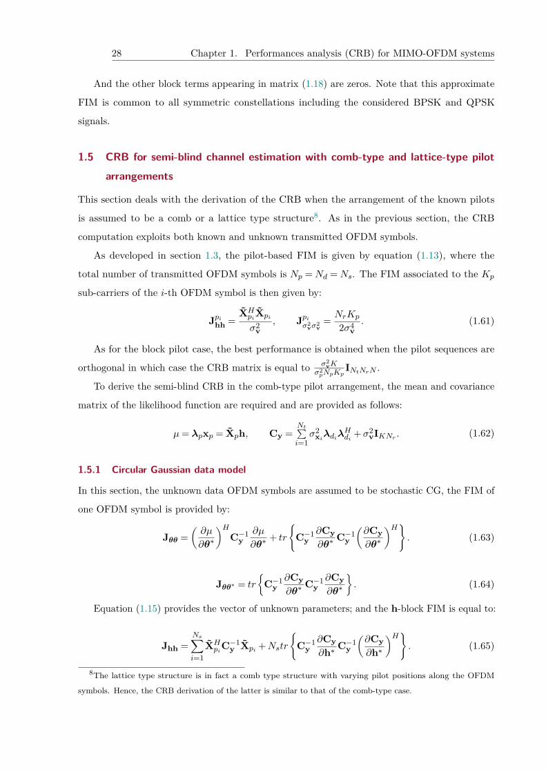
28 Chapter 1. Performances analysis (CRB) for MIMO-OFDM systems
And the other block terms appearing in matrix (1.18) are zeros. Note that this approximate
FIM is common to all symmetric constellations including the considered BPSK and QPSK
signals.
1.5 CRB for semi-blind channel estimation with comb-type and lattice-type pilot
arrangements
This section deals with the derivation of the CRB when the arrangement of the known pilots
is assumed to be a comb or a lattice type structure8. As in the previous section, the CRB
computation exploits both known and unknown transmitted OFDM symbols.
As developed in section 1.3, the pilot-based FIM is given by equation (1.13), where the
total number of transmitted OFDM symbols is Np =Nd =Ns. The FIM associated to the Kp
sub-carriers of the i-th OFDM symbol is then given by:
Jpihh =XHpiXpi
σ2v
, Jpiσ2vσ
2v
= NrKp
2σ4v. (1.61)
As for the block pilot case, the best performance is obtained when the pilot sequences are
orthogonal in which case the CRB matrix is equal to σ2vK
σ2pNpKp
INtNrN .
To derive the semi-blind CRB in the comb-type pilot arrangement, the mean and covariance
matrix of the likelihood function are required and are provided as follows:
µ= λpxp = Xph, Cy =Nt∑i=1
σ2xiλdiλ
Hdi
+σ2vIKNr . (1.62)
1.5.1 Circular Gaussian data model
In this section, the unknown data OFDM symbols are assumed to be stochastic CG, the FIM of
one OFDM symbol is provided by:
Jθθ =(∂µ
∂θ∗
)HC−1
y∂µ
∂θ∗+ tr
{C−1
y∂Cy∂θ∗
C−1y
(∂Cy∂θ∗
)H}. (1.63)
Jθθ∗ = tr
{C−1
y∂Cy∂θ∗
C−1y∂Cy∂θ∗
}. (1.64)
Equation (1.15) provides the vector of unknown parameters; and the h-block FIM is equal to:
Jhh =Ns∑i=1
XHpiC−1y Xpi +Nstr
{C−1
y∂Cy∂h∗ C−1
y
(∂Cy∂h∗
)H}. (1.65)
8The lattice type structure is in fact a comb type structure with varying pilot positions along the OFDM
symbols. Hence, the CRB derivation of the latter is similar to that of the comb-type case.
1.6. Computational issue in large MIMO-OFDM communications systems 29
Jhh∗ =Nstr
{C−1
y∂Cy∂h∗ C−1
y∂Cy∂h∗
}. (1.66)
The other entries of the FIM are obtained in a similar way as in section 1.4.1. Also, the
derivative of Cy w.r.t. the channel parameters is obtained as before after replacing λi by λdi .
1.5.2 Non-Circular Gaussian data model
In the NCG case, the FIM has the same form as the CG one described by equations (1.63)
and (1.64). We just need to extend the parameter vector as in section 1.4.2 and to replace Cy
by Cy provided in equation (1.29) and λi by λdi corresponding to the Kd data sub-carriers.
1.5.3 BPSK and QPSK data model
According to the results in section 1.4.3, the FIM is expressed as follows:
Jθθ = Jpθθ +NS
K∑k=Kp+1
Jdθθ(k), (1.67)
where Jpθθ is deduced from equation (1.61); and Jdθθ(k)k=Kp+1, ··· ,K is given in section 1.4.3 by
equations (1.49) and (1.58).
1.6 Computational issue in large MIMO-OFDM communications systems
The aim of this section is to study the semi-blind channel estimation performance in large
MIMO-OFDM communications systems where the base station is assumed to be equipped with
a relatively large number of antennas and serves a large number of users.
Depending on the data model (CG or NCG), the CRB are provided by equations (1.17), (1.28),
(1.65) and (1.66) in the previous sections. For a large MIMO-OFDM system, the implementation
of these equations consumes not only a huge memory space but also a high computational time.
Indeed the CRB computation requires the manipulation of several large dimensional matrix
operations such as inversion, Hermitian transpose, trace and product. To avoid these strong
implementation constraints, a new efficient algorithm is proposed. It exploits the structure of the
covariance matrix composed of diagonal blocks. Before describing the developed algorithm, the
following subsection introduces the new organization of the diagonal blocks into a new structure
called vector representation.
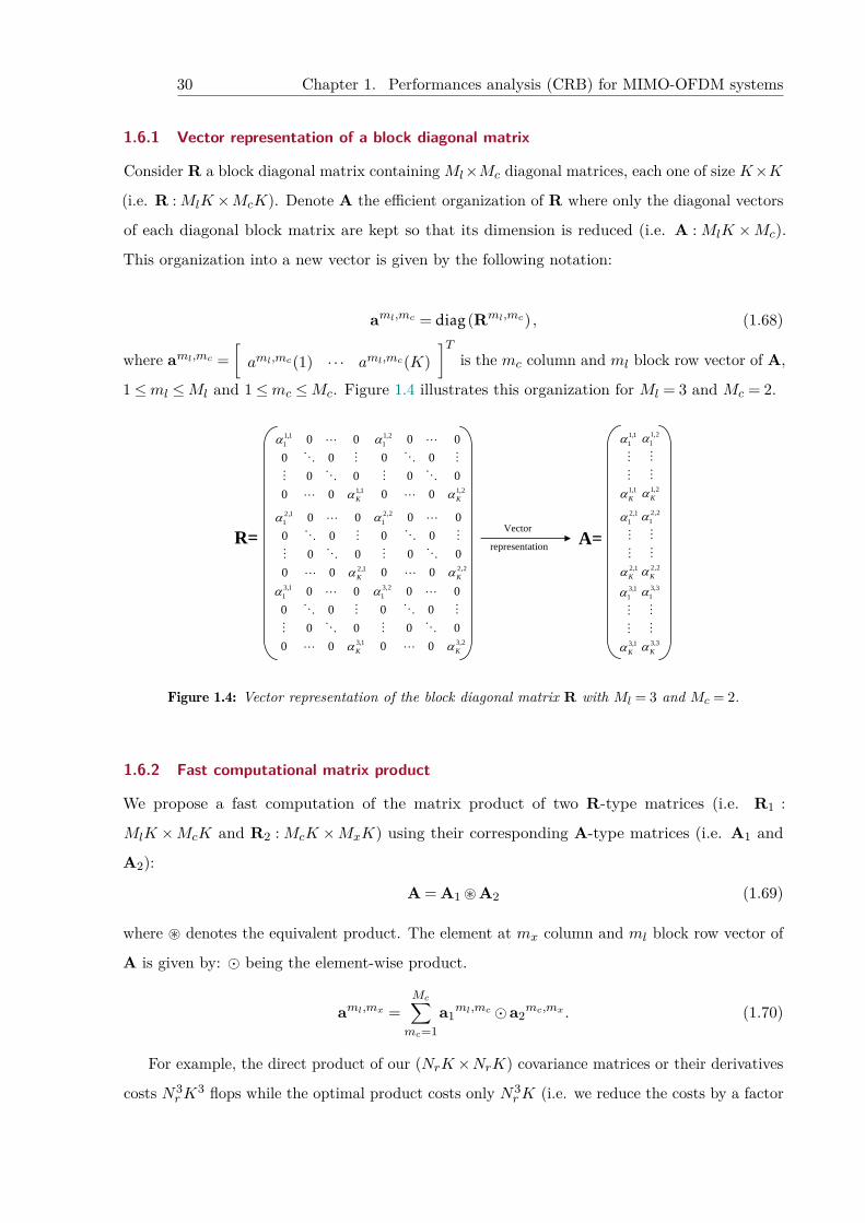
30 Chapter 1. Performances analysis (CRB) for MIMO-OFDM systems
1.6.1 Vector representation of a block diagonal matrix
Consider R a block diagonal matrix containingMl×Mc diagonal matrices, each one of size K×K
(i.e. R :MlK×McK). Denote A the efficient organization of R where only the diagonal vectors
of each diagonal block matrix are kept so that its dimension is reduced (i.e. A : MlK ×Mc).
This organization into a new vector is given by the following notation:
aml,mc = diag(Rml,mc) , (1.68)
where aml,mc =[aml,mc(1) · · · aml,mc(K)
]Tis the mc column and ml block row vector of A,
1≤ml ≤Ml and 1≤mc ≤Mc. Figure 1.4 illustrates this organization for Ml = 3 and Mc = 2.
Vector
representation
1,11
1,1
0 00 0
0 00 0 K
1,21
1,2
0 00 0
0 00 0 K
2,11
2,1
0 00 0
0 00 0 K
2,21
2,2
0 00 0
0 00 0 K
3,11
3,1
0 00 0
0 00 0 K
3,21
3,2
0 00 0
0 00 0 K
1,11
1,1K
2,11
2,1K
3,11
3,1K
1,21
1,2K
2,21
2,2K
3,31
3,3K
R= A=
Figure 1.4: Vector representation of the block diagonal matrix R with Ml = 3 and Mc = 2.
1.6.2 Fast computational matrix product
We propose a fast computation of the matrix product of two R-type matrices (i.e. R1 :
MlK ×McK and R2 : McK ×MxK) using their corresponding A-type matrices (i.e. A1 and
A2):
A = A1 ~A2 (1.69)
where ~ denotes the equivalent product. The element at mx column and ml block row vector of
A is given by: � being the element-wise product.
aml,mx =Mc∑mc=1
a1ml,mc �a2
mc,mx . (1.70)
For example, the direct product of our (NrK×NrK) covariance matrices or their derivatives
costs N3rK
3 flops while the optimal product costs only N3rK (i.e. we reduce the costs by a factor

1.6. Computational issue in large MIMO-OFDM communications systems 31
K2). The trace of a square matrix R based on it’s vector representation A is given by:
tr{R}=K∑k=1
Ml∑ml=1
aml,ml(k). (1.71)
1.6.3 Iterative matrix inversion algorithm
This subsection deals with the R-type matrix inversion (i.e. R−1) using its vector representation
A introduced previously. To do so, an iterative matrix inversion algorithm is proposed. It exploits
the Schur’s complement summarized as follows:
E F
G H
−1
=
E−1 + E−1FH−1GE−1 −E−1FH−1
−H−1GE−1 H−1
, (1.72)
where E and H are assumed to be invertible matrices. The proposed iterative matrix inversion
algorithm (starting from the top-left matrix sub-block) follows the steps described below:
• Initialization step:
- Set E0 = a1,1. The inversion of E0, denoted I1, is given by I1 = 1./E0, where ./ denotes
the element-wise division.
- Set E1 = a1,1, F1 = a1,2, G1 = a2,1 and H1 = a2,2. The inversion of the matrix E1 F1
G1 H1
of A-type, denoted I2, is given by:
I2 =
I1,12 I1,2
2
I2,12 I2,2
2
, (1.73)
where
I2,22 = 1./H1,
I1,12 = I1 + I1 ~F1 ~ I2,2
2 ~G1 ~ I1,
I1,22 =−I1 ~F1 ~ I2,2
2 ,
I2,12 =−I2,2
2 ~G1 ~ I1,
(1.74)
and ~ denotes the equivalent product as explained in section 1.6.2.
• The matrix inversion process is iterated. At the m-th iteration, the algorithm inverses the
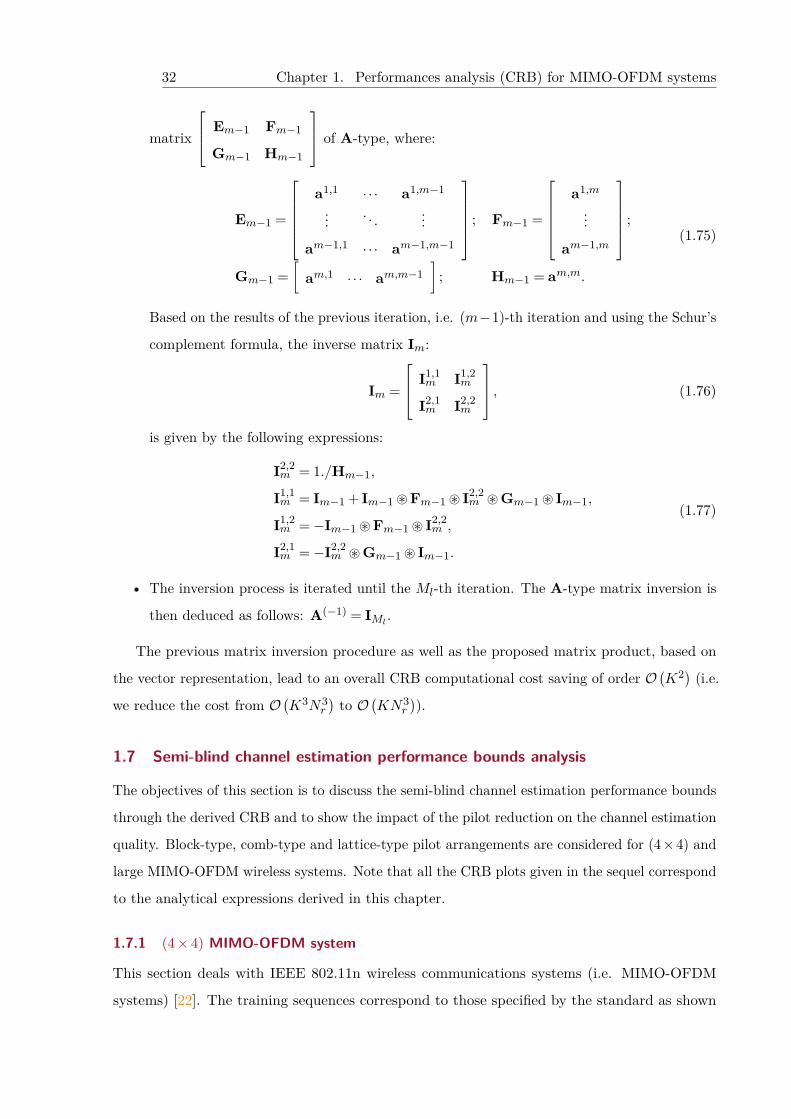
32 Chapter 1. Performances analysis (CRB) for MIMO-OFDM systems
matrix
Em−1 Fm−1
Gm−1 Hm−1
of A-type, where:
Em−1 =
a1,1 · · · a1,m−1
.... . .
...
am−1,1 · · · am−1,m−1
; Fm−1 =
a1,m
...
am−1,m
;
Gm−1 =[
am,1 · · · am,m−1]
; Hm−1 = am,m.
(1.75)
Based on the results of the previous iteration, i.e. (m−1)-th iteration and using the Schur’s
complement formula, the inverse matrix Im:
Im =
I1,1m I1,2
m
I2,1m I2,2
m
, (1.76)
is given by the following expressions:
I2,2m = 1./Hm−1,
I1,1m = Im−1 + Im−1 ~Fm−1 ~ I2,2
m ~Gm−1 ~ Im−1,
I1,2m =−Im−1 ~Fm−1 ~ I2,2
m ,
I2,1m =−I2,2
m ~Gm−1 ~ Im−1.
(1.77)
• The inversion process is iterated until the Ml-th iteration. The A-type matrix inversion is
then deduced as follows: A(−1) = IMl.
The previous matrix inversion procedure as well as the proposed matrix product, based on
the vector representation, lead to an overall CRB computational cost saving of order O(K2) (i.e.
we reduce the cost from O(K3N3
r
)to O
(KN3
r
)).
1.7 Semi-blind channel estimation performance bounds analysis
The objectives of this section is to discuss the semi-blind channel estimation performance bounds
through the derived CRB and to show the impact of the pilot reduction on the channel estimation
quality. Block-type, comb-type and lattice-type pilot arrangements are considered for (4×4) and
large MIMO-OFDM wireless systems. Note that all the CRB plots given in the sequel correspond
to the analytical expressions derived in this chapter.
1.7.1 (4× 4) MIMO-OFDM system
This section deals with IEEE 802.11n wireless communications systems (i.e. MIMO-OFDM
systems) [22]. The training sequences correspond to those specified by the standard as shown
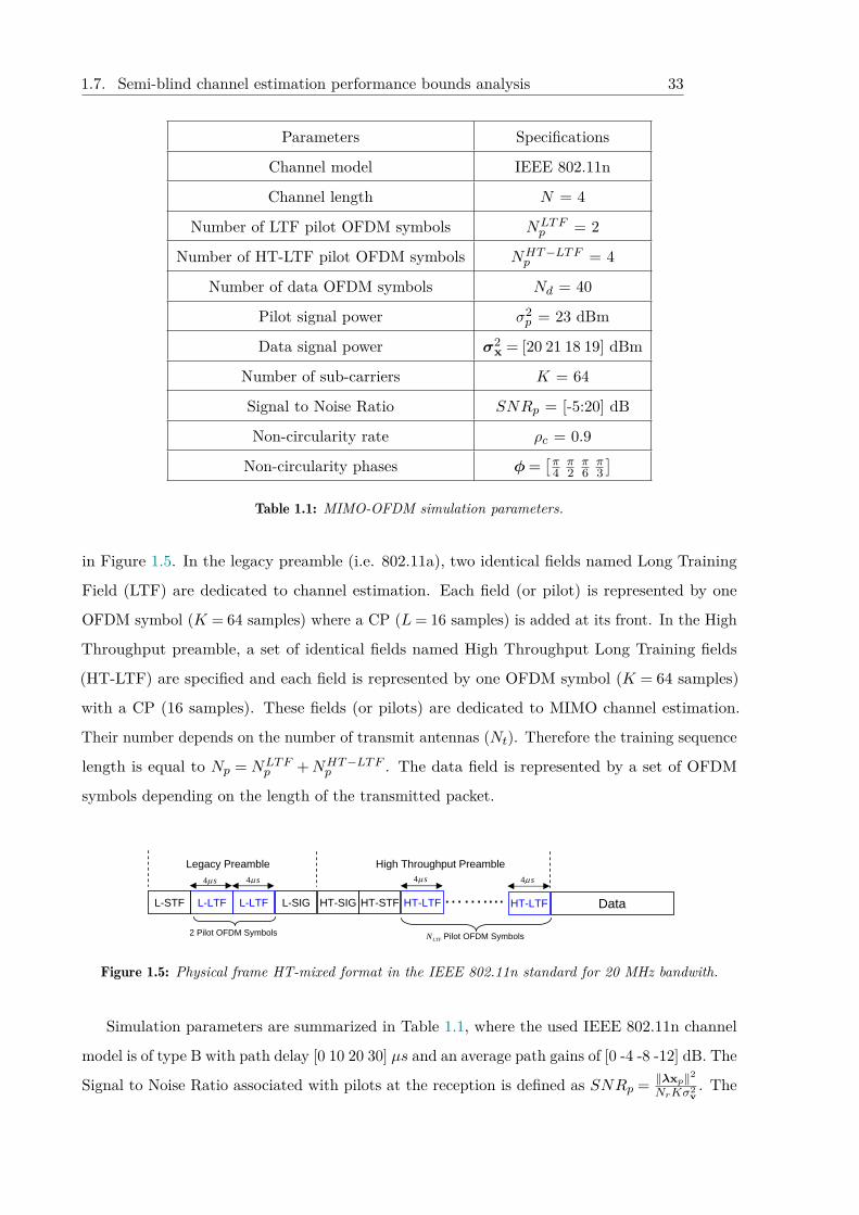
1.7. Semi-blind channel estimation performance bounds analysis 33
Parameters Specifications
Channel model IEEE 802.11n
Channel length N = 4
Number of LTF pilot OFDM symbols NLTFp = 2
Number of HT-LTF pilot OFDM symbols NHT−LTFp = 4
Number of data OFDM symbols Nd = 40
Pilot signal power σ2p = 23 dBm
Data signal power σ2x = [20 21 18 19] dBm
Number of sub-carriers K = 64
Signal to Noise Ratio SNRp = [-5:20] dB
Non-circularity rate ρc = 0.9
Non-circularity phases φ=[π
4π2π6π3]
Table 1.1: MIMO-OFDM simulation parameters.
in Figure 1.5. In the legacy preamble (i.e. 802.11a), two identical fields named Long Training
Field (LTF) are dedicated to channel estimation. Each field (or pilot) is represented by one
OFDM symbol (K = 64 samples) where a CP (L= 16 samples) is added at its front. In the High
Throughput preamble, a set of identical fields named High Throughput Long Training fields
(HT-LTF) are specified and each field is represented by one OFDM symbol (K = 64 samples)
with a CP (16 samples). These fields (or pilots) are dedicated to MIMO channel estimation.
Their number depends on the number of transmit antennas (Nt). Therefore the training sequence
length is equal to Np = NLTFp +NHT−LTF
p . The data field is represented by a set of OFDM
symbols depending on the length of the transmitted packet.
HT-LTF…….... Data
Legacy Preamble High Throughput Preamble
2 Pilot OFDM Symbols Pilot OFDM SymbolsLTFN
HT-LTFHT-STFHT-SIGL-SIGL-LTFL-LTFL-STF
4 s 4 s 4 s 4 s
Figure 1.5: Physical frame HT-mixed format in the IEEE 802.11n standard for 20 MHz bandwith.
Simulation parameters are summarized in Table 1.1, where the used IEEE 802.11n channel
model is of type B with path delay [0 10 20 30] µs and an average path gains of [0 -4 -8 -12] dB. The
Signal to Noise Ratio associated with pilots at the reception is defined as SNRp = ‖λxp‖2
NrKσ2v. The
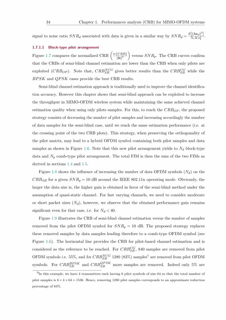
34 Chapter 1. Performances analysis (CRB) for MIMO-OFDM systems
signal to noise ratio SNRd associated with data is given in a similar way by SNRd = E[‖λxd‖2]NrKσ2
v.
1.7.1.1 Block-type pilot arrangement
Figure 1.7 compares the normalized CRB(tr{CRB}‖h‖2
)versus SNRp. The CRB curves confirm
that the CRBs of semi-blind channel estimation are lower than the CRB when only pilots are
exploited (CRBOP ). Note that, CRBNCGSB gives better results than the CRBCGSB while the
BPSK and QPSK cases provide the best CRB results.
Semi-blind channel estimation approach is traditionally used to improve the channel identifica-
tion accuracy. However this chapter shows that semi-blind approach can be exploited to increase
the throughput in MIMO-OFDM wireless system while maintaining the same achieved channel
estimation quality when using only pilots samples. For this, to reach the CRBOP , the proposed
strategy consists of decreasing the number of pilot samples and increasing accordingly the number
of data samples for the semi-blind case, until we reach the same estimation performance (i.e. at
the crossing point of the two CRB plots). This strategy, when preserving the orthogonality of
the pilot matrix, may lead to a hybrid OFDM symbol containing both pilot samples and data
samples as shown in Figure 1.6. Note that this new pilot arrangement yields to Nd block-type
data and Np comb-type pilot arrangement. The total FIM is then the sum of the two FIMs as
derived in sections 1.4 and 1.5.
Figure 1.8 shows the influence of increasing the number of data OFDM symbols (Nd) on the
CRBSB for a given SNRp = 10 dB around the IEEE 802.11n operating mode. Obviously, the
larger the data size is, the higher gain is obtained in favor of the semi-blind method under the
assumption of quasi-static channel. For fast varying channels, we need to consider moderate
or short packet sizes (Nd), however, we observe that the obtained performance gain remains
significant even for that case, i.e. for Nd < 40.
Figure 1.9 illustrates the CRB of semi-blind channel estimation versus the number of samples
removed from the pilot OFDM symbol for SNRp = 10 dB. The proposed strategy replaces
these removed samples by data samples leading therefore to a comb-type OFDM symbol (see
Figure 1.6). The horizontal line provides the CRB for pilot-based channel estimation and is
considered as the reference to be reached. For CRBCGSB , 840 samples are removed from pilot
OFDM symbols i.e. 55%, and for CRBNCGSB 1280 (83%) samples9 are removed from pilot OFDM
symbols. For CRBBPSKSB and CRBQPSKSB more samples are removed. Indeed only 5% are
9In this example, we have 4 transmitters each having 6 pilot symbols of size 64 so that the total number of
pilot samples is 6× 4× 64 = 1536. Hence, removing 1280 pilot samples corresponds to an approximate reduction
percentage of 83%.
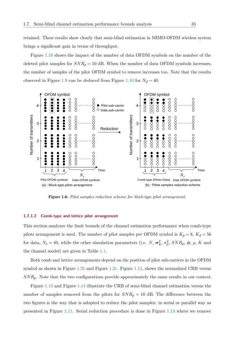
1.7. Semi-blind channel estimation performance bounds analysis 35
retained. These results show clearly that semi-blind estimation in MIMO-OFDM wireless system
brings a significant gain in terms of throughput.
Figure 1.10 shows the impact of the number of data OFDM symbols on the number of the
deleted pilot samples for SNRp = 10 dB. When the number of data OFDM symbols increases,
the number of samples of the pilot OFDM symbol to remove increases too. Note that the results
observed in Figure 1.9 can be deduced from Figure 1.10 for Nd = 40.
(a) : Block-type pilots arrangement (b) : Pilots samples reduction scheme
Pilot sub-carrierData sub-carrier
Time
OFDM symbol
1
4
Pilot OFDM symbols
Num
ber o
f tra
nsm
itter
s
2
3
1 2 3 4
Reduction
…………
…………
…………
…………
dNData OFDM symbols
Time
OFDM symbol
1
4
Comb-type (Pilots+Data)
Num
ber o
f tra
nsm
itter
s
2
3
1 2 3 4
…………
…………
…………
…………
dNData OFDM symbols
Figure 1.6: Pilot samples reduction scheme for block-type pilot arrangement.
1.7.1.2 Comb-type and lattice pilot arrangement
This section analyzes the limit bounds of the channel estimation performance when comb-type
pilots arrangement is used. The number of pilot samples per OFDM symbol is Kp = 8, Kd = 56
for data, Ns = 40, while the other simulation parameters (i.e. N , σ2x, σ2
p, SNRp, φ, ρ, K and
the channel model) are given in Table 1.1.
Both comb and lattice arrangements depend on the position of pilot sub-carriers in the OFDM
symbol as shown in Figure 1.2b and Figure 1.2c. Figure 1.12, shows the normalized CRB versus
SNRp. Note that the two configurations provide approximately the same results in our context.
Figure 1.13 and Figure 1.14 illustrate the CRB of semi-blind channel estimation versus the
number of samples removed from the pilots for SNRp = 10 dB. The difference between the
two figures is the way that is adopted to reduce the pilot samples: in serial or parallel way as
presented in Figure 1.11. Serial reduction procedure is done in Figure 1.13 where we remove
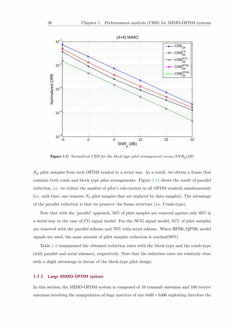
36 Chapter 1. Performances analysis (CRB) for MIMO-OFDM systems
−5 0 5 10 15 2010−5
10−4
10−3
10−2
10−1(4×4) MIMO
Nor
mal
ized
CR
B
SNRp (dB)
CRBOP
CRBSBCG
CRBSBNCG
CRBSBBPSK
CRBSBQPSK
Figure 1.7: Normalized CRB for the block-type pilot arrangement versus SNRp(dB)
Kp pilot samples from each OFDM symbol in a serial way. As a result, we obtain a frame that
contains both comb and block type pilot arrangements. Figure 1.14 shows the result of parallel
reduction, i.e. we reduce the number of pilot’s sub-carriers in all OFDM symbols simultaneously
(i.e. each time, one removes Ns pilot samples that are replaced by data samples). The advantage
of the parallel reduction is that we preserve the frame structure (i.e. Comb-type).
Note that with the ’parallel’ approach, 50% of pilot samples are removed against only 40% in
a serial way in the case of CG signal model. For the NCG signal model, 81% of pilot samples
are removed with the parallel scheme and 70% with serial scheme. When BPSK/QPSK model
signals are used, the same amount of pilot samples reduction is reached(90%).
Table 1.2 summarized the obtained reduction rates with the block-type and the comb-type
(with parallel and serial schemes), respectively. Note that the reduction rates are relatively close
with a slight advantage in favour of the block-type pilot design.
1.7.2 Large MIMO-OFDM system
In this section, the MIMO-OFDM system is composed of 10 transmit antennas and 100 receive
antennas involving the manipulation of huge matrices of size 6400×6400 exploiting therefore the
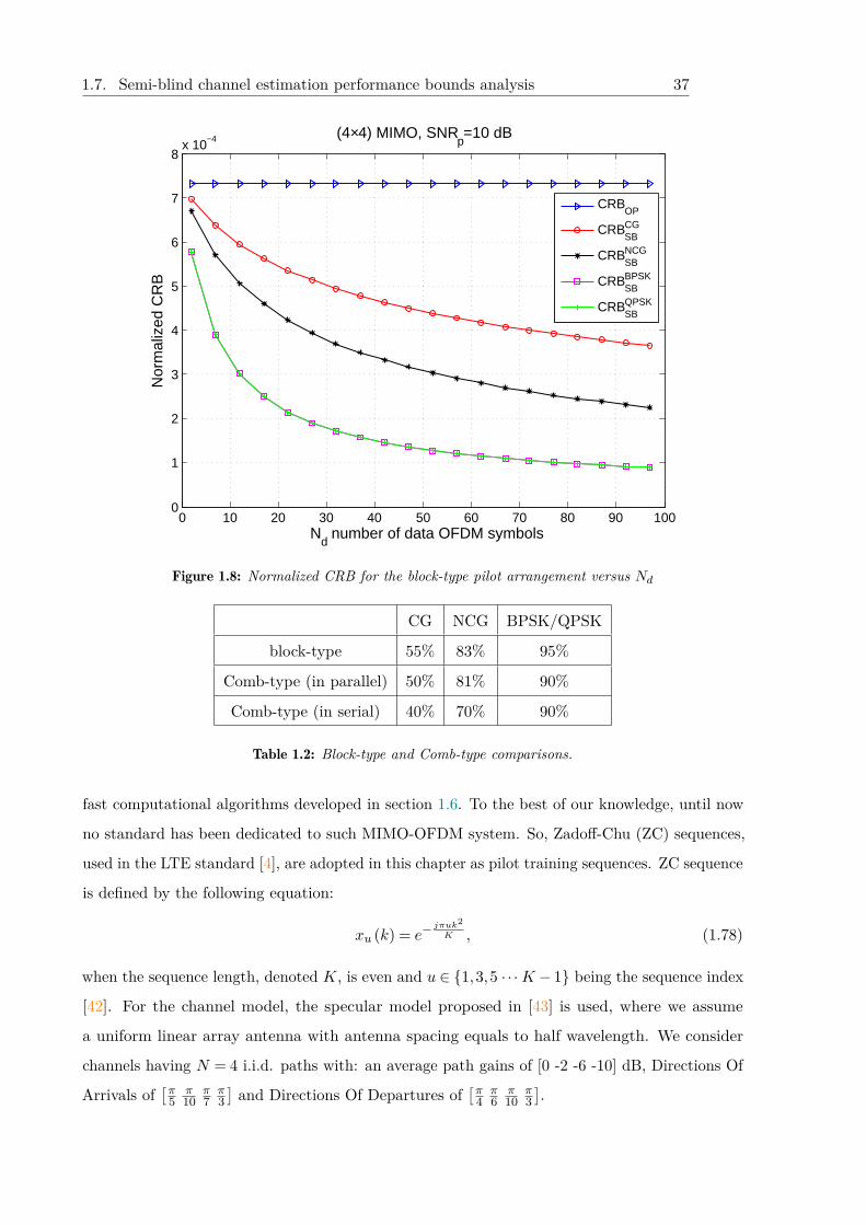
1.7. Semi-blind channel estimation performance bounds analysis 37
0 10 20 30 40 50 60 70 80 90 1000
1
2
3
4
5
6
7
8x 10⁻⁴ (4×4) MIMO, SNR
p=10 dB
Nor
mal
ized
CR
B
Nd number of data OFDM symbols
CRBOP
CRBSBCG
CRBSBNCG
CRBSBBPSK
CRBSBQPSK
Figure 1.8: Normalized CRB for the block-type pilot arrangement versus Nd
CG NCG BPSK/QPSK
block-type 55% 83% 95%
Comb-type (in parallel) 50% 81% 90%
Comb-type (in serial) 40% 70% 90%
Table 1.2: Block-type and Comb-type comparisons.
fast computational algorithms developed in section 1.6. To the best of our knowledge, until now
no standard has been dedicated to such MIMO-OFDM system. So, Zadoff-Chu (ZC) sequences,
used in the LTE standard [4], are adopted in this chapter as pilot training sequences. ZC sequence
is defined by the following equation:
xu (k) = e−jπuk2K , (1.78)
when the sequence length, denoted K, is even and u ∈ {1,3,5 · · ·K − 1} being the sequence index
[42]. For the channel model, the specular model proposed in [43] is used, where we assume
a uniform linear array antenna with antenna spacing equals to half wavelength. We consider
channels having N = 4 i.i.d. paths with: an average path gains of [0 -2 -6 -10] dB, Directions Of
Arrivals of[π
5π10
π7π3]and Directions Of Departures of
[π4π6π10
π3].
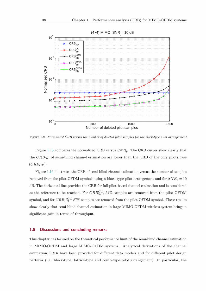
38 Chapter 1. Performances analysis (CRB) for MIMO-OFDM systems
0 500 1000 150010−4
10−3
10−2
10−1
100
(4×4) MIMO, SNRp= 10 dB
Nor
mal
ized
CR
B
Number of deleted pilot samples
CRBOP
CRBSBCG
CRBSBNCG
CRBSBBPSK
CRBSBQPSK
Figure 1.9: Normalized CRB versus the number of deleted pilot samples for the block-type pilot arrangement
Figure 1.15 compares the normalized CRB versus SNRp. The CRB curves show clearly that
the CRBSB of semi-blind channel estimation are lower than the CRB of the only pilots case
(CRBOP ).
Figure 1.16 illustrates the CRB of semi-blind channel estimation versus the number of samples
removed from the pilot OFDM symbols using a block-type pilot arrangement and for SNRp = 10
dB. The horizontal line provides the CRB for full pilot-based channel estimation and is considered
as the reference to be reached. For CRBCGSB , 54% samples are removed from the pilot OFDM
symbol, and for CRBNCGSB 87% samples are removed from the pilot OFDM symbol. These results
show clearly that semi-blind channel estimation in large MIMO-OFDM wireless system brings a
significant gain in terms of throughput.
1.8 Discussions and concluding remarks
This chapter has focused on the theoretical performance limit of the semi-blind channel estimation
in MIMO-OFDM and large MIMO-OFDM systems. Analytical derivations of the channel
estimation CRBs have been provided for different data models and for different pilot design
patterns (i.e. block-type, lattice-type and comb-type pilot arrangement). In particular, the
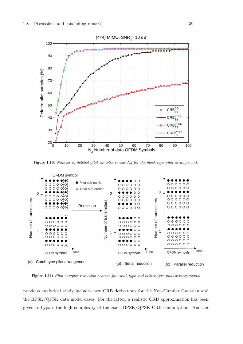
1.8. Discussions and concluding remarks 39
0 10 20 30 40 50 60 70 80 90 10020
30
40
50
60
70
80
90
100
(4×4) MIMO, SNRp= 10 dB
Del
eted
pilo
t sam
ples
(%
)
Nd Number of data OFDM Symbols
CRBSBCG
CRBSBNCG
CRBSBBPSK
CRBSBQPSK
Figure 1.10: Number of deleted pilot samples versus Nd for the block-type pilot arrangement.
Time
Num
ber o
f tra
nsm
itter
s
OFDM symbol
1
2
OFDM symbols
Pilot sub-carrier
Data sub-carrier
Reduction
Time
(a) : Comb-type pilot arrangement
1
2
OFDM symbols
(b) : Serial reduction
Num
ber o
f tra
nsm
itter
s
1
2
OFDM symbols
(c) : Parallel reduction
Time
Num
ber o
f tra
nsm
itter
s
Figure 1.11: Pilot samples reduction scheme for comb-type and lattice-type pilot arrangements.
previous analytical study includes new CRB derivations for the Non-Circular Gaussian and
the BPSK/QPSK data model cases. For the latter, a realistic CRB approximation has been
given to bypass the high complexity of the exact BPSK/QPSK CRB computation. Another
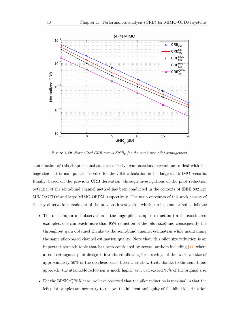
40 Chapter 1. Performances analysis (CRB) for MIMO-OFDM systems
−5 0 5 10 15 2010−5
10−4
10−3
10−2
10−1(4×4) MIMO
Nor
mal
ized
CR
B
SNRp (dB)
CRBOP
CRBSBCG
CRBSBNCG
CRBSBBPSK
CRBSBQPSK
Figure 1.12: Normalized CRB versus SNRp for the comb-type pilot arrangement
contribution of this chapter consists of an effective computational technique to deal with the
huge-size matrix manipulation needed for the CRB calculation in the large size MIMO scenario.
Finally, based on the previous CRB derivation, through investigations of the pilot reduction
potential of the semi-blind channel method has been conducted in the contexts of IEEE 802.11n
MIMO-OFDM and large MIMO-OFDM, respectively. The main outcomes of this work consist of
the key observations made out of the previous investigation which can be summarized as follows:
• The most important observation is the huge pilot samples reduction (in the considered
examples, one can reach more than 95% reduction of the pilot size) and consequently the
throughput gain obtained thanks to the semi-blind channel estimation while maintaining
the same pilot-based channel estimation quality. Note that, this pilot size reduction is an
important research topic that has been considered by several authors including [44] where
a semi-orthogonal pilot design is introduced allowing for a savings of the overhead size of
approximately 50% of the overhead size. Herein, we show that, thanks to the semi-blind
approach, the attainable reduction is much higher as it can exceed 95% of the original size.
• For the BPSK/QPSK case, we have observed that the pilot reduction is maximal in that the
left pilot samples are necessary to remove the inherent ambiguity of the blind identification
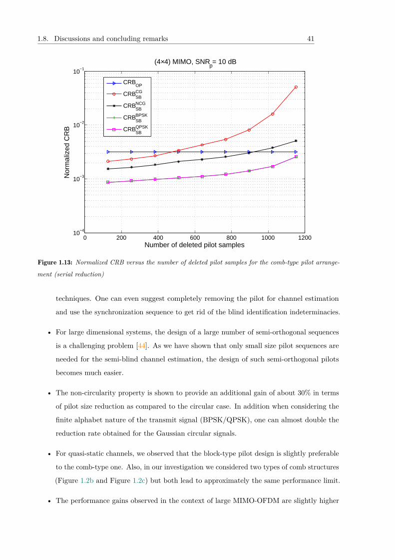
1.8. Discussions and concluding remarks 41
0 200 400 600 800 1000 120010−4
10−3
10−2
10−1
(4×4) MIMO, SNRp= 10 dB
Nor
mal
ized
CR
B
Number of deleted pilot samples
CRBOP
CRBSBCG
CRBSBNCG
CRBSBBPSK
CRBSBQPSK
Figure 1.13: Normalized CRB versus the number of deleted pilot samples for the comb-type pilot arrange-
ment (serial reduction)
techniques. One can even suggest completely removing the pilot for channel estimation
and use the synchronization sequence to get rid of the blind identification indeterminacies.
• For large dimensional systems, the design of a large number of semi-orthogonal sequences
is a challenging problem [44]. As we have shown that only small size pilot sequences are
needed for the semi-blind channel estimation, the design of such semi-orthogonal pilots
becomes much easier.
• The non-circularity property is shown to provide an additional gain of about 30% in terms
of pilot size reduction as compared to the circular case. In addition when considering the
finite alphabet nature of the transmit signal (BPSK/QPSK), one can almost double the
reduction rate obtained for the Gaussian circular signals.
• For quasi-static channels, we observed that the block-type pilot design is slightly preferable
to the comb-type one. Also, in our investigation we considered two types of comb structures
(Figure 1.2b and Figure 1.2c) but both lead to approximately the same performance limit.
• The performance gains observed in the context of large MIMO-OFDM are slightly higher
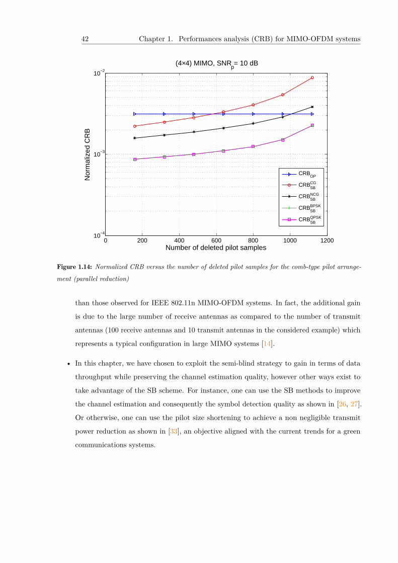
42 Chapter 1. Performances analysis (CRB) for MIMO-OFDM systems
0 200 400 600 800 1000 120010−4
10−3
10−2
(4×4) MIMO, SNRp= 10 dB
Nor
mal
ized
CR
B
Number of deleted pilot samples
CRBOP
CRBSBCG
CRBSBNCG
CRBSBBPSK
CRBSBQPSK
Figure 1.14: Normalized CRB versus the number of deleted pilot samples for the comb-type pilot arrange-
ment (parallel reduction)
than those observed for IEEE 802.11n MIMO-OFDM systems. In fact, the additional gain
is due to the large number of receive antennas as compared to the number of transmit
antennas (100 receive antennas and 10 transmit antennas in the considered example) which
represents a typical configuration in large MIMO systems [14].
• In this chapter, we have chosen to exploit the semi-blind strategy to gain in terms of data
throughput while preserving the channel estimation quality, however other ways exist to
take advantage of the SB scheme. For instance, one can use the SB methods to improve
the channel estimation and consequently the symbol detection quality as shown in [26, 27].
Or otherwise, one can use the pilot size shortening to achieve a non negligible transmit
power reduction as shown in [33], an objective aligned with the current trends for a green
communications systems.
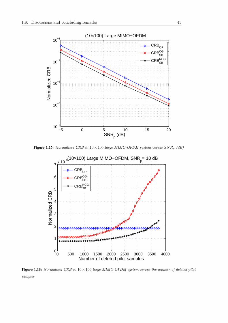
1.8. Discussions and concluding remarks 43
−5 0 5 10 15 2010−5
10−4
10−3
10−2
10−1(10×100) Large MIMO−OFDM
Nor
mal
ized
CR
B
SNRp (dB)
CRBOP
CRBSBCG
CRBSBNCG
Figure 1.15: Normalized CRB in 10× 100 large MIMO-OFDM system versus SNRp (dB)
0 500 1000 1500 2000 2500 3000 3500 40000
1
2
3
4
5
6
7x 10⁻³(10×100) Large MIMO−OFDM, SNR
p= 10 dB
Nor
mal
ized
CR
B
Number of deleted pilot samples
CRBOP
CRBSBCG
CRBSBNCG
Figure 1.16: Normalized CRB in 10× 100 large MIMO-OFDM system versus the number of deleted pilot
samples

44 Chapter 1. Performances analysis (CRB) for MIMO-OFDM systems
2
Ch
ap
te
r
Massive MIMO-OFDM semi-blind channel estimation per-
formance analysis
In order to succeed,
we must first believe that we can.
Nikos Kazantzakis.
This work has been done in collaboration with Ouahbi REKIK. It has been published in
EUSIPCO 2018 conference1.
Channel estimation is a critical process in a massive MIMO-OFDM system. However, pilot
contamination, an undeniable challenging issue, severely affects the performance of the system and
hence the aim of this chapter is to investigate the effectiveness of semi-blind channel estimation
approaches, using the Cramér Rao Bound (CRB) tool. This analysis demonstrates in particular
that when considering the finite alphabet signals, it is possible to efficiently solve the pilot
contamination problem with semi-blind channel estimation approach.
Abstract
1 [45] O. Rekik, A. Ladaycia, K. Abed-Meraim, and A. Mokraoui, "Performance Bounds Analysis for Semi-Blind
Channel Estimation with Pilot Contamination in Massive MIMO-OFDM Systems," in 2018 26th EUSIPCO, Sep.
2018, Rome, Italy.
46 Chapter 2. Performances analysis (CRB) for massive MIMO-OFDM systems
Chapter content2.1 Introduction . . . . . . . . . . . . . . . . . . . . . . . . . . . . . . . . . . . . . 47
2.2 Massive MIMO-OFDM system model . . . . . . . . . . . . . . . . . . . . . . . 48
2.3 Pilot contamination effect . . . . . . . . . . . . . . . . . . . . . . . . . . . . . . 50
2.4 Cramér Rao Bound derivation . . . . . . . . . . . . . . . . . . . . . . . . . . . 51
2.4.1 CRB for pilot-based channel estimation . . . . . . . . . . . . . . . . . . 51
2.4.2 CRB for semi-blind channel estimation . . . . . . . . . . . . . . . . . . . 52
2.4.2.1 Gaussian source signal . . . . . . . . . . . . . . . . . . . . . . . 52
2.4.2.2 Finite alphabet source signal . . . . . . . . . . . . . . . . . . . 53
2.5 Performance analysis and discussions . . . . . . . . . . . . . . . . . . . . . . . . 54
2.6 Conclusion . . . . . . . . . . . . . . . . . . . . . . . . . . . . . . . . . . . . . . 58
Appendix 2.A Proof of proposition 2.1 . . . . . . . . . . . . . . . . . . . . . . . . . 59
Appendix 2.B Proof of proposition 2.2 . . . . . . . . . . . . . . . . . . . . . . . . . 59
Appendix 2.C Proof of proposition 2.3 . . . . . . . . . . . . . . . . . . . . . . . . . 60
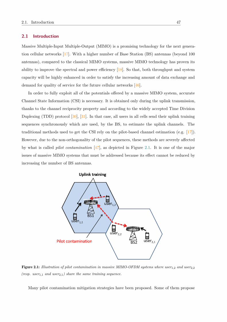
2.1. Introduction 47
2.1 Introduction
Massive Multiple-Input Multiple-Output (MIMO) is a promising technology for the next genera-
tion cellular networks [17]. With a higher number of Base Station (BS) antennas (beyond 100
antennas), compared to the classical MIMO systems, massive MIMO technology has proven its
ability to improve the spectral and power efficiency [18]. So that, both throughput and system
capacity will be highly enhanced in order to satisfy the increasing amount of data exchange and
demand for quality of service for the future cellular networks [46].
In order to fully exploit all of the potentials offered by a massive MIMO system, accurate
Channel State Information (CSI) is necessary. It is obtained only during the uplink transmission,
thanks to the channel reciprocity property and according to the widely accepted Time Division
Duplexing (TDD) protocol [30], [31]. In that case, all users in all cells send their uplink training
sequences synchronously which are used, by the BS, to estimate the uplink channels. The
traditional methods used to get the CSI rely on the pilot-based channel estimation (e.g. [17]).
However, due to the non-orthogonality of the pilot sequences, these methods are severely affected
by what is called pilot contamination [47], as depicted in Figure 2.1. It is one of the major
issues of massive MIMO systems that must be addressed because its effect cannot be reduced by
increasing the number of BS antennas.
Figure 2.1: Illustration of pilot contamination in massive MIMO-OFDM systems where user1,2 and user2,2
(resp. user1,1 and user2,1) share the same training sequence.
Many pilot contamination mitigation strategies have been proposed. Some of them propose
48 Chapter 2. Performances analysis (CRB) for massive MIMO-OFDM systems
to create more orthogonal pilots by slicing the time and frequency resources [48], however such a
choice will lead to a system capacity decrease. Other approaches are based on suppressing the
inter-cell interference by appropriate signal processing techniques, based on statistical information
of channel matrices [49], [50]. In such approaches, only a small portion of spatial dimensions
is used for data transmission, whereas the unemployed dimensions will be used for suppressing
noise and interference. However, many assumptions have to be considered to get statistical
information of channel matrices. Instead of depending only on pilot sequences, a data-aided
channel estimation has been considered (e.g. [51]). Thus, besides pilots, the decoded data is used
for channel estimation. Nonetheless, It is strongly assumed to have the ability to recover most of
data for accurate channel estimation. Some approaches have focused on designing appropriate
inter-cell communications protocols and resource allocation [52, 53, 54] in order to allow reusing
pilots without inter-cell interference. The counterpart is that the information exchange among
cells will add more complexity to the cellular networks.
In recent works, a particular attention has been drawn to blind (e.g. [55, 56]), and semi-blind
(e.g [57, 58, 59]) methods. The former is fully based on the statistical properties of the transmitted
data, whereas the latter depends on the joint use of pilots and data.
The focus of this study falls into the scope of performance analysis of semi-blind channel
estimation with pilot contamination in the context of multi-cell massive MIMO-OFDM systems.
For an estimator-independent performance analysis, the Cramér Rao Bound (CRB) is derived
for both pilot-based and semi-blind channel estimation by taking into account a perfect synchro-
nisation between the BS of the cell of interest and the neighboring cells BSs. This study is an
extension of the MIMO-OFDM case, done in chapter 1, to a massive MIMO-OFDM system, by
taking into account the multi-cell context and the phenomenon of pilot contamination in the
case of synchronized BSs transmissions.
It is worth to note that semi-blind techniques allow to retain the advantages of pilot-based and
blind-based approaches; i.e. more channel estimation accuracy and more robustness against pilot
contamination, while reducing their drawbacks; i.e. pilot contamination and inherent ambiguity
with high computational complexity.
2.2 Massive MIMO-OFDM system model
This section presents the massive MIMO-OFDM wireless system model adopted in this thesis.
An uplink transmission is considered. The system is composed of Nc cells each one having one
BS with Nr antennas and Nt randomly located users using each a single antenna.
2.2. Massive MIMO-OFDM system model 49
Let us ignore at first the received signals from the adjacent cells. Therefore the received
signal, after cyclic prefix removal and FFT, at the r-th BS antenna of the l-th cell, assumed to
be a K sub-carriers OFDM signal, is given by (see chapter 1):
yl,r =Nt∑i=1
F T (hl,i,r)FH
Kxl,i + vl,r, (2.1)
where K is the OFDM symbol length; F represents a K-point Fourier matrix; hl,i,r is a N × 1
vector representing the channel taps between the i-th user, of the l-th cell, and the r-th receive
antenna; T (hl,i,r) is a circulant matrix; xl,i is the i-th user OFDM symbol of cell l. vl,r is assumed
to be an additive white Circulant Gaussian (CG) noise so that E[vl,r(k)vl,r(i)H ] = σ2vlIKδki
where σ2vl is the noise variance at the l-th cell; δki being the Kronecker delta operator.
Using the eigenvalue decomposition of the circulant matrix T (hl,i,r) given by:
T (hl,i,r) = FH
Kdiag
{Whl,i,r
}F, (2.2)
the received signal, of dimension NrK × 1, at the l-th BS can be re-expressed as follows:
yl = λlxl + vl, (2.3)
where yl = [yTl,1...yTl,Nr ]T ; xl = [xTl,1...xTl,Nt ]
T ; vl = [vTl,1...vTl,Nr ]T ; λl = [λl,1...λl,Nt ] with λl,i =
[λl,i,1...λl,i,Nr ]T where λl,i,r = diag{Whl,i,r} and W is formed by the N first columns of F.
In order to facilitate the derivation of the CRB w.r.t. h1, equation (2.3) is rewritten as
follows:
yl = Xlhl + vl, (2.4)
where hl = [hTl,1,1...hTl,Nt,1......hTl,1,Nr ...h
Tl,Nt,Nr
]T is a NrNtN × 1 vector; Xl = INr ⊗Xl is a
NrK ×NrNtN dimensional matrix with Xl = [Xl,D1W...Xl,DNtW] of size K ×NtN , and Xl,Di
is a K×K diagonal matrix containing the i-th user symbols, i.e. Xl,Di = diag(xl,i), and ⊗ refers
to the Kronecker product.
Now, let us take into account the effect of the neighboring cells on the first one, considered
without loss of generality as the interest cell. With the assumption of perfect synchronization
between the Nc cells, equation (2.3) becomes:
y1 =Nc∑l=1λlxl + v1 = λtotxtot + v1, (2.5)
where λtot = [λ1 . . .λNc ] and xtot = [xT1 . . .xTNc]T .
Similarly to (2.4), equation (2.5) can be rewritten as follows:
y1 =Nc∑l=1
Xlhl + v1 = Xtothtot + v1, (2.6)
50 Chapter 2. Performances analysis (CRB) for massive MIMO-OFDM systems
where Xtot = [X1 . . .XNc ] and htot = [hT1 . . .hTNc ]T .
2.3 Pilot contamination effect
Herein, the effect of pilot contamination on the performance of semi-blind channel estimation
approaches is investigated, under the assumption of perfectly synchronized BSs in the different
Nc cells in a massive MIMO-OFDM system. In such a case, and with same pilots in all cells, the
worst case of pilot contamination occurs as explained next.
During the uplink data transmission, the BS has to learn the transmission channel by
exploiting the known symbols (i.e. pilots) at the uplink. To adopt this strategy the pilots used
within the same cell and in the neighboring cells should be mutually orthogonal. However this
necessitates a complex cell synchronization and cooperation scheme. In addition, the channel
time coherence [60], [61] limits the total number of orthogonal pilots leading to the reuse of the
same pilots in many neighboring cells. The worst case occurs when the same set of pilots is
reused in all Nc adjacent cells. In this situation, equation (2.6) becomes:
y1 =Nc∑l=1
X1Phl + v1 = X1P
Nc∑l=1
hl + v1, (2.7)
where X1P corresponds to the pilot symbols of the first cell.
To illustrate the pilot contamination effect in that case, the Least Squares (LS) estimate of
the first cell channel vector, i.e. h1, is given by:
hLS1 = X#1Py1 = h1 +
Nc∑l=1,l,1
hl + X#1Pv1, (2.8)
with X#1P = (XH
1P X1P )−1XH1P is the pseudo inverse of X1P .
This equation clearly shows that the channel estimate hLS1 is affected by an additional bias
corresponding to the sum of channel components of the users sharing the same pilot sequences
in different cells. This phenomenon, referred to as pilot contamination, severely degrades the
channel estimation performance. To overcome this problem, an alternative solution consists of
using semi-blind channel estimation approach. In the sequel, the potential of this approach is
analyzed and discussed through the use of the CRB tool.
2.4. Cramér Rao Bound derivation 51
2.4 Cramér Rao Bound derivation
Here we derive the CRB for pilot-based and semi-blind channel estimation. For the complex
valued channel taps, the parameters vector θ is defined, in our case, as follows:
θ = [hTtot (h∗tot)T ]T , (2.9)
where, for simplicity, the signal and noise powers are assumed to be known.
Under the assumption that pilots and data (corresponding to block-type arrangement) are
statistically independent, as in chapter 1 the FIM is given by equation (1.11).
2.4.1 CRB for pilot-based channel estimation
The noise components are assumed to be independent identically distributed (i.i.d.), and only
Np pilots are used for channel estimation. Based on the data model, the pilot-based FIM can be
expressed by:
Jpθθ =Np∑i=1
Jpiθθ, (2.10)
with Jpiθθ is the FIM associated to the pi-th pilot symbol given by:
Jpiθθ =
Jpihtothtot 0
0 Jpih∗toth∗tot
, (2.11)
where Jpih∗toth∗tot = (Jpihtothtot)∗.
By considering a massive MIMO-OFDM system with Nc cells, the pilot-based FIM associated
to the channel vector htot is then expressed as follows:
Jpihtothtot =XHtot,piXtot,pi
σ2v1
, (2.12)
which can also be written in a more detailed form:
Jpihtothtot = 1σ2
v1
XH
1piX1pi . . . XH
1piXNcpi
.... . .
...
XHNcpi
X1pi . . . XHNcpi
XNcpi
. (2.13)
Ideally, if the pilots of the cells are mutually orthogonal, i.e. XHi,pi
Xj,pi = 0 ∀ i , j, then the
FIM becomes a bloc diagonal matrix which is the most favorable case. On the other hand, if
the cells share the same set of pilots, i.e. the worst case of pilot contamination, the FIM is then
52 Chapter 2. Performances analysis (CRB) for massive MIMO-OFDM systems
equivalent to:
Jpihtothtot = 1σ2
v1
XH
1piX1pi . . . XH
1piX1pi
.... . .
XH1pi
X1pi . . . XH1pi
X1pi
. (2.14)
To compute the CRB, the FIM has to be inverted. However, according to this last equation,
Jpihtothtot , and consequently Jhtothtot , is not a full rank matrix. In fact, according to proposition
2.1, the kernel of this FIM is of dimension 2(Nc− 1)NtNrN , corresponding to the number of
indeterminacies we need to get rid of. In other words, this translates the non-identifiability of
the channel vector of the interest cell when pilot contamination occurs.
Proposition 2.1. The FIM in (2.14) is a singular matrix and its kernel dimension is 2(Nc−
1)NtNrN which corresponds to the number of indeterminacies of the problem (i.e. the number
of unknown real channel parameters for the Nc− 1 neighboring cells).
Proof: See appendix 2.A.
2.4.2 CRB for semi-blind channel estimation
In this section we derive the CRB for the semi-blind channel estimation for a multi-cell massive
MIMO-OFDM system with pilot contamination. Both pilots and data are taken into account in
the derivation of the FIM as shown in equation (1.11). At first, we investigate the performance
bounds of the semi-blind scheme when only the Second Order Statistics (SOS) are considered.
For that, we use a Circular Gaussian data model as developed in chapter 1. Latter on, we extend
this analysis to the case where information based on Higher Order Statistics is available. This
will be illustrated using a finite alphabet source signal.
2.4.2.1 Gaussian source signal
As mentioned previously, we consider here only the SOS corresponding to the Gaussian CRB.
Hence, we assume that the data symbols are i.i.d. Circular Gaussian distributed with zero mean
and a diagonal covariance matrix composed of the users’ transmit powers i.e. Cxl = diag(σ2xl,i)
with l = 1...Nc and i= 1...Nt. Under this assumption, the received signal y1 is Circular Gaussian
with covariance matrix:
Cy1 =Nc∑l=1λlCxlλ
Hl +σ2
v1IKNr . (2.15)
The data-based FIM can be expressed as follows (e.g.[62], [35]):
Jdhtothtot =
Jdhtothtot Jdhtoth∗totJdh∗tothtot Jdh∗toth∗tot
, (2.16)
2.4. Cramér Rao Bound derivation 53
where Jdhtothtot is a (NcNrNtN)-dimensional matrix with elements Jdhihj given by:
Jdhihj = tr
C−1y1
∂Cy1
∂h∗iC−1
y1
(∂Cy1
∂h∗j
)H . (2.17)
The i-th component of the vector htot corresponds to the channel tap of indices {iNc , iNt , iNr , iN}
associated to the cell, the user, the BS antenna and the time lag of hi. Based on the results
provided in chapter 1, Jdhihj is given by:
Jdhihj = (Jdh∗i h∗j )∗ = tr
C−1y1 σ
2iNc ,iNt
λiNc ,iNt
∂λHiNc ,iNt∂h∗i
C−1y1 σ
2jNc ,jNt
∂λjNc ,jNt∂hj
λHjNc ,jNt
(2.18)
and
Jdhih∗j= (Jdh∗i hj )
∗ = tr
C−1y1 σ
2iNc ,iNt
λiNc ,iNt
∂λHiNc ,iNt∂h∗i
C−1y1 σ
2jNc ,jNt
λjNc ,jNt
∂λHjNc ,jNt∂h∗j
(2.19)
It is important to notice that using a semi-blind estimation method with only the SOS of the
received data is not sufficient to alleviate the pilot contamination problem. Indeed, the SOS-SB
scheme reduces the number of indeterminacies but does not get rid of all of them. More precisely,
we have the following proposition:
Proposition 2.2. The FIM in (2.17) is a singular matrix and, in the case Nr >NcNt, its kernel
dimension is (NcNt)2 correponding to the number of indeterminacies in the blind channel
estimation case. When considering the SOS-based semi-blind channel estimation, the kernel
dimension of the FIM in (1.11) becomes ((Nc− 1)Nt)2.
Proof: See Appendix 2.B.
2.4.2.2 Finite alphabet source signal
Here we consider the non Gaussian nature of communications signals through the use of a finite
alphabet (BPSK) data model. The observed signal at the k-th sub-carrier is given by [32]:
y1(k) = λtot(k)Cx12 x(k) + v1(k) for k = 1, ...,K, (2.20)
where λtot(k) is the k-th Fourier component of htot; Cx is a block diagonal matrix formed by
users’ transmit powers of each cell; x(k) = [xT1,(k)...xTNc,(k)]
T with xl,(k) = [xl,1,(k)...xl,Nt,(k)]T so
that xl,i,(k) for k = 1...K are i.i.d. BPSK symbols taking values ±1 with equal probabilities.
In this case, the likelihood function is a sum of 2NcNt Gaussian pdfs given by:
p(y1(k),θ) = 12NcNt
2NcNt∑q=1
1(πσ2
v1)Nre
−
∥∥∥∥∥y1(k)−λtot(k) Cx12 xq
σ2v1
∥∥∥∥∥, (2.21)
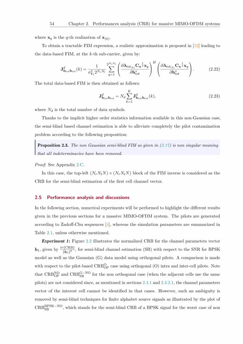
54 Chapter 2. Performances analysis (CRB) for massive MIMO-OFDM systems
where xq is the q-th realization of x(k).
To obtain a tractable FIM expression, a realistic approximation is proposed in [32] leading to
the data-based FIM, at the k-th sub-carrier, given by:
Jdhtothtot(k) = 1σ2
v12NcNt2NcNt∑q=1
∂λtot(k)Cx12 xq
∂h∗tot
H∂λtot(k)Cx12 xq
∂h∗tot
. (2.22)
The total data-based FIM is then obtained as follows:
Jdhtothtot =Nd
K∑k=1
Jdhtothtot(k), (2.23)
where Nd is the total number of data symbols.
Thanks to the implicit higher order statistics information available in this non-Gaussian case,
the semi-blind based channel estimation is able to alleviate completely the pilot contamination
problem according to the following proposition:
Proposition 2.3. The non Gaussian semi-blind FIM as given in (2.17) is non singular meaning
that all indeterminacies have been removed.
Proof: See Appendix 2.C.
In this case, the top-left (NrNtN)× (NrNtN) block of the FIM inverse is considered as the
CRB for the semi-blind estimation of the first cell channel vector.
2.5 Performance analysis and discussions
In the following section, numerical experiments will be performed to highlight the different results
given in the previous sections for a massive MIMO-OFDM system. The pilots are generated
according to Zadoff-Chu sequences [4], whereas the simulation parameters are summarized in
Table 2.1, unless otherwise mentioned.
Experiment 1: Figure 2.2 illustrates the normalized CRB for the channel parameters vector
h1, given by tr{CRB}‖h1‖2 , for semi-blind channel estimation (SB) with respect to the SNR for BPSK
model as well as the Gaussian (G) data model using orthogonal pilots. A comparison is made
with respect to the pilot-based CRBOOP case using orthogonal (O) intra and inter-cell pilots. Note
that CRBNOOP and CRBG−NO
SB for the non orthogonal case (when the adjacent cells use the same
pilots) are not considered since, as mentioned in sections 2.4.1 and 2.4.2.1, the channel parameters
vector of the interest cell cannot be identified in that cases. However, such an ambiguity is
removed by semi-blind techniques for finite alphabet source signals as illustrated by the plot of
CRBBPSK−NOSB , which stands for the semi-blind CRB of a BPSK signal for the worst case of non
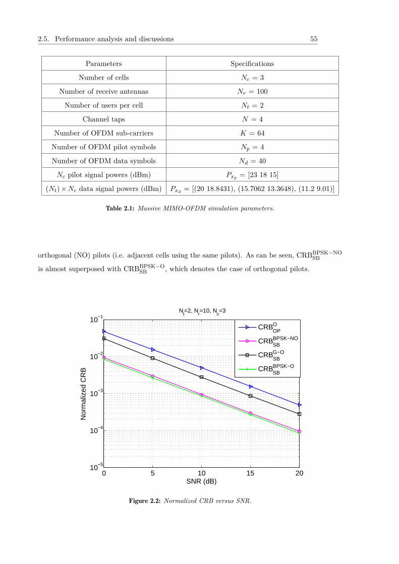
2.5. Performance analysis and discussions 55
Parameters Specifications
Number of cells Nc = 3
Number of receive antennas Nr = 100
Number of users per cell Nt = 2
Channel taps N = 4
Number of OFDM sub-carriers K = 64
Number of OFDM pilot symbols Np = 4
Number of OFDM data symbols Nd = 40
Nc pilot signal powers (dBm) Pxp = [23 18 15]
(Nt)×Nc data signal powers (dBm) Pxd = [(20 18.8431), (15.7062 13.3648), (11.2 9.01)]
Table 2.1: Massive MIMO-OFDM simulation parameters.
orthogonal (NO) pilots (i.e. adjacent cells using the same pilots). As can be seen, CRBBPSK−NOSB
is almost superposed with CRBBPSK−OSB , which denotes the case of orthogonal pilots.
0 5 10 15 2010−5
10−4
10−3
10−2
10−1N
t=2, N
r=10, N
c=3
Nor
mal
ized
CR
B
SNR (dB)
CRB
OPO
CRBSBBPSK−NO
CRBSBG−O
CRBSBBPSK−O
Figure 2.2: Normalized CRB versus SNR.
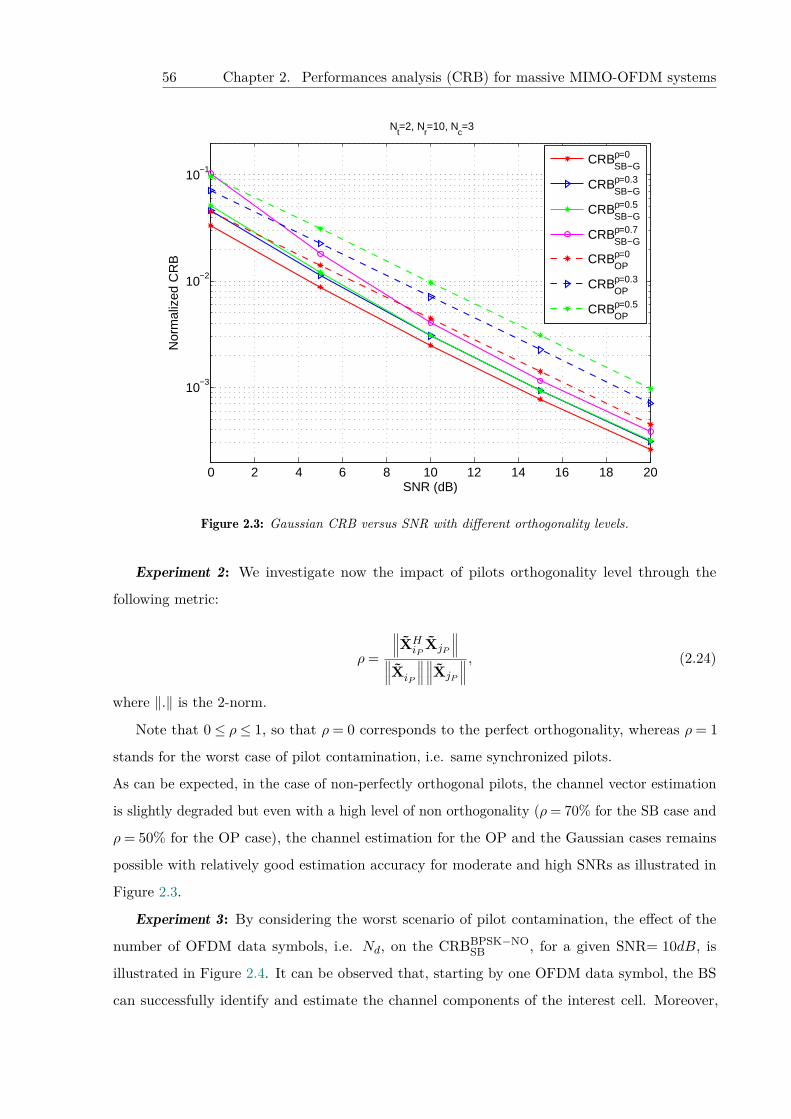
56 Chapter 2. Performances analysis (CRB) for massive MIMO-OFDM systems
0 2 4 6 8 10 12 14 16 18 20
10−3
10−2
10−1N
orm
aliz
ed C
RB
SNR (dB)
Nt=2, N
r=10, N
c=3
CRBSB−Gρ=0
CRBSB−Gρ=0.3
CRBSB−Gρ=0.5
CRBSB−Gρ=0.7
CRBOPρ=0
CRBOPρ=0.3
CRBOPρ=0.5
Figure 2.3: Gaussian CRB versus SNR with different orthogonality levels.
Experiment 2: We investigate now the impact of pilots orthogonality level through the
following metric:
ρ=
∥∥∥XHiP
XjP
∥∥∥∥∥∥XiP
∥∥∥∥∥∥XjP
∥∥∥ , (2.24)
where ‖.‖ is the 2-norm.
Note that 0 ≤ ρ ≤ 1, so that ρ= 0 corresponds to the perfect orthogonality, whereas ρ= 1
stands for the worst case of pilot contamination, i.e. same synchronized pilots.
As can be expected, in the case of non-perfectly orthogonal pilots, the channel vector estimation
is slightly degraded but even with a high level of non orthogonality (ρ= 70% for the SB case and
ρ= 50% for the OP case), the channel estimation for the OP and the Gaussian cases remains
possible with relatively good estimation accuracy for moderate and high SNRs as illustrated in
Figure 2.3.
Experiment 3: By considering the worst scenario of pilot contamination, the effect of the
number of OFDM data symbols, i.e. Nd, on the CRBBPSK−NOSB , for a given SNR= 10dB, is
illustrated in Figure 2.4. It can be observed that, starting by one OFDM data symbol, the BS
can successfully identify and estimate the channel components of the interest cell. Moreover,
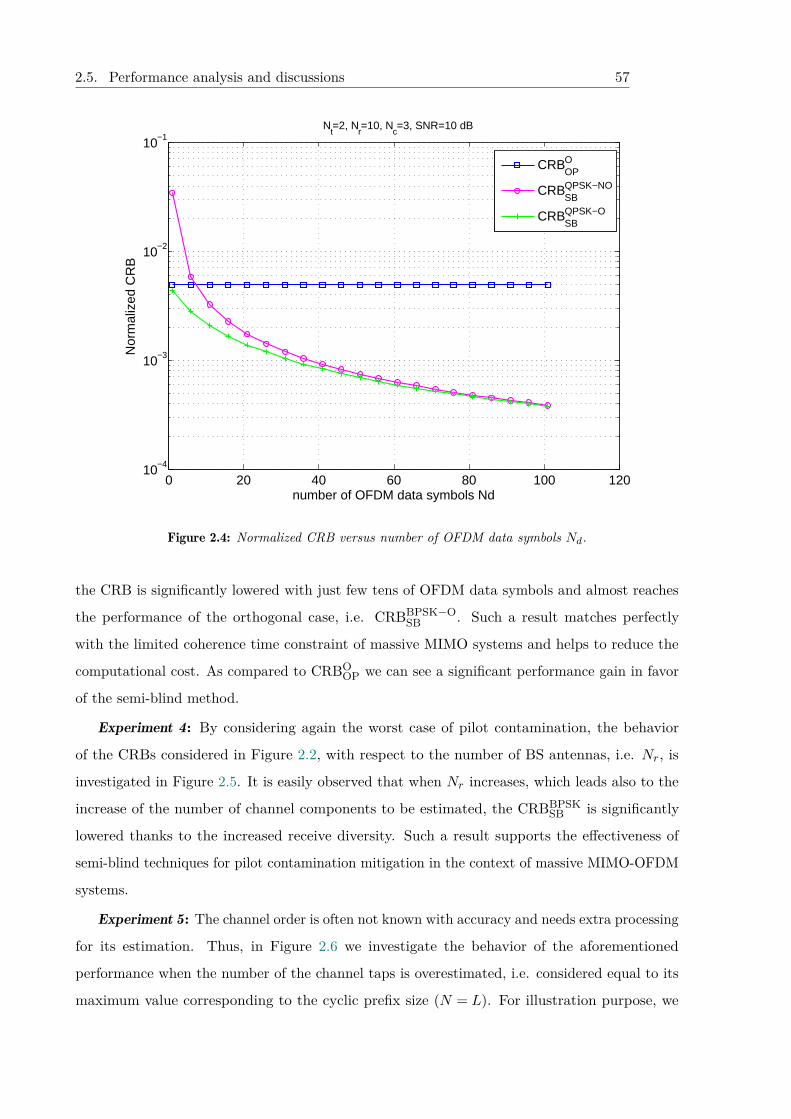
2.5. Performance analysis and discussions 57
0 20 40 60 80 100 12010−4
10−3
10−2
10−1
number of OFDM data symbols Nd
Nor
mal
ized
CR
BN
t=2, N
r=10, N
c=3, SNR=10 dB
CRBOPO
CRBSBQPSK−NO
CRBSBQPSK−O
Figure 2.4: Normalized CRB versus number of OFDM data symbols Nd.
the CRB is significantly lowered with just few tens of OFDM data symbols and almost reaches
the performance of the orthogonal case, i.e. CRBBPSK−OSB . Such a result matches perfectly
with the limited coherence time constraint of massive MIMO systems and helps to reduce the
computational cost. As compared to CRBOOP we can see a significant performance gain in favor
of the semi-blind method.
Experiment 4: By considering again the worst case of pilot contamination, the behavior
of the CRBs considered in Figure 2.2, with respect to the number of BS antennas, i.e. Nr, is
investigated in Figure 2.5. It is easily observed that when Nr increases, which leads also to the
increase of the number of channel components to be estimated, the CRBBPSKSB is significantly
lowered thanks to the increased receive diversity. Such a result supports the effectiveness of
semi-blind techniques for pilot contamination mitigation in the context of massive MIMO-OFDM
systems.
Experiment 5: The channel order is often not known with accuracy and needs extra processing
for its estimation. Thus, in Figure 2.6 we investigate the behavior of the aforementioned
performance when the number of the channel taps is overestimated, i.e. considered equal to its
maximum value corresponding to the cyclic prefix size (N = L). For illustration purpose, we
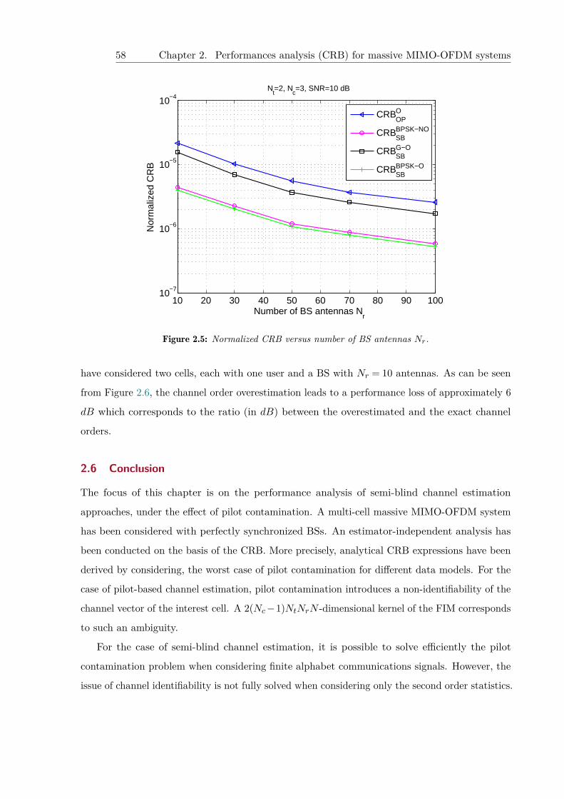
58 Chapter 2. Performances analysis (CRB) for massive MIMO-OFDM systems
10 20 30 40 50 60 70 80 90 10010−7
10−6
10−5
10−4
Nor
mal
ized
CR
B
Number of BS antennas Nr
Nt=2, N
c=3, SNR=10 dB
CRBOPO
CRBSBBPSK−NO
CRBSBG−O
CRBSBBPSK−O
Figure 2.5: Normalized CRB versus number of BS antennas Nr.
have considered two cells, each with one user and a BS with Nr = 10 antennas. As can be seen
from Figure 2.6, the channel order overestimation leads to a performance loss of approximately 6
dB which corresponds to the ratio (in dB) between the overestimated and the exact channel
orders.
2.6 Conclusion
The focus of this chapter is on the performance analysis of semi-blind channel estimation
approaches, under the effect of pilot contamination. A multi-cell massive MIMO-OFDM system
has been considered with perfectly synchronized BSs. An estimator-independent analysis has
been conducted on the basis of the CRB. More precisely, analytical CRB expressions have been
derived by considering, the worst case of pilot contamination for different data models. For the
case of pilot-based channel estimation, pilot contamination introduces a non-identifiability of the
channel vector of the interest cell. A 2(Nc−1)NtNrN -dimensional kernel of the FIM corresponds
to such an ambiguity.
For the case of semi-blind channel estimation, it is possible to solve efficiently the pilot
contamination problem when considering finite alphabet communications signals. However, the
issue of channel identifiability is not fully solved when considering only the second order statistics.
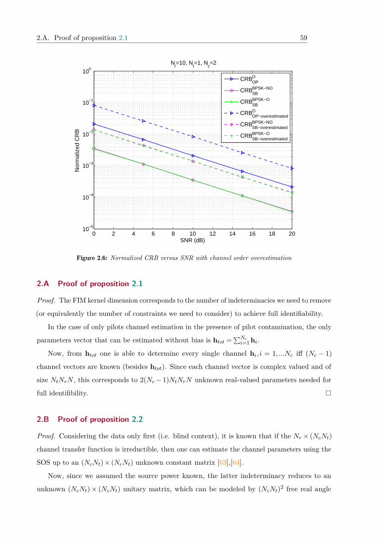
2.A. Proof of proposition 2.1 59
0 2 4 6 8 10 12 14 16 18 2010−5
10−4
10−3
10−2
10−1
100N
r=10, N
t=1, N
c=2
Nor
mal
ized
CR
B
SNR (dB)
CRBOPO
CRBSBBPSK−NO
CRBSBBPSK−O
CRBOP−overestimatedO
CRBSB−overestimatedBPSK−NO
CRBSB−overestimatedBPSK−O
Figure 2.6: Normalized CRB versus SNR with channel order overestimation
2.A Proof of proposition 2.1
Proof. The FIM kernel dimension corresponds to the number of indeterminacies we need to remove
(or equivalently the number of constraints we need to consider) to achieve full identifiability.
In the case of only pilots channel estimation in the presence of pilot contamination, the only
parameters vector that can be estimated without bias is htot =∑Nci=1 hi.
Now, from htot one is able to determine every single channel hi, i = 1, ...Nc iff (Nc − 1)
channel vectors are known (besides htot). Since each channel vector is complex valued and of
size NtNrN , this corresponds to 2(Nc− 1)NtNrN unknown real-valued parameters needed for
full identifibility.
2.B Proof of proposition 2.2
Proof. Considering the data only first (i.e. blind context), it is known that if the Nr × (NcNt)
channel transfer function is irreductible, then one can estimate the channel parameters using the
SOS up to an (NcNt)× (NcNt) unknown constant matrix [63],[64].
Now, since we assumed the source power known, the latter indeterminacy reduces to an
unknown (NcNt)× (NcNt) unitary matrix, which can be modeled by (NcNt)2 free real angle
60 Chapter 2. Performances analysis (CRB) for massive MIMO-OFDM systems
parameters.
Somehow, the data SOS allows us to reduce the convolution model into an instantaneous
(NcNt) dimensional linear mixture model.
Finally, as in the only pilots case, due to the pilot contamination, the only way to complete
the channel identification via the pilot use, is to have (know) the space directions of the interfering
users of the neighboring cells corresponding to ((Nc− 1)Nt)2 real parameters to determine.
2.C Proof of proposition 2.3
Proof. For non-Gaussian (communications) signals, the information provided by the Second
Order Statistics as well as Higher Order Statistics of the data allows us to identify the channels up
to an unknown (NcNt)× (NcNt) diagonal unitary matrix(see for example identifiability results in
[65]). This corresponds to NcNt unknown real parameters that can be easily estimated through
the use of the pilots.
3
Ch
ap
te
r
SIMO-OFDM system CRB derivation and application
Our greatest weakness lies in
giving up. The most certain way to
succeed is always to try just one more
time.
Thomas A. Edison.
This chapter focuses on SIMO-OFDM communications system, which is a particular case of
the MIMO-OFDM case derived in chapter 1. Unlike in chapter 1, where the CRB derivations
have been done in the frequency domain, the performances limits are derived in time domain. By
using the CRB tool, before performing Fourier transform (i.e. in time domain), we compare the
estimation error variance of the pilot-based and semi-blind based techniques for different data
models1(deterministic and stochastic models). A practical application of the derived CRB is
proposed in this chapter, which consists on the protection of the exchanged data between a drone
and mobile stations against blind interceptions2.
Abstract
1 [66] A. Ladaycia, A. Mokraoui, K. Abed-Meraim, and A. Belouchrani, "What semi-blind channel estimation
brings in terms of throughput gain?" in 2016 10th ICSPCS, Dec. 2016, pp. 1-6, Gold Coast, Australia.2 [67] A. Ladaycia, A. Belouchrani, K. Abed-Meraim, and A. Mokraoui, "Parameter optimization for defeating
blind interception in drone protection," in 2017 Seminar on Detection Systems Architectures and Technologies
(DAT), Feb. 2017, pp. 1-6, Alger, Algeria.
62 Chapter 3. SIMO-OFDM system CRB derivation and application
Chapter content3.1 Introduction . . . . . . . . . . . . . . . . . . . . . . . . . . . . . . . . . . . . . 63
3.2 SIMO-OFDM wireless communications system . . . . . . . . . . . . . . . . . . 63
3.3 CRB for SIMO-OFDM pilot-based channel estimation . . . . . . . . . . . . . . 65
3.4 CRB for SIMO-OFDM semi-blind channel estimation . . . . . . . . . . . . . . 65
3.4.1 Deterministic Gaussian data model . . . . . . . . . . . . . . . . . . . . . 66
3.4.1.1 Special-case: Hybrid pilot in semi-blind channel estimation
with deterministic Gaussian data model . . . . . . . . . . . . . 67
3.4.2 Stochastic Gaussian data model (CRBStochSB ) . . . . . . . . . . . . . . . 67
3.4.2.1 Special-case: Hybrid pilot in semi-blind channel estimation
with stochastic Gaussian model . . . . . . . . . . . . . . . . . 68
3.4.2.2 Reduction of the FIM computational complexity . . . . . . . . 69
3.5 CRB analysis for defeating blind interception . . . . . . . . . . . . . . . . . . . 70
3.6 Simulation results and discussions . . . . . . . . . . . . . . . . . . . . . . . . . 71
3.6.1 Throughput gain analysis of SIMO-OFDM semi-blind channel estimation 71
3.6.2 Blind interception analysis . . . . . . . . . . . . . . . . . . . . . . . . . 76
3.7 Conclusion . . . . . . . . . . . . . . . . . . . . . . . . . . . . . . . . . . . . . . 77
3.1. Introduction 63
3.1 Introduction
Channel estimation in SIMO-OFDM communications systems can be done in time domain
(i.e. before applying Fourier transform to the received signal) or in the frequency domain as
developed in chapter 1. This chapter focuses on the channel estimation performance of a SIMO-
OFDM wireless communications system. The objective is to show that a semi-blind channel
estimation approach based on a compromise between the inserted block-type arrangement pilots
and the transmitted symbols can preserve the SIMO-OFDM performance system while increasing
significantly the information throughput. In order to analyze the theoretical performance limit
of the different considered channel estimation approaches, CRB is derived. The CRB bounds, in
a IEEE 802.11n wireless context, are then analyzed and discussed.
A practical application of the derived CRBs consists of protecting the exchanged data between
a drone and mobile stations against blind interceptions. The developed strategy for a SIMO-
OFDM communications system consists to prevent the interceptors to achieve a good blind
channel estimation while allowing an accurate channel identification by the drone in the same
wireless transmission conditions. To do so, a relevant selection of the communication parameters
such as an appropriate data model with a specific data power is proposed. Simulations show
that, under the same wireless transmission conditions, the blind channel estimation approach
achieves the worst performance ensuring therefore the protection of the transmitted data.
3.2 SIMO-OFDM wireless communications system
Before deriving the CRB to analyze the performance of the channel estimation approaches, this
section introduces the mathematical representation, in time domain, of the SIMO-OFDM wireless
communications system.
Consider a SIMO-OFDM wireless system using Nr receive antennas, as shown in Figure 3.1,
receiving the signal y(k) given by:
y(k) =N−1∑i=0
h(i)x(k− i) + v(k), (3.1)
where h(i) = [h1(i) · · · hNr(i)]T ; y(k) = [y1(k) · · · yNr(k)]T ; and v(k) = [v1(k) · · · vNr(k)]T is an
additive independent white Complex-Gaussian circular noise with E[v(k)v(i)H
]= σ2
vINrδki.
The received signal is assumed to be an OFDM one where a Cyclic CP is introduced in each front
of an OFDM symbol. The signal x is composed of K samples and a CP of L samples. Under the
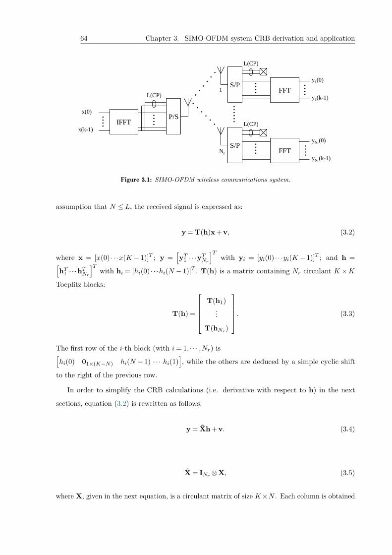
64 Chapter 3. SIMO-OFDM system CRB derivation and application
S/PFFT
L(CP)
S/PFFT
L(CP)
Nr
1
y1(0)
y1(k-1)
yNr(0)
yNr(k-1)
....
........
....
......P/SIFFT
L(CP)
x(0)
x(k-1)
....
....
Figure 3.1: SIMO-OFDM wireless communications system.
assumption that N ≤ L, the received signal is expressed as:
y = T(h)x + v, (3.2)
where x = [x(0) · · ·x(K − 1)]T ; y =[yT1 · · ·yTNr
]Twith yi = [yi(0) · · ·yi(K − 1)]T ; and h =[
hT1 · · ·hTNr]T
with hi = [hi(0) · · ·hi(N − 1)]T . T(h) is a matrix containing Nr circulant K ×K
Toeplitz blocks:
T(h) =
T(h1)...
T(hNr)
. (3.3)
The first row of the i-th block (with i= 1, · · · ,Nr) is[hi(0) 01×(K−N) hi(N − 1) · · · hi(1)
], while the others are deduced by a simple cyclic shift
to the right of the previous row.
In order to simplify the CRB calculations (i.e. derivative with respect to h) in the next
sections, equation (3.2) is rewritten as follows:
y = Xh + v. (3.4)
X = INr ⊗X, (3.5)
where X, given in the next equation, is a circulant matrix of size K×N . Each column is obtained
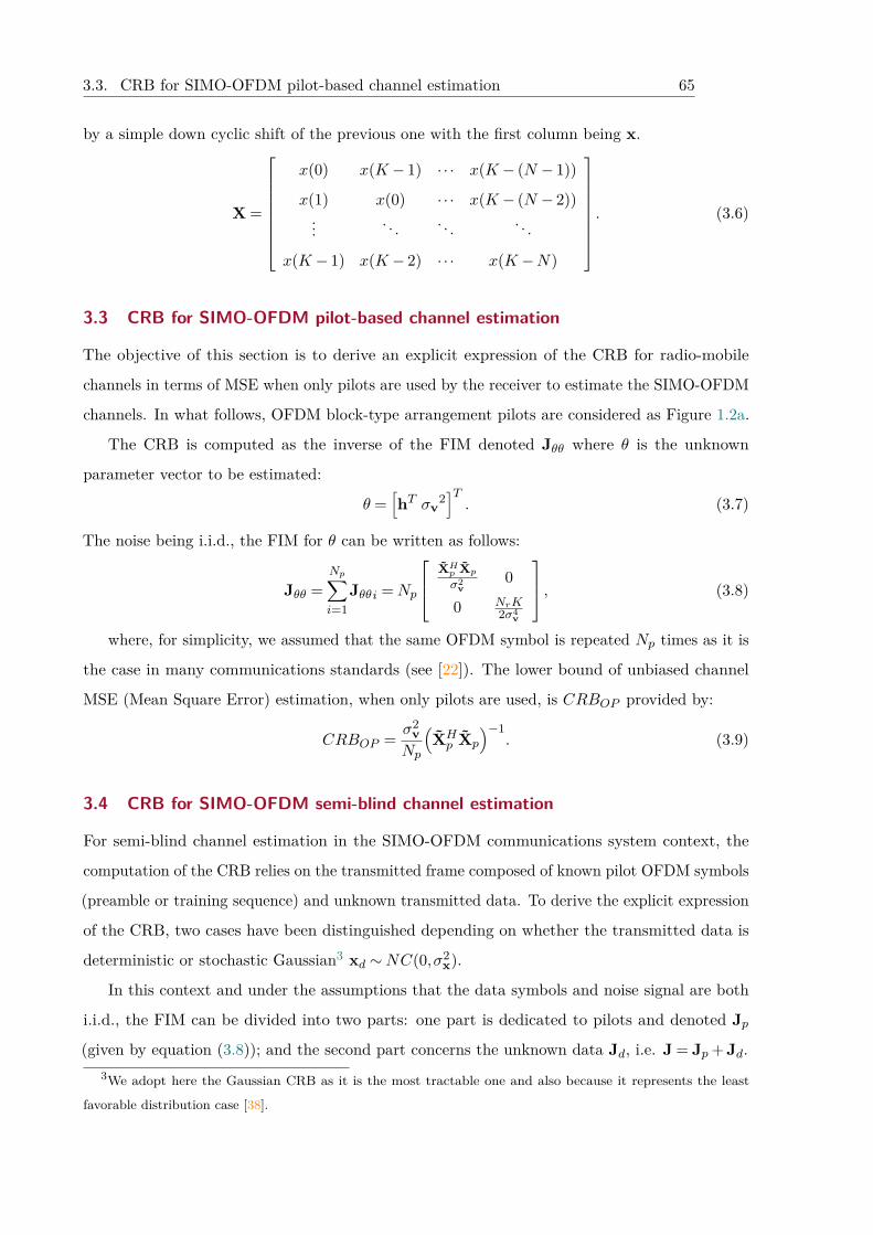
3.3. CRB for SIMO-OFDM pilot-based channel estimation 65
by a simple down cyclic shift of the previous one with the first column being x.
X =
x(0) x(K − 1) · · · x(K − (N − 1))
x(1) x(0) · · · x(K − (N − 2))...
. . .. . .
. . .
x(K − 1) x(K − 2) · · · x(K −N)
. (3.6)
3.3 CRB for SIMO-OFDM pilot-based channel estimation
The objective of this section is to derive an explicit expression of the CRB for radio-mobile
channels in terms of MSE when only pilots are used by the receiver to estimate the SIMO-OFDM
channels. In what follows, OFDM block-type arrangement pilots are considered as Figure 1.2a.
The CRB is computed as the inverse of the FIM denoted Jθθ where θ is the unknown
parameter vector to be estimated:
θ =[hT σv
2]T. (3.7)
The noise being i.i.d., the FIM for θ can be written as follows:
Jθθ =Np∑i=1
Jθθi =Np
XHp Xp
σ2v
0
0 NrK2σ4
v
, (3.8)
where, for simplicity, we assumed that the same OFDM symbol is repeated Np times as it is
the case in many communications standards (see [22]). The lower bound of unbiased channel
MSE (Mean Square Error) estimation, when only pilots are used, is CRBOP provided by:
CRBOP = σ2vNp
(XHp Xp
)−1. (3.9)
3.4 CRB for SIMO-OFDM semi-blind channel estimation
For semi-blind channel estimation in the SIMO-OFDM communications system context, the
computation of the CRB relies on the transmitted frame composed of known pilot OFDM symbols
(preamble or training sequence) and unknown transmitted data. To derive the explicit expression
of the CRB, two cases have been distinguished depending on whether the transmitted data is
deterministic or stochastic Gaussian3 xd ∼NC(0,σ2x).
In this context and under the assumptions that the data symbols and noise signal are both
i.i.d., the FIM can be divided into two parts: one part is dedicated to pilots and denoted Jp(given by equation (3.8)); and the second part concerns the unknown data Jd, i.e. J = Jp + Jd.
3We adopt here the Gaussian CRB as it is the most tractable one and also because it represents the least
favorable distribution case [38].
66 Chapter 3. SIMO-OFDM system CRB derivation and application
We assume that the unknown transmitted data, denoted xd, is composed ofNd OFDM symbols,
i.e xd = [xTs1 xTs2 · · · xTsNd
]T . Denote x the signal composed of known pilots and transmitted data:
x = [xTp xTd ]T . The received signal, denoted y, corresponding to the transmitted unknown data
xd is expressed as follows:
y = Td(h)xd + v = Xdh + v, (3.10)
where Xd has the following form:
Xd =[XTs1 XT
s2 · · · XTsNd
]T, (3.11)
with Xsi the matrix given by equation (3.5) and filled with the elements of the i-th data OFDM
symbol xsi . Matrix Td(h) is given by:
Td(h) = INd ⊗T(h). (3.12)
3.4.1 Deterministic Gaussian data model
Here the unknown data OFDM symbols are assumed to be deterministic so that the unknown
parameter vector θ becomes:
θ =[hT xT
d σ2v
]T. (3.13)
The corresponding FIM expression is given in [39, 68, 36]:
Jd =
XHd Xd
σv2XHd Td(h)σv2 0
Td(h)HXd
σv2Td(h)HTd(h)
σv2 0
0 0 NrMd2σ4
v
. (3.14)
The global FIM when taking into account the FIM of the pilots becomes:
J =
XHd Xd+Np(XH
p Xp)σ2
v
XHd Td(h)σ2
v0
Td(h)HXd
σ2v
Td(h)HTd(h)σ2
v0
0 0 Nr(Md+Mp)2σv4
. (3.15)
Therefore the CRB explicit expression for semi-blind channel estimation is given as follows:
CRBDetSB = σ2v
(A−BD−1C
)−1(3.16)
where A = XHd Xd +Np
(XHp Xp
); B = CH = XH
d Td(h); and D = Td(h)HTd(h). To avoid the
inversion of the very large matrix, we use the Schur’s complement as well as the properties of
circulant matrices to compute the CRB denoted CRBDetSB in a relatively simple way.
3.4. CRB for SIMO-OFDM semi-blind channel estimation 67
3.4.1.1 Special-case: Hybrid pilot in semi-blind channel estimation with deterministic Gaussian data
model
This section derives the CRBDetSB when an OFDM symbol may be considered as a hybrid OFDM
symbol containing both pilot samples and data samples, i.e. xhyb =[
xThybp xThybd
]T. The
received hybrid symbol has then the following form:
yhyb =[
Thybp(h) Thybd(h)] xhybp
xhybd
+ v. (3.17)
Finally CRBDetSB is given as in equation (3.16) where matrix A corresponds to:
A = XHd Xd +Np
(XHp Xp
)+ XH
hybXhyb
−XHhybThybd(h)
(THhybd
(h)Thybd(h))−1
Thybd(h)HXhyb.(3.18)
3.4.2 Stochastic Gaussian data model (CRBStochSB )
This section addresses the case where the unknown data is assumed to be stochastic Gaussian
and i.i.d. with zero mean and variance σ2x. Hence, the FIM is equal to the FIM of the first data
OFDM symbol multiplied by the number of symbols Nd. The vector of the unknown parameters
θ is:
θ =[hT σs2 σv
2]T. (3.19)
The FIM of this model is therefore given by [36]:
[Jθθ]i,j = tr
C−1Y Y
∂CY Y
∂θ∗iC−1Y Y
(∂CY Y
∂θ∗j
)H , (3.20)
where
CY Y = σ2sT(h)T(h)H +σ2
vINrK . (3.21)
To derive the FIM we used the following information:∂CY Y∂h∗i
= σ2sT(h)T
(∂h∂h∗i
)H, ∂CY Y
∂σ2s
= 12T(h)T(h)H , and ∂CY Y
∂σ2v
= 12INrK .
The FIM Jd has the following form:
Jd =Nd
Jhh Jhσ2
sJhσ2
v
Jσs2h Jσs2σs2 Jσs2σv2
Jσv2h Jσv2σs2 Jσv2σv2
, (3.22)
where[Jhh]i,j =
tr
{C−1Y Y σs
2T(h)T(∂h∂h∗i
)HC−1Y Y σs
2T(∂h∂h∗j
)T(h)H
},
(3.23)
68 Chapter 3. SIMO-OFDM system CRB derivation and application
Jσs2σs2 = 14 tr
{C−1Y Y T(h)T(h)HC−1
Y Y T(h)T(h)H}, (3.24)
Jσv2σv2 = 14 tr
{C−1Y Y C−1
Y Y
}, (3.25)
[Jhσs2
]i = 1
2 tr
C−1Y Y σs
2T(h)T(∂h∂h∗i
)HC−1Y Y T(h)T(h)H
, (3.26)
[Jhσv2
]i = 1
2 tr
C−1Y Y σs
2T(h)T(∂h∂h∗i
)HC−1Y Y
, (3.27)
[Jσs2σv2
]= 1
4 tr{C−1Y Y T(h)T(h)HC−1
Y Y
}. (3.28)
For the blind case, as well known, the blind estimation techniques through second order
statistics (i.e. using only the data FIM Jd given by equation (3.22)), channel impulse response
can be determined up to a complex unknown factor. Therefore, the FIM is rank deficient.
In order to avoid the ambiguity of the unknown factor and obtain the CRB, one can fix one
non-zero complex channel parameter, hn to its largest energy ‖hn‖2. Which is equivalent to
delete the rows and columns corresponding to hn in the FIM [69, 70]. Then the CRB denoted
by CRBCGBlind is given by the h-bloc of the inverse of FIM.
3.4.2.1 Special-case: Hybrid pilot in semi-blind channel estimation with stochastic Gaussian model
This section modifies the CRBStochSB expression when a hybrid OFDM symbol is considered
according to:
CY Yhyb = σs2Thybd(h)Thybd(h)H +σ2
v. (3.29)
µ(h) = xhybpThybp(h). (3.30)
The final FIM under the previous assumptions is expressed as: J = Jp + Jhyb + Jd, where each
element[Jhyb
]i,j has the following form:
[Jhyb
]i,j =
(∂µ(h)∂θ∗i
)HC−1Y Yhyb
(∂µ(h)∂θ∗j
)+tr
{C−1Y Yhyb
(∂CY Yhyb
∂θ∗i
)C−1Y Yhyb
(∂CY Yhyb
∂θ∗j
)H}.
(3.31)
3.4. CRB for SIMO-OFDM semi-blind channel estimation 69
3.4.2.2 Reduction of the FIM computational complexity
This section addresses the issue of reducing the computational complexity of the FIM. Note that
each element [Jd]i,j depends on C−1Y Y . Therefore it is important to reduce its computational
complexity.
To calculate C−1Y Y , we propose to exploit the circular structure of T(h). Moreover, we
exploit the sparsity structure of T(h) and T(∂h∂h∗i
)to reduce the matrix products that increase
dramatically with the number of antenna (Nr), OFDM symbol samples (K) and the channel
length (N).
Thereby T(h) can be written as:
T(h) = (INr ⊗F)DFH , (3.32)
where D =[
D1T · · · DNr
T
]Twith Di a diagonal matrix containing the Fourier transform
of hi and F the Fourier matrix operator. Equations (3.21) and (3.32) yield to:
CY Y = (INr ⊗F)(σs
2DDH +σv2INrK
)(INr ⊗FH
). (3.33)
Therefore to compute C−1Y Y , the inverse of
(σs
2DDH +σv2INrK
)is calculated using the
Woodbury matrix identity leading to this simplified expression:(σs
2DDH +σv2INrK
)−1=
1σv2 INrK −
σs2
σv4 D
IK + σs2
σv2
Nr∑i=1
DHi Di
−1
DH . (3.34)
To compute T(∂h∂h∗i
)with i = 1, · · · ,NNr, we start by calculating indices iNr and iN cor-
responding to the iNr -th antenna and the iN -th tap of the channel function (iNr = 1, · · · ,Nr,
iN = 1, · · · ,N) respectively. The fact that T(h) is block circular, so T(∂h∂h∗i
)contains Nr−1 zero
blocks and its iNr -th block is equal to the IK circularly shifted to the left by iN steps.
Finally, C−1Y Y
∂CY Y∂h∗i
is simplified as follows:
C−1Y Y
∂CY Y∂h∗i
=
0 · · · 0 σs
2C−1Y Y Tshift(h1) 0 · · · 0
......
......
......
...
0 · · · 0 σs2C−1
Y Y Tshift(hNr) 0 · · · 0
,(3.35)
where Tshift(hi) is equal to T(hi) circularly shifted to the left by iN steps.
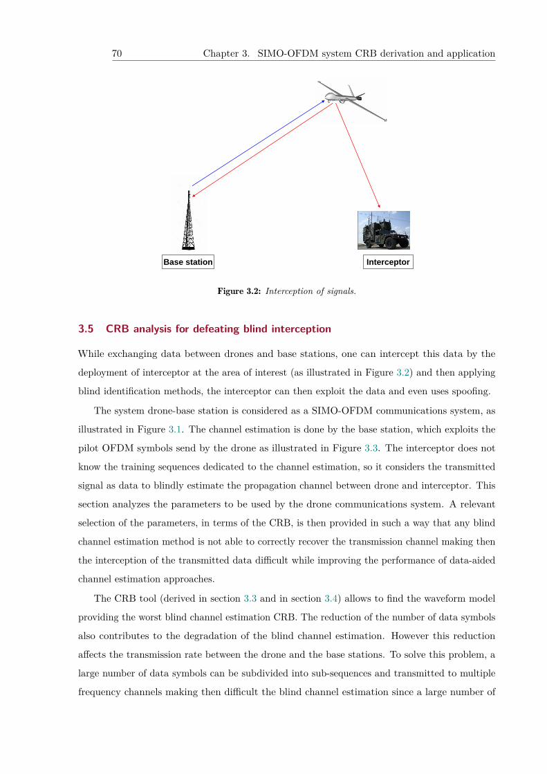
70 Chapter 3. SIMO-OFDM system CRB derivation and application
Base station Interceptor
Figure 3.2: Interception of signals.
3.5 CRB analysis for defeating blind interception
While exchanging data between drones and base stations, one can intercept this data by the
deployment of interceptor at the area of interest (as illustrated in Figure 3.2) and then applying
blind identification methods, the interceptor can then exploit the data and even uses spoofing.
The system drone-base station is considered as a SIMO-OFDM communications system, as
illustrated in Figure 3.1. The channel estimation is done by the base station, which exploits the
pilot OFDM symbols send by the drone as illustrated in Figure 3.3. The interceptor does not
know the training sequences dedicated to the channel estimation, so it considers the transmitted
signal as data to blindly estimate the propagation channel between drone and interceptor. This
section analyzes the parameters to be used by the drone communications system. A relevant
selection of the parameters, in terms of the CRB, is then provided in such a way that any blind
channel estimation method is not able to correctly recover the transmission channel making then
the interception of the transmitted data difficult while improving the performance of data-aided
channel estimation approaches.
The CRB tool (derived in section 3.3 and in section 3.4) allows to find the waveform model
providing the worst blind channel estimation CRB. The reduction of the number of data symbols
also contributes to the degradation of the blind channel estimation. However this reduction
affects the transmission rate between the drone and the base stations. To solve this problem, a
large number of data symbols can be subdivided into sub-sequences and transmitted to multiple
frequency channels making then difficult the blind channel estimation since a large number of
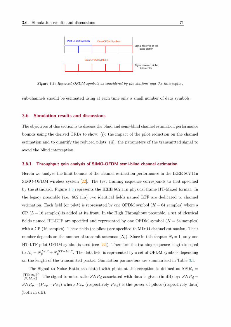
3.6. Simulation results and discussions 71
Pilot OFDM Symbols Data OFDM Symbols
Data OFDM Symbols
Signal received at the Base station
Signal received at the Interceptor
Figure 3.3: Received OFDM symbols as considered by the stations and the interceptor.
sub-channels should be estimated using at each time only a small number of data symbols.
3.6 Simulation results and discussions
The objectives of this section is to discuss the blind and semi-blind channel estimation performance
bounds using the derived CRBs to show: (i): the impact of the pilot reduction on the channel
estimation and to quantify the reduced pilots; (ii): the parameters of the transmitted signal to
avoid the blind interception.
3.6.1 Throughput gain analysis of SIMO-OFDM semi-blind channel estimation
Herein we analyze the limit bounds of the channel estimation performance in the IEEE 802.11n
SIMO-OFDM wireless system [22]. The test training sequence corresponds to that specified
by the standard. Figure 1.5 represents the IEEE 802.11n physical frame HT-Mixed format. In
the legacy preamble (i.e. 802.11a) two identical fields named LTF are dedicated to channel
estimation. Each field (or pilot) is represented by one OFDM symbol (K = 64 samples) where a
CP (L= 16 samples) is added at its front. In the High Throughput preamble, a set of identical
fields named HT-LTF are specified and represented by one OFDM symbol (K = 64 samples)
with a CP (16 samples). These fields (or pilots) are specified to MIMO channel estimation. Their
number depends on the number of transmit antennas (Nt). Since in this chapter Nt = 1, only one
HT-LTF pilot OFDM symbol is used (see [22]). Therefore the training sequence length is equal
to Np =NLTFp +NHT−LTF
p . The data field is represented by a set of OFDM symbols depending
on the length of the transmitted packet. Simulation parameters are summarized in Table 3.1.
The Signal to Noise Ratio associated with pilots at the reception is defined as SNRp =‖T(h)xp‖2
NrMpσ2v. The signal to noise ratio SNRd associated with data is given (in dB) by: SNRd =
SNRp− (Pxp−Pxd) where Pxp (respectively Pxd) is the power of pilots (respectively data)
(both in dB).
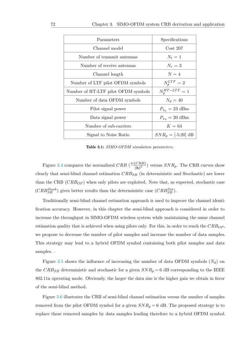
72 Chapter 3. SIMO-OFDM system CRB derivation and application
Parameters Specifications
Channel model Cost 207
Number of transmit antennas Nt = 1
Number of receive antennas Nr = 3
Channel length N = 4
Number of LTF pilot OFDM symbols NLTFp = 2
Number of HT-LTF pilot OFDM symbols NHT−LTFp = 1
Number of data OFDM symbols Nd = 40
Pilot signal power Pxp = 23 dBm
Data signal power Pxd = 20 dBm
Number of sub-carriers K = 64
Signal to Noise Ratio SNRp = [-5:20] dB
Table 3.1: SIMO-OFDM simulation parameters.
Figure 3.4 compares the normalized CRB ( tr{CRB}‖h‖2 ) versus SNRp. The CRB curves show
clearly that semi-blind channel estimation CRBSB (in deterministic and Stochastic) are lower
than the CRB (CRBOP ) when only pilots are exploited. Note that, as expected, stochastic case
(CRBStochSB ) gives better results than the deterministic case (CRBDetSB ).
Traditionally semi-blind channel estimation approach is used to improve the channel identi-
fication accuracy. However, in this chapter the semi-blind approach is considered in order to
increase the throughput in SIMO-OFDM wireless system while maintaining the same channel
estimation quality that is achieved when using pilots only. For this, in order to reach the CRBOP ,
we propose to decrease the number of pilot samples and increase the number of data samples.
This strategy may lead to a hybrid OFDM symbol containing both pilot samples and data
samples. .
Figure 3.5 shows the influence of increasing the number of data OFDM symbols (Nd) on
the CRBSB deterministic and stochastic for a given SNRp = 6 dB corresponding to the IEEE
802.11n operating mode. Obviously, the larger the data size is the higher gain we obtain in favor
of the semi-blind method.
Figure 3.6 illustrates the CRB of semi-blind channel estimation versus the number of samples
removed from the pilot OFDM symbol for a given SNRp = 6 dB. The proposed strategy is to
replace these removed samples by data samples leading therefore to a hybrid OFDM symbol.
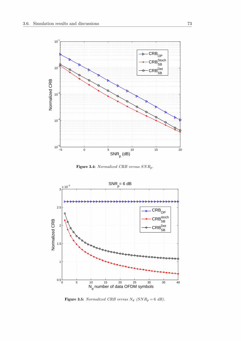
3.6. Simulation results and discussions 73
−5 0 5 10 15 2010
−5
10−4
10−3
10−2
10−1
Nor
mal
ized
CR
B
SNRp (dB)
CRBOP
CRBStochSB
CRBDetSB
Figure 3.4: Normalized CRB versus SNRp.
0 5 10 15 20 25 30 35 400.5
1
1.5
2
2.5
3x 10⁻³ SNR
p= 6 dB
Nor
mal
ized
CR
B
Nd number of data OFDM symbols
CRBOP
CRBstochSB
CRBDetSB
Figure 3.5: Normalized CRB versus Nd (SNRp = 6 dB).
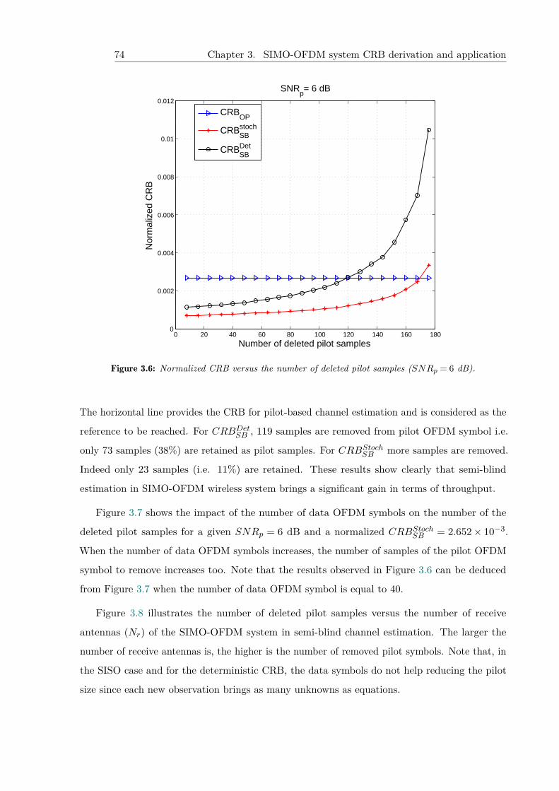
74 Chapter 3. SIMO-OFDM system CRB derivation and application
0 20 40 60 80 100 120 140 160 1800
0.002
0.004
0.006
0.008
0.01
0.012
SNRp= 6 dB
Nor
mal
ized
CR
B
Number of deleted pilot samples
CRBOP
CRBstochSB
CRBDetSB
Figure 3.6: Normalized CRB versus the number of deleted pilot samples (SNRp = 6 dB).
The horizontal line provides the CRB for pilot-based channel estimation and is considered as the
reference to be reached. For CRBDetSB , 119 samples are removed from pilot OFDM symbol i.e.
only 73 samples (38%) are retained as pilot samples. For CRBStochSB more samples are removed.
Indeed only 23 samples (i.e. 11%) are retained. These results show clearly that semi-blind
estimation in SIMO-OFDM wireless system brings a significant gain in terms of throughput.
Figure 3.7 shows the impact of the number of data OFDM symbols on the number of the
deleted pilot samples for a given SNRp = 6 dB and a normalized CRBStochSB = 2.652× 10⁻³.
When the number of data OFDM symbols increases, the number of samples of the pilot OFDM
symbol to remove increases too. Note that the results observed in Figure 3.6 can be deduced
from Figure 3.7 when the number of data OFDM symbol is equal to 40.
Figure 3.8 illustrates the number of deleted pilot samples versus the number of receive
antennas (Nr) of the SIMO-OFDM system in semi-blind channel estimation. The larger the
number of receive antennas is, the higher is the number of removed pilot symbols. Note that, in
the SISO case and for the deterministic CRB, the data symbols do not help reducing the pilot
size since each new observation brings as many unknowns as equations.
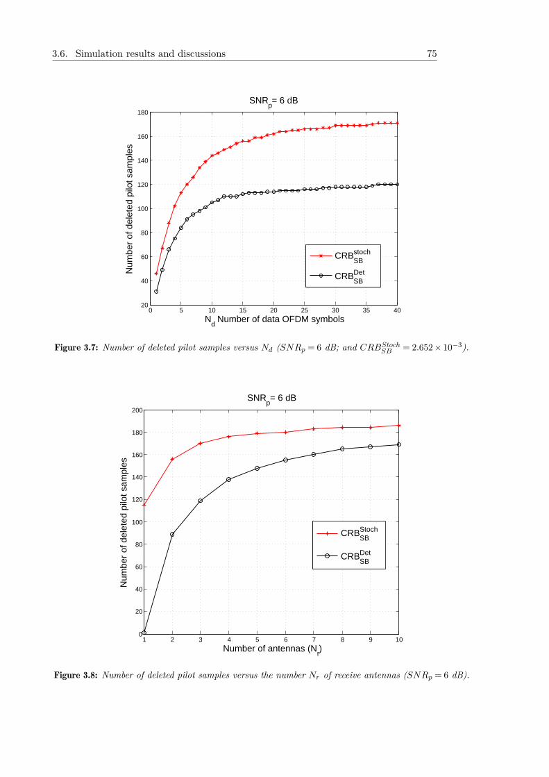
3.6. Simulation results and discussions 75
0 5 10 15 20 25 30 35 4020
40
60
80
100
120
140
160
180
SNRp= 6 dB
Num
ber
of d
elet
ed p
ilot s
ampl
es
Nd Number of data OFDM symbols
CRBstochSB
CRBDetSB
Figure 3.7: Number of deleted pilot samples versus Nd (SNRp = 6 dB; and CRBStochSB = 2.652× 10⁻³).
1 2 3 4 5 6 7 8 9 100
20
40
60
80
100
120
140
160
180
200
SNRp= 6 dB
Num
ber
of d
elet
ed p
ilot s
ampl
es
Number of antennas (Nr)
CRBStochSB
CRBDetSB
Figure 3.8: Number of deleted pilot samples versus the number Nr of receive antennas (SNRp = 6 dB).
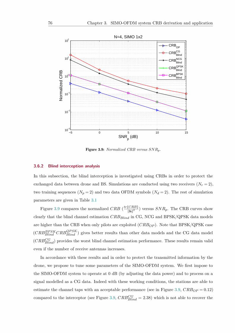
76 Chapter 3. SIMO-OFDM system CRB derivation and application
−5 0 5 10 1510
−3
10−2
10−1
100
101
102
N=4, SIMO 1x2
Nor
mal
ized
CR
B
SNRp (dB)
CRBOP
CRBBlindCG
CRBBlindNCG
CRBBlindQPSK
CRBBlindBPSK
Figure 3.9: Normalized CRB versus SNRp.
3.6.2 Blind interception analysis
In this subsection, the blind interception is investigated using CRBs in order to protect the
exchanged data between drone and BS. Simulations are conducted using two receivers (Nr = 2),
two training sequences (Np = 2) and two data OFDM symbols (Nd = 2). The rest of simulation
parameters are given in Table 3.1
Figure 3.9 compares the normalized CRB ( tr{CRB}‖h‖2 ) versus SNRp. The CRB curves show
clearly that the blind channel estimation CRBBlind in CG, NCG and BPSK/QPSK data models
are higher than the CRB when only pilots are exploited (CRBOP ). Note that BPSK/QPSK case
(CRBBPSKBlind CRBQPSKBlind ) gives better results than other data models and the CG data model
(CRBCGBlind) provides the worst blind channel estimation performance. These results remain valid
even if the number of receive antennas increases.
In accordance with these results and in order to protect the transmitted information by the
drone, we propose to tune some parameters of the SIMO-OFDM system. We first impose to
the SIMO-OFDM system to operate at 0 dB (by adjusting the data power) and to process on a
signal modelled as a CG data. Indeed with these working conditions, the stations are able to
estimate the channel taps with an acceptable performance (see in Figure 3.9, CRBOP = 0.12)
compared to the interceptor (see Figure 3.9, CRBCGBlind = 2.38) which is not able to recover the
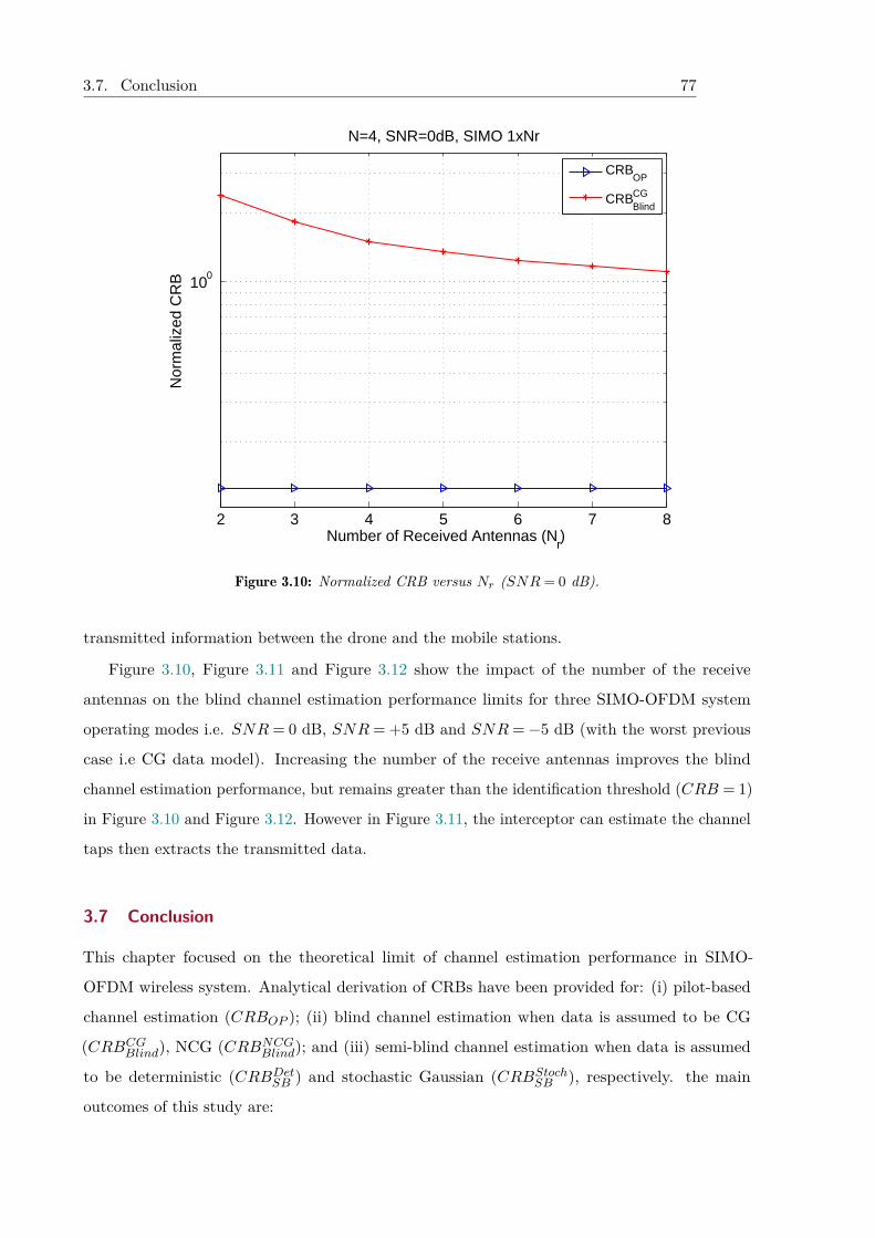
3.7. Conclusion 77
2 3 4 5 6 7 8
100
N=4, SNR=0dB, SIMO 1xNr
Nor
mal
ized
CR
B
Number of Received Antennas (Nr)
CRBOP
CRBBlindCG
Figure 3.10: Normalized CRB versus Nr (SNR= 0 dB).
transmitted information between the drone and the mobile stations.
Figure 3.10, Figure 3.11 and Figure 3.12 show the impact of the number of the receive
antennas on the blind channel estimation performance limits for three SIMO-OFDM system
operating modes i.e. SNR= 0 dB, SNR= +5 dB and SNR=−5 dB (with the worst previous
case i.e CG data model). Increasing the number of the receive antennas improves the blind
channel estimation performance, but remains greater than the identification threshold (CRB = 1)
in Figure 3.10 and Figure 3.12. However in Figure 3.11, the interceptor can estimate the channel
taps then extracts the transmitted data.
3.7 Conclusion
This chapter focused on the theoretical limit of channel estimation performance in SIMO-
OFDM wireless system. Analytical derivation of CRBs have been provided for: (i) pilot-based
channel estimation (CRBOP ); (ii) blind channel estimation when data is assumed to be CG
(CRBCGBlind), NCG (CRBNCGBlind); and (iii) semi-blind channel estimation when data is assumed
to be deterministic (CRBDetSB ) and stochastic Gaussian (CRBStochSB ), respectively. the main
outcomes of this study are:
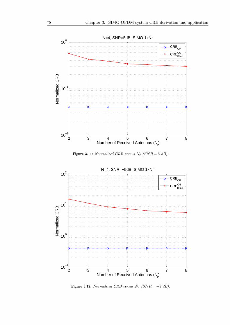
78 Chapter 3. SIMO-OFDM system CRB derivation and application
2 3 4 5 6 7 810
−2
10−1
100
N=4, SNR=5dB, SIMO 1xNr
Nor
mal
ized
CR
B
Number of Received Antennas (Nr)
CRBOP
CRBBlindCG
Figure 3.11: Normalized CRB versus Nr (SNR= 5 dB).
2 3 4 5 6 7 810
−1
100
101
102
N=4, SNR=−5dB, SIMO 1xNr
Nor
mal
ized
CR
B
Number of Received Antennas (Nr)
CRBOP
CRBBlindCG
Figure 3.12: Normalized CRB versus Nr (SNR=−5 dB).

3.7. Conclusion 79
• In the context of IEEE 802.11n SIMO-OFDM system, the test results showed clearly the
pilot samples reduction and consequently the throughput gain in SIMO-OFDM semi-blind
channel estimation while maintaining the same pilot-based limit channel estimation quality.
• In the context of blind interception, the analysis of simulation results show that the worst
blind channel estimation performance is obtained in the case of CG data model (CRBCGBlind)
while an acceptable performance of pilot-based channel estimation is achieved. Therefore
to avoid the interception of the information, the SIMO-OFDM communications system is
tuned in such away to adjust the power of the CG data depending on the number of pilots
and the length of the physical packet.

80 Chapter 3. SIMO-OFDM system CRB derivation and application
4
Ch
ap
te
r
Analysis of CFO and frequency domain channel estimation
effects
In theory there is no difference
between theory and practice. In
practice there is.
Lawrence “Yogui” Berra,1925
This study deals with semi-blind channel estimation CRB performance of MIMO-OFDM wireless
communications system in the uplink transmission. The first contribution shows that the Carrier
Frequency Offset (CFO) impacts advantageously the CRB of the semi-blind channel estimation
mainly due to the CFO cyclostationarity propriety. The second contribution states that when
the relation between the subcarrier channel coefficients is not taken into account, i.e. without
resorting to the inherent OFDM ’channel structure’ during the channel estimation, results in a
loss of the estimation performance. An evaluation of the significant performance loss resulting
from this approach is provided1.
Abstract
1 [71] A. Ladaycia, A. Mokraoui, K. Abed-Meraim, and A. Belouchrani, "Further investigations on the
performance bounds of MIMO-OFDM channel estimation," in The 13th International Wireless Communications
and Mobile Computing Conference (IWCMC 2017), June 2017, pp. 223-228, Valance, Spain.
82 Chapter 4. Analysis of CFO and frequency domain channel estimation effects
Chapter content4.1 Introduction . . . . . . . . . . . . . . . . . . . . . . . . . . . . . . . . . . . . . 83
4.2 MIMO-OFDM communications system model in the presence of MCFO . . . . 84
4.3 CRB for channel coefficients estimation in presence of MCFO . . . . . . . . . . 85
4.3.1 FIM for known pilot OFDM symbols . . . . . . . . . . . . . . . . . . . . 85
4.3.2 FIM for unknown data OFDM symbols . . . . . . . . . . . . . . . . . . 86
4.4 CRB for subcarrier channel coefficient estimation . . . . . . . . . . . . . . . . . 88
4.5 Simulation results . . . . . . . . . . . . . . . . . . . . . . . . . . . . . . . . . . 89
4.5.1 Experimental settings . . . . . . . . . . . . . . . . . . . . . . . . . . . . 89
4.5.2 Channel estimation performance analysis . . . . . . . . . . . . . . . . . 89
4.6 Conclusion . . . . . . . . . . . . . . . . . . . . . . . . . . . . . . . . . . . . . . 92
4.1. Introduction 83
4.1 Introduction
MIMO-OFDM wireless communications system provides many advantages as the channel capacity
enhancement and the improvement of the communications reliability. However to achieve good
performance, the receiver should pay attention to compensate the time and frequency offsets
before extracting the information from the transmitted physical packet. Indeed the Carrier
Frequency Offset (CFO) affects the subcarriers orthogonality and degrades the OFDM system
performance. A state of the art on this issue shows that the CFO estimation can be performed
either on redundant information (Non-Data-Aided (NDA) approaches) or training sequences
(Data-Aided (DA) approaches) included in the transmitted physical packet. DA approaches
exploit training sequences either designed by authors or specified by some standards. In [72], the
authors use null subcarriers and propose a suboptimal method to estimate the CFO. Pilot-based
estimators have been discussed in [73], [74], [75] and [76] where the authors exploit cascaded
orthogonal pilots to jointly estimate the CFO and CSI, which remains, in wireless communications
system, a current concern since the overall system performance depends strongly on it.
This chapter studies the lower bounds performance of semi-blind channel estimation of
a multiuser MIMO-OFDM wireless system in the uplink transmission for different receivers
according to the strategies described below.
The objective of the first study is to show that, by exploiting the cyclostationarity introduced
by the CFO to the NCG signals, the presence of Multiple CFO (MCFO), considered as a problem
in MIMO-OFDM systems, improves the channel identification when semi-blind techniques using
Zadoff Chu (ZC) training sequences are performed. To analyze the theoretical performance
of this approach, the analytical CRB is derived. The CRBs, in the case of NCG signal with
and without CFO, are then analyzed and discussed. To the best of our knowledge, despite the
existing huge of literature on the considered topic, this analysis is the only one that investigates
thoroughly how the CFO impacts the CRB of the semi-blind channel estimation advantageously.
The second study evaluates and compares the lower bounds performance for the estimation
of the subcarrier channel coefficients with and without considering the OFDM structure (i.e.
when taking into account the relation between these coefficients through the Fourier transform of
the channel taps and when ignoring this relation in the estimation process). Indeed, for the sake
of computational simplicity, many existing OFDM receivers estimate these channel coefficients
as if they were ’independent’ [77].
84 Chapter 4. Analysis of CFO and frequency domain channel estimation effects
4.2 MIMO-OFDM communications system model in the presence of MCFO
Before describing the multiuser MIMO-OFDM wireless communications system adopted in this
chapter, this section introduces some notations and assumptions.
The communications system is considered in the uplink transmission. It is composed of
Nt transmit antennas associated with users sharing the same radio ressources and Nr receive
antennas (see Figure 1.1) deployed on the same device (i.e. on a single transmitting base station).
In this context, the receiver has a single local oscillator and each transmitter has its own local
oscillator. Therefore the received signal may be affected by Multiple independent CFO (MCFO)
introduced by the difference in local oscillator frequencies at the transmitters and receiver. Denote
νi the normalized CFO occurred between the i-th transmitter local oscillator and the r-th user
of the receiver local oscillator.
Each OFDM symbol is composed of K samples (i.e K subcarriers). A Cyclic Prefix (CP)
of L samples (with L ≥ N ; N being the maximum delay of the channel) is inserted between
consecutive OFDM symbols to prevent against Inter-Symbol Interference. These samples are
chosen as the L last samples of the OFDM symbol preceding the CP.
The transmitted signal x is assumed to be independent Non-Circular complex-Gaussian
(NCG). It is represented by the vector x of size NtK× 1 and is given by x =[xT1 · · ·xTNt
]Twhere
xi is the OFDM symbol transmitted by the i-th antenna; and (.)T represents the transpose
operator. The covariance matrices for the transmitted signal x are expressed by:
Cx = E[xxH
]= diag
{σ2
x1 · · ·σ2xNt
}C′x = E
[xxT
]= ρcdiag
{ejφ1 · · ·ejφNt
}Cx,
(4.1)
where ρc is the non-circularity rate (with 0< ρc < 1); φi (with i= 1, · · · ,Nt) the non-circularity
phases; σ2xi the variance of the xi OFDM symbol.
Denote hi,r the vector Channel Impulse Response of size N × 1 between the i-th transmitter
and r-th receiver. The vector v of size NrK× 1 (v =[vT1 · · · vTNr
]T) is considered as an additive
channel noise assumed to be independent white Complex-Gaussian Circular of zero-mean and
variance σ2v.
After removing the CP, the received discrete baseband signal y associated with the ns-th
OFDM symbol (y =[yT1 · · ·yTNr
]Tof size NrK×1), in time domain, is given in a matrix form as:
y = Λnsx + v, (4.2)
4.3. CRB for channel coefficients estimation in presence of MCFO 85
where the matrix Λns of size NrK ×NtK is defined as:
Λns =[Λ1ns · · ·Λ
Ntns
]with
Λins = (INr ⊗Γns (νi))
[ΛTi,1 · · ·ΛT
i,Nr
]Tand
Λi,r = FH√Kdiag{Whi,r} ,
(4.3)
where Λi,r, Λins are matrices of size K ×K and NrK ×K respectively ; F the Discrete Fourier
Transform matrix; W the N first columns of F; and Γns (νi) the normalized CFO matrix of size
K ×K at the ns-th OFDM symbol given by:
Γns (νi) = ej2πνi(ns−1)(K+L)/K×
diag{
1, ej2πνi/K , · · · , ej2πνi(K−1)/K}.
(4.4)
To facilitate the CRB derivation for channel estimation in the next sections, equation (4.2) is
rewritten in this form:
y = Xh + v, (4.5)
where h is the MIMO channel vector h =[hT1 · · ·hTNr
]Tof sizeNNtNr×1 with hr =
[hT1,r · · ·hTNt,r
]T;
and X = INr ⊗X where the matrix X of size K ×NNt is defined by:
X =[Γns (ν1) FH√
Kdiag{x1}W · · ·
Γns (νNt) FH√Kdiag{xNt}W
].
(4.6)
4.3 CRB for channel coefficients estimation in presence of MCFO
The aim of this section is to derive, in the presence of MCFO, the lower bound on the semi-blind
channel estimator’s variance (of unbiased estimators) using not only the known pilot OFDM
symbols (i.e. training sequence) but also the encapsulated unknown data OFDM symbols in the
physical packet. Figure 1.2a illustrates the block-type arrangement OFDM pilots in a physical
packet adopted in this chapter.
The CRB for semi-blind channel estimation is deduced from the inverse of the complex FIM
denoted Jθθ which is composed of the FIMs associated to pilots and data, derived as follows.
4.3.1 FIM for known pilot OFDM symbols
This section, based on equations (4.2) and (4.5), focuses on the derivation of the FIM Jpθθ when
only Np received pilot OFDM symbols are used to estimate the MIMO channel. The vector of
parameters is then defined as:
θ =[hT h∗T νT σv
2]T, (4.7)
86 Chapter 4. Analysis of CFO and frequency domain channel estimation effects
where ν is the MCFO vector given by [ν1 · · ·νNt ]T .
Since the channel noise is assumed to be i.i.d., the FIM for θ when Np pilot OFDM symbols
are used is deduced as:
Jpθθ =Np∑i=1
Jpiθθ, (4.8)
where Jpiθθ is the FIM associated with the i-th pilot OFDM symbol defined as:
Jpiθθ =
Jhh Jhh∗ Jhν Jhσ2v
Jh∗h Jh∗h∗ Jh∗ν Jh∗σ2v
Jνh Jνh∗ Jνν Jνσ2v
Jσ2vh Jσ2
vh∗ Jσ2vν
Jσ2vσ
2v
. (4.9)
Each sub-matrix, Jθiθj (with θi, θj ∈Θ), is deduced according to:
Jθiθj = E
(∂ lnp(y(i),θ)
∂θi∗
)(∂ lnp(y(i),θ)
∂θj∗
)H (4.10)
where E(.) is the expectation operator; and p(y(i),θ) the probability density function of the
received baseband signal given θ.
Based on the complex derivative ( ∂∂θ∗ = 1
2
(∂∂α + j ∂
∂β
)for θ = α+ jβ), the derivation of
equation (4.10) leads to:
Jθiθj = 1σ2v
∂(Xh
)∂θ∗i
H∂(Xh
)∂θ∗j
with θi, θj ∈Θ. (4.11)
4.3.2 FIM for unknown data OFDM symbols
This section, based on equations (4.2) and (4.5), deals with the derivation of the FIM Jdθθ when
Nd unknown transmitted OFDM data symbols are used to estimate the MIMO channel. The
vector of parameters is defined as:
θ =[hT h∗T ΣT
x ΦT νTρc σv2]T, (4.12)
where Σx =[σ2
x1 · · ·σ2xNt
]Tand Φ = [φ1 · · ·φNt ]
T .
Since the channel noise is assumed to be i.i.d., the FIM for Nd unknown OFDM symbols is
then expressed as:
Jdθθ =Nd∑ns=1
Jdnsθθ , (4.13)
4.3. CRB for channel coefficients estimation in presence of MCFO 87
where Jdnsθθ is the FIM of the ns-th data OFDM symbol defined as:
Jdnsθθ =
Jhh Jhh∗ JhΣx JhΦ Jhν Jhρc Jhσ2v
Jh∗h Jh∗h∗ Jh∗Σx Jh∗Φ Jh∗ν Jh∗ρc Jh∗σ2v
JΣxh JΣxh∗ JΣxΣx JΣxΦ JΣxν JΣxρc JΣxσ2v
JΦh JΦh∗ JΦΣx JΦΦ JΦν JΦρc JΦσ2v
Jνh Jνh∗ JνΣx JνΦ Jνν Jνρc Jνσ2v
Jρch Jρch∗ JρcΣx JρcΦ Jρcν Jρcρc Jρcσ2v
Jσ2vh Jσ2
vh∗ Jσ2vΣx Jσ2
vΦJσ2
vνJσ2
vρcJσ2
vσ2v
. (4.14)
The FIM, Jθiθj (with θi, θj ∈Θ), has been derived in [36], [40], [39] and is expressed as:
Jθiθj = 12 tr
C−1Y Y
∂CY Y
∂θ∗iC−1Y Y
(∂CY Y
∂θ∗j
)H , (4.15)
where
CY Y =
CY Y C′Y YC′∗Y Y C∗Y Y
, (4.16)
with
CY Y =Nt∑i=1
σ2xiΛ
ins
(Λins
)H+σv
2IKNr , (4.17)
C′Y Y =Nt∑i=1
ρcejφiσ2
xiΛins
(Λins
)T. (4.18)
The FIM Jθiθj also requires the following information:
∂CY Y
∂σ2xi
= 12
Λins
(Λins
)Hρce
jφiΛins
(Λins
)Tρce−jφi
(Λins
)∗(Λins
)H (Λins
)∗(Λins
)T , (4.19)
∂CY Y
∂φi= 1
2(jφiρcσ
2xi
)×
0 ejφiΛins
(Λins
)T−e−jφi
(Λins
)∗(Λins
)H0
, (4.20)
∂CY Y
∂ρc= 1
2ρc
0 C′Y YC′∗Y Y 0
, (4.21)
∂CY Y
∂σ2v
= 12I2KNr . (4.22)
The computation of ∂CY Y∂h∗i
for each i= 1, · · · , NNrNt provides:
∂CY Y
∂h∗i=
D1 0
D2 + DT2 DT
1
, (4.23)
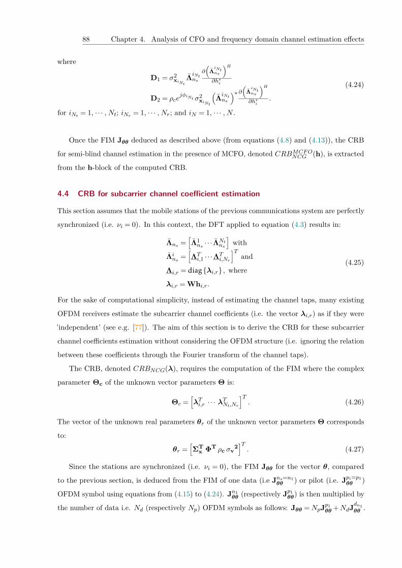
88 Chapter 4. Analysis of CFO and frequency domain channel estimation effects
where
D1 = σ2xiNt
ΛiNtns
∂
(ΛiNtns
)H∂h∗i
D2 = ρcejφiNt σ2
xiNt
(ΛiNtns
)∗ ∂(ΛiNtns
)H∂h∗i
.
(4.24)
for iNt = 1, · · · , Nt; iNr = 1, · · · , Nr; and iN = 1, · · · , N .
Once the FIM Jθθ deduced as described above (from equations (4.8) and (4.13)), the CRB
for semi-blind channel estimation in the presence of MCFO, denoted CRBMCFONCG (h), is extracted
from the h-block of the computed CRB.
4.4 CRB for subcarrier channel coefficient estimation
This section assumes that the mobile stations of the previous communications system are perfectly
synchronized (i.e. νi = 0). In this context, the DFT applied to equation (4.3) results in:
Λns =[Λ1ns · · ·Λ
Ntns
]with
Λins =
[ΛTi,1 · · ·ΛT
i,Nr
]Tand
Λi,r = diag{λi,r} , where
λi,r = Whi,r.
(4.25)
For the sake of computational simplicity, instead of estimating the channel taps, many existing
OFDM receivers estimate the subcarrier channel coefficients (i.e. the vector λi,r) as if they were
’independent’ (see e.g. [77]). The aim of this section is to derive the CRB for these subcarrier
channel coefficients estimation without considering the OFDM structure (i.e. ignoring the relation
between these coefficients through the Fourier transform of the channel taps).
The CRB, denoted CRBNCG(λ), requires the computation of the FIM where the complex
parameter Θc of the unknown vector parameters Θ is:
Θc =[λTi,r · · · λTNt,Nr
]T. (4.26)
The vector of the unknown real parameters θr of the unknown vector parameters Θ corresponds
to:
θr =[ΣT
x ΦT ρc σv2]T. (4.27)
Since the stations are synchronized (i.e. νi = 0), the FIM Jθθ for the vector θ, compared
to the previous section, is deduced from the FIM of one data (i.e Jns=n1θθ ) or pilot (i.e. Jpi=p1
θθ )
OFDM symbol using equations from (4.15) to (4.24). Jn1θθ (respectively Jp1
θθ) is then multiplied by
the number of data i.e. Nd (respectively Np) OFDM symbols as follows: Jθθ =NpJp1θθ +NdJ
dn1θθ .
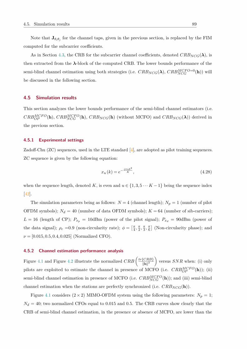
4.5. Simulation results 89
Note that Jθiθj for the channel taps, given in the previous section, is replaced by the FIM
computed for the subcarrier coefficients.
As in Section 4.3, the CRB for the subcarrier channel coefficients, denoted CRBNCG(λ), is
then extracted from the λ-block of the computed CRB. The lower bounds performance of the
semi-blind channel estimation using both strategies (i.e. CRBNCG(λ), CRBMCFO=0NCG (h)) will
be discussed in the following section.
4.5 Simulation results
This section analyzes the lower bounds performance of the semi-blind channel estimators (i.e.
CRBMCFOOP (h), CRBMCFO
NCG (h), CRBNCG(h) (without MCFO) and CRBNCG(λ)) derived in
the previous section.
4.5.1 Experimental settings
Zadoff-Chu (ZC) sequences, used in the LTE standard [4], are adopted as pilot training sequences.
ZC sequence is given by the following equation:
xu (k) = e−jπuk2K , (4.28)
when the sequence length, denoted K, is even and u ∈ {1,3,5 · · ·K − 1} being the sequence index
[42].
The simulation parameters being as follows: N = 4 (channel length); Np = 1 (number of pilot
OFDM symbols); Nd = 40 (number of data OFDM symbols); K = 64 (number of sib-carriers);
L = 16 (length of CP); Pxp = 10dBm (power of the pilot signal); Pxd = 90dBm (power of
the data signal); ρc =0.9 (non-circularity rate); φ =[π
4 ,π2 ,
π3 ,
π6](Non-circularity phase); and
ν = [0.015,0.5,0.4,0.025] (Normalized CFO).
4.5.2 Channel estimation performance analysis
Figure 4.1 and Figure 4.2 illustrate the normalized CRB(tr{CRB}‖h‖2
)versus SNR when: (i) only
pilots are exploited to estimate the channel in presence of MCFO (i.e. CRBMCFOOP (h)); (ii)
semi-blind channel estimation in presence of MCFO (i.e. CRBMCFONCG (h)); and (iii) semi-blind
channel estimation when the stations are perfectly synchronized (i.e. CRBNCG(h)).
Figure 4.1 considers (2× 2) MIMO-OFDM system using the following parameters: Np = 1;
Nd = 40; two normalized CFOs equal to 0.015 and 0.5. The CRB curves show clearly that the
CRB of semi-blind channel estimation, in the presence or absence of MCFO, are lower than the
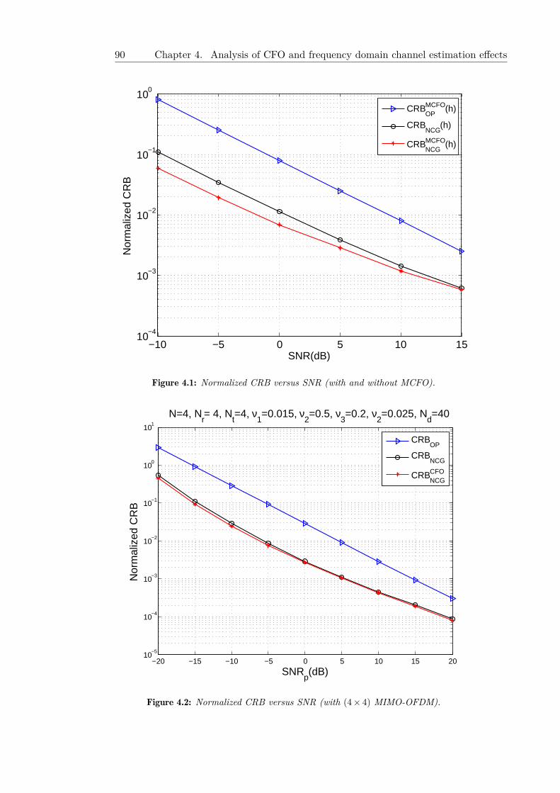
90 Chapter 4. Analysis of CFO and frequency domain channel estimation effects
−10 −5 0 5 10 1510
−4
10−3
10−2
10−1
100
Nor
mal
ized
CR
B
SNR(dB)
CRBOPMCFO(h)
CRBNCG
(h)
CRBNCGMCFO(h)
Figure 4.1: Normalized CRB versus SNR (with and without MCFO).
−20 −15 −10 −5 0 5 10 15 2010
−5
10−4
10−3
10−2
10−1
100
101
N=4, Nr= 4, N
t=4, ν
1=0.015, ν
2=0.5, ν
3=0.2, ν
2=0.025, N
d=40
Nor
mal
ized
CR
B
SNRp(dB)
CRBOP
CRBNCG
CRBNCGCFO
Figure 4.2: Normalized CRB versus SNR (with (4× 4) MIMO-OFDM).
4.5. Simulation results 91
−20 −15 −10 −5 0 5 10 15 2010
−5
10−4
10−3
10−2
10−1
100
101
N=4, Nr= 4, N
t=4, N
d=40
Nor
mal
ized
CR
B
SNR(dB)
CRBOP
CRBCG
CRBNCG
Figure 4.3: Normalized CRB versus SNR with circular Gaussian and non-circular Gaussian signals (with
(4× 4) MIMO-OFDM).
CRB when only pilots are used. Moreover the CRB in the presence of MCFO (CRBMCFONCG ) is
about 3 dB lower than the CRB when the transmitters and receiver are perfectly synchronized
(CRBNCG(h)). Although the CFO being a traditional problem when only pilots are used to
estimate the channel, the gain of 3 dB proves however to be an advantage in semi-blind channel
identification. Figure 4.2 provides additional results in (4×4) MIMO-OFDM system and confirm
our analysis.
Figure 4.3 provides the Circular and Non-circular Gaussian CRBs if (4× 4) MIMO-OFDM
system. Even thought the vector of the unknown parameters θ is larger, the CRB corresponding
to NCG data signal is lower than the CRB corresponding to the CG signal.
For a given SNR = 6 dB (around the operating mode of the IEEE 802.11n), Figure 4.4
presents the normalized CRB of the semi-blind channel estimation in the presence and absence of
MCFO (i.e. CRBNCG(h) and CRBMCFONCG (h)) versus the number of data OFDM symbols (Nd).
The analysis of the curves confirms the traditional result which states that when the number
of symbols to estimate the channel increases, the estimation performance is better. Moreover,
this analysis clearly shows the contribution of MCFO on the performance improvement of the
channel estimation.
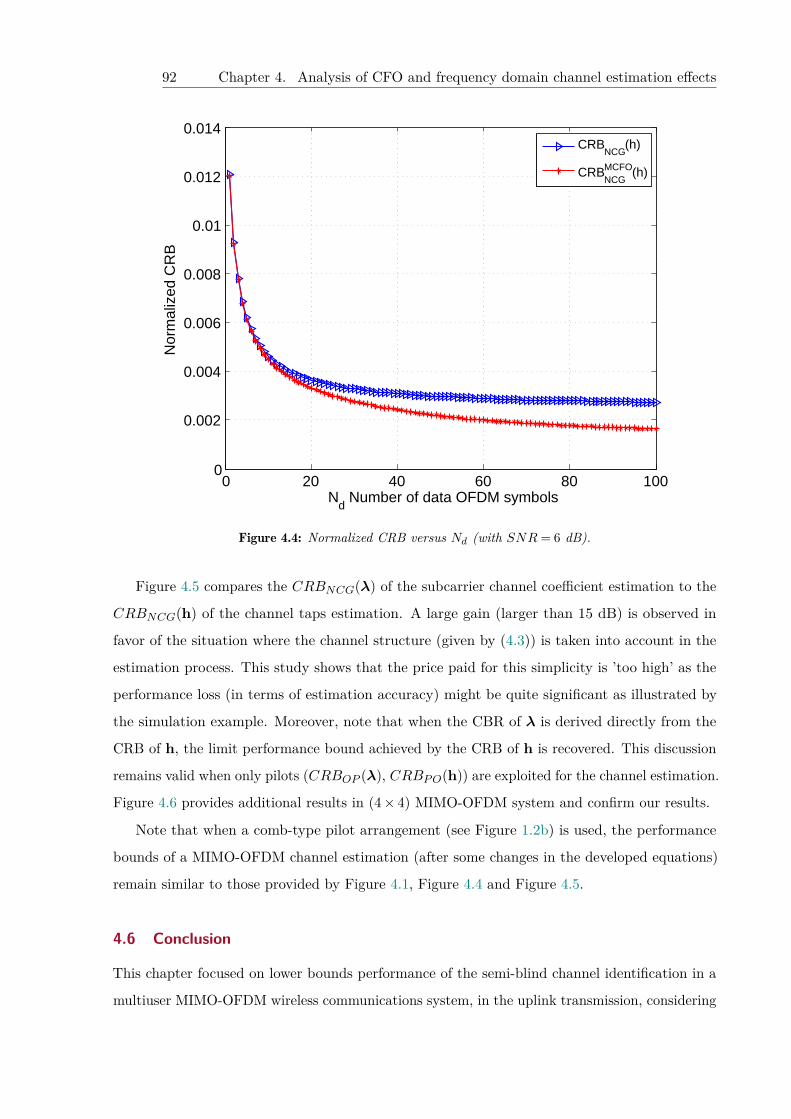
92 Chapter 4. Analysis of CFO and frequency domain channel estimation effects
0 20 40 60 80 1000
0.002
0.004
0.006
0.008
0.01
0.012
0.014
Nor
mal
ized
CR
B
Nd Number of data OFDM symbols
CRBNCG
(h)
CRBNCGMCFO(h)
Figure 4.4: Normalized CRB versus Nd (with SNR= 6 dB).
Figure 4.5 compares the CRBNCG(λ) of the subcarrier channel coefficient estimation to the
CRBNCG(h) of the channel taps estimation. A large gain (larger than 15 dB) is observed in
favor of the situation where the channel structure (given by (4.3)) is taken into account in the
estimation process. This study shows that the price paid for this simplicity is ’too high’ as the
performance loss (in terms of estimation accuracy) might be quite significant as illustrated by
the simulation example. Moreover, note that when the CBR of λ is derived directly from the
CRB of h, the limit performance bound achieved by the CRB of h is recovered. This discussion
remains valid when only pilots (CRBOP (λ), CRBPO(h)) are exploited for the channel estimation.
Figure 4.6 provides additional results in (4× 4) MIMO-OFDM system and confirm our results.
Note that when a comb-type pilot arrangement (see Figure 1.2b) is used, the performance
bounds of a MIMO-OFDM channel estimation (after some changes in the developed equations)
remain similar to those provided by Figure 4.1, Figure 4.4 and Figure 4.5.
4.6 Conclusion
This chapter focused on lower bounds performance of the semi-blind channel identification in a
multiuser MIMO-OFDM wireless communications system, in the uplink transmission, considering
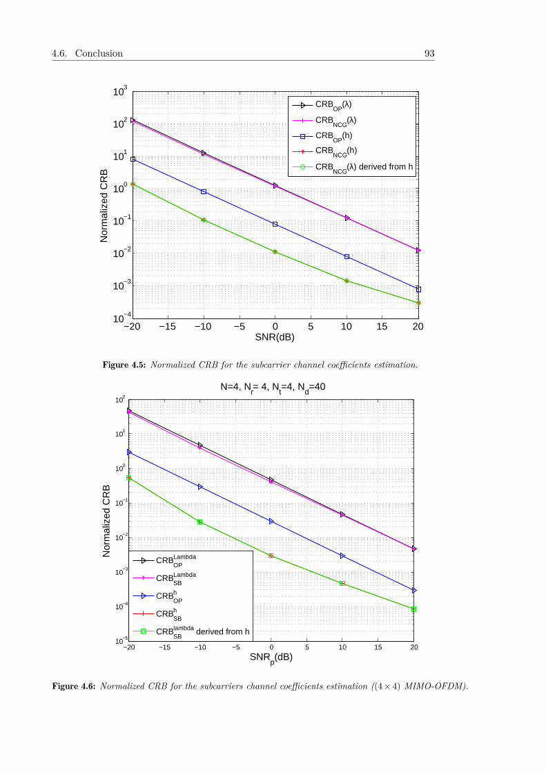
4.6. Conclusion 93
−20 −15 −10 −5 0 5 10 15 2010
−4
10−3
10−2
10−1
100
101
102
103
Nor
mal
ized
CR
B
SNR(dB)
CRBOP
(λ)
CRBNCG
(λ)
CRBOP
(h)
CRBNCG
(h)
CRBNCG
(λ) derived from h
Figure 4.5: Normalized CRB for the subcarrier channel coefficients estimation.
−20 −15 −10 −5 0 5 10 15 2010
−5
10−4
10−3
10−2
10−1
100
101
102
N=4, Nr= 4, N
t=4, N
d=40
Nor
mal
ized
CR
B
SNRp(dB)
CRBOPLambda
CRBSBLambda
CRBOPh
CRBSBh
CRBSBlambda derived from h
Figure 4.6: Normalized CRB for the subcarriers channel coefficients estimation ((4× 4) MIMO-OFDM).

94 Chapter 4. Analysis of CFO and frequency domain channel estimation effects
a NCG data model. Two important results have been derived as follow:
• The first one is related to the impact of the CFO on the improvement of the CRBMCFONCG (h)
compared to the CRBNCG(h) without CFO.
• The second one, is based on the approach that estimates the subcarrier channel coefficients
only for sake of simplicity. This strategy proved that the price paid for this simplicity is
too high because the CRBNCG(λ) performance loss might be quite significant compared
to the CRBNCG(h) of the channel taps estimation.

Part IIProposed semi-blind channel estimation approaches
95

5
Ch
ap
te
r
Least Squares Decision Feedback (LS-DF) Semi-blind es-
timator
To get what you love, you must
first be patient with what you hate.
Al-Ghazali.
This chapter proposes a Least Square Decision Feedback (LS-DF) semi-blind channel estimator
showing that a reduction of 76% of the pilot’s power is obtained compared to the LS pilot-based
estimator for the same channel estimation performance. The LS-DF performance are compared
then to the theoretical maximum power reduction of the transmitted pilots when semi-blind
channel estimator is deployed while ensuring the same pilot-based channel estimation performance
for BPSK/QPSK data models and a block-type pilot arrangement as specified in the IEEE
802.11n standard. The detailed description of our proposed algorithm has been published in the
conference EUSIPCO 20171
Abstract
1 [33] A. Ladaycia, A. Mokraoui, K. Abed-Meraim, and A. Belouchrani, "Toward green communications using
semi-blind channel estimation," in 2017 25th European Signal Processing Conference (EUSIPCO), Aug. 2017, pp.
2254-2258, Kos, Greece.
98Chapter 5. Least Squares Decision Feedback Semi-blind channel estimator for
MIMO-OFDM communications system
Chapter content5.1 Introduction . . . . . . . . . . . . . . . . . . . . . . . . . . . . . . . . . . . . . 99
5.2 LS-DF semi-blind channel estimation algorithm . . . . . . . . . . . . . . . . . . 99
5.2.1 Main steps of the LS-DF algorithm . . . . . . . . . . . . . . . . . . . . . 100
5.2.2 Computational cost comparison of LS and LS-DF algorithms . . . . . . 101
5.3 Performance analysis and discussions . . . . . . . . . . . . . . . . . . . . . . . . 102
5.3.1 Theoretical limit pilot’s power reduction . . . . . . . . . . . . . . . . . . 103
5.3.2 LS-DF performance in terms of power consumption . . . . . . . . . . . 105
5.4 conclusion . . . . . . . . . . . . . . . . . . . . . . . . . . . . . . . . . . . . . . . 108
5.1. Introduction 99
5.1 Introduction
Channel estimation is of paramount importance to equalization and symbol detection problems
in most wireless communications systems. This task is achieved using blind channel estimation
methods (e.g. [24]), or based on pilots [20, 21]. However these pilots consume not only a large
part of throughput but also significant power resources. This becomes even more important for
future communications systems such as massive-MIMO systems. Indeed the explosive growth of
high data rate applications where the corresponding energy consumption is also growing at a
staggering rate has urged for an intensive research work on green communications to protect
our environment and cope with global warming [78]. In [66], the throughput problem has been
investigated for SIMO-OFDM systems. In [79], authors present the state-of-the-art of the green
communications methods. Antenna selection using beamforming algorithm is proposed in [80].
This study suggests an unusual approach to reduce the consumed power making the most of
the advantages of semi-blind channel estimation approaches. The underlying idea consists of
removing pilot samples which are replaced by zero-samples while ensuring the same performance as
pilot-based channel estimation approaches. The maximal reduction of the theoretical transmitted
pilot’s power is first addressed when semi-blind approaches are deployed instead of pilot-based
approaches for the same estimation performance. To do so, the theoretical limit channel estimation
performance, based on the analytical CRB, is considered. The real gain in terms of pilot’s power
reduction at the transmitter is then evaluated when Least Square Decision Feedback (LS-DF)
semi-blind channel estimator is used. In addition, the overconsumption at the receiver is evaluated
and discussed.
5.2 LS-DF semi-blind channel estimation algorithm
The MIMO-OFDM system model adopted in this study is given in chapter 1 as depicted in Figure
1.1. Moreover, the CRBs derived in chapter 1 (subsection 1.4.3 for alphabet finite (BPSK and
QPSK) modulation), are used quantify the theoretical limit power reduction of the transmitted
pilots without affecting the channel estimation quality. This will be used to compute the power
saving due to this shortening at the transmitter side. For comparison fairness, we need to evaluate
to power consumption increase at the receiver side due to the use of a more elaborate semi-blind
estimation algorithm. For this reason, we introduce in this section a semi-blind estimation
method that has the advantages of simplicity and effectiveness (i.e. it reaches the CRB for
moderate and high SNRs).
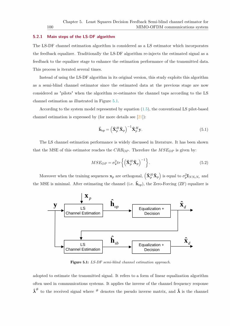
100Chapter 5. Least Squares Decision Feedback Semi-blind channel estimator for
MIMO-OFDM communications system
5.2.1 Main steps of the LS-DF algorithm
The LS-DF channel estimation algorithm is considered as a LS estimator which incorporates
the feedback equalizer. Traditionally the LS-DF algorithm re-injects the estimated signal as a
feedback to the equalizer stage to enhance the estimation performance of the transmitted data.
This process is iterated several times.
Instead of using the LS-DF algorithm in its original version, this study exploits this algorithm
as a semi-blind channel estimator since the estimated data at the previous stage are now
considered as "pilots" when the algorithm re-estimates the channel taps according to the LS
channel estimation as illustrated in Figure 5.1.
According to the system model represented by equation (1.5), the conventional LS pilot-based
channel estimation is expressed by (for more details see [21]):
hop =(XHp Xp
)−1XHp y. (5.1)
The LS channel estimation performance is widely discussed in literature. It has been shown
that the MSE of this estimator reaches the CRBOP . Therefore the MSEOP is given by:
MSEOP = σ2vtr
{(XHp Xp
)−1}. (5.2)
Moreover when the training sequences xp are orthogonal,(XHp Xp
)is equal to σ2
pINNtNr and
the MSE is minimal. After estimating the channel (i.e. hop), the Zero-Forcing (ZF) equalizer is
LS Channel Estimation
Equalization +Decision
ypx
ˆoph ˆ dx
LS Channel Estimation
Equalization +Decision
ˆsbh ˆ dx
Figure 5.1: LS-DF semi-blind channel estimation approach.
adopted to estimate the transmitted signal. It refers to a form of linear equalization algorithm
often used in communications systems. It applies the inverse of the channel frequency response
λ# to the received signal where # denotes the pseudo inverse matrix, and λ is the channel
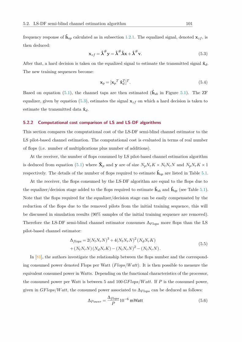
5.2. LS-DF semi-blind channel estimation algorithm 101
frequency response of hop calculated as in subsection 1.2.1. The equalized signal, denoted xzf , is
then deduced:
xzf = λ#y = λ#λx + λ#v. (5.3)
After that, a hard decision is taken on the equalized signal to estimate the transmitted signal xd.
The new training sequences become:
xp = [xpT xTd ]T . (5.4)
Based on equation (5.1), the channel taps are then estimated (hsb in Figure 5.1). The ZF
equalizer, given by equation (5.3), estimates the signal xzf on which a hard decision is taken to
estimate the transmitted data xd.
5.2.2 Computational cost comparison of LS and LS-DF algorithms
This section compares the computational cost of the LS-DF semi-blind channel estimator to the
LS pilot-based channel estimation. The computational cost is evaluated in terms of real number
of flops (i.e. number of multiplications plus number of additions).
At the receiver, the number of flops consumed by LS pilot-based channel estimation algorithm
is deduced from equation (5.1) where Xp and y are of size NpNrK ×NtNrN and NpNrK × 1
respectively. The details of the number of flops required to estimate hop are listed in Table 5.1.
At the receiver, the flops consumed by the LS-DF algorithm are equal to the flops due to
the equalizer/decision stage added to the flops required to estimate hsb and hop (see Table 5.1).
Note that the flops required for the equalizer/decision stage can be easily compensated by the
reduction of the flops due to the removed pilots from the initial training sequence, this will
be discussed in simulation results (90% samples of the initial training sequence are removed).
Therefore the LS-DF semi-blind channel estimator consumes ∆Flops more flops than the LS
pilot-based channel estimator:
∆flops = 2(NtNrN)3 + 4(NtNrN)2 (NdNrK)
+(NtNrN)(NdNrK)− (NtNrN)2− (NtNrN) .(5.5)
In [81], the authors investigate the relationship between the flops number and the correspond-
ing consumed power denoted Flops per Watt (Flops/Watt). It is then possible to measure the
equivalent consumed power in Watts. Depending on the functional characteristics of the processor,
the consumed power per Watt is between 5 and 100GFlops/Watt. If P is the consumed power,
given in GFlops/Watt, the consumed power associated to ∆Flops can be deduced as follows:
∆Power = ∆flops
P10−6 mWatt (5.6)
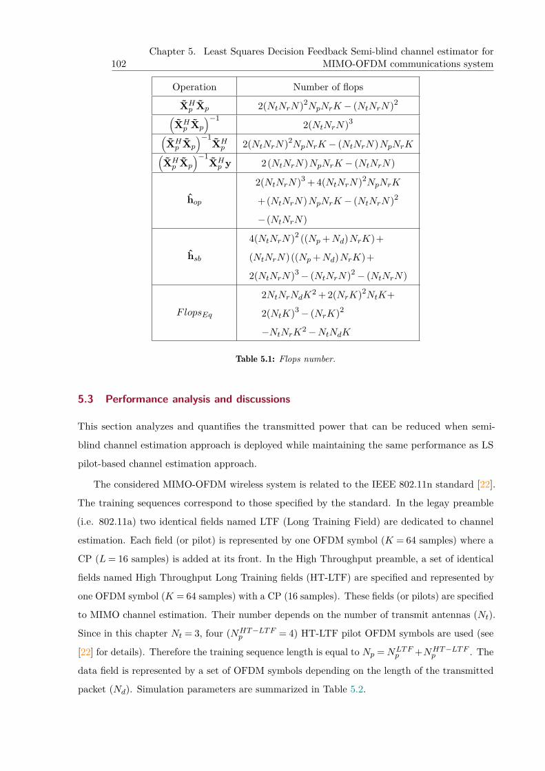
102Chapter 5. Least Squares Decision Feedback Semi-blind channel estimator for
MIMO-OFDM communications system
Operation Number of flops
XHp Xp 2(NtNrN)2NpNrK − (NtNrN)2(
XHp Xp
)−12(NtNrN)3(
XHp Xp
)−1XHp 2(NtNrN)2NpNrK − (NtNrN)NpNrK(
XHp Xp
)−1XHp y 2(NtNrN)NpNrK − (NtNrN)
hop
2(NtNrN)3 + 4(NtNrN)2NpNrK
+(NtNrN)NpNrK − (NtNrN)2
−(NtNrN)
hsb
4(NtNrN)2 ((Np +Nd)NrK)+
(NtNrN)((Np +Nd)NrK)+
2(NtNrN)3− (NtNrN)2− (NtNrN)
FlopsEq
2NtNrNdK2 + 2(NrK)2NtK+
2(NtK)3− (NrK)2
−NtNrK2−NtNdK
Table 5.1: Flops number.
5.3 Performance analysis and discussions
This section analyzes and quantifies the transmitted power that can be reduced when semi-
blind channel estimation approach is deployed while maintaining the same performance as LS
pilot-based channel estimation approach.
The considered MIMO-OFDM wireless system is related to the IEEE 802.11n standard [22].
The training sequences correspond to those specified by the standard. In the legay preamble
(i.e. 802.11a) two identical fields named LTF (Long Training Field) are dedicated to channel
estimation. Each field (or pilot) is represented by one OFDM symbol (K = 64 samples) where a
CP (L= 16 samples) is added at its front. In the High Throughput preamble, a set of identical
fields named High Throughput Long Training fields (HT-LTF) are specified and represented by
one OFDM symbol (K = 64 samples) with a CP (16 samples). These fields (or pilots) are specified
to MIMO channel estimation. Their number depends on the number of transmit antennas (Nt).
Since in this chapter Nt = 3, four (NHT−LTFp = 4) HT-LTF pilot OFDM symbols are used (see
[22] for details). Therefore the training sequence length is equal to Np =NLTFp +NHT−LTF
p . The
data field is represented by a set of OFDM symbols depending on the length of the transmitted
packet (Nd). Simulation parameters are summarized in Table 5.2.
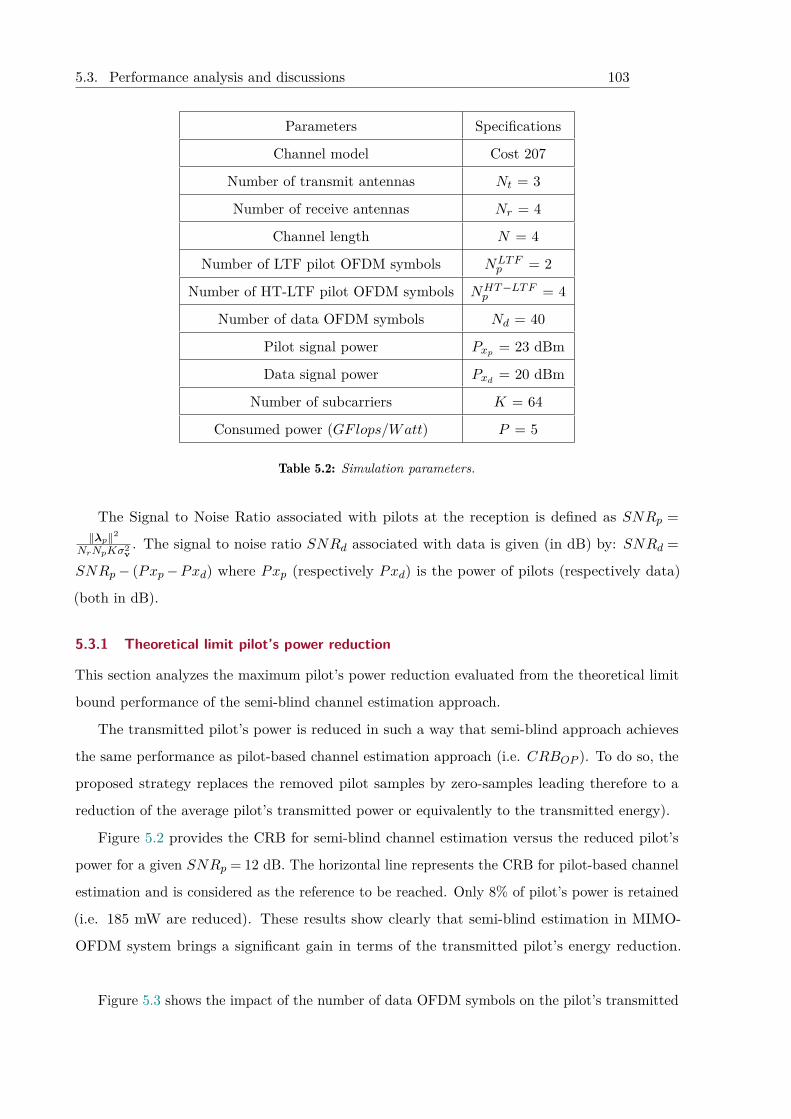
5.3. Performance analysis and discussions 103
Parameters Specifications
Channel model Cost 207
Number of transmit antennas Nt = 3
Number of receive antennas Nr = 4
Channel length N = 4
Number of LTF pilot OFDM symbols NLTFp = 2
Number of HT-LTF pilot OFDM symbols NHT−LTFp = 4
Number of data OFDM symbols Nd = 40
Pilot signal power Pxp = 23 dBm
Data signal power Pxd = 20 dBm
Number of subcarriers K = 64
Consumed power (GFlops/Watt) P = 5
Table 5.2: Simulation parameters.
The Signal to Noise Ratio associated with pilots at the reception is defined as SNRp =‖λp‖2
NrNpKσ2v. The signal to noise ratio SNRd associated with data is given (in dB) by: SNRd =
SNRp− (Pxp−Pxd) where Pxp (respectively Pxd) is the power of pilots (respectively data)
(both in dB).
5.3.1 Theoretical limit pilot’s power reduction
This section analyzes the maximum pilot’s power reduction evaluated from the theoretical limit
bound performance of the semi-blind channel estimation approach.
The transmitted pilot’s power is reduced in such a way that semi-blind approach achieves
the same performance as pilot-based channel estimation approach (i.e. CRBOP ). To do so, the
proposed strategy replaces the removed pilot samples by zero-samples leading therefore to a
reduction of the average pilot’s transmitted power or equivalently to the transmitted energy).
Figure 5.2 provides the CRB for semi-blind channel estimation versus the reduced pilot’s
power for a given SNRp = 12 dB. The horizontal line represents the CRB for pilot-based channel
estimation and is considered as the reference to be reached. Only 8% of pilot’s power is retained
(i.e. 185 mW are reduced). These results show clearly that semi-blind estimation in MIMO-
OFDM system brings a significant gain in terms of the transmitted pilot’s energy reduction.
Figure 5.3 shows the impact of the number of data OFDM symbols on the pilot’s transmitted
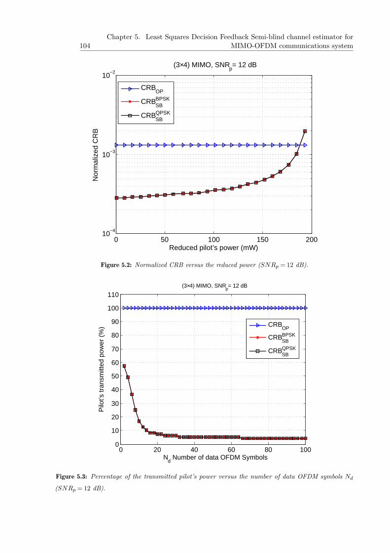
104Chapter 5. Least Squares Decision Feedback Semi-blind channel estimator for
MIMO-OFDM communications system
0 50 100 150 20010−4
10−3
10−2(3×4) MIMO, SNR
p= 12 dB
Nor
mal
ized
CR
B
Reduced pilot’s power (mW)
CRBOP
CRBSBBPSK
CRBSBQPSK
Figure 5.2: Normalized CRB versus the reduced power (SNRp = 12 dB).
0 20 40 60 80 1000
10
20
30
40
50
60
70
80
90
100
110(3×4) MIMO, SNR
p= 12 dB
Pilo
t’s tr
ansm
itted
pow
er (
%)
Nd Number of data OFDM Symbols
CRBOP
CRBSBBPSK
CRBSBQPSK
Figure 5.3: Percentage of the transmitted pilot’s power versus the number of data OFDM symbols Nd(SNRp = 12 dB).
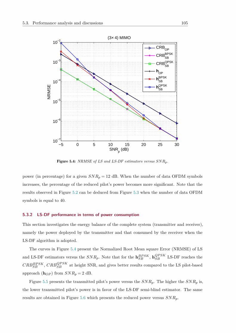
5.3. Performance analysis and discussions 105
−5 0 5 10 15 20 25 3010−7
10−6
10−5
10−4
10−3
10−2(3× 4) MIMO
NR
MS
E
SNRp (dB)
CRBOP
CRBSBBPSK
CRBSBQPSK
hOP
hSBBPSK
hSBQPSK
Figure 5.4: NRMSE of LS and LS-DF estimators versus SNRp.
power (in percentage) for a given SNRp = 12 dB. When the number of data OFDM symbols
increases, the percentage of the reduced pilot’s power becomes more significant. Note that the
results observed in Figure 5.2 can be deduced from Figure 5.3 when the number of data OFDM
symbols is equal to 40.
5.3.2 LS-DF performance in terms of power consumption
This section investigates the energy balance of the complete system (transmitter and receiver),
namely the power deployed by the transmitter and that consumed by the receiver when the
LS-DF algorithm is adopted.
The curves in Figure 5.4 present the Normalized Root Mean square Error (NRMSE) of LS
and LS-DF estimators versus the SNRp. Note that for the hBPSKSB , hQPSKSB LS-DF reaches the
CRBBPSKSB , CRBQPSKSB at height SNR, and gives better results compared to the LS pilot-based
approach (hOP ) from SNRp = 2 dB.
Figure 5.5 presents the transmitted pilot’s power versus the SNRp. The higher the SNRp is,
the lower transmitted pilot’s power is in favor of the LS-DF semi-blind estimator. The same
results are obtained in Figure 5.6 which presents the reduced power versus SNRp.
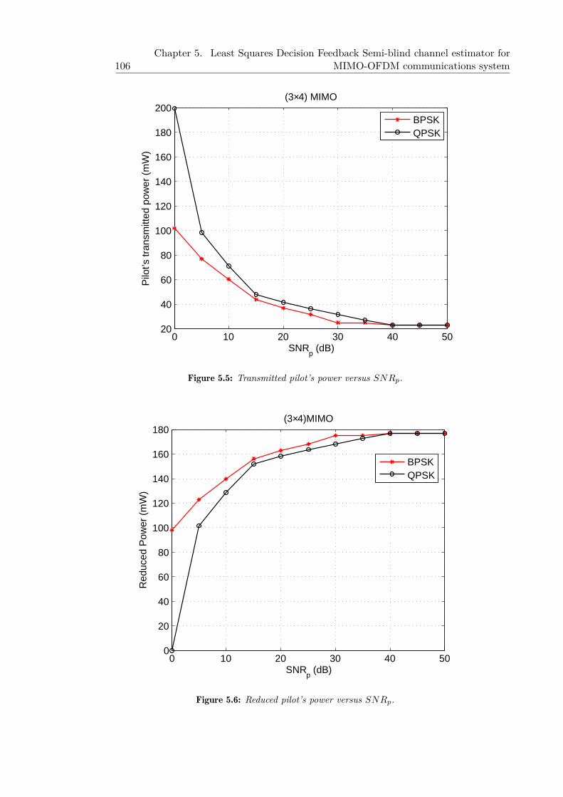
106Chapter 5. Least Squares Decision Feedback Semi-blind channel estimator for
MIMO-OFDM communications system
0 10 20 30 40 5020
40
60
80
100
120
140
160
180
200(3×4) MIMO
Pilo
t’s tr
ansm
itted
pow
er (
mW
)
SNRp (dB)
BPSKQPSK
Figure 5.5: Transmitted pilot’s power versus SNRp.
0 10 20 30 40 500
20
40
60
80
100
120
140
160
180(3×4)MIMO
Red
uced
Pow
er (
mW
)
SNRp (dB)
BPSKQPSK
Figure 5.6: Reduced pilot’s power versus SNRp.
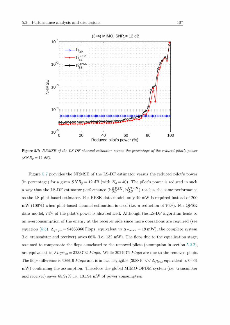
5.3. Performance analysis and discussions 107
0 20 40 60 80 10010−5
10−4
10−3
10−2
10−1(3×4) MIMO, SNR
p= 12 dB
NR
MS
E
Reduced pilot’s power (%)
hOP
hSBBPSK
hSBQPSK
Figure 5.7: NRMSE of the LS-DF channel estimator versus the percentage of the reduced pilot’s power
(SNRp = 12 dB).
Figure 5.7 provides the NRMSE of the LS-DF estimator versus the reduced pilot’s power
(in percentage) for a given SNRp = 12 dB (with Nd = 40). The pilot’s power is reduced in such
a way that the LS-DF estimator performance (hBPSKSB , hQPSKSB ) reaches the same performance
as the LS pilot-based estimator. For BPSK data model, only 49 mW is required instead of 200
mW (100%) when pilot-based channel estimation is used (i.e. a reduction of 76%). For QPSK
data model, 74% of the pilot’s power is also reduced. Although the LS-DF algorithm leads to
an overconsumption of the energy at the receiver side since more operations are required (see
equation (5.5), ∆flops = 94863360 Flops, equivalent to ∆Power = 19 mW), the complete system
(i.e. transmitter and receiver) saves 66% (i.e. 132 mW). The flops due to the equalization stage,
assumed to compensate the flops associated to the removed pilots (assumption in section 5.2.2),
are equivalent to Flopseq = 3233792 Flops. While 2924976 Flops are due to the removed pilots.
The flops difference is 308816 Flops and is in fact negligible (308816<< ∆flops equivalent to 0.061
mW) confirming the assumption. Therefore the global MIMO-OFDM system (i.e. transmitter
and receiver) saves 65,97% i.e. 131.94 mW of power consumption.
108Chapter 5. Least Squares Decision Feedback Semi-blind channel estimator for
MIMO-OFDM communications system
5.4 conclusion
This chapter focused on the power reduction problem in a MIMO-OFDM wireless system
specifically during the channel estimation stage. The study proposed to deploy semi-blind
channel estimation approach allowing the transmitter to reduce the number of samples in
the training sequence while ensuring the same estimation performance as pilot-based channel
estimation approach. The maximum theoretical reduction of the pilot’s power consumption,
based on the CRB for semi-blind channel estimation approach, is first investigated for the IEEE
802.11n MIMO-OFDM system with BPSK and QPSK data models. Simulation results, for the
same channel estimation performance, show clearly a significant reduction of the pilot’s power
equivalent to 76% when LS-DF semi-blind channel estimation is deployed instead of the LS
pilot-based channel estimation. A global power reduction of 65,97% is possible for the complete
wireless MIMO-OFDM system.
6
Ch
ap
te
r
EM-based blind and semi-blind channel estimation
Problems are not stop signs, they
are guidelines.
Robert H. Schuller.
This chapter deals with semi-blind channel estimation of MIMO-OFDM system using Max-
imum Likelihood (ML) technique. For the ML cost optimization function, new Expectation
Maximization (EM) algorithms for the channel taps estimation are introduced. Different approxi-
mation/simplification approaches are proposed for the algorithm’s computational cost reduction.
The first approach consists of decomposing the MIMO-OFDM system into parallel MISO-OFDM
systems. The EM algorithm is then applied in order to estimate the MIMO channel in a parallel
way. The second approach takes advantage of the semi-blind context to reduce the EM cost from
exponential to linear complexity by reducing the size of the search space. Finally, the last proposed
approach uses a parallel interference cancellation technique to decompose the MIMO-OFDM
system into several SIMO-OFDM systems. The latter are identified in a parallel scheme and with
a reduced complexity. These algorithms have been published in the conference ICASSP 20181and
submitted to IET communications2
Abstract
1 [82] A. Ladaycia, A. Belouchrani, K. Abed-Meraim, and A. Mokraoui, and, "EM-based semi-blind MIMO-
OFDM channel estimation," in 2018 IEEE International Conference on Acoustics, Speech and Signal Processing
(ICASSP2018), Apr. 2018, Alberta, Canada.2 [83] A. Ladaycia, A. Belouchrani, K. Abed-Meraim and A. Mokraoui, "Semi-Blind MIMO-OFDM Channel
Estimation using EM-like Techniques," IET communications, Mai. 2019.(submitted)
110 Chapter 6. EM-based blind and semi-blind channel estimation
Chapter content6.1 Introduction . . . . . . . . . . . . . . . . . . . . . . . . . . . . . . . . . . . . . 111
6.2 System model . . . . . . . . . . . . . . . . . . . . . . . . . . . . . . . . . . . . . 112
6.3 ML-based channel estimation . . . . . . . . . . . . . . . . . . . . . . . . . . . . 113
6.3.1 EM algorithm . . . . . . . . . . . . . . . . . . . . . . . . . . . . . . . . . 113
6.3.2 MIMO-OFDM semi-blind channel estimation for comb-type pilot ar-
rangement . . . . . . . . . . . . . . . . . . . . . . . . . . . . . . . . . . . 114
6.3.2.1 E-step . . . . . . . . . . . . . . . . . . . . . . . . . . . . . . . . 114
6.3.2.2 M-step . . . . . . . . . . . . . . . . . . . . . . . . . . . . . . . 115
6.3.3 MIMO-OFDM semi-blind channel estimation for block-type pilot ar-
rangement . . . . . . . . . . . . . . . . . . . . . . . . . . . . . . . . . . . 115
6.4 Approximate ML-estimation . . . . . . . . . . . . . . . . . . . . . . . . . . . . 117
6.4.1 MISO-OFDM SB channel estimation . . . . . . . . . . . . . . . . . . . . 117
6.4.2 Simplified EM algorithm (S-EM) . . . . . . . . . . . . . . . . . . . . . . 118
6.4.3 MIMO-OFDM SB-EM channel estimation algorithm based on Nt EM-
SIMO . . . . . . . . . . . . . . . . . . . . . . . . . . . . . . . . . . . . . 118
6.4.3.1 E-step . . . . . . . . . . . . . . . . . . . . . . . . . . . . . . . . 119
6.4.3.2 M-step . . . . . . . . . . . . . . . . . . . . . . . . . . . . . . . 120
6.5 Discussions . . . . . . . . . . . . . . . . . . . . . . . . . . . . . . . . . . . . . . 120
6.6 Simulation results . . . . . . . . . . . . . . . . . . . . . . . . . . . . . . . . . . 122
6.6.1 EM-MIMO performance analysis . . . . . . . . . . . . . . . . . . . . . . 123
6.6.2 EM-MIMO versus EM-MISO . . . . . . . . . . . . . . . . . . . . . . . . 127
6.6.3 EM-MIMO versus EM-SIMO . . . . . . . . . . . . . . . . . . . . . . . . 129
6.7 Conclusion . . . . . . . . . . . . . . . . . . . . . . . . . . . . . . . . . . . . . . 130
Appendix 6.A Derivation of the EM algorithm for comb-type scheme . . . . . . . . 131
Appendix 6.B Derivation of the EM algorithm for block-type scheme . . . . . . . . 132
6.1. Introduction 111
6.1 Introduction
As shown in chapter 1, for a target estimation quality, the SB approach improves the throughput
by reducing the training sequences up to 95%. In addition, SB methods can be used to reduce
the transmitted power (’green communications’), e.g. [33] (chapter 5) or eventually to improve
the estimation quality.
Among the channel estimation techniques, the Maximum Likelihood (ML) is one of the most
efficient in terms of quality but at the cost of high computational complexity. To achieve the
ML estimate at ’affordable’ costs, the Expectation Maximization (EM) algorithm is considered
for both channel and transmit data estimation (see e.g. [84]). In the case of a MIMO-OFDM
system using TDD mode, the CSI is estimated at the base station (uplink) and then transmitted
to the different users for channel equalization in the downlink.
The EM can be used blindly to estimate the channel or semi-blindly when training sequences
are available. In [84], the authors used a precoder and employ data tones as virtual pilots for
channel estimation. In [85] an alternative EM-based method is introduced for the estimation of
the channel taps in the frequency domain. In [86], the authors proposed an EM algorithm by
assuming a Gaussian distribution for the unknown data even when the data symbols are drawn
from a finite constellation such as QPSK. Recently, this work has been extended in [87] by using
a Gaussian mixture model, leading to improved estimation performance for high SNR (typically
SNR > 25dB).
The objective of this chapter is to propose alternative EM-based solutions with improved
efficiency as compared to similar existing methods3. First our EM-based algorithms are distinct
from the previous ones ([85], [84]) in terms of the channel parameters to be estimated. Instead
of estimating the channel coefficients in the frequency domain (i.e. subcarriers channel frequency
gains), we estimate directly the channel taps in the time domain so one can obtain a significant
gain as analyzed in chapter 1. Furthermore, in order to have parallelizable and/or reduced cost
estimation methods, three approximate EM algorithms are proposed.
Before doing so, this chapter introduces first the exact version where the MIMO-OFDM
system is treated as one block to estimate the overall channel vector through an iterative process.
Afterward, three complementary approximate EM versions are proposed.
The first approximate EM algorithm, useful if parallel processing machins are available,
decomposes the MIMO-OFDM system into parallel MISO-OFDM systems to estimate the vector
channel taps independently for each receiver. In the case of underdetermined system (i.e. number3Part of this work has been published in [82].
112 Chapter 6. EM-based blind and semi-blind channel estimation
of transmitters greater than the receivers one), where the traditional methods could not estimate
the transmit data, we succeed through the two proposed EM-based algorithms to estimate the
channel taps and data properly.
The second method consists of a Simplified EM algorithm, denoted S-EM, that allows to
reduce the computational heaviness based on an initial estimation of the channel and the data
using the pilots. More specifically, this approximation consists of limiting the averaging in
the expectation step to a neighborhood of the initial data vector estimate, hence reducing the
complexity from an exponential to a linear cost in terms of the number of transmitters.
The last proposed approach, again takes advantage of the semi-blind context using an
initial pilot-based estimation of the channel and the data together with a parallel interference
cancellation technique to transform the original MIMO problem into parallel SIMO systems
identification problems which can be solved in a parallel scheme and with reduced complexity.
6.2 System model
Consider a (Nt×Nr) MIMO-OFDM system composed of Nt transmit antennas and Nr receive
antennas, as illustrated in Figure 1.1. The transmitted signal is an OFDM one, composed of
K samples (subcarriers) and L Cyclic Prefix (CP) samples. The CP length is assumed to be
greater or equal to the maximum multipath channel delay denoted N (i.e. N ≤ L). The received
signal at the k-th subcarrier by the r-th receive antenna, denoted yr(k), after removing the L
CP samples and taking the K-point DFT, is given by:
yr (k) =Nt∑i=1
N−1∑n=0
hri(n)wnkK di(k) + vr(k) 0≤ k ≤K − 1, (6.1)
where di(k) represents the transmitted data by the i-th transmitter at the k-th subcarrier.
The noise vr is assumed to be an additive white Circular Complex Gaussian (CCG) satisfying
E[v(k)v(i)H
]= σ2
vIKδki where (.)H is the Hermitian operator; σ2v the noise variance; IK
the identity matrix of size K ×K and δki the Kronecker symbol. hri(n) is the n-th channel
taps coefficient between the i-th transmitter and the r-th receiver. wnkK (with wK = e−j2pi/K)
represents the (n,k)-th coefficient of the K-DFT matrix. The matrix form of equation (6.1) can
be given as:
yr (k) = wT (k)Hrd(k) + vr(k), (6.2)
6.3. ML-based channel estimation 113
where the transmitted data d(k) = [d1(k), · · · ,dNt(k)]T , and w(k) =[1 wkK , · · · ,w
(N−1)kK
]T. The
channel matrix taps Hr is given by:
Hr =
hr1(0) · · · hrNt(0)...
. . ....
hr1(N − 1) · · · hrNt(N − 1)
. (6.3)
The model equation (6.2), when considering all the received signal in a single vector
y(k) = [y1(k), · · · ,yNr(k)]T , can be rewritten in the following compact form:
y(k) = W(k)Hd(k) + v(k), (6.4)
where W(k) = INr ⊗wT (k) and H = [HT1 , · · · ,HT
Nr]T .
In the following, the received OFDM symbols are assumed to be independent and identically
distributed (i.i.d). The EM-algorithms are derived according to two different OFDM symbols
arrangement: (i) the comb-type scheme (Figure 1.2b) with Kp pilot’s subcarriers corresponding
(after index permutation) to k = 0, · · · ,Kp − 1 and Kd subcarriers dedicated to data; (ii) the
block-type pilot arrangement (Figure 1.2a) using Np OFDM symbols for the pilot and Nd symbols
for the data.
We assume the transmitted data to belong to a finite alphabet and we denote byD (respectively
|D|) the finite set of all possible realizations of the data vector d (respectively its cardinal).
6.3 ML-based channel estimation
Our objective is to estimate the unknown channel parameters through a Maximum Likelihood
(ML) criterion optimized by the EM technique, briefly reviewed in section (6.3.1). The unknown
parameters are grouped in θ containing the channel taps (vec(H) or vec(Hr)) and the noise
power σv2 (for simplicity, the signal power is assumed to be known). The ML estimation can be
written as:
θML = arg maxθ
logp(y;θ) , (6.5)
where p(y;θ) is the pdf of the observed vector y parameterized by θ.
6.3.1 EM algorithm
The EM algorithm is an iterative optimization technique that seeks for the ML estimate of the
unknown parameters using the marginal likelihood of the observed data y.
More precisely, the EM-algorithm is based on the two following steps:
114 Chapter 6. EM-based blind and semi-blind channel estimation
• Expectation step (E-step): Computation of the auxiliary function as:
Q(θ,θ[i]
)= Ed|y;θ[i] [logp(y,d;θ)] , (6.6)
Since p(y,d;θ) = p(y|d;θ)p(d), equation (6.6) becomes (up to a constant independent of
θ), equal:
Q(θ,θ[i]
)= Ed|y;θ[i] [logp(y|d;θ)] , (6.7)
• Maximization step (M-step): Derivation of θ[i+1] which maximizes the auxiliary function
Q(θ,θ[i]
)as:
θ[i+1] = arg maxθQ(θ,θ[i]
)(6.8)
This process is shown in [36], [88] to increase the likelihood value (L), i.e p(y|d;θ), and conse-
quently it leads to the algorithm’s convergence to a local maximum point since:
L(y,θ[i+1]
)≥ L
(y,θ[i]
)(6.9)
6.3.2 MIMO-OFDM semi-blind channel estimation for comb-type pilot arrangement
This subsection addresses the derivation of the EM algorithm for semi-blind channel estimation
when the pilot arrangement pattern is assumed to be a comb-type one (Figure 1.2b) or which
each OFDM symbol consists of Kp pilots subcarriers and Kd data one. The total number of
transmitted OFDM symbols is Ns.
The likelihood function, under the data model assumption, is expressed by:
p(y;θ) =Kp−1Πk=0
p(y(k) ;θ)K−1Π
k=Kpp(y(k) ;θ) , (6.10)
where p(y(k);θ)∼N(W(k)Hdp(k),σ2
vI), for k = 0, · · · , Kp− 1, dp(k) being the pilot vector at
the k-th subcarrier, and for k =Kp, · · ·K − 1
p(y(k) ;θ) =|D|∑ξ=1
p(y(k)|dξ;θ
)p(dξ), (6.11)
with p(y(k)|dξ;θ
)∼N
(W(k)Hdξ,σ2
vI).
The two steps of the EM algorithm are presented below.
6.3.2.1 E-step
After some straightforward derivations and simplifications (see Appendix 6.A), Q(θ,θ[i]
)can be
given by:
Q(θ,θ[i]
)=Kp−1∑k=0
logp(y(k)|dp(k);θ) +K−1∑k=Kp
|D|∑ξ=1
αk,ξ(θ[i])
logp(y(k)|dξ;θ
), (6.12)

6.3. ML-based channel estimation 115
whereαk,ξ
(θ[i])
= p(dξ|y;θ[i]
)= p(y(k)|dξ;θ[i])p(dξ)
p(y(k);θ[i])= p(y(k)|dξ;θ[i])p(dξ)|D|∑ξ′=1
p(y(k)|dξ′ ;θ[i])p(dξ′).
(6.13)
All the realizations dξ are assumed equiprobable and hence one can ignore the term p(dξ)in
equation (6.13).
6.3.2.2 M-step
The objective of the M-step is to find θ, i.e. the channel matrix H and the noise power σ2v
maximizing the auxiliary function:
θ[i+1] = arg maxθ
Q(θ,θ[i]
). (6.14)
By zeroing the derivative of Q(θ,θ[i]
)in (6.12) w.r.t. H and using the vec operator’s
properties(vec(ACB) =
(BT ⊗A
)vec(C)
), one obtains:
vec(H[i+1]
)=[
Kp−1∑k=0
(dp(k)∗dp(k)T ⊗W(k)HW(k)
)+
K−1∑k=Kp
|D|∑ξ=1
αk,ξ(θ[i])(
dξ∗dξT ⊗W(k)HW(k))]−1
×[Kp−1∑k=0
vec(W(k)Hyp (k)dp(k)H
)+
K−1∑k=Kp
|D|∑ξ=1
αk,ξ(θ[i])vec
(W(k)Hy(k)dξH
)].
(6.15)
Similarly, setting to zero the derivative of Q(θ,θ[i]
)w.r.t. σv
2 leads to:
{σv2}[i+1] =
1K
(Kp−1∑k=0
∥∥∥yp (k)−W(k)H[i+1]dp(k)∥∥∥2
+K−1∑k=Kp
|D|∑ξ=1
αk,ξ(θ[i])∥∥∥y(k)−W(k)H[i+1]dξ
∥∥∥2).
(6.16)
The algorithm is summarized in Algorithm 1 below.
6.3.3 MIMO-OFDM semi-blind channel estimation for block-type pilot arrangement
This subsection deals with EM algorithm for semi-blind channel estimation in the block-type
pilot case (Figure 1.2a). In order to ease the derivation of the EM algorithm, in this context, the
system model given in equation (6.4) can be rewritten as (1):
y = X Ph + v. (6.17)
where, for simplicity, the time index corresponding to OFDM symbols is omitted. The data
matrix is: X = INr ⊗X, where X =[XD1W · · ·XDNt
W]of size K ×NNt and XDi = diag{di}
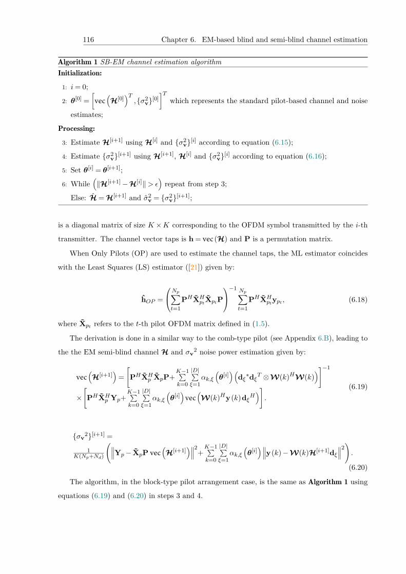
116 Chapter 6. EM-based blind and semi-blind channel estimation
Algorithm 1 SB-EM channel estimation algorithmInitialization:
1: i= 0;
2: θ[0] =[vec
(H[0]
)T,{σ2
v}[0]]T
which represents the standard pilot-based channel and noise
estimates;
Processing:
3: Estimate H[i+1] using H[i] and {σ2v}[i] according to equation (6.15);
4: Estimate {σ2v}[i+1] using H[i+1], H[i] and {σ2
v}[i] according to equation (6.16);
5: Set θ[i] = θ[i+1];
6: While(‖H[i+1]−H[i]‖> ε
)repeat from step 3;
Else: H = H[i+1] and σ2v = {σ2
v}[i+1];
is a diagonal matrix of size K ×K corresponding to the OFDM symbol transmitted by the i-th
transmitter. The channel vector taps is h = vec(H) and P is a permutation matrix.
When Only Pilots (OP) are used to estimate the channel taps, the ML estimator coincides
with the Least Squares (LS) estimator ([21]) given by:
hOP =
Np∑t=1
PHXHptXptP
−1 Np∑t=1
PHXHptypt , (6.18)
where Xpt refers to the t-th pilot OFDM matrix defined in (1.5).
The derivation is done in a similar way to the comb-type pilot (see Appendix 6.B), leading to
the the EM semi-blind channel H and σv2 noise power estimation given by:
vec(H[i+1]
)=[PHXH
p XpP+K−1∑k=0
|D|∑ξ=1
αk,ξ(θ[i])(
dξ∗dξT ⊗W(k)HW(k))]−1
×[PHXH
p Yp+K−1∑k=0
|D|∑ξ=1
αk,ξ(θ[i])vec
(W(k)Hy(k)dξH
)].
(6.19)
{σv2}[i+1] =
1K(Np+Nd)
(∥∥∥Yp− XpP vec(H[i+1]
)∥∥∥2+K−1∑k=0
|D|∑ξ=1
αk,ξ(θ[i])∥∥∥y(k)−W(k)H[i+1]dξ
∥∥∥2).
(6.20)
The algorithm, in the block-type pilot arrangement case, is the same as Algorithm 1 using
equations (6.19) and (6.20) in steps 3 and 4.
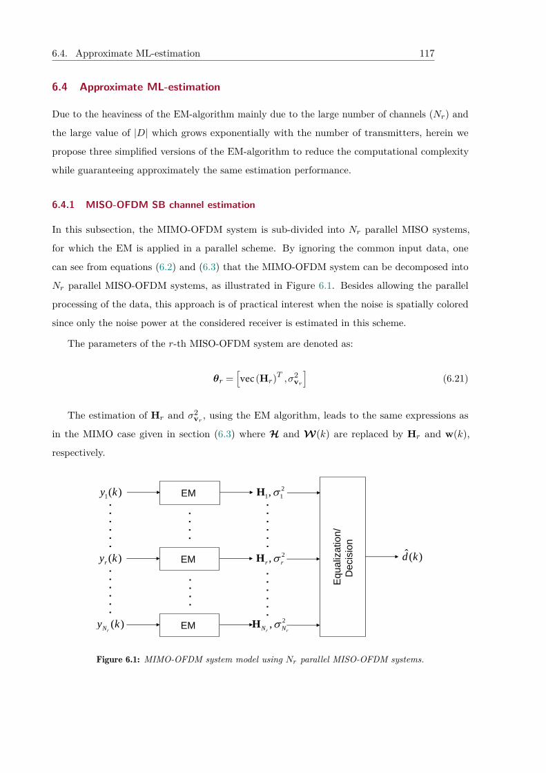
6.4. Approximate ML-estimation 117
6.4 Approximate ML-estimation
Due to the heaviness of the EM-algorithm mainly due to the large number of channels (Nr) and
the large value of |D| which grows exponentially with the number of transmitters, herein we
propose three simplified versions of the EM-algorithm to reduce the computational complexity
while guaranteeing approximately the same estimation performance.
6.4.1 MISO-OFDM SB channel estimation
In this subsection, the MIMO-OFDM system is sub-divided into Nr parallel MISO systems,
for which the EM is applied in a parallel scheme. By ignoring the common input data, one
can see from equations (6.2) and (6.3) that the MIMO-OFDM system can be decomposed into
Nr parallel MISO-OFDM systems, as illustrated in Figure 6.1. Besides allowing the parallel
processing of the data, this approach is of practical interest when the noise is spatially colored
since only the noise power at the considered receiver is estimated in this scheme.
The parameters of the r-th MISO-OFDM system are denoted as:
θr =[vec(Hr)T ,σ2
vr
](6.21)
The estimation of Hr and σ2vr , using the EM algorithm, leads to the same expressions as
in the MIMO case given in section (6.3) where H and W(k) are replaced by Hr and w(k),
respectively.
Equ
aliz
atio
n/D
ecis
ion
EM 1( )y k 21 1,H
EM ( )ry k 2,r rH
EM ( )rNy k 2,
r rN NH
ˆ( )d k
. .
. .
. .
. .
. .
. .
. .
. .
. .
. .
. .
. .
. .
. .
. .
. .
Figure 6.1: MIMO-OFDM system model using Nr parallel MISO-OFDM systems.
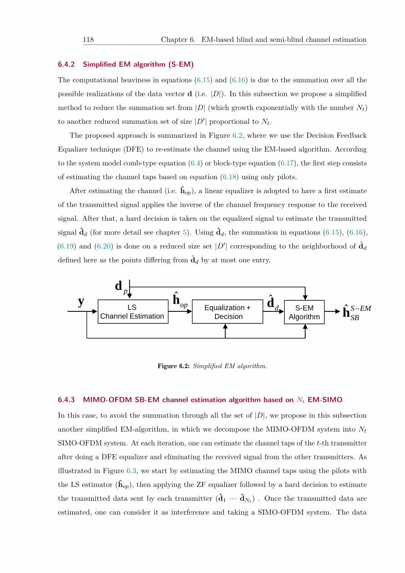
118 Chapter 6. EM-based blind and semi-blind channel estimation
6.4.2 Simplified EM algorithm (S-EM)
The computational heaviness in equations (6.15) and (6.16) is due to the summation over all the
possible realizations of the data vector d (i.e. |D|). In this subsection we propose a simplified
method to reduce the summation set from |D| (which growth exponentially with the number Nt)
to another reduced summation set of size |D′| proportional to Nt.
The proposed approach is summarized in Figure 6.2, where we use the Decision Feedback
Equalizer technique (DFE) to re-estimate the channel using the EM-based algorithm. According
to the system model comb-type equation (6.4) or block-type equation (6.17), the first step consists
of estimating the channel taps based on equation (6.18) using only pilots.
After estimating the channel (i.e. hop), a linear equalizer is adopted to have a first estimate
of the transmitted signal applies the inverse of the channel frequency response to the received
signal. After that, a hard decision is taken on the equalized signal to estimate the transmitted
signal dd (for more detail see chapter 5). Using dd, the summation in equations (6.15), (6.16),
(6.19) and (6.20) is done on a reduced size set |D′| corresponding to the neighborhood of dddefined here as the points differing from dd by at most one entry.
LS
Channel Estimation Equalization +
Decision
ypd
ˆoph ˆ
ddS-EM
Algorithmˆ S EM
SB
h
Figure 6.2: Simplified EM algorithm.
6.4.3 MIMO-OFDM SB-EM channel estimation algorithm based on Nt EM-SIMO
In this case, to avoid the summation through all the set of |D|, we propose in this subsection
another simplified EM-algorithm, in which we decompose the MIMO-OFDM system into NtSIMO-OFDM system. At each iteration, one can estimate the channel taps of the t-th transmitter
after doing a DFE equalizer and eliminating the received signal from the other transmitters. As
illustrated in Figure 6.3, we start by estimating the MIMO channel taps using the pilots with
the LS estimator (hop), then applying the ZF equalizer followed by a hard decision to estimate
the transmitted data sent by each transmitter (d1 · · · dNt) . Once the transmitted data are
estimated, one can consider it as interference and taking a SIMO-OFDM system. The data
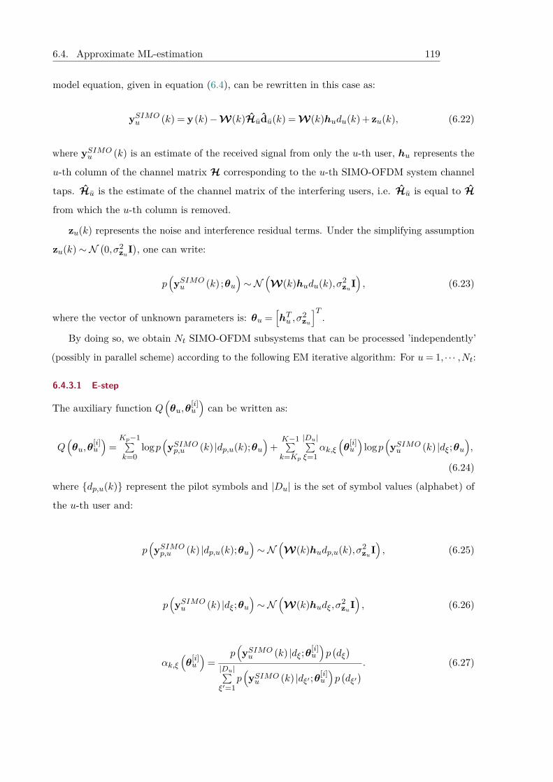
6.4. Approximate ML-estimation 119
model equation, given in equation (6.4), can be rewritten in this case as:
ySIMOu (k) = y(k)−W(k)Hudu(k) = W(k)hudu(k) + zu(k), (6.22)
where ySIMOu (k) is an estimate of the received signal from only the u-th user, hu represents the
u-th column of the channel matrix H corresponding to the u-th SIMO-OFDM system channel
taps. Hu is the estimate of the channel matrix of the interfering users, i.e. Hu is equal to H
from which the u-th column is removed.
zu(k) represents the noise and interference residual terms. Under the simplifying assumption
zu(k)∼N(0,σ2
zuI), one can write:
p(ySIMOu (k) ;θu
)∼N
(W(k)hudu(k),σ2
zuI), (6.23)
where the vector of unknown parameters is: θu =[hTu ,σ
2zu
]T.
By doing so, we obtain Nt SIMO-OFDM subsystems that can be processed ’independently’
(possibly in parallel scheme) according to the following EM iterative algorithm: For u= 1, · · · ,Nt:
6.4.3.1 E-step
The auxiliary function Q(θu,θ
[i]u
)can be written as:
Q(θu,θ
[i]u
)=Kp−1∑k=0
logp(ySIMOp,u (k) |dp,u(k);θu
)+
K−1∑k=Kp
|Du|∑ξ=1
αk,ξ(θ
[i]u
)logp
(ySIMOu (k) |dξ;θu
),
(6.24)
where {dp,u(k)} represent the pilot symbols and |Du| is the set of symbol values (alphabet) of
the u-th user and:
p(ySIMOp,u (k) |dp,u(k);θu
)∼N
(W(k)hudp,u(k),σ2
zuI), (6.25)
p(ySIMOu (k) |dξ;θu
)∼N
(W(k)hudξ,σ2
zuI), (6.26)
αk,ξ(θ
[i]u
)=
p(ySIMOu (k) |dξ;θ
[i]u
)p(dξ)
|Du|∑ξ′=1
p(ySIMOu (k) |dξ′ ;θ
[i]u
)p(dξ′) . (6.27)
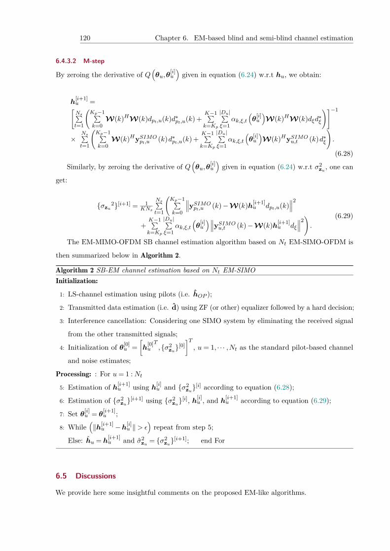
120 Chapter 6. EM-based blind and semi-blind channel estimation
6.4.3.2 M-step
By zeroing the derivative of Q(θu,θ
[i]u
)given in equation (6.24) w.r.t hu, we obtain:
h[i+1]u =[Ns∑t=1
(Kp−1∑k=0
W(k)HW(k)dpt,u(k)d∗pt,u(k) +K−1∑k=Kp
|Du|∑ξ=1
αk,ξ,t(θ
[i]u
)W(k)HW(k)dξd∗ξ
)]−1
×Ns∑t=1
(Kp−1∑k=0
W(k)HySIMOpt,u (k)d∗pt,u(k) +
K−1∑k=Kp
|Du|∑ξ=1
αk,ξ,t(θ
[i]u
)W(k)HySIMO
u,t (k)d∗ξ
).
(6.28)
Similarly, by zeroing the derivative of Q(θu,θ
[i]u
)given in equation (6.24) w.r.t σ2
zu , one can
get:
{σzu2}[i+1] = 1
KNs
Ns∑t=1
(Kp−1∑k=0
∥∥∥ySIMOpt,u (k)−W(k)h[i+1]
u dpt,u(k)∥∥∥2
+K−1∑k=Kp
|Du|∑ξ=1
αk,ξ,t(θ
[i]u
)∥∥∥ySIMOu,t (k)−W(k)h[i+1]
u dξ
∥∥∥2).
(6.29)
The EM-MIMO-OFDM SB channel estimation algorithm based on Nt EM-SIMO-OFDM is
then summarized below in Algorithm 2.
Algorithm 2 SB-EM channel estimation based on Nt EM-SIMOInitialization:
1: LS-channel estimation using pilots (i.e. hOP );
2: Transmitted data estimation (i.e. d) using ZF (or other) equalizer followed by a hard decision;
3: Interference cancellation: Considering one SIMO system by eliminating the received signal
from the other transmitted signals;
4: Initialization of θ[0]u =
[h
[0]uT,{σ2
zu}[0]]T
, u= 1, · · · ,Nt as the standard pilot-based channel
and noise estimates;
Processing: : For u= 1 :Nt5: Estimation of h[i+1]
u using h[i]u and {σ2
zu}[i] according to equation (6.28);
6: Estimation of {σ2zu}
[i+1] using {σ2zu}
[i], h[i]u , and h[i+1]
u according to equation (6.29);
7: Set θ[i]u = θ[i+1]
u ;
8: While(‖h[i+1]
u −h[i]u ‖> ε
)repeat from step 5;
Else: hu = h[i+1]u and σ2
zu = {σ2zu}
[i+1]; end For
6.5 Discussions
We provide here some insightful comments on the proposed EM-like algorithms.
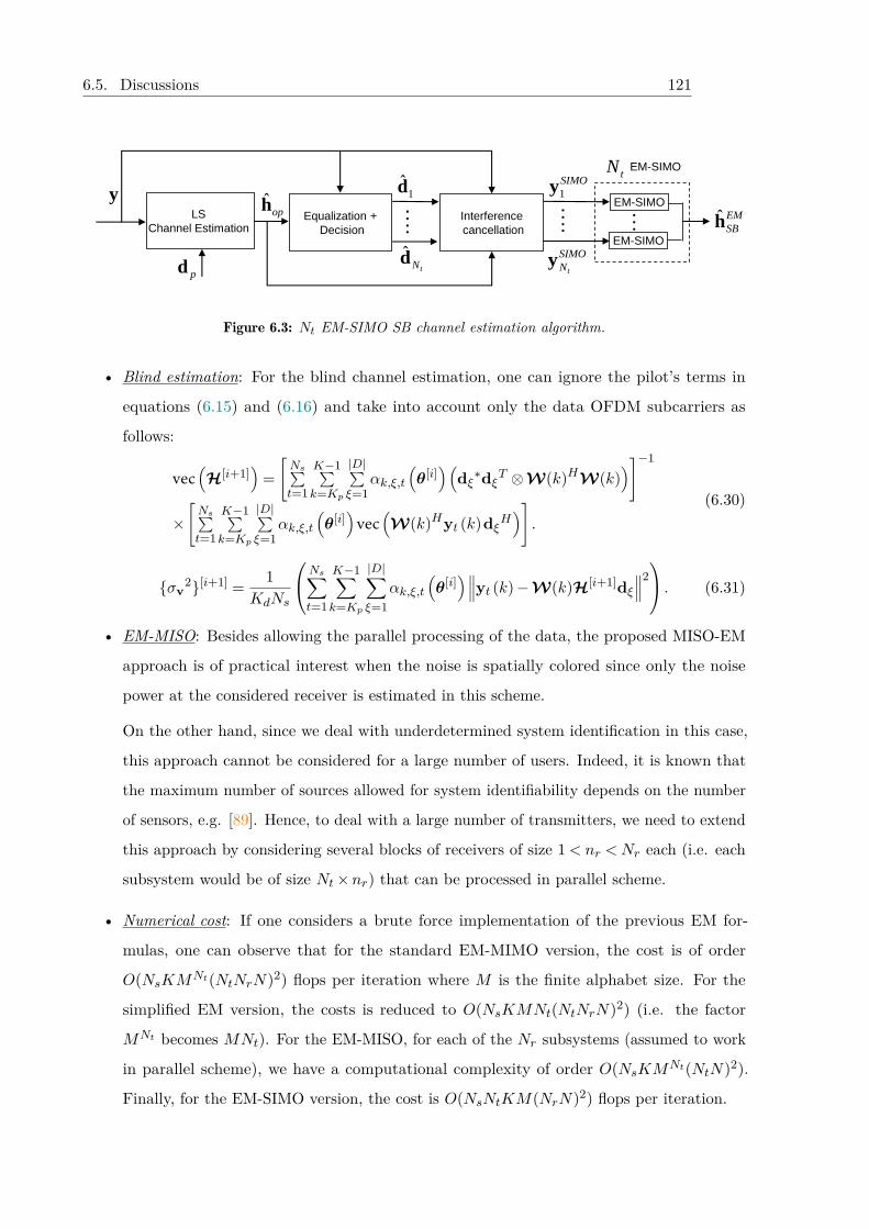
6.5. Discussions 121
….
LS
Channel Estimation Equalization +
Decision
y
pd
ˆoph
1d
ˆtNd
Interference
cancellation
1
SIMOy
t
SIMO
Ny
….
EM-SIMO
ˆ EM
SBhEM-SIMO
…
EM-SIMOtN
Figure 6.3: Nt EM-SIMO SB channel estimation algorithm.
• Blind estimation: For the blind channel estimation, one can ignore the pilot’s terms in
equations (6.15) and (6.16) and take into account only the data OFDM subcarriers as
follows:
vec(H[i+1]
)=[Ns∑t=1
K−1∑k=Kp
|D|∑ξ=1
αk,ξ,t(θ[i])(
dξ∗dξT ⊗W(k)HW(k))]−1
×[Ns∑t=1
K−1∑k=Kp
|D|∑ξ=1
αk,ξ,t(θ[i])vec
(W(k)Hyt (k)dξH
)].
(6.30)
{σv2}[i+1] = 1
KdNs
Ns∑t=1
K−1∑k=Kp
|D|∑ξ=1
αk,ξ,t(θ[i])∥∥∥yt (k)−W(k)H[i+1]dξ
∥∥∥2 . (6.31)
• EM-MISO: Besides allowing the parallel processing of the data, the proposed MISO-EM
approach is of practical interest when the noise is spatially colored since only the noise
power at the considered receiver is estimated in this scheme.
On the other hand, since we deal with underdetermined system identification in this case,
this approach cannot be considered for a large number of users. Indeed, it is known that
the maximum number of sources allowed for system identifiability depends on the number
of sensors, e.g. [89]. Hence, to deal with a large number of transmitters, we need to extend
this approach by considering several blocks of receivers of size 1< nr <Nr each (i.e. each
subsystem would be of size Nt×nr) that can be processed in parallel scheme.
• Numerical cost: If one considers a brute force implementation of the previous EM for-
mulas, one can observe that for the standard EM-MIMO version, the cost is of order
O(NsKMNt(NtNrN)2) flops per iteration where M is the finite alphabet size. For the
simplified EM version, the costs is reduced to O(NsKMNt(NtNrN)2) (i.e. the factor
MNt becomes MNt). For the EM-MISO, for each of the Nr subsystems (assumed to work
in parallel scheme), we have a computational complexity of order O(NsKMNt(NtN)2).
Finally, for the EM-SIMO version, the cost is O(NsNtKM(NrN)2) flops per iteration.
122 Chapter 6. EM-based blind and semi-blind channel estimation
• Algorithm’s convergence: As mentioned in section III-A, the EM-MIMO algorithm con-
verges to a local maximum point of the likelihood function [88]. This observation holds
for the EM-MISO but since the latter is underdetermined, the algorithm’s initialization is
more difficult and the risk of local (instead of global) convergence is higher. Also, since the
convergence rate of an EM algorithm is inversely related to the Fisher information of its
complete-data space [88], the rate of convergence would be lower in that case as compared
to the standard EM-MIMO algorithm. The EM-SIMO is somehow a specific version of
the SAGE (Space-Alternating Generalized Expectation-Maximization) algorithm which is
shown in [90] to lead to faster convergence under some mild assumptions. Finally, for the
simplified EM version, the convergence is dependent of the quality of the first LS estimate.
Indeed, since one restricts the search in (6.15), (6.16), (6.19) and (6.20) to the neighboring
of the initially detected input vector (i.e. the set |D′| instead of |D|), the estimation quality
as well as the algorithm’s convergence would depend strongly on this reduced size search
space. In fact, if the exact input vector belongs to the set |D′|, then, the S-EM would have
the same convergence properties as the standard EM-MIMO algorithm4.
• EM-SIMO: In our work, we have chosen to use a parallel interference cancellation technique
followed by an EM-based channel estimation for each SIMO subsystem. However, other
possible implementations might be used (not considered here) including: (i) the use
of sequential (instead of parallel) interference cancellation; (ii) the combination of the
interference cancellation and the EM-based channel up-date in each iteration of our recursive
EM algorithm.
6.6 Simulation results
This section analyzes the performance of the EM blind and semi-blind channel estimators in
terms of the NRMSE evaluated as:
NRMSE =
√√√√√ 1Nmc
Nmc∑i=1
∥∥∥h−h∥∥∥2
‖h‖2, (6.32)
where Nmc = 500 represents the number of independent Monte Carlo realizations. The perfor-
mance study is conducted for the three system configurations presented in this thesis i.e MIMO-
OFDM system (hEM−MIMOSB and hEM−MIMO
B ), parallel MISO-OFDM systems (hEM−MISOSB and
4Note that the error probability of the ZF equalizer is known in the literature, and hence, one can use this
information to get an upper bound of the convergence probability of our S-EM algorithm.
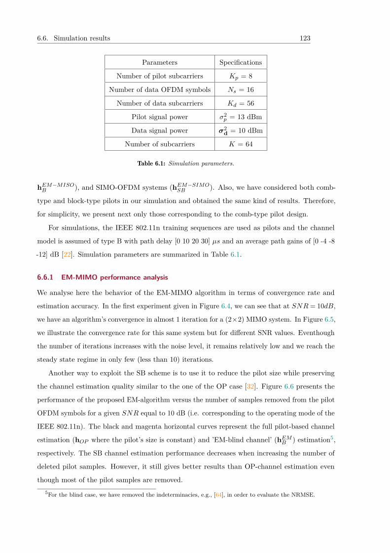
6.6. Simulation results 123
Parameters Specifications
Number of pilot subcarriers Kp = 8
Number of data OFDM symbols Ns = 16
Number of data subcarriers Kd = 56
Pilot signal power σ2p = 13 dBm
Data signal power σ2d = 10 dBm
Number of subcarriers K = 64
Table 6.1: Simulation parameters.
hEM−MISOB ), and SIMO-OFDM systems (hEM−SIMO
SB ). Also, we have considered both comb-
type and block-type pilots in our simulation and obtained the same kind of results. Therefore,
for simplicity, we present next only those corresponding to the comb-type pilot design.
For simulations, the IEEE 802.11n training sequences are used as pilots and the channel
model is assumed of type B with path delay [0 10 20 30] µs and an average path gains of [0 -4 -8
-12] dB [22]. Simulation parameters are summarized in Table 6.1.
6.6.1 EM-MIMO performance analysis
We analyse here the behavior of the EM-MIMO algorithm in terms of convergence rate and
estimation accuracy. In the first experiment given in Figure 6.4, we can see that at SNR = 10dB,
we have an algorithm’s convergence in almost 1 iteration for a (2×2) MIMO system. In Figure 6.5,
we illustrate the convergence rate for this same system but for different SNR values. Eventhough
the number of iterations increases with the noise level, it remains relatively low and we reach the
steady state regime in only few (less than 10) iterations.
Another way to exploit the SB scheme is to use it to reduce the pilot size while preserving
the channel estimation quality similar to the one of the OP case [32]. Figure 6.6 presents the
performance of the proposed EM-algorithm versus the number of samples removed from the pilot
OFDM symbols for a given SNR equal to 10 dB (i.e. corresponding to the operating mode of the
IEEE 802.11n). The black and magenta horizontal curves represent the full pilot-based channel
estimation (hOP where the pilot’s size is constant) and ’EM-blind channel’ (hEMB ) estimation5,
respectively. The SB channel estimation performance decreases when increasing the number of
deleted pilot samples. However, it still gives better results than OP-channel estimation even
though most of the pilot samples are removed.5For the blind case, we have removed the indeterminacies, e.g., [64], in order to evaluate the NRMSE.
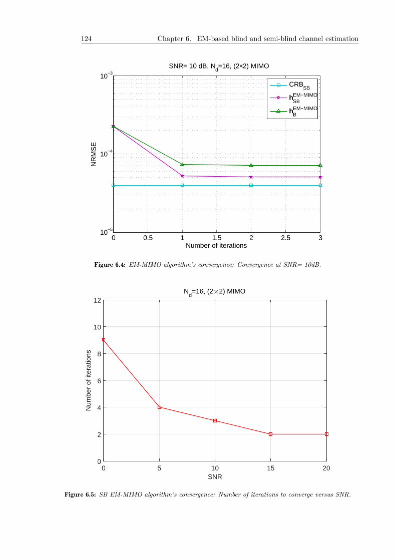
124 Chapter 6. EM-based blind and semi-blind channel estimation
0 0.5 1 1.5 2 2.5 310−5
10−4
10−3SNR= 10 dB, N
d=16, (2×2) MIMO
NR
MS
E
Number of iterations
CRBSB
hSBEM−MIMO
hBEM−MIMO
Figure 6.4: EM-MIMO algorithm’s convergence: Convergence at SNR= 10dB.
SNR0 5 10 15 20
Num
ber
of it
erat
ions
0
2
4
6
8
10
12N
d=16, (2#2) MIMO
Figure 6.5: SB EM-MIMO algorithm’s convergence: Number of iterations to converge versus SNR.
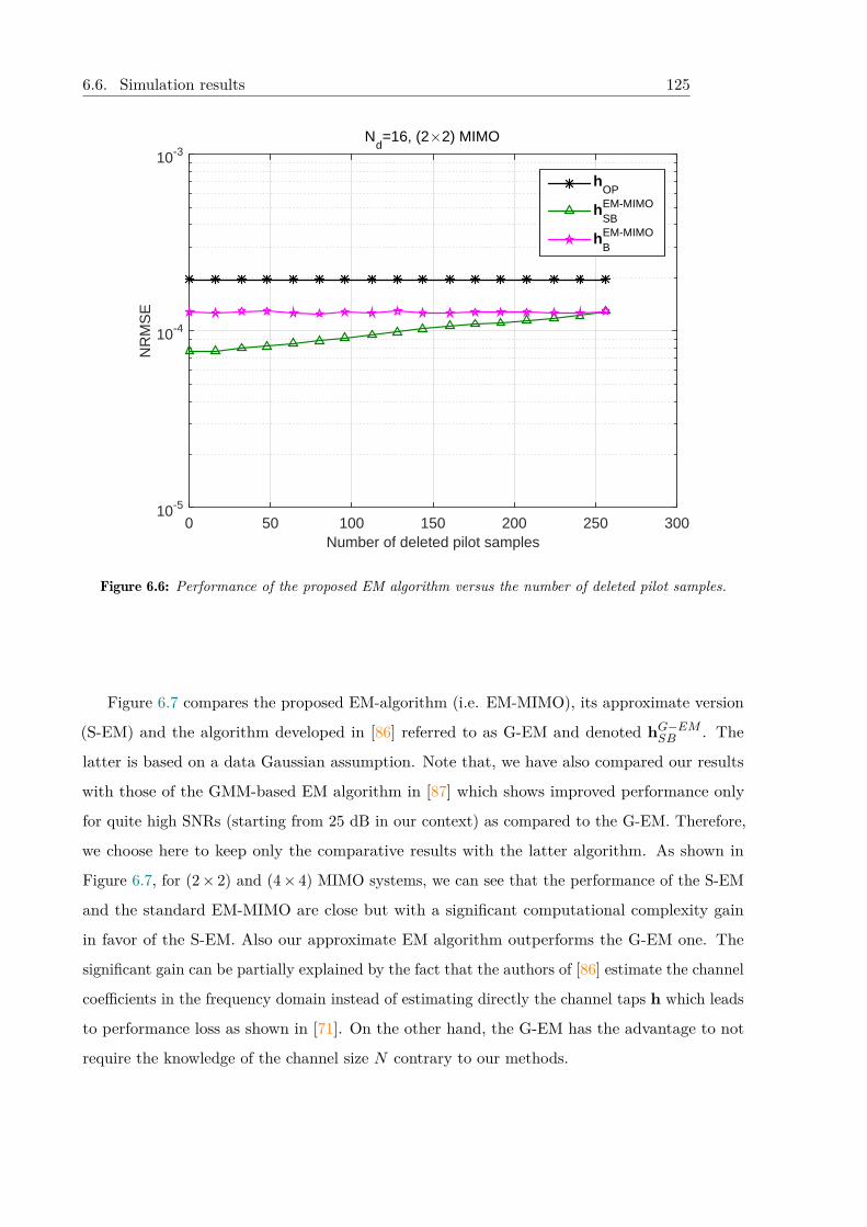
6.6. Simulation results 125
Number of deleted pilot samples0 50 100 150 200 250 300
NR
MS
E
10-5
10-4
10-3N
d=16, (2#2) MIMO
hOP
hSBEM-MIMO
hBEM-MIMO
Figure 6.6: Performance of the proposed EM algorithm versus the number of deleted pilot samples.
Figure 6.7 compares the proposed EM-algorithm (i.e. EM-MIMO), its approximate version
(S-EM) and the algorithm developed in [86] referred to as G-EM and denoted hG−EMSB . The
latter is based on a data Gaussian assumption. Note that, we have also compared our results
with those of the GMM-based EM algorithm in [87] which shows improved performance only
for quite high SNRs (starting from 25 dB in our context) as compared to the G-EM. Therefore,
we choose here to keep only the comparative results with the latter algorithm. As shown in
Figure 6.7, for (2× 2) and (4× 4) MIMO systems, we can see that the performance of the S-EM
and the standard EM-MIMO are close but with a significant computational complexity gain
in favor of the S-EM. Also our approximate EM algorithm outperforms the G-EM one. The
significant gain can be partially explained by the fact that the authors of [86] estimate the channel
coefficients in the frequency domain instead of estimating directly the channel taps h which leads
to performance loss as shown in [71]. On the other hand, the G-EM has the advantage to not
require the knowledge of the channel size N contrary to our methods.
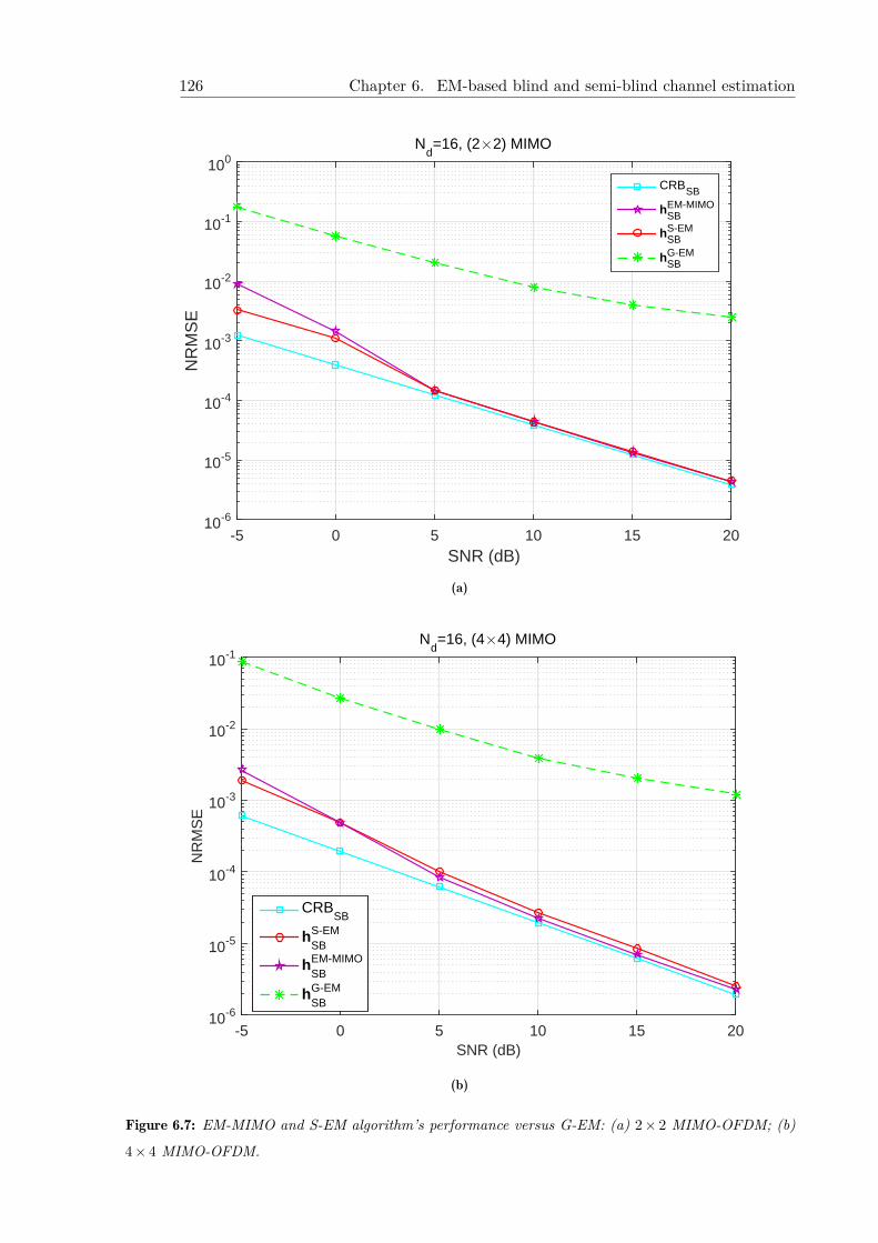
126 Chapter 6. EM-based blind and semi-blind channel estimation
SNR (dB)-5 0 5 10 15 20
NR
MS
E
10-6
10-5
10-4
10-3
10-2
10-1
100N
d=16, (2#2) MIMO
CRBSB
hSBEM-MIMO
hSBS-EM
hSBG-EM
(a)
SNR (dB)-5 0 5 10 15 20
NR
MS
E
10-6
10-5
10-4
10-3
10-2
10-1N
d=16, (4#4) MIMO
CRBSB
hSBS-EM
hSBEM-MIMO
hSBG-EM
(b)
Figure 6.7: EM-MIMO and S-EM algorithm’s performance versus G-EM: (a) 2× 2 MIMO-OFDM; (b)
4× 4 MIMO-OFDM.
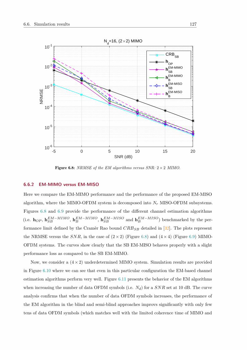
6.6. Simulation results 127
SNR (dB)-5 0 5 10 15 20
NR
MS
E
10-6
10-5
10-4
10-3
10-2
10-1N
d=16, (2#2) MIMO
CRBSB
hOP
hSBEM-MIMO
hBEM-MIMO
hSBEM-MISO
hBEM-MISO
Figure 6.8: NRMSE of the EM algorithms versus SNR: 2× 2 MIMO.
6.6.2 EM-MIMO versus EM-MISO
Here we compare the EM-MIMO performance and the performance of the proposed EM-MISO
algorithm, where the MIMO-OFDM system is decomposed into Nr MISO-OFDM subsystems.
Figures 6.8 and 6.9 provide the performance of the different channel estimation algorithms
(i.e. hOP , hEM−MIMOSB , hEM−MIMO
B , hEM−MISOSB and hEM−MISO
B ) benchmarked by the per-
formance limit defined by the Cramèr Rao bound CRBSB detailed in [32]. The plots represent
the NRMSE versus the SNR, in the case of (2× 2) (Figure 6.8) and (4× 4) (Figure 6.9) MIMO-
OFDM systems. The curves show clearly that the SB EM-MISO behaves properly with a slight
performance loss as compared to the SB EM-MIMO.
Now, we consider a (4× 2) underdetermined MIMO system. Simulation results are provided
in Figure 6.10 where we can see that even in this particular configuration the EM-based channel
estimation algorithms perform very well. Figure 6.11 presents the behavior of the EM algorithms
when increasing the number of data OFDM symbols (i.e. Nd) for a SNR set at 10 dB. The curve
analysis confirms that when the number of data OFDM symbols increases, the performance of
the EM algorithm in the blind and semi-blind approaches improvs significantly with only few
tens of data OFDM symbols (which matches well with the limited coherence time of MIMO and
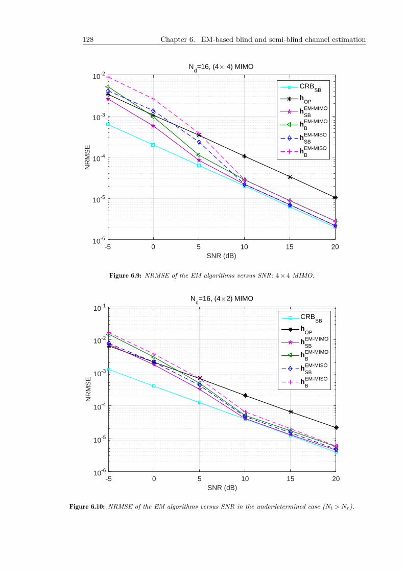
128 Chapter 6. EM-based blind and semi-blind channel estimation
SNR (dB)-5 0 5 10 15 20
NR
MS
E
10-6
10-5
10-4
10-3
10-2N
d=16, (4# 4) MIMO
CRBSB
hOP
hSBEM-MIMO
hBEM-MIMO
hSBEM-MISO
hBEM-MISO
Figure 6.9: NRMSE of the EM algorithms versus SNR: 4× 4 MIMO.
SNR (dB)-5 0 5 10 15 20
NR
MS
E
10-6
10-5
10-4
10-3
10-2
10-1N
d=16, (4#2) MIMO
CRBSB
hOP
hSBEM-MIMO
hBEM-MIMO
hSBEM-MISO
hBEM-MISO
Figure 6.10: NRMSE of the EM algorithms versus SNR in the underdetermined case (Nt >Nr).
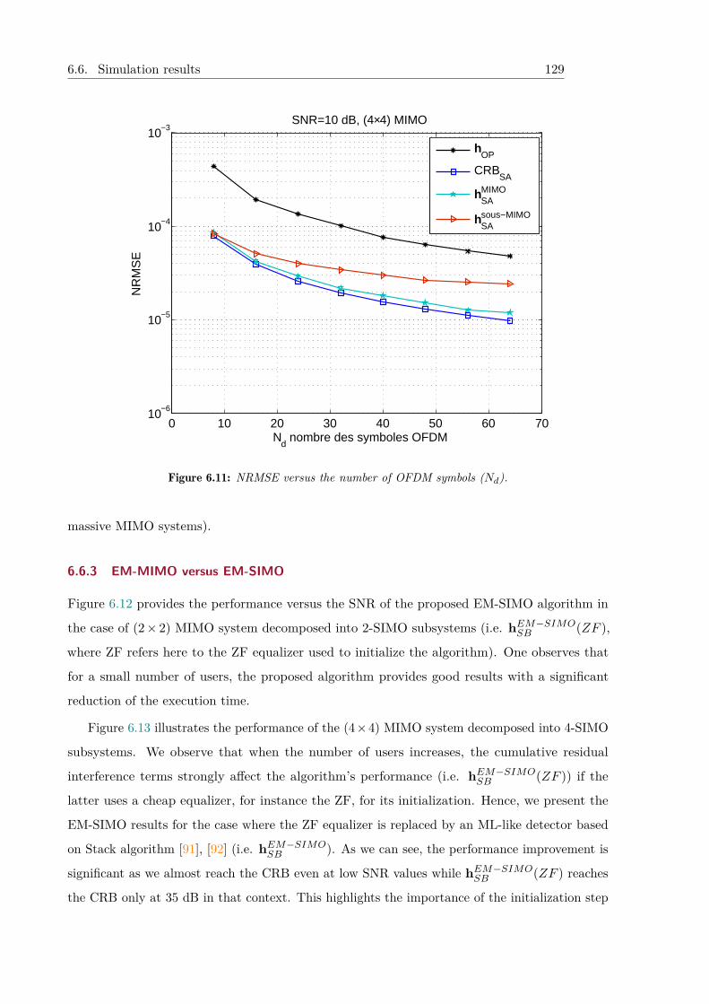
6.6. Simulation results 129
0 10 20 30 40 50 60 7010−6
10−5
10−4
10−3SNR=10 dB, (4×4) MIMO
NR
MS
E
Nd nombre des symboles OFDM
hOP
CRBSA
hSAMIMO
hSAsous−MIMO
Figure 6.11: NRMSE versus the number of OFDM symbols (Nd).
massive MIMO systems).
6.6.3 EM-MIMO versus EM-SIMO
Figure 6.12 provides the performance versus the SNR of the proposed EM-SIMO algorithm in
the case of (2× 2) MIMO system decomposed into 2-SIMO subsystems (i.e. hEM−SIMOSB (ZF ),
where ZF refers here to the ZF equalizer used to initialize the algorithm). One observes that
for a small number of users, the proposed algorithm provides good results with a significant
reduction of the execution time.
Figure 6.13 illustrates the performance of the (4×4) MIMO system decomposed into 4-SIMO
subsystems. We observe that when the number of users increases, the cumulative residual
interference terms strongly affect the algorithm’s performance (i.e. hEM−SIMOSB (ZF )) if the
latter uses a cheap equalizer, for instance the ZF, for its initialization. Hence, we present the
EM-SIMO results for the case where the ZF equalizer is replaced by an ML-like detector based
on Stack algorithm [91], [92] (i.e. hEM−SIMOSB ). As we can see, the performance improvement is
significant as we almost reach the CRB even at low SNR values while hEM−SIMOSB (ZF ) reaches
the CRB only at 35 dB in that context. This highlights the importance of the initialization step
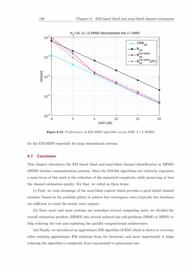
130 Chapter 6. EM-based blind and semi-blind channel estimation
SNR (dB)-5 0 5 10 15 20
NR
MS
E
10-6
10-5
10-4
10-3
10-2N
d=16, (2#2) MIMO decomposed into 2#SIMO
CRBSB
hOP
hSBEM-MIMO
hSBEM-SIMO(ZF)
Figure 6.12: Performance of EM-SIMO algorithm versus SNR: 2× 2 MIMO.
for the EM-SIMO especially for large dimensional systems.
6.7 Conclusion
This chapter introduces the EM based blind and semi-blind channel identification in MIMO-
OFDM wireless communications systems. Since the EM-like algorithms are relatively expensive,
a main focus of this work is the reduction of the numerical complexity while preserving at best
the channel estimation quality. For that, we relied on three items:
(i) First, we took advantage of the semi-blind context which provides a good initial channel
estimate (based on the available pilots) to achieve fast convergence rates (typically few iterations
are sufficient to reach the steady state regime).
(ii) Since more and more systems use nowadays several computing units, we divided the
overall estimation problem (MIMO) into several reduced size sub-problems (SIMO or MISO) to
help reducing the cost and exploiting the parallel computational architectures.
(iii) Finally, we introduced an approximate EM algorithm (S-EM) which is shown to overcome
other existing approximate EM solutions from the literature and more importantly it helps
reducing the algorithm’s complexity from exponential to polynomial one.
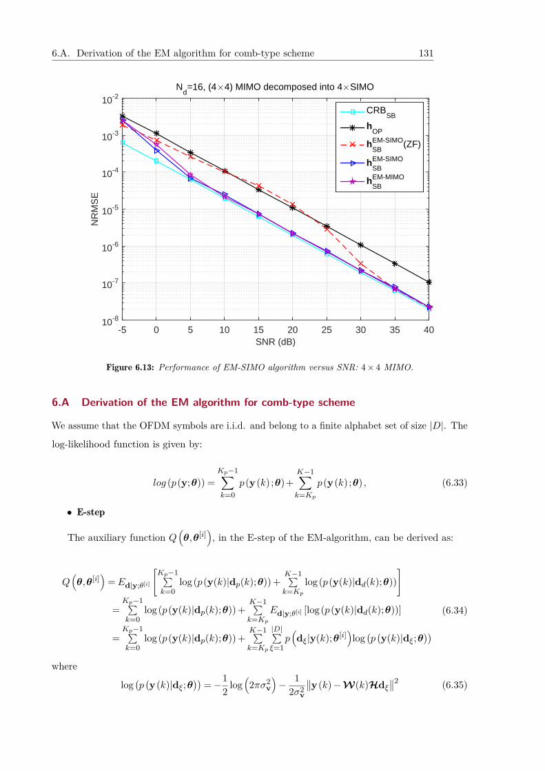
6.A. Derivation of the EM algorithm for comb-type scheme 131
SNR (dB)-5 0 5 10 15 20 25 30 35 40
NR
MS
E
10-8
10-7
10-6
10-5
10-4
10-3
10-2N
d=16, (4#4) MIMO decomposed into 4#SIMO
CRBSB
hOP
hSBEM-SIMO(ZF)
hSBEM-SIMO
hSBEM-MIMO
Figure 6.13: Performance of EM-SIMO algorithm versus SNR: 4× 4 MIMO.
6.A Derivation of the EM algorithm for comb-type scheme
We assume that the OFDM symbols are i.i.d. and belong to a finite alphabet set of size |D|. The
log-likelihood function is given by:
log (p(y;θ)) =Kp−1∑k=0
p(y(k) ;θ)+K−1∑k=Kp
p(y(k) ;θ) , (6.33)
• E-step
The auxiliary function Q(θ,θ[i]
), in the E-step of the EM-algorithm, can be derived as:
Q(θ,θ[i]
)= Ed|y;θ[i]
[Kp−1∑k=0
log(p(y(k)|dp(k);θ)) +K−1∑k=Kp
log(p(y(k)|dd(k);θ))]
=Kp−1∑k=0
log(p(y(k)|dp(k);θ)) +K−1∑k=Kp
Ed|y;θ[i] [log(p(y(k)|dd(k);θ))]
=Kp−1∑k=0
log(p(y(k)|dp(k);θ)) +K−1∑k=Kp
|D|∑ξ=1
p(dξ|y(k);θ[i]
)log(p(y(k)|dξ;θ
))(6.34)
where
log(p(y(k)|dξ;θ
))=−1
2 log(2πσ2
v
)− 1
2σ2v
∥∥y(k)−W(k)Hdξ∥∥2 (6.35)
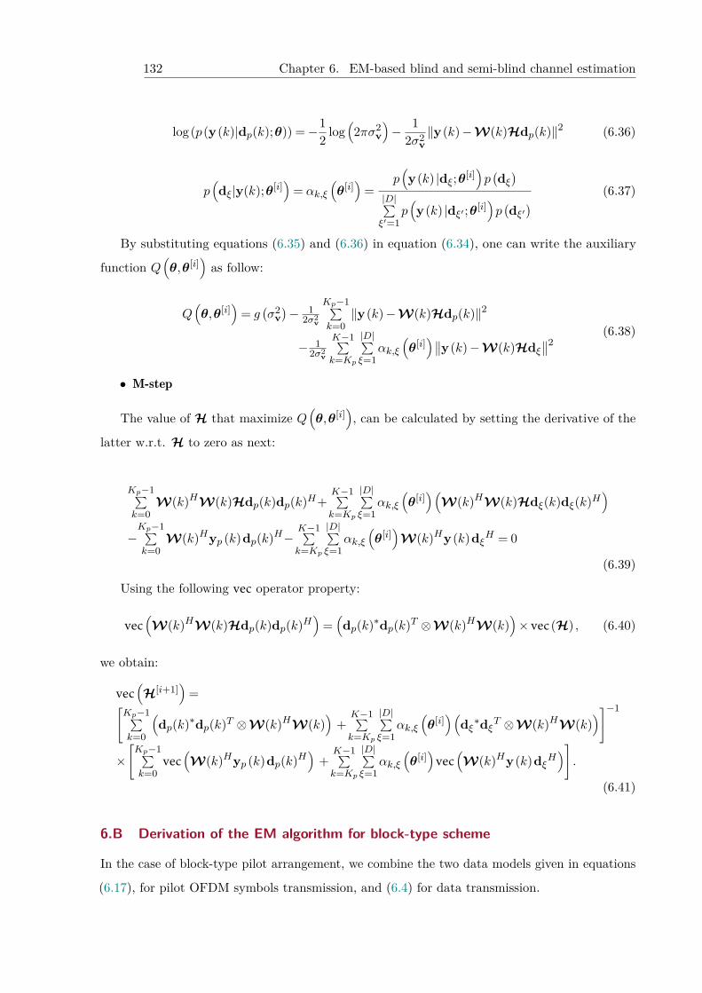
132 Chapter 6. EM-based blind and semi-blind channel estimation
log(p(y(k)|dp(k);θ)) =−12 log
(2πσ2
v
)− 1
2σ2v‖y(k)−W(k)Hdp(k)‖2 (6.36)
p(dξ|y(k);θ[i]
)= αk,ξ
(θ[i])
=p(y(k) |dξ;θ[i]
)p(dξ)
|D|∑ξ′=1
p(y(k) |dξ′ ;θ[i]
)p(dξ′) (6.37)
By substituting equations (6.35) and (6.36) in equation (6.34), one can write the auxiliary
function Q(θ,θ[i]
)as follow:
Q(θ,θ[i]
)= g
(σ2
v)− 1
2σ2v
Kp−1∑k=0‖y(k)−W(k)Hdp(k)‖2
− 12σ2
v
K−1∑k=Kp
|D|∑ξ=1
αk,ξ(θ[i])∥∥y(k)−W(k)Hdξ
∥∥2(6.38)
• M-step
The value of H that maximize Q(θ,θ[i]
), can be calculated by setting the derivative of the
latter w.r.t. H to zero as next:
Kp−1∑k=0
W(k)HW(k)Hdp(k)dp(k)H+K−1∑k=Kp
|D|∑ξ=1
αk,ξ(θ[i])(
W(k)HW(k)Hdξ(k)dξ(k)H)
−Kp−1∑k=0
W(k)Hyp (k)dp(k)H−K−1∑k=Kp
|D|∑ξ=1
αk,ξ(θ[i])
W(k)Hy(k)dξH = 0
(6.39)
Using the following vec operator property:
vec(W(k)HW(k)Hdp(k)dp(k)H
)=(dp(k)∗dp(k)T ⊗W(k)HW(k)
)× vec(H) , (6.40)
we obtain:
vec(H[i+1]
)=[
Kp−1∑k=0
(dp(k)∗dp(k)T ⊗W(k)HW(k)
)+
K−1∑k=Kp
|D|∑ξ=1
αk,ξ(θ[i])(
dξ∗dξT ⊗W(k)HW(k))]−1
×[Kp−1∑k=0
vec(W(k)Hyp (k)dp(k)H
)+
K−1∑k=Kp
|D|∑ξ=1
αk,ξ(θ[i])vec
(W(k)Hy(k)dξH
)].
(6.41)
6.B Derivation of the EM algorithm for block-type scheme
In the case of block-type pilot arrangement, we combine the two data models given in equations
(6.17), for pilot OFDM symbols transmission, and (6.4) for data transmission.
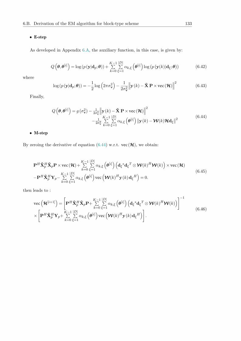
6.B. Derivation of the EM algorithm for block-type scheme 133
• E-step
As developed in Appendix 6.A, the auxiliary function, in this case, is given by:
Q(θ,θ[i]
)= log(p(y|dp;θ)) +
K−1∑k=0
|D|∑ξ=1
αk,ξ(θ[i])
log(p(y(k)|dξ;θ
))(6.42)
where
log(p(y|dp;θ)) =−12 log
(2πσ2
v
)− 1
2σ2v
∥∥∥y(k)− X P× vec(H)∥∥∥2
(6.43)
Finally,
Q(θ,θ[i]
)= g
(σ2
v)− 1
2σ2v
∥∥∥y(k)− X P× vec(H)∥∥∥2
− 12σ2
v
K−1∑k=0
|D|∑ξ=1
αk,ξ(θ[i])∥∥y(k)−W(k)Hdξ
∥∥2 (6.44)
• M-step
By zeroing the derivative of equation (6.44) w.r.t. vec(H), we obtain:
PHXHp XpP× vec(H)+
K−1∑k=0
|D|∑ξ=1
αk,ξ(θ[i])(
dξ∗dξT ⊗W(k)HW(k))× vec(H)
−PHXHp Yp−
K−1∑k=0
|D|∑ξ=1
αk,ξ(θ[i])vec
(W(k)Hy(k)dξH
)= 0.
(6.45)
then leads to :
vec(H[i+1]
)=[PHXH
p XpP+K−1∑k=0
|D|∑ξ=1
αk,ξ(θ[i])(
dξ∗dξT ⊗W(k)HW(k))]−1
×[PHXH
p Yp+K−1∑k=0
|D|∑ξ=1
αk,ξ(θ[i])vec
(W(k)Hy(k)dξH
)].
(6.46)

134 Chapter 6. EM-based blind and semi-blind channel estimation
7
Ch
ap
te
r
Subspace blind and semi-blind channel estimation
The only way of discovering the
limits of the possible is to venture a
little way past them into the
impossible.
Clarke’s Second Law.
In this chapter, we propose a semi-blind (SB) subspace channel estimation technique for which
an identifiability result is first established for the subspace based criterion. Our algorithm adopts
the MIMO-OFDM system model without cyclic prefix and takes advantage of the circulant
property of the channel matrix to achieve lower computational complexity and to accelerate the
algorithm’s convergence by generating a group of sub vectors from each received OFDM symbol.
The contributions of this work have been published in national 1and international 2conferences.
Abstract
1 [93] A. Ladaycia, A. Mokraoui, K. Abed-Meraim, and A. Belouchrani, "Contributions à l’estimation semi-
aveugle des canaux MIMO-OFDM," in GRETSI 2017, Sep. 2017, Nice, France.2 [94] A. Ladaycia, K. Abed-Meraim, A. Mokraoui, and A. Belouchrani, "Efficient Semi-Blind Subspace Channel
Estimation for MIMO-OFDM System," in 2018 26th European Signal Processing Conference (EUSIPCO), Sep.
2018, Rome, Italy.
136 Chapter 7. Subspace blind and semi-blind channel estimation
Chapter content7.1 Introduction . . . . . . . . . . . . . . . . . . . . . . . . . . . . . . . . . . . . . 137
7.2 System model . . . . . . . . . . . . . . . . . . . . . . . . . . . . . . . . . . . . . 137
7.3 MIMO channel estimation . . . . . . . . . . . . . . . . . . . . . . . . . . . . . . 138
7.3.1 Pilot-based channel estimation . . . . . . . . . . . . . . . . . . . . . . . 138
7.3.2 Subspace based SB channel estimation . . . . . . . . . . . . . . . . . . . 139
7.3.3 Fast semi-blind channel estimation . . . . . . . . . . . . . . . . . . . . . 141
7.4 Performance analysis and discussions . . . . . . . . . . . . . . . . . . . . . . . . 142
7.5 Conclusion . . . . . . . . . . . . . . . . . . . . . . . . . . . . . . . . . . . . . . 145
7.1. Introduction 137
7.1 Introduction
Research work on semi-blind methods can be divided into two categories. The first category
groups works that aim to improve the performance of the channel estimation through the joint
use of pilots and data symbols. This is the case, for example, of [95] where the authors used a
subspace approach or [26] which proposes a decomposition of the channel matrix into a whitening
matrix and another unitary. The second category includes works that focus on reducing the size
of the transmitted pilot signals in order to improve the throughput gain (see for example [66]).
In [33], the authors exploit the semi-blind approach to reduce the transmitted power ("green
communications").
This chapter proposes a semi-blind channel estimation method based on the subspace
decomposition (in signal subspace and noise subspace) of the covariance matrix of the received
signal. The derivation of subspace methods depends on the matrix system model. In our case,
we use an appropriate windowing that increases the convergence rate together with the circular
Toeplitz block structure of the system matrix associated with an OFDM symbol. First, we
establish a subspace identifiability result linked to this structure before using it for semi-blind
channel estimation.
Note that in the literature there exist already several versions of the subspace method, for
example [95, 96] differ from the one proposed in this thesis by incorporating the cyclic prefix
(CP) and virtual carriers (VC) into the system model which changes the size and structure of the
system channel matrix. The latter methods are efficient only for large sample sizes and hence
a fast alternative approach has been introduced in [97]. Compared to this last method, our
solution does not rely on the presence of VC and has a lower computational complexity. Finally,
we present simulation results with comparative study that assess the performance gain achieved
by the proposed solution.
7.2 System model
This MIMO-OFDM system adopted in this study is illustrated in Figure 1.1 and described in
chapter 1. The received signal y at the Nr receivers of the MIMO-OFDM system is given by 1
(after CP removal):
y = Hx + v, (7.1)
where y =[yT1 · · ·yTNr
]Tand x =
[xT1 · · ·xTNt
]T. The noise v =
[vT1 · · ·vTNr
]Tis assumed to
be additive independent white Circular Complex Gaussian (CCG) satisfying E[v(k)v(i)H
]=
138 Chapter 7. Subspace blind and semi-blind channel estimation
σ2vIKδki; (.)H being the Hermitian operator; σ2
v the noise variance; IK the identity matrix of
size K ×K. The channel matrix H is given by:
H =
H1,1 · · · H1,Nt...
. . ....
HNr,1 · · · HNr,Nt
. (7.2)
Each sub-block Hi,j (with i= 1, · · · , Nr and j = 1, · · · , Nt) of the matrix H is a circulantK×K
Toeplitz matrix. The first row of the (i, j)-th block contains the propagation channel coefficients
between the i-th transmitter and the j-th receiver hi,j i.e.(hi,j = [hi,j(0) · · · hi,j(N − 1)]T
), given
by:[hi,j(0) 01×(K−N) hi,j(N − 1) · · · hi,j(1)
]. The signal xi, sent by the i-th transmitter is
an OFDM signal, modulating the data signal di, using the inverse Fourier transform IFFT, as
follows
xi = WH
√K
di, (7.3)
where W represents the K-point Fourier matrix. Equation (7.1), can be rewritten as:
y = HWd + v = Ad + v, (7.4)
where A = HW and W = INt⊗W with ⊗ referring to the Kronecker product. The transmitted
data are regrouped in d =[dT1 · · ·dTNt
]T.
In the sequel the received OFDM symbols are assumed to be i.i.d and the Np pilots are
arranged according to the block-type scheme followed by Nd data OFDM symbols. To take into
account the time index (ignored in equations (7.1) and (7.4)), we will refer to the t-th OFDM
symbol by y(t) instead of y.
7.3 MIMO channel estimation
This section first reminds the well known Least Squares estimator, denoted LS, based on the
pilot symbols known at the receiver side. Our subspace blind estimator is then introduced
to ultimately derive the proposed semi-blind estimation solution. This is formulated by the
minimization of a cost function that incorporates both the pilot and the blind (data) part.
7.3.1 Pilot-based channel estimation
In order to derive LS estimator, based on the training sequences, equation (7.1) is rewritten as:
y = Xh + v, (7.5)
7.3. MIMO channel estimation 139
where h =[hT1 · · ·hTNr
]Tis a vector of size NrNtN × 1 representing the MIMO channel taps
(where hr =[hT1,r · · ·hTNt,r
]T). X = INr⊗X, with X = [X1 · · ·XNt ] where Xi is a circulant K×N
Toeplitz matrix containing the elements of xi. Each column is obtained by a simple down cyclic
shift of the previous one with the first column being the vector xi.
The LS channel estimator hLS , using Np pilot OFDM symbols, Xp =[X(1)T · · ·X(Np)
T]T
,
is obtained by the minimization of the following cost function:
C (h) =∥∥∥yp− Xph
∥∥∥2, (7.6)
with yp =[y(1)T · · ·y(Np)T
]T.
Then the LS estimator is given by [21]:
hLS =(XHp Xp
)−1XHp yp. (7.7)
7.3.2 Subspace based SB channel estimation
In this subsection, we consider the subspace approach for the data model given in equation (7.1).
Based on the data model assumptions, the data covariance matrix is equal to:
Cy = E(yyH) = σ2xHHH +σ2
vIKNr (7.8)
Hence, the signal subspace (principal subspace of Cy) coincides with the range space of H
while the noise subspace is its orthogonal complement. These subspaces can be estimated from
the eigenvalue decomposition (EVD) of Cy according to:
Cy = UΛUH = [Us |Un ]
Λs 0
0 Λn
UH
s
UHn
, (7.9)
where Cy is estimated using Nd data OFDM symbols as follows:
Cy = 1Nd
Nd∑t=1
y(t)y(t)H . (7.10)
Λ is a diagonal matrix containing the eigenvalues in descending order, the matrix Us of size
KNr×KNt contains the eigenvectors associated with the largest eigenvalues representing the
signal subspace. The noise subspace Un is associated with the K (Nr −Nt) smallest eigenvalues,
i.e.:
[Us |Un ] = [u1 · · · uKNt |uKNt+1 · · · uKNr ] . (7.11)
Now, the subspace identification applies only when the range space of matrix H (range(H))
characterizes uniquely the channel vector h (up to certain inherent indeterminacies [63]). For
140 Chapter 7. Subspace blind and semi-blind channel estimation
this purpose, we have proved the following identifiability result:
Lemma 7.1. Let H(z) be the Nr ×Nt polynomial filtering matrix which (i, j)-th entry is
given by hi,j(z) = ∑Nk=0hi,j(k)z−k. Under the assumption that H(z) is irreducible (i.e.
rank(H(z)) =Nt for all z), the range space of matrix H characterizes the channel as follows:
For any polynomial matrix H′(z) of degree N , we have range(H′) = range(H) if and only if
H′(z) = H(z)Q, where Q is a constant Nt×Nt matrix representing the inherent indeterminacy
of the blind approach [63].
Using the previous lemma, we can blindly identify the channel vector through the orthogonality
relation between the noise and signal subspaces according to:
uHi A = 0 i=KNt + 1, · · · ,KNr, (7.12)
where A is the channel matrix given in equation (7.4).
Solving this orthogonality relation in the least squares sense leads to:
C (H) =KNr∑
i=KNt+1
∥∥∥uHi A∥∥∥2
=KNr∑
i=KNt+1
∥∥∥uHi HW∥∥∥2. (7.13)
By partitioning vector ui of dimension KNr × 1 into Nr vectors vir (r = 1, · · · ,Nr) of size K
as follows:
ui =[
vi1T · · · viNr
T]T, (7.14)
one can generate the NNr ×K matrix Vi as:
Vi =[
Vi1 · · ·Vi
Nr
]T, (7.15)
where each matrix Vir is circulant of size N ×K constructed from the vector vir. Each line is
obtained by a simple left cyclic shift of the previous one with the first line being the vector virT .
The cost function given by equation (7.13), can then be rewritten in the following form:
C (H) =KNr∑
i=KNt+1
∥∥∥HTVi∗W
∥∥∥2=
KNr∑i=KNt+1
∥∥∥HTVi∗∥∥∥2, (7.16)
whereH =
[h1 · · · hNt
]h =
[hT1 · · · hTNt
]Thi =
[h1,i(0) · · · h1,i(N − 1) · · ·hNr,i(0) · · · hNr,i(N − 1)
]T .(7.17)
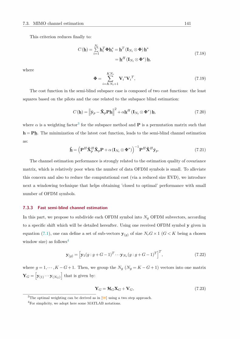
7.3. MIMO channel estimation 141
This criterion reduces finally to:
C (h) =Nt∑i=1
hTi Φh∗i = hT (INt ⊗Φ)h∗
= hH (INt ⊗Φ∗)h,(7.18)
where
Φ =KNr∑
i=KNt+1Vi∗Vi
T , (7.19)
The cost function in the semi-blind subspace case is composed of two cost functions: the least
squares based on the pilots and the one related to the subspace blind estimation:
C (h) =∥∥∥yp− XpPh
∥∥∥2+αhH (INt ⊗Φ∗)h, (7.20)
where α is a weighting factor3 for the subspace method and P is a permutation matrix such that
h = Ph. The minimization of the latest cost function, leads to the semi-blind channel estimation
as:
h =(PHXH
p XpP +α(INt ⊗Φ∗))−1
PHXH yp. (7.21)
The channel estimation performance is strongly related to the estimation quality of covariance
matrix, which is relatively poor when the number of data OFDM symbols is small. To alleviate
this concern and also to reduce the computational cost (via a reduced size EVD), we introduce
next a windowing technique that helps obtaining ’closed to optimal’ performance with small
number of OFDM symbols.
7.3.3 Fast semi-blind channel estimation
In this part, we propose to subdivide each OFDM symbol into Ng OFDM subvectors, according
to a specific shift which will be detailed hereafter. Using one received OFDM symbol y given in
equation (7.1), one can define a set of sub-vectors y(g) of size NrG× 1 (G<K being a chosen
window size) as follows4
y(g) =[y1(g : g+G− 1)T · · ·yNr(g : g+G− 1)T
]T, (7.22)
where g = 1, · · · ,K −G+ 1. Then, we group the Ng (Ng =K −G+ 1) vectors into one matrix
YG =[y(1) · · ·y(NG)
]that is given by:
YG = HGXG + VG, (7.23)3The optimal weighting can be derived as in [98] using a two step approach.4For simplicity, we adopt here some MATLAB notations.
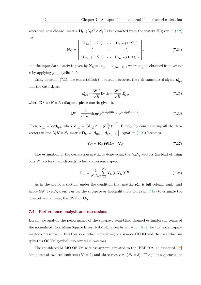
142 Chapter 7. Subspace blind and semi-blind channel estimation
where the new channel matrix HG (NrG×NtK) is extracted from the matrix H given in (7.2)
as:
HG =
H1,1(1 :G, :) · · · H1,Nt(1 :G, :)
.... . .
...
HNr,1(1 :G, :) · · · HNr,Nt(1 :G, :)
. (7.24)
and the input data matrix is given by XG =[x(0) · · ·x(NG−1)
], where x(g) is obtained from vector
x by applying g up-cyclic shifts.
Using equation (7.3), one can establish the relation between the i-th transmitted signal xi(g)and the data di as:
xi(g) = WH
√K
Dgdi = WH
√K
di(g), (7.25)
where Dg is (K ×K) diagonal phase matrix given by:
Dg = 1√(K)
diag{ej2π(g)(0) · · ·ej2π(g)(K−1)} (7.26)
Then, x(g) = Wd(g), where d(g) =[(d1
(g))T · · ·(dNt(g))
T]T
. Finally, by concatenating all the data
vectors in one NtK ×Ng matrix DG =[d(0) · · ·d(NG−1)
], equation (7.23) becomes:
YG = HGWDG + VG (7.27)
The estimation of the correlation matrix is done using the NdNg vectors (instead of using
only Nd vectors), which leads to fast convergence speed:
CG = 1NdNG
Nd∑t=1
YG(t)YG(t)H . (7.28)
As in the previous section, under the condition that matrix HG is full column rank (and
hence GNr >KNt), one can use the subspace orthogonality relation as in (7.12) to estimate the
channel vector using the EVD of CG.
7.4 Performance analysis and discussions
Herein, we analyze the performance of the subspace semi-blind channel estimators in terms of
the normalized Root Mean Square Error (NRMSE) given by equation (6.32) for the two subspace
methods presented in this thesis i.e. when considering one symbol OFDM and the case when we
split this OFDM symbol into several subvectors.
The considered MIMO-OFDM wireless system is related to the IEEE 802.11n standard [22]
composed of two transmitters (Nt = 2) and three receivers (Nr = 3). The pilot sequences (or
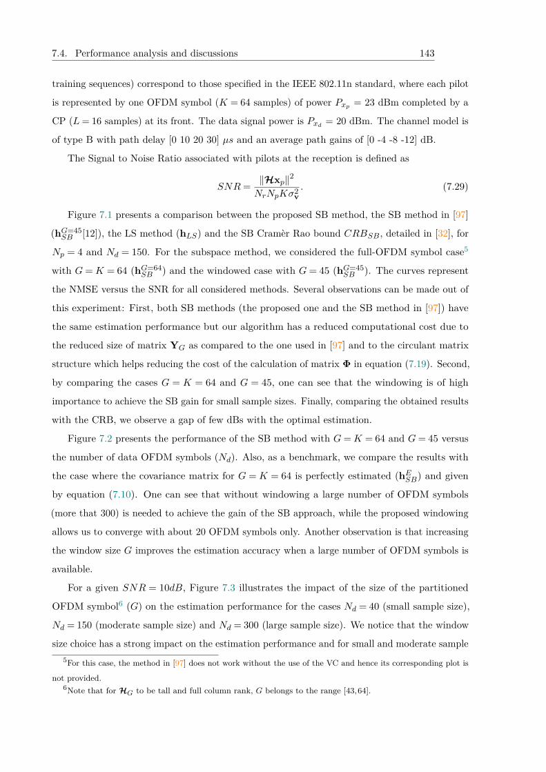
7.4. Performance analysis and discussions 143
training sequences) correspond to those specified in the IEEE 802.11n standard, where each pilot
is represented by one OFDM symbol (K = 64 samples) of power Pxp = 23 dBm completed by a
CP (L= 16 samples) at its front. The data signal power is Pxd = 20 dBm. The channel model is
of type B with path delay [0 10 20 30] µs and an average path gains of [0 -4 -8 -12] dB.
The Signal to Noise Ratio associated with pilots at the reception is defined as
SNR= ‖Hxp‖2
NrNpKσ2v. (7.29)
Figure 7.1 presents a comparison between the proposed SB method, the SB method in [97]
(hG=45SB [12]), the LS method (hLS) and the SB Cramèr Rao bound CRBSB , detailed in [32], for
Np = 4 and Nd = 150. For the subspace method, we considered the full-OFDM symbol case5
with G=K = 64 (hG=64SB ) and the windowed case with G= 45 (hG=45
SB ). The curves represent
the NMSE versus the SNR for all considered methods. Several observations can be made out of
this experiment: First, both SB methods (the proposed one and the SB method in [97]) have
the same estimation performance but our algorithm has a reduced computational cost due to
the reduced size of matrix YG as compared to the one used in [97] and to the circulant matrix
structure which helps reducing the cost of the calculation of matrix Φ in equation (7.19). Second,
by comparing the cases G = K = 64 and G = 45, one can see that the windowing is of high
importance to achieve the SB gain for small sample sizes. Finally, comparing the obtained results
with the CRB, we observe a gap of few dBs with the optimal estimation.
Figure 7.2 presents the performance of the SB method with G=K = 64 and G= 45 versus
the number of data OFDM symbols (Nd). Also, as a benchmark, we compare the results with
the case where the covariance matrix for G = K = 64 is perfectly estimated (hESB) and given
by equation (7.10). One can see that without windowing a large number of OFDM symbols
(more that 300) is needed to achieve the gain of the SB approach, while the proposed windowing
allows us to converge with about 20 OFDM symbols only. Another observation is that increasing
the window size G improves the estimation accuracy when a large number of OFDM symbols is
available.
For a given SNR = 10dB, Figure 7.3 illustrates the impact of the size of the partitioned
OFDM symbol6 (G) on the estimation performance for the cases Nd = 40 (small sample size),
Nd = 150 (moderate sample size) and Nd = 300 (large sample size). We notice that the window
size choice has a strong impact on the estimation performance and for small and moderate sample5For this case, the method in [97] does not work without the use of the VC and hence its corresponding plot is
not provided.6Note that for HG to be tall and full column rank, G belongs to the range [43,64].
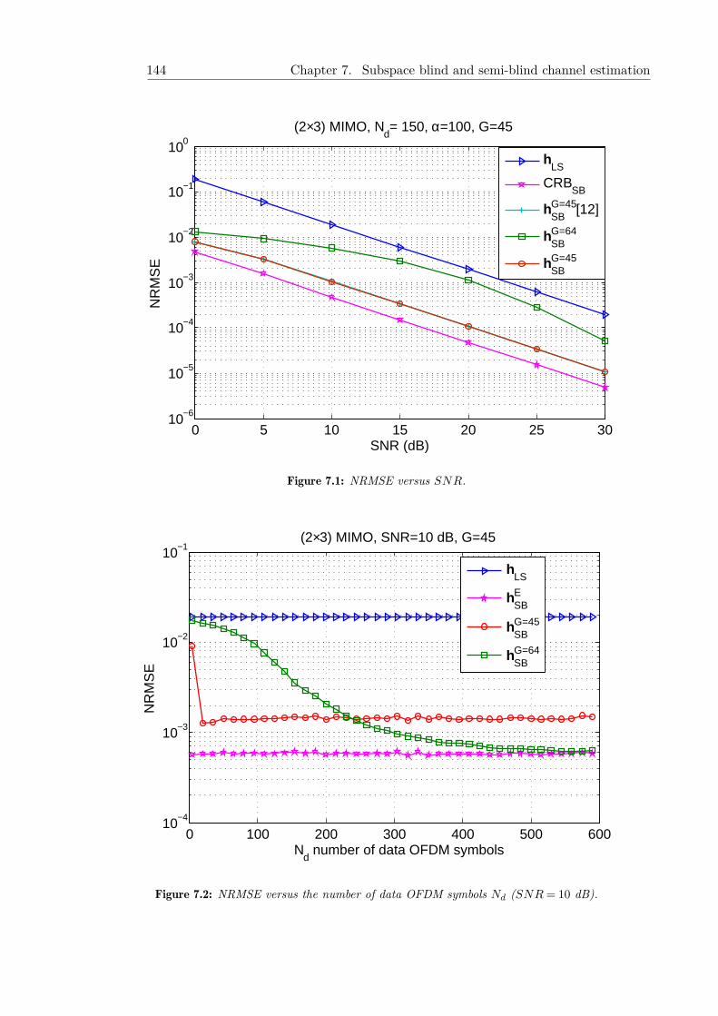
144 Chapter 7. Subspace blind and semi-blind channel estimation
0 5 10 15 20 25 3010−6
10−5
10−4
10−3
10−2
10−1
100(2×3) MIMO, N
d= 150, α=100, G=45
NR
MS
E
SNR (dB)
h
LS
CRBSB
hSBG=45[12]
hSBG=64
hSBG=45
Figure 7.1: NRMSE versus SNR.
0 100 200 300 400 500 60010−4
10−3
10−2
10−1(2×3) MIMO, SNR=10 dB, G=45
NR
MS
E
Nd number of data OFDM symbols
hLS
hSBE
hSBG=45
hSBG=64
Figure 7.2: NRMSE versus the number of data OFDM symbols Nd (SNR= 10 dB).
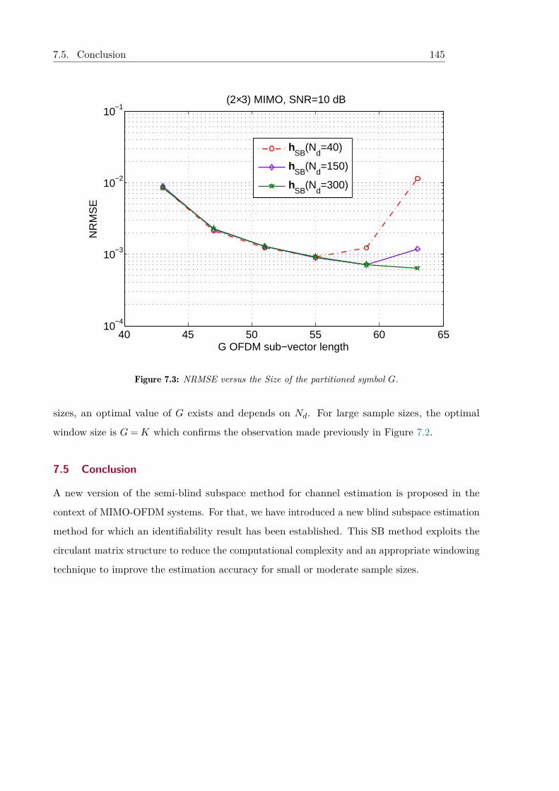
7.5. Conclusion 145
40 45 50 55 60 6510−4
10−3
10−2
10−1(2×3) MIMO, SNR=10 dB
NR
MS
E
G OFDM sub−vector length
hSB
(Nd=40)
hSB
(Nd=150)
hSB
(Nd=300)
Figure 7.3: NRMSE versus the Size of the partitioned symbol G.
sizes, an optimal value of G exists and depends on Nd. For large sample sizes, the optimal
window size is G=K which confirms the observation made previously in Figure 7.2.
7.5 Conclusion
A new version of the semi-blind subspace method for channel estimation is proposed in the
context of MIMO-OFDM systems. For that, we have introduced a new blind subspace estimation
method for which an identifiability result has been established. This SB method exploits the
circulant matrix structure to reduce the computational complexity and an appropriate windowing
technique to improve the estimation accuracy for small or moderate sample sizes.

146 Chapter 7. Subspace blind and semi-blind channel estimation
8
Ch
ap
te
r
Semi-blind estimation for specular channel model
It always seems impossible
until it’s done.
Nelson Mandela.
This work has been done in collaboration with Marius Pesavento as part of a mobility to
Germany (Darmstadt). It has been published in ICASSP 2019 conference1.
This study deals with semi-blind channel estimation in SISO-OFDM communications system in
the case of specular channel model. The proposed algorithm proceeds in two main stages. The
first one addresses the pilot-based Time-Of-Arrival (TOA) estimation using subspace methods
and then estimates the channel through its specular model. In the second stage, one considers a
decision feedback equalizer that is used to refine the channel parameters estimates.
Abstract
1 [99] A. Ladaycia, M. Pesavento, A. Mokraoui, K. Abed-Meraim, and A. Belouchrani, "Decision feedback
semi-blind estimation algorithm for specular OFDM channels," in 2019 IEEE International Conference on Acoustics,
Speech and Signal Processing (ICASSP2019), Accepted.
148 Chapter 8. Semi-blind estimation for specular channel model
Chapter content8.1 Introduction . . . . . . . . . . . . . . . . . . . . . . . . . . . . . . . . . . . . . 149
8.2 SISO-OFDM system communications model . . . . . . . . . . . . . . . . . . . . 149
8.3 Proposed channel estimation . . . . . . . . . . . . . . . . . . . . . . . . . . . . 150
8.3.1 First stage: pilot-based TOA estimation . . . . . . . . . . . . . . . . . . 151
8.3.2 Second stage: DF semi-blind channel estimation . . . . . . . . . . . . . 153
8.4 Simulation results . . . . . . . . . . . . . . . . . . . . . . . . . . . . . . . . . . 153
8.5 Conclusion . . . . . . . . . . . . . . . . . . . . . . . . . . . . . . . . . . . . . . 157
8.1. Introduction 149
8.1 Introduction
Channel identification can be done by estimating the channel parameters, i.e. parametric channel
estimation [100], or by estimating directly the channel coefficients [82]. Channel estimation
approaches based on the parametric channel modeling require Time-Of-Arrival (TOA) (multipath
delays) estimation.
Many TOA estimation approaches, based on pilots, have been developed and long established
in sensor array processing. Among these methods, one can cite the subspace techniques such
MUltiple SIgnal Classification (MUSIC) algorithm [101], [102], root MUSIC (rootMUSIC) [103],
[104], [105] and ESPRIT algorithm (Estimation of Signal Parameters via Rotational Invariance
Technique) [106]. A new subspace-like algorithm using Partial Relaxation (PR) technique is
proposed in [107] and considered here in our work.
The objective of this work is to propose an efficient pilot-based and semi-blind channel
estimation algorithms for SISO-OFDM system based on TOA estimation.
The first contribution is related to the TOA estimation using only one OFDM pilot. The
latter is used to generate a group of sub vectors, with an appropriate windowing, to which one
can apply subspace methods to estimate the TOA.
The second contribution is to incorporate the unknown data on the channel estimation process.
The semi-blind TOA estimation is done using a Decision Feedback process [33], where a first
estimate of the transmitted data is used with the existing pilot to enhance the TOA estimation
performance.
8.2 SISO-OFDM system communications model
The considered SISO-OFDM communications system is illustrated in Figure 8.1. Each OFDM
symbol is composed of K samples and is extended in time domain by the insertion of its last L
samples in its front considered as a Cyclic Prefix (CP). The CP duration is assumed to be greater
than or equal to delay spread. The received signal considered in baseband, after removing the
CP, is given in the time domain by the following equation:
y(t) = x(t) ∗N∑p=1
hisinc(t− τi) + v(t), (8.1)
where x(t) is the transmitted signal, N the number of multipaths, hi and τi are respectively the
complex gain and the time delay (TOA) of the i-th path.
After sampling the received OFDM signal (using the sampling rate Ts) and taking its K-point
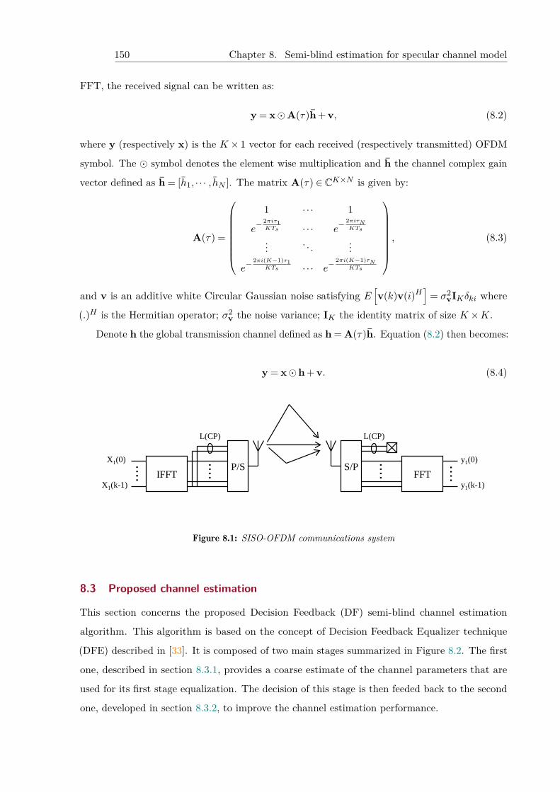
150 Chapter 8. Semi-blind estimation for specular channel model
FFT, the received signal can be written as:
y = x�A(τ)h + v, (8.2)
where y (respectively x) is the K × 1 vector for each received (respectively transmitted) OFDM
symbol. The � symbol denotes the element wise multiplication and h the channel complex gain
vector defined as h = [h1, · · · , hN ]. The matrix A(τ) ∈ CK×N is given by:
A(τ) =
1 · · · 1
e−2πiτ1KTs · · · e−
2πiτNKTs
.... . .
...
e−2πi(K−1)τ1
KTs · · · e−2πi(K−1)τN
KTs
, (8.3)
and v is an additive white Circular Gaussian noise satisfying E[v(k)v(i)H
]= σ2
vIKδki where
(.)H is the Hermitian operator; σ2v the noise variance; IK the identity matrix of size K ×K.
Denote h the global transmission channel defined as h = A(τ)h. Equation (8.2) then becomes:
y = x�h + v. (8.4)
P/SIFFT
L(CP)
S/PFFT
L(CP)
X1(0)
X1(k-1)
y1(0)
y1(k-1)
....
....
....
....
Figure 8.1: SISO-OFDM communications system
8.3 Proposed channel estimation
This section concerns the proposed Decision Feedback (DF) semi-blind channel estimation
algorithm. This algorithm is based on the concept of Decision Feedback Equalizer technique
(DFE) described in [33]. It is composed of two main stages summarized in Figure 8.2. The first
one, described in section 8.3.1, provides a coarse estimate of the channel parameters that are
used for its first stage equalization. The decision of this stage is then feeded back to the second
one, developed in section 8.3.2, to improve the channel estimation performance.
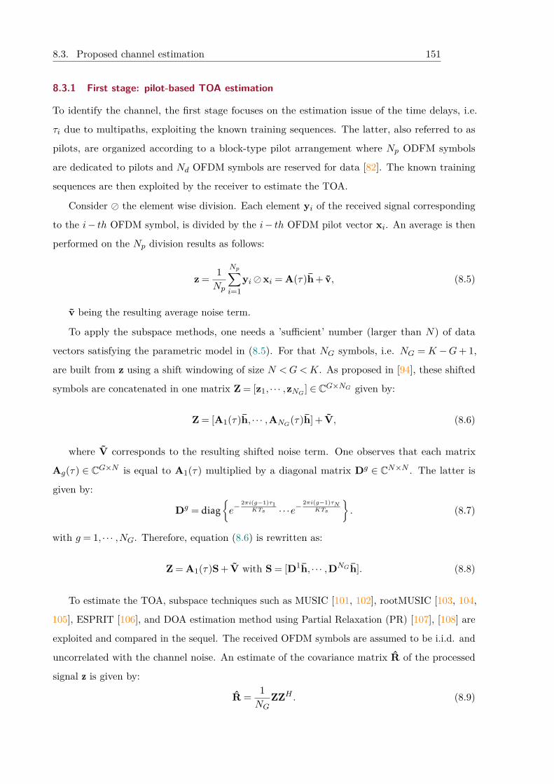
8.3. Proposed channel estimation 151
8.3.1 First stage: pilot-based TOA estimation
To identify the channel, the first stage focuses on the estimation issue of the time delays, i.e.
τi due to multipaths, exploiting the known training sequences. The latter, also referred to as
pilots, are organized according to a block-type pilot arrangement where Np ODFM symbols
are dedicated to pilots and Nd OFDM symbols are reserved for data [82]. The known training
sequences are then exploited by the receiver to estimate the TOA.
Consider � the element wise division. Each element yi of the received signal corresponding
to the i− th OFDM symbol, is divided by the i− th OFDM pilot vector xi. An average is then
performed on the Np division results as follows:
z = 1Np
Np∑i=1
yi�xi = A(τ)h + v, (8.5)
v being the resulting average noise term.
To apply the subspace methods, one needs a ’sufficient’ number (larger than N) of data
vectors satisfying the parametric model in (8.5). For that NG symbols, i.e. NG = K −G+ 1,
are built from z using a shift windowing of size N <G<K. As proposed in [94], these shifted
symbols are concatenated in one matrix Z = [z1, · · · ,zNG ] ∈ CG×NG given by:
Z = [A1(τ)h, · · · ,ANG(τ)h] + V, (8.6)
where V corresponds to the resulting shifted noise term. One observes that each matrix
Ag(τ) ∈ CG×N is equal to A1(τ) multiplied by a diagonal matrix Dg ∈ CN×N . The latter is
given by:
Dg = diag{e−
2πi(g−1)τ1KTs · · ·e−
2πi(g−1)τNKTs
}. (8.7)
with g = 1, · · · ,NG. Therefore, equation (8.6) is rewritten as:
Z = A1(τ)S + V with S = [D1h, · · · ,DNGh]. (8.8)
To estimate the TOA, subspace techniques such as MUSIC [101, 102], rootMUSIC [103, 104,
105], ESPRIT [106], and DOA estimation method using Partial Relaxation (PR) [107], [108] are
exploited and compared in the sequel. The received OFDM symbols are assumed to be i.i.d. and
uncorrelated with the channel noise. An estimate of the covariance matrix R of the processed
signal z is given by:
R = 1NG
ZZH . (8.9)
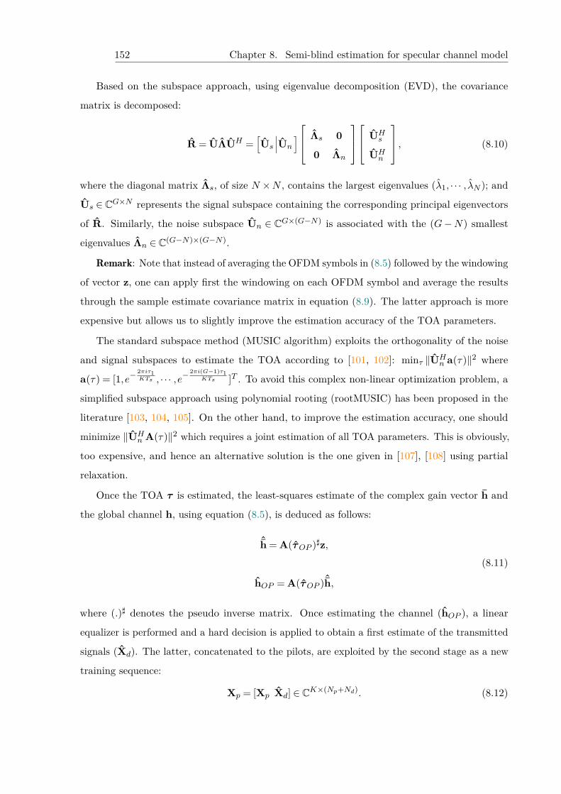
152 Chapter 8. Semi-blind estimation for specular channel model
Based on the subspace approach, using eigenvalue decomposition (EVD), the covariance
matrix is decomposed:
R = UΛUH =[Us
∣∣∣Un
] Λs 0
0 Λn
UH
s
UHn
, (8.10)
where the diagonal matrix Λs, of size N ×N , contains the largest eigenvalues (λ1, · · · , λN ); and
Us ∈ CG×N represents the signal subspace containing the corresponding principal eigenvectors
of R. Similarly, the noise subspace Un ∈ CG×(G−N) is associated with the (G−N) smallest
eigenvalues Λn ∈ C(G−N)×(G−N).
Remark: Note that instead of averaging the OFDM symbols in (8.5) followed by the windowing
of vector z, one can apply first the windowing on each OFDM symbol and average the results
through the sample estimate covariance matrix in equation (8.9). The latter approach is more
expensive but allows us to slightly improve the estimation accuracy of the TOA parameters.
The standard subspace method (MUSIC algorithm) exploits the orthogonality of the noise
and signal subspaces to estimate the TOA according to [101, 102]: minτ ‖UHn a(τ)‖2 where
a(τ) = [1,e−2πiτ1KTs , · · · ,e−
2πi(G−1)τ1KTs ]T . To avoid this complex non-linear optimization problem, a
simplified subspace approach using polynomial rooting (rootMUSIC) has been proposed in the
literature [103, 104, 105]. On the other hand, to improve the estimation accuracy, one should
minimize ‖UHn A(τ)‖2 which requires a joint estimation of all TOA parameters. This is obviously,
too expensive, and hence an alternative solution is the one given in [107], [108] using partial
relaxation.
Once the TOA τ is estimated, the least-squares estimate of the complex gain vector h and
the global channel h, using equation (8.5), is deduced as follows:
ˆh = A(τOP )]z,
hOP = A(τOP )ˆh,
(8.11)
where (.)] denotes the pseudo inverse matrix. Once estimating the channel (hOP ), a linear
equalizer is performed and a hard decision is applied to obtain a first estimate of the transmitted
signals (Xd). The latter, concatenated to the pilots, are exploited by the second stage as a new
training sequence:
Xp = [Xp Xd] ∈ CK×(Np+Nd). (8.12)
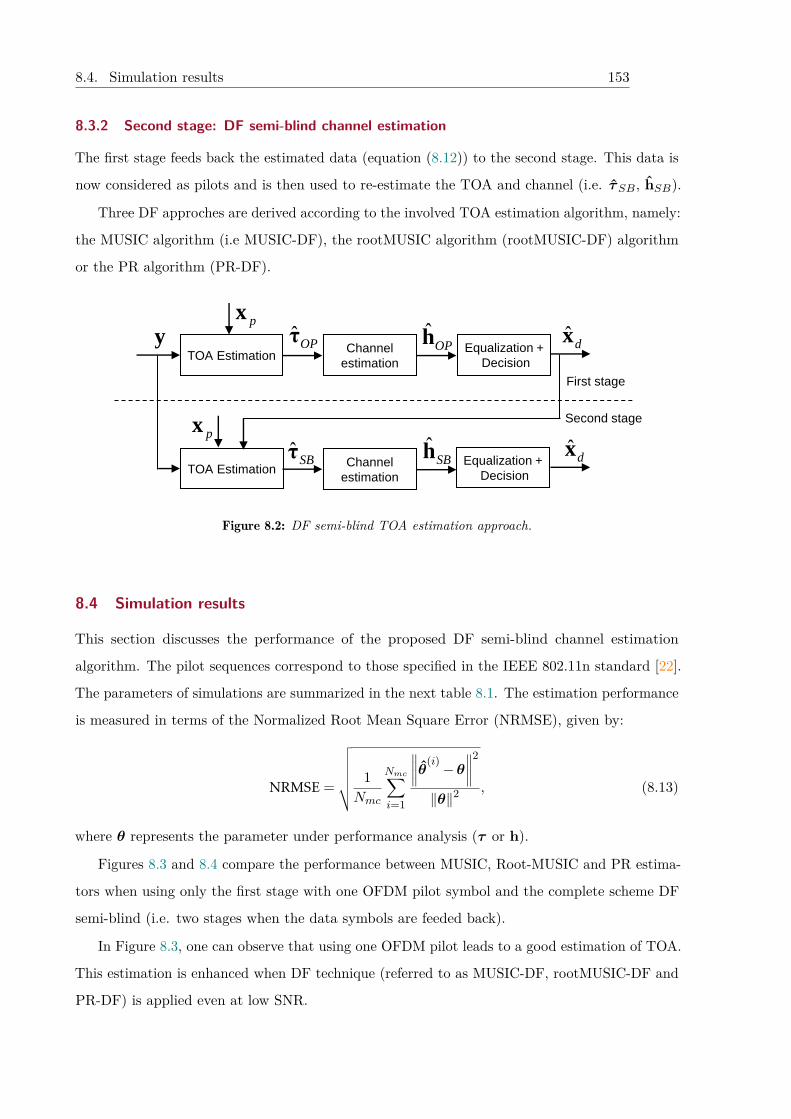
8.4. Simulation results 153
8.3.2 Second stage: DF semi-blind channel estimation
The first stage feeds back the estimated data (equation (8.12)) to the second stage. This data is
now considered as pilots and is then used to re-estimate the TOA and channel (i.e. τSB, hSB).
Three DF approches are derived according to the involved TOA estimation algorithm, namely:
the MUSIC algorithm (i.e MUSIC-DF), the rootMUSIC algorithm (rootMUSIC-DF) algorithm
or the PR algorithm (PR-DF).
TOA EstimationEqualization +
Decision
ypx
ˆOPτ ˆ
dx
TOA EstimationEqualization +
Decision
ˆdxˆ
SBτ
Channel
estimation
ˆOPh
Channel
estimation
ˆSBh
px
First stage
Second stage
Figure 8.2: DF semi-blind TOA estimation approach.
8.4 Simulation results
This section discusses the performance of the proposed DF semi-blind channel estimation
algorithm. The pilot sequences correspond to those specified in the IEEE 802.11n standard [22].
The parameters of simulations are summarized in the next table 8.1. The estimation performance
is measured in terms of the Normalized Root Mean Square Error (NRMSE), given by:
NRMSE =
√√√√√√ 1Nmc
Nmc∑i=1
∥∥∥∥θ(i)−θ∥∥∥∥2
‖θ‖2, (8.13)
where θ represents the parameter under performance analysis (τ or h).
Figures 8.3 and 8.4 compare the performance between MUSIC, Root-MUSIC and PR estima-
tors when using only the first stage with one OFDM pilot symbol and the complete scheme DF
semi-blind (i.e. two stages when the data symbols are feeded back).
In Figure 8.3, one can observe that using one OFDM pilot leads to a good estimation of TOA.
This estimation is enhanced when DF technique (referred to as MUSIC-DF, rootMUSIC-DF and
PR-DF) is applied even at low SNR.
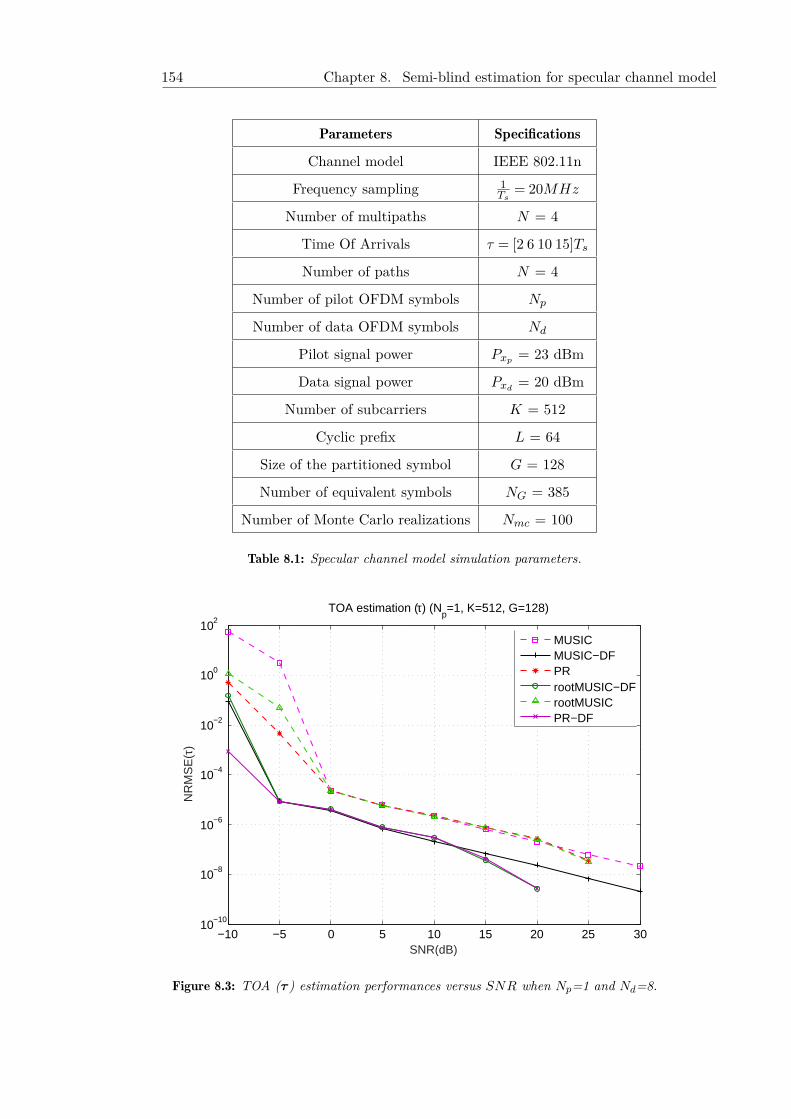
154 Chapter 8. Semi-blind estimation for specular channel model
Parameters Specifications
Channel model IEEE 802.11n
Frequency sampling 1Ts
= 20MHz
Number of multipaths N = 4
Time Of Arrivals τ = [2 6 10 15]TsNumber of paths N = 4
Number of pilot OFDM symbols Np
Number of data OFDM symbols Nd
Pilot signal power Pxp = 23 dBm
Data signal power Pxd = 20 dBm
Number of subcarriers K = 512
Cyclic prefix L = 64
Size of the partitioned symbol G = 128
Number of equivalent symbols NG = 385
Number of Monte Carlo realizations Nmc = 100
Table 8.1: Specular channel model simulation parameters.
−10 −5 0 5 10 15 20 25 3010−10
10−8
10−6
10−4
10−2
100
102
SNR(dB)
NR
MS
E(τ
)
TOA estimation (τ) (Np=1, K=512, G=128)
MUSICMUSIC−DFPRrootMUSIC−DFrootMUSICPR−DF
Figure 8.3: TOA (τ ) estimation performances versus SNR when Np=1 and Nd=8.
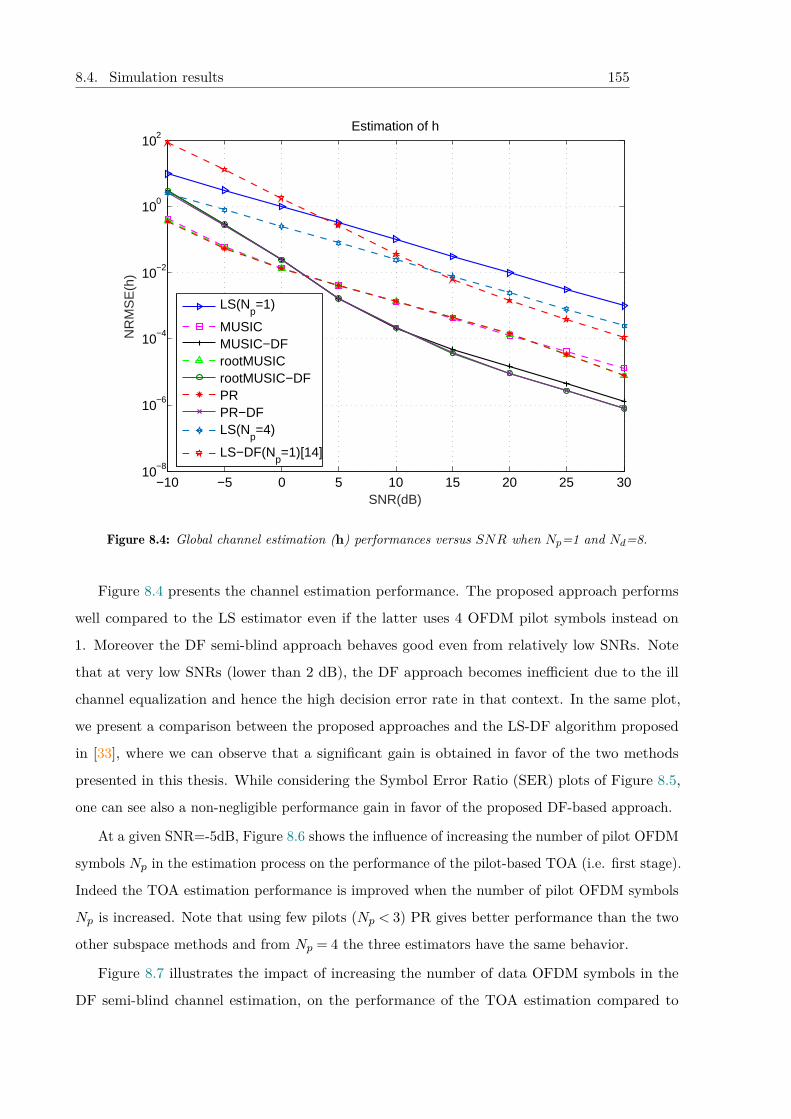
8.4. Simulation results 155
−10 −5 0 5 10 15 20 25 3010−8
10−6
10−4
10−2
100
102
SNR(dB)
NR
MS
E(h
)Estimation of h
LS(Np=1)
MUSICMUSIC−DFrootMUSICrootMUSIC−DFPRPR−DFLS(N
p=4)
LS−DF(Np=1)[14]
Figure 8.4: Global channel estimation (h) performances versus SNR when Np=1 and Nd=8.
Figure 8.4 presents the channel estimation performance. The proposed approach performs
well compared to the LS estimator even if the latter uses 4 OFDM pilot symbols instead on
1. Moreover the DF semi-blind approach behaves good even from relatively low SNRs. Note
that at very low SNRs (lower than 2 dB), the DF approach becomes inefficient due to the ill
channel equalization and hence the high decision error rate in that context. In the same plot,
we present a comparison between the proposed approaches and the LS-DF algorithm proposed
in [33], where we can observe that a significant gain is obtained in favor of the two methods
presented in this thesis. While considering the Symbol Error Ratio (SER) plots of Figure 8.5,
one can see also a non-negligible performance gain in favor of the proposed DF-based approach.
At a given SNR=-5dB, Figure 8.6 shows the influence of increasing the number of pilot OFDM
symbols Np in the estimation process on the performance of the pilot-based TOA (i.e. first stage).
Indeed the TOA estimation performance is improved when the number of pilot OFDM symbols
Np is increased. Note that using few pilots (Np < 3) PR gives better performance than the two
other subspace methods and from Np = 4 the three estimators have the same behavior.
Figure 8.7 illustrates the impact of increasing the number of data OFDM symbols in the
DF semi-blind channel estimation, on the performance of the TOA estimation compared to
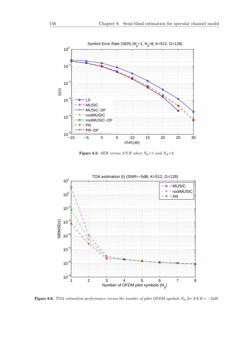
156 Chapter 8. Semi-blind estimation for specular channel model
−10 −5 0 5 10 15 20 25 3010−5
10−4
10−3
10−2
10−1
100
SNR(dB)
SE
R
Symbol Error Rate (SER) (Np=1, N
d=8, K=512, G=128)
LSMUSICMUSIC−DFrootMUSICrootMUSIC−DFPRPR−DF
Figure 8.5: SER versus SNR when Np=1 and Nd=8.
1 2 3 4 5 6 7 810−6
10−5
10−4
10−3
10−2
10−1
100
101
Number of OFDM pilot symbols (Np)
NR
MS
E(τ
)
TOA estimation (τ) (SNR=−5dB, K=512, G=128)
MUSICrootMUSICPR
Figure 8.6: TOA estimation performance versus the number of pilot OFDM symbols Np for SNR =−5dB.
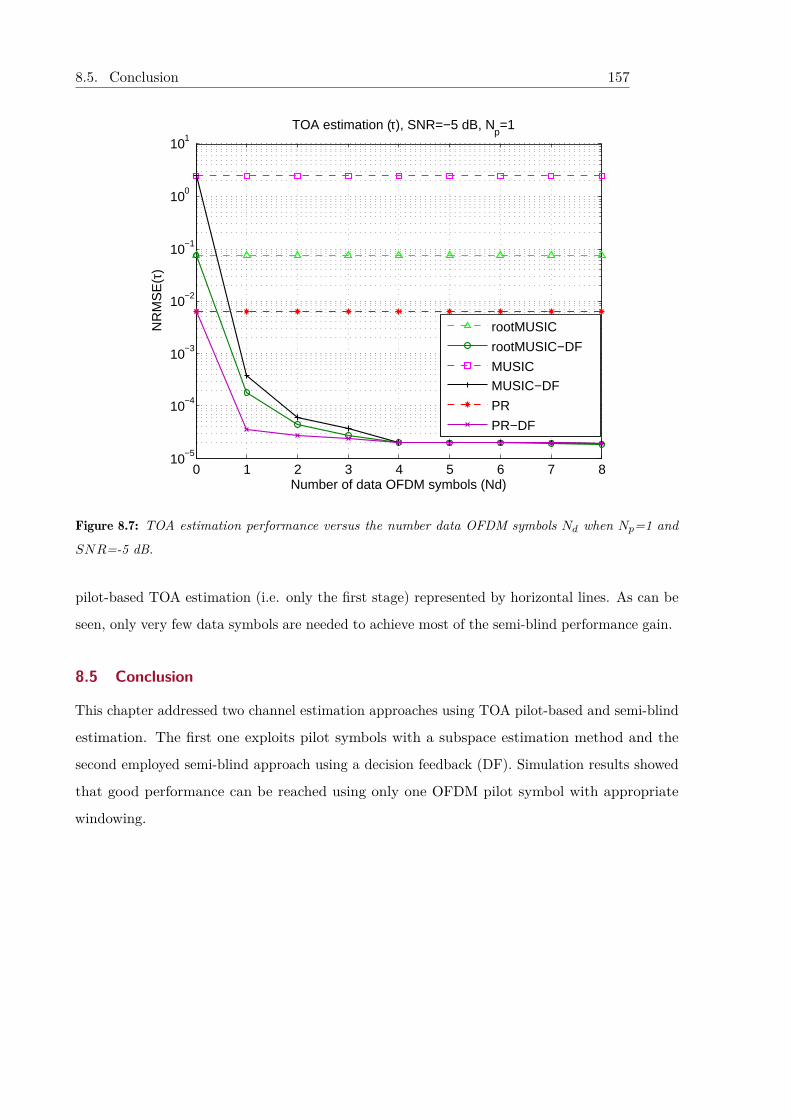
8.5. Conclusion 157
0 1 2 3 4 5 6 7 810−5
10−4
10−3
10−2
10−1
100
101TOA estimation (τ), SNR=−5 dB, N
p=1
Number of data OFDM symbols (Nd)
NR
MS
E(τ
)
rootMUSIC
rootMUSIC−DF
MUSIC
MUSIC−DF
PR
PR−DF
Figure 8.7: TOA estimation performance versus the number data OFDM symbols Nd when Np=1 and
SNR=-5 dB.
pilot-based TOA estimation (i.e. only the first stage) represented by horizontal lines. As can be
seen, only very few data symbols are needed to achieve most of the semi-blind performance gain.
8.5 Conclusion
This chapter addressed two channel estimation approaches using TOA pilot-based and semi-blind
estimation. The first one exploits pilot symbols with a subspace estimation method and the
second employed semi-blind approach using a decision feedback (DF). Simulation results showed
that good performance can be reached using only one OFDM pilot symbol with appropriate
windowing.

158 Chapter 8. Semi-blind estimation for specular channel model

Conclusion and future work
159


9
Ch
ap
te
r
Conclusion and future work
We ought not to be embarrassed
of appreciating the truth and of
obtaining it wherever it comes from,
even if it comes from races distant
and nations different from us.
Nothing should be dearer to the seeker
of truth than the truth itself, and there
is no deterioration of the truth, nor
belittling either of one who speaks it or
conveys it.
Al-Kindi.
Chapter content9.1 Achieved work . . . . . . . . . . . . . . . . . . . . . . . . . . . . . . . . . . . . 162
9.2 Thesis contributions . . . . . . . . . . . . . . . . . . . . . . . . . . . . . . . . . 164
9.3 Future work . . . . . . . . . . . . . . . . . . . . . . . . . . . . . . . . . . . . . . 165
162 Chapter 9. Conclusion and future work
9.1 Achieved work
Channel estimation is of paramount importance to equalization and symbol detection problems in
most wireless communications especially in MIMO-OFDM systems. Hence, it attracts the interest
of researchers and system developers since the twentieth century. A spectacular advance has been
realized with the development and implementation of pilot-based channel estimation algorithms
motivated by its low complexity and feasibility in regards of the available calculators at that
time. The appearance of powerful computers (processors) available at the base stations, and
the ever increasing demand for higher data rates have led to consider other channel estimation
approaches. The proposed approaches, mainly semi-blind (SB) techniques, increase the data
rates by reducing the number of transmitted pilots since the latter do not carry information and
represent a bandwidth waste. Moreover, many challenging aspects are moderately or weakly
investigated in the open literature with respect to semi-blind channel estimation. This thesis is
one of the contributions dealing with SB channel identification and its analysis in the context of
MIMO-OFDM systems.
Several contributions to the SB channel estimation have been realized in the thesis: the
quantification of the maximum rate of reduction of the transmitted pilots using SB channel
estimation while ensuring the same pilot-based estimation quality, then the development of
efficient SB channel estimators (LS-DF, subspace methods, EM-based algorithms). Moreover,
further investigations on the performance bounds of MIMO-OFDM channel estimation have
been successfully addressed including the analysis of the effect of CFO on channel estimation
performance.
Below, we briefly summarize the overall thesis work, before listing the points corresponding
to our main contributions.
First, the theoretical performance limits for the semi-blind and pilot-based channel estimation
methods have been addressed in the context of MIMO-OFDM and massive MIMO-OFDM
systems. This analysis has been conducted through the analytical derivation of the CRBs for
different data models (i.e. CG, NCG and BPSK/QPSK) and for different pilot design patterns
(i.e. block-type, lattice-type and comb-type pilot arrangement). The investigation of the derived
CRBs shows the huge pilot sample reduction and consequently the throughput gain obtained
thanks to the semi-blind approach while maintaining the same pilot-based channel estimation
quality. In this thesis, we show that, by properly using SB techniques, the attainable reduction
can exceed 95% (BPSK data model) of the original size.
This study has also been extended to large MIMO-OFDM systems (10× 10) where we show
9.1. Achieved work 163
that the performance gains are slightly higher than those observed for smaller size MIMO-OFDM
systems. Moreover, the same study, in chapter 2, has been generalized to multi-cell massive
MIMO-OFDM systems under the effect of pilot contamination. Thereafter, we have shown
that, using SB methods, it is possible to solve efficiently the pilot contamination problem when
considering finite alphabet communications signals.
Second, we investigated the effect of the CFO on channel estimation performance using
the CRB tool. Due to the CFO cyclostationarity propriety, we show that The CFO impacts
advantageously the semi-blind channel estimation. In the case of MISO-OFDM communications
system based on multi-relay transmission protocols, we have proposed two efficient approaches
to jointly estimate transmission channel and CFOs. In the same context, another study has
been conducted to evaluate and compare the CRB for the estimation of the subcarrier channel
coefficients with and without considering the OFDM structure (i.e. estimating the channel taps
in the time domain or in the frequency one). This study highlights the significant gain associated
to the time domain approach.
Thirdly, we proposed four SB channel estimation algorithms. We started with the simplest one
(LS-DF) which is based on the LS estimator used in conjunction with a decision feedback where
the estimated data are re-injected to the channel estimation stage to enhance the estimation
performance. In the context of green communications, we shown that, thanks to SB LS-DF
algorithm, one can reduce up to 76% of pilot’s transmitted power.
The second SB approach is based on the maximum-likelihood (ML) technique, one of
the most efficient but also most expensive estimation methods. The optimization of the ML
criterion is done through an iterative technique using the EM-algorithm. We proposed three
approximation/simplification approaches to deal with the numerical complexity of the classical
EM-algorithm. The proposed three approximations (i.e. EM-MISO, S-EM, EM-SIMO) give a
good performance at lower computational cost as compared to the standard EM-algorithm.
An intermediate solution (i.e. it is cheaper than the ML but more expensive as well as more
efficient than the LS-DF), is the one based on subspace technique introduced in chapter 7.
Finally, for the practical case of specular channel model, we proposed a parametric approach
based on TOA estimation using subspace methods for SISO-OFDM systems. The semi-blind
TOA estimation is realized using a Decision Feedback process that is considered to enhance
the TOA estimation performance starting from a first ’rough’ estimate obtained thanks to the
existing pilot.
164 Chapter 9. Conclusion and future work
9.2 Thesis contributions
The main contributions of this research are listed below:
• Derivation of the channel estimation CRBs for different data models (i.e. CG, NCG,
BPSK/QPSK) and for different pilot design patterns (i.e. block-type, lattice-type and
comb-type pilot arrangement) in the case of MIMO-OFDM system.
• For BPSK/QPSK data model, a realistic CRB approximation has been given to bypass the
high complexity of the exact CRB computation.
• Proposition of an effective computational technique to deal with the huge-size matrix
manipulation needed for the CRB calculation in the large size MIMO scenario and massive
MIMO.
• Quantification of rate of reduction of the overhead (pilots) due to the use of SB channel
estimation.
• Derivation of the SB channel estimation CRBs for multi-cell massive MIMO-OFDM system
under pilot contamination phenomenon.
• Investigation of the effectiveness of SB channel estimation to solve the pilot contamination
problem when considering finite alphabet communications signals.
• Contribution to drone protection against blind interception using CRBs analysis in the
blind context.
• Derivation of the SB channel estimation CRBs in the presence of CFO in MIMO-OFDM
system, and investigation of the positive impact of CFO on channel estimation performance.
• Proposition of two approaches to jointly estimate CFO and channel coefficients.
• Quantification of the performance degradation between estimating the channel coefficients
on time or frequency domain.
• Contribution to green communications by quantifying the reduced transmitted power using
SB channel estimation.
• Proposition of SB channel estimator based on decision feedback strategy (LS-DF).
• Contribution to SB channel estimation using EM-algorithm in the case of MIMO-OFDM
system.
9.3. Future work 165
• Derivation of four simplified versions of the SB EM-method.
• Contribution to SB subspace channel estimation for MIMO-OFDM system.
• Derivation of a parametric SB method to estimate channel parameters (TOA) in the case
of specular OFDM channel.
9.3 Future work
The research work related to SB channel estimation in MIMO-OFDM systems, carried out in
this thesis can be extended in several directions. Some recommendations for future work are
listed below.
• Extend the SB channel estimation performance analysis to non-Gaussian noise case, where
GMM (Gaussian Mixture Model) can be used to approximate the noise probability density
function to a GMM one using EM algorithm. Furthermore, consider the stochastic channel
model (instead of deterministic one) where Bayesian approach can be considered to evaluate
the CRB for a given channel type.
• As shown in appendix A, the major issue of the OMR protocol in the MISO communications
scenario, is the CFO. It will be interesting to evaluate, using the CRB, the maximum
allowed CFO to guarantee a target transmission quality.
• Extend the study of chapter 8 to the MIMO-OFDM systems. This study can also be
enriched by a performance analysis by deriving the corresponding CRBs.
• Implement the proposed algorithms in this thesis in a real system such as a video trans-
mission system and evaluate in practice the throughput gain due to the use of SB channel
estimation approaches.

166 Chapter 9. Conclusion and future work

Appendices
167

A
Ap
pe
nd
ix
CFO and channel estimation
Success is not final, failure is not
fatal: it is the courage to continue
that counts.
Winston Churchill.
This work has been done in collaboration with Ahmed Bader and Mohamed Slim Alouini from
KAUST, Saudi Arabia. It has been published in EUSIPCO 2017 conference1.
This study deals with the joint channel and carrier frequency offset (CFO) estimation in a MISO
communications system. This problem arises in OFDM based multi-relay transmission protocols
such that the geo-routing one proposed by A. Bader et al in 2012. Indeed, the outstanding
performance of this multi-hop relaying scheme relies heavily on the channel and CFO estimation
quality at the PHY layer. In this work, two approaches are considered: The first is based on
estimating the overall channel (including the CFO) as a time-varying one using an adaptive
scheme under the assumption of small or moderate CFOs while the second one performs separately,
the channel and CFO parameters estimation based on the considered data model.
Abstract
1 [109] A. Ladaycia, K. Abed-Meraim, A. Bader and M. S. Alouini, "CFO and channel estimation for MISO-
OFDM systems," in 2017 25th European Signal Processing Conference (EUSIPCO), Aug. 2017, pp. 2264-2268,
Kos, Greece.

170 Appendix A. CFO and channel estimation
Chapter contentA.1 Introduction . . . . . . . . . . . . . . . . . . . . . . . . . . . . . . . . . . . . . 171
A.2 MISO-OFDM communications system model . . . . . . . . . . . . . . . . . . . 171
A.3 Non-Parametric Channel Estimation . . . . . . . . . . . . . . . . . . . . . . . . 173
A.4 Parametric Channel Estimation . . . . . . . . . . . . . . . . . . . . . . . . . . . 174
A.5 Simulations results . . . . . . . . . . . . . . . . . . . . . . . . . . . . . . . . . . 176
A.6 Conclusion . . . . . . . . . . . . . . . . . . . . . . . . . . . . . . . . . . . . . . 181
A.1. Introduction 171
A.1 Introduction
Recently, an efficient beaconless geo-routing based multi-hop relaying protocol, namely OMR
(OFDM-based Multi-hop Relaying) protocol, has been proposed in [110], [111]. As for other
existing geo-routing protocols, in OMR the nodes can locally make their forwarding decisions
using very limited knowledge of the overall network topology. Relaying decisions in OMR are
taken in a distributed fashion at any given hop based on location information, in order to
alleviate the overhead which rapidly grows with node density. In addition, to deal with the fact
that the proposed paradigm leads to the creation of multiple copies of the same packet with
different propagation delays, OMR relies on the OFDM which allows correct packet detection at
a receiving node thanks to the use of the cyclic prefix (see [110] for more details).
In [111] and [110], it has been shown that the OMR overcomes existing contention based
geo-routing relaying protocols in terms of end-to-end performance (throughput and time-space
footprint). However, the performance analysis in [110], [112] relies on the assumption of perfect
frequency synchronization between the nodes.
In standard OFDM systems, it is well known that frequency desynchronization leads to a
carrier frequency offset (CFO) at the receiver node which deteriorates significantly the decoding
performance. Fortunately, this problem is well mastered and many solutions exist to track and
correct this CFO effect [113], [114].
The existing solutions from the literature are not adequate for our case, as we have several
simultaneous transmitters (i.e. we have a particular MISO system where all relays transmit the
same data packet through different channels) each with its own CFO and channel. The aim of
this study is to provide solutions to this severe problem in order to preserve the end-to-end high
performance of the OMR protocol.
A.2 MISO-OFDM communications system model
Consider an OFDM system with K subcarriers and using a cyclic prefix of length L larger
than the channel impulse response size N . Assume the received signal is affected by a carrier
frequency offset2 (due generally to desynchronization between the transmitter and receiver’s local
oscillators). Then, for one single transmitter, after sampling and removing the guard interval,
the received discrete baseband signal at time ns (associated with the ns-th OFDM symbol) is
2In this study, the effect of time desynchronization is neglected.
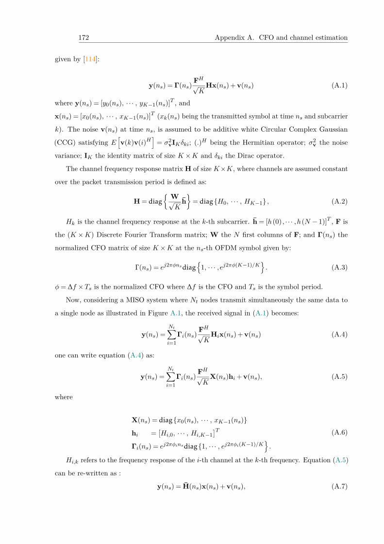
172 Appendix A. CFO and channel estimation
given by [114]:
y(ns) = Γ(ns)FH√K
Hx(ns) + v(ns) (A.1)
where y(ns) = [y0(ns), · · · , yK−1(ns)]T , and
x(ns) = [x0(ns), · · · , xK−1(ns)]T (xk(ns) being the transmitted symbol at time ns and subcarrier
k). The noise v(ns) at time ns, is assumed to be additive white Circular Complex Gaussian
(CCG) satisfying E[v(k)v(i)H
]= σ2
vIKδki; (.)H being the Hermitian operator; σ2v the noise
variance; IK the identity matrix of size K ×K and δki the Dirac operator.
The channel frequency response matrix H of size K×K, where channels are assumed constant
over the packet transmission period is defined as:
H = diag{ W√
Kh}
= diag{H0, · · · , HK−1} , (A.2)
Hk is the channel frequency response at the k-th subcarrier. h = [h(0) , · · · ,h(N − 1)]T , F is
the (K ×K) Discrete Fourier Transform matrix; W the N first columns of F; and Γ(ns) the
normalized CFO matrix of size K ×K at the ns-th OFDM symbol given by:
Γ (ns) = ej2πφnsdiag{
1, · · · ,ej2πφ(K−1)/K}. (A.3)
φ= ∆f ×Ts is the normalized CFO where ∆f is the CFO and Ts is the symbol period.
Now, considering a MISO system where Nt nodes transmit simultaneously the same data to
a single node as illustrated in Figure A.1, the received signal in (A.1) becomes:
y(ns) =Nt∑i=1
Γi(ns)FH√K
Hix(ns) + v(ns) (A.4)
one can write equation (A.4) as:
y(ns) =Nt∑i=1
Γi(ns)FH√K
X(ns)hi + v(ns), (A.5)
where
X(ns) = diag{x0(ns), · · · , xK−1(ns)}
hi =[Hi,0, · · · , Hi,K−1
]TΓi(ns) = ej2πφinsdiag{1, · · · , ej2πφi(K−1)/K
}.
(A.6)
Hi,k refers to the frequency response of the i-th channel at the k-th frequency. Equation (A.5)
can be re-written as :
y(ns) = H(ns)x(ns) + v(ns), (A.7)
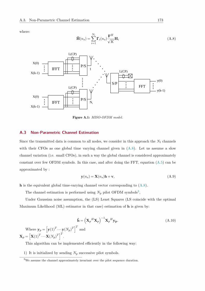
A.3. Non-Parametric Channel Estimation 173
where:
H(ns) =Nt∑i=1
Γi(ns)FH√K
Hi (A.8)
P/SIFFT
L(CP)
S/PFFT
L(CP)
P/SIFFT
L(CP)
Nt
1
X(0)
X(k-1)
X(0)
X(k-1)
y(0)
y(k-1)
........
....
....
....
......
....
Figure A.1: MISO-OFDM model.
A.3 Non-Parametric Channel Estimation
Since the transmitted data is common to all nodes, we consider in this approach the Nt channels
with their CFOs as one global time varying channel given in (A.8). Let us assume a slow
channel variation (i.e. small CFOs), in such a way the global channel is considered approximately
constant over few OFDM symbols. In this case, and after doing the FFT, equation (A.5) can be
approximated by :
y(ns) = X(ns)h + v, (A.9)
h is the equivalent global time-varying channel vector corresponding to (A.8).
The channel estimation is performed using Np pilot OFDM symbols3,
Under Gaussian noise assumption, the (LS) Least Squares (LS coincide with the optimal
Maximum Likelihood (ML) estimator in that case) estimation of h is given by:
h =(Xp
HXp
)−1Xp
Hyp. (A.10)
Where yp =[y(1)T · · ·y(Np)T
]Tand
Xp =[X(1)T · · ·X(Np)T
]T.
This algorithm can be implemented efficiently in the following way:
1) It is initialized by sending Np successive pilot symbols.3We assume the channel approximately invariant over the pilot sequence duration.
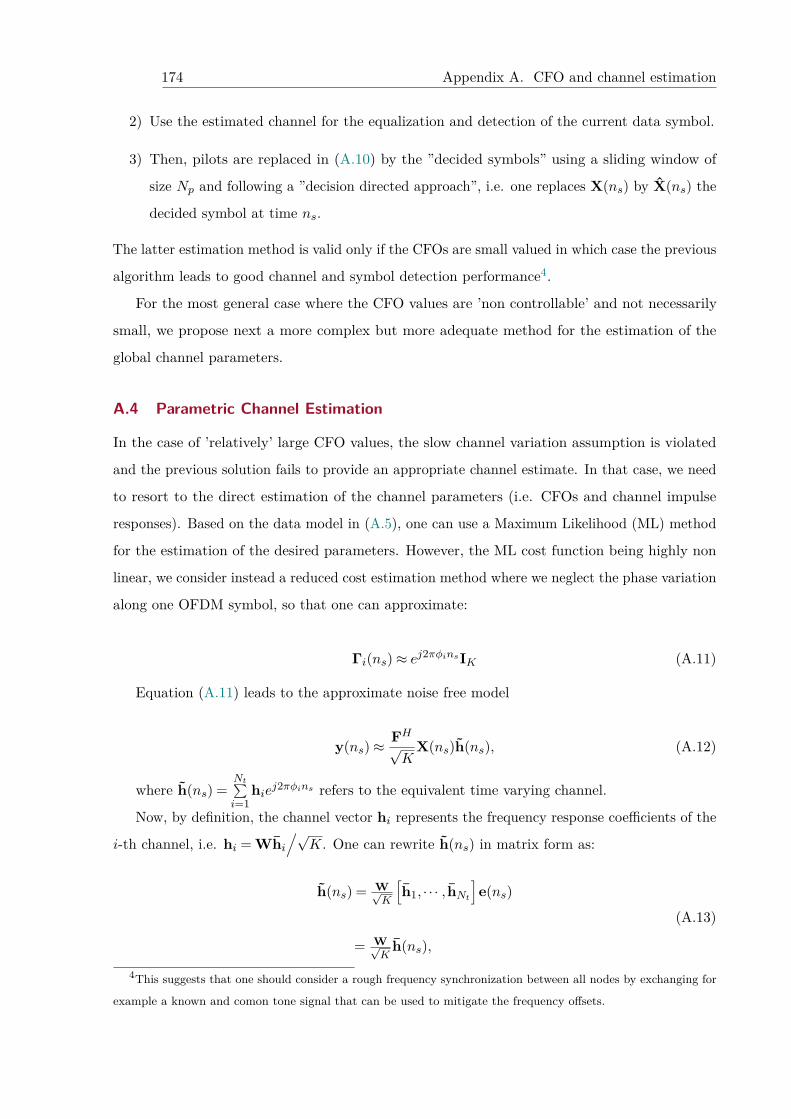
174 Appendix A. CFO and channel estimation
2) Use the estimated channel for the equalization and detection of the current data symbol.
3) Then, pilots are replaced in (A.10) by the ”decided symbols” using a sliding window of
size Np and following a ”decision directed approach”, i.e. one replaces X(ns) by X(ns) the
decided symbol at time ns.
The latter estimation method is valid only if the CFOs are small valued in which case the previous
algorithm leads to good channel and symbol detection performance4.
For the most general case where the CFO values are ’non controllable’ and not necessarily
small, we propose next a more complex but more adequate method for the estimation of the
global channel parameters.
A.4 Parametric Channel Estimation
In the case of ’relatively’ large CFO values, the slow channel variation assumption is violated
and the previous solution fails to provide an appropriate channel estimate. In that case, we need
to resort to the direct estimation of the channel parameters (i.e. CFOs and channel impulse
responses). Based on the data model in (A.5), one can use a Maximum Likelihood (ML) method
for the estimation of the desired parameters. However, the ML cost function being highly non
linear, we consider instead a reduced cost estimation method where we neglect the phase variation
along one OFDM symbol, so that one can approximate:
Γi(ns)≈ ej2πφinsIK (A.11)
Equation (A.11) leads to the approximate noise free model
y(ns)≈FH√K
X(ns)h(ns), (A.12)
where h(ns) =Nt∑i=1
hiej2πφins refers to the equivalent time varying channel.
Now, by definition, the channel vector hi represents the frequency response coefficients of the
i-th channel, i.e. hi = Whi/√
K. One can rewrite h(ns) in matrix form as:
h(ns) = W√K
[h1, · · · , hNt
]e(ns)
= W√K
h(ns),
(A.13)
4This suggests that one should consider a rough frequency synchronization between all nodes by exchanging for
example a known and comon tone signal that can be used to mitigate the frequency offsets.
A.4. Parametric Channel Estimation 175
where e(ns) =[ej2πφ1ns , · · · ,ej2πφNtns
]Tand h(ns) =
[h1, · · · , hNt
]e(ns).
The estimate of the channel impulse response h(ns) can be easily obtained in the LS sense
(using pilot symbols) as follows:
z(ns) = WH
√K
X(ns)−1 F√K
y(ns)≈ h(ns) (A.14)
By using Np successive OFDM pilots, one can hence estimate:
Z = [z(1) , · · · ,z(Np)]
≈[h1, · · · , hNt
]
ej2πφ1 · · · ej2πNpφ1
.... . .
...
ej2πφNt · · · ej2πNpφNt
=
^
HEH
(A.15)
From the rows of matrix Z, one can obtain an estimate of the channel’s CFO while the
column vectors provide an estimate of the channel impulse responses. Since, in general the CFO
values are relatively small and hence closely separated and the sample size (i.e. Np) is small too,
one needs to use high resolution techniques for the frequency estimation. One can use ESPRIT5
method to estimate the frequencies. To this end, by performing a regular SVD decomposition on
the composite matrix Z one can write
Z = UΣVH (A.16)
where, V : Np×Nt is a matrix of principal right singular vectors6. Since E and V span the
same subspace (i.e. the row space of Z), one can write V = EQ, where Q : Np×Np is a non
singular unknown matrix.
Let V1 = V (without the last row) and V2 = V (without the first row), then
V1 = E1Q, V2 = E2Q (A.17)
where, E1 = E without the last row and E2 = E without the first row. Hence, one can express
V2 in terms of E1 as follows
E2 = E1Φ, Φ = diag{e−j2πφ1 , · · · ,e−j2πφNt
}(A.18)
5ESPRIT stands for Estimation of Subspace Parameters via Rotational Invariance Technique [115].6We assume here that Np >Nt and that the CFOs are distinct, φi , φj if i , j.
176 Appendix A. CFO and channel estimation
Considering equations (A.17) and (A.18), we write V2 as:
V2 = E1ΦQ (A.19)
by evaluating Ψ as
Ψ = V1#V2 = Q−1ΦQ (A.20)
where (.)# refers to the pseudo-inverse operator. Φ is estimated as the matrix of eigenvalues
of Ψ and the CFOs are obtained from the phase arguments of the eigenvalues. Once Φ is
obtained, one can estimate^
H as
^
H≈ Z(EH
)#(A.21)
Remarks:
1) ESPRIT is an expensive method and can be replaced by a Fourier search if the CFOs, are
not too close as compared to the resolution limit of the DFT, i.e. |(φi−φj)| ≥ 2Np
.
2) The channel and CFO estimates in (A.20) and (A.21) can be used to initialize a numerical
method for ML optimization (e.g. for example with Levenberg-Marquardt method [116]) in
order to improve the estimation performance, especially when the approximation in (A.11)
is roughly satisfied.
A.5 Simulations results
This section analyzes the channel estimation performance for the considered MISO-OFDM
wireless system. The training sequence used in this work is the Zadoff-Chu sequence considered
in the LTE standard [4]. Fig. 1.2a represents the block-type pilot arrangement adopted in this
work. Each field (or pilot) is represented by one OFDM symbol (K = 64 samples) where a CP
(L= 16 samples) is added at its front. Simulation parameters are summarized in Table A.1.
The SNR associated with pilots at the receiver is defined as SNRp = ‖Xph‖2
KNpσ2v. The SNR,
denoted SNRd (in dB), associated with data is given by: SNRd = SNRp− (Pxp−Pxd) where
Pxp (respectively Pxd) is the power of pilots (respectively data) in dB.
Figure A.2 compares the NMSE of the estimated data (related to the considered channel
estimation methods followed by linear zero-forcing equalization) versus SNRp at relatively low
CFO. The NMSE curves show that the parametric method and the non-parametric one have
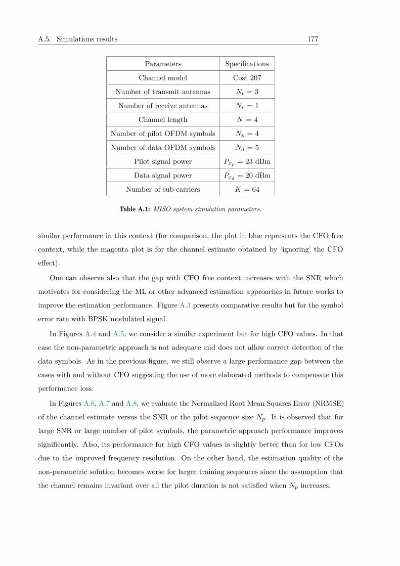
A.5. Simulations results 177
Parameters Specifications
Channel model Cost 207
Number of transmit antennas Nt = 3
Number of receive antennas Nr = 1
Channel length N = 4
Number of pilot OFDM symbols Np = 4
Number of data OFDM symbols Nd = 5
Pilot signal power Pxp = 23 dBm
Data signal power Pxd = 20 dBm
Number of sub-carriers K = 64
Table A.1: MISO system simulation parameters.
similar performance in this context (for comparison, the plot in blue represents the CFO free
context, while the magenta plot is for the channel estimate obtained by ’ignoring’ the CFO
effect).
One can observe also that the gap with CFO free context increases with the SNR which
motivates for considering the ML or other advanced estimation approaches in future works to
improve the estimation performance. Figure A.3 presents comparative results but for the symbol
error rate with BPSK modulated signal.
In Figures A.4 and A.5, we consider a similar experiment but for high CFO values. In that
case the non-parametric approach is not adequate and does not allow correct detection of the
data symbols. As in the previous figure, we still observe a large performance gap between the
cases with and without CFO suggesting the use of more elaborated methods to compensate this
performance loss.
In Figures A.6, A.7 and A.8, we evaluate the Normalized Root Mean Squares Error (NRMSE)
of the channel estimate versus the SNR or the pilot sequence size Np. It is observed that for
large SNR or large number of pilot symbols, the parametric approach performance improves
significantly. Also, its performance for high CFO values is slightly better than for low CFOs
due to the improved frequency resolution. On the other hand, the estimation quality of the
non-parametric solution becomes worse for larger training sequences since the assumption that
the channel remains invariant over all the pilot duration is not satisfied when Np increases.
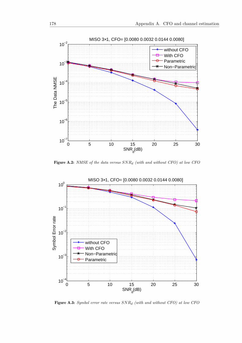
178 Appendix A. CFO and channel estimation
0 5 10 15 20 25 3010−7
10−6
10−5
10−4
10−3
10−2MISO 3×1, CFO= [0.0080 0.0032 0.0144 0.0080]
The
Dat
a N
MS
E
SNRd(dB)
without CFOWith CFOParametricNon−Parametric
Figure A.2: NMSE of the data versus SNRd (with and without CFO) at low CFO
0 5 10 15 20 25 3010−4
10−3
10−2
10−1
100MISO 3×1, CFO= [0.0080 0.0032 0.0144 0.0080]
Sym
bol E
rror
rat
e
SNRd(dB)
without CFOWith CFONon−ParametricParametric
Figure A.3: Symbol error rate versus SNRd (with and without CFO) at low CFO
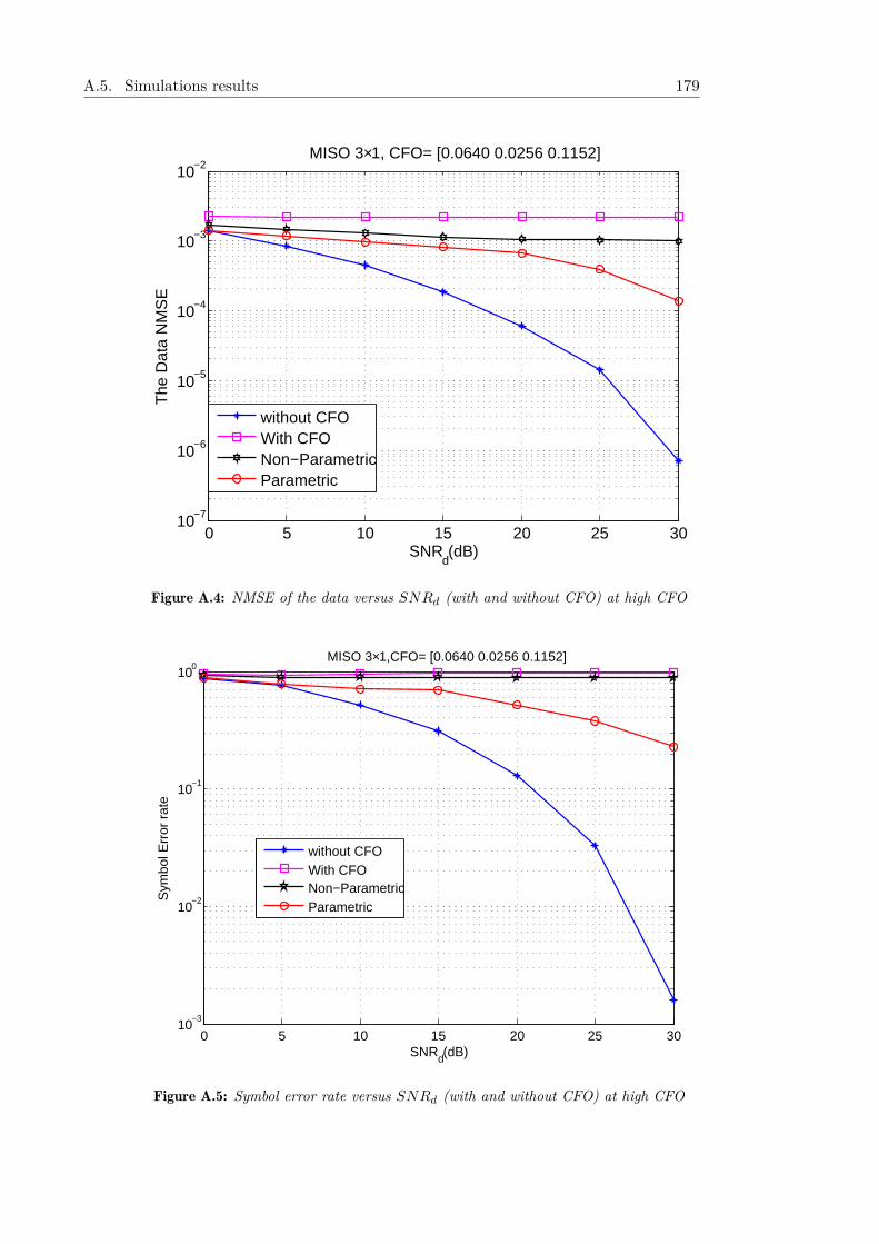
A.5. Simulations results 179
0 5 10 15 20 25 3010−7
10−6
10−5
10−4
10−3
10−2MISO 3×1, CFO= [0.0640 0.0256 0.1152]
The
Dat
a N
MS
E
SNRd(dB)
without CFOWith CFONon−ParametricParametric
Figure A.4: NMSE of the data versus SNRd (with and without CFO) at high CFO
0 5 10 15 20 25 3010
−3
10−2
10−1
100
MISO 3×1,CFO= [0.0640 0.0256 0.1152]
Sym
bol E
rror
rat
e
SNRd(dB)
without CFOWith CFONon−ParametricParametric
Figure A.5: Symbol error rate versus SNRd (with and without CFO) at high CFO
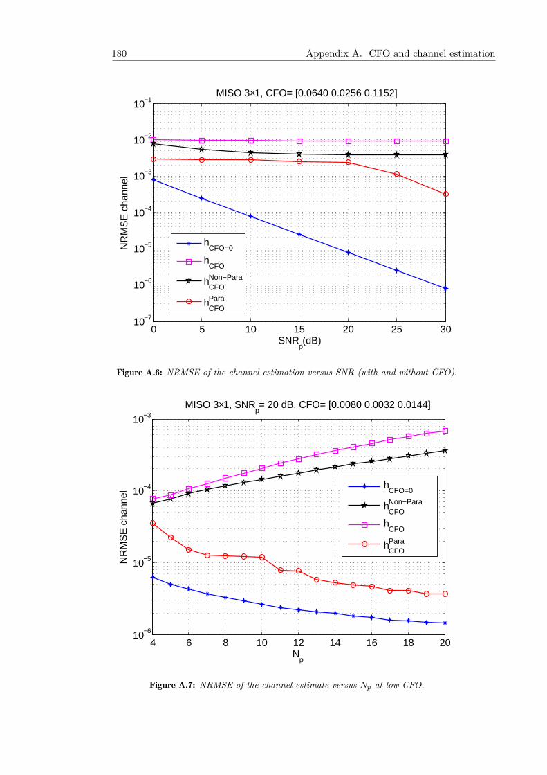
180 Appendix A. CFO and channel estimation
0 5 10 15 20 25 3010−7
10−6
10−5
10−4
10−3
10−2
10−1MISO 3×1, CFO= [0.0640 0.0256 0.1152]
NR
MS
E c
hann
el
SNRp(dB)
hCFO=0
hCFO
hCFONon−Para
hCFOPara
Figure A.6: NRMSE of the channel estimation versus SNR (with and without CFO).
4 6 8 10 12 14 16 18 2010−6
10−5
10−4
10−3MISO 3×1, SNR
p= 20 dB, CFO= [0.0080 0.0032 0.0144]
NR
MS
E c
hann
el
Np
hCFO=0
hCFONon−Para
hCFO
hCFOPara
Figure A.7: NRMSE of the channel estimate versus Np at low CFO.
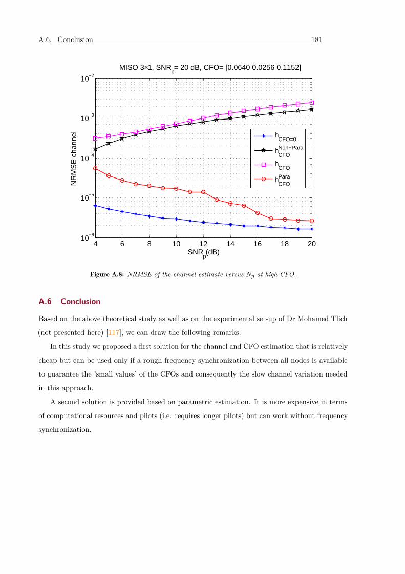
A.6. Conclusion 181
4 6 8 10 12 14 16 18 2010−6
10−5
10−4
10−3
10−2
MISO 3×1, SNRp= 20 dB, CFO= [0.0640 0.0256 0.1152]
NR
MS
E c
hann
el
SNRp(dB)
hCFO=0
hCFONon−Para
hCFO
hCFOPara
Figure A.8: NRMSE of the channel estimate versus Np at high CFO.
A.6 Conclusion
Based on the above theoretical study as well as on the experimental set-up of Dr Mohamed Tlich
(not presented here) [117], we can draw the following remarks:
In this study we proposed a first solution for the channel and CFO estimation that is relatively
cheap but can be used only if a rough frequency synchronization between all nodes is available
to guarantee the ’small values’ of the CFOs and consequently the slow channel variation needed
in this approach.
A second solution is provided based on parametric estimation. It is more expensive in terms
of computational resources and pilots (i.e. requires longer pilots) but can work without frequency
synchronization.

182 Appendix A. CFO and channel estimation

B
Ap
pe
nd
ix
French summary
184 Appendix B. French summary
Chapter contentB.1 Introduction . . . . . . . . . . . . . . . . . . . . . . . . . . . . . . . . . . . . . 185
B.1.1 Motivations . . . . . . . . . . . . . . . . . . . . . . . . . . . . . . . . . . 185
B.1.2 Estimation du canal de transmission . . . . . . . . . . . . . . . . . . . . 186
B.1.2.1 Estimation de canal basée sur les séquences pilotes . . . . . . . 186
B.1.2.2 Estimation aveugle du canal . . . . . . . . . . . . . . . . . . . 187
B.1.2.3 Estimation semi-aveugle du canal . . . . . . . . . . . . . . . . 187
B.1.3 Objectifs de la thèse . . . . . . . . . . . . . . . . . . . . . . . . . . . . . 187
B.1.4 Liste des publications . . . . . . . . . . . . . . . . . . . . . . . . . . . . 188
B.2 Analyse de performances limites d’estimation de canal des systèmes de commu-
nications MIMO-OFDM . . . . . . . . . . . . . . . . . . . . . . . . . . . . . . . 190
B.2.1 Systèmes de communications à porteuses multiples : concepts principaux 191
B.2.1.1 Modèle du système MIMO-OFDM . . . . . . . . . . . . . . . . 191
B.2.1.2 Principaux modèles d’arrangement des pilotes . . . . . . . . . 191
B.3 CRB pour une estimation de canal basée sur les pilotes arrangés selon le type
bloc . . . . . . . . . . . . . . . . . . . . . . . . . . . . . . . . . . . . . . . . . . 192
B.3.1 CRB pour une estimation semi-aveugle de canal dans le cas des pilotes
arrangés selon le type bloc . . . . . . . . . . . . . . . . . . . . . . . . . . 192
B.3.1.1 Modèle de données gaussien circulaire . . . . . . . . . . . . . . 193
B.3.1.2 Modèle de données gaussien non circulaire . . . . . . . . . . . 194
B.3.1.3 Modèle de données BPSK et QPSK . . . . . . . . . . . . . . . 194
B.3.2 Résultats de simulations . . . . . . . . . . . . . . . . . . . . . . . . . . . 195
B.4 Algorithme EM efficace pour l’estimation semi-aveugle de canal MIMO-OFDM 196
B.4.1 Système de communications MIMO-OFDM . . . . . . . . . . . . . . . . 197
B.4.2 Estimation semi-aveugle de canal MIMO . . . . . . . . . . . . . . . . . . 199
B.4.2.1 Algorithme EM pour l’estimation semi-aveugle de canal MIMO 200
B.4.2.2 Algorithme EM pour l’estimation semi-aveugle de canal des
sous-systèmes . . . . . . . . . . . . . . . . . . . . . . . . . . . . 201
B.4.3 Analyse des performances . . . . . . . . . . . . . . . . . . . . . . . . . . 204
B.5 Conclusion . . . . . . . . . . . . . . . . . . . . . . . . . . . . . . . . . . . . . . 206
B.1. Introduction 185
B.1 Introduction
Au cours des dernières décennies, les communications sans fil ont connu des développements
remarquables dans de nombreux domaines distincts. Cela a commencé avec la recherche universi-
taire, où de nombreuses améliorations et progrès ont été réalisés. Cela est également évident
dans les applications militaires, où la guerre et les armes traditionnelles ont été remplacées par
des armes autonomes (comme les véhicules aériens sans pilote (UAV)) et la guerre électronique
cybernétique. Le domaine civil a également vu sa part de progrès dans les communications sans
fil, en ce sens que nos vies sont devenues plus virtuelles et connectées.
L’utilisation de plusieurs antennes au niveau de l’émetteur ou du récepteur, ou des deux
(MIMO), peut considérablement améliorer les performances des systèmes de transmission [5, 6].
Les systèmes de communications MIMO offrent des degrés de liberté supplémentaires fournis
par la dimension spatiale, qui peuvent être exploités pour transmettre simultanément des flux
de données indépendants (multiplexage spatial) augmentant ainsi le débit de données, ou la
transmission multiplicative d’un flux de données unique (diversité spatiale) pour augmenter la
fiabilité du système [5, 7].
B.1.1 Motivations
L’utilisation sans précédent de téléphones intelligents, tablettes, super-téléphones, etc., équipés
d’applications gourmandes en données, telle que la vidéo en streaming, de lourdes interfaces
graphiques pour réseaux sociaux et des services de navigation en temps réel, a poussé à des
changements révolutionnaires de la 4G à la prochaine génération de systèmes sans fil . Bien
que les systèmes 4G puissent être chargés avec beaucoup plus de services, de fonctionnalités en
temps réel et de données que les anciens systèmes, il subsiste un écart considérable entre les
exigences pratiques de la population et ce que peuvent offrir les technologies 4G. Pour répondre
aux fortes demandes de la croissance explosive des utilisateurs de téléphones cellulaires et des
services potentiels associés, la norme de la cinquième génération (5G) fait actuellement l’objet
d’une enquête et de discussions approfondies. Avec des vitesses pouvant atteindre 10 gigabits par
seconde, la 5G devrait être 100 fois plus rapide que la 4G [14]. Les deux technologies principales
pour répondre aux exigences de la 5G sont l’utilisation des systèmes à ondes millimétriques
(mmWave) et des systèmes MIMO massifs [15].
Avec un nombre plus élevé d’antennes à la station de base (BS), quelques centaines, par
rapport aux systèmes MIMO classiques (8 antennes pour le LTE), des systèmes MIMO massifs
ou MIMO à grande échelle peuvent offrir un grand gains d’efficacité spectrale et énergétique
186 Appendix B. French summary
[14, 16, 17].
Les systèmes de communications MIMO massifs surmontent plusieurs limitations des systèmes
MIMO traditionnels, tel que la sécurité, la robustesse et le débit de traitement [18, 15]. Il a
été démontré que les énormes systèmes MIMO promettaient de multiplier par 10 le débit du
système tout en desservant simultanément des dizaines d’utilisateurs sur la même ressource
temps-fréquence [18]. Pour cela, le débit et la capacité du système seront fortement améliorés
afin de satisfaire la quantité croissante d’échange de données et demande de qualité de service
pour les futurs réseaux cellulaires.
Pour exploiter pleinement le potentiel des technologies susmentionnées, la connaissance du
canal de transmission (CSI) est indispensable. Pour améliorer les performances du système, il
est essentiel que la CSI soit disponible à la fois au niveau de l’émetteur et du récepteur. La
connaissance de CSI est utilisée pour la détection cohérente des signaux transmis du côté du
récepteur. Du côté des émetteurs, la CSI est essentielle pour concevoir des schémas de précodage
efficaces pour l’annulation des interférences entre utilisateurs. Cependant, la connaissance parfaite
de la CSI n’est pas disponible dans la pratique, elle doit donc être estimée. Cette thèse s’intéresse
aux algorithmes d’estimation du canal de transmission et de faible complexité pour les systèmes
MIMO-OFDM et les systèmes MIMO-OFDM massifs.
B.1.2 Estimation du canal de transmission
La bonne conduite de la mission du système de communications sans fil dépend en grande partie
de la disponibilité de la connaissance de son environnement. L’environnement de propagation fait
référence au canal de communications qui assure la connexion entre l’émetteur et le récepteur.
Ainsi, l’estimation de canal de transmission est d’une importance primordiale pour l’égalisation et
la détection de symboles. Plusieurs modèles de canaux et approches d’estimation de canaux ont
été développés dans la littérature en fonction de leurs applications et de la norme sélectionnée.
Les méthodes d’estimation peuvent être divisées en trois classes principales discutées ci-dessous.
B.1.2.1 Estimation de canal basée sur les séquences pilotes
En générale, l’estimation du canal de transmission est réalisée en insérant, dans la trame
transmise, des séquences d’apprentissage (appelées pilotes) connue a priori par le récepteur, selon
une disposition connue dans la trame (bloc, peigne ou réseau) [19, 20, 21]. Côté récepteur, en
observant la sortie en correspondance des symboles du pilote, il est possible d’estimer le canal.
Cette connaissance est ensuite introduite dans le processus de détection afin de permettre une
estimation optimale des données. Cette approche (estimation du canal basée sur les pilotes) est
B.1. Introduction 187
la plus utilisée dans les normes de communications [22, 13], pour sa faible complexité de calculs
et sa robustesse. Son inconvénient réside dans le fait que les symboles pilotes ne contiennent pas
d’informations utile, ils représentent donc un gaspillage de bande passante. De plus, la plupart
des observations (celles liées aux symboles inconnus) sont ignorées dans le processus d’estimation,
ce qui représente une occasion manquée d’améliorer la précision de l’estimation du canal.
B.1.2.2 Estimation aveugle du canal
Contrairement à l’estimation de canal basée sur les séquences pilotes, les méthodes d’estimation
de canal aveugle s’appuient entièrement sur les propriétés statistiques des symboles transmis
inconnus (c’est-à-dire qu’aucun pilote n’est transmis) [23, 24, 25]. Cette approche réduit le
temps de réponse du système, mais nécessite un grand nombre de symboles de données pour les
propriétés statistiques et de puissants algorithmes. De plus, les approches basées sur les pilotes
donnent de meilleures performances à faible complexité de calculs que les approches d’estimation
aveugles.
B.1.2.3 Estimation semi-aveugle du canal
Chaque méthodes d’estimation de canal a ses avantages et ses inconvénients. Généralement, la
première classe (c’est-à-dire un estimateur de canal basé sur les pilotes) fournit une estimation
de canal plus précise que la classe d’estimation aveugle. Cependant, la seconde classe, dans
la plupart des cas, augmente l’efficacité spectrale par rapport à la première. Par conséquent,
il serait avantageux de conserver les avantages des deux techniques en utilisant des méthodes
d’estimation semi-aveugles [26, 27, 28, 29], exploitant à la fois les données et les pilotes pour
identifier le canal de transmission.
B.1.3 Objectifs de la thèse
Un des problèmes majeurs de ces systèmes est le fort niveau d’interférences dû au grand
nombre d’émetteurs simultanés. Dans un tel contexte, les solutions ’classiques’ de conception de
pilotes ’orthogonaux’ sont extrêmement coûteuses en débit utile permettant ainsi aux solutions
d’identification de canal dites ’aveugles’ ou ’semi-aveugles’ (abandonnées dans les systèmes
de communications civiles) de revenir au-devant de la scène comme solutions intéressantes
d’identification ou de déconvolution de ces canaux MIMO.
Dans cette thèse, nous avons commencé, dans la première partie, par une analyse comparative
des performances, en se basant sur les bornes de Cramèr-Rao (CRB), afin de mesurer la réduction
potentielle de la taille des séquences pilotes en employant les méthodes dites semi-aveugles basées
sur l’exploitation conjointe des pilotes et des données. Les résultats d’analyse montrent que nous
188 Appendix B. French summary
pouvons réduire jusqu’à 95% des pilotes sans affecter les performances d’estimation du canal.
Nous avons par la suite, dans la deuxième partie, proposé de nouvelles méthodes d’estimation
semi-aveugle du canal, à faible coût, permettant d’approcher les performances limites (CRB).
Nous avons proposé un estimateur semi-aveugle, appelé LS-DF (Least Squares-Decision Feedback),
basé sur une estimation des moindres carrés avec retour de décision qui permet un bon compromis
performance / complexité numérique. Un autre estimateur semi-aveugle de type sous-espace a
aussi été proposé ainsi qu’un algorithme basé sur l’approche EM (Expectation Maximization)
pour lequel trois versions à coût réduit ont été étudiées. Dans le cas d’un canal spéculaire, nous
avons proposé un algorithme d’estimation paramétrique qui s’appuie sur l’estimation des temps
d’arrivés combinée avec la technique DF.
Dans cette annexe, nous présentons un résumé en langue Française des travaux réalisés.
B.1.4 Liste des publications
Les travaux de recherche développés dans cette thèse ont donné lieu aux publications suivantes :
Articles de revues :
1) Ladaycia, A. Mokraoui, K. Abed-Meraim, and A. Belouchrani, "Performance bounds
analysis for semi-blind channel estimation in MIMO-OFDM communications systems,"
IEEE Transactions on Wireless Communications, vol. 16, no. 9, pp. 5925-5938, Sep. 2017.
2) A. Ladaycia, A. Belouchrani, K. Abed-Meraim and A. Mokraoui, "Semi-Blind MIMO-
OFDM Channel Estimation using EM-like Techniques," IEEE Transactions on Wireless
Communications, May. 2019. (submitted).
3) O. Rekik, A. Ladaycia, K. Abed-Meraim, and A. Mokraoui, "Performance Bounds Analysis
for Semi-Blind Channel Estimation with Pilot Contamination in Massive MIMO-OFDM
Systems," IET Communications, May. 2019. (submitted).
Articles de conférences :
1) A. Ladaycia, A. Mokraoui, K. Abed-Meraim, and A. Belouchrani, "What semi-blind channel
estimation brings in terms of throughput gain?" in 2016 10th ICSPCS, Dec. 2016, pp. 1-6,
Gold Coast, Australia.
2) A. Ladaycia, A. Belouchrani, K. Abed-Meraim, and A. Mokraoui, "Parameter optimization
for defeating blind interception in drone protection," in 2017 Seminar on Detection Systems
Architectures and Technologies (DAT), Feb. 2017, pp. 1-6, Alger, Algeria.
B.1. Introduction 189
3) A. Ladaycia, A. Mokraoui, K. Abed-Meraim, and A. Belouchrani, "Further investigations on
the performance bounds of MIMO-OFDM channel estimation," in The 13th International
Wireless Communications and Mobile Computing Conference (IWCMC 2017), June 2017,
pp. 223-228, Valance, Spain.
4) A. Ladaycia, A. Mokraoui, K. Abed-Meraim, and A. Belouchrani, "Toward green commu-
nications using semi-blind channel estimation," in 2017 25th European Signal Processing
Conference (EUSIPCO), Aug. 2017, pp. 2254-2258, Kos, Greece.
5) A. Ladaycia, K. Abed-Meraim, A. Bader, and M.S. Alouini, "CFO and channel estimation for
MISO-OFDM systems," in 2017 25th European Signal Processing Conference (EUSIPCO),
Aug. 2017, pp. 2264-2268, Kos, Greece.
6) A. Ladaycia, A. Mokraoui, K. Abed-Meraim, and A. Belouchrani, "Contributions à
l’estimation semi-aveugle des canaux MIMO-OFDM," in GRETSI 2017, Sep. 2017, Nice,
France.
7) A. Ladaycia, A. Belouchrani, K. Abed-Meraim, and A. Mokraoui, "EM-based semi-blind
MIMO-OFDM channel estimation," in 2018 IEEE International Conference on Acoustics,
Speech and Signal Processing (ICASSP2018), Apr. 2018, Alberta, Canada.
8) A. Ladaycia, K. Abed-Meraim, A. Mokraoui, and A. Belouchrani, "Efficient Semi-Blind
Subspace Channel Estimation for MIMO-OFDM System," in 2018 26th European Signal
Processing Conference (EUSIPCO), Sep. 2018, Rome, Italy.
9) O. Rekik, A. Ladaycia, K. Abed-Meraim, and A. Mokraoui, "Performance Bounds Analysis
for Semi-Blind Channel Estimation with Pilot Contamination in Massive MIMO-OFDM
Systems," in 2018 26th European Signal Processing Conference (EUSIPCO), Sep. 2018,
Rome, Italy.
10) A. Ladaycia, M.Pesavento, A. Mokraoui, K. Abed-Meraim, and A. Belouchrani, "Decision
feedback semi-blind estimation algorithm for specular OFDM channels," in 2019 IEEE
International Conference on Acoustics, Speech and Signal Processing (ICASSP2019).
11) A. Ladaycia, A. Belouchrani, K. Abed-Meraim, and A. Mokraoui, "Efficient EM-algorithm
for MIMO-OFDM semi blind channel estimation," in 2019 Conference on Electrical Engi-
neering (CEE2019).
190 Appendix B. French summary
12) O. Rekik, A. Ladaycia, K. Abed-Meraim, and A. Mokraoui, "Semi-Blind Source Separation
based on Multi-Modulus Criterion: Application for Pilot Contamination Mitigation in
Massive MIMO Systems," in The 19th ISCIT, Ho Chi Minh City, Vietnam. in The 19th
ISCIT, Ho Chi Minh City, Vietnam.
13) A. Ladaycia, A. Belouchrani, K. Abed-Meraim, and A. Mokraoui, "Algorithme EM efficace
pour l’estimation semi-aveugle de canal MIMO-OFDM," in GRETSI 2019.
B.2 Analyse de performances limites d’estimation de canal des systèmes de com-
munications MIMO-OFDM
La combinaison de la technologie MIMO et de la modulation OFDM (c’est-à-dire MIMO-OFDM)
est largement déployée dans les systèmes de communications sans fil, comme dans le réseau sans
fil 802.11n [22], LTE et LTE-A [4]. En effet, l’utilisation de MIMO-OFDM améliore la capacité
de canal et la fiabilité des communications. En particulier, il a été montrée dans [14, 16] que
grâce au déploiement d’un grand nombre d’antennes dans les stations de base, le système pouvait
atteindre un débit de transmission élevé et offrir une efficacité spectrale très élevée.
Dans un tel système, l’estimation de canal de transmission reste une préoccupation actuelle
dans la mesure où la performance globale en dépend fortement, en particulier pour les grands
systèmes MIMO où l’estimation de canal de transmission devient plus complexe.
Cette section est consacré à l’analyse comparative de performances limites de de l’estimation
semi-aveugle et aux approches basées uniquement sur les pilotes de canal de transmission,
dans le contexte des systèmes MIMO-OFDM. Pour obtenir des résultats comparatifs généraux
indépendamment des algorithmes ou des méthodes d’estimation spécifiques, cette analyse est
réalisée à l’aide de la CRB.
Par conséquent, nous commençons par donner plusieurs dérivations de CRB pour différents
modèles de données (Gaussienne circulaire (CG), Gaussienne non circulaire (NCG), Binary /
Quadratic Phase Shift Keying (BPSK / QPSK)) et différentes organisations des pilotes (blocs,
peignes et treillis). Dans le cas particulier des systèmes MIMO de grandes dimensions, nous
avons exploité la structure diagonale des blocs des matrices de covariance pour développer une
technique numérique rapide qui évite les coûts prohibitifs et les problèmes de mémoire insuffisante
(dus aux grandes tailles de matrice) du calcul de la CRB. De plus, dans le cas BPSK / QPSK, une
approximation réaliste de la CRB est introduite pour éviter des calculs d’intégrales numériques
lourds. Après avoir calculé toutes les CRB nécessaires, nous les utiliserons pour comparer les
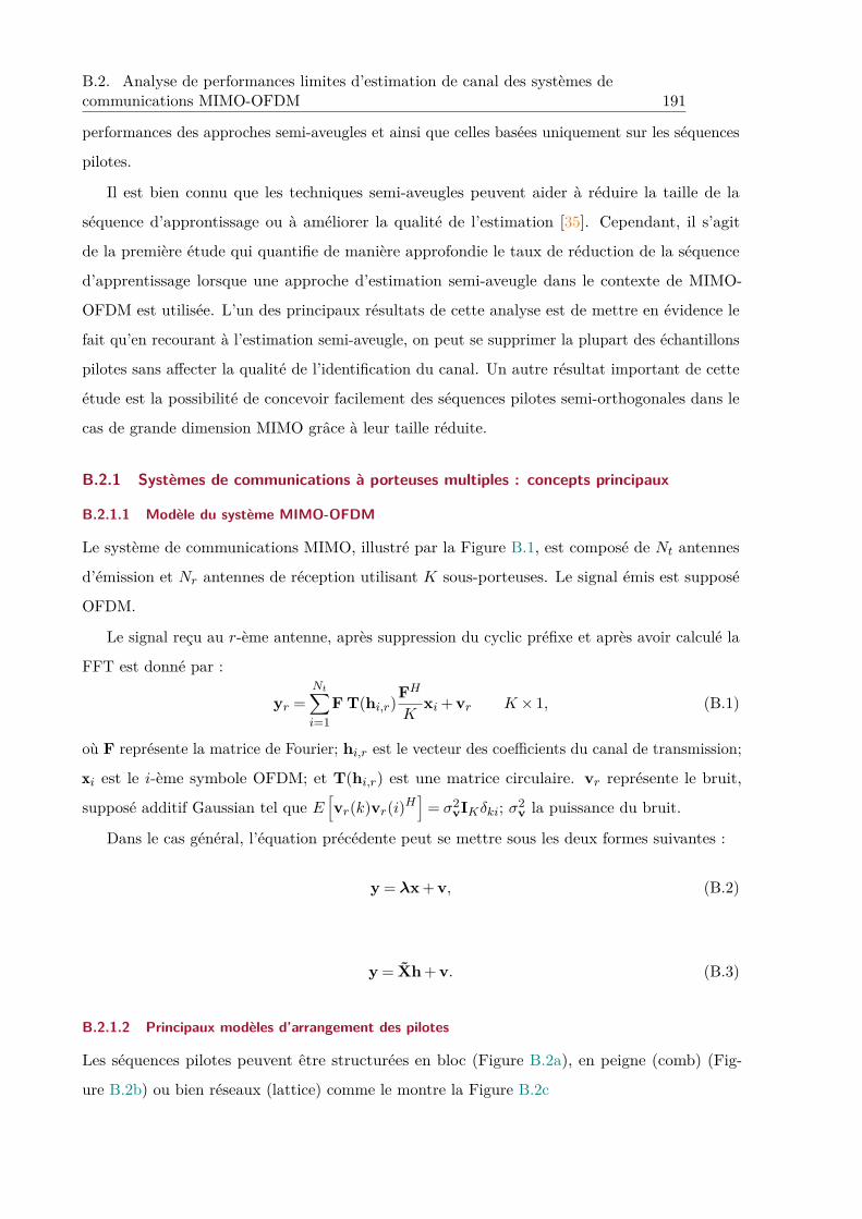
B.2. Analyse de performances limites d’estimation de canal des systèmes decommunications MIMO-OFDM 191
performances des approches semi-aveugles et ainsi que celles basées uniquement sur les séquences
pilotes.
Il est bien connu que les techniques semi-aveugles peuvent aider à réduire la taille de la
séquence d’approntissage ou à améliorer la qualité de l’estimation [35]. Cependant, il s’agit
de la première étude qui quantifie de manière approfondie le taux de réduction de la séquence
d’apprentissage lorsque une approche d’estimation semi-aveugle dans le contexte de MIMO-
OFDM est utilisée. L’un des principaux résultats de cette analyse est de mettre en évidence le
fait qu’en recourant à l’estimation semi-aveugle, on peut se supprimer la plupart des échantillons
pilotes sans affecter la qualité de l’identification du canal. Un autre résultat important de cette
étude est la possibilité de concevoir facilement des séquences pilotes semi-orthogonales dans le
cas de grande dimension MIMO grâce à leur taille réduite.
B.2.1 Systèmes de communications à porteuses multiples : concepts principaux
B.2.1.1 Modèle du système MIMO-OFDM
Le système de communications MIMO, illustré par la Figure B.1, est composé de Nt antennes
d’émission et Nr antennes de réception utilisant K sous-porteuses. Le signal émis est supposé
OFDM.
Le signal reçu au r-ème antenne, après suppression du cyclic préfixe et après avoir calculé la
FFT est donné par :
yr =Nt∑i=1
F T(hi,r)FH
Kxi + vr K × 1, (B.1)
où F représente la matrice de Fourier; hi,r est le vecteur des coefficients du canal de transmission;
xi est le i-ème symbole OFDM; et T(hi,r) est une matrice circulaire. vr représente le bruit,
supposé additif Gaussian tel que E[vr(k)vr(i)H
]= σ2
vIKδki; σ2v la puissance du bruit.
Dans le cas général, l’équation précédente peut se mettre sous les deux formes suivantes :
y = λx + v, (B.2)
y = Xh + v. (B.3)
B.2.1.2 Principaux modèles d’arrangement des pilotes
Les séquences pilotes peuvent être structurées en bloc (Figure B.2a), en peigne (comb) (Fig-
ure B.2b) ou bien réseaux (lattice) comme le montre la Figure B.2c
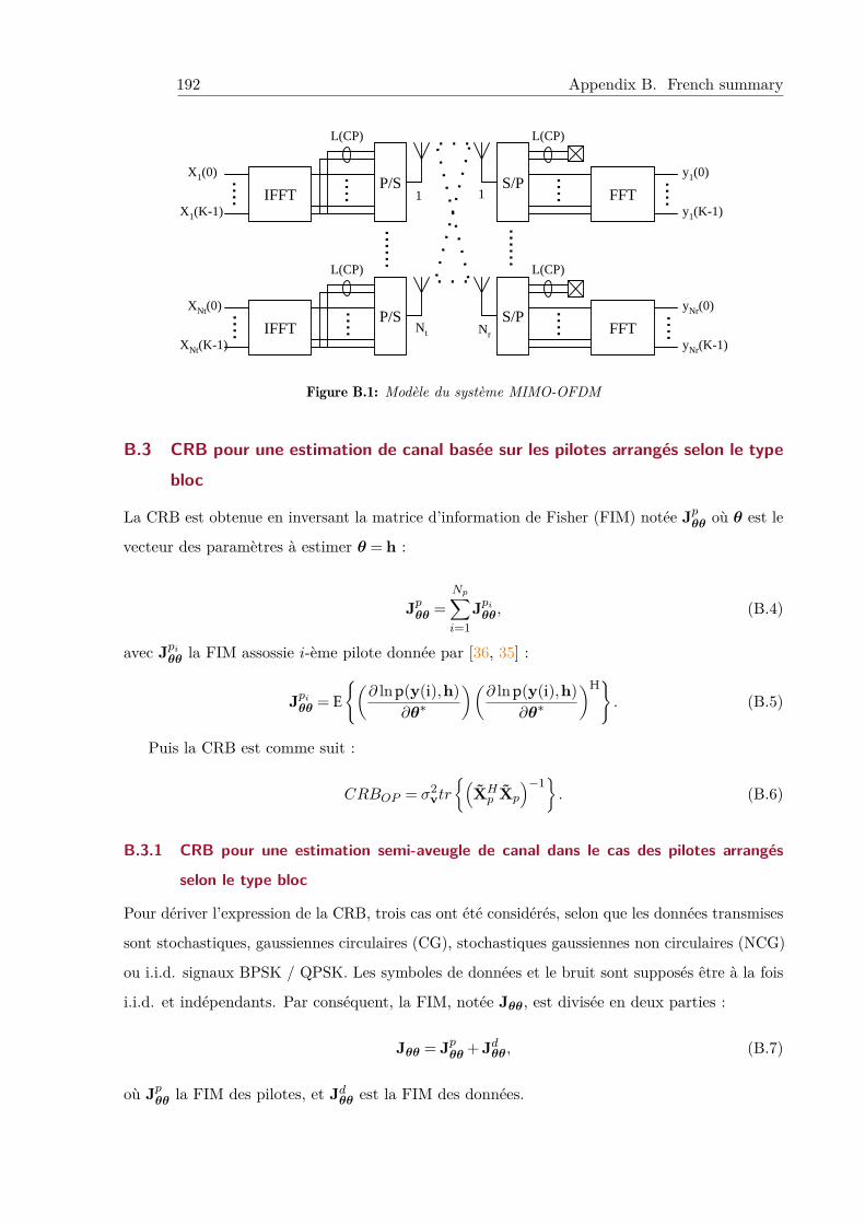
192 Appendix B. French summary
P/SIFFT
L(CP)
S/PFFT
L(CP)
P/SIFFT
L(CP)
S/PFFT
L(CP)
Nt Nr
1 1
X1 (0)
X1 (K-1)
XNt (0)
XNt (K-1)
y1 (0)
y1 (K-1)
yNr (0)
yNr (K-1)
........
....
.... ........
....
......
......
....
. . .
. . .
. . . . . . . . . . .. . . . . . . . . . .
Figure B.1: Modèle du système MIMO-OFDM
B.3 CRB pour une estimation de canal basée sur les pilotes arrangés selon le type
bloc
La CRB est obtenue en inversant la matrice d’information de Fisher (FIM) notée Jpθθ où θ est le
vecteur des paramètres à estimer θ = h :
Jpθθ =Np∑i=1
Jpiθθ, (B.4)
avec Jpiθθ la FIM assossie i-ème pilote donnée par [36, 35] :
Jpiθθ = E
{(∂ lnp(y(i),h)
∂θ∗
)(∂ lnp(y(i),h)
∂θ∗
)H}. (B.5)
Puis la CRB est comme suit :
CRBOP = σ2vtr
{(XHp Xp
)−1}. (B.6)
B.3.1 CRB pour une estimation semi-aveugle de canal dans le cas des pilotes arrangés
selon le type bloc
Pour dériver l’expression de la CRB, trois cas ont été considérés, selon que les données transmises
sont stochastiques, gaussiennes circulaires (CG), stochastiques gaussiennes non circulaires (NCG)
ou i.i.d. signaux BPSK / QPSK. Les symboles de données et le bruit sont supposés être à la fois
i.i.d. et indépendants. Par conséquent, la FIM, notée Jθθ, est divisée en deux parties :
Jθθ = Jpθθ + Jdθθ, (B.7)
où Jpθθ la FIM des pilotes, et Jdθθ est la FIM des données.
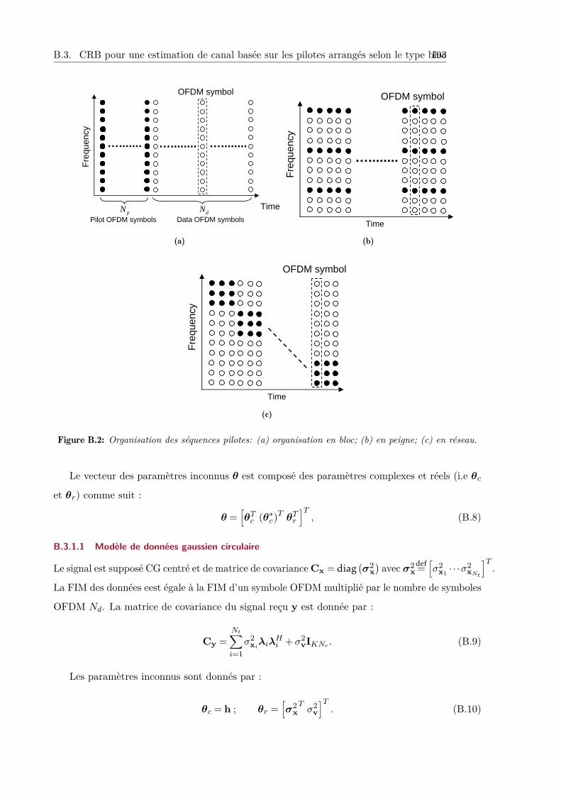
B.3. CRB pour une estimation de canal basée sur les pilotes arrangés selon le type bloc193
Pilot OFDM symbols Data OFDM symbols
Freq
uenc
y
Time
…....... …........ …........
OFDM symbol
pN dN
(a)
Time
Freq
uenc
y
…........
OFDM symbol
(b)
Time
Freq
uenc
y
OFDM symbol
(c)
Figure B.2: Organisation des séquences pilotes: (a) organisation en bloc; (b) en peigne; (c) en réseau.
Le vecteur des paramètres inconnus θ est composé des paramètres complexes et réels (i.e θcet θr) comme suit :
θ =[θTc (θ∗c)
T θTr
]T, (B.8)
B.3.1.1 Modèle de données gaussien circulaire
Le signal est supposé CG centré et de matrice de covariance Cx = diag(σ2
x)avec σ2
xdef=[σ2
x1 · · ·σ2xNt
]T.
La FIM des données eest égale à la FIM d’un symbole OFDM multiplié par le nombre de symboles
OFDM Nd. La matrice de covariance du signal reçu y est donnée par :
Cy =Nt∑i=1
σ2xiλiλ
Hi +σ2
vIKNr . (B.9)
Les paramètres inconnus sont donnés par :
θc = h ; θr =[σ2
xTσ2
v
]T. (B.10)
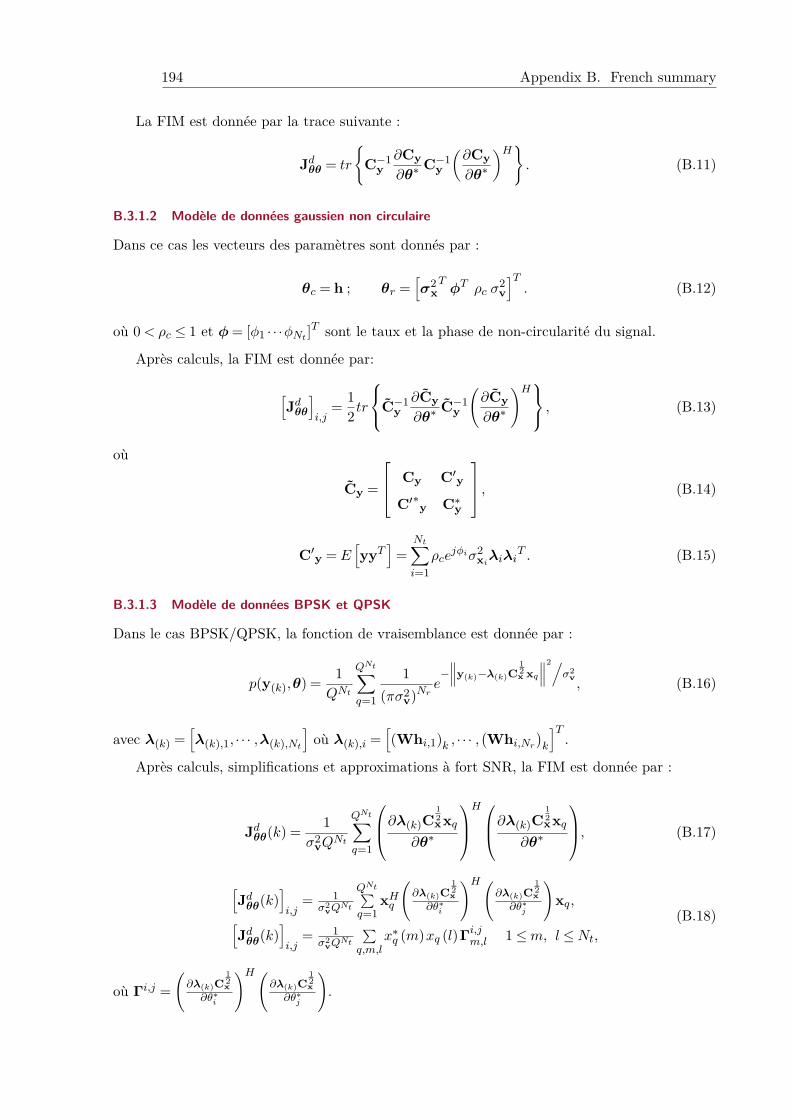
194 Appendix B. French summary
La FIM est donnée par la trace suivante :
Jdθθ = tr
{C−1
y∂Cy∂θ∗
C−1y
(∂Cy∂θ∗
)H}. (B.11)
B.3.1.2 Modèle de données gaussien non circulaire
Dans ce cas les vecteurs des paramètres sont donnés par :
θc = h ; θr =[σ2
xTφT ρc σ
2v
]T. (B.12)
où 0< ρc ≤ 1 et φ= [φ1 · · ·φNt ]T sont le taux et la phase de non-circularité du signal.
Après calculs, la FIM est donnée par:
[Jdθθ
]i,j
= 12 tr
C−1y∂Cy∂θ∗
C−1y
(∂Cy∂θ∗
)H , (B.13)
où
Cy =
Cy C′yC′∗y C∗y
, (B.14)
C′y = E[yyT
]=
Nt∑i=1
ρcejφiσ2
xiλiλiT . (B.15)
B.3.1.3 Modèle de données BPSK et QPSK
Dans le cas BPSK/QPSK, la fonction de vraisemblance est donnée par :
p(y(k),θ) = 1QNt
QNt∑q=1
1(πσ2
v)Nre−∥∥∥y(k)−λ(k)C
12x xq
∥∥∥2/σ2
v, (B.16)
avec λ(k) =[λ(k),1, · · · ,λ(k),Nt
]où λ(k),i =
[(Whi,1)k , · · · ,
(Whi,Nr
)k
]T.
Après calculs, simplifications et approximations à fort SNR, la FIM est donnée par :
Jdθθ(k) = 1σ2
vQNt
QNt∑q=1
∂λ(k)C12xxq
∂θ∗
H∂λ(k)C
12xxq
∂θ∗
, (B.17)
[Jdθθ(k)
]i,j
= 1σ2
vQNt
QNt∑q=1
xHq
(∂λ(k)C
12x
∂θ∗i
)H(∂λ(k)C
12x
∂θ∗j
)xq,[
Jdθθ(k)]i,j
= 1σ2
vQNt
∑q,m,l
x∗q (m)xq (l)Γi,jm,l 1≤m, l ≤Nt,(B.18)
où Γi,j =(∂λ(k)C
12x
∂θ∗i
)H(∂λ(k)C
12x
∂θ∗j
).
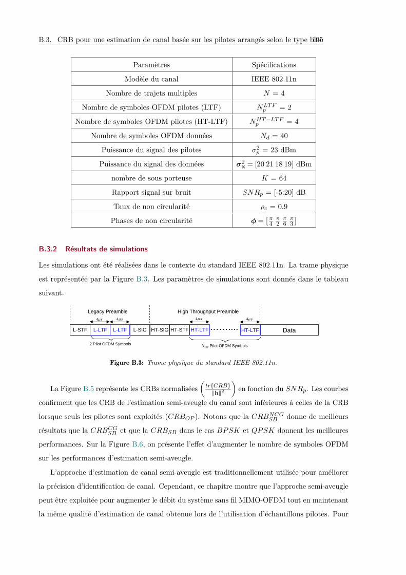
B.3. CRB pour une estimation de canal basée sur les pilotes arrangés selon le type bloc195
Paramètres Spécifications
Modèle du canal IEEE 802.11n
Nombre de trajets multiples N = 4
Nombre de symboles OFDM pilotes (LTF) NLTFp = 2
Nombre de symboles OFDM pilotes (HT-LTF) NHT−LTFp = 4
Nombre de symboles OFDM données Nd = 40
Puissance du signal des pilotes σ2p = 23 dBm
Puissance du signal des données σ2x = [20 21 18 19] dBm
nombre de sous porteuse K = 64
Rapport signal sur bruit SNRp = [-5:20] dB
Taux de non circularité ρc = 0.9
Phases de non circularité φ=[π
4π2π6π3]
B.3.2 Résultats de simulations
Les simulations ont été réalisées dans le contexte du standard IEEE 802.11n. La trame physique
est représentée par la Figure B.3. Les paramètres de simulations sont donnés dans le tableau
suivant.
HT-LTF…….... Data
Legacy Preamble High Throughput Preamble
2 Pilot OFDM Symbols Pilot OFDM SymbolsLTFN
HT-LTFHT-STFHT-SIGL-SIGL-LTFL-LTFL-STF
4 s 4 s 4 s 4 s
Figure B.3: Trame physique du standard IEEE 802.11n.
La Figure B.5 représente les CRBs normalisées(tr{CRB}‖h‖2
)en fonction du SNRp. Les courbes
confirment que les CRB de l’estimation semi-aveugle du canal sont inférieures à celles de la CRB
lorsque seuls les pilotes sont exploités (CRBOP ). Notons que la CRBNCGSB donne de meilleurs
résultats que la CRBCGSB et que la CRBSB dans le cas BPSK et QPSK donnent les meilleures
performances. Sur la Figure B.6, on présente l’effet d’augmenter le nombre de symboles OFDM
sur les performances d’estimation semi-aveugle.
L’approche d’estimation de canal semi-aveugle est traditionnellement utilisée pour améliorer
la précision d’identification de canal. Cependant, ce chapitre montre que l’approche semi-aveugle
peut être exploitée pour augmenter le débit du système sans fil MIMO-OFDM tout en maintenant
la même qualité d’estimation de canal obtenue lors de l’utilisation d’échantillons pilotes. Pour
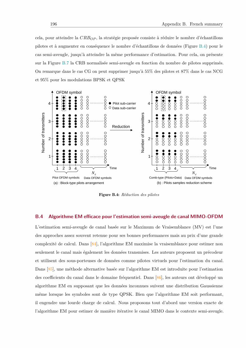
196 Appendix B. French summary
cela, pour atteindre la CRBOP , la stratégie proposée consiste à réduire le nombre d’échantillons
pilotes et à augmenter en conséquence le nombre d’échantillons de données (Figure B.4) pour le
cas semi-aveugle, jusqu’à atteindre la même performance d’estimation. Pour cela, on présente
sur la Figure B.7 la CRB normalisée semi-aveugle en fonction du nombre de pilotes supprimés.
On remarque dans le cas CG on peut supprimer jusqu’à 55% des pilotes et 87% dans le cas NCG
et 95% pour les modulations BPSK et QPSK
(a) : Block-type pilots arrangement (b) : Pilots samples reduction scheme
Pilot sub-carrierData sub-carrier
Time
OFDM symbol
1
4
Pilot OFDM symbols
Num
ber o
f tra
nsm
itter
s
2
3
1 2 3 4
Reduction
…………
…………
…………
…………
dNData OFDM symbols
Time
OFDM symbol
1
4
Comb-type (Pilots+Data)
Num
ber o
f tra
nsm
itter
s2
3
1 2 3 4
…………
…………
…………
…………
dNData OFDM symbols
Figure B.4: Réduction des pilotes
B.4 Algorithme EM efficace pour l’estimation semi-aveugle de canal MIMO-OFDM
L’estimation semi-aveugle de canal basée sur le Maximum de Vraisemblance (MV) est l’une
des approches assez souvent retenue pour ses bonnes performances mais au prix d’une grande
complexité de calcul. Dans [84], l’algorithme EM maximise la vraisemblance pour estimer non
seulement le canal mais également les données transmises. Les auteurs proposent un précodeur
et utilisent des sous-porteuses de données comme pilotes virtuels pour l’estimation du canal.
Dans [85], une méthode alternative basée sur l’algorithme EM est introduite pour l’estimation
des coefficients du canal dans le domaine fréquentiel. Dans [86], les auteurs ont développé un
algorithme EM en supposant que les données inconnues suivent une distribution Gaussienne
même lorsque les symboles sont de type QPSK. Bien que l’algorithme EM soit performant,
il engendre une lourde charge de calcul. Nous proposons tout d’abord une version exacte de
l’algorithme EM pour estimer de manière itérative le canal MIMO dans le contexte semi-aveugle.
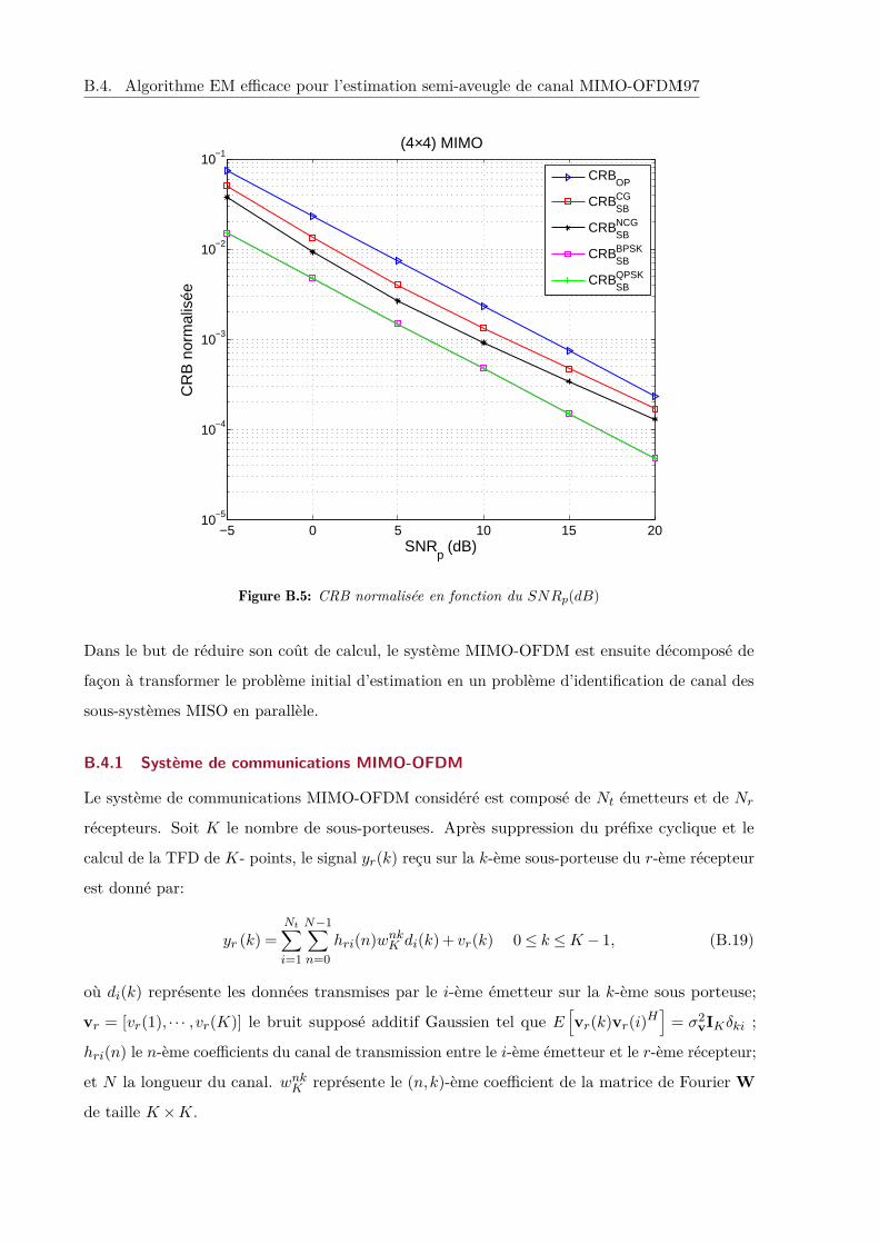
B.4. Algorithme EM efficace pour l’estimation semi-aveugle de canal MIMO-OFDM197
−5 0 5 10 15 2010−5
10−4
10−3
10−2
10−1(4×4) MIMO
CR
B n
orm
alis
ée
SNRp (dB)
CRBOP
CRBSBCG
CRBSBNCG
CRBSBBPSK
CRBSBQPSK
Figure B.5: CRB normalisée en fonction du SNRp(dB)
Dans le but de réduire son coût de calcul, le système MIMO-OFDM est ensuite décomposé de
façon à transformer le problème initial d’estimation en un problème d’identification de canal des
sous-systèmes MISO en parallèle.
B.4.1 Système de communications MIMO-OFDM
Le système de communications MIMO-OFDM considéré est composé de Nt émetteurs et de Nrrécepteurs. Soit K le nombre de sous-porteuses. Après suppression du préfixe cyclique et le
calcul de la TFD de K- points, le signal yr(k) reçu sur la k-ème sous-porteuse du r-ème récepteur
est donné par:
yr (k) =Nt∑i=1
N−1∑n=0
hri(n)wnkK di(k) + vr(k) 0≤ k ≤K − 1, (B.19)
où di(k) représente les données transmises par le i-ème émetteur sur la k-ème sous porteuse;
vr = [vr(1), · · · ,vr(K)] le bruit supposé additif Gaussien tel que E[vr(k)vr(i)H
]= σ2
vIKδki ;
hri(n) le n-ème coefficients du canal de transmission entre le i-ème émetteur et le r-ème récepteur;
et N la longueur du canal. wnkK représente le (n,k)-ème coefficient de la matrice de Fourier W
de taille K ×K.
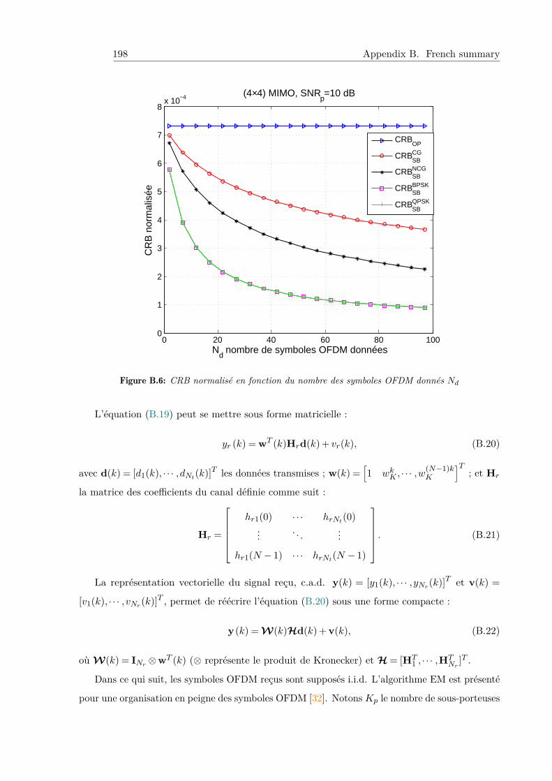
198 Appendix B. French summary
0 20 40 60 80 1000
1
2
3
4
5
6
7
8x 10⁻⁴ (4×4) MIMO, SNR
p=10 dB
CR
B n
orm
alis
ée
Nd nombre de symboles OFDM données
CRBOP
CRBSBCG
CRBSBNCG
CRBSBBPSK
CRBSBQPSK
Figure B.6: CRB normalisé en fonction du nombre des symboles OFDM donnés Nd
L’équation (B.19) peut se mettre sous forme matricielle :
yr (k) = wT (k)Hrd(k) + vr(k), (B.20)
avec d(k) = [d1(k), · · · ,dNt(k)]T les données transmises ; w(k) =[1 wkK , · · · ,w
(N−1)kK
]T; et Hr
la matrice des coefficients du canal définie comme suit :
Hr =
hr1(0) · · · hrNt(0)...
. . ....
hr1(N − 1) · · · hrNt(N − 1)
. (B.21)
La représentation vectorielle du signal reçu, c.a.d. y(k) = [y1(k), · · · ,yNr(k)]T et v(k) =
[v1(k), · · · ,vNr(k)]T , permet de réécrire l’équation (B.20) sous une forme compacte :
y(k) = W(k)Hd(k) + v(k), (B.22)
où W(k) = INr ⊗wT (k) (⊗ représente le produit de Kronecker) et H = [HT1 , · · · ,HT
Nr]T .
Dans ce qui suit, les symboles OFDM reçus sont supposés i.i.d. L’algorithme EM est présenté
pour une organisation en peigne des symboles OFDM [32]. NotonsKp le nombre de sous-porteuses
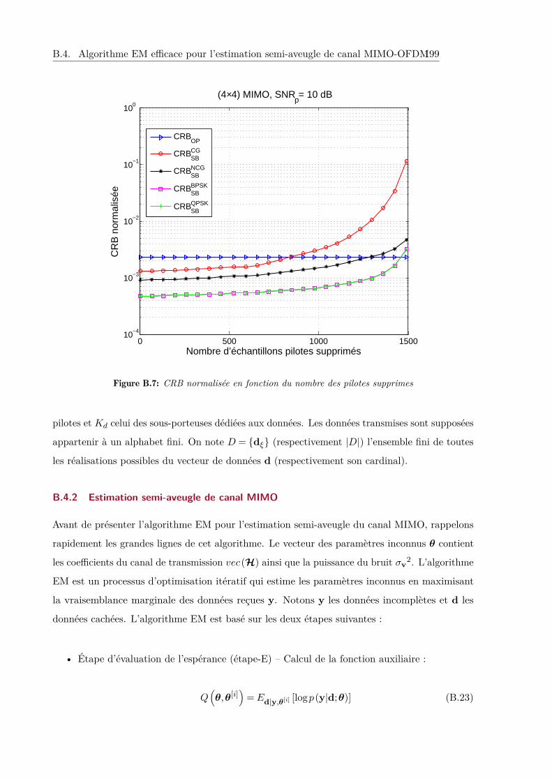
B.4. Algorithme EM efficace pour l’estimation semi-aveugle de canal MIMO-OFDM199
0 500 1000 150010−4
10−3
10−2
10−1
100
(4×4) MIMO, SNRp= 10 dB
CR
B n
orm
alis
ée
Nombre d’échantillons pilotes supprimés
CRBOP
CRBSBCG
CRBSBNCG
CRBSBBPSK
CRBSBQPSK
Figure B.7: CRB normalisée en fonction du nombre des pilotes supprimes
pilotes et Kd celui des sous-porteuses dédiées aux données. Les données transmises sont supposées
appartenir à un alphabet fini. On note D = {dξ} (respectivement |D|) l’ensemble fini de toutes
les réalisations possibles du vecteur de données d (respectivement son cardinal).
B.4.2 Estimation semi-aveugle de canal MIMO
Avant de présenter l’algorithme EM pour l’estimation semi-aveugle du canal MIMO, rappelons
rapidement les grandes lignes de cet algorithme. Le vecteur des paramètres inconnus θ contient
les coefficients du canal de transmission vec(H) ainsi que la puissance du bruit σv2. L’algorithme
EM est un processus d’optimisation itératif qui estime les paramètres inconnus en maximisant
la vraisemblance marginale des données reçues y. Notons y les données incomplètes et d les
données cachées. L’algorithme EM est basé sur les deux étapes suivantes :
• Étape d’évaluation de l’espérance (étape-E) – Calcul de la fonction auxiliaire :
Q(θ,θ[i]
)= Ed|y,θ[i] [logp(y|d;θ)] (B.23)
200 Appendix B. French summary
• Étape de maximisation (étape-M) – Calcul de θ[i+1] qui maximise Q(θ,θ[i]
)comme :
θ[i+1] = arg maxθQ(θ,θ[i]
)(B.24)
La convergence de l’algorithme EM à un maximum local a été montrée et discutée dans [88].
B.4.2.1 Algorithme EM pour l’estimation semi-aveugle de canal MIMO
Cette section met en oeuvre l’algorithme EM pour l’estimation semi-aveugle du canal MIMO. Lafonction du maximum de vraisemblance est donnée par :
p(y;θ) =Kp−1Πk=0
p(y(k) ;θ)K−1Π
k=Kpp(y(k) ;θ) , (B.25)
où p(y(k);θ)∼N(W(k)Hdp(k),σ2
vI), pour
k = 0, · · · , Kp− 1, dp(k) est le vecteur contenant la séquence pilote de la k-ème sous-porteuse; etpour k =Kp, · · ·K − 1, on a :
p(y(k) ;θ) =|D|∑ξ=1
p(y(k)|dξ;θ
)p(dξ), (B.26)
avec p(y(k)|dξ;θ
)∼N
(W(k)Hdξ,σ2
vI).
Étape-E : Après simplification, Q(θ,θ[i]
)devient :
Q(θ,θ[i]
)=Kp−1∑k=0
logp(y(k)|dp(k);θ) +K−1∑k=Kp
|D|∑ξ=1
αk,ξ
(θ[i])
logp(y(k)|dξ ;θ
), (B.27)
où
αk,ξ
(θ[i])
=p(
y(k) |dξ ;θ[i])p(dξ)
|D|∑ξ′=1
p(
y(k) |dξ′ ;θ[i])p(dξ′) . (B.28)
Dans ce travail, toutes les réalisations dξ sont équiprobables. Le terme p(dξ)est alors ignoré
dans l’équation (B.28).
Étape-M : Cette étape estime θ, c.a.d. la matrice des coefficients du canal H et la puissance
du bruit σ2v en maximisant la fonction auxiliaire :
θ[i+1] = arg maxθ
Q(θ,θ[i]
). (B.29)
En mettant à zéro la dérivée de Q(θ,θ[i]
), donnée par l’équation (B.27), par rapport à H et
en utilisant la propriété suivante de l’opérateur vec :vec(ACB) =
(BT ⊗A
)vec(C), on obtient :
vec(
H[i+1])
=
[Kp−1∑k=0
(dp(k)∗dp(k)T ⊗W(k)HW(k)
)+K−1∑k=Kp
|D|∑ξ=1
αk,ξ
(θ[i])(
dξ∗dξT ⊗W(k)HW(k))]−1
×
[Kp−1∑k=0
vec(
W(k)Hyp (k)dp(k)H)
+K−1∑k=Kp
|D|∑ξ=1
αk,ξ
(θ[i])vec(
W(k)Hy(k)dξH)]
.
(B.30)
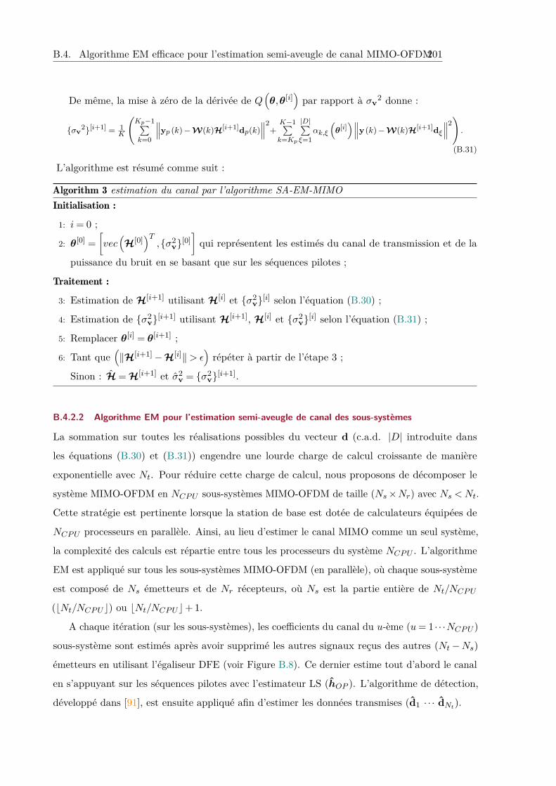
B.4. Algorithme EM efficace pour l’estimation semi-aveugle de canal MIMO-OFDM201
De même, la mise à zéro de la dérivée de Q(θ,θ[i]
)par rapport à σv
2 donne :
{σv2}[i+1] = 1K
(Kp−1∑k=0
∥∥∥yp (k)−W(k)H[i+1]dp(k)∥∥∥2
+K−1∑k=Kp
|D|∑ξ=1
αk,ξ
(θ[i])∥∥∥y(k)−W(k)H[i+1]dξ
∥∥∥2).
(B.31)
L’algorithme est résumé comme suit :
Algorithm 3 estimation du canal par l’algorithme SA-EM-MIMOInitialisation :
1: i= 0 ;
2: θ[0] =[vec
(H[0]
)T,{σ2
v}[0]]qui représentent les estimés du canal de transmission et de la
puissance du bruit en se basant que sur les séquences pilotes ;
Traitement :
3: Estimation de H[i+1] utilisant H[i] et {σ2v}[i] selon l’équation (B.30) ;
4: Estimation de {σ2v}[i+1] utilisant H[i+1], H[i] et {σ2
v}[i] selon l’équation (B.31) ;
5: Remplacer θ[i] = θ[i+1] ;
6: Tant que(‖H[i+1]−H[i]‖> ε
)répéter à partir de l’étape 3 ;
Sinon : H = H[i+1] et σ2v = {σ2
v}[i+1].
B.4.2.2 Algorithme EM pour l’estimation semi-aveugle de canal des sous-systèmes
La sommation sur toutes les réalisations possibles du vecteur d (c.a.d. |D| introduite dans
les équations (B.30) et (B.31)) engendre une lourde charge de calcul croissante de manière
exponentielle avec Nt. Pour réduire cette charge de calcul, nous proposons de décomposer le
système MIMO-OFDM en NCPU sous-systèmes MIMO-OFDM de taille (Ns×Nr) avec Ns <Nt.
Cette stratégie est pertinente lorsque la station de base est dotée de calculateurs équipées de
NCPU processeurs en parallèle. Ainsi, au lieu d’estimer le canal MIMO comme un seul système,
la complexité des calculs est répartie entre tous les processeurs du système NCPU . L’algorithme
EM est appliqué sur tous les sous-systèmes MIMO-OFDM (en parallèle), où chaque sous-système
est composé de Ns émetteurs et de Nr récepteurs, où Ns est la partie entière de Nt/NCPU(bNt/NCPUc) ou bNt/NCPUc+ 1.
A chaque itération (sur les sous-systèmes), les coefficients du canal du u-ème (u= 1 · · ·NCPU )
sous-système sont estimés après avoir supprimé les autres signaux reçus des autres (Nt−Ns)
émetteurs en utilisant l’égaliseur DFE (voir Figure B.8). Ce dernier estime tout d’abord le canal
en s’appuyant sur les séquences pilotes avec l’estimateur LS (hOP ). L’algorithme de détection,
développé dans [91], est ensuite appliqué afin d’estimer les données transmises (d1 · · · dNt).
202 Appendix B. French summary
Pour estimer le canal du u-ème sous-système MIMO, les signaux transmis par les autres
émetteurs sont considérés comme interférences et par conséquent sont soustraits au signal reçu
comme suit :
ysub−MIMOu (k) = y(k)−W(k)Hudu(k)
= W(k)Hudu(k) + zu(k),(B.32)
où ysub−MIMOu (k) est un estimé du signal reçu uniquement des Ns utilisateurs du u-ème sous-
système, Hu représente les Ns colonnes de la matrice H correspondant aux coefficients du canal
de transmission du u-ème sous-système. Hu est l’estimée de la matrice du canal des (Nt−Ns)
utilisateurs interférants, c.a.d. Hu est égale à H dans laquelle les Ns colonnes qui correspondent
au u-ème sous-système sont supprimés.zu(k) représente le bruit et les termes résiduels d’interférence. Sous l’hypothèse que zu(k)∼
N(0,σ2
zuI), on peut écrire :
p(
ysub−MIMOu (k) ;θu
)∼N
(W(k)Hudu(k),σ2
zuI), (B.33)
où θu =[HTu ,σ
2zu]T est le vecteur des paramètres inconnus.
En faisant ce traitement, on obtient NCPU sous-systèmes MIMO-OFDM pouvant être traités
indépendamment, en parallèle, selon l’algorithme EM itératif suivant :
Pour u= 1, · · · ,NCPU :Etape-E : La fonction auxiliaire Q
(θu,θ
[i]u
)est écrite comme suit :
Q(θu,θ
[i]u
)=Kp−1∑k=0
logp(
ysub−MIMOp,u (k) |dp,u(k);θu
)+
K−1∑k=Kp
|Du|∑ξ=1
αk,ξ
(θ
[i]u
)logp
(ysub−MIMOu (k) |dξ ;θu
),
(B.34)
où {dp,u(k)} représente les symboles pilotes, |Du| est l’ensemble des réalisations possibles dessymboles du u-ème sous-système avec :
p(
ysub−MIMOp,u (k) |dp,u(k);θu
)∼N
(W(k)Hudp,u(k),σ2
zuI), (B.35)
p(
ysub−MIMOu (k) |dξ ;θu
)∼N
(W(k)Hudξ ,σ
2zuI), (B.36)
αk,ξ
(θ
[i]u
)=
p(
ysub−MIMOu (k) |dξ ;θ
[i]u
)p(dξ)
|Du|∑ξ′=1
p(
ysub−MIMOu (k) |dξ′ ;θ
[i]u
)p(dξ′) . (B.37)
Étape-M : En mettant à zero la dérivée de Q(θu,θ
[i]u
)donnée dans l’équation (B.34) par rapport
à Hu, on obtient :
H[i+1]u =
[Kp−1∑k=0
W(k)HW(k)dpt,u(k)d∗pt,u(k) +K−1∑k=Kp
|Du|∑ξ=1
αk,ξ,t
(θ
[i]u
)W(k)HW(k)dξd∗ξ
]−1
×
(Kp−1∑k=0
W(k)Hysub−MIMOpt,u (k)d∗pt,u(k) +
K−1∑k=Kp
|Du|∑ξ=1
αk,ξ,t
(θ
[i]u
)W(k)Hysub−MIMO
u,t (k)d∗ξ
).
(B.38)
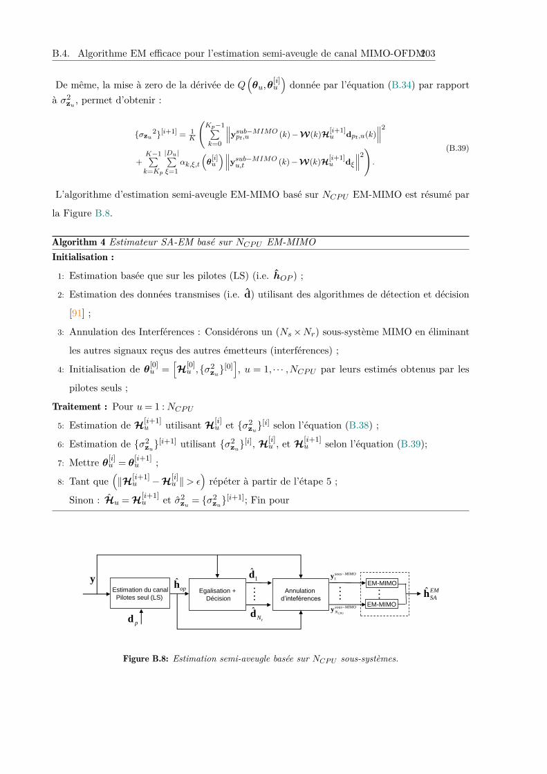
B.4. Algorithme EM efficace pour l’estimation semi-aveugle de canal MIMO-OFDM203
De même, la mise à zero de la dérivée de Q(θu,θ
[i]u
)donnée par l’équation (B.34) par rapport
à σ2zu , permet d’obtenir :
{σzu2}[i+1] = 1
K
(Kp−1∑k=0
∥∥∥ysub−MIMOpt,u (k)−W(k)H[i+1]
u dpt,u(k)∥∥∥2
+K−1∑k=Kp
|Du|∑ξ=1
αk,ξ,t
(θ
[i]u
)∥∥∥ysub−MIMOu,t (k)−W(k)H[i+1]
u dξ∥∥∥2).
(B.39)
L’algorithme d’estimation semi-aveugle EM-MIMO basé sur NCPU EM-MIMO est résumé par
la Figure B.8.
Algorithm 4 Estimateur SA-EM basé sur NCPU EM-MIMOInitialisation :
1: Estimation basée que sur les pilotes (LS) (i.e. hOP ) ;
2: Estimation des données transmises (i.e. d) utilisant des algorithmes de détection et décision
[91] ;
3: Annulation des Interférences : Considérons un (Ns×Nr) sous-système MIMO en éliminant
les autres signaux reçus des autres émetteurs (interférences) ;
4: Initialisation de θ[0]u =
[H[0]u ,{σ2
zu}[0]], u = 1, · · · ,NCPU par leurs estimés obtenus par les
pilotes seuls ;
Traitement : Pour u= 1 :NCPU5: Estimation de H[i+1]
u utilisant H[i]u et {σ2
zu}[i] selon l’équation (B.38) ;
6: Estimation de {σ2zu}
[i+1] utilisant {σ2zu}
[i], H[i]u , et H[i+1]
u selon l’équation (B.39);
7: Mettre θ[i]u = θ[i+1]
u ;
8: Tant que(‖H[i+1]
u −H[i]u ‖> ε
)répéter à partir de l’étape 5 ;
Sinon : Hu = H[i+1]u et σ2
zu = {σ2zu}
[i+1]; Fin pour
….
Estimation du canal
Pilotes seul (LS) Egalisation +
Décision
y
pd
ˆoph
1d
ˆtNd
Annulation
d’inteférences
1
sous MIMOy
….
EM-MIMO
ˆ EM
SAhEM-MIMO
…
CPU
sous MIMO
N
y
Figure B.8: Estimation semi-aveugle basée sur NCPU sous-systèmes.
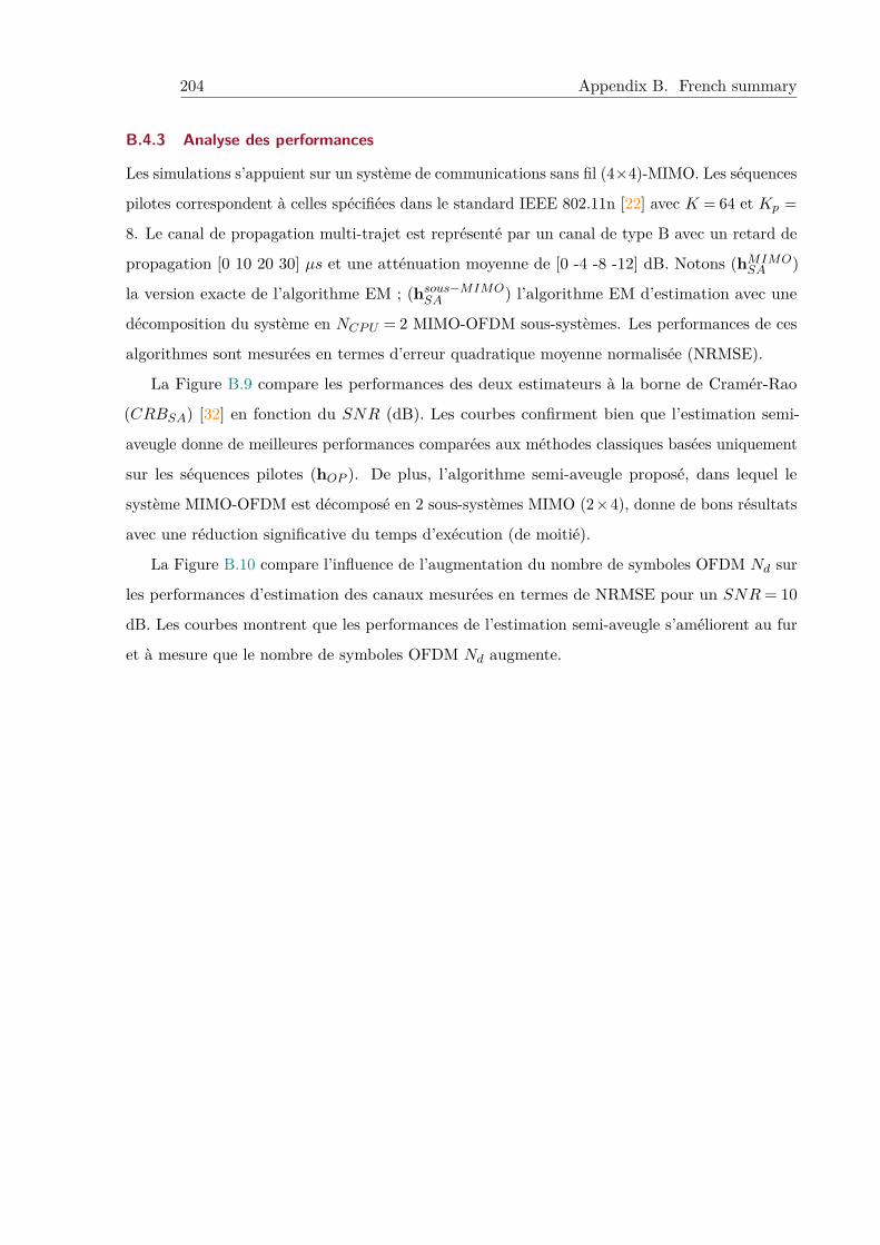
204 Appendix B. French summary
B.4.3 Analyse des performances
Les simulations s’appuient sur un système de communications sans fil (4×4)-MIMO. Les séquences
pilotes correspondent à celles spécifiées dans le standard IEEE 802.11n [22] avec K = 64 et Kp =
8. Le canal de propagation multi-trajet est représenté par un canal de type B avec un retard de
propagation [0 10 20 30] µs et une atténuation moyenne de [0 -4 -8 -12] dB. Notons (hMIMOSA )
la version exacte de l’algorithme EM ; (hsous−MIMOSA ) l’algorithme EM d’estimation avec une
décomposition du système en NCPU = 2 MIMO-OFDM sous-systèmes. Les performances de ces
algorithmes sont mesurées en termes d’erreur quadratique moyenne normalisée (NRMSE).
La Figure B.9 compare les performances des deux estimateurs à la borne de Cramér-Rao
(CRBSA) [32] en fonction du SNR (dB). Les courbes confirment bien que l’estimation semi-
aveugle donne de meilleures performances comparées aux méthodes classiques basées uniquement
sur les séquences pilotes (hOP ). De plus, l’algorithme semi-aveugle proposé, dans lequel le
système MIMO-OFDM est décomposé en 2 sous-systèmes MIMO (2×4), donne de bons résultats
avec une réduction significative du temps d’exécution (de moitié).
La Figure B.10 compare l’influence de l’augmentation du nombre de symboles OFDM Nd sur
les performances d’estimation des canaux mesurées en termes de NRMSE pour un SNR= 10
dB. Les courbes montrent que les performances de l’estimation semi-aveugle s’améliorent au fur
et à mesure que le nombre de symboles OFDM Nd augmente.
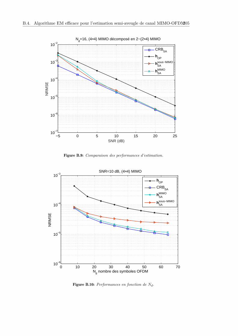
B.4. Algorithme EM efficace pour l’estimation semi-aveugle de canal MIMO-OFDM205
−5 0 5 10 15 20 2510−7
10−6
10−5
10−4
10−3
10−2
SNR (dB)
NR
MS
E
Nd=16, (4×4) MIMO décomposé en 2−(2×4) MIMO
CRBSA
hOP
hSAsous−MIMO
hSAMIMO
Figure B.9: Comparaison des performances d’estimation.
0 10 20 30 40 50 60 7010−6
10−5
10−4
10−3SNR=10 dB, (4×4) MIMO
NR
MS
E
Nd nombre des symboles OFDM
hOP
CRBSA
hSAMIMO
hSAsous−MIMO
Figure B.10: Performances en fonction de Nd.
206 Appendix B. French summary
B.5 Conclusion
L’estimation du canal est d’une importance capitale pour l’égalisation et la détection des symboles
dans la plupart des systèmes de communications sans fil, en particulier dans les systèmes MIMO-
OFDM. Il suscite dès lors l’intérêt des chercheurs et des développeurs de systèmes depuis le
XXe siècle. Une avancée spectaculaire a été réalisée avec le développement et la mise en œuvre
d’algorithmes d’estimation de canal basés sur les pilotes, motivés par sa faible complexité
et sa faisabilité en ce qui concerne les calculateurs disponibles à cette époque. L’apparition
d’ordinateurs puissants (processeurs) disponibles aux stations de base et la forte demande
en débits de données plus élevés ont conduit à envisager d’autres approches d’estimation de
canaux. Les approches proposées, principalement les techniques semi-aveugles, augmentent le
débit de données en réduisant le nombre de pilotes transmis, car ces derniers ne transmettent
pas d’informations et représentent un gaspillage de la bande passante. En outre, de nombreux
problématiques sont faiblement étudiés dans la littérature en ce qui concerne l’estimation du canal
semi-aveugle. Cette thèse est l’une des contributions traitant de l’identification de canaux de de
transmission en semi-aveugle et de son analyse dans le contexte des systèmes MIMO-OFDM.
Plusieurs contributions à l’estimation semi-aveugle du canal de transmission ont été réalisées
dans cette thèse : la quantification du taux maximum de réduction des pilotes transmis en
utilisant l’estimation semi-aveugle du canal tout en garantissant la même qualité d’estimation
basée sur les pilotes, puis le développement d’estimateurs semi-aveugles efficaces du canal (LS-DF,
méthodes sous-espace, algorithmes basés sur l’algorithme EM). De plus, d’autres études sur les
limites de performance de l’estimation de canal MIMO-OFDM ont été abordées, notamment
l’analyse de l’effet du CFO sur les performances de l’estimation de canal. Ci-dessous, nous
résumons brièvement le travail réalisé dans de cette thèse.
Premièrement, les limites de performance théoriques pour les méthodes d’estimation de
canaux semi-aveugles et basées sur des pilotes ont été abordées dans le contexte des systèmes
MIMO-OFDM et des systèmes massifs MIMO-OFDM. Cette analyse a été réalisée par le biais
de la dérivation analytique des CRB pour différents modèles de données (CG, NCG et BPSK /
QPSK) et pour différents modèles de conception pilotes (par exemple, agencement pilote de type
bloc, type réseau et type peigne). L’étude des CRB dérivés montre l’énorme réduction du nombre
d’échantillons pilotes et, par conséquent, le gain en débit obtenu grâce à l’approche semi-aveugle,
tout en conservant la même qualité d’estimation de canal en utilisant que les pilotes. Dans cette
thèse, nous montrons que, en utilisant les techniques semi-aveugle, la réduction peut dépasser
95% (modèle de données BPSK) de la taille originale.
B.5. Conclusion 207
Cette étude a également été étendue aux grands systèmes MIMO-OFDM (10× 10), où
nous montrons que les gains de performance sont légèrement supérieurs à ceux observés pour
les systèmes MIMO-OFDM de taille plus petite. De plus, la même étude, a été généralisée
aux systèmes massifs multi-cellules MIMO-OFDM sous l’effet de la contamination des pilotes.
Par la suite, nous avons montré qu’en utilisant les méthodes semi-aveugle, il est possible de
résoudre efficacement le problème de contamination des pilotes lorsqu’on considère des signaux
de communications en alphabet fini.
Deuxièmement, nous avons étudié l’effet du CFO sur les performances de l’estimation de
canal à l’aide de l’outil CRB. En raison de la propriété de cyclostationnarité du CFO, nous
montrons que le CFO impacte avantageusement l’estimation du canal semi-aveugle. Dans le cas
du système de communications MISO-OFDM basé sur des protocoles de transmission à relais
multiples, nous avons proposé deux approches efficaces pour estimer conjointement le canal de
transmission et les CFO. Dans le même contexte, une autre étude a été menée pour évaluer
et comparer les CRB pour l’estimation des coefficients de canal de sous-porteuse avec et sans
considération de la structure OFDM (c’est-à-dire l’estimation des coefficients de canal dans le
domaine temporel ou fréquentiel). Cette étude met en évidence le gain significatif associé à
l’approche du domaine temporel.
Troisièmement, nous avons proposé quatre algorithmes d’estimation semi-aveugle de canal.
Nous avons commencé par le plus simple (LS-DF) qui repose sur l’estimateur LS utilisé con-
jointement avec un retour de décision dans lequel les données estimées sont réinjectées à l’étape
d’estimation de canal pour améliorer les performances de l’estimation. Dans le contexte des
communications écologiques, nous avons montré que, grâce à l’algorithme semi-aveugle LS-DF,
on pouvait réduire jusqu’à 76% de la puissance transmise par les pilotes.
La seconde approche semi-aveugle repose sur la technique du maximum de vraisemblance (ML),
l’une des méthodes d’estimation les plus efficaces mais aussi les plus coûteuses. L’optimisation du
critère ML se fait par une technique itérative utilisant l’algorithme EM. Nous avons proposé trois
approches d’approximation/simplification pour traiter la complexité numérique de l’algorithme
EM classique. Les trois approximations proposées (à savoir EM-MISO, S-EM, EM-SIMO)
donnent de bonnes performances à un coût de calcul inférieur par rapport à l’algorithme EM
classique.
Enfin, pour le cas pratique du modèle à canal spéculaire, nous avons proposé une approche
paramétrique basée sur une estimation des temps d’arrivés (TOA) utilisant des méthodes sous-
espace pour les systèmes SISO-OFDM. L’estimation semi-aveugle des TOAs est réalisée à l’aide
208 Appendix B. French summary
d’un processus de retour de décision qui améliore les performances de l’estimation des TOAs à
partir d’une première estimation obtenue grâce aux pilotes existants. Les principales contributions
de cette thèse sont énumérées ci-dessous :
• Dérivation des CRB d’estimation de canal pour différents modèles de données (CG, NCG,
BPSK / QPSK) et pour différents modèles de conception pilote (agencement pilote de type
bloc, type réseau et type peigne) dans le cas du système MIMO-OFDM .
• Pour le modèle de données BPSK / QPSK, une approximation réaliste du CRB a été
donnée pour contourner la grande complexité du calcul exact du CRB.
• Proposition d’une technique de calcul efficace pour traiter la manipulation des matrices de
grande taille nécessaire pour le calcul des CRBs dans le scénario MIMO de grande taille et
le MIMO massif.
• Quantification du taux de réduction des séquences pilotes grâce à l’utilisation de l’estimation
semi-aveugle du canal.
• Dérivation des CRB d’estimation semi-aveugle du canal pour un système MIMO-OFDM
massif multicellulaire en tenant en compte le phénomène de contamination des pilotes.
• Étude de l’efficacité de l’estimation semi-aveugle du canal de transmission pour résoudre le
problème de contamination des pilotes.
• Contribution à la protection des drones contre l’interception aveugle à l’aide de l’analyse
des CRBs dans le contexte aveugle.
• Dérivation des CRB d’estimation semi-aveugle de canal en présence de CFO dans le système
MIMO-OFDM et l’étude de l’impact positif de CFO sur les performances de l’estimation
de canal.
• Proposition de deux approches pour estimer conjointement les coefficients CFO et le canal
de transmission.
• Quantification de la dégradation des performances entre l’estimation des coefficients de
canal dans le domaine temporel ou fréquentiel.
• Contribution aux communications écologiques en quantifiant la réduction de la puissance
transmise à l’aide d’une estimation semi-aveugle de canal.
B.5. Conclusion 209
• Proposition de un estimateur semi-aveugle de canal basé sur la stratégie de retour de
décision (LS-DF).
• Contribution à l’estimation semi-aveugle du canal en utilisant l’algorithme EM dans le cas
du système MIMO-OFDM.
• Dérivation de quatre versions simplifiées de l’algorithme semi-aveugle EM classique.
• Contribution à l’estimation semi-aveugle sous-espace du canal pour le système MIMO-
OFDM.
• Dérivation d’une méthode semi-aveugle paramétrique pour estimer les paramètres de canal
(TOA) dans le cas d’un canal OFDM spéculaire.

210 Appendix B. French summary
Bibliography
[1] J. A. del Peral-Rosado, R. Raulefs, J. A. López-Salcedo, and G. Seco-Granados, “Survey
of cellular mobile radio localization methods: From 1G to 5G,” IEEE Communications
Surveys Tutorials, vol. 20, no. 2, pp. 1124–1148, 2018.
[2] G. Gu and G. Peng, “The survey of GSM wireless communication system,” in 2010
International Conference on Computer and Information Application, Dec 2010, pp. 121–
124.
[3] L. L. Hanzo, L.-L. Yang, E.-L. Kuan, and K. Yen, Overview of Multicarrier CDMA.
IEEE, 2004. [Online]. Available: https://ieeexplore.ieee.org/document/5732959
[4] F. W. Y. Bouguen, E. Hardouin, LTE et les réseaux 4G. Paris, France: Editions Eyrolles,
2013.
[5] A. J. PAULRAJ, D. A. GORE, R. U. NABAR, and H. BOLCSKEI, “An overview of
MIMO communications - a key to gigabit wireless,” Proceedings of the IEEE, vol. 92, no. 2,
pp. 198–218, Feb 2004.
[6] K. Choi and H. Liu, MIMO System - Part II: Spatial Multiplexing. IEEE, 2016. [Online].
Available: https://ieeexplore.ieee.org/document/7435069
[7] F. D. Flaviis, L. Jofre, J. Romeu, and A. Grau, Multiantenna Systems
for MIMO Communications. Morgan and Claypool, 2013. [Online]. Available:
https://ieeexplore.ieee.org/document/6812510
[8] A. Narasimhamurthy, M. Banavar, and C. Tepedelenliouglu, OFDM Systems
for Wireless Communications. Morgan and Claypool, 2010. [Online]. Available:
https://ieeexplore.ieee.org/document/6812632
[9] C. O. B. Clerckx, MIMO wireless networks. The Boulevard, Langford Lane, Kindlinton,
Oxford, OX51 GB: ACADEMIC PRESS, 2013.
212 Bibliography
[10] M. Jiang and L. Hanzo, “Multiuser MIMO-OFDM for next-generation wireless systems,”
Proceedings of the IEEE, vol. 95, no. 7, pp. 1430–1469, July 2007.
[11] S. Aust, R. V. Prasad, and I. G. M. M. Niemegeers, “Outdoor long-range wlans: A lesson
for ieee 802.11ah,” IEEE Communications Surveys Tutorials, vol. 17, no. 3, pp. 1761–1775,
thirdquarter 2015.
[12] B. P. Crow, I. Widjaja, J. G. Kim, and P. T. Sakai, “Ieee 802.11 wireless local area
networks,” IEEE Communications Magazine, vol. 35, no. 9, pp. 116–126, Sep. 1997.
[13] I.-T. Lu and K.-J. Tsai, “Channel estimation in a proposed IEEE802.11n OFDM MIMO
WLAN system,” in IEEE Sarnoff Symposium, April 2007, pp. 1–5.
[14] E. G. Larsson, O. Edfors, F. Tufvesson, and T. L. Marzetta, “Massive MIMO for next
generation wireless systems,” IEEE Communications Magazine, vol. 52, no. 2, pp. 186–195,
February 2014.
[15] R. Vannithamby and S. Talwar, Massive MIMO Communications. Wiley, 2017. [Online].
Available: https://ieeexplore.ieee.org/document/8042298
[16] F. Rusek, D. Persson, B. K. Lau, E. G. Larsson, T. L. Marzetta, O. Edfors, and F. Tufvesson,
“Scaling up MIMO: Opportunities and challenges with very large arrays,” IEEE Signal
Processing Magazine, vol. 30, no. 1, pp. 40–60, Jan 2013.
[17] T. L. Marzetta, “Noncooperative cellular wireless with unlimited numbers of base station
antennas,” IEEE Transactions on Wireless Communications, vol. 9, no. 11, pp. 3590–3600,
2010.
[18] H. Q. Ngo, E. G. Larsson, and T. L. Marzetta, “Energy and spectral efficiency of very
large multiuser MIMO systems,” IEEE Transactions on Communications, vol. 61, no. 4,
pp. 1436–1449, 2013.
[19] O. Simeone, Y. Bar-Ness, and U. Spagnolini, “Pilot-based channel estimation for OFDM
systems by tracking the delay-subspace,” IEEE Trans. on Wireless Communications, vol. 3,
no. 1, pp. 315–325, Jan 2004.
[20] W. Zhang, X. G. Xia, and P. C. Ching, “Optimal training and pilot pattern design for
OFDM systems in Rayleigh fading,” IEEE Trans. on Broadcasting, vol. 52, no. 4, pp.
505–514, Dec 2006.
Bibliography 213
[21] G. B. Jency and S. J. Gladwin, “Channel estimation using optimized pilot placement in
OFDM system,” in Communications and Signal Processing (ICCSP), 2014 International
Conference on. IEEE, 2014, pp. 1529–1534.
[22] R. S. E. Perahi, Next Generation Wireless LANS. New York, USA: Cambridge University
Press, 2008.
[23] S. Noh, Y. Sung, and M. D. Zoltowski, “A new precoder design for blind channel estimation
in MIMO-OFDM systems,” IEEE Trans. on Wireless Communications, vol. 13, no. 12, pp.
7011–7024, Dec 2014.
[24] L. Tong, G. Xu, and T. Kailath, “Blind identification and equalization based on second-
order statistics: a time domain approach,” IEEE Trans. on Information Theory., Mar
1994.
[25] C. Shin, R. W. Heath, and E. J. Powers, “Blind channel estimation for MIMO-OFDM
systems,” IEEE Trans. on Vehicular Technology, vol. 56, no. 2, pp. 670–685, March 2007.
[26] A. K. Jagannatham and B. D. Rao, “Whitening-rotation-based semi-blind MIMO channel
estimation,” IEEE Trans. on Signal Processing, vol. 54, no. 3, pp. 861–869, March 2006.
[27] K. Liu, J. P. C. L. da Costa, H. C. So, and A. L. F. de Almeida, “Semi-blind receivers
for joint symbol and channel estimation in space-time-frequency MIMO-OFDM systems,”
IEEE Trans. on Signal Processing, vol. 61, no. 21, pp. 5444–5457, Nov 2013.
[28] G. Favier and A. L. F. de Almeida, “Tensor space-time-frequency coding with semi-blind
receivers for MIMO wireless communication systems,” IEEE Trans. on Signal Processing,
vol. 62, no. 22, pp. 5987–6002, Nov 2014.
[29] W. Yang, Y. Cai, and Y. Xun, “Semi-blind channel estimation for OFDM systems,” in
IEEE 63rd Vehicular Technology Conference, vol. 1, May 2006, pp. 226–230.
[30] R. C. de Lamare, “Massive MIMO systems: Signal processing challenges and research
trends,” arXiv preprint arXiv:1310.7282, 2013.
[31] N. Hassan and X. Fernando, “Massive MIMO wireless networks: An overview,” Electronics,
vol. 6, no. 3, p. 63, 2017.
214 Bibliography
[32] A. Ladaycia, A. Mokraoui, K. Abed-Meraim, and A. Belouchrani, “Performance bounds
analysis for semi-blind channel estimation in MIMO-OFDM communications systems,”
IEEE Trans. on Wireless Communications, vol. 16, no. 9, pp. 5925–5938, Sept 2017.
[33] ——, “Toward green communications using semi-blind channel estimation,” in 25th Euro-
pean Signal Processing Conference (EUSIPCO), Aug 2017, pp. 2254–2258.
[34] A. K. Jagannatham and B. D. Rao, “Complex constrained CRB and its application to
semi-blind MIMO and OFDM channel estimation,” in Processing Workshop Proceedings,
2004 Sensor Array and Multichannel Signal, July 2004, pp. 397–401.
[35] S.-M. Omar, D. Slock, and O. Bazzi, “Bayesian and deterministic crbs for semi-blind
channel estimation in SIMO single carrier cyclic prefix systems,” in IEEE 22nd International
Symposium on Personal Indoor and Mobile Radio Communications (PIMRC), Sept 2011,
pp. 1682–1686.
[36] S. M. Kay, Fundamentals of Statistical signal processing, Estimation Theory. Upper Saddle
River, New Jersey 07458, USA: Prentice Hall PTR, INC, 1993.
[37] D.-T. Do and D.-T. Vu, “New orthogonal pilot scheme for semi-blind channel estimation in
MIMO systems,” in International Conference on Networking and Information Technology,
June 2010, pp. 235–238.
[38] S. Park, E. Serpedin, and K. Qaraqe, “Gaussian assumption: The least favorable but the
most useful [lecture notes],” IEEE Signal Processing Magazine, vol. 30, no. 3, pp. 183–186,
May 2013.
[39] T. Menni, E. Chaumette, P. Larzabal, and J. Barbot, “New results on deterministic
cramer-rao bounds for real and complex parameters,” IEEE Trans. on Signal Processing,
vol. 60, no. 3, pp. 1032–1049, March 2012.
[40] L. Berriche and K. Abed-Meraim, “Stochastic Cramér-Rao bounds for semiblind MIMO
channel estimation,” in IEEE International Symposium on Signal Processing and Informa-
tion Technology, Dec 2004, pp. 119–122.
[41] J. P. Delmas and H. Abeida, “Stochastic cramer-rao bound for noncircular signals with
application to DOA estimation,” IEEE Trans. on Signal Processing, vol. 52, no. 11, pp.
3192–3199, Nov 2004.
Bibliography 215
[42] K. Lee, J. Kim, J. Jung, and I. Lee, “Zadoff-chu sequence based signature identification
for OFDM,” IEEE Trans. on Wireless Communications, vol. 12, no. 10, pp. 4932–4942,
October 2013.
[43] H. Yin, D. Gesbert, M. C. Filippou, and Y. Liu, “Decontaminating pilots in massive MIMO
systems,” in IEEE International Conference on Communications (ICC), June 2013, pp.
3170–3175.
[44] X. Zheng, H. Zhang, W. Xu, and X. You, “Semi-orthogonal pilot design for massive
MIMO systems using successive interference cancellation,” in IEEE Global Communications
Conference, Dec 2014, pp. 3719–3724.
[45] O. Rekik, A. Ladaycia, K. Abed-Meraim, and A. Mokraoui, “Performance bounds analysis
for semi-blind channel estimation with pilot contamination in massive MIMO-OFDM
systems,” in 26th European Signal Processing Conference (EUSIPCO), Sep 2018.
[46] F. Boccardi, R. W. Heath, A. Lozano, T. L. Marzetta, and P. Popovski, “Five disruptive
technology directions for 5G,” IEEE Communications Magazine, vol. 52, no. 2, pp. 74–80,
2014.
[47] J. Jose, A. Ashikhmin, T. L. Marzetta, and S. Vishwanath, “Pilot contamination problem
in multi-cell TDD systems,” in International Symposium on Information Theory (ISIT).
IEEE, 2009, pp. 2184–2188.
[48] F. Fernandes, A. Ashikhmin, and T. L. Marzetta, “Inter-cell interference in noncooperative
TDD large scale antenna systems,” IEEE Journal on Selected Areas in Communications,
vol. 31, no. 2, pp. 192–201, 2013.
[49] J. Hoydis, S. Ten Brink, and M. Debbah, “Massive MIMO in the UL/DL of cellular networks:
How many antennas do we need?” IEEE Journal on selected Areas in Communications,
vol. 31, no. 2, pp. 160–171, 2013.
[50] H. Yin, D. Gesbert, M. Filippou, and Y. Liu, “A coordinated approach to channel es-
timation in large-scale multiple-antenna systems,” IEEE Journal on Selected Areas in
Communications, vol. 31, no. 2, pp. 264–273, 2013.
[51] J. Ma and L. Ping, “Data-aided channel estimation in large antenna systems,” in Interna-
tional Conference on Communications (ICC). IEEE, 2014, pp. 4626–4631.
216 Bibliography
[52] A. Ashikhmin and T. Marzetta, “Pilot contamination precoding in multi-cell large scale
antenna systems,” in International Symposium on Information Theory (ISIT). IEEE,
2012, pp. 1137–1141.
[53] L. Li, A. Ashikhmin, and T. Marzetta, “Pilot contamination precoding for interference
reduction in large scale antenna systems,” in 51st Annual Allerton Conference on Commu-
nication, Control, and Computing. IEEE, 2013, pp. 226–232.
[54] J. Fan, W. Li, and Y. Zhang, “Pilot contamination mitigation by fractional pilot reuse
with threshold optimization in massive MIMO systems,” Digital Signal Processing, 2018.
[55] T. Peken, G. Vanhoy, and T. Bose, “Blind channel estimation for massive MIMO,” Analog
Integrated Circuits and Signal Processing, vol. 91, no. 2, pp. 257–266, 2017.
[56] E. Amiri, R. Mueller, and W. Gerstacker, “Blind pilot decontamination in massive MIMO
by Independent Component Analysis,” in Globecom Workshops. IEEE, 2017, pp. 1–5.
[57] D. Hu, L. He, and X. Wang, “Semi-blind pilot decontamination for massive MIMO systems,”
IEEE Transactions on Wireless Communications, vol. 15, no. 1, pp. 525–536, 2016.
[58] A. S. Alwakeel and A. H. Mehana, “Semi-blind channel estimation and interference align-
ment for massive MIMO network,” in Global Communications Conference GLOBECOM.
IEEE, 2017, pp. 1–6.
[59] N. Fatema, Y. Xiang, and I. Natgunanathan, “Analysis of a semi-blind pilot decontamina-
tion method in massive MIMO,” in 27th International Telecommunication Networks and
Applications Conference (ITNAC). IEEE, 2017, pp. 1–6.
[60] T. L. Marzetta, “How much training is required for multiuser MIMO?” in 40th Asilomar
Conference on Signals, Systems and Computers (ACSSC). IEEE, 2006, pp. 359–363.
[61] G. Caire, N. Jindal, M. Kobayashi, and N. Ravindran, “Multiuser MIMO achievable rates
with downlink training and channel state feedback,” IEEE Transactions on Information
Theory, vol. 56, no. 6, pp. 2845–2866, 2010.
[62] H. Abeida and J.-P. Delmas, “Gaussian Cramer-Rao bound for direction estimation of
noncircular signals in unknown noise fields,” IEEE Transactions on Signal Processing,
vol. 53, no. 12, pp. 4610–4618, 2005.
Bibliography 217
[63] K. Abed-Meraim, P. Loubaton, and E. Moulines, “A subspace algorithm for certain blind
identification problems,” IEEE Trans. on Information Theory, vol. 43, no. 2, pp. 499–511,
Mar 1997.
[64] K. Abed-Meraim, W. Qiu, and Y. Hua, “Blind system identification,” Proceedings of the
IEEE, vol. 85, no. 8, pp. 1310–1322, Aug 1997.
[65] P. Comon, “Independent Component Analysis, a new concept?” Signal processing, vol. 36,
no. 3, pp. 287–314, 1994.
[66] A. Ladaycia, A. Mokraoui, K. Abed-Meraim, and A. Belouchrani, “What semi-blind channel
estimation brings in terms of throughput gain ?” in 10th ICSPCS, Dec 2016, pp. 1–6.
[67] A. Ladaycia, A. Belouchrani, K. Abed-Meraim, and A. Mokraoui, “Parameter optimization
for defeating blind interception in drone protection,” in 2017 Seminar on Detection Systems
Architectures and Technologies (DAT), Feb 2017, pp. 1–6.
[68] S.-M. Omar, D. Slock, and O. Bazzi, “Recent insights in the bayesian and deterministic
crb for blind SIMO channel estimation,” in IEEE International Conference on Acoustics,
Speech and Signal Processing (ICASSP), March 2012, pp. 3549–3552.
[69] H. Liu and G. Xu, “Closed-form blind symbol estimation in digital communications,” IEEE
Transactions on Signal Processing, vol. 43, no. 11, pp. 2714–2723, Nov 1995.
[70] D. I. Iglesia, C. J. Escudero, and L. Castedo, “Cramer-rao bound for blind channel
estimation in multi-carrier CDMA systems,” in Signal Processing Conference, 2000 10th
European, Sept 2000, pp. 1–4.
[71] A. Ladaycia, A. Mokraoui, K. Abed-Meraim, and A. Belouchrani, “Further investigations
on the performance bounds of MIMO-OFDM channel estimation,” in 13th International
Wireless Communications and Mobile Computing Conference (IWCMC), June 2017, pp.
223–228.
[72] D. Huang and K. B. Letaief, “Carrier frequency offset estimation for ofdm systems using
subcarriers,” IEEE Trans. on Communications, vol. 54, no. 5, pp. 813–823, May 2006.
[73] J. Lei and T.-S. Ng, “A consistent OFDM carrier frequency offset estimator based on
distinctively spaced pilot tones,” IEEE Trans. on Wireless Communications, vol. 3, no. 2,
pp. 588–599, March 2004.
218 Bibliography
[74] H. Minn, Y. Li, N. Al-Dhahir, and R. Calderbank, “Pilot designs for consistent frequency
offset estimation in ofdm systems,” in IEEE International Conference on Communications,
vol. 10, June 2006, pp. 4566–4571.
[75] K. Lee and I. Lee, “Robust pilot designs for consistent frequency offset estimation in ofdm
systems,” in IEEE Global Telecommunications Conference (GLOBECOM 2010), Dec 2010,
pp. 1–5.
[76] Y. J. Liang and J. F. Chang, “Noniterative joint frequency offset and channel estimation
for mimo ofdm systems using cascaded orthogonal pilots,” IEEE Trans. on Vehicular
Technology, vol. 59, no. 8, pp. 4151–4156, Oct 2010.
[77] Y. Shen and E. Martinez, “Channel estimation in OFDM systems,” Freescale Semiconductor,
Tech. Rep., 2006.
[78] Y. Chen, S. Zhang, S. Xu, and G. Y. Li, “Fundamental trade-offs on green wireless
networks,” IEEE Commun. Magazine, June 2011.
[79] D. Feng, C. Jiang, G. Lim, L. J. Cimini, G. Feng, and G. Y. Li, “A survey of energy-efficient
wireless communications,” IEEE Commun. Surveys Tutorials, vol. 15, no. 1, pp. 167–178,
2013.
[80] K. Qian and W. Q. Wang, “Energy-efficient antenna selection in green MIMO relaying
communication systems,” Journal of Communications and Networks, vol. 18, no. 3, pp.
320–326, June 2016.
[81] T. Dong, V. Dobrev, T. Kolev, R. Rieben, S. Tomov, and J. Dongarra, “A step towards
energy efficient computing: Redesigning a hydrodynamic application on cpu-gpu,” in IEEE
28th Int. Parallel and Distributed Processing Symposium, May 2014, pp. 972–981.
[82] A. Ladaycia, A. Belouchrani, K. Abed-Meraim, and A. Mokraoui, “EM-based semi-blind
MIMO-OFDM channel estimation,” in 2018 IEEE International Conference on Acoustics,
Speech and Signal Processing (ICASSP), April 2018, pp. 3899–3903.
[83] ——, “Semi-blind MIMO-OFDM channel estimation using EM-like techniques,” IEEE
Trans. on Signal processing (submitted), July 2018.
[84] S. Park, J. W. Choi, J. Y. Seol, and B. Shim, “Expectation-maximization-based channel
estimation for multiuser MIMO systems,” IEEE Trans. on Communications, vol. 65, no. 6,
pp. 2397–2410, June 2017.
Bibliography 219
[85] G. Hu and D. Li, “EM-based channel estimation for MIMO OFDM system,” in International
Conference on Networks Security, Wireless Communications and Trusted Computing, vol. 1,
April 2009, pp. 159–162.
[86] E. Nayebi and B. D. Rao, “Semi-blind channel estimation for multiuser massive MIMO
systems,” IEEE Trans. on Signal Processing, vol. 66, no. 2, pp. 540–553, Jan 2018.
[87] ——, “Semi-blind channel estimation in massive MIMO systems with different priors on
data symbols,” in 43rd International Conference on Acoustics, Speech and Signal Processing
(ICASSP), Apr 2018.
[88] N. M. L. A. P. Dempster and D. B. Rubin, “Maximum likelihood from incomplete data
via the EM algorithm,” Journal of the Royal Statistical Society. Series B (Methodological),
vol. 39, no. 1, pp. 1–38, 1977.
[89] P. Comon and M. Rajih, “Blind identification of under-determined mixtures based on
the characteristic function,” in IEEE International Conference on Acoustics, Speech, and
Signal Processing, vol. 4, March 2005, pp. iv/1005–iv/1008 Vol. 4.
[90] J. A. Fessler and A. O. Hero, “Space-alternating generalized expectation-maximization
algorithm,” IEEE Trans. on Signal Processing, vol. 42, no. 10, pp. 2664–2677, Oct 1994.
[91] M. O. Damen, H. E. Gamal, and G. Caire, “On maximum-likelihood detection and the
search for the closest lattice point,” IEEE Trans. on Information Theory, vol. 49, no. 10,
pp. 2389–2402, Oct 2003.
[92] W. Abediseid and M. S. Alouini, “On lattice sequential decoding for the unconstrained
AWGN channel,” IEEE Trans. on Communications, vol. 61, no. 6, pp. 2446–2456, June
2013.
[93] A. Ladaycia, K. Abed-Meraim, A. Mokraoui, and A. Belouchrani, “Contributions à
l’estimation semi-aveugle des canaux MIMO-OFDM,” in GRETSI 2017, Sep 2017.
[94] ——, “Efficient semi-blind subspace channel estimation for MIMO-OFDM system,” in 26th
European Signal Processing Conference (EUSIPCO), Sep 2018.
[95] C. Shin, R. W. Heath, and E. J. Powers, “Blind channel estimation for MIMO-OFDM
systems,” IEEE Tran. on Vehicular Tech., March 2007.
220 Bibliography
[96] B. Muquet, M. de Courville, and P. Duhamel, “Subspace-based blind and semi-blind
channel estimation for OFDM systems,” IEEE Tran. on Signal Processing, Jul 2002.
[97] J. L. Yu and W. R. Kuo, “Fast semi-blind channel estimation for MIMO-OFDM systems
with virtual carriers,” in 1st IEEE International Conference on Communications in China
(ICCC), Aug 2012, pp. 356–361.
[98] A. Kammoun, K. Abed-Meraim, and S. Affes, “Quasi-convexity of the asymptotic channel
MSE in regularized semi blind estimation,” IEEE Trans. on Information Theory, vol. 57,
no. 7, pp. 4732–4739, July 2011.
[99] A. Ladaycia, M. Pesavento, A. Mokraoui, K. Abed-Meraim, and A. Belouchrani, “Decision
feedback semi-blind estimation algorithm for specular OFDM channels,” in 2018 IEEE
International Conference on Acoustics, Speech and Signal Processing (ICASSP) (submitted),
October 2018, pp. 3899–3903.
[100] M. R. Raghavendra, S. Bhashyam, and K. Giridhar, “Exploiting hopping pilots for para-
metric channel estimation in OFDM systems,” IEEE Signal Processing Letters, vol. 12,
no. 11, pp. 737–740, Nov 2005.
[101] R. Schmidt, “Multiple emitter location and signal parameter estimation,” IEEE Trans. on
Antennas and Propagation, vol. 34, no. 3, pp. 276–280, Mar 1986.
[102] K. V. Rangarao and S. Venkatanarasimhan, “gold-MUSIC: A variation on MUSIC to
accurately determine peaks of the spectrum,” IEEE Trans. on Antennas and Propagation,
vol. 61, no. 4, pp. 2263–2268, April 2013.
[103] B. D. Rao and K. V. S. Hari, “Performance analysis of root-MUSIC,” IEEE Trans. on
Acoustics, Speech, and Signal Processing, vol. 37, no. 12, pp. 1939–1949, Dec 1989.
[104] W. Suleiman, M. Pesavento, and A. Zoubir, “Performance analysis of direction-of-arrival
estimation using the decentralized root-MUSIC,” in IEEE 6th International Workshop on
Computational Advances in Multi-Sensor Adaptive Processing (CAMSAP), Dec 2015, pp.
329–332.
[105] M. V. Athi and S. A. Zekavat, “Real-time root-MUSIC DOA estimation via a parallel
polynomial rooting method,” in IEEE 25th Annual International Symposium on Personal,
Indoor, and Mobile Radio Communication (PIMRC), Sept 2014, pp. 290–295.
Bibliography 221
[106] R. Roy and T. Kailath, “Esprit-estimation of signal parameters via rotational invariance
techniques,” IEEE Trans. on Acoustics, Speech, and Signal Processing, vol. 37, no. 7, pp.
984–995, Jul 1989.
[107] M. Trinh-Hoang, M. Viberg, and M. Pesavento, “An improved DOA estimator based on
partial relaxation approach,” in 43rd International Conference on Acoustics, Speech and
Signal Processing (ICASSP), Apr 2018.
[108] ——, “Partial relaxation approach: An eigenvalue-based DOA estimator framework,” IEEE
Transactions on Signal Processing, pp. 1–1, 2018.
[109] A. Ladaycia, K. Abed-Meraim, A. Bader, and M. S. Alouini, “Cfo and channel estimation
for miso-ofdm systems,” in 25th European Signal Processing Conference (EUSIPCO), Aug
2017, pp. 2521–2525.
[110] A. Bader, “Contention-free multi-relay beaconless geo-routing”,” Ph.D. dessertation, Tele-
com ParisTech, 2013.
[111] A. Bader, K. Abed-Meraim, and M. S. Alouini, “An efficient multi-carrier position-based
packet forwarding protocol for wireless sensor networks,” IEEE Trans. on Wireless Com-
munications, vol. 11, no. 1, pp. 305–315, January 2012.
[112] ——, “Beaconless georouting under the spotlight: Practical link models and application
scenarios,” IEEE Systems Journal, vol. 9, no. 3, pp. 785–796, Sept 2015.
[113] R. O’Donnell, “Prolog to synchronization techniques for orthogonal frequency division
multiple access (ofdma): A tutorial review,” Proceedings of the IEEE, vol. 95, no. 7, pp.
1392–1393, July 2007.
[114] D. Huang and K. B. Letaief, “Carrier frequency offset estimation for ofdm systems using
subcarriers,” IEEE Trans. on Communications, vol. 54, no. 5, pp. 813–823, May 2006.
[115] R. Roy and T. Kailath, “Esprit-estimation of signal parameters via rotational invariance
techniques,” IEEE Trans. on Acoustics, Speech, and Signal Processing, vol. 37, no. 7, pp.
984–995, Jul 1989.
[116] D. W. Marquardt, “An algorithm for least-squares estimation of nonlinear parameters.”
Journal of the society for Industrial and Applied Mathematics, vol. 11, no. 2, p. 431–441,
1963.

[117] M. Tlich and M. S. Alouini, “Design and optimization of multi-node multihop relaying
techniques using cross-layer approach,” Technical report for the KACST project under
Grant RGC/3/1801-01-01, KAUST, KSA, 2015.
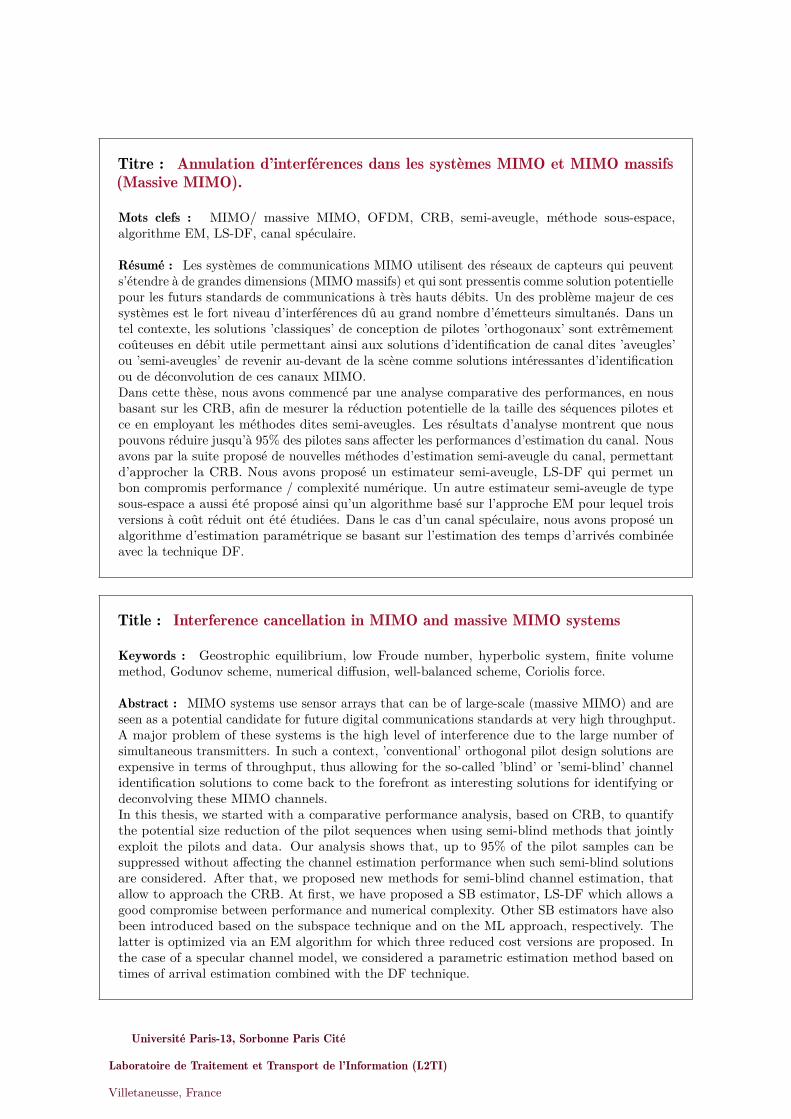
Titre : Annulation d’interférences dans les systèmes MIMO et MIMO massifs(Massive MIMO).
Mots clefs : MIMO/ massive MIMO, OFDM, CRB, semi-aveugle, méthode sous-espace,algorithme EM, LS-DF, canal spéculaire.
Résumé : Les systèmes de communications MIMO utilisent des réseaux de capteurs qui peuvents’étendre à de grandes dimensions (MIMO massifs) et qui sont pressentis comme solution potentiellepour les futurs standards de communications à très hauts débits. Un des problème majeur de cessystèmes est le fort niveau d’interférences dû au grand nombre d’émetteurs simultanés. Dans untel contexte, les solutions ’classiques’ de conception de pilotes ’orthogonaux’ sont extrêmementcoûteuses en débit utile permettant ainsi aux solutions d’identification de canal dites ’aveugles’ou ’semi-aveugles’ de revenir au-devant de la scène comme solutions intéressantes d’identificationou de déconvolution de ces canaux MIMO.Dans cette thèse, nous avons commencé par une analyse comparative des performances, en nousbasant sur les CRB, afin de mesurer la réduction potentielle de la taille des séquences pilotes etce en employant les méthodes dites semi-aveugles. Les résultats d’analyse montrent que nouspouvons réduire jusqu’à 95% des pilotes sans affecter les performances d’estimation du canal. Nousavons par la suite proposé de nouvelles méthodes d’estimation semi-aveugle du canal, permettantd’approcher la CRB. Nous avons proposé un estimateur semi-aveugle, LS-DF qui permet unbon compromis performance / complexité numérique. Un autre estimateur semi-aveugle de typesous-espace a aussi été proposé ainsi qu’un algorithme basé sur l’approche EM pour lequel troisversions à coût réduit ont été étudiées. Dans le cas d’un canal spéculaire, nous avons proposé unalgorithme d’estimation paramétrique se basant sur l’estimation des temps d’arrivés combinéeavec la technique DF.
Title : Interference cancellation in MIMO and massive MIMO systems
Keywords : Geostrophic equilibrium, low Froude number, hyperbolic system, finite volumemethod, Godunov scheme, numerical diffusion, well-balanced scheme, Coriolis force.
Abstract : MIMO systems use sensor arrays that can be of large-scale (massive MIMO) and areseen as a potential candidate for future digital communications standards at very high throughput.A major problem of these systems is the high level of interference due to the large number ofsimultaneous transmitters. In such a context, ’conventional’ orthogonal pilot design solutions areexpensive in terms of throughput, thus allowing for the so-called ’blind’ or ’semi-blind’ channelidentification solutions to come back to the forefront as interesting solutions for identifying ordeconvolving these MIMO channels.In this thesis, we started with a comparative performance analysis, based on CRB, to quantifythe potential size reduction of the pilot sequences when using semi-blind methods that jointlyexploit the pilots and data. Our analysis shows that, up to 95% of the pilot samples can besuppressed without affecting the channel estimation performance when such semi-blind solutionsare considered. After that, we proposed new methods for semi-blind channel estimation, thatallow to approach the CRB. At first, we have proposed a SB estimator, LS-DF which allows agood compromise between performance and numerical complexity. Other SB estimators have alsobeen introduced based on the subspace technique and on the ML approach, respectively. Thelatter is optimized via an EM algorithm for which three reduced cost versions are proposed. Inthe case of a specular channel model, we considered a parametric estimation method based ontimes of arrival estimation combined with the DF technique.
Université Paris-13, Sorbonne Paris Cité
Laboratoire de Traitement et Transport de l’Information (L2TI)
Villetaneusse, France
Bibliography 223
Related Documents